Embed Size (px)
Citation preview

ELECTROMAGNETIC WAVE PROPAGATION
IN ALMOST PERIODIC MEDIA
Thesis by
Alan R. Mickelson
In Partial Fulfillment of the Requirements
for the Degree of
Doctor of Philosophy
California Institute of Technology
Pasadena, California
1978

i i
ACKNOWLEDGEMENTS
For my scientific development during the early stages of my
research, I owe much to my original advisor, Professor Nichol as George.
While in Professor George•s optics group, I often worked with Dr. David
MacQuigg, a friend and colleague from whom I learned much . During this
period and following this period up to the present time, I would like to
acknowledge my friend and co-worker, Dr. ~~alter de Logi, for stimulating
discussions and collaboration on various projects.
Thi s present 1t10rk stemmed from an idea of my present advisor,
Professor C. H. Papas, whose encouragement and assistance were instrumental
in all stages of this research. I also acknowledge Dr. Dwight L. Jaggard
with whom I worked closely on various aspects of this work.
The style and accuracy of this work improved markedly upon careful
proofreadings by my advisor, Dr. Jaggard, Dr. de Logi, and Randy Bartman.
The reference lists could never have been so complete without the expert
assistance of Electrical Engineering librarian Paula Samazan. Addi
tional references were obtained from the private library of Dr. Crockett
L. Grabbe.
The ,~ough draft of this work was typed by my wife Susan , v1ho
really deserves to be acknowledged for more than typing. The expert
typing of the final draft was a product of Ruth Stratton, Susan Dycus
and Pat Neill.
My financial support while at Caltech has come from Caltech, the
Air Force Office of Scientific Research and the National Science Founda
tion.

iii
ABSTRACT
The problem of electromagnetic wave propagation in al most periodic
media is investigated and a solution is obtained directly from Maxwell's
equations. Techniques to evaluate this solution are developed. These
techniques involve a generalization to almost periodic media of the
Brillouin diagram of periodic media. The method of invariant imbedding
is applied to the coupled mode equations which determine the Brillouin
diagram for the purpose of transforming them to coupled Riccati equations.
These coupled Riccati equations, when subjected to a single boundary con
dition, determine the solutions to both the periodic and alnost periodic
boundary value problems. These evaluation techniques are used to place
in evidence similarities and differences of wave propagation in periodic
and clmost periodic media. It is shown that although the periodic and
almost periodic theories agree in many cases of interest,ther e exist
cases in which distinct differences appear. In cases of multi-tone per
turbations, the almost periodic theory yields both simpler and more rea
sonable results than the periodic theory.

I.
iv
TABLE OF CONTENTS
Introduction
Page
1-19
A. Statement of Purpose 1
B. The Theory of Almost Periodic Functions 1
1. Historical perspective 1
2. Important concepts involved in almost periodic
function theory 3
C. Why Bother to Study Wave Propagation in Almost
Periodic Media?
D. Preview of the Following Material
Bibliography
12
15
17
II. The General Theory of Wave Propagation in Almost
Periodic Structures 20-42
20
41
43-103
A. Longitudinal Media
Bibliography
III. Brillouin Diagrams in Almost Periodic Media
A. Basic Concepts 43
B. Brillouin Diagrams in Periodic Media - Information
Contained 50
1. Historical perspective 50
2. Use as a predictor 51
3. The Brillouin diagram as an ordering device 57
C. The Brillouin Diagram in Almost Periodic Media 66
D. The 6K + 0 Limit 78

IV.
v
TABLE OF CONTENTS
(continued)
1. Need for a new perturbation theory
2. Almost periodic perturbation theory
3. Periodic perturbation theory
Bibliography
The Reflection Coefficient
A. Standard Perturbation Theory for the Reflection
Page
78
83
87
102
l 04-151
Coefficient 104
1. Setting up the exact boundary value problem 104
2. Born-Neumann series 107
3. Secul arity of Born-Neumann series at resonance 108
B. The Electromagnetic Riccati Equation 109
l. Invariant imbedding- hi storical perspective 109
2. Stokes• recursion relation and conservation
of energy
3. The electromagnetic Riccati equation
C. A Generalized Look at Invariant Imbedding
l. First order wave equations from particle
counting
2. The energy conservation rel ations
3. Invari ant imbedding of coupled equations
D. Riccati Equations, Brillouin Diagrams and
Dispersion Matrices
1. Singl e harmonic perturbation
110
115
117
117
120
123
130
130

v.
vi
TABLE OF CONTENTS
(continued)
2. Al most periodic ~K + 0 solution
3. The periodic media small 6K limit
Bibliography
Conclusions
A. Relationship of the Brillouin Diagram to the
to the Reflection Coefficient
B. How Periodic and Almost Periodic Media Differ
1. Phase relations
Page
131
143
149
152-159
152
152
153
2. Band coalescence regime 153
C. The Basic Nature of Almost Periodic Structures 153
1. Multi-tone almost periodic perturbations 153
2. Almost periodic ensembles and stochastic
ensembles
D. Possible Research Directions
154
156
1. Extensions to more general geometries 156
2. Modeling of random perturbations 157
3. Extensions to active media- stability criteria 157
4. Experimental verification of the theory
Bibliography
APPENDI X A
157
159
160-167
167
168-171
172-175
Bibliography
APPENDIX B
APPENDIX C

Bibliography
APPENDIX 0
APPENDIX E
vii
TABLE OF CONTENTS
(continued)
Page
175
176-177
178-180

l.
Chapter I
Introduction
A. Statement of Purpose
To begin, we wish to enphasize that this report is an atte~pt
to unify an abstract mathe!71atical theory with \;ave propagation
theory and not an attempt to solve a specific engineering probl em.
!Je feel that the results of this report could become applicable to a
number of specific problems, but at the present tine we are not able
to predict in ~·thich areas this work will becor.1e important. The in
tent here is to present a theory of vJave propagation in this nev:ly
considered medium and to compare and contrast the electromagnetic
properties of this medium wi th the properties of better understood
media. In the process of the investigation , we in tend to re-express
certain abstract mathematical concepts in engineering terminology as
well as to develop new analytical techniques with wh ich to treat
wave-propagation phenomena. 'le hope the report achieves its purpose
and, moreover, provides an interesting treatise to the reader.
He v:i 11 novt proceed to give tile reader \"that lf!e fee 1 is the
necessary rnather:1atical history and ba.ckground.
B.
1.
The Theory of /\lmost Periodic Functions
Historical rerspective
The theory of al most periodic functions is a rather recent
development. Although the theory of Fourier seri es was essentially

2.
completed by the 1820 ' s with the work of Fourier, Poisson, Cauchy
anJ numerous others as footnoted in Hhittaker and Hatson's trea-1 ~ ~
t i se, it vias a century l ater v1hen Harald Bohrt.-, fou nd t::e alr.10st
periodi c gene·ral ization of Fouder series, borrm·dn~ heavily on the
1 Llr 5 quasi-periodic theory of Boh and Esclangon . Inspired by Bohr's
set of review papers6-8 , Bes i covitch9, Bochner10 and Favard11 found
various s impli f i cations of the theory soon after its inception . In
192612 and 192713 , Favard extended t he theory by considering li near
differential equations with almost periodic coefficients. (He l ater
unified his research into a book14 on the topic.) Other authors took
a different direction from Favard, concentrating their efforts more
on lifti ng restrictions on the class of almost periodic funct ions.
Besicovitch15 was the f i rst to publi sh a generalized theory, follm'led
by Stepanoff16 , P.es i cov i tch and Bohr17 , Linfoot18 and ~~iener19 . Al
though Bohr was the first to publ i sh a book20 on the topic, he was
closely followed by Bes i cov i tch . 21
Following this opening era of al most per·iodic theo:--y of the
1920 's and early 1930 ' s , there was a three-decade period of l i ttle
activity i n the fie ld. f-Jowever, \·Jith the davm of the 1960's there
came a deluge of papers and books on the topic . Characteris t i c of
this period of rene\\•ed interest in t he theory is Nichol as t1inorsky ' s
chapter on al most periodic solutions in his book on non-linear oscil
l ations22 . Hi s interest in the theory l ay in the relations hip
betv.Jeen al most periodic solut·ions and system stabi lity , a common

3.
reason for r enewed interest in the topic. To completely review the
developnents in this field in the last decade and a half is beyond
the scope of this report as is evidenced by the length of the ex
tensive, but not exhaustive, bibioaraphy in fJ •• tl. Fink's set of
lecture notes on almost periodic differential equations 23 . One
author's ~JOrk is of importance in t•elation to our study. That v1ould
b 24-25 . "d d h e the two papers of Jacob Abel who f1rst cons1 ere t e almost
periodic Mathieu equation, the same equation to be considered in this
work. Abel ran across the equation while ennaginq in a study of
stability of elastic systems.
2. Important Concepts Involved in Almost Periodic Function Theory
tie begin this section Hith a short qualitative di scuss ion of
almost periodic functions before jumping to the more abstract ele-
ments of the theory. Perhaps the most direct way of obtaining a
feeling for almost periodic functions is to compare theM Hith their
close relatives (actually a direct subclass), the periodi c fu nctions.
Consider the periodic function
fp(z) =COS TIZ +COS 3TIZ +COS 5TIZ (1)
and an almost periodic counterpa rt
1 7 5/3 cos TIZ + cos 3 _.- TIZ + cos D TIZ 13
(2)
These functions are plotted in figure (1).
For the first few periods of (1), the functions don't seem to

0 0 0 .
4.
~ r
~ ;; ~ ~ ~ ~ ~ ~q ~ n1 ~ ~ ~ ~ ~ ~ ~ ~ 11 ~ 'I ~ ~ ~ ~~ 'I ~ ~ LL
0 0 0
(II I
0 0 0 .
0.0 I
0.800 I
1.600 -.,
L
I CF LE ~f C TOR - 1 0
1
2.400 3.200 4.000
('11,--------.--------.-------~------~------~
~ t
~ ~~ ' ~ Ill!
"--./
LL ~ I I
l 0 0 0 0 1 . c L FACT DR = (II
I
0.0 0.800 1.600 2.1.!00 3.200 1.!.000
7 Figure 1.1. a) A plot of the periodic function fp(z) = cosnz + cos3nz
+ cos5nz. b) A plot of the almost periodic function fAP = cosnz +
COS 3 l . 7 1rZ + COS
51 137 TIZ.
/3 .

5.
differ too much. Farther on they certainly do, in spite of the fact
that their arguments differ by only a sr:tall amount. The oli:10st
periodic function appears to have ~ wandering phase with respect to
the periodic one. This is indeed the case as we notice that
313 - 3 + IR n-
where IR is an irrational number. He further note that we could
write (2) in the form
(3)
That IRis irrational is a fun0amental point . If, ~ n a sum of
trigonometric functions, the ratios of their frequencies can be
written as rational fractions, e.g. in the tv1o-tone case
(4)
p,q relatively pri~e integers
a period for the system can be found,and in fact the period is just
2n times p divided by Kl ~~hich is equal to 2n t imes q divided by K2.
If the ratio is irrational,however, it i s easily shown26 that no
period can exist. The function can come close to repeating at

6.
values of z ~here rational approximations to the irrational ratio of
Kl to K2 satisfy the above stated periodic condition, but t he function
can only come cl ose , as 2n times p divided by Kl i s no l onger equal to
2n times q divided by K2. The small difference in these two almost
periods will cause one or the other of the cosines to not truly re-
peat.
l•!e no1t1 fee l vJe are ready to approach the topic in a slightly
more rigorous l anguage for purposes of l ater exposition. We wi ll use
Bohr's 27 defini tion of almost periodicity .
Definition 1.
l et S(T) = {TJ Jf(t+T)- f(t)J < c Vt}.
Then f(t) is an al most periodic function iff S(T) for every c > 0,
is relatively dense.
Definition 2.
A set of Son R is called relatively dense if there exists a
positive L such that
[a,a+L] ns t ¢ VacR
A table of symbols for the definition is included in table (1).
It i s shown27 from Definition 1 that any almost peri odic func-
tion is un i formly continuous. It is also apparent from the definition
that an almost periodic function mus t have continually vacillating 28 .
values lest there be no al most periods in some regime. But a func-
tion possess ing these t wo attr ibutes must in some sense be stable,as

7.
TABLE I
Symbol ~1ea ni nn
{ } the set of
such that
!f(x)! the absolute value of f(x)
V for all
( ) the open interval
[ J the closed interval
U the union of
~ the intersection of
~ the null (empty)set
R the set of real nu~bers
A~ B A contains B
A c !3 P.. is contained by P,
TABLE I. LIST OF MATHEMATICAL SYr1BOLS H1PLOYED
ItJ THIS CHAPTER ALONG vfiTH THE f1Ef-\.NING OF THE
SY~·1BOLS.

8.
its values over sotr1e finite interval of time is 11 about the sar:1e 11 as
its values at any other time . The definition t~erefore ma kes clear
that the existence of almost periodic solutions to differentia l equa-
ti ons 9overning the output of machines or orbi ts of cel estial bod ies
somehm•/ i mplies the stability of the ma chine or the stability of the
orbi t . He can now understand one reason for the resurgence of inter-
est in almost periodic functions.
For further discussion we find it useful to use the results of the
basic theorem of almost periodic funct ions, that is to say:
Theo rem 1.
Any al most periodi c function f(t) is expressible as a gener
alized Fourier series
f(t) (5)
or more precisely, if for any qiven E: , att and A.N can be fou nd such
that
iA.t lf(t) - I a e N I < E:
N N (6)
then f(t) is an al Most periodi c funct ion. This theorem has immediate
consequences concerning composites of almost periodic functions. Con-
sider the addition of two al most periodic functions. If we f ind

9.
f(t) I ia~1t = aNe
N (a)
(7)
g(t) i f3Nt
= L btle . N
(b) \ .
then we can write
(8)
and t:1erefore \'/e finrl that the sum of tv10 alr1ost periodic functions
is also an almost periodic function. ~inilarly, we could show that
differences, products, quotients, integrals, anrl derivatives of
almost periodic functions are also almost periodic (with suitable
restrictions). It is then true that almost periodic functi ons are a
general class of functions which is closed under certain operations.
Implicit also in Theorem 1 is the inclusion of the periodic functions
as a subclass of the almost periodic functions as can be seen by
making the replacenent
(9)
in equation (5).
One more set of defintions will be included here f or the use-
fulness of the terMinology in discussing solutions of differential
equations with almost periodic coefficients.

10 .
Definition 3
The exponent exp of an almost periodic function f( t) is de-
fined as the set of A1 S contained in its generalized Fouri e r series,
i.e.,if
then
f(t)
exp[f(t)] = {A0
,A1 ,A2 , ••• }
Definition 4
The Module f.1 of the exp [f(t)] is the closure of t he set
under addition, i. e ., if
then
iAt f(t) = a
1e 1
Defintion 5
An almost periodic function g(t) is Modularly contained by
M[exp[f(t)]] iff
~1[exp[g ( t) ]] C r1[exp[f(t)]J
The usefulness of these defintions may at first seeM obscure. How-
ever, a simple example should prove their usefulness . t·'e consider the
case of a differential equation with periodic coefficients which can
be written in the form

11.
Of + Af = 0 ( 10)
where 0 is a differential operator and A a periodic function of basic
period K . Say that v1e know, from some very general techniques, that
a solution exists with the same period as .n... l·'e can then ahvays
write the solution in the form
( ll )
where the aN•s can be determined from a consistency requirement. We
would like to be able to generalize this argument to enable us to
solve systems of the form of equation (10) where A is an almost
periodic function, say for simplicity a two-tone a.lmost periodic
function expressible in the form
i K t i K2t A(t ) = b1e 1 + b2e ( 12)
~le wouldn•t know hov: to look for a solution of the same almost
period as the term"almost period"is still ill-ctefined. Hm,lever, \</e
could look for a "modular containment" solution, i.e. a soiution of
the form
( 13)
where the a•s, as in the argument above, are to be determined from a
consistency argument. The above argument is a simplification of the
argument that will appear in chapter two.

12.
C. \'/hy Bother to Study Have Propagation in J\l most Periodic t~1edia?
To this point the devel opment has seemed mathematical beyond
t he scope normally r equired for engineering application . The natural
question in the reader ' s mind i s v1hy bother vJith all tl,is mathemati cs
if no application i s imminent? He •t~~ish to all uy the reader's fears
by discussing briefly some promising areas of application .
Refore li sting these areas , thou9h , we wi sh to present a
brief discuss ion to motivate our reasoning. '·!e predicate th is dis
cuss ion on the fact that "real" el ectromagnetic (or optical) devices
are finite in length although periodic devices tend to contain many
periods \'Vithin this l ength . Further,these "periods" are never per
fect in practi ce . Hhether they be due to ampl itude wobbie, phase
wobble, crac ks in the structure or various other causes, t here are
ah1ays small perturbations to destroy the "perfecti on" of t he cellu
l ar structure of the device . A wave in travers ing such a media,
therefore, sees ma ny almost identical cell s . But an almost periodic
structure would l ook, at l east qualitatively, much li ke this to the
wave , as the almost periodic structure comes close to, but does not
quite achi eve , a "perfect" cellular structure . The almost periodic
structure seems to take imperfections into account and in t his sense
i s actua lly a more realistic model than a perfectly periodic struc
ture.
But is the increased effort r equ ired to evaluate an almost
periodic sol ution worth the effort? Although we don't know the

13.
answer to that question in general ,we do know of cases in wh ich the
almost periodic solution is simpler than the periodic solution. (Such
cases will be considered in chapters three and four.) He conclude
that if one believes that almost periodic modeling is in some sense
more realistic than periodic modeling, then there are certain cases
in which the almost periodic Modeling is worth the effort.
We will now list and briefly discuss some possible applica-
tions.
1. Stochastic Perturbations
Most random media propagation theory requires some type of
ensemble averaging wh ich may not always be desirable. For example,
consider a fiber optic link in ~.<Jh ich ~t/e wish to compute some quantity,
such as the amount of mode-coupling due to stochastic perturbations.
Ensemble averaging would correspond to averaging over many
similarly degraded links, whereas in practice we will use but one
link. In general, the stochastic solution would correspond to
finding the first and second moments of a distribution func tion v1h·ich
is too co~plex to obtain. But in certain cases (i.e., broad distribu
tions) the averaged result does not necessarily correspond very
closely to the situation in any one given link. In these cases, to
obtain more reasonable bounds on operational characteristics, it
would be desirable to solve the problem for a single member of the
ensemble. As will be discussed in more detail in chapter five of
this v1ork, a natural choice for an ensemble meMber ~·Jou ld be a

14.
specially constructed alMost periodically perturbed structure. Ry
solving this case deterministically, with free parameters, good
bounds could be obtained for operational characteristics.
2. Jnte9rated Optics
Although to this point in the technological development of
integrated optics most of the periodic structure devices have oper
ated very much as the periodic theory predicts they should, the possi-
bility remains that at some future date manufacturing limitat ions may
dictate that the theory be modified to agree with the experiment.
Under the assumption that almost periodic analysis, in some sense,
requires l ess restrictive assumptions than periodic analysis, the
almost periodic theory could provide a useful analytic technique for
predicting the limiting precisions Hith v1hich devices must be fabri
cated, or even the theory could suggest ~;rays to avoid technolog ical
limitations . Perhaps, in certain cases, almost periodic devi ces will
be preferable to their periodic counterparts.
3. Crystal Lattice Disorder Theory
l·Jork on the application of almost periodic function theory to
the theory of disordered crystal l attices has already been initiated
in t he \·fork of Romerio29 and Balanis. 30 l·!e feel a good direction in
which to continue would be to apply almost periodic Bri llouin diagram
analysis (developed in chapter three of this work for the one di men
sional case) to some s imple cases, follov!ing the l ead of Slater31 \'Jho

15.
so carefully and clearly treated the periodic lattice. tie feel that
it is possible by gaining better insight into almost periodic phonon
modes to better understand the collective quantum processes wh ich
cause solid state phenomena.
He beli eve the above listing represents only a sample of the
areas of possible utility of almost periodic \'Jave propagation but we
leave our discussion at this point so as not to unduly lengthen this
report.
D. Preview of the Following Material
In chapter t\-10 v1e solve the problem of \'Jave propagation in
longitudinally varying almost periodic media. The solution appears
as a generalization of Floquet's theorem for periodic media and is
therefore compared in structure to this familiar theory.
In chapter three the Brillouin diagram of periodic media is
generalized to the almost periodic case. The chapter begins with a
brief discussion of dispersion relations and diagrams, and an his
torical perspective on the development of the Brillouin di agram in
periodic wave propagation. The inclusion of this non-origi na l
mat~rial is justified on the basis that it expedites the di scussion
of almost periodic \•lave propagation by highlighting the underlying
concepts and techniques . The main devP.lopments of the chapter lie in
the generalization of the Brillouin diagram technique to al most
periodic media, and the detailed comparison of almost periodic wave
16.
propagation v!i th periodic v1ave propagation employing this newly de
veloped method.
In chapter four a technique is developed to calculate reflec
tion coefficients of finite logitudinally varying almost periodic
media. As in chapter three, this chapter also hegins by discussing a
certain amount of non-original, yet basic, material. The secularity
of standard perturbation expansions is illustrated and the method of
invariant imbedding) a pm'lerful technique of c:.voiding secul arity, is
developed in a more general way than has previously been accomplished.
The accomplishments of the chapter include numerical compa risons of
solutions of the exact Riccati equation for periodic and al ~ost
periodic media and the development of a technique for generating
reflection coefficients for "practical" media.
Chapter five is devoted to discussion and conclusions. Pos
sible research problems designed to extend and verify the theory are
suggested.
We are presently ready to embark on our exposition of the
theory of wave propa9ation in almost periodic structures.

17.
Bibliography for Chapter One
1. !Jhittaker, E. T. and G. N. Uatson, P.. Course of r1odern Analvsis
(London: Cambridge Univ. Press, Fourth Edition - 1927, re
printed - 1973). The references alluded to appear on page 160.
2. Bohr, H., Comptes Renjus 177, 737-739 (1923).
3. Bohr, H. , Cor1ptes Rend us 177, 1 090-1 092 ( 1923).
4. Bohl, Bull. Soc . t1ath. de France 38,5-144 (1910).
5. Although Bohr acknowledges Esclangon as being in part responsible
for the quasi-periodic theory, there seems to be no readily ac
cessible work by hi m. References we have seen ~iven are:
Esclangon, Annales de 1 'Observ. de Bordeaux (1019) and Esclangon,
t1. PhD. Thesis, France (1904). It seeMs that a portion of
Esclangon 's contribution lies in his coinage of the term quasi
periodic as Bohl uses no such classification.
6. Bohr, H., Acta Math. 45, 29-127 (1924).
7. Bohr, H., Jkta f1ath. 46. 101-214(1925).
8. Bohr, H., Acta Math. 47, 239-281 (1926).
9. Besicovitch, /1.. S., /\eta ~~ath. 47, 283-295 (1926).
10. Bochner, s ., Proc. London ~lath . Soc. 26, 433-452 (1926-1927).
11. Favard, J., Comptes Rendus 182, 757-759 (1926).
12. Favard, cl., Comptes Rendus 182, 1122-1124 (1926).
13. Favard, J. Acta r1ath . .§.!_, 31-81 (1927).

18.
14. Favard, J ., Fonctions Presque-Periodiques (Par-is: Cahiers
Scientifiques, 1933).
15. Besicovitch, A. S., Proc. London t1ath . Soc. 25, 495-562 (1926).
16. Steppanoff, H. , t'lath . Ann. ~. 473-498 ( 1928).
17. Besicovitch, A. S. and H. Bohr, J. London ~·1ath. Soc . _l, 172-176
(1928).
18. Linfoot, E. H., J. London Soc. ls 177-182 (1928).
19. l'liener, ~!.,Acta t~ath . .§_§_, 117-258 (1930). This \·Jork i s reprinted
in: Hiener, N. ,Generalized Harmonic Analvsis-Tauberian, Theorems
(Cambridge, M.I.T. Press, 1951).
20. Bohr , H., /\lmost Periodic Functions (New York: Che lsea , 1951).
21. Besicovitch, A. S. ,A1most Periodic Functions (London: Cambridge
University P1·ess , 1932).
22. t1inorsky, N. , ~lon1i near Oscillations (Huntington, N.Y. : R. E.
Kreiger Publishing Co., original ed. - 1962, reprinted- 1974).
23. Fink, A. t1. ,Alr1ost Periodic Differential Equations (Berlin:
Springer-Verlag), 1974).
24 . Abel, J., Q.J . of Jl.pp. Math. 28, no. 2, 205-217 (1970).
25. Abel,,)., J. ~ath . Anal . and Appl. 36, 110-122 (1 971).
26. Bedrosian, G. , PhD Thesis , C.I.1. (1 976 ) . See pp. 106-107.
27 . Definitions and proof of uniform continui ty are presented in
Fink's book (23) on pages 7-9.
28 . We have excluded the trivial case of a constant function.
29. Romerio, t~. V.,J. t1ath Phys. J.l, no. 3, ~07-835 (1971).

19.
30 . Bal anis , G., unpublished paper (1977).
31. Slater, J. C., Phys. Rev. 87, no. 5, 807-835 (1 952) .

20.
Chapter II
The General Theory of Wave Propagation in Almost Periodic
Media
A. Longitudinal Media
The motivation for the derivation contained in this chapter 1 comes in large part from the well known Floquet theory , so thoroughly
discussed in Whittaker and Watson•s treati se2 . However, the almost
periodic generalization of Floquet•s theory can neither be proved or
evaluated by techniques analogous to those applied to the periodic
case. For these reasons, the development herein contained will in-
vestigate the two theories simultaneously from a new vantage point
which naturally allows for illumination of the nature of the general-
ization.
To begin, let us remind ourselves of Floquet•s result. Given
the differential equation with periodic coefficients, e.g .• the
second order equation
( 1 )
where k is a periodic function of the variable z with period K ,
Floquet shows that ~ can be written in the form
~ = f(z)P(z) {2)
where P is a periodic function of z with period K and f is a propaga
tion factor which is to be determined. This result could be stated

21.
for the case of electromagnetic wave propagation as follows: the
wave solution to Maxwell's equations in a periodic medium ca n always
be written as a product of a propagation factor and a term i nvolving
the periodicity of the medium. We wish to find an almost periodic
generalization of this theory.
We now consider the problem of wave propagation insi de a
doubly infinite slab of a medium whose index of refraction varies
only with the coordinate z (refer to figure 1). We will consider
only plane wave solutions with propagation vector in the z-direction
and transverse polarization. For such a case, the wave equa tion is
easily derived from Maxwell's equations3, and found to be
(3)
where ~ denotes either the x or y polarized component of the E vector
and k2(z) is defined by
2 2 k (z) = w2 c (z)
c (4)
where w is the angular frequency of the wave and c the speed of
light in vacuum. We choose the medium's dielectric cons ta nt £ to be
a real (lossless ) function of z, as the generalization to complex re-
fractive index should be straightforward, as it is in the periodic
case4- 5. We further wish to consider cases in which £ is either a
periodic or almost periodic function of z and therefore expressible

~. y
E=
E(Z
)
1\
k(E
)=z,
B
k( E
)= -~,8
'"'J
,-
....
,;
"'
'"'J
-.....
..
--
-..
r r"
\ ~
\. r;J
-z
-
--
-_
n,.
- -
k { ~
}ei8
z -
iwt
€={~
} e-i
Sz-
iwl
Figu
re 2
.1.
Dia
gram
of
the
long
itud
inal
ge
omet
ry w
ith t
he t
wo
poss
ible
pl
ane
wav
e so
luti
ons
sche
mat
ical
ly d
raw
n in
.
N
N

23.
as
dz)
-1 iKNZ -i K Z -N e + I ~nN e N=-NT
(5)
where reality of s requires
* ni = n_i (6)
where the asterisk denotes complex conjugation. In the periodic case,
the K's must satisfy the relation
whereas in the almost periodic case
K -1
K. J
IR for at least one pair of i,j (iij)
(7)
(8)
where IR represents an irrational number. To simplify the present
discussion we will assume all n's to be purely real,although this re-
striction will be relaxed in the discussion of chapter III.
For present and future use we wish to define the Fourier trans-
form pair 00
- 1 r A i z (a) f(z) - 2n J f(y)e Y dy
- oo (9)
00
A
J -iyz f(y) ::; f(z)e dz (b)
- 00

24.
where theorems concerning transform relati onships to be employed in
present and future arguments can be found in any of numerous refer-6-8 ences
We now apply the Fourier transform (9b) to equation (3) where
the E is expressible as in (5) to obtain
( 1 0)
where we have reduced the separate summations of (5) to a s ingle sum
mation by defining K_N = KN' n0 = 2, k0
= 0. vJe have now reduced a
second-order differential equation to a non-local algebraic equation,
a type of equation whose solution we do not know how to find in gen-
eral. However, we can reduce the non-local equation to an infinite
set of local equations by assuming a solution of the form
and equating the coefficients of f at each given argument to zero. It
is not necessarily true that this procedure will work, but we will
assume it does and later show it yields a r easonabl e resul t . For
concreteness we assume that the dielectric constant has but t wo
"tones" in its spectrum in the almost periodic case, i.e.,

25.
NT = 2 (a)
nl = n_ l (b)
n2 = n_2 (c) ( 12)
no = 2 (d)
E:( z) i =N
IT 1 = £ '2n· r 1
i K.Z e
1 = s r[l+n1cosK1z+n2cosK2zJ (e)
i=-NT
but any number of tones in the periodic case. The tones in the periodic
case, however, must satisfy equation (7). Using our above ansatz we
see the solution s hould be written
A A
~ (y ) = L aN f( y+NK) period·ic (a)
( 13) A A
~ (y ) = l, aNM f( y+MK1+NK2) almost periodic (b)
To solve the resulting equation we could simply equate the coeffi
cients of f( y+NK ) for each N and solve the resulting infi nite set of
coupled algebraic equations. We elect not to do this in transform
space but to inverse transform and consider our result in configura-
tion space . The resulting forms of solution are
~ ( z ) =I aN eiNKZf(z) periodic (a) N
( 14) i (~1K l z+NK2z )
~ ( z ) = I aNM e f(z) almost periodic (b ) N .~1
Not too surpri singly, equation (l4a ) is exactly a statement of

26.
Floquet's theorem and perhaps in (14b) we have found its al most
periodic generalization. We feel the result is at least plausible
in the following sense. In Floquet's theory we find the fo rm of
solution to be the product of a propagation factor with a factor in-
volving the periodicity of the medium, in fact, the factor being
just the "modular containment" of the basic period. But in these
terms this is exactly what the almost periodic solution cont ains, the
product of a propagation factor and the modular containment of the
almost periods. The result agrees in form with that found by Abel?-10
who employed a different method in his derivation. However, we have
yet to show either existence or convergence of our scheme .
We wish to show that the aNM's die out for sufficiently large
N and M. We assume that the propagation constant does not go to zero
(or at least we are considering a frequency range in which it does not
go to zero) allowing us to divide both sides of (14b) by f, resulting
in
l>Je now define the mean va 1 ue operator by T
M{Q(z) } = ~~ 2i J Q(t)dt -T
( 15)
( 16)
Taking the square modulus of both sides of (15) and applying the
mean value operator of (16), we find the Parseval type relation

27.
( 17)
Let us consider this result. From energy considerations we would
expect the mean value of the squqred modulus of ~ (the energy density
of the phase front) to be a. bounded quantity and '>'Je have already re~
stricted ourselves to cases in which the propagation factor is
bounded away from zero. Accordingly, the lefthand side of (17) is
taken to be a bounded quantity, The conclusion is that only a finite
number of the aNM•s can be "appreciable" in order to satis fy (17).
Therefore, we can safely assume that the aNM•s die out for sufficiently
l arge N and M and the system of (15) can be effectively truncated.
Having convinced ourselves of the plausibility of the ansatz
contained in (l4b) we proceed to investigate the structure of the re-
sulting theory. The problem we have to solve to obtain a general
solution to (3) is to find the function f(z). We redefine our un
known by setting
f( z ) = ei Bz ( 18)
where B is now the variable, Using (18) in (14b) and subs tituting
in (3) using (12) we find

28.
As we have Kl and K2 non-commensurable, we can adopt a technique used
in generalized harmonic analysis11 to simplify the result. He simply
multiply by the kernel
A= ei Kz 2+ (20)
and integrate from -T toT taking the limit for T700. This procedure
removes both the complex exponentials and the summation signs and
leaves us with the doubly infinite set of algebraic equations 2
2 2 nk £r [k £r -( S+MKl+NK2) J aMN+ 2 [nl (aM-1 ,N+aM+l ,N )
(21)
where we have chosen n_ 1 to be equal to n1 and n_2 to be equal to n2.
This is the set of equations of which we spoke earl ier when
perusing the non-local equation (10) in transform space. The set is
homogeneous and it is useful to recast it in a matrix form. As the
aMN's are a countable set, we know that we can always map them into a
one-dimensional vector and thus write (21) in a familiar form

29.
D a = 0 ~ r-1"'
(22)
where a is the vector obtained by mapping the aMN's and ~ is the cor~
responding matrix of coefficients. Clearly then the condition B must
satisfy is
det D = 0 (23)
and by backsubstituting in (22) these values of 6, we can obta in all
th 1 t f ., 12 e a s as a one-parame er am1 y • Before discussing how to per-
form this feat, however, it is instructive to examine the ana logous
situation in the periodic case.
In the periodic case the wave equation i s found to take the
form of (22) with D defined as13
'D -2 ' ' ...
f,.., fl o_l 'f 'f L 1 2
D = fN - - f2 fl Do fl f2 - f N ( 24)
f2 fl' D+l fl ...... f2 .....
' ' 0+2 .....
' ' '
ON = 1 - (6+NK)2
k2 Er
fN = nN/2

30.
where all the el ements of the matrix have been normalized b.J~· k2E • . r
Evidently, we are faced with the impossible task of evaluating an in-
finite deter~inant. We see that the matrix must somehow be truncated
if we are to obtain a useful approximation, But it is equa ll y clear
that the infinite determinant cannot be uniformly convergent as its
diagonal grows with its dimension N~ casting uncertainty on any trun-
cation scheme, Hill 14 circumvented this problem, however, by a
clever argument so aptly treated in Whittaker and ~Jatson 2 and ob-
tained an alternative dispers ion relation, i.e. a relation connect·i ng
S with k , of the form
2 nk~ = 6(0) sin ( )
K
=
M = N
2 -k E r 2 2 2 f !M-NI' M 1 N
t-1 K -k E r
6(0) = det 6(0 ) "< -
(25)
Perhaps the major achievement of this approach is to explici t ly
illustrate the "v.Jell-behavedness" of the theory. Clearly, for each k
there exist an infinite number of s 's telling us that no pathology can
render this dispersion relation unsolvable, and hence (25) acts as an
existence theorem. Further, 6(0 ) is now uniformly convergent for
practically all values of k2E (Ref.l 5) and therefore can be truncated
r
with gay abandon.
Looking back at the almost periodic case,we see a bleak pic-
ture. As the mapping of a plane to a line is non-unique, we must use

31.
care in implementin~ our approach so as not to lose important terms.
Until we have defined this mapping from a plane to a line, we don't
even know the form of D, much less have a Hill's determinant-type "' "' theory, further~ \•te can a 1 readY see we are plagued with the same 1 ack
of uniform convergence so evident in (24), as our almost periodic
diagonal elements are of the form manifested in (24). However, having
come this far already, we push forward unrelentingly.
We now wish to define our plane-to-line mapping, with the moti
vation for our technique to come later, The basic scheme is illu
strated in figure 2, A grid is dra\<Jn with the points label ed by their
integer coordinates (i ,j). The boxes al~e formed by 1 ines passing
through points equidistant from the origin (0,0) in the sense that
the distance from point 1 (i 1 ,j1) to point 2 (i 2,j 2) is defined by
(26)
We label the boxes l ,2,3, etc., according to the order in which they
would be traversed in traveling out...tard from the origin, analogously
to the labeling of Brillouin zones in a plane16 . We say the points
on and within the ith box are the ith order points. Further, we de-
fine the points to the right of the origin to include those points
directly below the origin and the points to the left of the origin
to include those points that lie directly above the origin. To
specify a given order mapping,it remains only to specify the order in
which the points to the right and the points to the left must be

@
0
3,3
31
2
0 2,3
(a )
~ ~
0
3 -1
3,
-2 3
,-3
a 2,0~
-1 ~-2 2
~-3
1,0
'\:1
~-2~-3
0,0
//,-
1 0
,-2
0,-
3
. JS
c
-1,0
-1
,-1
-1,-
2-1,
-3
o G
~//o
e -2
3 -
2 2
-2
I -2
0 -
2 -I
-2
-2 -
2 -
3 1
1 1
l •
l I
I
(j
Q
<» \J
0
G
8
-33
-3
2 -
3 I
-3 0
-3-
1 -3
-2-3
-3
I I
I I
I I
1
(b)
~ 2
,0
~
lql
6110
1,-1
0,2
0, I
0
0 9
l_ ,
' 0,
-1
-I ,
I -1
,0~
I ~-1
-2 0
l
Figu
re 2
.2.
a)
Dia
gram
of
the
alm
ost
peri
odic
spa
ce
harm
onic
s w
ith
11Zo
nes11
dr
awn
in t
o in
dica
te w
hich
ha
rmon
ics
need
be
incl
uded
in
a gi
ven
orde
r th
eory
. b)
D
iagr
am o
f th
e al
mos
t pe
riod
ic s
pace
har
mon
ics
with
th
e pl
ane
to l
ine
map
ping
dra
wn
in,
v.>
N

33.
taken. This is illustrated in figure (2b) for the second-order mapping.
The general rule for points to the right for a given order 2N is to
begin directly below the origin on the surface of the 2Nth box, follow
the box around to the last point on the right, drop directly below to
the (2N-l)th box, follow it around to the last point on the right and
jump above to the (2N-2)th box, continuing the procedure to the origin.
Odd-order mappings and the points to the left are mapped analogously.
Now that we have picked the mapping we can investigate the re
sulting theory. First, we wish to clear up a notational point. Ab
stractly, we can represent our mapping by the symbolic equation
{M,N} ->- L (27)
Alternatively, using the definition
(28)
and
(29)
we could denote the mapping by the symbolic equation
[APJM,N -+ [AP]L (30)
We will find the opportunity to employ notations of (30) later in this
report.
We now wish to find the explicit form of the matrix D and the
vector a which appear in equation (22). Employing the mapping of
equation (30), we find from (21) and (22) that for the first order

34.
theory (first box)
(a)
T]2/2
Dlo nl/2
D = nl/2 0oo nl/2 (b) (31)
nl/2 D -10
n2/2
Although our further investigations will almost exclusively involve
only the first order, it is instructive to also look at the second
order D matrix and a vector which can be written as
(32)
and D as in figure 3.
A point noticed from the comparison of the two above orders is
the striking growth of the order of ~with the order of the theory.
For first order, D is five by five but in the second order D has bal-
looned to thirteen by thirteen. From elementary considerations it is th easy to see that for the theory of N order, the order of D (denoted

0 -20
0 0
0 0
fl
0 0
0 0
0 0
0 0 -l
-1
fl
91
0 o-2
91
o,_,
fl
91
fl
91
fl
0 0-1
91
fl
91
o_, o
fl
91
0
=
I 91
fl
0 oo
fl
91
I
w
()1
. gl
fl
01
0 gl
fl
91
0 o1
f 1 91
f1
91
fl
o_,
91
0 o2
l 91
fl
o
,
fl
0 20
Figu
re 2
.3.
The
disp
ersi
on m
atri
x Q
for
the
seco
nd o
rder
alm
ost
peri
odic
the
ory.
Th
e no
tati
on
f 1 =
n 1/2
and
g1
= n 2/2
has
be
en e
mpl
oyed
.

36.
O(D)) wi ll be given by
O(D) = 1 + 2N(Ntl) (33)
A second interesting point can be noti ced by compari ng the
f irst-order case (3lb) with the five-by-five) h-10-harmonic, periodic
Floquet matrix which can be written as
02 fl f2
fl o, fl f2
0 = f2 r, Do r, f2 (34 )
f2 f, D'"'l fl
f2 f, 0~2
lmmediately, it i s seen that the periodic 0 matri x is a fuller matrix. "' ,..,
There i s physical content in this fact. Were we to write the equa-
tions represented by (22 ) and D given by (34),we wou l d find a cou-"' "'
pling scheme represented by the following picture
a, a2 a±2 ao ao
' / '/ ~ ao a+, a +2 (35)
/' ~- ~-a_l a_2 a+l a±,
( a ) ( b ) ( c )
The double-arrowed line represents that the connected aN's appear
somewhere in the system in the same equati on . The al most periodic

37.
coupling scheme which results from equations (22) and (31) has repre-
sentation
0 10 0 01
"" / '\ 0 oo 0 oo 0 oo ~ ~ / '
(36) 0 ±10 0 0 ±I a a
-10 0-1
(a ) ( b ) ( c ) The conclusion is that the precision of the phase relation of the
periodic medium leads to the richer coupling scheme of (35). In the
almost periodic case, (36b) and (36c) almost give the impression that
the perturbations represented by the two n's act independently,
whereas (35b) indicates this is not so in the periodic case. We will
return to this point in chapters III and IV and delve more deeply
into the physical consequences.
At an earlier point we became somewhat perplexed at the lac k
of a Hill •s determinant theory for the almost periodic sol uti on. At
this point we will try to allay some of this apprehension by con-
sidering the limiting case of small perturbations. First, l et us
consider the case of no perturbation at all, i.e.,
(37)
The resulting D matrix of (31) becomes diagonal and has determinant

38.
00 00
det D = TI TI 1 - (38) t~=-oo N=~oo
He note that the product being over all N and M has terms symetrically
in plus and minus M and N. ~Je use this fact to simplify the product,
combining the term in M and N with the term in -M and -N. We find (after
some manipulation)
which tells us the product can be rewritten in the form
{40)
The result is interesting for two reasons. First, as no B's
appear off the diagonal,(40) implies the dispersion relat ion can be
expressed as a polynomial in s2. This gives us an important part of
the Hill's determinant information, namely that for a given k we can
always find some B's, i. e., no obvious pathology occurs. Second, (40 )
gives us information about the form that the solution can take, i.e.,
it gives both the S's and the aNM's. Consider the Brillouin (disper
sion) diagram (to be discussed in detail ' in chapter III) of f igure 4.
vJe see the roots of (40) are straight lines extending to infinity,

k~
-2K
2
-2K
1 -K
2 -
KI
0 K1
K
2 2
K1
2K
2
Figu
re 2
.4.
An u
nper
turb
ed a
lmos
t pe
riod
ic B
rill
ouin
dia
gram
. N
ote
that
onl
y m
ulti
ples
of
the
bas
ic h
arm
onic
s ar
e sh
own
alth
ough
man
y ot
her
sum
and
dif
fere
nce
harm
onic
s sh
ould
ap
pear
on
the
sam
e sc
ale.
{3
(;J
\..
:)

40.
all with slopes of ±l. As a determinant is a continuous function of
the elements of its constituent matrix,we should think t hat this
picture should not change too much for small perturbations. To find
the aNM's for a specific line in the diagram, say the lines
B = ±k~ (41) r
we go back to equation (22) and plug in our B value. For the pertur-
bationless case we are considering, the equations are quite simple,
i.e. ,
D_N a_N 0 N t- 0
ON aN = 0 (42)
0 X a 0
= 0 as Do = 0
We see that we can explicitly find the one-parameter string earlier
mentioned (equation 23), namely
a. = 0 1
i t 0
a0
arbitrary (43)
We see that any reasonable boundary condition on lji and hence on the
aN's gives us a nice bounded solution, and as the aN's are also (as
are the S's) continuous functions of the elements of the D matrix, we
would expect equally encouraging results for any small perturbation.
It seems, in the small perturbation limit anyhow, that we have no
need for a Hill's determinant theorem.

41.
Bibliography for Chapter II
1. Floquet, M.G., Ann. de l 1 Ecole norm.sup. (2), XII, 47-88,
(1883).
2. Whittaker, E. T. and G. N. vJatson, A Course of t-1odern Analysis
(London: Cambridge Univ. Press, Fourth Edition- 1927, re
printed - 1973).
3. The notation and form of Maxwell •s equations employed in this
report are those of: Papas, C. H., The Theory of Electromagnetic
Propagation (San Francisco: McGraw-Hill Book Co., 1962).
4. Jaggard, D. L. and C. Elachi, J.A.P. 48, no. 4, 1461-1466 (1977).
5. Jaggard, D. L., App. Phys. (Springer-Verlag) }l, 185-1 95 (1977).
6. Papoulis, A., The Fourier Integral and It•s Applications (San
Francisco: McGraw-Hill Book Co., 1962).
7. Papoulis, A., Systems and Transforms with Applications in Optics
(San Francisco: McGraw-Hill Book Co., 1968).
8. Goodman, J. W., Introduction to Fourier Optics (San Francisco:
McGraw-Hill Book Co., 1968).
9. Abel, J. M., Quart. of Appl. Math. xxviii, no. 2, 205-217 (1970).
10. Abel, J. M. J. Math. Anal. and Appl 36, 110-122 (1971).
11. Although the idea of using orthogonality properties of non-square
integrable functions on infinite intervals is probably quite old,
Norbert Wiener was certainly instrumental in systemetizing their
study. A good reference is: Wiener, N., Generalized Harmonic

42.
Analysis-Tauberian Theorems (Cambridge: M.I.T. Press, 1964).
12. That this statement is true is evident from the Fredholm alterna
tive theorem as applied to linear systems of algebraic equations .
If we substitute a characteristic value of multiplicity one
into D, we can always obtain the solutions as a string of one
free parameter. A method for solving the corresponding boundary
value problem is discussed in the first section of chapter IV of
this report.
13. Although the form of this matrix is well known in the literature
and easily derivable, the conventions and notation employed in
this report agree most closely with those of the PhD thesis of
Dwight L. Jaggard. The reference is: Jaggard, D. L., Antenna
Lab Report No. 75, C.I.T. (August 1976).
14. Hill, G. W., Acta Math. viii, 1-36 (1886) .
15. These other values are just simple poles and are counteracted by
the multiplicative sine function . Check reference (2), pp. 415-
417.
16. See any reference on solid state physics, for instance: Kittel,
C., Introduction to Solid State Physics (New York: John Wiley
& Sons, 1976).

43.
CHAPTER III
Brillouin Diagrams in Almost Periodic Nedia
In the present chapter v1e investigate the properties of 'vlaves
propagating in almost periodic media. As in the preceding and the fol-
low ·ing chapters, we borrm<~ heavily in our attempt to impl ement the new
theory on the well-known periodic theory and the techniques developed
to implement the periodic theory. As a first cut in atte111pting to under-
stand almost periodic phenomena, we concentrate on the inhomogeneity
induced dispersion of the medium. In studying the properties of the
dispersion relation we employ dispersion diagrams . \~e shall call these
diagrams Brillouin diagrams,as dispersion diagroms in periodic media are
usually called Brillouin diagrams. We feel the Brillouin diagram is an
effective artifice to employ in the atte111pt to gain physical i ns ight into
the medium's properties as pictorial information is rather easy to digest.
~~e begin this chapter with two review sections. The first is de-
voted to review of the use of dispersion relations and diagrams. We feel
its inclusion is warranted on the basis that the development introduces
the ensuing notation as well as providing an exposition of t he concepts
most useful in the following development. The second is devoted to a
review of the use of the Brillouin diagram in periodic media. This section
serves to highlight the techniques we are later to generalize, and gives
us historical perspective.
A) Basic Concepts
To begin, we simply define the phase and group velocities of the
wave, concepts so aptly treated elsewhere 1 For a component of the

44.
electric field which can be written in the form
we find that
=
ikz- i wt 1/J = e
w r =
dw (fie
(1)
(2)
Our Brillouin diagram will always be displayed in terms of quan-
tities which exist in absence of modulation versus quantities that
actually exist inside the medium. Using the superscript u to denote
unperturbed and the superscript p to denote perturbed, we therefore
write
ik0~- i wt 1/Ju = e
with th e subsequent identifications that
u = c vP (J..)
vp = -
1€ p B r
u dw vP dw vg = ---- = d(:l
d(k~) g
( 3)
( 4)
As ·r:e are in ten~sted only in variations with respect to the unpert1n'l~ed
medium, \\fe fur·the r· make the identifications that
d(k!E) r
dB (5)

45.
where r denotes relative. With reference to fi gu r e 1, an archetypal
Brillouin diagram, we can presently see the ease with which vr and vr p g
can be read. The relative phase ve locity of a 1t1ave is s i mply a quotient
of its frequency (free space 1-'Javenumher) and its '.'Javenumber i n the medium.
The relative group velocity is simply the slope of the wave's dispersion
line. The quadrant of the diagram gives the direction of the phase velo
city and the line's direction gives the direction of energy flow.
t~e now l'l·i sh to consider in some depth the different regions drawn
in on figure l. In region 1, v1e note that both the phase and group vela-
city of the \'/ave drop bel 0\'1 the unpe rturbed vel oci ties. Operation in
this regi me has been successfully emp loyed in various applic3tions such
as the particle accelerator 2• 3 and the traveling-wave tube 4 . We r efer
to this region as the slmiJ -ItJave regime. Region 3 exhibits vvave solutions
of greater phase velocity, yet smaller group velocity, than that of the
unperturbed region and therefore dons the title of fast 1t1ave regime.
Propagation in such a regime is reminiscent of plasma wave propagation
and has been treated elsewhere 5 . The region of real interest to the
present study, however, is region 2.
In region 2 there is an imaginary group velocity, indicating that
somehm'l the concept of group velocity needs rein terpre tation. In refer-
ring to figure 2 vie can see how the concept i s deficient . The derivation
of group velocity is predicated by our ability to construct a wave
packet about the various differently wave-numbe red components of electric
field in our medi -um. In region 2 our ability to construct such packets
is seriously impaired as the spatial dependence of our waves takes the

46 .
6 @) I 8 CQ
I E I
..._..
Lf I
~
E ~ s.... 01 ttl .,.... -c
0~ s:: 0
<5>~ .,....
s.... CJ
/)~ 0.. Vl .,....
0--~ -c ..-
(y~ ttl 0..
/) @ 18 >. +-' <lJ
I ..s:: u
I s.... ttl
I s:: c::c
I CQ ..-
a..> (V)
0::: CJ s.... ~ 01 .,....
~ I.J.. ..
~
I
~:e I

Vg
rou
p
[VE
LOC
ITY
O
F E
NV
ELO
PE
]
Vph
ase
[VE
LOC
ITY
O
F O
SCiL
LAT
ION
S]
(a)
FIE
LD
AM
PL
ITU
DE
REG
ION
S I
AN
D
3
(b)
FIE
LD
AM
PL
ITU
DE
Vg
rou
p =
?
REG
ION
2
Figu
re 3
.2.
a)
Sket
ch o
f a
wav
e pa
cket
, su
ch a
s wo
uld
exis
t in
a n
on-s
top
band
fre
quen
cy
rang
e.
On t
he s
ketc
h ar
e in
dica
ted
the
mea
ns f
or d
eter
min
ing
gro
up a
nd p
hase
vel
ocit
y.
b)
A w
ave
prop
agat
ing
thro
ugh
a m
ediu
m i
n th
e st
op-b
and
freq
uen
cy r
ange
. In
dica
ted
on
the
diag
ram
are
the
pha
se v
eloc
ity
and
hope
less
ness
of
dete
rmin
ing
a gr
oup
velo
city
.
z -J::
:> -..
..J

48.
form of growing or dying exponentials. No longer can ~"e f ind a specific
amplitude point on a packet and follm-1 it through the medium, as in this
case the point does not move .
A s lightly more physical picture of these phenomena can be con
structed by considering a truncated medium, one which extends from
z = 0 to some z = L. The situation is depicted in figure 3. We lump
the negative phase velocity waves together into a composite "backward"
wave and the positive phase velocity waves analogously into a "forv1ard"
wave as has often been done in the literature 6 The resulting picture
shows that \1/aves attempting to propagate into the med ium ~tlith fre
quencies corresponding to region 2 are "redistributed in enerqy content"
v1ith respect to waves with frequencies outside this region. From the
picture, we Houl d expect the considered regime to be one of 1 arge re
flection coefficient, as we will see it indeed is in the following
chapter.
As to the terminology employed in referring to this frequency
range, \-Je feel the terms stopband or bandgap are preferable, fo r our
purposes, to the commonly used so lid-state physics term, "forJidrlen
region" 7 The solid-state usage is justified in the sense that ther-
mal phonons generated in a "forbidden" energy range v1i 11 not ;Jropagate
through the lattice and therefore ~t1ill contribute negligibl y to its
specific heat . However, in our case the source is external and the
region is not truly forbidden, but only somewhat more reflective than
at other frequencies. The distinction may be moot, but be it made.

FIE
LD
A
MP
LITU
DE
z=O
z=
L
Figu
re 3
.3.
Sket
ch o
f th
e fi
eld
dis
trib
utio
n in
side
a p
erio
d m
ediu
m o
pera
ting
in
a st
op
band
fre
quen
cy r
ange
.
z
-~
(!'')

50.
B) Brillouin Diagrar.~s in Periodic f~edia--Information Contai ned
l) Historical Per·spective
The first use of a dispersion diagram for a periodi c medium in
an English language journal appears to be in a 1930 work by Kronig and
Penney 8 Inspired by the pioneering work of Bloch 9; who in late
1928 was the first to consider the problem of electron-~·iave propagation
in a three-dimensional ·lattice, Kronig and Penney considered in detail
the more tractable problem of one-dimensional propagation. However,
bet~-Jeen the publication of these b1o early works, independently Leon
Brillouin 10 applied dispersion diagram techniques to one-, two-, and
three-dimensional l attice models and published his results i n a French
journal. Brillouin expanded on his t echnique and pub li shed v1orks in
1932 and 1933 in which he considered problems of crystalline magnetic
properties 11 and superconductivity 12 , respectively. The first ap-
pearance of the name Brillouin being associated wi th an energy band
diagram was in the 1934 v10rk by J. C. Slater 13 . In this work Sl ater
t erms the zones on the diagram to be 8rillouin zones . This t erminol ogy
caught on as i s evidenced by the titl es of references incl uded in the
appendix to Brill ouin ' s definitive book 14 on the topic of wave propa
gation i n periodic structures . Th e book by Bri ll ouin stems from a 1936
work 15 of his in which he first real ·ized the great general ity of
periodic-media techniques. But in spite of Brillouin ' s realization, it
appears to have been Sl ater who first applierl the Bril loui n diagram
t echniques, not commonly in use , to the el ectromagnetic wave propagati on
probl em in his 1948 articl e on linear accelerators 16 The use of

51.
these techniques in electromagnetic problems was expanded as is evidenced
by the 1959 paper of 01 i ner and Hes sel 17 , and the term "Bri ll ouin
diagram" \'las certainly in standard usage by the time of the publication
of the 1965 reviev/ article of Cassedy and Oliner 18 .
2) Use as a Predictor
The greatest utility we have found for the Brillouin diagram is
that of a rule-of-thumb pictorial device which tells us not only which
effects are important, but also gives us an expectation for the results
of a physical measurement, such as that of the reflection coefficient.
We will adhere to this rule-of-thumb approach in the present section by
foregoing mathematical rigor in favor of physical pictures.
In considering periodic media, the first effect we should con-
sider is that described by Bragg's law 19 The familiar picture of
figure 4 should make plausibl e · the phase condition that
2A sin e = nA (6)
\'/here the Bragg order n is an integer. In the lon gitudin al case \-Jhich
we are considering, the condition simplifies to
kl€ = r
n 2K (7)
where K = 2rr/fl. .. In cases where equation (7) is satisfied we therefore
expect something to happen, the nature of which we will presently inves-
tigate.
The best vehicle with which to investigate the detailed Brillouin
di agram s tructure lr/Ould be Hill's determinant, already introduced in

A=
27r
K
Figu
re 3
.4.
Sche
mat
ic d
iagr
am o
f th
e pr
oof
of B
ragg
's l
aw.
A w
ave
inci
dent
on
a st
riat
ed
med
ia
is r
efle
cted
in
phas
e if
2A
sin
e =
nA
.
(J"1
N

53.
Chapter II of this report. For purposes of clear exposition vte express
the theory here as
where
and
. 2(7TI3) s1n -.K
= ARG
ARG 2 7Tk/E
= L1 (0) s in ( r) K
L1 (0)
( Sa )
( Bb)
(Be)
M = N
(Bd)
M ~ N
( Be)
We wish to examine the various S values in the proximity of the
various Bragg orders to gain more insight into the nature of the solu-
tion. He first notice that in the absence of perturbation (all n. ' s 1
equal to 0) the solution to (B) reduces to
S = k/£ + LK (L any integer ) r (9)
We also note that this solution is noticeably changed by the inclus ion
of any small perturbation due to the coefficient of the off diagonal
terms of L1 :
( l 0)
which become singular for

k.fE = 14K r
54.
(\·lith reference to equation ( 7) f1 = n/2) ( ll)
i.e., for all even Bragg orders. Let us presently break up the situa-
tion in to cases and examine the argumen t ARG at even and odd Bragg
orde rs. He see from equations (7) and (8b ) that f or!:!_ odd
ARG = .6 ( 0) I max (maximized with respect to variations in k)(l2a)
for i•1 even ---
ARG = 1 i m .6 (0 ) s in2( 1T +E) E: -+ 0
1 i m .6 (0) ->- - co ( l 2b) E: -+ 0
1 i m s i n2 (1T + s ) -+ 0 E: -+ 0
Th e situation is illustrated in figure 5 . The values of the
argument can become greater than one at odd Bragg orders and less than
zero at e ven Bragg orders, causing the value of B to become complex .
To make the preceding argument more qua li tative, consi de r the
f 11 . . f th . 20 o ow1ng expans1on o e arcs1n
ARCSIN(x+ iy) = k1T + (-) ks in- 1(v ) + (-)k Hn(~+Ji - l)
k integer
~ l [(x+l)2 + y2]l/2 + ~(x-l)2 + y2] l/2 2 2
( 13)

ARG
STO
PBAN
D ST
OPB
AND
+I
I ~~
~
l \
~
0 '
I ",•
n:h:
zl I
't'
I I
.,
I 2 I
STO
PBAN
D 3 2
7T
kF
, K
Figu
re 3
.5.
Sket
ch o
f th
e be
havi
or o
f th
e ar
gum
ent
of t
he s
in s
quar
ed
in t
he H
ill
1S
dete
rm
inan
t th
eory
, i.
e.
that
is
AR
Gas
gi
ven
by
(8b)
ve
rsus
~/
Sr.
Whe
n th
e ar
gum
ent
exce
eds
1
or b
ecom
es
nega
tive
, we
ent
er a
sto
pban
d re
gion
. K
v,
vi

56.
\,!e break up the expression (13) into cases to re duce this fo rmidab le
result to a more palatable form .
Case 1. When ARG > 1, then
B I , 1~ = F n + (- ) '" i Q,n [ IARG + IARG - 1]
F any half-odd integer
k any intege r
Case 2. When 0 s. ARG S 1, th en
nB = Fn + (-)k cos- 1(ARG) K
F any intege r or half-odd intege r
k any integer
Case 3. When ARG < 0, then
nB = Fn + (-)k i Q,n[/-ARG + /1 - ARG] K
F any integer
k any intege r
The reason for th e freely s pecifiabl e integer and half-odd integer
paramete rs is that there are an infinite numbe r of branches of the
( 14)
(15)
( 16)
arcsin function, causing an uncertainty as to the branch 'iJe are on.
Thi s just corresponds to th e infi nite numbe r of identical branches of

57.
the unperturbed case. We choose to call the regime of case 1 the
overflm'' bandgap regime, case 2 corresponds to the slov1 and fast
\1/ave regimes, and case 3 '>'le denote the underfloltl bandgap regime .
Using equations (14-16) and figure 5 we can construct, quali
tatively at l east, a typical Bri llouin diagra~ for a periodic structure
as depicted in figure ~. We see that the diagram contains all the
regimes which \'/e discussed in the dispersion diagram section, \·lith the
con~esponding interpretations. ~'le see, therefore, that from the pic-
torial representation of the dispersion relation much information about
the medium 's frequency dependence and reflection characteri stics can be
deduced. In this sense the Bril louin diagram is a guide t o the predic-
tion of a material's physical res ponse. However, this is not the only
use to '>'Jili ch we apply the diagram.
3) The Brillouin Diagram as an Ordering Device
In this section we will consider the use of the unperturbed
Brillouin diagram as a guide to choosing the important terms in truncat-
ing our infinitely dimensioned dispersion relation in the case of small
perturbations.
We begin by reconsidering the earli er de rived peri odic rel a-
tion:
0 a = 0 ( 17)
For the moment we vJi sh to examine the case in which '>'le only need con-
sider tvw space harmonics. In general, v1e ~"ill always start by con-
sidering the zeroth space harmonic, th at is to say, the space harmonic
corres ponding to the two lines on the Brillouin di ag ram closes t to

Re (k
jEr)
2K
3K
2 K
K 2
~
Re(k~)
UNPE
RTUR
BED
LINE
Pg
Re j3
Im
j3
Fig
ure
3.6
. A
ske
tch
of
a ty
pic
al
Bri
llo
uin
dia
gram
in
a p
erio
d m
ediu
m.
To m
ake
the
tie
in w
ith
the
argu
men
ts
valu
es w
e no
te t
hat
on
the
arc
P 1P 2,
0 <
ARG
< 1
, on
li
ne
P 2P 3, AR
G >
1,
on A
RC
P 3P 4,
0<
ARG
< l,
on
lin
e P 4P 5
, AR
G<
0,
etc.
<..'1
OJ

59.
those on the Brillouin diagram of the perturbationless structure with
the same basic dielectric constant,£. In this case \'ie shall consider r
only the zeroth and the so-called minus -one harmonic (refer to figure 7.
Strictly, the harmonics on the Brillouin diagram should al so be super-
scripted by the sign of their phase velocity as in equation 17; each
actually corresponds to tv;o lines of the Brillouin diagrar1.) ~/e con
tinue by writing out the resulting t\"o-by-ti'JO system obtained from
equation (17) by ignoring all the zeroth and minus space harmon ics
and by recalling that
D = +N
= 0
= 0 ( 18)
(N any integer) ( 19)
We proceed in our argument by assuming the perturbati on to be
small and expanding about the center of the assumed bandgaps. (This
approximation is consistent with the truncation which has already as
sumed a small perturbation). Letting
and
ki"E r
i3 = K /2 0
K /2
where 6S is assumed to be small, we find
(20)
( 21 )

X~ 0~ ()~
kJE7
~
'/ 0
0 '?()«'
.: ~o,
'?()~-'?
~
-2K
-K
K
2
K
Figu
re 3
.7.
A s
ketc
h of
an
unpe
rtur
bed
Bri
llou
in d
iagr
am f
or a
per
iodi
c m
ediu
m.
The
spac
e ha
rmon
ics
are
labe
led
by b
oth
thei
r nu
mbe
r an
d si
gn o
f th
eir
grou
p ve
loci
ty.
(3
C)
0

61.
-0 -1 - 468
- 0 (22) K
Substituting back into equations (1 8 ) we find the new system
68 a = - xa -1 0 (23a)
- 6!3 a0
- xa -1 (23b)
X - nK/8 (23c)
To proceed in our interpretation we borrol't from the widely used
?1-30 theory of coupled modes - and consider our electric field to be
compl~ised of a forward plus a backv1ard traveling \•lave, and i dentify
these \'laves as
F = a e+i 68z 0
B = a e+i 6Sz -1 (24)
With these substitutions we can rewrite our system (23) in the form
F' =ixB (25b)
-B' =ixF (25a)
wh e re the pri mes denote differentiation \•lith respect to z. \·Je could
stop at this point and attempt to determine the significance of thi s
derivation on the Brillouin diagram, but instead we choose to pus h one
more step fonvard for the sake of clarity.
We now wish to consider the system of equations complementary
to (1 8), name ly

62.
(26)
and make the expansion comparable to (20) and (21), but this time making
the replacement
s -+ -(3
We find, analogous to (22),
-Dl "" D "" 4t.S
- D 0 K
resulting in the system
Now, by adding (29a) to (23a) and (29b) to (23b), we find
= X(a +a 1
) 0 -
We could now follow the earlier line of reasoning by definin g
B = -i t.Sz + a ei t.Sz -a-1 e
0
(27)
(28)
(29a)
(29b )
(30a)
(30b)
( 31 a)
( 31 b)
and still recover equation (25) intact. We have now rediscovered a fact
already notice d in the literature 31 , namely, that it makes no differ-
ence in the expansion at the bandgap center whether we consider our

63.
fon>Jard (back~<~Jard) going wave as comprised of a single space harmonic
or a sum of space harmonics. The situation i s depicterl in figure 8.
On occasion we shall also use the schematic representations of (Aa) and
(8b) which would be
i( 32)
Elsewhere (Refs. 32-34) this picture is extended to include in-
teracti ons at all orders and for arbitrary numbers of nonzero harmonic
perturbation coefficients. \~e will 1 eave the reader to check the
mathematics, but include several more pictures to illustrate the tech-
nique. We feel this is a congruous approach, as the original idea of
using the Brillouin diagram as an ordering device was to alleviate us
from performing tedious numerical calculations until after ~'/e knew
which calculations we were interested in.
In figure 9 we use the notation that
(N any integer) ( 33)
and call it the nth order coupling coefficient. It can be
shown( 32- 34)that the nth_order coupling coefficient can only couple
waves differing in medium wave number by n units of the basic medium
(or equivalently grating) frequency. This is illustrated in fiqure 9
where only the first and second coupling coefficient are considered to
be non-zero. The figure also illustrates how the second-order coupling
derives its name. ~~e consider the coupling of the two waves at second-
order Bragg frequency to be second order if achieved by ti'IO first-order

kJEr
kv
'E;
OR
f3
a)
b)
Fig
ure
3.8.
a)
A
Bri
llou
in 11
inte
ract
ion
11
diag
ram
with
th
e in
terp
reta
tio
n t
hat
eac
h sp
ace
harm
onic
re
pres
ents
a s
epar
ate
wav
e.
b)
A B
rill
ou
in 11
inte
ract
ion
'' di
agra
m u
tili
zin
g t
he
inte
rpre
tati
on
th
at,
at a
sto
pban
d ce
nte
r, t
he f
orw
ard
and
back
war
d w
aves
ar
e de
scri
bed
as
spac
e ha
rmon
ic
inte
rsec
tio
ns,
th
at i
s to
say
su
ms
of
spac
e ha
rmon
ics.
f3
0'1
-J:::>

kJi;
{j
Figu
re 3
.9.
A B
rill
ouin
"in
tera
ctio
n" d
iagr
am i
ndic
atin
g fi
rst
and
seco
nd o
rder
cou
plin
gs
in a
per
iodi
c m
ediu
m.
~
l.l

66.
interactions, or to be first order if achieved by one second order coupl
ing. We will consider a system to be first order if it contains only
the forward-to-backwal~d vJave couplings which can he achieved by a
single coupling. Analogously, an nth-order system includes all space
harrnoni cs which are necessary to couple the forward-to-backw ard wave in
n couplings or l ess . In general, we consider the coupling strengths to
be small and therefore the (N-l)th_order couplings to be more important
than those of the Nth order.
Figure 10 illustrates the full second-order coupling system at
the second Bragg order, where only one harmonic perturbation coefficient
is non-zero. In second order we notice there exist couplings which
couple the fon,Jard and backward waves back to themselves. These effects
are termed to be self-coupling terms and result in a movement of the
bandgap center from its unperturbed location, as is shovm else,.there 32
It is important to remember that in the periodic case all band
gaps at a given frequency are identical regardless of on 1>1hich space
harmonic they lie. \~e will soon find that this is not true i n the almost
periodic case.
At this point we feel we have completed the discussion of the
basics and will presently push on to apply the above developed techniques
to the al most periodic case.
C) The Brillouin Diagram in Almost Periodic Media
Through the mapping derived in Chapter II we have seen that we
can write the almost periodic dispersion relation in the form of (17).
We now wish to use the Brillouin diagram to motivate our original use

kFEr
Figu
re 3
.10.
A
Bri
llou
in '
'inte
ract
ion'
' di
agra
m i
ndic
atin
g al
l th
e se
cond
ord
er c
oupl
ings
, in
clud
ing
the
self
-ene
rgy
coup
lings
at
the
seco
nd o
rder
Bra
gg f
requ
ency
re
gim
e.
Cl
... ,:
f3

68.
of th e mapping and associated ordering definitions. Again, as in the
periodic case, we consider that the externally applied wave couples
completely to the zeroth -order space harmonic, which here is actually
the zero-zero space harmonic.
Figure ll illustrates the notation used for space harmonics up
through the second-order theory. Also included in the diagram are all
of the first-order couplings. As alluded to earlier in this report,
there are but two first-order couplings, indicating, at this order of
approximation, that the space harmonics do not intercouple but couple
only to the zeroth-order harmonic. In this sense the theory is actually
simpler than the doubly perturbed periodic theory.
One may find disturbing the fact that as the theory is taken to
higher and higher order, the space harmonics do not, as in the periodic
theory, show up at higher and higher wavenumber , but that the difference
harmonics can become relatively dense about the origin. However, as long
as the perturbation remains small, only infinites imal amounts of energy
can couple to these \vaves . In the absence of a Hill's determinant
theorem, therefore, the almost periodic theory is limited to th is small
perturbation domain, as the effort necessary to generate the tremendous
matrices needed in these higher orde r theories is prohibitive.
From fi gure 11 we can reconstruct the dispersion rel ation derived
in Chapter II for the first-order theory. \,Je re•,.Jrite that dispersion
re 1 at i on here as

-K
-K
2
I
k./E
r
Kl
K2
2K
I 2K
2 (3
Fig
ure
3.11
. A
Br-
illo
uin
11in
tera
ctio
n11
di
agra
m
indi
cati
ng t
he f
irst
ord
er c
oupl
ings
in
a
two-
tone
alm
ost
peri
odic
med
ium
.
G''l
(.~
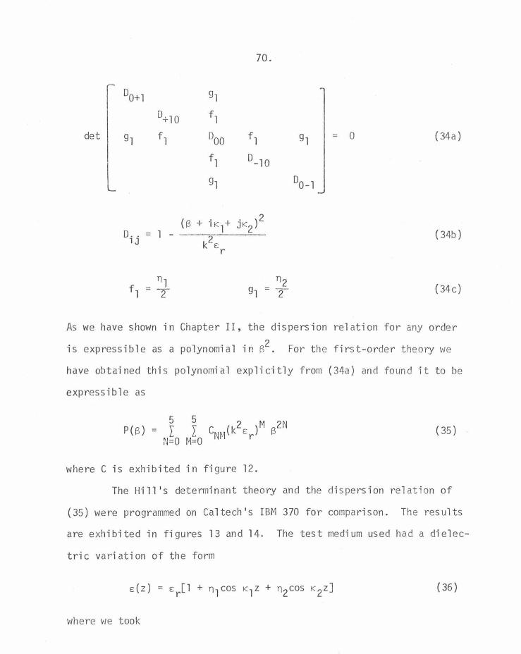
det
L
00+1
0+10
gl fl
D . . lJ
= l -
nl f = - ·
l 2
(S +
70.
gl
fl
0oo fl = 0 ( 34a )
fl o_lo
gl
i Kl+ . )2 JK2
k2£ r
( 34b)
( 34c)
As we have shown in Chapter II, the dispersion relation for any order
is expressible as a polynomial in s2 . For the first-order theory v;e
have obtained thi s polynomial explicitly from (34a) and found it to be
express i b 1 e as
P( S) ( 35)
where C is exhibited in figure 12.
The Hill's determinant theory and the dispersion rel ation of
(35) were programmed on Caltech ' s IBM 370 for compari son. The results
are exhibited in figures 13 and 14. The test medium used had a dielec-
tric variation of the form
( 36)
'rJhere V<Je took

I 1.
l -2
( K~
+
2)
2 -5
.
4 4
2 2
1 +
K2
+ 4
K1 K
2 2
2 4
.(K
1+
K2
) 1
2 2
1 o.-~ c
1 +
c2
)
2 2
2 2
. 4
4 ~2K
1 K 2
(K1+
K2
) -3
K 1 +
3K 2
1 2
2 2
2 ~2K
1 c 2
+ 2
K 2 c 1
3 2
2 -1
o.+
2(c
1 +
c2
)
2 2
-4K 1
K 2 2
2 2
2 -
1 c1
+ K
2 c2
)
4 4
-Kl
K 2 0
4 4
2 2
3K1
+ 3
K 2 -
4K1
K 2 2
2 -4
.(K 1
+K 2
) 3
2 2
5 -~ c
1 +
c2
)
I.
1 4
2 4
2 -
2(K
1 c2
+K2
c1
2 2
2 2
+ K
1 c1
+ K
2 c2
2 2
2 2
-2:
1 K2
(c1
+ c
2))
4 4
2 2
2 2
4 4
2 2
2 2
-1 +
¥ c~ +
c~)
K1 K
2 2K
1 K 2
(Kl
+ K
2)
-(K
l +
K2
-4K
l K 2
) 2(
K1
+ K
2)
1 2
2 2
2 -~
K1
K2(
Kl
C2
l 4
2 4
2 +~Kl
C2+
K2
Cl
1 2
2',
2 2
-~K
l c 2
T2
K 2=
cl
2 2
+ K
2 c1
·')
2 2
2 2
+ 2
Kl
K 2(c
1 +
c2
))
2 2
2 2
+ K
l cl
+ K
2 c2
Figu
re 3
.12.
Th
e m
atri
x of
coe
ffic
ient
s fo
r th
e fi
rst
orde
r al
mos
t pe
riod
ic d
ispe
rsio
n
poly
nom
ial.
-....J
.....
.

CJ CJ :::P
•
CJ a <D
•
CJ •
CJ
0.0
72.
0.800 1.600 2.400
BETR Figure 3.13. A plot of the Brillouin diagram computed from equation (8) for the period ic medium described by E(z ) = Er[l + .5cos2z +
.5cos3z]. The i maginary part of S is the dotted line superi mposed over the stopband regions. The scale of the imagi nary part can be determi ned from
I~( B)IMAv- .2 : n~ (the perturbation theory prediction)

0 0 ::f'
. 0 0 ::
f' .
N r----------.~--------~--------~~
Nr---------~.----,.----.-----.--~~
0 0 (.0
. - 0 0
~~
0 0 .
0
0.0
0.
800
1.60
0 2.
Ll00
REC
BET
R)
0 0 (.0
. - 0 a ~~
a a . 0
IMC
BET
R)
Figu
re 3
.14.
A
plo
t of
the
com
pute
d B
rill
ouin
dia
gram
for
the
alm
ost
peri
odic
med
ium
de
scri
bed
by s
(z)
= sr
[l
+ .
5cos
2z +
.5c
os(3
+o)
z w
here
o
+
0.
The
real
pa
rt o
f B
is
plot
ted
in
(a)
and
the
imag
inar
y pa
rt i
n (b
).
The
scal
e on
the
thr
ee i
mag
inar
y pa
rts
can
be d
eter
min
ed f
rom
Im
(B)!M
AX =
.215
'.J
w .

K = 2 l
K = 3 2
74.
( 37)
It might be remarked that this dielectric constant (36) is periodic
and does not make sense for use in an almost periodic theory. Th e
point, however, is moot as, to computer accuracy, there is no distinc-
tion betvJeen a rational and irrational number. The to.-1o theories, hO\tJ-
ever, do make the distinction automatically as the rationality or
irrationality of the ratio of the perturbation frequencies is inherent
in the dispersion relation derivation. Cl early, the different forms of
the tvw theories indicate that this is certainly the case. We therefore
are allm·Jed to make a direct comparison between tv1o media v1hose differ-
ence the computer cannot distinguish .
One interesting point noticeable on both plots is the greate r
size of the upper, with respect to the lower, bandgap. The ratio be-
tween the two sizes is seen to be close to three halves. There is a
simple reason for this. As can be seen from equation (25) the important
coupling parameter is always expressed per unit length. Because the
wave sees more "bumps" per unit length at the higher frequency, it
coupl es more strongly to th e higher frequency perturbation linearly in
a simple ratio of the frequencies. This result can be seen to be gen
erally true, at least if the perturbations are small, from extended 32-34 coupled-mode arguments presented elsewhere
A few words are necessary on how to read the diagrams. Figure
13 is relatively straightforward as it l ooks much li ke the simple dis-
persian diagram of earlier sections. Figure 14, though, is of a
s 1 i ghtly different form. It is hard to tell a computer ~-vhi ch branch of

75.
a dispersion relation to take, and therefore much eas i er t o have it
plot them al l, which i s wh at was done. We see if we pick the most
centra l root in figure 14, we come very cl ose to match ing the pl ot in
figure 13, and therefore thi s i s the branch we want . We can ma tch
thi s r ea l part with any combination of the complex conjugate imaginary
parts which are plotted separately and with a different scale. All
three imaginary parts are plotted and on sepa rate lines (i. e ., have
different zero points). Th ere is one minor embarras sment though, that
of the l arge imaginary part on root 1 extending right off the diagram.
Thi s i s eas ily exp l ained away , however , as the theory i s no l onger
valid in thi s region on thi s root. The polyn omi al only contains enough
information for the first two bandgaps and the problem bandgap region
1 i es in tile reg·i me of the second 01~ high er orde r theory.
As far as direct comparison i s concerned, apart from the differ
ent plotting format, the res ults of the t\>~o theori es appear to be almost
identi cal for th e gi ven set of paramete rs . Yet ~"e know t hey can't be
identi cal everywhere , as the dispersion relations do differ. Th i s
compels us to take a closer look at the respective dispersion re l ations .
Let us consider the effect of phas ing the tv10 perturbations di f -
ferently, that is to say , let
fl + fl e i <P 1
periodi c ( 38 )
f2 + f2 e i ¢2
fl fl ; ¢1
+ e
almost pe ri od~c ( 38b )
gl + gl e ; cp2

76.
We must perform this inte rch ange, however, in a manner whic~ 1 eaves
the medium loss l ess. \~e find the res ulting determinants can be vJri tten
as
0-2 fl f2
f* D_, fl f2 1 for the det D = det f* 2 f* 1 D
0 fl f2 periodi c ( 39a) case
f* 2 f* 1 Dl fl
f* 2 f* 1 D2
and as
DO-l 0 gl 0 0
0 D-lo fl 0 0 for the al mos t
det D = det g* f* D fl gl periodic ( 39h) 1 1 case 0 0 f* 1 DlO 0
0 0 gi 0 DOl
Direct evaluation of (39 a) leads to a formidable al gebraic equation in-
volving al l combinations and permutations of th e perturbati ons and th eir
conjugates. It would be too much to believe that the expression could
be phas e-independent and indeed it has been shown elsewhere 32 - 34 by
other techniques that it i s not. The evaluation of (39b), though , i s
mu ch s i mp l er and more inst ructive, as can be seen from its form
(40)

77.
Equation (40) is more important for VlhJt it lacks th an for what
it contains , namely the lack of an expli cit dependence on the phas ing
of the perturbations. In some sense the perturbations are i ndepende nt
of one another. Th e only 1vay that they caul d interact is t hrouqh
matrix elements involving Dij" However, in the scheme v.1e have been
using to analyze the interaction where attention is placed on a bandgap
center, the Dijs corresponding to different perturbations shm'i up ex
panded to different orders. To illustrate, cons ider the expansion around
the lowest order where we take
k,rsr
Kl k 1£ + 6k ~ -2 + 6k o r
Expanding the three important D's we find
where
D0 ~ i_ (6k - 6S )
Kl
D_1 ~ i_ (6k + 68 )
Kl
D_2 ~ 4K (6k + 68 ) - 46K l Kl
For validity of the expansion we must have
6k « B 0
6(3 << (3 0
=
=
K
2
K
2
(4la)
(4lb)
( 42a)
(42b)
(42c)
(43a)
( 43b)

78.
Hov1ever, \1/e have in no way specified /:,K , although we can eas ily see
that something fundamental changes wher. t,K is allowed to become the
same order as other parameters in the expansion. I·Je \vould perhaps ex-
pect that this limit will yield part of the information we seek concern-
ing the relation of periodic and almost periodic ~ave propagation, and
we will therefore take up this limit in detail in the next section,
where \"e wish to continue to cons ider the distinctions betv-1een the cases
when the harmonic perturbations are in phase and the bandgap spacing
goes to zero .
D) The /:,K + 0 Limit
1) Need for a New Perturbation Theory
The first necessity in investigating the small /:,K lim"it is to
find exactly how small /:,K mus t be to enter this li mit . 14e know that
this "band spacing" variable must be on the order of the other small
parameters in the calculation, namely t,k and /:,(3 • However, these param-
eters are variable and therefore we need to know their maxi~u~ region
of variation in terms of some other constant . The needed rel at ion i s
easily found from equation (25). It is easily shown 32- 34 that thP.
approximate bandgap width (figure 15) i s given by
Kcentral lAP = K
nKcentra l (44) t,k I ::::: ± x=± 8
(N + i)Kbas i c edges Kcentrall P =
where Kcentral is the average of Kl and K2. It therefore follows that
(45)

kjE
K
2
~K
{3/K
Figu
re 3
.15.
Sk
etch
of
a B
rill
ouin
dia
gram
with
the
im
port
ant
band
coa
lesc
ence
par
amet
ers
indi
cate
d.
The
stop
band
wid
th
is a
ssum
ed
to a
gree
with
th
e fi
rst-
orde
r pe
riod
ic t
heor
y.
-.1
1.
.0

80 .
As can be seen from f i gure 15, the li mit of (45) must corresoond to a
"coalescing" of t he two bands into one, or at l east some kind of over-
1 ap.
Figures 16 and 17 are attempts to delve into the band coalescence
regime e1np loying our almos t period dispersion relation program. Fi gure
16 just s t arts to enter t he interesti ng regime as
= • l ( 46a)
X = nK 07 8 rv. (46b)
Figure 17, hov1ever , although into ti1e band coalescence region, is some-
what disappointing, as th e variation of the band structure is too rapid
for our sorting routine to pick up and much interesting and valuable
informat ion i s los t. In the next sect·ion we will amend t hi s probl em .
Attempts to investigate the pe ri odic band coalescence with our
present program are equally disappointing. In the periodic case we are
forced to fix ~Kat unity and reach our desired l imit by app lying our
perturbations at l arge r and large r mu l tiples of the basic harmonic. But
as the perturbations are placed at the Nth and (N+l)th harmonic we
find the size of the matrix v1hose determinant we must evaluate must be
of order
0( ~) "' 2N +1 ( 47)
for any accuracy to be achieved. But (47) places a restriction on how
large we can reasonably let N become due to the expense of obtaining
the determinant of a l arge matrix numerical ly. As we have taken our

0 0
0 -
0 -
0 I
0 I
. 0
. 0
en r:
I \
I /l
en I
II a:
0
ol~
0 1
-0
u 0
u 0
a:
0 a:
•
u..
. u.
. (!)
(!)
w
w
_
j
_j
a:
a:
u u
(f)
(f)
r l
I I
~
~~l
0 0
~~
('r1
~I/
I SC
ALE
I FR
CT(jR
=
~0
-1
~I I
I EC
RLE
I FRC
TTR
= ~0
-1
0.0
3.
000
6.00
0 9
.000
0
.0
3.0
00
6.00
0 9
. 000
REC
BET
R)
IMC
BET
R)
Figu
re 3
.16.
P
lots
of
the
real
an
d im
agin
ary
part
s of
the
Bri
llou
in d
iagr
am fo
r th
e al
mos
t pe
riod
ic m
ediu
m c
hara
cter
ized
by
~(z)
=
l
+ .
5cos
z +
.5c
osl .
lz.
The
scal
e on
th
e im
agin
ary
part
s ca
n be
det
ermi
ned
from
Im(S
)jMAX
= .1
01

0 0 ...
. 0
I
. 0
en~:
1\
I /l
ol~ ~y
0 u
0 a:
•
lJ_
tD
~~l
/ ~
0 .
0 SC
RLE
FRCT
(jR =
I
I
0.0
3
.000
6.
000
REC
BET
R)
J J J -1
0 9.0
00
0 0 -
ol
ml7 a:
0 olJ
0 u
0 a:
•
lJ_
<D
w
_
J
a:
u (/)
.
Ol
I r
'I
0
~~
(T')
0 0 .
CRLE
.FRC
T(!)R
=
0
.0
3.00
0 6.
000
I MC
BE
TR
)
I J -
1 0 9.00
0
Figu
re 3
.17
Plo
ts o
f th
e re
al
and
imag
inar
y pa
rts
of
the
Bri
llou
in d
iagr
am f
or t
he a
lmos
t pe
riod
ic m
ediu
m c
hara
cter
ized
by s(
z)
= 1
+ .
5cos
z +
.5c
osl
.06z
Th
e sc
ale
of t
he i
mag
inar
y pa
rts
can
be d
eter
min
ed
from
Im(S
)IMAX
= 1.
025
CJ
N

83.
basic period to he unity we see that
nN K basic X = -----.:;;,..=-=._.:.....::_ = 8
nN 8
Taking the reasonable li mit of N = 20, we find that
( 48)
n ~ .4 (49)
to achieve the band coalescence limit. Figures 18 and 19 illustrate the
result for the values
nl = • 3 Figure 18 (50a)
nl = . 5 Figure 19 (50h)
The result i s rather surprising. Instead of t\'lo bands coming
together, we see many bands popping up at both s uper- and sub-harmonics
of the expected ones. But due to the large size of the pertu rbations we
must wonder if this effect is not really due to a breakdown of our per
turbation theory instead of some more physical reason. It is nov1 evident
from figures 16-19 that an improved theory v1ould be desirable for both
the periodic and almost periodic cases, especially if one could be devised
that could reach the band coalescence region without requiring a l arge
perturbation. Such a theory is the subject of the follm·1ing two sections.
2) Almost Periodic Perturbation Theory
Here we ~'/ish first to perform the expansions of equation (42) in
a more symmetric manner . We take the die l ectric constant to be in the
form
(51)

0 0 (Y) .. ~
0 0 ~ .. ~
0 0
~~ 0
0 0 r--.. 0
':> I' u-r.
-0
II
a: D ~ u a: lL
w ..... __J ' a: ' ' u I ({) .I
./
- ...--:-.. \ I
/ ;' _ ...... ....
SCALE FRCTLJA 0 1
0 .. 700 0 .. 900 1 .. 100 1 .. 300
BETR Figure 3.18. Plot of the Bri ll oui n diagram for t he periodic media characterized by
E(z) = 1 + .3cosl9z + . 3cos20z The imaginary part of S is superimposed on top of the stopband regions . The scal e of the imaginary part can be determined by noting that the maximum i maginary part i s
Im(S)IMAX = 7/8

0 0 (r)
• .........
0 0 .........
• ......
0 0
~~ 0
0 0 r-
• 0
-0
II
a: ~ J-u cr: lL
w _J cc u (/)
"\ ,
. .,~ u;.J •
' ' - _ _,!::...
\ I .....
-
"' \ \
\ I ,
I /
---<' " \
I I
/ /
/ --
I
SCALE FRCT(jR
0.700 0.900 1 .100
BETR
0 1
1.300
Figure 3.19. Plot of the Bri ll ouin diagram for the periodic media
characterized by s (z) = l + .5cosl9z + .5cos20z
The scal e of the superimposed i maginary part is determined by
Im( 6) I MAX = 1.4
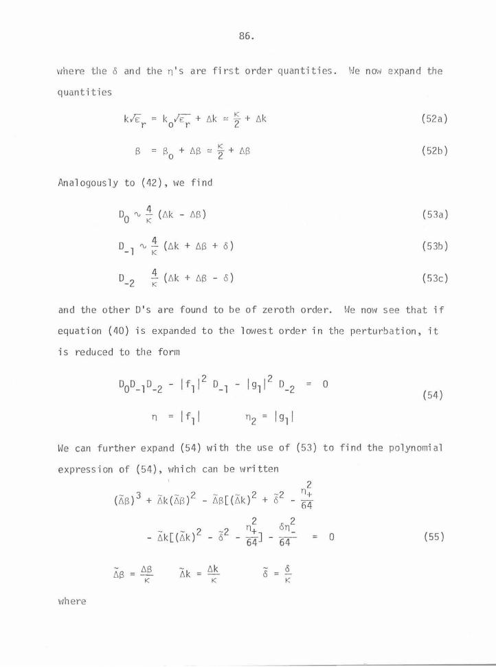
86.
\1/here the o and then ' s are first order quantit i es . \·Je nO'.I/ expand the
quantities
k IE = k 1£ + 6k ~ ~2 + 6k r o r (52a)
(52b)
Analogously to (42), we find
(53a)
o_ 1 ~ ~ (6k + 68 + o) (53b)
i (6k + 6B - o ) K
( 53c)
and the other D's are found to be of zeroth order. ~~e nm" see that if
equation (40) is expanded to the lowest order in the perturbation, it
is reduced to the form
(54)
We can further expand (54) with the use of (53) to find the polynomial
expression of (54), which can be written
v1here
2
( ~8 ) 3 + ~k (~S ) 2 - ~B [( ~k) 2 + 82 - ~~
2 2 2 2 n+ on
- 6k[(6k) - 6 - 64] - 64- = 0
- 6k 6k-K
0 0 - -K
(55)
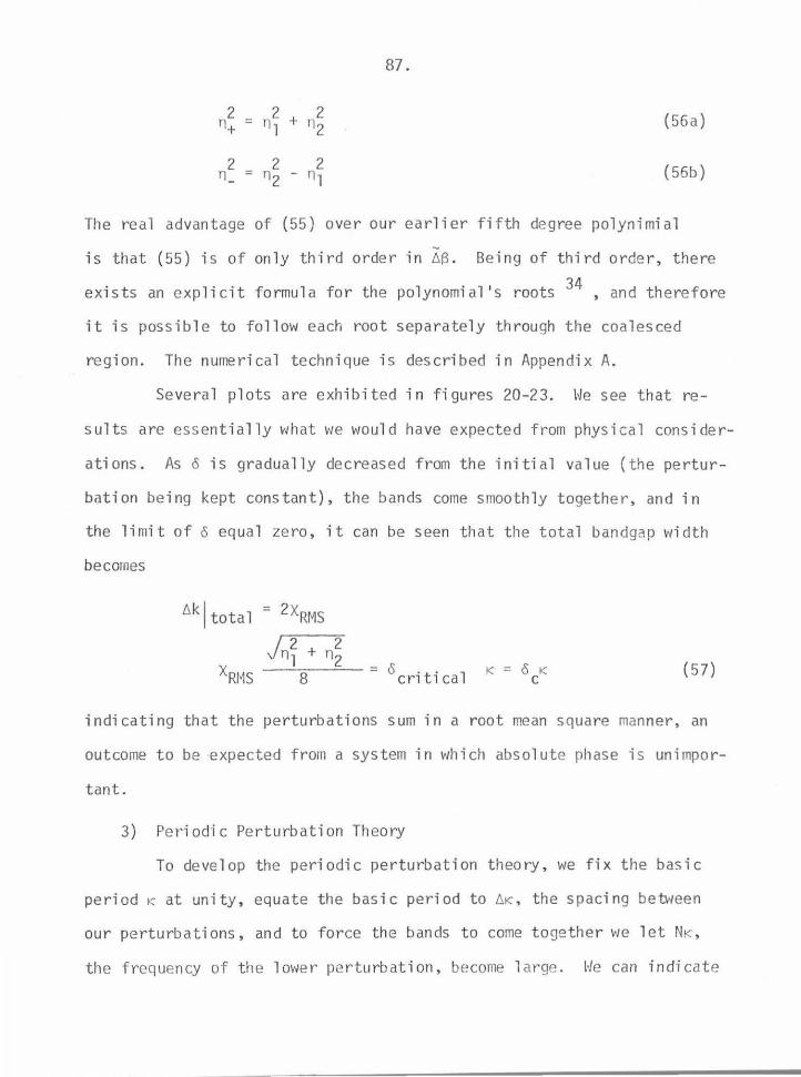
87.
2 2 2 Tl+ = nl + Tl2 (56 a)
2 2 2 Tl = Tl2 - nl (56b)
The real advantage of (55) over our earlier fifth degree polynimial
is that (55) is of only third order in L'l8. Being of third order, there
exists an explicit formula for the polynomial's roots 34 , and therefore
it is possible to follow each root separately through the coalesced
region. The numerical technique is described in Appendix A.
Several plots are exhibited in figures 20-23. \~e see that re-
sults are ess entially what we would have expected from physi cal consider
ations. As o is gradually decreased from the initial value (the pertur
bation being kept constant), the bands come smoothly together, and in
the limit of o equal zero, it can be seen that the total bandgap width
becomes
L'lk I total = 2XRMS
)ni + 2
XRI"lS Tl2
= 0 0 K (57) critical K = 8 c
i ndi cati ng that the perturbations sum in a root mean square manner, an
outcome to be ·expected from a system in which absolute phase i s unimpor-
tant.
3) Periodic Perturbation Th eory
To develop the periodic perturbation theory, we fix the basic
period K at unity, equate the basic period to L'IK , the spacing between
our perturbations, and to force the bands to come together we let NK,
the frequency of th e lov~e r pe rturbation, become l arge . He can indicate

0 0 ::3
' 0
I
~
0
('
CD
CD
.....
~('
CD
C
D . .....
I
0 0 0 .
-ij
0 Ll(
f/
I --
.. --I
· .. _
.-·\
. ~
.ooo
-5.0
00
-1
.66
7 1
.667
REC
BET
R)
0 0 :1
' 0
I
II a::
ID
('I I-
-C
D
U
CD
a:
•
u..
.....
~('
CD
C
D . .....
I 0 0 0 .
w
_J
a:
u (f)
CRLE
.FFlC
TClR
=
I MC
BETR
) Fi
gure
3.2
0.
Plo
t of
the
rea
l an
d im
agin
ary
part
s of
the
Bri
llou
in d
iagr
am f
or t
he a
lmos
t pe
riod
ic m
ediu
m c
hara
cter
ized
by
1 o-3
nl =
n2 =
2/2
I 2
2 -
o j
nl
+ n
2 o
=-
= l.
o =
1.
~ -
K
C
The
scal
e fo
r th
e im
agin
ary
part
can
be
def
ined
by
Im(S
)IMA
X =
4.65
10-
5
----
----~ --
--
0 -L
l
c:
CJ

0 0 ~
o• a
U1
-
L
CD
C
D .
__,
~("'
- CD
C.
D __, I
0 0 0 .
U1 I
VJ
-5.0
00
-1
.66
7
1.66
7
REC
BET
R)
0 -4
5.0
00
0 0 ~
o•
~
0 -=
--
L
CD
C.
D -
~("'
- C.D
C.D
- I 0 0 0 .
U1 I
II a:
0 1- u a:
LJ....
w
_j
a:
u (.()
CRLE
.FFlC
T(jR
=
IMC
BET
R)
Figu
re 3
.21.
Pl
ot
of t
he r
eal
and
imag
inar
y pa
rts
of t
he B
rill
ouin
dia
gram
for
the
alm
ost
peri
odic
med
ium
cha
ract
eriz
ed b
y 1 o
-3
n 1 =
n2
= 2
12
r:2
-:2
-
o I
Tll
T
n2
o =
-=
.7o
= .7
8
K
C
The
scal
e fo
r th
e im
agin
ary
part
can
be
def
ined
by
I -
-5
Im(B
) MA
X =
4.8
~ 10
-------
----
-----
0 -4
co
\.0
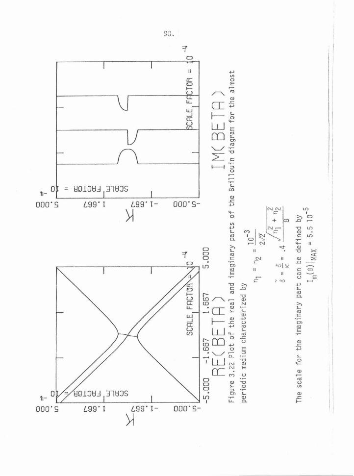
0 0 '=
' a'
~
0
r- CD
C
D . .....
UJ
_.J
a:
u ::::
S::::r-
a (f
)
CD
CD
. .....
I a a 0 .
lf)
-ij
0
a 0 ::
t a'
~
a II cr::
ID
r-1
I-
CD
U
C
D
a:
. ~
.....
::::S::
:::r--
(0
CD
. .....
I a a a . U1
w
_.J
a:
u (f
)
CRLE
.FFIC
TOR
=
I J
I ~------_.--~----~----~--~-------J
-5.0
00
-1.6
67
1
.66
7
5.00
0
REC
BETR
) IM
CB
ETR
) Fi
gure
3.2
2 P
lot
of t
he r
eal
and
imag
inar
y pa
rts
of t
he B
rill
ouin
dia
gram
for
the
alm
ost
peri
odic
med
ium
cha
ract
eriz
ed
by
l o-3
The
scal
e fo
r th
e
n =
n
= --
1 2
2/2
;-_
=2-+
-n-2
o
I nl
n2
0
= -
= .4
--.
..,.
..
K
imag
inar
y pa
rt c
an
be d
efin
ed b
y
Im(S
)IMA
X =
5.
5 10
-5
---
---
---·
--~--
----
0 -l
l
1...0
0

0 0 ~
0 I
L~
0
r (D
(.0
. ..... ·-
~('
(.0
(.
0 .
--<
I 0 0 0 .
Ln
w
_J
cr:
u ({)
0 0 =
' o
'
~
a ~~~.----.....--
II
cr.
0
r-1 1-
(.0
u
CD
a:
• ll-
........
~('
(.0
(.
0 .
........ I a 0 0 .
Ln
w
_J
cr:
u (f)
CRLE
FFtC
HjR
=
I ~----------~----------~----------~~
I ~------~--~----~----~--~------~
-5 . 0
00
-1
. 667
1
. 667
5
.000
REC
BET
R)
I MC
BET
R)
Figu
re 3
.23
Plo
t of
the
rea
l an
d im
agin
ary
part
s of
the
Bri
llou
in d
iagr
am f
or t
he a
lmos
t pe
riod
ic m
ediu
m c
hara
cter
ized
by
-3
10
nl
= n
2 =
212
/2
--2
-
o nl
+ n
2 o
= i<
= o
o c
= o
---'-
- 8.,..--
--
The
scal
e fo
r th
e im
agin
ary
part
can
be
defi
ned
by
Im(S
)IMA
X =
6.1
1 10
-5
I.:)
-J
0 -l
l

92.
this coupling scheme on a schematic Brillouin diagram ana logous to that
of (32), as follows:
which represents the system of equat ions
= 0
n1 n2 Doao + ~ a_N + ~ a-(N+l) = 0
nl D_ 1a_1+ ~ a-(N+l) = 0
= 0
Expanding the D's of equation (59), we find
D ~ 4 (6k + 68 - ~) -(N+l) (N + })K 2
~ 4 (6k + 68 + ~) (N + t)K
(58)
(59 a)
(59b)
(59 c)
(59 d)
(59e)
(60a)
(60b)

93.
0-1 ~ 4
1 (N + 2)K
(llk - liB - K) (60c)
Do ~ 4 (llk - liB ) 1
(N + 2)K (60d)
Dl 4 (llk - ll(3 + K) ~
1 (N + 2)K
(60e)
The rather surprising thing here is t hat all five D's are of the same
order. In fact , in general we can write
D(O ±R.) 4 (llk - liB ± R-K ) ~
1 (N + 2)K (61)
and
D- (N ±R. ) ~ 4 (llk + liB ± {2R.+l) K) 1 2 (N +2 )K
( 62)
R, intege r
The result that the D's fall off only algebraically is indeed disturbing
as it i s not clear how to truncate the general system
0 a = 0 (63)
However, if ~tie arbitrarily cut off t he system (63) with f i ve harmonics as
in (60), we f ind the system (assumi ng N to be very l arge)
liS a, - (llk + K) a, = n2NK -8- a_N (64a)
- llk ao n1NK n2NK
liB a0 =--a + -8- a-(N+l) (64b) 8 N
M3 a_1 - (llk-K)a_1 n1NK
= -8- a- ( N+ 1 ) (64c)

94.
( 64d)
(64e)
which can be rewritten in the matrix fo nn
(D - liS I) a :::CW ::: -
0 (65)
where I is the identity matrix. As (65) is a matrix eigenvalue equation,
we can obtain its solution numerically for any number of harmonics by
simply augmenting the system (64). This \•Je have done and \'Je have plotted
the results in figures 24-28, which shou ld be compared with the results
plotted in figures 18 and 19.
In figures 24 and 25 we use the values of the plots of figures 18
and 19 to obtain a direct comparison. Figures 18 and 24 are rather hard
to compare, as the precise meaning of 24 is not completely clear. The
figure seems to say there are three bandgaps, but they have not yet coal
esced. One probl em with figure 24 may be that the derivation of (64)
requires restrictive assumptions about fiK,perhaps li miting the system's
usefulness to cases in which coalescence has already occurred. In com-
paring figures 19 and 25 we see that this may be the case, as 25 indeed
resemb l es 19 c losely in l ength , however, not so closely in the center fre-
quency. This disagreement in center frequency is perhaps not so severe,
as figure 19 includes the second order e ffects. For the parameters given,
the coupling constant for second order couplings
2 x2 = .!J..Ji '\, . 4 (66)
8
which is indee d quite l arge and could lead to band-center offset. If N

C)
C)
C) •
C)
C)
C) .
~~~-------r----------~------~~
U) ~~------~r-----r-----TT------~~
C)
C)
C) .
N
~C)
C)
C) .
N I
C)
C)
C) .
U)
C)
C)
C) .
N
~C)
C)
C) .
N I
C)
C)
C) • ~
I ~~--------~----------~--------~
I ~~------~----~----~------L--J
-6.0
00
-2.0
00
2.00
0 6.
000
-6.0
00
-2.0
00
2.
000
REC
BET
R)
I MC
BETR
)
Figu
re 3
.24.
P
lot
of t
he f
ive-
harm
onic
app
roxi
mati
on t
o th
e B
rill
ouin
dia
gram
for
the
period~medium c
hara
cter
ized
by
E(z)
=
1 +
n c
os(2
nNz)
+
n c
os(2
n(N
+l)z
)
whe
re n
N =
6.
The
imag
inar
y sc
ale
can
be d
efin
ed b
y Im
(B)IM
AX =
1.
6.0
00
\.')
C:
·1

0 0 0 .
0 0 0 .
U) r-~--------~-----------.-------,--~
U) r-~-------.r-----r-----rT------,-~
0 0 0 .
N
~0
0 0 .
N I 0 0 0 .
U)
0 0 0 .
N
~0
0 0 .
N I
0 0 0 .
U)
I ~~~------~----------
·~--------~~
I L---L-------~------L-----~L-----~L-~
-6.0
00
-2.0
00
2.0
00
6.0
00
-6.0
00
-2.0
00
2.0
00
REC
BET
R)
I ~1C
BET
R)
Figu
re 3
.25.
P
lot
of t
he f
ive-
harm
onic
ap
prox
imat
ion
to t
he B
rill
ouin
dia
gram
for
the
pe
riod
ic m
ediu
m ch
arac
teri
zed
by
E(z)
=
1 +
n(c
os2n
Nz)
+
n c
os(2
n(N
+l)z
) w
here
nN
= 1
0.
The
imag
inar
y sc
ale
can
be d
efin
ed b
y Im
(S)I
MAX
= 1
.84
.
6.0
00
~
Ol

0 0 0 .
0 0 0 .
w r-~~-----.-----------.-------r--~
w r-.-----r---,-----r----~----r---~~
0 0 0 .
N
:::S::::
o 0 0 .
N I
0 0 0 . w
0 0 0 .
N
:::S::::
o 0 0 .
N I
0 0 0 .
I ~--L-----~----------~----~~~~
w I
'
-6.0
00
-2.0
00
2.0
00
6.00
0 -6
.00
0
-2.0
00
2.00
0
REC
BET
R)
I MC
BETR
)
Figu
re 3
.26.
P
lot
of t
he s
even
-har
mon
ic a
ppro
xim
atio
n to
the
Bri
llou
in d
iagr
am f
or t
he
peri
odic
med
ium
cha
ract
eriz
ed b
y £(
z) =
1 +
n c
os(2
nNz)
+
n c
os(2
n(N
+l)z
)
whe
re n
N =
10
The
imag
inar
y sc
ale
can
be d
efin
ed b
y Im
(S)I
MAX
= 2.
18.
6.00
0
\.0
-..
..J

0 0 0 .
0 0 0 .
U) ~~~--~--~-----------r--~--~--~
U)~~---.---.r---,----.~--~---r~
0 0 0 .
N
~0
0 0 .
N I 0 0 0 .
U) I
0 0 0 •
N
~0
0 0 .
N I 0 0 0 .
U) I
-6.0
00
-2.0
00
2.00
0 6.
000
-6.0
00
-2.0
00
2.00
0
REC
BET
R)
IMC
BET
R)
Figu
re 3
.27
. P
lot
of t
he s
even
-har
mon
ic a
ppro
xim
atio
n to
the
Bri
llou
in d
iagr
am f
or t
he
peri
odic
med
ium
cha
ract
eriz
ed b
y £(
z)
= 1
+ n
cos
(2~N
z)
+ n
cos
(2~(
N+l)
z)
\'Jhe
re n
N =
20.
Th
e im
agin
ary
scal
e ca
n be
def
ined
by
Im(S
) lr,I
AX
= 4
.66.
6.00
0
\.0
a:>

a a 0 .
a a a . (0
~~~~~~r-----------T-~~~~~
(0
~r---r---~~~--~--T-~~--~--~~
a a 0 .
N
~0
0 0 .
N I 0 a a .
a 0 0 .
N
~0
0 ~I
I I
N I a a a .
A
I \
J I
(0
I ,
I '
'-'
I fv
cc
Ci
-6.0
00
-2.0
00
2.00
0 6.
000
-6.0
00
-2.0
00
2.00
0
REC
BET
R)
I MC
BETR
)
Figu
re 3
.28.
P
lot
of t
he n
ine-
harm
onic
app
roxi
mat
ion
to t
he B
rill
ouin
dia
gram
fo
r th
e
peri
odic
med
ium
cha
ract
eriz
ed b
y £(
z) =
1 +
n c
os(2
nNz)
+ n
cos
(2n(
N+l
))z
whe
re n
N =
20.
The
imag
inar
y sc
ale
can
be d
efin
ed b
y Im
(8)j
MAX
= 4.
80.
r 6.00
0
'..:
) ._..
.,

100.
could be taken l arger and n sma ll er, the Floquet theo ry miqh! well ~ive
results more co~parable to fig ure 25 .
Figure 26 arises from t he coupling scheme
(67)
Figure 26 i s plagued ~vith the same di seas e as fi gure 24 ; that is to say ,
i t is hard to interpret. It seems to be t elli ng us that more har~onics
are taking part in the interaction but that not al l the bandgaps have yet
coalesced. If we combine the res ults of figures 25 and 26 using this
kind of interpretation, we decide that three bandgaps have coalesced,yet
at l eas t two more bandgaps exist. This interpretati on seems to agree
fairly well with the res ul t of figure 19.
To check if our in terpretation was correct.we raised the perturba
ti on value t o a hi ghe r level given by
X = ~N = 2. 5 ( 68)
and plotte d the seven and nine-harmonic results in figures 27 and 28. The
ni ne-harmonic coupling scheme is given by
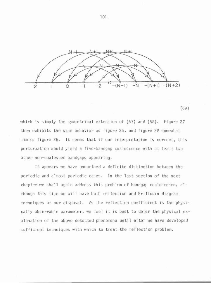
l 01.
2 0 -I -2 -(N-1) -N
(69)
which i s simp ly the symmetrical extension of (67) and (58) . Fi gure 27
th en exhibits the same behavior as f i gure 25, and figure 2R somewhat
mi mi cs figure 26. It seems that if ou r inte rpretati on i s correct, this
perturbation would yield a five-bandg ap coal escence with at least two
other non-coalesced bandgaps appearing .
It appears we have unearthed a definite distinction between the
periodic and a l most periodic cases. In tile last section of the next
chapter .,.,e shall again address this problem of bandgap coalescence, al
though this time we will have both reflection and Bril louin diagram
t echn i ques at our disposal . As the r efl ect ion coeffi cient is the physi
ca ll y observable parameter, we fee l it is best to defer the physical ex
pl anat ion of the above detected phenomena until after we have developed
suffi cient techniques with which to treat the reflection problem.

102 .
Bibliography for Chapter III
l) L. Rrillouin, Wave Propagation ~nd Group Velocity (Academic Press,
New York, N.Y., 1960).
2) J. C. Slater, Rev. t11od. Phys . .?.2_, 473-518 (1948).
3) L. Brillouin, J.A.P. _]2_, 1023- 104.1 (1948).
4) J. R. Pierce, Traveli ng Wave Tubes (D. Van Nostrand Co ., Princeton ,
N.J., 1950).
5) V. L. Ginzburg, The Propagation of Electromagnetic Waves in Pl asmas ,
(Pergamon Press, 14ew York, N.Y., 1970).
6) Perhaps the best referen ces for this are in the '<'iorks of A. Yariv.
See, for instance A. Yariv, Introduction t o Opti cal Electronics
(Rinehart and Winston, New York, N.Y., 1971), 2nd edition, Chapter 13;
A. Yariv, Quantum Electronics (John Wiley and Sons , New York , N.Y .,
1975) , 2nd edition, Chapter 19.
7) C. Kittel, Introducti on to Solid State Physics (John Wiley and Sons ,
New York, N. Y., 1976) 5th edition .
8) Kronig and Penney, Proc. Roy . Soc. Land. Al30, 499 -51 3 (1930) .
9) F. Bloch, Z. f. Phys. g, 555-600 (1 928).
10) L. Bri ll ouin, J. de Physique l· 377-400 (1 930) .
L. Brillouin, J. de Physique l• 565-581 ( 19 32).
L. Brillouin, J. de Physique i • 333-361 ( 19 33) .
J. c. Slater, Phys. Rev. 12_, 794-801 ( 19 34).
ll)
12)
13)
14) L. Bril l ouin, Wave ProQagation in Periodi c St ru ctures (Dover Pub. ,
York, N. Y. , 1953). [Original edition , McGraw-Hi 11 Book Co. , 1946 J.
15) L. Bri ll ouin, J. de Physique 1_, 401-410 (1936) .
New

103.
16 ) See section 1 o f reference (2).
17) Oline r and Hessel, I. R.E. Trans . on A. P., Special Supplemen t, Dec .
1959 , pp. s20l -20 8 .
18) Cassedy and Oline r, Proc . IEEE il· 1342 -1359 (1963) .
19) r·1any sources give good discussions of Bragg ' s law. The one perhaps
most appropriate to the di scussion here is: D. L. Jaggard , Antenna
Lab. Report No . 75 , Caltech (1976) .
20) Abram01-titz and Stegun, Handbook of t1athematical Fun ct i ons (Dover Pub . ,
New York, N.Y., 1970), seven th printing. See equation 4.4.37.
21) J. R. Pierce, J.A.P . e• 179-183 (1954) .
22) J. R. Pi erce, Proc. I RE~. 1389 -1396 (1954).
23) H. Kogel nik, Proc . Symp. Mod. Opti cs , Polytech. Inst., Brooklyn, N. Y.
(March 196 7).
24) H. Kogelnik, BSTJ 48 , 2909-2947 (1969).
25) H. Koge lni k and C. V. Shank , J.A . P. 43, 2327-2335 (1972) .
26) Sakuda and Yariv, Optics Comm. ~, l-4 (1 973).
27) H. Stoll and A. Yari v, Optics Comm. ~. 5-8 ( 1973).
28) A. Yariv, IEEE J. Quan tum Electr. QE-9, 919 - 933 (1973) .
29) A. Yariv and H -\~ Yen, Optics Comm . .lQ_, 120-1 22 (1974) .
30) D. L. Jaggard and G. A. Evans, Ante nn a Lab. Tech. Report No . 73 ,
Ca ltech (1975).
31) A. Yariv and A. Gover , App l . Phys. Lett . ~. 537-539 (1975).
32) D. L. Jaggard and C. Elachi, JOSA 66, 674-682 (1976) .
33) D. L. Jaggard and C. Elachi, JAP 48 , 1461 -1 466 (1977).
34) D. L. Jaggard, App1. Phys. (Springer-Verlag) ll_, 185-1 95 ( 1977) .
35) See reference 20, equation 3.8.2,

104.
CHAPTER IV
The Reflection Coefficient
Although the di scussion of the l ast chapter yielded information
concerning the differences between periodic and almost periodic \1/ave
propagation, the information was always contained in a Brillouin diagram.
The problem i s nm'' that v-1e have no experi mental technique to measure a
Brillouin diagram. Although \'Je feel that quantities on the Bri llouin
diagram relate to physically measurable parameters, such as the imaginary
part of the bandgap telling us about the relative magnitude of the reflec-
tion coefficient, we have no firm tie-in. This chapter will attempt to
mitigate this uncertainty by first considering the reflection coefficient
in some depth and then developing a technique to find the reflection coef-
ficient from the same eq uations with which we found the Brillouin diagram
in the l ast chapter .
i~e begin the discussion by reminding the reader of some elementary
considerations concerning reflection coefficients and perturb ation expan-1
s ions, essentia lly at the level of Morse and Feshbach. This discussion
is designed to point out the problem of secularity in perturbation expan-
sions, a problem which must later be overcome to obtain physically
acceptable results for the reflection coefficient.
A) Standard Perturbation Theory for the Reflection Coefficient
l) Setting up the Exact Boundary Value Problem
Figure l defines the parameters and regions of the probl em . l..Je begin
by writing the fields separately in each region:

CD
, TW
O-T
ON
E
ALM
OS
T P
ER
IOD
IC
/ /)
L/A
B/ /
Ld
z =
-..e
..e --
_..
_r-J
2 ..e
z=+
2
C3)
Figu
re 4
.1.
Sket
ch o
f th
e lo
ngit
udin
al
geom
etry
whi
ch d
efin
es t
he r
efle
ctio
n-co
effi
cien
t pr
oble
m.
Reg
ions
1
and
3 w
ill
be c
onsi
dere
d fr
ee s
pace
in
fur
ther
con
side
rati
ons.
_.
0 (.,I

106.
Region l
w = eikz + Re-ikz (l)
Region 2 iNKl Z + Hk2z .
6 \ + e e , z + L aNt~
N,M
Region 3
(3)
Note that we have assumed the almost periodic solution of Chapter II to
be valid in region 2.
Before equating the values and derivatives of w across the bound-
aries, we must r educe the numb er of constants in region 2 through use of
the dispersion relation. As w sati s fies a second-order differential
equation, only two of the doubly infinite number of constants must actu-
ally be arbitrary. vi e proceed by solving the determinantal equation of
Chapter I II,
det D = 0 (4)
2 for the doubly infinite set f3 .. • As discussed in Chapter II, for each 1 J
value of 6, we can back-s ubstitute into the equation
D a = 0 (5)
and obtain the a's as a one-parameter string, say in terms of a00as
as (6)

107.
Say that for each of the positive (negative) roots of (4) we carry out
the procedure indicated by (5) and (6), denoting the free parameter by
a~0 (a00 ). We then find the field in region 2 to be expressi b le as
+ i(NKl+ ~k2 )z i (3 .. z tjJ = aoo I I gNt•l( Kl ,K2 ,w) I e e 1J
i , j N, ~~1 +(3 .. 1 J
i(NKl+ MK2
)z -i B . . z
+ aoo I I gNM(Kl , K2 ,w) 1-13 .. e e 1 J (7) i , j N, 1'1
1 J
l~e have reduced the boundary value problem to four equat ions (continuity
of tjJ and its first de rivative across two boun daries) in four un kno~tms
+ -(a00 ,a00 , Rand T). Howeve r, the sheer compl exity of the system renders
exact solution impossible. The need for some perturbation theory i s evi-
dent.
2) Born-Neumann Series
Perhaps the most straightfonvard perturb ation scheme to apply i s
that of Born 2 and Neumann 3 If we expand ljJ in our wave equat ion
2 k2 e: tjJ =
k2 e: r Q, <! ( 8) _ d_ ljJ + - - < z --- AP(z) tjJ 2 2 di r 2
where AP(z} is an almost periodic function in terms of the parameter n,
and pick off the first order reflection coefficient R, "vie obtain the fami-
1 i ar form
i n k IE R(k~)-- 4 r r
8, [AP(z) rect(y- ~)]
13, = _2k~ (9)
where

108.
00
J e-i S' z f(z) dz (10)
~Je have found this Fourier trans form property to be a more general oroperty
of scattering than before stated in the literature, and in Appendix B we
show it to be true for three dimensional scattering in very general con
stitutive media. However, in spite of the generality, simplicity and
invertibility of this res ult, we Y.lill presently show it i s not of much
practical interest in our case.
3) Secularity of Born-Neumann Series at Bragg Resonance
Consider the s impl est of almost peri odic functions (periodic func
tions being a subc l ass)
AP ( z) = cos K Z ( ll )
A simpl e computation with (ll) yields the result, noted elsewhere J , that
i kre;: 4
sin(k/E +~)51. s in(k/E- -2)t [----r _ _ c._ + r ]
kre;: + f)$1. (kre;: - f)t
If we investigate the maximum of this equation, which occurs for
k~ = K
2
the longitudinal Bragg condition, we find
i nk/E . n R (~) = ---:-..:...r_ _ 1 nK;v 2 4 --8-
( 12)
( 13)
a most disconcerting result. The maximum value increases 1 inearly in both
the frequency and the l ength of the medium, not just in the perturbation.
It is as if we expanded in the quantity nkt instead of n an effect

109.
commonly termed secularity 6 . It appears we are stuck vlith a th eory
that breaks down as soon as we reach th e regime of interest v1here there
is strong wave-medium coupling.
It is easy to check that the problem does not improve in the
almost periodic case. Nor does it really improve by use of the various
renormalization t echniques 7 designed to remove secular terms, as the
increase in complexity leads to no certain increase in accuracy 8
Further, the method is not des igned to sho1<1 any difference between
periodic and almost periodic media. Clearly a new theory i s required.
B) The Electromagnetic Riccati Equation
Tile first and perhaps most basic result of the technique of i nvari
ant imbedding is that of the Riccati equation for the electromagnetic
reflection coefficient . This section is intended not only to introduce
the reader to th e basic precepts of this technique, but also to deve lop
and discuss this exact reflection coefficient equation .,./hose numerical
so lution we shall l ater emp l oy. \~e begin with a bri ef hi storical perspec
tive on the invariant imbedding technique.
1) Invari ant Imbedding--Historical Perspective
The invariant imbedding techniq ue was firs t applied by Sir George
Gabriel Stokes in an 1862 work 9 considering the propagation of l ight
through a striated medium. Some fifty years later, Lord Rayleigh l O,l l
somewhat extended the technique in investigations of a simi l ar problem .
H. ~~- Schmidt 12 vJas the first to continuously vary the length of a
medium rather than s impl y add a discrete s lab as had Stokes and Rayl eigh.
In spite of Schmidt 1 s 1907 study of 6-decay, howeve r, the first

110.
generally recognized work of invariant imbedding is that of V. A.
Arnbartsumian in 194513 . In this work as in his 1958 treatise14 ,
Ambartsumian employed the invariant imbedding technique to develop a
theory of radiative transfer. Although Ambartsumian's work stimulated
certain workers in the West15 , it was Chandresekhar's unifying treat
ment in his 1960 book16 on radiative transfer that brought the concept
to a research forefront. Coupling Chandresekhar's book with the earli
er developed functional equation techniques of Redheffer17 , various
workers in mathematics and physics then solved a plethora of problems
in numerous areas as evidenced by the reference li sts in recent books18
on the topic. Of the numerous references on the topic we have found
that of Bellman and Wing19 to be the most useful and in most of what
follows we adhere some\vhat to their notat ion and conventions .
2) Stokes Recursion Relation and the Conservation of Energy
It was prior to the publication of Maxwell's electromagnetic
theory20 that Stokes solved the problem of wave propagation in a
layered medium. He considered a geometry similar to that of figure (2)
and was armed essentially only with the Fresnel relations (refer to
figure (2b} for directional definition)

(a)
nr
I nr
-1
nl
no
Rr+
l R
r Rr
-1
Rz
Rl
--
l+-~
r-*'
"~r-
1+1
r--~
1 .. ,
.. ~0~
(b)
ni+
I nr
rr
rr'
tr
I
t r'
Figu
re 4
.2
a)
Sket
ch o
f th
e sl
ab g
eom
etry
ori
gina
lly
solv
ed b
y St
okes
. b)
Sk
etch
of
the
defi
niti
ons
of t
he F
resn
el
coef
fici
ents
.
__.
__.
__.
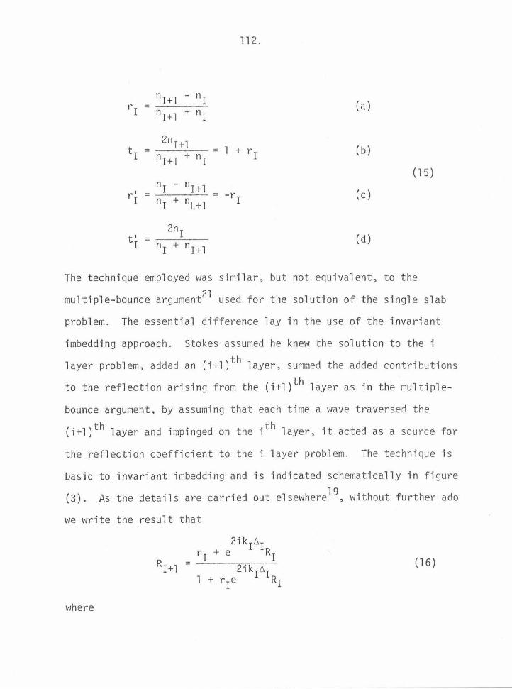
112.
ni + l - ni rl =
ni+l + ni (a)
tl 2nr + l
= l + rl = nl + l + ni
(b)
( 15)
r' nr - ni+l
= -r I ni + nl+l I (c)
t' = 2ni
I ni + ni+l (d)
The technique employed was simi l ar, but not equivalent, to the
multiple-bounce argument21 used for the solution of the single slab
problem. The essential difference l ay in the use of the invariant
imbedding approach. Stokes assumed he knew the solution to the i
layer problem, added an (i+l)th layer, summed the added contributions
to the reflection arising from the (i+l)th layer as in the multiple-
bounce argument, by assuming that each time a wave traversed the
(i+l)th layer and impinged on the ith layer, it acted as a source for
the reflection coefficient to the i layer problem. The t echni que is
basic to invariant imbedding and is indicated schematical l y in figure
(3). As the details are carried out elsewhere19 , without further ado
we write the result that
( 16)
where

(a)
(b)
__., --
Rr
I LA
YER
S R
I+II
I +
I LA
YER
S ---
(c) I
LA
YE
RS
etc
~6r--.j
Figu
re 4
.3
Sche
mat
ic
illu
stra
tio
n o
f th
e in
var
ian
t im
bedd
ing
tech
niqu
e as
app
lied
to
the
stri
ated
med
ium
pro
blem
. a)
Th
e as
sum
ed s
olve
d i
laye
r pr
oble
m,
b)
The
(i
+ 1
) la
yer
prob
lem
to
be s
olve
d, c
) Th
e kn
owns
an
d un
know
ns
used
in
the
sol
utio
n.
-'
w

114.
~0 is the fre e space wavelength .
The recursion relation (16) is sufficient to solve the problem given
some initial condition such as
Further, as Fresnel's formulas are rigorou sly derivable from Maxwell' s
equations, equation (16) represents an exact soluti on to the propaga-
tion problem.
Of primary interest in this is the property of non-secularity
and/or energy conservation. As (16) is an exact solution to a propa-
ga t ion problem, somehow it should include energy conservation. To
indicate that this may be the case, we cons ider the following argu
ment. If at some interface I the reflection coefficient has a magn i
tude of unity and some phase angle ~ . we find that at the next inter-
face
2ik 1 t~ 1 ei ~ + -2i k 1 t~ 1
RI+l r 1e
= i¢ ' ( 18) = e 2ik 1 t~ 1 i ~
e 1 + r 1e e
where ~ · is some new phase angle. The argument indicates that t he
reflection coefficient can never exceed the value one, and indicates
that (16) certainly has the attributes of energy conservation, as it
should.
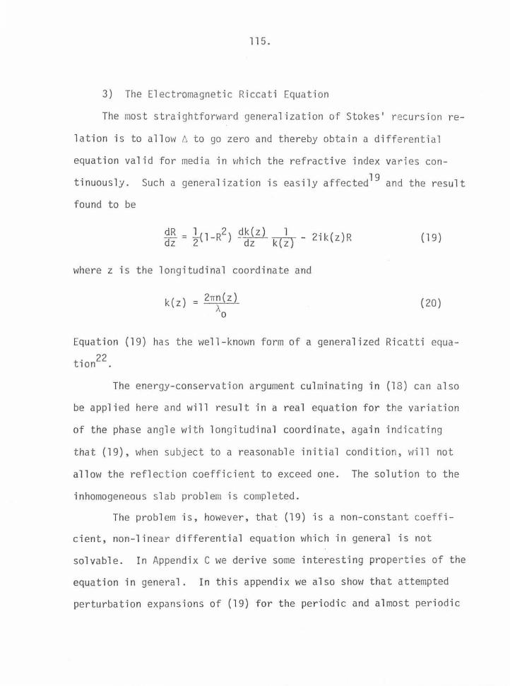
115.
3) The Electromagnetic Riccati Equation
The most straightforward generali zation of Stokes 1 recursion re-
l ation is to allow 6 to go zero and thereby obtain a differential
equation valid for media in ~1hich the refractive index varies con
tinuously. Such a generalization is easily affected19 and the result
found to be
dR = *<l-R2) _9k(z) nh- 2ik(z)R dz 2 dz k~z 1
where z is the longitudinal coordinate and
k(z) = 2nn(z) Ao
( 19)
(20)
Equation (19) has the well-known form of a generalized Ricatti equa-
t. 22 1on .
The energy-conservation argument culminating in (18) can also
be applied here and will result in a real equation for the variation
of the phase angle with longitudinal coordinate, again i ndicating
that (19), when subject to a reasonable initial condition, will not
allow the reflection coefficient to exceed one. The solution to the
inhomogeneous slab problem is completed .
The problem is, however, that (19) i s a non-constant coeffi-
cient, non-linear di fferentia l equation which in general is not
solvable. In Appendix C we derive some interesting properties of the
equation in general . In this appendix we al so show that attempted
perturbation expansions of (19) for the periodic and almost period ic
116.
cases contain first-order secul ariti es and are therefore of little
use. Essentially, the only way to solve (19) or (16) is n u~erically.
This we have also done and found the solution to (16) to be consider
ably faster for comparable accuracy.
Armed with a numerical solution, one might think the problem
is completed: only spec ific cases need be run off to compare the
two solutions whose difference is our primary concern. This is not
true for two reasons. First, the computer program becomes exces
sively expensive to run when more than a few periods of the dielectric
constant are included in the medium, yet to find any difference be
tween periodic and almost periodic media at all it is necessary to
include many periods, lest the phase between the 11 bumps 11 be rela
tively unimportant. Second, small numerical round-off errors will
cause an almost periodic equation to appear essentially periodic, at
least for small numbers of periods, which is to say that there is no
provision in the Riccati equation or computer to differentiate the
cases. Although the Riccati equation is a powerful tool in checking
perturbation solutions in its own regime of validity, it is not the
definitive solution to the problem. However , as we shall see in the
next section, in the derivation of the el ectromagnetic Riccati equa
tion, i.e., the technique of invariant i mbedding, lie the seeds of a
method to both circumvent the problem of secularity and further
illustrate the difference between periodic and almost periodic
structures.

117.
C) A Generalized Look at Invariant Imbedding
In this sect ion we wi ll generalize an argument due to Bell man
and Wing19 in two ways. First, we shall make the derivation appli
cable to arbitrary numbers of forward and back\-Jard waves , allowing
the resulting system of equations to fit the form of the coupled
equations we derived in the last section of chapter III. Secondly,
we will apply general i zed energy-conservation criteria to the char
acteristic parameters of the problem to deduce under what conditions
we can be assured of a unitary (energy conserving) solution.
1) First-Order Wave Equations from Particle Counting
Consider the diagram of figure (4). We wish to obtain the
"particle flux" (fi eld flow) t hrough the medium in terms of fo rward
and backward moving streams. We wil l assume that there are M dis
tinguishable states (modes) moving to the right, generically denoted
the forward wave, and N distinguishable states (modes) moving to the
l eft, generically denoted the backward wave. The physical situation
could be that of particles with spin moving down an accelerator, or
that of energy being propagated through a ribbed mul timode f i ber-optic
waveguide. The anisotropy between forward and backward waves could be
due to a magnetic field in the accelerator, or an anisotropic ribbing
structure in the li ghtguide. Whatever the situation, we wish to con
sider the change in the forwa rd and backward waves as they traverse a
tiny distance ~ in the medi a, a quantity which is later allowed to go
to zero . First, let us consider the contributions to the forward

F(z
) ~
B (z
) ~ - -
L
-- 2
- -F
(z+
6)
~
-- -
- - B(z
+6
) ~
z z+
6
J4--6~
Figu
re 4
.4.
The
long
itud
inal
ge
omet
~ fo
r so
luti
on o
f th
e M
forw
ard
mode
, N
bac
kwar
d m
ode
pro
blem
.
__.
w
L
- 2

119.
wave which l eaves our test region at z+~ . Certainly, it receives
a contribution from the impinging forward wave at z,which we shall
write in the form
1st contribution = (fM + i ~ F~ )~(z) ( 21 )
where !M i s the MXM identity matrix and ~F an MXM matr ix whose real
part denotes phase shift per unit l ength and whose imaginary part de
notes medium gain or loss per unit length. Note that in equati on (21)
we have only considered quantities of first order in ~ in anticipation
of a later limit. We have sti ll to include the contribution from the
backward wave impinging on z+~ from the l eft which gets backscattered
in traversing the infini te-s i ma l slab. Thi s contributi on is denoted
by
2nd contribution = i ~FB~ ~(z+~) (22)
where ~FB is an MXN matrix whose el ements denote the amount of each
backward wave component to get scattered into each forward wave com-
ponent. We also note at this point that
B(z+~) = B(z) + 0( ~ ) (23) - -where the 0 function indicates that any additional terms go to zero
at least as fast as~. Summing the contributions of (21) and (22)
with the use of (23) we find
(24)
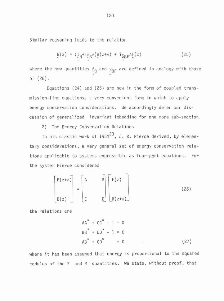
120.
Similar reasoning leads to the relation
(25)
where the new quantities ~B and ~BF are defined in analogy with those
of ( 26).
Equations (24) and (25) are now in the form of coupled trans
mission-line equations, a very convenient form in which to apply
energy conservation considerations. We accordingly defer our dis
cussion of generalized invariant imbedding for one more sub-section.
2) The Energy Conservation Relations
In hi s classic work of 195423 , J. R. Pierce derived, by elemen
tary cons iderations , a very general set of energy conservation rela
tions applicable to systems expressible as four-port equations. For
the system Pierce cons idered
F(z+L-.) A B F(z)
= (26)
B(z) c D B(z+L-.)
the relations are
* AA + cc * l 0
* * BB + DD 1 = 0
* * (27) AB + CD = 0
where it has been assumed that energy is proportional to the squared
modulus of the F and B quantities. We state, without proof, that

121.
the great generality of the derivation allows us to take the sys tem of
(26) and (27) directly over to a matrix case, or more specifically,
for the generalized four-port system
~(z+6] .....
B(z)
(28)
where F is an M vector and B an N vector, the energy conservation
relations can be written
* * A A + c c - !M = 2Mt1 (a) -*- - *- -B B + D D IN = 2NN (b) (29) - *- -*-A B + C D = 2MN (c)
where the definitions are as in (24) and (25), i.e., £J-,1N is the ~1XN
zero matrix, with the exception of the asterisk which here denotes
Hermitian transposition.
We note here that the system (28) is of equivalent f orm to our
system of (24) and (25) and therefore that (29) applies as well to
(24) and (25) . We now want to find what constraints (29) i mposes on
our propagation matrices if the system of (24) and (25) is to conserve
energy. We note, however, that the conditions of (29) need only be
satisfied to first order in the parameter 6 as the system of (24)
and (25) is only correct to this order in 6 . Bearing thi s in

122.
mind we note that for the identities
(a)
(b)
(30)
C = i ~BF b. (c)
D = I + i98 b. - - N ·-(d)
we find
(a)
(b)
(c)
( 31) (d)
* A B = i fl~FB (e)
* * C D = -i !J.~BF (f)
With the substitutions of (31) in (29), we find our energy conserva-
tion relations are
* ~ F - ~F = 2~1M (a)
* ~B - ~B = 2NN (b) {32)
~BF - ~FB = 0NM (c)

123.
We find that energy conservation dictates the reality and symmetry
of the t. ' s and a Herlilitian transpose equality of the x ' s . \·le vrill
later see that these relations do hold for our coupled-propagation
theory derived from the dispersion matrix.
3) Invariant Imbedding of Coupled Equations
We now wish to transform our system of (24) and (25) to a set of
differential equations. The change is easily effected as we need onl y
rewrite (24) and {25) in the form
F(z+t. ) - F(z) - - = i ~ F F(z) + i ~FB B(z) t.
B( z+t.) - B(z) = i ~ B ~(z) + i ~ BF F(z) t.
and take the limit of t. going to zero to find
dF( z) dz
dl3(z) dz
= i ~ F F(z) + i ~FB B(z)
= i ~B ~(z) + i ~BF ~(z)
(a)
(b)
(a)
(b)
In general our boundary conditions will take the form
where
t F(- .,-) =e. - t:. _ ,
t B(- ) = 0 - 2 -
... , .... A th component e~ = [0,-----, 0, 1, 0,----, OJ
1
corresponding to the situation in figure (4) where only one
(33)
(34)
(35)
(36)

124.
distinguishable wave would be impinging on the slab from the left and
no other source in the problem. Such two point boundary value
problems can be solved by a straightforward, yet arduous a"d usually
numerical, technique. This technique and its growth in complexity
with the order of the system are described in Appendix D. What we
wish to do here is to apply invariant imbedding and reduce the reflec
tion coefficient problem to one of the initial va l ue type .
Consider the diagram of figure (5). The diagram is very similar
to that of figure (3), the geometry that Stokes9 considered, with one
basic difference: ~ is now a continuous and not a discrete, variable.
The case here is equivalent to that considered by Schmidt12 in which ~
is at first considered smal l and later allowed to go to zero. Figure
(6) schematically illustrates the procedure of the calculation. In
(a) a source is incident on the added thickness of slab. This extra
slab immediately backscatters an amount given by the term in x written
to the left of the slab, and passes an amount given by the term in
~F written to the right of the slab. The term on the left
1st contribution = i~FB ~ (37)
is seen to directly contribute to the reflection coefficient as that
wave is lost to the system. The amount passed, however, is not lost
to the system but in fact acts as a source for the original slab
problem whose solution we have assumed is known. For this reason,
the ~F term returns to our considerations in (b) where the portion
of this secondary source

SOU
RCE
* ...
R(x
) "-J
"-J
(a)
~
X
•I
SOUR
*
(b)
CE ...
~(x+
6)
v R
(x)
"-J
~
"-J
-
---.{
6 14
X
•I
Figu
re 4
.5
The
inva
rian
t im
bedd
ing
geom
etry
for
sol
utio
n of
the
M fo
rwar
d m
ode
, N
bac
kwar
d
mode
pr
oble
m in
ter
ms
of
the
matr
ix r
efle
ctio
n co
effi
cien
t.
_,
N
C... I

s *
(a)
(b)
(c)
... ,
I (I
+i8
F6
) R(x
) (I
+i8
F6
)R(x
)
l+i8
F6
X
iX
8F
6R
(x)
X i
X8
F6
R(x
)
iXF
s6
l I
(I +i~
6) R
(x) J
x (I
+ i8
86
)
J(I+
i8F
6)
R(x
)
X (
I+i8
86
) I
I(I+
i8F
6)
I I
R(x
) iX
8F
6
~6~
14-.
6_--
.j
l<r-6~
1st
2n
d
3rd
PASS
PA
SS
PASS
Fi
gure
4.6
Sc
hem
atic
il
lust
rati
on o
f th
e so
luti
on o
f th
e in
vari
ant
imbe
ddin
g pr
oble
m w
here
th
e thickness
~ is
ass
umed
to
be s
mal
l.
The
2nd
and
3rd
pass
es a
re d
ue
to t
he t
ran
smit
ted
ener
gy o
f th
e fi
rst
pass
act
ing
as a
pum
p so
urce
for
the
11no
n-au
gmen
ted
by ~
~~ pr
oble
m.
__,
N
C"'l

127.
which passes through the extra slab, i s seen to directly contribute
to our reflection coefficient while the back reflected portion acts
as a tertiary source for the original slab. In (c) we note that this
tertiary source contributes an amount
to the reflection. We could continue this summi ng process ad infini
tum, but realize we already have more than we need as we are ex-
panding only to first order in 6. Ignoring the higher order terms in
~. we find that our expression can be written in the form
8(z + ~) - §(z) 6
+ i ~(z) ~BF ~(z)
which in the limit of vanishing ~ becomes
dR(z)
dz = i ~FB + i( ~F~(z) + ~(z) ~B) + i~( z)~BF~(z)
The assoc i ated initial condition would be
R(z = 0) = 2MN
if the media to either s ide of the s lab were equiva l ent .
(40)
(41)
(42)
A few words are necessary here about having a matrix reflection
coefficient. In measuring reflection in general we measure at best

128.
a vector, corresponding to distinguishabl e backward modes. But here
we have derived a matrix reflection. The explanation is simple
though. If we consider the i, j component of R we realize it denotes
the amount of wave exiting in the jth backward mode, given the ith
forward mode was incident. The vector we would therefore measure is
r* = F~ . t. 1 R ~lnl 1a ~
where ~initial should be normalized such that
F~ . t . 1 F . . t . 1 = l ~ 1m 1a - lm 1a
Therefore, if we measure only the total refl ected energy, the
quantity we mea sure would be
r* r = ~initial ~ ~* ~initial
(43)
(44)
(45)
A few words are necessary here about what we have actually
achieved. In (41) we have a non-linear differential equation fo r a
matrix, a very complicated system to solve analytically. The
achievement however lies in the fact that (41) has constant coef-
ficients in the cases whi ch we will presently consider. This is an
extremely desirable improvement over the electromagnetic Riccati
equation as we are no longer limited to some number of periods inside
the medium in a numerical solution, as the addition of more periods
simply causes the redefinition of one of th e constant coefficients of
a numerically stable system. We have succeeded in applying a per-
turbation theory to our original problem, which both simplifies the

ELE
CTR
O
MA
GN
ETI
C
RIC
CA
TI
EQ
UA
TIO
N
PU
RTU
R!B
ATI
ON
E
XP
AN
lSIO
N
SE
CU
LAR
TH
EO
RY
INV
AR
IAN
T
IMB
ED
DIN
G
EQ
UA
TIO
NS
O
F M
OTI
ON
PE
RTU
RtB
ATI
ON
E
XP
AN
SIO
N
SE
CU
LAR
TH
EO
RY
PA
RT
ICLE
CO
UN
TIN
G
CO
UP
LED
M
OD
E
EQ
UA
TIO
NS
I NV
AtR
IAN
T
IMB
E D
OIN
G
UN
ITA
RY
TH
EO
RY
Figu
re 4
.7
Cha
rt i
llu
stra
tin
g t
he v
ario
us p
ertu
rbat
ion
sche
mes
em
ploy
ed i
n so
lvin
g th
e re
flec
tion
coe
ffic
ient
pro
blem
in
alm
ost
peri
odic
med
ia,
and
thei
r ou
tcom
e.
The
only
ro
ute
endi
ng i
n a
unit
ary
theo
ry i
s th
at o
f co
uple
d m
ode
equa
tion
s w
hich
are
onl
y ob
tain
ab
le
in a
lmos
t pe
riod
ic m
edia
.
~
r-:>
\:)

130.
method of solution and preserves the unitarity of the theory. We
schematically illustrate our approach and the approaches that fail in
figure 7. More will be said on this in the next section where we
will apply (41) to some systems of Chapter III.
D) Riccati Equations, Brillouin Diagrams and Dispersion Matrices
1) Single Harmonic Perturbation
Before considering the case of bandcoalescence, we wish to
apply our technique to the simplest problem we know, that of a single
harmonic perturbation. The schematic Bri llouin diagram for this
problem would be
representing the set of equations
where
dF + i oF = i xB dz
~ + ,· s:B = . F dz u l X
0 = t.k
X _ nK -8
(a)
(b)
(a)
(b)
(46)
(47)
(48)
where the notations of Chapter III have been used. We note here
that indeed the system of {47) satisfies the criteria of (32). To
find the r eflection coefficient we can immediately employ the
Riccati equation (41), which now takes the simpl e form

131.
~~ = ix (l + R2) + 2i oR (49)
where the identifications of (48) apply. Equation (49) ha s constant
coefficients and can therefore be solved by quadrature
R dr z
~ = ~ dz . 0 ix(l + R2) + 2ioR 0
(50)
The integral on the left hand side is available in Gradshtein and
Ryzhik's manua1 24 and, with some algebraic manipulation, the
resulting equation can be inverted to yield
R(z) i x
= =o -c-o ·;-rt h-(.,.o--z,..) - ---:-i -;:;-o (51)
where
(52)
The result (51) is a familiar one from the literature25- 26
where it has been obtained by solving the coupled-mode two-point
boundary value problem. It has also been shown elsewhere25- 26 that
(51) gives a very good prediction of experimental results, and
further that the half-width of the main lobe i s very close to the
width of the bandgap. In Appendix E this result is compared with
that of the exact Riccati equation.
2) The .n.lmost Periodic liK-+0 Solution.
We next reconsider a problem from the l ast section of the pre
vious chapter, which can be represented by

132.
(53)
O.P.
where O.P. abreviates operating point and is used to indicate that
we are expanding about this point. The schematic (53) represents
the system
dF i o F = i( x1B1 + x2B2) (a) dz - 0
dB1 i o+Bl i x1F (b) (54) - dZ- :::
dB2 i 0-82 i x2F (c) - dZ- :::
where
0 ::: 6k 0 (a)
(55) 0 = 6k ± ± 6 {b)
and
x, = T] l K (a) 8
(56) T')2K
{b) x2 =a and
Kl + K2 {57) K :::
2
The notation employed here is just that of the l ast section of
- - - --------

133.
Chapter III except for 6 replacing o of Chapter Ill. Again we can di-
rectly employ the Riccati equation of (41), providing we make the
identifications
~F = 00 (a)
=[:+:_] (58)
~B (b)
and
XFB =[~~ (a)
(59)
XBF = [x1x2J (b)
We note at this point that (58) and (59) do indeed satisfy (32), the
Pierce energy-conservation criteria. The resu lting set of reflection
coefficient equations can now be written out explicitly and are
found to be
(60)
dR dz 2
= i x2(1 + R22 ) + i( o0 + o) R2 + i x1R1R2
We are not in so fortunate a position with equation (60) as we
were with equation (49) as although (60) has constant coefficients,
it is no longer integrable by simple quadratures. However we pro
grammed the system of (60) in a program called "Criccatti 11 and will

134 .
now present some of the results.
Figures (8) and (9) represent solutions of the system (60) for
parameters given by
KQ, = 8.1 o3 (a)
n, = 12 1 o-3 112 = 12 1 o- 3 (b) ( 61 )
X Q, -l - n x2Q. = 12 (c)
oQ. = {7. oc' 4 . o c } = {7 ./x 12 +x l , 4 .lx} +x l } (d)
i .e. , the widely spaced perturbation limit. It is notable that in
this limit the results appear much as the result of two independent
s ingle perturbation solutions (cf. APPENDIX E) patched togeth~r
might appear. From the co ns iderat ions of Chapter III we would
assume this would be the case.
In figures (10)-(13) we plot a sequence of graphs for constant
(62)
while varying oQ. through the values
oQ. = 2. oc = I 2 2 2. v'x, +x2 figure 10 (a)
oQ, = 1 .soc= 1 .s~1 2+x22 figure 11 (b) (63)
oQ, = l. oc = 1 ./x12 +x/ figure 12 (c)
oQ. = .5oc = . s/x12 +x22 figure 13 (d)
i.e . , the closely spaced perturbation limit . The results are just
what we would have expected qualitatively from the Brillouin diagram

0 0 0 •
.......
Zr
Dff
i . r-
--;
0
~
u w~
_j"
: LL
D
w
cc 0 .
0
-2.0
00
-1.2
00
-0.4
00
0.40
0 1.
200
FREQ
UENC
Y
0 1
~ 2.0
00
Figu
re 4
.8.
Plot
s of
R1,
R 2 an
d R
tota
l fo
r th
e al
mos
t pe
riod
ic m
ediu
m c
hara
cter
ized
by
£(z)
=
1 +
n c
os(K
-o)z
+ n
cos
(K+
o)z
3 fl)
1
-3
lln
d
whe
re K
~ =
8 x
10
, n
= v~
0
, o~
=
7.
oc =
7,
-
--'
<..>
(.
;1

0 0 0 • ~
Zr-0~ .
r--io
} u w~
_jc
r;
LLO
w
cc
0 •
0
-2.0
00
-1.2
00
-0.4
00
0.40
0 1.
200
2.00
0
FREQ
UENC
Y Fi
gure
4.9
. P
lots
of
R 1,
R 2 an
d R
tot
for
the
alm
ost
peri
odic
med
ium
char
acte
rize
d by
s(z)
= 1
+ n
cos
(K-o
)z +
n c
os(K
+o)z
\vhe
re d
. =
8 X
103 ,
n =
/[
10-3 ,
o.Q. =
4.
oC =
4. /2
~KQ,
-'
w
01

0 0 0 • ~ r-----------------,------------------~-------------------r------------------,----------------~
zl'
o~ •
1--
-i 0
J u w~
_j"
: 0
LL
w
ce
o • 0
0 1
-2.0
00
-1.2
00
-0.4
00
0.40
0 1.
200
2.00
0
FREQ
UENC
Y Fi
gure
4.1
0.
Plo
ts o
f R 1,
R 2 an
d R
tota
1 fo
r th
e al
mos
t pe
riod
ic m
ediu
m c
hara
cter
ized
by
£(z)
= 1
+ n
cos
(K-o
)z +
n c
os(K
+o)z
3
P>
-3
/2
nd
, w
here
K1
= 8
x 1
0 ,
n =
v2
10
, 61
=
2.
oc =
2.
8
w
"'-J

0 0 0 •
.,..
.I
Zr
Oill •
1---
-i a
1-
u w~
_j"
: a L
L
w
a= 0
• 0
0 1
-2.0
00
-1.2
00
-0.4
00
0.40
0 1.
200
2.00
0
FREQ
UENC
Y Fi
gure
4.1
1.
Plo
ts o
f R 1,
R 2 an
d R
tot
for
the
alm
ost
peri
odic
med
ium
cha
ract
eriz
ed b
y
£(z)
=
1 +
n c
os(K
-o)z
+ n
cos
(K+o
)z
whe
re K
~ =
8 x
103
, n
= 12
lo-
3, o~
= 1.
5oc
= 1.
5 12gK
~
-'
(..,.
)
C::>

0 0 0 .
.-4
Zc
Dff
i • 1-
---i
0
t u w~
_jc
r:
CJ
LL
w
(L
o .
0
-2.0
00
-1.
200
-0.4
00
0.4
00
1.20
0
FREQ
UENC
Y
0 1
~ 2.00
0
Figu
re 4
.12.
P
lots
of
R 1, R 2
and
Rto
t fo
r th
e al
mos
t pe
riod
ic m
ediu
m c
hara
cter
ized
by
£(z)
=
l +
n C
OS(K
-o)z
+ n
COS
{K+o
)z
3 12
-3
12
nKR,
whe
re K
~ =
8 x
l 0
, n
=
2 l 0
,
o~ =l
. oc
= l
. -
-
__,
(...
) \.
':)

a a a • ~
Zr-0~ .
l---
i 0
~
u w(Y) en
_j~
LLO
w
a=
a .
a 0
1
-2.0
00
-1
.200
-0
.40
0
0.4
00
1.20
0 2.
000
FREQ
UENC
Y Fi
gure
4.1
3.
Plo
ts o
f R 1
, R 2
and
Rto
t fo
r th
e al
mos
t pe
riod
ic m
ediu
m c
hara
cter
ized
by
E(z)
= 1
+ n
COS
(K-o
)z +
n C
OS(K
+o}z
3
rr;
-3
/2n
d.
whe
re d
=
8.
X 1
0 ,
n =
v2
10
, o
t =
. 5
oC =
. 5 --
--'
+'>
0

141.
plots of the last section of Chapter III (figures (20) -(23) of
Chapter III). We also note that in figure (14) the total reflection
coefficient appears to be just that of the root mean square x defined,
as in Chapter III, by
/n12
+ n/ "K 8 =
= n /2 T) = -a 12 X (64)
We can illustrate this effect analytically by the following argument.
If we take
xl = x2 = X
0 = 00 = 0 +
then we see that
= 0
R = R = R/ IZ 1 2
(a)
(b) (65)
(66)
where R denotes the total reflection coefficient which,from (45~ is
defined as
( 67)
We now write (60) in the form
(a)
(68) (b)
Now, substituting (66) in (68), we find the si ngl e equation

0 0 CJ • ~
Zr:
D
ffi .
~0
~
u w~
_jO
: 0
LL
w
a=
0 .
0 0
1
-2.0
00
-1.2
00
-0.4
00
0.4
00
1.20
0 2.
000
FREQ
UENC
Y Fi
gure
4.1
4.
Plo
ts o
f R 1
, R 2
and
Rto
t fo
r th
e al
mos
t pe
riod
ic m
ediu
m c
hara
cter
ized
by
E(Z
) =
1 +
n C
OS(K
-o)z
+ n
COS
(K+o
)z
3 /1
) -3
/2
nd
w
here
K~
= 8.
x
10
, n
= v2
10
, o~
=
0 oc
= 0
. --
- 8---
..... ~
N

143.
But (69) is equivalent to (49) with x replaced by xRMS and we have
illustrated that our system (60) has the correct limit in the sense
that it agrees with the result of the two-point boundary value problem,
which in turn is shown to cl osely agree with the electromagnetic
Riccati equation in Appendix E.
As the system (60) has the correct limits for ~ becoming large
and ~ going to zero, it seems a safe assumption to consider (60) the
result of a correct perturbation theory. Also the close analogy be-
tween the results of the reflection coefficients and the Brillouin
diagrams generated by our approach also tends to vindicate our
assumption that the Brillouin diagram does contain much information
about a medium's properties. As the refl ection coefficient and
Brillouin diagram calculations come from an equivalent set of equations
we therefore feel we can consider either of them basic quantities.
3) The Periodic Media Sma ll ~K Limit
We no te here that the system (34), assuming a harmonic spatial
dependence with characteristic exponent ~s.ca n be written in the
form
(70)
with the characteristic equation
det (D - ~B I)= 0 (71) -CW
which is equivalent to equation (65) of Chapter III. We a l so note

144.
that equation (65) of Chapter III satisfies the Pierce energy
conservation criteri a (Eqs. (32) of this chapter). The point of writ
ing (70) and (71) was t o point out that equati on (41) i s simply an
i mbedd ing of a problem we have essentia ll y solved in Chapter III;
that is to say, having been given the Brillouin diagram we have a
good idea of the structure of the reflection coef f icient. We
therefore, without further refl ect ion coefficient calcul at i ons em
ploying (41), will proceed to compare the almost periodic and
periodi c cases in a qualitative sense.
Recalling figures (1 8) , (19) and (24)-( 28) of Chapter III and
employing the results of thi s chapter, we would conc lude that the
reflection coefficient of periodic media in the small ~K limit i s a
compli cated, broad-band structure , probably containing many di ps and
peaks. An example is plotted in fi gure (1 5), employing the exact
Riccat i equation, and our conclusions are well borne out. The
basic point i s that the periodic case i s considerably more compli cated
than the a lmost period i c case . We now will attempt to give phys ical
meaning to this distinction.
Consi der the periodic or almost periodic dielectric constant
given by
£(z) = £r[l + n(cosKz + cos(( K + ~K )z)] (72)
Using a well known trigonometric identity we can write the second
bracketed term as
cosKz + cos((K + ~K ) z ) = 2cos(~~2 ) cos(( K + ~K )z) (73)
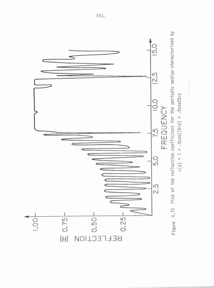
Figu
re
4,15
P
lot
of t
he r
efle
ctio
n co
effi
cien
t fo
r th
e pe
riod
ic m
ediu
m c
hara
cter
ized
by
s(z)
=
1 +
.5c
os(l8~z)
+ .
5cos
20~z

146.
The function (72) is sketched for the periodic and almost periodic
cases in figure (16).
To proceed we must fir st accept the principle of local reflection.
The idea behind it is that a wave is strongly reflected by portions
of a medium whi ch satisfy the Bragg relation but that the wave is not
very much affected by other parts of the medium .. Now with reference
to figure (16), we notice that the "wiggles" of (72) become more
closely spaced near the relative nulls of the wave packet. This
packing phenomena is caused by the slope of the modulating wave
packet increasing sinusoidally to a maximum at its nulls. The
unperturbed carrier peaks would be equally spaced without the wave
packet, but in the presence of this modulation, the peaks are
squashed inward toward the wave packet maximum at a rate which
increases as the slope of the wave packet, as the tips of the un
modulated peaks are being multiplied by a value of the modulation
function which is smaller than that which is multiplying the
perturbed peak l ocation. The gross effect of the varying peak spacing
is that along the z-axis different Bragg conditions are satisfied
at different locations . This means that waves of different fre
quencies are reflected from different positions and one would expect
a broadening of the reflected spectrum. But the spectral broadening
will only occur in the periodic case as in the periodic case the wave
is successively reflected nearly in phase by each of the carrier
humps, causing a cumulative effect. Thi s is not so in the almost

0 0 0
N
111
I I
N
7 47 .
l I
\11 ~J 0 0 0 . N
I I I I
s ~~ 1
ACTOR =
0 0 0 . N
0 0 0
N I
0.0 0.800
r
If'\
I
0.0 0.800
1.600 2.400
z
T T
w tl sc ~
I I
1.600 2.400
z Figure 4.16. a) Plot of the periodi c functi on
f(z) = cos(l .9Tiz) + cos (2.1Tiz )
3.200
I
1/1
~ACTOR
3.200
b) Plot of the almost periodic function
f( ) (1.9/3 ) + (2 .1 /2 ) Z = COS l .7 TIZ COS 1. 39 TIZ
=
0 1
4.000
0 1
4.000

148.
periodic case as the phasing of the "wiggles" ~tlithin each carrier
hump is essentially random and no cumul at ive effect occurs, other
than that due to the separate periods of (72). This effect, however,
will disappear gradual l y as 6K is increased as the number of carrier
humps per unit length decreases. We now can see a reason for the
behavior we have discovered in th i s report . In the large 6K l imit
the two-tone periodic and almost periodic theories should appear
identical; however, t hi s identity will disappear as the frequencies
of the two perturbations approach a central limit.

149.
Bibliography for Chapter Four
1. Morse, P.M. and H. Feshbach, Methods of Theoretical Physics, Vol. 2
(New York: McGraw-Hill Book Co., 1953).
2. The first term of the series is generally called the Born approxima
tion. See: Schiff, L.I., Quantum Mechanics (New York: McGraw-Hill
Book Co., 1968), 3rd edition.
3. Although the series solution to integral equations is generally
attributed to Neumann (See, for instance: (Mathews, J. and R.
Walker, Mathematical Methods of Physics (Menlo Park, Calif.: w. A.
Benjamin, Inc., 1970), 2nd edition or Stakgold, !.,Boundary Value
Problems of Mathematical Physics, Vol. 1 (New York: The Macmillan
Co., 1967).), it appears to actually have been originated by
Lioville. See: Whittaker, E. T. and G. N. Watson, A Course of
Modern Analysis (London: Cambridge Univ. Press, Fourth Edition -
1927, reprinted- 1973). See page 221.
4. The Fourier transform property of the first-order reflection coef
ficient can be deduced from the Bremmer series . See, for example:
Bellman, R. and F. M. Wing, An Introduction to Invariant Imbedding
(New York: J. l•Jiley and Sons, 1975) or Kline, M. (Ed.), The Theory
of Electromagnetic Waves (New York: Dover Pub., Inc., 1951). See
pages 169-180.
5. The result is well-known. See, for example: Jaggard, D. L.,
Caltech Antenna Laboratory Report No. 75, 1976. See pages 127-129.
6. For a more precise definition of this terminology, see, for

150.
instance: Nayfeh, A. H., Perturbation Methods (Ne~tJ York: J. Wiley
and Sons, 1973).
7. The two most commonly used renormalization techniques are that of
Fredholm and Rytov. For the Fredholm series, see the first refer
ence cited in ( 3), and for the Rytov series, see the reference
cited i n ( 6 ) .
8. Some discussion of the Fredholm series' applicabili ty is contained
in reference (1). The accuracy of the Rytov series relative to the
Born approximation is discussed in: Sancer, M. and A. Varvatsis,
Proc. IEEE 58, 140-141 (1970).
9. Stokes, G. G., Mathematical and Physical Papers, Vol. 4 (London:
10.
11.
12.
13.
14.
Cambridge Univ . Press, 1904). See pages 145-156. Note that this
reference is a reprint of: Stokes, G. G., Proc. Roy. Soc. (Janu
ary 23, 1862) .
Rayleigh, Lord, Proc. Roy. Soc. A86, 208-226 ( 1912) .
Rayleigh, Lord, Proc. Roy. Soc. A93, 565-573 (1917).
Schmidt, H. W., Ann. Phys. (Germany) ~. 671 (1907).
Ambartsumian,V. A.' Doklady 38, 229-232 (1943).
Ambartsumian,V. A., Theoretical Astrophxsics (New York: Pergamon
Press, 1958).
15 . See, for example: Papas, C. H., Caltech Antenna Laboratory Note,
March, 1954.
16. Chandresekhar, S., Radiative Transfer (New York: Dover Pub., Inc.,
1960).
17 . See Chapter 12 (authored by Redheffer) in t1odern ~1athematics for

151.
the Enginee~, edited by E. F. Beckenbach (New York: McGraw-Hill
Book Co., 1961), 2nd ed i tion.
18 . Specifically, we refer to the reference li sts in the first refer
ence of (4). Another usefu l reference i s : Adams, R. N. and
E. D. Denman, Wave Propagation and Turbul ent Media (New York :
American Elsevier, 1966).
19. The first reference of (4).
20. Ma xwell, J. C., A Treati se on Electricity and ~1agnetism (New York:
Dover Pub., Inc., 1954). This is a reprint of the first ed ition of
1873.
21. Born, M. and E. Wolf, Principles of Opt ics (New York: Pergamon
Press , 1975). See pa ge 324.
22. A good reference i s : Hatson, G. N., A Treatise on the Theory of
Bessel Functions (London: Cambridge Univ . Press, 1966) , 2nd edition .
See section 4. 2.
23. Pierce , J. R. , J. A. P . .£?.., 179- 183 ( 1954 ) .
24. Grads htein, I. S. and I. M. Ryzhik, Tabl es of Integral s, Seri es and
Products (New York: Academic Press , 1965).
25. Yariv, A., Introduction to Optical El ectroni cs (New York: Holt,
Rinehart and Winston, 1976 ) .
26. Yariv, A., Quantum Electroni cs (New York: J. vJi l ey and Sons, 1975).

152.
Chapter V
Conclusions
A) Rel at i onshi p of the Brillouin Diagram to t he Re fl ection
Coefficient
In Appendix E of this report the cl ose agreement of the exact
Riccati equation and the coupl ed mode two-point boundary value
probl em i s illustrated. Thi s agreement had previously been pointed
out elsewhere. 1 In Chapter IV of thi s report a technique was de
veloped in which the coupled-mode two-point boundary value problem
i s solv ed exactl y by constant-coef fi ci ent coupl ed Riccati equations.
The technique i s appli cable to cases in whi ch arbitrary numbers of
space harmoni cs are included. The constant-coefficient nature of
the coupl ed Riccati equat ions all ows numerical solu t i on of cases i n
whi ch the exact Ri ccati equat ion becomes numerically unstable and
therefore we are able to investi gate cases heretofore inaccessibl e .
As the coupled Riccati equations are derived from the same set of
equations that determine the Bri llouin di agram, the predictive
ability of the Brillouin diagram i s thus illustrated. In the al mos t
periodic case, numerical results illustrate that bandgap regions give
ri se to frequency regimes of large reflection, as one would expect.
The result all ows us to use t he Brillouin diagram and reflection
coeffi cient interchangeably in qualitat i ve di scuss i ons of periodic
and a lmost periodic media .
B) How Periodi c and Almost Periodic Structures Di ffer

153.
1) Phase Relations
As has already been explicitly shown, 2 different phasings of
harmonic perturbations in a periodic structure lead to diverse elec
tromagnetic responses, as evidenced by Bri 11 oui n-di a gram results. In
this report it has been s hown explicitly that such is not the case in
an almost periodi c structure to the most important order of approxima
tion . As precise phas ing of multiple harmonic perturbations is a
very complex task in practice, we f eel that thi s phas ing property
of almost periodic structures makes these structures in some sense
l ess abstract models than periodic structures.
2) The Band Coalescence Regime
In this report the cases of periodic and almost periodi c band
coalescence have been studied in detail. It has been found that
very closely spaced periodic perturbations give rise to an exceedingly
complex bandstructure which should lead to broadband reflection
characteristics . In the almost periodic case the picture is muc h sim
pler. As the band centers are brought together the reflection
"humps " add in a root-mean-square manner until total coalescence is
achieved. Each perturbation (or more correctly each associated back
ward mode) seems somewhat oblivious to the proximity of the other
perturbation, in contradistinction to the periodic case where all the
perturbations are coupl ed and many backward modes become important.
C) The Basic Nature of Almost Periodic Structures
1) Multi -tone Al most Periodic Perturbations

154.
Generalizing the mapping of Chapter II to the case of N almost
periodic tones, we find the first order dispersion matrix to be
D = ...
f * 'D 1 0 f* l
I
f* N
By induction it can be easily shown that the dispersion rela tion
resulting-from the determinant of this matrix i s again phase-
( l )
independent, indicating that the phase independence relation is very
bas i c to almost periodic wave propagation.
2) Almost Periodic Ensembles and Stochastic Ensembles
The apparent incoherency of al most periodic perturbations
when coupl ed together with their root-mean-square addition properties
tend to make one think of stochastic effects where phases are
averaged and probabilities added. To help force the ana l ogy, we have
plotted, in figure (1), the special l y constructed AM-FM modulated
almost periodic function
f(z) = [1 + ~ (COSKl Z + COSK2z + COSK3z)J ( 2 )

0 0 lJ) • ~I
I I
I I
d
...
" ...
~ ~ 0
No
H-.n
ltl
'---
/
LL
~ ~
v 0 0
"1111
lJ) •
. ~I
I I
I l
0.0
2.00
0 L!
.OOO
6.
000
8.00
0
z Fi
gure
5.1
P
lot
of t
he A
M-FM
mod
ulat
ed a
lmos
t pe
riod
f(z)
=
[1
+ i
(COS
KlZ
+ C
OSK 2z
+ C
OSK 3
z)J
X C
OS[
(K4
+ C
OSK 5z
+ C
OSK 6Z
+ C
OSK 7z)
z]
--
313
-5
1.7
--
-3
1.7
-5
13
Whe
re K
l -
TI,
K 2 -~ T
I,
K 3 -
/J
, K 4
-6
TI,
KS -
TI,
K 6 -
/:3
, K 7
-~ T
I
10.0
00
_,
(;1
U
1

156.
where
Kl = 7T K4 = 6.7T
3/3 (3) K2 =n 7T K5 = 7T
5 l. 7 3 1. 7 K3 = 7T K = 7T
/3 6 IT 5.13" K = 7 ~ 7T
(That (2) is almost periodic is evident from elementary AM and FM
considerations, i.e., its spectrum is a 1 i ne spectrum.) Although
(2) possesses a line spectrum we could consider the various K1 S as
random variables which vary between members of an ensemble of functions
of the form of (2), and thereby obtain a stationary ensemble of
arbitrary spectra. This could certainly be done with other deter
ministic functions, but we know of none with phase properties of the
almost periodic functions. Further, as (2) illustrates we can
generate very general almost periodic functions and still have the
ability to analyze the wave propagation characteristics in such media
through the matrix of (1 ) .
D) Possible Research Directions
1) Extensions to More General Geometries
Certainly the longitudinal geometry is not the only or even the
most common wave propagation geometry. By choosing separable
geometries and using the solution of Chapter II, a plethora of
interesti ng problems could be solved. A possibility would be the

157.
transverse geometry of holography ana l yzed by Burckhardt3. The
transverse geometry is nice as gratings are both fabricated and
operated in such a geometry. a fact which may make that geometry the
s implest in which t o attempt experimental verification of the
almost periodic wave propagation t heory. As was mentioned in Chapter
I, the three-d imensional geometry in whi ch phonons propagate could
also be of interest .
2) Modeling of Random Perturbations
As was discussed in (C) above, almost periodic structures seem
to be natural candidates for determin istic member s of stochast i c
ensembl es . By using AM, FM and/or more general s ums of almost
periodic tones , modeling of very general statistical perturbations
should be possible.
3) Extensions to Active Med ia-Stability Criteria
Following the lead of Jaggard and Elachi 4 and Jaggard 5, who
analyzed the periodi c case , one could attempt to analyze the
possibly more realistic almost period i c case. Such resul ts cou ld
be appli cable to distributed feedback l asers.
4) Experimental Verification of the Theory
This would cert a inly be the most important contr ibuti on to the
theory. Although the two-tone case discussed in this report would
be very hard to verify directly, it seems within the realm of
ima ginat ion that a more easi ly verifiable case could be constructed,
perhaps from the li st of suggested topics above. However , the

158.
verification could be performed, though care will have to be taken
to make sure that it is indeed the difference between periodic and
almost periodic media that is the measured quantity.

159.
Bibligraphy for Chapter Five
1. Various references could be cited on this point. We choose to
include those by A. Yariv and the reference therein cited: Yariv,
A., Introduction to Optical Electronics (New York: Holt, Rinehart
and Winston, 1976). See page 375 . See, also: Yariv, A., Quantum
Electronics (New York : J. Wiley and Sons, 1975). See page 524.
2. Jaggard, D. L. and C. Elachi, JOSA 66, 674-681, 1976.
3. Burckhardt, C. B., JOSA 56, 1502-1509, 1966.
4. Jaggard, D. L. and C. Elachi, J .A. P. 48, 1461-1466, 1977 .
5. Jaggard , D. L., App. Phys. (Springer-Verlag) }l, 185-195, 1977.

160.
APPENDIX A
Ordering the Roots of a Third Order Polynomial
We start from the set of equations for the roots of the third
order polynomial
which can be written as1
\'I here
s1 = [r + f] 113
s2 = [r- f] l /3
f = [q3 + r2]1/2
and
Using our dispersion relation of Chapter III
2 2 2 n+
-6k [ 6k - 6 - ~]
( 1 )
(a)
(2)
(a)
(b) (3)
(c)
(a)
(4)
(b)
(5)

161.
We can make the following identifications:
2 l 2 Tl+ 4 2
q = - 3 ( cS - 64) - 9 llk
2 8 2 2o2 l Tl+
r = llk[v llk - - 3- - 3 64]
(a)
(b)
The behavior of these functions is sketched in figure Al.
If we define the quantiti es
we find
We note that the roots of thi s express ion are at
llk2 = )c52 [P eS ±,jpo2 - 4(o2- ocz )6]
The behav ior of F2 i s sketched in figure A2.
(a)
(b)
(6)
(7)
(8)
(9)
The problem with direct evaluation of (3) i s the arbitrariness
of the phase in taking the cube root. Taking a cube root can put us
on any of three branc hes in the complex pl ane . l~e solve this problem
by invoking the dubious principle of monotonic phase, i.e., forcing
the absolute phase of the expression to increase monotonically. Be
fore directly addressing the branch problem, we summarize the
results of our ca l cul at ions and ad hoc rules us ing the notation for

(a) q
3 ;-
-:;:
2
-zv'
82+~
\
128
(b) r
2 I
TJ+
3 v
'82
+ 1
28
2 \
b:. k
I
1\.
/ 6
k
Figu
re A
l a)
q
plot
ted
vs 6
k pa
ram
etri
zed
by o
. b)
r
plot
ted
vs 6
k.
In b
oth
case
s n_
= o
.
__,
()
rv

F2
6k
Figu
re A
2 Th
e fu
ncti
on
F2 p
lott
ed v
s. 6
/2 a
nd p
aram
etri
zed
by o
. It
is
assu
med
th
at n
_ =
0.
__,
0)
w

164 .
our arbitrary branch variable
to find
Ca se
±i¢ s1
= s e
2
z1 2s cos <P
a2 z2 = -SCOS ¢ - 3 - iJ sin¢
a2 z3 = -s[cos <P - IJ si n¢] - 3
Case 2 f2 > 0
s l = I s1 I ei <P SP =
s = ls 21 -i <P SM = 2 e
a2 z1 = SPeas¢ - 3 + iSM si n¢
ls1 I + ls21
ls11 - ls 21
z = 2 -~(cos¢ + IJ si n¢) a2 . SM ( IJ . ) - - + 12 cos cp - s 1 ncp 3
SP 13" sincp ) a2
i ~M ( 13" coscp + s i ncp ) z3 = - 2 (cos¢ - - 3 -
Ad hoc rul e
If s1 and s2 have different s i gns, set
ls2l = - ls21
=- SP -+ SM
SM ->- SP
( 1 0)

165.
The branch problem is solved by the following rule (with
reference to figure A3): Start the phase 3¢ at 3n and subtrac t
out n for (D-+(V, (j)-+ ® and @ -+(j).

IM
Re
Figu
re A
3 A
ske
tch
of t
he s
chem
e to
kee
p th
e ph
ase
prog
ress
ion
mon
oton
ic
and
ther
eby
be a
ble
to f
ollo
w e
ach
of t
he t
hree
roo
ts o
f th
e po
lyno
mia
l
sepa
rate
ly.
......
G"'
C
J)

167 .
Bibl iography for Appendix A
1. Abramovitz, M. and I. Stegan, Handbook of Mathematical Functions,
(New York: Dover Pub., Inc., 1970) .

168 .
APPENDIX B
The Constitutive Interact ion
We start from the l ossless media electrodynamic action ( 1-2)
S = - l S d4xGa!3F + 4 a!3
S d4xA j n\JV \J \)
( 1 )
where
0 -E X
-E y -E z E 0 Bz -B
F X y A A (a) = ::.
IJ\1 Ey -B 0 B V, \J V,lJ.
z X
Ez B y -B X
0
0 ox Dy 0 z -0 0 Hz -H
GllV X y (b) = -0 y -H z 0 H
X
-0 z Hy -H X
0
(2) -1 0 0 0
0 1 0 0 . nllv = (c)
0 0 0
0 0 0 1
J" = [ ~ J (d)
and commas denote partial differentiation. It is easi ly seen that
variations performed on {1) yield

169.
GaB = .a ' B J
and that the other Maxwell equations
F[a8 ,y] = 0
follow from (2a):
We continue by defining the most general lossless, linear
constitutive relation by
where
G~v = C~vaBF = F~v _ M~v aS
01 02 03 : 23 31 12 I I I I I I
01 02 03
~vaS X = ------------·--------------* I 23
XEM : X( M) 31
= E - I
= I -1 ~
( ~v )aB ~v (aB ) X = X
X~vaB = ( x~vaB )*
M~v _ 1 ~vaBF - 2 X aS
=
=
: 12 I
X (~v )(aB ) =O
0 -P X
-P y
p X
0 Mz
p y -M z
0
pz My -M X
aB
!
-P z
-M y
M X
0
(a)
(b)
(c)
(d)
(e)
(f)
(g)
(3)
( 4)
With the above substitutions, we can rewr i te our action in the form

170.
s - -
If we perform variations with r espect to A on (5), we fin d the l.l
corr esponding Maxwell equations
·l.l J
bound + jlJ
free
with the corresponding interpretation that the E and B travel
( 5)
(6)
through free space augmented by a bound polarization current . Thi s
can be explicitly illustrated by integrating the second term of (5)
by parts , to obtain
(7)
Our argument ca n now be compl eted by noting that
Scatter ed field s a transition amplitude T a interaction action s 1~8)
Certainly for the first-o rder intera cti on with a l oss l ess , l i near
constitutive med ia,
S = J d4x A J. bound av I a v n
Taking the incomi ng and outgoing s tates to be plane wave states,
incoming of propagation vec tor 0 k, pol ari zation °£ , outgoing of
propagation vector 1 k,polariza t ion 1 £ , we evaluate (9) to find
(after some mani pulation)
(9)

171.
T a 1 k 1 £ a l-1
1 ( <XlJ Bv ) I o k o k X k= 1 k- 0 k B e:v . ( 1 0)
The result i s manifestly gauge invariant under transformations
1£ + 1 £ + y lk (a) l-1 l-1 l-1
( 11 ) 0£ + 0£ + y ok (b)
l-1 l-1 l-1
and explicitly illustrates that any first-order interaction with a
lossless, linear constitutive media is proportional to the Fourier
transform of the medium's constitutive tensor. The argument can be
carried to higher orders and can be s hown to be equivalent to the
Neumann series for simple media.
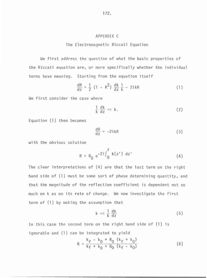
172 .
APPENDIX C
The Electromagnetic Riccati Equation
We first address the question of what the basic properties of
the Riccati equation are, or more specifically whether the individual
terms have meaning. Starting from the equation itself
dR = l (1 - R2) ~ l- 2ikR dz 2 dz k (1)
We first consider the case where
l~ « k k dz · ( 2)
Equation (1) then becomes
dR _ dz - -2ikR (3)
with the obvious solution
z R = Ro e-2iJ
0 k(z ' ) dz' (4)
The clear i nterpretations of (4) are that the last term on the right
hand side of (1) must be some sort of phase determining quantity, and
that the magnitude of the ref l ection coefficient is dependent not so
much on k as on its rate of change. We now investigate the first
term of (1) by making the assumption that
k « l~ k dz
In this case the second term on the right hand side of (1) is
ignorable and (1) can be integrated to yield
kf - ko + Ro (kf + ko) R = ~--~~~~r.-~~~
kf + k0 + R0 (kf - k0)
(5)
(6)

173.
This result contains as limits the two well-known results that as
Ro
R
and as
Ro
R
-+ 0
n-n0 -+ --n+n0
-+ 1
-+ 1
(a)
(b)
(a)
(b)
(7)
(8)
and therefore shows that the first term on the right hand side of
(1) contains the boundary effects. This is reasonable as the
condition (5) is satisfied only in the neighborhood of sharp inter-
faces.
There exist many perturbation schemes other than the Born-
Neumann series discussed in Chapter IV. Examples are the Bremmer
series1 and the Arth (R) transformation2. By considering explicitly
the behavior of t hese approximation sc hemes in periodic media it is
easily seen that they become secular. Here we wish to present a sim-
ple argument to show that any perturbation scheme which uses simple
ordering of terms will become sec ul ar at resonance. Let us write
the Riccati equation in the form
~ ~ = ; ( 1 - R 2 ) ddz ( 1 o g n ( z )) - 2 i k n ( z ) R (9)
where
k ( l 0)
and we take the index of refraction to be of the form

174.
n = n0[1 + nP(z)] (11)
where n is small and P denotes a periodic function. We now
Fourier transform (9) into the variable B to obtain
where the as teri sk denotes convolution. We now expand
log n = log no + log [1 + nP]
00 (nP)n+l = log no + E (-) n ( 13)
n=O n+ 1
= log no + E = a. + E
With this we find
J8 [log n] = a.o (S) + E (a) " ( 14)
] B [n] = n0o( f3 ) + n0nP (b)
Substituting (14 ) in (1 2) we find B A 1 A A A A
[ 2kn0 - S]R = - "2 E + "2 R*[R* BE - 2k0n0nP] {15)
The Bragg condition is just
2k n0 = s ( 16)
showing that the left-hand side of (15) vanishes on r esonance . But
the left-hand side is the only zeroth-order term in n of (15 ) .
Cl early, for this reason, any expansion in n of (9) must f ail as the
higher order terms in n become more important than the zeroth-order
term at resonance .

175.
Bibliography for Appendix C
l. The most recent reference is: Bellman, R. and G. M. Wing, An Intro
duction to Invariant Imbedding (New York: J. Wiley and Sons, 1975).
The original reference is: Kline, M. (Ed.), The Theory of Electro
magnetic Waves (New York: Dover Pub., Inc., 1951). See pages 169-
180.
2. There are two applicable papers in the Russian literature:
Gaydabura, I. S., Radio Eng. Electron. Phys. 1£, No. 10, 1625-1627,
1971 and Gaydabura, I. S. and I. A. Kozlov, Radio Eng. Electron.
Phys. ~. 1747-1749, 1973.
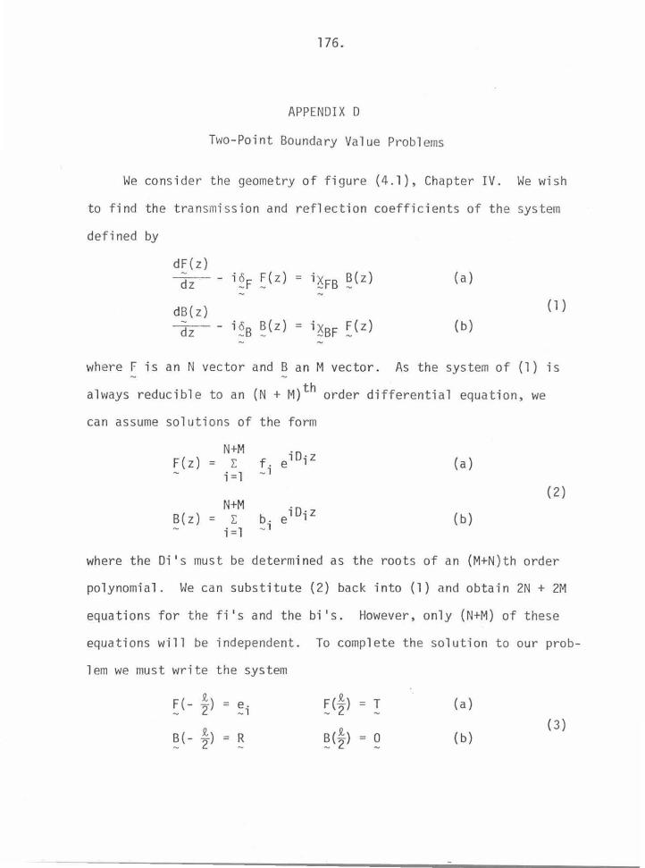
176.
APPENDIX 0
Two-Point Boundary Value Probl ems
We consider the geometry of figure (4.1), Chapter IV. We wish
to find the transmiss ion and reflection coefficients of the system
defined by
dF(z) dz i ~ F ~(z) = i~FB B(z) (a)
dB(z) (l) - i ~B B(z) = i ~BF F(z) dz (b)
where F is anN vector and Ban M vector. As the system of (1) is
always reducible to an (N + M)th order differential equation, we
can assume solutions of the form
N+M iD·z F(z) = E f. e 1 (a) i = 1 - 1
(2) N+M i 0. z B(z) = E b. e 1 (b) i =1 - 1
where the Di 1 S must be determined as the roots of an (M+N)th order
polynomial. We can substitute (2) back into (1) and obtain 2N +2M
equations for the fi 1 S and the bi 1 S . However, only (N+M) of these
equations will be independent. To complete the solution to our prob-
lem we must write the system
Q, F(- - ) = e - 2 -i
B(- .&.) - 2
R
F(.&.) T - 2
(a)
B(.&.) 0 - 2
(b) (3)

177.
where ei is a unit input vector. The system of (3) represents
2N +2M equations for 3N +3M unknowns: F, B, T, R. But when
coupled with the N+M independent equations obtained from sub
stituting (2) in (1), we are left with a 3(N+M) order system in
3(N+M) unknowns, and therefore can compute a unique solution for
Rand T. To summarize, solution of the two-point boundary va lue
problem requires: 1) derivation of the (N+~l)th-order differential
equation from the system of (1); 2) determination of the roots of the
(N+M)th-order polynomial resulting from the (N+M)th-order differential
equation; 3) solution of a 3(N+M) order system of algebraic equations.

0 0 0 . -
zt-
0~ .
1---
-i 0
~
u w~
_j~
LLO
w
cr= 0
• 0
0.0
0.
800
1.60
0 2.
400
3.20
0
FREQ
UENC
Y Fi
gure
El.
Th
e t\1
10
poin
t bo
unda
ry v
alue
pro
blem
sol
utio
n fo
r th
e re
flec
tion
coe
ffic
ient
of
the
medi
um c
hara
cter
ized
by
of l
engt
h ~
= 2
.
2 E(
Z)
= l
+ -
cos4
nz
n
4.0
00
-J
""-J
1.
0
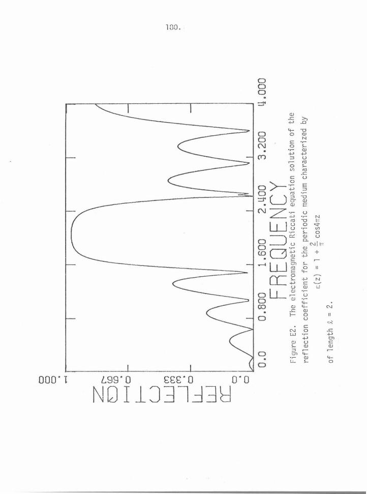
CJ
CJ
CJ •
.......
z('-
0~ •
~CJ
~
u w~
_j~
LLo
w
cr C
J . O
LC
: 0.0
0.80
0 1.
600
2.40
0 3.
200
FREQ
UENC
Y Fi
gure
E2.
Th
e el
ectr
omag
neti
c R
icca
ti
equa
tion
solu
tion
of
the
refl
ecti
on c
oeff
icie
nt f
or t
he
peri
odic
med
ium
cha
ract
eriz
ed b
y
E(z)
=
1 +
~ c
os4n
z TI
of l
engt
h ~
= 2.
4.00
0
--'
C::>
0


