INSTITUTE OF PHYSICS PUBLISHING JOURNAL OF PHYSICS D: APPLIED PHYSICS

J. Phys. D: Appl. Phys. 36 (2003) 2584–2597 PII: S0022-3727(03)63619-3

Electrohydrodynamics anddielectrophoresis in microsystems: scalinglawsA Castellanos1, A Ramos1, A Gonzalez1,2, N G Green3 andH Morgan3,4

1 Dpto. Electronica y Electromagnetismo, Facultad de Fısica, Universidad de Sevilla,Reina Mercedes s/n, 41012 Sevilla, Spain2 Dpto. de Fısica Aplicada III, E.S.I. Universidad de Sevilla, Camino de los Descubrimientoss/n 41092 Sevilla, Spain3 Bioelectronics Research Centre, Dept. Electronics and Electrical Engineering, University ofGlasgow, Oakfield Avenue, Glasgow G12 8LT, UK

Received 19 May 2003Published 1 October 2003Online at stacks.iop.org/JPhysD/36/2584

AbstractThe movement and behaviour of particles suspended in aqueous solutionssubjected to non-uniform ac electric fields is examined. The ac electricfields induce movement of polarizable particles, a phenomenon known asdielectrophoresis. The high strength electric fields that are often used inseparation systems can give rise to fluid motion, which in turn results in aviscous drag on the particle. The electric field generates heat, leading tovolume forces in the liquid. Gradients in conductivity and permittivity giverise to electrothermal forces and gradients in mass density to buoyancy. Inaddition, non-uniform ac electric fields produce forces on the inducedcharges in the diffuse double layer on the electrodes. This causes a steadyfluid motion termed ac electro-osmosis. The effects of Brownian motion arealso discussed in this context. The orders of magnitude of the various forcesexperienced by a particle in a model microelectrode system are estimated.The results are discussed in relation to experiments and the relative influenceof each type of force is described.

1. Introduction

The application of ac electrokinetic forces to controland manipulate isolated particles in suspension usingmicroelectrode structures is a well-established technique [1].In particular, the dielectrophoretic manipulation of sub-micronbioparticles such as viruses, cells and DNA is now possible.As the size of the particle is reduced, so the effects ofBrownian motion become greater. Therefore, to enable thedielectrophoretic manipulation of sub-micron particles usingrealistic voltages the characteristic dimensions of the systemmust be reduced to increase the electric field. However, a highstrength electric field also produces a force on the suspendingelectrolyte, setting it into motion. Indeed, this motion may bea far greater limiting factor than Brownian motion.

4 Current address: Department of Electronics and Computer Science, TheUniversity of Southampton, Highfield, Southampton S017 1BJ.

Owing to the intensity of the electric fields requiredto move sub-micrometre particles, Joule heating can be aproblem, often giving rise to electrical forces induced bythe variation in the conductivity and permittivity of thesuspending medium (electrothermal forces) [2–4]. In certaincircumstances, Joule heating may be great enough to causebuoyancy forces. In addition to Joule heating, the geometryof the electrodes used to generate dielectrophoretic forcesproduces a tangential electric field at the electrode–electrolytedouble layer. This induces steady motion of the liquid, a flowtermed ac electro-osmosis because of its similarity to electro-osmosis in a dc field [5–8]. It should be emphasized that theac electro-osmotic flow observed over microelectrodes differsfrom ac electro-osmosis observed in capillaries [9]. In thelatter case, the electric field is uniform along the capillary buttime-varying. The diffuse double layer charge is fixed and thefluid motion is oscillatory. However, in the former case both

0022-3727/03/202584+14$30.00 © 2003 IOP Publishing Ltd Printed in the UK 2584

Electrohydrodynamics and DEP in microsystems

the electric field and the double layer charge are time-varyingand give rise to a steady fluid motion.

Based on these mechanisms, the magnitude and directionof the surface and volume forces acting on the liquid canbe predicted analytically or, alternatively, using numericalsimulations. This means that it should be possible todesign and develop microelectrode structures that can translateexperimental and theoretical understanding into a givenspecification. However, the precise design of a complicatedmicroelectrode structure would require extensive numericalcalculations. The aim of this paper is to develop a generalframework that outlines the basic constraints of a system, thusreducing the need for intensive computation. A first stepin this process is prior knowledge of how the forces on theparticle scale with the size of the system, the shape of theelectrodes, the particle diameter, the magnitude and frequencyof the applied ac electric field, and the conductivity of thesuspending solution.

In this paper, we present an analysis of particle dynamicsand a summary of the type of fluid flow observed in a simplifiedsystem consisting of two co-planar parallel strip electrodes.Previously published data are reviewed and new analysesperformed to determine a general understanding of the scalinglaws governing this simple system. Within limits, these resultscan be generalized to more complicated microelectrode shapes,bearing in mind that different regions of the system may havedifferent characteristic length scales.

Bioparticles have sizes that range from 0.1 µm up to10 µm, e.g. viruses (0.01–0.1 µm), bacteria (0.5–5 µm),or plant or animal cells (5–15 µm). They are usuallysuspended in an aqueous saline solution with a conductivitythat ranges between 10−4 and 1 S m−1. Typical systemlengths of the microelectrodes (interelectrode gaps) used inthe dielectrophoretic manipulation of bioparticles vary from1 to 500 µm. The signals applied to these electrodes can beup to 20 V giving rise to electric fields that can be as high as5 × 106 V m−1. The applied signals have frequencies in therange 102–108 Hz.

As stated previously, measurement and analysis of flowhas been performed using a simple electrode design consistingof two coplanar rectangular electrodes fabricated on a glasssubstrate. The electrodes are 2 mm long and 500 µmwide, with parallel edges separated by a 25 µm gap [8, 10].A schematic diagram of the system is shown in figure 1,together with a simplified idealization of the system. Becausethe gap is small compared to the length and width of theelectrodes the system can be considered to be two-dimensional[7, 11], so that the analysis is restricted to the two-dimensionalcross-section shown in figure 1. Such a simplified systemcan give useful information on the relative magnitudes of thedifferent forces generated, together with the regions wherecertain approximations are valid. Extending the general resultsobtained for the two-dimensional planar electrode to othergeometries must be done with care. For example, figure 2shows two different electrode arrays: a hyperbolic polynomialelectrode and a castellated electrode. In this case, severaldifferent length scales act at the same time.

The first part of the paper is an analysis of the motionof particles caused by gravity, dielectrophoresis (DEP) andBrownian motion. The mechanical, electrical and thermal

θr

Glass substrateElectrodes

AC power supply

θr

Electrodes

Electric field lines

)cos(2

tV ω+)cos(

2t

V ω−

25 µm gap

Electrolyte

(a)

(b)

Figure 1. (a) Schematic diagram of the electrodes used to moveparticles and fluids. (b) Simplified ideal system showing theelectrical field lines.

equations that govern liquid motion in these microelectrodestructures are then formulated. The volume and surface forcesacting on the system are given, emphasizing how these forcesscale with system parameters. Finally, the relative importanceof the drag force (which comes from electrohydrodynamicflow) is discussed and compared with Brownian motion, DEPand gravitational forces.

2. Particle motion

2.1. Stokes force

For simplicity, consider the particles to be spherical. Assumingthat the Stokes drag is valid, the movement of a particle in afluid influenced by a force F, is governed by

mdudt

= −γ (u − v) + F (1)

where m is the particle mass, u the particle velocity and vthe fluid velocity, −γ (u − v) is the drag force with γ thefriction factor of the particle in the fluid. For a spherical particleγ = 6πηa, where a is the particle radius and η is the viscosityof the medium. Under the action of a constant force F andfluid velocity v, the particle velocity is

u =(

u0 − v − Fγ

)e−(γ /m)t + v +

Fγ

(2)

where u0 is the initial velocity of the particle. Thecharacteristic time of acceleration, τa = m/γ , is usually muchsmaller than the typical time of observation (∼1 s). For aspherical particle of mass density ρp, τa = ( 2

9 )(ρpa2/η), which

is smaller than 10−6 s for cells and sub-micrometre particles.Therefore, the particle can be considered to move at its terminalvelocity, given by

u = v +Fγ

(3)

This means that any measurement of particle velocity is a directmeasure of the fluid velocity, v, plus the velocity induced by theforce acting on the particle, F/γ . In general, the accelerationprocess is much more complicated than described by the simple

2585

A Castellanos et al

Figure 2. Diagram of a hyperbolic polynomial electrode (left) and a castellated electrode (right).

exponential solution, and the acceleration of the fluid anddiffusion of vorticity must also be considered [12]. However,the fact that the particle moves at its terminal velocity for timesmuch greater than ρpa

2/η is still valid.

2.2. Gravity

The main external influence on a particle suspended in a fluidis gravity. For a particle of mass density ρp in a fluid of densityρm the gravitational force is given by

Fg = υ(ρp − ρm)g (4)

where g is the acceleration due to gravity and υ is the volumeof the particle. The magnitude of the velocity of a sphericalparticle in a gravitational field is

ug = υ|ρp − ρm|gf

= 2

9

a2|ρp − ρm|gη

(5)

To a first-order approximation, assume |ρp −ρm| is of the orderof ρm; then, the magnitude of the gravitational velocity can beestimated to be

ug ∼ 0.2a2ρmg

η(6)

In this expression, the factor 0.2 may be smaller since manyparticles have densities that are close to that of water.

2.3. Dielectrophoresis

Particles in electric fields are subjected to electrophoreticand dielectrophoretic forces. In the thin double layerapproximation, the velocity induced by the former force isgiven by the Smoluchowsky formula, u = εζE/η, where ε

and η are, respectively, the electrical permittivity and dynamicviscosity of water, and ζ is the zeta potential of the particle.In ac electric fields, the particle displacement is oscillatorywith a maximum amplitude given by x = u/ω, which forsufficiently high frequencies can be neglected. For example,for a field amplitude of 105 V m−1, a frequency of 1 kHz anda zeta potential of 50 mV, the displacement x ∼ 0.5 µm.In fact this is a gross overestimation because particle inertiawould lead to a smaller net displacement that decreases withincreasing frequency, proportional to ω−2. In contrast, theDEP force has a non-zero time average and leads to net particledisplacement.

The dielectrophoretic force arises from the interaction ofa non-uniform electric field and the dipole induced in theparticle. For linear, isotropic dielectrics, the relationshipbetween the dipole moment phasor p of a spherical particleand the electric field phasor E is given by p(ω) = υα(ω)E,where α is the effective polarizability of the particle and ω isthe angular frequency of the electric field. The time-averagedforce on the particle is given by [13]

〈 FDEP〉 = 12 Re[( p · ∇)E∗] = 1

4υRe[α]∇|E|2− 1

2υIm[α](∇ × (Re[E] × Im[E])) (7)

where ∗ indicates complex conjugation, Re[A] and Im[A] thereal and imaginary parts of A and |E|2 = E · E∗. For thesecond equality, E has been considered to be solenoidal, i.e.∇ · E = 0. The first term on the right-hand side is non-zero ifthere is a spatially varying field magnitude, giving rise to DEP.The second term is non-zero if there is a spatially varying phase,as in the case of travelling wave dielectrophoresis (twDEP). Ifthe particle polarizes by the Maxwell–Wagner mechanism, andconsidering only the dipole force, the DEP-induced velocityof a spherical particle is

uDEP = υRe[α]

4γ∇|E|2 = a2ε

6ηRe

[εp − ε

εp + 2ε

]∇|E|2 (8)

Here ε indicates a complex permittivity, ε = ε − iσ/ω, whereε is the permittivity and σ is the conductivity. The expressionin brackets is referred to as the Clausius–Mossotti factorand describes the frequency variation of the dielectrophoreticmobility and force. This factor varies between +1 and − 1

2 ; theparticle moves towards (positive DEP) or away from (negativeDEP) regions of high field strength, depending on frequency.

For the sake of simplified analysis, the electric field linesbetween the electrodes can be considered semi-circular asshown in figure 1(b); in this case, the electric field is givenby E = V/πruθ , where V is the amplitude of the appliedvoltage and r is the distance to the centre of the gap. Thisexpression is the exact solution for the field when the electrodesare semi-infinite with an infinitely small gap.

Assuming a Clausius–Mossotti factor of 1 and anelectric field given by E = V/πr , the magnitude of thedielectrophoretic velocity of a particle in this system, at adistance r from the centre, is

uDEP ≈ 0.03a2ε

η

V 2

r3(9)

2586

Electrohydrodynamics and DEP in microsystems

2.4. Brownian motion

Thermal effects also influence colloidal particles. The forceand velocity associated with Brownian motion have zeroaverage; however, the random displacement of theparticle follows a Gaussian profile with a root-mean-squaredisplacement (in one dimension) given by

x =√

2Dt =√

kBT

3πaηt (10)

where kB is Boltzman’s constant, T is the absolute temperatureand t is the period of observation. To move an isolated particlein a deterministic manner during this period, the displacementdue to the deterministic force should be greater than thatdue to the random (Brownian) motion. This consideration ismeaningful only for single isolated particles. For a collectionof particles, diffusion of the ensemble must be considered.

2.5. Particle displacements

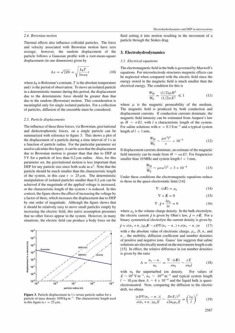
The influence of these three forces, viz Brownian, gravitationaland dielectrophoretic forces, on a single particle can besummarized with reference to figure 3. This shows a plot ofthe displacement of a particle during a time interval of 1 s asa function of particle radius. For the particular parameter setused to calculate this figure, it can be seen that the displacementdue to Brownian motion is greater than that due to DEP at5 V for a particle of less than 0.2 µm radius. Also, for thisparameter set, the gravitational motion is less important thanDEP for any particle size since both scale as a2. Note that theparticle should be much smaller than the characteristic lengthof the system, in this case r = 25 µm. The deterministicmanipulation of isolated particles smaller than 0.2 µm can beachieved if the magnitude of the applied voltage is increased,or the characteristic length of the system r is reduced. In thiscontext, the figure shows the effect of increasing the voltage bya factor of three, which increases the displacement due to DEPby one order of magnitude. Although the figure shows thatit should be relatively easy to move small particles simply byincreasing the electric field, this naıve assumption presumesthat no other forces appear in the system. However, in manysituations, the electric field can produce a body force on the

particle radius (m)

dis

pla

cem

ent

in a

sec

on

d (

m)

DEP(15V)

DEP(5V)

Brownian

Gravity

10-9

10-8

10-7

10-6

10-5

10-4

10-3

10-2

10-9 10-8 10-7 10-6 10-5

Figure 3. Particle displacement in 1 s versus particle radius for aparticle of mass density 1050 kg m−3. The characteristic length usedin this figure is r = 25 µm.

fluid setting it into motion resulting in the movement of aparticle through the Stokes drag.

3. Electrohydrodynamics

3.1. Electrical equations

The electromagnetic field in the bulk is governed by Maxwell’sequations. For microelectrode structures magnetic effects canbe neglected when compared with the electric field since theenergy stored in the magnetic field is much smaller than theelectrical energy. The condition for this is

WM

WE= (1/2)µH 2

(1/2)εE2� 1 (11)

where µ is the magnetic permeability of the medium.The magnetic field is produced by both conduction anddisplacement currents. If conduction currents dominate, themagnetic field intensity can be estimated from Ampere’s lawas H ∼ σEl, with l a characteristic length of the system.For saline solutions with σ < 0.1 S m−1 and a typical systemlength of l < 1 mm,

WM

WE∼ µσ 2l2

ε< 10−5 (12)

If displacement currents dominate, an estimate of the magneticfield intensity can be made from H ∼ ωεEl. For frequenciessmaller than 10 MHz and system length l < 1 mm,

WM

WE∼ µεω2l2 < 3 × 10−6 (13)

Under these conditions the electromagnetic equations reduceto those in the quasi-electrostatic limit [14]:

∇ · (εE) = ρq (14)

∇ × E = 0 (15)

∇ · j +∂ρq

∂t= 0 (16)

where ρq is the volume charge density. In the bulk electrolyte,the electric current j is given by Ohm’s law, j = σE. For abinary symmetrical electrolyte the current density is given by

j = e(n+ + n−)µeE − eD∇(n+ − n−) + e(n+ − n−)v (17)

with e the absolute value of electronic charge, µe, D, n+ andn−, the mobility, diffusion coefficient and number densitiesof positive and negative ions. Gauss’ law suggests that salinesolutions are electrically neutral on the micrometre length scale[15]. In effect, the relative difference in ion number densitiesis given by the ratio

� = n+ − n−n0

= ∇ · (εE)

en0∼ εE

en0l(18)

with n0 the unperturbed ion density. For values ofE ∼ 105 V m−1, n0 ∼ 1023 m−3 and typical system lengthl ∼ 10 µm then � ∼ 4 × 10−4 and the liquid bulk is quasi-electroneutral. Now, comparing the diffusion to the electricdrift, we obtain

|eD∇(n+ − n−)|e(n+ + n−)µeE

∼ DεE/l2

e2n0µeE=

(λD

l

)2

(19)

2587

A Castellanos et al

where λD = √εD/2en0µe is the Debye length, which is of

the order of several nanometres, much smaller than the typicalsystem length.

Defining σ = 2en0µe, we now compare the conductioncurrent, σE, to the convection current, ρqv in saline solutions.Taking typical values σ ∼ 10−3 S m−1, l ∼ 10 µm,v ∼ 100 µm s−1 gives

|∇ · (εE) v||σE| ∼ ε/σ

l/v∼ 7 × 10−6 (20)

The combination of parameters, εv/lσ , is called the electricalReynolds number [16], and since it is very small the electricalequations are decoupled from the mechanical equations.Therefore, neglecting the convective term, and assuming thatσ and ε are independent of time, equations (14) and (16) canbe combined (for an ac field of frequency ω) as

∇ · ((σ + iωε)E) = 0 (21)

where E is now a complex vector.In many cases, the gradients in permittivity and

conductivity are small [3, 11], so that the electric field canbe expanded to give E = E0 + E1, (|E1| � |E0|), where theelectric fields satisfy the equations

∇ · E0 = 0 (22)

∇ · E1 +

(∇σ + iω∇ε

σ + iωε

)· E0 = 0 (23)

The charge density of each order can be approximated to

ρ0 = ε∇ · E0 = 0 (24)

ρ1 = ε∇ · E1 + ∇ε · E0 =(

σ∇ε − ε∇σ

σ + iωε

)· E0 (25)

In our analysis, only the zero-order field E0 is required, whichis obtained from the solution of Laplace’s equation

∇2φ0 = 0 (26)

3.2. Mechanical equations

Liquid motion is governed by the Navier–Stokes equations foran incompressible fluid

∇ · v = 0 (27)

ρm

(∂v

∂t+ (v · ∇)v

)= −∇p + η∇2v + fE + ρmg (28)

where fE represents the electrical forces, and ρmg, the actionof gravity.

For microsystems the Reynolds number is usually verysmall; typical velocity v < 100 µm s−1, and dimensionl < 100 µm and

|ρm(v · ∇)v||η∇2v| ∼ Re = ρmvl

η� 10−2 (29)

Therefore, the convective term in the Navier–Stokes can beneglected.

After application of the electric field, a stationary stateis reached in a time of the order of t = ρml2/η, whichis usually smaller than 0.01 s. Since the electrical force isoscillatory with a non-zero time average, the steady-state liquidmotion can have both a non-zero time-averaged componentand an oscillating one. We are interested in the time-averagedcomponent, the one that is easily seen in the experiments. Theequation for the average velocity can then be written as

0 = −∇p + η∇2v + 〈 fE〉 + ρmg (30)

Here, since the mass density of the fluid is almosthomogeneous, the Boussineq approximation has been applied,i.e. changes in density are neglected except for the buoyancyforce [17]. As stated by this equation, the fluid motion iscaused by the combined action of gravity and electrical forces.The latter is given by [18]

fE = ρqE − 1

2|E|2∇ε + ∇

(1

2ρm

(∂ε

∂ρm

)T

E2

)(31)

For incompressible fluids, the third term in this equation, theelectrostriction, can be incorporated into the pressure [18] andomitted from the calculations. The first term, the Coulombforce, and the second term, the dielectric force, depend on thepresence of gradients in the conductivity and permittivity. Foran applied ac voltage, the electrical force has a non-zero timeaverage given by

〈 fE〉 = 12 Re(ρqE∗) − 1

4 E · E∗∇ε (32)

where the charge and field on the right-hand side are thecomplex amplitudes. Substituting for the charge fromequations (24) and (25), and provided the gradients are small,gives [3, 11]

〈 fE〉 = 1

2Re

(((σ∇ε − ε∇σ

σ + iωε

)· E0

)E∗

0

)− 1

4E0 · E∗

0∇ε

(33)

This expression for the electrical forces is clearly frequencydependent. If ω is much greater than σ/ε, the second term(the dielectric force) dominates. Likewise, if ω � σ/ε,the first term, the Coulomb force dominates because rel-ative variations in conductivity (σ/σ ) are usually muchgreater than relative variations in permittivity (ε/ε). Thisis the case for variations caused by gradients in tempera-ture, where for electrolytes (1/σ)(∂σ/∂T ) ≈ 0.02 K−1 and(1/ε)(∂ε/∂T ) ≈ −0.004 K−1.

Both electrical and gravitational forces are present whenthe liquid is inhomogeneous. In the following analysis,gradients in permittivity, conductivity and mass density areassumed to arise from the temperature gradients present in thefluid.

3.3. Energy equation

Together with the electrical and mechanical equations, theequation for the internal energy is required, which can berelated to the temperature distribution through [3]

ρmcp

(∂T

∂t+ (v · ∇)T

)= k∇2T + σE2 (34)

2588

Electrohydrodynamics and DEP in microsystems

where cp is the specific heat (at constant pressure) and k isthe thermal conductivity of the fluid. After the applicationof the electric field, the temperature field rapidly reaches astationary state that has both a time-independent componentand an oscillating one, in a manner similar to the velocity field.The effect of the oscillating component on the fluid dynamics isnegligible for frequencies higher than 1 kHz [3]. The steady-state is reached after a time of the order of t = ρmcpl2/k,which is usually smaller than 0.1 s.

For microsystems, heat convection is small comparedto heat diffusion, as demonstrated by the small value ofthe Peclet number, which, typically (v < 100 µm s−1 andl < 100 µm), is

|ρmcp(v · ∇)T ||k∇2T | ∼ Pe = ρmcpvl

k< 7 × 10−2 (35)

Therefore, the temperature equation reduces to Poisson’sequation, with Joule heating as the energy source

k∇2T = −σ 〈E2〉 (36)

4. Boundary conditions

A summary of the electrohydrodynamic equations are given intable 1. In order to solve the equations, appropriate boundaryconditions have to be defined. The domain boundary iscomposed of several parts. The boundary conditions for theelectrodes (which are fabricated on glass) are summarizedin figure 4, where the lateral and upper boundaries can beconsidered rigid and assumed to be far from the region ofinterest.

4.1. Electric potential

The electric field is produced by electrodes connected to acvoltage sources. The electric potential at the surface of theelectrodes, V is fixed by the source. However, this is notnecessarily the most suitable boundary condition to describethe behaviour of the potential in the bulk electrolyte φ, sincea double layer lies between the metallic surface and the bulkelectrolyte [19]. The appropriate boundary condition is thecharge conservation equation for the double layer: the currentinto an element of the double layer is equal to the increasein the stored charge. Since the typical system length is muchgreater than the double layer thickness, the thin double-layerapproximation can be used. Under this approximation, the

Table 1. Summary of electrohydrodynamic equations.

Electrical equationsGauss’ law ∇ · E0 = 0Faraday’s law ∇ × E0 = 0

Average electrical volume force 〈 fE〉 = 1

2Re

(((σ∇ε − ε∇σ

σ + iωε

)· E0

)E∗

0

)− 1

4E0 · E∗

0∇ε

Mechanical equationsIncompressibility ∇ · v = 0Stokes’ equation 0 = −∇p + η∇2v + 〈 fE〉 + ρg

Energy equation

Temperature diffusion ∇2T = −σ 〈E2〉k

lateral currents along the double layer (either convection orconduction) are negligible by comparison with the normalcurrent. The ratio between tangential and normal conductioncurrents is of the order of λD/l. The ratio between tangentialconvective and normal conduction currents is of the order ofqsv/σEl ∼ v ε/σλD, where qs is the surface charge densityin the double layer. If the slip velocity is much smaller than,typically, 10 cm s−1, then this ratio is much smaller than unity.Therefore, the normal current into the double layer is equal tothe increase in the stored charge. Essentially, the size of thedouble layer is so small that it does not enter into the problemspace. The electrical behaviour of a perfectly polarizabledouble layer can be modelled theoretically as a distributedcapacitor between the electrode and the bulk. The conservationof charge condition then becomes [7, 8]

σ∂φ

∂n= ∂

∂t(C(φ − V )) (37)

where n represents the outer normal, C the capacitance per unitarea and φ the electric potential just outside the double layer.A typical value of the specific double layer capacitance C isgiven by the ratio of the electrolyte permittivity to the Debyelength, C ∼ ε/λD. Using complex amplitudes, the boundarycondition for φ at the electrode is a mixed boundary condition:

φ − σ

iωC

∂φ

∂n= V (38)

More generally, the behaviour of the double layer can bemodelled through an empirical impedance. The boundarycondition for the potential then becomes

φ − σ

Y

∂φ

∂n= V (39)

with Y the admittance per unit area of the double layer. Forthe sake of simplicity we will assume that the electrodesare perfectly polarizable, with Y = iωC. For frequenciesω σ/(lC) ∼ (σ/ε)(λD/l), the boundary condition for theelectric potential at the electrodes reduces to a fixed value ofpotential.

In writing equation (37), it has been assumed thatω � σ/ε and the displacement current has not been taken intoaccount. This can be neglected since at a frequency wherethe displacement current dominates (ω > σ/ε), the potentialφ just outside the double layer becomes equal to the appliedpotential V.

2589

A Castellanos et al

For the gap between the electrodes, i.e. the glass/electrolyteinterface, the boundary condition is given by the continuity ofthe total normal current density:

(σG + iωεG)∂φG

∂n= (σ + iωε)

∂φ

∂n(40)

where the subscript G is used for the electrical properties ofthe glass. In most situations, the large difference betweenthe conductivities and permittivities of the water and the glassallows this boundary condition to be simplified to

∂φ

∂n= 0 (41)

If the upper boundary is far enough from the electrodes, itcan be considered to be at infinity and the electric field andpotential tend to zero.

4.2. Velocity

In any of the rigid boundaries, the normal velocity vanishes.The tangential velocity, however, can be non-zero on theelectrodes. This is due to the presence of the double layer atthe electrolyte/electrode interface. The effect of the tangentialac field on the oscillating induced charges in the double layercan be modelled as surface stresses that produce a slip velocitygiven by a generalization of the Smoluchowsky formula. Thetime-averaged expression for the slip velocity is given by [7, 8]

vslip = 1

2

ε

η�Re[(φ)E∗

t ] = −1

4

ε

η�

∂

∂x|φ|2 (42)

where φDL = φ − V represents the voltage drop across thedouble layer andEt is the tangential field just outside the doublelayer. The parameter � is an empirical constant that accountsfor the ratio of the voltage drop across the diffuse part of thedouble layer (where the stresse is) to the total voltage dropacross the double layer. For an ideal capacitive double layerformed by a Stern or compact layer (including electrode oxidelayers) and a diffuse layer, � is given by

� = CS

CS + CD(43)

where CS and CD are the capacitances per unit of area of theStern and diffuse layers, respectively. For the glass boundarythe effect of the double layer is negligible and the tangentialvelocity vanishes due to viscous friction [8]. The electrical andmechanical boundary conditions pertinent to the plane wherethe electrodes are located are summarized in figure 4.

4.3. Temperature

From the theoretical point of view, the boundary conditionsfor the temperature field are the usual ones of continuity oftemperature and continuity of normal heat fluxes at boundaries.In devices with microelectrodes, the boundary conditions forthe temperature field are given by the ambient surroundings,which can differ significantly from one experiment to another.For example, the electrodes might be thick and conduct heateasily, so that the electrodes can be considered to be at roomtemperature. Equally, they might be very thin, the heat passing

T=T0

φ → 0 v → 0 T → T0

φ−σY

∂φ∂

=n

V ∂φ∂

=n

0vt=Uslip

vn= 0v = 0

Electrode Glass

Figure 4. Electrical and mechanical boundary conditions on theplane of the electrodes.

through them as if they were transparent. For the calculationspresented in this work, the electrodes are considered to beat room temperature. In addition, the upper and lateralboundaries will also be considered to be at room temperature,and positioned at a distance of the order of the total sizeof the system. The differences that occur between differentextreme boundary conditions have been discussed in a previouspaper [11].

5. Fluid flow

5.1. Joule-heating induced fluid flow

5.1.1. Electrothermal flow. Joule heating produces a temp-erature field that depends on the boundary conditions withina system. An order of magnitude estimate of the incrementaltemperature rise can be made by substituting for the electricfield in equation (36) to give

kT

l2∼ σV 2

2l2or T ∼ σV 2

2k(44)

where V is the amplitude of the ac signal applied betweenelectrodes. Since the temperature increment does not dependon the typical size of the system, reducing the systemdimensions will lower the voltage required to produce a givenelectric field and as a result reduce the temperature increment.For the simplified ideal system of figure 1(b) and assumingthat the electrodes are at constant temperature, the analyticalsolution [3] is

T = σV 2

2k

(θ

π− θ2

π2

)(45)

where θ is the angle measured from one electrode. Thissolution gives a maximum temperature increment of T =σV 2/8k, which is comparable to the estimate given byequation (44).

The temperature field given by equation (45) generatesgradients in σ and ε, giving rise to an electrical body force.Using the analytical expression for the electric field for the twoco-planar electrodes, E = (V/πr)uθ , the expression for thevolume force is

fE = −MεσV 4

8k(πr)3T

(1 − 2θ

π

)uθ (46)

2590

Electrohydrodynamics and DEP in microsystems

In this expression M is a dimensionless factor given by

M = (T /σ)(∂σ/∂T ) − (T /ε)(∂ε/∂T )

1 + (ωε/σ)2+

1

2

T

ε

∂ε

∂T(47)

It predicts the variation of force with frequency (at T =300 K and for ωε/σ � 1, M = +6.6; for ωε/σ 1,M = −0.6). An analytical solution for the velocity inthe simplified system shown in figure 1 can be obtained bysubstituting the force given by equation (46) into the expressionfor velocity, equation (30). This analytical solution assumesthat the frequency is high enough for the electrode polarizationto be neglected. With this assumption, the potential at theelectrodes is fixed and the velocity is zero at the electrodes. Theradial component of the velocity varies from zero at θ = 0, π

(the electrodes) to a maximum at θ = π/2 and is given by

vmax = 5.28 × 10−4 |M|T

εσV 4

kηr(48)

The maximum velocity can be estimated for two cases:ωε/σ � 1 and ωε/σ 1

vmaxεω/σ�1

∼ 5 × 10−4 εσV 4

kηr

∣∣∣∣ 1

σ

∂σ

∂T

∣∣∣∣vmax

εω/σ1∼ 2.5 × 10−4 εσV 4

kηr

∣∣∣∣1

ε

∂ε

∂T

∣∣∣∣(49)

Note that because the electric field varies as 1/r , the velocityhas a singularity at r = 0. Calculations of the velocity usingthe finite element method have been made for the two-fingerstrip electrode shown in figure 1. Equations (49) agree with thefinite element calculations if r is set equal to the value of thetypical dimension of the convective roll in the computations.This value lies between the interelectrode gap length (25 µm)and the height of the upper boundary (200 µm).

5.1.2. Buoyancy. The gravitational body force generated bya temperature field, as given in (41), is

fg =(

∂ρm

∂T

)σV 2

2k

(θ

π− θ2

π2

)g (50)

An order of magnitude estimate of the ratio between theelectrical and gravitational forces for ωε/σ � 1 gives

fg

fE∼ (∂ρm/∂T )(πr)3g

(1/σ)(∂σ/∂T )εV 2(51)

For a characteristic length r = 25 µm and applied voltageV = 10 V (with other parameters as for water) the ratioof fg/fE ∼ 7 × 10−4 showing that the gravitationalforce is negligible compared to the electrical force. Asthe characteristic length of the system is increased, themagnitude of the gravitational force becomes greater than theelectrical force. The transition is at r ≈ 300 µm for thisapplied voltage of V = 10 V. Finite element calculationsconfirm that a transition between buoyancy and electricalconvection is obtained for a characteristic length r = 300 µm.The numerical calculations indicate that a typical velocitymagnitude for a buoyancy flow is

vmax ∼ 2 × 10−2

(∂ρm

∂T

)σV 2gr2

kη(52)

5.2. External sources of heat

5.2.1. Electrothermal flow. In addition to Joule heating, atemperature gradient can be generated by an external source,giving rise to electrothermal fluid flow. The heat sourcegenerates a temperature gradient in the system, which in turnproduces electrical body forces, as given by equation (33), andfluid flow occurs.

Considering an imposed vertical gradient of temperature∇T = −|∂T /∂y|uy and an electric field given byE = V/πruθ , the electrical body force is

fE ≈ 1

2ε

(V

πr

)2 ∣∣∣∣∂T

∂y

∣∣∣∣∣∣∣∣ 1

σ

∂σ

∂T

∣∣∣∣ cos θ uθ

for ω � σ/ε

(53a)

and

fE = −1

4ε

(V

πr

)2 ∣∣∣∣∂T

∂y

∣∣∣∣∣∣∣∣1

ε

∂ε

∂T

∣∣∣∣ (cos θ uθ + sin θ ur )

for ω σ

ε(53b)

For saline solutions, the frequency at which the behaviourchanges is given by

ω ∼ σ

ε

∣∣∣∣ (1/σ)(∂σ/∂T )

(1/ε)(∂ε/∂T )

∣∣∣∣1/2

∼ 2σ

ε(54)

The ratio between the amplitudes of the velocity at the highand low frequency limits is

vlow

vhigh∼ flow

fhigh∼ |(1/σ)(∂σ/∂T )|

|(1/ε)(∂ε/∂T )| ∼ 5 (55)

According to the Stokes equation, the fluid velocity shouldscale as v ∝ fEr2/η. Numerical calculations using finiteelement methods [11] indicate that the maximum value forthe velocity generated in the fluid (when ω � σ/ε) is

vmax ∼ 3 × 10−3 εV 2

η

∣∣∣∣∂T

∂y

∣∣∣∣∣∣∣∣ 1

σ

∂σ

∂T

∣∣∣∣ (56)

A possible external heat source is the incident light that isused for the observation of the micro-devices under strongillumination [10]. Both experiment and calculations [10, 11]suggest that there is a vertical gradient in temperature, withthe electrodes at a temperature above room temperature.Expressions (54) and (55) have been confirmed by experiment[10]. The calculations [11] agree with observations [10] ifan imposed vertical temperature gradient of 0.021 K µm−1

is assumed. According to equation (56), the fluid velocityis independent of the size of the system for any externallyimposed vertical temperature gradient. In the experimentalwork on light-induced flow [10], it was assumed that a givenfraction of the light power is transformed to heat at theelectrodes. If the light power per unit area is kept constant,but the size of the system is changed, the heat flux will remainconstant, as will the vertical gradient of temperature, sinceQ = −k∂T /∂y.

5.2.2. Buoyancy. The gravitational body force generatedby a vertical gradient in temperature can be compensated bya pure pressure gradient, so that there is no fluid motion.The Rayleigh–Benard instability breaks this equilibrium at

2591

A Castellanos et al

sufficiently high temperature gradients. If Rayleigh’s numberis of the order of 1500, natural convection can take place, i.e.

Ra = g|∂ρm/∂T |T h3

ηχ∼ 1500 (57)

where χ is the thermal diffusivity coefficient and h a systemheight. For an increment of temperature T ∼ 10 K, a typicalsystem height of 2 mm would be required to demonstrate theinstability.

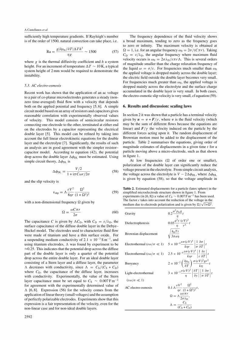
5.3. AC electro-osmosis

Recent work has shown that the application of an ac voltageto a pair of co-planar microelectrodes generates a steady (non-zero time-averaged) fluid flow with a velocity that dependsboth on the applied potential and frequency [5, 6]. A simplecircuit model based on an array of resistors and capacitors givesreasonable correlation with experimentally observed valuesof velocity. This model consists of semicircular resistorsconnecting one electrode to the other, terminated at either endon the electrodes by a capacitor representing the electricaldouble layer [5]. This model can be refined by taking intoaccount the full linear electrokinetic equations for the doublelayer and the electrolyte [7]. Significantly, the results of suchan analysis are in good agreement with the simpler resistor–capacitor model. According to equation (42), the potentialdrop across the double layer φDL must be estimated. Usingsimple circuit theory, φDL is

φDL = V/2

1 + iπCωr/2σ(58)

and the slip velocity is

vslip = �εV 2

8ηr

�2

(1 + �2)2(59)

with a non-dimensional frequency � given by

� = ωCπr

2σ(60)

The capacitance C is given by �CD, with CD = ε/λD, thesurface capacitance of the diffuse double layer in the Debye–Huckel model. The electrodes used to characterize fluid flowwere made of titanium and have a thin surface oxide. Fora suspending medium conductivity of 2.1 × 10−3 S m−1, andusing titanium electrodes, � was found by experiment to be≈0.25. This indicates that the potential drop across the diffusepart of the double layer is only a quarter of the potentialdrop across the entire double layer. For an ideal double layerconsisting of a Stern layer and a diffuse layer, the parameter� decreases with conductivity, since � = CS/(CS + CD)

where CD, the capacitance of the diffuse layer, increaseswith conductivity. Experimentally, the value of the Sternlayer capacitance must be set equal to CS ∼ 0.007 F m−2

for agreement with the experimentally determined value of� [6, 8]. Expression (56) for the velocity comes from theapplication of linear theory (small voltages) and the assumptionof perfectly polarizable electrodes. Experiments show that thisexpression is a fair representation of the velocity, even for thenon-linear case and for non-ideal double layers.

The frequency dependence of the fluid velocity showsa broad maximum, tending to zero as the frequency goesto zero or infinity. The maximum velocity is obtained at� = 1, i.e. for an angular frequency ω0 = 2σ/(Cπr). TakingCD = ε/λD, the angular frequency where maximum fluidvelocity occurs is ω0 = 2σλD/επr�. This is several ordersof magnitude smaller than the charge relaxation frequency ofthe liquid ω = σ/ε. For frequencies much smaller than ω0

the applied voltage is dropped mainly across the double layer;the electric field outside the double layer becomes very small.For frequencies much greater than ω0, the applied voltage isdropped mainly across the electrolyte and the surface chargeaccumulated in the double layer is very small. In both cases,the electro-osmotic slip velocity is very small, cf equation (59).

6. Results and discussion: scaling laws

In section 2 it was shown that a particle has a terminal velocitygiven by u = v + F/γ , where v is the fluid velocity (whichmay be the sum of different flows because the equations arelinear) and F/γ the velocity induced on the particle by thedifferent forces acting upon it. The random displacement ofBrownian motion must be added to the displacement of theparticle. Table 2 summarises the equations, giving order ofmagnitude estimates of displacements in a given time t for aparticle moving above a micro-electrode, such as that shownin figure 1.

At low frequencies (� of order one or smaller),polarization of the double layer can significantly reduce thevoltage present in the electrolyte. From simple circuit analysis,the voltage across the electrolyte is V − 2φDL, where φDL

is given by equation (58), so that the voltage amplitude in

Table 2. Estimated displacements for a particle (latex sphere) in thesimplified microelectrode structure shown in figure 1. Fromexperiments (in [6, 8]) a value of CS ∼ 0.007 F m−2 has been used.The factor c takes into account the reduction of the voltage in themedium due to electrode polarization and is given by �/

√1+�2.

Gravity 0.2a2ρmg

ηt

Dielectrophoresis 0.03a2ε

η

(cV )2

r3t

Brownian displacement

√kBT t

3πaη

Electrothermal (εω/σ � 1) 5 × 10−4 εσ (cV )4

kηr

∣∣∣∣ 1

σ

∂σ

∂T

∣∣∣∣ tElectrothermal (εω/σ � 1) 2.5 × 10−4 εσ (cV )4

kηr

∣∣∣∣1

ε

∂ε

∂T

∣∣∣∣ tBuoyancy 2 × 10−2

(∂ρm

∂T

)σ(cV )2gr2

kηt

Light-electrothermal 3 × 10−3 ε(cV )2

η

∣∣∣∣∂T

∂y

∣∣∣∣∣∣∣∣ 1

σ

∂σ

∂T

∣∣∣∣ t(εω/σ � 1)

AC electro-osmosis 0.1 �εV 2

ηr

�2

(1 + �2)2t,

� = �ωεπr

2σλD,

� = CS

(CS + CD)

2592

Electrohydrodynamics and DEP in microsystems

the electrolyte is V �/√

1 + �2. In other words, at lowfrequencies, the voltage in the electrolyte is reduced by a factorof the order of c = �

√1 + �2, where the parameter c is used

to scale the applied potential V when calculating bulk fluidflow (sections 5.1 and 5.2) and dielectrophoretic displacementat low frequencies.

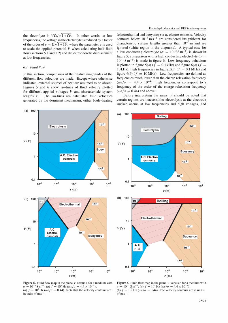
6.1. Fluid flow

In this section, comparisons of the relative magnitudes of thedifferent flow velocities are made. Except where otherwiseindicated, external sources of heat are assumed to be absent.Figures 5 and 6 show iso-lines of fluid velocity plottedfor different applied voltages V and characteristic systemlengths r . The iso-lines are calculated fluid velocitiesgenerated by the dominant mechanism, either Joule-heating

Buoy.

10-7

10-5

10-3

A.C. Electro-osmosis

Electrolysis

100(a)

(b)

10

1

0.1

10-5 10-4 10-3 10-210-6

r (m)

V (V)

•5. •5 •4. •4 •3. •3 •2. •2

•0.

0

0.

1

1.

2

Buoyancy

Electrothermal

10-7

10-5

A.C.Electro-osmosis

El.10-3

100

10

1

0.1

10-5 10-4 10-3 10-210-6

r (m)

V (V)

Figure 5. Fluid flow map in the plane V versus r for a medium withσ = 10−3 S m−1: (a) f = 102 Hz (ωε/σ = 4.4 × 10−4);(b) f = 105 Hz (ωε/σ = 0.44). Note that the velocity contours arein units of m s−1.

(electrothermal and buoyancy) or ac electro-osmosis. Velocitycontours below 10−8 m s−1 are considered insignificant forcharacteristic system lengths greater than 10−6 m and areignored (white region in the diagrams). A typical case fora low conducting electrolyte (σ = 10−3 S m−1) is shown infigure 5; comparison with a high conducting electrolyte (σ =10−1 S m−1) is made in figure 6. Low frequency behaviouris plotted in figure 5(a) (f = 0.1 kHz) and figure 6(a) (f =10 kHz); high frequencies in figure 5(b) (f = 0.1 MHz) andfigure 6(b) (f = 10 MHz). Low frequencies are defined asfrequencies much lower than the charge relaxation frequency(ωε/σ = 4.4 × 10−4); high frequencies correspond to afrequency of the order of the charge relaxation frequency(ωε/σ = 0.44) and above.

Before interpreting the maps, it should be noted thatcertain regions are inaccessible; electrolysis at the electrodesurface occurs at low frequencies and high voltages, and

0.

0

0.

1

1.

Buoyancy

ET

10-7

10-5

10-3

A.C. Electro-osmosis

Electrolysis

Boiling

10-1

100(a)

(b)

10

1

0.1

10-5 10-4 10-3 10-210-6

r (m)

V (V)

•5. •5 •4. •4 •3. •3 •2. •2

•0.

0

0.

1

1.

Buoyancy

Electrothermal

10-7

10-5A.C.E.O.

10-3

10-1

BoilingEl.100

10

1

0.1

10-5 10-4 10-3 10-210-6

r (m)

V (V)

Figure 6. Fluid flow map in the plane V versus r for a medium withσ = 10−1 S m−1: (a) f = 104 Hz (ωε/σ = 4.4 × 10−4);(b) f = 107 Hz (ωε/σ = 0.44). The velocity contours are in unitsof m s−1.

2593

A Castellanos et al

boiling due to Joule heating occurs at high voltages andconductivities. Under dc conditions, a few volts are enoughto produce electrolysis [20]; assuming that 2 V across thedouble layer is needed to produce electrolysis (|φDL| =2 V), the maximum permissible applied voltage is givenby V = 4

√1 + �2 V. According to equation (45), the

maximum applied voltage before boiling takes place is given byV = √

8kT/σ , where T ∼ 75 K (for a room temperatureof 25˚C). These boundaries are also depicted in the maps.

As is apparent from the figures, ac electro-osmosisprogressively disappears when the frequency is increased. Itdominates at low frequencies, and small characteristic lengths,and can reach velocities of several mm s−1. As the electrolyteconductivity is increased, the effect of electrothermal flowbecomes more important. At a characteristic system lengthof the order of 1 mm, buoyancy due to Joule heating alwaysdominates the fluid flow.

The experimental observations of ac electro-osmosis[6, 8, 21] confirm that it can dominate the behaviour of particlesat low frequencies, as suggested by figures 5(a) and 6(a).Note that the effect decreases with increasing conductivity.Electrothermal travelling wave pumping experiments [4, 22]show that voltages greater than 10 V are required to achievenoticeable fluid velocities, in agreement with the calculatedvoltages shown in the figures. The velocity measurementsgiven in [22] show that strong thermal convection is obtainedfor conductivities greater than 1.6 × 10−2 S m−1. In thesame work, it was shown that the velocity increases withconductivity (in the measured range of 4 × 10−3 to 1.6 ×10−2 S m−1), which is a clear indication of Joule heating.However, in this same set of experiments, no noticeabledependence of flow velocity on conductivity was observedfor conductivities lower than 4 × 10−3 S m−1; the reasonfor this is not clear. In another set of experiments [23, 24],it has been reported that the time-dependent collection ofparticles in a millimetre-scale system can be driven by Jouleheating-induced buoyancy forces. Large convective rollswere observed, with typical dimensions and velocities inagreement with the characteristic system length and expectedflow velocity shown in the maps.

Figure 7 shows the domain of influence of Joule heatingand light-induced electrothermal flow, plotted as a function ofvoltage and conductivity. A characteristic system length ofr = 50 µm has been chosen. For the light-induced heating,two vertical gradients of temperature are used: 0.02 K µm−1

in figure 7(a) and 0.002 K µm−1 in figure 7(b). The formertemperature gradient corresponds to that which was requiredto numerically model experimentally observed fluid velocitiesunder strong illumination [11] (at a conductivity of 2.1 ×10−3 S m−1). The variation in flow with conductivity isvery small since (1/σ)(dσ/dT ) is almost independent ofconductivity. Figure 7(a) shows that only for very highapplied voltages and conductivities is Joule heating moreimportant than the externally imposed temperature gradient of0.02 K µm−1. If the temperature gradient is reduced by a factorof 10 (figure 7(b)), light-induced fluid flow still occurs forconductivities smaller than 10−2 S m−1 and applied voltagesbelow 10 V, but the expected velocities are ten times smaller.

100

10

1

0.110-3 10-2 10-1 10010-4

V (V)

σσ (S/m)

Light inducedelectrothermal

Jouleelectrothermal

10-7

10-5 10-3

10-1

Light inducedelectrothermal

Jouleelectrothermal

10-7

10-5

10-3

100

10

1

0.110-3 10-2 10-1 10010-4

V (V)

σ (S/m)

(a)

(b)

Figure 7. Fluid flow map showing joule heating and light-inducedheating electrothermal flows in the plane V versus σ .(a) dT/dy = 0.02 K µm−1; (b) dT/dy = 0.002 K µm−1. Thevelocity contours are in units of m s−1.

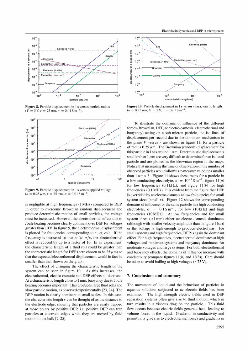
6.2. Particle displacement

Figure 8 shows the displacement of a particle for a time windowof 1 s in an electrolyte with conductivity 10−2 S m−1, plottedas a function of particle radius (with the same parameters asused to plot figure 3). The first point to note is that acelectro-osmosis dominates particle motion at a frequencyof 1 kHz. Only for large particles (greater than 5 µm indiameter) is the ac electro-osmotic-induced displacement lessthan that caused by DEP. This concurs with experimentalobservations, particularly of cells, where the subtle effects ofac electro-osmosis on particle dynamics at low frequencies areoften unnoticed. The electro-osmotic displacement becomesnegligible at high frequencies, as shown by the line calculatedat f = 1 MHz. This diagram shows that movement of sub-micron sized particles by DEP at low frequencies (∼1 kHz) isalmost impossible owing to ac electro-osmosis. At frequenciesaround 1 MHz, ac electro-osmosis is irrelevant and DEPdominates. However, as the particle size is decreased,the voltage required to induce particle movement becomesappreciably greater. This means that electrothermal flow dueto Joule heating can become important.

The data can be plotted in a different way; figure 9shows the displacement of a small particle (0.5 µm diameter)as a function of voltage for a small electrode structure(characteristic length r = 25 µm). Again, displacement dueto electro-osmosis dominates at low frequencies (∼1 kHz) but

2594

Electrohydrodynamics and DEP in microsystems

10-9

10-8

10-7

10-6

10-5

10-4

10-3

10-2

10-9 10-8 10-7 10-6 10-5

particle size (m)

Electroos (1kHz)

Electroos. (1 MHz)

Brownian

Electrother. (εω /σ <<1)

Electrother. (εω /σ >>1)

DEP

Gravity

Buoyancy

dis

pla

cem

ent

in a

sec

on

d (

m)

Figure 8. Particle displacement in 1 s versus particle radius(V = 5 V, r = 25 µm, σ = 0.01 S m−1).

10-9

10-8

10-7

10-6

10-5

10-4

10-3

10-2

0.1 1 10 100

applied voltage (V)

dis

pla

cem

ent

in a

sec

on

d (

m) Electroos (1kHz)

Electroos (1MHz)

Brownian

DEP

Gravity

Buoyancy

Electrother.

Figure 9. Particle displacement in 1 s versus applied voltage(a = 0.25 µm, r = 25 µm, σ = 0.01 S m−1).

is negligible at high frequencies (1 MHz) compared to DEP.In order to overcome Brownian random displacement andproduce deterministic motion of small particles, the voltagemust be increased. However, the electrothermal effect due toJoule heating becomes clearly dominant over DEP for voltagesgreater than 10 V. In figure 9, the electrothermal displacementis plotted for frequencies corresponding to ω � σ/ε. If thefrequency is increased so that ω σ/ε, the electrothermaleffect is reduced by up to a factor of 10. In an experiment,the characteristic length of a fluid roll could be greater thanthe characteristic length for DEP (here chosen to be 25 µm) sothat the expected electrothermal displacement would in fact besmaller than that shown on the graph.

The effect of changing the characteristic length of thesystem can be seen in figure 10. As this increases, theelectrothermal, electro-osmotic and DEP effects all decrease.At a characteristic length close to 1 mm, buoyancy due to Jouleheating becomes important. This produces large fluid rolls andslow particle motion, as observed experimentally [23, 24]. TheDEP motion is clearly dominant at small scales. In this case,the characteristic length r can be thought of as the distance tothe electrode edge, showing that particles are easily trappedat those points by positive DEP, i.e. positive DEP can trapparticles at electrode edges while they are moved by fluidmotion in the bulk [2, 25].

10-9

10-8

10-7

10-6

10-5

10-4

10-3

10-2

10-610-5 10-4 10-3

characteristic length (m)

Electroos. (1kHz)

Electroos. (1 MHz)

Brownian

Electrother. (εω ω /σ σ <<1)

DEP

Gravity

Buoyancydis

pla

cem

ent

in a

sec

on

d (

m)

Figure 10. Particle displacement in 1 s versus characteristic length(a = 0.25 µm, V = 5 V, σ = 0.01 S m−1).

To illustrate the domains of influence of the differentforces (Brownian, DEP, ac electro-osmosis, electrothermal andbuoyancy) acting on a sub-micron particle, the iso-lines ofdisplacement per second due to the dominant mechanism inthe plane V versus r are shown in figure 11, for a particleof radius 0.25 µm. The Brownian (random) displacement forthis particle in 1 s is around 1 µm. Deterministic displacementssmaller than 1 µm are very difficult to determine for an isolatedparticle and are plotted as the Brownian region in the maps.Notice that increasing the time of observation or the number ofobserved particles would allow us to measure velocities smallerthan 1 µm s−1. Figure 11 shows these maps for a particle ina low conducting electrolyte, σ = 10−3 S m−1; figure 11(a)for low frequencies (0.1 kHz), and figure 11(b) for highfrequencies (0.1 MHz). It is evident from the figure that DEPis overriden by ac electro-osmosis at low frequencies for smallsystem sizes (small r). Figure 12 shows the correspondingdomains of influence for the same particle in a high conductingelectrolyte, σ = 0.1 S m−1, for low (10 kHz) and highfrequencies (10 MHz). At low frequencies and for smallsystem sizes (<1 mm) either ac electro-osmosis dominates(although with smaller velocity amplitude than in figure 11(a))or the voltage is high enough to produce electrolysis. Forsmall systems and high frequencies, DEP is again the dominanteffect. For high frequencies, electrothermal dominates at highvoltages and moderate systems and buoyancy dominates formoderate voltages and large systems. For both electrothermaland buoyancy effects, the domains of influence increase withconductivity (compare figures 11(b) and 12(b)). Care shouldbe taken to avoid boiling at high voltages (∼75 V).

7. Conclusions and summary

The movement of liquid and the behaviour of particles inaqueous solutions subjected to ac electric fields has beenexamined. The high strength electric fields used in DEPseparation systems often give rise to fluid motion, which inturn results in a viscous drag on the particle. This fluidflow occurs because electric fields generate heat, leading tovolume forces in the liquid. Gradients in conductivity andpermittivity give rise to electrothermal forces and gradients in

2595

A Castellanos et al

(a)

(b)

•5. •5 •4. •4 •3. •3 •2. •2

0.

0

0.

1

1.

Buoy.

10-5

10-3

A.C. Electro-osmosis

Electrolysis

Brownianmotion

100

10

1

0.1

10-5 10-4 10-3 10-210-6

r (m)

V (V)

•5. •5 •4. •4 •3. •3 •2. •2

0.

0

0.

1

1.

2

Buoyancy

Electrothermal

10-5

DEP

El.10-3

Brownianmotion

100

10

1

0.1

10-5 10-4 10-3 10-210-6

r (m)

V (V)

Figure 11. Particle velocity maps in the plane V versus r for aparticle with radius a = 0.25 µm in medium with σ = 10−3 S m−1:(a) f = 102 Hz; (b) f = 105 Hz.

mass density to buoyancy. In addition, non-uniform ac electricfields produce forces on the induced charges in the diffusedouble layer on the electrodes. This effect gives oscillatingand steady fluid motions termed ac electro-osmosis. Wehave focused on steady fluid flow. The effects of Brownianmotion have also been discussed in this context. The ordersof magnitude of the various forces experienced by a particlein a model microelectrode system have been estimated. Theresults indicate that ac electro-osmosis dominates fluid motionat low frequencies and small system sizes, electrothermal flowdominates at high frequencies and voltages, and buoyancyat typical system sizes of the order of or greater than1 mm. DEP governs the motion of sub-micrometre particlesfor small systems and at high frequencies; otherwise, theparticle motion is due to fluid drag as shown in figures 11and 12.

•5. •5 •4. •4 •3. •3 •2. •2

•0.

0

0.

1

1.

Buoyancy

ET

10-5

A.C. Electro-osmosis

Electrolysis

Boiling

10-3

10-1

BrownianMotion

100(a)

(b)

10

1

0.1

10-5 10-4 10-3 10-210-6

r (m)

V (V)

•5. •5 •4. •4 •3. •3 •2. •2

Buoyancy

Electrothermal

Brownianmotion

10-5

DEP

10-3

10-1

BoilingEl.100

10

1

0.1

10-5 10-4 10-3 10-210-6

r (m)

V (V)

Figure 12. Particle velocity maps in the plane V versus r for aparticle with radius a = 0.25 µm in medium with σ = 0.1 S m−1:(a) f = 104 Hz; (b) f = 107 Hz.

References

[1] Morgan H and Green N G 2003 AC Electrokinetics: Colloidsand Nanoparticles (Herts: Research Studies Press)

[2] Muller T, Gerardino A, Schnelle T, Shirley S G, Bordoni F,DeGasperis G, Leoni R and Fuhr G 1996 Trapping ofmicrometre and sub-micrometre particles byhigh-frequency electric fields and hydrodynamic forcesJ. Phys. D: Appl. Phys. 29 340–9

[3] Ramos A, Morgan H, Green N G and Castellanos A 1998 ACelectrokinetics: a review of forces in microelectrodestructures J. Phys. D: Appl. Phys. 31 2338–53

[4] Fuhr G, Hagedorn R, Muller T, Benecke W and Wagner B1992 Microfabricated electrohydrodynamic (EHD) pumpsfor liquids of higher conductivity J. Microelectromech. Syst.1 141–6

[5] Ramos A, Morgan H, Green N G and Castellanos A 1999 ACelectric-field induced fluid flow in microelectrodesJ. Colloid Interface Sci. 217 420–2

2596

Electrohydrodynamics and DEP in microsystems

[6] Green N G, Ramos A, Gonzalez A, Morgan H andCastellanos A 2000 Fluid flow induced by non-uniform acelectric fields in electrolytes on microelectrodes I:experimental measurements Phys. Rev. E 61 4011–18

[7] Gonzalez A, Ramos A, Green N G, Castellanos A andMorgan H 2000 Fluid flow induced by non-uniform acelectric fields in electrolytes on microelectrodes II: A lineardouble-layer analysis Phys. Rev. E 61 4019–28

[8] Green N G, Ramos A, Gonzalez A, Morgan H andCastellanos A 2002 Fluid flow induced by non-uniform acelectric fields in electrolytes on microelectrodes III:Observation of streamlines and numerical simulation Phys.Rev. E 66 026305

[9] Reppert P M and Morgan F D 2002 Frequency-dependentelectroosmosis J Colloid Interface Sci. 254372–83

[10] Green N G, Ramos A, Gonzalez A, Castellanos A andMorgan H 2000 Electric field induced fluid flow onmicroelectrodes: the effect of illumination J. Phys. D: Appl.Phys. 33 L13–17

[11] Green N G, Ramos A, Morgan H, Castellanos A andGonzalez A 2001 Electrothermally induced fluid flow onmicroelectrodes J. Electrost. 53 71–87

[12] Clift R, Grace J R and Weber M E 1978 Bubbles, Drops andParticles (New York: Academic) chapter 11

[13] Green N G, Ramos A and Morgan H 2000 AC electrokinetics:a survey of sub-micrometre particle dynamics J. Phys. D:Appl. Phys. 33 632–41

[14] Castellanos A (ed) 1998 Electrohydrodynamics (New York:Springer)

[15] Saville D A 1997 Electrohydrodynamics: the Taylor-Melcherleaky dielectric model Ann. Rev. Fluid Mech. 29 27–64

[16] Melcher J R and Taylor G I 1969 Electrohydrodynamics: areview of the role of interfacial shear stresses Ann. Rev.Fluid Mech. 1 111–46

[17] Batchelor G K 1967 An Introduction to Fluid Dynamics(Cambridge: Cambridge University Press)

[18] Stratton J A 1941 Electromagnetic Theory (New York:McGraw-Hill)

[19] Hunter R J 1981 Zeta Potential in Colloid Science (London:Academic)

[20] Hamann C H, Hamnett A and Vielstich W 1998Electrochemistry (Weinheim: Wiley-VCH)

[21] Brown A B D, Smith C G and Rennie A R 2001 Pumping ofwater with ac electric fields applied to asymmetric pairs ofmicroelectrodes Phys. Rev. E 63 016305

[22] Gimsa J, Eppmann P and Pruger B 1997 Introducing phaseanalysis light scattering for dielectric characterization:measurement of travelling-wave pumping Biophys. J. 733309–16

[23] Arnold W M and Chapman B 2002 The Lev-vection particleconcentrator: some operational characteristics IEEE Conf.Elec. Ins. Dielectric Phenomena

[24] Arnold W M 2001 Positioning and levitation media for theseparation of biological cells IEEE Trans. Ind. Appl. 371468–75

[25] Green N G and Morgan H 1998 Separation of submicrometreparticles using a combination of dielectrophoresis andelectrohydrodynamic forces J. Phys. D: Appl. Phys. 31L25–30

2597