Embed Size (px)
Citation preview

ElasticWISP:Energy-Proportional WISP
Backhaul Networks
by
Duncan Ewan Cameron
A thesissubmitted to the Victoria University of Wellington
in fulfilment of therequirements for the degree of
Master of Engineeringin Network Engineering.
Victoria University of Wellington2020

Abstract
The provision of rural broadband infrastructure is a challenge for networkoperators across the globe, irrespective of their size. Wireless Internet Ser-vice Providers (WISPs) have shown that the small-scale deployment ofwireless broadband infrastructure is a viable alternative to relying on cellu-lar network providers for remote coverage. However, WISPs must oftenresort to using off-grid renewable energy sources such as solar energy forpowering network sites, often resulting in undesirable, low-performancebackhaul radios being used between sites out of concern for excessiveenergy consumption.
The challenges of managing performant wireless backhaul networks inrespect to energy constraints at remote, off-grid sites informs the need forenergy-proportional design. Backhaul radios typically used by WISPs arenot energy-proportional, meaning they use a consistent amount of energy,irrespective of wireless link utilisation. Using data from a real WISP net-work, diurnal traffic patterns show that WISP networks could benefit fromenergy-proportional design, without having to sacrifice performance.
To encourage the development of high-performance, energy-proportionalWISP backhaul networks, ElasticWISP, an optimisation architecture thatreduces network-wide backhaul energy consumption while satisfying theuser-demand for traffic, is introduced. ElasticWISP dynamically controlsthe configuration of backhaul radios based on bandwidth demands and thenetwork-wide energy consumption of these radios. Through simulationsdriven by real WISP topology and data traffic, results show that ElasticWISPcan offer energy savings of approximately 65% when WISP operators follow

the proposed backhaul design methodology.
Finally, a lightweight Multiprotocol Label Switching (MPLS)-based trafficengineering scheme, based on Segment Routing, is proposed. The imple-mentation, named Segment Routing over MPLS (SR-MPLS), keeps trafficengineering path-state within each packet, meaning per-flow state is onlyheld at SR-MPLS ingress routers. The lightweight approach of SR-MPLSalso eliminates the otherwise necessary network-wide label flooding of tra-ditional Segment Routing, making it ideal for bandwidth-sensitive wirelessbackhaul networks. Evaluation of SR-MPLS shows that it can perform aswell as – and sometimes better than – competitor schemes.

To my parents, Phil and Susanne Cameron.
iii

iv

Acknowledgements
Firstly, I would like to thank my admirable supervisor, Dr. Alvin Valera.You have taught me so much in the short two years that I have known you.I would not be where I am today without your well-considered advice.
A special thank you to Prof. Winston K.G. Seah for believing in me, and en-abling this research to be accomplished. Your weekly support has improvedmy research abilities immensely.
To my peers in the Wireless Networks (WiNe) Research Group – thank youfor making the last 12 months so gratifying.
Finally, I would like to acknowledge The Information Society InnovationFund (ISIF Asia), and InternetNZ/Ipurangi Aotearoa.
ISIF Asia’s generosity to the Wellington Faculty of Engineering has fundeda range of Internet research relevant to the Asia-Pacific region, includingmy own.
InternetNZ’s support of improving Internet access throughout all of NewZealand will enable me to attend the Institute of Electrical and Electron-ics Engineers (IEEE)/International Federation for Information Processing(IFIP) Network Operations and Management Symposium (NOMS 2020)later this year.
To ISIF Asia and InternetNZ: I am forever grateful. One day I hope to giveback as you have given to me.
v

vi

Contents
1 Introduction 111.1 About WISPs . . . . . . . . . . . . . . . . . . . . . . . . . . . . 12
1.2 Objectives . . . . . . . . . . . . . . . . . . . . . . . . . . . . . 13
1.3 Tasks . . . . . . . . . . . . . . . . . . . . . . . . . . . . . . . . 14
1.4 Contributions . . . . . . . . . . . . . . . . . . . . . . . . . . . 14
1.5 Thesis Organisation . . . . . . . . . . . . . . . . . . . . . . . . 15
1.6 Additional Information . . . . . . . . . . . . . . . . . . . . . . 15
2 Survey of Related Work 172.1 Sustainability . . . . . . . . . . . . . . . . . . . . . . . . . . . 17
2.1.1 Microwave Backhaul Networks . . . . . . . . . . . . . 18
2.1.2 Energy Optimisation . . . . . . . . . . . . . . . . . . . 21
2.2 Traffic Engineering . . . . . . . . . . . . . . . . . . . . . . . . 21
2.2.1 Recent Innovations . . . . . . . . . . . . . . . . . . . . 23
2.3 Summary . . . . . . . . . . . . . . . . . . . . . . . . . . . . . . 25
3 WISP Backhaul Networks 273.1 Backhaul Energy Measurement . . . . . . . . . . . . . . . . . 27
3.2 Backhaul Energy Consumption . . . . . . . . . . . . . . . . . 29
3.3 Benefits of Energy-Proportional Backhaul . . . . . . . . . . . 31
3.3.1 Sustainability . . . . . . . . . . . . . . . . . . . . . . . 32
3.4 Summary . . . . . . . . . . . . . . . . . . . . . . . . . . . . . . 32
vii
viii CONTENTS
4 Solution Architecture 35
4.1 Optimisation and Control . . . . . . . . . . . . . . . . . . . . 35
4.2 ElasticWISP Model Formulation . . . . . . . . . . . . . . . . . 37
4.2.1 Energy Minimisation Constraints . . . . . . . . . . . . 38
4.3 Flow-Path Enforcement . . . . . . . . . . . . . . . . . . . . . 40
4.4 Backhaul Power Control . . . . . . . . . . . . . . . . . . . . . 40
4.5 Summary . . . . . . . . . . . . . . . . . . . . . . . . . . . . . . 41
5 ElasticWISP Reference Implementation 43
5.1 Routing Protocol Integration and Control . . . . . . . . . . . 43
5.1.1 Practical Considerations . . . . . . . . . . . . . . . . . 45
5.2 Summary . . . . . . . . . . . . . . . . . . . . . . . . . . . . . . 46
6 MPLS Segment Routing Design 47
6.1 IGP Integration . . . . . . . . . . . . . . . . . . . . . . . . . . 48
6.2 About MPLS . . . . . . . . . . . . . . . . . . . . . . . . . . . . 49
6.3 SR-MPLS Terminology . . . . . . . . . . . . . . . . . . . . . . 50
6.4 IPv4 and IPv6 MPLS Encapsulation . . . . . . . . . . . . . . . 51
6.5 MPLS Forwarding . . . . . . . . . . . . . . . . . . . . . . . . . 53
6.5.1 Strict Source Routing . . . . . . . . . . . . . . . . . . . 54
6.5.2 Loose Source Routing . . . . . . . . . . . . . . . . . . 56
6.5.3 Shortest Path Forwarding . . . . . . . . . . . . . . . . 58
6.6 Control Plane . . . . . . . . . . . . . . . . . . . . . . . . . . . 59
6.7 Neighbour Label Resolution . . . . . . . . . . . . . . . . . . . 60
6.8 Bidirectional Forwarding Detection . . . . . . . . . . . . . . . 61
6.9 Time To Live Handling . . . . . . . . . . . . . . . . . . . . . . 63
6.10 MTU Considerations . . . . . . . . . . . . . . . . . . . . . . . 63
6.11 MPLS Services . . . . . . . . . . . . . . . . . . . . . . . . . . . 64
6.12 Backhaul Changeover . . . . . . . . . . . . . . . . . . . . . . 65
6.13 SR-MPLS Complexity . . . . . . . . . . . . . . . . . . . . . . . 65
6.14 Summary . . . . . . . . . . . . . . . . . . . . . . . . . . . . . . 66

CONTENTS ix
7 Backhaul Power Control 67
7.1 Cape Features . . . . . . . . . . . . . . . . . . . . . . . . . . . 68
7.2 PoE Injector Design . . . . . . . . . . . . . . . . . . . . . . . . 69
7.2.1 Design 1 . . . . . . . . . . . . . . . . . . . . . . . . . . 70
7.2.2 Design 2 . . . . . . . . . . . . . . . . . . . . . . . . . . 71
7.3 Summary . . . . . . . . . . . . . . . . . . . . . . . . . . . . . . 73
8 Validation 75
8.1 ElasticWISP Evaluation Setup . . . . . . . . . . . . . . . . . . 75
8.2 Traffic Playback . . . . . . . . . . . . . . . . . . . . . . . . . . 76
8.2.1 Traffic Capture . . . . . . . . . . . . . . . . . . . . . . 77
8.2.2 Optimiser Invocation . . . . . . . . . . . . . . . . . . . 79
8.2.3 Traffic Matrix Generation . . . . . . . . . . . . . . . . 81
8.3 QoS Preservation . . . . . . . . . . . . . . . . . . . . . . . . . 81
8.4 Energy Consumption . . . . . . . . . . . . . . . . . . . . . . . 84
8.4.1 Setup . . . . . . . . . . . . . . . . . . . . . . . . . . . . 84
8.4.2 Results . . . . . . . . . . . . . . . . . . . . . . . . . . . 87
8.5 Implementation Considerations . . . . . . . . . . . . . . . . . 90
8.6 SR-MPLS Benchmarks . . . . . . . . . . . . . . . . . . . . . . 92
8.6.1 Constraints . . . . . . . . . . . . . . . . . . . . . . . . 93
8.6.2 RTT Benchmarks . . . . . . . . . . . . . . . . . . . . . 93
8.6.3 Jitter Benchmarks . . . . . . . . . . . . . . . . . . . . . 97
8.6.4 Throughput Benchmarks . . . . . . . . . . . . . . . . 98
8.6.5 Encapsulation and Decapsulation Benchmarks . . . . 99
8.6.6 Improving Performance . . . . . . . . . . . . . . . . . 100
8.6.7 Scalability . . . . . . . . . . . . . . . . . . . . . . . . . 103
8.6.8 Why Kernel Bypass . . . . . . . . . . . . . . . . . . . . 104
8.7 Summary . . . . . . . . . . . . . . . . . . . . . . . . . . . . . . 105
9 Conclusion 107
9.1 Future Work . . . . . . . . . . . . . . . . . . . . . . . . . . . . 108

x CONTENTS
Appendices 113
Appendix A Evaluation Dataset 113
Appendix B Measurement and Control 115
Appendix C ElasticWISP Hardware 119
List of Figures
3.1 Able to Heights TX Traffic (With Bezier Curve). . . . . . . . . 29
3.2 Heights Road Battery Bank. . . . . . . . . . . . . . . . . . . . 30
4.1 ElasticWISP System Overview. . . . . . . . . . . . . . . . . . . 37
5.1 Link-Cost and Power Control Mechanism. . . . . . . . . . . . 44
6.1 MPLS Header. . . . . . . . . . . . . . . . . . . . . . . . . . . . 49
6.2 MPLS Packet. . . . . . . . . . . . . . . . . . . . . . . . . . . . 50
6.3 Strict Source Routing in an SR-MPLS Domain. . . . . . . . . 54
6.4 Flow Diagram of Strict Source Routing in an SR-MPLS Do-main (L3 Operation). . . . . . . . . . . . . . . . . . . . . . . . 55
6.5 Loose Source Routing in an SR-MPLS Domain. . . . . . . . . 56
6.6 Flow Diagram of Loose Source Routing in an SR-MPLS Do-main (L3 Operation). . . . . . . . . . . . . . . . . . . . . . . . 57
7.1 Backhaul Radio Power Control Board. . . . . . . . . . . . . . 69
7.2 Design 1. Low-Cost Gigabit PoE Injector. . . . . . . . . . . . 70
7.3 Design 1 Revision 1. Low-Cost Gigabit PoE Injector. . . . . . 71
7.4 Design 2. High-Power Gigabit PoE Injector. . . . . . . . . . . 72
8.1 Traffic Capture Setup (Simplified). . . . . . . . . . . . . . . . 78
8.2 4x4 Grid Topology. . . . . . . . . . . . . . . . . . . . . . . . . 82
8.3 Node 1 to Node 16 RTT. . . . . . . . . . . . . . . . . . . . . . 83
1

2 LIST OF FIGURES
8.4 Node 1 to Node 16 Jitter. . . . . . . . . . . . . . . . . . . . . . 838.5 Node 1 to Node 16 Datagram Loss. . . . . . . . . . . . . . . . 848.6 Evaluation Topology. . . . . . . . . . . . . . . . . . . . . . . . 858.7 Energy Consumption Over a 7-Day Period. . . . . . . . . . . 888.8 SR-MPLS Evaluation Setup. . . . . . . . . . . . . . . . . . . . 938.9 Host 1 to Host 2 RTT. . . . . . . . . . . . . . . . . . . . . . . . 948.10 Host 1 to Host 2 RTT (1 Gbps UDP Load). . . . . . . . . . . . 958.11 Host 1 to Host 2 RTT (2 Gbps UDP Load). . . . . . . . . . . . 968.12 Host 1 to Host 2 Jitter (1 Gbps UDP Load). . . . . . . . . . . 978.13 UDP Throughput vs. Packet Loss (0–3800 Mbps). . . . . . . . 988.14 UDP Throughput vs. Packet Loss (0–3300 Mbps). . . . . . . . 998.15 Packets Per Second, 84-Byte Frames on Wire. . . . . . . . . . 1008.16 SR-DPDK Evaluation Setup. . . . . . . . . . . . . . . . . . . . 1018.17 Packets Per Second, 84-Byte Frames on Wire (DPDK). . . . . 1028.18 Packets Per Second, 84-Byte Frames on Wire (PacketGen). . . 102
List of Tables
3.1 WISP Backhaul Radio Energy Consumption . . . . . . . . . . 283.2 WISP Relay Site (2 x airFiber5) . . . . . . . . . . . . . . . . . 313.3 WISP Relay Site (2 x Radio PowerBeam5AC G2) . . . . . . . 313.4 WISP Relay Site (2 x airFiber5 and Powerbeam5AC G2) . . . 31
4.1 Energy Minimisation Notation . . . . . . . . . . . . . . . . . 38
8.1 Validation: Competitors . . . . . . . . . . . . . . . . . . . . . 898.2 Segment Routing Performance . . . . . . . . . . . . . . . . . 1008.3 Segment Routing (PacketGen) Performance . . . . . . . . . . 103
B.1 Current Sense Ratio for IL . . . . . . . . . . . . . . . . . . . . 117
3

4 LIST OF TABLES

Acronyms
5G Fifth Generation.
AC Alternating Current.
ADC Analogue to Digital Converter.
Adj-SID Adjacency Segment.
AGM Absorbent Glass Mat.
Ah Ampere hour.
API Application Programming Interface.
AQM Active Queue Management.
ARP Address Resolution Protocol.
BFD Bidirectional Forwarding Detection.
CLI Command Line Interface.
CORE Common Open Research Emulator.
CPU Central Processing Unit.
CR-LDP Constraint-based Routing Label Distribution Protocol.
CRC Cyclic Redundancy Check.
5

6 Acronyms
CSA-IE Channel Switch Announcement Information Element.
CSPF Constrained Shortest Path First.
DC Direct Current.
DFS Dynamic Frequency Selection.
DPDK Data Plane Development Kit.
DVFS Dynamic Voltage and Frequency Scaling.
EAR Energy-Aware Routing.
eBGP External Border Gateway Protocol.
ECMP Equal-Cost Multi-Path.
EHF Extremely High Frequency.
FIB Forwarding Information Base.
FIFO First in, First out.
FQ-CoDel Flow Queue Controlled Delay.
GbE Gigabit Ethernet.
GDT Gas Discharge Tube.
GPIO General Purpose Input/Output.
GUI Graphical User Interface.
ICIC Inter-Cell Interference Coordination.
IEEE Institute of Electrical and Electronics Engineers.
IETF Internet Engineering Task Force.
IFIP International Federation for Information Processing.
Acronyms 7
IGP Interior Gateway Protocol.
IP Internet Protocol.
IPFIX IP Flow Information Export.
IPv4 Internet Protocol version 4.
IPv6 Internet Protocol version 6.
IS-IS Intermediate System to Intermediate System.
ISIF Asia The Information Society Innovation Fund.
ISP Internet Service Provider.
ITU International Telecommunication Union.
KVM Kernel Virtual Machine.
kWh Kilowatt hour.
L2VPN Layer 2 Virtual Private Network.
L3VPN Layer 3 Virtual Private Network.
LAG Link Aggregation Group.
LDP Label Distribution Protocol.
LER Label Edge Router.
LFIB Label Forwarding Information Base.
LRP Label Resolution Protocol.
LSA Link State Advertisement.
LSP Label Switched Path.
LSR Label Switching Router.

8 Acronyms
MAC Media Access Control.
MAN Metropolitan Area Network.
MCF Multi-Commodity Flow.
mmWave Millimeter Wave.
MPLS Multiprotocol Label Switching.
MPPT Maximum Power Point Tracking.
MTU Maximum Transmission Unit.
NIC Network Interface Controller.
NOMS 2020 Network Operations and Management Symposium.
OPEX Operational Expenditure.
OSPF Open Shortest Path First.
PCB Printed Circuit Board.
PHP Penultimate Hop Popping.
PLA Physical Link Aggregation.
PMSR Poor Man’s Segment Routing.
PoC Proof of Concept.
PoE Power over Ethernet.
PoP Point of Presence.
PPS Packets Per Second.
QoE Quality of Experience.
QoS Quality of Service.
Acronyms 9
RSS Root Sum Squared.
RSVP Resource Reservation Protocol.
RTT Round Trip Time.
SBC Single-Board Computer.
SDN Software-Defined Networking.
SID Segment Identifier.
SMA Simple Moving Average.
SNMP Simple Network Management Protocol.
SNR Signal-to-Noise Ratio.
SR-MPLS Segment Routing over MPLS.
SRv6 Segment Routing over IPv6.
SSID Service Set Identifier.
TCP Transmission Control Protocol.
TTL Time To Live.
UDP User Datagram Protocol.
VLAN Virtual Local Area Network.
VoIP Voice over IP.
VPLS Virtual Private LAN Service.
VPRN Virtual Private Routed Network.
Wh Watt hour.
WiNe Wireless Networks.

10 Acronyms
WISP Wireless Internet Service Provider.

Chapter 1
Introduction
WISP networks play an important role in connecting remote and rural areasto the Internet [1–6]. In New Zealand alone, there are over 30 regionalWISPs, connecting more than 70,000 households and businesses to theInternet [7]. Amongst various operational challenges, researchers haveidentified that many WISP operators build their networks out of necessityin order to provide faster connectivity to deprived communities, even ifthey lack requisite knowledge to design and maintain wireless networks [2,3, 8]. While efforts have been made to lower the barrier to entry for suchWISP operators to successfully operate networks [1–3, 9], little has beenaccomplished to overcome one of the greatest operational challenges: off-grid network energy consumption [2, 9, 10].
To gain a better understanding of why energy consumption is important toWISPs, their target markets must be considered. By nature, underservedremote and rural communities often lack ubiquitous deployment of otherinfrastructure, e.g. power networks. Where a WISP builds Internet in-frastructure in an unconnected frontier, there is often an assumption thatgrid-power will not be available, or will at a minimum be unreliable [3].To power network equipment such as radios and routers, an appropriate
11
12 CHAPTER 1. INTRODUCTION
energy harvesting system must be designed, taking into consideration thebusiness case and cost of the entire system. As WISP markets are typicallyremote and rural with low subscriber density, budgets are often limited.
WISPs are then presented with a dilemma: build low-cost, low-performanceinfrastructure to offer basic Internet connectivity, or build high-cost, high-performance infrastructure to offer services competitive to those foundin cities. The latter may not be sustainable, although not necessarily dueto prohibitively expensive radios, but rather the prohibitively expensiveenergy harvesting systems that are responsible for providing power toremote sites1. Therefore it is in a WISP’s best interest to conserve as muchenergy as possible in order to maintain a sustainable balance betweennetwork performance and capital expenditure.
1.1 About WISPs
A WISP network typically consists of a combination of point-to-multipointcustomer access radios, and point-to-point backhaul radios. The formeris used for distribution of Internet access to end-users, and the latter isused for backhaul, or connecting edge routers to the network core. Whendeciding what backhaul radios to purchase, WISPs may consider licensedmicrowave radios to prevent unwanted interference, and consequently,unpredictable service degradation. However, these higher-performanceradios, should they be licensed or unlicensed, typically consume far greaterenergy than their lower-performance counterparts.
Prior research has shown that WISPs can adapt network site configurationsto use less energy [8], such as using less radios for customer access purposes,often at the sacrifice of performance. However, many customer accessradios available to WISPs have a relatively low energy footprint. In evidentcontrast, one backhaul radio could use as much energy as five customer
1A remote site is also commonly referred to as a Point of Presence (PoP).
1.2. OBJECTIVES 13
access radios. Dedicated backhaul radios are also typically much lessflexible in deployment, unless a network operator sacrifices throughputfor lower energy consumption. Given this, reducing backhaul energyconsumption without disrupting network performance is of particularinterest.
Companies such as Ubiquiti Networks [11] have pioneered inexpensive,low-power radios that have enabled low-cost development of Internetaccess infrastructure in remote and rural communities [8]. However, themajority of these radios operate in unlicensed frequency bands in all but fewcountries, typically subjecting them to low power budgets and interferencefrom other unlicensed devices operating within the same frequency range.These factors result in unpredictable network performance, impairing evenwell-established WISP operators [8].
Where unlicensed backhaul radios can be replaced with licensed microwaveand other high-performance radios, WISPs must account for their substan-tially higher power consumption [1]. The considerable energy consumptionof high-performance radios makes them unsuitable for many WISPs witha limited budget. Another drawback of such radios is that they are notenergy-proportional, meaning that they consume a nearly constant amountof energy irrespective of the throughput over them [1, 12].
1.2 Objectives
The key objectives of this thesis are to:
• Investigate WISP backhaul networks and document opportunities forenergy reduction.
• Design an optimisation framework to reduce energy consumption inWISP backhaul networks.
• Design a traffic engineering architecture that is suitable for WISP
14 CHAPTER 1. INTRODUCTION
backhaul networks.
• Validate that the optimisation framework and traffic engineeringarchitecture is of acceptable performance for deployment in real WISPnetworks.
1.3 Tasks
The key tasks of this thesis are to:
• Survey related work in the area of WISP backhaul networks.
• Survey the state-of-the-art in “green” microwave backhaul networks.
• Implement an energy optimisation framework as required.
• Implement a traffic engineering architecture based on current state-of-the-art research.
1.4 Contributions
The contributions in this thesis are threefold. The first contribution is theWISP backhaul optimisation framework, ElasticWISP. The second contri-bution is the lightweight – or poor man’s – MPLS-based Segment Routingarchitecture, referred to SR-MPLS throughout this thesis. The SegmentRouting implementation leverages a source-routing paradigm, and enablesWISPs to perform fine-grained traffic engineering. By design, the Elas-ticWISP optimiser leverages this traffic engineering capability to enforceoptimal-flow paths in a given WISP backhaul topology. The third and finalcontribution is the power-control architecture that enables ElasticWISP tobe used as a part of real WISP networks. As a part of this contribution, aseries of remotely managed Gigabit Ethernet (GbE)-capable Power overEthernet (PoE) injectors were designed and manufactured. Additionally,

1.5. THESIS ORGANISATION 15
note that parts of the ElasticWISP related content in this thesis has beenaccepted into the IEEE/IFIP NOMS 2020 for publication.
1.5 Thesis Organisation
Following this introduction, Chapter 2 details a survey of related work,followed by the motivation for ElasticWISP in Chapter 3. A brief, high-leveloverview of the ElasticWISP and SR-MPLS architectures is then describedin Chapter 4. Chapter 4 also describes the formal model of ElasticWISP,which is based on a standard Multi-Commodity Flow (MCF) formulationenhanced with energy minimisation and radio configuration constraints.Chapter 5 concisely describes the reference implementation of ElasticWISP,as accepted for publication in the IEEE/IFIP NOMS 2020. Thereafter, Chap-ter 6 discusses the design of SR-MPLS.
An outline of the design and implementation of the hardware used to enablepractical application of ElasticWISP is then given in Chapter 7. Next, usinga real WISP network topology, a detailed evaluation of ElasticWISP and itsenergy minimisation potential is presented in Chapter 8. An evaluationof SR-MPLS is also provided, benchmarking it against similar existingschemes. Finally, Chapter 9 makes conclusions about ElasticWISP and SR-MPLS. Planned future improvements, and areas for future exploration, arealso outlined in this chapter.
1.6 Additional Information
Please note that when voltage is referred to in this thesis – e.g., 24V poweredradios – we assume Direct Current (DC), unless otherwise stated.

16 CHAPTER 1. INTRODUCTION

Chapter 2
Survey of Related Work
Several related efforts have addressed lowering the cost of expensive off-grid energy systems used by WISPs [9, 10]. While these efforts offer impor-tant contributions, they do not address the energy-proportionality issuesfaced by WISPs that desire to build higher-performance networks1. Thischapter examines related work and identifies gaps in the literature wherefurther opportunities for research exist.
2.1 Sustainability
The globally recognised viability of WISPs, to an extent, relies on thembeing perceived as sustainable. For a WISP to be sustainable and competewith other commercial network operators, they must be able to providea competitive service. In many circumstances WISPs are constrained toplacing their equipment, such as backhaul radios, in locations that aresub-optimal. Where a WISP places equipment in a remote area whereoff-grid energy must be harvested, it is critical that the total network energyconsumption is kept at a minimum. Ideally, not at the expense of network
1In the context of throughput and reliability.
17

18 CHAPTER 2. SURVEY OF RELATED WORK
Quality of Service (QoS) and negligent customer over-subscription ratios.
Previous research shows that energy consumption is one of the biggestchallenges faced by WISPs that rely on renewable energy sources [8]. Prag-matic research by the University of California, Berkeley and the Google-sponsored Further Reach network discusses the challenges involved withoperating solar energy systems and power-hungry backhaul radios [1].Overall, the challenges involved with using renewable energy harvestingfor WISP networks are well understood [2, 3, 9, 10, 13–15]. Despite the exis-tence of a well-grounded understanding, it must be recognised that littleresearch has been carried out to find an immediate means of addressingthese energy-related network operational difficulties.
2.1.1 Microwave Backhaul Networks
Closely related to WISP backhaul networks are microwave backhaul net-works. In some cases, especially where energy harvesting is not constrained,WISPs will use microwave backhaul radios for high-throughput links. Ithas been found that microwave backhaul networks can account for approx-imately 50% of overall network energy consumption [16, 17], showing theimportance of designing energy efficient network architectures. In an effortfocused on Millimeter Wave (mmWave) backhaul networks – specificallyfor supporting omnipresent deployment of 5G infrastructure – energy sav-ings of up to 65% were achieved through turning off both backhaul linksand small cells [18]. Evidently, wireless backhaul networks are an idealcandidate for energy efficiency improvements.
Upon further investigation into how cellular carriers handle microwavebackhaul energy conservation, it was determined that a common techniquesimply involves turning off redundant backhaul radios when they are beingunderutilised. Hence, traffic during periods of low-demand is consolidatedover a single link [19, 20]. It is further identified that due to the dynamicnature of working with microwave backhaul, e.g., considering frequency
2.1. SUSTAINABILITY 19
interface, multipath interference, and rain fade, Physical Link Aggregation(PLA) is often necessary to address throughput capacity concerns [20]. Prac-tically, the use of PLA binds microwave backhaul links together, forming aLink Aggregation Group (LAG), enabling higher aggregate throughput tobe distributed over the backhaul pairs.
Interestingly, it is also found that most microwave backhaul networks forma tree or chain network topology, and less frequently, a ring topology [20].While true today, there is a strong consensus that future backhaul networks,such as those that will support Fifth Generation (5G) cellular services, willrequire a new design paradigm to be realised [18, 20–23]. Particularly, itis believed that future backhaul networks will have dense geographicaldeployment, and leverage higher mmWave2 frequencies to ease current-day throughput capacity concerns. While the EHF nature of such backhaulnetworks enables impressive throughput capacity, it also constrains themto very short physical distance operation, presenting exciting new researchchallenges.
The use of mmWave backhaul networks within industry has already startedto take place. Facebook, in a collaborative effort with Qualcomm, Radwin,Intel, and Nokia, has launched a project named Terragraph [24]. The Ter-ragraph project uses mmWave radios to distribute high-speed – in excessof 1 GbE – Internet access in underconnected urban and suburban areas.Unlike traditional microwave backhaul links that can span tens of kilo-metres, the Terragraph links have a maximum operating range of 250m,making their use case for WISPs operating in sparsely populated ruralareas limited.
In addition, the use of mmWave backhaul radios in WISP networks mayonly exacerbate energy-related challenges. While urban and suburbanenvironments may be permissive of densely connected mmWave backhaul
2International Telecommunication Union (ITU) designated as Extremely High Fre-quency (EHF).
20 CHAPTER 2. SURVEY OF RELATED WORK
radios, due to readily available power infrastructure, rural areas are farless tolerant. Powering closely situated mmWave backhaul radios withrenewable energy resources may be possible in some circumstances, butwith low subscriber density, likely lacks long-term financial sustainability.
Global Internet traffic is predicted to surge to almost double what it istoday,3 by the end of 2022 [25]. Additionally, busy hour4 network trafficis increasing at an even faster rate. The rapid increase in demand forthroughput capacity is troubling for WISPs. Cellular networks are evolvingto become significantly faster than they are today, however, WISP networksare in a position where they could be left years behind their urban andsuburban counterparts. For Internet-connected rural populations acrossthe world, the lack of fast Internet access risks introducing a second digitaldivide. Improving energy efficiency of backhaul networks, for any wireless-centric service provider, WISP or cellular, should therefore be of paramountimportance to prevent rural communities falling behind.
Given the inevitable increase in throughput capacity required by futurebackhaul networks, 5G or otherwise, any research contribution madeshould be general enough to have application on a variety of networktopologies. While many existing microwave and WISP topologies might notbe meshed, future mmWave backhaul networks might, meaning topology-aware heuristics might not be a suitable approach to initially pursue. Inaddition, as mmWave technology has application for both WISPs and cellu-lar operators, the literature suggests that any meaningful energy-reductionscheme should be able to operate irrespective of the underlying backhaultechnology in use.
3As of December 2019.4The busiest 60-minute period of network traffic in a given day.
2.2. TRAFFIC ENGINEERING 21
2.1.2 Energy Optimisation
Numerous general efforts to reduce network wide energy consumptionhave been made. GreenTE [26] utilises both Open Shortest Path First(OSPF) routing and MPLS, and places line-cards into a sleep-state, reduc-ing backhaul energy consumption by 27%–42%. The GreenTE approachalso actively avoids triggering OSPF Link State Advertisements (LSAs)when links are sleeping. While useful for avoiding full network reconver-gence, this approach requires either OSPF implementation modification oramendments to the OSPF protocol specification. ElasticTree [27] is anotherexample, reducing energy consumption in data centre networks by up to60%. Unlike GreenTE, ElasticTree utilises OpenFlow [28] for network trafficforwarding, allowing for explicit enforcement of optimal flow paths. Otherconceptual approaches to Energy-Aware Routing (EAR) have achievedsimilar performance, with energy reduction of approximately 50% [12].
While optimisation approaches that turn off redundant links are generallysuccessful in reducing backhaul-network-wide energy consumption, otherapproaches to designing “green backhaul” within cellular networks includeInter-Cell Interference Coordination (ICIC) resource allocation schemes.Such ICIC schemes have been shown to improve energy efficiency by up to50%, however, at the expense of reduced spectral efficiency [29–31]. One ofthe key problems with applying the likes of ICIC approaches – or any otherspectral management solution – to WISP backhaul networks is the inabilityto integrate any potential design with closed-source vendor software andhardware implementations.
2.2 Traffic Engineering
In the process of researching the challenges involved with operating WISPbackhaul networks, it became apparent that traffic engineering is also achallenge faced by many WISPs. One recent example of this was presented

22 CHAPTER 2. SURVEY OF RELATED WORK
at FaucetCon 2019 [32]. Using the Faucet Software-Defined Networking(SDN) controller [33], a WISP consultancy firm showcased fine-grainedtraffic engineering, complete with real-time integration with some backhaulradios used by WISPs [34]. The purpose of this demonstration was to showthat traffic flows can be balanced across multiple backhaul links, and withrelative ease.
Like many SDN controllers, Faucet is designed for controlling OpenFlow-capable SDN switches. However, it should be questioned why WISPs needto use a protocol such as OpenFlow to achieve their traffic engineeringneeds to begin with. The answer is due to how WISPs build their networks.Previous work showed that OSPF is the prevalent Interior Gateway Protocol(IGP) in WISP networks. Unfortunately for WISPs, OSPF is also a best-effortprotocol, and will always use the lowest-cost path for routing traffic. Link-cost metrics can be adjusted to influence flow-paths, however, in manycircumstances this is not suitable for performing traffic engineering.
Despite the limitations of OSPF, WISPs have still found ways to use it fortraffic engineering. One such approach is the OSPF “Leapfrog” [35], whereVirtual Local Area Networks (VLANs) are used to create additional sub-networks. The VLAN tagged path is logically shorter than the alternativenon-VLAN tagged path, and an OSPF adjacency is established between theVLAN endpoints. However, inventive approaches to achieve traffic engi-neering over networks running OSPF do not stop here. Several solutionshave used a combination of exterior External Border Gateway Protocol(eBGP) and OSPF to achieve traffic engineering functionality [36–38].
Due to the challenges of implementing traffic engineering with OSPF, MPLShas become a topic of interest for many WISPs in recent years [8]. It shouldalso be noted that despite the recent interest, the concept of using MPLSfor traffic engineering has been well established since the early 2000s [39].However, traditional MPLS traffic engineering mechanisms require morethan just an MPLS capable router or switch. Generally, an MPLS traffic
2.2. TRAFFIC ENGINEERING 23
engineering scheme will require:
• Extensions to the IGP of choice, in order to distribute informationabout link attributes and the network topology.
• A means to perform path computation, such as the Constrained Short-est Path First (CSPF) algorithm.
• Signalling protocols to enable the creation of MPLS Label SwitchedPaths (LSPs), such as the Resource Reservation Protocol (RSVP), orthe Label Distribution Protocol (LDP).
• The necessary RSVP traffic engineering extensions (RSVP-TE) – ifusing RSVP. Note, RSVP-TE is the intended replacement – as deter-mined by the Internet Engineering Task Force (IETF) – for the nowdeprecated Constraint-based Routing Label Distribution Protocol(CR-LDP) [40].
It is reasonable to expect that experienced network engineers can build andmaintain MPLS networks, including traffic engineering mechanisms as nec-essary. However, we must also consider the complexity of such networks,as we desire to improve the sustainability of WISPs where possible. Whilenot a technical problem, the shoestring operational nature of many WISPsmeans that technical competencies may not be high, as discussed in Chap-ter 1. Irrespective of social challenges, the complexity of traffic engineeringmechanisms presents an opportunity for protocol simplification.
2.2.1 Recent Innovations
Given the complexity of implementing traffic engineering – even in apurpose-built MPLS environment – it must be questioned how furthersimplifications are possible. State-of-the-art research and developmentfrom Cisco and the IETF has proven a simple solution is possible: SegmentRouting [41]. Unlike traditional MPLS traffic engineering, Segment Routing
24 CHAPTER 2. SURVEY OF RELATED WORK
does not require a signalling protocol such as RSVP-TE. Instead, an IGP ofchoice such as OSPF or Intermediate System to Intermediate System (IS-IS)is extended to distribute segments used across the network. Routes arethen defined on a per-packet basis, typically either by an IGP or using anoptimiser. One of the benefits of Segment Routing is the path-computationflexibility, as even an application could decide on the best path to route itsown traffic.
Once a routing decision has been made, an ordered set of segments isencoded into each packet. Segment Routing capable devices then forwardthe packets based only on the list of segments within the packet. As the seg-ment information is distributed network wide, this ordered set of segmentsdoes not need to explicitly form a route. As a result, the encoded stack ofsegments can be arbitrary, meaning an IGP can route the traffic based onthe shortest path – or another constraint based algorithm depending onthe network operator’s needs – until the next segment – or alternatively,destination – has been reached.
Failure mitigation in Segment Routing networks is handled automaticallyby the IGP. In addition to IGPs such as OSPF and IS-IS being used todistribute segment information, they are also used for the computation ofbackup paths. Should failure occur over any path in the network, the IGPis able to automatically compute new paths without waiting for input froman external controller. As a result, Segment Routing has the flexibility towork in a distributed manner without losing the ability to integrate withexternal optimisation schemes.
Segment Routing has also gained traction in the research community [42],with an open-source IPv6 implementation now part of the Linux kernel [43].The implementation – known as Segment Routing over IPv6 (SRv6) – sup-ports many of the Segment Routing functionalities, and use cases, as de-fined in RFC 8402 [41]. However, the implementation of SRv6 in the Linuxkernel, at the time of writing, does not support IPv4 in IPv6 encapsulation,
2.3. SUMMARY 25
making it unsuitable for meeting the traffic engineering requirements foundin WISP backhaul networks.
Next, open-source implementations of MPLS-based Segment Routing weresought out. One approach, dubbed Poor Man’s Segment Routing (PMSR),was identified [44]. This approach is minimal, and leverages an MPLSforwarding plane. However, like the Linux kernel implementation ofSRv6, PMSR is also unsuitable for WISP traffic engineering, as its minimalapproach constrains it to using only a single link between nodes in thenetwork.
2.3 Summary
Despite an abundance of research towards green microwave backhaulnetworks, a strong opportunity to advance the energy efficiency of backhaulnetworks used by WISPs is present. In addition, the ability to improvethe energy efficiency of WISP backhaul networks is tightly coupled withthe ability to overcome traffic engineering challenges faced by WISPs, andby extension, Internet Service Providers (ISPs) of varying sizes. We haveseen that while Segment Routing offers a simplification over traditionalMPLS traffic engineering schemes, there is still an opportunity to designand implement a suitable MPLS-based approach, as a gap exists within theliterature.
Specifically, WISP backhaul networks may benefit most from a PMSRapproach to MPLS-based traffic engineering, ideally with very limitednetwork-wide state, and no IGP extensions necessary. Avoiding additionalnetwork state and flooding of network-wide MPLS labels is of particularinterest due to the unpredictable nature of wireless backhaul links. Next,Chapter 3 builds off the opportunities and challenges identified in thischapter, and motivates the need for energy-proportional design in WISPbackhaul networks.

26 CHAPTER 2. SURVEY OF RELATED WORK
Chapter 3
WISP Backhaul Networks
In this chapter, energy-proportionality is motivated by showing that trafficpatterns in WISP backhaul networks provide opportunities for reductionin energy consumption. It was discovered that for many hours duringa given day, high-throughput backhaul radio pairs could be substitutedfor lower-power alternatives, while still satisfying traffic demand fromsubscribers. Network access to a local WISP, Venture Networks [45], wasleveraged to determine where opportunities to improve WISP backhaulnetworks exist1.
3.1 Backhaul Energy Measurement
To understand the potential benefits of energy-proportional operation inWISP backhaul networks, the energy consumption of several backhaulradios targeted at the WISP market was studied. Table 3.1 provides theenergy consumption of three radios as reported in datasheets, from self-performed tests using an INA219 [46] energy monitor, and measurements
1Venture Networks is located within close proximity of Victoria University of Welling-ton, making practical data collection possible.
27

28 CHAPTER 3. WISP BACKHAUL NETWORKS
Table 3.1: WISP Backhaul Radio Energy Consumption
Radio Maxpowerdraw (W)a
Low load(W)b
Heavyload (W)b
Aggregatethroughput(Mbps)c
PowerBeam5AC G2
8.5 ≈ 4 ≈ 6 450+
Rocket 5ACPrism G2
9.5 ≈ 6 ≈ 8 500+
airFiber 5 50 ≈ 40 ≈ 40 1200+aFrom radio datasheets.bFrom self-performed measurements. Results may vary.cThroughput depends on external factors, e.g., variations in theSignal-to-Noise Ratio (SNR) caused by rain fade, interference, and pathobstruction. Maximum physical data rate. Values from radio datasheets.
using a Netonix [47] PoE switch that reports the energy draw per port.
Fig. 3.1 shows the daily traffic bandwidth, averaged in 20-second inter-vals, between two sites of a WISP backhaul network (Able and Heights).The daily traffic peaks at around 400 Mbps of TX traffic. Both sites usefull-duplex airFiber 5 radios to support the traffic peaks. From Table 3.1,measurements show that the airFiber 5 uses significantly more energy thanthe lower-power Rocket Prism, or PowerBeam radios. The most notableaspect of this data is that regardless of the traffic, the energy consumptionof the airFiber 5 would remain consistently high at approximately 40 W.
Although there are numerous intervals during the day when the trafficis relatively low – even passing less than 20 Mbps of traffic – the radiosstill operate (very close to) their maximum power consumption. There isa clear need to enable energy-proportional operation of the radios, i.e., thedynamic selection of radios such that energy consumption is minimised

3.2. BACKHAUL ENERGY CONSUMPTION 29
0
100
200
300
400
500
22:00 00:00 02:00 04:00 06:00 08:00 10:00 12:00 14:00 16:00 18:00 20:00 22:00
Bandw
idth
(M
bps)
Time
Able to Heights TX Throughput (Mbps)
Figure 3.1: Able to Heights TX Traffic (With Bezier Curve).
while maintaining data rate that is sufficient enough to meet traffic require-ments. This concept requires each site to be (additionally) equipped withlow-throughput, but low-power, radios.
In the case of Fig. 3.1, the high-power airFiber 5 radio would need tobe turned on for approximately six hours, depending on link-capacitysafety margins set by the network operator. For regular periods of lowthroughput, even the inexpensive PowerBeam 5AC G2 radio meets thetraffic requirements.
3.2 Backhaul Energy Consumption
To draw comparisons about how energy is used by WISP backhaul sites,we consider the energy harvesting and storage requirements of a basic relaysite with two backhaul radios operating 24 hours a day. For Tables 3.2, 3.3,and 3.4, we make a rudimentary assumption that the battery bank will becapable of powering the site for two days with severely impaired energyharvesting capability. As the battery banks are lead-acid, they should notbe discharged below 50% of their overall capacity.
30 CHAPTER 3. WISP BACKHAUL NETWORKS
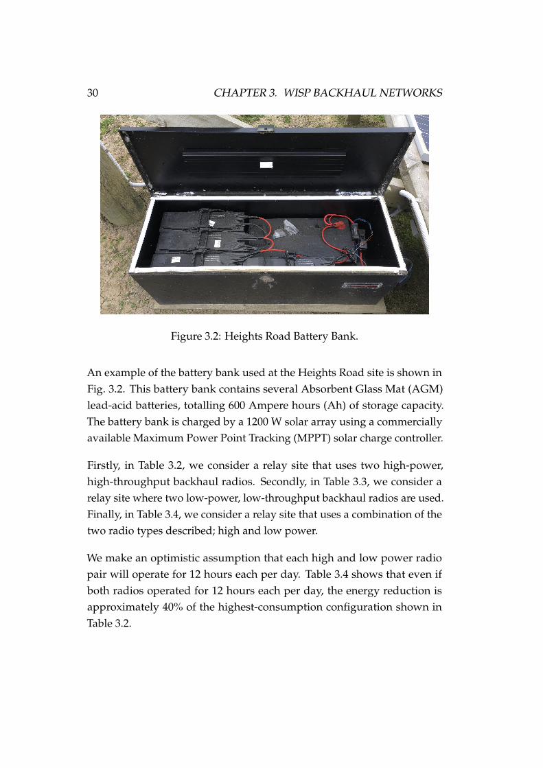
Figure 3.2: Heights Road Battery Bank.
An example of the battery bank used at the Heights Road site is shown inFig. 3.2. This battery bank contains several Absorbent Glass Mat (AGM)lead-acid batteries, totalling 600 Ampere hours (Ah) of storage capacity.The battery bank is charged by a 1200 W solar array using a commerciallyavailable Maximum Power Point Tracking (MPPT) solar charge controller.
Firstly, in Table 3.2, we consider a relay site that uses two high-power,high-throughput backhaul radios. Secondly, in Table 3.3, we consider arelay site where two low-power, low-throughput backhaul radios are used.Finally, in Table 3.4, we consider a relay site that uses a combination of thetwo radio types described; high and low power.
We make an optimistic assumption that each high and low power radiopair will operate for 12 hours each per day. Table 3.4 shows that even ifboth radios operated for 12 hours each per day, the energy reduction isapproximately 40% of the highest-consumption configuration shown inTable 3.2.

3.3. BENEFITS OF ENERGY-PROPORTIONAL BACKHAUL 31
Table 3.2: WISP Relay Site (2 x airFiber5)Component Minimum value
Daily consumption (Wh) 2400Battery bank size (Ah) 800Solar array capacity (W) 750
Table 3.3: WISP Relay Site (2 x Radio PowerBeam5AC G2)Component Minimum value
Daily consumption (Wh) 408Battery bank size (Ah) 140Solar array capacity (W) 150
Table 3.4: WISP Relay Site (2 x airFiber5 and Powerbeam5AC G2)Component Minimum valuea
Daily consumption (Wh) 1404Battery bank size (Ah) 470Solar array capacity (W) 450aWe assume each radio will operate for 12 hours per day.
3.3 Benefits of Energy-Proportional Backhaul
The energy and traffic throughput measurements show that it is possibleto enable WISP operators to benefit from energy-proportional operationin two ways. Firstly, being able to turn off idle resources when they arenot needed will make off-grid energy constrained sites more sustainable.For example, where redundant backhauls exist, we can disable and powerdown one backhaul radio pair to conserve energy.
Secondly, WISPs can be encouraged to design networks that have betterenergy-proportionality. Having energy-proportional network design is a

32 CHAPTER 3. WISP BACKHAUL NETWORKS
key benefit, as WISPs can use high-power, high-throughput radios onlyas they are needed. In practice, better energy-proportionality requires thedeployment of backhauls that include both high and low power radio pairs.Based on earlier measurements, it is shown that designing backhaul linksin this way is achievable and will reduce energy consumption should linkutilisation not be persistently high.
3.3.1 Sustainability
The dependence that some WISPs – such as Venture Networks – haveon off-grid energy systems is a strong motivator for energy-proportionalbackhaul network design. However, even when using grid-supplied energy,it must be questioned if sustainability – in a far greater scope than iscovered in this thesis – should be considered. For example, it is difficult togauge how much energy is wasted globally due to disproportionate energyconsumption of wireless backhaul networks. However, it should be in anynetwork operator’s best interest to improve their network sustainability.Ideally, improved sustainability will also decrease network OperationalExpenditure (OPEX).
3.4 Summary
Given the difficulty for WISPs to implement traffic engineering schemesusing existing routing protocols, there is an evident gap for improvement.Additionally, the “range anxiety” experienced by WISPs is reason itselfto aim for improved network energy efficiency. The literature coveredin Chapter 2 shows that many research efforts towards “green” backhaulnetworks are focused towards much larger service provider networks, andare widely not applicable to WISP networks. Efforts to design “green”microwave backhaul networks hold closer relevancy, but are still not tai-lored towards a WISP on a shoestring budget. To build upon the energy

3.4. SUMMARY 33
efficiency and traffic engineering gaps identified, the ElasticWISP solutionarchitecture is introduced next, in Chapter 4.

34 CHAPTER 3. WISP BACKHAUL NETWORKS
Chapter 4
Solution Architecture
The architecture of ElasticWISP consists of three distinct components:
• A network-aware optimiser.
• A flow-path enforcement mechanism.
• A backhaul radio power control mechanism.
This chapter details the high-level design of each component. Later, Chap-ters 5–7 detail the design and implementation of each major componentwithin the overall ElasticWISP architecture.
4.1 Optimisation and Control
The ElasticWISP optimiser is required to carry out several functions:
• Collect and process traffic flows to determine the active bandwidthbetween the network gateway and remote edge routers.
• Automatically update the network topology used for optimisationwhen link-state changes occur.
35
36 CHAPTER 4. SOLUTION ARCHITECTURE
• Turn off redundant backhaul radio pairs when the network trafficover them can be routed over lower (power) cost paths.
• Turn on backhaul radio pairs as necessary to manage increases innetwork throughput where routing over lower (power) cost pathsexceeds available network capacity.
• Compute the lowest (power) cost paths for network traffic flows.
• Compute the network-wide power state of backhaul radio pairs.
• Send Forwarding Information Base (FIB) updates to edge routers toenforce optimal flow-paths.
• Send power-control updates to remote backhaul radio pairs to enforcethe optimal power state.
• Log network-wide power and link-state changes.
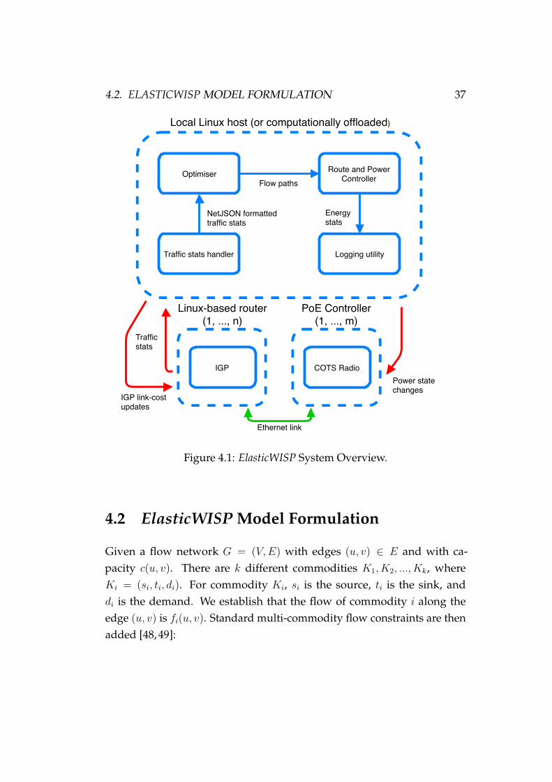
Fig. 4.1 illustrates a high-level, IGP independent overview of the Elas-ticWISP architecture.
Next, in Section 4.2, the multi-commodity flow model of ElasticWISP isdescribed. The formal model of ElasticWISP is designed to be flexibleenough that it can be applied to a variety of different backhaul networktypes, potentially such as those used in 5G networks. It is also anticipatedthat the formal model could be used as a benchmark for any future heuristicapproaches that are developed.
4.2. ELASTICWISP MODEL FORMULATION 37
Optimiser Route and PowerControllerFlow paths
Traffic stats handler
NetJSON formatted traffic stats
IGP link-cost updates
Traffic stats
Ethernet link
Energystats
Power state changes
Linux-based router(1, ..., n)
PoE Controller(1, ..., m)
COTS RadioIGP
Local Linux host (or computationally offloaded)
Logging utility
Figure 4.1: ElasticWISP System Overview.
4.2 ElasticWISP Model Formulation
Given a flow network G = (V,E) with edges (u, v) ∈ E and with ca-pacity c(u, v). There are k different commodities K1, K2, ..., Kk, whereKi = (si, ti, di). For commodity Ki, si is the source, ti is the sink, anddi is the demand. We establish that the flow of commodity i along theedge (u, v) is fi(u, v). Standard multi-commodity flow constraints are thenadded [48, 49]:

38 CHAPTER 4. SOLUTION ARCHITECTURE
Edge capacity: Ensure that all flows over each link do not exceed theavailable capacity, that is, ∀(u, v) ∈ V,
k∑i=1
fi(u, v) ≤ c(u, v). (4.1)
Flow conservation: Intermediary nodes cannot create or destroy commodi-ties. That is, ∀i ∈ [1, k],∑
w∈V
fi(u,w) = 0, when u 6= si and u 6= ti. (4.2)
Demand satisfaction: Every source and sink must send or receive anamount of flow equal to its demand. We have ∀i ∈ [1, k],∑
w∈V
fi(si, w) =∑w∈V
fi(w, ti) = di. (4.3)
4.2.1 Energy Minimisation Constraints
We now add energy-saving constraints to the multi-commodity flow for-mulation. We use the notation listed in Table 4.1 to describe the energyminimisation constraints [27].
Table 4.1: Energy Minimisation NotationNotation Definition
a(u, v) Power cost of the link (u, v)
Xu,v Binary decision variable for the power state oflink (u, v)
ri(u, v) Binary decision variable for indicating if com-modity i uses link (u, v)

4.2. ELASTICWISP MODEL FORMULATION 39
Deactivated links. Ensure that flows are restricted to only links (andradios) that are powered on. For all links (u, v) used by a given commodityi, fi(u, v) = 0 when Xu,v = 0. The flow variable f will always be positive inour formulation, and thus we can write the linear constraint as
k∑i=1
fi(u, v) ≤ c(u, v)×Xu,v, (4.4)
∀i ∈ [1, k],∀(u, v) ∈ E.
Bidirectional power. On a radio pair, both radios must be turned on,irrespective of which direction network traffic is flowing, hence, we have
Xu,v = Xv,u, ∀(u, v) ∈ E. (4.5)
Flow splitting. Finally, most IGPs support single-path routing by default1,we also add a constraint to prevent flow splitting. Additionally, we ac-knowledge that flow splitting is generally undesirable due to the effects ofTransmission Control Protocol (TCP) packet reordering [50]. We constrainthe flow of commodity i over link (u, v) to either the full demand or zero.Hence, ∀i,∀(u, v) ∈ E,
fi(u, v) = di × ri(u, v). (4.6)
Objective function. Now that the appropriate constraints have been added,the objective function is defined, which is to minimise the overall networkenergy consumption:
minimise∑
(u,v)∈E
Xu,v × a(u, v). (4.7)
Finally, find a flow assignment that satisfies the given constraints.
1Equal-Cost Multi-Path (ECMP) is possible in some circumstances. The design ofSR-MPLS is not ECMP capable at the time of writing.
40 CHAPTER 4. SOLUTION ARCHITECTURE
4.3 Flow-Path Enforcement
ElasticWISP cannot use traditional IGPs such as OSPF and IS-IS for explicitflow-path enforcement. While links can be adjusted to prevent them beingused before a radio pair is taken down, IGPs will take the shortest path,which in our case, may not always be the “best path”, or path that theoptimiser desires to be used. Although IGP flow-paths can be manipulatedfurther than what has been shown so far, the process of doing so is generallyundesirable. For ElasticWISP, explicit flow-path enforcement is beneficial,as we can ensure traffic flows over paths as determined by the optimiser.There are multiple criteria to achieve flow-path enforcement for use withthe ElasticWISP optimiser:
• Accept FIB updates from the optimiser.
• Perform FIB updates without degrading network performance anduser Quality of Experience (QoE).
• Program explicit flow-paths for a given traffic source and destination.
• Not be dependent on a central controller in the case of controllerfailure or unavailability.
• Not be dependent on the optimiser for normal use in the case ofoptimiser failure or unavailability.
• Be able to reconverge in the case of link-failure that is unknown tothe optimiser.
4.4 Backhaul Power Control
For ElasticWISP to run on real WISP networks, it is necessary to exposean Application Programming Interface (API) to control the power state ofbackhaul radios. In the case of most backhaul radios, this means controllingDC PoE, with voltages that range between 24V–48V. However, remote
4.5. SUMMARY 41
power control through APIs, or other mechanisms – other than through theswitch Graphical User Interface (GUI) or Command Line Interface (CLI)– is not possible on most commercially available PoE switches. The PoEcontrol device should be able to:
• Turn power on/off to a given radio.
• Return the on/off state of a given radio.
• Report the real-time power consumption of a given radio.
• Offer rudimentary protection against lightning and transient over-voltage.
• Expose a control API over L3 Internet Protocol (IP) connectivity.
• Provide authentication to mitigate unauthorised access.
4.5 Summary
This chapter has described the three pillars upon which the wider Elas-ticWISP scheme is built – an optimisation and control framework, explicitflow-path enforcement, and integration with specifically designed powercontrol hardware. When used together, it is envisioned that WISPs will beable to reduce energy consumption within their backhaul networks, engi-neer traffic paths based on the optimisation model designed, and deploythe scheme in a real network using the application-specific hardware devel-oped. Ultimately, these three pillars assert ElasticWISP as an architecturedesigned specifically for WISPs operating in remote and rural communities.Chapter 5 will next show how ElasticWISP can be applied to WISP backhaulnetworks that do not run speciality traffic engineering schemes.

42 CHAPTER 4. SOLUTION ARCHITECTURE
Chapter 5
ElasticWISP ReferenceImplementation
This chapter presents a concise overview about how ElasticWISP can in-tegrate with common IGPs, as published in the IEEE/IFIP NOMS 2020.At the core of ElasticWISP is a network flow model formulated as a multi-commodity flow problem that has been enhanced with energy minimisa-tion constraints, as described in Chapter 4. To make ElasticWISP useful onreal WISP backhaul networks, integration with commonly used dynamicrouting protocols (IGPs) such as OSPF is necessary1.
5.1 Routing Protocol Integration and Control
The best-effort approach to routing protocol integration is approached prag-matically. The OSPF routing daemon Quagga supports gracefully reroutingtraffic when an OSPF link-cost is increased. Other OSPF and non-OSPFrouting protocols generally function in this way, however Quagga waschosen due to its stability and mature codebase. Fig. 5.1 depicts the reli-
1If a traffic engineering scheme such as SR-MPLS is not in use.
43
44 CHAPTER 5. ELASTICWISP REFERENCE IMPLEMENTATION
able in-band control mechanism that was designed for adjusting the OSPFlink-costs of routers running the Quagga OSPF daemon. ZeroMQ [51]and MessagePack [52] based zerorpc [53] was leveraged for this controlmechanism.
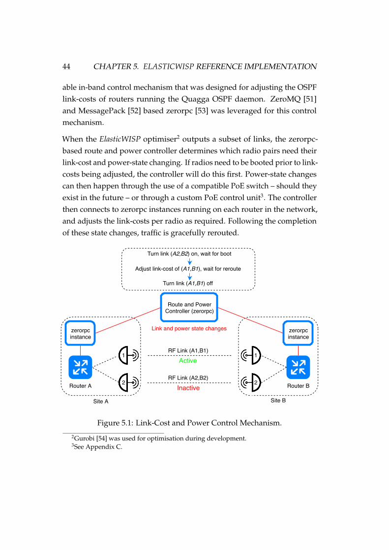
When the ElasticWISP optimiser2 outputs a subset of links, the zerorpc-based route and power controller determines which radio pairs need theirlink-cost and power-state changing. If radios need to be booted prior to link-costs being adjusted, the controller will do this first. Power-state changescan then happen through the use of a compatible PoE switch – should theyexist in the future – or through a custom PoE control unit3. The controllerthen connects to zerorpc instances running on each router in the network,and adjusts the link-costs per radio as required. Following the completionof these state changes, traffic is gracefully rerouted.
RF Link (A1,B1)
RF Link (A2,B2)Router BRouter A Inactive
Active
zerorpcinstance
Turn link (A2,B2) on, wait for boot
Adjust link-cost of (A1,B1), wait for reroute
Turn link (A1,B1) off
Link and power state changes
Site A Site B
Route and PowerController (zerorpc)
zerorpcinstance
1 1
2 2
Figure 5.1: Link-Cost and Power Control Mechanism.
2Gurobi [54] was used for optimisation during development.3See Appendix C.
5.1. ROUTING PROTOCOL INTEGRATION AND CONTROL 45
5.1.1 Practical Considerations
The best-effort implementation of ElasticWISP is focused toward practicalityand minimal effort integration with existing WISP backhaul networks. Toensure implementation viability, there can not be substantial packet loss,introduction of latency, or other QoS degradation metrics when a backhaulchangeover occurs. Backhaul changeover refers to either of two key eventshappening:
1. The reroute of traffic between different radio pairs on the same node.
2. The reroute of traffic through a different set of nodes.
In both cases, the originating OSPF router will flood area-wide LSAs no-tifying other routers of the respective change. In this implementation,adjusting router interface link-costs is leveraged to gracefully reroute trafficwithout degrading QoS. However, this approach is not without caveats.ElasticWISP staggers altering link-costs to avoid any unexpected conse-quences of simultaneous adjustments, and the excessive LSA flooding thatwould occur as a result.
Consequently, a staggering delay is incurred when processing topologychanges and switching the power state of radio pairs on any given node.Even on a large WISP topology with 16+ OSPF routers in operation, thetime overhead per radio adjusted is under three seconds4. Of course, thetime taken for backhaul radios to boot and reassociate to their remotepeers is much longer, and must be taken into careful consideration whenconfiguring a backhaul network to work with ElasticWISP5.
Unlike link-cost adjustments, network-wide power-on state changes can
4Measured using the Common Open Research Emulator (CORE). Reconvergence timewill vary in a physical network, but is not a concern if using SR-MPLS, as traffic can bererouted on demand.
5Radio boot and reassociation time depends on the radio make and model; typicallyranging between 30–120 seconds.
46 CHAPTER 5. ELASTICWISP REFERENCE IMPLEMENTATION
be carried out concurrently. As a result, the time taken to turn on links canbe reduced to the total concurrent radio boot time. However, should theywish, a network operator can still stagger turning on links. Generally thiswould only be required if a large number of radios are being turned onat the same time, and if excessive LSAs become problematic. Power-offstate changes can be handled in the same way, but should generally bestaggered, to avoid too many LSAs from occurring simultaneously as linksare taken down6. The backhaul changeover process is covered in greaterdetail in Chapter 6.12.
5.2 Summary
This chapter has briefly described the reference implementation of Elas-ticWISP. Leveraging OSPF as the IGP of choice, zerorpc for control, andGurobi for optimisation, ElasticWISP is able to reroute traffic – in a best-effort manner – gracefully, without degrading network QoS. We can con-clude that the best-effort approach used by ElasticWISP used in this chapteris appropriate for use where other traffic engineering solutions are notavailable. Following this summary, Chapter 6 presents the design of SR-MPLS, which enables WISPs to implement traffic engineering to achievecomplete integration with the wider ElasticWISP scheme.
6The variation in radio boot times allows for LSAs to be flooded at different timeintervals. Powering radios off happens instantaneously, resulting in LSAs being floodedat approximately the same time interval.
Chapter 6
MPLS Segment Routing Design
To enforce the optimal flow-paths being used, a lightweight, novel approachto MPLS Segment Routing (designated as SR-MPLS) was designed. SR-MPLS enforces explicit flow-paths by encoding the optimal set of backhaullinks to traverse within each packet. These links are known as AdjacencySegments (Adj-SIDs), and are pushed to the packet as an MPLS label stack.Finally, note that design decisions in this chapter were made assumingOSPF is in use, as previous work showed that it is the routing protocol ofchoice for most WISPs [8].
SR-MPLS has specifically been designed with constrained WISP backhaulnetworks in mind, and operates with minimal network state. TraditionalSegment Routing boasts of requiring next to no additional network stateon top of what is already provided by the underlying IGP. SR-MPLS goesfurther. In an SR-MPLS domain, global network state (outside of what isprovided by the IGP) is only present should it be explicitly enabled by anetwork operator, for the purpose of loose source routing. The followingsubsections describe Segment Routing paradigms, and the design rationaleof SR-MPLS.
47
48 CHAPTER 6. MPLS SEGMENT ROUTING DESIGN
6.1 IGP Integration
Two approaches to IGP integration were designed:
• Label distribution with opaque LSAs, as per RFC 8402 [41].
• Unmodified IGP integration with on-demand hop-by-hop shortest-path routing. This was designed as a “poor man’s” approach toSegment Routing, and is the focus of this chapter.
Traditionally, Segment Routing relies on an IGP such as OSPF or IS-IS todistribute labels. OSPF implementations such as Quagga, in their currentform, do not support the extensions necessary to distribute labels usedto enable Segment Routing. These extensions, such as those for OSPF,are defined in RFC 8402 [41] and RFC 8665 [55]. The second approach(SR-MPLS) requires no extension to IGPs, and leverages the native IGP link-state database to perform next-hop forwarding where explicit flow-pathsdo not exist.
In a typical Segment Routing domain, path computation can be performedby a central entity, such as the ElasticWISP optimiser, or in a distributednode-by-node manner, using the link-state information available from theIGP. In the case of the distributed approach, this requires that each SegmentRouting capable node in the network has a global view of all other SegmentRouters, as described in RFC 8402. In this regard, the process of packetforwarding is very similar to what would traditionally happen with anIGP. However, unlike traditional IP forwarding, a list of segments (MPLSheaders) must be inserted into each respective packet.
Between intermediary nodes, forwarding is performed based on the MPLSlabel headers that have been encoded into the packet. Each MPLS headerhas a bottom of stack flag. If this flag is set to 0, then the last MPLS header inthe packet has been reached. In this case, the MPLS header will be stripped,and the inner IP packet will be forwarded normally.

6.2. ABOUT MPLS 49
6.2 About MPLS
An MPLS header is a total of 32 bits, made up of:
• A 20-bit label1.
• A 3-bit class of service field2.
• A 1-bit bottom of stack flag.
• An 8-bit Time To Live (TTL) field.
Fig. 6.1 shows a visual representation of an MPLS header.
Label EXP TTL
0 19 22
B
23 31
Bits 0 ... 31
Figure 6.1: MPLS Header.
Rather than using IP next-hop information for forwarding, MPLS useslabels. MPLS originally became widespread in service provider networksdue to the perceived inefficiencies of IP routing, in addition to the short-comings of IP-based traffic engineering [56]. Despite the recent boom inSDN research, MPLS has remained an important part of service providernetworks, especially so for WISPs [8].
One of the most important MPLS concepts is “label stacking”. In brief, anMPLS label stack permits a variety of forwarding operations to take placebased on the value – and network-wide significance – of the label headerswithin the stack. In the case of Segment Routing, labels in the stack canbe used with both strict and loose source routing paradigms. For clarity,Fig. 6.2 depicts how an MPLS label stack fits within an Ethernet frame.
1Ranging from 0 – 1048575.2Also known as the experimental (EXP) field.
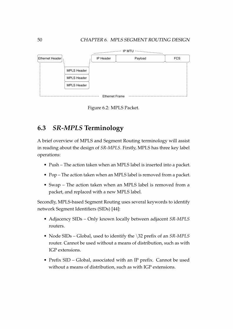
50 CHAPTER 6. MPLS SEGMENT ROUTING DESIGN
Ethernet Header IP Header Payload
MPLS Header
FCS
IP MTU
Ethernet Frame
MPLS Header
MPLS Header
Figure 6.2: MPLS Packet.
6.3 SR-MPLS Terminology
A brief overview of MPLS and Segment Routing terminology will assistin reading about the design of SR-MPLS. Firstly, MPLS has three key labeloperations:
• Push – The action taken when an MPLS label is inserted into a packet.
• Pop – The action taken when an MPLS label is removed from a packet.
• Swap – The action taken when an MPLS label is removed from apacket, and replaced with a new MPLS label.
Secondly, MPLS-based Segment Routing uses several keywords to identifynetwork Segment Identifiers (SIDs) [44]:
• Adjacency SIDs – Only known locally between adjacent SR-MPLSrouters.
• Node SIDs – Global, used to identify the \32 prefix of an SR-MPLSrouter. Cannot be used without a means of distribution, such as withIGP extensions.
• Prefix SID – Global, associated with an IP prefix. Cannot be usedwithout a means of distribution, such as with IGP extensions.
6.4. IPV4 AND IPV6 MPLS ENCAPSULATION 51
The design of SR-MPLS does not utilise prefix SIDs. Instead, SR-MPLS usesadjacency SIDs where possible, to keep network state at a minimum, whilenode SIDs are used only if required by the network operator.
Additionally, general MPLS terminology can be applied to SR-MPLS:
• LSP – a unidirectional tunnel between a pair of SR-MPLS routersacross a larger SR-MPLS domain.
• Label Edge Router (LER) – makes the initial path selection, and en-codes the explicit adjacency SID label stack. Encapsulates IP packetsthat will traverse the LSP.
• Label Switching Router (LSR) – what is alternatively called a “transitnode”. An LSR only performs label-switching in the middle of anLSP.
• Egress node – the final SR-MPLS router in a LSP, which “pops” thefinal MPLS header.
6.4 IPv4 and IPv6 MPLS Encapsulation
Additionally, while Internet Protocol version 6 (IPv6) Segment Routing(SRv6) exists, SR-MPLS can be used for either Internet Protocol version4 (IPv4) or IPv6 transportation (of L3 packets). The design of SR-MPLSis focused toward IPv4, as SRv6 is a well established, promising area ofresearch. Of course, designing a dual-stack IPv4 and IPv6 scheme presentssome challenges. For one, easily determining what EtherType3 the innerpacket requires is straightforward if you are dealing with a single IP proto-col, i.e., IPv4 or IPv6. However, a dual-stack scheme requires a means ofdetermining what inner IP header follows an MPLS header.
3A data link layer (or L2) Ethernet header contains a 16-bit field that represents thetype of payload encapsulated within the Ethernet frame.

52 CHAPTER 6. MPLS SEGMENT ROUTING DESIGN
Determining the next-header is necessary prior to forwarding an inner L3packet to its destination. If the incorrect EtherType (derived from the next-header) is set, the packet will be dropped before, or at, its destination. Notethat when an IPv4 or IPv6 packet is encapsulated, the original EtherType ischanged (from IPv4 or IPv6) to MPLS, and forwarded through the SR-MPLSdomain. Leaving the EtherType set as MPLS after the final MPLS label hasbeen popped will also ultimately result in the packet being dropped.
In an IPv4 and IPv6 dual-stack environment, several approaches couldbe taken to determine the correct next-header (and subsequently set thecorrect EtherType during decapsulation):
• Using the MPLS class of service bit-field – typically used for QoSpurposes – to represent IPv4 or IPv6 EtherTypes (3-bit field).
• Using proposed MPLS-extensions that include an 8-bit field for anext-header [57].
• Using specific, separate label ranges for IPv4 and IPv6 addresses.
Alternatively, a network operator could simply use SRv6 for their IPv6traffic engineering needs.
6.5. MPLS FORWARDING 53
6.5 MPLS Forwarding
The typical operation of an SR-MPLS router follows a strict source routingparadigm. If instructions to match IP traffic to an explicit flow-path exist inthe FIB – also referred to as the Label Forwarding Information Base (LFIB) –of an SR-MPLS router, traffic destined to the match address – e.g., 10.1.1.0/24– will be encoded with an MPLS label stack. The label stack consists of anordered set of MPLS labels, which represent segments in the SR-MPLSdomain. As mentioned in Subsection 6.3, these can be adjacency SIDs,or node SIDs. The subsequent subsections detail the design of SR-MPLSmodes of operation in terms of L3 functionality.
Also note that in MPLS networks, there are typically two approaches topopping MPLS labels (or formally, terminating an LSP):
• Implicit Null – also known as Penultimate Hop Popping (PHP).
• Explicit Null.
The PHP approach pops the last MPLS label on the second-to-last hop (thepenultimate hop). PHP is used to avoid the final router (ultimate hop)having to perform two operations: (i) popping the remaining MPLS label,and (ii), performing an IP lookup. In contrast, the Explicit Null approachrequires that MPLS labels are used until the ultimate hop is reached. Upondecapsulation of the final MPLS header, an IP lookup must be performedin order to forward the underlying packet. In an SR-MPLS domain, theExplicit Null approach is used, however, PHP support could be added inthe future.
54 CHAPTER 6. MPLS SEGMENT ROUTING DESIGN
SR-MPLS-6
SR-MPLS-5
SR-MPLS-4
SR-MPLS-3SR-MPLS-1
SR-MPLS Domain
SR-MPLS-2
107
108
105
106
111
112
103
104
113
114
101
100
109
110
OptimiserSet SR-MPLS-1
default gateway via:101,104,110
To WAN Router
Eth+104+110+IP+Payload
Packet from SR-MPLS-1 on wire
Eth+110+IP+Payload
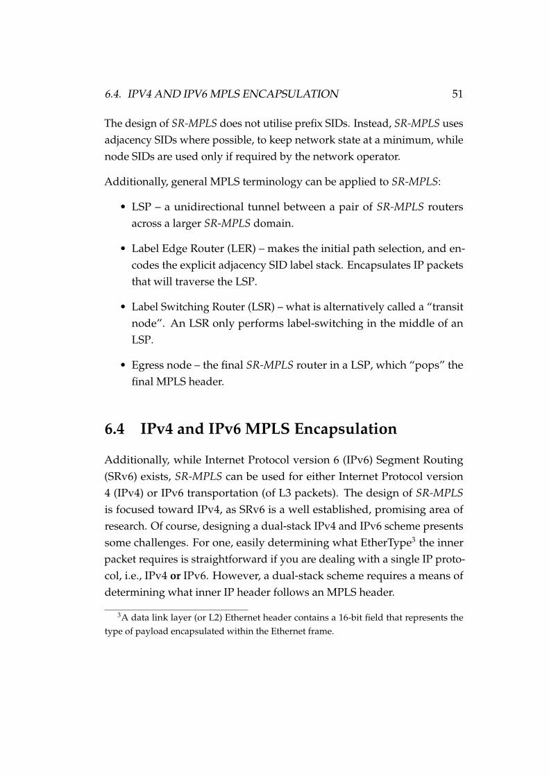
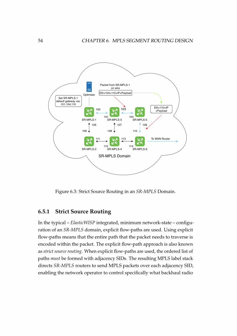
Figure 6.3: Strict Source Routing in an SR-MPLS Domain.
6.5.1 Strict Source Routing
In the typical – ElasticWISP integrated, minimum network-state – configu-ration of an SR-MPLS domain, explicit flow-paths are used. Using explicitflow-paths means that the entire path that the packet needs to traverse isencoded within the packet. The explicit flow-path approach is also knownas strict source routing. When explicit flow-paths are used, the ordered list ofpaths must be formed with adjacency SIDs. The resulting MPLS label stackdirects SR-MPLS routers to send MPLS packets over each adjacency SID,enabling the network operator to control specifically what backhaul radio
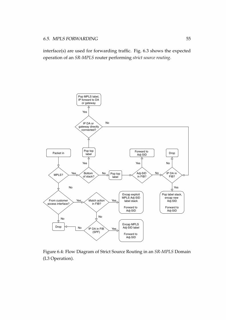
6.5. MPLS FORWARDING 55
interface(s) are used for forwarding traffic. Fig. 6.3 shows the expectedoperation of an SR-MPLS router performing strict source routing.
Packet in
No
YesMPLS?
From customeraccess interface?
Encap MPLS Adj-SID label
Forward to Adj-SID
Adj-SID in FIB?
Forward to Adj-SID
Yes
IP DA in FIB?
Pop label stack,encap new
Adj-SID
Forward toAdj-SID
Drop
Drop
Yes Match action in FIB?
Yes
No
Encap explicitMPLS Adj-SID
label stack
Forward to Adj-SID
Bottom of stack?
Yes
No
No
Yes
Pop MPLS label,IP forward to DA
or gateway
IP DA or gateway directly
connected?
IP DA in FIB(SPF)
No
Yes
Yes
No
No
Pop toplabel
Pop toplabel
No
Figure 6.4: Flow Diagram of Strict Source Routing in an SR-MPLS Domain(L3 Operation).
56 CHAPTER 6. MPLS SEGMENT ROUTING DESIGN
6.5.2 Loose Source Routing
SR-MPLS-6
SR-MPLS-5
SR-MPLS-4
SR-MPLS-3SR-MPLS-1
SR-MPLS Domain
SR-MPLS-2
107
108
105
106
111
112
103
104
113
114
101
100
109
110
OptimiserSet SR-MPLS-1
default gateway via:205
To WAN Router
Eth+104+205+IP+Payload
Packet from SR-MPLS-1 on wire
SR-MPLS-5Node SID 205
Eth+110+IP+Payload
Figure 6.5: Loose Source Routing in an SR-MPLS Domain.
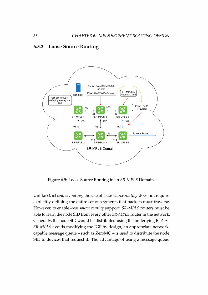
Unlike strict source routing, the use of loose source routing does not requireexplicitly defining the entire set of segments that packets must traverse.However, to enable loose source routing support, SR-MPLS routers must beable to learn the node SID from every other SR-MPLS router in the network.Generally, the node SID would be distributed using the underlying IGP. AsSR-MPLS avoids modifying the IGP by design, an appropriate network-capable message queue – such as ZeroMQ – is used to distribute the nodeSID to devices that request it. The advantage of using a message queue
6.5. MPLS FORWARDING 57
over a “roll-your-own” sockets-based approach is that more attention canbe given to other core areas of SR-MPLS. Essentially, the message queueensures reliable inter-node exchange can take place, without requiringan application specific protocol design to be developed. Routing proto-cols such as Facebook’s Open/R have also leveraged the message-queueapproach for state exchange between nodes [58].
Packet in
No
YesMPLS?
From customeraccess interface?
Encap MPLS Adj-SID label
Forward to Adj-SID
Adj-SID in FIB?
Forward to Adj-SID
Yes
IP DA in FIB?
Pop label stack, encapnew Adj-SID
Forward to Adj-SID
Drop
Drop
Yes Match action in FIB?
Yes
No
Encap explicitMPLS Adj-SID orNode-SID label
stack
Forward to Adj-SID
Bottom of stack?
Yes
No
No
Yes
IP forward to DAor gateway
IP DA or gateway directly
connected?
IP DA in FIB(SPF)
No
Yes
Yes
No
No
No Node-SID in FIB?
No
Yes
Get next-hop Adj-SID for Node-SID using IGP
Encap Adj-SID for next-hop and append Node-
SID
Forward to Adj-SID
Node-SIDdirectly
connected?No
Pop toplabel
Pop toplabel
Pop Node-SID. EncapMPLS Adj-SID ofneighbour node
Forward to Adj-SID
Yes
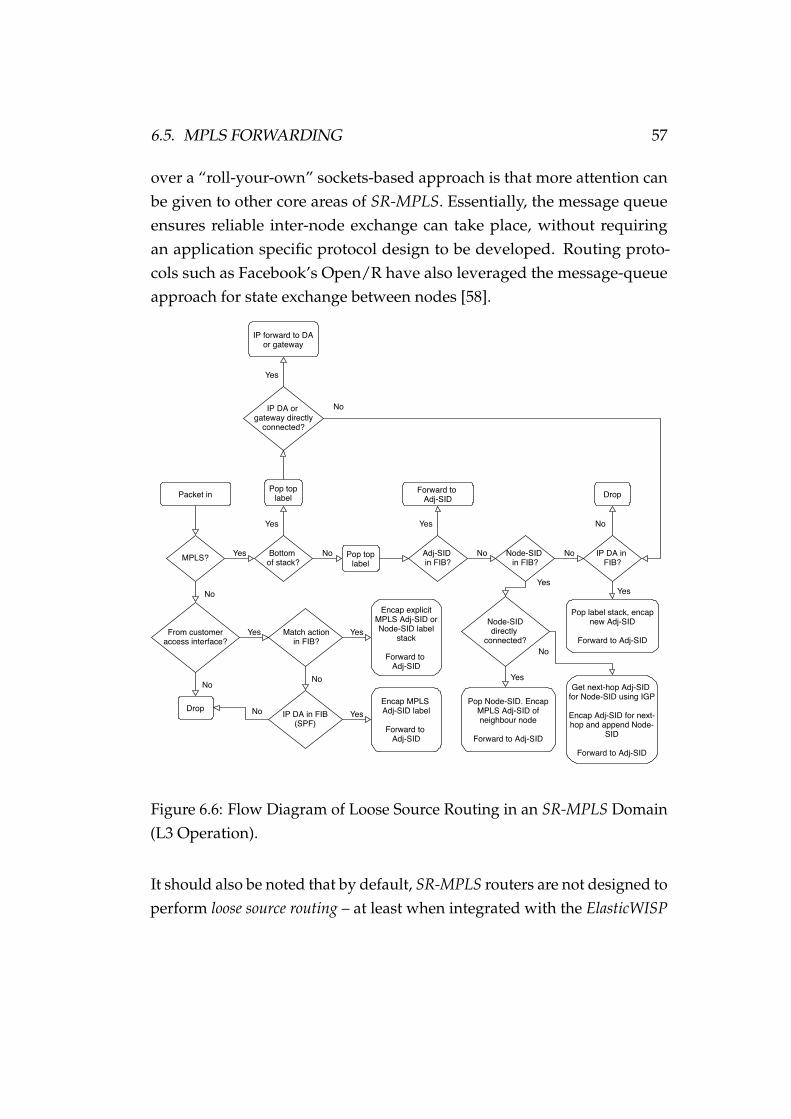
Figure 6.6: Flow Diagram of Loose Source Routing in an SR-MPLS Domain(L3 Operation).
It should also be noted that by default, SR-MPLS routers are not designed toperform loose source routing – at least when integrated with the ElasticWISP
58 CHAPTER 6. MPLS SEGMENT ROUTING DESIGN
optimiser – but loose source routing functionality is accounted for, should anetwork operator desire to use it. Fig. 6.5 shows the expected operation ofan SR-MPLS router performing loose source routing.
6.5.3 Shortest Path Forwarding
Shortest path forwarding is used in several circumstances:
• When an explicit steering policy has not been installed in the SR-MPLS FIB.
• When loose source routing is being used4.
• When a link failure occurs during normal strict source routing opera-tion.
Also note that shortest path forwarding also does not require node SIDs tobe enabled. When an adjacency SID is unavailable, or no steering policyhas been installed in the SR-MPLS FIB, the packet is forwarded based onits IP destination address. To achieve this, and forward the packet over theshortest path, the IGP link-state database is queried. The database providesthe best outgoing interface to forward the packet, which is then used to findan adjacency SID. The adjacency SID – which is an MPLS label – is thenpushed onto the MPLS label header, and the packet is forwarded to theadjacent SR-MPLS router. The procedure is then repeated until the packetreaches its destination.
The shortest path forwarding mechanism is also important in the case of alink failure. Should a link go down while traffic flows are being forwardedover it – e.g., using the hop-by-hop explicit source routing approach – theSR-MPLS routers will detect that the neighbouring adjacency SID has beenremoved from the FIB. Subsequently, the SR-MPLS routers will pop allof the MPLS labels – i.e., the adjacency SIDs – in the MPLS stack. After
4Node SID distribution must be enabled.
6.6. CONTROL PLANE 59
performing a lookup using the IGP link-state database, a new adjacencySID is pushed onto the packet. Until the link failure is resolved, shortestpath forwarding will continue. Additional details about how path-failuredetection occurs is detailed in Subsection 6.8.
6.6 Control Plane
The design of a traditional Segment Routing control plane is left at thediscretion of the network operator. In the case of SR-MPLS capable routers,the control plane is responsible for installing FIB entries. These FIB entriesare the output of the ElasticWISP optimiser, and are necessary for explicitflow-path enforcement to take place. Of course, in addition to the output ofthe ElasticWISP optimiser, the SR-MPLS scheme is reliant on the underlyingIGP control plane for normal operations to take place. While it would bepossible to run an SR-MPLS router without an IGP, static routing would berequired, and the network would lack fault tolerance.
The installation of FIB entries on SR-MPLS routers could take place with anynumber of control plane protocols. As we depend on an IGP for normaloperation, the message queue approach mentioned earlier can also beleveraged for reliable – and in many cases, programming language agnostic– message delivery. An in-band control plane approach that leveragesa message queue can coexist with MPLS-based SR-MPLS routers, as inaddition to the SR-MPLS domain, there is still a functional IPv4 and/orIPv6 underlay network, meaning control packets pass through the networkwithout being encapsulated.
Most modern message queues support a generic client–server model, inaddition to the classical pub–sub and push–pull approaches. While othercommunication schemes are possible, the generic client–server model isused to establish communications between SR-MPLS routers and the Elas-ticWISP optimiser. In such a configuration, SR-MPLS routers act as servers
60 CHAPTER 6. MPLS SEGMENT ROUTING DESIGN
listening for requests from the ElasticWISP optimiser. The optimiser canthen install new FIB entries, update them, delete them, and query them asrequired.
6.7 Neighbour Label Resolution
To minimise the amount of manual configuration required for setting up anSR-MPLS domain, a basic Media Access Control (MAC) address to MPLSlabel discovery mechanism was designed. Once IGP adjacencies have beenestablished, an appropriate message queue is used to setup bidirectionalcommunication between the pairs of adjacent SR-MPLS routers, solely forthe purpose of label exchange. Once the label exchange takes place, SR-MPLS routers are able to begin forwarding MPLS packets. Following theinitial label exchange, no additional communication is necessary betweenthe neighbours. Should a failure occur, such as the reboot of an SR-MPLSrouter, the recovering node will reconnect to its neighbour following anadjacency being formed by the IGP, and subsequently regain the labelassociated with the adjacent interface MAC address.
Incorporating a message queue into the design of SR-MPLS means thatlabel exchange and installation is reliable, and a range of authenticationoptions are available, should they be required by the network operator, e.g.,CURVE [59] if ZeroMQ is used as the message queue of choice. Even if afailure occurs in the message queue-based label installation mechanism, SR-MPLS routers can continue to forward packets normally, however must fallback to using the hop-by-hop method discussed earlier. Note that the MACaddress of the neighbour IP is still found using the Address ResolutionProtocol (ARP). The neighbour label resolution mechanism described hereis solely for the purpose of learning adjacent labels. In the future thisexchange mechanism could be extended to become a separate protocol,perhaps appropriately named the Label Resolution Protocol (LRP).
6.8. BIDIRECTIONAL FORWARDING DETECTION 61
6.8 Bidirectional Forwarding Detection
In traditional Segment Routing, failure detection is handled completely bythe IGP. Should a failure occur, the IGP can recompute the shortest pathusing its global view of the Segment Routing domain. In an IP networkrunning an IGP such as OSPF, the same process occurs. When a failurehappens, the IGP can recompute the shortest path as it has a global view ofother routers in the network. In this “poor man’s” approach to SegmentRouting, each node in the network does not have a global view of segmentsin use across the network. Because of this, failure mitigation must behandled differently.
To detect link failure – ideally even faster than the IGP in use can – Bidirec-tional Forwarding Detection (BFD) is used to detect if an explicit flow-pathis up or down. When the ElasticWISP optimiser computes explicit flow-paths, it installs them in the FIB of the SR-MPLS routers across the network.Each specific IP or IP subnetwork with explicit flow-paths will have a FIBentry. For unique source–destination pairs, BFD sessions are then estab-lished. An MPLS packet is then generated, with the explicit flow-pathencoded into the packet. If no response is seen in the defined period, thelink is deemed to be down.
As we consider if the entire explicit path (the LSP) is up or not, we donot get a “fine-grained” view of where link failure exists between pairsof SR-MPLS routers. While possible with BFD, detecting failure betweenadjacent SR-MPLS routers is performed automatically by the IGP in use5.Note that MPLS-specific BFD is defined in RFC 5884 [60]. The concept ofusing BFD for multihop paths – as intended for SR-MPLS routers – is alsowell established, and is defined in RFC 5883 [61].
Should a failure be detected in an explicit flow-path, the originating SR-
5Link-failure detection is typically handled by the IGP in a traditional Segment Routingdomain.
62 CHAPTER 6. MPLS SEGMENT ROUTING DESIGN
MPLS router reverts back to shortest-path forwarding. Next, the SR-MPLSrouter alerts the optimiser that the explicit flow-path is down, and requestsnew explicit paths be installed. The response time between the SR-MPLSrouter reverting to shortest-path forwarding and then having a FIB updateinstalled will depend on operator-defined settings, as it is generally desir-able to limit how frequently the ElasticWISP optimiser is run within quicksuccession.
In addition, the BFD mechanism may detect link-failure before the IGPdoes. As ElasticWISP builds the topology used for optimisation from anIGP’s link-state database, requesting new routes before the IGP can react tofailure may result in the same routes being installed in SR-MPLS FIBs. As aresult, limiting frequent runs of the optimiser should be done with carefulconsideration in respect to the configuration of the IGPs dead-intervaltimer.
It should also be noted that BFD is not intended to be run between adjacentpairs of SR-MPLS routers, although this is also possible, and is common-place practice between adjacent OSPF routers. In this configuration, BFDmonitors the forwarding plane availability between the adjacent routers.In the case of OSPF, Hello messages are used to ensure links are working asintended. BFD is used alongside this mechanism as it can be configuredwith much lower-latency exchange intervals, meaning link failure can bedetected significantly faster [62].
Finally, the use of BFD with SR-MPLS routers can take two approaches:
• With an explicit return path encoded into each BFD packet.
• Using a return path as determined by the destination node.
These two modes of operation exist as in some cases the return path couldbe different to the path that was originally used to reach the destination.In most cases, the return path should be determined by the destinationSR-MPLS router, as this will verify bidirectional connectivity as packets

6.9. TIME TO LIVE HANDLING 63
would normally flow in either direction from source to destination SR-MPLS routers. However, the flexibility exists to enable network operatorsto probe specific flow-paths should they wish.
Of course, should explicit return paths be defined, the source router mustbe aware of the position of other SR-MPLS routers within the network. Asadjacency SIDs are only shared between adjacent neighbours, this approachwould generally require the use of node SIDs, subsequently introducingadditional network state. Alternatively, a device, such as the ElasticWISPoptimiser, which has global network knowledge, could be delegated toprobing bidirectional connectivity between SR-MPLS routers. Leverag-ing the ElasticWISP optimiser for this purpose will be a topic of futureexploration.
6.9 Time To Live Handling
When an IP packet is encapsulated by an SR-MPLS router, the TTL fieldof the IP packet is copied into the TTL field of the top label in the MPLSlabel stack, i.e., the stack of MPLS SIDs. The top MPLS label header TTLis decremented each time an MPLS packet is passed through an SR-MPLSrouter. The top label is popped, and the decremented TTL field is copied tothe next label header in the label stack. When an MPLS label header with abottom of stack flag is encountered – and an IP address entry exists in theSR-MPLS FIB – the MPLS TTL is then copied into the IP header TTL fieldof the outgoing packet.
6.10 MTU Considerations
Networks that leverage Segment Routing, should it be SRv6 or SR-MPLS,must take the lowest Maximum Transmission Unit (MTU), that networkequipment within the domain supports, into careful consideration. Each
64 CHAPTER 6. MPLS SEGMENT ROUTING DESIGN
MPLS label header – or MPLS SID – is 4 Bytes, or 32 bits. In comparison,an SRv6 SID is 16 Bytes, or 128 bits. The MTU used between devices in theSegment Routing domain should be coordinated. Coordination should becompleted in respect to the network topology, planned future expansion ofthe network, and the maximum segment depth – i.e., the number of SIDs –that will be encoded into packets within the domain. Unexpected situationswill result if MTUs are configured incorrectly across the domain – or worse,the network will simply not work. In addition, if the maximum segmentdepth is high, and the MTU is set at the default 1500 Bytes, outgoingpackets could be dropped if the Network Interface Controller (NIC) doesnot support jumbo frames.
6.11 MPLS Services
The core focus of SR-MPLS is to enable simple traffic engineering for layer3 (IP) traffic. In MPLS terminology, the behaviour of SR-MPLS routers iswhat is referred to as a Layer 3 Virtual Private Network (L3VPN), alsoknown as a Virtual Private Routed Network (VPRN). However, while notdiscussed in detail, it is also possible to utilise layer 2 MPLS services suchas point-to-point (pseudowire) and Virtual Private LAN Service (VPLS)Layer 2 Virtual Private Networks (L2VPNs).
While possible, additional considerations need to be made regarding fail-ure mitigation when using L2 services. In an SR-MPLS domain, failuremitigation leverages the IGP, and can reroute traffic based on L3 addresses.Should an entire L2 frame be encapsulated, and failure happen duringtransit, an SR-MPLS router can look at the inner L3 address to determinewhere to forward the packet – but this approach may not always result indesirable results.
Consider a L2VPN setup between two customer sites created by a WISP.The traffic being forwarded over the L2VPN may not be ever destined for

6.12. BACKHAUL CHANGEOVER 65
the public Internet. Private IP space – that the IGP is unaware of – couldalso be in use. Should a failure happen in transit, or should a link in anexplicit flow-path fail, the hop-by-hop approach, and, to an extent, the loosesource routing approach would not be suitable for mitigation. As the innerL3 address, in this example, is not destined for a prefix being advertisedby OSPF, or the Internet, it provides no usable information to determinemitigation paths for forwarding.
Alternatively, a network operator could define a path for a L2VPN totraverse which must include the Node-SID of the destination node. Shoulda failure happen during transit, the Node-SID can still be used to determinean alternative hop-by-hop path to be taken.
6.12 Backhaul Changeover
One of the most important features of SR-MPLS is the ability to reroute traf-fic on demand, without having to wait for IGP reconvergence to take place.When the ElasticWISP optimiser installs FIB entries in SR-MPLS routers,the flow-paths being enforced can be changed immediately. In contrast, theElasticWISP reference implementation must wait for IGP reconvergence, orrisk packet loss, due to prematurely powering down backhaul radios priorto traffic being routed over the intended backhaul pair. However, whenbackhaul radios in a link are powered down, network reconvergence willstill occur, irrespective of the scheme being used.
6.13 SR-MPLS Complexity
Let n be the number of SR-MPLS routers, k be the number of commoditiesoriginating at an SR-MPLS router, m be the number of adjacent neighboursof an SR-MPLS router, and d be the number of unidirectional links in anSR-MPLS domain. Firstly, adjacency SIDs must be setup, requiring O(n)
66 CHAPTER 6. MPLS SEGMENT ROUTING DESIGN
SR-MPLS routers to be configured. The routing state of an SR-MPLS routerusing explicit source routing can be given as O(m). Resultantly, the routingstate of an SR-MPLS router is minimal, as it is only necessary to storeneighbour adjacency SID information in the FIB.
Should explicit source routing be used, the routing state is O(n + m), as eachSR-MPLS router must be aware of the node SID of every other SR-MPLSrouter in the network, in addition to being aware of adjacency SIDs. Whenoperating an SR-MPLS network, the complexity of running BFD on a per-router basis can be given as O(k), as a BFD session for each commodityk must be established to a remote peer. Finally, we expect that there willtypically not be more than O(n2) unidirectional links (d) in a given SR-MPLS domain.
6.14 Summary
This chapter has shown that SR-MPLS promises to radically simplify theway that WISPs perform traffic engineering in their backhaul networks.The design of SR-MPLS requires minimal routing state, and can integratewith IGPs without them requiring any further extensions, as is necessarywith traditional Segment Routing. Most importantly, the design of SR-MPLS enables explicit flow-paths as computed by the ElasticWISP optimiserto be enforced, enabling the overall ElasticWISP scheme to function asintended. Next, Chapter 7 presents the power control hardware designedand implemented to enable real-world application of ElasticWISP and SR-MPLS.

Chapter 7
Backhaul Power Control
To enable the control of PoE devices, a power control “cape” was designedfor the BeagleBone Green [63] Single-Board Computer (SBC). The capeincludes 24V and 48V inputs, making it useful for low-cost 24V radiosas well as higher-cost radios such as the Ubiquiti airFiber series. TheBeagleBone Green was selected as it is open hardware, includes 10/100Mbps Ethernet connectivity, has numerous General Purpose Input/Output(GPIO) pins, and includes 7 analogue inputs. Furthermore, these analogueinputs mean that no external Analogue to Digital Converter (ADC) isnecessary, which is commonplace in many other SBCs, such as all variantsof the Raspberry Pi [64]. Adding an external ADC to the already spaceconstrained Printed Circuit Board (PCB) would mean that there is less roomfor the required power switching electronics.
In this case, analogue inputs are required for two reasons:
• To read the 24V and 48V output voltages.
• To read the current sense voltage of each high-side switch.
Subsequent sections in this chapter describe the design decisions made forthe power control cape.
67

68 CHAPTER 7. BACKHAUL POWER CONTROL
7.1 Cape Features
Unlike the BeagleBone Black, the BeagleBone Green has no barrel jack topower the board. Instead, the board is powered entirely through USB, at 5V.Alternatively, it is possible to power the BeagleBone Green by supplying 5Vto the VDD 5V pin. In practice, this board should be powered by batteriesthat reside at a remote site used by WISPs, and powered with a 12V–24Vinput supply. To accommodate for this, a 5V switching regulator – with anultra-wide 9V–72V input range – is included on the cape.
Power switching on the cape is performed using two Infineon [65] high-side switches. The high-side switch of choice – the BTT6050-1ERA [66] –supports voltages ranging from 5V–48V, with a nominal current of 4.5A,making it an ideal fit for powering both low-power and high-power back-haul radios. The BTT60X0 series high-side switches are also microcontrollerfriendly, and can be controlled with 3.3V and 5V logic inputs. The BTT60X0series also have “current sense” capability, which eliminates the need foran external current sense amplifier, should we measure the current beingused by a given radio.
Finally, the cape uses a fundamental circuit – a voltage divider – to measurethe voltage of both the 24V and 48V outputs1. The voltage measurementrequires either of the high-side switches to be on, as we wish to preventback-powering the BeagleBone Green through the analogue input pinsshould an unexpected failure occur. Back-powering could also otherwisehappen in the event that the 24V input is inactive, but the 48V input islive. This would mean that the BeagleBone is not receiving power from the5V regulator, and would instead receive voltage from the voltage divider.As either high-side switch having an on state depends on the BeagleBonereceiving power through its 5V regulator, these issues are eliminated. Thisapproach is aligned with BeagleBone recommendations [67].
1As opposed to directly measuring the input voltages.
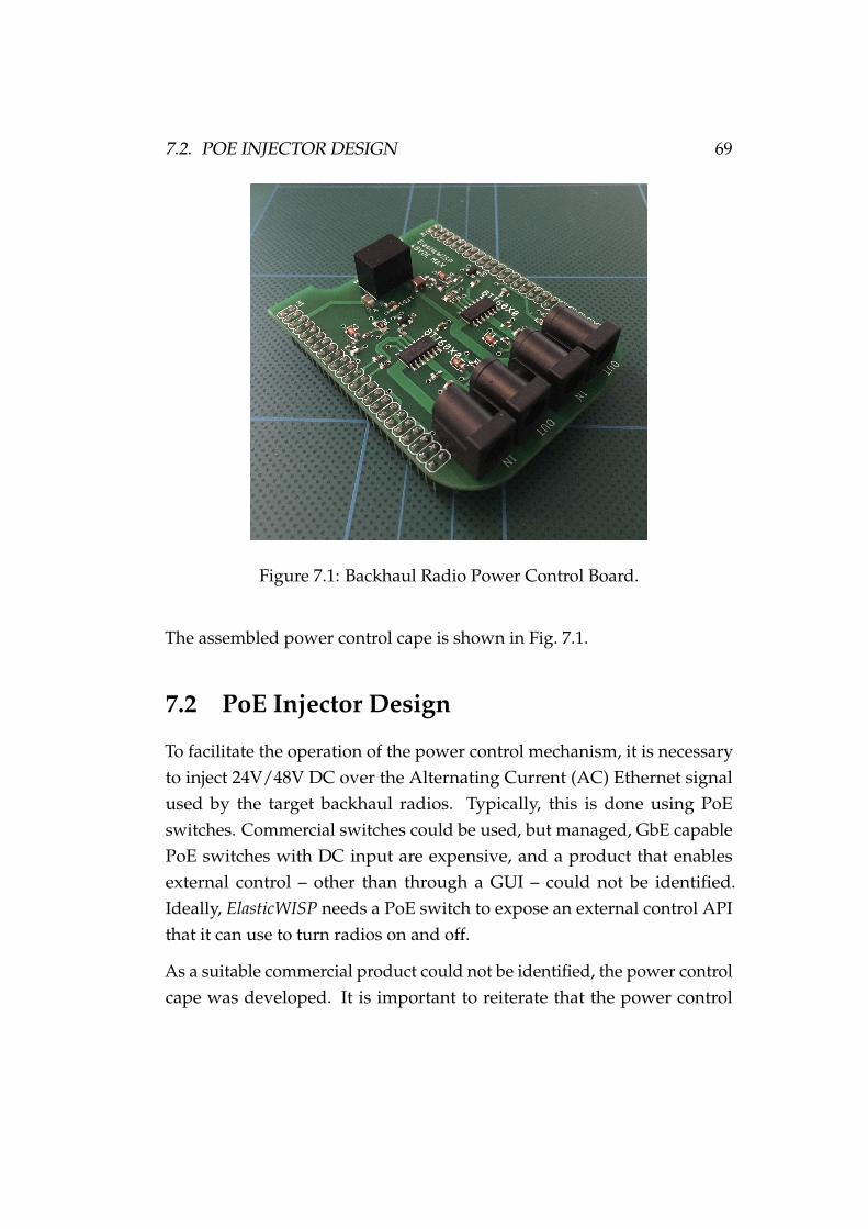
7.2. POE INJECTOR DESIGN 69
Figure 7.1: Backhaul Radio Power Control Board.
The assembled power control cape is shown in Fig. 7.1.
7.2 PoE Injector Design
To facilitate the operation of the power control mechanism, it is necessaryto inject 24V/48V DC over the Alternating Current (AC) Ethernet signalused by the target backhaul radios. Typically, this is done using PoEswitches. Commercial switches could be used, but managed, GbE capablePoE switches with DC input are expensive, and a product that enablesexternal control – other than through a GUI – could not be identified.Ideally, ElasticWISP needs a PoE switch to expose an external control APIthat it can use to turn radios on and off.
As a suitable commercial product could not be identified, the power controlcape was developed. It is important to reiterate that the power control

70 CHAPTER 7. BACKHAUL POWER CONTROL
cape can only switch power. Due to this, PoE injectors are still necessary.Commercial PoE injectors are readily available, but are also often costly,especially when we must support up to 60 W to safely power the airFiberradios. Given the long-term desired integration with other components ofthe ElasticWISP architecture, these commercial injectors also may not besuitable. Consequently, two GbE-capable PoE injector designs were created,one suitable for up to 0.5A at 24V/48V, and another improved design thatsupports 2.5A at 24V/48V2.
7.2.1 Design 1
Figure 7.2: Design 1. Low-Cost Gigabit PoE Injector.
The purpose of the first PoE injector design was to serve as a low-cost Proofof Concept (PoC). In brief, two Coilcraft [68] KA4909-AL [69] bias injectionchokes were used to inject a common-mode DC voltage into a GigabitEthernet signal. If necessary, the injector can also act as a PoE “splitter”,
2Two-pair operation at 1.25A, four-pair operation at 2.5A.
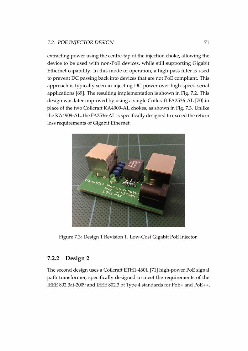
7.2. POE INJECTOR DESIGN 71
extracting power using the centre-tap of the injection choke, allowing thedevice to be used with non-PoE devices, while still supporting GigabitEthernet capability. In this mode of operation, a high-pass filter is usedto prevent DC passing back into devices that are not PoE compliant. Thisapproach is typically seen in injecting DC power over high-speed serialapplications [69]. The resulting implementation is shown in Fig. 7.2. Thisdesign was later improved by using a single Coilcraft FA2536-AL [70] inplace of the two Coilcraft KA4909-AL chokes, as shown in Fig. 7.3. Unlikethe KA4909-AL, the FA2536-AL is specifically designed to exceed the returnloss requirements of Gigabit Ethernet.
Figure 7.3: Design 1 Revision 1. Low-Cost Gigabit PoE Injector.
7.2.2 Design 2
The second design uses a Coilcraft ETH1-460L [71] high-power PoE signalpath transformer, specifically designed to meet the requirements of theIEEE 802.3at-2009 and IEEE 802.3.bt Type 4 standards for PoE+ and PoE++,

72 CHAPTER 7. BACKHAUL POWER CONTROL
making the injector suitable for use with radios that have very high powerconsumption. Practically, this means the power through the ETH1-460L canbe up to 120 W. High-power transmission is achieved by sending powerover all four Ethernet pairs, as opposed to over just two pairs as shown inthe first design. Two-pair operation is also possible, as the injector requirestwo jumpers be connected for full four-pair operation. It was necessaryto create this design as high-power radios such as as the airFiber 5 seriesrequire power over all four Ethernet pairs.
Figure 7.4: Design 2. High-Power Gigabit PoE Injector.
In addition to power injection, the second design includes Gas DischargeTubes (GDTs) for lightning protection, a protective earth connector, and aresettable fuse for protection against overcurrent. Finally, it should be notedthat both PoE injector designs are passive only, and will damage or destroynon-passive PoE compliant devices. This means that power is always beingsent over (a minimum of) two Ethernet pairs. In the case of both injectors,this means a common-mode voltage is injected over the Ethernet twisted

7.3. SUMMARY 73
pairs (4,5) and (7,8), which is also known as Mode B operation [72]. Whenthe four-pair “enable jumpers” are connected on the second design, poweris also injected over the Ethernet twisted pairs (1,2) and (3,6). This approachis known as Mode A operation [72]. When all Ethernet twisted pairs areutilised, the operation can be referred to as PoE four-pair mode.
The choice to design passive injectors was due to the backhaul radios tar-geted during the development of ElasticWISP. Particularly, Ubiquiti back-haul radios typically only support passive PoE. For high-end microwaveradios, active PoE would likely be needed. Unfortunately, time constraintsrendered further designs a subject of future work.
7.3 Summary
DC PoE switches can be expensive, closed source, and generally unsuitablefor adaption to work with ElasticWISP. This chapter has presented tworobust PoE injector designs: (i) a low-cost, low-power model (up to 30 W),and (ii), a higher-cost, high-power model (up to 120 W). To leverage thesePoE injectors, a power control “cape” for the BeagleBone Green was de-signed. Together, the power control “cape” and PoE injectors enable WISPsto disaggregate backhaul power control from traditional PoE switches, sub-sequently enabling practical application of the ElasticWISP scheme. As thedesign of the three pillars within the wider ElasticWISP architecture hasnow been concluded, Chapter 8 presents an evaluation of ElasticWISP andSR-MPLS.

74 CHAPTER 7. BACKHAUL POWER CONTROL
Chapter 8
Validation
In this chapter, an evaluation of the ElasticWISP and SR-MPLS schemes isprovided. Firstly, a brief description of the ElasticWISP evaluation setupis given, followed by an overview of how traffic was captured and subse-quently “played back” to validate the optimisation scheme. QoS preservationusing the best effort OSPF link cost-adjustment approach is then evaluated,followed by an analysis of the energy-saving potential of ElasticWISP. Fi-nally, performance of the SR-MPLS Segment Routing scheme is validated.
8.1 ElasticWISP Evaluation Setup
The formal model of ElasticWISP, presented in Section 4.2, was imple-mented using the state-of-the-art optimisation solver, Gurobi. For Gurobito solve the optimisation problem, it must have an input network topology,the capacity and energy consumption of links, and finally, a traffic matrix.The Venture Networks backhaul network topology was first defined usingNetJSON [73]. The NetJSON formatted topology was then extended byadding radio capacity and power consumption attributes. Next, a topologyparser for Gurobi was written in Python. The parser takes the NetJSON file,
75

76 CHAPTER 8. VALIDATION
and processes it ready for optimisation using the Gurobi Python interface,GurobiPy.
The output of the Gurobi optimiser is a subset of the original networktopology, and a set of optimal flow-paths that are used later for MPLSFIB installation with SR-MPLS capable routers. The topology subset ispassed to the zerorpc based link-cost and power controller, which subse-quently turns on and off backhaul links as appropriate. The time it takesGurobi to output a subset of a given topology depends on the size of thattopology. As most WISP topologies are comparatively small compared totraditional ISPs, the optimisation time is of negligible concern, and topol-ogy subsets can be computed rapidly, even on low-end hardware. In theevaluation of ElasticWISP, the computation time for the Venture Networkstopology never exceeded 10 milliseconds. However, in very large networks,evaluations of optimiser performance would need to be made. Topically,the computational complexity of finding an optimal flow assignment forinteger flows alone is NP-complete [74].
In extremely constrained environments, Gurobi optimisation tasks can alsobe offloaded to an external compute server [75]. Given this, the ElasticWISParchitecture could be extended to support computational offloading. Itshould also be noted that Gurobi claims to be up to 50% faster than otherstate-of-the-art commercial solvers [76]. The substitution of Gurobi witha solver that is substantially slower may mean that an approximationalgorithm of the model is necessary in constrained environments.
8.2 Traffic Playback
ElasticWISP is evaluated through the playback of captured network traffic,provided by Venture Networks. To use ElasticWISP, a network operatormust first specify a link-saturation threshold for backhaul links. This canbe per link, or on a network-wide basis. If the traffic passing over a link

8.2. TRAFFIC PLAYBACK 77
exceeds a threshold for more than a given number of consecutive periods,the “safe capacity” of a given link will be used for solving the optimisationproblem. Where faster links are available, this will result in them beingturned on, as the sum of all measured flows across the link will exceed whatthe optimiser knows the active link can provide. Although this approach isnaıve and cannot ascertain the actual demand, it is an effective operator-tunable means of powering up higher-capacity radios when they are mostlikely needed. Furthermore, due to unavoidable Ethernet overheads – i.e.,preamble, inter-frame spacing, and Cyclic Redundancy Check (CRC) –specifying a link safety margin is necessary, as the recorded demand doesnot take these into account.
Reading from the packet capture, ElasticWISP “plays back” the recordednetwork traffic. The demand for network traffic across backhaul pairs isanalysed, and Gurobi is invoked with the appropriate traffic demands asnecessary1. ElasticWISP then calculates the sum of network-wide energyconservation. However, despite the ElasticWISP scheme having a completeoverview of traffic demands between backhaul pairs, the responsiveness ofElasticWISP to network demand, and variation in traffic patterns, is depen-dent on the operator specified configuration. The ability of ElasticWISP torespond to change in traffic patterns is also inherently limited by the timeit takes a pair of wireless radios to boot and reassociate. As expected, thetime taken for radio pairs to boot and reassociate varies between make andmodel.
8.2.1 Traffic Capture
Traffic was captured from Venture Networks’ core switch. Due to the highaggregate throughput in the network, there were concerns that traditionalpacket capture software such as tcpdump [77] might lack the performanceto capture packets at 1 GbE line-rate or beyond. Consequently, a Data
1Formatted as a traffic matrix.
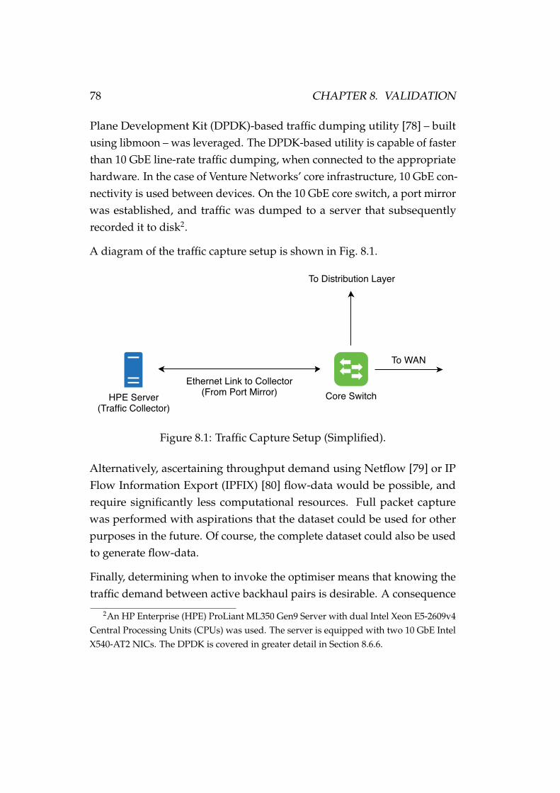
78 CHAPTER 8. VALIDATION
Plane Development Kit (DPDK)-based traffic dumping utility [78] – builtusing libmoon – was leveraged. The DPDK-based utility is capable of fasterthan 10 GbE line-rate traffic dumping, when connected to the appropriatehardware. In the case of Venture Networks’ core infrastructure, 10 GbE con-nectivity is used between devices. On the 10 GbE core switch, a port mirrorwas established, and traffic was dumped to a server that subsequentlyrecorded it to disk2.
A diagram of the traffic capture setup is shown in Fig. 8.1.
Core SwitchHPE Server(Traffic Collector)
Ethernet Link to Collector(From Port Mirror)
To Distribution Layer
To WAN
Figure 8.1: Traffic Capture Setup (Simplified).
Alternatively, ascertaining throughput demand using Netflow [79] or IPFlow Information Export (IPFIX) [80] flow-data would be possible, andrequire significantly less computational resources. Full packet capturewas performed with aspirations that the dataset could be used for otherpurposes in the future. Of course, the complete dataset could also be usedto generate flow-data.
Finally, determining when to invoke the optimiser means that knowing thetraffic demand between active backhaul pairs is desirable. A consequence
2An HP Enterprise (HPE) ProLiant ML350 Gen9 Server with dual Intel Xeon E5-2609v4Central Processing Units (CPUs) was used. The server is equipped with two 10 GbE IntelX540-AT2 NICs. The DPDK is covered in greater detail in Section 8.6.6.

8.2. TRAFFIC PLAYBACK 79
of capturing data at a central location is that this may often be difficult.In the case of the Venture Networks topology, the process is simple, aswe know what IP addresses are in use at each site, and that traffic mustalways pass between the same physical sites (irrespective of what backhaulradios are in use). However, in a more complicated network topology, thisprocess might not be straightforward. Using Simple Network ManagementProtocol (SNMP) is a viable solution, as it is supported by default by mostbackhaul radios, and querying active throughput is generally simple.
8.2.2 Optimiser Invocation
A wide range of predictive models could be used with the ElasticWISPoptimiser. For validation, a straightforward, Simple Moving Average (SMA)approach was used [81]. For each backhaul interface connected to a node –or SR-MPLS router – the network operator must:
• Specify an average interval for throughput sampling, e.g., 30 seconds.
• Specify the number of consecutive sampling periods (the time definedabove) needed above a given (link throughput) safety margin in orderto invoke the optimiser.
Next, the process of averaging the throughput using a SMA is straightfor-ward. To determine when to invoke the optimiser, counters are appliedto the consecutive periods of increase – or decrease – (at given thresholds)shown in the moving average:
1. Average the throughput over the given length of the moving average.If the rate is above the given invocation threshold, increment thecounter. Else, continue.
2. If the rate is below the given threshold, reset the counter.
3. If the counter is equal to the number of consecutive periods requiredto invoke the optimiser, then invoke the optimiser. Finally, reset the
80 CHAPTER 8. VALIDATION
counter.
The same concept is applied for determining when to turn links off3. Itcan be observed from the traffic dataset that when the throughput over alink increases steadily, it will generally do so and remain high (or low ifdecreasing) for some time. Usually this period is long enough that we canjustify powering up a faster radio, and hence the naıve approach aboveis effective. Other factors such as the average throughput over other link-pairs must also be considered4. For example, if the optimiser is invokeddue to high-demand over a particular backhaul pair, and another backhaulpair is experiencing a transient spike in traffic, ElasticWISP may attemptto power up a faster radio pair to accommodate the surge. Having thissituation occur is problematic, as even if the transient spike in demand doesnot meet the innovation criteria, the optimiser is unaware. One approach tomitigating this is using the average throughput over an extended time forlinks that did not invoke the optimiser, in order to avoid any unnecessaryradio power-ups5.
To leverage the SMA approach, link safety margins are set, meaning theoptimiser is invoked with reduced link capacities. Effectively, this meansthat when the sum of all commodities going over any link i, j, exceeds the(safe) capacity of that link, the optimiser will be invoked, and try to find aalternative path. Of course, in some rare circumstances this can introducemodel infeasibility. To deal with infeasibility, an overflow arc is set for anylink i, j in the topology used by ElasticWISP for optimisation. The overflowarc has a very high-cost, and is only used when no alternative paths exist.Practically, the overflow arc results in the highest-throughput backhaulradio between two nodes being turned on. From practical experienceworking with Venture Networks, the self-reported capacities of backhaul
3The process is only necessary to avoid excessive runs of the ElasticWISP optimiser.4“Smoothing” the throughput between backhaul pairs was performed using a SMA
during evaluation.5See Section 8.2.3
8.3. QOS PRESERVATION 81
radio pairs are overly optimistic, which makes extracting their capacities inreal time a challenge.
8.2.3 Traffic Matrix Generation
During the “playback” of network traffic, ElasticWISP must generate atraffic matrix that is used as an input for Gurobi. To solve the optimisationproblem, we consider each WISP site to represent a single commodity6.Practically, this means the traffic matrix used for optimisation consists ofa list of demands between network sites and the gateway. The averagethroughput from a network site to the network gateway over an arbitraryperiod of time could be used as an input. However, if the period of time istoo small, the optimiser itself is unaware of any diurnal trends, and couldturn links on or off unnecessarily. Of course, using a simple approach, suchas a moving average, will reveal throughput trend more effectively thanthe instantaneous rate as reported using SNMP from routers7.
8.3 QoS Preservation
One of the most important considerations for the design of ElasticWISP wasensuring QoS preservation. More than anything else, packet loss, latencyspikes, and excessive jitter should always be avoided. From previouspractical work, it was established that when OSPF link-costs are adjusted,Quagga will reroute traffic to the next shortest path without disruptingnetwork performance. To determine the impact on QoS caused by thererouting process, a 4x4 grid topology (see Fig. 8.2) was emulated using theCORE [82] network emulator.
6When using SR-MPLS, individual customer IP prefixes could be considered as individ-ual commodities, which may result in improved distribution of flows under high networkload.
7Manufacturer specific. Some SNMP-capable devices report filtered values.
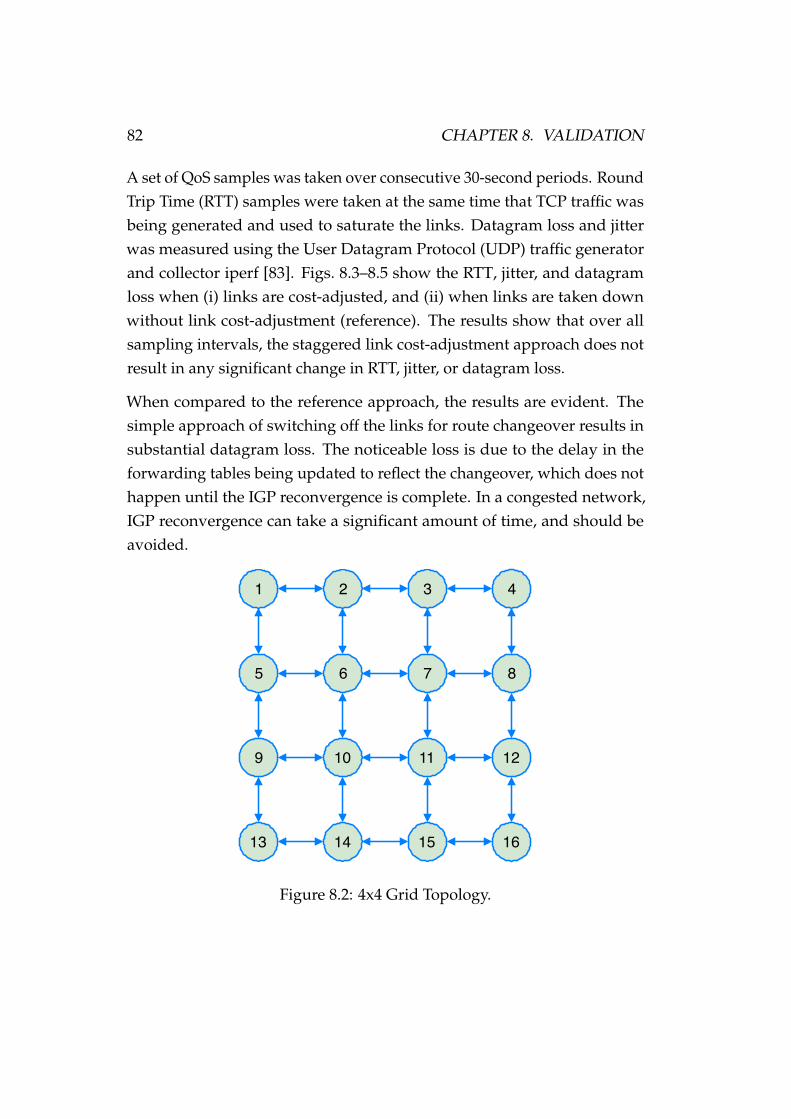
82 CHAPTER 8. VALIDATION
A set of QoS samples was taken over consecutive 30-second periods. RoundTrip Time (RTT) samples were taken at the same time that TCP traffic wasbeing generated and used to saturate the links. Datagram loss and jitterwas measured using the User Datagram Protocol (UDP) traffic generatorand collector iperf [83]. Figs. 8.3–8.5 show the RTT, jitter, and datagramloss when (i) links are cost-adjusted, and (ii) when links are taken downwithout link cost-adjustment (reference). The results show that over allsampling intervals, the staggered link cost-adjustment approach does notresult in any significant change in RTT, jitter, or datagram loss.
When compared to the reference approach, the results are evident. Thesimple approach of switching off the links for route changeover results insubstantial datagram loss. The noticeable loss is due to the delay in theforwarding tables being updated to reflect the changeover, which does nothappen until the IGP reconvergence is complete. In a congested network,IGP reconvergence can take a significant amount of time, and should beavoided.
1 2 3 4
8765
1211109
16151413
Figure 8.2: 4x4 Grid Topology.
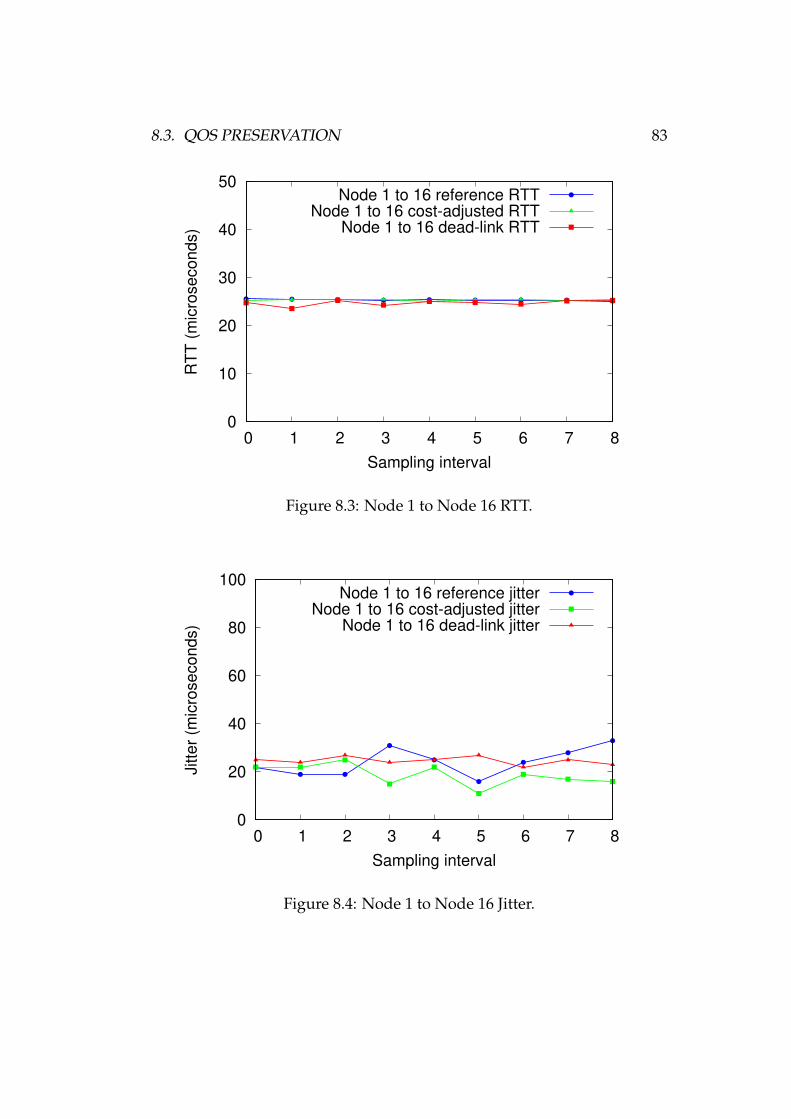
8.3. QOS PRESERVATION 83
0
10
20
30
40
50
0 1 2 3 4 5 6 7 8
RT
T (
mic
rose
co
nd
s)
Sampling interval
Node 1 to 16 reference RTTNode 1 to 16 cost-adjusted RTT
Node 1 to 16 dead-link RTT
Figure 8.3: Node 1 to Node 16 RTT.
0
20
40
60
80
100
0 1 2 3 4 5 6 7 8
Jitte
r (m
icro
se
co
nd
s)
Sampling interval
Node 1 to 16 reference jitterNode 1 to 16 cost-adjusted jitter
Node 1 to 16 dead-link jitter
Figure 8.4: Node 1 to Node 16 Jitter.

84 CHAPTER 8. VALIDATION
0
5
10
15
20
25
0 1 2 3 4 5 6 7 8
Lo
ss (
%)
Sampling interval
Node 1 to 16 reference lossNode 1 to 16 cost-adjusted loss
Node 1 to 16 dead-link loss
Figure 8.5: Node 1 to Node 16 Datagram Loss.
8.4 Energy Consumption
Next, the performance of ElasticWISP is evaluated in terms of energy con-sumption. Like many other optimisation schemes that aim to reduce energyconsumption, the most important metric we are concerned with is the en-ergy consumption of the reduced topology as a percentage of the originalenergy consumption:
Energy consumed by ElasticWISPEnergy consumed by original WISP topology
× 100 (8.1)
8.4.1 Setup
The performance of ElasticWISP is evaluated using the network topology ofVenture Networks’ Horowhenua WISP network. In addition, the traffic cap-
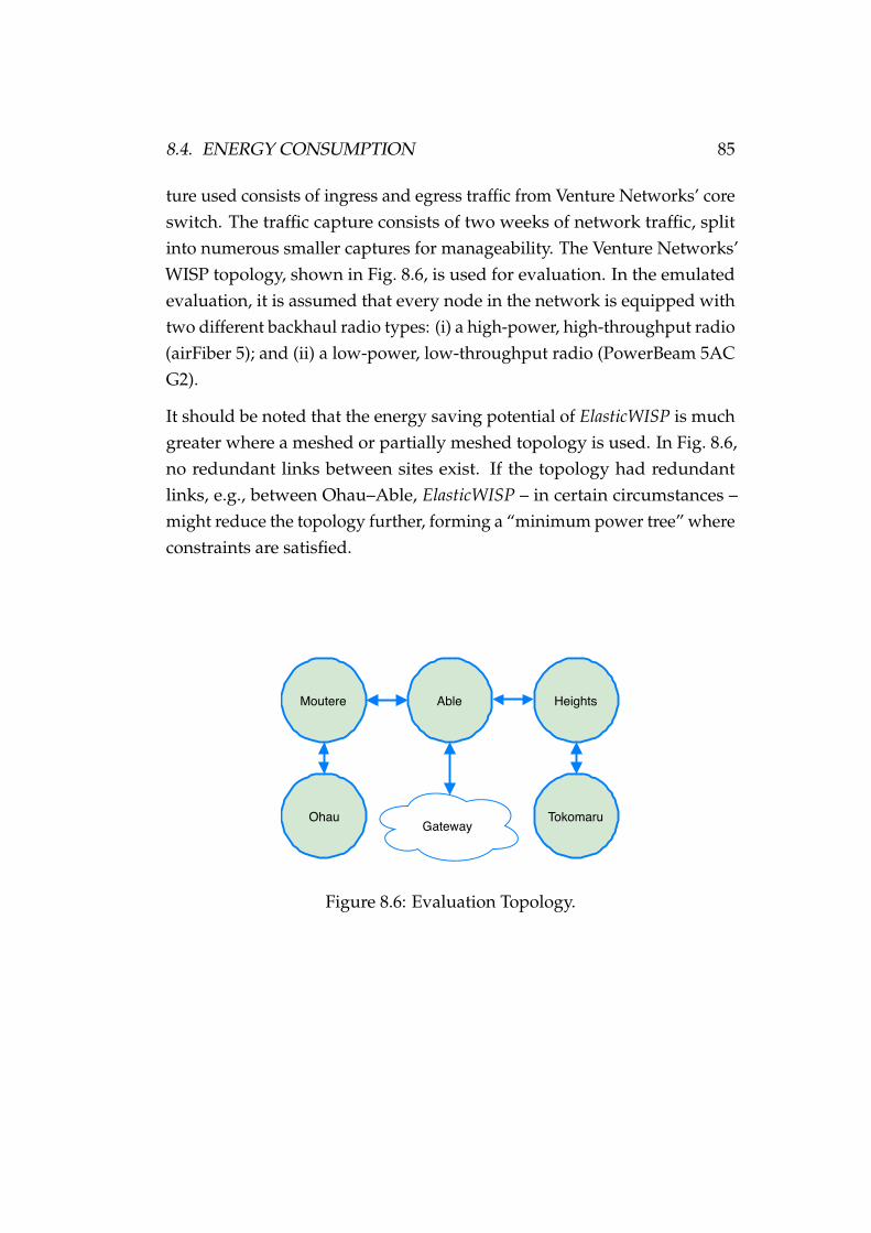
8.4. ENERGY CONSUMPTION 85
ture used consists of ingress and egress traffic from Venture Networks’ coreswitch. The traffic capture consists of two weeks of network traffic, splitinto numerous smaller captures for manageability. The Venture Networks’WISP topology, shown in Fig. 8.6, is used for evaluation. In the emulatedevaluation, it is assumed that every node in the network is equipped withtwo different backhaul radio types: (i) a high-power, high-throughput radio(airFiber 5); and (ii) a low-power, low-throughput radio (PowerBeam 5ACG2).
It should be noted that the energy saving potential of ElasticWISP is muchgreater where a meshed or partially meshed topology is used. In Fig. 8.6,no redundant links between sites exist. If the topology had redundantlinks, e.g., between Ohau–Able, ElasticWISP – in certain circumstances –might reduce the topology further, forming a “minimum power tree” whereconstraints are satisfied.
Able Heights
Ohau
Moutere
TokomaruGateway
Figure 8.6: Evaluation Topology.
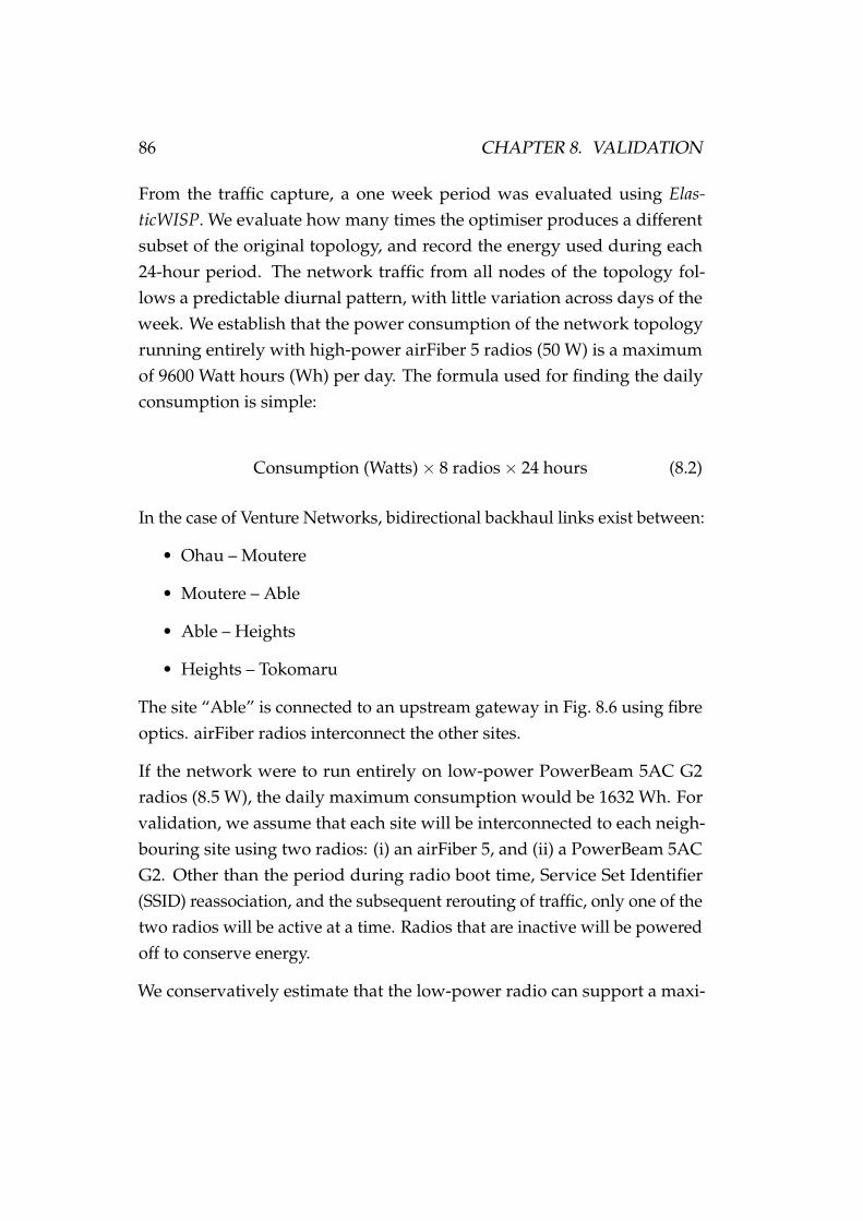
86 CHAPTER 8. VALIDATION
From the traffic capture, a one week period was evaluated using Elas-ticWISP. We evaluate how many times the optimiser produces a differentsubset of the original topology, and record the energy used during each24-hour period. The network traffic from all nodes of the topology fol-lows a predictable diurnal pattern, with little variation across days of theweek. We establish that the power consumption of the network topologyrunning entirely with high-power airFiber 5 radios (50 W) is a maximumof 9600 Watt hours (Wh) per day. The formula used for finding the dailyconsumption is simple:
Consumption (Watts)× 8 radios× 24 hours (8.2)
In the case of Venture Networks, bidirectional backhaul links exist between:
• Ohau – Moutere
• Moutere – Able
• Able – Heights
• Heights – Tokomaru
The site “Able” is connected to an upstream gateway in Fig. 8.6 using fibreoptics. airFiber radios interconnect the other sites.
If the network were to run entirely on low-power PowerBeam 5AC G2radios (8.5 W), the daily maximum consumption would be 1632 Wh. Forvalidation, we assume that each site will be interconnected to each neigh-bouring site using two radios: (i) an airFiber 5, and (ii) a PowerBeam 5ACG2. Other than the period during radio boot time, Service Set Identifier(SSID) reassociation, and the subsequent rerouting of traffic, only one of thetwo radios will be active at a time. Radios that are inactive will be poweredoff to conserve energy.
We conservatively estimate that the low-power radio can support a maxi-

8.4. ENERGY CONSUMPTION 87
mum of 100 Mbps of capacity when transmitting or receiving L2 frames. Weassume the high-power radio can support up to 500 Mbps while transmit-ting or receiving L2 frames. We know in reality these values will be different.The performance of unlicensed radios is – at a minimum – challenging toaccurately predict, and is subject to factors such as external interference,rain fade, and obstructions in the line of sight and Fresnel zone. Lastly, inthis topology we expect that distant links, i.e., Ohau–Moutere and Heights–Tokomaru, will offer the best potential for energy conservation as they carrythe least amount of transient traffic from other nodes.
8.4.2 Results
Upon running our evaluation of ElasticWISP we discovered promisingresults. We assume that using a straw man configuration with only high-power airFiber 5 radios, the evaluation topology would consume approxi-mately:
50 W× 8 radios× 24 hours per day× 7 days of the week (8.3)
Overall, the weekly consumption should be approximately 67,200 Wh, or67.2 Kilowatt hour (kWh). Utilising ElasticWISP and the provided dataset with a combination of airFiber 5 and PowerBeam 5AC G2 radios, wewere able to reduce the consumption for a given week to 23,765 Wh, or≈23.8 kWh. Overall, this saves 65% of network-wide energy, a significantreduction. Of course, this figure uses the maximum power consumptionof the radios. In practice, the energy reduction may in fact be greater, aswe know that low-power backhaul radios – such as the PowerBeam 5ACG2 – available to WISPs typically use much less energy than their designmaximum, whereas high-power, full-duplex radios – such as the airFiber 5– use near their design maximum energy consumption continuously.
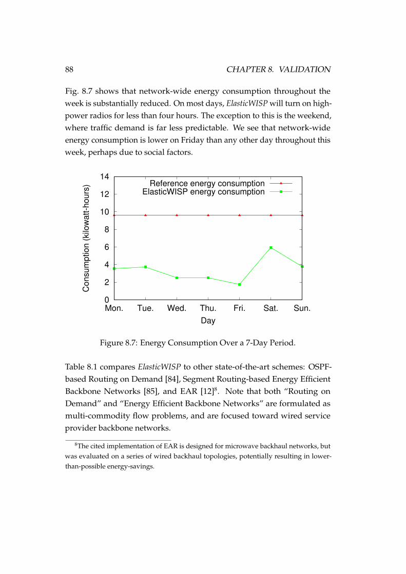
88 CHAPTER 8. VALIDATION
Fig. 8.7 shows that network-wide energy consumption throughout theweek is substantially reduced. On most days, ElasticWISP will turn on high-power radios for less than four hours. The exception to this is the weekend,where traffic demand is far less predictable. We see that network-wideenergy consumption is lower on Friday than any other day throughout thisweek, perhaps due to social factors.
0
2
4
6
8
10
12
14
Mon. Tue. Wed. Thu. Fri. Sat. Sun.
Co
nsu
mp
tio
n (
kilo
wa
tt-h
ou
rs)
Day
Reference energy consumptionElasticWISP energy consumption
Figure 8.7: Energy Consumption Over a 7-Day Period.
Table 8.1 compares ElasticWISP to other state-of-the-art schemes: OSPF-based Routing on Demand [84], Segment Routing-based Energy EfficientBackbone Networks [85], and EAR [12]8. Note that both “Routing onDemand” and “Energy Efficient Backbone Networks” are formulated asmulti-commodity flow problems, and are focused toward wired serviceprovider backbone networks.
8The cited implementation of EAR is designed for microwave backhaul networks, butwas evaluated on a series of wired backhaul topologies, potentially resulting in lower-than-possible energy-savings.

8.4. ENERGY CONSUMPTION 89
Table 8.1: Validation: CompetitorsPlatform Flow path en-
forcementEnergy saving Approach
ElasticWISP IGP best-path orSR-MPLS
≈ 65% Radiochangeover,turning off links
Routing on De-mand [84]
IGP best-path(with optimallink-weights)
≈ 43% Turning off links
Energy Effi-cient BackboneNetworks [85]
Explicit (Seg-ment Routing)
≈ 44% Turning off links
Energy-AwareRouting [12]
Numerical eval-uation
≈ 28% Turning off links
A key advantage ElasticWISP has over competitor schemes, and specifi-cally for WISP – and perhaps microwave – use, is the ability to performradio changeover based on traffic demand. Practically, this is similar toapproaches that turn off links in a bundle – e.g., of line-cards – to conserveenergy in a wired service provider network. However, ElasticWISP’s en-ergy saving potential is high due to the disparity of energy consumptionbetween the backhaul radios that were studied. As a result, in comparisonto other schemes, ElasticWISP can conserve more energy in WISP networkswhere both high and low power backhaul radios are used.
Formally, ElasticWISP is similar to ElasticTree9, which itself is formally sim-ilar to earlier efforts to conserve energy in service provider networks [86].As ElasticWISP uses a subset of the energy minimisation constraints pro-posed by ElasticTree and earlier efforts, the performance difference betweenthe two platforms will be negligible for any given test topology. However,
9See Chapter 2.1.2.
90 CHAPTER 8. VALIDATION
unlike ElasticTree, we do not consider turning off switches, or in our case,nodes at each network site. As a result, ElasticTree can conserve additionalenergy where it is able to turn off redundant switches.
Functionally, ElasticWISP is very different to ElasticTree. The use of OSPFand later Segment Routing, as opposed to OpenFlow, introduces its ownunique challenges, as does dealing with the unpredictable nature of un-licensed radio links. In addition, ElasticTree deals with links that can bebrought up and down very quickly, whereas radio links will always havecomparatively expensive boot and reassociation times. In addition to this,practical deployment of ElasticWISP itself required a new architecture ofremotely managed PoE devices to be developed.
8.5 Implementation Considerations
While the OSPF-based link cost-adjustment design and implementationof ElasticWISP can help WISP operators realise substantial energy savings,it is not without caveats. The time taken for traffic to be rerouted is notinstantaneous; the OSPF link-costs of a given link (radio pair) must beadjusted prior to powering them down. The time it takes for traffic to berouted over a lower-cost path is OSPF implementation-specific. While thesechangeover times were consistently low in this implementation, there is noguarantee that other OSPF daemons – and their given configurations – willperform in the same way.
If an appropriate traffic engineering mechanism was to be implementedalongside ElasticWISP instances – such as the Segment Routing approachdescribed later in this chapter – this problem could be eliminated. If thepath of a given flow was computed in advance with packets set to traversea specific set of segments, then a WISP operator would not need to wait foran IGP-computed path reroute to happen prior to powering a link down.
Lastly, ElasticWISP is designed for the optimisation of backhaul links on
8.5. IMPLEMENTATION CONSIDERATIONS 91
WISP networks. While it was shown that full-duplex (airFiber) backhaulradios used by WISPs account for a significant portion of energy consump-tion per site, we must also consider the point-to-multipoint radios that areused for customer access purposes. Much like their point-to-point coun-terparts, customer access radios typically used by WISPs have very littlevariation in energy consumption, irrespective of how much traffic is beingpassed over them. Typically these access radios are connected to sectorantennas that distribute Internet access to customers. Sector antennas usedwill have a manufacturer specified azimuth and elevation radiation pattern.For example, in a high-capacity configuration, a WISP may have numeroussector antennas, each with a 30 degree azimuth radiation pattern serving acollection of customers.
During off-peak periods of network consumption, we propose that WISPoperators could offload traffic from numerous high-capacity radios onto alesser number of (low-power) radios that have antennas covering a widerazimuth. Essentially, customers would be transitioned to use an accesspoint that can only handle low-demand for throughput. This approach hassimilarities to historical work proposed for energy conservation [87]. Whileexisting equipment from the likes of Ubiquiti Networks enables WISPs toset a fallback SSID, there is currently no way of carrying out a gracefultransition between access radios.
A recently developed handover scheme, BigAP [88], has shown that Dy-namic Frequency Selection (DFS) Channel Switch Announcement Informa-tion Element (CSA-IE) can be used as a seamless infrastructure initiatedhandover mechanism between access points. Unfortunately for WISPs,this mechanism is likely not an option, as BigAP relies on radios beingcompliant with the IEEE 802.11n/ac standards, which both include theIEEE 802.11h amendment. Radios from the likes of Ubiquiti Networks etal. make no claim to be compliant with such IEEE standards, and nowtypically use custom radio chipsets for improved spectral efficiency [89].
92 CHAPTER 8. VALIDATION
8.6 SR-MPLS Benchmarks
To evaluate the performance of the SR-MPLS scheme, a simple linear topol-ogy10 consisting of four hosts was created in the CORE emulator11. TheSR-MPLS evaluation setup consisted of two standard Linux hosts. Thefirst host was responsible for UDP packet generation, with the second hostacting as a traffic collector. The two other hosts performed MPLS encap-sulation and decapsulation duties. While simple, this topology enables usto evaluate how well the scheme can perform in a worst-case scenario, i.e.,performing encapsulation or decapsulation. In contrast, MPLS to MPLSforwarding within an SR-MPLS domain is less taxing, as shown earlier inFig. 6.4.
The SR-MPLS setup described was evaluated against an equivalent IProuting based implementation. The two SR-MPLS encapsulation and de-capsulation hosts were replaced with standard Linux hosts running theQuagga routing suite, with OSPFv2 enabled for the creation of IPv4 routes.An overview of this reference setup is shown in Fig. 8.8.
Furthermore, the design of SR-MPLS as described in Chapter 6 is imple-mented using the systems programming language Rust [90], which hascompetitive performance with C. Rust was used due to familiarity with thelow-level libpnet [91] networking library, which offers an excellent trade-offbetween ease-of-programming and performance. In merit of using Rustand the libpnet library for implementation, UDP packet generators writtenusing libpnet have – marginally – outperformed their equivalent C counter-parts12. Finally, ZeroMQ was used as the message queue of choice in thisimplementation.
10Using a simple linear topology for evaluation is consistent with previous SegmentRouting research [43].
11Evaluation was performed on an Ubuntu Server 18.04.3 LTS host with an Intel i79700K CPU and 16GB of 2666 MHz DDR4 RAM.
12Rust and C benchmarks are available on the libpnet GitHub repository [92].
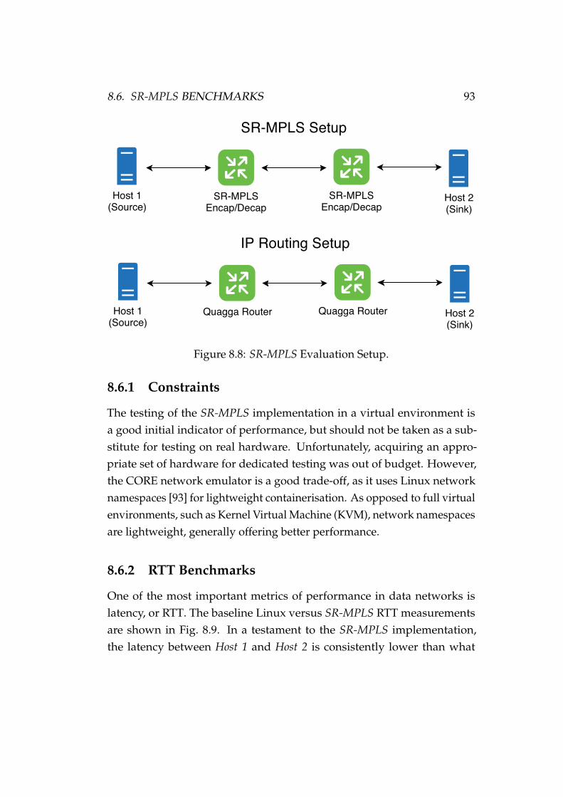
8.6. SR-MPLS BENCHMARKS 93
SR-MPLSEncap/Decap
SR-MPLSEncap/Decap
Host 1(Source)
Host 2(Sink)
SR-MPLS Setup
Quagga Router Quagga RouterHost 1(Source)
Host 2(Sink)
IP Routing Setup
Figure 8.8: SR-MPLS Evaluation Setup.
8.6.1 Constraints
The testing of the SR-MPLS implementation in a virtual environment isa good initial indicator of performance, but should not be taken as a sub-stitute for testing on real hardware. Unfortunately, acquiring an appro-priate set of hardware for dedicated testing was out of budget. However,the CORE network emulator is a good trade-off, as it uses Linux networknamespaces [93] for lightweight containerisation. As opposed to full virtualenvironments, such as Kernel Virtual Machine (KVM), network namespacesare lightweight, generally offering better performance.
8.6.2 RTT Benchmarks
One of the most important metrics of performance in data networks islatency, or RTT. The baseline Linux versus SR-MPLS RTT measurementsare shown in Fig. 8.9. In a testament to the SR-MPLS implementation,the latency between Host 1 and Host 2 is consistently lower than what

94 CHAPTER 8. VALIDATION
is achieved using standard IP forwarding, with the use of Quagga forroute setup. One of the reasons SR-MPLS can achieve very low-latencyforwarding is the minimal processing overhead required in the evaluationsetup. In the linear topology, the MPLS FIB of the SR-MPLS routers consistsof one MPLS-capable SR-MPLS neighbour. When IP packets come intoeither SR-MPLS router, only the single FIB entry is found, and the IP packetssubsequently have a single adjacency SID pushed onto them.
The process is repeated when the MPLS packets are decapsulated, or“popped”. The IP packet must be forwarded out an interface, but there willonly be one customer attached subnetwork to either SR-MPLS router in thetopology – either Host 1 or Host 2. In short, the SR-MPLS routers behavein a very simple, predictable way. Another consideration, as the SR-MPLSrouters run in user space, is process priority. The priority of the SR-MPLSrouters in this example – and all other figures in this series of subsections –is normal, and their niceness values have not been altered.
0
20
40
60
80
100
0 1 2 3 4 5 6 7 8
RT
T (
mic
rose
co
nd
s)
Sampling interval
IP Routing RTTSR-MPLS RTT
Figure 8.9: Host 1 to Host 2 RTT.
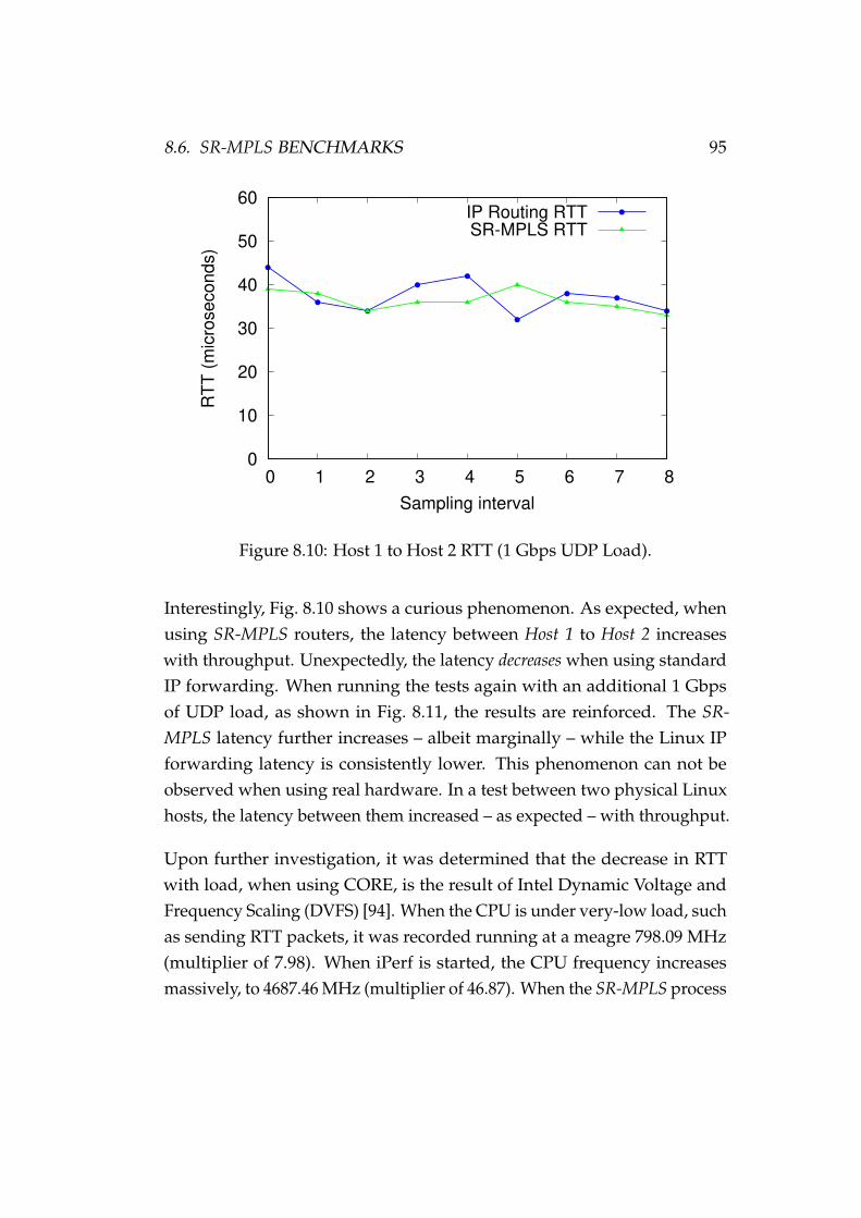
8.6. SR-MPLS BENCHMARKS 95
0
10
20
30
40
50
60
0 1 2 3 4 5 6 7 8
RT
T (
mic
rose
co
nd
s)
Sampling interval
IP Routing RTTSR-MPLS RTT
Figure 8.10: Host 1 to Host 2 RTT (1 Gbps UDP Load).
Interestingly, Fig. 8.10 shows a curious phenomenon. As expected, whenusing SR-MPLS routers, the latency between Host 1 to Host 2 increaseswith throughput. Unexpectedly, the latency decreases when using standardIP forwarding. When running the tests again with an additional 1 Gbpsof UDP load, as shown in Fig. 8.11, the results are reinforced. The SR-MPLS latency further increases – albeit marginally – while the Linux IPforwarding latency is consistently lower. This phenomenon can not beobserved when using real hardware. In a test between two physical Linuxhosts, the latency between them increased – as expected – with throughput.
Upon further investigation, it was determined that the decrease in RTTwith load, when using CORE, is the result of Intel Dynamic Voltage andFrequency Scaling (DVFS) [94]. When the CPU is under very-low load, suchas sending RTT packets, it was recorded running at a meagre 798.09 MHz(multiplier of 7.98). When iPerf is started, the CPU frequency increasesmassively, to 4687.46 MHz (multiplier of 46.87). When the SR-MPLS process
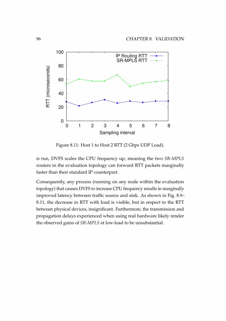
96 CHAPTER 8. VALIDATION
0
20
40
60
80
100
0 1 2 3 4 5 6 7 8
RT
T (
mic
rose
co
nd
s)
Sampling interval
IP Routing RTTSR-MPLS RTT
Figure 8.11: Host 1 to Host 2 RTT (2 Gbps UDP Load).
is run, DVFS scales the CPU frequency up, meaning the two SR-MPLSrouters in the evaluation topology can forward RTT packets marginallyfaster than their standard IP counterpart.
Consequently, any process (running on any node within the evaluationtopology) that causes DVFS to increase CPU frequency results in marginallyimproved latency between traffic source and sink. As shown in Fig. 8.9–8.11, the decrease in RTT with load is visible, but in respect to the RTTbetween physical devices, insignificant. Furthermore, the transmission andpropagation delays experienced when using real hardware likely renderthe observed gains of SR-MPLS at low-load to be unsubstantial.
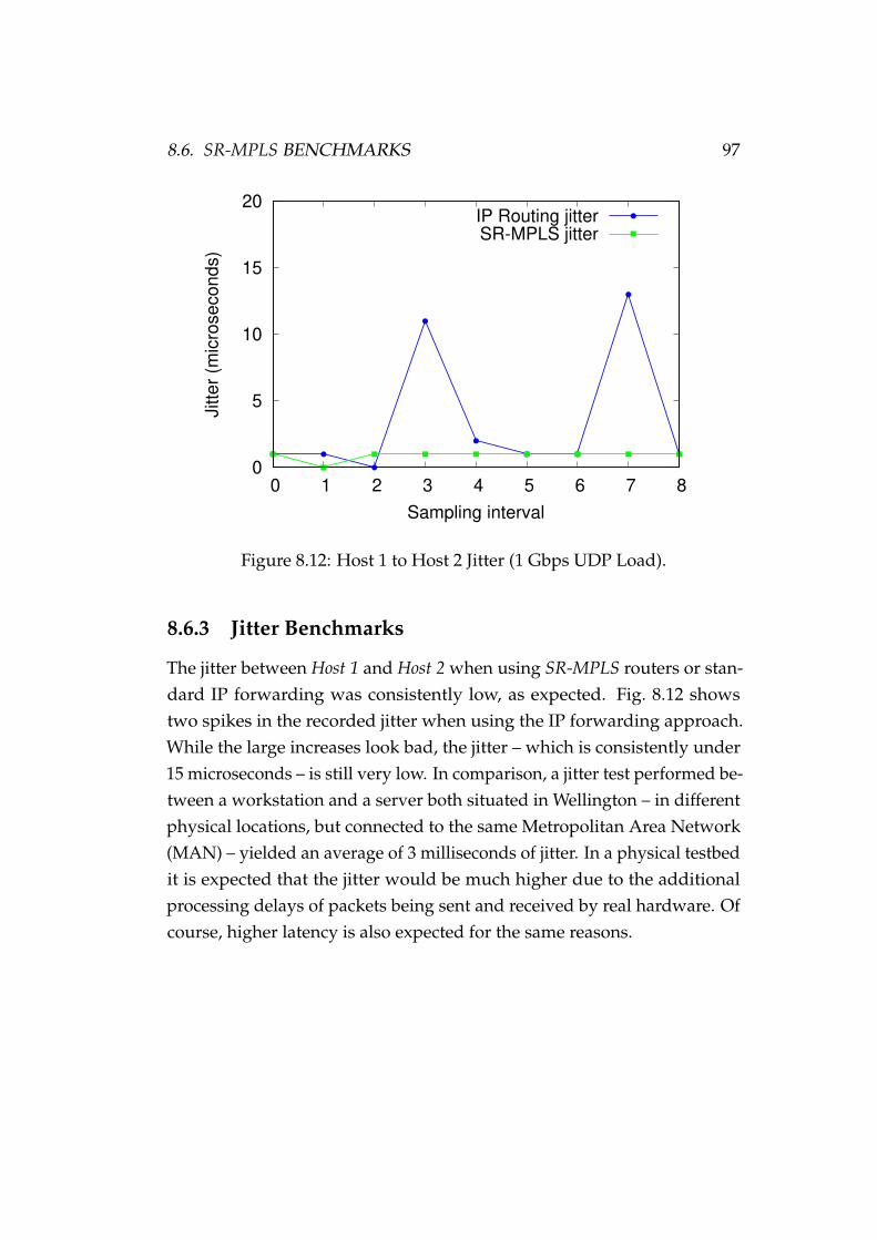
8.6. SR-MPLS BENCHMARKS 97
0
5
10
15
20
0 1 2 3 4 5 6 7 8
Jitte
r (m
icro
se
co
nd
s)
Sampling interval
IP Routing jitterSR-MPLS jitter
Figure 8.12: Host 1 to Host 2 Jitter (1 Gbps UDP Load).
8.6.3 Jitter Benchmarks
The jitter between Host 1 and Host 2 when using SR-MPLS routers or stan-dard IP forwarding was consistently low, as expected. Fig. 8.12 showstwo spikes in the recorded jitter when using the IP forwarding approach.While the large increases look bad, the jitter – which is consistently under15 microseconds – is still very low. In comparison, a jitter test performed be-tween a workstation and a server both situated in Wellington – in differentphysical locations, but connected to the same Metropolitan Area Network(MAN) – yielded an average of 3 milliseconds of jitter. In a physical testbedit is expected that the jitter would be much higher due to the additionalprocessing delays of packets being sent and received by real hardware. Ofcourse, higher latency is also expected for the same reasons.
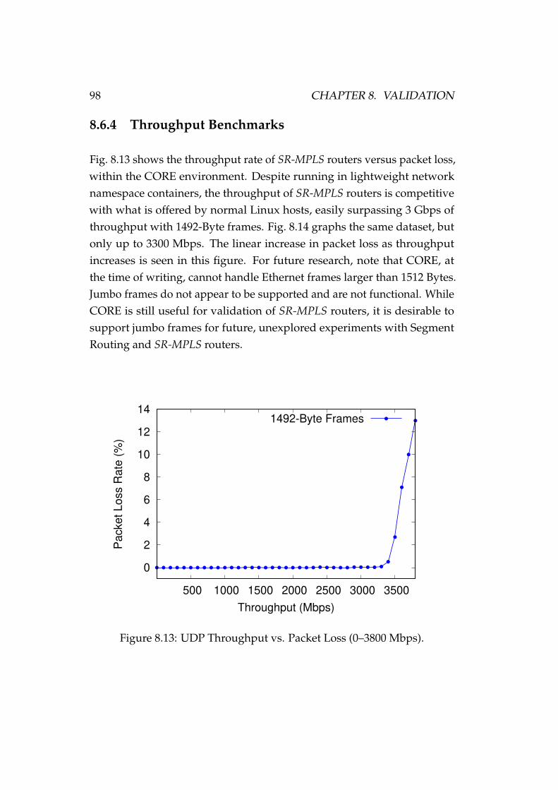
98 CHAPTER 8. VALIDATION
8.6.4 Throughput Benchmarks
Fig. 8.13 shows the throughput rate of SR-MPLS routers versus packet loss,within the CORE environment. Despite running in lightweight networknamespace containers, the throughput of SR-MPLS routers is competitivewith what is offered by normal Linux hosts, easily surpassing 3 Gbps ofthroughput with 1492-Byte frames. Fig. 8.14 graphs the same dataset, butonly up to 3300 Mbps. The linear increase in packet loss as throughputincreases is seen in this figure. For future research, note that CORE, atthe time of writing, cannot handle Ethernet frames larger than 1512 Bytes.Jumbo frames do not appear to be supported and are not functional. WhileCORE is still useful for validation of SR-MPLS routers, it is desirable tosupport jumbo frames for future, unexplored experiments with SegmentRouting and SR-MPLS routers.
0
2
4
6
8
10
12
14
500 1000 1500 2000 2500 3000 3500
Pa
cke
t L
oss R
ate
(%
)
Throughput (Mbps)
1492-Byte Frames
Figure 8.13: UDP Throughput vs. Packet Loss (0–3800 Mbps).
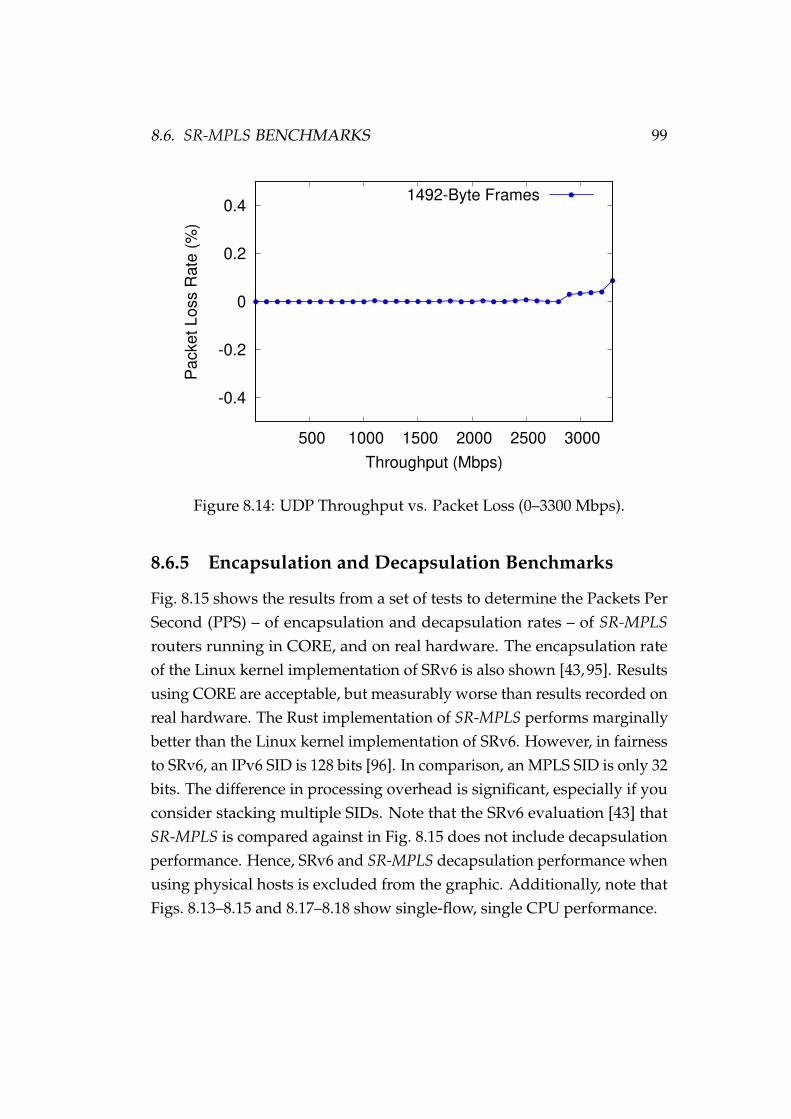
8.6. SR-MPLS BENCHMARKS 99
-0.4
-0.2
0
0.2
0.4
500 1000 1500 2000 2500 3000
Pa
cke
t L
oss R
ate
(%
)
Throughput (Mbps)
1492-Byte Frames
Figure 8.14: UDP Throughput vs. Packet Loss (0–3300 Mbps).
8.6.5 Encapsulation and Decapsulation Benchmarks
Fig. 8.15 shows the results from a set of tests to determine the Packets PerSecond (PPS) – of encapsulation and decapsulation rates – of SR-MPLSrouters running in CORE, and on real hardware. The encapsulation rateof the Linux kernel implementation of SRv6 is also shown [43, 95]. Resultsusing CORE are acceptable, but measurably worse than results recorded onreal hardware. The Rust implementation of SR-MPLS performs marginallybetter than the Linux kernel implementation of SRv6. However, in fairnessto SRv6, an IPv6 SID is 128 bits [96]. In comparison, an MPLS SID is only 32bits. The difference in processing overhead is significant, especially if youconsider stacking multiple SIDs. Note that the SRv6 evaluation [43] thatSR-MPLS is compared against in Fig. 8.15 does not include decapsulationperformance. Hence, SRv6 and SR-MPLS decapsulation performance whenusing physical hosts is excluded from the graphic. Additionally, note thatFigs. 8.13–8.15 and 8.17–8.18 show single-flow, single CPU performance.
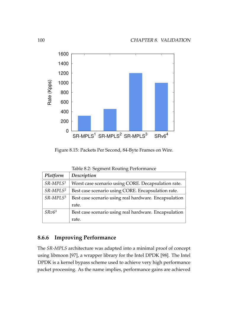
100 CHAPTER 8. VALIDATION
0
200
400
600
800
1000
1200
1400
1600
SR-MPLS1
SR-MPLS2
SR-MPLS3
SRv64
Ra
te (
Kp
ps)
Figure 8.15: Packets Per Second, 84-Byte Frames on Wire.
Table 8.2: Segment Routing PerformancePlatform Description
SR-MPLS1 Worst case scenario using CORE. Decapsulation rate.SR-MPLS2 Best case scenario using CORE. Encapsulation rate.SR-MPLS3 Best case scenario using real hardware. Encapsulation
rate.SRv64 Best case scenario using real hardware. Encapsulation
rate.
8.6.6 Improving Performance
The SR-MPLS architecture was adapted into a minimal proof of conceptusing libmoon [97], a wrapper library for the Intel DPDK [98]. The IntelDPDK is a kernel bypass scheme used to achieve very high performancepacket processing. As the name implies, performance gains are achieved

8.6. SR-MPLS BENCHMARKS 101
through bypassing the packet processing inefficiencies of the Linux kernel.Intel has shown DPDK to be capable of L3 forwarding – with 64-Byte packetsizes – at rates up to 233 Gbps, or 347 Mpps [99]. Even on commodity x86hardware – using 10 GbE Intel NICs – the DPDK can be used to forward64-Byte packets at line-rate using a single CPU core.
The evaluation setup for the libmoon/DPDK implementation is shown inFig. 8.16. The setup was limited in comparison to the emulated (CORE)environment due to the prohibitive cost of high-end workstation hardware,and 10 GbE Intel NICs. The first workstation, equipped with an Intel i75820k, was used for packet generation. The workstation used for evaluatingencapsulation performance is equipped with an Intel i7 9700k, which hassubstantially faster per-core CPU performance than the i7 5820k. To com-pensate for the slower CPU, libmoon was used for UDP packet generation.Finally, the workstation responsible for encapsulation was also connectedto a 10 GbE switch. The switch was monitored to ensure MPLS packetswere being received.
i7 5820k w/10GbE NIC(Source/Packet Gen)
i7 9700k w/10GbE NIC (x2)(Encap/Send)
DPDK Setup
10 GbE Switch(Used for link-up)
Figure 8.16: SR-DPDK Evaluation Setup.
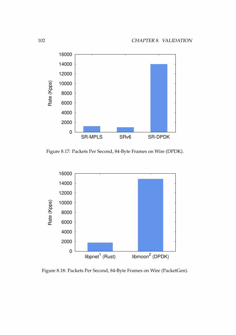
102 CHAPTER 8. VALIDATION
0
2000
4000
6000
8000
10000
12000
14000
16000
SR-MPLS SRv6 SR-DPDK
Ra
te (
Kp
ps)
Figure 8.17: Packets Per Second, 84-Byte Frames on Wire (DPDK).
0
2000
4000
6000
8000
10000
12000
14000
16000
libpnet1 (Rust) libmoon
2 (DPDK)
Ra
te (
Kp
ps)
Figure 8.18: Packets Per Second, 84-Byte Frames on Wire (PacketGen).
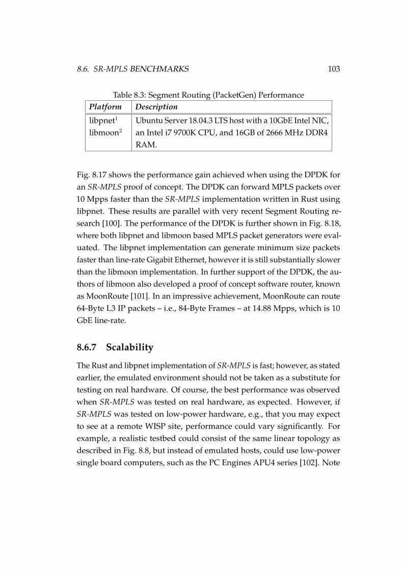
8.6. SR-MPLS BENCHMARKS 103
Table 8.3: Segment Routing (PacketGen) PerformancePlatform Description
libpnet1
libmoon2
Ubuntu Server 18.04.3 LTS host with a 10GbE Intel NIC,an Intel i7 9700K CPU, and 16GB of 2666 MHz DDR4RAM.
Fig. 8.17 shows the performance gain achieved when using the DPDK foran SR-MPLS proof of concept. The DPDK can forward MPLS packets over10 Mpps faster than the SR-MPLS implementation written in Rust usinglibpnet. These results are parallel with very recent Segment Routing re-search [100]. The performance of the DPDK is further shown in Fig. 8.18,where both libpnet and libmoon based MPLS packet generators were eval-uated. The libpnet implementation can generate minimum size packetsfaster than line-rate Gigabit Ethernet, however it is still substantially slowerthan the libmoon implementation. In further support of the DPDK, the au-thors of libmoon also developed a proof of concept software router, knownas MoonRoute [101]. In an impressive achievement, MoonRoute can route64-Byte L3 IP packets – i.e., 84-Byte Frames – at 14.88 Mpps, which is 10GbE line-rate.
8.6.7 Scalability
The Rust and libpnet implementation of SR-MPLS is fast; however, as statedearlier, the emulated environment should not be taken as a substitute fortesting on real hardware. Of course, the best performance was observedwhen SR-MPLS was tested on real hardware, as expected. However, ifSR-MPLS was tested on low-power hardware, e.g., that you may expectto see at a remote WISP site, performance could vary significantly. Forexample, a realistic testbed could consist of the same linear topology asdescribed in Fig. 8.8, but instead of emulated hosts, could use low-powersingle board computers, such as the PC Engines APU4 series [102]. Note
104 CHAPTER 8. VALIDATION
that the APU4 series also appears to be capable of running the DPDK.
While the choice of hardware is important in determining the scalabilityof an SR-MPLS domain, it is also important to consider the maximumsegment depth, and the the MTU being used across the network. A keyadvantage SR-MPLS has over its IPv6 counterpart, SRv6, is SID size. The32-bit SID is substantially smaller than the 128-bit IPv6 SID, meaning evenif a network is constrained to using an MTU of 1500 Bytes, the performance– as shown in Fig. 8.13–8.14 – is still acceptable. If the maximum segmentdepth is large, e.g., 32 SIDs, the overhead is still only 128 Bytes. If usingSRv6, the equivalent overhead would be 512 Bytes.
The overhead of both SR-MPLS and SRv6 should also be taken into con-sideration when determining the scalability of a domain running eitherarchitecture. For most WISPs, dealing with larger-than-normal Ethernetframes should not be problematic, as common backhaul radios such as theairFiber series support jumbo frames of up to 9600 Bytes [103].
8.6.8 Why Kernel Bypass
Despite the current implementation of SR-MPLS having acceptable per-formance for use in real WISP networks, the ever-growing demand forthroughput capacity must be considered. While the Linux kernel now sup-ports basic MPLS functionality, as of version 4.3 [104, 105], the performancelimitations of the kernel network stack mean that other options shouldalso be considered. While familiarity with the libpnet library was useful incompleting this evaluation, the library can also leverage netmap [106] as abackend for sending and receiving packets. Like the DPDK, netmap is akernel bypass framework that focuses on implementing a faster-than-kernelnetwork stack.
The benefit of using a library, such as libpnet, over utilising in-kernel MPLShandling functionality is simplicity. It also means that straightforward
8.7. SUMMARY 105
integration with kernel bypass frameworks such as netmap and the DPDKcan be leveraged at a later date13. Looking to the future, and at at potentialthroughput capacity requirements, leveraging kernel bypass approachescould be mandatory to meet demand. Furthermore, implementing SR-MPLS from the ground up using Rust and libpnet meant that completecontrol was maintained over the development of the scheme; eliminatingkernel dependence and any associated development complexities14.
8.7 Summary
The results presented throughout this validation chapter have shown thatElasticWISP and SR-MPLS are all but ready for deployment in real WISPnetworks. Following further validation on a greater range of hardware, itis expected that both schemes will be trialled at Venture Networks. Thecomplete set of hardware developed for power control will enable straight-forward deployment, without having to further modify devices such asPoE switches to integrate with the ElasticWISP optimiser. Finally, the resultsof the DPDK evaluation have shown that Linux kernel bypass approachesto networking have merit, and are an exciting avenue for further research.Concluding this thesis, Chapter 9 will next present a summary of findingsand planned future work.
13DPDK support for libpnet is a work in progress.14Normal operation of SR-MPLS using libpnet utilises the AF PACKET socket for send-
ing and receiving packets.

106 CHAPTER 8. VALIDATION

Chapter 9
Conclusion
This thesis has presented ElasticWISP, a practical architecture to enable thedesign of high-throughput, energy-proportional WISP backhaul networks.Through “playing back” daily network traffic, it has been shown that it ispossible to employ high-throughput radios on demand while maintainingenergy-proportionality during off-peak periods, reducing overall networkenergy consumption by around 65%. For a WISP constrained by their localenvironment, this may mean they can build a higher-performance networkthan they otherwise would be able to, due to limited energy harvestingcapability.
Throughout this thesis, it has been shown that the ElasticWISP architecturehas been divided into three key categories:
• The ElasticWISP optimiser, for computing optimal flow-paths.
• The SR-MPLS Segment Routing approach, for explicit flow-path en-forcement.
• The backhaul power control hardware, for switching radios on andoff based on the output of the ElasticWISP optimiser.
Together, these categories form a cohesive platform that has application
107

108 CHAPTER 9. CONCLUSION
not only for WISPs, but for microwave operators, cellular providers, andeven carriers with wired topologies. It is hoped that the concepts used forElasticWISP can be applied to a variety of different physical hardware.
The power control hardware developed for integration with ElasticWISPand SR-MPLS further asserts the practicality of the architecture. While PoEswitches specifically targeted at WISPs are readily available for purchase,they lack features that would enable them to integrate with the ElasticWISParchitecture. In addition, such switches typically lack sophisticated en-ergy monitoring capability, often lacking even minimal per-port powerconsumption metrics. Using the ElasticWISP power control hardware willenable future researchers to not only to control the power to radios, but tohave a fine-grained view of their energy consumption.
Finally, the design and validation of the Segment Routing architecture,SR-MPLS, shows that it is capable of being used as-is on real WISP net-works. When deployed, the SR-MPLS implementation enables networkoperators to steer packets across an ordered list of segments with explicitor arbitrary precision. Validation also showed that the minimal SR-MPLSimplementation using the DPDK is competitive with even the most recentstate-of-the-art Segment Routing research.
9.1 Future Work
The performance of the minimal SR-MPLS implementation using the DPDKmakes it an appealing topic for future work. Should a full Segment Routingimplementation be completed utilising the DPDK, it would have competi-tive packet processing rates to commercial Segment Routing solutions fromvendors such as Cisco and Juniper. Releasing such an implementation asopen-source could also have great benefit to the wider Internet commu-nity. Additionally, extending the open-source Linux kernel implementationof SRv6 to support IPv4 encapsulation would also mean that IPv6 only
9.1. FUTURE WORK 109
networks could easily be used for IPv4 over IPv6 transportation.
The dataset used to evaluate the performance of the ElasticWISP optimiserwas not straightforward to collect. However, it is still desirable to evaluatethe performance of ElasticWISP on other WISP topologies, ideally alsousing data collected from each respective network. Working with largerWISPs would generally require using flow-data rather than full trafficdumps to run the ElasticWISP optimiser, due to the computational resourcesneeded, even when using platforms such as the DPDK. Consequently, datacollection should be easier, as most commercial routers are able to exportflow-data, often in a variety of formats, e.g., Netflow and IPFIX.
Furthermore, deploying ElasticWISP in a real WISP network introducesnew and exciting challenges. The predictive – or in the ElasticWISP case,reactive – model responsible for invoking the optimiser must use link safetymargins. In a scenario where a link becomes congested before a faster radiocan be turned on, it is important a WISP can still maintain QoS and QoEfor important latency-sensitive traffic such as Voice over IP (VoIP).
In a situation where links become saturated before faster links can be turnedon, standard First in, First out (FIFO) queues may result in network users –who are likely paying customers – experiencing poor network QoE. One ofthe most problematic issues that can arise is bufferbloat [107]. Essentially,bufferbloat is undesirable latency, and is caused by devices within thenetwork buffering excessive data. To avoid service degradation for VoIPand other latency-sensitive real-time applications, bufferbloat must becarefully managed.
A common approach to managing bufferbloat is using Active Queue Man-agement (AQM) [107]. One recent innovation, Flow Queue ControlledDelay (FQ-CoDel) [108, 109], is a hybrid packet scheduler and AQM algo-rithm, and has specifically been shown to reduce bufferbloat in capacity-constrained rural broadband access networks [110]. Future research willexamine how AQM approaches, such as FQ-CoDel, can be used to im-

110 CHAPTER 9. CONCLUSION
prove network QoE alongside the existing ElasticWISP energy-optimisationscheme.

Appendices
111


Appendix A
Evaluation Dataset
The dataset used for evaluation of ElasticWISP has not been anonymised,and could potentially be used to identify Venture Networks’ customersand their browsing habits. Researchers wishing to access the dataset, or torun additional packet captures, are advised to contact Venture Networksdirectly.
113

114 APPENDIX A. EVALUATION DATASET

Appendix B
Measurement and Control
In order to use a voltage divider to measure the voltage of the high-sideswitch output ports, we must first determine the correct resistors to use tobuild the voltage division circuit. Using the voltage division rule [111], weknow that:
VOUT = VIN(R2
R1 + R2
) (B.1)
Following the Infineon design guide for their PROFET+ series high-sideswitches [112], we consider using 1.5kΩ and 47kΩ resistors to form thevoltage divider. Using the voltage division rule, we find that where R1 =
47kΩ and R2 = 1.5kΩ, VOUT ≈ 1.48V when VIN is at a nominal 48V. Thisis within the 1.8V limit of the ADC. Of course, the resistors used in thevoltage divider should be chosen so that their output does not exceed themaximum input voltage of the ADC used:
VIN =VOUT × (R1 + R2)
R2
(B.2)
Using the formula above, we find that VIN = 58.2V when R1 = 47kΩ,
115

116 APPENDIX B. MEASUREMENT AND CONTROL
R2 = 1.5kΩ and VOUT = 1.8V . Although we do not expect VIN to exceed48V, a Zener diode is added on each voltage sense circuit to protect theanalogue input pins on the BeagleBone from overvoltage. Now suitableresistor values have been found and incorporated into the design, we mustread the input from the ADC. This process is straightforward. Once wehave read from the ADC we then need to convert the digital value back tothe original analogue value, measured in volts:
VOUT =digitalInput× VREF
2n − 1(B.3)
Where n is the number of ADC bits, VREF is the reference voltage of theADC being used, and digitalInput is the ADC reading. Now VOUT is known,we can calculate the voltage passing through the high-side switch. We usethe following formula:
VIN =VOUT
( R2
(R1+R2))
(B.4)
Likewise, if we know VIN and need to determine what the ADC converteddigital value will be, we can use:
digitalInput =VIN × (2n − 1)
VREF
(B.5)
Additional steps are necessary in order to determine the load currentthrough the high-side switches. The process for attaining the analogueinput voltage remains the same, however we must determine the current atthe current sense pin. We place a resistor – RIS – between the current sensepin on the high-side switch and the analogue input pin on the BeagleBone.Using Ohm’s law, we can find the current using:
IIS =VIS
RIS
(B.6)

117
Table B.1: Current Sense Ratio for ILLoad Min Typical Max
IL0 = 50mA -50% 1600 +50%IL1 = 500mA -25% 1500 +25%IL2 = 1A -12% 1500 +12%IL3 = 2A -9% 1500 +9%IL4 = 4A -8% 1500 +8%
Where IIS is the sense current proportional to the load current, VIS is thevoltage out of the current sense pin on the high-side switch, and RIS is thevalue of the pull-down resistor, measured in ohms. The ratio between thesense current and the load current is given by:
kILIS =ILIIS
(B.7)
Given this, we can show that:
IIS =IL
kILIS(B.8)
Finally, we determine the current, in amperes, being used by backhaulradios connected to the high-side switch:
IL = IIS × kILIS (B.9)
Using the correct kILIS ratio is important to determine the load IL withaccuracy. Table B.1 shows the typical current sense ratio – kILIS – for loadsranging from 50mA to 4A [66]. While not mandatory, given the variationof the current sense ration when IL < 500mA, a precise current senseamplifier can be used for more precise measurement at low load current.As an example, the Texas Instruments INA282 [113] is a precise current

118 APPENDIX B. MEASUREMENT AND CONTROL
sense amplifier. At 24V/500mA, the Root Sum Squared (RSS) error ofthe amplifier would be < 2.5%. At 24V/50mA, the total RSS error of theamplifier would be ≈ 15% [114]. Even when calibrated, the variation inthe current sense ratio kILIS of the high-side switches makes the INA282 adesirable choice for precision load current measurement.

Appendix C
ElasticWISP Hardware
The hardware developed for enabling the use of ElasticWISP on real WISPnetworks is open source and freely available for download on GitHub [115].
119

120 APPENDIX C. ELASTICWISP HARDWARE
Bibliography
[1] Y. Ben-David, “Connecting the Last Billion,” Ph.D. dissertation, EECSDepartment, University of California, Berkeley, Dec. 2015. [Online].Available: http://www2.eecs.berkeley.edu/Pubs/TechRpts/2015/EECS-2015-233.html
[2] S. Hasan, Y. Ben-David, M. Bittman, and B. Raghavan, “The Chal-lenges of Scaling WISPs,” in Proceedings of the 2015 Annual Symposiumon Computing for Development (DEV ’15), 2015.
[3] T. Potsch, S. Yousaf, B. Raghavan, and J. Chen, “Zyxt: A NetworkPlanning Tool for Rural Wireless ISPs,” in Proceedings of the 1st ACMSIGCAS Conference on Computing and Sustainable Societies (COMPASS’18). New York, NY, USA: ACM, 2018, pp. 16:1–16:11. [Online].Available: http://doi.acm.org/10.1145/3209811.3209874
[4] C. Rey-Moreno, Z. Roro, W. D. Tucker, M. J. Siya, N. J. Bidwell,and J. Simo-Reigadas, “Experiences, Challenges and Lessons fromRolling out a Rural WiFi Mesh Network,” in Proceedings of the 3rdACM Symposium on Computing for Development (DEV ’13). NewYork, NY, USA: ACM, 2013, pp. 11:1–11:10. [Online]. Available:http://doi.acm.org/10.1145/2442882.2442897
[5] S. M. Mishra, J. Hwang, D. Filippini, R. Moazzami, L. Subramanian,and T. Du, “Economic Analysis of Networking Technologies for RuralDeveloping Regions,” in Internet and Network Economics, X. Deng and
121

122 BIBLIOGRAPHY
Y. Ye, Eds. Berlin, Heidelberg: Springer Berlin Heidelberg, 2005, pp.184–194.
[6] W. Waites, J. Sweet, R. Baig, P. Buneman, M. Fayed, G. Hughes,M. Fourman, and R. Simmons, “RemIX: A Distributed InternetExchange for Remote and Rural Networks,” in Proceedings of the 2016Workshop on Global Access to the Internet for All (GAIA ’16). New York,NY, USA: Association for Computing Machinery, 2016, p. 25–30.[Online]. Available: https://doi.org/10.1145/2940157.2940162
[7] W. I. S. P. A. of New Zealand Inc. (2019) Don’t Waste Our Spectrum:A message to rural New Zealand. Accessed: 8 Feb. 2020. [Online].Available: http://www.wispa.nz/wp/wp-content/uploads/2019/06/dont waste our spectrum.pdf
[8] D. Cameron, “Broadband for Remote and Rural Communities,” Mas-ter’s thesis, Victoria University of Wellington, 2020.
[9] S. Surana, R. Patra, S. Nedevschi, M. Ramos, L. Subramanian, Y. Ben-David, and E. Brewer, “Beyond Pilots: Keeping Rural Wireless Net-works Alive,” in Proceedings of the 5th USENIX Symposium on Net-worked Systems Design & Implementation (NSDI ’08), 2008.
[10] A. Nungu, R. Olsson, and B. Pehrson, “On Powering CommunicationNetworks in Developing Regions,” in Proceedings of the 2011 IEEESymposium on Computers and Communications (ISCC ’11), Jun. 2011, pp.383–390.
[11] Ubiquiti Networks. (no date) Ubiquiti Networks. Accessed: 23 Aug.2019. [Online]. Available: https://www.ui.com/
[12] K. Alvinice, “Design and optimization of wireless backhaulnetworks,” Ph.D. dissertation, Universite Nice Sophia Antipolis,Dec. 2014. [Online]. Available: https://tel.archives-ouvertes.fr/tel-01165064/document

BIBLIOGRAPHY 123
[13] C. Rey-Moreno. (2017, May) Supporting the Creation and Scala-bility of Affordable Access Solutions: Understanding CommunityNetworks in Africa. Accessed: 21 Aug. 2019. [Online]. Avail-able: https://www.internetsociety.org/wp-content/uploads/2017/08/CommunityNetworkingAfrica report May2017 1.pdf/
[14] E. Blantz and B. Baike, “Case Study: The Haiti Rural Broadband Ini-tiative,” in Proceedings of the 6th USENIX/ACM Workshop on NetworkedSystems for Developing Regions (NSDR ’12), 2012.
[15] A. Nungu, R. Olsson, and B. Pehrson, “On the Design of InclusiveUbiquitous Access,” in Proceedings of the 3rd International Conferenceon Ubiquitous and Future Networks (ICUFN ’11), 2011.
[16] S. Tombaz, P. Monti, F. Farias, M. Fiorani, L. Wosinska, and J. Zan-der, “Is Backhaul Becoming a Bottleneck for Green Wireless AccessNetworks?” in Proceedings of the 2014 IEEE International Conference onCommunications (ICC ’14), Jun. 2014, pp. 4029–4035.
[17] M. Fiorani, S. Tombaz, P. Monti, M. Casoni, and L. Wosinska, “GreenBackhauling for Rural Areas,” in Proceedings of the 2014 InternationalConference on Optical Network Design and Modelling (ONDM ’14), May2014, pp. 114–119.
[18] E. Zola, A. J. Kassler, and W. Kim, “Joint User Association and EnergyAware Routing for Green Small Cell mmWave Backhaul Networks,”in Proceedings of the 2017 IEEE Wireless Communications and NetworkingConference (WCNC ’17), Mar. 2017, pp. 1–6.
[19] W. K. Seah, B. Ng, and M. Libunao, “Autonomic Link Managementin Wireless Backhaul Networks with OpenFlow and Traffic Predic-tion,” in Proceedings of the 2017 IEEE/CIC International Conference onCommunications in China (ICCC ’17), 2017.

124 BIBLIOGRAPHY
[20] L. Dong. (2017) Application of SDN in Microwave Transmission.Accessed: 31 Jan. 2020. [Online]. Available: https://res-www.zte.com.cn/mediares/magazine/publication/tech en/pdf/201706.pdf
[21] C. Dehos, J. L. Gonzalez, A. D. Domenico, D. Ktenas, and L. Dussopt,“Millimeter-wave access and backhauling: the solution to the expo-nential data traffic increase in 5G mobile communications systems?”IEEE Communications Magazine, vol. 52, no. 9, pp. 88–95, Sep. 2014.
[22] D. Yuan, H. Lin, J. Widmer, and M. Hollick, “Optimal Joint Routingand Scheduling in Millimeter-Wave Cellular Networks,” in Proceed-ings of the 2018 IEEE International Conference on Computer Communica-tions (INFOCOM ’18), Apr. 2018, pp. 1205–1213.
[23] M. Jaber, M. A. Imran, R. Tafazolli, and A. Tukmanov, “5G BackhaulChallenges and Emerging Research Directions: A Survey,” IEEEAccess, vol. 4, pp. 1743–1766, Apr. 2016.
[24] Facebook Connectivity. (2020) Terragraph. Accessed: 31 Jan. 2020.[Online]. Available: https://connectivity.fb.com/terragraph/
[25] Cisco. (2019) Cisco Visual Networking Index: Forecast and Trends,2017–2022. Accessed: 31 Jan. 2020. [Online]. Available: https://www.cisco.com/c/en/us/solutions/collateral/service-provider/visual-networking-index-vni/white-paper-c11-741490.pdf
[26] M. Zhang, C. Yi, B. Liu, and B. Zhang, “GreenTE: Power-Aware TrafficEngineering,” in Proceedings of the 18th IEEE International Conferenceon Network Protocols (ICNP ’10), Oct. 2010, pp. 21–30.
[27] B. Heller, S. Seetharaman, P. Mahadevan, Y. Yiakoumis, P. Sharma,S. Banerjee, and N. McKeown, “ElasticTree: Saving Energy in DataCenter Networks,” in Proceedings of the 7th USENIX Conference on Net-worked Systems Design and Implementation (NSDI ’10). USA: USENIXAssociation, 2010, p. 17.

BIBLIOGRAPHY 125
[28] N. McKeown, T. Anderson, H. Balakrishnan, G. Parulkar, L. Peterson,J. Rexford, S. Shenker, and J. Turner, “OpenFlow: EnablingInnovation in Campus Networks,” SIGCOMM Comput. Commun.Rev., vol. 38, no. 2, pp. 69–74, Mar. 2008. [Online]. Available:http://doi.acm.org/10.1145/1355734.1355746
[29] K. M. S. Huq, S. Mumtaz, J. Rodriguez, and C. Verikoukis, “Inves-tigation on Energy Efficiency in HetNet CoMP Architecture,” inProceedings of the 2014 IEEE International Conference on Communications(ICC ’14), Jun. 2014, pp. 1112–1117.
[30] K. M. S. Huq, S. Mumtaz, and J. Rodriguez, “QoS Aware Energy-Efficient Resource Scheduling for HetNet CoMP,” in Proceedings of the2015 IEEE International Conference on Communications (ICC ’15), Jun.2015, pp. 5954–5960.
[31] K. M. S. Huq, S. Mumtaz, J. Bachmatiuk, J. Rodriguez, X. Wang,and R. L. Aguiar, “Green HetNet CoMP: Energy Efficiency Analysisand Optimization,” IEEE Transactions on Vehicular Technology, vol. 64,no. 10, pp. 4670–4683, Oct. 2015.
[32] Faucet. (no date) Faucet Conference. Accessed: 26 Jan. 2020. [Online].Available: https://conference.faucet.nz/
[33] ——. (no date) Faucet: Open source SDN Controller forproduction networks. Accessed: 26 Jan. 2020. [Online]. Available:https://faucet.nz/
[34] K. Myers and S. Parikh. (2019) SDN Traffic Engineering forWireless ISPs. Accessed: 26 Jan. 2020. [Online]. Available:https://youtu.be/HyFXpEJdkNI
[35] K. Myers. (2018) WISP Design: OSPF “Leapfrog”path for traffic engineering. Accessed: 26 Jan. 2020.
126 BIBLIOGRAPHY
[Online]. Available: https://stubarea51.net/2018/06/01/wisp-design-ospf-leapfrog-path-for-traffic-engineering/
[36] ——. (2017) WISP Design: Using eBGP and OSPF transitfabric for traffic engineering. Accessed: 26 Jan. 2020. [On-line]. Available: https://mum.mikrotik.com/presentations/US17/presentation 4519 1496062656.pdf
[37] ——. (2016) WISP Design: Using OSPF to build atransit fabric over unequal links. Accessed: 26 Jan.2020. [Online]. Available: https://stubarea51.net/2016/10/27/wisp-design-using-ospf-to-build-a-transit-fabric-over-unequal-links/#comment-2694
[38] Noction. (2018) BGP and Traffic Engineering Mechanisms for WISPs.Accessed: 26 Jan. 2020. [Online]. Available: https://www.noction.com/blog/bgp-and-traffic-engineering-mechanisms-for-wisps
[39] Xipeng Xiao, A. Hannan, B. Bailey, and L. M. Ni, “Traffic Engineeringwith MPLS in the Internet,” IEEE Network, vol. 14, no. 2, pp. 28–33,Mar. 2000.
[40] G. Swallow and L. Andersson, “The Multiprotocol Label Switching(MPLS) Working Group decision on MPLS signaling protocols,”RFC 3468, Feb. 2003. [Online]. Available: https://rfc-editor.org/rfc/rfc3468.txt
[41] C. Filsfils, S. Previdi, L. Ginsberg, B. Decraene, S. Litkowski, andR. Shakir, “Segment Routing Architecture,” RFC 8402, Jul. 2018.[Online]. Available: https://rfc-editor.org/rfc/rfc8402.txt
[42] P. L. Ventre, S. Salsano, M. Polverini, A. Cianfrani, A. Abdelsalam,C. Filsfils, P. Camarillo, and F. Clad, “Segment Routing: aComprehensive Survey of Research Activities, Standardization

BIBLIOGRAPHY 127
Efforts and Implementation Results,” CoRR, vol. abs/1904.03471,2019. [Online]. Available: http://arxiv.org/abs/1904.03471
[43] D. Lebrun and O. Bonaventure, “Implementing IPv6 SegmentRouting in the Linux Kernel,” in Proceedings of the Applied NetworkingResearch Workshop (ANRW ’17). New York, NY, USA: Associationfor Computing Machinery, 2017, p. 35–41. [Online]. Available:https://doi.org/10.1145/3106328.3106329
[44] S. Salsano, L. Veltri, L. Davoli, P. L. Ventre, and G. Siracusano, “PMSR— Poor Man’s Segment Routing, a minimalistic approach to SegmentRouting and a Traffic Engineering use case,” in Proceedings of the 2016IEEE/IFIP Network Operations and Management Symposium (NOMS’16), Apr. 2016, pp. 598–604.
[45] Venture Networks. (no date) Super-Fast Rural Broadband. Accessed:21 Aug. 2019. [Online]. Available: https://www.venturenetworks.co.nz/
[46] Texas Instruments. (2015) INA219: Zerø-Drift, BidirectionalCurrent/Power Monitor With I2C Interface. Accessed: 31 Jan. 2020.[Online]. Available: http://www.ti.com/lit/ds/symlink/ina219.pdf
[47] Netonix. (2014) Our Story. Accessed: 26 Aug. 2019. [Online].Available: https://www.netonix.com/about-netonix/
[48] S. Even, A. Itai, and A. Shamir, “On the Complexity of Time Tableand Multi-Commodity Flow Problems,” in Proceedings of the 16thAnnual Symposium on Foundations of Computer Science (SFCS ’75), Oct.1975, pp. 184–193.
[49] T. H. Cormen, C. E. Leiserson, R. L. Rivest, and C. Stein, Introductionto Algorithms, Third Edition, 3rd ed. The MIT Press, 2009.
[50] S. Kandula, D. Katabi, S. Sinha, and A. Berger, “Dynamic LoadBalancing Without Packet Reordering,” SIGCOMM Comput. Commun.
128 BIBLIOGRAPHY
Rev., vol. 37, no. 2, pp. 51–62, Mar. 2007. [Online]. Available:http://doi.acm.org/10.1145/1232919.1232925
[51] The ZeroMQ Community. (2019) ZeroMQ - An open-sourceuniversal messaging library. Accessed: 21 May 2019. [Online].Available: https://zeromq.org/
[52] S. Furuhashi. (2019) MessagePack. Accessed: 21 May 2019. [Online].Available: https://msgpack.org/index.html
[53] F.-X. Bourlet. (2015, May) zerorpc Protocol. Accessed: 14 Apr. 2019.[Online]. Available: https://github.com/0rpc/zerorpc-python/blob/master/doc/protocol.md
[54] Gurobi Optimization, LLC. (no date) About Gurobi. Accessed: 21Aug. 2019. [Online]. Available: https://www.gurobi.com/company/about-gurobi/
[55] P. Psenak, S. Previdi, C. Filsfils, H. Gredler, R. Shakir, W. Henderickx,and J. Tantsura, “OSPF Extensions for Segment Routing,” RFC 8665,Dec. 2019. [Online]. Available: https://rfc-editor.org/rfc/rfc8665.txt
[56] J. W. Evans and C. Filsfils, Deploying IP and MPLS QoS for MultiserviceNetworks: Theory & Practice. San Francisco, CA, USA: MorganKaufmann Publishers Inc., 2007.
[57] H. Song, Z. Li, T. Zhou, and L. Andersson, “MPLS Ex-tension Header,” Internet Engineering Task Force, Internet-Draft draft-song-mpls-extension-header-02, Feb. 2019, work inProgress. [Online]. Available: https://datatracker.ietf.org/doc/html/draft-song-mpls-extension-header-02
[58] S. Hasan, P. Lapukhov, A. Madan, and O. Baldonado. (2017)Open/R: Open routing for modern networks. Accessed: 31 Jan.2020. [Online]. Available: https://engineering.fb.com/connectivity/open-r-open-routing-for-modern-networks/

BIBLIOGRAPHY 129
[59] The ZeroMQ Community. (no date) ZMTP CURVE. Accessed: 31 Jan.2020. [Online]. Available: https://rfc.zeromq.org/spec/25/
[60] T. Nadeau, R. Aggarwal, K. Kompella, and G. Swallow,“Bidirectional Forwarding Detection (BFD) for MPLS LabelSwitched Paths (LSPs),” RFC 5884, Jun. 2010. [Online]. Available:https://rfc-editor.org/rfc/rfc5884.txt
[61] D. Katz and D. Ward, “Bidirectional Forwarding Detection (BFD)for Multihop Paths,” RFC 5883, Jun. 2010. [Online]. Available:https://rfc-editor.org/rfc/rfc5883.txt
[62] Juniper. (2019) Understanding BFD for OSPF. Accessed: 28 Jan.2020. [Online]. Available: https://www.juniper.net/documentation/en US/junos/topics/concept/ospf-bfd-overview.html
[63] BeagleBone.org Foundation. (2018) SeeedStudio BeagleBone Green.Accessed: 14 Jan. 2020. [Online]. Available: https://beagleboard.org/green
[64] Raspberry Pi Foundation. (2020) About Us. Accessed: 14 Jan. 2020.[Online]. Available: https://www.raspberrypi.org/about/
[65] Infineon Technologies AG. (no date) About Us. Accessed: 21Aug. 2019. [Online]. Available: https://www.infineon.com/cms/en/about-infineon/
[66] ——. (2019) BTT6050-1ERA. Accessed: 16 Jan.2020. [Online]. Available: https://www.infineon.com/cms/en/product/power/smart-low-side-high-side-switches/automotive-smart-high-side-switch-profet/profet-24v/btt6050-1era/
[67] BeagleBone.org Foundation. (2015) SeeedStudio BeagleBoneGreen. Accessed: 17 Jan. 2020. [Online]. Available: https://

130 BIBLIOGRAPHY
raw.githubusercontent.com/SeeedDocument/BeagleBone Green/master/resources/BBG SRM V1a 20151009.pdf
[68] Coilcraft. (no date) The one company to call for all yourmagnetics. Accessed: 19 Jan. 2020. [Online]. Available: https://www.coilcraft.com/general/about.cfm
[69] ——. (2016) Bias Injection Choke. Accessed: 19 Jan. 2020. [Online].Available: https://www.coilcraft.com/pdfs/ka4909.pdf
[70] ——. (2017) Mid-Span PoE Plus Magnetics. Accessed: 19 Jan. 2020.[Online]. Available: https://www.coilcraft.com/pdfs/fa2536.pdf
[71] ——. (no date) PoE Signal Path Transformer. Accessed: 20 Jan. 2020.[Online]. Available: https://www.coilcraft.com/pdfs/eth1-460.pdf
[72] Microsemi. (2014) IEEE802.3bt 4-Pair Power over Ethernet TaskForce: 4P PoE systems use cases and proposed requirements.Accessed: 21 Jan. 2020. [Online]. Available: http://www.ieee802.org/3/bt/public/jan14/darshan 01 0114.pdf
[73] F. Capoano and A. Kaplan. (2015, Jul.) NetJSON: data interchangeformat for networks. Accessed: 13 May 2019. [Online]. Available:http://netjson.org/rfc.html
[74] C. Larsson, “Chapter 3 - Advanced Flow Theory,” in Design of ModernCommunication Networks, C. Larsson, Ed. Oxford: Academic Press,2014, pp. 57 – 84. [Online]. Available: http://www.sciencedirect.com/science/article/pii/B9780124072381000038
[75] Gurobi Optimization, LLC. (no date) Gurobi Compute Server.Accessed: 21 Aug. 2019. [Online]. Available: https://www.gurobi.com/products/gurobi-compute-server-2/
[76] ——. (no date) Use Benchmarks to Find the Best Solverfor Your Needs. Accessed: 31 Jan. 2020. [Online]. Available:https://www.gurobi.com/case study/benchmarks/
BIBLIOGRAPHY 131
[77] T. T. Group. (2019) Manpage of TCPDUMP. Accessed: 31 Jan.2020. [Online]. Available: https://www.tcpdump.org/manpages/tcpdump.1.html
[78] P. Emmerich. (2018) libmoon. Accessed: 31 Jan. 2020. [Online].Available: https://github.com/libmoon/libmoon/blob/master/examples/dump-pkts.lua
[79] B. Claise, “Cisco Systems NetFlow Services Export Version 9,” RFC3954, Oct. 2004. [Online]. Available: https://rfc-editor.org/rfc/rfc3954.txt
[80] P. Aitken, B. Claise, and B. Trammell, “Specification of the IPFlow Information Export (IPFIX) Protocol for the Exchange ofFlow Information,” RFC 7011, Sep. 2013. [Online]. Available:https://rfc-editor.org/rfc/rfc7011.txt
[81] A. Pyattaev. (2012) QoS metrics and requirements. Accessed: 31 Jan.2020. [Online]. Available: http://www.cs.tut.fi/kurssit/TLT-2727/lect06.pdf
[82] J. Ahrenholz, “Comparison of CORE Network Emulation Platforms,”in Proceedings of the 2010 Military Communications Conference (MIL-COM ’10), Oct. 2010, pp. 166–171.
[83] J. Dugan, S. Elliott, B. A. Mah, J. Poskanzer, and K. Prabhu. (no date)What is iPerf / iPerf3 ? Accessed: 31 Jan. 2020. [Online]. Available:https://iperf.fr/
[84] M. Shen, H. Liu, K. Xu, N. Wang, and Y. Zhong, “Routing On De-mand: Toward the Energy-Aware Traffic Engineering with OSPF,” inProceedings of the 11th International IFIP TC 6 Conference on Networking(IFIP ’12). Berlin, Heidelberg: Springer-Verlag, 2012, pp. 232–246.
[85] R. Carpa, O. Gluck, and L. Lefevre, “Segment Routing based TrafficEngineering for Energy Efficient Backbone Networks,” in Proceedings

132 BIBLIOGRAPHY
of the 2014 IEEE International Conference on Advanced Networks andTelecommunications Systems (ANTS ’14), Dec. 2014, pp. 1–6.
[86] J. Chabarek, J. Sommers, P. Barford, C. Estan, D. Tsiang, and S. Wright,“Power Awareness in Network Design and Routing,” in Proceedingsof the 27th IEEE International Conference on Computer Communications(INFOCOM ’08), Apr. 2008, pp. 457–465.
[87] Zhuochuan Huang, Chien-Chung Shen, C. Srisathapornphat, andC. Jaikaeo, “Topology Control for Ad hoc Networks with DirectionalAntennas,” in Proceedings of the Eleventh International Conference onComputer Communications and Networks (ICCCN ’02), Oct. 2002, pp.16–21.
[88] S. Zehl, A. Zubow, and A. Wolisz, “BIGAP – Seamless Handover inHigh Performance Enterprise IEEE 802.11 Networks,” in Proceedingsof the 2016 IEEE/IFIP Network Operations and Management Symposium(NOMS ’16), Apr. 2016, pp. 1015–1016.
[89] Ubiquiti Networks. (2018) airFiber 5XHD. Accessed: 17 Jan. 2020.[Online]. Available: https://www.ui.com/airfiber/airfiber5xhd/
[90] S. Klabnik and C. Nichols, The Rust Programming Language. USA:No Starch Press, 2018.
[91] R. Clipsham. (2015) Safe, Correct, and Fast Low-Level Networking.Accessed: 31 Jan. 2020. [Online]. Available: https://csperkins.org/research/thesis-msci-clipsham.pdf
[92] R. Clipsham, B. Decker, L. Farnstrand, R. Scheibe, and M. Gehring.(2018) libpnet. Accessed: 31 Jan. 2020. [Online]. Available:https://github.com/libpnet/libpnet/tree/master/benches
[93] D. P. Garcıa. (2016) Network namespaces. Accessed: 31 Jan. 2020.[Online]. Available: https://blogs.igalia.com/dpino/2016/04/10/network-namespaces/

BIBLIOGRAPHY 133
[94] W. Bao, C. Hong, S. Chunduri, S. Krishnamoorthy, L.-N. Pouchet,F. Rastello, and P. Sadayappan, “Static and Dynamic Frequency Scal-ing on Multicore CPUs,” ACM Transactions on Architecture and CodeOptimization, vol. 13, no. 4, Dec. 2016.
[95] A. Abdelsalam, P. L. Ventre, A. Mayer, S. Salsano, P. Camarillo,F. Clad, and C. Filsfils, “Performance of IPv6 Segment Routing inLinux Kernel,” in Proceedings of the 14th International Conference onNetwork and Service Management (CNSM ’18), Nov. 2018, pp. 414–419.
[96] C. Filsfils, D. Dukes, S. Previdi, J. Leddy, S. Matsushima, and D. Voyer,“IPv6 Segment Routing Header (SRH),” Internet Engineering TaskForce, Internet-Draft draft-ietf-6man-segment-routing-header-26,Oct. 2019, work in Progress. [Online]. Available: https://datatracker.ietf.org/doc/html/draft-ietf-6man-segment-routing-header-26
[97] P. Emmerich, S. Gallenmuller, D. Raumer, F. Wohlfart, and G. Carle,“MoonGen: A Scriptable High-Speed Packet Generator,” in Proceed-ings of the Internet Measurement Conference 2015 (IMC ’15), Tokyo,Japan, Oct. 2015.
[98] DPDK Project. (no date) Developer Quick Start Guide. Accessed: 23Jan. 2020. [Online]. Available: https://www.dpdk.org/about/
[99] Intel Corporation. (no date) DPDK Boosts Packet Processing,Performance, and Throughput. Accessed: 23 Jan. 2020. [On-line]. Available: https://www.intel.com/content/www/us/en/communications/data-plane-development-kit.html
[100] A. Abdelsalam, P. L. Ventre, C. Scarpitta, A. Mayer, S. Salsano, P. Ca-marillo, F. Clad, and C. Filsfils, “SRPerf: a Performance EvaluationFramework for IPv6 Segment Routing,” 2020.
[101] S. Gallenmuller, P. Emmerich, R. Schonberger, D. Raumer, andG. Carle, “Building Fast but Flexible Software Routers,” in Proceed-
134 BIBLIOGRAPHY
ings of the ACM/IEEE Symposium on Architectures for Networking andCommunications Systems (ANCS ’17), May 2017, pp. 101–102.
[102] PC Engines GmbH. (no date) apu4d4. Accessed: 31 Jan. 2020.[Online]. Available: https://www.pcengines.ch/apu4d4.htm
[103] Ubiquiti Networks. airFiber Datasheet. Accessed: 21 Aug.2019. [Online]. Available: https://dl.ubnt.com/datasheets/airfiber/airFiber DS.pdf
[104] D. S. Miller, L. Torvalds, and E. W. Biederman. (2015)index : kernel/git/torvalds/linux.git. Accessed: 23Feb. 2020. [Online]. Available: https://git.kernel.org/pub/scm/linux/kernel/git/torvalds/linux.git/commit/?id=e69724f32e62502a6e686eae36b7aadfeea60dca&h=master
[105] E. W. Biederman. (2015) Basic MPLS support. Accessed: 23 Feb. 2020.[Online]. Available: https://lwn.net/Articles/634788/
[106] L. Rizzo, “netmap: A Novel Framework for Fast Packet I/O,”in Proceedings of the 2012 USENIX Annual Technical Conference(ATC ’12). Boston, MA: USENIX Association, 2012, pp. 101–112.[Online]. Available: https://www.usenix.org/conference/atc12/technical-sessions/presentation/rizzo
[107] V. J. Kathleen Nichols. (2012) Controlling Queue Delay. Accessed: 31Jan. 2020. [Online]. Available: https://queue.acm.org/detail.cfm?id=2209336
[108] K. Nichols, V. Jacobson, A. McGregor, and J. Iyengar, “ControlledDelay Active Queue Management,” RFC 8289, Jan. 2018. [Online].Available: https://rfc-editor.org/rfc/rfc8289.txt
[109] T. Hoeiland-Joergensen, P. McKenney, D. Taht, J. Gettys, andE. Dumazet, “The Flow Queue CoDel Packet Scheduler and Active

BIBLIOGRAPHY 135
Queue Management Algorithm,” RFC 8290, Jan. 2018. [Online].Available: https://rfc-editor.org/rfc/rfc8290.txt
[110] C. Kulatunga, N. Kuhn, G. Fairhurst, and D. Ros, “TacklingBufferbloat in Capacity-limited Networks,” in Proceedings of the 2015European Conference on Networks and Communications (EuCNC ’15), Jun.2015, pp. 381–385.
[111] M. A. Salam and Q. M. Rahman, Electrical Laws. Singapore:Springer Singapore, 2018, pp. 25–73. [Online]. Available: https://doi.org/10.1007/978-981-10-8624-3 2
[112] Infineon Technologies AG. (2014) PROFET+ Current Sense – Whatthe designer should know. Accessed: 17 Jan. 2020. [Online]. Available:https://www.infineon.com/dgdl/Infineon-Infineon-PROFET+Current Sense-AN-v01 01-EN.pdf-AN-v01 00-EN.pdf?fileId=
5546d4625b62cd8a015bcee64e406db4
[113] Texas Instruments. (2015) INA28x High-Accuracy, Wide Common-Mode Range, Bidirectional Current Shunt Monitors, Zero-DriftSeries. Accessed: 17 Jan. 2020. [Online]. Available: http://www.ti.com/lit/ds/symlink/ina282.pdf
[114] ——. (2015) INA282 Error Analysis. Accessed: 17 Jan. 2020. [Online].Available: http://www.ti.com/product/INA282
[115] D. Cameron. (2020) ElasticWISP Hardware. Accessed: 30 Jan.2020. [Online]. Available: https://github.com/twominutesalad/ElasticWISP-Hardware


