Research ReportResearch Project Agreement T1803, Task 30

Prey Impacts on Salmon

EFFECTS OF LARGE OVERWATER STRUCTURESON EPIBENTHIC JUVENILE SALMON PREY

ASSEMBLAGES IN PUGET SOUND, WASHINGTON

by

Melora Elizabeth Haas Charles A. SimenstadGraduate Research Assistant Senior Fisheries Biologist

Jeffery R. Cordell David A. Beauchamp Bruce S. MillerSenior Research Biologist Asst. Unit Leader–Fisheries Professor

School of Aquatic and Fishery SciencesUniversity of Washington

Seattle, Washington 98195

Washington State Transportation Center (TRAC)University of Washington, Box 354802

1107 NE 45th Street, Suite 535Seattle, Washington 98105-4631

Washington State Department of TransportationTechnical Monitor

Tina Stotz, Environmental Program Manager Washington State Ferries

Prepared for

Washington State Transportation CommissionDepartment of Transportation

and in cooperation withU.S. Department of Transportation

Federal Highway Administration

June 2002

TECHNICAL REPORT STANDARD TITLE PAGE1. REPORT NO. 2. GOVERNMENT ACCESSION NO. 3. RECIPIENT'S CATALOG NO.

WA-RD 550.1

4. TITLE AND SUBTITLE 5. REPORT DATE

EFFECTS OF LARGE OVERWATER STRUCTURES ON June 2002EPIBENTHIC JUVENILE SALMON PREY ASSEMBLAGES 6. PERFORMING ORGANIZATION CODE

IN PUGET SOUND, WASHINGTON7. AUTHOR(S) 8. PERFORMING ORGANIZATION REPORT NO.

Melora Elizabeth Haas, Charles A. Simenstad, Jeffery R. Cordell,David A. Beauchamp, Bruce S. Miller9. PERFORMING ORGANIZATION NAME AND ADDRESS 10. WORK UNIT NO.

Washington State Transportation Center (TRAC)University of Washington, Box 354802 11. CONTRACT OR GRANT NO.

University District Building; 1107 NE 45th Street, Suite 535 Agreement T1803, Task 30Seattle, Washington 98105-463112. SPONSORING AGENCY NAME AND ADDRESS 13. TYPE OF REPORT AND PERIOD COVERED

Research OfficeWashington State Department of TransportationTransportation Building, MS 47370

Final Research Report

Olympia, Washington 98504-7370 14. SPONSORING AGENCY CODE

James Toohey, Project Manager, 360-407-088515. SUPPLEMENTARY NOTES

This study was conducted in cooperation with the U.S. Department of Transportation, Federal HighwayAdministration.16. ABSTRACT

Although large over-water structures alter nearshore habitat in a number of ways, little work hasbeen done to study how docks affect nearshore fauna. In Puget Sound, juvenile chum, pink, and ocean-type chinook salmon migrate along the shorelines and feed extensively on shallow water epibenthicinvertebrates. As part of an ongoing project on the effects of ferry terminals on juvenile salmon, this studylooked at the effects of large overwater structures on juvenile salmon and their prey. The epibenthicassemblage was sampled for juvenile salmon prey with four sampling regimes: monthly-stratifiedsampling of epibenthic invertebrates at three terminals, one-time eelgrass patch at a single terminal, one-time high-resolution cross-terminal at a single terminal, and one-time terminal structure sampling at twoterminals. The response variables tested included taxa richness and densities of (1) total epibenthos, (2)total juvenile salmon prey, (3) common or abundant salmon prey taxa and (4) common or abundant non-salmon prey taxa.

Both the stratified-monthly and eelgrass sampling indicated that terminals negatively affected allsummary response variables and many individual taxa. High-resolution cross-terminal sampling resultswere less clear, but the negative impacts of the terminal were evident for some taxa. Finally, terminalstructure sampling results showed some differences in assemblages on different structure-types andelevations, and an overall smaller abundance of epibenthos on terminal structures than on intertidalsediment and benthic vegetation. In general, these results agreed with impact predictions based on vesseldisturbance (propeller wash) and shading of benthic vegetation, and with assessments of these attributescompleted during the sampling season. The researchers concluded that decreases or changes in theepibenthos density, diversity, and assemblage at these large overwater structures were probably caused byfour interacting factors: direct disturbance or removal by vessel traffic, reduced or compromised benthicvegetation, physical habitat alterations, and biological habitat alterations.

17. KEY WORDS 18. DISTRIBUTION STATEMENT

Overwater structures, ferry terminals, nearshorehabitat, juvenile salmon, epibenthic assemblage

No restrictions. This document is available to thepublic through the National Technical InformationService, Springfield, VA 22616

19. SECURITY CLASSIF. (of this report) 20. SECURITY CLASSIF. (of this page) 21. NO. OF PAGES 22. PRICE

None None

DISCLAIMER

The contents of this report reflect the views of the authors, who are responsible for

the facts and the accuracy of the data presented herein. The contents do not necessarily

reflect the official views or policies of the Washington State Transportation Commission,

Department of Transportation, or the Federal Highway Administration. This report does

not constitute a standard, specification, or regulation.

i

TABLE OF CONTENTS

LIST OF FIGURES ............................................................................................................................... ii

LIST OF TABLES................................................................................................................................ iv

INTRODUCTION ................................................................................................................................. 1

REVIEW OF THE RELEVANT LITERATURE ................................................................................ 5

Juvenile Pacific Salmon, Epibenthos, and the Estuarine-Nearshore ............................................... 5

Impacts of Non-Ferry Terminal Overwater Structures on the Nearshore ....................................... 7

Impacts of Ferry Terminals on the Nearshore Environment.......................................................... 10

STATEMENT OF RESEARCH HYPOTHESES AND OBJECTIVES ........................................... 14

APPROACH AND SAMPLING DESIGN......................................................................................... 15

Study Site Descriptions ................................................................................................................... 15

General Approach and Sampling Design ....................................................................................... 17

Data Analyses .................................................................................................................................. 19

METHODS........................................................................................................................................... 26

Field Effort....................................................................................................................................... 26

Lab Methods .................................................................................................................................... 27

RESULTS............................................................................................................................................. 30

Stratified-Monthly Sampling .......................................................................................................... 30

Eelgrass Sampling ........................................................................................................................... 35

High-Resolution Cross-Terminal Sampling ................................................................................... 37

Terminal Structure Sampling .......................................................................................................... 38

DISCUSSION ...................................................................................................................................... 77

LITERATURE CITED ........................................................................................................................ 90

APPENDIX A: Environmental Conditions.......................................................................................102

APPENDIX B: List of Taxa in Study ...............................................................................................103

APPENDIX C: Summary Statistics for Stratified-Monthly Sampling ............................................106

ii

LIST OF FIGURES

Figure 1. Central Puget Sound, Washington, Washington State Department of Transportation

ferry terminals used as study sites. ............................................................................................. 22

Figure 2. Generalized sampling schematic for monthly-stratified sampling. .................................... 23

Figure 3. Generalized sampling schematic for eelgrass sampling. .................................................... 23

Figure 4. Generalized sampling schematic for transect sampling...................................................... 24

Figure 5. Summary variables for Bainbridge stratified-monthly sampling.. ..................................... 40

Figure 6. JSP taxa from Bainbridge stratified-monthly sampling...................................................... 41

Figure 7. Common non-JSP taxa from Bainbridge stratified-monthly sampling .............................. 42

Figure 8. Assemblage composition at Bainbridge .............................................................................. 44

Figure 9. Summary variables for Clinton stratified-monthly sampling. ............................................ 45

Figure 10. JSP taxa from Clinton stratified-monthly sampling.......................................................... 46

Figure 11. Common non-JSP taxa from Clinton stratified monthly-sampling.................................. 48

Figure 12. Assemblage composition at Clinton .................................................................................. 49

Figure 13. Summary variables for Southworth stratified-monthly sampling .................................... 50

Figure 14. Abundant JSP taxa from Southworth stratified-monthly sampling.................................. 51

Figure 15. Additional abundant JSP taxa from Southworth stratified-monthly sampling. ............... 52

Figure 16. Common non-JSP taxa from Southworth stratified-monthly sampling ........................... 53

Figure 17. Assemblage composition at Southworth ........................................................................... 54

Figure 18. Summary variables for eelgrass sampling......................................................................... 55

Figure 19. JSP taxa for eelgrass sampling........................................................................................... 56

Figure 20. Harpacticoid non-JSP taxa for eelgrass sampling............................................................. 57

Figure 21. Additional non-JSP taxa for eelgrass sampling................................................................. 58

Figure 22. Assemblage composition for eelgrass sampling ............................................................... 59

Figure 23. Summary variables for transect sampling ......................................................................... 60

iii

Figure 24. Abundant JSP taxa for transect sampling.......................................................................... 61

Figure 25. Abundant non-JSP taxa for transect sampling .................................................................. 62

Figure 26. Assemblage composition for transect sampling................................................................ 63

Figure 27. Summary variables and some abundant taxa from Bainbridge piling sampling.............. 64

Figure 28. Summary variables from Clinton piling sampling. ........................................................... 65

Figure 29. Abundant taxa from Clinton piling sampling.................................................................... 66

Figure 30. Total epibenthos, JSP, and all taxa present on float at Clinton ........................................ 67

Figure 31. Sediment grain size analysis for the stratified-monthly sampling strata.......................... 88

Figure 32. Relative proportion of shell hash in sediment grain size fractions................................... 89

iv

LIST OF TABLES

Table 1. Field sampling design summary for all tasks ....................................................................... 25

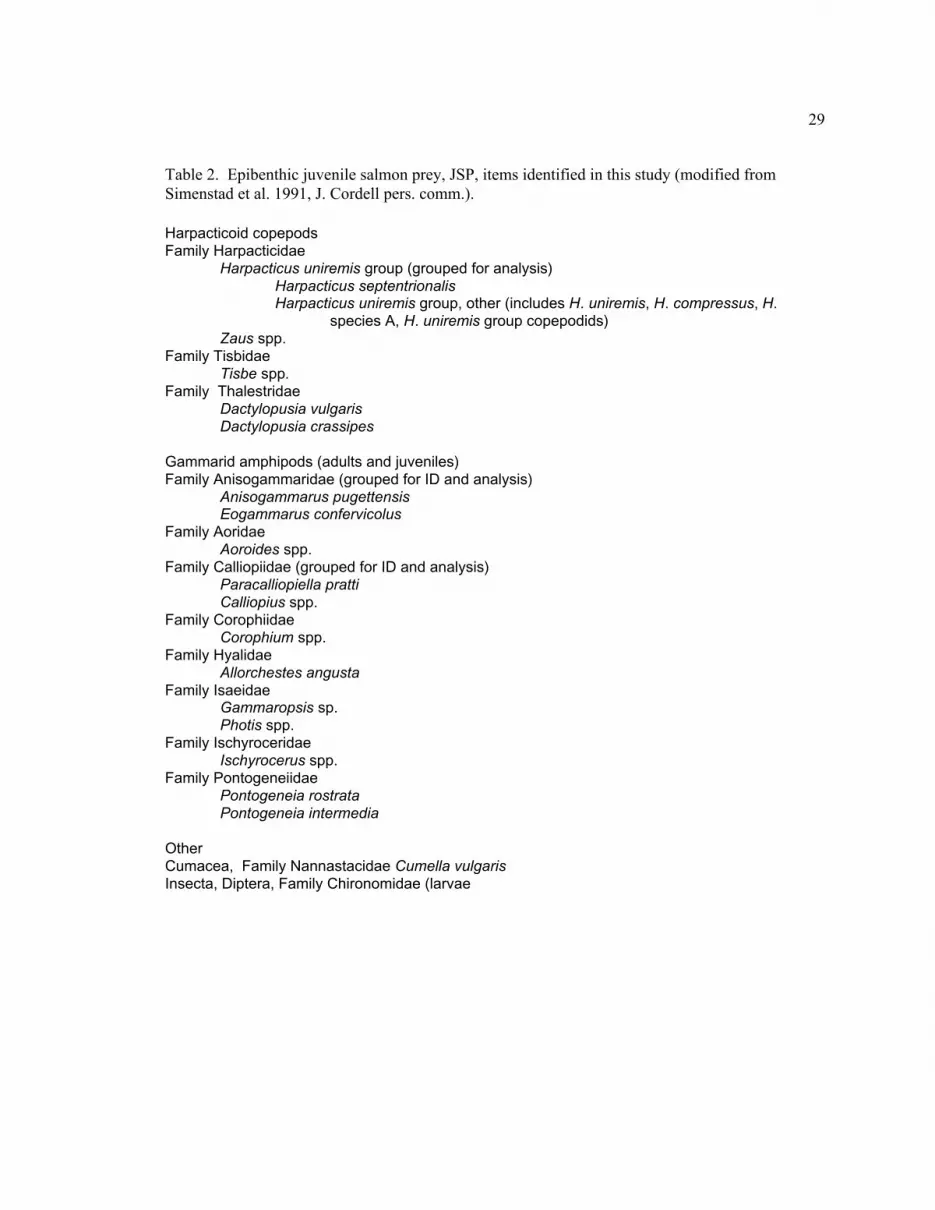
Table 2. Epibenthic juvenile salmon prey items................................................................................ 29

Table 3. Summary of statistical results for Bainbridge stratified-monthly sampling........................ 68

Table 4. Summary of statistical results for Clinton stratified-monthly sampling.............................. 71

Table 5. Summary of statistical for Southworth stratified-monthly sampling for all summary

variables, all present JSP taxa, and common and abundant non-JSP taxa................................ 73

Table 6. Summary of statistical tests for eelgrass sampling............................................................... 75

Table 7. Summary of statistical results for piling sampling. .............................................................. 76

1

INTRODUCTION

With increasing human populations, coastal regions have been subjected to rising

development and urbanization. For instance, approximately one third (~1230 km) of the Puget

Sound shoreline has been anthropogenically modified in the 150 years since the designation of

the Washington Territory (Bailey et al. 1998), and the population in this region has more than

doubled in the last 50 years (Puget Sound Regional Council 2001). Anthropogenic modifications

of estuarine and marine shorelines include armoring and stabilization as well as the construction

of facilities ranging from private docks to marinas to large-scale port facilities. Overwater

structures (OWS), including piers and docks, are among the more common nearshore1

modifications, yet the effects of these structures on nearshore organisms have not been

extensively studied.

In the Puget Sound region, this dramatic increase in human population, with

accompanying development and exploitation of regional natural resources, coincides with a

decline in some wild Pacific salmon populations. Many Pacific salmon stocks on the West coast

of the United States are depleted or otherwise considered at risk (Nehlsen et al. 1991, Huntington

et al. 1996). Two Puget Sound Evolutionarily Significant Units (ESUs) are designated as

threatened under the Federal Endangered Species Act: Hood Canal summer chum (Johnson et al.

1997) and Puget Sound chinook (Department of Commerce 1999). A third ESU, Puget

Sound/Georgia Strait coho, is also a candidate for federal listing (Weitkamp et al. 1995). This

pervasive decline in Puget Sound salmon stocks has added to the concern for Pacific salmon and

their habitat.

1 per Simenstad et al. 1999, nearshore is defined as beaches, intertidal, and subtidal zones between extremehigh high water and –20m

2

All Pacific salmon utilize estuarine-nearshore habitats during their lives (e.g. Thorpe

1994), but ocean-type juvenile salmon entering estuaries and marine waters early in their first

year, generally chum (Oncorhynchus keta), pink (O. gorbuscha) and ocean-type2 chinook

(Oncorhynchus tshawytscha) (Healey 1991), are particularly reliant on these shorelines (Healey

1980, Healey 1982, Simenstad et al. 1982). For chum and chinook, this habitat also is of great

importance for foraging. While these fish are small (<45 to 55mm fork length) their diets in

estuarine-nearshore areas (as opposed to tidal emergent marshes) are dominated by epibenthic

crustaceans, including harpacticoid copepods, gammarid amphipods, and cumaceans (e.g., Feller

and Kaczynski 1975, Healey 1979, Healey 1980, Simenstad et al. 1980). Though small pink

salmon eat more planktonic organisms than do small chum and chinook, they also feed on

epibenthic organisms (Kaczynski et al. 1973, Godin 1981). Even after these fish begin to eat

more planktonic organisms, they continue to utilize shallow waters where vegetation, turbidity,

and the shallowness of the water may provide refugia from predators (Simenstad et al. 1982, Orth

et al. 1984, Gregory and Levings 1996, Gregory and Levings 1998). The term “juvenile salmon”

hereafter refers only to ocean-type chinook, chum and pink salmon that are shoreline dependent.

In shallow estuarine waters, including nearshore Puget Sound, juvenile salmon depend

most on those epibenthic crustaceans associated with benthic vegetation (eelgrass Zostera marina

and its epiphytes, benthic macroalgae, diatoms), sand, and mudflats (Simenstad et al. 1991).

Some taxa in the juvenile salmon prey (JSP) assemblage occur commonly among these habitat

types while others may be more specific to one or two (Simenstad et al. 1979, Thom et al. 1984,

Simenstad et al. 1988a). This is also the case with small epibenthic crustacean assemblages in

other regions (Hicks 1986, Iwasaki 1993). Juvenile salmon appear to target specific taxa and life

2 The term “ocean-type” refers to salmon leaving freshwater early in their first year of life (some chinook,chum, and pink) versus those rearing extensively in freshwater (some chinook, coho, and sockeye).

3

history stages within the epibenthic crustacean assemblage on which they are feeding (Healey

1979, Sibert 1979, D’Amours 1987, Webb 1991a&b, Simenstad et al. 1995). Many of the taxa

typically found in their diets are among those with strong habitat affinities (Thom et al. 1984,

Simenstad et al. 1988a, Simenstad et al. 1995).

Intertidal habitats are susceptible to impacts of OWS (reviewed by Nightingale and

Simenstad 2001). Initial construction may involve impacts such as shading from barges, and

substrate disturbance from pile driving (Feist 1991), and destruction of existing eelgrass or other

habitat (Thom et al. 1995). Once built, shade from the structure can reduce or completely

eliminate benthic vegetation (Loflin 1995, Burdick and Short 1999, Shafer 1999). Other long-

term physical alterations may include redistribution and alteration of grain size of sediments

resulting from changes in current and tidal flows around pilings (Ratte 1985, Francisco 1995),

analogous to scour common around bridge pilings in rivers. If the structure receives boat traffic,

there can be more light attenuation both from moorage and turbidity, and physical disturbance

from propeller wash, scour, and propeller or landing scarring (Loflin 1995, Sargent 1995, Thom

et al. 1996, Simenstad et al. 1997a, Burdick and Short 1999, Shreffler and Gardiner 1999).

All of these effects of OWS ultimately result in biological changes. Changes in fish

assemblages around OWS have been correlated with decreased habitat quality for certain fish,

including juveniles that rear in estuarine-nearshore waters (Able et al. 1998). Shading has been

demonstrated to reduce fish growth potential in the vicinity of OWS (Able et al. 1999, Duffy-

Anderson and Able 2001), even when the crustacean prey assemblage was not significantly

reduced (Duffy-Anderson and Able 1999). The reduction or elimination of benthic vegetation is

presumed to result in alterations in the epibenthic faunal assemblage, since many of those

organisms are closely associated with the vegetation. Such decreases have been demonstrated

with the experimental removal of macroalgae in California (Everett 1994). Similarly, alterations

4

in sediment structure and distribution may also alter the epibenthic assemblage composition.

Finally, regular disturbance from strong propeller wash can be expected to remove or redistribute

organisms not fixed to the substrate. While the surface of the structure itself provides a novel

habitat for large and small epifauna (e.g., pilings and floats as described by Kozloff 1983) and

reef-like habitat structure for fish and large invertebrates (Miller 1980, Shreffler and Gardiner

1999) these assemblages can differ markedly from those inhabiting adjacent areas (Glasby 1999a,

Glasby 1999b, Connell 2000).

Research exploring OWS effects on smaller fauna, such as epibenthic invertebrates used

by juvenile salmon and other fish, is limited (Duffy-Anderson and Able 2001). One expects that

epiphytic fauna would be negatively impacted by shading from OWS. In addition, fauna not

specifically associated with benthic vegetation may also be susceptible to the other OWS impacts

described above. The goal of this study was to examine the effects of this suite of potential OWS

impacts on the epibenthic crustacean assemblage on which juvenile salmon forage. Since the mid

1990s, the Washington State Department of Transportation (WSDOT) has sponsored a research

program exploring the effects of its Puget Sound region ferry terminals on various estuarine-

nearshore resources, including focusing on effects on juvenile salmon and their habitat. The

research presented here was conducted during the spring of 2000 as a part of this program. The

primary object was to test for differences in epibenthic juvenile salmon prey in the vicinity of and

farther away from WSDOT ferry terminals.

5

REVIEW OF THE RELEVANT LITERATURE

Juvenile Pacific Salmon, Epibenthos, and the Estuarine-Nearshore

Pacific salmon exhibit a variety of life history types (Groot and Margolis 1991) with

highly variable traits including length of rearing in fresh water, extent of utilization of estuarine-

nearshore habitats, time spent in the open ocean, and time of return to spawning grounds.

Juveniles can be divided into life-history types relating to the time spent rearing in fresh water

versus salt water. “Stream-type” fish usually rear for an extended period in fresh water, up to

three years, and transition to salt water at a relatively large fork length (FL), while “ocean-type”

fish enter salt water at a much smaller size, shortly within days or months of emergence in late

winter and early spring. In general, sockeye, coho, and some chinook populations fall into the

stream-type category, while other chinook, chum, and pink are ocean-type. Stream- and ocean-

type chinook often correlate with whether their parents’ return to freshwater to spawn in the

spring or fall, respectively. The majority of ocean-type fish in the Pacific Northwest outmigrate

between March and June, with peak times varying between species and populations.

Ocean-type juvenile salmon utilize nearshore estuarine and marine habitats during

outmigration, until moving offshore in the late spring and summer (e.g. Kaczynski et al. 1973,

Healey 1982, Simenstad et al. 1982). In addition to the migration and predation refuge functions

(Simenstad et al. 1982, Thorpe 1994, Gregory and Levings 1996), the nearshore affords foraging

opportunity for these fish (e.g., Mason 1970, Macdonald et al. 1987, Levings 1994). They feed in

three different zones: epibenthic, planktonic, and neustonic. Epibenthic organisms (collectively

referred to as the epibenthos) that are on or close to the sediment surface or macrophytes;

planktonic organisms (plankton) that are in the water column; and neustonic organisms (neuston)

that are on the water surface. Juvenile salmon may feed in one or any combination of these three

6

zones, though pink salmon often feed primarily on plankton (Kaczynski et al. 1973, Miller et al.

1977, Simenstad et al. 1982, Cordell 1986) and chinook feed heavily on neuston and plankton in

certain habitats (Fresh et al. 1979, Simenstad et al. 1980, Healey 1982). Smaller chum and

chinook (FL<45 to 55mm) are particularly dependent on the epibenthos in nearshore marine

habitats with benthic vegetation (eelgrass Zostera marina and macroalgae) and intertidal flats

(Simenstad et al. 1991).

Epibenthic feeding chum and pink salmon forage more on the large meiofauna

component of the epibenthos while juvenile chinook feed more on smaller macrofauna.

Meiofauna refers to a size class of organisms between 0.0063 (or 0.0045) and 0.5 mm,

macrofauna are > 0.5 mm (International Association of Meiobenthologists 2001). Taken together,

this assemblage is primarily composed of crustaceans, including harpacticoid copepods,

gammarid amphipods, and cumaceans, as well as a variety of worms, molluscs, and other

organisms. The majority of the epibenthic invertebrates consumed by juvenile salmon are

crustaceans: generally gammarid amphipods and cumaceans in the case of chinook, and

harpacticoid copepods in pink and chum (Simenstad et al. 1991). In Puget Sound, the epibenthic

assemblage composition depends on a variety of interacting factors (e.g., sediment type/grain

size, vegetation type, wave exposure and tidal elevation), with some taxa generally occurring in a

specific habitat type while others are more ubiquitous (e.g. Simenstad et al. 1979, Thom et al.

1984, Simenstad et al. 1988a, Simenstad et al. 1988b, Thom et al. 1989).

In many cases, juvenile salmon feeding on epibenthos selectively target specific prey

items. For example, Feller and Kaczynski (1975) demonstrated that chum selected harpacticoids

in a size distribution significantly smaller than those available in the general epibenthos. In

companion papers, Healey (1979) and Sibert (1979) showed a strong preference for the relatively

rare harpacticoid Harpacticus uniremis by outmigrating chum in the Nanaimo River estuary, BC.

7

Webb (1991a,b) and D’Amours (1987) both established that chum and pink juveniles on Roberts

Bank, near the Fraser River estuary BC, fed primarily on H. uniremis, Tisbe cf. furcata, and Zaus

aurelii. Furthermore, while T. cf. furcata was generally the most abundant taxon of the three, the

rarer taxa H. uniremis and Z. aurelii dominated fish diets. Simenstad et al. (1998a) showed that

chum in Padilla Bay, Washington also extensively fed on these same harpacticoids, and that H.

uniremis and Zaus sp. were available only in one of four habitat types sampled (eelgrass).

Cordell (1986) also demonstrated extensive feeding on H. uniremis and Tisbe spp. by chum and

pink salmon in Auke Bay, Alaska, but in contrast to much of the work in Puget Sound and the

Georgia Strait, H. uniremis was the most abundant harpacticoid in epibenthic samples taken

during fish sampling. Because there is some potential for selective feeding, it is important to

identify known prey items to a relatively high taxonomic resolution when considering the

juvenile salmon prey (JSP) assemblage, as opposed to simply enumerating the total epibenthos.

Impacts of Non-Ferry Terminal Overwater Structures on the Nearshore

There are a number of potential impacts of overwater structures (OWS) and resulting

changes in the nearshore environment that could affect the JSP assemblage (see Nightingale and

Simenstad 2001). The primary longer-term impacts appear to be associated with shading of the

intertidal and shallow subtidal environment by the structure. Loflin (1995) reported reductions in

seagrasses in Florida underneath small, recreational boat docks and attributed this to shading, but

was unable to correlated decreased shading to any particular dock factor beyond total area. He

also noted decreased epiphyte load on seagrass blades in more shaded areas. Seagrass epiphytes

have been positively correlated with meiofauna abundance (Hall and Bell 1993). Burdick and

Short (1999) demonstrated decreased shoot density and canopy height of eelgrass underneath and

adjacent to docks in Massachusetts, as well as decreased light available for photosynthesis. They

8

concluded that those dock-types that allowed the most light to pass (e.g. tall, narrow, north-south

orientation) had the least severe impacts on the eelgrass habitat. Shafer (1999) found similar

dock impacts on the seagrass Halodule wrightii in Alabama, including decreased available light

and decreased seagrass condition that was variable according to dock-type. Fresh et al. (1995,

2001) found similar effects Puget Sound, as did Pentilla and Doty (1990 in Simenstad et al. 1999)

for both eelgrass and macroalgae. The docks in these three studies were mostly small, privately

owned structures used for recreational swimming and boating. Light levels under and around

much larger commercial structures were also measured with a number of projects in the Hudson

River estuary (Able et al. 1998, 1999, Duffy-Anderson and Able 1999, Duffy-Anderson and Able

2001). These studies consistently reported significant decreases of light levels in the vicinity of

large piers. One expected result of shading would be reductions in benthic vegetation and its

associated invertebrates, possibly similar to those seen with experimental removal of macroalgae

(e.g., Everett 1994).

Disturbance of the inter- and subtidal environment during dock and pier construction is

another potential impact of OWS. Shading impacts from floats are generally more severe that

those of structures above the water surface (Burdick and Short 1999), and construction barges

may have serious negative impacts associated with their presence in the nearshore. Feist (1991)

found that pile driving during OWS construction altered schooling behavior and distribution of

juvenile chum and pink salmon, and that hydraulic pile driving used in dock construction had the

potential to significantly alter the long-term sediment grain size composition. Whether such

activities impact the epibenthic faunal assemblage are unknown, but they could alter the

epibenthos, at least temporarily.

Once a structure is in place, boat traffic associated with it may have additional impacts.

Though understudied in marine systems, resuspended sediments from boat traffic can increase

9

water turbidity around docks and piers (Yousef 1974, Hilton and Phillips 1982, Garrad and Hey

1988), which can further attenuate light and decrease visibility for organisms in the area.

Vegetation also may be affected directly by boat traffic. Burdick and Short (1999) found that

eelgrass adjacent to many docks was shorter than that away from or underneath docks, and

attributed this difference in part to boat damage. They also noted that turbulence from propeller

wash was severe enough to erode sediment around eelgrass rhizomes. Sargent et al. (1995)

documented extensive scarring of Florida seagrasses and attributed the majority of it to direct

damage from propellers, an impact also noted by Loflin (1995).

Dock structures, such as pilings and floats, provide substrate for epifauna of all sizes

including encrusting organisms (e.g. barnacles, mussels, sponges), micro- and macroalgae, and

mobile macrofauna (e.g. sea stars). Kozloff (1983) described many common float and piling

organisms on the northern Pacific coast. Glasby (1991a) and Connell (2000) demonstrated that

the assemblages present on pilings and floats in Sydney Harbor, Australia, were different from

those present on nearby natural hard substrates. However, Glasby (1999b) found the assemblages

on freestanding pilings more similar to those on the natural substrates, and concluded that shading

from OWS was the primary cause of the assemblage difference.

Though largely undocumented, shading, structure, and other habitat alterations caused by

OWS may also affect changes in macrofauna assemblages including increased densities of

infauna (e.g., bivalves, Shreffler and Gardiner 1999, author pers. obs.), mobile macroinvertebrates

(e.g., crustaceans and sea stars, Shreffler and Gardiner 1999, author pers. obs.), and fish (e.g., pile

perch and flatfish, Miller 1980). Because effects of bioturbation on epibenthos have been

demonstrated to be positive, neutral, and negative, as well as density dependent, it is unclear what

role it may play a role at OWS. One might expect bioturbation by large aggregations of

macrofauna, such as red rock crabs (Cancer productus) or flatfish, to induce changes in the

10

epibenthic assemblage. Bioturbation by larger crustaceans on meiofauna has demonstrated in

some studies, but others are inconclusive. Escaravage and Castel (1990) demonstrated a positive

relationship between the presence of palaemonid shrimp and the densities of nematodes, insect

larvae, and a harpacticoid copepod. Warwick et al. (1990) showed decreased species richness for

nematodes in areas with high densities of soldier crabs, though total abundance of nematodes,

abundance and diversity of copepods were not affected. Ólafsson and Ndaro (1997)

demonstrated no effects of mangrove crab bioturbation on meiofauna (principally harpacticoids

and nematodes) in experimental microcosms. Larger organisms may also be affected by

bioturbation. A study on the impacts of bioturbation by a tube dwelling polychaete on larger

organisms demonstrated negative effects on some taxa (e.g., the cumacean Cumella vulgaris), but

not others (e.g., the amphipod Corophium salmonis) (Wilson 1981). Widdicombe and Austen

(1999) demonstrated effects of bioturbation by some bivalves on macrofauna diversity to be

density dependent, with a positive response at intermediate bivalve densities

Impacts of Ferry Terminals on the Nearshore Environment

Some aspects of nearshore impacts of Washington State Department of Transportation

(WSDOT) ferry terminals have been relatively well studied. Simenstad et al. (1997a) evaluated

potential impacts of WSDOT terminals on eelgrass. Recent documents, including an extensive

literature review, have evaluated potential impacts of WSDOT terminals on juvenile salmon and

their habitat (Simenstad et al. 1997a, 1999). A number of individual technical reports (e.g.

Shreffler and Moursund 1999, Blanton et al. 2001) also imply potential impacts on the epibenthos

in descriptions of the physical environment around ferry terminals, including shading, propeller

wash, and changes in macrofaunal assemblages, sediment composition, and benthic vegetation.

11

The light environment and potential shading impacts around ferry terminals have been

well described. Surveys have included light measurements above and in water, generally using

the light spectra utilized by primary producers for photosynthesis (photosynthetically active

radiation). Walking and diving transects underneath terminals consistently demonstrated reduced

photosynthetically active radiation under terminals, with some light extending underneath the

south margin and shade extending just beyond the north margin (Olson et al. 1997, Shreffler and

Gardiner 1999, Shreffler and Moursund 1999, Blanton et al. 2001). As with other OWS studies,

factors influencing the extent of shading included terminal width and height above MLLW.

Olson et al. (1997) and Visconty (1997) used light measurements to create models

describing the duration and intensity of shading around a number of ferry terminals at different

times during the year, as well as to predict shading impacts from proposed terminal additions. As

expected, the model predicted shading to be most temporally intense in midwinter and spatially

intense underneath and along the north margin of the structures. While monitoring in-water

photosynthetically active radiation, they and Thom et al. (1996) found additional shading during

ferry docking due to sediment resuspension and bubbles from the propeller wash. They

concluded that shading from the combined sources was in part responsible for reduced eelgrass

presence in the vicinity of the terminal.

Benthic vegetation, including eelgrass, also has been reduced in the vicinity of WSDOT

terminals. Underwater video surveys from eelgrass around three terminals (Clinton, Edmonds,

Port Townsend) were used to create a model describing eelgrass distribution at each site

(Simenstad et al. 1997b). At Clinton, a continuous band of eelgrass around the structure was

disrupted by complete absence of vegetation underneath and directly adjacent to the terminal

decking. Similar impacts of smaller magnitude occurred at the other two terminals. While

impacts were not as evident at Edmonds or Port Townsend, they specifically noted reduced shoot

12

density under the terminal at Edmonds. On the other hand, epiphyte loads on blades did not

appear to be impacted by dock proximity at any of the sites. The same authors also surveyed

macrofauna under the structures and in adjacent eelgrass, and the currents generated by ferry

docking. They concluded that the observed decrease in eelgrass was probably due to a

combination of shading, bioturbation by macrofauna (specifically crabs and sea stars), and

erosion from propeller wash scour. Blanton et al. (2001) also described reduced benthic

vegetation, including macroalgae and eelgrass, underneath the Clinton, Bainbridge, and

Southworth terminals, with vegetation occurring under the decking only at Southworth.

Ferry terminals differ from many other overwater structures in the frequency of large

boat traffic. At some WSDOT terminals, ferries depart every half-hour for certain portions of the

day, meaning that with docking and departing there are up to four propeller wash events per hour

(see Olson et al. 1997). Francisco (1995) demonstrated that most resuspended sediments from

ferry traffic in downtown Seattle was of a fine grain size. Over time, this can lead to a coarsening

of the sediments underneath the terminal. Shreffler and Gardiner (1999) observed changes in

bathymetry around pilings supporting the Clinton terminal, resulting in scour pits ringed with

lighter debris. I observed similar pits at the Bainbridge terminal during field sampling. Propeller

wash generated currents can be over six times the background current (Olson et al. 1997), which

could result in a regular flushing of epibenthic meiofauna out of the terminal vicinity.

In most cases, presence-absence macrofauna surveys have been completed along with

adjacent vegetation and light surveys at WSDOT structures. In general, macrofauna diversity

underneath the terminal appears somewhat reduced, and those organisms restricted to underneath

the terminal either inhabit the pilings and floats of the structure or are fish using the terminal as a

reef (Thom and Schafer 1995, Simenstad et al. 1997a). Shreffler and Gardiner (1999) noted

increased shell hash from sea star predation on barnacles and molluscs around pilings, and

13

Simenstad et al. (1997) mention that bioturbation from sea stars as well as bivalves may be a

factor in the reduction of benthic vegetation near the terminal structures. I observed much higher

densities of large clams, crabs, and sea stars underneath all three terminals than in the areas

adjacent to them during the fieldwork for this project.

It is clear that these factors (shading, reduced benthic vegetation, propeller wash from

boat traffic, and changes in macrofaunal assemblages) in combination have great potential to alter

the epibenthos underneath and adjacent to WSDOT ferry terminals via habitat alteration or

physical removal during propeller wash events. Though the implication had been made many

times that these factors could be altering the epibenthos, specifically those taxa which ocean-type

juvenile salmon use, this study is the first to sample the epibenthos directly.

14

STATEMENT OF RESEARCH HYPOTHESES AND OBJECTIVES

This study was organized around a major research hypothesis and corresponding

objective. This hypothesis (null) was as follows:

H0: There are no differences in the epibenthic juvenile salmon prey (JSP) assemblage(density and composition) between areas in close vicinity to and farther away from ferryterminals.

The major hypothesis was subsequently divided into four component hypotheses testing different

aspects of overwater (ferry terminal) structure effects on epibenthic JSP assemblages:

H01: There are no differences in the epibenthic assemblage (density and composition)under, near to, and away from the terminal structure during the period of the juvenilesalmon outmigration.

H02: There are no differences in the epibenthic assemblage (density and composition)associated with eelgrass patches at increasing distances from the terminal structure.

H03: There are no changes in the epibenthic assemblage (density and composition) alonga cross-terminal gradient.

H04: There are no differences in the epibenthic assemblage (density and composition)between different piling construction types (e.g., treated timber vs. concrete).

Generally, the research objective for each of these hypotheses was to describe the epibenthic JSP

assemblage around ferry terminals (with specific regard to factors noted in each hypothesis) and

to determine if differences could be attributed to terminal effects.

15

APPROACH AND SAMPLING DESIGN

Study Site Descriptions

WSDOT operates 20 ferry terminals in Puget Sound, from the Talequah terminal at Point

Defiance north to the Sydney, BC terminal (Figure 1). The three terminals selected for this study

were taken from a list of terminals with high research priority provided by WSDOT (Simenstad et

al. 1999). The terminals selected were not intended to act as replicate sample sites, but instead to

represent some of the diversity of terminal types in the WSDOT system. The Winslow terminal,

at Eagle Harbor on Bainbridge Island, is an example of more modern terminal design and with

both original timber and newer concrete construction materials and is one of the largest terminals

in the system. The Clinton terminal, on south Whidbey Island, is the site of ongoing eelgrass

transplant research, and also pairs the newest style of terminal design (2000 expansion) with the

original timber construction. The Southworth terminal, south of Bremerton, is representative of

the old timber style terminal construction and is a relatively small structure. These three

terminals hereafter are referred to as Bainbridge, Clinton, and Southworth, respectively.

Bainbridge: The Bainbridge terminal is a concrete and timber structure 105 m long

(trestle length, slip to MLLW approximately 90 m), 35 m wide (at MLLW), and 5.5 m above

MLLW. It is oriented perpendicular to shore, but points roughly SE into Eagle Harbor. The

original construction in 1966 used creosote-treated timber pilings, with an addition in 1984

supported by concrete pilings. There is moderate shoreline development around the terminal

(Simenstad et al. 1999), mostly consisting of the terminal offices and waiting areas. It is situated

on a steep bank armored under and to the north of the terminal. Shoreline hardening at

Bainbridge is well above MLLW.

16

Due to large ferries docking on a relatively short trestle, propeller wash and bottom scour

are greatest at Bainbridge, with a large halo around the terminal which is largely devoid of

benthic vegetation (author pers. obs.). Because of scour and the large terminal width (and

associated shading effects), I hypothesized that this terminal would have the largest effect on the

epibenthos.

Clinton: The Clinton terminal is a concrete and timber structure, 195 m long (slip to

MLLW approximately 104 m), 48 m wide (at MLLW), and 4.2 m above MLLW. It is oriented

perpendicular to the shore and approximately NE into Possession Sound. There are two slips,

North and South. In 1999-2000, construction on the south edge of the pier widened it from 31.5

m to 48 m. During field sampling, the South slip was under construction at the end of the

terminal, where it was unlikely to have direct effects on the nearshore sampling sites. The

support pilings in the older (north) section are creosote treated timbers installed in 1951 and 1968.

The pilings in the new (south) section are steel construction coated with epoxy paint. There is a

small floating public access dock at the midpoint of the terminal. The terminal is surrounded by

moderate shoreline development (Simenstad et al. 1999), consisting of the ferry terminal office,

several small businesses, and private residences. North of the terminal, the beach consists of a

berm with driftwood and a few houses well above the waterline. South of the terminal a concrete

bulkhead separates the beach from houses.

With a much longer trestle, propeller wash and scour are less severe at Clinton than at the

Bainbridge terminal and there is more benthic vegetation near its edge (author pers. obs.).

However, the terminal is both wider and lower, and despite grating in its middle, there is much

intertidal shading. I hypothesized that impacts on the epibenthos would be moderate compared to

the Bainbridge terminal, but still quite evident.

17

Southworth: The Southworth terminal is a timber structure, 141 m long (slip to MLLW

approximately 97 m), 15.7 m wide (at MLLW), and 5.3 m above MLLW. It is perpendicular to

shore, oriented NE into Puget Sound, but curves to the north just past MLLW. The support

pilings are creosote-treated timber driven in 1957. There is relatively low shoreline development

at Southworth (Simenstad et al. 1999), with houses set far back from the waterline to the north of

the terminal and a public beach access street-end adjacent to the terminal. To the south on the

upland is a large park-and-ride lot for ferry riders, with no additional development of nearshore.

There is no shoreline armoring at Southworth comparable to that at Bainbridge or at Clinton.

The trestle length at Southworth is between that at Clinton and Bainbridge, and the ferries

are generally smaller, so propeller wash and scour is lowest at this terminal (author pers.

observation). Benthic vegetation is present up to the edge of terminal decking. The terminal is

relatively narrow, less than half that of Bainbridge, and is higher than at Clinton. I hypothesized

that terminal effects would be lowest at Southworth.

General Approach and Sampling Design

Research objectives were addressed through four separate tasks (Table 1). The field

component was completed in spring 2000. All sampling used the epibenthic pump system

commonly used to collect JSP in this region (Simenstad et al. 1988a, Simenstad et al. 1988b,

Thom et al. 1988, Thom et al. 1989, Simenstad et al. 1995) and recommended by the Estuarine

Habitat Assessment Protocol (Simenstad et al. 1991). Salinity and water temperature were

recorded for each sampling date (Appendix 1). Sediment samples for grain size analysis were

collected once at each site in early March. Battelle Marine Sciences Laboratory collected

additional data on light availability, benthic vegetation cover, and sediment composition (Blanton

et al. 2001).

18

Task 1 – Stratified-monthly sampling: Stratified-monthly sampling was used to address

the research objective for H01 and test for terminal effects on the epibenthos. Three strata (Under,

Near, and Away) were sampled (Figure 2). The Under stratum was the area directly underneath

the terminal structure, where potential terminal impacts (including shading and propeller wash

disturbance) were at their greatest. The Near stratum was directly adjacent to the north edge of

the terminal where propeller wash was expected to be similar to the Under stratum, but shading

impacts would be variable depending on the time of day, time of year, and distance from terminal

and terminal orientation. The Away stratum was arbitrarily set 100 m north of the terminal

margin, which was assumed to be beyond direct shading and propeller wash impacts.

Task 2 – Eelgrass sampling: Because the stratified-monthly sampling at MLLW was

above the upper margin of eelgrass, the research objective for H02 was addressed by targeted

eelgrass sampling at Clinton. Three patches of eelgrass north of the terminal edge were sampled

during low tides (Figure 3). Each patch extended at least 15 m parallel to the shoreline. Paired

samples were taken on eelgrass and on non-eelgrass substrate adjacent to the patch.

Task 3 – High-resolution cross-terminal transect sampling: Stratified-monthly sampling

combined the entire area of shading gradient adjacent to the terminals in a single stratum.

However, as distance from terminal edge increases there is a gradient of decreasing shading and

propeller wash intensity. The research objective for H03 was addressed by sampling along a

cross-terminal gradient at a relatively fine spatial resolution (Figure 4). Samples were taken at -

0.6m because lower intertidal vegetation in this zone that would be more susceptible to shading

effects (R. Thom, BMSL, pers. comm.). BMSL collected in-air PAR, benthic vegetation cover,

and sediment composition data along the same transect within two weeks of epibenthic sampling

(Blanton et al. 2001).

19

Task 4 – Terminal structure sampling: Terminal structures add fixed substrate for

epibenthic organisms, such as pilings, decking, and floating structures. The research objective for

H04 was addressed by sampling pilings at Bainbridge and Clinton, and a floating dock at Clinton,

to compare the assemblage between different piling construction types (see site descriptions). It

was also designed to compare their epibenthic fauna with those from the intertidal substrates

sampled.

Data Analyses

Summary statistics (e.g., means, standard deviations) were calculated in Excel® 98 for

Macintosh (Microsoft Corporation 1998) and SPSS® version 10 for Macintosh (SPSS Inc. 2000).

Statistical tests consisted of single- and two-factor Analysis of Variance (ANOVA, Zar 1999)

with Student-Newman-Keuls (SNK, Zar 1999) post-hoc tests where appropriate. Statistical tests

were completed in SPSS® using the General Linear Model data analysis tool. Unless noted

otherwise, for all tests α=0.05 (significant results if p ≤ 0.05). Tests always were run for three

summary variables (total epibenthos density m-2, total juvenile salmon prey (JSP) density m-2,

taxa richness sample-1), certain individual JSP taxa (see criteria in each section), and common or

abundant non-JSP taxa (see criteria in each section). The individual taxa and groups tested varied

between sites and sample sets. All graphs were created in CA-Cricket Graph III® version 1.53

(Computer Associates International 1995).

Stratified-monthly sampling: Because the three terminals were not intended to act as

replicate sites, each site was analyzed separately. The stratified-monthly sampling was designed

for testing between strata differences over the entire outmigration period using two-factor

ANOVA, with month and strata as the factors. High within-strata replication and equal sample

sizes improved the robustness of the parametric ANOVA with respect to violations of normality

20

assumptions (Zar 1999, L. Tear, Parametrix, pers. comm.). Where results were borderline

significant (0.01 ≤ p ≤ 0.05), and data were seriously non-normal, tests were repeated using log10

transformed data. If significant differences occurred among strata using the two-factor ANOVA,

additional single factor ANOVA tests for strata were completed for each month with SNK post-

hoc analyses to determine among-strata differences and groupings. Response variables analyzed

included the three summary variables, all JSP taxa present, and non-JSP taxa meeting at least one

of two criteria: 1) individual taxon >1% of the total epibenthos density for half (six of 12) of the

date*strata combinations (e.g., March, Away); or, 2) individual taxon was >1% of the total

epibenthos density for a single strata over all four months.

Eelgrass sampling: The eelgrass sampling was also designed to be tested with a two-

factor ANOVA, with distance of each eelgrass patch from terminal and on or off eelgrass as

factors. SNK post-hoc analyses identified significant differences for patch distance from

terminal, where interaction terms were not significant (Zar 1999). Borderline significant, non-

normal data were log10 transformed as with the stratified-monthly sampling. Response variables

were the same as for stratified-monthly sampling. Common or abundant non-JSP taxa were

selected for analyses based on meeting at least one of two criteria: 1) individual taxon was >1%

of the total epibenthos density for four of the six patch*on/off combinations (e.g., 95-m, off); or,

2) individual taxon was >1% of the total epibenthos density among patch (e.g., 95-m both on and

off) or among on/off (e.g., 10-m on, 95-m on, 235-m on).

High-gradient cross-terminal transect sampling: Because this sampling was along a

gradient, with no replication in time or space, standard statistical tests were not used. The data

were evaluated graphically, relative to the terminal structure, with line graphs and stacked area

graphs of densities and percent composition. Response variables were the same as for monthly

21

stratified sampling; an individual taxon (JSP or non-JSP) was included only if its average density

was >1% of the total epibenthos.

Terminal structure sampling: As with the stratified-monthly sampling, the two terminals

sampled were not intended to act as replicate sites, and the results for Bainbridge and Clinton

were analyzed separately. The piling data-set at each terminal was designed to be analyzed with

a two-factor ANOVA (elevation, piling-type), while the floating dock samples at Clinton were

described and evaluated graphically. Response variables were the same as for stratified-monthly

sampling; an individual taxon (JSP or non-JSP) was only included if it was present in at least

25% of the samples, or had an average density greater than 10% of the total epibenthos average

density.

22

Figure 1. Central Puget Sound, Washington, Washington State Department of Transportationferry terminals used as study sites for spring 2000 overwater structures sampling field effort.

23

Figure 2. Generalized sampling schematic for monthly-stratified sampling (not to scale).

Figure 3. Generalized sampling schematic for eelgrass sampling (not to scale).

0 m MLLW

N

terminal decking

slip

sampling strata(10 m)

0 m MLLW

N

terminal decking

slip

eelgrass patches(10 m, 95 m, 235 m)

24

Figure 4. Generalized sampling schematic for transect sampling (not to scale)

0 m MLLW

N

terminal decking

slip

sampling transect-.6 m MLLW

25

Table 1. Field sampling design summary for all tasks for this study.

Task Dates (2000) Terminal Samplingelevation(m)

Tide Replicationand samplesize (perterminal)

Design notes

Stratified-monthlysampling

Monthly,early Marchto late May(two sets inMay fourweeks apart)

Bainbridge,Clinton,Southworth

MLLW ebb 15 reps * 3strata * 4months; 135total samples

random samplingwithin 3 strata: Under(center of structure),Near (north edge ofstructure), and Away(100 m north)

Eelgrasssampling

June 5 Clinton -0.6 to -1.6 ebb 7 reps * 2substrates * 3patches; 42total samples

patch distance relativeto north edge ofstructure (10m, 95m,235m); haphazardsampling on eelgrasson non-eelgrasssubstrate at patch edge

High-resolutioncross-terminalgradientsampling

May 31,June 1

Clinton -0.6 flood 111 samples(56processed,every othersample)

cross-terminalsampling every meteralong 111m transect,from 12m south to 43m north; sampled overtwo days (center tonorth day one, centerto south day two)

Terminalstructuresampling

May 3, 4 Clinton,Bainbridge

-0.6, 0, 0.6,1.2;floatingdock

flood 5 reps * 2piling-types *4 elevations;40 samples(plus 5 repson floatingdock)

random sampling ofpaired piling-types;floating dock at Clintononly; modifiedepibenthic pump (seedescription)

26

METHODS

Field Effort

Epibenthic natural substrate sampling: The epibenthic pump system consisted of a 2000

gallon hour-1 electric bilge pump housed in a 14.8 cm wide PVC sampling cylinder, open only at

the base. Inflow ports on the sampling cylinder were covered with a 33 µm mesh screen.

Outflow from the pump traveled though a PVC hose and is collected in a handheld sieve (106

µm). The sampling cylinder was attached to a 1.2 m handle with a switch at the top. For each

sample the pump was placed through the water column slowly and carefully set into the substrate

with a twist. Pump outflow with entrained epibenthos was filtered through a hand-held 106 µm

sieve for twenty seconds, or until the sieve began to back up with sediment (lifting of the top

layer of sediment indicated clogged inflow ports, but ensured all epibenthic organisms were also

lifted and captured on the sieve). The pump was purged with surface water between samples.

See Simenstad et al. (1988b) for additional information about the design and use of the epibenthic

pump system.

Tide charts were generated for each site and date (Tides and Currents®, Nautical

Software Inc. 1996). Tidal elevations were determined by cross-referencing the current time and

tide chart, and wading out to water of the appropriate depth (using a PVC pole marked every 0.25

feet), or checking water depth at site and current time to determine elevation. All tidal elevations

were converted to metric post-sampling.

Epibenthic samples were preserved in the field within two hours of collection. Upon

completion of sampling, undiluted formalin, buffered with Borax, was added to each jar to reach

a final concentration of 5-10% formalin. Sample jars with large quantities of sediment were

stirred vigorously to allow even distribution of formalin.

27

Epibenthic terminal structure sampling: Terminal structure sampling was completed using a

modified epibenthic pump. This sampling cylinder was identical to the standard epibenthic pump

described above, except that it had no handle or switch (operated with manual battery

connection). The mouth of the sample cylinder was fitted with a neoprene collar allowing it to fit

flush against the curve of a piling or the flat surface of the floating dock edge. The sampling

cylinder was placed against the terminal structure and a sample was taken as for the standard

system.

Lab Methods

In the lab, formalin was decanted from the samples through a 73 µm mesh sieve.

Epibenthic organisms were removed from sandy samples by vigorous swirling with fresh water in

a round bottomed pitcher (after Webb 1989). Samples were then screened into three size

fractions: 153-246 µm, 246–500 µm, >500 µm. Initial findings demonstrated no significant

difference between results for juvenile salmon prey (JSP) with or without the smallest size

fraction and it was not processed for the remainder of the samples.

The 246-500 µm and larger size fractions were sorted using a dissecting microscope.

Sample fractions with high numbers of organisms were split to a manageable number (>200

target organisms) using a Folsom plankton splitter or Henson-Stempel pipette. Pelagic

zooplankton, likely a contamination from purging the system between samples, was not counted.

Nematoda were not counted from the stratified-monthly sample set because they were very

abundant in some sandy samples, but are not prey. For analyses, final counts were totaled from

both size fractions.

Important juvenile salmon prey items (Simenstad et al. 1991, J. Cordell, University of

Washington, pers. comm.) were generally identified to the taxonomic resolution described in the

28

Estuarine Habitat Assessment Protocol (Simenstad et al. 1991). Harpacticoid copepod prey taxa

were identified to genus or species, except for the Harpacticus uniremis group complex. Where

juveniles precluded species identification, gammarid amphipods were identified to genus or

family. Other prey items were identified as per Table 2. Non-prey organisms were not all

identified to the same level. Many non-prey harpacticoids were identified to species (e.g.,

Amphiascoides sp. A, Amonardia perturbata), while others were only identified to family (e.g.,

Ectinosomatidae, Laophontidae). The same applied to non-prey gammarids and cumaceans.

Other non-prey organisms were identified at most to family level, and sometimes as coarsely as

phyla (Appendix 1). Taxonomic identification was completed using taxonomic keys, the

assistance of Mr. Jeffery Cordell (University of Washington), and reference collections from

other Puget Sound epibenthos sampling (author; B. Bachman, United States Army Corps of

Engineers).

29

Table 2. Epibenthic juvenile salmon prey, JSP, items identified in this study (modified fromSimenstad et al. 1991, J. Cordell pers. comm.).

Harpacticoid copepodsFamily Harpacticidae

Harpacticus uniremis group (grouped for analysis)Harpacticus septentrionalisHarpacticus uniremis group, other (includes H. uniremis, H. compressus, H.

species A, H. uniremis group copepodids)Zaus spp.

Family TisbidaeTisbe spp.

Family ThalestridaeDactylopusia vulgarisDactylopusia crassipes

Gammarid amphipods (adults and juveniles)Family Anisogammaridae (grouped for ID and analysis)

Anisogammarus pugettensisEogammarus confervicolus

Family AoridaeAoroides spp.

Family Calliopiidae (grouped for ID and analysis)Paracalliopiella prattiCalliopius spp.

Family CorophiidaeCorophium spp.

Family HyalidaeAllorchestes angusta

Family IsaeidaeGammaropsis sp.Photis spp.

Family IschyroceridaeIschyrocerus spp.

Family PontogeneiidaePontogeneia rostrataPontogeneia intermedia

OtherCumacea, Family Nannastacidae Cumella vulgarisInsecta, Diptera, Family Chironomidae (larvae

30

RESULTS

Stratified-Monthly Sampling

Bainbridge: Negative impacts on the epibenthos at Bainbridge were pervasive, both

Under and Near compared to Away from the terminal. The two-factor ANOVA tests for

differences between strata were significant for all three summary variables, 12 of 17 juvenile

salmon prey (JSP) taxa, and all 10 non-JSP taxa (Table 3). For all variables and taxa but

Cyclopinidae (epibenthic cyclopoid copepod) and Polychaeta the overall impact of the terminal

structure was negative.

Results of the two-factor ANOVA tests for among strata differences were all highly

significant for summary variables (total epibenthos, total JSP, taxa richness) (Figure 5). Within-

month tests for strata differences were all significant and SNK results indicated that Near and

Under values were similar and less than Away values. Taking all months together, the average

total epibenthos density Away was 96,145 m-2 (± 1 SD 67,266) compared to 5,505 m-2 (± 6,880)

and 7,402 m-2 (± 6,629) for Near and Under. The average JSP density Away was 26,079 m-2 (±

26,014) compared to 1,698 m-2 (± 2,732) and 1,962 m-2 (± 2,430) for Near and Under. Average

taxa richness in the Away strata was 29 (± 9), more than twice those of Near (13 ± 8) and Under

(12 ± 6).

All JSP taxa were found at least once at Bainbridge, and 12 of 17 of them had highly

significant two-factor ANOVA tests for strata differences. All of these showed negative impacts

of the terminal on densities. Where within-month strata differences were significant, SNK results

were the same as for summary variables, with Near and Under similar and less than Away.

31

Common or abundant JSP taxa3 were the harpacticoid copepods Harpacticus uniremis group,

Tisbe spp., Zaus spp., the cumacean Cumella vulgaris, and the gammarid amphipods Pontogeneia

rostrata, Photis spp., and Calliopiidae (mainly Paracalliopiella pratti) (Figure 6). Results were

similar for the less abundant, but significant JSP taxa (the harpacticoids Dactylopusia vulgaris

and Dactylopusia crassipes, and the amphipods Aoroides sp., Corophium spp., Allorchestes

angusta, and Gammaropsis sp.). JSP taxa for which densities among strata were non-

significantly different (the amphipods Anisogammaridae, Pontogeneia intermedia, Ischyrocerus

spp., and Chironomidae fly larvae) were relatively rare in all strata.

Ten non-JSP taxa were abundant or common (the harpacticoids Ectinosomatidae,

Harpacticus spinulosus, Laophontidae, Robertsonia sp., Amphiascoides sp. A, Thalestridae

copepodids, Turbellarian flatworms, Oligochaete worms, Cyclopinid copepods, and Polychaete

worms). All of these had highly significant two-factor ANOVA tests for strata differences. Eight

of the ten non-JSP taxa were present in higher densities Away from the terminal, generally with

corresponding within-month SNK results but with some between month variation. Cyclopinidae

and Polychaeta had greater densities in the Under strata (Figure 7).

For the combined epibenthos averaged across sampling periods, densities decreased

significantly in the Under and Near strata. This was also true for most individual taxa (Figure 8).

However, percent composition was strongly affected by the terminal, shifting from a harpacticoid

dominated to an annelid worm dominated assemblage in the Near and Under strata. One taxon of

harpacticoids, Tisbe spp., increased in proportion in close proximity to the terminal but most

other harpacticoids decreased or disappeared close to it (e.g., Robertsonia sp., Laophontidae).

3 For stratified-monthly sampling these taxa fit the criteria for common or abundant non-JSP taxa, as statedin Data Analysis, or are > 1% of the total epibenthos at any strata*date combination.

32

Clinton: Negative impacts on the epibenthos similar to those at the Bainbridge terminal

were apparent at Clinton. Most response variables were lower at the Near and Under strata, with

Near values generally closer to those of Under or midway between Under and Away. Two-factor

ANOVA tests were significant for strata differences for all three summary variables, nine of 15

JSP taxa present at the site, and five of seven non-JSP taxa (Table 4). For all but two taxa with

significant results the overall impact of the terminal structure was negative.

All two-factor ANOVA tests of strata differences were highly significant for the

summary variables, with overall negative impacts for each one (Figure 9). The average density of

the total epibenthos, over all months, was 67,085 m-2 Away (± 65,708) compared to 18,304 m-2

Near (± 17,784) and 24,193 m-2 Under (± 21,528). The average JSP density Away was 57,107 m-

2 (± 59,988) compared to 11,773 m-2 (± 12,773) and 16,794 m-2 (± 18,525) for Near and Under.

All within-month ANOVA tests for strata differences for these two variables were highly

significant with Away consistently greater than Under, except for total epibenthos during May

when they were not different. The average taxa richness was 22 (± 3), 21 (± 10), and 19 (± 5) for

Away, Near, and Under. The within-month ANOVA results for strata differences were also

highly significant for all summary variables, but SNK groupings and pattern of taxa richness were

not consistent between months.

Fifteen JSP taxa were found at Clinton, nine of which had highly significant two-factor

ANOVA results indicating negative impacts in close proximity to the terminal (Figure 10). The

six JSP taxa with non-significant results were relatively rare (the amphipods Pontogeneia

rostrata, Aoroides sp., Corophium spp., Pontogeneia intermedia, Photis spp., and Chironomidae

fly larvae). Two of the amphipod JSP taxa, Gammaropsis sp. and Ischyrocerus spp., were not

found. The JSP taxa with significant results all were relatively common or abundant. Of these,

six generally had higher densities for the Away stratum higher than for the other two (Figure 10),

33

though there was some variability for within-month SNKs (Table 4). Three JSP taxa, Tisbe spp.,

Cumella vulgaris, and Calliopiidae (mainly Calliopius sp.) had somewhat different results, but

during the months with significant strata differences the highest density stratum was generally

Away or Near (Table 4).

Seven non-JSP taxa were common or abundant (Figure 11), six of which had significant

results for two-factor ANOVA tests for strata differences. Results for Polychaeta were borderline

significant (p ≤ 0.019) but log10-transformed data for this taxon indicated no significant among

strata differences (p ≤ 0.602). Of the remaining five non-JSP taxa with significant two-factor

ANOVA results, three had an overall decrease in organism densities in vicinity of the terminal

(Thalestridae copepodids, Ectinosomatidae, Turbellaria) and two had increased densities

(Ameiridae, Oligochaeta). Within month ANOVA and SNK results were variable between

months, and did not always separate Under and Away (Table 4). Two-factor ANOVA tests for

strata differences for Nemertea and Polychaeta (log10-transformed) were not significant.

For all months combined, total epibenthos decreased by approximately two-thirds in

close proximity to the terminal. Most of the numerically dominant taxa either decreased or

increased on such a small scale it could not be easily detected as a function of assemblage density

(Figure 12). In percent composition two dominant taxa were strongly affected by terminal

proximity, Tisbe spp. increased and Anisogammaridae decreased.

Southworth: As with the other two terminals, at Southworth the epibenthos was affected

negatively by the terminal. Two-factor ANOVA tests for strata differences were significant for

all three summary variables, six of 17 JSP taxa present at the site, and six of eight non-JSP taxa

(Table 5). For all but two of these (Amonardia perturbata, Harpacticus spinulosus) the impact of

the terminal structure was negative.

34

Strata differences in the two-factor ANOVA results for summary variables were all

highly significant (Figure 13). The average density of the total epibenthos, over all months, was

84,200 m-2 (± 64,364) Away compared to 83,799 m-2 (± 61,042) Near and 43,673 m-2 (± 40,117)

Under. The average JSP density Away was 51,231 m-2 (± 37,624) compared to 44,974 m-2 (±

33,638) and 32,737 m-2 (± 29,213) for Near and Under. Most within-month ANOVA results for

these two variables were highly significant, with densities for Away and Near generally greater

than Under and often grouped together in SNK results (Table 5). Average taxa richnesses, over

all months, were 29 (± 7), 25 (± 9), and 20 (± 7) for Away, Near, and Under. Within-month

ANOVA results were also all highly significant for strata differences, and SNK results were

similar to those for total epibenthos and JSP. In all cases, the impact of the terminal structure on

the summary variables was negative, with the lowest values generally occurring in the Under

stratum and similar, higher values for Near and Away.

All seventeen JSP taxa were found at Southworth, seven had significant two-factor

ANOVA results for strata differences indicating negative impacts. Two taxa (Tisbe spp. and

Dactylopusia vulgaris) had borderline significant p-values. Tisbe spp. distributions were not

seriously deviated from normal and the original result was accepted, but those for Dactylopusia

vulgaris were and the subsequent two-factor ANOVA on the log10-transformed data was not

significant for strata (p ≤ 0.079). Of the six remaining taxa, one (Corophium spp.) was extremely

rare and its ANOVA results were not reliable. The five remaining significant JSP taxa (Figure

14) all had at least one significant within-month ANOVA result and tended to have either Away

or Near as the highest density strata, with SNK results supporting those trends. Most of the 11

remaining JSP taxa with non-significant results were relatively rare, but Dactylopusia vulgaris,

Calliopiidae (mainly Paracalliopiella pratti) and Pontogeneia rostrata were more abundant

35

(Figure 15). Where present, impacts on JSP taxa were negative, but were variable as to whether

densities Near, Away, or both were highest relative to Under.

Eight non-JSP taxa were common or abundant, one of which (Amonardia perturbata)

increased significantly in the Near and Under strata. Of the remaining seven, five had

significantly decreased densities relative to the terminal, though densities for the Near stratum

sometimes were similar to those from the Under stratum. SNK results supported these trends

(Table 5). Harpacticus spinulosus was the exception, being abundant only in the Near stratum.

Polychaeta and Thalestridae copepodids both were relatively common or abundant, but were not

significantly different between strata.

Density of the epibenthos for all months combined decreased by approximately half and

percent composition showed a shift in many taxa relative to the terminal (Figure 17). Tisbe spp.

was dominant both in density and numerical proportion. While its numerical abundance

remained relatively constant, its proportion of the assemblage increased in the Under stratum

compared to Near and Away strata. Zaus spp. decreased in proximity to the terminal both in

terms of abundance and proportion. Harpacticus spinulosus was the second most numerous

taxon in the Near stratum, but was scarce in the Away or Under strata.

Eelgrass Sampling

Results for the eelgrass patch sampling indicated negative impacts of the Clinton terminal

on the epibenthos associated with eelgrass. ANOVA results for patch differences were

significant for all three summary variables, all eight JSP taxa, and seven of nine non-JSP taxa,

and though SNKs were variable, the 10-m patch was in the lowest density or taxa richness group

for all significant results (Table 6).

36

Total epibenthos and JSP densities were not significantly different on eelgrass versus

non-eelgrass substrates. Their pooled between-patch densities were significantly lower for the

10-m patch than for either 95-m or 235-m patches (Figure 18). Taxa richness was significantly

higher on eelgrass versus non-eelgrass, and the non-eelgrass values were lower for the 10-m

patch (average of 21 taxa) less than for the grouped 95-m (26 taxa) and 235-m (27 taxa) patches

(Figure 18).

All eight JSP taxa found (Figure 19) had significant ANOVA results for patch differences

indicating negative impacts of the terminal. Tisbe spp. and Dactylopusia vulgaris densities were

not significantly different on eelgrass versus non-eelgrass substrates. Of the six remaining JSP

taxa, Anisogammaridae (mainly Anisogammarus pugettensis) was the only taxon more abundant

on the non-eelgrass substrate.

Of the five non-JSP harpacticoids (Figure 20), only Harpacticus spinulosus were

significantly different on eelgrass versus non-eelgrass substrates, being lower on eelgrass. On

non-eelgrass its densities increased from the 10-m patch to the 95-m and 235-m patches. The

other four taxa were all significantly denser in the 95-m and 235-m patches (grouped) than the

10-m patch. Of the four remaining non-JSP taxa (Figure 21), only Nematoda and Oligochaeta

densities had significant patch differences, also with 10-m densities less than those for 95-m and

235-m patches (grouped). Densities of Turbellaria and Polychaeta were not significantly

different among patches.

Densities of Nematoda were numerically dominant in the assemblage, particularly in the

10-m and 235-m patches, but for greater clarity in seeing JSP trends, they were removed prior to

creating assemblage composition plots (Figure 22). Densities of Tisbe spp. were prominent in the

total assemblage, particularly at the 95-m patch. The non-eelgrass substrate assemblages at 10-m

37

and 95-m were similar, despite large differences in overall abundance. This was also true for the

eelgrass assemblages from the 10-m and 235-m patches.

High-Resolution Cross-Terminal Sampling

Despite high among-sample variability, and apparent between-day variability, some

trends in the cross-terminal epibenthos gradient were apparent (Figures 23-26). From south to

north, there was generally a small decrease in organism density with consistently lower values

under the south half of the terminal. Densities for many taxa increased under the north half of the

terminal. At the north edge of the terminal, densities generally either decreased or remained

constant to a final increasing trend to the north end of the transect. Densities for total epibenthos

and JSP also follow this pattern, with some of the largest single density samples occurring under

the north half of the terminal (Figure 23). Taxa richness was also highly variable, initially

decreasing from the south end of the transect approaching the terminal, and increasing to the

north for most of the transect (Figure 23).

Of the six abundant JSP taxa, only densities for Harpacticus uniremis group (mostly H.

septentrionalis and copepodids) appeared to have a clear negative response to the terminal

structure (Figure 24). Tisbe spp. and Zaus spp., the numerically dominant crustacean taxa in set,

and the less abundant Cumella vulgaris all had similar responses to those for total epibenthos.

Anisogammaridae appeared to have a positive association with the terminal with consistently

higher densities under the entire structure.

Two of the six abundant non-JSP taxa, Harpacticus spinulosus and Acrenhydrosoma sp.

appeared to have a negative response to the structure (Figure 25). Results for the other taxa were

less clear, with Ectinosomatidae, Ameiridae, and Thalestridae copepodids all following the

38

pattern found for total epibenthos. Polychaeta, however, had consistently highest densities

underneath the north half of the terminal.

Nematoda dominated within the total epibenthos (Figure 23), and was removed from the

data to calculate assemblage composition (Figure 26). The assemblage was initially dominated

by Harpacticus spinulosus in abundance and composition, but changed to dominance by

Anisogammaridae under the south portion of the dock. While Anisogammaridae was still a

relatively large proportion of the under dock assemblage in the north half, the dominance again

shifted to Tisbe spp. and, to a lesser extent, Zaus spp.. There was a more evenly distributed

assemblage away from and to the north of the dock.

Terminal Structure Sampling

The encrusting organisms on pilings at Bainbridge were similar on the older wood and

newer concrete pilings. Small barnacles were the dominant organisms at all elevations, with

compound ascidians present at lower elevations and mussels present higher. Macroalgae was not

abundant. The highest elevation (1.2 m) for both piling-types was different from the other

elevations with large (3-5 cm diameter) barnacles as well as relatively large mussels. Total

densities and taxa richness of epibenthos on pilings at Bainbridge were all extremely low (Figure

27). Differences in piling-type were not significant for any summary variable or individual taxon,

but there were significant elevation differences for all variables but Polychaeta, with densities and

taxa richness decreasing with increasing elevation (Table 7).

At Clinton, encrusting organisms both on older wood and new epoxy-steel pilings were

mainly barnacles and mussels. Mussels and barnacles were generally larger, and mussels were

denser, on the wood pilings, but at the sampling elevations the epoxy-steel pilings also were

completely encrusted. Both piling-types had thicker encrustations and greater mussel densities at

39

higher elevations. Macroalgae was minimal on all pilings. Total epibenthos densities and taxa

richness were relatively higher at Clinton than at a Bainbridge, and more taxa fit the criteria for

ANOVA testing (Table 7). The three summary variables were significantly different based on

both piling-type and elevation, with new pilings having higher densities and taxa richness than

old pilings, and low elevations having higher densities and taxa richness than higher elevations

(Figure 28). Differences in density of three JSP taxa were significant by piling-type. The test

results for Tisbe spp. were borderline significant and were not significant at all when log10-

transformed. Densities of Dactylopusia vulgaris were significantly different by both elevation

and piling-type. Densities of Calliopiidae were only significant for piling-type. Densities of

three non-JSP taxa were significant for piling-type and elevation (Figure 29), Thalestridae

copepodids, Ectinosomatidae, and Ameiridae. For all taxa with significant results new pilings

had higher densities than old pilings. Amphiascoides sp. A was significant for elevation, but not

piling-type. For all individual taxa with significant results for elevation, densities were higher at

lower elevations.

There was much attached macroalgae on the float at Clinton, as well as mussels,

barnacles, tube worms, and anemones. The epibenthos had relatively low taxa richness, average

5.8 (± 2.17), with a total of 10 taxa (Figure 30) five of which were JSP taxa (Calliopiidae, H.

uniremis group copepodids, Zaus spp., Pontogeneia rostrata, and Ischyrocerus spp.). Non-JSP

taxa included Caridea, Robertsonia sp., Lamprops quadriplicata, and Munna ubiquita.

Calliopiidae (mainly Calliopius spp.) was the numerically dominant taxon, approximately half of

the total epibenthos. Harpacticus uniremis group copepodids, Mesochra pygmaea, and Caridea

(shrimp larvae) were also abundant.

40

Figure 5. Mean response of summary variables for Bainbridge stratified-monthly sampling.Asterisks denote significant strata differences within month. Error bars are ± 1 standard deviation.

den

sity

m-2

aver

age

taxa

sam

ple

-1

0

50000

100000

150000

200000

250000total epibenthos

UnderNearAway

0

25000

50000

75000

100000JSP

0

10

20

30

40

50

March April May (E) May (L)

taxa richness

*

*

*

*

*

*

*

*

*

*

**

41

Figure 6. Mean response of JSP taxa from Bainbridge stratified-monthly sampling withsignificant two-factor ANOVA results for strata. Asterisks denote significant within month stratadifferences. Error bars are ± 1 standard deviation.

den

sity

m-2

0

20000

40000

60000

80000Harpacticus uniremis grp.

UnderNearAway

0

2500

5000

7500

10000Zaus spp.

0

10000

20000

30000

40000Tisbe spp.

0

1000

2000

3000

4000

5000Cumella vulgaris

0

500

1000

1500Calliopiidae

0

1000

2000

3000

4000

5000

March April May (E) May (L)

Pontogeneia rostrata

0

1000

2000

3000

4000

March April May (E) May (L)

Photis sp.

*

*

* ** *

*

* **

*

*

**

*

*

**

*

*

*

*

* *

42

Figure 7. Mean response of common non-JSP taxa from Bainbridge stratified-monthly sampling.All taxa have significant two-factor ANOVA results for strata. Asterisks denote significantwithin month strata differences. Error bars are ± 1 standard deviation.

0

5000

10000

15000

20000Laophontidae

den

sity

m-2

0

10000

20000

30000

40000

50000Ectinosomatidae

UnderNearAway

0

25000

50000

75000

100000Harpacticus spinulosus

0

5000

10000

15000

20000

25000

30000Robertsonia sp.

0

2500

5000

7500

10000

March April May (E) May (L)

Amphiascoides sp. A

*

**

*

**

*

*

*

*

*

* **

*

* *

*

**

0

1000

2000

3000

4000

March April May (E) May (L)

Thalestridae copepodids

*

*

43

Figure 7 (continued). Mean response of common non-JSP taxa from Bainbridge stratified-monthly sampling. All taxa have significant two-factor ANOVA results for strata. Asterisksdenote significant within month strata differences. Error bars are ± 1 standard deviation.

0

500

1000

1500

2000

2500

3000

March April May (E) May (L)

Cyclopinidae

0

5000

10000

15000

20000Turbellaria

UnderNearAwayd

ensi

ty m

-2

0

1000

2000

3000

4000

5000

6000

March April May (E) May (L)

Oligochaeta

0

2500

5000

7500

10000Polychaeta

*

*

* **

*

*

* *

**

* *

44

Figure 8. Assemblage composition at Bainbridge (total density and relative density); stratified-monthly sampling averaged across all months.

0%

25%

50%

75%

100%

rela

tive

ab

un

dan

ce

Away Near Under

other

Polychaeta

Oligochaeta

Turbellaria

Amphiascoides sp. A

Robertsonia sp.

Laophontidae

Tisbe spp.

Harpacticus uniremis grp.

Harpacticus spinulosus

Ectinosomatidae

0

25000

50000

75000

100000

den

sity

m-2

Away Near Under

a. b.

45

Figure 9. Mean response of summary variables for Clinton stratified-monthly sampling.Asterisks denote significant strata differences within month. Error bars are ± 1 standard deviation.

0

50000

100000

150000

200000

250000total epibenthos

UnderNearAway

0

50000

100000

150000

200000

250000JSP

0

10

20

30

40

March April May (E) May (L)

taxa richness

den

sity

m-2

aver

age

taxa

sam

ple

-1

**

*

*

**

*

*

* * *

*

46

Figure 10. Mean response of JSP taxa from Clinton stratified-monthly sampling with significanttwo-factor ANOVA results for strata. Asterisks denote significant within month stratadifferences. Error bars are ± 1 standard deviation.

den

sity

m-2

0

1000

2000

3000

4000

5000

6000Harpacticus uniremis grp.

UnderNearAway

0

10000

20000

30000

40000

50000Zaus spp.

0

10000

20000

30000

40000Tisbe spp.

0

1000

2000

3000

4000

5000

6000

March April May (E) May (L)

Dactylopusia vulgaris

0

1000

2000

3000

4000

March April May (E) May (L)

Dactylopusia crassipes

**

*

*

*

*

*

**

*

*

**

*

*

**

*

*

47

Figure 10 (continued). Mean response of JSP taxa from Clinton stratified-monthly sampling withsignificant two-factor ANOVA results for strata. Asterisks denote significant within month stratadifferences. Error bars are ± 1 standard deviation.

0

1000

2000

3000

4000

5000

6000

March April May (E) May (L)

Allorchestes angusta

0

500

1000

1500

2000Cumella vulgaris

UnderNearAway

0

1000

2000

3000

4000

5000Calliopiidae

0

25000

50000

75000

100000

125000

March April May (E) May (L)

Anisogammaridae

den

sity

m-2

**

*

**

*

*

** *

*

** *

*

48

Figure 11. Mean response of common non-JSP taxa from Clinton stratified monthly-sampling, a –d with significant two-factor ANOVA results for strata. Asterisks (a – d) denote significantwithin month strata differences. Error bars are ± 1 standard deviation.

0

1000

2000

3000

4000

5000Ectinosomatidae

UnderNearAway

0

500

1000

1500

2000

2500

3000Ameiridae

0

2500

5000

7500

10000

12500Turbellaria

0

1000

2000

3000

4000Oligochaeta

0

1000

2000

3000

4000

March April May (E) May (L)

Polychaeta

0

1000

2000

3000

4000

5000

March April May (E) May (L)

Nemertea

de

ns

ity

m

-2

a. b.

c. d.

e. f.

*

*

*

*

*

*

* *

*

*

*

*

49

Figure 12. Assemblage composition at Clinton (total density and relative density); stratified-monthly sampling averaged across all months.

0

20000

40000

60000

80000

den

sity

m-2

Away Near Under

0%

25%

50%

75%

100%

rela

tive

ab

un

dan

ce

Away Near Under

other

Polychaeta

Nemertea

Turbellaria

Calliopiidae

Anisogammaridae

Dactylopusia vulgaris

Ameiridae

Tisbe spp.

Zaus spp.

Ectinosomatidae

a. b.

50

Figure 13. Mean response of summary variables for Southworth stratified-monthly sampling.Asterisks denote significant strata differences within month. Error bars are ± 1 standard deviation.

0

50000

100000

150000

200000

250000total epibenthos

UnderNearAway

0

25000

50000

75000

100000

125000juvenile salmon prey

0

10

20

30

40

50

March April May (E) May (L)

taxa richness

den

sity

m-2

aver

age

taxa

sam

ple

-1

*

*

*

*

*

**

*

* **

51

Figure 14. Mean response of abundant JSP taxa from Southworth stratified-monthly samplingwith significant two-factor ANOVA results for strata. Asterisks denote significant within monthstrata differences. Error bars are ± 1 standard deviation.

0

20000

40000

60000

80000Tisbe spp.

0

10000

20000

30000

40000Zaus spp.

UnderNearAway

0

500

1000

1500

2000

2500Cumella vulgaris

0

500

1000

1500

2000

2500

March April May (E) May (L)

Photis sp.

0

500

1000

1500

2000

March April May (E) May (L)

Gammaropsis sp.

den

sity

m-2

*

*

* **

*

*

*

*

*

* *

*

*

*

52

Figure 15. Mean response of abundant JSP taxa from Southworth stratified-monthly samplingwith non-significant two-factor ANOVA results for strata. Error bars are ± 1 standard deviation.

0

5000

10000

15000

20000Dactylopusia vulgaris

UnderNearAway

0

5000

10000

15000

20000Calliopiidae

0

2500

5000

7500

10000

March April May (E) May (L)

Pontogeneia rostrata

den

sity

m-2

53

Figure 16. Mean response of common by non-JSP taxa from Southworth stratified-monthlysampling, a – f with significant two-factor ANOVA results for strata. Asterisks (a – f) denotesignificant within month strata differences. Error bars are ± 1 standard deviation.

0

2000

4000

6000

8000

March April May (E) May (L)

Polychaeta

0

10000

20000

30000

40000

50000

60000Harpacticus spinulosus

0

2500

5000

7500

10000Scutellidium sp.

0

5000

10000

15000

20000

25000Laophontidae

0

2500

5000

7500

10000Amonardia perturbata

0

2000

4000

6000

8000Orthopsyllus sp.

0

1000

2000

3000

4000

5000

6000

March April May (E) May (L)

Thalestridae copepodids

den

sity

m-2

e. f..

g. h.

c. d.

a. b.

0

10000

20000

30000

40000Ectinosomatidae

UnderNearAway

*

*

*

**

* *

**

* *

** *

**

*

* *

*

54

Figure 17. Assemblage composition at Southworth (total density and relative density); stratified-monthly sampling averaged across all months.

0

25000

50000

75000

100000

den

sity

m-2

Away Near Under0%

25%

50%

75%

100%

rela

tive

ab

un

dan

ce

Away Near Under

other

Polychaete

Calliopiidae

Pontogeneia rostrata

Dactylopusia vulgaris

Amonardia perturbata

Laophontidae

Zaus spp.

Tisbe spp.

Harpacticus spinulosus

Ectinosomatidae

a. b.

55

Figure 18. Mean response of summary variables for eelgrass sampling at the Clinton terminal.Total is the pooled eelgrass and non-eelgrass substrate averages where there was no significantdifference between the two. Error bars are ± 1 standard deviation.

0

20000

40000

60000

80000JSP

0

50000

100000

150000total epibenthos

totalonoff

0

10

20

30

40

10-m 95-m 235-m

taxa richness

den

sity

m-2

aver

age

taxa

sam

ple

-1

56

Figure 19. Mean response of JSP taxa for eelgrass sampling at the Clinton terminal. Total is theaverage of off and on eelgrass where there was no significant difference between the two. Errorbars are ± 1 standard deviation.

totalonoffd

ensi

ty m

-2

0

10000

20000

30000

40000

50000Tisbe spp.

0

5000

10000

15000Zaus spp.

0

2000

4000

6000

8000Harpacticus septentrionalis

0

2000

4000

6000

8000Harpacticus uniremis grp.

0

2000

4000

6000

8000Dactylopusia vulgaris

0

500

1000

1500

2000

2500

3000Dactylopusia crassipes

0

1000

2000

3000

4000

5000

6000

10-m 95-m 235-m

Cumella vulgaris

0

5000

10000

15000

10-m 95-m 235-m

Anisogammaridae

57

Figure 20. Mean response of harpacticoid non-JSP taxa for eelgrass sampling at the Clintonterminal. Total is the average of off and on eelgrass where there was no significant differencebetween the two. Error bars are ± 1 standard deviation.

totalonoffd

ensi

ty m

-2

0

5000

10000

15000Ectinosomatidae

0

5000

10000

15000Harpacticus spinulosus

0

1000

2000

3000

4000Ameiridae

0

1000

2000

3000

4000

10-m 95-m 235-m

Amphiascoides sp. A

0

1000

2000

3000

4000

10-m 95-m 235-m

Thalestridae copepodids

58

Figure 21. Mean response of additional non-JSP taxa for eelgrass sampling at the Clintonterminal. Polychaeta and Turbellaria are not significantly different among patch distances fromterminal. Total is the average of off and on eelgrass where there was no significant differencebetween the two. Error bars are ± 1 standard deviation.

totalonoff

den

sity

m-2

0

20000

40000

60000

80000Nematoda

0

500

1000

1500

2000Polychaeta

0

500

1000

1500

2000

10-m 95-m 235-m

Turbellaria

0

500

1000

1500

2000Oligochaeta

59

Figure 22. Assemblage composition for the 10 most abundant taxa present (after nematodes) ineelgrass patch sampling at the Clinton terminal. Total is the pooled the average of eelgrass (on)and non-eelgrass (off) substrate values.

0

25000

50000

75000

100000

den

sity

m-2

other

Harpacticus uniremis grp.

Thalestridae copepodids

Cumella vulgaris

Harpacticus septentrionalis

Dactylopusia vulgaris

Anisogammaridae

Harpacticus spinulosus

Zaus spp.

Ectinosomatidae

Tisbe spp.

total off on

0%

25%

50%

75%

100%

rela

tive

ab

un

dan

ce

10-m 95-m 235-m 10-m 95-m 235-m 10-m 95-m 235-m

60

Figure 23. Response of summary variables for transect sampling. Dotted line in epibenthos graphshows nematode density, which was removed from subsequent assemblage composition graphs.Gray shading indicates cover by terminal decking, center line separates day two (south) and dayone (north) sampling.

0

50000

100000

150000

200000

250000JSP

den

sity

m-2

tax

a s

am

ple

-1

0

50000

100000

150000

200000

250000epibenthos

0

10

20

30

40

-40 -20 0 +20 +40 +60

taxa richness

distance (m) from center of terminal

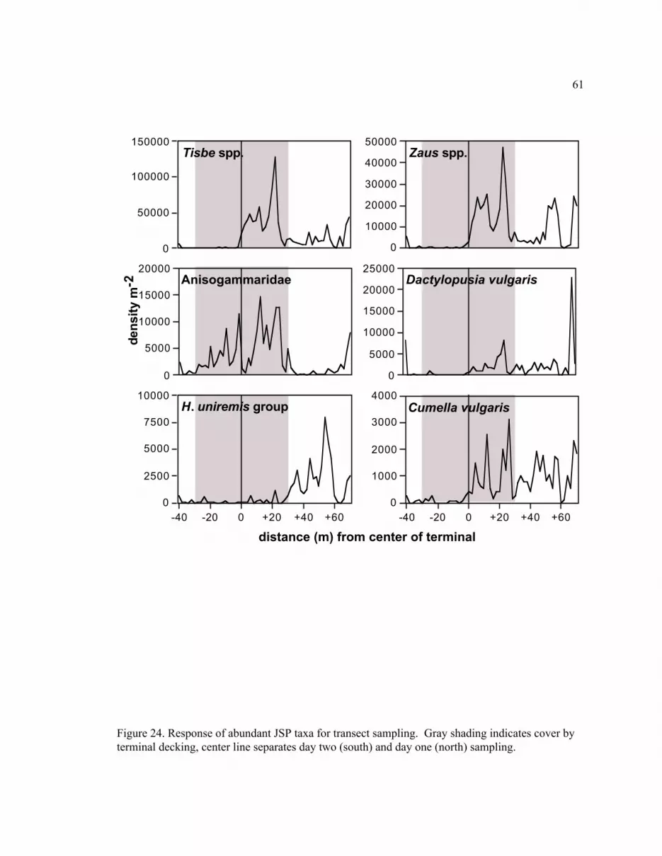
61

Figure 24. Response of abundant JSP taxa for transect sampling. Gray shading indicates cover byterminal decking, center line separates day two (south) and day one (north) sampling.

0

2500

5000

7500

10000

-40 -20 0 +20 +40 +60

H. uniremis group

0

10000

20000

30000

40000

50000Zaus spp.

0

1000

2000

3000

4000

-40 -20 0 +20 +40 +60

Cumella vulgaris

0

5000

10000

15000

20000Anisogammaridae

0

5000

10000

15000

20000

25000Dactylopusia vulgaris

0

50000

100000

150000Tisbe spp.

den

sity

m-2

distance (m) from center of terminal

62

Figure 25. Response of abundant non-JSP taxa for transect sampling. Gray shading indicatescover by terminal decking, center line separates day two (south) and day one (north) sampling.

0

10000

20000

30000

40000Harpacticus spinulosus

0

5000

10000

15000Ectinosomatidae

0

1000

2000

3000

4000

5000Ameiridae

0

2500

5000

7500

10000Thalestridae copepodids

0

1000

2000

3000

4000

-40 -20 0 +20 +40 +60

Polychaeta

0

1000

2000

3000

4000

5000

-40 -20 0 +20 +40 +60

Acrenhydrosoma

distance (m) from center of terminal

den

sity

m-2

63

Figure 26. Assemblage composition for transect sampling. Taxa included are > 1% of the totalepibenthos without nematodes. Gray shading indicates cover by terminal decking, center lineseparates day two (south) and day one (north) sampling.

0

50000

100000

150000

200000

250000

den

sity

m-2

Ectinosomatidae

H. uniremis grp .

Harpacticus spinulosus

Zaus spp.

Tisbe spp.

Acrenhydrosoma sp.

Ameiridae

Dactylopusia vulgaris

Thalestridae copepodids

Cumella vulgaris

Anisogammaridae

Polychaeta

other

0%

25%

50%

75%

100%

rela

tive

ab

un

dan

ce

-40 -30 -20 -10 0 +10 +20 +30 +40 +50 +60 +70

64

Figure 27. Mean response of summary variables and abundant taxa with significant two-factorANOVA results for elevation from Bainbridge piling sampling. Results for piling-type type arenot significant. Error bars are ± 1 standard deviation.

0

500

1000

1500total epibenthos

totalnewold

0

500

1000

1500JSP

0

100

200

300

400

500Tisbe spp.

0

50

100

150

-0.6m 0m 0.6m 1.2m

Dactylopusia vulgaris

0

5

10

15

-0.6m 0m 0.6m 1.2m

taxa richness

den

sity

m-2

aver

age

taxa

sam

ple

-1

elevation (MLLW)

65

Figure 28. Mean response of summary variables from Clinton piling sampling. Piling-type andelevation factors are significant for all. Error bars are ± 1 standard deviation.

totalnewold

den

sity

m-2

aver

age

taxa

sam

ple

-1

elevation (MLLW)

0

5000

10000

15000

20000

25000total epibenthos

0

5000

10000

15000

20000

25000JSP

0

5

10

15

20

25

30

-0.6m 0m 0.6m 1.2m

taxa richness

66

Figure 29. Mean response of abundant taxa from Clinton piling sampling. Total is the average forold and new piles where piling-type type is not significant. Elevation not significant forCalliopiidae. Error bars are ± 1 standard deviation.

totalnewoldd

ensi

ty m

-2

elevation (MLLW)

0

5000

10000

15000Tisbe spp.

0

500

1000

1500

2000

2500

3000Dactylopusia vulgaris

0

500

1000

1500

2000

2500Thalestridae copepodids

0

200

400

600

800Ectinosomatidae

0

100

200

300

400

500

600Calliopiidae

0

100

200

300

400

-0.6m 0m 0.6m 1.2m

Ameiridae

0

50

100

150

200

-0.6m 0m 0.6m 1.2m

Amphiascoides sp. A

67

Figure 30. Average densities of total epibenthos, JSP, and all taxa present on floating publicaccess dock at Clinton. Error bars are ± 1 standard deviation.

0

500

1000

1500d

ensi

ty m

-2

summary and individual taxa densities

Peltidiidae

Munna ubiquita

Lamprops quadriplicata

Robertsonia sp.

Caridea

Mesochra pygmaea

Ischyrocerus spp.

Pontogeneia rostrata

Zaus spp.

H. uniremis group copepodids

Calliopiidae

JSP

total epibenthos

68

Table 3. Summary of statistical results (two-factor ANOVA, within month ANOVA, SNK post-hoc analyses) for Bainbridge stratified-monthly sampling for all summary variables, all presentJSP taxa, and common and abundant non-JSP taxa (significant variables in shaded cells).

Taxa or Variable(JSP in bold)

2-factor ANOVAp-value (strata) month p-value

SNK(increasing)

total epibenthos 0.000 March 0.000 NU AApril 0.000 NU AMay, early 0.000 NU AMay, late 0.000 NU A

JSP 0.000 March 0.000 NU AApril 0.000 UN AMay, early 0.000 NU AMay, late 0.000 NU A

taxa richness 0.000 March 0.000 NU AApril 0.000 UN AMay, early 0.000 UN AMay, late 0.003 UN A

Harpacticus uniremis grp. 0.000 March 0.000 UN AApril 0.000 NU AMay, early 0.000 UN AMay, late 0.000 UN A

Zaus spp. 0.000 March 0.472April 0.002 UN AMay, early 0.025 NU AMay, late 0.000 NU A

Tisbe spp. 0.000 March 0.000 NU AApril 0.000 NU AMay, early 0.048 NU AMay, late 0.000 NU A

Dactylopusia vulgaris 0.000 March 0.004 NU AApril 0.000 NU AMay, early 0.360May, late 0.622

Dactylopusia crassipes 0.012 March NO BUGSApril 0.015 UN AMay, early 0.129May, late 0.139

Cumella vulgaris 0.000 March 0.000 UN AApril 0.000 UN AMay, early 0.000 UN AMay, late 0.000 UN A

Calliopiidae 0.123

69

Table 3 (continued). Summary of statistical results (two-factor ANOVA, within month ANOVA,SNK post-hoc analyses) for Bainbridge stratified-monthly sampling for all summary variables, allpresent JSP taxa, and common and abundant non-JSP taxa (significant variables in shaded cells).

Taxa or Variable(JSP in bold)

2-factor ANOVAp-value (strata) month p-value

SNK(increasing)

Pontogeneia rostrata 0.000 March 0.003 UN AApril 0.002 UN AMay, early 0.024 UN AMay, late 0.000 UN A

Anisogammaridae 0.370Aoroides spp. 0.000 March 0.079

April 0.000 NU AMay, early 0.376May, late 0.186

Corophium spp. 0.001 March 0.376April 0.004 NU AMay, early 0.036 U(N A)May, late 0.134

Pontogeneia intermedia 0.370Allorchestes angusta 0.000 March NO BUGS

April NO BUGSMay, early 0.129May, late 0.000 NU A

Photis spp. 0.000 March 0.022 NU AApril 0.000 NU AMay, early 0.024 NU AMay, late 0.400

Gammaropsis sp. 0.000 March NO BUGSApril 0.000 UN AMay, early 0.610May, late NO BUGS

Ischyrocerus spp. 0.139Chironomidae 0.607Ectinosomatidae 0.000 March 0.004 NU A

April 0.000 UN AMay, early 0.000 NU AMay, late 0.000 NU A

Harpacticus spinulosus 0.000 March 0.000 UN AApril 0.000 UN AMay, early 0.000 UN AMay, late 0.000 UN A

Laophontidae 0.000 March 0.000 NU AApril 0.000 UN AMay, early 0.000 NU AMay, late 0.000 UN A

70

Table 3 (continued). Summary of statistical results (two-factor ANOVA, within month ANOVA,SNK post-hoc analyses) for Bainbridge stratified-monthly sampling for all summary variables, allpresent JSP taxa, and common and abundant non-JSP taxa (significant variables in shaded cells).

Taxa or Variable(JSP in bold)

2-factor ANOVAp-value (strata) month p-value

SNK(increasing)

Amphiascoides sp. A 0.000 March 0.001 NU AApril 0.000 UN AMay, early 0.000 NU AMay, late 0.000 UN A

Robertsonia sp. 0.000 March 0.001 NU AApril 0.000 NU AMay, early 0.000 NU AMay, late 0.000 NU A

Thalestridae copepodids 0.000 March 0.150April 0.000 NU AMay, early 0.498May, late 0.001 UN A

Cyclopinidae 0.000 March 0.403April 0.905May, early 0.000 A N UMay, late 0.000 AN U

Turbellaria 0.000 March 0.013 UN AApril 0.634May, early 0.000 UN AMay, late 0.000 UN A

Polychaeta 0.000 March 0.003 NA UApril 0.000 N U AMay, early 0.000 NU AMay, late 0.000 AN U

Oligochaeta 0.000 March 0.013 NU AApril 0.000 NU AMay, early 0.000 NU AMay, late 0.006 N(A U)

71

Table 4. Summary of statistical results (two-factor ANOVA, within month ANOVA, SNK post-hoc analyses) for Clinton stratified-monthly sampling for all summary variables, all present JSPtaxa, and common and abundant non-JSP taxa (significant variables in shaded cells).

Taxa or Variable(JSP in bold)

2-factor ANOVAp-value (strata)

month p-value SNK(increasing)

total epibenthos 0.000 March 0.000 N U AApril 0.000 UN AMay, early 0.000 N UAMay, late 0.000 NU A

JSP 0.000 March 0.000 N U AApril 0.000 UN AMay, early 0.000 NU AMay, late 0.000 N U A

taxa richness 0.000 March 0.000 NU AApril 0.003 U(A N)May, early 0.000 N UAMay, late 0.000 UN A

Harpacticus uniremis grp. 0.000 March 0.000 NU AApril 0.000 UN AMay, early 0.079May, late 0.000 UN A

Zaus spp. 0.000 March 0.000 NU AApril 0.000 UN AMay, early 0.000 NA UMay, late 0.000 N U A

Tisbe spp. 0.000 March 0.000 N U AApril 0.000 U N AMay, early 0.000 N UAMay, late 0.000 N UA

Dactylopusia vulgaris 0.000 March 0.000 NU AApril 0.000 NU AMay, early 0.003 NA UMay, late 0.000 UN A

Dactylopusia crassipes 0.000 March 0.000 UN AApril 0.000 UN AMay, early 0.004 NU AMay, late 0.000 UN A

Cumella vulgaris 0.000 March 0.000 UN AApril 0.023 U ANMay, early 0.068May, late 0.000 UA N

Calliopiidae 0.000 March 0.000 UN AApril 0.000 U A NMay, early 0.000 UA NMay, late 0.000 UN A

72

Table 4 (continued). Summary of statistical results (two-factor ANOVA, within month ANOVA,SNK post-hoc analyses) for Clinton stratified-monthly sampling for all summary variables, allpresent JSP taxa, and common and abundant non-JSP taxa (significant variables in shaded cells).

Taxa or Variable(JSP in bold)

2-factor ANOVAp-value (strata)

month p-value SNK(increasing)

Pontogeneia rostrata 0.292Anisogammaridae 0.000 March 0.000 NU A

April 0.000 UN AMay, early 0.000 N U AMay, late 0.000 UN A

Aoroides spp. 0.835Corophium spp. 0.633Pontogeneia intermedia 0.370Allorchestes angusta 0.000 March 0.000 NU A

April 0.000 NU AMay, early 0.010 N UAMay, late 0.000 NU A

Photis spp. 0.291Chironomidae 0.443Ectinosomatidae 0.000 March 0.000 N UA

April 0.000 NU AMay, early 0.000 N A UMay, late 0.002 N UA

Ameiridae 0.000 March 0.280April 0.080May, early 0.003 NA UMay, late 0.001 NA U

Thalestridae copepodids 0.000 March 0.000 NU AApril 0.000 UN AMay, early 0.605May, late 0.024 U(N A)

Polychaeta 0.019 very non-normal, NSD (p ≤ 0.602) log10Oligochaeta 0.000 March 0.591

April 0.001 AU NMay, early 0.001 AN UMay, late 0.004 A(U N)

Turbellaria 0.000 March 0.625April 0.000 AN UMay, early 0.002 N UAMay, late 0.000 UN A

Nemertea 0.136

73

Table 5. Summary of statistical results (two-factor ANOVA, within month ANOVA, SNK post-hoc analyses) for Southworth stratified-monthly sampling for all summary variables, all presentJSP taxa, and common and abundant non-JSP taxa (significant variables in shaded cells).

Taxa or Variable(JSP in bold)

2-factor ANOVAp-value (strata) month p-value

SNK(increasing)

total epibenthos 0.000 March 0.002 UA NApril 0.000 U NAMay, early 0.003 U ANMay, late 0.006 U NA

JSP 0.001 March 0.000 UA NApril 0.004 U NAMay, early 0.018 N(U A)May, late 0.572

taxa richness 0.000 March 0.000 U N AApril 0.000 UN AMay, early 0.000 U ANMay, late 0.001 U AN

Harpacticus uniremis grp. 0.055Zaus spp. 0.000 March 0.000 NU A

April 0.000 UN AMay, early 0.000 UN AMay, late 0.000 UN A

Tisbe spp. 0.039 March 0.000 AU NApril 0.065May, early 0.085May, late 0.392

Dactylopusia vulgaris .029 non-normalDactylopusia crassipes 0.137Cumella vulgaris 0.000 March 0.365

April 0.025 U ANMay, early 0.000 UA NMay, late 0.000 U A N

Calliopiidae 0.076Pontogeneia rostrata 0.524Anisogammaridae 0.504Aoroides spp. 0.222Corophium spp. 0.005 March NO BUGS

April NO BUGSMay, early 0.610May, late 0.007 AU N

Pontogeneia intermedia 0.081Allorchestes angusta 0.114

74

Table 5 (continued). Summary of statistical results (two-factor ANOVA, within month ANOVA,SNK post-hoc analyses) for Southworth stratified-monthly sampling for all summary variables,all present JSP taxa, and common and abundant non-JSP taxa (significant variables in shadedcells).

Taxa or Variable(JSP in bold)

2-factor ANOVAp-value (strata) month p-value

SNK(increasing)

Photis spp. 0.000 March 0.773April 0.193May, early 0.073May, late 0.000 UA N

Gammaropsis sp. 0.000 March 0.078April 0.001 UN AMay, early 0.000 UA NMay, late 0.000 UA N

Ischyrocerus spp. 0.498Chironomidae 0.37Ectinosomatidae 0.000 March 0.341

April 0.000 U NAMay, early 0.000 UA NMay, late 0.000 U AN

Harpacticus spinulosus 0.000 March 0.006 UA NApril 0.000 UA NMay, early 0.000 AU NMay, late 0.000 UA N

Scutellidium sp. 0.000 March 0.051April 0.000 NU AMay, early 0.000 NU AMay, late 0.000 NU A

Laophontidae 0.000 March 0.000 UN AApril 0.000 UN AMay, early 0.000 UN AMay, late 0.000 U N A

Amonardia perturbata 0.000 March 0.081April 0.001 A UNMay, early 0.008 A NUMay, late 0.758

Orthopsyllus sp. 0.000 March 0.000 NU AApril 0.000 NU AMay, early 0.000 UN AMay, late 0.000 UN A

Thalestridae copepodids 0.098Polychaeta 0.285

75

Table 6. Summary of statistical tests for eelgrass patch sampling (two-factor ANOVA, SNKwhere appropriate). Shaded cells indicate statistically significant results for the Patch (10-m, 95-m, 235-m) factor.

Taxa or Variable(JSP in bold)

Patchp-value

Eelgrass/non-Eelgrassp-value

interactionp-value

Type SNK Off/Ondirection

total epibenthos 0.000 0.267 0.170 10 (95 253)JSP 0.000 0.765 0.010 10 235 95taxa richness 0.002 0.000 0.392 off 10 (95 235) off < on

on not significantHarpacticusseptentrionalis

0.005 0.006 0.100 off (10 95) 235 off < on

on (95 10) 235Harpacticus uniremisgrp. other

0.000 0.020 0.550 off (10 95) 235 off < on

on (95 10) 235Zaus spp. 0.000 0.024 0.118 off (10 235) 95 off < on

on 10 235 95Tisbe spp. 0.000 0.292 0.005 (10 235) 95Dactylopusia vulgaris 0.029 0.076 0.377 (10 235) 95Dactylopusia crassipes 0.005 0.001 0.111 off not significant off < on

on (10 95) 235Cumella vulgaris 0.000 0.028 0.168 off (10 95) 235 off < on

on (95 10) 235Anisogammaridae 0.000 0.000 0.000 * on < offEctinosomatidae 0.000 0.175 0.537 10 (235 95)Harpacticus spinulosus 0.019 0.000 0.011 * off < onAmeiridae 0.013 0.252 0.552 10 (95 235)Amphiascoides sp. A 0.008 0.815 0.195 10 (235 95)Thalestridae copepodids 0.021 0.138 0.797 10 (235 95)Turbellaria 0.191 0.140 0.055Nematoda 0.000 0.125 0.604 (95 10) 253Polychaeta 0.114 0.035 0.912 on < offOligochaeta 0.000 0.650 0.711 (10 95) 235* SNK not appropriate due to significant interaction factor

76

Table 7. Summary of statistical results for piling sampling (two-factor ANOVA for Pile andElevation). Shaded cells indicate significant results for either factor.

Site Taxa or Variable (JSPin bold)

Pile p-value Elevation p-value Interaction p-value

Bainbridge total epibenthos 0.782 0.050 0.308JSP 0.271 0.023 0.219taxa richness 0.479 0.005 0.504Polychaeta 0.327 0.607 0.893Tisbe spp. 0.171 0.000 0.000Dactylopusiavulgaris

0.496 0.004 0.801

Clinton total epibenthos 0.005 0.000 0.002JSP 0.008 0.000 0.008taxa richness 0.002 0.000 0.008Harpacticus uniremisgrp. other

0.308 0.131 0.070

Harpacticusseptentrionalis

0.260 0.540 0.785

Zaus spp. 0.170 0.137 0.368Tisbe spp. 0.013 0.000 0.004Tisbe spp. (logged) 0.258 0.000 0.264Dactylopusiavulgaris

0.006 0.000 0.031

Dactylopusiacrassipes

0.420 0.801 0.515

Anisogammaridae 0.166 0.231 0.302Calliopiidae 0.037 0.103 0.327Calliopiidae (logged) 0.023 0.001 0.254Ectinosomatidae 0.000 0.000 0.000Harpacticusspinulosus

0.754 0.124 0.731

Laophontidae 0.256 0.095 0.053Ameiridae 0.008 0.015 0.903Ameiridae (logged) 0.003 0.009 0.050Amphiascoides sp. A 0.772 0.012 0.032Amphiascoides sp. A(logged)

0.412 0.005 0.123

Thalestridaecopepodid

0.008 0.000 0.010

Cyclopinidae 0.082 0.105 0.191

77

DISCUSSION

The main purpose of this project was to describe the intertidal and shallow subtidal

epibenthos (large meiofauna and small macrofauna), particularly juvenile salmon prey, around

ferry terminals in order to determine if they impacted that assemblage. Although variable, the

differences indicated negative impacts of the terminals. The major null hypothesis was “there are

no differences in the epibenthic JSP assemblage (density and composition) between areas in close

vicinity to and farther away from ferry terminals”. My results demonstrated many clear,

significant differences both in density and composition of the epibenthos at three ferry terminal

structures, both over time (stratified-monthly sampling) and at several tidal elevations and habitat

types (stratified-monthly sampling, eelgrass sampling, and cross-terminal sampling). Therefore,

the major null hypothesis was rejected: significant differences in epibenthic assemblages do exist

around the ferry terminals.

While this project was not designed to determine causal factors, there are several that

may be responsible. Blanton et al. (2001) described the light environment, benthic vegetation

cover, and general substrate composition (visual assessment) at -0.6 m (-2’) at each of the three

terminals. The magnitude of under-terminal shading impacts, in terms of distance of intense

shading, was greatest at Clinton, where the decking is nearly 20 meters wider than at Bainbridge

and 35 meters wider than at Southworth. However, the north side of the Bainbridge main

terminal structure has two overhead walkways, which produced variable but less intense intertidal

shading than under the terminal. The area of intense shading at Southworth was not as wide as at

the other two terminals. In addition, adjusted in-water photosynthetically active radiation

(corrected from in-air readings) was generally close to zero under the structure at Bainbridge and

Clinton, whereas at Southworth it was reduced but detectable. Coverage of attached vegetation

followed similar patterns to those for light. Bainbridge and Clinton had no vegetation under or

78

within five meters of the terminal. Bainbridge had relatively lower vegetation cover

(Enteromorpha sp., Ulva sp., and Porphyra sp.) than Clinton (eelgrass, Ulva sp., Laminaria sp.,

and Enteromorpha sp.). Southworth had the highest coverage of benthic vegetation (primarily

Enteromorpha sp. and Ulva sp., also eelgrass), extending underneath the terminal decking by five

meters on both sides. Substrate compositions for all three terminals were noticeably different

around the structure, with higher gravel, shell, and cobble proportions as compared to sand, the

dominant component of all substrates.

The findings of Blanton et al. (2001) provide evidence for shading and propeller wash

impacts, as well as possible biotic sources of changes in sediment composition (increased shell

hash from sea star foraging). The documented lack of vegetation beyond the edge of the terminal

at Clinton and Bainbridge was likely an indicator of propeller wash as well as shading impacts on

the intertidal area. The apparent substrate coarsening was a predicted response to propeller wash,

as was increased shell or shell hash in the sediments. I completed additional sediment grain size

analysis from within each stratified-monthly sampling stratum that confirmed sediment

coarsening close to the terminal at Bainbridge, some at Southworth (Figure 31), and increased

proportions of shell hash in sediments closer to all three terminals (Figure 32). This was most

likely due to a combination of sea star foraging on pilings and in substrate, and the decomposition

of shells from the large numbers of bivalves in the sediments under and near to the terminals.

Clearly, the structures and ferries altered the biological and physical environments around these

structures.

At all three terminals, there were consistent, clear, highly statistically significant

differences in both the density and composition of the epibenthos among the Under, Near, and

Away strata. Given this, H01 was rejected: significant differences do exist for the epibenthic JSP

assemblage among these three strata relative to ferry terminals during the period of salmon

79

outmigration. With few exceptions (only non-prey taxa), significant differences suggested

negative impacts of these ferry terminals on the epibenthos. The differences in the epibenthos

corresponded with the predictions made based on the differences in magnitude of disturbances

from propeller wash, shading (i.e., benthic vegetation reduction), and substrate composition

changes. Therefore, it is likely that the combination of these factors related to terminal size and

boat traffic caused differences seen in the epibenthos.

As hypothesized, the most seriously impacted epibenthos occurred at Bainbridge, with

the greatest difference between the Away and Under strata for most variables. Because the Under

and Near strata were similar, the causes of impact at Bainbridge extended beyond shading, which

affected the Near stratum but was less strong as the completely shaded Under stratum (Olson et

al. 1997, Visconty 1997, Blanton 2001). I observed docking events at Bainbridge to subject both

the Under and Near strata to extreme propeller wash: water levels rose by over 0.3 m, and

currents were strong enough to move barnacle encrusted bivalve shells as well as sediment and

organic debris in both the Under and Near strata. Without benthic vegetation on which to attach,

it was likely that such strong and regular disturbance resuspended and redistributed much of the

epibenthic meiofauna and small macrofauna close to the terminal. This may explain the

assemblage shift at Bainbridge, from ~75% harpacticoids, distributed among many groups, Away

from the terminal to one in which Tisbe spp. was the only abundant harpacticoid (~25% of the

total) and where over 40% of the organisms were annelids (Polychaeta, Oligochaeta). Tisbe spp.

has been demonstrated to be more ubiquitous among habitat-types within close proximity to one

another (Simenstad et al. 1988a), and may spend a relatively large amount of time higher in the

water column (Marcotte 1983), in this case making it susceptible to transport by propeller wash.

In contrast, the larger annelids may have been partially burrowed in the sediment, allowing them

withstand the wash disturbance. Neither Clinton nor Southworth had such strong differences in

80

the density or assemblage of the epibenthos relative to the terminal structure, but negative

impacts on the epibenthos were clear. The overall abundance of most individual taxa, taxa

richness, and total epibenthos declined. The decline in taxa richness may have been due to the

decreased probability of finding rarer organisms in lower total abundance samples (especially at

Bainbridge). However, these results agree with those from the Hudson River estuary, where

invertebrate density decreased under piers even though total abundance increased (J. Duffy-

Anderson, NMFS, pers. comm.). In this way, OWS may be similar to other disturbed habitats,

which often have high densities of a few organisms that can withstand the disturbance.

Compared to Bainbridge, the total assemblage close to Clinton and Southworth terminals

remained relatively well distributed among those taxa found away from them, with the few

exceptions covered in the Results section. These smaller differences in the epibenthos matched

the relatively smaller differences observed the physical and biotic environment.

Because clear, highly statistically significant differences in both the density and

composition of the epibenthos were found among the eelgrass patches at Clinton, H02 was

rejected. Moreover, most significant differences indicated negative impacts of these OWS on the

epibenthos. There were a few cases in which patch effects unrelated to terminal proximity were

significant. The substrate in the middle patch was coarse, gravel and cobble with eelgrass,

compared to the sand and fine sand close to and farthest away from the terminal. The middle

patch was also at a slightly higher tidal elevation. These physical differences may explain the

cases when certain taxa within the epibenthos from the patches closest and farthest from the

terminal were grouped and less dense than the middle patch.

The eelgrass results suggest that it is important to assess habitat function, not just

presence, absence, or condition (e.g., blade density, canopy height, and patch size). A visual

assessment of the area around the Clinton terminal would indicate potential juvenile salmon

81

habitat, such as the 10-m eelgrass patch, within just meters of the terminal margin. This eelgrass

withstands the magnitude of the OWS impacts present, including shading and propeller wash.

However, the data showed that the epibenthos sampled both directly on and just adjacent to this

near-terminal eelgrass were significantly reduced, and that in terms its role as a source of JSP, its

function was probably compromised.

High-resolution cross-terminal sampling at Clinton demonstrated some differences in

both the density and composition of the epibenthos along the sampling transect, though the

differences were not always those predicted prior to the study. H03 was tentatively rejected:

significant differences do exist the in epibenthic JSP assemblage along a cross-terminal gradient.

Whether or not those differences indicate negative impacts of OWS on the epibenthos was less

clear. Some less abundant taxa, including Harpacticus uniremis group, Harpacticus spinulosis,

and Acrenhydrosoma indicated a negative impact on the epibenthos correlating well with the light

and benthic vegetation surveys completed by Blanton et al. (2001). Eight of the 12 taxa

considered, including the highly abundant Tisbe spp, Zaus spp, and Ectinosomatidae, had

anomalous large densities under the north half of the terminal, but not the south. Because the

sampling took place in essentially the same habitat, during the same time in the tide cycle, over

two days, there are several possible explanations for these results. The first is changes in the

sediment composition along the sampling transect. Blanton et al. (2001) described an abrupt

change in substrate at the mid-terminal line from sand dominated to the south to gravel or shell

dominated substrate to the north, extending up the terminal edge prior to returning to sandy

substrate. This corresponds very well with to the cross-terminal epibenthos results under the

terminal decking, though the to the north of the decking it is vegetation rather than sediment that

appears to correspond with the epibenthos. A second possible explanation is between-day

variability. Sampling on day one went from the center of the terminal to the north, and on day

82

two went to the south. The water was rougher and more turbid on day two, with winds in the area

were stronger. However, one would expect to see more of the easily transported organisms (i.e.,

Tisbe spp.) under these conditions, opposite of what the data showed. Finally, the large numbers

of organisms found under the terminal may have resulted from organism transport during docking

events. These occurred during sampling, but were not recorded and cannot be compared to the

peaks of organisms observed.

The limited results from terminal structure sampling indicated that, whether old or new

construction, pilings or floats, terminal structures may not be great sources of JSP, or total

epibenthos, in any way comparable to those from in non-impacted or impacted intertidal habitats.

While there were differences between piling-type and elevation comparisons, and between

structure types (floats and pilings) in terms of JSP availability the more interesting comparison

was between the terminal and intertidal substrates. For instance, at Clinton, the total JSP on the

pilings at the lowest elevation was less than half of that from the intertidal substrate (MLLW) in

the Under stratum, and less than a third of that from the Away stratum. The float had JSP

densities of about 2% compared the Away stratum. Low densities of epibenthic organisms on the

terminal structures made statistical evaluation of these data difficult, particularly at Bainbridge.

However, when differences were detected, individual taxa or summary variables were less dense

or diverse on older timber pilings than on newer concrete or epoxy-steel pilings. For this reason,

H04 was rejected: differences appear to exist in the epibenthic assemblage among piling

construction types. The consistent finding was overall greater densities and diversity of

organisms at lower elevations on the pilings. During sampling, the tide was never below -0.6 m

(the lowest elevation sampled), and the epibenthos were not exposed. The pilings at Clinton and

Bainbridge both had extensive evidence of sea star feeding, with the lower piling elevations kept

relatively clear of everything except small barnacles and small mussels up to about +0.6 m

83

(author pers. obs.). This left little available habitat for epibenthic organisms during tidal

exposure. Above +0.6 m, the tidal exposure may be too extreme for many of them.

The float epibenthic assemblage at Clinton was very different from that on either piling-

type. While Tisbe spp. and Dactylopusia vulgaris were dominant on the pilings, they were

completely absent from assemblage on the float. Calliopiidae was the dominant taxon on the

float and was almost twice as dense there than at –0.6 m and 0 (the two highest densities) on the

epoxy-steel pilings. The dominance of Calliopiidae may be in part explained by the large amount

of attached macroalgae on the float. Calliopius pacificus, the most common Calliopius spp. in

the region, is strongly associated with submerged plants and algae (Bousefield and Hendrycks

1997). Low epibenthos densities from the float also may have been due to flattening of the

macroalgae by the pump system, trapping some organisms between algae rather than sampling

them.

Stratified-monthly sampling generated the most robust data-set, particularly in terms of

generating similar results at multiple sites and over a period of time. Distributions of many

epibenthic organisms, including harpacticoid copepods, are highly variable on a very small scale

depending on differences in substrate, elevation, vegetation, and micro-habitat features such as

wave ripples (as reviewed by Hicks and Coull 1983, Coull 1988). Stratified-monthly sampling

was designed with high replication in order to account for this variability. The other three sample

sets had no replication in time and low replication in space. Therefore, they were much more

susceptible to variability on a variety of scales, demonstrated by strong differences in individual

taxon densities and assemblage features between day one and two of cross-terminal sampling.

These results provide a good starting point for additional investigations, particularly in terms of

eelgrass or other habitat function near to and farther from the terminal. However, where one-time

sampling appears to contradict results from stratified-monthly sampling (e.g., high-resolution

84

cross-terminal results for total epibenthos, JSP, Tisbe spp., and Zaus spp.), the latter should be

considered the more reliable result. Ideally, both the eelgrass and high-gradient cross-terminal

sampling could be improved upon (e.g., sampling eelgrass blades as well as epibenthic pumps)

and repeated multiple times during the spring.

Ultimately this research implicates large OWS (ferry terminals) induce decreases or

changes in epibenthos density, diversity, and assemblage composition probably caused by the

following four interacting factors:

1) direct disturbance and/or removal by regular vessel disturbance

2) reduced benthic vegetation or compromised benthic vegetation function due to

shading and physical disturbance

3) physical habitat alterations (e.g., altered grain-size distribution from propeller wash

or piling effects), and

4) biological habitat alterations (e.g., increased shell hash from sea star foraging and

reduced eelgrass density due to benthic macrofauna disturbance).

These factors in interaction provide a good explanation for the observed differences in the

epibenthos around ferry terminals. It is clear that at some sites a single factor can completely

overwhelm others. At Southworth, where shading was the likely primary impact, there was a

reduction in some organisms (e.g., Harpacticus uniremis group,) strongly affiliated with benthic

macrovegetation, particularly eelgrass. Other organisms that are more strongly associated with

shell-gravel (Amonardia per Hicks and Coull 1983), and sand (Harpacticus spinulosis, J. Cordell,

University of Washington, pers. comm.) were present in greatest densities near to or under the

structure. A similar positive response to physical conditions may also account for increased

densities of Ameiridae under the structure at Clinton. Alternatively, at Bainbridge the intensity of

vessel disturbance apparently was so great that few harpacticoids or gammarids could persist.

85

Perhaps the strongest demonstration of OWS effects is that those epibenthic organisms

most closely affiliated with benthic vegetation showed consistently negative large OWS impacts,

even when other organisms were less affected. When in an environment where Harpacticus

uniremis group, Zaus spp., and Tisbe spp. are all present, juvenile chum salmon have been

demonstrated to feed preferentially on the first two, especially H. uniremis group, though they are

less available than the latter (Sibert 1979, Simenstad et al. 1980, D’amours 1987, Simenstad et al.

1988a, Webb 1991 a,b). As discussed previously, H. uniremis and Zaus spp. have much stronger

affinities to benthic macrovegetation than does Tisbe spp.. This is one reason why conserving

benthic vegetation (by reducing shading impacts) may be equally important to reducing vessel

disturbance for the protection of JSP resources around ferry terminals.

WSDOT ferry terminals make good models for relatively high-decked, fixed large OWS

with very high levels of vessel disturbance. Most of the major suspected modes of impact from

OWS are present at ferry terminals, and my results confirm impacts of these large OWS on JSP

and epibenthos. However, it is difficult to use these results to predict the magnitude of impact

from other types of OWS. Compared to many other types of OWS, ferry terminals are wide and

have extensive shading potential. But they also have fixed-height decking that allows greater

light penetration underneath the terminal footprint than do floating docks. Impacts from

relatively high frequency and intense disturbance from ferry docking events is greater than

propeller wash or scour associated with residential boat use, though these smaller boats disturb

the benthos directly with propeller scarring or boat landings over wider areas. The four listed

factors causing impacts on the epibenthos may be particularly damaging in cases such as these

where the undisturbed state of the estuarine-nearshore includes some benthic vegetation. The

extent and type of impact on the estuarine-nearshore from other types of OWS will likely vary

with intensity of those factors. This study demonstrated significant OWS impacts associated with

86

large ferry terminals set in otherwise relatively undisturbed intertidal areas. Additional research

to determine the thresholds at which epibenthos becomes affected could include sampling at

variety of dock sizes and degrees of vessel disturbance. Information about the mechanisms of

OWS impacts would be gained by sampling around pilings without structures, OWS over non-

vegetated substrates or in areas of chronic impacts (industrial waterfronts), and before-after-

control-impact designs at proposed OWS construction sites.

Thom et al. (1995) recommended a number of measures for the expansion of the Clinton

terminal in order to mitigate for eelgrass impacts from construction, the new structure, and

continued vessel use. These included (1) a longer, narrower terminal deck, which would decrease

intertidal shading and reduce propeller wash by keeping the ferries in deeper water; (2) the use of

light passing structures (glass blocks and grating) in the decking to increase photosynthetically

active radiation underneath the terminal; (3) newer construction that used fewer, more widely

spaced pilings in order to reduce sea star and crab bioturbation. Because factors impacting

eelgrass also impact the epibenthos associated with it, these types of mitigation measures also

apply for conserving epibenthos at various OWS types. Since the completion of this study, all

ferries at Clinton have used a new south slip, incorporating these mitigation recommendations,

while the north slip has been undergoing retrofitting. This older north slip, in use during the 2000

field season, was closer to the shoreline. Because construction was already underway at the time

of 2000 sampling, re-sampling would not constitute a true before-after control-impact design, but

a comparison of my results with a true post-construction sampling design could give some

information about the success of the mitigation efforts.

Large overwater structures have serious impacts on the intertidal and shallow subtidal

estuarine nearshore, including reduced benthic vegetation and decreased densities of epibenthic

juvenile salmon prey organisms. There are only twenty WSDOT ferry terminals, but given the

87

potential for impacts by other types of OWS, the cumulative effects in such densely populated

regions such as Puget Sound may be large. To what extent this reduced prey availability may be

limiting to juvenile salmon is unknown. Much more information on the carrying capacity of

Puget Sound for juvenile salmon, including thresholds at which they may become food-limited, is

needed. Additionally, knowledge of minimum patch size or connectivity of eelgrass required for

it to function as a prey source is required in order to quantify these impacts. Given the hundreds

or thousands of OWS encountered during a fish’s outmigration, the potential for cumulative

impacts may be great. Extensive impacts such as those occurring at the Bainbridge ferry terminal

also illustrate the potential for habitat fragmentation of the estuarine-nearshore juvenile migratory

corridor. Effects of this fragmentation on fish condition and survival (reduced refugia and prey,

barriers to outmigration) have been considered in several reviews but are not well understood

(e.g., Simenstad et al. 1999, Nightingale and Simenstad 2001, Williams and Thom 2001). My

results provide strong evidence of the negative effects of ferry terminals on nearshore habitat

function, and suggest that further research should be conducted to determine if other types of

OWS have similar impacts.

88

Figure 31. Sediment grain size analysis for the stratified-monthly sampling strata by minimumscreen size.

0%

25%

50%

75%

100%Bainbridge

2000 µm1000 µm500 µm

250 µm125 µm63 µm23 µm

0%

25%

50%

75%

100%

rela

tive

co

mp

osi

tio

n

Clinton

0%

25%

50%

75%

100%

Away Near Under

Southworth

89

Figure 32. Relative proportion of shell hash in sediment grain size fractions (by minimum screensize) for stratified-monthly sampling strata. Sand dominated values are negative, shell hashdominated values are positive, the zero line represents a 50/50 mix of sand and shell hash

-3

-2

-1

0

1

2

3Bainbridge

2000 µm1000 µm500 µm

250 µm125 µm63 µm23 µm

-3

-2

-1

0

1

2

3

com

po

siti

on

of

san

d v

s. s

hel

l has

h

Clinton

-3

-2

-1

0

1

2

3

Away Near Under

Southworth

90

LITERATURE CITED

Able, K. W., J. P. Manderson, and A. L. Studholme. 1998. The distribution of shallow water

juvenile fishes in an urban estuary: the effects of manmade structures in the lower Hudson

River. Estuaries 21:731-744

Able, K. W., J. P. Manderson, and A. L. Studholme. 1999. Habitat quality for shallow water

fishes in an urban estuary: the effects of man-made structures on growth. Marine Ecology

Progress Series 187:227-235

Bailey A., H. Berry, A. Bookheim, and D. Stevens. 1998. Probability-based estimation of

nearshore characteristics. In proceedings of Puget Sound research ’98 conference. Puget

Sound Water Quality Action Team, Olympia Washington, USA.

Blanton, S. L., R. M. Thom, J. A. Southard. 2001. Documentation of ferry terminal shading,

substrate composition, and algal and eelgrass coverage. Battelle Marine Sciences Laboratory,

Sequim, Washington. Letter Report prepared for University of Washington, School of

Aquatic and Fishery Sciences, Seattle, Washington. 17 pp.

Burdick, D. M., and F. T. Short. 1999. The effects of boat docks on eelgrass beds in coastal

waters of Massachusetts. Environmental Management 23:231-240

Connell, S. D. 2000. Floating pontoons create novel habitats for subtidal epibiota. Journal of

Experimental Marine Biology and Ecology. 247:183-194

Cordell, J. R. 1986. Structure and dynamics or an epibenthic harpacticoid assemblage and the role

of predation by juvenile salmon. M.S. thesis, University of Washington, Seattle, Washington,

164 pp.

Cordell, J. R. Personal Communication. Conversations with M. Haas June 1999 through June

2002.

91

Coull, B. C. 1988. Ecology of the marine meiofauna). Pp. 18-38 in R. P. Higgins and H. Theil

(eds.). Introduction to the study of meiofauna, Smithsonian Institution Press, Washington,

D.C., USA. 488 pp.

D’Amours, D. 1987. Trophic phasing of juvenile chum salmon Oncorhynchus keta Walbaum and

harpacticoid copepods in the Fraser River Estuary, British Columbia. Ph.D. thesis, University

of British Columbia, Vancouver, British Columbia. 163 pp.

Department of Commerce, National Oceanic and Atmospheric Administration. 1999. Endangered

and threatened species: threatened status for three chinook salmon evolutionarily significant

units in Washington and Oregon, and endangered status of one chinook salmon ESU in

Washington; final rule. Federal Register 64:14307-14328

Duffy-Anderson, J. T. Personal Communication. E-mails to M. Haas May 12, 2002.

Duffy-Anderson, J. T. and K. W. Able. 1999. Effects of municipal piers on the growth of juvenile

fishes in the Hudson River estuary: a study across a pier edge. Marine Biology 133: 409-418

Duffy-Anderson, J. T. and K. W. Able. 2001. As assessment of the feeding success of young-of-

the-year winter flounder (Pseudopleuronectes americanus) near a municipal pier in the lower

Hudson River. Estuaries 2001:430-440

Escaravage, V. and Castel, J. 1990. The impact of the lagoonal shrimp Palaemonetes varians

(Leach) on meiofauna in a temperate coastal impoundment. Acta-Oecologica 11: 409-418

Everett, R. A. 1994. Macroalgae in marine soft-sediment communities: effects on benthic faunal

assemblages. Journal of Experimental Marine Biology and Ecology 175:253-274

Feist, B. E. 1991. Potential impacts of pile driving on juvenile pink (Oncorhynchus gorbuscha)

and chum (O. keta) salmon behavior and distribution. M.S. thesis, University of Washington,

Seattle, Washington, 66 pp.

92

Feller, R. J. and V. W. Kaczynski. 1975. Size selective predation by juvenile chum salmon

(Oncorhynchus keta) on epibenthic prey in Puget Sound. Journal of the Fisheries Research

Board of Canada 32:1419-1429

Francisco, M. D. 1995. Propeller scour and sediment remediation at the Seattle waterfront. M.S.

thesis, University of Washington, Seattle, Washington, 97pp.

Fresh, K.L., D. Rabin, C. Simenstad, E.O. Salo, K. Garrison, and L. Matheson. 1979. Fish

ecology studies in the Nisqually Reach area of southern Puget Sound, Washington. Fin. Rep.

Univ. Wash., Fish. Res. Inst., FRI-UW-7904. Seattle, WA. 229 pp.

Fresh, K.L, B. Williams, and D. Pentilla. 1995. Overwater structures and impacts on eelgrass in

Puget Sound, Washington. Pp. 537-543 in Proceedings of Puget Sound Research 95, Vol. 2,

Seattle, Washington.

Fresh, K.L, B. W. Williams, S. Wyllie-Echeverria, and T. Wyllie-Echeverria. 2001. Mitigating

impacts of overwater floats on eelgrass Zostera marina l. in Puget Sound, Washington. in

Puget Sound Water Quality Action Team. 2002. Proceedings of the 2001 Puget Sound

Research Conference. T. Droscher, editor. Puget Sound Water Quality Action Team.

Olympia, Washington. Available on World Wide Web at

http://www.wa.gov/puget_sound/Publications/01_proceedings/PSRC_2001.htm

Garad, P. N. and R. D. Hey. 1988. River management to reduce turbidity in navigable Broadland

rivers. Journal of Environmental Management 27:273-288

Glasby, T. M. 1999a. Differences between subtidal epibiota on pier pilings and rocky reefs at

marinas in Sydney, Australia. Estuarine, Coastal and Shelf Science. 1999. 48:281-290

Glasby, T. M. 1999b. Effects of shading on subtidal epibiotic assemblages. Journal of

Experimental Marine Biology and Ecology. 234:275-290

93

Godin, J.-G. J. 1981. Daily patterns of feeding behavior, daily rations, and diets of juvenile pink

salmon (Oncorhynchus gorbuscha) in two marine bays of British Columbia. Canadian

Journal of Fisheries and Aquatic Sciences. 38:10-15

Gregory, R. S. and C. D. Levings. 1996. The effects of turbidity and vegetation on the risk of

juvenile salmonids, Oncorhynchus spp., to predation by adult cutthroat trout, O. clarkii.

Environmental biology of fishes. 47:279-288

Gregory, R. S. and C. D. Levings. 1998. Turbidity reduces predation on migration juvenile

Pacific salmon. Transactions of the American Fisheries Society 127:275-285

Groot, C. and L. Margolis (eds.). 1991. Pacific Salmon Life Histories, UBC Press, Vancouver,

Canada. 564 pp.

Hall, M. O. and S. S. Bell. 1993. Meiofauna on the seagrass Thalassia testudinum: population

characteristics of harpacticoid copepods and associations with algal epiphytes. Marine

Biology 116: 137-146

Healey, M. C. 1979. Detritus and juvenile salmon production in the Nanaimo Estuary: I.

Production and feeding rates of juvenile chum salmon (Oncorhynchus keta). Journal of the

Fisheries Research Board of Canada 36: 488-496

Healey, M. C. 1980. Utilization of the Nanaimo River estuary by juvenile Chinook salmon,

Oncorhynchus tshawytscha. Fishery Bulletin 77:653-668

Healey, M. C. 1982. Juvenile Pacific salmon in estuaries: the life support system. Pp. 315-341 in

V. S. Kennedy (ed.), Estuarine Comparisons, Academic Press, New York, NY. 709 pp.

Healey, M. C. 1991. Life history of chinook salmon (Oncorhynchus tshawytscha). pp. 311-394 in

C. Groot. and L. Margolis (eds.). Pacific Salmon Life Histories, UBC Press, Vancouver,

Canada. 564 pp.

Hicks, G. R. F. 1986. Distribution and behaviour (sic) of meiofaunal copepods inside and outside

seagrass beds. Marine Ecology Progress Series 31:159-170

94

Hicks, G. R. F. and B. C. Coull. 1983. The ecology of marine meiobenthic harpacticoid copepods.

Oceanography and Marine Biology Annual Review 21: 67-175

Hilton, J. & G. L. Phillips. 1982. The effect of boat activity on turbidity in a shallow broadland

river. Journal of Applied Ecology 19:143-150

Huntington, C., W. Nehlsen, and J. Bowers. 1996. A survey of healthy native stocks of

anadromous salmonids in the Pacific Northwest and California. Fisheries 21:6-14

International Association of Meiobenthologists. 2001. IAM homepage. Available from World

Wide Web http://www.mtsu.edu/~kwalt/meio/phyla34.html.

Iwasaki, N. 1993. Distribution of meiobenthic copepods from various habitats in Pauatahanui

Inlet, New Zealand. New Zealand Journal of Marine and Freshwater Research 27:399-405

Johnson, O. W., W. S. Grant, R. G. Kope, K. Neely, F. W. Waknitz, and R. S. Waples. 1997.

Status review of chum salmon from Washington, Oregon, and California. U.S. Dept.

Commer., NOAA Tech. Memo. NMFS-NWFSC-32, 280 p.

Kaczynski, V. W. and R. J. Feller, J. Clayton, R. J. Gerke. 1973. Trophic analysis of juvenile pink

and chum salmon (Oncorhynchus gorbuscha and O. keta) in Puget Sound. Journal of the

Fisheries Research Board of Canada 30:1003-1008

Kozloff, E. N. 1983. Seashore life of the Northern Pacific Coast, University of Washington Press,

Seattle, Washington. 370pp.

Levings, C.D. 1994. Feeding behavior of juvenile salmon and significance of habitat during

estuary and early sea phase. Nordic Journal of Freshwater Research 69:7-16

Loflin, R. K. 1995. The effects of docks on seagrass beds in the Charlotte Harbor estuary. Florida

Scientist 58:198-205

95

Macdonald, J. S., I. K. Birtwell, and G. M. Kruzynski. 1987. Food and habitat utilization by

juvenile salmonids in the Campbell River Estuary. Canadian Journal of Fisheries and Aquatic

Sciences 22:1233-1246

Marcotte, B. M. 1983. The imperatives of copepod diversity: perception, cognition, and

competition and predation. pp. 47-72 in F. R. Schram (ed.). Crustacean Issues 1: Crustacean

Phylogeny, A.A. Balkema, Rotterdam, Netherlands. 372 pp.

Mason, J. C. 1970. Behavioral ecology of chum salmon fry (Oncorhynchus keta) in a small

estuary. Journal of the Fisheries Research Board of Canada 31:83-92

Miller, B. S. 1980. Survey of resident marine fishes at Terminals 91 and 37 (Elliot Bay, Seattle,

Washington). Final report to Port of Seattle. FRI-UW-8014. Fisheries Research Institute,

University of Washington, Seattle, Washington. 29 pp.

Miller, B. S., C. A. Simenstad, L. L. Moulton, K. L. Fresh, F. C. Funk, W. A. Karp, and S. F.

Borton. 1977. Puget Sound Nearshore Baseline Program nearshore fish survey. Fin. Rep.

Univ. Wash., Fish. Res. Inst., FRI-UW-7710. Seattle, WA. 220 pp.

Nehlsen, W., J. E. Williams, and L. A. Lichatowich. 1991. Pacific salmon at the crossroads:

stocks at risk from California, Oregon, Idaho, and Washington. Fisheries 16:4-21

Nightingale, B. and C. A. Simenstad. 2001. Overwater structures: Marine Issues (White Paper).

Washington State Department of Transportation Report number WA-RD 508.1 Prepared for

Washington State Transportation Center, University of Washington, Seattle, Washington. 133

plus appendices

Ólafsson, E. and S. G. M. Ndaro. 1997. Impact of the mangrove crabs Uca annulipes and Dotilla

fenestrata on meiobenthos. Marine Ecological Progress Series 158:225-231

96

Olson, A. M., S. V. Visconty, B. W. (III) Witherspoon, K. Sweeny, R. M. Thom, and D. K.

Shreffler. 1997. Light environment and eelgrass shading around three WSDOT ferry

terminals. pp. 52 – 74 in Simenstad, C. A., R. M. Thom, and A. M. Olson (eds.). 1997.

Mitigation between regional transportation needs and preservation of eelgrass beds. Research

report, vol. 1. Washington State Transportation Commission/USDOT. 103 pp.

Orth, R.J., K. L. Heck and J. van M. 1984. Faunal communities in seagrass beds: a review of the

influence of plant structure and prey characteristics on predator-prey relationships. Estuaries

7:339-350

Pentilla, D. and D. Doty. 1990. Results of 1989 eelgrass shading studies in Puget Sound. Draft

Progress Report, Marine Fish Habitat Investigation Division, Washington Department of

Fisheries, Olympia, Washington. Annotated bibliography in Simenstad, C. A., B. J.

Nightengale, R. M. Thom, and D. K. Shreffler (eds.). 1999. Impacts of ferry terminals on

juvenile salmon migrating along Puget Sound shorelines. Phase I: Synthesis of State of

Knowledge. Washington State Transportation Center, Univ. of Wash. WA-RD 472.1. 116

pp. plus appendices

Puget Sound Research Council. 2001. Population, housing, and household trends in the central

Puget Sound region. Puget Sound Trends D2. 3 pp. Available from World Wide Web

http://www.psrc.org/datapubs/pubs/trends/d2trend.pdf.

Ratte, L. D. 1985. Under-pier ecology of juvenile Pacific salmon (Oncorhynchus spp.) in

Commencement Bay, Washington. M.S. thesis, Univ. Wash. 182pp.

Sargent, F. J., T. J. Leary, D. W. Crewz, and C. R. Kruer. 1995. Scarring of Florida’s seagrasses:

assessment and management options. Florida Marine Research Institute Technical Report

TR-1. Florida Marine Research Technical Institute, St. Petersburg, Florida. 37pp. plus

appendices

Shafer, D. J. 1999. The effects of dock shading on the seagrass Halodule wrightii in Perdido Bay,

Alabama. Estuaries 22:936-43

97

Shreffler, D. K., and W. M. Gardiner. 1999. Preliminary findings of diving and light surveys. in

Simenstad, C. A., B. J. Nightengale, R. M. Thom, and D. K. Shreffler (eds.) 1999. Impacts of

ferry terminals on juvenile salmon migrating along Puget Sound shorelines. Phase I:

Synthesis of State of Knowledge. Washington State Transportation Center, Univ. of Wash.

WA-RD 472.1. 116 pp. plus appendices

Shreffler, D. K. and R. A. Moursund. 1999. Impacts of ferry terminals on juvenile salmon

migrating along Puget Sound Shorelines. Phase II: Field Studies at Port Townsend Ferry

Terminals. Washington State Transportation Center, University of Washington, Seattle,

Washington. WA-RD 480.1 83 pp.

Sibert, J. R. 1979. Detritus and juvenile salmon production in the Nanaimo estuary. II. Meiofauna

available as food for juvenile chum salmon. Journal of the Fisheries Research Board of

Canada 36:497-503

Simenstad, C. A., J. R. Cordell, K. L. Fresh, and M. Carr. 1995. Trophic linkages from epibenthic

crustaceans in littoral flat habitats: Seasonal and regional comparisons. Washington State

Department of Ecology Publication No. 01-06-029, Padilla Bay National Estuarine Research

Reserve Reprint Series No. 35.

Simenstad, C. A., J. R. Cordell, R. M. Thom, S. Wyllie-Echeverria, J. Norris, and A. M. Olson.

1997b. Distribution and abundance of eelgrass and associated epiphytes. pp. 32 – 51 in

Simenstad, C. A., R. M. Thom, and A. M. Olson (eds.). 1997. Mitigation between regional

transportation needs and preservation of eelgrass beds. Research report, vol. 1. Washington

State Transportation Commission/USDOT. 103 pp.

Simenstad, C. A., B. J. Nightengale, R. M. Thom, and D. K. Shreffler (eds.). 1999. Impacts of

ferry terminals on juvenile salmon migrating along Puget Sound shorelines. Phase I:

Synthesis of State of Knowledge. Washington State Transportation Center, Univ. of Wash.

WA-RD 472.1. 116 pp. + appendices

98

Simenstad, C. A., C. D. Tanner, R. M. Thom, and L. L. Conquest. 1991. Estuarine Habitat

Assessment Protocol. Report to U. S. Environmental Protection Agency, Region 10, Seattle,

Washington. EPA 910/9/91/037. 201pp.

Simenstad, C. A., J. R. Cordell, R. C. Wissmar, K. L. Fresh, S. L. Schroeder, M. Carr, G.

Sanborn, and M. Burg. 1988a. Assemblage structure, microhabitat distribution, and food web

linkages of epibenthic crustaceans in Padilla Bay National Estuarine Research Reserve,

Washington. Report to NOAA/OCRM/MEMD by Univ. Wash., Fish. Res. Inst., FRI-UW-

8813. 60 pp. Seattle, WA. Padilla Bay National Estuarine Research Reserve Reprint Series

No. 9, 1990.

Simenstad, C. A., R. M. Thom, and A. M. Olson (eds.). 1997a. Mitigation between regional

transportation needs and preservation of eelgrass beds. Research report, vol. 1. Washington

State Transportation Commission/USDOT. 103 pp.

Simenstad, C. A., W. J. Kinney, and B. S. Miller. 1979. Epibenthic zooplankton assemblages at

selected sites along the Strait of Juan de Fuca. Final Rep. to NOAA/MESA Puget Sound

Project. Univ. Wash., Fish. Res. Inst., Seattle, WA. NOAA Tech. Memo. ERL MESA-46. 73

pp.

Simenstad, C. A., W. J. Kinney, S. S. Parker, E. O. Salo, J. R. Cordell, and H. Buechner. 1980.

Prey community structures and trophic ecology of outmigrating juvenile chum and pink

salmon in Hood Canal, Washington: A synthesis of three years’ studies, 1977-1979. Final

Rep., Univ. Wash., Fish. Res. Inst., FRI-UW-8026. Seattle, WA. 113 pp.

Simenstad, C.A., K. L. Fresh, and E. O. Salo. 1982. The role of Puget Sound and Washington

coastal estuaries in the life history of Pacific salmon: an unappreciated function. pp. 343-364

in V. S. Kennedy (ed.), Estuarine Comparisons, Academic Press, New York, N.Y. 709 pp.

Simenstad. C. A., R. M. Thom, K. A. Kuzis, J. R. Cordell, and D. K. Shreffler. 1988b. Nearshore

community studies of Neah Bay, Washington. Fin. Rep. Univ. Wash., Fish. Res. Inst., FRI-

UW-8811. Seattle, WA. 201 pp.

99

Tear, L. M. Personal Communication. Conversations and E-mails with M. Haas September 1999

through May 2002.

Thom, R. M. Personal Communication. E-mail to M. Haas on April 3, 2000.

Thom, R. M., A. B. Borde, P. J. Farley, M. C. Horn, and A. Ogston. 1996. Passenger-only ferry

propeller wash study: threshold velocity determinations and field study, Vashon terminal.

PNWD-2376/UC000. Prepared for the Washington State Department of Transportation.

Battelle, Pacific Northwest Division of Battelle Memorial Institute, Sequim, Washington. 16

pp. plus appendices.

Thom, R. M., D. K. Shreffler, and J. Schafer. 1995. Mitigation plan for impacts to subtidal

vegetation associated with reconstruction and expansion of the ferry terminal at Clinton,

Whidbey Island, Washington. PNL-10844. Prepared for the Washington State Department of

Transportation. Battelle, Pacific Northwest Division of Battelle Memorial Institute, Sequim,

Washington. 25pp.

Thom, R. M., C. A. Simenstad, J. R. Cordell, and E. O. Salo. 1988. Fisheries mitigation plan for

expansion of moorage at Blaine Marina, Blaine, Washington. Final Rep., Univ. Wash. Fish.

Res. Inst., FRI-UW-8817. Seattle, WA. 24 pp.

Thom, R. M., C. A. Simenstad, J. R. Cordell, and E. O. Salo. 1989. Fish and their epibenthic prey

in a marina and adjacent mudflats and eelgrass meadow in a small estuarine bay. Univ.

Wash., Fish. Res. Inst., FRI-UW-8901. Seattle, WA. 27 pp.

Thom. R., R. Albright, C. Simenstad, J. Hampel, J. Cordell and K. Chew. 1984. Intertidal and

shallow subtidal benthic ecology. Vol. IV sec. 5 in Q. L. Stober and K. K. Chew. Renton

Sewage Treatment Plant Project: Seahurst Baseline Study. Final Rep. Univ. Wash. Fish. Res.

Inst., FRI-UW-8413. Seattle, WA. 176 pp.

Thorpe, J. E. 1994. Salmonid fishes and the estuarine environment. Estuaries 17:76-93

100

Visconty, S. D. 1997. Modeling the shade cast by overwater structures: a technical approach to

eelgrass preservation. M.S. thesis, Univ. Wash. 56pp.

Warwick, R. M., K. R. Clarke, and J. M. Gee. 1990. The effect of disturbance by the soldier crab

Mictyris platycheles H. Milne Edwards on meiobenthic community structure. Journal of

Experimental Marine Biology an d Ecology 135: 19-33

Webb, D. G. 1989. Predation by juvenile salmonids on harpacticoid copepods in a shallow

subtidal seagrass bed: effects on copepod community structure and dynamics. Ph.D. thesis,

University of British Columbia, Vancouver, British Columbia. 246 pp.

Webb, D. G. 1991a. Effect of predation by juvenile Pacific salmon on marine harpacticoid

copepods. I. Comparisons of patters of copepod mortality with patterns of salmon

consumption. Marine Ecology Progress Series 72:25-36

Webb, D. G. 1991b. Effect of predation by juvenile Pacific salmon on marine harpacticoid

copepods. II. Predator density manipulation experiments. Marine Ecology Progress Series

72:37-47

Weitkamp, L. E., T. C. Wainwright, G. J. Bryant, G. B. Milner, D. J. Teel, R. G. Kope, and R. S.

Waples. 1995. Status review of coho salmon from Washington, Oregon, and California. U.S.

Dept. Commer., NOAA Tech. Memo. NMFS-NWFSC-24, 280 p.

Wilson, W. H. Jr. 1981. Sediment-mediated interactions in a densely populated infaunal

assemblage: the effects of the polychaete Abarenicola pacifica. Journal of Marine Research

39: 735-748

Widdicombe, S. and M. C. Austen. Mesocosm investigation into the effects of bioturbation on the

diversity and structure of a subtidal macrobenthic community. Marine Ecological Progress

Series 198: 181-193

101

Yousef, Y. A. 1974. Assessing effects on water quality by boating activity. United States

Environmental Protection Agency, Environmental Protection Agency Technical Serv.

Number EPA-670/2-74072

Zar, J. H. 1999. Biostatistical Analysis, 4th edition. Prentice Hall, New Jersey, USA.

102

APPENDIX A. Environmental Conditions

Water temperature and salinity readings for all sampling dates. YSI readings were taken at thebeginning of each sampling trip after wading into approximately .5 m deep water 30m north ofthe terminal edge.

Date Sampling TerminalTimeBegin Time End

WaterTemp (C)

Salinity(ppt)

3/10/00 Stratified Southworth 12:00 14:00 8.7 24.93/11/00 Stratified Clinton 12:20 14:20 8.8 24.93/12/00 Stratified Bainbridge 13:45 16:15 8.5 24.94/5/00 Stratified Bainbridge 10:10 9.6 24.04/6/00 Stratified Southworth 10:20 12:00 8.7 24.94/7/00 Stratified Clinton 10:30 9.5 18.55/1/00 Stratified Southworth 8:10 10:15 9.3 25.25/2/00 Stratified Bainbridge 8:20 10.3 23.25/3/00 Stratified,

Terminalstructure

Clinton 8:45 14:20 9.9 21.0

5/4/00 Terminalstructure

Bainbridge 12:00 10.6 23.1

5/29/00 Stratified Southworth 6:55 9:20 10.6 24.55/30/00 Stratified Bainbridge 7:30 11.7 19.45/31/00 Stratified,

Cross-terminal (N)

Clinton 7:15 12.4 15.0

6/1/00 Cross-terminal (S)

Clinton 11:30 13:05 13.0 16.4

6/5/00 Eelgrass Clinton 11:30 13:00

103

APPENDIX B. List of Taxa in Study

The following is a list of all taxa recorded during spring 2000 WSDOT epibenthic sampling.

Phylum Order or Class

Family (Harpacticoids and Gammarid Amphipods only) Organism Identification Data Set *

Platyhelminthes Turbellaria SM, EG, CT, TS

unknown unk. worm SM, EG, CT

Nemertea Nemertea SM, EG, CT, TS

Nematoda Nematoda EG, CT

Annelida Polychaeta SM, EG, CT, TSArchiannelida SM, EG, CT, TSOligochaeta SM, EG, CT, TS

Mollusca Gastropoda SM, EG, CT, TSNudibranchia SM, EG, CT

Arthropoda O. Acarina Halacaridae SM, EG, CT, TS

C. Pycnogonida Pycnogonidae SM, CT

O. Harpacticoida

Harpacticoida copepodids SM, EG, CTHarpacticoida misc. SM, CT

Tegastidae Tegastidae SM

Porcellidiidae Porcellidium sp. SM, EG, CT

Longipediidae Longipedia sp. SM, EG, CT

Ectinosomatidae Ectinosomatidae SM, EG, CT, TS

Harpacticidae Harpacticus uniremis SM, EG, TSHarpacticus spinulosus SM, EG, CT, TSHarpacticus septentrionalis SM, EG, CT, TSHarpacticus obscurus SM, EG, CT, TSHarpacticus uniremis grp. SM, EG, CT, TSHarpacticus uniremis grp. copepodids SM, EG, CT, TSZaus spp. SM, EG, CT, TS

Peltidiidae Peltidiidae SM, EG, CT, TS

Tisbidae Tisbe spp. SM, EG, CT, TSScutellidium sp. SM, EG, CT, TS

Tachidiidae Microarthridion spp. SM, CTTachidius triangularis SMDanielssenia sp. SM, EG, CT, TS

Laophontidae Laophontidae SM, EG, CT, TS

Ameiridae Ameiridae SM, EG, CT, TS

Ancorabolidae Ancorabolidae SM

Cletodidae Cletodidae SMEnhydrosoma sp. SMHuntemannia jadensis SM, EG, CTAcrenhydrosoma sp. SM, EG, CT, TS

Diosaccidae Diosaccidae SM, EG, CT, TSAmonardia perturbata SM, EG, CT, TSAmonardia normani SM, CTDiosaccus spinatus SM, EG, CT, TSAmphiascopsis cinctus SM, EG, CT, TSAmphiascus undosus EG, CTAmphiascus spp. SM, EG, CT, TSAmphiascus sp. A SMStenhelia spp. SM, EG, CT

104

Phylum Order or Class

Family (Harpacticoids and Gammarid Amphipods only) Organism Identification Data Set *

Tymphlamphiascus sp. SM, EG, TSAmphiascoides sp. SMAmphiascoides sp. A SM, EG, CT, TSBulbamphiascus sp. SMRobertsonia sp. SM, EG, CT, TSParamphiascella sp. SM

Canthocamptidae Orthopsyllus sp. SM, CT, TSLeimia vaga SMMesochra pygmaea SM, EG, CT, TS

Thalestridae Thalestridae copepodids SM, EG, CT, TSDactlyopusia spp. SM, EGDactylopusia vulgaris SM, EG, CT, TSDactylopusia crassipes SM, EG, CT, TSParadactylopodia spp. SM, EG, CT, TSParathalestris californica SM, EG, CT, TSParathalestris sp. A SMDiarthrodes spp. SM, EG, CT, TSThalestris sp. SMRhyncothalestris helgolandica SMIdomene purpurocincta SM

Parastenhelidae Parastenhelia spinosa TS

O. Cyclopoidea Cyclopinidae SM, CT, TS

O. Leptostraca Nebalia sp. SM, EG

O. Mysidacea Mysidacea SMArchaeomysis grebnitzkii SM

O. Cumacea Lamprops quadriplicata SM, EG, CT, TSDiastylopsis sp. SMDiastylis santamariensis SM, CTCumella vulgaris SM, EG, CT, TS

O. Tanaidacea Leptochelia dubia SM, EG, CT

O. Isopoda

Gnorimosphaeroma oregonense SM, TSExosphaeroma sp. SMIdotea sp. EG, CTSynidotea sp. SMIaniropsis tridens SMIaniropsis kincaidi SMMunna ubiquita SM, EG, CT, TSExocirolana vancouverensis SMEpicaridea SM, EG, CT, TS

O. Amphipoda

Sub. O. Gammaridea Gammaridea SM, EG, CT, TS

Ampeliscidae Ampelisca sp. SM

Amphithodae Ampithoe sp. SM

Aoroidae Aoroides spp. SM, EG, CT

Calliopiidae Calliopiidae SM, EG, CT, TSParacalliopiella pratti SM, EG, CT, TS

105

Calliopius sp. SM, EG, CT, TS

Corophiidae Corophium spp. SM, EG, CT, TS

Dexaminidae Guernea reduncans SM

Pontogeneidae Pontogeneia intermedia SMPontogeneia rostrata SM, EG, CT, TS

Anisogammaridae Anisogammaridae SM, EG, CT, TSAnisogammarus pugettensis SM, EG, CT, TSEogammarus confervicolus SM

Melitidae Melitadae SMDesdimelita sp. SM

Hyalidae Hyalidae SMAllorchestes angusta grp. SM, EG, CT, TS

Isaeidae Photis sp. SM, EG, CT, TSProtomedeia sp. SMGammaropsis sp. SM

Ischyroceridae Ischyrocerus spp. SM, EG, CT, TSMicrojassa sp. TSJassa sp. TS

Lysianassidae Lysianassidae SM

Oedicerotidae Westwoodilla caecula SM, CTAmerichelidium sp. SM, CT

Phoxocephalidae Phoxocephalidae SM, EG, CT

Pleustidae Pleustidae SM, EG, CT, TS

Podoceridae Podoceridae SM

Stenothoidae Stenothoidae SM

Sub. O. Caprellidea Caprella SM, EG, CT, TS

O. Decapoda Caridea SM, EG, CT, TSAnomura SM, EG, CTBrachyura juvenile SM, CTBrachyura megalopae SM

C. Insecta Collembola SM, EG, CTColeoptera larvae SMDiptera larvae SMChironomidae SM, EG, CT, TS

Echinodermata Asteroidea SMOphiuroidea SMEchinoidea SM, EG

* SM, stratified-monthly; EG, eelgrass patch; CT, high-gradient cross-terminal; TS,terminal structure

Phylum Order or Class

Family (Harpacticoids and Gammarid Amphipods only) Organism Identification Data Set *

106

APPENDIX C. Summary Statistics for Stratified-Monthly Sampling

Summary statistics for all summary variable,s, JSP (bold), and abundant or common non-JSP taxa;

n = 15 for all. Strata designations: A, Away; N, Near; U, Under.Bainbridge Clinton Southworth

Organism Month strata Average St. Dev. Average St. Dev. Average St. Dev.

March A 22196 25154 22719 5667 9156 5190

N 663 831 2130 2236 20622 17904

U 1622 1483 7189 6904 6359 4820

April A 146785 69769 57011 16358 81493 24087

N 1319 1578 17289 4587 68163 35047

U 2289 1371 13044 4075 35863 12282

May (Early) A 79956 37007 26367 5489 103785 35597

N 7056 3918 8722 5725 120063 47122

U 8215 3636 22819 8666 61963 49377

May (Late) A 135644 40214 162244 64574 142367 74207

N 12981 8637 43996 13687 126348 63613

U 16041 4898 53722 20846 70515 38505

March A 26 10 22 4 23 7

N 6 3 11 4 15 6

U 7 4 13 5 10 4

April A 39 4 21 2 31 3

N 9 6 22 4 21 6

U 9 4 19 2 18 3

May (Early) A 22 5 22 3 29 4

N 14 5 17 4 30 4

U 12 4 21 4 23 4

May (Late) A 27 4 25 3 35 7

N 22 7 34 2 35 5

U 20 4 23 3 28 4

March A 5307 5410 19507 4898 4967 2962

N 74 75 1167 895 15189 12085

U 137 216 4559 4448 4633 3259

April A 54900 29929 47370 14589 58252 22423

N 244 267 11141 3010 50585 29641

U 230 169 5078 1356 30426 10824

May (Early) A 8689 4406 18989 4672 79159 28374

N 4063 2791 4589 2734 61952 25007

U 4067 2319 14304 5878 46867 35233

May (Late) A 35422 11733 142563 62525 62548 36469

N 3159 3221 30193 11422 52170 42072

U 3589 2255 43237 18079 49033 29612

March A 604 545 122 90 0 0

N 15 33 0 0 11 31

U 0 0 0 0 0 0

April A 42270 27012 689 388 30 41

N 11 23 26 41 15 25

U 15 25 19 34 30 59

May (Early) A 600 481 104 103 304 284

N 26 46 22 28 196 335

U 15 44 93 142 119 157

May (Late) A 752 608 3285 1873 419 559

N 37 40 415 254 159 162

U 26 41 22 62 285 221

Total epibenthos

Taxa Richness

JSP

Harpacticus uniremis grp.

107

Bainbridge Clinton SouthworthOrganism Month strata Average St. Dev. Average St. Dev. Average St. Dev.

Zaus spp. March A 15 57 1567 787 1311 1570

N 4 14 70 102 19 40

U 0 0 189 297 63 75

April A 430 585 17341 5895 5248 1985

N 26 59 1641 769 500 657

U 4 14 837 340 263 261

May (Early) A 204 374 1000 461 18381 12097

N 4 14 359 197 2430 2563

U 15 25 3211 1781 241 297

May (Late) A 5359 2684 30004 14033 12400 10719

N 7 20 10752 5149 3426 3990

U 26 46 14533 4828 963 1480

March A 341 529 1396 1118 896 648

N 0 0 70 77 481 521

U 0 0 222 157 74 78

April A 696 501 1207 586 2267 1350

N 11 31 30 41 3304 1854

U 11 23 63 46 2774 1329

May (Early) A 11 43 59 90 3022 2209

N 33 59 30 41 6944 4765

U 48 98 181 184 7359 9077

May (Late) A 89 202 3656 1652 5507 4152

N 104 96 748 387 6481 5209

U 141 139 407 258 9137 5611

March A 0 0 104 100 0 0

N 0 0 0 0 0 0

U 0 0 0 0 0 0

April A 152 261 541 498 22 72

N 11 31 4 14 4 14

U 0 0 0 0 19 40

May (Early) A 7 20 119 119 11 31

N 0 0 11 23 4 14

U 0 0 52 83 0 0

May (Late) A 0 0 2489 1337 111 295

N 15 33 459 306 4 14

U 4 14 22 62 37 88

March A 956 1070 293 207 74 62

N 7 20 52 65 41 102

U 4 14 30 51 41 44

April A 2019 1364 311 446 181 142

N 63 78 352 179 181 219

U 7 20 78 75 44 43

May (Early) A 1437 868 96 57 341 346

N 59 61 133 111 759 545

U 19 27 204 177 148 171

May (Late) A 3000 1831 456 417 611 525

N 363 514 1322 569 1396 869

U 52 77 156 113 41 65

Dactlyopusia vulgaris

Dactylopusia crassipes

Cumella vulgaris

108

Calliopiidae March A 104 260 926 371 644 501

N 11 23 19 27 148 151

U 0 0 15 33 59 74

April A 604 794 437 397 9170 6918

N 7 20 1233 578 930 1023

U 4 14 59 61 44 85

May (Early) A 41 65 356 245 2670 1094

N 26 75 870 466 2967 1585

U 41 102 270 142 704 411

May (Late) A 59 44 2593 1883 2430 1775

N 11 43 722 509 6852 5632

U 4 14 152 104 1730 2503

March A 315 470 4 14 652 646

N 4 14 11 31 78 148

U 0 0 0 0 100 136

April A 1737 2513 0 0 4878 2531

N 4 14 4 14 826 646

U 0 0 7 29 352 285

May (Early) A 52 85 0 0 1878 976

N 11 31 4 14 4867 2823

U 0 0 11 43 3833 2636

May (Late) A 178 133 0 0 1319 1069

N 56 79 7 20 4678 3638

U 4 14 0 0 4830 4355

March A 0 0 3644 968 0 0

N 0 0 89 69 0 0

U 0 0 237 560 0 0

April A 0 0 12074 8936 0 0

N 0 0 1359 561 4 14

U 0 0 607 274 0 0

May (Early) A 4 14 8748 2870 0 0

N 0 0 1159 706 0 0

U 0 0 3044 1542 0 0

May (Late) A 0 0 67133 40434 30 115

N 0 0 7663 3342 11 31

U 0 0 5363 3258 0 0

March A 30 69 7 20 89 228

N 0 0 4 14 4 14

U 0 0 0 0 0 0

April A 559 682 15 57 130 396

N 0 0 4 14 0 0

U 0 0 0 0 4 14

May (Early) A 0 0 0 0 189 373

N 7 29 0 0 130 217

U 0 0 4 14 96 149

May (Late) A 11 23 30 115 115 156

N 11 23 26 46 411 614

U 0 0 33 66 141 177

Pontogeneia rostrata

Anisogammaridae

Aoroides spp.

Bainbridge Clinton SouthworthOrganism Month strata Average St. Dev. Average St. Dev. Average St. Dev.

109

Corophium spp. March A 11 43 0 0 0 0

N 0 0 0 0 0 0

U 0 0 7 29 0 0

April A 59 90 0 0 0 0

N 0 0 0 0 0 0

U 0 0 0 0 0 0

May (Early) A 30 51 0 0 0 0

N 7 20 11 23 4 14

U 0 0 19 34 4 14

May (Late) A 44 67 37 143 0 0

N 63 86 59 68 33 55

U 15 25 41 71 0 0

March A 0 0 0 0 4 14

N 0 0 0 0 0 0

U 0 0 0 0 0 0

April A 0 0 0 0 0 0

N 0 0 0 0 0 0

U 0 0 0 0 0 0

May (Early) A 0 0 0 0 0 0

N 4 14 0 0 4 14

U 0 0 0 0 0 0

May (Late) A 0 0 15 57 7 29

N 0 0 0 0 7 20

U 0 0 0 0 52 90

March A 0 0 37 34 0 0

N 0 0 0 0 0 0

U 0 0 0 0 0 0

April A 0 0 363 337 0 0

N 0 0 11 23 0 0

U 0 0 11 31 0 0

May (Early) A 7 20 130 124 4 14

N 0 0 22 28 0 0

U 0 0 100 105 0 0

May (Late) A 96 116 3300 1896 0 0

N 0 0 100 79 11 23

U 0 0 100 224 0 0

March A 56 105 0 0 7 20

N 0 0 0 0 4 14

U 0 0 0 0 4 14

April A 1604 1570 30 115 122 311

N 0 0 4 14 30 100

U 4 14 0 0 0 0

May (Early) A 70 135 11 31 70 114

N 0 0 0 0 230 314

U 0 0 0 0 81 127

May (Late) A 56 141 74 161 222 325

N 22 46 48 51 1241 1046

U 15 25 52 71 100 128

Photis spp.

Pontogeneia intermedia

Allorchestes angusta

Bainbridge Clinton SouthworthOrganism Month strata Average St. Dev. Average St. Dev. Average St. Dev.

110

Bainbridge Clinton SouthworthOrganism Month strata Average St. Dev. Average St. Dev. Average St. Dev.Gammaropsis sp. March A 0 0 0 0 74 159

N 0 0 0 0 7 20

U 0 0 0 0 4 14

April A 226 264 0 0 189 192

N 4 14 0 0 52 74

U 0 0 0 0 26 36

May (Early) A 0 0 0 0 111 81

N 4 14 0 0 915 774

U 4 14 0 0 322 272

May (Late) A 0 0 0 0 22 41

N 0 0 0 0 333 248

U 0 0 0 0 52 102

March A 4 14 0 0 0 0

N 0 0 0 0 4 14

U 0 0 0 0 0 0

April A 4 14 0 0 11 31

N 0 0 0 0 7 20

U 0 0 0 0 0 0

May (Early) A 0 0 0 0 0 0

N 0 0 0 0 0 0

U 0 0 0 0 4 14

May (Late) A 0 0 0 0 15 39

N 0 0 0 0 0 0

U 0 0 0 0 11 23

March A 0 0 0 0 0 0

N 0 0 0 0 0 0

U 0 0 4 14 0 0

April A 0 0 0 0 0 0

N 0 0 0 0 0 0

U 4 14 4 14 0 0

May (Early) A 0 0 4 14 0 0

N 0 0 4 14 0 0

U 0 0 7 29 4 14

May (Late) A 0 0 15 57 0 0

N 4 14 15 25 0 0

U 0 0 26 59 0 0

March A 5722 8638 689 380 915 568

N 78 124 148 235 967 1077

U 93 114 467 397 522 963

April A 30011 18461 2289 1074 6770 2834

N 115 219 256 242 4848 4815

U 30 46 348 181 1044 891

May (Early) A 20041 10652 333 206 5233 4990

N 122 123 78 69 15233 6521

U 144 137 552 419 3544 3752

May (Late) A 18052 6154 2393 1654 19056 12610

N 167 101 763 384 22263 12207

U 189 127 1752 1195 2885 1568

Ischyrocerus spp.

Chironomidae

Ectinosomatidae

111

Bainbridge Clinton SouthworthOrganism Month strata Average St. Dev. Average St. Dev. Average St. Dev.

March A 522 416 163 350 70 155

N 22 35 44 52 2256 3504

U 4 14 11 23 48 78

April A 2707 2687 200 273 322 491

N 41 53 52 61 5411 6496

U 26 41 30 46 156 192

May (Early) A 25493 12330 107 123 96 294

N 559 360 30 29 26741 26643

U 356 233 11 31 207 380

May (Late) A 61152 30130 333 614 207 398

N 2422 3336 1359 660 24752 23098

U 174 131 267 375 307 908

March A 81 134 33 59 700 919

N 37 50 0 0 370 847

U 7 20 4 14 611 548

April A 48 89 0 0 1800 970

N 0 0 0 0 181 232

U 7 20 7 20 337 273

May (Early) A 0 0 0 0 2033 2300

N 0 0 0 0 11 31

U 4 14 0 0 130 274

May (Late) A 0 0 0 0 4670 3358

N 0 0 0 0 426 553

U 0 0 26 86 130 200

March A 815 707 48 63 348 294

N 7 20 26 46 44 76

U 7 29 56 76 37 58

April A 9822 6381 193 250 2763 1462

N 11 23 293 407 663 894

U 7 20 59 61 126 116

May (Early) A 2800 1763 81 75 3815 1629

N 26 41 44 52 1519 1398

U 37 58 267 186 696 621

May (Late) A 3400 1597 1137 810 12211 8030

N 89 145 559 302 5881 3874

U 63 66 552 386 1978 1927

March A 344 903 267 220 52 90

N 4 14 130 337 59 127

U 100 203 259 203 56 200

April A 1030 1099 593 529 211 482

N 11 23 430 792 393 612

U 22 41 1230 1445 237 230

May (Early) A 56 115 411 336 407 391

N 22 46 200 236 1000 1192

U 22 35 785 644 544 472

May (Late) A 0 0 722 491 959 787

N 19 34 556 275 1607 2348

U 37 65 1552 1148 441 553

Scutellidium sp.

Laophontidae

Ameiridae

Harpacticus spinulosis

112

Amphiascoides sp. March A 2741 3701 74 72 30 59

N 4 14 15 25 156 223

U 15 25 107 120 11 31

April A 4956 3942 1674 1095 81 120

N 26 51 93 78 270 317

U 4 14 326 266 96 93

May (Early) A 2433 1705 137 122 59 155

N 52 71 11 23 326 453

U 63 81 241 262 48 124

May (Late) A 3263 1944 833 645 152 311

N 85 94 215 191 315 444

U 41 25 444 289 133 206

March A 115 165 11 31 67 97

N 4 14 0 0 278 502

U 0 0 0 0 52 88

April A 1841 1200 0 0 763 519

N 0 0 0 0 2874 1922

U 0 0 0 0 2393 1477

May (Early) A 63 154 0 0 248 271

N 52 49 0 0 3874 3169

U 26 41 0 0 4193 5449

May (Late) A 219 283 44 92 3252 3302

N 144 131 26 51 3870 3463

U 30 55 26 69 4019 1936

March A 770 1002 7 20 7 20

N 0 0 4 14 7 29

U 0 0 0 0 7 20

April A 17363 7752 0 0 170 259

N 0 0 0 0 56 131

U 0 0 0 0 0 0

May (Early) A 2237 1617 7 20 0 0

N 0 0 0 0 119 237

U 0 0 15 57 37 143

May (Late) A 1967 2255 37 143 78 206

N 30 55 63 100 511 588

U 26 41 15 57 74 287

March A 41 80 4 14 615 738

N 0 0 0 0 0 0

U 0 0 0 0 0 0

April A 211 350 0 0 1763 1458

N 0 0 67 128 0 0

U 0 0 0 0 0 0

May (Early) A 26 72 4 14 1933 1646

N 0 0 0 0 89 192

U 0 0 7 29 0 0

May (Late) A 78 195 37 143 4063 3271

N 7 20 52 61 133 267

U 11 23 59 178 26 63

Amonardia perturbata

Robertsonia sp.

Orthopsyllus sp.

Bainbridge Clinton SouthworthOrganism Month strata Average St. Dev. Average St. Dev. Average St. Dev.

113

Bainbridge Clinton SouthworthOrganism Month strata Average St. Dev. Average St. Dev. Average St. Dev.

March A 89 228 270 236 341 223

N 7 20 11 23 393 878

U 4 14 44 67 37 72

April A 1919 1483 830 493 1359 1010

N 4 14 33 28 837 679

U 11 23 15 25 152 152

May (Early) A 37 143 56 66 1111 812

N 7 20 30 59 3148 2645

U 4 14 48 89 2530 2687

May (Late) A 426 524 1070 997 2856 2766

N 56 79 674 457 1630 1225

U 37 50 363 435 1067 982

March A 233 291 126 95 15 25

N 126 118 85 103 52 71

U 200 219 278 298 137 455

April A 274 403 0 0 0 0

N 237 246 0 0 4 14

U 285 248 0 0 7 29

May (Early) A 100 168 15 39 19 72

N 844 519 7 29 119 309

U 1785 889 111 151 96 132

May (Late) A 115 229 830 657 1070 1104

N 233 199 167 164 81 216

U 1511 1103 411 614 63 124

March A 159 203 256 185 174 182

N 56 87 159 209 119 183

U 589 695 237 276 67 113

April A 1526 716 1185 911 1422 986

N 219 232 1019 789 393 347

U 726 601 763 322 122 180

May (Early) A 2256 1362 256 278 689 415

N 474 361 1481 2179 733 573

U 541 418 537 420 393 316

May (Late) A 3452 1354 1274 877 4167 2521

N 3526 2200 1374 737 4344 2269

U 6815 2058 793 446 4459 2165

March A 1419 2196 30 46 4 14

N 44 119 30 75 15 57

U 281 405 11 43 0 0

April A 3230 1823 7 29 641 703

N 48 107 767 977 52 123

U 719 733 67 70 4 14

May (Early) A 2359 1302 41 71 256 293

N 411 403 463 481 107 140

U 889 597 1741 2087 78 109

May (Late) A 2030 777 74 155 1374 2128

N 1437 1039 1067 693 200 225

U 2581 929 507 1112 63 81

Thalestridae copepodids

Cyclopinidae

Polychaeta

Oligochaeta

114

Bainbridge Clinton SouthworthOrganism Month strata Average St. Dev. Average St. Dev. Average St. Dev.

Turbellaria March A 730 1241 152 424 7 29

N 37 143 59 104 33 66

U 11 31 119 134 7 20

April A 48 172 667 394 4 14

N 30 55 1185 743 0 0

U 11 31 2837 1528 37 58

May (Early) A 10115 6036 2611 2118 0 0

N 67 52 652 579 111 230

U 30 46 1722 1085 126 221

May (Late) A 1985 1778 7348 2780 96 200

N 307 218 2085 1070 281 356

U 85 94 1715 2168 126 216

March A 0 0 70 145 7 20

N 0 0 0 0 0 0

U 4 14 41 106 11 23

April A 4 14 578 692 544 782

N 181 461 619 406 11 43

U 41 80 1248 752 122 178

May (Early) A 44 143 1896 1199 37 58

N 156 438 126 161 4 14

U 26 46 644 691 4 14

May (Late) A 33 69 1285 3386 352 420

N 504 291 1489 953 230 398

U 256 195 556 896 511 554

Nemertea