Dynamical complexities in the Leslie-Gower predator-prey model as consequences of the Allee effect on prey

Applied Mathematical Modelling 35 (2011) 366–381

Contents lists available at ScienceDirect

Applied Mathematical Modelling

journal homepage: www.elsevier .com/locate /apm

Dynamical complexities in the Leslie–Gower predator–prey modelas consequences of the Allee effect on prey

Eduardo González-Olivares a,*, Jaime Mena-Lorca a, Alejandro Rojas-Palma a, José D. Flores b

a Grupo de Ecología Matemática, Instituto de Matemáticas, Pontificia Universidad Católica de Valparaíso, Chileb Department of Mathematical Sciences, The University of South Dakota, USA

a r t i c l e i n f o a b s t r a c t

Article history:Received 20 December 2009Received in revised form 15 June 2010Accepted 5 July 2010Available online 27 July 2010

Keywords:Allee effectLeslie–Gower predator–prey modelsFunctional responseLimit cycleBifurcationsSeparatrix curves

0307-904X/$ - see front matter � 2010 Elsevier Incdoi:10.1016/j.apm.2010.07.001

* Corresponding author. Tel.: +56 322274023; faxE-mail address: [email protected] (E. González-Oli

This work deals with the analysis of a predator–prey model derived from the Leslie–Gowertype model, where the most common mathematical form to express the Allee effect in theprey growth function is considered.

It is well-known that the Leslie–Gower model has a unique globally asymptotically sta-ble equilibrium point. However, it is shown here the Allee effect significantly modifies theoriginal system dynamics, as the studied model involves many non-topological equivalentbehaviors.

None, one or two equilibrium points can exist at the interior of the first quadrant of themodified Leslie–Gower model with strong Allee effect on prey. However, a collapse may beseen when two positive equilibrium points exist.

Moreover, we proved the existence of parameter subsets for which the system can have:a cusp point (Bogdanov–Takens bifurcation), homoclinic curves (homoclinic bifurcation),Hopf bifurcation and the existence of two limit cycles, the innermost stable and the outer-most unstable, in inverse stability as they usually appear in the Gause-type predator–preymodels.

In contrast, the system modelling an special of weak Allee effect, may include none orjust one positive equilibrium point and no homoclinic curve; the latter implies a significantdifference between the mathematical properties of these forms of the phenomenon,although both systems show some rich and interesting dynamics.

� 2010 Elsevier Inc. All rights reserved.

1. Introduction

The basis for analyzing the dynamics of complex ecological systems, such as food chains, are the interactions betweentwo species, particularly the dynamical relationship between predators and their prey [1]. From the seminal Lotka–Volterramodel, several alternatives for modeling continuous time consumer–resource interactions have been proposed [2]. In thispresentation a predator–prey model described by an autonomous bidimensional differential equation system is analyzedconsidering the following aspects:

(i) the prey population is affected by the Allee effect [3,4],(ii) the functional response is linear [5], and

(iii) the equation for predator is a logistic-type growth function as in the Leslie–Gower model [6].

. All rights reserved.

: +56 322274041.vares).

http://dx.doi.org/10.1016/j.apm.2010.07.001

mailto:[email protected]

http://dx.doi.org/10.1016/j.apm.2010.07.001

http://www.sciencedirect.com/science/journal/0307904X

http://www.elsevier.com/locate/apm

E. González-Olivares et al. / Applied Mathematical Modelling 35 (2011) 366–381 367

The main objective of this study is to describe the model behavior and to establish the quantity of limit cycles for thesystem. These results are quite significant for the analysis of most applied mathematical models, thus facilitating the under-standing of many real world oscillatory phenomena in nature.

The problem of determining conditions, which guarantees the uniqueness of a limit cycle or the global stability of theunique positive equilibrium in predator–prey systems, has been extensively studied over the last decades. This questionstarts with the work by Cheng [7], who was the first to prove the uniqueness of a limit cycle for a specific predator–preysystem with a Holling type-II functional response, using the symmetry of prey isocline.

It is well-known that if a unique unstable positive equilibrium exists in a compact region then, according to the Poincaré–Bendixon theorem, at least one limit cycle must exist.

On the other hand, if the unique positive equilibrium of a predator–prey system is locally stable but not hyperbolic, theremight be more than one limit cycle created via multiple Hopf bifurcations [8] and the number of limit cycles must beestablished.

The studied system is defined in an open positive invariant region and the Poincaré–Bendixon theorem does not apply.Due to the existence of an heteroclinic curve determined by the equilibrium point associated to the strong Allee effect, a sub-region in the phase plane is determined where two limit cycles exist for certain parameter values, the innermost stable andthe outermost unstable. Such result has not been reported in previous papers and represents a significant difference with theGause-type predation models [9]. In these type of models, an inverse stability is observed when two limit cycles exist, theinnermost unstable and the outermost stable.

1.1. Leslie–Gower type model

The Leslie [2,5] or Leslie–Gower [6,10] type models are characterized by a logistic-type predator growth equation, wherethe environmental carrying capacity of predators Ky is a function of the available prey quantity [2], that is, Ky(x) = nx, wherex = x(t) indicates the prey population size.

In this work, we consider that the predator subsistence exclusively depends on prey population, i.e., the predator is spe-cialist [2]. When Ky is expressed by the function Ky(x) = nx + c, the predator is considered to be generalist and c > 0 representsan alternative food (its constant carrying capacity when x = 0); in that case, it is said that the model is represented by aLeslie–Gower scheme and it is also known as modified Leslie–Gower model [6,10].

When c = 0, the predator growth function assumes that predators affect each others vital rates; thus, for a given prey den-sity, the increasing predator density slows down the growth rate of the predator population, as would happen if the predatorwas territorial [11].

In this type of models, the predator population growth rate depends on the predator population size ratio to the prey pop-ulation size, a positive growth rate is predicted when the absolute prey and predator densities are significantly low [2]. How-ever, these models have been recently employed to describe a real predator–prey interaction without considering thisobjection [11], which is not important for c > 0.

The importance of the Leslie–Gower model is highlighted by Collings [12], who stated ‘‘ratio-dependent Leslie model pro-vides a way to avoid the biological control paradox wherein classical prey-dependent exploitation models generally do notallow for a pest (prey) equilibrium density that is both low and stable”.

1.2. The Allee effect

Allee effect refers to any mechanism leading to a positive relationship between a component of individual fitness andeither the number or density of conspecifics [4,13]; it has been denominated in different ways in Population Dynamics[14] and depensation in fisheries sciences [14–17].

This is a common phenomenon in some animal populations, expressing a positive relation between the populationgrowth rate and low densities [18].

The difficulty of finding mates among the individuals of the same species at low population densities is one of the maincauses for the Allee effect, although it can be generated by several other factors (see Table 1 in [3] or Table 2.1 in [19]). Recentecological research has suggested two or more Allee effects can generate mechanisms acting simultaneously on a single pop-ulation (see Table 2 in [3] or Table 2.4 in [19]); the combined influence of some of these phenomena has been called multipleAllee effect [3].

Different mathematical tools have been used to analyze the Allee effect; however, few works have considered the dy-namic consequences of the Allee effect in bidimensional differential equations systems [12,20]. Furthermore, unlike themodel in this work, such works have not considered the dynamical complexities, except in [21] where a constant immigra-tion or harvest (constant inflow or outflow) has been included on the prey growth equation of a Gause-type predator–preymodel [2,22].

The most significant consequences of the Allee effect on the species conservation on a given environment are widelyknown as well as it can be regarded as the basis of animal sociality [13]. Mathematically, simple models for this effectcan reveal much about its dynamics [13] and can imply the apparition of a new equilibrium point that changes the structuralstability of the system, thus causing changes in stability of other equilibrium points.

368 E. González-Olivares et al. / Applied Mathematical Modelling 35 (2011) 366–381

This phenomenon has become crucial for population dynamics since in fact it has a surprising number of ramificationstowards different branches of ecology [19] and the knowledge of this effect on simple models is essential to understand morecomplicated ones.

1.2.1. Single-species population model with Allee effectIn mathematical terms, this effect is expressed modifying the natural growth function (usually the logistic growth func-

tion). An alternative is to use a multiplicative factor, the most common mathematical form describing this phenomenon for asingle species is given by the equation

dxdt¼ r 1� x

K

� �ðx�mÞx; ð1Þ

as is proposed in [20,23]. Here x = x(t) is the population size, r is the intrinsic growth rate and K is the environmental carryingcapacity. If m > 0, Eq. (1) represents the strong Allee effect [24] also known as critical depensation in fisheries sciences [14–16].The parameter m is a threshold population level; clearly, if 0 < x < m, the per capita growth rate is negative, that is, 1

xdxdt < 0,

implying the extinction of the population.If m 6 0, Eq. (1) represents the weak Allee effect. If m < 0, then the equation represents a compensatory growth function

[14–16] that will not be analyzed in this work.Other mathematical forms have been proposed to model the Allee effect [3,20,25–27] and most of them are topologically

equivalent [28]. However, used in predator–prey models, some of these forms could imply a change in the number of limitcycles surrounding a positive equilibrium point [29]. For instance, in [4,13] the following equation is proposed

dxdt¼ r 1� x

K� n

xþ b

� �x; ð1bÞ

which has been called additive Allee effect and used in the Leslie–Gower model, showing the existence of up to three limitcycles [30,31]; Eq. (1b) allows the modelling of a multiple Allee effect [3].

1.3. Functional response

The predator–prey interaction is expressed by a functional response or consumption rate function, which refers to thechange in the density of prey attacked per unit time per predator as the prey density changes. The simplest functional re-sponse model is obtained assuming the total change in prey density is proportional to the prey density in the availablesearching time, which is expressed by the function h(x) = qx, where q > 0 is a constant and x(t) represents the prey densityat time t > 0.

This functional response is known as linear [2,32], which is an unbounded straight line through the origin. Such a re-sponse was used almost simultaneously by Lotka in 1925 for studying a hypothetical chemical reaction and Volterra in1926 for modeling a predator–prey interaction [32]; but other forms have been assumed in earlier works considering alsothe Leslie–Gower type models [6].

More appropriate functions should be nonlinear and bounded, such as Holling types II, III and IV functional responses.Types II and III are both similar as they consider the per capita rate of predation increases as the prey density goes to a max-imum [12]; however, the domed type IV functional response [32], incorporates prey interference with predation, where theper capita predation rate increases with prey density to a maximum at a critical prey density beyond which it starts decreas-ing [12].

The incorporation of these type of functional responses in the Leslie–Gower type model originates different and morecomplex behaviors associated to Gause-type models [1,33,34] as happens with the May–Holling–Tanner model [35].

Considering Eq. (1b) for modelling the Allee effect and using a non-monotonic functional response in [30], the existence oftwo concentric limit cycles is demonstrated and in [31] the existence of a third limit cycle coexisting with the above isproved.

Using Eq. (1), we make a classification of the family of systems analyzing the behavior of a class of systems topologicallyequivalent to the original [8]. Furthermore, it is shown the Allee effect causes a significant modification to the well-knownLeslie type model, where it is possible to prove through a suitable Liapunov function that the unique equilibrium point at theinterior of the first quadrant is globally asymptotically stable [10].

One of the significant results of this work, not reported in previous works, was obtained using the Liapunov quantities orLiapunov numbers [8], is the existence of a parameter subset for which a positive equilibrium point results in a two orderweak focus. The existence of a homoclinic curve bifurcating in an unstable limit cycle is also shown.

Therefore, the detailed study of the dynamics of the model presented in this paper is crucial by not only considering themathematical interest, but also regarding such studies could provide more useful information to analyze practical problemsand a better understanding of nonlinear dynamical systems.

The model is presented in Section 2; the main properties are established in Section 3 and its consequences are shown inSection 4. In addition, simulations are given to verify the main results.


2. The model

The Leslie–Gower predator–prey model incorporating the Allee effect phenomenon on prey is described by the Kolmogo-rov type differential equation system [22] given by:

Xl :dxdt ¼ r 1� x

K

� �ðx�mÞ � qy

� �x;

dydt ¼ s 1� y

nx

� �y;

(ð2Þ

with x = x(t) and y = y(t), indicating the prey and predators population size, respectively, and l 2 D ¼ fðr;K;m; q;s;nÞ 2 R6

þ=0 6 m < Kg; the parameters have the following biological meanings:

r and s represent the intrinsic prey and predator growth rates, respectively,K is the prey environment carrying capacity,m is the Allee threshold or minimum of viable population,q is the maximal per capita consumption rate, i.e., the maximum number of prey that can be eaten by a predator in eachtime unit,n is a measure of food quality that the prey provides for conversion into predator births.

We note that system (2) is not defined at the y-axis [36], particularly at the point (0,0), but both isoclines pass throughthis point, and in this case, it is a point of particular interest [36], then system (2) or vector field Xl is defined on the set:

X ¼ fðx; yÞ 2 R2jx > 0; y P 0g ¼ Rþ � Rþ0 :

Equilibrium points or singularities of system (2) are (K,0), (m,0) and the equilibrium points (xe,nxe), where xe satisfies thequadratic equation

rx2 � ðKr þmr � KnqÞxþ Kmr ¼ 0:

Then, the equation can have positive roots, if and only if, Kr + mr � Knq > 0 and K = (Kr + mr � Knq)2 � 4Kmr2 P 0, or noneif Kr + mr � Knq 6 0.

If m = 0, then we have a particular weak Allee effect on the prey and the model is described by the Kolmogorov system

Xc :dxdt ¼ r 1� x

K

� �x� qy

� �x;

dydt ¼ s 1� y

nx

� �y;

(ð3Þ

with c ¼ ðr;K; q; s;nÞ 2 R5þ. For a comparative analysis, we remember the well-known Leslie–Gower model, without Allee ef-

fect, given by

Xb :dxdt ¼ r 1� x

K

� �� qy

� �x;

dydt ¼ s 1� y

nx

� �y;

(ð4Þ

with b = (r,K,q,s,n); this model has a unique positive singularity KrrþKqn ;

qnKrðrþKqnÞ

� �, which is globally asymptotically stable; this

is easily demonstrated using a suitable Liapunov function [10].To simplify the calculus in system (2), we follow the methodology used in [34,35,37,38], changing the variables by x = Ku,

y = nKv, and the time rescaling given by s ¼ rKuþ c

nKt ; then, we construct the function

u : ~X� R! X� R;

such that

uðu; v; sÞ ¼ Ku;nKv ;uþ c

nK

rKs

� �¼ ðx; y; tÞ;

with

det Duðu;v ; sÞ ¼ Knr

uþ cnK

� �> 0:

Then, u is a diffeomorphism preserving time orientation; thus, we get a topologically equivalent system Zg = u*Xl [8]with Zgðu;vÞ ¼ Pðu;vÞ @

@uþ Qðu;vÞ @@v, obtaining the four parameter polynomial differential equations system of Kolmogorov

type given by

Zg :duds ¼ ðð1� uÞðu�MÞ � QvÞu2;

dvds ¼ Sðu� vÞv ;

(ð5Þ

where g 2 D ¼ fðM;Q ; SÞ 2 Rþ0 � R2þj0 6 M < 1g with M ¼ m

K ; Q ¼ qnr ; C ¼ c

nK and S ¼ srK.

System (5) or vector field Zg is a continuous extension of system (2) and is defined at


eX ¼ fðu;vÞ 2 R2ju P 0; v P 0g ¼ Rþ0 � Rþ0 :

The singularities of system (5) are (0,0), (M,0), (1,0) and (ue,ue), where ue satisfies the equation

u2 � ð1þM � QÞuþM ¼ 0: ð6Þ

Moreover, the Jacobian matrix of system (5) is

DZgðu;vÞ ¼J11 �Qu2

Sv Sðu� 2vÞ

!;

with J11 = �4u3 + 3(M + 1)u2 � (M + Qv)u.

3. Main results

For simplicity we consider A = 1 + M � Q and W2 = (1 + M � Q)2 � 4M = A2 � 4M.

Lemma 1. Existence of equilibrium points

(1.1) Suppose A > 0 and M > 0, in Eq. (6), then we have that
(a) If W2 > 0, then it has two positive roots given by
ue1 ¼12ðA�WÞ ¼ B;

ue2 ¼12ðAþWÞ ¼ H;

with M < B < H < 1. Moreover, if ue1 – M and ue2 – 1, system (5) has two singularities (B,B) and (H,H) in the interior of the firstquadrant.

(b) If W2 = 0, then there exists a unique positive root of multiplicity two given by ue ¼ 12 A. In this case, we have that

Q ¼ 1þM � 2ffiffiffiffiffiMp

; therefore, ue ¼ffiffiffiffiffiMp

and system (5) has a unique positive equilibrium point.(c) If W2 < 0, then no positive roots exist and then, system (5) has no singularities at the interior of the first quadrant.

(1.2) If A < 0, Eq. (6) has no positive roots and then, system (5) has no singularities at the interior of the first quadrant.(1.3) When M = 0, a particular case of the weak Allee effect, Eq. (6) has a unique positive root ue = 1 � Q, if and only if Q < 1, and

system (5) has a unique positive equilibrium point.

Proof. It is clear that if M > 0, the quantity of positive roots depends on the linear coefficient A = 1 + M � Q of Eq. (6) andW2 = (1 + M � Q) 2 � 4M

Assuming that M = ue1 or ue2 = 1, a contradiction is obtained. h

As Eq. (6) has only a unique positive root for M = 0, then in the Leslie–Gower predator–prey model there is a significantdifference between the dynamical behavior of systems modelling strong and this particular case of weak Allee effect de-scribed by system (2) and (3), respectively. Then, the properties of each system must be separately established; particularly,different analysis must be made to determine the quantity of limit cycles surrounding a positive equilibrium point. The latteris not regularly observed in the Gause-type predator–prey models [29,37,38].

3.1. Strong Allee effect

For the vector field Zg or system (5) we consider M > 0, and the following results are obtained:

Lemma 2

(a) The set bC ¼ fðu;vÞ 2 ðRþ0 Þ2=0 6 u 6 1; v P 0g is an invariant region.(b) The solutions are bounded.

Proof

(a) The axis u and v are clearly invariant sets, as the system is of Kolmogorov type [22]. If u = 1, we have that dudt ¼ �Qv < 0,

therefore, all solutions with initial conditions born out of the region C enter and remain at C, for any sign of dvdt .

(b) In order to demonstrate the trajectories are bounded, we analyze the behavior at infinite using the Poincaré compac-tification [8] by means of the transformation X ¼ u

v and Y ¼ 1v; then dX

ds ¼ 1v2 ðv du

ds� u dvdsÞ and dY

ds ¼ � 1v2

dvds. After algebraic

manipulations [36], the new system is given by

bZg :dXds ¼ � X

Y3 �YX2 þ XMY2 þ X3 � X2MY þ QXY þ SY2X � SY2� �

;

dYds ¼ �SðX � 1Þ;

8<:


making the time rescaling given by T ¼ 1Y3 s, we obtain the vector field

�Zg :dXdT ¼ �Xð�YX2 þ XMY2 þ X3 � X2MY þ QXY þ SY2X � SY2Þ;dYdT ¼ �SðX � 1ÞY3:

(

Through the blowing-up method [39] for desingularizing the origin of �Zg we obtain a new rescaled vector field Zg, for which

DZgð0;0Þ ¼�1 00 3

� �. Thus, (0,0) of vector field Zg is an hyperbolic saddle point and (0,0) of vector field �Zg is a non-hyper-

bolic saddle point; hence, the point (0,1) is a non-hyperbolic saddle point for the vector field Zg at the compactification ofbC. h

Lemma 3. For all parameter values

(a) The point (M,0) is a hyperbolic repellor point.(b) The point (1,0) is a hyperbolic saddle point.

Proof. Evaluating the Jacobian matrix at this equilibrium point we have that

(a) (M,0) is a repellor node, since detDZg(M,0) = SM3(1 �M) > 0 and trDZg(M,0) = M(M(1 �M) + S) > 0.(b) the singularity (1,0) is a saddle point since detDZg(1,0) < 0. h

Lemma 4. The point (0,0) of the vector field Zg has a hyperbolic and a parabolic sector [40] determined for the line v ¼ SþMS u, i.e.,

there exists a separatrix curve in the phase plane that divides the behavior of trajectories; the point (0,0) is then an attractor pointfor certain trajectories and a saddle point for others.

Proof. As DZg(0,0) is the zero matrix, we use the vertical blowing-up [39] given by the function W(p,q) = (pq,q) = (u,v); wehave that dp

ds ¼ 1q ðdu

ds� p dqdsÞ;

dqds ¼ dv

ds and rescaling the time by T = qs, it becomes

Yg :dpdT ¼ pððð1� pqÞðpq�MÞ � QqÞp � Sðp� 1ÞÞ;dqdT ¼ Sqðp� 1Þ:

(
Clearly, if q = 0 then dq
dT ¼ 0. Moreover,

dpdT¼ pð�Mp� Sðp� 1ÞÞ:

Then, the singularities of the vector field Yg are (0,0) and SMþS ;0� �

, i.e., a separatrix straight exists in the phase plane pq,given by p ¼ S

MþS. The Jacobian matrix for vector field Yg is

DYgðp; qÞ ¼Yg11 �p2ð2p2q� pM � pþ QÞ

Sq Sðp� 1Þ

!
with
Yg11 ¼ 3p2q� 2pM � 4p3q2 þ 3p2qM � 2pQq� 2Spþ S:

We have that

DYgð0;0Þ ¼S 00 �S

� �;

then, (0,0) is a hyperbolic saddle point of the vector field Yg, and

DYgS

M þ S;0

� �¼�S �S2 �SM�SþQMþQS

ðMþSÞ3

0 � MSMþS

!

and SMþS ;0� �

is an attractor point for vector field Yg. Then, using the blowing down, the point (0,0) is a saddle-node in system(5) and the line v= S

MþS u divides the behavior of trajectories on the phase plane. h

We note that the point (0,0) of the vector field Zg is a non-hyperbolic attractor point. Moreover, the line v ¼ MþSS u, is tan-

gent to the separatrix curve in the phase plane dividing the behavior of the trajectories. As the point (M,0) is a repellor, thetrajectories below the separatrix have this point as their a-limit. As will be shown later, the trajectories above this separatrixhave different a-limits.


Now, we consider the case where system (5) has two equilibrium points at the interior of the first quadrant, i.e., Eq. (6)must fulfill that A = 1 + M � Q > 0 and W2 = (1 + M � Q)2 � 4M > 0.

Let P1 = (ue1,ue1) = (B,B) and P2 = (ue2,ue2) = (H,H), with 0 < M < B < H < 1. The Jacobian matrix evaluated in the equilibriumpoint (u,u) is

DZgðu;uÞ ¼J11 �Qu2

Su �Su

!
with J11 = �4u3 + (3M + 3 � Q)u2 �Mu.
In both equilibrium points, the determinant of the Jacobian matrix is

det DZgðu;uÞ ¼ u2Sð4u2 � 3uð1þM � QÞ þ 2MÞ;

then, the sign of detDZg(u,u) depends on the factor

f ½u� ¼ 4u2 � 3Auþ 2M:

Theorem 5. Singularity (B,B) is a saddle point.

Proof. At the point (B,B) we have that

f ½B� ¼ 412ðA�WÞ

� �2

� 3A12ðA�WÞ

� �þ 2M ¼ 1

2ðW � AÞðAþ 2WÞ þ 2M ¼W2 � 1

2AW � 1

2A2 þ 2M:

As W2 = A2 � 4M, we have that

f ½B� ¼ 12

W2 � 12

AW ¼ �12

WðA�WÞ ¼ �WB < 0;

then, detDZg(B,B) < 0 and the singularity (B,B) is a saddle point. h

Theorem 6. The singularity (H,H) is:

(1) a stable equilibrium point, if and only if,

S > �4H2 þ 3M þ 3� 2Qð ÞH � 2M;

(2) an unstable singularity surrounding a stable limit cycle, if and only if,

S < �4H2 þ ð3M þ 3� 2QÞH � 2M:

Proof. At the point (H,H) we have that

f ½H� ¼ 412ðAþWÞ

� �2

� 3A12ðAþWÞ

� �þ 2M ¼W2 þ 1

2AW � 1

2A2 þ 2M ¼W2 þ 1

2AW � 1

2ðA2 � 4MÞ

¼ 12

W2 þ 12

AW ¼ 12

WðAþWÞ ¼WH

as f[H] > 0, then, detDZg(H,H) > 0 and the nature of singularity (H,H) depends on the trace given by

trDZgðH;HÞ ¼ �H½4H2 � ð3ð1þMÞ � 2QÞH þ 2M þ S�

that is, it depends on the factor

T ¼ 4H2 � 3Hð1þM � QÞ þ 2M � HQ þ S:

Clearly,

(a) If S > �4H2 + (3M + 3 � 2Q)H � 2M, then trDZg(H,H) < 0, and the point (H,H) is a stable equilibrium point.(b) If S < �4H2 + (3M + 3 � 2Q)H � 2M, then trDZg(H,H) > 0, and the point (H,H) is an unstable equilibrium point.

By Hopf Bifurcation Theorem, a stable limit cycle is generated at this point. h

Theorem 7. The singularity (H,H) of vector field Zg is at least a two order weak focus, if and only if,

S ¼ �4H2 þ ð3M þ 3� 2QÞH � 2M ¼ HðM � 2H þ 1Þ:


Proof. As Q ¼ 1H ð1� HÞðH �MÞ then S = H(M � 2H + 1); thus, for H < 1þM

2 , system (5) can be expressed by

Zm :duds ¼ ð1� uÞðu�MÞ � 1

H ð1� HÞðH �MÞv� �

u2;

dvds ¼ HðM � 2H þ 1Þðu� vÞv ;

(ð5aÞ

where m = (M,H)2]0,1[ � ]0,1[.Setting u = U + C and v = V + L, then the new system translated to origin of coordinates system is

Zm :dUds ¼ ðð1� U � HÞðU þ H �MÞ � 1

H ð1� HÞðH �MÞðV þ HÞÞðU þ HÞ2;dVds ¼ ðM � 2H þ 1ÞHðU � VÞðV þ HÞ

(ð7Þ

and the Jacobian matrix of system (7) at the point (0,0) is

DZmð0;0Þ ¼ðM � 2H þ 1ÞH2 �ð1� HÞðH �MÞHðM � 2H þ 1ÞH2 �ðM � 2H þ 1ÞH2

!:

The Jordan matrix associated [41] to vector field Zm is

J ¼0 �L

L 0

� �;

with L2 ¼ det DZmð0;0Þ ¼ H3ð�M þ H2ÞðM � 2H þ 1Þ and f1(M,H) = M � 2H + 1 > 0; the first Liapunov quantity [8] isg1 ¼ trDZgðH;HÞ ¼ trDZmð0;0Þ ¼ 0. Then, using the matrix change of basis [41]

M ¼0 1

ðM�2Hþ1ÞH2

� 1L

1L

!;

and after a large algebraic calculus and time rescaling given by T = Ls, we derive to the normal form [8] given by

eZm :

dxdT ¼ �y� HðM � 2H þ 1Þxy;

dydT ¼

xþ H4ð�2M þ 3H2Þ ðM�2Hþ1Þ2

L2 x2

þ H2ð�H�2M�HMþ6H2Þð2H�M�1ÞL xyþ Hð5H � 2M � 2Þy2

þH5ð�M þ 3H2Þ ðM�2Hþ1Þ3

L2 x3

� H3ð�H�2M�HMþ10H2ÞðM�2Hþ1Þ2L x2y

þHð�2H �M � 2HM þ 11H2ÞðM � 2H þ 1Þxy2

�Lð�1þ 4H �MÞy3 þ H8

L2 ðM � 2H þ 1Þ4x4

� 4H6ðM�2Hþ1Þ3L x3yþ 6H4ðM � 2H þ 1Þ2x2y2

�4H2LðM � 2H þ 1Þxy3 þ L2y4:

8>>>>>>>>>>>>>>>>>>>>>>>>>>>>><>>>>>>>>>>>>>>>>>>>>>>>>>>>>>:
Using the Mathematica package [42] we obtain that the second Liapunov quantity [8] is
g2 ¼�ðð1� HÞH6ðH �MÞð1� 2H þMÞ2ð2H3 þM � 6HM þM2ÞÞ

8L3

with f2(M,H) = 2H3 + M � 6HM + M2.Clearly, f2(M,H) can change of sign; then, the equilibrium (0,0) of vector field eZm is surrounded by at least two limit cycles.

If (0,0) is a two order weak focus, then g3 must be the first non-zero Liapunov quantity. We obtain

g3 ¼ �ð1� HÞH13ðH �MÞð1� 2H þMÞ4

192L7 f3ðM;HÞ

with

f3ðM;HÞ ¼ f30 þ f31 þ f32 þ f33 þ f34 þ f35 þ f36;

where


f30 ¼ 2H7ð103H � 542H2 þ 804H3 � 1Þ;f31 ¼ �H4ð1� 115H þ 1794H2 � 7312H3 þ 8944H4 þ 1084H5ÞM;

f32 ¼ H2ð1� 333H þ 3997H2 � 14015H3 þ 13016H4 þ 7312H5 þ 206H6ÞM2;

f33 ¼ �Hð�230þ 2474H � 7239H2 þ 904H3 þ 14015H4 þ 1794H5 þ 2H6ÞM3;

f34 ¼ ð�15þ 778H � 5066H2 þ 7239H3 þ 3997H4 þ 115H5ÞM4;

f35 ¼ �30þ 778H � 2474H2 � 333H3 � H4� �

M5;

f36 ¼ �15þ 230H þ H2� �

M6:

The sign of f3(M,H) could change, and therefore, g4 must be calculated to determine the existence of a third limit cycle.However, such task will not be tackled in this work. When f3(M,H) < 0, g3 is positive; if f2(M,H) < 0 and trDeZmð0;0Þ > 0, thepoint (0,0) of the vector field eZm is a two order weak focus surrounded by two limit cycles, the innermost stable and the out-ermost unstable. Then, the equilibrium point (H,H) is at least a two order weak focus of the vector field Zg or system (5). h

In Fig. 1 the two limit cycles are shown.

Theorem 8. There are conditions on the parameter values for which:

(a) There is a homoclinic curve determined by the stable and unstable manifold of point P1 = (B,B).(b) There is an unstable limit cycle that bifurcates from the homoclinic surrounding point P2 = (H,H).

0 1

0

u

v

(0,0) (M,0) (1,0)

P 1

2 P

Uns table C ycle

Stable C ycle

Fig. 1. Two limit cycles in system (5) for H = 0.45, M = 0.1 and S = 0.0891875.

0 1

0

u

v

(M,0 ) (1 ,0 )

P1

P2

(0 ,0 )

W+

s

W+

u

Fig. 2. For H = 0.5 and M = 0.1, the right unstable manifold Wuþ (P1) is below to the superior stable manifold Ws

þ (P1).

0 1

0

u

v

(0 ,0) (M,0) (1 ,0)

P1

P2

Separatrix ( W+ s ( P

1 ) )

Heteroclinic trajectory ( W+ u (M, 0) )


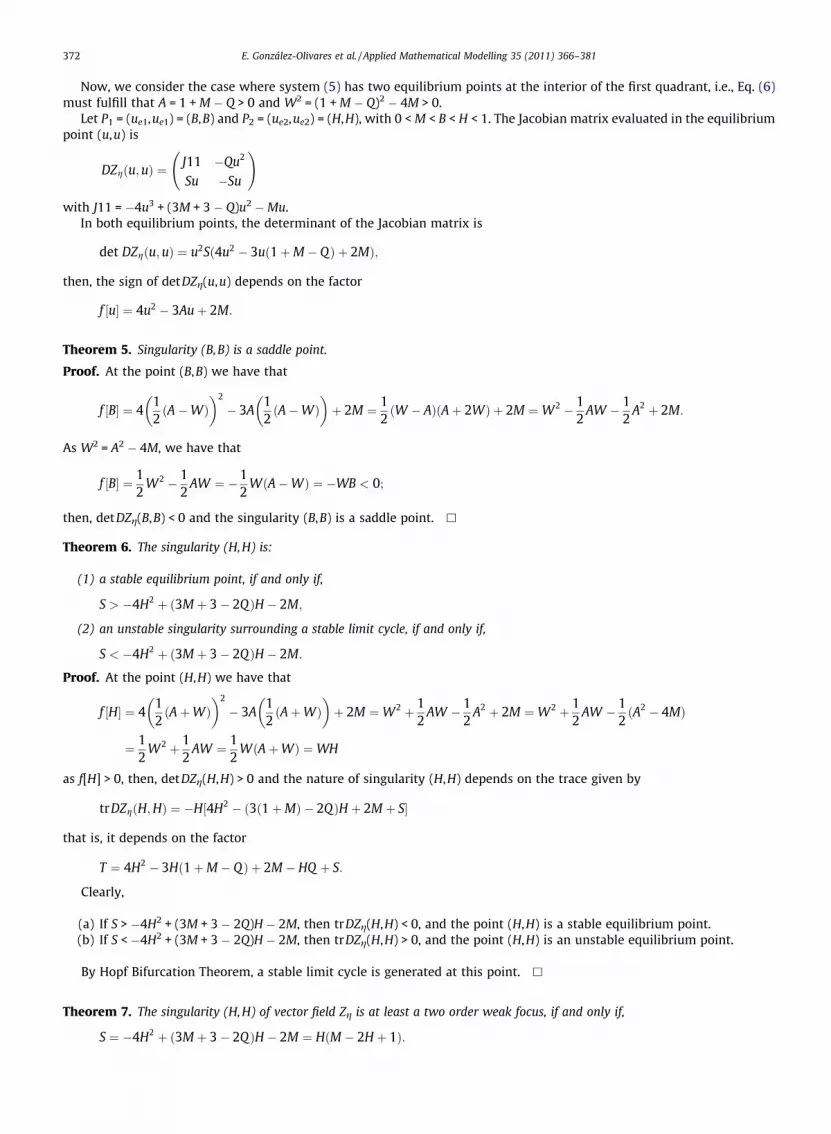
Fig. 3. For H = 0.1, M = 0.05, the unstable manifold Wuþ (P1) is below to the stable manifold Wu

þ (P1) and the point P2 is an attractor.

Proof. We note that if the point ðu;vÞ 2 P1P2, then dudt > 0, and the direction of the vector field at the point lying in the line

v = u is clearly to the right, since dudt ¼ u2ðð1� uÞðu�MÞ � QuÞ > 0 and dv

dt ¼ 0.We denote by Ws

þðP1Þ and WuþðP1Þ, the superior stable manifolds and the right unstable manifolds of P1, respectively.(a)

As C is an invariant region, the orbits cannot cross the straight line u = 1 towards the right. The trajectory determined by theright unstable manifold Wu

þðP1Þ cannot cut or cross the trajectory determined by the superior stable manifold WsþðP1Þ, by

theorem of existence and uniqueness (see Fig. 2).Moreover, the a-limit of the Ws

þðP1Þ can lie at the point (M,0) by Lemma 3 or at infinity in the direction of u-axis.On the other hand, the x-limit of the right unstable manifold Wu

þðP1Þ must be:

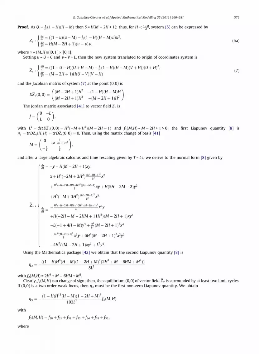
(i) point P2, when this is an attractor (see Fig. 3);(ii) a stable limit cycle, if P2 is a repellor (see Fig. 4).

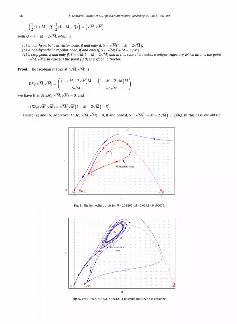
(iii) the point (0,0) (see Fig. 6).

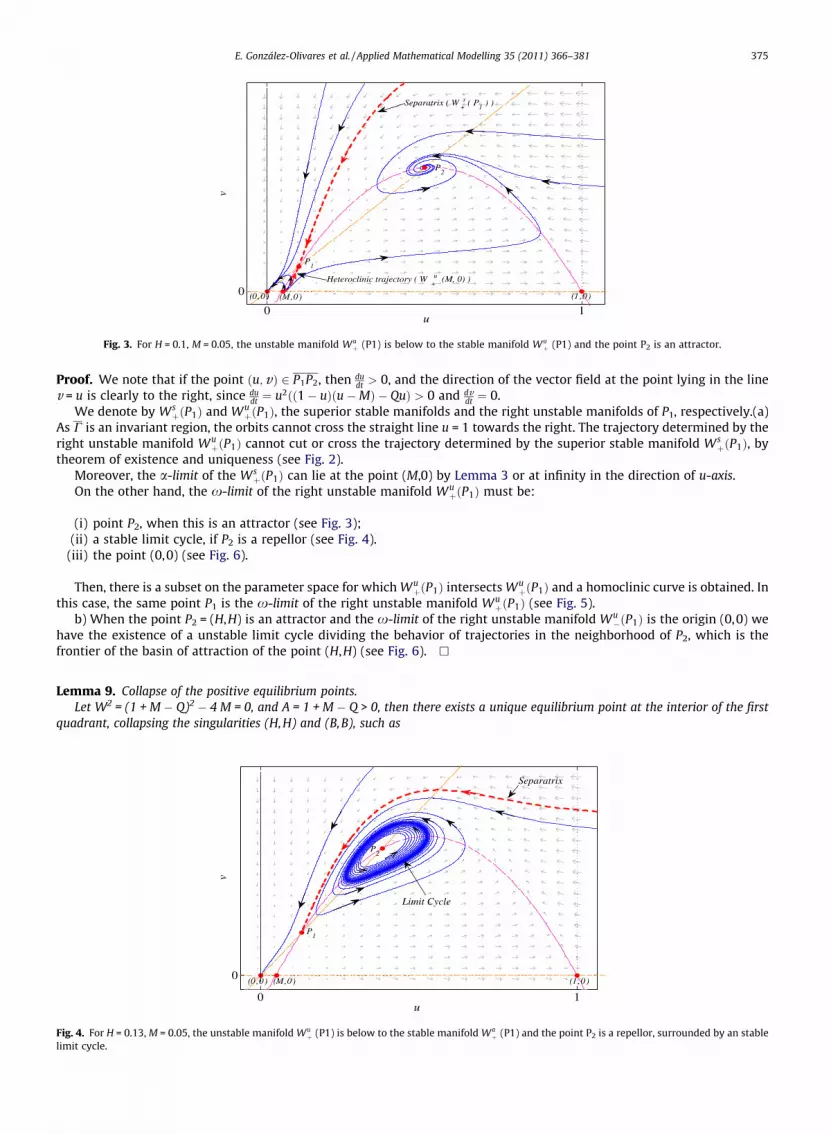
Then, there is a subset on the parameter space for which WuþðP1Þ intersects Wu

þðP1Þ and a homoclinic curve is obtained. Inthis case, the same point P1 is the x-limit of the right unstable manifold Wu

þðP1Þ (see Fig. 5).b) When the point P2 = (H,H) is an attractor and the x-limit of the right unstable manifold Wu

�ðP1Þ is the origin (0,0) wehave the existence of a unstable limit cycle dividing the behavior of trajectories in the neighborhood of P2, which is thefrontier of the basin of attraction of the point (H,H) (see Fig. 6). h

Lemma 9. Collapse of the positive equilibrium points.Let W2 = (1 + M � Q)2 � 4 M = 0, and A = 1 + M � Q > 0, then there exists a unique equilibrium point at the interior of the first

quadrant, collapsing the singularities (H,H) and (B,B), such as

0 1

0

u

v

Limit Cycle

(0 ,0) (M,0) (1 ,0)

P1

P2

Separatrix

Fig. 4. For H = 0.13, M = 0.05, the unstable manifold Wuþ (P1) is below to the stable manifold Wa

þ (P1) and the point P2 is a repellor, surrounded by an stablelimit cycle.


12ð1þM � QÞ;1

2ð1þM � QÞ

� �¼

ffiffiffiffiffiMp

;ffiffiffiffiffiMp� �

with Q ¼ 1þM � 2ffiffiffiffiffiMp

, which is

(a) a non-hyperbolic attractor node, if and only if, S >ffiffiffiffiffiMp

1þM � 2ffiffiffiffiffiMp� �

,(b) a non-hyperbolic repellor node, if and only if, S <

ffiffiffiffiffiMpð1þM � 2

ffiffiffiffiffiMpÞ,

(c) a cusp point, if and only if, S ¼ffiffiffiffiffiMpð1þM � 2

ffiffiffiffiffiMpÞ and in this case, there exists a unique trajectory which attains the point

ðffiffiffiffiffiMp

;ffiffiffiffiffiMpÞ. In case (b) the point (0,0) is a global attractor.

Proof. The Jacobian matrix at ðffiffiffiffiffiMp

;ffiffiffiffiffiMpÞ is

DZgðffiffiffiffiffiMp

;ffiffiffiffiffiMpÞ ¼


M � 1þM � 2ffiffiffiffiffiMp� �

M

SffiffiffiffiffiMp

�SffiffiffiffiffiMp

0@ 1A;
we have that det DZgð
ffiffiffiffiffiMp

;ffiffiffiffiffiMpÞ ¼ 0, and

trDZgðffiffiffiffiffiMp

;ffiffiffiffiffiMpÞ ¼

ffiffiffiffiffiMp ffiffiffiffiffi

Mp


� S� �

:

Hence (a) and (b). Moreover trDZgðffiffiffiffiffiMp

;ffiffiffiffiffiMpÞ ¼ 0, if and only if, S ¼

ffiffiffiffiffiMp


¼ffiffiffiffiffiMp

Q . In this case we obtain

0 1

0

u

v

Homoclinic curve

P2

(0,0) (M,0) (1,0)

P1

Fig. 5. The homoclinic orbit for H = 0.39266; M = 0.065,S = 0.100075.

u

v

Unstable limit cycle

P

P1

2

(0,0) (M,0) (1,0)

Fig. 6. For H = 0.4, M = 0.1, S = 0.121 a unstable limit cycle is obtained.


DZgffiffiffiffiffiMp

;ffiffiffiffiffiMp� �

¼1þM � 2

ffiffiffiffiffiMp� �


M



M

0B@1CA ¼ 1þM � 2

ffiffiffiffiffiMp� �

M1 �11 �1

� �;

and the associate Jordan matrix is

J ¼ 0 � 1þM � 2ffiffiffiffiffiMp� �

M

0 0

!;

then, the singularity ðffiffiffiffiffiMp

;ffiffiffiffiffiMpÞ is a cusp point, since it is a point of codimension 2 and we have a Bogdanov–Takens bifur-

cation [39,41]. h

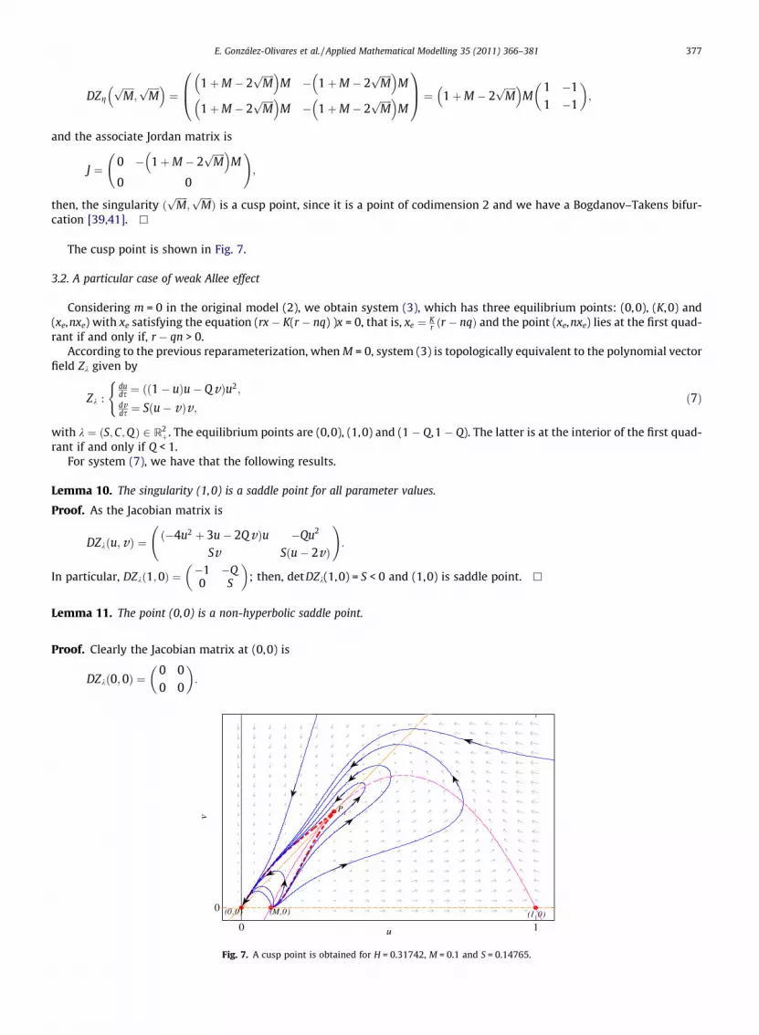
The cusp point is shown in Fig. 7.

3.2. A particular case of weak Allee effect

Considering m = 0 in the original model (2), we obtain system (3), which has three equilibrium points: (0,0), (K,0) and(xe,nxe) with xe satisfying the equation (rx � K(r � nq) )x = 0, that is, xe ¼ K

r ðr � nqÞ and the point (xe,nxe) lies at the first quad-rant if and only if, r � qn > 0.

According to the previous reparameterization, when M = 0, system (3) is topologically equivalent to the polynomial vectorfield Zk given by

Zk :duds ¼ ðð1� uÞu� QvÞu2;

dvds ¼ Sðu� vÞv;

(ð7Þ

with k ¼ ðS;C;QÞ 2 R2þ. The equilibrium points are (0,0), (1,0) and (1 � Q,1 � Q). The latter is at the interior of the first quad-

rant if and only if Q < 1.For system (7), we have that the following results.

Lemma 10. The singularity (1,0) is a saddle point for all parameter values.

Proof. As the Jacobian matrix is

DZkðu; vÞ ¼ð�4u2 þ 3u� 2QvÞu �Qu2

Sv Sðu� 2vÞ

!:� �

In particular, DZkð1;0Þ ¼�1 �Q0 S ; then, detDZk(1,0) = S < 0 and (1,0) is saddle point. h

Lemma 11. The point (0,0) is a non-hyperbolic saddle point.

Proof. Clearly the Jacobian matrix at (0,0) is

DZkð0;0Þ ¼0 00 0

� �:

0 1

0

u

v

(M,0) (1,0)

P1

(0,0)

Fig. 7. A cusp point is obtained for H = 0.31742, M = 0.1 and S = 0.14765.


For its analysis we make the vertical blowing-up [39] given by the function W(p,q) = (pq,q) = (u,v), thus, dpds ¼ 1

qduds� p dq

ds

� �and dq

ds ¼ dvds.

Substituting the new variables in the vector field Yg we have

Zx :dpds ¼ pqððð1� pqÞp� QÞðpqÞ � Sðp� 1ÞÞdqds ¼ Sq2ðp� 1Þ

(
making a time rescaling given by T = qs we obtain:
1q

Zx ¼ Zx :dpdT ¼ pððð1� pqÞp� QÞðpqÞ � Sðp� 1ÞÞdqdT ¼ Sqðp� 1Þ

:

(
If q = 0, then dq
dT ¼ 0; moreover, dpdT ¼ pð�Sðp� 1ÞÞ ¼ 0. When dp

dT ¼ 0, we have the solutions p = 0 or p = 1.The Jacobian matrix for vector field Zx is

DZxðp; qÞ ¼3p2q� 4p3q2 � 2pQq� 2Spþ S �p2ð2p2q� pþ QÞSq Sðp� 1Þ

!
and we have that
(i) DZxð1;0Þ ¼�S ð1� QÞ0 0

� �; then, the point (1,0) in the p � q system is a non-hyperbolic attractor equilibrium point,

and

(ii) DZxð0;0Þ ¼S 00 �S

� �; then, the singularity (0,0) is a saddle point since det DZxð0;0Þ ¼ �S2 < 0. Then, the point (0,0)

of vector field Zk has a hyperbolic and a parabolic sector [40]. Therefore, these sector determine a separatrix curvedividing the behavior of trajectories in the phase plane. h

Now, let

P ¼ ðtrDZgð1� Q ;1� QÞÞ2 � 4det DZgð1� Q ;1� QÞ

¼ ð1� QÞ2ð4Q 4 þ 13Q2 � 12Q 3 þ Qð2S� 6Þ þ S2 � 2Sþ 1Þ and T ¼ ð1� QÞð2Q � 1Þ � S:

Theorem 12. For the singularity (1 � Q,1 � Q) we have that:

(a) If S > (1 � Q)(2Q � 1), then the point is a local attractor (stable).(b) If S < (1 � Q)(2Q � 1), then the point is a repellor (unstable).

(b1) If P < 0, then the point is a repellor focus surrounded by a limit cycle.(b2) If P > 0, then the point is a repellor node, and the point (0,0) is globally asymptotically stable.

Proof. The Jacobian matrix evaluated at the unique positive equilibrium point is

DZkð1� Q ;1� QÞ ¼ �ð1� QÞ2ð1� 2QÞ �Qð1� QÞ2

Sð1� QÞ �Sð1� QÞ

!;

then, detDZk(1 � Q,1 � Q) = S(1 � Q)4 > 0, andtrDZk(1 � Q,1 � Q) = (1 � Q)((1 � Q)(2Q � 1) � S) = (1 � Q)T,

(a) trD Zk(1 � Q,1 � Q) < 0, if and only if, T < 0 and the singularity (1 � Q,1 � Q) is a local attractor.(b) trDZk(1 � Q,1 � Q) > 0, if and only if, T > 0 and (1 � Q,1 � Q) is a repellor and, by the Poincaré–Bendixon theorem, there

exists at least one surrounding limit cycle in the subregion compact determined by the separatrix curve, the straightline u = 1, and the u-axis; moreover, the trajectories under the separatrix determined by Ws the stable manifold of (0,0)tend to this limit cycle.

When vs = vu, the limit cycle collapses with the heteroclinic that joins both saddle points. h

Theorem 13. If S = (1 � Q)(2Q � 1), the point (1 � Q,1 � Q) is a weak focus of order one, that is, if the limit cycle exists, then it isunique.

Proof. To determine the order of weakness, we consider thatS = (1 � Q)(2Q � 1) and we obtain detDZk(1 � Q,1 � Q) = (2Q � 1)(1 � Q)5 > 0.Following the same procedure used in Theorem 7 with Q = 1 � H, we obtain that detDZk(H,H) = (1 � 2H)H5 = L2.


Making an extensive algebraic calculus and using the time rescaling given by T = Hs we becomes

eZp :

dxdT ¼ �y� Hð1� 2HÞxy;

dydT ¼

xþ 3Hð1� 2HÞx2 þ H3ð1�2HÞð1�6HÞL xy

�ð2� 5HÞHy2 þ 3ðHð1� 2HÞÞ2x3

þ ð1�10HÞð1�2HÞ2H4

L x2y� ð2� 11HÞH2ð1� 2HÞxy2

þLð1� 4HÞy3 þ ðHð1� 2HÞÞ3x4 � 4H6ð1�2HÞ3L x3y

þ6H4ð1� 2HÞ2x2y2 � 4H2ð1� 2HÞLxy3

þH5ð1� 2HÞy4:

8>>>>>>>>>>>>><>>>>>>>>>>>>>:
We note the vector field eZp can be obtained if M = 0 in the vector field eZm. Using the Mathematica software [42] to cal-
culate the focal values for the vector field eZp and for the second Liapunov quantity [8] after simplifications, we obtain

g2 ¼ �2H10ð1� 2HÞ2ð1� HÞ

8L3

which is always negative for 0 < H < 1.Then, the equilibrium point (0,0) of vector field eZp is a first order weak focus; consequently, the point (H,H) is a first order

weak focus and the limit cycle is unique for system (7) or vector field Zk. h

Theorem 14. Let Ws(0,0) be the stable manifold of (0,0), Wu(1,0) the unstable manifold of (1,0), (u,vs) 2Ws and (u,vu) 2Wu, thenthere is a subset on the parameters space for which an heteroclinic joining both equilibrium points exists.

Proof. The a-limit of Ws(0,0) and x-limit of Wu(1,0) are not the infinity on the direction of the v-axis; the x-limit of Wu(1,0)is not over the u-axis; then, the points (u*,vs) 2Ws(0,0) and (u*,vu) 2Wu(1,0) exist, with vs and vu, such that vs = s(A,E,S,M)and vu = u(A,E,S,M), that is, depending on the parameters values.

It may be observed that if 0 < u*� 1, then vs < vu and if 0� u* < 1, then vs > vu. Since the vector field Zk or system (7) iscontinuous with respect to parameters values, then the stable manifold Ws(0,0) intersects the unstable manifold Wu(1,0).Hence, there exists ðu�;v�Þ 2 bC, such that v*s = v*u and we have the equation

sðA; E; S;MÞ ¼ uðA; E; S;MÞ

which defines a surface at the parameter space D for which a heteroclinic curve exists. h

4. Conclusions

In this work we have analyzed the significant impact produced by the phenomenon known as Allee effect in a simple Les-lie predator–prey model also called Leslie–Gower model [6], which is structurally stable because it has a unique equilibriumpoint at the interior of the first quadrant that is globally asymptotically stable. Ecologically speaking, this means the prey andpredator species coexist for any parameter values.

We have modified the Leslie–Gower model by introducing a new factor in the prey growth rate, describing the Allee effectand we obtained a new model with a rich and varied dynamics, where two of them are not topologically equivalent. We haveespecially shown the importance of the singularity (0,0) in the dynamics of the modified Leslie–Grower model, demonstrat-ing the existence of a bistability phenomenon, since (0,0) is always an attractor in addition to either an stable positive equi-librium point or an stable limit cycle for determined parameter values.

For system (3), we proved the existence of a separatrix curve at the stable point (0,0) that separates the behavior of tra-jectories of the system, implying that the model is highly sensitive to the initial conditions. Moreover, the model can havetwo different attractors for the orbits of the system, and there exist solutions that have the origin as its x-limit. This impliesthat the possibility of depletion for both species is high, although the ratio prey–predator x

y is small.This situation illustrates the dynamical complexities in a relatively simple differential equations system based on a pop-

ulation predation model, including interesting results given the inherent complexity of the current interactions.We have shown that the Allee effect may be a destabilizing force in predator–prey models, since the equilibrium point of

the system could be changed from stable to unstable or otherwise.We note that in the analyzed models a big difference between the dynamics of the system with strong or weak Allee effect

(m > 0 or m = 0) exists. System (3) can only have one unique equilibrium point at the interior of the first quadrant, if and onlyif, r > nq. This point, for certain parameter values, is surrounded by a unique limit cycle, which can disappear when theparameters vary. Also, the trajectories of the system can have different behaviors strongly depending on the initialconditions.


In system (2), describing the strong Allee effect, two positive equilibrium points can coexist for a subset of parameterswith a varied dynamics, but different to other Leslie–Gower models analyzed above [30,33,34]. We have shown that oneof this equilibrium points is always a saddle point and originates a homoclinic curve for a certain constraint of parameters,which surrounds the other positive equilibrium point. This second singularity, when is unstable, is surrounded by a stablelimit cycle and there exists an unstable limit cycle originated by the breaking of the homoclinic curve.

The study of Leslie–Gower type predator–prey models, considering strong and weak Allee effects and the linear functionalresponse, shows that the behavior differs in the uniqueness of the limit cycle and the amount of positive equilibrium point.For a general theory, models using other mathematical forms to express the Allee effect [28], or else, assuming that predatorshave an alternative food (modified Leslie–Gower schemes [6]), must be analyzed in future.

In short, the consideration of Allee effect on prey population has a high impact on the dynamics of the classical Leslie–Gower model, resulting in a new system with various different mathematical behaviors, which have adequate biologicalmeanings.

Acknowledgements

The authors thank to the members of the Mathematical Ecology Group of the Instituto de Matemáticas at the PontificiaUniversidad Católica de Valparaı́so, for their valuable comments and suggestions. EGO was partially supported by the projectDII PUCV N�124.720/2009 and JF has been partially supported by grants from the National Science Foundation (NSF – GrantDMPS-0838704), the National Security Agency (NSA – Grant H98230-09-1-0104), the Alfred P. Sloan Foundation and the Of-fice of the Provost of Arizona State University.

References

[1] Y. Li, D. Xiao, Bifurcations of a predator–prey system of Holling and Leslie types, Chaos Solitons Fract. 34 (2007) 8606–8620.[2] P. Turchin, Complex Population Dynamics. A Theoretical/Empirical Synthesis, Monographs in Population Biology, vol. 35, Princeton University Press,

2003.[3] L. Berec, E. Angulo, F. Courchamp, Multiple Allee effects and population management, Trends Ecol. Evol. 22 (2007) 185–191.[4] F. Courchamp, T. Clutton-Brock, B. Grenfell, Inverse density dependence and the Allee effect, Trends Ecol. Evol. 14 (10) (1999) 405–410.[5] G. Seo, M. Kot, A comparison of two predator–prey models with Holling’s type I functional response, Math. Biosci. 212 (2008) 161–179.[6] M.A. Aziz-Alaoui, M. Daher Okiye, Boundedness and global stability for a predator–prey model with modified Leslie–Gower and Holling-type II

schemes, Appl. Math. Lett. 16 (2003) 1069–1075.[7] K.S. Cheng, Uniqueness of a limit cycle for a predator–prey system, SIAM J. Math. Anal. 12 (1981) 541–548.[8] C. Chicone, Ordinary Differential Equations with Applications, Texts in Applied Mathematics, second ed., vol. 34, Springer, 2006.[9] E. González-Olivares, B. González-Yañez, E. S áez, I. Szántó, On the number of limit cycles in a predator–prey model with non-monotonic functional

response, Discrete Contin. Dynam. Syst. Ser. B 6 (2006) 525–534.[10] A. Korobeinikov, A Lyapunov function for Leslie–Gower predator–prey models, Appl. Math. Lett. 14 (2001) 697–699.[11] I. Hanski, H. Hentonnen, E. Korpimaki, L. Oksanen, P. Turchin, Small-rodent dynamics and predation, Ecology 82 (2001) 1505–1520.[12] J.B. Collings, The effect of the functional response on the bifurcation behavior of a mite predator–prey interaction model, J. Math. Biol. 36 (1997) 149–

168.[13] P.A. Stephens, W.J. Sutherland, Consequences of the Allee effect for behaviour, ecology and conservation, Trends Ecol. Evol. 14 (10) (1999) 401–405.[14] M. Liermann, R. Hilborn, Depensation: evidence, models and implications, Fish Fisheries 2 (2001) 33–58.[15] C.W. Clark, Mathematical Bioeconomics: The Optimal Management of Renewable Resources, second ed., John Wiley and Sons, 1990.[16] C.W. Clark, The Worldwide Crisis in Fisheries: Economic Model and Human Behavior, Cambridge University Press, 2007.[17] B. Dennis, Allee effects: population growth, critical density, and the chance of extinction, Nat. Resour. Model. 3 (4) (1989) 481–538.[18] P.A. Stephens, W.J. Sutherland, R.P. Freckleton, What is the Allee effect?, Oikos 87 (1999) 185–190[19] F. Courchamp, L. Berec, J. Gascoigne, Allee Effects in Ecology and Conservation, Oxford University Press, 2008.[20] E.D. Conway, J.A. Smoller, Global analysis of a system of predator–prey equations, SIAM J. Appl. Math. 46 (4) (1986) 630–642.[21] A.D. Bazykin, F.S. Berezovskaya, A.S. Isaev, R.G. Khlebopros, Dynamics of forest insect density: bifurcation approach, J. Theoret. Biol. 186 (1997) 267–

278.[22] H.I. Freedman, Deterministic Mathematical Models in Population Ecology, Marcel Dekker, 1980.[23] A.D. Bazykin, Nonlinear Dynamics of Interacting Populations, World Scientific, 1998.[24] G.A.K. van Voorn, L. Hemerik, M.P. Boer, B.W. Kooi, Heteroclinic orbits indicate overexploitation in predator–prey systems with a strong Allee, Math.

Biosci. 209 (2007) 451–469.[25] D.S. Boukal, L. Berec, Single-species models and the Allee effect: extinction boundaries, sex ratios and mate encounters, J. Theoret. Biol. 218 (2002)

375–394.[26] D.S. Boukal, M.W. Sabelis, L. Berec, How predator functional responses and Allee effects in prey affect the paradox of enrichment and population

collapses, Theoret. Popul. Biol. 72 (2007) 136–147.[27] G. Wang, X.-G. Liang, F.-Z. Wang, The competitive dynamics of populations subject to an Allee effect, Ecol. Model. 124 (1999) 183–192.[28] E. González-Olivares, B. González-Yañez, J. Mena-Lorca, R. Ramos-Jiliberto, Modelling the Allee effect: Are the different mathematical forms proposed

equivalents? in: R. Mondaini (Ed.), Proceedings of the International Symposium on Mathematical and Computational Biology BIOMAT 2006, E-papersServiços Editoriais Ltda., Rio de Janeiro, 2007, pp. 53–71.

[29] J.D. Flores, J. Mena-Lorca, B. González-Yañez, E. González-Olivares, Consequences of depensation in a Smith’s bioeconomic model for open-accessfishery, in: R. Mondaini (Ed.), Proceedings of the International Symposium on Mathematical and Computational Biology BIOMAT 2006, E-papersServiços Editoriais Ltda., 2007, pp. 219–232.

[30] P. Aguirre, E. González-Olivares, E. Sáez, Two limit cycles in a Leslie–Gower predator–prey model with additive Allee effect, Nonlinear Anal.: RealWorld Appl. 10 (3) (2009) 1401–1416.

[31] P. Aguirre, E. González-Olivares, E. Sáez, Three limit cycles in a Leslie–Gower predator–prey model with additive Allee effect, SIAM J. Appl. Math. 69 (5)(2009) 1244–1262.

[32] R.J. Taylor, Predation, Chapman and Hall, 1984.[33] L.M. Gallego-Berrı́o, Consecuencias del efecto Allee en el modelo de depredación de May–Holling–Tanner, Master Thesis on Biomatemathics,

Universidad del Quindı́o, Colombia, 2004.


[34] B. González-Yañez, E. González-Olivares, J. Mena-Lorca, Multistability on a Leslie–Gower type predator–prey model with nonmonotonic functionalresponse, in: R. Mondaini, R. Dilao (Eds.), BIOMAT 2006 – International Symposium on Mathematical and Computational Biology, World Scientific Co.Pvt. Ltd., 2007, pp. 359–384.

[35] E. Sáez, E. González-Olivares, Dynamics on a predator–prey model, SIAM J. Appl. Math. 59 (5) (1999) 1867–1878.[36] J. Mena-Lorca, E. González-Olivares, B. González-Ya ñez, The Leslie–Gower predator–prey model with Allee effect on prey: a simple model with a rich

and interesting dynamics, in: R. Mondaini (Ed.), Proceedings of the International Symposium on Mathematical and Computational Biology BIOMAT2006, E-papers Serviços Editoriais Ltda., R ı́o de Janeiro, 2007, pp. 105–132.

[37] E. González-Olivares, J. Mena-Lorca, H. Meneses-Alcay, B. González-Yañez, J.D. Flores, Allee effect, emigration and immigration in a class of predator–prey models, Biophys. Rev. Lett. (BRL) 3 (1/2) (2008) 195–215.

[38] H. Meneses-Alcay, E. González-Olivares, Consequences of the Allee effect on Rosenzweig–McArthur predator–prey model, in: R. Mondaini (Ed.),Proceedings of the Third Brazilian Symposium on Mathematical and Computational Biology BIOMAT 2003, E-papers Serviços Editoriais Ltda., Rı́o deJaneiro, vol. 2, 2004, pp. 264–277.

[39] F. Dumortier, J. Llibre, J.C. Artés, Qualitative Theory of Planar Differential Systems, Springer, 2006.[40] L. Perko, Differential Equations and Dynamical Systems, Springer-Verlag, 1991.[41] D.K. Arrowsmith, C.M. Place, Dynamical Systems, Differential Equations, Maps and Chaotic Behaviour, Chapman and Hall, 1992.[42] Wolfram Research, Mathematica: A System for Doing Mathematics by Computer, Champaign, IL, 1988.

Documents

Dynamical complexities in the Leslie-Gower predator-prey model as consequences of the Allee effect on prey