1

EFFECT OF TRADE LIBERALIZATION ON THE

ECONOMIC GROWTH OF NIGERIA

BY

NWAKOH, Francis Ifeanyi PG/14/15/229963

BEING DISSERTATION SUBMITTED TO THE DEPARTMENT OF ACCOUNTING/BANKING & FINANCE, FACULTY

OF MANAGEMENT SCIENCES, DELTA STATE UNIVERSITY, ABRAKA.

(ASABA CAMPUS)

IN PARTIAL FULFILMENT OF THE REQUIREMENT FOR THE AWARD MASTER OF SCIENCE (M.Sc.) DEGREE IN BANKING AND FINANCE

SUPERVISOR: DR EHIEDU VICTOR

AUGUST, 2017

2

DECLARATION I hereby declare that this dissertation is my original work and has not been

previously presented wholly or in part for the award of other degrees. NWAKOH Francis Ifeanyi Signature………………….......... Date………………………………

3

CERTIFICATION We the undersigned, certify that this research dissertation Effect of Trade Liberalization on the Economic Growth of Nigeria (1981 – 2016). An Empirical Review is the original work of the candidate and has been fully supervised, and found worthy of acceptance in partial fulfillment of the award of Master of Science (M.Sc) Degree in Banking and Finance.

………………………………… ……………………… Date Dr.Ehiedu Victor (Supervisor) …………………………………. ……………………… Dr. C.C Osuji Date (Head of Department) …………………………………. ……………………… Prof. (Mrs.) R.N. Okoh Date (Dean Faculty of Management Science) …………………………………. ……………………… External Examiner Date

4

DEDICATION This dissertation is dedicated to Almighty God who has given me the wisdom

and strength to accomplish this degree and my Late siblings Mr. Chuks Nwakoh (Father Chunky) and Mrs. Nkem Alagbada.

5

ACKNOWLEDGEMENTS

I thank God almighty for giving me the grace to complete this programme. I wish to express my profound gratitude to my supervisor Dr Ehiedu Victor for his advice, contributions, corrections and comments and also to the HOD Accounting, Banking and Finance, Dr C.C Osuji for their support in my course of study for my Master Degree and research. Their patience, motivation, enthusiasm, constructive critism, immense knowledge and guidance helped me in writing my dissertation. Besides my supervisor, I owe my gratitude to the PG Coordinator, Dr (Mrs.) A.C Onuorah for her motherly role and guidance, Dean Faculty of Management Science (Prof Mrs Okoh),Prof P.N Osiegbu, Dr Odita, Dr Agbada, Dr Olanye, Dr Salami, Prof Agbonifo, other academic and non academic staff of the department. I am also grateful to my wife Mrs. Julian Ojoma Nwakoh and my children Bryan and Juanita for their unconditional love in my endeavours. My profound gratitude also goes to my friends and families; Mr Augustine Nwakoh, Madam Florence Ukpere, Mrs Jane Osibodo, Mrs Mercy Shogbamu, Dr Edema Ogbe, Jimmy Omo-Agege, Onyekachi Ebuh, Joel Erigbuem, Edwin Usiade, Ike Okwueze, Jangali Famata, Taiwo Fadairo, Somiebi Cookey-Gam, DSP Abejegah, Jude Meteke, Solomon Christopher and my coursemates. I pray that the almighty God will continue to reward our labour.

6

ABSTRACT

This research examined the effect of Trade Liberalization on economic growth of Nigeria for the period 1981-2016. The data collection was secondary and existing data extracted from the statistical bulletin of the Central bank of Nigeria 2016. Five specific objectives, research questions and hypothesis were simultaneously formulated. The major objective of this study is to analyze how trade Liberalization affects economic growth in Nigeria. The study applied E-view 7.0 version and the estimation technique applied are Ordinary least square (OLS), diagnostic test, serial correlation test, stability test and Granger causality test. The independent variable used for the study are Degree of Openness, Net Import, Net Export, Exchange Rate and Balance of Payment while the dependent variable is Gross Domestic Product(GDP).Based on time series data all variables considered are relevant indicators of economic growth. Result of the analysis shows that the whole independent variables have 94% positive impact to GDP in Nigeria, moreso (AdjstR2) is 0.926 which suggest that 93% of the independent variable could be explained by the changes in the dependent variable and the remaining 7% could not be explained due to some error in the financial system. The Durbin Watson test is 2.133 which revealed no presence of serial correlation and good for prediction. The p-value of the F-stat is 0.00<0.05 which suggest that the whole independent variables are statistically significant. We accept the alternative hypotheses HA and conclude that the whole independent variables are significant to GDP in Nigeria. Consequently, the study recommended that Government must continue to adopt appropriate policies to diversify the productive base of the economy in order to promote net export and build an efficient service infrastructure. Exchange rate liberalization is also critical in facilitating trade in any economy. The study contributed to knowledge by developing a model that can predict Trade Liberalization in Nigeria (GDP=f(DOP,NEXP,NIMP,EXCH,BOP).

7

TABLE OF CONTENTS

Page Title Page………………………………………………………………………………… i Declaration………………………………………………………………………………...ii Certification………………………………………………………………………………..iii Dedication…………………………………………………………………………………iv Acknowledgement………………………………………………………………………...v Abstract…………………………………………………………………………………….vi Table of Content…………………………………………………………………………..vii List of Tables………………………………………………………………………………80 List of Graph……………………………………………………………………………….82

CHAPTER ONE 1.0 INTRODUCTION…………………………………………………………………1 1.1 Background to the Study………………………………………………………....1 1.2 Statement of the Problem…………………………………………….................3 1.3 Research Questions ………………………………………………….................5 1.4 Objectives of the Study …………………..…………………………..................6 1.5 Statement of Hypotheses………………………………………………………...6 1.6 Scope of This Study……………………………………………………...............7 1.7 Significance of The Study…………………………………………………….......7 1.8 Limitations of The Study………………………………………………................8 1.9 Definitions Of Terms………………………………………………………...........9 1.10 Organization of the Study………………………………………………………..10

8

CHAPTER TWO 2.0 LITERATURE REVIEW…………………………………………………………11 2.1 Introduction……………………………………………………………………11 2.1.1 Conceptual Issues on Trade Liberalization…………………………………..11 2.1.2 Advantages of Trade Liberalization…………………………………………..12 2.1.3 Problems of Trade Liberalization……………………………………………..13 2.1.4 Importance of Trade Liberalization In developing Country Like Nigeria....14 2.1.5 Degree of Openness: Historical Experience……………………………….16 2.1.6 Export…………………………………………………………………………19 2.1.6.1 Trade Barriers……………………………………………………………......20 2.1.6.2 Tariffs………………………………………………………………………….20 2.1.6.3 Export Strategy……………………………………………………………….21 2.1.6.4 Advantages of Exporting…………………………………………………….22 2.1.6.5 Disadvantages of Exporting…………………………………………….......23 2.1.6.6 Ways of Exporting…………………………………………………………….24 2.1.7 Import………………………………………………………………………….27 2.1.7.1 Balance of Trade……………………………………………………………...29 2.1.7.2 Types of Import………………………………………………………………..29 2.1.8 Balance of Payment (BOP)…………………………………………………..30 2.1.8.1 Components of Balance of Payment………………………………………..33 2.1.8.2 Variations in Balance of Payment…………………………………………36 2.1.8.3 Balance of Payment (BOP) Imbalances…………………………………..37 2.1.8.4 Causes of BOP Imbalances………………………………………………...37 2.1.8.5 Reserve Asset………………………………………………………………...38 2.1.8.6 Balance of Payment (BOP) Crisis…………………………………………..39

9

2.1.8.7 Balancing Mechanisms………………………………………………………40 2.1.9 Trade Policy and Industrial Growth in Nigeria……………………………..44 2.1.10 Strategies of Diversification and Export Promotion……………………….45 2.1.11 Benefits of Export Promotion Strategy……………………………………..47 2.1.12 Obstacles to Nigeria’s Export Promotion…………………………………..48 2.2 Theoretical Literature Review………………………………………………..49 2.2.1 Classical or Country Based Theories……………………………………….50 2.2.2 Modern Firm Based Theories………………………………………………..54 2.3 Empirical Literature Review………………………………………………….59 2.4 Literature Gap………………………………………………………………….70 CHAPTER THREE 3.0 RESEARCH METHODOLOGY……………………………………………71 3.1 Introduction……………………………………………………………………...71 3.2 Research Design……………………………………………………………….71 3.3. Population and Sample Size………………………………………………….72 3.4 Sampling Technique…………………………………………………………...72 3.5 Method of Data Collection……………………………………………………..73 3.6 Techniques for Data Analysis………………………………………………....73 3.7 Data Estimation Procedure…………………………………………………...73 3.7.1 The Ordinary Least Square (OLS)……………………………………………73 3.7.2 The Diagnostic Test…………………………………………………………….75 3.7.3 Granger Causality Test………………………………………………………...76 3.7.4 Co-Integration Test……………………………………………………………..77 3.8 Model Specification…………………………………………………………….78 3.9 Summary………………………………………………………………………..79

10

CHAPTER FOUR 4.0 RESULT AND DISCUSSIONS……………………………………………………80 4.1 Introduction…………………………………………………………………………...80

4.2 Data Presentation……………………………………………………………………80 4.2.1 Discussion of Data………………………………………………………………...81 4.3 Test of Hypotheses………………………………………………………………….82 4.4 Analysis of Data Techniques………………………………………………………83 4.5 Discussion of Findings……………………………………………………………...87 4.6 SUMMARY…………………………………………………………………………...90

CHAPTER FIVE 5.0 CONCLUSION AND RECOMMENDATIONS…………………………..........................91 5.1 CONCLUSION……………………………………………………………………………….91 5.2 RECOMMENDATIONS…………………………………………………………………......92 5.3 CONTRIBUTION TO KNOWLEDGE………………………………………………93 References………………………………………………………………………………..94

11

CHAPTER ONE INTRODUCTION 1.1 Background to the Study Trade has long been identified as a veritable way through which the quest of nations for improved well-being of their citizens could be achieved. Adam Smith recommended division of labour, specialization and the pursuit of foreign trade as a way of increasing the wealth of nations Obadan, (2014) & Ajayi, (2015). He went further to state that division of labour was limited by size of the domestic market (Bakare, 2014). Trade liberalization started in 1947 after the 2nd World war with the inception of the General Agreement on Tariffs and Trade (GATT). The GATT was negotiated in 1947 by 23 countries of which 12 are industrialized countries and 11 developing countries. The main focal point of GATT was to lower trade barriers. GATT was later replaced by the WTO (World Trade Organization) in 1994. According to Echekoba, Okonkwo and Adigwe (2015) the main purpose of trade liberalization is to allow countries to export those goods and services that they can produce efficiently while they import the goods and services that they produce inefficiently. The developing countries continued to experience underdevelopment despite the economic growth of the early and late sixties. According to Mesike (2014) the sustained crisis evidenced in low productivity, high rates of inflation, high rates of unemployment, deterioration in standard of living, huge external debts, social and political chaos etc. prompted the countries to implement one trade policy or the other. Nigeria with the aim of liberalizing the economy and achieving greater openness plus greater integration with the world

12

economy has put various policies in place to ensure a higher degree of openness of the Nigerian economy. Such policies as Maintenance of stable and consistent macroeconomic plans, eliminating the commercial function of public sector through deregulation, privatization and further trade exchange liberalization, various export incentives, bilateral/ regional and trade preference agreements with different countries and so on. From 1986, there was a significant shift in trade policy direction towards greater liberalization. The shift in policy was directly attributed to Structural Adjustment Programme.It provided for a seven-year (1988 – 1994) tariff regime with the objective of achieving transparency and predictability of tariff rates. According to Adeyemi (2012) “the regime of Gen. Sanni Abacha (1993 – 1998) abandoned some aspects of the economic reform and pursued what it called “guided deregulation”. Gen. Abdusalam Abubakar laid legal framework for the second phase of the privatization exercise. It continued under President Obasanjo (1999 – 2007) regime. Nigeria thus faced daunting challenges in its efforts to revive economic growth and improve the living conditions of the people. The trade policy regime from 1999 has been geared to enhance competitiveness of domestic industries with a view of encouraging local value-added and promoting as well as diversifying exports. The strategy is to encourage private sector-led economic growth. The policy focus among others includes accelerated privatization, liberalization and private sector development.

At the end of the 34th meeting held by international monetary fund (IMF, 2016) in Washington D.C, The chair of the committee/Governor of the Bank of Mexico Mr. Agustín Carstens also noted that excessive volatility and disorderly movements in exchange rates could have adverse implications for economic and financial stability.

13

According to him the international monetary fund committee (IMFC) would use all policy tools: structural reforms, fiscal and monetary policies both individually and collectively to tackle the wave of soft economic growth across the globe.

Trade liberalization is one of the most controversial policies in international Economics and Finance. Eleanya (2013) noted that while various theoretical models predict that openness to international trade accelerates economic growth, the empirical evidence has been mixed or imprecise. Supporters and opposition argue about if free trade and reduction of trade barriers will help the economy or not.

1.2 Statement of The Problem It has been stated theoretically and proven empirically that economic openness contributes to the level of the economy. This is because in a competitive environment prices get lower and the products become diversified through which consumer surplus emerges. Gains from specialization and efficiency are also further advantages of economic openness. Hence it is quite reasonable that economies generally desire to be economically open.

Nigeria have been involved in immense economic reforms for the past few decades in order to remove or substantially reduce market distortions created mainly by government intervention in the productive sector since independence. Their ability to succeed will depend on the political will to allow private firms to play their role as the engine of growth in their economies but only when the proper attention and encouragement has been given to the private sector to ensure growth, sustainability and the ability to export. Reform programmes come in sharp contrast of existing economic policies that were pursued after independence.

14

The institutions necessary to aid the success of trade liberalization and ultimately growth/development are unavailable or are deficient. Having a vast population, Nigeria has not utilized it in achieving this goal of development but however it has brought about a disequilibrium i.e. widening the gap between the rich and the poor. Since there are no functional and corrupt-free institutions in the country, corruption does not seem but has vehemently proven to have eaten deep into the bone marrows of the economy. However there exist many different types of institutions (social arrangements, laws, regulations, enforcement of property rights, etc.). The issue is about what specific types of institutions are important for the country to benefit from openness. Another constraint is fiscal and monetary policy indiscipline. Most times policies and investments made are not profitable and amount to waste of resources. International trade is expected to be beneficial to participants (in form of lower prices, variety of products etc) to firms and businesses (as studies have it that firms exposed to the world’s best practices demonstrate higher productivity through many channels such as learning from these best practices thus creating new products and processes in response to this exposure). In the case of Nigeria, it has left our industries in a state of comma as domestic infant industries are destroyed by competition with already established international firms without bringing about a creation of new ones. Hence all these in addition to both fiscal and monetary indiscipline have made the reverse the case in these years. Furthermore the problem of hoarding and secrecy abound. The major aim of trade liberalization is to open up economies so that countries can learn from themselves to improve production and output. However most developed countries are not truly willing to expose their methods of production and technologies simply for the fear of

15

domination. Majority of the countries engaging in trade hoard important commodities which are needed in Nigeria; yet they get every single thing they need from Nigeria. This therefore results in a situation where trade is liberalized only in words but not in action. The developing countries specifically Nigeria learn close to nothing when it comes to improved ways of doing things. Instead we are used as a dumping ground by other countries. This research work is to assess the effect of trade liberalization on the economic growth of Nigeria. 1.3 Research Questions Based on the specific objectives the following research questions were raised:

1. To what extent does Degree of Openness (DOP) affect Nigeria’s Gross Domestic Product (GDP)?

2. To what extent does Net Export (NEXP) affect Nigeria’s Gross Domestic Product (GDP)?

3. To what extent does Net Import (NIMP) affect Nigeria’s Gross Domestic Product (GDP)?

4. To what extent does Exchange Rate (EXCH) affect Nigeria’s Gross Domestic Product (GDP)?

5. To what extent does Balance of Payment (BOP) affect Nigeria’s Gross Domestic Product (GDP)?

16

1.4 Objectives of The Study The main objective of this study is to determine the effect of trade liberalization on the economic growth of Nigeria.

Therefore the specific objectives are:

1. To examine the relationship between Degree of Openness (DOP) and Nigeria’s Gross Domestic Product (GDP).

2. To examine the relationship between Net Export (NEXP) and Nigeria’s Gross Domestic Product (GDP).

3. To examine the relationship between Net Import (NIMP) and Nigeria’s Gross Domestic Product (GDP).

4. To examine the relationship between Exchange Rate (EXCH) and Nigeria’s Gross Domestic Product (GDP).

5. To examine the relationship between Balance of Payment (BOP) and Nigeria’s Gross Domestic Product (GDP).

1.5 Statement of Hypotheses

In order to achieve the objective of this study, the following Null hypotheses were postulated: Ho1: Degree of Openness (DOP) has no significant impact on Nigeria’s Gross

Domestic Product (GDP). Ho2: Net Export (NEXP) has no significant impact on Nigeria’s Gross Domestic

Product (GDP).

17

Ho3: Net Import (NIMP) has no significant impact on Nigeria’s Gross Domestic Product (GDP).

Ho4: Exchange Rate (EXCH) has no significant impact on Nigeria’s Gross Domestic Product (GDP).

Ho5: Balance of Payment (BOP) has no significant impact on Nigeria’s Gross Domestic Product (GDP).

1.6 Scope of This Study The scope of this study covers effect of trade liberalization on the economic growth in Nigeria using variables like Trade Openness, Net Export, Net Import, Exchange Rate and Balance of Payment within the period 1981-2016. For the purpose of this study, secondary data was used and the type of secondary data is time series data.

1.7 Significance of the Study

The role of international trade in the developmental journey of an economy cannot be over emphasized especially with the current trend of globalization. Nigeria being part of the global village is not left out of this world development.

The study would contribute to existing literature on Trade Liberalization especially its justification. The study would evaluate the importance of Trade Liberalization by examining its impact on the growth process of the economy. The study is also significant in the following ways:

1. It would help to take a stand on the controversial role of trade liberalization in the growth process of developing countries with special focus on Nigeria.

2. The research would help to identify the factors hindering cordial trade relations with other countries.

18

3. It would also help to evaluate the performance of different trade policies Nigerian government has adopted.

4. The research would also be an invaluable tool for students and researchers that want to know more about the effect of trade liberalization on the Nigerian economy.

5. It is significant to the government in terms of formulating policies.

1.8 Limitations of the Study Some limitations encountered include:

1. Bureaucracy: In government establishment, bureaucracy has made it difficult for researchers to obtain some research information and vital documents because of uncooperative attitude of the various Ministries to disclose the relevant data. Often these documents are regarded as classified data and confidential which are hardly made available for the use of the researcher.

2. Lack of Material: Research involves a cumulative process whereby present research builds upon prior research. The paucity of research practices often results to a few available research materials for further research.

Irrespective of all these limitations the data available for this study is sufficient to achieve the desired objectives.

19

1.9 DEFINITIONS OF TERMS Balance of Payment: Balance of Payment is the method countries use to monitor all international monetary transactions at a specific period of time. All trades conducted by both the private and public sectors are accounted for in the BOP in order to determine how much money is going in and out of a country.

Degree of Openness: Is an economic ratio calculated as the ratio of a country’s total trade, (the sum of exports and imports) to the country’s gross domestic product i.e ா௫ାீ

Exchange Rate: This is the price for which a currency of a country can be exchanged for another country’s currency.

Gross Domestic Product: The monetary value of all the finished goods and services produced within a country's borders in a specific time period though GDP is usually calculated on an annual basis. It includes all of private and public consumption, government outlays, investments and exports less imports that occur within a defined territory.

Net Export: This refers to the value of a country’s total exports minus the value of its total imports. In other words it equals the amount by which foreign spending on a home country’s goods and services exceeds the home country’s spending on foreign goods and services.

Net Import: This refers to the value of a country’s total imports minus the value of its total export.

20

1.10 Organization of The Study The organization of the work highlights the content of each chapter as follows: Chapter one contains the introduction to the study, statement of the problem, objective of the study, research question, research hypothesis, scope of the study, significance of the study, limitations of the study, definitions of terms and organization of the study. Chapter two generally embodies the review of literature but carefully distilled into the conceptual issues, theoretical issues and empirical issues. Chapter three contains the research methodology and is sub divided into the Introduction, research design, population and sample size, sample techniques, Method of data collection, techniques of data analysis and summary. Chapter four shows the data presentation and analysis. Chapter five covers the summary, conclusion, recommendation and contribution to knowledge.

21

CHAPTER TWO LITERATURE REVIEW

2.1 Introduction Trade liberalization is a key economic reform policy and institutional change adopted by Nigeria in 1986 to stimulate its exports. Trade openness also aims at liberalization of the economy as well as achievement of greater openness and greater integration of the world economy (Harberzar, 2014). Liberalization can simply be said to mean a shift from direct policy and regulatory controls to market driven behavior to set prices and allocate resources. Trade liberalization deals with the increasing breakdown of barriers and the increasing integration of the World market ECOWAS, (2014). Ayonrinde and Olayinka (2012) viewed adverse effect of trade liberalization on the rate of inflation when he said that lowering tariffs and relaxation of quantitative restriction can lead to expansionary fiscal and monetary policies. The goal of expansionary fiscal reform is to reduce budget deficit. The concomitant effect which is the rapid growth of money supply will inevitably boost price inflation in an economy. Jerome and Adenikinju (2013) opined that Nigeria’s non-oil export go mainly to West European Economic Community Countries and more so new markets are merging in Asia and other parts of the World especially in Sub-Sahara Africa. 2.1.1 Conceptual Issues on Trade Liberalization Liberalization can simply be said to mean a shift from direct policy and regulatory controls to market driven behavior to set prices and allocate resources. Trade liberalization involves removing barrier to trade between different countries and encouraging free trade.

22

According to DeRosa (2012), Trade Liberalization was referred to as the increasing integration of international market for goods, trade able services and financial assets. In the real sense it also referred as the increasing integration of markets for major inputs to production (not only mobile physical capital) but also labour in its various forms: basic labour, skilled labour and other professional services. Trade liberalization is thus a multidimensional concept and may be viewed as the forging of multiplicity of linkages and interconnectedness between States and the societies which make up the modern World called the global village. It is also a process by which occurrences, decision and activities in one part of the World come to have significant consequence on individual and communities in quite distant part of the globe.

Trade liberalization involves:

Reducing tariffs Reducing / eliminating quotas Reducing non-tariff barriers.

Non-tariff barriers are factors that make trade difficult and expensive. For example having specific regulations on imported goods can give an unfair advantage to domestic producers. Harmonizing environmental and safety legislation makes it easier for international trade.

2.1.2 Advantages of Trade Liberalization

According to Ogujiuba, Oji and Adenuga (2014), the following are the advantages of trade liberalization:

23

1. Trade liberalization allows countries to specialize in producing the goods and services where they have a comparative advantage (produce at lowest opportunity cost). This enables a net gain in economic welfare.

2. Lower prices: The removal of tariff barriers can lead to lower prices for consumers. For example removing food tariffs in the West would help reduce the global price of agricultural commodities. This would translate to benefit for countries who are importers of food.

3. Increased competition: Trade liberalization means firms will face greater competition from abroad. This should act as a spur to increase efficiency and cut costs or it may act as an incentive for an economy to shift resources into new industries where they can maintain a competitive advantage. For example, Trade Liberalization has been a factor in encouraging the United Kingdom (UK) to concentrate less on manufacturing and more on the service sector.

4. Economies of scale: Trade liberalization enables greater specialization. Economies concentrate on producing particular goods. This can enable big efficiency savings from economies of scale.

2.1.3 Problems of Trade Liberalization

According to Romer (2013), some of the problems of trade liberalization include:

1. Trade liberalization often leads to a shift in the balance of an economy. Some industries grow, some decline. Therefore there may often be structural unemployment from certain industries winding up. Trade liberalization can often be painful in the short run as some industries and workers suffer from the decline in uncompetitive firms.

24

2. Trade liberalization could lead to greater exploitation of the environment e.g. greater production of raw materials and trading toxic waste to countries with lower environmental laws.

3. Trade liberalization may be damaging for developing economies that cannot compete against free trade. The infant industry argument suggests that trade protection is justified to help developing economies diversify and develop new industries. Most economies had a period of trade protectionism. It is unfair to insist that developing economies cannot use some tariff protectionism.

4. Given this assumption some argue that trade liberalization often benefits developed countries more than developing countries.

2.1.4 Importance of Trade Liberalization in developing Country According to Adelowokan and Maku (2013) countries trade with each other because trading typically makes a country better off. In international trade, competition occurs at the firm level while citizens of every country can benefit from free trade. Citizens enjoy a greater variety of goods and services generally at a lower cost. Imagine a country that decides to isolate itself economically from the rest of the world. In order to survive the citizens of this country would need to grow their own food, make their own clothes and build their own houses. However if this country open its border to trade, its citizens would specialize in the activities they do best. Specialization leads to higher productivity, higher income and better living standards.

Can every country benefit from free trade? A fundamental principle of economic comparative advantage holds that when a country produces more of one product, it will create less of some other product. This trade-off occurs because resources are scarce and societies want to get the maximum benefit from them (Lopez, 2013).

25

The central question in international trade is not how much it costs in either money or resources to produce goods such as T-shirts, computers in one country compared to another. The question is how many T-shirts it costs to produce a computer when resources are shifted from producing one product to another. The country that can produce more computers by say forgoing production of 1,000 T-shirts can benefit from trading with the country that gets fewer computers in return for not producing 1,000 T-shirts. In order words, countries benefit from free trade because of their comparative advantages, which means that there is no a single country in the world that can produce everything more cheaply than others (Bakare, 2012).

The benefits of comparative advantage are particularly important to developing nations. In Thomas Sowell’s Basic Economics he quotes an unattributed statement: “Comparative advantage means there is a place under the free trade sun for every nation no matter how poor because people of every nation can produce some products relatively more efficiently than they produce other products”. The relationship between trade openness and economic growth has been thoroughly analyzed and the findings in most papers support the notion that greater openness to trade generates positive growth effects (Joshi, 2014).

In a seminar paper Dr. Sebastian Edwards of UCLA find out countries that liberalize their international trade and become more open in the sense of lower tariff and non-tariff barriers to trade will tend to grow faster especially in the developing world. In a country-specific study for Turkey, (Shaffaedin, 2014) find that a positive correlation between trade liberalization and economic growth is plausible. Moreover their most important finding is that a reduction in trade distortions is linked to growth thereby

26

highlighting the importance of trade policy on the economic performance of that country.

Most recently Antinie (2013) analyzed the relationship between economic growth and trade openness with annual time-series data for Bolivia during the 1940-2010 period. This is the first study that covers seventy years in that country. The result shows that there is indeed a long-run equilibrium relationship between economic growth and trade openness .Also causality runs from trade liberalization to economic growth. The policy implications of these findings are particularly relevant today as the current government in Bolivia is trying to revert many of the reforms that were painfully implemented during the 1980s and 1990s.

2.1.5 Degree of Openness: Historical Experience According to Krueger, (2015) Nigeria is regarded to have the largest economy in Sub-Saharan Africa excluding South Africa. In the last four decades there has been little or no progress realized in alleviating poverty despite the massive effort made and many programmes established for that purpose. Indeed as in many other sub-Saharan Africa countries, the number and proportion of the poor have been increasing in Nigeria. In particular the 1998 United Nations human development report declares that 48% of Nigeria’s population lives below the poverty line. According to the report (UNDP, 2012),the bitter reality of the Nigerian situation is not just that the poverty level is getting worse by the day but more than four in ten Nigerians live in conditions of extreme poverty of less than N320 per capita/month which barely provides for a quarter of the nutritional requirements of healthy living. This is approximately US 8.2 Dollar per month or US 27 cents per day.

27

According to Sachs and Warner (2015), Nigeria economy is not merely volatile; it is one of the most volatile economies in the world. There is evidence that this volatility is adversely affecting the real growth rate of Nigeria’s Gross Domestic Product (GDP) by inhibiting investment and reducing the productivity of investment (public and private). Economic theory and empirical evidence suggest that sustained high future growth and poverty reduction are unlikely without a significant reduction in volatility. Oil price fluctuations drive only part of Nigeria’s volatility policy, choices have also contributed to the problem. Yet policy choices are available that can help accelerate growth and thus help reduce the percentage of people living in poverty despite the severity of Nigeria’s problems.

According to Saibu (2014) the analysis of the growth of exports and imports gives an indication as to the extent of the openness of an economy. However trade flow analysis provides the basis of robust empirical investigation of the openness of an economy. Empirically openness can be measured by the share of trade (import plus export) in total output measured by the Gross Domestic Product (GDP). This is a broad concept of openness; in the narrow context the ratio of imports or exports to GDP can represent the degree of openness of an economy.

Chakraverty and Singh (2014) argued that openness is a multidimensional concept. Apart from trade a country can be open or not so open with respect to financial and capital market in relation to technology, science, culture, education, inward and outward migration. Moreover a country can choose to be open in some direction like trade but not so open in others such as foreign Direct Investment (FDI).Their analysis suggests that there is no unique optimum for or degree of openness which holds true for all countries at all time. Therefore in the real sense no country is open or closed.

28

There are several measures of trade openness as listed by Rodriquez and Rodrik (2014):

1. Trade Dependency Ratio: The growth rate of exports over the specified period.

2. Growth Rate of Export: The growth rate of exports over the specified period. 3. Tariff Averages: A simple or trade weighted average of tariff level. 4. Collected Tariff Ratio: The ratio of tariff revenues to import. 5. Coverage of Quantitative Restrictions: The percentage of good covered by

quantitative restrictions. 6. Black Market Premium: The black market premium for foreign exchange, a

proxy for the overall degree of external sector distortions. 7. Trade Bias Index: The extent to which policy increase the ratio of importable

goods price relative to exportable goods prices compared to the same ratio in world market.

8. Sarch and warner Index: A composite index that uses several trade–related indicator; tariffs, quota coverage, black market premier, social organization and the existence of export market boards.

9. Learner’s Openness Index: an index that estimate the difference between the actual trade flows and those that was expected from a theoretical trade model. For a long time economists have tried to provide comparative measure of openness. This has proved to be controversial and elusive. This is illustrated by the fact that while according to Greenway, Wynn, Wright (2012) South Korea has an open and outward oriented economy. For others like wade (2014) it is an example of a semi closed economy with a high degree of government intervention.

29

2.1.6 Export According to Saibu (2014), the term export means shipping goods and services out of the jurisdiction of a country. The seller of such goods and services is referred to as an “exporter” and is based in the country of export whereas the overseas based buyer is referred to as an “importer”. International trade, “exports” refers to selling goods and services produced in the home country to other markets.

Export of commercial quantities of goods normally requires involvement of the customs authorities in both the country of export and the country of import. The advent of small trades over the internet such as through Amazon and E Bay have largely bypassed the involvement of Customs in many countries because of the low individual values of these trades (Jeffrey 2015). Nonetheless these small exports are still subject to legal restrictions applied by the country of export. An export's counterpart is an import.

Daniels, Radebaugh and Sullivan (2013), the theory of international trade and commercial policy is one of the oldest branches of economic thought. Exporting is a major component of international trade. The macroeconomic risks and benefits of exporting are regularly discussed and disputed by economists and others. Two views concerning international trade present different perspectives. The first recognizes the benefits of international trade. The second concerns itself with the possibility that certain domestic industries (or labourers, culture) could be harmed by foreign competition.

Methods of export include a product, good or information being mailed, hand-delivered, shipped by air, shipped by vessel, uploaded to an internet site or downloaded from an internet site. Exports also include the distribution of information

30

that can be sent in the form of an email, an email attachment, a fax or shared during a telephone conversation.

2.1.6.1 Trade Barriers

Trade barriers are generally defined as government laws, regulations, policies or practices that either protect domestic products from foreign competition or artificially stimulate exports of particular domestic products. While restrictive business practices sometimes have a similar effect, they are not usually regarded as trade barriers. The most common foreign trade barriers are government imposed measures and policies that restrict, prevent, or impede the international exchange of goods and services (Daniels, 2014).

2.1.6.2 Tariffs

A Tariff is a tax placed on a specific good or set of goods exported from or imported to a country creating an economic barrier to trade. Usually the tactics is used when a country’s domestic output of good is falling and imports from foreign competitors are rising particularly if there exist strategic reasons for retaining a domestic production capability. Some failing industries receive protection with an effect similar to subsidies by placing the tariff on the industry. The industry is less enticed to produce goods in a quicker, cheaper and more productive fashion. According to Mike (2015) tariff also involves addressing the issue of dumping. Dumping involves a country producing highly excessive amounts of goods and dumping the goods on another foreign country producing the effect of prices that are too low. This can refer to either pricing the good from the foreign market at a price lower than charged in the domestic market of the country of origin. The other reference to dumping relates or

31

refers to the producer selling the product at a price in which there is no profit or a loss (Mike 2015). The purpose and expected outcome of the tariff is to encourage spending on domestic goods and services.

According to Joshi (2015) protective tariffs sometimes protect what are known as infant industries that are in the phase of expansive growth. A tariff is used temporarily to allow the industry to succeed in spite of strong competition. Protective tariffs are considered valid if the resources are more productive in their new use than they would be if the industry had not been started. The infant industry eventually must incorporate itself into a market without the protection of government subsidies.

According to Darren (2014) tariffs can create tension between countries. Examples include the United States steel tariff of 2002 when China placed a 14% tariff on imported auto parts. Such tariffs usually lead to filing a complaint with the World Trade Organization (WTO) and if that fails could eventually lead towards the country placing a tariff against the other nation so as to mount pressure to remove the tariff.

2.1.6.3 Export Strategy

Export strategy is to ship commodities to other places or countries for sale or exchange. In economics an export is any good or commodity transported from one country to another country in a legitimate fashion typically for use in trade. The four key pillars of a successful export strategy according to Joshi (2015) are:

Internal 1: Export readiness assessment of a company (gap analysis with recommendations on how to address the change required).

32

Internal 2: Export readiness assessment of a product (including benchmarking with similar products that are currently successfully traded on target markets; technical characteristics; packaging and labeling).

External 3: Research of 220 countries and the World’s major trade channels to find target markets.

External 4: Develop export strategy to enter the selected above target markets (that will include such considerations like transport, partnership, key distribution channels, pricing, volumes, advertising, etc.).

2.1.6.4 Advantages of Exporting

According to Mike (2015), ownership advantages are the firm's specific assets, international experience and the ability to develop either low cost or differentiated products within the contacts of its value chain. The locational advantages of a particular market are a combination of market potential and investment risk. Internationalization advantages are the benefits of retaining a core competence within the company and threading it though the value chain rather than obtain to license, outsource or sell it. In relation to the Eclectic paradigm, companies that have low levels of ownership advantages either do not enter foreign markets. If the company and its products are equipped with ownership advantage and internalization advantage they enter through low risk modes such as exporting (Mwaba 2013). Exporting requires significantly lower level of investment than other modes of international expansion such as FDI. As you might expect, the lower risk of export typically results in a lower rate of return on sales than possible through other modes of international business. In other words the usual return on export sales may

33

not be tremendous but neither is the risk. Exporting allows managers to exercise operation control but does not provide them the option to exercise as much marketing control. An exporter usually resides far from the end consumer and often enlists various intermediaries to manage marketing activities. After two straight months of contraction, exports from India rose to a whopping 11.64% at $25.83 billion in July 2013 against $23.14 billion in the same month of the previous year (Obioma 2012).

2.1.6.5 Disadvantages of Exporting

For Small-and-Medium Enterprises (SME) with less than 250 employees, selling goods and services to foreign markets seems to be more difficult than serving the domestic market. The lack of knowledge for trade regulations, cultural differences, different languages and foreign exchange situations as well as the strain of resources and staff interact like a block for exporting. Indeed, there are some SME's which are exporting, but nearly two-third of them sell only to one foreign market (Daniels, Radebaugh and Sullivan, 2014). According to Daniels et al (2014) the following assumption shows the main disadvantages of exporting:

1. Financial management effort: To minimize the risk of exchange rate fluctuation and transactions processes of export activity, the financial management needs more capacity to curb the major effort.

2. Customer demand: International customers demand more services from their vendor like installation and start up of equipment, maintenance or more delivery services.

3. Communication technologies improvement: The improvement of communication technologies in recent years has enabled the customer to

34

interact with more suppliers while receiving more information and cheaper communications cost at the same time like 20 years ago. This leads to more transparency. The vendor is in duty to follow the real-time demand and to submit all transaction details.

4. Management mistakes: The management might tap in some of the organizational pitfalls like poor selection of oversea agents, distributors or chaotic global organization.

2.1.6.6 Ways of Exporting

According to Mike, M (2015) the company can decide to export directly or indirectly to a foreign country:

Direct Selling in Export Strategy

Direct selling involves sales representatives, distributors or retailers who are located outside the exporter's home country. Direct exports are goods and services that are sold to an independent party outside of the exporter’s home country. Mainly the companies are pushed by core competencies whilst improving their performance of value chain.

Direct Selling Through Distributors

It is considered to be the most popular option for companies to develop their own international marketing capability. This is achieved by charging personnel from the company to give them greater control over their operations. Direct selling also give the company greater control over the marketing function and the opportunity to earn more profits. In other cases where there are network of sales representatives, the

35

company can transfer their exclusive rights to sell in a particular geographic region (Saibu, (2014).

According to Joshi, et al (2014), a distributor in a foreign country is a merchant who purchases the product from the manufacturer and sells them at a profit. Distributors usually carry stock inventory and service the product. In most cases distributors deal with retailers rather than end users. Furthermore he emphasized that there are certain concept to consider when evaluating distributors, they are:

The size and capabilities of its sales force. An analysis of its territory. Its current product mix. Its facilities and equipment. Its marketing polices. Its customer profit. Its promotional strategy. Its policy against the abstract data protocols.

Direct Selling Through Foreign Retailers and End Users

Exporters can also sell directly to foreign retailers. Usually products are limited to consumer lines; it can also sell to direct end users. A good way to generate such sales is by printing catalogs or attending trade shows.

Direct selling over the Internet

Electronic commerce is an important means to small and big companies all over the world to trade internationally. We can see how important E-commerce is for

36

marketing growth among exporting companies in emerging economies in order to overcome capital and infrastructure barriers.

E-commerce ease engagements, provides faster and cheaper delivery of information, generates quick feedback on new products, improves customer service, accesses a global audience, levels the field of companies and support electronic data interchange with suppliers and customers (Mwaba, 2013).

Indirect Selling

An indirect export is simply selling goods to or through an independent domestic intermediary in their home country. Then intermediaries export the products to customers in foreign markets.

Making the export decision

According to Manson, N. (2014) once a company determines it has exportable products; it must still consider other factors such as:

1. What does the company want to gain from exporting? 2. Is exporting consistent with other company goals? 3. What demands will export place on the company's key resources -

management and personnel, production capacity, finance and how will these demands be met?

4. Are the expected benefits worth the costs or would company resources be better used for developing new domestic business?

37

2.1.7 Import An import is a good brought into a jurisdiction especially across a national border from an external source. The party bringing in the goods is called an importer (Osllivan, 2013). An import in the receiving country is an export from the sending country. Importation and exportation are the defining financial transactions of international trade.

According to (Mwaba, 2013), in international trade the importation and exportation of goods are limited by import quotas and mandates from the customs authority. The importing and exporting jurisdictions may impose a tariff (tax) on the goods. In addition, the importation and exportation of goods are subject to trade agreements between the importing and exporting jurisdictions.

According to Lequiller (2013) imports further consist of transactions in goods and services to a resident of a jurisdiction (such as a nation) from non-residents. The exact definition of imports in national account includes and excludes specific borderline cases. A general delimitation of imports in national accounts according to Lequiller (2013) is given below:

An import of a good occurs when there is a change of ownership from a non-resident to a resident; this does not necessarily imply that the good in question physically crosses the frontier. However in specific cases national accounts impute changes of ownership even though in legal terms no change of ownership takes place (e.g. cross border financial leasing, cross border deliveries between affiliates of the same enterprise, goods crossing the border for significant processing to order or repair). Also smuggled goods must be included in the import measurement.

38

Import of services consists of all services rendered by non-residents to residents. In national accounts any direct purchases by residents outside the economic territory of a country are recorded as imports of services; therefore all expenditure by tourists in the economic territory of another country are considered part of the imports of services. Also international flows of illegal services must be included.

Edwards, S. (2012) opined that basic trade statistics often differ in terms of definition and coverage from the requirements in the national accounts:

Data on international trade in goods are mostly obtained through declarations to custom services. If a country applies the general trade system, all goods entering the country are recorded as imports. If the special trade system (e.g. extra-EU trade statistics) is applied goods which are received into customs warehouses are not recorded in external trade statistics unless they subsequently go into free circulation of the importing country.

A special case is the intra-EU trade statistics. Since goods move freely between the member states of the EU without customs controls, statistics on trade in goods between the member states must be obtained through surveys. To reduce the statistical burden on the respondents small scale traders are excluded from the reporting obligation.

Statistical recording of trade in services is based on declarations by banks to their central banks or by surveys of the main operators. In a globalized economy where services can be rendered via electronic means (e.g. internet) the related international flows of services are difficult to identify.

39

Basic statistics on international trade normally do not record smuggled goods or international flows of illegal services. A small fraction of the smuggled goods and illegal services may nevertheless be included in official trade statistics through dummy shipments or dummy declarations that serve to conceal the illegal nature of the activities.

2.1.7.1 Balance of Trade

Balance of trade represents a difference in value for import and export for a country. A country has demand for an import when domestic quantity demanded exceeds domestic quantity supplied or when the price of goods or services on the world market is less than the price on the domestic market. Lequiller (2013)

The balance of trade, usually denoted by (NX) is the difference between the value of the goods and services a country exports and the value of the goods the country imports i.e. NX = X-1.

According to Carmen and Kenneth (2014) a trade deficit occurs when imports are large relative to exports. Imports are impacted principally by a country's income and its productive resources. For example the US imports oil from Canada even though the US has oil and Canada uses oil. However consumers in the US are willing to pay more for the marginal barrel of oil than Canadian consumers are, because there is more oil demands in the US than there is oil produced.

2.1.7.2 Types of Import

According to Joshi, et al (2014) there are two basic types of import:

1. Industrial and consumer goods

40

2. Intermediate goods and services

Companies import goods and services to supply to the domestic market at a cheaper price and better quality than competing goods manufactured in the domestic market. Companies import products that are not available in the local market.

Joshi et al (2014) also asserted that there are three broad types of importers:

1. Looking for any product around the world to import and sell. 2. Looking for foreign sourcing to get their products at the cheapest price. 3. Using foreign sourcing as part of their global supply chain.

Direct-import refers to a type of business importation involving a major retailer (e.g. Wal-Mart) and an overseas manufacturer. A retailer typically purchases products designed by local companies that can be manufactured overseas. In a direct-import program, the retailer bypasses the local supplier (colloquial middle-man) and buys the final product directly from the manufacturer thereby saving in added cost data on the value of imports.Their quantities often broken down by detailed lists of products are available in statistical collections on international trade published by the statistical services of intergovernmental organizations.

2.1.8 Balance of Payment (BOP)

The balance of payment also known as balance of international payments and abbreviated as (BOP) of a country is the record of all economic transactions between the residents of the country and the rest of the world in a particular period over a quarter of a year or over a year period (Harberzar, 2016). These transactions are

41

made by individuals, firms and government bodies. Thus the balance of payment includes all external visible and non-visible transactions of a country.

According to Cheol and Bruce (2013), it is an important issue to be studied especially in international financial management field for a few reasons. First the balance of payment provides detailed information concerning the demand and supply of a country's currency. For example if the United States imports more than it exports then this means that the supply of dollars is likely to exceed the demand in the foreign exchanging market ceteris paribus. One can thus infer that the U.S. dollar would be under pressure to depreciate against other currencies. On the other hand, if the United States exports more than it imports, then the dollar would be likely to appreciate. Secondly a country's balance of payment data may signal its potential as a business partner for the rest of the world. If a country is grappling with a major balance of payment difficulty it may not be able to expand imports from the outside world. Instead the country may be tempted to impose measures to restrict imports and discourage capital outflows in order to improve the Balance of Payment situation. On the other hand a country experiencing a significant Balance of Payment surplus would be more likely to expand imports offering marketing opportunities for foreign enterprises and less likely to impose foreign exchange restrictions. Thirdly Balance of Payments data can be used to evaluate the performance of the country in international economic competition supposing a country is experiencing trade deficits year after year. This trade data may then signal that the country's domestic industries lack international competitiveness. To interpret Balance of Payments data properly it is necessary to understand how the Balance of Payment account is constructed (Cheol, and Bruce, 2013). These transactions include payment for the country's exports and imports of goods, services, financial capital and financial

42

transfers. It is prepared in a single currency typically the domestic currency for the country concerned. Sources of funds for a nation such as exports or the receipts of loans and investments are recorded as positive or surplus items. Uses of funds such as for imports or to invest in foreign countries are recorded as negative or deficit items.

According to IMF (2014) when all components of the BOP accounts are included they must sum to zero with no overall surplus or deficit. For example, if a country is importing more than it exports, its trade balance will be in deficit but the shortfall will have to be counterbalanced in other ways such as by funds earned from its foreign investments by running down currency reserves or by receiving loans from other countries. While the overall BOP accounts will always balance when all types of payments are included. Imbalances are possible on individual elements of the BOP such as the current account, the capital account excluding the central bank's reserve account, or the sum of the two. Imbalances in the latter sum can result in surplus countries accumulating wealth while deficit nations become increasingly indebted.

According to Dani, (2013) a country's Balance of Payments is said to be in surplus (equivalently the balance of payments is positive) by a specific amount if sources of funds (such as export goods sold and bonds sold) exceed uses of funds (such as paying for imported goods and paying for foreign bonds purchased) by that amount. There is said to be a balance of payments deficit (the balance of payments is said to be negative) if the former are less than the latter. A BOP surplus (or deficit) is accompanied by an accumulation (or de-accumulation) of foreign exchange reserves by the central bank.

43

Under a fixed exchange rate system, the central bank accommodates those flows by buying up any net inflow of funds into the country or by providing foreign currency funds to the foreign exchange market to match any international outflow of funds, thus preventing the funds flows from affecting the exchange rate between the country's currency and other currencies. Then the net change per year in the central bank's foreign exchange reserves is sometimes called the balance of payments surplus or deficit. Alternatives to a fixed exchange rate system include a managed float where some changes of exchange rates are allowed or at the other extreme a purely floating exchange rate (also known as a purely flexible exchange rate). With a pure float the central bank does not intervene at all to protect or devalue its currency, allowing the rate to be set by the market, and the central bank's foreign exchange reserves do not change whilst the balance of payments is always zero (IMF, 2014).

2.1.8.1 Components of Balance of Payment

The current account shows the net amount a country is earning. If it is in surplus or if it is in deficit. It is the sum of the balance of trade (net earnings on exports minus payments for imports), factor income (earnings on foreign investments minus payments made to foreign investors) and cash transfers. It is called the current account as it covers transactions in the “here and now” those that don't give rise to future claims (Adam, 2015).

According to Stein, (2014) the capital account records the net change in ownership of foreign assets. It includes the reserve account (the foreign exchange market operations of a nation's central bank) along with loans and investments between the country and the rest of world (but not the future interest payments and dividends that the loans and investments yield; those are earnings and will be recorded in the

44

current account). If a country purchases more foreign assets for cash than the assets it sells for cash to other countries, the capital account is said to be negative or in deficit.

The term capital account is also used in the narrower sense that excludes central bank foreign exchange market operations: Sometimes the reserve account is classified as below the line and so not reported as part of the capital account (Orlin, 2012).

Orlin (2012) expressed the broader meaning for the capital account, the BOP identity states that any current account surplus will be balanced by a capital account deficit of equal size – or alternatively a current account deficit will be balanced by a corresponding capital account surplus expressed as:

Current account + Broadly defined capital account + Balancing item = 0

The balancing item which may be positive or negative is simply an amount that accounts for any statistical errors and assures that the current and capital accounts sum to zero. By the principles of double entry accounting, an entry in the current account gives rise to an entry in the capital account and in aggregate the two accounts automatically balance. A balance isn’t always reflected in reported figures for the current and capital accounts which might for example report a surplus for both accounts but when this happens it always means something has been missed, most commonly the operations of the country's central bank and what has been missed is recorded in the statistical discrepancy term i.e the balancing item (Orlin 2012).

45

According to David, (2013) an actual balance sheet will typically have numerous sub headings under the principal divisions. For example, entries under Current account might include:

Trade – buying and selling of goods and services o Exports – a credit entry o Imports – a debit entry

Trade balance – the sum of Exports and Imports Factor income – repayments and dividends from loans and investments

o Factor earnings – a credit entry o Factor payments – a debit entry

Factor income balance – the sum of earnings and payments.

Especially in older balance sheets a common division was between visible and invisible entries. Visible trade recorded imports and exports of physical goods (entries for trade in physical goods excluding services is now often called the merchandise balance). Invisible trade would record international buying and selling of services and sometimes would be grouped with transfer and factor income as invisible earnings (Sloman, 2014).

According to Mike, M (2014) the term balance of payments surplus (or deficit, a deficit is simply a negative surplus) refers to the sum of the surpluses in the current account and the narrowly defined capital account (excluding changes in central bank reserves). Denoting the balance of payments surplus as BOP surplus, the relevant identity is expressed below:

BOP surplus = current account surplus + narrowly defined capital account surplus.

46

2.1.8.2 Variations in Balance of Payment

The International Monetary Fund (IMF) use a particular set of definitions for the BOP accounts which is also used by the Organization for Economic Co-operation and Development (OECD) and the United Nations System of National Accounts (SNA) (IMF, 2015).

The main difference in the IMF terminology is that it uses the term financial account to capture transactions that would under alternative definitions be recorded in the capital account. The IMF uses the term capital account to designate a subset of transactions that, according to other usage, previously formed a small part of the overall current account (IMF, 2015). The IMF separates these transactions out to form an additional top level division of the BOP accounts. Expressed with the IMF definition, the BOP identity can be written:

Current account + financial account + capital account + balancing item = 0

The IMF uses the term current account with the same meaning as that used by other organizations, although it has its own names for its three leading sub divisions which are:

The goods and services account (the overall trade balance) The primary income account (factor income such as from loans and

investments) The secondary income account (transfer payments)

47

2.1.8.3 Balance of Payment (BOP) Imbalances

While the BOP has to balance overall, surpluses or deficits on its individual elements can lead to imbalances between countries. In general there is concern over deficits in the current account. Countries with deficits in their current accounts will build up increasing debt and/or see increased foreign ownership of their assets.

According to Sloman (2014) the types of deficits that typically raise concern are:

A visible trade deficit where a nation is importing more physical goods than it exports (even if this is balanced by the other components of the current account.)

An overall current account deficit. A basic deficit which is the current account plus foreign direct investment (but

excluding other elements of the capital account like short terms loans and the reserve account.)

2.1.8.4 Causes of BOP Imbalances

Richard, (2012) opined that there are conflicting views as to the primary cause of BOP imbalances with much attention on the United States of America (USA) which currently has by far the biggest deficit. The conventional view is that current account factors are the primary cause. These include the exchange rate, government's fiscal deficit, business competitiveness and private behaviour such as the willingness of consumers to go into debt to finance extra consumption (Richard, 2012). An alternative view argued at length in a 2015 paper by Ben Bernanke is that the

48

primary driver is the capital account where a global savings glut caused by savers in surplus countries run ahead of the available investment opportunities and is pushed into the US resulting in excess consumption and asset price inflation Ben, (2015).

2.1.8.5 Reserve Asset

According to Ralph (2011) in the context of BOP and international monetary systems, the reserve asset is the currency or other store of value that is primarily used by nations for their foreign reserves. BOP imbalances tend to manifest as hoards of the reserve asset being amassed by surplus countries with deficit countries building debts denominated in the reserve asset or at least depleting their supply. Under a gold standard the reserve asset for all members is gold. In the Bretton Woods system either gold or the U.S. dollar could serve as the reserve asset though its smooth operation depended on countries apart from the US choosing to keep most of their holdings in dollars (Richard (2012).

The International Monetary Fund (IMF) estimates that between 2000 and mid-2009, official reserves rose from $1,900bn to $6,800bn (John, 2013). Global reserves had peaked at about $7,500bn in mid-2008 and then declined by about $430bn as countries without their own reserve currency used them to shield themselves from the worst effects of the financial crisis. From Feb 2009 global reserves began increasing again to reach close to $9,200bn by the end of 2010 (Martin, 2013).

As of 2009, approximately 65% of the world’s $6,800bn total is held in U.S. dollars and approximately 25% in Euros. The UK pound, Japanese yen, IMF special drawing rights (SDRs) and precious metals also play a role. In 2009, Zhou Xiaochuan, governor of the People's Bank of China proposed a gradual move

49

towards increased use of SDRs and also for the national currencies backing SDRs to be expanded to include the currencies of all major economies. Dr Zhou's proposal has been described as one of the most significant ideas expressed in 2009 (Geoff, 2014).

2.1.8.6 Balance of Payment (BOP) Crisis

A BOP crisis also called a currency crisis occurs when a nation is unable to pay for essential imports and/or service its debt repayments. Typically this is accompanied by a rapid decline in the value of the affected nation's currency. Crises are generally preceded by large capital inflows which are associated at first with rapid economic growth (Eirc, 2013). However a point is reached where overseas investors become concerned about the level of debt their inbound capital is generating and decide to pull out their funds. The resulting outbound capital flows are associated with a rapid drop in the value of the affected nation’s currency. This causes issues for firms of the affected nation who have received the inbound investments and loans, as the revenue of those firms is typically mostly derived domestically but their debts are often denominated in a reserve currency.

According to Mankiw, N.G. (2013) once the nation's government has exhausted its foreign reserves trying to support the value of the domestic currency, its policy options are very limited. It can raise its interest rates to try and prevent further declines in the value of its currency but while this can help those with debts denominated in foreign currencies, it generally further depresses the local economy.

50

2.1.8.7 Balancing Mechanisms

According to Roberts, (2014) one of the three fundamental functions of an international monetary system is to provide mechanisms to correct imbalances. Broadly speaking there are three possible methods to correct BOP imbalances. In practice a mixture including some degree of at least the first two methods tends to be used. These methods are adjustments of exchange rates; adjustment of a nation’s internal price along with its levels of demand; and rules based adjustment. Improving productivity and hence competitiveness can also help just as increasing the desirability of exports through other means. Though it is generally assumed a nation is always trying to develop and sell its products to the best of its abilities.

Rebalancing by Changing the Exchange Rate

According to Roberts (2014) an upwards shift in the value of a nation’s currency relative to others will make a nation’s exports less competitive, make imports cheaper and so will tend to correct a current account surplus. It also tend to make investment flows into the capital account less attractive. Conversely a downward shift in the value of a nation’s currency makes it more expensive for its citizens to buy imports and increase the competitiveness of their exports thus helping to correct a deficit (though the solution often doesn’t have a positive impact immediately due to the Marshall–Lerner condition).

Exchange rates can be adjusted by government in a rule based or managed currency regime. When left to float freely in the market they also tend to change in the direction that will restore balance. When a country is selling more than it imports, the demand for its currency will tend to increase as other countries ultimately need

51

the selling country's currency to make payments for the exports. The extra demand tends to cause a rise of the currency's price relative to others. When a country is importing more than it exports, the supply of its own currency in the international market tends to increase as it tries to exchange it for foreign currency to pay for its imports and this extra supply tends to cause the price to fall. BOP effects are not the only market influence on exchange rates however they are also influenced by differences in national interest rates and by speculation (Richard, 2014).

Rebalancing by Adjusting Internal Prices and Demand

When exchange rates are fixed by a rigid gold standard or when imbalances exist between members of a currency union such as the Euro zone, the standard approach to correct imbalances is by making changes to the domestic economy (Roberts, 2014). To a large degree, the change is optional for the surplus country but compulsory for the deficit country. In the case of a gold standard, the mechanism is largely automatic. When a country has a favourable trade balance as a consequence of selling more than it buys it will experience a net inflow of gold. The natural effect of this will be to increase the money supply which leads to inflation and an increase in prices which then tends to make its goods less competitive and so will decrease its trade surplus. However the nation has the option of taking the gold out of the economy (sterilizing the inflationary effect) thus building up a hoard of gold and retaining its favourable balance of payments. On the other hand, if a country has an adverse BOP it will experience a net loss of gold which will automatically have a deflationary effect unless it chooses to leave the gold standard. Prices will be reduced making its exports more competitive and thus correcting the imbalance. While the gold standard is generally considered to have been successful until 1914,

52

correction by deflation to the degree required by the large imbalances that arose after WWI proved painful with deflationary policies contributing to prolonged unemployment but not re-establishing balance. Apart from the US most former members had left the gold standard by the mid-1930s (Richard, 2014).

A possible method for surplus countries such as Germany to contribute to re-balancing efforts when exchange rate adjustment is not suitable is to increase its level of internal demand (i.e. its spending on goods). While a current account surplus is commonly understood as the excess of earnings over spending. An alternative expression is that it is the excess of savings over investment (Wolfgang, (2013). That is:

CA = NS – NI

Where CA = Current Account, NS = National Savings (private plus government sector), NI = National Investment.

Edwards, (2012) opined that if a nation is earning more than it spends the net effect will be to build up savings except to the extent that those savings are being used for investment. If consumers can be encouraged to spend more instead of saving; or if the government runs a fiscal deficit to offset private savings; or if the corporate sector divert more of their profits to investment then any current account surplus will tend to be reduced. However in 2009 Germany amended its constitution to prohibit running a deficit greater than 0.35% of its GDP and calls to reduce its surplus by increasing demand. It has not been welcomed by officials0.

.

53

adding to fears that the 2010”s will not be an easy decade for the Euro zone (Bertrand, 2013). In their April 2010 world economic outlook report, the IMF presented a study showing how with the right choice of policy options governments can shift away from a sustained current account surplus with no negative effect on growth and with a positive impact on unemployment.

Rules Based Rebalancing Mechanisms

Nations can agree to fix their exchange rates against each other and then correct any imbalances that arise by rules based and negotiated exchange rate changes and other methods (Roberts, 2014). The Bretton Woods system of fixed but adjustable exchange rates was an example of a rules based system. John Maynard Keynes, one of the architects of the Bretton Woods system had wanted additional rules to encourage surplus countries to share the burden of rebalancing as he argued that they were in a stronger position to do so and as he regarded their surpluses as negative externalities imposed on the global economy. Keynes (2012) suggested that traditional balancing mechanisms should be supplemented by the threat of confiscation of a portion of excess revenue if the surplus country did not choose to spend it on additional imports. However his ideas were not accepted by the Americans at the time. In 2011 and 2012, American economist Paul Davidson had been promoting his revamped form of Keynes's plan as a possible solution to global imbalances which in his opinion would expand growth all round without the downside risk of other rebalancing methods.

54

2.1.9 Trade Policy and Industrial Growth in Nigeria The policy of trade liberalization was earlier advocated by Smith (1776) who has in the past posited that it is always safer to allow the economy to be propelled by an invisible hand, that is, the forces of competition motivated by industrial self-interest. Smith’s (1776) argument for trade liberalization is based on the role which division of labour plays in economic growth. For example, expansion of international trade is an important method of widening the market and promoting the division of labour while trade restrictions limit the size of the market, diminishes the scope for international specialization thus lowering domestic productivity Ogujiuba et al (2014). Smith’s proposition found support from Ricardo (1817), who emphasized the role of “comparative advantage, market mechanism” and “competition” in the growth of the economy. According to the classical theory of international trade, “free trade is the best policy” and it leads to the optimization of world’s resources through international division of labour. Indeed these authors long viewed international trade as engine of economic growth and hence as engine of mutual economic gain among countries. Any assessment of the impact of trade policy reforms on industrial growth requires an understanding of the notion of trade liberalization. The hypothesis on trade policy reforms includes several distinct concepts of “trade liberalization”. It encompasses both openness and changes in trade orientation. Openness is an economy wide measure whereas trade orientation is an industry specific measure (Pritchett, 2014). For developing countries like Nigeria, a more open international trade system means greater opportunity to earn foreign exchange through exports since the availability of foreign exchange is imperative for the purchase of imported capital goods and raw materials necessary for rapid growth.

55

According to Omoke, P. (2014) the trade policy reforms that have been adopted by the Nigerian government over the years include the partial abolition of import license scheme, granting of special tax incentives and tax holidays(to enable local industries build up adequate funds for expansion and encourage firms invest in economically disadvantaged areas), reduction of corporate income tax rate, introduction of tax-free dividends for foreign persons and to encourage local research and development. Other reforms include the promulgation of export incentives decree in which various incentives to enhance export promotion were stipulated, establishment of export credit guarantee and insurance scheme to assist Nigeria companies compete effectively in the international market, government grant of 140 percent tax relief to firms in respect of research and development of raw materials, export stimulation loan (ESL) scheme to provide for foreign producers that require imported inputs essential to the production of export products, opening of domiciliary account to keep firms’ export earnings in foreign currencies, government institutional supports through the establishment of industrial development coordinating committee (IDCC), data bank, raw material research and development council (RMROC), project development agency (PRODA), Federal Institute of Industrial Research (FIIR), Export Processing Zones (EPZs), Nigeria investment promotion council, simplification of industrial licensing, deregulation of the exchange market and devaluation of the naira (Ude & Agodi, 2015). 2.1.10 Strategies of Diversification and Export Promotion From 1986 government introduced and continued to administer a number of far reaching economic measures and institutional support arrangements aimed at

56

promoting non-oil exports. According to Echekoba, et al (2015) these measures among others include the following: 1. Exchange rate devaluation: The Nigerian currency was devalued to make her

export cheaper in the international market. This was expected to increase the demand for these exports in the international market.

2. Other Institutional Supports i. The introduction of import duty drawback which allows importers to claim

repayment of the import duty paid on raw materials used in producing export goods.

ii. Manufacture in bond scheme which allows the clearance of imported raw materials for use in export production without repayment of import duty.

iii. In 1990, the Act establishing the Nigeria Export Promotion Council (NEPC) was passed. It was later established with the major role of provision of grants to exporters for export expansion.

iv. Establishment of the Nigerian Export Import Bank (NEXIM) in 1991 as an export credit agency with the broad objective of attaining overall export growth as well as structural balance and diversifying the composition and destination of Nigerian Exports.

v. In 1991 the Federal Government promulgated Nigeria Export Processing Zone Decree No. 34. Later the Export Processing Zone located in Calabar was established. Export processing zones are special enclaves created within a country where firms mostly foreign may manufacture or assemble goods for export without being subjected to the normal customs duties on imported raw materials and finished products present in that economy; firms operating within the zone are normally exempted from industrial regulation applying

57

within the domestic economy, especially with regards to foreign ownership of firms, repatriation of profits, employments of nationals, access of foreign exchange, etc Afeikhana, (2015).

2.1.11 Benefits of Export Promotion Strategy According to Echekoba, et al (2015) the benefits of export promotion strategy include the following: 1. They provide many incentives to earn foreign exchange and charges to exporters

are fairly uniform and are not discriminatory across the commodity groups. 2. The avoidance of quantitative restoration and use of tariffs with relatively simple

procedures to permit exporters access to the international prices for their input. 3. A well articulated export promotion strategy enables a developing country,

regardless of the size of its domestic market to establish plants of economically efficient size and to maintain production in the long run.

4. It permits the exploration of infant industries beyond the size of its domestic market to establish plants of economically efficient size and to maintain production in the long run.

5. Properly programmed and implemented outward-looking strategy enables a country to realize the benefits of international specialization according to comparative advantage. It provides stimulus to efficiency as a result of exposure in foreign competition and technology and a prospect of a global market for products.

6. Industries of a country adopting export promotion strategy would also reap the benefits of internal economics of scale that could not have been achieved by providing for only the limited home market available under protectionist policies.

58

2.1.12 Obstacles to Nigeria’s Export Promotion Although Nigeria’s exports have continued to increase according to Yarbrough. (2014) a number of factors can be identified as the major obstacles to export promotion in Nigeria. Some of which includes:

1. High cost of production in our manufacturing sector due to high dependence on imported intermediate inputs. This limits the competitiveness of our exports in the international markets.

2. There are also the problems of vagaries in weather, poor and unstable world prices and low income elasticity of demands for primary products in the work market.

3. The inaccessibility to foreign markets, high tariff and non-tariff barriers against exports from developing countries is also major obstacles facing Nigeria exporters.

4. Another obstacle to export promotion is the lack of broad domestic supply base to service both domestic and foreign demand.

5. Three is also lack of adequate information about Nigeria’s potential exports overseas.

6. Tedious and oppressive exports documentation processes also hinders growth of export sector in Nigeria.

59

2.2 Theoretical Literature Review The essence of the economic approach to trade is grounded in free market economic analysis. According to Winters (2014) the original focus of pure trade theory has been on examining the maximization of economic welfare within an abstract general equilibrium situation with no market imperfections. It is an established fact that various prosperous world cultures throughout history have engaged in trade. Based on this, theoretical rationalization as to why a policy of free trade would be beneficial to nations developed over time. These theories were developed in its academic sense. To better understand how modern global trade has evolved, it is important to understand how countries traded with one another historically. Over time, economists have developed theories to explain the mechanisms of global trade. The main historical theories are called classical and are from the perspective of a country or country-based. By the mid-twentieth century, the theories began to shift to explain trade from a firm rather than a country’s perspective. These theories are referred to as modern and are firm-based or company-based. Both of these categories classical and modern consist of several international theories (Ukwueze, 2013). Table 1: Classical and Modern Theory Classical Country Based Theory Modern Firms Based Theories Mercantilism Country Similarity Absolute Advantage Product Life Cycle Comparative Advantage Global Strategic Rivalry Heckscher-Ohlin Porter’s National Competitive Advantage Source: books.lardbucket.org/books (2012).

60

2.2.1 Classical or Country Based Theories Mercantilism Trade Theory It was developed in the sixteenth century; mercantilism was one of the earliest efforts to develop an economic theory. This theory stated that a country’s wealth was determined by the amount of its gold and silver holdings. In its simplest sense, mercantilists believed that a country should increase its holdings of gold and silver by promoting exports and discouraging imports. In other words, if people in other countries buy more from you (exports) than they sell to you (imports) then they have to pay you the difference in gold and silver. The objective of each country was to have a trade surplus or a situation where the value of exports are greater than the value of imports and to avoid a trade deficit, or a situation where the value of imports is greater than the value of exports(Ude, and Agodi, 2015).

A closer look at world history from the 1500s to the late 1800s helps explain why mercantilism flourished. The 1500s marked the rise of new nation-states whose rulers wanted to strengthen their nations by building larger armies and national institutions. By increasing exports and trade these rulers were able to amass more gold and wealth for their countries. One way that many of these new nations promoted exports was to impose restrictions on imports. This strategy is called protectionism and is still used today.

Paul, (2014) asserts that nations expanded their wealth by using their colonies around the world in an effort to control more trade and amass more riches. The British colonial empire was one of the more successful examples; it sought to increase its wealth by using raw materials from places ranging from what are now the Americas and India, France, the Netherlands, Portugal and Spain were also

61

successful in building large colonial empires that generated extensive wealth for their governing nations.

Although mercantilism is one of the oldest trade theories, it remains part of modern thinking. Countries such as Japan, China, Singapore, Taiwan and even Germany still favor exports and discourage imports through a form of neo-mercantilism in which the countries promote a combination of protectionist policies/restrictions and domestic-industry subsidies. Nearly every country at one point or another has implemented some form of protectionist policy to guard key industries in its economy. While export-oriented companies usually support protectionist policies that favor their industries or firms, other companies and consumers are hurt by protectionism. Taxpayers pay for government subsidies of select exports in the form of higher taxes. Import restrictions lead to higher prices for consumers who pay more for foreign-made goods or services. Free-trade advocates highlight how free trade benefits all members of the global community while mercantilism’s protectionist policies only benefit select industries at the expense of both consumers and other companies within and outside of the industry (Ude, & Agodi, 2015).

Absolute Advantage Trade Theory In 1776, Adam Smith questioned the leading mercantile theory of the time in The Wealth of Nations. Adam Smith, An Inquiry into the Nature and Causes of the Wealth of Nations (London: W. Strahan and T. Cadell, 1776). Recent versions have been edited by scholars and economists. Smith offered a new trade theory called absolute advantage which focused on the ability of a country to produce a good more efficiently than another nation. Smith reasoned that trade between countries shouldn’t be regulated or restricted by government policy or intervention. He stated

62

that trade should flow naturally according to market forces. In a hypothetical two-country world, if Country A could produce a good cheaper or faster (or both) than Country B, then Country A had the advantage and could focus on specializing on producing that good. Similarly, if Country B was better at producing another good, it could focus on specialization as well. By specialization, countries would generate efficiencies because their labor force would become more skilled by doing the same tasks. Production would also become more efficient because there would be an incentive to create faster and better production methods to increase the specialization Echekoba et al (2015).

Smith’s theory reasoned that with increased efficiencies people in both countries would benefit and trade should be encouraged. His theory stated that a nation’s wealth shouldn’t be judged by how much gold and silver it had but rather by the living standards of its people.

Comparative Advantage Trade Theory According to Ricardo (1817) the challenge to the absolute advantage theory was that some countries may be better at producing both goods and, therefore, have an advantage in many areas. In contrast another country may not have any useful absolute advantages. To answer this challenge David Ricardo, an English economist, introduced the theory of comparative advantage in 1817. Ricardo reasoned that even if Country A had the absolute advantage in the production of products, specialization and trade could still occur between two countries.

Comparative advantage occurs when a country cannot produce a product more efficiently than the other country; however it can produce that product better and more efficiently than it does other goods. The difference between these two theories

63

is subtle. Comparative advantage focuses on the relative productivity differences whereas absolute advantage looks at the absolute productivity.

Let’s look at a simplified hypothetical example to illustrate the subtle difference between these principles. Miranda is a Wall Street lawyer who charges N5000 per hour for her legal services. It turns out that Miranda can also type faster than the administrative assistants in her office, who are paid N400 per hour. Even though Miranda clearly has the absolute advantage in both skill sets, should she do both jobs? No. For every hour Miranda decides to type instead of do legal work, she would be given up N4,600 in income. Her productivity and income will be highest if she specializes in the higher-paid legal services and hires the most qualified administrative assistant who can type fast although a little slower than Miranda. By having both Miranda and her assistant concentrate on their respective tasks, their overall productivity as a team is higher. This is comparative advantage. A person or a country will specialize in doing what they do relatively better. In reality the world economy is more complex and consists of more than two countries and products. Barriers to trade may exist and goods must be transported, stored, and distributed. However, this simplistic example demonstrates the basis of the comparative advantage theory (Sloman, 2014).

Heckscher-Ohlin Trade Theory

The theories of Smith and Ricardo didn’t help countries determine which products would give a country an advantage. Both theories assumed that free and open markets would lead countries and producers to determine which goods they could produce more efficiently. In the early 1900s, two Swedish economists Eli Heckscher and Bertil Ohlin (2013) focused their attention on how a country could gain

64

comparative advantage by producing products that utilized factors that were in abundance in the country. Their theory is based on a country’s production factors: land, labor, and capital which provide the funds for investment in plants and equipment. They determined that the cost of any factor or resource was a function of supply and demand. Factors that were in great supply relative to demand would be cheaper; factors in great demand relative to supply would be more expensive. Their theory also called the factor proportions theory stated that countries would produce and export goods that required resources or factors that were in great supply and therefore cheaper production factors. In contrast countries would import goods that required resources that were in short supply but higher in demand (Yarbrough and Yarbrough, 2014).

For example China and India are home to cheap, large pools of labour. Hence these countries have become the optimal locations for labour-intensive industries like textiles and garments.

2.2.2 Modern Firm Based Theories In contrast to classical country-based trade theories, the category of modern firm-based theories emerged after World War II and was developed in large part by business school professors not economists. According to Omoke (2014) the firm-based theories evolved with the growth of the multinational company (MNC). The country-based theories couldn’t adequately address the expansion of either MNCs or intra-industry trade which refers to trade between two countries of goods produced in the same industry. For example, Japan exports Toyota vehicles to Germany and imports Mercedes-Benz automobiles from Germany.

65

Unlike the country-based theories, firm-based theories incorporate other product and service factors including brand and customer loyalty, technology and quality into the understanding of trade flows (Omoke (2014).

Country Similarity Theory

Swedish economist Steffan Linder developed the country similarity theory in 1961 as he tried to explain the concept of intra-industry trade. Linder’s theory proposed that consumers in countries that are in the same or similar stage of development would have similar preferences. In this firm-based theory, Linder suggested that companies first produce for domestic consumption. When they explore exporting the companies often find that markets that look similar to their domestic ones in terms of customer preferences offer the most potential for success. Linder’s country similarity theory then states that most trade in manufactured goods will be between countries with similar per capita income and intra-industry trade will be common. This theory is often most useful in understanding trade in goods where brand names and product reputations are important factors in the buyers’ decision-making and purchasing processes (Steffan, 2015).

Product Life Cycle Theory

Raymond Vernon, a Harvard Business School professor developed the product life cycle theory in the 1960s. The theory originating in the field of marketing stated that a product life cycle has three distinct stages: (1) new product (2) maturing product and (3) standardized product. The theory assumed that production of the new product will occur completely in the home country of its innovation. In the 1960s this was a useful theory to explain the manufacturing success of the United States. US

66

manufacturing was the globally dominant producer in many industries after World War II.

According to Raymond (2012), it has also been used to describe how the personal computer (PC) went through its product cycle. The PC was a new product in the 1970s and developed into a mature product during the 1980s and 1990s. Today the PC is in the standardized product stage and the majority of manufacturing and production process is done in low-cost countries in Asia and Mexico.

The product life cycle theory has been less able to explain current trade patterns where innovation and manufacturing occur around the world. For example, global companies even conduct research and development in developing markets where highly skilled labor and facilities are usually cheaper. Even though research and development is typically associated with the first or new product stage and therefore completed in the home country. These developing or emerging-market countries such as India and China offer both highly skilled labor and new research facilities at a substantial cost advantage for global firms (Paul, 2015).

Global Strategic Rival Theory

Global strategic rivalry theory emerged in the 1980s and was based on the work of economists Paul Krugman and Kelvin Lancaster. Their theory focused on MNCs and their efforts to gain a competitive advantage against other global firms in their industry. Firms will encounter global competition in their industries and in order to prosper they must develop competitive advantages. The critical ways that firms can obtain a sustainable competitive advantage are called the barriers to entry for that industry. The barriers to entry refer to the obstacles a new firm may face when trying

67

to enter into an industry or new market. According to Krugman and Lancaster (2012) the barriers to entry that corporations may seek to optimize include:

1. Research and development 2. The ownership of intellectual property rights 3. Economies of scale 4. Unique business processes or methods as well as extensive experience in the

industry 5. The control of resources or favorable access to raw materials.

Porter’s National Competitive Advantage Theory In the continuing evolution of international trade theories, Michael Porter of Harvard Business School developed a new model to explain national competitive advantage in 1990. Porter’s theory stated that a nation’s competitiveness in an industry depends on the capacity of the industry to innovate and upgrade. His theory focused on explaining why some nations are more competitive in certain industries. To explain his theory, Porter (1990) identified four determinants that he linked together. The four determinants are (1) local market resources and capabilities (2) local market demand conditions (3) local suppliers and complementary industries (4) local firm characteristics.

1. Local market resources and capabilities (Factor Conditions). Porter (2013) recognized the value of the factor proportions theory which considers a nation’s resources (e.g., natural resources and available labour) as key factors in determining what products a country will import or export. Porter added to these basic factors a new list of advanced factors which he defined as skilled labor, investments in

68

education, technology and infrastructure. He perceived these advanced factors as providing a country with a sustainable competitive advantage.

2. Local market demand conditions. Porter believed that a sophisticated home market is critical to ensuring ongoing innovation thereby creating a sustainable competitive advantage. Companies whose domestic markets are sophisticated, trendsetting and demanding forces continuous innovation thereby developing new products and technologies. Many sources credit the demanding US consumer with forcing US software companies to continuously innovate thus creating a sustainable competitive advantage in software products and services.

3. Local suppliers and complementary industries. To remain competitive large global firms benefit from having strong, efficient supporting and related industries to provide the inputs required by the industry. Certain industries cluster geographically which provides efficiencies and productivity.

4. Local firm characteristics. Local firm characteristics include firm strategy, industry structure and industry rivalry. Local strategy affects a firm’s competitiveness. A healthy level of rivalry between local firms will spur innovation and competitiveness.

In addition to the four determinants of the demand, Porter also noted that government and chance play a part in the national competitiveness of industries. Government can by their actions and policies increase the competitiveness of firms and occasionally the entire industries.

69

Porter’s theory along with the other modern firm-based theories offers an interesting interpretation of international trade trends. Nevertheless they remain relatively new Ude, and Agodi, (2015).

2.3 Empirical Literature Review Trade openness may generate significant gains that enhance economic transformation. With trade openness, allocations of productive resources tend towards activities with comparatively great efficiency. Trade liberalization may Improve productive and economic well-being of nations by increasing knowledge spillovers from more advanced trading partners to less develop ones (Agenor, 2012). Trade openness may foster greater possibility of exploitation of economies of scale and location effects as efficient producer expand their market share which further reduces costs (Tybout, 2012; Baldwin2012, Schiff and Winter 2012; Drabek and Laird 2013). Harrison (2012) looked at a number of openness indicator that turnout to have a positive association with economic growth. He supports a bi-directional casualty between openness (trade share) and economic growth. However further research questioned the robustness of such relationship. For instance, Harrison and Hanson (2015) show that the often-quoted Sachs and Warner (2015) findings do not provide evidence for an openness and growth as claimed. Harrison (2013) and Pritchett (2012) show that the various measure tend to be only weakly correlated and are often on the wrong sign. Baldwin (2013) explains the difference among researchers of the openness-growth nexus. According to him econometric analysis based on quantitative data are limited by the scope and comparability of available quantitative data. The difference is what investigators regard to as appropriate econometric models and tests for sensitivity of the results to alternative specification

70

that may be based on the personal policy of authors which often result to significant differences in the conclusion reached under such quantitative approach. Dollar (2012) find that growth in 95 developing country over the period 1976-1985 is negative correlated to two indices of how closed developing economy are to trade; an index of real exchange in rate distortion and an index real exchange rate variability. Sachs and Warner (2015) find that growth has a positive relation with openness indicator based on a number of policies that affect international economic integration. Edward (2014) regress his estimate of total factor productivity growth on a range of pre-existing indicator of openness to trade and find that most indictors are strangely positively correlated with productivity growth. Greenaway et al (2012) perform a similar analysis for GDP growth rate in developing country and find that growth is positively related with a lag to trade liberalization. Ben-David (2013) find that trade openness reduces income dispersion amongst the liberalizing countries. Frankel and Romer (2013) find that countries that trade more due to favorable geography grow more quickly after World War II, a result that was extended to the early 20th century by Irwind and Tervio (2012). Dollar and Kraay (2014) find that more trade increases the income of the poor. However, Rodriquez and Rodrik (2014) take issue with all of these Studies arguing that the measure of openness are often a poor measure of trade barrier or are highly correlated with other causes of economic performers or have no link to trade policy. Rodrik et al (2014) find that more favourable geography affect income level through the quality of institution and not through trade integration. Ogounyele and Ayeni (2014), analyses the link between export and productivity growth in Nigerian manufacturing sector. The empirical analysis results provide

71

support for a link between export and productivity growth. The direction of causality runs in both directions. The association between exports and productivity is ambiguous (Kankesu, 2012). One can argue that growth of exports brings higher growth of productivity through an educative process. For example a higher level of contact with foreign competitors as a result of export growth can motivate rapid technical changes and managerial know-how and reduce ‘X-inefficiency’ locally. If this is true, then export trade growth in form of liberalization is a precondition for improvement in productivity. Alternatively, high growth of productivity is essential for high growth of exports. For example, highly sophisticated management techniques may originate within local firms/industries regardless of any government policy towards exports. Haddad, et al (2013), in Morocco accepted the hypothesis that export growth causes productivity growth and rejected the causality in the opposite direction. Dollar and Kraay (2014) also find evidence that greater openness to trade can generate economies of scale and productivity gains. However there has been an Increasing recognition in recent years of the importance of complementary policies in enhancing the benefits of a more open trade regime. Such policies include sound macroeconomic policies, market supporting institutions, good infrastructures, appropriate business regulations, well functioning credit markets and flexible labour markets (Chang, Kaltani, and Loayza, 2013). We use the ratio of imports plus exports to total GDP as a proxy for trade openness. However this indicator can introduce a bias particularly for countries whose trade flows are dominated by natural resources such as oil. To account for this bias we also use two alternative indicators: the degree of trade openness at the beginning of the sample period and the fraction

72

of the sample period in which the country has been considered open according to the Welch-Wacziarg (2013) index. Daniel, K., Denilson and Adelar, (2013) examines the relationship between trade openness and economic growth for the period 1952-2003. The analysis involves three variables: the annual growth rate of GDP per capita, the openness index (exports plus imports divided by GDP) and the investment share of the GDP. The data was obtained from the Penn World table version 6.2. They applied the Granger non-causality test using a panel data approach based on SUR (seemingly unrelated regression) systems. The relationship between trade openness and growth is a highly debated topic in the growth and development literature yet this issue is far from being resolved. There is a long history of research both theoretical and empirical that provides at least an answer to the question: does openness to trade result in the growth of output (say, GDP)? But currently there is no consensus either empirically or theoretically on the nature of the relationship between trade openness and output growth. In fact this is because the mechanisms behind it are not well understood. The existing empirical literature however does not provide clear evidence on relationship between trade openness and growth. Many studies provide evidence that increasing openness has a positive effect on GDP growth. On the other hand some studies report that it is difficult to find robust positive relationships or even that there is negative relationship between openness and growth. Some studies among others Rodrik and Rodriguez (2014), critically argue that trade policy variables are mostly uncorrelated with growth while the trade shares can correlate with income levels and growth rates. The complexity of links of causality and endogeneity among trade shares, growth and other sources of growth makes it difficult to define a strong effect of openness on

73

economic growth. Theoretical growth studies suggest very complex and different relationships between openness and growth. The empirical evidence is not unambiguous. The growth theory supposes that “a country’s openness to world trade improves domestic technology and hence an open economy grows faster than a closed economy through its impact on technological enhancement”. Razin and Rose (2014) study the impact of trade and financial openness on the volatility of output, consumption and investment for a sample of 138 countries over the period 1950-1988. They found that there is no significant empirical link between openness and macroeconomic volatility.

Klein and Olivei (2012) also showed that capital account liberalization had a positive impact on growth in the case of developed countries. However these two authors did not identify any positive link between capital account liberalization and economic growth in the case of non-industrialized countries. Baillu (2012) also finds that capital account liberalization boosts economic growth. The argument that the growth impacts of capital account liberalization depend on the level of economic development is defended by Edwards (2012). He shows that the level of financial liberalization is positively linked to strong GDP per capital growth.

Harrison (2012) asserted that openness to trade provides access to imported inputs which embody new technology, increase the size of the market faced by the domestic producers. This would invariably raise the return to innovation and facilitate a country’s specialization in research intensive production. In line with potential dynamic gains of trade openness, most early empirical studies have examined a set of trade openness measures and their correlation with each other to economic growth. They found a clear positive link. For example Harrison (2012) looked at a number of openness indicators that turned out to have a positive

74

‘association’ with economic growth and produced evidence in support of bi-directional casualty between openness (trade share) and economic growth. Recent research however has questioned the robustness of the relationship. Rodriguez and Rodrik (2014) confirm the Harrison Hanson (2013) critique and argued that much of the work to correlate trade openness and economic growth has been plagued with subjective and collinear measures of openness that though positively related with economic growth arrive at their conclusion through problematic econometric methodologies. Harrison (2012) shows that the various measure of trade openness tends to be only weakly correlated and are often of the wrong sign. Lucas (2013) in a work titled ‘On the Mechanics of Economic Development’ states that free trade might cause a country sufficiently far from its steady state to become completely specialized in the low-technology goods with its short-run comparative advantage, although it has a long-run comparative advantage in high technology goods. In theory the best option for trade policy in this case is to have restricted or prohibited trade until the economy has gained short -run comparative advantage in the high-tech goods. In a working paper by Gundlach (2015) titled ‘Openness and Economic growth in developing countries’ in ascertaining if openness has a strong impact on economic growth in developing countries, examining it using aneo-classical growth model with partial capital mobility, physical capital’s share in factor income determines the difference in the predicted convergence rates for open and closed economies. This study concludes that openness along with factor accumulation matters for economic growth, especially in DCs (Developing Countries). Mwaba (2013) in a paper on Trade Liberalization and Growth: Policy Options for African Countries in a Global Economy tried to explore the relationship between

75

trade liberalization and growth in developing countries. The study concludes that while opening an economy to trade may not provide the desired quick fix, the removal or relaxation of quantitative import/ export restrictions and lowering of tariffs would result in increased exports and growth. In an investigation carried out by the United States International Trade Commission, USITC (2012), titled ‘The Dynamic Effects of Trade Liberalization: An Empirical Analysis,’ it was found that there is a positive linkage between trade liberalization and the rate of investment, generating an indirect linkage between trade and growth. The Commission also found a statistical association between a country’s degree of trade liberalization and increased female labor force participation a potential source of economic growth. They concluded finally that the linkages among trade, investment and growth are particularly strong for foreign direct investment but less strong for investment financed by domestic savings. Greenway et al (2012) in their work titled ‘Trade liberalization and growth in developing countries,’ tried to ascertain the effect of trade liberalization in developing countries. Using a dynamic panel framework and three different indicators of liberalization, it was found that liberalization does appear to impact favourably on growth of GDP per capital albeit with a lag. They conclude that liberalization never amounts to an immediate shift to free trade but are often first rather than final steps as through time. Other factors such as: reductions in transportation and communication costs, technological change and so on contribute to the openness of the economy. Rodrik (2014) in ‘The global governance of trade as if development really mattered’ came up with a new principle which had to be considered by those engaged in theoretical and practical debate over trade policies: economic development as the

76

objective and trade as a tool to achieving it. To him each country had the right to choose their development priorities, their own institutions and should be protected from external pressure. He is against any trade sanction; such as using diplomatic channels, (foreign aid instead) anti dumping measures of industrialized countries against imports from developing nations. Philippe (2013) in a paper titled ‘The Unequal Effects of Liberalization: Theory and Evidence from India,’ exploits the 1991 Indian liberalization to illustrate how such a reform may have unequal effects on industries and regions within a single country. Using a Schumpeterian growth model and panel data set for the sixteen main states of India over the period 1980-1997 to analyze the effects on growth and inequality of liberalization reforms aimed at increasing entry. The empirical results confirm that the 1991 liberalization in India had strong equalizing effects by fostering productivity growth and profits in 3-digit industries that were initially closer to the Indian productivity frontier and in states with more flexible labor market institutions. And finally concludes that the initial level of technology and institutional context mattered for whether and to what extent industries and states in India benefited from liberalization. In ‘Trade Liberalization, Economic Growth and Poverty Reduction Strategies’ by Ron and Doan (2013), the major objective was to examine the impact of trade on economic growth and poverty reduction. Empirical evidence was used to draw conclusions and it was concluded that based on the empirical evidence to date, trade liberalization appears to have a positive impact on growth; although the impact seems to depend on the existence of important economic institutions and complementary policies. According to this study, there is also strong evidence that economic growth reduces absolute poverty.

77

Low (2014) in a work titled ‘The Political Economy of Trade Liberalization’ tried to examine the overall impact of trade liberalization with the aid of empirical evidence. It was concluded that trade policy and liberalization constitute only necessary but not sufficient conditions to growth and development and that it should be strategically tempered with pragmatism as a second best policy. Winters (2014) examined Trade Liberalization and Economic Performance using the method of Ordinary Least Squares and found that liberalization generally induces a temporary (but possibly long-lived) increase in growth. A major component of this was an increase in productivity. In a paper titled, ‘Trade Liberalization and Economic Reform in Developing Countries: Structural Change or De-Industrialization?’ Shafaeddin (2014) analyses the economic performance of a sample of developing countries that have undertaken trade liberalization and structural reforms since the early 1980s with the objective of expansion of exports and diversification in favour of manufacturing sector. The results obtained are varied. The author concludes that no doubt trade liberalization is essential when an industry reaches a certain level of maturity provided it is undertaken selectively and gradually. Shafaeddin (2014) in a work titled ‘Does Trade Openness Favour or Hinder industrialization and development?’ sought to explore the relationship between openness and industrialization. Using what he called a Trade Liberalization Hypothesis (TLH) which is a theoretical abstraction based on the doctrine of comparative cost advantage in its H-O version, he tried to ascertain whether a liberal trade regime would help or hinder the process of industrialization of developing countries. Finally he concluded that, trade liberalization is essential when an industry reaches a certain level of maturity provided it is undertaken selectively and gradually.

78

Musibau (2015) in paper titled, ‘Trade Policy Reform, Regional Integration and Export Performance in the ECOWAS Sub-Region’ based on results of a gravity model analysis, the result revealed that participation in preferential trade agreements within the ECOWAS sub-region is beneficial and trade-facilitating. In addition the existence of artificial barriers to trade among ECOWAS countries negatively affects export performance. The study therefore concluded that unilateral trade barrier reductions and participation in preferential trade agreements can enhance export performance within the ECOWAS sub-region. Bushra, Zainab and Muhammad (2014) in a work titled ‘Trade Liberalization and Economic Development: Evidence from Pakistan sought to explain the relationship between trade liberalization and economic development in Pakistan. Using simultaneous equation model and the 2SLS technique of regression analysis, they analyzed how trade liberalization has affected economic development in the country. Its effects were examined with respect to four measures of economic development: per capita GDP, income inequality, poverty and employment over the period from 1960-2003. The analysis showed that over the study period, trade liberalization did not affect all the chosen indicators of development uniformly. It affected employment positively but per capita GDP and income distribution negatively. However it did not affect poverty in any way. The study found out that trade liberalization did not affect all the indicators of development favorably in Pakistan. Hence the study concluded that, indeed there is a need for a cautious move towards liberalization. Keith (2014) in a thesis titled ‘Trade Liberalization and the Environment: A Study of NAFTA’s Impact in El Paso, Texas And Juarez, Mexico,’ sought to promote a clearer understanding of relationships between trade liberalization and environmental quality in a free trade zone along an international border between countries unevenly

79

matched in development and infrastructure. The research indicates that trade liberalization is not necessarily environmentally harmful. The conclusion based on data suggests that NAFTA had little to no direct negative impact on the region’s environmental condition, but they also do not provide evidence that NAFTA improved the environment. George (2013) in ‘Trade Liberalization and Economic Expansion: A sensitivity analysis,’ tried to explore the nature of the relationship between trade liberalization and economic expansion. Granger multivariate tests were used in ascertaining why exports represent a fundamental determinant of economic performance in Ireland whereas in the case of Greece, Portugal and Spain exports do not affect economic growth and it was concluded that it was very difficult to analyze the role of trade liberalization in economic performance and to determine the factors which affect the causal links between exports and real GDP, stating that more empirical evidence from developed and developing countries is needed in order to examine the quantitative and qualitative factors which affect the direction of causality between exports and economic growth. The theoretical possibility that trade liberalization might have a negative effect on economic performance has been demonstrated in various endogenous growth studies. Arhan (2014) in his work ‘Differential Effects of Trade Liberalization on Economic Growth: Role of Human Capital Accumulation’ tried to analyze the impact of trade liberalization on economic growth using the Schumpeterian growth model. It was discovered that in an economy in which more unskilled labour resources are abundantly available compared to its trading partners in the short-run, trade liberalization may have beneficial effects on the per capita income growth rate

80

whereas in the long-run it may decrease the equilibrium growth rate. He also adds that it is not plausible to think that trade openness across the countries would have the same effect stating rather that it depends on the specific circumstances. 2.4 Literature Gap The study investigated the relationship that exists between degree of openness, net export, net import, exchange rate, balance of payment and Gross domestic product in Nigeria from 1981-2016. It also created insight into policy recommendation that is capable of enhancing economic growth in Nigeria. It used a more robust technique in analyzing the relationship between trade liberalization and economic growth in Nigeria. Most studies like Shafaeddin (2014) and Low (2014) focused on trade liberalization variables like degree of openness, import and export but this study took a step further to introduce additional variables like exchange rate and balance of payment.

81

CHAPTER THREE RESEARCH METHODOLOGY

3.1 Introduction

Methodology in most research works refers to the general strategy followed by the researcher in gathering and analyzing the data necessary for the work. In this regard this chapter presents the research design, population and sample of the study, method of data collection, technique for data analysis, data estimation procedure and model specification.

3.2 Research Design

The research design is a guide showing how the data or information regarding a research problem is to be collected and analyzed within the research setting and economy of time and materials, (Anyiwe, Idahosa and Ibeh, 2013; Agbonifoh and Yomere (2013); Nkonyeasua (2013) and Olannye (2013).

In view of the above expert positions and in order to achieve the objectives of the study, a number of design options were considered. At the end of it all the ex-post-facto research design was employed. According to Anyiwe, Idahosa and Ibeh (2013) and Agbonifoh and Yomere (2013), ex-post-facto research design is a design measuring or ascertaining the impact of one variable on another or the relationship between one variable and another. The justification for the use of ex-post-facto research design is the fact that the design is suitable for variables that inherently cannot be manipulated or because its manifestation has already occurred; Agbonifoh and Yomere (2013); Newbold (2012) and Anyiwe, Idahosa Ibeh (2013) and Emanakuku (2012).

82

In this study the type of secondary data used is the time series data which has occurred and cannot be manipulated by the researcher since it is taken as given or as published by the World Bank, Central Bank of Nigeria statistical bulletin, annual reports and statement of accounts of Central Bank of Nigeria.

The measurement procedure for this work adopts the E-Views 7.0 and it is justified because the E-Views 7.0 is quite robust, highly effective and technically efficient as noted by (Lyon 2013; Harris 2012; Jaramillo 2013; Chris Brooks 2012; Sargan and Alok 2012).

3.3. Population and Sample Size

The sampling frame which comprises of all the trade liberalization variables in the world at large serves as the population of study. Thus the sample size comprise of Nigerian economy (chosen by the researcher for the sake of convenience) will be used for the analysis of this study.

3.4 Sampling Technique The simple random sampling technique was adopted for the purpose of this research work. According to Anderson, Sweeney and Williams (2013); Olannye (2013), in random sampling technique the selection method makes it possible for the researcher to estimate the chances that a given element of the population will be selected to be a member of the sample. In the process of arriving at the sample size the researcher adopted the lottery method.

83

3.5 Method of Data Collection For the purpose of this study the method of data collection used is secondary data which was collected from Central bank of Nigeria Statistical Bulletin 2015. 3.6 Techniques for Data Analysis In order to estimate the regression model the software used in the analysis is the E-View version 7.0. Chris Brooks (2012) opined that the E-View is encouraged and justified for such time series regression analysis because it is more robust, highly technical and highly efficient. The procedure involves specifying the dependent and independent variables. In this process we shall obtain the values of constant (slope), coefficient of regression and the error term. In addition, Caner and Kilian (2012) noted that the estimation will show the t-statistic and the p-values for the coefficient which result in either rejecting or accepting the hypothesis at a specific level of significance. The p-value is the probability of getting a result that is least extreme as the critical value. 3.7 Data Estimation Procedure This work used the application of E-View version 7.0 for its estimation procedure. This particular software will adopt the following procedures: 3.7.1 The Ordinary Least Square (OLS) The OLS is a regression estimate of models to test the relative and global statistics. A. The Relative Statistics

According to Eliot, Rothenberg and Stock (2012), this statistic measures: i. The relationship between or among variables in a model

84

ii. It tells us the direction of variables between or among dependent and independent variables.

iii. It shows the magnitude of the independent variables in relation to the dependent variable, i.e. how a unit change in independent variable can affect quantity change in the dependent variable

iv. It tests the significance of the individual variables especially the independent variables.

a. The Global Statistics

According to Dickey and Fuller (2012) and Hatanaka (2012), this statistic measures:

i. The degree of relationship of association using correlation coefficient (r). ii. R2 is used to determine the degree of accuracy of the analysis. It is called the

coefficient of determination. iii. The adjusted R2 is an important parameter in econometrics because it is used

to find out the extent with which the independent variables explain the dependent variable. This is also known as coefficient of variation.

iv. The Durbin-Watson is used to test for first order serial correlation. v. The F-statistic is used to determine the overall significance of the variables.

b. Decision Rule for Durbin-Watson:

If Durbin-Watson test falls into the rule of the thumb (between 2.0 and 4.0), there is no presence of first order serial correlation. Hence the variables are significant (Dickey and Fuller (2012, 2012, 2013); Hamilton 2013). However if it falls below 2.0

85

e.g. 1.5 — 1.9, it shows there is weak presence of serial correlation but can be ignored.

c. Decision Rule for F-Statistic

According to Kwiatkowski (2012) the probability associated with the F-statistic (0.0000) is less than the critical values; we accept H1 and conclude that there is statistical significance in the overall parameter. 3.7.2 The Diagnostic Test This is a test that is widely used in regression to test for normality of the residual (data), serial correlation, heteroskedasticity and stability. The procedures are as follows:

a. Normality Test

This test uses histogram to visualize normality of distribution using the Jarque-Bera approach (Mac-Kinnon 2014). b. Test of Hypothesis for Normality:

Ho: The distribution is not normal

Decision Rule for Normality Test:

If the probability of the Jarque-Bera statistic is less than critical value, we accept H1 and conclude that it is normal. However if the probability value of the Jarque-Bera is greater than the critical value, we accept H0 and conclude that the distribution is not normal (Maddala 2012).

86

C.Serial Correlation Test

According to Ng and Perron (2013), serial correlation test uses the Breusch-Godfrey and the Langranger Multiplier tests. It follows the F-statistic.

d. Test of Hypothesis for Serial Correlation Ho: There is no serial correlation.

e. Decision Rule for Serial Correlation Test

Bowerman, O’Connel and Hand (2013), Iyoha and Ekanem (2012); Phillips 2013) posited that the interest here is the probability of the F-statistic. Whenever probability of F-statistic is greater than the critical value, we accept H0 and conclude that there is no serial correlation otherwise we accept H1 and conclude there is presence of serial correlation.

3.7.3 Granger Causality Test According to Granger and Newbold (2012), and Ernanakuku (2013), granger

causality test measures the impact, effect or influence of one variable on the other. Causality test shows the direction of effect and also measures the short and long-run) economic problem(s) so as to enable policy makers know which of the economic policies is to be implemented at one point or the other.

The directions in Granger causality are: a) Unidirectional b) Bi-Directional c) Non-Directional

It is unidirectional if one variable is granger causes the other. It is bi-directional if both variables granger causes each other. It is non-direction if none of the variables

87

granger causes each other. If it is unidirectional it is said to be short term economic problem. If it is bi-directional it is said to be a long-term economic problem.

Test Hypothesis for Granger Causality Test

H1: P does not Granger cause Q Decision Rule for Granger Causality Test If the P-values of the F-Statistics is less than the critical value it implies that granger causes Q by accepting H1. However if the probability of F-Statistics is greater than the critical value, we accept H0 and conclude that P does not granger cause Q. Our interest is in H1, i.e. (Granger Cause).

3.7.4 Co-Integration Test According to Granger and Newbold (2012) and Emanakuku (2013), to test for co-

integration we must ensure that the variable is stationary. The test procedure to be adopted for the co-integration test is the Johansen-Juselius (JJ) which utilizes two test statistics to determine the number of co-integrating vectors. These are trace and maximum eigenvalue test statistics. The essence of co-integration is to find out if there is co-integration among variable; to determine the number of co-integrating equation and finally to define normalization of equation.

a. Test of Hypotheses for Co-Integration

There is co-integration among variables

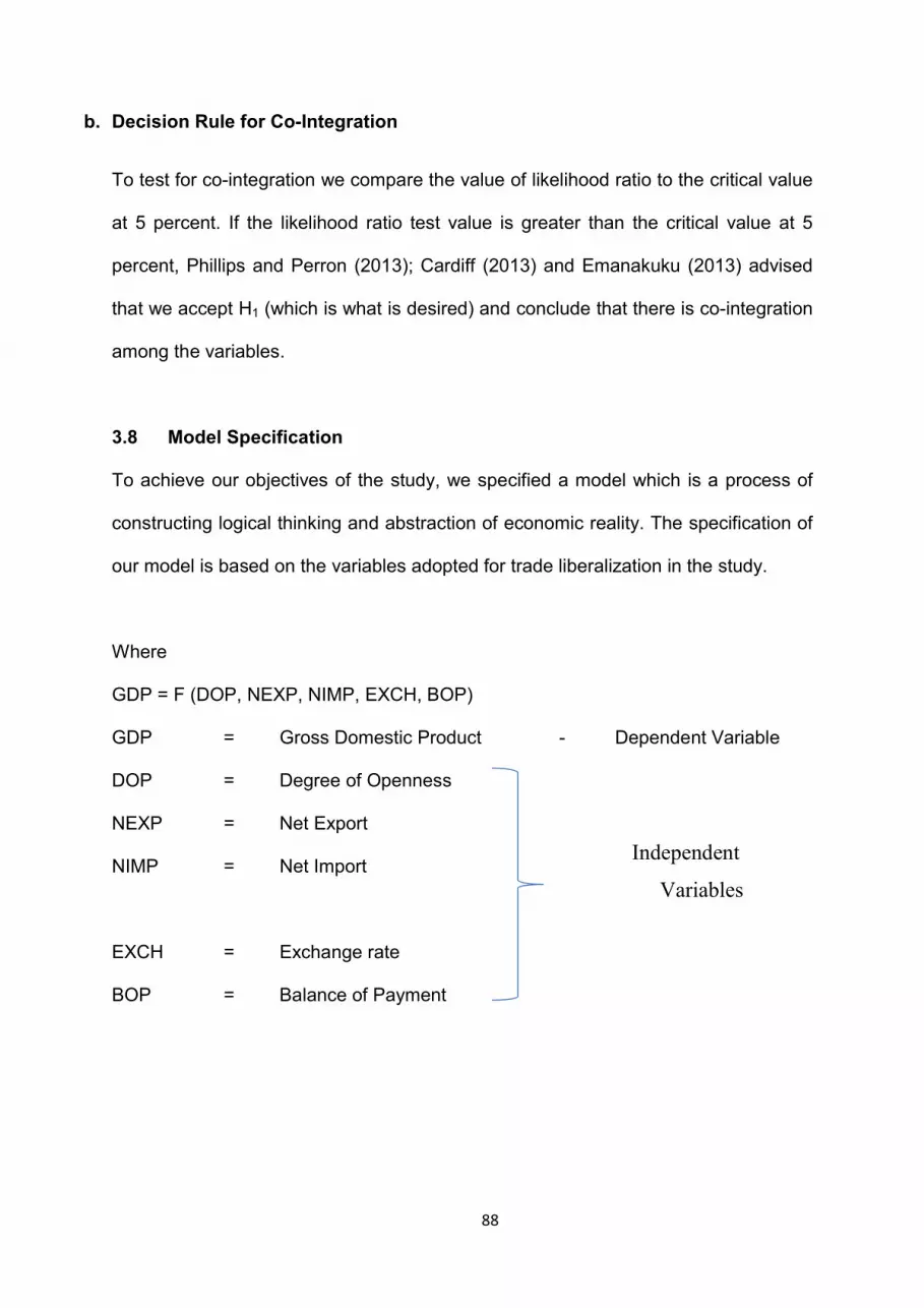
88

b. Decision Rule for Co-Integration

To test for co-integration we compare the value of likelihood ratio to the critical value at 5 percent. If the likelihood ratio test value is greater than the critical value at 5 percent, Phillips and Perron (2013); Cardiff (2013) and Emanakuku (2013) advised that we accept H1 (which is what is desired) and conclude that there is co-integration among the variables. 3.8 Model Specification To achieve our objectives of the study, we specified a model which is a process of constructing logical thinking and abstraction of economic reality. The specification of our model is based on the variables adopted for trade liberalization in the study. Where GDP = F (DOP, NEXP, NIMP, EXCH, BOP) GDP = Gross Domestic Product - Dependent Variable DOP = Degree of Openness NEXP = Net Export NIMP = Net Import EXCH = Exchange rate BOP = Balance of Payment

Independent Variables

89

The model can be expressed in estimation form as follows: GDP = β0 + β1DOP + β2NEXP+ β3NIMP + β4EXCH + β5BOP + µ Where β0 = Constant Intercept; β1- β5 = Coefficients; µ = Error term Apriori Expectation β1, β2, β5 >0 β3, β4 < 0. 3.9 Summary This chapter is dedicated to research methodology. It systematically and scientifically presented a detailed order in which the objectives of the study are to be accomplished. The issues discussed include the research design, population and sample size, sample techniques, method of data collection, techniques of data analysis, data estimation procedure, the model specification and finally the apriori expectations. This chapter noted that the software for analyzing the E-View version 7.0 is justified for such multi regression analysis because it is robust, highly technical and highly efficient. The data estimation procedure was presented with much lucidity and purposefulness.

90

CHAPTER FOUR RESULT AND DISCUSSIONS

4.1 Introduction This chapter considered the presentation and analysis of data from trade liberalization. It considered proxies like Trade Openness, Net Export, Net Import, Exchange Rate and Balance of Payment in Nigeria for the period from 1981-2016 collected from the Central Bank of Nigeria (CBN) Statistical Bulletin (2016). It is critical and vital in order to test the validity of the hypotheses stated in chapter one. 4.2 Data Presentation Table 4.2.1: Data for Trade Liberalization

Dependent Variable Independent Variables YEAR Gross Domestic

Product N’000 B

Degree of Openness%

Net Export N Billion

Net Import N Billion

Exchange rate (N/US$1.00)

BOP (Capital Account) N Billion

1981 15,258.00 0.001 -1.8 1.8 0.6100 -3.8 1982 14,985.08 0.001 -2.6 2.6 0.6729 -1.3 1983 13,849.73 0.000 -1.4 1.4 0.7241 -301.3 1984 13,779.26 0.000 1.9 -1.9 0.7649 354.9 1985 14,953.91 0.000 4.6 -4.6 0.8938 -349.1 1986 15,237.99 0.000 2.9 -2.9 2.0206 -4.1 1987 15,263.93 0.000 12.5 -12.5 4.0179 -17.8 1988 16,215.68 0.000 9.8 -9.8 4.5367 -20.0 1989 17,294.68 0.001 27.1 -27.1 7.3916 -22.5 1990 19,305.63 0.001 64.2 -64.2 8.0378 -5.9 1991 19,199.06 0.011 32 -32 9.9095 -15.6 1992 19,620.19 0.017 62.4 -62.4 17.2984 -101.9 1993 19,927.99 0.019 53.2 -53.2 22.0511 -41.8 1994 19,979.12 0.018 43.3 -43.3 21.8861 -42.6 1995 20,353.20 0.083 195.6 -195.6 21.8861 -195.2 1996 21,177.92 0.088 746.9 -746.9 21.8861 -53.2 1997 21,789.10 0.095 396 -396 21.8861 1.1 1998 22,332.87 0.071 -85.5 85.5 21.8861 -220.7 1999 22,449.41 0.091 326.5 -326.5 92.6934 -326.6 2000 23,688.28 0.123 960.7 -960.7 102.1052 314.1 2001 25,267.54 0.127 509.8 -509.8 111.9433 24.7 2002 28,957.71 0.112 231.5 -231.5 120.9702 -563.5 2003 31,709.45 0.162 1007.7 -1007.7 129.3565 -162.3 2004 35,020.55 0.188 2615.8 -2615.8 133.5004 1124.2 2005 37,474.95 0.268 4445.6 -4445.6 132.1470 -2394.9 2006 39,995.50 0.260 4216.2 -4216.2 128.6516 -2206.5 2007 42,922.41 0.284 4397.8 -4397.8 125.8331 -1811.8 2008 46,012.52 0.347 4794.5 -4794.5 118.5669 -2463.4 2009 49,856.10 0.282 3125.6 -3125.6 148.8802 3927.5 2010 54,612.26 0.369 3847.5 -3847.5 150.2980 -2276.2 2011 57,511.04 0.456 4240.8 -4240.8 153.8616 -810.1 2012 59,929.89 0.415 5372.7 -5372.7 157.4994 -787.3 2013 63,218.72 0.390 5822.6 -5822.6 157.3112 -4205.7 2014 67,152.79 0.349 2421.7 -2421.7 158.5526 2074.8 2015 69,023.93 0.288 2134.4 -1955.1 193.2792 3235.5 2016 67,984.19 1.028 -536.05 536.05 372.8600 1773.9 Source: CBN Statistical Bulletin 2016, Vol. 5 No. 4

91

4.2.1 Discussion of Data Table 4.2.1 shows the trend of Gross Domestic Product, Degree of Openness, Net Export, Net Import, Exchange Rate and Balance of Payment gotten from Central Bank of Nigeria Statistical Bulletin, December 2016, volume 5 number 4. For the purpose of this study, Gross Domestic Product is the dependent variable. It started from N15,258.00B in 1981 and rose to N67,984.19B in 2016 as shown in the table above. Summarily there was a positive increase which can also be interpreted as economic growth during the period under review. This can be attributed to the Net Export, because a rise in a country’s Net Export encourage domestic production thereby stimulating Gross Domestic Product while a fall in the Net Export discourage domestic production which will invariably reduce the Gross Domestic Product. Degree of openness is the sum of export and import divided by Gross domestic product. It recorded between 0.000-1.028 during the period under study. The degree of openness will affect Export, Import and to a considerable level Balance of Payment. Exchange rate has been on a steady rise from 1981 to 2016 increasing from 61Kobo to 372Naira. This is as a result of the country’s high dependence on imported and finished goods which ultimately increased the demand for dollars and put pressure on the local currency (Naira).Likewise a rise in exchange rate will stimulate export by making the goods produced in a country attractive. Balance of payment (capital account) recorded negative values for most part of the period under review. This is because the net earnings on export was less than payment on imports and also the payments made to foreign investors exceeded earnings on foreign investments (factor earnings).It also shows that payment exceeded receipt from international trade. This is attributed to the fluctuations in the price of crude oil which is Nigeria’s major source of foreign exchange earnings. The import figures recorded fluctuated was mostly negative in the period under review.This was attributed to macro-economic conditions and various Government policies in the period.

92

4.2.2 Graphical Illustration Figure 1: Gross Domestic Product (GDP) and Degree of Openness (DOP)

Source: Researcher’s Computation (2017). (Excel, 2010). The figure above illustrates the relationship that exists between gross domestic product (GDP) and degree of openness (DOP). The blue node represents the period under study, the red node represents GDP while the green node represents BOP. GDP figure started between 10,000 and 20, 000, it rose gradually to between 60,000-70,000. On the other hand, BOP was between 0-10,000 all through the period under study.

4.3 Test of Hypotheses Ho1: Degree of Openness (DOP) has no significant impact on Nigeria’s Gross

Domestic Product (GDP). Ho2: Net Export (NEXP) has no significant impact on Nigeria’s Gross Domestic

Product (GDP). Ho3: Net Import (NIMP) has no significant impact on Nigeria’s Gross Domestic

Product (GDP).

01000020000300004000050000600007000080000

1 3 5 7 9 11 13 15 17 19 21 23 25 27 29 31 33 35

YEARGDPDOP

93

Ho4: Exchange Rate (EXCH) has no significant impact on Nigeria’s Gross Domestic Product (GDP).

Ho5: Balance of Payment (BOP) has no significant impact on Nigeria’s Gross Domestic Product (GDP).

4.4 Analysis of Data Techniques 4.4.1 Ordinary Least Square (OLS) Table 4.2.2: Ordinary Least Square (OLS) Output Result Dependent Variable: GDP Method: Least Squares Date: 07/16/17 Time: 16:45 Sample: 1981 2016 Included observations: 36

Variable Coefficient Std. Error t-Statistic Prob. C 16221.89 1226.542 13.22571 0.0000

DOP 45456.92 12584.33 3.612183 0.0011 NEXP 118.1156 32.96514 3.583046 0.0012 NIMP 113.8759 33.07876 3.442567 0.0017 EXCH 21.76110 33.36075 0.652296 0.5192 BOP 1.865941 0.758744 2.459249 0.0199

R-squared 0.936741 Mean dependent var 31758.63 Adjusted R-squared 0.926198 S.D. dependent var 18154.72 S.E. of regression 4932.006 Akaike info criterion 19.99589 Sum squared resid 7.30E+08 Schwarz criterion 20.25981 Log likelihood -353.9260 Hannan-Quinn criter. 20.08801 F-statistic 88.84843 Durbin-Watson stat 2.133978 Prob(F-statistic) 0.000000

Source: E-view 7.0 The least square method tested the results into two folds: The Utility Effect The utility effect tested each variable separate from the other to ascertain the relationship and significance level of each variable to the dependent variable. Below is the discussion of results of each independent variable using the coefficients and p-value of the t-stat.

94

Degree of Openness (DOP): the coefficient of DOP is 45456.92 which show positive impact on Nigeria’s Gross Domestic Product. It revealed positive relationship and significant to GDP as the prob-value of the t-stat for DOP is 0.001< 0.05 critical level. Net Export (NEXP): the coefficient of NEXP is 118.11.It revealed positive relationship but significant to GDP as the prob-value of the t-stat for (NEXP) is 0.001> 0.05 critical level. Net Import (NIMP): the coefficient of (NIMP) is 113.87, which show positive relationship and significant to GDP as the prob-value of the t-stat for (NIMP) is 0.001< 0.05 critical level. Exchange Rate (EXCH): the coefficient of (EXCH) is 21.76, which show positive impact on Nigeria’s Gross Domestic Product. It revealed not significant to GDP as the prob-value of the t-stat for EXCH is 0.519> 0.05 critical level. Balance of Payment (BOP): the coefficient of (BOP) is 1.865. It revealed positive relationship and significant to GDP as the prob-value of the t-stat for (BOP) is 0.01< 0.05 critical level. The Global Effect Global statistics tested the overall independent variables using the R2, Adj R2, Durbin Watson (DW) and F-statistics. The parameter revealed that the coefficients of R2 is 0.936 which is very high and revealed that the whole independent variables DOP, NEXP, NIMP, EXCH and BOP have 94% positive impact to Nigeria’s GDP and indicate that the model is highly accurate and fitted at 94%. More so the coefficients of Adjusted R2 (AdjstR2) is 0.926 which suggest that 93% of the independent variables could be explained by the

95

changes in the dependent variable and the remaining 7% could not be explained due to some error in the financial system. Durbin Watson test is 2.133, this revealed no presence of serial correlation in the series and it is significant. The p-value of the F-stat is 0.000 < 0.05 which suggest that the whole independent variables are statistically significant. 4.4.2 Diagnostic Check Analysis To understand the residual behaviour of the indicators, the indicators are subjected to diagnostic test: Normality test, Serial, Heteroskedasticity and Stability test. Table 4.2.3: Results of Diagnostic Test Diagnostic Check Test F-stat Prob. Conclusion Normality JB 45.151 0.000 It is not normally distributed. Serial LM Test 0.981 0.474 No Presence of serial correlation. Heteroskedasticity BPG 1.308 0.286 No Presence of

heteroskedasticity. Stability Ramsey Reset 0.010 0.918 It is structurally stable. Prob. Value > 0.05, Sig. at 5% for normality, serial, heteroskedasticity and stability tests. Source: Author’s Result, 2017.vice versa 4.4.3 Unit Root Test Table 4.2.4: Unit Root Based on Augmented Dickey Fuller Test Result Variable Order ADF Critical value ADF>Critical Value Conclusion GDP I(2) -5.1361 -2.9540 No unit root Stationary DOP I(2) -3.7481 -2.9918 No unit root Stationary NEXP I(0) -3.3614 -2.9718 No unit root Stationary NIMP I(0) -3.2837 -2.9718 No unit root Stationary EXCH I(2) -3.7044 -2.9540 No unit root Stationary BOP I(2) -4.6416 -2.9718 No unit root Stationary Source: Author’s Unit Root Output

96

4.4.4 Granger Causality Analysis This test was applied to confirm the assumptions of the ordinary least square (OLS). Table 4.2.5: Results of Ganger Causality Test Diagnostic Check F-stat Prob. Conclusion DOP and GDP 12.0877 0.0002 DOP granger cause GDP GDP and DOP 10.5851 0.0004 GDP granger cause DOP NEXP and GDP 6.77118 0.0039 NEXP granger cause GDP GDP and NEXP 3.72251 0.0336 GDP granger cause NEXP NIMP and GDP 6.86920 0.0036 NIMP granger cause GDP GDP and NIMP 3.52323 0.0427 GDP granger cause NIMP EXCR and GDP 2.9972 0.0654 EXCR does not granger cause GDP GDP and EXCR 4.69193 0.0172 GDP granger cause EXCR BOP and GDP 3.92001 0.0311 BOP granger cause GDP GDP and BOP 0.42123 0.6602 GDP does not granger cause BOP Prob. Value < 0.05, Sig. at 5% for granger causality test, vice versa. Source: Author’s Result, 2017. 4.4.5 Co integration Output Date: 07/18/17 Time: 09:24 Sample (adjusted): 1982 2016 Included observations: 35 after adjustments Trend assumption: Linear deterministic trend Series: GDP DOP NEXP NIMP EXCH BOP Lags interval (in first differences):

Unrestricted Co integration Rank Test (Trace) Hypothesized Trace 0.05

No. of CE(s) Eigenvalue Statistic Critical Value Prob.** None * 0.973813 291.4982 95.75366 0.0000

At most 1 * 0.879050 164.0106 69.81889 0.0000 At most 2 * 0.694629 90.07726 47.85613 0.0000 At most 3 * 0.532443 48.55927 29.79707 0.0001 At most 4 * 0.382570 21.95106 15.49471 0.0046 At most 5 * 0.134963 5.074425 3.841466 0.0243

Trace test indicates 6 cointegratingeqn(s) at the 0.05 level * denotes rejection of the hypothesis at the 0.05 level **MacKinnon-Haug-Michelis (1999) p-values Source: E-view 7.0

97

4.5 DISCUSSION OF FINDINGS The model included the basic trade liberalization variables affecting economic growth in Nigeria such as Degree of Openness, Net Export, Net Import, Exchange Rate and Balance of Payment. From the result, it can be seen that there is a positive relationship between Degree of Openness (DOP) and Economic Growth as a unit increase in degree of openness leads to 16221.89 unit increase in economic growth. There is a positive relationship between Net Export (NEXP) and Economic Growth as a unit increase in net export (NEXP) leads to 118.11 unit increase in economic growth. There is a positive relationship between Net import (NIMP) and Economic Growth as a unit increase in net import (NIMP) leads to 113.87 unit increase in economic growth. Positive relationship exists between Exchange Rate (EXCR) and Economic Growth as a unit increase in exchange rate (EXCR) leads to 21.76 unit decrease in economic growth. Similarly, there is a positive relationship between Balance of Payment (BOP) and Economic Growth as a unit increase in balance of payment (BOP) leads to 1.865 unit increase in economic growth. The test of individual significant of each of the independent variable was done using the t-stat and their respective p-values. The p-values reveal that Degree of Openness (DOP), Net Export (NEXP), Net Import (NIMP) and Balance of Payment (BOP) are statistically significant while Exchange Rate (EXCH) is not statistically significant. The model has high explanatory and predictive power as suggested by the

98

R-squared and Adjusted R-squared respectively. The R2 is 0.936741and AdjR2 is 0.926198.This further shows that (DOP, NEXP, NIMP, EXCH and BOP) have 93% positive impact on Nigeria’s GDP. Furthermore (AdjstR2) is 0.926 which suggest that 92% of (DOP, NEXP, NIMP, EXCH and BOP) could be explained by the changes in the economic growth and the remaining 7% could not be explained due to some error in the financial system. The Durbin Watson test is 2.133, which revealed no presence of serial correlation and good for prediction. The p-value of the F-stat is 0.000 < 0.05 which suggest that the whole independent variables (DOP, NEXP, NIMP, EXCH and BOP) are statistically significant. We accept the alternate hypothesis HA and conclude that the whole independent variables are significant to GDP in Nigeria. The normality test determines normal distribution of the variables. The normality output in table 4.2.3 suggests that the series distribution is not normal as the p-value is 0.000 which is less than 5% significant level. For serial correlation test the p-value of the f-statistics is 0.4745 which is greater that the critical value of 5%, we conclude by accepting H0 that there is no presence of serial correlation which is desirable and the model is fit to predict trade liberalization and Gross domestic product in Nigeria. In heteroskedasticity test the p-value of the observed R squared is 0.265 which is greater than the critical value of 5%, therefore we accept null hypothesis that the residuals are not heteroskedastic which means that the residuals are homoskedastic and it is desirable. Also the p-value of the f-stat in functionality test is 0.9181which implies that the series is in functional form and statistically stable.

99

The Augmented Dicker Fuller test (ADF) at order 2I (2) for GDP is 5.136 > 2.954 at 0.05 level of significance, this shows no unit root which implies that the series is stationary. DOP at order 2I (2) is 3.748 > 2.991 at 0.05 level of significance, this shows no unit root and the series is stationary. NEXP at level I (0) is 3.361 > 2.971 at 0.05 significant level, this shows no unit root and that the series is stationary. NIMP at level I (0) is 3.283 > 2.971 at 0.05 significant level, this shows no unit root and that the series is stationary. BOP at level I (0) is 4.641 > 2.971 at 0.05 significant level, this shows no unit root and the series is stationary. The result suggests that there is no presence of unit root as the ADF values are greater than the critical value at 5%. Hence the variables are stationary which informs co-integration and granger causality test. For granger causality test, the probability value of DOP, NEXP, NIMP and BOP are 0.0002, 0.0039, 0.0036 and 0.0311 respectively and are less than 0.05 at 5% level. This shows that DOP, NEXP, NIMP and BOP granger cause GDP and GDP granger cause DOP, NEXP and NIMP as the probability values are 0.0004, 0.0364 and 0.0427 which are less than 5% level.GDP does not granger cause BOP because the p-value is 0.6602 which is greater than 5%. However the probability value of EXCH is 0.0654 which is greater than 5% level. This shows that EXCH does not granger cause GDP, but GDP granger cause EXCH because its p-value is 0.0172 and less than 5%. Furthermore DOP and GDP have a dual causality because the two variables granger causes each other. This also applies to NEXP and GDP, NIMP and GDP.While EXCR and GDP, BOP and GDP have a bi-causality relationship because only one variable granger causes each other. Johansen co-integration test was carried out to measure the long run equilibrium relationship among GDP, DOP, NEXP, NIMP, EXCH and BOP.

100

The co-integration result shows that the trace statistics of all the independent variables (164.0106, 90.0772, 48.5592, 21.9510 and 5.0744) are greater than all the critical values at 5% (69.81889, 47.85613, 29.79707, 15.49471 and 3.8414). There is enough evidence to accept Ho and conclude that the variables are co integrated at most1* to at most 5*. The probability associated with the trace statistics are all less than 5% which connote that the variables have long run equilibrium that is the variables move together in the long run. 4.6 SUMMARY The section above made emphasis on the presentation and analysis of data gotten from Central Bank of Nigeria Statistical Bulletin (2016). Efforts were made to present the results in factual and original form, interpretation were made and inference drawn from the results.

101

CHAPTER FIVE CONCLUSION AND RECOMMENDATIONS 5.1 CONCLUSION The importance of trade liberalization on the Nigerian economy cannot be over-emphasized; a lot of studies and arguments have taken place over the years in order to ascertain the relationship between trade liberalization and Nigeria’s economic growth. While some have found a positive relationship or effect, others share contradictory views. The findings of this study are in line with the work of Harrison (2012), Greenaway et al (2012) and Dollar & Kraay (2014).The following are the derivable conclusion:

i. Degrees of Openness (DOP), Net Export (NEXP), Net Import (NIMP) and Balance of Payment (BOP) have positive and significant impact on the economic growth in Nigeria. Exchange rate (EXCH) has positive relationship but not significant to economic growth in Nigeria. Holistically all the independent variables have positive and significant effect on the growth of Nigeria economy.

ii. The diagnostic test suggests that the series distribution is not normal, there is no presence of serial correlation which is desirable, in heteroskedasticity test we accept the null hypothesis that the residuals are homoscedastic in nature and it is desirable.

iii. In granger causality test, DOP and GDP have dual causality because the two variables granger causes each other. This also applies to NEXP and GDP, NIMP and GDP. While EXCR and GDP, BOP and GDP have a bi-causality relationship because only one variable granger cause each other.

102

iv. The co integration result shows enough evidence to accept Ho and conclude that the variables are co-integrated. The probability associated with the trace statistic is 0.000<0.05 at 5%. The variables have long run equilibrium that is the variables move together in the long run.

v. The study conclude that trade liberalization have positive and significant effect on the economic growth in Nigeria.

5.2 RECOMMENDATIONS

The study thereby recommends the following:

1. Government must continue to adopt appropriate policies to diversify the productive base of the economy, in order to promote net exports, and build up an efficient service infrastructure to drive private domestic and foreign investment. Hence, it is further suggested that government should provide necessary incentives to produce export products. Furthermore, to enhance export performance, the government has to undertake systematic review of the effectiveness of the subsidy reinvestment program (SUREP). Domestic trade policies have to be reformed by reducing anti- export bias through fully implementing the lower duty rates of ECOWAS. Nigeria should continue the privatization program and service sector liberalization to reap the benefits from openness.

2. Exchange rate liberalization is also critical in facilitating trade in any economy, we therefore advise the policy makers to ensure that exchange rate should be determine by the forces of demand and supply.

103

3. Dependency on import goods both at domestic and industrial production level should be discouraged with the aim of embarking on import substitution approach to economic development in Nigeria.

4. The financial sector has to be closely monitored by the Central Bank, especially commercial banks. This is to ensure stability in the interest and exchange rate.

5. The Nigerian government also needs to moderate its trade liberalization policy as the economy seems too weak to absorb the negative shocks from external trade.

5.3 CONTRIBUTION TO KNOWLEDGE A study contributes to knowledge when that study provides answer to the existing research question.

1. Therefore the study contributed to knowledge because it has developed a model that can predict trade liberalization in Nigeria. GDP = f(DOP,NEXP,NIMP,EXCH,BOP).

2. The study contributed to knowledge by investigating the relationship that exists between Degree of Openness, Net Export, Net Import, Exchange Rate, Balance of Payment and Gross domestic product in Nigeria between 1981-2016.It also created insight into policy recommendation that is capable of enhancing economic growth in Nigeria.

3. The study used a more robust technique in analyzing the relationship between trade liberalization and economic growth in Nigeria.

Most studies like Shafaeddin (2014), Low (2014) focused on trade liberalization variables like degree of openness, import and export, but this study took a step further to introduce additional variables like exchange rate and balance of payment.

104

REFERENCES

Adelowokan, O.A., and Maku, A.O. (2013). Trade Openness, Foreign Investment and Economic Growth in Nigeria: A Long-Run Analysis. European Journal of Globalization and Development Research, Vol. 7, No. 1.

Adeyemi, K.S. (2012). Economic Policy Reforms in Nigeria: Achievements and Challenges in Union Digest. An Economic and Business Publication of Union Bank of Nigeria, PLC, Vol 10, No 2.

Ajayi, K. (2015). International Administration and Economic Relations in a Changing World. Damas Educational Services Limited, Accra North, Ghana.

Anderson, D.R., Sweeney, D.J., & Williams, T.A. (2013). Modern Business Statistics. Melissa Acuna Publishers. South-Western, 5101 Madison Road, Cincinnati,

Ohio, 45227.USA. Antinie, C., Khour, E.L. & Andreas, S. (2013). Openness in Service Trade and Economic Growth. University of Maryland Baltimore, U S A.

Anyiwe, M.A., Idahosa D.O. & Ibeh S.E., (2013). Basic Research Methods in Social Sciences. Mindex Press. Benin City.

Arhan, S. E. (2014). Differential Effects of Trade Liberalization on Economic Growth: Role of Human Capital Accumulation. American Economic Review, 50 (6), 130-140.

Ayonrinde, F. & Olayinka, O. (2012).Trade liberalization and technology acquisition in the manufacturing sector: evidence from Nigeria.AERC Research Paper. No. 117.

Bakare, A.S. (2014). The consequences of Trade Liberalization for Economic Growth in Nigeria: A Stocastic Investigation. Contemporary Marketing Review Vol 1(14) pp.14- 23.http://www.businessjournalz.org/emr.

105

Baldwin, R.E. (2012). Growth effects of Anticipated trade liberalization and the Baldwin Multiplier. Economic letters volume 59, issues 2.

Baldwin, R.E. (2013). Trade and Growth: Still Disagreement about the Relationship. OECD Economics Department working Paper No 11.26x. OECD Economics Department.

Baridam, D.M. (2013). Research Methods in Administrative Sciences. Port Harcourt: Sherbrook Association.

Ben, D. (2013). Equalizing Exchange: Trade Liberalization and income convergence. Quarterly Journal of Economics 108: 653-679.

Ben, S. & Bernanke, (2015).The Global Saving Glut and the U.S. Current Account Deficit.Federalreserve.gov. March 2005.Retrieved 2015-01-13.

Bertrand, C. (2013). The Unequal Effects of Liberalization: Theory and Evidence from India. Harvard University and CEPR.

Bowerman, O’Connel & Hand, B. (2013). Business Statistics in Practice. Second Edition. McGraw-Hill Books.NY.USA.

Bushra, Y., Zainab, J. & Muhammad, A. C. (2014). Trade Liberalization and Economic Development: Evidence from Pakistan. Journal of Economics, pp.19-34.

Caner, M. & Kilian, L. (2012). Size Distortions of Tests of the Null Hypothesis of capital Structure: Evidence and Implications for the PPP Debate. Journal of International Money and Finance. Vol. 234.No. 34.p.60-79.

Cardiff, C.O. (2013). The Structural Adjustment Programme: The Journey so far. Economic and Financial Review. The Central Bank of Nigeria. Vol. 25. No, 4. p.25-28.

Carmen, R. & Kenneth, R. (2014). This Time Is Different: Eight Centuries of Financial Folly. Princeton University Press. pp. 208–212. ISBN 0-19-926584

106

Chakraverty, S. & Singh, .A. (2014).The Desirable Forms of Economic Openness in the South Mimeo. Helsinki, WIDER (World Institute for Development Economics Research.

Chaudhry, Malik & Faridi. (2013).Greek Lessons for the World Economy Project Syndicate Retrieved 2010-05-19.

Cheol, S. &, Bruce, G. R. (2013). International Financial Management China Machine.

Chris, Brooks. (2012). Introductory Econometrics for Finance, Cambridge University Press. The Edinburg Building, Cambridge. UK.

Daniel, k., Denilson, & Adelar. (2013). Trade Liberalization and Environment in the Pacific Basin; Coordinated Approaches to Mexican Trade and Environment Policy. American Journal of Agricultural Economics.

Daniels, J., Radebaugh, L. &, Sullivan, D. (2013). International Business: environment and operations, 11th edition.Princeton Hall.ISBN 0-13-186942-6.

Darren, S. (2014). Balance of Payments. In David R. Henderson (ed.). Concise Encyclopedia of Economics (2nd ed.). Indianapolis: Library of Economics and Liberty.

DeRosa, D.A. (2012). Regional integration arrangements: Static economic theory, Quantitative findings and policy guidelines. World Bank, Development

Research Group, Policy Research Working Paper No. 2012. Dickey, D. & Fuller, W. (2012). Lag Length Selection and the Construction of Unit

Root Tests with Good Size and Power. Econometrica.Vol. 69. No. 8 p. 13-30. Dickey, D. & Fuller, W. (2012). Likelihood Ratio Statistics for Autoregressive Time

Series with a Unit root. Econometrica.Vol. 4. No. 4 p. 1-4.

107

Dickey, D. & Fuller, W. (2012).Distributions of the Estimators for Autoregressive Time Series. Journal of the American Statistical Association. Vol. 67.No.12 p.37-76.

Doan, Q. & Ron, D. (2013).Trade Liberalization, Economic Growth and Poverty Reduction Strategies. National Centre for Development Studies, Australian National University.

Dollar, D. & Kraay, R. (2014).Trade, Growth and Poverty. Mimeo, the World Bank. Dollar, D. (2012). Outward-Oriented developing Countries really do grow more. Drabeck, B. & Laird, S. (2013). Can trade policy help mobilize financial resources for

economic development? WTO Research and Analysis Working Paper 2012. Echekoba, F.N, Okonkwo, V.I & Adigwe, P.K. (2015). Trade Liberalization and

Economic Growth: The Nigerian Experience: Journal of Poverty, Investment and Development. Vol. 14, 51-72.

Edwards, S. (2012). Openness, productivity and growth: What do we really know? Economic Journal 108.383-98.

Eleanya, K.N. (2013). Openness and Economic Growth in Nigeria. Journal of Education and Practise. Vol. 4 no. 1.Pp. 68-73.

Eli, Hecksher & Bertil, Ohlin. (2013). Trade Liberalization and Environment in the Pacific Basin; Coordinated Approaches to Mexican Trade and Environment Policy. American Journal of Agricultural Economics.24(2).

Elliot, G., Rothenberg, T.J. & Stock J.H. (2012). Efficient Tests for an Autoregressive Unit Root. Econometrica.Vol. 7 No. 3. P.23-45

Emanakuku, E. (2012). Some Tests of Specification for Pane Data: Equilibrium Model. Quarterly Journal of Economics, Vol. 3.No.4 p.587-609.

Eric, G. (2013).Trade Policies and Developing Nations.Washington, DC:

108

Ersoy, B.& Deniz, G. (2012). Openness and inflation: Theory and Evidence. Journal of Economics 5(1).700 – 930.

Esene, R.A.(2012). Research Methods in Education, Social Sciences and Vocational Studies. Royal Pace Publications.Agbor. Nigeria.

Frankel, J.A.& Romer,D. (2013).Does Trade Case Grow ?American Economic Review (2013) Volume 83 (3). 379-399.

Geoff, K. (2014). Balance of Payments.In David R. Henderson (ed.). Concise Encyclopedia of Economics (2nd ed.). Indianapolis: Library of Economics and Liberty.

George, A. V. (2013). Trade Liberalization and Economic Expansion: A Sensitivity Analysis. Athens: University of Economics and Business, 71-88.

Granger,G.&Newbold,P.(2012).Time Series Regression with a Unit Root. Econometrica.Vol. 55.No. 15 p.15-25.

Greenway, M. D.,Wynn, C. & Wright, P. (2012).Trade Liberalization and Growth in Developing Countries. Journal of Development Economics, 67(1):229-244.

Gundlach, E. (2015). Openness and Economic Growth in Developing Countries. Research Working paper.pp 749.

Haddad, B. A. (2013). International Financial Management China Machine. Hamilton, J. (2013).Time Series Analysis.Princeton University Press. New Jersey. Hatanaka,T. (2012). Time Series Based Econometrics: Unit Roots and Co-

Integration. Journal of Econometrics.Vol. 22.No.26. p.9-12. Harberzar, A. C. (2014). Currency Depreciation, Income and Balance of

Trade.Journal of Political Economy. HR focus 31, 4-7. Harris, T.W. (2012). Introduction to Econometrics.Hall Mark Publishing House.

London.

109

Harrison, A. (2012).Openness and Growth: A Time Series, Cross – Country Analysis for Developing Countries. Journal development economics.; 48:419–447.

Harrison, A. & Hanson, G. (2013). Who gains from trade reform? Some remaining puzzles. Journal of Development Economics. 59. 125-154.

IMF, (2014). Balance of Payments Manual. Chapter 2 Overview of the Framework, Paragraph 2. (15).

Irwind,D. & Tervio, H. (2012). Does trade raise income? Evidence from the Twentieth Century. Journal of international Economics, Volume 58 (1) PP1

Iyoha, M.A. & Ekanem, O.T. (2012).Introduction to Econometrics. Mareh Books Ltd. Benin City.

Jaramillo, F. (2013). Capital Market Imperfections Before and After Financial Liberalization: A Euler Equation Approach to Panel Data for Ecuadorian Firms. World Bank Working Paper WPS 1091.p.34-53

Jeffrey, H. (2015). The Unequal Effects of Liberalization: Theory and Evidence from India. Harvard University, University College London and CEPR.

Jerome, A. & Adenikinju, A. (2013).Trade policies and the promotion of manufactured Exports in Nigeria. Proceeding of Nigeria Economic Society Annual Conference. Ibadan.

Joshi, Rakesh Mohan. (2014).International Business, Oxford University Press, New Delhi and New York ISBN 0-19-568909-7.

Kankesu, A. (2012). Outward-Oriented developing Countries really do grow more. Keith, H. (2014). Trade Liberalization and the Environment: A Study of NAFTA’S

Impact on El Paso, Texas and Juarez, Mexico (Master’s Thesis). Virginia Polytechnic Institute and State University.

110

Keynes, T. (2013). Equalizing Exchange: Trade Liberalization and income convergence. Quarterly Journal of Economics 108: 653-679.

Klein, A.& Olivei, F. (2012). Openness, productivity and growth: What do we really know?.Economic Journal 108,383-98.

Kothari, C.R (2014). Research Methodology Methods and Techniques. New Delhi, New Age International Publishers Limited.

Krueger, A.O.,(2015).Trade Policies and Developing Nations. Washington, DC: Brooking Institution.

Krugman,& Lancaster, (2012). Rethinking International Trade.MIT press, Cambridge, Mass.

Kwiatkowski, S.A.(2012).Testing the Null Hypothesis of Stationarity Against Alternative of a Unit Root. Journal of Econometrics.Vol. 54.No, 5.p.33-39.

Lopez, R. A. (2013). Trade and growth: Reconciling the macroeconomic and microeconomic evidence.Journal of Economic Surveys 19, 623-48.

Low, L. (2014). The Political Economy of Trade Liberalization.Asia-Pacific Development Journal, 1(1).

Loayze, V. (2013).Openness and Growth: A Time Series, Cross – Country Analysis for Developing Countries. Journal development economics.

Lucas, R. E. (2013). On the Mechanics of Economic Development. Journal of Monetary Economics, 2 (2): 3-42.

Lyon, A. (2013).Taxation, Information Asymmetries, and a Firm’s Financing Choices. World Bank Working Paper.Vol.19. No. 35.p.50-71.

Mac-Kinnon, J. (2014). Numerical Distribution Functions for Unit Root and Co integration Tests. Journal of Applied Econometrics.Vol. 4.No. 34.P.7.

111

Maddala, G.S. (2012). Unit Roots, Cointegration and Structural Change.Oxford University Press.

Mankiw, N.G. (2013). Macroeconomics.Sixth Edition, Harvard University. Manson, N. (2014). Trade Liberalisation and Poverty in Nigeria; Lessons from the

past, Nigeria. African Institute for Applied Economics. www.rldis.org/assets/Docs.

Martins, D. (2013). On the Mechanics of Economic Development. Journal of Monetary Economics.

Mesike, C.S. et al (2014). Analyzing the effects of Trade Liberalisation policy on Nigerian Rubber Industry.Journal of Agriculture and Social Science. http://www.fspublishers,org.

Mike, M (2015). The Economic Effect of Tariffs. Retrieved 27 July 2015. Musibau, A.B. (2015). Trade Policy Reform, Integration and Export Performance in

ECOWAS Sub- Region. University of Ibadan, Nigeria. Mwaba, A. (2013). Trade Liberalization and Growth: Policy Options for African

Countries in a Global Economy. African Development Bank, Economic research papers No 60.

Ndiyo, N.A (2013). Fundamentals of Research in Behavioural Sciences and Humanities. Calabar: Wusan Publishers.

Nwako, G. (2015).Trade Liberalization and Growth in Developing Countries. Journal of Development Economics.

Newbold, P.(2012). Spurious Regression in Econometrics.Journal of Econometrics.Vol. 2.No.6. p.90-112.

Ng, S.& Perron, P. (2013).Unit Roots and Co integration Analysis. Journal of Applied Econometrics.Vol. 1.No. 19.P.113-189.

112

Nkonyeasua, P.O. (2013). Practical Approach to Research Methodology. Pee Jen Publications. Asaba Nigeria.

Obadan, M.I. (2014). Economic Globalisation, Markets and National Development: How sensibly do the poor countries (Nigeria included) stand?,Inaugural lecture series.University of Benin, Benin City, September 18.

Obioma, O. S. (2012). Trade Openness, Productivity and Economic Growth in Nigeria.University of NigeriaNsukka, Enugu. Ogujiuba,K.K., Oji, G.O.,& Adenuga (2014). Is “Trade” Openness Valid for Nigeria’s

Long Run Growth: A Co integration Approach” A Paper Presented to the USAID-Nigeria.

Olannye, P. I. (2013). Research Methods for Business: A Skill Building Approach. Lagos: Peejan Publication Pg. 45.57.

Omoke, P. (2014). Impact of trade Liberalization on the Environment in Developing Countries p 40.

Osllivan, D. (2013). Trade Liberalization and Growth: Policy Options for African Countries in a Global Economy. African Development Bank, Economic research papers

Paul, D. (2014). The Keynes Solution: The Path to Global Economic Prosperity. Palgrave Macmillan. pp. 123–138. ISBN 978-0-230-61920-3.

Philippe, A. (2013). The Unequal Effects of Liberalization: Theory and Evidence from India. Harvard University, University College London and CEPR.

Phillips, P.C.B.& Perron P. (2013).Testing for Unit Roots in Time Series in the State of Development Economics. Presented to Conference on Capital Market Development and Privatization. Lagos.

113

Porter, E. (2015).Trade Liberalization and Economic Performance: An overview. The Economic Journal, 214 USA.

Pritchett, A. W. (2014). Openness and Growth: A Time Series, Cross-Country Analysis for Developing Countries. NBER Working Paper 5221, Cambridge, Massachusetts.

Ralph, A. (2012). The Bundesbank and global imbalances. The Financial Times. Retrieved 2010-01-12.

Raymond, A. (2012). Trade Liberalization and Economic Expansion: A Sensitivity Analysis. Athens: University of Economics and Business,

Razin, & Rose, (2014).Does Trade Case Growth? American Economic Review (2014) Volume 53 (3).

Ricardo, D (2012). The Theory of comparative Advantage. Richard, T. (2012). Does Globalization Hurt that the Poor? Policy Research working

paper 2922: Poverty Reduction and Economic Management Division. World Bank Institute.

Richard, T (2012). An Inquiry into the Nature and Causes of the Wealth of Nations. New York: Random House. (Originally 1776).

Roberts, (2014). On the Mechanics of Economic Development. Journal of Monetary Economics, 2 (2): 8-45.

Rodriguez, F. & Rodrik D, (2014).Trade Policy and economic growth: a skeptic’s guide to the Cross – national evidence; NBER, 27081.

Rodrik, D. (2014). The Global Governance of Trade as if Development Really Mattered.UNDP.

Romer,D.(2013). Openness and inflation: Theory and Evidence. Journal of Economics 4(1), 869 – 903.

114

Sachs, J.D. & Warner, A. (2015).Economic reform and the process of global integration. Brookings Papers on Economic Activity 1, 1-118.

Saibu, A. (2014). Trade Policy Reform, Integration and Export Performance in ECOWAS Sub- Region. University of Ibadan, Nigeria.

Sakyi,J.(2012).Openness, productivity and growth: What do we really know?.Economic Journal 108,383-98.

Sargan J. D. & Alok Bhargava (2012) .Maximum Likelihood Estimation of Regression Models with First Order Moving Average. Econometrica. Vol.87.No. 5 p.10-22.

Sargan, J.D. & Alok ,Bhargava. (2012).Testing Residuals from Least Square Regression by the Gaussian Random Walk. Econometrica. Vol. 51.No. 12. P11-38.

Schiff, J. & Winter, M. (2012). Trade Liberalization and Environment in the Pacific Basin; Coordinated Approaches to Mexican Trade and Environment Policy. American Journal of Agricultural Economics.24 (2).

Schwert, W. (2013).Test for Unit Roots: A Monte Carlo Investigation. Journal of Business and Economic Statistics.Vol. 7 No.3 p.99-123.

Shafaeddin, M. (2014). Does Trade Openness Favour or Hinder Industrialization and Development? Third World Network, Malaysia.

Shokan, O. O. (2014). Research Methodology and Seminar for all discipline: Shokan Investment Company Ltd., Nigeria.

Sloman, K. (2014). Balance of Payments Deficit in Developing Countries. Stein, H. (2014). Balance of Payments. In David R. Henderson (ed.). Concise

Encyclopedia of Economics (2nd ed.). Indianapolis: Library of Economics and Liberty.

115

Tybout, N. (2012).Product Quality, Productive Efficiency, and International Technology Diffusion. Bernard Heokman and Beats Smarzynska Javorick, eds, Global Integration and Technology transfer. Washington, DC; The World Bank and Palgrave McMillan, 2012.

Ude, D.K. & Agodi, J.E. (2015). Does Trade Openness Make Sense? Investigation of Nigeria Trade Policy. International Journal of Academic Research in Economics and Management Sciences.Vol. 4, No 1.

Ukwueze, E. R. (2013). The Concept of Trade and Economic Reliance for Nigeria, in Obiora Anichebe (ed), Issues in Nigeria People and Culture. (Nsukka, Afro-Orbis publication Ltd 2013). 175 – 179.

UNDP, (2013).World Investment Report (2013). Winters, A. L. (2014). Trade Liberalization and Economic Performance: An overview.

The Economic Journal, 114 USA. Yarbrough, B. & Yarbrough, R. (2014). The World Economy, Trade and Finance (3rd

Ed.).USA: The Dryden Press Harcourt Brace College Publisher. Yomere, G.O. & Agbonifoh, B.A. (2013).Research Methodology in Social Sciences

and Education.Uniben Press. Benin City. Nigeria. Yusuf, Malarvizhi & Khin (2013).Openness and inflation: Theory and Evidence.

Journal of Economics.

116

APPENDIX Ordinary Least Square (OLS) Output Result Dependent Variable: GDP Method: Least Squares Date: 04/14/17 Time: 16:08 Sample: 2000 2015 Included observations: 16

Variable Coefficient Std. Error t-Statistic Prob. DOP -298532.7 128463.6 -2.323870 0.0425

NEXP -25.58884 51.28348 -0.498968 0.6286 NIMP -34.68046 53.58017 -0.647263 0.5320 EXCH 314.8451 151.0385 2.084536 0.0637 BOP 0.764161 0.865075 0.883347 0.3978

C -6587.002 18998.64 -0.346709 0.7360 R-squared 0.935794 Mean dependent var 45772.10

Adjusted R-squared 0.903691 S.D. dependent var 14943.98 S.E. of regression 4637.675 Akaike info criterion 20.00181 Sum squared resid 2.15E+08 Schwarz criterion 20.29153 Log likelihood -154.0145 Hannan-Quinn criter. 20.01665 F-statistic 29.14966 Durbin-Watson stat 2.133978 Prob(F-statistic) 0.000012

Source: E-view 7.0 Normality test

012345678

-5000 -2500 0 2500 5000 7500 10000 12500

Series: ResidualsSample 2000 2015Observations 16Mean -2.14e-11Median -696.4857Maximum 10964.81Minimum -4746.531Std. Dev. 3786.646Skewness 1.525297Kurtosis 5.473770Jarque-Bera 10.28377Probability 0.005847

117

Breusch-Godfrey Serial Correlation LM Test: F-statistic 1.175298 Prob. F(2,8) 0.3569

Obs*R-squared 3.633562 Prob. Chi-Square(2) 0.1625

Test Equation: Dependent Variable: RESID Method: Least Squares Date: 04/14/17 Time: 16:09 Sample: 2000 2015 Included observations: 16 Presample missing value lagged residuals set to zero.

Variable Coefficient Std. Error t-Statistic Prob. DOP -155152.2 168590.8 -0.920288 0.3843

NEXP -5.923091 57.32397 -0.103327 0.9202 NIMP -10.34580 58.74169 -0.176124 0.8646 EXCH -220.6717 231.2938 -0.954075 0.3680 BOP 1.169699 1.512355 0.773429 0.4615

C 26092.94 27743.01 0.940523 0.3745 RESID(-1) -0.792196 0.882897 -0.897269 0.3958 RESID(-2) -0.756487 0.548845 -1.378326 0.2054

R-squared 0.227098 Mean dependent var -2.14E-11 Adjusted R-squared -0.449192 S.D. dependent var 3786.646 S.E. of regression 4558.455 Akaike info criterion 19.99421 Sum squared resid 1.66E+08 Schwarz criterion 20.38050 Log likelihood -151.9537 Hannan-Quinn criter. 20.01399 F-statistic 0.335799 Durbin-Watson stat 2.046818 Prob(F-statistic) 0.915857

Heteroskedasticity Test: Breusch-Pagan-Godfrey

F-statistic 0.981220 Prob. F(5,10) 0.4745 Obs*R-squared 5.266139 Prob. Chi-Square(5) 0.3843 Scaled explained SS 4.601463 Prob. Chi-Square(5) 0.4664

Test Equation: Dependent Variable: RESID^2 Method: Least Squares Date: 04/14/17 Time: 16:10 Sample: 2000 2015 Included observations: 16

Variable Coefficient Std. Error t-Statistic Prob. C -28341474 1.21E+08 -0.234858 0.8191

DOP -2.96E+08 8.16E+08 -0.363204 0.7240 NEXP -388236.3 325741.2 -1.191855 0.2608 NIMP -393265.7 340329.2 -1.155545 0.2747 EXCH 379608.1 959362.4 0.395688 0.7006 BOP 5838.210 5494.760 1.062505 0.3130

R-squared 0.329134 Mean dependent var 13442519 Adjusted R-squared -0.006300 S.D. dependent var 29365123

118

S.E. of regression 29457470 Akaike info criterion 37.51479 Sum squared resid 8.68E+15 Schwarz criterion 37.80451 Log likelihood -294.1183 Hannan-Quinn criter. 37.52963 F-statistic 0.981220 Durbin-Watson stat 2.046270 Prob(F-statistic) 0.474512

Ramsey RESET Test Equation: UNTITLED Specification: GDP DOP NEXP NIMP EXCH BOP C Omitted Variables: Squares of fitted values

Value df Probability t-statistic 0.955206 9 0.3644 F-statistic 0.912419 (1, 9) 0.3644 Likelihood ratio 1.545022 1 0.2139

F-test summary: Sum of Sq. df

Mean Squares

Test SSR 19797730 1 19797730 Restricted SSR 2.15E+08 10 21508030 Unrestricted SSR 1.95E+08 9 21698063 Unrestricted SSR 1.95E+08 9 21698063

LR test summary: Value df

Restricted LogL -154.0145 10 Unrestricted LogL -153.2420 9

Unrestricted Test Equation: Dependent Variable: GDP Method: Least Squares Date: 04/14/17 Time: 16:11 Sample: 2000 2015 Included observations: 16

Variable Coefficient Std. Error t-Statistic Prob. DOP -616698.8 357204.7 -1.726458 0.1183

NEXP -44.42315 55.15445 -0.805432 0.4413 NIMP -62.36447 61.12421 -1.020291 0.3342 EXCH 524.7314 267.0111 1.965205 0.0810 BOP 1.336194 1.055271 1.266209 0.2372

C -21652.06 24756.38 -0.874605 0.4045 FITTED^2 -9.22E-06 9.65E-06 -0.955206 0.3644

R-squared 0.941704 Mean dependent var 45772.10 Adjusted R-squared 0.902840 S.D. dependent var 14943.98 S.E. of regression 4658.118 Akaike info criterion 20.03025 Sum squared resid 1.95E+08 Schwarz criterion 20.36825 Log likelihood -153.2420 Hannan-Quinn criter. 20.04756 F-statistic 24.23071 Durbin-Watson stat 2.005852 Prob(F-statistic) 0.000045

119

Granger Causality Test Pairwise Granger Causality Tests Date: 04/14/17 Time: 21:17 Sample: 2000 2015 Lags: 2

Null Hypothesis: Obs F-Statistic Prob. DOP does not Granger Cause GDP 14 0.50430 0.6200

GDP does not Granger Cause DOP 0.90405 0.4388 NEXP does not Granger Cause GDP 14 0.58485 0.5770

GDP does not Granger Cause NEXP 0.16324 0.8519 NIMP does not Granger Cause GDP 14 0.57963 0.5797

GDP does not Granger Cause NIMP 0.14821 0.8643 EXCH does not Granger Cause GDP 14 4.44971 0.0453

GDP does not Granger Cause EXCH 2.60524 0.1280 BOP does not Granger Cause GDP 14 0.02890 0.9716

GDP does not Granger Cause BOP 0.89101 0.4435 NEXP does not Granger Cause DOP 14 1.29825 0.3196

DOP does not Granger Cause NEXP 0.23454 0.7956 NIMP does not Granger Cause DOP 14 1.25671 0.3301

DOP does not Granger Cause NIMP 0.20994 0.8145 EXCH does not Granger Cause DOP 14 2.56762 0.1311

DOP does not Granger Cause EXCH 0.37737 0.6960 BOP does not Granger Cause DOP 14 1.53252 0.2674

DOP does not Granger Cause BOP 1.77015 0.2248 NIMP does not Granger Cause NEXP 14 NA NA

NEXP does not Granger Cause NIMP NA NA EXCH does not Granger Cause NEXP 14 0.70116 0.5212

NEXP does not Granger Cause EXCH 0.21947 0.8071 BOP does not Granger Cause NEXP 14 3.91373 0.0598

NEXP does not Granger Cause BOP 2.33682 0.1523 EXCH does not Granger Cause NIMP 14 0.70890 0.5177

NIMP does not Granger Cause EXCH 0.21921 0.8073 BOP does not Granger Cause NIMP 14 3.91579 0.0598

NIMP does not Granger Cause BOP 2.34622 0.1513 BOP does not Granger Cause EXCH 14 0.01915 0.9811

EXCH does not Granger Cause BOP 0.11224 0.8951