Embed Size (px)
Citation preview
��������� �� ������� ����������������������
������ ��
Edited byJay Krishna Thakur
Department of Hydrogeology and Environmental GeologyInstitute of Geosciences and Geography
Martin Luther University, Halle (Saale), Germany
Sudhir Kumar SinghCentre of Atmospheric and Ocean Science
KBCAOS, IIDS, University of Allahabad, India
AL. RamanathanSchool of Environmental Sciences
Jawaharlal Nehru University, New Delhi, India
M. Bala Krishna PrasadEarth System Science Interdisciplinary Center
University of Maryland, USA
Wolfgang GosselDepartment of Hydrogeology and Environmental Geology
Institute of Geosciences and GeographyMartin Luther University, Halle (Saale), Germany
A C.I.P. Catalogue record for this book is available from the Library of Congress.
ISBN 978-94-007-1857-9 (HB)ISBN 978-94-007-1858-6 (e-book)
Copublished by Springer,P.O. Box 17, 3300 AA Dordrecht, The Netherlandswith Capital Publishing Company, New Delhi, India.
Sold and distributed in North, Central and South America by Springer,233 Spring Street, New York 10013, USA.
In all other countries, except SAARC countriesó Afghanistan, Bangladesh,Bhutan, India, Maldives, Nepal, Pakistan and Sri Lankaó sold and distributed bySpringer, Haberstrasse 7, D-69126 Heidelberg, Germany.
In SAARC countriesó Afghanistan, Bangladesh, Bhutan, India, Maldives, Nepal,Pakistan and Sri Lankaó sold and distributed by Capital Publishing Company,7/28, Mahaveer Street, Ansari Road, Daryaganj, New Delhi, 110 002, India.
www.springer.com
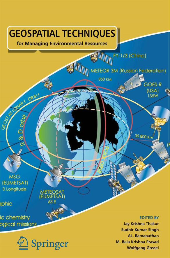
Cover photo credit: http://www.wmo.int/pages/prog/www/images/GOS/Figure%20II-10%20Satellites.jpg
Printed on acid-free paper
All Rights Reserved© 2011 Capital Publishing CompanyNo part of this work may be reproduced, stored in a retrieval system, ortransmitted in any form or by any means, electronic, mechanical, photocopying,microfilming, recording or otherwise, without written permission from thePublisher, with the exception of any material supplied specifically for the purposeof being entered and executed on a computer system, for exclusive use by thepurchaser of the work.
Printed in India.
��������
ì Geospatial informationî is spatial data concerning a place or, in space,collected in real time. Geospatial techniques together with remote sensing,geographic information science, Global Positioning System (GPS), cartography,geovisualization, and spatial statistics are being used to capture, store,manipulate and analyze to understand complex situations to solve mysteriesof the universe. These techniques have been applied in various fields likemetrology, forestry, air-water-land management, agriculture, health, homelandsecurity etc. around the globe. This book has made an effort to provide asingle record of current research status, technologies and applications ofgeospatial techniques in various fields and will be useful to academics,researchers and industry practitioners who are involved or interested in thestudy, use, design and development of advanced and emerging geospatialtechnologies around the world with ultimate aim to empower individuals andorganizations in building competencies for exploiting the opportunities of theknowledge society.
The chapters in this book demonstrate the need for the integratingenvironmental management approaches in combination with other fields usinggeospatial techniques. This book presents case studies and examples fromvarious parts of the world and provides a broad overview of various geospatialmanagement approaches and tools used to promote environmental sustainabilityin the context of global environmental change and natural hazards. These casestudies provide an insight into present day issues, challenges and opportunities;and highlight the key features, application of commercial and non-commercialsatellite and sensors, principles and new approaches that need to be consideredin future efforts for efficient integrated management in these fields. It isnecessary to address the scientific strategies which underpin the implementationof geospatial techniques development for overall integrated management ofvarious fields.
I would like to congratulate the great efforts of the editorial team of thisvolume which will serve as a scientific information base for future planningof the geospatial techniques development around the world and energize
v

synergy among academicians, researchers, stakeholders, INGOs, policy makersand the corporate sector for documentation and dissemination of knowledgefor the global welfare management.
Dr. Prem Chand PandeyEmeritus Professor, Indian Institute of Technology, Kharagpur, India
Founder Director, National Centre for Antarctic & Ocean Research(NCAOR), Goa, India
�� ��������

����� �
The recent advancement of geospatial techniques and geodatasets have growndramatically in size and number and become more widely distributed. Theterm Geospatial is generally used to describe the combination of spatialanalytical methods and software with geographic datasets in conjunction withGeographic Information Systems (GIS), spatial statistics, remote sensing,cartography, geo-visualization and geomatics for aquatic and terrestrialenvironment especially for a civilian, business, government and militaryorganizations. GIS as a system is integrating hardware, software, and data thatcaptures, stores, analyzes, manages, and presents data that are linked to thelocations with the merging of statistical analysis, and database technology. Itis being used in cartography, remote sensing, land surveying, utilitymanagement, natural resource management, photogrammetry, geography, urbanplanning, emergency management, navigation, and localized search engines.Remote sensing is the acquisition of information of an object or phenomenon,by the use of either recording or real-time sensing device(s) that are wireless,or not in physical or intimate contact with the object. While, Geomatics is afairly new terminology which is the combination of geodesy and geoinformaticterms and includes the tools and techniques used in land surveying, remotesensing, cartography, GIS, Global Navigation Satellite Systems (GNSS),photogrammetry, and related forms of earth mapping. Integration of theseresearch and developments to real world application in these fields are nowrequired for local, regional and global development. In this umbrella book ofgeospatial techniques, there are total seventeen chapters presenting the recentadvancement in the GIS, remote sensing, Global Positioning System (GPS),geovisualization and geomatics for application in the field of Agriculture,Business GIS, Climate change, Energy, Environmental services, Geology,Glaciology, Health, Land information system, Natural hazard management,Natural resource management, Corporate studies, Urban planning and Utilitymanagement.
This book represents the inter- and multi-disciplinary view of authors fora meaningful and practical guidance for the better application of geospatialtechniques that comprises contribution from distinguished scientists from bothacademia and institutions from around the globe who are actively working inthis area. This volume presents the case studies and examples from various
vii
parts of the globe and provides a broader overview of various approachesinvolved in data acquiring, monitoring and dissemination methods. This bookprovides a detailed knowledge of various platforms, satellites, and sensors;tools and techniques and application to various fields for the sustainablemanagement of environmental resources in the context of global environmentalchange and natural hazards.
To the beginners, we suggest not to be panicked by seeing advancedmethods, applications and integrated approaches. It is necessary to understandfrom basics and link presented methods and application of techniques to otherfields, as there are amalgamation of various processes and thoughts. The bookprovides a holistic application of geospatial techniques in managing naturalresources in the present scenario. This book is a comprehensive collection ofarticles from around the world, which reflects importance of this technologyin making the earth habitable. These case studies provide an insight intopresent-day issues, challenges and opportunities; and highlight the key features,principles, and new approaches that need to be considered in future efforts tomake the earth a livable place.
We would like to thank all the contributors to this volume and take thisopportunity to acknowledge all our colleagues for their time-consuming effortsto review the manuscripts of the chapters for this volume. Their efforts withhigh quality review of the manuscripts contributed significantly to keep thehigh scientific contents of the book. The editors also would like to thankcollaborators and research scholars for supporting their research activities thathelped in bringing out this volume successfully.
The book is scientific and research-oriented, yet appealing to a broadaudience interested in environmental applications of geospatial technologies,thus making it an important reference source for the fields of GIS, remotesensing, geography, environmental policy, and environmental science. Wehope that this book will be useful for geospatial scientists, remote sensing andGIS scientists, engineers, managers and administrators in both academia andindustries, decision and policy makers and for government and regulatorybodies dealing with geospatial issues by providing an opportunity to acquirerelevant scientific information and experiences in ì Geospatial Techniques forManaging Environmental Resourcesî .
Lastly, the editors wish to thank the publishers for bringing out this volumesuccessfully.
Jay Krishna ThakurSudhir Kumar Singh
AL. RamanathanM. Bala Krishna Prasad
Wolfgang Gossel
���� ����� �
������ ���� ������
Jay Krishna Thakur is Higrade Fellow at Department of Hydrogeology andEnvironmental Geology, Martin Luther University, Halle, Germany and visitingscientist at Helmholtz Centre for Environmental Research, UFZ, Leipzig,Germany. He has specialized on application of geospatial techniques inhydrogeology, hydrology, water resources and environmental managementand worked extensively on the wetland management studies, quantification ofwater cycle components and its dynamics, modelling of surface water andgroundwater, groundwater monitoring network optimization, GEONETCastenvironmental data streams for climate, water and environmental studies,clouds process, climate change impacts and adaptation, analysis and monitoringtechniques of climate change etc. He has been awarded with various researchfellowships including Netherlands Fellowship Program and Higrade FellowshipProgram. He has also contributed in conference papers, book chapters andpapers in reputed peer-reviewed journals.
Sudhir Kumar Singh is working at the Centre of Atmospheric and OceanScience, University of Allahabad, Allahabad, India. He has also worked atDepartment of Forestry, Mizoram Central University, Aizwal, India. His mainresearch areas are Remote Sensing and GIS applications in the field of resourcemanagement, environmental modelling and environmental pollution studiesin order to solve real world problems. He has received many prestigiousscholarships and has national and international collaboration with leadinginstitutes in the United Kingdom, Germany, Turkey and Nepal. He hascontributed many research papers in peer-reviewed journals and has reviewedpapers, CVs and research proposal for several journals and various researchinstitutions including the National Research Foundation, South Africa. As asupervisor, he guided over fifteen Diploma and MSc theses.
AL. Ramanathan, PhD in sedimentary geochemistry from Centre ofAdvanced Studies, Panjab University, worked as faculty in GeologyDepartment, Annamalai University, for a decade. He is currently Professor ofenvironmental geology, hydrogeochemistry, biogeochemistry, glaciology andapplication of geospatial techniques in environmental hydrogeology in theSchool of Environmental Sciences, Jawaharlal Nehru University, New Delhi,India. He has specialized on application of geospatial techniques in hydro-
ix
geology, hydrology, environmental resources management and workedextensively on the mangroves, estuaries, coastal ground waters, surface andgroundwater contamination modelling of India for the past two decades. He isengaged in coastal research with a number of universities and researchorganisations in India, Australia, France, Japan, Sweden, Russia, USA, etc.He has guided over thirty PhDs and MPhils in the above subject and publishedmore than seventy papers in referred reputed journals. He has also publishedtwelve books and contributed several chapters in many others. He has thricereceived the IFS Sweden (Project) Awards to work on mangrovebiogeochemistry besides working in national and international projects fromIndo-Australian, Indo-Russian, DST, MoEF, MoWR, etc. He has been guesteditor for the International Journal of Ecology and Environmental Sciences.He is a member of editorial board in the Indian Journal of Marine Sciencesand served as referee for many national and international journals as well.
M. Bala Krishna Prasad is a Research Associate at Earth System ScienceInterdisciplinary Center, University of Maryland, College Park, USA. He didPhD in Biogeochemistry at School of Environmental Sciences, JawaharlalNehru University, India. His primary research interest is evaluation andmodelling of climate change and anthropogenic impacts on the water qualityand aquatic ecosystem dynamics. He is a recipient of the Young ScientistAward from the Ministry of Science & Technology (India), Linnaeus-PalmeResearch Fellowship from Department of Earth Sciences, Uppsala University(Sweden), Berkner Fellowship of AGU (USA) and Junior Research Fellowshipsas well. He has contributed more than a dozen papers in reputed peer-reviewedinternational journals.
Wolfgang Gossel, habilitated in 2008 in Applied Geosciences at MartinLuther University, Halle (Germany) and worked for nearly 20 years inhydrogeology. He is a specialist in groundwater flow and transport modelling,GIS data processing and the application of interpolation techniques inhydrogeology. He is mainly working on the regional scale and since 2002 hasgot published several papers about the numerical groundwater flow models ofthe Nubian Aquifer System in Northeast Africa and the map Hydrogeology ofGermany. He has also collaborated with the Jawaharlal Nehru University inNew Delhi, Assiut University and Ain Shams University in Egypt, UniversidadAutonoma de Merida and Universidad Autonoma de San Luis Potosi in Mexico.He was Associate Editor of Hydrogeology Journal and Grundwasser. As asupervisor he guided about 50 Diploma and MSc theses.
� ����������������
�������
Foreword vPreface viiAbout the Editors ix
1. Environmental Informatics: Advancing Data IntensiveSciences to Solve Environmental Problems 1Chaowei Yang, Yan Xu and Daniel Fay
2. Hierarchical Geospatial Computing Environment forData-intensive Geographic Process Simulation 15Mingyuan Hu, Hui Lin, Bingli Xu, Ya Hu,Sammy Tang and Weitao Che
3. Integration of Geographic Information Systems for Monitoringand Dissemination of Marine Environment Data 33Marcin Kulawiak and Marek Moszynski
4. Estimation of Evapotranspiration from Wetlands UsingGeospatial and Hydrometeorological Data 53Jay Krishna Thakur, P.K. Srivastava, Arun Kumar Pratihastand Sudhir Kumar Singh
5. Climbing the Water Ladder ñ The New GIS Approach 68Amos Kabo-bah and Kamila Lis
6. Supraglacial Lake Classification in the Everest Regionof Nepal Himalaya 86Prajjwal K. Panday, Henry Bulley, Umesh Haritashyaand Bardan Ghimire
7. Towards the Improvement of Water Resource Managementby Combining Technologies for Spatial Data Collection,Storage, Analysis and Dissemination 100Nafa������������� �������������
8. Geomorphologic Risk Modelling of the Sibiu DepressionUsing Geospatial Surface Analyses 119Marioara Costea, Roxana Giusca and Rodica Ciobanu
xi
9. Geospatial Technique to Study Forest Cover UsingALOS/PALSAR Data 139Ram Avtar, Jay Krishna Thakur, Amit Kumar Mishraand Pankaj Kumar
10. Assessment of Land Use/Land Cover Using GeospatialTechniques in a Semi-arid Region of Madhya Pradesh, India 152Prafull Singh, Jay Krishna Thakur, Suyash Kumar and U.C. Singh
11. The Environmental Calculator: A Tool for the Efficient Assessmentof Environmental Services Loss due to Deforestation 164Miguel Mart������������������ ��!��!�"# �$�and Jos#�%����&�����'#��
12. Urban Tree Detection Using Mobile Laser Scanning Data 188Arun Kumar Pratihast and Jay Krishna Thakur
13. Multisensor Fusion of Remote Sensing Data for CropDisease Detection 201Dimitrios Moshou, Ioannis Gravalos, Dimitrios Kateris CedricBravo, Roberto Oberti, Jon S. West and Herman Ramon
14. Geospatial Analysis of Cancer Cases in the EasternBlack Sea Region of Turkey 220Ebru H. Colak and Tahsin Yomralioglu
15. GIS for the Determination of Bioenergy Potential inthe Centre Region of Portugal 238Tanya C.J. Esteves, Pedro Cabral, Jos#���&!�����(���and Ant)��!������*����
16. Use of Geospatial Data in Planning for OffshoreWind Development 256John Madsen, Alison Bates, John Callahan and Jeremy Firestone
17. Social Vulnerability Assessment through GIS Techniques:A Case Study of Flood Risk Mapping in Mexico 276P. Krishna Krishnamurthy and L. Krishnamurthy
Index 293
��� �������

Environmental Informatics 1
1Environmental Informatics:
Advancing Data Intensive Sciencesto Solve Environmental Problems
Chaowei Yang, Yan Xu1 and Daniel Fay1
Center for Intelligent Spatial Computing, and Department of Geographyand GeoInformation Sciences, George Mason University
Fairfax, VA, USA1Earth, Energy and Environment at Microsoft Research Connections
Microsoft Corporation, Redmond, WA, USA
Introduction
The 21st Century witnesses emergence of geospatial cyberinfrastructure andother relevant geospatial technologies (Yang et al., 2010) for collecting data,extracting information, simulating phenomena scenarios, and supportingdecision making (Caragea et al., 2005; Stadler et al., 2006). The advancementsof the geospatial technologies not only provide great opportunities for us tobetter understand environmental issues and better position us to solve globalto local environmental problems (Pecar-Ilic and Ruzic, 2006), but also posegreat challenges for us to handle terabytes to petabytes of heterogeneousenvironmental data. Environmental informatics (Green and Klomp, 1998;Hilty, Page and Hr¡ebíc¡ek, 2006) should be revisited to efficiently and effectivelymanage, integrate, and mine information and knowledge from the vast amountof data for supporting environmental decisions (Hey, Tansley and Tolle, 2008).
Information/knowledge mining often starts with heterogeneous data fromvarious resources, and ends with re-aggregated data in numbers and/or intuitivegraphics adopted by decision makers. On one hand, there are many conventionalgeospatial techniques that can be used to facilitate generating information andknowledge from environmental data to produce social impact. There are alsomany computing technologies that are not specifically designed for managingenvironmental data but can be used innovatively to significantly acceleratethe mining process. On the other hand, it is a challenge to decide whattechniques to choose and to integrate with, so that strategies could be taken to
DOI 10.1007/978-94-007-1858-6_1, © Capital Publishing Company 2012
1e ,J.K. Thakur et al. (eds.), G ospatial Techniques for Managing Environmental Resources
2 Chaowei Yang, Yan Xu and Daniel Fay
design solution by leveraging the techniques efficiently in managingenvironmental data.
Based on our past decade’s investigation on utilizing geospatialtechnologies for managing environmental data, this chapter illustrates how toutilize a set of computational geospatial techniques to manage and processenvironmental data through presenting five examples. The chapter concludeswith a discussion on future directions of environmental informatics to handlepotential problems from the arena of data intensive, computing intensive,spatiotemporal intensive and concurrent access intensive (Yang et al., 2011).
Background
Environmental data are of essential values in support of environmental decisionsby providing historical and real-time representation of the facts aboutenvironmental phenomena. The data have the characteristics of: (1) globaldistribution (Pillmann, Geiger and Voigt, 2006; Zhizhin et al., 2007), forexample, dust storm generated from northern Africa could travel to Europeand forest fire emissions in Washington state can impact air quality in Iowa(Xie et al., 2010); (2) multi-dimensionality, though many datasets are twodimensional, the collection of three and four dimensional data has begun, forexample, a four dimensional dataset is measured of daily nitrogenconcentrations at different depths within Chesapeake Bay; (3) heterogeneity,which exists in many ways such as within data formats, data contents, dataaccuracy, data spatial resolution and time scale (Devarakonda et al., 2010;Yang et al., 2008), geographic coverage, and jurisdiction or culture boundaries;and (4) large volume, intensive data up to petabytes in size may be collectedto record observations in four dimensions of space and time (Goodchild, Yuanand Cova, 2007).
The emerging requirements for data of high resolution and collected as atime series when compared to existing information may result in gaps in time,geographic coverage, and jurisdiction or culture boundaries. The time scalesover which relevant environmental data may be collected also varies by thetype of observations that are required (Karatzas, Nikolaou and Moussiopoulos,2004), for example, data in response to environmental disasters, climate changeand/or policy decisions may require daily, yearly or decadal measurements.Spatial constraints and scientific principles must also be represented withinenvironmental datasets (Yang et al., 2011b). An illustration of this is howtoxic material will travel in rivers at a much faster speed than hazardousmaterial percolating through soil, but slower than hazardous gas emissionstravelling through the atmosphere. These movements of material are governedby different geophysical principles and therefore require different models ofvarious complexities to simulate and produce accurate predictions in supportof decision making.
Environmental Informatics 3
From an informatics perspective, these problems are also reflected as dataintensive, computing intensive, spatiotemporal intensive, and concurrent accessintensive (Yang et al., 2011a): (1) the data in terabytes to petabytes are volumeintensive; (2) the various geophysical models and interpolation methods requirecutting-edge computer or high end computing support to simulateenvironmental phenomena; (3) data are increasingly demanded to be taggedup with both spatial and temporal information in order to be useful (Rasuly,Naghdifar and Rasoli, 2010). Near-real time data requirements are becomingmore common for environmental emergency responses that happened muchmore frequently within our globalized world (Karatzas et al., 2004); and (4)some datasets and model predictions are of public interest to be accessed bythousands to millions of citizens in a very short time period. For example, theair quality information, just like the weather information, is essential for thepublic to make personal decisions about their outdoor activities and travelplans based on individual health considerations.
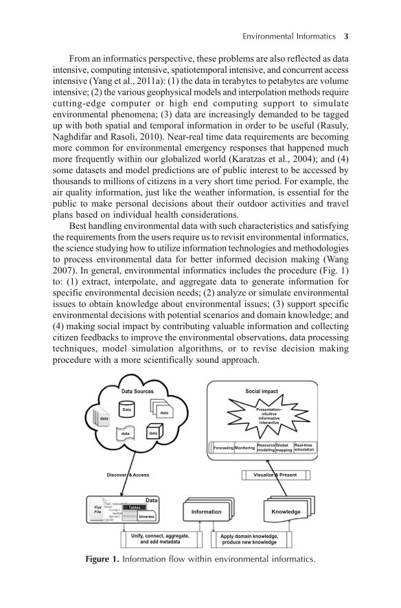
Best handling environmental data with such characteristics and satisfyingthe requirements from the users require us to revisit environmental informatics,the science studying how to utilize information technologies and methodologiesto process environmental data for better informed decision making (Wang2007). In general, environmental informatics includes the procedure (Fig. 1)to: (1) extract, interpolate, and aggregate data to generate information forspecific environmental decision needs; (2) analyze or simulate environmentalissues to obtain knowledge about environmental issues; (3) support specificenvironmental decisions with potential scenarios and domain knowledge; and(4) making social impact by contributing valuable information and collectingcitizen feedbacks to improve the environmental observations, data processingtechniques, model simulation algorithms, or to revise decision makingprocedure with a more scientifically sound approach.
MonitoringForecastingResourcemodeling
Globalmapping
Real-timesimulation
Presentation–intuitive
informativeinteractive
data
data
data data
Data
Data Sources Social impact
Visualize & Present
KnowledgeInformation
DataFlat
File
Unify, connect, aggregate,and add metadata
Apply domain knowledge,produce new knowledge
binaries
Tables
Discover & Access
Figure 1. Information flow within environmental informatics.
4 Chaowei Yang, Yan Xu and Daniel Fay
Research Examples
Observing the characteristics of environmental data, the requirements for dataprocessing, and the procedure to address user requirements, we reviewenvironmental informatics in the context of data intensive science that includestransforming environmental data, to information, to knowledge, to decisionsupport, and ultimately to social impact. Each of the four steps is exemplifiedthrough literature reviews and research examples from the EnvironmentalInformatics Framework, a Microsoft eScience initiative and George MasonUniversity (GMU) Center for Intelligent Spatial Computing (CISC)’s researchprojects: (1) A virtual Earth observatory project shows the discovery andintegration of data from widely distributed services for environmentaloperations based on interoperability and on-the-fly integration; (2) A UnitedStates ozone observation and interpolation project illustrates data toinformation transformation; (3) An on-demand MODIS science projectdemonstrates how cloud computing can help to enable science questionanswered in near real-time; (4) A Chinese land cover change projectdemonstrates how to utilize intensive data and sophisticated models to supportdecision making; and (5) A citizen sensing flooding project is usedto demonstrate how the data, information, modelling, and knowledge canproduce social impact and benefit from citizen sciences. Scenarios withintegrative solutions based on cutting-edge Microsoft data and informationtechnologies are laid out in the examples to illustrate the future of environmentalinformatics.
Data Discovery, Access and Utilization with Virtual Observatory
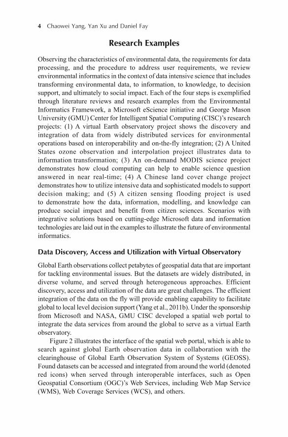
Global Earth observations collect petabytes of geospatial data that are importantfor tackling environmental issues. But the datasets are widely distributed, indiverse volume, and served through heterogeneous approaches. Efficientdiscovery, access and utilization of the data are great challenges. The efficientintegration of the data on the fly will provide enabling capability to facilitateglobal to local level decision support (Yang et al., 2011b). Under the sponsorshipfrom Microsoft and NASA, GMU CISC developed a spatial web portal tointegrate the data services from around the global to serve as a virtual Earthobservatory.
Figure 2 illustrates the interface of the spatial web portal, which is able tosearch against global Earth observation data in collaboration with theclearinghouse of Global Earth Observation System of Systems (GEOSS).Found datasets can be accessed and integrated from around the world (denotedred icons) when served through interoperable interfaces, such as OpenGeospatial Consortium (OGC)’s Web Services, including Web Map Service(WMS), Web Coverage Services (WCS), and others.
Environmental Informatics 5
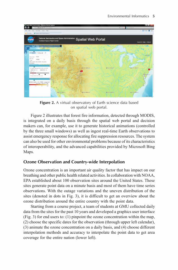
Figure 2. A virtual observatory of Earth science data basedon spatial web portal.
Figure 2 illustrates that forest fire information, detected through MODIS,is integrated on a daily basis through the spatial web portal and decisionmakers can, for example, use it to generate historical animations (controlledby the three small windows) as well as ingest real-time Earth observations toassist emergency response for allocating fire suppression resources. The systemcan also be used for other environmental problems because of its characteristicsof interoperability, and the advanced capabilities provided by Microsoft BingMaps.
Ozone Observation and Country-wide Interpolation
Ozone concentration is an important air quality factor that has impact on ourbreathing and other public health related activities. In collaboration with NOAA,EPA established about 100 observation sites around the United States. Thesesites generate point data on a minute basis and most of them have time seriesobservations. With the outage variations and the uneven distribution of thesites (denoted in dots in Fig. 3), it is difficult to get an overview about theozone distribution around the entire country with the point data.
Starting from a course project, a team of students at GMU collected dailydata from the sites for the past 10 years and developed a graphics user interface(Fig. 3) for end users to: (1) pinpoint the ozone concentration within the map,(2) choose the specific dates for the observation (through upper left calendar),(3) animate the ozone concentration on a daily basis, and (4) choose differentinterpolation methods and accuracy to interpolate the point data to get areacoverage for the entire nation (lower left).

6 Chaowei Yang, Yan Xu and Daniel Fay
Figure 3. Ozone interpolation and navigation tool for the United States.
This tool could help us to have a better view of the entire nation for ozoneconcentration based on the site point observations and statistical interpolation.To some degree, it helps us to interpolate or extract information for missingplaces. But on the other hand, it demonstrates, through comparison ofinterpolation methods (right side images of Fig. 3), that simple interpolationis too arbitrary to generate accurate ozone concentration maps. Therefore,follow-on studies are needed to incorporate weather information and othersource of observations, such as satellite remote sensing, to generate moreaccurate interpolations and eventually to forecast the ozone concentrationsbased on the historical and weather forecasting (Slini, Karatzas andMoussiopoulos, 2003). Making the data and interpolation services availablethrough OGC web services would also help them to be easily discovered,accessed and utilized through, for example, virtual observatory described inprevious section.
Knowledge Generation from Long-term Observation
Earth observations are invaluable for scientists to track the phenomena factsof the Earth surface. Complex data processing algorithms, such as subsettingand parameter extracting, are needed to process the observations before finalproducts can be used by scientists or decision makers. And these productsrequirements are quite different. Therefore, an infrastructure is needed toprovide on-demand science queries for specific parameters or products.
Environmental Informatics 7
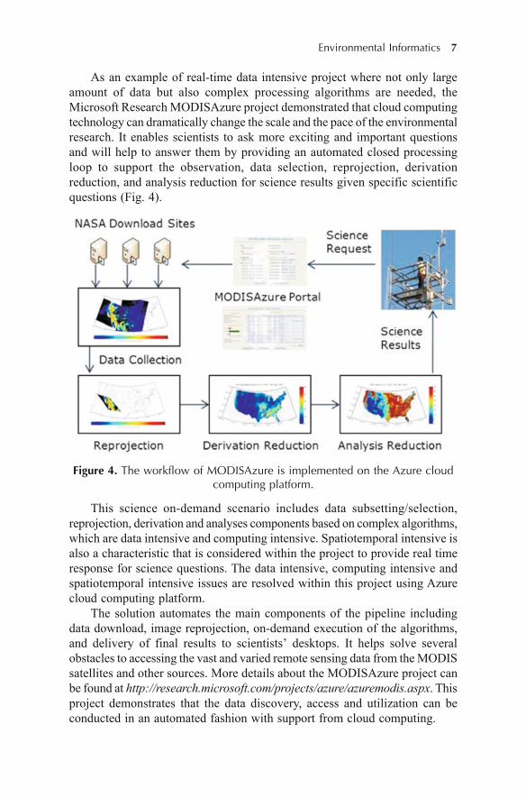
As an example of real-time data intensive project where not only largeamount of data but also complex processing algorithms are needed, theMicrosoft Research MODISAzure project demonstrated that cloud computingtechnology can dramatically change the scale and the pace of the environmentalresearch. It enables scientists to ask more exciting and important questionsand will help to answer them by providing an automated closed processingloop to support the observation, data selection, reprojection, derivationreduction, and analysis reduction for science results given specific scientificquestions (Fig. 4).
Figure 4. The workflow of MODISAzure is implemented on the Azure cloudcomputing platform.
This science on-demand scenario includes data subsetting/selection,reprojection, derivation and analyses components based on complex algorithms,which are data intensive and computing intensive. Spatiotemporal intensive isalso a characteristic that is considered within the project to provide real timeresponse for science questions. The data intensive, computing intensive andspatiotemporal intensive issues are resolved within this project using Azurecloud computing platform.
The solution automates the main components of the pipeline includingdata download, image reprojection, on-demand execution of the algorithms,and delivery of final results to scientists’ desktops. It helps solve severalobstacles to accessing the vast and varied remote sensing data from the MODISsatellites and other sources. More details about the MODISAzure project canbe found at http://research.microsoft.com/projects/azure/azuremodis.aspx. Thisproject demonstrates that the data discovery, access and utilization can beconducted in an automated fashion with support from cloud computing.
8 Chaowei Yang, Yan Xu and Daniel Fay
Forecasting Changes in Urban Land Use
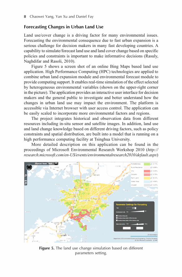
Land use/cover change is a driving factor for many environmental issues.Forecasting the environmental consequence due to fast urban expansion is aserious challenge for decision makers in many fast developing countries. Acapability to simulate/forecast land use and land cover change based on specificpolicies and constraints is important to make informative decisions (Rasuly,Naghdifar and Rasoli, 2010).
Figure 5 shows a screen shot of an online Bing Maps based land useapplication. High Performance Computing (HPC) technologies are applied tocombine urban land expansion module and environmental forecast module toprovide computing support. It enables real-time simulation of the effect selectedby heterogeneous environmental variables (shown on the upper-right cornerin the picture). The application provides an interactive user interface for decisionmakers and the general public to investigate and better understand how thechanges in urban land use may impact the environment. The platform isaccessible via Internet browser with user access control. The application canbe easily scaled to incorporate more environmental factors and regions.
The project integrates historical and observation data from differentresources including in-situ sensor and satellite images. In addition, land useand land change knowledge based on different driving factors, such as policyconstraints and spatial distribution, are built into a model that is running on ahigh performance computing facility at Tsinghua University.
More detailed description on this application can be found in theproceedings of Microsoft Environmental Research Workshop 2010 (http://research.microsoft.com/en-US/events/environmentalresearch2010/default.aspx)
Figure 5. The land use change simulation based on differentparameters setting.
Environmental Informatics 9
Social Impact and Citizen Sensing for Flooding Management
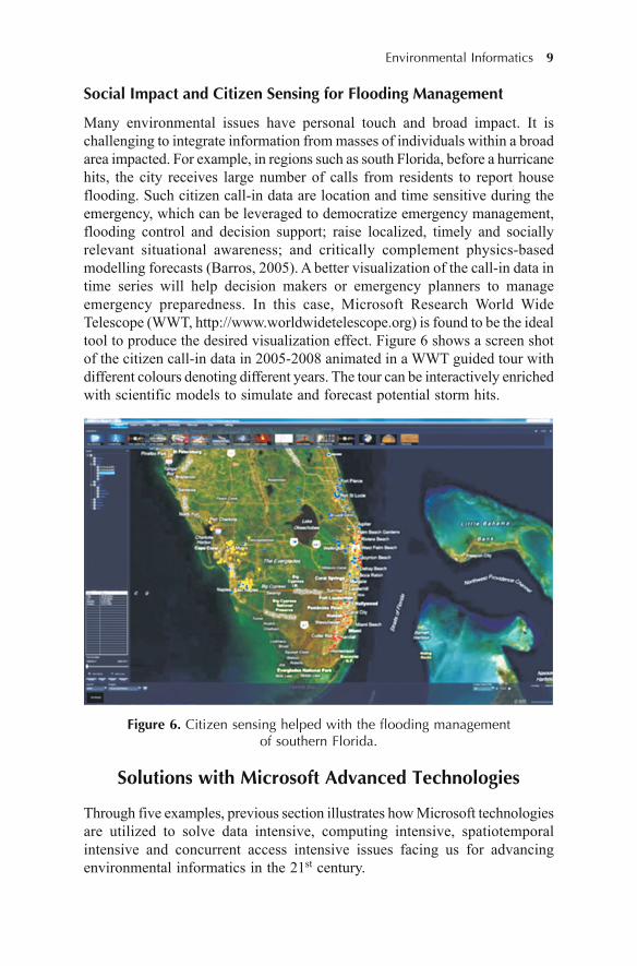
Many environmental issues have personal touch and broad impact. It ischallenging to integrate information from masses of individuals within a broadarea impacted. For example, in regions such as south Florida, before a hurricanehits, the city receives large number of calls from residents to report houseflooding. Such citizen call-in data are location and time sensitive during theemergency, which can be leveraged to democratize emergency management,flooding control and decision support; raise localized, timely and sociallyrelevant situational awareness; and critically complement physics-basedmodelling forecasts (Barros, 2005). A better visualization of the call-in data intime series will help decision makers or emergency planners to manageemergency preparedness. In this case, Microsoft Research World WideTelescope (WWT, http://www.worldwidetelescope.org) is found to be the idealtool to produce the desired visualization effect. Figure 6 shows a screen shotof the citizen call-in data in 2005-2008 animated in a WWT guided tour withdifferent colours denoting different years. The tour can be interactively enrichedwith scientific models to simulate and forecast potential storm hits.
Figure 6. Citizen sensing helped with the flooding managementof southern Florida.
Solutions with Microsoft Advanced Technologies
Through five examples, previous section illustrates how Microsoft technologiesare utilized to solve data intensive, computing intensive, spatiotemporalintensive and concurrent access intensive issues facing us for advancingenvironmental informatics in the 21st century.
10 Chaowei Yang, Yan Xu and Daniel Fay
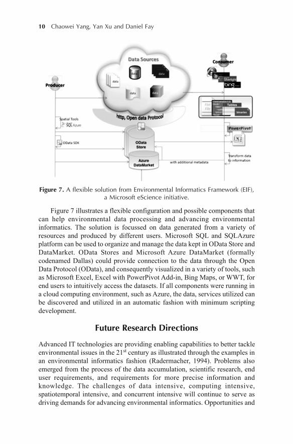
Figure 7. A flexible solution from Environmental Informatics Framework (EIF),a Microsoft eScience initiative.
Figure 7 illustrates a flexible configuration and possible components thatcan help environmental data processing and advancing environmentalinformatics. The solution is focussed on data generated from a variety ofresources and produced by different users. Microsoft SQL and SQLAzureplatform can be used to organize and manage the data kept in OData Store andDataMarket. OData Stores and Microsoft Azure DataMarket (formallycodenamed Dallas) could provide connection to the data through the OpenData Protocol (OData), and consequently visualized in a variety of tools, suchas Microsoft Excel, Excel with PowerPivot Add-in, Bing Maps, or WWT, forend users to intuitively access the datasets. If all components were running ina cloud computing environment, such as Azure, the data, services utilized canbe discovered and utilized in an automatic fashion with minimum scriptingdevelopment.
Future Research Directions
Advanced IT technologies are providing enabling capabilities to better tackleenvironmental issues in the 21st century as illustrated through the examples inan environmental informatics fashion (Radermacher, 1994). Problems alsoemerged from the process of the data accumulation, scientific research, enduser requirements, and requirements for more precise information andknowledge. The challenges of data intensive, computing intensive,spatiotemporal intensive, and concurrent intensive will continue to serve asdriving demands for advancing environmental informatics. Opportunities and
Environmental Informatics 11
challenges coexist within our efforts to tackle the issues (Yang et al., 2011b).The following directions need further attention for research and developmentin the following decade to advance environmental informatics.
• An environmental informatics infrastructure is needed for fast integrationand aggregation of environmental observations from different organizationsinto a virtual simulation centre that can produce scientifically sounddecision support information (MacDonell, Morgan and Newland, 2002).This can benefit from the recent geospatial cyberinfrastructureadvancement at different agencies (Yang et al., 2010), especially withinthe environmental protection agency and companies, such as Microsoft,who are willing to contribute advanced technologies to address our globalenvironmental issues.
• Advanced computing technologies are still needed to be further developed,especially in a spatial cloud computing fashion (Yang et al., 2011a and2011b) to best leverage the distributed computing resources to handleenvironmental observations accumulated from local to global locationsand to best handle environmental models, observations, and simulationsin an optimized fashion.
• Data integration and interoperability is an inevitable task that will endurethe entire life cycle of environmental informatics to solve dataheterogeneous and service heterogeneous problems in the 21st century.
• Spatiotemporal models are becoming increasingly important from boththeoretical and technological research and development to handle real-time and historical environmental data for better simulating potentiallyresulting scenarios from environmental decisions.
• Human knowledge about our planet is critical to the advancement ofenvironmental informatics (Chen et al., 2007) and should be integrated insolutions (Tochtermann and Maurer, 2000). But our understanding ofEarth has been very much divided according to different domains including,for example, biology, physics, ocean, atmosphere and land. Modelintegration is much needed to couple individualized models to formintegrative systems to better simulate the response of geophysical systemsfrom any event triggered by either human activities, such as hazardousmaterial emission, or by nature, such as a tsunami.
• All resources supporting the advancements of environmental informaticswill have their own relevant quality and usage limitation based on theproviders, operational status and end users. The research on the qualityand authority of data, service, information, knowledge and models will becritical to guarantee better decision making. Assessing the accuracy isessential within environmental informatics processes (Kalapanidas andAvouris, 2003).
• Citizen science is emerging as a phenomenon to involve citizens in popularscientific discoveries and science and policy comment and verification(Gruiz, 2009). For environmental science, this is especially true when
12 Chaowei Yang, Yan Xu and Daniel Fay
observations are still the best approach to obtain environmental information(Mayfield, Joliat and Cowan, 2001). Large amount of environmental issuesare reported by citizen (Stockwell et al., 2006). Citizens could alsocontribute their computing resources in a Seti@Home fashion to solvepublic environmental issues, such as climate change throughClimate@Home.
• An automated and self-adaptive environment for discovery, access andutilization of data and services will be needed in the future for quicklyintegrating data, information, knowledge, citizen sciences, and decisionsmade to produce knowledge for rapid, broad and precise environmentalproblems solving.
Conclusion
Within the data explosion era, environmental informatics faces great challengesto better manage, integrate, simulate and forecast environmental informationto extract knowledge for better environmental decisions. This chaptersummarizes environmental informatics through analyzing the characteristicsof environmental data and five research examples.
We report: (1) How the environmental data observed can be interpolatedto have a reasonable geographic coverage; (2) How data can be discovered,accessed and integrated and visualized through Bing Maps to conductinformation integration on the fly; (3) How to utilize Azure cloud computingand MODIS knowledge to produce decision support results in real time; (4)How to utilize cloud computing and distributed data integration to supportenvironmental scenario simulations for decision making with potentialscenarios; and (5) How to involve citizens in environmental sciences to helpobserve, respond and mitigate hazardous issues. Through advanced technologiesprovided by Microsoft, these projects demonstrate exemplary solutions forthe four steps within environmental informatics.
The research benefits from recent advancements in computer science,data sciences, and information technologies and methodologies. To fullyintegrate observation data worldwide, utilize elastic cloud computing platforms,and serve users with right environmental information in the right place, at theright time will be a driving objective for the next decade in advancingenvironmental informatics for (1) solving environmental issues, (2) advancingenvironmental sciences, (3) responding to environmental emergency, and(4) protecting our home planet for future generations.
Research is needed in (1) bridging advanced technologies andenvironmental sciences, (2) advancing sciences and technology, informationtheory within a globalized context, and (3) improving end users awarenessand utilization of environmental data, information and knowledge in a morecreative and beneficial decision environment.

Environmental Informatics 13
Acknowledgements
Research reported is sponsored by Microsoft, NASA and Federal GeographicData Committee. The authors would also like to acknowledge Yi Liu fromTsinghua University, China, for his contribution in the example as shown inFig. 5; South Florida Water Management District, USA, and Yong Liu fromNational Center for Supercomputing Applications (http://www.ncsa.illinois.edu/), for their contribution in the example as shown in Fig. 6; Xi Zhou, ChenXu, Jizhe Xia, Xin Qu, and Min Sun, Qunying Huang from George MasonUniversity (cisc.gmu.edu) for their contributions to examples as shown inFigs 2 and 3.
References
Barros, A.P. (2005, Jul. 31-Aug.4). Environmental informatics - Long-lead floodforecasting using Bayesian neural networks. Paper presented at the InternationalJoint Conference on Neural Networks, Montreal, Canada.
Caragea, D., Zhang, J., Bao, J., Pathak, J. and Honavar, V. (2005). Algorithms andsoftware for collaborative discovery from autonomous, semantically heterogeneous,distributed information sources. Lecture Notes in Computer Science, 3734, 13–44.
Chen, Z., Gangopadhyay, A., Karabatis, G., McGuire, M. and Welty, C. (2007). Semanticintegration and knowledge discovery for environmental research. Journal ofDatabase Management, 18, 43–68.
Devarakonda, R., Palanisamy, G., Green, J.M. and Wilson, B.E. (2010). Data sharingand retrieval using OAI-PMH. Earth Science Informatics, 3, 1–5.
Dhanushkodi, S.R., Mahinpey, N., Srinivasan, A. and Wilson, M. (2008). Life cycleanalysis of fuel cell technology. Journal of Environmental Informatics, 11, 36–44.
Goodchild M., Yuan, M. and Cova, T.J. (2007). Towards a general theory of geographicrepresentation in GIS. International Journal of Geographical Information Science,21, 239–260.
Green, D.G. and Klomp, N.I. (1998). Environmental informatics—A new paradigmfor coping with complexity in nature. Complexity International, 6.
Gruiz, K. (2009). Web-based information system and decision support tool: The structureand use of the MOKKA IT tool. Land Contamination and Reclamation, 17, 695–702.
Hey, T., Tansley, S. and Tolle, K. (2009). The Fourth Paradigm: Data-Intensive ScientificDiscovery. Microsoft Press, Redmond, WA.
Hilty, L.M., Page, B. and Hr¡ebíc¡ek, J. (2006). Environmental informatics.Environmental Modelling and Software, 21, 1517–1518.
Karatzas, K., Nikolaou, K. and Moussiopoulos, N. (2004). Timely and valid air qualityinformation: The APNEE-TU Project. Fresenius Environmental Bulletin, 13, 874–878.
Kalapanidas, E. and Avouris, N. (2003). Feature selection for air quality forecasting:A genetic algorithm approach. AI Communications, 16, 235–251.
14 Chaowei Yang, Yan Xu and Daniel Fay
MacDonell, M., Morgan, K. and Newland, L. (2002). Integrating information forbetter environmental decisions. Environmental Science and Pollution Research, 9,359–368.
Mayfield, C., Joliat, M. and Cowan, D. (2001). The roles of community networks inenvironmental monitoring and environmental informatics. Advances inEnvironmental Research, 5, 385–393.
Pecar-Ilic, J. and Ruzic, I. (2006). Application of GIS and Web technologies forDanube waterway data management in Croatia. Environmental Modelling andSoftware, 21, 1562–1571.
Pillmann, W., Geiger, W. and Voigt, K. (2006). Survey of environmental informaticsin Europe. Environmental Modelling and Software, 21, 1519–1527.
Radermacher, F.J., Riekert, W.-F., Page, B. and Hilty, L.M. (1994). Trends inenvironmental information processing. IFIP Transactions. A: Computer Scienceand Technology (A-52), 597–604.
Rasuly, A., Naghdifar, R. and Rasoli, M. (2010). Detecting of Arasbaran forest changesapplying image processing procedures and GIS Techniques. Procedia EnvironmentalSciences, 2, 454–464.
Stadler, M., Ahlers, D., Bekker, R.M., Finke, J., Kunzmann, D. and Sonnenschein, M.(2006). Web-based tools for data analysis and quality assurance on a life-historytrait database of plants of Northwest Europe. Environmental Modelling and Software,21, 1536–1543.
Slini, T., Karatzas, K. and Moussiopoulos, N. (2003). Correlation of air pollution andmeteorological data using neural networks. International Journal of Environmentand Pollution, 20, 218–229.
Stockwell, D.R.B., Beach, J.H., Stewart, A., Vorontsov, G., Vieglais, D. and Pereira,R.S. (2006). The use of the GARP genetic algorithm and Internet grid computingin the Lifemapper world atlas of species biodiversity. Ecological Modelling, 195,139–145.
Tochtermann, K. and Maurer, H. (2000). Knowledge Management and EnvironmentalInformatics. Journal of Universal Computer Science, 6, 517–536.
Wang, X. (2007). Environmental informatics for environmental planning andmanagement. Journal of Environmental Informatics, 9, 1–3.
Xie, J., Yang, C., Zhou, B. and Huang, Q. (2010). High performance computing forthe simulation of dust storms. Computers, Environment, and Urban Systems, 34,278–290.
Yang, C., Goodchild, M., Huang, Q., Nebert, D., Raskin, R., Xu, Y., Fay, D. andBambacus, M. (2011a). Spatial Cloud Computing – How geospatial science useand help to shape cloud computing. International Journal of Digital Earth, 4, 305–329.
Yang, C., Raskin, R., Goodchild, M.F. and Gahegan, M. (2010). GeospatialCyberinfrastructure: Past, Present and Future. Computers, Environment, and UrbanSystems, 34, 264–277.
Yang, C., Wu, H., Huang, Q., Li, Z. and Li, J. (2011b). Utilizing spatial principles tooptimize distributed computing for enabling physical science discoveries.Proceedings of National Academy of Sciences, doi: /10.1073/pnas.0909315108.
Zhizhin, M., Kihn, E., Redmon, R., Poyda, A., Mishin, D., Medvedev, D. et al. (2007).Integrating and mining distributed environmental archives on Grids. ConcurrencyComputation Practice and Experience, 19, 2157–2170.

Hierarchical Geospatial Computing Environment 15
2Hierarchical Geospatial Computing
Environment for Data-intensiveGeographic Process Simulation
Mingyuan Hu, Hui Lin, Bingli Xu1, Ya Hu2,Sammy Tang3 and Weitao Che
Institute of Space and Earth in Information Science, the ChineseUniversity of Hong Kong, China
1Department of Information Engineering, The Academy of ArmoredForces Engineering, Beijing 100072, China
2Remote Sensing Information Engineering Department, Facultyof Geosciences and Environmental Engineering
Southwest Jiaotong University, Chengdu 610031, China3Information Technology Services Center, the Chinese University
of Hong Kong, China
Introduction
Geographic information system (GIS) professionals recognize that geographicprocess is essential for understanding what is happening in the world, learninghow the environment is changing, modelling how complex systems work andgiving context to other types of data. Consequently, geographic process modelshave been increasingly featured for the next generation geographic informationscience (system), as a method for phenomena simulation and mechanismanalysis of the physical environment and its live activities, thereby drivingconventional GIS based on data manipulation into the world of dynamic andcomputational processes (Goodchild, 2006; Yuan and Hornsby, 2008; Torrens,2009; CSDGS et al., 2010).
However, geographic process models such as atmospheric models generallyare toward computational models, large data-intensive sets based, and atmultiple spatiotemporal scales, which often take time-consuming computingor need immediately simulated responses to explain these dynamic phenomena(Openshaw, 2000; Guan et al., 2006; Brimicombe, 2009). In order tomake better and full use of the vast geographic data and exploit the
DOI 10.1007/978-94-007-1858-6_2, © Capital Publishing Company 2012
15e ,J.K. Thakur et al. (eds.), G ospatial Techniques for Managing Environmental Resources
16 Mingyuan Hu et al.
valuable information beyond the original data resources, data intensivecomputing is now considered as the “fourth paradigm” in scientific discoveryafter theoretical, experimental and computational science (Tony et al., 2009).New computing technologies such as cloud computing, grid technology andmulticore processors have spawned GIS fields to meet the new scientificchallenges, including computationally-intensive scientific, mathematical andacademic problems through volunteer computing (Foster, 2002; Goodchild,2010).
Some pilot studies in geospatial fields are spatial statistical analysis (Wanget al., 2008; Harris, 2010), air-borne laser scanning data sequential processing(Han et al., 2009), hyperspectral image processing (Plaza et al., 2006), parallelcellular automata modelling (Guan and Clarke, 2010; Li et al., 2010), as wellas simulations with parallelized mesoscale environmental models (Xie et al.,2009; Xu et al., 2010) and wildland fire behaviour simulation (Douglas andCoen, 2010). Despite the existence of commercially available dispersedcomputing resources, they are highly priced and are largely inaccessible togeneral users (Sugato, 2005; Zhang, 2010). Furthermore, these systems cannotprovide the entire solution in their generic forms (Foster and Kesselman,2004) and they are also difficult for geographical tasks schedule, leveragingthe built-in geospatial data management as well as inherent implementingcomputing tasks in heterogeneous environments (Curran and Shearer, 2009;Huang et al., 2009). On the other hand, when the number of processors gobeyond a threshold, normalized speedups of grid/cloud computing could slowdown significantly, which might be caused by the combined factors ofcommunication/scheduling overheads, workload imbalances and contentionof shared resources (Xie et al., 2009; Li et al., 2010). There is also an increasingrecognition that the scalability and controllability of high PC clusters allowprogress beyond remote computational resources limited by the networkbandwidth, security authentication and queue requests, etc. (Marín et al.,2011). The low cost high performance PCs thus has fostered research to usethem to drive immediately geographic process computing (Zhang, 2010). Inparticular, personal PC clusters computing advances the linkage across existingresources, but also offers the power of self-control to the management ofgeospatial data resources and dataflow for real time dynamic simulation at thelocal area. Consequently, in this chapter, a distributed problem-solvingenvironment is proposed in order to reveal fully the real features ofspatiotemporal geographic process and support both 3D analysis andhierarchical emergency decision making, comprising the geographic processmodels, the hierarchical geospatial computation involving grid computinglayer and local PC clusters effectively coordinated, and Viz Wall for real-timedata visualization and geographic analysis.
The remainder of this chapter is organized as follows. Second part describesthe related background of geographic process models and high performance
Hierarchical Geospatial Computing Environment 17
hierarchical geospatial computing environment for data-intensive computing.A hierarchical geospatial computing environment for data-intensive geographicprocess simulation is introduced in third part. The fourth part discusses thecase study: the grid computing based regional atmospheric simulation, PCcluster based parallel computation of a Gauss dispersion model, and the visualwall for geographic visualization. Final part gives the conclusion of this workwith thoughts on the future prospects.
Advanced Features in Geographic Process Computation
Geographic Process Models
Geographic process models are not only geo-knowledge in them, but can alsogenerate new geo-knowledge by changing the input initiate parameters.Therefore, being different from digital representation such as geometricconstruction, what a geographic process model highlights are dynamicalgeographical process simulation and geographical phenomenon analysis, so itfocusses on not only the cities or communities, but also all geographicalenvironments such as atmospheric pollution, oceans dynamics and soil horizon.In this case of air pollution simulation research, Mesoscale Model5 (MM5)and Gauss plume model for simulation and analysis are typically introduced.
MM5 (Dudhia et al., 2005)
The PSU/NCAR mesoscale model5 (known as MM5) is a regional,nonhydrostatic, terrain-following sigma-coordinate model designed to simulateor predict mesoscale atmospheric circulation. The model is supported byseveral pre- and post-processing programs, which are referred to collectivelyas the MM5 modelling system. The MM5 modelling system software is mostlywritten in Fortran, and has been developed at Penn State and NCAR as acommunity mesoscale model with contributions from users worldwide. Sincethat time it has undergone many changes designed to broaden its applications.These include (i) a multiple-nest capability, (ii) nonhydrostatic dynamics,(iii) a four-dimensional data assimilation (Newtonian nudging) capability,(iv) increased number of physics options, and (v) portability to a wider rangeof computer platforms, including OpenMP and MPI systems. There are abouteight modules for MM5, which are TERRAIN, REGRID, LITTLE_R/RAWINS, INTERPF, INTERPB, NESTDOWN, MM5 and GRAPH/RIP.
Gauss Plume Model (Turner, 1994)
Based on statistic theory, in steady turbulence environment, particle dispersionand transport behaviours accord with Gaussian plume model, which is alsocalled Gaussian dispersion model. Gaussian plume model does not includechemical reaction among pollutants and wet and dry deposition, and is anidealized simplified dispersion model. Gaussian plume model is relatively
18 Mingyuan Hu et al.
simple and easy for calculation to point source emitters, such as coal-burningelectricity-producing plants, which is the reason that it is still widely used.
CU Grid
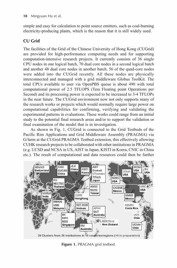
The facilities of the Grid of the Chinese University of Hong Kong (CUGrid)are provided for high-performance computing needs and for supportingcomputation-intensive research projects. It currently consists of 36 singleCPU nodes in one logical batch, 70 dual core nodes in a second logical batchand another 48 dual core nodes in another batch. 56 of the quad-core nodeswere added into the CUGrid recently. All these nodes are physicallyinterconnected and managed with a grid middleware Globus ToolKit. Thetotal CPUs available to user via OpenPBS queue is about 490 with totalcomputational power of 2.5 TFLOPS (Tera Floating point Operations perSecond) and its processing power is expected to be increased to 3-4 TFLOPsin the near future. The CUGrid environment now not only supports many ofthe research works or projects which would normally require large power oncomputational capabilities for confirming, verifying and validating theexperimental patterns in evaluations. These works could range from an initialstudy to the potential final research areas and/or to support the validation orfinal examination of the model that is in investigation.
As shown in Fig. 1, CUGrid is connected to the Grid Testbeds of thePacific Rim Applications and Grid Middleware Assembly (PRAGMA) viaG/farm at the CUGrid PRAGMA Testbed extension, this effectively allowingCUHK research projects to be collaborated with other institutions in PRAGMA(e.g. UCSD and NCSA in US, AIST in Japan, KISTI in Koera, CNIC in Chinaetc.). The result of computational and data resources could then be further
Figure 1. PRAGMA grid testbed.
Hierarchical Geospatial Computing Environment 19
expanded and utilized by the researcher for further needs which is beyond theCUGrid capacity.
Globus ToolKit (Globus Toolkit, 2010)
Computing grids are often constructed by the general-purpose grid softwarelibraries known as middleware. Globus Toolkit, currently at version 5, is anopen source grid middleware for building computing grids developed andprovided by the Globus Alliance. With the recent advancement onGrid computing technology and the maturity of the related supportingsoftware environment of Globus ToolKit, CUHK has successfully built a 200plus nodes grid environment, for supporting large scale scientific researchprojects.
Rocks Clusters (Rocks, 2010)
Rocks clusters have played a pivotal role in the research of cluster computing.Driven by one goal: make clusters easy to deploy, manage, upgrade and scale,the Rocks group has been addressing the difficulties of deploying manageableclusters, which help deliver the computational power of clusters to a widerange of scientific users, improve the state of the art in parallel tools insupporting stable and manageable parallel computing platforms available to awide range of scientists.
SAGE (SAGE, 2010)
SAGE (Scalable Adaptive Graphics Environment) is a scalable pixeldistribution architecture for supporting collaborative scientific visualizationenvironments with potentially high display resolution on tiled walls. Incollaborative scientific visualization, it is crucial to share high-resolutionimagery as well as high-definition video among groups of collaborators atlocal or remote sites.
The Conceptual Model of Hierarchical GeospatialComputing Environment for Data-intensive
Geographic Process Simulation
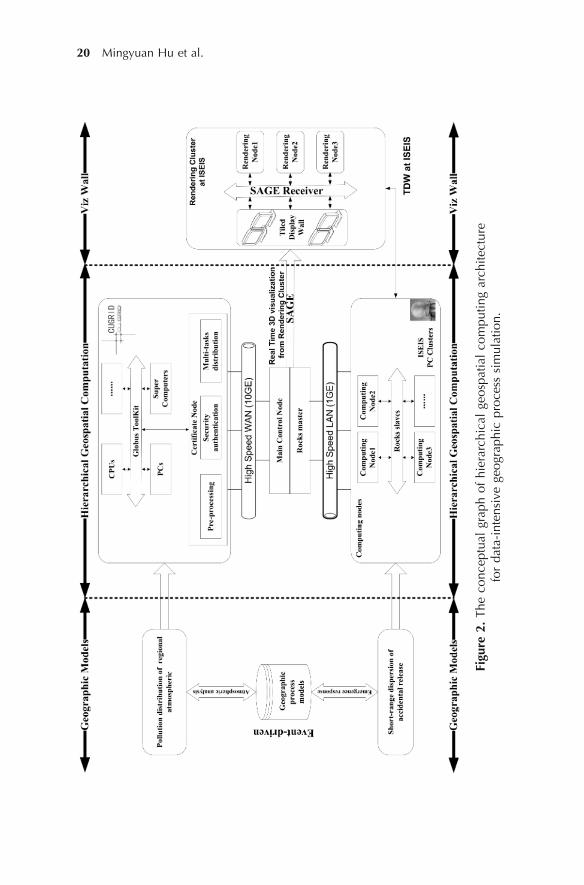
This section provides a hierarchical geospatial computing environment appliedto the data-intensive environmental processes, with support for a geographicprocess model for urban air pollution, hierarchical geospatial computation fordata-intensive environmental processes, as well as the Viz Wall for 3D scientificvisualization, as shown in Fig. 2.
20 Mingyuan Hu et al.
Figu
re 2
. Th
e co
ncep
tual
gra
ph o
f hi
erar
chic
al g
eosp
atia
l co
mpu
ting
arch
itect
ure
for
data
-int
ensi
ve g
eogr
aphi
c pr
oces
s si
mul
atio
n.

Hierarchical Geospatial Computing Environment 21
Multi-scale Geographic Process Models
Environmental phenomena are generally recognized as different cognitivescales and include very intricate spatiotemporal processes and continuouslyincreasing geospatial data. The better way of presenting these changes isthrough geographic process models, not geo-data. For example, atmosphericsimulation can be regarded as meso-scale urban pollution or micro-scaleemergency response, especially for the case of an industrial hazard. As shownin Fig. 2, regional model (such as MM5) is adopted to quantify and explainvariability in the distribution of atmospheric pollution in a given PRD citycluster area; the local dispersion model (such as Gauss model) aims to revealthe source-receptor (relationships) features of the short-range dispersion ofaccidental release for local emergency decision support.
Hierarchical Geospatial Computation
It is based on a hierarchical design targeted at enhancing the flexibility andscalability of data-intensive computing. It provides the integration of gridcomputing based on the available distributed computational resources andself-organized PC clusters to solve time-consuming and complicated scientificproblems. The hierarchical relationships among CUGrid, PC clusters andmain control are illustrated in Fig. 2. The grid system of the Chinese Universityof Hong Kong (CUGrid) is introduced in the framework for high-performancecomputing needs and for supporting computation-intensive research projects,in which hybrid computers such as loosely coupled, heterogeneous, andgeographically dispersed CPU nodes and massively parallel supercomputersare physically interconnected and managed with a grid middleware GlobusToolKit. In the completely computing environment, the CUGrid is responsiblefor the MM5 computing, which is deployed in the authorized master node ofthe CUGrid computers. The master node receives and executes commands,allocates jobs to other computers on the CUGrid, collects the computationoutput and stores this output and information to the main and high speednetworked storage spaces for visualization, analysis and collaboration.
The PC computing clusters are related to the deployment of parallelcomputation on PCs for the Gauss plume model; such computation takesplace in idle computers at the Institute of Space and Earth Information Science(ISEIS) in CUHK. The PC clusters computing nodes installation process isbased on the Rocks clusters, after installing Rocks on the main control node(front-end), all computing nodes installation and configuration are handledautomatically by Rocks (Rocks, 2010). Computing nodes are equipped withparallel computing algorithms, which are also responsible for the division anddistribution of tasks and a summary of the computing results. The Rocks-based main control node is designed as the coordinator for the wholehierarchical computing structure (Rocks, 2010), which establishes a directcorrelation between the CUGrid (with a 10 Gbps network) and PC clusters(1 Gbps network), controls and mediates all access to the CUGrid and PC

22 Mingyuan Hu et al.
cluster resources and facilitates the system services provisioning, management,deployment and job scheduling for the stable and manageable parallelcomputing platforms available to a wide range of scientific users.
Viz Wall for Geo-visualization and Geo-analysis
For the scientific visualization and geographic decision-making analysis, thereis a significant challenge posed by data-intensive science applications,especially for the areas of high definition geographic process simulation suchas atmospheric pollution simulation with large volume computing data streamand the low-latency networking impact. As shown in Fig. 2, in the proposedISEIS Tiled Display Wall (TDW), backing up with the power of the backgroundCUGrid computing power, user can also view multiple datasets in parallel forcertain very complex and large images simultaneously with interactive control.The development of the ISEIS TDW, thus, on a relatively inexpensive easilyuseable tiled display would also be useful for departments seeking their owndisplay facility for large datasets but without the financial resources to builda visualization portal. SAGE (Scalable Adaptive Graphics Environment) is anappropriate option for allowing the seamless display of various networkedapplications over the whole display, in which PC rendering nodes with graphicscards are responsible for the large data volume 3D rendering, where each PCpowers one or two of the tiles in the display. Parallel visualization is thusdesigned to improve decision-making efficiency, and the TDW is deployedfor distributing visualization to a large-scale, high-dimensional and highresolution display, which would be targeted to provide the necessary foundationto explore the possibility of creating a multi-pipe graphics engine thatcould either be driven by the CUGrid or to drive parallel PC cluster computingon its own to form the final display required for a particular visualizationneed.
Distributed Management
Geographic process models are generally many program/function codes, andthe management on geo-models can be referenced from open-source orcommercial program developing platforms, such as Fortran, Python, VisualStudio.Net and Java. In these platforms, models are coded as functions andstored in function libraries or dynamic link libraries (DLL), which also providedescription files (such as .h files for VC++ platform) as the metadata ofmodels, to tell users what functions (models) are used for, what the meaningsfor input and output variables of models are. Based on the computing frameworkof Fig. 2, in the following case study, MM5, which is computation intensive,is suggested to be distributed on the computational grid of CUGrid. Theenvironmental data to support the running of MM5 is also loaded on theCUGrid. The Gauss plume model is distributed on the PC clusters for theparallel computation. MM5 and the Gauss plume model are both well controlledin the system main control interface by using 2D/3D visualization node in
Hierarchical Geospatial Computing Environment 23
TDW, which integrate geographic information to visualize and analyse pollutionresults, including geo-model computation visualization, air pollution result(both distribution and dispersion) visualization, analysis visualization andcollaboration visualization.
Case Study: Towards the Improvement of Air PollutionSimulation and Data Visualization
In this case study area of Pearl River Delta (PRD) of China, we try to integrateMM5, Gauss plume model, geographic information and tiled display wall for2D and 3D visualization into a comprehensive environment, to facilitate airpollution research and to shorten gaps between air pollution research and geo-located visualization and spatial-temporal analysis.
CUGrid-based Regional Air Pollution Simulation
CUGrid is constructed for providing the fundamental computational facilitiesfor all the computing needs in CUHK, which currently consists of 36 singleCPU nodes, 70 dual core nodes, 48 dual core nodes, and another 56 quad-corenodes in multiple batches. As the set of input and outfile from MM5 are textbase file, and with the scale of the problem, the files could be very large, thiswould greatly reduce the performance of the model analysis if the traditionalfile system is used (e.g. NFSV3). This not only limits the overall parallelprocess of the model analysis, but also reduces the total throughput of themodel calculation. In the process of the computing in the CUGrid, we set upa parallel file and data access architecture, the output is confined to few files(domain output files); therefore, both reading and writing operations areconcentrating on a set of few files.
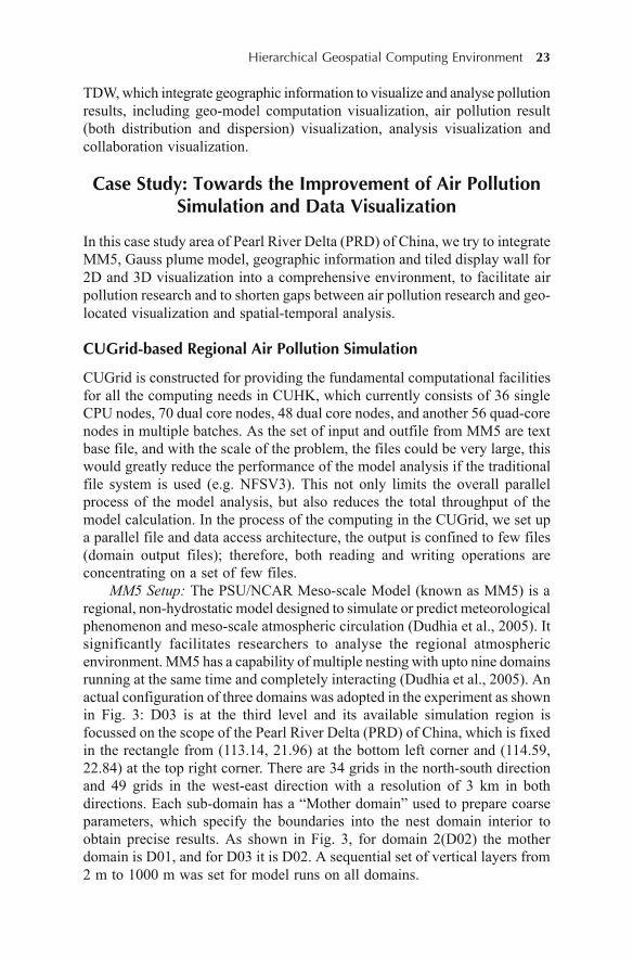
MM5 Setup: The PSU/NCAR Meso-scale Model (known as MM5) is aregional, non-hydrostatic model designed to simulate or predict meteorologicalphenomenon and meso-scale atmospheric circulation (Dudhia et al., 2005). Itsignificantly facilitates researchers to analyse the regional atmosphericenvironment. MM5 has a capability of multiple nesting with upto nine domainsrunning at the same time and completely interacting (Dudhia et al., 2005). Anactual configuration of three domains was adopted in the experiment as shownin Fig. 3: D03 is at the third level and its available simulation region isfocussed on the scope of the Pearl River Delta (PRD) of China, which is fixedin the rectangle from (113.14, 21.96) at the bottom left corner and (114.59,22.84) at the top right corner. There are 34 grids in the north-south directionand 49 grids in the west-east direction with a resolution of 3 km in bothdirections. Each sub-domain has a “Mother domain” used to prepare coarseparameters, which specify the boundaries into the nest domain interior toobtain precise results. As shown in Fig. 3, for domain 2(D02) the motherdomain is D01, and for D03 it is D02. A sequential set of vertical layers from2 m to 1000 m was set for model runs on all domains.

24 Mingyuan Hu et al.
Figure 3. (a) Actual simulation area selection. (b) Parameters settingfor selected area.
Data Mapping and Parallel Implementation of MM5: To run the MM5model, lateral boundary values for each horizontal layer have to be set asinitial values for running a simulation. As shown in Fig. 4, there are m × n
Figure 4. Grid-based allocation for parallel computation of Domain 3.
Hierarchical Geospatial Computing Environment 25
grids in each horizontal layer and each grid in the same vertical column hasa similar boundary condition index as its mother domain. Based on theconsideration described above, the prime goal of this parallel computingdecomposition is to allow the computations in a vertical column (as shown inleft-bottom) of grid nodes to easily acquire their boundary values, which canbe assigned to a single processor as depicted by Fig. 4 left-bottom. For alllayers of the selected simulation region, Fig. 4 also gives the parallel computingdecomposition with computers.
Based on the MM5’s meteorological computing outputs including three-dimensional wind, temperature, pressure and specific humidity fields, the airpollution transportation and dispersion is necessary for predicting time-varyingtrace gas concentrations for the PRD area.
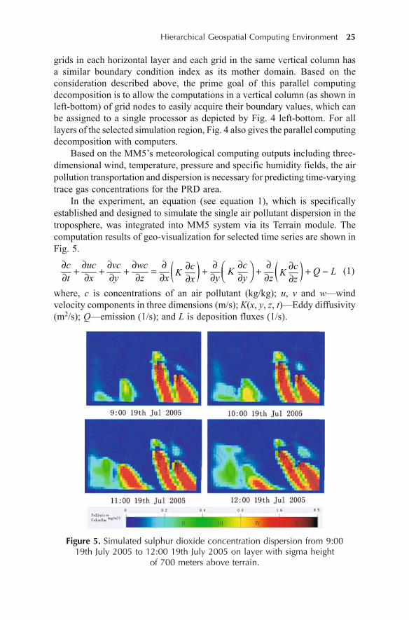
In the experiment, an equation (see equation 1), which is specificallyestablished and designed to simulate the single air pollutant dispersion in thetroposphere, was integrated into MM5 system via its Terrain module. Thecomputation results of geo-visualization for selected time series are shown inFig. 5.
� � � �c uc vc wc cc cK Q LK Kt x y z x y y zx z� � � � � � � �� �È Ø� � � � � � �É ÙÊ Ú� � � � � � � �� �
(1)
where, c is concentrations of an air pollutant (kg/kg); u, v and w—windvelocity components in three dimensions (m/s); K(x, y, z, t)—Eddy diffusivity(m2/s); Q—emission (1/s); and L is deposition fluxes (1/s).
Figure 5. Simulated sulphur dioxide concentration dispersion from 9:0019th July 2005 to 12:00 19th July 2005 on layer with sigma height
of 700 meters above terrain.
26 Mingyuan Hu et al.
PC Clusters-based Parallel Computation of Gauss PollutionDispersion Model for Multi-point Sources
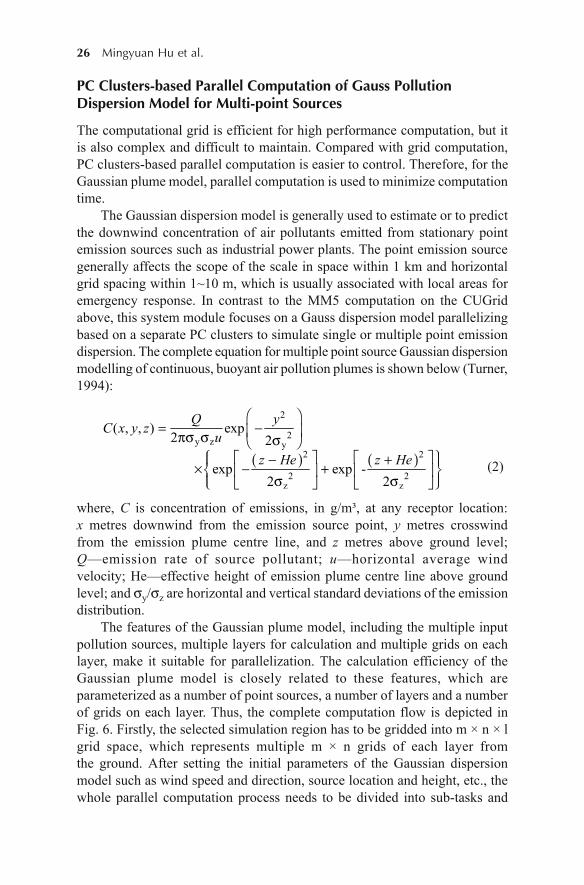
The computational grid is efficient for high performance computation, but itis also complex and difficult to maintain. Compared with grid computation,PC clusters-based parallel computation is easier to control. Therefore, for theGaussian plume model, parallel computation is used to minimize computationtime.
The Gaussian dispersion model is generally used to estimate or to predictthe downwind concentration of air pollutants emitted from stationary pointemission sources such as industrial power plants. The point emission sourcegenerally affects the scope of the scale in space within 1 km and horizontalgrid spacing within 1~10 m, which is usually associated with local areas foremergency response. In contrast to the MM5 computation on the CUGridabove, this system module focuses on a Gauss dispersion model parallelizingbased on a separate PC clusters to simulate single or multiple point emissiondispersion. The complete equation for multiple point source Gaussian dispersionmodelling of continuous, buoyant air pollution plumes is shown below (Turner,1994):
� � � �
2
2y z y2 2
2 2z z
( , , ) exp2 2
exp exp -2 2
Q yC x y z
uz He z He
È Ø �É ÙSV V VÊ Ú
Î Ë Û Ë Û Þ� �Ñ Ñ� � �Ï ßÌ Ü Ì ÜV VÑ ÑÍ Ý Í ÝÐ à
(2)
where, C is concentration of emissions, in g/m³, at any receptor location:x metres downwind from the emission source point, y metres crosswindfrom the emission plume centre line, and z metres above ground level;Q—emission rate of source pollutant; u—horizontal average windvelocity; He—effective height of emission plume centre line above groundlevel; and Vy/Vz are horizontal and vertical standard deviations of the emissiondistribution.
The features of the Gaussian plume model, including the multiple inputpollution sources, multiple layers for calculation and multiple grids on eachlayer, make it suitable for parallelization. The calculation efficiency of theGaussian plume model is closely related to these features, which areparameterized as a number of point sources, a number of layers and a numberof grids on each layer. Thus, the complete computation flow is depicted inFig. 6. Firstly, the selected simulation region has to be gridded into m × n × lgrid space, which represents multiple m × n grids of each layer fromthe ground. After setting the initial parameters of the Gaussian dispersionmodel such as wind speed and direction, source location and height, etc., thewhole parallel computation process needs to be divided into sub-tasks and
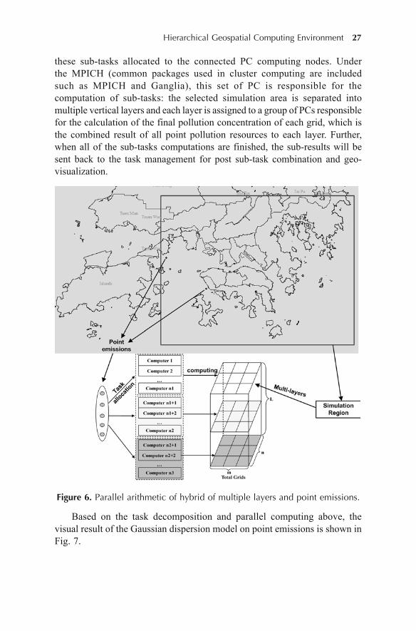
Hierarchical Geospatial Computing Environment 27
these sub-tasks allocated to the connected PC computing nodes. Underthe MPICH (common packages used in cluster computing are includedsuch as MPICH and Ganglia), this set of PC is responsible for thecomputation of sub-tasks: the selected simulation area is separated intomultiple vertical layers and each layer is assigned to a group of PCs responsiblefor the calculation of the final pollution concentration of each grid, which isthe combined result of all point pollution resources to each layer. Further,when all of the sub-tasks computations are finished, the sub-results will besent back to the task management for post sub-task combination and geo-visualization.
Figure 6. Parallel arithmetic of hybrid of multiple layers and point emissions.
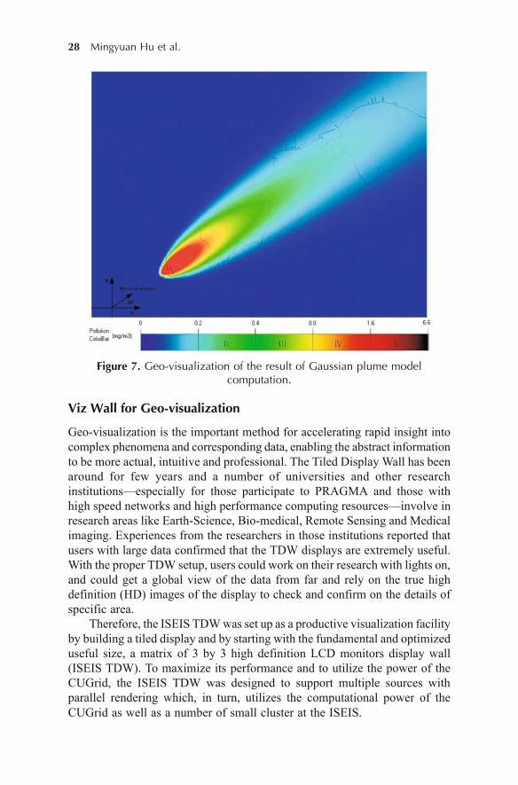
Based on the task decomposition and parallel computing above, thevisual result of the Gaussian dispersion model on point emissions is shown inFig. 7.
28 Mingyuan Hu et al.
Figure 7. Geo-visualization of the result of Gaussian plume modelcomputation.
Viz Wall for Geo-visualization
Geo-visualization is the important method for accelerating rapid insight intocomplex phenomena and corresponding data, enabling the abstract informationto be more actual, intuitive and professional. The Tiled Display Wall has beenaround for few years and a number of universities and other researchinstitutions—especially for those participate to PRAGMA and those withhigh speed networks and high performance computing resources—involve inresearch areas like Earth-Science, Bio-medical, Remote Sensing and Medicalimaging. Experiences from the researchers in those institutions reported thatusers with large data confirmed that the TDW displays are extremely useful.With the proper TDW setup, users could work on their research with lights on,and could get a global view of the data from far and rely on the true highdefinition (HD) images of the display to check and confirm on the details ofspecific area.
Therefore, the ISEIS TDW was set up as a productive visualization facilityby building a tiled display and by starting with the fundamental and optimizeduseful size, a matrix of 3 by 3 high definition LCD monitors display wall(ISEIS TDW). To maximize its performance and to utilize the power of theCUGrid, the ISEIS TDW was designed to support multiple sources withparallel rendering which, in turn, utilizes the computational power of theCUGrid as well as a number of small cluster at the ISEIS.
Hierarchical Geospatial Computing Environment 29
As shown in Fig. 8, combining the visualization facilities with the PCrendering clusters capability, ISEIS TDW allows the creation of a collaborativevisualization environment for supporting a large research group and for manyresearchers at the same time. In our TDW system, the whole visualization isbased on the SAGE configuration for supporting collaborative scientificvisualization. The 10G network is used as a high speed network connection tosupport the storage needs and the high bandwidth requirement for thetransmission of the dataset between the computational nodes, the renderingnodes and the SAN storage. It would also be used to allow for multiplerendered streams of pixels from local and remote sites with similar displaysettings. With the ISEIS TDW, the rendering and display PCs in the displaycluster perform the necessary parallel rendering for parallel session of themultiple dataset, while the PCs in the compute cluster in CUGrid compute theiso-surfaces from the scientific data, and the SAN storage holds the data.
Furthermore, since it is built with standard components (Viz Wall underRocks cluster, EVL’s SAGE), the underlying network can easily be expandedusing flexible, inexpensive switches to accommodate additional servers forincreased horizontal and overall performance on bandwidth and computationalcapacity.
Figure 8. Tiled display wall-based geo-visualization and geographic analysis.
Conclusions and Perspective Remarks
A scalable geospatial computation environment is proposed for solving theproblems of increasingly complicated geo-referenced phenomenon simulation,with support for local computing clusters for point source simulation, meso-scale regional air pollution analysis for large data sets and intensive calculations,
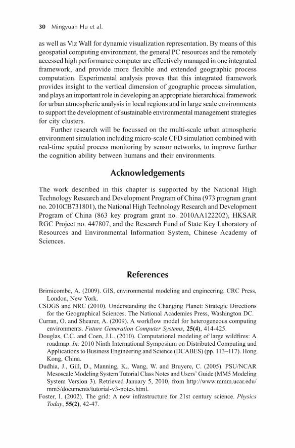
30 Mingyuan Hu et al.
as well as Viz Wall for dynamic visualization representation. By means of thisgeospatial computing environment, the general PC resources and the remotelyaccessed high performance computer are effectively managed in one integratedframework, and provide more flexible and extended geographic processcomputation. Experimental analysis proves that this integrated frameworkprovides insight to the vertical dimension of geographic process simulation,and plays an important role in developing an appropriate hierarchical frameworkfor urban atmospheric analysis in local regions and in large scale environmentsto support the development of sustainable environmental management strategiesfor city clusters.
Further research will be focussed on the multi-scale urban atmosphericenvironment simulation including micro-scale CFD simulation combined withreal-time spatial process monitoring by sensor networks, to improve furtherthe cognition ability between humans and their environments.
Acknowledgements
The work described in this chapter is supported by the National HighTechnology Research and Development Program of China (973 program grantno. 2010CB731801), the National High Technology Research and DevelopmentProgram of China (863 key program grant no. 2010AA122202), HKSARRGC Project no. 447807, and the Research Fund of State Key Laboratory ofResources and Environmental Information System, Chinese Academy ofSciences.
References
Brimicombe, A. (2009). GIS, environmental modeling and engineering. CRC Press,London, New York.
CSDGS and NRC (2010). Understanding the Changing Planet: Strategic Directionsfor the Geographical Sciences. The National Academies Press, Washington DC.
Curran, O. and Shearer, A. (2009). A workflow model for heterogeneous computingenvironments. Future Generation Computer Systems, 25(4), 414-425.
Douglas, C.C. and Coen, J.L. (2010). Computational modeling of large wildfires: Aroadmap. In: 2010 Ninth International Symposium on Distributed Computing andApplications to Business Engineering and Science (DCABES) (pp. 113–117). HongKong, China.
Dudhia, J., Gill, D., Manning, K., Wang, W. and Bruyere, C. (2005). PSU/NCARMesoscale Modeling System Tutorial Class Notes and Users’ Guide (MM5 ModelingSystem Version 3). Retrieved January 5, 2010, from http://www.mmm.ucar.edu/mm5/documents/tutorial-v3-notes.html.
Foster, I. (2002). The grid: A new infrastructure for 21st century science. PhysicsToday, 55(2), 42-47.
Hierarchical Geospatial Computing Environment 31
Foster, I. and Kesselman, C. (2004). The Grid2: Blueprint for a New ComputingInfrastructure (2nd ed.). Kaufmann Publishers, Morgan.
Globus Toolkit (2010). About the Globus Toolkit. Retrieved January 2, 2010, fromhttp://www.globus.org/toolkit/about.html.
Goodchild, M.F. (2006). Geographical information science: fifteen years later. In: P.F.Fisher (Ed.), Classics from IJGIS: Twenty years of the International Journal ofGeographical Information Science and Systems (pp. 199–204). CRC Press, BocaRaton.
Goodchild, M.F. (2010). Twenty years of progress: Giscience in 2010. Journal ofSpatial Information Science, 1, 3–20.
Guan, Q., Zhang, T. and Clarke, K. (2006). GeoComputation in the Grid ComputingAge. Lecture Notes in Computer Science: Web and Wireless GeographicalInformation Systems, 4295/2006, 237–246.
Guan, Q. and Clarke, K. (2010). A general-purpose parallel raster processingprogramming library test application using a geographic cellular automata model.International Journal of Geographic Information Science, 24(5), 695–722.
Han, S.H., Heo, J., Sohn, H. and Yu, K. (2009). Parallel processing method forairborne laser scanning data using a pc cluster and a virtual grid. Sensors, 9(4),2555–2573.
Harris, R., Singleton, A., Grose, D., Brunsdon, C. and Longley, P. (2010). Grid-enabling geographically weighted regression: A case study of participation in highereducation in England. Transactions in GIS, 14(1), 43–61.
Huang, P., Peng, H., Lin, P. and Li, X. (2009). Static strategy and dynamic adjustment:An effective method for grid task scheduling. Future Generation Computer Systems,25(8), 884–892.
Li, X., Zhang, X.H., Yeh, A. and Liu, X. (2010). Parallel cellular automata for large-scale urban simulation using load-balancing techniques. International Journal ofGeographic Information Science, 24(6), 803–820.
Marín Pérez, J.M., Bernabé, J.B., Alcaraz Calero, J.M., Garcia Clemente, F.J., Pérez,G.M. and Gómez Skarmeta, A.F. (2011). Semantic-based authorization architecturefor grid. Future Generation Computer Systems, 27(1), 40–55.
Openshaw, S. (2000). Geocomputation. In: Stan Openshaw and R.J. Abrahart (Eds.),Geocomputation (pp. 1–32). Taylor and Francis, London and New York.
Plaza, A.D., Valencia, J.P. and Martinez, P. (2006). Commodity cluster-based parallelprocessing of hyperspectral imagery. Journal of Parallel and Distributed Computing,66(3), 345–358.
Rocks (2010). Rocks cluster distribution. Retrieved June 2, 2010, from http://www.rocksclusters.org.
SAGE (2010). SAGE introduction. Retrieved January 2, 2010, from http://www.sagecommons.org/.
Sugato, B. (2005). Simulation of grid computing infrastructure: challenges and solutions.In: Proceedings of the 37th conference on Winter Simulation (pp. 1773 Londonand New York: 1780), Orlando, Florida.
Tony, H., Stewart, T. and Krist, T. (Eds.) (2009). The Fourth Paradigm: Data-IntensiveScientific Discovery. United States of America, Microsoft Research.
Torrens, P.M. (2009). Process Models and Next-Generation Geographic InformationTechnology. Retrieved February 10, 2010, from http://www.esri.com/news/arcnews/summer09articles/process-models.html.

32 Mingyuan Hu et al.
Turner, D.B. (1994). Workbook of Atmospheric Dispersion Estimates: An Introductionto Dispersion Modeling (2nd ed.). CRC Press, Boca Raton.
Wang, S.W., Cowles, M.K. and Armstrong, M.P. (2008). Grid computing of spatialstatistics: using the TeraGrid for g(i)*(d) analysis. Concurrency and Computation:Practice and Experience, 20(14), 1697–1720.
Xie, J.B., Yang, C., Zhou, B. and Huang, Q. (2009). High-performance computing forthe simulation of dust storms. Computers Environment and Urban Systems, 34(4),278–290.
Xu, B., Lin, H., Chiu, L.S., Tang, S., Cheung, J., Hu, Y. and Zeng, L. (2010). Vge-cugrid: An integrated platform for efficient configuration, computation, andvisualization of mm5. Environmental Modelling and Software, 25(12), 1894–1896.
Yuan, M. and Hornsby, K.S. (2008). Computation and Visualization for UnderstandingDynamics in Geographic Domains: A Research Agenda (1st ed.). CRC Press, NewYork.
Zhang, J. (2010). Towards personal high-performance geospatial computing (HPC-G): perspectives and a case study. In: Proceedings of the ACM SIGSPATIALInternational Workshop on High Performance and Distributed GeographicInformation Systems (pp. 3–10). San Jose, California.
Integration of Geographic Information Systems 33
3Integration of Geographic
Information Systems forMonitoring and Dissemination
of Marine Environment Data
Marcin Kulawiak and Marek MoszynskiDepartment of Geoinformatics, Gdansk University of Technology
Narutowicza 11/12 Str., 80-233 Gdansk, Poland
Introduction
The issue of monitoring, analysis and visualization of marine activity, eitherfor the purpose of environment protection or threat sensing, has been thesubject of intensive research for many years. In the last decades, presentedsolutions have shown the advantages of dedicated software for storing andmanagement of acoustic and spatial data (Stepnowski et al., 1996; Trygonis etal., 2009; Thakur et al., 2011) as well as the potential of web mapping inapplication to environmental modelling (Maceachren and Kraak, 1997; Doyleet al., 1998; Goodall et al., 2011). In more recent years, many commercial andscientific institutions have been continuously contributing to the process ofdevelopment and application of various tools for aquatic sensing. Because ofthis, the variety of marine sensors is very wide, ranging from simple techniquessuch as direct sampling or hydrological measurements using CTD probes,through hydroacoustic surveys, air-borne photographs and satellite imaging tonumerical modelling and simulation.
In this context, the acquisition, processing, integration and visualizationof various kinds of aforementioned data is a key feature of applicationsdedicated to aquatic ecosystems management, as it has been shown e.g. byTsou (2004). At the same time, Kraak (2004) has shown that a commongeographical coordinate space is an excellent place to combine many types ofinformation concerning the environment. In this context, it has become clearthat the proper way of processing and visualization of data acquired fromvarious marine sensors should involve the use of a Geographic Information
DOI 10.1007/978-94-007-1858-6_3, © Capital Publishing Company 2012
e ,J.K. Thakur et al. (eds.), G ospatial Techniques for Managing Environmental Resources 33
34 Marcin Kulawiak and Marek Moszynski
System. Since that time, Rao et al. (2007) used the ESRI ArcIMS platform toimplement a web GIS Decision Support System (DSS) for use in resourcemanagement and assessment of environmental quality, while Kruger et al.(2007) demonstrated a web GIS dedicated for verification of hydrologicforecasts built with Open Source technologies. In the same year, Tuama andHamre (2007) presented a web-based DSS for monitoring, integration anddissemination of marine pollution data collected from multiple sensors bymeans of non-proprietary technologies. Several months later Bakare et al.(2008) demonstrated the application of commercial technologies like ESRIArcGIS to morphological modelling of the seabed, aiming to identify theareas which may require resurveying to maintain navigation safety in Britishterritorial waters. A year afterwards, Hamre et al. (2009) presented a web GISportal dedicated to integration and dissemination of multi-source data for thepurpose of environmental risk management in marine and coastal areas ofEurope. More recently, successful attempts at dynamic presentation of marinedata collected from a variety of sensors by means of web GIS have beenpresented by Kulawiak et al. (2010a).
Nevertheless, dynamic processing and integration of remote sensor dataremains one of the greatest challenges related to application of GIS to marineenvironment monitoring. The origin of this issue lies in the steady progressthat the different methods of marine data acquisition have seen throughout thesecond part of the twentieth century. Tools such as the multibeam echosounderhave acquired range and resolution high enough to produce megabytes of dataper every second of survey. On the other hand, diverse methods of processingand analysis of such information have also been constantly evolving. Theadvent of high performance PC’s with multicore CPU’s, gigabytes of RAMand terabytes of hard drive storage space, coupled with widespread access tobroadband Internet has made it possible to process and visualize high-resolutiondata from remote sensors in near-real time without the need for dedicatedhardware.
Therefore, the greatest limitation of current technology lies not in lack ofprecision or processing powers, but in absence of common standards of dataexchange and proper visualization. Without architecture-independent meansof accelerated web-based three-dimensional presentation of geographical data,its remote visualization will always be a compromise between realisticcomplexity of source data and imperfect methods of its delivery to the endusers. In the current situation, developers need to carefully balance betweenremote processing and presentation of impaired data and precise on-site 3Dvisualization of the entire available dataset.
This chapter presents the common types of marine data sensors, discussespopular technologies used for constructing GIS, and describes the results thatmay be obtained by application of the discussed technologies to processing,integration, analysis and visualization of data from the presented sources.
Integration of Geographic Information Systems 35
Featured Technologies
There are many techniques of presenting and processing GIS data. Some ofthem are more suited towards visualization, others provide means for betterspatial analysis and some, to an extent, allow for both. The technologiespresented in this section are some of the most prominent in the GIS sector. Butmore importantly, they all have proven to effectively constitute advancedGeographical Information Systems dedicated to integration and processing ofdata pertaining to the marine environment.
The ESRI ArcGIS Engine
The ArcGIS Engine is a set of libraries which can be used to create new GISapplications as well as extend the functionality of existing ones. The corecomponents of ArcGIS are referred to as ArcObjects. They are platform-independent object-oriented libraries which may be accessed through availableC++, COM, Java and .NET Application Programming Interfaces (API’s).Because the libraries are platform-independent, they need to be invoked fromthe platform-specific ArcGIS Engine runtime, which is available on Windows,UNIX and Linux. ArcObjects realize a set of functionalities which allow thebuilt application e.g. to display a map with multiple layers, transform betweencoordinate systems, create and update geographic features or interact withpersonal and enterprise geodatabases.
Building an application with ArcObjects involves choosing the desiredfunctionality from the available controls and linking it with custom C++, C#or Java code. For example, a custom version of the ESRI ArcMap desktopGIS application may be created by joining the “Map” and “Table of Content”controls with a Map Navigation toolbar. In a similar manner, adding 3Ddisplay functionality to the application would require the inclusion of ArcScenecontrol.
Being a commercial product, the ArcGIS Engine is available in severalconfigurations, with the standard edition offering basic data creation anddisplay functionality, and Geodatabase Update, Spatial, 3D and StreetMapUSA extensions providing additional libraries for additional prices. Animportant aspect of ArcGIS Engine is that although purchasing an ESRIDeveloper Network (EDN) annual subscription grants access to these libraries,deploying a developed application to a client requires the purchase of a separateArcGIS Engine license, as well as licenses for optional extensions.
The ArcGlobe
The ESRI ArcGlobe is a part of the ArcGIS 3D Analyst package. The applicationpresents the user with a freely explorable three-dimensional Earth globe in away that is similar to the freely available Google Earth. However, ArcGlobeis a part of the ArcGIS package and therefore shares a lot of functionalities
36 Marcin Kulawiak and Marek Moszynski
with its other elements. In particular, ArcGlobe supports most data formatsnative to ESRI software, such as Shapefiles, TIN’s and SDE databases. Thismeans that data created e.g. with ArcMap may be easily imported into ArcGlobeand displayed in three dimensions. Base maps may also be imported throughthe Internet from ArcGIS Online services, with most recent versions ofArcGlobe also supporting Microsoft Bing Maps. The software allows to loadand display three-dimensional features such as buildings and bridges andsupports extrusion of two-dimensional features to three dimensions usingattribute data. In addition, ArcGlobe allows to perform three-dimensionalspatial analysis of viewshed and line-of-sight, as well as spot heightinterpolation, profiling, and steepest path determination. Integration with 3DAnalyst provides tools for calculating surface area, volume, slope, aspect, andhillshade, as well as data query based on attributes or location.
Because any geographical data loaded in the ArcGlobe will be displayedin the context of a three-dimensional model of the Earth, the software is bestsuited for presentation and analysis of large environments such as cities orcoastal areas.
The GeoTools Open Source Java GIS Toolkit
GeoTools is an Open Source Java library which provides methods formanipulating various types of geospatial data. The functionality of GeoToolsincludes creation, modification, integration, analysis as well as styling andrendering of raster and vector data. The library provides the user with easyaccess to geographic data, whether it is stored in files or in geodatabases.
GeoTools is developed by the Open Source Geospatial Foundation and isusually the first software to implement new standards established by the OpenGeospatial Consortium (OGC). Examples of such standards are the Web MapService (WMS) and Web Feature Service (WFS) protocols, as well as theCommon Query Language (CQL) format. The library also supports OGC’sXML-based Styled Layer Descriptor (SLD) files, which may be used tocustomize the look of vector features. Classes provided by GeoTools allow toquickly build GIS applications which enable the composition and display ofstyled maps, as well as spatial analysis of geographical data such as graphsand networks. Data created with the GeoTools package may be easily referencedwith and transformed between coordinate systems compatible with theEuropean Petroleum Survey Group (EPSG) specifications. The streamingdata readers used by GeoTools allow to avoid memory limitations on theamount of data that can be accessed by an application.
Due to its flexibility, the library may serve as a foundation of server aswell as desktop GIS projects. The most prominent applications built withGeoTools are the Open Source GeoServer Web map server and uDig OpenSource desktop application framework.
Integration of Geographic Information Systems 37
The GeoServer
The GeoServer is a dynamically developing Open Source GIS server whichfully supports OGC WMS, WFS, Web Coverage Service and Web FeatureService Transactional (WFS-T) protocols. Through the use of GeoTools, theGeoServer supports PostGIS, Shapefile, ArcSDE, DB2, Oracle, VPF, MySQL,MapInfo, and Cascading WFS data sources, as well as Web Map output asjpeg, gif, png, SVG, GeoJSON, GeoRSS and pdf, including support forantialiased images. The presentation of every layer stored in the GeoServerdatabase can be individually customized using SLD files, which can bedynamically swapped and altered during web queries. An embedded EPSGdatabase allows for real-time data reprojection between hundreds of existingas well as user-defined projections.
The GeoServer is based on Java Enterprise Edition (JEE) Servlettechnology and can run in any Servlet container. Its open architecture allowsfor easy adoption of new data formats with GeoTools DataStore interfaces andhelper classes. Existing GeoTools DataStores instantly plug-in to GeoServer,showing up as an option in the user-friendly configuration Graphical UserInterface (GUI).
In order to fully utilize its GIS capabilities, the GeoServer should be usedin conjunction with compatible client software. While this may be anyapplication supporting open standards of data exchange, such as Google Earth,uDig, GVSig and others, the GeoServer is known for its effective integrationwith OpenLayers, which is also a dynamically developing Open Source project.
The OpenLayers Web GIS Client Library
OpenLayers is an Open Source object-oriented JavaScript library for displayingmap data in most modern web browsers, with no server-side dependencies. Itimplements a constantly developing JavaScript API for building rich web-based geographic applications. OpenLayers allows the developer to utilizemany readily available and fully customizable components for easy constructionof GIS client solutions which can be embedded into any Web page. As aframework, OpenLayers is intended to separate map tools from map data sothat all the tools can operate on all the data sources by means of industry-standard methods, such as the OGC WMS and WFS protocols (Schmidt,2008). Although it exhibits similarities to the Google Maps and MSN VirtualEarth APIs, OpenLayers has the advantage of being developed for and by theOpen Source software community, which makes it free for modification andredistribution.
The default installation of OpenLayers provides only basic GIS featureslike zooming and panning, and advanced functionalities must be addedmanually by the developer, using a selection of existing controls as well ascustom code. In practice, however, building a Web GIS client with OpenLayers
38 Marcin Kulawiak and Marek Moszynski
is very easy thanks to the vast library of examples. This, along with gooddocumentation and support for tiled layer caches, makes this Open Sourceproduct a very flexible alternative to commercial solutions.
This innovative technology is becoming increasingly popular amongdevelopers of Web mapping systems and is now utilized in several majorprojects like the NOAA National Weather Service (http://radar.srh.noaa.gov/)and the European Union GeoPortal (www.inspire-geoportal.eu).
Means of Monitoring the Marine Environment
Thorough monitoring of the marine environment is a complex task which notonly consists of measurements but also analysis, validation and interpretationof information acquired by various sensors. The most commonly used sensorsmay be divided into two groups. The first group, dedicated to monitoring theunderwater environment, includes sonar systems like echosounders andsidescan sonars. The second group deals with sensing of activities on thewater surface and consists of radars, satellite images and AutomaticIdentification System (AIS) of marine vessels.
Underwater Sensors
Producing maps of the sea floor has always been a unique challenge. Through-out the years different tools have been developed to meet these specificrequirements. The produced tools include underwater devices like single-beam echosounder, sidescan sonar and bathymetric systems that remotelymap the sea floor and subsurface. These systems are deployed from the fantailor a sidemount of a ship and towed continuously throughout a survey area.Navigational systems are run concurrently to precisely locate the gathereddata.
Historically, the information on sea depth has been collected with the helpof simple, relatively easy to use, low-cost echosounder equipped with a singlepiezoelectric transducer. These single-beam bathymetry systems measure thewater depth directly beneath the vessel. The transceiver transmits a high-frequency acoustic pulse in a beam downward into the water column, theacoustic energy is reflected off the sea floor beneath the vessel and receivedat the transceiver. The continuous recording of water depth below the vesselyields high-resolution measurements, but only along the survey track. Theoperating frequency of single-beam systems ranges from 3.5 kHz to 400 kHz.A low-frequency system may also function as a subbottom profiler, as theenergy can penetrate the sea floor and produce a very detailed map of surficialsediment thickness. The resulting depth values in the form of a point datasetrepresent accurate and reliable bathymetry. In order to show depths along thesurvey transects, bathymetry data can be displayed in the form of a colouredtrack or as a series of numbers called soundings (very common on marinecharts). When the echosounder is equipped with bottom classification software,
Integration of Geographic Information Systems 39
an interpolated image with bottom types may be generated. Modern digitalechosounders can produce detailed echograms in the form of raster imagesthat represent a vertical transect of the whole survey. Although the echogramrepresents a vertical glimpse into the water column, sea bottom and sub-bottom areas, scientists very often embed the image in the horizontal untruecontext of the map. It is very advantageous especially when the surveys areorganized along map parallels and the track is sparse in meridians. The truepresentation of an echogram data in three-dimensional geographic coordinatesis still rare as the graphical rendering of such data in 3D GIS systems is highlydemanding.
Data provided by a single-beam echosounder, in general, has limited usesbecause features lying between tracklines (which are often spaced between afew dozen and several hundred metres apart) are not visible to the system.Because of this, the provided data is quite sparse and requires a great degreeof interpolation. Single beam surveys are still necessary for a number ofapplications; however more sophisticated devices are manufactured that usemore than one transmitting and/or receiving piezoelectric element.
A sidescan sonar constitutes the optimal trade-off between resolution andswath coverage, with moderate complexity and cost. It produces data whichallows to characterize surface sediment and identify sea floor objects. Imagingthe sea floor with a sidescan sonar system is accomplished by towing a sonar(referred to as “tow-fish”) over the study area. The tow-fish is equipped witha linear array of transducers that emit, and later receive, an acoustic energypulse in a specific frequency range. The acoustic pulse is specifically designedso that it is wide in the across-track direction and narrow in the along-trackdirection. The acoustic backscattered energy received by the sidescan sonartow vehicle provides information regarding the general distribution andcharacteristics of the surficial sediment and outcropping strata. Sidescan sonarsystems typically operate in the 100 kHz to 1 MHz frequency range. Swathwidth depends on water depth and ranges from around 50 m to 500 m withinthese operating frequencies. The higher the frequency, the higher the resolutionof the resultant sidescan sonar image. Such imagery data may be embedded inthe map context as it represents near horizontal plane of sea floor with rangesthat could be calculated from tow-fish track and the geometry of acquisition.However, although the acquired image is rectangular, its referencing in themap context is not straightforward because each pixel needs to be referencedaccording to the geometry of measurement. It means that nonlinear stretchingof image is required, followed by application of graphical path technique tothe whole image according to recorded geographical location. This processproduces pixel holes in the image, which need to be removed via interpolation.A more sophisticated approach uses specialized software which creates alarge image by assembling, or mosaicing, each swath of data into ageoreferenced composite that represents the acoustic character of the sea floorwithin the study area.
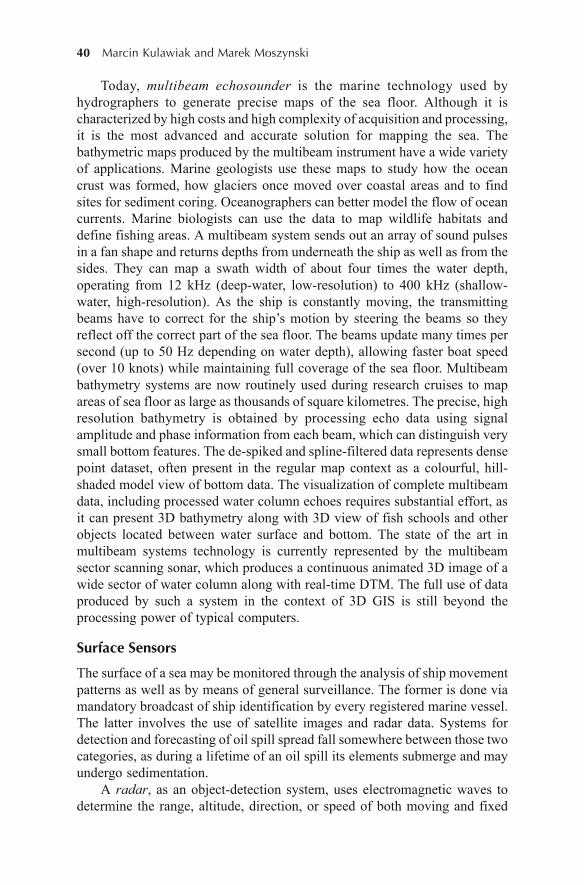
40 Marcin Kulawiak and Marek Moszynski
Today, multibeam echosounder is the marine technology used byhydrographers to generate precise maps of the sea floor. Although it ischaracterized by high costs and high complexity of acquisition and processing,it is the most advanced and accurate solution for mapping the sea. Thebathymetric maps produced by the multibeam instrument have a wide varietyof applications. Marine geologists use these maps to study how the oceancrust was formed, how glaciers once moved over coastal areas and to findsites for sediment coring. Oceanographers can better model the flow of oceancurrents. Marine biologists can use the data to map wildlife habitats anddefine fishing areas. A multibeam system sends out an array of sound pulsesin a fan shape and returns depths from underneath the ship as well as from thesides. They can map a swath width of about four times the water depth,operating from 12 kHz (deep-water, low-resolution) to 400 kHz (shallow-water, high-resolution). As the ship is constantly moving, the transmittingbeams have to correct for the ship’s motion by steering the beams so theyreflect off the correct part of the sea floor. The beams update many times persecond (up to 50 Hz depending on water depth), allowing faster boat speed(over 10 knots) while maintaining full coverage of the sea floor. Multibeambathymetry systems are now routinely used during research cruises to mapareas of sea floor as large as thousands of square kilometres. The precise, highresolution bathymetry is obtained by processing echo data using signalamplitude and phase information from each beam, which can distinguish verysmall bottom features. The de-spiked and spline-filtered data represents densepoint dataset, often present in the regular map context as a colourful, hill-shaded model view of bottom data. The visualization of complete multibeamdata, including processed water column echoes requires substantial effort, asit can present 3D bathymetry along with 3D view of fish schools and otherobjects located between water surface and bottom. The state of the art inmultibeam systems technology is currently represented by the multibeamsector scanning sonar, which produces a continuous animated 3D image of awide sector of water column along with real-time DTM. The full use of dataproduced by such a system in the context of 3D GIS is still beyond theprocessing power of typical computers.
Surface Sensors
The surface of a sea may be monitored through the analysis of ship movementpatterns as well as by means of general surveillance. The former is done viamandatory broadcast of ship identification by every registered marine vessel.The latter involves the use of satellite images and radar data. Systems fordetection and forecasting of oil spill spread fall somewhere between those twocategories, as during a lifetime of an oil spill its elements submerge and mayundergo sedimentation.
A radar, as an object-detection system, uses electromagnetic waves todetermine the range, altitude, direction, or speed of both moving and fixed
Integration of Geographic Information Systems 41
objects. In marine environment nautical radars installed on-board are typicallyused to detect approaching ships and aircraft, observe weather formations anddistant terrains as well as locate landmarks, as transmitted pulses of radiowaves reflect from any object in their path as long as it exhibits differentdensity from air medium. In a way similar to air traffic control, stationaryinstallations of radars are present in coastal areas. Although the reflected radarsignals captured by the receiving antenna are usually very weak, sophisticatedmethods of signal processing are used in order to recover useful information.The modern uses of radar are highly diverse, mostly because modern systemsrecord and process radar image data in digital form. For example, commercialradar imaging satellites use active sensors that illuminate surface featureswith broadcast microwave energy at wavelengths which propagate throughthe atmosphere and clouds with almost no interaction or weakening. Becauseof this, they can record the returned signal during the day as well as night andunder virtually any weather conditions. The image data that originates fromrotating the transmitting/receiving antenna is typically internally processed tohave rectangular coverage suitable for being stored as the false-scaled bitmapimage. Its georeference is immediately obtained from known geographicposition of the radar antenna and the radar range, typically expressed in nauticalmiles. Hence, the conversion to Universal Transverse Mercator projectedmarine maps is straightforward. However, as the stream of radar data is typicallyrefreshed every 1 or 2 seconds, and additionally the radar range may bechanged by the operator, the image georeferencing must be setup in real-time,what may be challenging in a real-time GIS system.
Satellite sensors provide means of measuring electromagnetic reflectanceof objects on the Earth’s surface as well as in the atmosphere. They offer goodstability, capability for repeated measurements, potential of global coverageand spatial resolution ranging from 1 km to 1 m. The most prominentcharacteristic differentiating satellite platforms is mobility. Geostationarysatellites maintain a fixed position over an area of the Earth, and thus are mostuseful in activities which involve among others continuous monitoring of theenvironment. Satellites which orbit the planet along fixed paths allow forsurveillance of large portions of the globe, but at the cost of long delaysbetween consecutive surveys of the same area. In addition, each platform maybe equipped with several types of sensors providing information for differentpurposes. Some of the more popular platforms include the Meteosat SecondGeneration (MSG) geostationary satellites equipped with Spinning EnhancedVisible and InfraRed Imager (SEVIRI), the Meteorological Operational(MetOp) orbiting satellites equipped with Advanced Very High ResolutionRadiometer (AVHRR), Terra and Aqua polar orbiting satellites equipped withModerate-resolution Imaging Spectroradiometer (MODIS), the Envisat polarorbiting satellite with Advanced Synthetic Aperture Radar (ASAR), and theGeoEye-1 polar orbiting satellite equipped with sensor capable to capturevery high resolution satellite photographs.

42 Marcin Kulawiak and Marek Moszynski
Satellites most often produce data in the form of photographs of an areain a given amount of spectral bands or groups of wavelengths. In most cases,images captured in the visible spectrum are ready for use (e.g. as backgroundGIS imagery) shortly after their reception by a satellite ground station.Photographs of other spectra may require further processing (e.g identificationand extraction of data such as vegetation zones). Although reception of satellitedata generally requires access to a satellite ground station, many institutionspublish satellite images through various media. An example is the EumetSatBroadcast System for Environmental Data (EumetCast), a multi-servicedissemination system based on standard Digital Video Broadcast (DVB)technology. It uses commercial telecommunication geostationary satellites tomulticast files received from meteorological satellites. Because of limitedbandwidth, a full data scan is available every 15 minutes after reception by asatellite antenna. The data contains twelve spectral channels spread from thevisible band centered on 0.6 Pm to the carbon dioxide band centered on 13.4Pm, including one broadband high-resolution visible band channel. Datareceived from all channels is segmented to 8 or 24 (for high-resolution channel)strips, as a 3712 × 464 raster (5568 × 464 for high-resolution channel). Becauseof the utilized technology, access to this data is available to anyone equippedwith a PC and a DVB-compatible receiver.
The Automatic Identification System is used for automatic recognitionand tracking of marine vessels. It works by electronically exchanging datasuch as vessel name, position, speed and course with other nearby ships andVessel Traffic Service (VTS) stations. By requirement of the InternationalMaritime Organization (IMO), AIS is mandatory on all passenger ships aswell as other vessels which exceed gross tonnage (GT) of 299 tonnes. Inaddition to vessel tracking, AIS may be used to assist the crew and portoperators in traffic monitoring and avoidance of collisions.
Although AIS data requires a dedicated receiver, several institutions havemade it available in semi real-time over the Internet. An example of such aservice is www.marinetraffic.com, a website provided by the University ofthe Aegean in Greece. The marine traffic Web service manages radio signalsobtained by AIS receivers from all over the world and makes them availablethrough HTTP queries in the form of XML files.
An oil spill simulation system usually consists of several sub-moduleswhich are responsible for modelling different elements of the marineenvironment. For example, the POSEIDON operational tool for prediction offloating pollutant transport, developed for the Aegean Sea by the HellenicCentre for Marine Research (HCMR), consists of two discrete modules(Papadopoulos et al., 2002). The first one is a three-dimensional oil-spillweathering and drift module that simulates the dispersion of oil droplets andtheir chemical transformations. The second is a forcing module that providesdata for wind, waves, currents and diffusivity to the oil-drift module. The oil-spill weathering and drift module is designed to simulate the drift of the oil as
Integration of Geographic Information Systems 43
well as its chemical reactions with the environment. The oil slick is simulatedin the form of a thousand particles which have individual chemical and physicalcharacteristics. The model uses advection and diffusion estimates to calculatethe three-dimensional position of each particle, while information such aswind and wave conditions and hydrological characteristics are required forthe simulation of its time-varying physiochemical properties. The latter includeevaporation, emulsification, beaching and sedimentation, which correspondto the transfer of oil from the sea surface to the atmosphere, the mixing ofwater in the heavier fractions of the hydrocarbons, the trapping of oil alongthe coast and trapping of oil particles that reach the sea bottom (Pollani et al.,2001). The forcing module, which provides data for wind, waves and three-dimensional currents, collects information from three different operationalmodels for the Greek Seas. These consist of a meteorological forecastingmodel, a wind-wave model, and a 3D hydrodynamic model. With this data themodule is able to provide 72-hour forecasts for the Aegean and the EasternMediterranean Sea on a daily basis (Kulawiak et al., 2010b).
A different example of an oil spill simulation model is Computer AidedRescue and Oil Combating System (CAROCS), designed and developed bythe Maritime Institute in Gdansk (MIG) for the Baltic Sea. From among theprocesses influencing oil spill dispersion, this particular model considers (1)advection caused by sea currents and wind, (2) wave height and direction, (3)vertical and horizontal diffusion of oil spill droplets and (4) vapourization anddispersion. The model also utilizes the High Resolution Operational Modelfor the Baltic Sea (HIROMB) as well as WAM4 wave forecast model as input(see e.g., Chybicki et al., 2008). The model generates consecutive spill layerswith a spatial resolution of 3 NM at one hour intervals.
Integration of GIS for Monitoring of MarineEnvironment
This section describes several systems which utilize some of the technologiespresented in this chapter for integration, processing and visualization of datafrom various marine sensors. The depicted Geographic Information Systemshave been developed by the Gdansk University of Technology Department ofGeoinformatics in the course of different projects.
Visualization of Oil Spill Simulation Results
The Web-based Geographic Information System for monitoring and mappingof marine pollution was developed by GUT in cooperation with the HCMR asa dissemination and analysis backend for the oil spill spread forecasts producedby POSEIDON. The process of integrating the Web-GIS into a complexsystem for oil spill spread simulation and Web-based dissemination, designedas an advanced marine pollution awareness and emergency management tool
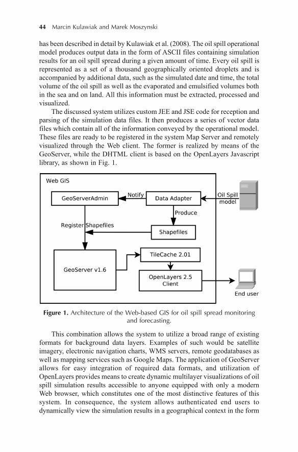
44 Marcin Kulawiak and Marek Moszynski
has been described in detail by Kulawiak et al. (2008). The oil spill operationalmodel produces output data in the form of ASCII files containing simulationresults for an oil spill spread during a given amount of time. Every oil spill isrepresented as a set of a thousand geographically oriented droplets and isaccompanied by additional data, such as the simulated date and time, the totalvolume of the oil spill as well as the evaporated and emulsified volumes bothin the sea and on land. All this information must be extracted, processed andvisualized.
The discussed system utilizes custom JEE and JSE code for reception andparsing of the simulation data files. It then produces a series of vector datafiles which contain all of the information conveyed by the operational model.These files are ready to be registered in the system Map Server and remotelyvisualized through the Web client. The former is realized by means of theGeoServer, while the DHTML client is based on the OpenLayers Javascriptlibrary, as shown in Fig. 1.
Figure 1. Architecture of the Web-based GIS for oil spill spread monitoringand forecasting.
This combination allows the system to utilize a broad range of existingformats for background data layers. Examples of such would be satelliteimagery, electronic navigation charts, WMS servers, remote geodatabases aswell as mapping services such as Google Maps. The application of GeoServerallows for easy integration of required data formats, and utilization ofOpenLayers provides means to create dynamic multilayer visualizations of oilspill simulation results accessible to anyone equipped with only a modernWeb browser, which constitutes one of the most distinctive features of thissystem. In consequence, the system allows authenticated end users todynamically view the simulation results in a geographical context in the form
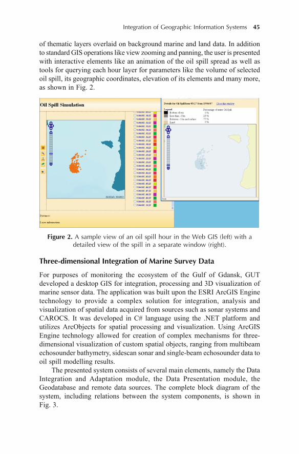
Integration of Geographic Information Systems 45
of thematic layers overlaid on background marine and land data. In additionto standard GIS operations like view zooming and panning, the user is presentedwith interactive elements like an animation of the oil spill spread as well astools for querying each hour layer for parameters like the volume of selectedoil spill, its geographic coordinates, elevation of its elements and many more,as shown in Fig. 2.
Figure 2. A sample view of an oil spill hour in the Web GIS (left) with adetailed view of the spill in a separate window (right).
Three-dimensional Integration of Marine Survey Data
For purposes of monitoring the ecosystem of the Gulf of Gdansk, GUTdeveloped a desktop GIS for integration, processing and 3D visualization ofmarine sensor data. The application was built upon the ESRI ArcGIS Enginetechnology to provide a complex solution for integration, analysis andvisualization of spatial data acquired from sources such as sonar systems andCAROCS. It was developed in C# language using the .NET platform andutilizes ArcObjects for spatial processing and visualization. Using ArcGISEngine technology allowed for creation of complex mechanisms for three-dimensional visualization of custom spatial objects, ranging from multibeamechosounder bathymetry, sidescan sonar and single-beam echosounder data tooil spill modelling results.
The presented system consists of several main elements, namely the DataIntegration and Adaptation module, the Data Presentation module, theGeodatabase and remote data sources. The complete block diagram of thesystem, including relations between the system components, is shown inFig. 3.

46 Marcin Kulawiak and Marek Moszynski
Figure 3. Architecture of the GIS for 3D integration, processing andvisualization of marine sensor data.
The Data Integration and Adaptation module is developed using theMicrosoft .NET platform and corresponding elements of ArcGIS Engine. Thesystem employs custom algorithms for processing MBS data. After such datais extracted from a raw stream of bytes, it is filtered with the use of informationsuch as the transducer depth relative to water level, number of valid beams,sample rate, quality factor, and reflectivity in order to minimize possibleacquisition artifacts. Multibeam bathymetry is then validated and georeferencedusing data acquired from the ship’s GPS receiver. In a similar way the systemprocesses data from the sidescan sonar and single-beam echosounder. Becausethe stream of survey data is typically processed in chunks, this results in aseries of georeferenced vector and raster data. In the case of single-beamechosounders, the horizontal axis of each image represents the time ofacquisition. With the use of navigational information from the surveying vessel,it is converted into geographic position on the map. The acquired informationis then stored in ESRI ArcSDE, an application server that facilitates storingand managing spatial data in an underlying database. CAROCS oil spill data,being dynamic, is handled differently. After being generated by the DataIntegration and Adaptation module, it is passed directly to the visualizationsubsystem. The Data Presentation module uses ArcGIS Engine MapControland GlobeControl components to provide a standard set of GIS functionalitieslike map viewing, zooming and panning for two-dimensional and three-dimensional display, respectively. However, efficient visualization of certaindata required the creation of dedicated OpenGL procedures for display andanimation of three-dimensional objects. For example, the system allows todisplay MBS data in two forms, either as a series of points containingbathymetry data, or as a series of two-dimensional fan-shaped images (water-column) that can be used to visualize objects other than the seabed, such asfish or pollution. In order to maintain visibility, signal values below a certainthreshold can be made completely transparent. This method can be used to
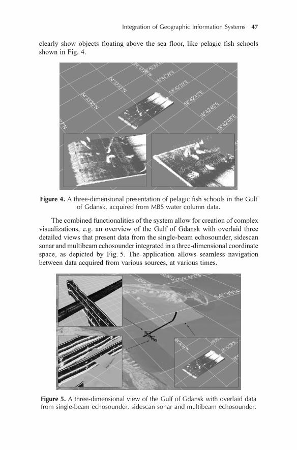
Integration of Geographic Information Systems 47
clearly show objects floating above the sea floor, like pelagic fish schoolsshown in Fig. 4.
Figure 4. A three-dimensional presentation of pelagic fish schools in the Gulfof Gdansk, acquired from MBS water column data.
The combined functionalities of the system allow for creation of complexvisualizations, e.g. an overview of the Gulf of Gdansk with overlaid threedetailed views that present data from the single-beam echosounder, sidescansonar and multibeam echosounder integrated in a three-dimensional coordinatespace, as depicted by Fig. 5. The application allows seamless navigationbetween data acquired from various sources, at various times.
Figure 5. A three-dimensional view of the Gulf of Gdansk with overlaid datafrom single-beam echosounder, sidescan sonar and multibeam echosounder.
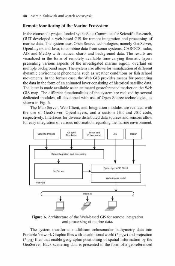
48 Marcin Kulawiak and Marek Moszynski
Remote Monitoring of the Marine Ecosystem
In the course of a project funded by the State Committee for Scientific Research,GUT developed a web-based GIS for remote integration and processing ofmarine data. The system uses Open Source technologies, namely GeoServer,OpenLayers and Java, to combine data from sonar systems, CAROCS, radar,AIS and MetOp with nautical charts and background data. The results arevisualized in the form of remotely available time-varying thematic layerspresenting various aspects of the investigated marine region, overlaid onmultiple background maps. The system also allows for visualization of differentdynamic environment phenomena such as weather conditions or fish schoolmovements. In the former case, the Web GIS provides means for presentingthe data in the form of an animated layer consisting of historical satellite data.The latter is made available as an animated georeferenced marker on the WebGIS map. The different functionalities of the system are realized by severaldedicated modules, all developed with use of Open-Source technologies, asshown in Fig. 6.
The Map Server, Web Client, and Integration modules are realized withthe use of GeoServer, OpenLayers, and a custom JEE and JSE code,respectively. Interfaces for diverse distributed data sources and sensors allowfor easy integration of various information regarding the marine environment.
Figure 6. Architecture of the Web-based GIS for remote integrationand processing of marine data.
The system transforms multibeam echosounder bathymetry data intoPortable Network Graphic files with an additional world (*.pgw) and projection(*.prj) files that enable geographic positioning of spatial information by theGeoServer. Back-scattering data is presented in the form of a georeferenced
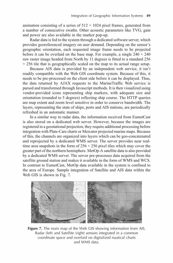
Integration of Geographic Information Systems 49
animation consisting of a series of 512 × 1024 pixel frames, generated froma number of consecutive swaths. Other acoustic parameters like TVG, gainand power are also available in the marker pop-up.
Radar data is fed to the system through a dedicated software server, whichprovides georeferenced imagery on user demand. Depending on the sensor’sgeographic orientation, each requested image frame needs to be projectedbefore it can be overlaid on the base map. For example, a single 240 × 240raw raster image headed from North by 11 degrees is fitted to a standard 256× 256 tile that is geographically scaled on the map to its actual range setup.
Because AIS data is provided by an independent web service, it isn’treadily compatible with the Web GIS coordinate system. Because of this, itneeds to be pre-processed on the client side before it can be displayed. Thus,the data returned by AJAX requests to the MarineTraffic Web service isparsed and transformed through Javascript methods. It is then visualized usingvendor-provided icons representing ship markers, with adequate size andorientation (rounded to 5 degrees) reflecting ship course. The HTTP queriesare map extent and zoom level sensitive in order to conserve bandwidth. Thelayers, representing the state of ships, ports and AIS stations, are periodicallyrefreshed in an automatic manner.
In a similar way to radar data, the information received from EumetCastis also stored on a dedicated web server. However, because the images areregistered in a geostational projection, they require additional processing beforeintegration with Plate-Care charts or Mercator projected marine maps. Becauseof this, the channels are organized into layers which can be geo-concatenatedand reprojected by a dedicated WMS server. The server provides near real-time area snapshots in the form of 256 × 256 pixel tiles which may cover thegreater part of the northern hemisphere. MetOp-A satellite data is also providedby a dedicated WMS server. The server pre-processes data acquired from thesatellite ground station and makes it available in the form of WMS and WCS.In contrast to EumetCast, MetOp data available in the system is confined tothe area of Europe. Sample integration of Satellite and AIS data within theWeb GIS is shown in Fig. 7.
Figure 7. The main map of the Web GIS showing information from AIS,Radar (left) and Satellite (right) sensors integrated in a common
coordinate space and overlaid on digitalized nautical chartsand WMS data.
50 Marcin Kulawiak and Marek Moszynski
Perspectives
Monitoring of marine environment and visualization of results is not a newfield of research. During the years it has seen slow but stable evolution ofmeans of collecting and processing data. At the same time GeographicInformation Systems have evolved from specialized single-user workstationsoftware into freely available tools for remote mapping, geocoding, and spatialanalysis. Their expansion closely followed the progress of informationtechnology, as they entered new niches when the opportunity presented itself.The introduction of 3D acceleration hardware enabled the creation of three-dimensional GIS. The advent of Dynamic HTML laid the foundations forJavascript-based services such as Google Maps. The development ofSmartphones brought Web GIS to mobile devices. In a similar way the adoptionof HTML5 and WebGL will catalyze the development of remotely accessiblebrowser-based 3D GIS.
Thus, the foreseeable future trends do not involve a revolution but insteadrely on further progress of existing solutions. Taking into account the progressof wireless Internet, remote three-dimensional visualization of data collectedfrom mobile sensors in real time will likely become possible.
Conclusion
This chapter presented common types of marine sensors which allow formonitoring and sensing of underwater as well as surface activities. The chapteralso discussed several popular commercial and Open Source technologiesused for constructing custom Geographic Information Systems. Finally, thechapter exemplified the application of the discussed technologies to processing,integration, analysis and visualization of data from the presented sources.
For a long time commercial solutions have seen little competition,especially in the area of desktop GIS. In the recent years this state of affairshas been rapidly changing, with organizations like the Open Source GeospatialFoundation concentrating efforts on the development of alternative solutions.In consequence, although commercial software still prevails in desktopapplications, Open Source solutions such as GeoServer and OpenLayers holda strong position in development of web-based GIS.
The technologies presented in this chapter are constantly evolving,developing methods of improved presentation and analysis of geographic datawith the power of new generations of computer hardware. Thus far mostfunctionalities of regular desktop GIS have been implemented in Webapplications with the use of Server-side data processing and an interactiveDHTML client. Even features like processing and visualization of back-scatterand bathymetry data based on various acoustic parameters like TVG, gain andwater-column information may be implemented in the form of a Web service,as it has been exemplified by the presented Web-based GIS for monitoring ofthe marine ecosystem.

Integration of Geographic Information Systems 51
The only element of desktop GIS which still requires at least a standaloneweb client such as Google Earth is remote presentation of three-dimensionaldata. However, there is good chance that the possibilities brought by newstandards like HTML5 and WebGL will alleviate this problem and in the nearfuture the full functionality of three-dimensional marine GIS will be freelyavailable to anyone equipped with a modern web browser.
References
Bakare, A.M., Morley, J.G. and Simons, R.R. (2008). Developing a seabed resurveystrategy: A GIS approach to modelling seabed changes and resurvey risk. Computers,Environment and Urban Systems, 32(4), 293–302.
Chybicki, A., Kulawiak, M., Lubniewski, Z., Luba, M., Moszynski, M. and Dabrowski,J. (2008). GIS for Remote Sensing, Analysis and Visualization of Marine Pollutionand Other Marine Ecosystem Components. Proceedings of 2008 1st InternationalConference on Information Technology, 223–226.
Doyle, S., Dodge, M. and Smith, A. (1998). The potential of Web-based mapping andvirtual reality technologies for modelling urban environments. Computer,Environment and Urban Systems, 22(2), 137–155.
Goodall, J.L., Robinson, B.F. and Castronova, A.M. (2011). Modeling water resourcesystems using a service-oriented computing paradigm. Environmental Modelling& Software, 26(5), 573–582.
Hamre, T., Krasemann, H., Groom, S., Dunne, D., Breitbach, G., Hackett, B., Sørensen,K. and Sandven, S. (2009). Interoperable web GIS services for marine pollutionmonitoring and forecasting. Journal of Coastal Conservation, 13(1), 1–13.
Kraak, M.-J. (2004). The role of the map in a Web-GIS environment. Journal ofGeographical Systems, 6, 83–93.
Kruger, A., Khandelwal, S.G. and Bradley, A. (2007). AHPSVER: A web-based systemfor hydrologic forecast verification. Computers & Geosciences, 33, 739–748.
Kulawiak, M., Luba, M., Stepnowski, A., Prospathopoulos, A., Kioroglou, S.,Perivoliotis, L. and Grammatikaki, M. (2008). Integrating a Web-based GIS to amarine pollution monitoring and forecasting system. Proceedings of the InternationalConference on Marine Data and Information Systems, Athens (Greece).
Kulawiak, M., Chybicki, A. and Moszynski, M. (2010a). Web-based GIS as a tool forsupporting marine research. Marine Geodesy, 33(2 and 3), 135–153.
Kulawiak, M., Prospathopoulos, A., Perivoliotis, L., Luba, M., Kioroglou, S. andStepnowski, A. (2010b). Interactive visualization of marine pollution monitoringand forecasting data via a Web-based GIS. Computers & Geosciences, 36(8),1069–1080.
Maceachren, A.M. and Kraak, M.-J. (1997). Exploratory cartographic visualization:Advancing the agenda. Computers & Geosciences, 23(4), 335–343.
Papadopoulos, A., Kallos, G., Katsafados, P. and Nickovic, S. (2002). The Poseidonweather forecasting system: An overview. The Global Atmosphere and OceanSystems, 8(2-3), 219–237.
52 Marcin Kulawiak and Marek Moszynski
Pollani, A., Triantafyllou, G., Petihakis, G., Nittis, K., Dounas, K. and Koutitas, C.(2001). The POSEIDON Operational Tool for the Prediction of Floating PollutantTransport. Marine Pollution Bulletin, 43(7-12), 270–278.
Rao, M., Fan, G., Thomas, J., Cherian, G., Chudiwale, V. and Awawdeh, M. (2007). Aweb-based GIS Decision Support System for managing and planning USDA’sConservation Reserve Program (CRP). Environmental Modelling & Software, 22,1270–1280.
Schmidt, C. (2008). OpenLayers: Free Maps for the Web. Retrieved October 22, 2009,from http://www.openlayers.org
Stepnowski, A., Burczynski, J., Ostrowski, M., Moszynski, M., Lenkiewicz, J. andPartyka, A. (1996). ECHOBASE – A Portable Geographic Fishery ResearchDatabase System. Marine Geodesy, 19, 269–280.
Thakur, J.K., Srivastava, P.K., Singh, S.K. and Vekerdy, Z. (2011). Ecologicalmonitoring of wetlands in semi-arid region of Konya closed basin, Turkey. RegionalEnvironmental Change (DOI: 10.1007/s10113-011-0241-x).
Trygonis, V., Georgakarakos, S. and Simmonds, E.J. (2009). An operational systemfor automatic school identification on multibeam sonar echoes. ICES Journal ofMarine Science, 66(5), 935–949.
Tsou, M.-H. (2004). Integrating Web-based GIS and image processing tools forenvironmental monitoring and natural resource management. Journal ofGeographical Systems, 6, 155–174.
Tuama, É.Ó. and Hamre, T. (2007). Design and Implementation of a Distributed GISPortal for Oil Spill and Harmful Algal Bloom Monitoring in the Marine Environment.Marine Geodesy, 30, 145–168.

Estimation of Evapotranspiration from Wetlands 53
4Estimation of Evapotranspiration
from Wetlands Using Geospatialand Hydrometeorological Data
Jay Krishna Thakur, P.K. Srivastava1, Arun Kumar Pratihast2
and Sudhir Kumar Singh3
Department of Hydrogeology and Environmental Geology, Institute ofGeosciences, Martin Luther University, Halle (Saale), Germany
1Water and Environment Management Research CentreDepartment of Civil Engineering
University of Bristol, Bristol BS8 1TR, United Kingdom2Center for Geo-information, Wageningen University
Wageningen, The Netherlands3Department of Atmospheric and Ocean Science
University of Allahabad, Allahabad 211001, India
Introduction
Over recent decades, wetlands have been recognized increasingly for theirhigh biodiversity and for the important hydrological functions, including floodalleviation, low-flow support, nutrient cycling and groundwater recharge(Thakur, 2010; Thakur et al., 2011). Wetland hydrology is a primary drivingforce influencing wetland ecology, its development and persistence (Mitschand Gosselink, 1993). For most wetlands, evapotranspiration (ET) is the majorcomponent of water loss, and when considered as its energy equivalent, thelatent heat flux (LE), the largest consumer of incoming energy (Reynolds etal., 2000; Wilson et al., 2001). The radiation and the turbulent heating drivethe dynamics of the land-atmosphere energy exchanges in the wetlands.Estimation of these radiation and turbulent heating through mass energy balanceequations is the core of numerical weather forecast, climate research, waterresources and environmental management and long-term agriculture production.Most of the conventional methods which use point measurement in measuringthe energy balance, such as Bowen ratio, Penman-Monteith, Priestley andTaylor, give results that can be efficient on local level but could not be extendedto large scale or global scale measurement in time and space (Stewart, 1989).
DOI 10.1007/978-94-007-1858-6_4, © Capital Publishing Company 2012
e ,J.K. Thakur et al. (eds.), G ospatial Techniques for Managing Environmental Resources 53
54 Jay Krishna Thakur et al.
ET depends upon many factors including the availability of water at theevaporating surface, solar radiation, air temperature, humidity and wind speed,type and density of vegetation cover, rooting depth and reflective land surfacecharacteristics (Hupet and Vanclooster, 2001; Kalmar and Currie, 2006; Yao,1974).
Several scientists have demonstrated the relationship between land surfacetemperature, soil moisture and canopy based on a combination of a soilmoisture-balance equation and energy-balance theory (Moran et al., 1994;Nemani and Running, 1989; Sandholt et al., 2002; Srivastava et al., 2009; Yueet al., 2007). The normalized deviation vegetation index (NDVI) and landsurface temperature can be used to establish an integrated model to monitorland use/cover (Singh et al., 2010; Yue et al., 2007). The most commonly usedone is land surface temperature (LST), which is shown in a two-dimensionalspace composed of NDVI and land surface temperature (Sandholt et al., 2002;Yue et al., 2007). The land surface temperature can be directly linked to ET;several scientists show that they are proportional to each other (Cox et al.,1999; Noilhan and Planton, 1989; Shukla and Mintz, 1982; Weng et al.,2004).
Various remote sensing algorithms have been used over the years toestimate the atmospheric turbulent fluxes. In this study, Surface Energy BalanceSystem (SEBS) algorithm was employed to estimate actual ET (ETa). Thealgorithm has been used for the application of evaporation estimates in SpainBarrax (Z. Su and Jacobs, 2001), Taiyuan basin in China (Jin et al., 2005), inestimation of sensible heat flux in Spain Tomelloso area (Jia et al., 2003), andfor drought monitoring purposes in north west China (Zhongbo Su et al.,2003). SEBS has been evaluated for its application to ASTER imagery withflux-measurements in Barrax, Spain (van der Kwast et al., 2009).
The aim of this chapter is to describe method to quantify ETspatiotemporally in wetlands of semi-arid region using open source softwareand geospatial-hydrometeorological data and to study hydrological dynamicsin term of ET in various types of wetlands around Tuz Lake in Konya closedbasin, Turkey.
Study Area
The wetlands, around Lake Tuz, irregular shape having total area of 7651km2, are located between 38o11� - 39o18� N latitudes and 32o15� - 34o15� Elongitudes in the Konya closed basin to the south from Ankara in the heart ofTurkey (Fig. 1). The study area is situated at an elevation of 905 m abovemean sea level (Gökmen, 2009; Thakur and Singh, 2010). The climate inKonya closed basin represents a typical arid to semi-arid climate dominatedby halophytic and simple steppes (Tektas, 2007). Sandstones and shalescompose the surface layer whereas schist-quartz schist-mica schist, marble,calc schist-quartz schist-mica schist, dolomitic limestone and serpentinite-radiolarite-limestone-glaucophane schist sequences compose sub-surface layersof the wetlands floor in the study area (Zeki Camur and Mutlu, 1996). Aeolian

Estimation of Evapotranspiration from Wetlands 55
depositional landforms can be seen on the northern and western areas of thewetlands.
Figure 1. Location map of study area showing wetlands around Tuz Lake, inKonya closed basin, Turkey (Shape file source: Environmental Protection Agencyfor Special Areas (EPASA)). D6.1, E1.2 and E6.2 are habitat codes for inlandsalt marshes, perennial calcareous grassland and continental inland salt
steppes respectively.
Data and Methods
Datasets Used and Analysis
SEBS requires the following set of input from remote sensing data: the landsurface temperature, emissivity, land surface albedo, NDVI and vegetationproportion. Air pressure at surface and reference height, hourly air temperatureand mean daily air temperature, specific humidity, wind speed at the referenceheight and sunshine hours per day are the second input provided by groundmeteorological data. The air temperature and wind speed are scaled to theblending height (100 m) assumed to apply for all pixels of the image. Thirdly,downward solar radiation and long wave radiations are required input for theenergy balance component. The downward solar radiation is taken from hourlymeteorological data for each of the satellite pass time of the images, whereasthe outgoing long wave radiation is derived from satellite data with someparameterization. In the study area, meteorological variables are measuredfrom station having height 2 m above the ground surface (Thakur et al., 2011).
The methodology for the research consists of three different stages viz.pre-field work, field work and post-field work. Time series meteorologicaland hydrological data were collected to analyse the trend and the variability ofrainfall, evaporation, temperature and groundwater level. Fieldwork was carriedout in the wetlands of the Konya closed basin, Turkey for ground truthcollection. The ground control points were collected using hand-held GPS forgeoreferencing of the images and land cover classification purposes. In this
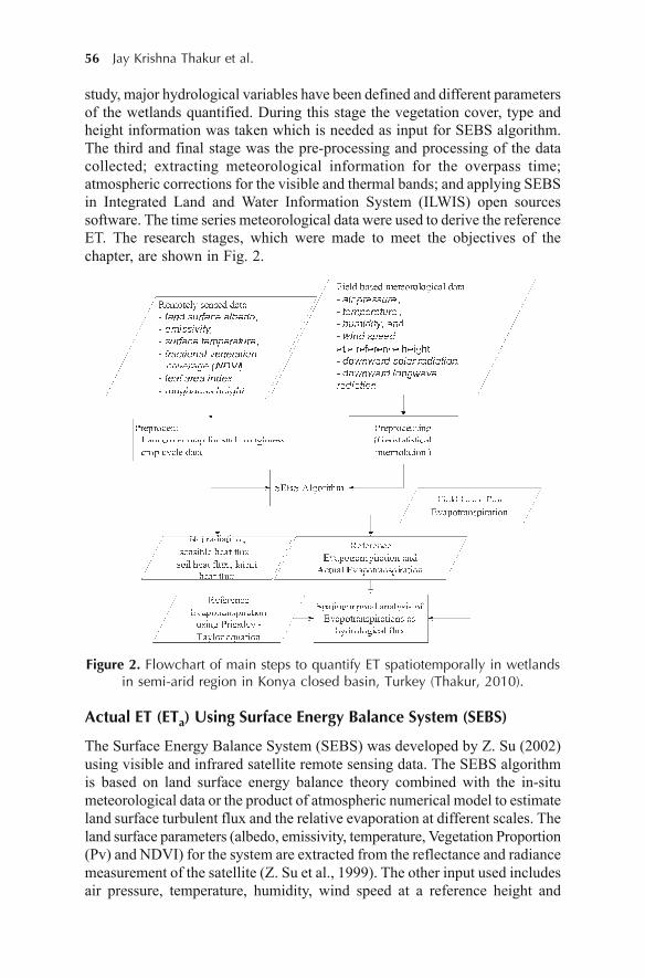
56 Jay Krishna Thakur et al.
study, major hydrological variables have been defined and different parametersof the wetlands quantified. During this stage the vegetation cover, type andheight information was taken which is needed as input for SEBS algorithm.The third and final stage was the pre-processing and processing of the datacollected; extracting meteorological information for the overpass time;atmospheric corrections for the visible and thermal bands; and applying SEBSin Integrated Land and Water Information System (ILWIS) open sourcessoftware. The time series meteorological data were used to derive the referenceET. The research stages, which were made to meet the objectives of thechapter, are shown in Fig. 2.
Figure 2. Flowchart of main steps to quantify ET spatiotemporally in wetlandsin semi-arid region in Konya closed basin, Turkey (Thakur, 2010).
Actual ET (ETa) Using Surface Energy Balance System (SEBS)
The Surface Energy Balance System (SEBS) was developed by Z. Su (2002)using visible and infrared satellite remote sensing data. The SEBS algorithmis based on land surface energy balance theory combined with the in-situmeteorological data or the product of atmospheric numerical model to estimateland surface turbulent flux and the relative evaporation at different scales. Theland surface parameters (albedo, emissivity, temperature, Vegetation Proportion(Pv) and NDVI) for the system are extracted from the reflectance and radiancemeasurement of the satellite (Z. Su et al., 1999). The other input used includesair pressure, temperature, humidity, wind speed at a reference height and

Estimation of Evapotranspiration from Wetlands 57
sunshine hours per day. These climatological data are accessed from thestandard meteorological station at the reference height. SEBS is very sensibleto the meteorological input like the air temperature. The difference betweenthe surface and air temperature forces the sensible heat flux. SEBS is anextension of Surface Energy Balance Index (SEBI) concept with theimprovement of estimation of thermal roughness length with a dynamic modelwhich is based on the work of Massman (1999) and Z. Su and Jacobs (2001).The algorithm has an advantage of using both Bulk Atmospheric Similarity(BAS) of Brutsaert (1999) and the Monin-Obukhov atmospheric surface layer(ASL) similarity which can be used for regional and local scale estimation ofthe turbulent fluxes respectively.
The Surface Energy Balance System (SEBS), developed by Su (Z. Su,2002), is used to estimate the atmospheric turbulent fluxes and evaporativefraction using satellite earth observation data, in combination withmeteorological information of study area at proper scales (Qin et al., 2008).This system retrieves ET using measurements of incoming surface radiation,surface skin temperature, surface meteorology, and surface and vegetationproperties (H. Su et al., 2005). SEBS also includes physical model that considerssurface heterogeneity in the estimation of the roughness height for heat transfer.This system consists of a set of tools for the determination of the land surfacephysical properties and state variables, such as albedo, emissivity, temperature,vegetation coverage etc. from spectral reflectance and radiance—an extendedmodel for the determination of the roughness length for heat transfer andevaporative fraction from the energy balance at limiting cases (Z. Su andJacobs, 2001). The surface energy balance equation is written as
Rn = 0G H E� � O (1)
where Rn is the net radiation, G0 is the soil heat flux, H is the turbulentsensible heat flux, and OE is the turbulent latent heat flux (O is the latent heatof vapourization and E is the actual ET).
Under the dry-limit, the latent heat becomes zero due to the limitation ofsoil moisture and the sensible heat flux is at its maximum value. From Eqn.(1), we can write
OEdry = n 0 dry 0R G H� � � (2)or Hdry = Rn – G0
And under the wet-limit, where the evaporation takes place at potentialrate, the sensible heat flux takes its minimum value, Hwet and is given by,
OEwet = n 0 wetR G H� � (3)or Hwet = Rn – G0 ��OEwet
Then the relative evaporation /r can be written as
/r =wet
dry wet1 H H
H H���
(4)
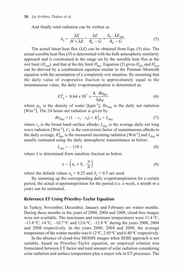
58 Jay Krishna Thakur et al.
And finally total radiation can be written as
/r =r wet
n n
E E E=H E R G R GO O / ¹ O � O � � (5)
The actual latent heat flux (OE) can be obtained from Eqn. (5) also. Theactual sensible heat flux (H) is determined with the bulk atmospheric similarityapproach and is constrained in the range set by the sensible heat flux at thewet limit (Hwet), and that at the dry limit Hdry. Equation (2) gives Hdry and Hwetcan be derived by a combination equation similar to the Penman–Monteithequation with the assumption of a completely wet situation. By assuming thatthe daily value of evaporative fraction is approximately equal to theinstantaneous value, the daily evapotranspiration is determined as:
ETa =day7
W8.64 10
Rn/ ¹� �
OU(6)
where Uw is the density of water [kgm-3], Rnday is the daily net radiation[Wm-2]. The 24 hours net radiation is given by
Rnday = (1 – c1 ¹ r0) × K�24 + Lday (7)
where ro is the broad band surface albedo, Lday is the average daily net longwave radiation [Wm-2], C1 is the conversion factor of instantaneous albedo tothe daily average, K�
day is the measured incoming radiation [Wm-2] and Lday isusually estimated using the daily atmospheric transmittance as below:
Lday = – 110 W (8)where W is determined from sunshine fraction as below:
W = � �s sna bN
� ¹ (9)
where the default values as = 0.25 and bs = 0.5 are used.By summing up the corresponding daily evapotranspiration for a certain
period, the actual evapotranspiration for the period (i.e. a week, a month or ayear) can be estimated.
Reference ET Using Priestley-Taylor Equation
In Turkey, November, December, January and February are winter months.During these months in the years of 2000, 2004 and 2008, cloud-free imageswere not available. The maximum and minimum temperatures were 11.4 oC,–13.8 oC; 14 oC, –10.7 oC and 13.6 oC, –12.8 oC during the years 2000, 2004and 2008 respectively. In the years 2000, 2004 and 2008, the averagetemperature of the winter months was 0.12 oC, 2.05 oC and 0.40 oC respectively.
In the absence of cloud-free MODIS images when SEBS approach is notsuitable, based on Priestley-Taylor equation, an empirical relation wasformulated between ET factor and total amount of solar radiation consideringsolar radiation and surface temperature play a major role in ET processes. The
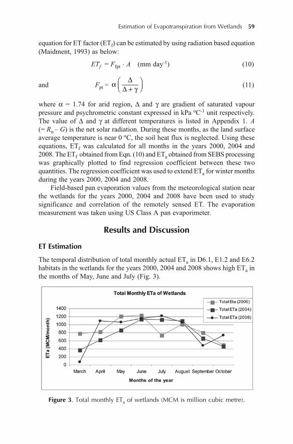
Estimation of Evapotranspiration from Wetlands 59
equation for ET factor (ETf) can be estimated by using radiation based equation(Maidment, 1993) as below:
ETf = Ffpt ¹ A (mm day-1) (10)
and Fpt ='È ØD É ÙÊ Ú' � J (11)
where D = 1.74 for arid region, ' and J are gradient of saturated vapourpressure and psychrometric constant expressed in kPa oC-1 unit respectively.The value of ' and J at different temperatures is listed in Appendix 1. A(= Rn – G) is the net solar radiation. During these months, as the land surfaceaverage temperature is near 0 oC, the soil heat flux is neglected. Using theseequations, ETf was calculated for all months in the years 2000, 2004 and2008. The ETf obtained from Eqn. (10) and ETa obtained from SEBS processingwas graphically plotted to find regression coefficient between these twoquantities. The regression coefficient was used to extend ETa for winter monthsduring the years 2000, 2004 and 2008.
Field-based pan evaporation values from the meteorological station nearthe wetlands for the years 2000, 2004 and 2008 have been used to studysignificance and correlation of the remotely sensed ET. The evaporationmeasurement was taken using US Class A pan evaporimeter.
Results and Discussion
ET Estimation
The temporal distribution of total monthly actual ETa in D6.1, E1.2 and E6.2habitats in the wetlands for the years 2000, 2004 and 2008 shows high ETa inthe months of May, June and July (Fig. 3).
Figure 3. Total monthly ETa of wetlands (MCM is million cubic metre).
60 Jay Krishna Thakur et al.
In the months January and February of year 2000, January of the year2004; and January and February of 2008 the average atmospheric temperaturewas below 0 oC. During these periods, the ETa of the wetlands is considered0 mm/day. In the remaining months of these years (during the months ofNovember, December, January and February) when average monthlytemperature is above 0 oC, the ETa was calculated on the basis of empiricalequation explained in Eqns (10) and (11). The average and total ETa duringthe years 2000, 2004 and 2008 is graphically plotted in Fig. 4. The averageETa value represents average of daily ETa values for all the habitat types fromthe month March to November when MODIS images were available. Inaddition, the total ETa value represents sum of daily ETa values of all habitattypes throughout the year, from both the ETa calculated by SEBS methodswhen MODIS images were available and ETa calculated by empirical methodbased on daily solar radiation when MODIS images were not available. Thetrend of average ETa and total ETa is in reverse direction. Although averageETa has increasing trend, the total ETa has decreasing trend. The value of totalETa during the year 2008 is lower than the year 2000. This is because, duringthe year 2008, the ETa contribution in the months of January, February,November and December was low. The ETa values in the years 2000, 2004and 2008 ranges from 0.00 mm/day to 13.21 mm/day, 0.50 mm/day to 14.94mm/day and 1.85 mm/day to 14.02 mm/day respectively. Moreover, the averageETa for overall study area is 5.17 mm/day, 4.44 mm/day and 5.51 mm/dayduring the years 2000, 2004 and 2008 respectively. The total ETa in the years2000, 2004 and 2008 are 648 MCM (Million Cubic metres)/year, 551 MCM/year and 616 MCM/year in the overall study area.
Figure 4. Total and average ETa of the wetlands(MCM is million cubic metre).
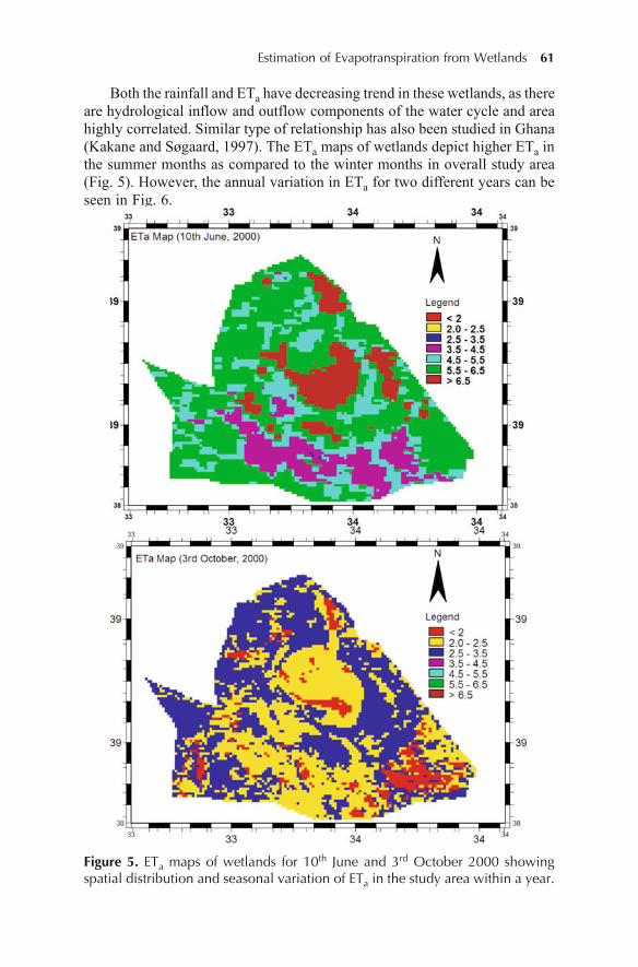
Estimation of Evapotranspiration from Wetlands 61
Both the rainfall and ETa have decreasing trend in these wetlands, as thereare hydrological inflow and outflow components of the water cycle and areahighly correlated. Similar type of relationship has also been studied in Ghana(Kakane and Søgaard, 1997). The ETa maps of wetlands depict higher ETa inthe summer months as compared to the winter months in overall study area(Fig. 5). However, the annual variation in ETa for two different years can beseen in Fig. 6.
Figure 5. ETa maps of wetlands for 10th June and 3rd October 2000 showingspatial distribution and seasonal variation of ETa in the study area within a year.
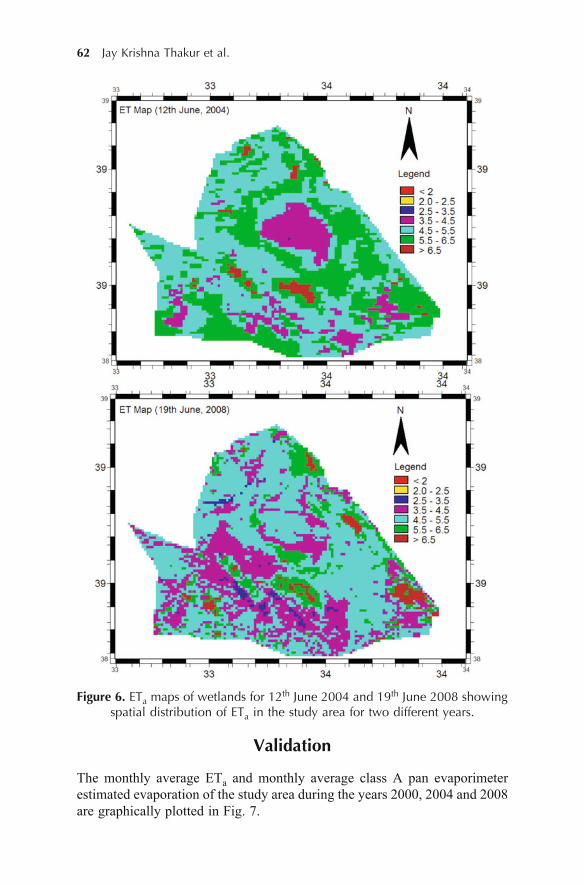
62 Jay Krishna Thakur et al.
Figure 6. ETa maps of wetlands for 12th June 2004 and 19th June 2008 showingspatial distribution of ETa in the study area for two different years.
Validation
The monthly average ETa and monthly average class A pan evaporimeterestimated evaporation of the study area during the years 2000, 2004 and 2008are graphically plotted in Fig. 7.
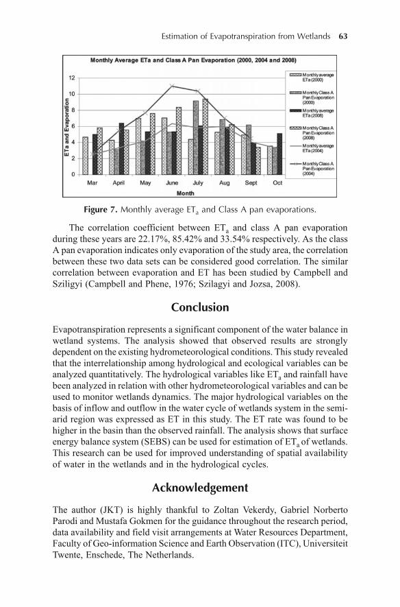
Estimation of Evapotranspiration from Wetlands 63
Figure 7. Monthly average ETa and Class A pan evaporations.
The correlation coefficient between ETa and class A pan evaporationduring these years are 22.17%, 85.42% and 33.54% respectively. As the classA pan evaporation indicates only evaporation of the study area, the correlationbetween these two data sets can be considered good correlation. The similarcorrelation between evaporation and ET has been studied by Campbell andSziligyi (Campbell and Phene, 1976; Szilagyi and Jozsa, 2008).
Conclusion
Evapotranspiration represents a significant component of the water balance inwetland systems. The analysis showed that observed results are stronglydependent on the existing hydrometeorological conditions. This study revealedthat the interrelationship among hydrological and ecological variables can beanalyzed quantitatively. The hydrological variables like ETa and rainfall havebeen analyzed in relation with other hydrometeorological variables and can beused to monitor wetlands dynamics. The major hydrological variables on thebasis of inflow and outflow in the water cycle of wetlands system in the semi-arid region was expressed as ET in this study. The ET rate was found to behigher in the basin than the observed rainfall. The analysis shows that surfaceenergy balance system (SEBS) can be used for estimation of ETa of wetlands.This research can be used for improved understanding of spatial availabilityof water in the wetlands and in the hydrological cycles.
Acknowledgement
The author (JKT) is highly thankful to Zoltan Vekerdy, Gabriel NorbertoParodi and Mustafa Gokmen for the guidance throughout the research period,data availability and field visit arrangements at Water Resources Department,Faculty of Geo-information Science and Earth Observation (ITC), UniversiteitTwente, Enschede, The Netherlands.
64 Jay Krishna Thakur et al.
References
Brutsaert, W. (1999). Aspects of bulk atmospheric boundary layer similarity underfree convective conditions. Reviews of Geophysics, 37(4), 439–451.
Campbell, R.B. and Phene, C.J. (1976). Estimating potential evaporation from screenedpan evaporation. Agricultural meteorology, 16, 343–352.
Cox, P., Betts, R., Bunton, C., Essery, R., Rowntree, P. and Smith, J. (1999). Theimpact of new land surface physics on the GCM simulation of climate and climatesensitivity. Climate Dynamics, 15(3), 183–203.
Gökmen, M., Vekerdy, Z. and Verhoef, W. (2009). Earth Observation for QuantifyingEcohydrological Fluxes. Paper presented at the European Geosciences Union (EGU)Conference.
Hupet, F. and Vanclooster, M. (2001). Effect of the sampling frequency ofmeteorological variables on the estimation of the reference evapotranspiration.Journal of Hydrology, 243(3-4), 192–204.
Jia, L., Yrisarry, J., Ibanez, M. and Cuesta, A. (2003). Estimation of sensible heat fluxusing the Surface Energy Balance System (SEBS) and ATSR measurements. Physicsand Chemistry of the Earth, Parts A/B/C, 28(1-3), 75–88.
Jin, X., Wan, L. and Su, Z. (2005). Research on evaporation of Taiyuan basin area byusing remote sensing. HAL - CCSD.
Kakane, V.C.K. and Søgaard, H. (1997). Estimation of Surface Temperature andRainfall in Ghana. Geografisk Tidsskrift, Danish Journal of Geography, 97, 76–85.
Kalmar, A. and Currie, D.J. (2006). A global model of island biogeography. GlobalEcology and Biogeography, 15(1), 72–81.
Maidment, D.R. (Ed.). (1993). Handbook of Hydrology: McGraw-Hill Professional.Massman, W.J. (1999). A model study of kBH-1 for vegetated surfaces using localized
near-field Lagrangian theory. Journal of Hydrology, 223(1-2), 27–43.Mitsch, W.J. and Gosselink, J.G. (Eds.). (1993). Wetlands (Second ed.): Van Nostrand
Reinhold, New York.Moran, M., Clarke, T., Inoue, Y. and Vidal, A. (1994). Estimating crop water deficit
using the relation between surface-air temperature and spectral vegetation index.Remote Sensing of Environment, 49(3), 246–263.
Nemani, R.R. and Running, S.W. (1989). Estimation of Regional Surface-Resistanceto Evapotranspiration from Ndvi and Thermal-Ir Avhrr Data. Journal of AppliedMeteorology, 28(4), 276–284.
Noilhan, J. and Planton, S. (1989). A simple parameterization of land surface processesfor meteorological models. Monthly Weather Review, 117(3), 536–549.
Qin, C., Jia, Y., Su, Z., Zhou, Z., Qiu, Y. and Suhui, S. (2008). Integrating RemoteSensing Information into a Distributed Hydrological Model for Improving WaterBudget Predictions in Large-scale Basins through Data Assimilation. Sensors, 8(7),4441–4465.
Reynolds, J.F., Kemp, P.R. and Tenhunen, J.D. (2000). Effects of long-term rainfallvariability on evapotranspiration and soil water distribution in the ChihuahuanDesert: a modeling analysis. Plant Ecology, 150(1), 145–159.
Sandholt, I., Rasmussen, K. and Andersen, J. (2002). A simple interpretation of thesurface temperature/vegetation index space for assessment of surface moisturestatus. Remote Sensing of Environment, 79(2-3), 213–224.
Estimation of Evapotranspiration from Wetlands 65
Shukla, J. and Mintz, Y. (1982). Influence of land-surface evapotranspiration on theearth’s climate. Science, 215(4539), 1498.
Singh, S.K., Thakur, J.K. and Singh, U.K. (2010). Environmental Monitoring of Landcover/land use change in Shiwalik Hills, Rupnagar District of Punjab, India usingRemote Sensing and Ancillary data. Paper presented at the International Conferenceon Global Climate Change.
Srivastava, P.K., Majumdar, T.J. and Bhattacharya, A.K. (2009). Surface temperatureestimation in Singhbhum Shear Zone of India using Landsat-7 ETM+ thermalinfrared data. Advances in Space Research, 43(10), 1563–1574.
Stewart, J.B. (1989). On the use of the Penrnan-Monteith equation for determiningarea! évapotranspiration. Paper presented at the Estimation of ArealEvapotranspiration Vancouver, B.C., Canada.
Su, H., McCabe, M.F., Wood, E.F., Su, Z. and Prueger, J.H. (2005). ModelingEvapotranspiration during SMACEX: Comparing Two Approaches for Local andRegional-Scale Prediction. Journal of Hydrometeorology, 6(6), 910.
Su, Z. (2002). The Surface Energy Balance System (SEBS) for estimation of turbulentheat fluxes. Hydrology and Earth System Sciences, 6, 85–100.
Su, Z. and Jacobs, C. (2001). ENVISAT: actual evaporation. BCRS Report 2001:USP-2 Report 2001 01-02, Beleidscommissie Remote Sensing (BCRS) Delft.
Su, Z., Pelgrum, H. and Menenti, M. (1999). Aggregation effects of surfaceheterogeneity in land surface processes. Hydrol. Earth Syst. Sci., 3(4), 549–563.
Su, Z., Yacob, A., Wen, J., Roerink, G., He, Y., Gao, B., Boogaard, H. and Diepen,C.V. (2003). Assessing relative soil moisture with remote sensing data: theory,experimental validation, and application to drought monitoring over the NorthChina Plain. Physics and Chemistry of the Earth, 28, 89–101.
Szilagyi, J. and Jozsa, J. (2008). New findings about the complementary relationship-based evaporation estimation methods. Journal of Hydrology, 354(1-4), 171–186.
Tektas, A. (2007). Determination of Biological diversity, Biyolojik Çesitlilig�in Tespiti/Tuz Gölü Projesi: Corporate head office of special environmental protection.
Thakur, J.K. (2010). Eco-hydrological wetland monitoring in a semi-arid region (Acase study of Konya Closed Basin, Turkey). Faculty of International Institute forGeo-Information Science and Earth Observation (ITC), Universiteit Twente,Enschede, the Netherlands.
Thakur, J.K. and Singh, S.K. (2010). Eco-hydrological monitoring of wetlands in asemi-arid region using remote sensing, GIS, GPS and various data sets: a casestudy of Konya closed basin, Turkey. Paper presented at the IAH 2010.
Thakur, J.K., Singh, S.K. and Diwakar, J. (2011). Estimation of actual evapotranspiration(ETa) using Surface Energy Balance System (SEBS) and remote sensing approachfor Water Resources Management of Wetlands in Semi Arid region. Paper presentedat the Sustainable Water Resource Management and Treatment Technology, Nagpur,India.
Thakur, J.K., Srivastava, P.K., Singh, S.K. and Vekerdy, Z. (2011). Ecologicalmonitoring of wetlands in semi-arid region of Konya closed basin, Turkey. RegionalEnvironmental Change (DOI: 10.1007/s10113-011-0241-x).
van der Kwast, J., Timmermans, W., Gieske, A., Su, Z., Olioso, A., Jia, L., Elbers, J.,Karssenberg, D. and Jong, S.de (2009). Evaluation of the Surface Energy BalanceSystem (SEBS) applied to ASTER imagery with flux-measurements at the SPARC
66 Jay Krishna Thakur et al.
2004 site (Barrax, Spain). Hydrology and Earth System Sciences Discussions, 6(1),1165–1196.
Weng, Q., Lu, D. and Schubring, J. (2004). Estimation of land surface temperature-vegetation abundance relationship for urban heat island studies. Remote Sensing ofEnvironment, 89(4), 467-483.
Wilson, K.B., Hanson, P.J., Mulholland, P.J., Baldocchi, D.D. and Wullschleger, S.D.(2001). A comparison of methods for determining forest evapotranspiration and itscomponents: Sap-flow, soil water budget, eddy covariance and catchment waterbalance. Agricultural and Forest Meteorology, 106(2), 153–168.
Yao, A.Y.M. (1974). Agricultural potential estimated from the ratio of actual to potentialevapotranspiration. Agricultural Meteorology, 13(3), 405–417.
Yue, W., Xu, J., Tan, W. and Xu, L. (2007). The relationship between land surfacetemperature and NDVI with remote sensing: application to Shanghai Landsat 7ETM+ data. International Journal of Remote Sensing, 28(15), 3205–3226.
Zeki Camur, M. and Mutlu, H. (1996). Major-ion geochemistry and mineralogy of theSalt Lake (Tuz Gölü) basin, Turkey. Chemical Geology, 127(4), 313–329.
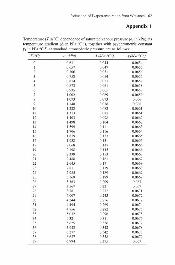
Estimation of Evapotranspiration from Wetlands 67
Appendix 1
Temperature (T in oC) dependence of saturated vapour pressure (ea in kPa), itstemperature gradient (' in kPa oC-1), together with psychrometric constant(J in kPa oC-1) at standard atmospheric pressure are as follows:
T (oC) ea (kPa) ' (kPa oC-1) J (kPa oC-1)
0 0.611 0.044 0.06541 0.657 0.047 0.06552 0.706 0.051 0.06563 0.758 0.054 0.06564 0.814 0.057 0.06575 0.873 0.061 0.06586 0.935 0.065 0.06597 1.002 0.069 0.06598 1.073 0.073 0.0669 1.148 0.078 0.06610 1.228 0.082 0.066111 1.313 0.087 0.066112 1.403 0.098 0.066213 1.498 0.104 0.066314 1.599 0.11 0.066315 1.706 0.116 0.066416 1.819 0.123 0.066517 1.938 0.13 0.066518 2.068 0.137 0.066619 2.198 0.145 0.066620 2.339 0.153 0.066721 2.488 0.161 0.066722 2.645 0.17 0.066823 2.81 0.179 0.066824 2.985 0.189 0.066925 3.169 0.199 0.066926 3.363 0.209 0.06727 3.567 0.22 0.06728 3.781 0.232 0.067129 4.007 0.243 0.067230 4.244 0.256 0.067231 4.494 0.269 0.067432 4.756 0.282 0.067533 5.032 0.296 0.067534 5.321 0.311 0.067635 5.625 0.326 0.067736 5.943 0.342 0.067837 6.277 0.342 0.067838 6.627 0.358 0.067939 6.994 0.375 0.067
68 Amos Kabo-bah and Kamila Lis
5Climbing the Water Ladder –
The New GIS Approach
Amos Kabo-bah and Kamila Lis1
College of Hydrology and Water Resources, Hohai University1 Xikang Road, Nanjing 210098, China
1Faculty of Biology and Earth Science, Department of LandscapeGeography, Nicolaus Copernicus University in Torun
Gagarina Str. 9, 87-100 Torun, Poland
Introduction
There are numerous precious natural resources in the world but the onlyresource which is needed by everybody, by every country, by rich or poorpeople and by all other living creatures is water. Water therefore becomes veryessential part of daily lives. Unfortunately, our water resources have beenstruggling over the decades to fully reach the required attention it needed byall people around the world. This is because freshwater still faces challengesincluding increasing scarcity, lack of accessibility to adequate clean drinkingwater, deterioration of water quality, fragmentation of water managementboth nationally and globally, decline of financial resources allocation forwater development, threat to world peace and security and a continuing lackof awareness of the magnitude of the problem by the decision makers and thepublic at large. Nations with abundance of freshwater resources can have aneconomic advantage over those less endowed. For instance most developednations today enjoy a degree of abundance in renewable freshwater resourcescompared to developing nations especially in Africa (Abu-Zeid, 1998). Theworld population of about six billion is projected to double in the second halfof this century and majority of this population will be in the developingnations. Unfortunately, developing nations currently face water and sanitationproblems and water-borne diseases (Bouwer, 2000; Thakur et al., 2011).
Regardless, all human beings have an inherent right to have access towater of adequate quantity and quality necessary to meet their basic needs(Gleick, 1998). However, this is not always the case as seen in current challengesfaced across the world. Water is central to improving of food security but this
DOI 10.1007/978-94-007-1858-6_5, © Capital Publishing Company 2012
e ,J.K. Thakur et al. (eds.), G ospatial Techniques for Managing Environmental Resources 68
Climbing the Water Ladder – The New GIS Approach 69
is always complicated by water scarcity especially in regions in Sub-SaharanAfrica that are currently hit by water scarcity (Gowing, 2003). There arenumber of new concepts that attempt to solve this challenge by adopting aprinciple of “water trade”. For instance; water-scarce areas can minimize theiruse of water by importing commodities that take a lot of water to producefood and electric power from communities or countries that have more water.Water can then be economically shared among those that have and thosewithout water resources. Since this water is `virtually’ embedded in thecommodity, it is called virtual water (Allan, 1998).
The world over countries will face serious water shortages with littleprospect of having adequate water for their inhabitants. This can be achievedby either moving more water to people or by moving more people to water.Imports of virtual water embedded in food and other commodities may theneconomically and politically be a very good solution, and probably the easiestway to achieve peaceful solutions to water conflicts (Bouwer, 2000). After theWorld Summit on Sustainable Development (WSSD) held in Johannesburg in2002, the international community took an important step towards moresustainable patterns of water management by including, in the WSSD Plan ofImplementation, a call for all countries to “develop integrated water resourcemanagement and water efficiency plans by 2005”, with support to developingcountries. From then on, many countries have taken crucial steps to embarkon the WSSD target (Jønch-Clausen, 2004). It is believed that sustainabledevelopment can be attained if water is managed in an integrated manner, orprecisely through Integrated Water Resources Management (Rahaman andVaris, 2005). Savenije and Van der Zaag (2008) in their research on integratedwater resources management realised that at least five of the eight MillenniumDevelopment Goals (MDGs) require good water management; they cannot beachieved without it.
These current challenges and proposals on best ways of addressing watermanagement in a sustainable manner may be a failure when considering thecurrent prevailing challenges in the water sector. For instance, by 2020, between75 and 250 million people are projected to be exposed to an increase of waterstress due to climate change in Africa; increase flooding and water scarcity inAsia; and inland flooding and more coastal flooding in nearly all Europeanregions. Increases in temperature and associated decreases in soil water areprojected to lead to gradual replacement of tropical forest by savannah ineastern Amazonia and loss of biodiversity through species extinction in manyareas of tropical Latin America (IPCC, 2007).
The scale of water challenges and associated impact on people are morenational and global as discussed previously. Therefore, the required actionstoo must also follow similar trend in order to address the use and managementof water in a more efficient manner. The fast growing computer age, gives usa huge opportunity to better understand our water challenges in large scales.Geo-information Systems (GIS) together with space technology has shown
70 Amos Kabo-bah and Kamila Lis
the enormous advantage in the understanding of the dynamics of naturalresources including water resources. The only disadvantage to this technologyin the past was that it was limited to few professionals and few commercialorganisations. With the growing new trend, this technology can be used byany body in any part of the world. In fact, GIS is becoming a technology justlike ‘mobile phones’. To further facilitate this technology towards efficientunderstanding of the dynamics of our water resources, this chapter introducestwo technologies that can greatly support water use and management; andalso greatly improve the knowledge of grass root communities across theworld to better understand their resource base. The authors believe that whengrassroots better understand their environment and water associated challengesas spelt out in IPCC, 2007, they can within their own capacity develop copingstrategies to adapt to these situations. In so doing better adoption of IWRMand Climate Change policies spelt out in the various protocols such as Kyotoand various conferences on Climate Change would be attained.
This chapter considers that to be able to clearly understand the crucialrole water has in our lives, we need to adopt step by step approach to understandthe complex water ecology. This step by step approach can better be achievedthrough the use of low cost technologies to inform people properly about whatresources they have and what they can do with it. The chapter, therefore,presents two technologies: GEONETCast initiative and use of PublicParticipatory GIS as a way of better understanding what we have as waterresource. The authors believe there are other green initiatives such as rainwaterharvesting but concentrates on these new methods which promise hugeopportunities for communities across the world.
Water Resources – Issues and Challenges
Water is central to the achievement of MDGs as identified by Savenije andVan der Zaag (2008). It therefore means that significant progress towards theMDGs target implies a relative impact too on adequate water provision andsound water management. Some reports indicate significant improvementstowards the meeting of the MDGs throughout east Asia and south Asia.However, there are huge disparities from continent to continent. Sub-SaharanAfrica is in pervasive crisis, with rising extreme poverty, shockingly highchild and maternal mortality, and many countries in the region are failing tomeet most of goals of the MDGs. Additionally, Latin America, the MiddleEast, and north Africa have made little headway in reducing the rates ofextreme poverty in recent years. Even Asia remains home to hundreds ofmillions of people living in extreme poverty. Virtually all countries are failingin the goal of achieving environmental sustainability, and most lag severelyon the goals for gender equality and maternal mortality (Sachs and McArthur,2005; Thakur, 2010; Thakur et al., 2011). In next five years when worldleaders assess the progress that has been made in meeting the commitmentenunciated in the Millennium Declaration of 2000 and encapsulated in the

Climbing the Water Ladder – The New GIS Approach 71
eight Millennium Development Goals (MDGs), more emphasis need to belaid on how best water provision, use and management can be better enforcedto ensure that the MDGs are met (MDG, 2010).
Though significant effort has been made by many organisations andindividuals the world over, our world’s fresh water is still under critical state.Throughout the world, the challenge of too little water, too much water andtoo dirty water continue to be one of the biggest challenges by communitiesand governments in various countries. As described in Fig. 1, these problemsare often encapsulated by international and national agenda to become moreeconomically powerful or are as a result of cultural and social norms of thecountry. The impact of natural phenomenon such as climate change alsoworsens the existing conditions of this three-pillar water paradigm. As identifiedby Abu-Zeid (1998), the following issues continue to be a core of problemsstill faced by various nations:
a. Water scarcity: Fresh water available for human consumption, for social,economic and cultural needs and for environmental requirements is rapidlybecoming scarcer. In the 1950s, only a handful of countries faced watershortages. In the late 1990s, the number of countries facing a water deficithas grown to 26 with a total population of 300 million. It is predicted thattwo-thirds of the world’s population will face water shortages in one formor another by the year 2050. Food production which consumes 70% of theworld’s fresh water is at risk if no measures are taken.
b. Lack of accessibility to clean drinking water and sanitation: Despiteinternational efforts over the last decades, approximately 1.2 billion peoplelack access to clean drinking water, 2.2 billion lack adequate sanitationand four billion do not have sewerage service. Those most affected areparticularly the poor (especially women and children).
Figure 1. Simplified water problems and challenges likelyto be faced by any country.
72 Amos Kabo-bah and Kamila Lis
c. Water quality problems: Rapid industrialization, urbanization, the growthof mega-cities and the intensification of agriculture at the expense of theenvironment and water bodies result in highly polluted water rivers, lakesand streams. The impact of this on the human health and aquatic life isimmeasurable.
d. Decline of financial resources allocation and fragmentation ofwater management: Addressing the water problems and challengesrequire significant financial investments. However, there is a steadydecline in financial allocations to water projects since 1980s.Developing countries in particular suffer this decline. Apart fromthis problem, there has been enormous growth of various institutions e.g.Non-Governmental Organisations (NGOs) and others all working towardsthe goal of water use in a more efficient manner. As a result of thefragmentation of institutions nation-wide and globally, it is difficult toconsolidate efforts towards efficient use of financial resources for waterresources management.
e. Lack of awareness by decision-makers and the public: Water over theyears has been taken for granted as being abundant and of good quality.This wrong perception continues to persist and more work is needed toproperly educate all people to understand and then to reverse thisphenomenon. This chapter therefore seeks to address this situation as away of bringing to fore some tools that can enhance the understanding ofthe dynamics of our water resources. This will help educational institutions,professional associations and NGOs to incorporate the simple techniquesinto their working programmes and framework for better understanding ofwater issues and pending crises.
f. Fragile world peace and security: Water is the foundation of our veryexistence and the socio-economic foundation of society and its environment.The decline of its availability is a threat to peace and security to manyparts of the world. It so happens that most countries facing water shortagesalso suffer from political instability, social tension and public unrest.National and international trans-boundary water conflicts are on a timebomb ready to explode at any moment.
As discussed the water problems are complicated and interlinked withvarious sectors of social and economic development. The issue of sociallearning and the importance of the involvement of informal sectors becomevery important towards this. As noticed by Pahl-Wostl et al. (2007), sociallearning and participation of informal actors is key to the implementationof integrated water policies and programmes in an eco-friendly manner. Thenext sections of this chapter look on how efforts from GEONETCast(http://www.earthobservations.org/geonetcast.shtml) and PPGIS can becomean integral part of water management.
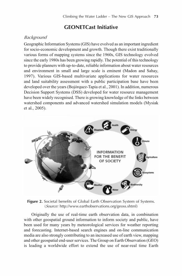
Climbing the Water Ladder – The New GIS Approach 73
GEONETCast Initiative
Background
Geographic Information Systems (GIS) have evolved as an important ingredientfor socio-economic development and growth. Though there exist traditionallyvarious forms of mapping systems since the 1960s, GIS technology evolvedsince the early 1980s has been growing rapidly. The potential of this technologyto provide planners with up-to-date, reliable information about water resourcesand environment in small and large scale is eminent (Madon and Sahay,1997). Various GIS-based multivariate applications for water resourcesand land suitability assessment with a public participation base have beendeveloped over the years (Bojórquez-Tapia et al., 2001). In addition, numerousDecision Support Systems (DSS) developed for water resource managementhave been widely recognised. There is growing knowledge of the links betweenwatershed components and advanced watershed simulation models (Mysiaket al., 2005).
Figure 2. Societal benefits of Global Earth Observation System of Systems.(Source: http://www.earthobservations.org/geoss.shtml)
Originally the use of real-time earth observation data, in combinationwith other geospatial ground information to inform society and public, havebeen used for many years by meteorological services for weather reportingand forecasting. Internet-based search engines and on-line communicationmedia are also strongly contributing to an increased use of earth view, mappingand other geospatial end-user services. The Group on Earth Observation (GEO)is leading a worldwide effort to extend the use of near-real time Earth
74 Amos Kabo-bah and Kamila Lis
Observation combined with in situ ground data to a broad array of societalbenefit areas, including climate, weather, water, health, energy, disasters,agriculture, biodiversity and ecosystems (Mannaerts et al., 2009). This initiativeis called the GEONETCast Initiative. This is a global data disseminationsystem to deliver near-real time Earth observation (EO) and in-situ data andproducts derived from the Global Earth Observation System of Systems(GEOSS) to the user community. The information is relevant for policyformulation and management decision making and is covering the full rangeof societal benefit areas. Backbone of the data dissemination system isEUMETCast, already used globally by the meteorological organizations fornear real-time data reception using low cost ground receiving stations. Largevolumes of data are broadcasted and received using this one-way disseminationsystem. Delivery of self-training packages to users operating a ground receptionsystem is currently possible using the so-called “training-channel” onEUMETCast (Ben Maathuis and Mannaerts, 2009).
The last two decades have shown an important shift towards stand-alonesoftware systems to networked ones, often client/server applications usingdistributed geo- (web-) services. This allows organisations to combine withoutmuch effort their own data with remotely available data and processingfunctionality. Another important aspect of an integrated spatial data analysisis a low-cost access to data from within user-friendly and flexible software.Web-based open source software solutions are more often a powerful optionfor developing countries. The Integrated Land and Water Information System(ILWIS) is a PC-based GIS and Remote Sensing software, comprising acomplete package of image processing, spatial analysis and digital mappingand was developed as commercial software from the early nineties onwards.Fortunately, recent project efforts have migrated ILWIS into a modular, plug-in-based open source software, and provide web-service support for OGC-based web mapping and processing. The core objective of the ILWIS opensource project is to provide a maintainable framework for researchers andsoftware developers to implement training components, scientific toolboxesand (web-) services. The latest plug-ins have been developed for multi-criteriadecision making, water resources analysis and spatial statistics analysis. Thedevelopment of this framework is done since 2007 in the context of 52°North,which is an open initiative that advances the development of cutting edgeopen source geospatial software, using the GPL license. GEONETCast makesavailable satellite images via Digital Video Broadcast (DVB) technology (seeFig. 3). An OGC WMS interface and plug-ins which convert GEONETCastdata streams allow an ILWIS user to integrate various distributed data sourceswith data locally stored on the machine (Lemmens et al., 2009).
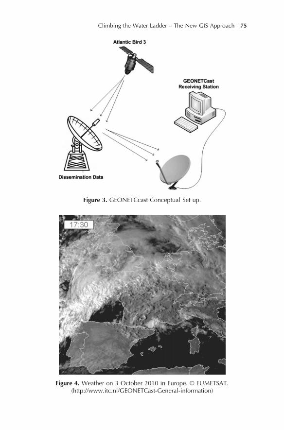
Climbing the Water Ladder – The New GIS Approach 75
Figure 3. GEONETCcast Conceptual Set up.
Figure 4. Weather on 3 October 2010 in Europe. © EUMETSAT.(http://www.itc.nl/GEONETCast-General-information)
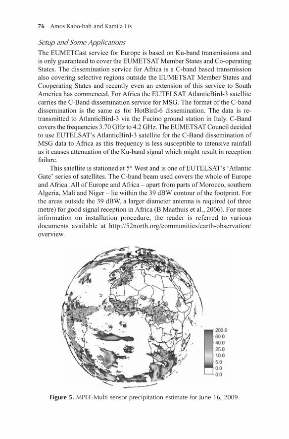
76 Amos Kabo-bah and Kamila Lis
Setup and Some Applications
The EUMETCast service for Europe is based on Ku-band transmissions andis only guaranteed to cover the EUMETSAT Member States and Co-operatingStates. The dissemination service for Africa is a C-band based transmissionalso covering selective regions outside the EUMETSAT Member States andCooperating States and recently even an extension of this service to SouthAmerica has commenced. For Africa the EUTELSAT AtlanticBird-3 satellitecarries the C-Band dissemination service for MSG. The format of the C-banddissemination is the same as for HotBird-6 dissemination. The data is re-transmitted to AtlanticBird-3 via the Fucino ground station in Italy. C-Bandcovers the frequencies 3.70 GHz to 4.2 GHz. The EUMETSAT Council decidedto use EUTELSAT’s AtlanticBird-3 satellite for the C-Band dissemination ofMSG data to Africa as this frequency is less susceptible to intensive rainfallas it causes attenuation of the Ku-band signal which might result in receptionfailure.
This satellite is stationed at 5° West and is one of EUTELSAT’s ‘AtlanticGate’ series of satellites. The C-band beam used covers the whole of Europeand Africa. All of Europe and Africa – apart from parts of Morocco, southernAlgeria, Mali and Niger – lie within the 39 dBW contour of the footprint. Forthe areas outside the 39 dBW, a larger diameter antenna is required (of threemetre) for good signal reception in Africa (B Maathuis et al., 2006). For moreinformation on installation procedure, the reader is referred to variousdocuments available at http://52north.org/communities/earth-observation/overview.
Figure 5. MPEF-Multi sensor precipitation estimate for June 16, 2009.
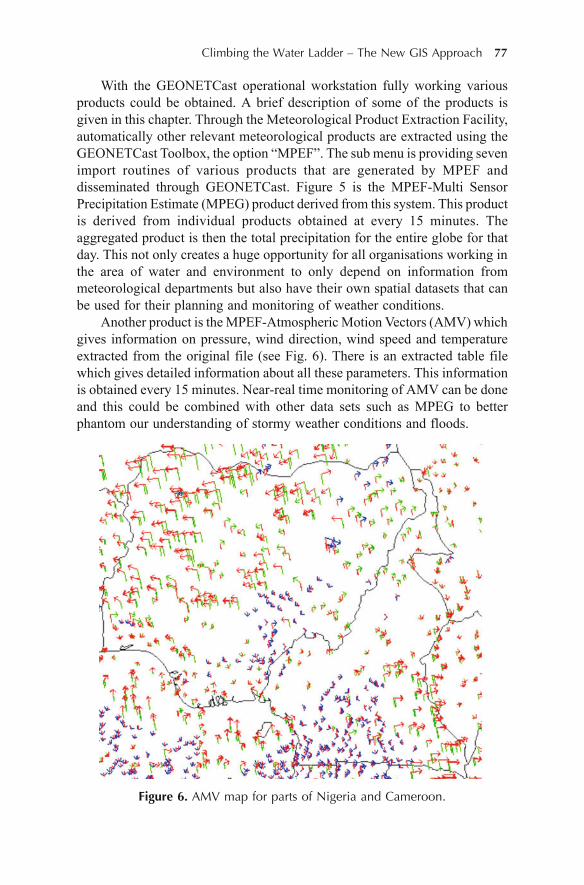
Climbing the Water Ladder – The New GIS Approach 77
With the GEONETCast operational workstation fully working variousproducts could be obtained. A brief description of some of the products isgiven in this chapter. Through the Meteorological Product Extraction Facility,automatically other relevant meteorological products are extracted using theGEONETCast Toolbox, the option “MPEF”. The sub menu is providing sevenimport routines of various products that are generated by MPEF anddisseminated through GEONETCast. Figure 5 is the MPEF-Multi SensorPrecipitation Estimate (MPEG) product derived from this system. This productis derived from individual products obtained at every 15 minutes. Theaggregated product is then the total precipitation for the entire globe for thatday. This not only creates a huge opportunity for all organisations working inthe area of water and environment to only depend on information frommeteorological departments but also have their own spatial datasets that canbe used for their planning and monitoring of weather conditions.
Another product is the MPEF-Atmospheric Motion Vectors (AMV) whichgives information on pressure, wind direction, wind speed and temperatureextracted from the original file (see Fig. 6). There is an extracted table filewhich gives detailed information about all these parameters. This informationis obtained every 15 minutes. Near-real time monitoring of AMV can be doneand this could be combined with other data sets such as MPEG to betterphantom our understanding of stormy weather conditions and floods.
Figure 6. AMV map for parts of Nigeria and Cameroon.

78 Amos Kabo-bah and Kamila Lis
Figure 7. LSA SAF-Fraction of Vegetation Cover (FVC)for Africa on June 13, 2009.
Satellite Application Facilities (SAFs) are specialised development andprocessing centres within the EUMETSAT Applications Ground Segment. Inthe GEONETCast Toolbox you will find four menu items: “SAF Africa”,“SAF Euro”, “SAF South America” and “SAF SST MSG-GOES Combined”.More detail description about these products can be obtained from the usermanual of the GEONETCast toolbox. Figure 7 is one of these products forfraction of vegetation cover (FVC) for Africa obtained on the June 13, 2009(see Fig. 7).
In water resources management, modelling and understanding the surfaceenergy balance is important for assessing the re-distribution of moisture andheat in soil and atmosphere. The Surface Energy Balance System (SEBS)estimates turbulent heat fluxes using satellite earth observation data in thevisible, near-infrared, and thermal spectral domain (B. Z. Su, 2009; Z. Su,2002; van der Kwast and de Jong, 2004). SEBS is made up of two sets of toolsfor the determination of the land surface physical parameters, such as albedo,emissivity, temperature, vegetation coverage etc. from spectral reflectanceand radiance; air pressure, temperature, humidity, and wind speed at a referenceheight can all be derived from GEONETCast toolbox. In a simple application,the GEONETCast toolbox was used to derive all the input requirements forSEBS to compute the daily evapotranspiration for Zambia region (see Fig. 8).

Climbing the Water Ladder – The New GIS Approach 79
Figure 8. Daily evapotranspiration for Zambia.
Here we have presented few products and an application, but the toolboxgives the derivation of several products. These data sources can be applicablefor various sectoral operations ranging from meteorological to water resourcesmanagement. It is hoped that organisations be signed up for this system andbegin to use this to understand the spatio-temporal variation of water-land usedynamics in their environment. This system, because of its low cost natureand full operational support from 52 North organisation (www.52north.org),can greatly help the communities and institutions across the world tobetter appreciate the complex dynamics in their environment. In thiscase, land surface temperature maps, land cover maps, humidity maps etc.could be combined in the same window to better understand the inter-relationship. Another important feature of this system of GEONETCast andILWIS is that, information processed can be viewed in near-real time anddisplayed via a map service. Therefore processed information by organisations,individuals and communities can easily be shared with the larger communityworldwide.
Also the availability of 3G-Network, providing wireless accelerated dataspeeds and simultaneous voice and data capabilities, offer new possibilitiesfor Distance Education and E-Learning in Africa and other developing countriesacross the world. With relatively cheap 3G enabled modem or mobile phone,connected to a computer or laptop, larger bandwidth is obtained which can beutilized for these types of training activities, irrespective of available fixednetwork infrastructure. Through this community (http://52north.org/communities/earth-observation/overview), users share ideas and products andnew applications developed from using the application. All tools and utilitiesto support the GEONETCast-Community are also available via this web address(Ben Maathuis and Mannaerts, 2009). As technology advancement indeveloping countries keep improving everyday, it implies that internet
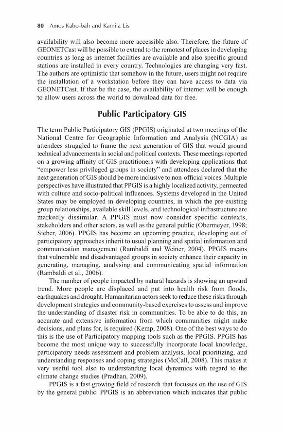
80 Amos Kabo-bah and Kamila Lis
availability will also become more accessible also. Therefore, the future ofGEONETCast will be possible to extend to the remotest of places in developingcountries as long as internet facilities are available and also specific groundstations are installed in every country. Technologies are changing very fast.The authors are optimistic that somehow in the future, users might not requirethe installation of a workstation before they can have access to data viaGEONETCast. If that be the case, the availability of internet will be enoughto allow users across the world to download data for free.
Public Participatory GIS
The term Public Participatory GIS (PPGIS) originated at two meetings of theNational Centre for Geographic Information and Analysis (NCGIA) asattendees struggled to frame the next generation of GIS that would groundtechnical advancements in social and political contexts. These meetings reportedon a growing affinity of GIS practitioners with developing applications that“empower less privileged groups in society” and attendees declared that thenext generation of GIS should be more inclusive to non-official voices. Multipleperspectives have illustrated that PPGIS is a highly localized activity, permeatedwith culture and socio-political influences. Systems developed in the UnitedStates may be employed in developing countries, in which the pre-existinggroup relationships, available skill levels, and technological infrastructure aremarkedly dissimilar. A PPGIS must now consider specific contexts,stakeholders and other actors, as well as the general public (Obermeyer, 1998;Sieber, 2006). PPGIS has become an upcoming practice, developing out ofparticipatory approaches inherit to usual planning and spatial information andcommunication management (Rambaldi and Weiner, 2004). PPGIS meansthat vulnerable and disadvantaged groups in society enhance their capacity ingenerating, managing, analysing and communicating spatial information(Rambaldi et al., 2006).
The number of people impacted by natural hazards is showing an upwardtrend. More people are displaced and put into health risk from floods,earthquakes and drought. Humanitarian actors seek to reduce these risks throughdevelopment strategies and community-based exercises to assess and improvethe understanding of disaster risk in communities. To be able to do this, anaccurate and extensive information from which communities might makedecisions, and plans for, is required (Kemp, 2008). One of the best ways to dothis is the use of Participatory mapping tools such as the PPGIS. PPGIS hasbecome the most unique way to successfully incorporate local knowledge,participatory needs assessment and problem analysis, local prioritizing, andunderstanding responses and coping strategies (McCall, 2008). This makes itvery useful tool also to understanding local dynamics with regard to theclimate change studies (Pradhan, 2009).
PPGIS is a fast growing field of research that focusses on the use of GISby the general public. PPGIS is an abbreviation which indicates that public
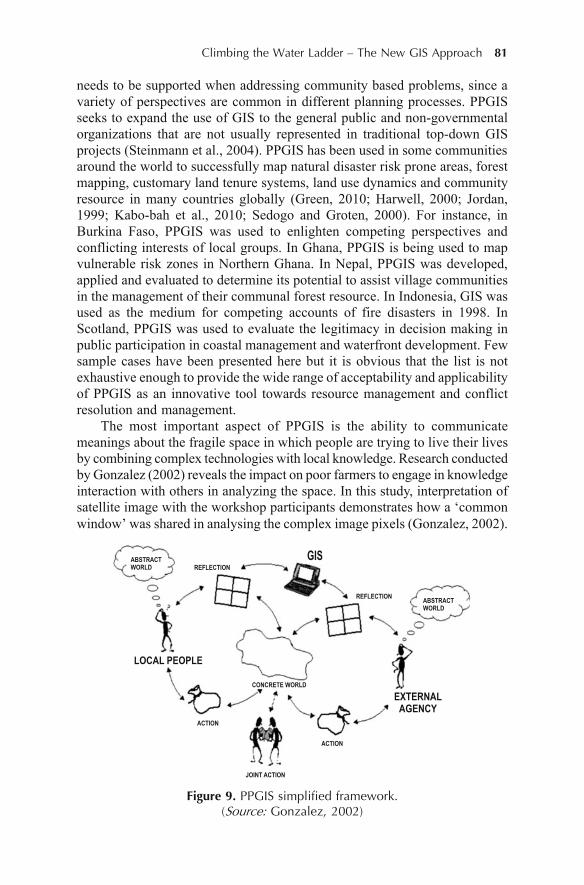
Climbing the Water Ladder – The New GIS Approach 81
needs to be supported when addressing community based problems, since avariety of perspectives are common in different planning processes. PPGISseeks to expand the use of GIS to the general public and non-governmentalorganizations that are not usually represented in traditional top-down GISprojects (Steinmann et al., 2004). PPGIS has been used in some communitiesaround the world to successfully map natural disaster risk prone areas, forestmapping, customary land tenure systems, land use dynamics and communityresource in many countries globally (Green, 2010; Harwell, 2000; Jordan,1999; Kabo-bah et al., 2010; Sedogo and Groten, 2000). For instance, inBurkina Faso, PPGIS was used to enlighten competing perspectives andconflicting interests of local groups. In Ghana, PPGIS is being used to mapvulnerable risk zones in Northern Ghana. In Nepal, PPGIS was developed,applied and evaluated to determine its potential to assist village communitiesin the management of their communal forest resource. In Indonesia, GIS wasused as the medium for competing accounts of fire disasters in 1998. InScotland, PPGIS was used to evaluate the legitimacy in decision making inpublic participation in coastal management and waterfront development. Fewsample cases have been presented here but it is obvious that the list is notexhaustive enough to provide the wide range of acceptability and applicabilityof PPGIS as an innovative tool towards resource management and conflictresolution and management.
The most important aspect of PPGIS is the ability to communicatemeanings about the fragile space in which people are trying to live their livesby combining complex technologies with local knowledge. Research conductedby Gonzalez (2002) reveals the impact on poor farmers to engage in knowledgeinteraction with others in analyzing the space. In this study, interpretation ofsatellite image with the workshop participants demonstrates how a ‘commonwindow’ was shared in analysing the complex image pixels (Gonzalez, 2002).
ABSTRACTWORLD REFLECTION
GIS
REFLECTIONABSTRACTWORLD
ACTION
EXTERNALAGENCY
JOINT ACTION
ACTION
CONCRETE WORLD
LOCAL PEOPLE
Figure 9. PPGIS simplified framework.(Source: Gonzalez, 2002)
82 Amos Kabo-bah and Kamila Lis
In this way, PPGIS has a more people-centred GIS compared to a traditionaltechnocratic, expert-driven tool or methodology (Schlossberg and Shuford,2005). PPGIS has a critical role in the implementation of IWRM plans,understanding climate change scenarios and better development of copingstrategies for communities around the world. PPGIS has in recent past shownthat it has capabilities for introducing good governance, by improving dialogue,and using local knowledge, exposing local stakeholders to geospatial analysisand empowerment by supporting community members’ participation in decisionmaking and actions and by enabling land use planning decisions (McCall andMinang, 2005).
Regardless of the theoretical feasibility and acceptance of the PPGISglobally, there are some few technical issues which make the completerealisation of the PPGIS a mirage, especially for disadvantaged communities.Most applications currently developed make use of the ArcGIS Desktop andsome internet based applications. However, most disadvantaged communitiesdo not have the financial resources and sustainable infrastructure tocontinuously upgrade the PPGIS products by themselves. This poses, somehow,a sustainable question for the full acceptance of PPGIS for communityparticipation. In other cases also, it is still often quite difficult to involve all ofthe public in the use of GIS and this can lead to marginalisation of somegroups and possibly disengagement from the process (Green, 2010). Therefore,for full realisation of PPGIS in most disadvantaged communities, expertsmust begin to explore low cost PPGIS techniques. This might includedeveloping applications with more open source GIS and also helpingcommunities to set up their own community based GIS database. This is ofcourse a huge challenge but if vulnerable communities are to be empoweredwith GIS, we must begin to think of alternative solutions.
As identified by some authors, the future of PPGIS will be dependent onthe development of more decision support systems such as the web-basedPPGIS (Tan and Ori, 2008) and the use of low cost GIS software. There ishowever some concern about the integration of PPGIS applications into theInternet which raises some prospects as well as concerns for the future ofPPGIS applications among disadvantaged people (Kyem, 2002). As lessprivileged people are also challenged for internet infrastructure, it means asPPGIS applications via the web increases, these will however have limiteduse for this group of people. However, as there is also increasing availabilityof mobile phones among the less privileged people, one option out of thisforeseen challenge will be to develop more mobile-based PPGIS applications.In this way, disadvantaged communities can and will be able to benefit fromPPGIS applications.
Therefore in trying daily to understand our water problems and challengesin our societies better, it is hoped that with the fast growing GIS sector,methods such as PPGIS should be upheld as one of the techniques in climbingthe water ladder to reach our optimum goal of sustainable water developmentand management around the world. Here, we acknowledge the merits of the
Climbing the Water Ladder – The New GIS Approach 83
methodology and trust that few case studies, especially for water resourcesmanagement, will be developed in the coming years.
Conclusion
Water continues to be a central topic in our daily lives and in our politics inthe world for economic growth. With the fast growing GIS sector in mostcountries, it is important we realise some of the low cost GIS technologiesthat can upscale the works of professionals in the water sector and also increasethe participation of local people in the complete decision making process.This chapter presents two of these technologies; the GEONETCast initiativevia the GEONETCast toolbox supported by the 52North organisation and thePPGIS. It is believed that recognition of these tools and methods can helptremendously towards a better understanding of our water resources. With therecent outcry on climate change effects, participation from local communitiesis very crucial to the holistic mitigation and adaptation measures to beimplemented and adopted by various countries. Therefore, the use of low costGIS and satellite data comes in handy as an answer towards these globalissues.
References
Abu-Zeid, M. (1998). Water and sustainable development: the vision for world water,life and the environment. Water Policy, 1(1), 9–19.
Allan, J. (1998). Virtual water: A strategic resource global solutions to regional deficits.Ground Water, 36(4), 545–546.
Bojórquez-Tapia, L., Diaz-Mondragon, S. and Ezcurra, E. (2001). GIS-based approachfor participatory decision making and land suitability assessment. InternationalJournal of Geographical Information Science, 15(2), 129–151.
Bouwer, H. (2000). Integrated water management: emerging issues and challenges.Agricultural Water Management, 45(3), 217–228.
Gleick, P. (1998). The human right to water. Water Policy, 1(5), 487–503.Gonzalez, R. (2002). Joint learning with GIS: multi-actor resource management.
Agricultural Systems, 73(1), 99–111.Gowing, J. (2003). Food security for sub-Saharan Africa: Does water scarcity limit the
options? Land Use and Water Resources Research, 3, 2.1–2.7.Green, D.R. (2010). The role of Public Participatory Geographical Information Systems
(PPGIS) in coastal decision-making processes: An example from Scotland, UK.Ocean and Coastal Management, 53(12), 816–821.
Harwell, E. (2000). Remote sensibilities: discourses of technology and the making ofIndonesia’s natural disaster. Development and Change, 31(1), 307–340.
IPCC. (2007). Climate change 2007: Impacts, adaptation and vulnerability. Contributionof the Working Group II to the Fourth Assessment report of the IntergovernmentalPanel on Climate Change.

84 Amos Kabo-bah and Kamila Lis
Jønch-Clausen, T. (2004). Integrated water resources management (IWRM) and waterefficiency plans by 2005: Why, what and how. Integrated Water Resources Manage-ment (IWRM) and Water Efficiency Plans by 2005. Global Water Partnership.
Jordan, G. (1999). A public participation GIS for community forestry user groups inNepal: Putting people before the technology.
Kabo-bah, A., Odoi, J. and Lis, K. (2010). Vulnerability Assessment maps forcommunities in Northern Ghana: Planet Action.
Kemp, R. (2008). Public participatory GIS in community-based disaster risk reduction.tripleC – Cognition, Communication, Co-operation, 6(2), 88.
Kyem, P.A.K. (2002). Public participatory GIS: A new kind of GIS Application.Lemmens, R., Maathuis, B., Mannaerts, C., Foerster, T., Schaeffer, B. and Wytzisk, A.
(2009). Web-based spatial analysis with the ILWIS open source GIS software andsatellite images from GEONETCast.
Maathuis, B. and Mannaerts, C. (2009). Potentials of GEONETCast for DistanceEducation in EO in Africa. ISPRS TCVI Special Sessions on Education and OutreachEnschede, ITC.
Maathuis, B., Retsios, V., Lasry, F. and Schilling, M. (2006). Installation, setup anduse of a low cost C-band meteosat-8 ground receiving station in Rwanda: AARSE,Cairo, Egypt.
Madon, S. and Sahay, S. (1997). Managing natural resources using GIS: Experiencesin India. Information and Management, 32(1), 45–53.
Mannaerts, C., Maathuis, B., Molenaar, M. and Lemmens, R. (2009). The ITCGEONETCast Toolbox: A Geo capacity building component for education andtraining in Global earth observation and Geo information provision to society.
McCall, M.K. (2008). Participatory Mapping and Participatory GIS (PGIS) for DRR,Community Risk and Hazard Assessment.
McCall, M.K. and Minang, P.A. (2005). Assessing participatory GIS for community-based natural resource management: claiming community forests in Cameroon.Geographical Journal, 171(4), 340–356.
MDG (2010). Assessing Progress in Africa toward the Millennium DevelopmentGoals: ECA, AU, ADB Group and UNDP.
Mysiak, J., Giupponi, C. and Rosato, P. (2005). Towards the development of a decisionsupport system for water resource management. Environmental Modelling andSoftware, 20(2), 203–214.
Obermeyer, N. (1998). PPGIS: the evolution of public participation GIS. Cartogr.GIS, 25, 65–66.
Pahl-Wostl, C., Craps, M., Dewulf, A., Mostert, E., Tabara, D. and Taillieu, T. (2007).Social learning and water resources management. Ecology and Society, 12(2), 5.
Pradhan, B.M. (2009). Making GIS work in Forest management. Geoinformatics forResource Mapping and Analysis, Pokhara, Institute of Forestry.
Rahaman, M. and Varis, O. (2005). Integrated water resources management: evolution,prospects and future challenges. Sustainability: Science, Practice and Policy, 1(1),15–21.
Rambaldi, G., Kyem, P.A.K., McCall, M. and Weiner, D. (2006). Participatory spatialinformation management and communication in developing countries. TheElectronic Journal of Information Systems in Developing Countries, 25(1), 1–9.
Rambaldi, G. and Weiner, D. (2004). Summary proceedings of the “Track onInternational PPGIS Perspectives”.
Climbing the Water Ladder – The New GIS Approach 85
Sachs, J. and McArthur, J. (2005). The millennium project: a plan for meeting themillennium development goals. Lancet, 365(9456), 347–353.
Savenije, H. and Van der Zaag, P. (2008). Integrated water resources management:Concepts and issues. Physics and Chemistry of the Earth, Parts A/B/C, 33(5), 290–297.
Schlossberg, M. and Shuford, E. (2005). Delineating ‘public’ and ‘participation’ inppgis. Editors and Review Board, 16(2), 15.
Sedogo, L.G. and Groten, S.M.E. (2000). Definition of land management units forGIS support to participatory planning: a case study on participatory land managementin Burkina Faso. Canadian Journal of Development Studies, 21 (Special Issue),523–542.
Sieber, R. (2006). Public participation geographic information systems: A literaturereview and framework. Annals of the Association of American Geographers, 96(3),491–507.
Steinmann, R., Krek, A. and Blaschke, T. (2004). Analysis of online public participatoryGIS applications with respect to the differences between the US and Europe.
Su, B.Z. (2009). Introduction to the Surface Energy Balance System (SEBS), ITC,Enschede.
Su, Z. (2002). The Surface Energy Balance System (SEBS) for estimation of turbulentheat fluxes. Hydrology and Earth System Sciences, 6(1), 85–99.
Tan, Y. and Ori, G. (2008). Web-based public participatory GIS.Thakur, J.K. (2010). Eco-hydrological wetland monitoring in a semi-arid region (A
case study of Konya Closed Basin, Turkey). Faculty of International Institute forGeo-Information Science and Earth Observation (ITC), Universiteit Twente,Enschede, the Netherlands.
Thakur, J.K., Srivastava, P.K., Singh, S.K. and Vekerdy, Z. (2011). Ecologicalmonitoring of wetlands in semi-arid region of Konya closed basin, Turkey. RegionalEnvironmental Change (DOI: 10.1007/s 10113-011-0241-x).
Thakur, J.K., Thakur, R.K., Ramanathan, A., Kumar, M. and Singh, S.K. (2011).Arsenic Contamination of Groundwater in Nepal – An Overview. Water, 3(1),1–20.
van der Kwast, J. and de Jong, S. (2004). Modelling evapotranspiration using thesurface energy balance system (SEBS) and Landsat TM data (Rabat region,Morocco).

86 Prajjwal K. Panday et al.
6Supraglacial Lake Classification in
the Everest Region of NepalHimalaya
Prajjwal K. Panday, Henry Bulley1, Umesh Haritashya2
and Bardan GhimireClark Graduate School of Geography, Clark University
950 Main Street, Worcester, MA 01610, USA1Central Connecticut State University, 1615 Stanley Street
New Britain, CT 06050, USA2Department of Geology, University of Dayton, 300 College
Park Avenue, Dayton, OH 45469, USA
Introduction
Climate change has been linked to widespread retreats and recentdisappearances of small glaciers in mountainous regions such as the Patagonia,Andes, Alps and Himalaya (Dyurgerov and Meier, 2000; Fujita et al., 2006;Kargel et al., 2005; Oerlemans, 2005; Paul, Kaab et al., 2004; Racoviteanu etal., 2008; Thakur, 2010). Alpine glaciers are particularly sensitive to changesin climate due to their proximity to melting conditions, wide altitude range,and variability in debris cover (Haeberli et al., 2007; Racoviteanu et al.,2008). Alpine glacial retreat in response to climate change and recent warmingtrends may have severe hydroecological consequences to surroundingcommunities (Kehrwald et al., 2008; Milner et al., 2009). The recession ofglaciers has been further linked to increases in glacier-related hazards in highmountainous areas such as avalanches, glacial lake outburst floods and debrisflows which can increasingly threaten human lives, settlements, andinfrastructure (Huggel et al., 2002; Quincey et al., 2005). This has necessitatedthe assessment and monitoring of potentially hazardous glacial lakes throughthe use of remote sensing, especially in high mountainous areas due toinaccessibility and lack of field surveys (Quincey et al., 2005).
There is a general pattern of glacial retreat and melting in the NepalHimalayas leading to increased production of glacial melt water and
DOI 10.1007/978-94-007-1858-6_6, © Capital Publishing Company 2012
e ,J.K. Thakur et al. (eds.), G ospatial Techniques for Managing Environmental Resources 86
Supraglacial Lake Classification in the Everest Region of Nepal Himalaya 87
development of supraglacial lakes that are potentially hazardous (Fujita et al.,2006; Richardson and Reynolds, 2000; Yamada et al., 1992). An inventory ofglaciers and glacial lakes in the Nepal Himalaya indicates increased frequencyand magnitude of supraglacial and moraine-dammed lakes in the region (Kargelet al., 2005; Mool et al., 2001). Although remote sensing offers greatopportunities in the Himalayas and in areas lacking traditional field-basedglaciologic methods, there are challenges and limitations to its use in glacierstudies especially in the Himalayan context. Challenges in mapping debris-covered glaciers include limited field validation data, lack of aerial photographs,lack of accurate elevation data for remote glacierized areas, lack of algorithmsfor automatically discerning debris-covered ice from non-ice areas with debris,and limited capability to discern changes in glacier thickness. Thesecomplexities pose several challenges in quantitative characterization of glaciersurfaces, glacial lakes and mass balance (Kargel et al., 2005; Racoviteanu etal., 2008). Although aerial photographs have been primarily used for extractionof glacier parameters throughout the early 1970s, availability of aerialphotographs have been either limited or restricted for certain areas such as theHimalayas (Racoviteanu et al., 2008). The classification of glaciers remainsan important step for any glacier-related assessment and manual digitizationremains the most common approach for glacier classification despite theabundance of multi-spectral classification methods (Raup et al., 2007).
Few studies have attempted automated classification in the Himalayanregion (Bolch et al., 2008), while most studies have relied on manual digitization(Kulkarni et al., 2007; Kulkarni and Buch, 1991), band ratioing (Bolch,Buchroithner, Pieczonka, et al., 2008), and semi-automated thresholding andclassification (Keshri et al., 2009; Paul, Huggel et al., 2004). Delineation ofglacial lakes for identification of potentially hazardous lakes are also mostlycarried out through manual digitization (Bajracharya et al., 2007) orthresholding using the normalized difference water index (NDVI) (Bolch,Buchroithner, Peters et al., 2008; Huggel et al., 2002). Supraglacial debrisposes a major challenge in automatic delineation of glaciers due to the spectralsimilarity to the surrounding debris (Bolch et al., 2008; Bulley et al., 2011).This further confounds accurate classification of glacial lakes, particularly inthe Himalayan region (Bolch et al., 2008; Bolch, Buchroithner, Pieczonka etal., 2008; Racoviteanu et al., 2008; Raup et al., 2007). Supraglacial covermapping in the Chenab basin through the use of ratios in a systematic fashionresulted in a 91% overall accuracy (Keshri et al., 2009). Bolch et al. (2008)used a morphometry- and temperature-based glacier delineation using ASTERbands and DEM (Digital Elevation Model) in the Khumbu Glacier of Nepalthat produced a discrepancy of 5% between the calculated and the manuallydigitized polygons. The dependence of thresholds in different sensors andseasons (Hall et al., 1995) and the possibility of underestimation oroverestimation of cover classes from a slight error necessitate the selection ofappropriate threshold values in supraglacial classification (Keshri et al., 2009).
88 Prajjwal K. Panday et al.
A semi-automated approach to map debris-covered glaciers developed byPaul (2004a) failed when transferred to the Himalayan region (Bolch et al.,2008). It is important to develop a sequential, systematic method for glacierclassification that takes spectral characteristics of supraglacial cover intoaccount and delineates potentially hazardous glacial lakes.
Substantial effort has been focussed on the use of spatial information andrecently the use of geometric attributes of features such as shape in remotelysensed imagery for improving classification (Frohn, 2006; Frohn and Hao,2006; Zhou et al., 1995). Land use/land cover features with similar spectralresponses but differing shape of spatial properties have been discriminated bythe use of shape index (Zhou et al., 1995). Frohn (2006) used a perimeter-to-area shape complexity metric called the Square Pixel Metric (SqP) todifferentiate lakes from rivers in Alaska and classify natural vs. anthropogenicpastures in Bolivia. The utility of landscape and shape metrics is yet to betested in glacier classification where spectral inseparability among featureshas been a major problem. The SqP used by Frohn (2006) is used here todifferentiate supraglacial lakes from other glacier features to improveclassification.
This chapter proposes a hybrid approach of glacial lake classificationusing a non-parametric classification tree model combined with a squaredpixel shape complexity spatial metric to differentiate supraglacial cover typesand effectively discriminate supraglacial lakes. There have been recent interestsin machine learning algorithms (MLA) such as classification trees andregression trees as a response to the limitations posed by multivariateclassification algorithms (Hansen et al., 1996; Rogan et al., 2008; Bulley etal., 2008; Bulley et al., 2011). Classification trees involve a binary, recursivepartitioning of the data and result in hierarchical trees of decision rules thatcan be used for classification and have proved superior to conventionalclassifiers in almost all cases (Rogan and Chen, 2004; Bulley et al., 2008;Bulley et al., 2011). Classification trees can further incorporate ancillaryvariables in the form of indices, ratios and image-based derivatives that havebeen used by other studies in glacier classification (Rogan et al., 2008). Aninitial segmentation using a classification tree is improved by the use of aspatial metric to differentiate supraglacial lakes from other supraglacial featuressuch as shadow, ice, ice cliffs and ice-mixed debris. This chapter demonstratesthe utility of this hybrid approach in producing a semi-automated and replicabletechnique for supraglacial characterization and delineation of glacial lakesrather than using a subjective, statistical thresholding or ratio-based glaciermapping. The value of methods presented in this chapter is demonstrated byits use on a small portion of glaciated regions in the Everest region. Continuedglacier recession is expected with increased warming of the atmosphere in thefuture particularly in the eastern Himalaya and therefore the implication ofresults presented here can be crucial in terms of monitoring glacier recessionand mitigation with regard to consequential increase in glacial lakedevelopment.
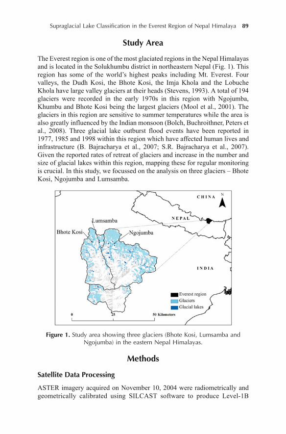
Supraglacial Lake Classification in the Everest Region of Nepal Himalaya 89
Study Area
The Everest region is one of the most glaciated regions in the Nepal Himalayasand is located in the Solukhumbu district in northeastern Nepal (Fig. 1). Thisregion has some of the world’s highest peaks including Mt. Everest. Fourvalleys, the Dudh Kosi, the Bhote Kosi, the Imja Khola and the LobucheKhola have large valley glaciers at their heads (Stevens, 1993). A total of 194glaciers were recorded in the early 1970s in this region with Ngojumba,Khumbu and Bhote Kosi being the largest glaciers (Mool et al., 2001). Theglaciers in this region are sensitive to summer temperatures while the area isalso greatly influenced by the Indian monsoon (Bolch, Buchroithner, Peters etal., 2008). Three glacial lake outburst flood events have been reported in1977, 1985 and 1998 within this region which have affected human lives andinfrastructure (B. Bajracharya et al., 2007; S.R. Bajracharya et al., 2007).Given the reported rates of retreat of glaciers and increase in the number andsize of glacial lakes within this region, mapping these for regular monitoringis crucial. In this study, we focussed on the analysis on three glaciers – BhoteKosi, Ngojumba and Lumsamba.
Figure 1. Study area showing three glaciers (Bhote Kosi, Lumsamba andNgojumba) in the eastern Nepal Himalayas.
Methods
Satellite Data Processing
ASTER imagery acquired on November 10, 2004 were radiometrically andgeometrically calibrated using SILCAST software to produce Level-1B
90 Prajjwal K. Panday et al.
products (http://www.silc.co.jp). An orthorectified DEM of 15 m spatialresolution was also generated using 3N (nadir-viewing) and 3B (backward-viewing) spectral bands of the ASTER Level-1A VNIR data. The SWIRbands with 30 m spatial resolution were then resampled to 15 m to match thefiner spatial resolution of ASTER Level-1B VNIR and DEM datasets. Glacierboundary outlines of Bhote Kosi, Ngojumba and Lumsamba glaciers wereobtained from Global Land Measurements from Space (GLIMS—www.glims.org) (Armstrong et al., 2005) and used to clip the respective glaciersfrom the ASTER imagery to limit the area of analysis for supraglacialcharacterization.
Image Derivatives
The ASTER-derived DEM was used to generate first derivatives, slope andaspect. The ASTER, VNIR and SWIR bands were used to compute imageband ratios and image indices which have been used in glacier classification(Table 1). The Normalized Difference Snow Index (NDSI) utilizes the spectralproperties of snow and ice which has a high reflectance in the visible regionand a strong absorption in the SWIR region (Hall et al., 1995). Further, NDSIfrequency distribution exhibits a bimodal distribution for a glacier with lowerNDSI associated with debris and higher NDSI peak associated with snow, iceand ice-mixed debris (Keshri et al., 2009). A Normalized Difference WaterIndex (NDWI) was also derived using a green band, which exhibits maximumreflectance of water and near-infrared band which exhibits minimum reflectanceof water (Bolch, Buchroithner, Peters et al., 2008; Huggel et al., 2002;McFeeters, 1996). A similar index to indicate the presence of water surfacebased on a spectral characteristic of water corresponding to stronger absorptionin SWIR bands than in VNIR bands was proposed by Suzuki et al. (2007) ascalculated from band 2 and band 4 of ASTER imagery. The NormalizedDifference Glacier Index (NDGI), as proposed by Keshri et al. (2009), usesdifference in spectral characteristics of snow/ice and ice-mixed debris in greenand red bands.
Classification Methodology
The classification tree analysis is non-parametric and structurally explicitallowing interpretations of decision rules that relate thresholds in the predictorvariables with pixel classes during partitioning of remote sensing data (Friedlet al., 1999; Lawrence and Wright, 2001). As other machine learning algorithms,CTA is sensitive to quality of training data and the number of training samplesper category classified (Rogan et al., 2008; Rogan et al., 2003). Given thelimited ground reference data for this region, training pixels for snow, ice, ice-mixed debris, debris, and others that included shadow were selected fromwithin the ASTER scene. Training pixels were assessed for their spectralcharacteristic using ERDAS Imagine and reference supraglacial cover classes

Supraglacial Lake Classification in the Everest Region of Nepal Himalaya 91
were assigned on the basis of spectral curve analysis and visual interpretation(Fig. 2). Independent variables to the classification tree were ASTER bands1-9, band ratios, indices and environmental ancillary data (elevation, slopeand aspect) (see Table 1 and Fig. 3).
CTA partitions the remotely sensed data recursively and hierarchically toform homogeneous subsets where the splitting algorithm searches for thevariable that best explains the partitioning. The selection of splitting rules inCTA is not a critical factor for overall accuracy of decision-tree-basedclassification (Zambon et al., 2006). CTA was performed in IDRISI softwareusing gain ratio splitting rule and the trees were pruned by removing leaveswith observations less than or equal to a predetermined within class proportionof 1%. Entropy, which provides a measure of how much we know about a
Table 1. Input image files used for classification tree analysis
No. Variables Description
1 Green2 Red3 Near Infrared (NIR)4 Shortwave Infrared 1 (SWIR1) Also Middle Infrared (MIR)5 SWIR26 SWIR37 SWIR48 SWIR59 SWIR6
10 NIR/Red11 MIR/Red12 MIR/Green13 MIR/NIR14 Normalized Difference
Vegetsation Index (NDVI) (NIR – Red/NIR + Red)15 Normalized Difference (Green – Red/Green + Red)
Glacier Index (NDGI) (Keshri et al., 2009)16 Normalized Difference (Green – SWIR1/Green + SWIR1)
Snow Index (NDSI) (Hall et al., 1995; Keshri et al., 2009)
17 Normalized Difference (Green – NIR/Green + NIR)Water Index (NDWI) (Bolch, Buchroithner, Peters et al.,
2008; McFeeters, 1996)18 NDWI2 (Red – MIR/Red + MIR)
(Suzuki et al., 2007)19 Elevation (m)20 Aspect (degrees)21 Slope (degrees)
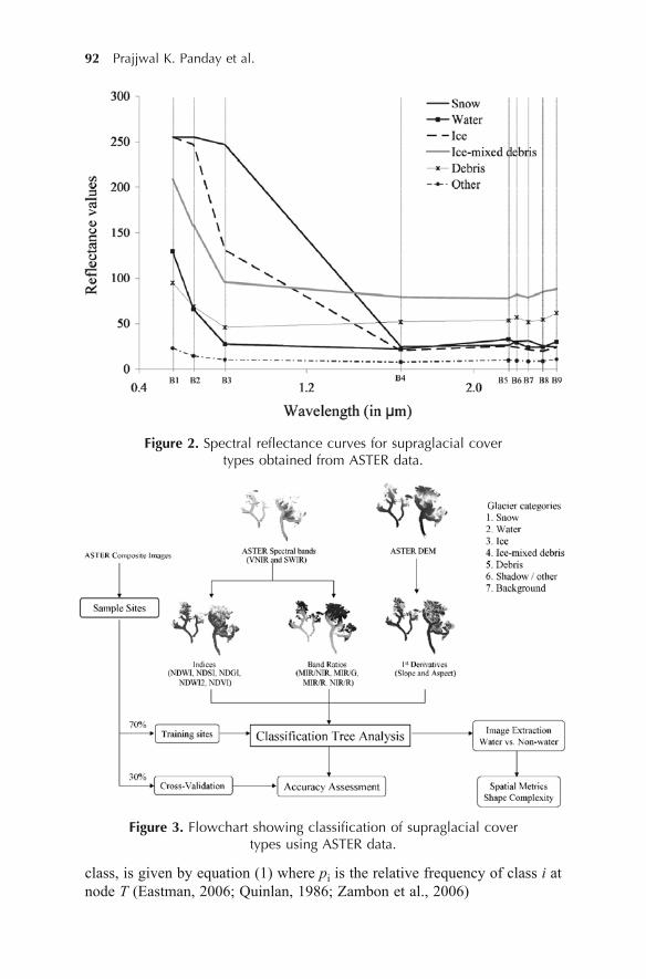
92 Prajjwal K. Panday et al.
Figure 2. Spectral reflectance curves for supraglacial covertypes obtained from ASTER data.
Figure 3. Flowchart showing classification of supraglacial covertypes using ASTER data.
class, is given by equation (1) where pi is the relative frequency of class i atnode T (Eastman, 2006; Quinlan, 1986; Zambon et al., 2006)
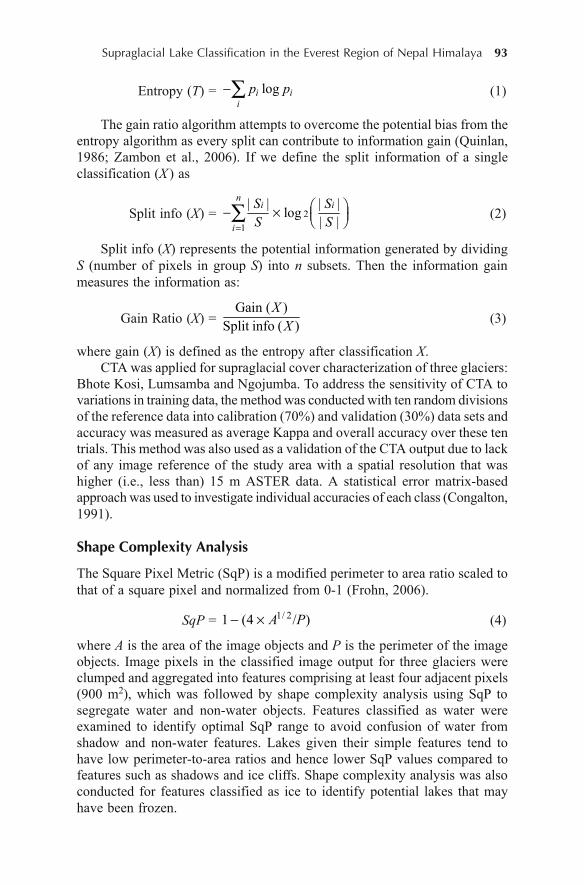
Supraglacial Lake Classification in the Everest Region of Nepal Himalaya 93
Entropy (T) = logi ii
p p�Ç (1)
The gain ratio algorithm attempts to overcome the potential bias from theentropy algorithm as every split can contribute to information gain (Quinlan,1986; Zambon et al., 2006). If we define the split information of a singleclassification (X ) as
Split info (X) = 21
| | | |log| |
ni i
i
S SS S
È Ø� � É ÙÊ ÚÇ (2)
Split info (X) represents the potential information generated by dividingS (number of pixels in group S) into n subsets. Then the information gainmeasures the information as:
Gain Ratio (X) =Gain ( )
Split info ( )X
X
(3)
where gain (X) is defined as the entropy after classification X.CTA was applied for supraglacial cover characterization of three glaciers:
Bhote Kosi, Lumsamba and Ngojumba. To address the sensitivity of CTA tovariations in training data, the method was conducted with ten random divisionsof the reference data into calibration (70%) and validation (30%) data sets andaccuracy was measured as average Kappa and overall accuracy over these tentrials. This method was also used as a validation of the CTA output due to lackof any image reference of the study area with a spatial resolution that washigher (i.e., less than) 15 m ASTER data. A statistical error matrix-basedapproach was used to investigate individual accuracies of each class (Congalton,1991).
Shape Complexity Analysis
The Square Pixel Metric (SqP) is a modified perimeter to area ratio scaled tothat of a square pixel and normalized from 0-1 (Frohn, 2006).
SqP = 1/ 21 (4 / )A P� � (4)
where A is the area of the image objects and P is the perimeter of the imageobjects. Image pixels in the classified image output for three glaciers wereclumped and aggregated into features comprising at least four adjacent pixels(900 m2), which was followed by shape complexity analysis using SqP tosegregate water and non-water objects. Features classified as water wereexamined to identify optimal SqP range to avoid confusion of water fromshadow and non-water features. Lakes given their simple features tend tohave low perimeter-to-area ratios and hence lower SqP values compared tofeatures such as shadows and ice cliffs. Shape complexity analysis was alsoconducted for features classified as ice to identify potential lakes that mayhave been frozen.
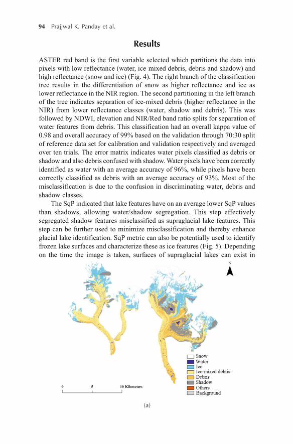
94 Prajjwal K. Panday et al.
Results
ASTER red band is the first variable selected which partitions the data intopixels with low reflectance (water, ice-mixed debris, debris and shadow) andhigh reflectance (snow and ice) (Fig. 4). The right branch of the classificationtree results in the differentiation of snow as higher reflectance and ice aslower reflectance in the NIR region. The second partitioning in the left branchof the tree indicates separation of ice-mixed debris (higher reflectance in theNIR) from lower reflectance classes (water, shadow and debris). This wasfollowed by NDWI, elevation and NIR/Red band ratio splits for separation ofwater features from debris. This classification had an overall kappa value of0.98 and overall accuracy of 99% based on the validation through 70:30 splitof reference data set for calibration and validation respectively and averagedover ten trials. The error matrix indicates water pixels classified as debris orshadow and also debris confused with shadow. Water pixels have been correctlyidentified as water with an average accuracy of 96%, while pixels have beencorrectly classified as debris with an average accuracy of 93%. Most of themisclassification is due to the confusion in discriminating water, debris andshadow classes.
The SqP indicated that lake features have on an average lower SqP valuesthan shadows, allowing water/shadow segregation. This step effectivelysegregated shadow features misclassified as supraglacial lake features. Thisstep can be further used to minimize misclassification and thereby enhanceglacial lake identification. SqP metric can also be potentially used to identifyfrozen lake surfaces and characterize these as ice features (Fig. 5). Dependingon the time the image is taken, surfaces of supraglacial lakes can exist in
(a)
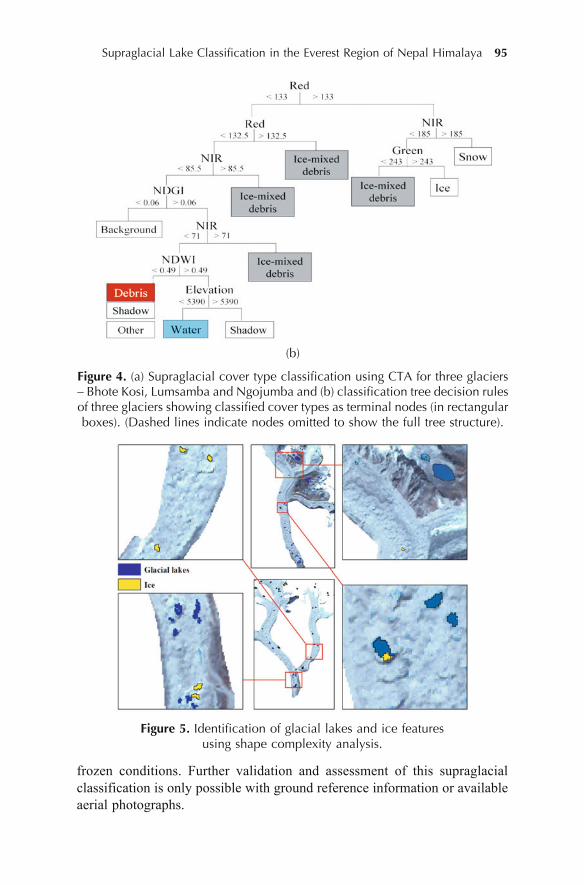
Supraglacial Lake Classification in the Everest Region of Nepal Himalaya 95
(b)
Figure 4. (a) Supraglacial cover type classification using CTA for three glaciers– Bhote Kosi, Lumsamba and Ngojumba and (b) classification tree decision rulesof three glaciers showing classified cover types as terminal nodes (in rectangularboxes). (Dashed lines indicate nodes omitted to show the full tree structure).
Figure 5. Identification of glacial lakes and ice featuresusing shape complexity analysis.
frozen conditions. Further validation and assessment of this supraglacialclassification is only possible with ground reference information or availableaerial photographs.
96 Prajjwal K. Panday et al.
Discussion and Conclusion
The objective of this chapter is to utilize a hybrid approach of classificationtree analysis with shape complexity metric thresholds to map supraglacialconditions in the Everest region in the eastern Nepal Himalayas. Distal partsof the debris-covered glaciers which are spectrally very similar to thesurrounding environment are difficult to separate. Much of the supraglacialdebris along the glacier tongues can be spectrally separated and delineatedgiven the cooling effect from the underlying ice. Bolch et al. (2008a) hasshown this to be true in the same region using a morphometric and temperaturebased glacier mapping method.
CTA is able to utilize ancillary variables such as image based ratios andindices effectively to facilitate classification of glaciers and snow from thesurrounding environment. This method is also effective in segregating waterfrom ice and other supraglacial features. A major advantage of classificationtree is the ability of the users to investigate the linkage between the dependentvariable of class membership and remote sensing data (Rogan et al., 2008).The hierarchical partitioning indicates the dominance of ASTER bands (green,red and near-infrared) in supraglacial characterization and the importance ofNDWI in delineating supraglacial water bodies. Furthermore, classificationtree analysis is less subjective compared to visual or statistical derivation ofthreshold values for glacier or supraglacial lake delineation. Rather thanselecting particular indices or thresholds for classification, CTA allows theability to include as many predictor variables to choose the one that bestexplains the partitioning of the data and hence allows data-derived thresholding.
The results of this study show that supraglacial lake delineation in theEverest region of the eastern Nepal Himalayas using ASTER data is promising.The study has shown that CTA is able to utilize ancillary variables such asimage based ratios and indices effectively to facilitate classification of glaciersand snow from the surrounding environment. On the other hand, the shapecomplexity metric such as SqP was effective in reducing misclassification ofglacial lakes. This chapter provides a less subjective methodology of classifyingsupraglacial cover types and lakes utilizing data-derived thresholds andpartitioning to assign class membership. Shadows and debris-covered icepresented a majority of the classification problems in distinguishing glaciersfrom surrounding environment towards distal parts of the glacier tongues.Glaciers and glacial lakes are delineated using a variety of techniques asdescribed in this chapter. While advanced techniques for better identificationis certainly important, it is also essential to maintain consistency in techniquesused across an image time series for conducting change analysis. The accuracyin identification of glacial retreat lies in the accuracy of glaciers/glacial lakedelineation as well as use of a standardized procedure to do so. This jointapproach of glacier delineation using classification tree and shape metricanalysis certainly provides a first-order exploration for glacier assessment.

Supraglacial Lake Classification in the Everest Region of Nepal Himalaya 97
The applicability of proposed method needs to be tested in other glaciatedareas around the world in order to extend the work for examining hazardpotential of glacier lakes.
References
Armstrong, R., Raup, B., Khalsa, S.J.S., Barry, R., Kargel, J., Helm, C. and Kieffer,H. (2005). GLIMS glacier database. from National Snow and Ice Data CenterBoulder, Colorado USA.
Bajracharya, B., Shrestha, A.B. and Rajbhandari, L. (2007). Glacial lake outburstfloods in the Sagarmatha region. Mountain Research Development, 27(4), 336–344.
Bajracharya, S.R., Mool, P.K. and Shrestha, B.R. (2007). Impact of climate change onHimalayan glaciers and glacial lakes. Kathmandu, Nepal: ICIMOD.
Bolch, T., Buchroithner, M.F., Kunert, A. and Kamp, U. (2008). Automated delineationof debris-covered glaciers based on ASTER data. Paper presented at theGeoInformation in Europe (=Proc. 27th EARSeL-Symposium, 4.-7.6.07, Bozen,Italy), Netherlands.
Bolch, T., Buchroithner, M.F., Peters, J., Baessler, M. and Bajracharya, S. (2008).Identification of glacier motion and potentially dangerous glacial lakes in the Mt.Everest region/Nepal using space-borne imagery. Natural Hazards and EarthSystems Science, 8, 1329–1340.
Bolch, T., Buchroithner, M.F., Pieczonka, T. and Kunert, A. (2008). Planimetric andVolumetric Glacier Changes in the Khumbu Himalaya since 1962 Using Corona,Landsat TM and ASTER Data. Journal of Glaciology, 54(187), 592–600.
Bulley, H.N.N., Marx, D.B., Merchant, J.W., Holz, J.C. and Holz, A.A. (2008). Acomparison of Nebraska reservoir classes estimated from watershed-basedclassification models and ecoregions. Journal of Environmental Informatics, 11(2),90-102.
Bulley, H.N.N., Bishop, M.P., Shroder Jr., J.F. and Haritashya, U.K. (2011). Integrationof classification tree analysis and spatial metrics to assess changes in supraglaciallakes in the Karakoram Himalaya. International Journal of Remote Sensing(accepted).
Congalton, R.G. (1991). A review of assessing the accuracy of classifications ofremotely sensed data. Remote Sensing of Environment, 37, 35–37.
Dyurgerov, M.B. and Meier, M.F. (2000). Twentieth century climate change : Evidencefrom small glaciers. Proceedings of the National Academy of Sciences, 97(4),1406–1411.
Eastman, J.R. (2006). IDRISI Andes Guide to GIS and Image Processing. Worcester,MA: Clark Labs.
Friedl, M., Brodley, C.E. and Strahler, A.H. (1999). Maximizing land-coverclassification accuracies produced by decision trees at continental to global scales.IEEE Transactions of Geoscience and Remote Sensing, 37(2), 969–977.
Frohn, R.C. (2006). The use of landscape pattern metrics in remote sensing imageclassification. International Journal of Remote Sensing, 27(10), 2025–2032.
98 Prajjwal K. Panday et al.
Frohn, R.C. and Hao, Y. (2006). Landscape metric performance in analyzing twodecades of deforestation in the Amazon Basin of Rondonia, Brazil. Remote Sensingof Environment, 100, 237–251.
Fujita, K., Thompson, L.G., Ageta, Y., Yasunari, T., Kajikawa, Y., Sakai, A. andTakeuchi, N. (2006). Thirty-year history of glacier melting in the Nepal Himalayas.Journal of Geophysical Research, 111(DO3109), 1–6.
Haeberli, W., Hoelzle, M., Paul, F. and Zemp, M. (2007). Integrated monitoring ofmountain glaciers as key indicators of global climate change: the European Alps.Annals of Glaciology, 46, 150–160.
Hall, D.K., Riggs, A. and Salomonson, V.V. (1995). Development of methods formapping global snow cover using moderate resolution imaging spectroradiometerdata. Remote Sensing of Environment, 54, 127–140.
Hansen, M., Dubayah, R. and Defries, R. (1996). Classification trees: an alternative totraditional land cover classifiers. International Journal of Remote Sensing, 17(5),1075–1081.
Huggel, C., Kääb, A., Haeberli, W., Teysseire, P. and Paul, F. (2002). Remote sensingbased assessment of hazards from glacier lake outbursts: a case study in the SwissAlps. Canadian Geotechnical Journal, 39, 316–330.
Kargel, J.S., Abrams, M.J., Bishop, M.P., Bush, A., Hamilton, G., Jiskoot, H., Kaab,A., Kieffer, H., Leet, E.M., Paul, F., Raup, B., Shroeder, J.F., Soltesz, D., Stainforth,D., Stearns, L. and Wessels, R. (2005). Multispectral imaging contributions toglobal land ice measurements from space. Remote Sensing of Environment, 99,187–219.
Kehrwald, N.M., Thompson, L.G., Tangdong, Y., Mosley-Thompson, E., Schotterer,U., Alfimov, V., Beer, J., Eikenberg, J. and Davis, M.E. (2008). Mass loss onHimalayan glacier endangers water resources. Geophysical Research Letters,35(L22503), 1–6.
Keshri, A.K., Shukla, A. and Gupta, R.P. (2009). ASTER ratio indices for supraglacialterrain mapping. International Journal of Remote Sensing, 30(2), 519–524.
Kulkarni, A.V., Bahuguna, I.M., Rathore, B.P., Singh, S.K., Randhawa, S.S., Sood,R.K. and Dhar, S. (2007). Glacial retreat in Himalaya using Indian Remote Sensingsatellite data. Current Science, 92(1), 69–74.
Kulkarni, A.V. and Buch, A.M. (1991). Glacier atlas of the Indian Himalaya.Lawrence, R.L. and Wright, A. (2001). Rule-based classification systems using
classification and regression tree (CART) analysis. Photogrammetric Engineeringand Remote Sensing, 67(10), 1137–1142.
McFeeters, S.K. (1996). The use of the Normalized Difference Water Index (NDWI)in the delineation of open water features International Journal of Remote Sensing,17(7), 1425–1432.
Milner, A.M., Brown, L.E. and Hannah, D.M. (2009). Hydroecological response ofriver systems to shrinking glaciers. Hydrological Processes, 23, 62–77.
Mool, P.K., Bajracharya, S.R. and Joshi, S.P. (2001). Inventory of glaciers, glaciallakes and glacial lake outburst floods: Monitoring and Early Warning Systems inthe Hindu Kush-Himalayan Region Nepal. Kathmandu, Nepal: International Centrefor Integrated Mountain Development.
Oerlemans, J. (2005). Extracting a climate signal from 169 glacier records. Science,308(29), 675–677.
Paul, F., Huggel, C. and Kaab, A. (2004). Combining satellite multispectral imagedata and a digital elevation model for mapping debris-covered glaciers. RemoteSensing of Environment, 89, 510–518.
Supraglacial Lake Classification in the Everest Region of Nepal Himalaya 99
Paul, F., Kaab, A., Maisch, M., Kellenberger, T. and Haeberli, W. (2004). Rapiddisintegration of Alpine glaciers observed with satellite data. Geophysical ResearchLetters, 31(21402), 1–4.
Quincey, D.J., Lucas, R.M., Richardson, S.D., Glasser, N.F., Hambrey, M.J. andReynolds, J.M. (2005). Optical remote sensing techniques in high-mountainenvironments: applications to glacial hazards. Progress in Physical Geography,29(4), 475–505.
Quinlan, J.R. (1986). Induction of decision trees. Machine learning, 1, 81–106.Racoviteanu, A.E., Williams, M.W. and Barry, R.G. (2008). Optical remote sensing of
glacier characteristics: A review with focus on the Himalaya. Sensors, 8, 3355–3383.
Raup, B., Kaab, A., Kargel, J.S., Bishop, M.P., Hamilton, G., Lee, E., Paul, F., Rau, F.,Soltesz, D., Khalsa, S.J.S., Beedle, M. and Helm, C. (2007). Remote sensing andGIS technology in the Global Land Ice Measurements from Space (GLIMS) Project.Computers and Geosciences, 33, 104–125.
Richardson, S.D. and Reynolds, J.M. (2000). An overview of glacial hazards in theHimalayas. Quaternary International, 65-66, 31–47.
Rogan, J. and Chen, D.M. (2004). Remote sensing technology for mapping andmonitoring land-cover and land-use change. Progress in Planning, 61(4), 301–325.
Rogan, J., Franklin, J., Stow, D., Miller, J., Roberts, D.A. and Woodcock, C. (2008).Mapping land cover modifications over large areas: A comparison of machinelearning techniques. Remote Sensing of Environment, 112, 2272–2283.
Rogan, J., Miller, J., Stow, D., Franklin, J., Levien, J. and Fischer, C. (2003). Land-cover change monitoring with classification trees using Landsat TM and ancillarydata. Photogrammetric Engineering and Remote Sensing, 69, 793–804.
Stevens, S.F. (1993). Claiming the high ground: Sherpas, subsistence, and environmentalchange in the highest Himalaya. Berkeley and Los Angeles: University of CaliforniaPress.
Suzuki, R., Fujita, K. and Ageta, Y. (2007). Spatial distribution of thermal propertieson debris-covered glaciers in the Himalayas derived from ASTER data. Bulletin ofGlaciological Research, 24, 13–22.
Thakur, J.K. (2010). Eco-hydrological wetland monitoring in a semi-arid region (Acase study of Konya Closed Basin, Turkey). Faculty of International Institute forGeo-Information Science and Earth Observation (ITC), Universiteit Twente,Enschede, the Netherlands.
Yamada, T., Shiraiwa, T., Iida, H., Kadota, T., Watanabe, T., Rana, B., Ageta, Y. andFushimi, H. (1992). Fluctuations of the glaciers from the 1970s to 1989 in theKhumbu, Shorong, and Langtang regions, Nepal Himalayas. Bulletin of GlacierResearch, 10, 11–19.
Zambon, M., Lawrence, R., Bunn, A. and Powell, S. (2006). Effect of alternativesplitting rules on image processing using classification tree analysis.Photogrammetric Engineering and Remote Sensing, 72(1), 25–30.
Zhou, Y., Narumalani, S. and Jelinski, D.E. (1995). Improving remote sensing derivedland use/land cover classification with the aid of spatial information. Paper presentedat the ACSM/ASPRS Annual Convention and Exposition Technical Papers,Bethesda, MD.
100 Nafaâ Jabeur and James D. McCarthy
7Towards the Improvement of Water
Resource Management byCombining Technologies for
Spatial Data Collection, Storage,Analysis and Dissemination
Nafaâ Jabeur and James D. McCarthy1
Computer Science Department, Dhofar University, Oman1Mapping, Analysis and Design, Faculty of Environment
University of Waterloo, Canada
Introduction
Water resource managers regularly deal with situations where timely, relevantinformation can be of significant benefit. One only needs to look at the extensiveflooding in Australia in 2010 and 2011, and the associated loss of property andlife, to discover why the desire for hydrologic monitoring tools is so great.When water resource managers deal with floods, they want to be able tomonitor and predict water levels and direct emergency response efforts.However, flooding is not the only situation where water resources need to bemonitored and analyzed (Thakur et al., 2011). To ensure appropriate waterquality and supply for a region, these parameters must be regularly monitored,and appropriate entities must be alerted when certain warning thresholds areapproached or broken. To study and preserve biodiversity, resource managersneed access to long-term data about the environmental conditions in theirstudy area, including any hydrologic factors that may have an impact on it.Several established and emerging technologies are currently providing expertswith great benefit in managing environmental resources. In the hydrologicaldomain, the use of Sensor Webs (SWs) in data collection provides decisionmakers with ever-growing amounts of relevant data and allows them to alwaysbe aware of conditions in their study area (Guru et al., 2008). These data canbe supplemented with data collected using emerging mobile GIS technology
DOI 10.1007/978-94-007-1858-6_7, © Capital Publishing Company 2012
100e ,J.K. Thakur et al. (eds.), G ospatial Techniques for Managing Environmental Resources

Improvement of Water Resource Management by Combining Technologies 101
and applications. Currently, a multitude of mobile platforms integrating GPStechnology can support data entry through generic or dedicated applications.
Once the data are collected from the field, spatial database technologyand sensor network representation standards can be used to effectively makethese data available to experts for analysis. To this end, information can beretrieved from the spatial databases in a format that is not only machine-readable, but also laden with information relevant to the water resource domain(McCarthy, Graniero and Rozic, 2008). Analysis methods that use these datacould be supported by several tools and techniques, such as rule-based reasoning(Rozic, 2006). Web GIS and mapping technologies can make analysis results,as well as the data which spawned them, available for use by others regardlessof their skills. The use of multiagent systems (Jabeur, Graniero, McCarthyand Xing, 2009) provides an interesting solution towards autonomous andintelligent use of spatial data.
The relevant technologies for spatial data collection, storage, analysis anddissemination are all rapidly growing in both numbers and functionality.However it remains to be seen what form the convergence of these technologieswill take. In addition to being developed to address only one or two of thesefour key areas of geomatics, most of these technologies are developed bydifferent software and hardware vendors. This results in datasets that areincompatible with analysis tools, or multiple format conversions that introducethe potential for accuracy and precision problems. For reasons such as these,there is a need for tools and techniques to handle the interchange of databetween these applications and data formats in a standardized manner thatinterferes as little as possible with the analysis the user wishes to perform.
This chapter will examine many of the relevant technologies involved inSW design, deployment and usage, and it will explore how these technologiesmay be integrated into a complete framework for sensor network management.It will also highlight some applications that have been developed specificallyfor water resources management and how they would fit into the proposedframework.
Spatial Data Collection Technologies
Sensor Webs
Overview of Sensor Webs
A Sensor Web (SW) is a network consisting of large numbers of sensingplatforms allowing the spatio-temporal understanding of the environment whereit is deployed. This network could be compared to a sophisticated sensingtapestry draped over the environment (Delin and Small, 2009) and has thebasic functionality to access data remotely. Extended and complexfunctionalities could generally be achieved through coordinated efforts betweenthe deployed sensors. SWs are characterized by their multidisciplinary nature
102 Nafaâ Jabeur and James D. McCarthy
that requires knowledge from a variety of fields such as microelectronics,mechanics, physics and computer science, and some domain knowledge ofthe environments being sensed. They typically face several challenges relatedto limited power, depletion failures, restricted resources, unstable topology,unpredictable conditions and unbounded information flow delays. Thesechallenges are more serious when the SWs are operating unattended in hostileenvironments. Several initiatives have been proposed to cope with the problemsfacing the deployment of SWs. These initiatives span hardware (e.g. Hempstead,Tripathi, Muro, Wei and Brooks, 2005), network protocols (e.g.Intanagonwiwat, Govindan and Estrin, 2000; Jabeur and Graniero, 2007),applications (e.g. Levis et al., 2005; McCarthy et al., 2008), and operatingsystems (e.g. Levis et al., 2005).
Recent advances in miniaturization and wireless communications havebrought a new generation of SWs comprising large numbers of cooperatingsmall-scale sensor nodes. This cooperation allows the sensor nodes to gobeyond their individual capabilities and carry out complex operations. Duringtheir interaction, the nodes have to share their collected observations andsupport each other in processing and routing data while taking into accounttheir individual characteristics. To this end, they have to adapt their behavioursindividually, which consequently leads to a global self-organizing behaviourallowing the SW to evolve towards a better configuration that adapts to suitthe current situation (Jabeur, McCarthy and Graniero, 2008).
Thanks to their spatially distributed configurations, SWs are able to collectimportant spatio-temporal data for a variety of applications. These data becomehighly valuable when sensors are fielded in harsh environments, such asdeserts, mountains and Antarctica. In addition to environmental sciencepurposes (e.g., Heavner, Fatland, Hood and Connor, 2007), SWs have provedvaluable in urban search, rescue and tracking (e.g., Howe et al., 2008),infrastructure protection (e.g., Delin and Small, 2009), hazard management(e.g., Jabeur and Haddad, 2009), and wild fire monitoring (e.g., Sahli, Jabeurand Badra, 2011). The technology is also used for controlling the environmentby actuating devices (Collins, 2004). As future directions, SWs could be usedto track in-field personnel during operations, protect infrastructure,decontaminate air and buildings, monitor rails and highways, and controlventilation (Delin and Small, 2009). In this chapter, we particularly focus onwater resource management where SWs are being used for several purposes,such as flood monitoring, water contamination detection and agriculturaldevelopment.
SW for Water Resource Management
Several research works and applications have used SWs for water resourcemanagement and its related issues, such as irrigation, water contamination,water surface movement, water infiltration and flood control. In this context,the COMMONSense Net project (Jacques, Seshagiri, Prabhakar, Jean-Pierre
Improvement of Water Resource Management by Combining Technologies 103
and Jamadagni, 2007) is an initiative that focussed on the design andimplementation of a SW for agricultural management in developing countries.This project had emphasized semi-arid regions in a cluster of villages inSouthern Karnataka (India). When water is polluted, for example, by industrialwaste, fertilization or pesticides, SWs could be efficiently used to detect anycontamination and thus prevent casualties. This is the case in Ganges delta(Bangladesh/India) where SW-based technology is being used for detectingthe Arsenic pollutant in water (Zennaro, Pehrson and Bagula, 2008). Markovic,Stanimirovic and Stoimenov (2009) have developed a SW-based system calledthe River Water Monitoring and Alert System (RWMAS) that enables operatorsin crisis management centres to discover and prevent water pollution.
SWs can also facilitate the detection and monitoring of water surfacemovement and water infiltration in real time. This would particularly help incharacterizing hydrologic phenomena (e.g. surface water movement, soilmoisture and storm induced floods) and monitoring floods in real time. Towork towards the elimination of the problems caused by floods, the CAVSARP(Central Avra Valley Storage and Recovery Project) (Delin and Jackson, 2003)has been proposed by the NASA Jet Propulsion Laboratory for hydrologystudies located to the west of Tucson, Arizona, USA. In this location, a numberof artificial recharge basins are used in a desert environment to monitor varioushydrologic processes and geomorphologic features, such as wave cut terraces,polygonal patterns in soil, and ridges related to the drying of the basin floormaterials. The deployed SW monitors the front movement of a potential floodand water infiltration into ground. The data are transferred to the Internet froma portal sensor pod connected to a computer. Thanks to the SW, the spatial andtemporal patterns of wetting and drying of the basins that have been identifiedprovide a hydrological model for the analysis of floods.
At a higher abstraction level, some SW-based frameworks and systemshave been proposed and applied to water resource management. In this context,Xitao (2008) has proposed and designed an architectural framework to developadvanced integrated environmental monitoring systems (A-ITEMS), whichfeeds the requirements of complex environmental monitoring systems. In thiswork, an Integrated Watershed Telemetry (IWT) system has been implemented.Graniero, Weiler, Nickerson and Jabeur (2007) have presented the SWAN(Sensor Web Automation Network) project that aims at developing SW designand deployment tools that blend varied sensor and communication hardware,both mobile and stationary, into one watershed monitoring system. In a relatedwork (Jabeur et al., 2009), we have proposed a meta-framework to guide thedevelopment of a cyberinfrastructure that can lead the way for emergingsensor infrastructures to interoperate. Without being restricted to water resourcemanagement, our meta-framework is guided by the DAST principle thatsummarizes the overall goal of any sensor infrastructure: acquire the rightData from the right Area using the right Sensors at the right Time.
104 Nafaâ Jabeur and James D. McCarthy
In order to implement the DAST principle, we have proposed a SensorObservation Service server agent that uses semantic, logical and physicalconnections between sensors in order to better adapt to network changes andprovide adjustable services suitable for monitoring water resource conditions(Jabeur et al., 2009). In another work (Jabeur and Haddad, 2009), we haveproposed to encode causality relationships about natural phenomena and theireffects in time and space in order to allow the system to set up prioritiesbetween the sensor network activities and thus implement a progressiveapproach for the management of hazardous events, such as floods.
GPS and Manual Data Collection
While the evolution of the Sensor Web as a macro-instrument is rapid, therewill always be gaps (both physical and conceptual) that require the interventionof a domain expert in the data collection process. Some areas may be tooremote or too difficult to reach to make a sensor network cost-effective.Perhaps conditions are expected to change in a study area in a way that thesensor network won’t be able to capture in time, or wasn’t designed to capture.Whatever the reason, supplementing sensor network data with manualmeasurements from the field can provide a more complete picture of conditionsin a study area.
Collection can be handled with dedicated data collection applicationssuch as Esri’s ArcPad or Trimble’s TerraSync. These software tools run onhardware specifically designed for data collection in the field using GPSreceivers. The advantage of using these tools is that, depending on the hardware,they can accurately record a user’s position in the field within a few centimetres.Since hydrologic issues are often local in scale, this repeatability and accuracyof measurement becomes very important to users looking to supplement datacollected by a sensor network. These tools are also customizable so that adeveloper can create an application to work on the device which streamlinesthe data collection process so that domain experts such as hydrologists, ratherthan GIS/GPS experts, can spend their time in the field collecting data. Thisis important as they will be more qualified to judge what is important whileout in the field.
This is not to say, however, that specialized devices are the only way tocollect data from the field. The increasing number of applications developedfor mobile devices are providing experts with valuable support in collectingdata, anywhere, anytime.
From a hydrologic perspective, data collection from mobile devices couldbe handled in a number of ways. Expert users can enter the field equippedwith specialized equipment for precisely measuring various parameters oftheir watershed or other study area which can then be supplied to applicationseither wirelessly or when the user returns from the field. Depending on theneeds of the application there are other ways of handling data collection. Theidea of crowd-sourcing data (encouraging the public to participate in the

Improvement of Water Resource Management by Combining Technologies 105
collection process) has merit for certain applications as well. For example,COMAP systems (McGarry, 2008) have been successfully used in diverseareas such as heritage resource tracking, invasive species tracking and moraineanalysis. In all cases, the systems are deployed with an eye towards publicparticipation in the data collection and verification process.
Remote Sensing and Satellite Imagery
In situations where sensor webs simply aren’t feasible, or where they haven’tbeen installed, there are still ways of gathering relevant information about asite from a distance. Satellite imagery can provide data that can act as a proxyfor in situ measurements. Nakamura et al. (2005) described a process bywhich sea ice thickness can be measured with Synthetic Aperture Radar data.Image processing can be automated to provide information gathered by remotesensing satellites in a quantitative form to supplement sensor data. Visiblesatellite imagery can show the state of a study area with great accuracy. If theimages are of a high enough resolution, relative measurements can be made ifimages are captured with any regularity and their scale is known. LIDAR datacan provide extremely fine-grained measurement of physical parameters.Though not typically collected regularly like other satellite imagery, LIDARsensors can be targeted and flown at a specific site to provide detailedinformation about that site. Detailed bathymetric (Irish and White, 1998),water level (Stockdon, Sallenger, List and Holman, 2002), and water quality(Barbini, Colao, Fantoni, Palucci and Ribezzo, 1995) data have all beengathered via the use of LIDAR.
Spatial Data Storage Technologies
This section of the chapter will illustrate how varied the representation formatsfor spatial data have become. It begins with an examination of the mostcommon spatial databases and then describes some of the standards beingused for SW representation. A discussion of ontologies follows. This conceptis referenced again later in the chapter. Finally, some strategies for dealingwith the multitude of data formats in existence are suggested.
Spatial Databases
Enterprise-level databases drive many applications on and off the web. Mostof the major players in the enterprise database market have created spatially-enabled database products in recent years to keep up with the demand for geo-location and other location-based services that have exploded on the web.These spatial databases typically take one of two forms: Extensions to existingdatabase products that enable spatial information to be stored within an existingdatabase product, and database products specifically designed for holdingspatial data.
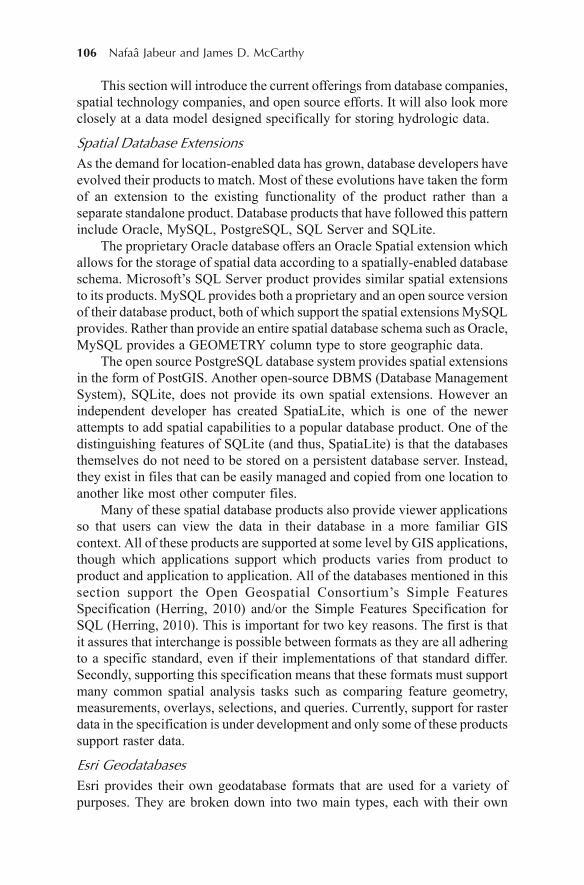
106 Nafaâ Jabeur and James D. McCarthy
This section will introduce the current offerings from database companies,spatial technology companies, and open source efforts. It will also look moreclosely at a data model designed specifically for storing hydrologic data.
Spatial Database Extensions
As the demand for location-enabled data has grown, database developers haveevolved their products to match. Most of these evolutions have taken the formof an extension to the existing functionality of the product rather than aseparate standalone product. Database products that have followed this patterninclude Oracle, MySQL, PostgreSQL, SQL Server and SQLite.
The proprietary Oracle database offers an Oracle Spatial extension whichallows for the storage of spatial data according to a spatially-enabled databaseschema. Microsoft’s SQL Server product provides similar spatial extensionsto its products. MySQL provides both a proprietary and an open source versionof their database product, both of which support the spatial extensions MySQLprovides. Rather than provide an entire spatial database schema such as Oracle,MySQL provides a GEOMETRY column type to store geographic data.
The open source PostgreSQL database system provides spatial extensionsin the form of PostGIS. Another open-source DBMS (Database ManagementSystem), SQLite, does not provide its own spatial extensions. However anindependent developer has created SpatiaLite, which is one of the newerattempts to add spatial capabilities to a popular database product. One of thedistinguishing features of SQLite (and thus, SpatiaLite) is that the databasesthemselves do not need to be stored on a persistent database server. Instead,they exist in files that can be easily managed and copied from one location toanother like most other computer files.
Many of these spatial database products also provide viewer applicationsso that users can view the data in their database in a more familiar GIScontext. All of these products are supported at some level by GIS applications,though which applications support which products varies from product toproduct and application to application. All of the databases mentioned in thissection support the Open Geospatial Consortium’s Simple FeaturesSpecification (Herring, 2010) and/or the Simple Features Specification forSQL (Herring, 2010). This is important for two key reasons. The first is thatit assures that interchange is possible between formats as they are all adheringto a specific standard, even if their implementations of that standard differ.Secondly, supporting this specification means that these formats must supportmany common spatial analysis tasks such as comparing feature geometry,measurements, overlays, selections, and queries. Currently, support for rasterdata in the specification is under development and only some of these productssupport raster data.
Esri Geodatabases
Esri provides their own geodatabase formats that are used for a variety ofpurposes. They are broken down into two main types, each with their own
Improvement of Water Resource Management by Combining Technologies 107
subtypes. The two main types are Single-user and Multiuser geodatabases.Single-user geodatabases can be either File or Personal geodatabases, andMultiuser geodatabases can be Enterprise, Workgroup, and Desktopgeodatabases. The choice of database type is typically made based on thetype(s) of users and products that will consume it. A small number of userswith only one editor can use a File Geodatabase, whereas a database that isbeing edited by multiple people and accessed via multiple web applicationswould be more suited to one of the multi-user variations. Feature geometriesare stored internally in the database and so are not as easily accessed as someof the other spatial database types mentioned here. However, the specificationhas been made available so that non-Esri applications can access featuresstored in Esri geodatabase formats.
ArcHydro
ArcHydro is a data model designed specifically for water resources,implemented in an Esri geodatabase. ArcHydro is one of the most completesystems available for managing and analyzing hydrologically-themed spatialdata. Because of the explicitness and level of detail in the model, sophisticatedanalysis tools can be built to take advantage of the information stored in thedata model (more on this later in the chapter).
ArcHydro models water resources from the watershed level down to thestream level while also maintaining a network of the features involved in thewatershed. Hydrologic features are modeled in four groups: Hydrographyfeatures (dams, waterbodies, monitoring points, etc.), Network features (edgesand junctions of hydrologic features), Drainage features (catchments,watersheds, basins, etc.), and Channel features (cross-sections and profiles).The geodatabase also provides support for time series data and built-in layertypes such as terrain and streams. The level of detail provided by ArcHydromakes for a relatively complex geodatabase with many tables, feature classesand relationships. However it is this level of detail that makes the ArcHydrotools extremely useful.
GML
The Geography Markup Language (GML) is an XML-based OGC specificationintended for representing geographic features, geometries, spatial referencesystems, and other spatial primitives. GML provides the basis for representingfeatures in many of the Sensor Web Enablement specifications the OGCmaintains.
SensorML and O&M
Encodings and representations of sensor descriptions and sensor measurementshave been created to facilitate the discovery and interpretation of data providedby sensor networks. The OGC’s Sensor Web Enablement working group has
108 Nafaâ Jabeur and James D. McCarthy
created an entire suite of standards related to sensor networks. The two thatwill be focussed on in this chapter are SensorML and O&M. SensorML is anXML schema that describes sensors and sensor platforms and their parameters.These parameters can include hardware-specific information such asmeasurement accuracy and calibration information, as well as site- andapplication-specific information like sampling rates. While much of thisinformation can be read from manuals or site descriptions, encoding it directlyinto an XML document makes it feasible for software to have access to thisinformation when needed.
O&M (Observations and Measurements) is an XML schema whichcomplements SensorML. It describes measurements made by sensors and canprovide insight into the significance of a measurement. When combined withSensorML and other representations, applications and expert users can have acomplete view of the state of a sensor network in the field.
SOS
A Sensor Observation Service (SOS) makes use of SensorML and O&M toprovide an interactive, useful view of current and historical conditions at asite. More specifically, it stores, manages and organizes sensor data as well assensor descriptions. If made public, these data can be queried and discoveredby other users, which aids in collaboration. The service can respond to queriesfrom an application or an expert user and provide current or historical datathat are relevant to the user’s needs.
Ontologies
This chapter has shown that sensor measurements are most useful when theyhave context that gives them meaning. This meaning can be encoded in theform of an ontology. Ontologies can be made machine-readable through theuse of various ontology representation formats. This section will examine twoof those representation formats: OWL and CLIPS. In order to compare thesetwo formats, however, a basic understanding of ontologies is necessary and isprovided here.
Ontologies are a means of explicitly describing a particular area of interest.The term ‘area of interest’ is used in a broad context here and could refer toan application domain or more general concepts. An ontology is generallycomposed of the facts, objects, rules and relationships that make up anapplication domain. It can look similar to an object model or a databasemodel, and this is something that can be leveraged when trying to integrateontologies into applications. The ArcHydro data model provides an excellent,detailed basis on which an ontology could be formed. The additionalinformation provided by an ontology can be used by an application to betterinterpret or apply meaning from simple data. For example knowing that acertain stream is flowing at 2000 m3/sec can be useful, but knowing precisely
Improvement of Water Resource Management by Combining Technologies 109
where on the stream the measurement was taken, by what type of instrument,what that instrument’s typical accuracy is, and what other instruments arenearby, can provide an expert user with far more information in a moreupfront fashion. This enables the user to make more informed decisions.
OWL (Web Ontology Language) and CLIPS are two ontologyrepresentation approaches that have proven to have particular utility inenhancing the information that can be gained from a hydrologic sensor network.OWL is a W3C endorsed, XML-based specification for representing ontologicalinformation. It is one of the most commonly used ontology specificationformats. OWL is reasonably human-readable while being machine-readable.In OWL, concepts are broken down into Instances, Classes, Properties andOperators. These concepts could be further subcategorized in the OWLspecification when necessary. CLIPS is not by its nature an ontology definitionlanguage, but rather a rule-based programming language. In this language,concepts of a domain can be represented as facts and rules, and as in mostrule-based programming languages, these facts and rules are what governthe execution of the program, not a sequence of pre-programmed steps.This allows a language such as CLIPS to react dynamically to changingconditions, and to have a current snapshot of the conditions of the program atany time.
Strategies for Negotiating between Data Formats
With the plethora of data formats available to use, the decision about whatformat to use is often not under the user’s control. When the user wishes touse data from one application in another application, ideally the data is alreadyin a format supported by both applications. Practically, however, this is oftennot the case. Therefore a conversion is needed to make the data usable in thenew application. Two approaches to conversion are discussed here.
FME
FME is a commercial product created by Safe Software which has the primarygoal of allowing users to convert their data from one spatial format to another.While the list of spatial data formats that is supported is quite exhaustive,FME also provides tools to process the data as well. These tools allow the userto automate data manipulation and processing within the FME environment inorder to streamline data processing tasks.
GDAL/OGR
GDAL (Geospatial Data Abstraction Library) and the OGR Simple FeaturesLibrary are part of the GDAL library which is a C++ library used primarily toconvert data between different geospatial formats. GDAL provides manycommand line tools to achieve these conversions, and because it is an opensource library its functionality is built into many free and open source GISdesktop packages.
110 Nafaâ Jabeur and James D. McCarthy
Spatial Data Analysis Technologies
Rule-based Systems
Rule-based systems such as CLIPS are based on a defined set of facts andrules which make up a body of knowledge. Rather than executing sequentiallylike a more common procedural analysis, a rule-based analysis reacts tochanging conditions. When the facts of a situation change, the rules of thesystem are re-evaluated and new outcomes are decided. In situations such aswater resource management where conditions are changing rapidly andunpredictably, a rule-based system is able to be more responsive and is morelikely to be capable of handling an unforeseen situation. McCarthy et al.(2008) describe how a rule-based analysis system integrated into ArcGIS isable to track the movement of sensors embedded in a hillslide. Rules aredefined that classify what the risk characteristics are for slope failure and atevery time step the facts of the situation are evaluated against these rules. Thefacts in the system in this case are the measurements being made by two typesof sensors: inclinometers to measure the movement of the slope material, andpiezometers to track the water level. The system also understands the makeupof slope material and how susceptible the different materials are to sliding.These facts are evaluated against the rule base which includes rules aboutacceptable movement for that particular slope and the interaction between thewater table and the elastic portion of the slope. According to these rules, a risklevel is determined based on a decision tree and the map is symbolizedaccordingly. If a high risk level is indicated, an alert could be sounded. Thedescribed system was designed to be portable to other domains (Rozic andGraniero, 2005), and so could be applied to the monitoring of a watershed.
ArcHydro and HEC
Earlier in the chapter was a discussion on the ArcHydro data model and howit represents hydrologic features. This representation scheme enables powerfulanalysis tools within the ArcGIS environment. In addition to tools that helpusers bring their existing hydrologic data into the ArcHydro environment,ArcHydro provides tools for examining terrain, watersheds, stream networks,flow rates, time series analysis, watershed delineation, and several othercommon water resource based tasks.
An alternative to the ArcHydro environment for hydrologic analysis is thesuite of tools provided by the U.S. Army Corps of Engineers HydrologicEngineering Center (HEC). Many of the tools are provided for a specificpurpose, such as river analysis, hydrologic modelling and ecosystem study.The tool that is most relevant to this chapter is the Corps Water ManagementSystem (CWMS). It attempts to provide a suite of water resource managementand spatial-decisions support tools, and integrates both incoming sensor dataand modelled or simulated data to supplement analysis.
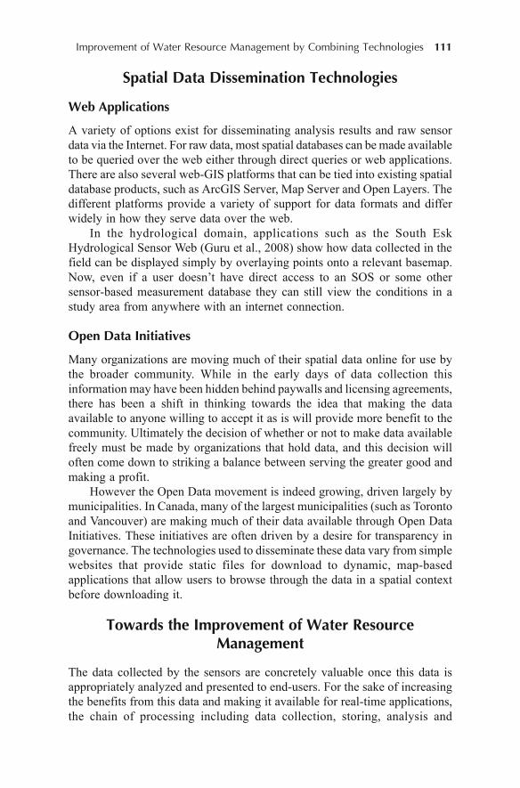
Improvement of Water Resource Management by Combining Technologies 111
Spatial Data Dissemination Technologies
Web Applications
A variety of options exist for disseminating analysis results and raw sensordata via the Internet. For raw data, most spatial databases can be made availableto be queried over the web either through direct queries or web applications.There are also several web-GIS platforms that can be tied into existing spatialdatabase products, such as ArcGIS Server, Map Server and Open Layers. Thedifferent platforms provide a variety of support for data formats and differwidely in how they serve data over the web.
In the hydrological domain, applications such as the South EskHydrological Sensor Web (Guru et al., 2008) show how data collected in thefield can be displayed simply by overlaying points onto a relevant basemap.Now, even if a user doesn’t have direct access to an SOS or some othersensor-based measurement database they can still view the conditions in astudy area from anywhere with an internet connection.
Open Data Initiatives
Many organizations are moving much of their spatial data online for use bythe broader community. While in the early days of data collection thisinformation may have been hidden behind paywalls and licensing agreements,there has been a shift in thinking towards the idea that making the dataavailable to anyone willing to accept it as is will provide more benefit to thecommunity. Ultimately the decision of whether or not to make data availablefreely must be made by organizations that hold data, and this decision willoften come down to striking a balance between serving the greater good andmaking a profit.
However the Open Data movement is indeed growing, driven largely bymunicipalities. In Canada, many of the largest municipalities (such as Torontoand Vancouver) are making much of their data available through Open DataInitiatives. These initiatives are often driven by a desire for transparency ingovernance. The technologies used to disseminate these data vary from simplewebsites that provide static files for download to dynamic, map-basedapplications that allow users to browse through the data in a spatial contextbefore downloading it.
Towards the Improvement of Water ResourceManagement
The data collected by the sensors are concretely valuable once this data isappropriately analyzed and presented to end-users. For the sake of increasingthe benefits from this data and making it available for real-time applications,the chain of processing including data collection, storing, analysis and
112 Nafaâ Jabeur and James D. McCarthy
dissemination must be coordinated in order to allow a smooth data flowbetween the different processing steps. To achieve this goal, a variety oftechnological tools could be necessary and the intervention of experts wouldbe inevitable. Thus, our idea is not limited to combining a package oftechnologies. It is rather an attempt to make automatic the entire processstarting from the field until the data are accessible to the end user.
Combining Data Collection, Storage, Analysis and Dissemination
In Fig. 1, we present a high-level framework that aims at combining datacollection, storage, analysis and dissemination within one single system forsensor network management. This framework could be used for spatio-temporalapplications, including water resource management. We guide our framework
Figure 1. High-level framework combining data collection, storage,analysis and dissemination.
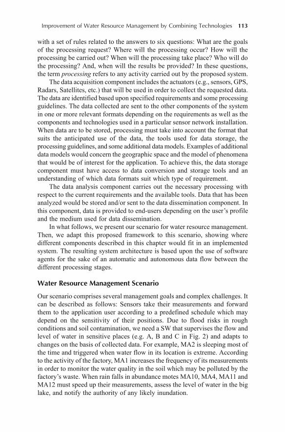
Improvement of Water Resource Management by Combining Technologies 113
with a set of rules related to the answers to six questions: What are the goalsof the processing request? Where will the processing occur? How will theprocessing be carried out? When will the processing take place? Who will dothe processing? And, when will the results be provided? In these questions,the term processing refers to any activity carried out by the proposed system.
The data acquisition component includes the actuators (e.g., sensors, GPS,Radars, Satellites, etc.) that will be used in order to collect the requested data.The data are identified based upon specified requirements and some processingguidelines. The data collected are sent to the other components of the systemin one or more relevant formats depending on the requirements as well as thecomponents and technologies used in a particular sensor network installation.When data are to be stored, processing must take into account the format thatsuits the anticipated use of the data, the tools used for data storage, theprocessing guidelines, and some additional data models. Examples of additionaldata models would concern the geographic space and the model of phenomenathat would be of interest for the application. To achieve this, the data storagecomponent must have access to data conversion and storage tools and anunderstanding of which data formats suit which type of requirement.
The data analysis component carries out the necessary processing withrespect to the current requirements and the available tools. Data that has beenanalyzed would be stored and/or sent to the data dissemination component. Inthis component, data is provided to end-users depending on the user’s profileand the medium used for data dissemination.
In what follows, we present our scenario for water resource management.Then, we adapt this proposed framework to this scenario, showing wheredifferent components described in this chapter would fit in an implementedsystem. The resulting system architecture is based upon the use of softwareagents for the sake of an automatic and autonomous data flow between thedifferent processing stages.
Water Resource Management Scenario
Our scenario comprises several management goals and complex challenges. Itcan be described as follows: Sensors take their measurements and forwardthem to the application user according to a predefined schedule which maydepend on the sensitivity of their positions. Due to flood risks in roughconditions and soil contamination, we need a SW that supervises the flow andlevel of water in sensitive places (e.g. A, B and C in Fig. 2) and adapts tochanges on the basis of collected data. For example, MA2 is sleeping most ofthe time and triggered when water flow in its location is extreme. Accordingto the activity of the factory, MA1 increases the frequency of its measurementsin order to monitor the water quality in the soil which may be polluted by thefactory’s waste. When rain falls in abundance motes MA10, MA4, MA11 andMA12 must speed up their measurements, assess the level of water in the biglake, and notify the authority of any likely inundation.
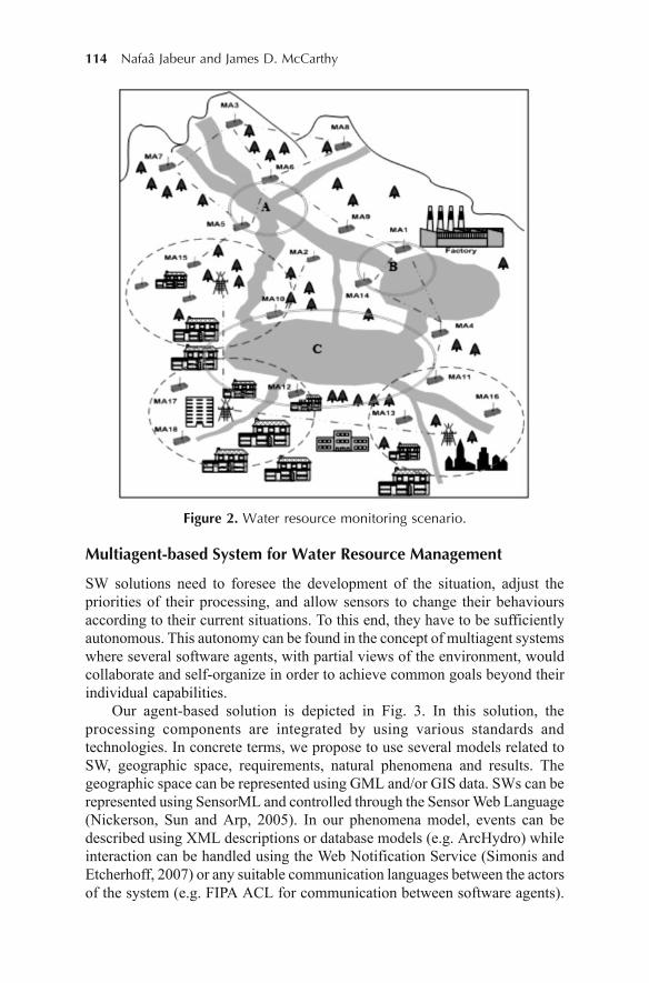
114 Nafaâ Jabeur and James D. McCarthy
Figure 2. Water resource monitoring scenario.
Multiagent-based System for Water Resource Management
SW solutions need to foresee the development of the situation, adjust thepriorities of their processing, and allow sensors to change their behavioursaccording to their current situations. To this end, they have to be sufficientlyautonomous. This autonomy can be found in the concept of multiagent systemswhere several software agents, with partial views of the environment, wouldcollaborate and self-organize in order to achieve common goals beyond theirindividual capabilities.
Our agent-based solution is depicted in Fig. 3. In this solution, theprocessing components are integrated by using various standards andtechnologies. In concrete terms, we propose to use several models related toSW, geographic space, requirements, natural phenomena and results. Thegeographic space can be represented using GML and/or GIS data. SWs can berepresented using SensorML and controlled through the Sensor Web Language(Nickerson, Sun and Arp, 2005). In our phenomena model, events can bedescribed using XML descriptions or database models (e.g. ArcHydro) whileinteraction can be handled using the Web Notification Service (Simonis andEtcherhoff, 2007) or any suitable communication languages between the actorsof the system (e.g. FIPA ACL for communication between software agents).
Improvement of Water Resource Management by Combining Technologies 115
Measurements and results can be described using Observations andMeasurements (O&M). Requirements may be handled through the SensorPlanning Service (Simonis, 2005). For the sake of integration, databases usingthe ArcHydro model provide GIS data organized in a way that enables domain-specific tools to be used for analysis of hydrologic phenomena. Many of theOGC representations can be easily integrated as well. A system such as FMEor ENGINE (McCarthy et al., 2008) can be used to mediate the conversionbetween different data formats.
In order to integrate the different components of our system, we proposeto wrap them with software agents. In this case, a Data Model Agent (DMA)maintains update information about the geographic space, the SW, the naturalphenomena and the results. A Data Acquisition Agent (DAA) is responsible
Figure 3. Our agent-based solution for water resource management.
116 Nafaâ Jabeur and James D. McCarthy
for the monitoring of the data acquisition component. It receives therequirements of the user and returns the measurements to the other componentsdepending on the need. A Data Storing Agent (DSA) controls the storing ofdata in the right format. A Data Analysis Agent (DAA) is responsible for theanalysis of data. A Data Dissemination Agent (DDA) is responsible fordisseminating the requested data to the right user using the right medium. Oursoftware can be built using any existing multiagent-system platform, such asJade, Jack, Beegent and AgentBuilder. They may coordinate their processingby exchanging FIPA ACL messages.
Future Research and Conclusions
Moving forward policy makers will continue to demand tools that providethem with meaningful information as opposed to raw data with little semanticvalue. Ideally these tools and their associated data will be made available tothe public so they can contribute to, and remain informed about, themanagement of the hydrologic resources that impact their daily lives. Muchof the development in the water resource management sector will revolvearound the integration of the technologies mentioned throughout this chapter,as well as technologies that have yet to emerge. This integration will also needto become more seamless to both the domain expert and the end-user. Havinga guiding framework to facilitate this integration will be very important toavoid fragmentation in the market that will result in systems that are harderfor domain experts such as hydrologists to use. Data models, analysis methodsand sensor hardware will always need to be designed to match the requirementsof the specific application domain they are being deployed in, but the tools fordissemination and management should develop in a way that is domain-agnostic whenever possible to reduce duplication of effort.
This chapter focussed on and explored some existing technologies relatedto four main aspects of geomatics: collecting, storing, analyzing anddisseminating data. It thoroughly studied the interoperability between thesetechnologies and proposed a high-level framework allowing for theirapproachable and collaborative use. It also serves as a guideline for theintegration of components provided by a variety of vendors and organizationswith different goals. It may also be used by those developing new tools as ameans of guiding their development in a way that promotes integration ofcomponents. This framework could be applied to a variety of applicationdomains, and was illustrated with examples that would be used in an agent-based hydrologic monitoring and analysis system. In addition to making thismanagement seamless to researchers and end-users, agents provide our solutionwith flexibility, autonomy and intelligence that would be very helpful inintegrating new components relevant to data collection, storing, analysis ordissemination.
Improvement of Water Resource Management by Combining Technologies 117
References
Barbini, R., Colao, F., Fantoni, R., Palucci, A. and Ribezzo, S. (1995). Remote sea-water quality monitoring by means of a lidar fluorosensor. Global ProcessMonitoring and Remote Sensing of the Ocean and Sea Ice. Volume 2586. pp 46–55.
Colllins, J. (2004). NASA creates thinking RF sensors. RFID Journal, RetrievedJanuary 20, 2011 from http://www.rfidjournal.com/article/articleview/1146/1/47/
Delin, K. and Small, E. (2009). The Sensor Web: Advanced Technology for SituationalAwareness. Wiley Handbook of Science and Technology for Homeland Security.John Wiley and Sons.
Delin, K.A. and Jackson, S.P. (2003). The Sensor Web: A New Instrument Concept.SPIE Symposium on Integrated Optics, San Jose, CA.
Graniero, P.A., Weiler, M., Nickerson, B.G., Arp, P.A. and Jabeur, N. (2007). Anintegrated sensor web design and deployment infrastructure for watershedmonitoring. Retrieved February 5, 2011 from http://matrix.memf.uwindsor.ca/publications/posters/SWAN-GranieroEtAl-SWANOverview-GEOIDE2007.pdf
Guru, S.M., Taylor, P., Neuhaus, H., Shu, Y., Smith, D. and Terhorst, A. (2008).Hydrological Sensor Web for the South Esk Catchment in the Tasmanian state ofAustralia. In: IEEE 4th International Conference on eScience, 7(12), 432–433.
Heavner, M.J., Fatland, D.R., Hood, E. and Connor, C. (2007). SEAMONSTER: ASensor Web Technology Implementation and Testbed in Southeast Alaska. Paperpresented at NASA Science and Technology Conference, College Park, MD.
Hempstead, M., Tripathi, N., Mauro, P., Wei, G-Y. and Brooks, D. (2005). An ultralow power system architecture for sensor network applications. Proceedings ofSIGARCH Computational Architecture, 33, 208–219.
Herring, J.R. (2010). OpenGIS Implementation Standard for Geographic information– Simple feature access – Part 1: Common architecture. Open GeospatialConsortium. 93 pp. Retreived February 15, 2011 from http://www.opengeospatial.org/standards/sfa
Howe, B.M., Parrish, N., Tracy, L., Gray, A., Chao, Y., McGinnis, T., Arabshahi, P.and Roy, S. (2008). A Smart Sensor Web for Ocean Observation: IntegratedAcoustics, Satellite Networking, and Predictive Modeling. In: Proceedings of NASAScience Technology Conference (NSTC2008), University of Maryland.
Intanagonwiwat, C., Govindan, R. and Estrin, D. (2000). Directed diffusion: a scalableand robust communication paradigm for sensor networks. In: Proceedings ofInternational conference on Mobile Computing and Networking.
Irish, J.L. and White, T.E. (1998). Coastal engineering applications of high-resolutionlidar bathymetry. Proceedings of Coastal Engineering, 35(1), 47–71.
Jabeur N. and Haddad, H. (2009). Using Causality Relationships for a ProgressiveManagement of Hazardous Phenomena with Sensor Networks. In: Proceedings ofthe International Conference on Computational Science and Applications(ICCSA’09), Yongin, Korea, pp. 1–16
Jabeur, N. and Graniero, P. (2007). A Hybrid Location-Semantic Approach to RoutingAssisted by Agents in a Virtual Network. In: Frontiers of High PerformanceComputing and Networking. ISPA 2007 Workshops, pp. 523–533.
Jabeur, N., Graniero, P., McCarthy, J. and Xing, X. (2009). A Knowledge-OrientedMeta-Framework for Integrating Sensor Network Infrastructures. InternationalJournal of Computers and Geosciences, 35, 1–14.
118 Nafaâ Jabeur and James D. McCarthy
Jabeur, N., McCarthy, J.D. and Graniero, P. (2008). Improving Wireless Sensor NetworkEfficiency and Adaptability through an SOS Server Agent. In: Proceeding of the 1st
IEEE International Workshop on the Applications of Digital Information and WebTechnologies (ICADIWT 2008), Ostrava, Czech Republic, pp. 409–414.
Jacques, P., Seshagiri, R., Prabhakar, T.V., Jean-Pierre, H. and Jamadagni, H.S. (2007).COMMONSense Net: A Wireless Sensor Network for Resource-Poor Agriculturein the Semiarid Areas of Developing Countries. Journal of Information Technologiesand International Development, 4(1), 51–67.
Levis, Ph., Gay, D., Handziski, V., Hauer, J.H., Greenstein, B., Turon, M., Huio, J.,Klues, K., Sharp, C., Szewczyk, R., Polastre, J., Buonadonnao, Ph., Nachman, L.,Tolleo, G., Cullero, D. and Wolisz, A. (2005). T2: A Second Generation OS forEmbedded Sensor Networks. Technical Reports Series, (Ed.) Dr.-Ing. Adam Wolisz.
Markovic, N., Stanimirovic, A. and Stoimenov, L. (2009). Sensor Web for RiverWater Pollution Monitoring and Alert System. In: Proceedings of 12th AGILEInternational Conference on Geographic Information Science Advances inGIScience, Germany. ISSN 2073–8013.
McCarthy, J.D., Graniero, P.A. and Rozic, S.M. (2008). An Integrated GIS-expertsystem framework for live hazard monitoring and detection. Sensors InternationalJournal, 8, 830–846.
McGarry, F. (2008). Collaborative Geomatics for Social Innovation in EnvironmentalPractice. Presented at the First Nations GIS Workshop. Retrieved February 10,2011 from http://www.comap.ca/index.php?MenuItemID=7
Nakamura, K., Wakabayashi, H., Naoki, K., Nishio, F., Moriyama, T. and Uratsuka,S. (2005). Observation of sea-ice thickness in the sea of Okhotsk by using dual-frequency and fully polarimetric airborne SAR (pi-SAR) data. IEEE Transactionsin Geoscience and Remote Sensing, 43 (11), 2460-2469.
Nickerson, B.G., Sun, Z. and Arp, J. (2005). A sensor web language for mesharchitectures. Proceedings of the 3rd Annual Communication Networks and ServicesResearch Conference (CNSR’05), Halifax, NS, Canada. IEEE Computer Society,pp. 269–274.
Rozic, S.M. and Graniero, P.A. (2005). Representing domain and spatial knowledgewith ontologies in a spatial decision support framework. In: Proceedings ofGeoComputation 2005, Ann Arbor, MI. 15 (CD-ROM).
Sahli, N., Jabeur, N. and Badra, M. 2011. Agent-Based Approach to Plan SensorsRelocation in a Virtual Geographic Environment. In: Proceeding of InternationalConference on New Technologies, Mobility and Security (NTMS’2011).
Stockdon, H.F., Sallenger, Jr., A.H., List, J.H. and Holman, R.A. (2002). Estimationof Shoreline Position and Change using Airborne Topographic Lidar Data. Journalof Coastal Research, 18(3), 502–513.
Thakur, J.K., Thakur, R.K., Ramanathan, A., Kumar, M. and Singh, S.K. (2011).Arsenic Contamination of Groundwater in Nepal – An Overview. Water, 3(1), 1–20.
Xing, X. (2008). An architectural framework for developing advanced integratedenvironmental monitoring systems. Unpublished MSc thesis, Department of Earthand Environmental Sciences, University of Windsor.
Zennaro, M., Pehrson, B. and Bagula, A. (2008). Wireless Sensor Networks: a greatopportunity for researchers in Developing Countries. In: Proceedings of 2nd IFIPInternational Symposium on Wireless Communications and Information Technologyin Developing Countries (South Africa).
Geomorphologic Risk Modelling of the Sibiu Depression 119
8Geomorphologic Risk Modelling
of the Sibiu Depression UsingGeospatial Surface Analyses
Marioara Costea, Roxana Giusca1 and Rodica Ciobanu2
“Lucian Blaga” University of Sibiu, Faculty of Sciences, Department ofEcology and Environment Protection, Sibiu, Romania
1American Sentinel University, Aurora, Colorado, USA2National Brukenthal Museum, Sibiu, Romania
Introduction
Extreme events in general, and the geomorphologic ones in particular, arehighly topical problems. There were addresses by many researchers in thefield of geology and physical geography (more specific by the climatologistsand geomorphologists), but also by biologists, chemists, ecologists, etc. Theseare studied through the analysis of some types of processes and productionmechanisms, and secondly by the effects they create on other environmentalsubsystems.
Triggering causes and mechanisms of geomorphologic processes areknown. Nevertheless they constitute a threat by their magnitude that occur insome areas and which have a negative impact on short and long term, as well.Among these are: changes in the landscape, land degradation and loss of soilfertility, sometimes irreversible, damage to transport infrastructure, economiclosses and even social effects, etc.
Although geomorphologic processes are natural phenomena, man is nostranger to them. He is an integral part in this chain of causes-mechanisms-effects, involving all the chain links. In the context of demographic explosion,industrialization and urban explosion, man has had an impact on theenvironment, and especially on the landscape through land use, resourcemanagement, industry, agriculture and habitat—putting unprecedented pressureon it. Changes of these components can be caused directly or indirectly byhuman activities resulting in transformations in modelling conditions and inthe action mechanisms of the external agents. Avoiding such situations and
DOI 10.1007/978-94-007-1858-6_8, © Capital Publishing Company 2012
119e ,J.K. Thakur et al. (eds.), G ospatial Techniques for Managing Environmental Resources
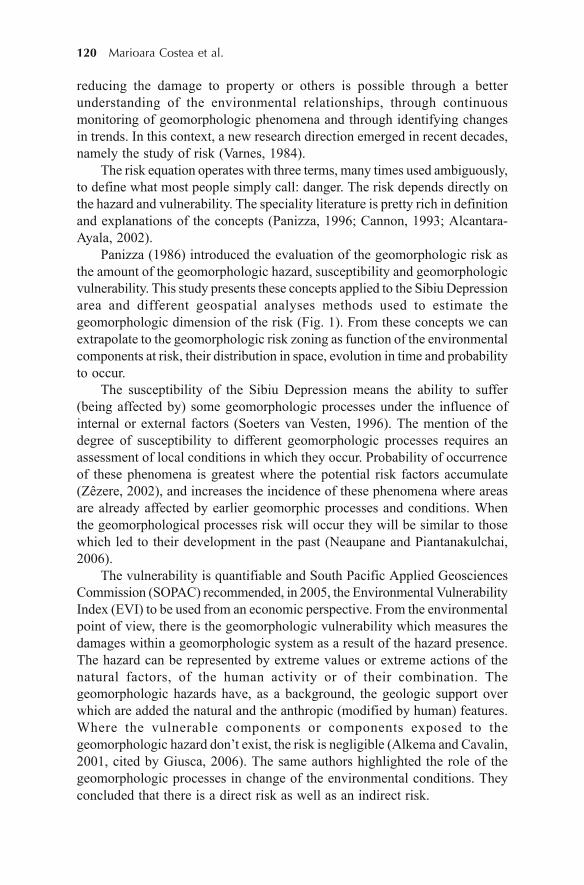
120 Marioara Costea et al.
reducing the damage to property or others is possible through a betterunderstanding of the environmental relationships, through continuousmonitoring of geomorphologic phenomena and through identifying changesin trends. In this context, a new research direction emerged in recent decades,namely the study of risk (Varnes, 1984).
The risk equation operates with three terms, many times used ambiguously,to define what most people simply call: danger. The risk depends directly onthe hazard and vulnerability. The speciality literature is pretty rich in definitionand explanations of the concepts (Panizza, 1996; Cannon, 1993; Alcantara-Ayala, 2002).
Panizza (1986) introduced the evaluation of the geomorphologic risk asthe amount of the geomorphologic hazard, susceptibility and geomorphologicvulnerability. This study presents these concepts applied to the Sibiu Depressionarea and different geospatial analyses methods used to estimate thegeomorphologic dimension of the risk (Fig. 1). From these concepts we canextrapolate to the geomorphologic risk zoning as function of the environmentalcomponents at risk, their distribution in space, evolution in time and probabilityto occur.
The susceptibility of the Sibiu Depression means the ability to suffer(being affected by) some geomorphologic processes under the influence ofinternal or external factors (Soeters van Vesten, 1996). The mention of thedegree of susceptibility to different geomorphologic processes requires anassessment of local conditions in which they occur. Probability of occurrenceof these phenomena is greatest where the potential risk factors accumulate(Zêzere, 2002), and increases the incidence of these phenomena where areasare already affected by earlier geomorphic processes and conditions. Whenthe geomorphological processes risk will occur they will be similar to thosewhich led to their development in the past (Neaupane and Piantanakulchai,2006).
The vulnerability is quantifiable and South Pacific Applied GeosciencesCommission (SOPAC) recommended, in 2005, the Environmental VulnerabilityIndex (EVI) to be used from an economic perspective. From the environmentalpoint of view, there is the geomorphologic vulnerability which measures thedamages within a geomorphologic system as a result of the hazard presence.The hazard can be represented by extreme values or extreme actions of thenatural factors, of the human activity or of their combination. Thegeomorphologic hazards have, as a background, the geologic support overwhich are added the natural and the anthropic (modified by human) features.Where the vulnerable components or components exposed to thegeomorphologic hazard don’t exist, the risk is negligible (Alkema and Cavalin,2001, cited by Giusca, 2006). The same authors highlighted the role of thegeomorphologic processes in change of the environmental conditions. Theyconcluded that there is a direct risk as well as an indirect risk.
Geomorphologic Risk Modelling of the Sibiu Depression 121
Figu
re 1
. Th
e in
tera
ctio
n re
latio
ns a
mon
g th
e ge
olog
ic s
ubst
ratu
m a
nd t
he g
eom
orph
olog
ic r
isk
phen
omen
on.
Source: C
ioba
nu R
(20
07).
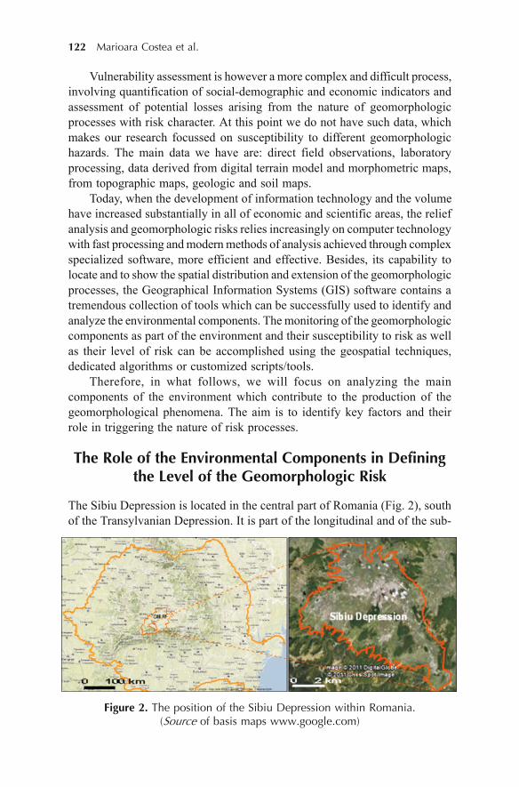
122 Marioara Costea et al.
Vulnerability assessment is however a more complex and difficult process,involving quantification of social-demographic and economic indicators andassessment of potential losses arising from the nature of geomorphologicprocesses with risk character. At this point we do not have such data, whichmakes our research focussed on susceptibility to different geomorphologichazards. The main data we have are: direct field observations, laboratoryprocessing, data derived from digital terrain model and morphometric maps,from topographic maps, geologic and soil maps.
Today, when the development of information technology and the volumehave increased substantially in all of economic and scientific areas, the reliefanalysis and geomorphologic risks relies increasingly on computer technologywith fast processing and modern methods of analysis achieved through complexspecialized software, more efficient and effective. Besides, its capability tolocate and to show the spatial distribution and extension of the geomorphologicprocesses, the Geographical Information Systems (GIS) software contains atremendous collection of tools which can be successfully used to identify andanalyze the environmental components. The monitoring of the geomorphologiccomponents as part of the environment and their susceptibility to risk as wellas their level of risk can be accomplished using the geospatial techniques,dedicated algorithms or customized scripts/tools.
Therefore, in what follows, we will focus on analyzing the maincomponents of the environment which contribute to the production of thegeomorphological phenomena. The aim is to identify key factors and theirrole in triggering the nature of risk processes.
The Role of the Environmental Components in Definingthe Level of the Geomorphologic Risk
The Sibiu Depression is located in the central part of Romania (Fig. 2), southof the Transylvanian Depression. It is part of the longitudinal and of the sub-
Figure 2. The position of the Sibiu Depression within Romania.(Source of basis maps www.google.com)
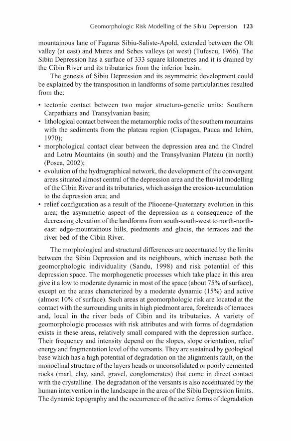
Geomorphologic Risk Modelling of the Sibiu Depression 123
mountainous lane of Fagaras Sibiu-Saliste-Apold, extended between the Oltvalley (at east) and Mures and Sebes valleys (at west) (Tufescu, 1966). TheSibiu Depression has a surface of 333 square kilometres and it is drained bythe Cibin River and its tributaries from the inferior basin.
The genesis of Sibiu Depression and its asymmetric development couldbe explained by the transposition in landforms of some particularities resultedfrom the:
• tectonic contact between two major structuro-genetic units: SouthernCarpathians and Transylvanian basin;
• lithological contact between the metamorphic rocks of the southern mountainswith the sediments from the plateau region (Ciupagea, Pauca and Ichim,1970);
• morphological contact clear between the depression area and the Cindreland Lotru Mountains (in south) and the Transylvanian Plateau (in north)(Posea, 2002);
• evolution of the hydrographical network, the development of the convergentareas situated almost central of the depression area and the fluvial modellingof the Cibin River and its tributaries, which assign the erosion-accumulationto the depression area; and
• relief configuration as a result of the Pliocene-Quaternary evolution in thisarea; the asymmetric aspect of the depression as a consequence of thedecreasing elevation of the landforms from south-south-west to north-north-east: edge-mountainous hills, piedmonts and glacis, the terraces and theriver bed of the Cibin River.
The morphological and structural differences are accentuated by the limitsbetween the Sibiu Depression and its neighbours, which increase both thegeomorphologic individuality (Sandu, 1998) and risk potential of thisdepression space. The morphogenetic processes which take place in this areagive it a low to moderate dynamic in most of the space (about 75% of surface),except on the areas characterized by a moderate dynamic (15%) and active(almost 10% of surface). Such areas at geomorphologic risk are located at thecontact with the surrounding units in high piedmont area, foreheads of terracesand, local in the river beds of Cibin and its tributaries. A variety ofgeomorphologic processes with risk attributes and with forms of degradationexists in these areas, relatively small compared with the depression surface.Their frequency and intensity depend on the slopes, slope orientation, reliefenergy and fragmentation level of the versants. They are sustained by geologicalbase which has a high potential of degradation on the alignments fault, on themonoclinal structure of the layers heads or unconsolidated or poorly cementedrocks (marl, clay, sand, gravel, conglomerates) that come in direct contactwith the crystalline. The degradation of the versants is also accentuated by thehuman intervention in the landscape in the area of the Sibiu Depression limits.The dynamic topography and the occurrence of the active forms of degradation

124 Marioara Costea et al.
are explained by the accumulation in this small space of propitious naturalfactors such as lithology, structure, climate and relief morphometry associatedwith land use (Fig. 3).
Figure 3. Landforms and risk factors in Sibiu Depression.
The inventory of the environmental components, focussed on recordingand analysis of the causes of the geomorphologic risk processes, revealsseveral key issues, namely:
• The accentuated oscillation of level and the convergence of the hydrographicnetwork to the bottom of the depression generate a sum and a transfer ofmatter and energy that is mirrored in the morphology of the relief, speciallyof the bounds.
• The lithology and structure, as passive factors condition the selective dynamicof the landforms, and implicitly of landscape, by different mechanical andchemical behaviour of rocks and deposits and by their spatial arrangement.The versants mobility is more pronounced in the contact zone of the studiedarea with the plateau area, where clay deposits (monoclinal structure) alternatewith sand deposits, and in the contact area: Cindrel mountains – SibiuDepression, where the sedimentary deposits cover the crystalline, whichhas the function of a bed slip (Ciobanu, 2007).
• Thermal stress is an active factor through: deviation (till +1.5 oC, or till–1.5 oC) from the multiannual average of temperature (8.7 oC), inversions(3-5 oC and >5 oC) and their duration (2-20 days) on the depression bottom,diurnal temperature variation and sunstroke on Cuesta Hartibaciu Plateau
Geomorphologic Risk Modelling of the Sibiu Depression 125
and low temperatures on the shadow slopes at the contact mountain-depression; heat waves, as well as the freezing prepare and favour theaction of the gravitational or of the run-off processes.
• Mechanical action of the precipitation is favoured by strong heatstroke ofthe southern slopes of south-western exhibition (Hartibaciu Cuesta, foreheadof the rivers terraces), structural steep of the plateau; kinetic energy ofrainfall is responsible for ravening and gullying associated to the raindropsimpact and rill erosion; this action is amplified by variability of rainfallwhich fall into depression (precipitation average is 650-700 mm/year), thealternating periods of wet (10-320 mm in excess respect multiannual average)and dry (deficit between 8 and 280 mm) and their torrential character inspring and autumn (the average yearly rainfall in the period from Septemberto November being 30-50 mm).
• The hydrological factors, as a consequence of climatic factors, support thegeomorphological risk in riverbeds by the oscillations of flows and levelsand their deviations from the normal values of flow (4.72 m3/s at Sibiu; 14.3m3/s at Talmaciu). Maximum flow is not a risk at Sibiu, because the CibinRiver is arranged as hydropower, but downstream to the confluence withHartibaci River, Cisnadia, and with Talmacel stream it does exists floodingrisk due to the confluences in series and due to the progressive contributionof the local tributaries from the plateau or depression.
• One explanation for the degradation of the versants in Sibiu Depression isthe deforestation of oak forests in ancient time and changes of the land use.The forest area in the early nineteenth century is still preserved today onlyabout 20%, dispersed in territory.
• The anthropogenic intervention in Sibiu Depression changed the conditionsand mechanisms for production of geomorphological processes, leading tovulnerability of the geomorphological system, determining the increasingof climatic and hydrological action. The actual morphodynamic is acceleratedby the land use of space by agricultural practices, by the mechanic stressgenerated by the traffic and heavy constructions on the terraces and glacisand by the clay mine pits on the structural steep of the plateau. However,they represent the nucleus of the intensive degradation of the terraces foreheadand versants by undermining and new plans of “attack” for the run-off,gullying, sliding and collapse processes. The impact of the exploits is alsodue to the drainage, uncover of the soil on the cuesta, and the lack of thefixing work of the deposits and the lack of the ecological rehabilitation.
The combination of the potential factors mentioned above, the alternationand the coincidence of the manifestation of these in time and space assign anactive, morpho-dynamic and high degradation potential for some sectors ofthe Sibiu Depression versants. The geomorphologic processes which lead tothe terrain degradation in these areas don’t act isolated, they act associated inmorphogenetic systems (Ielenicz, 2004). The conditions discussed aboveinteract with each other and cause potential instability of geomorphological
126 Marioara Costea et al.
system in Sibiu Depression. We must understand that cascaded relationship ofthese conditions (factors) can affect the geomorphologic system and they cantrigger geomorphological processes with risk character. Therefore, it isnecessary to raise awareness of the danger that could be generated by theseprocesses and a constant monitoring of the environmental conditions (of theactive factors, in particular) (Thakur et al., 2011) and a correct forecast ofweather-climatic and hydrological phenomena. The scratchy geologicalsubstrate, the high drainage of the landforms in the contact sector between thedepression and the neighbour units, the tilt and the differentiated exhibit of theversants determine the variation of the spatial distribution of the actualgeomorphologic processes and their grouping by representative zones. Thesetypes of grouping will be analysed in three case studies that have differentpositions within the Sibiu Depression. Delimitation and practical analysis ofthese areas are subject to the following case studies.
The Evaluation of the Morphological Parameters Usingthe Surface Analysis Techniques: Case Studies
Since, as we stated earlier, geomorphologic hazard occurs where repeatedevents occurred and where it is recorded a combination of morphologicalfactors, the analysis of the modelling conditions must be accompanied by ananalysis of morphometric parameters. Comparative analysis of geologicalmap, of the direct observations on the land use and of the spontaneousdistribution of the vegetation and the morphometric analysis of maps producedfor depression based on GIS methods and techniques, coupled with hydro-climatic conditions, have enabled us to identify areas susceptible to theproduction of the geomorphologic risk.
To analyse, quantify and estimate the contribution of the environmentalcomponents to the geomorphologic risk, we used the surface analyses tools.Using tabular and raster data, we have processed and obtained vectorial dataand other raster formats as output. Some of the surface analyses algorithmsused to generate the maps are: Slope, Aspect, Curvature, Hillshade etc. Thesemaps were generated for the case studies presented below and offered as thegreat opportunity to compare the results from one area to another area.
As techniques we also used the Overlay between different maps, such as:topographic map on top of the Digital Elevation Model, slope map combinedwith the hypsometric maps, stream flow map on top of the topographic mapor Digital Elevation Model etc. The overlay provided us the chance to correlatedifferent values of the components, such as elevation with slope, stream orderwith the slope, aspect etc.
Having the maps in the digital format represents a huge advantage in theprocess of estimating the geomorphologic risk because there can be run queries,calculate predictions, generate hot-spot maps etc. The quantification of theparameters of various components was critical and GIS algorithms and software

Geomorphologic Risk Modelling of the Sibiu Depression 127
were used to obtain the values of some index. Few of the indices we havecalculated were inserted below as parts of the case studies. These processesoccur in some areas where they act more intensive and most of the timecombined. The areas presented as case studies definitely prove these aspects.
Cibin River Confluence with Sadu River
One of the major confluence areas, it is represented by the Cibin River withone of its main tributaries, Sadu River.
In this sector, the asymmetry of the Cibin Valley is obvious. On the rightside the elevation of the relief decreases in stairs: the Sadu piedmont, Saduand Cibin terraces and the common meadow of both the rivers; on the left sidethe contact with the Hartibaciu cuesta is steep (at over 500 m altitude). Theoverlay of the Slope map, Aspect map, Stream Order map, Elevation Modeletc. was very helpful in the process of extraction of some values of interestand to realize the correlation between the analysed parameters (Fig. 4).
Thus, the Slope and Aspect map of this confluence area shows the highvalues of the slope on the south-east of the confluence. This is the result of thelithology of the versant. The same map contains a dejection cone created bythe Sadu River. While the most part of its stream is on the mountain area, after
Figure 4. Cibin confluence with Sadu – Slope and Aspect map.
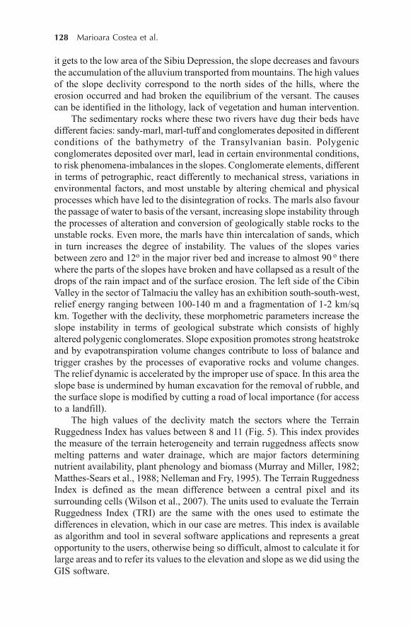
128 Marioara Costea et al.
it gets to the low area of the Sibiu Depression, the slope decreases and favoursthe accumulation of the alluvium transported from mountains. The high valuesof the slope declivity correspond to the north sides of the hills, where theerosion occurred and had broken the equilibrium of the versant. The causescan be identified in the lithology, lack of vegetation and human intervention.
The sedimentary rocks where these two rivers have dug their beds havedifferent facies: sandy-marl, marl-tuff and conglomerates deposited in differentconditions of the bathymetry of the Transylvanian basin. Polygenicconglomerates deposited over marl, lead in certain environmental conditions,to risk phenomena-imbalances in the slopes. Conglomerate elements, differentin terms of petrographic, react differently to mechanical stress, variations inenvironmental factors, and most unstable by altering chemical and physicalprocesses which have led to the disintegration of rocks. The marls also favourthe passage of water to basis of the versant, increasing slope instability throughthe processes of alteration and conversion of geologically stable rocks to theunstable rocks. Even more, the marls have thin intercalation of sands, whichin turn increases the degree of instability. The values of the slopes variesbetween zero and 12o in the major river bed and increase to almost 90 o therewhere the parts of the slopes have broken and have collapsed as a result of thedrops of the rain impact and of the surface erosion. The left side of the CibinValley in the sector of Talmaciu the valley has an exhibition south-south-west,relief energy ranging between 100-140 m and a fragmentation of 1-2 km/sqkm. Together with the declivity, these morphometric parameters increase theslope instability in terms of geological substrate which consists of highlyaltered polygenic conglomerates. Slope exposition promotes strong heatstrokeand by evapotranspiration volume changes contribute to loss of balance andtrigger crashes by the processes of evaporative rocks and volume changes.The relief dynamic is accelerated by the improper use of space. In this area theslope base is undermined by human excavation for the removal of rubble, andthe surface slope is modified by cutting a road of local importance (for accessto a landfill).
The high values of the declivity match the sectors where the TerrainRuggedness Index has values between 8 and 11 (Fig. 5). This index providesthe measure of the terrain heterogeneity and terrain ruggedness affects snowmelting patterns and water drainage, which are major factors determiningnutrient availability, plant phenology and biomass (Murray and Miller, 1982;Matthes-Sears et al., 1988; Nelleman and Fry, 1995). The Terrain RuggednessIndex is defined as the mean difference between a central pixel and itssurrounding cells (Wilson et al., 2007). The units used to evaluate the TerrainRuggedness Index (TRI) are the same with the ones used to estimate thedifferences in elevation, which in our case are metres. This index is availableas algorithm and tool in several software applications and represents a greatopportunity to the users, otherwise being so difficult, almost to calculate it forlarge areas and to refer its values to the elevation and slope as we did using theGIS software.
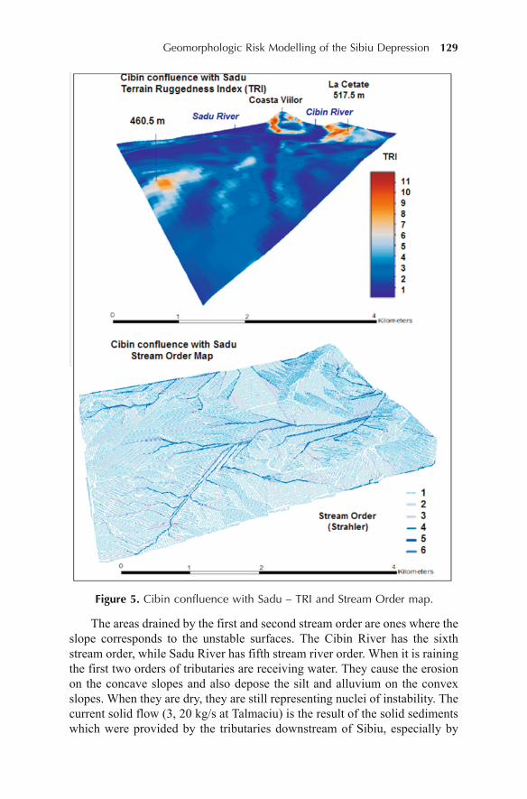
Geomorphologic Risk Modelling of the Sibiu Depression 129
The areas drained by the first and second stream order are ones where theslope corresponds to the unstable surfaces. The Cibin River has the sixthstream order, while Sadu River has fifth stream river order. When it is rainingthe first two orders of tributaries are receiving water. They cause the erosionon the concave slopes and also depose the silt and alluvium on the convexslopes. When they are dry, they are still representing nuclei of instability. Thecurrent solid flow (3, 20 kg/s at Talmaciu) is the result of the solid sedimentswhich were provided by the tributaries downstream of Sibiu, especially by
Figure 5. Cibin confluence with Sadu – TRI and Stream Order map.
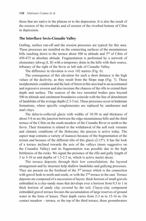
130 Marioara Costea et al.
those that are native to the plateau or to the depression. It is also the result ofthe erosion of the riverbanks and of erosion of the riverbed bottom of Cibinin depression.
The Interfluve Sevis-Cisnadie Valley
Gulling, surface run-off and the erosion processes are typical for this area.These processes are installed on the connecting surfaces of the mountainoushills reaching down to the terrace about 500 m altitude and 3rd of Cibin of450-475 m absolute altitude. Fragmentation is performed by a network ofelementary talweg (I, II) with a temporary drain in the hills with their source,tributary of the right of the Sevis or left side of Cisnadie Valley.
The difference in elevation is over 142 metres (Fig. 6).The consequence of this elevation for such a short distance is the high
values of the declivity, as they result from the Slope map (Fig. 7). Thesemorphometric conditions and the lack of forest in this area lead to an accentuatedand regressive erosion and also increase the chances of the rills to extend theirdepth and surface. The sources of the two torrential bodies pass beyond500 m altitude and catchment boundaries coincide with the line of detachmentof landslides of the average depth (2.5-5 m). These processes occur in badenianformations, where specific conglomerates are replaced by sandstones andmarl clays.
The deluvio-colluvial glacis with widths of 10-50 m and thickness ofabout 5-6 m are the junction between the edge-mountainous hills and the thirdterrace of the Cibin on the south meadow of the Cisnadie River or north to theSevis. Their formation is related to the withdrawal of the soft rock versantsand climatic conditions of the Holocene; the process is active today. Theaspect map contains a variety of nuances because of the fragmentation of theterrain and because of the different tilts of this glacis (2-15o). It has the lookof a terrace inclined towards the axis of the valleys (more suggestive onthe Cisnadiei Valley) and its fragmentation was possible due to the highbrittleness of the rocks. We signal the presence of the rills and gully length of3 to 5-10 m and depths of 1.5-2.5 m, which is active nuclei decay.
The terrace deposits through their low consolidation, the layeredarrangement and by structure help shallow landslides and gullying processes.They are present on the forehead of the 3rd terrace which is the connectionwith gravel beds to north and south, or with the 2nd terrace to the east. Terracedeposits are composed of a succession of layers: thick horizon of small gravelsembedded in a clay-sandy mass that develops over a horizon from 0.5 to 1 mthick horizon of sandy clay covered by the soil. Clayey-clay componentembedded gravel terrace favours the accumulation of large reserves of groundwater in the form of lenses. Their depth varies from 2-3 m to 15-16 m. Oncontact meadow – terrace, or the top of the third terrace, these groundwaters
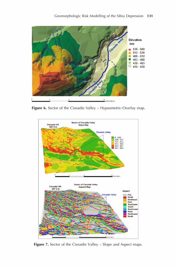
Geomorphologic Risk Modelling of the Sibiu Depression 131
Figure 6. Sector of the Cisnadie Valley – Hypsometric-Overlay map.
Figure 7. Sector of the Cisnadie Valley – Slope and Aspect maps.

132 Marioara Costea et al.
affect surface as springs or maintaining wetlands. Thirty years ago, in order toeliminate excess water and for the agricultural land use, land reclamation anddrainage works were made. Unfortunately, these arrangements have beenneglected over time and drainage channels were clogged and gradually returnedto a land use predominantly in the form of pasture and meadow.
The riverbed is also very clearly delineated by the forehead of terracebecause of the lateral erosion produced by the river under the condition of richdebits (melt of snow or torrential rains). The Cisnadie River has developed apretty large meadow and its base level is lower (416 m) than the Sevis level(450 m).
The meadow in this sector is bilateral but asymmetrical, its width varyingfrom 250 m to 1 km. The mobility of the talweg by meanders and splitting isaccentuated by the decrease of the slope, and due to the action of the streamswhich come from the left side of the Cisnadie valley. The meadow landscapeis represented by meanders and holms. The sinuosity of Cisnadiei riverbedvaries between 1.0 and 1.5 and increases significantly to downstream in termsof a solid carrier composed predominantly of fine sediments (shores, sand)and small gravel, becoming even stronger meandering riverbed downstreamto Cisnadie and until the confluence with Cibin river. Some of the sinuosityvalues presented in this chapter were obtained by using the formula afterdoing the measurements based on aerial photographs and some are the resultof using the Fractal dimension algorithm, which can be finding as tool ofsome of the GIS software.
Gusterita Hill
Gusterita Hill lies north and east of the city of Sibiu and it is part of the contactbetween the depression area and Hartibaciu plateau, marking the alignmentcuesta relief units located in the north-west of the county of Sibiu. This areacontains elements of the combined action of natural factors as triggers of thegeomorphologic processes and of the human action.
In the Gusterita area, geomorphologic risk phenomena are intensified bythe rock lithology. Geological deposits of the area include marl and clay at thebase, and sand and gravel at the top. Intercalation sand (unconsolidated rock)increased the instability of the stack of rocks on the slopes. Clays, underconditions of high rainfall, retain water, their volume is increasing, they arebecoming plastic and cause “flow” along the slopes. Marls also let the waterfrom rainfall to pass, leading to the base of the slope – at the clay level –phenomena of undermining of slope.
The morphometric characteristics have an important role in the morpho-dynamic of this sector. The isometric line of 400 m separates Cibin meadowin this sector and it insinuates to the base of the steep of the plateau structure.The amplitude of the elevation varies from 400 m (on valley) to 598 metreson Padurii Hill (Fig. 8). Besides the valleys, the Wetness Index has high
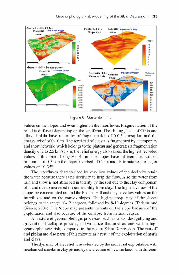
Geomorphologic Risk Modelling of the Sibiu Depression 133
values on the slopes and even higher on the interfluves. Fragmentation of therelief is different depending on the landform. The sliding glacis of Cibin andalluvial plain have a density of fragmentation of 0-0.5 km/sq km and theenergy relief of 0-10 m. The forehead of cuesta is fragmented by a temporaryand short network, which belongs to the plateau and generates a fragmentationdensity of 2 to 2.5 km/sq km; the relief energy also varies, the highest recordedvalues in this sector being 80-140 m. The slopes have differentiated values:minimum of 0-5° on the major riverbed of Cibin and its tributaries, to majorvalues of 10-35°.
The interfluves characterized by very low values of the declivity retainthe water because there is no declivity to help the flow. Also the water fromrain and snow is not absorbed in totality by the soil due to the clay componentof it and due to increased impermeability from clay. The highest values of theslope are concentrated around the Padurii Hill and they have low values on theinterfluves and on the convex slopes. The highest frequency of the slopesbelongs to the range 10-12 degrees, followed by 8-10 degrees (Toderas andGiusca, 2004). The Slope map presents the cuts on the slope because of theexploitation and also because of the collapse from natural causes.
A mixture of geomorphologic processes, such as landslides, gullying andgravitational collapse process, individualize this area as one with a highgeomorphologic risk, compared to the rest of Sibiu Depression. The run-offand piping are also parts of this mixture as a result of the exploitation of marlsand clays.
The dynamic of the relief is accelerated by the industrial exploitation withmechanical shocks in clay pit and by the creation of new surfaces with different
Figure 8. Gusterita Hill.
134 Marioara Costea et al.
slopes and slope differential suitability for processes. The mining terraces(lower slopes) are subject to compaction and suffusion, while operating slopes(greater slopes, even 90o) are subject to sheet erosion, rill erosion and thecollapses. Deluvial contribution due to the run-off and gravitational processesalso determine the remodelling of the waste dumps stored at the base of theexploits on Gusterita Hill. The intensive exploitation of clay explains thecontribution of the coluvio-proluvial deposits to the riverbeds of the creeks.These creeks have an independent character by the monoclinale structure ofthe layers and they fragment the cuesta Hartibaciu Plateau in this sector(Farmandoala Valley, Pe Remeti Valley).
As we have mentioned, the erosion is present on the concave banks, whilethe accumulation is representative for the convex banks. To present this processtogether with the prognosis of their future evolution and to evaluate the potentialof the erosion caused by the water streams, we have created and analysed theStream Power (SP) Index map. This is a function of the surface of the basinand of the slope gradient. Its values for the Gusterita Hill vary within a rangebetween 1000 and 10000. The lowest numbers belong to the interfluves andthe highest to the creeks. There are also intermediate values which correspondto ravines and to the rills created on the slopes exploited for clay. An importantrole is played by the lack of the forest. The vegetation is only represented bythe meadow and several sporadic trees, far from enough to retain part of thewater which flows on the slopes. An overlay of the maps: Wetness Index,Stream Power Index and Length of Slope, together with the NDVI map(Normalized Difference Vegetation Index), geological, soil and stream orderhelps to identify the zones with the highest susceptibility at geomorphologicrisk.
The Comparative Analysis
The comparative analysis of case studies allowed us to establish direct, indirect,strong or weak connections between morphology, morphometric parameters,conditions and geomorphological processes with the character of risk on thefour areas representative of Sibiu Depression. Links are positive whenmorphometric parameters and conditions determined an increase ofgeomorphological phenomena and they are negative when the factors takeninto account lower the geomorphological processes with risk character.Conclusive analysis reveals the following aspects:
a. Direct, strong and positive connection between:
• high values of the fragmentation, the geologic support composited byunconsolidated and low cemented deposits and the extensions of the gullyingand torrentiality on the forehead of Cibin’s terraces, the deluvial glacis atGusterita and at the base of the interfluve Sevis-Cisnadie;
• the values of the slopes, density of the fragmentation, the rain wash processes,gullying and torrentiality are favoured and amplified by the land use aspasture and hay field;

Geomorphologic Risk Modelling of the Sibiu Depression 135
• the fragmentation indexes and the human pressure developed in time byclearing, fallowing, shepherded, agricultural practices of ploughing alongthe slope;
• the geologic base (clay deposits laminated, clayey sands), the energy ofrelief, steep slopes (head of cuesta), the land use (slope excavation andexploitation materials) and gravitational processes (collapses, deep landslides)at Gusterita and Talmaciu; a triggering factor is represented by the mechanicalshock on the physical and chemical behaviour of rocks and preparatoryfactors (meteorization); and
• low slopes on the top of terraces or waterside terraces, the terrace or alluvialdeposits with high porosity and un-cemented, the density of thecommunication ways and of buildings and the compaction process (Cibinmeadow and terraces).
b. Direct, strong and negative connection between the use of forestry andof the orchards and current geomorphologic processes under conditions oflow to moderate slope, due to the stability and due to the protection theyprovide to the land and geological substrate (the forest area of Gusterita Hilland the forest and fruit trees areas in Cisnadie); that use also is involved inregulating of the flow through rainfall interception.
c. Indirect, weak and positive connection between the density offragmentation, slope index, forest plantations on small areas and the torrentialityand gullying; this was demonstrated in the resurgence of the phenomenon inGusterita Hill because of land reclamation through afforestation measuresonly in the drains of the torrents zone and not in the catchment, which didn’thave the desired effect.
d. Indirect, strong and positive connection between:
• the morphological sloping surfaces and their division into small areas (lots)and the rain wash and gullying processes which increases the drainagedensity on the border between the lots boundaries (Gusterita Hill, foreheadsof terraces, Cisnadie Hill); and
• from the sloping surface morphology, the land use, drainage channelprocesses and river bed processes. Cibin and Cisnadie river’s beds stand bythe recrudescence of riverbed erosion processes during wet and dry storageperiods. This oscillation is subject to vulnerability of climatic andhydrological conditions, and watershed management related areas (Costea,2006).
Reports identified above are valid for the whole depression area, but at adifferent scale of intensity. They are driven primarily by slope, relief intensityand density of fragmentation and anthropogenic climate conditions listed above.Given that, the largest area of central depression located almost in middle(about 230 sq km, i.e. 69%) has slopes ranging from 0-5°, fragmentationbetween 0 and 0.75 km/sq km and energy of relief 0-40 m/sq km, is to beemphasized that the stability of the landscape and geomorphological processes
136 Marioara Costea et al.
are reduced in the centre and steep at the periphery (where the relief variesfrom 50 to 150 m/sq km, drainage density is 2-5 km/sq km and slopes vary upto 45°).
In this context, the results of the quantification of the susceptibility ofgeomorphologic risk for the entire surface of the Sibiu Depression (333 sqkm) shows that: 54.41% doesn’t present the risk of producing actualgeomorphologic processes, 9.23% are settlements (covered with infrastructure),and the rest of 36.36% present different levels of risk: 5.38% high risk,21.41% average risk and 9.57% low risk. The case studies presented by usbelong to the high and moderate geomorphologic risk.
While most of the indexes and the values of the parameters presented inthis chapter were calculated and plotted using GIS techniques and models, thedata is stored and it consists in a database which is very valuable to thedecision makers from the local administration, transportation, real-estate etc.Other advantages consist in following the temporal evolution of the data andthe environmental monitoring in space.
Conclusions
Geomorphologic risk assessment must be made by reference to natural andthe anthropic factor. The study conducted for the Sibiu Depression, based onthe weight analysis of morphological parameters, the identification of criticalthresholds in the evolution of geomorphologic processes and selective areasof GIS methods, made possible identifying some risk areas.
Moderate risk area includes a low floodplain area of Cibin Riverdownstream Sibiu, lower meadows of the tributaries, terraced overheads andsliding glacis at the base of cuesta. Land use is diverse (grassland, pastures,farms and industrial). As risk factors we include: the direct influence of riversby floods, moisture excess due to the presence of the groundwater near thesurface and due to the sources. The channel processes are predominant:accumulation, meandering, lateral erosion, undermining and collapse of banks.On slopes with low-moderate inclination on glacis and top of terraces thepredominant processes are: splash and sheet erosion, rill erosion and gullying,associated with superficial and small depth landslides.
High risk area covering the entire surface of the western slope of theHartibaci Plateau between Sibiu and Talmaciu, with a reduced stability inducedby high levels of declivity and relief energy. The very active morphodynamicprocesses is due to mass movement (landslides deep collapse), and due to thegullying and torentiality. Reactivation potential is high due to high rainfalland the presence of coastal springs. We note the presence of very high-risknuclei caused by human activity as exploits of clay in the industrial system.Most of the classification criteria and of the typologies presented in thischapter can be inserted to the GIS software as algorithms to enable thespecialists to realize selective analyses of the geomorphologic risk. To extract
Geomorphologic Risk Modelling of the Sibiu Depression 137
the indices which concur to the geomorphologic risk study, these analysescould be realised using the overlay technique. Even more, the data from thegeomorphologic studies can be overlaid to the demographical data (plottedfrom the statistics) to show the impact of the geomorphologic processes withdifferent levels of risk to the human habitats. That will ease the assessment ofthe risk. To ensure the accuracy and the precision of the data, Global Position(GPS) receivers with under-metre accuracy can be used. This high accuracy isnecessary to evaluate the dynamic of the landslides, gullying and other currentprocesses and the data is easy to be made accessible to the GIS.
In conclusion, the technology we have used in the monitoring activity hadstarted since the phase of planning, have continued with the data acquisitionprocess, analyses algorithms and it ended with the interpretation of the resultsand their storage to a database. We have also used Remote Sensing data suchas aerial images to follow the meanders and other changes occurred to theenvironment. These images, integrated to GIS offer valued information aboutthe evolution, which may be positive or negative of the components of thegeomorphologic system.
The research we have done using the geospatial techniques can be thescientifically based startup to establish the specific strategies and objectivesof the management to reduce, prevent and protect against the geomorphologicprocesses with risk character. We refer to the interventions which interest thedurable development of the space by the control of the building developmentareas, land reclamation, works to improve the degradation and ecologicalrestoration of degraded areas. Local government involvement is imperative inthe development of risk maps and action plans that will lead to a better spacemanagement. This can be accomplished with the participation of the geologists,geomorphologists and of the advanced techniques to process the data in regionaland local planning projects.
References
Alcantara-Ayala, I. (2002). Geomorphology, natural hazards, vulnerability andprevention of natural disasters in developing countries. Geomorphology, 47, 107–124, Amsterdam, Elsevier.
Alkema, D. and Cavallin, A. (2001). Geomorphologic Risk Assessment for EIA, StudiTrontini, di Scienze Natureli. Acta Geologica, 78, 139–145.
Cannon, T. (1993). A hazard need not a disaster make: vulnerability and the causes ofnatural disasters. In: Merriman, P.A., Browitt, C.W.A. (Eds.), Natural Disasters:Protecting Vulnerable Communities (pp. 92– 105). Thomas Telford, London.
Ciobanu, R. (2007). The implications of the geological support in the geographicalrisk phenomena: the Sibiu County case. Brukenthal. Acta Musei, Sibiu, II(3),19–29.
138 Marioara Costea et al.
Ciupangea, D., Pauca, M. and Ichim, Tr. (1970). Geologia Depresiunii Transilvaniei.Bucuresti, Editura Academiei.
Costea, M. (2006). Riscul la inundatii. Impactul in peisaj. In: Stef, V. and Costea, M.(Eds.), Hidrologie aplicata (pp. 205–240). Sibiu, Editura Universitatii “LucianBlaga”.
Giusca, R. (2006). Modele ale degradarilor de teren din Muntii Sureanu, MuntiiCindrel si Depresiunea Sibiului. Sibiu, Editura Universitatii “Lucian Blaga”.
Ielenicz, M. (2004). Geomorfologie, Editura Universitatii, Bucuresti.Matthes-Sears, U., Matthes-Sears, W.C., Hastings, J.C. and Oechel, W.C. (1988). The
effects of topography and nutrient status on the biomass, vegetative characteristics,and gas exchange of two deciduous shrubs on an arctic tundra slope. Arctic andAlpine Research, 20, 342–351.
Murray, C. and Miller, P.C. (1982). Phenological observations of major plant growthforms and species in montane and Eriophorum vaginatum tussock tundra in centralAlaska. Holarctic Ecology, 5, 109–116.
Neaupane, K.M. and Piantanakulchai, M. (2006). Analytic network process model forlandslide hazard zonation. Engeneering Geology, 85, 281–294.
Nellemand, C. and Fry, G. (1995). Quantitative Analysis of Terrain Ruggedness inReindeer Winter Grounds. Arctic, 48(2), 172–176.
Panizza, M. (1986). The geomorphological hazard assessment and the analysis ofgeomorphological risk. In: V. Gardiner (ed.). International Geomorphology. Wiley,Chichester, 225–229.
Panizza, M. (1996). Environmental Geomorphology in Developments. Earth SurfaceProcesses 4, Elsevier, Amsterdam.
Posea, Gr. (2002). Geomorfologia Romaniei. Bucuresti, Editura Fundatiei “Romaniade Maine”.
Sandu, M. (1998). Culoarul depresionar Sibiu – Apold. Studiu geomorfologic. Bucuresti,Editura Academiei.
Soeters, R. and van Westen, C.J. (1996). Slope instability recognition, analysis andzonation. In: Turner, A.K. and Schuster, R.L. (Eds.), Landslides. Investigation,Mitigation, Transportation Research Board (pp. 129–177). Special Report 247,National Academy Press, Washington D.C.
Thakur, J.K., Srivastava, P.K., Singh, S.K. and Vekerdy, Z. (2011). Ecologicalmonitoring of wetlands in semi-arid region of Konya closed basin, Turkey. RegionalEnvironmental Change (DOI: 10.1007/s10113-011-0241-x).
Toderas, T. and Giusca, R. (2004). Aplicarea noilor tehnici GIS in evaluarea reliefuluidin Depresiunea Sibiului. Revista Geografica, Bucuresti, 68–72.
Tufescu, V. (1966). Subcarpatii si Depresiunile marginale ale Transilvaniei, Bucuresti,Editura Stiintifica.
Varnes, D.J. (1984). Landslide hazard zonation: A review of principles and practice.United Nations International, Paris.
Wilson, M.F.J. et al. (2007). Multiscale terrain analysis of multibeam bathymetry datafor habitat mapping on the continental slope. Marine Geodesy, 30, 3–35.
Zêzere, J.L. (2002). Landslide susceptibility assessment considering landslide typology.A case study in the north Lisbon (Portugal). Natural Hazards and Earth SystemSciences, EGU. 2, 73–82.
http://www.vulnerabilityindex.net/evi_2005.htm
Geospatial Technique to Study Forest Cover Using ALOS/PALSAR Data 139
9Geospatial Technique to
Study Forest Cover UsingALOS/PALSAR Data
Ram Avtar, Jay Krishna Thakur1, Amit Kumar Mishra2
and Pankaj Kumar3
Institute of Industrial Science, The University of Tokyo, 4-6-1 KomabaMeguro-Ku, Tokyo-153-8505, Japan
1Department Hydrogeology and Environmental Geology, Institute ofGeosciences, Martin Luther University, Halle (Saale), Germany2Graduate School of Environmental Studies, Nagoya University
Nagoya 464-8601, Japan3Graduate School of Life and Environmental Sciences
University of Tsukuba, Tsukuba, Japan
Introduction
Forests are one of the most crucial life supporting system that provide rangeof economic, social and environmental benefits, including essential ecosystemservices such as climate change mitigation and adaptation. Forest plays animportant role in maintaining ecological balance and homeostatic in theenvironment (Wulder and Franklin, 2003). Forest cover mapping is necessaryfor sustainable management and utilization of forest resources. Forest covermonitoring based on geospatial data can significantly contribute in futureforest management plans for reducing deforestation and implementation ofclimate change mitigation policies. Establishing a reliable baseline of forestcover and monitoring forest cover change in the tropical countries becomeessential (FAO, 2001; REDD, 2010). Recent report of FRA (2010) shows theglobal change in forest area is about –5.2 million hectares per year during2001-2010.
Forest cover mapping through ground surveys is labour intensive, timeconsuming, relatively infrequent and very expensive and these maps becomeeasily outdated. Geospatial techniques like remote sensing and geographicalinformation system (GIS) become useful for forest cover monitoring in a costand time effective way (Williams et al., 2006). In tropical countries the frequent
DOI 10.1007/978-94-007-1858-6_9, © Capital Publishing Company 2012
139e ,J.K. Thakur et al. (eds.), G ospatial Techniques for Managing Environmental Resources

140 Ram Avtar et al.
cloud cover often restrains the acquisition of optical remote sensing data.Radar data become feasible way of acquiring remotely sensed data within agiven time frame because radar system can collect data in all weather conditions.Due to this unique feature, radar data have been used extensively in manyfields, including forest cover identification and mapping (Lu, 2006).
In January, 2006, Japan Aerospace Exploration Agency (JAXA) launchedthe Advanced Land Observation Satellite (ALOS) with Phased Array typeL-band Synthetic Aperture Radar (PALSAR) sensor. PALSAR providesL-band synthetic aperture radar (SAR) data, which is quite useful for forestcover and deforestation monitoring because, it has the higher penetration tothe vegetative areas (Rosenqvist, 2007). It has quad polarization (HH, HV,VH and VV) mode, which characterize various targets on the basis of physical,dielectric and geometric properties. The ability of PALSAR data to retrievemore information about physical properties of the targets has led to widerange of its applications; for example in crop monitoring, hydrologicalmodelling, soil moisture, forest monitoring, disaster monitoring, ocean andcoastal monitoring etc. (Mcnairn et al., 2009; Entekhabi et al., 2010; Mitnik,2008).
This study demonstrates the application of full polarimetric PALSARdata for forest cover classification. Full polarimetric PALSAR data determinesthe types of interaction with different types of forest cover based on theirbiophysical parameters (tree height, crown diameter, diameter at breast height,biomass, tree density, etc.). Co-polarized signal interact with similar orientation,so vertical stalks interact strongly with VV polarization. Horizontal branchesand soil surface interact strongly with HH polarization and cross-polarizedsignal HV is related to volume scattering (Rignot et al., 1995). On the basis ofinteraction between various polarization and targets; surface, volume anddouble-bounce scattering occurs from the scatterers. There are basically twodecomposition techniques: (a) coherent decomposition (pure targets) and(b) incoherent decomposition (distributed targets). In this study we havedemonstrated the application of eigen vector based Cloude-Pottierdecomposition. Cloude-Pottier decomposition for polarimetric classificationis based on eigen value and eigen vector calculation of the coherency matrixof quad polarization PALSAR data. This decomposition is useful for extractingthe information about polarimetric scattering of various features (Cloude andPottier, 1996, 1997). Classification based on different polarimetricdecomposition entropy (H), alpha (D) and anisotropy (A) is used to understandpolarimetric response of SAR data to study purity of target, mean scatteringmechanism and number of scattering mechanism involved for each targets(Patel et al., 2009).We used Wishart unsupervised classification method, whichclassify the image automatically by finding the cluster based on certain criterion(Singh et al., 2008).
The important role of forest in global carbon cycle was pointed out inmany previous studies (Brown, 2002; Houghton, 2005; IPCC, 2007; Thakuret al., 2010; Thakur et al., 2011, Avtar et al., 2011). Therefore, it becomes
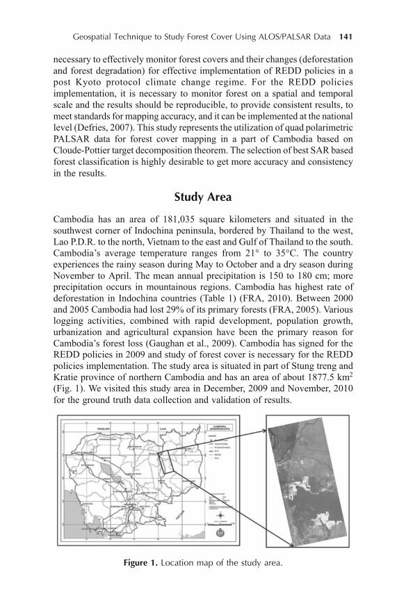
Geospatial Technique to Study Forest Cover Using ALOS/PALSAR Data 141
necessary to effectively monitor forest covers and their changes (deforestationand forest degradation) for effective implementation of REDD policies in apost Kyoto protocol climate change regime. For the REDD policiesimplementation, it is necessary to monitor forest on a spatial and temporalscale and the results should be reproducible, to provide consistent results, tomeet standards for mapping accuracy, and it can be implemented at the nationallevel (Defries, 2007). This study represents the utilization of quad polarimetricPALSAR data for forest cover mapping in a part of Cambodia based onCloude-Pottier target decomposition theorem. The selection of best SAR basedforest classification is highly desirable to get more accuracy and consistencyin the results.
Study Area
Cambodia has an area of 181,035 square kilometers and situated in thesouthwest corner of Indochina peninsula, bordered by Thailand to the west,Lao P.D.R. to the north, Vietnam to the east and Gulf of Thailand to the south.Cambodia’s average temperature ranges from 21° to 35°C. The countryexperiences the rainy season during May to October and a dry season duringNovember to April. The mean annual precipitation is 150 to 180 cm; moreprecipitation occurs in mountainous regions. Cambodia has highest rate ofdeforestation in Indochina countries (Table 1) (FRA, 2010). Between 2000and 2005 Cambodia had lost 29% of its primary forests (FRA, 2005). Variouslogging activities, combined with rapid development, population growth,urbanization and agricultural expansion have been the primary reason forCambodia’s forest loss (Gaughan et al., 2009). Cambodia has signed for theREDD policies in 2009 and study of forest cover is necessary for the REDDpolicies implementation. The study area is situated in part of Stung treng andKratie province of northern Cambodia and has an area of about 1877.5 km2
(Fig. 1). We visited this study area in December, 2009 and November, 2010for the ground truth data collection and validation of results.
Figure 1. Location map of the study area.
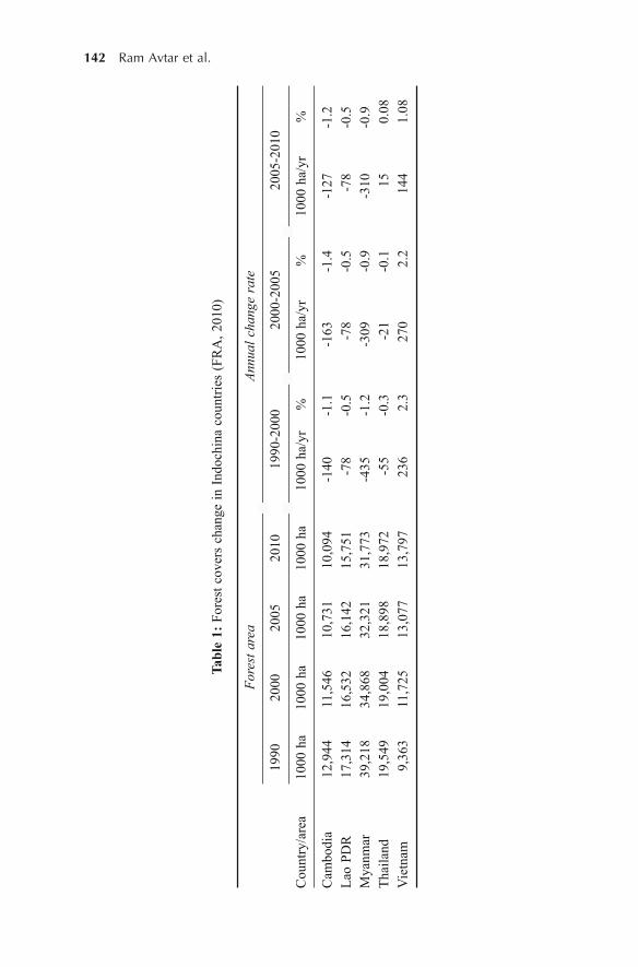
142 Ram Avtar et al.
Tabl
e 1:
For
est c
over
s ch
ange
in In
doch
ina
coun
tries
(FR
A, 2
010)
Fore
st a
rea
Annu
al c
hang
e ra
te
1990
2000
2005
2010
1990
-200
020
00-2
005
2005
-201
0
Cou
ntry
/are
a10
00 h
a10
00 h
a10
00 h
a10
00 h
a10
00 h
a/yr
%10
00 h
a/yr
%10
00 h
a/yr
%
Cam
bodi
a12
,944
11,5
4610
,731
10,0
94-1
40-1
.1-1
63-1
.4-1
27-1
.2La
o PD
R17
,314
16,5
3216
,142
15,7
51-7
8-0
.5-7
8-0
.5-7
8-0
.5M
yanm
ar39
,218
34,8
6832
,321
31,7
73-4
35-1
.2-3
09-0
.9-3
10-0
.9Th
aila
nd19
,549
19,0
0418
,898
18,9
72-5
5-0
.3-2
1-0
.115
0.08
Vie
tnam
9,36
311
,725
13,0
7713
,797
236
2.3
270
2.2
144
1.08
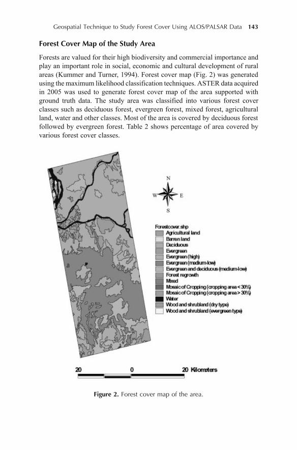
Geospatial Technique to Study Forest Cover Using ALOS/PALSAR Data 143
Forest Cover Map of the Study Area
Forests are valued for their high biodiversity and commercial importance andplay an important role in social, economic and cultural development of ruralareas (Kummer and Turner, 1994). Forest cover map (Fig. 2) was generatedusing the maximum likelihood classification techniques. ASTER data acquiredin 2005 was used to generate forest cover map of the area supported withground truth data. The study area was classified into various forest coverclasses such as deciduous forest, evergreen forest, mixed forest, agriculturalland, water and other classes. Most of the area is covered by deciduous forestfollowed by evergreen forest. Table 2 shows percentage of area covered byvarious forest cover classes.
Figure 2. Forest cover map of the area.
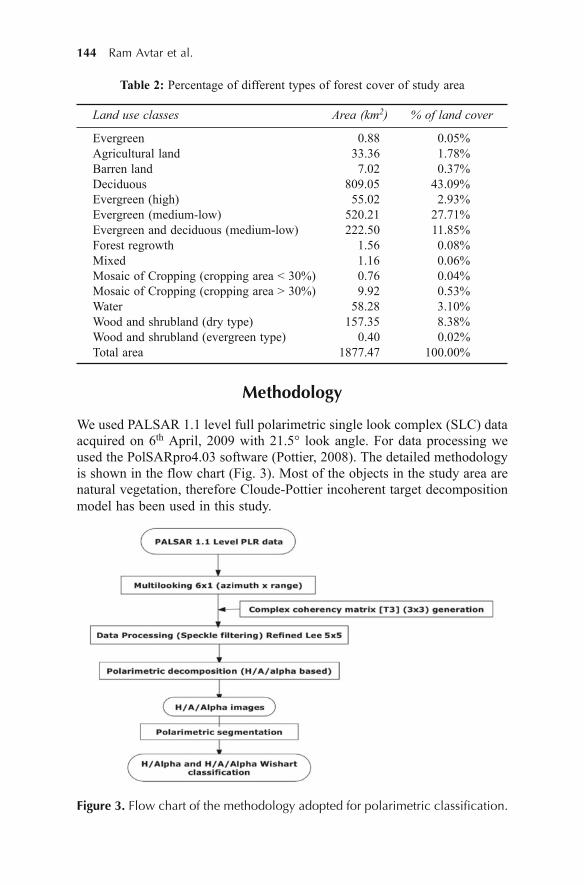
144 Ram Avtar et al.
Table 2: Percentage of different types of forest cover of study area
Land use classes Area (km2) % of land cover
Evergreen 0.88 0.05%Agricultural land 33.36 1.78%Barren land 7.02 0.37%Deciduous 809.05 43.09%Evergreen (high) 55.02 2.93%Evergreen (medium-low) 520.21 27.71%Evergreen and deciduous (medium-low) 222.50 11.85%Forest regrowth 1.56 0.08%Mixed 1.16 0.06%Mosaic of Cropping (cropping area < 30%) 0.76 0.04%Mosaic of Cropping (cropping area > 30%) 9.92 0.53%Water 58.28 3.10%Wood and shrubland (dry type) 157.35 8.38%Wood and shrubland (evergreen type) 0.40 0.02%Total area 1877.47 100.00%
Methodology
We used PALSAR 1.1 level full polarimetric single look complex (SLC) dataacquired on 6th April, 2009 with 21.5° look angle. For data processing weused the PolSARpro4.03 software (Pottier, 2008). The detailed methodologyis shown in the flow chart (Fig. 3). Most of the objects in the study area arenatural vegetation, therefore Cloude-Pottier incoherent target decompositionmodel has been used in this study.
Figure 3. Flow chart of the methodology adopted for polarimetric classification.

Geospatial Technique to Study Forest Cover Using ALOS/PALSAR Data 145
Cloude-Pottier Decomposition
Polarimetric decomposition is used to understand the physical characteristicsof various scatterers. Cloude and Pottier proposed a method of extraction ofmean diffusion based on eigen values/eigen vectors decomposition of coherencematrix (Cloude and Pottier, 1997). A target coherence matrix [T] can beexpressed as
[T] = > @> @> @ 1U U �/ (1)
where [/] is a diagonal matrix with non negative real element and [U] is aunitary matrix.
The real nonnegative diagonal matrix [/] of eigen value of coherencymatrix is defined by
> @/ =1
2
3
0 00 00 0
OË ÛÌ ÜOÌ ÜÌ ÜOÍ Ý
(2)
If only one eigen value is non zero then the scattering can be related topure target. If all eigen values are non zero and identical then the averagecoherency matrix represents a completely decorrelated, unpolarized randomscattering target. In between these two cases, scattering matrix represents thedistributed or partially polarized scatterers.
The 3 × 3 unitary matrix [U] of the three eigen vectors of coherencymatrix is
[U] = > @1 2 3u u u (3)
where u1, u2 and u3 are the three unit orthogonal eigen vectors. The eigenvector can be expressed as
ui =i
ji i
ji i
cos
sin cos
sin cos
i
i
e
e
� G
� J
DË ÛÌ Ü
D EÌ ÜÌ ÜD EÍ Ý
(4)
where i = 1, 2 and 3.Equation (4) can be expressed as
[T] =3
*i i
, 1
T
i ju u
OÇ (5)
Based on this eigen value decomposition three secondary parameters viz.,entropy, anisotropy and alpha can be defined as function of the eigen values
146 Ram Avtar et al.
of the coherency matrix. Entropy, D angle and anisotropy are polarimetricfeatures derived from eigen values and eigen vectors (Lee and Pottier, 2009).H/D/A is used to interpret target scattering properties. Entropy (H) indicatesthe randomness of the scatterers. H equals to 0 for the pure targets, whereas1 for the distributed target (no dominant scatterers).
H =3
i 3 i1
logi
P P �Ç (6)
i0 P� = i3
i1
1
i
O �OÇ
(7)
where Pi is pseudo-probabilities, which can be obtained from the eigen values,Oi represents relative intensity of the i-th scattering process.
The alpha (D) angle is acquired from Di angle of each of the eigen vectorsas follows
D � 3
i i1i
P
DÇ (8)
D measures the dominant scattering mechanism within a specified target. Itvaries between 0° to 90°. D = 0° represents odd-bounce scattering from flatsurfaces, D = 45° represents dipole or volume scattering, while D = 90°represents a double bounce scatterer or dipole scattering.
In case of more than one dominant scatterer (H > 0.7), anisotropy (A) isintroduced because the second and third eigenvalues are highly affected bynoise for low entropies. A is acquired from the second and third eigen valuesas
A = 2 3
2 3
O � OO � O
(9)
where O2 and O3 are smaller eigen values. Anisotropy measures the relativeimportance of the second and third eigenvalues of the eigen decomposition. IfA = 1, the second scattering process is fairly important and could be employedin discriminating similar surface characteristics (Trisasongko, 2010).
Classification Technique
H/Alpha and H/A/Alpha Wishart classification approaches have been attemptedfor the classification of PALSAR image. The Wishart distribution can beexpressed by:
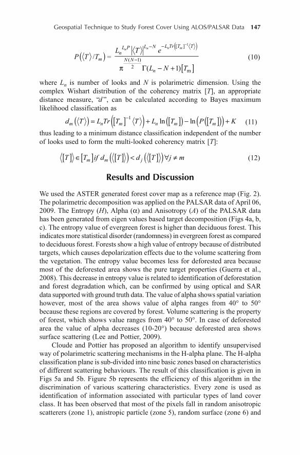
Geospatial Technique to Study Forest Cover Using ALOS/PALSAR Data 147
� �/ mP T T =� �
> @
1[ ]
( 1)2
m( 1)
n mnnL Tr T TL NL P
nN N
n
L T e
L N T
���
�
S * � � (10)
where Ln is number of looks and N is polarimetric dimension. Using thecomplex Wishart distribution of the coherency matrix [T], an appropriatedistance measure, “d ”, can be calculated according to Bayes maximumlikelihood classification as
� � > @� � > @� � > @� �� �1 ln lnm n m n m md T L Tr T T L T P T K� � � � (11)thus leading to a minimum distance classification independent of the numberof looks used to form the multi-looked coherency matrix [T]:
> @ > @ > @� � > @� �m m jT T if d T d T j m° � � � (12)
Results and Discussion
We used the ASTER generated forest cover map as a reference map (Fig. 2).The polarimetric decomposition was applied on the PALSAR data of April 06,2009. The Entropy (H), Alpha (D) and Anisotropy (A) of the PALSAR datahas been generated from eigen values based target decomposition (Figs 4a, b,c). The entropy value of evergreen forest is higher than deciduous forest. Thisindicates more statistical disorder (randomness) in evergreen forest as comparedto deciduous forest. Forests show a high value of entropy because of distributedtargets, which causes depolarization effects due to the volume scattering fromthe vegetation. The entropy value becomes less for deforested area becausemost of the deforested area shows the pure target properties (Guerra et al.,2008). This decrease in entropy value is related to identification of deforestationand forest degradation which, can be confirmed by using optical and SARdata supported with ground truth data. The value of alpha shows spatial variationhowever, most of the area shows value of alpha ranges from 40° to 50°because these regions are covered by forest. Volume scattering is the propertyof forest, which shows value ranges from 40° to 50°. In case of deforestedarea the value of alpha decreases (10-20°) because deforested area showssurface scattering (Lee and Pottier, 2009).
Cloude and Pottier has proposed an algorithm to identify unsupervisedway of polarimetric scattering mechanisms in the H-alpha plane. The H-alphaclassification plane is sub-divided into nine basic zones based on characteristicsof different scattering behaviours. The result of this classification is given inFigs 5a and 5b. Figure 5b represents the efficiency of this algorithm in thediscrimination of various scattering characteristics. Every zone is used asidentification of information associated with particular types of land coverclass. It has been observed that most of the pixels fall in random anisotropicscatterers (zone 1), anistropic particle (zone 5), random surface (zone 6) and
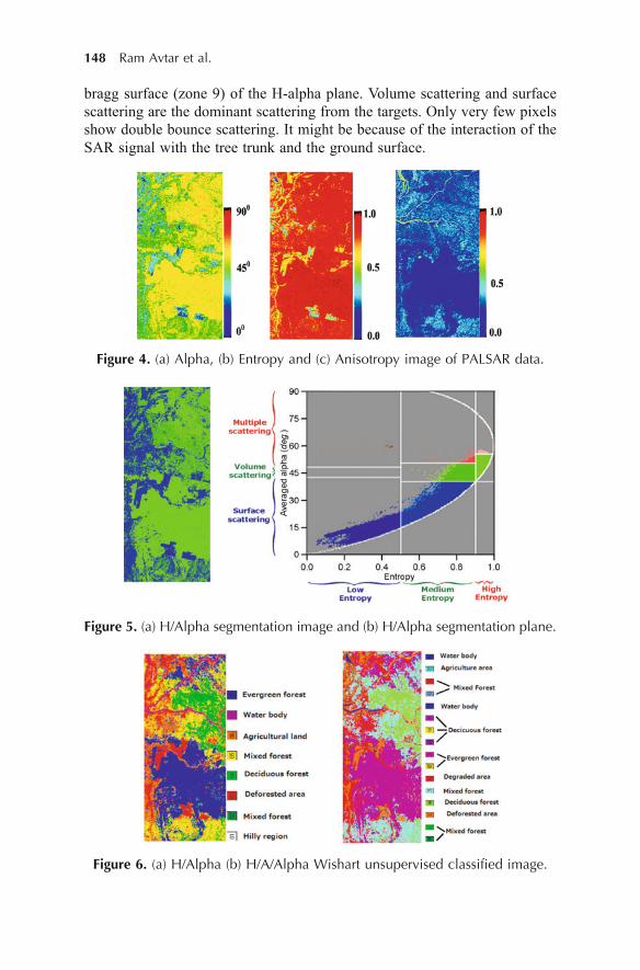
148 Ram Avtar et al.
bragg surface (zone 9) of the H-alpha plane. Volume scattering and surfacescattering are the dominant scattering from the targets. Only very few pixelsshow double bounce scattering. It might be because of the interaction of theSAR signal with the tree trunk and the ground surface.
Figure 4. (a) Alpha, (b) Entropy and (c) Anisotropy image of PALSAR data.
Figure 5. (a) H/Alpha segmentation image and (b) H/Alpha segmentation plane.
Figure 6. (a) H/Alpha (b) H/A/Alpha Wishart unsupervised classified image.
Geospatial Technique to Study Forest Cover Using ALOS/PALSAR Data 149
Wishart unsupervised H/Alpha and H/A/Alpha classification is based uponpolarimetric decomposition classification parameters i.e. H, A, alpha. The H/Alpha Wishart classifier group the total image into eight different classes (Fig.6a). After introducing anisotropy (A), the classifier identifies sixteen differentclasses (Fig. 6b). Anisotropy (A) is useful to discriminate scattering mechanismwith different eigen value distribution but with similar intermediate entropyvalues. The anisotropy image (Fig. 4c) shows most of the area having lowvalue of A which corresponds to dominant first scattering and low secondaryscattering mechanism. ASTER based classification and field data has beenused to add legends in the image. H/A/Alpha technique classify image into 16classes therefore we can discriminate different types of forest on the basis oftypes and density. In Fig. 6b deciduous forest has been divided into threeclasses and evergreen into two classes as compared to Fig. 6a. These threeclasses of deciduous forests represents dense deciduous, sparsely deciduousand medium deciduous forest whereas, two classes of evergreen forestrepresents medium evergreen and medium-low evergreen forest. H/A/AlphaWishart classification is better than H/Alpha classification. We find somemisclassification between deforested area and agricultural area because boththe classes show same types of surface scattering properties. If agriculturalarea has some crops then it might be easy to distinguish from the deforestedarea as such crops vary in scattering characteristics.
Conclusion
This study shows use of full polarimetric L-band PALSAR data for forestcover classification. H-alpha plane showed most of the pixels fall in randomanisotropic scatterers (zone 1), anistropic particle (zone 5), random surface(zone 6) and bragg surface (zone 9) to discriminate different types of scatteringbehaviours of targets. Wishart unsupervised classification is useful for forestcover classification. Results show that use of full polarimetric data improvesthe detection of structural differences between forest canopies, thus helping inbetter forest type mapping and provide additional information for forestmanagement practices. Based on the experiment, it was concluded that Cloude-Pottier based classification is useful for forest cover mapping. However, furtherstudies should concentrate on the capability of other target decompositiontheorems such as Freeman-Durden three component (1998) and Yamaguchifour component decomposition (2006) and their applicability in forestry areais needed to be explored. The new generation of geospatial techniques withfull polarimetric SAR data could help to study various biophysical parametersof forest for better implementation of REDD policies.
Acknowledgements
The authors are highly thankful to the Monbukagakusho (MEXT) JapaneseGovernment fellowship which helped to pursue research. Authors also want
150 Ram Avtar et al.
to put on record contribution of Institute of Industrial Science, The Universityof Tokyo for facilitating data analysis in its labs and also to the Department ofCivil Engineering, The University of Tokyo for providing fund during thefield visit.
References
Avtar, R., Singh, C.K., Shashtri, S. and Mukherjee, S. (2011). Identification of erosionaland inundation hazard zones in Ken-Betwa River Linking Area, India using remotesensing and GIS. Environmental Monitoring and Assessment, doi.org/10.1007/s10661-011-1880-6.
Brown, S. (2002). Measuring carbon in forests: Current status and futurechallenges. Environ. Pollut., 116, 363–372.
Cloude, S.R. and Pottier, E. (1996). A review of target decomposition theorms in radarpolarimetry. IEEE transactions on Geoscience and Remote Sensing, 34(2), 498–518.
Cloude, S.R. and Pottier, E. (1997). An entropy based classification scheme for landapplications of polarimetric SAR. IEEE Transaction on Geoscience and RemoteSensing, 35, 68–78.
Defries, R., Achard, F., Brown, S., Herold, M., Murdiyarso, D., Schlamadinger, B.and De Souza Jr C. (2007). Earth observations for estimating greenhouse gasemissions from deforestation in developing countries. Environmental Science andPolicy, 10, 385–394.
Entekhabi, D., Njoku, E.G., O’Neill, P.E., Kellogg, K.H., Crow, W.T., Ed e lstein,W.N., Entin, J.K., Goodman, S.D., Jackson, T.J., Johnson, J., Kimball, J., Piepmeier,J.R., Koster, R.D., Martin, N., McDonald, K.C., Moghaddam, M., Moran, S.,Reichle, R., Shi, J.C., Spencer, M.W., Thurman, S.W., Tsang, L. and Van Zyl, J.(2010). The soil moisture active passive (SMAP) mission. Proceedings of theIEEE, 98(5), 704–716.
FAO (2001). State of the World’s forests. Food and Agriculture Organisation of theUnited Nations, Rome.
FRA (2005). Global Forest Resources Assessment. Food and Agriculture Organisationof the United Nations, Rome.
FRA (2010). Global Forest Resources Assessment. Food and Agriculture Organisationof the United Nations, Rome.
Freeman, A. and Durden, S.L. (1998). A three-component scattering model forpolarimetric SAR data. IEEE transactions on Geoscience and Remote Sensing, 36,963–973.
Gaughan, A.E., Binford, M.W. and Southworth, J. (2009). Tourism, forest conversion,and land transformations in the Angkor basin, Cambodia, Applied Geography, 29,212–223.
Guerra, J.B., Freitas, C.D.C. and Mura, J.C. (2008). Evaluating potential of band polardata to discrimination increment areas in Amazon rain forest. Proceedings of IEEEIGARSS08.
Geospatial Technique to Study Forest Cover Using ALOS/PALSAR Data 151
Houghton, R.A. (2005). Aboveground forest biomass and the global carbon balance.Global Change Biology, 11, 945–958.
IPCC (2007), Climate Change 2007: Fourth Assessment Report of theIntergovernmental Panel on Climate Change, edited by S. Solomon et al. CambridgeUniv. Press, Cambridge, U.K.
Kummer, D.M. and Turner, B.L. (1994). The human causes of deforestation in SoutheastAsia. Bioscience, 44(5), 323–326.
Lee, J.S. and Pottier, E. (2009). Polarimetric radar imaging: From basics to application,CRC Press, Taylor and Francis Group, Boca Raton.
Lu, D. (2006). The potential and challenge of remote sensing-based biomass estimation.International Journal of Remote Sensing, 27(7), 1297–1328.
McNairn, H., Shang, J., Jiao, X. and Champagne, C. (2009). The contribution ofALOS PALSAR multipolarization and polarimetric data to crop classification.IEEE Transactions on Geoscience and Remote Sensing, 47(12), 3981–3992.
Mitnil, L.M. (2008). Advanced land observing satellite PALSAR observations of theoceanic dynamic phenomena in the coastal zone. IEEE, IGARSS 2008.
Patel, P., Srivastava, H.S. and Navalgund, R.R. (2009). Use of synthetic aperture radarpolarimetry to characterize wetland targets of Keoladeo National Park, Bharatpur,India. Current Science, 97(4), 25, 529–537.
Pottier, E., Ferro-Famil and Lee, J.S. (2008). POLSARPRO V4.0 – lecture notes:Advanced concepts. Available at: http://earth.esa.int/polsarpro/.
REDD (2010). Resource book, GOFC-GOLD.Rignot, E., Zimmermann, R. and Zyl, van J. (1995). Spaceborne applications of P
band imaging radars for measuring forest biomass. IEEE Transactions on Geoscienceand Remote Sensing, 33(5), 1162–1165.
Rosenqvist, A. et al. (2007). ALOS PALSAR: A Pathfinder Mission for Global-ScaleMonitoring of the Environment, IEEE Transactions on Geoscience and RemoteSensing, 45(11), 3307–3316.
Singh, G., Venkataraman, G., Kumar, V., Rao, Y.S. and Snehmani (2008). The H/A/Alpha polarimetric decomposition theorem and complex wishart distribution forsnow cover monitoring. Presented in IGARSS’08 at Boston, USA.
Thakur, J.K., Srivastava, P.K., Singh, S.K. and Vekerdy, Z. (2011). Ecologicalmonitoring of wetlands in semi-arid region of Konya closed Basin, Turkey. RegionalEnvironmental Change (DOI: 10.1007/s10113-011-0241-x).
Thakur, J.K. and Singh, S.K. (2010). Eco-hydrological monitoring of wetlands in asemi-arid region using remote sensing, GIS, GPS and various data sets: A casestudy of Konya closed basin, Turkey IAH 2010, Krakow, Poland.
Trisasongko, B.H. (2010). The use of polarimetric SAR data for forest disturbancemonitoring. Sens Imaging, 11, 1–13.
Williams, K., Sader, S.A., Pryor, C. and Reed, F. (2006). Application of geospatialtechnology to monitor legacy conservation easements. Journal of Forestry, 104,89–93.
Wulder, M.A. and Franklin, S.E. (2003). Remote sensing of forest environmentsconcepts and case studies. Kluwer Academic Publishers, London.
Yamaguchi, Y., Yajima, Y. and Yamada, H. (2006). A four-component decompositionof POLSAR images based on the coherency matrix. IEEE Geoscience and RemoteSensing Letter, 3, 292–296.
152 Prafull Singh et al.
10Assessment of Land Use/Land Cover
Using Geospatial Techniquesin a Semi-arid Region of
Madhya Pradesh, India
Prafull Singh, Jay Krishna Thakur1,Suyash Kumar2 and U.C. Singh3
Dept. of Civil Engineering, SAMCET, Bhopal, Madhya Pradesh, India1Dept. Hydrogeology and Environmental Geology, Institute of
Geosciences, Martin Luther University, Halle, Germany2Department of Geology, Govt. PG Science College, Gwalior, India
3School of Studies in Earth Science, Jiwaji University, Gwalior, India
Introduction
The Earth’s land cover characteristics and its use are key variables in globalchange. The society today is already in the mainstream of another revolution– the information revolution. This brings enormous changes to life and living,providing new approaches: how to advance the frontiers of previous revolutionsparticularly those of earth resources mapping and monitoring. Over the lastfew decades, there has been a significant change on land use and land cover(LULC) across the globe due to the climatic changes and over demand of thegrowing inhabitants. Semi-arid regions are undergoing severe stresses due tothe combined effects of growing population and climate change (Mukherjeeet al., 2009). In the last three decades, the technologies and methods of remotesensing have progressed significantly. Now a days remote sensing data, alongwith increased resolution from satellite platforms, makes these technologyappear poised to make better impact on land resource management initiativesinvolved in monitoring LULC mapping and change detection at varying spatialranges (Singh et al., 2010; Thakur, 2010). Remote sensing technology offerscollection and analysis of data from ground-based, space and Earth-orbitingplatforms, with linkages to Global Positioning System (GPS) and geographic
DOI 10.1007/978-94-007-1858-6_10, © Capital Publishing Company 2012
152e ,J.K. Thakur et al. (eds.), G ospatial Techniques for Managing Environmental Resources
Assessment of Land Use/Land Cover Using Geospatial Techniques 153
information system (GIS) data with promising modelling capabilities (Franklin,2001; Thakur et al., 2010). This has made remote sensing valuable for landcover and land use information.
As the demand for quantity and quality of information and technologycontinues to improve, remote sensing is becoming more significant for thefuture. Therefore, the chapter focuses on the issues and challenges associatedwith monitoring LULC mapping in semi-arid region. For example, at therural-urban fringe, large tracts of undeveloped rural land are rapidly convertedto urban land use. To maintain up-to-date land-cover and land use information,where typical updating processes are on an interval scale of five years, isdifficult task for planners (Chen et al., 2002). The full potential of geospatialtechnology for change detection applications still has to be realized for plannersat local, regional, and international levels. In the near future, the field ofremote sensing will change dramatically with the projected increase in numberof satellites of all types (Glackin, 1998). In order to have better understandingof the rapid advancements in geospatial technology, we provide a brief historyof the advances in geospatial technology.
In developing countries like India, efforts are being made for the sustainableland resource planning and management with reliable and updatedgeoinformation, which is pre-requisite for land use planning. Such informationcould only be obtained through the modern techniques and equipment forresearch and mapping. Since land use and land cover changes are activefeatures over space and time, it is difficult to obtain real time informationthrough conventional resources and these methods are time consuming,laborious, high cost and work force oriented. Spatial variation of LULC createsdoubt about the point data collected by conventional methods. In moderntimes, satellite based remote sensing technology has been developed, whichare of immense value for preparing LULC map and their monitoring at regularperiodic intervals of time (Kumar et al., 2004).
As such, spatial repetitive and synoptic coverage from satellites collectedover a wide range of electromagnetic spectrum admirably suit the requirementof LULC mapping and monitoring. These spatial data indicates the distributionof various LULC categories in an area. Due to the availability of repetitivedata, it is possible to update existing database for various land use planningand design making. Therefore, with the use of geospatial technology (remotesensing, GIS, GPS and computational techniques) it is evident that thesecould be used effectively to prepare LULC mapping (Tejaswini, 2005; Rao etal., 1996, Mukherjee et al., 2009; Srivastava et al., 2010). Geospatial technologyguarantees the availability and quick access of real time data, geospatialinformation for resource mapping.
LULC relates to the observable earth surface expressions, such asvegetation, geology, water resources and anthropogenic features whichdescribes the Earth’s physical condition in terms of the natural environmentwith man-made structures.
154 Prafull Singh et al.
In India, spatial accounting and monitoring have been carried out at anational level on 1:250,000 scale, using multi-temporal Indian Remote Sensing(IRS) satellites to address the spatial and temporal variability in landuse patterns(NRSA, 1989). In the absence of basic information about the current land usepattern, it would be difficult to determine future improvements and theirdeterioration. Therefore, it is necessary to provide up-to-date informationabout earth resources that helps planners in decision-making for sustainabledevelopment and utilization of the earth resources. The use of geospatialinformation establishes a discussion between science, and national developmentstrategies.
Background
The relative evaluation of land for various uses is an urgent issue in the semi-arid regions. Industrial and recreational park, and nature preserves versusdiverse agricultural and pastoral uses of the land should be evaluated. Optionsfor gathering the problems, though limited, are based on the ecology of thespecific local area or region (Dhinva et al., 1992).
Application of remote sensing technology for LULC change analysis hasbeen carried out in semi-arid region of Madhya Pradesh and found that the useof remote sensing along with Survey of India toposheets could be usedappropriately for LULC mapping of semi-arid area (Jaiswal et al., 1999).
The semi-arid regions are characterized by erratic rainfall and high rate ofvegetation dynamics. The dynamics of plant species over time is mainly dueto continuous and complex interactions of the plant communities with theirenvironment. The human interferences and climatic variations are commondriving forces in bringing changes to the environment (Shetty et al., 2005).The increasing biotic pressure together with increasing human demands exertspressure on the available land resources all over the region. Therefore, inorder to have best possible use of land, it is not only necessary to have theinformation on the existing LULC, but also to monitor the dynamic land useresulting because of increasing demands aroused from the growing population(Raghavswamy et al., 2005). Continuous overexploitation of natural resourceslike land, water, and forest has caused serious threat to the local population ofthe semi-arid region (Rao et al., 2006). This causes problems like little scopefor soil moisture storage, high rate of soil erosion, declining groundwaterlevel and shortage of drinking water. In a semi-arid area, there will be lessvegetation so the diverse classes of vegetation will not be clearly recognized;and are the major problem of LULC mapping (Chaudhary et al., 2008).
It has extreme importance to the planners and decision makers forformulating the long-term plans for land resources development andmanagement to improve the quality of habitat in semi-arid regions. In general,the study area has limited rainfall and, subject to prolonged droughts as well
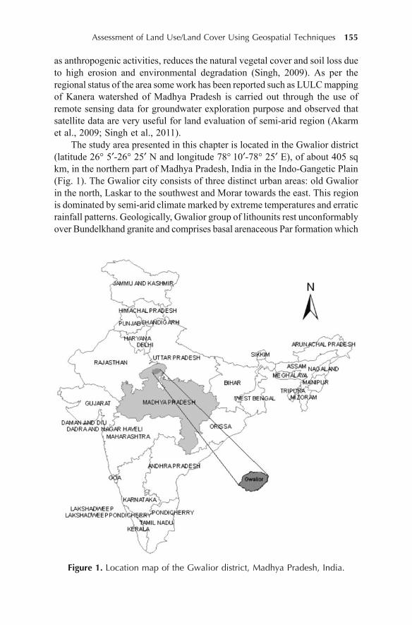
Assessment of Land Use/Land Cover Using Geospatial Techniques 155
as anthropogenic activities, reduces the natural vegetal cover and soil loss dueto high erosion and environmental degradation (Singh, 2009). As per theregional status of the area some work has been reported such as LULC mappingof Kanera watershed of Madhya Pradesh is carried out through the use ofremote sensing data for groundwater exploration purpose and observed thatsatellite data are very useful for land evaluation of semi-arid region (Akarmet al., 2009; Singh et al., 2011).
The study area presented in this chapter is located in the Gwalior district(latitude 26° 5�-26° 25� N and longitude 78° 10�-78° 25� E), of about 405 sqkm, in the northern part of Madhya Pradesh, India in the Indo-Gangetic Plain(Fig. 1). The Gwalior city consists of three distinct urban areas: old Gwaliorin the north, Laskar to the southwest and Morar towards the east. This regionis dominated by semi-arid climate marked by extreme temperatures and erraticrainfall patterns. Geologically, Gwalior group of lithounits rest unconformablyover Bundelkhand granite and comprises basal arenaceous Par formation which
Figure 1. Location map of the Gwalior district, Madhya Pradesh, India.
156 Prafull Singh et al.
are overlain by volcano-sedimentary sequences of Morar formation consistingof ferruginous shale with bands of chert-jasper.
The main objective of this chapter is to explore the role of geospatialtechnologies for land use mapping of one of the drought prone city of MadhyaPradesh, India and to examine the present status of LULC within the basinusing satellite data for sustainable utilization of resources and theirdevelopment.
Data Used and Methodology
National LULC classification system using remote sensing data for mappinghas been attempted by National Remote Sensing Agency (NRSA, 1995) of thecountry to understand and manage country’s natural resources. Thereafterfurther efforts to map on 1:50,000 scales followed certain standards that requiredmodifications in the current day’s context. To this extent, an exhaustive LULCclassification was evolved to facilitate an in-depth assessment of all the LULCcategories (NRSA, 2005). The benefits of adopting a classification are tendingto persuade for evolving a standard classification system that is guided bypractical experience and continuous observation over the past many years andabove all that meet the user requirements. The remotely sensed data, thematicmaps and ground truth data used are in Table 1.
Table 1: Remote sensing and other data used in the study
S.No. Data Sources
1. IRS ID LISS III image and PAN image National Remote Sensing Agency(NRSA), Hyderabad, India
2. Survey of India Topographic Map Survey of India(Sheet numbers 54 J/3, J/4, J/7 and J/8on 1:50,000 scale)
3. Field data on land use/land cover Ground truth collection duringfield survey and district revenuedepartment
Image interpretation has been carried out in two most popular ways e.g.digital analysis and visual interpretation. In the digital classification process,training areas for different classes were defined for the satellite imagery onspectral response pattern in different spectral bands generated. Based on thesetraining areas, satellite imagery was classified into different classes usingparametric or non-parametric classifiers (Lu et al., 2007). Following imageprocessing steps were involved in image classification starting from processingof IRS LISS III Image to correct for atmospheric errors, registration of LISSIII and Pan images with reference to toposheets from Survey of India (SOI),generation of other secondary data, image classification and accuracyassessment. The information provided by the satellites in combination withother sources to quantify the various parameters for efficient mapping of land
Assessment of Land Use/Land Cover Using Geospatial Techniques 157
use of the basin was evaluated by applying various image processing stepsusing ERDAS Imagine and ArcGIS 9.3.
Preprocessing
Accurate registrations of satellite images are essential for analyzing LULCconditions of a particular geographic position. The atmospheric scattering iscommon in remote sensing images, which are more pronounced in the shorterwavelength regions, and they cause some additional contribution to spectralreflectance. In the present study, satellite data was geometrically corrected forthe distortions and degradations caused by the errors due to variation in altitude,velocity of the sensor platform, earth curvature and relief displacement.
The images of IRS ID and PAN (Path 97 and Row 53) were geometricallycorrected and geocoded to the Universal Transverse Mercator (UTM)coordinate system by using a reference image of SOI toposheets. A minimumof 45 regularly distributed ground control points were selected from the images.The registration was performed using first order polynominal transformation,resampling using a nearest neighbour algorithm. The transformation with aRoot Mean Square (RMS) error is 0.643. Image enhancement, contraststretching and false colour composites were worked out.
Image Classification
Supervised classification was performed to produce land cover map from theIRS satellite data. Defining of the training sites, extraction of signatures fromthe image and then classification of the image was done. Training data extractionwas a critical step in supervised classification; these must be selected from theregions representative of the land cover classes under consideration. Thus,data were collected from relatively homogeneous areas consisting of thoseclasses. The collection of training data was time consuming and tedious process,as it involved laborious field surveys and accumulation of reference data fromvarious sources. The features of training sites were digitized. Three trainingsites were selected for this purpose. This procedure assures both the accuracyof classification and the true interpretation of the results. After the training siteareas digitization, the statistical characterizations of the information werecreated. These were called signatures. Finally, the classification methods wereapplied. All the classification techniques like the maximum likelihoodclassification (MLC), parallelepiped and minimum distance to meanclassification were applied for the images and the best classification techniquewas then chosen. It was observed that Maximum Likelihood Classification(MLC) gave good results as compared to the other two techniques. To determinethe accuracy of classification, a simple testing pixel was selected on theground trothed reference data. In thematic mapping from remotely senseddata, the accuracy, and the degree of ‘correctness’ of a map or classificationwas calculated.
158 Prafull Singh et al.
Result and Discussions
Land is one of the most important natural resources. The landuse pattern andits spatial distribution are the prime requisites for the preparation of an effectivelanduse policy needed for the proper planning and management of any area.The land use map prepared using above methodology has been shown inFig. 2 and their spatial distributions are given in Table 2. The various LULCclasses delineated from the available data include built-up, agriculture,
Figure 2. Land Use/Land Cover map of the Morar River BasinMadhya Pradesh, India.
Assessment of Land Use/Land Cover Using Geospatial Techniques 159
wasteland, forest and water bodies. Three types of built-up lands weredelineated: urban settlement, rural settlement and industrial complex. Onsatellite images these structures look as block-like appearance and show bluishtone on the image and on the PAN data they look typically blocky appearancewith light tone.
The urban settlements are widely spread in central part of the basin. Itcovers an area of about 31.87 sq km. About 20 villages are identified fromsatellite image, covering an area of about 5.82 sq km. Within the basin, one ofthe important industrial complexes is named as Malanpur Industrial Complexcovering an area of about 20.95 sq km. The total area covered by settlementsin the basin constitutes 58.64 sq km (16.23%) respectively.
Forest is discerned by their red to dark red tone and varying in sizes. Theyshow irregular shape and smooth texture. These forest areas are found onlower side of the basin. Based on the tonal and textual variations, the forestsof the basin are divided into three categories as dense, open and forest blank.Dense forests are found in lower and central side of the area at uplandtopography. Approximately such dense forests cover an area of about 50.76 sqkm. Open forests cover an area of about 11.74 sq km. Forest blank appears inlight yellow to light brown tone generally small and most of these forests arefound on hilltops and slopes. Forest blanks account very small having an areaof about 1.85 sq km. These forests cover an area of about 19.05%. Agriculturalland is shown in pink colour with smooth appearance on pan data and darkpatches with step-like arrangement and agricultural land without crops isshown in bluish/greenish grey with smooth texture. In the present study, suchcropped areas were found mostly in the northeastern portion and some amountin southwestern portion. Such cropped areas cover approximately 61.51 sqkm (16.71%). Fallow lands were identified by their dark greenish tone, smallersize, regular shape and medium texture. Such fallow lands are found welldistributed in the central and northeastern portion of the basin, which occupies110.53 sq km (29.33%).
Due to non-availability of satellite data of Kharif season, some agriculturalland is marked as fallow land in the basin as they were verified during fieldsurvey. Three categories of wasteland are identified such as land with scrub,land without scrub and gullied/ravenous land from satellite image and theycover approximately 83.34 sq km (20.61%). Land without scrub is in thelower part of the basin. Gullies are formed because of localized surface run-off affecting the unconsolidated material resulting in the formation ofperceptible channels causing undulating terrain. They are mostly associatedwith stream courses and sloping grounds with good rainfall and entrencheddrainage. Number of surface water bodies such as ponds, one reservoir namedRamaua with one perennial and one seasonal river are delineated from thesatellite image and they cover 9.10 sq km (2.48%).

160 Prafull Singh et al.
Table 2: Areas under different classes of Land Use/Land Cover
S.No. Land use/Land cover Area (in sq km) Area (in %)
1 Urban settlement 31.87 8.872 Rural settlement 5.82 1.443 Industrial complex 20.95 5.924 Dense forest 50.76 14.045 Open forest 11.74 2.906 Forest blank 1.85 2.117 Agricultural land 61.51 16.718 Fallow land 110.53 29.339 Land with scrub 31.25 7.73
10 Land without scrub 46.04 11.3911 Gullied/ravenous land 5.05 1.4912 Reservoir 1.40 0.3413 River 6.08 1.5014 Ponds 1.62 0.64
Conclusion and Recommendation
The present research work demonstrates the capability of geospatial techniquesto capture the land use categories in a semi-arid region of Madhya Pradesh,India, which are necessary for optimum and sustainable utilization of landresources and prevention of further undesirable deterioration in land use.Analysis shows the agricultural area mostly found in the northern portionwhereas southern portion of the basin is occupied by the forest cover over thedenudational hills. The observation also shows major portion of the basinaffected by severe soil erosion due to the occurrence of shales and steep slope.Therefore, the present work suggested that area urgently needs to minimizesoil erosion by applying various techniques of soil conservation and large-scale aforestation.
Wastelands must be converted into cultivable land through massiveprogrammes of afforestation, plantation or pasture development to increasefood, fodder and fuel production. Land with and without scrub can be utilizedfor growing plants, which need soil cover. These plants are a source of fuelwood whereas some of them are of medicinal and economic importance.Check bunds should be constructed with waste-weirs wherever necessary tocontrol soil erosion in the gullied/ravenous land. These bunds allow retentionof water and soil whereby lands can be reclaimed and brought under cultivation.
To ensure planned development and monitor the land utilization pattern,preparation of LULC maps is necessary in the area. Scientists should usegeospatial as reliable mapping and monitoring tool for new research andplanning applications. It is expected that this trend will have dramaticimplications in the field of geoinformatics for the natural resource mapping,monitoring and modelling over the next decade.
Assessment of Land Use/Land Cover Using Geospatial Techniques 161
References
Balak, Ram and Kolarkar, A.S. (1993). Remote sensing application in monitoring landuse changes in arid region of Rajasthan. International Journal of Remote Sensing,14(17), 3191–3200.
Chaudhary, B.S., Saroha, G.P. and Yadav, Manoj (2008). Human induced land use/land cover changes in Northern part of Gurgaon district, Haryana, India. Journalof Human Ecology, 23(3), 243–252.
Chaurasia, R. and Sharma, P.K. (1999). Land Use/Land Cover Mapping and ChangeDetection using Satellite Data—A Case Study of Dehlon Block, District Ludhiana,Punjab. Journal of Indian Society of Remote Sensing, 27(2), 115–121.
Chen, D. and Stow, D. (2002). The effect of training strategies on supervisedclassification at different spatial resolutions. Photogrammetric Engineering andRemote Sensing, 68, 1155–1161.
Cihlar (2000). Land cover mapping of large areas from satellites: status and researchpriorities. International Journal of Remote Sensing, 21(6&7), 1093–1114.
Dhinwa, P.S., Pathak, S.K., Sastry, S.V.C., Rao, M., Majumdar, K.L., Chotani, M.L.,Singh, P.J. and Sinha, R.L.P. (1992). Land use change analysis of Bharatpur Districtusing GIS. Journal of the Indian Society of Remote Sensing, 20(4), 237–250.
Diouf, A. and Lambin, E.F. (2001). Monitoring land-cover changes in semi-arid regions:remote sensing data and field observations in the Ferlo, Senegal. Journal of AridEnvironments, 48(2), 129–148.
Foody, M.G. (2002). Status of land cover classification accuracy assessment. RemoteSensing of Environment, 8, 185–201.
Franklin, S.E. (2001). Remote Sensing for Sustainable Forest Management. LewisPublishers, Boca Raton, FL.
Gautam, N.C. and Channiah, C.H. (1985). Land use and land cover mapping andchange detection in Tripura using satellite Landsat data. Journal of the IndianSociety of Remote Sensing, 6(3&4), 517–528.
Glackin, D.L. (1998). International space-based remote sensing overview: 1980–2007.Canadian Journal of Remote Sensing, 24, 307–314.
Jaiswal, R.K., Saxena, R. and Mukherjee, S. (1999). Application of remote sensingtechnology for landuse/landcover change analysis. Journal of the Indian Society ofRemote Sensing, 27, 123–128.
Javed, Akram, Khanday, M.Y. and Ahmed, Rizwan (2009). Prioritization of sub-watersheds based on morphometric and land use analysis using remote sensing andGIS techniques. Journal of the Indian Society of Remote Sensing, 37(2), 261–274.
Jensen, J.R. (1996). Introductory Digital Image Processing, Second Edition. Prentice-hall Press, New Jersey.
Jensen, J.R. and Cowen, D.J. (1999). Remote sensing of urban/suburban infrastructureand socio-economic attributes. Photogrammetric Engineering and Remote Sensing,65, 611–622.
Kumar, Vijay, Rai, S.P. and Rathore, D.S. (2004). Land use mapping of Kandi Beltsof Jammu Region. Journal of Indian Society of Remote, 32(4), 323–328.
Kunwar, P., Kachhwaha, T.S., Kumar, Anil, Agrawal, A.K., Singh, A.N. and Mendiratta,Nisha (2010). Use of high-resolution IKONOS data and GIS technique fortransformation of landuse/landcover for sustainable development. Current Science,98(2), 204–212.
162 Prafull Singh et al.
Lillesand, T.M., Kiefer, R.W. and Chipman, J.W. (2008). Remote sensing and imageinterpretation. John Wiley & Sons, Inc., New York.
Lu, D. and Weng, Q. (2007). A survey of image classification methods and techniquesfor improving classification performance. International Journal of Remote Sensing,28(5), 823–870.
Merem, E.C. and Twumasi, Y.A. (2008). Using Geospatial Information Technology inNatural Resources Management: The Case of Urban Land Management in WestAfrica. Sensors, 8, 607–619.
Mukherjee, S., Shashtri, S., Singh, C., Srivastava, P. and Gupta, M. (2009). Effect ofcanal on land use/land cover using remote sensing and GIS. Journal of the IndianSociety of Remote Sensing, 37(3), 527–537.
National Remote Sensing Agency (1989). Manual of Nation wide Land use/Landcover Mapping using satellite imagery, Part I. NRSA, Hyderabad.
National Remote Sensing Agency (1995). IMSD Technical Guidelines. National RemoteSensing.
NRSA (2005). Integrated Mission for Sustainable Development. Technical Guidelines,Hyderabad.
Palaniswami, C., Upadhyay, A.K. and Maheswarappa, H.P. (2006). Spectral MixtureAnalysis for sub pixel classification of coconut. Current Science, 91(12), 1706–1711.
Raghavswamy, V., Pathan, S.K., Ram, Mohan, P., Bhanderi, R.J., Padma, Priya (2005).IRS-IC applications for urban planning and development. Current Science, 70,582–588.
Ranjeet, J., Jiquan, Chen, Nan, Lu, Ke, Guo, Cunzhu, Liang, Yafen, Wei et al. (2008).Predicting plant diversity based on remote sensing products in the semi-arid regionof Inner Mongolia. Remote Sensing of Environment, 112(5), 2018–2032.
Rao, D.P., Gautam, N.C., Nagaraja, R. and Ram, M.P. (1996). IRS-1C applications inland use mapping and planning. Current Science. 70(7), 575–581.
Rao, K.N. and Narendra, K. (2006). Mapping and evaluation of urban sprawling in theMehadrigedda watershed in Visakhapatnam metropolitan region using remotesensing and GIS. Current Science, 91(11), 1552 –1557.
Rogana, John and Chen, D.M. (2004). Remote sensing technology for mapping andmonitoring land-cover and land-use change. Progress in Planning, 61, 301–325.
Saha, A.K., Arora, M.K., Csaplovics, E. and Gupta, P.K. (2005). Land coverclassification using IRS LISS III image and DEM in a rugged terrain: A case studyin Himalayas. Geocarto International, 20(2), 33–40.
Shetty, Amba, Lakshman, N., Sangeeta, T. and Rajesh, M.V.S. (2005). Land use-landcover mapping using satellite data for a forested watershed, Udipi district, Karnatakastate, India. J. Indian Soc. Remote Sensing, 33, 233–238.
Singh, Praful, Kumar Suyash and Singh, U.C. (2011). Groundwater resource evaluationin the Gwalior area, India, using satellite data: an integrated geomorphological andgeophysical approach. Hydrogeology Journal, (DOI:10.1007/s10040.011-0758-6).
Singh, P.K. (2009). Remote sensing and GIS based hydrogeological study of MorarWatershed, District Gwalior (M.P) India. Unpublished Ph.D. thesis, Faculty ofScience, Jiwaji University, Gwalior, M.P., India.
Singh, A. (1989). Digital change detection technique using remote sensing data.International Journal of Remote Sensing, 26, 1–6.
Assessment of Land Use/Land Cover Using Geospatial Techniques 163
Singh, P.K. and Singh, U.C. (2009). Water resource evaluation and management forMorar River basin, Gwalior District, Madhya Pradesh, using GIS. E-journal ofEarth Science India, 2(3), 174–186.
Singh, S.K., Thakur, J.K. and Singh, U.K. (2010). Environmental monitoring of landcover/land use changes in Siwalik Hills, Rupnagar district of Punjab, India usingremote sensing and ancillary data. Paper presented at the International Conferenceon Global Climate Change.
Srivastava, P., Mukherjee, S. and Gupta, M. (2010). Impact of Urbanization on LandUse/Land Cover Change using Remote Sensing and GIS: A Case Study. Journal ofEcological Economics and Statistics, 18, 106–117.
Tapiador, F. and Casanova, J.L. (2003). Land use mapping methodology using remotesensing for the regional planning directives in Segovia, Spain.
Tejaswini, N.B. (2005). Land use/Land cover mapping in the coastal area of NorthKarnataka using remote sensing data. Journal of the Indian Society of RemoteSensing, 33(2), 253–257.
Thakur, J.K. (2010). Eco-hydrological wetland monitoring in a semi-arid region (Acase study of Konya Closed Basin, Turkey). Faculty of International Institute forGeo-Information Science and Earth Observation (ITC), Universiteit Twente,Enschede, the Netherlands.
Thakur, J.K. and Singh, S.K. (2010). Eco-hydrological monitoring of wetlands in asemi-arid region using remote sensing, GIS, GPS and various data sets: A casestudy of Konya closed basin, Turkey. Paper presented at the IAH 2010.
164 Miguel Martínez Tapia et al.
11The Environmental Calculator:
A Tool for the Efficient Assessmentof Environmental Services Loss
due to Deforestation
Miguel Martínez Tapia, Xanat Antonio Némigaand José Isabel Juan Pérez
Autonomous University of the State of Mexico, Mexico
Introduction: Why an Environmental Calculator?
Forest ecosystems contribute to protect soils from erosion and to regulatewatersheds and local hydrological systems by reducing variation in waterflows. They also provide local and global climate regulation, carbon storageas well as air and water purification. Forests contain the largest assortment ofspecies found in any terrestrial ecosystem and supply numerous social andcultural services. They are also part of our cultural and historical heritage(Stenger et al., 2009). Information about forest values might be needed forlegal processes of damage compensation, but also for cost-benefit analyses,for the establishment of governmental regulations, for ‘‘environmental pricing’’or simply for general information (Elsasser et al., 2009). The unavailability ofcartographical values, representing differential prices for the economical valueof environmental services which forest provides, make it difficult to use suchresources on a sustainable basis. One major threat to forest sustainability isdeforestation. Deforestation has several side effects on the ecosystem servicesof a site. As runoff and erosion increase, they modify soil structure, which inturn reduces water infiltration and reservoirs recharge. The associated functionsthat a forest cover usually plays are also affected: thermal regulation,biodiversity support, and carbon sequestration, among others.
Forest resources at the Biosphere Reserve of Monarch Butterfly havehistorically been under heavy pressure. Therefore, deforestation at this zonehas been documented, along with ecosystem deterioration and depletion ofwooden resources (PROFEPA, 2001). For such reason, the tool here presentedattempts to economically calculate the losses on ecosystem services that
DOI 10.1007/978-94-007-1858-6_11, © Capital Publishing Company 2012
164e ,J.K. Thakur et al. (eds.), G ospatial Techniques for Managing Environmental Resources
The Environmental Calculator 165
are associated to deforestation, to suggest an adequate fine. It integratesmethods for soil erosion assessment (Domínguez-Cortazar et al., 2001; CortésT. et al., 1991; Sanaphre-Villanueva et al., 2003), for water infiltrationestimation (Hernández-Valdez, 2005; Mobayed, 2001); and carbonsequestration calculation. Once modelled, its outcome is linked to one platformthat allows entering the site coordinates and returns the estimated value ofsuch loss. To develop it, Geographic Information Systems (GIS) technologywas used to visualize, analyze and correlate said environmental variables.This tool is based on the theory of value and that of environmental economy(Martínez-Alier et al., 2001; Pearce et al., 1995) and integrates territory valuesas currency to make them comparable in time and space (Gómez-Jiménez etal., 2007).
Background
Ecosystem services are the processes of ecosystems that support human well-being. Common forest ecosystem services are timber, non-timber forestproducts, wildlife habitat, water quantity and quality, carbon sequestrationand storage, and recreation opportunities (Patterson and Coehlo, 2009). Notall forests provide the same ecosystem services: the structure, compositionand location have a key role in the determination of the services that a forestcan offer and whom those services can be offered to (Baskin, 1997; Myers,1997; Roper and Park, 1999; Schmidt et al., 1999; Sharma, 1992). Theimportance of these functions is strictly linked to the socio-economic andenvironmental context of which the forest is a part (Goio et al., 2008). Since2000, a growing number of researches related to the economic evaluation ofthe ecosystem services that forests provide can be found worldwide, especiallyon the valuation of non-market environmental goods and services (McCombaet al., 2006). This is because it is widely accepted that an improvedunderstanding of the value of forests can be useful to determine their optimaluse among competing users, often providing a strong economic argument forforest conservation, or at least lessening the incentive for deforestation (Lange,2004). These methods are being increasingly used and applied to conductcost-benefit analysis of environmental regulations, to value environmentalservices and raise awareness on its linkages to economy, and to aid in thedevelopment of green national accounts (McComba et al., 2006); a thoroughrevision of the methods applied for non-timber forest benefits valuation isprovided by Lindhjema (2007). Tools to economically valuate theenvironmental services consider direct use value, indirect use value, optionvalue, and intrinsic value in terms of capital (natural, human and technological).The total economic value is the sum of all these values (Leff, 2004). A sounddescription of the total economic value (TEV) framework and related conceptscan be found at Croitoru (2007).
The economical and environmental valuation of the space implies theallocation of the natural loss of goods and environmental services and theirprices in a given time lag (Gómez-Jiménez et al., 2007). In Mexico, several
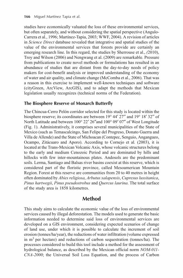
166 Miguel Martínez Tapia et al.
studies have economically valuated the loss of these environmental services,but often separately, and without considering the spatial perspective (Angulo-Carrera et al., 1996; Martínez-Tapia, 2003; WWF, 2004). A revision of articlesin Science Direct database revealed that integrative and spatial studies of thevalue of the environmental services that forests provide are certainly anemerging research line. In this regard, the studies by Sherrouse et al., (2010),Troy and Wilson (2006) and Nengwang et al. (2009) are remarkable. Pressurefrom publications to create novel methods or formulations has resulted in anabundance of studies that are distant from the day-to-day needs of policymakers for cost-benefit analysis or improved understanding of the economyof water and air quality, and climate change (McComba et al., 2006). That wasa reason in this exercise to implement well-known techniques and software(cityGreen, ArcView, ArcGIS), and to adapt the methods that Mexicanlegislation usually recognizes (technical norms of the Federation).
The Biosphere Reserve of Monarch Butterfly
The Chincua-Cerro Pelón corridor selected for this study is located within thebiosphere reserve; its coordinates are between 19° 44� 27�� and 19° 18� 32�� ofNorth Latitude and between 100° 22� 26�and 100° 09� 07� of West Longitude(Fig. 1). Administratively, it comprises several municipalities of the State ofMexico (such as Temascalcingo, San Felipe del Progreso, Donato Guerra andVilla de Allende) and the State of Michoacan (Contepec, Senguio, Angangueo,Ocampo, Zitácuaro and Aporo). According to Cornejo et al. (2003), it islocated at the Trans-Mexican Volcanic Axis, whose volcanic structures belongto the early and medium Cenozoic Period and are dominated by hills andhillocks with few inter-mountainous plates. Andosols are the predominantsoils. Lerma, Santiago and Balsas river basins coexist at this reserve, which isconsidered part of the floristic province, called Mesoamerican MountainRegion. Forest at this reserve are communities from 20 to 40 metres in heightoften dominated by Abies religiosa, Arbutus xalapensis, Cupresus lussitanica,Pinus hartwegii, Pinus pseudostrobus and Quercus laurina. The total surfaceof the study area is 1858 kilometres.
Method
This study aims to calculate the economic value of the loss of environmentalservices caused by illegal deforestation. The models used to generate the basicinformation needed to determine said loss of environmental services aredeveloped on a GIS environment, considering expected scenarios of changeof land use, under which it is possible to calculate the increment of soilerosion (tonnes/ha/year), the reductions of water infiltration (volume expressedin m3 per hectare) and reductions of carbon sequestration (tonnes/ha). Theprocesses considered to build this tool include a method for the assessment ofhydrological balance, as described by the Mexican official norm NOM-011-CNA-2000; the Universal Soil Loss Equation, and the process of Carbon

The Environmental Calculator 167
Figure 1. Study area location and land use types.
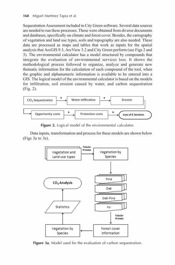
168 Miguel Martínez Tapia et al.
Sequestration Assessment included in City Green software. Several data sourcesare needed to run these processes. These were obtained from diverse documentsand databases, specifically on climate and forest cover. Besides, the cartographyof vegetation and land use types, soils and topography are also needed. Thesedata are processed as maps and tables that work as inputs for the spatialanalysis that ArcGIS 9.3, ArcView 3.2 and City Green perform (see Figs 2 and3). The environmental calculator has a model structured by compounds thatintegrate the evaluation of environmental services loss. It shows themethodological process followed to organize, analyze and generate newthematic information for the calculation of each compound of the tool, whenthe graphic and alphanumeric information is available to be entered into aGIS. The logical model of the environmental calculator is based on the modelsfor infiltration, soil erosion caused by water, and carbon sequestration(Fig. 2).
Figure 2. Logical model of the environmental calculator.
Data inputs, transformation and process for these models are shown below(Figs 3a to 3e).
Figure 3a. Model used for the evaluation of carbon sequestration.
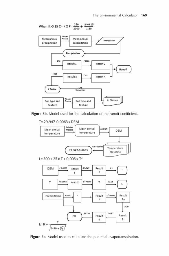
The Environmental Calculator 169
Figure 3b. Model used for the calculation of the runoff coefficient.
Figure 3c. Model used to calculate the potential evapotranspiration.

170 Miguel Martínez Tapia et al.
Figure 3d. Model used to calculate total infiltration.
Result 1/ 0.45
POWER m
Result 2 By 0.65/ 0.65
PixelSize
Slopelength
/ 22.13
Result 3
Slope(%)
RECLASSLS
Topography TINSlope(%)
S factor
L factor
Mean annualprecipitation
Tabular
Process
INTERPOLATION
Mean annualprecipitation
Precipitation P
POWERResult 5
EI30
TabularProcess
x
R
Soil typeand texture
Soil type andtexture
TabularProcess
K-Classes
KGrid Conversion
m expClass
POWER m
BY Result 4
Index
y
R K LS C P
Coefficient Soil type andtexture
TabularProcess
CoefficientClasses
GridConversion
C
By ByErosion
ByBy
Figure 3e. Structure of the model used to calculate soil erosion caused by water.
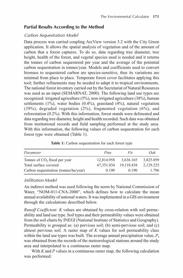
The Environmental Calculator 171
Partial Results According to the Method
Carbon Sequestration Model
Data process was carried coupling ArcView version 3.2 with the City Greenapplication. It allows the spatial analysis of vegetation and of the amount ofcarbon that a forest captures. To do so, data regarding tree diameter, treeheight, health of the forest, and vegetal species used is needed and it returnsthe tonnes of carbon sequestered per year and the average of the potentialcarbon sequestration in tonnes/year. Models and coefficients used to convertbiomass to sequestered carbon are species-sensitive, thus its variations areminimal from place to place. Temperate forest cover facilitates applying thistool; further refinements may be needed to adapt it to tropical environments.The national forest inventory carried out by the Secretariat of Natural Resourceswas used as an input (SEMARNAT, 2000). The following land use types arerecognized: irrigated agriculture (5%), non-irrigated agriculture (38%), humansettlements (1%), water bodies (0.4%), grassland (4%), natural vegetation(39%), degraded vegetation (2%), fragmented vegetation (6%), andreforestation (0.2%). With this information, forest stands were delineated anddata regarding tree diameter, height and health recorded. Such data was obtainedfrom institutional records and field sampling performed at the study area.With this information, the following values of carbon sequestration for eachforest type were obtained (Table 1).
Table 1: Carbon sequestration for each forest type
Parameter Pine Fir Oak
Tonnes of CO2 fixed per year 12,814.958 3,636.165 3,825.059Total surface covered 67,351.034 19,110.438 2,129.225Carbon sequestration (tonnes/ha/year) 0.190 0.190 1.796
Infiltration Model
An indirect method was used following the norm by National Commission ofWater, “NOM-011-CNA-2000”, which defines how to calculate the meanannual availability of national waters. It was implemented in a GIS environmentthrough the calculations described below.
Runoff Coefficient: K values are obtained by cross-relation with soil perme-ability and land use type. Soil types and their permeability values were obtainedfrom the soil charts by INEGI (National Institute of Statistics and Geography).Permeability is grouped as: (a) pervious soil; (b) semi-pervious soil; and (c)almost pervious soil. A raster map of K values for soil permeability classwithin the land use types was built. The average annual precipitation value, P,was obtained from the records of the meteorological stations around the studyarea and interpolated to a continuous raster map.
With K and P values in a continuous raster map, the following calculationwas performed:
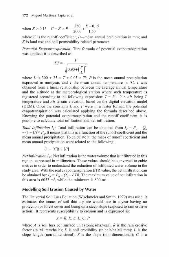
172 Miguel Martínez Tapia et al.
when K > 0.15 C = K × P – 250 0.152000 1.50
K ��
where C is the runoff coefficient; P—mean annual precipitation in mm; andK is land use and soil permeability related parameter.
Potential Evapotranspiration: Turc formula of potential evapotranspirationwas applied; it is described as:
ET =
� �20.90
P
PL
�
where L is 300 + 25 × T + 0.05 × T³; P is the mean annual precipitationexpressed in mm/year, and T the mean annual temperature in °C. T wasobtained from a linear relationship between the average annual temperatureand the altitude at the meteorological station where such temperature isregistered according to the following expression: T = X – Y × Alt, being Ttemperature and Alt terrain elevation, based on the digital elevation model(DEM). Once the constants L and P were in a raster format, the potentialevapotranspiration was calculated applying the formula described above.Knowing the potential evapotranspiration and the runoff coefficient, it ispossible to calculate total infiltration and net infiltration.
Total Infiltration IT: Total infiltration can be obtained from IT = Pa – Qa= (1 – C) × Pa. It means that this is a function of the runoff coefficient and themean annual precipitation. To calculate it, the maps of runoff coefficient andmean annual precipitation were related to the following:
(1 – [C]) × [P]
Net Infiltration IN : Net infiltration is the water volume that is infiltrated in thisregion, expressed in millimetres. These values should be converted to cubicmetres in order to understand the reduction of infiltrated water volume in thestudy area. With the real evapotranspiration ETR value, the net infiltration canbe obtained by: IN = Pa – Qa – ETR. The maximum value of net infiltration inthis area is 6053 m3, while the minimum is 800 m3.
Modelling Soil Erosion Caused by Water
The Universal Soil Loss Equation (Wischmeier and Smith, 1979) was used. Itestimates the tonnes of soil that a place would lose in a year having noprotection or forest cover and being on a steep slope (exposed to rain erosiveaction). It represents susceptibility to erosion and is expressed as:
A = R. K. S. L. C. P
where A is soil loss per surface unit (tonnes/ha.year); R is the rain erosivefactor (in MJ.mm/ha h); K is soil erodibility (tn.ha.h/ha.MJ.mm); L is theslope length (non-dimensional); S is the slope (non-dimensional); C is a
The Environmental Calculator 173
cultivation and territorial ordination factor and P is a factor related to cultivationpractices. These R, K, LS and C factors were calculated with ArcGis 9.3software, using the procedures described below.
Rain Erosive Factor R: Usually R is calculated using the Wischmeier index.However in order to calculate it, rain intensity values and rain graphic recordsare needed. Being such data unavailable, the mapping developed by Cortés(1991) was used instead. According to this author, the study area belongs tothe region V. The equation used is then Y = 3.4880 X + 0.000188 X2. Y is theannual index of rain erosive factor expressed in MJ mm/ha h and X is themean annual precipitation expressed in mm.
K Factor Determination: This factor represents the susceptibility of soils tosoil erosion caused by water. Its value depends on the content of organicmatter, soil superficial texture, soil structure, and permeability. Again, thealternative method provided by Cortés (1991), which includes the soil typeunit and its superficial texture, was used. FAO soil classes and the records ofsoil superficial texture provided by the soil chart were considered to assignthe K value for each soil and texture combination.
LS Factor Determination: To determine the LS factor the following equationwas used: LS = (O/22.13) × (0.065 + 0.045. S + 0.0065 S2), where O is theslope length expressed in metres; (S) is the slope expressed as percentage, andm an exponent directly related to slope. Its values range between 0.2 and 0.5.To assign this value Table 2 was used.
Table 2. Values assigned to m exponent
Slope (%) M
Above 5% 0.53% to 5% 0.41% to 3% 0.3Below 1% 0.2
Then, the LS factor was obtained typing on the map calculator of ArcGisthe expression:
([slope_s] × .045 + .065 + .006541 × [slope_s] × [slope_s])× pow ((50/22.1), [m])
C Factor: To calculate the maximum potential erosion in theory, it is assumedthat there is no vegetation cover (C = 1), that the soil is on a steep slope andthere are not implemented practices of soil conservation (P = 1). C factor wasdetermined using the table of C factor values proposed and described byRamos-Taipe (2001). With the previously calculated values R, K, LS and C,soil erosion in the study area was calculated. At the reserve, the maximumvalue of soil erosion caused by water was 5109 tonnes/ha a year, while theminimum was 0.002 tonnes/ha a year.

174 Miguel Martínez Tapia et al.
Economic Valuation of Environmental Services
Two scenarios were considered to economically calculate the environmentalservices loss caused by the illegal activity of deforestation. The first scenarioattempts to evaluate the hectares of soils that may be lost to deforestation. Itwas defined considering the forest cover, comparing the current conditions ofthe forest against the conditions that would result with the change of use of theforest terrain due to illegal activities (Table 3). The forest cover defined underthis scenario is used to calculate C value, and with it, the soil erosion causedby deforestation is estimated.
Table 3: Forest cover conditions considered to determine C value
Current condition Scenario of change of land use
Natural forests Fragmented forestsFragmented forests Degraded forestsDegraded forests Non-irrigated agriculture
These scenarios were designed considering the documented patterns ofchange of land use in the study area (PROFEPA, 2001).
The second scenario considers the forest current structure in order todetermine the K value, which is used to establish the runoff coefficient that inturn is needed to evaluate total and net infiltration at a given place. For thisscenario, the condition of the forest cover was determined under the followingfeasible percentages of forest cover change due to illegal activities (Table 4).
Table 4. Forest cover conditions to determine K value
Current condition Condition on the land use change scenery
Closed forest canopy Forest canopy from 25 to 50% of densityFragmented forest canopy Forest canopy with less than 25% of densityDegraded forest Non irrigated agriculture with annual species
C and K factors calculated under these two scenarios were then used tocalculate the amount of soil and the volume of water which can be lost due todeforestation.
The economic value of the loss of environmental services in the studyarea was calculated using the following formula:
PCN = CO + EH + DI + DCCO2In said formula PCN is the economic value of the loss of environmental
services; CO is the opportunity cost; EH is the economic value of soil erosioncaused by water, DI are reductions of water infiltration and DCCO2 arereductions of carbon sequestration.
Economic Value of Soil Erosion Caused by Water
Total soil lost PS was calculated by subtracting the current soil erosion valueESA to soil erosion under ESE scenario, according to PS = ESE – ESA. Figure4 shows: (A) a fragmented forest (SEMARNAT, 2000); (B) current soil loss
The Environmental Calculator 175
Figu
re 4
. In
crea
se o
f so
il er
osio
n ca
used
by
wat
er;
caus
ed b
y th
e tr
ansi
tion
from
fra
gmen
ted
fore
st t
o ag
ricu
lture
.
176 Miguel Martínez Tapia et al.
value calculated with USLE equation; (C) soil erosion caused by the transitionfrom fragmented forest to agriculture; and, (D) soil lost that can occur by thetransition at C. Due to this transition, an area previously considered with lighterosion turns into an area where erosion is moderate, reaching more than 10tonnes/ha/year (Fig. 5). It proves the increase of soil erosion due to forestcover loss.
The direct costs of soil erosion CEH are calculated multiplying the priceof soil nutrients lost per hectare PN, by the total lost soil PS expressed intonnes/ha/year using CEH = (PN × PS).
Soil erosion caused by water is a selective process that removes thesmallest particles where most organic matter in the soil is, thereby, the mostfertile soils. A moderate erosion level of 30 tonnes/hectare/year can causelosses from 16 to 34 kg of nitrogen (34 to 72 kg of urea); 3 to 5.5 kg ofphosphorous, 16 to 34 kg of potassium and 23 to 45 kg of calcium every year.The first upper millimetres of soil are the richest in humus and nutrients andalso the first to be lost by accelerated erosion (Rivera-Ruiz, 2005). Therefore,to evaluate the costs of soil lost nutrients, the outcome of USLE equation,which was given in tonnes/hectare/year, was translated into costs using currentcosts of soil nutrients (Table 5).
Table 5. Costs of soil nutrient loss at the reserve area
Minimal cost of Unit I II Unit Requiredcost cost
Nitrogen Kg 16 0.53 $ 3.50 1.87Phosphorous Kg 3 0.10 $ 3.50 0.35Potassium Kg 16 0.53 $ 3.50 1.87Calcium Kg 23 0.77 $ 3.50 2.68Cost of soil nutrients lost by hectare 4.08
The final economic cost of soil erosion EH is the sum of restoration costsCR and the costs directly caused by erosion itself, using: CEH: EH = CR +CEH. Such costs were estimated considering that many of the raw materials,from fires, cuts and dead wood, which are required to build the infrastructurefor soil retention, are already available. Therefore, to build one of the artisanaldams to preserve soil, commonly of two metres long and one metre deep, thecosts are approximately $255 Mexican pesos (MXN). Such costs are due tothe following concepts: material collection and transportation, surface cleaningand alignment, cornerstone establishment, and installation of galvanic wiresof 14�. In surfaces of one hectare, ten of such dams would be required to stopsoil loss due to water erosive effect, which would cost 2550 MXN. The finaleconomic value of soil erosion caused by water reaches a maximum value of15,849.5 MXN, and a minimum value of 2550 MXN per hectare. Since the
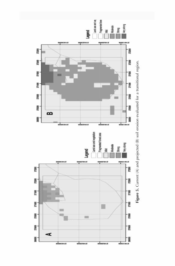
The Environmental Calculator 177
Figu
re 5
. C
urre
nt (
A)
and
proj
ecte
d (B
) so
il er
osio
n ev
alua
ted
for
a tr
ansi
tiona
l re
gion
.
178 Miguel Martínez Tapia et al.
spatial analysis is performed in raster format at pixel level, it allows thecalculation of differentiated prices for soil loss of environmental services.
Economic Value of Changes in Infiltration
The economic evaluation of infiltration also followed three steps. First, anassessment of the amount of water infiltrated under two scenarios is performed;then the costs of that infiltrated water is estimated; and finally, the economicvalue of the reduction of water infiltration is evaluated by adding the costs ofwater to the costs of reforestation. In order to estimate the volume of waterthat is infiltrated by hectare, the procedure for hydraulic balance, which hasbeen described under the technical norm NOM-011-CNA-2000 of the NationalCommission of Water, was followed. Infiltration capacity depends on theforested surface, forest condition, rain availability and soil characteristics.Cartographical records from the National Forest Inventory (SEMARNAT,2000) were used, as well as the records for the annual total precipitation from1950 to 2000 (García-Reyna et al., 2010). To evaluate the differences on netinfiltration due to deforestation, K values of the second scenario were used tocalculate the runoff coefficient. Figure 6 shows how net infiltration is reduced:(A) a fragmented forest; (B) net infiltration (m3); (C) infiltration consideringland use change; and (D) volume that would be lost by the removal of forestcover. This was calculated using the formula:
DCI ha = INA – INE
where DCI ha are differences in cubic metres that are infiltrated in a hectare;INA are Net Infiltration under current conditions, expressed in m3 and INE isthe net infiltration under the evaluated scenario, expressed in m3.
The loss of capacity for water infiltration in a forest of the extension of1858 sq. km that has lost nearly 75% of its tree cover could be around 1400.00m3 of water. This estimated reduction of water infiltration capacity DCI ha isused for the economic valuation of infiltration reduction. The amount of non-infiltrated water is multiplied by the prices that Mexican government definesconsidering both the aggregated value of water, and its availability. To do so,Mexico has been divided into regions, and on each one a price has been givento a cubic metre of water. The regions belonging to zone 1 are labelled as lowavailability or high demand, whereas the 9th zone represents the oppositeconditions. Considering that this area belongs to zone 5, the cost for a cubicmeter of water is 5.5053 MXN, according to the equation
CAI = PM × DCI ha
where CAI are the costs of infiltrated water, PM is the price for a cubic metreof water, and DCI ha are differences in cubic metres infiltrated in a hectare.These costs are added to the costs of reforestation in order to obtain total costs
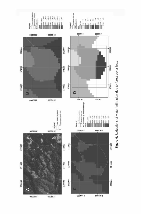
The Environmental Calculator 179
Figu
re 6
. R
educ
tions
of
wat
er i
nfilt
ratio
n du
e to
for
est
cove
r lo
ss.

180 Miguel Martínez Tapia et al.
of the reductions in water infiltration. Reforestation costs were estimated byhectare and the concepts for cleaning, digging, distribution of materials, seedlingcosts, and transportation were taken into account. In the region, these costsreach the amount of 1360.00 MXN. Such costs are included in the formula
DI = CR + CAI
where DI stands for reductions on infiltration, CR are reforestation costs, andCAI the costs of infiltrated water. The maximum cost for loss of water infiltrationthat can be obtained in this region is 9829.85 MXN per hectare, while theminimum cost is 1360.00 MXN per hectare. It is also feasible to obtaindifferentiated values for the economic value associated to loss of waterinfiltration.
Economic Valuation of the Variations of Carbon Sequestration
The amount of carbon that can be sequestrated was calculated using thecarbon sequestration model under the current condition and the land usechange scenario (Table 4). Prospective carbon sequestration was subtracted ofthe current carbon sequestration, and the following formula applied
DCCO2 = (CP + PICO2)
where DCCO2 are reductions of the amount of CO2 that is sequestrated; CPprotection costs, and PICO2 international price for carbon sequestration. Thecost of protection was considered to be equal to the amount that local authorityspends on forest vigilance to protect the study area, where only one ForestGuard has been paid for 144 days, at a price of 60 MXN a day, which meansthat the Local Authority has invested 8640 MXN. The international price ofcarbon sequestration PICO2 is estimated on a surface basis. The cost is givenper hectare considering the potential for carbon sequestration of a specificsite. In this study area, according to the models of carbon sequestration andthe forest cover density and preservation, the cost was estimated to be 14 USDper hectare, as
PICO2 = (CT × PS/Ha)
where PICO2 is international price of carbon sequestration, Ct is theinternational price per ton, and Ps/ha is the total amount of carbon that can bepotentially sequestrated by the forest surface (ha). With these considerations,the maximum cost by the reduction of carbon sequestration is 8966.85 MXN,and the minimal cost is 8640 MXN per hectare.
Economic Value of the Loss of Environmental Services
Having estimated the environmental value of increased erosion, decreasedwater infiltration and decreased carbon sequestration that are associated to
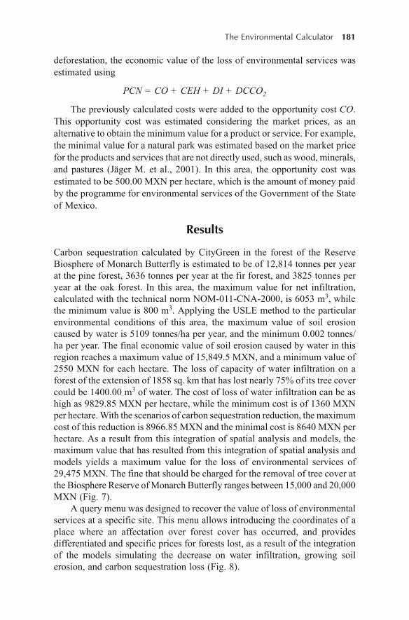
The Environmental Calculator 181
deforestation, the economic value of the loss of environmental services wasestimated using
PCN = CO + CEH + DI + DCCO2
The previously calculated costs were added to the opportunity cost CO.This opportunity cost was estimated considering the market prices, as analternative to obtain the minimum value for a product or service. For example,the minimal value for a natural park was estimated based on the market pricefor the products and services that are not directly used, such as wood, minerals,and pastures (Jäger M. et al., 2001). In this area, the opportunity cost wasestimated to be 500.00 MXN per hectare, which is the amount of money paidby the programme for environmental services of the Government of the Stateof Mexico.
Results
Carbon sequestration calculated by CityGreen in the forest of the ReserveBiosphere of Monarch Butterfly is estimated to be of 12,814 tonnes per yearat the pine forest, 3636 tonnes per year at the fir forest, and 3825 tonnes peryear at the oak forest. In this area, the maximum value for net infiltration,calculated with the technical norm NOM-011-CNA-2000, is 6053 m3, whilethe minimum value is 800 m3. Applying the USLE method to the particularenvironmental conditions of this area, the maximum value of soil erosioncaused by water is 5109 tonnes/ha per year, and the minimum 0.002 tonnes/ha per year. The final economic value of soil erosion caused by water in thisregion reaches a maximum value of 15,849.5 MXN, and a minimum value of2550 MXN for each hectare. The loss of capacity of water infiltration on aforest of the extension of 1858 sq. km that has lost nearly 75% of its tree covercould be 1400.00 m3 of water. The cost of loss of water infiltration can be ashigh as 9829.85 MXN per hectare, while the minimum cost is of 1360 MXNper hectare. With the scenarios of carbon sequestration reduction, the maximumcost of this reduction is 8966.85 MXN and the minimal cost is 8640 MXN perhectare. As a result from this integration of spatial analysis and models, themaximum value that has resulted from this integration of spatial analysis andmodels yields a maximum value for the loss of environmental services of29,475 MXN. The fine that should be charged for the removal of tree cover atthe Biosphere Reserve of Monarch Butterfly ranges between 15,000 and 20,000MXN (Fig. 7).
A query menu was designed to recover the value of loss of environmentalservices at a specific site. This menu allows introducing the coordinates of aplace where an affectation over forest cover has occurred, and providesdifferentiated and specific prices for forests lost, as a result of the integrationof the models simulating the decrease on water infiltration, growing soilerosion, and carbon sequestration loss (Fig. 8).
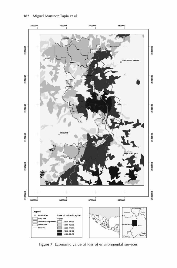
182 Miguel Martínez Tapia et al.
Figure 7. Economic value of loss of environmental services.
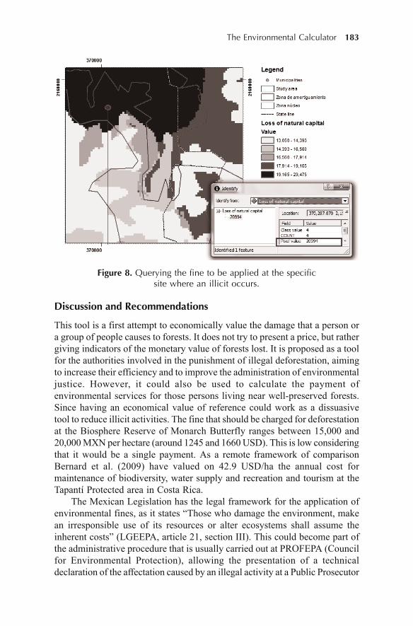
The Environmental Calculator 183
Figure 8. Querying the fine to be applied at the specificsite where an illicit occurs.
Discussion and Recommendations
This tool is a first attempt to economically value the damage that a person ora group of people causes to forests. It does not try to present a price, but rathergiving indicators of the monetary value of forests lost. It is proposed as a toolfor the authorities involved in the punishment of illegal deforestation, aimingto increase their efficiency and to improve the administration of environmentaljustice. However, it could also be used to calculate the payment ofenvironmental services for those persons living near well-preserved forests.Since having an economical value of reference could work as a dissuasivetool to reduce illicit activities. The fine that should be charged for deforestationat the Biosphere Reserve of Monarch Butterfly ranges between 15,000 and20,000 MXN per hectare (around 1245 and 1660 USD). This is low consideringthat it would be a single payment. As a remote framework of comparisonBernard et al. (2009) have valued on 42.9 USD/ha the annual cost formaintenance of biodiversity, water supply and recreation and tourism at theTapantí Protected area in Costa Rica.
The Mexican Legislation has the legal framework for the application ofenvironmental fines, as it states “Those who damage the environment, makean irresponsible use of its resources or alter ecosystems shall assume theinherent costs” (LGEEPA, article 21, section III). This could become part ofthe administrative procedure that is usually carried out at PROFEPA (Councilfor Environmental Protection), allowing the presentation of a technicaldeclaration of the affectation caused by an illegal activity at a Public Prosecutor
184 Miguel Martínez Tapia et al.
Office, including affectations to forests, soil and water. Thus, the environmentalfine is a mechanism of value transference for the regeneration of naturalresources that are affected by an environmental irregularity. To effectivelyoperate, a mechanism to carry out a follow-up of the money received throughthe fine and an effective application of such resources for the protection andrestoration of the reserve shall be operated by PROFEPA. Properlyinstrumented, this mechanism would imply an improvement of forest conditionsby the generation of a fund to finance the activities of vigilance, reforestation,and soil restoration, among others. The application into other countries wouldrequire the proper legal framework and institutional infrastructure. In thisspecific case the feasibility to implement this tool is high due to the fact thatthis reserve has a huge biological importance (for the presence of MonarchButterfly), but also a key role as income generator through ecotourism. Themain author of this work has been working on this tool diffusion andacceptation.
Conclusions
Geographic information technologies can be successfully adapted to the legaland policy framework and procedures for the economic evaluation of loss ofenvironmental services. This could ultimately aid in the process of forestvigilance and restoration at the Biosphere Reserve of Monarch Butterfly,through the calculation of an appropriate fine for deforestation, consideringthe associated loss of environmental services. Indeed, it could be establishedin other natural protected areas of Mexico. The unavailability of cartographicalvalues representing differential prices of the economic value of environmentalservices that forest provides makes it difficult to use said resources on asustainable basis; therefore detailed, integrative and spatially focussed studieson the value of environmental services which forests provide are required.These should take advantage of the emerging technologies of geographicinformation to collect and process data regarding the state, processes andvalues of environmental services, and also must incorporate the social,economical and institutional framework to generate sound initiatives for thepeculiarities of each country and region. Increasing and improving the strategiesto preserve our remaining forests using the best of our knowledge andtechnologies is still a priority for our world management agenda.
References
Angulo-Carrera, A., De Jesús-Apolinar B., Duran-Gálvez B., González-Jácome, O.,Leyva-López J.A., Martínez-Tapia M., Moreno-Cárdenas G. and Valdés-Muciño, I.(1997). Cuenta patrimonial del recurso suelo en la reserva de la biósfera mariposamonarca. Centro de Monitoreo y Evaluación de Daños a los Recursos Naturales.Internal document SEMARNAP-PROFEPA.
The Environmental Calculator 185
Baskin, Y. (1997). The Work Of Nature: How The Diversity Of Life Sustains Us.Washington: Island Press.
Bernard, F., De Groot, R. and Campos J.J. (2009) Valuation of tropical forest servicesand mechanisms to finance their conservation and sustainable use: A case study ofTapantí National Park, Costa Rica. Forest Policy and Economics, 11, 174–183.
Comisión Nacional de Áreas Naturales Protegidas. (2001). Programa de Manejo de laReserva de la Biosfera Mariposa Monarca. CONABIO. Mexico 139 pp.
Cornejo, T., Casas, G.A., Farfán, B., Villaseñor, J. and Ibarra G. (2003). Flora yVegetación de la zona núcleo de la Reserva de la Biosfera de la Mariposa Monarca.Bol. Soc. Bot. Mex, 73, 43–62.
Cortés, T. H. (1991). Caracterización de la erosividad de la lluvia en México utilizandométodos multivariados. Master degree thesis. Colegio de Postgraduados,Montecillos, Mexico. 168 pp.
Croitoru, L. (2007). How much are Mediterranean forests worth? Forest Policy andEconomics, 9, 536–545.
Diario Oficial de la Federación (2000). NORMA OFICIAL MEXICANA NOM-011-CNA-2000, Conservación del Recurso Agua que Establece las Especificaciones yel Método para determinar la Disponibilidad Media Anual de las Aguas Nacionales.Gobierno Constitucional de los Estados Unidos Mexicanos. April 7th 2002. Mexico.
Diario Oficial de la Federación (2000). Decreto de la Reserva de la Biosfera MariposaMonarca. Gobierno Constitucional de los Estados Unidos Mexicanos. November10th 2000. Mexico.
Domínguez-Cortazar, M.A. and Ventura-Ramos E. (2001). Evaluación del riesgo deerosión hídrica en el estado de Querétaro. Informe Técnico para la Secretaria delMedio Ambiente y Recursos Naturales, Delegación Querétaro. Facultad deIngeniería, División de Estudios de Posgrado, Universidad Autónoma de Querétaro.
Elsasser, P., Meyerhoff, J., Montagne, C. and Stenger, A. (2009). A bibliography anddatabase on forest benefit valuation studies from Austria, France, Germany andSwitzerland – A possible base for a concerted European approach. Journal ofForest Economics, 15, 93–107.
García-Reyna, M.E. and Martínez-Ramón, O. (2010). Temperatura y Precipitaciónmedia anual, Sistema de Consulta a la Base de Datos del Servicio MeteorológicoNacional. Tesis de Licenciatura. Facultad de Geografía, Universidad Autónomadel Estado de México. Toluca, Mexico. 100 p.
Goio, I., Gios, G. and Pollini C. (2008). The development of forest accounting in theprovince of Trento (Italy). Journal of Forest Economics, 14, 177–196.
Gómez-Jiménez, I., Martínez de Anguita P. and Romero-Calcerrada, R. (2008).Evaluación de la viabilidad del uso de los métodos de valoración económico-ambiental en un contexto espacial. UNED. Espacio, Tiempo y Forma. Serie VI.No. 1.
Jäger M., García-Fernández, J., Cajal, J., Burkart, R. and Riegelhaupt, E. (2001).Valoración económica de los bosques Revisión, evaluación, propuestas. Fundaciónpara la Conservación de las Especies y el Medio Ambiente, FUCEMA. InformeFinal para la Unión Mundial para la Naturaleza, UICN Oficina Regional paraAmérica del Sur.
Lange, G.-M. (2004). Manual for Environmental and Economic Account for forestry:a tool for crosssectoral policy analysis. Working Paper, FAO, Forestry Department,Rome.
186 Miguel Martínez Tapia et al.
Leff E. (2004). Racionalidad ambiental, La reapropiación social de la naturaleza, Lateoría objetiva del valor, la revolución científico-tecnológica y las fuerzasproductivas de la naturaleza. Siglo XXI Editores, S.A de C.V. Mexico, D. F. 1-43p.
Lindhjema, H. (2007). 20 years of stated preference valuation of non-timber benefitsfrom Fennoscandian forests: A meta-analysis. Journal of Forest Economics, 12,251–277.
Martínez-Alier, J. and Roca-Jusmet, J. (2006). Economía Ecológica y PolíticaAmbiental. Colección Economía, 2ª edición, Mexico. 489 p.
Martínez-Tapia M. (2003). Pago de servicios ambientales en el estado de Querétaro.Internal document. SEMARNAT, Querétaro. Mexico. 110 p.
McComba, G., Lantz, V., Nash K. and Rittmaster, R. (2006). International valuationdatabases: Overview, methods and operational issues. Ecological Economic, 60,461–472.
Mobayed, K.N. and Soto-Ávila, A. (2002). Sistema Hidro-fisiográfico del estado deGuanajuato. Seminario “intercambio del conocimiento y experiencias en el manejodel recurso hídrico. Guanajuato, Mexico. Retrieved May 2010 http://seia.guanajuato.gob.mx/panel/document/vinculos/doc1870/A20207.pdf.
Myers, N. (1997). The World’s Forests and Their Ecosystem Services. En: G. Daily(ed.). Nature’s Services: Societal Dependence on Natural Ecosystems. Island Press,Washington.
Nengwang, Ch., Huancheng, L., Lihong, W.(2009). A GIS-based approach for mappingdirect use value of ecosystem services at a county scale: Management implications.Ecological Economics, 68, 2768–2776.
Patterson, T. and Coelho, D. (2009). Ecosystem services: Foundations, opportunities,and challenges for the forest products sector. Forest Ecology and Management,257, 1637–1646.
Pearce, D.W. and Turner, K.H. (1995). Economía de los Recursos Naturales y delMedio Ambiente. Celeste, Madrid.
PROFEPA (2001). Informe Final del Operativo Mariposa Monarca. (Documentointerno). Procuraduría Federal de Protección al Ambiente. México. 15 p.
Ramos-Taipe, C. L. (2001). Modelamiento Ambiental para análisis de susceptibilidaderosiva en la cuecna media y alta del Río Cañete y Determinación del Mapa deErosión. Universidad Nacional Agraria Molina. Retrieved September 2009 http://tarwi.lamolina.edu.pe/~cramostMODELO%20DE%20EROSION% 20HIDRICA%20-%20SIG.pdf.
Rivera, Ruiz (2005). Curso-Taller-Práctico para formar promotores técnicos en“Diseño y establecimiento de prácticas conservacionistas para la cuenca VillaVictoria”. Comisión Nacional del Agua, Gerencia Regional de Aguas del Valle deMéxico y Sistema Cutzamala, Gerencia de Organismos del Agua.
Roper, C.S. and Park, A. (Editors) (1999). The Living Forest: Non-Market Benefits ofForestry. Proceedings of an International Symposium. Edinburgh 24-28 June 1996,Forestry Commission. London: HMSO.
Sanaphre-Villanueva, L. and Ventura-Ramos, J. (2003). Evaluación de la erosiónhídrica en la microcuenca San Pedro (Huimilpan, Querétaro) y selecciónmulticriterio de especies de vegetación nativa para su control. UniversidadAutónoma de Querétaro. Retrieved October 2009: http://www.ine.gob.mx/descargas/cuencas/cong_nal_06/tema_03/19_lucia_sanaphre.pdf.

The Environmental Calculator 187
Schmidt, R., Berry, J.K. and Gordon, J.C. (Editors) (1999). Forests to Fight Poverty:Creating National Strategies. Yale University Press, New Haven.
Sharma, N.P. (ed.) (1992). Managing the World’s Forests: Looking for Balance BetweenConservation and Development. Ames: Kendall/Hunt Publishing Company.
Sherrouse, B., Clement J.M. and Semmens, J.D. (2010). A GIS application for assessing,mapping, and quantifying the social values of ecosystem services. AppliedGeography, 1, 13. In press.
Stenger, A., Haroub, P. and Navrud, S. (2009). Valuing environmental goods andservices derived from the forests. Journal of Forest Economics, 15, 1–14.
Troy, A. and Wilson, M. (2006). Mapping ecosystem services: Practical challengesand opportunities in linking GIS and value transfer. Ecological Economics, 60,435–449.
WWF. Programa México (2004). La tala ilegal y su impacto en la Reserva de labiosfera Mariposa monarca. Report. WWF-Programa México. Retrieved August2006 http://eco-index.org/search/pdfs/363report_2.pdf
Cartography• SEMARNAT (2000). National Forest Inventory. Scale 1:250,000. Secretaría de
Medio Ambiente y Recursos Naturales, Mexico.• INEGI (1980). Soil chart. Scale 1:250,000. Instituto Nacional de Estadística y
Geografía. Aguascalientes, Mexico.• INEGI (1976). Topographical map. Scale 1: 50000. Charts: E14a15, E14a16,
E14a25, E14a26, E14a35, E14a36. Instituto Nacional de Estadística y Geografía.Aguascalientes, Mexico.
• Secretaría de Marina. SPOT 4 Satellite Imagery. HERMEX, Mexico. February2006.
Software used: ArcView 3.3 ™ by ESRI., City green ™ by American Forester Org.,and ArcMap 9.3 ™ by ESRI.
188 Arun Kumar Pratihast and Jay Krishna Thakur
12Urban Tree Detection Using Mobile
Laser Scanning Data
Arun Kumar Pratihast and Jay Krishna Thakur1
ITT, Cologne University of Applied Science, Cologne, Germany; andCenter for Geo-information, Wageningen University
Wageningen, The Netherlands1Department of Hydrogeology and Environmental Geology, Institute of
Geosciences, Martin Luther University, Halle, Germany
Introduction
Nearly half of the world’s population (47 per cent) lives in urban areas and isexpected to grow by two per cent per year during 2000-15 (UN, 2001). Urbantrees are essential data sets for studies on urban biomass, ecological function,water budgets and radiation transfer in an urban system. Furthermore, it isalso useful for 3D cadastre and 3D city models used by planners andenvironmentalists for planning, modelling and ecological assessments of thecity.
Traditionally, optical remote sensing methods have been usedfor acquisition of urban data sets. These data sets have been extensivelyused for tree identification, 3D modelling, and biomass estimation.An advantage of these methods is that the data is being collected for alarge area in a single attempt. Whereas the disadvantages of these methodsinclude comparatively coarse resolutions and some shadow effect on all theoptical images. Therefore, it is complicated to identify the single tree pixeland also two-dimensional measurements is not sufficient to determine canopystructure.
Nowadays, laser scanning is a well-established technology to acquire thethree dimensional data. Several experiments have been carried to detect thetree and estimation of tree geometry parameters such as canopy height, crownwidth and foliage for the forest monitoring applications and modelling of 3Dtree using airborne as well as terrestrial laser scanning (TLS) data (Buckschand Lindenbergh, 2008; Mallet and Bretar, 2009; Rosell et al., 2009; Vauhkonenet al., 2009).
DOI 10.1007/978-94-007-1858-6_12, © Capital Publishing Company 2012
188e ,J.K. Thakur et al. (eds.), G ospatial Techniques for Managing Environmental Resources
Urban Tree Detection Using Mobile Laser Scanning Data 189
Mobile laser scanning (MLS), an extension of Terrestrial Laser Scanning(TLS) technique, is emerging nowadays. This technique captures highly dense3D point cloud of larger urban areas in a rapid and cost effective way (Norbertet al., 2008). The point density of these MLS data depends upon speed ofthe vehicles, sensor configuration and season of the acquisition. Limitedresearch has been done to extract the information and model the tree fromthese data sets (Pratihast, 2010; M. Rutzinger et al., 2010; Ussyshkin, 2009).In this context, taking account of the problems and suggestions given byprevious researches and taking the advantages of MLS data, the aim of thischapter is to describe an automatic method that can detect the tree in urbanareas.
Laser Scanning
Laser scanning is an active remote sensing technology used for mappingtopography, vegetation, urban areas, ice and infrastructures. The scanner usedis an active sensor that measures the distance from the sensor to the ground onwhich the laser beam is reflected. It uses the time of flight measurementprinciple to capture the three dimensional structure of the earth surface. Themain working principle in this scanning is range measurement. The approachesto measure distance with lasers range finding are time-of-flight andtriangulation. In time of flight measurement, time elapsed between the emittedlaser pulse and reflected pulse back to the photosensitive sensor is measured.If t is the amount of time taken by laser pulse to travel and return back tosensor and c is the speed of light, then d is the distance of object, which isapproximately half the distance travelled by the laser pulse. Followingmathematical relation is being used to calculate the d:
d = c × t/2 (1)
Precision in distance measurement is improved by applying phase shiftmeasurement. The phase shift between transmitted and received signal iscalculated by:
r = ')/(23) × J/2 + J/2 × n (2)
where ') is the phase difference measured in radian, J is the wavelengthmeasured in metre and n is number of full waveform between the sensor andobject surface. Range is determined via angle measurement instead of directmeasurement to have higher precision with laser scanning. Two laser beamsproduced by either separate laser or formed by splitting of the single laserbeam is used for triangulation. Based on the source position, the angle ofintersection between two laser beams is measured and finally the distance totarget object is calculated. Collected data of laser scanning, called point
190 Arun Kumar Pratihast and Jay Krishna Thakur
cloud, contains three dimensional information (X, Y, Z) and reflection intensityvalue.
The first air-borne platforms for terrain measurement using laser scanninghad been done in the early 1965 (Miller, 1965). Air-borne laser scanningcombining with GPS and inertial navigation system were started in 1988(Lindenberger, 1989). With the advancement in the development of sensors inthe recent years, collection of multiple echo and full waveform of reflectedrays is easier and accurate. The accuracy of ALS increases up to a fewcentimetres (Mallet and Bretar, 2009). Terrestrial laser scanning (TLS) wasstarted in late 1990’s as an alternative way of laser scanning which is usedto capture the 3D information of complex surfaces in high speed and oftenin accessible environment. Based on the sensor movement, there are twotypes of terrestrial laser scanning techniques namely static and mobile laserscanning.
Static Terrestrial Laser Scanning
The static terrestrial laser scanning is used for the measurement of buildings,bridges and tunnel facilities and energy infrastructures development. Thescanners used in this type of laser scanning are fully integrated with highquality digital cameras. Obtained point clouds are highly dense and accurate.Scanning is independent of weather conditions.
Mobile Laser Scanning
Mobile laser scanning (MLS) is a dynamic means of terrestrial laser scanningused to capture highly accurate and high resolution dynamic 3-dimensionalspatial data at normal traffic speeds. One or several scanners mounted on amobile platform are used to acquire the point cloud. These mobile platformsmight be car, train or vessel. Shan and Toth (2008) published a comprehensivestudy on current devices and specification of mobile platform. During thescanning, a rotating mirror (scanner) deflects the laser beam across the drivingdirection and the swath terrain along the driven direction is recorded. Runtimemeasurement is conducted for the calculation of distance to the surface. Figure1 shows the field of view of MLS sensors. The recorded point cloud is highlydense and complete georeferenced which has high potential in the corridormapping (Barber et al., 2008) and 3D modelling of urban environment liketree, building and poles (N. Haala et al., 2008; Ussyshkin, 2009). The vehicle-based MLS used for the data acquisition in this research is shown in Fig. 1.The main elements of mobile laser scanning are Differential GPS, Inertialmeasurement unit (IMU), Distance measurement instrument (DMI) asOdometer, Software and hardware for registering and processing data, laserscanner(s) and/or digital camera(s) and/or video camera(s).
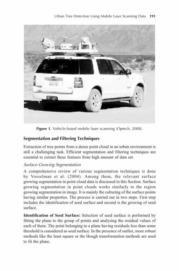
Urban Tree Detection Using Mobile Laser Scanning Data 191
Figure 1. Vehicle-based mobile laser scanning (Optech, 2008).
Segmentation and Filtering Techniques
Extraction of tree points from a dense point cloud in an urban environment isstill a challenging task. Efficient segmentation and filtering techniques areessential to extract these features from high amount of data set.
Surface Growing Segmentation
A comprehensive review of various segmentation techniques is doneby Vosselman et al. (2004). Among them, the relevant surfacegrowing segmentation in point cloud data is discussed in this Section. Surfacegrowing segmentation in point clouds works similarly to the regiongrowing segmentation in image. It is mainly the culturing of the surface pointshaving similar properties. The process is carried out in two steps. First stepincludes the identification of seed surface and second is the growing of seedsurface.
Identification of Seed Surface: Selection of seed surface is performed byfitting the plane to the group of points and analysing the residual values ofeach of them. The point belonging to a plane having residuals less than somethreshold is considered as seed surface. In the presence of outlier, more robustmethods like the least square or the Hough transformation methods are usedto fit the plane.
192 Arun Kumar Pratihast and Jay Krishna Thakur
Growing of Seed Surface: Once the seed surface is identified, the growing ofthe seed surface towards the neighbourhood points is done based on theproximity, global planarity and smooth normal vector field.
Proximity of points: The points, which are within a certain distance fromthe selected seed surface, are added to the surface. 2.5 D and TIN data structuresare used to identify the points on the surface.
Locally planar: For this, first the equation of enclosed plane through allthe surface points within the radius is determined. A candidate point is selectedfrom surface points. The selection criterion is based on the orthogonal distanceof a point to the plane. The point within this distance is selected if all theneighbouring points in a plane are below some threshold value.
Smooth normal vector field: To implement these criteria, local surfacenormal for each point in the point cloud is calculated. A candidate point ischosen if the angle between the normal of growing surface and local normalof point is below some threshold value.
Rabbani et al. (2006) presents the smoothness constraint to segment theunstructured point cloud of industrial scene. The method is based on twosteps, local surface estimation and surface growing. Local surface normal isestimated by fitting the plane to neighbourhood points based on the k-nearestneighbourhood (KNN) or the fixed distance neighbourhood (FDN). KNNuses K-D tree data structure to create adjacency information of points bymaintaining a list of indices for each neighbourhood points. FDN considers agiven fixed Area of Interest (AOI), and selection is done within the area foreach query point. The surface growing of segment is performed based on thecalculated norms and its residuals. In this phase, additional points are addedto the segment based on the proximity and smoothness criteria of the surface.
Filtering Ground Points
Different approaches for identification and filtering ground and no groundpoints in ALS datasets are proposed in different literatures. Vosselman (2000)proposed a slope based filtering method for the identification of ground pointsby comparing slopes between the laser point and its neighbours. The workingprinciple of this algorithm is closely related to the erosion operator used inmathematical morphology. A point is classified as a ground if the calculatedslopes value between a point and its neighbourhood point is less than apredefined threshold. The critical step in this method is setting of slopethreshold, by using prior knowledge of the terrain, which is somewhatsubjective. The improvement is done by using progressive morphologicalfilter (Zhang et al., 2003). The method utilizes different windows size for theidentification of ground and no ground surface from laser scanning data. Thefiltering results are satisfactory in both the urban and mountainous areas;however selection of windows size is a difficult task.
Several attempts have been made for the improvement of slope-basedfilter. Slope adaptive neighbourhood method was proposed as a modification

Urban Tree Detection Using Mobile Laser Scanning Data 193
of the slope-based filter to correct the problem regarding the steep slopedterrain (Filin and Pfeifer, 2006). Cluster-based segmentation approach is usedfor computing the features like normal vector and the classification of surfacebased on the similar orientation. It has improvement over the feature qualityso the segment tends to be greater with respect to triangulation-basedsegmentation. A slope-based planar-fitting filtering algorithm for data filteringand feature extraction in urban area is presented by Qihong (2008). Theirmethods analyse the spatial distribution of laser point cloud. This study usesa plane fitting algorithm. It fits the horizontal planes for filtering the groundpoints and vertical planes for the building walls in the urban areas. Meng,Wang et al. (2009) explore the Multi-directional ground filtering (MGF)algorithm which is sensitive to detect steep slopes as it integrates the advantagesof neighbourhood-based and directional scanning approaches. The majorlimitation of these algorithms is on the assumption of slope difference. Mostof these slope-based algorithms assume that the slope difference between theground point to another neighbouring point are gradual. However, these areabrupt in reality. The scan line directly produces an elevation or slope profilefor each scan line. An adaptive filtering technique for identification of groundpoints by utilizing the slope threshold of a profiler has been proposed inSithole and Vosselman (2001). The scan line technique produce a slope profilefor each scan line, which is useful for the identifications of ground pointsalong the profiles. Elevation differences along scan lines are used by Sitholeand Vosselman (2005) for the identification of ground and non-ground pointsalong the scan lines. The major drawback of these approaches is that the resultis highly influenced by the choice of filtering direction.
Urban Tree Point Cloud Detection
An urban area is a heterogeneous composition of objects like tree, building,poles, vehicles etc. Several researches have been done for the detection andfiltering of these objects. Haala and Brenner (1999) proposed an integratedclassification approach from the multi spectral images and laser altimetry datafor the extraction of urban objects like building, tree and grass covered area.The algorithm requires normalised DSM derived from laser data to get theheight information of each image pixel. The morphological filtering operationto detect and filter urban objects was used by Chen et al. (2007). Their methodperformed well even in many complicated objects such as large buildings,steep slopes, bridges, ramps and vegetation on steep slopes. However, themain limitation of this method is every data sets, parameters should be specifiedon trial and error basis, which leads to more manual iteration.
Normalized difference vegetation index (NDVI) is a numerical indicator,used by researchers to detect the vegetation in urban environment. Lovan etal. (2007) detect the urban vegetation by combining NDVI and saturationindex (SI) from a high resolution aerial image and a DSM with 20 cm resolutionin an automatic way. Tao and Yasuoka (2002) used high resolution satellite
194 Arun Kumar Pratihast and Jay Krishna Thakur
imagery and ALS data for the detection of urban tree. The methods use digitalelevation model (DEM) derived from ALS data. There is a limitation in thecalculation of NDVI value due to a number of perturbing factors includingspectral effects, atmospheric effects, clouds, soil effects etc.
Derivative approach was used to separate building and tree by Morganand Tempfli (2000). The main concept behind this algorithm was: canopystructure of tree was irregular whereas roof surface of buildings were consideredas planer. The first and second derivatives of an irregular surface should bevariable whereas the first derivatives planar surfaces were either zero in flatroof case or constant in sloped roof case, and the second derivatives of asloped planar surface were zero. These methods are not free from limitationsbecause of the small features such as chimneys or water tanks that introducethe discontinuity in the measurement and finally lead to abnormal derivativesvalue.
Laser scanning systems have the capability to record the multiplereflections caused by the objects on the earth’s surface. Alharthy and Bethel(2002) used the difference between the first and last echo to separate buildingand tree. Tovari and Vogtle (2004) had implemented a fuzzy logic approachbased on first and last echo differences to classify vegetation. The differenceis generally larger for tree and close to zero for building measurements.However, their method does not work well for dense trees area where laserpulses cannot penetrate.
Object-based point cloud analysis (OBPA) was used for the detection ofurban vegetation by M. Rutzinger et al. (2007). The presented algorithm usedsurface roughness, the ratio between 3D and 2D point density and the statisticson first and last echo occurrence within the segments for the extraction ofobjects. The main advantage of this method is that it does not require DTMcalculation. Their algorithm has limitations over heterogeneous distributionof point cloud.
Data Sets and Test Site
Implementation of developed algorithm was done on two data sets havingdifferent point density. Data set contains both deciduous and coniferous speciesof tree. The following sub section explains the details of both data sets.
Data Set and Test Site I
The first data set was acquired with a LYNX Mobile Mapper V100 system(Optech, 2008) by surveying eight kilometre long track city of Enschede, TheNetherlands in 2008. The scanning system consists of two 360° rotating lasersensors mounted at the backside of the vehicle orientated diagonal to eachother. The sensor setup is proven to be minimal shadow effects and safer touse. The manufactory information of the sensor is shown in Table 1.
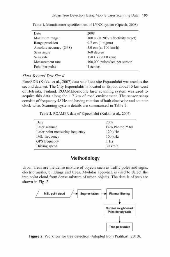
Urban Tree Detection Using Mobile Laser Scanning Data 195
Table 1. Manufacturer specifications of LYNX system (Optech, 2008)
Date 2008Maximum range 100 m (at 20% reflectivity target)Range precision 0.7 cm (1 sigma)Absolute accuracy (GPS) 5.0 cm (at 100 km/h)Scan angle 360 degreeScan rate 150 Hz (9000 rpm)Measurement rate 100,000 pulses/sec per sensorEcho per pulse 4 echoes
Data Set and Test Site II
EuroSDR (Kukko et al., 2007) data set of test site Espoonlahti was used as thesecond data set. The City Espoonlahti is located in Espoo, about 15 km westof Helsinki, Finland. ROAMER-mobile laser scanning system was used toacquire this data along the 1.7 km of road environment. The sensor setupconsists of frequency 48 Hz and having rotation of both clockwise and counterclock wise. Scanning system details are summarised in Table 2.
Table 2. ROAMER data of Espoonlahti (Kukko et al., 2007)
Date 2009Laser scanner Faro Photon™ 80Laser point measuring frequency 120 kHzIMU frequency 100 kHzGPS frequency 1 HzDriving speed 30 km/h
Methodology
Urban areas are the dense mixture of objects such as traffic poles and signs,electric masks, buildings and trees. Modular approach is used to detect thetree point cloud from dense mixture of urban objects. The details of step areshown in Fig. 2.
Figure 2: Workflow for tree detection (Adopted from Pratihast, 2010).
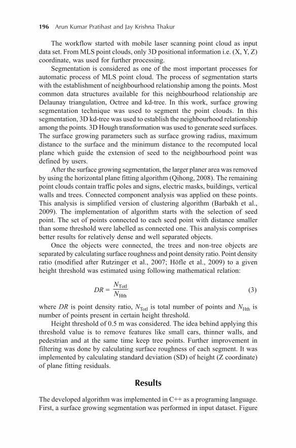
196 Arun Kumar Pratihast and Jay Krishna Thakur
The workflow started with mobile laser scanning point cloud as inputdata set. From MLS point clouds, only 3D positional information i.e. (X, Y, Z)coordinate, was used for further processing.
Segmentation is considered as one of the most important processes forautomatic process of MLS point cloud. The process of segmentation startswith the establishment of neighbourhood relationship among the points. Mostcommon data structures available for this neighbourhood relationship areDelaunay triangulation, Octree and kd-tree. In this work, surface growingsegmentation technique was used to segment the point clouds. In thissegmentation, 3D kd-tree was used to establish the neighbourhood relationshipamong the points. 3D Hough transformation was used to generate seed surfaces.The surface growing parameters such as surface growing radius, maximumdistance to the surface and the minimum distance to the recomputed localplane which guide the extension of seed to the neighbourhood point wasdefined by users.
After the surface growing segmentation, the larger planer area was removedby using the horizontal plane fitting algorithm (Qihong, 2008). The remainingpoint clouds contain traffic poles and signs, electric masks, buildings, verticalwalls and trees. Connected component analysis was applied on these points.This analysis is simplified version of clustering algorithm (Barbakh et al.,2009). The implementation of algorithm starts with the selection of seedpoint. The set of points connected to each seed point with distance smallerthan some threshold were labelled as connected one. This analysis comprisesbetter results for relatively dense and well separated objects.
Once the objects were connected, the trees and non-tree objects areseparated by calculating surface roughness and point density ratio. Point densityratio (modified after Rutzinger et al., 2007; Höfle et al., 2009) to a givenheight threshold was estimated using following mathematical relation:
DR = Totl
Hth
NN (3)
where DR is point density ratio, NTotl is total number of points and NHth isnumber of points present in certain height threshold.
Height threshold of 0.5 m was considered. The idea behind applying thisthreshold value is to remove features like small cars, thinner walls, andpedestrian and at the same time keep tree points. Further improvement infiltering was done by calculating surface roughness of each segment. It wasimplemented by calculating standard deviation (SD) of height (Z coordinate)of plane fitting residuals.
Results
The developed algorithm was implemented in C++ as a programing language.First, a surface growing segmentation was performed in input dataset. Figure
Urban Tree Detection Using Mobile Laser Scanning Data 197
3(a) is the visual representation of input data sets. The parameters of thesegmentation were obtained by trial and error basis to obtain larger plannerground segment area. Table 3 shows the parameters for surface growingsegmentation.
Table 3. Surface growing segmentation parameters used in point cloud mapper
Surface growing parameters ValueSurface model PlanerSurface growing neighbourhood definition Direct neighboursSurface growing radius 0.6 mMaximum distance to surface 0.3 mMinimum distance to recomputed location 0.15 m
The result of surface growing segmentation is shown in Fig. 3(b). It canbe clearly identified that the larger segmented area is a planer region.The larger planer regions were filtered by fitting the horizontal plane toeach segment. Threshold of Angle 10 ° and area 100 m² was used to fit theplane.
Figure 3(c) represents the dataset after removing planer segments.Connected component analysis was performed on remaining data sets. Theparameters used for this analysis are listed in Table 4.
Figure 3. Left: Enschede data set I (Adopted from Pratihast, 2010), Right: EuroSDRdata set II (a. Input data, b. Segmented point clouds, c. Removal of planer
surface, d. Connected component analysis, e. Tree point clouds).

198 Arun Kumar Pratihast and Jay Krishna Thakur
Table 4. Parameters for connected component used in point cloud
Connected component parameters ValueMaximum distance between the points 1.5 mMinimum number of points 10
The result after application of connected component analysis is shown inFig. 3(d). Each unique colour represents each connected segments. Furtherimprovement in filtering was done by using surface roughness and pointcloud density ratio value. The threshold of surface roughness of greater than0.85 and point density ratio larger than 2 was used to select the trees. The finaloutput is shown in Fig. 3(e). From the final output, it is clear that the datasetscontains only the tree point clouds.
Conclusions
It is noticeable that the mobile laser scanning has provided the opportunity tobe of use for larger scale mapping. The developed algorithm has shown potentialto detect the trees inventories in larger data sets. The overall accuracy of thedetected trees in both data sets is 78% and 85%. What our study has shown isthat surface roughness and point density ratio are significant features to separatethe tree and non-tree objects. The detected point clouds are highly suitable for3D tree modelling (Pratihast, 2010; M. Rutzinger et al., 2010; Martin Rutzingeret al., 2011) and urban biomass estimations. More testing of methods is requiredin forest data sets. Further development is required in differentiating bushesand small trees.
Acknowledgement
We would like to thank Optech and EuroSDR for providing data for thisresearch. The authors are also thankful to Faculty of Geo-information Scienceand Earth Observation (ITC), Universiteit Twente, Enschede, The Netherlands,especially Geoinformatics department, for overall research arrangements andvaluable advice during the study.
References
Alharthy, A. and Bethel, J. (2002). Heuristic filtering and 3D feature extraction fromLIDAR data. International Archives of Photogrammetry Remote Sensing and SpatialInformation Science, 34(3/A), 29–34.
Barbakh, W., Wu, Y. and Fyfe, C. (2009). Review of Clustering Algorithms. Non-Standard Parameter Adaptation for Exploratory Data Analysis (pp. 7–28).
Urban Tree Detection Using Mobile Laser Scanning Data 199
Barber, D., Mills, J. and Smith-Voysey, S. (2008). Geometric validation of a ground-based mobile laser scanning system. ISPRS Journal of Photogrammetry and RemoteSensing, 63(1), 128–141.
Bucksch, A. and Lindenbergh, R. (2008). CAMPINO – A skeletonization method forpoint cloud processing. ISPRS Journal of Photogrammetry and Remote Sensing,63(1), 115–127.
Chen, Q., Gong, P., Baldocchi, D. and Xie, G. (2007). Filtering airborne laser scanningdata with morphological methods. Photogrammetric Engineering and RemoteSensing, 73(2), 175.
Filin, S. and Pfeifer, N. (2006). Segmentation of airborne laser scanning data using aslope adaptive neighborhood. ISPRS Journal of Photogrammetry and RemoteSensing, 60(2), 71–80.
Haala, N. and Brenner, C. (1999). Extraction of buildings and trees in urbanenvironments. ISPRS Journal of Photogrammetry and Remote Sensing, 54(2–3),130–137.
Haala, N., Peter, M., Cefalu, A. and Kremer, J. (2008). Mobile lidar mapping forurban data capture. Paper presented at the Conference on Virtual Systems andMultiMedia Dedicated to Digital Heritage, Limassol, Cyprus.
Iovan, C., Boldo, D. and Cord, M. (2007). Automatic extraction of urban vegetationstructures from high resolution imagery and digital elevation model. Urban RemoteSensing Joint Event, 2007, 1–5.
Kukko, A., Andrei, C., Salminen, V., Kaartinen, H., Chen, Y., Rönnholm, P. et al.(2007). Road Environment Mapping System of the Finnish Geodetic Institute–FGIRoamer. Paper presented at the International Archives of Photogrammetry, RemoteSensing and Spatial Information Sciences.
Lindenberger, J. (1989). Test Results of Laser Profiling for Topographic Terrain Survey.Schriftenreihe des Instituts für Photogrammetrie der Universität Stuttgart, 13, 25–39.
Mallet, C. and Bretar, F. (2009). Full-waveform topographic lidar: State-of-the-art.ISPRS Journal of Photogrammetry and Remote Sensing, 64(1), 1–16.
Meng, X., Wang, L., Silvun-Curdenas, J.L. and Currit, N. (2009). A multi-directionalground filtering algorithm for airborne LIDAR. ISPRS Journal of Photogrammetryand Remote Sensing, 64(1), 117–124.
Morgan, M. and Tempfli, K. (2000). Automatic building extraction from airbornelaser scanning data. International Archives of Photogrammetry and Remote Sensing,33(B3/2; Part 3), 616–623.
Norbert, H., Michael, P., Alessandro, C. and Jens, K. (2008). Mobile Lidar MappingFor Urban Data Capture. Digital Heritage – Proceedings of the 14th InternationalConference on Virtual Systems and Multimedia, VSMM, 95–100.
Optech (2008). LYNX Mobile Mapper Data Sheet. http://www.optech.ca/pdf/LynxDataSheet.pdf, accessed on 2-10-2009.
Pratihast, A.K. (2010). 3d tree modelling using mobile laser scanning data. Universityof Twente, Faculty of Geo-Information and Earth Observation ITC, Enschede.
Qihong, Z. (2008). Data filtering and feature extraction of urban typical objects fromairborne lidar point cloud. The International Archives of the Photogrammetry,Remote Sensing and Spatial Information Science, 37 (Part B3b).
Rabbani, T., van den Heuvel, F. and Vosselmann, G. (2006). Segmentation of pointclouds using smoothness constraint. International Archives of Photogrammetry,Remote Sensing and Spatial Information Sciences, 36(5), 248–253.
200 Arun Kumar Pratihast and Jay Krishna Thakur
Rosell, J.R., Llorens, J., Sanz, R., Arnó, J., Ribes-Dasi, M., Masip, J., Escola., A.,Camp, F., Solanelles, F., Gracia, F., Gil, E., Val, L., Planas, S. and Palacin, J.(2009). Obtaining the three-dimensional structure of tree orchards from remote 2Dterrestrial LIDAR scanning. Agricultural and Forest Meteorology, 149, 1505–1515.
Rutzinger, M., Hofle, B. and Pfeifer, N. (2007). Detection of high urban vegetationwith airborne laser scanning data. Proceedings Forestat, Montpellier, France.
Rutzinger, M., Pratihast, A.K., Oude Elberink, S.J. and Vosselman, G. (2010). Detectionand modelling of 3D trees from mobile laser scanning data. In: Proceedings of theISPRS Commission V mid - term symposium : Close Range Image MeasurementTechniques, 21-24 June 2010, Newcastle, UK/ed. by J.P. Mills et al. TheInternational Archives of the Photogrammetry, Remote Sensing and SpatialInformation Sciences (ISPRS), 38(part 5), 520–525.
Rutzinger, M., Pratihast, A.K., Oude Elberink, S.J. and Vosselman, G. (2011). Treemodelling from mobile laser scanning data-sets. The Photogrammetric Record,(10.1111/j.1477-9730.2011.00635.x).
Shan, J. and Toth, C. (2008). Topographic Laser Ranging and Scanning: Principlesand Processing. Taylor and Francis Group.
Sithole, G. and Vosselman, G. (2001). Filtering of laser altimetry data using a slopeadaptive filter. International Archives of Photogrammetry and Remote Sensing,34(3/W4), 203–210.
Sithole, G. and Vosselman, G. (2005). Filtering of airborne laser scanner data based onsegmented point clouds. International Archives of Photogrammetry, Remote Sensingand Spatial Information Sciences, 36(part 3), 12–14.
Tao, G. and Yasuoka, Y. (2002). Combining high resolution satellite imagery andairborne laser scanning data for generating bareland DEM in urban areas.International Archives of the Photogrammetry, Remote Sensing and SpatialInformation Sciences, 30.
Tovari, D. and Vogtle, T. (2004). Classification methods for 3D objects in laser-scanning data. Int. Archives of Photogrammetry and Remote Sensing, 1682–1750.
UN (2001). World urbanization prospects: the 1999 revision – Key findings. Retrieved25.05.2011, from http://www.un.org/esa/population/publications/wup1999/urbanization.pdf
Ussyshkin, V. (2009). Mobile Laser Scanning Technology for Surveying Application:From Data Collection to End-Products. Paper presented at the FIG Working Week,Surveyors Key Role in Accelerated Development Eilat, Israel, 3–8 May 2009.
Vauhkonen, J., Tokola, T., Packal, N.P. and Maltamo, M. (2009). Identification ofScandinavian Commercial Species of Individual Trees from Airborne Laser ScanningData Using Alpha Shape Metrics. Forest Science, 55(1), 37–47.
Vosselman, G. (2000). Slope based filtering of laser altimetry data. InternationalArchives of Photogrammetry and Remote Sensing, 33(B3/2; Part 3), 935–942.
Vosselman, G., Gorte, B., Sithole, G. and Rabbani, T. (2004). Recognising structure inlaser scanner point clouds. International Archives of Photogrammetry, RemoteSensing and Spatial Information Sciences, 46(Part 8), 4–6.
Zhang, K., Chen, S., Whitman, D., Shyu, M., Yan, J. and Zhang, C. (2003). A progressivemorphological filter for removing nonground measurements from airborne LIDARdata. IEEE Transactions on Geoscience and Remote Sensing, 41(4), 872–882.
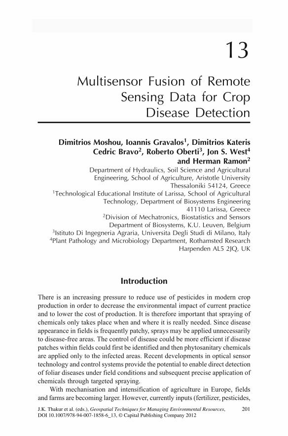
Multisensor Fusion of Remote Sensing Data for Crop Disease Detection 201
13Multisensor Fusion of Remote
Sensing Data for CropDisease Detection
Dimitrios Moshou, Ioannis Gravalos1, Dimitrios KaterisCedric Bravo2, Roberto Oberti3, Jon S. West4
and Herman Ramon2
Department of Hydraulics, Soil Science and AgriculturalEngineering, School of Agriculture, Aristotle University
Thessaloniki 54124, Greece1Technological Educational Institute of Larissa, School of Agricultural
Technology, Department of Biosystems Engineering41110 Larissa, Greece
2Division of Mechatronics, Biostatistics and SensorsDepartment of Biosystems, K.U. Leuven, Belgium
3Istituto Di Ingegneria Agraria, Universita Degli Studi di Milano, Italy4Plant Pathology and Microbiology Department, Rothamsted Research
Harpenden AL5 2JQ, UK
Introduction
There is an increasing pressure to reduce use of pesticides in modern cropproduction in order to decrease the environmental impact of current practiceand to lower the cost of production. It is therefore important that spraying ofchemicals only takes place when and where it is really needed. Since diseaseappearance in fields is frequently patchy, sprays may be applied unnecessarilyto disease-free areas. The control of disease could be more efficient if diseasepatches within fields could first be identified and then phytosanitary chemicalsare applied only to the infected areas. Recent developments in optical sensortechnology and control systems provide the potential to enable direct detectionof foliar diseases under field conditions and subsequent precise application ofchemicals through targeted spraying.
With mechanisation and intensification of agriculture in Europe, fieldsand farms are becoming larger. However, currently inputs (fertilizer, pesticides,
DOI 10.1007/978-94-007-1858-6_13, © Capital Publishing Company 2012
e ,J.K. Thakur et al. (eds.), G ospatial Techniques for Managing Environmental Resources 201
202 Dimitrios Moshou et al.
fungicides) are applied uniformly despite substantial variability in soil type,crop density or disease pressure. Recent developments in agriculturalautomation have made it possible to spatially adjust farm application ofphytosanitary chemicals. New technologies such as the global positioningsystem (GPS) and variable rate spraying systems allow the prospect of PrecisionPest Management (PPM), which aims to target phytosanitary chemicals whereand when needed and at an appropriate dose. PPM could make an importantcontribution by assisting farmers in the reduction of inputs and it could alsosignificantly reduce both residues in produce and environmental contamination.Patchiness can pose a problem to the accurate assessment of disease, whichcould influence the decision to spray and the dose to apply. Methods forassessing the spatial distribution of disease in fields would greatly assist bothspray decision making and spray application. Disease can cause changes intranspiration rate, leaf colour, morphology and crop density, which in turnaffect, to a certain extent, the optical properties of the canopy. Indeed, changesin optical properties have been used to assess visually the risk of diseasefor many years, but such assessments by the farmer or the extensionworker are time consuming and can be relatively inaccurate. Recent progressin sensor technology (Moshou, Bravo, West, McCartney and Ramon, 2004)has made possible the differentiation of diseased and healthy areas of thecrop, and thus the prospect of automatically measuring the spatial distributionof crop diseases.
In the current work, data fusion has been used to improve crop diseasedetection in the field. The data fusion was performed using a Support VectorMachine (SVM) neural network which decreased the error to 1%. The SVM-based disease classifier can be implemented in on-line field disease detection.
Background
Sensing for Disease Detection
There are strong indicators that crop diseases can be detected automatically(Moshou et al., 2004). The carriers of information for detection considered inthis work are electromagnetic waves. The working hypothesis is that healthyplants interact (absorb, reflect, emit, transmit or fluoresce) with electromagneticradiation in a different way compared to infected plants. Plants show differentoptical properties. Some of these differences can be spotted by the naked eye,others are revealed by using advanced equipment. According to Lee et al.(2010), at the earliest infection stages fluorescence is the most appropriatetechnique for fungal disease detection since it samples the health status interms of photosynthetic efficiency. However, fluorescence alone cannot providea clear indication of specific stress factors, having only medium detectionaccuracy, while accuracy is sensitive to light intensity.
Multisensor Fusion of Remote Sensing Data for Crop Disease Detection 203
Following initial metabolic changes, the fungus spreads radially aroundits infection point. The initial infection area necroses: it loses pigmentation,the photosynthetic apparatus is disassembled and the cell walls collapse. Atthis moment infection patterns become visible. According to Lee et al. (2010),analysis of the light reflection can help in detecting infection from this stageonwards. Pathogen propagules can be detected in the visible spectrum (400-700 nm) depending on the pathogen; chlorophyll degradation in the visiblespectrum and red-edge; senescence in the visible spectrum and short-wavenear-infrared (680-800 nm) due to browning and near-infrared (1400-1600nm and 1900-2100 nm) due to dryness and variations in canopy density andleaf area in the short-wave near-infrared.
The disease will gradually take control over the entire plant, which willshow a global stress leading to general closure of the stomata, in order toreduce water losses. This change in transpiration can be monitored bythermographic sensors. However, the overall leaf temperatures change rapidly,and are heavily dependent upon ambient temperature, illumination and wind.Therefore, due to changing environmental factors, thermography gives poorresults when used on proximal sensing platforms.
Previous work on wheat yellow rust detection has been based on singlesensors or fusion of sensor data. Examples include the work of Zhang andDickinson (2001), where fluorescence is used to assess the dynamics of fungalgrowth in wheat. Another approach presented by Bravo, Moshou, West,McCartney and Ramon (2003) concerns the detection of yellow rust in wheatby using spectral information from a spectrograph. This approach was extendedto include the use of neural networks in order to increase detection performance(Moshou et al., 2004). The advantage of using sensor fusion of spectral andfluorescence imaging features has been shown by Moshou et al. (2005). Imageprocessing methods to detect soybean rust from multispectral images underlaboratory conditions have been presented by Cui, Zhang, Li, Hartman andZhao (2010).
Remote Sensing for Crop Disease Detection
Remote sensing either by using satellites, aerial or ground-based platformshas been used extensively for the detection of crop diseases. Myers (1983)reviewed studies on the use of aerial photography for detecting potato lateblight, clitocybe root rot of pecans, bunch disease of pecans, phony disease ofpeaches, corn leaf blight, bacterial blights and root rot in beans, and root rotin cotton and alfalfa fields. Ryerson, Curran and Stevens (1997) reviewedmore aerial photographic studies grouped by four major types of crop diseases:air-borne, seed-borne, insect-borne, and soil-borne. In addition to the abovementioned diseases, they reported that aerial photography has been successfullyused to detect the following diseases: yellow rust of wheat, stem canker inrape, leaf spot and rust of the sugar-bearing crops of beet and cane, mould anddwarf-mosaic virus in corn, virus yellows in sugar beet, barley yellow dwarf

204 Dimitrios Moshou et al.
virus in winter wheat, barley yellow mosaic virus, take-all in winter wheat,and docking disorder root infection in sugar crops. Johnson, Alldredge, Hammand Frazier (2003) investigated the spatial and temporal dynamics of lateblight from colour-infrared (CIR) aerial photographs of five commercial potatofields and they concluded that aerial photography coupled with spatial analysiswas an effective technique to quantitatively assess disease patterns in relativelylarge fields and was useful in quantifying an intensification of aggregationduring the epidemic process on a large scale. Although aerial photography hasbeen the primary remote sensing technique used for study of crop diseases,multispectral and hyperspectral electronic imaging systems have also beenused for this purpose.
Apan, Held, Phinn and Markley (2004) demonstrated that Hyperion satellitehyperspectral imagery can be used to detect the orange rust disease in sugarcane.Du, French, Skaria, Yang, and Everitt (2004) evaluated the potential of air-borne multispectral and hyperspectral imagery for detecting citrus greasyspot. Franke and Menz (2007) evaluated high resolution QuickBird satellitemultispectral imagery and air-borne HyMap hyperspectral imagery for detectingpowdery mildew and leaf rust in winter wheat and their results showed thathigh enough classification accuracies were achieved only when the infectionwas severe at the late crop growth stages.
Pre-mapping of diseases and stresses could also be achieved using air-borne systems. Spatial resolutions down to a few metres are possible fromsatellites and to below 1 m from aircraft (Blakeman, Bryson and Dampney,2000). Current commercial satellite sensing is probably not suitable for earlydisease detection (even if the wavelengths at which data are collected weresuitable) because of limitations in spatial resolution. At best, satellite imagescan be useful by highlighting relatively large areas of disease or other stressesin a crop, which can then be checked by the farmer. In addition, revisit timeand variability in cloud cover could mean that even this simple informationmay not be available when required. Aircraft-mounted systems do not havethese constraints and could be used when required. However, data acquisitionequipment would likely have to be faster, more sophisticated, and moreexpensive than for terrestrial vehicle-mounted systems. Disease maps, whetherproduced by tractor-, aircraft-, or satellite-mounted detection systems, couldbe used to control spray equipment, positioned using GPS or a local referencesystem.
As far as we are aware, practical disease-mapping/spray applicationsystems based on remote sensing are not yet available for any crop/diseasesystem. Cropforecaster™, a service of Infoterra and ZedX (http://www.cropforecaster.com/) offers a comprehensive set of online productsincluding maps and summary statistics of crop status. Products includeinformation on crop stage, acreage, condition and expected yields. Thisinformation is updated on a daily basis thereby quantifying the impacts ofeach day’s weather observations and forecasts.

Multisensor Fusion of Remote Sensing Data for Crop Disease Detection 205
Fusion-based Classifiers in Remote Sensing
Some studies employ SVM classifiers in remote sensing tasks. In some cases,the performance of SVM-based classification is improved through data fusion.Zhang, Huang, Huang and Li (2006) proposed a pixel shape index describingcontextual information of nearby pixels and evaluated its usability for landcover classification using QuickBird data based on SVMs. Pixel shape indiceswere combined with transformed spectral bands such as principal componentanalysis or independent component analysis. They found that fusion of spectraland shape features as well as transformed spectral components in an SVMwere able to improve the accuracy of classification. Mitra, Shankar and Pal(2004) proposed an active learning-based approach to reduce the selectedsupport vectors. Their semi-supervised method gradually created clusters basedon user input. Their method yielded better results than a typical SVM; howeverthe authors cautioned on the sensitivity of the algorithm regarding user-providederroneous labelling. Zhang and Ma (2008) proposed an SVM variant, thePotential SVM as an alternative for multispectral image classification. ThePotential SVM is an attractive variant due to its ability to handle non-Mercerkernels and its mathematical formulation that addresses SVM scalability issues.A fusion approach to classification using extended morphological profileswas proposed in Fauvel, Benediktsson, Chanussot and Sveinsson (2008). Theyevaluated the approach using high spatial/spectral resolution ROSIS data inurban areas based on SVM classification. Ensemble methods for multipleSVM integration were evaluated by Pal (2008).
Multisensor Fusion for Crop Disease Detection
Fields, Plants and Material
Yellow rust patches were established in six plots of winter wheat, 10 × 9 m insize and surrounded by 3 m wide guard rows, and located on IACR-Rothamsted’s experimental farm. Pots (10 cm diameter) containing six winterwheat plants (cv. Madrigal) at the second leaf stage (GS 12) and growing inpotting compost, were dusted with uredospores of pathogen Puccinia striiformis(which causes yellow rust), mixed with 10 parts talcum powder. The plantswere then covered with transparent plastic cloches to maintain a high humidityand were kept at 10 °C. The cloches were removed after two days and theplants were transferred to a glasshouse (14–20 °C). The procedure was repeatedseven days after the first inoculation to ensure that all plants would be wellcolonized. Chlorosis was visible 15 days after the first inoculation (sporulationafter about two weeks). One pot of infected plants was planted at the centre ofeach of the six field-plots, approximately three weeks after the first inoculation.Similar uninoculated plots were used as a control. Forty days later, theinoculated plots had clearly visible patches (plants with over 5% diseaseseverity) of yellow rust approximately 2–3 m in diameter. This was the stageof yellow rust development at which the decision to use pesticides had to be
206 Dimitrios Moshou et al.
made. Measurements of plants infected with yellow rust and healthy plantswere obtained using spectrographic and fluorescence equipment in plots ofwinter wheat. So, a disease spread simulating realistic situation has beenreproduced and examined by experts visually to provide reference data for theautomated classification. The classification accuracy of the automatedclassification has been tested against expert visual inspection.
Spectral Equipment and Data Acquisition
The spectral equipment used during the experiments consisted of a JAI CV-M300 digital visual monochromatic camera on which a V9 Specim spectrograph(Herrala, Okkonen, Hyvarinen, Aikio and Lammasniemi, 1994) was mounted.The spectrograph measured a line on the canopy. The length of the measuredline was 0.5 m and its width was 4 mm. For every single area of 0.65 mm by4 mm along this line the spectrograph projected a spectrum (between 460-900nm) onto the camera. The projections from all these small areas created aspectral image, with spectral and spatial axes. Light was directed through aCanon 13 mm 1:1.5 C-mount objective into the spectrograph. An irradiationreference of 50% reflectance (Spectralon SRS 50-010, 1.25� diameter, constant50% reflectance over the 300-2500 nm band) was placed at a constant verticaldistance of 70 cm from the objective. It had a flat surface and was positionedhorizontally. The equipment was fixed on a buggy, and it was possible tomaintain a constant distance between objectives and canopy. Measurementswere made in plots of winter wheat under ambient conditions. The objectiveswere positioned at spray boom height (approx. 1 m). After data acquisition,the images were stored as 8-bit matrices with a spectral and a spatial dimension.An example of how the images were stored is shown in Fig. 1.
Figure 1. A spectral image as it was stored. Numbers on the verticalaxis correspond with wavebands in nm, the horizontal axis
represents the spatial dimension in camera pixel units.
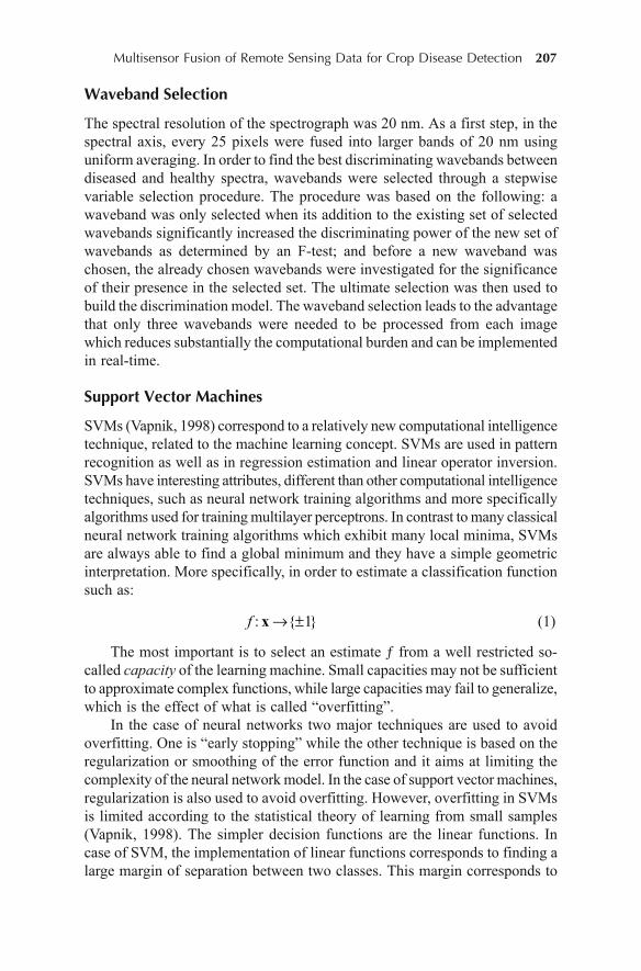
Multisensor Fusion of Remote Sensing Data for Crop Disease Detection 207
Waveband Selection
The spectral resolution of the spectrograph was 20 nm. As a first step, in thespectral axis, every 25 pixels were fused into larger bands of 20 nm usinguniform averaging. In order to find the best discriminating wavebands betweendiseased and healthy spectra, wavebands were selected through a stepwisevariable selection procedure. The procedure was based on the following: awaveband was only selected when its addition to the existing set of selectedwavebands significantly increased the discriminating power of the new set ofwavebands as determined by an F-test; and before a new waveband waschosen, the already chosen wavebands were investigated for the significanceof their presence in the selected set. The ultimate selection was then used tobuild the discrimination model. The waveband selection leads to the advantagethat only three wavebands were needed to be processed from each imagewhich reduces substantially the computational burden and can be implementedin real-time.
Support Vector Machines
SVMs (Vapnik, 1998) correspond to a relatively new computational intelligencetechnique, related to the machine learning concept. SVMs are used in patternrecognition as well as in regression estimation and linear operator inversion.SVMs have interesting attributes, different than other computational intelligencetechniques, such as neural network training algorithms and more specificallyalgorithms used for training multilayer perceptrons. In contrast to many classicalneural network training algorithms which exhibit many local minima, SVMsare always able to find a global minimum and they have a simple geometricinterpretation. More specifically, in order to estimate a classification functionsuch as:
��� : { 1}f � �x (1)
The most important is to select an estimate � from a well restricted so-called capacity of the learning machine. Small capacities may not be sufficientto approximate complex functions, while large capacities may fail to generalize,which is the effect of what is called “overfitting”.
In the case of neural networks two major techniques are used to avoidoverfitting. One is “early stopping” while the other technique is based on theregularization or smoothing of the error function and it aims at limiting thecomplexity of the neural network model. In the case of support vector machines,regularization is also used to avoid overfitting. However, overfitting in SVMsis limited according to the statistical theory of learning from small samples(Vapnik, 1998). The simpler decision functions are the linear functions. Incase of SVM, the implementation of linear functions corresponds to finding alarge margin of separation between two classes. This margin corresponds to

208 Dimitrios Moshou et al.
the minimum distance of the training data points from the separating surface.The procedure that is followed in order to find the maximum margin ofseparation is formulated as a convex quadratic problem (Vapnik, 1999). Anadditional parameter enables the SVM to misclassify some outlying trainingdata in exchange for obtaining a larger margin between the rest of the trainingdata, without however affecting the optimization of the quadratic problem.
The input data are projected into a feature space F using a map such as:
: FI �x (2)
Then a linear learning machine can be extended to a non-linear one. InSVMs the latter procedure is applied implicitly. What has to be supplied is a
dot product of pairs of data points ( ) ( )i j FI ¹I °x x in the feature space. Thus,in order to compute these dot products, one has to supply the kernel functionsthat define the feature space via:
( , ) ( ) ( )i j i jK x x I ¹ Ix x (3)
It is not necessary to know the mapping I since it is performed implicitly.SVMs can also learn which of the features implied by the kernel are distinctivefor the two classes. The selection of an appropriate kernel function may boostthe learning process.
Sensor Fusion
Introduction
Multi-sensor data fusion systems (Hall, 1992) combine data from multiplesensors to perform inferences that may not be possible from a single sensoralone. Applications span military problems (target identification, threatassessment), remote sensing problems (location of mineral resources), medicaldiagnosis, control of complex machinery and automated manufacturing. Datafusion is analogous to the ongoing cognitive process used by humans tointegrate data continually from their senses to make inferences about theexternal world.
Development issues for data fusion systems depend on the phenomenathat are observed, the type of sensors utilised, and the inferences sought.These inferences in turn determine the type of techniques required. Generallyapplications aimed at higher-level inferences require techniques from theartificial intelligence domain such as expert systems, template matching, neuralnetworks and fuzzy logic. The relative advantages and disadvantages of thedifferent sensing techniques lead to consideration of a combination of spectraltechniques with fluorescence imaging as clearly advantageous due to higherrecognition accuracy and less sensitivity to environmental factors. So there isa need to employ sensor fusion.
Multisensor Fusion of Remote Sensing Data for Crop Disease Detection 209
Generic Scheme for Sensor Combination
A generic scheme for sensor fusion has to include a number of steps to assurethat the handling of the data doesn’t result in loss of information critical forthe classification. Also due to the typically small datasets that are available themethod that is used should be able to handle missing or sparse data. From thispoint of view a network like the SVM is preferable in the case of small andsparse datasets. The feedforward neural networks also known as multilayerperceptrons (MLP) typically need a large supply of data to be able to producean accurate mapping. Therefore in the case of small datasets the MLP is notrecommended. Independent of the type of neural network in use, the proposedscheme is shown in Fig. 2.
Figure 2. Schematic representation of a conceptual sensor fusion systembased on Neural Networks (either SVM or MLP).
In practice a situation can arise where a failure of one or more of thesensors can actually jeopardise the successful operation of the whole fusion-based disease detection system. In such a case a modular decision architecturethat is based on the remaining sensors must be in place ready to switch intoaction or operate in parallel and provide a decision in parallel to the fusionsystem. A generic modular scheme for sensor fusion (conceptual design shownin Fig. 3) has to include a number of steps to assure that the handling of the
Figure 3. Schematic of a modular sensor fusion system based on neural networks.
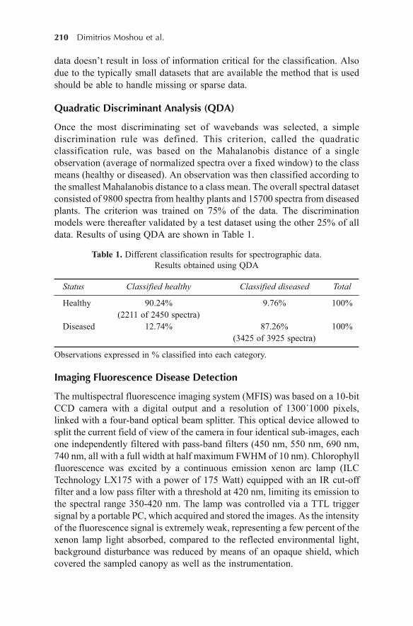
210 Dimitrios Moshou et al.
data doesn’t result in loss of information critical for the classification. Alsodue to the typically small datasets that are available the method that is usedshould be able to handle missing or sparse data.
Quadratic Discriminant Analysis (QDA)
Once the most discriminating set of wavebands was selected, a simplediscrimination rule was defined. This criterion, called the quadraticclassification rule, was based on the Mahalanobis distance of a singleobservation (average of normalized spectra over a fixed window) to the classmeans (healthy or diseased). An observation was then classified according tothe smallest Mahalanobis distance to a class mean. The overall spectral datasetconsisted of 9800 spectra from healthy plants and 15700 spectra from diseasedplants. The criterion was trained on 75% of the data. The discriminationmodels were thereafter validated by a test dataset using the other 25% of alldata. Results of using QDA are shown in Table 1.
Table 1. Different classification results for spectrographic data.Results obtained using QDA
Status Classified healthy Classified diseased Total
Healthy 90.24% 9.76% 100%(2211 of 2450 spectra)
Diseased 12.74% 87.26% 100%(3425 of 3925 spectra)
Observations expressed in % classified into each category.
Imaging Fluorescence Disease Detection
The multispectral fluorescence imaging system (MFIS) was based on a 10-bitCCD camera with a digital output and a resolution of 1300´1000 pixels,linked with a four-band optical beam splitter. This optical device allowed tosplit the current field of view of the camera in four identical sub-images, eachone independently filtered with pass-band filters (450 nm, 550 nm, 690 nm,740 nm, all with a full width at half maximum FWHM of 10 nm). Chlorophyllfluorescence was excited by a continuous emission xenon arc lamp (ILCTechnology LX175 with a power of 175 Watt) equipped with an IR cut-offfilter and a low pass filter with a threshold at 420 nm, limiting its emission tothe spectral range 350-420 nm. The lamp was controlled via a TTL triggersignal by a portable PC, which acquired and stored the images. As the intensityof the fluorescence signal is extremely weak, representing a few percent of thexenon lamp light absorbed, compared to the reflected environmental light,background disturbance was reduced by means of an opaque shield, whichcovered the sampled canopy as well as the instrumentation.
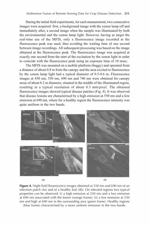
Multisensor Fusion of Remote Sensing Data for Crop Disease Detection 211
During the initial field experiments, for each measurement, two consecutiveimages were acquired: first, a background image with the xenon lamp off andimmediately after, a second image when the sample was illuminated by boththe environmental and the xenon lamp light. However, having as target thereal-time use of the MFIS, only a fluorescence image recorded at thefluorescence peak was used, thus avoiding the waiting time of one secondbetween image recordings. All subsequent processing was based on the imageobtained at the fluorescence peak. The fluorescence image was acquired atexactly one second from the start of the excitation by the xenon light in orderto coincide with the fluorescence peak using an exposure time of 10 msec.
The MFIS was mounted on a mobile platform (buggy) and operated froma distance of about 0.8 m from the canopy and the area excited to fluorescenceby the xenon lamp light had a typical diameter of 0.5-0.6 m. Fluorescenceimages at 450 nm, 550 nm, 690 nm and 740 nm were obtained for canopyareas of about 0.2 m diameter, situated in the middle of the illuminated region,resulting in a typical resolution of about 0.3 mm/pixel. The obtainedfluorescence images showed typical disease patches (Fig. 4). It was observedthat disease lesions are characterised by a high emission at 550 nm and a lowemission at 690 nm, where for a healthy region the fluorescence intensity wasquite uniform in the two bands.
Figure 4. Night field fluorescence images obtained at 550 nm and 690 nm of aninfection patch (4a) and of a healthy leaf (4b). On infected regions two typicalproperties can be observed: (i) a high emission at 550 nm and a low emissionat 690 nm associated with the lesion (orange frame); (ii) a low emission at 550nm and high at 690 nm in the surrounding area (green frame). Healthy regions
(blue frame) characterised by a more uniform emission in the two bands.
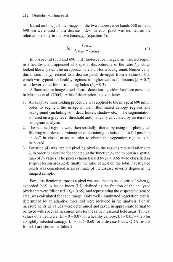
212 Dimitrios Moshou et al.
Based on this, just the images in the two fluorescence bands 550 nm and690 nm were used and a disease index for each pixel was defined as therelative intensity in the two bands, fG (equation 4).
550nm
550nm 690nm=G
IfI I� (4)
In bi-spectral (550 and 690 nm) fluorescence images, an infected regionin a healthy plant appeared as a spatial discontinuity of the ratio fG, whichlooked like a “patch”, on an approximately uniform background. Numerically,this means that fG related to a disease patch diverged from a value of 0.5,which was typical for healthy regions, to higher values for lesions (fG � 0.7)or to lower value for surrounding halos (fG � 0.3).
A fluorescence image based disease detection algorithm has been presentedin Moshou et al. (2005). A brief description is given here:
1. An adaptive thresholding procedure was applied to the image at 690 nm inorder to segment the image in well illuminated canopy regions andbackground (including soil, dead leaves, shadow etc.). The segmentationis based on a grey level threshold automatically calculated by an iterativehistogram analysis.
2. The retained regions were then spatially filtered by using morphologicalfiltering in order to eliminate spots pertaining to noise and to fill possible“holes” in closed areas in order to obtain the vegetation region to beinspected.
3. Equation (4) was applied pixel by pixel to the regions retained after step2, in order to calculate for each point the function fG and to obtain a spatialmap of fG values. The pixels characterised by fG > 0.65 were classified assuspect lesion area SLA; finally the ratio of SLA on the total investigatedpixels was considered as an estimate of the disease severity degree in theimaged sample.
For classification purposes a pixel was assumed to be “diseased” when fGexceeded 0.65. A lesion index (LI), defined as the fraction of the analyzedpixels that were “diseased” (fG > 0.65), and representing the suspected diseasedarea, was calculated for each image. Only well illuminated vegetation pixels,determined by an adaptive threshold were included in the analysis. For allmeasurements LI values were determined and saved in appropriate format tobe fused with spectral measurements for the same measured field areas. Typicalvalues obtained were: LI = 0 – 0.07 for a healthy canopy; LI = 0.05 – 0.20 fora slightly infected canopy; LI = 0.35–0.60 for a disease focus. QDA resultsfrom LI are shown in Table 2.
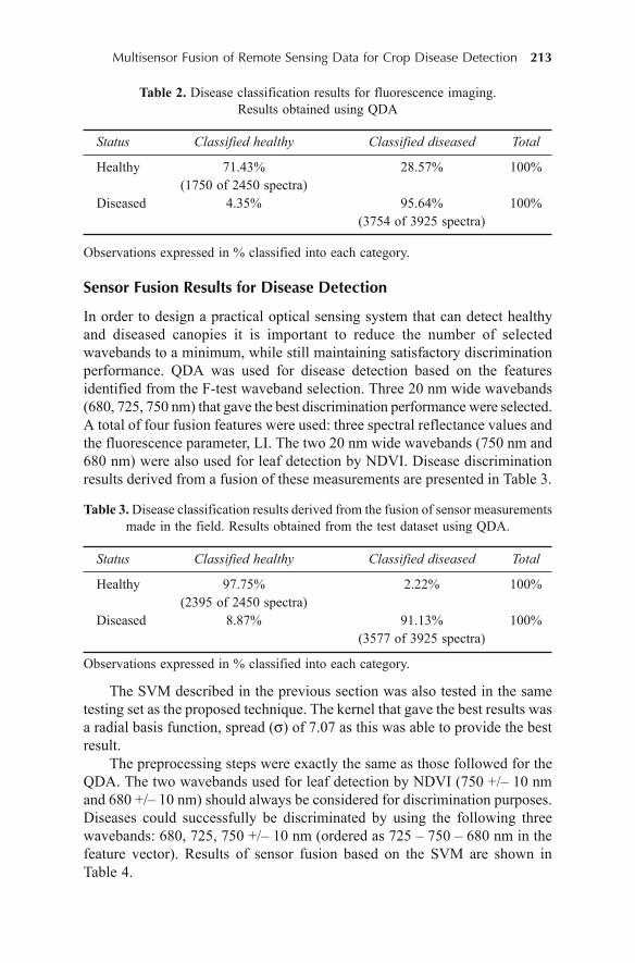
Multisensor Fusion of Remote Sensing Data for Crop Disease Detection 213
Table 2. Disease classification results for fluorescence imaging.Results obtained using QDA
Status Classified healthy Classified diseased Total
Healthy 71.43% 28.57% 100%(1750 of 2450 spectra)
Diseased 4.35% 95.64% 100%(3754 of 3925 spectra)
Observations expressed in % classified into each category.
Sensor Fusion Results for Disease Detection
In order to design a practical optical sensing system that can detect healthyand diseased canopies it is important to reduce the number of selectedwavebands to a minimum, while still maintaining satisfactory discriminationperformance. QDA was used for disease detection based on the featuresidentified from the F-test waveband selection. Three 20 nm wide wavebands(680, 725, 750 nm) that gave the best discrimination performance were selected.A total of four fusion features were used: three spectral reflectance values andthe fluorescence parameter, LI. The two 20 nm wide wavebands (750 nm and680 nm) were also used for leaf detection by NDVI. Disease discriminationresults derived from a fusion of these measurements are presented in Table 3.
Table 3. Disease classification results derived from the fusion of sensor measurementsmade in the field. Results obtained from the test dataset using QDA.
Status Classified healthy Classified diseased Total
Healthy 97.75% 2.22% 100%(2395 of 2450 spectra)
Diseased 8.87% 91.13% 100%(3577 of 3925 spectra)
Observations expressed in % classified into each category.
The SVM described in the previous section was also tested in the sametesting set as the proposed technique. The kernel that gave the best results wasa radial basis function, spread (V) of 7.07 as this was able to provide the bestresult.
The preprocessing steps were exactly the same as those followed for theQDA. The two wavebands used for leaf detection by NDVI (750 +/– 10 nmand 680 +/– 10 nm) should always be considered for discrimination purposes.Diseases could successfully be discriminated by using the following threewavebands: 680, 725, 750 +/– 10 nm (ordered as 725 – 750 – 680 nm in thefeature vector). Results of sensor fusion based on the SVM are shown inTable 4.
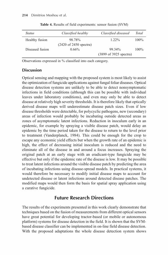
214 Dimitrios Moshou et al.
Table 4. Results of field experiments: sensor fusion (SVM)
Status Classified healthy Classified diseased Total
Healthy fusion 98.78% 1.22% 100%(2420 of 2450 spectra)
Diseased fusion 0.66% 99.34% 100%(3899 of 3925 spectra)
Observations expressed in % classified into each category.
Discussion
Optical sensing and mapping with the proposed system is most likely to assistthe optimization of fungicide applications against fungal foliar diseases. Opticaldisease detection systems are unlikely to be able to detect nonsymptomaticinfections in field conditions (although this can be possible with individualleaves under laboratory conditions), and even may only be able to detectdisease at relatively high severity thresholds. It is therefore likely that opticallyderived disease maps will underestimate disease patch sizes. Even if lowdisease thresholds were detectable, for polycyclic pathogens, new (secondary)areas of infection would probably be incubating outside detected areas aszones of asymptomatic latent infections. Reduction in inoculum early in anepidemic, for example by spraying a visible disease patch, would delay anepidemic by the time period taken for the disease to return to the level priorto treatment (Vanderplanck, 1984). This could be enough for the crop toescape any economic yield effects but when the growth rate of an epidemic ishigh, the effect of decreasing initial inoculum is reduced and the need toeliminate all of the disease in and around a focus increases. Spraying theoriginal patch at an early stage with an eradicant-type fungicide may beeffective but only if the epidemic rate of the disease is low. It may be possibleto treat latent infections around the visible disease patch by predicting the areaof incubating infections using disease-spread models. In practical systems, itwould therefore be necessary to modify initial disease maps to account forundetected disease or latent infections around detected disease patches. Themodified maps would then form the basis for spatial spray application usinga curative fungicide.
Future Research Directions
The results of the experiments presented in this work clearly demonstrate thattechniques based on the fusion of measurements from different optical sensorshave great potential for developing tractor-based (or mobile or autonomousplatform) systems for disease detection in the field. It is shown that the SVM-based disease classifier can be implemented in on-line field disease detection.With the proposed adaptations the whole disease detection system shows

Multisensor Fusion of Remote Sensing Data for Crop Disease Detection 215
clear potential for real-time field based disease detection. Some of the challengesin these techniques are: (i) the effect of background data in the resultingprofile or data, (ii) optimization of the technique for a specific plant/tree anddisease, and (iii) automation of the technique for continuous automatedmonitoring of plant diseases under real world field conditions.
Future investigations could encompass comparisons of the accuracy ofdata obtained from satellite, air-borne and ground data on the same fieldswhere crop diseases have appeared. An interesting approach would be tocombine data at different scales through data fusion techniques.
One particular emerging issue is the sensor-web or sensor networks. Earthenvironments are exceptionally dynamic and interrelated through a number ofsystems. To understand Earth systems and dynamics, significant improvementsin spatial and temporal observations are required. The consensus is that fusionof data from multiple sensor systems is currently one of the optimal solutions.However, increasingly inexpensive, yet sophisticated, chips for the computerand telecommunication industries provide an unique opportunity to develop adistributed, heterogeneous, and adaptive observing system or sensor web inthe future. Such sensor networks can enable the continuous monitoring of vastareas of cultivated land and issue warnings over early symptoms of pathogenattacks on crops.
Kung, Hua and Chen (2006) described a Drought Forecast and AlertSystem (DFAS), which is a four-tier system framework composed of mobileusers, ecology monitoring sensors, integrated service server, and intelligentdrought decision system. DFAS combines wireless sensor networks, embeddedmultimedia communications, and neural network decision technologies toeffectively achieve the forecast and alert of the drought. Emphasis is on multi-sensor fusion of large arrays of local sensors, joined with other assets, toprovide real-time imagery, weather, targeting information, mission planning,and simulations for military operations on land, sea and air. A similar forecastand alert system might benefit the early detection of the onset of diseaseepidemics.
Machine learning techniques, such as artificial neural networks (ANN),support vector machines and regression trees, have been widely used in manyapplications. However, they are often considered to be “black-box” approachesthat do not reflect the physics of the modelled process in remote sensing(Krasnopolsky and Schiller, 2003; Loyola, 2006). With the rapid developmentof these techniques, their potential needs further exploration. For example,neural networks have been combined into hierarchical or multi-neural systemswith either redundant or modular elements. The combination of neural networkssolves complex tasks more effectively and can furthermore result in dramaticperformance improvement. It fully exploits the advantages of neural methodsand expands the range of applicability. An important drawback of many ANNsis their lack of explanation capability. It is increasingly apparent that, withoutsome form of explanation capability, the full potential of trained ANNs may
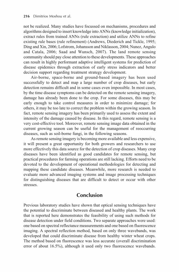
216 Dimitrios Moshou et al.
not be realized. Many studies have focussed on mechanisms, procedures andalgorithms designed to insert knowledge into ANNs (knowledge initialization),extract rules from trained ANNs (rule extraction) and utilize ANNs to refineexisting rule bases (rule refinement) (Andrews, Diederich and Tickle, 1995;Ding and Xin, 2006; Lofstrom, Johansson and Niklasson, 2004; Nunez, Anguloand Catala, 2006; Saad and Wunsch, 2007). The land remote sensingcommunity should pay close attention to these developments. These approachescan result in highly performant adaptive intelligent systems for prediction ofdisease epidemics through extraction of early stress indicators and betterdecision support regarding treatment strategy development.
Air-borne, space-borne and ground-based imagery has been usedsuccessfully to detect and map a large number of crop diseases, but earlydetection remains difficult and in some cases even impossible. In most cases,by the time disease symptoms can be detected on the remote sensing imagery,damage has already been done to the crop. For some diseases, this may beearly enough to take control measures in order to minimize damage; forothers, it may be too late to correct the problem within the growing season. Infact, remote sensing imagery has been primarily used to assess the extent andintensity of the damage caused by disease. In this regard, remote sensing is avery cost-effective tool. Moreover, remote sensing image data obtained in thecurrent growing season can be useful for the management of reoccurringdiseases, such as soil-borne fungi, in the following seasons.
As remote sensing imagery is becoming more available and less expensive,it will present a great opportunity for both growers and researchers to usemore effectively this data source for the detection of crop diseases. Many cropdiseases have been identified as good candidates for remote sensing, butpractical procedures for farming operations are still lacking. Efforts need to bedevoted to the development of operational methodologies for detecting andmapping these candidate diseases. Meanwhile, more research is needed toevaluate more advanced imaging systems and image processing techniquesfor distinguishing diseases that are difficult to detect or occur with otherstresses.
Conclusion
Previous laboratory studies have shown that optical sensing techniques havethe potential to discriminate between diseased and healthy plants. The workthat is reported here demonstrates the feasibility of using such methods fordisease detection under field conditions. Two separate approaches were used:one based on spectral reflectance measurements and one based on fluorescenceimaging. A spectral reflection method, based on only three wavebands, wasdeveloped that could discriminate disease from healthy winter wheat crops.The method based on fluorescence was less accurate (overall discriminationerror of about 16.5%), although it used only two fluorescence wavebands.
Multisensor Fusion of Remote Sensing Data for Crop Disease Detection 217
However, fusing the measurements from the two approaches together allowedoverall disease from healthy discrimination of 94.5% by using QDA(discrimination error of 5.5%). Further, by using SVM for the fusion classifier,increased the overall discrimination performance to around 99%. Moresignificantly, while the advantage of SVM over QDA in healthy plant detectionwas marginal (only 1% improvement), the improvement in diseased plantdetection increased over 8%. The results of these experiments clearlydemonstrate that techniques based on the fusion of measurements from differentoptical sensors have great potential for developing tractor-based systems fordisease detection in the field. It is shown that the SVM-based disease classifiercan be implemented in field disease detection. The results suggest that thesemethods of disease detection show a good potential with an ability to detectplant diseases accurately. The spectrographic and fluorescence imagingtechnology could be integrated in a fusion prototype carried by a vehicle or arobotic platform for reliable and real-time plant disease detection in order toachieve superior plant disease control and management.
References
Andrews, R., Diederich, J. and Tickle, A.B. (1995). Survey and critique of techniquesfor extracting rules from trained artificial neural networks. Knowledge-BasedSystems, 8(6), 373–389.
Apan, A., Held, A., Phinn, S. and Markley, J. (2004). Detecting sugarcane orange rustdisease using EO-1 Hyperion hyperspectral imagery. International Journal of RemoteSensing, 25(2), 489–498.
Blakeman, R.H., Bryson, R.J. and Dampney, P. (2000). Assessing crop condition inreal time using high resolution satellite imagery. In: Aspects of Applied Biology60, Remote Sensing in Agriculture (pp. 163–171). The Association of AppliedBiologists, Wellesbourne, UK.
Bravo, C., Moshou, D., West, J., McCartney, A. and Ramon, H. (2003). DetailedSpectral Reflection Information for Early Disease Detection in Wheat Fields.Biosystems Engineering, 84(2), 137–145.
Bravo, C., Moshou, D., Oberti, R., West, J., McCartney, A., Bodria, L. and Ramon, H.(2004, December). Foliar disease detection in the field using optical sensor fusion.International Commission of Agricultural Engineering (CIGR, CommissionInternationale du Genie Rural) E-Journal, Manuscript FP 04 008, 6. RetrievedApril 7, 2011, from http://www.cigrjournal.org/index.php/Ejournal/article/view/537/531.
Cui, D., Zhang, Q., Li, M. Hartman, G.L. and Zhao, Y. (2010). Image processingmethods for quantitatively detecting soybean rust from multispectral images.Biosystems Engineering, 107(3), 186–193.
Ding, X.Q. and Xin, S. (2006). Application research on extraction of rule from artificialneural networks for nonlinear regression. Dynamics of Continuous, Discrete andImpulsive Systems. Series A: Mathematical Analysis, 13, 565–568.
218 Dimitrios Moshou et al.
Du, Q., French, J.V., Skaria, M., Yang, C. and Everitt, J.H. (2004). Citrus pest stressmonitoring using airborne hyperspectral imagery. In: Conference Proceedings ofthe International Geoscience and Remote Sensing Symposia Vol. VI (pp. 3981–3984). Piscataway, New Jersey, IEEE.
Fauvel, M., Benediktsson, J.A., Chanussot, J. and Sveinsson, J.R. (2008). Spectraland spatial classification of hyperspectral data using SVMs and morphologicalprofiles. IEEE Transactions on Geoscience and Remote Sensing, 46(11), 3804–3814.
Franke, J. and Menz, G. (2007). Multi-temporal wheat disease detection by multi-spectral remote sensing. Precision Agriculture, 8, 161–172.
Hall, D.L. (1992). Mathematical Techniques in Multisensor Data Fusion. Artech House,Boston/London, UK.
Herrala, E., Okkonen, J., Hyvarinen, T., Aikio, M. and Lammasniemi, J. (1994).Imaging spectrometer for process industry applications. Paper presented at OpticalMeasurements and Sensors for the Process Industries, Frankfurt, Germany.
Johnson, D.A., Alldredge, J.R., Hamm, P.B. and Frazier, B.E. (2003). Aerialphotography used for spatial pattern analysis of late blight infection in irrigatedpotato circles. Phytopathology, 93(7), 805–812.
Krasnopolsky, V.M. and Schiller, H. (2003). Some neural network applications inenvironmental sciences. Part I: Forward and inverse problems in geophysical remotemeasurements. Neural Networks, 16(3–4), 321–334.
Kung, H.Y., Hua, J.S. and Chen, C.T. (2006). Drought forecast model and frameworkusing wireless sensor networks. Journal of Information Science and Engineering,22(4), 751–769.
Lee, W.S., Alchanatis, V., Yang, C., Hirafuji, M., Moshou, D. and Li, C. (2010).Sensing technologies for precision specialty crop production. Computers andElectronics in Agriculture, 74(1), 2–33.
Lofstrom, T., Johansson, U. and Niklasson, L. (2004). Rule extraction by seeingthrough the model. In: N.R. Pal et al. (Eds.), Lecture Notes in Computer Science3316: Neural Information Processing (pp. 555–560). Springer, Berlin-Heidelberg,Germany.
Loyola, R.D.G. (2006). Applications of neural network methods to the processing ofEarth observation satellite data. Neural Networks, 19(2), 168–177.
Mitra, P., Shankar, B.U. and Pal, S. (2004). Segmentation of multispectral remotesensing images using active support vector machines. Pattern Recognition Letters,25(9), 1067–1074.
Moshou, D., Bravo, C., West, J., McCartney, A. and Ramon, H. (2004). Automaticdetection of yellow rust in wheat using reflectance measurements and neuralnetworks. Computers and Electronics in Agriculture, 44(3), 173–188.
Moshou, D., Bravo, C., Oberti, R., West, J., Bodria, L., McCartney, A. and Ramon, H.(2005). Plant disease detection based on data fusion of hyper-spectral and multi-spectral fluorescence imaging using Kohonen maps. Real-Time Imaging, 11(2),75–83.
Myers, V.I. (1983). Remote sensing applications in agriculture. In: R.N. Colwell(Ed.), Manual of Remote Sensing (pp. 2111–2228). American Society ofPhotogrammetry, Falls Church, VA.
Nunez, H., Angulo, C. and Catala, A. (2006). Rule-based learning systems for supportvector machines. Neural Processing Letters, 24(1), 1–18.

Multisensor Fusion of Remote Sensing Data for Crop Disease Detection 219
Pal, M. (2008). Ensemble of support vector machines for land cover classification.International Journal of Remote Sensing, 29(10), 3043–3049.
Ryerson, R.A., Curran, P.J. and Stephens, P.R. (1997). Applications: agriculture. In:W.R. Philipson (Ed.), Manual of Photographic Interpretation (pp. 365–397).American Society for Photogrammetry and Remote Sensing, Bethesda, MD.
Saad, E.W. and Wunsch, D.C. (2007). Neural network explanation using inversion.Neural Networks, 20(1), 78–93.
Vanderplank, J.E. (1984). Disease Resistance in Plants. Academic, New York/London,UK.
Vapnik, V.N. (1998). Statistical Learning Theory. Wiley Interscience, New York.Vapnik, V.N. (1999). The Nature of Statistical Learning Theory. Springer-Verlag, New
York.Zhang, L. and Dickinson, M. (2001). Fluorescence from rust fungi: a simple and
effective method to monitor the dynamics of fungal growth in planta. Physiologicaland Molecular Plant Pathology, 59(3), 137–141.
Zhang, L., Huang, X., Huang, B. and Li, P. (2006). A pixel shape index coupled withspectral information for classification of high spatial resolution remotely sensedimagery. IEEE Transactions on Geoscience and Remote Sensing, 44(10), 2950–2961.
Zhang, R. and Ma, J. (2008). An improved SVM method P-SVM for classification ofremotely sensed data. International Journal of Remote Sensing, 29(20), 6029–6036.
220 Ebru H. Colak and Tahsin Yomralioglu
14Geospatial Analysis of Cancer
Cases in the Eastern Black SeaRegion of Turkey
Ebru H. Colak and Tahsin Yomralioglu1
Karadeniz Technical University, Dept. of Surveying EngineeringGISLab, Trabzon, Turkey
1Istanbul Technical University, Dept. of Geomatics EngineeringIstanbul, Turkey
Introduction
Cancer has remained an important health issue in recent years. Examiningvariations of cancer cases temporally and spatially is necessary to developstrategies to combat its occurrence and to put cancer control programmes intopractice. Creating cancer maps is necessary for obtaining information such asthe location and frequency of cancer cases, the geographic distribution ofcancer types and the location of the highest densities of cases. Consequently,creating more reliable and precise data infrastructures will increase the numberof accurate decision making options available and aid in determining how andwhere to implement control strategies.
Numerous studies have been conducted on cancer epidemiology, themajority of which are thematic mapping studies including the observation ofspatial distribution of cancer (Pickle et al., 2007; Kulldorff et al., 2006; Brewer,2006; Morra et al., 2006; Jacquez, 2004; Berke, 2004; Vieira et al., 2002). Inaddition, more specific cancer studies exist in which advanced statisticalanalyses are performed (Yomralioglu et al., 2009; Draper et al., 2005; Greilinget al., 2005; Oliver et al., 2005; Flinton and Walters, 2004; Diggle, 2000).
In Turkey, the number of studies on cancer epidemiology remainsinsufficient. Although control policies were developed and employed againstcancer by the Turkish Ministry of Health (2004), comprehensive cancer-mapping for the whole country are not yet available. The studies conductedare mostly regional and oriented toward a specific feature of cancer due to the
DOI 10.1007/978-94-007-1858-6_14, © Capital Publishing Company 2012
e ,J.K. Thakur et al. (eds.), G ospatial Techniques for Managing Environmental Resources 220
Geospatial Analysis of Cancer Cases in the Eastern Black Sea Region 221
problems regarding reliable cancer statistics for all of Turkey. In line with thecurrent cancer policies, the importance of a cancer registry has graduallyincreased in recent years. Some regions and cities have initiated pilot schemesfor a cancer registry, including the cancer registry centre in the city of Trabzon,located in the Eastern Black Sea region of Turkey.
Spatial epidemiology studies aim to investigate the relationships betweenimportant health and environmental factors. Information about the causalfactor of the disease is vital for the investigation of the relationship betweenthe geography and the disease. For the spatial relationships among healthissues to be explored, information about the disease and the environmentalfactors that influence it should first be collected and then be analyzed usingstatistical methods in line with the requirements. Such analyses can beperformed effectively using GIS, which can evaluate spatial information,information related to health issues and information related to environmentalfactors together.
In this study, cancer density maps were produced using GIS techniquesfor an area that comprises seven cities in Turkey. A model proposal wasdeveloped through which statistical studies could be performed about whethercarcinogenic environmental factors affect the cases in the defined cancerdensity areas. Mapping cancer cases enables the consideration of the cancerdensities within each administrative unit by also considering the populationsizes of these administrative units and the demonstration of an integratedapproach to addressing carcinogenic environmental factors. Several studiesoriented toward cancer mapping and defining cancer cluster areas exist. Studiesthat investigate the impacts of environmental factors on cancer focus primarilyon more specific issues, including examinations of the relationships betweena specific type of cancer and a specific carcinogenic factor. Studies that examineall of these factors in an integrated framework are needed. This study proposesa higher-scale integrated approach that could guide studies on cancer and thisproposal promotes the simultaneous operation of the desired specific studiesand the consideration of other factors. Different thematic cancer maps havebeen created using GIS for more detailed studies in the region inepidemiological topics. Consequently, the results of this study would helpdevelop and apply cancer control programmes in the country.
Background and Context
Cancer incidence has been increasing worldwide and specifically in developingcountries. In Turkey, the cancer incidence is calculated as 180-200 per 100,000people, a rate half that of the European Union countries; this difference is duein part to the age distribution of the population of each region. Turkey expects144,000 new cancer cases among its population of 72 million and currentcancer incidence of 200 per 100,000 (Tuncer, 2009).
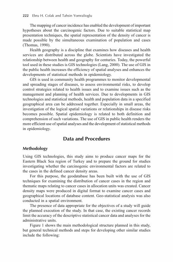
222 Ebru H. Colak and Tahsin Yomralioglu
The mapping of cancer incidence has enabled the development of importanthypotheses about the carcinogenic factors. Due to suitable statistical mappresentation techniques, the spatial representation of the density of cancer ismade possible by the simultaneous examination of population and cases(Thomas, 1990).
Health geography is a discipline that examines how diseases and healthservices are distributed across the globe. Scientists have investigated therelationship between health and geography for centuries. Today, the powerfultool used in these studies is GIS technologies (Lang, 2000). The use of GIS inthe public health increases the efficiency of spatial analyses and enhances thedevelopments of statistical methods in epidemiology.
GIS is used in community health programmes to monitor developmentaland spreading stages of diseases, to assess environmental risks, to developcontrol strategies related to health issues and to examine issues such as themanagement and planning of health services. Due to developments in GIStechnologies and statistical methods, health and population data in a specifiedgeographical area can be addressed together. Especially in small areas, theinvestigation of the logical spatial variations or relationships in disease risksbecomes possible. Spatial epidemiology is related to both definition andcomprehension of such variations. The use of GIS in public health renders themore efficient use of spatial analyses and the development of statistical methodsin epidemiology.
Data and Procedures
Methodology
Using GIS technologies, this study aims to produce cancer maps for theEastern Black Sea region of Turkey and to prepare the ground for studiesinvestigating whether the carcinogenic environmental factors are related tothe cases in the defined cancer density areas.
For this purpose, the geodatabase has been built with the use of GIStechniques for examining the distribution of cancer cases in the region andthematic maps relating to cancer cases in allocation units was created. Cancerdensity maps were produced in digital format to examine cancer cases andgeographical locations of database content. Geo-statistical analysis was alsoconducted in a spatial environment.
The presence of data appropriate for the objectives of a study will guidethe planned execution of the study. In that case, the existing cancer recordslimit the accuracy of the descriptive statistical cancer data and analyses for theadministrative units.
Figure 1 shows the main methodological structure planned in this study,but general technical methods and steps for developing other similar studiesinclude the following:
Geospatial Analysis of Cancer Cases in the Eastern Black Sea Region 223
• Researching the current literature about health GIS, cancer maps andgeostatistics
• Designing and establishing a geospatial database for cancer oriented GIS• Obtaining cancer statistics for cancer mapping and controlling the address
data of cancer cases• Determining and providing spatial and non-spatial data for the designed
cancer based geospatial database and integrating these data into thegeodatabase
Figure 1. A methodological framework of geospatial analysis ofcancer cases and associated environmental features.
224 Ebru H. Colak and Tahsin Yomralioglu
• Establishing the geo-relationship of cancer cases on the base maps andmapping the spatial distribution of cancer cases
• Performing population-based studies on cancer statistics (incidence,mortality, morbidity, age-standardized cancer incidence rate, etc.)
• Calculating and analyzing the cancer incidence rate for each administrativeunit
• Verifying statistical rates associated with cancer risk by cancer types, sexand age groups and integrating these rates into GIS
• Mapping the cancer density maps using geostatistic methods anddetermining the high cancer density regions
• Applying spatial analysis to the data by cancer types and geostatisticmethods
• Determining cancer cluster areas and generating a cancer clustering map• Examining the relationship between cancer data and geographic features
using statistical methods and geostatistics• Using advanced statistical methods for cancer risk areas• Identifying high risk areas associated with cancer and environmental
exposure• Representing the final products as thematic maps and other cartography
products• Producing final reports and GIS-based thematic maps
Cancer-based GIS
Designing the database that enabled the management of the cancer case dataand produced spatial statistical data in the GIS environment enabled futurestudies to use the produced data. The geodatabase managed the data obtainedfrom different sources through different methods by categorizing them in thegeospatial data groups of Health (HE), Administrative Unit (AU), Topography(TO), Land Cover (LC) and Geophysics/Environment (GE). In the Cancer-Based Geospatial database shown in Figure 2, each geospatial data groupconsists of interoperable feature classes.
Data Inputs
Administrative Units and Demographic Data
The correlation of health events with the geography of residential units wasbased on administrative units, depending on the scope of the research. TheEastern Black Sea region of Turkey was selected as a case study (Fig. 3),including a total of seven cities (Trabzon, Rize, Artvin, Giresun, Ordu, Bayburtand Gumushane) in the region. Based on this, geospatial data about theadministrative centres and boundaries of provinces, counties, districts andvillages were collected.

Geospatial Analysis of Cancer Cases in the Eastern Black Sea Region 225
Figure 2. Designing the cancer-based geospatial database.
Figure 3. Study area: The Eastern Black Sea region of Turkey.
226 Ebru H. Colak and Tahsin Yomralioglu
In the Administrative Units data group, provinces, counties and districts/villages are defined in the GIS “polygon” feature class and the centres ofadministrative units are defined in the “point” feature class. The AdministrativeUnit Code (AUC) was used to establish an effective relationship between thedatabases that represent administrative units and statistical health data. Thespatial relationship was established by geocoding according to the AUC definedfor each administrative unit.
Demographic data regarding the administrative units were gathered fromthe Turkish Statistical Institute (TURKSTAT). Demographic information onspatial locations was added to the database containing administrative unitdata. Demographic data were further classified according to gender. Thedemographic data used in calculating cancer density rates in the administrativeunits were important, and the comparison of the number of cancer cases withthe population ensured the accurate interpretation of cancer frequency.
Cancer Data
Address specifications were of the utmost importance for the spatialdistributions of cancer cases. Statistical cancer data were obtained from theProvincial Directorates of Health with the permission of the Ministry of Healthand consisted of information such as the patient’s age, gender, address,diagnosis, the disease’s ICD code, topology and the diagnosis date.
Cancer statistics from between 2000 and 2007 were obtained from theCancer Registry Centres (CRC) in the seven provinces included in the scopeof this study in the Eastern Black Sea region of Turkey. In total, 15,299 cancercases were obtained from these CRCs and included in the cancer database, ofwhich 9,520 were males and 5,779 were females.
To place each case in the cancer database on the map, the AdministrativeUnit Code was added to the designed database according to the address dataof the cases. The relationship between the database that includes cancer casesand the database that includes administrative units was formed through theAUC, enabling the transfer of the cancer database to the designed geographicalinformation system. In addition, with the help of geocoding, each cancer casewas identified as a point on the map according to its address information.
Topographic and Land Use Data
Geospatial data that represent height describe Earth’s topography and are usedin base maps and many other mapping practices. In this study, expressing therelationship of cancer cases to height required contour data. Relevant institutionsprovided 286 pieces of 1/25,000 scale digital maps of the study area that wereobtained through the digitizing of contour lines and formed the base data ofthis study. Using the Spatial Analysis function, a Digital Elevation Model ofthe area was produced and converted into grid representation.
The land cover map of the Eastern Black Sea region of Turkey wasproduced using satellite images, including Landsat ETM+ satellite imagesfrom 2000. A total of four satellite images in an East-West orientation cover
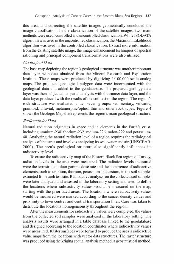
Geospatial Analysis of Cancer Cases in the Eastern Black Sea Region 227
this area, and correcting the satellite images geometrically concluded theimage classification. In the classification of the satellite images, two mainmethods were used: controlled and uncontrolled classification. While ISODATAalgorithm was used in the uncontrolled classification, the Maximum Likelihoodalgorithm was used in the controlled classification. Extract more informationfrom the existing satellite image, the image enhancement techniques of spectralrationing and principal component transformations were also utilized.
Geological Data
The base map depicting the region’s geological structure was another importantdata layer, with data obtained from the Mineral Research and ExplorationInstitute. These maps were produced by digitizing 1/100,000 scale analogmaps. The produced geological polygon data were incorporated with thegeological data and added to the geodatabase. The prepared geology datalayer was then subjected to spatial analysis with the cancer data layer, and thedata layer produced with the results of the soil test of the region. The region’srock structure was evaluated under seven groups: sedimentary, volcanic,granitoid, alluvial, metamorphic/ophiolithic and other rock types. Figure 4shows the Geologic Map that represents the region’s main geological structure.
Radioactivity Data
Natural radiation originates in space and in elements in the Earth’s crust,including uranium-238, thorium-232, radium-226, radon-222 and potassium-40. Analyzing the natural radiation level of a region requires the radiologicalanalysis of that area and involves analyzing its soil, water and air (UNSCEAR,2000). The area’s geological structure also significantly influences itsradioactivity level.
To create the radioactivity map of the Eastern Black Sea region of Turkey,radiation levels in the area were measured. The radiation levels measuredwere the terrestrial outdoor gamma dose rate and the occurrence of radioactiveelements, such as uranium, thorium, potassium and cesium, in the soil samplesextracted from each test site. Radioactive analyses on the collected soil sampleswere later analyzed and assessed in the laboratory setting and used to definethe locations where radioactivity values would be measured on the map,starting with the prioritized areas. The locations where radioactivity valueswould be measured were marked according to the cancer density values andproximity to town centres and central transportation lines. Care was taken todistribute the locations homogeneously throughout the region.
After the measurements for radioactivity values were completed, the valuesfrom the collected soil samples were analyzed in the laboratory setting. Theanalysis results were arranged in a table database linked to the geodatabaseand designed according to the location coordinates where radioactivity valueswere measured. Raster surfaces were formed to produce the area’s radioactivevalue maps from the locations with vector data structures. The raster structurewas produced using the kriging spatial analysis method, a geostatistical method.
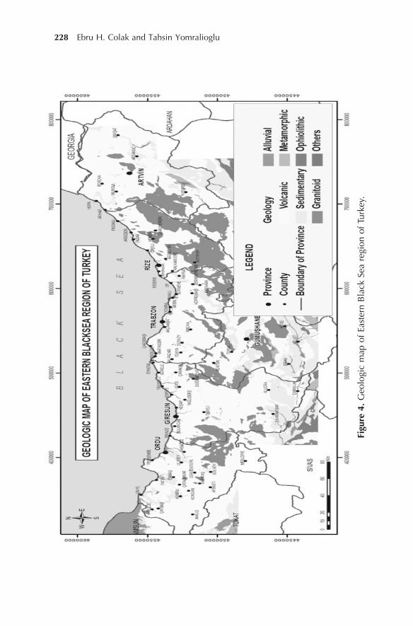
228 Ebru H. Colak and Tahsin Yomralioglu
Figu
re 4
. G
eolo
gic
map
of
East
ern
Bla
ck S
ea r
egio
n of
Tur
key.
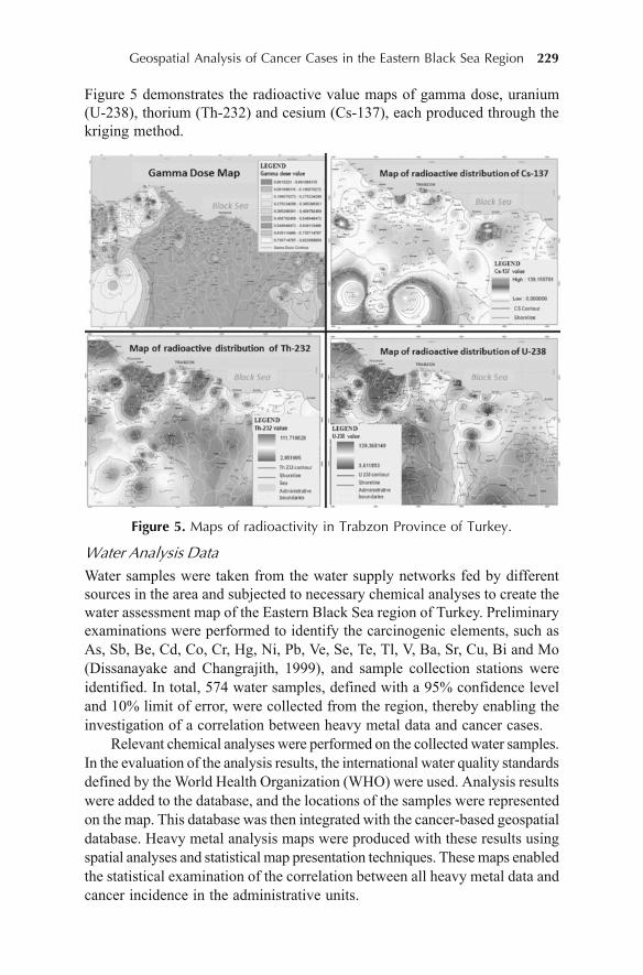
Geospatial Analysis of Cancer Cases in the Eastern Black Sea Region 229
Figure 5 demonstrates the radioactive value maps of gamma dose, uranium(U-238), thorium (Th-232) and cesium (Cs-137), each produced through thekriging method.
Figure 5. Maps of radioactivity in Trabzon Province of Turkey.
Water Analysis Data
Water samples were taken from the water supply networks fed by differentsources in the area and subjected to necessary chemical analyses to create thewater assessment map of the Eastern Black Sea region of Turkey. Preliminaryexaminations were performed to identify the carcinogenic elements, such asAs, Sb, Be, Cd, Co, Cr, Hg, Ni, Pb, Ve, Se, Te, Tl, V, Ba, Sr, Cu, Bi and Mo(Dissanayake and Changrajith, 1999), and sample collection stations wereidentified. In total, 574 water samples, defined with a 95% confidence leveland 10% limit of error, were collected from the region, thereby enabling theinvestigation of a correlation between heavy metal data and cancer cases.
Relevant chemical analyses were performed on the collected water samples.In the evaluation of the analysis results, the international water quality standardsdefined by the World Health Organization (WHO) were used. Analysis resultswere added to the database, and the locations of the samples were representedon the map. This database was then integrated with the cancer-based geospatialdatabase. Heavy metal analysis maps were produced with these results usingspatial analyses and statistical map presentation techniques. These maps enabledthe statistical examination of the correlation between all heavy metal data andcancer incidence in the administrative units.
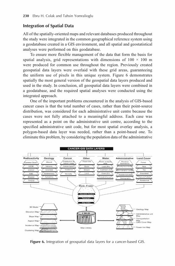
230 Ebru H. Colak and Tahsin Yomralioglu
Integration of Spatial Data
All of the spatially-oriented maps and relevant databases produced throughoutthe study were integrated in the common geographical reference system usinga geodatabase created in a GIS environment, and all spatial and geostatisticalanalyses were performed on this geodatabase.
To ensure more flexible management of the data that form the basis forspatial analysis, grid representations with dimensions of 100 × 100 mwere produced for common use throughout the region. Previously createdgeospatial data layers were overlaid with these grid areas, guaranteeingthe uniform use of pixels in this unique system. Figure 6 demonstratesspatially the most general version of the geospatial data layers produced andused in the study. In conclusion, all geospatial data layers were combined ina geodatabase, and the required spatial analyses were conducted using theintegrated approach.
One of the important problems encountered in the analysis of GIS-basedcancer cases is that the total number of cases, rather than their point-sourcedistribution, was considered for each administrative unit centre because thecases were not fully attached to a meaningful address. Each case wasrepresented as a point on the administrative unit centre, according to thespecified administrative unit code, but for most spatial overlay analysis, apolygon-based data layer was needed, rather than a point-based one. Toeliminate this problem, by considering the population data of the administrative
Figure 6. Integration of geospatial data layers for a cancer-based GIS.

Geospatial Analysis of Cancer Cases in the Eastern Black Sea Region 231
centres, a polygon-based data layer including detailed data about cancer caseswas produced through the application of “buffer” analysis for the spatialrepresentation of administrative units. Most spatial overlay activities wereperformed with this data layer. This approach prevented unnecessary processesand time loss in GIS.
Mapping Process for Cancer Cases
The cancer datasets collected in the study and all other required spatial datawere incorporated into the geodatabases. Then, various thematic maps wereproduced through the data presentation opportunities provided by GIS in thescope of the cancer-based Geospatial Database (GDB).
In this study, the spatial distribution of the cancer cases observed in theEastern Black Sea region of Turkey between 2000 and 2007 was integrated ina geodatabase and shown on base maps using GIS technologies. The caseswere represented as points on the administrative units on the map accordingto the address data obtained. After the cancer cases distribution map wascreated, incidence rates and the cancer density criteria in each administrativeunits were calculated and added to the database. Various cancer density mapsthat depict the cancer densities in the administrative units in the region wereproduced drawing on the incidence rate data.
In the production of cancer maps, incidence rates indicated the density ofcancer in administrative units. The map of distribution of cancer cases observedin the Eastern Black Sea region between 2000 and 2007 was produced in theform of a thematic map presentation, and the map of incidence rates inadministrative units was produced using the proportional symbol mappingtechniques. In these maps, the representations of cancer density weresymbolized by scaling proportional symbols calculated by the incidence values.This chapter includes only one sample map depicting cancer densities in theadministrative units produced using the geostatistical method. This cancerdensity map, shown in Fig. 7, was produced using the kriging interpolationmethod based on the cancer incidence values.
Statistical Methods
Although the cancer density rates in administrative units were assessedstatistically, only the cancer incidence rate, standardized cancer incidence rateor specific cancer incidence rate was used.
Incidence is defined as the number of new cases of a disease or a healthevent that occur in a specified time period (Stewart, 2002). Incidence rateindicates the number of new cases within a given time period (i.e. in a year),in a society, the rate of which is known.
Standardization is necessary when comparing two or more societies orcommunities, the differing basic characteristics (e.g., age, race and socio-economic status) of which influence their respective risks of disease (Esteve
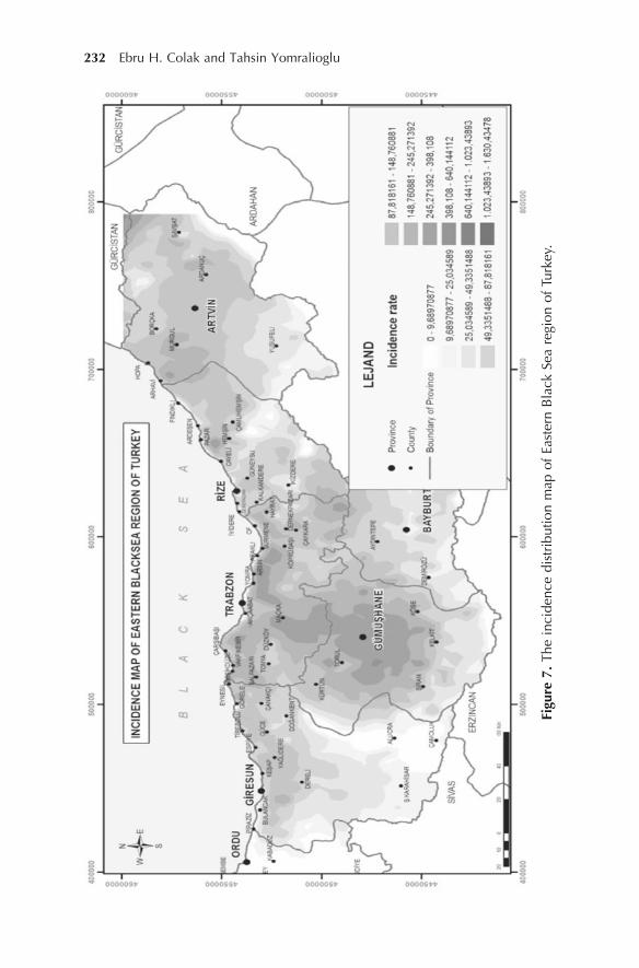
232 Ebru H. Colak and Tahsin Yomralioglu
Figu
re 7
. The
inc
iden
ce d
istr
ibut
ion
map
of
East
ern
Bla
ck S
ea r
egio
n of
Tur
key.

Geospatial Analysis of Cancer Cases in the Eastern Black Sea Region 233
et al., 1994). The standardized cancer incidence rate refers to the applicationof common or homogenous characteristics such as age, gender or diseasegroup among different cancer incidence data to enable comparison.
After the incidence densities in the administrative units were calculated,kriging geostatistical analysis method was used to map these densities ongeography. In this study, cancer densities were shown on the map of theregion in the raster format, using the kriging method. Cancer cluster areaswere defined through the Kernel density analysis.
To examine the correlations between cancer frequency and density in theadministrative units and the environmental carcinogenic factors, all data wereassessed in an integrated style in the GIS environment through spatial analysisand investigations. Relationships between the possible carcinogenic factortargets for investigation and the cancer frequency in residential areas wereassessed using the necessary statistical analyses. The Pearson chi-squarestatistical analysis was used to investigate one-to-one or one-to-manycorrelations, and other statistical analysis methods, such as the IndependentSamples t-test and linear regression, were used in the hypothesis test of bilateralcorrelations and the analysis of correlations between multifactor environmentalcauses and cancer frequency, respectively. Statistical methods differed withrespect to the content of the hypothesis constructed between each environmentalfactor and cancer frequencies.
Examining the Association between EnvironmentalFactors and Cancer
To explore the cancer cases and environmental carcinogenic factors, variousspatially based examinations were performed, based on the cancer-based GDB.The cancer data were subjected to overlay analyses in either separate orintegrated ways with layers including regional environmental data such astopography, geological structure, water, land cover and radioactivity. Theresults were then analyzed statistically.
The spatial and statistical analyses in this study tested whether a correlationexists between cancer types and aspect, land cover, geological structure andradioactivity. The chemical analysis results of the heavy metals found in thewater samples collected from the administrative units in the region wereassessed and represented on maps, and their relationships with the cancerfrequencies were tested through geostatistical analyses.
Correlations between cancer cases observed in administrative units orcancer frequency and the environmental factors were considered separatelyand assessed both geospatially and statistically.
This model allows the examination and statistical assessment of numeroushypotheses regarding environmental factors. However, this book chapterfocussed on only one case study. To explore its uses, a sample hypothesis was
234 Ebru H. Colak and Tahsin Yomralioglu
developed to examine the correlation between the geological structure and thetypes of cancer, and the necessary spatial examinations and statisticalevaluations were carried out.
Examination of the Correlation between the Geological Structureand Types of Cancer
To examine the correlation between the region’s geological structure andtypes of cancer, spatially-based statistical analyses were performed. With thehelp of the spatial examinations carried out using the Eastern Black Searegion geological map and the map of the point distribution of the administrativeunits, the number of cancer cases encountered depending on the geologicalstructure were categorized by cancer type. The Pearson chi-square test wasused to identify any correlation between the land’s geological structure andtypes of cancer. The data were classified and arranged for assessment bystatistical software.
Pearson chi-square test was employed through a statistics software inorder to statistically examine whether there exists a correlation between typesof cancer and the land’s geological structure. The statistical analysis usedclasses of seven rock types and ten types of cancer (lung/bronchial/larynx,skin, leukemia, breast, stomach, colon/rectum, bladder, prostate, thyroid andother types of cancer). The impact of elevation on cancer types was significantaccording to the results of the Pearson chi-square test (F2 = 82.378, SD = 45,p = 0.001). According to the results of the statistical analyses, 10.3% of15,223 cancer cases were observed in sedimentary rock type, 83.1% in volcanic,2.7% in granitoid, 2.3% in alluvial, 0.1% in metamorphic and ophiolitic mixtureand 1.4% in other rock types.
In determining the correlation between types of cancer and rock types,examining the environments that cause this correlation is necessary. Adjustedresiduals were used for this purpose. An adjusted residual greater or equal totwo is significant for the correlation between two categories of data (rock typeand type of cancer). Based on the results of the statistical analysis, stomachand breast cancers were encountered more in areas where the rock type isvolcanic, and stomach cancer was observed more in areas where the rock typeis granitoid (adjusted R2 � |2|).
Conclusion
Accurately analyzing diseases that threaten public health is necessary todetermine prevention and control strategies. To this end, the spatial distributionof the disease, its density areas and relevant statistical dimensions should beexamined. Obtaining patient address information and medical history enablesthe investigation of the health-location relationship. Today, the monitoring ofthe spatial distribution of diseases uses GIS to produce information systems
Geospatial Analysis of Cancer Cases in the Eastern Black Sea Region 235
based on location and to conduct various spatial and statistical examinations.These systems allow for the simultaneous consideration of health and location,and these systems increase the flexibility and comprehensiveness to demonstratethe regional differences in terms of health and the correlation between adisease and its spatial distribution, land cover, land use, geological structureand elevation.
The frequency of cancer cases in administrative units was spatiallycompared with population, and its various relationships with environmentalfactors were investigated through geospatial analyses and statisticalexaminations. The study aimed to bring together the variety of studies orientedtoward cancer epidemiology and address them with an integrated approach.Regions and locations in need of more detailed studies can be determined, andmore specifically, environmental exposure studies focussing on a certain typeof cancer can utilize these locations. In conclusion, GIS enabled thesimultaneous consideration of many environmental factors and played asignificant role in this research.
This study demonstrated the effective use of GIS in cancer preventionand control programmes through the spatial representation of cancer casedistributions. Performing numerous epidemiological statistical analyses andexaminations using the digital cancer maps was enabled by GIS. Visualrepresentation of cancer incidence became possible through these maps, andthe important data became available for decision-makers and public healthresearchers.
The use of GIS in public health management and practice has provided adescriptive and analytic tool that increases the understanding of geographicpatterns, spatial relationships and related phenomena. GIS can also utilizemathematical modelling to predict spatial trends and future occurrences (Thrall,1999). Recent studies have been more concerned with the production of canceratlases, and studies investigating the relationship between environmental healthrisks and cancer have covered smaller areas. Future studies on cancer mappingmay demonstrate the differences between countries or even continents ratherthan small areas, and more sophisticated mathematical and statistical algorithmswill enable the modelling of the complex relationship between theenvironmental exposures and human health.
All environmental exposures including pollution discharge sites,underground storage tanks, hazardous waste sites, water discharge pipes andplumes, radioactive elements and others, can also be monitored and analyzedusing GIS, and the relationship between human health and these environmentalexposures can be examined. GIS will also enable researchers to share thelatest analyzed data. The ability to publish results immediately with thestatistical outputs in GIS will strengthen health research and enhanceinformation sharing.
236 Ebru H. Colak and Tahsin Yomralioglu
Acknowledgements
The authors would like to acknowledge the support of the Scientific andTechnical Research Council of Turkey (TUBITAK) for the research grant thatenabled this study (Project ID: 105Y308).
References
Berke, O. (2004). Exploratory disease mapping: kriging the spatial risk function fromregional count data. International Journal of Health Geographics, 3, 18.
Brewer, C.A. (2006). Basic Mapping Principles for Visualizing Cancer Data UsingGeographic Information Systems (GIS). American Journal of Preventive Medicine,30(2), 25–36.
Diggle, P.J. (2000). Overview of statistical methods for disease mapping and itsrelationship to cluster detection. In: Elliot, P., Wakefield, J.C., Best, N.G. andBriggs, D.J. (Eds.), Spatial Epidemiology: Methods and Applications (pp. 87–104). Oxford University Press, New York.
Dissanayake, C.B. and Changrajith, R. (1999). Medical geochemistry of tropicalenvironments. Earth Science Reviews, 47, 219–258.
Drapper, G., Vincent, T., Kroll, M.E. and Swanson, J. (2005). Childhood cancer inrelation to distance from high voltage power lines in England and Wales: a case-control study. BMJ, 330, 1290.
Esteve, J., Benhamou, E. and Raymond, L. (1994). Statistical Methods in CancerResearch, Vol. IV: Descriptive Epidemiology (Pub. No. 128). IARC ScientificPublications, Lyon.
Flinton, D.M. and Walters, N.J. (2004). Occupational activity and risk of prostatecancer in Ireland. Journal of Radiotherapy in Practice, 4, 102–106.
Greiling, D.A., Jacquez, G.M., Kauföamm, A.M. and Rommel, R.G. (2005). Space-time visualization and analysis in the Cancer Atlas Viewer. Journal of GeographicalSystem, 7, 67–84.
Jacquez, G.M. (2004). Current practices in the spatial analysis of cancer: flies in theointment. International Journal of Health Geographics, 3, 22.
Kulldorff, M., Song, C., Gregorio, D., Samociuk, H. and DeChello L. (2006). CancerMap Patterns: Are They Random or Not?. American Jorunal of Preventive Medicine,30(2), 37–49.
Lang, L. (2000). GIS for Health Organisation. ESRI Press, California, USA.Morra, P., Bagli, S. and Spadoni, G. (2006). The analysis of human health risk with a
detailed procedure operating in a GIS environment. Environment International, 32,444–454.
Oliver, M.N., Matthews, K.A., Siadaty, M., Hauck,F.R. and Pickle, L.W. (2005).Geographic bias related to geocoding in epidemiologic studies. International Journalof Health Geographics, 4, 29.
Pickle, L.W., Hao, Y., Jemal, A., Zou, Z., Tiwari, R.C., Ward, E., Hachey, M., Howe,H.L. and Feuer, Ej.J. (2007). A New Method of Estimating United States and State-level Cancer Incidence Counts for the Current Calendar Year. CA Cancer Journalof Clinicians, 57, 30–42.

Geospatial Analysis of Cancer Cases in the Eastern Black Sea Region 237
Stewart, A. (2002). Basic Statistics and Epidemiology: A practical guide. The RedcliffeMedical Press, Oxford.
Thomas, R.W. (1990). Introduction: Issues in Spatial Epidemiology. In: Thomas (Ed.),Spatial Epidemiology, (pp. 1–14). Pion Publication, London.
Thrall, G.I. (1999). The Future of GIS in Public Health Management and Practice.Journal of Public Health Management & Practice, 5(4), 82.
Tuncer, M. (2009). National Cancer Programme 2009–2015 (Rep. No. 760). TurkishMinistry of Health, Department of Cancer Control, Ankara, Turkey.
Turkish Ministry of Health (2004). Turkey’s National Health Information SystemReport. Turkish Ministry of Health, Ankara, Turkey.
UNSCEAR (2000). Sources and Effects of Ionizing Radiation, Annex B: Exposurefrom natural radiation sources (Rep. Vol. 1). UN Committee on the Effects ofAtomic Radiation, New York.
Vieira, V., Webster, T., Aschengrau, A. and Ozonoff, D. (2002). A method for spatialanalysis of risk in a population-based case-control study. International Journal ofEnvironmental Health, 205, 115–120.
Yomralioglu, T., Colak, H.E. and Aydinoglu, A.C. (2009). Geo-Relationship betweenCancer Cases and the Environment by GIS: A Case Study of Trabzon in Turkey.International Journal of Environmental Research and Public Health, 6(12), 3190–3204.
238 Tanya C.J. Esteves et al.
15GIS for the Determination of
Bioenergy Potential in the CentreRegion of Portugal
Tanya C.J. Esteves, Pedro Cabral1, José Carlos Teixeira2
and António J.D. FerreiraCentro de Estudos de Recursos Naturais, Ambiente e Sociedade
Escola Superior Agrária de Coimbra – Instituto Politécnico de CoimbraBencanta 3040-316 Coimbra, Portugal
1Instituto Superior de Estatística e Gestão de Informação – UniversidadeNova de Lisboa, Campus de Campolide, 1070-312 Lisboa, Portugal2Departamento de Engenharia Mecânica – Universidade do Minho
Campus de Azurém, 4800-058 Guimarães, Portugal
Introduction
Every activity performed by mankind is directly or indirectly dependant onthe use of energy. Fossil fuels are the main source used nowadays, a presumablylimited energy source that may end in the near future (Boyle, 2004). Worldtotal annual consumption of all forms of primary energy increased drastically,and in the year 2006 it reached an estimated 10,800 Mtoe (million tons of oilequivalent) (U.S. Energy Information Administration [USEIA], 2009). Theannual average energy consumption per person of the world population in2006 was about 1.65 toe (ton of oil equivalent) (Population Reference Bureau,2010). In 2010, the consumption of this energy may reach 12,800 Mtoe (USEIA,2009) and in 2050 it is expected to achieve a range of 14,300 Mtoe to 23,900Mtoe (International Energy Agency for Bioenergy [IEAB], 2009). We canalso assume that it might possibly never end. The current energy crisis isaffecting great part of the world population (U.S. Department of Energy,2009).
The fluctuation of the oil price is causing a severe economic disruptionworldwide, where steps must be taken as to guarantee mankind’s future. Mostfossil fuels must be substituted by other kinds of energy sources to preserveenvironmental and economic resources. This transformation may lead to a
DOI 10.1007/978-94-007-1858-6_15, © Capital Publishing Company 2012
e ,J.K. Thakur et al. (eds.), G ospatial Techniques for Managing Environmental Resources 238
GIS for the Determination of Bioenergy Potential 239
much needed sustainability. Sustainable development is defined as being thedevelopment that meets the needs of the present without compromising theability of future generations to meet their own needs (World Commission onEnvironment and Development, 1990), involving environmental, social andoperational management strategies, an equilibrium not easily attained due totheir interdependency. Boyle (2004) considers that a sustainable energy sourceis one that ideally does not deplete substantially by its continuous use, onethat does not entail significant pollutant emissions or other environmentalproblems, or one that does not involve the perpetuation of substantial healthhazards and/or social injustices. Renewable energies appear generally moresustainable than fossil fuels, once they are essentially inexhaustible and theiruse usually entails less green house gases (GHG) and pollutant emissions. Byusing renewables, a higher level of sustainability may be achieved by modernsociety (Richardson and Verwijst, 2005).
Portugal is extremely fortunate, as it is rich in bioenergy sources of manysorts. Solar, wind, hydro and tides are just a few of the rich sources that maybe harnessed to produce bioenergy in this country. However, this chapter willfocus solely on biomass, delineating a GIS-based strategy to comprehend theamount of available bioenergy resources commonly considered as residues.Hence, the aim is to analyze the potential of bioenergy in the Centre Regionof Portugal (CRP) for several biomass resources, namely from energeticcultures, forest, agricultural and food residues and the biogas produced as by-product from some human activities. Spatial and non-spatial data are collectedand transformed into a comparable energy unit (toe). Another goal is todetermine the optimal location for the BCC. This entity encompasses a largerange of services before and after bioenergy production, e.g., technicalassistance throughout the production process, research, personnel training andproduct certification. Adequately implementing this infrastructure in the terrainis essential for a flourishing development of bioenergy use in the study area.The two overall outcomes of the developed work will be two maps: onedepicting the bioenergy potential for the CRP and another withrecommendations for the optimal implementation of the BCC.
Bioenergy
This chapter presents the main considerations in the bioenergy study field,defining what bioenergy is, its sources, and the current situation in Portugal.
Bioenergy: What is it?
The renewable energy directive defines biomass as “the biodegradable fractionof products, wastes and residues from biological origin from agriculture(including vegetable and animal substances), forestry and related industriesincluding fisheries and aquaculture, as well as the biodegradable fraction of
240 Tanya C.J. Esteves et al.
industrial and municipal waste” (European Parliament and of the Council[EPC], 2009).
Obtaining a reliable estimate of the total world-wide energy contributionfrom bioenergy sources is not an easy task. Although the benefits from the useof bioenergy are irrefutable, there are still technical issues that have to besurpassed, e.g., the intermittency of some renewables. Nonetheless, the biggestobstacle has more to do with politics and policy issues than with technicalones. When these renewable technologies are developed in a sensitive way,they have the benefit of being environmentally benign, diverse, secure, locallybased and abundant, promoting the involvement of the local communities.Numerous challenges need to be addressed for its untapped potential to beused in a sustainable way (IEAB, 2009). One has to take into account a largenumber of influencing factors, and not only the environmental aspect. Recently,“new” biomass sources have emerged, being composed of materials that areprocessed on a large, commercial scale, normally in the more industrializedcountries. They are normally purpose-grown energy crops or organic wastesthat are capable to create heat or any wide range of solid, liquid or gaseousbiofuel (Boyle, 2004).
Bioenergy Sources
Biomass accounts for about a third of total primary energy consumptions indeveloping countries. Wood plays an indubitable role as an energy source;nevertheless, its patterns of demand and supply, and its associated economic,social and environmental impacts are still poorly understood (Boyle, 2004;Masera, Ghilardi, Drigo and Trossero, 2006). There are many bioenergysources, from which this chapter will only focus on some of the purpose-grown energy crops (agricultural crops) and wastes.
Farmers in Europe have been discovering the advantages of producingrenewable energy and biomaterials. Due to changes in the food productionand consumption in Europe, agriculture has shown potential to be a majorbioenergy production contributor in the EU27, supporting the efforts tosignificantly increase the share of renewable energy sources production(European Environment Agency [EEA], 2007). The most widely grown cropsfor bioenergy purposes are maize, sugar cane, sunflowers, oilseed rape, soyabeans, etc. However, future agricultural biomass production should not imposeadditional economic, social and environmental pressure on farmlandbiodiversity and environmental resources than is currently the case (EEA,2007).
A multitude of wastes can be used to produce bioenergy. However, a mainquestion remains: should this material be regarded as a renewable resource?Wood residues that come from thinning plantations and trimming operationsgenerate large volumes of forest residues. It is customary to let these residues
GIS for the Determination of Bioenergy Potential 241
rot on site. Although this fact has the environmental merit of retaining nutrients,they may enhance the forest fire risk in many regions. Reusing these residuesfor energy production is possible. Temperate crop wastes are also able to beused. Surplus in agricultural production often leads to burning in the field,even though air pollution concerns and legislation restrain such practices(Boyle, 2004). Despite animal manure being a major source of importantpollutants, particularly methane (CH4), their use is a viable form of energyproduction through anaerobic digestion (Ramachandra, 2008). Animal wastesfrom the confined animal feeding operations lead to new, state-of-the-artwaste management systems (anaerobic digestion technology) that make animaloperations economically viable and environmentally benign (Cantrell, Ducey,Ro and Hunt, 2008). This leads farmers to reduce their dependency on importedfossil fuels while concurrently improving the soil, water and air quality, andconverting the treatment of livestock waste from a liability or cost into a profitcentre that can simultaneously generate annual revenues, moderate the impactsof commodity prices and diversify farm income (Cantrell et al., 2008).Municipal solid waste (MSW) is generally considered to include all kind ofresidues generated from homes, businesses, and the cleaning of public placessuch as streets, parks, beaches and other recreational areas. They can also beused to produce energy, by recovering landfill gas, incineration, gasification,H2 production, pyrolysis and anaerobic digestion of the organic fraction(Gómez, Zubizarreta, Rodrigues, Dopazo and Fueyo, 2010). A large proportionof MSW is biological material and its anaerobic digestion reproduces thenatural process of degradation of the organic matter in the landfill. This processproduces methane, and compost is also an often by-product. The produced gasin landfill biogas plants is increasingly used to generate electricity for localuse or for sale and have been amongst the most financially attractive of theexisting systems (Boyle, 2004; Gómez et al., 2010).
Bioenergy in Portugal
Countries like Portugal that have low or inexistent access to fossil fuels aresubject to the prices of international entities: in 2007, Portugal had anapproximate consumption from oil of 54% of the primary energy. However,the country still has a final energy consumption per inhabitant lower than themean of other EU-25 countries (1.7 toe/inhabitant versus 2.5 toe/inhabitant)(Agência Portuguesa do Ambiente [APA], 2008). But it still represents aconstant exit of currency to supplying countries, with a consequent weakeningof the economy. This is a very important reason to invest in alternative energiesand energetic efficiency, to escape the dependence on the volatility of oil,natural gas and coal prices. The national renewable sector has been stronglydeveloping (Associação das Energias Renováveis [APREN], 2010). TheDirective 2001/77/CE of 27 September 2001 stipulated that Portugal wouldhave to produce 39% of electricity from renewable energy sources until 2010

242 Tanya C.J. Esteves et al.
(EPC, 2001). By early 2007, this aim had already been achieved, havingaltered the stipulated target to an ambitious 45% (Direcção Geral de Energiae Geologia, 2005; European Commission, 2007).
Biomass dedicated power plants are of recognized importance for theglobal bioenergy balance. Portugal has nine biomass plants working in acogeneration regime, with a total of 308 MW electric energy generation(APREN, 2010). In what refers to the national production of solid waste,between 1995 and 2008 the increase of these residues accompanied the GrossDomestic Product (GDP) growth, were a respective increase of approximately32% and 33%. These values translate a production of 5059 million tonnes, atotal higher than the one perceived in the Portuguese Strategic Plan forMunicipal Solid Waste 2007-2016 – 4993 million tonnes (Ministério doAmbiente e Ordenamento do Território, 2007). In 2008, a mean of 1.3 kg/inhabitant.day was produced (European capitation – 1.4 kg/inhabitant.day)(APA, 2009). Landfills are the main destination for final disposal of municipalsolid waste in Portugal. About 65% of the total produced waste is landfilled,followed by incineration with energy valorization (18%), separate collection(9%) and 8% for organic valorization (APA, 2009).
The Centre Region of Portugal
Portugal is a 92,094 km2 west coast European country, in the Iberian Peninsula.It benefits from its privileged geographic location, between Europe, Americaand Africa (Agência para o Investimento e Comércio Externo de Portugal[AICEP], 2008). The littoral, generally more flat, is distinguished from theinland sloped areas, where the higher altitudes are in the mountain rangelocated in the Centre Region of the country (AICEP, 2008; Instituto Nacionalde Estatística [INE], 2009). As for the territorial units for statistics(Nomenclature of Territorial Units for Statistics – NUTS), the country is atNUTS I level, divided into seven NUTS II territories (Regions), in which theCRP is included. This region is divided into 12 NUTS III areas (Fig. 1). Itoccupies 28,200 km2, comprising a total of 100 municipalities (AICEP, 2008).As for the protected areas, there are 4,560.31 km2 classified in the Natura2000 network, as well as 1,981.67 km2 of various types of protected areas(INE, 2009). The 2001 Census states that this region has 2,371,700 inhabitants(AICEP, 2008), which in 2006 produced 1,060,968 t of municipal urban waste(71,466 t from selective collection) (INE, 2009). The CRP is one of therichest, in terms of forest stands. Olive groves, pine and eucalyptus foreststands are prominent (AICEP, 2008). A massive yearly problem are forestfires: in 2007 and 2008, a total of 4,482 wildfires occurred, burning 77.88 km2
of land (INE, 2009). In agriculture, there was a variety of crops planted (e.g.,wheat, rice, cherries). Potato crops produced a total of 28,470 t in 2008,although the planted area was only of 152.08 km2. Maize was the crop withmost planted area (342.04 km2), although the total production was 174,015 t.

GIS for the Determination of Bioenergy Potential 243
Wine and olive oil production are also common in this region. In 2008,1,507,444 hl of wine were produced, as well as 144,743 hl of olive oil, from309 olive oil mills (INE, 2009).
Figure 1. NUTS levels of the CRP.
Regional energy consumption can be categorized in domestic, non-domestic, industrial, agriculture, lighting of public roads, inner lighting ofState/public buildings and others. In 2007, the industrial sector used mostenergy (547,085.76 toe), in contrast with the others sector (12,157.36 toe).The domestic and agriculture sector spent 256,006.69 toe and 25,946.79 toe,respectively. The consumption of electric energy per inhabitant was of 0.107toe, as opposed to the national average of 0.112 toe. As expected, the industrialsector spends most energy per consumer (15.239 toe), whilst the agriculturesector spends 0.201 toe and the domestic uses 0.361 toe (INE, 2009). Grossproduction of electricity was of 1,387,955.62 toe, having 176,528.05 toe comefrom wind power, 123,427.47 toe from hydropower and 1.332 toe fromphotovoltaics. Thermal power was also produced (1,087,998.77 toe), fromwhich 182,571.88 toe came from central cogeneration (INE, 2009).

244 Tanya C.J. Esteves et al.
The Bioenergy Potential Map for the CentreRegion of Portugal
The bioenergy map for the CRP is one of the two results of the present studythat may help us attain a general overview of the amount of available biomassand to understand how that biomass is distributed throughout the region. Toaid in this study, a multicriteria decision analysis will be used as to obtain afinal result.
Input Resource Collection and Treatment
The collection and treatment of the information presented a difficult task: thesize of the study area, the dispersion and availability of data were real concernsto deal with upon this stage. Only freely available data was used to create thismap. One of the main struggles faced was that recent data was seldom available(the 1999 information for the agricultural sector is used). Information fromseveral sectors was collected, namely: forest residue biomass, agriculturalresidue biomass, energetic cultures, animal husbandry residues, municipalsolid waste, used vegetable oils, agricultural and food industries. In whatrefers to geographical data, only the 2010 Official Administrative Map ofPortugal was used (Instituto Geográfico Português [IGP], 2009).
The analysis scale is at the municipality level. A municipality is a politicalunit that has an incorporated local self-government. It was the level consideredadequate to perform an analysis of the bioenergy potential, that at a largerscale (e.g., parish), too many details would have to be taken into consideration,not being compatible with the aim of the present study. Depending on thesubsequent results, a more detailed analysis on a larger scale that is based onthe results could be produced for some territorial clusters. On the contrary, alarger scale (e.g., district, NUTS III) would omit too much information,something not desirable at this point.
In general, bioenergy potential for each source was obtained by knowingthe area occupied by the source in each municipality of the study region, theannual production of residues for each source and their Low Heat Value(LHV). Multiplying these values and transforming them into a unique unit(toe), bioenergy results appear for forest (maritime pine, cork oak, eucalyptus,holm oak, stone pine, Portuguese oak, sweet chestnut, other hardwood trees,other softwood trees); burned areas; shrublands; agriculture (fresh fruit, citron,nut, vineyard and olive grove permanent drops and maize, wheat, barley, rye,sorghum, oat and rice temporary crops); and energy crops (maize, wheat,barley, rye, sorghum, potato and sugar beet amylaceous crops and sunfloweroleaginous crops). For this last production, two details differed from theprevious: first, as to not compete with food production, only agricultural areasthat have been abandoned throughout the last 20 years were used for these
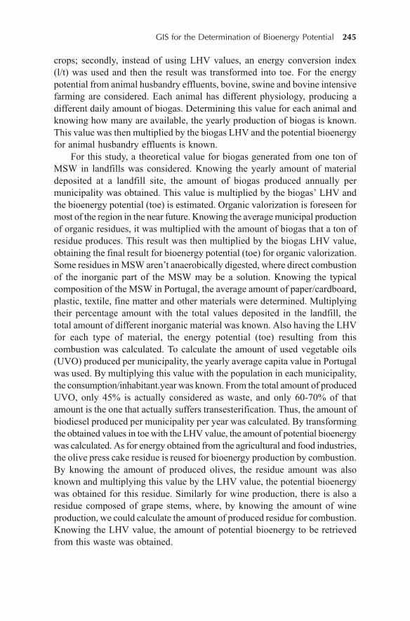
GIS for the Determination of Bioenergy Potential 245
crops; secondly, instead of using LHV values, an energy conversion index(l/t) was used and then the result was transformed into toe. For the energypotential from animal husbandry effluents, bovine, swine and bovine intensivefarming are considered. Each animal has different physiology, producing adifferent daily amount of biogas. Determining this value for each animal andknowing how many are available, the yearly production of biogas is known.This value was then multiplied by the biogas LHV and the potential bioenergyfor animal husbandry effluents is known.
For this study, a theoretical value for biogas generated from one ton ofMSW in landfills was considered. Knowing the yearly amount of materialdeposited at a landfill site, the amount of biogas produced annually permunicipality was obtained. This value is multiplied by the biogas’ LHV andthe bioenergy potential (toe) is estimated. Organic valorization is foreseen formost of the region in the near future. Knowing the average municipal productionof organic residues, it was multiplied with the amount of biogas that a ton ofresidue produces. This result was then multiplied by the biogas LHV value,obtaining the final result for bioenergy potential (toe) for organic valorization.Some residues in MSW aren’t anaerobically digested, where direct combustionof the inorganic part of the MSW may be a solution. Knowing the typicalcomposition of the MSW in Portugal, the average amount of paper/cardboard,plastic, textile, fine matter and other materials were determined. Multiplyingtheir percentage amount with the total values deposited in the landfill, thetotal amount of different inorganic material was known. Also having the LHVfor each type of material, the energy potential (toe) resulting from thiscombustion was calculated. To calculate the amount of used vegetable oils(UVO) produced per municipality, the yearly average capita value in Portugalwas used. By multiplying this value with the population in each municipality,the consumption/inhabitant.year was known. From the total amount of producedUVO, only 45% is actually considered as waste, and only 60-70% of thatamount is the one that actually suffers transesterification. Thus, the amount ofbiodiesel produced per municipality per year was calculated. By transformingthe obtained values in toe with the LHV value, the amount of potential bioenergywas calculated. As for energy obtained from the agricultural and food industries,the olive press cake residue is reused for bioenergy production by combustion.By knowing the amount of produced olives, the residue amount was alsoknown and multiplying this value by the LHV value, the potential bioenergywas obtained for this residue. Similarly for wine production, there is also aresidue composed of grape stems, where, by knowing the amount of wineproduction, we could calculate the amount of produced residue for combustion.Knowing the LHV value, the amount of potential bioenergy to be retrievedfrom this waste was obtained.
246 Tanya C.J. Esteves et al.
Using GIS for the Multicriteria Decision Analysis forBioenergy Potential
This study used the ArcInfo 9.3 software, produced by ESRI, to perform themulticriteria decision analysis. Most of the data used by managers and decisionmakers is somehow related to a geographical level. Data that is undigested,unorganized or unevaluated may be processed to obtain information in orderto have some kind of significance. Doing so adds extra value to the originaldata, proving useful to decision makers to produce quality decisions(Malczewski, 1999). Typically, spatial decision problems involve a large setof feasible alternatives and multiple, conflicting and incommensurate evaluationcriteria, while some are of the qualitative and other of the quantitative nature(Malczewski, 1999, 2006a, b). Multicriteria decision analysis is a useful toolto help solve this type of problems. It uses two types of criteria: constraintsand factors. The former are based on boolean criteria restricting the analysesto specific regions while the latter define a degree of suitability for the wholegeographical space, specifying areas or alternatives according to a continuousmeasure of suitability (Hansen, 2005). The decision making process involvesthe aggregation of selected criteria that need to be standardized to a commonscale (Hansen, 2005). A boolean overlay approach involves the application ofoperators such as intersection (AND) or union (OR) resulting in binary mapswhere only the suitable (TRUE) and non-suitable (FALSE) locations arepresent. An alternative method is the weighted linear combination that weighsand combines the factor maps to evaluate the suitability of each cell (Jiangand Eastman, 2000). The suitability s at the kth pixel may be determined by aweighted linear combination (Hansen. 2005):
sk = 6 wi xki (1)
where wi is the weight and xki is the value of criteria i in the kth pixel. The
weights w1, …, wn show each criteria’s relative importance and their sumshould not exceed 1.0 (Hansen. 2005). Here, a combination of the booleanoverlay and the weighted linear combination was used.
The data described in Section 4.1 was introduced into a geographic databaseand, with the aid of the ModelBuider tool, input data turned into information.This functionality created the model to process the input data, allowing tochain together sequences of tools, feeding the output of one tool into another(Environmental Systems Research Institute [ESRI], 2010). Used functions inthis model were merge, dissolve, feature to raster, weighted sum and dividetools. No personalized formulas were used in this particular model, only thestandardized ones available by the ArcInfo 9.3 tools.
The merge tool merged the polygon data (municipalities with the bioenergyinformation) of the different input residue feature classes, and the dissolvetool aggregated the potential bioenergy field for each municipality featureclass. The feature to raster tool transformed the vector data into raster so that
GIS for the Determination of Bioenergy Potential 247
the weighted overlay tool could be used, overlaying the rasters, using a commonscale and weights and outputting the final result of the model (ESRI, 2010).
Results
Currently, there is no method to fully yield 100% of the potential that isavailable by each and every considered residue. Due to technology constantlyprogressing and presenting new solutions, these are frequently surpassingexisting boundaries, so, whatever considered yield for bioenergy productionin this study would rapidly be outdated. The outputted map can be found inFig. 2. We find that the most promising area in terms of bioenergy productionis the northern inland area, Beira Interior Norte, achieving a maximum of98,912.40 toe in the Sabugal municipality. This fact may be due to thecombination of climatic factors with the high amount of agricultural andforest areas, leading to higher biomass yield. The littoral part of the CRP hasa much lower potential, where the lowest production is of 1,848.54 toe(Entroncamento). The general middle region of the study area and the OesteNUTSIII are not appropriate for bioenergy production from biomass.
Figure 2. Bioenergy potential for the CRP.
248 Tanya C.J. Esteves et al.
The component that most influences this final map is the forest wastebiomass. The source’s produced amount is overtaking the remaining sources,mainly due to shrubland contribution.
Information confidentiality for some municipalities is a factor hamperingthe true potential analysis. For various waste sources, many municipalities(around 5%) had confidential data in the consulted bibliography. This factmay certainly alter the presented results drastically, once that the municipalitiescan produce enough waste to make a great difference in the final value forthose municipalities, making the presented results rapidly obsolete.
Location of the Bioenergy Competency Centre
The BCC will not produce energy itself. Rather, it will have several criticalfunctions for the further development of bioenergy production. In general, itis thought to constantly manage and update information produced in the firstsection of this work and study the costs of production/collection and processingof the materials needed for the production of bioenergy, as well as the definitionof the threshold of economic viability. Its tasks include product certification,research, development and innovation, consultancy, training and trials. It willintegrate the main stakeholders in the CRP, as to maximize the profitability ofthe various laboratorial, management and economical infrastructures andavailable knowledge. Information flow will be key in this organization’s workprocesses. Taking these important functions into consideration, theimplementation of the BCC is of utmost importance. Acknowledging thisfact, it should be located in a place of easy access to all stakeholders.
Input Resource Collection and Treatment
For the implementation of the BCC, several suppositions had to be considered.As before, all information is freely available to the general public. The nationalnetwork of the protected areas was used to determine the existing naturalprotected areas; the Corine Land Cover 2006 for Portugal (IGP, 2009) wasused to determine land use; the itinerary map for Portugal (Instituto Geográficodo Exército, 2009) was used for road information; Shuttle Radar TopographyMission (SRTM) digital elevation data (Consultative Group on InternationalAgricultural Research, 2008) was used to obtain slope information; the locationof existing and future biomass power plants in the CRP was also used. Otherinformation can be used, such as sight-seeing and recreation areas, as toexclude them from the final result (one does not want to implement the BCCin these areas). To the author’s knowledge, there is no information of the sortavailable for the study region. What can be done is, when selecting the locationfrom the final map, to compare this information with the Municipal MasterPlan, once this document contains the previously stated information. If themap were done at a single municipal level, the information would certainly beeasier to incorporate in the created model.

GIS for the Determination of Bioenergy Potential 249
Using GIS for the Multicriteria Decision Analysisfor the BCC Implementation
The ArcInfo 9.3 ModelBuilder functionality was again a valued tool to locatethe BCC. In general, all the information is classified into five different classes,being 1 the least favourable condition and 5 the most preferable one. Threeapproaches for using the roads were used: the first one expressed the importanceof the existing types of roads, making sure that the BCC is easily accessibleto all stakeholders; the second approach considered the distance to roads,preferably locating the BCC closer to the roads; and, finally, the use of serviceareas (with the Network Analyst extension) to know the time (hours) it takesthe main stakeholders to access the BCC. The resulting map from bioenergypotential analysis is also used as input, so that the BCC can be located preferablyin areas with higher production of biomass.
Some restricting conditions also influence the final map results. Theprotected areas information was used to exclude these areas, once it is illegalto build in such areas. In what refers to the land use, some features wereexcluded from this feature class once that a construction such as the BCCcould not be located in the areas: continuous urban fabric; discontinuousurban fabric; wetlands; and airports. Having considered the aforementionedrestrictions, these were merged and transformed into a raster informationlayer reclassified from 1 to 5. The restricted areas were excluded from theanalysis (NoData).
Slope plays a major financial role in building an infrastructure. The steepera terrain is, the higher will be the construction costs. It also influences travelling:steeper slopes bring more difficulties in transportation (with more fuelconsumption). After reclassifying all the inputs in a 1 to 5 scale, a weightedoverlay carried out using all the rasters. Table 1 shows four different scenariosfor the inputs. Scenario 1 translates the fact that both stakeholders (biomassplants and waste producers) represent an important role for the BCC (higherweights, both with 25%). Slope and restrictions parameters were constant inall scenarios.
Table 1. Weighting of different inputs for determination of the location of the BCC
Inputs Scenario 1 Scenario 2 Scenario 3 Scenario 4
Restrictions 5 5 5 5Slope 10 10 10 10Road differentiation 15 20 15 20Distance to roads 20 15 20 15Network analysis from biomass plants 25 25 30 30Bioenergy potential 25 25 20 20
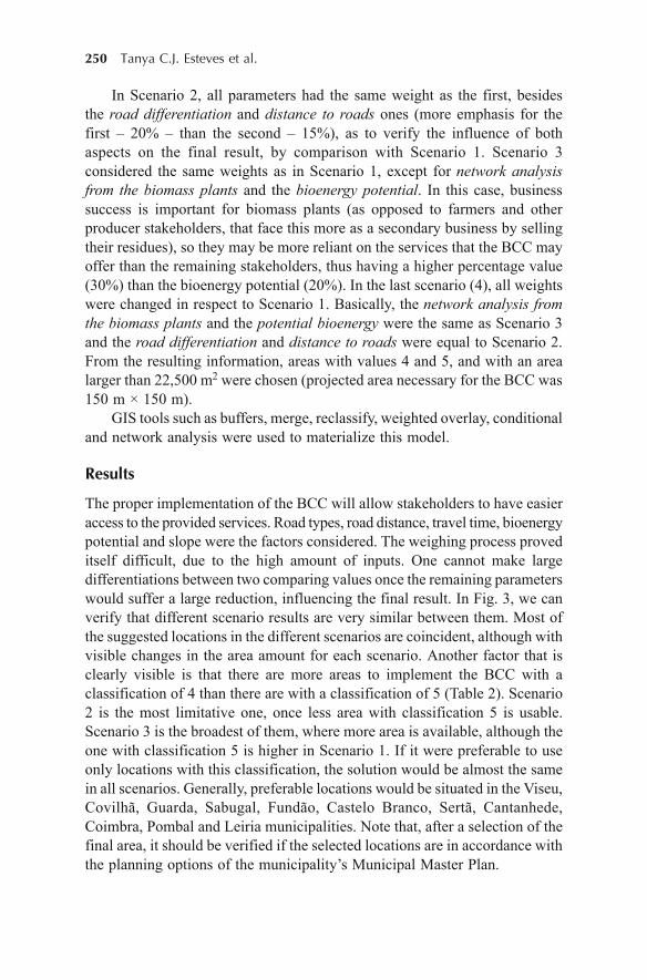
250 Tanya C.J. Esteves et al.
In Scenario 2, all parameters had the same weight as the first, besidesthe road differentiation and distance to roads ones (more emphasis for thefirst – 20% – than the second – 15%), as to verify the influence of bothaspects on the final result, by comparison with Scenario 1. Scenario 3considered the same weights as in Scenario 1, except for network analysisfrom the biomass plants and the bioenergy potential. In this case, businesssuccess is important for biomass plants (as opposed to farmers and otherproducer stakeholders, that face this more as a secondary business by sellingtheir residues), so they may be more reliant on the services that the BCC mayoffer than the remaining stakeholders, thus having a higher percentage value(30%) than the bioenergy potential (20%). In the last scenario (4), all weightswere changed in respect to Scenario 1. Basically, the network analysis fromthe biomass plants and the potential bioenergy were the same as Scenario 3and the road differentiation and distance to roads were equal to Scenario 2.From the resulting information, areas with values 4 and 5, and with an arealarger than 22,500 m2 were chosen (projected area necessary for the BCC was150 m × 150 m).
GIS tools such as buffers, merge, reclassify, weighted overlay, conditionaland network analysis were used to materialize this model.
Results
The proper implementation of the BCC will allow stakeholders to have easieraccess to the provided services. Road types, road distance, travel time, bioenergypotential and slope were the factors considered. The weighing process proveditself difficult, due to the high amount of inputs. One cannot make largedifferentiations between two comparing values once the remaining parameterswould suffer a large reduction, influencing the final result. In Fig. 3, we canverify that different scenario results are very similar between them. Most ofthe suggested locations in the different scenarios are coincident, although withvisible changes in the area amount for each scenario. Another factor that isclearly visible is that there are more areas to implement the BCC with aclassification of 4 than there are with a classification of 5 (Table 2). Scenario2 is the most limitative one, once less area with classification 5 is usable.Scenario 3 is the broadest of them, where more area is available, although theone with classification 5 is higher in Scenario 1. If it were preferable to useonly locations with this classification, the solution would be almost the samein all scenarios. Generally, preferable locations would be situated in the Viseu,Covilhã, Guarda, Sabugal, Fundão, Castelo Branco, Sertã, Cantanhede,Coimbra, Pombal and Leiria municipalities. Note that, after a selection of thefinal area, it should be verified if the selected locations are in accordance withthe planning options of the municipality’s Municipal Master Plan.
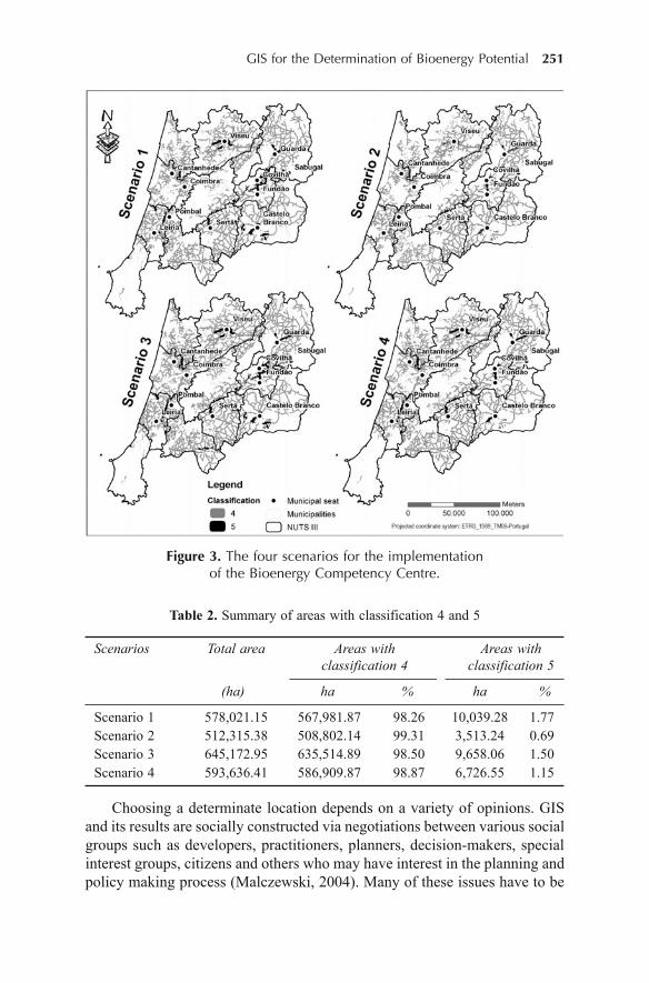
GIS for the Determination of Bioenergy Potential 251
Figure 3. The four scenarios for the implementationof the Bioenergy Competency Centre.
Table 2. Summary of areas with classification 4 and 5
Scenarios Total area Areas with Areas withclassification 4 classification 5
(ha) ha % ha %
Scenario 1 578,021.15 567,981.87 98.26 10,039.28 1.77Scenario 2 512,315.38 508,802.14 99.31 3,513.24 0.69Scenario 3 645,172.95 635,514.89 98.50 9,658.06 1.50Scenario 4 593,636.41 586,909.87 98.87 6,726.55 1.15
Choosing a determinate location depends on a variety of opinions. GISand its results are socially constructed via negotiations between various socialgroups such as developers, practitioners, planners, decision-makers, specialinterest groups, citizens and others who may have interest in the planning andpolicy making process (Malczewski, 2004). Many of these issues have to be
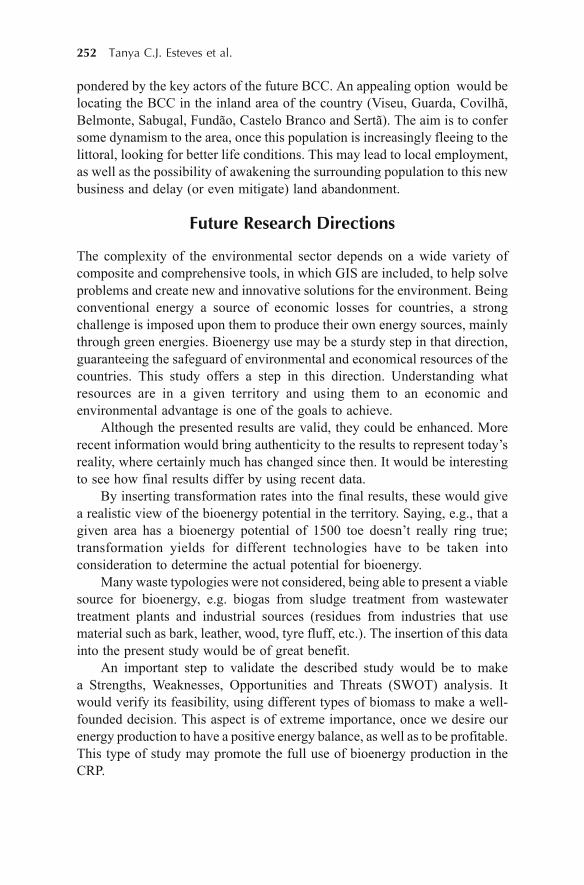
252 Tanya C.J. Esteves et al.
pondered by the key actors of the future BCC. An appealing option would belocating the BCC in the inland area of the country (Viseu, Guarda, Covilhã,Belmonte, Sabugal, Fundão, Castelo Branco and Sertã). The aim is to confersome dynamism to the area, once this population is increasingly fleeing to thelittoral, looking for better life conditions. This may lead to local employment,as well as the possibility of awakening the surrounding population to this newbusiness and delay (or even mitigate) land abandonment.
Future Research Directions
The complexity of the environmental sector depends on a wide variety ofcomposite and comprehensive tools, in which GIS are included, to help solveproblems and create new and innovative solutions for the environment. Beingconventional energy a source of economic losses for countries, a strongchallenge is imposed upon them to produce their own energy sources, mainlythrough green energies. Bioenergy use may be a sturdy step in that direction,guaranteeing the safeguard of environmental and economical resources of thecountries. This study offers a step in this direction. Understanding whatresources are in a given territory and using them to an economic andenvironmental advantage is one of the goals to achieve.
Although the presented results are valid, they could be enhanced. Morerecent information would bring authenticity to the results to represent today’sreality, where certainly much has changed since then. It would be interestingto see how final results differ by using recent data.
By inserting transformation rates into the final results, these would givea realistic view of the bioenergy potential in the territory. Saying, e.g., that agiven area has a bioenergy potential of 1500 toe doesn’t really ring true;transformation yields for different technologies have to be taken intoconsideration to determine the actual potential for bioenergy.
Many waste typologies were not considered, being able to present a viablesource for bioenergy, e.g. biogas from sludge treatment from wastewatertreatment plants and industrial sources (residues from industries that usematerial such as bark, leather, wood, tyre fluff, etc.). The insertion of this datainto the present study would be of great benefit.
An important step to validate the described study would be to makea Strengths, Weaknesses, Opportunities and Threats (SWOT) analysis. Itwould verify its feasibility, using different types of biomass to make a well-founded decision. This aspect is of extreme importance, once we desire ourenergy production to have a positive energy balance, as well as to be profitable.This type of study may promote the full use of bioenergy production in theCRP.
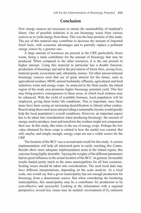
GIS for the Determination of Bioenergy Potential 253
Conclusion
New energy sources are necessary to ensure the sustainability of mankind’sfuture. One of possible solutions is to use bioenergy waste from varioussources as to yield energy from them. This was the base premise of this study.The use of this material may contribute to decrease the amount of importedfossil fuels, with economic advantages and to partially replace a pollutantenergy source by a greener one.
A large amount of resources are present in the CRP, particularly forestwaste, being a main contributor for the amount of bioenergy that may beproduced. When compared to the other resources, it is the one present inhigher amount. Using this material in particular has a double function:production of bioenergy and aid in the prevention of forest fires, saving lives,material goods, ecosystems and, ultimately, money. Yet other unconventionalbioenergy sources exist that are of great interest for the future, such asagricultural residues, MSW, animal husbandry effluents, agricultural and foodindustries waste and energy crops. As analyzed in the final results, the inlandregion of the study area promotes higher bioenergy potential yield. This factmay bring positive consequences to these areas, in which local richness maybe enhanced. With the yield of available biomass, local population will beemployed, giving them better life conditions. This is important, once theseareas have been seeing an increasing desertification to littoral urban centres.Reactivating these rural areas and providing a sustainable income would greatlyhelp the local population’s overall conditions. However, an important aspecthas to be taken into consideration when producing bioenergy: the amount ofenergy used to produce, treat and transform the residues might not compensatetheir use. In this study, this refers to the use of energy crops. Perhaps the lowvalue obtained for these crops is related to how the model was created. Butstill, maybe, and simply enough, energy crops are not a viable source for theCRP.
The location of the BCC was a second main result for this study. A correctimplementation will help all interested parts in easily reaching this Centre.Results show more adequate implementation areas in the inland region, thisoutcome being highly desirable. Varying the weights of the different parametershad no great influence in the actual location of the BCC. In general, favourableresults landed pretty much in the same municipalities for all four scenarios.Scaling issues should be taken into consideration. The used local data mayhave different interpretations, depending on the scale analysis. At a localscale, one would say that a given municipality has not enough production forbioenergy from a determinate source. But when considering the borderingmunicipalities, this municipality may be a contributor for production to becost-effective and successful. Looking at the information with a regionalperspective, several key issues may be tackled: environment (CO2 emission
254 Tanya C.J. Esteves et al.
reduction, less wildfires, etc.), economic, society (employment, localdevelopment) and politics (more subsidies to promote bioenergy productionfrom biomass).
References
Agência para o Investimento e Comércio Externo de Portugal (2008). Portugal - Perfilpaís. AICEP Portugal Global, Lisboa.
Agência Portuguesa do Ambiente (2008). Relatório do Estado do Ambiente 2007.Agência Portuguesa do Ambiente, Amadora.
Agência Portuguesa do Ambiente (2009). Relatório do Estado do Ambiente 2009.Agência Portuguesa do Ambiente, Amadora:.
Associação das Energias Renováveis (2010). Roteiro Nacional das Energias Renováveis- Aplicação da Directiva 2009/28/CE. Associação de Energias Renováveis, Lisboa.
Boyle, G. (2004). Renewable energy: power for a sustainable future (2 ed.). OxfordUniversity Press, United Kingdom.
Cantrell, K.B., Ducey, T., Ro, K.S. and Hunt, P.G. (2008). Livestock waste-to-bioenergygeneration opportunities. Bioresource Technology, 99, 7941–7953.
Consultative Group on International Agricultural Research (2008). CGIAR –Consortium for Spatial Information. Retrieved August 19, 2008, from http://srtm.csi.cgiar.org/
Direcção Geral de Energia e Geologia (2005). Direcção Geral de Energia e GeologiaHomepage. Retrieved November 5, 2010, from http://www.dgge.pt/
Environmental Systems Research Institute (2010). ArcGis 9.3 Desktop Help. ESRI,USA.
European Commission (2007). Evaluation report on the implementation in Portugal ofthe European sustainable development strategy – June (No. Tech. Rep. SG/743/07-EN). European Commission, Brussels.
European Environment Agency (2007). Estimating the environmentally compatiblebioenergy potential from agriculture (No. Tech. Rep. 12/2007). EuropeanEnvironment Agency, Copenhagen.
European Parliament and of the Council (2007). Directive 2001/77/EC. Promotion ofelectricity produced from renewable energy sources in the internal electricity market.Official Journal of the European Communities, Brussels.
European Parliament and of the Council (2009). Directive 2009/28/CE. Promotion ofthe use of energy from renewable sources and amending and subsequently repealingDirectives 2001/77/EC and 2003/30/EC. Official Journal of the EuropeanCommunities, Brussels.
Gómez, A., Zubizarreta, J., Rodrigues, M., Dopazo, C. and Fueyo, N. (2010). Potentialand cost of electricity generation from human and animal waste in Spain. RenewableEnergy, 35, 495–505.
Hansen, H.S. (2005). GIS-based Multi-Criteria Analysis of Wind Farm Development.Paper presented at the ScanGis 2005 – 10th Scandinavian Research Conference onGeographical Information Science, Stockholm, Sweden.
Instituto Geográfico do Exército (2010). Instituto Geográfico do Exército. RetrievedOctober 7, 2010, from http://www.igeoe.pt
GIS for the Determination of Bioenergy Potential 255
Instituto Geográfico Português (2009). Instituto Geográfico Português. Grupo deDetecção Remota. Retrieved September 12, 2009, from http://www.igeo.pt/gdr/
Instituto Nacional de Estatística (2009). Estatísticas Agrícolas 2008. Instituto Nacionalde Estatística. I.P., Lisboa.
International Energy Agency for Bioenergy (2009). Bioenergy – A sustainable andreliable energy Source (No. Main Report). s.l.: IEA Bioenergy.
Jiang, H. and Eastman, J.R. (2000). Application of fuzzy measures in multi-criteriaevaluation in GIS. International Journal of Geographical Information Science,14(2), 173–184.
Malczewski, J. (1999). GIS and multicriteria decision analysis. John Wiley and Sons,Inc., USA.
Malczewski, J. (2004). GIS-based land-use suitability analysis: A critical overview.Progress in Planning, 62, 3–65.
Malczewski, J. (2006a). GIS-based multicriteria decision analysis: A survey of theliterature. International Journal of Geographical Information Science, 20(7), 703–726.
Malczewski, J. (2006b). Integrating multicriteria analysis and geographic informationsystems: the ordered weighted averaging (OWA) approach. International Journalof Environmental Technology and Management, 6(1/2), 7–19.
Masera, O., Ghilardi, A., Drigo, R. and Trossero, M.A. (2006). WISDOM: A GIS-based supply demand mapping tool for woodfuel management. Biomass andBioenergy, 30, 618–637.
Ministério do Ambiente e Ordenamento do Território. (2007). Plano Estratégico paraos Resíduos Sólidos Urbanos 2007–2016. Ministério do Ambiente, do Ordenamentodo Território e do Desenvolvimento Regional, Lisboa.
Population Reference Bureau (2010). 2006 World Population Data Sheet. PopulationReference Bureau, Washington.
Ramachandra, T.V. (2008). Geographical information system approach for regionalbiogas potential assessment. Research Journal of Environmental Sciences, 3(2),170–184.
Richardson, J. and Verwijst, T. (2005). Sustainable bioenergy production systems:Environmental, operational and social implications. Biomass and Bioenergy, 28(Preface), 95–96.
U.S. Department of Energy (2009). Department of Energy. Retrieved June 23, 2009,from http://tonto.eia.doe.gov/oog/info/twip/twipcrvwall.xls#’Data 2'!A1
U.S. Energy Information Administration (2009). World Total Primary EnergyConsumption by Region. Reference Case, 1990-2030. Energy InformationAdministration/International Energy Outlook. Retrieved July 27, 2010, from http://www.eia.doe.gov/oiaf/ieo/pdf/ieoreftab_1.pdf
World Commission on Environment and Development (1990). Our common future.Oxford University Press, USA.

256 John Madsen et al.
16Use of Geospatial Data in Planning
for Offshore Wind Development
John Madsen, Alison Bates, John Callahanand Jeremy Firestone
College of Earth, Ocean and Environment, University of DelawareNewark, Delaware, US
Introduction
Offshore wind projects currently provide over two gigawatts of power to theglobal energy market (Global Wind Energy Council, 2010). Nearly all of thisis generated in the North Sea dominated by projects in the United Kingdomand Denmark (Global Wind Energy Council, 2010). The development ofoffshore wind energy is moving forward in the United States (US) with therecently approved Cape Wind project in federal waters off Massachusetts, thecontinued planning for offshore wind projects in the Great Lakes and thegranting of limited leases for study and calls for requests for interest in leasingselected portions of the eastern outer continental shelf (e.g., MineralsManagement Service, 2009; Bureau of Ocean Energy Management, Regulationand Enforcement, 2010; Great Lakes Wind Council, 2010). In addition to theUnited Kingdom in Europe, large-scale offshore wind projects are projectedfor France, Belgium and the Netherlands, as well as, in China (Global WindEnergy Council, 2010). The development of offshore wind projects furthercontributes to the existing pressures on the marine environment increasing thepotential benefits of comprehensive, integrated, ecosystem-based planning.This type of marine spatial planning (MSP) is based on sound science andconsiders current and anticipated uses of the ocean and coastal environment(Ehler and Douvere, 2009). Geospatial techniques provide the framework bywhich data can be manipulated to aid in implementation of MSP.
The specific objective of this chapter is to use a “case study” approach toillustrate how the gathering, manipulation and interpretation of geospatialdata are used in the implementation of MSP. The studies are fromMassachusetts, Rhode Island and Delaware in the US and Belgium in Europe.
DOI 10.1007/978-94-007-1858-6_16, © Capital Publishing Company 2012
e ,J.K. Thakur et al. (eds.), G ospatial Techniques for Managing Environmental Resources 256

Use of Geospatial Data in Planning for Offshore Wind Development 257
The Delaware study represents an initial effort at compiling data within ageospatial framework to assess the potential location of offshore wind projectswithin state and adjacent federal waters. The Belgian, Rhode Island andMassachusetts projects illustrate how geospatial data have been integratedand analyzed to provide the information that, in concert with policy, has beenused in the MSP process to develop integrated plans concerning effective, andecologically mindful, use of marine resources, including offshore wind.
Background
A commonly accepted definition of marine spatial planning (MSP) is that it isa public process of analyzing and allocating the spatial and temporal distributionof human activities in marine areas to achieve ecological, economic, andsocial objectives that are usually specified through a political process (Ehlerand Douvere, 2009). The six major characteristics of MSP are that it is: (1)ecosystem-based, (2) integrated, (3) place- or area-based, (4) adaptive, (5)strategic and anticipatory and (6) participatory (Ehler and Douvere, 2009).MSP was established in Europe, and plays a fundamental role in themanagement of the marine environment. The US Interagency Ocean PolicyTask Force, established by President Obama, identifies coastal and marinespatial planning as one of its nine priority objectives in its finalrecommendations regarding sustainable stewardship of the ocean, coasts andGreat Lakes (Interagency Ocean Policy Task Force, 2010).
MSP requires a governing framework: a set of goals, priorities andstandards; a legal basis for authority and funding; and procedures defining theplanning process, public and stakeholder participation, and the lifetime andextent of the plan (Ehler and Douvere, 2009). In concert with policy, MSPrequires a significant data-compilation effort: information requirements mustbe identified and data gathered from disparate sources; these datasets must bechecked for quality and synthesized into a common platform; data gaps mustbe identified; and results processed and presented in a usable format (e.g.,Ehler and Douvere, 2009). It is this data-compilation effort that is bestimplemented using geospatial techniques. In planning for the location ofoffshore wind projects the vast majority of data that must be considered isspatial in nature. That is, the information contained in a data point is a functionof its geographic position (both in a horizontal and a vertical sense). Geospatialtechniques, such as those offered in Geographic Information Systems (GIS),are ideally suited to manipulate and represent these data. GIS allows users toview, understand, interpret and visualize data in many ways that can revealrelationships, patterns and trends in various forms including maps (e.g., Ehlerand Douvere, 2009).
258 John Madsen et al.
Use of Geospatial Data in MSP for OffshoreWind—Case Studies
The following case studies of Massachusetts, Rhode Island and Delaware inthe US and Belgium in Europe illustrate how through the use of GIS, MSP foroffshore wind projects can be built upon the framework provided by the bestavailable, science-based data. Examples of the geospatial techniques appliedto integrate, manipulate and analyze the data in the case studies are describedin the “Methods to Analyze Data for Offshore Wind Development” and“Methods of Data Sharing and Display for Users of MSP” sections of thischapter.
Massachusetts Ocean Management Plan
The Commonwealth of Massachusetts passed the Oceans Act of 2008 to laythe framework for managing human activities in its state and adjacent federalwaters using an ecosystem-based approach (Massachusetts Executive Officeof Energy and Environmental Affairs [MA-EEA], 2009a). This Act requiredthe MA-EEA to develop an Ocean Management Plan that includes thedevelopment of renewable energy facilities in appropriate locations. The plancalls for the use of scientific data and the setting forth of plans that arecognizant of marine biological and physical processes, that incorporate publicinput in the planning process and that identify goals and priorities. The planmust include current uses with valuation of those activities and locations andstandards for activities that are allowable under the State’s pre-existing OceansSanctuaries Act (MA-EEA, 2009a).
The Ocean Management Plan defines areas based upon existing uses andproposed allowable activities. It establishes three primary areas for futuredevelopment: prohibited, renewable energy and multi-use (MA-EEA, 2009a).Prohibited areas are those protected under the Oceans Sanctuaries Act; nofurther development may occur. Renewable energy areas are delineated toprovide the optimal location for both commercial and community scalerenewable energy, including offshore wind development. Areas of multi-usecomprise the vast majority of the state’s ocean waters and they are open to alluses allowable under the Ocean Sanctuaries Act. Rather than being determinedby spatially defined boundaries, multi-use areas are managed by siting andperformance standards. These areas could support the development ofcommunity-scale offshore wind projects (MA-EEA, 2009a).
In the development of the plan, a baseline assessment was conducted tocharacterize the current status of the state’s ocean waters (MA-EEA, 2009b).A scientific advisory council and six working groups consisting of expertsfrom fisheries, marine habitat, ocean recreational and cultural services, regionalsediment management, renewable energy and transportation, navigation andinfrastructure were formed to gather, coordinate and analyze pertinent data
Use of Geospatial Data in Planning for Offshore Wind Development 259
from their area of focus. The groups were also charged with identifying datagaps and proposing long term research goals (MA-EEA, 2009b).
The baseline data assessment was aided by the use of MORIS, a web-based GIS-mapping tool that was developed by the Massachusetts Office ofCoastal Zone Management, the Massachusetts Office of Geographic andEnvironmental Information, the Massachusetts Ocean Partnership, and AppliedScience Associates (Massachusetts Office of Coastal Zone Management [MA-CZM], 2011). MORIS utilizes a central repository of GIS data and allowsusers, such as resource managers, scientists and the general public, to createmaps of selected layers (MA-CZM, 2011). As with most MSP efforts, thebaseline assessment data had to be amassed from a variety of sources and itwas incomplete for the entire study area. The details of how MORIS supportsdata storage, management, analysis and visualization is described in furtherdetail in the “Methods of Data Sharing and Display for Users of MSP” sectionof this chapter.
After analysis of the data layers compiled by the working groups, and inconcert with an assessment of priorities, three zones for future activities(prohibited, renewable energy and multi-use) were delineated. To identifypotential areas for wind energy development, a screening process was appliedwhich involved passing areas through “filters” that included exclusionary andconstraint of potential impacts criteria (MA-EEA, 2009a). As a result of thescreening process, two areas, the Gosnold Wind Energy Area and the Martha’sVineyard Wind Energy Area, have been designated as appropriate forcommercial-scale wind energy facility siting (MA-EEA, 2009a). Each of thetwo wind energy areas is expected to support a maximum of 150, 3.6 megawattturbines. Three additional areas, within the state’s waters, were designated asprovisional sites for wind energy development, although they have limitationsand are not slated for near-future development. Within the framework of thestate’s ocean management plan, suitable locations for offshore wind facilitiesin federal waters have also been recommended (MA-EEA, 2009a).
Rhode Island Ocean SAMP
The state of Rhode Island Coastal Resources Management Council used MSPto develop a Special Area Management Plan (SAMP) for the state’s oceanenvironment (Rhode Island Coastal Resources Management Council [RI-CRMC], 2010). The Ocean SAMP lays out enforceable policies andrecommendations that promote a balanced and comprehensive ecosystem-based management approach for the state’s ocean-based resources. It protectscurrent uses and habitats by establishing zones for commercial fishing, criticalhabitats for fish, marine animals and birds and marine transportation. It alsoincludes comprehensive new regulatory standards for offshore development.In doing so, it delineates appropriate areas in the state’s offshore waters forrenewable energy and also suggests suitable sites in nearby federal waters.
260 John Madsen et al.
The Ocean SAMP area includes approximately 3800 km2 of portions of BlockIsland Sound, Rhode Island Sound and the Atlantic Ocean. It extends laterallyacross 48 km and abuts the state waters of neighbouring Massachusetts,Connecticut and New York (RI-CRMC, 2010). Currently, a 28.8 megawattproject southeast of Block Island, consisting of five to eight turbines, is in theplanning and approvals phase with construction as early as 2012 (DeepwaterWind LLC, 2011).
The RI-CRMC acknowledges that one of the biggest challenges of theOcean SAMP process was gathering the extensive amount of data needed toinitiate the MSP process and turning it into usable GIS layers (RI-CRMC,2010). In an effort to manage the database, the University of Rhode IslandEnvironmental Data Center (EDC) provides guidelines for data submittal.Users are asked to provide data in an ESRI ArcGIS-ready format (e.g.,shapefiles, coverages, GRIDs, LATTICEs, TINs, geodatabases or conventionalgeoreferenced images). Non-GIS data are accepted in a limited capacity, aslong as they are accompanied by proper metadata. The data that has beencompiled is listed in Table 2. Through the EDC, many of the data layers areavailable for public use.
In terms of offshore wind development within the designation of aRenewable Energy Zone, the Ocean SAMP provides a technical analysis ofwind resource, bathymetry and seabed geology, followed by exclusionarycriteria (RI-CRMC, 2010). The wind resource was characterized in 2007 andagain in 2010 (Applied Technology Management, 2007; Grilli, Spaulding,Crosby and Sharma, 2010). From these data, maps were developed to depictthe regions of best wind resource within the Ocean SAMP area. This wasfollowed by a comprehensive analysis using the Technology DevelopmentIndex (TDI) developed by Spaulding, Grilli, Damon and Fugate (2010). Thespecifics of the TDI are described in the “Methods to Analyze Data for OffshoreWind Development” section of this chapter.
After using the TDI as a measure of determining general areas suitable foroffshore wind development, the siting was further refined using exclusionarycriteria. Each of the criteria was added as a data layer, progressively reducingthe available preferred areas. The exclusionary data layers include: marinetransportation routes, regulated uses including disposal sites, presence ofpotential unexploded ordinance, protected areas, conservation zones andmilitary areas, licensed extractive development areas, airport setbacks and acoastal buffer zone (RI-CRMC, 2010).
Although the Renewable Energy Zone was delineated as a special usearea within a broad multi-use region, renewable energy may be developed inother areas within state waters, provided no significant conflicts with existinghuman uses and natural resources are found (RI-CRMC, 2010). Prohibitedareas from large- and small-scale development are named as Areas of ParticularConcern (APCs) and Areas Designated for Preservation (ADPs). APCs areareas of high conservation value, important habitat features, sensitive cultural

Use of Geospatial Data in Planning for Offshore Wind Development 261
resources, high human use value or areas important for activities such asshipping, military use, or navigation. ADPs are more stringently protected andinclude habitat of endangered species and other sensitive species zones (RI-CRMC, 2010).
Delaware MSP for Offshore Wind
In an effort that is being undertaken by the University of Delaware to focus onthe potential for offshore wind power development off the Delaware coast instate and adjacent federal waters up to 50 m deep, geospatial techniques arebeing employed to synthesize existing data, identify gaps, and develop projectsto collect the necessary missing data to develop an initial framework for MSPthat could form the basis of stakeholder engagement. The goal of the projectis to generate interactive multi-layered maps, accompanied by a policydocument, which will display current information about wind resources,ecological features, bathymetry and marine geology and existing use andusers. Maps will indicate zones that are optimal for wind projects, as well as,exclusionary zones and zones where further data collection and investigationare needed to determine suitability for wind project developments. The projectresults will set the groundwork for Delaware’s MSP efforts and may serve todirect initial proposals for locating new offshore wind projects.
The data layers and their sources that the Delaware MSP project seeksand intends to compile are summarized in Table 1. The data sources providea good example of the various repositories including federal, state, academicand private that may contain data that must be obtained and integrated toapply MSP for offshore wind projects.
Spatial Analysis of the Belgian Part of the North Sea
Belgium is one of the global leaders in implementing MSP as a method ofecosystem-based management for its territorial sea and exclusive economiczone. The Belgian part of the North Sea (BPNS) covers about 3600 km2 witha coastline that is 66 km in length. Despite its relative small area (i.e., only0.5% of the North Sea) the BPNS is intensely used (Maes et al., 2005).Belgium began to implement its Master Plan for the BPNS starting in 2003using GIS to delineate areas for offshore wind development and sand/gravelextraction; this was followed by designation of marine protected areas (Douvere,Maes, Van Hulle and Schrijvers, 2007).
The criteria used to delineate these areas included fishing activity, natureand biodiversity and visual impacts from shore (Douvere et al., 2007). Theeffort produced a spatial plan that included a geo-referenced map of acceptableuses of the BPNS, with a 263.7 km2 zone identified for potential offshorewind development (Degraer, Brabant and Rumes, 2010). This zone begins 22km from the shoreline and extends seaward to the northern navigation route(Van Hulle et al., 2004). Belgium has continued to use this zone as the

262 John Madsen et al.
Tabl
e 1.
GIS
dat
a la
yers
and
sou
rces
for d
ata
to b
e us
ed in
the
Del
awar
e M
SP fo
r offs
hore
win
d
GIS
dat
a la
yer
Des
crip
tion
of la
yer
and
note
sSo
urce
of d
ata
Vess
el tr
affic
Obs
erve
d sh
ip m
ovem
ents
, fa
irway
s an
d es
tabl
ishe
d sh
ippi
ng l
anes
,in
clud
ing
pilo
t boa
rdin
g ar
eas
and
anch
orag
es. G
ener
ally
exc
lusi
onar
yto
offs
hore
win
d pr
ojec
ts.
Mar
ine
wild
life
Nes
ting,
sta
ging
and
im
porta
nt f
eedi
ng a
reas
for
crit
ical
wat
erbi
rds;
avia
n fly
way
s; m
igra
tory
pat
hway
s of m
arin
e mam
mal
s; an
d di
strib
utio
nof
impo
rtant
spec
ies.
Gen
eral
ly e
xclu
sion
ary
to o
ffsho
re w
ind
proj
ects
.
Proh
ibite
d ar
eas
Proh
ibite
d ar
eas i
nclu
de a
min
efie
ld, c
hem
ical
was
te d
ump,
and
dre
dge
spoi
l gro
unds
. Exc
lusi
onar
y to
offs
hore
win
d pr
ojec
ts.
Reg
ulat
ed a
irspa
ceA
irspa
ce re
stric
ted
by th
e US
Fede
ral A
viat
ion
Age
ncy
(FA
A).
Gen
eral
lyex
clus
iona
ry to
offs
hore
win
d pr
ojec
ts.
Arti
ficia
l ree
fsG
ener
ally
exc
lusi
onar
y to
offs
hore
win
d pr
ojec
ts.
Sand
bor
row
site
sA
ctiv
e an
d po
tent
ial s
and
min
ing
oper
atio
ns fo
r bea
ch re
plen
ishm
ent.
Gen
eral
ly e
xclu
sion
ary
to o
ffsho
re w
ind
deve
lopm
ent.
Bat
hym
etry
and
Wat
er d
epth
, cha
ract
eriz
atio
n of
sea
floor
sed
imen
ts fr
om g
rab
sam
ples
mar
ine
geol
ogy
and
sub-
botto
m s
edim
ents
fro
m c
ores
and
sei
smic
ref
lect
ion
prof
iles.
Dep
ths
and
sedi
men
t ty
pes
have
im
pact
on
foun
datio
n ty
pe a
ndin
stal
latio
n co
sts.
Win
d re
sour
ceM
etric
indi
catin
g st
reng
th o
f win
d re
sour
ce.
Ener
gyLo
catio
n an
d ca
paci
ties
of o
nsho
re a
nd o
ffsho
re tr
ansm
issi
on c
ritic
alin
fras
truct
ure
for o
ptim
izin
g lo
catio
n of
offs
hore
ene
rgy
proj
ects
.M
SP,S
tate
/Fed
eral
Exte
nt o
f MSP
effo
rt an
d bo
unda
ries f
or st
ate/
fede
ral w
ater
s and
fede
ral
boun
darie
sO
CS
leas
e bl
ocks
.
Inte
rnat
iona
l C
ompr
ehen
sive
Oce
an-A
tmos
pher
eD
ata
Set;
Wat
erw
ay N
etw
ork
Ship
Tra
ffic
, Ene
rgy
and
Env
iron
men
t M
odel
; U
S D
epar
tmen
t of
Tran
spor
tatio
n C
omm
erci
ally
Nav
igab
le W
ater
way
s;B
urea
u of
Oce
an E
nerg
y M
anag
emen
t, R
egul
atio
nan
d En
forc
emen
t (B
OEM
RE)
Mar
ine
Cad
astre
Del
awar
e D
epar
tmen
t of
Nat
ural
Res
ourc
es a
ndEn
viro
nmen
tal
Con
trol
(DN
REC
), N
orth
Atla
ntic
Rig
ht W
hale
Cat
alog
, O
cean
Bio
geog
raph
icIn
form
atio
n Sy
stem
(OB
IS)-
SEA
MA
PN
OA
A E
lect
roni
c N
avig
atio
n C
harts
(EN
Cs)
FAA
DN
REC
DN
REC
, US
Arm
y C
orps
of
Engi
neer
s, D
elaw
are
Geo
logi
cal S
urve
y (D
GS)
NO
AA
Bat
hym
etry
, U
SGS
CO
NM
AP,
DG
S,U
nive
rsity
of D
elaw
are
(UD
)
Nat
iona
l Ren
ewab
le E
nerg
y La
b (N
REL
), N
OA
AB
uoy
Dat
aN
REL
and
PJM
Inte
rcon
nect
ion
LLC
UD
, BO
EMR
E M
arin
e C
adas
tre
Use of Geospatial Data in Planning for Offshore Wind Development 263
permissible area for offshore wind development as it adopts permittingguidelines. To date, Belgium has granted domain concessions to six windprojects, three of which have also obtained the appropriate environmentalpermits. Thus far, sixty-one offshore wind turbines have been installed, fifty-five on Bligh Bank and six on Thornton Bank; Eldepasco is expected to beginconstruction in 2011 (Royal Belgian Institute of Natural Sciences, 2011).
Following its initial MSP effort, Belgium conducted a comprehensivescientific study to set the framework for planning efforts into the future (Maeset al., 2005). This two-year study, the GAUFRE project, adapted land-basedplanning methods to the BPNS and produced an integrated vision for futureuse. The final recommendations of GAUFRE are a flexible structure thatallows the government to adapt policies as needs change (Maes et al., 2005).The GAUFRE project involved substantial data gathering from a multitude ofsources and integration of these data to produce GIS maps. The data compiledin the project is listed in Table 2. With exception of tourism, a geo-referencedmap was generated for each component listed. During this process, areas ofsignificant data gaps were identified and will be used to guide future datagathering efforts (Maes et al., 2005).
The second phase of the GAUFRE project analyzed the interactionamong stakeholders where use overlapped spatially or temporally (Maes etal., 2005). Both positive interactions and conflict areas were identified anddescribed. The MSP process in Belgium is set apart through the vision of theGAUFRE project. Rather than a final, end-use spatial plan, the project offersa strategic vision for development of the marine environment that incorporatesthe interconnectedness of each use and allows for continual adaptation overtime. The vision is expressed through the integration of impact of use withthree core values: well-being, ecological value and economic value. Sixscenarios are displayed on structure maps with each map incorporatingimportant use categories with core values. The scenarios include: the relaxed,playful, natural, mobile, rich and sailing sea; each with different emphasis onecological value, economic value and well-being. As examples, the relaxedsea scenario places an emphasis on providing opportunities for tourism andrecreational activities; the rich sea scenario places economic development asthe most important objective in which many more resources can be exploited(Maes et al., 2005).
Essential Techniques in Use of GeospatialData for Offshore Wind
Table 2 provides an example of the types of geospatial data that are needed toprovide the framework for implementing MSP for offshore wind projects. Thetwo case studies, Belgium and Rhode Island, offer a good sampling of thetypes of data that are required.

264 John Madsen et al.
Tabl
e 2.
Exa
mpl
es o
f geo
spat
ial d
ata
for M
SP fo
r offs
hore
win
d pr
ojec
ts
Geo
spat
ial D
ata
Cas
e St
udy
Belg
ium
Rhod
e Is
land
Win
d
Wat
er d
epth
s, M
arin
e ge
olog
yan
d O
cean
ogra
phy
Ecol
ogy
Infr
astru
ctur
e
Nav
igat
ion
conc
erns
Excl
usio
nal u
se
Oth
er u
se a
nd c
once
rns
Cul
tura
l/His
toric
al fe
atur
es
Bou
ndar
ies
Plan
ned
win
d pa
rks
Bat
hym
etry
, Sa
nd b
anks
, B
otto
m a
nd s
ub-b
otto
mse
dim
ents
, Oce
an c
urre
nts,
Wat
er p
ollu
tion
Bent
hic s
ampl
es, F
lora
and
faun
a, E
colo
gica
l val
uatio
n,B
ird
spec
ies,
mig
rato
ry r
oute
s an
d di
stur
banc
e,Po
llutio
n/di
stur
bed
bent
hos,
Are
as o
f nat
ure p
rote
ctio
nB
urie
d ca
bles
and
pip
elin
es, C
oast
al d
efen
se, T
ower
s/pl
atfo
rms,
Ports
, anc
hora
ge a
reas
Ship
ping
rout
esD
redg
ing/
dum
ping
of
dred
ge m
ater
ial,
Sand
/gra
vel
extra
ctio
n, M
ilita
ry u
se, A
mm
uniti
on d
umpi
ngFi
shin
g an
d sh
ippi
ng i
nten
sity
, To
uris
m/re
crea
tion,
Aqu
acul
ture
, Wat
er p
ollu
tion,
Res
earc
h zo
nes
Ship
wre
cks
Terr
itoria
l wat
ers
and
EEZ
Win
d re
sour
ce, T
DI,
Tier
1 an
alys
es, R
enew
able
ener
gyzo
nes
Bat
hym
etry
, B
otto
m s
edim
ents
, B
enth
ic h
abita
t,Su
bsur
face
geo
logy
, B
OEM
RE
prio
rity
area
s fo
rge
olog
ic s
tudy
, M
eteo
rolo
gica
l da
ta,
Wav
es,
tides
,hy
drog
raph
y an
d ci
rcul
atio
nB
enth
ic e
cosy
stem
, Pl
ankt
on,
Fish
es,
Sea
turtl
es,
Mar
ine
mam
mal
s, R
ight
wha
le m
anag
emen
t ar
ea,
Avifa
nua,
nut
rient
s an
d to
xins
Cab
les
and
subm
arin
e ca
bles
, A
ncho
rage
s, P
orts
/ha
rbou
rs, a
irpor
ts a
nd a
irpor
t buf
fers
NO
AA
EN
C n
avig
atio
n la
nes
Dis
posa
l site
s, N
OA
A re
gula
ted
area
s
Fish
erie
s an
d fi
sh h
abita
t, A
IS v
esse
l po
sitio
ns,
Ship
ping
act
ivity
, fer
ry ro
utes
, Une
xplo
ded
ordn
ance
,to
uris
m a
nd re
crea
tion
Subm
erge
d ar
chae
olog
ical
site
sA
djac
ent h
isto
ric o
nsho
re s
ites
Coa
stal
buf
fer z
one,
Oce
an S
AM
P ar
ea, S
tate
wat
ers
boun
dary
, BO
EMR
E O
CS
leas
e bl
ocks
Use of Geospatial Data in Planning for Offshore Wind Development 265
Not included in Table 2, and of concern in siting offshore projects, is theinfluence of wind turbines on aviation and marine radar. In the US, the FederalAviation Administration considers not only risks of aircraft collisions withblades, turbines or towers, but also the potential for wind projects to degraderadar performance. The Department of Homeland Security has issued an interimpolicy calling for federal opposition to the establishment of any wind project“within radar line of sight” of a Department of Defense or Homeland Securityradar installation. Research on the effects of turbines on radar and ways tomitigate associated problems have been conducted and are on-going (e.g.,Brenner et al., 2008; Hawk, 2009).
In addition to the identification, acquisition and compilation of the criticalgeospatial data described in the case studies and listed in Tables 1 and 2,geospatial techniques must be applied to make this data useable within anMSP framework. These techniques involve: (1) standardizing individualdatasets into a common platform, (2) deciding upon and carrying out themethods (e.g., modelling vs. visual inspection) that are used to analyze thedata in terms of offshore wind development, and (3) determining and applyingthe appropriate methods of data sharing and display that will create an outputthat is easy to use in MSP.
Geospatial Techniques: Standardizing Datasets into aCommon Platform
Offshore wind datasets are highly varied and typically compiled from disparatesources (Tables 1 and 2). After the significant initial work of identificationand compilation are complete, bringing these datasets together in a usefultechnological platform is necessary. In some cases, digitization andgeoreferencing are required. This is the process of scanning or sketching thegeospatial features on a hard-copy map or drawing into a digital format, andis usually done through any GIS package. However, most offshore windgeospatial data pre-exist in digital format, and thus translation of the datasetsinto a common spatial reference system (SRS) is generally the first step inprocessing.
SRSs define the type of coordinates used to represent the spatial data.Having all of the data georeferenced to a common SRS allows it to be easilymanipulated within a comprehensive GIS, a geospatial data viewer such asGoogle Earth or NASA World Wind or any mapping software. Using a commonSRS is critical when doing nearly any type of analysis, such as computingdistance matrices, performing grid algebra or any vector-based geoprocessing(e.g., union, buffer, intersection). Within a SRS, the shape and orientation ofthe Earth are taken into account, and described by the horizontal referencedatum. A common global datum is the WGS 84, World Geodetic System of1984 and it is the datum used in the GAUFRE project in the BPNS. For theMassachusetts Ocean Management Plan, the MassGIS database associatedwith the MORIS mapping tool contains data that are referenced to the
266 John Madsen et al.
Massachusetts State Plane Mainland NAD83 datum with units in metres. Inthe Rhode Island SAMP, the RIGIS data stored at the EDC are referenced tothe Rhode Island State Plane Feet NAD83 coordinate system. Researchersmay submit data to the EDC in either the RI State Plane Feet NAD83 orgeographic (latitude/longitude) WGS84 coordinate systems. The DelawareMSP project will use Delaware State Plane NAD83 coordinates with units inmetres.
SRSs also include the mathematical projection of 3D real-world geographiccoordinates (latitude and longitude) to 2D planar coordinates (metres or feet)that are used for display. This is known as the projection of the SRS. Theterms “projection” and “SRS” are often confused. It is important to note thata SRS incorporates all of the information about how a feature is referenced tothe Earth. A projection is only the mathematical algorithms used to convertgeographic to planar coordinates and has no bearing to the ellipsoid or thedatum being applied. Because the data is being transformed from 3D to 2D,only some aspects of the data can be preserved, and therefore projections areusually classified by which aspects the transformation preserves. Projectionsmay preserve distances (equidistant), areas (equal area), direction (azimuthal)or shape (conformal) (United States Geological Survey, 1989). For analysesthat utilize distance calculations (e.g., distance to shore), it is optimal to keepthe datasets in an equidistant projection. Likewise for analyses that visuallycompare regions (e.g., areas where development is prohibited, migratory paths/nesting grounds), keeping these data in an equal area projection is beneficial.Multiple types of analyses can be performed on the same data by projectingthe source data to multiple output reference systems. However in terms ofmapping these results, one common SRS should be used.
In addition to translating data to a common SRS, care must be taken todetermine the appropriate file format and resolutions. These are typicallydetermined by the analytical or distribution requirements. For example, if datawill be distributed via the web, keeping data in widely supported formats isideal, such as shapefiles for vectors or TIFFs for rasters. Data may also needto be converted to raster or vector formats, or generalized/down-sampledbased upon the analysis techniques employed.
Geospatial Techniques: Methods to Analyze Data for OffshoreWind Development
Once the data has been translated into a common platform, the types ofanalysis that will be performed need to be determined and then carried out.Depending on the analysis chosen, data may need to be further preprocessedin some way. General approaches include using data required for MSP inanalytical modelling methods or in maps and drawings as illustrations forvisual inspection (Beck, 2009). Both approaches may be used for differentpurposes, on different data sources, or on the same data source at differentstages of the project life cycle.
Use of Geospatial Data in Planning for Offshore Wind Development 267
Incorporating the data into analytical modelling methods usually meansto apply numerical equations or logical algorithms to values within the sourcedata. Within a GIS or programing environment, source datasets are typicallyconverted to raster, cell-based formats. Vector-based data (points, lines andpolygons) are converted to rasters using a variety of techniques, depending onthe nature of the data. For example, for marine wildlife tracking (such asmarine mammal or avian movement), data points may represent individualsightings. To convert these points to raster data, they may be summarized asthe number of observations that occur within a given grid cell. Grid cellresolution is variable depending on the scale of study, with a 1 km × 1 km sizebeing considered reasonable for local to regional coverage. Algorithms arethen applied to each cell in the spatial domain of the study area. Resultingrasters may represent physical calculations, index values, priority ranking, ortrue/false values.
The analyses that are required must be run in capable and readily availablesoftware. In recent years, many free and open source software (FOSS) programsfor geospatial use have become popular due to their maturity, advanced features,active communities and low barrier to adoption. FOSS that can be used toperform analyses that are needed for offshore wind development projectsinclude GRASS GIS, Quantum GIS and GDAL/OGR (for display, conversionand GIS analysis); PostGIS (for data storage); R Geo (for statistical analysis);and Mapserver and Open Layers (for display).
The Technology Development Index (TDI) developed by Spaulding et al.(2010) for the Rhode Island SAMP is a good example of an analytical modellingapproach that can be applied in the planning for offshore wind development.The TDI is expressed by the ratio between the Technical Challenge Index(TCI) and the Power Production Potential (PPP) of the energy extractionequipment (e.g., wind turbines). The TCI is a sum of the measures of howdifficult it is to site an energy project at a given location plus the distance ofthe site to the nearest electrical grid connection. As suggested by Spaulding etal. (2010), TCI could be estimated from the structural design and installationincluding cabling to shore (influenced by local factors including bottomsediments and subsurface geology) and the associated costs for a given location.In this case, numerical values of TCI could be assigned to individual categoriesranked in level of difficulty/expense, with lower numbers being assigned tolocations that are the least difficult and/or expensive to develop. The PPP isdefined as the annual mean power density for the energy project multiplied bythe capacity factor for the facility. In the case of offshore winds, the meanannual power density (kW/m2) is determined at the turbine’s hub height andthe capacity factor is approximately 35% (Renewable Energy ResearchLaboratory, 2008). Minimum values of the ratio TCI/PPP identify areas ofoptimum siting based on these factors (Spaulding et al., 2010).
In practice, the area of study is typically gridded (e.g., 100 m square gridsize for the Rhode Island SAMP) and the TDI (TCI and PPP) is calculated for
268 John Madsen et al.
each grid space. The results can be presented in the form of contours of TDI(Spaulding et al., 2010). As noted by Spaulding et al. (2010), this techniqueexplicitly accounts for the spatial variability of all input data. In addition,simulations can be performed either deterministically or stochastically, usinga Monte Carlo method, so that uncertainties in the underlying input data canbe reflected in the estimated TDI values (Spaulding et al., 2010). The stochasticapproach allows detailed assessment of the sensitivity of the estimates to theinput data used to calculate the TCI and PPP values (Spaulding et al., 2010).
The most common application of visual inspection techniques for offshorewind projects is the determination of exclusionary zones based upon thelocations of features that would preclude development. In the MassachusettsOcean Management Plan, areas of exclusion as shown on GIS generated mapsinclude: locations within 1.6 km from inhabited shorelines, Coast Guard-designated navigation areas (i.e., shipping channels and traffic lanes,precautionary areas, anchorage areas and pilot boarding areas), the presenceof eelgrass and intertidal flats, ferry routes, high concentrations of avianresources (e.g., nesting, staging and critical foraging areas for Roseate Tern;nesting, staging and core foraging areas for special concern Arctic, Least andCommon tern species), high concentrations of whale populations (i.e., NorthAtlantic Right Whale core habitat), areas of significant commercial andrecreational fishing effort and value, direct transit navigation routes for shippingand fishing and regulated airspace. Also removed from further considerationwere areas determined to have excessive cumulative effects, constraints ofwind turbine technology, visual impacts and other existing uses as determinedthrough qualitative assessment, public input and stakeholder feedback (MA-EEA, 2009a).
Visual inspection techniques also can be used to delineate preferred areasfor development based on the absence of exclusionary features and theminimization of impact on ecological resources or competing uses. In the caseof the Rhode Island SAMP, the results from numerical analyses and the TDIcontours were combined with maps of exclusionary zones to delineate themost suitable areas for renewable energy development. A similar approachwas used in the Belgian MSP effort. Intensity of use maps for categories thatincluded fisheries, mineral extraction, aquaculture, dredging, dredge disposal,dumping, wrecks, anchoring, shipping, research, military, cables and pipes,wind projects, coastal defense, marine protected areas and recreation weregenerated for the BPNS area using a grid interval of 1 km2. Each of the useswas qualitatively scored based on its intensity of occurrence within each gridinterval. The intensity values assigned ranged from 3, high intensity of use, to0, no activity (Maes et al., 2005). The expected impact of each category of usein terms of its disturbance based upon ecological, physical and chemicalfactors was then ranked qualitatively using a numerical scale. This scale alsoranged from 3 to 0, with major impacts assigned a value of 3 and negligibleor no impact a value of 0 (Maes et al., 2005). Maps delineating the full
Use of Geospatial Data in Planning for Offshore Wind Development 269
environmental impact of each use were then generated by multiplying theintensity value by the impact value for each 1 km2 grid interval. These GISmaps were used in a suitability analysis that incorporated technical andjurisdictional constraints, as well as ecological and socio-economicconsiderations to identify appropriate use areas within the BPNS (Maes et al.,2005).
Regardless of the approach, the scope, resolution and scale of the analysismust be considered and boundaries of the analysis clearly defined. This makesit easier to develop models and maps, and focuses the interpretation of results.Primarily within a modelling approach, grid cell resolution plays a key role.Beck (2009) argues that marine spatial plans should consider information attwo spatial scales and resolutions: a sub-regional or ‘state’ scale with relativelyfine resolution and a regional scale with coarser resolution. The sub-regionalscale makes it feasible to use a resolution that approximates the largest scale(smallest area) used. Models can run at this resolution (typically a few km orless) to produce numerical results as is common for projects within stateboundaries or smaller study areas. Both the Rhode Island and Belgium MSPexamples to identify preferred areas for offshore wind development used agrid interval of 1 km2 and thus were conducted at what would be consideredthe sub-regional scale.
Processes that happen or data aggregated at regional scales may have lessspatial detail but are just as critical for planning purposes. Analyses at thisscale (a few km or larger) are typically done through maps and illustrationsfor visual inspection. They can serve as a study mask and help focus prioritizing,coordinating and evaluating sub-regional investigations. For example, inexamining ship vessel traffic within the Delaware MSP study area, a moreregional scale analysis is required based upon the resolution of the availabledata. To understand where ships travel within the Delaware study area andwhere conflicts appear to be most prevalent, the International ComprehensiveOcean-Atmosphere Data Set (ICOADS) will be used. ICOADS is a data setof global marine surface conditions collected and reported by a fleet of about4000 ships known as the Voluntary Observing Ships (VOS) (Corbett, Wangand Firestone, 2006). The ICOADS dataset and the Waterway Network ShipTraffic, Energy and Environment Model (STEEM) can be imported into a GISto identify areas of high traffic within the Delaware MSP study area (Wang,Corbett and Firestone, 2007). Totals of ship transits are represented within a4 km by 4 km grid, or 16 km2. Any geospatial analysis methods incorporatingthis data must be performed with a resolution of 4 km × 4 km or larger. Thus,resolution becomes a factor when focussing on the Delaware study area giventhe global nature of the dataset, but it remains the best available to determinehabitual shipping traffic patterns. Preliminary analysis of the ICOADS andSTEEM data indicates that clear economic shipping lanes emerge. They willbe incorporated into the Delaware MSP.
270 John Madsen et al.
The discussed case studies and approaches used have limitations to theaccuracy of the information. Inherent in geospatial analyses is that the GISdata and models represent approximations or indicators of the physicalphenomena, not the phenomena itself (Longley, Goodchild, Maguire and Rhind,2005). Ambiguity and vagueness are always introduced. It is non-trivial togenerate probability of error or uncertainty maps in typical GIS programs.Additional steps must be taken, usually including installation of plug-ins orwriting code with advanced technical or statistical expertise, to approximateassociated errors. However, it is helpful to understand the errors associatedwith any analysis to improve understanding and help make better decisions. IfMSP takes a scientific approach to the collection, manipulation, analysis andpresentation of geographic information, it is then inappropriate that GIS usersremain unable to describe how close their information is to the truth it represents(Hunter, 1998).
Uncertainty may come into play many times during a GIS-based offshorewind project. There is measurement error in the input source data and muchuncertainty in the interpretation of that data. This varies widely among thetypes of data used. For example, the errors associated with estimating migratingbird populations from many years of individual sightings is much differentthan errors introduced when creating a smooth surface (i.e., digital elevationmodel) of ocean bathymetry. Yet, these data may be used in a common analysisto derive a single result (e.g., where to optimally locate offshore wind projects).Mowrer (2000) discusses the data life cycle and how inaccuracies can beintroduced at many times during a project, from data collection to dataconversion, to limitations in the algorithms applied, to approximations orcategorizations used for aesthetic display. Accuracy assessments can beperformed at any time in the cycle and modifications can be made to datamodels or methods applied (Mowrer, 2000).
The spatial and temporal scale at which analyses are conducted plays arole in the uncertainty of the results, although the scale is usually dictated bythe availability of the data. Generally, the more averaging (aggregation or‘scaling up’) done to the data, the stronger the perceived relationships tend tobe (Longley et al., 2005). More uncertainty is introduced as further processingis done in order to prepare data for the selected analysis method or approach,particularly when converting from vector-based data to raster. It is difficult toassign appropriate fundamental units (e.g., grid cell resolutions for rastermodelling, minimum mapping areas for vector drawings) for many naturaland human phenomena, it is even more difficult when these are integrated.Data used as illustrative purposes will have errors in the details at theboundaries. Within MSP, these can be mitigated somewhat by usingconservative estimates for inclusionary areas and over estimates forexclusionary areas. Performing analyses at two separate scales, each withtheir own sets of uncertainty, improves confidence if they indicate similarresults.
Use of Geospatial Data in Planning for Offshore Wind Development 271
Other measures can also be taken to reduce uncertainty. Proper metadataand complete descriptions of data collection methods and any preprocessingperformed (with notes about associated errors) are extremely useful. In thecase studies that are presented in this chapter, metadata are available for all ofthe complied GIS layers. The Massachusetts, Rhode Island and DelawareMSP projects utilize metadata that are Federal Geographic Data Committee(FGDC) complaint. Obtaining data from trusted sources and field checkinginformation are obvious choices but are difficult, sometimes impossible, toachieve in practice. Establishing an independent scientific panel to evaluatemethods and data, such as the working groups and advisory council in theMassachusetts case study, is recommended (Beck, 2009). Openshaw (1989)suggests uncertainty estimations might not require hard quantitativeassessments, but instead may involve a more pragmatic approach of determiningthat errors and uncertainty levels are not so high as to doubt the validity of aparticular result for a given set of data applied to a specific situation.
Geospatial Techniques: Methods of Data Sharing and Display forUsers of MSP
In order to implement MSP, decisions must be made on how best to share anddisplay the data and results with other project participants, relevant stakeholders,and the general public. In all of the case studies that are discussed in thischapter, digital multi-layered maps in a GIS or maps embedded in PDF or asgraphic images are used to present results. An approach to sharing data withvaried audiences is to develop comprehensive web-based mapping applicationswith the ability for users to show/hide various data layers. An example of thisis the MORIS tool developed for the Massachusetts MSP. MORIS is designedto provide spatial data that are accurate, scientifically sound and credible in aneasily accessible and useful manner using a collaborative, interactive processthat involves a variety of partners and data sources (MA-CZM, 2011). TheMORIS implementation is open source and can be accessed via its website(http://www.mass.gov/czm/mapping/index.htm).
MORIS is a JavaScript web application, run through a client-side webbrowser that utilizes various components of OpenLayers/GeoExt, JavaScripttoolkits for rich mapping applications (MA-CZM, 2011). It pulls data throughGeoServer mapping software, a free, open-source, map-serving platform thatserves data using Open Geospatial Consortium, Inc. (OGC) WMS and WFSformats, among others. OGC is a nonprofit, international, voluntary consensusstandards organization that is involved in the development of standards forgeospatial- and location-based services. The developers of MORIS note thatan advantage of serving the data layers through OGC-compliant map servicesis that in addition to supplying the MORIS client, layers are available to beconsumed by other clients including ArcMap, Quantum GIS and Google Earth(MA-CZM, 2011).
272 John Madsen et al.
The EDC at the University of Rhode Island, working in concert with theRI-CRMC, has developed a web-based portal system in which users can viewand access data related to the Rhode Island SAMP project (http://www.narrbay.org/). Options are available to view maps with data layers via arapid watershed viewer, download images of maps in pdf format, or downloaddata in shapefile or ARC/INFO interchange file formats. The initial effort ofthe Delaware MSP offshore wind project will be to generate maps in pdfformat that will be web viewable and available for download.
Another method is to use KML for sharing data to large audiences. It isthe default display format, and can be created and edited, in Google Earth.KML can store both individual geographic features with raw coordinates (forvectors: points, lines polygons) or links to geospatial data stored remotely,including georeferenced graphic images, WMS and WFS map services and3D models. Many GIS programs can export more traditional formats to KML.If the datasets are small (less than a few MB), they can be completely containedinside a KML and no server side technology is required. This is ideal forsituations where very little IT support is available. KML can serve largedatasets easily by pointing to the server that houses the data. In addition tobeing easy to use and having native KML support, an advantage of usingGoogle Earth is the availability of background data. Google Earth includesaerial imagery, subsurface ocean data, point of interest and georeferencedphotographs with user contributed data.
Conclusion
The case studies outlined in this chapter demonstrate the variety and quantityof geospatial data that is required for successfully implementing MSP foroffshore wind projects. Far beyond simply requiring information about thewind resource, water depths, distance to shore and the local ecosystem, datapertaining to such diverse categories as coastal tourism, commercial andrecreational fishing, established shipping lanes, sand borrow sites, disposaland unexploded ordinance sites, marine archaeological sites, submergedtransmission lines, the locations of local and federal boundaries and nearbyland-based energy infrastructure and local socio-economic and socio-culturalconsiderations need to be compiled.
Once gathered, geospatial techniques must be employed to first standardizeindividual datasets into a common platform and then apply analysis methodsgenerally involving both visual comparisons and raster-based impact studies.As a final task in the application of geospatial techniques to offshore winddevelopment projects, the relevant data and results of analyses must bedisplayed and shared with stakeholders and decision makers. As illustrated bythe case studies, geospatial maps, especially those that are able to integratemultiple layers of data and that can be evaluated in the determination of
Use of Geospatial Data in Planning for Offshore Wind Development 273
preferred locations for offshore wind development projects, provide invaluableinput to the MSP process.
In addition to the case studies presented in this chapter, major MSP effortspertaining to offshore wind development are on-going in countries such as theUnited Kingdom and the Netherlands in Europe, as well as states along theEast Coast of the US and the Great Lakes. These efforts, in concert with thecases presented in this chapter, indicate the importance and increasing needfor the application of geospatial techniques in the planning for offshore winddevelopment.
Acknowledgement
This chapter was prepared by the authors under award NA10OAR4170084from the National Oceanic and Atmospheric Administration, US Departmentof Commerce. The statements, findings, conclusions and recommendationsare those of the authors and do not necessarily reflect the views of the NationalOceanic and Atmospheric Administration or the Department of Commerce.
References
Applied Technology and Management (2007). Rhode Island Winds Summary Report.Retrieved from the State of Rhode Island Office of Energy Resources Web site:http://www.energy.ri.gov/documents/renewable/RIWINDS_RANKING.pdf
Beck, M., Ferdana, Z., Kachmar, J., Morrison, K.K. and Taylor, P. (2009). BestPractices for Marine Spatial Planning. The Nature Conservancy, Arlington, VA.
Brenner, M., Cazares, S., Cornwall, M.J., Dyson, F., Earley, D., Horowitz, P., Long,D., Sullivan, J., Vesecky, J. and Weinberger, P. (2008). Wind farms and radar.Retrieved from the Department of Defense Intelligence and Related OrganizationsWeb site: http://fas.org/irp/agency/dod/jason/wind.pdf
Bureau of Ocean Energy Management, Regulation and Enforcement (2010). CapeWind Associates, LLC Commercial lease of submerged lands for renewable energydevelopment on the outer continental shelf. Retrieved from the Bureau of OceanEnergy Management, Regulation and Enforcement Web site: http://www.boemre.gov/offshore/RenewableEnergy/PDFs/CapeWind_signed_lease.pdf
Corbett, J., Wang, C. and Firestone, J. (2006). Estimation, validation, and forecasts ofregional commercial marine vessel inventories. Retrieved from the University ofDelaware, College of Earth, Ocean and Environment Web site: http://coast.CEOE.udel.edu/NorthAmericanSTEEM/ARBCEC_SECA_task1-2ReportMay2006.pdf
Deepwater Wind LLC (2011). Block Island Wind Farm Overview. Retrieved fromhttp://dwwind.com /block-island/block-island-project-overview
Degraer, S., Brabant, R. and Rumes, B. (Eds.) (2010). Offshore wind farms in theBelgian part of the North Sea: Early environmental impact assessment and spatio-temporal variability. Royal Belgian Institute of Natural Sciences, Brussels, Belgium.
274 John Madsen et al.
Douvere, F., Maes, A., Van Hulle, F. and Schrijvers, J. (2007). The role of marinespatial planning in sea use management: The Belgian case. Marine Policy, 31,182–191.
Ehler, C. and Douvere, F. (2009). Marine spatial planning: A step-by-step approachtoward ecosystem-based management. UNESCO Intergovernmental OceanographicCommission and Man and the Biosphere Programme, Paris, France.
Global Wind Energy Council (2010). Global Wind 2009 Report. Brussels, Belgium,Author.
Great Lakes Wind Council (2010). Report of the Michigan Great Lakes Wind Council.Retrieved from the Michigan Great Lakes Wind Council Web site: http://www.michiganglowcouncil.org/GLOW Report 9-1-09_FINAL.pdf
Grilli, A., Spaulding, M.L., Crosby, A. and Sharma, R. (2010). Evaluation of windstatistics and energy resources in southern Rhode Island coastal waters for theRhode Island Ocean Special Area Management Plan. Retrieved from the RhodeIsland Sea Grant Web site: http://seagrant.gso.uri.edu/oceansamp/pdf/appendix/20-AGrilliEtAl-EvalWind.pdf
Hawk, S. (2009). Impact study of 130 offshore wind turbines in Nantucket Sound.Retrieved from the Federal Aviation Agency Web site: https://oeaaa.faa.gov/document /Study_of_Nantucket_Wind_Farm_Report.pdf
Hunter, G.J. (1998). Managing Uncertainty in GIS. Retrieved from the NCGIA CoreCurriculum in Geographic Information Science Web site: http://www.ncgia.ucsb.edu/giscc/units/u187/u1871.html
Interagency Ocean Policy Task Force (2010). Final recommendations of the InteragencyOcean Policy Task Force. Executive Office of the President of the United States,Washington, DC.
Longley, P.A., Goodchild, M.F., Maguire, D.J. and Rhind, D.W. (2005). GeographicInformation Systems and Science (2nd ed.). John F. Wiley and Sons, New York,NY.
Maes, F., Schrijvers, J., Van Lancker, V., Verfaillie, E., Degraer, S., Derous, S., DeWachter, B., Volckaert, A., Vanhulle, A., Vandenabeele, P., Cliquet, A., Douvere,F., Lambrecht, J. and Makgill, R. (2005). A flood of space: Towards a spatialstructure plan for sustainable management of the North Sea. De Windroos, Beernem,Belgium.
Massachusetts Executive Office of Energy and Environmental Affairs (2009a).Massachusetts Ocean Management Plan, Volume 1: Management andAdministration. Retrieved from Massachusetts Executive Office of Energy andEnvironmental Affairs Web site: http://www.env.state.ma.us/eea/mop/final-v1/v1-complete.pdf
Massachusetts Executive Office of Energy and Environmental Affairs (2009b).Massachusetts Ocean Management Plan, Volume 2: Baseline Assessment andScientific Framework. Retrieved from Massachusetts Executive Office of Energyand Environmental Affairs Web site: http://www.env.state.ma.us/eea/mop/ final-v2/v2-complete.pdf
Massachusetts Office of Coastal Zone Management (2011). MORIS: MassachusettsOcean Resource Information System: CZM’s Online Mapping Tool. Retrievedfrom Massachusetts Office of Coastal Zone Management Web site: http://www.mass.gov/czm/mapping/index.htm
Use of Geospatial Data in Planning for Offshore Wind Development 275
Minerals Management Service (2009). Bluewater Wind Delaware, LLC. Lease ofsubmerged lands for alternative energy activities on the outer continental shelf.Retrieved from the Bureau of Ocean Energy Management, Regulation andEnforcement Web site: http://www.boemre.gov/offshore/RenewableEnergy/PDFs/LeaseA0474.pdf
Mowrer, T.H. and Congalton, R.G. (2000). Quantifying Spatial Uncertainty in NaturalResources: Theory and Applications for GIS and Remote Sensing. CRC Press,New York, NY.
Openshaw, S. (1989). Learning to live with errors in spatial databases. In: M. Goodchildand S. Gopal (Eds.), The accuracy of spatial databases (pp. 263–276). Taylor &Francis, London, England.
Rhode Island Coastal Resources Management Council (2010). Rhode Island OceanSpecial Area Management Plan. Retrieved from the Rhode Island Sea Grant Website: http://seagrant.gso.uri.edu/oceansamp/documents.html#samp
Royal Belgian Institute of Natural Sciences (2011). Offshore Wind Farms in Belgium.Retrieved from http://www.mumm.ac.be/EN/Management/Sea-based/windmills.php
Spaulding, M.L., Grilli, A., Damon, C. and Fugate, G. (2010). Application of TechnologyDevelopment Index and Principal Component Analysis and Cluster Methods toOcean Renewable Energy Facility Siting for the Rhode Island Ocean Special AreaManagement Plan 2010. Retrieved from the Rhode Island Sea Grant Web site:http://seagrant.gso.uri.edu/oceansamp/pdf/appendix/16-SpauldingTDI.pdf
United States Geological Survey (1989). Map Projections. Retrieved from the UnitedStates Geological Survey Web site: http://egsc.usgs.gov/isb/pubs/MapProjections/projections.pdf
Van Hulle, F., Le Bot, S., Cabooter, Y., Soens, J., Van Lancker, V., Deleu, S., Henriet,J.P., Palmers, G., Dewilde, L., Driesen, J., Van Roy, P. and Belmans, R. (2004).Optimal Offshore Wind Energy Developments in Belgium. Part I. Sustainableproduction and consumption patterns. Belgium Science Policy, Brussels, Belgium.
Wang, C., Corbett, J.J. and Firestone, J. (2007). Modeling energy use and emissionsfrom North American shipping: An application of ship traffic, energy, andenvironment model. Environmental Science & Technology, 41, 3226–3232.
276 P. Krishna Krishnamurthy and L. Krishnamurthy
17Social Vulnerability Assessment
through GIS Techniques:A Case Study of Flood Risk
Mapping in Mexico
P. Krishna Krishnamurthy and L. KrishnamurthyAgroforestry Centre for Sustainable Development
University of Chapingo, Chapingo 56235, Mexico
Introduction
The most significant impact of natural disasters is at the local level, wherehuman settlements are destroyed and livelihoods are put at risk, economiclosses are ensued, and there may be injuries or loss of life in the affected areas(Smith, 2004; Tran et al., 2009). Disaster potential can be conceptualised asthe simultaneous occurrence of hazard (the geophysical environmental risk)and vulnerability (the social risk) (cf. Alexander, 1998). Within the context ofclimate change, in particular, hydrometeorological hazards are becoming morecomplex and the potential for greater adverse impacts increases (Pielke, 2005;IPCC WGI, 2007). One-in-one-hundred-years flooding events such as that of2007 in the Gulf of Mexico are expected to become more frequent(SEMARNAT and INE, 2010). The number of recorded floods in Mexico hasincreased four-fold in the past fifty years and the associated economic losseshave increased exponentially in the same period (EM-DAT, 2011). The policychallenge is complicated as coastal societies continue to settle in hazard-proneareas with as many as 600 million globally (and 50 million in the Gulf ofMexico) living in floodplains by 2100 (Nicholls and Mimura, 1998), and areplicable methodology for the analysis of social vulnerability is needed.
Social vulnerability is inherently complex and no consensual definitionfor the term exists (Ebert et al., 2009). As it is societies that define theirvulnerabilities, the concept has different meanings to different people indifferent places at different times (Clark et al., 1998; Wisner et al., 2004). Forthe purposes of this essay, however, social vulnerability is defined as the
DOI 10.1007/978-94-007-1858-6_17, © Capital Publishing Company 2012
e ,J.K. Thakur et al. (eds.), G ospatial Techniques for Managing Environmental Resources 276
Social Vulnerability Assessment through GIS Techniques 277
characteristics of a person (or group) that render them incapable of dealingwith hazards (cf. Adger, 1999). Having operationalised vulnerability in termsof characteristics, it is possible to define spatial physical proxies that influencesocial vulnerability.
This chapter proposes an approach to assess and monitor socialvulnerability at the municipal level by using open source data for vulnerabilityproxy indicators: population below the poverty line (socioeconomic structure),distance to hospitals, emergency shelters and federal roads (infrastructure),population density per municipality (population dynamics), and flood frequency(historical hazards). It is argued that these data, integrated onto a GeographicInformation System (GIS), can provide useful vulnerability maps to informpolicymaking.
This three-step analysis illustrates (i) distributional patterns of vulnerabilityat municipal, (ii) the impact of different proxy indicators on overallvulnerability, and (iii) what steps can be taken to reduce disaster risks. Indoing so, this chapter models the vulnerability of the study site. The advantagesand disadvantages of the mapping process are explored through a case studyof the flood-prone State of Veracruz, Mexico.
Geospatial Techniques:Vulnerability and Flood Risk Assessment
The use of geospatial techniques to assess vulnerability to hydrometeorologicalhazards has been comparatively unexamined because they are difficult tomodel and predict, especially in the context of climate change (Daniel andAbkowitz, 2005). At the time of printing, only one GIS-based study on flooding(Tran et al., 2009) was found in the literature (SCOPUS, Web of Knowledge,Google Scholar, key words = GIS AND flood*). Vulnerability studies usingGIS tools are similarly limited, focussing on topographical and hydrologicalfeatures, rather than social factors (e.g. Hart and Knight, 2009). In a study ofcoastal vulnerability to flooding in Vietnam, Tran et al. (2009), however, mapsix physical proxies that relate to local vulnerabilities: house type, flood levelsin (i) 1999 and (ii) 2004, proximity to rivers, proximity to safe shelter, andproximity to main roads.
The use of Geographic Information Systems in disaster studies is relativelyrecent (Hart and Knight, 2009). The importance of integrating GIS in hazardassessment is recognized by Hatfield (2006): hazard maps are useful tools inthe identification of disaster risk as they display the social vulnerabilities andcan facilitate target policy to assist vulnerable populations. The use of GIStools in hazard studies has been mainly restricted to geological hazardassessment such as landslide zonation (Nagarajan et al., 1998), volcanic riskmanagement (Pareschi et al., 2000) and earthquake evacuation planning(Rashed and Weeks, 2003a).
278 P. Krishna Krishnamurthy and L. Krishnamurthy
GIS tools and maps are important for effective disaster management policy(Tran et al., 2009). Such integration is important for three reasons: (i) avulnerability map can help in communicating available knowledge through avisual medium; (ii) context-specific information is crucial in reducing disasterrisk at a relevant spatial resolution, such as the municipal level; and (iii) GISmaps are advantageous as they allow for complex spatial analysis (Hatfield,2006).
First, mapping is one of the initial steps in understanding the factorsleading to vulnerability and its distribution within a given context (Wisner etal., 2004). Maps provide clear pictures of the distribution of hazards andvulnerability that can be appreciated by people with no specialist knowledge(Tran et al., 2009). Further, maps can provide a compelling visual to motivatepolitical action (Pradan, 2004). The mapping process, followed by acomprehensive spatial analysis, can also help in identifying areas that areparticularly vulnerable and that require prioritisation. As such, a GIS-basedanalysis of vulnerability can help in allocating resources more efficiently(Morrow, 1999). Maps are thus an important way of communicating localperceptions of risk and vulnerability to policymakers through a simple andcompelling visual mode.
Second, information at very detailed geographical level is often notavailable for the most vulnerable countries and communities whereinfrastructure for data collection is limited. Where it is available, it is often notpresented in a clear manner that is useful to decision-makers. For this reason,the primary aim of GIS mapping is to make this knowledge visible bytransferring information to a map (Tran et al., 2009). This type ofcommunication allows policy-makers to rapidly understand the needs of localgovernments and communities as well as opportunities for disaster riskreduction (Twigg, 2001).
Third, technological advances have facilitated the creation of maps, andthe development of GIS software has made spatial analysis easier. Producingconventional maps is a time-consuming process based on information gatheredfrom historical data. Correction or expansion of maps has traditionally beencomplicated and that it has been difficult to update maps with data on (i)environmental change (erosion, hazard patterns) and (ii) anthropogenic change(land use change, development of infrastructure, human settlements).Consequently, vulnerability maps could potentially become obsolete as soonas they are published.
A limitation of conventional maps refers to the resolution: municipal-level data dealing with information about infrastructure, demographicconditions, and economic factors is lacking in conventional maps. All of thesedata are essential in mapping local vulnerability to flood risk. In contrast, GISsoftware allows for the integration of non-geographical attributes with graphicfeatures through geographical referencing and allows for the management,display and query of socio-economic information (Dash, 1997).
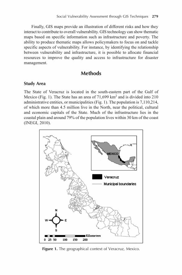
Social Vulnerability Assessment through GIS Techniques 279
Finally, GIS maps provide an illustration of different risks and how theyinteract to contribute to overall vulnerability. GIS technology can show thematicmaps based on specific information such as infrastructure and poverty. Theability to produce thematic maps allows policymakers to focus on and tacklespecific aspects of vulnerability. For instance, by identifying the relationshipbetween vulnerability and infrastructure, it is possible to allocate financialresources to improve the quality and access to infrastructure for disastermanagement.
Methods
Study Area
The State of Veracruz is located in the south-eastern part of the Gulf ofMexico (Fig. 1). The State has an area of 71,699 km2 and is divided into 210administrative entities, or municipalities (Fig. 1). The population is 7,110,214,of which more than 4.5 million live in the North, near the political, culturaland economic capitals of the State. Much of the infrastructure lies in thecoastal plain and around 79% of the population lives within 30 km of the coast(INEGI, 2010).
Figure 1. The geographical context of Veracruz, Mexico.
280 P. Krishna Krishnamurthy and L. Krishnamurthy
Like several coastal areas in Mexico, the State of Veracruz is vulnerableto hydrometeorological hazards including hurricanes and floods. Indeed, it isconsidered to be among the most disaster-prone areas in Mexico, losing up to15% of its gross domestic product (GDP) annually due to hazards(CENAPRED, 2009). The main economic activity of Veracruz is citrus-basedagriculture which accounts for 60% of its GDP. During the rainy season(October-December), crops are cyclically affected and huge economic lossesare incurred due to flood events and migration is commonplace (Krishnamurthyand Krishnamurthy, 2011). Hazards, therefore, hinder the social and economicstability of the State. In September 2007, an early rainy season was accompaniedwith a one-in-one-hundred-years flood event occurred in the southern part ofthe State affecting 10,000 households, some 35,000 people, 17,000 hectaresof agricultural land and incurring losses of around US$20 million.
Scope and Limitations of the Study
The State of Veracruz suffers several hazards such as floods, hurricanes anddrought; this study focuses only on flood risk mapping. While the inclusion ofgeophysical data (such as topography, soil type and rivers) may enhance theassessment of overall vulnerability (Rashed and Weeks, 2003b), this study isconcerned with the social elements of vulnerability, and so the emphasis is oncensus and infrastructure data. Moreover, the study focuses on vulnerability atthe municipal level, thereby disregarding vulnerabilities at smaller scales (i.e.at the community and household levels). This was necessary given the availabledata. However, the study demonstrates the potential for using GIS tools indisaster management and planning based on the assessment of socialvulnerability at resolutions that are relevant for policymaking using opensource data.
Data
The principal data collected for this vulnerability assessment consisted of apoverty indicator, flood records, information about existing infrastructure(distribution of hospitals, federal roads and emergency shelters—publicbuildings such as schools assigned a ‘safe’ status under the Civil ProtectionStrategy)—and population density. These data were obtained from national(INEGI, SPC) and international (UNDP, CRED, EM-DAT) databases andwere uploaded on the GIS software. The base map represents the boundariesof each municipality. All data were projected in UTM, WGS84, with a latitude-longitude coordinate system. Based on the existing literature and therecommendations of the Civil Protection Strategy and the National Centre forDisaster Prevention, six socially relevant physical proxies were selected:population density at the municipal level, historical flood frequency, distanceto hospitals, distance to emergency shelters and proximity to federal roads(Table 1).
Social Vulnerability Assessment through GIS Techniques 281
Tabl
e 1.
Crit
eria
for t
he a
sses
smen
t of s
ocia
l vul
nera
bilit
y.
Prox
y in
dica
tor
Ratio
nale
File
type
Dat
a so
urce
Poly
gon
shap
efile
UN
DP,
200
7
Poly
gon
shap
efile
CR
ED
, 20
10;
EM
-D
AT, 2
010;
SPC
, 201
0
Poly
gon
shap
efile
INEG
I, 20
10
Poin
t sha
pefil
eIN
EGI,
2010
Poin
t sha
pefil
eIN
EGI,
2010
Poly
line
shap
efile
INEG
I, 20
10
Popu
latio
n be
low
the
Pove
rty is
one
of t
he m
ain
fact
ors c
ontri
butin
g to
vul
nera
bilit
y, al
thou
ghpo
verty
line
the
rela
tions
hip
is c
ompl
ex (
Cut
ter
et a
l., 2
003)
. One
of
the
dire
ct(p
erce
ntag
e)w
ays
in w
hich
pov
erty
inf
luen
ces
vuln
erab
ility
is
thro
ugh
lack
of
finan
cial
reso
urce
s, w
hich
lead
s to
low
er ca
paci
ties t
o co
pe an
d re
cove
rfr
om a
dis
aste
r.Fr
eque
ncy
ofH
azar
ds a
re c
hara
cter
istic
of
the
plac
es w
here
the
y oc
cur.
Hen
ce,
flood
haz
ard
mun
icip
aliti
es th
at h
ave b
een
affe
cted
by
flood
s are
like
ly to
be a
ffect
edin
the
futu
re. A
ny h
azar
d as
sess
men
t sho
uld
cons
ider
are
as th
at h
ave
been
affe
cted
in th
e pa
st (J
ones
, 199
1).
Popu
latio
n de
nsity
Den
sely
pop
ulat
ed a
reas
are
mor
e af
fect
ed b
y flo
od h
azar
d as
ther
e is
grea
ter p
oten
tial f
or lo
ss. C
onve
rsel
y, w
here
ther
e ar
e no
peo
ple,
ther
ear
e no
dis
aste
rs (W
isne
r et a
l., 2
008)
.D
ista
nce
to h
ospi
tals
Popu
latio
ns th
at a
re n
ear h
ospi
tals
are
mor
e re
silie
nt a
s th
ey a
re a
ble
to re
cove
r fro
m in
jurie
s m
ore
quic
kly.
Pop
ulat
ions
nea
r hos
pita
ls a
rele
ss a
ffect
ed. U
nder
the
Civ
il Pr
otec
tion
Stra
tegy
, hos
pita
ls m
ay a
lso
act a
s im
prov
ised
she
lters
if n
eces
sary
(SN
PC, 2
009)
.D
ista
nce
to n
eare
stSh
elte
rs re
duce
vul
nera
bilit
y by
redu
cing
exp
osur
e to
haz
ard
durin
gem
erge
ncy
shel
ter
extre
me
wea
ther
eve
nts.
Popu
latio
ns n
ear e
mer
genc
y sh
elte
rs a
re le
ssvu
lner
able
(CEN
APR
ED, 2
009)
.D
ista
nce
toU
nlik
e hi
ghw
ays,
fede
ral
road
s ar
e fr
ee a
nd c
onne
ct m
unic
ipal
ities
fede
ral r
oads
and
Stat
es, a
llow
ing
for s
peed
y ev
acua
tion
from
a ri
sk-p
rone
are
a. B
yth
is r
atio
nale
, pop
ulat
ions
far
ther
aw
ay f
rom
fed
eral
roa
ds a
re m
ore
vuln
erab
le (C
ENA
PRED
, 200
9).
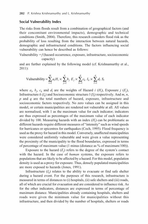
282 P. Krishna Krishnamurthy and L. Krishnamurthy
Social Vulnerability Index
The risks from floods result from a combination of geographical factors (andtheir concomitant environmental impacts), demographic and technicalconditions (Smith, 2004). Therefore, this research considers flood risk as theprobability of loss resulting from the interaction between natural hazards,demographic and infrastructural conditions. The factors influencing socialvulnerability can hence be described as follows:Vulnerability = f (hazard occurrence, exposure, infrastructure, socioeconomic
capacity)and are further explained by the following model (cf. Krishnamurthy et al.,2011):
1 1 1 1Vulnerability
m n p a
i i j j k k l li j k l
a H b E c I d S
� � �Ç Ç Ç Ç
where ai, bj, ck and dl are the weights of Hazard i (Hi), Exposure j (Ej),Infrastructure k (Ik) and Socioeconomic structure l (Sl) respectively. And m, n,p and q are the total numbers of hazard, exposure, infrastructure andsocioeconomic factors respectively. No zero values can be assigned in thismodel, or certain municipalities are rendered not vulnerable at all. All valuesare normalised, with 1 as the maximum value for each indicator; indicatorsare thus expressed as percentages of the maximum value of each indicatordivided by 100. Measuring hazards with an index (Hi) can be problematic asdifferent hazards require different measures of “intensity” such as wind speedsfor hurricanes or epicentres for earthquakes (Coch, 1995). Flood frequency isused as the proxy for hazard in this model. Conversely, unaffected municipalitieswere considered uniformly vulnerable and were given a value representingthe proximity of the municipality to the flood boundaries, expressed in termsof percentage of maximum value (1 minus (distance as % of maximum/100)).
Exposure to the hazard (Ej) refers to the degree of the system’s contactwith the hazard. In the case of human systems, the exposure refers topopulations that are likely to be affected by a hazard. For this model, populationdensity is used as a proxy for exposure. Thus, densely populated municipalitiesare more exposed to hazards (Jones, 1991).
Infrastructure (Ik) relates to the ability to evacuate or find safe shelterduring a hazard event. For the purposes of this research, infrastructure ismeasured in terms of distances to (i) hospitals, (ii) safe shelters and (iii) roads,all of which are crucial for evacuation and are considered to influence risk. Asfor the other indicators, distances are expressed in terms of percentage ofmaximum distance. Municipalities already containing hospitals, shelters androads were given the minimum value for municipalities without thisinfrastructure, and then divided by the number of hospitals, shelters or roads

Social Vulnerability Assessment through GIS Techniques 283
in the municipality. For the model, all distances were measured with theMeasure Tool in the ArcMap software.
Socioeconomic structure (Sl) is a measure of adaptive capacity, and canprovide information about the ability of communities to cope with disasters.For this chapter, the relevant socioeconomic indicator is poverty, whichinfluences the ability of a household to manage risks. Poverty is measured interms of the percentage of population in the municipality that is below thenational poverty line ($52 Mexican pesos, ~ US$ 4.21).
The weightings attributed to each of the indicators were definedqualitatively on a scale of 1-5 through expert opinion. Population density andpoverty were considered to be the most significant indicators (weighting = 5).Hazard incidence was considered to be the second most important indicator,and was given slightly lower weighting because vulnerable populations canmobilise during a hazard event and reduce their exposure accordingly(weighting = 4). Distance to hospitals and shelters were deemed equallysignificant but less important (weighting = 3). Distance to federal roads wasregarded to be the least important of the indicators because alternatemobilisation mechanisms can be improvised by vulnerable communities(weighting = 2). The results of the calculation were again normalised so thatthe vulnerability scores range from 0 to 100 and these were divided into fivedifferent ranges using the quintile method, with each range cumulativelyrepresenting 20% of the maximum vulnerability.
Results
The mapping process shows a skewed distribution of infrastructure andvulnerabilities across the study area. What becomes apparent from the analysisis that the northern and central parts of Veracruz have more institutions tocope with flood hazards: 29 out of the 45 hospitals (64%) and eight of the 25emergency shelters (32%) are concentrated in this region; similarly, the roadnetwork in the central part is well developed, connecting all the major centresof tourism in the State (Gobierno de Veracruz, 2010). The southern part of theState is more vulnerable due to the co-incidence of poorer communities,weaker infrastructure and higher flood frequency. Crucially, however, it isalso important to note that the more densely populated municipalities arelocated in the northern part of the State (and only four high-densitymunicipalities are in the south).
Using the composite score obtained from the model outlined above, eachpolygon (municipality) was assigned a value which allowed for the ranking ofits vulnerability to flooding. Values were divided into quintiles, with eachquintile assigned a qualitative indication of severity (from very low to veryhigh). The results of the calculations are shown in Fig. 2 where each polygonhas been classified according to the severity of flood vulnerability. There areeight polygons associated with very high flood vulnerability and they are all
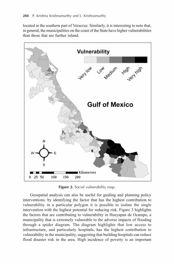
284 P. Krishna Krishnamurthy and L. Krishnamurthy
located in the southern part of Veracruz. Similarly, it is interesting to note that,in general, the municipalities on the coast of the State have higher vulnerabilitiesthan those that are further inland.
Figure 2. Social vulnerability map.
Geospatial analysis can also be useful for guiding and planning policyinterventions: by identifying the factor that has the highest contribution tovulnerability in a particular polygon it is possible to isolate the singleintervention with the highest potential for reducing risk. Figure 3 highlightsthe factors that are contributing to vulnerability in Hueyapan de Ocampo, amunicipality that is extremely vulnerable to the adverse impacts of floodingthrough a spider diagram. The diagram highlights that low access toinfrastructure, and particularly hospitals, has the highest contribution tovulnerability in the municipality, suggesting that building hospitals can reduceflood disaster risk in the area. High incidence of poverty is an important

Social Vulnerability Assessment through GIS Techniques 285
contributing factor to overall vulnerability in the municipality; therefore,disaster risk reduction policy that includes effective poverty reduction strategiesis essential in the context of the municipality. This type of information andanalysis can be used to monitor and even anticipate the outcomes of a givenintervention by altering the value of an indicator (as per expected or observedchanges) and re-calculating the vulnerability score and can be very useful forplanning. Similarly, vulnerability index analyses could be used to projectfuture vulnerability under simple environmental change scenarios; for example,if flood frequency is expected to increase as a result of anthropogenic climatechange, the values can be altered and the vulnerability score can be re-calculated(cf. Hahn et al., 2009).
Figure 3. Spider diagram highlighting the contribution of indicatorsto the social vulnerability to floods in Hueyapan de Ocampo,
a highly vulnerable municipality.
Discussion
Social vulnerability is a critical aspect of hazard risk assessment. Yet it israrely incorporated in hazard studies due to conceptual difficulties on the onehand, and a lack of suitable data on the other (Ebert et al., 2009). The principalaim of this study was to test the utility of indicators that could be obtainedfrom spatial data in identifying social vulnerability for Veracruz. Six proxyvariables, i.e. indicators that express the non-observable concept of socialvulnerability were defined and their explanatory capacity was assessed. Theindicators described social vulnerability with high accuracy. The final outputof the model showed higher vulnerabilities to flood events in the southern partof the State than in the north. The skewed distribution of vulnerability resultedfrom poorer infrastructure in the southern part of the state. Moreover, the

286 P. Krishna Krishnamurthy and L. Krishnamurthy
model predicted higher social vulnerability on the coastal areas compared toinland municipalities. Methodologically, this can be explained by the higherpopulation densities on the coastal municipalities (indeed, the three mostdensely populated municipalities were located on the coast). Conceptually,this is explained by the fact that coastal societies are more exposed tohydrometeorological hazards as they are closer to the source of the hazard(Wisner et al., 2004).
With the use of only six proxy variables (flood frequency, poverty rates,population density, distance to (i) hospitals, (ii) emergency shelters and (iii)roads), the model presented in this study generally corresponds with theexpected vulnerabilities of the state. However, a number of limitations in theprocedure must be pointed out. Although a literature review was conductedand consultation was held with experts in the field, the selection of proxyvariables (and the weighting attributed to each variable) was a highly subjectiveexercise. Factors influencing social vulnerability vary geographically andtemporally, and different societies are affected by hazards in different ways.
The number and selection of indicators is also subject to debate. Themodel used for this study considered “only” six variables. In a study oferosion risk in the South Downs region of England, Boardman et al. (2003)suggest a vulnerability index based on two factors: land use (crop choice) andslope. By contrast, Ebert et al. (2009) propose an index of social vulnerabilityto landslides in Tegucigalpa based on 47 variables. The argument can be madethat consideration of more variables can enhance the explanatory power of amodel, but it can also involve higher costs (for data collection) and highercomputing power (for data analysis). Models which require fewer indicatorsmay be preferred when time, resources and data are limited. Ultimately, thechoice and number of indicators should relate to the end use of the tool: forpolicy purposes, indicators must have a relevant recommendation for disasterrisk reduction interventions.
Further, it is possible that the model presented in this study overestimatedvulnerability to flooding in the State of Veracruz. The initial predictionssuggested that the central part of the state would be the least vulnerable toflood hazard due to the amount of infrastructure. However, attributing a higherweighting to population density resulted in the estimation that fourteenmunicipalities have medium vulnerability and one is highly vulnerable.Similarly, ten municipalities in the southern part had very low vulnerabilityscores due to low population densities (these municipalities had populationdensities of less than 15 inhabitants per kilometre square). This shows thecrucial impact of population density on the modelled predictions.
Another way in which the model may overestimate vulnerability is byignoring the distribution of infrastructure in the adjacent states: populationshave the option of mobilising and temporarily resettling in the hospitals orshelters of adjacent, less affected states. Furthermore, infrastructure at thelocal level was not included. Such local institutions as clinics and improvised
Social Vulnerability Assessment through GIS Techniques 287
shelters may play important roles in reducing social vulnerability. No suitablelocal datasets exist for clinics and improvised emergency shelters; for suchdata to be included a field study may be necessary. The scope of this studywas therefore limited to data available through federal organisations.Nevertheless, inclusion of additional field data may be pertinent in the futurefor more accurate assessments of social vulnerability. Given the limitationsoutlined above, the final output must be taken to represent one of several toolsthat can inform flood risk assessment.
Future Research Directions
Understanding social vulnerability is a significant first step in developingdisaster risk reduction policies and in planning for hazard mitigation (Cutteret al., 2003). Contextualising vulnerability within a societal framework canhelp improve knowledge of the local institutions that enhance (or reduce) theability of a community to cope with hazardous events (Wisner et al., 2004).The present study suggests that infrastructure (hospitals, safe shelter and roads)is an important element of social vulnerability. However, it is also importantto recognize that social vulnerability is hazard-dependent (Tran et al., 2009):for example, the south of Veracruz is periodically disturbed by flood eventsbut the adverse impacts of hurricane hazard affect on the northern part of thestate more frequently. An important advancement in the understanding ofvulnerability will therefore necessitate multiple-hazard assessment.
This chapter has proposed a methodology to integrate GIS tools in theassessment of social vulnerability to flood risk. The approach suggested inthis essay can be replicated for other hazards and other comparable coastalzones provided that data and the technology to carry out an analysis areavailable. A map model such as the one presented in this chapter can behelpful in informing (i) local communities of their vulnerabilities and (ii)decision-makers of the factors that lead to social vulnerability.
To improve the quality of vulnerability assessments, it is important toobtain data—this research used open source data to illustrate the extent of dataavailable at relatively high spatial resolution, but more data are required to domore complex analyses. Increasing access to geospatial information throughonline open source (for example, GeoCommons) can enhance the capacitiesto map and assess vulnerability. An important challenge, however, relates tothe quality of data. This research used secondary data, for which it is impossibleto estimate measurement errors or potential biases. To the extent that databasesfrom international organisations and government-owned institutions were usedfor the research, potential biases are accounted for to a large extent. But asdata for higher spatial resolution are collected, it will be important to collecthigh quality data that are reliable.
To overcome the challenges of secondary data collection, it is importantto involve vulnerable communities themselves in the process: communities
288 P. Krishna Krishnamurthy and L. Krishnamurthy
have long-term links with their surroundings, but transmit this informationorally. Hence, this knowledge is invisible (or unknown) to people outside thecommunity. Different members of the community, including communityleaders, professionals, women and children, can contribute by offering theirperceptions on disaster risk and the factors that lead to vulnerability.Communities also have a strong cultural understanding of the risks associatedwith specific hazards. They can identify the crops that are most resilient andthat are best adapted to the local conditions; the areas that are most affectedduring hurricane events (although satellite data is increasingly used tocorroborate this information); the houses that are damaged either throughinundation or through wind impacts; the families that are most vulnerable tohurricane hazard. Participatory GIS analyses can also be used to map social(e.g. caste), economics (e.g. income) and environmental (e.g. land use)differences that may not be already available and are therefore difficult to mapwithout frequent field visits to the study site (Peters-Guarín et al., 2005).Beyond simply identifying risks, local people are also able to explainrelationships between risk and vulnerability.
Vulnerability assessments through GIS analyses are being increasinglymainstreamed in disaster risk reduction strategies, and this trend is likely tocontinue over the coming decades as geospatial data becomes increasinglyavailable and the technology increasingly accessible. More specifically,geospatial techniques for assessing vulnerability are likely to become a usefultool in guiding disaster risk reduction and in monitoring policy outcomes. Inthe context of Mexico, for instance, the National Risk Atlas (available onlineat http://www.atlasnacionalderiesgos.gob.mx/) highlights the hotspots fordifferent risks in the country, including geological, hydrometeorological andchemical hazards. Further, in its fourth and latest National Communication tothe United Nations Framework Convention on Climate Change, the MexicanGovernment highlights the importance of mapping techniques to identifyadaptation priorities for vulnerable areas in the context of climate change(SEMARNAT and INE, 2010).
Conclusion
This chapter demonstrates the needs, rationale and procedures for assessingsocial vulnerability through geospatial techniques. This information has beeninterpreted through a vulnerability map which outlines the factors that contributeto flood vulnerability at municipal level in the State of Veracruz, Mexico. Bydeveloping a GIS-based method based on open source data, this chapterproposes a framework for communicating vulnerability analysis to policy-making which can be replicated elsewhere. Here, it is important to note thatmodelling human systems is not necessarily universally robust: the modelused for this research is based on the perceptions of the local community andshould be seen as a visual representation of local risk perceptions in both time
Social Vulnerability Assessment through GIS Techniques 289
and space. However, the incorporation of social indicators of vulnerabilitycan illustrate vulnerability as well as feasible adaptation mechanisms. Thisknowledge can be conveyed to policy-makers to develop disaster managementstrategies that focus on specific vulnerabilities. Understanding vulnerability athigh spatial resolutions can help improve knowledge of the social,environmental and institutional situations which enhance (or reduce) the abilityof a community to cope with hazards.
References
Adger, W.N. (1999). Social Vulnerability to Climate Change and Extremes in CoastalVietnam. World Development, 27(2), 249–269.
Alexander, D. (1998). Natural Disasters. University College London Press, London,United Kingdom.
Boardman, J., Evans, R. and Ford, J. (2003). Muddy floods on the South Downs,Southern England: Problems and responses. Environmental Science and Policy, 6,69–83.
Centro Nacional de Prevención de Desastres [CENAPRED] (2009). Dirección decapacitación. Retrieved December 10, 2010, from http://www.cenapred.unam.mx/es/Capacitacion/
Clark, G.E., Moser, S.C., Ratick, S.J., Dow, K., Meyer, W.B., Emani, S., Jin, W.,Kasperson, J.X. and Schwars, H.E. (1998). Assessing the vulnerability of coastalcommunities to extreme storms: the case of Revere, MA, USA. Mitigation andAdaptation Strategies for Global Change, 3(1), 59–82.
Coch, N.K. (1995). Geohazards: Natural and Human. Prentice Hall, New Jersey,United States.
Cutter, S.L., Boruff, B.J. and Shirley, W.L. (2003). Social vulnerability to environmentalhazards. Social Science Quarterly, 82, 242–260.
Daniel, E.B. and Abkowitz, M.D. (2005). Predicting storm-induced beach erosion inCaribbean Small Islands. Coastal Management, 33, 53–69.
Dash, N. (1997). The use of geographic information system in disaster research.International Journal of Mass Emergencies and Disasters, 15(1), 135–146.
Ebert, A., Kerle, N. and Stein, A. (2009). Urban social vulnerability assessment withphysical proxies and spatial metrics derived from air- and space-borne imagery andGIS data. Natural Hazards, 48, 275–294.
Emergency Events Databases [EM-DAT] (2011). Retrieved January 2, 2011, fromhttp://www.emdat.be/Database/CountryProfile/countryprofile2.php
Gobierno de Veracruz (2010). Cuarto Informe de Gobierno. Gobierno de Veracruz,Xalapa, Mexico.
Hahn, M.B., Riederer, A.M. and Foster, S.O. (2009). The Livelihood VulnerabilityIndex: A pragmatic approach to assessing risks from climate variability and change—A case study in Mozambique. Global Environmental Change, 19(1), 74–88.
Hart, D.E. and Knight, G.A. (2009). ‘Geographic Information System assessment oftsunami vulnerability on a dune coast’. Journal of Coastal Research, 25(1), 131–141.
290 P. Krishna Krishnamurthy and L. Krishnamurthy
Hatfield Consultants (2006). Using Participatory Methodologies, GeographicInformation Systems and Earth Observation Data to Map Traditional EcologicalKnowledge in Hong Ha Commune, Thua Thien Hue, Viet Nam. EOSTEM ProjectMilestone 9 Report. Hatfield Consultants, West Vancouver, Canada.
Intergovernmental Panel on Climate Change Working Group I [IPCC WGI] (2007).Climate Change 2007 - The Physical Science Basis: Contribution of WorkingGroup I to the Fourth Assessment Report of the IPCC. Cambridge UniversityPress, Cambridge, United Kingdom.
National Institute for Geographic Studies and Informatics [INEGI] (2010). RetrievedJanuary 3, 2011, from http://www.inegi.org.mx/
Jones, D.K.C. (1991). Environmental Hazards. In: Bennett, R. and Estall, R. (Eds)Global Change and Challenge (pp. 27–56). Routledge, London.
Krishnamurthy, P.K., Fisher, J.B. and Johnson, C. (2011). Mainstreaming localperceptions of hurricane risk into policymaking. Global Environmental Change,21(1), 143–153.
Krishnamurthy, P.K. and Krishnamurthy, L. (2011). Agrobiodiversity for livelihoodsecurity: A case study of agroforestry technologies in Mexico. Journal of LifeSciences, 5(2), 108–119.
Morrow, B.H. (1999). Identifying and mapping community vulnerability. Disasters,21(1), 1–18.
Nagarajan, R., Mukherjee, A., Roy, A. and Khire, M.V. (1998). Technical note: Temporalremote sensing data and GIS application in landslide hazard zonation of part ofWestern Ghat, India. International Journal of Remote Sensing, 19(4), 573–585.
Nicholls, R.J. and Mimura, N. (1998). Regional issues raised by sea-level rise andtheir policy implications. Climate Research, 11(1), 5–18.
Pareschi, M.T., Cavarra, L., Favalli, M., Giannini, F. and Meriggi, A. (2000). GIS andvolcanic risk assessment. Natural Hazards, 21(2-3), 361–379.
Peters-Guarín, G., van Westen, C.J. and Monotya, L. (2005). Community-Based FloodRisk Assessment Using GIS for the Town of San Sebastián, Guatemala. Journal ofHuman Security and Development, 1(1), 29–49.
Pielke, Jr., R.A. (2005). Are there trends in hurricane destruction? Nature, 438, E11.Pradan, A. (2004, July 26-28). GIS and remote sensing for flood disaster identification:
A case study of Koshi River basin in Nepal. Paper presented at the GlobalSymposium for Hazard Risk Reduction: Lessons Learned from the Applied ResearchGrants for Disaster Risk Reduction Program, Washington, DC, United States.
Rashed, T. and Weeks, J. (2003a). Assessing vulnerability to earthquake hazardsthrough spatial multicriteria analysis of urban areas. International Journal ofGeographical Information Science, 17(6), 547–576.
Rashed, T. and Weeks, J. (2003b). Exploring the spatial association between measuresfrom satellite imagery and patterns of urban vulnerability to earthquake hazards.The International Archives of the Photogrammetry, Remote Sensing and SpatialInformation Sciences XXXIV, 7(W9), 144–152.
Secretaría de Medio Ambiente y Recursos Naturales y el Instituto Nacional de Ecología[SEMARNAT and INE] (2008). Mexico’s Third National Communication to theUnited Nations Framework Convention on Climate Change. SEMARNAT, MexicoCity, Mexico.

Social Vulnerability Assessment through GIS Techniques 291
Sistema Nacional de Protección Civil [SNPC] (2009). Normatividad de ProtecciónCivil: Ley de Protección Civil para el Estado Libre y Soberano de Veracruz-Llave.SNPC, Mexico City, Mexico.
Smith, K. (2004). Environmental Hazards: Assessing Risk and Reducing Disaster.Routledge, London, United Kingdom.
Tran, P., Shaw, R., Chantry, G. and Norton, J. (2009). GIS and local knowledge indisaster management: A case study of flood risk mapping in Viet Nam. Disasters,33(1), 152–169.
Twigg, J. (2001). Sustainable livelihoods and vulnerability to disasters. Working Paper2. Benfield, London.
Wisner, B., Blaikie, P., Cannon, T. and Davis, I. (2004). At Risk: Natural hazards,people’s vulnerability and disasters. Routledge, London, United Kingdom.

3D city models 1893D GIS 393D modelling 189
accuracy 87administrative unit code (AUC) 226Advanced Land Observation Satellite
(ALOS) 140advanced synthetic aperture radar 41agricultural land 160alpha 140anisotropy 140application programming interfaces (APIs)
35ArcHydro 107ASCII files 44aspect 126ASTER 87, 140atmospheric motion vectors (AMV) 77Automatic Identification System (AIS)
37
Bing Maps 4bioenergy competency centre 248bioenergy potential 238, 244bioenergy potential map 244biomass estimation 189biosphere reserve 164boundaries 264Bowen ratio 53
Cambodia 141cancer 220cancer data 226cancer statistics 226carbon sequestration model 171carbon storage 164C-Band dissemination 76
Centre Region of Portugal (CRP) 239cesium 229Chesapeake Bay 2civil protection strategy 280classification 87climate change 69cloud computing 4Cloude-Pottier decomposition 145colour-infrared (CIR) 204conglomerate 123convex slopes 129crop disease detection 201cropforecaster 204curvature 126cyberinfrastructure 1, 11
data manipulation 16data processing algorithms 6database management system 106decision making 1decision support system (DSS) 34deforestation 164Delaware 257Deluvial 134demographic information 226digital elevation data 249digital elevation model (DEM) 87, 194digital terrain model 122Digital Video Broadcast (DVB) 42distance measurement instrument (DMI)
191distance to hospitals 281dynamic link libraries (DLL) 22
Earthís land cover 152Eastern Black Sea 220echosounder 34
�����
DOI 10.1007/978-94-007-1858-6, © Capital Publishing Company 2012
e ,J.K. Thakur et al. (eds.), G ospatial Techniques for Managing Environmental Resources 293
��� �����
ecology 264economic value 178efficient assessment 164energy and environmental affairs 258entropy 91, 140environmental calculator 164environmental decisions 3environmental emergency responses 1environmental factors 233environmental goods 165environmental informatics 1environmental informatics framework 11environmental pricing 164environmental problems 1environmental services 164, 165Environmental Vulnerability Index (EVI)
120eScience 4European Environment Agency (EEA)
240EuroSDR 195evapotranspiration 53Everest 87
facies 128filtering ground points 193filtering techniques 191flood risk 276flood risk assessment 277forecast 8forest cover map 142forest ecosystems 164Fortran 19free and open source software (FOSS)
267freshwater resources 68
gain ratio 93gamma dose 229Gauss dispersion model 17Geographic Information System (GIS) 15,
165Geography Markup Language (GML) 107geological data 229geomorphologic risk modelling 119geophysical models 3geophysical system 11GeoServer 36
geospatial analysis 220geospatial database (GDB) 223, 231geospatial surface analyses 119geospatial techniques 1GeoTools 36Global Positioning System (GPS) 152,
202Globus Toolkit 18GPS receiver 46Graphical User Interface (GUI) 37green house gases (GHG) 239Gwalior 155
hazard 282hazardous 2health geography 222hierarchical emergency decision making
16high performance computing 8Hillshade 126Himalaya 86hydrometeorological data 53hyperspectral image processing 16
imaging fluorescence disease detection210
Indochina peninsula 141inertial measurement unit (IMU) 191infiltration model 171infrastructure 281integrated land and water information system
(ILWIS) 56integration of spatial data 230interfluve 130interoperability 4
Japan Aerospace Exploration Agency(JAXA) 140
Java 22
kappa 93Kyoto protocol 141
land use data 226land use/land cover 152landfill 128landuse pattern 158laser scanning 189LIDAR 105
����� ���
locally planar 193long wave radiation 55low heat value (LHV) 244
machine learning algorithms (MLA) 88Madhya Pradesh, India 152map server 48mapping process 231marine spatial planning (MSP) 256marine wildlife 262Massachusetts Ocean Management Plan
258maximum likelihood classification (MLC)
157Mesoscale Model5 (MM5) 17methane (CH4) 241Mexico 165, 276Millennium Development Goals (MDGs)
69mobile laser scanning 190mobile laser scanning data 189modelling soil erosion 172models 281MODIS images 54Monarch Butterfly 165Morar River Basin 158multiagent-based system 114multicriteria decision analysis 245multisensor fusion 201multispectral fluorescence imaging system
(MFIS) 210multivariate classification algorithms 88municipal solid waste (MSW) 241municipality 288MySQL 106
National Centre for Disaster Prevention280
National Remote Sensing Agency (NRSA)156
national risk atlas 288Nepal 87normalized deviation vegetation index
(NDVI) 54normalized difference glacier index
(NDGI) 90normalized difference snow index
(NDSI) 90
normalized difference vegetation index(NDVI) 193
North Sea 261numerical weather forecast 53
object-based point cloud analysis (OBPA)194
ocean management plan 258offshore wind 256offshore wind development 256ontologies 105Open Geospatial Consortium (OGC)s 4Oracle 106OWL (Web Ontology Language) 108ozone concentrations 6
Pearson chi-square test 234Penman-Monteith 53petabytes 4Phased Array type L-band Synthetic
Aperture Radar (PALSAR) 140polygenic conglomerate 128population density 281Portugal 238PostgreSQL 106PPGIS 80precision pest management (PPM) 202Priestley prohibited areas 262proximity of points 193Python 22
quadratic discriminant analysis (QDA) 210
radar 38radioactive value maps 229radioactivity data 229rain erosive 173real-time 2REDD policies 141regulated airspace 262relief 122remote sensing 6, 204reservoir 160resource collection 244resource management 100Rhode Island Ocean SAMP 259river water monitoring and alert system
103
��� �����
runoff coefficient 171
SAGE (Scalable Adaptive GraphicsEnvironment) 19
sanitation problems 68satellite application facilities (SAFs) 78sedimentary rocks 128seed surface 191semi-arid region 152sensor fusion 208Sensor Observation Service (SOS) 108server 106shape complexity analysis 93shapefile 36shuttle radar topography mission (SRTM)
249simulate 2single look complex (SLC) 144smooth normal vector field 193social impact 9social vulnerability assessment 276social vulnerability index 282socioeconomic structure 281solar radiation 54Sonar spatial databases 101spatial epidemiology 220spatial reference system (SRS) 265split info 93SQL 106SQLite 106square pixel metric 88State of Veracruz 277static terrestrial laser scanning 190statistical methods 232stream power (SP) index map 134Studio.Net Visual 22supervised classification 157support vector machine (SVM) 202supraglacial lake 86surface energy balance index 56
surface energy balance system (SEBS) 54synthetic aperture radar (SAR) 140
technical challenge index (TCI) 267terrain ruggedness index (TRI) 128terrestrial laser scanning (TLS) 189TFLOPS (Tera Floating point Operations
per Second) 18Thailand 141thorium 229topographic 226topographic map 156Turkey 220Turkish Statistical Institute (TURKSTAT)
226
uranium 229urban settlement 160urban tree detection 189
vessel traffic 262virtual observatory 6visualization 9vulnerability 277
wastelands 160water analysis data 229water ladder 68water scarcity 71water-borne diseases 68waveband selection 207web coverage services (WCS) 4web GIS 34web map service (WMS) 4wetlands 53wetness index 134wind resource 262Wishart unsupervised classification 140World Summit on Sustainable Development
(WSSD) 69