Edge Structure Preserving 3-D Image Denoising

Peihua QiuUniversity of Minnesota

School of StatisticsMinneapolis, MN 55455

USAqiu@stat.umn.edu

Partha Sarathi MukherjeeUniversity of Minnesota

School of StatisticsMinneapolis, MN 55455

USApsm@stat.umn.edu

Abstract: In various applications, including magnetic resonance imaging (MRI) and functional MRI (fMRI), 3-D images get increasingly popular. To improve reliability of subsequent image analyses, 3-D image denoisingis often a necessary pre-processing step, which is the focus of the current paper. In the literature, most existingimage denoising procedures are for 2-D images. Their direct extensions to 3-D cases generally can not handle 3-Dimages efficiently, because the structure of a typical 3-D image is substantially more complicated than that of atypical 2-D image. For instance, edge locations are surfaces in 3-D cases, which would be much more challengingto handle, compared to edge curves in 2-D cases. In this paper, we propose a novel 3-D image denoising procedure,by approximating the edge surfaces properly, using local smoothing and nonparametric regression methods. Oneimportant feature of this method is its ability to preserve edges and major edge structures (e.g., intersections of twoedge surfaces and pointed corners). Numerical studies show that it works well in various applications.

Key–Words:Edge-preserving image restoration, jump regression analysis, surface estimation.

1 Introduction

In real life, most objects are three-dimensional (3-D). Due to limitation of image acquisition techniques,people traditionally acquire a set of two-dimensional(2-D) images from a sequence of slices of a 3-D ob-ject (e.g., a patient’s head), and then the 3-D objectis reconstructed from the 2-D images, to study thebiological mechanism of the object. The related re-search area is termed 3-D image reconstruction in theliterature (e.g., Chapters 11 and 12 in [13]). 3-D im-age reconstruction is technically challenging, and thereconstructed 3-D image often contains a substantialamount of estimation error. This limitation is recentlylifted in certain applications, including magnetic reso-nance imaging (MRI) and functional MRI (fMRI). Wecan now acquire 3-D images directly in these appli-cations, although observed 3-D images often containnoise due to hardware imperfection and other reasons.

Noise removal is important for the reliability ofsubsequent image analyses, and is often one major fo-cus during the pre-processing stage in image process-ing. However, most existing image denoising methodsare for analyzing 2-D images (e.g., [5],[8],[9],[11]).Their direct extensions to 3-D cases generally can nothandle 3-D images efficiently, because the structure ofa typical 3-D image is often substantially more com-plicated than that of a typical 2-D image. For instance,edge locations are surfaces in 3-D cases, which have

much more complicated structures (e.g., intersectionsof two edge surfaces, pointed corners, and so forth),compared to edge curves in 2-D cases.

In the literature, a number of 3-D image denoisingprocedures have been developed. Some of them areconstructed after properly generalizing and/or modi-fying their 2-D counterparts. For instance, 3-D im-age denoising based on minimization of total variation(TV) has gained certain popularity in the literature(e.g., [4]), and the TV approach is initially suggestedfor denoising 2-D images (e.g. [12]). MATLAB pro-grams for 3-D image denoising using anisotropic dif-fusion have also been developed (e.g., [6]). Otherexisting 3-D image denoising procedures include theones based on 3-D wavelet transformations (e.g., [1]),non-local means (e.g., [2]), distance-weighted Wienerfiltering (e.g. [7]), and so forth.

Besides noise removal, another important require-ment for image denoising procedures is that theyshould preserve important image structures, such asedges and major edge features (e.g., intersections oftwo edge surfaces, pointed corners, and so forth).Most existing image denoising procedures mentionedabove can preserve parts of the edges where the cur-vature of edge surfaces is relatively small, but wouldusually blur or round certain edge features at placeswhere the curvature of edge surfaces is relativelylarge. In our opinion, edge features corresponding torelatively large curvature of the edge surfaces are an

Applications of Mathematics and Computer Engineering

ISBN: 978-960-474-270-7 111

important component of the image under study, be-cause they often represent major characteristics of theimage objects and are easier to capture our visual at-tention, compared to places on the edge surfaces withrelatively small curvature. Therefore, they should bewell preserved during image denoising.

In this paper, we propose a new 3-D image de-noising procedure which can preserve edges and ma-jor edge features well. Our procedure is based on lo-cal approximation of the edge surfaces, using certainjump regression analysis (JRA) methodologies [10].Our proposed procedure is described in detail in Sec-tion 2. Some numerical examples are presented inSection 3 to evaluate its performance. Several remarksconclude the article in Section 4.

2 Proposed MethodOur proposed 3-D image denoising procedure can bebriefly described as follows. In a neighborhood of agiven voxel, the edge surfaces are first approximatedby a surface template, and then the true image inten-sity at the given voxel is estimated by a weighted av-erage of the observed image intensities whose voxelsare located on the same side of the surface template asthe given voxel. Details of the procedure are describedin several parts below.

2.1 Identification of Edge VoxelsAssume that an observed 3-D image follows the re-gression model

ξijk = f(xi, yj, zk) + εijk, for i, j, k = 1, 2, . . . , n,(1)

where (xi, yj, zk) = (i/n, j/n, k/n), i, j, k =1, 2, . . . , n are the equally spaced voxels in the de-sign spaceΩ = [0, 1] × [0, 1] × [0, 1], εijk are i.i.d.random errors with mean 0 and unknown varianceσ2, f(x, y, z) is an unknown image intensity func-tion, andN = n3 is the total number of voxels. Ata given voxel(x, y, z) ∈ Ω, to know whether it is anedge voxel, let us consider its spherical neighborhoodO∗(x, y, z) with radiush∗

n. In O∗(x, y, z), a 3-D planeis fitted using the local linear kernel (LLK) smoothing[3] as follows.

mina,b,c,d

n∑

i,j,k=1

ξijk − [a + b(xi − x)+

c(yj − y) + d(zk − z)]2 Kh∗

n(xi, yj, zk),(2)

whereKh∗

n(xi, yj , zk) = K(xi−x

h∗

n,

yj−y

h∗

n, zk−z

h∗

n), and

K is a 3-D density kernel function defined in a

unit ball. The solution to(a, b, c, d) of (2) is de-noted as(a(x, y, z), b(x, y, z), c(x, y, z), d(x, y, z)),and their expressions are given in the appendix. Then,a(x, y, z) is the LLK estimator off(x, y, z), and(b(x, y, z), c(x, y, z), d(x, y, z)) are LLK estimatorsof (f ′

x(x, y, z), f ′

y(x, y, z), f ′

z(x, y, z)).

The gradient vector β(x, y, z) =

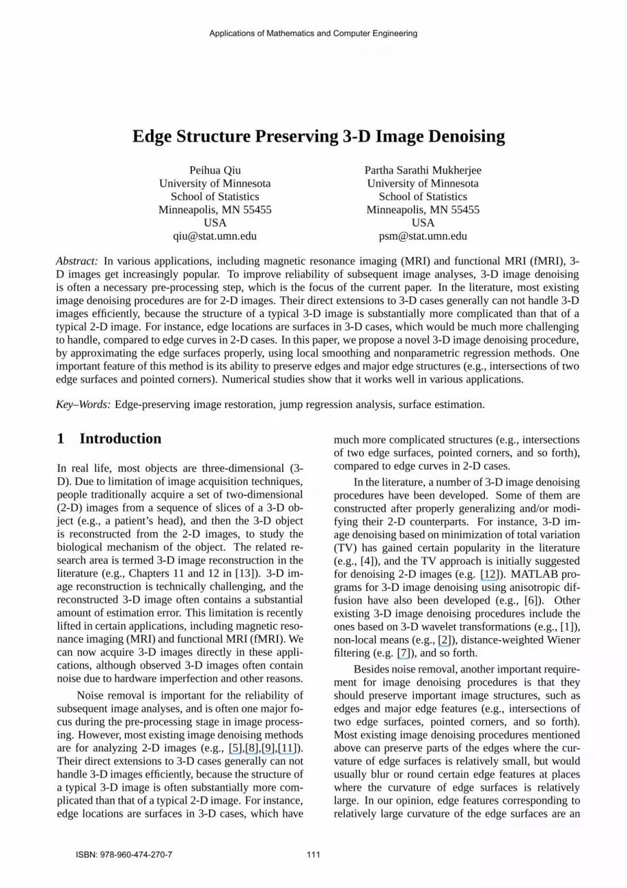
(b(x, y, z), c(x, y, z), d(x, y, z))T provides anestimate of the direction thatf increases the fastest.Let us consider a plane that passes(x, y, z) andis orthogonal toβ(x, y, z). Then, this plan di-vides O∗(x, y, z) into two halvesO∗

1(x, y, z) and

O∗

2(x, y, z), as demonstrated in Fig. 1. InO∗

1(x, y, z)

and O∗

2(x, y, z), we compute weighted averages of

the observed image intensities, respectively, with theweights determined byK. The weighted averages aredenoted asa1(x, y, z) anda2(x, y, z). Then,(x, y, z)is flagged as an edge voxel if

|a1(x, y, z) − a2(x, y, z)| > Tn, (3)

where Tn is a threshold. In the case when thereare no edge voxels inO∗(x, y, z), it can be checkedthat a1(x, y, z) − a2(x, y, z) is distributed approxi-mately asN(0, 4σ2

∑K2

h∗

n(xi, yj, zk), whereσ2 =

1

N

∑ni,j,k=1

(ξijk − a(xi, yj, zk))2. Therefore, a rea-

sonable choice ofTn is

Tn = 2Z1−αn σ

√∑K2

h∗

n(xi, yj , zk),

whereZ1−αn is the(1−αn)th quantile of the standardnormal distribution, andαn is a pre-specified signif-icance level. In this paper, we chooseαn = 0.0001.

Figure 1: The spherical neighborhoodO∗(x, y, z) isdivided into two halvesO∗

1(x, y, z) andO∗

2(x, y, z) by

a plane passing the center(x, y, z) and perpendicularto the estimated gradientβ(x, y, z).

2.2 Local Approximation of Edge SurfacesTo estimatef at a given voxel(x, y, z), we suggestfirst approximating the edge surfaces in its spherical

Applications of Mathematics and Computer Engineering

ISBN: 978-960-474-270-7 112

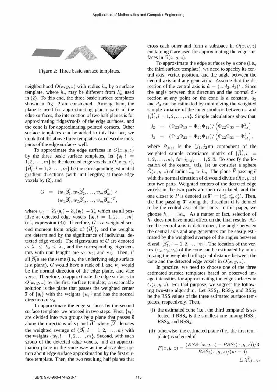
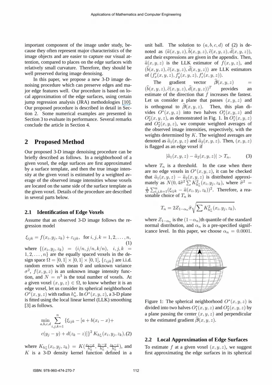
Figure 2: Three basic surface templates.

neighborhoodO(x, y, z) with radiushn by a surfacetemplate, wherehn may be different fromh∗

n usedin (2). To this end, the three basic surface templatesshown in Fig. 2 are considered. Among them, theplane is used for approximating planar parts of theedge surfaces, the intersection of two half planes is forapproximating ridges/roofs of the edge surfaces, andthe cone is for approximating pointed corners. Othersurface templates can be added to this list; but, wethink that the above three templates can describe mostparts of the edge surfaces well.

To approximate the edge surfaces inO(x, y, z)by the three basic surface templates, letsl, l =1, 2, . . . ,m be the detected edge voxels inO(x, y, z),β

∗

l , l = 1, 2, . . . ,m be the corresponding estimatedgradient directions (with unit lengths) at these edgevoxels by (2), and

G = (w1β∗

1, w2β

∗

2, . . . , wmβ

∗

m) ×

(w1β∗

1, w2β

∗

2, . . . , wmβ

∗

m)T ,

wherewl = |a1(sl) − a2(sl)| − Tn which are all pos-itive at detected edge voxelssl, l = 1, 2, . . . ,m(cf., expression (3)). Therefore,G is a weighted sec-ond moment from origin ofβ

∗

l , and the weightsare determined by the significance of individual de-tected edge voxels. The eigenvalues ofG are denotedasλ1 ≤ λ2 ≤ λ3, and the corresponding eigenvec-tors with unit lengths arev1,v2, and v3. Then, ifall β

∗

l s are the same (i.e., the underlying edge surfaceis a plane),G would have a rank of 1 andv3 wouldbe the normal direction of the edge plane, and viceversa. Therefore, to approximate the edge surfaces inO(x, y, z) by the first surface template, a reasonablesolution is the plane that passes the weighted centers of sl with the weightswl and has the normaldirection ofv3.

To approximate the edge surfaces by the secondsurface template, we proceed in two steps. First,slare divided into two groups by a plane that passess

along the directions ofv1 andβ∗

whereβ∗

denotesthe weighted average ofβ

∗

l , l = 1, 2, . . . ,m withthe weightswl, l = 1, 2, . . . ,m. Second, with eachgroup of the detected edge voxels, find an approxi-mation plane in the same way as the above descrip-tion about edge surface approximation by the first sur-face template. Then, the two resulting half planes that

cross each other and form a subspace inO(x, y, z)containings are used for approximating the edge sur-faces inO(x, y, z).

To approximate the edge surfaces by a cone (i.e.,the third surface template), we need to specify its cen-tral axis, vertex position, and the angle between thecentral axis and any generatrix. Assume that the di-rection of the central axis isd = (1, d2, d3)

T . Sincethe angle between this direction and the normal di-rection at any point on the cone is a constant,d2

andd3 can be estimated by minimizing the weightedsample variance of the inner products betweend andβ

∗

l , l = 1, 2, . . . ,m. Simple calculations show that

d2 = (Ψ23Ψ13 − Ψ33Ψ12)/(Ψ22Ψ33 − Ψ2

23

)

d3 = (Ψ12Ψ23 − Ψ22Ψ13)/(Ψ22Ψ33 − Ψ2

23

),

where Ψj1j2 is the (j1, j2)th component of the

weighted sample covariance matrix ofβ∗

l , l =1, 2, . . . ,m, for j1, j2 = 1, 2, 3. To specify the lo-cation of the central axis, let us consider a sphereO(x, y, z) of radiushn > hn. The planeP passingswith the normal direction ofd would divideO(x, y, z)into two parts. Weighted centers of the detected edgevoxels in the two parts are then calculated, and theone closer toP is denoted ass∗ = (c∗x, c∗y, c

∗

z). Then,the line passings∗ along the directiond is definedto be the central axis of the cone. In this paper, wechoosehn = 3hn. As a matter of fact, selection ofhn does not have much effect on the final results. Af-ter the central axis is determined, the angle betweenthe central axis and any generatrix can be easily esti-mated by the weighted average of the angles betweend andβ

∗

l , l = 1, 2, . . . ,m. The location of the ver-tex (vx, vy, vz) of the cone can be estimated by mini-mizing the weighted orthogonal distance between thecone and the detected edge voxels inO(x, y, z).

In practice, we need to choose one of the threeestimated surface templates based on observed im-age intensities for approximating the edge surfaces inO(x, y, z). For that purpose, we suggest the follow-ing two-step algorithm. Let RSS1, RSS2, and RSS3be the RSS values of the three estimated surface tem-plates, respectively. Then,

(i) the estimated cone (i.e., the third template) is se-lected if RSS3 is the smallest one among RSS1,RSS2, and RSS3;

(ii) otherwise, the estimated plane (i.e., the first tem-plate) is selected if

F (x, y, z) =(RSS1(x, y, z) − RSS2(x, y, z))/3

RSS2(x, y, z)/(m − 6)

≤ χ2

3,1−α,

Applications of Mathematics and Computer Engineering

ISBN: 978-960-474-270-7 113

and the estimated crossing half-planes (i.e., thesecond template) is selected ifF (x, y, z) >χ2

3,1−α, whereχ2

3,1−α is the (1 − α)th quantileof theχ2

3distribution.

In step (ii), we have used the statistical result thatF (x, y, z) is distributed asymptotically asχ2

3whenm

increases [?], which is true here because the first tem-plate is a special case of the second template and thesecond template has three more parameters than thefirst template. In this paper, we fixα = 0.01.

2.3 3-D Image DenoisingAfter determining the surface template for approxi-mating the edge surfaces inO(x, y, z), O(x, y, z) isdivided into two parts by the surface template, in caseswhen the first template is selected, or when the sec-ond or third template is selected and their ridge orvertex is contained inO(x, y, z). In cases when thesecond or third template is selected and their ridge orvertex is outsideO(x, y, z), O(x, y, z) could be di-vided into three parts. In any case, the part contain-ing the voxel(x, y, z) is denoted asU(x, y, z). Then,f(x, y, z) can be estimated by the solution toa of theminimization problem (2), afterKh∗

n(xi, yj, zk) is re-

placed byI((xi, yj, zk) ∈ U(x, y, z))Khn(xi, yj , zk),

whereI(·) is the indicator function and it equals 1 ifits argument is “true” and 0 otherwise. From (2) andthe expressions given in the appendix for its solutions,we can see thatf(x, y, z) is a weighted average of theobserved image intensities whose voxels are locatedon the same side of the estimated surface template inO(x, y, z) as the given voxel(x, y, z). Intuitively, aslong as the estimated surface template approximatesthe underlying edge surfaces well,f(x, y, z) wouldpreserve edges and major edge features well.

For a real image, there are regions wheref issmooth. In these regions, the number of detectededge voxels should be small. So, before estimat-ing f , we suggest counting the number of detectededge voxels inO(x, y, z). If the number is so small(e.g., smaller than(nhn)2) that a potential edge sur-face inO(x, y, z) is unlikely, thenf(x, y, z) can beestimated simply by the conventional LLK estimatorconstructed from all observations inO(x, y, z). Thedenoising procedure described in the previous para-graph is used only when the number of detected edgevoxels inO(x, y, z) is relatively large. To do so, thereare at least two benefits. One is that much computa-tion is saved, because the conventional LLK estimatoris much easier to compute, compared to the proposeddenoising procedure based on local edge surface ap-proximation. The other benefit is that the estimatedf would be more accurate in cases when the number

of detected edge voxels is small, because it is con-structed from all observations inO(x, y, z), instead offrom part observations. Considering the fact that mostvoxels in an image are not edge voxels, these benefitsshould be substantial.

In the proposed denoising procedure, there aretwo parametersh∗

n and hn involved. We suggestchoosing them by the following cross-validation (CV)procedure:

CV (h∗

n, hn) =1

n3

n∑

i,j,k=1

(ξijk − f−i,−j,−k(xi, yj , zk)

)2

,

(4)where f−i,−j,−k(xi, yj, zk) is the estimate of

f(xi, yj, zk) when the(i, j, k)-th voxel (xi, yj, zk)is excluded from all subsequent steps of the pro-posed image denoising procedure after edge detec-tion. Then, h∗

n and hn are chosen by minimizingCV (h∗

n, hn).

3 Numerical StudyIn this section, we present some numerical exam-ples to evaluate the performance of the proposed 3-D image denoising procedure (denoted as NEW), incomparison with three existing procedures, includ-ing the ones based on total variation [4] (denoted asTV), anisotropic diffusion [6] (denoted as AD), andoptimized non-local means [2] (denoted as ONLM).The procedure TV has a regularization parameter in-volved, the procedure AD is an iterative algorithmand contains two parameters, i.e., the diffusion pa-rameter and the number of iterations, and the proce-dure ONLM has two bandwidth parameters to choose.To evaluate the performance of a denoised imagef ,a standard statistical criterion is the mean integratedsquared error (MISE), defined as MISE(f , f) =∫

1

0

∫1

0

∫1

0[f(x, y, z) − f(x, y, z)]2 dxdydz, which is

estimated by the sample mean of

ISE(f , f) =1

n3

n∑

i=1

n∑

j=1

n∑

k=1

[f(xi, yj , zk) − f(xi, yj, zk)

]2

based on 100 replications.A 3-D MRI image of a human brain is used here

as a test image, which has128 × 128 × 52 voxels. Itsimage intensity levels range from 0 to 809. A demon-stration of the 3-D image and its three slices are shownin Fig. 3. Then, i.i.d. random noise from the distribu-tion N(0, σ2) is added to the image, andσ is chosen tobe 80, 100, or 120. With eachσ value, the parametersof the four denoising procedures are chosen such thattheir estimated MISE values based on 100 replicationsreach the minimum. For the proposed denoising pro-cedure, we also consider choosing its parameters by

Applications of Mathematics and Computer Engineering

ISBN: 978-960-474-270-7 114

Figure 3: A demonstration of a 3-D image and three 2-D slices.

Table 1: In each entry, the first line presents the esti-mated MISE value and their standard errors (in paren-thesis), the second line presents the searched proce-dure parameter values.

Method σ = 80 σ = 100 σ = 120

TV 1119.3 (2.9) 1401.1 (3.9) 1649.1 (4.9).0030 .0025 .0019

AD 1157.8 (3.5) 1525.0 (4.8) 1916.9 (6.3)475,1 700,1 900,1

ONLM 884.8 (3.4) 1127.5 (4.6) 1364.0 (6.2)12,1 16,1 25,1

NEW 837.3 (2.4) 1022.7 (3.1) 1189.2 (4.1).0172,.0156 .0188,.0188 .0188,.0188

NEW-CV 850.4 (2.4) 1029.0 (2.9) 1189.2 (4.1).0117,.0156 .0172,.0188 .0188,.0188

the CV procedure (4). The corresponding method isdenoted as NEW-CV.

The estimated MISE values, their standard er-rors, and the procedure parameter values of the re-lated methods are presented in the first three columnsof Table 1. From the table, we can see that the pro-posed procedure NEW outperforms all three compet-ing methods in all cases, and the outperformance isstatistically significant because the difference of theMISE values of the procedure NEW and any one of itspeers is larger than 2 times of the sum of the two corre-sponding standard errors. Also, when its parametersare chosen by the CV procedure (cf., NEW-CV), itsperformance gets slightly worse, compared to the pro-cedure NEW with the parameters chosen by minimiz-ing MISE. But, NEW-CV still outperforms all threecompeting methods in all cases by a reasonably bigmargin.

To investigate the denoised images, the densitycurves of the image intensities of the denoised imageswhenσ = 100 are shown in Fig. 4. Because the den-sity curves of the procedures NEW and NEW-CV arealmost identical, only the one of NEW-CV is visiblein the plot. From the plot, it can be seen that the den-sity curves of NEW and NEW-CV are closer to the

density curve of the true image, shown by the thicksolid curve in the plot, than the density curves of thethree competing procedures.

0 50 100 150 200

0.00

00.

005

0.01

00.

015

0.02

0

Image intensity values

Den

sity

TRUTHTVADONLMNEWNEW−CV

Figure 4: Density curves of the image intensities ofthe true image (i.e., the 3rd one in Fig. 3) and thedenoised images whenσ = 100

At the end of this section, we consider adding theRician noise to the 3-D test image. By adding the Ri-cian noise, the observed image intensity at the voxel

(x, y, z) is generated by√

[f(x, y, z) + ǫ1]2 + ǫ22,

whereǫ1 andǫ2 are i.i.d. noise from the distributionN(0, σ2). As in the previous examples, we considercases whenσ = 80, 100, and 120. For each denois-ing procedure, we use the bias correction method pro-posed in [?] to remove estimation bias. Letf(x, y, z)be the intensity of the denoised image by a given de-noising procedure. Then, its bias-corrected version

is defined to be√

f2(x, y, z) − 2σ2. In practice,σis often unknown and should be estimated from theobserved image. In this example, it is estimated by√

s/2, wheres is the sample standard deviation of thesquared observed intensities at the first16 × 16 × 13

Applications of Mathematics and Computer Engineering

ISBN: 978-960-474-270-7 115

voxels. The calculated MISE values based on 100replications of all five procedures are presented in Fig.5. Again, the MISE curve of the procedure NEW isnot visible in the plot because it is overlapped withthe one of NEW-CV. From the plot, it can be seenthat procedures NEW and NEW-CV outperform allthree competing procedures in all cases except thecase whenσ = 80. In that case, the procedure ONLMis the best.

80 90 100 110 120

1000

1500

2000

σ~

MIS

E

TVADONLMNEWNEW−CV

Figure 5: MISE values of various methods based on100 replications.

4 ConclusionWe have presented a 3-D image denoising procedurewhich can preserve edges and major edge structureswell. Numerical examples show that it performs fa-vorably compare to several existing methods in vari-ous cases. However, 3-D image denoising is a chal-lenging problem. The current version of the proposedprocedure may not be able to preserve edges aroundplaces where three or more edge surfaces cross orwhere jump magnitudes in image intensity are closeto zero. To solve these problems, it might help by in-cluding more surface templates in the denoising pro-cedure than the ones shown in Fig. 2 when locallyapproximating the edge surfaces. Such potential im-provements are left to our future research.

Acknowledgements: This research was supported inpart by an NSF grant.

References:

[1] P. Coupe, P. Hellier, S. Prima, C. Kervrann andC. Barillot, 3D wavelet subbands mixing for im-

age denoising,International Journal of Biomed-ical Imaging2008, 2008, pp. 1–11.

[2] P. Coupe, P. Yger, S. Prima, P. Hellier, C.Kervrann and C. Barillot, An optimized block-wise nonlocal means denoising filter for 3-Dmagnetic resonance images,IEEE Transactionson Medical Imaging27, 2008, pp. 425–441.

[3] J. Fan and I. Gijbels,Local Polynomial Mod-elling and Its Applications, Chapman & Hall,London 1996

[4] P. Getreuer, tvdenoise.m (a MATLAB program),http://www.mathworks.co.uk/matlabcentral/,2007.

[5] I. Gijbel, A. Lambert and P. Qiu, Edge-preserving image denoising and estimation ofdiscontinuous surfaces,IEEE Transactions onPattern Analysis and Machine Intelligence28,2006, pp. 1075–1087.

[6] D.S. Lopes, anisodiff3D.m(a MATLAB program),http://www.mathworks.co.uk/matlabcentral/,2007.

[7] H. Lu, C. Jui-Hsi, G. Han, L. Li and Z. Liang, A3D distance-weighted Wiener filter for Poissonnoise reduction in sinogram space for SPECTimaging, SPIE proceedings series4320, 2001,pp. 905-913.

[8] P. Qiu, Discontinuous regression surfaces fitting,The Annals of Statistics26, 1998, pp. 2218–2245.

[9] P. Qiu, The local piecewisely linear kernelsmoothing procedure for fitting jump regressionsurfaces,Technometrics46, 2004, pp. 87–98.

[10] P. Qiu, Image Processing and Jump RegressionAnalysis, John Wiley, New York 2005.

[11] P. Qiu, Jump surface estimation, edge detection,and image restoration,Journal of the AmericanStatistical Association102, 2007, pp. 745–756.

[12] L. Rudin, S. Osher and E. Fatemi, Nonlineartotal variation based noise removal algorithms,IEEE Transactions on Pattern Analysis and Ma-chine Intelligence14, 1992, pp. 259–268.

[13] M. Sonka, V. Hlavac and R. Boyle,Image Pro-cessing, Analysis, and Machine Vision (3rd ed),Thomson Learning, Toronto 2008.

Applications of Mathematics and Computer Engineering

ISBN: 978-960-474-270-7 116