Copyright © 2007 by the Association for Computing Machinery, Inc. Permission to make digital or hard copies of part or all of this work for personal or classroom use is granted without fee provided that copies are not made or distributed for commercial advantage and that copies bear this notice and the full citation on the first page. Copyrights for components of this work owned by others than ACM must be honored. Abstracting with credit is permitted. To copy otherwise, to republish, to post on servers, or to redistribute to lists, requires prior specific permission and/or a fee. Request permissions from Permissions Dept, ACM Inc., fax +1 (212) 869-0481 or e-mail permissions@acm.org. SPM 2007, Beijing, China, June 04 – 06, 2007. © 2007 ACM 978-1-59593-666-0/07/0006 $5.00

Random Walks for Mesh Denoising

Xianfang Sun∗

Cardiff University, UKBeihang University, China

Paul L. Rosin†

Cardiff University, UKRalph R. Martin‡

Cardiff University, UKFrank C. Langbein§

Cardiff University, UK

Abstract

This paper considers an approach to mesh denoising based on theconcept of random walks. The proposed method consists of twostages: a face normal filtering procedure, followed by a vertex po-sition updating procedure which integrates the denoised face nor-mals in a least-squares sense. Face normal filtering is performed byweighted averaging of normals in a neighbourhood. The weightsare based on the probability of arriving at a given neighbour after arandom walk of a virtual particle starting at a given face of the meshand moving a fixed number of steps. The probability of a particlestepping from its current face to a given neighboring face is deter-mined by the angle between the two face normals, using a Gaus-sian distribution whose width is adaptively adjusted to enhance thefeature-preserving property of the algorithm. The vertex positionupdating procedure uses the conjugate gradient algorithm for speedof convergence. Analysis and experiments show that random walksof different step lengths yield similar denoising results. In particu-lar, iterative application of a one-step random walk in a progressivemanner effectively preserves detailed features while denoising themesh very well. We observe that this approach is faster than manyother feature-preserving mesh denoising algorithms.

CR Categories: I.3.5 [Computer Graphics]: Computational Ge-ometry and Object Modelling—Curve, surface, solid, and objectrepresentations

Keywords: Mesh Denoising, Mesh Smoothing, Random Walk,Feature Preservation

1 Introduction

3D surface mesh denoising has been an active research field forseveral years. Although much progress has been made, mesh de-noising technology is still not mature. When there are intrinsic finedetails or sharp features in a noisy mesh, it is hard to both denoisethe mesh and preserve the mesh features. In this paper, we present anew feature-preserving mesh denoising method based on a randomwalk model.

In basic terms, mesh denoising can be seen as a requirement to ad-just vertex positions—vertices affected by noise are not where theyshould be, and should be moved to their estimated noise-free po-sitions. Generally, the vertex positions are the primary measureddata, not mesh triangles, which is why we adjust vertex positions.In practice, adjusting vertices directly is not always done, however.

∗e-mail: Xianfang.Sun@cs.cardiff.ac.uk†e-mail: Paul.Rosin@cs.cardiff.ac.uk‡e-mail: Ralph.Martin@cs.cardiff.ac.uk§e-mail: F.C.Langbein@cs.cardiff.ac.uk

New vertex coordinates are often computed in two steps. One-stepapproaches directly update vertex positions using the original ver-tex coordinates, sometimes together with face normal information,in a neighbourhood around the current vertex. Two-step approachesfirst adjust face normals and then update vertex positions usingsome error minimization criterion based on the adjusted normals.

In many cases, a single pass of a one-step or two-step approachdoes not yield a satisfactory result, and iterated operations are per-formed. In iterative two-step approaches, the iterations can be per-formed in two distinct ways: the two steps can be coupled as apair to give an overall iteration procedure informally described as(Step 1+Step 2)n0 , or two separate iteration procedures can be per-formed, informally (Step 1)n1 +(Step 2)n2 , where n0, n1 and n2 arenumbers of iterations. To distinguish these two schemes, we callthese interleaved and consecutive iteration schemes respectively.

The relative advantages of these two schemes merits detailed inves-tigation. One advantage of the interleaved scheme is that it onlydepends on choice of a single iteration parameter n0, while the con-secutive scheme involves two iteration parameters n1 and n2. How-ever, in an interleaved scheme, normal updating and vertex positionupdating have different optimization end points, so their interactiongenerally means that more iterations are needed for a given degreeof denoising than in a consecutive scheme, i.e. max(n1,n2) < n0.In addition, small normal errors, but not vertex position errors, maycause significant aliasing problems [Botsch and Kobbelt 2001], sowe need to pay more attention to the normal updating step. Hence,it is preferable to separately process normal updating and vertexposition updating. The approach proposed in this paper is thus aconsecutive iterative method.

Random walks are used as models in many areas of mathemat-ics and physics. Application of random walk models to computervision and image processing first appeared in the work of Wech-sler and Kidode [1979] for texture discrimination. More recently,random walks have been applied to image enhancement [Smolkaand Wojciechowski 2001; Azzabou et al. 2006], image filter-ing [Smolka and Wojciechowski 2001; Szczepanski et al. 2003],and image segmentation [Grady 2006]. Although image process-ing is closely linked to mesh processing, it appears that applyingrandom walks to mesh processing is new. Random walks on animage only deal with a 2D domain, which furthermore has a reg-ular structure. It is not straightforward to extend such 2D meth-ods to 3D mesh applications. In this paper, we provide a methodof applying random walks to 3D mesh denoising, motivated by therandom walk-based image denoising approach proposed by Smolkaand Wojciechowski [2001].

The rest of the paper is organized as follows. Section 2 gives a briefreview of previous work on mesh denoising. Section 3 describesthe notation used in this paper. Section 4 presents a simple intro-duction to random walk models. Section 5 is the core of the paper,discussing mesh normal filtering using random walks. We also in-troduce an adaptive parameter adjustment method, and analyze thefeature-preserving property of our approach. Section 6 states howwe perform vertex position updating using the conjugate gradientmethod. Section 7 presents experimental results and compares ourmethod to other recent feature-preserving mesh denoising methods.Finally, Section 8 concludes the paper.

11

2 Previous Work

Many surface smoothing, fairing and denoising methods have beenproposed, and to a large degree their differing aims have beenconfused—smoothing algorithms have often been suggested fornoise removal. Classical Laplacian smoothing [Field 1988; Vollmeret al. 1999] is the fastest and simplest surface smoothing method.However, when applied to a noisy 3D surface, significant shapedistortion and surface shrinkage may result in addition to noise re-moval. To overcome the shrinkage problem, Taubin [1995] pro-posed a filtering method with positive and negative damping fac-tors. A first-order filter with positive damping factor shrinks andsmooths the mesh surface, while a first-order filter with negativedamping factor expands the surface, to compensate for the shrink-age. This method is fast and simple, but still suffers from distortionof prominent mesh features. In addition, if the parameters of thetwo filters are not chosen carefully, the algorithm can be numeri-cally unstable.

Desbrun et al. [1999] introduced diffusion and curvature flow intosurface fairing, proposing a simple and numerically stable implicitfiltering method which can deal with irregular meshes. They over-come the problem of shrinkage by re-scaling the mesh to preserveits volume. Again, however, distortion of prominent mesh featuresoccurs.

From the viewpoint of signal processing, Taubin’s [1995] and Des-brun et al.’s [1999] methods can both be though of as filtering meth-ods. The former can be considered as moving average (MA), orfinite impulse response (FIR) filtering, while the later can be seenas autoregressive (AR), or infinite impulse response (IIR) filtering.Combining the above two approaches, Kim and Rossignac [2005]developed a general autoregressive moving average (ARMA) filterapproach. Through suitable choice of parameters, the filter can actas a lowpass, bandpass, highpass, notch, band amplification or bandattenuation filter, thus enabling it to filter out e.g. high-frequencynoise and, at the same time, enhance or suppress certain features.However, it is difficult to design a suitable filter that does both well.

The above are all isotropic filtering methods, in which the filteracts independently of direction. This makes it hard for such fil-ters to preserve prominent directional mesh features, particularlyedges. Thus, various anisotropic filtering schemes have been pro-posed which smooth surfaces while simultaneously preserving edgefeatures. Anisotropic filtering schemes can be divided into threemain classes, plus various others.

The first class is based on anisotropic geometric diffusion [Clarenzet al. 2000; Desbrun et al. 2000; Tasdizen et al. 2002; Bajaj andXu 2003; Hildebrandt and Polthier 2004]. Such methods have beenused for smoothing height fields and bivariate data [Desbrun et al.2000], level set surfaces [Tasdizen et al. 2002], and general dis-cretized surfaces [Clarenz et al. 2000; Bajaj and Xu 2003; Hilde-brandt and Polthier 2004].

The second class is based on bilateral filters [Jones et al. 2003;Fleishman et al. 2003]. Fleishman et al. [2003] use an iterativeone-step approach, in which new vertex coordinates are computeddirectly from the vertex’s neighbourhood. This approach is rela-tively fast because a one-step computation is used for each itera-tion of vertex updating. However, our experiments show that thismethod does not always accurately preserve fine features of a mesh.Jones et al.’s [2003] robust estimation smoothing is a non-iterativetwo-step approach. Although non-iterative, this approach is slowbecause it treats normal smoothing and vertex updating as globalproblems.

The third class is based on combining normal filtering and vertexposition updating [Ohtake et al. 2001; Taubin 2001; Yagou et al.

2002; Yagou et al. 2003; Shen and Barner 2004; Chen and Cheng2005]. Ohtake et al.’s [2001] nonlinear diffusion method, Yagou etal.’s [2002; 2003] mean, median, and alpha-trimming methods, andChen and Cheng’s [2005] sharpness dependent method are inter-leaved iterative two-step approaches. Taubin’s [2001] anisotropicfiltering algorithm and Shen and Barner’s [2004] fuzzy vectormedian filtering approach are consecutive iterative two-step ap-proaches.

Other approaches have also been considered. Shen et al.’s [2005]method consists of three steps: feature-preserving pre-smoothing,feature and non-feature region partitioning, and feature and non-feature region smoothing using two separate methods. Nehab etal. [2005] give an energy minimization method in which the en-ergy is the sum of the position error and the normal error. Diebelet al. [2006] use a Bayesian technique for reconstruction and deci-mation of noisy 3D surface models, again based on an energy mini-mization problem where the energy is a sum of position and normalerrors. [Nehab et al. 2005] uses additional information about themeasured normals which the latter does not, yielding a linear solu-tion unlike Diebel’s method.

The above-mentioned anisotropic filtering approaches generallysuffer from one of two problems: either they do not preserve fea-tures effectively, or they are complex and computationally expen-sive. Our approach preserves features efficiently and is computa-tionally inexpensive.

3 Notation

We use T = (V,E,F,X) to reporesent a triangular mesh, where V ={i : i = 1, ...,n} is the vertex set, E = {(i, j) : (i, j) ∈ V ×V} is theedge set, F = {(i, j,k) : (i, j),(i,k),( j,k) ∈ E} is the face set, andX = {xi : xi ∈ R3, i ∈ V} is the vertex coordinate set. We use | · |to denote the cardinality of a set: e.g. |V | denotes the number ofvertices. A vertex, edge, or face is sometimes loosely representedby its corresponding index, i.e. a number i may be used to denotethe ith vertex Vi, edge Ei, or face Fi, where this is not ambiguous.The area of face Fi is denoted by Ai; the normal of Fi is denoted byni. ∂Fi denotes the set of edges bounding face Fi.

In algorithms, various quantities are iteratively updated. We use ′

to represent the updated value, relative to the current value: e.g. n′idenotes the updated value of ni.

The 1-ring vertex neighbourhood of a vertex Vi, denoted by NV (i),is the set of vertices that are connected to Vi by an edge. The set offaces that share a common vertex Vi is denoted by FV (i). The facesin the 1-ring face neighbourhood of a face Fi can be divided intotwo types. The first type, denoted by NFI(i), is the set of faces thathave a common vertex or edge with the face Fi, and the second type,denoted by NFII(i), is the set of faces that share an edge with theface Fi. Fig. 1 shows the two types of face neighbourhoods. Notethat the NFI(i)⊃ NFII(i). We will also wish to refer to the union ofFi and its neighbourhood, so we define N∗

FI(i) = NFI(i)⋃{Fi} and

N∗FII(i) = NFII(i)

⋃{Fi}.

4 Markov Chains and Random Walks

In this section, we introduce random walks from a practical point ofview. For more mathematical descriptions of these concepts, read-ers are referred to a standard textbook, e.g. [Spitzer 2001]. Becauserandom walks are closely related to Markov chains, we begin withan explanation of Markov chains.

A Markov chain is a sequence of random variables {Xt :t = 0,1,2, . . .} with the property that, given the present state, the

12

Figure 1: Face neighbourhoods. Faces labeled I belong to NFI(i);faces labeled II belong to NFII(i).

future state is conditionally independent of earlier states. In otherwords,

P(Xn+1 = xn+1|Xn = xn,Xn−1 = xn−1, . . . ,X0 = x0) =P(Xn+1 = xn+1|Xn = xn). (1)

The possible values of Xt form a countable set called the state spacewhich can be either finite or infinite. In this paper, we only considerfinite state spaces, and we simply use an index set I = {1, . . . ,N}to represent the state space.

In general, P(Xn+1 = x|Xn = y) need not equal P(Xn = x|Xn−1 = y).However, if P(Xn+1 = x|Xn = y) = P(Xn = x|Xn−1 = y) for all n, wehave a stationary Markov chain, a stochastic process in which thetransition probabilities do not depend on n.

The transition probability from state i to state j at the nth time step isdenoted by pi, j(n) = P(Xn = j|Xn−1 = i). We can now construct anN×N matrix Π(n), the transition probability matrix, whose (i, j)th

entry is pi, j(n), where i, j ∈ I . Thus, Π(n) is a stochastic matrixin which each row sums to 1. We denote the probability that theMarkov chain reaches the state i at time step n by pi(n) = P(Xn = i).We can now use a vector P(n) = [p1(n), . . . , pN(n)] to represent theprobability distribution of the Markov chain over all states at timen. Note that ∑i∈I pi(n) = 1.

The transition probability matrices together with the initial prob-ability distribution completely determine the Markov chain. Letthe initial distribution be denoted by P(0). Then the distributionof the Markov chain is P(1) = P(0)Π(1) after one step, and isP(n) = P(0)Πn after n steps, where Πn = Π(1) · · ·Π(n). We callΠn the n-step transition probability matrix. The (i, j)th element ofΠn is denoted by pn

i, j, and is the probability of going from state i toj after n steps.

A random walk is a discrete stochastic process consisting of a se-quence of steps, each in a random direction. A random walk canbe viewed as a special type of Markov chain. In general, a singlestep of a random walk can only reach a small state set in the statespace—the neighbouring states of the current state. Thus its transi-tion matrix Π(n) is sparse for small n. However, in the limit aftermany steps, a random walk can reach any state, and as n grows, Πn

becomes non-sparse.

5 Normal Filtering

In this section, we discuss we use a random walk model to denoisethe face normals. The basic motivation is that if probabilities ofstepping from one triangle to another depend on how similar theirnormals are, and then we average normals according to the finalprobabilities, we will give greater weight to similar triangles (simi-lar parts of the surface) and less weight to ones that are e.g. on the

other side of an edge feature. Similar ideas were used by Smolkaand Wojciechowski [2001] for image denoising.

5.1 Random Walk for Normal Filtering

At the initial time, we suppose that a single virtual particle is placedon each face of the mesh, and this particle remembers the normalof its original face. At each step, the virtual particle can move toa neighbour of its current face, or stay in its current position, withprobabilities that depend on the face normals. After n steps of sucha random walk, the particles will have been redistributed on themesh surface according to the n-step transition probability matrixΠn, which we then use to compute the new face normals in ournormal filtering algorithm. We perform normal updating using

n′i =∑ j∈F pn

i, jn j∣∣∣∑ j∈F pni, jn j

∣∣∣ . (2)

The updated normal here is a weighted averaging of the normals ofthe faces on the whole mesh. Note that weighted averaging is a fre-quently used approach to updating normals in the literature: [Taubin2001; Ohtake et al. 2001; Ohtake et al. 2002; Yagou et al. 2002;Yagou et al. 2003; Shen and Barner 2004].

To implement Equation (2), we need to know how to compute pni, j.

This depends on two elements: the choice of n, the number of steps,and pi, j(n), the transition probabilities. We first discuss the single-step transition probability.

Intuitively, the larger the difference between the normals of twoneighbouring faces, the less similar they are, and hence the lessappropriate it is that they should be included in the same aver-age. Thus, the larger the difference, the smaller the probability weshould use of the virtual particle on one face visiting the other face.Hence, the single-step transition probability pi, j(n) should be a de-creasing function of the normal difference ‖ni −n j‖. Moreover, itis usually required that this function is also convex in [0,∞), andtends to zero as its variable tends to infinity (of course, the nor-mal difference here is in the range [0,2], rather than [0,∞), but thismakes little difference for the function we choose later). Numerousfunctions satisfy the above conditions. Typical functions used inthe literature are [Szczepanski et al. 2003]

f1(x) = Ce−βx2, (3)

f2(x) = Ce−βx, (4)

f3(x) = C1

1+βx, (5)

f4(x) = C1

(1+ x)β, (6)

f5(x) = C(

1− 2π

arctan(βx))

, (7)

f6(x) = C2

(1+ eβx), (8)

f7(x) = C1

1+ xβ, (9)

f8(x) ={

C(1−βx) if x < 1/β ,0 if x ≥ 1/β ,

(10)

where β ∈ (0,∞) is a parameter, and C is a normalization coefficientto make the probabilities of all possible events sum to one.

A priori knowledge and experiments can help to choose a suitablefunction. In this work, we have used the Gaussian function f1(x)

13

since the Gaussian distribution occurs commonly in the real world,and our experiments show that it yields very good results. We notethat Ohtake et al. [2001; 2002] also use a Gaussian function as aweighting function in their weighted averaging of normals. Thedifference between our approach and Ohtake et al.’s [2001; 2002]is that we have chosen different variables, and our variable—thenormal difference—is simpler than their variable—the directionalcurvature.

Because‖ni −n j‖2 = 2(1−ni ·n j), (11)

we have, after combining the above coefficient 2 into the parameterβ of the Gaussian function f1(x),

pi, j(n) ={

Ce−β (1−ni·n j) if j ∈ NF (i)0 otherwise

, (12)

where the normalization coefficient C is given by

C = 1/ ∑k∈NF (i)

e−β (1−ni·nk), (13)

and NF (i) is the 1-ring face neighbourhood of the face Fi, which wemay take to be either NFI(i) or NFII(i).

Next, we consider the choice of the number of steps, n, for the walk.As discussed in Section 4, as n becomes larger, more nonzero ele-ments appear in the matrix Πn, which means that more face normalsare used in the computation of the new normal in Equation (2), andbetter results can be obtained. However, because the number ofnonzero elements increases, the computational cost of Equation (2)also becomes larger. We must seek a tradeoff between computa-tional cost and quality of results.

If we adopt a non-iterative scheme to update face normals, n mustbe large enough to obtain a result satisfying the qualitative require-ments of denoising. However, if we adopt an iterative scheme,then using small n can also produce good results in conjunctionwith several iterations. Because a non-iterative scheme only needsto update face normals once, it might appear that a non-iterativescheme would be computationally more efficient than an iterativescheme. However, just as was found in a comparison of computa-tional cost between two bilateral filtering schemes [Fleishman et al.2003; Jones et al. 2003], the non-iterative scheme is in practicemore time-consuming. Thus, we adopt an iterative scheme to up-date face normals.

To investigate the effect of n on the final quality and computationalcost, we first give the face normal updating formulae for different n.In the simplest case n = 1, we get p1

i, j = pi, j(1). So the face normalupdating formula in Equation (2) becomes

n′i =∑ j∈N∗

F (i) e−β (1−ni·n j)n j∣∣∣∑ j∈N∗F (i) e−β (1−ni·n j)n j

∣∣∣ , (14)

or,

n′i =∑ j∈NF (i) e−β (1−ni·n j)n j∣∣∣∑ j∈NF (i) e−β (1−ni·n j)n j

∣∣∣ , (15)

where N∗F (i) is the union of Fi and NF (i). These alternatives corre-

spond to the cases in which the virtual particle on the current faceFi is or is not allowed to stay on Fi in the next step, respectively.The normalization coefficient C does not need to explicitly appearin the above formulae because the last step of computing n′i is tonormalize it.

Note that in each iteration, n′i is computed sequentially from i = 1to i = |F |. Thus when we compute n′i using Equation (14) or (15),some right-hand-side normals n j may have a new value n′j avail-able. We can either use their old values n j obtained in the lastiteration, or the new values n′j in this iteration when computing n′i.We call the former scheme the batch scheme and the latter the pro-gressive one. It is expected that the progressive scheme will morequickly give a result of the same quality than the batch scheme be-cause n′j used in the progressive scheme is closer to the requireddenoised normal than n j used in the batch scheme. Our experi-ments justify this conclusion.

Now consider the case n > 1. If we directly use Equation (2) toupdate normals, we need to compute Πn. Because Πn will becomenon-sparse as n grows, the computational cost will grow quickly,and additional memory will be required to store the whole matrixΠn. To save memory and computation time, we propose to updatenormals sequentially:

ni(k) = ∑j∈N∗

F (i)pi, j(k)n j(k−1), k = {1, . . . ,n}, (16)

or, with a different neighborhood,

ni(k) = ∑j∈NF (i)

pi, j(k)n j(k−1), k = {1, . . . ,n}, (17)

and finally,

n′i =ni(n)|ni(n)|

. (18)

The algorithm given by Equation (16) or (17) updates normals{ni(k), i ∈ V} starting from k = 1 with known {n j(0) : j ∈ V}which take the values {n j} of the last iteration or the initial nor-mals during the first iteration. This is repeated until the normalvalues for k = n are computed. Then Equation (18) is used to given′i. It can easily be shown that Equation (18) together with Equa-tion (16) or (17) is equivalent to Equation (2). However, becausefor given k, only a sparse matrix Π(k) is required in the compu-tation of Equation (16) or (17), the memory requirement and thecomputational cost are greatly reduced.

Note that the above implementation is a batch scheme for the casen > 1. If we adopt a progressive scheme, i.e. once we obtain a ni(k),we immediately normalize it, take it as ni(k− 1), and use it in thecomputation of pi, j(k), then one iteration of the n-step algorithmin Equation (16) or (17) is equivalent to n iterations of the 1-stepalgorithm in Equation (14) or (15), respectively. Thus, when con-sidering the progressive scheme, it makes no difference whether wetalk about it as a 1-step or n-step algorithm.

Another explanation of the progressive scheme can be given. Wecan consider it as random walks in which different virtual parti-cles on the surface start walking at different time—the particle onface 1 begins walking first (which causes the first normal and cor-responding probabilities to be changed), and then the one on face2, and so on. After all the particles have taken one step, the firstparticle begins its second step, then the second particle, and so on.This process of updating normals and probabilities continues untilall particles have finished their n-step walks. We can consider thisprocedure as n iterations of 1-step random walks. We can also con-sider it as one iteration of n-step random walks, but with differentprobabilities for different steps.

5.2 Adaptive Parameter Adjustment

In the computation of n′i, the only parameter involved is β . Choos-ing a suitable parameter value affects the quality of the result. Since

14

we have chosen a Gaussian function for the probability distributionfunction, and β is inversely proportional to the variance, we cangive a qualitative indication for choice of β : when the model noiseis high, β should be small, and vice versa. On the other hand, ifpreservation of surface features such as sharp edges and corners isimportant, we should make β large so that neighbouring normalswhich deviate far from the current normal ni make a very smallcontribution to the computation of n′i. While the above qualitativeanalysis can guide the choice of β , more is needed to quantitativelydetermine β . One method of doing so is through experiments: ourexperiments show that β ∈ [8,12] generally works well for mostmodels we have tested.

If an iterative approach is used to denoising, normal noise will re-duce after each iteration. The qualitative analysis suggests that weshould dynamically adjust β so that it becomes larger after eachiteration. In their work, Smolka and Wojciechowski [2001] sug-gested that β should be adjusted using β ′ = δβ , where β > 1; seealso [Szczepanski et al. 2003]. We have performed experimentsusing such a parameter adjustment scheme, but found that it onlyprovides a small improvement.

Instead, we introduce an alternative adaptive method for parame-ter adjustment, using a similar idea to that introduced by Shen andBarner [2004]. Let ni0 be the initial noisy normal of face Fi, andlet n′i(β ) be the updated normal using a parameter value of β . Wewish to minimize the cost function J(β ) = E(|ni0 −n′i(β )|), whereE is the expectation operator. This is equivalent to

J(β ) = E(−ni0 ·n′i(β )

). (19)

We use a stochastic gradient-based algorithm to solve the problemof minimizing J(β ). The parameter is updated using

β′ = β −µ

∂J∂β

, (20)

where µ is the damping factor, and J is the current value of|ni0 −n′i(β )|. In the following derivation, we use Equation (14) asa specific example definition for n′i(β ); using Equation (15) givessimilar results. When Equations (16)–(18) are used to update nor-mals, it is not as easy to derive similar results. However, fortunately,when we adopt the progressive scheme, this is not a problem be-cause, as we have pointed out, one iteration of the n-step schemein Equation (16) or (17) is equivalent to n iterations of the 1-stepscheme in Equation (14) or (15), respectively. Let us now define

ni = ∑j∈N∗

F (i)e−β (1−ni·n j)n j. (21)

The derivative of ni with respect to β is given by

˙ni =∂ ni

∂β= − ∑

j∈N∗F (i)

(1−ni ·n j)e−β (1−ni·n j)n j. (22)

As n′i(β ) = ni/‖ni‖, the gradient can be written as

∂J∂β

=1

‖ni‖2

(ni0 · ni

∂‖ni‖∂β

−ni0 · ˙ni‖ni‖)

. (23)

By further noting that ‖ni‖∂‖ni‖/∂β = ni · ˙ni, Equation (23) be-comes

∂J∂β

=1

‖ni‖3

((ni0 · ni)(ni · ˙ni)− (ni0 · ˙ni)‖ni‖2

). (24)

Combining (20) and (24), we obtain the parameter updating for-mula

β′ = β − µ

‖ni‖3

((ni0 · ni)(ni · ˙ni)− (ni0 · ˙ni)‖ni‖2

). (25)

This gives a parameter updating rule based on only one face on themesh. Because the optimal parameter depends on all faces, we keepthe parameter unchanged during each iteration, and update the pa-rameter only after a whole iteration step is finished. The magnitudeof the parameter update from one iteration to the next is the accu-mulated update magnitude for all faces (while an average might bemore intuitively correct, we allow for this by scaling µ appropri-ately, as described shortly), i.e.,

β′ = β − ∑

i∈F

µ

‖ni‖3

((ni0 · ni)(ni · ˙ni)− (ni0 · ˙ni)‖ni‖2

). (26)

To implement the idea in Equation (26), initial values of β and µ

need to be given. We have chosen µ = 500/|F | in all of our ex-periments, which seems to work well. Our experiments show thatβ can vary over a large range with little difference in experimentalresults. We have used β = 8 in most of our experiments.

5.3 Feature-Preserving Property

Equations (14)–(18) show that the updated normal of each face isa weighted average of the normals of its neighbouring faces. Be-cause the weight function is a decreasing function of the differencebetween the normal of the central face and that of the neighbouringface, the further the normal of a neighbouring face deviates fromthat of the central face, the less influence this neighbouring face hason the central face normal. Where part of a mesh lies on a fea-ture, it is required that the neighbouring faces have small influenceon each other, and normals of neighbouring faces usually substan-tially deviate from each other. Hence, our algorithm has an inbuiltfeature-preserving property. In addition, because the parameter β isadaptively adjusted to minimize the cost of the difference betweenthe initial normal and the updated normal, the feature-preservingproperty is further improved.

Various other anisotropic mesh filtering algorithms also computeweighted averages of neighbouring face normals. Mean filteringalgorithms [Taubin 2001; Yagou et al. 2002] treat all neighbour-ing faces the same, and so do not have a feature-preserving prop-erty. Median filtering algorithms [Yagou et al. 2002] use the me-dian of neighbouring face normals for the updated normal. Thiscan preserve features but cannot satisfactorily smooth the mesh sur-face. The alpha-trimming filtering algorithm [Yagou et al. 2003]is a simple compromise between mean and median filtering algo-rithms. However, it is not a good compromise because the feature-preserving property can easily be ruined. The fuzzy vector medianfiltering algorithm [Shen and Barner 2004] can effectively preservefeatures and smooth the mesh. However, it is time-consuming incomparison to our algorithm given here.

6 Vertex Position Updating

After adjusting the face normals, the vertex positions are up-dated based on the new normals. Several algorithms exist to dothis [Taubin 2001; Ohtake et al. 2001; Ohtake et al. 2002; Yu et al.2004]. Taubin [2001] uses orthogonality between the face normaland the face plane on the mesh to give a system of linear equationsfor vertex position updating. Since in general this system of equa-tions has no non-trivial solution, he solves it in a least-squares senseusing the gradient descent method. Unfortunately, this method con-verges slowly, and if the step size is not suitably chosen, it may beunstable. Ohtake et al. [2001] gave a vertex updating algorithmsimilar to Taubin’s with a particular step size and additional areaweights. Because it is intrinsically a gradient descent method, italso converges slowly. Ohtake et al. [2002] propose another ver-tex position updating algorithm based on the minimization of the

15

area-weighted sum of the squared differences between the originaland the new face normals. The solution to this minimization prob-lem is also performed using gradient descent. However, since itsgradient computation is more complex, it is computationally moreexpensive than Taubin’s algorithm. Again, it also has the problemof choosing a suitable step size. Yu et al. [2004]’s method is animplicit method which updates vertex positions through gradientfield manipulation. A gradient field is first computed using a lo-cal rotation matrix derived from ni and n′i, which is then used in aPoisson equation to compute the updated vertex positions. Becausethe Poisson equation is linear, a linear system solver can be used.Compared to Taubin’s method, Yu et al.’s method is computation-ally more complex, however, because of its extra computation ofthe gradient field.

The least-squares problem for vertex position updating is linear andits normal equations are given by a symmetric sparse matrix, sothere are various efficient linear solvers available which could beused. Botsch et al. [2005] discuss various linear solvers and theirrespective advantages and disadvantages. Here, we adopt a simpleand yet relatively efficient approach, the conjugate gradient method.We start with the face orthogonality conditions which yield the fol-lowing family of simultaneous linear equations [Taubin 2001]: n′k · (xk1 −xk2) = 0

n′k · (xk2 −xk3) = 0n′k · (xk3 −xk1) = 0

, ∀k ∈ F, (27)

where k1, k2, and k3 are the vertices of face k. The least-squarescost function corresponding to the above system is

e(X) = ∑k∈F

∑(i, j)∈∂Fk

(n′k · (xi −x j)

)2. (28)

We could generalize the right hand side of Equation (28) to addweights related to the triangle areas, edge lengths, or shapes. Suit-ably chosen weight functions might produce better quality meshesaccording to particular criteria. However, introducing weight func-tions also requires additional computational effort. Because manymeshes in practice have fairly uniform triangle sizes, we only con-sider Equation (28) itself in this paper. In fact, our experimentsshow that we can obtain satisfactory results by simply using Equa-tion (28) even for nonuniform meshes.

General formulae for solving least-squares problems using the con-jugate gradient method can be found in many standard textbooks:e.g. [Press et al. 1992]. However, as the problem here is reducedto solving a sparse system, we give detailed formulae here to makeour paper self-contained.

Let us introduce vectors {gi ∈ R3, i ∈ V}, {pi ∈ R3, i ∈ V}, and{qk ∈R3, k ∈ F}, and separately concatenate {gi}, {pi}, and {qk},respectively, to form three long vectors G ∈ R3|V |, P ∈ R3|V |, andQ ∈ R3|F |. The initial values of gi and pi are computed by

gi = pi = 3 ∑k∈FV (i)

n′k(n′k · (xk −xi)), (29)

where xk = 13 ∑

3j=1 xk j is the mid-point of face k. The conjugate

gradient method then updates the vertex positions together with gi,pi, and qk in the following way:

qk =

nk · (pk1 −pk2)nk · (pk2 −pk3)nk · (pk3 −pk1)

, ∀k ∈ F, (30)

α = ‖G‖2/‖Q‖2, (31)

2 4 6 8 100

0.01

0.02

MS

AE

2 4 6 8 100

0.5

1

Tim

e (s

ecs.

)

2 4 6 8 100

10

20

n

Itera

tions Double−torus

FandiskBunnyiH

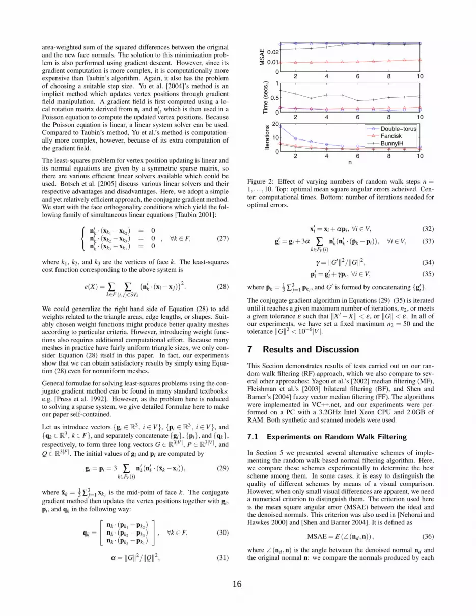
Figure 2: Effect of varying numbers of random walk steps n =1, . . . ,10. Top: optimal mean square angular errors acheived. Cen-ter: computational times. Bottom: number of iterations needed foroptimal errors.

x′i = xi +αpi, ∀i ∈V, (32)

g′i = gi +3α ∑k∈FV (i)

n′k(n′k · (pk −pi)), ∀i ∈V, (33)

γ = ‖G′‖2/‖G‖2, (34)

p′i = g′i + γpi, ∀i ∈V, (35)

where pk = 13 ∑

3j=1 pk j , and G′ is formed by concatenating {g′i}.

The conjugate gradient algorithm in Equations (29)–(35) is iterateduntil it reaches a given maximum number of iterations, n2, or meetsa given tolerance ε such that ‖X ′−X‖ < ε , or ‖G‖ < ε . In all ofour experiments, we have set a fixed maximum n2 = 50 and thetolerance ‖G‖2 < 10−6|V |.

7 Results and Discussion

This Section demonstrates results of tests carried out on our ran-dom walk filtering (RF) approach, which we also compare to sev-eral other approaches: Yagou et al.’s [2002] median filtering (MF),Fleishman et al.’s [2003] bilateral filtering (BF), and Shen andBarner’s [2004] fuzzy vector median filtering (FF). The algorithmswere implemented in VC++.net, and our experiments were per-formed on a PC with a 3.2GHz Intel Xeon CPU and 2.0GB ofRAM. Both synthetic and scanned models were used.

7.1 Experiments on Random Walk Filtering

In Section 5 we presented several alternative schemes of imple-menting the random walk-based normal filtering algorithm. Here,we compare these schemes experimentally to determine the bestscheme among them. In some cases, it is easy to distinguish thequality of different schemes by means of a visual comparison.However, when only small visual differences are apparent, we needa numerical criterion to distinguish them. The criterion used hereis the mean square angular error (MSAE) between the ideal andthe denoised normals. This criterion was also used in [Nehorai andHawkes 2000] and [Shen and Barner 2004]. It is defined as

MSAE = E (∠(nd ,n)) , (36)

where ∠(nd ,n) is the angle between the denoised normal nd andthe original normal n: we compare the normals produced by each

16

0 5 10 15 20 250

0.05

0.1

0.15

0.2

0.25

n1

MS

AE

Double−torus:n=1Double−torus:n=10BunnyiH:n=1BunnyiH:n=10

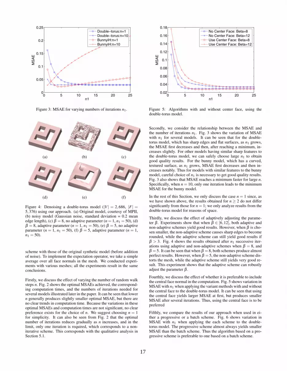
Figure 3: MSAE for varying numbers of iterations n1.

(a) (b) (c)

(d) (e) (f)

Figure 4: Denoising a double-torus model (|V | = 2,686, |F | =5,376) using our approach. (a) Original model, courtesy of MPII,(b) noisy model (Gaussian noise, standard deviation = 0.2 meanedge length), (c) β = 8, no adaptive parameter (n = 1, n1 = 50), (d)β = 8, adaptive parameter (n = 1, n1 = 50), (e) β = 5, no adaptiveparameter (n = 1, n1 = 50), (f) β = 5, adaptive parameter (n = 1,n1 = 50).

scheme with those of the original synthetic model (before additionof noise). To implement the expectation operator, we take a simpleaverage over all face normals in the mesh. We conducted experi-ments with various meshes; all the experiments result in the sameconclusions.

Firstly, we discuss the effect of varying the number of random walksteps n. Fig. 2 shows the optimal MSAEs achieved, the correspond-ing computation times, and the numbers of iterations needed forseveral models illustrated later in the paper. It can be seen that lowern generally produces slightly smaller optimal MSAE, but there areno clear trends in computation time. Because the variations in theseoptimal MSAEs and computation times are not significant, no clearpreference exists for the choice of n. We suggest choosing n = 1for simplicity. It can also be seen from Fig. 2 that the optimalnumber of iterations reduces gradually as n increases, and in thelimit, only one iteration is required, which corresponds to a non-iterative scheme. This corresponds with the qualitative analysis inSection 5.1.

0 5 10 15 20 250.02

0.04

0.06

0.08

0.1

0.12

0.14

0.16

0.18

n1

MS

AE

No Center Face: Beta=8No Center Face: Beta=12Use Center Face: Beta=8Use Center Face: Beta=12

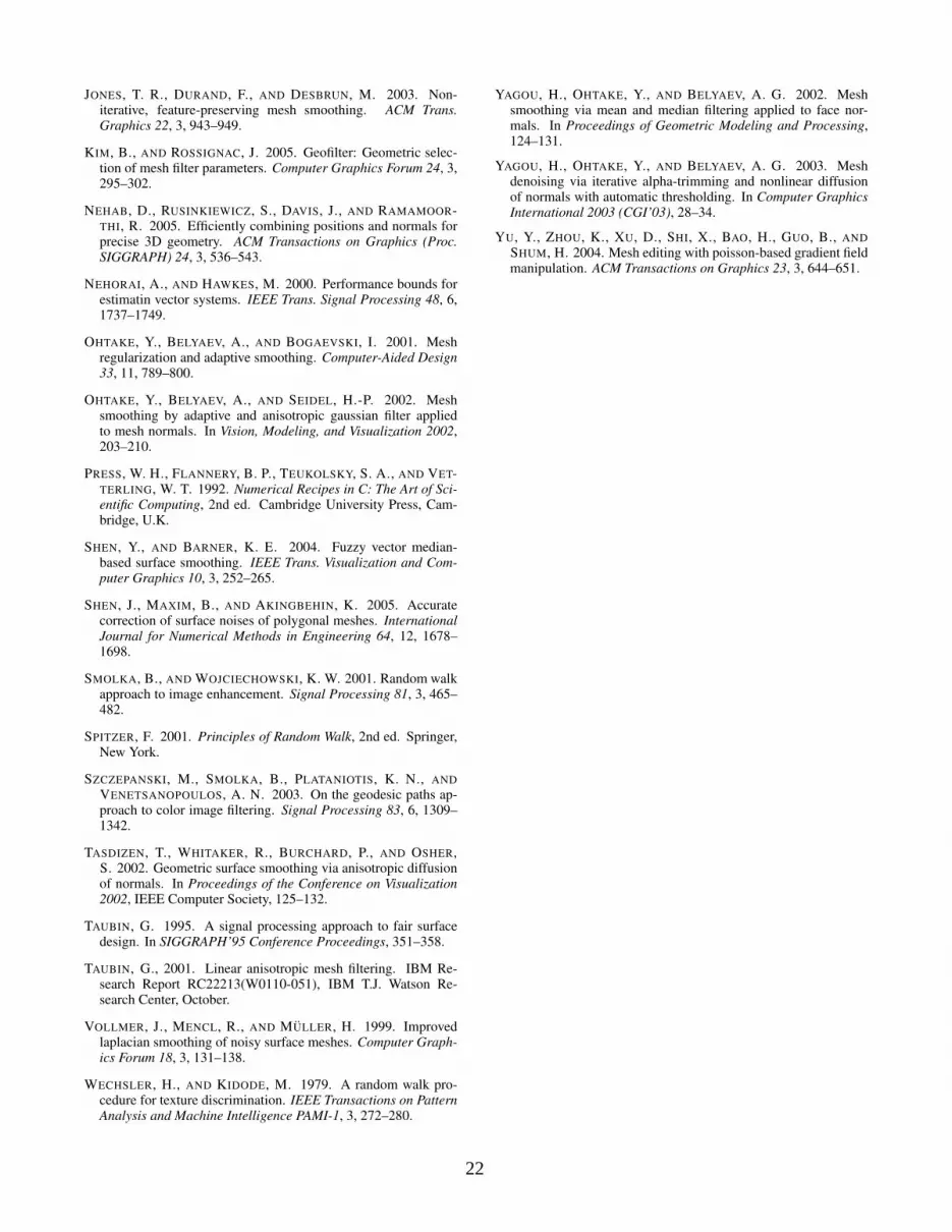
Figure 5: Algorithms with and without center face, using thedouble-torus model.

Secondly, we consider the relationship between the MSAE andthe number of iterations n1. Fig. 3 shows the variation of MSAEwith n1 for several models. It can be seen that for the double-torus model, which has sharp edges and flat surfaces, as n1 grows,the MSAE first decreases and then, after reaching a minimum, in-creases slightly. For other models having similar sharp features tothe double-torus model, we can safely choose large n1 to obtaingood quality results. For the bunny model, which has a curved,textured surface, as n1 grows, MSAE first decreases and then in-creases notably. Thus for models with similar features to the bunnymodel, careful choice of n1 is necessary to get good quality results.Fig. 3 also shows that MSAE reaches a minimum faster for large n.Specifically, when n = 10, only one iteration leads to the minimumMSAE for the bunny model.

In the rest of this Section, we only discuss the case n = 1 since, aswe have shown above, the results obtained for n ≥ 2 do not differsignificantly from those for n = 1; we only analyze results from thedouble-torus model for reasons of space.

Thirdly, we discuss the effect of adaptively adjusting the parame-ter β . Experiments show that when β ∈ [6,12], both adaptive andnon-adaptive schemes yield good results. However, when β is cho-sen smaller, the non-adaptive scheme causes sharp edges to becomerounded, while the adaptive scheme can still yield good results ifβ > 3. Fig. 4 shows the results obtained after n1 successive iter-ations using adaptive and non-adaptive schemes when β = 8, andβ = 5. It can be seen that when β = 8, both schemes produce almostperfect results. However, when β = 5, the non-adaptive scheme dis-torts the mesh, while the adaptive scheme still yields very good re-sult. This experiment shows that the adaptive scheme can robustlyadjust the parameter β .

Fourthly, we discuss the effect of whether it is preferable to includethe central face normal in the computation. Fig. 5 shows variation inMSAE with n1 when applying the variant methods with and withoutthe central face to the double-torus model. It can be seen that usingthe central face yields larger MSAE at first, but produces smallerMSAE after several iterations. Thus, using the central face is to bepreferred

Fifthly, we compare the results of our approach when used in ei-ther a progressive or a batch scheme. Fig. 6 shows variation inMSAE with n1 when applying the each scheme to the double-torus model. The progressive scheme almost always yields smallerMSAE than the batch scheme. Thus the algorithm based on a pro-gressive scheme is preferable to one based on a batch scheme.

17

0 5 10 15 20 250

0.05

0.1

0.15

0.2

n1

MS

AE

Progressive: Beta=8Progressive: Beta=12Batch: Beta=8Batch: Beta=12

Figure 6: Progressive and batch schemes, using the double-torusmodel.

Finally, we briefly discuss the two possible types of face neighbour-hood. Our experiments show that our algorithm using Type I faceneighbourhoods generally produces better qualitative mesh resultsthan using Type II face neighbourhoods. On the other hand, thealgorithm is faster when using Type II face neighbourhoods. Onbalance, we suggest using Type I face neighbourhoods in our ap-proach; all other comparisons are based on using Type I face neigh-bourhoods.

In summary, our experiments show that progressively using Equa-tion (14) with β adjusted adaptively is the best scheme when usingour approach. Thus, we use this scheme in the rest of our experi-ments and comparisons.

7.2 Comparisons with Other Approaches

We now turn our attention to comparing our RF approach withYagou et al.’s [2002] MF, Fleishman et al.’s [2003] BF, and Shenand Barner’s [2004] FF approaches.

7.2.1 Quality

We first visually compare the results obtained. In each case, weshow the best results we were able to obtain for each approach aftercarefully tuning its parameters. All models are rendered using flatshading to aid in comparing normals.

Fig. 7 shows denoising results for a CAD-like model with sharpedges—a double-pyramid. It can be seen that all the four filteringmethod approaches preserve sharp features to some extent. How-ever, the BF approach cannot smooth vertices with large errors,as Fleishman et al. [2003] point out. The MF approach cannotsmooth flat areas completely, and cannot preserve corner features.In contrast, the FF approach and our RF approach produce surfacesthat look very like the original model. (We also tested mean filter-ing [Yagou et al. 2002] and alpha-trimming filtering [Yagou et al.2003], but both methods blur sharp edges, so we have not illustratedthe corresponding poor results.)

Fig. 8 shows denoising results for a faceted and triangulated cylin-der, which has both flat and curved areas, and sharp edges. It canbe seen that the BF approach does not preserve sharp edges in thiscase. The MF approach preserves sharp edges, but also introducesspurious additional sharp edges. The FF approach and our RF ap-proach preserve both sharp edges and the surface characteristics.

(a) (b) (c)

(d) (e) (f)

Figure 7: Denoising of a double-pyramid model (|V |= 1026, |F |=2048). (a) Original model, (b) noisy model (Gaussian noise, stan-dard deviation = 0.2 mean edge length), (c) BF result, (d) MF result,(e) FF result, (f) RF result (n1 = 10,β = 12).

(a) (b) (c)

(d) (e) (f)

Figure 8: Denoising of a cylinder model (|V |= 404, |F |= 804). (a)Original model, (b) noisy model (Gaussian noise, standard devia-tion = 0.2 mean edge length), (c) BF result, (d) MF result, (e) FMresult, (f) RF result (n1 = 10,β = 8).

Fig. 9 shows denoising results for a fandisk model. All four ap-proaches preserve most of the sharp edges. The BF and MF ap-proaches even preserve those sharp edges with small angles be-tween the neighbouring surfaces, but on the other hand some cor-ner vertices are not correctly smoothed. Furthermore, the surfacesproduced by the MF approach are not particularly smooth in otherareas. The FF approach and our RF approach produce smooth sur-faces and preserve most sharp edges, but blur edges with small an-gles. The BF approach preserves sharp edges better on this modelthan on the previous models. The reason seems to be that the noiselevel in this model is relatively small, and few iterations of filter-ing are required. We also performed a test on the fandisk modelafter adding Gaussian noise with a standard deviation of 20% ofthe mean edge length. In this case, bilateral filtering blurs the sharpedges if we try to achieve a reasonably smooth final surface.

Fig. 10 shows denoising results on a mesh model with details atvarious sizes—the “iH” embossed Stanford Bunny Model. All ap-proaches do well apart from the MF approach. The MF approach

18

(a) (b) (c)

(d) (e) (f)

Figure 10: Denoising of an “iH” embossed Stanford Bunny model (|V |= 34,834, |F |= 69,451). (a) Original model, courtesy of A. Belyaev,(b) noisy model (Gaussian noise, standard deviation = 0.2 mean edge length), (c) BF result, (d) MF result, (e) FF result, (f) RF result(n1 = 3,β = 8).

(a) (b) (c)

(d) (e) (f)

Figure 9: Denoising of a fandisk model (|V | = 6,475, |F | =12,946). (a) Original model, courtesy of H. Hoppe. (b) noisy model(Gaussian noise, standard deviation = 0.1 mean edge length), (c) BFresult, (d) MF result, (e) FF result, (f) RF result (n1 = 4,β = 8).

has a tendency to enhance features in the noisy model, and the re-sulting surface is not smooth. For this model, perhaps the BF ap-proach provides the best overall result, with the FF approach, and

to a lesser extent the RF approach, losing a little of the finer detail.

Fig. 11 shows results of denoising a scanned model with tinydetails—the Maoi model. For this model, MF cannot effectivelysmooth the surface. FF smoothes some tiny details away. The BFand RF approaches both preserve tiny details and smooth the sur-face better. Again, the BF approach seems provides the best overallresult.

Fig. 12 and 13 show the results of denoising two 3D photographymesh models. From the figures it can be seen that, as for the Moaimodel, the MF method enhances certain details, but cannot effec-tively smooth the surfaces. All three other methods both smooththe mesh surfaces while preserving tiny details to some extent. Thedifferences between the results of these three methods are visuallyvery small. It seems that the results of the BF approach and our RFapproach are very close and preserve details a little better than theFF approach.

From the above comparisons we can see that the results from the FFapproach and our RF approach are generally visually similar, andboth produce better results than either the BF or MF approach incases where sharp edges exist in the models. In cases where thereare tiny details in the models, the BF approach probably producesthe best results, while our RF approach produces results slightlybetter than the FF approach.

19

(a) (b) (c) (d) (e)

Figure 11: Denoising of the Moai model (|V | = 10,002, |F | = 20,000). (a) Original model, courtesy of Y. Ohtake, (b) BF result, (c) MFresult, (d) FF result, (e) RF result (n1 = 3,β = 30).

(a) (b) (c) (d) (e)

Figure 12: Denoising of a 3D photography model (|V |= 14,770, |F |= 28,878). (a) Original model, courtesy of J.-Y. Bouguet, (b) BF result,(c) MF result, (d) FF result, (e) RF result (n1 = 5,β = 30).

(a) (b) (c) (d) (e)

Figure 13: Denoising of a head model (|V | = 19,324, |F | = 37,922). (a) Original model, courtesy of J.-Y. Bouguet, (b) BF result, (c) MFresult, (d) FF result, (e) RF result (n1 = 3,β = 30).

7.2.2 Speed

We now compare the computational cost of the approaches dis-cussed above. Since Shen and Barner’s [2004] FF approach gener-ally produces similar results to our RF approach, we first comparethese two approaches. Both approaches use a consecutive, iterativescheme. Because the vertex position updating stage takes very lit-tle time compared to the normal updating stage, we first comparespecifically the times taken by the normal updating stages of theRF and BF approaches. Table 1 shows the CPU times recorded inour experiments. Note that we have used some other large (well-known) models which are not shown in this paper. For comparativepurposes, we performed 50 iterations of normal updating for each

algorithm, although it is not necessary in practice to use so manyiterations. From the table it can be seen that our RF approach ismore than ten times faster than the FF approach.

We continue in Table 2 by comparing the overall time taken byour approach with that required by other approaches. The valuesin parentheses are the numbers of iterations we found necessary tosatisfactorily denoise the models. For the BF and MF approachesthese correspond to n0, for the FF approach to n1,n2 and for our RFapproach to n1. Overall, the BF (bilateral filtering) approach is gen-erally fastest. However, our approach requires a time similar to thatof bilateral filtering; sometimes, our approach is even faster thanbilateral filtering. The other approaches take significantly longer.

20

Fandisk iH Bunny Igea Dragon Buddha|V | 6475 34834 134345 437645 757490|F | 12946 69451 268686 871414 1514962RF 0.703 4.078 15.391 47.657 83.078FF 9.391 48.406 196.531 677.719 1263.06

Table 1: Normal updating times for RF and FF methods (seconds,for 50 iterations)

Fandisk iH Bunny Igea Dragon BuddhaBF 0.046 0.313 1.313 3.75 7.094

(5) (5) (5) (5) (5)MF 0.281 2.594 7.25 33.219 39.047

(10) (15) (10) (15) (10)FF 1.891 5.141 12.641 140.438 70.093

(10, 10) (5, 20) (3, 10) (10, 15) (3, 10)RF 0.078 0.422 1.484 6.078 6.922

(4) (3) (3) (5) (3)

Table 2: Overall times for various methods (seconds, for givennumbers of iterations)

Overall, our method can provide denoising results of a quality oftencomparable to the slowest of these methods, with nearly the speedof the fastest.

8 Conclusions

In this paper, we have shown how to use random walks for mesh de-noising, and proposed a new consecutive iterative mesh denoisingalgorithm. In the first stage, the face normals are updated throughweighted averaging of the face normals, with the weights being de-termined by probabilities of random walk steps between the currentface and neighbors. Analysis and experiments show that the schemein Equation (14), together with adaptively adjusting parameter β ,and progressively updating face normals, provides the best imple-mentation of our approach. In the second stage, we use a conjugategradient algorithm to solve the vertex position update least-squaresproblem rather than the more generally used gradient descent algo-rithm [Taubin 2001; Ohtake et al. 2001; Shen and Barner 2004].The conjugate gradient algorithm is stable and converges rapidly,and is particularly suitable for solving the least-squares problemarising here as it results from a sparse system.

A basic requirement for a mesh denoising algorithm is that it canboth remove noise and preserve mesh features effectively. How-ever, many early mesh denoising algorithms did not consider thefeature-preserving requirement. Several more recent mesh denois-ing methods do consider it, but most such methods are computa-tionally expensive. Our proposed mesh denoising algorithm effec-tively preserves features and yet is very simple and computationallycheap. Experiments presented here have compared our approachwith other recent feature-preserving mesh denoising approaches.Bilateral filtering [Fleishman et al. 2003] is a fast feature-preservingmesh denoising approach. Experiments show that our approach isas fast as the bilateral filtering approach [Fleishman et al. 2003]:e.g. it can denoise the well-known Buddha model with 1.5 milliontriangles within 7 seconds; however, our approach preserves sharpedges better than the bilateral filtering approach. Compared to thefuzzy vector median filtering approach [Shen and Barner 2004], ourapproach is over ten times faster, yet produces a final surface qualitysimilar to or better than that approach.

Although our algorithm is simple and efficient for feature-preserving mesh denoising, it is not immune to certain problems

that other algorithms also meet. One is that we have to interactivelydetermine the number of normal updating iterations. Using too fewiterations fails to fully denoise the mesh normals, while too manycauses oversmoothing of the mesh. Future work is needed to find anautomatic method of determining the optimal number of iterations.Other problems such as mesh folding, self interaction and poorly-shaped triangles caused by vertex position updates should also beconsidered in future work.

Acknowledgment

This work was supported by EPSRC Grant EP/C007972 and NSFCGrant 60674030.

References

AZZABOU, N., PARAGIOS, N., AND GUICHARD, F. 2006.Random walks, constrained multiple hypothesis testing andimage enhancement. In ECCV 2006 Proceedings, Springer,A. Leonardis, H. Bischof, and A. Pinz, Eds., vol. 1, 379–390.

BAJAJ, C. L., AND XU, G. 2003. Anisotropic diffusion of surfacesand functions on surfaces. ACM Trans. Graphics 22, 1, 4–32.

BOTSCH, M., AND KOBBELT, L. P. 2001. Resampling feature andblend regions in polygonal meshes for surface anti-aliasing. InEG 2001 Proceedings, Blackwell Publishing, A. Chalmers andT.-M. Rhyne, Eds., vol. 20(3), 402–410.

BOTSCH, M., BOMMES, D., AND KOBBELT, L. 2005. Efficientlinear system solvers for mesh processing. In Proceedings ofthe IMA Mathematics of Surfaces XI, Lecture Notes in ComputerScience, vol. 3604, 62–83.

CHEN, C.-Y., AND CHENG, H.-Y. 2005. A sharp dependent fil-ter for mesh smoothing. Computer Aided Geometric Design 22,376–391.

CLARENZ, U., DIEWALD, U., AND RUMPF, M. 2000. Anisotropicgeometric diffusion in surface processing. In Proceedings ofthe Conference on Visualization 2000, IEEE Computer Society,397–405.

DESBRUN, M., MEYER, M., SCHRODER, P., AND BARR, A. H.1999. Implicit fairing of irregular meshes using diffusion andcurvature flow. In Proceedings of SIGGRAPH’99, 317–324.

DESBRUN, M., MEYER, M., SCHRODER, P., AND BARR, A. H.2000. Anisotropic Feature-Preserving denoising of height fieldsand bivariate data. In Graphics Interface’2000 Proceedings,145–152.

DIEBEL, J. R., THRUN, S., AND BRUNIG, M. 2006. Abayesian method for probable surface reconstruction and deci-mation. ACM Trans. Graphics 25, 1, 39–59.

FIELD, D. A. 1988. Laplacian smoothing and delaunay triangula-tions. Communications in Numerical Methods in Engineering 4,709–712.

FLEISHMAN, S., DRORI, I., AND COHEN-OR, D. 2003. Bilateralmesh denoising. ACM Trans. Graphics 22, 3, 950–953.

GRADY, L. 2006. Random walks for image segmentation. IEEETransactions Pattern Analysis and Machine Intelligence Ac-cepted.

HILDEBRANDT, K., AND POLTHIER, K. 2004. Anisotropic fil-tering of non-linear surface features. Computer Graphics Forum23, 3, 391–400.

21

JONES, T. R., DURAND, F., AND DESBRUN, M. 2003. Non-iterative, feature-preserving mesh smoothing. ACM Trans.Graphics 22, 3, 943–949.

KIM, B., AND ROSSIGNAC, J. 2005. Geofilter: Geometric selec-tion of mesh filter parameters. Computer Graphics Forum 24, 3,295–302.

NEHAB, D., RUSINKIEWICZ, S., DAVIS, J., AND RAMAMOOR-THI, R. 2005. Efficiently combining positions and normals forprecise 3D geometry. ACM Transactions on Graphics (Proc.SIGGRAPH) 24, 3, 536–543.

NEHORAI, A., AND HAWKES, M. 2000. Performance bounds forestimatin vector systems. IEEE Trans. Signal Processing 48, 6,1737–1749.

OHTAKE, Y., BELYAEV, A., AND BOGAEVSKI, I. 2001. Meshregularization and adaptive smoothing. Computer-Aided Design33, 11, 789–800.

OHTAKE, Y., BELYAEV, A., AND SEIDEL, H.-P. 2002. Meshsmoothing by adaptive and anisotropic gaussian filter appliedto mesh normals. In Vision, Modeling, and Visualization 2002,203–210.

PRESS, W. H., FLANNERY, B. P., TEUKOLSKY, S. A., AND VET-TERLING, W. T. 1992. Numerical Recipes in C: The Art of Sci-entific Computing, 2nd ed. Cambridge University Press, Cam-bridge, U.K.

SHEN, Y., AND BARNER, K. E. 2004. Fuzzy vector median-based surface smoothing. IEEE Trans. Visualization and Com-puter Graphics 10, 3, 252–265.

SHEN, J., MAXIM, B., AND AKINGBEHIN, K. 2005. Accuratecorrection of surface noises of polygonal meshes. InternationalJournal for Numerical Methods in Engineering 64, 12, 1678–1698.

SMOLKA, B., AND WOJCIECHOWSKI, K. W. 2001. Random walkapproach to image enhancement. Signal Processing 81, 3, 465–482.

SPITZER, F. 2001. Principles of Random Walk, 2nd ed. Springer,New York.

SZCZEPANSKI, M., SMOLKA, B., PLATANIOTIS, K. N., ANDVENETSANOPOULOS, A. N. 2003. On the geodesic paths ap-proach to color image filtering. Signal Processing 83, 6, 1309–1342.

TASDIZEN, T., WHITAKER, R., BURCHARD, P., AND OSHER,S. 2002. Geometric surface smoothing via anisotropic diffusionof normals. In Proceedings of the Conference on Visualization2002, IEEE Computer Society, 125–132.

TAUBIN, G. 1995. A signal processing approach to fair surfacedesign. In SIGGRAPH’95 Conference Proceedings, 351–358.

TAUBIN, G., 2001. Linear anisotropic mesh filtering. IBM Re-search Report RC22213(W0110-051), IBM T.J. Watson Re-search Center, October.

VOLLMER, J., MENCL, R., AND MULLER, H. 1999. Improvedlaplacian smoothing of noisy surface meshes. Computer Graph-ics Forum 18, 3, 131–138.

WECHSLER, H., AND KIDODE, M. 1979. A random walk pro-cedure for texture discrimination. IEEE Transactions on PatternAnalysis and Machine Intelligence PAMI-1, 3, 272–280.

YAGOU, H., OHTAKE, Y., AND BELYAEV, A. G. 2002. Meshsmoothing via mean and median filtering applied to face nor-mals. In Proceedings of Geometric Modeling and Processing,124–131.

YAGOU, H., OHTAKE, Y., AND BELYAEV, A. G. 2003. Meshdenoising via iterative alpha-trimming and nonlinear diffusionof normals with automatic thresholding. In Computer GraphicsInternational 2003 (CGI’03), 28–34.

YU, Y., ZHOU, K., XU, D., SHI, X., BAO, H., GUO, B., ANDSHUM, H. 2004. Mesh editing with poisson-based gradient fieldmanipulation. ACM Transactions on Graphics 23, 3, 644–651.

22