Embed Size (px)
Citation preview

Economic Analysis of Snohvit
Expansion Project
COVER
Trian Hendro Asmoro
51445172
August, 2015
A thesis presented in partial fulfilment of the requirements for
the degree of MSc Petroleum Energy Economics and Finance
at the University of Aberdeen

ii
for Dika, Safa, Aidan

iii
DISCLAIMER
I declare that this thesis has been composed by myself, that it has not been accepted in any
previous application for a degree, that the work of which it is record has been done by
myself, and that all quotations have been distinguished appropriately and the source of
information specifically acknowledged.
Trian Hendro Asmoro
August 10th
, 2015

iv
ABSTRACT
Norway has clear interests in hydrocarbon production in arctic provinces. Barents Sea
in Arctic region has played significant role in producing hydrocarbon for Norway since the
establishment of Snohvit LNG plant in 2007 by Statoil. It was estimated to be a new frontier
for further development projects in the region. Some recent discoveries have likely indicated
a plan to expand current LNG operation. Meanwhile, northern sea route has become more
commercially attractive in connecting North-East Asia countries, e.g. Japan and China, with
their North-Western European counterparts, e.g. Netherlands and Norway, as a result of
melting arctic ice caps.
There would be opportunities in the near future for Snohvit expansion project to supply
LNG to North-East Asia as well as obtaining LNG technology suppliers from North-East
Asia. The project needs therefore to be analysed using key project’s variables, such as
discoverable gas reserve, LNG price and project costs in which Snohvit is one of most
expensive LNG projects. Project economics model with discounted cash flow method and
montecarlo simulation is used to do economic analysis. This research shows that project
scenario, development options and prospects in the LNG market play role to determine the
feasibility of Snohvit expansion project.

v
LIST OF CONTENTS
COVER ....................................................................................................................................... i
DISCLAIMER ......................................................................................................................... iii
ABSTRACT .............................................................................................................................. iv
LIST OF CONTENTS ............................................................................................................... v
LIST OF FIGURES .................................................................................................................. vi
LIST OF TABLES ................................................................................................................... vii
CHAPTER I: INTRODUCTION ............................................................................................... 1
CHAPTER II: LITERATURE REVIEW .................................................................................. 4
2.1. Norwegian Barents Sea ............................................................................................... 4
2.2. Snohvit LNG ............................................................................................................... 7
2.3. Norwegian Petroleum Fiscal System .......................................................................... 9
2.4. LNG Market and Price .............................................................................................. 11
2.5. Northern Sea Route ................................................................................................... 14
CHAPTER III: METHODOLOGY AND DATA ................................................................... 17
3.1. Methodology ............................................................................................................. 17
3.2. Data and Assumptions ............................................................................................... 19
CHAPTER IV: RESULT AND ANALYSIS .......................................................................... 24
4.1. Economic Indicators .................................................................................................. 24
4.2. Sensitivity Analysis ................................................................................................... 24
4.3. Probabilistic Output................................................................................................... 29
4.4. Scenario Analysis ...................................................................................................... 32
4.5. Discussion ................................................................................................................. 35
CHAPTER V: CONCLUSION................................................................................................ 39
BIBLIOGRAPHY .................................................................................................................... 42
APPENDIX 1: MODEL INPUT .............................................................................................. 46
APPENDIX 2: MODEL CALCULATION ............................................................................. 47
APPENDIX 3: MODEL SIMULATION INPUT .................................................................... 51
APPENDIX 4: UNIT COST PROBABILITY ........................................................................ 52
GLOSSARY ............................................................................................................................ 53

vi
LIST OF FIGURES
Figure 1-1 Potential Arctic Oil and Gas Resources ................................................................... 1
Figure 2-1 Norwegian Oil and Gas Provinces ........................................................................... 4
Figure 2-2 Oil and Gas Discoveries in the Barents Sea ............................................................. 5
Figure 2-3 Snohvit Field in the Barents Sea .............................................................................. 7
Figure 2-4 Petroleum Taxation System in Norway ................................................................. 10
Figure 2-5 Natural Gas Prices .................................................................................................. 12
Figure 2-6 Typical LNG Value Chain ..................................................................................... 13
Figure 2-7 NSR and Current SSR ............................................................................................ 14
Figure 2-8 Vessels and Tons Cargo Sailed in the NSR ........................................................... 15
Figure 2-9 Northern Sea Route Detail ..................................................................................... 16
Figure 3-1 Research Framework of Snohvit Expansion Project .............................................. 17
Figure 3-2 Research Methodology........................................................................................... 19
Figure 3-3 Triangular Distribution of Development Cost ....................................................... 20
Figure 3-4 LNG Unit Cost for High Cost Projects .................................................................. 21
Figure 4-1 Sensitivity Chart of NPV ....................................................................................... 25
Figure 4-2 Sensitivity Chart of NPV without Uplift ................................................................ 26
Figure 4-3 Sensitivity Chart of IRR ......................................................................................... 27
Figure 4-4 Sensitivity Chart of IRR without Uplift ................................................................. 28
Figure 4-5 Simulation Result of Project’s NPV ...................................................................... 30
Figure 4-6 Simulation Result of Project’s IRR ........................................................................ 30
Figure 4-7 Simulation Result of Project’s NPV and NPV Capex Ratio .................................. 31
Figure 4-8 Unit Cost Probability for 1.3 MTPA ...................................................................... 36
Figure 4-9 Liquefaction Plant Metric Cost .............................................................................. 37

vii
LIST OF TABLES
Table 4-1 Deterministic Output of Economics Model ............................................................. 24
Table 4-2 Project Scenario ....................................................................................................... 33
Table 4-3 Decision Table for Project’s NPV ........................................................................... 33
Table 4-4 Decision Table for NPV Project and Capex Ratio .................................................. 34
Table 4-5 Project Scenario and Development Cost (Mean Capex) ......................................... 35
Table 4-6 Project Scenario and Decision Table ....................................................................... 35
Table 4-7 Probability of Unit Cost........................................................................................... 36

1
CHAPTER I: INTRODUCTION
In 2008, the U.S. Geological Survey (USGS) completed an appraisal of possible future
additions to world oil and gas reserves from new field discoveries in the Arctic. It resulted in
an assessment of potential undiscovered and technically recoverable crude oil, natural gas,
and natural gas liquid resources in the Arctic region including the Barents Sea Shelf of
Norway. According to USGS, the total mean undiscovered conventional oil and gas resources
of the Arctic are estimated to be approximately 90 billion barrels of oil (BOE), 1,669 trillion
cubic feet (TCF) of natural gas, and 44 billion barrels of natural gas liquids. Converting these
figures to BOE and adding them up, a total of 412 billion BOE could be found (USGS 2008).
The USGS study estimated that the Arctic could hold about 13% of the world’s undiscovered
oil resources and as much as 30% of the world’s undiscovered natural gas resources. In other
words, it was about 22% of the global undiscovered conventional oil and gas resources
(Lindholt, Glomsrød 2012). By allocating the estimated resources/provinces to the nearest
country, Norway is estimated to hold 12% of the total Arctic resources (EY 2013), where
most of it is gas resources as shown in Figure 1-1. However, hydrocarbon exploration and
production (E&P) activities in the Arctic are always challenging and cash-intensive.
Figure 1-1 Potential Arctic Oil and Gas Resources
(Source: EY 2013)
The Barents Sea has played increasingly significant role in producing hydrocarbon for
Norway during the last few years, as the country is experiencing considerable shrinkage of its
hydrocarbon production from Norwegian and North Sea. The Barents Sea has also been
considered as the most exciting new area of oil and gas, along with the northern part of the

2
Norwegian Sea since the establishment of Snohvit LNG plant in Melkoya Island in 2007 by
Statoil (Auran et al. 2012). It is important to note, however, that the significant development
costs have hampered its economics. In addition, harsh winters with extreme temperatures,
combined with limited supply lines to energy consumers, as well as a lack of adequate
infrastructure and delicate environmental issues, provide problematic conditions for
developing oil and gas fields in arctic (Harsem, Eide & Heen 2011). Although LNG transport
from Melkoya is the only gas infrastructure developed in the northern part of the world today,
Snohvit LNG plant was one of the most expensive LNG investments ever (Songhurst 2014).
There have been some discoveries in the Barents Sea in recent years that leads to the
possibility of building the second train of Snohvit LNG plant (Auran et al. 2012, EY 2013).
Norway, one of the world’s largest gas exporters, has clear interests in oil and gas production
in arctic provinces. The country is heavily dependent on the oil and gas sector, as the industry
accounted for 23% of the Norwegian GNP, 30% of the state revenues and 52% of Norway’s
total exports in 2012 (Moe 2013). If Norway wants to continue its current output level, arctic
oil and gas activities must intensify. There is an estimate of 0.3 billion standard cubic meters
of oil equivalents of extractable hydrocarbon identified (mainly gas) in the Norwegian
Barents Sea, with additional estimate of 1 billion standard cubic meters of oil equivalents
resources unidentified (Kullerud 2011). Nevertheless, the country’s aggressiveness in
exploring and developing the Arctic region may also be adversely affected by its caution of
the CO2 emissions impact of the activities (Harsem, Eide & Heen 2011).
The most important factor in exploring the Arctic region, unsurprisingly, is the super-
cooled gas, commonly known as LNG, that is averagely traded at a premium of about US$16
per million British thermal unit (MMBTU) in Far East market (BP 2015). In addition, global
investment in LNG infrastructure and facilities has risen, and they are now spread across
more countries, while the size of the LNG tanker fleet has expanded significantly, and
transport costs have fallen (Ritz 2014). Moreover, the trend of relatively higher LNG prices
in Asian markets is believed to continue further as countries such as Japan, South Korea,
Taiwan, India and China keep experiencing relatively high economic growth (Rogers, Stern
2015). Meanwhile, climate change has played a significant role in expanding access to the
Arctic region. The northern sea route (NSR) has therefore become more commercially
attractive in connecting North-East Asia countries, such as Japan, South Korea, Taiwan and
China, with their North-Western European counterparts, such as Netherlands, Norway, UK
and Germany, as a result of melting arctic ice caps (Bekkers, Francois & Rojas-Romagosa

3
2015). All things considered, there would be opportunity in the near future to supply LNG
from second train of Snohvit LNG plant to North-East Asia in addition to equipment and
services movement from North-East Asia to support the Snohvit expansion project.
In correspondence with research background above, there are three research questions
that have to be answered through the research. First, how main variables of project
economics, e.g. cost, recoverable gas, LNG prices, behave in determining the project
economics output of Snohvit expansion project. Second, how factors within internal project’s
boundaries are required to make the project feasible, given current conditions faced by the
project. Third, how development options or project scenario and prospects in the LNG market
play role to determine the project’s feasibility.
To discuss and answer the research questions, this dissertation is organised as follows:
Chapter 1: Introduction. This chapter mainly describes about background or motivation of
the research.
Chapter 2: Literature Review. This chapter will discuss some relevant literatures to
support the research.
Chapter 3: Methodology and Data. This chapter will explain methodology, data and
assumptions used in the research.
Chapter 4: Result and Analysis. This chapter will present and analyse the results of the
research.
Chapter 5: Conclusion. This chapter will consist of conclusion and recommendation
obtained from the research.

4
CHAPTER II: LITERATURE REVIEW
2.1. Norwegian Barents Sea
Norway is estimated to hold 12% of the total Arctic resources with most of it being gas
resources (USGS 2008, EY 2013). More specifically 0.3 billion standard cubic meters of oil
equivalents of extractable hydrocarbon have been identified (mainly gas) in the Norwegian
Barents Sea, with additional 1 billion standard cubic meters of oil equivalents resources
estimated to be unidentified (Kullerud 2011, Klett, Gautier 2009). In recent years, the
country’s interest in the Barents has picked up significantly as it is estimated to contain up to
42% of Norway’s undiscovered reserves (ECC 2013). Another contributing factor to the
significance of Barents Sea’s activities is that the recent years’ decline of Norwegian
hydrocarbon output. Meanwhile, liquefied natural gas (LNG) production that is processed
from Snohvit and other fields has significantly contributed to Norwegian production level in
mitigating the fast decline of Norwegian hydrocarbon production (Moe 2013). This along
with the maturity of Norwegian Sea and North Sea fields suggest that the development of the
Norwegian Arctic region, e.g. Barents Sea, as new petroleum provinces will attract more
interests from the country government, despite the uncertainties associated with the resource
estimates and their cost (Lindholt, Glomsrød 2012). The Norwegian oil and gas provinces are
shown in Figure 2-1.
Figure 2-1 Norwegian Oil and Gas Provinces
(Source: Heiersted 2005)

5
Oil and gas activities in the Barents Sea had led to a sensitive issue regarding the shared
border between Russia and Norway. The 2010 agreement between the two countries on
Arctic border in Barents Sea generated significant opportunities for resource development
(Wilson Centre 2013). The countries agree to set aside their differences and establish a
maritime border so that they can explore in the region. The treaty represents a compromise,
with the two countries agreeing to a border that splits this area roughly in half (EY 2013).
This has led to increasing activities in the Barents Sea, resulting to several discoveries, such
as Skrugard and Havis during 2011-2012 which is believed to have proven resources of 400-
600 million barrels of recoverable oil (Statoil 2014a). The latest discovery in the Drivis
prospect in the Barents Sea was announced by Statoil, a Norwegian-owned oil and gas
company, in 2014 after conducting exploration program around the Johan Castberg (former
Skrugard) field. The discovery will add the existing portfolio of other discoveries within the
Johan Castberg province as shown in Figure 2-2, so that it creates a basis for further Johan
Castberg development project (Statoil 2014a).
Figure 2-2 Oil and Gas Discoveries in the Barents Sea
(Source: Statoil 2014a)
The development of gas fields will be more challenging if they are contaminated with
CO2 or other pollutants, because it would impact on how oil and gas in the Barents Sea will
be developed. Snohvit LNG is the world’s first LNG plant with CO2 capture and storage,
since the country strongly supports for the Kyoto agreement, and for a worldwide reduction
of carbon emissions (Harsem, Eide & Heen 2011). The government had even deferred the

6
decision to give a green light for further exploration activities in the region due to sensitive
ecological-related issues associated with this area (Wilson Centre 2013). There are
recognised risks related with oil and gas activities particularly in offshore installation and
production, such as hydrocarbon leaks from subsea production systems, pipelines, risers and
subsea well kicks or loss of well control (Vinnem et al. 2006). These risks have risen
significantly, in parallel with the growing offshore oil and gas activities recently. In particular
to LNG operation, most LNG tankers are new and safe, while gas leaks and LNG spills
accidents are infrequent. Risks such as LNG accidents which include collisions and
groundings are small and manageable due to current safety policies and practises (Auran et
al. 2012). An accidental discharge of oil and gas mixture below sea level, for instance, can
instigate a release of toxic chemicals into the water column and sediment pore water. This
may increase morbidity and mortality of marine life of various species in the long-term
(Nazir et al. 2008).
In spite of the increased activity in arctic resources, their development is still both high-
cost and high-risk. The major challenges related with arctic development include harsh
climate effects such as the intense cold for most of the year, long periods of near-total
darkness, and the potential ice-pack damage to offshore facilities, limited existing
infrastructure, spill containment/spill recovery, overlapping/competing economic sovereignty
claims, country-specific environment laws/regulations (EY 2013). On the other hand, the
booming global gas supply, both from conventional and unconventional sources, will
significantly challenge the Arctic gas development. There are increasing estimates of non-
frontier resource potential of which almost all could be developed at less cost and with lower
environmental risk compared with Arctic resources (EY 2013). Therefore, if the Norwegian
government wants to increase the activities in the Barents Sea, there are many things that
should be taken into account regarding the economics feasibility of Arctic development,
environmental concerns, and perhaps most importantly, public opinion (Harsem, Eide &
Heen 2011).
Since Snohvit, the first hydrocarbon development in the Arctic region is viewed as one
of high cost LNG investments (Songhurst 2014), the next section will describe the profile of
Snohvit LNG and Norwegian petroleum fiscal system. Subsequently, LNG market and price
mechanism will be discussed. Finally, northern sea route will be seen as an alternative route
to transport LNG from Barents Sea to Asia.

7
2.2. Snohvit LNG
Snohvit LNG plant is located in Melkoya Island, a dedicated island in the Barents Sea,
near Hammerfest, Norway. It processes natural gas produced from Snohvit, Albatross and
Askeladd field which lie about 140 km northwest of Hammerfest. The Snohvit and Albatross
fields came on stream in 2007, while the Askeladd is due to come on stream in 2014-15
(Hydrocarbon-technology 2012). The total reserve from those producing fields is estimated
190 billion cubic meters (BCM) gas or about 6.8 trillion cubic feet (TCF) (Heiersted 2005).
Those fields have nine production wells and the other 20 production wells are planned to
drill. The wells are producing gas by means of a remote-controlled subsea solution that
includes pipelines to land, while the production plant is located on the seabed between 250
and 345 metres below the sea surface (Statoil 2013a) as depicted in Figure 2-3.
Figure 2-3 Snohvit Field in the Barents Sea
(Source: Norwegian Ministry of Environment 2011)
Large volumes of natural gas are transported through a 143-kilometre multiphase
transport pipeline to shore. It has set a new record for long-distance transportation of
unprocessed well stream (Statoil 2013a). The feed gas has 5-8 % CO2 content. Consequently,
it also has a carbon dioxide capture and storage facility. A 153-km separate pipeline ensures
that CO2 from the plant is returned to the Snohvit field, where it is stored in an appropriate
geological layer located 2.6 km beneath the seabed of the Snohvit field. Snohvit plant was
designed to operate until 2035, started producing gas in October 2007, while the first CO2
was injected in April 2008 (Hydrocarbon-technology 2012) . In addition, it is the first LNG
facility with CO2 capture and storage in the world. A total of nearly 2 million tonnes of CO2
had been stored in the Snohvit field until early 2013 (Statoil 2014a).

8
Regarding the commercial aspects of the project, it requires total investment of US$ 5.6
Billion (NOK 39.5 billion). Most of the capital invested goes to offshore, land and flow
systems 58 %, in which some portion will be spent for further drilling and development in 20
years of 25-year production period. It was constructed for 48 months from its investment
decision (Heiersted 2005). Snohvit has single train LNG with production capacity of 4.3
million tonnes per annum (MTPA) LNG or equivalent to approximately 5.7 BCM of LNG.
Thus, the unit cost of LNG per annum will be about US$ 1,300 per tonne per annum (TPA).
Although it was a green field project, it is regarded as one of high cost LNG projects
compared to the low cost ones that cost below 1,000 US$/TPA (Songhurst 2014). LNG
contracts were agreed with customers for 25 years delivery as follows: 1.8 MTPA to the US
east coast (El Paso), 1.2 MTPA to the Spain (Iberdrola), and the remaining capacity will go to
Gaz de France and Total (Hydrocarbon-technology 2012, Heiersted 2005).
Snohvit is considered by Statoil as a milestone project for further development project
in the Norwegian Barents Sea. The company estimated that Snohvit would be a new frontier
in the Arctic which could cover gas fields within about 250 km from LNG plant (Heiersted
2005). Thus, it can foster an opportunity to expand the Snohvit LNG plant for its second train
in relation to some following discoveries in the Barents Sea. However, the latest discoveries
in the Barents Sea, e.g. Skrugard (2011) and Havis (2012) have been oil discoveries as
compared to the expected gas reservoirs (Auran et al. 2012). As a result, Statoil as main
operator in the Barents Sea and its partners decided in 2013 to stop work on a possible
capacity increase on Snohvit LNG because the gas discoveries had not provided a sufficient
basis for such expansion project. It was also reported that other scenario such as new pipeline
transportation could not make the project profitable (Statoil 2013b).
However, there were some other hydrocarbon discoveries in the following years in
Johan Castberg (former Skrugard) region, e.g. Nunatak (2013), Iskrystall (2013), Skavl
(2013), Kramsno (2014) and Drivis (2014). The first two discoveries proved only gas
reservoirs, whereas the rest proved oil reservoirs as shown in Figure 2-2. Although the
exploration program around the Johan Castberg field has been vital in providing area
knowledge, but the company stated that it has not delivered expected oil volumes to make the
project profitable (Statoil 2014a). Johan Castberg has reflected the possible discovery area
company mentioned before that can actually feed the natural gas for Snohvit expansion
project. It is located in the Barents Sea, about 100 km north of the Snohvit field and nearly
240 km from Melkoya Island (Statoil 2014b). Nevertheless, Statoil and its partners have not

9
amended the last decision they made that they stopped work on possible capacity increase in
Snohvit LNG plant.
2.3. Norwegian Petroleum Fiscal System
After looking at the possible discoverable gas fields, petroleum fiscal system needs to
be taken into account in analysing the project. The ultimate objective of a petroleum fiscal
system is to balance the associated risk and reward between investors and government (state).
The Norwegian government has modified the fiscal system in several versions to achieve the
objective. Oil and gas industry itself have operated in Norway since 1965 when the first
Norwegian licences were awarded. The first discovery was Ekofisk field in 1969, and the first
production commenced in 1971 (Jansen, Bjerke 2012). The country has been heavily
dependent on the oil and gas sector since then, for example it accounted for 23% of the
Norwegian GNP, 30% of the state revenues and 52% of Norway’s total exports in 2012 (Moe
2013). The revenue is derived from petroleum resources partly through direct participation in
the petroleum sector with SDFI (State's Direct Financial Interest) mechanism, and partly
through taxation. The petroleum revenues have contributed significant value to the
Norwegian state over the years, and it will likely continue to do so for years to come (Jansen,
Bjerke 2012, Moe 2013).
The Norwegian petroleum taxation code includes direct and indirect taxation. The
direct taxation relates to company upstream activities comprising 28% general income tax
and an additional 50% special tax on income from petroleum production and pipeline
transportation activities (Jansen, Bjerke 2012). This 50% special tax on petroleum activities is
intended to capture the resource rent, which is defined as the return over and above normal
profits from oil and gas activities after deducted all necessary costs. The idea behind this
special tax is that Norway provides licences to oil and gas companies under the term that the
state can capture this resource rent (Aarsnes, Lindgren 2012). Thus, a total marginal tax rate
78% is levied to oil and gas earnings in Norway. Meanwhile, indirect taxation consists of
carbon dioxide (CO2), nitrogen oxide (NOx) tax, VAT and an area fee charged for acreage.
These indirect taxations play a limited role for companies engaged in exploration and
production as well as having less importance to the state finance compared to direct taxations
(Jansen, Bjerke 2012, Deloitte 2014). Finance cost of interest bearing debt that has relevance
for the petroleum investment is allowed as tax deductible item in the taxation system. To
encourage investment, a special uplift of 7.5% of capital expenditure is provided for 4 years
(totalling 30%). This is intended to protect normal profits from being taxed with the 50%

10
special tax, which can be deducted against the tax base before the special tax of 50% is
applied (Aarsnes, Lindgren 2012). The taxation system is summarised in Figure 2-4.
Figure 2-4 Petroleum Taxation System in Norway
(Source: Aarsnes, Lindgren 2012)
The Norwegian petroleum tax system is regarded as a neutral tax system that performs
well regarding net present value per dollar invested and break-even prices. In addition, it
provides considerably low risk and few distortions to pre-tax economics. The system uses a
company based tax system, not project/field based or ring fence mechanism (Moe 2013).
Most importantly, the state offers some special rules and incentives aside of capital uplift.
Firstly, there is a loss carry-forward in the petroleum tax system, and the loss is allowed to be
carried forward indefinitely with interest based on discount factors as stipulated by
Norwegian Finance Ministry (Aarsnes, Lindgren 2012). Secondly, highly attractive 78% tax
refund will be given by the Norwegian Petroleum Directorate for costs of exploration wells as
alternative to carrying the losses forward. Such costs include all direct and indirect costs
incurred except finance costs. This refund also applies to any unused losses at the point when
a company abandon its Norwegian offshore activities (Deloitte 2014). This tax refund
mechanism clearly shows that the government want to maintain Norway’s present status as a
major and reliable oil and gas producer, and create the basis for the commercial development
of resources in the region (ECC 2013).
Some other incentives have been also applied for very specific projects, such as Snohvit
LNG project. Snohvit had accelerated depreciation that was a three-year straight-line
depreciation from and including the year the investment was made instead of a normal six-
year straight-line depreciation (Aarsnes, Lindgren 2012). Moreover, the scope of the
petroleum taxation actually makes it necessary to distinguish between the activities of a
company which fall within the 78% special tax, and other activities which are only liable to
the general income tax of 28%. The distinction is often referred to as offshore income and

11
onshore income (Jansen, Bjerke 2012). As a result, Snohvit LNG project actually had two
separate tax system, i.e. onshore operations are only liable to 28% corporate tax, while the
offshore are also liable to 50% special tax in addition to the corporate tax (Jansen, Bjerke
2012). The LNG- facilities would most likely fall outside the scope of special tax and be
considered an onshore activity. However, since the Snohvit-project was granted specific tax
benefits in the form of accelerated depreciation and uplift, LNG-facilities were included to be
within the scope of special tax (Jansen, Bjerke 2012).
2.4. LNG Market and Price
The realisation of profit as result of petroleum fiscal system to the investor and the state
relies heavily on LNG price. Thus, the current and future LNG market is extremely important
in analysing the expansion project. Global natural gas demand itself has increased
significantly over the last twenty five years, where global natural gas consumption in 2013
was double than that in 1988. Meanwhile, global LNG business has so far been driven by
Asia, underpinned by consumption in Japan, South Korea and Taiwan. In addition, India,
China, Singapore, Vietnam and Thailand are the newly emerging consumers of LNG in Asia
pacific (Kumar et al. 2011). The growth of natural gas consumption in Asia Pacific from
2013 to 2014 was 2.0%, whereas the global growth of natural gas consumption for the same
period was only 0.4% (BP 2015). The rapid Asian economic growth has become the main
factor of increasing gas demand. The LNG consumption from Asia Pacific is expected to
continue to rise in the upcoming years from three established LNG markets of Japan, Korea
and Taiwan. Although the rate of growth in LNG imports in Japan is expected to slow, it will
remain the largest and one of the most important markets in the region (Kumar et al. 2011).
The Fukushima accident of March 2011 has effectively switched off large parts of Japanese
nuclear power implying to an increase in demand for imported LNG to “fill the gap” (Ritz
2014). In addition, strong growth is also projected in the emerging LNG markets of India and
China as both countries seek LNG imports to complement existing domestic gas supplies and
to fuel expected fast growth in economic output and electricity generation, and to increase the
use of clean energy sources (Kumar et al. 2011). In particular, China has shown strong
growth in LNG demand of 8.6% from 2013 to 2014 (BP 2015).
The LNG prices around the world vary widely, and the increasing LNG demand from
Asian countries causes higher LNG prices in Asia than those in Europe and North America as
shown in Figure 2-5. Moreover, the international LNG trade in Asia has been based on the
Japan Crude Cocktail or Japanese Customs-Cleared Crude Oil (JCC) price mechanism, a

12
monthly published index by the Japanese government representing the average oil import
prices into Japan, over the past 25 years. Due to high natural gas prices in Japan, it attracts
more LNG supplies to Northeast Asia countries, e.g. Japan, South Korea, Taiwan, and China
(Rogers, Stern 2015). Before 2010, Asia Pacific imported LNG from Middle East countries,
such as Abu Dhabi, Qatar, and Oman accounting for only 10–15% of total LNG consumption
(Kumar et al. 2011), but it increased dramatically to about 40% of total LNG consumption in
Asia Pacific during 2014 (BP 2015). In addition, LNG from US is forecasted to start
supplying Asian LNG importers in the post 2015 periods. This may create a tighter LNG
market, and shift LNG pricing mechanism in Asia implying a decrease trend in the LNG
contract prices and in the long term LNG contracts (Rogers, Stern 2015).
Figure 2-5 Natural Gas Prices
(Source: BP 2015)
In the contract side, long-term contracts between exporters and importers of LNG have
been widely used in LNG trades. These contracts provide certainty, and increase the debt
capacity of large, long-lived, capital investments by reducing cash flow variability (Hartley
2013). Despite a decline trend in the dominance of long-term contracts, LNG producers have
preference to long-term contracts because LNG projects are very capital intensive. The
contract prices are determined based on whether LNG is priced free-on-board (FOB) or ex-
ship. The ex-ship contract reflects downstream market prices (Henry Hub for the US or JCC
for Japan) less gasification and other destination terminal costs and shipping, including
insurance. The remainder (netback to producer) must be sufficient enough to cover all costs
associated with developing of natural gas fields, liquefaction plant and export terminal costs
plus yield a sufficient return to equity. The FOB prices are prices of LNG delivered to the

13
tanker at the export terminal at producer’s premise. In this type, shipping and insurance are
the responsibility of the buyer. FOB contracts give buyers greater flexibility regarding
shipping costs and the ability to exploit profit opportunities through arbitrage (Maxwell, Zhu
2011). However, FOB contract prices can be linked to established spot market prices to avoid
big price differentials. In addition, it could have a formula in sales agreement to share any
gains from exercising arbitrage opportunities (Kellas 2008).
Global investment in LNG infrastructure and facilities has risen and diverged across
more countries in accordance with the higher LNG demand in the world. Although cost of
LNG development did fall significantly during the 1990s and early 2000s mostly due to
improved technology, there was a very substantial cost escalation which greatly exceeded the
overall increase in oil and gas production and development costs from the mid-2000s
(Songhurst 2014). Some LNG projects even experienced cost overruns of up to 30% such as
in Australia. The capital costs of existing projects was in the range of US$1,000-1,500 per ton
of LNG per annum (MTPA), while newer projects could be in the range of 2,500-3,600
US$/TPA (Rogers, Stern 2015). However, other less expensive types of LNG projects have
been developed in recent years, such as Floating LNG (FLNG) and smaller scale LNG, i.e.
medium, small, and mini LNG plant (Castillo, Dorao 2010, Marmolejo 2014).
Figure 2-6 Typical LNG Value Chain
(Source: Office of Fossil Energy 2005)
The size of the LNG tanker fleet has expanded significantly as result of increasing LNG
trades, thus transport costs have also fallen (Ritz 2014). For a typical LNG value chain as
shown in Figure 2-6, shipping represents 10 to 30% of total capital costs, exploration and
production of feed gas accounts for 15 to 20%, liquefaction comprises 30 to 45% of costs,
and gasification and storage account for the remainder, 15 to 25% (Office of Fossil Energy
2005). LNG shipping rates are usually sensitive not only to daily charter rates, but also to the
number of days in moving from point of departure to point of destination. Thus, decreases in
shipping costs increase netbacks and returns to equity for producers that deliver LNG on an
ex-ship basis. For FOB contracts, lower shipping costs increase profit margins for buyers
Exploration and Production
Processing and Liquefaction
Shipping Regasification and
Storage

14
(Maxwell, Zhu 2011). However, LNG shipping costs are determined not only by moving
costs on a set of known parameters, but also the level of price spreads between regions across
the global gas market. As global prices have diverged particularly post Fukushima accident,
shipping costs have played important role in recent years in determining the decisions on
cargo diversion to markets with higher price (Timera Energy 2015).
2.5. Northern Sea Route
As Northeast Asian countries would be the main targeted market by all LNG players
including Snohvit expansion project, northern sea route (NSR) could be taken into account as
the shorter shipping route that may lead to cheaper shipping cost to deliver the LNG to the
importers compared to southern south route (SSR) through Suez Canal. By definition, the
NSR, also known as northeast passage (NEP) before the beginning of the 20th century, is a
shipping lane between the Atlantic Ocean and the Pacific Ocean along the Russian coast of
Siberia and the Far East, crossing five Arctic Seas: the Barents Sea, the Kara Sea, the Laptev
Sea, the East Siberian Sea and the Chukchi Sea (Liu, Kronbak 2010), as shown in Figure 2-7.
The NSR has been seen as more viable alternative aside of the current SSR due to global
climate change that has melted arctic ice caps resulting in expanding access to the arctic
region (Bekkers, Francois & Rojas-Romagosa 2013).
Figure 2-7 NSR and Current SSR
(Source: Liu, Kronbak 2010)
NSR offers reductions on shipping distance between Northeast Asia countries, such as
Japan, South Korea, Taiwan and China, with Northern European countries, such as
Netherlands, Belgium, UK and Germany. For instance, the effective distance is reduced by
around 37% from Japan to North European countries, while the same figure is around 31%
for South Korea, 23% for China and 17% for Taiwan (Bekkers, Francois & Rojas-Romagosa
2013). The shipping-distance reductions can even be increased by about 3%, if the route from
Northern Asia countries continues to the region along the Scandinavian countries, such as

15
Norway, Sweden and Denmark (Lee, Song 2014). As a result, it could save 20-30% of
transport costs (Bekkers, Francois & Rojas-Romagosa 2013). In addition, since LNG contract
is preferably based on FOB, the shorter duration of shipping will be considered by the LNG
buyers since it could cut the shipping costs significantly.
The utilisation of NSR has generally shown an increase trend after 2010, though it was
open for navigation only for certain months in a year during summer months. In 2010, the
route was only used by four vessels carrying 111,000 tons of cargo. Then, the traffic
increased extremely with thirty-four vessels carrying 820,000 tons of cargo in 2011. One of
the reasons for the increase is the route that connects Europe to the Asia- Pacific region was
open for 141 days in 2011, one month longer than the norm of three months during a year
(CSIS 2013, Pettersen 2014). The numbers of vessels and tons cargo sailed along the NSR
from 2010 to 2014 is compiled in Figure 2-8 below. A steep downturn in 2014 was caused
by a downfall in bulk cargo transports from natural resources-based companies due to the
lower prices (Pettersen 2014). These figures are however still extremely low compared to the
traffic through the Suez Canal, reported 17,800 ships and about 690 million tons of cargo in
2011 (CSIS 2013). The main reasons of using Suez Canal compared to the NSR are because
the Suez Canal route offers larger vessel capacity, greater predictability, and opportunities to
stop at multiple ports along the way for maintenance and support. Most importantly, it
provides access to multiple markets along highly populated coastal areas, as container ships
rarely unload all cargo at a single destination (Buixadé Farré et al. 2014).
Figure 2-8 Vessels and Tons Cargo Sailed in the NSR
(Source: CSIS 2013, Pettersen 2014)
An economic analysis revealed that a 30% reduction in shipping distance using the
NSR does not correspond to a 30% cost saving. Thus, the benefits from the distance

16
reduction is offset by other factors, e.g. harsh weather, higher building costs for ice-classed
ships, non-regularity of route operation and slower speeds, navigation difficulties and greater
risks that drive to higher insurance fee, as well as the need for extra ice breaker service and
for extra time of obtaining the shipping permit (Liu, Kronbak 2010). The distance-saving
effects do not entirely guarantee the reduction of annual shipping time and cost as well as
increasing annual profit due to seasonal operation (Lee, Song 2014). Nevertheless, shipping
along the NSR depicted in Figure 2-9 still offers greater opportunities for bulk carriage of
resources, i.e. minerals and energy, from the Eurasian Arctic because it is more point to point
shipping that does not access to multiple markets. In addition, extensive exploration and
production activities in the region are likely to drive Arctic resource development, leading to
a growth of shipping traffic along the NSR (Buixadé Farré et al. 2014).
Figure 2-9 Northern Sea Route Detail
(Source: Buixadé Farré et al. 2014)
The NSR utilisation for LNG shipping has actually been initiated. There was a tanker
loaded with LNG first sailing the NSR from Snohvit plant in Hammerfest, Norway to Japan
in 2012. It was only a two-week shipping, an extreme shipping-time reduction up to 20 days
if using SSR (Nilsen 2012). Moreover, LNG Yamal project located on the eastern shore of
the Yamal Peninsula, Russia will also use the NSR to ship LNG to Asian markets. The Yamal
LNG plant will have a capacity of 16.5 MTPA and will be ready in 2017 (Staalesen 2014).
Furthermore, NSR is projected to operate for six months in a year during 2020 to 2024, for
nine months in a year from 2025 to 2029, and for twelve months starting from 2030. It is also
expected that some current barriers in the NSR as mentioned before would reduce after 2020
(Lee, Song 2014).

17
CHAPTER III: METHODOLOGY AND DATA
3.1. Methodology
Based on literature review from previous chapter, the following framework in Figure
3- describes the way of thinking used in the research and how key variables and boundaries in
the research relate to the others. The economic analysis of Snohvit expansion project will be
determined by project scope, fiscal system, project costs, LNG prices and potential gas
discoveries. The discoveries are related to gas reserve and its properties. Although northern
sea route (NSR) might impact to the project on reducing travel and shipping costs between
Norway and North-East Asia countries, it will not include in the economic model.
Figure 3-1 Research Framework of Snohvit Expansion Project
A discounted cash flow (DCF) method will be used to conduct economic analysis of
Snohvit expansion project. This method discounts the stream of asset net cash flows in the
forecast realization of the future at a constant rate. This constant discount rate is typically set
to an estimate of an average discount rate appropriate for valuing the assets of the corporation
as a whole. The discount rate also can represent the composition between external and
internal funding for the project (Berk, DeMarzo 2007). The DCF will be used to analyse and
assess the profitability of the project with various indicators. The estimate of asset or project
value is the sum over time of these discounted net cash flows, called NPV (net present value).
The other outputs of DCF calculation normally are internal rate of return (IRR) and pay out
time (POT) or payback period. IRR is the discount rate (interest) such that NPV equals zero,
and POT is an indicator of the rate at which cash flows are generated early in the project

18
(Newendorp, Schuyler 2000). These outputs are generated using a spread sheet model. In
practice, one-point estimated input of a DCF model is used to estimate the economic
indicators, hence it is called a deterministic method.
Sensitivity analysis will then be performed to test the robustness of the model as well as
investigating on how main variables influence the economic output. The analysis would help
answer one of research questions, i.e. how main variables of project economic, e.g. project
cost, recoverable gas, LNG price, behave in determining the economic output of Snohvit
expansion project. Subsequently, probabilistic method will be undertaken to reflect the risks
associated with the project. Probabilistic inputs of economic models for main variables are
generated using montecarlo simulation. Montecarlo simulation is a type of parametric
simulation in which specific parameters are required prior to do the simulation. This is more
appropriate when the historical data is entirely completed, similar to a project that never
creates equal to the others in terms of project parameters, e.g. scope, time, cost and risk
(Newendorp, Schuyler 2000).
Simulation helps describe risk and uncertainty of input variables in the form of
probability distribution. Triangular distribution is set for project costs since it reflects the
variation in typical project data (Mun 2010). In the triangular distribution, a straight line
relationship is assumed between the minimum value, up to the most likely value, and from
the most likely value down to the maximum value, as profiled in Figure 3-3. It is also used to
reflect asymmetric density of probable values. However, these three inputs are often confused
with the worst-case, moderate-case, and best-case scenarios. This assumption is indeed
incorrect, because the minimum and maximum cases will almost never occur, with a
probability of occurrence set at zero (Mun 2010). Subsequently, montecarlo with 1000 trials
will be performed to result in possible outcomes of project costs as well as the model outputs.
In other words, montecarlo will be used to take a closer look at the risk diversity in a project.
As a result, the probabilistic model can be analysed to complement the deterministic one.
A combination of deterministic and probabilistic analysis is employed in order to
identify factors within internal project’s boundaries required to make the project feasible,
given current conditions faced by the project. Firstly, some scenarios of LNG capacity of
Snohvit expansion project are set to capture variety possible reserve of discovered gas fields.
In addition, some scenarios of LNG FOB prices are set to reflect the LNG market in Asian
countries. These approaches are deterministic method by setting fixed decision variables.

19
Subsequently, probabilistic method is applied into main project costs, i.e. capital and
operation costs. This will create a decision table as guidance in controlling the project on an
economical track. As a result, a guide on how much of the LNG capacity and price should be
required, with a maximum allowable project costs to maintain positive NPV and or any other
investment indicators. Finally, it is required to identify and briefly assess key strategies based
on the results of the second research question. These strategies include development options
and scenario to capture the allowable capital cost, as well as LNG price determination with
regards to prospects of the LNG produced from Snohvit expansion project in the LNG
market. This will address the last research question, i.e. how development options or scenario
including prospects in the LNG market play roles to support the project feasibility. The
methodology is described in the Figure 3-2 below.
Figure 3-2 Research Methodology
3.2. Data and Assumptions
Some data and assumptions required to build the economic model of Snohvit expansion
project as follows:
1. Field and Project Scope
Hypothetical gas-fields will be used to build the economic model. The fields in the
Barents Sea have enough recoverable gas to build a 4.3 million ton per annum (MTPA)
LNG plant as current Snohvit capacity. These assumptions are taken in regards to Statoil
that has discovered hydrocarbon in Johan Castberg province. The gas reserve required for
expansion project is determined by LNG capacity that will be decided by the company. In
other words, the LNG capacity for the project can also be determined by the available gas
reserve in the Barents Sea. In addition, the gas fields are assumed to have similar
hydrocarbon properties or composition as Snohvit producing fields.
The expansion project will cover a complete LNG plant, which consists of
development drilling, subsea gathering line from producing fields to the LNG plant,

20
processing and liquefaction technology and all supporting system or facilities. Like
Snohvit project, the expansion project is assumed to last for 48 months from the time the
investment decision will be made by the company. The plant capacity would be one of
decision variables to make, because it is assumed that the expansion project can have
different capacity compared to the current plant. Total production of LNG is assumed not
to exceed 76.5% of gas reserve referring to the ratio of LNG sales agreement and gas
reserve on current Snohvit LNG operation. This ratio could also reflect the gas required
for LNG cargo and own use, e.g. fuel.
2. Project Cost
a. Development cost
Since the discovered fields have similar gas properties, the expansion LNG plant
would have similar processing and liquefaction technology with current Snohvit plant.
Consequently, the capital cost for building the expansion plant can refer to the Snohvit’s
capital expenditure. The Snohvit project with 4.3 MTPA LNG requires total investment
of US$ 5.6 billion, thus the unit cost is about US$ 1,300 per ton LNG per annum (TPA).
The project will cost 1,500 US$/TPA to incorporate inflation factor. Triangular
distribution is then employed into the unit cost input of such expansion project. The
minimum, most likely and maximum unit cost is 1,000 US$/TPA, 1,500 US$/TPA, and
2,500 US$/TPA respectively as shown in Figure 3-3. These triangular costs are used
since the project will locate in the harsh environment, therefore it belongs to high cost
projects that have had unit cost between 1,000 and 2,500 US$/TPA in recent years
(Songhurst 2014, Ritz 2014), as depicted in Figure 3-4. For example, current capital
expenditure (capex) of green field LNG developments in Australia (includes upstream
development and LNG plant) is between A$ 2,500 and 3,000/TPA or about 1,880 to
2,250 US$/TPA (White, Morgan 2012).
Figure 3-3 Triangular Distribution of Development Cost

21
Figure 3-4 LNG Unit Cost for High Cost Projects
(Modified from: Songhurst 2014)
Another assumption to make is the capital cost will be all incurred in the first five
years of field life, since the capital cost invested in the latter years of field life would have
less significant to the economic indicators rather than in the beginning years of field life.
Furthermore, capacity factor method is used to estimate the capital cost of similar facility
of a known (but usually different) capacity. It relies on the nonlinear relationship between
capacity and cost. In other words, the ratio of costs between the two similar facilities of
different capacities equals the ratio capacities multiplied by an exponent, usually between
0.6 and 0.7 (Amos 2010). In this economic model, 0.7 is used as an exponent factor for
capacity and cost relationship.
b. Operation cost
The operation expenditure (opex) of a LNG plant can generally be divided into
several categories, e.g. personnel, energy, maintenance and other costs including CO2
costs. The opex also depends on the type of liquefaction technology used in the plant, in
which there are two main technology in liquefaction, i.e. mixed refrigerant and expander
technology (Castillo, Dorao 2010). As Snohvit LNG uses refrigerant technology
combined with sea water cooling system (Pettersen et al. 2013), the opex of Snohvit LNG
can therefore be defined as following:
Opex = Makeup refrigerants + Energy costs + CO2 cost + Fixed Cost
Each of those components is used in the economic model. The mixed process of
refrigerants based on a plant of 1 MTPA of LNG can be 644 TPA of ethane with a cost

22
about 1,400 USD/ton and 154 TPA of propane with a cost about 620 USD/ton (Castillo,
Dorao 2010). Regarding to energy costs, Snohvit uses gas turbines as main electricity
generator for supplying power for the plant (Pettersen et al. 2013), so that it is not
required to get electricity suppliers from other parties. Meanwhile, the cost related to CO2
(carbon) production is taken into account as an operation cost. Carbon is produced in
several stages of LNG plant, but it is assumed that only carbon related to energy
consumption for using gas turbine considered that is about 0.7 KgCO2/kWh because CO2
from processing feed gas will be re-injected into the field. Having said that Norway is
highly aware of carbon emission, thus the company should consider the production of
carbon in their operations. Energy consumption for a mixed refrigerants process is 350
kWh/ton LNG, and the price under the European Union Emission Trading System (EU
ETS) for the emission used in the model is assumed 15 US$/ton carbon (Castillo, Dorao
2010). It is based on the historical spot prices of carbon emission allowance in the EU
ETS, where the price was about 30 €/ton carbon in 2008. But it has been around 10 €/ton
carbon since then (Siikamäki, Munnings & Ferris 2012). Moreover, fixed cost includes
personnel, maintenance and other costs that are not directly related to the volume of
production. The annual fixed cost is assumed 2% of total capex. As a result, total annual
opex of the project is slightly below of a rule of thumb for unescalated opex that is 3% of
capex per annum (White, Morgan 2012).
c. Exploration and decommissioning cost
Exploration activities including sunk costs are assumed to cost US$ 1 billion, while
decommissioning cost is 200 US$/TPA or about one seventh of the most likely
development cost. In accordance with petroleum taxation system in Norway, the company
can spread out the decommissioning cost yearly during production period to become
decommissioning schedule, thus it make less tax payment for the company. There is no
three point input for exploration and decommissioning cost. The reason is because
exploration cost incurred prior to investment decision being made, so that there will be no
more uncertainty for it. Meanwhile, decommissioning cost that will incur in the latter
years of field lifetime would intuitively have less impact on the project economic.
3. LNG Price
A long-term contract between producer and buyer is used as an assumption for this
project because LNG projects are very capital intensive in addition to extreme

23
environment of the Snohvit expansion project. The contract will include escalation factor
3% per year over production lifetime. The contracted price would also be free-on-board
(FOB) basis that means that LNG price set at the producer’s export terminal and the
shipping and insurance costs are the responsibility of the buyer. As the plant is projected
to supply LNG to Northeast Asian countries, e.g. Japan, South Korea, Taiwan and China,
the Japan natural gas price is used for reference in determining gas price input for the
economic model because international LNG trade in Asia has been based on the Japanese
Customs-Cleared Crude Oil (JCC) price mechanism (Rogers, Stern 2015). Having said
that the average natural gas prices in Japan with ex-ship basis or CIF (cost, insurance,
freight) contract has been around US$ 16 per million British thermal unit (MMBTU) in
the past three years (BP 2015), the model will use 14 US$/MMBTU as base price to
reflect the possible price at 2020 as baseline year, assumed the cost for a 31-day LNG
shipping to Japan is about 2 US$/MMBTU (Timera Energy 2015, Searates 2015).
The base price will be used in the price scenario combined with the scenario of plant
capacity to create project scenario and eventually to produce the decision tables. The gas
price and the plant capacity will be the two decision variables, and the decision tables will
consist of each combination of decision variable values. Furthermore, some assumptions are
included for inputs of the economic model of Snohvit expansion project attached in in
Appendix 1 as follows:
1. A 10% discount rate is used, and a 3% yearly inflation factor is applied to operation
expenditures, decommissioning schedule and cost, and carbon emission price. There is no
escalation factor on capital cost because the contract for engineering, procurement and
construction (EPC) works is assumed in lump sum basis at the beginning of the project.
2. There is no nitrogen oxide (NOx) tax imposed to the project because there is no
significant nitrogen contaminant in the gas properties, and there is no area tax paid for the
expansion project since it would utilise the existing plant area.

24
CHAPTER IV: RESULT AND ANALYSIS
4.1. Economic Indicators
Investors and companies heavily refer to economic indicators to make decisions on the
investment of a project. Following the methodology as described in the previous chapter, it is
found that Snohvit expansion project results in economic indicators as presented in Table 4-1.
This simply indicates that project is financially feasible for the company due to the positive
NPV (net present value) and the IRR (internal rate of return) above 10% of project discount
rate. NPV presents that the project is able to generate additional value of 5.1 billion US$ after
taking into account all necessary costs and real term (time value of money). In addition, the
project has approximately 7 years of payback period from the beginning of investment and
0.96 of post-tax NPV and NPV capex ratio. The ratio describes that the project could
generate value 96% of capital expenditure (capex) in real terms.
Table 4-1 Deterministic Output of Economics Model
These indicators are the deterministic output since it is obtained from single model
input as shown in Appendix 1. It is then calculated to reach post-tax net cash flow using a
spread sheet attached in Appendix 2. Moreover, the output is from company’s point of view
to reflect the decision that will be made by the company to do the project. In other words, if
the project is seen as an unprofitable one, the company will not make any investment.
Nevertheless, it shall be noted that the model uses input data and assumptions that may differ
from the actual data. Further analysis therefore needs to be performed to look at the project
economics more comprehensively in order to capture the uncertainties that project may face
during executing the project.
4.2. Sensitivity Analysis
After finding that the project is financially feasible, it is important to identify which of
the used variables are more important and how much they can influence the economic output.
Sensitivity analysis is therefore undertaken to investigate on how main variables influence the

25
economic output as well as testing the robustness of the model. It is conducted by giving 20%
range values for each main variable, e.g. gas price, plant capacity, tax rate, and costs. The
20% range is assumed only to capture the influence of variable changes to the output. The
sensitivity charts of post-tax NPV and IRR are shown figures below.
Figure 4-1 Sensitivity Chart of NPV
From sensitivity chart in Figure 4-1, if gas price decreases by 20%, project’s NPV will
decrease from US$ 5.1 billion to US$ 3.3 billion. On the other hand, if gas price increases by
20%, project’s NPV will increase from US$ 5.1 billion to US$ 6.9 billion. Similar response is
shown by changes in plant capacity, if gas price decreases by 20%, project’s NPV will

26
decrease to US$ 3.8 billion and if gas price increases by 20%, project’s NPV will increase to
US$ 6.6 billion. Consequently, gas price and plant capacity are the two most influential
variables that determine the project’s NPV. Furthermore, if capital uplift 7.5% for 4 years
according to offshore taxation system is not applied in the model, gas price and rent tax rate
become the two most influential variables which determine the project’s NPV as shown in
Figure 4-2. The base case NPV falls from US$ 5.1 billion to US$ 4.6 billion indicating that
the company would face early fiscal burden because the system allows the company to
receive 7.5% uplift allowance. In overall, gas price, plant capacity, rent tax rate, development
cost, corporate tax rate, and exploration cost are the significant variables to the NPV.
Figure 4-2 Sensitivity Chart of NPV without Uplift

27
Figure 4-3 Sensitivity Chart of IRR
From sensitivity chart of IRR in Figure 4-3, it indicates that if gas price decreases by
20%, project’s IRR will fall from 18.8% to 16.2%. On the other hand, if gas price rises by
20%, project’s IRR will also rise from 18.8% to 21.1%. Meanwhile, if development cost
decreases by 20%, project’s IRR will increase from 18.8% to 20.8% and if gas price rises by
20%, project’s IRR will fall from 18.8% to 17.1%. For IRR’s sensitivity, the two most
influential variables are gas price and development cost. Nevertheless, if capital uplift 7.5%

28
for 4 years is not applied in the model, unlike in the project’s NPV, capital uplift would not
significantly change the sensitivity chart in which gas price and development cost are still the
two most influential variables which determine the project’s IRR as shown in Figure 4-4.
However, the base case IRR falls from 18.8% to 17.7% indicating that the company would
face early fiscal burden because the system allows the company to receive 7.5% uplift
allowance. In addition, rent tax rate, plant capacity, corporate tax rate and exploration cost
considerably impact on the sensitivity of project’s IRR.
Figure 4-4 Sensitivity Chart of IRR without Uplift

29
These results are reasonable because those variables are key parameters in determining
the project economics. From internal project’s boundaries, gas price, development cost and
plant capacity which is associated with recoverable gas volume are the most three influential
variables. Rent tax and corporate tax rate are also significant variables, but they are outside
project boundaries meaning that the company cannot fully authorise to realise them. There
are some other important variables that could influence the economics, such as capex
spending distribution and construction duration. Intuitively, the more capex spending in the
latter years, the higher the economic output will be. And the shorter construction period or
the quicker production start, the higher the output will be. The company may also exercise
any possible actions to improve the economics.
4.3. Probabilistic Output
Following the deterministic model above, probabilistic model needs to be built to
consider some probable values of variables input. The probabilistic model has probabilistic
inputs, i.e. development cost (capex) that is generated using montecarlo simulation as
explained in the previous chapter. In fact, the actual development cost in the end of the
project’s period is unlikely the same as the cost stated in the beginning of the project. Some
other factors can lead to the deviation of the actual cost from its initial budget or assumption,
such as scope modifications and global market changes. As a result, the simulation has
generated the profile of the project’s NPV and IRR as depicted in Figure 4-5 and Figure 4-6.
The mean of project’s NPV and IRR is US$ 4.8 billion and 18% respectively. The simulation
results in no negative NPV and no IRR less than discount rate 10%.

30
Figure 4-5 Simulation Result of Project’s NPV
Figure 4-6 Simulation Result of Project’s IRR
The project is therefore profitable for company based on this probabilistic approach,
even though the simulated mean of project’s NPV and IRR is lower than the indicators
resulted from the deterministic model in Table 4-1. This is because the most likely input of
31
triangular distribution in the model fell more in the minimum side rather than in the
maximum side as shown in previous chapter, while the simulation generated probable values
of capex from minimum to maximum input to eventually obtain the mean of project’s NPV
and IRR. In addition, these results represent the project economic profile in facing the
probable values of capex (development cost). Moreover, the company may also use other
indicators to make its final investment decision.
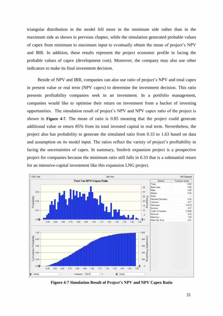
Beside of NPV and IRR, companies can also use ratio of project’s NPV and total capex
in present value or real term (NPV capex) to determine the investment decision. This ratio
presents profitability companies seek in an investment. In a portfolio management,
companies would like to optimise their return on investment from a bucket of investing
opportunities. The simulation result of project’s NPV and NPV capex ratio of the project is
shown in Figure 4-7. The mean of ratio is 0.85 meaning that the project could generate
additional value or return 85% from its total invested capital in real term. Nevertheless, the
project also has probability to generate the simulated ratio from 0.33 to 1.63 based on data
and assumption on its model input. The ratios reflect the variety of project’s profitability in
facing the uncertainties of capex. In summary, Snohvit expansion project is a prospective
project for companies because the minimum ratio still falls in 0.33 that is a substantial return
for an intensive-capital investment like this expansion LNG project.
Figure 4-7 Simulation Result of Project’s NPV and NPV Capex Ratio

32
4.4. Scenario Analysis
In the real world, some values of the project economic variables are uncertain. The
economics of project should be ideally modelled for a wide variety of scenario decisions.
Snohvit expansion project in particular that requires very intensive capital needs to be
assessed using scenario and probabilistic method, so that the project feasibility can be
comprehensively analysed. According to sensitivity analysis, gas prices and recoverable gas
reserve or plant capacity are the most influential variables that lead to the economic output.
Plant capacity and gas price are also the two variables which have to be firstly defined before
taking an investment decision. Therefore, plant capacity and gas price are selected to define
project scenarios. The scenario of plant capacity is determined based on an assumption that
the company can build the plant with capacity less than the current capacity of 4.3 million ton
per annum (MTPA). In this case, there are four scenarios of plant capacity, i.e. 1.3, 2.3, 3.3,
and 4.3 MTPA.
For gas price, there are four scenarios, i.e. US$ 10, 12, 14 and 16 per million British
thermal unit (MMBTU). They are defined referring to the average natural gas prices in Japan
that have been about US$ 16 per million BTU in the last three years for CIF (cost, insurance,
freight) contract, while the European hub prices have been around 10 and 11 US$/MMBTU
since 2011 (BP 2015). In addition, LNG from US forecasted to supply Asian LNG importers
in the post 2015 periods may shift LNG pricing mechanism in Asia, and bring the LNG
prices down (Rogers, Stern 2015). Thus, the gas prices in Asia and Europe as main target
market of the project may fall in the range of 10 to 16 US$/MMBTU for FOB (free-on-board)
contract in the upcoming years. Meanwhile, the baseline of the model uses a scenario with
gas reserve 175 billion cubic meter (BCM), LNG capacity 4.3 MTPA and baseline gas price
14 US$/MMBTU with a 3% escalation per year starting from the year of first cargo shipment
as explained in previous chapter.
The project will have a total of 16 scenarios that combine scenarios of plant capacity
and gas price as shown in Table 4-2. For example, the upside reserve in scenario 4 will have a
recoverable reserve with a volume of 175 billion cubic meter (BCM), thus it will have a 4.3
MTPA plant. The downside reserve in scenario 1 will only have a recoverable reserve of 53
BCM, thus it will have a 1.3 MTPA plant. Then, these scenarios are used to develop a
decision table in which companies can refer to in deciding the investment. The decision table
compiles the results in a table of forecast cells indexed by the decision variables. It is
obtained from a simulation of input variables for each combination of decision variable

33
values. The model for producing decision tables has plant capacity and gas price as decision
variables, and development cost as input variables. Subsequently, the simulation will generate
the model outputs for each scenario, e.g. the mean of project’s NPV, project’s IRR, project’s
NPV and NPV capex ratio. As a result, a decision table for project’s NPV is resulted in Table
4-3, while a decision table for project’s NPV and NPV capex ratio is shown in Table 4-4. This
will eventually identify the required factors within internal project’s boundaries that make the
project financially feasible.
Table 4-2 Project Scenario
Table 4-3 Decision Table for Project’s NPV
Based on Table 4-3 above, it provides the variability in the mean of project’s NPV
according to project scenario. Scenario with capacity 4.3 MTPA and gas price 16
US$/MMBTU clearly results in the highest NPV value, whereas scenario with capacity 1.3
MTPA and gas price 10 US$/MMBTU provides the lowest NPV value. It presents that a 1.3

34
MTPA plant and gas prices up to 12 US$/MMBTU will likely result in negative NPV.
Meanwhile, Table 4-4 describes the variability in the mean of project’s NPV and NPV capex
ratio based on project scenario. Like result in Table 4-3, scenario with capacity 4.3 MTPA
and gas price 16 US$/MMBTU results in the highest ratio value, whereas scenario with
capacity 1.3 MTPA and gas price 10 US$/MMBTU provides the lowest ratio value.
Table 4-4 Decision Table for NPV Project and Capex Ratio
Using the decision tables, companies can decide their investment depending on the real
scenario that would happen, and they have also taken into account project risk analysis in a
form of simulating the probable values of development cost. Companies may use a cut-off
point of NPV project and capex ratio in assessing the project economics, such as using 0.3 as
an investment limit. This implies that only projects which have ratio 0.3 will qualify and go
further for other investment assessments. For instance, if the reserve is big enough to build a
2.3 MTPA plant but the company is failed to secure the gas price at 14 US$/MMBTU in the
baseline year with a 3% escalation per year, then there will be no investment decision for the
project. Consequently, the less reserve discovered, the less capacity can be built, and the
higher the gas price.
Furthermore, the combination of project scenario and montecarlo simulation can result
in the probable values of development cost or capex. Table 4-5 presents the mean of
development cost as a result of montecarlo simulation for each of project scenarios. The
development cost only relies on plant capacity, so that the cost will generate the same
development cost for any gas price scenario. This output can then be used as guidance in
controlling the actual development cost during project execution. As a result, the
development cost for each plant capacity scenario will confine the limit of actual cost to
guide the project on an economical track according to indicators as shown in the decision
tables. For example, if LNG plant is decided with capacity 1.3 MTPA and baseline gas price

35
is set at 14 US$/MMBTU, then the maximum development cost should be US$ 3.1 billion in
order to achieve project’s NPV of US$ 210 million as shown in Table 4-3. In other words, if
the cost significantly exceeds US$ 3.1 billion, it will decrease the project’s NPV and it may
lead to negative NPV implying the project becomes unprofitable for the company.
Table 4-5 Project Scenario and Development Cost (Mean Capex)
4.5. Discussion
Snohvit expansion project is a feasible project based on project economic indicators
obtained from deterministic and probabilistic method. Scenario analysis however reveals it
can turn to be an unfavourable project if the company is less aware of project risks in relation
with gas reserve or LNG capacity, gas price and project cost. Having said that Snohvit project
is a capital intensive project, project cost becomes very sensitive in determining the economic
indicators. Therefore, the cost needs to be profiled depending upon project scenario and
decision tables. In this case, it is assumed that the company requires minimum additional
value 30% from its initial investment in real term. Consequently, the profile of project
scenario and decision table at 0.3 ratio of project’s NPV and NPV capex is presented in Table
4-6. It summaries the minimum gas price required according to the discovered gas reserve
and the maximum development cost in order to achieve a 0.3 NPV capex ratio. Unit cost
derived from development cost and plant capacity is used as benchmark to discuss the cost
and its association. The unit cost is greater when the capacity is smaller, because of the
capacity factor principle where there is a nonlinear relationship between capacity and cost.
Table 4-6 Project Scenario and Decision Table

36
Unit cost for each plant capacity has a probability chart as a result of montecarlo
simulation. Figure 4-8 shows the probability of unit cost for 1.3 MTPA plant in which the unit
cost lies between 1,473 and 3,545 US$/TPA with the mean of 2,389 US$/TPA. The
probability of unit costs for 2.3, 3.3, and 4.3 MTPA are attached in Appendix 3, and they are
summarised in Table 4-7. In overall, the smaller LNG capacity, the more expensive unit cost
and the wider range between maximum and minimum probable values of unit cost. It is such
an industry practice that LNG plants with small capacity tend to have more expensive unit
cost than those with bigger capacity (Castillo, Dorao 2010, Kerbers, Hartnel 2010).
Figure 4-8 Unit Cost Probability for 1.3 MTPA
Table 4-7 Probability of Unit Cost
Furthermore, LNG plant unit costs are essentially driven by two major factors
associated with development options, as follows:
1. Project scope and complexity
Each plant in the world is created unique with its own scope, location and complexity.
Although the project is an expansion project that will be built on the existing plant or next
to it. In particular, Snohvit project is viewed as one of the most expensive LNG plants in
the world due to its scope, location and complexity. Snohvit LNG plant was equipped

37
including with all subsea facilities, carbon capture and injection facilities. The Snohvit
location near arctic pole required specific and expensive materials. Using a basic
assumption that the expansion project will have the same scope, the unit cost for it is
therefore similar. Moreover, it belongs to complete facility with high cost referring to
liquefaction plant metric cost in Figure 4-9. By comparing the metric cost and the
probability of unit cost in Table 4-7, it concludes that the probable values of Snohvit unit
cost are within the range of plant metric cost.
Figure 4-9 Liquefaction Plant Metric Cost
(Source: Songhurst 2014)
2. Technology and provider
Two liquefaction process paths that exist are Mixed Refrigerant (MR) and Expander (E)
technology (Kerbers, Hartnel 2010). Although LNG plants with smaller capacity tend to
have more expensive unit cost, technology providers actually play a significant role in
bringing the technology cost up or down in addition to further competing among
technology providers. For example, a small-scale LNG barge with 0.5 MTPA has been
constructed in China at a cost of 700 US$/TPA, and another larger LNG barge with 4
MTPA has been quoted by a Korean company at a cost of 600 US$/TPA (Songhurst
2014). These plants are most likely for liquefaction units only mounting on a barge,
whereas Snohvit had a complete facility with subsea facilities, CCS and injection
facilities. However, these facts actually reveal two things, first that a floating LNG
(FLNG) generally has less unit cost compared to an onshore LNG plant, and second that
some Asian LNG providers offer very attractive LNG costs.
From LNG market perspective, Northeast Asian countries (Japan, Korea and China)
have shown a strong growth in recent years, and are still expected to drive the world LNG
consumption for years to come (Kumar et al. 2011). Nevertheless, market competition among
LNG suppliers could put more pressure on LNG prices in Asia. In fact, LNG cargo from
Middle East has increasingly shipped to Asian countries during the last five years. In
addition, some upcoming LNG suppliers in Asia Pacific, such as Australia and US have

38
targeted the same market in North-East Asia. As a result, there are competition in the region
implying the average LNG prices in 2014 was slightly lower than those in 2013 (BP 2014,
Rogers, Stern 2015). Nevertheless, there is opportunity for Snhovit expansion project to
access Northeast Asian importers by utilising northern sea route (NSR) that can make the
shipping costs cheaper. Although the LNG price between LNG supplier and buyer is in free
on board (FOB) basis, the cheaper shipping cost could significantly impact on total cost
charged to the buyers. This implies that the Snohvit expansion project could compete with
LNG suppliers from Australia that generally have higher unit cost.
In summary, the things discussed above describe that project scenario, development
options and prospects in the LNG market play role to support the feasibility of Snohvit
expansion project. The company can finally assess some project risks and project
performances, such as the actual data or parameters, to achieve the profitable project as
guided in the decision tables.

39
CHAPTER V: CONCLUSION
Snohvit LNG, the first LNG plant in Artic region, has played important role in
mitigating the decline trend of hydrocarbon production in Norway. It was estimated to be a
new frontier for further development projects in the Norwegian Barents Sea. Some other
hydrocarbon discoveries likely indicated that it could be sufficient to expand current Snohvit
LNG operation. Therefore, the expansion project need to be analysed in accordance with key
project’s variables, such as discoverable gas reserve, LNG price and project costs in which
Snohvit is one of most expensive LNG projects in the world. Project economics model with
discounted cash flow (DCF) method is used to do economic analysis of Snohvit expansion
project based on relevant data and assumptions.
The economic model provides economics performance of Snohvit expansion project
that can be used as first tool by company to analyse the prospect of such project using several
economic indicators, e.g. net present value (NPV), internal rate of return (IRR) and payback
period. Using baseline model inputs which are based on reasonable data and assumptions
described in chapter three, e.g. plant capacity 4.3 million ton per annum (MTPA),
development cost 1,500 US$/TPA, gas price US$ 14 per million British thermal unit
(MMBTU) in first production year, the project has NPV US$ 5.1 billion, IRR 18.8%, NPV
and NPV capex ratio 0.96, and payback period 7 years. Therefore, it is a feasible project since
it generates positive NPV and IRR above 10% of project’s discount rate.
Sensitivity analysis is then undertaken to look at how main variables in project
economics influence the outputs. The analysis shows that gas price, development cost and
plant capacity which is associated with recoverable gas volume are the most influential
variables that define the economics of the project. This helps company focus on those
influential factors. In addition, it can address the first research question on how main
variables of project economics, e.g. project cost, recoverable gas, and LNG price, would
behave in determining the project economics output of Snohvit expansion project.
Furthermore, probabilistic method is applied to profile uncertain input variables in the
model, i.e. development cost, using montecarlo simulation. The economic indicators as result
of the simulation show that the project with LNG capacity 4.3 MTPA and baseline gas price
14 US$/MMBTU is also viable. The simulated mean of project’s NPV and IRR is US$ 4.8

40
billion and 18% respectively. Moreover, project scenario is developed to incorporate a wide
variety of decision scenarios. Gas price and plant capacity as the two influential variables
based on sensitivity analysis are selected as decision variables, while montecarlo simulation
on development cost is undertaken to profile project’s uncertainty. The result is set in a
decision table that has 16 project scenarios and economic indicators.
Project scenario analysis can then address the second research question on how to
identify the required factors within internal project’s boundaries, e.g. gas price, recoverable
gas and plant capacity, that make the project feasible. The analysis indicates that the less
reserve discovered, the less capacity can be built, and the higher the gas price. In addition, the
montecarlo simulation results in the maximum allowable development cost or unit cost for
each plant capacity scenario to guide the project on an economical track according to
economic indicators in the decision tables. The result shows that the smaller LNG capacity,
the more expensive the unit cost will be. However, the unit cost is also determined by
development options, type of technology and technology provider. Floating LNG could be an
option if it has less unit cost compared to landed LNG plant. Meanwhile, technology
providers from Asia could also offer attractive development costs for LNG projects.
In LNG market, Asian countries particularly Japan, Korea and China are expected to
keep demanding LNG for upcoming years. In addition, the gas price scenario set for the
project is also within the current average gas prices in Asian countries with consideration of a
decline trend in the gas prices due to extra supplies from other LNG exporters such as from
Australia and US. Meanwhile, northern sea route (NSR) utilisation may also affect to the total
cost of LNG charged to the buyers. Thus, Snohvit expansion project may exercise this
opportunity if some requirements in the project scenario are achieved. This analysis can
actually address the third research question on how project scenario, development options
and prospects in the LNG market play role to determine the feasibility of Snohvit expansion
project.
Further researches can be performed to do more detailed and comprehensive analysis in
assessing the project economics of Snohvit expansion project. Such researches include the
more detailed cost estimate in calculating development cost as development cost is a very
essential variable as resulted in sensitivity analysis. In addition, the utilisation of northern sea
route (NSR) need to be taken into account into the model, such as how reduced shipping cost
from NSR utilisation will not only influence the decision made by buyers in Northeast Asian

41
Countries to determine the willingness to pay of the LNG, but also reduce the development
cost by using LNG technology providers from Northeast Asian Countries.

42
BIBLIOGRAPHY
Aarsnes, F. & Lindgren, P. 2012, Fossil Fuels – At What Cost? Government support for
upstream oil and gas activities in Norway, the Global Subsidies Initiative (GSI) of the
International Institute for Sustainable Development (IISD), Geneva.
Amos, S.J. 2010, Skills and Knowledge of Cost Engineering, 5th edn, Association of
Advancement Cost Engineering, USA.
Auran, C., Bandopadhyay, B., Khanam, A. & Schulz, S. 2012, Pipeline from the Barents Sea
Versus LNG Transport by Ship, NTNU.
Bekkers, E., Francois, J.F. & Rojas-Romagosa, H. 2013, "Melting Ice Caps and the
Economic Impact of Opening the Northern Sea Route", vol. 307, no. CPB Netherlands
Bureau for Economic and Public Policy.
Berk, J.B. & DeMarzo, P.M. 2007, Corporate finance, Pearson international edn, Pearson
Addison Wesley, Boston.
BP 2015, BP Statistical Review of World Energy, British Petroleum, bp.com/statisticalreview.
Buixadé Farré, A., Stephenson, S.R., Chen, L., Czub, M., Dai, Y., Demchev, D., Efimov, Y.,
Graczyk, P., Grythe, H., Keil, K., Kivekäs, N., Kumar, N., Liu, N., Matelenok, I.,
Myksvoll, M., O'Leary, D., Olsen, J., Pavithran.A.P., S., Petersen, E., Raspotnik, A.,
Ryzhov, I., Solski, J., Suo, L., Troein, C., Valeeva, V., van Rijckevorsel, J. & Wighting,
J. 2014, "Commercial Arctic shipping through the Northeast Passage: routes, resources,
governance, technology, and infrastructure", Polar Geography, vol. 37, no. 4, pp. 298-
324.
Castillo, L. & Dorao, C.A. 2010, "Influence of the plot area in an economical analysis for
selecting small scale LNG technologies for remote gas production", Journal of Natural
Gas Science and Engineering, vol. 2, no. 6, pp. 302-309.
CSIS 2013, Arctic Economics in the 21st Century: The Benefits and Costs of Cold, Center for
Strategic & International Studies, Washington.
Deloitte 2014, Oil and Gas Taxation in Norway, Deloitte, Oslo.
ECC 2013, ECC Insight the Barents Sea: will the region become a dominant new oil and gas
province?, The Energy Contract Company, http://www.energy-contract.com.
EY 2013, Arctic oil and gas, Ernst & Young,
http://www.ey.com/Publication/vwLUAssets/Arctic_oil_and_gas/$FILE/Arctic_oil_and
_gas.pdf.
Harsem, Ø, Eide, A. & Heen, K. 2011, "Factors influencing future oil and gas prospects in
the Arctic", Energy Policy, vol. 39, no. 12, pp. 8037-8045.

43
Hartley, P. 2013, The Future of Long-term LNG Contracts, DISCUSSION PAPER 13.22
edn, The University of Western Australia, Houston.
Heiersted, R.J. 2005, Snøhvit LNG Project: Status and progress of the project execution,
Statoil, GASTECH Bilbao.
Hydrocarbon-technology 2012, , Snohvit LNG Export Terminal, Melkøya Island, Norway
[Homepage of Hydrocarbon-technology], [Online]. Available:
http://www.hydrocarbons-technology.com/projects/snohvit-lng/ [2015, 06/02].
Jansen, J.B. & Bjerke, J.M. 2012, Norwegian Petroleum Taxation: An Introduction, BAHR,
Oslo.
Kerbers, I. & Hartnel, G. 2010, A Breakthrough For Floating LNG?, Poten & Partners, New
York.
Klett, T.R. & Gautier, D.L. 2009, Assessment of undiscovered petroleum resources of the
Barents Sea Shelf, U.S. Geological Survey, http://pubs.usgs.gov/fs/2009/3037/.
Kullerud, L. 2011, , Oil and Gas resources in the Barents Sea [Homepage of Grid Arsendal],
[Online]. Available: www.grida.no/publications/et/at/page/2543.aspx [2015, May/31].
Kumar, S., Kwon, H., Choi, K., Hyun Cho, J., Lim, W. & Moon, I. 2011, "Current status and
future projections of LNG demand and supplies: A global prospective", Energy Policy,
vol. 39, no. 7, pp. 4097-4104.
Lee, S. & Song, J. 2014, "Economic Possibilities of Shipping though Northern Sea Route1",
The Asian Journal of Shipping and Logistics, vol. 30, no. 3, pp. 415-430.
Lindholt, L. & Glomsrød, S. 2012, "The Arctic: No big bonanza for the global petroleum
industry", Energy Economics, vol. 34, no. 5, pp. 1465-1474.
Liu, M. & Kronbak, J. 2010, "The potential economic viability of using the Northern Sea
Route (NSR) as an alternative route between Asia and Europe", Journal of Transport
Geography, vol. 18, no. 3, pp. 434-444.
Marmolejo, P.C. 2014, An Economic Analysis of Floating Liquefied Natural Gas (FLNG),
Massachusetts Institute of Technology.
Maxwell, D. & Zhu, Z. 2011, "Natural gas prices, LNG transport costs, and the dynamics of
LNG imports", Energy Economics, vol. 33, no. 2, pp. 217-226.
Moe, O.B. 2013, The Norwegian Model: Evolution, performance and benefits, Secretaría De
Energía,
http://sener.gob.mx/Experiencia_Noruega_Materia_Petrolera/res/2congreso/The_Norwe
gian_Model-%20Evolution_performance_and_benefits.pdf.
Mun, J. 2010, Modeling Risk, Applying Monte Carlo Simulation, Strategic Real Options,
Stochastic Forecasting, and Portfolio Optimization, Second Edition edn, John Wiley &
Sons Inc, New Jersey.

44
Nazir, M., Khan, F., Amyotte, P. & Sadiq, R. 2008, "Subsea Release of Oil from a Riser: An
Ecological Risk Assessment", Risk Analysis, vol. 28, no. 5, pp. 1173-1196.
Newendorp, P.D. & Schuyler, J.R. 2000, Decision analysis for petroleum exploration, 2nd
edn, Planning Press, Aurora, Colo.
Nilsen, T. 2012, 06 Novermber 2012-last update, Hammerfest LNG set sails for Japan via
Arctic route [Homepage of Barets Observer], [Online]. Available:
http://barentsobserver.com/en/arctic/hammerfest-lng-set-sails-japan-arctic-route-06-11
[2015, 06/06].
Norwegian Ministry of Environment 2011, Meld. St. 10 (2010–2011) Report to the Storting
(white paper); First update of the Integrated Management Plan for the Marine
Environment of the Barents Sea−Lofoten Area, Norwegian Ministry of Environment,
Oslo.
Office of Fossil Energy 2005, Liquefied Natural Gas: Understanding the Basic Facts, U.S.
Department of Energy,
http://www.fossil.energy.gov/programs/oilgas/publications/lng/LNG_primerupd.pdf.
Pettersen, J., Nilsen, Ø, Giljarhus, L.E.N., Fredheim, A.O., Aasekjær, K. & Neeraas, B.O.
2013, "Technical and Operational Innovation for Onshore and Floating LNG", American
Gas Association, Houston, 19 April 2013.
Pettersen, T. 2014, 16 December-last update, Northern Sea Route traffic plummeted
[Homepage of Barents Observer], [Online]. Available:
http://barentsobserver.com/en/arctic/2014/12/northern-sea-route-traffic-plummeted-16-
12 [2015, June/05].
Ritz, R.A. 2014, "Price discrimination and limits to arbitrage: An analysis of global LNG
markets", Energy Economics, vol. 45, no. 0, pp. 324-332.
Rogers, H.V. & Stern, J. 2015, Challenge to JCC Pricing in Asian LNG Markets, The Oxford
Institute for Studies, London.
Searates 2015, , Sea Rates: Bonny Offshore Terminal Nigeria to Sakai Japan [Homepage of
Sea Rates], [Online]. Available:
http://www.searates.com/reference/portdistance/?B=33686&E=10179& [2015, July/05].
Siikamäki, J., Munnings, C. & Ferris, J. 2012, The European Union Emissions Trading
System, Resources for the Future, Washington DC.
Songhurst, B. 2014, LNG Plant Cost Escalation, The Oxford Institute for Studies, London.
Staalesen, A. 2014, 11 November 2014-last update, To Yamal with world’s most powerful
LNG carriers [Homepage of Barets Observer], [Online]. Available:
http://barentsobserver.com/en/energy/2014/11/yamal-worlds-most-powerful-lng-
carriers-11-11 [2015, 06/06].

45
Statoil 2014a, 02 May 2014-last update, Exploration well in Drivis completed [Homepage of
Statoil], [Online]. Available:
http://www.statoil.com/en/NewsAndMedia/News/2014/Pages/02May_Drivis.aspx
[2015, 06/01].
Statoil 2014b, 13 November 2014-last update, Johan Castberg [Homepage of Statoil],
[Online]. Available:
http://www.statoil.com/en/OurOperations/FutureVolumes/ProjectDevelopment/Pages/Sk
rugard.aspx [2015, 06/02].
Statoil 2013a, 19 November 2013-last update, Snøhvit [Homepage of Statoil], [Online].
Available:
http://www.statoil.com/en/TechnologyInnovation/FieldDevelopment/AboutSubsea/Subs
eaPresentation/Pages/Snohvit.aspx [2015, 06/01].
Statoil 2013b, 19 November 2013-last update, Snøhvit expansion dependent on new gas
discovery [Homepage of Statoil], [Online]. Available:
http://www.statoil.com/en/NewsAndMedia/News/2012/Pages/02October_Snohvit.aspx
[2015, 06/01].
Timera Energy 2015, , Getting to grips with LNG shipping costs [Homepage of Timera
Energy], [Online]. Available: http://www.timera-energy.com/getting-to-grips-with-lng-
shipping-costs/ [2015, 06/03].
USGS 2008, Circum-Arctic Resource Appraisal: Estimates of Undiscovered Oil and Gas
North of the Arctic Circle, U.S. Geological Survey, http://pubs.usgs.gov/fs/2008/3049/.
Vinnem, J.E., Aven, T., Husebø, T., Seljelid, J. & Tveit, O.J. 2006, "Major hazard risk
indicators for monitoring of trends in the Norwegian offshore petroleum sector",
Reliability Engineering & System Safety, vol. 91, no. 7, pp. 778-791.
White, N. & Morgan, J. 2012, Rules of Thumb for Screening LNG Developments, IE Aust
Perth edn, The Institution of Engineers Australia, Perth.
Wilson Centre 2013, Opportunities And Challenges For Arctic Oil And Gas Development,
The Wilson Center,
http://www.wilsoncenter.org/sites/default/files/Artic%20Report_F2.pdf.

46
APPENDIX 1: MODEL INPUT

47
APPENDIX 2: MODEL CALCULATION
Calculations
1 Year 0 1 2 3 4 5 6 7 8 9 10 11 12
2
3 Exploration & Appraisal Cost
4 E&A (USD) 1,000,000,000
5
6 Capex and Decommissioning
7 Capacity to Cost ratio 1.00 1.00 1.00 1.00 1.00 1.00 1.00 1.00 1.00 1.00 1.00 1.00 1.00
8 Capex (USD) 967,500,000 1,290,000,000 1,612,500,000 1,935,000,000 645,000,000 0 0 0 0 0 0 0 0
9 Decomm Cost (USD) 0 0 0 0 0 0 0 0 0 0 0 0 0
10
11 Production
12 Gas Production (MMBTU) 0 0 0 0 208,980,000 208,980,000 208,980,000 208,980,000 208,980,000 208,980,000 208,980,000 208,980,000 208,980,000
13 CO2 Production (Ton) 0 0 0 0 1,053,500 1,053,500 1,053,500 1,053,500 1,053,500 1,053,500 1,053,500 1,053,500 1,053,500
14 MR Ethane (Ton) 0 0 0 0 2,769 2,769 2,769 2,769 2,769 2,769 2,769 2,769 2,769
15 MR Propane (Ton) 0 0 0 0 662 662 662 662 662 662 662 662 662
16
17 Opex
18 Opex Fixed (USD) 0 0 0 0 145,190,636 149,546,356 154,032,746 158,653,729 163,413,340 168,315,741 173,365,213 178,566,169 183,923,154
19 OPEX Variable (USD) 0 0 0 0 4,825,556 4,970,323 5,119,432 5,273,015 5,431,206 5,594,142 5,761,966 5,934,825 6,112,870
20 OPEX (USD) 0 0 0 0 150,016,192 154,516,678 159,152,179 163,926,744 168,844,546 173,909,883 179,127,179 184,500,995 190,036,024
21
22 Price FOB
23 LNG Price (USD / MMBtu) 0.0 0.0 0.0 0.0 14.0 14.4 14.9 15.3 15.8 16.2 16.7 17.2 17.7
24 Carbon Price (USD / Ton) 0.0 0.0 0.0 0.0 15.0 15.5 15.9 16.4 16.9 17.4 17.9 18.4 19.0
25
26 Revenue and Cost
27 Revenue (USD) 0 0 0 0 2,925,720,000 3,013,491,600 3,103,896,348 3,197,013,238 3,292,923,636 3,391,711,345 3,493,462,685 3,598,266,566 3,706,214,563
28 Costs (USD) 1,967,500,000 1,290,000,000 1,612,500,000 1,935,000,000 795,016,192 154,516,678 159,152,179 163,926,744 168,844,546 173,909,883 179,127,179 184,500,995 190,036,024
29
30 Depreciation and Decommissioning
31 Depreciation schedule 0 0 0 0 1,075,000,000 1,075,000,000 1,075,000,000 1,075,000,000 1,075,000,000 1,075,000,000 0 0 0
32 Decommissioning schedule 0 0 0 0 42,084,242 43,346,770 44,647,173 45,986,588 47,366,186 48,787,171 50,250,786 51,758,310 53,311,059
33
34 Tax pre NCF
35 CO2 Tax 0 0 0 0 15,802,500 16,276,575 16,764,872 17,267,818 17,785,853 18,319,429 18,869,011 19,435,082 20,018,134
36 Area Tax 0 0 0 0 0 0 0 0 0 0 0 0 0
37 Tax Paid pre NCF 0 0 0 0 15,802,500 16,276,575 16,764,872 17,267,818 17,785,853 18,319,429 18,869,011 19,435,082 20,018,134
38

48
13 14 15 16 17 18 19 20 21 22 23 24 25 26 27 28 29 1
2
3
4
5
6
1.00 1.00 1.00 1.00 1.00 1.00 1.00 1.00 1.00 1.00 1.00 1.00 1.00 1.00 1.00 1.00 1.00 7
0 0 0 0 0 0 0 0 0 0 0 0 0 0 0 0 0 8
0 0 0 0 0 0 0 0 0 0 0 0 0 0 636,769,515 655,872,600 675,548,778 9
10
11
208,980,000 208,980,000 208,980,000 208,980,000 208,980,000 208,980,000 208,980,000 208,980,000 208,980,000 208,980,000 208,980,000 208,980,000 208,980,000 208,980,000 0 0 0 12
1,053,500 1,053,500 1,053,500 1,053,500 1,053,500 1,053,500 1,053,500 1,053,500 1,053,500 1,053,500 1,053,500 1,053,500 1,053,500 1,053,500 0 0 0 13
2,769 2,769 2,769 2,769 2,769 2,769 2,769 2,769 2,769 2,769 2,769 2,769 2,769 2,769 0 0 0 14
662 662 662 662 662 662 662 662 662 662 662 662 662 662 0 0 0 15
16
17
189,440,849 195,124,075 200,977,797 207,007,131 213,217,345 219,613,865 226,202,281 232,988,349 239,978,000 247,177,340 254,592,660 262,230,440 270,097,353 278,200,274 0 0 0 18
6,296,256 6,485,144 6,679,698 6,880,089 7,086,492 7,299,086 7,518,059 7,743,601 7,975,909 8,215,186 8,461,642 8,715,491 8,976,956 9,246,264 0 0 0 19
195,737,105 201,609,218 207,657,495 213,887,220 220,303,836 226,912,951 233,720,340 240,731,950 247,953,909 255,392,526 263,054,302 270,945,931 279,074,309 287,446,538 0 0 0 20
21
22
18.3 18.8 19.4 20.0 20.6 21.2 21.8 22.5 23.1 23.8 24.5 25.3 26.0 26.8 27.6 28.5 29.3 23
19.6 20.2 20.8 21.4 22.0 22.7 23.4 24.1 24.8 25.5 26.3 27.1 27.9 28.7 29.6 30.5 31.4 24
25
26
3,817,400,999 3,931,923,029 4,049,880,720 4,171,377,142 4,296,518,456 4,425,414,010 4,558,176,430 4,694,921,723 4,835,769,375 4,980,842,456 5,130,267,730 5,284,175,761 5,442,701,034 5,605,982,065 0 0 0 27
195,737,105 201,609,218 207,657,495 213,887,220 220,303,836 226,912,951 233,720,340 240,731,950 247,953,909 255,392,526 263,054,302 270,945,931 279,074,309 287,446,538 636,769,515 655,872,600 675,548,778 28
29
30
0 0 0 0 0 0 0 0 0 0 0 0 0 0 0 0 0 31
54,910,391 56,557,703 58,254,434 60,002,067 61,802,129 63,656,193 65,565,879 67,532,855 69,558,841 71,645,606 73,794,974 76,008,823 78,289,088 80,637,760 0 0 0 32
33
34
20,618,678 21,237,239 21,874,356 22,530,586 23,206,504 23,902,699 24,619,780 25,358,374 26,119,125 26,902,698 27,709,779 28,541,073 29,397,305 30,279,224 0 0 0 35
0 0 0 0 0 0 0 0 0 0 0 0 0 0 0 0 0 36
20,618,678 21,237,239 21,874,356 22,530,586 23,206,504 23,902,699 24,619,780 25,358,374 26,119,125 26,902,698 27,709,779 28,541,073 29,397,305 30,279,224 0 0 0 37
38

49
39 Year 0 1 2 3 4 5 6 7 8 9 10 11 12
40
41 Cash Flow42 Pre Tax Net Cash Flow -1,967,500,000 -1,290,000,000 -1,612,500,000 -1,935,000,000 2,114,901,308 2,842,698,347 2,927,979,297 3,015,818,676 3,106,293,236 3,199,482,033 3,295,466,494 3,394,330,489 3,496,160,404
43 Taxable Corporate Tax -1,967,500,000 -1,290,000,000 -1,612,500,000 -1,935,000,000 997,817,065 1,724,351,577 1,808,332,124 1,894,832,088 1,983,927,051 2,075,694,862 3,245,215,708 3,342,572,179 3,442,849,345
44 Corporate Tax Paid 0 0 0 0 279,388,778 482,818,442 506,332,995 530,552,985 555,499,574 581,194,561 908,660,398 935,920,210 963,997,817
45 Cash Flow after CT Paid -1,967,500,000 -1,290,000,000 -1,612,500,000 -1,935,000,000 718,428,287 1,241,533,135 1,301,999,130 1,364,279,103 1,428,427,476 1,494,500,301 2,336,555,310 2,406,651,969 2,478,851,528
46 Capital Uplift Allowance 0 0 0 0 483,750,000 483,750,000 483,750,000 483,750,000 0 0 0 0 0
47 Taxable Special Tax 0 0 0 0 234,678,287 757,783,135 818,249,130 880,529,103 1,428,427,476 1,494,500,301 2,336,555,310 2,406,651,969 2,478,851,528
48 Special Tax Paid 0 0 0 0 117,339,143 378,891,568 409,124,565 440,264,552 714,213,738 747,250,150 1,168,277,655 1,203,325,985 1,239,425,764
49 Post Tax Net Cash Flow -1,967,500,000 -1,290,000,000 -1,612,500,000 -1,935,000,000 1,718,173,386 1,980,988,337 2,012,521,738 2,045,001,140 1,836,579,924 1,871,037,322 1,218,528,441 1,255,084,295 1,292,736,823
50
51 Payback Calculation52 Cumulative Net CF (USD) -1,967,500,000 -3,257,500,000 -4,870,000,000 -6,805,000,000 -5,086,826,614 -3,105,838,277 -1,093,316,539 951,684,601 2,788,264,525 4,659,301,846 5,877,830,287 7,132,914,582 8,425,651,405
53 Cumulative Net CF Positive Indicator 0 0 0 0 0 0 0 1 1 1 1 1 1
54 Lagged Cumulative Net CF Positive Indicator 0 0 0 0 0 0 0 1 1 1 1 1
55 Payback Year 0 0 0 0 0 0 0 7 0 0 0 0 0
56
57 Revenue Allocation58 Revenue 0 0 0 0 2,925,720,000 3,013,491,600 3,103,896,348 3,197,013,238 3,292,923,636 3,391,711,345 3,493,462,685 3,598,266,566 3,706,214,563
59 Cost 1,967,500,000 1,290,000,000 1,612,500,000 1,935,000,000 795,016,192 154,516,678 159,152,179 163,926,744 168,844,546 173,909,883 179,127,179 184,500,995 190,036,024
60 Company (Post Tax NCF) -1,967,500,000 -1,290,000,000 -1,612,500,000 -1,935,000,000 1,718,173,386 1,980,988,337 2,012,521,738 2,045,001,140 1,836,579,924 1,871,037,322 1,218,528,441 1,255,084,295 1,292,736,823
61 Government (Pre + Corp + Spec Tax) 0 0 0 0 412,530,422 877,986,584 932,222,432 988,085,355 1,287,499,165 1,346,764,140 2,095,807,065 2,158,681,277 2,223,441,715
62 Check 0 0 0 0 0 0 0 0 0 0 0 0 0
63
64 Summary Output65 Post Tax Net Present Value (USD) 5,144,345,284
66 Post Tax Internal Rate of Return 18.8%
67 NPV Capex (USD) 5,367,209,719
68 Post Tax NPV Capex Ratio 0.96
69 Approximate Payback (years) 770
71 Revenue Distribution72 Total Revenue - MOD (USD) 94,948,050,911 100.0%
73 Cumulative Net CF (Company) - MOD (USD) 29,208,224,544 30.8%
74 Government Take - MOD (USD) 51,453,177,425 54.2%
75 Development, Operation & Decom - MOD (USD) 14,286,648,942 15.0%76
77 Total Revenue - Real (USD) 24,480,758,590 100.0%
78 Cumulative Net CF (Company) - Real (USD) 5,144,345,284 21.0%
79 Government Take - Real (USD) 11,577,315,629 47.3%
80 Development, Operation & Decom - Real (USD) 7,759,097,677 31.7%81
82 Development Cost (US$) 6,450,000,000
83 Unit Cost Capital (US$/MTPA) 1,500
84 CO2 Price (US$/ton CO2) 15

50
13 14 15 16 17 18 19 20 21 22 23 24 25 26 27 28 29 39
40
41
3,601,045,216 3,709,076,573 3,820,348,870 3,934,959,336 4,053,008,116 4,174,598,359 4,299,836,310 4,428,831,399 4,561,696,341 4,698,547,232 4,839,503,649 4,984,688,758 5,134,229,421 5,288,256,303 -636,769,515 -655,872,600 -675,548,778 42
3,546,134,825 3,652,518,870 3,762,094,436 3,874,957,269 3,991,205,987 4,110,942,167 4,234,270,432 4,361,298,545 4,492,137,501 4,626,901,626 4,765,708,675 4,908,679,935 5,055,940,333 5,207,618,543 -636,769,515 -655,872,600 -675,548,778 43
992,917,751 1,022,705,284 1,053,386,442 1,084,988,035 1,117,537,676 1,151,063,807 1,185,595,721 1,221,163,592 1,257,798,500 1,295,532,455 1,334,398,429 1,374,430,382 1,415,663,293 1,458,133,192 0 0 0 44
2,553,217,074 2,629,813,586 2,708,707,994 2,789,969,234 2,873,668,311 2,959,878,360 3,048,674,711 3,140,134,952 3,234,339,001 3,331,369,171 3,431,310,246 3,534,249,553 3,640,277,040 3,749,485,351 -636,769,515 -655,872,600 -675,548,778 45
0 0 0 0 0 0 0 0 0 0 0 0 0 0 0 0 0 46
2,553,217,074 2,629,813,586 2,708,707,994 2,789,969,234 2,873,668,311 2,959,878,360 3,048,674,711 3,140,134,952 3,234,339,001 3,331,369,171 3,431,310,246 3,534,249,553 3,640,277,040 3,749,485,351 0 0 0 47
1,276,608,537 1,314,906,793 1,354,353,997 1,394,984,617 1,436,834,155 1,479,939,180 1,524,337,355 1,570,067,476 1,617,169,500 1,665,684,585 1,715,655,123 1,767,124,777 1,820,138,520 1,874,742,675 0 0 0 48
1,331,518,928 1,371,464,496 1,412,608,431 1,454,986,684 1,498,636,284 1,543,595,373 1,589,903,234 1,637,600,331 1,686,728,341 1,737,330,191 1,789,450,097 1,843,133,600 1,898,427,608 1,955,380,436 -636,769,515 -655,872,600 -675,548,778 49
50
51
9,757,170,333 11,128,634,829 12,541,243,260 13,996,229,944 15,494,866,228 17,038,461,601 18,628,364,834 20,265,965,165 21,952,693,506 23,690,023,697 25,479,473,794 27,322,607,394 29,221,035,001 31,176,415,437 30,539,645,922 29,883,773,322 29,208,224,544 52
1 1 1 1 1 1 1 1 1 1 1 1 1 1 1 1 1 53
1 1 1 1 1 1 1 1 1 1 1 1 1 1 1 1 1 54
0 0 0 0 0 0 0 0 0 0 0 0 0 0 0 0 0 55
56
57
3,817,400,999 3,931,923,029 4,049,880,720 4,171,377,142 4,296,518,456 4,425,414,010 4,558,176,430 4,694,921,723 4,835,769,375 4,980,842,456 5,130,267,730 5,284,175,761 5,442,701,034 5,605,982,065 0 0 0 58
195,737,105 201,609,218 207,657,495 213,887,220 220,303,836 226,912,951 233,720,340 240,731,950 247,953,909 255,392,526 263,054,302 270,945,931 279,074,309 287,446,538 636,769,515 655,872,600 675,548,778 59
1,331,518,928 1,371,464,496 1,412,608,431 1,454,986,684 1,498,636,284 1,543,595,373 1,589,903,234 1,637,600,331 1,686,728,341 1,737,330,191 1,789,450,097 1,843,133,600 1,898,427,608 1,955,380,436 -636,769,515 -655,872,600 -675,548,778 60
2,290,144,966 2,358,849,315 2,429,614,795 2,502,503,239 2,577,578,336 2,654,905,686 2,734,552,856 2,816,589,442 2,901,087,125 2,988,119,739 3,077,763,331 3,170,096,231 3,265,199,118 3,363,155,092 0 0 0 61
0 0 0 0 0 0 0 0 0 0 0 0 0 0 0 0 0 62
63
64
65
66
67
68
69
70
71
72
73
74
7576
77
78
79
80
81
82
83
84

51
APPENDIX 3: MODEL SIMULATION INPUT
Development costs from montecarlo simulation

52
APPENDIX 4: UNIT COST PROBABILITY
a. Unit Cost Probability for 2.3 MTPA
b. Unit Cost Probability for 3.3 MTPA
c. Unit Cost Probability for 4.3 MTPA

53
GLOSSARY
BCM : Billion Cubic Meters
BOE : Barrels of Oil Equivalent
BP : British Petroleum
Capex : Capital Expenditure
CIF : Cost, Insurance, Freight
CO2 : Carbon Dioxide
DCF : Discounted Cash Flow
EU ETS : European Union Emission Trading System
FOB : Free on Board
IRR : Internal Rate of Return
JCC : Japan Crude Cocktail or the Japanese Customs-Cleared Crude Oil
KWh : Kilo Watt Hour
LNG : Liquefied Natural Gas
MMBTU : Million British thermal unit
MTPA : Million Ton per Annum
NOx : Nitrogen Oxide
NPV : Net Present Value
NSR : Northern Sea Route
Opex : Operation Expenditure
POT : Pay Out Time
SSR : Southern Sea Route
TCF : Trillion Cubic Feet
TPA : Ton per Annum
USGS : United States Geological Survey