Quantum state expansion

Jae-Seung Lee and A. K. Khitrin

Department of Chemistry, Kent State University, Kent, Ohio 44242-0001

Abstract

It is experimentally demonstrated that an arbitrary quantum state of a single spin 1/2:

↓+↑ ba can be converted into a superposition of the two ferromagnetic states of a

spin cluster: ↓↓↓↓+↑↑↑↑ ba . The physical system is a cluster of seven

dipolar-coupled nuclear spins of single-labeled 13C-benzene molecules in a liquid-

crystalline matrix. In this complex system, the pseudopure ground state and the required

controlled unitary transformations have been implemented. The experimental scheme can

be considered as an explicit model of quantum measurement.

PACS: 03.65.-w, 03.67.Mn, 42.50.Dv, 76.60.-k

Theory of quantum measurements, which describes a boundary between quantum and

classical worlds [1,2], is the least established part of quantum theory. Different

approaches to this problem lead to different interpretations of quantum mechanics. A

serious difficulty in exploring this subject is that practical measuring devices are too

complex to allow a detail analysis of their dynamics. It may be helpful to consider some

simple and explicit models of quantum measurement, using systems with controllable

quantum dynamics. One of possible experimental models is proposed and studied in this

work.

Let us consider a system of 1+N spins 1/2 (qubits) in the initial state

NNba 0000)10(ψ

12100in −+= … , 122 =+ ba , (1)

where the qubit notations kk

↑≡0 and kk

↓≡1 are used. In this state, the 0-th qubit

is in some arbitrary state, defined by two complex coefficients a and b , while the qubits

1 to are in the ground state. Quantum logic circuit [3] N

1,02,11,2,1 CNOTCNOTCNOTCNOTU NNNN …−−−= (2)

is a chain of unitary controlled-not gates , which flip the target qubit n when

the control qubit m is in the state

nmCNOT ,

m1 and do not change the qubit n when the qubit m

is in the state m

0 . If the 0-th qubit is in the state 0

1 , it flips the qubit 1, the qubit 1 flips

the qubit 2, and so on. A wave of flipped qubits, triggered by the 0-th qubit, propagates

until it covers the entire system. As a result, the circuit (2) converts the initial state (1)

into the final state

NNNNbaU 11110000ψψ

110110inout −−+== …… . (3)

2

This state is a superposition of the most macroscopically distinct states: the ferromagnetic

states with all spins up and all spins down. An advantage of the circuit (2) is that it

requires only interactions between neighbor qubits and, therefore, potentially can be

implemented in large systems.

One might think that, since a macroscopic polarization is associated with the state (3), a

single measurement can provide some information about the state. However,

transforming the state (1) to the state (3) does not decrease relative quantum fluctuations.

It can be seen, as an example, by considering an ensemble average of the square of

polarization: it has its maximum value, , indicating that possible outcomes of

polarization measurement for a single system are one of the two extreme values,

(Ensemble average values of powers of an observable give unambiguous

information about probabilities of possible outcomes in single-system measurement).

Therefore, the only goal of creating the state (3) is to increase a signal produced by a

system, without making this signal more classical.

2)1( +N

)1( +± N

The experimental scheme for converting the initial state (1) into the state (3) has been

implemented on a cluster of seven dipolar-coupled nuclear spins. The experiment has

been performed with a Varian Unity/Inova 500 MHz NMR spectrometer. The sample

contained 5% of single-labeled 13C-benzene (Aldrich) dissolved in liquid-crystalline

solvent MLC-6815 (EMD Chemical). In this system, fast molecular motions average out

all intermolecular spin-spin interactions. Intramolecular dipole-dipole interactions are not

averaged to zero due to orientational order induced by a liquid-crystalline matrix.

Therefore, the system is a good example of an ensemble of non-interacting spin clusters,

3

where each benzene molecule contains seven nuclear spins, one 13C and six protons,

coupled by residual dipole-dipole interactions. The spin Hamiltonian is

)21

21()(

6

0

6

1000

6

10 jYkY

jkjXkXjZkZjk

kkZZkk

kkZHZC SSSSSSbSIJbSIH −−+++−−= ∑∑∑

>>==

ωω , (4)

where index 0 is used for the 13C spin and indexes 1 to 6 numerate 1H spins, starting from

the one closest to 13C nucleus. I and are corresponding spin operators, S Cω and Hω

are the Larmor frequencies, are the constants of residual dipole-dipole interaction,

and are the J-coupling constants. Among J-constants, only has a considerable

value of

jkb

jkJ 01J

=π201J 158 Hz [4], the rest of the J-coupling constants are small and can be

neglected on the time scale of our experiment. The 1H and 13C thermal equilibrium

spectra of 13C-benzene in MLC-6815 are presented in Figs. 2a and 2a’, respectively. For

individual peaks in equilibrium spectra, the longitudinal relaxation times (T1) were

measured to be 1.7-2.3 sec for proton spins and 1.4-2.9 sec for the 13C spin. Transverse

relaxation times (T2) were measured to be 0.1-0.7 sec for proton spins and 0.3-1.1 sec for

the 13C spin.

In what follows, we will use spin notations ↑ and ↓ for the two states of the 13C

spin, ↑↑↑↑↑↑=u and ↓↓↓↓↓↓=d for the states of protons with all spins up or

down.

Two experimental challenges for a seven-qubit system are preparing the state (1) and

implementing the unitary operation which converts the state (1) into the state (3). For the

system under study, we have recently demonstrated that the superposition state of protons

)(2 2/1 du +− could be used to amplify the effect of interaction with 13C spin [5]. Some

4

basic elements used in that work, together with preparation of the pseudopure state u

for the proton subsystem [6], are also the building blocks of the experimental scheme in

Fig. 1, and will be only briefly described here. More details can be found in Refs. [5] and

[6]. To better understand the following steps, it is convenient to introduce the Pauli

operators for a subspace of two proton states u and d : ))(2/1( dduuZ −=Σ ,

))(2/1( udduX +=Σ and ))(2/( udduiY −=Σ .

The first two steps, A and B (Fig. 1) are designed to prepare the pseudopure ground

state u↑ of the seven-spin cluster. The experiment starts with a sequence of

pulses and gradient pulses to saturate the

90

13C magnetization. Then, the proton

magnetization is converted into multiple-quantum coherences by 20 cycles of the eight-

pulse sequence [7]. The pulse sequence automatically decouples protons from the 13C

spin. The six-quantum (6Q) coherence YΣ is filtered by a combination of phase cycling

and pulse. The next step is the evolution caused by the interaction with the 180 13C spin,

which rotates towards depending on the state of the YΣ XΣ±13C spin. After

rotation, the state density matrix

90

XZI Σ− 0 is achieved. Then, evolution with another 20-

cycle pulse sequence follows. The multi-pulse period, with about 90% fidelity,

corresponds to a “ pulse” in the 90 Σ -subspace around some axis in the XY-plane. The

phase of this “pulse” in the Σ -subspace is adjusted by the global phase of the pulse

sequence. As an example, 90 phase shift can be achieved by phase shifting

of all pulses of the sequence. The “ Y-pulse” in the

156/90 =

90 Σ -subspace converts the state

into the state XZI Σ− 0 ))((0 dduuZZ −↓↓−↑↑=Σρ IA = . This state is the

5

mixture of four pure states. The 1H and 13C linear-response spectra for this state are

shown in Figs. 2b and 2b’, respectively.

The pseudopure ground state u↑ ( uuB ↑↑=ρ ) is obtained by redistributing the

excess population of the other three states. Redistribution is achieved by partial saturation

with Gaussian shaped pulses, which have practically zero spectral intensity at the

frequencies of allowed single-quantum transitions from the state u↑ (step B). As a

result, population of the state u↑ remains “trapped”. The 1H and 13C linear-response

spectra for the pseudopure state u↑ are presented in Figs. 2c and 2c’, respectively. It

may be noted that pseudopure states for systems of up to seven spins have been already

demonstrated with liquid-state NMR [8]. However, our seven-spin system with dipole-

dipole interactions is dynamically much more complex than any of the previously studied

systems. Compared to ZZ-coupled system in Ref. [8], dipole-dipole couplings have all

three components, providing more “mixing” dynamics. As a result, the maximum number

of peaks in a spectrum of N dipolar coupled spins, , grows much faster with

increasing N than the number of peaks in a spectrum of ZZ-coupled system, .

Integrated intensities of the pseudopure state spectra, relative to that of the thermal

equilibrium spectra, for proton and carbon spins are 3.5% and 3.3%, respectively. To

verify the state, we applied hard pulses on the

N

NN 22~

12

⎟⎟⎠

⎞⎜⎜⎝

⎛+

12 −NN

180 13C and proton spins and compared

the spectra with numerically calculated spectra. As one illustration, the spectra for the

state u↓ are shown in Figs. 2d and 2d’. The calculated spectra for the states u↑ and

u↓ are shown in Figs. 2e and 2e’.

6

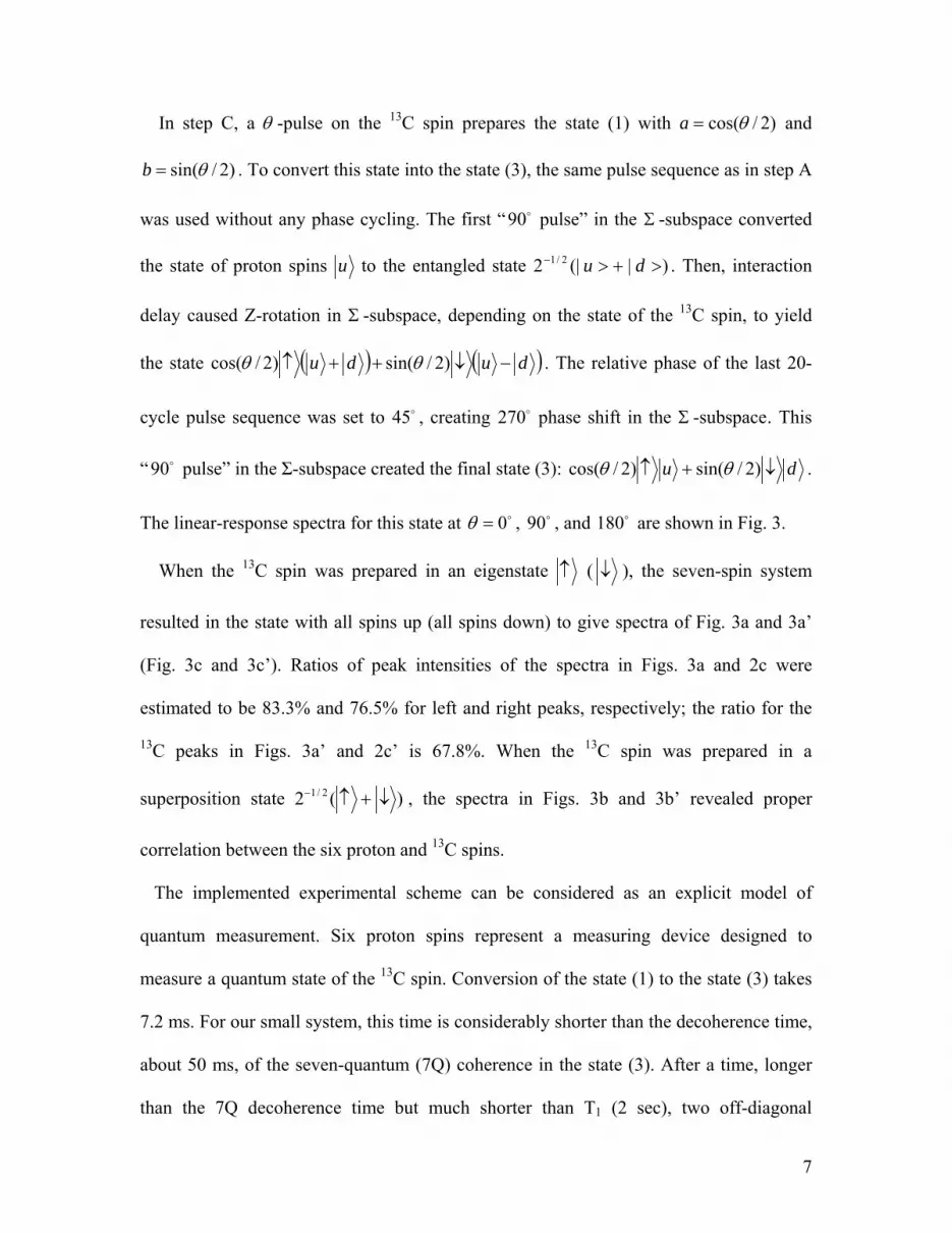
In step C, a θ -pulse on the 13C spin prepares the state (1) with )2/cos(θ=a and

)2/sin(θ=b . To convert this state into the state (3), the same pulse sequence as in step A

was used without any phase cycling. The first “ pulse” in the 90 Σ -subspace converted

the state of proton spins u to the entangled state . Then, interaction

delay caused Z-rotation in Σ -subspace, depending on the state of the

)|(|2 2/1 >d+>− u

13C spin, to yield

the state ( ) ( )duu −↓++↑ )2/sin()2/ θθ dcos( . The relative phase of the last 20-

cycle pulse sequence was set to , creating phase shift in the Σ -subspace. This

“ pulse” in the Σ-subspace created the final state (3):

45 270

90 du ↓+↑ )2/sin()2/ θθcos( .

The linear-response spectra for this state at , , and are shown in Fig. 3. 0=θ 90 180

When the 13C spin was prepared in an eigenstate ↑ ( ↓ ), the seven-spin system

resulted in the state with all spins up (all spins down) to give spectra of Fig. 3a and 3a’

(Fig. 3c and 3c’). Ratios of peak intensities of the spectra in Figs. 3a and 2c were

estimated to be 83.3% and 76.5% for left and right peaks, respectively; the ratio for the

13C peaks in Figs. 3a’ and 2c’ is 67.8%. When the 13C spin was prepared in a

superposition state )(2 2/1 ↓+↑− , the spectra in Figs. 3b and 3b’ revealed proper

correlation between the six proton and 13C spins.

The implemented experimental scheme can be considered as an explicit model of

quantum measurement. Six proton spins represent a measuring device designed to

measure a quantum state of the 13C spin. Conversion of the state (1) to the state (3) takes

7.2 ms. For our small system, this time is considerably shorter than the decoherence time,

about 50 ms, of the seven-quantum (7Q) coherence in the state (3). After a time, longer

than the 7Q decoherence time but much shorter than T1 (2 sec), two off-diagonal

7

elements of the density matrix of the state (3) decay, and the pure state (3) is converted

into a mixed state with the density matrix ddbuua ↓↓+↑↑ 22 . This state is

indistinguishable from the mixture, with fractions 2a and 2b , of molecules in one of the

two pure states: u↑ or d↓ . Each of the molecules presents a result of individual

measurement, where “macroscopic” magnetization of protons gives the result of this

measurement while the state of the 13C spin is collapsed to the corresponding eigenstate.

In the studied experimental model, different dynamic processes associated with quantum

measurement have different time scales and can be analyzed separately.

The work was supported by the Kent State University and the US-Israel Binational

Science Foundation.

P.S. This manuscript has been submitted to Physical Review Letters on Aug 20, 2004

and was presented at KIAS-KAIST 2004 Workshop on Quantum Information Science on

Aug 31, 2004.

References

[1] J. P. Paz and W. H. Zurek, Environment-induced decoherence and the transition from

quantum to classical, in Fundamentals of quantum information : quantum computation,

communication, decoherence and all that, edited by D. Heiss (Springer, Berlin, 2002) pp.

77-148.

8

[2] E. Joos, Elements of environmental decoherence, in Decoherence: Theoretical,

Experimental, and Conceptual Problems, edited by Ph. Balnchard, D. Giulini, E. Joos, C.

Kiefer, and I.-O. Stamatescu (Springer, Berlin, 2000) pp.1-17.

[3] P. Cappellaro, J. Emerson, N. Boulant, C. Ramanathan, S. Lloyd, and D. G. Cory,

Phys. Rev. Lett. 94, 020502 (2005).

[4] A. K. Khitrin and B. M. Fung, J. Chem. Phys. 111, 7480 (1999).

[5] J.-S. Lee and A. K. Khitrin, J. Chem. Phys. 121, 3949 (2004).

[6] J.-S. Lee and A. K. Khitrin, Phys. Rev. A 70, 022330 (2004).

[7] J. Baum, M. Munovitz, A. N. Garroway, and A. Pines, J. Chem. Phys. 83, 2015

(1985).

[8] L. M. K. Vandersypen, M. Steffen, G. Breyta, C. S. Yannoni, M. H. Sherwood, and

I. L. Chuang, Nature, 414, 883 (2001).

Figure captions

Fig. 1. NMR pulse sequence.

Fig. 2. (a) and (a’) 1H and 13C spectra of the thermal equilibrium state; (b) and (b’) 1H

and 13C spectra of the state ZZA I Σ= 0ρ ; (c) and (c’) 1H and 13C spectra of the pseudopure

state u↑ ; (d) and (d’) 1H and 13C spectra of the pseudopure state u↓ ; (e) and (e’)

numerically calculated 1H and 13C spectra.

Fig. 3. (a) and (a’) 1H and 13C spectra at ; (b) and (b’) 0=θ 1H and 13C spectra at

; (c) and (c’) 90=θ 1H and 13C spectra at . 180=θ

9

DρC

θ

Bρ

������

������

xxxx xxx_x

__ _xxxx xxx

_x

__ _yy y yyyy y

_ __ _yy y yyyy y

_ __ _

H1

C

G

G

G

13

ρ0

x

y

zA

18020,φ 20

ρAB

20 20, 45o

C

Fig. 1

10

Fig. 2

11

Fig. 3

12