Embed Size (px)
Citation preview
Dynamics and Control of a High Speed TrainPantograph System
Tiago Manuel Oliveira Valezim Teixeira
Dissertacao para obtencao do Grau de Mestre em
Engenharia Mecanica
Juri
Presidente: Professor Jose Manuel Gutierrez Sa da Costa
Orientador: Professor Jose Manuel Gutierrez Sa da Costa
Co-Orientador: Professor Jorge Manuel Mateus Martins
Vogal: Professor Miguel Afonso Dias de Ayala Botto
Setembro - 2007


Este trabalho reflecte as ideias dos seus
autores que, eventualmente, poderao nao
coincidir com as do Instituto Superior Tecnico.

Abstract
High speed trains permit faster travelling between long distance destinations, making it an easy and
comfortable way of travelling. The pantograph is the element of the train that collects electrical current
from the cable system above (the catenary), to the train motors. The contact force variation can cause
contact losses, electric arc formations and sparking. This deteriorates the quality of current collection
and increases the electrical related wear, therefor becoming a limiting factor for the maximum train
speed. The increase of the static contact force is not an efficient way to deal with the problem,
because it increases mechanical abrasive wear and produces an excessive uplift of the contact wire.
Maintaining the contact force in an admissible region is crucial for high speed trains. In this work
a model in SimMechanics R© is created for the pantograph and the catenary; the complexity of the
contact interface between the pantograph and the catenary is studied. The control strategy is based
on a PID controller, and robust H2 and H∞ controllers. Both approaches are studied and compared.
A virtual reality pantograph is created for better perception of the motion of the pantograph. The
main targeted conclusion is to confirm that the usage of robust control is superior and more flexible
then classical PID control strategies making the current collection constant, and therefore producing
low wear of the registration strip. Furthermore, we verify that model approximations are very influent
on contact force dynamics.
Keywords: Pantograph, Catenary, Robust controller, Modelling, Closed chain systems.
i

ii
Resumo
Os comboios de alta velocidade permitem viajar de forma rapida a longas distancias, de forma facil
e confortavel. O pantografo e o elemento do comboio que recolhe a corrente electrica do sistema de
cabos acima (a catenaria), distribuindo-a aos motores do comboio. A variacao da forca pode causar
perdas de contacto, formando arcos eletricos. Com a deterioracao da qualidade da colecta de corrente
ha um aumento do desgaste relacionado com arcos eletricos, transformando-se num factor limitativo
para o comboio atingir velocidades elevadas. O aumento da forca estatica de contacto nao e uma
forma eficaz de tratar o problema, porque aumenta o desgaste abrasivo mecanico entre o pantografo
e o cabo da catenaria. Manter a forca de contacto numa regiao admissıvel e crucial para comboios
de alta velocidade. Neste trabalho e criado um modelo em SimMechanics R© para o pantografo e a
catenaria; a complexidade do interface de contacto entre o pantografo e a catenaria sera estudada.
A estrategia de controlo sera baseada num controlador PID, e num controlador robusto H2 e H∞,
ambas as abordagens serao estudadas e comparadas. Sera criado um pantografo em realidade virtual
para melhor percepcao do seu movimento. A principal conclusao alvejada e confirmar que o uso de
controlo robusto, e superior e mais flexıvel a estrategias de controlo do tipo PID, fazendo com que a
colecta de corrente electrica seja constante, diminuindo o desgaste no pantografo. Tambem e verificado
que as aproximacoes definidas no modelo criado sao muito influentes nos valores da foca de contacto
e comportamento do sistema.
Palavras chave: Pantografo, Catenaria, Controlador Robusto, Modelacao, Sistema em arvore
fechado.
iii

iv

Acknowledgments
I would like to make a special thanks to Professor Jose Manuel Gutierrez Sa da Costa and Professor
Jorge Manuel Mateus Martins for the time spent in the project. I am very grateful to Professor
Rui Loureiro for giving important information relative to railway norms including pantographs and
for setting up a study visit to the Fertagus repair station. I am also very grateful to Eng. Victor
Goncalves for all the help and information given in the study visit.
v

vi

Index
1 Introduction 1
1.1 Pantograph systems . . . . . . . . . . . . . . . . . . . . . . . . . . . . . . . . . . . . . 3
1.2 Objectives . . . . . . . . . . . . . . . . . . . . . . . . . . . . . . . . . . . . . . . . . . . 4
1.3 Contributions of this thesis . . . . . . . . . . . . . . . . . . . . . . . . . . . . . . . . . 5
1.4 Thesis Outline . . . . . . . . . . . . . . . . . . . . . . . . . . . . . . . . . . . . . . . . 5
2 Basic rail system concepts 7
2.1 Power supply . . . . . . . . . . . . . . . . . . . . . . . . . . . . . . . . . . . . . . . . . 7
2.1.1 AC or DC traction . . . . . . . . . . . . . . . . . . . . . . . . . . . . . . . . . . 8
2.2 The catenary . . . . . . . . . . . . . . . . . . . . . . . . . . . . . . . . . . . . . . . . . 8
2.2.1 Catenary suspension systems . . . . . . . . . . . . . . . . . . . . . . . . . . . . 10
2.3 The pantograph . . . . . . . . . . . . . . . . . . . . . . . . . . . . . . . . . . . . . . . . 10
2.3.1 Standard speed trains . . . . . . . . . . . . . . . . . . . . . . . . . . . . . . . . 11
2.3.2 High speed trains . . . . . . . . . . . . . . . . . . . . . . . . . . . . . . . . . . . 12
2.3.3 Force control pantograph on high speed train . . . . . . . . . . . . . . . . . . . 12
2.4 Passive pantograph limitations . . . . . . . . . . . . . . . . . . . . . . . . . . . . . . . 13
vii
viii INDEX
3 Dynamics modelling in SimMechanics R© 15
3.1 SimMechanics R© . . . . . . . . . . . . . . . . . . . . . . . . . . . . . . . . . . . . . . . . 15
3.2 Modelling multibody systems . . . . . . . . . . . . . . . . . . . . . . . . . . . . . . . . 16
3.3 Relative versus absolute coordinate formulations . . . . . . . . . . . . . . . . . . . . . 16
3.4 Unconstrained systems . . . . . . . . . . . . . . . . . . . . . . . . . . . . . . . . . . . . 17
3.5 Analysis of simple chain systems . . . . . . . . . . . . . . . . . . . . . . . . . . . . . . 17
3.6 Linearization . . . . . . . . . . . . . . . . . . . . . . . . . . . . . . . . . . . . . . . . . 22
4 SimMechanics R© pantograph model 25
4.1 Pantograph body elements . . . . . . . . . . . . . . . . . . . . . . . . . . . . . . . . . . 26
4.1.1 Basic components . . . . . . . . . . . . . . . . . . . . . . . . . . . . . . . . . . 26
4.1.2 Passive elements . . . . . . . . . . . . . . . . . . . . . . . . . . . . . . . . . . . 26
4.1.3 Active elements . . . . . . . . . . . . . . . . . . . . . . . . . . . . . . . . . . . . 28
4.1.4 Joints . . . . . . . . . . . . . . . . . . . . . . . . . . . . . . . . . . . . . . . . . 29
4.2 Physical modelling blocks . . . . . . . . . . . . . . . . . . . . . . . . . . . . . . . . . . 29
4.3 Major Steps of the Dynamical Analysis . . . . . . . . . . . . . . . . . . . . . . . . . . 30
4.4 Creating a Pantograph in SimMechanics R© . . . . . . . . . . . . . . . . . . . . . . . . . 31
4.4.1 Initial configurations . . . . . . . . . . . . . . . . . . . . . . . . . . . . . . . . . 31
4.4.2 Linking the data file to the SimMechanics R© model . . . . . . . . . . . . . . . . 32
4.4.3 SimMechanics R© pantograph model . . . . . . . . . . . . . . . . . . . . . . . . . 33
4.4.4 The catenary model . . . . . . . . . . . . . . . . . . . . . . . . . . . . . . . . . 34
4.5 Pantograph models . . . . . . . . . . . . . . . . . . . . . . . . . . . . . . . . . . . . . . 35
INDEX ix
4.6 Linearization and Trimming in SimMechanics R© . . . . . . . . . . . . . . . . . . . . . . 37
4.7 Visualization Tools . . . . . . . . . . . . . . . . . . . . . . . . . . . . . . . . . . . . . . 38
4.8 Virtual model and world creation . . . . . . . . . . . . . . . . . . . . . . . . . . . . . . 38
4.9 SimMechanics R© VRML model integration . . . . . . . . . . . . . . . . . . . . . . . . . 39
5 Pantograph control 41
5.1 Introduction to robust controllers . . . . . . . . . . . . . . . . . . . . . . . . . . . . . . 42
5.1.1 Robust control preliminaries . . . . . . . . . . . . . . . . . . . . . . . . . . . . 42
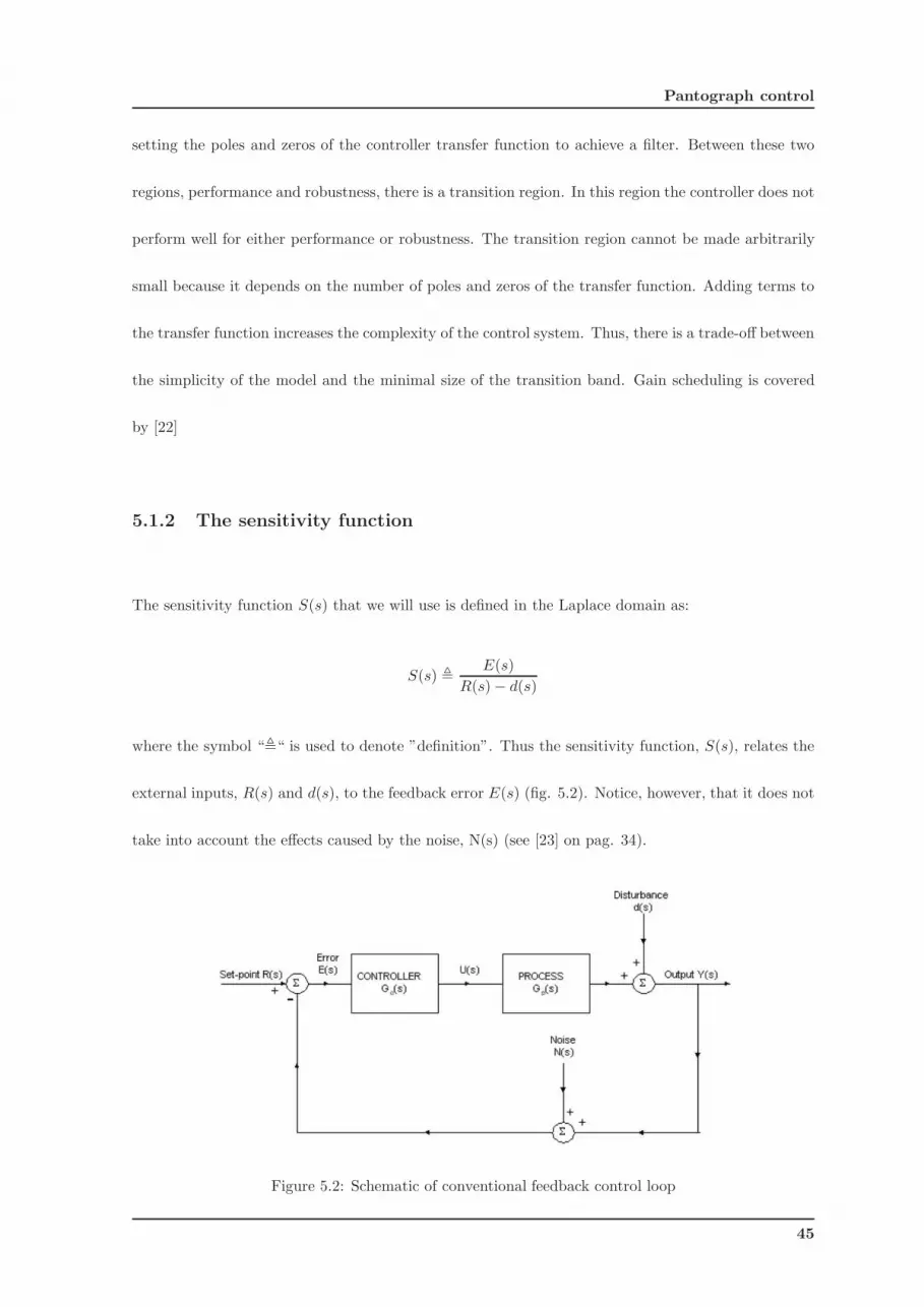
5.1.2 The sensitivity function . . . . . . . . . . . . . . . . . . . . . . . . . . . . . . . 45
5.1.3 The complementary sensitivity function . . . . . . . . . . . . . . . . . . . . . . 47
5.1.4 The trade-off . . . . . . . . . . . . . . . . . . . . . . . . . . . . . . . . . . . . . 48
5.1.5 Weighted sensitivity . . . . . . . . . . . . . . . . . . . . . . . . . . . . . . . . . 48
5.1.6 Summary . . . . . . . . . . . . . . . . . . . . . . . . . . . . . . . . . . . . . . . 49
5.2 H2 and H∞ optimal control . . . . . . . . . . . . . . . . . . . . . . . . . . . . . . . . . 50
5.2.1 H2 optimal control . . . . . . . . . . . . . . . . . . . . . . . . . . . . . . . . . . 51
5.2.2 H∞ optimal control . . . . . . . . . . . . . . . . . . . . . . . . . . . . . . . . . 52
5.2.3 Robustness . . . . . . . . . . . . . . . . . . . . . . . . . . . . . . . . . . . . . . 52
5.3 Pantograph control implementation . . . . . . . . . . . . . . . . . . . . . . . . . . . . . 52
6 Results and discussion 55
6.1 Pantograph type overview . . . . . . . . . . . . . . . . . . . . . . . . . . . . . . . . . . 55
6.2 Pantograph type overview . . . . . . . . . . . . . . . . . . . . . . . . . . . . . . . . . . 56
6.3 Linearization . . . . . . . . . . . . . . . . . . . . . . . . . . . . . . . . . . . . . . . . . 58
x INDEX
6.3.1 Linearization of the nonlinear model . . . . . . . . . . . . . . . . . . . . . . . . 59
6.3.2 Conclusions from linearization . . . . . . . . . . . . . . . . . . . . . . . . . . . 62
6.4 Problem statement . . . . . . . . . . . . . . . . . . . . . . . . . . . . . . . . . . . . . . 63
6.5 Experimental results and motivation . . . . . . . . . . . . . . . . . . . . . . . . . . . . 64
6.6 Pantograph and catenary nonlinear model attributes . . . . . . . . . . . . . . . . . . . 67
6.6.1 Conclusions from open-loop modelling . . . . . . . . . . . . . . . . . . . . . . . 69
6.6.2 Model comparison with experimental results . . . . . . . . . . . . . . . . . . . . 71
6.7 Model sensitivity to parameter changes . . . . . . . . . . . . . . . . . . . . . . . . . . . 71
6.8 Closed-loop pantograph analysis . . . . . . . . . . . . . . . . . . . . . . . . . . . . . . 73
6.8.1 Controller development . . . . . . . . . . . . . . . . . . . . . . . . . . . . . . . 74
6.8.2 Results . . . . . . . . . . . . . . . . . . . . . . . . . . . . . . . . . . . . . . . . 79
6.9 Mixed control analysis . . . . . . . . . . . . . . . . . . . . . . . . . . . . . . . . . . . . 85
6.10 Sliding catenary control . . . . . . . . . . . . . . . . . . . . . . . . . . . . . . . . . . . 87
6.11 Controller robustness to model changes . . . . . . . . . . . . . . . . . . . . . . . . . . 88
7 Conclusions and future work 91
7.1 Future work . . . . . . . . . . . . . . . . . . . . . . . . . . . . . . . . . . . . . . . . . . 93
Bibliography 94

Figure Index
1.1 Model and Control diagram . . . . . . . . . . . . . . . . . . . . . . . . . . . . . . . . . 3
2.1 Catenary system . . . . . . . . . . . . . . . . . . . . . . . . . . . . . . . . . . . . . . . 9
2.2 Catenary . . . . . . . . . . . . . . . . . . . . . . . . . . . . . . . . . . . . . . . . . . . 10
2.3 Pantograph and train . . . . . . . . . . . . . . . . . . . . . . . . . . . . . . . . . . . . 11
2.4 Faiveley pantograph CX . . . . . . . . . . . . . . . . . . . . . . . . . . . . . . . . . . . 12
2.5 Pantograph calibration . . . . . . . . . . . . . . . . . . . . . . . . . . . . . . . . . . . . 13
3.1 Bodies and joints in a serial chain . . . . . . . . . . . . . . . . . . . . . . . . . . . . . . 21
3.2 Plant to linearize . . . . . . . . . . . . . . . . . . . . . . . . . . . . . . . . . . . . . . . 23
4.1 The pantograph . . . . . . . . . . . . . . . . . . . . . . . . . . . . . . . . . . . . . . . . 25
4.2 Pantograph elements . . . . . . . . . . . . . . . . . . . . . . . . . . . . . . . . . . . . . 28
4.3 Passive elements . . . . . . . . . . . . . . . . . . . . . . . . . . . . . . . . . . . . . . . 28
4.4 Joint positioning . . . . . . . . . . . . . . . . . . . . . . . . . . . . . . . . . . . . . . . 29
4.5 Joints (SimMechanics R© representation) . . . . . . . . . . . . . . . . . . . . . . . . . . 30
4.6 SimMechanics: Parameters . . . . . . . . . . . . . . . . . . . . . . . . . . . . . . . . . 31
4.7 Data model . . . . . . . . . . . . . . . . . . . . . . . . . . . . . . . . . . . . . . . . . . 32
xi
xii FIGURE INDEX
4.8 Generic mass data . . . . . . . . . . . . . . . . . . . . . . . . . . . . . . . . . . . . . . 33
4.9 Mass orientation . . . . . . . . . . . . . . . . . . . . . . . . . . . . . . . . . . . . . . . 33
4.10 Equivalent model of the Catenary . . . . . . . . . . . . . . . . . . . . . . . . . . . . . . 34
4.11 Catenary representation . . . . . . . . . . . . . . . . . . . . . . . . . . . . . . . . . . . 35
4.12 Linearization process for control . . . . . . . . . . . . . . . . . . . . . . . . . . . . . . 36
4.13 Pantograph configurations studied . . . . . . . . . . . . . . . . . . . . . . . . . . . . . 36
4.14 VRML model . . . . . . . . . . . . . . . . . . . . . . . . . . . . . . . . . . . . . . . . . 39
4.15 Linking SimMechanics with VR Sink . . . . . . . . . . . . . . . . . . . . . . . . . . . . 39
4.16 SimMechanics model connection to VRML model . . . . . . . . . . . . . . . . . . . . . 40
5.1 Simple control loop system with uncertainty . . . . . . . . . . . . . . . . . . . . . . . . 43
5.2 Schematic of conventional feedback control loop . . . . . . . . . . . . . . . . . . . . . . 45
5.3 Sensitivity and Complementary Sensitivity functions of a closed-loop with a PI con-
troller and a 1st-order system without delay . . . . . . . . . . . . . . . . . . . . . . . . 50
5.4 Weight functions . . . . . . . . . . . . . . . . . . . . . . . . . . . . . . . . . . . . . . . 51
5.5 Pantograph control closed loop representation . . . . . . . . . . . . . . . . . . . . . . . 53
6.1 Pantograph with one actuator and with springs and dampers present in the registration
strip (Type 1) . . . . . . . . . . . . . . . . . . . . . . . . . . . . . . . . . . . . . . . . . 55
6.2 One actuator pantograph with fixed registration strip (Type 2) . . . . . . . . . . . . . 57
6.3 One actuator pantograph with 2 DOF registration strip (Type 3) . . . . . . . . . . . . 57
6.4 The Type 4 and Type 5 pantograph models . . . . . . . . . . . . . . . . . . . . . . . . 58
6.5 Model validation: input variation . . . . . . . . . . . . . . . . . . . . . . . . . . . . . . 60

FIGURE INDEX xiii
6.6 Pole Zero Map: Torque in joint vs Force in catenary (G1) . . . . . . . . . . . . . . . . 61
6.7 Pantograph linear models . . . . . . . . . . . . . . . . . . . . . . . . . . . . . . . . . . 63
6.8 Training Session in High Speed Systems . . . . . . . . . . . . . . . . . . . . . . . . . . 65
6.9 SNCF experimental results . . . . . . . . . . . . . . . . . . . . . . . . . . . . . . . . . 66
6.10 Free body diagram of Type 1 registration strip . . . . . . . . . . . . . . . . . . . . . . 67
6.11 Pantograph model representation . . . . . . . . . . . . . . . . . . . . . . . . . . . . . . 68
6.12 Pantograph open-loop with catenary step perturbation . . . . . . . . . . . . . . . . . 69
6.13 Pantograph open-loop with catenary sine perturbation . . . . . . . . . . . . . . . . . 70
6.14 Type 1, 2Hz, with 10 cm amplitude, sinusoidal catenary perturbation . . . . . . . . . 71
6.15 Type 3, 2Hz, with 10 cm amplitude, sinusoidal catenary perturbation . . . . . . . . . 72
6.16 Model mass parameter and pole-zero map . . . . . . . . . . . . . . . . . . . . . . . . . 72
6.17 Model spring parameter and pole-zero map . . . . . . . . . . . . . . . . . . . . . . . . 73
6.18 Model damper parameter pole-zero map . . . . . . . . . . . . . . . . . . . . . . . . . . 74
6.19 Testing w1: Loop shaping . . . . . . . . . . . . . . . . . . . . . . . . . . . . . . . . . . 76
6.20 Multiple models based on Type 1 model . . . . . . . . . . . . . . . . . . . . . . . . . . 76
6.21 Robust Controller gain plot . . . . . . . . . . . . . . . . . . . . . . . . . . . . . . . . . 78
6.22 Type 1 with 2Hz sine perturbation controller comparisons . . . . . . . . . . . . . . . . 79
6.23 Type 1 step perturbation controller comparisons . . . . . . . . . . . . . . . . . . . . . 79
6.24 Type 1 with 20Hz sine perturbation controller comparisons . . . . . . . . . . . . . . . 80
6.25 Type 1 step perturbation with new controller . . . . . . . . . . . . . . . . . . . . . . . 81
6.26 Type 1 with 20Hz sine perturbation and new controller . . . . . . . . . . . . . . . . . 81
xiv FIGURE INDEX
6.27 Type 3 with 2Hz sine perturbation with new controller . . . . . . . . . . . . . . . . . . 83
6.28 Type 3 with 20Hz sine perturbation and new controller . . . . . . . . . . . . . . . . . 83
6.29 H∞ controller, with no damper in lower joint . . . . . . . . . . . . . . . . . . . . . . . 85
6.30 Type 4 controller implementation results to sine perturbation . . . . . . . . . . . . . . 86
6.31 Type 4 controller implementation results to step perturbation . . . . . . . . . . . . . . 86
6.32 Independent control function of Type 5 model . . . . . . . . . . . . . . . . . . . . . . . 87
6.33 Type 5 control implementation for 2Hz perturbation . . . . . . . . . . . . . . . . . . . 88
6.34 H∞ VS PID controlled with altered model (no lower damper) . . . . . . . . . . . . . . 89
6.35 Noise influence on Type 1 model with 2Hz catenary influence . . . . . . . . . . . . . . 90
Table Index
4.1 Rigid body mass and inertia . . . . . . . . . . . . . . . . . . . . . . . . . . . . . . . . . 27
4.2 Rigid body initial position and orientation . . . . . . . . . . . . . . . . . . . . . . . . . 27
4.3 Passive elements information . . . . . . . . . . . . . . . . . . . . . . . . . . . . . . . . 29
4.4 Pantograph model type considerations . . . . . . . . . . . . . . . . . . . . . . . . . . . 37
6.1 Poles and Zeros . . . . . . . . . . . . . . . . . . . . . . . . . . . . . . . . . . . . . . . . 61
6.2 Global SNCF pantograph experimental results . . . . . . . . . . . . . . . . . . . . . . 66
6.3 Experimental results highlights . . . . . . . . . . . . . . . . . . . . . . . . . . . . . . . 66
xv

xvi TABLE INDEX

Abbreviations
AC Alternate current
DC Continuous current
PID Proportional Integrative Derivative
PD Proportional Derivative
CT Continuous Time
LTI Linear Time Invariant
k Stiffness coefficient
l Natural length
c Damping coefficient
RNE Recursive Newton Euler
CM Center of mass
ODE Ordinary differential equations
PDE Partial differential equations
VRML Virtual Reality Modelling Language
CX SNCF high speed pantograph model
SNCF Railway company in France
xvii

xviii TABLE INDEX
Chapter 1
Introduction
High speed rail vehicles are a comfortable and fast way of transportation. Until today open loop
pantograph systems proved to be a very robust solution for trains. Because of rail line degradation,
train circulation with adverse weather conditions, like intense wind, and the desire to achieve higher
speeds, can cause excessive wear in the pantograph contact interface. Improving high speed circulation
on the railway isn’t the only goal in the present study, low cost maintenance of the pantograph and
the catenary is equally important, thus the ideal solution would be of having a system that has
low maintenance comparing with present solutions, higher train circulation speeds and to avoid the
necessity of changing the hole railway system, including the catenary. Train speed, and pantograph
actuating force with the catenary, are the primary variables to maintain a stable current collection.
High speeds generally produce lower contact forces. A problem that arises from building faster
trains is in the current collector of the train, the pantograph. In order to collect electric current from
the cable network system above the train, the catenary, it is necessary for the pantograph to contact
the catenary. Excessive contact force causes damage to the pantograph and the lack of contact force
causes current perturbation and electric arcs which damages the pantograph.
1
Maintaining the contact force in an admissible region is very important, in order to achieve sus-
tainable high speeds. Comparing to standard open loop systems, closed loop systems allow train
circulation speed to up to 500 Km/h and more depending on other limiting factors (not the panto-
graph interface but to other train related variables).
There is a wide variety of electric traction systems around the world, which have been built
according to the type of railway, its location and the technology available at the time of the installation.
Many installations seen today were first built up to 100 years ago, when electric traction was barely
out, and this has had a great influence on what is seen today.
However, in the last 20 years there has been a gigantic acceleration in railway traction development.
This has run in parallel with the development of power electronics and microprocessors. What have
been the accepted norms for the industry for, 80 years, have suddenly been thrown out and replaced by
fundamental changes in design, manufacture and operation. The result has been top speed circulation
of 500 Km/h.
The SNCF train pantograph functions as follows: it is activated by a pneumatic device comprised
of an air cushion controlled by an electro-pneumatic plate and assisted by an electronic board. The
system adjusts the air cushion pressure, and at the same time, the force to apply on the catenary,
in real time, to obtain the best possible electrical contact between the catenary and the pantograph,
regardless of operating conditions. The applied pressure is calculated according to the speed of the
train-set, taking the load bearing capacity of the pantograph itself, the movement direction and the
composition of the train-set (single unit or multiple unit) into account.
In order to have active control in the pantograph, it is necessary to know the dynamic nonlinear
model of a real pantograph. In this work we consider the CX pantograph model of the SNCF trains.
2

Introduction
The catenary will be modelled as a parallel spring / damper system connected to the registration strip
of the pantograph, this element has direct contact with the catenary. After obtaining the nonlinear
model, a virtual reality model will be created in order to visualize the motion of the pantograph.
The control strategies will be applied to the nonlinear model in order to get the contact force in an
admissible region of tolerance. Three controllers will be studied: PID controller, robust H2 and H∞
controllers. The robust controllers will require a linear model of the system which will be obtained
by linearizing the nonlinear model around the nominal conditions. Figure 1.1 shows a view of the
integrated modelling and control process, an example of this approach can be seen in [1].
Figure 1.1: Model and Control diagram
Figure 1.1 illustrates the process of creation of the closed loop system presented in this work. A
model has to be created, which contains all the information of a real pantograph. After the model has
been created, a closed loop feedback system has to be developed. Using the model created (represented
in the figure as G) and a controller K that has to be tuned. The motion of the pantograph is visualized
in a virtual reality world.
1.1 Pantograph systems
Much investigation has been done around turning the railway system faster and safer. In order for the
train to work, current collection has to be done and thus the usage of a catenary to deliver current
from the energy power plant, and the pantograph to collect current towards the train engines. These
3
1.2 Objectives
systems act together as one but research was done separately until today.
Modeling a pantograph and catenary system was one of the main objectives in the past to correctly
simulate a high speed train. Many authors studied this with sensitivity analysis [2] which finds relations
in model variables and performance of a catenary - pantograph system, they also modelled the catenary
with a FEM (finite element method) based approach. A more extended approach has been used in
[3], [4] and [5], a model was developed and studied but in a more explicit way. The catenary elements
and derivation are farther developed. The effect of locomotive vibration on pantograph is treated
in [6]. A pantograph system isn’t just about modelling, new advances have been made in robust
controlling of pantograph systems and some interesting results are presented in [7], [8] and [9]. The
controllers implemented in these papers range from simple PID controllers to more complex theories
like robust controllers. All citations made until now are essential to the problem layout and solution
search, but although the results look interesting the implementation is fairly complicated, the best
approach found can be seen in [1]. In this paper a engineering point of view in robust controller tuning
was used, recurring to simple sinusoidal perturbation functions.
1.2 Objectives
The main goal of this study is to model and control the CX pantograph to maintain the contact
force in a admissible region; to study the best control configuration and control strategy. Two control
strategies will be studied: a PID controller which is a standard control method and an advanced
controller based on the robust control theory H2 and H∞.
4

Introduction
1.3 Contributions of this thesis
To simplify the modelling process, instead of using classical formulations to obtain numerical results,
SimMechanics R© was used. To simMechanics R© a pantograph is a multibody closed mechanical system
and thus the theory presented in [10] and [11] where useful in the model creation.
The primary software used is Matlab R© / Simulink R© with its mechanical modelling environment
called SimMechanics R©. This environment is built upon the basic concepts of general mechanical
systems, details can be seen in [12]. Many new researchers are starting to use Matlab’s powerful
modelling environment for system analysis, and some research has been done in this area [13].
This project brings a pantograph model constructed upon SimMechanics R©, with a robust controller
attached to the target joints (will be studied in the next chapters). Not only is it important to model
and control a pantograph, but to understand the limitations and advantages of the combination of
many Matlab R© toolbox tools. Another contribution of this theses is the use of many Matlab tools
applied to robust control of a pantograph, like the usage of the Robust Control Toolbox.
1.4 Thesis Outline
In chapter 1, an introduction to all work developed is made. In chapter 2, basic railway definitions
are introduced. In chapter 3, it is explained how SimMechanics R© formulates the dynamic equations
solved numerically. In chapter 4: various pantograph model and catenary elements are developed and
explained their SimMechanics R© implementation. In chapter 5, the control theory used to project the
closed loop controller is presented. In chapter 6, results are presented and discussed. In chapter 7,
conclusions and future work are presented.
5

1.4 Thesis Outline
6
Chapter 2
Basic rail system concepts
2.1 Power supply
The electric railway needs a power supply that the trains can access at all times. It must be safe,
economical and easy to maintain. It can use either direct current (DC) or alternating current (AC).
The former has been for many years, simpler for railway traction purposes. The latter is better over
long distances and cheaper to install however, it has been until recently, it has been more complicated
to control at train level.
Transmission of power is always performed along the track by means of an overhead wire or at
ground level, using an extra third rail laid close to the running rails. AC systems always use overhead
wires, DC can use either an overhead wire or a third rail, both are common. Both overhead systems
require at least one collector attached to the train so it can always be in contact with the power cable.
Overhead current collectors use a ”pantograph”, so called because that was the shape of most of them
until about 30 years ago. The return circuit is via the running rails back to the substation. The
running rails are at earth potential and are connected to the substation.
7

2.2 The catenary
2.1.1 AC or DC traction
It doesn’t really matter whether we have AC or DC motors, nowadays either can work with an AC or
DC supply. The only requirement is to have the right sort of power electronics between the supply and
the motor. However, the choice of AC or DC power transmission system along the line is important.
Generally, it’s a question of what sort of railway is available. It can be summarized simply as AC for
long distance and DC for short distance.
It is easier to boost the voltage of AC than that of DC, so it is easier to send more power over
transmission lines with AC. As AC is easier to transmit over long distances, it is an ideal medium for
electric railways. DC, on the other hand, is the preferred option for shorter lines: urban systems and
tramways. However, it is also used on a small number of main line railway systems.
2.2 The catenary
The mechanics of power supply wiring is not as simple as it may seem. Hanging a wire over the track,
providing it with current and running trains under it is not that easy if it is to do the job properly
and last long enough to justify the expense of installing it. The wire must be able to carry the current
(several thousand amps), remain in line with the route, withstand wind , extreme cold and heat and
other hostile weather conditions.
Overhead catenary systems, called “catenary” due to the curve formed by the supporting cable
(fig. 2.1), have a complex geometry, nowadays usually designed by computer. The contact wire has
to be held in tension horizontally and pulled laterally to negotiate curves in the track. The contact
wire tension is typically in the region of 2 tonnes. The wire length is usually between 1000 and 1500
meters, depending on the temperature ranges. The wire is zigzagged relative to the center line of the
8
Basic rail system concepts
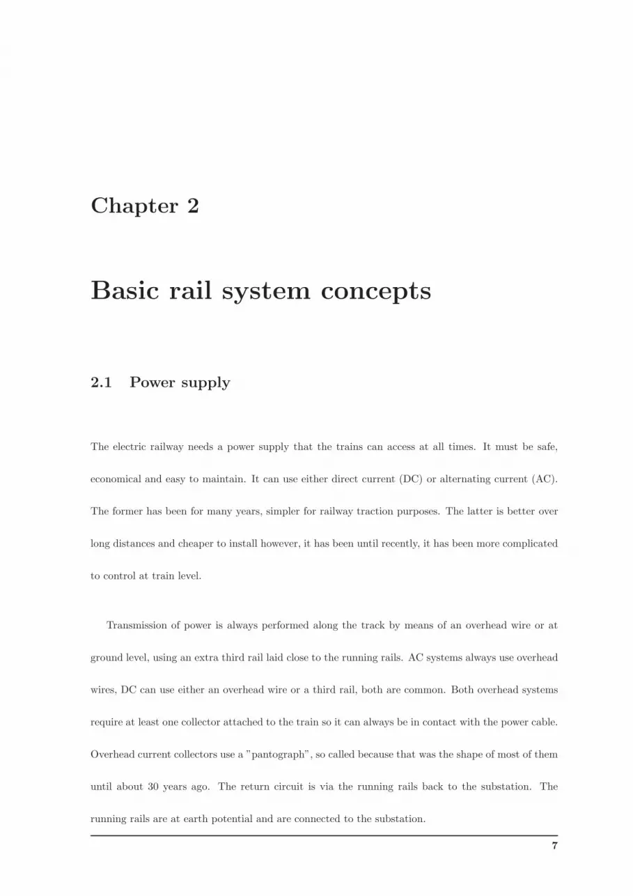
track to even the wear on the trains registration strip as it runs underneath (fig. 2.2b).
Figure 2.1: Catenary system
The contact wire is grooved to allow a clip to be fixed on the top side. The clip is used to attach
the dropper wire. The tension of the wire is maintained by weights suspended at each end of its
length. Each length is overlapped by its neighbor to ensure a smooth passage for the registration
strip. Incorrect tension, combined with the wrong speed of a train, will cause the pantograph head
to start bouncing. An electric arc occurs with each bounce, the registration strip and wire will both
become worn through under such conditions.
More than one pantograph on a train can cause a similar problem when the leading pantograph
head sets up a wave in the wire and the rear head can’t stay in contact. High speeds worsen the
problem. The French TGV (High Speed Train) formation has a power car at each end of the train
but only runs with one pantograph raised under the high speed 25 kV AC lines. The rear car is
supplied through a 25 kV cable running the length of the train. This is prohibited in Britain due to
the inflexible safety approach there.
A waving wire will cause another problem. It can cause the dropper wires, from which the contact
wire is hung, to “kink” and form little loops. The contact wire then becomes too high and decreases
9
2.3 The pantograph
contact.
2.2.1 Catenary suspension systems
Various forms of catenary suspension are used (fig. 2.1). Catenary information may be found in
[14] for example, and depends on the system, its age, its location and the speed of trains using
it. Broadly speaking, the higher the speeds, the more complex the “stitching“, although a simple
catenary will usually suffice if the support posts are close enough together on a high speed route.
Modern installations often use the simple catenary, slightly sagged to provide a good contact. It has
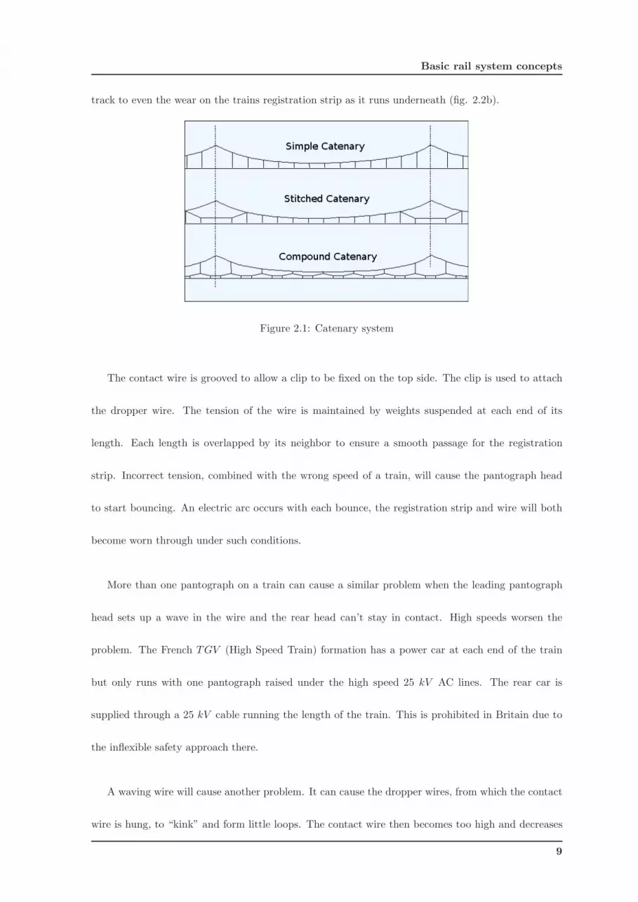
been found to perform well at speeds up to 200 km/h. Figure 2.2a showns a catenary support element.
This element doesn’t follow the railway exactly along side, it crosses the rail line from side to side fig.
2.2b.
(a) Post (b) Line
Figure 2.2: Catenary
2.3 The pantograph
The only objective of the pantograph is to collect electrical current from the catenary cable system.
10
Basic rail system concepts
2.3.1 Standard speed trains
Standard speed trains of about 100 Km/h, normally use old Catenary network systems. This type of
train uses a pressure cushion, which makes the pantograph raise when it gains pressure or descend
when it loses pressure.
At maximum speed these pantographs suffer from low contact force between registration strip and
catenary, a deceiving higher calibration contact force doesn’t solve the problem due to high wear in
the contact system. A solution to this problem was successfully used by adding an aerodynamic wing
to the pantograph registration strip, permitting the usage of lower calibration pressures giving better
contact at higher speeds. The pantograph may or may not have passive elements depending on the
supplier; passive elements aren’t very common in standard low cost trains. Passive elements consist
of spring and damper elements attached between bodies.
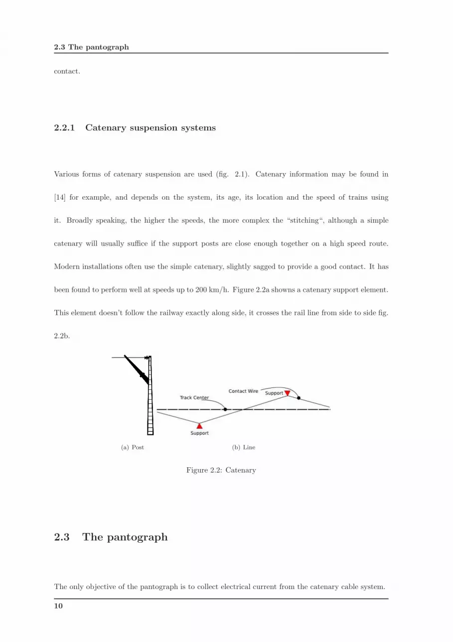
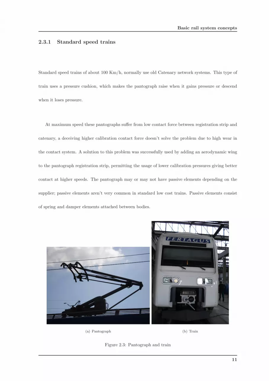
(a) Pantograph (b) Train
Figure 2.3: Pantograph and train
11
2.3 The pantograph
2.3.2 High speed trains
According to UIC (Union Internationale des Chemins de Fer), ”high-speed train” is a train that runs
at over 250 km/h (TGV train) on dedicated tracks, or over 200 km/h (Pendular train) on upgraded
conventional tracks. These trains are equipped with passive control regulators; depending on the
velocity of the train the air cushion pressure gets regulated. These type of trains achieve high speeds
because of the dedicated rail lines or of upgraded ones which involves great investment.
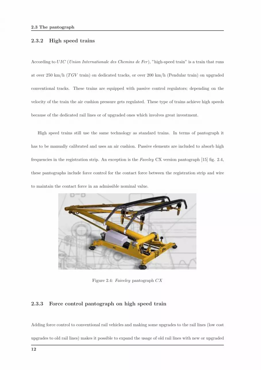
High speed trains still use the same technology as standard trains. In terms of pantograph it
has to be manually calibrated and uses an air cushion. Passive elements are included to absorb high
frequencies in the registration strip. An exception is the Faveley CX version pantograph [15] fig. 2.4,
these pantographs include force control for the contact force between the registration strip and wire
to maintain the contact force in an admissible nominal value.
Figure 2.4: Faiveley pantograph CX
2.3.3 Force control pantograph on high speed train
Adding force control to conventional rail vehicles and making some upgrades to the rail lines (low cost
upgrades to old rail lines) makes it possible to expand the usage of old rail lines with new or upgraded
12
Basic rail system concepts
trains. Normal trains could circulate faster in old railways; high speed trains in new rail lines could
go even faster then the TGV ’s 500 Km/h record in dedicated rails.
2.4 Passive pantograph limitations
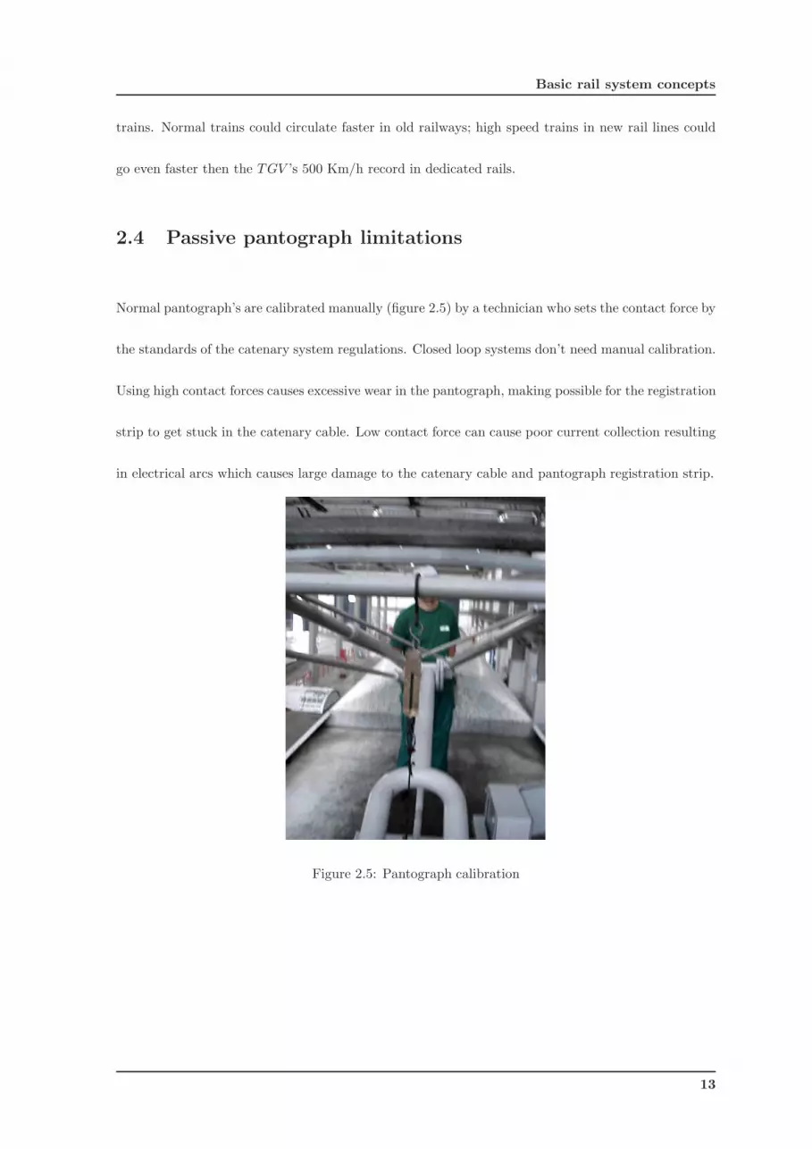
Normal pantograph’s are calibrated manually (figure 2.5) by a technician who sets the contact force by
the standards of the catenary system regulations. Closed loop systems don’t need manual calibration.
Using high contact forces causes excessive wear in the pantograph, making possible for the registration
strip to get stuck in the catenary cable. Low contact force can cause poor current collection resulting
in electrical arcs which causes large damage to the catenary cable and pantograph registration strip.
Figure 2.5: Pantograph calibration
13

2.4 Passive pantograph limitations
14
Chapter 3
Dynamics modelling in
SimMechanics R©
3.1 SimMechanics R©
SimMechanics R© is a tool for modelling and simulating mechanical systems, it’s an extension to Mat-
lab’s Simulink environment, using the newest and more robust mechanical modelling theory’s adding
it to Simulink’s efficient numerical solver. A comparison with other types of simulation applications
can be seen in [7]. Although SimMechanics uses the most recent methods it still has it’s bases on
the Newton Euler Method. This application can handle relative or absolute coordinates to define the
position of all element masses or joints. The orientation of these elements can be introduced using
Euler rotation matrices or even quaternion. An overview on Matlab’s potential and comparison to
other alternatives is studied in [13].
The motion of bodies is described by its kinematics behavior. The dynamic behavior results due
to the equilibrium of applied forces and the rate of change in the momentum. As an important
feature, multibody system formalisms usually offer an algorithmic, computer-aided way to model,
15
3.2 Modelling multibody systems
analyze, simulate and optimize the arbitrary motion of possibly thousands of interconnected bodies.
The advantage of using SimMechanics R© is obvious, no formal mechanical formulations are directly
required and the differential equations are automatically solved. The equations governing the motion
of mechanical systems are typically higher-index differential algebraic equations (DAEs). Simulink R©
is currently designed to model systems governed by ordinary differential equations (ODEs) and a
restricted class of index-1 DAEs. This chapter is based on a paper presented by Mathworks R© for
SimMechanics R© [12, 16].
3.2 Modelling multibody systems
A multibody system is an abstract collection of bodies whose relative motions are constrained by
means of joints. The representation of a multibody system is given by an abstract graph. The
bodies are placed in direct correspondence with the nodes of the graph, and the constraints (where
pairs of bodies interact) are represented by means of edges. Two fundamental types of systems exists,
multibody systems whose graphs are acyclic, often referred to as tree topology systems, and multibody
systems that give rise to cyclic graphs with closed-loops.
3.3 Relative versus absolute coordinate formulations
The structure of the equations of motion depends largely on the choice of coordinates. Many com-
mercial software packages for multibody dynamics use the formulation in absolute coordinates. In
this approach, each body is first assigned 6 degrees of freedom. Then, depending on the interaction
of bodies due to joints. suitable constraint equations are formed. This results in a large number of
configuration variables and relatively simple constraint equations, but also in a sparse mass matrix M .
16

Dynamics modelling in SimMechanics R©
This sparseness and the uniformity in which the equations of motions are derived is exploited by the
software. However, due to the large number of constraint equations, this strategy is not suitable for
SimMechanics R©. It uses relative coordinates. In this approach, a body is initially given zero degrees
of freedom. They are “added” by connecting joints to the body. Therefore, far fewer configuration
variables and constraint equations are required. Acyclic systems can even be simulated without form-
ing any constraint equations. The drawback of this approach is the dense mass matrix M , which now
contains the constraints implicitly, and the more complex constraint equations.
3.4 Unconstrained systems
In this section we restrict attention to the class of multibody systems represented by noncyclic graphs,
otherwise known as branched trees, by virtue of the fact that the graphs have the form of a rooted tree.
For simplification purposes we further restrict attention to the subset of simple- chain systems. The
results are easily extended to the more general case of branched trees but the analysis is much clearer
in the case of simple chains. Simple chains are multibody systems where each body is connected
to a unique predecessor body and a unique successor body (with the exception of the first and last
bodies in the chain) by means of a joint. A common example is a robotic manipulator. In recent
years, a number of techniques have appeared for solving the dynamics of these systems, ranging in
computational complexity from O(n) (where n is the number of bodies in the system) to O(n3)
3.5 Analysis of simple chain systems
Consider the n-link serial chain in fig. 3.1, the tip of the chain to the base, which also acts as the
inertial reference frame. Each body is connected to two joints, an inboard joint (closer to the base),
17
3.5 Analysis of simple chain systems
and an outboard joint (closer to the tip).
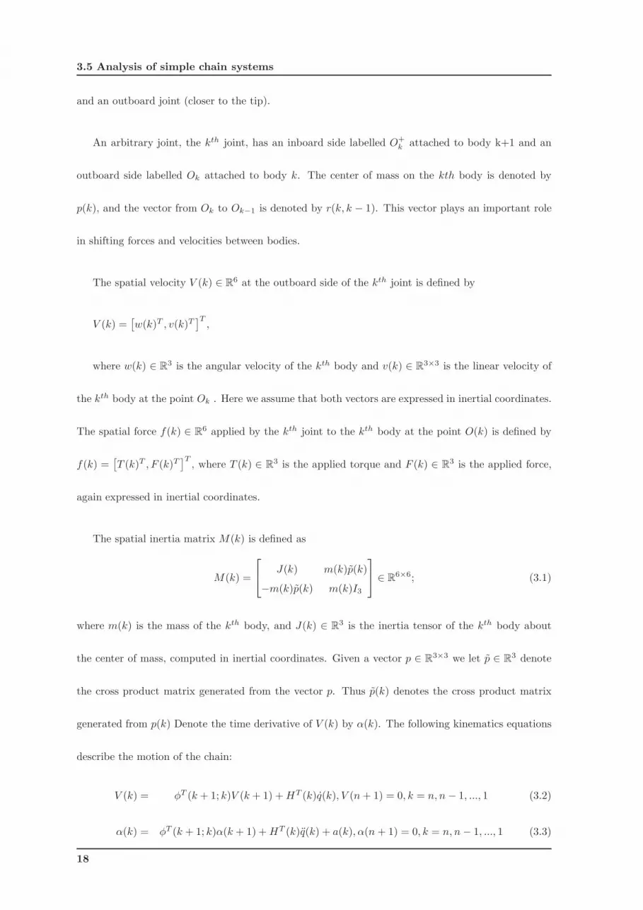
An arbitrary joint, the kth joint, has an inboard side labelled O+k attached to body k+1 and an
outboard side labelled Ok attached to body k. The center of mass on the kth body is denoted by
p(k), and the vector from Ok to Ok−1 is denoted by r(k, k − 1). This vector plays an important role
in shifting forces and velocities between bodies.
The spatial velocity V (k) ∈ R6 at the outboard side of the kth joint is defined by
V (k) =[
w(k)T , v(k)T]T
,
where w(k) ∈ R3 is the angular velocity of the kth body and v(k) ∈ R
3×3 is the linear velocity of
the kth body at the point Ok . Here we assume that both vectors are expressed in inertial coordinates.
The spatial force f(k) ∈ R6 applied by the kth joint to the kth body at the point O(k) is defined by
f(k) =[
T (k)T , F (k)T]T
, where T (k) ∈ R3 is the applied torque and F (k) ∈ R
3 is the applied force,
again expressed in inertial coordinates.
The spatial inertia matrix M(k) is defined as
M(k) =
J(k) m(k)p(k)
−m(k)p(k) m(k)I3
∈ R6×6; (3.1)
where m(k) is the mass of the kth body, and J(k) ∈ R3 is the inertia tensor of the kth body about
the center of mass, computed in inertial coordinates. Given a vector p ∈ R3×3 we let p ∈ R
3 denote
the cross product matrix generated from the vector p. Thus p(k) denotes the cross product matrix
generated from p(k) Denote the time derivative of V (k) by α(k). The following kinematics equations
describe the motion of the chain:
V (k) = φT (k + 1; k)V (k + 1) + HT (k)q(k), V (n + 1) = 0, k = n, n − 1, ..., 1 (3.2)
α(k) = φT (k + 1; k)α(k + 1) + HT (k)q(k) + a(k), α(n + 1) = 0, k = n, n − 1, ..., 1 (3.3)
18
Dynamics modelling in SimMechanics R©
Here, q(k) ∈ Rnnq is the vector of configuration variables for the kth joint, the columns of HT (k) ∈
R6×nnq span the relative velocity space between the kth body and the (k+1)th body, and φT (k +1; k)
is the transpose of the matrix
φ(k + 1, k) =
I3 r(k + 1, k)
0 I3
(3.4)
where the vector r(k +1, k) is the vector from the outboard side of the (k +1)th joint to the outboard
side of the kth joint. The vector a(k) ∈ R6 represents the Coriolis acceleration of the kth body and is
given by
a(k) =
w(k + 1)w(k)
w(k + 1)(v(k) − v(k + 1))
(3.5)
Given the joint velocity degrees of freedom (DoFs) q(k) and acceleration DOF q(k), these equations
provide a simple recursive procedure for determining the velocities and accelerations of the bodies
constituting the chain. The equations of motion, formulated about the reference points O(k), are
f(k) = φ(k, k − 1)f(k − 1) + M(k)α(k) + b(k)
f(k) = φ(k, k − 1)f(k − 1) + M(k)α(k) + b(k)T (k) = H(k)f(k) (3.6)
We can express these recursive relationships in matrix form as follows. Using the sum of the
velocity recursion and the fact that φ(i, i) = I6 and φ(i, k)φ(k, j) = φ(i, j). The second relationship
follows from the fact that shifting a spatial force from Oj to Ok and then from Ok to Oi is equivalent
to shifting the force directly from Oj to Oi . Then
V (k) =
n∑
i=1
φT (i, k)HT (i)qi (3.7)
A natural definition of the matrix operators follows:
HT = diag[HT (1), ..., HT (n)] (3.8)
19
3.5 Analysis of simple chain systems
The operator φ is defined by:
φ =
I6×6 0 . . . 0
φ(2, 1) I6×6 . . . 0...
.... . .
...
φ(n, 1) φ(n, 2) . . . I6×6
(3.9)
In terms of the matrix φ, the velocity and force recursions can be written as
V = φT HT q (3.10)
α = φ[HT q + a] (3.11)
f = φ[Mα + b] (3.12)
T = Hf (3.13)
where the spatial velocity vector V is defined as V T = [V T (1), V T (2), . . . V T (n)] ∈ R6n, and similarly
for the spatial acceleration vector α ∈ R6n, the Coriolis acceleration vector a ∈ R
6n, the gyroscopic
force vector b ∈ R6n, and the spatial force vector f ∈ R
6n. Finally the matrix M ∈ R6×6 is defined to
be M = diag[M(1), M(2), . . . , M(n)]. Substituting into the last equation, we obtain the equations of
motion:
T = HφMφT HT q + Hφ[MφT a + b] (3.14)
This equation is in a factorized form, and its structure may be exploited to obtain a global or
recursive solution.
In the simulation problem, the motion of a mechanical system is calculated based on the knowledge
of the torques and forces applied by the actuators, and the initial state of the machine:
1. The forward dynamics problem in which the joint accelerations are computed given the actuator
torques and forces.
20

Dynamics modelling in SimMechanics R©
Figure 3.1: Bodies and joints in a serial chain
2. The motion integration problem in which the joint trajectories are computed based on the given
acceleration.
Several computational techniques have been developed for the forward dynamics problem. Most
of them are recursive methods. Two popular ones are the O(n3) Composite Rigid Body Method
(CRBM) and the O(n) Articulated Rigid Body Method (ABM) which are derived in [17]. The ABM
uses the sparsity structure of large systems with many bodies (> 7) efficiently, but produces more
computational overhead than the CRBM which can be preferable for smaller systems. The compu-
tational cost of the forward dynamics problem is only half the story, however. The characteristics
of the resulting equations also have an influence on the performance of the adaptive time-step ODE
solvers of Simulink (“formulation stiffness”). The ABM often produces better results, especially for
ill-conditioned problems [18].
For unconstrained systems, the application of the CRBM and ABM methods, and the following
integration of the ODEs is straightforward. A simulation program, however, must be able to handle
arbitrary mechanisms. In SimMechanics R©, cyclic systems are reduced to open topology systems by
21

3.6 Linearization
cutting joints, which are (mathematically) replaced by a set of constraint equations. They ensure,
that the system with the cut joints moves exactly as the original cyclic mechanism. The user can
choose if he wants to select the cut-set by himself or if he leaves this task to SimMechanics R©. Of
course, the structure of the resulting equations depends largely on this choice. In all cases, however,
the equations of motion of constrained systems are index-3 DAEs, which have to be transformed into
ODEs in order to be solvable with the Simulink R© ODE solver suite.
The approach taken by SimMechanics R© is to differentiate the constraint equation twice and solve
for the Lagrange multiplier, λ. Near singularities of the mechanism, i.e. near points where the number
of independent constraint equations is decreased and the solution for λ is no longer unique, numerical
difficulties arise. To deal with this problem, the user chooses between two solvers. One, based on
Cholesky decomposition (the default), which is generally faster, and one based on QR decomposition,
which is more robust in the presence of singularities [19].
3.6 Linearization
A linearized model is an approximation to a nonlinear system, which is valid in a small region around
the operating point of the system. Engineers often use linearization in the design and analysis of
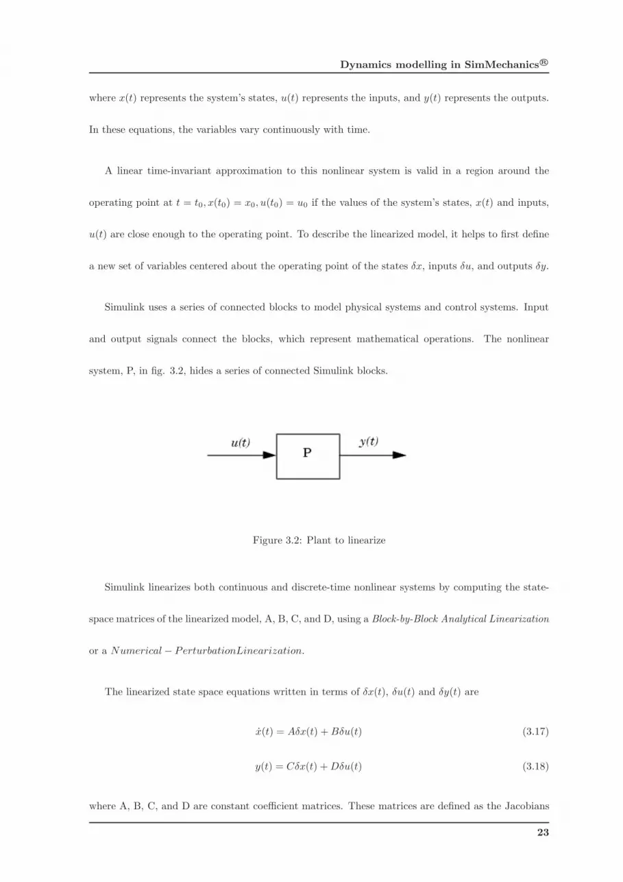
control systems and physical models. The following figure shows a visual representation of a nonlinear
system as a block diagram. The diagram consists of an external input signal, u(t), a measured output
signal, y(t), and the nonlinear system that describes the system’s states and its dynamic behavior, P .
It is possible to express a nonlinear system in terms of the state space equations
x(t) = f(x(t), u(t), t) (3.15)
y(t) = g(x(t), u(t), t) (3.16)
22
Dynamics modelling in SimMechanics R©
where x(t) represents the system’s states, u(t) represents the inputs, and y(t) represents the outputs.
In these equations, the variables vary continuously with time.
A linear time-invariant approximation to this nonlinear system is valid in a region around the
operating point at t = t0, x(t0) = x0, u(t0) = u0 if the values of the system’s states, x(t) and inputs,
u(t) are close enough to the operating point. To describe the linearized model, it helps to first define
a new set of variables centered about the operating point of the states δx, inputs δu, and outputs δy.
Simulink uses a series of connected blocks to model physical systems and control systems. Input
and output signals connect the blocks, which represent mathematical operations. The nonlinear
system, P, in fig. 3.2, hides a series of connected Simulink blocks.
Figure 3.2: Plant to linearize
Simulink linearizes both continuous and discrete-time nonlinear systems by computing the state-
space matrices of the linearized model, A, B, C, and D, using a Block-by-Block Analytical Linearization
or a Numerical − PerturbationLinearization.
The linearized state space equations written in terms of δx(t), δu(t) and δy(t) are
x(t) = Aδx(t) + Bδu(t) (3.17)
y(t) = Cδx(t) + Dδu(t) (3.18)
where A, B, C, and D are constant coefficient matrices. These matrices are defined as the Jacobians
23
3.6 Linearization
of the system, evaluated at the operating point
A =∂f
∂x|t0,x0,u0
B = ∂f∂u
|t0,x0,u0(3.19)
(3.20)
C =∂g
∂x|t0,x0,u0
D = ∂g∂u
|t0,x0,u0(3.21)
The transfer function representation may also be obtained. To this end we apply the Laplace
transform to eq. 3.18 and eq. 3.18 and manipulate to obtain, provided (x0, u0) = (0, 0)
Y(s)
U(s)= Plin(s) = C(sI − A)−1B + D
Where s is the Laplace variable and I is the identity matrix.
24
Chapter 4
SimMechanics R© pantograph model
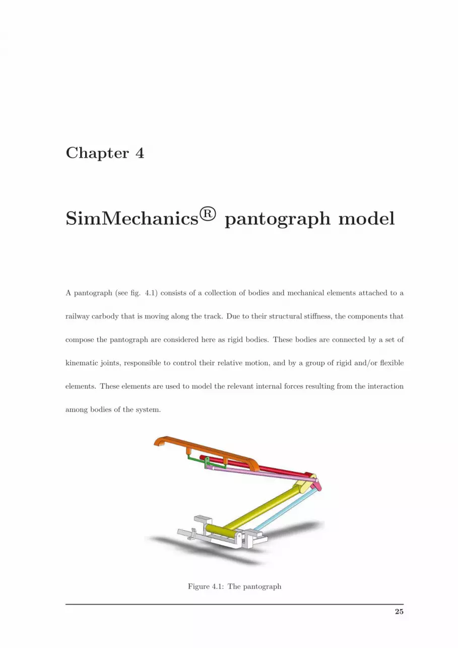
A pantograph (see fig. 4.1) consists of a collection of bodies and mechanical elements attached to a
railway carbody that is moving along the track. Due to their structural stiffness, the components that
compose the pantograph are considered here as rigid bodies. These bodies are connected by a set of
kinematic joints, responsible to control their relative motion, and by a group of rigid and/or flexible
elements. These elements are used to model the relevant internal forces resulting from the interaction
among bodies of the system.
Figure 4.1: The pantograph
25

4.1 Pantograph body elements
4.1 Pantograph body elements
4.1.1 Basic components
The pantograph model is such that the origin of the pantograph reference frame (x, y, z) is the
insertion point on the carbody. A local reference frame (ξ, η, ζ) is rigidly attached to the center of
mass (CM) of each body of the pantograph and its spatial orientation is such that the axes are aligned
with the principal inertia directions of the rigid bodies. Therefore, the inertia tensor of each body is
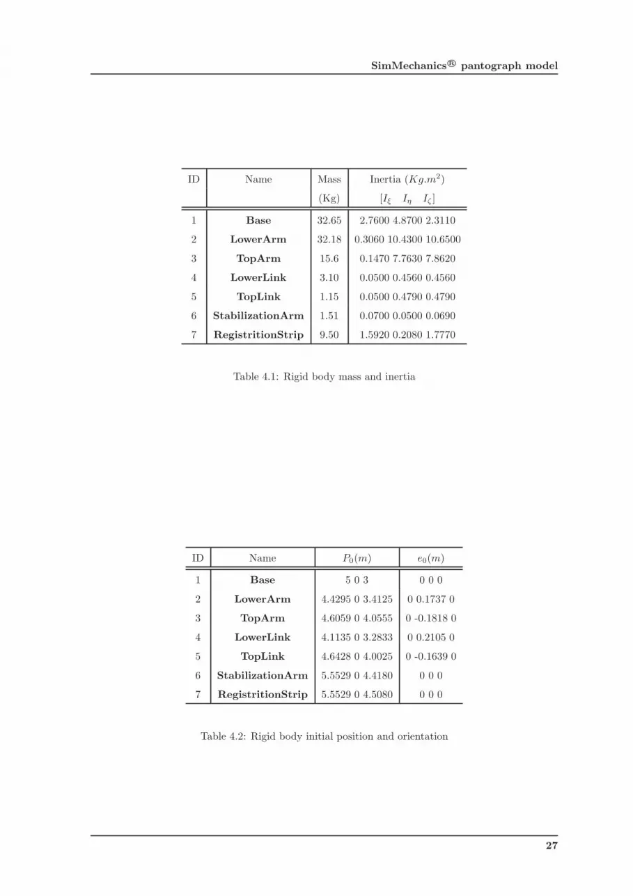
completely defined by the inertia moments (Iξ Iη Iζ).
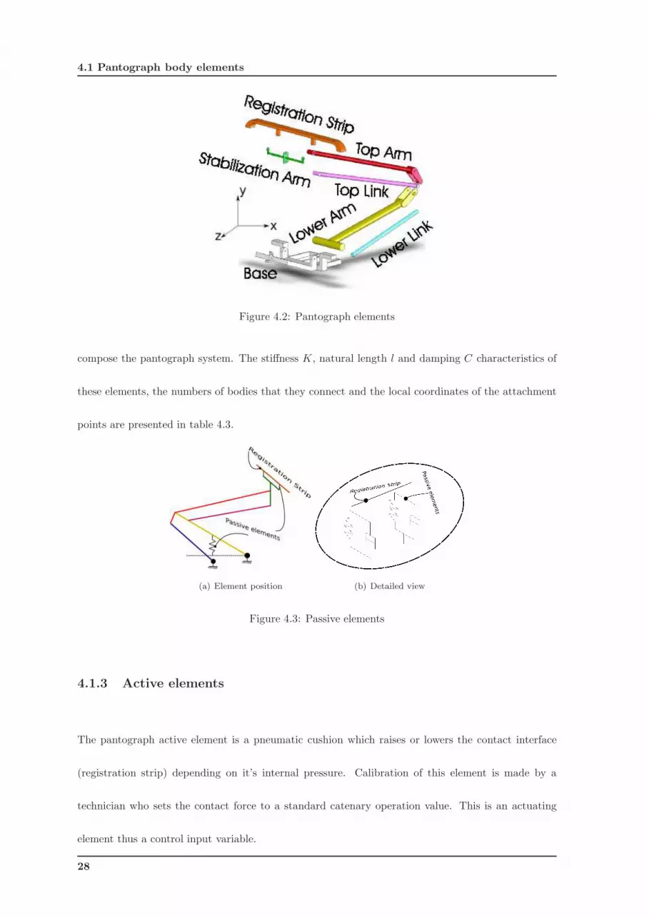
The pantograph is composed by seven rigid elements (figure 4.2):
1 Base 5 Top link
2 Lower arm 6 Stabilization armTop link
3 Top arm 7 Registration strip
4 Lower link
The initial position and initial orientation of each body in the system is given, respectively, by the
location of it’s CM and by the orientation of it’s local reference frame (ξ, η, ζ) with respect to the
pantograph reference frame (x, y, z). The inertia properties with respect to the three principal axes
(Iξ, Iη, Iζ) are presented in table 4.1, the initial position and the initial orientation of each rigid body
are presented in table 4.2 were e0 are the Euler angles. The data presented in this section is from the
CX pantograph.
4.1.2 Passive elements
Passive elements are spring and dampers which are placed in the registration strip to absorb the
catenary dynamics (figure 4.3). Furthermore, there is a spring damper element at the base joint.
These elements are also considered force elements that are transmitted among the rigid bodies that
26
SimMechanics R© pantograph model
ID Name Mass Inertia (Kg.m2)
(Kg) [Iξ Iη Iζ ]
1 Base 32.65 2.7600 4.8700 2.3110
2 LowerArm 32.18 0.3060 10.4300 10.6500
3 TopArm 15.6 0.1470 7.7630 7.8620
4 LowerLink 3.10 0.0500 0.4560 0.4560
5 TopLink 1.15 0.0500 0.4790 0.4790
6 StabilizationArm 1.51 0.0700 0.0500 0.0690
7 RegistritionStrip 9.50 1.5920 0.2080 1.7770
Table 4.1: Rigid body mass and inertia
ID Name P0(m) e0(m)
1 Base 5 0 3 0 0 0
2 LowerArm 4.4295 0 3.4125 0 0.1737 0
3 TopArm 4.6059 0 4.0555 0 -0.1818 0
4 LowerLink 4.1135 0 3.2833 0 0.2105 0
5 TopLink 4.6428 0 4.0025 0 -0.1639 0
6 StabilizationArm 5.5529 0 4.4180 0 0 0
7 RegistritionStrip 5.5529 0 4.5080 0 0 0
Table 4.2: Rigid body initial position and orientation
27
4.1 Pantograph body elements
Figure 4.2: Pantograph elements
compose the pantograph system. The stiffness K, natural length l and damping C characteristics of
these elements, the numbers of bodies that they connect and the local coordinates of the attachment
points are presented in table 4.3.
(a) Element position (b) Detailed view
Figure 4.3: Passive elements
4.1.3 Active elements
The pantograph active element is a pneumatic cushion which raises or lowers the contact interface
(registration strip) depending on it’s internal pressure. Calibration of this element is made by a
technician who sets the contact force to a standard catenary operation value. This is an actuating
element thus a control input variable.
28
SimMechanics R© pantograph model
ID i linked to ID j Body [i j] Pi [x y z] (m) Pj [x y z] (m) [K l C] (N/m, m, Ns/m )
ID 1 - ID 2 [1 2] [-0.5705 0 0] [0 0 0] [1000 0.4131 3000]
ID 6 - ID 7 [6 7] [0 0.3350 0] [0 0.3350 0] [3600 0.1033 13]
ID 6 - ID 7 [6 7] [0 -0.3350 0] [0 -0.3350 0] [3600 0.1033 13]
Table 4.3: Passive elements information
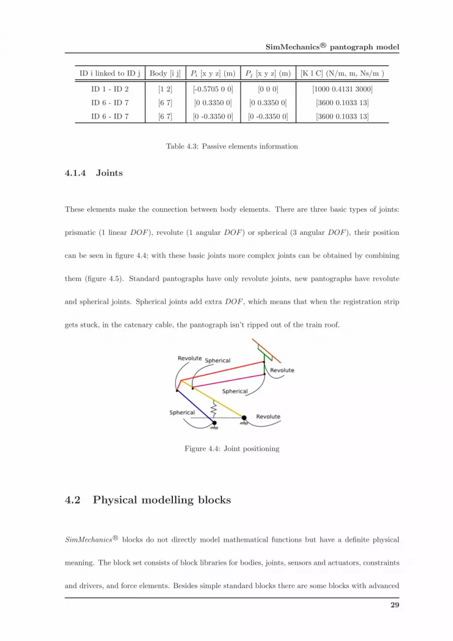
4.1.4 Joints
These elements make the connection between body elements. There are three basic types of joints:
prismatic (1 linear DOF ), revolute (1 angular DOF ) or spherical (3 angular DOF ), their position
can be seen in figure 4.4; with these basic joints more complex joints can be obtained by combining
them (figure 4.5). Standard pantographs have only revolute joints, new pantographs have revolute
and spherical joints. Spherical joints add extra DOF , which means that when the registration strip
gets stuck, in the catenary cable, the pantograph isn’t ripped out of the train roof.
Figure 4.4: Joint positioning
4.2 Physical modelling blocks
SimMechanics R© blocks do not directly model mathematical functions but have a definite physical
meaning. The block set consists of block libraries for bodies, joints, sensors and actuators, constraints
and drivers, and force elements. Besides simple standard blocks there are some blocks with advanced
29
4.3 Major Steps of the Dynamical Analysis
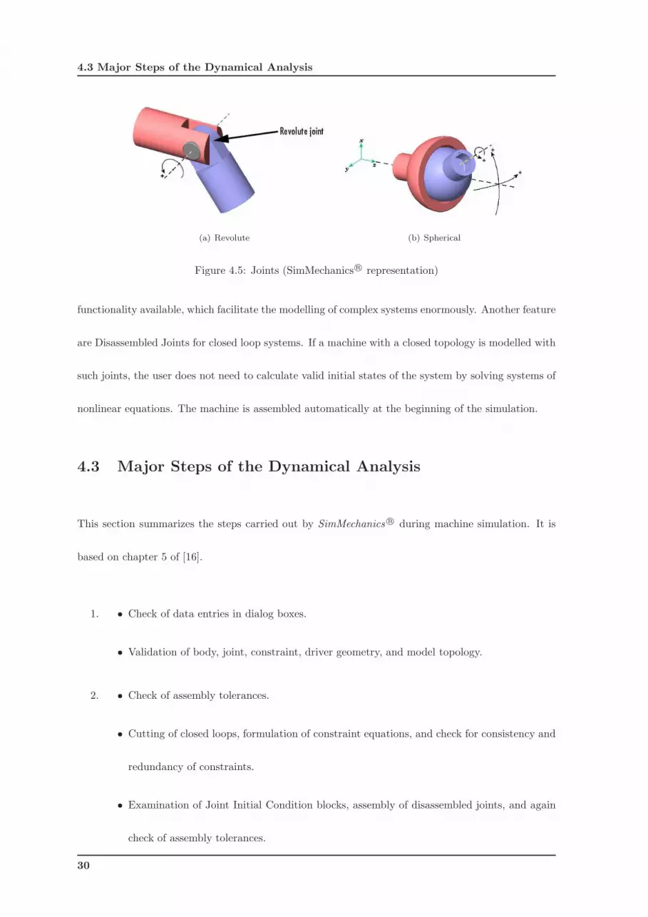
(a) Revolute (b) Spherical
Figure 4.5: Joints (SimMechanics R© representation)
functionality available, which facilitate the modelling of complex systems enormously. Another feature
are Disassembled Joints for closed loop systems. If a machine with a closed topology is modelled with
such joints, the user does not need to calculate valid initial states of the system by solving systems of
nonlinear equations. The machine is assembled automatically at the beginning of the simulation.
4.3 Major Steps of the Dynamical Analysis
This section summarizes the steps carried out by SimMechanics R© during machine simulation. It is
based on chapter 5 of [16].
1. • Check of data entries in dialog boxes.
• Validation of body, joint, constraint, driver geometry, and model topology.
2. • Check of assembly tolerances.
• Cutting of closed loops, formulation of constraint equations, and check for consistency and
redundancy of constraints.
• Examination of Joint Initial Condition blocks, assembly of disassembled joints, and again
check of assembly tolerances.
30
SimMechanics R© pantograph model
• Mode iteration for sticky joints.
3. • Forward Dynamics/ Trimming modes: Application of external torques and forces. Formu-
lation and integration of the equations of motion and solution for machine motion.
• Inverse Dynamics/ Kinematics modes: Application of motion constraints, drivers, actua-
tors. Formulation of equations of motion and solution for machine motion and actuator
torques and forces.
• After each time step in all analysis modes: check of assembly, constraint, and solver toler-
ances, constraint and driver consistency and joint axis singularities.
4.4 Creating a Pantograph in SimMechanics R©
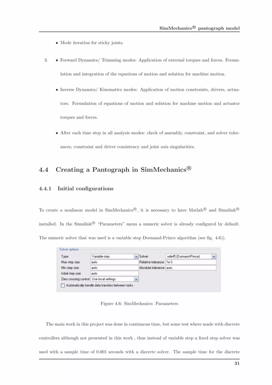
4.4.1 Initial configurations
To create a nonlinear model in SimMechanics R©, it is necessary to have Matlab R© and Simulink R©
installed. In the Simulink R© “Parameters” menu a numeric solver is already configured by default.
The numeric solver that was used is a variable step Dormand-Prince algorithm (see fig. 4.6)).
Figure 4.6: SimMechanics: Parameters
The main work in this project was done in continuous time, but some test where made with discrete
controllers although not presented in this work , thus instead of variable step a fixed step solver was
used with a sample time of 0.001 seconds with a discrete solver. The sample time for the discrete
31
4.4 Creating a Pantograph in SimMechanics R©
solver was obtained by finding the linear model poles of the open loop system. The most distant pole
found in successive model analysis was of 35 rad/s (see eq. 4.4.1).
T =1
f, f =
w
2π, sample time =
1
20f
For convenience, instead of the value obtained which is 0.00879 s, a more regular value for the
sample time is used, the value is 1 ms.
sample time = .00879 ≈ 0.001s
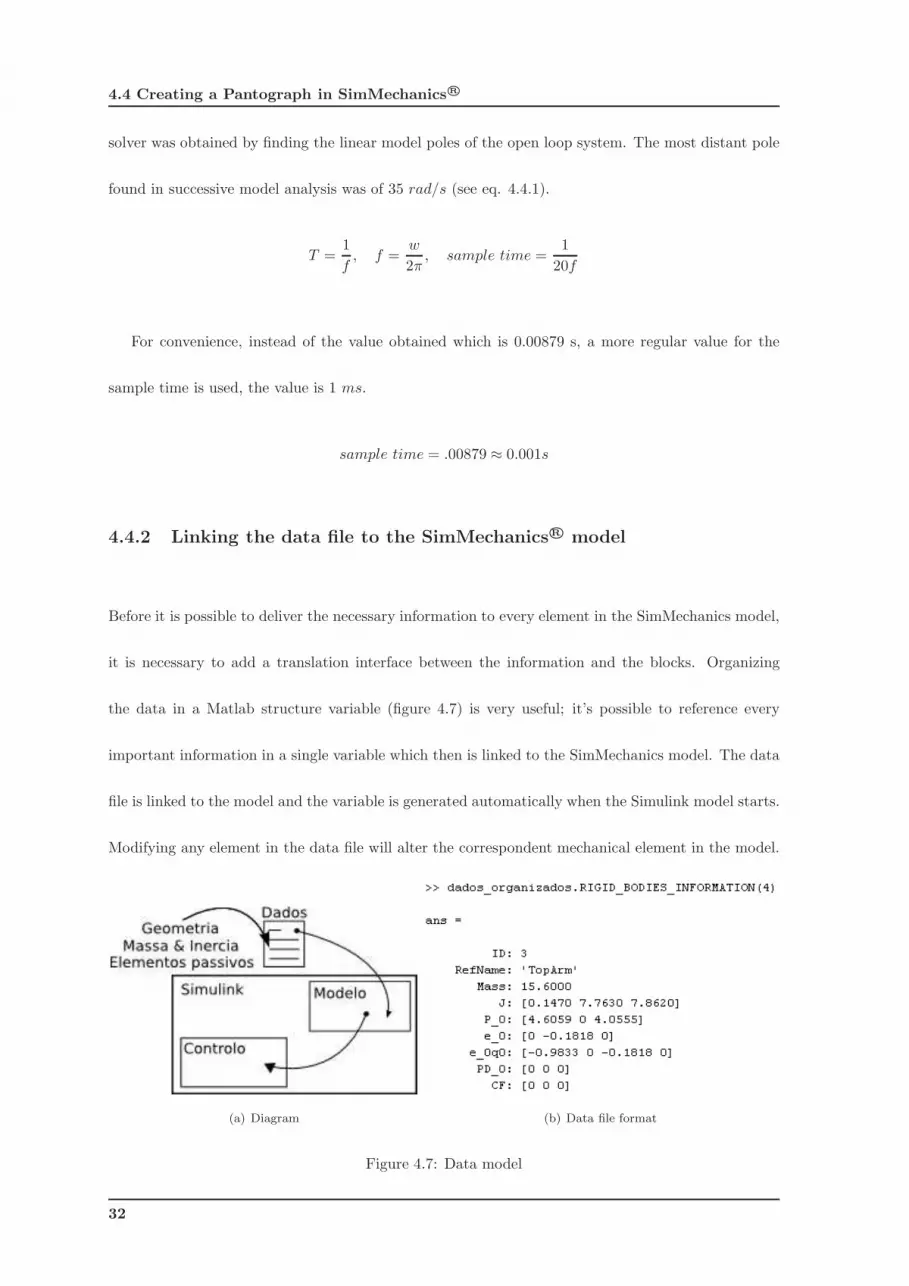
4.4.2 Linking the data file to the SimMechanicsR© model
Before it is possible to deliver the necessary information to every element in the SimMechanics model,
it is necessary to add a translation interface between the information and the blocks. Organizing
the data in a Matlab structure variable (figure 4.7) is very useful; it’s possible to reference every
important information in a single variable which then is linked to the SimMechanics model. The data
file is linked to the model and the variable is generated automatically when the Simulink model starts.
Modifying any element in the data file will alter the correspondent mechanical element in the model.
(a) Diagram (b) Data file format
Figure 4.7: Data model
32
SimMechanics R© pantograph model
4.4.3 SimMechanicsR© pantograph model
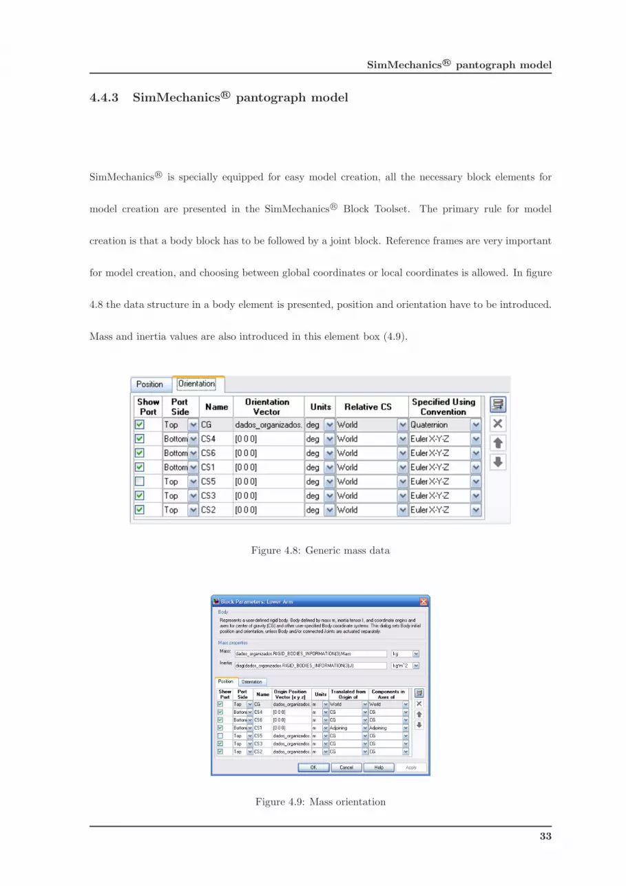
SimMechanics R© is specially equipped for easy model creation, all the necessary block elements for
model creation are presented in the SimMechanics R© Block Toolset. The primary rule for model
creation is that a body block has to be followed by a joint block. Reference frames are very important
for model creation, and choosing between global coordinates or local coordinates is allowed. In figure
4.8 the data structure in a body element is presented, position and orientation have to be introduced.
Mass and inertia values are also introduced in this element box (4.9).
Figure 4.8: Generic mass data
Figure 4.9: Mass orientation
33
4.4 Creating a Pantograph in SimMechanics R©
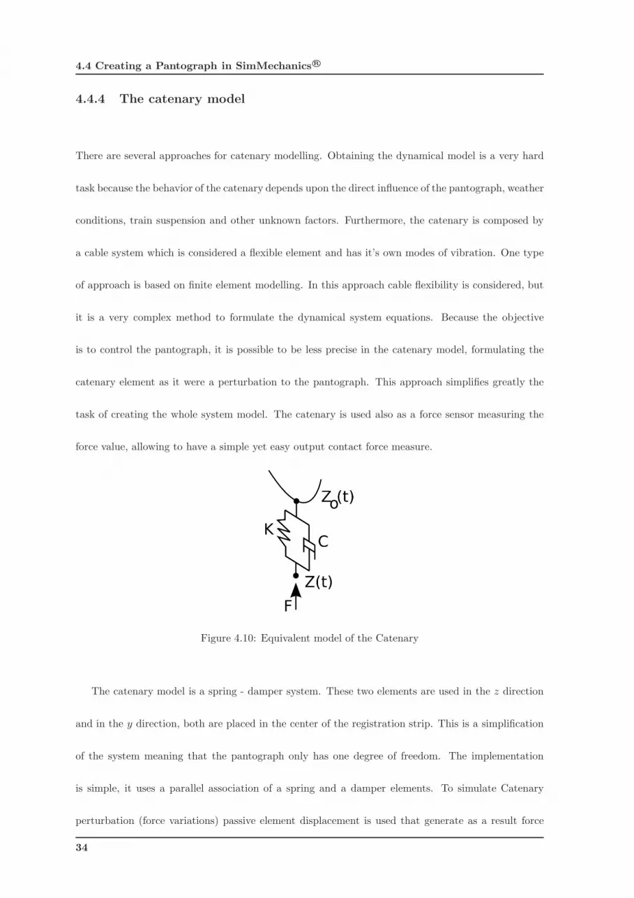
4.4.4 The catenary model
There are several approaches for catenary modelling. Obtaining the dynamical model is a very hard
task because the behavior of the catenary depends upon the direct influence of the pantograph, weather
conditions, train suspension and other unknown factors. Furthermore, the catenary is composed by
a cable system which is considered a flexible element and has it’s own modes of vibration. One type
of approach is based on finite element modelling. In this approach cable flexibility is considered, but
it is a very complex method to formulate the dynamical system equations. Because the objective
is to control the pantograph, it is possible to be less precise in the catenary model, formulating the
catenary element as it were a perturbation to the pantograph. This approach simplifies greatly the
task of creating the whole system model. The catenary is used also as a force sensor measuring the
force value, allowing to have a simple yet easy output contact force measure.
Figure 4.10: Equivalent model of the Catenary
The catenary model is a spring - damper system. These two elements are used in the z direction
and in the y direction, both are placed in the center of the registration strip. This is a simplification
of the system meaning that the pantograph only has one degree of freedom. The implementation
is simple, it uses a parallel association of a spring and a damper elements. To simulate Catenary
perturbation (force variations) passive element displacement is used that generate as a result force
34

SimMechanics R© pantograph model
variations. The implementation follows in figure 4.11 and it’s global positioning in the pantograph.
F = K [z − z0(t)] + C [z − z0(t)] (4.1)
(a) Positioning (b) Detail
Figure 4.11: Catenary representation
An important note is that K and C (spring and damper constants) can be altered in time which
can make the simulation more realistic. To simplify the model, K and C were considered constant over
time. Furthermore, F is the contact force between the pantograph and the catenary. The position z
is the height of the registration strip and z0 is the initial position of the registration strip.
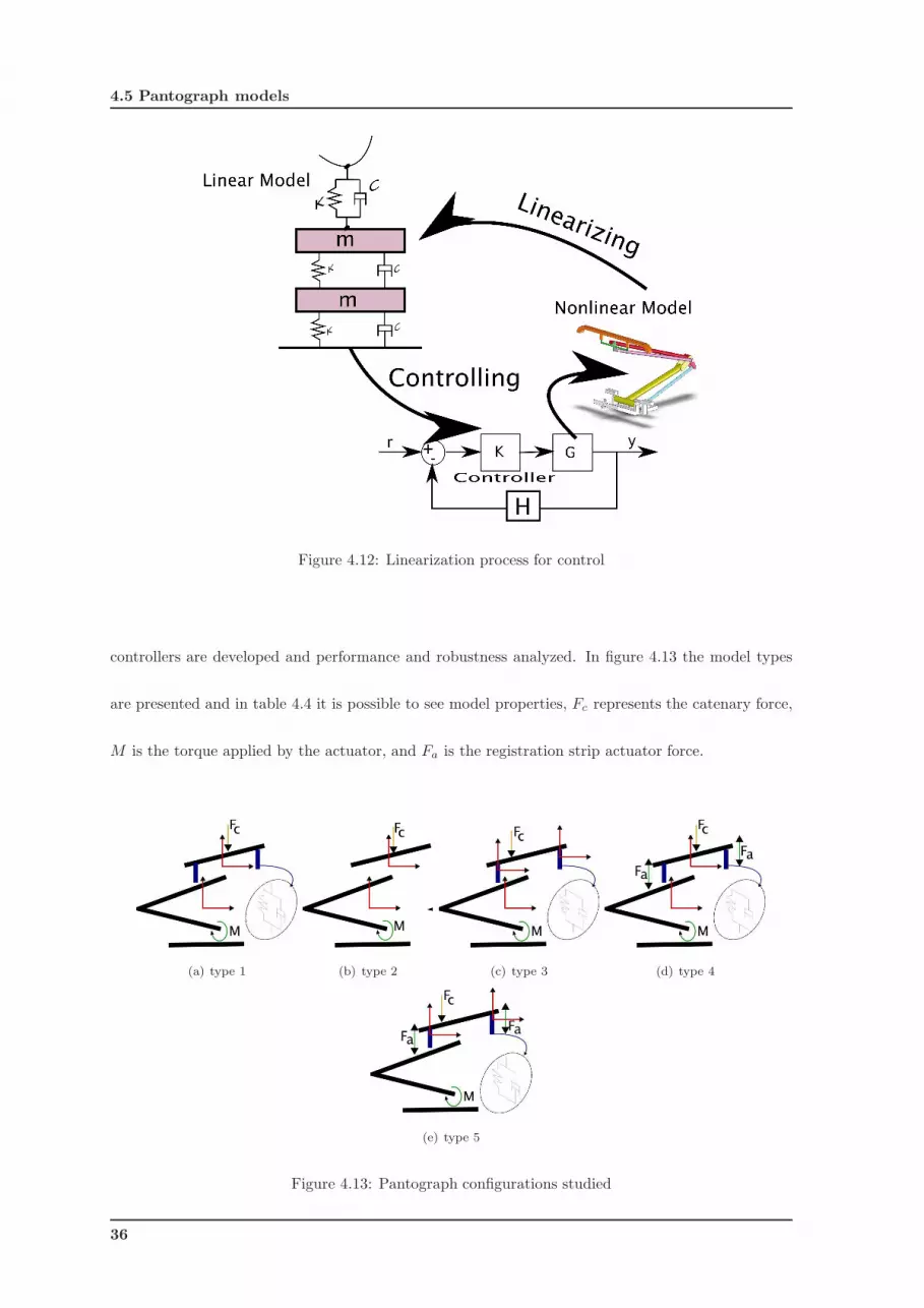
4.5 Pantograph models
A correct model of the pantograph means that the contact interface has to be as realistic as possible.
A progressive complexity approach was used to obtain the nonlinear model and thus the pantograph
dynamics. Nonlinear models are more complex to study, and in order to simplify the system, lin-
earization is used. All linear models are obtained in the nominal conditions, the process can be seen
in figure 4.12.
In order to analyze the pantograph five different types of pantographs are studied. Model and
35
4.5 Pantograph models
Figure 4.12: Linearization process for control
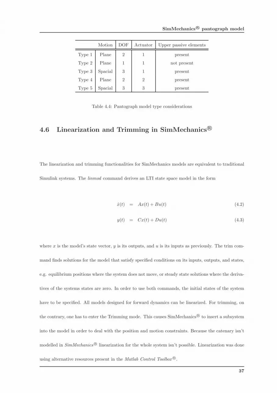
controllers are developed and performance and robustness analyzed. In figure 4.13 the model types
are presented and in table 4.4 it is possible to see model properties, Fc represents the catenary force,
M is the torque applied by the actuator, and Fa is the registration strip actuator force.
(a) type 1 (b) type 2 (c) type 3 (d) type 4
(e) type 5
Figure 4.13: Pantograph configurations studied
36
SimMechanics R© pantograph model
Motion DOF Actuator Upper passive elements
Type 1 Plane 2 1 present
Type 2 Plane 1 1 not present
Type 3 Spacial 3 1 present
Type 4 Plane 2 2 present
Type 5 Spacial 3 3 present
Table 4.4: Pantograph model type considerations
4.6 Linearization and Trimming in SimMechanics R©
The linearization and trimming functionalities for SimMechanics models are equivalent to traditional
Simulink systems. The linmod command derives an LTI state space model in the form
x(t) = Ax(t) + Bu(t) (4.2)
y(t) = Cx(t) + Du(t) (4.3)
where x is the model’s state vector, y is its outputs, and u is its inputs as previously. The trim com-
mand finds solutions for the model that satisfy specified conditions on its inputs, outputs, and states,
e.g. equilibrium positions where the system does not move, or steady state solutions where the deriva-
tives of the systems states are zero. In order to use both commands, the initial states of the system
have to be specified. All models designed for forward dynamics can be linearized. For trimming, on
the contrary, one has to enter the Trimming mode. This causes SimMechanics R© to insert a subsystem
into the model in order to deal with the position and motion constraints. Because the catenary isn’t
modelled in SimMechanics R© linearization for the whole system isn’t possible. Linearization was done
using alternative resources present in the Matlab Control Toolbox R©.
37

4.7 Visualization Tools
4.7 Visualization Tools
SimMechanics R© offers two ways to visualize and animate machines. One is the build-in Handle
Graphics tool, which uses the standard Handle Graphics facilities known from Matlab with some
special features unique to SimMechanics. It can be used while building the model as a guide in
the assembly process. If a body is added or changed in the block diagram, it is also automatically
added or changed in the figure window. This gives immediate feedback and is especially helpful for
new users or for complex systems. The visualization tool can also be used to animate the motion
of the system during simulation. This can be much more expressive than ordinary plots of motion
variables over time. The drawback is a considerably increased in computation time if the animation
functionality is used. The bodies of the machine can be represented as convex hulls. These are surfaces
of minimum area with convex curvature that pass through or surrounds all of the points fixed on a
body. The visualization of an entire machine is the set of the convex hulls of all its bodies. More
realistic renderings of bodies are possible if the Virtual Reality Toolbox R© for Matlab R© is installed.
Arbitrary virtual worlds can be designed with the Virtual Reality Modelling Language (VRML) and
interfaced to the SimMechanics R© model.
4.8 Virtual model and world creation
The main application for model building and world creation is VR Builder. This is an old application
but it’s the application that is bundled with Matlab. The problem of creating the pantograph’s
elements in VR Builder is that it isn’t a very good element creator. To bypass this problem the usage
of SolidWorks for element creation makes it an easier solution for the creation of individual pantograph
elements; this approach has the advantage of using some of SolidWorks R© advanced functions for
38
SimMechanics R© pantograph model
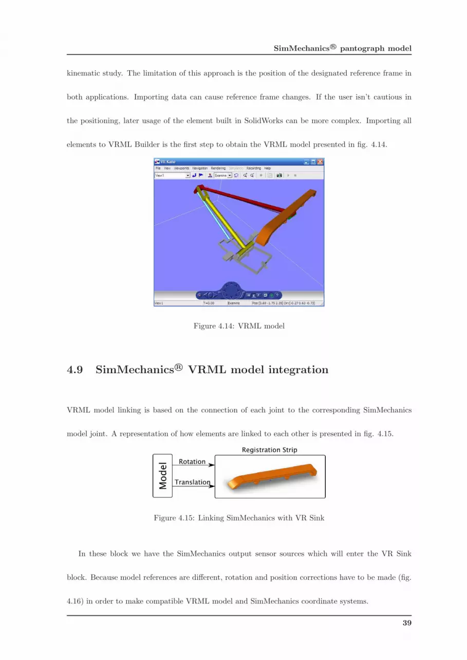
kinematic study. The limitation of this approach is the position of the designated reference frame in
both applications. Importing data can cause reference frame changes. If the user isn’t cautious in
the positioning, later usage of the element built in SolidWorks can be more complex. Importing all
elements to VRML Builder is the first step to obtain the VRML model presented in fig. 4.14.
Figure 4.14: VRML model
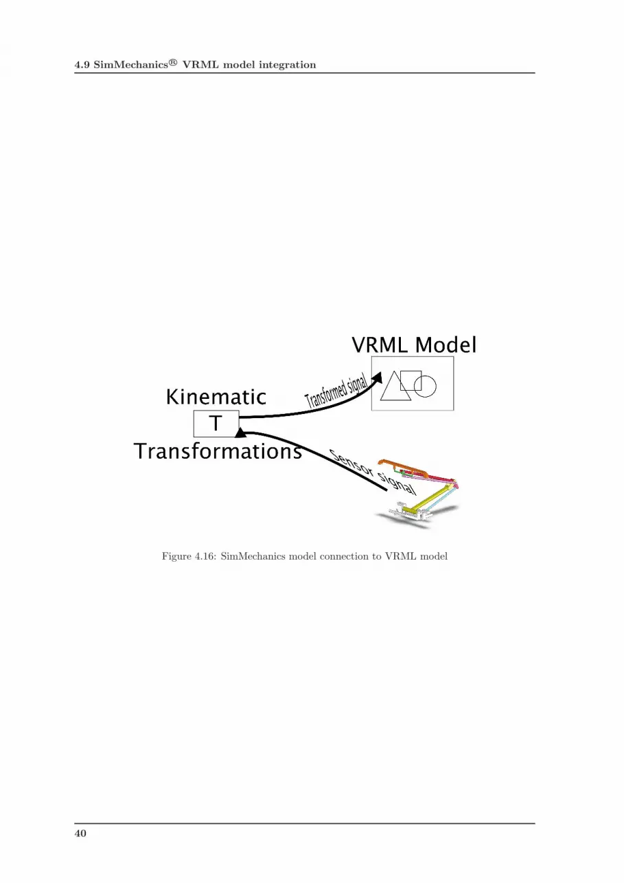
4.9 SimMechanics R© VRML model integration
VRML model linking is based on the connection of each joint to the corresponding SimMechanics
model joint. A representation of how elements are linked to each other is presented in fig. 4.15.
Figure 4.15: Linking SimMechanics with VR Sink
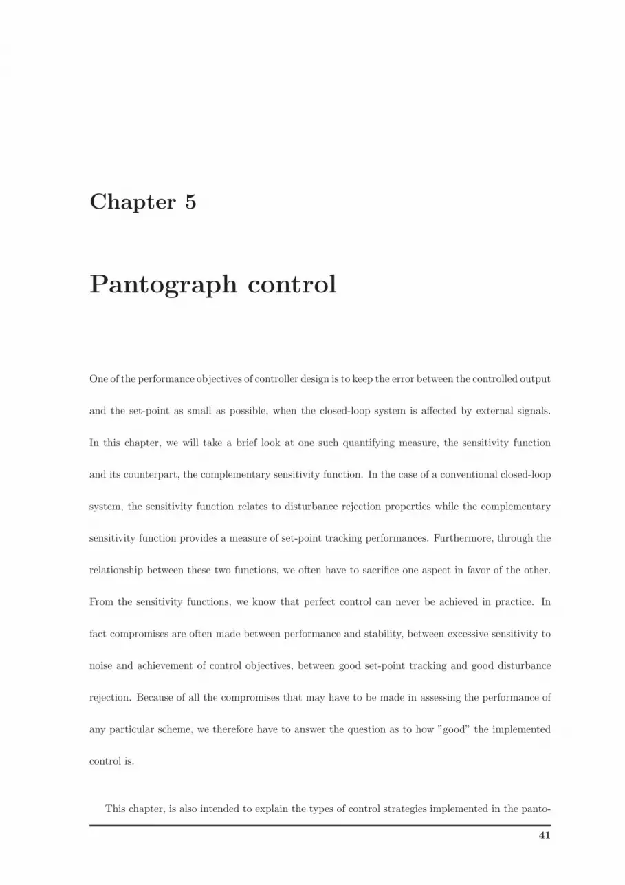
In these block we have the SimMechanics output sensor sources which will enter the VR Sink
block. Because model references are different, rotation and position corrections have to be made (fig.
4.16) in order to make compatible VRML model and SimMechanics coordinate systems.
39
4.9 SimMechanics R© VRML model integration
Figure 4.16: SimMechanics model connection to VRML model
40
Chapter 5
Pantograph control
One of the performance objectives of controller design is to keep the error between the controlled output
and the set-point as small as possible, when the closed-loop system is affected by external signals.
In this chapter, we will take a brief look at one such quantifying measure, the sensitivity function
and its counterpart, the complementary sensitivity function. In the case of a conventional closed-loop
system, the sensitivity function relates to disturbance rejection properties while the complementary
sensitivity function provides a measure of set-point tracking performances. Furthermore, through the
relationship between these two functions, we often have to sacrifice one aspect in favor of the other.
From the sensitivity functions, we know that perfect control can never be achieved in practice. In
fact compromises are often made between performance and stability, between excessive sensitivity to
noise and achievement of control objectives, between good set-point tracking and good disturbance
rejection. Because of all the compromises that may have to be made in assessing the performance of
any particular scheme, we therefore have to answer the question as to how ”good” the implemented
control is.
This chapter, is also intended to explain the types of control strategies implemented in the panto-
41
5.1 Introduction to robust controllers
graph. A simple PID controller was implemented as a term of comparison with the robust controllers
developed. Two types of robust controllers were studied H2 and H∞. A key reason for using feed-
back is to reduce the effects of uncertainty which may appear in different forms as disturbances or as
other imperfections in the models used to design the feedback law. Model uncertainty and robustness
have been a central theme in the development of the field of automatic control. H2 or H∞ control
techniques belong to a wider class of robust control techniques. The aim of this class of controllers is
to prevent the negative consequences on closed-loop performances of uncertainties affecting the plant
model.
5.1 Introduction to robust controllers
5.1.1 Robust control preliminaries
From [20], ”Robust control refers to the control of unknown plants with unknown dynamics subject to
unknown disturbances”. Clearly, the key issue with robust control systems is uncertainty and how the
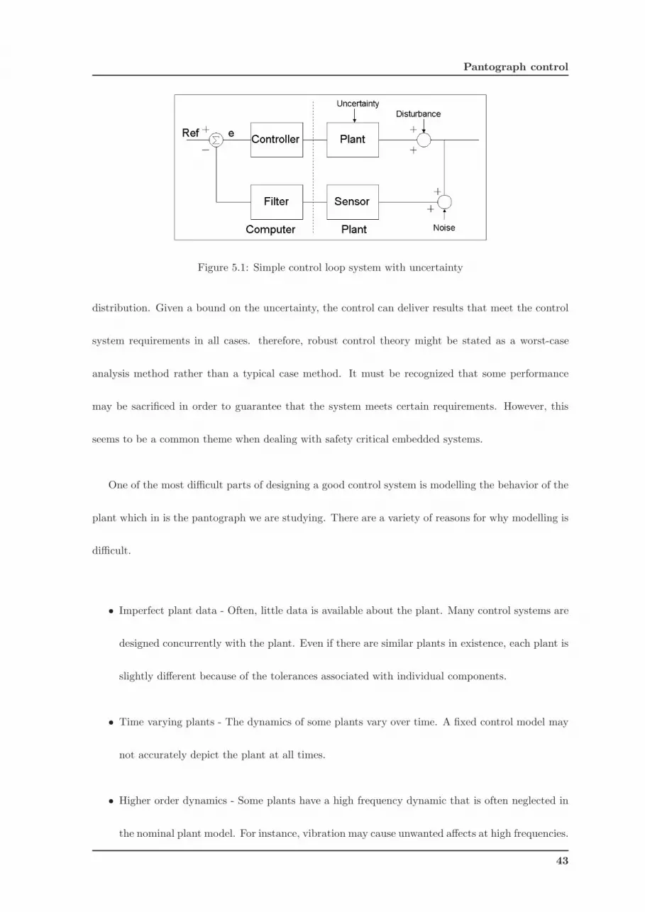
control system can deal with this problem. Figure 5.1 shows an expanded view of the simple control
loop. Uncertainty is shown entering the system in three places. There is uncertainty in the model of
the plant. There are disturbances that occur in the plant system. Also there is noise which is read on
the sensor inputs. Each of these uncertainties can have an additive or multiplicative component.
From fig. 5.1 we can see the separation of the computer control system with that of the plant. It
is important to understand that the control system designer has little control of the uncertainty in
the plant. The designer creates a control system that is based on a model of the plant. However, the
implemented control system must interact with the actual plant, not the model of the plant.
Robust control methods seek to bound the uncertainty rather than express it in the form of a
42
Pantograph control
Figure 5.1: Simple control loop system with uncertainty
distribution. Given a bound on the uncertainty, the control can deliver results that meet the control
system requirements in all cases. therefore, robust control theory might be stated as a worst-case
analysis method rather than a typical case method. It must be recognized that some performance
may be sacrificed in order to guarantee that the system meets certain requirements. However, this
seems to be a common theme when dealing with safety critical embedded systems.
One of the most difficult parts of designing a good control system is modelling the behavior of the
plant which in is the pantograph we are studying. There are a variety of reasons for why modelling is
difficult.
• Imperfect plant data - Often, little data is available about the plant. Many control systems are
designed concurrently with the plant. Even if there are similar plants in existence, each plant is
slightly different because of the tolerances associated with individual components.
• Time varying plants - The dynamics of some plants vary over time. A fixed control model may
not accurately depict the plant at all times.
• Higher order dynamics - Some plants have a high frequency dynamic that is often neglected in
the nominal plant model. For instance, vibration may cause unwanted affects at high frequencies.
43

5.1 Introduction to robust controllers
Sometimes this dynamic is unknown and sometimes it is deliberately ignored in order to simplify
the model.
• Non-linearity - Most control systems are designed assuming linear time invariant systems. This
is done because it greatly simplifies the analysis of the system. However, all of the systems
encountered in the real world have some non-linear component. Thus the model will always be
an approximation of the real world behavior.
• Complexity - Mechanical and electrical systems are inherently complex to model. Even a simple
system requires complex differential equations to describe its behavior.
The issue for modeling is to synthesize a model that is simple enough to implement within these
constraints but performs accurately enough to meet the performance requirements with a simple
model which is insensitive to uncertainty. This simplification of the plant model is often referred to
as model reduction. A more detailed treatment of modelling for a variety of physical system types
can be found in [21]. In this work modelling is done with SimMechanics and thus all computational
related problems where dealt by this application.
One technique for handling the model uncertainty that often occurs at high frequencies is to balance
performance and robustness in the system through gain scheduling. A high gain means that the system
will respond quickly to differences between the desired state and the actual state of the plant. At
low frequencies where the plant is accurately modelled, this high gain results in high performance
of the system. This region of operation is called the performance band. At high frequencies where
the plant is not modelled accurately, the gain is lower. A low gain at high frequencies results in a
larger error term between the measured output and the reference signal. This region is called the
robustness band. In this region the feedback from the output is essentially ignored. This involves
44
Pantograph control
setting the poles and zeros of the controller transfer function to achieve a filter. Between these two
regions, performance and robustness, there is a transition region. In this region the controller does not
perform well for either performance or robustness. The transition region cannot be made arbitrarily
small because it depends on the number of poles and zeros of the transfer function. Adding terms to
the transfer function increases the complexity of the control system. Thus, there is a trade-off between
the simplicity of the model and the minimal size of the transition band. Gain scheduling is covered
by [22]
5.1.2 The sensitivity function
The sensitivity function S(s) that we will use is defined in the Laplace domain as:
S(s) ,E(s)
R(s) − d(s)
where the symbol “,“ is used to denote ”definition”. Thus the sensitivity function, S(s), relates the
external inputs, R(s) and d(s), to the feedback error E(s) (fig. 5.2). Notice, however, that it does not
take into account the effects caused by the noise, N(s) (see [23] on pag. 34).
Figure 5.2: Schematic of conventional feedback control loop
45
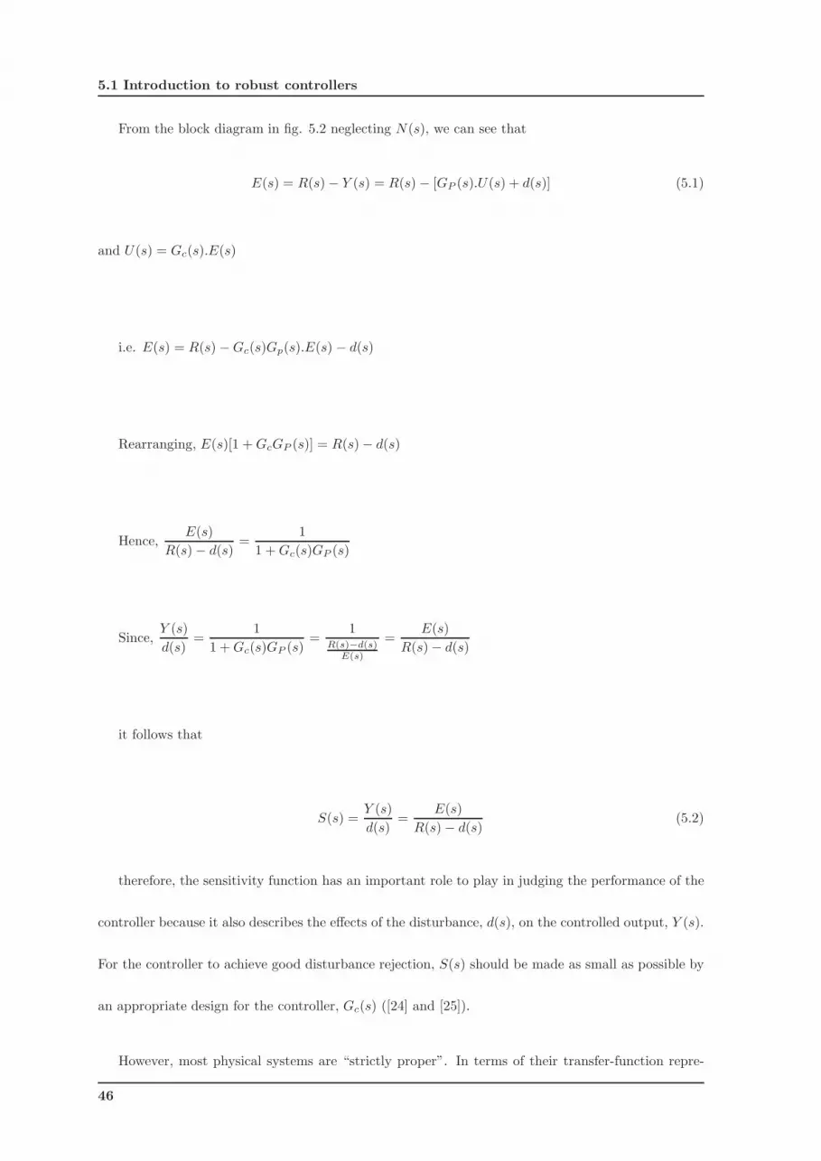
5.1 Introduction to robust controllers
From the block diagram in fig. 5.2 neglecting N(s), we can see that
E(s) = R(s) − Y (s) = R(s) − [GP (s).U(s) + d(s)] (5.1)
and U(s) = Gc(s).E(s)
i.e. E(s) = R(s) − Gc(s)Gp(s).E(s) − d(s)
Rearranging, E(s)[1 + GcGP (s)] = R(s) − d(s)
Hence,E(s)
R(s) − d(s)=
1
1 + Gc(s)GP (s)
Since,Y (s)
d(s)=
1
1 + Gc(s)GP (s)=
1R(s)−d(s)
E(s)
=E(s)
R(s) − d(s)
it follows that
S(s) =Y (s)
d(s)=
E(s)
R(s) − d(s)(5.2)
therefore, the sensitivity function has an important role to play in judging the performance of the
controller because it also describes the effects of the disturbance, d(s), on the controlled output, Y (s).
For the controller to achieve good disturbance rejection, S(s) should be made as small as possible by
an appropriate design for the controller, Gc(s) ([24] and [25]).
However, most physical systems are “strictly proper”. In terms of their transfer-function repre-
46
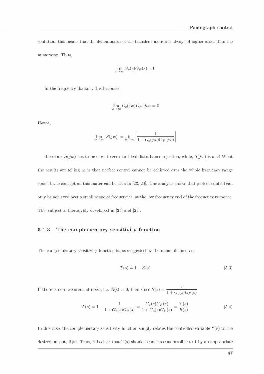
Pantograph control
sentation, this means that the denominator of the transfer function is always of higher order than the
numerator. Thus,
lims→∞
Gc(s)GP (s) = 0
In the frequency domain, this becomes
limw→∞
Gc(jw)GP (jw) = 0
Hence,
limw→∞
|S(jw)| = limw→∞
∣
∣
∣
∣
1
1 + Gc(jw)GP (jw)
∣
∣
∣
∣
therefore, S(jw) has to be close to zero for ideal disturbance rejection, while, S(jw) is one! What
the results are telling us is that perfect control cannot be achieved over the whole frequency range
some, basic concept on this mater can be seen in [23, 26]. The analysis shows that perfect control can
only be achieved over a small range of frequencies, at the low frequency end of the frequency response.
This subject is thoroughly developed in [24] and [25].
5.1.3 The complementary sensitivity function
The complementary sensitivity function is, as suggested by the name, defined as:
T (s) , 1 − S(s) (5.3)
If there is no measurement noise, i.e. N(s) = 0, then since S(s) =1
1 + Gc(s)GP (s)
T (s) = 1 −1
1 + Gc(s)GP (s)=
Gc(s)GP (s)
1 + Gc(s)GP (s)=
Y (s)
R(s)(5.4)
In this case, the complementary sensitivity function simply relates the controlled variable Y(s) to the
desired output, R(s). Thus, it is clear that T(s) should be as close as possible to 1 by an appropriate
47
5.1 Introduction to robust controllers
choice of the controller. Again, since most physical processes are strictly proper in the open-loop, i.e.
lims→∞
Gc(s)GP (s) = 0
this means that, in the frequency domain,
limw→∞
|T (jw)| = limw→∞
∣
∣
∣
∣
Gc(jw)GP (jw)
1 + Gc(jw)GP (jw)
∣
∣
∣
∣
= 0
As in the case of the sensitivity function, S(jw), the desired value of the complementary sensitivity
function, T (jw), can be achieved only near low frequencies. This subject is thoroughly developed in
[24] and [25].
5.1.4 The trade-off
When there is process noise, in terms of process inputs and outputs, T (s) is also affected by N(s).
In this case, T (s) has to be made small so as to reduce the influence of random inputs on system
characteristics. In other words, we want T (s) ≈ 0 or equivalently, S(s) ≈ 1. Comparing this with the
noise free situation where we require T (s) ≈ 1 or S(s) ≈ 0. This illustrates the compromise that often
has to be made in control systems design: good set-point tracking and disturbance rejection has to
be traded off against suppression of process noise (see [26] on pag. 203).
5.1.5 Weighted sensitivity
The sensitivity function S is a very good indicator of closed-loop performance, both for SISO and
MIMO systems. The main advantage of considering S is that because we ideally want S small, it is
sufficient to consider just its magnitude. Typical specifications in terms of S include:
1. Minimum bandwidth frequency.
48
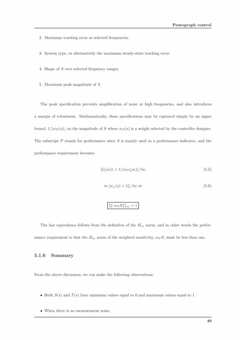
Pantograph control
2. Maximum tracking error at selected frequencies.
3. System type, or alternatively the maximum steady-state tracking error.
4. Shape of S over selected frequency ranges.
5. Maximum peak magnitude of S.
The peak specification prevents amplification of noise at high frequencies, and also introduces
a margin of robustness. Mathematically, these specifications may be captured simply by an upper
bound, 1/|wP (s)|, on the magnitude of S where wP (s) is a weight selected by the controller designer.
The subscript P stands for performance since S is mainly used as a performance indicator, and the
performance requirement becomes
|L(jw)| < 1/|wP (jw)|, ∀w (5.5)
⇔ |wP(s) < 1‖, ∀w ⇔ (5.6)
‖‖ wP S‖‖∞ < 1
The last equivalence follows from the definition of the H∞ norm, and in other words the perfor-
mance requirement is that the H∞ norm of the weighted sensitivity, wP S, must be less than one.
5.1.6 Summary
From the above discussion, we can make the following observations:
• Both S(s) and T (s) have minimum values equal to 0 and maximum values equal to 1
• When there is no measurement noise,
49
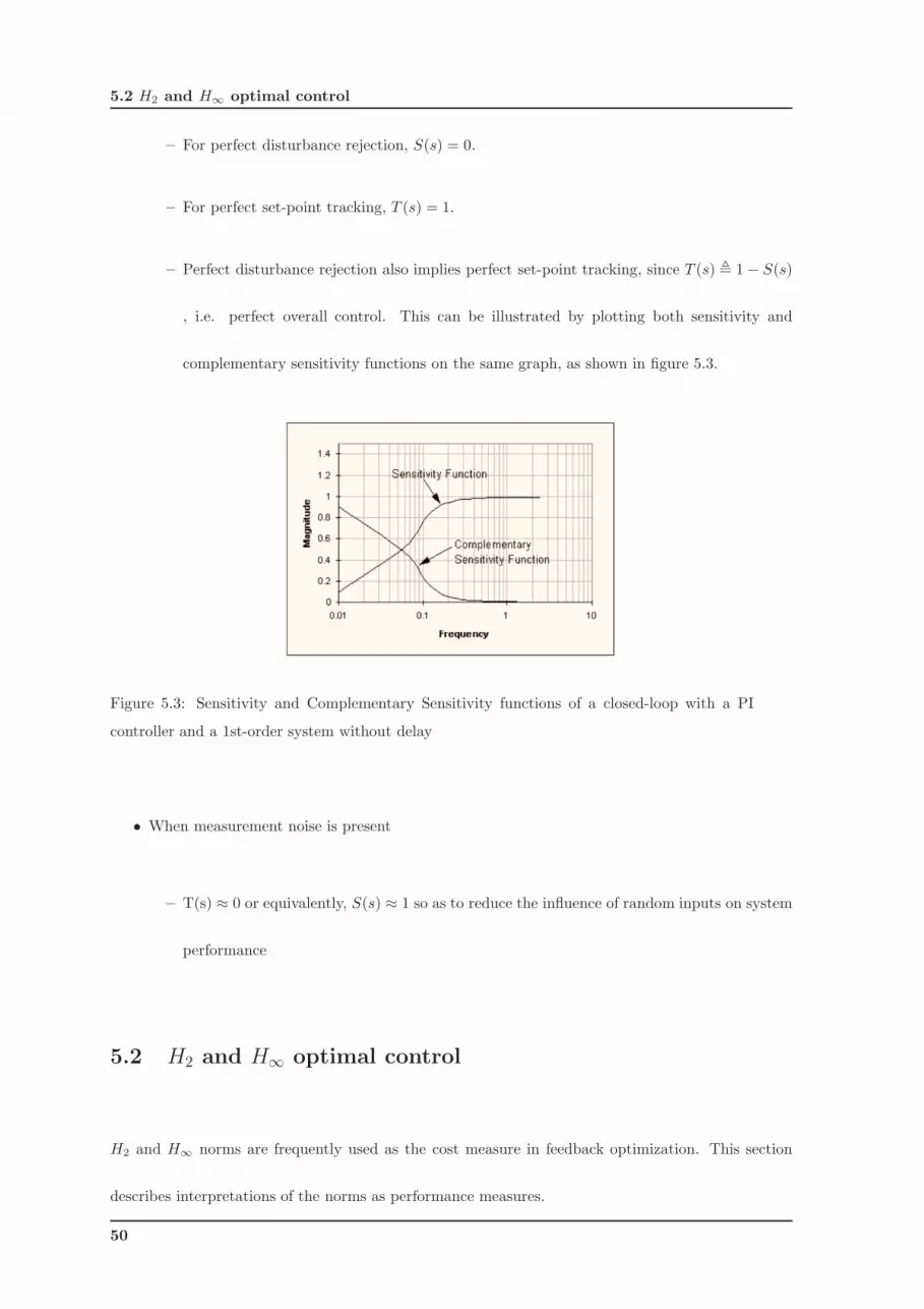
5.2 H2 and H∞ optimal control
– For perfect disturbance rejection, S(s) = 0.
– For perfect set-point tracking, T (s) = 1.
– Perfect disturbance rejection also implies perfect set-point tracking, since T (s) , 1 − S(s)
, i.e. perfect overall control. This can be illustrated by plotting both sensitivity and
complementary sensitivity functions on the same graph, as shown in figure 5.3.
Figure 5.3: Sensitivity and Complementary Sensitivity functions of a closed-loop with a PI
controller and a 1st-order system without delay
• When measurement noise is present
– T(s) ≈ 0 or equivalently, S(s) ≈ 1 so as to reduce the influence of random inputs on system
performance
5.2 H2 and H∞ optimal control
H2 and H∞ norms are frequently used as the cost measure in feedback optimization. This section
describes interpretations of the norms as performance measures.
50
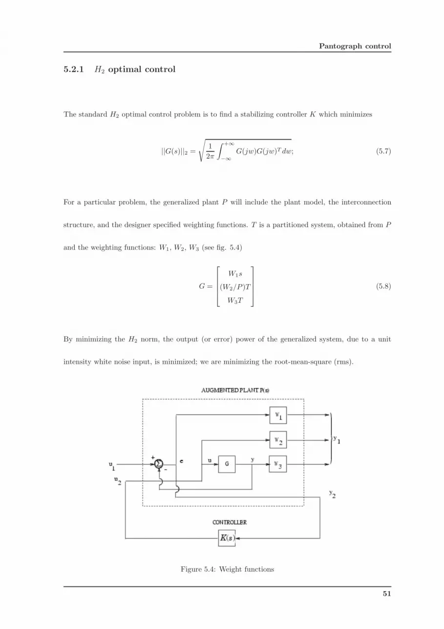
Pantograph control
5.2.1 H2 optimal control
The standard H2 optimal control problem is to find a stabilizing controller K which minimizes
||G(s)||2 =
√
1
2π
∫ +∞
−∞
G(jw)G(jw)T dw; (5.7)
For a particular problem, the generalized plant P will include the plant model, the interconnection
structure, and the designer specified weighting functions. T is a partitioned system, obtained from P
and the weighting functions: W1, W2, W3 (see fig. 5.4)
G =
W1s
(W2/P )T
W3T
(5.8)
By minimizing the H2 norm, the output (or error) power of the generalized system, due to a unit
intensity white noise input, is minimized; we are minimizing the root-mean-square (rms).
Figure 5.4: Weight functions
51
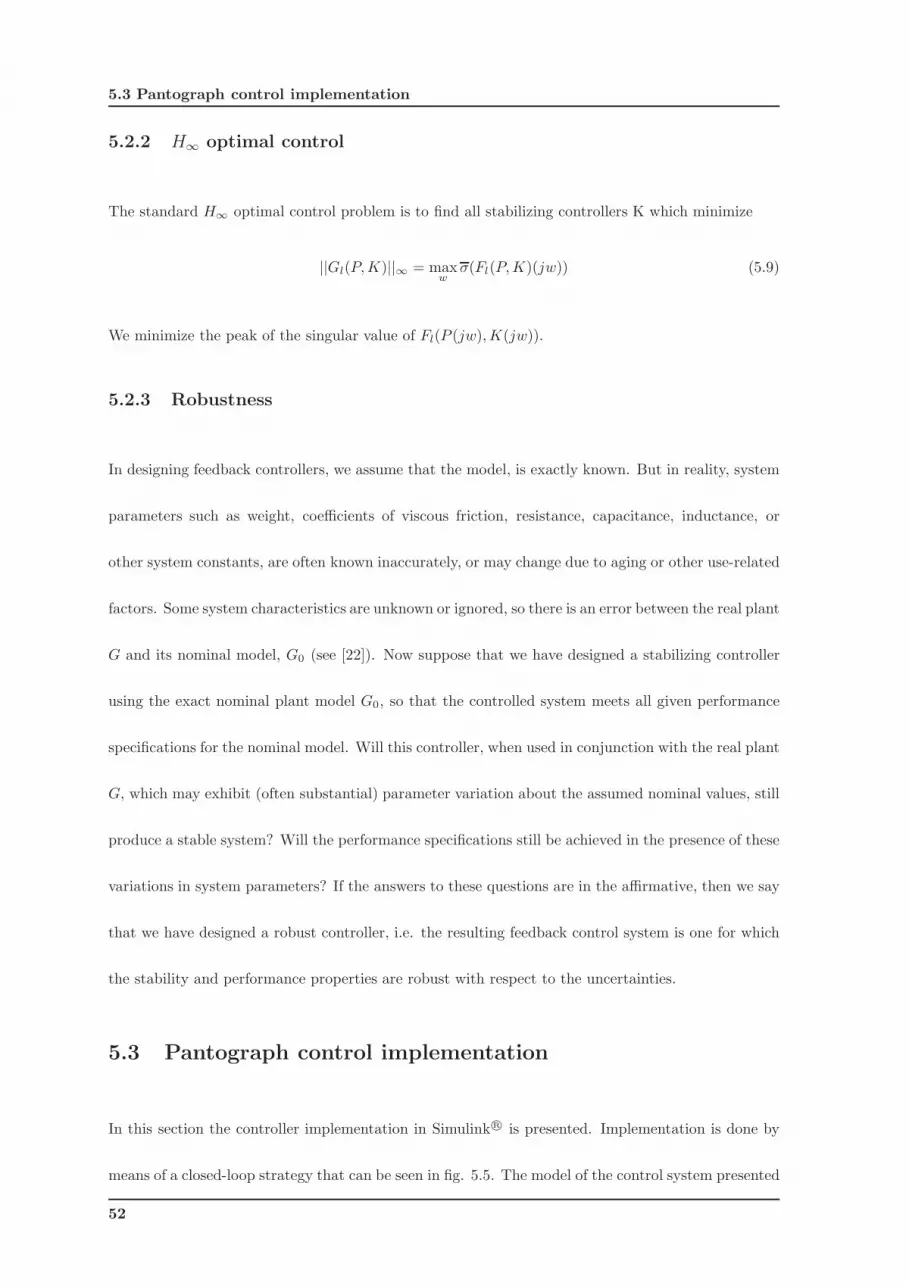
5.3 Pantograph control implementation
5.2.2 H∞
optimal control
The standard H∞ optimal control problem is to find all stabilizing controllers K which minimize
||Gl(P, K)||∞ = maxw
σ(Fl(P, K)(jw)) (5.9)
We minimize the peak of the singular value of Fl(P (jw), K(jw)).
5.2.3 Robustness
In designing feedback controllers, we assume that the model, is exactly known. But in reality, system
parameters such as weight, coefficients of viscous friction, resistance, capacitance, inductance, or
other system constants, are often known inaccurately, or may change due to aging or other use-related
factors. Some system characteristics are unknown or ignored, so there is an error between the real plant
G and its nominal model, G0 (see [22]). Now suppose that we have designed a stabilizing controller
using the exact nominal plant model G0, so that the controlled system meets all given performance
specifications for the nominal model. Will this controller, when used in conjunction with the real plant
G, which may exhibit (often substantial) parameter variation about the assumed nominal values, still
produce a stable system? Will the performance specifications still be achieved in the presence of these
variations in system parameters? If the answers to these questions are in the affirmative, then we say
that we have designed a robust controller, i.e. the resulting feedback control system is one for which
the stability and performance properties are robust with respect to the uncertainties.
5.3 Pantograph control implementation
In this section the controller implementation in Simulink R© is presented. Implementation is done by
means of a closed-loop strategy that can be seen in fig. 5.5. The model of the control system presented
52
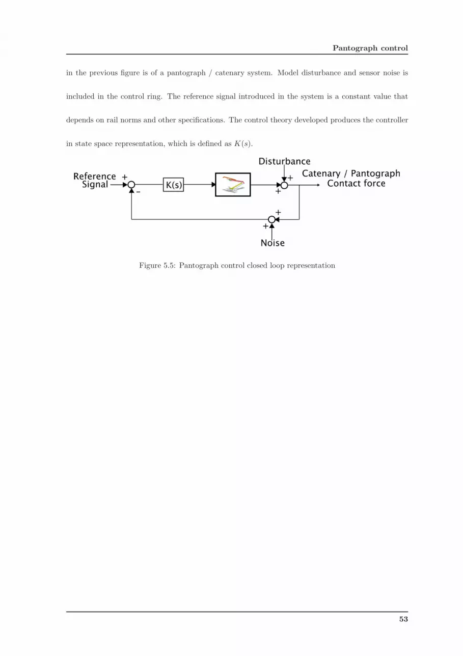
Pantograph control
in the previous figure is of a pantograph / catenary system. Model disturbance and sensor noise is
included in the control ring. The reference signal introduced in the system is a constant value that
depends on rail norms and other specifications. The control theory developed produces the controller
in state space representation, which is defined as K(s).
Figure 5.5: Pantograph control closed loop representation
53

5.3 Pantograph control implementation
54
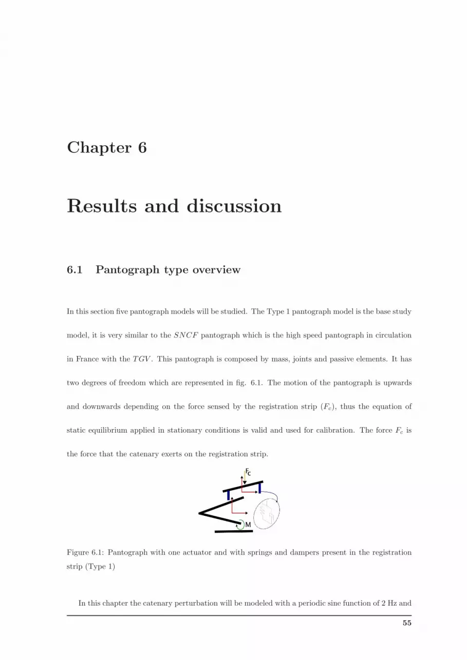
Chapter 6
Results and discussion
6.1 Pantograph type overview
In this section five pantograph models will be studied. The Type 1 pantograph model is the base study
model, it is very similar to the SNCF pantograph which is the high speed pantograph in circulation
in France with the TGV . This pantograph is composed by mass, joints and passive elements. It has
two degrees of freedom which are represented in fig. 6.1. The motion of the pantograph is upwards
and downwards depending on the force sensed by the registration strip (Fc), thus the equation of
static equilibrium applied in stationary conditions is valid and used for calibration. The force Fc is
the force that the catenary exerts on the registration strip.
Figure 6.1: Pantograph with one actuator and with springs and dampers present in the registration
strip (Type 1)
In this chapter the catenary perturbation will be modeled with a periodic sine function of 2 Hz and
55

6.2 Pantograph type overview
20 Hz or a step function. The amplitude of the perturbation signals are the same and of magnitude
of 10 cm. These settings apply to all experiments. The first experiments are for the Type 1 and type
3 pantographs, and all types of perturbations were used. From the first experiments two controller
settings were developed focusing robustness with poor performance and a second controller with better
performance but inferior robustness to model change. The second set of experiments tend to focus on
passive element presence. These sets of experiments were also made with the Type 1 and Type3 models
The third set of experiments was dedicated to study the model behavior due to physical parameter
changes The fourth set of experiments was to evaluate the performace of a double actuated pantograph
The fifth set of experiments was to test the Type 5 pantograph with a periodic perturbation function
and to understand isolated controller for top actuation, and combined lower and top actuation All sets
of tests use for control a PID controller or a robust controller. The final set of experiments confronts
the model obtained with the experimental results.
6.2 Pantograph type overview
The Type 2 pantograph, is a representative of a standard pantograph which is used in normal train
lines (CP or Fertagus transportation companies), to study their behavior and to suggest the best
physical implementation in terms of springs, dampers or actuated elements and to study the influence
in system dynamics. In the preceding chapter, robust controllers were developed and thoroughly
analyzed. With these results, a better understanding was gained over the controller limitations and
potentialities that can be used with high speed trains. The modelled registration strip, is attached to
the stabilization arm as can be seen in fig. 6.2 with no passive elements.
The Type 3 model purpose is to better simulate the motion of the catenary cable on top of the
56
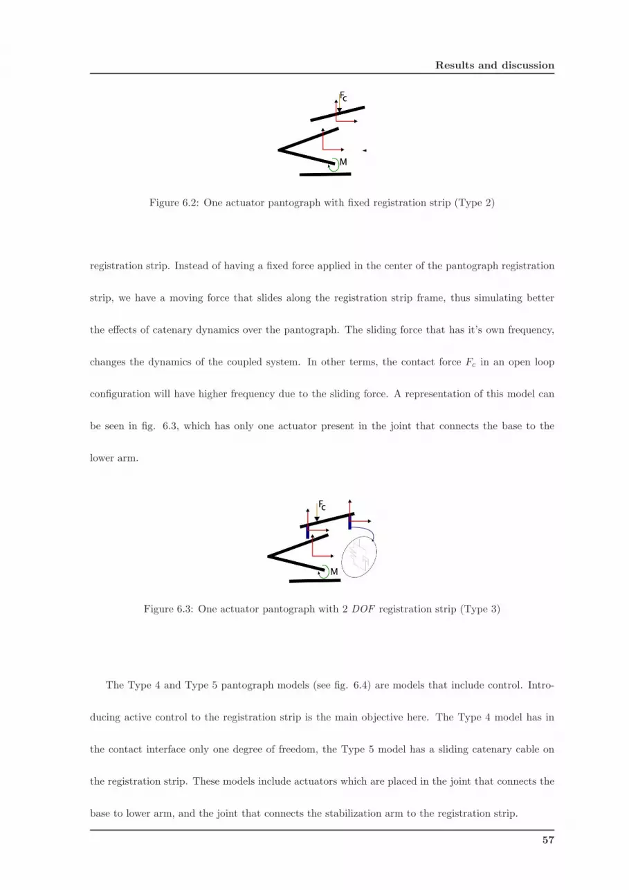
Results and discussion
Figure 6.2: One actuator pantograph with fixed registration strip (Type 2)
registration strip. Instead of having a fixed force applied in the center of the pantograph registration
strip, we have a moving force that slides along the registration strip frame, thus simulating better
the effects of catenary dynamics over the pantograph. The sliding force that has it’s own frequency,
changes the dynamics of the coupled system. In other terms, the contact force Fc in an open loop
configuration will have higher frequency due to the sliding force. A representation of this model can
be seen in fig. 6.3, which has only one actuator present in the joint that connects the base to the
lower arm.
Figure 6.3: One actuator pantograph with 2 DOF registration strip (Type 3)
The Type 4 and Type 5 pantograph models (see fig. 6.4) are models that include control. Intro-
ducing active control to the registration strip is the main objective here. The Type 4 model has in
the contact interface only one degree of freedom, the Type 5 model has a sliding catenary cable on
the registration strip. These models include actuators which are placed in the joint that connects the
base to lower arm, and the joint that connects the stabilization arm to the registration strip.
57
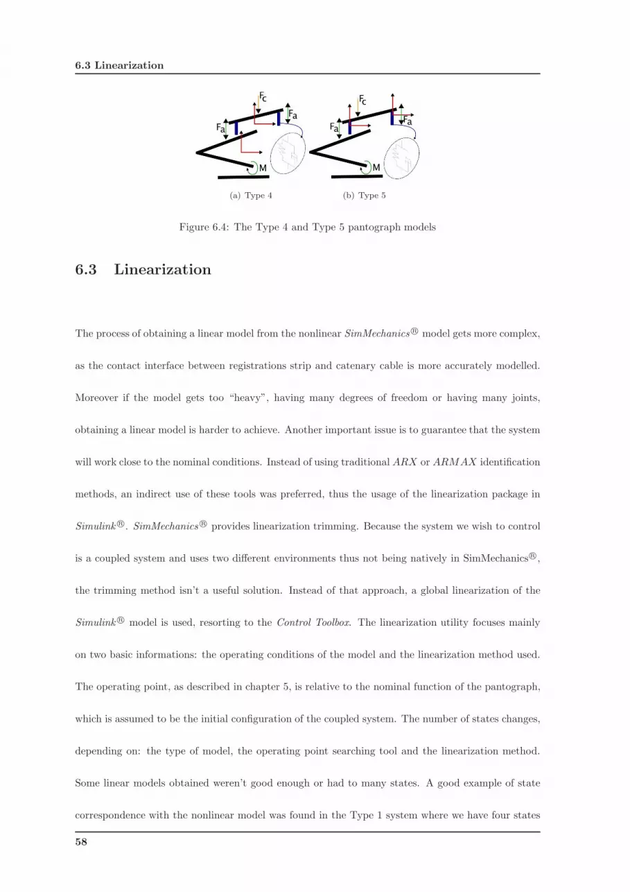
6.3 Linearization
(a) Type 4 (b) Type 5
Figure 6.4: The Type 4 and Type 5 pantograph models
6.3 Linearization
The process of obtaining a linear model from the nonlinear SimMechanics R© model gets more complex,
as the contact interface between registrations strip and catenary cable is more accurately modelled.
Moreover if the model gets too “heavy”, having many degrees of freedom or having many joints,
obtaining a linear model is harder to achieve. Another important issue is to guarantee that the system
will work close to the nominal conditions. Instead of using traditional ARX or ARMAX identification
methods, an indirect use of these tools was preferred, thus the usage of the linearization package in
Simulink R©. SimMechanics R© provides linearization trimming. Because the system we wish to control
is a coupled system and uses two different environments thus not being natively in SimMechanics R©,
the trimming method isn’t a useful solution. Instead of that approach, a global linearization of the
Simulink R© model is used, resorting to the Control Toolbox. The linearization utility focuses mainly
on two basic informations: the operating conditions of the model and the linearization method used.
The operating point, as described in chapter 5, is relative to the nominal function of the pantograph,
which is assumed to be the initial configuration of the coupled system. The number of states changes,
depending on: the type of model, the operating point searching tool and the linearization method.
Some linear models obtained weren’t good enough or had to many states. A good example of state
correspondence with the nonlinear model was found in the Type 1 system where we have four states
58
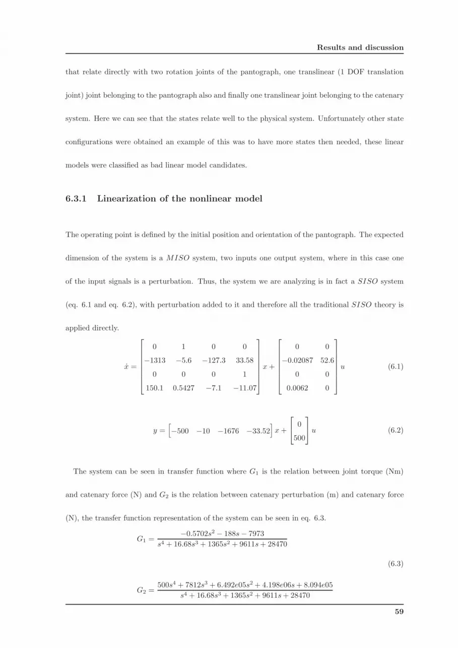
Results and discussion
that relate directly with two rotation joints of the pantograph, one translinear (1 DOF translation
joint) joint belonging to the pantograph also and finally one translinear joint belonging to the catenary
system. Here we can see that the states relate well to the physical system. Unfortunately other state
configurations were obtained an example of this was to have more states then needed, these linear
models were classified as bad linear model candidates.
6.3.1 Linearization of the nonlinear model
The operating point is defined by the initial position and orientation of the pantograph. The expected
dimension of the system is a MISO system, two inputs one output system, where in this case one
of the input signals is a perturbation. Thus, the system we are analyzing is in fact a SISO system
(eq. 6.1 and eq. 6.2), with perturbation added to it and therefore all the traditional SISO theory is
applied directly.
x =
0 1 0 0
−1313 −5.6 −127.3 33.58
0 0 0 1
150.1 0.5427 −7.1 −11.07
x +
0 0
−0.02087 52.6
0 0
0.0062 0
u (6.1)
y =[
−500 −10 −1676 −33.52]
x +
0
500
u (6.2)
The system can be seen in transfer function where G1 is the relation between joint torque (Nm)
and catenary force (N) and G2 is the relation between catenary perturbation (m) and catenary force
(N), the transfer function representation of the system can be seen in eq. 6.3.
G1 =−0.5702s2 − 188s− 7973
s4 + 16.68s3 + 1365s2 + 9611s + 28470
G2 =500s4 + 7812s3 + 6.492e05s2 + 4.198e06s + 8.094e05
s4 + 16.68s3 + 1365s2 + 9611s + 28470
(6.3)
59
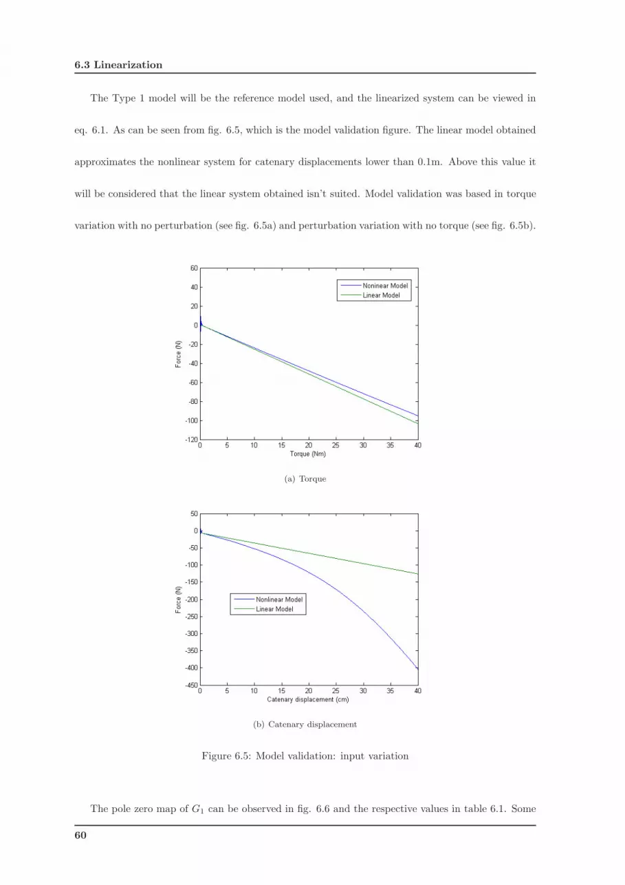
6.3 Linearization
The Type 1 model will be the reference model used, and the linearized system can be viewed in
eq. 6.1. As can be seen from fig. 6.5, which is the model validation figure. The linear model obtained
approximates the nonlinear system for catenary displacements lower than 0.1m. Above this value it
will be considered that the linear system obtained isn’t suited. Model validation was based in torque
variation with no perturbation (see fig. 6.5a) and perturbation variation with no torque (see fig. 6.5b).
(a) Torque
(b) Catenary displacement
Figure 6.5: Model validation: input variation
The pole zero map of G1 can be observed in fig. 6.6 and the respective values in table 6.1. Some
60
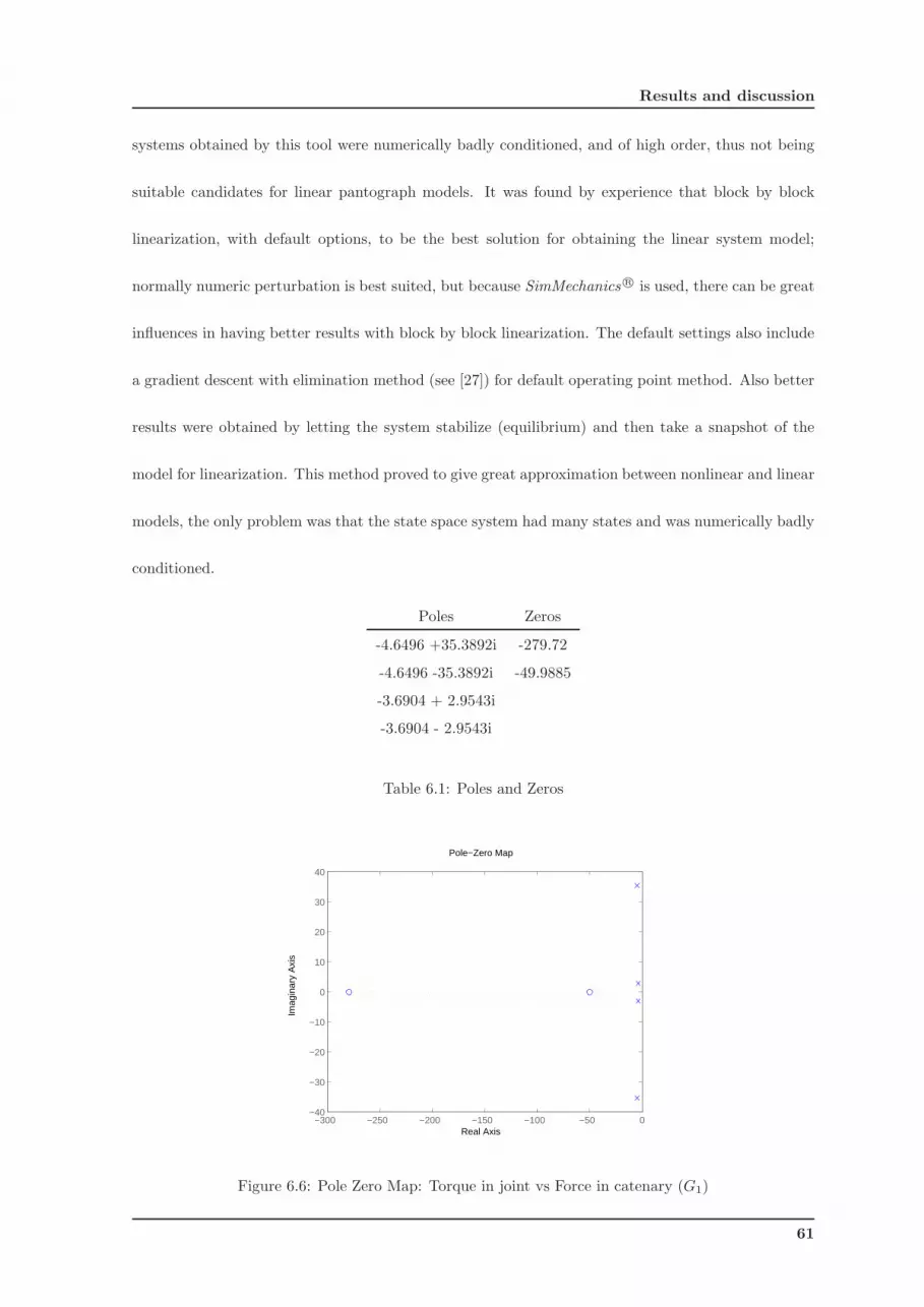
Results and discussion
systems obtained by this tool were numerically badly conditioned, and of high order, thus not being
suitable candidates for linear pantograph models. It was found by experience that block by block
linearization, with default options, to be the best solution for obtaining the linear system model;
normally numeric perturbation is best suited, but because SimMechanics R© is used, there can be great
influences in having better results with block by block linearization. The default settings also include
a gradient descent with elimination method (see [27]) for default operating point method. Also better
results were obtained by letting the system stabilize (equilibrium) and then take a snapshot of the
model for linearization. This method proved to give great approximation between nonlinear and linear
models, the only problem was that the state space system had many states and was numerically badly
conditioned.
Poles Zeros
-4.6496 +35.3892i -279.72
-4.6496 -35.3892i -49.9885
-3.6904 + 2.9543i
-3.6904 - 2.9543i
Table 6.1: Poles and Zeros
Pole−Zero Map
Real Axis
Imag
inar
y A
xis
−300 −250 −200 −150 −100 −50 0−40
−30
−20
−10
0
10
20
30
40
Figure 6.6: Pole Zero Map: Torque in joint vs Force in catenary (G1)
61

6.3 Linearization
To correctly introduce the linear model, pole-zero maps, controllability and observability analysis
had to be done. In fig. 6.6 and eq. 6.3 we can see that the system is stable in an open-loop
configuration alike the nonlinear model, and that it is observable and controllable. We can see that
rank(C) = 4 and that rank(O) = 4, this means the system is observable and controllable (see 5).
Controllability matrix
C =
0 −0.0208 0.3255 22.0641
−0.0208 0.3255 22.0641 −611.9188
0 0.0062 −0.0801 −2.1098
0.0062 −0.0801 −2.1098 84.7572
(6.4)
Observability matrix
O =
−500 −10 −1675.9778 −33.5196
8104.4101 −462.1093 1517.3624 −1640.6978
360743.1467 9805.6851 70788.1001 4163.1773
−12255792.3557 308038.4084 −1278405.276 353978.097
(6.5)
6.3.2 Conclusions from linearization
In this section, it was learned that the linear systems work in a small region. From table 6.2 is
shown that the catenary displacement varies about 3 cm. From this point it will be considered a
maximum displacement of 10 cm which is a little out of the functioning zone but will help to test
model robustness. The type one model as expected is controllable, observable and well conditioned and
thus proper for deriving a robust controller. Unfortunately it wasn’t possible to use other methods for
model linearization other then block by block linearization because of the state space badly conditioned
matrices.
Many types of linearization techniques were tried, but with no success: all the linear models
obtained had very poor resemblances with the nonlinear model. The approximated linear model can
62
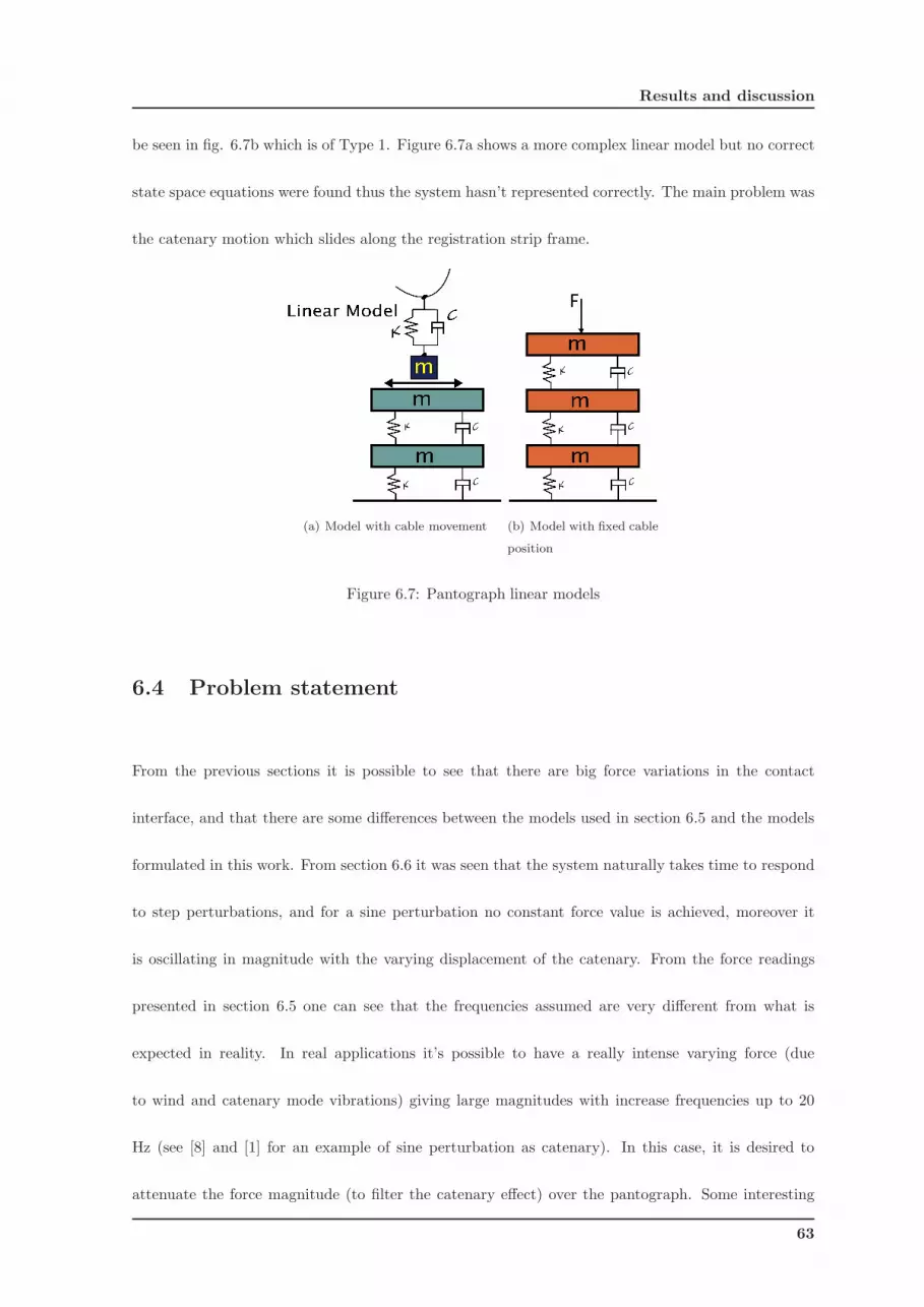
Results and discussion
be seen in fig. 6.7b which is of Type 1. Figure 6.7a shows a more complex linear model but no correct
state space equations were found thus the system hasn’t represented correctly. The main problem was
the catenary motion which slides along the registration strip frame.
(a) Model with cable movement (b) Model with fixed cable
position
Figure 6.7: Pantograph linear models
6.4 Problem statement
From the previous sections it is possible to see that there are big force variations in the contact
interface, and that there are some differences between the models used in section 6.5 and the models
formulated in this work. From section 6.6 it was seen that the system naturally takes time to respond
to step perturbations, and for a sine perturbation no constant force value is achieved, moreover it
is oscillating in magnitude with the varying displacement of the catenary. From the force readings
presented in section 6.5 one can see that the frequencies assumed are very different from what is
expected in reality. In real applications it’s possible to have a really intense varying force (due
to wind and catenary mode vibrations) giving large magnitudes with increase frequencies up to 20
Hz (see [8] and [1] for an example of sine perturbation as catenary). In this case, it is desired to
attenuate the force magnitude (to filter the catenary effect) over the pantograph. Some interesting
63
6.5 Experimental results and motivation
tests were made with the Type 1 and Type 2 models, as can be seen in fig 6.12 and 6.13, that the force
magnitude sensed by the pantograph is catenary frequency dependent. This means that to balance
the high frequencies, not only will the system need to react faster, but also will have to deal with
bigger force deviating amplitudes offered by the system inertia.
Because the pantograph will be used for human transportation lines, safety and reliability is
an important factor. The objective of this work is to present a reliable robust system for train
implementation. Industrial applications normally tend to use standard PID systems due to simplicity.
The problem of using robust controllers is normally on the order of the controller, that is in general
of higher order than normal PID solutions. This means that they are harder to configure and
to design. In order for the control scheme to be valid, some important criteria will have to be
set: the controller has to withstand model parameter variations (mass, springs and dampers), and
other model uncertainties. Instead of deriving uncertainty directly from the model parameters, and
designing a controller that withstands the desired robustness and performance requirements, the
approach followed deals with uncertainty in terms of controller actuating frequencies. This means
that on specific frequencies (normally high frequencies) the controller will have low action and on
working frequencies it will have high action, thus having a bigger margin of stability. The problem
of this type of controller is that not always there will be a solution that minimizes the energy and
therefore not having simultaneous robustness and performance.
6.5 Experimental results and motivation
To motivate the study in this chapter, experimental results from SNCF train circulation were used.
These results are presented in fig. 6.8, which can be found in the SNCF training session manuals
64
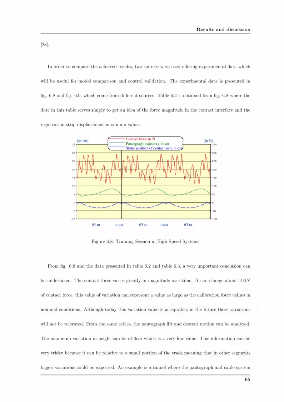
Results and discussion
[28].
In order to compare the achieved results, two sources were used offering experimental data which
will be useful for model comparison and control validation. The experimental data is presented in
fig. 6.8 and fig. 6.9, which come from different sources. Table 6.2 is obtained from fig. 6.8 where the
date in this table serves simply to get an idea of the force magnitude in the contact interface and the
registration strip displacement maximum values
Figure 6.8: Training Session in High Speed Systems
From fig. 6.8 and the data presented in table 6.2 and table 6.3, a very important conclusion can
be undertaken. The contact force varies greatly in magnitude over time. It can change about 190N
of contact force, this value of variation can represent a value as large as the calibration force values in
nominal conditions. Although today this variation value is acceptable, in the future these variations
will not be tolerated. From the same tables, the pantograph lift and descent motion can be analyzed.
The maximum variation in height can be of 3cm which is a very low value. This information can be
very tricky because it can be relative to a small portion of the track meaning that in other segments
bigger variations could be expected. An example is a tunnel where the pantograph and cable system
65
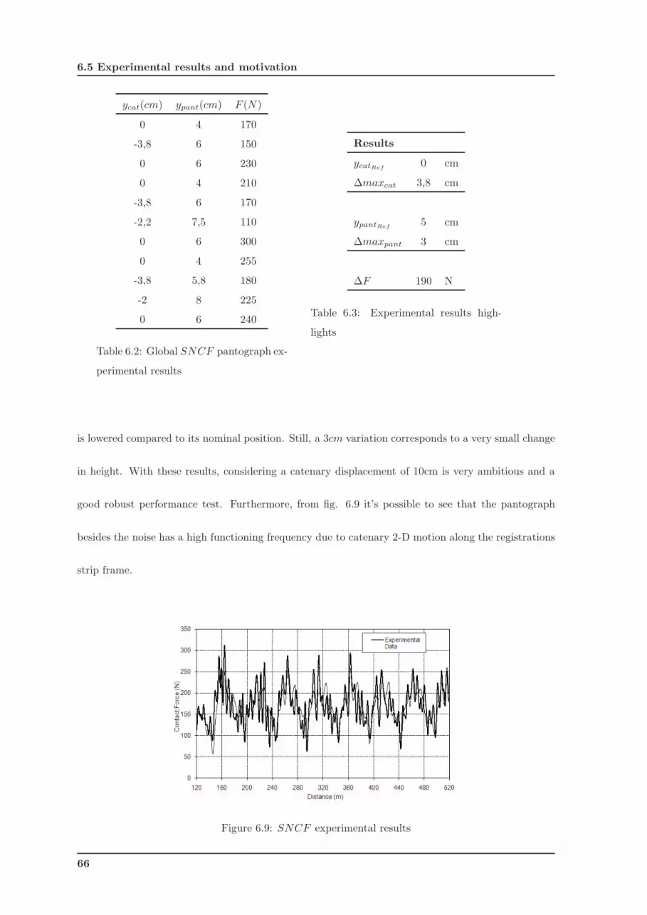
6.5 Experimental results and motivation
ycat(cm) ypant(cm) F (N)
0 4 170
-3,8 6 150
0 6 230
0 4 210
-3,8 6 170
-2,2 7,5 110
0 6 300
0 4 255
-3,8 5,8 180
-2 8 225
0 6 240
Table 6.2: Global SNCF pantograph ex-
perimental results
Results
ycatRef0 cm
∆maxcat 3,8 cm
ypantRef5 cm
∆maxpant 3 cm
∆F 190 N
Table 6.3: Experimental results high-
lights
is lowered compared to its nominal position. Still, a 3cm variation corresponds to a very small change
in height. With these results, considering a catenary displacement of 10cm is very ambitious and a
good robust performance test. Furthermore, from fig. 6.9 it’s possible to see that the pantograph
besides the noise has a high functioning frequency due to catenary 2-D motion along the registrations
strip frame.
Figure 6.9: SNCF experimental results
66
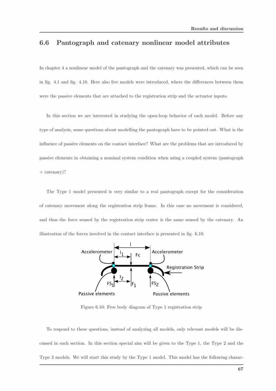
Results and discussion
6.6 Pantograph and catenary nonlinear model attributes
In chapter 4 a nonlinear model of the pantograph and the catenary was presented, which can be seen
in fig. 4.1 and fig. 4.10. Here also five models were introduced, where the differences between them
were the passive elements that are attached to the registration strip and the actuator inputs.
In this section we are interested in studying the open-loop behavior of each model. Before any
type of analysis, some questions about modelling the pantograph have to be pointed out. What is the
influence of passive elements on the contact interface? What are the problems that are introduced by
passive elements in obtaining a nominal system condition when using a coupled system (pantograph
+ catenary)?
The Type 1 model presented is very similar to a real pantograph except for the consideration
of catenary movement along the registration strip frame. In this case no movement is considered,
and thus the force sensed by the registration strip center is the same sensed by the catenary. An
illustration of the forces involved in the contact interface is presented in fig. 6.10.
Figure 6.10: Free body diagram of Type 1 registration strip
To respond to these questions, instead of analyzing all models, only relevant models will be dis-
cussed in each section. In this section special aim will be given to the Type 1, the Type 2 and the
Type 3 models. We will start this study by the Type 1 model. This model has the following charac-
67
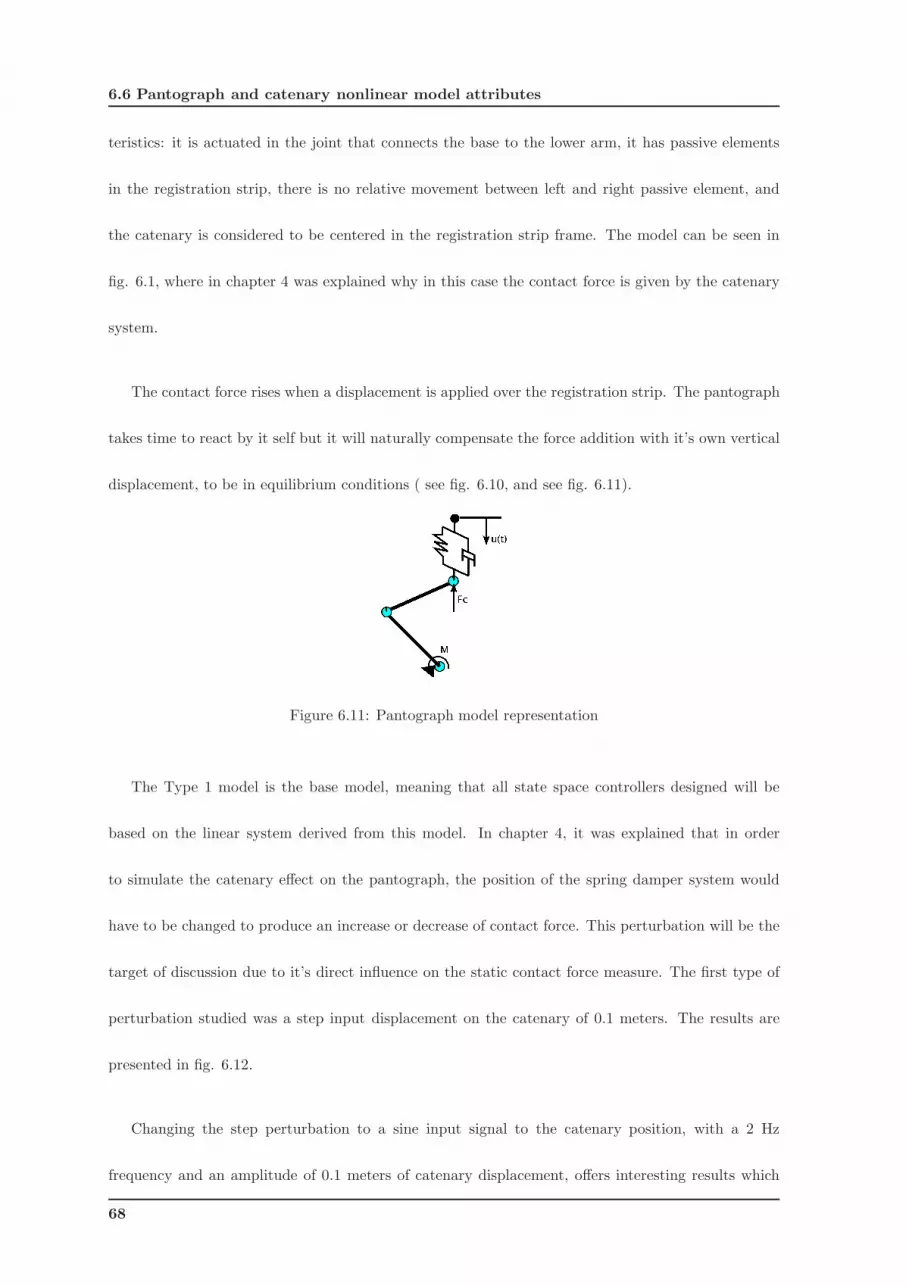
6.6 Pantograph and catenary nonlinear model attributes
teristics: it is actuated in the joint that connects the base to the lower arm, it has passive elements
in the registration strip, there is no relative movement between left and right passive element, and
the catenary is considered to be centered in the registration strip frame. The model can be seen in
fig. 6.1, where in chapter 4 was explained why in this case the contact force is given by the catenary
system.
The contact force rises when a displacement is applied over the registration strip. The pantograph
takes time to react by it self but it will naturally compensate the force addition with it’s own vertical
displacement, to be in equilibrium conditions ( see fig. 6.10, and see fig. 6.11).
Figure 6.11: Pantograph model representation
The Type 1 model is the base model, meaning that all state space controllers designed will be
based on the linear system derived from this model. In chapter 4, it was explained that in order
to simulate the catenary effect on the pantograph, the position of the spring damper system would
have to be changed to produce an increase or decrease of contact force. This perturbation will be the
target of discussion due to it’s direct influence on the static contact force measure. The first type of
perturbation studied was a step input displacement on the catenary of 0.1 meters. The results are
presented in fig. 6.12.
Changing the step perturbation to a sine input signal to the catenary position, with a 2 Hz
frequency and an amplitude of 0.1 meters of catenary displacement, offers interesting results which
68
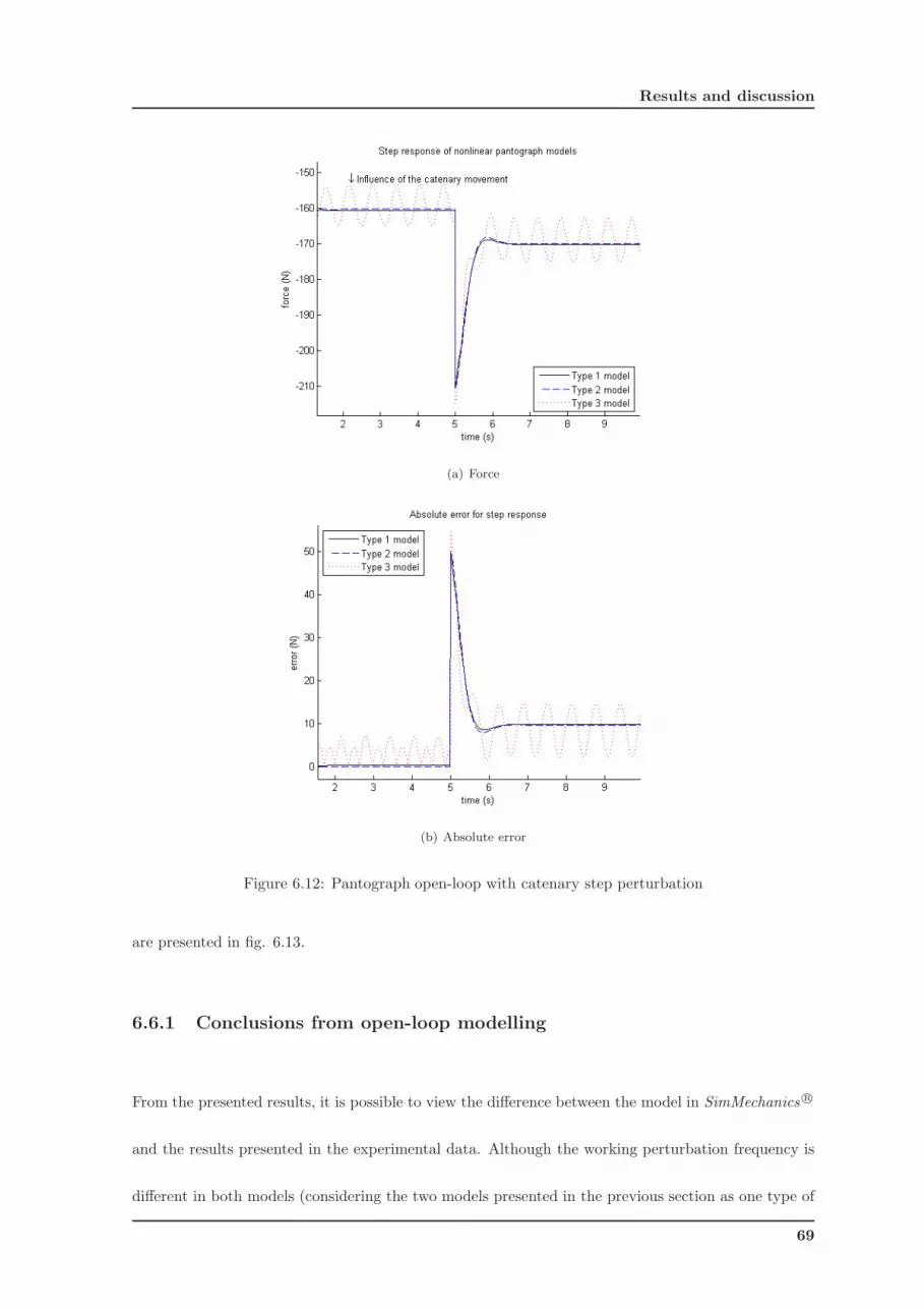
Results and discussion
(a) Force
(b) Absolute error
Figure 6.12: Pantograph open-loop with catenary step perturbation
are presented in fig. 6.13.
6.6.1 Conclusions from open-loop modelling
From the presented results, it is possible to view the difference between the model in SimMechanics R©
and the results presented in the experimental data. Although the working perturbation frequency is
different in both models (considering the two models presented in the previous section as one type of
69
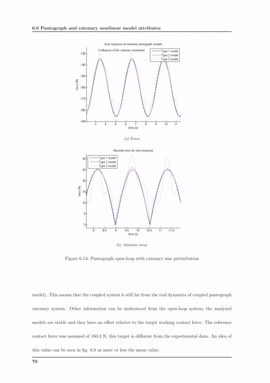
6.6 Pantograph and catenary nonlinear model attributes
(a) Force
(b) Absolute error
Figure 6.13: Pantograph open-loop with catenary sine perturbation
model). This means that the coupled system is still far from the real dynamics of coupled pantograph
catenary system. Other information can be understood from the open-loop system, the analyzed
models are stable and they have an offset relative to the target working contact force. The reference
contact force was assumed of 160.3 N, this target is different from the experimental data. An idea of
this value can be seen in fig. 6.8 as more or less the mean value.
70
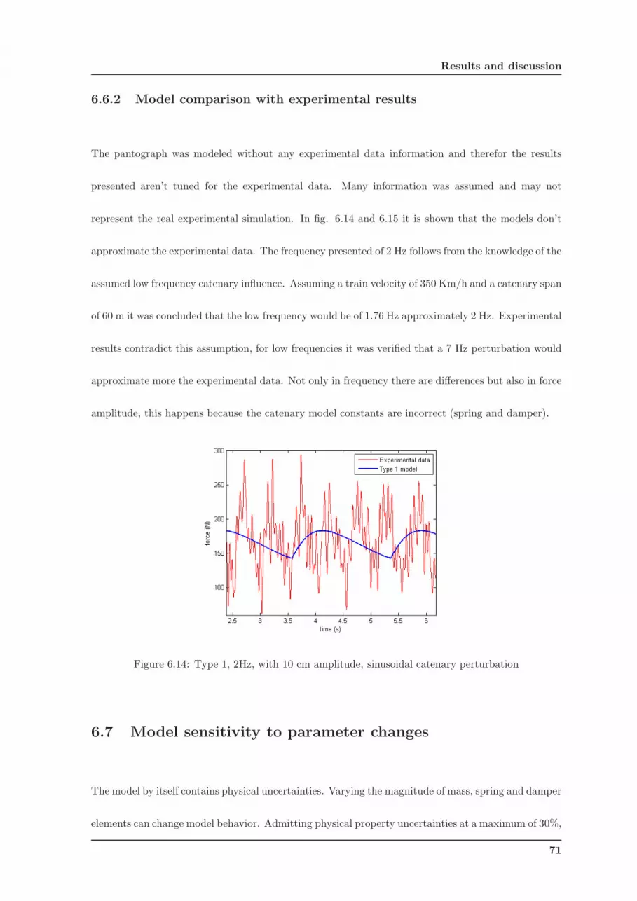
Results and discussion
6.6.2 Model comparison with experimental results
The pantograph was modeled without any experimental data information and therefor the results
presented aren’t tuned for the experimental data. Many information was assumed and may not
represent the real experimental simulation. In fig. 6.14 and 6.15 it is shown that the models don’t
approximate the experimental data. The frequency presented of 2 Hz follows from the knowledge of the
assumed low frequency catenary influence. Assuming a train velocity of 350 Km/h and a catenary span
of 60 m it was concluded that the low frequency would be of 1.76 Hz approximately 2 Hz. Experimental
results contradict this assumption, for low frequencies it was verified that a 7 Hz perturbation would
approximate more the experimental data. Not only in frequency there are differences but also in force
amplitude, this happens because the catenary model constants are incorrect (spring and damper).
Figure 6.14: Type 1, 2Hz, with 10 cm amplitude, sinusoidal catenary perturbation
6.7 Model sensitivity to parameter changes
The model by itself contains physical uncertainties. Varying the magnitude of mass, spring and damper
elements can change model behavior. Admitting physical property uncertainties at a maximum of 30%,
71
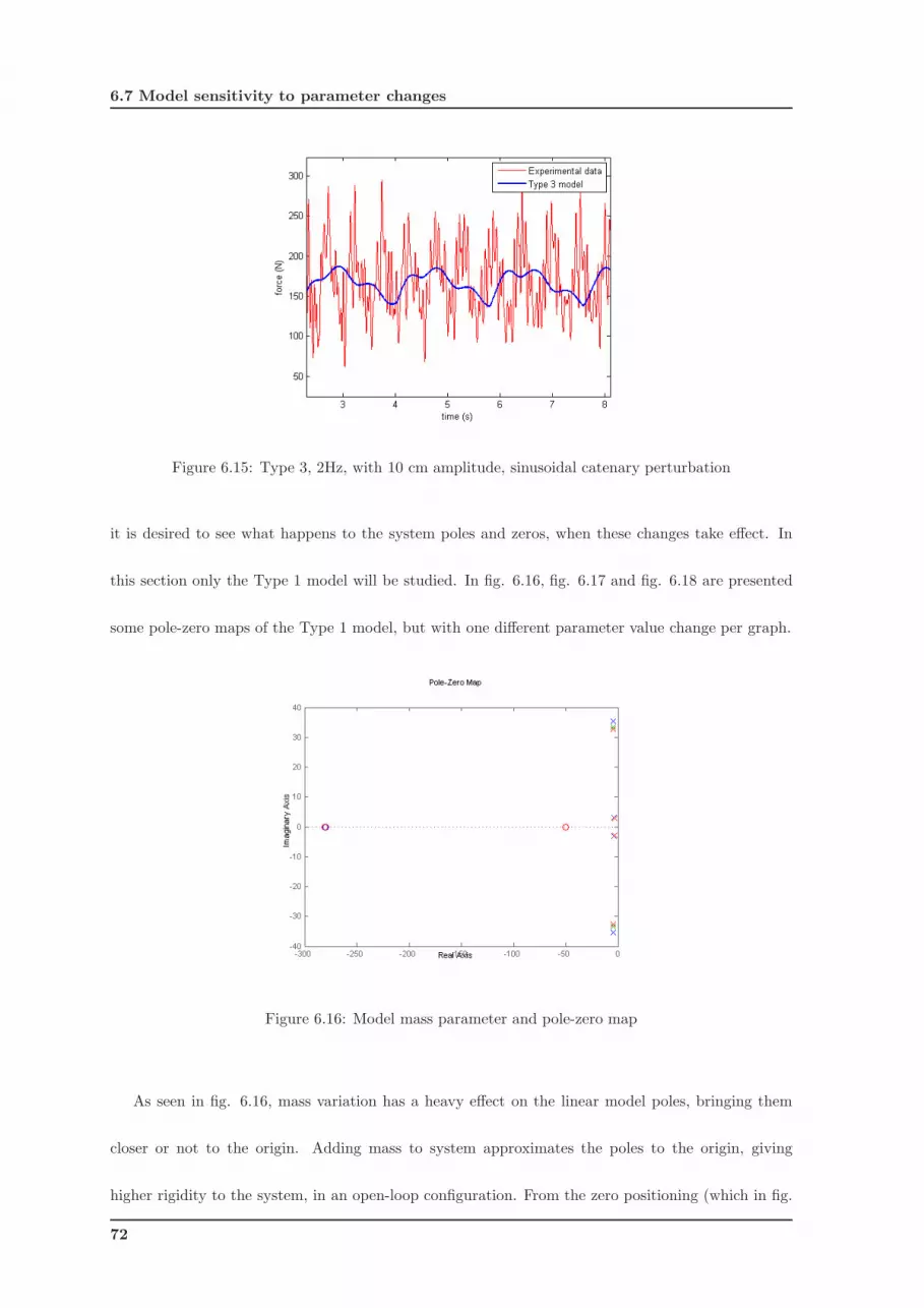
6.7 Model sensitivity to parameter changes
Figure 6.15: Type 3, 2Hz, with 10 cm amplitude, sinusoidal catenary perturbation
it is desired to see what happens to the system poles and zeros, when these changes take effect. In
this section only the Type 1 model will be studied. In fig. 6.16, fig. 6.17 and fig. 6.18 are presented
some pole-zero maps of the Type 1 model, but with one different parameter value change per graph.
Figure 6.16: Model mass parameter and pole-zero map
As seen in fig. 6.16, mass variation has a heavy effect on the linear model poles, bringing them
closer or not to the origin. Adding mass to system approximates the poles to the origin, giving
higher rigidity to the system, in an open-loop configuration. From the zero positioning (which in fig.
72
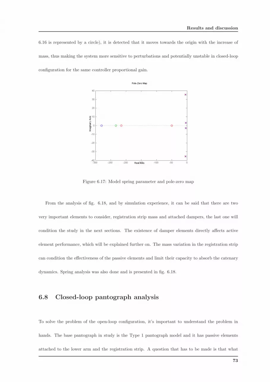
Results and discussion
6.16 is represented by a circle), it is detected that it moves towards the origin with the increase of
mass, thus making the system more sensitive to perturbations and potentially unstable in closed-loop
configuration for the same controller proportional gain.
Figure 6.17: Model spring parameter and pole-zero map
From the analysis of fig. 6.18, and by simulation experience, it can be said that there are two
very important elements to consider, registration strip mass and attached dampers, the last one will
condition the study in the next sections. The existence of damper elements directly affects active
element performance, which will be explained further on. The mass variation in the registration strip
can condition the effectiveness of the passive elements and limit their capacity to absorb the catenary
dynamics. Spring analysis was also done and is presented in fig. 6.18.
6.8 Closed-loop pantograph analysis
To solve the problem of the open-loop configuration, it’s important to understand the problem in
hands. The base pantograph in study is the Type 1 pantograph model and it has passive elements
attached to the lower arm and the registration strip. A question that has to be made is that what
73
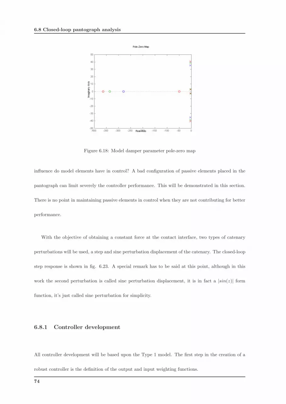
6.8 Closed-loop pantograph analysis
Figure 6.18: Model damper parameter pole-zero map
influence do model elements have in control? A bad configuration of passive elements placed in the
pantograph can limit severely the controller performance. This will be demonstrated in this section.
There is no point in maintaining passive elements in control when they are not contributing for better
performance.
With the objective of obtaining a constant force at the contact interface, two types of catenary
perturbations will be used, a step and sine perturbation displacement of the catenary. The closed-loop
step response is shown in fig. 6.23. A special remark has to be said at this point, although in this
work the second perturbation is called sine perturbation displacement, it is in fact a |sin(z)| form
function, it’s just called sine perturbation for simplicity.
6.8.1 Controller development
All controller development will be based upon the Type 1 model. The first step in the creation of a
robust controller is the definition of the output and input weighting functions.
74

Results and discussion
Weighting functions
The weighting functions are chosen by the controller designer. Unfortunately it’s not possible to
achieve easily a perfect weighting function combination, some configurations can produce low perfor-
mance controllers, others will produce high performance with no change in robustness. The weighting
functions obtained were used both on H∞ and H2 controllers. Two sets of weighting functions are
used, the first is a more conservative approach, the second is a more aggressive controller but with
the possibility of robustness reduction. Many orders for the weighting functions were tested and for
simplicity a first order transfer function was used (see eq. 6.6)
w1 = (w0
τs + 1)n, w2 = 0.1, w3 = 10−3 (6.6)
w0 = 10; τ = 50; n = 1 (6.7)
Where the w3 is the actuator effort weighting function. Alike standard PID controllers, robust con-
trollers have to be tuned. There are essentially two important weighting functions which are the
output and input plant error weights, these parameters were obtained with trial and error, an exam-
ple of the process can be seen in fig. 6.19. Here we can see the evolution of changing the τ parameter
in a first order w1 weighting function.
Uncertainty model and controller development
To make a preliminary study of model robustness, a family of systems similar to the Type 1 model
are derived and thus creating an uncertainty block. This can be seen in fig. 6.20, which is a frequency
response for the nominal system, with 10 samples of uncertain system and the uncertainty. With the
help of the Robust Control Toolbox these elements are studied to understand the controller robustness
due to plant variation. A remark has to be done here, instead of analyzing the system from it’s basic
75
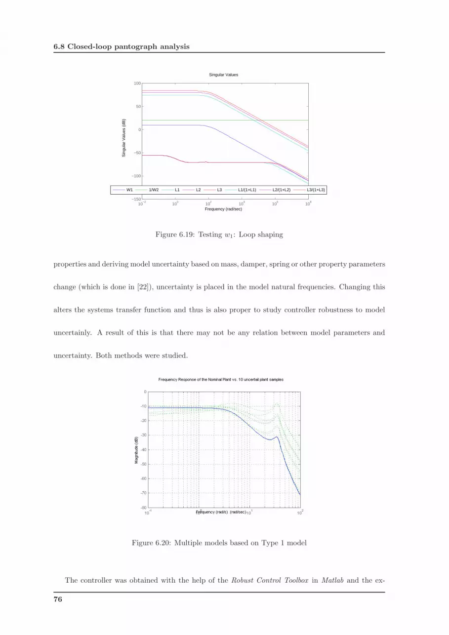
6.8 Closed-loop pantograph analysis
10−2
100
102
104
106
108
−150
−100
−50
0
50
100
Singular Values
Frequency (rad/sec)
Sin
gula
r V
alue
s (d
B)
W1 1/W2 L1 L2 L3 L1/(1+L1) L2/(1+L2) L3/(1+L3)
Figure 6.19: Testing w1: Loop shaping
properties and deriving model uncertainty based on mass, damper, spring or other property parameters
change (which is done in [22]), uncertainty is placed in the model natural frequencies. Changing this
alters the systems transfer function and thus is also proper to study controller robustness to model
uncertainly. A result of this is that there may not be any relation between model parameters and
uncertainty. Both methods were studied.
Figure 6.20: Multiple models based on Type 1 model
The controller was obtained with the help of the Robust Control Toolbox in Matlab and the ex-
76
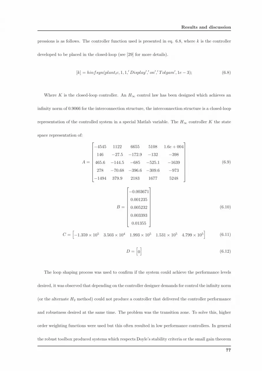
Results and discussion
pressions is as follows. The controller function used is presented in eq. 6.8, where k is the controller
developed to be placed in the closed-loop (see [29] for more details).
[k] = hinfsyn(plantic, 1, 1,′ Display′,′ on′,′ Tolgam′, 1e − 3); (6.8)
Where K is the closed-loop controller. An H∞ control law has been designed which achieves an
infinity norm of 0.9066 for the interconnection structure, the interconnection structure is a closed-loop
representation of the controlled system in a special Matlab variable. The H∞ controller K the state
space representation of:
A =
−4545 1122 6655 5108 1.6e + 004
146 −27.5 −172.9 −132 −398
465.6 −144.5 −685 −525.1 −1639
278 −70.68 −396.6 −309.6 −973
−1494 379.9 2183 1677 5248
(6.9)
B =
−0.003671
0.001235
0.005232
0.003393
0.01355
(6.10)
C =[
−1.359× 10⁵ 3.503 × 10⁴ 1.993 × 10⁵ 1.531 × 10⁵ 4.799 × 10⁵]
(6.11)
D =[
0]
(6.12)
The loop shaping process was used to confirm if the system could achieve the performance levels
desired, it was observed that depending on the controller designer demands for control the infinity norm
(or the alternate H2 method) could not produce a controller that delivered the controller performance
and robustness desired at the same time. The problem was the transition zone. To solve this, higher
order weighting functions were used but this often resulted in low performance controllers. In general
the robust toolbox produced systems which respects Doyle’s stability criteria or the small gain theorem
77
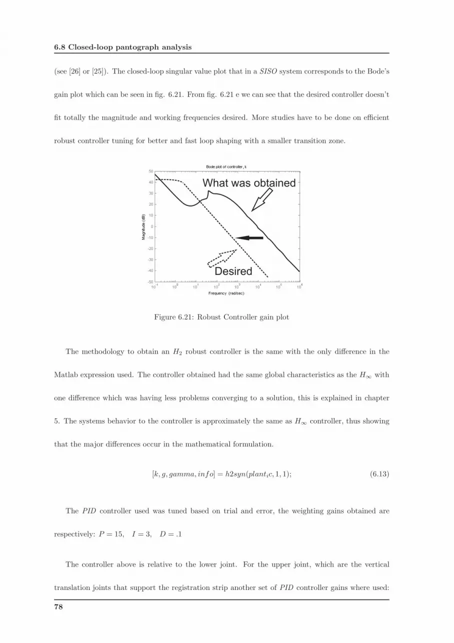
6.8 Closed-loop pantograph analysis
(see [26] or [25]). The closed-loop singular value plot that in a SISO system corresponds to the Bode’s
gain plot which can be seen in fig. 6.21. From fig. 6.21 e we can see that the desired controller doesn’t
fit totally the magnitude and working frequencies desired. More studies have to be done on efficient
robust controller tuning for better and fast loop shaping with a smaller transition zone.
Desired
What was obtained
Figure 6.21: Robust Controller gain plot
The methodology to obtain an H2 robust controller is the same with the only difference in the
Matlab expression used. The controller obtained had the same global characteristics as the H∞ with
one difference which was having less problems converging to a solution, this is explained in chapter
5. The systems behavior to the controller is approximately the same as H∞ controller, thus showing
that the major differences occur in the mathematical formulation.
[k, g, gamma, info] = h2syn(plantic, 1, 1); (6.13)
The PID controller used was tuned based on trial and error, the weighting gains obtained are
respectively: P = 15, I = 3, D = .1
The controller above is relative to the lower joint. For the upper joint, which are the vertical
translation joints that support the registration strip another set of PID controller gains where used:
78
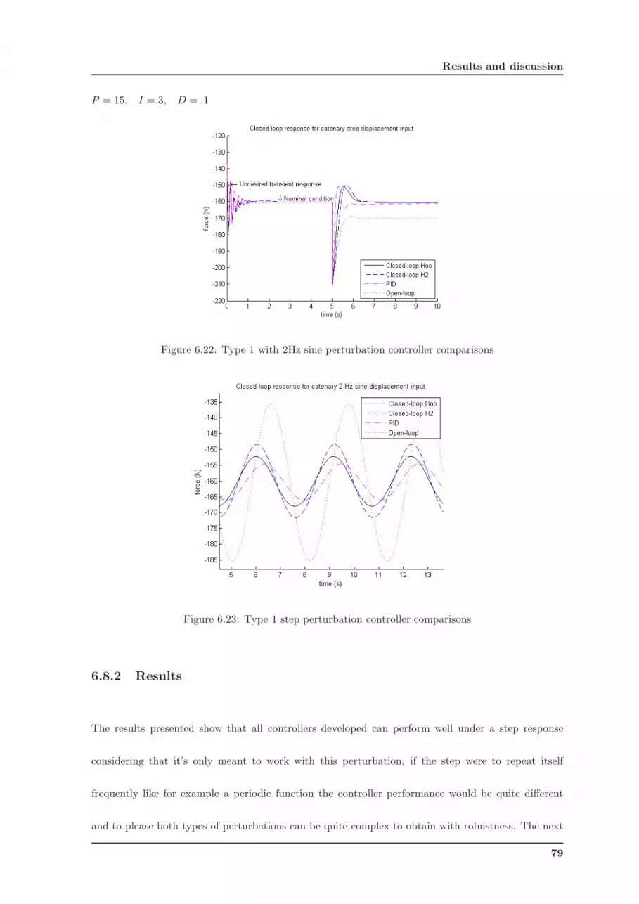
Results and discussion
P = 15, I = 3, D = .1
Figure 6.22: Type 1 with 2Hz sine perturbation controller comparisons
Figure 6.23: Type 1 step perturbation controller comparisons
6.8.2 Results
The results presented show that all controllers developed can perform well under a step response
considering that it’s only meant to work with this perturbation, if the step were to repeat itself
frequently like for example a periodic function the controller performance would be quite different
and to please both types of perturbations can be quite complex to obtain with robustness. The next
79
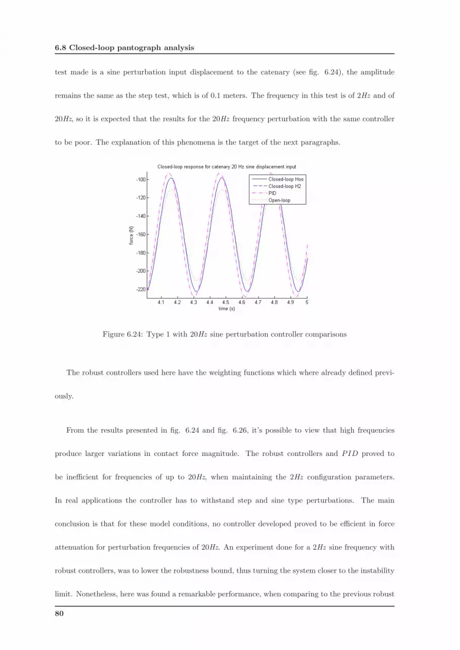
6.8 Closed-loop pantograph analysis
test made is a sine perturbation input displacement to the catenary (see fig. 6.24), the amplitude
remains the same as the step test, which is of 0.1 meters. The frequency in this test is of 2Hz and of
20Hz, so it is expected that the results for the 20Hz frequency perturbation with the same controller
to be poor. The explanation of this phenomena is the target of the next paragraphs.
Figure 6.24: Type 1 with 20Hz sine perturbation controller comparisons
The robust controllers used here have the weighting functions which where already defined previ-
ously.
From the results presented in fig. 6.24 and fig. 6.26, it’s possible to view that high frequencies
produce larger variations in contact force magnitude. The robust controllers and PID proved to
be inefficient for frequencies of up to 20Hz, when maintaining the 2Hz configuration parameters.
In real applications the controller has to withstand step and sine type perturbations. The main
conclusion is that for these model conditions, no controller developed proved to be efficient in force
attenuation for perturbation frequencies of 20Hz. An experiment done for a 2Hz sine frequency with
robust controllers, was to lower the robustness bound, thus turning the system closer to the instability
limit. Nonetheless, here was found a remarkable performance, when comparing to the previous robust
80
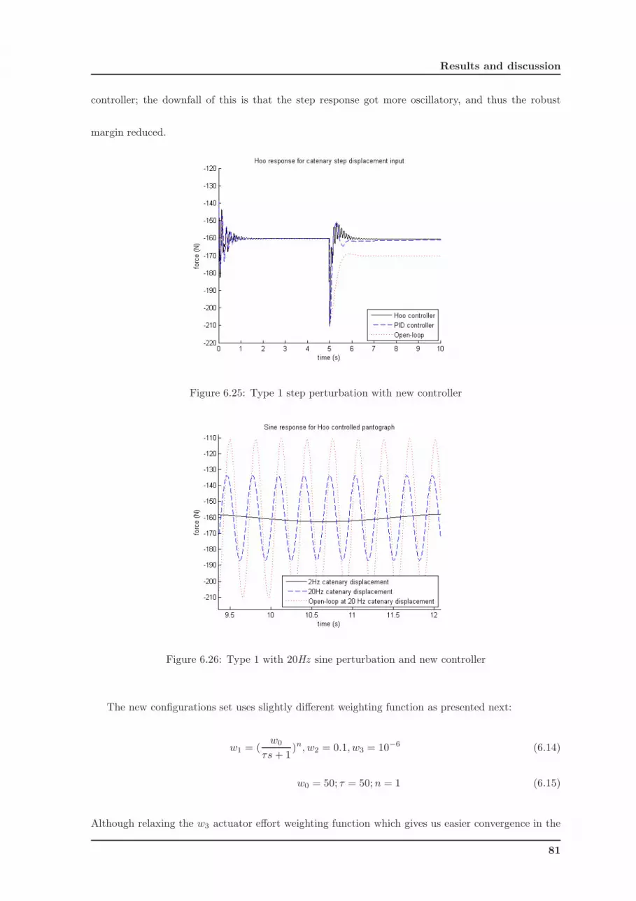
Results and discussion
controller; the downfall of this is that the step response got more oscillatory, and thus the robust
margin reduced.
Figure 6.25: Type 1 step perturbation with new controller
Figure 6.26: Type 1 with 20Hz sine perturbation and new controller
The new configurations set uses slightly different weighting function as presented next:
w1 = (w0
τs + 1)n, w2 = 0.1, w3 = 10−6 (6.14)
w0 = 50; τ = 50; n = 1 (6.15)
Although relaxing the w3 actuator effort weighting function which gives us easier convergence in the
81
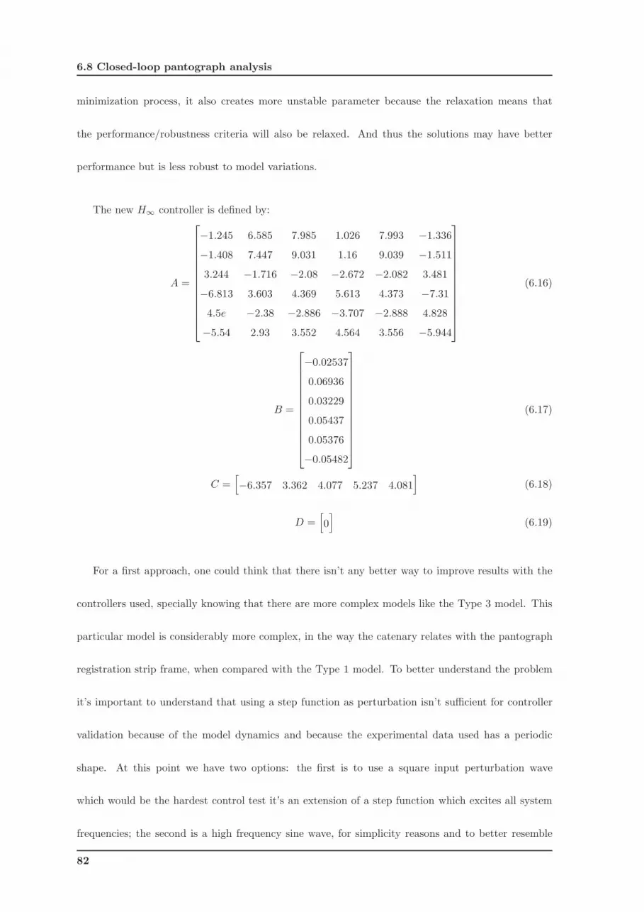
6.8 Closed-loop pantograph analysis
minimization process, it also creates more unstable parameter because the relaxation means that
the performance/robustness criteria will also be relaxed. And thus the solutions may have better
performance but is less robust to model variations.
The new H∞ controller is defined by:
A =
−1.245 6.585 7.985 1.026 7.993 −1.336
−1.408 7.447 9.031 1.16 9.039 −1.511
3.244 −1.716 −2.08 −2.672 −2.082 3.481
−6.813 3.603 4.369 5.613 4.373 −7.31
4.5e −2.38 −2.886 −3.707 −2.888 4.828
−5.54 2.93 3.552 4.564 3.556 −5.944
(6.16)
B =
−0.02537
0.06936
0.03229
0.05437
0.05376
−0.05482
(6.17)
C =[
−6.357 3.362 4.077 5.237 4.081]
(6.18)
D =[
0]
(6.19)
For a first approach, one could think that there isn’t any better way to improve results with the
controllers used, specially knowing that there are more complex models like the Type 3 model. This
particular model is considerably more complex, in the way the catenary relates with the pantograph
registration strip frame, when compared with the Type 1 model. To better understand the problem
it’s important to understand that using a step function as perturbation isn’t sufficient for controller
validation because of the model dynamics and because the experimental data used has a periodic
shape. At this point we have two options: the first is to use a square input perturbation wave
which would be the hardest control test it’s an extension of a step function which excites all system
frequencies; the second is a high frequency sine wave, for simplicity reasons and to better resemble
82
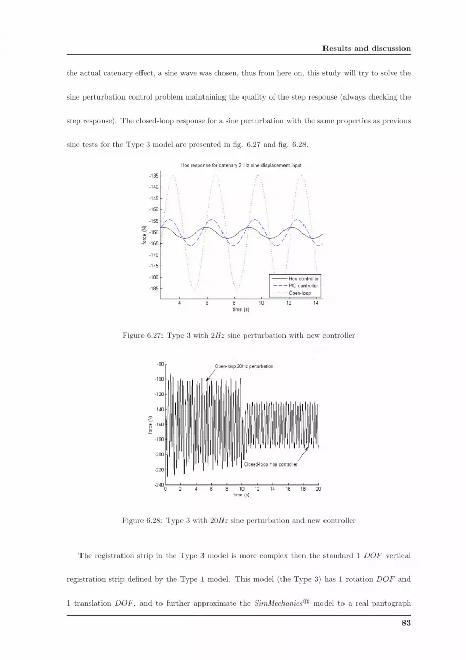
Results and discussion
the actual catenary effect, a sine wave was chosen, thus from here on, this study will try to solve the
sine perturbation control problem maintaining the quality of the step response (always checking the
step response). The closed-loop response for a sine perturbation with the same properties as previous
sine tests for the Type 3 model are presented in fig. 6.27 and fig. 6.28.
Figure 6.27: Type 3 with 2Hz sine perturbation with new controller
Figure 6.28: Type 3 with 20Hz sine perturbation and new controller
The registration strip in the Type 3 model is more complex then the standard 1 DOF vertical
registration strip defined by the Type 1 model. This model (the Type 3) has 1 rotation DOF and
1 translation DOF , and to further approximate the SimMechanics R© model to a real pantograph
83

6.8 Closed-loop pantograph analysis
implementation, the motion of the catenary along the registration strip frame is considered. In this
context, the same controller developed for the Type 1 model was used for the Type 3 model and the
results for high frequencies were as expected: they were very poor. These results and this conclusion
comes from an extensive trial and error weight function development.
At this point, it was thought that it was a very complicated task to control high frequencies in
the contact interface of the pantograph. From all the studies made till now, no modifications to the
models where made, with one exclusion which is in section 5. Because the catenary already contains
a damper, problems were found due to the existence of instant catenary movement (like the step
perturbation), which caused an infinite force magnitude. This happened because we considered that
the catenary displacement was infinity fast, thus moving instantly to the final step position. Because
Fc = C(dx/dt − dx0/dt)) and because for a step ∆T = 0, dx/dt = ∞, means that the force tends
to infinity. Because the numeric integrator has it’s own step time, the system doesn’t crash, but this
”glitch” explains why the controller didn’t have good performance in the first place, for high frequency
solicitations on the pantograph. In the step response with the same Type 3 model, the damper has
a good energy absorption, but if we introduce a controller to this joint, letting the passive damper
element there, the controller effectiveness is largely reduced. In contrast, the spring only intensifies
the energy cost to move the joint. Because energy optimization isn’t the main focus in this work, the
springs are maintained, but the dampers are eliminated in the actuated joints. These modifications
improves the performance of the robust and PID controllers in every actuated joint for every model.
In fig. 6.29 it’s possible to see the improvement in control, due to the changes made in the model for
an H∞ controller for a Type 1 and a Type 3 model. The only problem of this is when there is no
control and because this situation can occur in real pantograph circulation this can be a big problem.
Removing the lower damper can turn the open loop response more oscillatory.
84
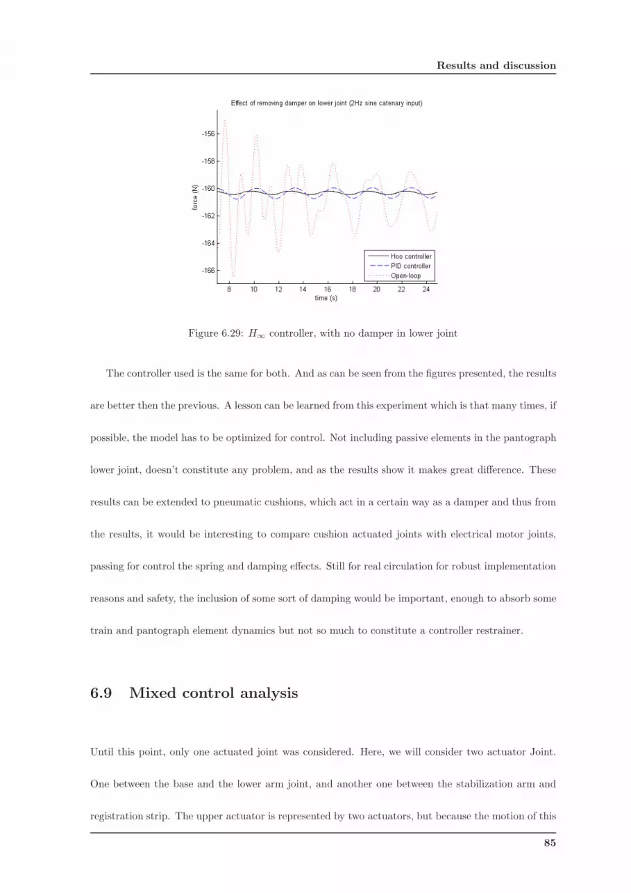
Results and discussion
Figure 6.29: H∞ controller, with no damper in lower joint
The controller used is the same for both. And as can be seen from the figures presented, the results
are better then the previous. A lesson can be learned from this experiment which is that many times, if
possible, the model has to be optimized for control. Not including passive elements in the pantograph
lower joint, doesn’t constitute any problem, and as the results show it makes great difference. These
results can be extended to pneumatic cushions, which act in a certain way as a damper and thus from
the results, it would be interesting to compare cushion actuated joints with electrical motor joints,
passing for control the spring and damping effects. Still for real circulation for robust implementation
reasons and safety, the inclusion of some sort of damping would be important, enough to absorb some
train and pantograph element dynamics but not so much to constitute a controller restrainer.
6.9 Mixed control analysis
Until this point, only one actuated joint was considered. Here, we will consider two actuator Joint.
One between the base and the lower arm joint, and another one between the stabilization arm and
registration strip. The upper actuator is represented by two actuators, but because the motion of this
85
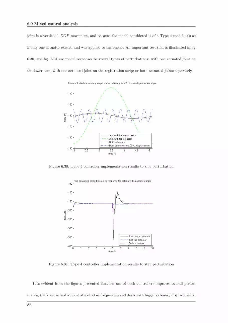
6.9 Mixed control analysis
joint is a vertical 1 DOF movement, and because the model considered is of a Type 4 model, it’s as
if only one actuator existed and was applied to the center. An important test that is illustrated in fig
6.30, and fig. 6.31 are model responses to several types of perturbations: with one actuated joint on
the lower arm; with one actuated joint on the registration strip; or both actuated joints separately.
Figure 6.30: Type 4 controller implementation results to sine perturbation
Figure 6.31: Type 4 controller implementation results to step perturbation
It is evident from the figures presented that the use of both controllers improves overall perfor-
mance, the lower actuated joint absorbs low frequencies and deals with bigger catenary displacements,
86
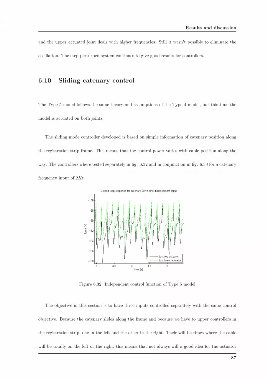
Results and discussion
and the upper actuated joint deals with higher frequencies. Still it wasn’t possible to eliminate the
oscillation. The step-perturbed system continues to give good results for controllers.
6.10 Sliding catenary control
The Type 5 model follows the same theory and assumptions of the Type 4 model, but this time the
model is actuated on both joints.
The sliding mode controller developed is based on simple information of catenary position along
the registration strip frame. This means that the control power varies with cable position along the
way. The controllers where tested separately in fig. 6.32 and in conjunction in fig. 6.33 for a catenary
frequency input of 2Hz.
Figure 6.32: Independent control function of Type 5 model
The objective in this section is to have three inputs controlled separately with the same control
objective. Because the catenary slides along the frame and because we have to upper controllers in
the registration strip, one in the left and the other in the right. Their will be times where the cable
will be totally on the left or the right, this means that not always will a good idea for the actuator
87
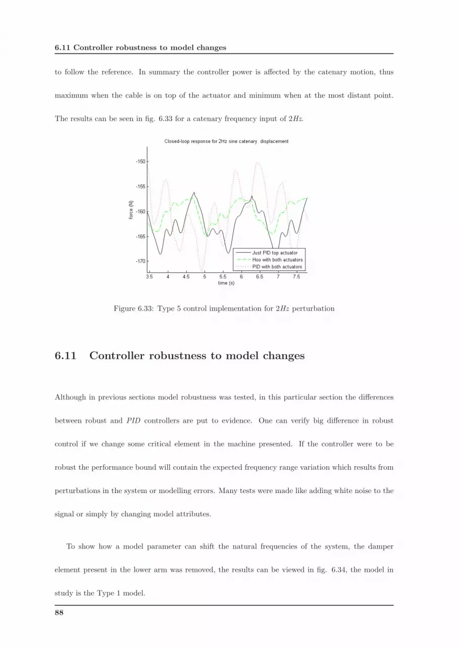
6.11 Controller robustness to model changes
to follow the reference. In summary the controller power is affected by the catenary motion, thus
maximum when the cable is on top of the actuator and minimum when at the most distant point.
The results can be seen in fig. 6.33 for a catenary frequency input of 2Hz.
Figure 6.33: Type 5 control implementation for 2Hz perturbation
6.11 Controller robustness to model changes
Although in previous sections model robustness was tested, in this particular section the differences
between robust and PID controllers are put to evidence. One can verify big difference in robust
control if we change some critical element in the machine presented. If the controller were to be
robust the performance bound will contain the expected frequency range variation which results from
perturbations in the system or modelling errors. Many tests were made like adding white noise to the
signal or simply by changing model attributes.
To show how a model parameter can shift the natural frequencies of the system, the damper
element present in the lower arm was removed, the results can be viewed in fig. 6.34, the model in
study is the Type 1 model.
88
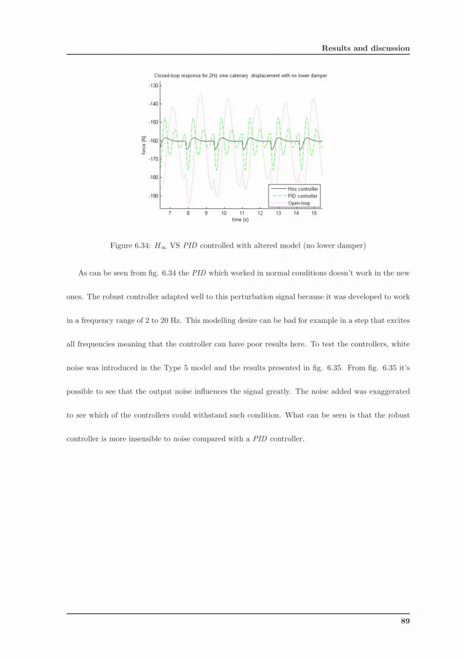
Results and discussion
Figure 6.34: H∞ VS PID controlled with altered model (no lower damper)
As can be seen from fig. 6.34 the PID which worked in normal conditions doesn’t work in the new
ones. The robust controller adapted well to this perturbation signal because it was developed to work
in a frequency range of 2 to 20 Hz. This modelling desire can be bad for example in a step that excites
all frequencies meaning that the controller can have poor results here. To test the controllers, white
noise was introduced in the Type 5 model and the results presented in fig. 6.35. From fig. 6.35 it’s
possible to see that the output noise influences the signal greatly. The noise added was exaggerated
to see which of the controllers could withstand such condition. What can be seen is that the robust
controller is more insensible to noise compared with a PID controller.
89
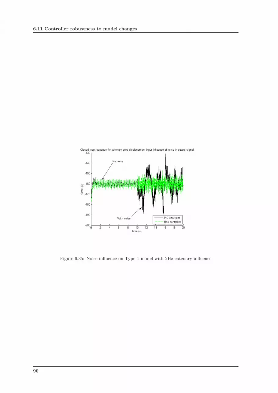
6.11 Controller robustness to model changes
Figure 6.35: Noise influence on Type 1 model with 2Hz catenary influence
90

Chapter 7
Conclusions and future work
The main objective of this project was to design and control a pantograph, with robust stability. To
engage these objectives a pantograph model was created. The model presented in this study isn’t the
exact model used by the SNCF pantograph, it’s a mere simplification of the real model.
In this work it wasn’t only intended to study a pantograph for high speeds but to study the
feasibility of using in standard train speed lines, controlled pantograph. The inclusion of control in
pantograph systems cannot only be associated to decreasing the travel time between destinations , it
has a more brooder area of influence. Pantograph systems have typically low maintenance, but this
machine is an expensive component of the train, due to it’s robustness to sustain physical contact with
the wires and to resist to bad weather conditions and electric arc formations. Traditional approaches
(with no control) resort to aerodynamic wings in the registration strip. Good results have been
obtained resorting to this technology using the air lift that rises the registration strip with higher
train velocities ensuring better contact at high speeds. But excessive wear to the interface elements
still occur and pantograph fixation to the cable system are still present. Evolving to systems that have
very low wear to the pantograph and catenary, that have very low maintenance and have minimum risk
91
of pantograph fixation to the cable system are a very appealing solution for every train transportation
company.
It was shown, for the models Type 1 and Type 2, that these are simple and easy to linearize and
control. Compared to the Type 3 model. Robust stability was obtained for H2 and H∞ controllers
(following [8] and [9]), and proved that modifying these models in reasonable values, the controller
still reaches reasonable margins of stability providing acceptable results. Acceptable results are better
results than the ones provided by the experimental data thus the force amplitude being the lower as
possible.
Regarding to modelling, it was shown that standard one dimensional registration strip, doesn’t
model exactly the real dynamics of a pantograph due to catenary movement along the registration
strip. The model that was found to represent better the real system was the Type 3 model. The Type
1 and the Type 3 models don’t approximate correctly the experimental results in amplitude and in
frequency because they weren’t projected with the experimental results. Furthermore it is important
to reconstruct the model based on the target experimental model frequencies and amplitudes.
Finding the right sensitivity transfer functions was a wearisome ordeal, because the working fre-
quencies of a pantograph can go up to 20 Hz (20 Hz of perturbation signal). Providing a controller that
could be robust and have good performance, wasn’t possible for the Type 3 model, so a compromise
had to be reached.
From the experiments made in control it was found that high input frequencies applied on the
pantograph affect the control performance, this means that the controller must only work in specific
frequency regions for safety reasons.
92
Conclusions and future work
Lower arm damper effect was studied and found to be a critical element in high frequencies
with high amplitudes. Although a damper limits the actuated inputs on how fast it responds to
system change, it is a instant energy absorber and therefore a better it is important to have a better
combination of damper and actuator constant values for better controlling. Upper active elements
proved to be efficient with low amplitude high frequencies.
In general, the robust controller proved to be better than a normal PID controller with exception
to the tuning steps which are more complex. It’s not elementary to find the right combination of
weights that filter the objective designer frequency specifications for the robust controllers. Further
more as expected the robust controller proved to have better performance to model parameter changes
and signal noise than the PID controller.
7.1 Future work
Using a standard train pantograph would be the ideal experimental platform for more results and
comparisons. In this work a SimMechanics R© model was developed, with this we can now compare
with other types of approaches, moreover a model like the Type 1 but built upon the closed chains
Denavit-Hartenberg method. The objective is to have a more numerically efficient method for realtime
applications. This could be useful for system observers or real time animations. The method suggested
is different than the standard global coordinates approaches, having good potentialities due to it’s
simplicity comparing to other approaches.
93

7.1 Future work
94
Bibliography
[1] B. Allotta, M. Papi, P. Toni, and A. G. Violi. Experimental campaign on a servo-actuated
pantograph. Advanced Intelligent Mechatronics, 1:237–242, 2001.
[2] Park Tong Jin, Han Chang Soo, and Jang Jin Hee. Dynamic sensitivity analysis for the panto-
graph of a high-speed rail vehicle. Journal of Sound and Vibration, 266:235–260, 2002.
[3] Jong-Hwi Seo, Seok-Won Kim, Il-Ho Jung, Tae-Won Park, Jin-Yong Mok, Young-Guk Kim,
and Jang-Bom Chai. Dynamic analysis of a pantograph - catenary system using absolute nodal
coordinates. Elsevier, 44:615–630, 2006.
[4] M. Schaub. and B. Simeon. Pantograph - catenary dynamics: An analysis of models and simula-
tion techniques. Mathematical and Computer Modelling of Dynamical Systems, Vol. 7:225–238,
2001.
[5] A. Kumaniecka. Dynamics of an overhead line and pantograph system. The Dynamics of vehicles
on roads and on tracks, pages 104–113, 1998.
[6] W. M. Zhai and C. B. Cai. Effect of locomotive vibrations on pantograph-catenary system
dynamics. The dynamics of vehicles on roads and on tracks, 29:47–58, 2000.
[7] A. Pisano and E. Usai. Output-feedback regulation of the contact-force in high-speed train
pantographs. Dynamic Systems, Measurement, and Control, 126:82–87, 2004.
95
BIBLIOGRAPHY
[8] A. Collina, A. Facchinetti, F. Fossati, and F. Resta. An application of active control to the
collector of an high-speed pantograph: Simulation and laboratory tests. Advanced Intelligent
Mechatronics, 2001. Proceedings. 2001 IEEE/ASME International Conference, 1:243–248, 2005.
[9] D. J. Hartland. Developments towards an active pantograph. Current Collections for High Speed
Trains Seminar (Ref. No. 1998/509), IEE, Current Collections for High Speed Trains Seminar:
5/1–5/5, 1998.
[10] J. Y. S. Luh and Yuan Fang Zheng. Computation of input generalized forces for robots with
closed kinematic chain mechanisms. Robotics and Automation, IEEE Journal of [legacy, pre -
1988], pages 95– 103, 1985.
[11] Xiang-Rong Xu, Won-Jee Chung, Young-Hyu Choi, , and Xiang-Feng Ma. A new dynamic
formulation for robot manipulators containing closed kinematic chains. Robotica, 17:261–267,
1999.
[12] Giles D. Wood and Dallas C. Kennedy. Simulating mechanical systems in simulink with simme-
chanics. The Mathworks, Inc.,www.mathworks.com/matlabcentral/fileexchange/(PDF file), MA,
USA, 2003.
[13] Leon Zlajpah. Simulation of robotic manipulators. RAAD 2006, 2005.
[14] F. Kiessling, W. Harprecht, and R. Seifert. Tractive power supply at german federal railway’s
400 km/h runs. Railroad Conference, 1989. Proceedings., Technical Papers Presented at the 1989
IEEE/ASME Joint, pages 23–32, 1989.
[15] Faiveley. CX - The piloted pantograph system for optimal current collection. Faiveley Transport,
2006.
96
BIBLIOGRAPHY
[16] The Mathworks. The MathWorks, Inc. SimMechanics Users Guide. The MathWorks, November
2002.
[17] D. Pai, U. Ascher, and P. Kry. Forward dynamics algorithms for multibody chains and contact.
IEEE International Conference on Robotics and Automation, 2:857–863, 2000.
[18] Uri M. Ascher, Dinesh K. Pai, , and Benoit P. Cloutier. Forward dynamics. elimination methods,
and formulation stiffness in robot simulation. Technical report, Department of Computer Science,
University of British Columbia, 1996.
[19] Ahmed A. Shabana. Computational Dynamics. Wiley-Interscience, 2005.
[20] P. C. Chandrasekharan. Robust Control of Linear Dynamical Systems. Academic Press, 1996.
[21] M. C. Close and D. K. Frederick. Modeling and Analysis of Dynamic Systems. Houghton Mifflin
Company, 1974.
[22] J. Ackermann. Robust Control, Systems with Uncertain Physical Parameters. Springer-Verlag,
1993.
[23] Miguel Ayala Botto. Controlo de Sistemas, acetatos das aulas teoricas. Departamento de Engen-
haria Mecnica, Seccao de sistemas, 2006.
[24] Sigurd Skogestad and Ian Postlethwaite. Multivariable Feedback Control - Analysis and Design.
John Wiley & Sons, 2005.
[25] Kemin Zhou, John Doyle, and Keith Glover. Robust and Optimal control. Prentice Hall, 1996.
[26] Miguel Ayala Botto. Controlo Nao Linear, acetatos das aulas teoricas. DEM, 2004.
[27] The Mathworks. Control System Toolbox 8 User’s Guide. The Mathworks, 2007.
97
BIBLIOGRAPHY
[28] J. P. Menuet. Training Session in High Speed Systems. SNCF, 2006.
[29] Gary Balas, Richard Chiang, Andy Packard, and Michael Safonov. Robust Control Toolbox. The
Mathworks, The MathWorks, Inc. 3 Apple Hill Drive Natick, MA 01760-2098, 2006. Users Guide.
[30] D. Abramovitch. ”some crisp thoughts on fuzzy logic”, proceedings of the american control.
Proceedings of the American Control Conference,, pages 168–172, 1994.
[31] Uri M. Ascher, Hongsheng Chin, Linda R. Petzold, and Sebastian Reich. Stabilization of con-
strained mechanical systems with daes and invariant manifolds. Technical report, Department of
Computer Science, 1994.
[32] J. K. Astrom. Adaptive control around 1960. IEEE Control Systems, 1:44–49, 1996.
[33] Aldo Balestrino, Ottorino Bruno, Alberto Landi, and Luca Sani. Innovative solutions for overhead
catenary-pantograph system wire actuated control and observed contact force. Vehicle System
Dynamics, 33:69–89, 2000.
[34] Claus Bendtsen and Per Grove Thomsen. Numerical Solution of Differential Algebraic Equations.
Department of Mathematical Modelling, Technical University of Denmark, 1999.
[35] Robert H. Bishop. Modern Control Systems Analysis and Design Using Matlab. Addison-Wesley,
2005.
[36] Miguel Ayala Botto. Identificacao de Sistemas, acetatos das aulas teoricas. Departamento de
Engenharia Mecnica, Seccao de sistemas, 2003.
[37] W. P. Boyle and K. Liu. The fourbar linkage pseudographic kinematic analysis. Int. J. Engng
Ed., 13:262–268, 1997.
[38] Roland S. Burns. Advanced Control Engineering. Butterworth-Heinemann, 2001.
98
BIBLIOGRAPHY
[39] Union Internationale des Chemins de fer. Code UIC 505-1. Union Internationale des Chemins de
fer, 1997.
[40] Union Internationale des Chemins de fer. Code UIC 505-5. Union Internationale des Chemins de
fer, 1997.
[41] Peter I. Corke. Robotics Toolbox. CSIRO, 2002.
[42] Ad Damen and Siep Weiland. Robust control.
[43] Roy Featherstone and David Orin. Robot dynamics: Equations and algorithms. Robotics and
Automation, 2000. Proceedings. ICRA ’00. IEEE International Conference, 1:826–834, 2000.
[44] Luc Jaulin, Michel kieffer, Olivier Didrit, and Eric Walter. Applied Interval Analysis With Ex-
amples to Parameter and State Estimation Robust Control and Robotics. Springer, 2001.
[45] Ogata Katsuhiko. Modern Control Engineering, Third edition. Longman Pearson Education,
1997.
[46] Haniph A. Latchman. Simulink Control Design 2 User’s guide. Matlab, 2007.
[47] Haniph A. Latchman. Modern Control Systems - A State Variables Approach. University of
Florida, Electrical & Computer Engineering, 2003.
[48] Michael Lemmon. Robust Control Multivariable Control. Dept. of Electrical Engineering, Uni-
versity of Notre Dame, 2005.
[49] Michael Lemmon. Essentials of Robust Control. Dept. of Electrical Engineering, University of
Notre Dame, 2005.
[50] Daniel R. Lewin. Process Control Laboratory. Department of Chemical Engineering, 2003.
99
BIBLIOGRAPHY
[51] F. L. Lewis. Optimal Estimation with an Introduction to Stochastic Control Theory. John Wiley
& Sons, 1986.
[52] Jorge M. M. Martins. Modelling and identification of flexible manipulators towards robust control.
Tese de Mestrado, Universidade Tcnica de Lisboa, Instituto Superior Tecnico, Portugal, 2000.
[53] Parviz E. Nikravesh. Computer-Aided Analysis of Mechanical Systems. Prentice Hall, 1987.
[54] Z. Qu. Robust Control of Nonlinear Uncertain Systems. John Wiley & Sons, 1998.
[55] Ricardo S. Sanchez-Pena and Mario Sznaier. Robust Systems, theory and applications. John
Wiley & Sons, 1998.
[56] Paula Silva, Relogio Ribeiro, and Nuno Maia. Vibracoes e Ruuido - Guia de ensaios experimen-
tais. Seccao de projecto mecanico, edicao aeist edition, 2001.
[57] Mark W. Spong and M. Vidyasagar. Robot Dynamics and Control. Jonh Wiley & Sons, 1989.
[58] Chia-Chi Tsui. Robust Control System Design Advanced State Space Techniques. Marcel Dekker,
2004.
100


