energies

Article

Dynamic Rating Management of Overhead Transmission LinesOperating under Multiple Weather Conditions

Raquel Martinez 1,∗ , Mario Manana 1 , Alberto Arroyo 1 , Sergio Bustamante 1 , Alberto Laso 1 ,Pablo Castro 1 and Rafael Minguez 2

Citation: Martinez, R.; Manana, M.;

Arroyo, A.; Bustamante, S.; Laso, A.;

Castro, P.; Minguez, R. Dynamic

Rating Management of Overhead

Transmission Lines Operating under

Multiple Weather Conditions.

Energies 2021, 14, 1136. https://

doi.org/10.3390/en14041136

Academic Editors: Antonio Bracale,

Pasquale De Falco and Andrea

Michiorri

Received: 27 January 2021

Accepted: 11 February 2021

Published: 21 February 2021

Publisher’s Note: MDPI stays neutral

with regard to jurisdictional claims in

published maps and institutional affil-

iations.

Copyright: © 2021 by the authors.

Licensee MDPI, Basel, Switzerland.

This article is an open access article

distributed under the terms and

conditions of the Creative Commons

Attribution (CC BY) license (https://

creativecommons.org/licenses/by/

4.0/).

1 Department of Electrical and Energy Engineering, University of Cantabria, Av. Los Castros s/n.,39005 Santander, Spain; mananam@unican.es (M.M.); arroyoa@unican.es (A.A.);bustamantes@unican.es (S.B.); alberto.laso@unican.es (A.L.); pablo.castro@unican.es (P.C.)

2 Viesgo Distribution, S.L. C/ Isabel Torres 25, (PCTCAN), 39011 Santander, Spain; rafael.minguez@viesgo.com* Correspondence: raquel.martinez@unican.es; Tel.: +34-942846518

Abstract: Integration of a large number of renewable systems produces line congestions, resulting ina problem for distribution companies, since the lines are not capable of transporting all the energythat is generated. Both environmental and economic constraints do not allow the building new linesto manage the energy from renewable sources, so the efforts have to focus on the existing facilities.Dynamic Rating Management (DRM) of power lines is one of the best options to achieve an increasein the capacity of the lines. The practical application of DRM, based on standards IEEE (Std.738, 2012)and CIGRE TB601 (Technical Brochure 601, 2014) , allows to find several deficiencies related to errorsin estimations. These errors encourage the design of a procedure to obtain high accuracy ampacityvalues. In the case of this paper, two methodologies have been tested to reduce estimation errors.Both methodologies use the variation of the weather inputs. It is demonstrated that a reduction ofthe conductor temperature calculation error has been achieved and, consequently, a reduction ofampacity error.

Keywords: ampacity; conductor temperature; overhead transmission lines; weather parameters;real-time monitoring

1. Introduction

The integration of renewable energies into existing power lines has become a majordifficulty to power distribution companies. The installation of a large number of renewablesystems produces line congestions, resulting in a problem for distribution companies,since lines are not capable to transport all the energy generated. In addition, it results in aproblem for generation companies, since they will be requested to limit production.

Increasing the capacity of overhead lines is an important research issue due to the greatexpansion of the renewable installations. Both environmental and economic constraintsdo not allow the construction of new lines to manage the energy from renewable sources,so the efforts have to focus on the existing facilities. Several techniques exist to increase linecapacity: increase tension levels, increase the number of circuits, use of special conductors,and ampacity calculations (Imax). Ampacity means the maximum current a conductor cancarry before sustaining deterioration. Procedures to calculate ampacity are divided byaccuracy: use of deterministic meteorological conditions [1], use of probabilistic meteo-rological conditions [2], and real time monitoring (meteorological conditions, conductortemperature, line current, sag, and tilt) [3–5].

Monitoring of weather conditions and electric current of the overhead lines allowsto estimate the capacity of the lines and the conductor temperature in a dynamic way.Dynamic Rating Management (DRM) of power lines is one of the best options to achievean increase in the capacity of the lines [6]. Today, the development of this technique isenabling companies to operate in real time with higher capacities based on the real time

Energies 2021, 14, 1136. https://doi.org/10.3390/en14041136 https://www.mdpi.com/journal/energies

Energies 2021, 14, 1136 2 of 21

meteorological variables. These types of techniques can operate acting over two mainvalues, conductor temperature (Tc) or ampacity (Imax). On one hand, DRM based on Tcallows to estimate the temperature of the line; operators can make decisions about whetherincrease or decrease the current of the lines with this temperature value. On the otherhand, DRM based on Imax and the optimum loadability due to conductor thermal limitrestrictions [7]. This information combined with other flexibility options increases theoperational capability of the grid in several ways [8,9].

During the develop of different research projects with some of the leading electricalcompanies of Spain (DYNELEC: Dynamic Management in Lines, Fail Analysis and Qual-ity of Supply in Distribution Viesgo Network (IPT-2011-1447-920000), SPADI: PredictiveSystem for Dynamic Management of Overhead and Underground Power Lines (RETOSCOLABORACIÓN RTC-2015-3795-3), and Development Model of Dynamic Capacity ofOverhead Lines (FP7 EC-GA Nº 249812)), the authors found that the accuracy of the resultsin the the practical application of DRM was a weak point. In addition, in technical litera-ture there are references about the problems with the accuracy of the DRM systems [9–12].The practical application of DRM allows finding several deficiencies related to errors in Tcestimations, and consequently in Imax [13]. Therefore, the aim of this paper was to developa methodology to increase of the dynamic rating methods.

2. Dynamic Rating Management (DRM) Using a Multiple Weather Station System

Existing dynamic rating models are mainly based on IEEE (Institute of Electricaland Electronics Engineers) 738 [14] and CIGRE (International Council on Large ElectricSystems) TB601 [15] procedures. These procedures can be used to provide Tc and Imaxusing the same thermal model. In the case of Tc estimation, conductor parameters, weatherconditions and current through the conductor are required, while, in Imax estimations,conductor parameters, weather conditions, and maximum temperature of the conductorare required (Tcmax ).

First of all, it is raised the thermal balance equation:

Heat loss = Heat gain. (1)

The thermal balance raised in IEEE 738 and in CIGRE TB601 provides calculationsterms for all possible thermal flows as Joule heating, magnetic heating, solar heating,convective cooling, and radiative cooling. Magnetic heating is neglected or integrated as acoefficient. The thermal balance follows the next equation:

qc + qr = qs + qj, (2)

where qc is the cooling due to convection, qr is the cooling due to the radiation to thesurroundings, qs is the heating due to the solar radiation, and qj is the heating due to theJoule effect.

If the thermal inertia of the conductor is considered, the following dynamic thermalbalance is used instead:

m · c dTc

dt+ qc + qr = qs + qj, (3)

where m is the mass per unit length, c the specific heat capacity, and Tc the theoreticalconductor temperature.

Although both IEEE 738 and CIGRE TB601 use the same thermal balance equation,heat terms are obtained with different approaches. As a result, Tc and Imax calculations willbe different using each of the procedures, and, hence, they will have unequal accuracies [16].

The accuracy of the estimations depends on several aspects, the most important are:errors arising from the estimations procedures, errors due to the sensors, and errors due tothe spot measurements.

Weather conditions are very important inputs in both procedures; hence, accuracy ofthe results highly depend on the number and location of the spot measurements. For this

Energies 2021, 14, 1136 3 of 21

reason, it is important to define a multiple weather station system to monitor most ofthe line.

A generic i-th Weather Station WSi can be modeled from a numerical point of view asa multi-sensor device. Considering that the time is sampled in slots, then, for each time slotn ∈ N , the weather conditions of the generic WSi can be defined as Ωi

n = Tin, ωi

n, φin, Ri

n∀n ∈ N , where Ti

n is the ambient temperature, ωin is the wind speed, φi

n is the winddirection, and Ri

n is the solar radiation at sample n in weather station i.Both IEEE 738 and CIGRE TB601 define a function f IEEE ≡ fCIGRE that verifies

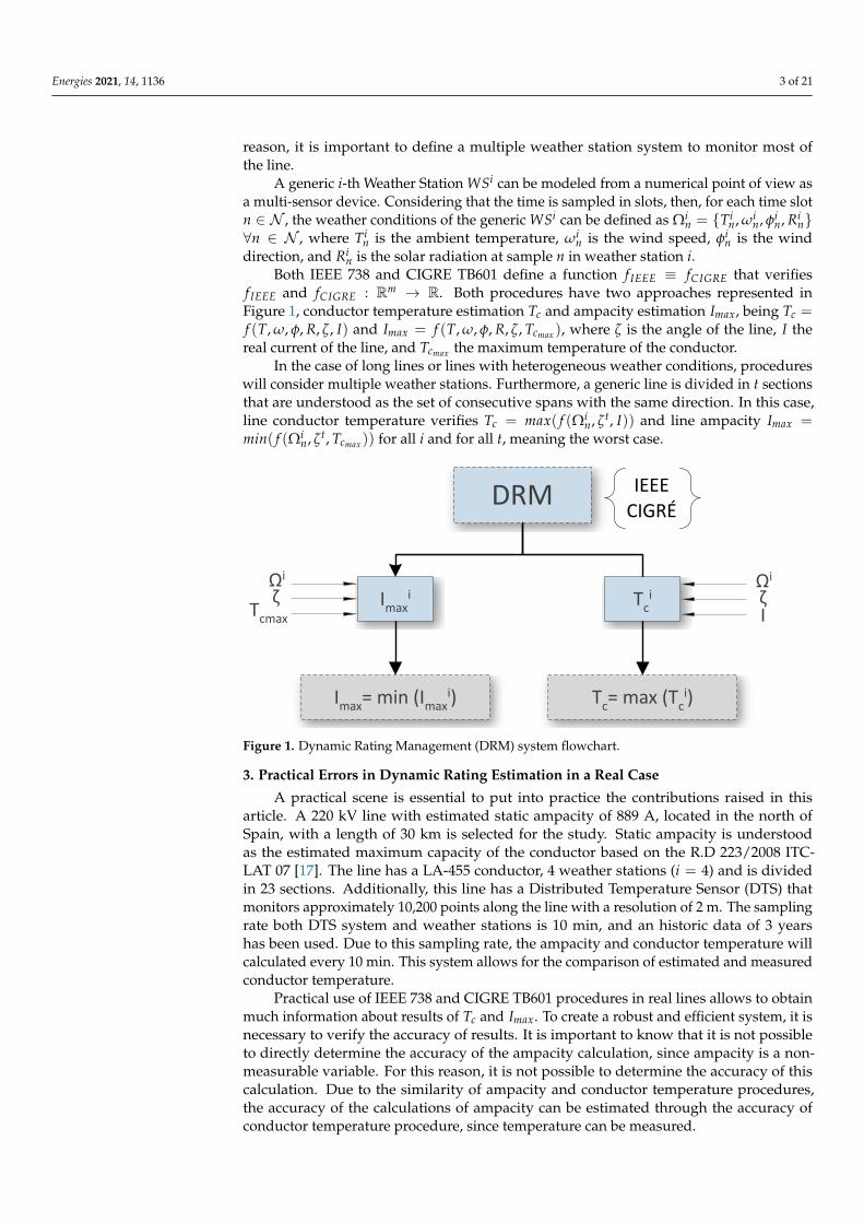
f IEEE and fCIGRE : Rm → R. Both procedures have two approaches represented inFigure 1, conductor temperature estimation Tc and ampacity estimation Imax, being Tc =f (T, ω, φ, R, ζ, I) and Imax = f (T, ω, φ, R, ζ, Tcmax ), where ζ is the angle of the line, I thereal current of the line, and Tcmax the maximum temperature of the conductor.

In the case of long lines or lines with heterogeneous weather conditions, procedureswill consider multiple weather stations. Furthermore, a generic line is divided in t sectionsthat are understood as the set of consecutive spans with the same direction. In this case,line conductor temperature verifies Tc = max( f (Ωi

n, ζt, I)) and line ampacity Imax =min( f (Ωi

n, ζt, Tcmax )) for all i and for all t, meaning the worst case.

DRM

Imaxi Tc

iΩi

ζ I

IEEECIGRÉ

Imax= min (Imaxi) Tc= max (Tc

i)

Ωi

ζ Tcmax

Figure 1. Dynamic Rating Management (DRM) system flowchart.

3. Practical Errors in Dynamic Rating Estimation in a Real Case

A practical scene is essential to put into practice the contributions raised in thisarticle. A 220 kV line with estimated static ampacity of 889 A, located in the north ofSpain, with a length of 30 km is selected for the study. Static ampacity is understoodas the estimated maximum capacity of the conductor based on the R.D 223/2008 ITC-LAT 07 [17]. The line has a LA-455 conductor, 4 weather stations (i = 4) and is dividedin 23 sections. Additionally, this line has a Distributed Temperature Sensor (DTS) thatmonitors approximately 10,200 points along the line with a resolution of 2 m. The samplingrate both DTS system and weather stations is 10 min, and an historic data of 3 yearshas been used. Due to this sampling rate, the ampacity and conductor temperature willcalculated every 10 min. This system allows for the comparison of estimated and measuredconductor temperature.

Practical use of IEEE 738 and CIGRE TB601 procedures in real lines allows to obtainmuch information about results of Tc and Imax. To create a robust and efficient system, it isnecessary to verify the accuracy of results. It is important to know that it is not possibleto directly determine the accuracy of the ampacity calculation, since ampacity is a non-measurable variable. For this reason, it is not possible to determine the accuracy of thiscalculation. Due to the similarity of ampacity and conductor temperature procedures,the accuracy of the calculations of ampacity can be estimated through the accuracy ofconductor temperature procedure, since temperature can be measured.

Energies 2021, 14, 1136 4 of 21

Accuracy of the procedures is defined as:

εTc = TDTSc − Tc, (4)

where εTc represents the error in Tc estimations, and TDTSc represents the measured con-

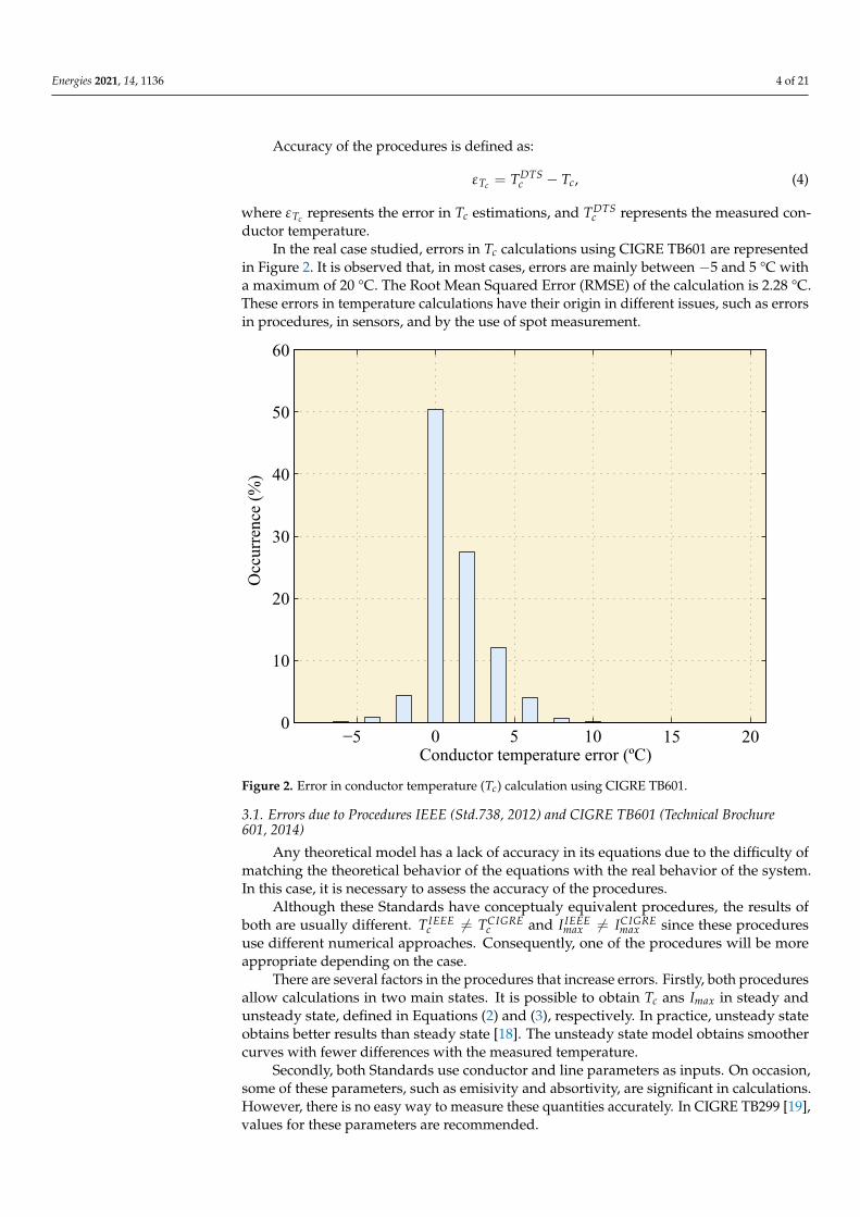
ductor temperature.In the real case studied, errors in Tc calculations using CIGRE TB601 are represented

in Figure 2. It is observed that, in most cases, errors are mainly between −5 and 5 °C witha maximum of 20 °C. The Root Mean Squared Error (RMSE) of the calculation is 2.28 °C.These errors in temperature calculations have their origin in different issues, such as errorsin procedures, in sensors, and by the use of spot measurement.

−5 15 200

10

20

30

40

50

60

0 5 10 Conductor temperature error (ºC)

Occ

urre

nce

(%)

Figure 2. Error in conductor temperature (Tc) calculation using CIGRE TB601.

3.1. Errors due to Procedures IEEE (Std.738, 2012) and CIGRE TB601 (Technical Brochure601, 2014)

Any theoretical model has a lack of accuracy in its equations due to the difficulty ofmatching the theoretical behavior of the equations with the real behavior of the system.In this case, it is necessary to assess the accuracy of the procedures.

Although these Standards have conceptualy equivalent procedures, the results ofboth are usually different. T IEEE

c 6= TCIGREc and I IEEE

max 6= ICIGREmax since these procedures

use different numerical approaches. Consequently, one of the procedures will be moreappropriate depending on the case.

There are several factors in the procedures that increase errors. Firstly, both proceduresallow calculations in two main states. It is possible to obtain Tc ans Imax in steady andunsteady state, defined in Equations (2) and (3), respectively. In practice, unsteady stateobtains better results than steady state [18]. The unsteady state model obtains smoothercurves with fewer differences with the measured temperature.

Secondly, both Standards use conductor and line parameters as inputs. On occasion,some of these parameters, such as emisivity and absortivity, are significant in calculations.However, there is no easy way to measure these quantities accurately. In CIGRE TB299 [19],values for these parameters are recommended.

Energies 2021, 14, 1136 5 of 21

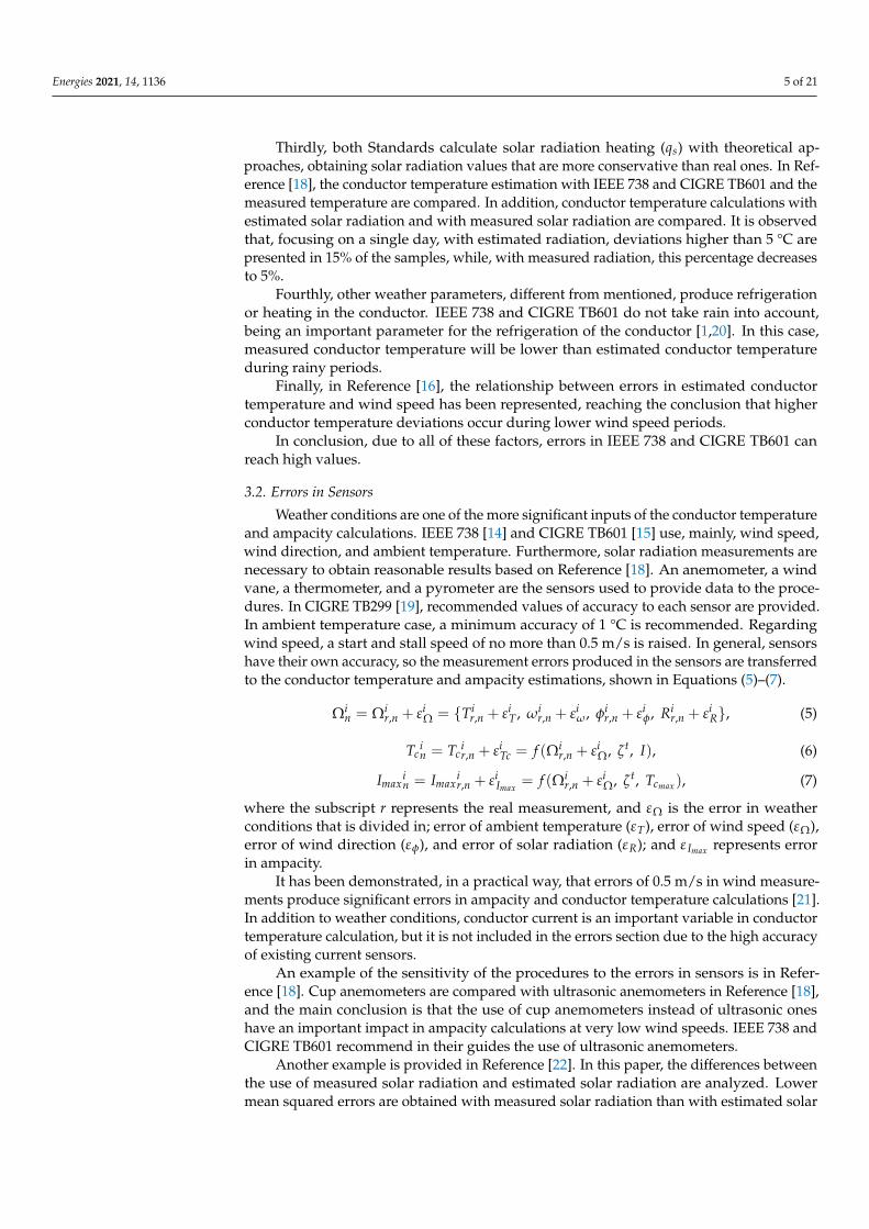
Thirdly, both Standards calculate solar radiation heating (qs) with theoretical ap-proaches, obtaining solar radiation values that are more conservative than real ones. In Ref-erence [18], the conductor temperature estimation with IEEE 738 and CIGRE TB601 and themeasured temperature are compared. In addition, conductor temperature calculations withestimated solar radiation and with measured solar radiation are compared. It is observedthat, focusing on a single day, with estimated radiation, deviations higher than 5 °C arepresented in 15% of the samples, while, with measured radiation, this percentage decreasesto 5%.

Fourthly, other weather parameters, different from mentioned, produce refrigerationor heating in the conductor. IEEE 738 and CIGRE TB601 do not take rain into account,being an important parameter for the refrigeration of the conductor [1,20]. In this case,measured conductor temperature will be lower than estimated conductor temperatureduring rainy periods.

Finally, in Reference [16], the relationship between errors in estimated conductortemperature and wind speed has been represented, reaching the conclusion that higherconductor temperature deviations occur during lower wind speed periods.

In conclusion, due to all of these factors, errors in IEEE 738 and CIGRE TB601 canreach high values.

3.2. Errors in Sensors

Weather conditions are one of the more significant inputs of the conductor temperatureand ampacity calculations. IEEE 738 [14] and CIGRE TB601 [15] use, mainly, wind speed,wind direction, and ambient temperature. Furthermore, solar radiation measurements arenecessary to obtain reasonable results based on Reference [18]. An anemometer, a windvane, a thermometer, and a pyrometer are the sensors used to provide data to the proce-dures. In CIGRE TB299 [19], recommended values of accuracy to each sensor are provided.In ambient temperature case, a minimum accuracy of 1 °C is recommended. Regardingwind speed, a start and stall speed of no more than 0.5 m/s is raised. In general, sensorshave their own accuracy, so the measurement errors produced in the sensors are transferredto the conductor temperature and ampacity estimations, shown in Equations (5)–(7).

Ωin = Ωi

r,n + εiΩ = Ti

r,n + εiT , ωi

r,n + εiω, φi

r,n + εiφ, Ri

r,n + εiR, (5)

Tcin = Tc

ir,n + εi

Tc = f (Ωir,n + εi

Ω, ζt, I), (6)

Imaxin = Imax

ir,n + εi

Imax= f (Ωi

r,n + εiΩ, ζt, Tcmax ), (7)

where the subscript r represents the real measurement, and εΩ is the error in weatherconditions that is divided in; error of ambient temperature (εT), error of wind speed (εΩ),error of wind direction (εφ), and error of solar radiation (εR); and ε Imax represents errorin ampacity.

It has been demonstrated, in a practical way, that errors of 0.5 m/s in wind measure-ments produce significant errors in ampacity and conductor temperature calculations [21].In addition to weather conditions, conductor current is an important variable in conductortemperature calculation, but it is not included in the errors section due to the high accuracyof existing current sensors.

An example of the sensitivity of the procedures to the errors in sensors is in Refer-ence [18]. Cup anemometers are compared with ultrasonic anemometers in Reference [18],and the main conclusion is that the use of cup anemometers instead of ultrasonic oneshave an important impact in ampacity calculations at very low wind speeds. IEEE 738 andCIGRE TB601 recommend in their guides the use of ultrasonic anemometers.

Another example is provided in Reference [22]. In this paper, the differences betweenthe use of measured solar radiation and estimated solar radiation are analyzed. Lowermean squared errors are obtained with measured solar radiation than with estimated solar

Energies 2021, 14, 1136 6 of 21

radiation. In addition, this paper concludes that differences increase when the sun rises,reaching errors up to 15 °C.

This type of error is analyzed with historical data of spring and summer of thestudied line.

All sensors have their own errors, but, in some of them, it is difficult to know if thedata is erroneous. In the case of wind speed, the high variability of its values make itdifficult to find errors. In the case of ambient temperature, depending on the geographicsituation, it is possible to find out off the normal range for all the WS.

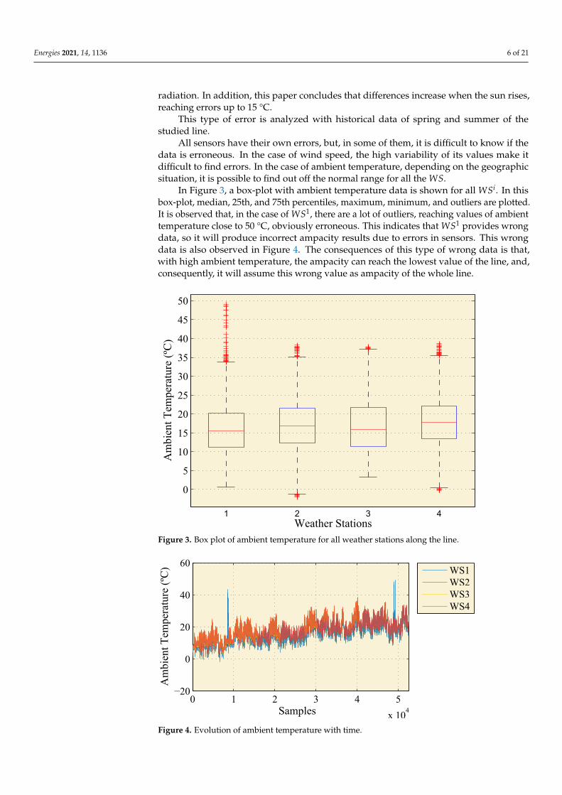
In Figure 3, a box-plot with ambient temperature data is shown for all WSi. In thisbox-plot, median, 25th, and 75th percentiles, maximum, minimum, and outliers are plotted.It is observed that, in the case of WS1, there are a lot of outliers, reaching values of ambienttemperature close to 50 °C, obviously erroneous. This indicates that WS1 provides wrongdata, so it will produce incorrect ampacity results due to errors in sensors. This wrongdata is also observed in Figure 4. The consequences of this type of wrong data is that,with high ambient temperature, the ampacity can reach the lowest value of the line, and,consequently, it will assume this wrong value as ampacity of the whole line.

0

5

10

15

20

25

30

35

40

45

50

1 2 3 4Weather Stations

Am

bien

t Tem

pera

ture

(ºC

)

Figure 3. Box plot of ambient temperature for all weather stations along the line.

0 1 2 3 4 5

x 104

−20

0

20

40

60

Samples

Am

bien

t Tem

pera

ture

(ºC

) WS1WS2WS3WS4

Figure 4. Evolution of ambient temperature with time.

Energies 2021, 14, 1136 7 of 21

In the case of solar radiation, it is easy to find wrong data if values at night are notzero or are much higher than normal values of the geographical zone. In the real case ofthis paper, there have been no sensor failures.

3.3. Errors due to the Use of Spot Measurements in a Long Line

Overhead lines have, usually, lengths from few to hundreds of kilometers. Due tothese long distances, weather conditions can vary considerably along the line. Since itis not possible to monitor the weather conditions in a continuous way, it is necessary toinstall several weather stations. The number of the weather stations depends on the lengthof the line and the climatic and orographic characteristics of the zone. Overhead lines withlong lengths or with different refrigeration characteristic along the line need more weatherstations than short lines or lines with uniform atmospheric characteristics. To decide thenumber of weather stations, a complete statistical study of the climatology of the zone willbe necessary.

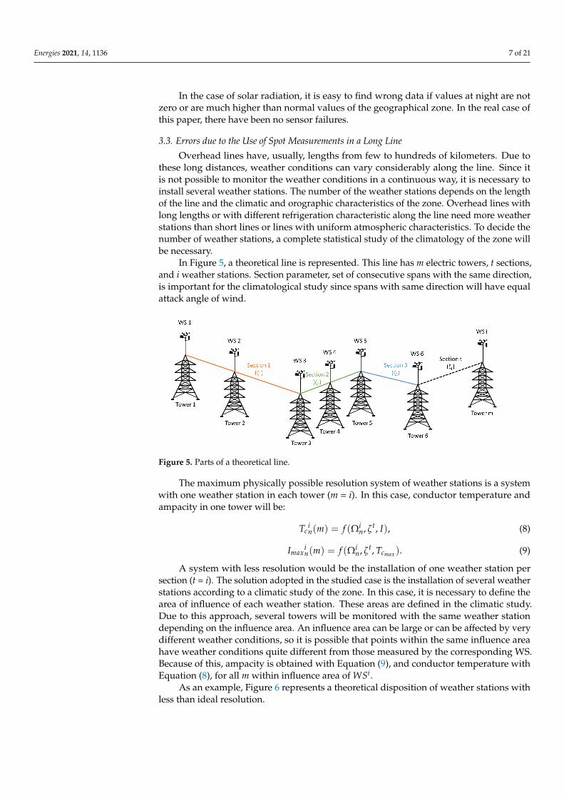
In Figure 5, a theoretical line is represented. This line has m electric towers, t sections,and i weather stations. Section parameter, set of consecutive spans with the same direction,is important for the climatological study since spans with same direction will have equalattack angle of wind.

Figure 5. Parts of a theoretical line.

The maximum physically possible resolution system of weather stations is a systemwith one weather station in each tower (m = i). In this case, conductor temperature andampacity in one tower will be:

Tcin(m) = f (Ωi

n, ζt, I), (8)

Imaxin(m) = f (Ωi

n, ζt, Tcmax ). (9)

A system with less resolution would be the installation of one weather station persection (t = i). The solution adopted in the studied case is the installation of several weatherstations according to a climatic study of the zone. In this case, it is necessary to define thearea of influence of each weather station. These areas are defined in the climatic study.Due to this approach, several towers will be monitored with the same weather stationdepending on the influence area. An influence area can be large or can be affected by verydifferent weather conditions, so it is possible that points within the same influence areahave weather conditions quite different from those measured by the corresponding WS.Because of this, ampacity is obtained with Equation (9), and conductor temperature withEquation (8), for all m within influence area of WSi.

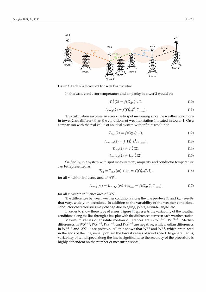
As an example, Figure 6 represents a theoretical disposition of weather stations withless than ideal resolution.

Energies 2021, 14, 1136 8 of 21

Figure 6. Parts of a theoretical line with less resolution.

In this case, conductor temperature and ampacity in tower 2 would be:

Tc1n(2) = f (Ω1

n, ζ1, I), (10)

Imax1n(2) = f (Ω1

n, ζ1, Tcmax ). (11)

This calculation involves an error due to spot measuring since the weather conditionsin tower 2 are different than the conditions of weather station 1 located in tower 1. On acomparison with the real value of an ideal system with infinite resolution:

Tcr,n(2) = f (Ω2n, ζ1, I), (12)

Imaxr,n(2) = f (Ω2n, ζ1, Tcmax ), (13)

Tcr,n(2) 6= Tc1n(2), (14)

Imaxr,n(2) 6= Imax1n(2). (15)

So, finally, in a system with spot measurement, ampacity and conductor temperaturecan be represented as:

Tcin = Tcr,n(m) + εTc = f (Ωi

n, ζt, I), (16)

for all m within influence area of WSi.

Imaxin(m) = Imaxr,n(m) + ε Imax = f (Ωi

n, ζt, Tcmax ), (17)

for all m within influence area of WSi.The differences between weather conditions along the line produce Tc and Imax results

that vary, widely on occasions. In addition to the variability of the weather conditions,conductor characteristics may change due to aging, joints, altitude, angle, etc.

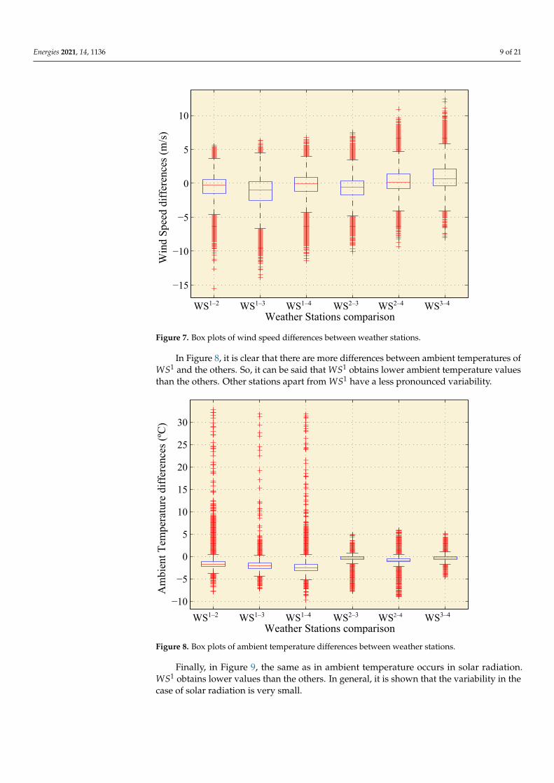
In order to show these type of errors, Figure 7 represents the variability of the weatherconditions along the line through a box plot with the differences between each weather station.

Maximum values of absolute median differences are in WS1−3, WS3−4. Mediandifferences in WS1−2, WS1−3, WS1−4, and WS2−3 are negative, while median differencesin WS2−4 and WS3−4 are positive. All this shows that WS1 and WS4, which are placedin the ends of the line, usually obtain the lowest values of wind speed. In general terms,variability of wind speed along the line is significant, so the accuracy of the procedure ishighly dependent on the number of measuring spots.

Energies 2021, 14, 1136 9 of 21

WS1–2 WS1–3 WS1–4 WS2–3 WS2–4 WS3–4

−15

−10

−5

0

5

10

Weather Stations comparison

Win

d S

peed

dif

fere

nces

(m

/s)

Figure 7. Box plots of wind speed differences between weather stations.

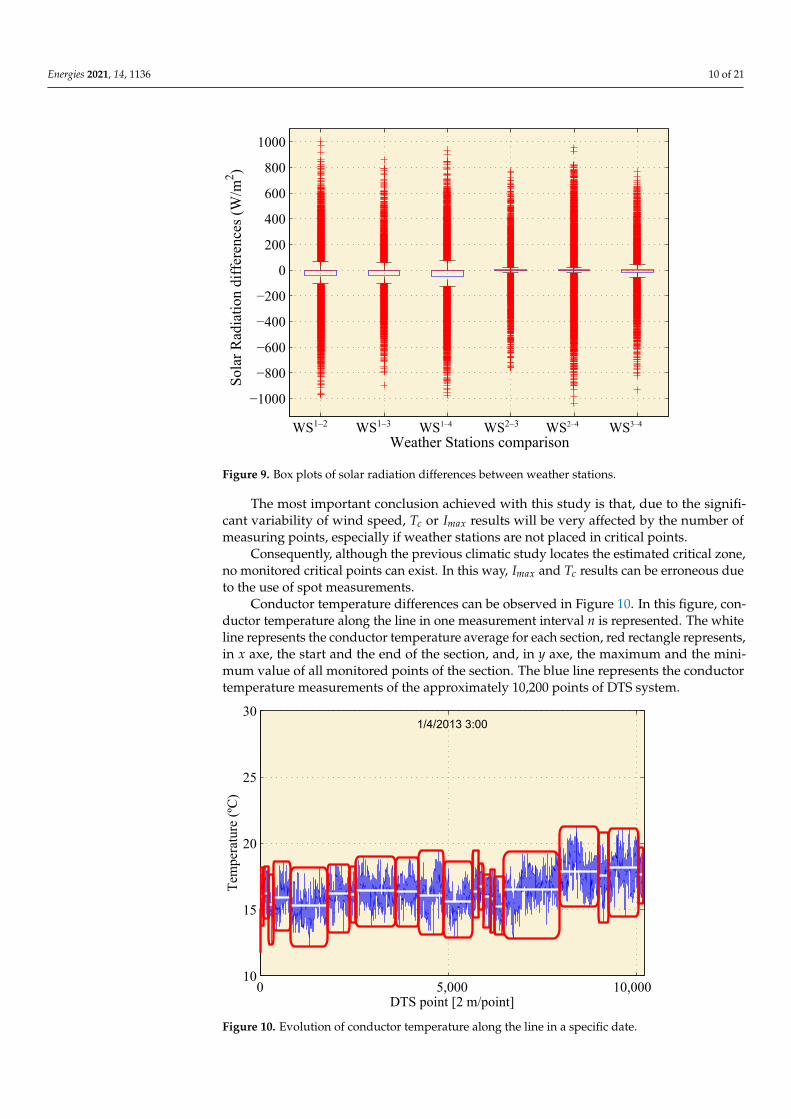
In Figure 8, it is clear that there are more differences between ambient temperatures ofWS1 and the others. So, it can be said that WS1 obtains lower ambient temperature valuesthan the others. Other stations apart from WS1 have a less pronounced variability.

WS1–2 WS1–3 WS1–4 WS2–3 WS2–4 WS3–4

−10

−5

0

5

10

15

20

25

30

Weather Stations comparison

Am

bien

t Tem

pera

ture

dif

fere

nces

(ºC

)

Figure 8. Box plots of ambient temperature differences between weather stations.

Finally, in Figure 9, the same as in ambient temperature occurs in solar radiation.WS1 obtains lower values than the others. In general, it is shown that the variability in thecase of solar radiation is very small.

Energies 2021, 14, 1136 10 of 21

WS1–2 WS1–3 WS1–4 WS2–3 WS2–4 WS3–4

−1000

−800

−600

−400

−200

0

200

400

600

800

1000

Weather Stations comparison

Sol

ar R

adia

tion

dif

fere

nces

(W

/m2 )

Figure 9. Box plots of solar radiation differences between weather stations.

The most important conclusion achieved with this study is that, due to the signifi-cant variability of wind speed, Tc or Imax results will be very affected by the number ofmeasuring points, especially if weather stations are not placed in critical points.

Consequently, although the previous climatic study locates the estimated critical zone,no monitored critical points can exist. In this way, Imax and Tc results can be erroneous dueto the use of spot measurements.

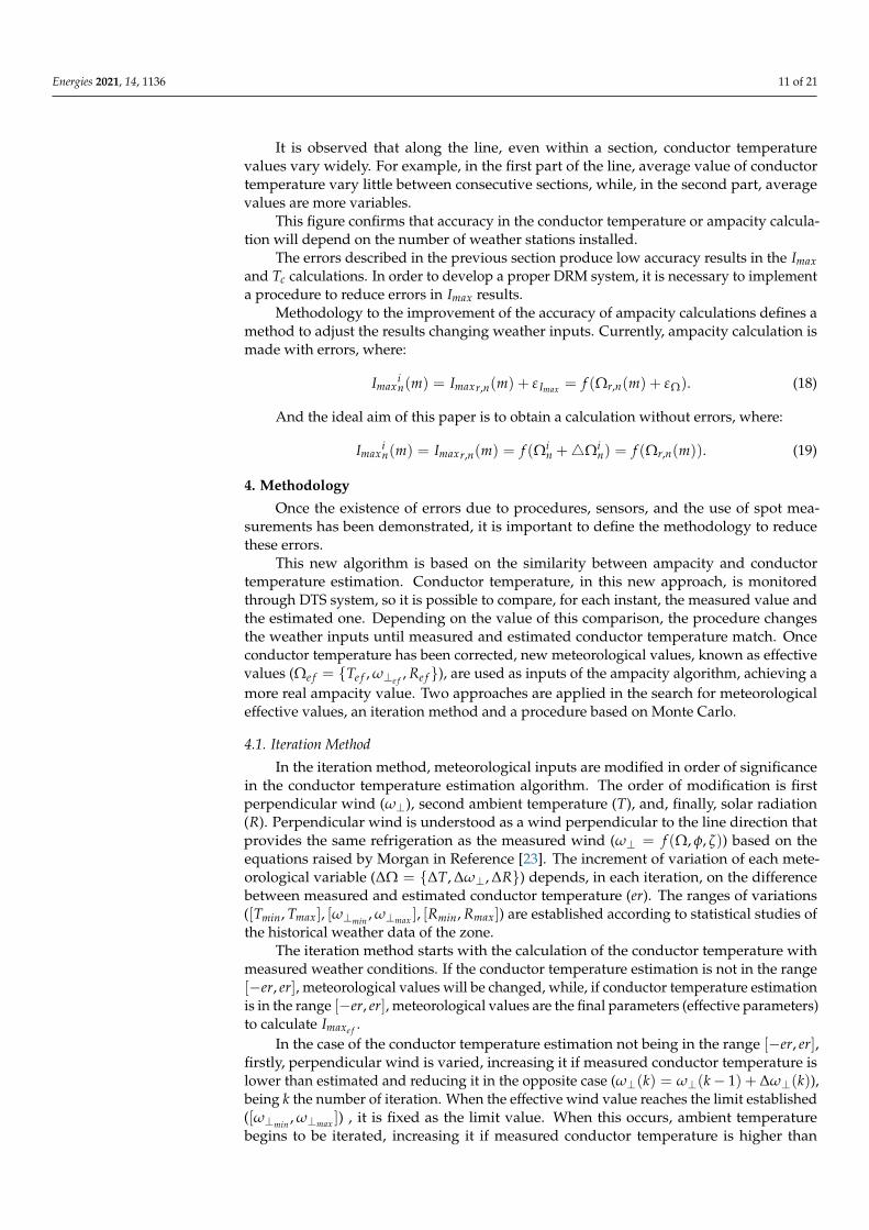
Conductor temperature differences can be observed in Figure 10. In this figure, con-ductor temperature along the line in one measurement interval n is represented. The whiteline represents the conductor temperature average for each section, red rectangle represents,in x axe, the start and the end of the section, and, in y axe, the maximum and the mini-mum value of all monitored points of the section. The blue line represents the conductortemperature measurements of the approximately 10,200 points of DTS system.

0 10,00010

15

20

25

30

5,000DTS point [2 m/point]

Tem

pera

ture

(ºC)

1/4/2013 3:00

Figure 10. Evolution of conductor temperature along the line in a specific date.

Energies 2021, 14, 1136 11 of 21

It is observed that along the line, even within a section, conductor temperaturevalues vary widely. For example, in the first part of the line, average value of conductortemperature vary little between consecutive sections, while, in the second part, averagevalues are more variables.

This figure confirms that accuracy in the conductor temperature or ampacity calcula-tion will depend on the number of weather stations installed.

The errors described in the previous section produce low accuracy results in the Imaxand Tc calculations. In order to develop a proper DRM system, it is necessary to implementa procedure to reduce errors in Imax results.

Methodology to the improvement of the accuracy of ampacity calculations defines amethod to adjust the results changing weather inputs. Currently, ampacity calculation ismade with errors, where:

Imaxin(m) = Imaxr,n(m) + ε Imax = f (Ωr,n(m) + εΩ). (18)

And the ideal aim of this paper is to obtain a calculation without errors, where:

Imaxin(m) = Imaxr,n(m) = f (Ωi

n +4Ωin) = f (Ωr,n(m)). (19)

4. Methodology

Once the existence of errors due to procedures, sensors, and the use of spot mea-surements has been demonstrated, it is important to define the methodology to reducethese errors.

This new algorithm is based on the similarity between ampacity and conductortemperature estimation. Conductor temperature, in this new approach, is monitoredthrough DTS system, so it is possible to compare, for each instant, the measured value andthe estimated one. Depending on the value of this comparison, the procedure changesthe weather inputs until measured and estimated conductor temperature match. Onceconductor temperature has been corrected, new meteorological values, known as effectivevalues (Ωe f = Te f , ω⊥e f

, Re f ), are used as inputs of the ampacity algorithm, achieving amore real ampacity value. Two approaches are applied in the search for meteorologicaleffective values, an iteration method and a procedure based on Monte Carlo.

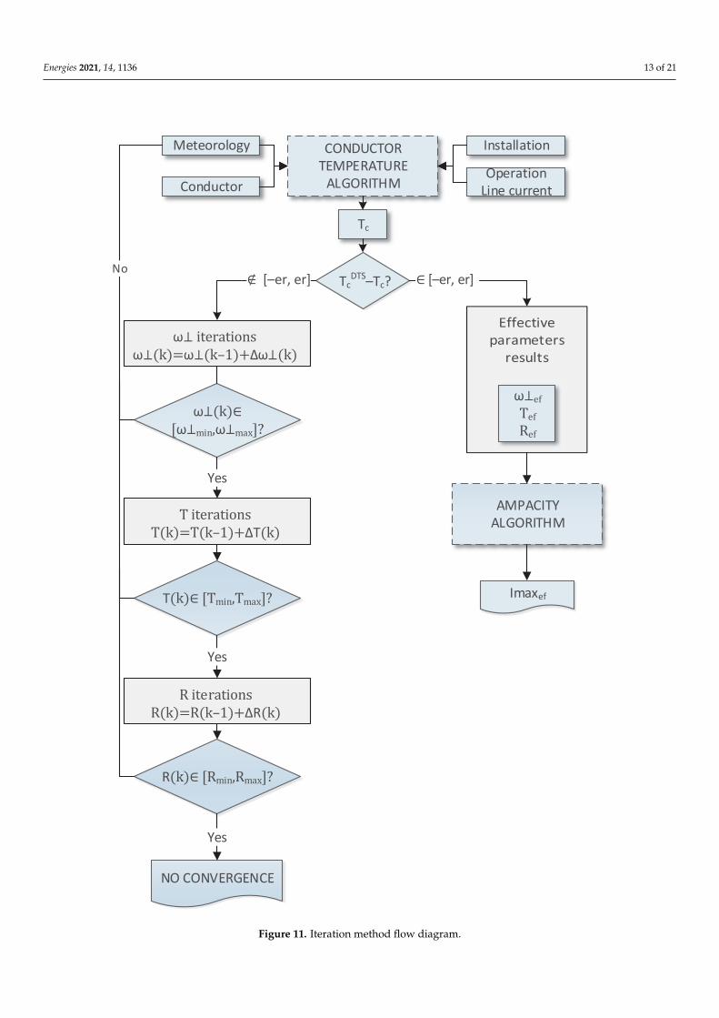
4.1. Iteration Method

In the iteration method, meteorological inputs are modified in order of significancein the conductor temperature estimation algorithm. The order of modification is firstperpendicular wind (ω⊥), second ambient temperature (T), and, finally, solar radiation(R). Perpendicular wind is understood as a wind perpendicular to the line direction thatprovides the same refrigeration as the measured wind (ω⊥ = f (Ω, φ, ζ)) based on theequations raised by Morgan in Reference [23]. The increment of variation of each mete-orological variable (∆Ω = ∆T, ∆ω⊥, ∆R) depends, in each iteration, on the differencebetween measured and estimated conductor temperature (er). The ranges of variations([Tmin, Tmax], [ω⊥min , ω⊥max ], [Rmin, Rmax]) are established according to statistical studies ofthe historical weather data of the zone.

The iteration method starts with the calculation of the conductor temperature withmeasured weather conditions. If the conductor temperature estimation is not in the range[−er, er], meteorological values will be changed, while, if conductor temperature estimationis in the range [−er, er], meteorological values are the final parameters (effective parameters)to calculate Imaxe f .

In the case of the conductor temperature estimation not being in the range [−er, er],firstly, perpendicular wind is varied, increasing it if measured conductor temperature islower than estimated and reducing it in the opposite case (ω⊥(k) = ω⊥(k− 1) + ∆ω⊥(k)),being k the number of iteration. When the effective wind value reaches the limit established([ω⊥min , ω⊥max ]) , it is fixed as the limit value. When this occurs, ambient temperaturebegins to be iterated, increasing it if measured conductor temperature is higher than

Energies 2021, 14, 1136 12 of 21

estimated and reducing it in the opposite case (T(k) = T(k− 1) + ∆T(k)). In the sameway as perpendicular wind, when ambient temperature value reaches the established limit([Tmin, Tmax]), it is fixed as the limit value. Finally, solar radiation is changed, increasingit if measured conductor temperature is higher than estimated and reducing it in theopposite case (R(k) = R(k− 1) + ∆R(k)). If solar radiation reaches the established limit([Rmin, Rmax]) and estimated conductor temperature does not match with the measuredone, it is considered that the method does not converge.

In the case convergence is achieved, the effective meteorological values will be theinputs of the ampacity model. Figure 11 summarizes the proposed methodology.

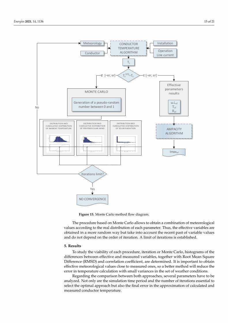
4.2. Monte Carlo Method

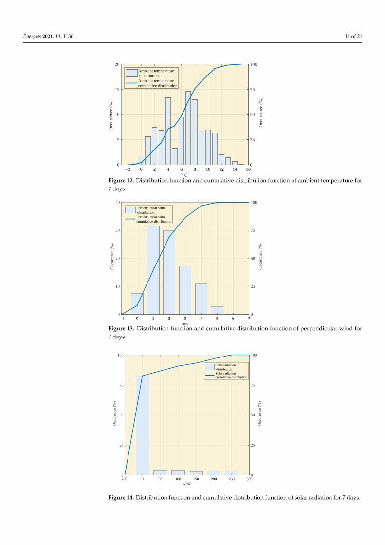
Monte Carlo is a non-deterministic method used to model complex mathematical ex-pressions. This method provides approximate solutions using a sample of the total of thecalculations in base on pseudo-random samples. In the case of this paper, Monte Carlomethod is employed to obtain successive pseudo-random meteorological samples, among allthe possible values. The pseudo-random samples are based on the distribution function ofeach parameter to give a physical base to the randomness. Distribution functions of ambienttemperature, perpendicular wind, and solar radiation are estimated with historical valuesfrom a established time (7 days). This method is suggested by the necessity to perform the cal-culation of effective variables with a physical base. In the iteration case, limits of variation ofeach meteorological variable are established, but, in certain scenarios, effective meteorologicalresults are not realistic. These unrealistic values can appear because of several reasons but aremainly due to errors in the procedure, in the measurement of the weather conditions, or bythe use of spot measurements. These errors make the algorithm to introduce huge changes inthe weather conditions to achieve values of measured conductor temperature. For this reason,in some cases, effective meteorological results are not realistic. In the case of Monte Carlomethod, the effective meteorological values will always be within the distribution functionof the preceding 7 days. An example of distribution function and cumulative distributionfunction for the meteorological variables is represented in Figures 12–14.

The calculation of effective parameters, with Monte Carlo method, starts with thecalculation of Tc with the measured meteorological variables. If the error between thecalculated Tc and the measured Tc by the DTS system is higher than an established error,the Monte Carlo method is applied. The first step in this method is to generate a pseudo-random number between 0 and 1. This value represents the occurrence in the cumulativedistribution function of ambient temperature, perpendicular wind, and solar radiation.Therefore, a value of ambient temperature, perpendicular wind, and solar radiation willcorrespond with the pseudo-random occurrence value. These values are used as meteo-rological input in the temperature calculation algorithm. This will iterate until the errorbetween the calculated Tc and the measured Tc by the DTS system is lower than establishedone or the Monte Carlo iteration limit is reached. A distribution with 7 previous days ofhistorical data is obtained every instant of Tc and ampacity calculation. Figure 15 showsthe flow diagram of the Monte Carlo method.

Energies 2021, 14, 1136 13 of 21

ωω ω – Δω

– ΔT

– ΔR

CONDUCTOR TEMPERATURE

ALGORITHM

Tc

TcDTS–Tc? [–er, er]

ωω ω

NO CONVERGENCE

[–er, er]

Meteorology

Conductor

Installation

Operation Line current

Yes

T

Yes

R

Yes

ω

AMPACITY ALGORITHM

Imaxef

No

Figure 11. Iteration method flow diagram.

Energies 2021, 14, 1136 14 of 21

0 2 4 6 8 10 12 14 16º C

0

5

10

15

20

Occ

urre

nce

(%)

Ambient temperature distributionAmbient temperaturecumulative distribution

– 2 0 2 4 6 8 10 12 14 160

25

50

75

100

Occ

urre

nce

(%)

Figure 12. Distribution function and cumulative distribution function of ambient temperature for7 days.

0 1 2 3 4 5 6 7m/s

0

10

20

30

40

Occ

urre

nce

(%)

Perpendicular wind distributionPerpendicular windcumulative distribution

– 1 0 1 2 3 4 5 6 70

25

50

75

100

Occ

urre

nce

(%)

Figure 13. Distribution function and cumulative distribution function of perpendicular wind for7 days.

-50 0 50 100 150 200 250 300W/m2

0

25

50

75

100

Occ

urre

nce

(%)

Solar radiation distributionSolar radiationcumulative distribution

-50 0 50 100 150 200 250 3000

25

50

75

100

Occ

urre

nce

(%)

Figure 14. Distribution function and cumulative distribution function of solar radiation for 7 days.

Energies 2021, 14, 1136 15 of 21

Generation of a pseudo-random number between 0 and 1

0 5 10 15 20 25 300

0.02

0.04

0.06

0.08

0.1

0.12

Temperatura ambiente [ºC]

fdp

0 5 10 15 20 25 300

20

40

60

80

100

Temperatura ambiente [ºC]

fpa

0 2 4 6 8 10 12 14 16 180

0.05

0.1

0.15

0.2

Magnitud del viento [m/s]

fdp

0 2 4 6 8 10 12 14 16 180

20

40

60

80

100

Magnitud del viento [m/s]

fpa

0 200 400 600 800 1000 1200 14000

0.1

0.2

0.3

0.4

0.5

Radiación solar [W/m2]

fdp

0 200 400 600 800 1000 1200 14000

20

40

60

80

100

Radiación solar [W/m2]

fpa

CONDUCTOR TEMPERATURE

ALGORITHM

Tc

TcDTS–Tc [–er, er] [–er, er]

Meteorology

Conductor

Installation

OperationLine current

ω

AMPACITY ALGORITHM

Imaxef

Iterations limit?

No

NO CONVERGENCE

Yes

Figure 15. Monte Carlo method flow diagram.

The procedure based on Monte Carlo allows to obtain a combination of meteorologicalvalues according to the real distribution of each parameter. Thus, the effective variables areobtained in a more random way but take into account the recent past of variable valuesand do not depend on the order of iteration. A limit of iterations is established.

5. Results

To study the viability of each procedure, iteration or Monte Carlo, histograms of thedifferences between effective and measured variables, together with Root Mean SquareDifference (RMSD) and correlation coefficient, are determined. It is important to obtaineffective meteorological values close to measured ones, so a better method will reduce theerror in temperature calculation with small variances in the set of weather conditions.

Regarding the comparison between both approaches, several parameters have to beanalyzed. Not only are the simulation time period and the number of iterations essential toselect the optimal approach but also the final error in the approximation of calculated andmeasured conductor temperature.

Energies 2021, 14, 1136 16 of 21

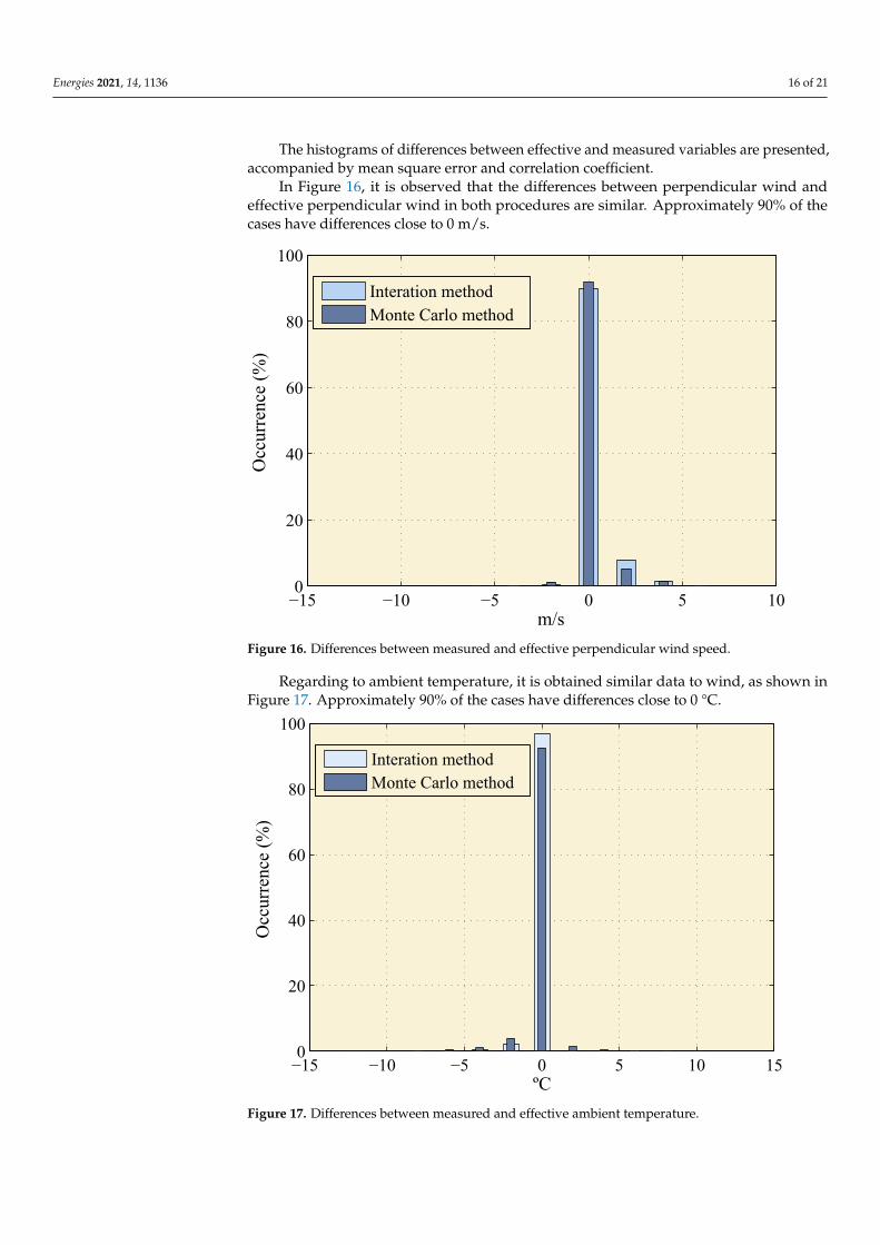
The histograms of differences between effective and measured variables are presented,accompanied by mean square error and correlation coefficient.

In Figure 16, it is observed that the differences between perpendicular wind andeffective perpendicular wind in both procedures are similar. Approximately 90% of thecases have differences close to 0 m/s.

−15 −10 −5 0 5 100

20

40

60

80

100

m/s

Occ

urre

nce

(%)

Interation methodMonte Carlo method

Figure 16. Differences between measured and effective perpendicular wind speed.

Regarding to ambient temperature, it is obtained similar data to wind, as shown inFigure 17. Approximately 90% of the cases have differences close to 0 °C.

−15 −10 −5 0 5 10 150

20

40

60

80

100

ºC

Occ

urre

nce

(%)

Interation methodMonte Carlo method

Figure 17. Differences between measured and effective ambient temperature.

Energies 2021, 14, 1136 17 of 21

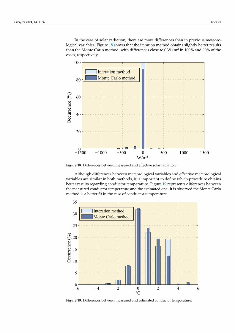
In the case of solar radiation, there are more differences than in previous meteoro-logical variables. Figure 18 shows that the iteration method obtains slightly better resultsthan the Monte Carlo method, with differences close to 0 W/m2 in 100% and 90% of thecases, respectively.

−1500 −1000 −500 0 500 1000 15000

20

40

60

80

100

W/m²

Occ

urre

nce

(%)

Interation methodMonte Carlo method

Figure 18. Differences between measured and effective solar radiation.

Although differences between meteorological variables and effective meteorologicalvariables are similar in both methods, it is important to define which procedure obtainsbetter results regarding conductor temperature. Figure 19 represents differences betweenthe measured conductor temperature and the estimated one. It is observed the Monte Carlomethod is a better fit in the case of conductor temperature.

−6 −4 −2 0 2 4 60

5

10

15

20

25

30

35

ºC

Occ

urre

nce

(%)

Interation methodMonte Carlo method

Figure 19. Differences between measured and estimated conductor temperature.

Energies 2021, 14, 1136 18 of 21

Table 1 shows the numerical results of RMSD of meteorological variables and RMSEof conductor temperature.and the correlation coefficient. In the same way as histograms,numerical results show that RMSD in perpendicular wind is lower in the Monte Carlomethod, while, in ambient temperature and solar radiation, it is higher than the iterationmethod. Regarding conductor temperature, although the results are similar, RMSE islower in Monte Carlo method. The latter indicates that the Monte Carlo method correctsconductor temperature slighly better than the iteration method.

Table 1. Numerical results of RMSD (for metheorological variables) and RMSE (for conductor temperature) differencesbetween measured and estimated values.

Perpendicular Wind (m/s) Ambient Temperature (C) Solar Radiation (W/m2) Conductor Temperature (C)

Iteration Monte Carlo Iteration Monte Carlo Iteration Monte Carlo Iteration Monte Carlomethod method method method method method method method

RMSD 0.821 0.724 0.440 0.911 0.000 104.6 1.613 1.572Correlation 0.848 0.875 0.997 0.987 1.000 0.914 0.980 0.980

Other important parameters for the optimal selection of the procedure are the timeof simulation and the iterations required in each algorithm, defined as the average num-ber of iterations. In the case of iteration method, the simulation time was 7.36 min for55,000 samples, with an average of iterations of 1.58. On the other hand, the Monte Carlomethod simulation time was 90.20 min for 55,000 samples, with an average of iterationsof 28.80.

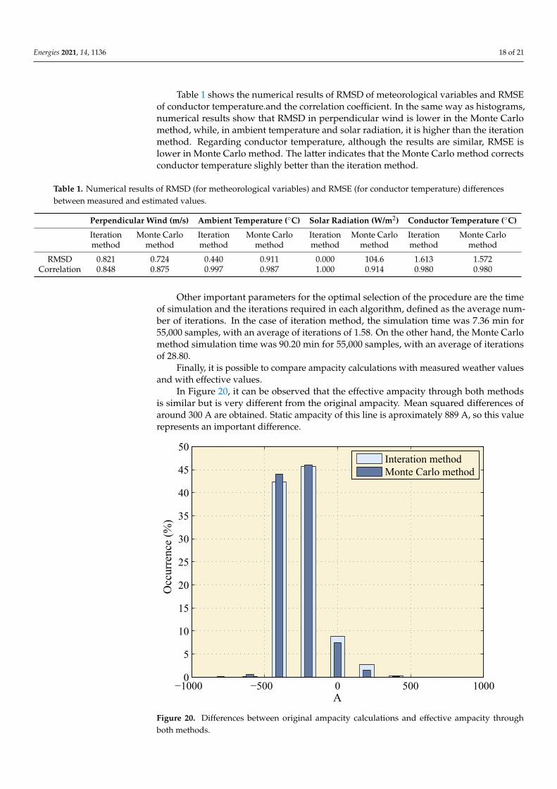
Finally, it is possible to compare ampacity calculations with measured weather valuesand with effective values.

In Figure 20, it can be observed that the effective ampacity through both methodsis similar but is very different from the original ampacity. Mean squared differences ofaround 300 A are obtained. Static ampacity of this line is aproximately 889 A, so this valuerepresents an important difference.

−1000 −500 0 500 10000

5

10

15

20

25

30

35

40

45

50

A

Occ

urre

nce

(%)

Interation methodMonte Carlo method

Figure 20. Differences between original ampacity calculations and effective ampacity throughboth methods.

Energies 2021, 14, 1136 19 of 21

6. Discussion

Focusing on the effective perpendicular wind, the difference between the measuredperpendicular wind and the effective perpendicular wind is very similar. Based on this, it isconcluded that with small variations of perpendicular wind is possible to correct conductortemperature errors. In addition, both iteration and Monte Carlo methods obtain similarresults in the case of perpendicular wind analysis. Monte Carlo method obtains slightlybetter results.

In the case of effective ambient temperature, similarly to effective perpendicularwind, the differences are small in most of the cases. Therefore, with small variationsof the ambient temperature, correction of the conductor temperature errors is achieved.In addition, both iteration and Monte Carlo methods obtain similar results. In contrast toperpendicular wind, iteration method obtains slightly better results.

In the case of effective solar radiation, although the differences between effective andmeasured values are small in most of the cases, the iteration method obtains better resultsthan Monte Carlo method.

Finally, although the results of the calculation of conductor temperature shows thatMonte Carlo method obtains more accurate results than iteration method, the differencebetween RMSDs is small.

Taking into account the slightly difference between the RMSDs of each method, it isimportant to analyze the computing workload of the methods. In this case, the resultsindicate that the iteration method has a simulation time period markedly lower thanMonte Carlo method. In addition, the iteration method makes less iterations to obtain thecorrected conductor temperature. Specifically, the Iteration method takes 8 ms per sample,while Monte Carlo method takes 98.4 ms per sample. With these results, both approachesare valid to implement in a real time system without significant delays.

7. Conclusions

An important difficulty in the integration of renewable energies is the existing limitsin the power lines. Today, several techniques exist to increase the capacity of overheadlines. Due to economic, legal, and environmental constraints, the most appropriate solutionis to monitor weather conditions and electric current of the overhead lines to estimatecapacity and conductor temperature in real time. Distribution companies use DRM systemto operate overhead lines today.

The practical application of DRM allows to find several deficiencies related to errorsin Tc estimations, and consequently in Imax. In this paper, errors between estimated andmeasured conductor temperature are presented. These errors in conductor temperatureand, consequently, in ampacity estimations are, in certain occasions, large, with a RMSE of2.28 °C.

These errors encourage the design of a procedure to obtain high accuracy ampacityvalues. In the case of this paper, two methodologies have been tested to reduce estimationerrors. Both methodologies use the variation of the weather inputs, and it is demonstratedthat a reduction of the conductor temperature calculation error has been achieved and,consequently, a reduction of ampacity error. With the iteration method, a RMSE of 1.61 °C isobtained, and, with the Monte Carlo method, a RMSE of 1.57 °C. This involves a reductionof the RMSE of approximately 30%.

Once the capacity of both procedures to achieve a reduction in errors is proven, it isnecessary make a decision about the most appropriate procedure. Several aspects areconsidered to find the optimal methodology. The more appropriate method must presentthe lowest errors in conductor temperature estimation with small differences betweeneffective and measured weather values, minimum simulation time, and minimum averageof iterations.

In view of the results, it can be considered that the iteration method is more suitablefor the optimization of ampacity estimation. Although both methods achieve, with smallvariances of weather conditions, low conductor temperature errors, the iteration method

Energies 2021, 14, 1136 20 of 21

obtains better results than the Monte Carlo method. In the case of simulation time andaverage of iterations, iteration method simulations take 8 ms per sample and convergein an average of 1.58 iterations of the weather conditions, while, with the Monte Carlomethod, simulations take 98.4 ms per sample and converge in an average of 28.8 iterationsof the weather conditions.

The limitations of these procedures are based on the availability and the accuracy ofreal measurements of conductor temperature. Most of the DRM systems used are basedonly on the ampacity values without measurement of conductor temperature. In this typeof system, the approaches presented in this paper are not valid to increase the accuracy.In the case of DRM systems with conductor temperature measurements, the effectiveness ofthe approaches of this paper will depend on the accuracy of the conductor temperature mea-sures. In the case of DTS systems, the accuracy is higher than spot measurement systems,but they are not yet widely used due to its cost and the difficulties to install. Spot mea-surement sensors are widely used, but its accuracy is lower than DTS systems, and thecontinuity of the measurements is a problem when the location is remote. Between thetwo procedures, the Monte Carlo method has more limitations since, if the accuracy of themeasurements is low, the algorithm could achieve the iteration limit without solution.

A future research would analyze the reduction of the limitations of these approaches,implementing an algorithm to estimate the conductor temperature measurements when alack of measurement occurs in base on the historical values.

Author Contributions: Conceptualization, M.M. and R.M. (Raquel Martinez); methodology, M.M.and R.M. (Raquel Martinez); software, R.M. (Raquel Martinez); validation, M.M. and R.M. (RaquelMartinez); formal analysis, A.A., S.B. and A.L.; investigation, R.M. (Raquel Martinez); resources, A.A.and M.M.; data curation, R.M. (Raquel Martinez); writing—original draft preparation, A.A. and R.M.(Raquel Martinez); writing—review and editing, A.A., S.B., P.C., A.L. and R.M. (Raquel Martinez).;visualization, R.M. (Rafael Minguez); supervision, R.M. (Rafael Minguez); project administration,M.M. and R.M. (Rafael Minguez); funding acquisition, M.M. All authors have read and agreed to thepublished version of the manuscript.

Funding: This research was funded by the Spanish Government AND FEDER funds under the R+Dinitiative RETOS COLABORACIÓN 2015” with reference RETOS COLABORACIÓN RTC-2015-3795-3 and Spanish R+D initiative with reference ENE2013-42720-R.

Institutional Review Board Statement: Not applicable.

Informed Consent Statement: Not applicable.

Data Availability Statement: Restrictions apply to the availability of these data. Data was obtainedfrom Viesgo and REE and are available from the authors with the permission of Viesgo and REE.

Acknowledgments: The authors would like to acknowledge the Spanish Government AND FEDERfunds for the economical support and Viesgo and REE for technical support and data provision.

Conflicts of Interest: The authors declare no conflict of interest.

References1. Fernandez, E.; Albizu, I.; Mazon, A.J.; Etxegarai, A.; Buigues, G.; Alberdi, R. Power line monitoring for the analysis of overhead

line rating forecasting methods. IEEE PES Power Afr. 2016, 119–123. [CrossRef]2. Zhou, X.; Wang, S.; Li, T.; Cao, J.; Zou, Y.; Xiang, X. Probabilistic Ampacity Rating of 500 kV Overhead Transmission Lines in

Zhejiang Province. In Proceedings of the IEEE 3rd International Conference on Integrated Circuits and Microsystems (ICICM),Shanghai, China, 24–26 November 2018; pp. 98–103.

3. Pyka, K.; Piskorski, R. DSM Based on ALS Data for Needs of Urban Space Analysis. In Proceedings of the 2018 Baltic GeodeticCongress (BGC Geomatics), Olsztyn, Poland, 21–23 June 2018; pp. 164–168.

4. Cho, J.; Kim, J.H.; Lee, H.J.; Kim, J.Y.; Song, I.K.; Choi, J.H. Development and Improvement of an Intelligent Cable MonitoringSystem for Underground Distribution Networks Using Distributed Temperature Sensing. Energies 2014, 7, 1076–1094. [CrossRef]

5. Holyk, C.; Liess, H.D.; Grondel, S.; Kanbach, H.; Loos, F. Simulation and measurement of the steady-state temperature inmulti-core cables. Electr. Power Syst. Res. 2014, 116, 54–66. [CrossRef]

Energies 2021, 14, 1136 21 of 21

6. Marins, D.S.; Antunes, F.L.M.; Sampaio, M.V.F. Increasing Capacity of Overhead Transmission Lines—A Challenge for BrazilianWind Farms. In Proceedings of the 6th IEEE International Energy Conference (ENERGYCon), Gammarth, Tunisia, 28 September–1 October 2020; pp. 434–438.

7. Lauria, D.; Mottola, F.; Quaia, S. Analytical Description of Overhead Transmission Lines Loadability. Energies 2019, 12, 3119.[CrossRef]

8. Erdinç, F.G.; Erdinç, O.; Yumurtacı, R.; Catalão, J.P.S. A Comprehensive Overview of Dynamic Line Rating Combined with OtherFlexibility Options from an Operational Point of View. Energies 2020, 13, 6563. [CrossRef]

9. Minguez, R.; Martínez, R.; Manana, M.; Arroyo, A.;Domingo, R.; Laso, A. Dynamic management in overhead lines: A successfulcase of reducing restrictions in renewable energy sources integration. Electr. Power Syst. Res. 2019, 173, 135–142. [CrossRef]

10. Martinez, R.; Useros, A.; Castro, P.; Arroyo, A.; Manana, A. Distributed vs. spot temperature measurements in dynamic rating ofoverhead power lines. Electr. Power Syst. Res. 2019, 170, 273–276. [CrossRef]

11. Alvarez, D.L.; da Silva, F.F.; Mombello, E.E.; Bak, C.L.; Rosero, J.A. Conductor Temperature Estimation and Prediction at ThermalTransient State in Dynamic Line Rating Application. IEEE Trans. Power Deliv. 2018, 33, 2236–2245. [CrossRef]

12. Douglass, D.A.; Gentle, J.; Nguyen, H.M.; Chisholm, W.; Xu, C.; Goodwin, T.; Chen, H.; Nuthalapati, S.; Hurst, N.; Grant, I.; et al.A Review of Dynamic Thermal Line Rating Methods With Forecasting. IEEE Trans. Power Deliv. 2019, 34, 2100–2109. [CrossRef]

13. Puffer, R.; Schmale, M.; Rusek, B. Area-wide dynamic line ratings based on weather measurements. In Proceedings of theConference on Cigre Session, Paris, France, 26–31 August 2012.

14. IEEE Standard for Calculating the Current-Temperature Relationship of Bare Overhead Conductors. IEEE Std 738-2012 (Revisionof IEEE Std 738-2006); IEEE: Piscataway, NJ, USA, 2012.

15. International Council on Large Electric Systems, Working Group B2.43. TB 601. Guide for Thermal Rating Calculations of OverheadLines; CIGRE: Paris, France, 2014.

16. Arroyo, A.; Castro, P.; Martinez, R.; Manana, M.; Madrazo, A.; Lecuna, R.; Gonzalez, A. Comparison between IEEE and CIGREThermal Behaviour Standards and Measured Temperature on a 132-kV Overhead Power Line. Energies 2015, 8, 13660–13671.[CrossRef]

17. R.D. 223/2008 ITC-LAT 07: Lineas Aereas con Conductores Desnudos. 2008. Available online: https://industria.gob.es/Calidad-Industrial/seguridadindustrial/instalacionesindustriales/lineas-alta-tension/Documents/guia-itc-lat-07-rev-2.pdf (accesed on20 February 2021).

18. Castro, P.; Arroyo, A.; Martinez, R.; Manana, M.; Domingo, R.; Laso, A.; Lecuna, R. Study of different mathematical approaches indetermining the dynamic rating of overhead power lines and a comparison with real time monitoring data. Appl. Therm. Eng.2017, 111, 95–102. [CrossRef]

19. International Council on Large Electric Systems. Guide for Selection of Weather Parameters for Bare Overhead Conductor Ratings;Technical Brochure 299; CIGRE: Paris, France, 2006.

20. Kosec, G.; Maksic, M.; Djurica, V. Dynamic thermal rating of power lines—Model and measurements in rainy conditions. Int. J.Electr. Power 2017, 91, 222–229. [CrossRef]

21. Laso, A.; Manana, M.; Arroyo, A.; Gonzalez, A.; Lecuna, R. A comparison of mechanical and ultrasonic anemometers for ampacitythermal rating in overhead lines. ICREPQ 2016. [CrossRef]

22. Domingo, R.; Gonzalez, A.; Manana, M.; Arroyo, A.; Cavia, M.A.; del Olmo, C. Differences Using Measured and Calculated SolarRadiation in Order to Estimate the Temperature of the Conductor in Overhead Lines. ICREPQ 2016. [CrossRef]

23. Morgan, V.T. Thermal Behaviour of Electrical Conductors, Steady, Dynamic and Fault-Current Ratings; Research Studies; John Wileyand Sons: Hoboken, NJ, USA, 1991.