Embed Size (px)
Citation preview

Economic Analysis and Policy 44 (2014) 417–441
Contents lists available at ScienceDirect
Economic Analysis and Policy
journal homepage: www.elsevier.com/locate/eap
Full length article
Does oil price volatility matter for Asian emergingeconomies?Shuddhasattwa Rafiq a, Ruhul Salim b,∗
a Deakin Graduate School of Business, Faculty of Business & Law, Deakin University, 221 Burwood Highway, Melbourne, Victoria 3125,Australiab School of Economics and Finance, Curtin Business School, Curtin University, Perth, WA 6845, Australia
a r t i c l e i n f o
Article history:Received 8 August 2014Received in revised form 4 November 2014Accepted 4 November 2014Available online 8 November 2014
Keywords:Oil price volatilityCross-sectional dependenceBayesian VARGeneralized impulse response functionsGeneralized variance decompositions
a b s t r a c t
This article investigates the impact of oil price volatility on six major emerging economiesin Asia using time-series cross-section and time-series econometric techniques. To assessthe robustness of the findings, we further implement such heterogeneous panel dataestimation methods as Mean Group (MG), Common Correlated Effects Mean Group(CCEMG) and Augmented Mean Group (AMG) estimators to allow for cross-sectionaldependence. The empirical results reveal that oil price volatility has a detrimental effecton these emerging economies. In the short run, oil price volatility influenced outputgrowth in China and affected both GDP growth and inflation in India. In the Philippines,oil price volatility impacted on inflation, but in Indonesia, it impacted on both GDP growthand inflation before and after the Asian financial crisis. In Malaysia, oil price volatilityimpacted on GDP growth, although there is notably little feedback from the oppositeside. For Thailand, oil price volatility influenced output growth prior to the Asian financialcrisis, but the impact disappeared after the crisis. It appears that oil subsidization by theThai Government via introduction of the oil fund played a significant role in improvingthe economic performance by lessening the adverse effects of oil price volatility onmacroeconomic indicators.
© 2014 Economic Society of Australia, Queensland. Published by Elsevier B.V. All rightsreserved.
1. Introduction
An impressive body of literature demonstrates that oil price shocks exert adverse impacts on economies from both thesupply and demand sides (Hamilton, 1983; Loungani, 1986; Mory, 1993; Brown and Yucel, 2002; Jimenez-Rodriguez, 2008;Jbir andZouari-Ghorbel, 2009). Alternatively, large increases or decreases in oil price variability (i.e., oil price volatility)mightadversely affect the economy in the short run by delaying business investment by raising uncertainty (Bernanke, 1983) orby inducing costly sectoral resource reallocation (Hamilton, 1988). Hence, previous research on oil prices and economicactivities primarily investigates two different aspects of the relationship between oil price and economic activities: theimpact of oil price shocks and the impact of oil price volatility. These two approaches differ in the manner in which theyincorporate oil price into their models. The first approach takes oil prices at their levels, and the second approach employsdifferent volatility measures to capture the oil price uncertainty.
∗ Corresponding author. Tel.: +61 8 9266 4577; fax: +61 8 9266 3026.E-mail addresses: [email protected] (S. Rafiq), [email protected] (R. Salim).
http://dx.doi.org/10.1016/j.eap.2014.11.0020313-5926/© 2014 Economic Society of Australia, Queensland. Published by Elsevier B.V. All rights reserved.

418 S. Rafiq, R. Salim / Economic Analysis and Policy 44 (2014) 417–441
In contrast to the large number of studies that analyze the impact of oil price shocks, papers that investigate the impactof oil price volatility on economic activities are rather limited and originate from the increase in oil price volatility thatoccurred in the mid-1980s. Furthermore, studies that identify the impact of oil price volatility in the context of developingnations are almost non-existent in the literature. One exception is thework of Rafiq et al. (2009) inwhich the authors analyzethe impact of oil price volatility on the Thai economy. Nevertheless, in light of increasing demand for oil from developingnations, comprehensive studies on the impact of oil price volatility on major developing economies are warranted. Thispaper attempts to fill this research gap in the oil price–output literature. Although Rafiq et al. (2009) address only theThai economy, this study analyzes the impact of oil price volatility on six emerging Asian economies, namely, China, India,Indonesia, Malaysia, the Philippines, and Thailand.
The remainder of the paper is organized as follows. Section 2 elaborates on two different channels throughwhich oil pricevolatility may impact the macro-economy. Section 3 presents a critical review of earlier literature followed by descriptionof an analytical framework in Section 4. Empirical results from the estimation are presented in Section 5, and conclusionsand policy implications are offered in the final section.
2. Macroeconomic implications of oil price volatility
Findings from studies that investigate the impact of oil price shocks on macro-economies are mixed. A large body ofempirical and theoretical literature that analyze the impacts of the oil shocks of 1970s claim that oil price shocks exertadverse impacts on different macroeconomic indicators by raising production and operational costs (Hamilton, 1983;Burbridge and Harrison, 1984; Gisser and Goodwin, 1986;Mork, 1989, Chen and Chen, 2007). However, recent studies arguethat the effects of oil price shocks onmacroeconomic variables such as inflation are not as large and significant as they werein the 1970s because producers have continuously substituted away from oil over time (e.g. Hooker, 2002; Bachmeier andCha, 2011; Katayama, 2013).
Alternatively, large oil price changes, i.e., either increases or decreases (volatility), may affect the economy adverselybecause they delay business investment by raising uncertainty or by inducing costly sectoral resource reallocation. Bernanke(1983) offers a theoretical explanation for the uncertainty channel by demonstrating that if firms experience increaseduncertainty relative to the future price of oil, then it is optimal for them to postpone irreversible investment expenditures.If a firm is confronted with a choice of whether to add energy-efficient or energy-inefficient capital, increased uncertaintyborn by oil price volatility raises the option value associated with waiting to invest. As the firm waits for more updatedinformation, it forgoes returns obtained by making an early commitment, but the chances of making the right investmentdecision increase. Thus, as the level of oil price volatility increases, the option value rises, and the incentive to investmentdeclines (Ferderer, 1996). The downward trend in investment incentives ultimately transmits to different sectors of theeconomy.
Hamilton (1988) discusses the sectoral resource allocation channel. In this study, by constructing a multi-sector model,the author demonstrates that relative price shocks can lead to a reduction in aggregate employment by inducing workersin the adversely affected sectors to remain unemployed while waiting for conditions to improve in their own sector ratherthan moving to other positively affected sectors. Lilien (1982) extends Hamilton’s work further by showing that aggregateunemployment rises when relative price shocks become more variable.
3. Oil price volatility and the economy
In response to two consecutive oil price shocks in the early and late 1970s, a considerable number of studies examine theimpact of shocks in oil price levels on economic activities. This huge list of studies is led by Hamilton (1983) and extendedby Burbridge and Harrison (1984), Gisser and Goodwin (1986), Mork (1989), Mork and Olsen (1994), Cunado and Perez deGracia (2005), Huang et al. (2005), Lardic andMignon (2006), Chen and Chen (2007), Huntington (2007), Cologni andManera(2008), Hamilton (2008), Chen (2009), Jimenez-Rodriguez (2009), Jbir and Zouari-Ghorbel (2009), and several others. Amongthe impressive body of literature on the oil price and economy relationship, studies such asMork (1989), Jimenez-Rodriguezand Sanchez (2005) and Farzanegan and Markwardt (2009) indicate that for certain economies, this impact of oil price oneconomic activities is asymmetric, i.e., the negative impact of oil price increases is larger than the positive impact of oilprice decreases. In a recent paper, Omojolaibi (2013) finds that domestic policies rather than oil-booms should be blamedfor inflation in Nigeria. This paper employs the structural vector autoregressive (SVAR) technique on inflation, output,money supply and oil prices from 1985:Q1 to 2010:Q4. Another recent trend in the oil price literature looks at structuralbreaks in the price data. One such paper is that of Salisu and Fasanya (2013) in which the authors implement two differentstructural break tests in theWTI and Brent oil prices and identify two structural breaks that occurred in 1990 and 2008 thatcoincidentally correspond to the Iraqi/Kuwait conflict and the global financial crisis, respectively.
In contrast to the above studies that analyze the impact of oil price shocks, articles that investigate the impact of oil pricevolatility on the economies are quite limited and originate from the increase in oil price volatility from the mid-1980s. Leeet al. (1995) find that oil price changes have a substantial impact on the economic activities of the US (notably GNP andunemployment) only when prices are relatively stable rather than highly volatile or erratic. Ferderer (1996) analyzes the USdata spanning from 1970:01 to 1990:12 to assess whether the relationship between oil price volatility and macroeconomic

S. Rafiq, R. Salim / Economic Analysis and Policy 44 (2014) 417–441 419
performance is significant. In this study, the oil price volatility is measured using the simple standard deviation, and thepaper concludes that sectoral shocks and uncertainty channels offer a partial solution to the asymmetry puzzle between oilprice and output.
Using the measure of realized volatility constructed from daily crude oil future prices traded on the NYMEX (New YorkMercantile Exchange), Guo and Kliesen (2005) find that over the period 1984–2004, oil price volatility has a significant effecton various keyUSmacroeconomic indicators, i.e., fixed investment, consumption, employment, and the unemployment rate.The findings suggest that changes in oil prices are less significant than the uncertainty in future prices. It should be noted thatall of the abovementioned studies on identifying the impact of oil price volatility are within the context of the US economy.One recent paper that investigates the impact of oil price volatility in the context of developing economies is Rafiq et al.(2009).
Rafiq et al. (2009) investigate the impact of oil price volatility on key macroeconomic variables in Thailand usingvector auto-regression systems. The variables they use for this purpose are oil price volatility, GDP growth, investment,unemployment, inflation, interest rate, trade balance and the budget deficit of Thailand for the period 1993:1 to 2006:4.The oil price volatility data are constructed using the realized volatility measure. Because the structural break test indicatesbreaks during the Asian financial crisis, this study employs two different VAR systems, one for the entire period and the otherfor the period after the crisis. For the entire time period, the causality test together with impulse response functions andvariance decomposition tests indicate that oil price volatility has a significant impact on unemployment and investment.However, the empirical analysis for the post-crisis period shows that the impact of oil price volatility is transmitted tothe budget deficit. This study nevertheless suffers from several theoretical and empirical flaws. First, given the small dataset, this study includes too many variables, which may cause model misspecification issues. Second, consideration of suchvariables as output, employment, and investment within the same model with few data points may raise multi-collinearityissues. Third, performance of a structural break test on a stationary series does not add any value to the overall empiricalperformance of the study. Fourth, this study employs orthogonalized forms of impulse response functions and variancedecompositions, the results from which are sensitive to the ordering of variables. Hence, this study includes only twomacroeconomic variables in themodel thatmay indicate the overallmacroeconomic performance of the economies, namely,GDP growth and inflation. Furthermore, this study employs a generalized version of the impulse response functions andvariance decompositions tests, which provide more robust results in small samples and are not sensitive to the ordering ofthe variables.
Certain observations can be made from the above discussion on the relationship between oil prices and/or volatilityand the economy. First, evidence exists that oil price shocks have an important impact on such aggregate macroeconomicindicators as GDP, interest rates, investment, inflation, unemployment and exchange rates. Second, the evidence generallysuggests that the impact of oil price changes on the economy is asymmetric, i.e., the negative impact of oil price increasesis larger than the positive impact of oil price decreases. Finally, a few academic studies analyze the impact of oil pricevolatility per se on economic activities, and more importantly, such studies are conducted almost exclusively in the contextof developed countries, especially the US. The current study fills that gap in the oil price–economy nexus in the literature.
4. Data sources and analytical framework
(a) Data: This study uses quarterly data on three different variables, namely, oil price volatility, GDP growth and inflation.The data periods for China, India, Indonesia, Malaysia, the Philippines and Thailand are 2000:2 to 2013:1, 1997:1 to 2013:21,1993:2 to 2013:4, 1991:2 to 2013:3, 1986:1 to 2013:3, and 1993:2 to 2013:3, respectively. The GDP growth rates andinflation data are given in terms of quarter-to-quarter change based on real GDP and CPI data. For China, real GDP isconstructed from nominal GDP. The nominal GDP, GDP deflator, and CPI data are collected from IFS CD September 2009,and the base year for real GDP is 2000. For India, the nominal GDP data are collected fromMain Economic Indicators (MEI), apublication of Organization for Economic Co-operation and Development (OECD). Data on GDP deflators are collected fromInternational Financial Statistics (IFS). Both nominal GDP and GDP deflators are given in units of Million Indian Rupees. RealGDP data with a base year of 2005 are calculated by adjusting nominal GDP with deflators. CPI data are also extracted fromIFS based on units of Million Indian Rupees.
For Indonesia, real GDP data with the base year of 2005 are collected fromMain Economic Indicators (MEI) by OECD. Theunit for real GDP is Billion Indonesian Rupiahs. The CPI for Indonesia is collected from IFS. With respect to Malaysia, all ofthe relevant data for nominal GDP, GDP deflator and CPI are collected from IFS, and the base year for the GDP deflator andCPI is 2005. The scale for all series is given in Million Malaysian Ringgits.
The nominal GDP, GDP deflator and CPI data for the Philippines are also found from IFS, and the base year for the GDPdeflator and CPI is 2005. The scale for all series is given in Million Philippines Pesos. Similar to Malaysia and the Philippines,all three series for Thailand are collected from IFS. The base year for GDP Deflator and CPI is 2005. The real GDP of all theconcerned countries are not seasonality adjusted.
Realized oil price variance: Based on the nature of the data under consideration and various volatility measures, bothparametric and non-parametric (i.e., historical volatility (HS), stochastic volatility (SV), implied volatility (IV), realizedvolatility (RV) and conditional volatility (CV)) models are available in the literature. The parametric models can revealwell documented time-varying and clustering features of conditional and implied volatility. However, the validity of theestimate relies to a great extent on the model specifications together with the particular distributional assumptions,

420 S. Rafiq, R. Salim / Economic Analysis and Policy 44 (2014) 417–441
and in the instances of implied volatility, another assumption with respect to the market price of volatility risk mustbe met (ABDE hereafter Andersen et al., 2001a). This stylized fact is also unveiled in a seminal article by Andersen et al.(2001b, ABDL hereafter), which argues that the existence of multiple competing parametric models notes the problem ofmisspecification. Moreover, the conditional volatility (CV) and stochastic volatility (SV) models are difficult to adopt in amultivariate framework for most practical applications.
An alternative measure of volatility, referred to as realized volatility, is introduced by ABDE (2001a) and ABDL (2001b,2003). Furthermore, the theory of quadratic variation suggests that under the appropriate conditions, realized volatilityis an unbiased and highly efficient estimator of volatility of returns, as shown in ABDL (2001 and 2003), and Barndorff-Nielsen and Shephard (2002, 2001). In addition, by treating volatility as observed rather than latent, the approach facilitatesmodeling and forecasting using simple methods based on observable data (ABDL, 2003).
According to Andersen et al. (2004), realized volatility or realized variance is the summation of intra-period squaredreturns:
RVt(h) ≡
t/hi=1
r (h)2t−1+ih
where the h-period return (in this study, this is the daily oil price return) is given by r (h)t = log(St) − log(St−h), t is the total
number of working days in a quarter and h is 1 because this study uses daily price data. Hence, 1/h is a positive integer.In accordance with the theory of quadratic variation, the realized volatility RVt(h) converges uniformly in probability to IVtas h → 0 and, as such, allows for ever more accurate nonparametric measurements of integrated volatility. Furthermore,Zhang et al. (2005) and Aït-Sahalia et al. (2005) state that the realized variance is a consistent and asymptotically normalestimator once suitable scaling is performed.
In calculating the quarterly volatilitymeasure, the daily crude oil prices of ‘‘Arab Gulf Dubai FOB $US/BBL’’ are consideredand transformed into local prices by adjusting the world oil prices with the respective foreign exchange rates. The Dubaioil prices are collected from Datastream, and the source is ICIS (Independent chemical information service). Pricing andexchange rates for different currencies are also taken from Datastream, and the source is GTIS-FTID.
Because this study addresses quarterly data, at the outset of empirical analyses, the authors decompose the observed datainto trend, seasonal and idiosyncratic or random components. Graphical representations of the decomposed data are shownin Fig. 1. These figures reveal two important facts: (i) crude oil prices have been highly volatile in recent years, particularly inthe second half of the 1990s, and (ii) because none of the variables are seasonally adjusted, signs of seasonality appear in alldata series for all of the countries. Hence, this study performs seasonal adjustment for the GDP growth data of all countries.
The seasonal adjustment is carried out by implementing the US Census Bureau’s X12 seasonal adjustment program. TheX11 additive method together with the default X12 seasonal filter was adopted for this task.
From visual scrutiny of the decomposed series together with the realized volatility and inflation data, it can be inferredthatwith respect tomost of the series for Indonesia,Malaysia and Thailand, spikes occur near the period of theAsian financialcrisis, i.e., from early 1997 to mid-1998. This observation is not unusual given that these three economies were among themost severely affected during the crisis period. In addition, all of the variables appear to be stationary at levels.
Summary statistics of all variables and for the entire time-series cross-section indicate that GDP growth rate, oil pricevolatility and inflation are significantly correlated for most of the countries.1 Another significant finding is that for most ofthe countries, GDP growth is negatively correlated and inflation is positively correlated with the oil price volatility. Priorto identifying causality among the variables, an investigation of time-series properties of the data is warranted, and thefollowing section discusses these properties.
(b) Methodology: This article employs both time-series cross-section and time-series analyses such that the linkagesamong the studied variables are identified for the entire panel as well as for individual countries. In addition to examiningthe panel behavior, it is worth looking at the country level because each of these developing countries contains certaincountry-specific dynamics. This study also implements contemporary second-generation panel data estimation proceduresfor heterogeneous slope coefficients under cross-sectional dependence to check the robustness of the results.
With respect to time-series cross-section, this study investigates the following equation:
ggdpit = β1irvit + β2iinfit + v1i + ε1it (1)
where ggdp, rv and inf denote GDP growth, oil price volatility and inflation, respectively. Countries are indicated by thesubscript i (i = 1, 2, . . . ,N), and the subscript t (t = 1, 2, . . . , T ) indicates the time period. Country-specific effectsare included through vi, and εit represents the random error term. This study implements Pesaran’s (2004) cross-sectionaldependence. Cross-section dependence can pose serious problems in testing the null hypothesis of the unit root (Westerlundand Breitung, 2013). Thus, much effort has been invested in development of the commonly known ‘second-generation’ testprocedures that are robust to such dependences. The cross-section augments Dickey–Fuller (CADF) and Im et al. (2003)CIPS of Pesaran (2007) are two of the most popular second-generation panel unit root tests available. Although Gengenbachet al. (2009), De Silva et al. (2009) and others inspect the small-sample property of these tests, Westerlund and Breitung
1 Results not reported due to space limitation. However, results will be provided upon request.

S. Rafiq, R. Salim / Economic Analysis and Policy 44 (2014) 417–441 421
–0.0
40.
000.
04–0
.08
0.00
40.
000
–0.0
040.
000.
100.
020.
200.
100.
00
rand
omse
ason
altr
end
obse
rved
rand
omse
ason
altr
end
obse
rved
rand
omse
ason
altr
end
obse
rved
2000 2002 2004 2006 2008 2010 2012
Time
2000 2002 2004 2006 2008 2010 2012
Time
2000 2002 2004 2006 2008 2010 2012
Time
3020
100
–10
–30
3.5
4.0
4.5
5.0
2010
0–1
0–3
02
10
–1–2
02
46
80
24
6–0
.04
0.00
0.04
–1.0
1.0
0.0
0.5
Decomposed RV De composed GGDP
Decomposed INF
(a) China.
Fig. 1. Variables used in this paper. Note: RV, GGDP and INF stand for realized volatility for oil prices, GDP growth and inflation, respectively.
(2013) scrutinize the local power of these tests. Beck and Katz’s (2007) Monte Carlo experiments suggest that the randomcoefficientmodels give superior estimates of overall β , whether or not significant unit heterogeneity exists, and also providegood estimates of the unit βi. Hence, this study performs random coefficient regression to identify the overall β for the giventime-series-cross-section data.
To check the robustness of the time-series-cross-section estimations, this study further implements panel estimationprocedures. If we assume a homogeneous panel, then the abovemodels (Eq. (1)) can be estimatedwithin the standard panelregression techniques, i.e., pooled OLS (POLS) and various fixed effects (FE), random effect (RE), or Generalized Methodof Moments (GMM) specifications (Sadorsky, 2014). Nonetheless, the assumption that all of the factors affecting GDPgrowth in our model (i.e., oil price volatility and inflation) across all of the six studied countries are homogeneous is quiteunrealistic. Moreover, in our panel setting, we include countries from different economic, social and cultural backgrounds.Contemporary models with heterogeneous slope coefficients can be estimated usingmean group (MG) estimators (Pesaran,1997; Pesaran and Smith, 1995) or variants of MG estimators. In addition to allowing for heterogeneous slope coefficientsacross group members, these estimators also account for correlation across panel members (cross-sectional dependence).To implement these models, i.e., Mean Group estimator of Pesaran and Smith (1995), Pesaran’s (2006) Common CorrelatedEffects Mean Group (CCEMG) estimator, the AugmentedMean Group (AMG) due to Eberhardt and Teal (2010) and Bond and

422 S. Rafiq, R. Salim / Economic Analysis and Policy 44 (2014) 417–441
Decomposed INF
Time
rand
omse
ason
altr
end
obse
rved
0.20
0.10
0.00
rand
omse
ason
altr
end
obse
rved
0.00
0.10
0.02
0.00
5–0
.005
–0.0
40.
000.
040.
08
2000 2005 2010
Time
Time
2000 2005 2010
rand
omse
ason
altr
end
obse
rved
2010
0–1
05
–510
0–1
03.
01.
52.
02.
55
–50
05
1015
46
812
10–0
.04
–0.0
20.
02–2
40
2
2000 2005 2010
Decomposed RV Decomposed GGDP
(b) India.Fig. 1. (continued)
Eberhardt (2009), we estimate a dynamic panel of the following form:
ggdpit = α1iggdpit−1 + α2rvit + α3irvit−1 + α4infit + α5infit−1 + ρ1i + ε1i. (2)
The authors appreciate the fact that there are many country-specific factors that must be considered, especially foremerging countries in which the economic cycles move quite rapidly. Hence, this paper further implements time seriesanalyses for individual countries. For this purpose, this study performs the Granger causality test to examine the causalrelationships among oil price volatility, output growth, and inflation of six major emerging economies of Asia.
Vector Auto-regression (VAR) of the following form is considered for this purpose:
Yt = α0 +
ni=1
βiYt−i +
ni=1
λiXt−i + µt (3)
Xt = φ0 +
ni=1
ϕiYt−i +
ni=1
ηiXt−i + νt (4)
where n is the number of the optimum lag length. In this study, the optimum lag lengths are determined empirically bythe Schwarz Information Criterion (SIC). For each equation in the above VAR, Wald χ2 statistics are used to test the joint

S. Rafiq, R. Salim / Economic Analysis and Policy 44 (2014) 417–441 423
Decomposed RV Decomposed GGDP
Decomposed INF
rand
omse
ason
altr
end
obse
rved
0.6
0.4
0.2
0.0
0.20
0.10
0.00
0.03
0.01
–0.0
10.
10.
20.
3–0
.10.
0
1995 2000 2005 2010
Time
1995 2000 2005 2010
Time
Time
1995 2000 2005 2010
rand
omse
ason
altr
end
obse
rved 0
4–4
–6–8
2–2
–4–2
10
20.
0–0
.4–0
.80.
4–2
–44
02
rand
omse
ason
altr
end
obse
rved
6020
080
4040
2010
060
5030
0.3
0.1
–0.1
–0.3
–5–1
010
150
5
(c) Indonesia.Fig. 1. (continued)
significance of each of the other lagged endogenous variables in the equation. In addition, the Wald χ2 statistics tell uswhether an endogenous variable can be treated as exogenous. Moreover, the roots of the characteristics polynomial test areapplied to confirm whether the VAR system satisfies the stability condition.
The conventional Granger causality test based on the standard VAR is conditional on the assumption of stationarityof the variables that constitute the VAR. This study employs the Augmented Dickey–Fuller (ADF ), Phillips–Perron (PP),and Kwiatkowski–Phillips–Schmidt–Shin (KPSS) unit root tests for this purpose. The combined use of these tests makesit possible to test for both the null hypotheses of non-stationarity and stationarity. This process of joint use of the unit root(ADF and PP) and stationarity (KPSS) tests is known as confirmatory data analysis (Brooks, 2002).
The Granger causality test suggests which variables in the models have significant impacts on the future values of eachof the variables in the system. However, the result will not, by construction, be able to indicate how long these impactswill remain effective in the future. Variance decomposition and impulse response functions give this information. Hence,this paper conducts generalized variance decompositions and generalized impulse response functions analyses proposedby Koop et al. (1996) and Pesaran and Shin (1998). The unique features of these approaches are that the results from theseanalyses are invariant to the ordering of the variables entering the VAR system and provide more robust results for smallsamples. Impulse response functions trace the responsiveness of the dependent variable in the VAR system to a unit shock

424 S. Rafiq, R. Salim / Economic Analysis and Policy 44 (2014) 417–441
Decomposed RV
Decomposed INF
Decomposed GGDP
1995 2000 2005 2010
Time Time
rand
omse
ason
altr
end
obse
rved
0.05
0.00
50.
010
–0.0
100.
150.
100.
40.
00.
60.
20.
1–0
.10.
3
rand
omse
ason
altr
end
obse
rved
010
–5–1
05
–3–2
–12
10
3–4
–22
0–2
–44
02
rand
omse
ason
altr
end
obse
rved
0
1995 2000 2005 2010
Time
1995 2000 2005 2010
02
48
–2–4
62
13
45
0.05
–0.0
5–0
.15
–2–4
–60
2
(d) Malaysia.Fig. 1. (continued)
in error terms. Variance decomposition gives the proportions of the movement in the dependent variables that are due totheir ‘‘own’’ shocks versus shocks to the other variables.
5. Analyses and findings
(a) Time-Series Properties of Data: This study performs three different unit root tests, namely, the AugmentedDickey–Fuller (ADF), Phillips–Perron (PP) and Kwiatkowski–Phillips–Schmidt–Shin (KPSS) unit root tests.2 According tothe results of the unit root tests, it can be inferred that all three series for all countries are stationary at their levels.3 Thegraphical representations of the variables reveal a number of spikes in the applicable variables for Indonesia, Malaysia andThailand during the Asian financial crisis. Thus, this study performs two different VAR analyses for these three countries;one VAR analysis is performed for the whole time period, and another VAR analysis is performed for the period after thecrisis, i.e., from the fourth quarter of 1998 after which the impact of the crisis seems to diminish. Findings from the VARanalyses for each of the countries are in order.
2 Same as footnote 1.3 This result is expected because both GDP growth and inflation have already been differenced and RV is the sum of the squares of price returns.

S. Rafiq, R. Salim / Economic Analysis and Policy 44 (2014) 417–441 425
Decomposed RV Decomposed GGDP
Decomposed INF
rand
omse
ason
altr
end
obse
rved
Time19951985 1990 2000 2005 2010
0.3
0.1
0.2
0.0
0.10
0.15
0.05
0.01
00.
000
–0.0
100.
100.
00–0
.10
tren
dob
serv
ed
Time
2.0
1.0
1.5
0.5
0.0
19951985 1990 2000 2005 2010
10–5
–15
05
rand
omse
ason
altr
end
obse
rved
Time
19951985 1990 2000 2005 2010
100
56
24
08
0.2
0.0
–0.2
–33
–2–1
10
2
rand
omse
ason
al
10–5
–10
05
–6–4
–20
24
(e) Philippines.Fig. 1. (continued)
Recently, Bayesian VAR methods have become popular because the use of prior information provides a formal avenuefor shrinking parameters. Working with large and medium Bayesian VARs, Banbura et al. (2010) and Koop (2013) find thatBayesian VARs tend to provide better forecasts than factor methods and that the simple Minnesota prior forecasts performwell in medium and large VARs. Therefore, these methods are attractive relative to computationally more demandingalternatives. Hence, this paper implements Bayesian VAR and uses forecasting tools such as the Generalized ImpulseResponses and Variance Decomposition methods within the Bayesian VAR system.
(b) Impact of oil price volatility on economic activities—a simple time-series cross-section exercise: This sub-sectionprovides an overview of the panel behavior of GDP growth, oil price volatility and inflation. Before applying econometrictests, the authors measure simple correlations. The measures indicate that although the correlation between volatility andinflation is positive, correlations between oil price volatility and GDP growth and between volatility inflation and growthare negative.4
Beginning with the time-series-cross-section econometric exercise, this study proceeds to formalize this process bychecking the stationarity properties of the variables to avoid the danger of spurious relationships among the variables. Thisstudy implements both IM-Pesaran–Shin and Fisher-type unit root tests and does not accept the null of non-stationarity.5Unit root tests that assume cross-sectional independence can suffer from a lack of power if estimated on a time-series cross-section that contains cross-sectional dependence. To account for such possibility, Pesaran’s (2004) cross-section dependence
4 Same as footnote 1.5 Same as footnote 1.

426 S. Rafiq, R. Salim / Economic Analysis and Policy 44 (2014) 417–441
Decomposed RV Decomposed GGDP
Decomposed INF
rand
omse
ason
altr
end
obse
rved
Time
0.04
0.08
0.00
–0.0
4
1995 2000 2005 2010
0.10
0.20
0.00
0.06
0.10
0.02
0.00
6–0
.006
0.00
0
rand
omse
ason
altr
end
obse
rved
100
5–5
0–2
–1–3
13
2–4
4–2
02
10–1
00
5–5
Time
1995 2000 2005 2010
rand
omse
ason
altr
end
obse
rved
13
Time
1995 2000 2005 2010
46
–20
24
02
0.1
0.3
0.0
0.2
–0.2
0–2
–11
2
(f) Thailand. Fig. 1. (continued)
Table 1Tests for cross-section dependence and panel unit roots.
Series CD-test p-value Corr Abs(corr) CIPS p-value
GGDP 4.188 0.000 0.190 0.513 0.246 0.014RV 9.022 0.000 0.434 0.931 0.053 0.000INF 9.022 0.000 0.025 0.514 0.134 0.009
(CD) test is implemented. The CD tests for each of the variables indicate that all exhibit cross-section dependence (Table 1).This study therefore implements Pesaran’s (2007) CIPS (Z(t-bar)) test for unit roots, a unit root test that allows for cross-sectional dependence. These tests are estimated with a constant term and two lags. The CIPS test also indicates that each ofthe series is stationary at its level. Thus, it can be inferred from all of the tests that the variables involved do not contain unitroots.
Once it is determined that the series are stationary and that the regression carried out will not be spurious, this studyperforms simple random coefficient time-series cross-section regression to identify the dynamic relationships amongvariables. The results of the random coefficient models are reported in Table 2.
The results from the random coefficient regression models suggest that oil price volatility and inflation have significantnegative impacts on GDP growth. To check the robustness of the results from the time-series cross-section estimations,

S. Rafiq, R. Salim / Economic Analysis and Policy 44 (2014) 417–441 427
Table 2Time-series-cross-section and panel estimations.
Time-series-cross-section estimates Panel estimatesEquations/Series Random-effects
GLS regressionMean Group (MG) Correlated Effects MG
estimator (CCEMG)Augmented MeanGroup (AMG)
Dependent variable-GGDPRV −10.409 (0.031) −11.001 (0.009) −16.506 (0.048) −7.091 (0.003)INF −0.1699 (0.013) −0.194 (0.067) −0.076 (0.002) −0.216 (0.054)
Note: p-values are in the parenthesis. No. of observations = 484. For panel estimation models, elasticities are based onPesaran and Smith (1995) Mean Group estimator, Pesaran (2006) Common Correlated Effects Mean Group estimator andAugmented Mean Group estimator was developed in Eberhardt and Teal (2010).
Table A.1Granger causality test for China.
Null hypotheses χ2 Probability
RV does not Granger causes GGDP 8.342 0.065INF does not Granger causes GGDP 6.638 0.084GGDP does not Granger causes RV 8.838 0.052INF does not Granger causes RV 3.894 0.273GGDP does not Granger causes INF 31.697 0.000RV does not Granger causes INF 0.618 0.892
Note: Here RV is dependent variable.
we implement contemporary models with heterogeneous slope coefficients that can be estimated using mean group (MG)estimators (Pesaran, 1997; Pesaran and Smith, 1995) or variants of MG estimators.
(c) Impact of oil price volatility on economic activities—second-generation panel estimation: As indicated by thesecond, third and fourth columns of Table 2, all three panel datamodels confirm the findings from time-series-cross-sectionanalyses that both oil price volatility and inflation significantly influence GDP in a negative manner.
(d) Impact of oil price volatility on economic activities—time series analyses: This sub-section separately discusses theimpacts of oil price volatility on each economy. For Indonesia, Malaysia and Thailand, which are the countries most affectedby the financial crisis, two different VAR systems are employed to investigate and compare the impact of oil price volatilityon economic activities for the entire time period and for the period after the crisis. For China, India and the Philippines,which are the least affected economies, one VAR analysis is performed for the entire time period.
To select the appropriate lag length, the Schwarz Information Criterion (SIC) VAR lag order selection criteria are consulted.Because we use quarterly data for this study, themaximum lag length provided in lag selection test is 6. The test for stabilityof the VAR systems is carried out, and the inverse characteristic roots of the auto-regressive (AR) polynomial indicate thatall of the VARs with the suggested lags are appropriate for investigating the relationships between volatility of oil pricesand other applicable macroeconomic indicators. Although the Granger causality tests are performedwithin the normal VARsystem, the Generalized Impulse Response and Variance Decomposition forecasting tests are performedwithin the BayesianVAR environment.
5.1. Impact analysis for China
According to the Bayesian VAR result of China, the coefficients and t-statistics for most of the lags in the GDP growthequation reveal that oil price volatility appears to have a negative impact on GDP growth [Table A.2]. The Granger causalitytests are consulted to determine the direction of causality among the variables. The results of the Granger causality tests forChina are reported in Table A.1. The causality tests reveal that in China, a bi-directional causality exists between oil pricevolatility and GDP growth. In addition, a bi-directional causality also exists between GDP growth and inflation.
The results of the impulse response functions are presented in Fig. A.1. According to the figures, in response to a one S.E.shock on the realized volatility of oil prices, GDP growth instantly becomes negative, and after a one-quarter time horizon,the response appears to diminish. Furthermore, in response to a one S.E. shock in GDP growth, inflation responds positivelybefore it diminishes after three quarters.
In response to a one S.E. shock in inflation, GDP growth rises during the first quarter, and from the second-quarter timehorizon, the response appears to die down and persist horizontally into the future. Thus, the impulse response functionsof China confirm most of the findings from the causality test except for the causality of GDP growth and oil price volatility.Thus, according to the impulse response functions, oil price volatility has a short-term negative impact on GDP growth inChina.
The results of variance decompositions are presented in Table A.3. According to the results, 17.10% of the variation inGDP growth can be explained by realized volatility at the end of five quarters, but this figure goes up to 20.90% after twentyquarters. Inflation also explains a fair portion of the variation in output growth. However, 25.50% of the variation in realizedvolatility can be explained by GDP growth after five quarters because it decreases to 16.80% at the end of twenty quarters.

428 S. Rafiq, R. Salim / Economic Analysis and Policy 44 (2014) 417–441
Fig. A.1. Findings from generalized impulse response function for China.
Table A.2Bayesian VAR estimates for China.
GGDP RV INF
GGDP(−1) −4.065791 −0.001563 7.027548[−2.80730] [−0.92727] [4.50008]
GGDP(−2) −3.025617 −0.000355 6.018085[−2.54358] [−0.36539] [3.56899]
RV(−1) 1.555661 0.222277 −7.481045[0.41503] [2.82941] [−2.93255]
RV(−2) 0.403624 0.011923 −1.379334[0.18053] [0.25376] [−0.90655]
INF(−1) −0.051392 1.62E−05 0.617725[−0.61143] [0.00923] [10.7411]
INF(−2) −0.025009 0.001682 0.040673[−0.39506] [1.27593] [0.93615]
C 4.808395 0.028562 0.955795[9.15165] [2.62134] [2.68574]
R2 0.65697 0.773962 0.766630
Note: Litterman/Minnesota prior type used with hyper parameter Mu: 0, L1:0.1, L2: 0.99, L3: 1. T -statistics are provided in the parenthesis.
Table A.3Findings from generalized forecast error variance decomposition for China.
Quarters Variance decomposition of GGDP Variance decomposition of RV Variance decomposition ofINF
GGDP RV INF GGDP RV INF GGDP RV INF
1 0.829 0.178 0.154 0.270 0.875 0.012 0.224 0.154 0.7335 0.693 0.171 0.225 0.255 0.852 0.077 0.289 0.141 0.613
10 0.624 0.201 0.259 0.202 0.677 0.149 0.298 0.148 0.60315 0.579 0.205 0.284 0.179 0.633 0.106 0.297 0.148 0.60320 0.551 0.209 0.299 0.168 0.609 0.135 0.297 0.148 0.603
Note: All the figures are estimates rounded to three decimal places. 500 Monte Carlo reputations were used. 500 Monte Carlo repetitionswere implemented.
The GDP growth explains 28.90% of inflation after five quarters, which increases up to 29.70% at the end of twenty quarters.Hence, the results of variance decomposition analysis also conform to the causality directions that were identified.
Therefore, according to the Bayesian VAR analysis together with the results of the causality test, impulse responsefunctions and variance decompositions, it can be inferred that in China, oil price volatility impacts GDP growth in the short

S. Rafiq, R. Salim / Economic Analysis and Policy 44 (2014) 417–441 429
Table A.4Granger causality test for India.
Null hypotheses χ2 Probability
RV does not Granger causes GGDP 4.3341 0.098INF does not Granger causes GGDP 5.107 0.093GGDP does not Granger causes RV 4.095 0.088INF does not Granger causes RV 2.851 0.091GGDP does not Granger causes INF 6.976 0.031RV does not Granger causes INF 11.091 0.004
Note: Here RV is dependent variable.
Table A.5Bayesian VAR estimates for India.
GGDP RV INF
GGDP(−1) −0.216400 0.000538 −0.007516[−3.64201] [0.59640] [−0.11977]
GGDP(−2) −0.135036 3.69E−05 −0.004193[−3.28632] [0.05932] [−0.09690]
GGDP(−3) −0.062370 −0.000131 −0.001345[−2.05939] [−0.28669] [−0.04223]
RV(−1) −0.248246 0.231887 −0.012797[−4.05056] [3.08218] [−0.00246]
RV(−2) −1.050176 0.010831 0.952198[−2.34912] [0.23429] [5.61204]
RV(−3) −0.395685 −0.002200 1.068456[−0.18986] [−0.06865] [6.48349]
INF(−1) −0.003042 0.000903 0.550382[−0.05225] [1.01808] [8.86903]
INF(−2) −0.004958 −0.000181 0.061453[−0.11858] [−0.28402] [1.37406]
INF(−3) 0.001458 −0.000158 0.011573[0.05026] [−0.35775] [0.37300]
C 3.066624 0.020994 2.633360[6.00197] [2.69848] [4.85780]
R2 0.615809 0.621730 0.657550
Note: Litterman/Minnesota prior type used with hyper parameter Mu: 0, L1:0.1, L2: 0.99, L3: 1. T -statistics are provided in the parenthesis.
run, and both GDP growth and inflation are strongly tied together. It should be mentioned that due to space limitations, theremainder of this study will provide major findings with respect to different countries for different time periods.
5.2. Impact analysis for India
According to the VAR output for India, it can be inferred that oil price volatility has a significant negative impact onGDP growth and a positive impact on inflation, as indicated by the coefficients and t-statistics of RV in the GDP growth andinflation equationswithin the VAR system, respectively [Table A.5]. The results from the Granger causality test are presentedin Table A.4. The causality test reveals that a bi-directional causality exists between realized volatility and GDP growth. A bi-directional causality is also found between realized volatility and inflation. The causality between GDP growth and inflationis also bi-directional.
The impulse response functions are presented in Fig. A.2. The results of variance decomposition are reported in Table A.6.The results of both of these tests are consistent with the Granger causality test results even if the time horizon is expandedto 20 quarters. Hence, according to the VAR analysis for India, it can be inferred that oil price volatility impacts both GDPgrowth and inflation in the Indian economy. Furthermore, both GDP growth and inflation are closely related.
5.3. Impact analysis for Indonesia
This study analyzes the Indonesian economy based on two different VAR systems for two different time periods. The firsttime period covers the entire data set, i.e., from 1993:2 to 2013:4, and the second VAR refers to the period after the crisis,i.e., from 1998:4 to 2013:4. These two VARs are implemented to capture any significant change in the impact analysis dueto the Asian financial crisis.
From the Bayesian VAR results, the coefficients and t-statistics for RV in theGGDP growth and inflation equations indicatea negative link between oil price volatility and GGDP growth and a positive relationship between inflation and oil pricevolatility [Table A.8]. The results of the Granger causality test are reported in Table A.7.
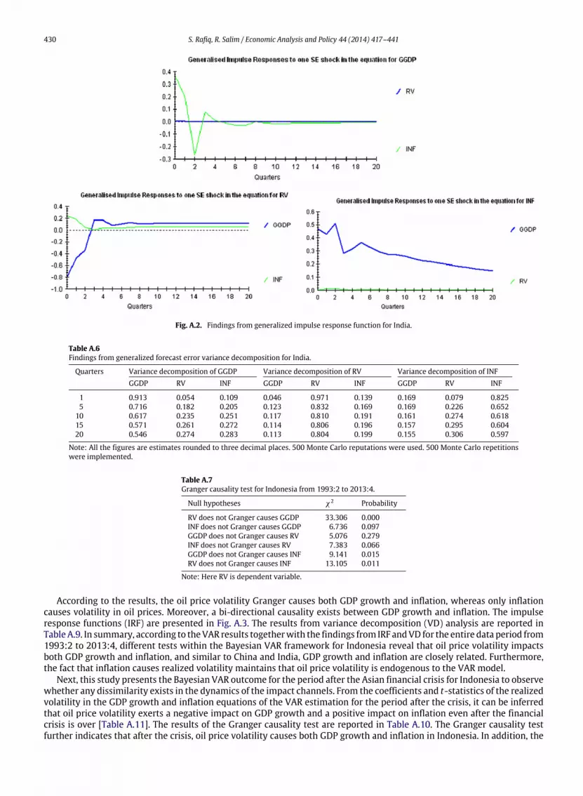
430 S. Rafiq, R. Salim / Economic Analysis and Policy 44 (2014) 417–441
Fig. A.2. Findings from generalized impulse response function for India.
Table A.6Findings from generalized forecast error variance decomposition for India.
Quarters Variance decomposition of GGDP Variance decomposition of RV Variance decomposition of INFGGDP RV INF GGDP RV INF GGDP RV INF
1 0.913 0.054 0.109 0.046 0.971 0.139 0.169 0.079 0.8255 0.716 0.182 0.205 0.123 0.832 0.169 0.169 0.226 0.652
10 0.617 0.235 0.251 0.117 0.810 0.191 0.161 0.274 0.61815 0.571 0.261 0.272 0.114 0.806 0.196 0.157 0.295 0.60420 0.546 0.274 0.283 0.113 0.804 0.199 0.155 0.306 0.597
Note: All the figures are estimates rounded to three decimal places. 500 Monte Carlo reputations were used. 500 Monte Carlo repetitionswere implemented.
Table A.7Granger causality test for Indonesia from 1993:2 to 2013:4.
Null hypotheses χ2 Probability
RV does not Granger causes GGDP 33.306 0.000INF does not Granger causes GGDP 6.736 0.097GGDP does not Granger causes RV 5.076 0.279INF does not Granger causes RV 7.383 0.066GGDP does not Granger causes INF 9.141 0.015RV does not Granger causes INF 13.105 0.011
Note: Here RV is dependent variable.
According to the results, the oil price volatility Granger causes both GDP growth and inflation, whereas only inflationcauses volatility in oil prices. Moreover, a bi-directional causality exists between GDP growth and inflation. The impulseresponse functions (IRF) are presented in Fig. A.3. The results from variance decomposition (VD) analysis are reported inTableA.9. In summary, according to theVAR results togetherwith the findings from IRF andVD for the entire data period from1993:2 to 2013:4, different tests within the Bayesian VAR framework for Indonesia reveal that oil price volatility impactsboth GDP growth and inflation, and similar to China and India, GDP growth and inflation are closely related. Furthermore,the fact that inflation causes realized volatility maintains that oil price volatility is endogenous to the VAR model.
Next, this study presents the Bayesian VAR outcome for the period after the Asian financial crisis for Indonesia to observewhether any dissimilarity exists in the dynamics of the impact channels. From the coefficients and t-statistics of the realizedvolatility in the GDP growth and inflation equations of the VAR estimation for the period after the crisis, it can be inferredthat oil price volatility exerts a negative impact on GDP growth and a positive impact on inflation even after the financialcrisis is over [Table A.11]. The results of the Granger causality test are reported in Table A.10. The Granger causality testfurther indicates that after the crisis, oil price volatility causes both GDP growth and inflation in Indonesia. In addition, the

S. Rafiq, R. Salim / Economic Analysis and Policy 44 (2014) 417–441 431
Fig. A.3. Findings from generalized impulse response function for Indonesia from 1993:2 to 2013:4.
Table A.8Bayesian VAR Estimates for Indonesia from 1993:2 to 2013:4.
GGDP RV INF
GGDP(−1) 0.034514 −0.004278 −0.649043[0.44041] [−1.45759] [−4.20076]
GGDP(−2) −0.016495 0.000407 −0.204991[−0.35224] [0.23259] [−2.22623]
RV(−1) −5.007620 0.174866 14.46214[−2.51753] [2.32061] [3.66632]
RV(−2) −0.321644 0.003992 5.107086[−5.26379] [0.08616] [2.11164]
INF(−1) −0.020116 0.000684 0.767375[−0.84656] [0.76422] [16.2052]
INF(−2) 0.013658 −0.000272 −0.092745[0.69894] [−0.36933] [−12.37578]
C 1.407801 0.039337 3.601403[4.04165] [3.00123] [5.21960]
R2 0.585607 0.678397 0.892766
Note: Litterman/Minnesota prior type used with hyper parameter Mu: 0, L1:0.1, L2: 0.99, L3: 1. T -statistics are provided in the parenthesis.
Table A.9Findings from generalized forecast error variance decomposition for Indonesia from 1993:2 to 2013:4.
Quarters Variance decomposition of GGDP Variance decomposition of RV Variance decomposition of INFGGDP RV INF GGDP RV INF GGDP RV INF
1 0.641 0.618 0.319 0.149 0.987 0.254 0.244 0.761 0.8475 0.529 0.679 0.350 0.124 0.956 0.227 0.223 0.804 0.686
10 0.532 0.664 0.344 0.123 0.943 0.216 0.221 0.791 0.67115 0.519 0.658 0.345 0.119 0.934 0.213 0.215 0.776 0.65820 0.511 0.653 0.345 0.117 0.926 0.211 0.211 0.766 0.649
Note: All the figures are estimates rounded to three decimal places. 500 Monte Carlo reputations were used. 500 Monte Carlo repetitionswere implemented.
bi-directional causality between GDP growth and inflation also holds true for the time period after the crisis. However, asignificant dissimilarity between two models is that after the crisis, oil price volatility appears to become exogenous in themodel because none of the variables seem to cause realized volatility after the Asian financial crisis.

432 S. Rafiq, R. Salim / Economic Analysis and Policy 44 (2014) 417–441
Table A.10Granger Causality Test for Indonesia from 1998:4 to 2013:4.
Null hypotheses χ2 Probability
RV does not Granger causes GGDP 54.799 0.000INF does not Granger causes GGDP 4.265 0.087GGDP does not Granger causes RV 1.237 0.872INF does not Granger causes RV 1.031 0.905GGDP does not Granger causes INF 7.237 0.047RV does not Granger causes INF 3.031 0.091
Note: Here RV is dependent variable.
Table A.11Bayesian VAR Estimates for Indonesia from 1998:4 to 2013:4.
GGDP RV INF
GGDP(−1) −0.162352 −0.008682 −0.066929[−2.30135] [−1.81200] [−3.42819]
GGDP(−2) −0.074445 0.000992 −0.013181[−1.65329] [0.32543] [−0.13253]
GGDP(−3) −0.022796 0.000125 −0.001301[−0.72298] [0.05875] [−3.01869]
GGDP(−4) 0.038299 9.46E−06 0.002265[1.58896] [0.00580] [0.04259]
RV(−1) −0.301835 0.062427 −1.604498[−6.25552] [0.76901] [−0.60995]
RV(−2) −0.265322 0.007106 −0.900986[−0.38861] [0.15110] [−0.59257]
RV(−3) −0.246975 0.001208 −0.288435[−2.52520] [0.03726] [−0.27542]
RV(−4) −0.002643 −0.003480 −0.083653[−0.00740] [−0.14138] [−0.10522]
INF(−1) −0.019128 0.001406 0.504821[−0.67965] [0.73174] [8.01354]
INF(−2) −0.005450 0.000333 0.035493[−0.28462] [0.25494] [0.82528]
INF(−3) 0.003794 −0.000206 −0.030926[0.30088] [−0.23942] [−1.09187]
INF(−4) 0.003061 −6.94E−05 −0.046647[0.35148] [−0.11673] [−2.38677]
C 1.772295 0.034331 4.405804[5.86816] [1.66783] [6.55126]
R2 0.593864 0.730849 0.934435
Note: Litterman/Minnesota prior type used with hyper parameter Mu: 0, L1:0.1, L2: 0.99, L3: 1. T -statistics are provided in the parenthesis.
Table A.12Findings from generalized forecast error variance decomposition for Indonesia from 1998:4 to 2013:3.
Quarters Variance decomposition of GGDP Variance decomposition of RV Variance decomposition of INFGGDP RV INF GGDP RV INF GGDP RV INF
1 0.879 0.114 0.055 0.053 0.939 0.020 0.154 0.149 0.8465 0.784 0.124 0.177 0.095 0.893 0.029 0.227 0.192 0.735
10 0.754 0.154 0.180 0.172 0.802 0.064 0.264 0.225 0.67115 0.737 0.172 0.181 0.106 0.862 0.082 0.285 0.244 0.63420 0.728 0.182 0.181 0.122 0.841 0.091 0.296 0.255 0.613
Note: All the figures are estimates rounded to three decimal places. 500 Monte Carlo reputations were used.
This study further performs impulse response function and variance decomposition analyses to check the robustness ofthe causality test. The results from impulse response functions are presented in Fig. A.4, and the results from the variancedecomposition analysis are presented in Table A.12. The findings from the Impulse Responses and Variance Decompositionsare consistent with the causality test results in most cases.
Based on two different VAR analyses for Indonesia, it can be inferred that for the Indonesian economy, oil price volatilityimpacts both GDP growth and inflation for both of the time periods, i.e., for the entire sample period and for the periodafter the Asian financial crisis. Furthermore, the link between GDP growth and inflation is bi-directional for both of the VARsystems.

S. Rafiq, R. Salim / Economic Analysis and Policy 44 (2014) 417–441 433
Fig. A.4. Findings from generalized impulse response function for Indonesia from 1998:4 to 2013:4.
Table A.13Granger causality test for Malaysia from 1991:2 to 2013:3.
Null hypotheses χ2 Probability
RV does not Granger causes GGDP 4.957 0.084INF does not Granger causes GGDP 4.077 0.096GGDP does not Granger causes RV 4.625 0.099INF does not Granger causes RV 7.765 0.021GGDP does not Granger causes INF 7.721 0.006RV does not Granger causes INF 3.013 0.222
Note: Here RV is dependent variable.
5.4. Impact analysis for Malaysia
The data plots for Malaysia portray a spike during early 1997 to mid-1998 and indicate that the Malaysian economy wasone of the most adversely affected economies during the Asian financial crisis. Thus, Malaysian data are also investigatedbased on two different VAR systems, one for the entire period from 1991:2 to 2013:3 and the other for the period afterthe crisis, i.e., from 1998:4 to 2013:3. The Bayesian VAR results for the entire periods indicate that the realized volatilitynegatively impacts output growth inMalaysia [see Table A.14]. The Granger causality test results are presented in Table A.13.According to the causality results, a bi-directional causality exists between oil price volatility and GDP growth, a uni-directional causality runs from inflation to realized volatility, and a bi-directional causality between GDP growth andinflation in Malaysia is observed for the entire period from 1991:2 to 2013:3.
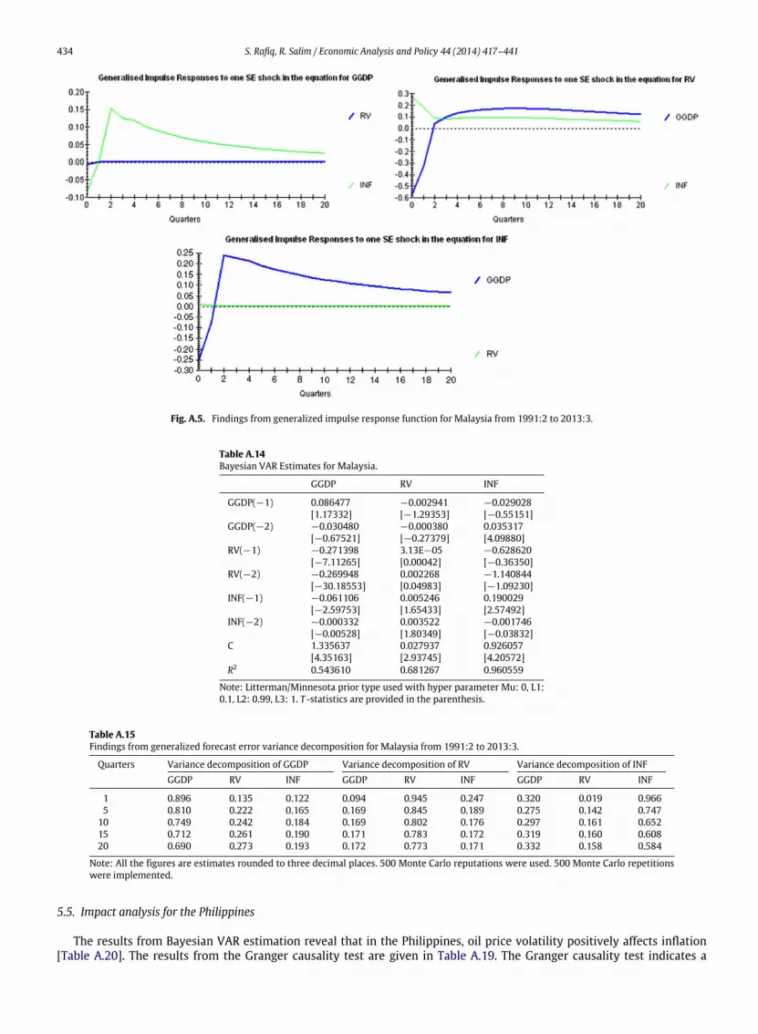
The impulse response function findings are presented in Fig. A.5, and the results of variance decompositions are reportedin Table A.15. According to the VAR results together with impulse response functions and variance decompositions for theentire period, it can be inferred that oil price volatility impacts GDP growth in Malaysia, GDP growth and inflation impacteach other, and both GDP growth and inflation have a small impact on realized volatility.
The analysis for the Malaysian economy after the financial crisis begins with the Bayesian VAR estimation [Table A.17].The coefficients of realized volatility in the GDP growth equation indicate that oil price volatility has a negative impact onthe Malaysian output growth. Findings from the causality tests are reported in Table A.16. The causality test results for theperiod after the crisis are nearly similar to those of the causality test results for the entire period. A bi-directional causalityexists between GDP growth and realized volatility, a bi-directional causality exists between inflation and GDP growth, anda uni-directional causality runs from inflation to oil price volatility. The results from the impulse response functions andvariance decompositions are presented in Fig. A.6 and Table A.18, respectively. All of the tests reveal minor changes inthe two VAR analyses performed for the Malaysian economy. In both of the VAR systems, oil price volatility impacts GDPgrowth, but there is little feedback from the opposite side. Furthermore, similar to the other economies analyzed thus far,GDP growth and inflation appear to be strongly tied together in the Malaysian economy.
434 S. Rafiq, R. Salim / Economic Analysis and Policy 44 (2014) 417–441
Fig. A.5. Findings from generalized impulse response function for Malaysia from 1991:2 to 2013:3.
Table A.14Bayesian VAR Estimates for Malaysia.
GGDP RV INF
GGDP(−1) 0.086477 −0.002941 −0.029028[1.17332] [−1.29353] [−0.55151]
GGDP(−2) −0.030480 −0.000380 0.035317[−0.67521] [−0.27379] [4.09880]
RV(−1) −0.271398 3.13E−05 −0.628620[−7.11265] [0.00042] [−0.36350]
RV(−2) −0.269948 0.002268 −1.140844[−30.18553] [0.04983] [−1.09230]
INF(−1) −0.061106 0.005246 0.190029[−2.59753] [1.65433] [2.57492]
INF(−2) −0.000332 0.003522 −0.001746[−0.00528] [1.80349] [−0.03832]
C 1.335637 0.027937 0.926057[4.35163] [2.93745] [4.20572]
R2 0.543610 0.681267 0.960559
Note: Litterman/Minnesota prior type used with hyper parameter Mu: 0, L1:0.1, L2: 0.99, L3: 1. T -statistics are provided in the parenthesis.
Table A.15Findings from generalized forecast error variance decomposition for Malaysia from 1991:2 to 2013:3.
Quarters Variance decomposition of GGDP Variance decomposition of RV Variance decomposition of INFGGDP RV INF GGDP RV INF GGDP RV INF
1 0.896 0.135 0.122 0.094 0.945 0.247 0.320 0.019 0.9665 0.810 0.222 0.165 0.169 0.845 0.189 0.275 0.142 0.747
10 0.749 0.242 0.184 0.169 0.802 0.176 0.297 0.161 0.65215 0.712 0.261 0.190 0.171 0.783 0.172 0.319 0.160 0.60820 0.690 0.273 0.193 0.172 0.773 0.171 0.332 0.158 0.584
Note: All the figures are estimates rounded to three decimal places. 500 Monte Carlo reputations were used. 500 Monte Carlo repetitionswere implemented.
5.5. Impact analysis for the Philippines
The results from Bayesian VAR estimation reveal that in the Philippines, oil price volatility positively affects inflation[Table A.20]. The results from the Granger causality test are given in Table A.19. The Granger causality test indicates a

S. Rafiq, R. Salim / Economic Analysis and Policy 44 (2014) 417–441 435
Table A.16Granger causality test for Malaysia from 1998:4 to 2013:3.
Null hypotheses χ2 Probability
RV does not Granger causes GGDP 4.490 0.088INF does not Granger causes GGDP 7.806 0.066GGDP does not Granger causes RV 5.957 0.071INF does not Granger causes RV 4.343 0.091GGDP does not Granger causes INF 13.586 0.016RV does not Granger causes INF 3.099 0.212
Note: Here RV is dependent variable.
Table A.17Bayesian VAR estimates for Malaysia from 1998:4 to 2013:3.
GGDP RV INF
GGDP(−1) 0.059027 −0.004344 −0.042481[0.73960] [−1.24423] [−0.53746]
GGDP(−2) −0.041131 −0.000110 0.040782[−0.88455] [−0.05416] [0.88780]
GGDP(−3) −0.007934 −0.000277 0.014618[−0.24816] [−0.19854] [0.46307]
GGDP(−4) 0.003932 5.09E−05 −0.007750[0.16114] [0.04786] [−0.32180]
RV(−1) −0.842312 −0.008926 −0.618848[−0.45490] [−0.10879] [−0.33541]
RV(−2) −0.400436 0.000942 −0.841638[−2.37827] [0.02005] [−0.79786]
RV(−3) −0.126929 0.000646 −0.141066[−0.17407] [0.01992] [−0.19413]
RV(−4) −0.015181 −0.001721 0.033145[−0.02744] [−0.06998] [0.06013]
INF(−1) −0.057192 0.004252 0.157585[−0.71608] [1.20972] [1.96770]
INF(−2) −0.005960 0.002611 0.002025[−5.12782] [1.27184] [0.04320]
INF(−3) −0.000500 0.000613 −0.000201[−3.01547] [0.43080] [−0.00617]
INF(−4) 0.001144 1.94E−05 0.003569[0.04672] [0.01803] [0.14487]
C 1.343493 0.034146 1.010803[4.42865] [2.55975] [3.34618]
R2 0.535987 0.609745 0.866070
Note: Litterman/Minnesota prior type used with hyper parameter Mu: 0, L1:0.1, L2: 0.99, L3: 1. T -statistics are provided in the parenthesis.
Table A.18Findings from generalized forecast error variance decomposition for Malaysia from 1998:4 to 2013:3.
Quarters Variance decomposition of GGDP Variance decomposition of RV Variance decomposition of INFGGDP RV INF GGDP RV INF GGDP RV INF
1 0.870 0.140 0.045 0.096 0.954 0.235 0.189 0.137 0.8835 0.818 0.205 0.153 0.134 0.859 0.137 0.237 0.271 0.847
10 0.724 0.287 0.217 0.134 0.814 0.105 0.243 0.319 0.82615 0.687 0.308 0.201 0.133 0.797 0.095 0.243 0.330 0.77620 0.672 0.315 0.194 0.132 0.790 0.092 0.242 0.333 0.757
Note: All the figures are estimates rounded to three decimal places. 500 Monte Carlo reputations were used. 500 Monte Carlo repetitionswere implemented.
bi-directional causality between oil price volatility and inflation and also a bi-directional causality between GDP growthand inflation. For the purpose of checking the robustness of the Granger causality test, impulse responses and variancedecompositions are implemented.
The impulse response functions and variance decompositions are presented in Fig. A.7 and Table A.21. According to theresults from the Bayesian VAR, Granger causality, impulse response and variance decompositions tests, it can be inferredthat in the Philippines, oil price volatility impacts inflation and that GDP growth and inflation are closely related in the shortrun.

436 S. Rafiq, R. Salim / Economic Analysis and Policy 44 (2014) 417–441
Fig. A.6. Findings from generalized impulse response function for Malaysia from 1998:4 to 2013:3.
Table A.19Granger causality test for Philippines.
Null hypotheses χ2 Probability
RV does not Granger causes GGDP 0.042 0.837INF does not Granger causes GGDP 7.681 0.019GGDP does not Granger causes RV 0.661 0.416INF does not Granger causes RV 3.652 0.091GGDP does not Granger causes INF 6.107 0.014RV does not Granger causes INF 4.013 0.072
Note: Here RV is dependent variable.
Table A.20Bayesian VAR estimates for Philippines.
GGDP RV INF
GGDP(−1) −0.101637 0.000205 −0.004600[−1.57991] [0.15172] [−0.10574]
GGDP(−2) −0.133297 −0.000717 0.005596[−3.10284] [−0.79658] [5.19327]
RV(−1) −1.902061 0.172632 0.137039[−0.58112] [2.48484] [0.06165]
RV(−2) −2.792260 0.026812 −0.672931[−1.35413] [0.61082] [−0.48057]
INF(−1) −0.049707 0.003782 0.474218[−0.56564] [2.03710] [7.91146]
INF(−2) −0.038301 0.000447 0.033154[−0.61093] [0.33756] [0.77273]
C 1.630947 0.021023 1.170319[5.25630] [3.20786] [5.55247]
R2 0.673041 0.777880 0.865006
Note: Litterman/Minnesota prior type used with hyper parameter Mu: 0, L1:0.1, L2: 0.99, L3: 1. T -statistics are provided in the parenthesis.
5.6. Impact analysis for Thailand
Because the Thai economyalsowas severely affected by theAsian financial crisis and as the data suggest a spike during thecrisis period, similar to Indonesia and Malaysia, this study implements two different VARs for Thailand in a similar fashion.The Bayesian VAR output for the entire period of Thailand indicates that in the Thai economy, GDP growth is significantlyimpacted negatively by oil price volatility [Table A.23].
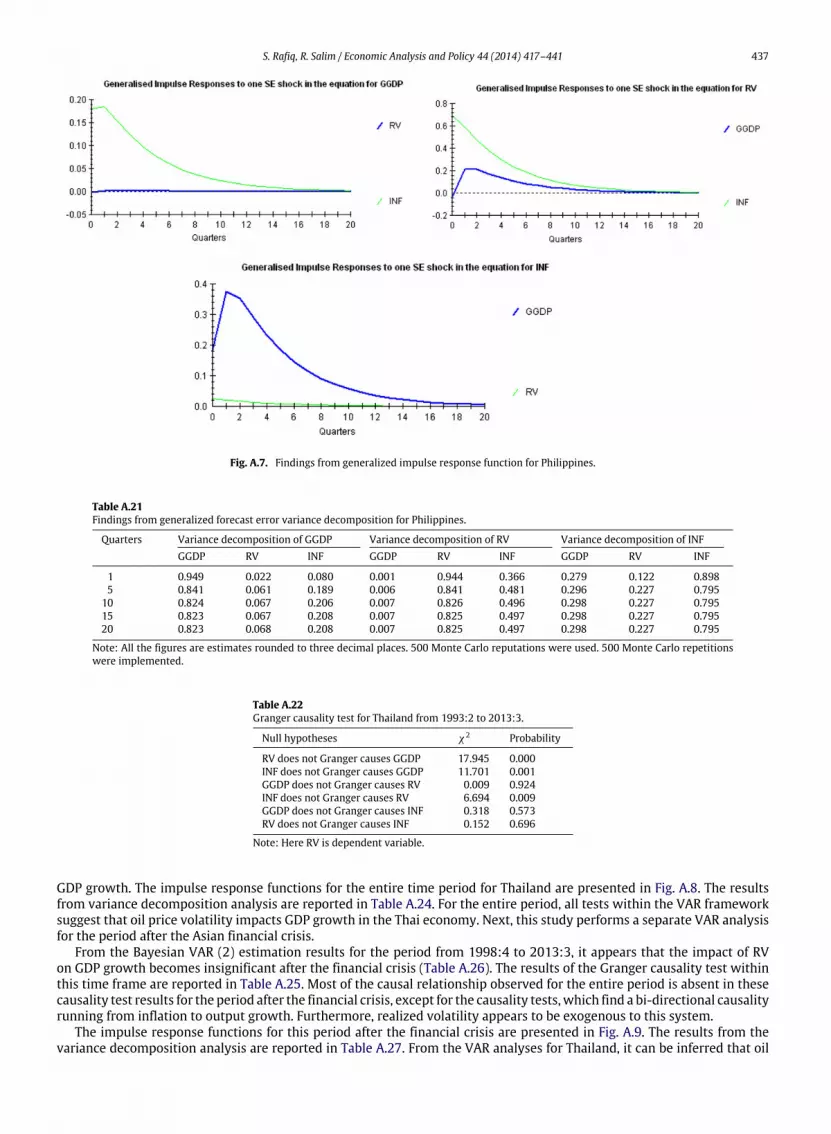
The causality test findings for the entire data set are reported in Table A.22. The causality test results indicate that inThailand, the oil price volatility Granger causes GDP growth and that inflation Granger causes both oil price volatility and
S. Rafiq, R. Salim / Economic Analysis and Policy 44 (2014) 417–441 437
Fig. A.7. Findings from generalized impulse response function for Philippines.
Table A.21Findings from generalized forecast error variance decomposition for Philippines.
Quarters Variance decomposition of GGDP Variance decomposition of RV Variance decomposition of INFGGDP RV INF GGDP RV INF GGDP RV INF
1 0.949 0.022 0.080 0.001 0.944 0.366 0.279 0.122 0.8985 0.841 0.061 0.189 0.006 0.841 0.481 0.296 0.227 0.795
10 0.824 0.067 0.206 0.007 0.826 0.496 0.298 0.227 0.79515 0.823 0.067 0.208 0.007 0.825 0.497 0.298 0.227 0.79520 0.823 0.068 0.208 0.007 0.825 0.497 0.298 0.227 0.795
Note: All the figures are estimates rounded to three decimal places. 500 Monte Carlo reputations were used. 500 Monte Carlo repetitionswere implemented.
Table A.22Granger causality test for Thailand from 1993:2 to 2013:3.
Null hypotheses χ2 Probability
RV does not Granger causes GGDP 17.945 0.000INF does not Granger causes GGDP 11.701 0.001GGDP does not Granger causes RV 0.009 0.924INF does not Granger causes RV 6.694 0.009GGDP does not Granger causes INF 0.318 0.573RV does not Granger causes INF 0.152 0.696
Note: Here RV is dependent variable.
GDP growth. The impulse response functions for the entire time period for Thailand are presented in Fig. A.8. The resultsfrom variance decomposition analysis are reported in Table A.24. For the entire period, all tests within the VAR frameworksuggest that oil price volatility impacts GDP growth in the Thai economy. Next, this study performs a separate VAR analysisfor the period after the Asian financial crisis.
From the Bayesian VAR (2) estimation results for the period from 1998:4 to 2013:3, it appears that the impact of RVon GDP growth becomes insignificant after the financial crisis (Table A.26). The results of the Granger causality test withinthis time frame are reported in Table A.25. Most of the causal relationship observed for the entire period is absent in thesecausality test results for the period after the financial crisis, except for the causality tests, which find a bi-directional causalityrunning from inflation to output growth. Furthermore, realized volatility appears to be exogenous to this system.
The impulse response functions for this period after the financial crisis are presented in Fig. A.9. The results from thevariance decomposition analysis are reported in Table A.27. From the VAR analyses for Thailand, it can be inferred that oil

438 S. Rafiq, R. Salim / Economic Analysis and Policy 44 (2014) 417–441
Fig. A.8. Findings from generalized impulse response function for Thailand from 1993:2 to 2009:1.
Table A.23Bayesian VAR Estimates for Thailand from 1993:2 to 2013:3.
GGDP RV INF
GGDP(−1) −0.062981 −0.000862 −0.004031[−0.82957] [−1.28801] [−0.13522]
GGDP(−2) −0.011764 −0.000251 0.014704[−0.25627] [−0.62228] [0.81803]
RV(−1) −13.15033 0.250750 −7.350609[−1.63254] [3.49329] [−2.31093]
RV(−2) 0.046025 0.028020 −2.414874[0.00904] [0.61560] [−1.20101]
INF(−1) −0.305901 0.001425 0.390537[−1.84917] [0.97151] [5.94880]
INF(−2) −0.065756 0.001613 0.008692[−0.59005] [1.63312] [0.19589]
C 1.974302 0.020392 1.155401[3.67642] [4.27799] [5.44633]
R2 0.713548 0.7894672 0.9165726
Note: Litterman/Minnesota prior type used with hyper parameter Mu: 0, L1:0.1, L2: 0.99, L3: 1. T -statistics are provided in the parenthesis.
Table A.24Findings from generalized forecast error variance decomposition for Thailand from 1993:2 to 2013:3.
Quarters Variance decomposition of GGDP Variance decomposition of RV Variance decomposition of INFGGDP RV INF GGDP RV INF GGDP RV INF
1 0.969 0.045 0.051 0.037 0.947 0.053 0.021 0.030 0.9615 0.894 0.152 0.104 0.046 0.786 0.213 0.058 0.044 0.834
10 0.891 0.154 0.106 0.055 0.735 0.261 0.065 0.088 0.78915 0.889 0.154 0.106 0.057 0.721 0.273 0.066 0.101 0.77620 0.889 0.155 0.107 0.058 0.717 0.276 0.067 0.105 0.772
Note: All the figures are estimates rounded to three decimal places. 500 Monte Carlo reputations were used. 500 Monte Carlo repetitionswere implemented.
price volatility impacts output growth for the entire period; however, after the Asian financial crisis, the impact seems todisappear. This finding is consistent with that of Rafiq et al. (2009) inwhich the authors find that impact of oil price volatilityno longer exists in the Thai economy after the financial crisis.

S. Rafiq, R. Salim / Economic Analysis and Policy 44 (2014) 417–441 439
Fig. A.9. Findings from generalized impulse response function for Thailand from 1998:4 to 2013:3.
Table A.25Granger Causality Test for Thailand from 1998:4 to 2013:3.
Null hypotheses χ2 Probability
RV does not Granger causes GGDP 3.774 0.152INF does not Granger causes GGDP 5.609 0.074GGDP does not Granger causes RV 1.568 0.114INF does not Granger causes RV 0.446 0.800GGDP does not Granger causes INF 17.655 0.000RV does not Granger causes INF 4.159 0.125
Note: Here RV is dependent variable.
Table A.26Bayesian VAR estimates for Thailand from 1998:1 to 2013:3.
GGDP RV INF
GGDP(−1) −0.122699 −0.000674 −0.002098[−1.54489] [−0.88269] [−0.05644]
GGDP(−2) −0.015799 −0.000154 0.015796[−0.33883] [−0.34356] [0.72542]
RV(−1) −8.165248 0.237357 −8.533456[−1.04868] [3.13472] [−2.32641]
RV(−2) 1.139720 0.016890 −2.416204(4.75550) (0.04638) (2.24044)[0.23966] [0.36416] [−1.07845]
INF(−1) −0.207193 0.001236 0.344899[−1.39763] [0.86217] [4.91163]
INF(−2) −0.074671 0.001303 0.016141[−0.78207] [1.41149] [0.35578]
C 1.927972 0.022002 1.244987[3.55405] [4.18896] [4.87004]
R2 0.69016428 0.7953171 0.9340562
Note: Litterman/Minnesota prior type used with hyper parameter Mu: 0, L1:0.1, L2: 0.99, L3: 1. T -statistics are provided in the parenthesis.
6. Conclusions and policy implications
This article investigates the short-term impact of oil price volatility in six emerging economies of Asia. One of the uniquefeatures of this paper is that in this work, the oil price volatility for each country is calculated using a non-parametricapproach, namely, the realized oil price variance. Furthermore, to the author’s best knowledge, this is one of the first studies

440 S. Rafiq, R. Salim / Economic Analysis and Policy 44 (2014) 417–441
Table A.27Findings from generalized forecast error variance decomposition for Thailand from 1998:4 to 2013:3.
Quarters Variance decomposition of GGDP Variance decomposition of RV Variance decomposition of INFGGDP RV INF GGDP RV INF GGDP RV INF
1 0.986 0.058 0.182 0.037 0.985 0.032 0.109 0.016 0.9795 0.867 0.069 0.301 0.118 0.945 0.114 0.203 0.060 0.885
10 0.891 0.077 0.345 0.129 0.933 0.163 0.224 0.105 0.83515 0.863 0.078 0.361 0.103 0.944 0.180 0.233 0.124 0.81320 0.850 0.075 0.369 0.108 0.934 0.188 0.237 0.134 0.802
Note: All the figures are estimates rounded to three decimal places. 500 Monte Carlo reputations were used. 500 Monte Carlo repetitionswere implemented.
that analyzes the impact of oil price volatility on developing economies. Because Indonesia, Malaysia and Thailand wereseverely affected by the Asian financial crisis and because the data in this work portray spikes during this period, this studyimplements two different VAR systems for these countries in an attempt to compare the impact channels for the entireperiod and for the period after the crisis.
For China, according to the VAR analysis, the Granger causality test, and impulse response functions and variancedecompositions, it can be inferred that oil price volatility impacted output growth in the short run. For India, oil pricevolatility affected both GDP growth and inflation. In the Philippines, oil price volatility influenced inflation. Furthermore,for all of these economies, GDP growth and inflation are closely related in the short run. Another important feature of theresults from these three countries is that for all of the VAR models, oil price volatility appears to be slightly endogenous.This result may be due to the use of exchange rates in constructing the realized volatility measure.
Based on two different VAR analyses for Indonesia, it can be inferred that for the Indonesian economy, oil price volatilityimpacted both GDP growth and inflation for both of the time periods, i.e., for the entire sample period and for the periodafter the Asian financial crisis. Furthermore, the link between GDP growth and inflation is bi-directional for both of theVAR systems. However, one significant difference in the results from the two VARs is that oil price volatility appears tobecome exogenous to the economy after the financial crisis. Minor differences are observed between the two VAR analysesperformed for the Malaysian economy. In both of the VAR systems, oil price volatility affected GDP growth, but there isnotably little feedback from the opposite side. Furthermore, similar to the other economies analyzed thus far, GDP growthand inflation appear to be strongly tied in the Malaysian economy.
From the VAR analyses for Thailand, it can be inferred that oil price volatility influenced output growth for the entireperiod. However, after the Asian financial crisis, the impact seems to disappear. This finding is consistent with that of Rafiqet al. (2009) in which the authors find that the impact of oil price volatility no longer exists in the Thai economy after thefinancial crisis. Thus, the results after the financial crisis show that the adverse effect of oil price volatility has beenmitigatedto a certain extent. It appears that oil subsidization by the Thai Government via the introduction of the oil fund played asignificant role in improving economic performance by lessening the adverse effect of oil price volatility onmacroeconomicindicators. The policy implication of this result is that the government should continue to pursue its policy to stabilizedomestic oil prices through subsidization and thus aid in stabilizing economic growth.
Acknowledgments
The authors are grateful to the two anonymous referees and the editor of this journal for valuable insights and recom-mendations that significantly improved the quality and presentation of the paper. The authors are solely responsible for anyremaining errors.
Appendix
See Tables A.1–A.27 and Figs. A.1–A.9.
References
Aït-Sahalia, Yacine, Mykland, Per A., Zhang, Lan, 2005. How often to sample a continuous-time process in the presence of market microstructure noise.Rev. Financ. Stu. 18 (2), 351–416.
Andersen, Torben G., Bollerslev, Tim, Diebold, Francis X., Ebens, Heiko, 2001a. The distribution of realized stock return volatility. J. Financ. Econ. 61 (1),43–76.
Andersen, Torben G., Bollerslev, Tim, Diebold, Francis X., Labys, Paul, 2001b. The distribution of realized exchange rate volatility. J. Amer. Statist. Assoc. 96,42–55.
Andersen, Torben G., Bollerslev, Tim, Meddahi, Nour, 2004. Analytical evaluation of volatility forecasts. Internat. Econom. Rev. 45 (4), 1079–1110.Bachmeier, L.J., Cha, I., 2011. Why don’t oil shocks cause inflation? evidence from disaggregate inflation data. J. Money, Credit, Bank. 43 (6), 1165–1183.Banbura, M., Giannone, D., Reichlin, L., 2010. Large Bayesian vector auto regressions. J. Appl. Econometrics 25, 71–92.Barndorff-Nielsen, Ole E., Shephard, Neil, 2001. Non-Gaussian Ornstein–Uhlenbeck-Based models and some of their uses in financial economics. J. R. Stat.
Soc. Ser. B 63 (2), 167–241.Barndorff-Nielsen, Ole E., Shephard, Neil, 2002. Econometric analysis of realized volatility and its use in estimating stochastic volatility models. J. R. Stat.
Soc. Ser. B 64 (2), 253–280.

S. Rafiq, R. Salim / Economic Analysis and Policy 44 (2014) 417–441 441
Beck, Nathaniel, Katz, Jonathan N., 2007. Random coefficient models for time-series-cross-section data: Monte Carlo experiments. Polit. Anal. 15, 182–195.Bernanke, Ben S., 1983. Irreversibility, uncertainty, and cyclical investment. Q. J. Econ. 98 (1), 85.Bond, S., Eberhardt, M., 2009. Cross-section dependence in nonstationary panel models: A novel estimator, Paper presented in the Nordic Econometrics
Conference in Lund, Sweden.Brooks, Chris, 2002. Introductory Econometrics for Finance. Cambridge University Press.Brown, Stephen P.A., Yucel, Mine K., 2002. Energy prices and aggregate economic activity: an interpretative survey. Q. Rev. Econ. Finance 42 (2), 193–208.Burbridge, John, Harrison, Alan, 1984. Testing for the effects of oil price rises using vector autoregressions. Internat. Econom. Rev. 25 (2), 459–484.Chen, Shiu-Sheng, 2009. Oil price pass-through into inflation. Energy Econ. 31 (1), 126–133.Chen, Shiu-Sheng, Chen, Hung-Chyn, 2007. Oil prices and real exchange rates. Energy Econ. 29 (3), 390–404.Cologni, Alessandro, Manera, Matteo, 2008. Oil prices, inflation and interest rates in a structural cointegrated VAR model for the G-7 countries. Energy
Econ. 30 (3), 856–888.Cunado, J., Perez de Gracia, F., 2005. Oil prices, economic activity and inflation: Evidence for some Asian countries. Q. Rev. Econ. Finance 45 (1), 65–83.De Silva, S., Hadri, K., Tremayne, A.R., 2009. Panel Unit Root Tests in the presence of cross-sectional dependencies: Finite sample performance and an
application. Econometric J. 12, 340–366.Eberhardt, M., Teal, F., 2010. Productivity analysis in global manufacturing production, Economics Series Working Papers. University of Oxford.Farzanegan, Mohammad Reza, Markwardt, Gunther, 2009. The effect of oil price shocks on the Iranian economy. Energy Econ. 31 (1), 134–151.Ferderer, J Peter., 1996. Oil price volatility and the macroeconomy. J. Macroeconomics 18 (1), 1–26.Gengenbach, C., Palm, F.C., Urbain, J.-P., 2009. Panel unit root tests in the presence of cross-sectional dependencies: Comparisons and implications for
modelling. Econometric Rev. 29, 111–145.Gisser, Micha, Goodwin, Thomas H., 1986. Crude oil and the macroeconomy: Tests of some popular notions. J. Money, Credit Bank. 18 (1), 95–103.Guo, Hui, Kliesen, Kevin L, 2005. Oil price volatility and U.S. macroeconomic activity. Rev.—Federal Reserve Bank of St. Louis 57 (6), 669–683.Hamilton, James D., 1983. Oil and the macroeconomy since world war II. J. Polit. Economy 91 (2), 228–248.Hamilton, James D., 1988. A neoclassical model of unemployment and the business cycle. J. Polit. Economy 96 (3), 593–617.Hamilton, JamesD., 2008. In: Durlauf, S.N., Blume, L.E. (Eds.), Oil and theMacroeconomy. In: TheNewPalgraveDictionary of Economics, PalgraveMacmillan.Hooker, M.A., 2002. Are oil shocks inflationary? Asymmetric and nonlinear specifications versus changes in regime. J. Money, Credit Bank. 34, 540–561.Huang, Bwo-Nung, Hwang, M.J., Peng, Hsiao-Ping, 2005. The asymmetry of the impact of oil price shocks on economic activities: An application of the
multivariate threshold model. Energy Econ. 27 (3), 455–476.Huntington, Hillard G., 2007. Oil shocks and real U.S. income. Energy J. 28 (4), 31–46.Im, K.S., Pesaran, M.H., Shin, Y., 2003. Testing for unit roots in heterogeneous pnels. J. Econometrics 122, 81–126.Jbir, Rafik, Zouari-Ghorbel, Sonia, 2009. Recent oil price shock and Tunisian economy. Energy Policy 37 (3), 1041–1051.Jimenez-Rodriguez, Rebeca., 2008. The impact of oil price shocks: Evidence from the industries of six OECD countries. Energy Econ. 30 (6), 3095–3108.Jimenez-Rodriguez, Rebeca., 2009. Oil price shocks and real GDP growth: Testing for non-linearity. Energy J. 30 (1), 1–23.Jimenez-Rodriguez, Rebeca, Sanchez, Marcelo, 2005. Oil price shocks and real GDP growth: Empirical evidence for some OECD countries. Appl. Econ. 37
(2), 201–228.Katayama, M., 2013. Declining effects of oil price shocks. J. Money, Credit Bank. 45 (6), 977–1016.Koop, G., 2013. Forecasting with medium and large Bayesian VARs. J. Appl. Econometrics 28 (2), 177–203.Koop, G., Pesaran, M.H., Potters, S.M., 1996. Impulse response analysis in nonlinear multivariate models. J. Econometrics 74 (1), 119–147.Lardic, Sandrine, Mignon, Valerie, 2006. The impact of oil prices on GDP in European countries: An empirical investigation based on asymmetric
cointegration. Energy Policy 34 (18), 3910–3915.Lee, Kiseok, Ni, Shawn, Ratti, R., 1995. Oil shocks and the macroeconomy: The role of price variability. Energy J. 16 (4), 39–56.Lilien, David M., 1982. Sectoral shifts and cyclical unemployment. J. Polit. Economy 90 (4), 777–793.Loungani, Prakash, 1986. On price shocks and the dispersion hypothesis. Rev. Econ. Stat. 68 (3), 536–539.Mork, Knut Anton, 1989. Oil and the macroeconomy when prices go up and down: An extension of Hamilton’s results. J. Polit. Economy 97 (3), 740–744.Mork, Knut Anton, Olsen, Olstein, 1994. Macroeconomic responses to oil price increases and decreases in seven OECD countries. Energy J. 15 (4), 19–35.Mory, Javier F., 1993. Oil prices and economic activity: Is the relationship symmetric? Energy J. 14 (4), 151–161.Omojolaibi, Joseph Ayoola, 2013. Does volatility in crude oil price precipitate macroeconomic performance in Nigeria?. Int. J. Energy Econ. Policy 3 (2),
143–152.Pesaran, M.H., 1997. The role of economic theory in modelling the long run. Econ. J. 107, 178–191.Pesaran, M.H., 2006. Estimation and inference in large heterogeneous panels with a multifactor error structure. Econometrica 74, 967–1012.Pesaran, M.H., 2007. A simple panel unit root test in the presence of cross section dependence. J. Appl. Econometrics 22, 265–312.Pesaran, M.H., Smith, R.P., 1995. Estimating long-run relationships from dynamic heterogeneous panels. J. Eco. 68, 79–113.Pesaran, M.H., Shin, Yongcheol, 1998. Generalized impulse response analysis in linear multivariate models. Econom. Lett. 58, 17–29.Rafiq, S., Salim, R., Bloch, H., 2009. Impact of crude oil price volatility on economic activities: an empirical investigation in the Thai economy. Resour. Policy
34 (3), 121–132.Sadorsky, P., 2014. The effect of urbanization on CO2 emissions in emerging economies. Energy Econ. 41, 147–153.Salisu, A.A., Fasanya, O.A, 2013. Modelling oil price volatility with structural breaks. Energy Policy 52, 554–562.Westerlund, J., Breitung,, 2013. Lessons from a decade of IPS and LLC. Econometric Rev. 32, 547–591.Zhang, Lan, Mykland, Per A., Ait-Sahalia, Yacine, 2005. A tale of two time scales: Determining integrated volatility with noisy high-frequency data. J. Amer.
Statist. Assoc. 100 (472), 1394–1411.


