1

Does Land Tenure Security Matter for Investment in Soil and

Water Conservation? Evidence From Kenya*

Jane Kabubo–Mariara Corresponding author

School of Economics, University of Nairobi.

P.O Box 30197,00100 Nairobi

Tel 254 20 318 262 ext 28122

Fax 254 20 245 566

Email:jkmariara@yahoo.com;jmariara@uonbi.ac.ke

Vincent Linderhof Institute for Environmental Studies, Vrije Universiteit.

Gideon Kruseman Agricultural Economics Research Institute (LEI), the Hague

Abstract

This paper investigates the impact of tenure security and other factors on investment in soil and

water conservation (SWC) strategies using survey data from Kenya. A combination of factor

analysis, step wise regression and reduced form model approaches are used to explain the

willingness, likelihood and intensity of adoption of SWC investments. The results affirm the

importance of tenure security, household assets, agro ecological diversity and other development

domain dimensions in determining the likelihood and intensity of adoption of SWC investments.

The results suggest that to ensure that land tenure policy is pro-SWC (environment), it is

important to consider whether household plots are owned, rented out, or rented in. The impact of

household assets implies a poverty environment link. We also find that the factors affecting the

level of investment are the same as the factors determining the decision whether or not to invest

in SWC. The results suggest the need for region specific soil and water conservation practices

and for broad policies that provide incentives for environmental conservation and poverty

reduction.

Key words: Development domain dimensions; error correction models; factor analysis; soil and

water conservation; tenure security.

* The authors are grateful to Poverty Reduction and Environment Management (PREM) for financial support. The

usual disclaimer applies.

2

1. Introduction

There is enormous literature on the impact of land rights on investment in soil and water

conservation (SWC) in developing countries. Divergent views however abound on the causal

relationship between the two. It has been argued that if property rights are both durable and

assured, this could lead to increased investment due to two effects: First households perceive

greater security of receiving the full benefits of long-term investments in land improvement;

second, secure land rights may help in obtaining investment loans from potential lenders (Besley,

1995). It is however difficult to separate out the two effects. Other studies have shown that well

defined, durable and assure property rights may be a necessary, but not a sufficient condition to

have access to finance (Feder et al., 1992; Carter and Olinto,1998). Substantial theoretical

literature however advocates for privatization of land based on the premise that farmer’s

incentives to invest in technologies are inhibited by weak tenure security arising from indigenous

property right institutions and by lack of land titles hindering their capacity to obtain credit to

make investments (Shiferaw and Holden, 1999; Kabubo-Mariara, 2004, 2007).

There are three reasons why secure land tenure might lead to more willingness to invest in SWC

measures. The first is the original idea that if farmers feel more secure in their right or ability to

use their land in the long-run and they will be more willing to make investments that take a

longer period to repay (high sunk costs) (Demsetz, 1967; Feder et al., 1988; Zimmerman and

Carter, 1997; Shiferaw and Holden 1999; Place and Otsuka, 2000; Gebremedhin and Swinton,

2003; Deininger and Jin 2002; Li et al. 1998; Jacoby et al. 2002). A second reason is that if land

markets exist and farmers can freely dispose of their land, the added value of SWC investments

3

can be made liquid, and hence the return to those investments can be realized without having to

wait the full length of gestation period of the investment. This is an important consideration

because when time horizons are relatively short, there are high subjective discount rates and

myopic time preference (Besley, 1995; Platteau, 2000,1996). The third reason is the collateral

effect that states that if farmer’s have more secure land titles, it will be easier for them to use

their land as collateral to gain access to the necessary credit in order to do the SWC investments.

This is an important issue with formal credit when there is asymmetric information about

borrowers and repayment. An alternative strand of thought claims that land tenure insecurity

might also lead to more investment in land quality. Through land improvement the farmers

expect their rights to that particular plot of land to improve. Very often this is linked to very

specific types of investment and tree planting is often cited as an example of tenure security

enhancing investments (Place and Hazell, 1993; Sjaastad and Bromley, 1997; Brasselle et al.,

2002; Otsuka et al., 2003)

Some studies have however shown that tenure security is not important for land conservation

(Migot-Adholla, et al. 1991, 1994, Place and Hazell, 1993, Pinckney and Kimuyu, 1994), while

others suggest that highly individualized rights to land are more important for long-term than for

short-term investments (Place and Otsuka, 2000, Gebremedhin and Swinton, 2003). The main

reason for different findings is the definition of land rights and methodological approaches

employed. In terms of definition, most studies focus on security of tenure rather than

transferability. Methodologically, some studies use binary dummies to capture security (such as

having a land title: Pinckney and Kimuyu, 1994; Migot-Adholla, et al. 1994; Shiferaw and

Holden 1999; Place and Otsuka, 2002), while other studies take a continuum of expected rights

4

(Place and Otsuka, 2002; Gebremedhin and Swinton, 2003; Kabubo-Mariara 2004, 2007). Others

have focused on the mode of land acquisition such as purchased, borrowed, and gifted (see

Brasselle et al.2002; Otsuka et al. 2003). To overcome this arbitrariness in choice of indicators of

tenure security, some studies have used factor analysis to derive measures of tenure from

existing information on various aspects of security (Kruseman, 2006).

In addition to the challenges in defining and measuring property rights and tenure security,

theoretical and empirical difficulties (e.g. defining technology, identifying key dimensions of

property rights and accounting for the endogenous determination of property rights) also rise.

Another issue is that researchers have different reasons for undertaking studies of the

relationship between property rights and technology adoption and each reason may have

different implications on methodology and results (Kabubo-Mariara, 2007).

Following the seminal work of Feder et al. (1988) a large body of field studies have come to

light on the impact of different land tenure arrangements on input use, labour allocation and

investment decisions, in Sub-Saharan Africa along with studies in other areas in the developing

world. The empirical evidence for the economic logic that predicts productivity gains from

increased tenure security is, however, rather mixed. Many studies in sub Saharan Africa show

relationship between land-tenure security measured in terms of land titles and productivity gains

(Migot-Adholla et al, 1991; Roth et al, 1994b; Place and Otsuka, 2002). Other studies find

positive effects that disappear when factors related to development domain dimensions,

especially farm size, and market access are controlled for (Roth et al., 1994b; Bruce et al, 1994).

5

This study contributes to the diverse studies on the impact of tenure security and other factors on

investment in soil and water conservation in Africa. The paper makes an important contribution

due to the richness of data used and also due to methodological innovations over existing

literature. We focus on all the key investment strategies adopted by farmers in our sample,

including permanent and seasonal technologies. The paper analyses the determinants of the

willingness to adopt, the actual adoption and the intensity of adoption of SWC. The study

addresses the following questions: what are the main land conservation strategies adopted by

households in Kenya? What factors determine investment in soil and water conservation? To

what extent does investment in soil and water conservation depend on development domain

dimensions? Is there any link between investment in soil and water conservation and poverty?

The rest of the paper is organized as follows: section two presents the study site and the data.

Section three presents the conceptual framework and methodology, section four presents the

results and section five concludes.

2. The study site and the data

This study is based on data collected from a self weighting probability sample of 457 households

in November and December 2004. The National Sample Survey and Evaluation Programme

(NASSEPi) IV of the Central Bureau of Statistics, Ministry of Planning and National

Development was used as the sampling frame for the field survey. The sample survey utilized a

6

multi-stage sample design. A mixture of purposive, stratified and random sampling methods

were employed to arrive at the final sample.

The first stage in the sampling procedure involved selecting study districts, based on differences

in poverty, population density, terrain and tenure security issues. The second stage involved

selecting administrative divisions within each of the three districts, based on agro-ecological

diversity. The third stage involved selection of locations and sub-locations, which were also

based on agro-ecological diversity. The fourth stage involved selection of sample points

(clusters) from the NASSEP frame, which was based on the total number of clusters within a sub

location and the number of households in each cluster. In the final stage, the desired number of

households were selected from each cluster. To arrive at the total number of households actually

visited, we took a self weighting probability sample from each cluster in a district making a total

of 457 households from the three districts (151, 188 and 151 from Murang’a, Maragua and

Narok districts respectively). In addition to the household survey, a community questionnaire

was administered to selected key informants in each cluster (village). The village survey

collected information on product and input prices, market access and village infrastructure and

was meant to supplement information collected from households. Full details on sampling, data

and all descriptive statistics are available from the authors.

7

3. Conceptual framework and methodology

Economists concur that analysis of agricultural household behaviour is best based on the farm

household model. The model assumes that a household engages in activities using their scarce

resources in order to attain their goals and aspirations taking into account that they are

constrained by external environmental and socio-economic circumstances. The model can be

summarized in a number of basic equations that are a slight expansion of the original model

(Singh et al., 1986). The first equation is the utility function where u denotes utility and c a

vector of consumption goods and l denotes leisure, ξ denotes household characteristics, Fn

denotes the cumulative distribution function of states of nature that captures the inherent risk and

uncertainty of rural livelihood systems in terms of prices, weather and in some cases tenure (see

for instance Kruseman, 2000). The inclusion of SWC technology implies a longer time horizon,

which requires the inclusion of a subjective time preference as discount rate r comparable to the

general formulation of optimal control models (Bulte and van Soest, 1999). Suppressing time

and nature subscripts (as in all following equations), the utility function is:

∫ ∫−= dFdtelcuu

rt),,( ξ ………………………………………….………….… …… (1)

Utility is maximized subject to a cash income constraint where cm and c

a are vectors of market

purchased and household produced consumption commodities, q is a vector of commodities

produced by the household, pm and p

a are vectors of market and farm-gate commodity prices

respectively, pb is a vector of input prices related to material inputs x, w

i and w

o are vectors of

8

factor prices (including wage rates and land rents) for hiring in or renting out production factors

(f i and f

o respectively), and y* is exogenous income:

( ) *yfwfwxpcqpcp ooiibaamm ++−−−= ……………………………………… (2)

The household faces a set of resource constraints that specify that the household cannot allocate

more resources to activities than is available in terms of total stock fT:

factors allfor Tao fff ≤+ ……………………………………………… (3)

For labour there is an additional component of leisure:

T

L

a

L

o

L flff =++ ………………………………………….………….… ……………(3a)

The household faces a production constraint reflected by a technology function that depicts the

relationship between inputs (x, fi, f

a) and outputs (q) conditional on farm characteristics ζ , soil

quality s and technology level τ :

),,,,( sffxqq ai τζ+= ………………………………...………….……………...… (4)

Solving the agricultural household model can be done in a number of ways: the first is to estimate the

full structure of the model, by estimating each equation separately and then using the quantified

model to simulate responses as commonly done in bio-economic modelling (Kruseman, 2000).

The alternative is to estimate reduced form equations of the household model. Using reduced

form equations is traditionally considered the most appropriate way of dealing with these types

of complexities. The coefficients in the reduced form equations capture the sum of both direct

and indirect effects. Because of this characteristic, it is imperative to include all relevant

explanatory variables in the analysis, even if their coefficients are insignificant for the analysis

being undertaken. This approach however deserves some attention. If we derive the first-order

conditions for the agricultural household model and meticulously combine and collapse the

9

resulting equations, the end result is a system of equations where the dependent variables consist

of the choice variables of the household (production structure, investment, consumption,

resource allocation) and the right-hand side all the exogenous factors (household characteristics,

farm characteristics, institutional characteristics). However, we have to be very careful about

causality and attribution in the inter-temporal context.

The equations that capture these decision processes include quasi-fixed inputs and determinants

of wealth. The problem is however, that past decisions that lead to current wealth and already

available SWC structures are based, in principle, on the same set of independent variables. Total

cumulative investment and wealth are part of a set of inter-temporal dependent variables. This

inter-temporal aspect is something that is often not taken fully into account.

In studies of land tenure security and tree planting, there is the feedback mechanism between

tenure security and investment in soil and water conservation. Otsuka et al., (2003) develop a

model with the two equations that are substituted in one another to get a reduced form equation

that could be estimated econometrically. However the inter-temporal aspect is missing and hence

tree-planting now to improve security and trees planted in the past that have increased security

are mixed. In their case the types of investment are the same (cacao tree planting) and so the

overall result is only somewhat biased). However such an approach using different types of

investments would be seriously flawed, especially when taking into account that tenure security

has influence not only on willingness to invest but also on the type of investments undertaken

(Gebremedhin and Swinton, 2003).

10

The basic model we want to estimate is the probability of investment in SWC on a plot, (Pinv_j)

which is defined as:

jinvjinv fp _

*

_ ),,( ενξς += ………………………………………….……………..… (5)

Where j refers to the plot, ζ is a vector of farm characteristics, including land tenure

arrangements surrounding the arable land and the asset base of the household; ξ is a vector of

household characteristics and υ is a vector of village characteristics, including development

domain dimensions and quantifiable institutional arrangements at village level. The regression

coefficients capture the sum of direct and indirect effects of the truly independent variables on

household choice variables.

The institutional factors such as the presence of special interest groups and extension agencies,

and the willingness to invest in SWC are (partly) endogenous. In particular, the presence of

interest groups and the willingness to listen to extension agents affect the willingness to invest.

In order to disentangle partly endogenous effects, we use a step-wise estimation approach.

Institutional factors are indicators of how well households/villages organize themselves for soil

and water conservation. To capture the impact of the membership of the household in village

institutions (pm_grp), we use the following probability model.

*

_ _( , , )

m grp m grpP f vζ ξ ε= + ………………………………………..….………….(6)

In addition, we are interested in analyzing the impact of extension services on household welfare.

However, we do not have direct information on the presence of natural resource management

11

(NRM) extension possibilities at village level. What we do have is information on whether

households use extension for a variety of purposes. Even though we have information on specific

NRM extension, information may have been supplied through other extension sources without

the household realizing this. The expected willingness to listen to extension services pex_yn, can

be estimated as a probit model.

ynexynex vfp __ ),,( εξζ += ………………………………………….………….…… (7)

The willingness to listen to extension in NRM, pex_NRM, is also a probit model, which can be

specified as:

NRMexNRMex vfp __ ),,( εξζ += ……………………………………..………… (8)

The willingness to invest in NRM at household level (pI_hh) depends on household, farm and

village characteristics. The willingness to invest is taken for investments made up to five years

ago. If the household made no investments in the past 5 years, the investment is set to zero. Past

investments (EvNRMξδ ) are SWC investments made more than 5 years ago. Next to the common

determinant, the willingness to invest depends on the willingness to listen to NRM extension,

and the willingness to listen to extension in general as well as the awareness of the presence and

membership of NRM and other special interest groups. However, since these variables are

endogenous, we need to apply a nested methodology for capturing these variables. We can then

use the residual terms of each of the equations (membership in village institutions, probability of

listening to extension services and probability of listening to extension in NRM) as explanatory

variables in the willingness to invest equation. The reason for using these residual terms for

12

estimating the endogenous variables is that the terms are orthogonal to the other independent

variables in the equation at handii. The truly independent variables still capture the sum of the

direct and indirect effects, while the residual terms capture the effect of the endogenous

variables.

The willingness to invest at household level then becomes:

_ _ , _ _ _( , , , , , )

I hh m grp ex yn ex N RM EvN RM I hhp f v p p pε ε ε

ξζ ξ δ ε= + ……………… (9)

where the superscript ε over a variable denotes that the variable is a residual. However, we note that

the equations deriving the residuals are a set of identical equations. In principal membership in

special interest groups and willingness to listen to extension services (including extension in NRM)

are related and therefore we should correct for correlation of variances. However application of

methods such as seemingly unrelated regression (SUR) cannot be applied with probit models. We

can however find a common variance factor by applying a factor analysis on the residuals of each of

the probit results for each equation. Since all observations are present in all equations and the set of

exogenous explanatory variables of each model is identical, the residuals are uncorrelated with the

set of explanatory variables. The un-rotated factors with eigenvalues greater than 1.0 provide us with

a measure of common variance. This can be included in the final estimation model of the willingness

to invest in SWC. In the empirical analysis, the factor analysis loads on two factors, willingness to

listen to extension in general and membership in special interest groups in general (village

institutions). These two factors are then used in the final estimating model of the willingness to invest

at the household level. Equation (9) therefore becomes

hhgrpmexthhI vfp ___ ),,,,( ϕεϕϕξζ += … …………………………………. (10)

13

To capture the effect of membership in interest groups, willingness to listen to extension and the

willingness to invest in SWC, we enter the residual terms of equations (6), (7) and (10) into equation

(5). This way we are able to capture the sum of direct and indirect effects of both the exogenous and

potentially endogenous variables. The final estimating equationiii becomes:

( )*

_ _ _ _ _, , , , ,inv j m grp ex yn I hh inv jp f v p p pε ε εζ ξ ε= + … ……………………………………. (11)

Where pεm_grpi, p

εex_yn and p

εI_hh refer to the residuals of the willingness to listen to extension in

general, membership in special interest groups and the willingness to invest at the household

level respectively.

Equation (11) is based on actual investments made by a household. We limit the analysis to plots that

have had investments in the last two seasons. We specify the investment model for both dichotomous

choice investments and continuous variable investments. We base the analysis for the dichotomous

choice investments on 7 main types of investments: grass strips, mulching, tree planting, general

terraces, soil terraces, grass stripped terraces and all other investments (fallowing, ridging and crop

rotation). We further categorize these investments into permanent and seasonal investments,

depending on how they were adopted. Probit regression method is used to explain adoption of each

of these investments. For continuous variable investments, we apply the Tobit regression method to

explain how much (intensity) investments have been made at the plot level because some plots have

no investment. The dependent variable is obtained by a count of all SWC investments per plot.

In this paper, we use the analysis of residuals or error correction (ECM) approach because use of

proper instrumental variables to take into account endogeneity is only possible in the case of longer

14

time series relationships, which is highly uncommon in household level analyses based on survey

data. However the principles that underpin the use of instrumentation in time series analysis don’t

just disappear in cross-sectional analysis. In order to capture the effects of endogenous variables we

can make use of time related variables from the survey data. In this paper, recall data on for instance

past investments as opposed to investments made in the past season lets us distinguish between the

two. The investments made in the past two seasons (the time horizon of all the choice variables in the

model) are assumed to be related to strictly exogenous variables and can also be related to the

somewhat exogenous variable of past investments. The past investments themselves have been

determined by the values of strictly exogenous variables at the time of the decision making process

concerning those investments.

By using an error correction formulation where we take the deviations from the expected value, we

can capture the effects of partially endogenous variables. We cannot relate the effects of strictly

endogenous variables directly, such as current incomes and current investments, because both jointly

depend on the same set of exogenous variables. If all the exogenous variables are included on the

RHS of all equations related to household choice, then the error terms of the equations are unbiased,

and the results are comparable to those of seemingly unrelated regressions (Davidson and McKinnon,

1993). Correlations between current choice variables can, therefore, be explored by comparing the

correlation matrix of the error terms. The effect of income on investments in SWC measures can be

explored using this last procedure, but not by using an error correction formulation. The error

correction formulation would only be valid if information was used over past income streams and

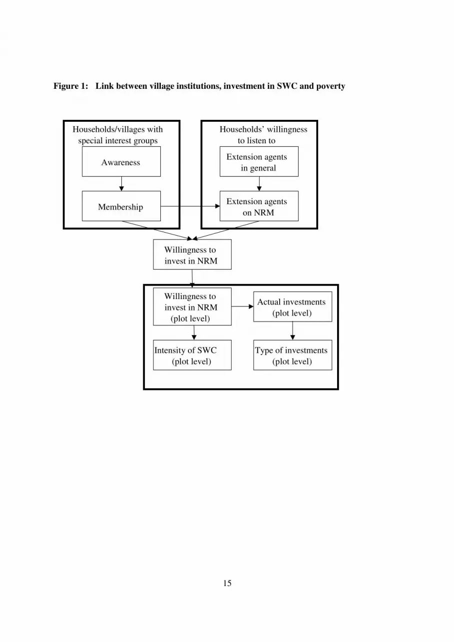
their effect on current SWC investments. The relationships modelled above are illustrated in figure 1.

15

Figure 1: Link between village institutions, investment in SWC and poverty

Households/villages with

special interest groups

Households’ willingness

to listen to

Awareness

Membership

Extension agents

in general

Extension agents

on NRM

Willingness to

invest in NRM

Willingness to

invest in NRM

(plot level)

Actual investments

(plot level)

Type of investments

(plot level)

Intensity of SWC

(plot level)

16

4. Results and discussion

4.1 Descriptive statistics

Though some variables are observed at the household level, the analysis in this paper is based on

plot level dataiv

. In this section, we present a brief description of the key variables utilized in the

empirical analysis. Due to limitation of space, we focus attention on the dependent variable,

tenure security, soil, topography and village level factorsv. For investment in soil and water

conservation (SWC), the study collected data on the type of improvements, the number of SWC

structures, when the improvement was elected and whether or not any SWC strategy had been

abandoned. Tree planting was the most common form of land improvements in all the districts.

This was followed by terracing with grass strips and grass strips alone. The data shows that 70%

of all households were willing to take up SWC strategies, while every household had at least one

SWC strategy in place and one previous SWC strategy. The three most frequently observed

SWC investments in the survey were tree planting (28%), terracing with grass strips (26%), and

grass strips alone (23%). Most investments (72%) were permanent investments, while 31%

investments had been elected the year prior to the year. One-third of the investments were more

than five years old. In 5% of the cases, the investments had already been abandoned.

To capture all aspects of tenure security, this study collected data on both the mode of

acquisition and expected land rights on all plots owned, used or rented/lent out by the household.

The mode of acquisition probed on how, when and for how long the plot had been in the hands

of the household. The expected land rights probed on the perception on land rights in terms of

17

tenure security (whether land is shared, whether it can be taken away from household and by

whom e.t.c. In addition, we probed nature of rental arrangements and land rights on rented out

and lent out land. The data shows that 71% of the plots were owned (and often used) by the

household, 22% of the plots were rented in, and 7% of the plots were rented out. More than half

of the plots were inherited, and the duration of ownership was more than 18 years on average. In

addition, 5% of the plots had been in the household’s ownership for more than 50 years. In 46%

of the cases the plots were registered to the household management team (head or spouse) while

31% of the plots were registered to other relatives.

Including all aspects of tenure security in the empirical analysis would however be cumbersome

because the choice of specific indicators is more or less arbitrary. To avoid such arbitrariness we

used factor analysis (FA) at the plot level to filter out the key elements of tenure security out of a

wide range of tenure security variables. This limited the number of tenure security variables in

our analysis to retain only the key elements. From the factor analysis, only five factors were

constructed. The first variable was own farmland (registered in head of household or spouse)

ranging from full ownership to indefinite rental arrangements. The second factor reflected plots

owned by the extended family. The third factor was plots for which other relatives have to give

permission for selling or bequeath, and the fourth factor covered rented out land. The final factor

reflected rental conditions of plots that were either rented or lent with or without permission.

The soil characteristics included the type of soil, the soil depth, the slope, fertility, workability

and texture of the soil. In the survey, 42%, 23% and 25% of the plots had red, black and a

mixture of the two soils respectively. More than half of the plots were slightly to steeply sloped,

18

while 22% of the plots were flat. The workability in 60% of the plots was easy, and almost half

of the plots had fine soils. Only 14% of the plots had coarse soils. The average soil depth was

22.5 cm though the respondents perceived the soil to be generally infertile.

Final variables related to soil quality and topographical factors were also constructed using factor

analysis. Except for depth of soil which was unique, all categories of soil quality variables were

retained in the factor analysis and were therefore used as explanatory variables for welfare.

Topography was measured through the terrain (whether sloped, flat or undulating) and three

topographical factors were obtained from the factor analysis: flatness, moderate slope and

undulating terrain.

Market access was based on information on distance, mode of travel, travel time and expenses

from the village to particular destinations like markets and roads amongst others collected using

the community questionnaire. The FA for market access was limited to four facilities, namely

distance to local market, all-weather roads, public transport and nearest town. However, only one

factor covering almost 75% of the variation in the distance to facility data set under

consideration was selected.

4.2 Regression Results

Determinants of adoption of soil and water conservation investments

The key task of this paper is to test the role of tenure security among other household, farm and

community characteristics (including development domain dimensions) on soil and water

conservation investment decisions at the plot level. We also analyze the determinants of adoption of

19

permanent and seasonal SWC investments. The types of investments that we consider are determined

by the same set of factors. Furthermore, we expect that all important variables will influence them in

the same direction. It is therefore important to investigate for any possible correlation between the

adoption decisions. This is done in several steps. First, we run the individual Probit type models for

each of the adoption decisions. Second, we derive individual residuals from each investment

regression equation and examine the relationship between investment decisions further by carrying

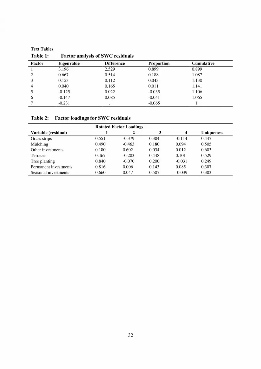
out a factor analysis on the residuals from each of the regression equations. The results of the factor

analysis, (Table 1) shows that there is only one factor in which residuals for more long-term SWC

investments, such as permanent investments in soil fertility and tree planting, are significantly

present. Since the residual of seasonal or short-term investments in SWC are not present, we refer to

this unique factor as the “speed of regenerating chemical fertility” because higher levels of

regenerating soil fertility characterize these long-term investments. This is further supported by

factor loadings based on Varimax rotation (Table 2). The results of the factor analysis support our

intuition and findings of the regression equations on investment decisions: different types of SWC

investments are explained by similar sets of explanatory variables.

****************** Table 1 here ******************

****************** Table 2 here ******************

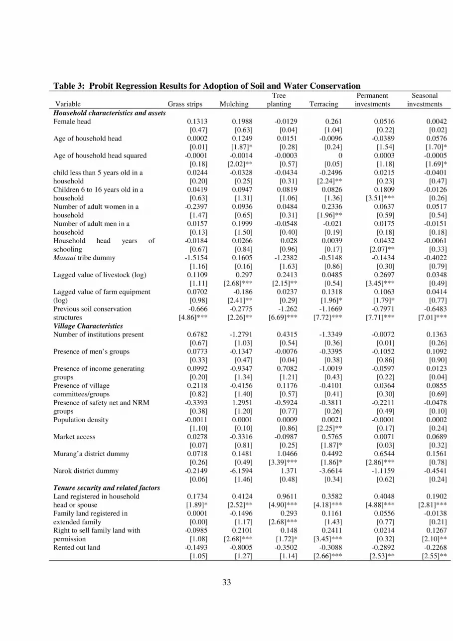
The Probit regression results are presented in Table 3. Since we are interested in both the direct and

indirect effects on the probability of adopting SWC, we retain all variables in the regression models,

irrespective of whether they are significant or not.

The regression results suggest that most household characteristics do not matter much in influencing

the adoption decision. While this result is not uncommon in the literature (see for instance,

Gebremedhin and Swinton, 2003), it could also be due to the fact that our models capture both direct

20

and indirect effects of the explanatory factors. However, age seems to matter for mulching and all

seasonal improvements. Specifically, age exhibits an inverted U-shaped relationship with the

decision to adopt these types of investments. This suggests life cycle impacts on the investment

decision. Younger farmers may have more energy to engage in labour intensive conservation

practices but after some threshold, the likelihood of adoption declines. Presence of children aged less

than 5 years is negatively correlated with adoption of all types of terraces. Given that terracing is

labour intensive, the result implies that presence of young children diverts labour from conservation

activities to childcare. However, presence of older children (aged 6 to 16 years) is positively

correlated with investment decisions (more so terracing), suggesting that they provide additional

labour inputs for soil and water conservation. Another important finding is that number of adult

females in a household is positively correlated with adoption of all SWC investments except grass

strip. The significant impact on adoption of terracing suggests the importance of female labour in

adoption of SWC investments. This is further supported by the coefficient for total males, which is

negative (though insignificant) for most types of SWC investments.

****************** Table 3 here ******************

We do not uncover much impact of the presence of village institutions on adoption of SWC

investments. The presence and type of institutions only matter for adoption of soil and grass stripped

terraces (results not presented). In particular, the number of institutions present, presence of men’s

groups, household income generation and other village committees are positively and significantly

correlated with the decision to adopt these forms of SWC.

21

Similarly, market access and population density are positively correlated with terracing, which

suggests the importance of development domain dimensions in adoption of SWC investments.

We do not uncover any important impact of population density and market access on the other

methods of conservation. The two district dummies (Murang’a and Narok) suggest that location

is an important determinant of the decision to adopt some SWC. Specifically, there is a higher

probability of adoption if a household is located in Murang’a relative to Maragua district, more

so for all permanent investments. The likelihood of adoption is lower in Narok district but the

coefficients are insignificant. Given the diversity of agro-ecology in the three districts, we

conclude that the impact of district dummies reflect the unobserved relative importance of different

development domains.

The impact of tenure security factors is captured by five variables: owned plots (which are often

inherited); family land that can be sold or bequeathed with or without permission; land registered

in family name; rented out and the right to rent out land without permission. In this case, the first

three rights represent the strongest rights to land. The coefficients of these variables exhibit

positive and significant coefficients for most adoption models, suggesting the importance of

tenure security in adoption of SWC investments. The negative and mostly significant coefficients

of the last two variables show that weak security of tenure will discourage investment in SWC,

more so long term investments such as grass strips, terracing and tree planting. These results also

concur with previous studies on soil and conservation in Kenya (Kabubo-Mariara, 2006, 2007).

The differences in coefficients for permanent and seasonal investments support the finding that

tenure security favours long term conservation investments more than short term investments.

Previous literature has also shown that farmers with long term tenure security are more likely to

invest in costly and durable conservation measures (Gebremedhin and Swinton 2003). Farmers’

22

attitudes towards adoption of new technology have also been shown to depend on the

profitability and riskness of the new technology. Given the type of land right issues posed to

respondents, the results suggest that to ensure that land tenure policy is pro-environment, it is

important to consider whether household plots are owned, rented out, or rented in. The issues

related to owned plots include mode of acquisition, length of ownership, registration of land,

shared rights (with family or community) and both formal and informal assurance. Issues on

rented in or rented out plots include length and type of arrangement and modes of payment.

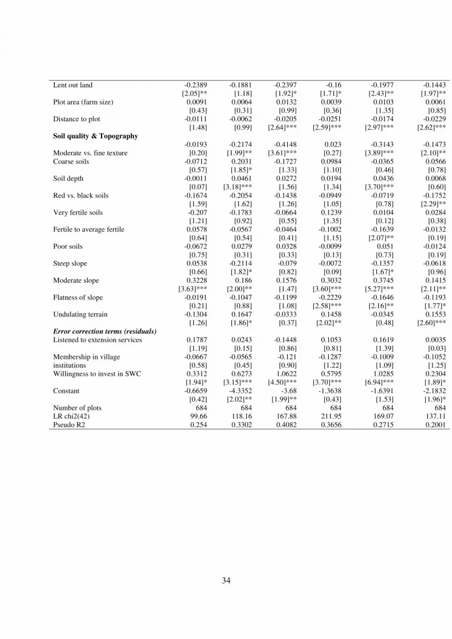
Soil texture does not seem to matter much for conservation. For instance, moderate versus fine soils

are inversely and significantly correlated with the probability of adopting all practices except all

forms of terracing. Course and very fertile soils encourage adoption of terracing, while there is less

likelihood of investment in SWC on fertile soils compared to average fertile soils. Red versus black

soils is also inversely related with adoption of SWC investments. Soil depth is however positively

correlated with most investments: mulching, terracing and all permanent investments. Turning to

topography, moderate slopes and undulating terrain favour adoption of grass strips, mulching,

terracing and all permanent investments. Undulating terrain is also positively correlated with the

probability of adopting seasonal investments. Conversely, steep slopes lower probability of adoption

of all SWC investments. There is also less likelihood of adoption of most SWC investments on flat

land.

Household assets are captured by a vector of variables namely: lagged values of farm equipment

and livestock wealth, plot size and existing conservation assets (permanent SWC investments not

made in the past year but still in function). Farm equipment is positively correlated to all

permanent improvements, including mulching and tree planting. Livestock wealth is also

positively correlated with permanent improvements but is only significant for terraces and soil

23

terraces. Livestock wealth is inversely correlated with mulching. This is probably due to the fact

that most material used for mulching is crop residuals, which is also used as feed for cattle.

Mulching and livestock feeding are therefore competing alternatives rather than complements.

The results for household wealth are consistent with studies that argue for an inter-linked

connection where tenure and wealth are jointly responsible for investments in SWC (Place et al.,

1995; Smith, 2004).

Plot size increases the likelihood of adoption of other investments (fallowing, crop rotation and

ridging) as well as grass stripped terracing (results not presented). The results for other investment is

because fallowing and crop rotation are land intensive and households may not leave land fallow or

rotate crops if there is land scarcity. The impact of plot size on other technologies, including all

permanent and seasonal SWC investments is insignificant. This could also imply that factor markets

are not efficient to allow large farmers to hire labour in sufficient quantities. However, results from

previous literature also suggests that the size of holdings may be a substitute for many potentially

important factors like credit, risk bearing capacity, access to inputs and access to information (Feder

et al., 1985). Distance to plot is inversely and significantly correlated with adoption of all SWC

technologies, implying that all technologies are more likely to be adopted on home plots rather than

distant plots. Literature suggests that transaction costs of travelling to plots will determine the type of

conservation measures on such plots (Gebremedhin and Swinton, 2003), such that plots distant from

the homestead or highly fragmented plots are more likely to be developed with less expensive SWC

investments.

24

Existing soil and water conservation assets on a plot are inversely related to the probability of

making new investments. This implies that additional investments are more likely to be made on

plots without any prior land improvements than plots with existing investments.

We include three error correction residuals in the determination of the investment decision. We

test the impact of listening to agricultural extension services in general, membership in village

institutions and the willingness to invest in SWC. We uncover no important impact of the

residuals of extension services and membership in village institutions. However, the residual of

the willingness to invest is positively correlated with all investment decisions, both permanent

and seasonal, implying the need to provide incentives for SWC.

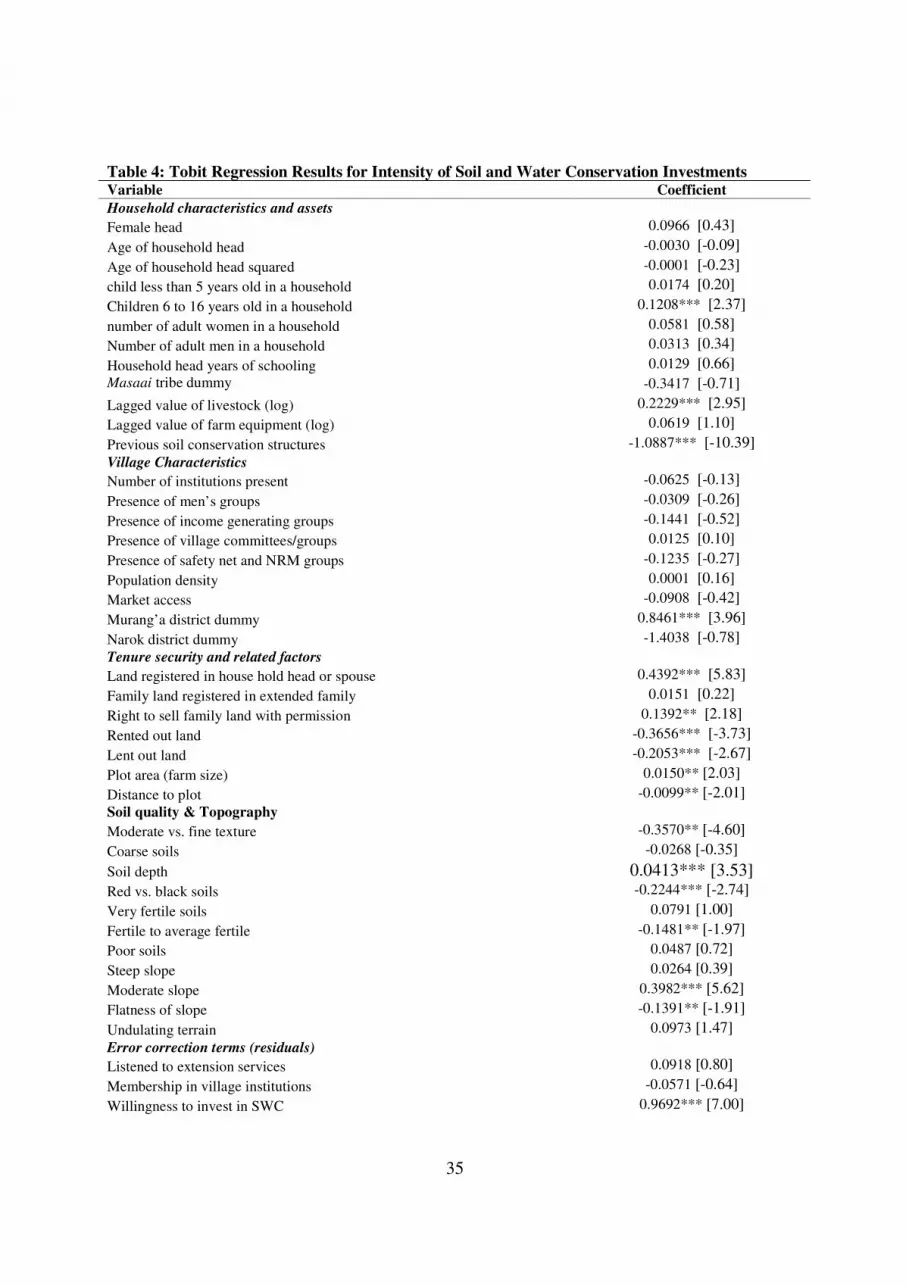
Determinants of the intensity of SWC investments

In addition to the determinants of the probability of adoption of various SWC investments, we also

measure the extent or intensity of adoption, measured through the number of SWC investment

structures on a plot. Since some plots have no SWC structures, we use the Tobit model to explain

how much households participate in SWC investments. The results are presented in Table 4.

Presence of children aged 6 to 16 years is the only household characteristics that seem to matter for

intensity of adoption, which implies the importance of family labour in SWC. We uncover no impact

of presence of village institutions, population density and market access on intensity of adoption,

which is consistent with findings for adoption of general permanent and seasonal technologies. This

result implies that though development domain dimensions may matter for some individual

investment decisions, they may not matter much for intensity of conservation. There is a higher

intensity of adoption in Murang’a relative to Maragua district but the reverse is observed for Narok.

25

****************** Table 4 here ******************

This is consistent with the results for the adoption of individual conservation investments.

The results further show that tenure security variables not only influence the probability of adopting

various SWC technologies but also determine how much to invest in SWC. Soil quality and

topography also matter, and the results are comparable to those of adoption. Plot size is positively

correlated to the number of actual investment structures, but the reverse is observed for distance to

plot. Previously owned farm equipment and livestock wealth are positively correlated with number of

investments but only the former has a significant coefficient. The permanent SWC investments not

made in the past year but still in function are inversely related with the intensity of conservation,

implying that most investment structures are seasonal rather than permanent. Like in the adoption

model, we uncover no impact of extension services and membership in village institutions on the

intensity of conservation. The residual for willingness to invest in SWC is however positively

correlated with the intensity of conservation, supporting earlier results that willingness to invest

raises participation in SWC.

Comparing the intensity of adoption with the adoption of seasonal and permanent investments,

the results suggest that except for a few variables, intensity of adoption is determined by the

same set of factors that influence the decision to invest. This is consistent with most empirical

literature though a few studies have shown that factors explaining adoption of SWC investments

may differ from those determining the intensity of adoption (see for instance Gebremedhin and

Swinton, 2003).

26

5. Conclusions

In this paper, we investigate the impact of tenure security and other household, farm and village

characteristics, including development domain dimensions on adoption of soil and water

conservation investments in Kenya. The analysis is based on plot level data for a sample of 457

households collected from 3 districts in Kenya in November and December 2004. We estimate

probit models for adoption of various SWC technologies, including seasonal and permanent

technologies, then explain the intensity of adoption using the tobit regression method. A step

wise regression approach is employed to derive residuals of village level institutional variables

and willingness to invest in soil and water conservation. The residuals are used as error

correction models to control for partial endogeneity of these variables. The truly exogenous

variables capture the sum of the direct and indirect effects, while the residual terms capture the

effect of the endogenous variables. Factor analysis is used to select variables for tenure security

that explain adoption and intensity of soil and water conservation. Factor analysis is also applied

to create variables for soil quality and topography, institutional presence and market access.

The results indicate the importance of tenure security in determining adoption and also the

intensity of SWC investments. In addition the results indicate the importance of household

assets, farm characteristics (soils and topography), presence of village institutions and

development domain dimensions (market access and population density) in adoption of soil and

water conservation investments. Soil quality and topography, as well as location (agro ecological

diversity) are particularly important determinants of investment in SWC. These results suggest

that the use of appropriate productivity increasing technologies must consider the type of soil

27

quality and topography and their effect on land degradation. The results on village institutions

highlight the importance of institutional presence in adoption of technology, though these

variables seem to matter most only for adoption of grass strips. The impact of household assets

on investment in soil and water conservation implies a poverty environment link because

households that are poor in assets are less likely to invest in soil and water conservation. The

intensity of adoption is also lower for households poorer in assets than their richer counterparts.

The results further suggest that the factors affecting the level of investment are the same as the

factors determining the decision whether or not to invest in SWC.

In summary, the results suggest the need for a policy that improves security of tenure as a way of

encouraging investments on long term conservation measures. It is recognized in Kenya that land

conservation policy and laws have not been effective in generating environmentally sound land

use practices. This policy needs to be strengthened. It is also apparent from the results that

policies aimed at environmental conservation need to be region/area specific. In addition, given

the strong support for the existence of an environment-poverty link in this study, there is need for

broad policies that provide incentives for environmental conservation and poverty reduction.

28

References

Besley, T. (1995). Property Rights and Investment Incentives: Theory and Evidence from Ghana.

Journal of Political Economics 103(5), 903-937.

Boserup, E. (1965). The Conditions of Agricultural Growth: The Economics of Agrarian Change

under Population Pressure. New York: Aldine Press.

Brasselle, A.S., Gaspart, F. & Platteau, J-P. (2002). Land Tenure Security and Investment

Incentives: Puzzling Evidence from Burkina Faso, Journal of Development Economics 67,

373-418.

Bruce, J. W., Migot-Adholla, S. E., & Atherton, J. (1994). The findings and their policy

implications: Institutional adaptation or replacement. In: Bruce, J. W. & Migot-Adholla, S. E.

(eds.). Searching for land tenure security in Africa. Dubuque, Iowa: Kendall/Hunt Publishing

Company. 251-265.

Bulte, E.H. & Soest, D.P. van (1999). A note on soil depth, failing markets and agricultural

pricing. Journal of Development Economics 58(1), 245-254.

Carter, M.R. & Olinto, P. (2003). Getting Institutions Right for Whom? Credit Constraints and

the Impact of Property Rights on the Quantity and Composition of Investment. American

Journal of Agricultural Economics 85(1), 173-186.

Davidson, R. and J.G. MacKinnon. 1993. Estimation and Inference in Econometrics, New York,

Oxford University Press.

Deininger K. & Jin, S. (2002). The Impact of Property Rights on Households’ Investment, Risk

Coping and Policy Preferences: Evidence from China. World Bank Policy Research Working

Paper 2931. The World Bank. Washington D.C.

29

Demsetz, H. (1967). Toward a Theory of Property Rights. American Economic Review 57(2),

347-359.

Feder G., Just, R.E. & Zilberman, D. (1985). Adoption of Agricultural Innovations in

Developing Countries: A survey. Economic Development and Cultural Change 32(2), 255-

297.

Feder, G., Onchan, T., Chalamwong, Y. & Hongladarom, C. (1988). Land policies and farm

productivity in Thailand. Baltimore and London: Johns Hopkins University Press for the

World Bank.

Gebremedhin B. & Swinton, S.M. (2003). Investment in Soil Conservation in Northern Ethiopia:

The Role of Land Tenure Security and Public Programs. Agricultural Economics 29, 69-84.

Jacoby H.G., Li, G. & Rozelle, S. (2002). Hazards of Expropriation: Tenure Insecurity and

Investment in Rural China. American Economic Review 92(5), 1420-1477.

Kabubo-Mariara, J. (2007). Land Conservation and Tenure Security in Kenya: Boserup’s

Hypothesis Revisited”. Ecological Economics, doi:10.1016/j.ecolecon.2007.06.007

Kabubo-Mariara, J. (2004). Poverty, Property Rights and Socio-economic incentives for Land

Conservation: The case for Kenya. African Journal of Economic Policy 11(1), 35-68.

Kruseman, G., (2000). Bio-economic household modeling for agricultural intensification. PhD

Thesis. Wageningen University. Mansholt Studies No. 20, Wageningen.

Kruseman, G. Ruben, R. & Tesfay, G. (2006). Diversity and development in the Ethiopian

highlands. Agricultural Systems 88. 75-91.

Li G., Rozelle, S. & Brandt, L. (1998). Tenure, Land Rights, and Farmer Investment Incentives

in China. Agricultural Economics 19, 63-71

30

Migot-Adholla, S.E., Place, F. & Oluoch-Kosura, W. (1994). Security of Tenure and Land

Productivity in Kenya. In: Bruce, J.W. & Migot-Adholla, S.E. (eds.), Searching for Land

Tenure Security in Africa. Dubuque, Iowa: Kendall/Hunt Publishing Cy. 119-40.

Migot-Adholla S. E., Hazell, P., Blarel, B. & F. Place, F. (1991), Indigenous Land Right Systems

in Sub-Saharan Africa: A Constraint on Productivity? The World Bank Economic Review,

5(1) 155-175.

Pinckney C. & Kimuyu, P.K. (1994). Land Tenure Reform in East Africa: Good, Bad or

Unimportant? Journal of African Economies 3(1), 1-28.

Place, F. & Hazell, P. (1993). Productivity effects of indigenous land tenure systems in Sub-

Saharan Africa. American Journal of Agricultural Economics 75(1), 10-19.

Place F. & Otsuka, K. (2002). Land Tenure Systems and their Impacts on Productivity in

Uganda. Journal of Development Studies 38(6), 105-128.

Place F. & Otsuka, K. (2000), The Role of Tenure in the Management of trees at the Community

Level: Theoretical and Empirical Analysis From Uganda and Malawi: CAPRi Working Paper

No. 9. International Food Policy Research Institute, Washington D.C.

Platteau J.P. (2000), Institutions, Social Norms, and Economic Development. Amsterdam:

Harwood Academic Publishers.

Platteau, J.P. (1996), The Evolutionary Theory of Land Rights As Applied to Sub-Saharan Africa:

A Critical Assessment. Development and Change 27(1), 29-86.

Roth, M., Unruh, J. & Barrows, R. (1994). Land Registration, Tenure Security, Credit Use, and

Investment in the Shebelle Region of Somalia. In: Bruce, J.W. & Migot-Adholla, S. (eds.).

Searching for Land Tenure Security in Africa. Dubuque, Iowa: Kendall/Hunt Publishing Cy.

199-230.

31

Shiferaw B. & Holden, S. (1999). Soil Erosion and Smallholders’ Conservation Decisions in the

Highlands of Ethiopia. World Development 27(4), 739-752.

Singh, I., Squire, L. & Strauss, J. (1986). Agricultural household models: extensions,

applications, and policy. Baltimore: The Johns Hopkins University Press.

Sjaastad, E. & Bromley, D.W. (1997). Indigenous Land Rights in Sub-Saharan Africa:

Appropriation, Security, and Investment Demand. World Development 25, 549-562.

Tiffen M., Mortimore, M. & Gichuki, F. (1994). More People, Less Erosion: Environmental

Recovery in Kenya. Chichester: John Wiley and Sons.

Zimmerman, F. & Carter, M. (1999). A Dynamic Option Value for Institutional Change:

Marketable Property Rights in the Sahel. American Journal of Agricultural Economics 81(2),

467-478.

32

Text Tables

Table 1: Factor analysis of SWC residuals

Factor Eigenvalue Difference Proportion Cumulative

1 3.196 2.529 0.899 0.899

2 0.667 0.514 0.188 1.087

3 0.153 0.112 0.043 1.130

4 0.040 0.165 0.011 1.141

5 -0.125 0.022 -0.035 1.106

6 -0.147 0.085 -0.041 1.065

7 -0.231 . -0.065 1

Table 2: Factor loadings for SWC residuals

Rotated Factor Loadings

Variable (residual) 1 2 3 4 Uniqueness

Grass strips 0.551 -0.379 0.304 -0.114 0.447

Mulching 0.490 -0.463 0.180 0.094 0.505

Other investments 0.180 0.602 0.034 0.012 0.603

Terraces 0.467 -0.203 0.448 0.101 0.529

Tree planting 0.840 -0.070 0.200 -0.031 0.249

Permanent investments 0.816 0.006 0.143 0.085 0.307

Seasonal investments 0.660 0.047 0.507 -0.039 0.303

33

Table 3: Probit Regression Results for Adoption of Soil and Water Conservation

Variable Grass strips Mulching

Tree

planting Terracing

Permanent

investments

Seasonal

investments

Household characteristics and assets

Female head 0.1313 0.1988 -0.0129 0.261 0.0516 0.0042

[0.47] [0.63] [0.04] [1.04] [0.22] [0.02]

0.0002 0.1249 0.0151 -0.0096 -0.0389 0.0576 Age of household head

[0.01] [1.87]* [0.28] [0.24] [1.54] [1.70]*

-0.0001 -0.0014 -0.0003 0 0.0003 -0.0005 Age of household head squared

[0.18] [2.02]** [0.57] [0.05] [1.18] [1.69]*

0.0244 -0.0328 -0.0434 -0.2496 0.0215 -0.0401 child less than 5 years old in a

household [0.20] [0.25] [0.31] [2.24]** [0.23] [0.47]

0.0419 0.0947 0.0819 0.0826 0.1809 -0.0126 Children 6 to 16 years old in a

household [0.63] [1.31] [1.06] [1.36] [3.51]*** [0.26]

-0.2397 0.0936 0.0484 0.2336 0.0637 0.0517 Number of adult women in a

household [1.47] [0.65] [0.31] [1.96]** [0.59] [0.54]

0.0157 0.1999 -0.0548 -0.021 0.0175 -0.0151 Number of adult men in a

household [0.13] [1.50] [0.40] [0.19] [0.18] [0.18]

-0.0184 0.0266 0.028 0.0039 0.0432 -0.0061 Household head years of

schooling [0.67] [0.84] [0.96] [0.17] [2.07]** [0.33]

Masaai tribe dummy -1.5154 0.1605 -1.2382 -0.5148 -0.1434 -0.4022

[1.16] [0.16] [1.63] [0.86] [0.30] [0.79]

0.1109 0.297 0.2413 0.0485 0.2697 0.0348 Lagged value of livestock (log)

[1.11] [2.68]*** [2.15]** [0.54] [3.45]*** [0.49]

0.0702 -0.186 0.0237 0.1318 0.1063 0.0414 Lagged value of farm equipment

(log) [0.98] [2.41]** [0.29] [1.96]* [1.79]* [0.77]

-0.666 -0.2775 -1.262 -1.1669 -0.7971 -0.6483 Previous soil conservation

structures [4.86]*** [2.26]** [6.69]*** [7.72]*** [7.71]*** [7.01]***

Village Characteristics

0.6782 -1.2791 0.4315 -1.3349 -0.0072 0.1363 Number of institutions present

[0.67] [1.03] [0.54] [0.36] [0.01] [0.26]

0.0773 -0.1347 -0.0076 -0.3395 -0.1052 0.1092 Presence of men’s groups

[0.33] [0.47] [0.04] [0.38] [0.86] [0.90]

0.0992 -0.9347 0.7082 -1.0019 -0.0597 0.0123 Presence of income generating

groups [0.20] [1.34] [1.21] [0.43] [0.22] [0.04]

0.2118 -0.4156 0.1176 -0.4101 0.0364 0.0855 Presence of village

committees/groups [0.82] [1.40] [0.57] [0.41] [0.30] [0.69]

-0.3393 1.2951 -0.5924 -0.3811 -0.2211 -0.0478 Presence of safety net and NRM

groups [0.38] [1.20] [0.77] [0.26] [0.49] [0.10]

Population density -0.0011 0.0001 0.0009 0.0021 -0.0001 0.0002

[1.10] [0.10] [0.86] [2.25]** [0.17] [0.24]

Market access 0.0278 -0.3316 -0.0987 0.5765 0.0071 0.0689

[0.07] [0.81] [0.25] [1.87]* [0.03] [0.32]

0.0718 0.1481 1.0466 0.4492 0.6544 0.1561 Murang’a district dummy

[0.26] [0.49] [3.39]*** [1.86]* [2.86]*** [0.78]

-0.2149 -6.1594 1.371 -3.6614 -1.1159 -0.4541 Narok district dummy

[0.06] [1.46] [0.48] [0.34] [0.62] [0.24]

Tenure security and related factors

0.1734 0.4124 0.9611 0.3582 0.4048 0.1902 Land registered in household

head or spouse [1.89]* [2.52]** [4.90]*** [4.18]*** [4.88]*** [2.81]***

0.0001 -0.1496 0.293 0.1161 0.0556 -0.0138 Family land registered in

extended family [0.00] [1.17] [2.68]*** [1.43] [0.77] [0.21]

-0.0985 0.2101 0.148 0.2411 0.0214 0.1267 Right to sell family land with

permission [1.08] [2.68]*** [1.72]* [3.45]*** [0.32] [2.10]**

Rented out land -0.1493 -0.8005 -0.3502 -0.3088 -0.2892 -0.2268

[1.05] [1.27] [1.14] [2.66]*** [2.53]** [2.55]**

34

Lent out land -0.2389 -0.1881 -0.2397 -0.16 -0.1977 -0.1443

[2.05]** [1.18] [1.92]* [1.71]* [2.43]** [1.97]**

Plot area (farm size) 0.0091 0.0064 0.0132 0.0039 0.0103 0.0061

[0.43] [0.31] [0.99] [0.36] [1.35] [0.85]

Distance to plot -0.0111 -0.0062 -0.0205 -0.0251 -0.0174 -0.0229

[1.48] [0.99] [2.64]*** [2.59]*** [2.97]*** [2.62]***

Soil quality & Topography

-0.0193 -0.2174 -0.4148 0.023 -0.3143 -0.1473

Moderate vs. fine texture [0.20] [1.99]** [3.61]*** [0.27] [3.89]*** [2.10]**

Coarse soils -0.0712 0.2031 -0.1727 0.0984 -0.0365 0.0566

[0.57] [1.85]* [1.33] [1.10] [0.46] [0.78]

Soil depth -0.0011 0.0461 0.0272 0.0194 0.0436 0.0068

[0.07] [3.18]*** [1.56] [1.34] [3.70]*** [0.60]

Red vs. black soils -0.1674 -0.2054 -0.1438 -0.0949 -0.0719 -0.1752

[1.59] [1.62] [1.26] [1.05] [0.78] [2.29]**

Very fertile soils -0.207 -0.1783 -0.0664 0.1239 0.0104 0.0284

[1.21] [0.92] [0.55] [1.35] [0.12] [0.38]

0.0578 -0.0567 -0.0464 -0.1002 -0.1639 -0.0132 Fertile to average fertile

[0.64] [0.54] [0.41] [1.15] [2.07]** [0.19]

Poor soils -0.0672 0.0279 0.0328 -0.0099 0.051 -0.0124

[0.75] [0.31] [0.33] [0.13] [0.73] [0.19]

Steep slope 0.0538 -0.2114 -0.079 -0.0072 -0.1357 -0.0618

[0.66] [1.82]* [0.82] [0.09] [1.67]* [0.96]

Moderate slope 0.3228 0.186 0.1576 0.3032 0.3745 0.1415

[3.63]*** [2.00]** [1.47] [3.60]*** [5.27]*** [2.11]**

Flatness of slope -0.0191 -0.1047 -0.1199 -0.2229 -0.1646 -0.1193

[0.21] [0.88] [1.08] [2.58]*** [2.16]** [1.77]*

Undulating terrain -0.1304 0.1647 -0.0333 0.1458 -0.0345 0.1553

[1.26] [1.86]* [0.37] [2.02]** [0.48] [2.60]***

Error correction terms (residuals)

0.1787 0.0243 -0.1448 0.1053 0.1619 0.0035 Listened to extension services

[1.19] [0.15] [0.86] [0.81] [1.39] [0.03]

-0.0667 -0.0565 -0.121 -0.1287 -0.1009 -0.1052 Membership in village

institutions [0.58] [0.45] [0.90] [1.22] [1.09] [1.25]

0.3312 0.6273 1.0622 0.5795 1.0285 0.2304 Willingness to invest in SWC

[1.94]* [3.15]*** [4.50]*** [3.70]*** [6.94]*** [1.89]*

Constant -0.6659 -4.3352 -3.68 -1.3638 -1.6391 -2.1832

[0.42] [2.02]** [1.99]** [0.43] [1.53] [1.96]*

Number of plots 684 684 684 684 684 684

LR chi2(42) 99.66 118.16 167.88 211.95 169.07 137.11

Pseudo R2 0.254 0.3302 0.4082 0.3656 0.2715 0.2001

35

Table 4: Tobit Regression Results for Intensity of Soil and Water Conservation Investments Variable Coefficient

Household characteristics and assets

Female head 0.0966 [0.43]

Age of household head -0.0030 [-0.09]

Age of household head squared -0.0001 [-0.23]

child less than 5 years old in a household 0.0174 [0.20]

Children 6 to 16 years old in a household 0.1208*** [2.37]

number of adult women in a household 0.0581 [0.58]

Number of adult men in a household 0.0313 [0.34]

Household head years of schooling 0.0129 [0.66]

Masaai tribe dummy -0.3417 [-0.71]

Lagged value of livestock (log) 0.2229*** [2.95]

Lagged value of farm equipment (log) 0.0619 [1.10]

Previous soil conservation structures -1.0887*** [-10.39]

Village Characteristics

Number of institutions present -0.0625 [-0.13]

Presence of men’s groups -0.0309 [-0.26]

Presence of income generating groups -0.1441 [-0.52]

Presence of village committees/groups 0.0125 [0.10]

Presence of safety net and NRM groups -0.1235 [-0.27]

Population density 0.0001 [0.16]

Market access -0.0908 [-0.42]

Murang’a district dummy 0.8461*** [3.96]

Narok district dummy -1.4038 [-0.78]

Tenure security and related factors

Land registered in house hold head or spouse 0.4392*** [5.83]

Family land registered in extended family 0.0151 [0.22]

Right to sell family land with permission 0.1392** [2.18]

Rented out land -0.3656*** [-3.73]

Lent out land -0.2053*** [-2.67]

Plot area (farm size) 0.0150** [2.03]

Distance to plot -0.0099** [-2.01]

Soil quality & Topography

Moderate vs. fine texture -0.3570** [-4.60]

Coarse soils -0.0268 [-0.35]

Soil depth 0.0413*** [3.53]

Red vs. black soils -0.2244*** [-2.74]

Very fertile soils 0.0791 [1.00]

Fertile to average fertile -0.1481** [-1.97]

Poor soils 0.0487 [0.72]

Steep slope 0.0264 [0.39]

Moderate slope 0.3982*** [5.62]

Flatness of slope -0.1391** [-1.91]

Undulating terrain 0.0973 [1.47]

Error correction terms (residuals)

Listened to extension services 0.0918 [0.80]

Membership in village institutions -0.0571 [-0.64]

Willingness to invest in SWC 0.9692*** [7.00]

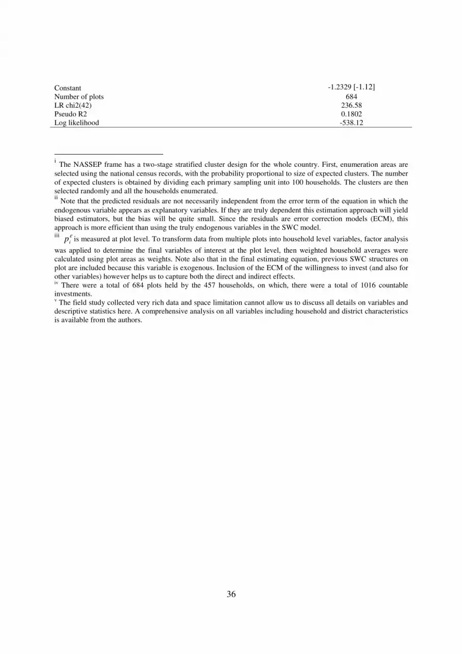
36

Constant -1.2329 [-1.12]

Number of plots 684

LR chi2(42) 236.58

Pseudo R2 0.1802

Log likelihood -538.12

i The NASSEP frame has a two-stage stratified cluster design for the whole country. First, enumeration areas are

selected using the national census records, with the probability proportional to size of expected clusters. The number

of expected clusters is obtained by dividing each primary sampling unit into 100 households. The clusters are then

selected randomly and all the households enumerated. ii Note that the predicted residuals are not necessarily independent from the error term of the equation in which the

endogenous variable appears as explanatory variables. If they are truly dependent this estimation approach will yield

biased estimators, but the bias will be quite small. Since the residuals are error correction models (ECM), this

approach is more efficient than using the truly endogenous variables in the SWC model. iii

εip is measured at plot level. To transform data from multiple plots into household level variables, factor analysis

was applied to determine the final variables of interest at the plot level, then weighted household averages were

calculated using plot areas as weights. Note also that in the final estimating equation, previous SWC structures on

plot are included because this variable is exogenous. Inclusion of the ECM of the willingness to invest (and also for

other variables) however helps us to capture both the direct and indirect effects. iv There were a total of 684 plots held by the 457 households, on which, there were a total of 1016 countable

investments. v The field study collected very rich data and space limitation cannot allow us to discuss all details on variables and

descriptive statistics here. A comprehensive analysis on all variables including household and district characteristics

is available from the authors.