Documento Tesis superdef_jmar - ADDI

MEASUREMENT OF POLYCYCLIC AROMATIC HYDROCARBONS IN AMBIENT AIR BY

FLUORESCENCE SPECTROSCOPIC TECHNIQUES

A dissertation submitted to the University of the Basque Country to apply for the degree of Doctor

of Philosophy

by

Saioa Elcoroaristizabal Martín

Directed by: Prof. Lucio Alonso Alonso Dr. Jose Antonio García Fernández

Bilbao, 2015

llzitbel

Texto escrito a máquina

(cc) 2015 SAIOA ELCOROARISTIZABAL MARTIN (cc by-nc 4.0)

A mis padres, Aurelia y Francisco Javier

“Quien nunca ha cometido un error, nunca ha intentado algo nuevo”

Albert Einstein

“El camino del progreso no es rápido ni fácil”

Marie Curie

ACKNOWLEDGEMENTS

Hoy es un día perfecto para echar la vista atrás y ser consciente de lo que ha supuesto

llegar hasta aquí. Han sido muchos años rodeada de un equipo de fluorescencia que

hacía subir la temperatura del “zulo”, de matraces, extractores, captadores, PAHs y de

mi hoy en día, gran amigo Matlab. Pero sobre todo, ha sido mucho tiempo rodeada de

gente que ha hecho que este esfuerzo haya valido la pena. Por todo ello quisiera

aprovechar estas líneas para agradecer a todas esas personas que de alguna u otra

manera han colaborado en la realización de esta tesis doctoral.

En primer lugar, gracias a mis directores de tesis, Dr. Jose Antonio García Fernández

y Prof. Lucio Alonso Alonso por la confianza depositada en mí y por darme la

oportunidad de llevar a cabo este trabajo. Pero sobre todo, por haber tenido siempre la

puerta abierta para mí, haber sabido escucharme y guiarme.

Extender mi agradecimiento también al resto de componentes del “Grupo de

Investigación Atmosférica” del Departamento de Ingeniería Química y del Medio

Ambiente de la Escuela Técnica Superior de Ingeniería de Bilbao. De todos ellos he

tenido en algún momento la ayuda que he necesitado y no puedo estar más

agradecida por ello, en especial a Nieves por ser a veces como mi tercera tutora y a

Estíbaliz por sus consejos.

Debo agradecer también al Departamento de Ingeniería Química y del Medio

Ambiente por los medios que ha puesto a mi disposición, y a la Universidad del País

Vasco por las becas concedidas.

Voldria, de la mateixa manera, fer una menció especial a la meva tutora durant la

meva estada a Barcelona, la Dr. Anna de Juan. Gràcies de tot cor per donar-me la

oportunitat de treballar i aprendre de tu, i per fer-me sentir una més dins el vostre grup.

Tant a nivel profesional com personal, ha estat una experiencia inolvidable.

Jeg vil også gerne takke Spektroskopi og Kemometri gruppen ved Københavns

Universitet (Danmark) for deres store gæstfrihed og professionalisme. En speciel tak

skal rettes til professor Rasmus Bro for at have givet mig muligheden for studere

avancerede multi-way dataanalyseteknikker og for hans fantastiske støtte og

vejledning.

No me podía olvidar tampoco del Dr. Jose Manuel Amigo por su incansable labor en

hacerme vivir una Copenhague diferente y abrirme las puertas a nuevas experiencias

laborales; me llevo a un gran Amigo.

A todos mis compañeros de faena: Jarol, Inés, Asun y especialmente a Iñaki, porque

ha demostrado ser un gran compañero ayudándome siempre que lo he necesitado y

desde aquí le quería animar en la ardua tarea que supone escribir una tesis doctoral,

sobre todo en inglés: Yes, you can! A esas “Bilboko neskak” con las que empecé:

Iratxe, Tamara y Miren, por animarme y apoyarme tanto. Espero que sigamos

disfrutando de esas “sagardotegis” por muchos años más.

Gracias también a todos los becarios del Aula de I+D del Departamento de Ingeniería

Química y Medio Ambiente de la Escuela Técnica Superior de Ingeniería de Bilbao, en

particular a ese “turno golfo” por esos momentos distendidos en la comida.

Finalmente, aunque su influencia sobre este trabajo haya sido menos directa, con toda

seguridad no ha sido menos importante. Quiero agradecer de la manera más especial

a mis padres, Aurelia y Javi, por todos estos años de apoyo y cariño incondicional.

Extender mi más sentido agradecimiento a mis hermanos, demás familia y resto de

amigos. Y por supuesto a Egoitz, por todos estos años a mi lado, gran parte de esto te

lo de debo también a ti.

Ahora sí, a todos los que os habéis preguntado alguna vez qué es lo que hacía en el

laboratorio y con esos “algoritmos raros”, aquí tenéis la oportunidad de continuar

leyendo…

| I

TABLE OF CONTENTS

SUMMARY ................................................................................................................... 1

RESUMEN .................................................................................................................... 5

LIST OF FIGURES ..................................................................................................... 11

LIST OF TABLES .................................... ................................................................... 17

CHAPTER 1. GENERAL INTRODUCTION ................................... 21

1.1 ATMOSPHERIC POLYCYCLIC AROMATIC HYDROCARBONS ...... ................. 23

1.1.1 Definition and physicochemical properties ......... ................................... 23

1.1.2 Origin and sources ................................ ................................................... 26

1.1.3 Fate and transformations in the atmosphere ........ .................................. 28

1.1.4 Priority PAHs and Legislation ..................... ............................................. 30

1.2 PAHs PRESENCE IN URBAN AREAS ...................... ......................................... 32

1.2.1 Ambient air concentration levels .................. ........................................... 32

1.2.2 Source identification of PAHs ..................... ............................................. 35

1.3 ANALYSIS OF PAHs IN AIR MEDIA ..................... ............................................. 38

1.3.1 Chromatographic techniques ........................ .......................................... 38

1.3.2 Fluorescence spectroscopy ......................... ............................................ 40

1.3.2.1 Excitation – emission fluorescence spectroscopy ................................................. 41

1.3.2.2 Second-order multivariate analysis methods applied to EEMs ............................. 43

CHAPTER 2. OBJECTIVES AND APPROACH ................ ............ 51

2.1 APPROACH .......................................... .............................................................. 53

2.2 GENERAL OBJECTIVE ................................. ..................................................... 55

2.2.1 Specific objectives ............................... ..................................................... 55

CHAPTER 3. EXPERIMENTAL ........................... ......................... 57

3.1. MATERIALS ......................................... ............................................................... 59

3.1.1 Reagents and solutions ............................ ................................................ 59

3.1.2 Particle collection filters ....................... .................................................... 60

II|

3.2 AIR SAMPLING PROCEDURE ............................ ............................................... 60

3.3 SAMPLE PREPARATION: EXTRACTION PROTOCOL ........... .......................... 62

3.4 ANALYTICAL METHODS ................................ ................................................... 65

3.4.1 UV-Vis Absorption spectroscopy measurements ....... ........................... 65

3.4.2 Gas chromatography Mass spectrometry analysis ..... ........................... 66

3.4.3 Fluorescence spectrometry measurements ............ ............................... 68

3.5 DATASETS .......................................... ............................................................... 70

3.5.1 Pure component samples (dpure) .................... ....................................... 70

3.5.2 Calibration set samples (dcal) .................... ............................................. 71

3.5.3 Validation set samples (dval) ..................... .............................................. 73

3.5.4 Interference set samples (dinterf) ................ ............................................ 74

3.5.5 PAH extraction samples (dextract) ................. ......................................... 75

3.5.6 NIST SRM 1649b reference material samples (dsrm) .. ........................... 76

3.5.7 Daily urban aerosol samples (d24air) .............. ........................................ 77

3.5.8 8-h urban aerosol samples (d8air) ................. .......................................... 78

CHAPTER 4. METHODOLOGY ............................ ........................ 79

4.1 GENERAL METHODOLOGY ............................... ............................................... 81

4.2 EEM MULTIVARIATE AND MULTI-WAY DATA ANALYSIS ...... ........................ 84

4.3 DATA IMPORT ....................................... ............................................................. 87

4.3.1 Software .......................................... .......................................................... 87

4.4 PREPROCESSING OF EEM RAW DATA ..................... ...................................... 87

4.4.1 Instrumental corrections .......................... ................................................ 87

4.4.2 Scattering Effects ................................ ..................................................... 88

4.4.3 Inner Filter Effect ............................... ....................................................... 91

4.5 MULTIVARIATE AND MULTI-WAY MODELING ............... ................................. 93

4.5.1 Parallel Factor Analysis .......................... .................................................. 93

4.5.2 Multivariate curve resolution - alternating least s quares ....................... 99

4.5.3 Unfolded Partial Least Squares coupled to Residual Bilinearization .. 104

4.6 VALIDATION OF THE MODELS .......................... ............................................. 109

4.6.1 Internal validation of PARAFAC and MCR-ALS ........ ............................ 110

4.6.2 Internal validation of U-PLS ...................... ............................................. 111

4.6.3 External validation ............................... ................................................... 113

| III

CHAPTER 5. RESULTS................................. ............................. 115

5.1 DEFINITION OF EEM DATA ACQUISITION PROTOCOL ....... ......................... 117

5.1.1 Selection of spectral ranges ...................... ............................................ 117

5.1.2 Fluorescence measurements optimization ............ ............................... 119

5.1.3 Spectral characterization of target PAHs .......... .................................... 123

5.2. DEVELOPMENT OF PRELIMINARY EEM DATA MODELS ........ ..................... 131

5.2.1 Optimization of preprocessing methods for EEM model ing ................ 132

5.2.2 Construction and validation of second-order calibra tion models ....... 140

5.2.3 Screening and determination of PAHs in presence of interferences .. 151

5.3. OPTIMIZATION OF THE EXTRACTION PROTOCOL ........... ........................... 162

5.3.1 Selection of solvent and surrogate ................ ........................................ 163

5.3.2 Optimization of the extraction mode ............... ...................................... 165

5.3.3 Optimization of the extraction time ............... ........................................ 180

5.4 VALIDATION OF THE MODELS TO DETERMINE TARGET PAHs I N AEROSOL

SAMPLES ........................................... ................................................................... 186

5.4.1 Qualitative PAH analysis in aerosol samples ....... ................................ 187

5.4.2 Quantitative comparison with GC-MS ................ ................................... 191

5.4.3 Validation of the methods ......................... ............................................. 196

5.5 APPLICATION OF THE DEVELOPED METHODOLOGY TO URBAN A IR

SAMPLES ........................................... ................................................................... 201

5.5.1 Data .......................................................................................................... 202

5.5.2 Data treatment and structure ...................... ........................................... 204

5.5.3 PAH analysis ...................................... ..................................................... 206

5.5.4 Results and discussion ..................... ..................................................... 206

5.5.5 Conclusions ................................ ............................................................ 219

CHAPTER 6. CONCLUSIONS ............................ ........................ 223

CHAPTER 7. BIBLIOGRAPHY ........................... ........................ 227

APPENDIX .................................................................................. 245

| 1

SUMMARY

This Ph.D. Thesis started in March 2011 with the support of the University of the

Basque Country (UPV/EHU, Spain), under the program named “Formación de

Personal Investigador”, to work in the Atmospheric Research Group (GIA) at the

Chemical and Environmental Engineering Department in the Faculty of Engineering of

Bilbao (University of the Basque Country, UPV/EHU). Part of this research work has

also been developed in collaboration with other national and international research

groups through two research stays. First, with the Chemometrics Group at the

Department of Analytical Chemistry of the University of Barcelona (UB, Spain), during a

period of 4 months (April-July 2013). Second, with the Spectroscopy and

Chemometrics Group at the Department of Food Sciences of the University of

Copenhagen (Denmark), during also a 4-month period (September-December 2014).

Along these years, this work has been aimed at the development of alternative

methods to those specified in the current regulations, to determine particle-bound

polycyclic aromatic hydrocarbons (PAHs) in ambient air, based on fluorescence

spectroscopic techniques coupled to advanced data analysis methods. As a

consequence, various scientific articles have been published in different peer-reviewed

journals, such as Chemometrics and Intelligent Laboratory Systems and Journal of

Chemometrics, as well as diverse scientific contributions have been presented in

international conferences.

Regarding the structure of this memory, first, a general index indicating the starting

page number of each chapter is shown. Next, a summary , written both in English and

Spanish, is included providing the reader with an overall idea of the research work

carried out. Afterwards, the memory has been divided into the following seven

Chapters:

Chapter 1 consists of an introduction describing the features and significance of the

PAHs in atmosphere, and evaluating the state-of-the-art of the analysis of PAHs by

fluorescence spectroscopic techniques. This chapter provides an overview of their

main properties, fates in the atmosphere, physico-chemical transformations and health

effects as well as the legislation and existing air quality criteria. Next, PAHs ambient

levels and the diagnostic ratios used for source identification in urban areas are

discussed. Finally, the main methods for PAHs analysis in air media are described,

2|

emphasizing the state-of-the-art of the fluorescence spectroscopic techniques and

multivariate data analysis applied up to now.

Chapter 2 presents the methodological approach used in this research and its

justification. The main objective and the specific objectives of this Ph.D. work are also

indicated herein.

The experimental section is fully described in Chapter 3 , including the materials and

the analytical methods used. Moreover, the experimental datasets, how they were

obtained, and the aim of each one of them are also described in detail.

Chapter 4 specifies the methodology applied in this research. First, the general

methodology is presented, describing the main aspects developed and the strategies

adopted during the research work. Second, a brief guide to the discipline of multivariate

data analysis and the main features of the second-order data analysis algorithms used

are explained. This part is focused on the practical aspects and on the decision making

process involved in the multivariate analysis of excitation-emission (EEM) fluorescence

matrices. This is done by discussing the most important aspects of each method used:

PARAllel FACtor analysis (PARAFAC), as a multi-way curve resolution method,

Multivariate Curve Resolution - Alternating Least Squares (MCR-ALS), as a

multivariate curve resolution method, and Unfolded Partial Least Squares coupled to

Residual BiLinearization (U-PLS/RBL), as a pure multivariate regression method.

Since the main objective of this Ph.D. Thesis is the development of a new methodology

based on fluorescence spectroscopic techniques, the use of the above mentioned

chemometric methods applied on EEMs have been studied and compared. Therefore,

the developing methodology is applied, optimized and evaluated in Chapter 5 , where

the main results are summarized in the following sections:

Section 5.1 defines the EEM data acquisition protocol, emphasizing the selection of

the proper spectral ranges, the optimization of the main instrumental parameters and

the fluorescence characterization of the target compounds. Moreover, given the

spectral features of the PAHs under study, it is clearly pointed out the necessity of the

application of multivariate data analysis coupled to EEMs for qualitative and

quantitative analysis.

| 3

The optimization and validation of the main aspects involved in multivariate/multi-way

data analysis for EEM data are encountered in Section 5.2. In this section, the

preliminary bases which will be considered for EEM data modeling in aerosol samples

are set. This implies the analysis and optimization of the preprocessing methods

required to construct reliable models, selecting the interpolation procedure as the best

preprocessing strategy to apply in further analysis. Subsequently, the specific

characteristics and criteria adopted for each data analysis method for second-order

calibration are defined, stressing the effect of constraints in the context of complex

samples analysis. Finally, the selected chemometric methods are assessed under the

presence of uncalibrated interferents, to provide an insight of their performance for

analyzing PAHs in aerosol samples. In this sense, it is shown how MCR-ALS and

PARAFAC can be used for a fast qualitative and semi-quantitative screening of

environmental samples. However, these methods are more sensitive to sample matrix

effects, according to the different matrix nature of the samples. In contrast, although U-

PLS/RBL provides the best quantitative information, the difficulty in estimating the

number of unexpected contributions in the RBL step as well as its time-consuming

analysis are revealed as weak points for fast screening of environmental samples.

Section 5.3 covers the optimization of the extraction protocol of aerosol samples

required before PAHs fluorescence analysis. First, the selection of the appropriate

solvent and surrogate to correct for the extraction efficiency is discussed, where n-

hexane as solvent and 2-2’ binaphthyl as surrogate, fulfill the physicochemical and

spectrofluorimetric requirements. Then, the Soxhlet extraction protocol is optimized by

means of a design of experiments approach which led to the selection of the warm

mode as the most suitable extraction mode. Finally, the extraction time was optimized

by using a standard reference material, where the 5-h procedure was selected as the

extraction protocol for aerosol sample analysis.

Given the particular complexity of the analysis of PAHs in aerosol samples, in Section

5.4 the three second-order algorithms are validated for qualitative and quantitative

purposes in extracts of aerosol samples. The second-order curve resolution methods

applied, PARAFAC and MCR-ALS, are suitable for semi-quantitative determinations

and for monitoring PAHs patterns in the fine particulate fraction of ambient air. In

addition, these methodologies show higher sensitivity than the one obtained by GC-

MS, offering strong advantages from the point of view of the sampling methodology for

short-time monitoring. Regarding the quantification, both methods lead to inaccurate

predictions due to the difference in the matrix between the samples analyzed and the

4|

calibration samples. Thus, the combination of standard addition methods and second-

order data analysis algorithms is recommended to cope with matrix effects in the urban

air samples analyzed, being validated by means of a standard reference material. The

results obtained establish the combination of MCR-ALS with standard addition method

as the quantification method for aerosol samples analysis.

Once the different approaches have been extensively proven, optimized and validated,

Section 5.5 explores the application of the developed methodology to carry out a

preliminary study of determination of 9 PAHs in urban aerosol samples for several

months. In this sense, monthly and daily variation patterns are compared, discussed

and related to traffic patterns. Moreover, the complementary monitoring of heavy PAHs

is pointed out to conveniently assess the total toxic potential of particle-bound PAHs.

Furthermore, the influence of other factors such as meteorological parameters and

other related pollutants is analyzed for a better description of the atmospheric fates of

particle-bound PAHs. Finally, different diagnostic ratios and other multivariate

approaches (e.g. Principal Component Analysis) are used to give a deeper

characterization of the area of study, in order to identify and apportion the sources of

apportionment of these pollutants.

Chapter 6 summarizes the main conclusions achieved throughout this Ph.D. work.

Chapter 7 encloses the bibliography used in this memory, including the articles,

monographs, dissertations and other publications.

Finally, an Appendix presents the published articles and the list of scientific

contributions to international conferences.

| 5

RESUMEN

Este proyecto de Tesis Doctoral se inició en marzo de 2011 gracias a la beca

predoctoral otorgada por la Universidad del País Vasco (UPV/EHU), a través del

programa de “Formación de Personal Investigador”, para trabajar en el Grupo de

Investigación Atmosférica (GIA) del Departamento de Ingeniería Química y del Medio

Ambiente de la Escuela Técnica Superior de Ingeniería de Bilbao (Universidad del

País Vasco, UPV/EHU). Asimismo, parte de este trabajo de investigación se ha

desarrollado en colaboración con otros grupos de investigación nacionales e

internacionales a través de dos estancias. En primer lugar, con el Grupo de

Quimiometría del Departamento de Química Analítica de la Universidad de Barcelona

(UB), durante un período de 4 meses, de abril a julio de 2013. En segundo lugar, con

el grupo de Espectroscopia y Quimiometría del Departamento de Ciencias de los

Alimentos de la Universidad de Copenhague (Dinamarca), también durante 4 meses,

de septiembre a diciembre de 2014.

A lo largo de estos años, el trabajo realizado ha estado orientado al desarrollo de

métodos, alternativos a los indicados en la normativa actual, para la determinación de

hidrocarburos aromáticos policíclicos (HAPs) en la fracción particulada del aerosol

atmosférico, basándose en el uso de técnicas de espectroscopia de fluorescencia en

combinación con técnicas avanzadas de análisis de datos. Como resultado, se han

publicado varios artículos científicos en diferentes revistas indexadas como

Chemometrics and Intelligent Laboratory Systems o Journal of Chemometrics, y se

han presentado también diversas contribuciones en conferencias internacionales.

En cuanto a la estructura de esta memoria, se presenta en primer lugar un índice

general indicando la numeración de cada capítulo. Seguidamente, se incluye un

resumen , escrito tanto en inglés como en castellano, que proporciona al lector una

idea general de la labor realizada. Posteriormente, la memoria se estructura en los

siguientes siete capítulos:

El Capítulo 1 consiste en una introducción en la cual se describen las características y

la importancia del análisis de los HAPs en la atmósfera, así como una evaluación del

estado del arte sobre su análisis mediante técnicas de espectroscopia de

fluorescencia. Este capítulo proporciona una visión general de sus principales

propiedades, dispersión en la atmósfera, transformaciones físico-químicas, y efectos

sobre la salud, así como las normas y criterios de calidad del aire existentes. A

6|

continuación, se discuten los niveles y los ratios utilizados en la identificación de sus

fuentes en zonas urbanas. Por último, se describen los principales métodos de análisis

de los HAPs en aire, haciendo especial énfasis en el estado del arte de las técnicas de

espectroscopia de fluorescencia y análisis multivariante de datos aplicados hasta

ahora.

El Capítulo 2 presenta el enfoque metodológico utilizado así como su justificación.

Además, se indica el objetivo principal y los objetivos específicos de este proyecto de

tesis doctoral.

La parte experimental se describe en el Capítulo 3 , incluyendo los materiales y los

métodos analíticos utilizados. Asimismo, se detallan los diferentes conjuntos de datos

experimentales, la forma en la que se obtuvieron y su finalidad.

El Capítulo 4 desarrolla la metodología aplicada a lo largo de esta memoria. En primer

lugar, se presenta la metodología general, en la que se describen los principales

aspectos desarrollados así como las estrategias adoptadas durante este trabajo de

investigación. En segundo lugar se proporciona una breve guía sobre el análisis

multivariante de datos, así como las principales características de los algoritmos de

análisis de datos de segundo orden utilizados. Esta parte se centra en los aspectos

prácticos y en el proceso de toma de decisiones involucradas en el análisis

multivariante de matrices de excitación - emisión (MEE) de fluorescencia. Para ello se

discuten los aspectos más importantes de cada método utilizado: Análisis de Factores

Paralelos (PARAFAC), como método de resolución de curvas de múltiples vías,

Resolución Multivariante de Curvas por Mínimos Cuadrados Alternados (MCR-ALS),

como método de resolución de curvas multivariante, y Mínimos Cuadrados Parciales

Desdoblados con Bilinealización Residual (U-PLS/RBL), como método de regresión

multivariante puro.

Dado que el objetivo principal de este proyecto de Tesis Doctoral es el desarrollo de

una nueva metodología basada en técnicas de espectroscopia de fluorescencia, se

han estudiado y comparado el uso de diferentes métodos quimiométricos aplicados

sobre MEE de fluorescencia. Por lo tanto, la evaluación y optimización de la

metodología desarrollada se realiza a lo largo del Capítulo 5 , donde los principales

resultados obtenidos se resumen en las siguientes secciones:

| 7

En la Sección 5.1 se define el protocolo de adquisición de datos de MEE, haciendo

hincapié en la adecuada selección de los rangos espectrales, la optimización de los

principales parámetros instrumentales de medida y la determinación de las

características de fluorescencia de los compuestos objetivo. Además, dadas las

características espectrales de los HAPs bajo estudio, se señala claramente la

necesidad de aplicación de métodos de análisis multivariante de datos en combinación

con las medidas de MEE para fines cualitativos y cuantitativos.

La optimización y validación de los principales aspectos involucrados en el análisis

multivariante de datos y análisis de múltiples vías de MEE de fluorescencia se recogen

en la Sección 5.2 . En ella se establecen también las bases preliminares a considerar

en el modelado de datos de MEE procedentes de muestras de aerosoles. Esto implica

el análisis y la optimización de los métodos de pre-procesamiento de datos necesarios

para construir modelos robustos, seleccionando el procedimiento de interpolación

como la mejor estrategia a seguir para posteriores análisis. A continuación, se definen

específicamente las características y los criterios adoptados para cada método de

análisis de datos utilizados en calibración de segundo orden, haciendo hincapié en el

efecto de las restricciones en el contexto del análisis de muestras complejas.

Finalmente, se evalúan los métodos quimiométricos seleccionados en virtud de la

existencia de compuestos interferentes no presentes en las muestras de calibración,

con el fin de proporcionar una visión general sobre el rendimiento de los modelos en el

análisis de HAPs en muestras de aerosol. En este sentido, se muestra cómo MCR-

ALS y PARAFAC pueden utilizarse para una rápida detección cualitativa y semi-

cuantitativa de HAPs en muestras ambientales, aunque estos métodos son más

sensibles a desviaciones provocadas por efectos de matriz en las muestras. En

contraste, aunque el método U-PLS/RBL proporciona la mejor información cuantitativa,

la dificultad de estimar el número de contribuciones inesperadas en el paso RBL, así

como su elevado tiempo de análisis, se revelan como puntos débiles para un cribado

rápido de muestras ambientales.

La Sección 5.3 engloba la optimización del protocolo de extracción de muestras de

aerosol, previamente requerido al análisis de HAPs por espectroscopia de

fluorescencia. En primer lugar, se discute la selección del disolvente y subrogado más

apropiado para la corrección de la eficiencia de extracción, donde el n-hexano como

disolvente y el 2-2' binaftilo como subrogado, cumplen con los requisitos fisicoquímicos

y espectrofluorimétricos necesarios. Después, se presenta la optimización del

protocolo de extracción Soxhlet, utilizando un diseño de experimentos que condujo a la

8|

elección del modo “warm” como el modo de extracción más adecuado. Finalmente, la

optimización del tiempo de extracción se realizó utilizando un material de referencia

estándar, con el que se seleccionó un tiempo de extracción de 5 horas para el

posterior análisis de las muestras de aerosol.

Dada la particular complejidad del análisis de HAPs en muestras de aerosoles, en la

Sección 5.4 se validan los tres algoritmos de segundo orden indicados, con fines

cualitativos y cuantitativos, en extractos de muestras de aerosoles. Los métodos de

segundo orden de resolución de curvas, PARAFAC y MCR-ALS, se muestran

adecuados para la determinación semi-cuantitativa y el seguimiento de los patrones de

variación de los HAPs en la fracción fina de partículas en aire ambiente. Además,

estas metodologías muestran una mayor sensibilidad que la obtenida mediante GC-

MS, ofreciendo grandes ventajas desde el punto de vista del muestreo para la

monitorización de estos contaminantes con una mayor resolución temporal. En cuanto

a la cuantificación, ambos métodos proporcionan predicciones inexactas, debido a la

diferencia en la matriz entre las muestras analizadas y las muestras de calibración. De

esta forma y con el fin de evitar efectos de matriz en las muestras de aire urbano

analizadas, se aconseja optar por la combinación de métodos de adición estándar y

algoritmos de análisis de datos de segundo orden, validados por medio de un material

estándar de referencia. Los resultados obtenidos definen la combinación de MCR-ALS

y adición estándar como método de cuantificación para el análisis de muestras de

aerosol.

Una vez que los diferentes enfoques han sido ampliamente probados, optimizados y

validados, la Sección 5.5 explora la aplicación de la metodología desarrollada para

llevar a cabo un estudio preliminar de detección y cuantificación de 9 HAPs en

muestras de aerosoles urbanos durante varios meses. En este sentido, se discuten y

comparan los patrones de variación mensual y diaria de los HAPs, en relación con los

patrones de tráfico. Por otra parte, la vigilancia complementaria de otros HAPs

pesados se revela necesaria para poder evaluar convenientemente el potencial tóxico

total de los HAPs asociados a partículas. Además, se analiza la influencia de otros

factores, como diversos parámetros meteorológicos y otros contaminantes

convencionales, para una descripción más completa de los patrones atmosféricos de

los HAPs asociados a partículas. Finalmente, se hace uso de ratios de diagnóstico y

otros métodos multivariantes (e.g. el Análisis de Componentes Principales) para una

caracterización más profunda del área de estudio, aplicable a la asignación de fuentes

de HAPs.

| 9

El Capítulo 6 presenta las conclusiones alcanzadas a lo largo de este trabajo de

investigación.

El Capítulo 7 recoge la bibliografía utilizada en esta memoria, incluyendo artículos,

monografías, tesis y otras publicaciones.

Finalmente, se adjuntan en Anexo los artículos publicados y la lista de contribuciones

científicas presentadas en conferencias internacionales, derivadas del trabajo

realizado.

| 11

LIST OF FIGURES

Figure 1.1. Relative contribution of the main anthropogenic sources of PAHs in 2011.

Adapted from [EEA, 2013a]. ....................................................................................... 27

Figure 1.2. Fluorescence emission spectra of BaP, 6-component PAH mixture (BaP,

BkF, BbF, Flt, perylene and BghiP) and cigarette smoke (λex 380 nm). Taken from

[Patra, 2003]. .............................................................................................................. 40

Figure 1.3. Typical excitation - emission fluorescence matrix and its coordinates. ...... 42

Figure 1.4. Contour plot of phenanthrene (PHE), pyrene (PY) and anthracene (AN).

Taken from [Wang et al., 2010]. .................................................................................. 43

Figure 1.5. Graphical representation of the data structure employed by the second-

order algorithms .......................................................................................................... 44

Figure 3.1. Geographic location of the sampling site (blue dot on the right). ............... 61

Figure 3.2. Sampler devices used in the sampling campaigns: (A) Low volume

sampling system and (B) High volume sampler. ......................................................... 61

Figure 3.3. Extraction system B-811 (BÜCHI). ............................................................ 62

Figure 3.4. Extraction techniques available in the B-811 extraction system. ............... 63

Figure 3.5. Steps involved in the extraction procedure. ............................................... 64

Figure 3.6. UV-Vis absorption spectrometer JASCO V-630. ....................................... 66

Figure 3.7. Gas chromatography Mass spectrometer used. ........................................ 67

Figure 3.8. Schematic drawing of the spectrofluorometer configuration. ..................... 69

Figure 4.1. Main steps in the development, optimization, validation and implementation

of multivariate/multi-way methods for spectrofluorimetric determination of PAHs in

urban air samples. ...................................................................................................... 82

Figure 4.2. Pictorial illustration of the different data arrays that can be measured for a

single sample and for a sample set, and the nomenclature employed for their

classification. Taken from [Olivieri, 2012]. ................................................................... 85

Figure 4.3. Schematic of the steps involved in multivariate/multi-way analysis of

fluorescence excitation emission matrices (EEMs). Taken from [Murphy et al., 2013]. 86

Figure 4.4. Correction factors for the photomultiplier signal in the case of a diffraction

grating of 1200 lines mm-1 and a blaze angle of 300 nm. ............................................ 88

Figure 4.5. A typical EEM of a mixture of fluorophores in n-hexane. ........................... 89

Figure 4.6. Schematic representation of the inner filter effects through a solution

analyzed by fluorescence inside a 1 cm cuvette with right-angle geometry. ................ 91

Figure 4.7. (A) Absorbance of an aerosol sample and (B) calculated correction matrix

accounting for its inner filter effect. .............................................................................. 93

12|

Figure 4.8. Example of the arrangement of excitation-emission data into a three-way

array. Taken from [Amigo and Marini, 2013]. .............................................................. 94

Figure 4.9. Graphical representation of a two-factor PARAFAC model of the three-way

X. Taken from [Amigo and Marini, 2013]. .................................................................... 95

Figure 4.10. Graphical representation of PARAFAC second-order calibration and

prediction. ................................................................................................................... 98

Figure 4.11. Graphical representation of the data structure employed in MCR-ALS and

its bilinear model decomposition. (Left) three-way array and (right) augmented data

matrix. ....................................................................................................................... 100

Figure 4.12. Decomposition of the EEM multiset using the trilinearity constraint during

the Alternating Least Squares optimization in MCR-ALS. Modified from [Zhang et al.,

2014]. ....................................................................................................................... 102

Figure 4.13. Two samples with different amounts of three fluorophores measured by

EEM giving two landscapes/matrices of data shown in the middle. Taken from [Amigo

and Marini, 2013]. ..................................................................................................... 104

Figure 4.14. Graphical representation of PLS model. ................................................ 105

Figure 4.15. Plot of PRESS against the number of latent variables (A). .................... 106

Figure 4.16. Graphical representation of the data structure employed in PLS. .......... 107

Figure 5.1. EEMs of several target PAHs. ................................................................. 118

Figure 5.2. Effects of the bandwidths on the fluorescence measurements of 16 US-EPA

PAHs at 1 ng mL-1 and 10 ng mL-1 varying (A) the emission bandwidths and (B) the

excitation bandwidths. Fixed excitation wavelength at 260 nm. ................................. 120

Figure 5.3. Effects of the photomultiplier integration time on the fluorescence

measurements: (A) PAHs at 1 ng mL-1, (B) PAHs at 10 ng mL-1. Fixed excitation

wavelength 260 nm. .................................................................................................. 122

Figure 5.4. Normalized EEM and excitation and emission profiles of 2-2’ binaphthyl. 124

Figure 5.5. Normalized EEM and excitation and emission profiles of fluoranthene. ... 124

Figure 5.6. Normalized EEM and excitation and emission profiles of

benzo[a]anthracene. ................................................................................................. 125

Figure 5.7. Normalized EEM and excitation and emission profiles of chrysene. ........ 125


benzo[b]fluoranthene. ............................................................................................... 126


benzo[k]fluoranthene. ............................................................................................... 126

Figure 5.10. Normalized EEM and excitation and emission profiles of benzo[a]pyrene.

................................................................................................................................. 127

| 13


dibenzo[a,h]anthracene. ........................................................................................... 127


benzo[ghi]perylene. .................................................................................................. 128

Figure 5.13. Normalized EEM and excitation and emission profiles of indeno[1,2,3-

cd]pyrene. ................................................................................................................. 128

Figure 5.14. Contour plot of all excitation–emission fluorescence spectra for the 10

pure PAHs. ............................................................................................................... 130

Figure 5.15. One sample for each dataset: (A) Dataset 1, (B) Dataset 2, showing the

raw data, data after removing scattering effects and replacing them with missing data,

and landscapes with interpolated values. .................................................................. 135

Figure 5.16. Fitting values (percent variation explained) of each PARAFAC model

calculated using interpolated or missing values for (A) Dataset 1 and (B) Dataset 2. 137

Figure 5.17. 50 PARAFAC decompositions of dataset 2 for (A) missing data, (B)

interpolated data. ...................................................................................................... 138

Figure 5.18. Excitation and emission spectra of (A) benzo[ghi]perylene (BghiP),

benzo[k]fluoranthene (BkF), benzo[a]pyrene (BaP), dibenzo[a,h]anthracene (DahA),

benzo[a]anthracene (BaA); (B) indeno[1,2,3-cd]pyrene (IcdP), benzo[b]fluoranthene

(BbF), 2-2’ Binaphthyl (22B), chrysene (Chr), fluoranthene (Flt). .............................. 141

Figure 5.19. Different sample set configurations used for PAHs analysis. ................. 141

Figure 5.20. Contour map of the EEM matrices before (left) and after (right) scatter

correction. ................................................................................................................. 142

Figure 5.21. Number of latent variables of U-PLS models versus the PAH signal norm.

................................................................................................................................. 147

Figure 5.22. Multiset configuration for PAH analysis. ................................................ 152

Figure 5.23. Excitation and emission loading for the interferences: (Left) MCR-ALS

(rem=0.9909 and rex=0.9990), (Right) PARAFAC (rem=0.9848 and rex=0.9981). .......... 153

Figure 5.24. Contour plot of the excitation- emission fluorescence matrix of n-hexane

showing only the signals due to the Raman and Rayleigh scattering phenomena. .... 163

Figure 5.25. Excitation and emission spectra of the selected surrogates: 7-

methylbenzo[a]pyrene (black line), 6-metylchrysene (black dotted line) and

2,2'binaphthyl (grey) ................................................................................................. 164

Figure 5.26. Recovery distribution between the extract and solvent under drying step

for: (A) Dibenzo[a,h]anthracene and (B) Indeno[1,2,3-c,d]pyrene. ............................ 170

Figure 5.27. Recovery distribution between the extract and solvent under drying step

for: (A) Fluoranthene and (B) Benzo[a]pyrene........................................................... 170

14|

Figure 5.28. Normal plot 1 of the standardized effects for the percentage of recovery of

Dibenzo[a,h]anthracene. ........................................................................................... 172


Fluoranthene. ........................................................................................................... 172

Figure 5.30. Main effects plot for the percentage of recovery of


Figure 5.31. Main effects plot for the percentage of recovery of Fluoranthene. ......... 173

Figure 5.32. Mode-drying step interaction plot for the percentage of recovery of



Fluoranthene. ........................................................................................................... 174




Fluoranthene. ........................................................................................................... 176

Figure 5.36. Main effects plot 2 for the percentage of recovery of


Figure 5.37. Main effects plot 2 for the percentage of recovery of Fluoranthene. ...... 177

Figure 5.38. Mode-drying step interaction plot 2 for the percentage of recovery of



Fluoranthene. ........................................................................................................... 178

Figure 5.40. Values obtained in the optimization of the extraction process. .............. 179

Figure 5.41. Multiset used in the optimization of the extraction protocol by PARAFAC

and MCR-ALS. .......................................................................................................... 181

Figure 5.42. Three-dimensional plot for the excitation-emission fluorescence matrix

corresponding to an urban dust sample (dsrm). ........................................................ 182

Figure 5.43. PARAFAC excitation and emission spectra of the five additional factors

calculated for the NIST SRM 1649b set. ................................................................... 183

Figure 5.44. Evolution of the MCR-ALS normalized scores as a function of the time for

the 10 target PAHs. .................................................................................................. 184

Figure 5.45. Evolution of the MCR-ALS scores of the interfering species as a function

of the time. Left axis for 3 hours scores. Right axis for 5 and 8 hours scores. ........... 185

Figure 5.46. Mass of PM collected, in mg, and concentration, in µg m-3 (bold and

italics), for the PM sampling campaign # 1 (2003). .................................................... 187

Figure 5.47. Multiset used for PAHs calculation by PARAFAC and MCR-ALS in section

5.4. ........................................................................................................................... 188

| 15


corresponding to an aerosol sample (d24air). ........................................................... 188

Figure 5.49. PARAFAC excitation and emission spectra of the five additional factors

calculated for the urban aerosol samples set. ........................................................... 189

Figure 5.50. Scores of PARAFAC and MCR-ALS and mass (ng) calculated by GC-MS

of: (A) DahA, (B) BaP, (C) Flt and (D) Chr, in PM10 and PM2.5 fraction.. .................... 190

Figure 5.51. Normalized mass (ng) of (A) BkF and (B) BbF calculated by each method

in PM10 and PM2.5 fraction. *Indicates 72 h average samples. ................................... 193

Figure 5.52. Multiset used for PAHs calculation by PARAFAC and MCR-ALS. ......... 197

Figure 5.53. Evolution of the PARAFAC scores for Benzo[k]fluoranthene as a function

of the time applying the standard addition method. ................................................... 198

Figure 5.54. Mass collected, mg (top), and concentration, μg m-3 (bottom), for the PM10

2014 sampling campaign. ......................................................................................... 202

Figure 5.55. Geographic location of the sampling site (blue dot on the left) and fixedsite

monitoring stations. ................................................................................................... 203

Figure 5.56. Maximum calculated correction factor matrix accounting for its inner filter

effect. ........................................................................................................................ 205

Figure 5.57. (A) Multiset used for PAHs calculation in section 5.5 and (B) standard

addition calibration curve. ......................................................................................... 205

Figure 5.58. Average concentration (ng m-3) for each day of measurement for the whole

sampling period (January – April). ............................................................................. 208

Figure 5.59. Loading plot of the PCA global model. .................................................. 213

Figure 5.60. Score plot according to the rain. The samples are colored depending on

the rain...................................................................................................................... 215

Figure 5.61. Score plot of PAHs according to month. The samples are colored

depending on the month. .......................................................................................... 215

Figure 5.62. Score plot of PAHs according to the wind direction. The samples are

colored depending on the wind direction. .................................................................. 216

Figure 5.63. Loading plot of the PCA model including only the chemical variables. .. 217

Figure 5.64. Score plot of the PCA model including only the chemical variables. The

samples are colored depending on the month........................................................... 218

Figure 5.65. Score plot of the PCA model for March including only the chemical

variables. The samples are colored depending on the period of the day. .................. 218

| 17

LIST OF TABLES

Table 1.1. Chemical structure and physicochemical properties of the US-EPA selected

PAHs [ATSDR, 1995; EC, 2001]. ................................................................................ 24

Table 1.2. Toxicological profile, classification and phase distribution of the 16 US-EPA

priority PAHs [IARC, 1987, ATSDR, 1995, Ravindra et al., 2008a]. ............................ 31

Table 1.3. PAHs concentration in urban areas reported in the literature...................... 33

Table 1.4. PAH ratios proposed for source identification. ............................................ 36

Table 1.5. Standard methods for determination of PAHs in air. ................................... 38

Table 3.1. Characteristic PAHs ions. ........................................................................... 68

Table 3.2. Summary of the datasets used. .................................................................. 70

Table 3.3. Samples of pure PAHs used in the linearity study. ..................................... 71

Table 3.4. Parameters used for the construction of a 7-level calibration set. ............... 72

Table 3.5. Concentration levels of each PAH compound in the calibration set. ........... 72

Table 3.6. Parameters used for the construction of a 5-level validation set. ................ 73

Table 3.7. Concentration levels of each PAH compound in the validation set. ............ 74

Table 3.8. Concentrations of each 16 US-EPA PAHs in the interference set no.1. ...... 74

Table 3.9. Concentrations of each target PAHs in the interference set no.2. ............... 75

Table 3.10. Parameters of the PAH extraction samples set no.1. ............................... 75

Table 3.11. Parameters of the PAH extraction samples set no.2. ............................... 76

Table 3.12. Concentrations (mg kg-1) of each target PAH in NIST SRM 1649b ........... 76

Table 3.13. Mass of NIST SRM 1649b samples used at each extraction time............. 77

Table 3.14. Concentration of each standard in the stock solution................................ 77

Table 4.1. Cross-validation parameters used for U-PLS validation. ........................... 112

Table 5.1. Excitation and emission bandwidths used in the optimization study. ........ 119

Table 5.2. Maximum excitation and emission wavelengths for each PAH. ................ 129

Table 5.3. Fluorescence intensity norms of target PAHs. .......................................... 130

Table 5.4. Quality parameters of the PARAFAC models (percentage of fit (%), core

consistency value (CORCONDIA)), number of iterations (# it.) and computational time

obtained from each dataset (number of PARAFAC factors). ..................................... 136

Table 5.5. Emission and Excitation correlation coefficients and relative error of

prediction (*REP(%)) for the best fitting PARAFAC models with interpolated and

missing data. ............................................................................................................ 139

Table 5.6. Limit of detection and sensitivity for each PAH, calculated by MCR-ALS,

PARAFAC and U-PLS algorithms. ............................................................................ 143

Table 5.7. Quality parameters of the MCR-ALS and PARAFAC models for an

increasing number of factors. .................................................................................... 144

18|

Table 5.8. Emission and excitation correlation coefficients between resolved and

reference PAH spectra obtained with eleven–factor PARAFAC and MCR-ALS models.

................................................................................................................................. 145

Table 5.9. Emission correlation coefficients between reference PAHs. ..................... 146

Table 5.10. Excitation correlation coefficients between reference PAHs. .................. 146

Table 5.11. Determination coefficient between predicted and nominal values in the

calibration set (dcal) obtained by MCR-ALS, PARAFC and U-PLS. .......................... 147

Table 5.12. Statistical results for the quantification of the target PAHs in validation

samples. ................................................................................................................... 148

Table 5.13. Correlation coefficients between the predicted and nominal concentration

values in the validation set obtained by MCR-ALS, PARAFAC and U-PLS/RBL. ...... 149

Table 5.14. Calculated α level between algorithms predictions for validation samples

(calculated from the calibration model obtained with the calibration set (dcal)) ......... 149


reference PAH spectra obtained with thirteen–factor PARAFAC and MCR-ALS models.

................................................................................................................................. 154

Table 5.16. Regression line between predicted and nominal concentrations using the

calibration model obtained from the calibration or the interfering set. ........................ 155

Table 5.17. Number of RBL factors for several samples of set no.1, estimated

according to Braga and Bortolato methods. .............................................................. 158

Table 5.18. Statistical results for the quantification of the target PAHs in interfering

samples by U-PLS/RBL. ........................................................................................... 159

Table 5.19. Chemical properties of selected surrogates. ........................................... 164

Table 5.20. Two-factor full factorial design with center points. .................................. 167

Table 5.21. Experimental domain set no.1. ............................................................... 167

Table 5.22. Experimental domain set no.2. ............................................................... 167

Table 5.23. Recovery Levels (%) ± RSD (%), according to different extraction modes

and time, without drying step. PAHs are sorted in decreasing order of volatility. ....... 168

Table 5.24. Recovery Levels (%) ± RSD (%), according to different extraction modes

and time, under drying step. PAHs are sorted in decreasing order of volatility. ......... 169

Table 5.25. Figures of merit for DahA and Flt linear models 1. .................................. 173

Table 5.26. Figures of merit for DahA and Flt linear models 2. .................................. 176


reference PAH spectra obtained with a partial trilinear fifteen–factor MCR-ALS model.

................................................................................................................................. 182

Table 5.28. Increment of the recovery rate (%) between 3 to 5 hours of extraction. .. 184

| 19


reference PAH spectra obtained with fifteen–factor PARAFAC and MCR-ALS models.

................................................................................................................................. 189

Table 5.30. Regression line (slope and intercept) and determination coefficients of the

mass (ng) calculated between PARAFAC, MCR-ALS, U-PLS/RBL and the values

provided by GC-MS. ................................................................................................. 192

Table 5.31. Number of RBL latent variables for the 17 urban aerosol samples, after 5

hours of extraction. ................................................................................................... 193

Table 5.32. Concentrations and LODs of US-EPA PAHs in aerosol samples. ........... 194

Table 5.33. Correlation coefficient between MCR-ALS scores and concentration of

added standard for samples extracted after 5 hours. ................................................ 198

Table 5.34. Number of RBL latent variables for NIST SRM 1649b reference material

samples 1 and 2, after 5 hours of extraction. ............................................................ 199

Table 5.35. Quantification of 9 US-EPA PAHs in NIST SRM 1649b by chemometric

methods. PAHs are sorted in decreasing order, according to the norm of unit PAH EEM

signal normalized with respect to benzo[k]fluoranthene (norm value in brackets). .... 200

Table 5.36. Mean and Standard Deviations (SD) of the meteorological conditions for

the whole sampling campaign. .................................................................................. 203

Table 5.37. Mean and Standard Deviations (SD) of organic and inorganic pollutants (µg

m-3) for the whole sampling campaign. ...................................................................... 204

Table 5.38. Limit of detection and quantification of the method in aerosol samples. . 206

Table 5.39. Monthly average concentrations and Standard Deviation in brackets (SD)

(in ng m-3) of individual PAHs and total PAHs for the sampling period. ..................... 207

Table 5.40. 8-h time-bins average concentrations and Standard Deviation in brackets

(SD) (in ng m-3) of individual PAHs and total PAHs for the sampling period. ............. 209

Table 5.41. 8 h average benzo[a]pyrene equivalent concentration over the sampling

period. ...................................................................................................................... 210

Table 5.42. Diagnostic ratios calculated during the sampling campaign. ................... 211

CHAPTER 1

GENERAL

INTRODUCTION

Introduction

| 23

1.1 ATMOSPHERIC POLYCYCLIC AROMATIC HYDROCARBONS

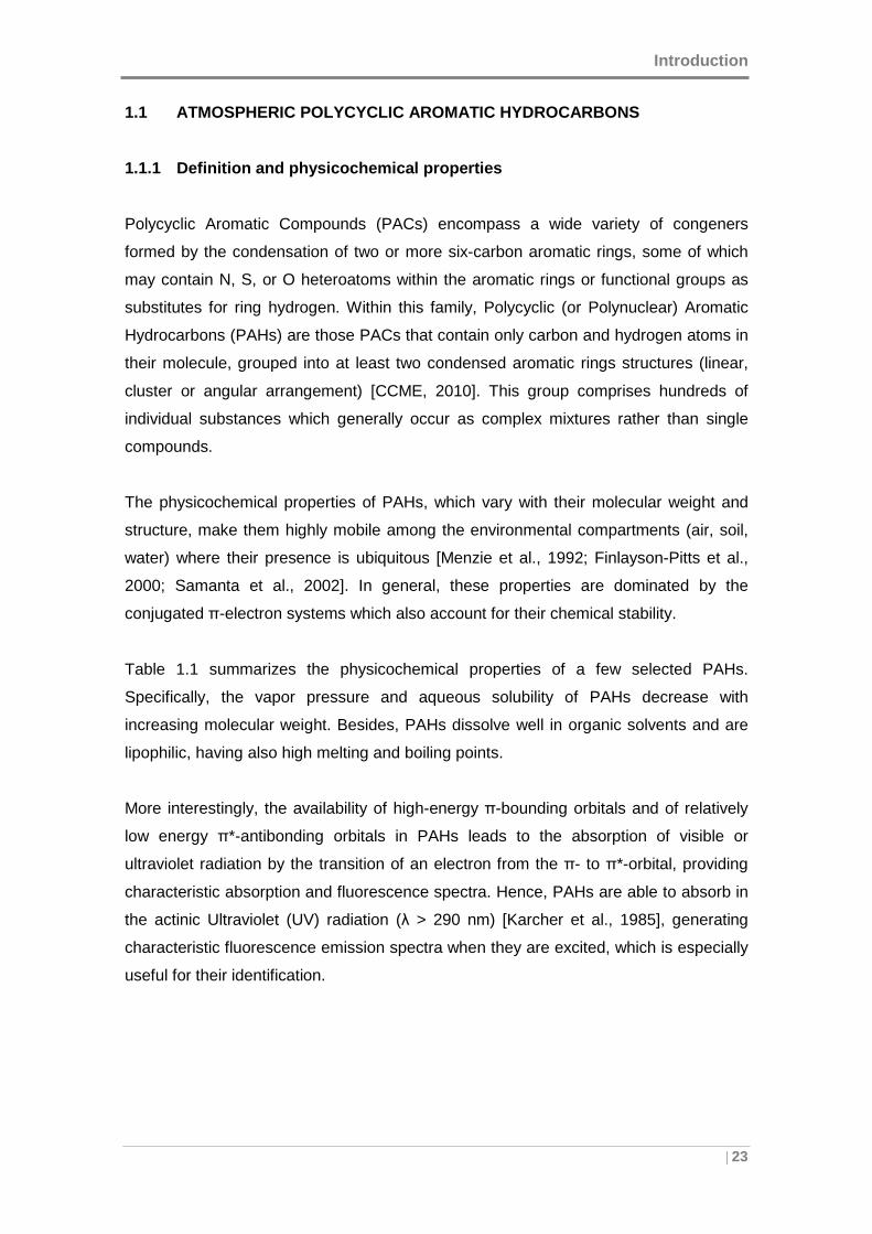
1.1.1 Definition and physicochemical properties

Polycyclic Aromatic Compounds (PACs) encompass a wide variety of congeners

formed by the condensation of two or more six-carbon aromatic rings, some of which

may contain N, S, or O heteroatoms within the aromatic rings or functional groups as

substitutes for ring hydrogen. Within this family, Polycyclic (or Polynuclear) Aromatic

Hydrocarbons (PAHs) are those PACs that contain only carbon and hydrogen atoms in

their molecule, grouped into at least two condensed aromatic rings structures (linear,

cluster or angular arrangement) [CCME, 2010]. This group comprises hundreds of

individual substances which generally occur as complex mixtures rather than single

compounds.

The physicochemical properties of PAHs, which vary with their molecular weight and

structure, make them highly mobile among the environmental compartments (air, soil,

water) where their presence is ubiquitous [Menzie et al., 1992; Finlayson-Pitts et al.,

2000; Samanta et al., 2002]. In general, these properties are dominated by the

conjugated π-electron systems which also account for their chemical stability.

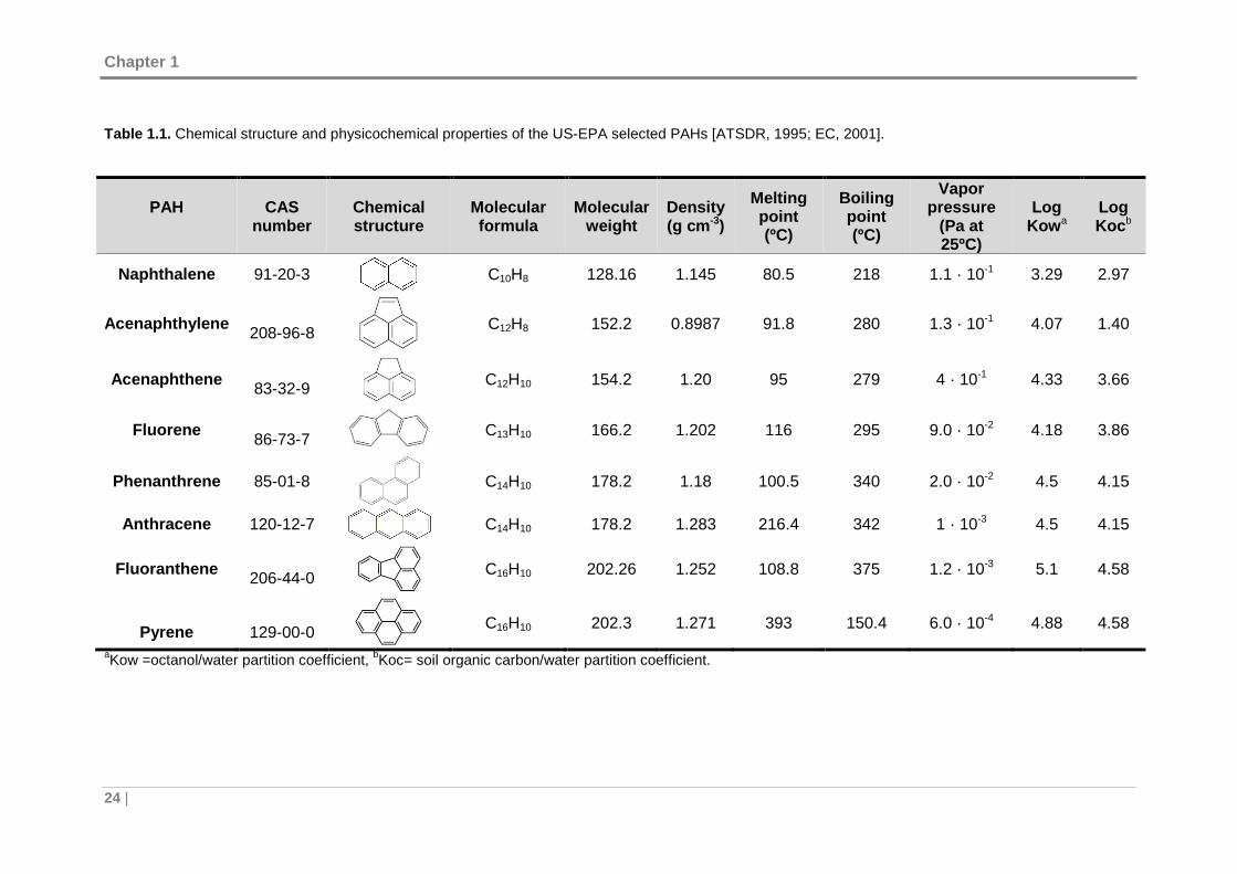
Table 1.1 summarizes the physicochemical properties of a few selected PAHs.

Specifically, the vapor pressure and aqueous solubility of PAHs decrease with

increasing molecular weight. Besides, PAHs dissolve well in organic solvents and are

lipophilic, having also high melting and boiling points.

More interestingly, the availability of high-energy π-bounding orbitals and of relatively

low energy π*-antibonding orbitals in PAHs leads to the absorption of visible or

ultraviolet radiation by the transition of an electron from the π- to π*-orbital, providing

characteristic absorption and fluorescence spectra. Hence, PAHs are able to absorb in

the actinic Ultraviolet (UV) radiation (λ > 290 nm) [Karcher et al., 1985], generating

characteristic fluorescence emission spectra when they are excited, which is especially

useful for their identification.

Chapter 1

24 |

Table 1.1. Chemical structure and physicochemical properties of the US-EPA selected PAHs [ATSDR, 1995; EC, 2001].

PAH

CAS number

Chemical structure

Molecular formula

Molecular weight

Density (g cm -3)

Melting point (ºC)

Boiling point (ºC)

Vapor pressure

(Pa at 25ºC)

Log Kow a

Log Koc b

Naphthalene 91-20-3

C10H8 128.16 1.145 80.5 218 1.1 · 10-1 3.29 2.97

Acenaphthylene 208-96-8

C12H8 152.2 0.8987 91.8 280 1.3 · 10-1 4.07 1.40

Acenaphthene 83-32-9

C12H10 154.2 1.20 95 279 4 · 10-1 4.33 3.66

Fluorene 86-73-7

C13H10 166.2 1.202 116 295 9.0 · 10-2 4.18 3.86

Phenanthrene 85-01-8

C14H10 178.2 1.18 100.5 340 2.0 · 10-2 4.5 4.15

Anthracene 120-12-7

C14H10 178.2 1.283 216.4 342 1 · 10-3 4.5 4.15

Fluoranthene 206-44-0

C16H10 202.26 1.252 108.8 375 1.2 · 10-3 5.1 4.58

Pyrene

129-00-0

C16H10 202.3 1.271 393 150.4 6.0 · 10-4 4.88 4.58

aKow =octanol/water partition coefficient, bKoc= soil organic carbon/water partition coefficient.

Introduction

| 25

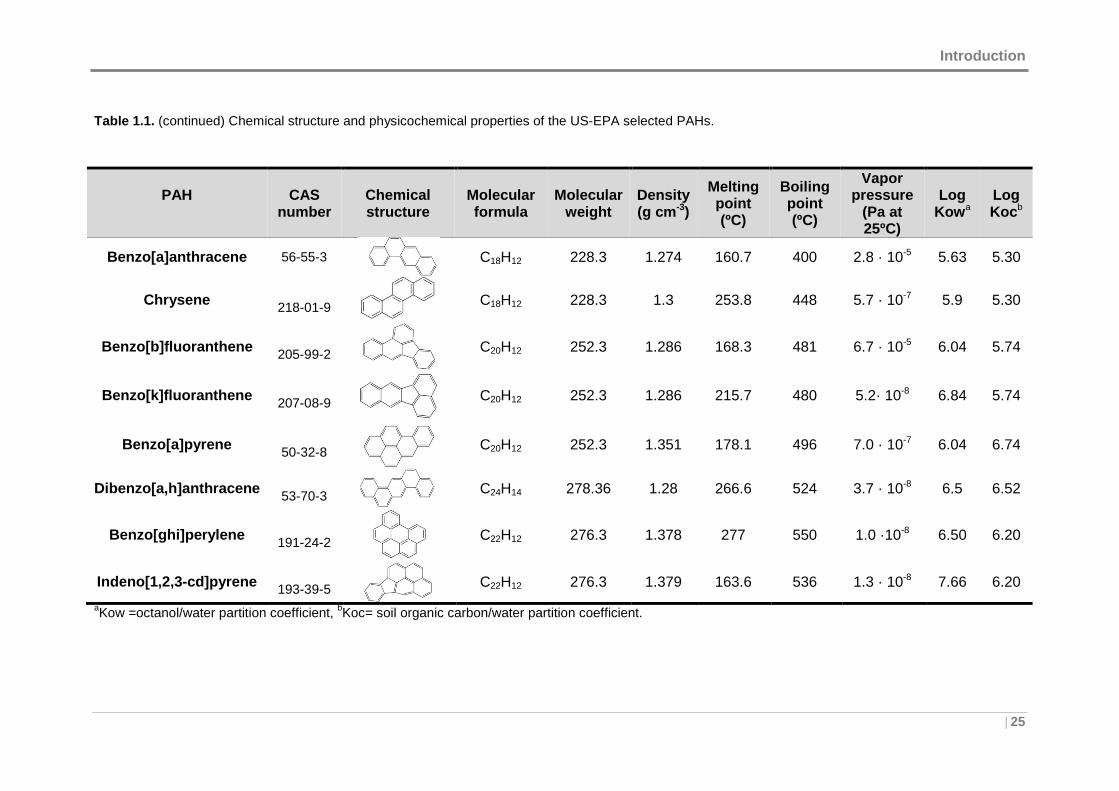
Table 1.1. (continued) Chemical structure and physicochemical properties of the US-EPA selected PAHs.

PAH

CAS number

Chemical structure

Molecular formula

Molecular weight

Density (g cm -3)

Melting point (ºC)

Boiling point (ºC)

Vapor pressure

(Pa at 25ºC)

Log Kow a

Log Koc b

Benzo[a]anthracene 56-55-3

C18H12 228.3 1.274 160.7 400 2.8 · 10-5 5.63 5.30

Chrysene 218-01-9

C18H12 228.3 1.3 253.8 448 5.7 · 10-7 5.9 5.30

Benzo[b]fluoranthene 205-99-2

C20H12 252.3 1.286 168.3 481 6.7 · 10-5 6.04 5.74

Benzo[k]fluoranthene 207-08-9

C20H12 252.3 1.286 215.7 480

5.2· 10-8

6.84 5.74

Benzo[a]pyrene 50-32-8

C20H12 252.3 1.351 178.1 496 7.0 · 10-7 6.04 6.74

Dibenzo[a,h]anthracene 53-70-3

C24H14 278.36 1.28 266.6 524 3.7 · 10-8 6.5 6.52

Benzo[ghi]perylene 191-24-2

C22H12 276.3 1.378 277 550 1.0 ·10-8 6.50 6.20

Indeno[1,2,3-cd]pyrene 193-39-5

C22H12 276.3 1.379 163.6 536 1.3 · 10-8 7.66 6.20

aKow =octanol/water partition coefficient, bKoc= soil organic carbon/water partition coefficient.

Chapter 1

26 |

1.1.2 Origin and sources

PAHs are released to the atmosphere as by-products from all incomplete combustion

processes of organic material. In nature, PAHs may be formed in three ways: (a) high

temperature (500 to 800ºC) thermal decomposition (pyrolysis) and subsequent

recombination (pyrosynthesis) of organic molecules [Haynes, 1991], (b) low to

moderate (100 to 300ºC) temperature diagenesis of sedimentary organic material to

form fossil fuel, and (c) direct biosynthesis by microorganisms and plants [Neff, 1979].

Comparatively, pyrosynthesis and pyrolysis are the main contribution mechanisms in

which the amount and range of produced PAHs vary widely according to the type of

fuel and the combustion conditions (temperature, turbulence, residence time, and

oxygen availability) [Westerholm et al., 1988].

PAHs have a widespread occurrence largely due to their production by virtually all

types of combustion sources of organic substances. But in general, they can be

grouped in five major emission source types: domestic, mobile, industrial, agricultural,

and natural [EC, 2001].

In Europe, 27 Member States report emissions data for benzo[a]pyrene (BaP),

benzo[b]fluoranthene (BbF), benzo[k]fluoranthene (BkF) and indeno[1,2,3-cd]pyrene

(IcdP) (total PAHs is expressed as the sum of these 4 PAHs), compiled in the annual

European Union emission inventory report under the UNECE Convention on Long-

range Transboundary Air Pollution [EEA, 2013a]. Other countries (the USA and UK)

and regions (the former USSR and North America) have also developed PAHs

emission inventories, which show that the global PAHs emissions are dominated by

anthropogenic activities (>90%), in which combustion is the major contributor

[Rehwagen et al., 2005]. In particular, residential heating, coke and aluminum

production and power generation as stationary sources, and mobile sources comprise

most of the anthropogenic atmospheric emission sources of PAHs [Baek et al., 1991b;

Zhang and Tao, 2009]. Forest fires and volcanic eruptions also contribute to the natural

budget of the PAHs inventory, but in a minor range (<1%) [Zhang and Tao, 2009].

Recent data on PAHs emissions in Europe evidenced a significantly reduction of 58%

from 1990 (2596 tonnes) to 2011 (1098 tonnes). The highest relative reduction in

emissions (between 1990 and 2011) was achieved in the aluminum production

category (– 81.6 %), mainly due to technological changes. Accordingly, individual

Introduction

| 27

PAHs emissions for BaP, BbF, BkF and IcdP, decreased by 45%, 25%, 19% and 14%,

respectively.

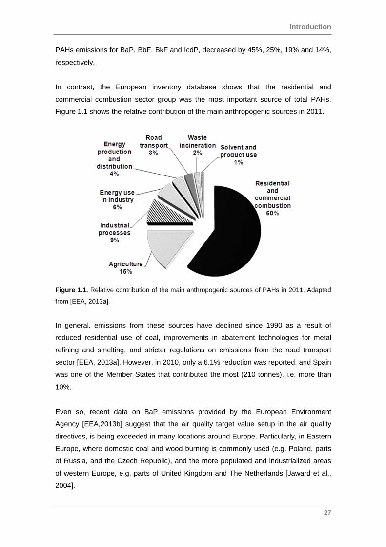
In contrast, the European inventory database shows that the residential and

commercial combustion sector group was the most important source of total PAHs.

Figure 1.1 shows the relative contribution of the main anthropogenic sources in 2011.

Figure 1.1. Relative contribution of the main anthropogenic sources of PAHs in 2011. Adapted

from [EEA, 2013a].

In general, emissions from these sources have declined since 1990 as a result of

reduced residential use of coal, improvements in abatement technologies for metal

refining and smelting, and stricter regulations on emissions from the road transport

sector [EEA, 2013a]. However, in 2010, only a 6.1% reduction was reported, and Spain

was one of the Member States that contributed the most (210 tonnes), i.e. more than

10%.

Even so, recent data on BaP emissions provided by the European Environment

Agency [EEA,2013b] suggest that the air quality target value setup in the air quality

directives, is being exceeded in many locations around Europe. Particularly, in Eastern

Europe, where domestic coal and wood burning is commonly used (e.g. Poland, parts

of Russia, and the Czech Republic), and the more populated and industrialized areas

of western Europe, e.g. parts of United Kingdom and The Netherlands [Jaward et al.,

2004].

Chapter 1

28 |

More specifically, it is likely that the overall annual average BaP target value will be met

in some countries, but it seems more challenging in urban areas and/or near emission

sources. In fact, although it has been estimated that stationary sources contribute

approximately 90% of total PAH emissions, in urban and suburban areas the mobile

sources (motor vehicle exhausts) are prevailing [Baek et al., 1991a; Jamhari et al.,

2014], with some minor contribution from combustion processes, petrogenic sources

and the resuspension of road dust [Omar et al., 2006, 2007].

1.1.3 Fate and transformations in the atmosphere

After emission to the atmosphere, PAHs are ubiquitously distributed and partitioned

between the gaseous and the particulate phase. This distribution varies with the

properties of the individual PAH (e.g. vapor pressure), meteorological conditions

(temperature, solar radiation, relative humidity, wind speed and direction), and the

nature of the aerosol (size distribution, concentrations of PAHs, chemical composition,

carbon content, etc.) [Ravindra et al., 2008a; Kim et al., 2013].

Generally, ambient temperature, solar radiation, and ozone show opposite trends

compared to particulate PAHs [Amodio et al., 2009]. In contrast, there is usually a

positive correlation between relative humidity and total PAHs concentration, due to a

depositional effect on the particulate matter of PAHs in the gas phase, as a

consequence of environmental humidity [Mastral et al., 2003]. Additionally, strong

winds tend to disperse particulate PAHs and reduce their concentration levels [Sikalos

et al., 2002], whereas wind direction provides information on long-distance transport,

being an important mechanism to explain PAHs levels. Hence, partitioning of PAHs

between gas/particulate phases plays an important role, which determines their

physical and chemical fates in the atmosphere (dry and wet deposition, chemical

reactivity, lifetime) [Zhu et al., 2009; Delgado-Saborit et al., 2010], transport and

transformation through the environment, and their toxicological effects [Kaupp and

McLachlan, 1999; Offenberg and Baker, 2002; Poor et al., 2004].

Low-molecular weight PAHs (two or three aromatic rings) are more volatile (low

temperatures of condensation), and are almost exclusively found in the gaseous phase

(>90%) [Kameda et al., 2011]. These hydrocarbons, included in the moderately/high

mobility categories, are able to undergo world-wide atmospheric dispersion (they

accumulate preferentially in polar latitudes). Although the lighter PAH compounds are

considered to be less toxic (section 1.1.4), they are able to react with other pollutants

Introduction

| 29

(such as ozone, nitrogen oxides, and sulfur dioxide) to form diones, nitro- and dinitro-

PAHs, and sulfonic acids, respectively, whose toxicity may be more significant [Baek et

al., 1991b].

Semi-volatile 4-ring PAHs are distributed between both phases and their gas to particle

partition coefficients are most susceptible to the influence of environmental factors.

They are deposited and accumulate mainly in mid latitudes.

Low-volatile PAHs with 5 or more aromatic rings (low vapor pressure) show

insignificant vaporization under all environmental conditions, and are primarily

adsorbed/absorbed onto the surfaces of fine respirable aerosol particles (aerodynamic

diameter ≤ 2.5 µm) [Baek et al., 1991a,b; Eiguren-Fernandez et al. 2004]. They are

classified in the low mobility category of persistent organic pollutants (POPs), subjected

to rapid deposition and retention close to the source. Since most carcinogenic PAHs (5

and 6 aromatic rings) (section 1.1.4) are mostly associated with particulate matter (PM)

(Table 1.2), many studies on PAHs in ambient air have been focused on PAHs bound

to PM, particularly PM10 and PM2.5 [Ohura et al. 2004; Villar-Vidal et al., 2014; Jamhari

et al., 2014].

In general, the concentration of PAHs in the gas phase increases with high summer

temperatures whereas during winter particulate phase PAHs dominate [Subramanyam

et al., 1994]. Even so, PAHs concentration shows little seasonality in areas where local

sources are mostly industrial, because the emissions are more uniform throughout the

year. In contrast, in most urban, residential and rural areas, where the local sources

are related to residential and commercial heating, seasonal variation in concentrations

of particle phase PAHs show similar trends (higher concentrations during winter

[Ravindra et al., 2008b; Amodio et al., 2009]). In fact, several studies carried out in

Europe and in the USA found that PAHs concentration was generally higher in winter

than in summer by a factor of 1.5 – 10 [Baek et al., 1991a; Harrison et al., 1996;

Eiguren-Fernandez et al., 2004].

In this context, several authors have reported that higher concentrations in winter are

most likely due to (a) reduced vertical dispersion due to lower thermal inversions; (b)

less intense atmospheric reactions; (c) enhanced sorption to particles at lower

temperatures (as a result of reduced vapor pressure and/or shifting in the gas/particle

distribution induced by ambient temperature variation [Subramanyam et al., 1994]); and

(d) increased emissions from domestic heating and power plants during winter with low

Chapter 1

30 |

temperatures [Lee et al., 2005]. In addition, some cities show diurnal and nocturnal

variations of PAH concentrations related to traffic emissions [Ringuet et al., 2012].

1.1.4 Priority PAHs and Legislation

PAHs are widely distributed in the atmosphere and are of environmental concern due

to their persistence and toxicity. One member of the PAHs family, benzo[a]pyrene, was

the first chemical compound and atmospheric pollutant identified as human

carcinogen [Boström et al., 2002; Chen and Liao, 2006], with also well-known

mutagenic properties [IARC, 1983; Lewtas, 1993]. Additionally, as mentioned above,

PAHs belong to the group of POPs, whose persistence increases with the ring number

and the condensation degree. Thus, due to their mobility, persistence, tendency to

bioaccumulation, and toxic effects on human health and ecosystems, PAHs were

included in the list of 16 POPs specified by the UNECE Convention on Long-Range

Transboundary Air Pollution Protocol on Persistent Organic Pollutants [UNECE, 1979;

Council Decision 2004/259/EC, 2004].

Because of these features, several international agencies have listed these

compounds as priority pollutants. Seventeen priority PAHs were chosen by the Agency

for Toxic Substances and Disease Registry [ATSDR, 1995] on the base of their

toxicological profile. Except for benzo[j]fluoranthene (BjF), the other 16 compounds

were also specified by the United States Environmental Protection Agency (US-EPA)

as priority pollutants [OFR, 1982]. In contrast, the World Health Organization adds 17

additional PAHs to make a total of 33 [WHO, 1998].

Table 1.2 indicates the toxicology classifications of the 16 US-EPA priority PAHs by

specific agencies. The carcinogenicity classification by the US-EPA Carcinogenicity

Risk Assessment Endeavor Work Group [US-EPA, 1994] shows that seven PAH

compounds are considered to be probable human carcinogens (Group B2): BaA, BaP,

BbF, BkF, Chr, DahA, and IcdP. In contrast, according to a public health statement by

the Agency for Toxic Substances and Disease Registry [ATSDR, 1995], the

International Agency for Research on Cancer (IARC) considers several PAHs to be

probable (Group 2A): BaA, BaP and DahA, possible (Group 2B): BbF, BjF, BkF, IcdP

human carcinogens, and not classifiable carcinogens (Group 3) [IARC, 1983; IARC

1987]. Among these ones, the most potent PAH carcinogens have been identified to be

benzo[a]anthracene, benzo[a]pyrene and dibenzo[a,h]anthracene [Armstrong et al.,

2004; CCME, 2010]. Nevertheless, benzo[a]pyrene is the only PAH for which

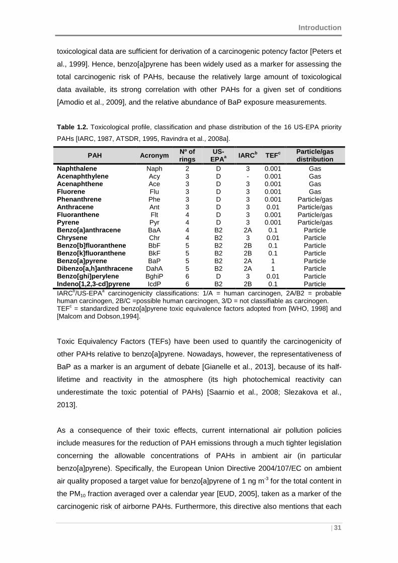
Introduction

| 31

toxicological data are sufficient for derivation of a carcinogenic potency factor [Peters et

al., 1999]. Hence, benzo[a]pyrene has been widely used as a marker for assessing the

total carcinogenic risk of PAHs, because the relatively large amount of toxicological

data available, its strong correlation with other PAHs for a given set of conditions

[Amodio et al., 2009], and the relative abundance of BaP exposure measurements.

Table 1.2. Toxicological profile, classification and phase distribution of the 16 US-EPA priority

PAHs [IARC, 1987, ATSDR, 1995, Ravindra et al., 2008a].

PAH Acronym Nº of rings

US-EPAa IARCb TEFc Particle/gas

distribution Naphthalene Naph 2 D 3 0.001 Gas Acenaphthylene Acy 3 D - 0.001 Gas Acenaphthene Ace 3 D 3 0.001 Gas Fluorene Flu 3 D 3 0.001 Gas Phenanthrene Phe 3 D 3 0.001 Particle/gas Anthracene Ant 3 D 3 0.01 Particle/gas Fluoranthene Flt 4 D 3 0.001 Particle/gas Pyrene Pyr 4 D 3 0.001 Particle/gas Benzo[a]anthracene BaA 4 B2 2A 0.1 Particle Chrysene Chr 4 B2 3 0.01 Particle Benzo[b]fluoranthene BbF 5 B2 2B 0.1 Particle Benzo[k]fluoranthene BkF 5 B2 2B 0.1 Particle Benzo[a]pyrene BaP 5 B2 2A 1 Particle Dibenzo[a,h]anthracene DahA 5 B2 2A 1 Particle Benzo[ghi]perylene BghiP 6 D 3 0.01 Particle Indeno[1,2,3 -cd]pyrene IcdP 6 B2 2B 0.1 Particle IARCb/US-EPAa carcinogenicity classifications: 1/A = human carcinogen, 2A/B2 = probable human carcinogen, 2B/C =possible human carcinogen, 3/D = not classifiable as carcinogen. TEFc = standardized benzo[a]pyrene toxic equivalence factors adopted from [WHO, 1998] and [Malcom and Dobson,1994].

Toxic Equivalency Factors (TEFs) have been used to quantify the carcinogenicity of

other PAHs relative to benzo[a]pyrene. Nowadays, however, the representativeness of

BaP as a marker is an argument of debate [Gianelle et al., 2013], because of its half-

lifetime and reactivity in the atmosphere (its high photochemical reactivity can

underestimate the toxic potential of PAHs) [Saarnio et al., 2008; Slezakova et al.,

2013].

As a consequence of their toxic effects, current international air pollution policies

include measures for the reduction of PAH emissions through a much tighter legislation

concerning the allowable concentrations of PAHs in ambient air (in particular

benzo[a]pyrene). Specifically, the European Union Directive 2004/107/EC on ambient

air quality proposed a target value for benzo[a]pyrene of 1 ng m-3 for the total content in

the PM10 fraction averaged over a calendar year [EUD, 2005], taken as a marker of the

carcinogenic risk of airborne PAHs. Furthermore, this directive also mentions that each

Chapter 1

32 |

member state shall monitor other relevant PAHs to assess the contribution of PAHs in

ambient air: BaA, BbF, BjF, BkF and IcdP and DahA; although no target values have

been set yet for these compounds. Other countries, like the United Kingdom, have

adopted even more strict air quality standards for BaP (annual mean of 0.25 ng m-3).

1.2 PAHs PRESENCE IN URBAN AREAS

1.2.1 Ambient air concentration levels

Several authors have reported high PAH concentrations in ambient air and in street

dust close to traffic sites in urban areas [Sitaras et al., 2004] probably due to the

increasing vehicular traffic and the scarce dispersion of the atmospheric pollutants.

Most of the studies state that the emissions from vehicle exhausts are the largest

contributors of PAHs in cities [Khalili et al., 1995; Miguel et al., 1998; Ravindra et al.,

2006]. Specifically, in urban and suburban areas, PAHs are present in the fine

particulate fraction (PM2.5) and within the solvent extractable fraction, in which the most

toxic PAHs (5 and 6-ring) can contribute to up to 80% of the total PAHs in the

particulate phase. This, coupled to the higher density of population in cities, makes the

risk associated with the human exposure to atmospheric PAHs higher in urban areas

[Sharma et al., 2007].

Hence, many works have been focused on the study of the concentration, distribution

and sources, to assess the health risk exposure to airborne PAHs in cities. However, a

mean PAHs concentration value cannot be considered as indicator of urban areas, as it

can be inferred from the significant variations depending on the location and period of

study reported in the literature (Table 1.3).

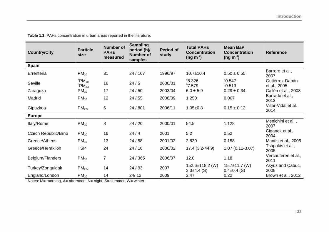
Introduction

| 33

Table 1.3. PAHs concentration in urban areas reported in the literature.

Country/City

Particle size

Number of PAHs measured

Sampling period (h)/ Number of samples

Period of study

Total PAHs Concentration (ng m -3)

Mean BaP Concentration (ng m -3)

Reference

Spain

Errenteria PM10 31 24 / 167 1996/97 10.7±10.4 0.50 ± 0.55 Barrero et al., 2007

Seville aPM10 bPM2.5

16 24 / 5 2000/01 a8.326 b7.579

a0.547 b0.513

Gutiérrez-Dabán et al., 2005

Zaragoza PM10 17 24 / 50 2003/04 6.0 ± 5.9 0.29 ± 0.34 Callén et al., 2008

Madrid PM10 12 24 / 55 2008/09 1.250 0.067 Barrado et al., 2013

Gipuzkoa PM2.5 6 24 / 801 2006/11 1.05±0.8 0.15 ± 0.12 Villar-Vidal et al.

2014 Europe

Italy/Rome PM10 8 24 / 20 2000/01 54.5 1.128 Menichini et al. , 2007

Czech Republic/Brno PM10 16 24 / 4 2001 5.2 0.52 Ciganek et al., 2004

Greece/Athens PM10 13 24 / 58 2001/02 2.839 0.158 Mantis et al., 2005

Greece/Heraklion TSP 24 24 / 16 2000/02 17.4 (3.2-44.9) 1.07 (0.11-3.07) Tsapakis et al., 2005

Belgium/Flanders PM10 7 24 / 365 2006/07 12.0 1.18 Vercauteren et al., 2011

Turkey/Zonguldak PM2.5 14 24 / 93 2007 152.6±118.2 (W) 3.3±4.4 (S)

15.7±11.7 (W) 0.4±0.4 (S)

Akyüz and Çabuc, 2008

England/London PM10 14 24/ 12 2009 2.47 0.22 Brown et al., 2012 Notes: M= morning, A= afternoon, N= night, S= summer, W= winter.

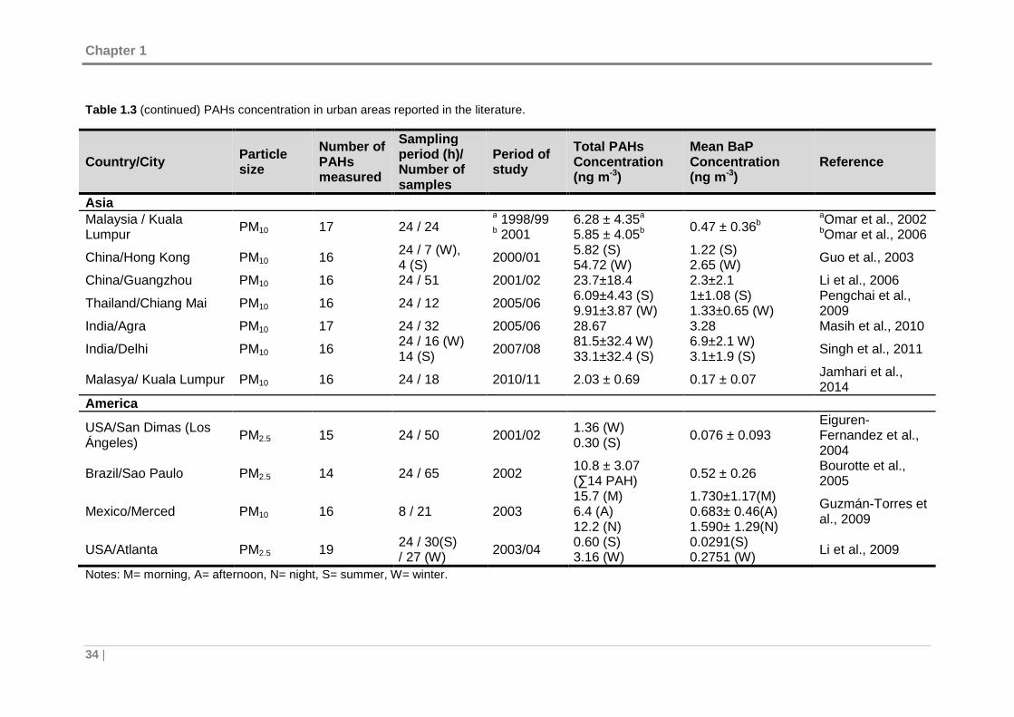
Chapter 1

34 |

Table 1.3 (continued) PAHs concentration in urban areas reported in the literature.

Country/City

Particle size

Number of PAHs measured

Sampling period (h)/ Number of samples

Period of study

Total PAHs Concentration (ng m -3)

Mean BaP Concentration (ng m -3)

Reference

Asia Malaysia / Kuala Lumpur PM10 17 24 / 24

a 1998/99 b 2001

6.28 ± 4.35a 5.85 ± 4.05b 0.47 ± 0.36b

aOmar et al., 2002

bOmar et al., 2006

China/Hong Kong PM10 16 24 / 7 (W), 4 (S) 2000/01 5.82 (S)

54.72 (W) 1.22 (S) 2.65 (W) Guo et al., 2003

China/Guangzhou PM10 16 24 / 51 2001/02 23.7±18.4 2.3±2.1 Li et al., 2006

Thailand/Chiang Mai PM10 16 24 / 12 2005/06 6.09±4.43 (S) 9.91±3.87 (W)

1±1.08 (S) 1.33±0.65 (W)

Pengchai et al., 2009

India/Agra PM10 17 24 / 32 2005/06 28.67 3.28 Masih et al., 2010

India/Delhi PM10 16 24 / 16 (W) 14 (S) 2007/08 81.5±32.4 W)

33.1±32.4 (S) 6.9±2.1 W) 3.1±1.9 (S) Singh et al., 2011

Malasya/ Kuala Lumpur PM10 16 24 / 18 2010/11 2.03 ± 0.69 0.17 ± 0.07 Jamhari et al., 2014

America

USA/San Dimas (Los Ángeles) PM2.5 15 24 / 50 2001/02 1.36 (W)

0.30 (S) 0.076 ± 0.093 Eiguren-Fernandez et al., 2004

Brazil/Sao Paulo PM2.5 14 24 / 65 2002 10.8 ± 3.07 (∑14 PAH) 0.52 ± 0.26 Bourotte et al.,

2005

Mexico/Merced PM10 16 8 / 21 2003 15.7 (M) 6.4 (A) 12.2 (N)

1.730±1.17(M) 0.683± 0.46(A) 1.590± 1.29(N)

Guzmán-Torres et al., 2009

USA/Atlanta PM2.5 19 24 / 30(S) / 27 (W) 2003/04 0.60 (S)

3.16 (W) 0.0291(S) 0.2751 (W) Li et al., 2009

Notes: M= morning, A= afternoon, N= night, S= summer, W= winter.

Introduction

| 35

1.2.2 Source identification of PAHs

Specific PAHs have been suggested as markers for certain processes of PAHs

release, for which PAHs concentration profiles and ratios could be used as diagnostic

tools to identify PAH sources, classify samples by location and estimate the importance

of combustion and petroleum-derived PAHs [Kavouras et al., 1999; Yunker et al., 2002;

Ravindra et al., 2008a].

Chrysene and benzo[k]fluoranthene were reported to be indicators of coal combustion

[Ravindra et al., 2006, 2008a]. Higher levels of benzo[ghi]pyrene, coronene, and

phenanthrene were proposed for motor vehicle emissions [Ravindra et al., 2006].

Meanwhile, several authors have found that lighter PAHs (3-benzene ring PAHs and

naphthalene) are more related to Heavy Duty Vehicles (HDVs), whereas Light-Duty

Vehicles (LDVs) were the dominant sources of heavy PAHs (4- and 5- benzene ring

PAHs, such as benzo[a]pyrene and dibenzo[a,h]anthracene) [Miguel et al., 1998; Marr

et al., 1999]. Pyrene, fluoranthene, and phenanthrene show higher levels in emission

from incineration [Ravindra et al., 2006], and have been also found associated with salt

particles (from salting road during winter), which appear to adsorb volatile PAHs

emissions from motor vehicles [Harrison et al., 1996].

The more volatile PAHs (fluorene, fluoranthene, and pyrene) were reported to be

associated with oil combustion emissions, along with moderate levels of the higher

molecular weight compounds (benzo[b]fluoranthene and indeno[1,2,3-cd]pyrene)

[Harrison et al., 1996; Ravindra et al., 2006]. Specially, benzo[ghi]perylene has been

identified as a typical tracer of vehicular sources of PAHs [Harrison et al.,1996]. Yang

et al. (1998) also suggested marker PAHs for cement plants (acenaphthylene,

acenaphthene and anthracene), waste incineration (indeno[1,2,3-cd]pyrene and

chrysene), and industrial stacks (4- and 5-benzene ring PAHs).

Nonetheless, ratios of pairs of PAHs are more frequently used for source identification.

Table 1.4 lists the typical diagnostic ratios, taken from literature, attributed to specific

sources.

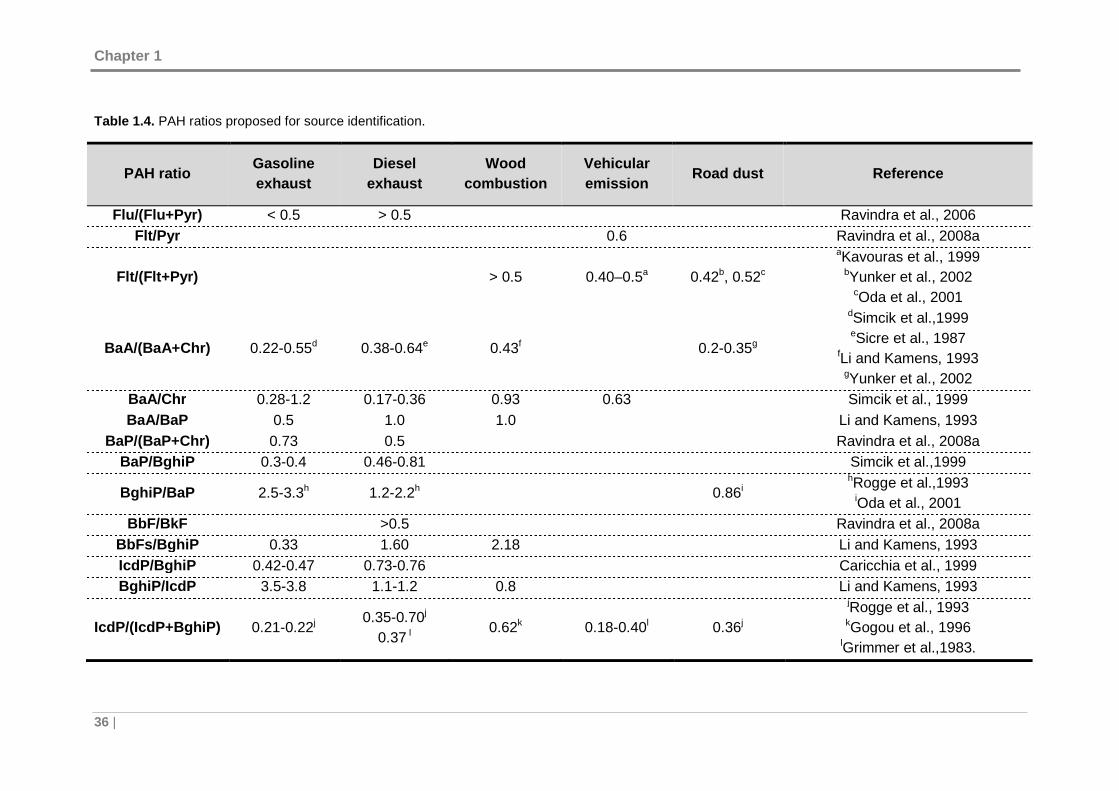
Chapter 1

36 |

Table 1.4. PAH ratios proposed for source identification.

PAH ratio

Gasoline exhaust

Diesel exhaust

Wood combustion

Vehicular emission

Road dust Reference

Flu/(Flu+Pyr) < 0.5 > 0.5 Ravindra et al., 2006 Flt/Pyr 0.6 Ravindra et al., 2008a

Flt/(Flt+Pyr) > 0.5

0.40–0.5a

0.42b, 0.52c

aKavouras et al., 1999 bYunker et al., 2002

cOda et al., 2001

BaA/(BaA+Chr) 0.22-0.55d 0.38-0.64e 0.43f 0.2-0.35g

dSimcik et al.,1999 eSicre et al., 1987

fLi and Kamens, 1993 gYunker et al., 2002

BaA/Chr 0.28-1.2 0.17-0.36 0.93 0.63 Simcik et al., 1999 BaA/BaP 0.5 1.0 1.0 Li and Kamens, 1993

BaP/(BaP+Chr ) 0.73 0.5 Ravindra et al., 2008a BaP/BghiP 0.3-0.4 0.46-0.81 Simcik et al.,1999

BghiP/BaP 2.5-3.3h 1.2-2.2h 0.86i hRogge et al.,1993

iOda et al., 2001 BbF/BkF >0.5 Ravindra et al., 2008a

BbFs/BghiP 0.33 1.60 2.18 Li and Kamens, 1993 IcdP/BghiP 0.42-0.47 0.73-0.76 Caricchia et al., 1999 BghiP/IcdP 3.5-3.8 1.1-1.2 0.8 Li and Kamens, 1993

IcdP/(IcdP+BghiP) 0.21-0.22j 0.35-0.70j

0.37 l 0.62k 0.18-0.40l 0.36j

jRogge et al., 1993 kGogou et al., 1996

lGrimmer et al.,1983.

Introduction

| 37

Nevertheless, these diagnostic ratios should be used with caution because the

reactivity of some PAHs species with other atmospheric pollutants, such as ozone

and/or oxides of nitrogen, can modify the value of the diagnostic ratio [Robinson et al.,

2006 a,b]. In fact, it is assumed that paired chemicals are diluted to a similar extent and

that the ratios remain constant in route from sources to the downwind point of

measurement. But the difference in chemical reactivity, volatility and solubility of PAH

species can modify the atmospheric PAHs levels and thus the ratios between PAHs.

Herein it is argued that these assumptions only hold for PAHs under a limited set of

conditions [Galarneau, 2008]. For instance, the ratios of the principal parent PAHs with

mass 178 (Phe and Ant), 202 (Flt and Pyr), 228 (BaA and Chr) and 276 (IcdP and

BghiP) have been widely used to distinguish different origins in urban and rural areas

[Cotham and Bidleman, 1995; Ding et al., 2007]. But, as discussed above, the

atmospheric degradation of Ant and BaA is much faster than that of their isomers

[Kamens et al., 1998]. As a consequence, the ratios of Ant/Phe and BaA/Chr will

change with the aging of the air mass [Ding et al., 2007]. In contrast, the Flt/Pyr and

IcdP/BghiP isomer pairs, photolytically degrade at comparable rates [Behymer and

Hites, 1988; Ding et al., 2007]. In this case, their ratios preserve the original

compositional information during atmospheric transport. Therefore, diagnostic ratios of

PAHs with similar physicochemical properties should be used to minimize this error

[Goriaux et al., 2006, Ravindra et al., 2008a].

Studies reported in Table 1.4 also indicate that it is further possible to differentiate the

traffic emissions from gasoline or diesel exhausts in urban areas. However, due to the

large variability in reported isomer ratios it is questionable that any single ratio or profile

selected from the literature will be representative of a source under different conditions

[Galarneau, 2008]. Thus, source identification can be improved using various other

ratios proposed in Table 1.4 and performing their relative comparison.

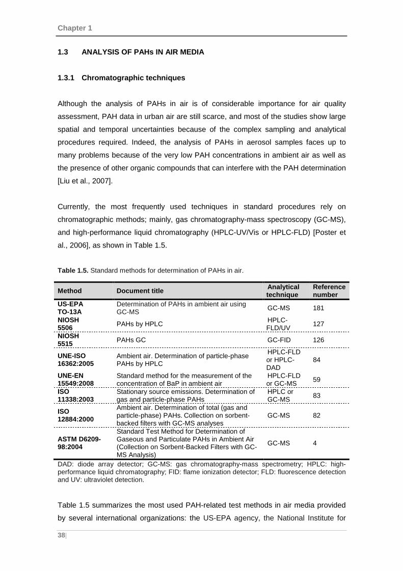
Chapter 1

38|

1.3 ANALYSIS OF PAHs IN AIR MEDIA

1.3.1 Chromatographic techniques

Although the analysis of PAHs in air is of considerable importance for air quality

assessment, PAH data in urban air are still scarce, and most of the studies show large

spatial and temporal uncertainties because of the complex sampling and analytical

procedures required. Indeed, the analysis of PAHs in aerosol samples faces up to

many problems because of the very low PAH concentrations in ambient air as well as

the presence of other organic compounds that can interfere with the PAH determination

[Liu et al., 2007].

Currently, the most frequently used techniques in standard procedures rely on

chromatographic methods; mainly, gas chromatography-mass spectroscopy (GC-MS),

and high-performance liquid chromatography (HPLC-UV/Vis or HPLC-FLD) [Poster et

al., 2006], as shown in Table 1.5.

Table 1.5. Standard methods for determination of PAHs in air.

DAD: diode array detector; GC-MS: gas chromatography-mass spectrometry; HPLC: high-performance liquid chromatography; FID: flame ionization detector; FLD: fluorescence detection and UV: ultraviolet detection.

Table 1.5 summarizes the most used PAH-related test methods in air media provided

by several international organizations: the US-EPA agency, the National Institute for

Method Document title Analytical technique

Reference number

US-EPA TO-13A

Determination of PAHs in ambient air using GC-MS

GC-MS 181

NIOSH 5506 PAHs by HPLC

HPLC-FLD/UV

127

NIOSH 5515 PAHs GC GC-FID 126

UNE-ISO 16362:2005

Ambient air. Determination of particle-phase PAHs by HPLC

HPLC-FLD or HPLC-DAD

84

UNE-EN 15549:2008

Standard method for the measurement of the concentration of BaP in ambient air

HPLC-FLD or GC-MS

59

ISO 11338:2003

Stationary source emissions. Determination of gas and particle-phase PAHs

HPLC or GC-MS

83

ISO 12884:2000

Ambient air. Determination of total (gas and particle-phase) PAHs. Collection on sorbent-backed filters with GC-MS analyses

GC-MS 82

ASTM D6209-98:2004

Standard Test Method for Determination of Gaseous and Particulate PAHs in Ambient Air (Collection on Sorbent-Backed Filters with GC-MS Analysis)

GC-MS 4

Introduction

| 39

Occupational Safety and Health (NIOSH), the International Organization for

Standardization (ISO), the American Society for Testing and Materials (ASTM), and the

European Committee for Standardization (CEN), which develops the European

standards (ENs), now transposed into Spanish legislation as UNE standards.

Chromatographic methods for PAHs analyses have been developed and evaluated

extensively over the past few decades. Each technique, HPLC or GC, offers unique

information or has unique aspects. For example, GC-MS provides more accurate

results than HPLC–FLD for the determination of BghiP because of its inherently low

fluorescence sensitivity. In contrast, at low concentrations anthracene and perylene are

best measured by HPLC coupled with fluorescence detection (HPLC-FLD) because of

their selective and sensitive fluorescence-detection characteristics [Poster et al., 2006].

Additionally, GC-MS is often more accurate than GC-FID for the quantification of PAHs,

because interferences from co-eluting compounds are minimized by the selective

nature of the detector.

Hence, generally for the analysis of PAHs in air, gas chromatography is the most

common analytical separation mechanism, in combination with mass spectrometry.

However, this method usually requires a great number of sample preparation steps,

including matrix extraction and clean-up approaches, to increase its selectivity,

resolution, and sensitivity. As a consequence, these measurements tend to be

laborious, relatively expensive, and time-consuming, which also increases the

likelihood of sample contamination and losses during their handling and preparation.

Therefore, there is still a great interest in developing more sensitive and selective

methods to analyze PAHs in aerosol samples for which analytical methods not

requiring separation of mixture at all, or requiring only a partial fractionation of complex

mixtures, would be undoubtedly very advantageous. In this sense, there have been a

number of efforts to develop solvent-free analysis of PAHs. These methods, which

mostly are still in development, usually rely on the collection of the airborne PAHs on

filter materials for subsequent release by thermal desorption (TD-GC-MS) [Moltó et al.,

2009] and other approaches such as Laser-Desorption-Ionization Time-Of-Flight MS

(LDI-TOF-MS) [Pandey et al., 2011].

Alternatively, some methods based on modern fluorescence spectroscopy techniques

can also comply with these needs, since they are simple, sensitive, rapid and

nondestructive. They rely on the fact that fluorescence spectroscopy is a powerful tool

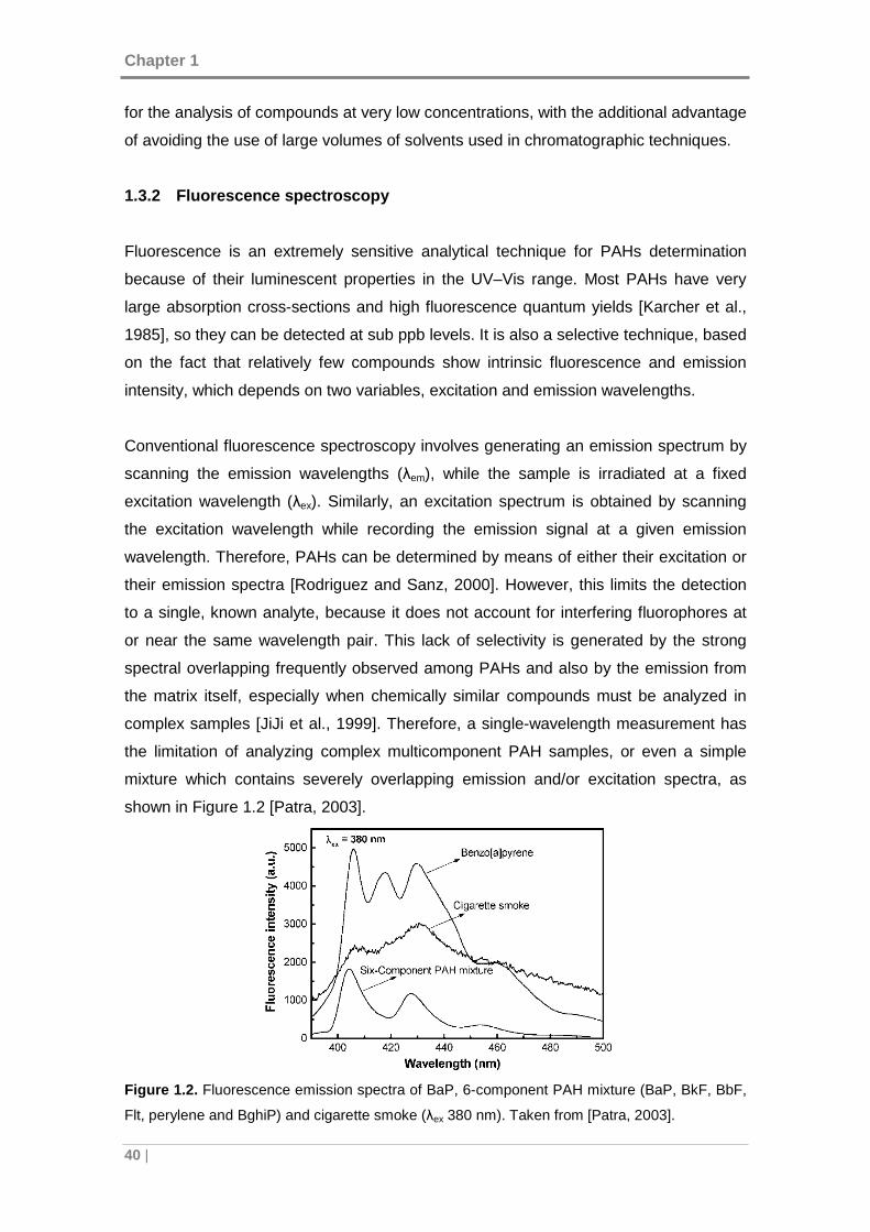
Chapter 1

40 |

for the analysis of compounds at very low concentrations, with the additional advantage

of avoiding the use of large volumes of solvents used in chromatographic techniques.

1.3.2 Fluorescence spectroscopy

Fluorescence is an extremely sensitive analytical technique for PAHs determination

because of their luminescent properties in the UV–Vis range. Most PAHs have very

large absorption cross-sections and high fluorescence quantum yields [Karcher et al.,

1985], so they can be detected at sub ppb levels. It is also a selective technique, based

on the fact that relatively few compounds show intrinsic fluorescence and emission

intensity, which depends on two variables, excitation and emission wavelengths.

Conventional fluorescence spectroscopy involves generating an emission spectrum by

scanning the emission wavelengths (λem), while the sample is irradiated at a fixed

excitation wavelength (λex). Similarly, an excitation spectrum is obtained by scanning

the excitation wavelength while recording the emission signal at a given emission

wavelength. Therefore, PAHs can be determined by means of either their excitation or

their emission spectra [Rodriguez and Sanz, 2000]. However, this limits the detection

to a single, known analyte, because it does not account for interfering fluorophores at

or near the same wavelength pair. This lack of selectivity is generated by the strong

spectral overlapping frequently observed among PAHs and also by the emission from

the matrix itself, especially when chemically similar compounds must be analyzed in

complex samples [JiJi et al., 1999]. Therefore, a single-wavelength measurement has

the limitation of analyzing complex multicomponent PAH samples, or even a simple

mixture which contains severely overlapping emission and/or excitation spectra, as

shown in Figure 1.2 [Patra, 2003].

Figure 1.2. Fluorescence emission spectra of BaP, 6-component PAH mixture (BaP, BkF, BbF,

Flt, perylene and BghiP) and cigarette smoke (λex 380 nm). Taken from [Patra, 2003].

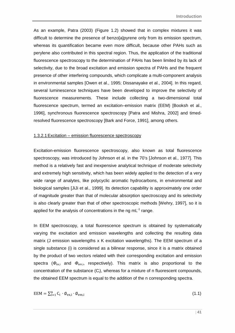
Introduction

| 41

As an example, Patra (2003) (Figure 1.2) showed that in complex mixtures it was

difficult to determine the presence of benzo[a]pyrene only from its emission spectrum,

whereas its quantification became even more difficult, because other PAHs such as

perylene also contributed in this spectral region. Thus, the application of the traditional

fluorescence spectroscopy to the determination of PAHs has been limited by its lack of

selectivity, due to the broad excitation and emission spectra of PAHs and the frequent

presence of other interfering compounds, which complicate a multi-component analysis

in environmental samples [Owen et al., 1995; Dissanayake et al., 2004]. In this regard,

several luminescence techniques have been developed to improve the selectivity of

fluorescence measurements. These include collecting a two-dimensional total

fluorescence spectrum, termed an excitation–emission matrix (EEM) [Booksh et al.,

1996], synchronous fluorescence spectroscopy [Patra and Mishra, 2002] and timed-

resolved fluorescence spectroscopy [Bark and Force, 1991], among others.

1.3.2.1 Excitation – emission fluorescence spectroscopy

Excitation-emission fluorescence spectroscopy, also known as total fluorescence

spectroscopy, was introduced by Johnson et al. in the 70’s [Johnson et al., 1977]. This

method is a relatively fast and inexpensive analytical technique of moderate selectivity

and extremely high sensitivity, which has been widely applied to the detection of a very

wide range of analytes, like polycyclic aromatic hydrocarbons, in environmental and

biological samples [JiJi et al., 1999]. Its detection capability is approximately one order

of magnitude greater than that of molecular absorption spectroscopy and its selectivity

is also clearly greater than that of other spectroscopic methods [Wehry, 1997], so it is

applied for the analysis of concentrations in the ng mL-1 range.

In EEM spectroscopy, a total fluorescence spectrum is obtained by systematically

varying the excitation and emission wavelengths and collecting the resulting data

matrix (J emission wavelengths x K excitation wavelengths). The EEM spectrum of a

single substance (i) is considered as a bilinear response, since it is a matrix obtained

by the product of two vectors related with their corresponding excitation and emission

spectra (Фex,i and Фem,i, respectively). This matrix is also proportional to the

concentration of the substance (Ci), whereas for a mixture of n fluorescent compounds,

the obtained EEM spectrum is equal to the addition of the n corresponding spectra.

EEM = ∑ C� ∙ ∅�,� �� ∙ ∅�,� (1.1)

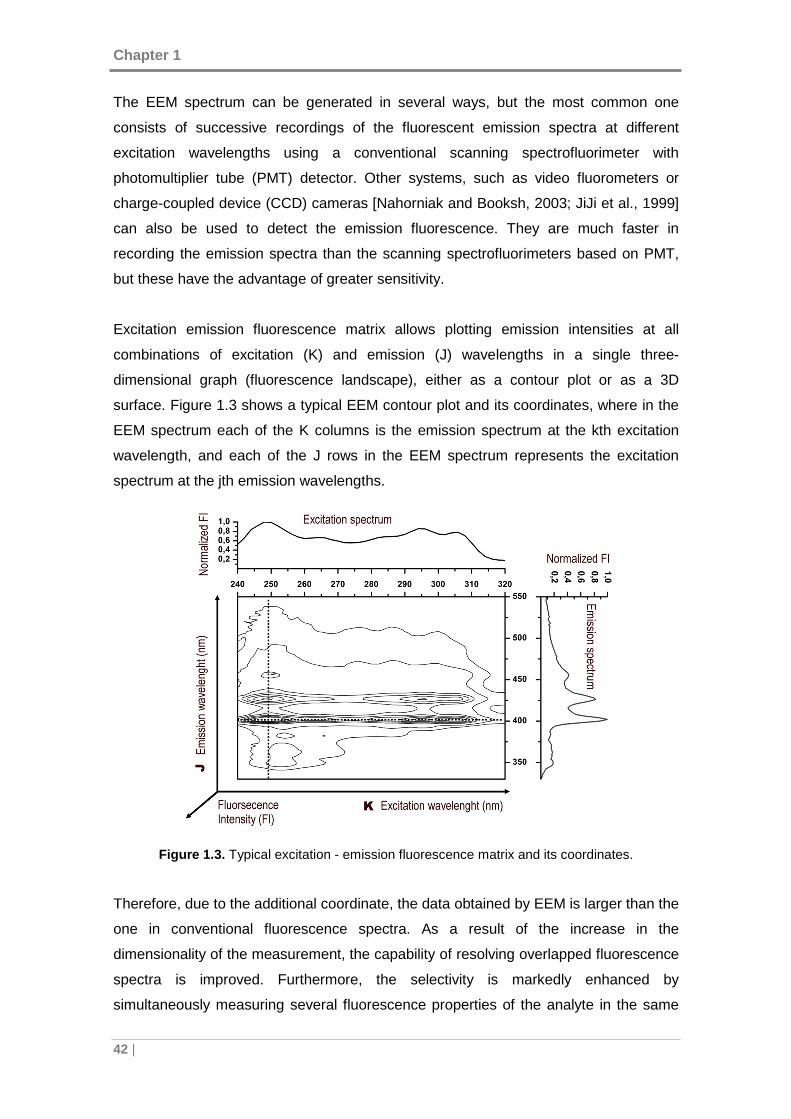
Chapter 1

42 |

The EEM spectrum can be generated in several ways, but the most common one

consists of successive recordings of the fluorescent emission spectra at different

excitation wavelengths using a conventional scanning spectrofluorimeter with

photomultiplier tube (PMT) detector. Other systems, such as video fluorometers or

charge-coupled device (CCD) cameras [Nahorniak and Booksh, 2003; JiJi et al., 1999]

can also be used to detect the emission fluorescence. They are much faster in

recording the emission spectra than the scanning spectrofluorimeters based on PMT,

but these have the advantage of greater sensitivity.

Excitation emission fluorescence matrix allows plotting emission intensities at all

combinations of excitation (K) and emission (J) wavelengths in a single three-

dimensional graph (fluorescence landscape), either as a contour plot or as a 3D

surface. Figure 1.3 shows a typical EEM contour plot and its coordinates, where in the

EEM spectrum each of the K columns is the emission spectrum at the kth excitation

wavelength, and each of the J rows in the EEM spectrum represents the excitation

spectrum at the jth emission wavelengths.

Figure 1.3. Typical excitation - emission fluorescence matrix and its coordinates.

Therefore, due to the additional coordinate, the data obtained by EEM is larger than the

one in conventional fluorescence spectra. As a result of the increase in the

dimensionality of the measurement, the capability of resolving overlapped fluorescence

spectra is improved. Furthermore, the selectivity is markedly enhanced by

simultaneously measuring several fluorescence properties of the analyte in the same

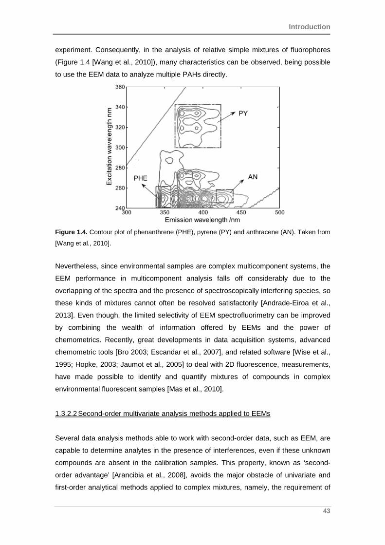
Introduction

| 43

experiment. Consequently, in the analysis of relative simple mixtures of fluorophores

(Figure 1.4 [Wang et al., 2010]), many characteristics can be observed, being possible

to use the EEM data to analyze multiple PAHs directly.

Figure 1.4. Contour plot of phenanthrene (PHE), pyrene (PY) and anthracene (AN). Taken from

[Wang et al., 2010].

Nevertheless, since environmental samples are complex multicomponent systems, the

EEM performance in multicomponent analysis falls off considerably due to the

overlapping of the spectra and the presence of spectroscopically interfering species, so

these kinds of mixtures cannot often be resolved satisfactorily [Andrade-Eiroa et al.,

2013]. Even though, the limited selectivity of EEM spectrofluorimetry can be improved

by combining the wealth of information offered by EEMs and the power of

chemometrics. Recently, great developments in data acquisition systems, advanced

chemometric tools [Bro 2003; Escandar et al., 2007], and related software [Wise et al.,

1995; Hopke, 2003; Jaumot et al., 2005] to deal with 2D fluorescence, measurements,

have made possible to identify and quantify mixtures of compounds in complex

environmental fluorescent samples [Mas et al., 2010].

1.3.2.2 Second-order multivariate analysis methods applied to EEMs

Several data analysis methods able to work with second-order data, such as EEM, are

capable to determine analytes in the presence of interferences, even if these unknown

compounds are absent in the calibration samples. This property, known as ‘second-

order advantage’ [Arancibia et al., 2008], avoids the major obstacle of univariate and

first-order analytical methods applied to complex mixtures, namely, the requirement of

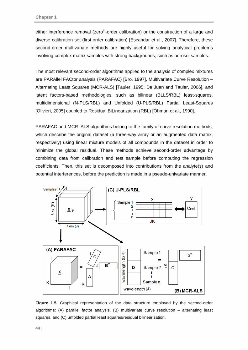
Chapter 1

44 |

either interference removal (zeroth-order calibration) or the construction of a large and

diverse calibration set (first-order calibration) [Escandar et al., 2007]. Therefore, these

second-order multivariate methods are highly useful for solving analytical problems

involving complex matrix samples with strong backgrounds, such as aerosol samples.

The most relevant second-order algorithms applied to the analysis of complex mixtures

are PARAllel FACtor analysis (PARAFAC) [Bro, 1997], Multivariate Curve Resolution –

Alternating Least Squares (MCR-ALS) [Tauler, 1995; De Juan and Tauler, 2006], and

latent factors-based methodologies, such as bilinear (BLLS/RBL) least-squares,

multidimensional (N-PLS/RBL) and Unfolded (U-PLS/RBL) Partial Least-Squares

[Olivieri, 2005] coupled to Residual BiLinearization (RBL) [Öhman et al., 1990].

PARAFAC and MCR–ALS algorithms belong to the family of curve resolution methods,

which describe the original dataset (a three-way array or an augmented data matrix,

respectively) using linear mixture models of all compounds in the dataset in order to

minimize the global residual. These methods achieve second-order advantage by

combining data from calibration and test sample before computing the regression

coefficients. Then, this set is decomposed into contributions from the analyte(s) and

potential interferences, before the prediction is made in a pseudo-univariate manner.

Figure 1.5. Graphical representation of the data structure employed by the second-order

algorithms: (A) parallel factor analysis, (B) multivariate curve resolution – alternating least

squares, and (C) unfolded partial least squares/residual bilinearization.

Introduction

| 45

The most commonly used second-order algorithm, PARAFAC (section 4.5.1), is an

iterative, least squares-type algorithm that allows the simultaneous extraction of

multiple pure spectral profiles from multi-way data, even in the presence of unknown,

uncalibrated interferences. PARAFAC has been extensively applied to the analysis of

EEMs based three-way arrays (dimension: samples x λem x λex) (Figure 1.5.A), mainly

due to the trilinear structure of the EEM dataset, which makes it compatible with

PARAFAC. Trilinear structure to the EEM dataset comes from the fact that the profiles

of the fluorophores in both orders of the data matrix (excitation and emission profiles)

for different samples are equal, except in its size that depends on the concentration of

the sample. Thus, given a number of factors (fluorescent species), PARAFAC yields a

trilinear decomposition of the data, in which matrix A accounts for pure normalized

excitation spectra, matrix B for the related normalized emission spectra, and matrix C

for the PARAFAC scores that contain relative concentration values of the compounds

in the different samples. This decomposition is often unique, one advantage against

bilinear models which suffer the known problem of rotational freedom.

Although PARAFAC has been considered as an ideal algorithm for modeling EEM

data, there are in fact a number of drawbacks for its application: (a) the resolution of

complex mixtures by iterative procedures is a lengthy task, (b) Rayleigh and Raman

scattering, which do not have a trilinear structure, must be removed from EEM data by

selecting a suitable wavelength range or modeled with a specific algorithm [Bahram et

al, 2006], and (c) this algorithm assumes no interactions between fluorophores and

thus, it cannot model interactions among solutes such as inner filter effect, quenching,

or dimer formation.

Hence, when there is no strict trilinearity in any of the orders, MCR-ALS (section 4.5.2)

is a useful alternative to PARAFAC, because it is more flexible with regards to

trilinearity. By default, MCR–ALS method relies on a bilinear model and it only requires

that one of the two dimensions (excitation or emission) matches between the different

data matrices. Additionally, the trilinear behavior can be introduced as an optional

constraint to the different compounds in the system. The fact that the implementation of

this constraint works in a ‘compound-wise’ way allows working on scenarios presenting

completely trilinear, partially trilinear or completely bilinear models, when all, some or

none of the compounds are constrained to obey a trilinear behavior, respectively. This

flexibility in the application of the trilinearity condition is helpful to minimize rotational

ambiguities, and to accommodate deviations from trilinearity of the experimental data

[Tauler et al., 2009]. Thus, MCR-ALS provides a basic bilinear decomposition of the

Chapter 1

46 |

matrix D (augmented data matrix) (Figure 1.5.B), in which ST contains normalized pure

emission spectra and the submatrices in C the excitation profiles related to each of the

samples. Integrating the areas under the excitation profiles in each of the samples,

relative concentration values, analogous to PARAFAC scores are obtained.

An alternative to working with second-order data is to rearrange the data into vectors

and apply a first-order algorithm, leading to Unfolded-Principal Component Regression

(U-PCR) and Unfolded-Partial Least Squares (U-PLS). These approaches were used

first to model EEM second-order data, before true second-order methods were

developed. Recent developments in PLS algorithms have led to their extension to data

of higher orders, giving rise up to N-PLS, the multidimensional variant of PLS

regression [Bro, 1996]. However, these methods do not have the second-order

advantage, because they build the calibration models using the set of training data

together with the nominal analyte concentrations (which are unavailable for a test

sample). If any of these models is then applied to a test sample having unexpected

components, the analyte quantification will not be accurate because the test sample

signals will give a poor fit to the calibration model. The second-order advantage is

achieved only when the above mentioned algorithms are coupled to an adequate post-

calibration procedure, known as residual bilinearization (RBL) [Öhman et al., 1990],

which is able to model the contribution of the potential interferences. U-PLS/RBL

(section 4.5.3) is therefore a promising method, enjoying all the capabilities of latent

factors methodologies, while preserving the important second-order advantage. It is

interesting to note that the combination of N-PLS/RBL has been also suggested in this

regard [Linder and Sundberg, 2002], although the pertinent algorithms have not yet

been developed.

In contrast to PARAFAC or MCR-ALS, U-PLS/RBL is a calibration method, therefore,

no decomposition is obtained; instead, matrices X (containing vectorized EEM data

matrices) and Y (containing concentration of analytes) from calibration samples are

related through a PLS model (Figure 1.5.C), and the model obtained is used to predict

new concentration values for unknown samples from the related EEM matrices.

Whenever unexpected interferences are found in new samples that were not present in

the calibration set, the additional RBL step has to be used for accurate prediction of the

analytes. Additionally, thanks to its flexible structure, U-PLS/RBL algorithm can handle

signal-to-concentration changes among samples such as inner filter effect, which are

compensated by adding more latent variables to the model, as long as they are

represented in the calibration set and they are not too extreme. Even though U-

Introduction

| 47

PLS/RBL is more flexible, its flexibility implies also non-unique solutions, due to the

presence of rotation ambiguities in the RBL step.

In the recent years, the applicability of these second-order multivariate methods has

been increasingly investigated for environmental monitoring, because of the inherent

complexity of environmental samples. Modern approaches based on fluorescence

excitation–emission matrices combined with advanced chemometric algorithms, allow

for a direct determination of PAHs without previous sample separation and

pretreatment by chromatographic means [Nahorniak and Booksh 2006], providing an

alternative for qualitative and quantitative PAH environmental monitoring [Jiji et al.,

2000]. PARAFAC seems to be the most frequently applied algorithm, although some

competitors are increasingly employed, particularly latent variable methodologies, such

as U-PLS/RBL.

Nahorniak and Booksh (2003) employed a field-portable EEM fluorometer in

conjunction with PARAFAC for sub-ppb PAHs determination in the presence of spectral

interferences, for which they studied the combination of data density optimization and

automation of PARAFAC model selection to lead to a simple and rapid multi-way data

analysis. Later, Nahorniak and Booksh (2006) used the optimized method to determine

sub-ppb concentrations of several PAHs (BkF and BaP) in various matrices, including

aqueous motor oil extract and asphalt leachate, where the rapid field EEM analyses

proved to be a good screening method for tracking pollutants and prioritizing further

sampling and analysis.

The application of photocatalytic degradation EEMs in combination with PARAFAC was

proposed to determine BaA, BkF and DahA in synthetic water samples. Three and

four-way PARAFAC analyses were employed to extract the fluorescent species spectra

from overlapping EEMs [Kim et al., 2005], where the additional time profiles yield an

additional dimension that increased the selectivity for each PAH determination.

Bosco et al. (2006) applied PARAFAC to EEMs, with the aim at determining DahA,

BaA, BaP and BkF throughout the degradation process in the aqueous medium,

showing to be a good alternative to the habitual methods of analysis in

photodegradation processes. Later, Bosco and Larrechi (2007) applied MCR-ALS and

PARAFAC to obtain semi-quantitative information related to the photodegradation

processes of PAHs, by using three-dimensional EEMs. The results obtained showed

Chapter 1

48 |

no statistical differences with data obtained using an HPLC reference methodology and

suggested the EEM approach as a time saving and more ecological alternative.

EEM coupled with multivariate algorithms has also been proposed as an alternative

method for the characterization and quantification of PAHs in water samples [Beltrán et

al., 1998]. PARAFAC was compared with other multivariate calibration techniques such

as PLS1, PLS2, three-way PLS1, and three-way PLS2 to quantify 10 PAHs from the

EEM spectra of a set of standards in samples of tap and mineral waters. In most cases,

the best results were obtained by the application of three-way PLS2, due to the use of

both spectra and concentration of the standards to build the calibration model, whereas

in PARAFAC calibration, only the spectra are adjusted.

Similarly, PARAFAC showed to have a prediction performance worse than U-PLS/RBL

in the simultaneous ultra-trace determination of BaP and DahA in presence of the

remaining fourteen US-EPA PAHs [Bortolato et al., 2008]. The approach consisted of

measuring EEMs on a nylon-membrane surface, combining the ability of this

membrane to retain and concentrate PAHs on its surface, the sensitivity of molecular

fluorescence, and the selectivity of second-order chemometric algorithms: PARAFAC

and U-PLS/RBL. The superiority of U-PLS/RBL to quantify BaP and DahA at

concentrations below 10 ng L−1 in tap, underground, mineral and river water samples

was demonstrated.

Recently, Alarcón et al. (2013) assessed the possibility of simultaneous determination

of 7 PAHs in extra virgin olive and sunflower oils, using U-PLS/RBL and PARAFAC.

Again, U-PLS/RBL algorithm exhibited the best performance for resolving the PAH

mixture in the presence of both highly complex oil matrix and other unpredicted PAHs.

Moreover, the predicted U-PLS/RBL concentrations were satisfactorily compared with

those obtained using HPLC with fluorescence detection, suggesting the EEM approach

as a time saving and simpler alternative.

Additionally, U-PLS/RBL has proved to be a successful method to deal with EEMs

showing inner filter effects [Bohoyo et al., 2006]. Comparisons of the prediction results

obtained from PARAFAC and MCR-ALS showed that U-PLS/RBL achieved

significantly better recoveries, even though MCR-ALS seemed to give better results

than PARAFAC.

Introduction

| 49

Nevertheless, to our knowledge, the use of EEMs coupled to second-order calibration

algorithms has not yet been evaluated to carry out a qualitative and quantitative

analysis of multiple PAHs in extracts of aerosol samples, a much more complex type of

chemical sample from an analytical and compositional point of view.

CHAPTER 2

OBJECTIVES AND

APPROACH

Objectives and approach

| 53

2.1 APPROACH

Air pollution is a major environmental problem in urban areas and also an important

issue for public health and global climate. In particular, ambient air Particulate Matter

(PM) represents a complex mixture of substances linked to increased morbidity and

mortality rates [WHO, 2003]. One group of chemical compounds associated with PM

are the polycyclic aromatic hydrocarbons (PAHs), which can contribute to, or even

enhance, the PM adverse health effects due to their well-known carcinogenic and

mutagenic properties. The occurrence of PAHs in ambient air is an increasing

environmental concern due to their persistence and toxicity. These adverse properties

demand an assessment of their concentration, trends and profiles in the ambient air

and in known emission sources, to provide the basis for source apportionment and air

pollution control strategies.

Specifically, in urban and suburban areas the most toxic PAHs (5- and 6- rings PAHs)

are linked to the respirable fraction of particulate matter (aerodynamic diameter ≤2.5

µm), where their emissions are mainly attributed to vehicle exhausts. Considering the

population density, the overall risk associated with human exposure to atmospheric

PAHs is higher in urban environments. For these reasons, 9 particle-bound of the US-

EPA priority list: Flt, BaA, Chr, BbF, BkF, BaP, DahA, BghiP and IcdP, were selected

as target analytes according to their higher toxic potential [IARC, 1987]. Additionally,

the sampling site was located in one of the main access to the urban area of Bilbao,

influenced by traffic emissions.

Monitoring of pollutants, especially PAHs concentrations in air is, arguably, one of the

most difficult tasks in environmental chemistry. The large variability and uncertainty in

spatial and temporal trends, together with their complex sampling and analytical

procedures, promotes that the data available for urban areas is scarce. Indeed, the

very low PAH concentrations in ambient air in addition to the presence of other

interfering organic compounds may hamper a proper analysis.

The currently used techniques in standard procedures (mainly chromatographic

methods) tend to be laborious, relatively expensive, and time-consuming, because they

require a great pretreatment of the samples in order to increase the sensitivity and

selectivity of the PAH analysis. Therefore, the development of alternative sensitive and

selective methods for determining PAHs in aerosol samples is still of great interest for

routine analysis in environmental monitoring and health protection.

Chapter 2

54|

Fluorescence spectroscopy is a non-destructive and sensitive analytical technique for

PAH determination, which can be detected at ppb levels because of their intrinsic

fluorescence properties in the UV–Vis spectral range. Nonetheless, the lack of

selectivity in classical fluorescence spectroscopy, due to the high overlapping between

the PAHs spectra, hinders its direct usage for multi-component analysis in

environmental samples.

In this regard, continuous developments and improvements in data acquisition

systems, advanced chemometric tools, and related software to deal with EEM

fluorescence measurements, have enabled the identification and quantification of

mixtures of compounds in fluorescent samples. These modern approaches provide a

promising alternative for fast screening of PAHs in environmental samples without (or

with minimal) previous sample separation and pretreatment.

Consequently, fluorescence spectroscopy in EEM mode was adopted as data

acquisition procedure, generating a wide range of datasets to analyze the results from

which comprehensive methods of analysis of PAHs in urban aerosols will be developed

and validated. The analysis of the EEMs is carried out by different multivariate/multi-

way data analysis methods, which are able to model and determine the analytes of

interest in the presence of potential interferences and unexpected constituents, a

property known as the “second-order advantage”. The most relevant second-order

algorithms used to analyze complex mixtures, like parallel factor analysis (PARAFAC),

multivariate curve resolution–alternating least squares (MCR–ALS) and unfolded partial

least-squares coupled to residual bilinearization (U-PLS/RBL), are consequently

encountered in this research work.

Due to the complexity of environmental samples, second-order multivariate methods

have gained strong importance for environmental monitoring in the last years.

Nevertheless, to our knowledge, the use of EEMs coupled to second-order algorithms

has not yet been evaluated to carry out a qualitative and quantitative analysis of

multiple PAHs in extracts of aerosol samples.

Therefore, the application and validation of flexible methods that can successfully

model the different fluorescence contributions in this kind of samples poses an

important challenge in this field.

Objectives and approach

| 55

2.2 GENERAL OBJECTIVE

This Ph.D. Thesis aims at developing and validating alternative methodologies based

on the combination of fluorescence spectroscopic techniques and advanced

multivariate and multi-way data analysis methods to determine particle-bound PAHs in

ambient air from solvent-extracted samples.

Given the drawbacks of the standard conventional methods presented in the literature

(e.g. chromatographic techniques) for the qualitative and quantitative measurement of

PAHs in airborne samples, this research work will also emphasize the reduction of

sample handling and the time required for sample preparation to allow a fast, easy and

reliable application for routine control PAHs measurements on urban air quality

monitoring.

2.2.1 Specific objectives

To achieve the main objective of this Ph.D. Thesis, the following partial objectives need

to be fulfilled:

- Selection of appropriate instrumental parameters for fluorescence measurement

optimization.

- Characterization of the spectral features of the individual PAHs.

- Optimization of the preprocessing methods required before modeling.

- Assessment of the performance of the multi-way/multivariate methods to qualitative

and quantitative analysis of the selected PAHs in the presence of interferences and

sample matrix effects.

- Optimization of the extraction protocol.

- Evaluation of the extraction recoveries of each PAH, by analysis of standard

reference materials.

- Study the feasibility of qualitative and quantitative analysis of target PAHs in aerosol

samples by combining multi-way/multivariate algorithms and fluorescence

spectroscopy.

- Validation of the developed methodologies for PAH determination in aerosol

samples with the now conventional techniques of liquid extraction and analysis by

GC-MS.

- Determination of the figures of merit related to the applicability of the technique for

the target individual PAHs.

Chapter 2

56|

- Highlight the advantages and drawbacks of each developed approach to determine

PAHs in airborne samples.

- Apply the proposed multi-way/multivariate methods to characterize an urban area by

studying the PAH concentrations and trends obtained in field measurements.

CHAPTER 3

EXPERIMENTAL

Experimental

| 59

3.1. MATERIALS

3.1.1 Reagents and solutions

Individual US-EPA PAHs solutions at 10 ng µL−1 in acetonitrile were purchased from

Dr. Ehrenstorfer GmbH (Augsburg, Germany): anthracene (Ant), fluoranthene (Flt), 2-2′

binaphthyl (22B), benzo[a]anthracene (BaA), chrysene (Chr), benzo[b]fluoranthene

(BbF), benzo[k]fluoranthene (BkF), benzo[a]pyrene (BaP), dibenzo[a,h]anthracene

(DahA), benzo[ghi]perylene (BghiP), and indeno[1,2,3-cd]pyrene (IcdP).

Mixtures of the 16 US-EPA PAHs were supplied by RESTEK Corporation (Bellefonte,

PA 16823, USA): SV Calibration Mix #5/610 PAH Mix solution in methylene chloride at

2000 ng µL−1 per compound, and PAH Mix 39 obtained from Dr. Ehrenstorfer with a

variable PAH concentration in the range 10–100 ng µL−1 in acetonitrile.

For fluorescence analyses, stock solutions of each PAH at 100 ng mL−1 were prepared

in n-hexane and stored at 4 °C in capped amber vials.

The standard reference material (SRM 1649b urban dust) provided by the National

Institute of Standards and Technology (NIST, USA) was used for validation of the

extraction method.

For GC-MS analysis, perdeuterated PAH internal standard solutions of naphthalene-

d8, byphenyl-d10, phenanthrene-d10, pyrene-d10, benzo[a]anthracene-d12,

benzo[a]pyrene-d10 and benzo[ghi]perylene-d12 at 200 µg mL-1, and surrogate standard

solution of indeno[1,2,3-cd]pyrene-d12 at 100 µg mL-1 in toluene were supplied by

Chiron AS (Stiklestadveine 1, N-7041 Trondheim, Norway); whereas surrogate

solutions of decafluorobiphenyl, 4,4'-dibromobiphenyl and 4,4'-

dibromooctafluorobiphenyl at 2000 µg mL-1 in methylene chloride were obtained from

RESTEK Corporation. Internal and surrogate standards were used for sample

quantification and quantifying procedural recovery by GC-MS.

N-hexane 95% analytical HPLC grade (Lab-scan analytical sciences, Spain) was used

as solvent to prepare the stock and working solutions by dilution of the appropriate

aliquots.

Chapter 3

60|

3.1.2 Particle collection filters

Quartz fiber filters (Whatman International Ltd., UK) were selected to collect the

aerosol samples. Particles were captured onto 47 mm diameter filters in the low-

volume sampling device, whereas for high-volume sampling system 150 mm diameter

filters were used.

3.2 AIR SAMPLING PROCEDURE

The measurements campaigns analyzed in this research work were carried out at the

Faculty of Engineering of Bilbao (Spain) (longitude 2°56′56.24″W, latitude

43°15′44.86″N) (Figure 3.1 right), sited in Bilbao, an urban area in Northern Spain

(Figure 3.1, left).

The city of Bilbao is located along an estuary that runs almost 16 km from the center of

the city to the sea. Bilbao has about 400.000 inhabitants, but nearly one million live in

Bilbao and the surrounding areas along the estuary (metropolitan area of Bilbao). Two

mountain ranges run parallel to the waterway and, due to this fact, the most frequent

air circulations are channeled along this valley (SE–NW axis). The combined effect of

these two facts make Bilbao and surroundings a complex terrain area with land–sea

interactions.

Although in the past industry was the most important source of air pollution in the

metropolitan area of Bilbao, with very high levels of SO2, since the 1990s traffic has

become a very important source of air pollution. Nowadays, the main source of PAHs

in this urban area should be related to vehicle emissions due to the entrance and exit

traffic flows to and from the city.

The selected sampling site is located near one of the main access roads to Bilbao city,

highly influenced by vehicle traffic due to the proximity of the A-8 highway (average

daily volume of approximately 100000 vehicles in 2012), road N-634 and the central

bus station (Figure 3.1, right). Thus, this sampling site can be clearly considered as an

urban area with high traffic flow.

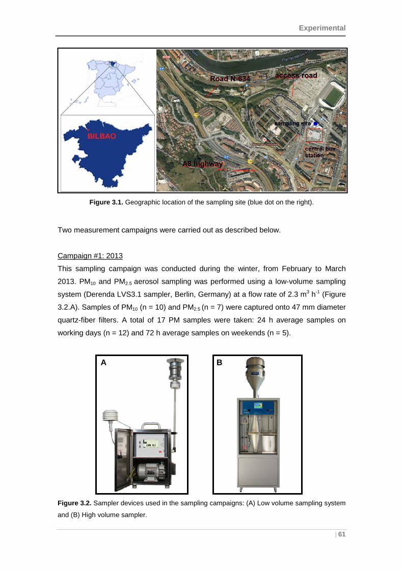
Experimental

| 61

Figure 3.1. Geographic location of the sampling site (blue dot on the right).

Two measurement campaigns were carried out as described below.

Campaign #1: 2013

This sampling campaign was conducted during the winter, from February to March

2013. PM10 and PM2.5 aerosol sampling was performed using a low-volume sampling

system (Derenda LVS3.1 sampler, Berlin, Germany) at a flow rate of 2.3 m3 h-1 (Figure

3.2.A). Samples of PM10 (n = 10) and PM2.5 (n = 7) were captured onto 47 mm diameter

quartz-fiber filters. A total of 17 PM samples were taken: 24 h average samples on

working days (n = 12) and 72 h average samples on weekends (n = 5).

Figure 3.2. Sampler devices used in the sampling campaigns: (A) Low volume sampling system

and (B) High volume sampler.

B A

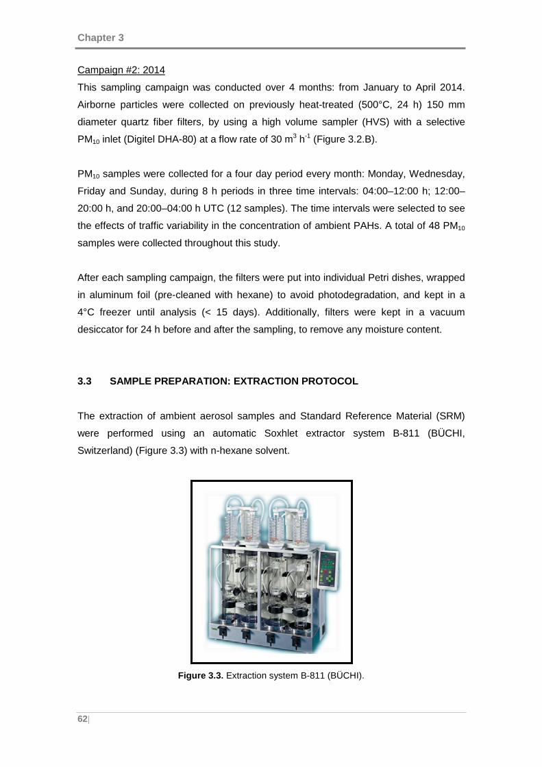
Chapter 3

62|

Campaign #2: 2014

This sampling campaign was conducted over 4 months: from January to April 2014.

Airborne particles were collected on previously heat-treated (500°C, 24 h) 150 mm

diameter quartz fiber filters, by using a high volume sampler (HVS) with a selective

PM10 inlet (Digitel DHA-80) at a flow rate of 30 m3 h-1 (Figure 3.2.B).

PM10 samples were collected for a four day period every month: Monday, Wednesday,

Friday and Sunday, during 8 h periods in three time intervals: 04:00–12:00 h; 12:00–

20:00 h, and 20:00–04:00 h UTC (12 samples). The time intervals were selected to see

the effects of traffic variability in the concentration of ambient PAHs. A total of 48 PM10

samples were collected throughout this study.

After each sampling campaign, the filters were put into individual Petri dishes, wrapped

in aluminum foil (pre-cleaned with hexane) to avoid photodegradation, and kept in a

4°C freezer until analysis (< 15 days). Additionally, filters were kept in a vacuum

desiccator for 24 h before and after the sampling, to remove any moisture content.

3.3 SAMPLE PREPARATION: EXTRACTION PROTOCOL

The extraction of ambient aerosol samples and Standard Reference Material (SRM)

were performed using an automatic Soxhlet extractor system B-811 (BÜCHI,

Switzerland) (Figure 3.3) with n-hexane solvent.

Figure 3.3. Extraction system B-811 (BÜCHI).

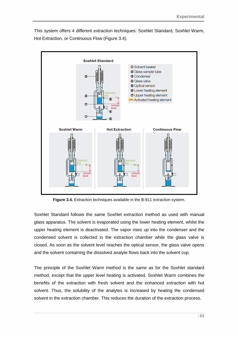
Experimental

| 63

This system offers 4 different extraction techniques: Soxhlet Standard, Soxhlet Warm,

Hot Extraction, or Continuous Flow (Figure 3.4).

Figure 3.4. Extraction techniques available in the B-811 extraction system.

Soxhlet Standard follows the same Soxhlet extraction method as used with manual

glass apparatus. The solvent is evaporated using the lower heating element, whilst the

upper heating element is deactivated. The vapor rises up into the condenser and the

condensed solvent is collected in the extraction chamber while the glass valve is

closed. As soon as the solvent level reaches the optical sensor, the glass valve opens

and the solvent containing the dissolved analyte flows back into the solvent cup.

The principle of the Soxhlet Warm method is the same as for the Soxhlet standard

method, except that the upper level heating is activated. Soxhlet Warm combines the

benefits of the extraction with fresh solvent and the enhanced extraction with hot

solvent. Thus, the solubility of the analytes is increased by heating the condensed

solvent in the extraction chamber. This reduces the duration of the extraction process.

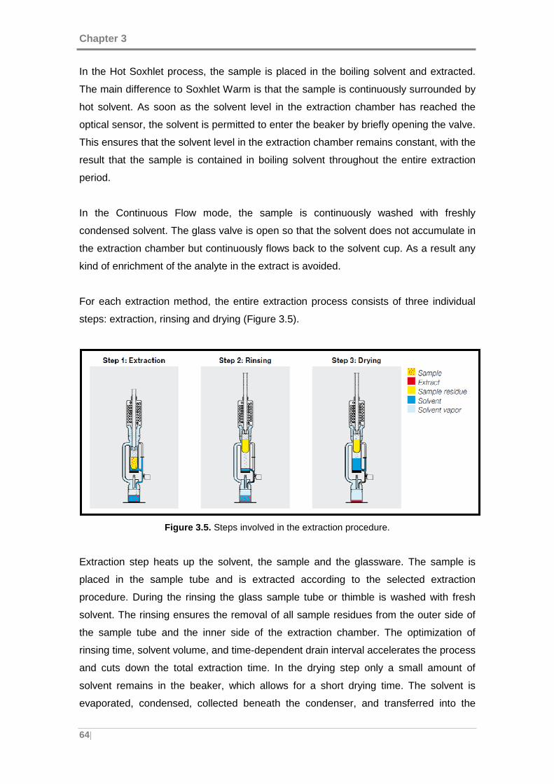
Chapter 3

64|

In the Hot Soxhlet process, the sample is placed in the boiling solvent and extracted.

The main difference to Soxhlet Warm is that the sample is continuously surrounded by

hot solvent. As soon as the solvent level in the extraction chamber has reached the

optical sensor, the solvent is permitted to enter the beaker by briefly opening the valve.

This ensures that the solvent level in the extraction chamber remains constant, with the

result that the sample is contained in boiling solvent throughout the entire extraction

period.

In the Continuous Flow mode, the sample is continuously washed with freshly

condensed solvent. The glass valve is open so that the solvent does not accumulate in

the extraction chamber but continuously flows back to the solvent cup. As a result any

kind of enrichment of the analyte in the extract is avoided.

For each extraction method, the entire extraction process consists of three individual

steps: extraction, rinsing and drying (Figure 3.5).

Figure 3.5. Steps involved in the extraction procedure.

Extraction step heats up the solvent, the sample and the glassware. The sample is

placed in the sample tube and is extracted according to the selected extraction

procedure. During the rinsing the glass sample tube or thimble is washed with fresh

solvent. The rinsing ensures the removal of all sample residues from the outer side of

the sample tube and the inner side of the extraction chamber. The optimization of

rinsing time, solvent volume, and time-dependent drain interval accelerates the process

and cuts down the total extraction time. In the drying step only a small amount of

solvent remains in the beaker, which allows for a short drying time. The solvent is

evaporated, condensed, collected beneath the condenser, and transferred into the

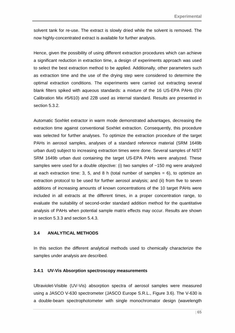
Experimental

| 65

solvent tank for re-use. The extract is slowly dried while the solvent is removed. The

now highly-concentrated extract is available for further analysis.

Hence, given the possibility of using different extraction procedures which can achieve

a significant reduction in extraction time, a design of experiments approach was used

to select the best extraction method to be applied. Additionally, other parameters such

as extraction time and the use of the drying step were considered to determine the

optimal extraction conditions. The experiments were carried out extracting several

blank filters spiked with aqueous standards: a mixture of the 16 US-EPA PAHs (SV

Calibration Mix #5/610) and 22B used as internal standard. Results are presented in

section 5.3.2.

Automatic Soxhlet extractor in warm mode demonstrated advantages, decreasing the

extraction time against conventional Soxhlet extraction. Consequently, this procedure

was selected for further analyses. To optimize the extraction procedure of the target

PAHs in aerosol samples, analyses of a standard reference material (SRM 1649b

urban dust) subject to increasing extraction times were done. Several samples of NIST

SRM 1649b urban dust containing the target US-EPA PAHs were analyzed. These

samples were used for a double objective: (i) two samples of ~150 mg were analyzed

at each extraction time: 3, 5, and 8 h (total number of samples = 6), to optimize an

extraction protocol to be used for further aerosol analysis; and (ii) from five to seven

additions of increasing amounts of known concentrations of the 10 target PAHs were

included in all extracts at the different times, in a proper concentration range, to

evaluate the suitability of second-order standard addition method for the quantitative

analysis of PAHs when potential sample matrix effects may occur. Results are shown

in section 5.3.3 and section 5.4.3.

3.4 ANALYTICAL METHODS

In this section the different analytical methods used to chemically characterize the

samples under analysis are described.

3.4.1 UV-Vis Absorption spectroscopy measurements

Ultraviolet-Visible (UV-Vis) absorption spectra of aerosol samples were measured

using a JASCO V-630 spectrometer (JASCO Europe S.R.L., Figure 3.6). The V-630 is

a double-beam spectrophotometer with single monochromator design (wavelength

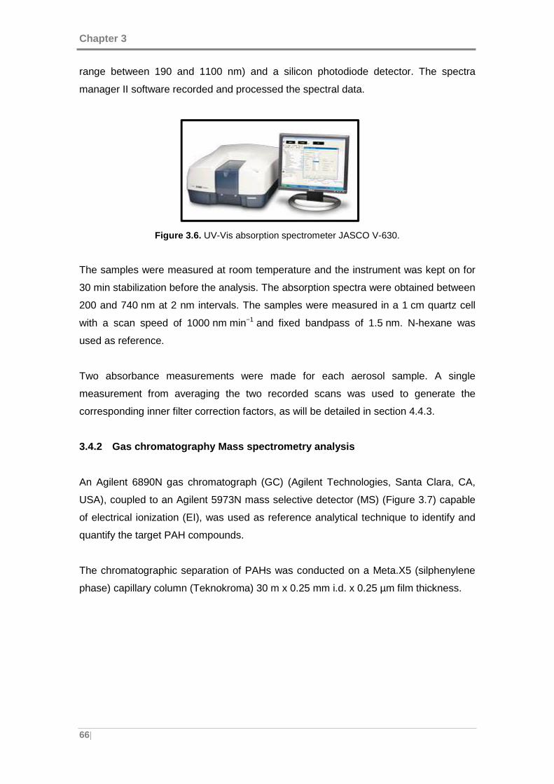
Chapter 3

66|

range between 190 and 1100 nm) and a silicon photodiode detector. The spectra

manager II software recorded and processed the spectral data.

Figure 3.6. UV-Vis absorption spectrometer JASCO V-630.

The samples were measured at room temperature and the instrument was kept on for

30 min stabilization before the analysis. The absorption spectra were obtained between

200 and 740 nm at 2 nm intervals. The samples were measured in a 1 cm quartz cell

with a scan speed of 1000 nm min−1 and fixed bandpass of 1.5 nm. N-hexane was

used as reference.

Two absorbance measurements were made for each aerosol sample. A single

measurement from averaging the two recorded scans was used to generate the

corresponding inner filter correction factors, as will be detailed in section 4.4.3.

3.4.2 Gas chromatography Mass spectrometry analysis

An Agilent 6890N gas chromatograph (GC) (Agilent Technologies, Santa Clara, CA,

USA), coupled to an Agilent 5973N mass selective detector (MS) (Figure 3.7) capable

of electrical ionization (EI), was used as reference analytical technique to identify and

quantify the target PAH compounds.

The chromatographic separation of PAHs was conducted on a Meta.X5 (silphenylene

phase) capillary column (Teknokroma) 30 m x 0.25 mm i.d. x 0.25 µm film thickness.

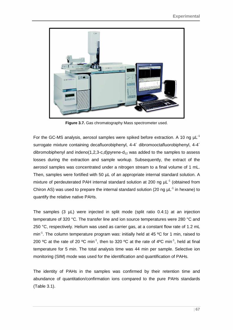
Experimental

| 67

Figure 3.7. Gas chromatography Mass spectrometer used.

For the GC-MS analysis, aerosol samples were spiked before extraction. A 10 ng µL-1

surrogate mixture containing decafluorobiphenyl, 4-4´ dibromooctafluorobiphenyl, 4-4´

dibromobiphenyl and indeno(1,2,3-c,d)pyrene-d12 was added to the samples to assess

losses during the extraction and sample workup. Subsequently, the extract of the

aerosol samples was concentrated under a nitrogen stream to a final volume of 1 mL.

Then, samples were fortified with 50 µL of an appropriate internal standard solution. A

mixture of perdeuterated PAH internal standard solution at 200 ng µL-1 (obtained from

Chiron AS) was used to prepare the internal standard solution (20 ng µL-1 in hexane) to

quantify the relative native PAHs.

The samples (3 µL) were injected in split mode (split ratio 0.4:1) at an injection

temperature of 320 °C. The transfer line and ion source temperatures were 280 °C and

250 °C, respectively. Helium was used as carrier gas, at a constant flow rate of 1.2 mL

min-1. The column temperature program was: initially held at 45 ºC for 1 min, raised to

200 ºC at the rate of 20 ºC min-1, then to 320 ºC at the rate of 4ºC min-1, held at final

temperature for 5 min. The total analysis time was 44 min per sample. Selective ion

monitoring (SIM) mode was used for the identification and quantification of PAHs.

The identity of PAHs in the samples was confirmed by their retention time and

abundance of quantitation/confirmation ions compared to the pure PAHs standards

(Table 3.1).

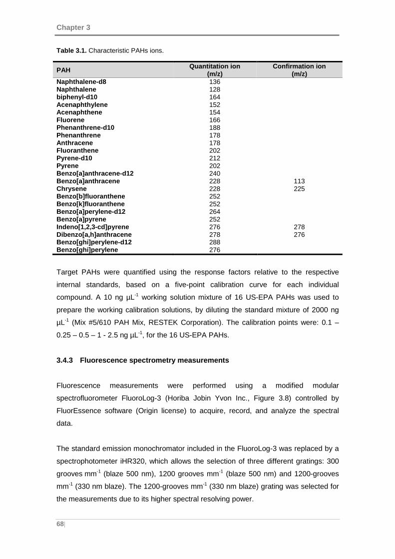
Chapter 3

68|

Table 3.1. Characteristic PAHs ions.

PAH Quantitation ion (m/z)

Confirmation ion (m/z)

Naphthalene -d8 136 Naphthalene 128 biphenyl -d10 164 Acenaphthylene 152 Acenaphthene 154 Fluorene 166 Phenanthrene -d10 188 Phenanthrene 178 Anthracene 178 Fluoranthene 202 Pyrene -d10 212 Pyrene 202 Benzo[a]anthracene -d12 240 Benzo[a]anthracene 228 113 Chrysene 228 225 Benzo[b]fluoranthene 252 Benzo[k]fluoranthene 252 Benzo[a]perylene -d12 264 Benzo[a]pyrene 252 Indeno[1,2,3 -cd]pyrene 276 278 Dibenzo[a,h]anthracene 278 276 Benzo[ghi]perylene -d12 288 Benzo[ghi]perylene 276

Target PAHs were quantified using the response factors relative to the respective

internal standards, based on a five-point calibration curve for each individual

compound. A 10 ng µL-1 working solution mixture of 16 US-EPA PAHs was used to

prepare the working calibration solutions, by diluting the standard mixture of 2000 ng

µL-1 (Mix #5/610 PAH Mix, RESTEK Corporation). The calibration points were: 0.1 –

0.25 – 0.5 – 1 - 2.5 ng µL-1, for the 16 US-EPA PAHs.

3.4.3 Fluorescence spectrometry measurements

Fluorescence measurements were performed using a modified modular

spectrofluorometer FluoroLog-3 (Horiba Jobin Yvon Inc., Figure 3.8) controlled by

FluorEssence software (Origin license) to acquire, record, and analyze the spectral

data.

The standard emission monochromator included in the FluoroLog-3 was replaced by a

spectrophotometer iHR320, which allows the selection of three different gratings: 300

grooves mm-1 (blaze 500 nm), 1200 grooves mm-1 (blaze 500 nm) and 1200-grooves

mm-1 (330 nm blaze). The 1200-grooves mm-1 (330 nm blaze) grating was selected for

the measurements due to its higher spectral resolving power.

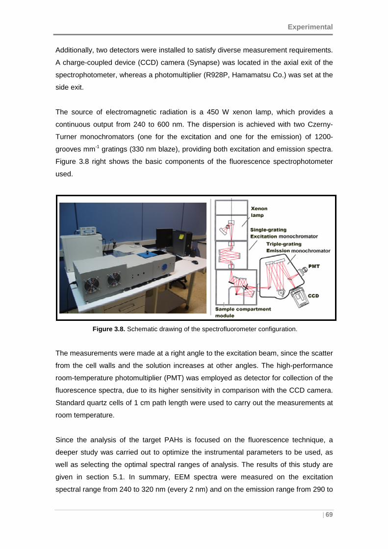
Experimental

| 69

Additionally, two detectors were installed to satisfy diverse measurement requirements.

A charge-coupled device (CCD) camera (Synapse) was located in the axial exit of the

spectrophotometer, whereas a photomultiplier (R928P, Hamamatsu Co.) was set at the

side exit.

The source of electromagnetic radiation is a 450 W xenon lamp, which provides a

continuous output from 240 to 600 nm. The dispersion is achieved with two Czerny-

Turner monochromators (one for the excitation and one for the emission) of 1200-

grooves mm-1 gratings (330 nm blaze), providing both excitation and emission spectra.

Figure 3.8 right shows the basic components of the fluorescence spectrophotometer

used.

Figure 3.8. Schematic drawing of the spectrofluorometer configuration.

The measurements were made at a right angle to the excitation beam, since the scatter

from the cell walls and the solution increases at other angles. The high-performance

room-temperature photomultiplier (PMT) was employed as detector for collection of the

fluorescence spectra, due to its higher sensitivity in comparison with the CCD camera.

Standard quartz cells of 1 cm path length were used to carry out the measurements at

room temperature.

Since the analysis of the target PAHs is focused on the fluorescence technique, a

deeper study was carried out to optimize the instrumental parameters to be used, as

well as selecting the optimal spectral ranges of analysis. The results of this study are

given in section 5.1. In summary, EEM spectra were measured on the excitation

spectral range from 240 to 320 nm (every 2 nm) and on the emission range from 290 to

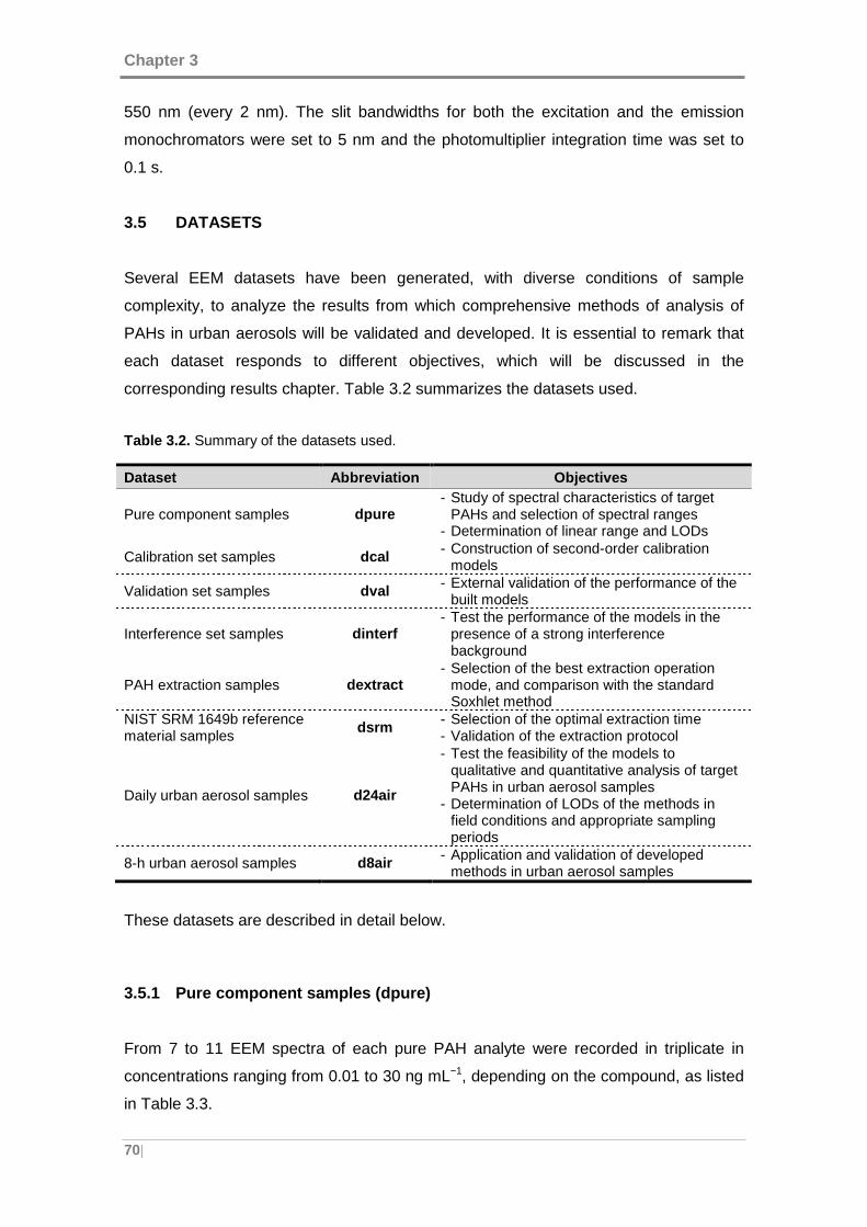
Chapter 3

70|

550 nm (every 2 nm). The slit bandwidths for both the excitation and the emission

monochromators were set to 5 nm and the photomultiplier integration time was set to

0.1 s.

3.5 DATASETS

Several EEM datasets have been generated, with diverse conditions of sample

complexity, to analyze the results from which comprehensive methods of analysis of

PAHs in urban aerosols will be validated and developed. It is essential to remark that

each dataset responds to different objectives, which will be discussed in the

corresponding results chapter. Table 3.2 summarizes the datasets used.

Table 3.2. Summary of the datasets used.

Dataset Abbreviation Objectives

Pure component samples dpure - Study of spectral characteristics of target

PAHs and selection of spectral ranges - Determination of linear range and LODs

Calibration set samples dcal - Construction of second-order calibration models

Validation set samples dval - External validation of the performance of the built models

Interference set samples dinterf - Test the performance of the models in the

presence of a strong interference background

PAH extraction samples dextract - Selection of the best extraction operation

mode, and comparison with the standard Soxhlet method

NIST SRM 1649b reference material samples

dsrm - Selection of the optimal extraction time - Validation of the extraction protocol

Daily urban aerosol samples d24air

- Test the feasibility of the models to qualitative and quantitative analysis of target PAHs in urban aerosol samples

- Determination of LODs of the methods in field conditions and appropriate sampling periods

8-h urban aerosol samples d8air - Application and validation of developed methods in urban aerosol samples

These datasets are described in detail below.

3.5.1 Pure component samples (dpure)

From 7 to 11 EEM spectra of each pure PAH analyte were recorded in triplicate in

concentrations ranging from 0.01 to 30 ng mL−1, depending on the compound, as listed

in Table 3.3.

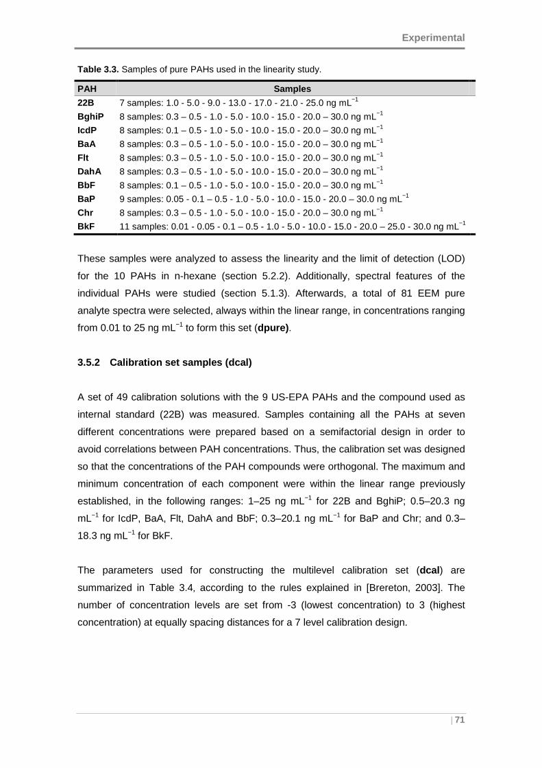
Experimental

| 71

Table 3.3. Samples of pure PAHs used in the linearity study.

PAH Samples 22B 7 samples: 1.0 - 5.0 - 9.0 - 13.0 - 17.0 - 21.0 - 25.0 ng mL−1

BghiP 8 samples: 0.3 – 0.5 - 1.0 - 5.0 - 10.0 - 15.0 - 20.0 – 30.0 ng mL−1

IcdP 8 samples: 0.1 – 0.5 - 1.0 - 5.0 - 10.0 - 15.0 - 20.0 – 30.0 ng mL−1

BaA 8 samples: 0.3 – 0.5 - 1.0 - 5.0 - 10.0 - 15.0 - 20.0 – 30.0 ng mL−1

Flt 8 samples: 0.3 – 0.5 - 1.0 - 5.0 - 10.0 - 15.0 - 20.0 – 30.0 ng mL−1

DahA 8 samples: 0.3 – 0.5 - 1.0 - 5.0 - 10.0 - 15.0 - 20.0 – 30.0 ng mL−1

BbF 8 samples: 0.1 – 0.5 - 1.0 - 5.0 - 10.0 - 15.0 - 20.0 – 30.0 ng mL−1

BaP 9 samples: 0.05 - 0.1 – 0.5 - 1.0 - 5.0 - 10.0 - 15.0 - 20.0 – 30.0 ng mL−1

Chr 8 samples: 0.3 – 0.5 - 1.0 - 5.0 - 10.0 - 15.0 - 20.0 – 30.0 ng mL−1 BkF 11 samples: 0.01 - 0.05 - 0.1 – 0.5 - 1.0 - 5.0 - 10.0 - 15.0 - 20.0 – 25.0 - 30.0 ng mL−1

These samples were analyzed to assess the linearity and the limit of detection (LOD)

for the 10 PAHs in n-hexane (section 5.2.2). Additionally, spectral features of the

individual PAHs were studied (section 5.1.3). Afterwards, a total of 81 EEM pure

analyte spectra were selected, always within the linear range, in concentrations ranging

from 0.01 to 25 ng mL−1 to form this set (dpure) .

3.5.2 Calibration set samples (dcal)

A set of 49 calibration solutions with the 9 US-EPA PAHs and the compound used as

internal standard (22B) was measured. Samples containing all the PAHs at seven

different concentrations were prepared based on a semifactorial design in order to

avoid correlations between PAH concentrations. Thus, the calibration set was designed

so that the concentrations of the PAH compounds were orthogonal. The maximum and

minimum concentration of each component were within the linear range previously

established, in the following ranges: 1–25 ng mL−1 for 22B and BghiP; 0.5–20.3 ng

mL−1 for IcdP, BaA, Flt, DahA and BbF; 0.3–20.1 ng mL−1 for BaP and Chr; and 0.3–

18.3 ng mL−1 for BkF.

The parameters used for constructing the multilevel calibration set (dcal ) are

summarized in Table 3.4, according to the rules explained in [Brereton, 2003]. The

number of concentration levels are set from -3 (lowest concentration) to 3 (highest

concentration) at equally spacing distances for a 7 level calibration design.

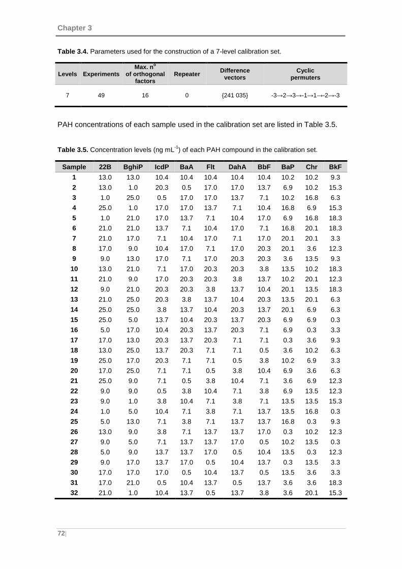
Chapter 3

72|

Table 3.4. Parameters used for the construction of a 7-level calibration set.

Levels Experiments Max. n o

of orthogonal factors

Repeater Difference vectors

Cyclic permuters

7 49 16 0

{241 035}

-3→2→3→-1→1→-2→-3

PAH concentrations of each sample used in the calibration set are listed in Table 3.5.

Table 3.5. Concentration levels (ng mL-1) of each PAH compound in the calibration set.

Sample 22B BghiP IcdP BaA Flt DahA BbF BaP Chr BkF

1 13.0 13.0 10.4 10.4 10.4 10.4 10.4 10.2 10.2 9.3

2 13.0 1.0 20.3 0.5 17.0 17.0 13.7 6.9 10.2 15.3

3 1.0 25.0 0.5 17.0 17.0 13.7 7.1 10.2 16.8 6.3

4 25.0 1.0 17.0 17.0 13.7 7.1 10.4 16.8 6.9 15.3

5 1.0 21.0 17.0 13.7 7.1 10.4 17.0 6.9 16.8 18.3

6 21.0 21.0 13.7 7.1 10.4 17.0 7.1 16.8 20.1 18.3

7 21.0 17.0 7.1 10.4 17.0 7.1 17.0 20.1 20.1 3.3

8 17.0 9.0 10.4 17.0 7.1 17.0 20.3 20.1 3.6 12.3

9 9.0 13.0 17.0 7.1 17.0 20.3 20.3 3.6 13.5 9.3

10 13.0 21.0 7.1 17.0 20.3 20.3 3.8 13.5 10.2 18.3

11 21.0 9.0 17.0 20.3 20.3 3.8 13.7 10.2 20.1 12.3

12 9.0 21.0 20.3 20.3 3.8 13.7 10.4 20.1 13.5 18.3

13 21.0 25.0 20.3 3.8 13.7 10.4 20.3 13.5 20.1 6.3

14 25.0 25.0 3.8 13.7 10.4 20.3 13.7 20.1 6.9 6.3

15 25.0 5.0 13.7 10.4 20.3 13.7 20.3 6.9 6.9 0.3

16 5.0 17.0 10.4 20.3 13.7 20.3 7.1 6.9 0.3 3.3

17 17.0 13.0 20.3 13.7 20.3 7.1 7.1 0.3 3.6 9.3

18 13.0 25.0 13.7 20.3 7.1 7.1 0.5 3.6 10.2 6.3

19 25.0 17.0 20.3 7.1 7.1 0.5 3.8 10.2 6.9 3.3

20 17.0 25.0 7.1 7.1 0.5 3.8 10.4 6.9 3.6 6.3

21 25.0 9.0 7.1 0.5 3.8 10.4 7.1 3.6 6.9 12.3

22 9.0 9.0 0.5 3.8 10.4 7.1 3.8 6.9 13.5 12.3

23 9.0 1.0 3.8 10.4 7.1 3.8 7.1 13.5 13.5 15.3

24 1.0 5.0 10.4 7.1 3.8 7.1 13.7 13.5 16.8 0.3

25 5.0 13.0 7.1 3.8 7.1 13.7 13.7 16.8 0.3 9.3

26 13.0 9.0 3.8 7.1 13.7 13.7 17.0 0.3 10.2 12.3

27 9.0 5.0 7.1 13.7 13.7 17.0 0.5 10.2 13.5 0.3

28 5.0 9.0 13.7 13.7 17.0 0.5 10.4 13.5 0.3 12.3

29 9.0 17.0 13.7 17.0 0.5 10.4 13.7 0.3 13.5 3.3

30 17.0 17.0 17.0 0.5 10.4 13.7 0.5 13.5 3.6 3.3

31 17.0 21.0 0.5 10.4 13.7 0.5 13.7 3.6 3.6 18.3

32 21.0 1.0 10.4 13.7 0.5 13.7 3.8 3.6 20.1 15.3

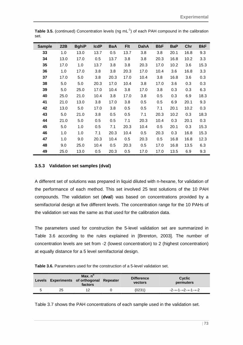
Experimental

| 73

Table 3.5. (continued) Concentration levels (ng mL-1) of each PAH compound in the calibration set.


33 1.0 13.0 13.7 0.5 13.7 3.8 3.8 20.1 16.8 9.3

34 13.0 17.0 0.5 13.7 3.8 3.8 20.3 16.8 10.2 3.3

35 17.0 1.0 13.7 3.8 3.8 20.3 17.0 10.2 3.6 15.3

36 1.0 17.0 3.8 3.8 20.3 17.0 10.4 3.6 16.8 3.3

37 17.0 5.0 3.8 20.3 17.0 10.4 3.8 16.8 3.6 0.3

38 5.0 5.0 20.3 17.0 10.4 3.8 17.0 3.6 0.3 0.3

39 5.0 25.0 17.0 10.4 3.8 17.0 3.8 0.3 0.3 6.3

40 25.0 21.0 10.4 3.8 17.0 3.8 0.5 0.3 6.9 18.3

41 21.0 13.0 3.8 17.0 3.8 0.5 0.5 6.9 20.1 9.3

42 13.0 5.0 17.0 3.8 0.5 0.5 7.1 20.1 10.2 0.3

43 5.0 21.0 3.8 0.5 0.5 7.1 20.3 10.2 0.3 18.3

44 21.0 5.0 0.5 0.5 7.1 20.3 10.4 0.3 20.1 0.3

45 5.0 1.0 0.5 7.1 20.3 10.4 0.5 20.1 0.3 15.3

46 1.0 1.0 7.1 20.3 10.4 0.5 20.3 0.3 16.8 15.3

47 1.0 9.0 20.3 10.4 0.5 20.3 0.5 16.8 16.8 12.3

48 9.0 25.0 10.4 0.5 20.3 0.5 17.0 16.8 13.5 6.3

49 25.0 13.0 0.5 20.3 0.5 17.0 17.0 13.5 6.9 9.3

3.5.3 Validation set samples (dval)

A different set of solutions was prepared in liquid diluted with n-hexane, for validation of

the performance of each method. This set involved 25 test solutions of the 10 PAH

compounds. The validation set (dval ) was based on concentrations provided by a

semifactorial design at five different levels. The concentration range for the 10 PAHs of

the validation set was the same as that used for the calibration data.

The parameters used for construction the 5-level validation set are summarized in

Table 3.6 according to the rules explained in [Brereton, 2003]. The number of

concentration levels are set from -2 (lowest concentration) to 2 (highest concentration)

at equally distance for a 5 level semifactorial design.

Table 3.6. Parameters used for the construction of a 5-level validation set.

Levels Experiments Max. n o

of orthogonal factors

Repeater Difference vectors

Cyclic permuters

5 25 12 0 {0231} -2→-1→2→-1→-2

Table 3.7 shows the PAH concentrations of each sample used in the validation set.

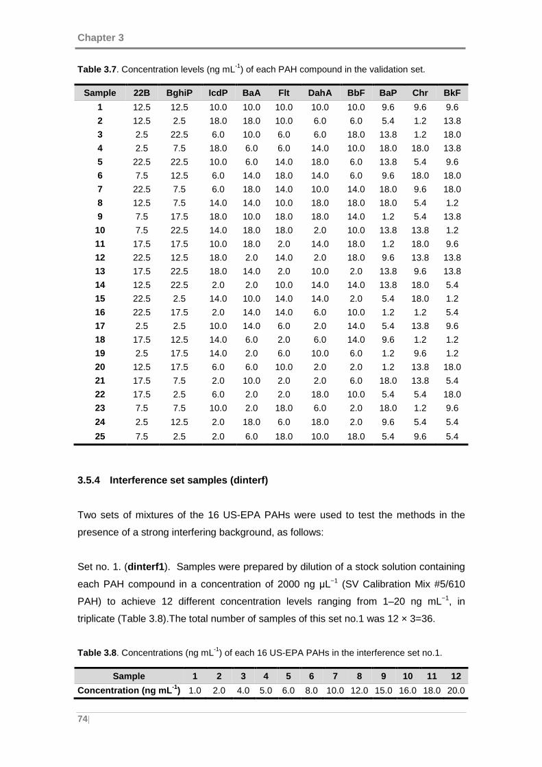
Chapter 3

74|

Table 3.7 . Concentration levels (ng mL-1) of each PAH compound in the validation set.


1 12.5 12.5 10.0 10.0 10.0 10.0 10.0 9.6 9.6 9.6

2 12.5 2.5 18.0 18.0 10.0 6.0 6.0 5.4 1.2 13.8

3 2.5 22.5 6.0 10.0 6.0 6.0 18.0 13.8 1.2 18.0

4 2.5 7.5 18.0 6.0 6.0 14.0 10.0 18.0 18.0 13.8

5 22.5 22.5 10.0 6.0 14.0 18.0 6.0 13.8 5.4 9.6

6 7.5 12.5 6.0 14.0 18.0 14.0 6.0 9.6 18.0 18.0

7 22.5 7.5 6.0 18.0 14.0 10.0 14.0 18.0 9.6 18.0

8 12.5 7.5 14.0 14.0 10.0 18.0 18.0 18.0 5.4 1.2

9 7.5 17.5 18.0 10.0 18.0 18.0 14.0 1.2 5.4 13.8

10 7.5 22.5 14.0 18.0 18.0 2.0 10.0 13.8 13.8 1.2

11 17.5 17.5 10.0 18.0 2.0 14.0 18.0 1.2 18.0 9.6

12 22.5 12.5 18.0 2.0 14.0 2.0 18.0 9.6 13.8 13.8

13 17.5 22.5 18.0 14.0 2.0 10.0 2.0 13.8 9.6 13.8

14 12.5 22.5 2.0 2.0 10.0 14.0 14.0 13.8 18.0 5.4

15 22.5 2.5 14.0 10.0 14.0 14.0 2.0 5.4 18.0 1.2

16 22.5 17.5 2.0 14.0 14.0 6.0 10.0 1.2 1.2 5.4

17 2.5 2.5 10.0 14.0 6.0 2.0 14.0 5.4 13.8 9.6

18 17.5 12.5 14.0 6.0 2.0 6.0 14.0 9.6 1.2 1.2

19 2.5 17.5 14.0 2.0 6.0 10.0 6.0 1.2 9.6 1.2

20 12.5 17.5 6.0 6.0 10.0 2.0 2.0 1.2 13.8 18.0

21 17.5 7.5 2.0 10.0 2.0 2.0 6.0 18.0 13.8 5.4

22 17.5 2.5 6.0 2.0 2.0 18.0 10.0 5.4 5.4 18.0

23 7.5 7.5 10.0 2.0 18.0 6.0 2.0 18.0 1.2 9.6

24 2.5 12.5 2.0 18.0 6.0 18.0 2.0 9.6 5.4 5.4

25 7.5 2.5 2.0 6.0 18.0 10.0 18.0 5.4 9.6 5.4

3.5.4 Interference set samples (dinterf)

Two sets of mixtures of the 16 US-EPA PAHs were used to test the methods in the

presence of a strong interfering background, as follows:

Set no. 1. (dinterf1 ). Samples were prepared by dilution of a stock solution containing

each PAH compound in a concentration of 2000 ng µL−1 (SV Calibration Mix #5/610

PAH) to achieve 12 different concentration levels ranging from 1–20 ng mL−1, in

triplicate (Table 3.8).The total number of samples of this set no.1 was 12 × 3=36.

Table 3.8 . Concentrations (ng mL-1) of each 16 US-EPA PAHs in the interference set no.1.

Sample 1 2 3 4 5 6 7 8 9 10 11 12

Concentration (ng mL -1) 1.0 2.0 4.0 5.0 6.0 8.0 10.0 12.0 15.0 16.0 18.0 20.0

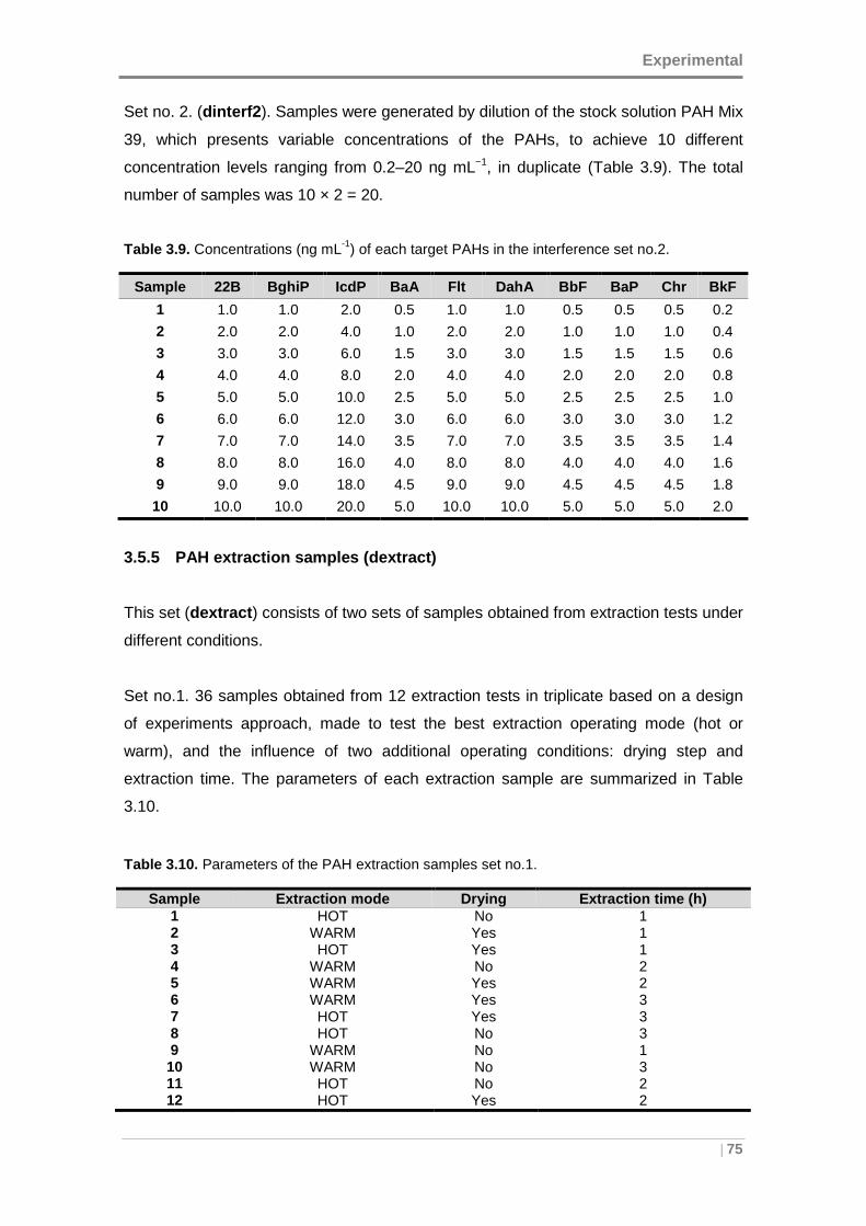
Experimental

| 75

Set no. 2. (dinterf2 ). Samples were generated by dilution of the stock solution PAH Mix

39, which presents variable concentrations of the PAHs, to achieve 10 different

concentration levels ranging from 0.2–20 ng mL−1, in duplicate (Table 3.9). The total

number of samples was 10 × 2 = 20.

Table 3.9. Concentrations (ng mL-1) of each target PAHs in the interference set no.2.


1 1.0 1.0 2.0 0.5 1.0 1.0 0.5 0.5 0.5 0.2

2 2.0 2.0 4.0 1.0 2.0 2.0 1.0 1.0 1.0 0.4

3 3.0 3.0 6.0 1.5 3.0 3.0 1.5 1.5 1.5 0.6

4 4.0 4.0 8.0 2.0 4.0 4.0 2.0 2.0 2.0 0.8

5 5.0 5.0 10.0 2.5 5.0 5.0 2.5 2.5 2.5 1.0

6 6.0 6.0 12.0 3.0 6.0 6.0 3.0 3.0 3.0 1.2

7 7.0 7.0 14.0 3.5 7.0 7.0 3.5 3.5 3.5 1.4

8 8.0 8.0 16.0 4.0 8.0 8.0 4.0 4.0 4.0 1.6

9 9.0 9.0 18.0 4.5 9.0 9.0 4.5 4.5 4.5 1.8

10 10.0 10.0 20.0 5.0 10.0 10.0 5.0 5.0 5.0 2.0

3.5.5 PAH extraction samples (dextract)

This set (dextract ) consists of two sets of samples obtained from extraction tests under

different conditions.

Set no.1. 36 samples obtained from 12 extraction tests in triplicate based on a design

of experiments approach, made to test the best extraction operating mode (hot or

warm), and the influence of two additional operating conditions: drying step and

extraction time. The parameters of each extraction sample are summarized in Table

3.10.

Table 3.10. Parameters of the PAH extraction samples set no.1.

Sample Extraction mode Drying Extraction time (h) 1 HOT No 1 2 WARM Yes 1 3 HOT Yes 1 4 WARM No 2 5 WARM Yes 2 6 WARM Yes 3 7 HOT Yes 3 8 HOT No 3 9 WARM No 1 10 WARM No 3 11 HOT No 2 12 HOT Yes 2

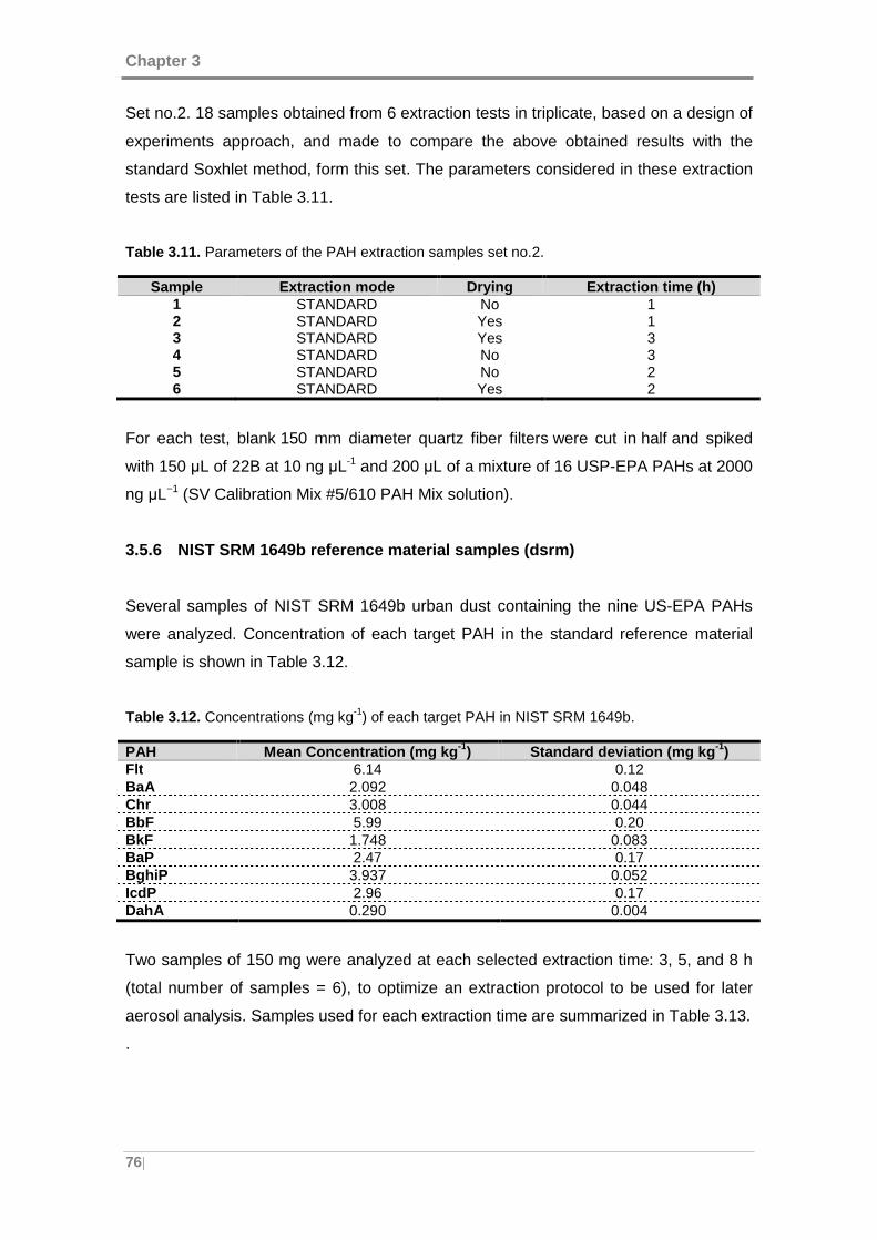
Chapter 3

76|

Set no.2. 18 samples obtained from 6 extraction tests in triplicate, based on a design of

experiments approach, and made to compare the above obtained results with the

standard Soxhlet method, form this set. The parameters considered in these extraction

tests are listed in Table 3.11.

Table 3.11. Parameters of the PAH extraction samples set no.2.

Sample Extraction mode Drying Extraction time (h) 1 STANDARD No 1 2 STANDARD Yes 1 3 STANDARD Yes 3 4 STANDARD No 3 5 STANDARD No 2 6 STANDARD Yes 2

For each test, blank 150 mm diameter quartz fiber filters were cut in half and spiked

with 150 µL of 22B at 10 ng µL-1 and 200 µL of a mixture of 16 USP-EPA PAHs at 2000

ng µL−1 (SV Calibration Mix #5/610 PAH Mix solution).

3.5.6 NIST SRM 1649b reference material samples (dsrm)

Several samples of NIST SRM 1649b urban dust containing the nine US-EPA PAHs

were analyzed. Concentration of each target PAH in the standard reference material

sample is shown in Table 3.12.

Table 3.12. Concentrations (mg kg-1) of each target PAH in NIST SRM 1649b.

PAH Mean Concentration (mg kg -1) Standard deviation (mg kg -1) Flt 6.14 0.12 BaA 2.092 0.048 Chr 3.008 0.044 BbF 5.99 0.20 BkF 1.748 0.083 BaP 2.47 0.17 BghiP 3.937 0.052 IcdP 2.96 0.17 DahA 0.290 0.004

Two samples of 150 mg were analyzed at each selected extraction time: 3, 5, and 8 h

(total number of samples = 6), to optimize an extraction protocol to be used for later

aerosol analysis. Samples used for each extraction time are summarized in Table 3.13.

.

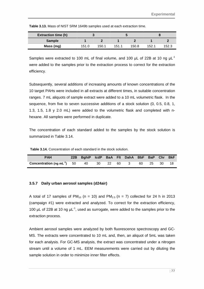
Experimental

| 77

Table 3.13. Mass of NIST SRM 1649b samples used at each extraction time.

Extraction time (h) 3 5 8

Sample 1 2 1 2 1 2

Mass (mg) 151.0 150.1 151.1 150.8 152.1 152.3

Samples were extracted to 100 mL of final volume, and 100 µL of 22B at 10 ng µL-1

were added to the samples prior to the extraction process to correct for the extraction

efficiency.

Subsequently, several additions of increasing amounts of known concentrations of the

10 target PAHs were included in all extracts at different times, in suitable concentration

ranges. 7 mL aliquots of sample extract were added to a 10 mL volumetric flask. In the

sequence, from five to seven successive additions of a stock solution (0, 0.5, 0.8, 1,

1.3, 1.5, 1.8 y 2.0 mL) were added to the volumetric flask and completed with n-

hexane. All samples were performed in duplicate.

The concentration of each standard added to the samples by the stock solution is

summarized in Table 3.14.

Table 3.14. Concentration of each standard in the stock solution.

PAH 22B BghiP IcdP BaA Flt DahA BbF BaP Chr BkF

Concentration (ng mL -1) 50 40 30 22 60 3 60 25 30 18

3.5.7 Daily urban aerosol samples (d24air)

A total of 17 samples of PM10 (n = 10) and PM2.5 (n = 7) collected for 24 h in 2013

(campaign #1) were extracted and analyzed. To correct for the extraction efficiency,

100 µL of 22B at 10 ng µL-1, used as surrogate, were added to the samples prior to the

extraction process.

Ambient aerosol samples were analyzed by both fluorescence spectroscopy and GC-

MS. The extracts were concentrated to 10 mL and, then, an aliquot of 5mL was taken

for each analysis. For GC-MS analysis, the extract was concentrated under a nitrogen

stream until a volume of 1 mL. EEM measurements were carried out by diluting the

sample solution in order to minimize inner filter effects.

Chapter 3

78|

EEMs were measured for each sample, and the concentrations of the nine particle-

bound US-EPA PAHs were estimated using the proposed chemometric algorithms,

presented in section 4.5, and the standard GC-MS reference technique.

3.5.8 8-h urban aerosol samples (d8air)

A total of 48 PM10 samples collected during 2014 (campaign #2) form this set. These

PM10 samples were collected for 8 h periods, in three time bins: 04:00–12:00 h; 12:00–

20:00 h, and 20:00–04:00 h UTC, corresponding to morning, afternoon and night

periods.

Filters were extracted for 5 h in warm mode and concentrated to a suitable volume for

further analysis. To correct for the extraction efficiency, from 50 to 20 µL of 22B at 10

ng µL-1, used as surrogate, were added to the samples prior to the extraction process.

Additionally, two standard additions of increasing known concentrations of the 10 target

PAHs were added to all extracts in order to prove the feasibility of second-order

standard addition methods to avoid potential sample matrix effects in the quantitative

analysis. 2.5 mL aliquots of sample extract were added to a 5 mL volumetric flask. In

the sequence, two standard additions of increasing amounts of known concentrations

of the 10 target PAHs of a stock solution (2 and 4 ng mL-1, or 4 and 8 ng mL-1,

depending on the concentration of the compound) were added to the volumetric flask

and completed with n-hexane. Finally, absorbance measurements were made for each

extracted sample.

CHAPTER 4

METHODOLOGY

Methodology

| 81

4.1 GENERAL METHODOLOGY

This chapter defines the methodology applied in developing and validating alternative

methods to determine particle-bound PAHs in ambient air. This methodology is based

in the common analytical steps which include: development- optimization - validation

and implementation. These steps are implemented for both the fluorescence analytical

procedure and the multivariate and multi-way data methods, according to each of the

main tasks illustrated in Figure 4.1.

DEFINITION OF EEM DATA ACQUISITION PROTOCOL

Fluorescence spectroscopy is the main technique used for PAHs analysis. Thus, the

development of a measurement protocol, setting the optimal instrumental and spectral

parameters to be used for further analysis comprises this first (central) task.

First, the proper spectral ranges in which EEM measurements will be recorded, have to

be set. Second, instrumental parameters, such as bandwidths of both excitation and

emission monochromators, and photomultiplier integration time, need to be studied and

optimized. Finally, the spectral characterization of target PAHs is essential to define the

EEM data acquisition procedure. The tests carried out in this section have been made

with synthetic PAHs solutions prepared in the laboratory (dpure, dinterf datasets)

previously described.

DEVELOPMENT OF PRELIMINARY EEM DATA MODELS

Given the spectral features of the target PAHs, a combination of EEM measurements

with advanced multi-way and multivariate methods are required for accomplishing both

quantitative and qualitative analysis. These data analysis methods need also to be

optimized and validated.

As a first step, the optimization of the fluorescence signal preprocessing methods

necessary to construct reliable models is performed. Subsequently, second-order

calibration models are built using the calibration set of samples (dcal ) for which specific

characteristics of each proposed method are studied and compared. Validation of the

performance of the models is then accomplished internally, with mathematical

parameters, and externally, using the validation dataset (dval ). Finally, the feasibility of

screening and determination of target PAHs in the presence of interferences is

explored using the interference dataset (dinterf ).This step is developed using synthetic

PAHs solutions, setting the preliminary bases for EEM data modeling in more complex

aerosol samples.

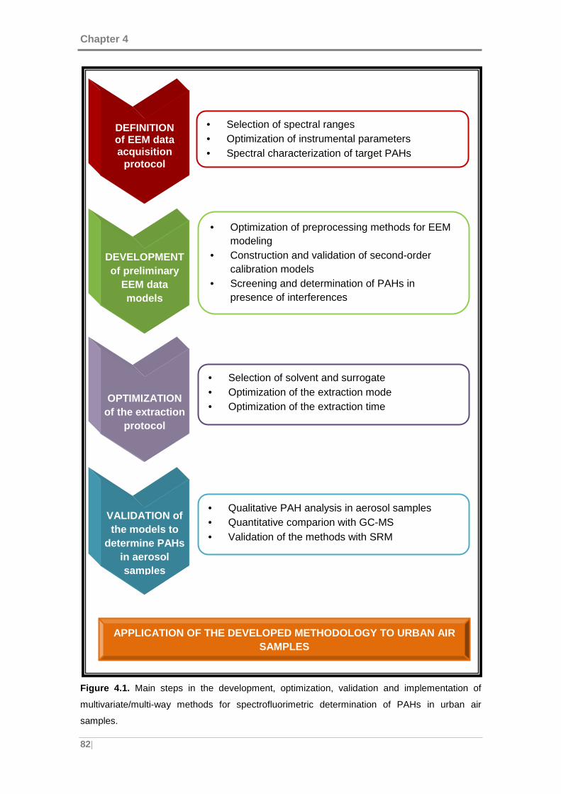
Chapter 4

82|

Figure 4.1. Main steps in the development, optimization, validation and implementation of

multivariate/multi-way methods for spectrofluorimetric determination of PAHs in urban air

samples.

• Selection of spectral ranges • Optimization of instrumental parameters • Spectral characterization of target PAHs

OPTIMIZATION of the extraction

protocol

DEVELOPMENTof preliminary

EEM data models

DEFINITION of EEM data acquisition

protocol

VALIDATION of the models to

determine PAHs in aerosol samples

APPLICATION OF THE DEVELOPED METHODOLOGY TO URBAN AIR SAMPLES

• Optimization of preprocessing methods for EEM modeling

• Construction and validation of second-order calibration models

• Screening and determination of PAHs in presence of interferences

• Selection of solvent and surrogate • Optimization of the extraction mode • Optimization of the extraction time •

• Qualitative PAH analysis in aerosol samples • Quantitative comparion with GC-MS • Validation of the methods with SRM

Methodology

| 83

OPTIMIZATION OF THE EXTRACTION PROTOCOL

Soxhlet extraction method is crucial in the sample preparation step previous to

fluorescence analysis. Consequently, the selection of the optimal operation parameters

and the definition of the most suitable extraction protocol according to the

characteristics of the target PAHs must be thoughtfully evaluated.

First, the selection of the solvent and the surrogate is accomplished taking into account

their physicochemical and spectrofluorimetric properties. Then, a deeper study, based

on a design of experiments approach, is used to select the best extraction mode

(dextract ). Then, standard reference material (dsrm ) subjected to increasing

extraction times is analyzed in order to optimize the extraction time.

VALIDATION OF THE MODELS TO DETERMINE TARGET PAHs I N AEROSOL

SAMPLES

The feasibility to identify and quantify PAHs in extracts of urban PM collection filters is

tested and validated taking into account the bases established in the second task.

Figures of merit of the technique for the target PAHs are also defined (d24air ).

Moreover, the advantages and drawbacks of each developed approach to determine

PAHs in airborne samples are highlighted.

Validation of the developed methodologies for PAH determination in aerosol samples is

carried out with the conventional technique of liquid extraction and analysis by Gas

Chromatography-Mass Spectrometry (GC-MS), comparing the qualitative and

quantitative performance of each model.

Finally, due to the complexity of aerosol samples, the use of second-order standard

addition method to account for potential sample matrix effects is assessed, validating

the optimized analysis method and extraction protocol with an standard reference

material (dsrm ).

APPLICATION OF THE DEVELOPED METHODOLOGY TO URBAN A IR SAMPLES

This point combines all the practical aspects and specific approaches developed and

optimized through the previous steps, in order to develop improved methodologies for

the sampling and analysis of target PAHs in urban air samples. These improved

methodologies are applied to characterize PAH pollution in an urban area (d8air ).

Chapter 4

84|

4.2 EEM MULTIVARIATE AND MULTI-WAY DATA ANALYSIS

As pointed out before, EEM data has an inherent three-dimensional structure (samples

x emission x excitation). Therefore, the analysis of such data structure is based on

advanced multivariate and multi-way data methods. This section is an overview of the

details considered during EEM data modeling as well as the model validation

procedures.

Analytical data can differ in its dimensionality. Zeroth-order data corresponds to

instruments producing a single response (i.e. single data point) per sample (scalar

datum), such as the fluorescence emission at a certain excitation wavelength. For

analytical purposes, zeroth-order data are usually fitted to a straight line by least

squares, a procedure known as univariate calibration, which requires full selectivity for

the analyte of interest. In contrast, multivariate data analysis is concerned with the

analysis of data consisting of multiple variables measured from many samples. For

instance, if the fluorescence is measured at more than one emission wavelength, the

resulting spectrum is arranged as a vector, or first-order tensor (Figure 4.2 [Olivieri,

2012]). When multivariate data for a single sample can be meaningfully arranged into a

mathematical object with at least two different ways (e.g. samples and wavelengths) a

data matrix is created, generating a second-order tensor. Furthermore, when a set of

samples is arranged into at least a three-way array (third-order tensor), they belong to

the multi-way class. This is the case of data matrices or second-order data for a single

sample, such as excitation-emission fluorescence matrices (EEMs). Consequently,

introducing extra dimensions in the dataset leads to higher-order data. For example,

the mathematical object obtained by grouping third-order data for several samples into

a fourth dimension is known as a four-way array and so on. Examples of four-way

arrays are those obtained by, for instance, following the kinetics of EEM fluorescence

spectroscopy. In this case, the four dimensions are samples, excitation, emission and

reaction time.

The mutual relationship among univariate, multivariate and multi-way data is pictorially

illustrated in Figure 4.2 [Olivieri, 2012].

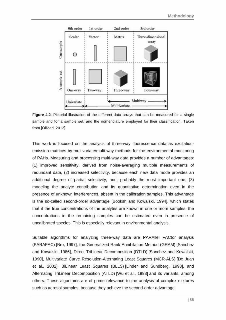
Methodology

| 85

Figure 4.2 . Pictorial illustration of the different data arrays that can be measured for a single

sample and for a sample set, and the nomenclature employed for their classification. Taken

from [Olivieri, 2012].

This work is focused on the analysis of three-way fluorescence data as excitation-

emission matrices by multivariate/multi-way methods for the environmental monitoring

of PAHs. Measuring and processing multi-way data provides a number of advantages:

(1) improved sensitivity, derived from noise-averaging multiple measurements of

redundant data, (2) increased selectivity, because each new data mode provides an

additional degree of partial selectivity, and, probably the most important one, (3)

modeling the analyte contribution and its quantitative determination even in the

presence of unknown interferences, absent in the calibration samples. This advantage

is the so-called second-order advantage [Booksh and Kowalski, 1994], which states

that if the true concentrations of the analytes are known in one or more samples, the

concentrations in the remaining samples can be estimated even in presence of

uncalibrated species. This is especially relevant in environmental analysis.

Suitable algorithms for analyzing three-way data are PARAllel FACtor analysis

(PARAFAC) [Bro, 1997], the Generalized Rank Annihilation Method (GRAM) [Sanchez

and Kowalski, 1986], Direct TriLinear Decomposition (DTLD) [Sanchez and Kowalski,

1990], Multivariate Curve Resolution-Alternating Least Squares (MCR-ALS) [De Juan

et al., 2002], BiLinear Least Squares (BLLS) [Linder and Sundberg, 1998], and

Alternating TriLinear Decomposition (ATLD) [Wu et al., 1998] and its variants, among

others. These algorithms are of prime relevance to the analysis of complex mixtures

such as aerosol samples, because they achieve the second-order advantage.

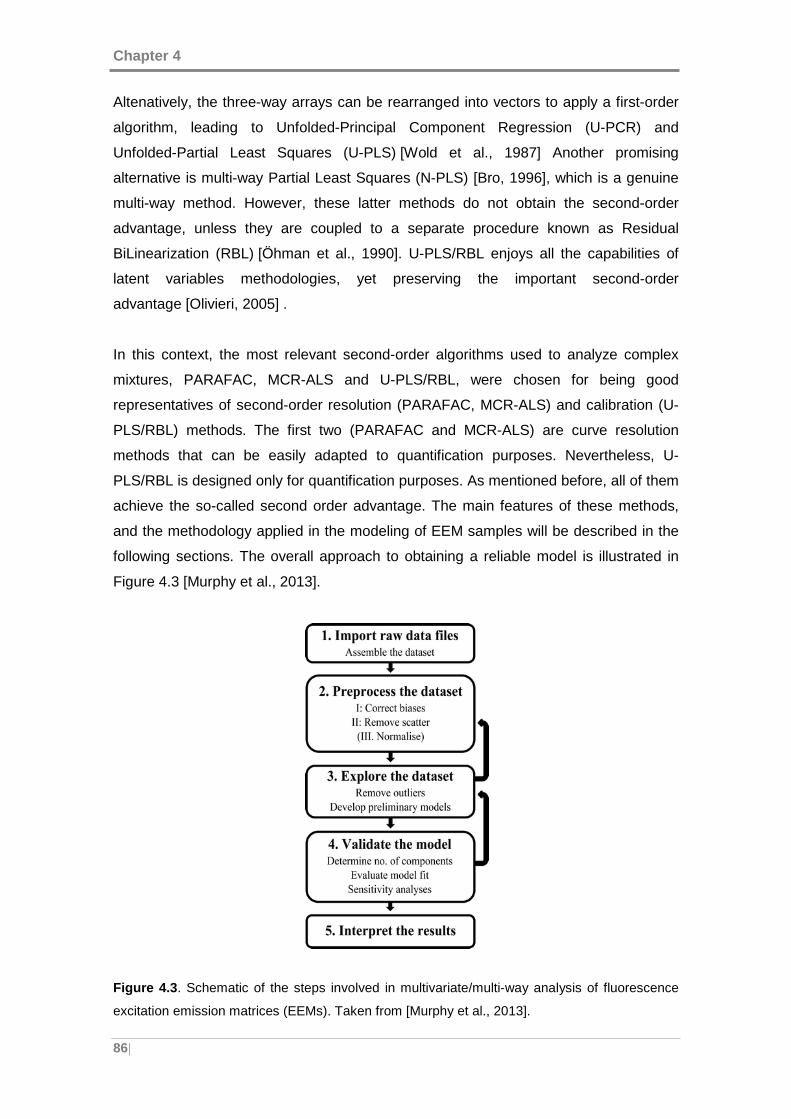
Chapter 4

86|

Altenatively, the three-way arrays can be rearranged into vectors to apply a first-order

algorithm, leading to Unfolded-Principal Component Regression (U-PCR) and

Unfolded-Partial Least Squares (U-PLS) [Wold et al., 1987] Another promising

alternative is multi-way Partial Least Squares (N-PLS) [Bro, 1996], which is a genuine

multi-way method. However, these latter methods do not obtain the second-order

advantage, unless they are coupled to a separate procedure known as Residual

BiLinearization (RBL) [Öhman et al., 1990]. U-PLS/RBL enjoys all the capabilities of

latent variables methodologies, yet preserving the important second-order

advantage [Olivieri, 2005] .

In this context, the most relevant second-order algorithms used to analyze complex

mixtures, PARAFAC, MCR-ALS and U-PLS/RBL, were chosen for being good

representatives of second-order resolution (PARAFAC, MCR-ALS) and calibration (U-

PLS/RBL) methods. The first two (PARAFAC and MCR-ALS) are curve resolution

methods that can be easily adapted to quantification purposes. Nevertheless, U-

PLS/RBL is designed only for quantification purposes. As mentioned before, all of them

achieve the so-called second order advantage. The main features of these methods,

and the methodology applied in the modeling of EEM samples will be described in the

following sections. The overall approach to obtaining a reliable model is illustrated in

Figure 4.3 [Murphy et al., 2013].

Figure 4.3 . Schematic of the steps involved in multivariate/multi-way analysis of fluorescence

excitation emission matrices (EEMs). Taken from [Murphy et al., 2013].

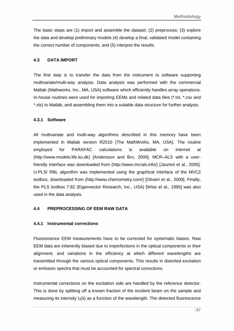
Methodology

| 87

The basic steps are (1) import and assemble the dataset; (2) preprocess; (3) explore

the data and develop preliminary models (4) develop a final, validated model containing

the correct number of components, and (5) interpret the results.

4.3 DATA IMPORT

The first step is to transfer the data from the instrument to software supporting

multivariate/multi-way analysis. Data analysis was performed with the commercial

Matlab (Mathworks, Inc., MA, USA) software which efficiently handles array operations.

In-house routines were used for importing EEMs and related data files (*.txt, *.csv and

*.xls) to Matlab, and assembling them into a suitable data structure for further analysis.

4.3.1 Software

All multivariate and multi-way algorithms described in this memory have been

implemented in Matlab version R2010 (The MathWorks, MA, USA). The routine

employed for PARAFAC calculations is available on internet at

(http://www.models.life.ku.dk) [Andersson and Bro, 2000]. MCR–ALS with a user-

friendly interface was downloaded from (http://www.mcrals.info/) [Jaumot et al., 2005].

U-PLS/ RBL algorithm was implemented using the graphical interface of the MVC2

toolbox, downloaded from (http://www.chemometry.com/) [Olivieri et al., 2009]. Finally,

the PLS toolbox 7.82 (Eigenvector Research, Inc., USA) [Wise et al., 1995] was also

used in the data analysis.

4.4 PREPROCESSING OF EEM RAW DATA

4.4.1 Instrumental corrections

Fluorescence EEM measurements have to be corrected for systematic biases. Raw

EEM data are inherently biased due to imperfections in the optical components or their

alignment, and variations in the efficiency at which different wavelengths are

transmitted through the various optical components. This results in distorted excitation

or emission spectra that must be accounted for spectral corrections.

Instrumental corrections on the excitation side are handled by the reference detector.

This is done by splitting off a known fraction of the incident beam on the sample and

measuring its intensity I0(λ) as a function of the wavelength. The detected fluorescence

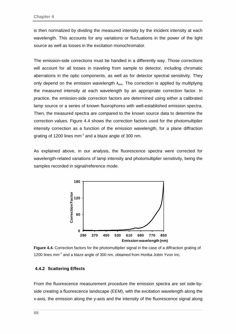
Chapter 4

88|

is then normalized by dividing the measured intensity by the incident intensity at each

wavelength. This accounts for any variations or fluctuations in the power of the light

source as well as losses in the excitation monochromator.

The emission-side corrections must be handled in a differently way. Those corrections

will account for all losses in traveling from sample to detector, including chromatic

aberrations in the optic components, as well as for detector spectral sensitivity. They

only depend on the emission wavelength λem. The correction is applied by multiplying

the measured intensity at each wavelength by an appropriate correction factor. In

practice, the emission-side correction factors are determined using either a calibrated

lamp source or a series of known fluorophores with well-established emission spectra.

Then, the measured spectra are compared to the known source data to determine the

correction values. Figure 4.4 shows the correction factors used for the photomultiplier

intensity correction as a function of the emission wavelength, for a plane diffraction

grating of 1200 lines mm-1 and a blaze angle of 300 nm.

As explained above, in our analysis, the fluorescence spectra were corrected for

wavelength-related variations of lamp intensity and photomultiplier sensitivity, being the

samples recorded in signal/reference mode.

Figure 4.4. Correction factors for the photomultiplier signal in the case of a diffraction grating of

1200 lines mm-1 and a blaze angle of 300 nm, obtained from Horiba Jobin Yvon Inc.

4.4.2 Scattering Effects

From the fluorescence measurement procedure the emission spectra are set side-by-

side creating a fluorescence landscape (EEM), with the excitation wavelength along the

x-axis, the emission along the y-axis and the intensity of the fluorescence signal along

0

60

120

180

290 370 450 530 610 690 770 850

Cor

rect

ion

Fac

tor

Emission wavelength (nm)

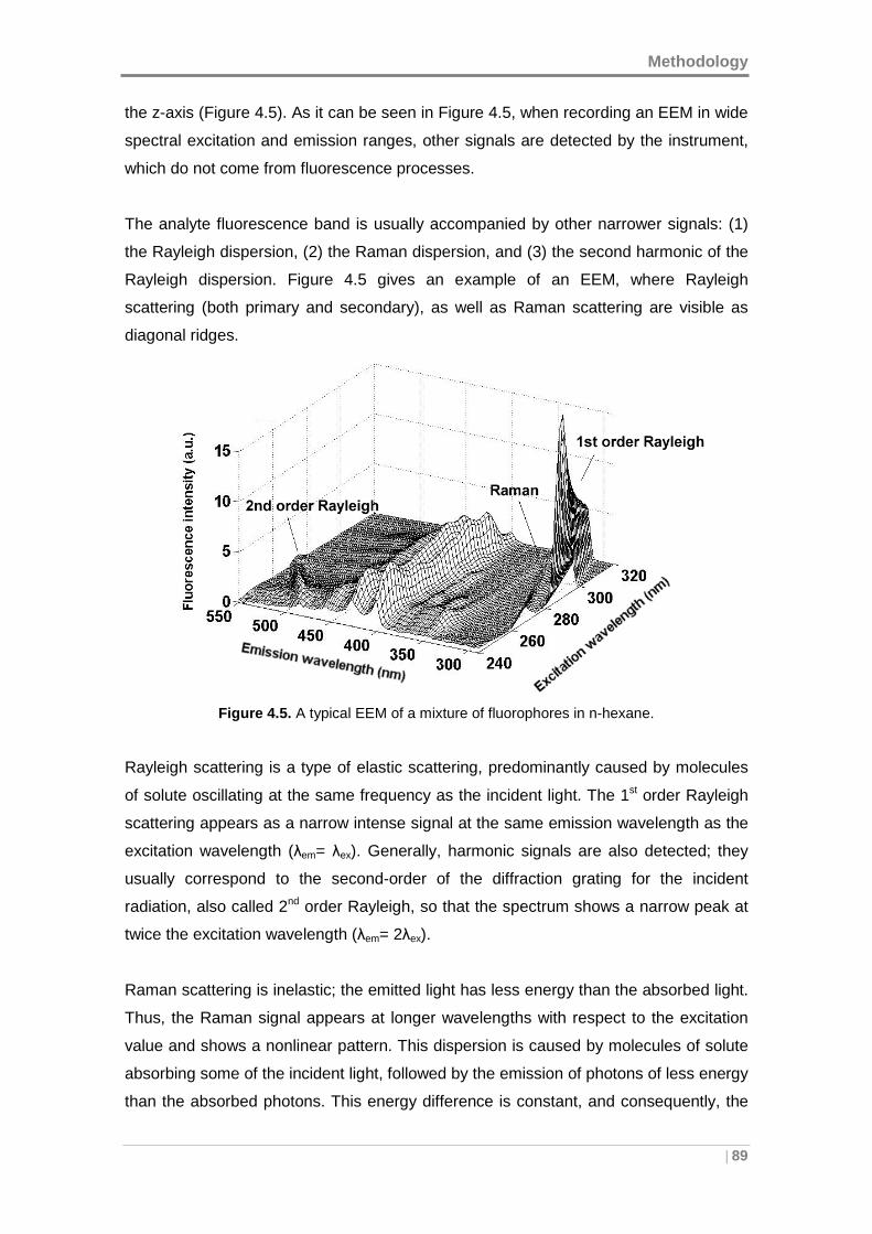
Methodology

| 89

the z-axis (Figure 4.5). As it can be seen in Figure 4.5, when recording an EEM in wide

spectral excitation and emission ranges, other signals are detected by the instrument,

which do not come from fluorescence processes.

The analyte fluorescence band is usually accompanied by other narrower signals: (1)

the Rayleigh dispersion, (2) the Raman dispersion, and (3) the second harmonic of the

Rayleigh dispersion. Figure 4.5 gives an example of an EEM, where Rayleigh

scattering (both primary and secondary), as well as Raman scattering are visible as

diagonal ridges.

Figure 4.5. A typical EEM of a mixture of fluorophores in n-hexane.

Rayleigh scattering is a type of elastic scattering, predominantly caused by molecules

of solute oscillating at the same frequency as the incident light. The 1st order Rayleigh

scattering appears as a narrow intense signal at the same emission wavelength as the

excitation wavelength (λem= λex). Generally, harmonic signals are also detected; they

usually correspond to the second-order of the diffraction grating for the incident

radiation, also called 2nd order Rayleigh, so that the spectrum shows a narrow peak at

twice the excitation wavelength (λem= 2λex).

Raman scattering is inelastic; the emitted light has less energy than the absorbed light.

Thus, the Raman signal appears at longer wavelengths with respect to the excitation

value and shows a nonlinear pattern. This dispersion is caused by molecules of solute

absorbing some of the incident light, followed by the emission of photons of less energy

than the absorbed photons. This energy difference is constant, and consequently, the

Chapter 4

90|

Raman scattering pattern is at a constant energy loss from the elastic Rayleigh

scattering pattern throughout the EEM landscape (Figure 4.5). This energy loss is

dependent on the solute. The energy difference between the excitation and Raman

dispersion, measured in frequency units, is on the order of a vibrational frequency of

the solvent molecule. For instance, the distance between the first-order Rayleigh and

the Raman scattering line for water is 3600 cm−1. This information can be also used in

the analysis of EEM data to separate the Raman scattering line from the signal of the

fluorophores.

The light scattering processes described above are unwanted in the analysis of EEM

data, because they do not hold any chemical information about the fluorophores in the

solution. Moreover, while the EEM analyte signal is trilinear, these scattering effects

are not trilinear, so they can disturb the mathematical modeling of the chemical

compounds. Therefore, it is advisable to remove or reduce the influence of these

scattering effects before modeling.

There are several ways of removing the Rayleigh or Raman scattering: down-weighting

of the scattering region (Maximum likelihood via Iterative Least squares EStimation,

MILES) [Bro et al., 2002], specific modeling of scattering [Rinnan et al., 2005],

subtraction of a standard [McKnight et al., 2001], application of constraints in the

decomposition [Andersen and Bro, 2003], inserting missing values [Christensen et al.,

2003], or inserting zeros outside the data area [Thygesen et al., 2004]. Among these,

the most commonly used consists of subtracting the spectrum of the solvent (if it is

available), to minimize the Raman scattering, and then, replacing the Rayleigh affected

areas by missing values [Munck et al., 1998]. Another possibility consists of replacing

the removed scattering areas with interpolated values.

Therefore, since one important part of analyzing EEM data is the proper handling of

Rayleigh and Raman scattering, here the two most common methods of handling

scattering have been evaluated and compared: replacing the scattering area with

missing elements or with interpolated values. A comparison of how missing or

interpolated data can affect the modeling of EEMs is given in section 5.2.1. Thus, all

the EEM data have been preprocessed to remove the scattering effects before

modeling, which is described in section 4.5.

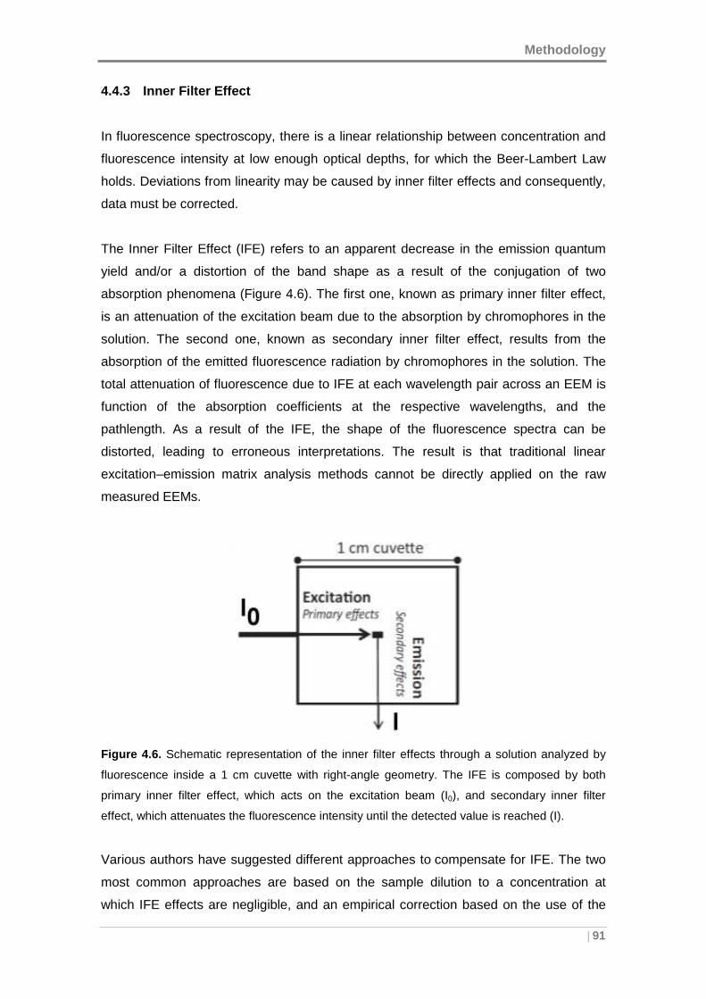
Methodology

| 91

4.4.3 Inner Filter Effect

In fluorescence spectroscopy, there is a linear relationship between concentration and

fluorescence intensity at low enough optical depths, for which the Beer-Lambert Law

holds. Deviations from linearity may be caused by inner filter effects and consequently,

data must be corrected.

The Inner Filter Effect (IFE) refers to an apparent decrease in the emission quantum

yield and/or a distortion of the band shape as a result of the conjugation of two

absorption phenomena (Figure 4.6). The first one, known as primary inner filter effect,

is an attenuation of the excitation beam due to the absorption by chromophores in the

solution. The second one, known as secondary inner filter effect, results from the

absorption of the emitted fluorescence radiation by chromophores in the solution. The

total attenuation of fluorescence due to IFE at each wavelength pair across an EEM is

function of the absorption coefficients at the respective wavelengths, and the

pathlength. As a result of the IFE, the shape of the fluorescence spectra can be

distorted, leading to erroneous interpretations. The result is that traditional linear

excitation–emission matrix analysis methods cannot be directly applied on the raw

measured EEMs.

Figure 4.6. Schematic representation of the inner filter effects through a solution analyzed by

fluorescence inside a 1 cm cuvette with right-angle geometry. The IFE is composed by both

primary inner filter effect, which acts on the excitation beam (I0), and secondary inner filter

effect, which attenuates the fluorescence intensity until the detected value is reached (I).

Various authors have suggested different approaches to compensate for IFE. The two

most common approaches are based on the sample dilution to a concentration at

which IFE effects are negligible, and an empirical correction based on the use of the

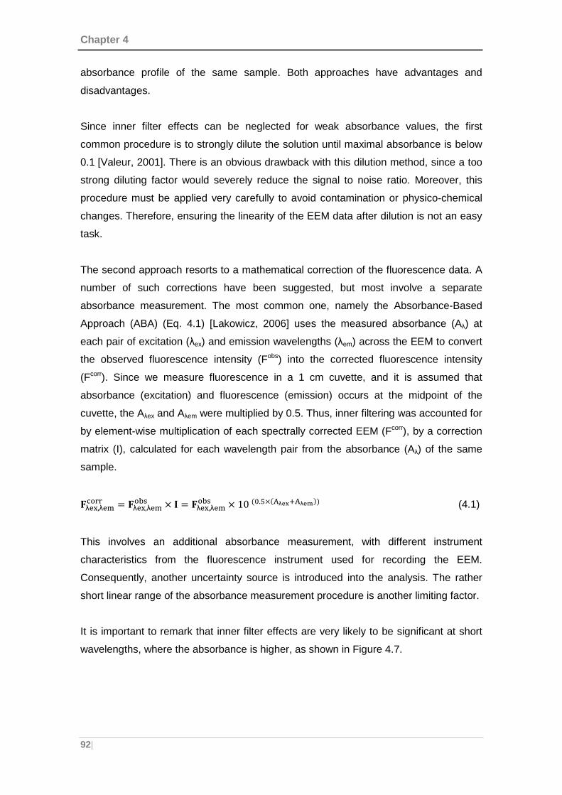
Chapter 4

92|

absorbance profile of the same sample. Both approaches have advantages and

disadvantages.

Since inner filter effects can be neglected for weak absorbance values, the first

common procedure is to strongly dilute the solution until maximal absorbance is below

0.1 [Valeur, 2001]. There is an obvious drawback with this dilution method, since a too

strong diluting factor would severely reduce the signal to noise ratio. Moreover, this

procedure must be applied very carefully to avoid contamination or physico-chemical

changes. Therefore, ensuring the linearity of the EEM data after dilution is not an easy

task.

The second approach resorts to a mathematical correction of the fluorescence data. A

number of such corrections have been suggested, but most involve a separate

absorbance measurement. The most common one, namely the Absorbance-Based

Approach (ABA) (Eq. 4.1) [Lakowicz, 2006] uses the measured absorbance (Aλ) at

each pair of excitation (λex) and emission wavelengths (λem) across the EEM to convert

the observed fluorescence intensity (Fobs) into the corrected fluorescence intensity

(Fcorr). Since we measure fluorescence in a 1 cm cuvette, and it is assumed that

absorbance (excitation) and fluorescence (emission) occurs at the midpoint of the

cuvette, the Aλex and Aλem were multiplied by 0.5. Thus, inner filtering was accounted for

by element-wise multiplication of each spectrally corrected EEM (Fcorr), by a correction

matrix (I), calculated for each wavelength pair from the absorbance (Aλ) of the same

sample.

�λ�,λ�� = �λ�,λ�� × � = �λ�,λ�� × 10(�.�×(�λ !"�λ #$$ (4.1)

This involves an additional absorbance measurement, with different instrument

characteristics from the fluorescence instrument used for recording the EEM.

Consequently, another uncertainty source is introduced into the analysis. The rather

short linear range of the absorbance measurement procedure is another limiting factor.

It is important to remark that inner filter effects are very likely to be significant at short

wavelengths, where the absorbance is higher, as shown in Figure 4.7.

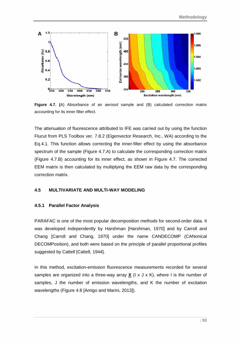
Methodology

| 93

Figure 4.7. ( A) Absorbance of an aerosol sample and (B) calculated correction matrix

accounting for its inner filter effect.

The attenuation of fluorescence attributed to IFE was carried out by using the function

Flucut from PLS Toolbox ver. 7.8.2 (Eigenvector Research, Inc., WA) according to the

Eq.4.1. This function allows correcting the inner-filter effect by using the absorbance

spectrum of the sample (Figure 4.7.A) to calculate the corresponding correction matrix

(Figure 4.7.B) accounting for its inner effect, as shown in Figure 4.7. The corrected

EEM matrix is then calculated by multiplying the EEM raw data by the corresponding

correction matrix.

4.5 MULTIVARIATE AND MULTI-WAY MODELING

4.5.1 Parallel Factor Analysis

PARAFAC is one of the most popular decomposition methods for second-order data. It

was developed independently by Harshman [Harshman, 1970] and by Carroll and

Chang [Carroll and Chang, 1970] under the name CANDECOMP (CANonical

DECOMPosition), and both were based on the principle of parallel proportional profiles

suggested by Cattell [Cattell, 1944].

In this method, excitation-emission fluorescence measurements recorded for several

samples are organized into a three-way array X (I x J x K), where I is the number of

samples, J the number of emission wavelengths, and K the number of excitation

wavelengths (Figure 4.8 [Amigo and Marini, 2013]).

AA

B

Chapter 4

94|

Figure 4.8 . Example of the arrangement of excitation-emission data into a three-way array.

Taken from [Amigo and Marini, 2013].

The structure of the EEM data, two independent sets of variables (excitation and

emission profiles) and one variable dependent on both spectral profiles (concentration

profiles), fulfills the requirement of trilinearity required by PARAFAC, if no uncontrolled

effects/artifacts are present in the samples. Trilinearity assumes that the measured

signal is the sum of the individual peaks of each analyte and that the profiles in each

mode for the analytes are proportional in all the samples [Smilde et al., 2004].

Therefore, for the EEM dataset (X), each responsive component (f) can be defined by a

triad of profiles: one score vector representing the relative concentration of the samples

(af) and two loading vectors (for the emission (b f) and the excitation (c f) modes).

Then, the PARAFAC model decomposes the data array X as indicated in Eq.4.2:

x�&' = ∑ a�)*)�� b&)c') + e�&' (4.2)

where xijk is the fluorescence intensity of the ith sample, at the kth excitation and the jth

emission wavelength. The number of columns in the loading matrices (F) is the number

of PARAFAC factors and eijk the related residual (Figure 4.9 [Amigo and Marini,

2013]).

X (J,K)

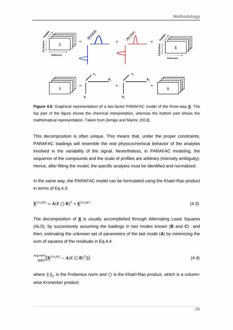
Methodology

| 95

Figure 4.9. Graphical representation of a two-factor PARAFAC model of the three-way X. The

top part of the figure shows the chemical interpretation, whereas the bottom part shows the

mathematical representation. Taken from [Amigo and Marini, 2013].

This decomposition is often unique. This means that, under the proper constraints,

PARAFAC loadings will resemble the real physicochemical behavior of the analytes

involved in the variability of the signal. Nevertheless, in PARAFAC modeling, the

sequence of the compounds and the scale of profiles are arbitrary (intensity ambiguity).

Hence, after fitting the model, the specific analytes must be identified and normalized.

In the same way, the PARAFAC model can be formulated using the Khatri-Rao product

in terms of Eq.4.3:

/(0×12$ = 3(4⊙ 6$7 + 8(0×12$ (4.3)

The decomposition of X is usually accomplished through Alternating Least Squares

(ALS), by successively assuming the loadings in two modes known (B and C) and

then, estimating the unknown set of parameters of the last mode (A) by minimizing the

sum of squares of the residuals in Eq.4.4.

9/(0×12$ : 3(4⊙ 6$7‖<=>,?,@A�BCDE (4.4)

where ‖F‖< is the Frobenius norm and ⊙ is the Khatri-Rao product, which is a column-

wise Kronecker product.

Chapter 4

96|

There are two main facts to consider in this iterative process. The first fact is the need

of initial estimations. Good starting values help to speed up the algorithm and decrease

the risk of converging to a local minimum. Several possible kinds of initializations have

been proposed in the literature [Bro, 1998]. These include the use of random starting

values, the Direct TriLinear Decomposition/Generalized Rank Annihilation Methods

(DTLD/GRAM), Singular Value Decomposition (SVD), orthogonalized random

numbers, or the best-fitting model of many small runs or even using old values. The

second fact is that an end point of iterations has to be established. That is, the point in

which the obtained reconstructed data are most similar to the original ones. In most

cases, a stopping criterion of 10-6 is chosen to assure that the absolute minimum in the

iterations has been reached. If the model parameters are very difficult to estimate, a

lower criterion may be chosen.

Specifically, in this research work, the initialization of the PARAFAC models was

usually made by using the best-fitting model of several models fitted using a few

iterations. Additionally, a relative change in fit of less than 10-6 was set as a suitable

stopping criterion.

A critical stage to build a PARAFAC model is the determination of the number of

factors in the model which are necessary to reconstruct the data [Christensen et al.,

2006]. This is, probably, the most crucial and complex step. Extracting too few factors

(under-fitted model) is usually detected by the non-random distribution of the residuals

and their values. On the contrary, extracting too many factors (over-fitted model) does

not only mean that noise is being increasingly modeled, but also that the true factors

are being modeled by more (correlated) factors [Bro, 1997].

There are multiple criteria to do this estimation and it is extremely advisable the

combined use of several of them. In this work, the CORe CONsistency DIAgnostic test

(CORCONDIA), which is 100% for a completely trilinear model [Bro and Kiers, 2003],

the percentage of lack of fit and the variance explained by the model, the residual

analysis and previous chemical knowledge of the data when available (such as the

quality of the recovered spectral loadings assessed by a correlation coefficient (r) with

reference spectral shapes), have been used (section 4.6.1).

The core consistency diagnostic test indicates how well the model is in concert with the

distribution of superdiagonal and off-superdiagonal elements of the Tucker3 core. If the

PARAFAC model is correct, then it is expected that the superdiagonal elements will be

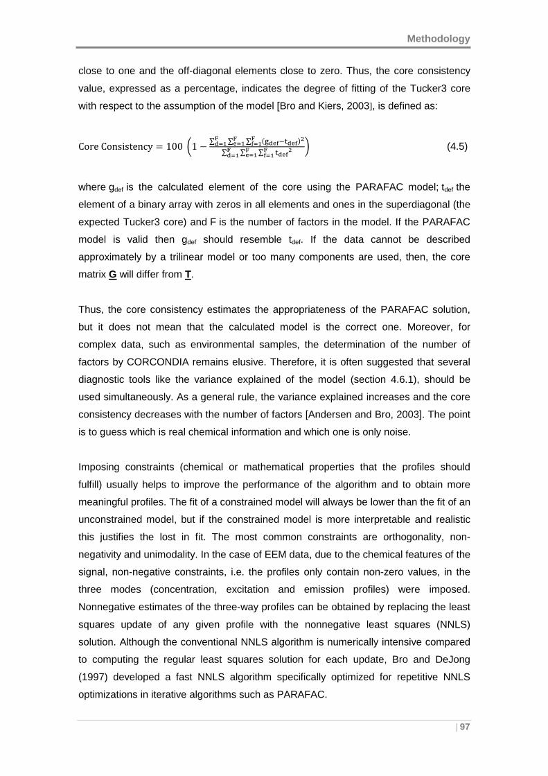
Methodology

| 97

close to one and the off-diagonal elements close to zero. Thus, the core consistency

value, expressed as a percentage, indicates the degree of fitting of the Tucker3 core

with respect to the assumption of the model [Bro and Kiers, 2003], is defined as:

Core Consistency = 100 N1 : ∑ ∑ ∑ (BO PQRO P$STPUVT UVTOUV∑ ∑ ∑ RO PSTPUVT UVTOUV W (4.5)

where gdef is the calculated element of the core using the PARAFAC model; tdef the

element of a binary array with zeros in all elements and ones in the superdiagonal (the

expected Tucker3 core) and F is the number of factors in the model. If the PARAFAC

model is valid then gdef should resemble tdef. If the data cannot be described

approximately by a trilinear model or too many components are used, then, the core

matrix G will differ from T.

Thus, the core consistency estimates the appropriateness of the PARAFAC solution,

but it does not mean that the calculated model is the correct one. Moreover, for

complex data, such as environmental samples, the determination of the number of

factors by CORCONDIA remains elusive. Therefore, it is often suggested that several

diagnostic tools like the variance explained of the model (section 4.6.1), should be

used simultaneously. As a general rule, the variance explained increases and the core

consistency decreases with the number of factors [Andersen and Bro, 2003]. The point

is to guess which is real chemical information and which one is only noise.

Imposing constraints (chemical or mathematical properties that the profiles should

fulfill) usually helps to improve the performance of the algorithm and to obtain more

meaningful profiles. The fit of a constrained model will always be lower than the fit of an

unconstrained model, but if the constrained model is more interpretable and realistic

this justifies the lost in fit. The most common constraints are orthogonality, non-

negativity and unimodality. In the case of EEM data, due to the chemical features of the

signal, non-negative constraints, i.e. the profiles only contain non-zero values, in the

three modes (concentration, excitation and emission profiles) were imposed.

Nonnegative estimates of the three-way profiles can be obtained by replacing the least

squares update of any given profile with the nonnegative least squares (NNLS)

solution. Although the conventional NNLS algorithm is numerically intensive compared

to computing the regular least squares solution for each update, Bro and DeJong

(1997) developed a fast NNLS algorithm specifically optimized for repetitive NNLS

optimizations in iterative algorithms such as PARAFAC.

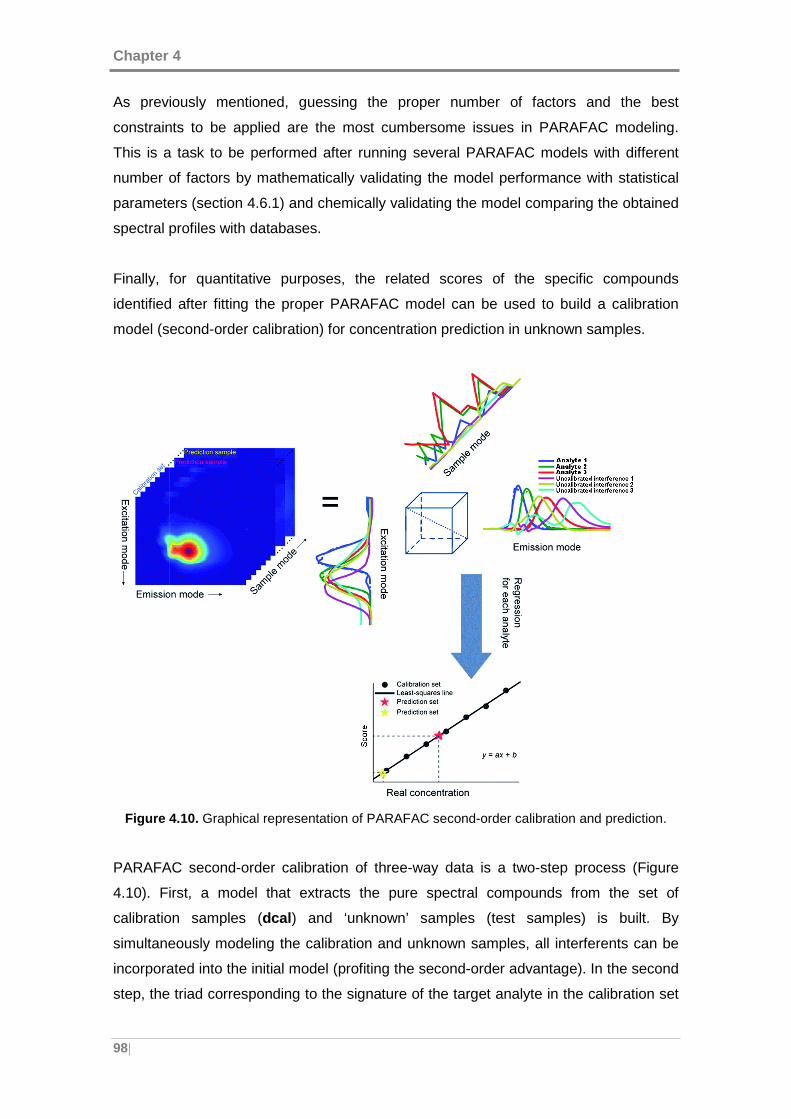
Chapter 4

98|

As previously mentioned, guessing the proper number of factors and the best

constraints to be applied are the most cumbersome issues in PARAFAC modeling.

This is a task to be performed after running several PARAFAC models with different

number of factors by mathematically validating the model performance with statistical

parameters (section 4.6.1) and chemically validating the model comparing the obtained

spectral profiles with databases.

Finally, for quantitative purposes, the related scores of the specific compounds

identified after fitting the proper PARAFAC model can be used to build a calibration

model (second-order calibration) for concentration prediction in unknown samples.

Figure 4.10. Graphical representation of PARAFAC second-order calibration and prediction.

PARAFAC second-order calibration of three-way data is a two-step process (Figure

4.10). First, a model that extracts the pure spectral compounds from the set of

calibration samples (dcal ) and ‘unknown’ samples (test samples) is built. By

simultaneously modeling the calibration and unknown samples, all interferents can be

incorporated into the initial model (profiting the second-order advantage). In the second

step, the triad corresponding to the signature of the target analyte in the calibration set

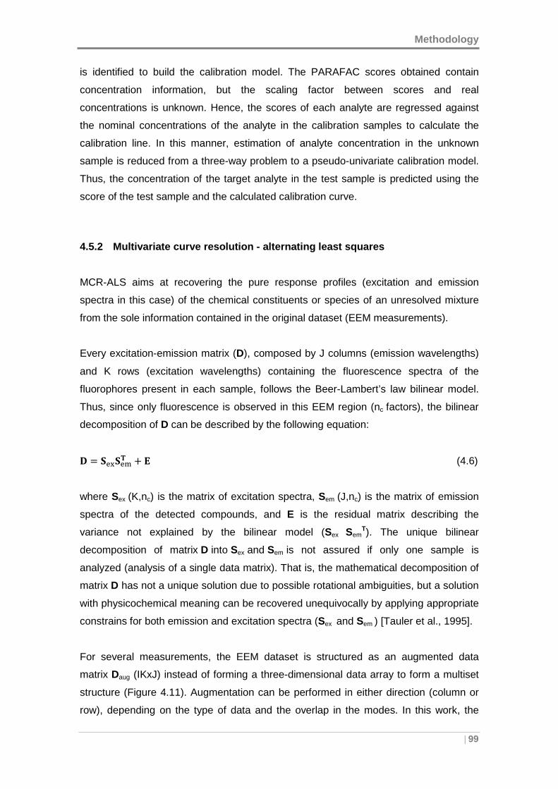
Methodology

| 99

is identified to build the calibration model. The PARAFAC scores obtained contain

concentration information, but the scaling factor between scores and real

concentrations is unknown. Hence, the scores of each analyte are regressed against

the nominal concentrations of the analyte in the calibration samples to calculate the

calibration line. In this manner, estimation of analyte concentration in the unknown

sample is reduced from a three-way problem to a pseudo-univariate calibration model.

Thus, the concentration of the target analyte in the test sample is predicted using the

score of the test sample and the calculated calibration curve.

4.5.2 Multivariate curve resolution - alternating l east squares

MCR-ALS aims at recovering the pure response profiles (excitation and emission

spectra in this case) of the chemical constituents or species of an unresolved mixture

from the sole information contained in the original dataset (EEM measurements).

Every excitation-emission matrix (D), composed by J columns (emission wavelengths)

and K rows (excitation wavelengths) containing the fluorescence spectra of the

fluorophores present in each sample, follows the Beer-Lambert’s law bilinear model.

Thus, since only fluorescence is observed in this EEM region (nc factors), the bilinear

decomposition of D can be described by the following equation:

_ = `�`�a + 8 (4.6)

where Sex (K,nc) is the matrix of excitation spectra, Sem

(J,nc) is the matrix of emission

spectra of the detected compounds, and E is the residual matrix describing the

variance not explained by the bilinear model (Sex SemT). The unique bilinear

decomposition of matrix D into Sex and Sem is not assured if only one sample is

analyzed (analysis of a single data matrix). That is, the mathematical decomposition of

matrix D has not a unique solution due to possible rotational ambiguities, but a solution

with physicochemical meaning can be recovered unequivocally by applying appropriate

constrains for both emission and excitation spectra (Sex and Sem ) [Tauler et al., 1995].

For several measurements, the EEM dataset is structured as an augmented data

matrix Daug (IKxJ) instead of forming a three-dimensional data array to form a multiset

structure (Figure 4.11). Augmentation can be performed in either direction (column or

row), depending on the type of data and the overlap in the modes. In this work, the

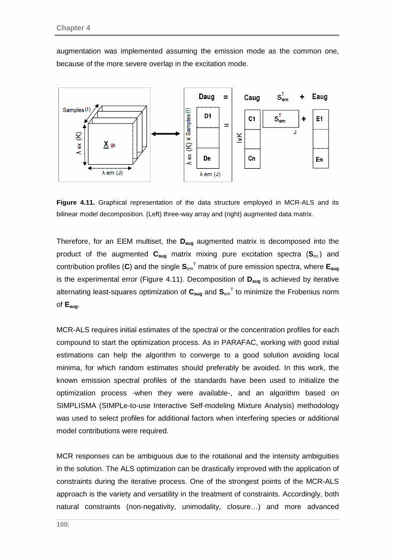
Chapter 4

100|

augmentation was implemented assuming the emission mode as the common one,

because of the more severe overlap in the excitation mode.

Figure 4.11. Graphical representation of the data structure employed in MCR-ALS and its

bilinear model decomposition. (Left) three-way array and (right) augmented data matrix.

Therefore, for an EEM multiset, the Daug augmented matrix is decomposed into the

product of the augmented Caug matrix mixing pure excitation spectra (Sex ) and

contribution profiles (C) and the single SemT matrix of pure emission spectra, where Eaug

is the experimental error (Figure 4.11). Decomposition of Daug is achieved by iterative

alternating least-squares optimization of Caug and SemT to minimize the Frobenius norm

of Eaug.

MCR-ALS requires initial estimates of the spectral or the concentration profiles for each

compound to start the optimization process. As in PARAFAC, working with good initial

estimations can help the algorithm to converge to a good solution avoiding local

minima, for which random estimates should preferably be avoided. In this work, the

known emission spectral profiles of the standards have been used to initialize the

optimization process -when they were available-, and an algorithm based on

SIMPLISMA (SIMPLe-to-use Interactive Self-modeling Mixture Analysis) methodology

was used to select profiles for additional factors when interfering species or additional

model contributions were required.

MCR responses can be ambiguous due to the rotational and the intensity ambiguities

in the solution. The ALS optimization can be drastically improved with the application of

constraints during the iterative process. One of the strongest points of the MCR-ALS

approach is the variety and versatility in the treatment of constraints. Accordingly, both

natural constraints (non-negativity, unimodality, closure…) and more advanced

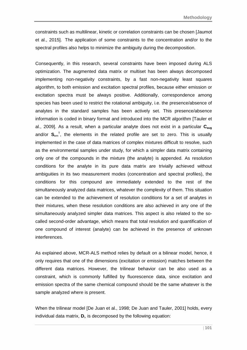
Methodology

| 101

constraints such as multilinear, kinetic or correlation constraints can be chosen [Jaumot

et al., 2015]. The application of some constraints to the concentration and/or to the

spectral profiles also helps to minimize the ambiguity during the decomposition.

Consequently, in this research, several constraints have been imposed during ALS

optimization. The augmented data matrix or multiset has been always decomposed

implementing non-negativity constraints, by a fast non-negativity least squares

algorithm, to both emission and excitation spectral profiles, because either emission or

excitation spectra must be always positive. Additionally, correspondence among

species has been used to restrict the rotational ambiguity, i.e. the presence/absence of

analytes in the standard samples has been actively set. This presence/absence

information is coded in binary format and introduced into the MCR algorithm [Tauler et

al., 2009]. As a result, when a particular analyte does not exist in a particular Caug

and/or SemT, the elements in the related profile are set to zero. This is usually

implemented in the case of data matrices of complex mixtures difficult to resolve, such

as the environmental samples under study, for which a simpler data matrix containing

only one of the compounds in the mixture (the analyte) is appended. As resolution

conditions for the analyte in its pure data matrix are trivially achieved without

ambiguities in its two measurement modes (concentration and spectral profiles), the

conditions for this compound are immediately extended to the rest of the

simultaneously analyzed data matrices, whatever the complexity of them. This situation

can be extended to the achievement of resolution conditions for a set of analytes in

their mixtures, when these resolution conditions are also achieved in any one of the

simultaneously analyzed simpler data matrices. This aspect is also related to the so-

called second-order advantage, which means that total resolution and quantification of

one compound of interest (analyte) can be achieved in the presence of unknown

interferences.

As explained above, MCR-ALS method relies by default on a bilinear model, hence, it

only requires that one of the dimensions (excitation or emission) matches between the

different data matrices. However, the trilinear behavior can be also used as a

constraint, which is commonly fulfilled by fluorescence data, since excitation and

emission spectra of the same chemical compound should be the same whatever is the

sample analyzed where is present.

When the trilinear model [De Juan et al., 1998; De Juan and Tauler, 2001] holds, every

individual data matrix, Di, is decomposed by the following equation:

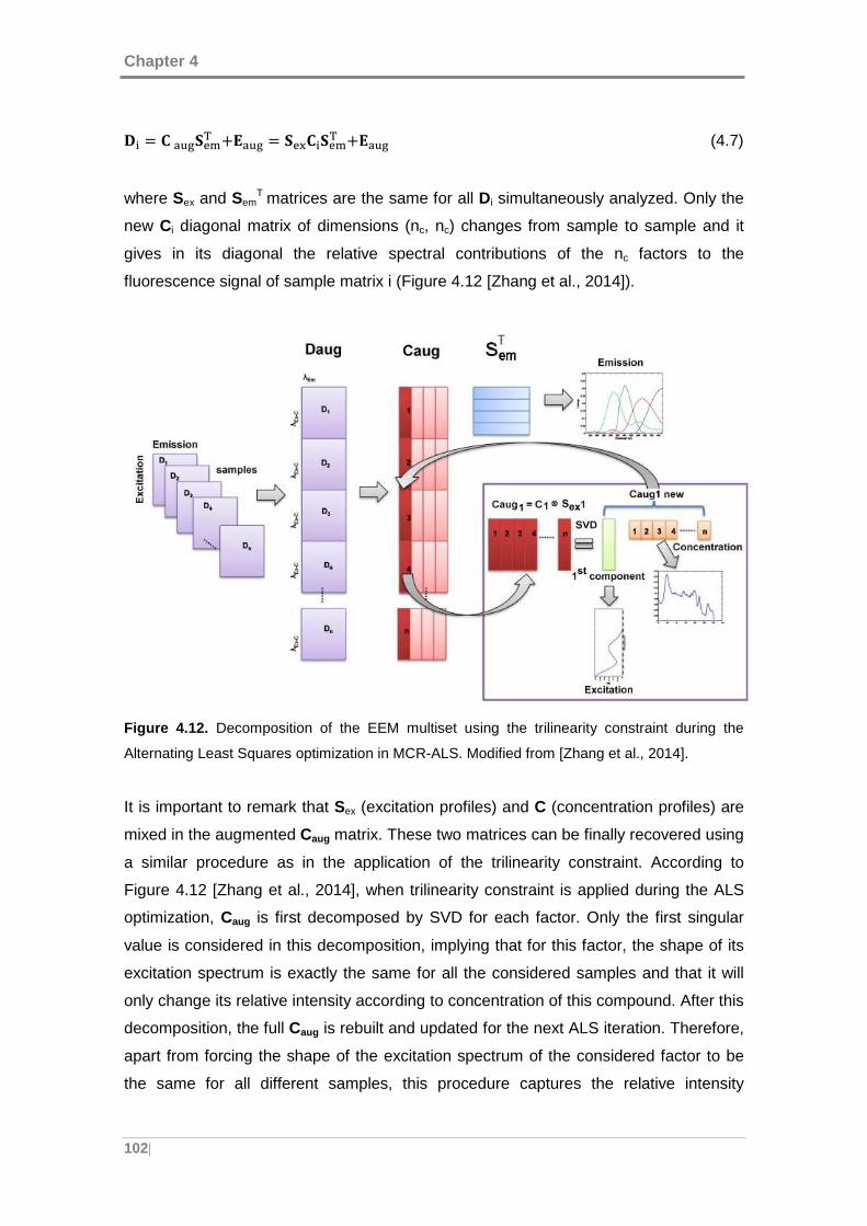
Chapter 4

102|

_� = 4AbB`�c +8AbB = `�4�`�c +8AbB (4.7)

where Sex and SemT matrices are the same for all Di simultaneously analyzed. Only the

new Ci diagonal matrix of dimensions (nc, nc) changes from sample to sample and it

gives in its diagonal the relative spectral contributions of the nc factors to the

fluorescence signal of sample matrix i (Figure 4.12 [Zhang et al., 2014]).

Figure 4.12. Decomposition of the EEM multiset using the trilinearity constraint during the

Alternating Least Squares optimization in MCR-ALS. Modified from [Zhang et al., 2014].

It is important to remark that Sex (excitation profiles) and C (concentration profiles) are

mixed in the augmented Caug matrix. These two matrices can be finally recovered using

a similar procedure as in the application of the trilinearity constraint. According to

Figure 4.12 [Zhang et al., 2014], when trilinearity constraint is applied during the ALS

optimization, Caug is first decomposed by SVD for each factor. Only the first singular

value is considered in this decomposition, implying that for this factor, the shape of its

excitation spectrum is exactly the same for all the considered samples and that it will

only change its relative intensity according to concentration of this compound. After this

decomposition, the full Caug is rebuilt and updated for the next ALS iteration. Therefore,

apart from forcing the shape of the excitation spectrum of the considered factor to be

the same for all different samples, this procedure captures the relative intensity

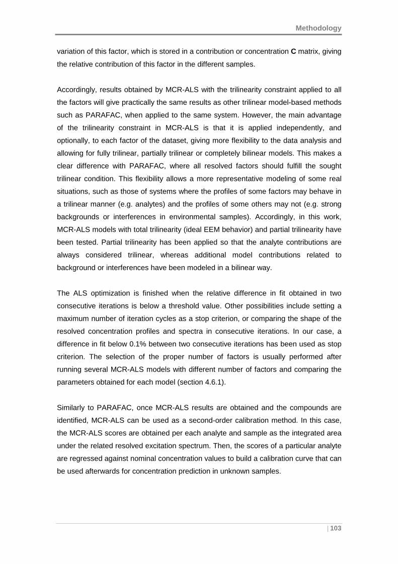
Methodology

| 103

variation of this factor, which is stored in a contribution or concentration C matrix, giving

the relative contribution of this factor in the different samples.

Accordingly, results obtained by MCR-ALS with the trilinearity constraint applied to all

the factors will give practically the same results as other trilinear model-based methods

such as PARAFAC, when applied to the same system. However, the main advantage

of the trilinearity constraint in MCR-ALS is that it is applied independently, and

optionally, to each factor of the dataset, giving more flexibility to the data analysis and

allowing for fully trilinear, partially trilinear or completely bilinear models. This makes a

clear difference with PARAFAC, where all resolved factors should fulfill the sought

trilinear condition. This flexibility allows a more representative modeling of some real

situations, such as those of systems where the profiles of some factors may behave in

a trilinear manner (e.g. analytes) and the profiles of some others may not (e.g. strong

backgrounds or interferences in environmental samples). Accordingly, in this work,

MCR-ALS models with total trilinearity (ideal EEM behavior) and partial trilinearity have

been tested. Partial trilinearity has been applied so that the analyte contributions are

always considered trilinear, whereas additional model contributions related to

background or interferences have been modeled in a bilinear way.

The ALS optimization is finished when the relative difference in fit obtained in two

consecutive iterations is below a threshold value. Other possibilities include setting a

maximum number of iteration cycles as a stop criterion, or comparing the shape of the

resolved concentration profiles and spectra in consecutive iterations. In our case, a

difference in fit below 0.1% between two consecutive iterations has been used as stop

criterion. The selection of the proper number of factors is usually performed after

running several MCR-ALS models with different number of factors and comparing the

parameters obtained for each model (section 4.6.1).

Similarly to PARAFAC, once MCR-ALS results are obtained and the compounds are

identified, MCR-ALS can be used as a second-order calibration method. In this case,

the MCR-ALS scores are obtained per each analyte and sample as the integrated area

under the related resolved excitation spectrum. Then, the scores of a particular analyte

are regressed against nominal concentration values to build a calibration curve that can

be used afterwards for concentration prediction in unknown samples.

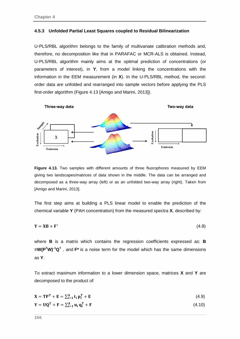
Chapter 4

104|

4.5.3 Unfolded Partial Least Squares coupled to Res idual Bilinearization

U-PLS/RBL algorithm belongs to the family of multivariate calibration methods and,

therefore, no decomposition like that in PARAFAC or MCR-ALS is obtained. Instead,

U-PLS/RBL algorithm mainly aims at the optimal prediction of concentrations (or

parameters of interest), in Y, from a model linking the concentrations with the

information in the EEM measurement (in X). In the U-PLS/RBL method, the second-

order data are unfolded and rearranged into sample vectors before applying the PLS

first-order algorithm (Figure 4.13 [Amigo and Marini, 2013]).

Figure 4.13. Two samples with different amounts of three fluorophores measured by EEM

giving two landscapes/matrices of data shown in the middle. The data can be arranged and

decomposed as a three-way array (left) or as an unfolded two-way array (right). Taken from

[Amigo and Marini, 2013].

The first step aims at building a PLS linear model to enable the prediction of the

chemical variable Y (PAH concentration) from the measured spectra X, described by:

d = /6 + �∗ (4.8)

where B is a matrix which contains the regression coefficients expressed as: B

=W(PTW)−−−−1QT , and F* is a noise term for the model which has the same dimensions

as Y.

To extract maximum information to a lower dimension space, matrices X and Y are

decomposed to the product of:

/ = afa + 8 = ∑ gh3h�i jha + 8 (4.9)

d = kla + � = ∑ mh3h�i nha + � (4.10)

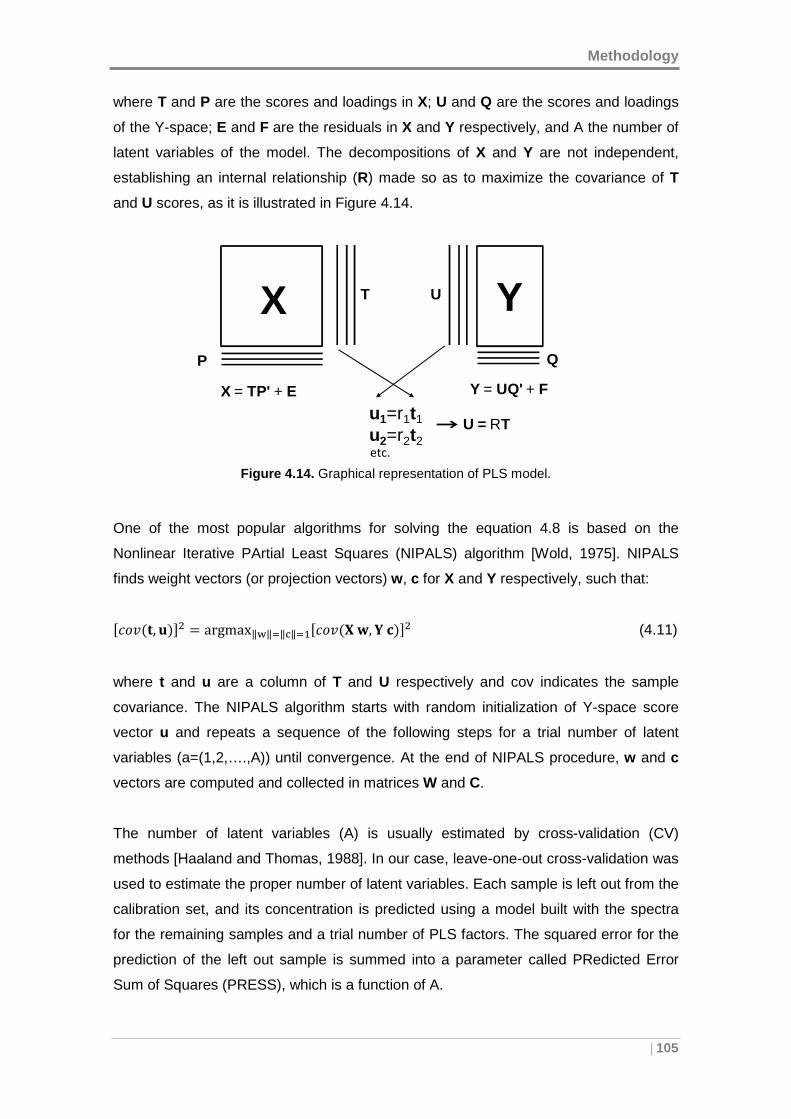
Methodology

| 105

where T and P are the scores and loadings in X; U and Q are the scores and loadings

of the Y-space; E and F are the residuals in X and Y respectively, and A the number of

latent variables of the model. The decompositions of X and Y are not independent,

establishing an internal relationship (R) made so as to maximize the covariance of T

and U scores, as it is illustrated in Figure 4.14.

Figure 4.14. Graphical representation of PLS model.

One of the most popular algorithms for solving the equation 4.8 is based on the

Nonlinear Iterative PArtial Least Squares (NIPALS) algorithm [Wold, 1975]. NIPALS

finds weight vectors (or projection vectors) w, c for X and Y respectively, such that:

oOHp(g, m$q= = argmax‖u‖�‖�‖��oOHp(/v, dw$q= (4.11)

where t and u are a column of T and U respectively and cov indicates the sample

covariance. The NIPALS algorithm starts with random initialization of Y-space score

vector u and repeats a sequence of the following steps for a trial number of latent

variables (a=(1,2,….,A)) until convergence. At the end of NIPALS procedure, w and c

vectors are computed and collected in matrices W and C.

The number of latent variables (A) is usually estimated by cross-validation (CV)

methods [Haaland and Thomas, 1988]. In our case, leave-one-out cross-validation was

used to estimate the proper number of latent variables. Each sample is left out from the

calibration set, and its concentration is predicted using a model built with the spectra

for the remaining samples and a trial number of PLS factors. The squared error for the

prediction of the left out sample is summed into a parameter called PRedicted Error

Sum of Squares (PRESS), which is a function of A.

YX T U

P Q

Y = UQ' + FX = TP' + E

u1=r1t1

u2=r2t2U = RT

etc.

Chapter 4

106|

PRESS = ∑ uy�, �� : y�,v�wx=y�� (4.12)

where I is the number of calibration samples, and “nom” and “pred” stand for nominal

and predicted, respectively.

The PRESS is estimated for values of A ranging from 1 to a certain maximum, larger

than the suspected optimal value. As an example, Figure 4.15 shows the evolution of

the PRESS statistic against the number of latent variables. As shown, PRESS initially

decreases with increasing values of A, but then tends to increase, because the last

latent variables represent noise rather than true chemical effects. Intuitively, one would

select the optimum A as that corresponding to the minimum PRESS, but some

uncertainty is always involved in the cross-validation process, and therefore, in the

PRESS values. The principle of parsimony, popularly known as Ockham’s razor

[Hoffmann et al., 1997], suggests that the optimum A is the minimum value whose

PRESS is not statistically larger than the minimum PRESS.

Figure 4.15. Plot of PRESS against the number of latent variables (A).

In this context, the optimum number of latent variables can be obtained by computing

the following F(A) ratios:

F(A$ = PRESS(A < A∗$/PRESS(A∗$ (4.13)

where A* leads to the minimum PRESS. Then a probability p(A) is assigned to each

F(A), corresponding to the Snedecor’s F value with I degrees of freedom for both the

numerator and denominator. The optimum value of A is selected as the one leading to

a probability of less than 75% (i.e., p(A) < 0.75), and F>1.

In contrast to PARAFAC and MCR-ALS, where the calibration and test samples are

jointly decomposed by the model, U-PLS does not include the unknown samples in the

calibration step. Hence, once the optimum number of latent variables is calculated, a

0 2 4 6 8 10

PR

ES

S

Number of Latent Variables (A)

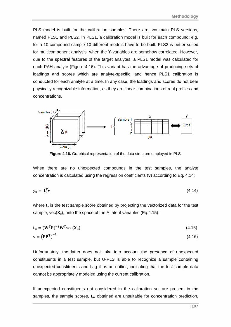
Methodology

| 107

PLS model is built for the calibration samples. There are two main PLS versions,

named PLS1 and PLS2. In PLS1, a calibration model is built for each compound; e.g.

for a 10-compound sample 10 different models have to be built. PLS2 is better suited

for multicomponent analysis, when the Y-variables are somehow correlated. However,

due to the spectral features of the target analytes, a PLS1 model was calculated for

each PAH analyte (Figure 4.16). This variant has the advantage of producing sets of

loadings and scores which are analyte-specific, and hence PLS1 calibration is

conducted for each analyte at a time. In any case, the loadings and scores do not bear

physically recognizable information, as they are linear combinations of real profiles and

concentrations.

Figure 4.16. Graphical representation of the data structure employed in PLS.

When there are no unexpected compounds in the test samples, the analyte

concentration is calculated using the regression coefficients (v) according to Eq. 4.14:

~[ = `[\� (4.14)

where tu is the test sample score obtained by projecting the vectorized data for the test

sample, vec(Xu), onto the space of the A latent variables (Eq.4.15):

`[ = (�\_$Q��\vec(/[) (4.15)

� = u__ZxQb (4.16)

Unfortunately, the latter does not take into account the presence of unexpected

constituents in a test sample, but U-PLS is able to recognize a sample containing

unexpected constituents and flag it as an outlier, indicating that the test sample data

cannot be appropriately modeled using the current calibration.

If unexpected constituents not considered in the calibration set are present in the

samples, the sample scores, tu, obtained are unsuitable for concentration prediction,

Chapter 4

108|

because the residuals of the U-PLS prediction step (sp), will be abnormally large in

comparison with the typical instrumental noise level (Eq.4.17):

�v = 9�v9/(JK : A$� =� = ‖vec(/[$ : _`[‖/(JK : A$� =� (4.17)

Of course this is not the aim of second-order calibration, where we wish to employ

simple calibration sets, and demand to the processing algorithm, not only to recognize

the presence of an unexpected component, but also to model it, remove its contribution

from the test sample, and accurately quantify the analyte, i.e., to achieve the second-

order advantage. Here, a complementary technique was developed to be applied

together with U-PLS, a post-calibration procedure called Residual BiLinearization

(RBL), a name which derives from its intention to model the residues of U-PLS for the

test sample as a sum of bilinear contributions from the unexpected components. The

mission of RBL is to free the “raw” test sample scores from potential interfering effects,

leaving filtered scores, which do only contain information about calibrated constituents,

to be employed in Eq. 4.14 for analyte prediction.

RBL intends to model the residuals (the part of the test sample unexplained by the PLS

model) assuming that they can be arranged into a bilinear matrix, minimizing the norm

of the residual vector eu, computed while fitting the sample data to the sum of the

relevant contributions. For a single unexpected component, the expression is:

vec(/[$ = _`[ + h�[ �g[ �(q[ �$\l + �� (4.18)

where gunx is a scaling factor appropriate for SVD (Single Value Decomposition)

analysis, bunx and cunx are the left and right eigenvectors of the residual matrix ERBL,

obtained after reshaping the computed residual vector eRBL, and assuming that

interferences are absent, as indicated in Eq. 4.19:

�[ �g[ �(q[ �$\ = SVD{reshapehvec(/[$ : _`[l} (4.19)

Specifically, the RBL procedure fits the sample data to the sum of two contributions: (1)

the fraction of the test data which can be explained by the calibration PLS loadings,

and (2) the contribution from potential interferents, modeled by a number of principal

components (NRBL). SVD is performed using the first Nunx principal components, where

Methodology

| 109

Nunx indicates the number of unexpected test sample constituents. When Nunx = 1, the

RBL profiles should be excellent approximations to those for the potential interferents

in each data mode. Unfortunately, for additional unexpected components, these

matrices contain linear combinations of profiles, because they are the result of a SVD

analysis, and these profiles are no longer recognizable as true unexpected profiles.

The RBL procedure consists of maintaining the matrix of loadings P (in

Eq. 4.18) constant at the calibration values, and varying tu in this latter equation (4.19)

to minimize the norm of eRBL (║eRBL║). During the RBL minimization, profiles for the

unexpected constituents are continually updated through Eq. 4.18. Once eRBL is

minimized, the compound concentrations are calculated by Eq. 4.14, introducing the

final tu vector found by the RBL procedure.

U-PLS/RBL is intrinsically more flexible than PARAFAC or MCR–ALS, it can handle

signal-to-concentration changes among samples, which are compensated by adding

more latent variables to the model, as long as they are represented in the calibration

set, and they are not too extreme. But this added flexibility comes at the cost of some

disadvantages. First, its flexibility implies also non-unique solutions, due to rotation

ambiguities in the RBL step. Second, and the most conspicuous one, is the inability of

U-PLS/RBL to render approximations to pure constituent profiles, thereby loosing

chemical interpretability for the sake of accurate analyte quantification.

4.6 VALIDATION OF THE MODELS

Since it is always possible to make a mathematical model of any system, validation of

the built models is a crucial step to make sure that the results can be extrapolated to

new data, and also to decide whether the conclusions drawn from it are reliable.

Validation can be divided into two main types: internal and external. Internal validation

means utilizing the data that has been used to build the model to validate it. External

validation means that new data, not previously used in the model, are used for

validation. As a general rule, the models should be first internally validated

(mathematically), and then they should be externally validated, applying the

constructed model to new datasets. In internal and external validation a number of

statistical parameters are applied and the discussion that follows relies on the

chemometric methods used in this research.

Chapter 4

110|

4.6.1 Internal validation of PARAFAC and MCR-ALS

The quality and reliability of the model solution may be assessed using the variance

explained (r2), and the Lack Of data Fit (LOF), parameters that allow assessing the

dissimilarity among the experimental data and the data modeled.

For PARAFAC, the percentage of variance explained for the assumed number of

factors (F) is calculated by taking into account the sum of the squares of the

residuals, eijk, and the sum of the squares of the elements of the matrix X, xijk, as

follows:

r=(%$ = 100 × Q1 : ∑ ∑ ∑ ¡¢£Z¤£\]¥¢\]¦¡\]∑ ∑ ∑ �¡¢£Z¤£\]¥¢\]¦¡\] ^ (4.20)

The percentage of LOF is calculated according the following equation:

LackofFit(LOF$(%$ = 100x®∑ ∑ ∑ ¡¢£Z¤£\]¥¢\]¦¡\]∑ ∑ ∑ �¡¢£Z¤£\]¥¢\]¦¡\] (4.21)

Similarly, for MCR-ALS the equations defining these two parameters are:

r=(%$ = 100 ×®∑ }¡¢Z¡,¢ W∑ ¡¢Z¡,¢∑ }¡¢Z¡,¢ (4.22)

LackofFit(LOF$(%$ = 100 ×®∑ ¡¢Z¡,¢∑ }¡¢Z¡,¢ (4.23)

where dij is an element of the experimental data matrix and eij is the related residual

value obtained from the difference between the experimental data (matrix D) and the

reproduced data (CST matrix product obtained by MCR-ALS).

The variance explained measures the fraction of the total variability in the response

that is accounted by the model. Thus, the variance explained should be high in order to

consider the built model as reliable.

Methodology

| 111

The lack of fit gives a measure of the fit quality in relative terms with the same units as

the measured data, and is comparable with experimental relative error estimations. A

low lack of fit percentage indicates that a model fits the data well.

Since PARAFAC and MCR-ALS are able to calculate the spectral profiles of the

fluorophores present in the samples, the similarity between the recovered spectral

profiles and the pure spectra of the target PAH compounds is used here also to assess

the performance of the models. This is expressed by the correlation coefficients (rem

and rex) in the emission and excitation modes with the related reference spectra.

Correlation coefficients r=1 indicate a completely similarity between calculated and

pure profiles of the analytes in the samples, calculated in accordance with the following

equation:

I = cos ° = ±²³±̂²‖±²‖∙‖±̂²‖ (4.24)

where ° is the angle defined by the vectors associated with the recovered spectra (L̂D) and the pure spectra (LD) of the studied compound.

4.6.2 Internal validation of U-PLS

In contrast, cross validation methods (section 4.5.3) are used to estimate the predictive

ability of the U-PLS models. The statistical parameters of Table 4.1 are used to

internally validate the U-PLS models. This table shows the progression of the PRESS

values (Eq. 4.12) for an increasing number of latent variables (A), the Standard Error of

Prediction (SEP) and the associated values of the Snedecor’s F statistical indicator and

its probability, p. The last column is the probability associated to Van der Voet’s

randomization test: p < 0.05 indicates that the PRESS with A latent variables is

significantly larger than the minimum PRESS.

The predictive applicability of the U-PLS regression model is described by the Standard

Error of Prediction (SEP), or Standard Error of Calibration (SEC), which is given in the

following equation:

SEP(SEC$ = µ∑ R¶¡,·¸#W¶¡,¹º »YZ¦¡\] W� (4.25)

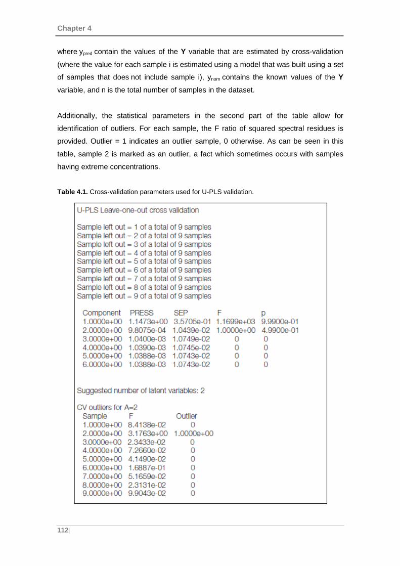
Chapter 4

112|

where ypred contain the values of the Y variable that are estimated by cross-validation

(where the value for each sample i is estimated using a model that was built using a set

of samples that does not include sample i), ynom contains the known values of the Y

variable, and n is the total number of samples in the dataset.

Additionally, the statistical parameters in the second part of the table allow for

identification of outliers. For each sample, the F ratio of squared spectral residues is

provided. Outlier = 1 indicates an outlier sample, 0 otherwise. As can be seen in this

table, sample 2 is marked as an outlier, a fact which sometimes occurs with samples

having extreme concentrations.

Table 4.1. Cross-validation parameters used for U-PLS validation.

Methodology

| 113

Moreover, for U-PLS models, the variance explained of the model for the X and Y

variables are calculated in the same way as PARAFAC or MCR-ALS models.

Finally, in the internal validation of a model the residuals are also important. The

residuals are the difference between the experimental and modeled values. They

should be normally distributed around 0, with a magnitude lower than the signal-to-

noise ratio of the data, and without any trend. In this regard, plots of the residuals of a

model help to reveal the presence of outliers, trends, unexplained sources of variability,

and so on.

4.6.3 External validation

In external validation, new data, not used in the construction of the model, and for

which the concentration of the components is perfectly known, are used to check the

prediction ability of the model. These sets of new samples are usually called test sets

or validation sets. The combination of model and number of factors that perform best

on the test set is usually selected as the right model. By the parsimony principle, if a

number of models perform equivalently, the simplest model should be chosen.

Hence, in second-order calibration, once the calibration model is built, a good estimate

of the predictive ability of the model can be made by comparing the predictions with the

true values of the test set samples, and thereby validation of the model can be

achieved. The statistical parameters used here to assess the goodness of the

calibration models will be the Root Mean Square Error of Prediction (RMSEP), the

Relative Error of Prediction (REP) and the coefficient of determination (R2).

The RMSEP, an estimator of the prediction performance during the external validation

of the calibration model, is defined as:

RMSEP = ¼(1 I⁄ $∑ (y ��~� :y|�}$=¿� =� (4.26)

where I is the total number of samples in the test set, ynom are the known

concentrations and ypred the calculated concentrations by the calibration model. The

RMSEP value gives an average error in the analysis for each compound in the same

units as the concentration values used, in this case ng mL-1.

Chapter 4

114|

The REP, which estimates the accuracy of the prediction for each compound in

percentage, is calculated as:

REP = 100 × RMSEP C�A ⁄ (4.27)

where Cmean is the mean of the true concentrations in the test set.

The coefficient of determination (R2) indicates the quality of the fit between the

experimental concentration and the one calculated by the model, and is calculated for

testing each calibration as follow:

R= = 1 : ∑u§�,¨©#Q §�,ª« OxS∑u§�,¨©#Q §xS (4.28)

where ° denotes the mean of the nominal y values.

CHAPTER 5

RESULTS

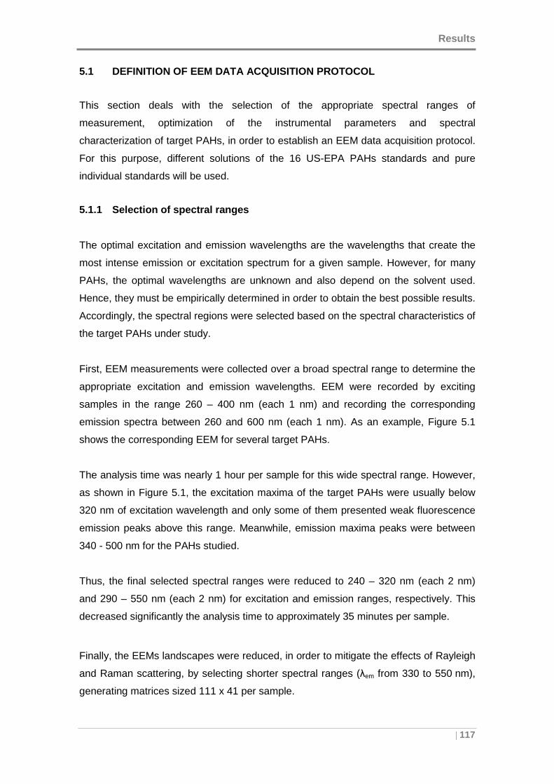
Results

| 117

5.1 DEFINITION OF EEM DATA ACQUISITION PROTOCOL

This section deals with the selection of the appropriate spectral ranges of

measurement, optimization of the instrumental parameters and spectral

characterization of target PAHs, in order to establish an EEM data acquisition protocol.

For this purpose, different solutions of the 16 US-EPA PAHs standards and pure

individual standards will be used.

5.1.1 Selection of spectral ranges

The optimal excitation and emission wavelengths are the wavelengths that create the

most intense emission or excitation spectrum for a given sample. However, for many

PAHs, the optimal wavelengths are unknown and also depend on the solvent used.

Hence, they must be empirically determined in order to obtain the best possible results.

Accordingly, the spectral regions were selected based on the spectral characteristics of

the target PAHs under study.

First, EEM measurements were collected over a broad spectral range to determine the

appropriate excitation and emission wavelengths. EEM were recorded by exciting

samples in the range 260 – 400 nm (each 1 nm) and recording the corresponding

emission spectra between 260 and 600 nm (each 1 nm). As an example, Figure 5.1

shows the corresponding EEM for several target PAHs.

The analysis time was nearly 1 hour per sample for this wide spectral range. However,

as shown in Figure 5.1, the excitation maxima of the target PAHs were usually below

320 nm of excitation wavelength and only some of them presented weak fluorescence

emission peaks above this range. Meanwhile, emission maxima peaks were between

340 - 500 nm for the PAHs studied.

Thus, the final selected spectral ranges were reduced to 240 – 320 nm (each 2 nm)

and 290 – 550 nm (each 2 nm) for excitation and emission ranges, respectively. This

decreased significantly the analysis time to approximately 35 minutes per sample.

Finally, the EEMs landscapes were reduced, in order to mitigate the effects of Rayleigh

and Raman scattering, by selecting shorter spectral ranges (λem from 330 to 550 nm),

generating matrices sized 111 x 41 per sample.

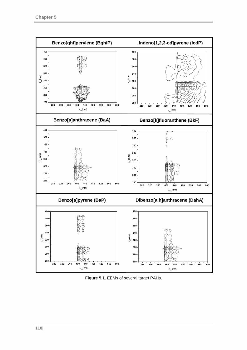
Chapter 5

118|

Figure 5.1. EEMs of several target PAHs.

Benzo[ghi]perylene (BghiP) Indeno[1,2,3 -cd]pyrene (IcdP)

Benzo[ a]anthracene (BaA ) Benzo[ k]fluoranthene (BkF )

Benzo[ a]pyrene (BaP ) Dibenzo[a,h]anthracene (DahA)

Results

| 119

5.1.2 Fluorescence measurements optimization

Several instrumental parameters have to be analyzed and optimized in fluorescence

measurements in order to obtain reliable information. The quality of the acquired data

is largely determined by the signal-to-noise ratio (S/N), which is especially important for

weakly fluorescing samples with low quantum yields. In this sense, the S/N can be

improved by:

- Changing the spectral resolution and bandwidth by adjusting the slit widths.

- Using the appropriate integration time.

- Scanning a region several times and averaging the results.

- Mathematically smoothing the data.

The first two options can be instrumentally modified, and are the subject of this section.

5.1.2.1 Selection of the bandwidths

The slit width of the monochromators affects the resolution of the recorded spectra. If

the slit width is too broad, narrow peaks separated by a small change in wavelength

may be unresolved. By adjusting the slit widths, the intensity and bandwidth of the light

can be controlled. In this regard, the slits of the excitation monochromator determine

the amount of light that passes through the sample. In contrast, the slits of the emission

spectrometer control the amount of luminescence recorded by the detector.

The use of narrow excitation bandwidths generally means increased selectivity and

decreased sensitivity, while wide emission bandwidths result in high sensitivity. Thus, a

good selectivity-sensitivity relationship relies on finding a proper agreement between

the bandwidths of both monochromators. Consequently, the effect of the bandwidths of

both excitation and emission monochromator on two 16 US-EPA PAHs solutions at 1

ng mL-1 and 10 ng mL-1, were assessed by using the bandwidths listed in Table 5.1.

Table 5.1. Excitation and emission bandwidths used in the optimization study.

Excitation bandwidth (nm) Emission bandwidth (nm)

2.5 5

2.5 2.5

5 5

1 5

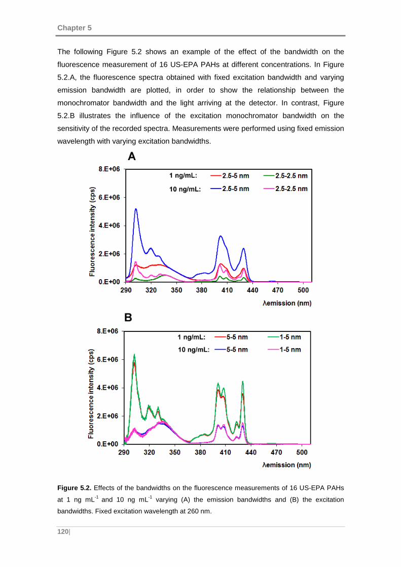
Chapter 5

120|

The following Figure 5.2 shows an example of the effect of the bandwidth on the

fluorescence measurement of 16 US-EPA PAHs at different concentrations. In Figure

5.2.A, the fluorescence spectra obtained with fixed excitation bandwidth and varying

emission bandwidth are plotted, in order to show the relationship between the

monochromator bandwidth and the light arriving at the detector. In contrast, Figure

5.2.B illustrates the influence of the excitation monochromator bandwidth on the

sensitivity of the recorded spectra. Measurements were performed using fixed emission

wavelength with varying excitation bandwidths.

Figure 5.2. Effects of the bandwidths on the fluorescence measurements of 16 US-EPA PAHs

at 1 ng mL-1 and 10 ng mL-1 varying (A) the emission bandwidths and (B) the excitation

bandwidths. Fixed excitation wavelength at 260 nm.

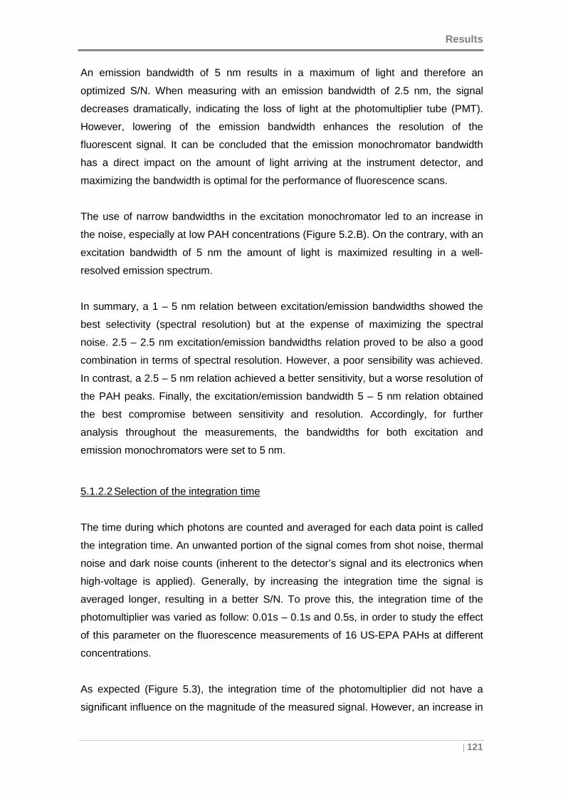
Results

| 121

An emission bandwidth of 5 nm results in a maximum of light and therefore an

optimized S/N. When measuring with an emission bandwidth of 2.5 nm, the signal

decreases dramatically, indicating the loss of light at the photomultiplier tube (PMT).

However, lowering of the emission bandwidth enhances the resolution of the

fluorescent signal. It can be concluded that the emission monochromator bandwidth

has a direct impact on the amount of light arriving at the instrument detector, and

maximizing the bandwidth is optimal for the performance of fluorescence scans.

The use of narrow bandwidths in the excitation monochromator led to an increase in

the noise, especially at low PAH concentrations (Figure 5.2.B). On the contrary, with an

excitation bandwidth of 5 nm the amount of light is maximized resulting in a well-

resolved emission spectrum.

In summary, a 1 – 5 nm relation between excitation/emission bandwidths showed the

best selectivity (spectral resolution) but at the expense of maximizing the spectral

noise. 2.5 – 2.5 nm excitation/emission bandwidths relation proved to be also a good

combination in terms of spectral resolution. However, a poor sensibility was achieved.

In contrast, a 2.5 – 5 nm relation achieved a better sensitivity, but a worse resolution of

the PAH peaks. Finally, the excitation/emission bandwidth 5 – 5 nm relation obtained

the best compromise between sensitivity and resolution. Accordingly, for further

analysis throughout the measurements, the bandwidths for both excitation and

emission monochromators were set to 5 nm.

5.1.2.2 Selection of the integration time

The time during which photons are counted and averaged for each data point is called

the integration time. An unwanted portion of the signal comes from shot noise, thermal

noise and dark noise counts (inherent to the detector’s signal and its electronics when

high-voltage is applied). Generally, by increasing the integration time the signal is

averaged longer, resulting in a better S/N. To prove this, the integration time of the

photomultiplier was varied as follow: 0.01s – 0.1s and 0.5s, in order to study the effect

of this parameter on the fluorescence measurements of 16 US-EPA PAHs at different

concentrations.

As expected (Figure 5.3), the integration time of the photomultiplier did not have a

significant influence on the magnitude of the measured signal. However, an increase in

Chapter 5

122|

the S/N was observed at higher values of this variable. Thereby, integration times

below 0.1 s increased significantly the noise, especially at low PAH concentrations

(Figure 5.3.A). In contrast, an integration time of 0.5 s did not improve either the

sensitivity or the selectivity of the measurements and, more important, it resulted in an

excessive analysis time. Therefore, in view of the results obtained, an integration time

of 0.1s was considered as the optimal value of this variable, giving good sensitivity and

S/N.

Figure 5.3 . Effects of the photomultiplier integration time on the fluorescence measurements:

(A) PAHs at 1 ng mL-1, (B) PAHs at 10 ng mL-1. Fixed excitation wavelength 260 nm.

s

s

s

s

s

s

Results

| 123

5.1.2.3 Other considerations

It is also important to remark that the Xenon lamp, like most of the light sources,

requires a definite warming up time to yield stable output power. Any measurement of

spectra before this time results in an unwanted spectral variation correlated with the

source fluctuation. In our case, the Xenon lamp takes around 30 minutes to get

stabilized, thus 45 min of warming up were established before measuring. After this

time, this source can be employed continuously for several hours without significant

fluctuations in intensity.

5.1.2.4 Conclusions

In fluorescence spectroscopy, the flexibility of the monochromators bandwidth selection

as well as the integration time, enables us to improve the data quality (S/N ratio) while

maintaining a good spectral resolution. When it comes to determinations near to the

detection limit, optimizing the relation of the adjustable slit widths and the value of the

integration time yields an optimal operation of the PMT and amplification electronics,

and a minimization of the background noise.

Summarizing, the instrumental parameters obtained as optimal and, therefore, used

throughout this research work, were:

- The bandwidths for both excitation and emission monochromators were set to 5 nm.

- The integration time was set to 0.1s.

- The measurements were made after 45 m of warming up the Xenon lamp.

5.1.3 Spectral characterization of target PAHs

The identification and quantification of each PAH by fluorescence routine analysis

benefits from the availability of their reference spectra. However, due to the different

instrumental conditions and solvents used in fluorescence measurements, nowadays

there is not a standard data collection of these compounds available.

Therefore, given the instrumental and analytical conditions of the measurement, the

EEM of each target PAH needing identification and quantification were obtained using

the corresponding pure standard diluted in n-hexane, as shown in the following figures,

where the excitation and emission wavelengths of the maximum are also indicated.

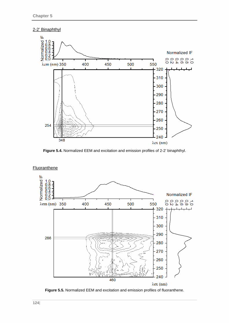
Chapter 5

124|

2-2’ Binaphthyl

Figure 5.4. Normalized EEM and excitation and emission profiles of 2-2’ binaphthyl.

Fluoranthene

Figure 5.5. Normalized EEM and excitation and emission profiles of fluoranthene.

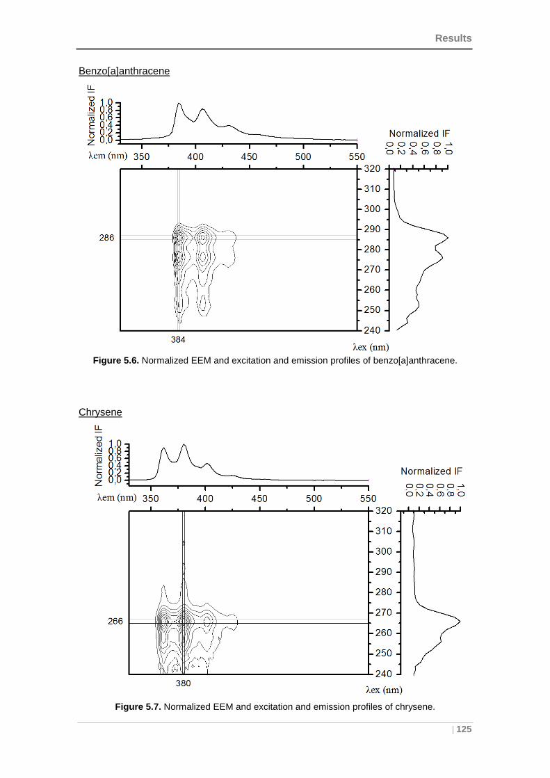
Results

| 125

Benzo[a]anthracene

Figure 5.6. Normalized EEM and excitation and emission profiles of benzo[a]anthracene.

Chrysene

Figure 5.7. Normalized EEM and excitation and emission profiles of chrysene.

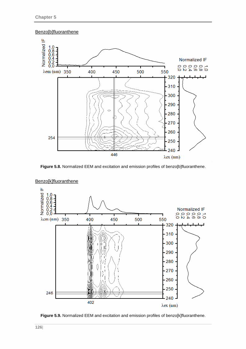
Chapter 5

126|

Benzo[b]fluoranthene

Figure 5.8. Normalized EEM and excitation and emission profiles of benzo[b]fluoranthene.

Benzo[k]fluoranthene

Figure 5.9. Normalized EEM and excitation and emission profiles of benzo[k]fluoranthene.

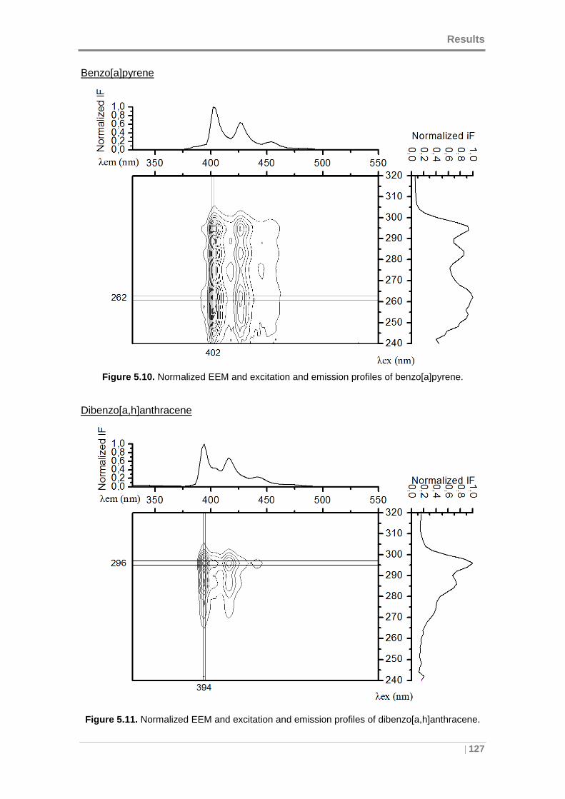
Results

| 127

Benzo[a]pyrene

Figure 5.10. Normalized EEM and excitation and emission profiles of benzo[a]pyrene.

Dibenzo[a,h]anthracene

Figure 5.11. Normalized EEM and excitation and emission profiles of dibenzo[a,h]anthracene.

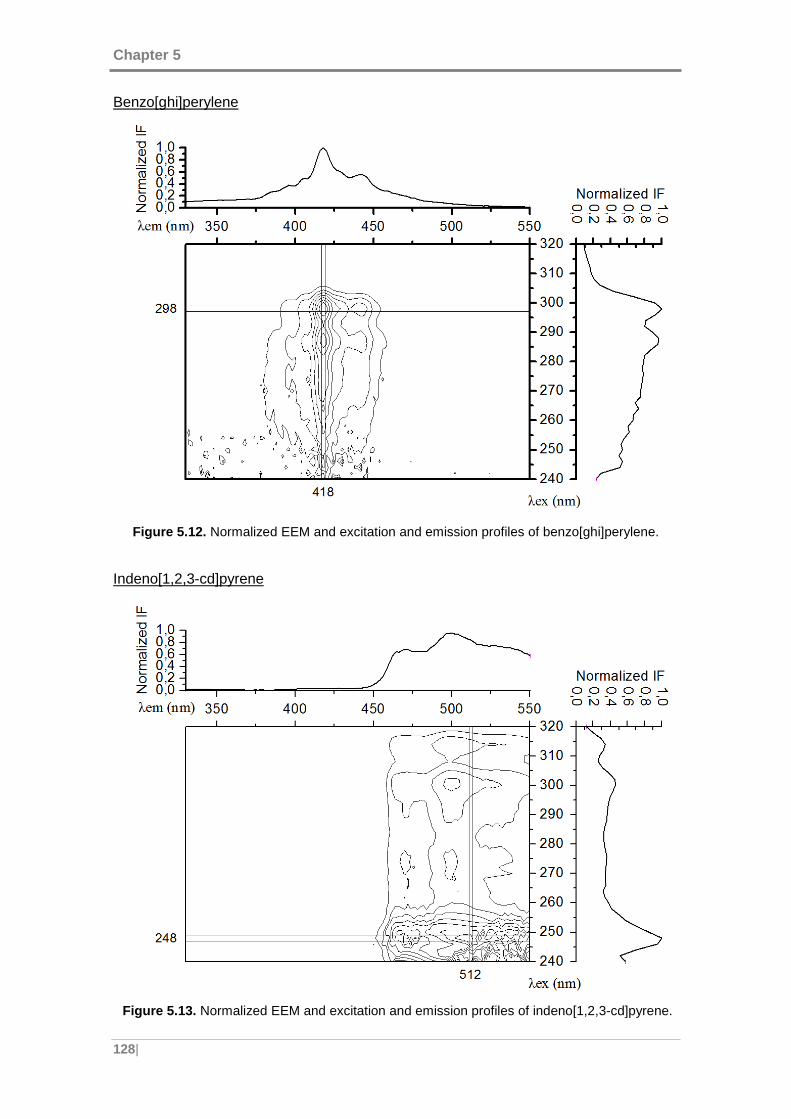
Chapter 5

128|

Benzo[ghi]perylene

Figure 5.12. Normalized EEM and excitation and emission profiles of benzo[ghi]perylene.

Indeno[1,2,3-cd]pyrene

Figure 5.13. Normalized EEM and excitation and emission profiles of indeno[1,2,3-cd]pyrene.

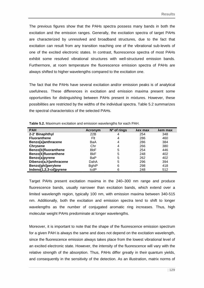
Results

| 129

The previous figures show that the PAHs spectra possess many bands in both the

excitation and the emission ranges. Generally, the excitation spectra of target PAHs

are characterized by unresolved and broadband structures, due to the fact that

excitation can result from any transition reaching one of the vibrational sub-levels of

one of the excited electronic states. In contrast, fluorescence spectra of most PAHs

exhibit some resolved vibrational structures with well-structured emission bands.

Furthermore, at room temperature the fluorescence emission spectra of PAHs are

always shifted to higher wavelengths compared to the excitation one.

The fact that the PAHs have several excitation and/or emission peaks is of analytical

usefulness. These differences in excitation and emission maxima present some

opportunities for distinguishing between PAHs present in mixtures. However, these

possibilities are restricted by the widths of the individual spectra. Table 5.2 summarizes

the spectral characteristics of the selected PAHs.

Table 5.2. Maximum excitation and emission wavelengths for each PAH.

PAH Acronym Nº of rings λex max λem max 2-2’ Binaphthyl 22B 4 254 348 Fluoranthene Flt 4 286 460 Benzo[a]anthracene BaA 4 286 384 Chrysene Chr 4 266 380 Benzo[b]fluoranthene BbF 5 254 446 Benzo[k]fluoranthene BkF 5 248 402 Benzo[a]pyrene BaP 5 262 402 Dibenzo[a,h]anthracene DahA 5 296 394 Benzo[ghi]perylene BghiP 6 298 418 Indeno[1,2,3 -cd]pyrene IcdP 6 248 512

Target PAHs present excitation maxima in the 240–300 nm range and produce

fluorescence bands, usually narrower than excitation bands, which extend over a

limited wavelength region, typically 100 nm, with emission maxima between 340-515

nm. Additionally, both the excitation and emission spectra tend to shift to longer

wavelengths as the number of conjugated aromatic ring increases. Thus, high

molecular weight PAHs predominate at longer wavelengths.

Moreover, it is important to note that the shape of the fluorescence emission spectrum

for a given PAH is always the same and does not depend on the excitation wavelength,

since the fluorescence emission always takes place from the lowest vibrational level of

an excited electronic state. However, the intensity of the fluorescence will vary with the

relative strength of the absorption. Thus, PAHs differ greatly in their quantum yields,

and consequently in the sensitivity of the detection. As an illustration, matrix norms of

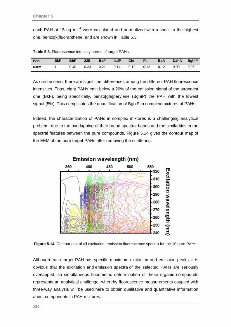
Chapter 5

130|

each PAH at 15 ng mL-1 were calculated and normalized with respect to the highest

one, benzo[k]fluoranthene, and are shown in Table 5.3.

Table 5.3. Fluorescence intensity norms of target PAHs.

PAH BkF BbF 22B BaP IcdP Chr Flt BaA DahA BghiP

Norm 1 0.40 0.23 0.21 0.14 0.12 0.12 0.12 0.09 0.05

As can be seen, there are significant differences among the different PAH fluorescence

intensities. Thus, eight PAHs emit below a 20% of the emission signal of the strongest

one (BkF), being specifically, benzo[ghi]perylene (BghiP) the PAH with the lowest

signal (5%). This complicates the quantification of BghiP in complex mixtures of PAHs.

Indeed, the characterization of PAHs in complex mixtures is a challenging analytical

problem, due to the overlapping of their broad spectral bands and the similarities in the

spectral features between the pure compounds. Figure 5.14 gives the contour map of

the EEM of the pure target PAHs after removing the scattering.

Figure 5.14. Contour plot of all excitation–emission fluorescence spectra for the 10 pure PAHs.

Although each target PAH has specific maximum excitation and emission peaks, it is

obvious that the excitation and emission spectra of the selected PAHs are seriously

overlapped, so simultaneous fluorimetric determination of these organic compounds

represents an analytical challenge, whereby fluorescence measurements coupled with

three-way analysis will be used here to obtain qualitative and quantitative information

about components in PAH mixtures.

Results

| 131

5.2. DEVELOPMENT OF PRELIMINARY EEM DATA MODELS

Before developing EEM models for the analysis of target PAHs in urban aerosol air

samples, some aspects involved in multivariate/multi-way data analysis need to be

evaluated, optimized and validated. These theoretical and methodological aspects are

therefore presented in the following sections as follows:

Section 5.2.1 deals with the spectral corrections required to remove broad features,

such Rayleigh and Raman scattering, that inhibit the correct modeling by contributing

with random or systematic variation, or both, to the raw EEM data. Although specific

methods of scattering correction exist in the literature, there is not an unified protocol

for the treatment of these scattering effects among the scientific community, coexisting

many different approaches. Thus, a further study was required in order to optimize and

define the best strategy for the preprocessing step required before EEM modeling.

Section 5.2.2 includes a detailed analysis of the different modeling approaches used to

build second-order calibration methods for efficient qualitative and quantitative analysis

of multicomponent PAHs samples. Here, the best possible strategies for EEM modeling

are set, stressing the different criteria required to build each calibration model.

Finally, section 5.2.3 provides an insight into how each second-order calibration

method performs under the presence of uncalibrated interferences, a common situation

to be taken into consideration when analyzing PAHs in aerosol samples.

Chapter 5

132|

5.2.1 Optimization of preprocessing methods for EEM modeling

The intrinsic presence of scattering effects in the EEM measurements poses a practical

problem because they do not hold any chemical information about the fluorophores in

the solution. Thus, appropriate handling of the scattering is necessary to avoid its

detrimental influence on the models.

Among the available methods for removing scattering (section 4.4.2), the most

commonly used one consists of subtracting the spectrum of the solvent (if it is

available) to minimize the Raman scattering, and then, replacing the Rayleigh affected

areas by missing values. However, in some situations it is preferred to avoid the use of

missing values for various reasons. For example, some algorithms (like U-PLS) or

visualization tools do not handle missing data or, even worse, interesting information

might be removed. Moreover, algorithms dealing with missing data can be extremely

slow and computationally cumbersome, and the amount of missing values may

possibly affect the convergence of the models and the quality of the results.

Another possibility consists of replacing the removed scatter areas with interpolated

values. This can potentially speed up the modeling and allows the use of software that

is not able to handle missing data. Despite these potential advantages, there has not

been yet thoughtfully discussed -nor published- any comprehensive comparison of the

effect of inserting missing data or interpolated data on the quality of the obtained model

or even the resolved spectra and subsequent predictions. Thus, it is of great interest to

evaluate the two most common methods of handling scatter: replacing the scattering

area with missing elements or with interpolated values, in order to optimize the

preprocessing step required before EEM modeling.

Given that the U-PLS algorithm implemented in this research work does not handle

missing data, one of the other second-order multi-way methods, PARAFAC, was

selected for this analysis. In addition, since the objective here is the optimization of the

preprocessing methods, no information about how to select the appropriate PARAFAC

model is included, as this will be discussed in detail in section 5.2.2.

5.2.1.1 Objective

In this section a comparison of how missing or interpolated data can affect the

PARAFAC modeling of EEMs is provided. Both approaches were evaluated and

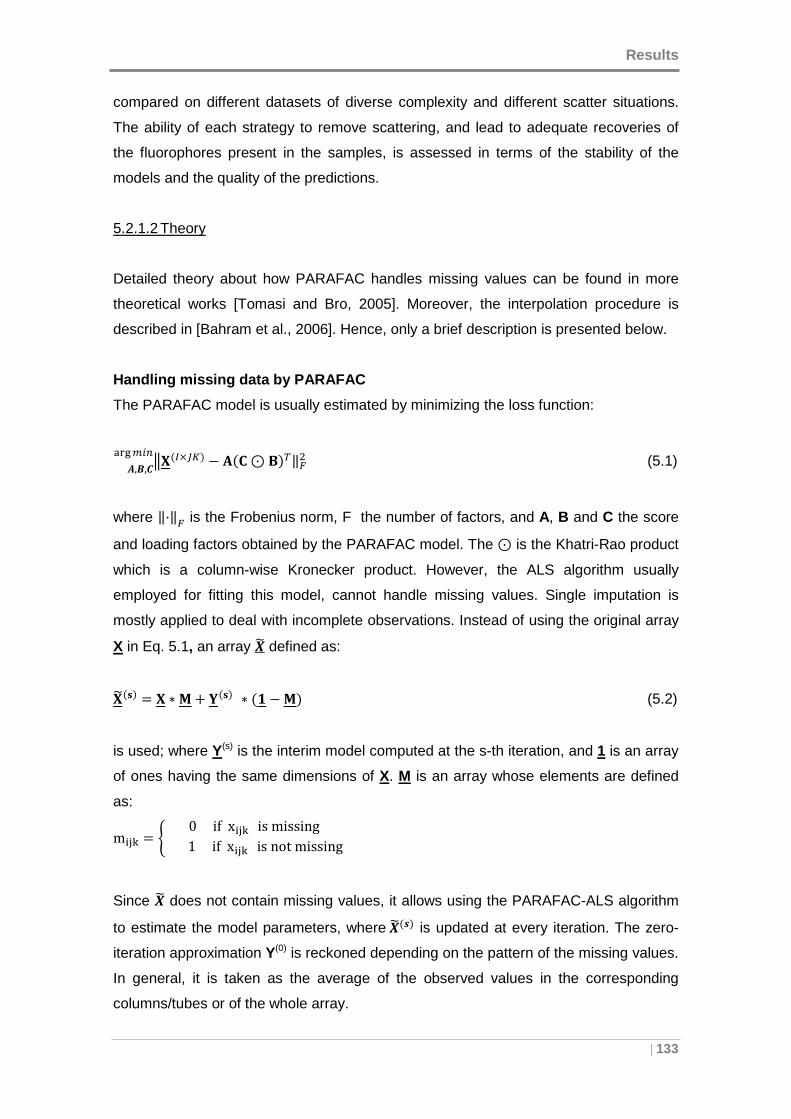
Results

| 133

compared on different datasets of diverse complexity and different scatter situations.

The ability of each strategy to remove scattering, and lead to adequate recoveries of

the fluorophores present in the samples, is assessed in terms of the stability of the

models and the quality of the predictions.

5.2.1.2 Theory

Detailed theory about how PARAFAC handles missing values can be found in more

theoretical works [Tomasi and Bro, 2005]. Moreover, the interpolation procedure is

described in [Bahram et al., 2006]. Hence, only a brief description is presented below.

Handling missing data by PARAFAC

The PARAFAC model is usually estimated by minimizing the loss function:

9/(0×12$ : 3(4⊙ 6$7‖<=>,?,@A�BCDE (5.1)

where ‖F‖< is the Frobenius norm, F the number of factors, and A, B and C the score

and loading factors obtained by the PARAFAC model. The ⊙ is the Khatri-Rao product

which is a column-wise Kronecker product. However, the ALS algorithm usually

employed for fitting this model, cannot handle missing values. Single imputation is

mostly applied to deal with incomplete observations. Instead of using the original array

X in Eq. 5.1, an array �Ç defined as:

/Ç(�$ = / ∗ È+ d(�$ ∗ (i :È$ (5.2)

is used; where Y(s) is the interim model computed at the s-th iteration, and 1 is an array

of ones having the same dimensions of X. M is an array whose elements are defined

as:

m�&' = É 0ifx�&'ismissing1ifx�&'isnotmissing

Since �Ç does not contain missing values, it allows using the PARAFAC-ALS algorithm

to estimate the model parameters, where�Ç(Ë$ is updated at every iteration. The zero-

iteration approximation Y(0) is reckoned depending on the pattern of the missing values.

In general, it is taken as the average of the observed values in the corresponding

columns/tubes or of the whole array.

Chapter 5

134|

Handling missing data by imputation generally leads to slower convergence.

Furthermore, a large amount of missing elements may increase the risk of

convergence to a local minimum.

Replacing scattering areas with interpolated data

The interpolation procedure is based on excising scatter areas and replacing them

using a shape-preserving piecewise cubic polynomial.

The interpolation is implemented in the following way. The first step consists of defining

the window width for the relevant areas. Normally this would be done for the first and

possibly also the second-order Rayleigh, but it can also be done for the Raman scatter

region. These widths are user-defined parameters required in the interpolation. In the

second step, the measured signal in the width-defined window is removed around the

scatter lines for every emission spectrum. Subsequently, the whole spectrum, except

the window, is used for interpolation, and the window is replaced with the interpolated

values.

Two parts of the EEM require special care during the interpolation. In the first situation,

where there is no emission below the window, an artificial lower emission zero is added

during interpolation 30 nm below the window of interpolation. In the second one, where

there are no emission values at greater wavelengths than the window to be

interpolated, the missing values in the last excitation spectrum are interpolated in order

to provide end values for the emission interpolation.

5.2.1.3 Data and software

For analyzing the performance of the two methods, two EEM datasets of different

complexity and scattering situations were used, as described below.

Dataset 1: second-order Rayleigh overlapping the ch emical signal

From the dpure dataset, a total of twelve samples of indeno[1,2,3-cd]pyrene (IcdP) at

four different concentration levels: 5-10-15-20 ng mL-1, measured by triplicate, were

used. In this dataset a two-component PARAFAC model was the most suitable due to

the presence of an additional interfering compound. Moreover, solvent blank

subtraction (n-hexane) was made for each measure to mitigate the Raman scattering in

each EEM.

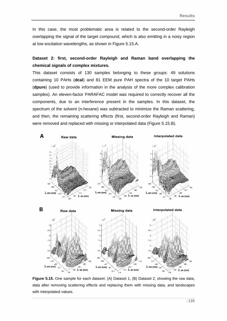
Results

| 135

In this case, the most problematic area is related to the second-order Rayleigh

overlapping the signal of the target compound, which is also emitting in a noisy region

at low excitation wavelengths, as shown in Figure 5.15.A.

Dataset 2: first, second-order Rayleigh and Raman b and overlapping the

chemical signals of complex mixtures.

This dataset consists of 130 samples belonging to these groups: 49 solutions

containing 10 PAHs (dcal ) and 81 EEM pure PAH spectra of the 10 target PAHs

(dpure ) (used to provide information in the analysis of the more complex calibration

samples). An eleven-factor PARAFAC model was required to correctly recover all the

components, due to an interference present in the samples. In this dataset, the

spectrum of the solvent (n-hexane) was subtracted to minimize the Raman scattering,

and then, the remaining scattering effects (first, second-order Rayleigh and Raman)

were removed and replaced with missing or interpolated data (Figure 5.15.B).

Figure 5.15. One sample for each dataset: (A) Dataset 1, (B) Dataset 2, showing the raw data,

data after removing scattering effects and replacing them with missing data, and landscapes

with interpolated values.

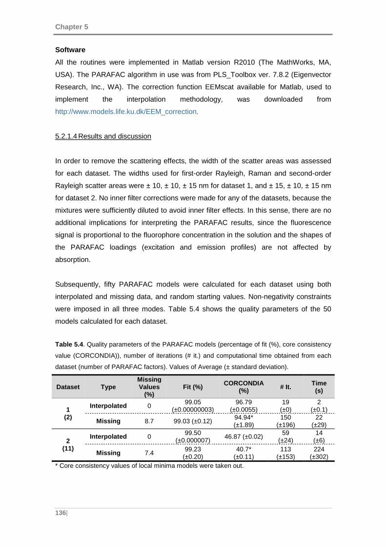
Chapter 5

136|

Software

All the routines were implemented in Matlab version R2010 (The MathWorks, MA,

USA). The PARAFAC algorithm in use was from PLS_Toolbox ver. 7.8.2 (Eigenvector

Research, Inc., WA). The correction function EEMscat available for Matlab, used to

implement the interpolation methodology, was downloaded from

http://www.models.life.ku.dk/EEM_correction.

5.2.1.4 Results and discussion

In order to remove the scattering effects, the width of the scatter areas was assessed

for each dataset. The widths used for first-order Rayleigh, Raman and second-order

Rayleigh scatter areas were ± 10, ± 10, ± 15 nm for dataset 1, and ± 15, ± 10, ± 15 nm

for dataset 2. No inner filter corrections were made for any of the datasets, because the

mixtures were sufficiently diluted to avoid inner filter effects. In this sense, there are no

additional implications for interpreting the PARAFAC results, since the fluorescence

signal is proportional to the fluorophore concentration in the solution and the shapes of

the PARAFAC loadings (excitation and emission profiles) are not affected by

absorption.

Subsequently, fifty PARAFAC models were calculated for each dataset using both

interpolated and missing data, and random starting values. Non-negativity constraints

were imposed in all three modes. Table 5.4 shows the quality parameters of the 50

models calculated for each dataset.

Table 5.4 . Quality parameters of the PARAFAC models (percentage of fit (%), core consistency

value (CORCONDIA)), number of iterations (# it.) and computational time obtained from each

dataset (number of PARAFAC factors). Values of Average (± standard deviation).

Dataset Type Missing Values

(%) Fit (%) CORCONDIA

(%) # It. Time (s)

1 (2)

Interpolated 0 99.05

(±0.00000003) 96.79

(±0.0055) 19

(±0) 2

(±0.1)

Missing 8.7 99.03 (±0.12) 94.94* (±1.89)

150 (±196)

22 (±29)

2 (11)

Interpolated 0 99.50

(±0.000007) 46.87 (±0.02)

59 (±24)

14 (±6)

Missing 7.4 99.23

(±0.20) 40.7*

(±0.11) 113

(±153) 224

(±302) * Core consistency values of local minima models were taken out.

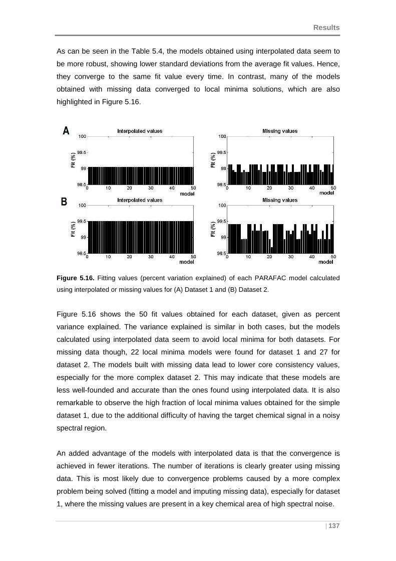
Results

| 137

As can be seen in the Table 5.4, the models obtained using interpolated data seem to

be more robust, showing lower standard deviations from the average fit values. Hence,

they converge to the same fit value every time. In contrast, many of the models

obtained with missing data converged to local minima solutions, which are also

highlighted in Figure 5.16.

Figure 5.16. Fitting values (percent variation explained) of each PARAFAC model calculated

using interpolated or missing values for (A) Dataset 1 and (B) Dataset 2.

Figure 5.16 shows the 50 fit values obtained for each dataset, given as percent

variance explained. The variance explained is similar in both cases, but the models

calculated using interpolated data seem to avoid local minima for both datasets. For

missing data though, 22 local minima models were found for dataset 1 and 27 for

dataset 2. The models built with missing data lead to lower core consistency values,

especially for the more complex dataset 2. This may indicate that these models are

less well-founded and accurate than the ones found using interpolated data. It is also

remarkable to observe the high fraction of local minima values obtained for the simple

dataset 1, due to the additional difficulty of having the target chemical signal in a noisy

spectral region.

An added advantage of the models with interpolated data is that the convergence is

achieved in fewer iterations. The number of iterations is clearly greater using missing

data. This is most likely due to convergence problems caused by a more complex

problem being solved (fitting a model and imputing missing data), especially for dataset

1, where the missing values are present in a key chemical area of high spectral noise.

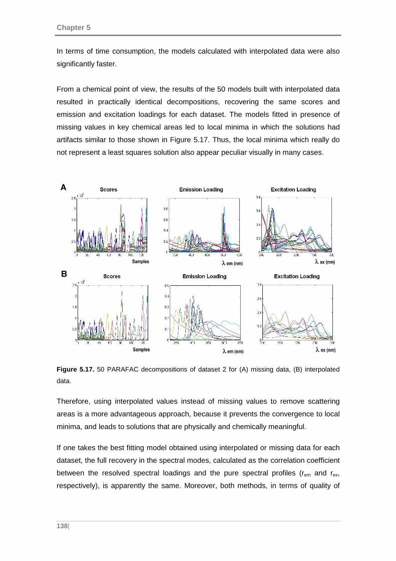
Chapter 5

138|

In terms of time consumption, the models calculated with interpolated data were also

significantly faster.

From a chemical point of view, the results of the 50 models built with interpolated data

resulted in practically identical decompositions, recovering the same scores and

emission and excitation loadings for each dataset. The models fitted in presence of

missing values in key chemical areas led to local minima in which the solutions had

artifacts similar to those shown in Figure 5.17. Thus, the local minima which really do

not represent a least squares solution also appear peculiar visually in many cases.

Figure 5.17. 50 PARAFAC decompositions of dataset 2 for (A) missing data, (B) interpolated

data.

Therefore, using interpolated values instead of missing values to remove scattering

areas is a more advantageous approach, because it prevents the convergence to local

minima, and leads to solutions that are physically and chemically meaningful.

If one takes the best fitting model obtained using interpolated or missing data for each

dataset, the full recovery in the spectral modes, calculated as the correlation coefficient

between the resolved spectral loadings and the pure spectral profiles (rem and rex,

respectively), is apparently the same. Moreover, both methods, in terms of quality of

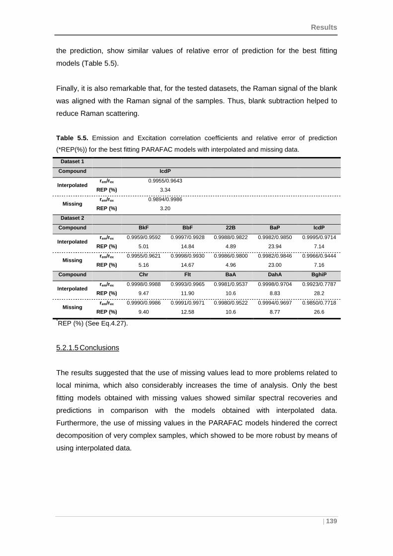
Results

| 139

the prediction, show similar values of relative error of prediction for the best fitting

models (Table 5.5).

Finally, it is also remarkable that, for the tested datasets, the Raman signal of the blank

was aligned with the Raman signal of the samples. Thus, blank subtraction helped to

reduce Raman scattering.

Table 5.5. Emission and Excitation correlation coefficients and relative error of prediction

(*REP(%)) for the best fitting PARAFAC models with interpolated and missing data.

Dataset 1

Compound IcdP

Interpolated rem/rex 0.9955/0.9643

REP (%) 3.34

Missing rem/rex 0.9894/0.9986

REP (%) 3.20

Dataset 2

Compound BkF BbF 22B BaP IcdP

Interpolated rem/rex 0.9959/0.9592 0.9997/0.9928 0.9988/0.9822 0.9982/0.9850 0.9995/0.9714

REP (%) 5.01 14.84 4.89 23.94 7.14

Missing rem/rex 0.9955/0.9621 0.9998/0.9930 0.9986/0.9800 0.9982/0.9846 0.9966/0.9444

REP (%) 5.16 14.67 4.96 23.00 7.16

Compound Chr Flt BaA DahA BghiP

Interpolated rem/rex 0.9998/0.9988 0.9993/0.9965 0.9981/0.9537 0.9998/0.9704 0.9923/0.7787

REP (%) 9.47 11.90 10.6 8.83 28.2

Missing rem/rex 0.9990/0.9986 0.9991/0.9971 0.9980/0.9522 0.9994/0.9697 0.9850/0.7718

REP (%) 9.40 12.58 10.6 8.77 26.6

*REP (%) (See Eq.4.27).

5.2.1.5 Conclusions

The results suggested that the use of missing values lead to more problems related to

local minima, which also considerably increases the time of analysis. Only the best

fitting models obtained with missing values showed similar spectral recoveries and

predictions in comparison with the models obtained with interpolated data.

Furthermore, the use of missing values in the PARAFAC models hindered the correct

decomposition of very complex samples, which showed to be more robust by means of

using interpolated data.

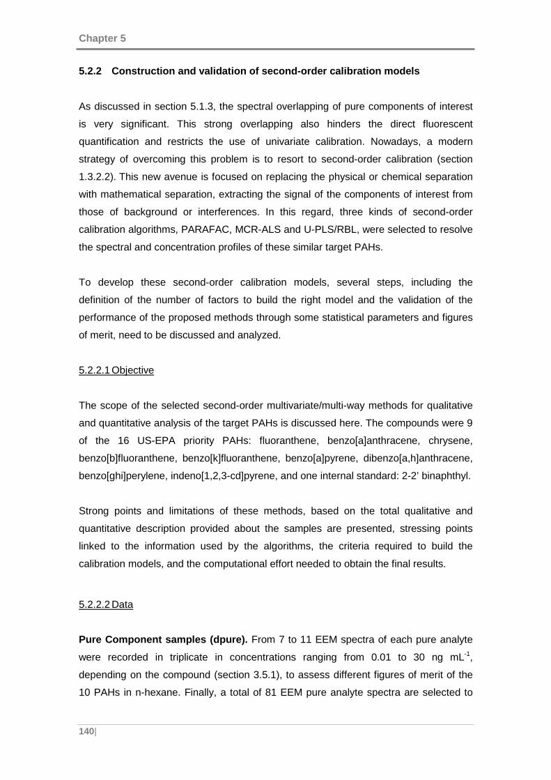
Chapter 5

140|

5.2.2 Construction and validation of second-order c alibration models

As discussed in section 5.1.3, the spectral overlapping of pure components of interest

is very significant. This strong overlapping also hinders the direct fluorescent

quantification and restricts the use of univariate calibration. Nowadays, a modern

strategy of overcoming this problem is to resort to second-order calibration (section

1.3.2.2). This new avenue is focused on replacing the physical or chemical separation

with mathematical separation, extracting the signal of the components of interest from

those of background or interferences. In this regard, three kinds of second-order

calibration algorithms, PARAFAC, MCR-ALS and U-PLS/RBL, were selected to resolve

the spectral and concentration profiles of these similar target PAHs.

To develop these second-order calibration models, several steps, including the

definition of the number of factors to build the right model and the validation of the

performance of the proposed methods through some statistical parameters and figures

of merit, need to be discussed and analyzed.

5.2.2.1 Objective

The scope of the selected second-order multivariate/multi-way methods for qualitative

and quantitative analysis of the target PAHs is discussed here. The compounds were 9

of the 16 US-EPA priority PAHs: fluoranthene, benzo[a]anthracene, chrysene,

benzo[b]fluoranthene, benzo[k]fluoranthene, benzo[a]pyrene, dibenzo[a,h]anthracene,

benzo[ghi]perylene, indeno[1,2,3-cd]pyrene, and one internal standard: 2-2’ binaphthyl.

Strong points and limitations of these methods, based on the total qualitative and

quantitative description provided about the samples are presented, stressing points

linked to the information used by the algorithms, the criteria required to build the

calibration models, and the computational effort needed to obtain the final results.

5.2.2.2 Data

Pure Component samples (dpure). From 7 to 11 EEM spectra of each pure analyte

were recorded in triplicate in concentrations ranging from 0.01 to 30 ng mL-1,

depending on the compound (section 3.5.1), to assess different figures of merit of the

10 PAHs in n-hexane. Finally, a total of 81 EEM pure analyte spectra are selected to

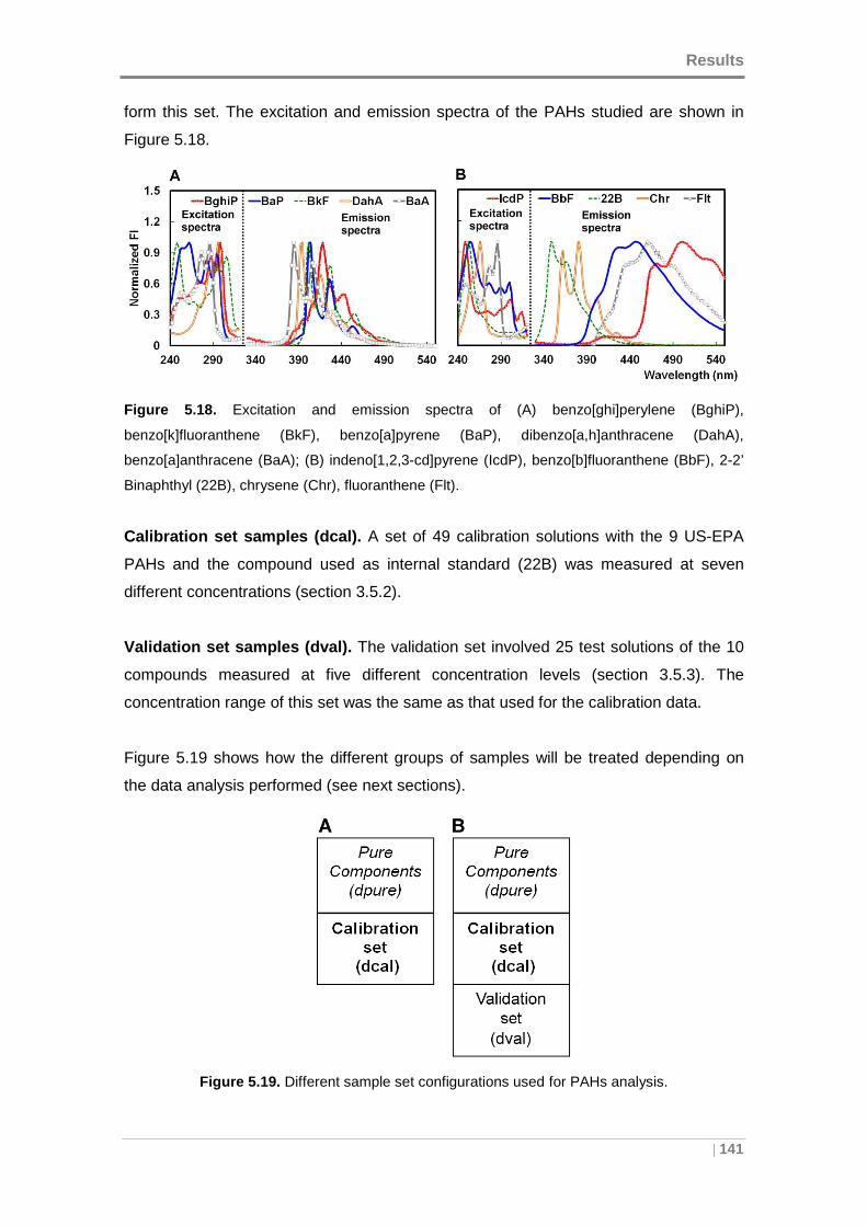
Results

| 141

form this set. The excitation and emission spectra of the PAHs studied are shown in

Figure 5.18.

Figure 5.18. Excitation and emission spectra of (A) benzo[ghi]perylene (BghiP),

benzo[k]fluoranthene (BkF), benzo[a]pyrene (BaP), dibenzo[a,h]anthracene (DahA),

benzo[a]anthracene (BaA); (B) indeno[1,2,3-cd]pyrene (IcdP), benzo[b]fluoranthene (BbF), 2-2’

Binaphthyl (22B), chrysene (Chr), fluoranthene (Flt).

Calibration set samples (dcal). A set of 49 calibration solutions with the 9 US-EPA

PAHs and the compound used as internal standard (22B) was measured at seven

different concentrations (section 3.5.2).

Validation set samples (dval). The validation set involved 25 test solutions of the 10

compounds measured at five different concentration levels (section 3.5.3). The

concentration range of this set was the same as that used for the calibration data.

Figure 5.19 shows how the different groups of samples will be treated depending on

the data analysis performed (see next sections).

Figure 5.19. Different sample set configurations used for PAHs analysis.

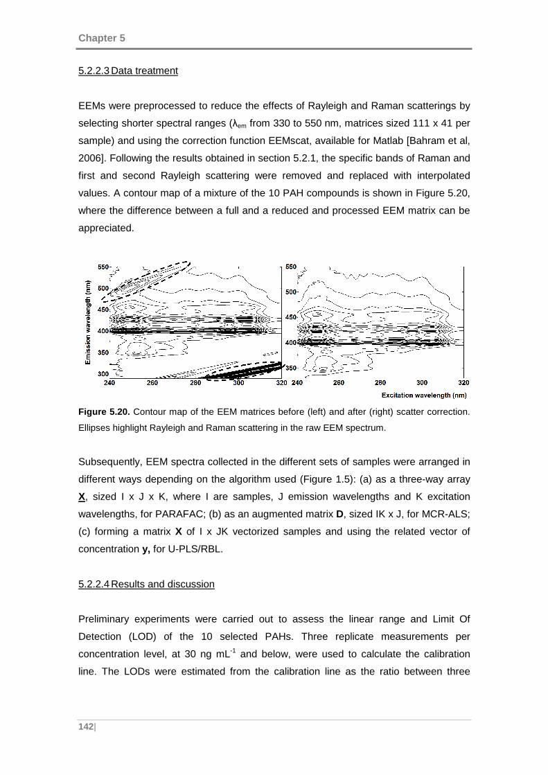
Chapter 5

142|

5.2.2.3 Data treatment

EEMs were preprocessed to reduce the effects of Rayleigh and Raman scatterings by

selecting shorter spectral ranges (λem from 330 to 550 nm, matrices sized 111 x 41 per

sample) and using the correction function EEMscat, available for Matlab [Bahram et al,

2006]. Following the results obtained in section 5.2.1, the specific bands of Raman and

first and second Rayleigh scattering were removed and replaced with interpolated

values. A contour map of a mixture of the 10 PAH compounds is shown in Figure 5.20,

where the difference between a full and a reduced and processed EEM matrix can be

appreciated.

Figure 5.20. Contour map of the EEM matrices before (left) and after (right) scatter correction.

Ellipses highlight Rayleigh and Raman scattering in the raw EEM spectrum.

Subsequently, EEM spectra collected in the different sets of samples were arranged in

different ways depending on the algorithm used (Figure 1.5): (a) as a three-way array

X, sized I x J x K, where I are samples, J emission wavelengths and K excitation

wavelengths, for PARAFAC; (b) as an augmented matrix D, sized IK x J, for MCR-ALS;

(c) forming a matrix X of I x JK vectorized samples and using the related vector of

concentration y, for U-PLS/RBL.


Preliminary experiments were carried out to assess the linear range and Limit Of

Detection (LOD) of the 10 selected PAHs. Three replicate measurements per

concentration level, at 30 ng mL-1 and below, were used to calculate the calibration

line. The LODs were estimated from the calibration line as the ratio between three

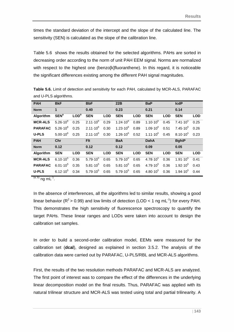
Results

| 143

times the standard deviation of the intercept and the slope of the calculated line. The

sensitivity (SEN) is calculated as the slope of the calibration line.

Table 5.6 shows the results obtained for the selected algorithms. PAHs are sorted in

decreasing order according to the norm of unit PAH EEM signal. Norms are normalized

with respect to the highest one (benzo[k]fluoranthene). In this regard, it is noticeable

the significant differences existing among the different PAH signal magnitudes.

Table 5.6. Limit of detection and sensitivity for each PAH, calculated by MCR-ALS, PARAFAC

and U-PLS algorithms.

PAH BkF BbF 22B BaP IcdP

Norm 1 0.40 0.23 0.21 0.14

Algorithm SENa LODb SEN LOD SEN LOD SEN LOD SEN LOD

MCR-ALS 5.26·106 0.25 2.11·106 0.29 1.24·106 0.89 1.10·106 0.45 7.41·105 0.25

PARAFAC 5.26·106 0.25 2.11·106 0.30 1.23·106 0.89 1.09·106 0.51 7.45·105 0.26

U-PLS 5.00·106 0.25 2.11·106 0.30 1.26·106 0.52 1.11·106 0.45 8.10·105 0.23

PAH Chr Flt BaA DahA BghiP

Norm 0.12 0.12 0.12 0.09 0.05

Algorithm SEN LOD SEN LOD SEN LOD SEN LOD SEN LOD

MCR-ALS 6.10·105 0.36 5.79·105 0.65 5.79·105 0.65 4.78·105 0.36 1.91·105 0.41

PARAFAC 6.01·105 0.35 5.81·105 0.65 5.81·105 0.65 4.79·105 0.36 1.92·105 0.43

U-PLS 6.12·105 0.34 5.79·105 0.65 5.79·105 0.65 4.80·105 0.36 1.94·105 0.44

(a, b) ng mL-1.

In the absence of interferences, all the algorithms led to similar results, showing a good

linear behavior (R2 > 0.99) and low limits of detection (LOD < 1 ng mL-1) for every PAH.

This demonstrates the high sensitivity of fluorescence spectroscopy to quantify the

target PAHs. These linear ranges and LODs were taken into account to design the

calibration set samples.

In order to build a second-order calibration model, EEMs were measured for the

calibration set (dcal ), designed as explained in section 3.5.2. The analysis of the

calibration data were carried out by PARAFAC, U-PLS/RBL and MCR-ALS algorithms.

First, the results of the two resolution methods PARAFAC and MCR-ALS are analyzed.

The first point of interest was to compare the effect of the differences in the underlying

linear decomposition model on the final results. Thus, PARAFAC was applied with its

natural trilinear structure and MCR-ALS was tested using total and partial trilinearity. A

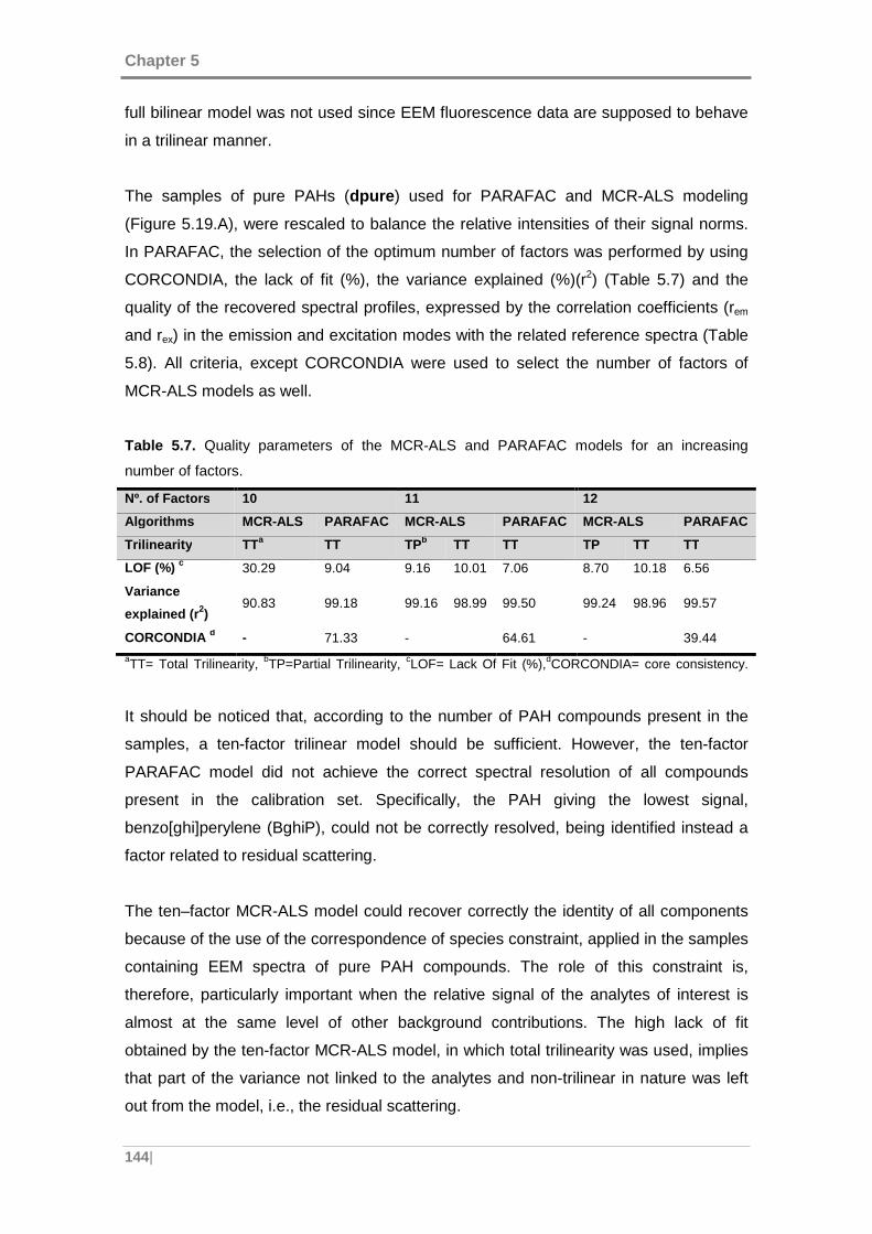
Chapter 5

144|

full bilinear model was not used since EEM fluorescence data are supposed to behave

in a trilinear manner.

The samples of pure PAHs (dpure ) used for PARAFAC and MCR-ALS modeling

(Figure 5.19.A), were rescaled to balance the relative intensities of their signal norms.

In PARAFAC, the selection of the optimum number of factors was performed by using

CORCONDIA, the lack of fit (%), the variance explained (%)(r2) (Table 5.7) and the

quality of the recovered spectral profiles, expressed by the correlation coefficients (rem

and rex) in the emission and excitation modes with the related reference spectra (Table

5.8). All criteria, except CORCONDIA were used to select the number of factors of

MCR-ALS models as well.

Table 5.7. Quality parameters of the MCR-ALS and PARAFAC models for an increasing

number of factors.

Nº. of Factors 10 11 12

Algorithms MCR-ALS PARAFAC MCR-ALS PARAFAC MCR-ALS PARAFAC

Trilinearity TTa TT TPb TT TT TP TT TT

LOF (%) c 30.29 9.04 9.16 10.01 7.06 8.70 10.18 6.56

Variance

explained (r 2) 90.83 99.18 99.16 98.99 99.50 99.24 98.96 99.57

CORCONDIA d - 71.33 - 64.61 - 39.44

aTT= Total Trilinearity, bTP=Partial Trilinearity, cLOF= Lack Of Fit (%),dCORCONDIA= core consistency.

It should be noticed that, according to the number of PAH compounds present in the

samples, a ten-factor trilinear model should be sufficient. However, the ten-factor

PARAFAC model did not achieve the correct spectral resolution of all compounds

present in the calibration set. Specifically, the PAH giving the lowest signal,

benzo[ghi]perylene (BghiP), could not be correctly resolved, being identified instead a

factor related to residual scattering.

The ten–factor MCR-ALS model could recover correctly the identity of all components

because of the use of the correspondence of species constraint, applied in the samples

containing EEM spectra of pure PAH compounds. The role of this constraint is,

therefore, particularly important when the relative signal of the analytes of interest is

almost at the same level of other background contributions. The high lack of fit

obtained by the ten-factor MCR-ALS model, in which total trilinearity was used, implies

that part of the variance not linked to the analytes and non-trilinear in nature was left

out from the model, i.e., the residual scattering.

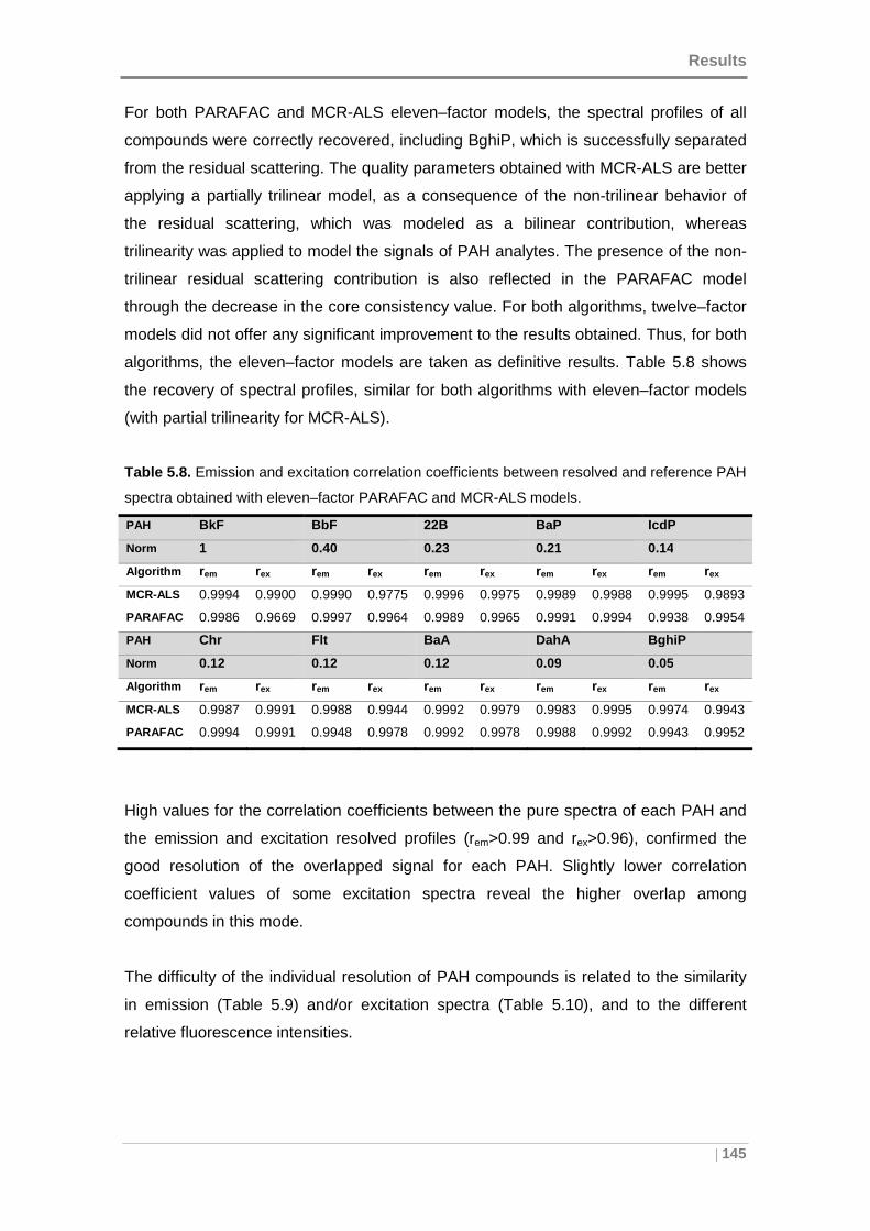
Results

| 145

For both PARAFAC and MCR-ALS eleven–factor models, the spectral profiles of all

compounds were correctly recovered, including BghiP, which is successfully separated

from the residual scattering. The quality parameters obtained with MCR-ALS are better

applying a partially trilinear model, as a consequence of the non-trilinear behavior of

the residual scattering, which was modeled as a bilinear contribution, whereas

trilinearity was applied to model the signals of PAH analytes. The presence of the non-

trilinear residual scattering contribution is also reflected in the PARAFAC model

through the decrease in the core consistency value. For both algorithms, twelve–factor

models did not offer any significant improvement to the results obtained. Thus, for both

algorithms, the eleven–factor models are taken as definitive results. Table 5.8 shows

the recovery of spectral profiles, similar for both algorithms with eleven–factor models

(with partial trilinearity for MCR-ALS).

Table 5.8. Emission and excitation correlation coefficients between resolved and reference PAH

spectra obtained with eleven–factor PARAFAC and MCR-ALS models.


Norm 1 0.40 0.23 0.21 0.14

Algorithm rem rex rem rex rem rex rem rex rem rex

MCR-ALS 0.9994 0.9900 0.9990 0.9775 0.9996 0.9975 0.9989 0.9988 0.9995 0.9893

PARAFAC 0.9986 0.9669 0.9997 0.9964 0.9989 0.9965 0.9991 0.9994 0.9938 0.9954


Norm 0.12 0.12 0.12 0.09 0.05


MCR-ALS 0.9987 0.9991 0.9988 0.9944 0.9992 0.9979 0.9983 0.9995 0.9974 0.9943

PARAFAC 0.9994 0.9991 0.9948 0.9978 0.9992 0.9978 0.9988 0.9992 0.9943 0.9952

High values for the correlation coefficients between the pure spectra of each PAH and

the emission and excitation resolved profiles (rem>0.99 and rex>0.96), confirmed the

good resolution of the overlapped signal for each PAH. Slightly lower correlation

coefficient values of some excitation spectra reveal the higher overlap among

compounds in this mode.

The difficulty of the individual resolution of PAH compounds is related to the similarity

in emission (Table 5.9) and/or excitation spectra (Table 5.10), and to the different

relative fluorescence intensities.

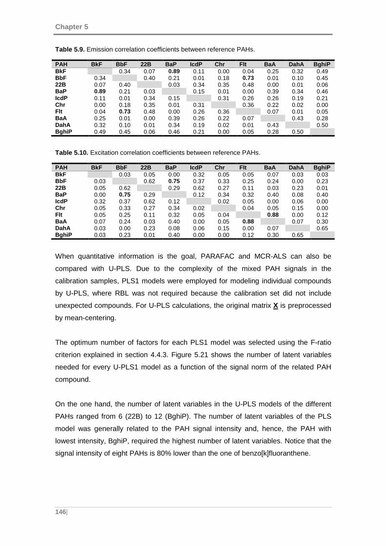
Chapter 5

146|

Table 5.9. Emission correlation coefficients between reference PAHs.

PAH BkF BbF 22B BaP IcdP Chr Flt BaA DahA BghiP BkF 0.34 0.07 0.89 0.11 0.00 0.04 0.25 0.32 0.49 BbF 0.34 0.40 0.21 0.01 0.18 0.73 0.01 0.10 0.45 22B 0.07 0.40 0.03 0.34 0.35 0.48 0.00 0.01 0.06 BaP 0.89 0.21 0.03 0.15 0.01 0.00 0.39 0.34 0.46 IcdP 0.11 0.01 0.34 0.15 0.31 0.26 0.26 0.19 0.21 Chr 0.00 0.18 0.35 0.01 0.31 0.36 0.22 0.02 0.00 Flt 0.04 0.73 0.48 0.00 0.26 0.36 0.07 0.01 0.05 BaA 0.25 0.01 0.00 0.39 0.26 0.22 0.07 0.43 0.28 DahA 0.32 0.10 0.01 0.34 0.19 0.02 0.01 0.43 0.50 BghiP 0.49 0.45 0.06 0.46 0.21 0.00 0.05 0.28 0.50

Table 5.10. Excitation correlation coefficients between reference PAHs.

PAH BkF BbF 22B BaP IcdP Chr Flt BaA DahA BghiP BkF 0.03 0.05 0.00 0.32 0.05 0.05 0.07 0.03 0.03 BbF 0.03 0.62 0.75 0.37 0.33 0.25 0.24 0.00 0.23 22B 0.05 0.62 0.29 0.62 0.27 0.11 0.03 0.23 0.01 BaP 0.00 0.75 0.29 0.12 0.34 0.32 0.40 0.08 0.40 IcdP 0.32 0.37 0.62 0.12 0.02 0.05 0.00 0.06 0.00 Chr 0.05 0.33 0.27 0.34 0.02 0.04 0.05 0.15 0.00 Flt 0.05 0.25 0.11 0.32 0.05 0.04 0.88 0.00 0.12 BaA 0.07 0.24 0.03 0.40 0.00 0.05 0.88 0.07 0.30 DahA 0.03 0.00 0.23 0.08 0.06 0.15 0.00 0.07 0.65 BghiP 0.03 0.23 0.01 0.40 0.00 0.00 0.12 0.30 0.65

When quantitative information is the goal, PARAFAC and MCR-ALS can also be

compared with U-PLS. Due to the complexity of the mixed PAH signals in the

calibration samples, PLS1 models were employed for modeling individual compounds

by U-PLS, where RBL was not required because the calibration set did not include

unexpected compounds. For U-PLS calculations, the original matrix X is preprocessed

by mean-centering.

The optimum number of factors for each PLS1 model was selected using the F-ratio

criterion explained in section 4.4.3. Figure 5.21 shows the number of latent variables

needed for every U-PLS1 model as a function of the signal norm of the related PAH

compound.

On the one hand, the number of latent variables in the U-PLS models of the different

PAHs ranged from 6 (22B) to 12 (BghiP). The number of latent variables of the PLS

model was generally related to the PAH signal intensity and, hence, the PAH with

lowest intensity, BghiP, required the highest number of latent variables. Notice that the

signal intensity of eight PAHs is 80% lower than the one of benzo[k]fluoranthene.

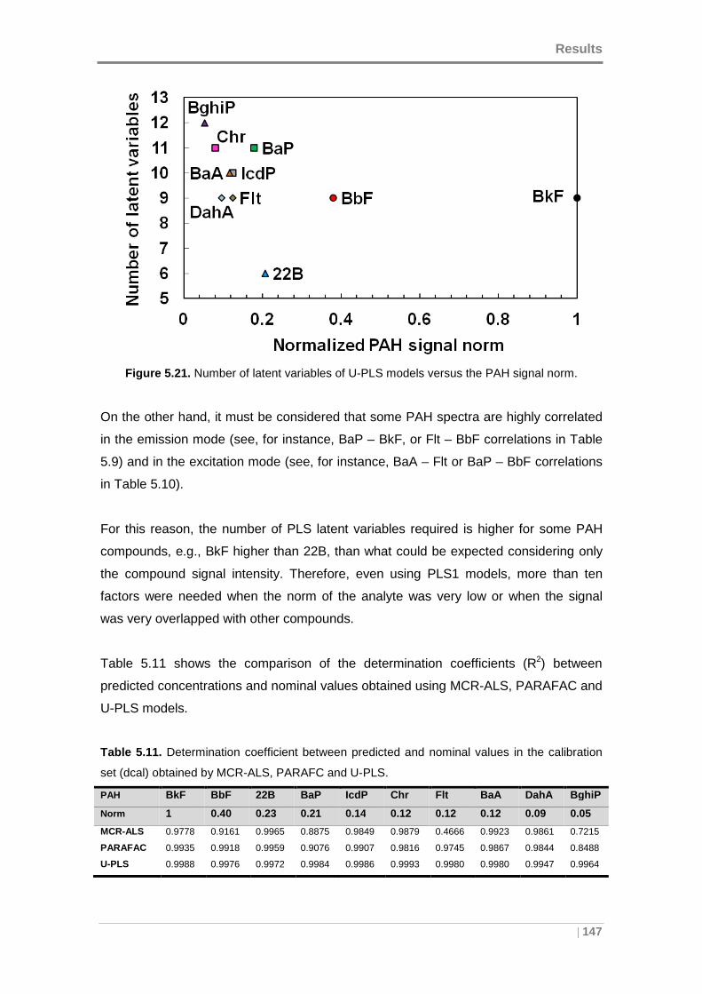
Results

| 147

Figure 5.21. Number of latent variables of U-PLS models versus the PAH signal norm.

On the other hand, it must be considered that some PAH spectra are highly correlated

in the emission mode (see, for instance, BaP – BkF, or Flt – BbF correlations in Table

5.9) and in the excitation mode (see, for instance, BaA – Flt or BaP – BbF correlations

in Table 5.10).

For this reason, the number of PLS latent variables required is higher for some PAH

compounds, e.g., BkF higher than 22B, than what could be expected considering only

the compound signal intensity. Therefore, even using PLS1 models, more than ten

factors were needed when the norm of the analyte was very low or when the signal

was very overlapped with other compounds.

Table 5.11 shows the comparison of the determination coefficients (R2) between

predicted concentrations and nominal values obtained using MCR-ALS, PARAFAC and

U-PLS models.

Table 5.11. Determination coefficient between predicted and nominal values in the calibration

set (dcal) obtained by MCR-ALS, PARAFC and U-PLS.


Norm 1 0.40 0.23 0.21 0.14 0.12 0.12 0.12 0.09 0.05

MCR-ALS 0.9778 0.9161 0.9965 0.8875 0.9849 0.9879 0.4666 0.9923 0.9861 0.7215

PARAFAC 0.9935 0.9918 0.9959 0.9076 0.9907 0.9816 0.9745 0.9867 0.9844 0.8488

U-PLS 0.9988 0.9976 0.9972 0.9984 0.9986 0.9993 0.9980 0.9980 0.9947 0.9964

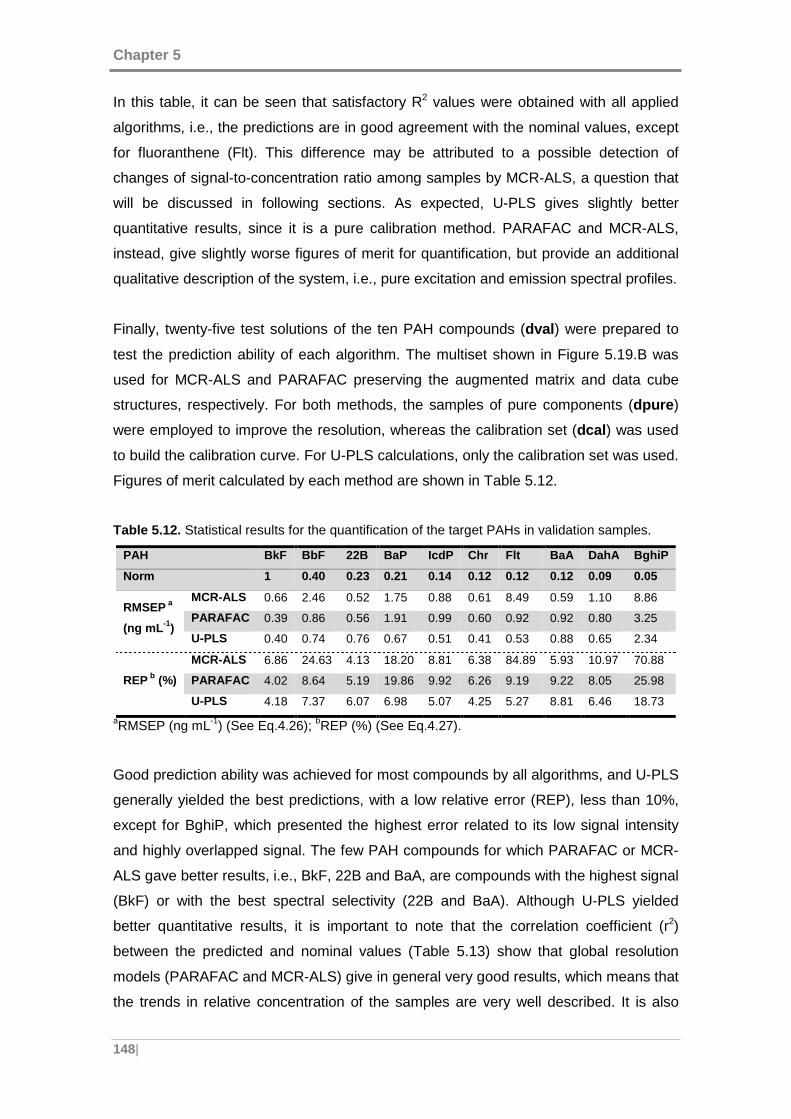
Chapter 5

148|

In this table, it can be seen that satisfactory R2 values were obtained with all applied

algorithms, i.e., the predictions are in good agreement with the nominal values, except

for fluoranthene (Flt). This difference may be attributed to a possible detection of

changes of signal-to-concentration ratio among samples by MCR-ALS, a question that

will be discussed in following sections. As expected, U-PLS gives slightly better

quantitative results, since it is a pure calibration method. PARAFAC and MCR-ALS,

instead, give slightly worse figures of merit for quantification, but provide an additional

qualitative description of the system, i.e., pure excitation and emission spectral profiles.

Finally, twenty-five test solutions of the ten PAH compounds (dval ) were prepared to

test the prediction ability of each algorithm. The multiset shown in Figure 5.19.B was

used for MCR-ALS and PARAFAC preserving the augmented matrix and data cube

structures, respectively. For both methods, the samples of pure components (dpure )

were employed to improve the resolution, whereas the calibration set (dcal ) was used

to build the calibration curve. For U-PLS calculations, only the calibration set was used.

Figures of merit calculated by each method are shown in Table 5.12.

Table 5.12. Statistical results for the quantification of the target PAHs in validation samples.


Norm 1 0.40 0.23 0.21 0.14 0.12 0.12 0.12 0.09 0.05

RMSEP a

(ng mL -1)

MCR-ALS 0.66 2.46 0.52 1.75 0.88 0.61 8.49 0.59 1.10 8.86

PARAFAC 0.39 0.86 0.56 1.91 0.99 0.60 0.92 0.92 0.80 3.25

U-PLS 0.40 0.74 0.76 0.67 0.51 0.41 0.53 0.88 0.65 2.34

REP b (%)

MCR-ALS 6.86 24.63 4.13 18.20 8.81 6.38 84.89 5.93 10.97 70.88

PARAFAC 4.02 8.64 5.19 19.86 9.92 6.26 9.19 9.22 8.05 25.98

U-PLS 4.18 7.37 6.07 6.98 5.07 4.25 5.27 8.81 6.46 18.73

aRMSEP (ng mL-1) (See Eq.4.26); bREP (%) (See Eq.4.27).

Good prediction ability was achieved for most compounds by all algorithms, and U-PLS

generally yielded the best predictions, with a low relative error (REP), less than 10%,

except for BghiP, which presented the highest error related to its low signal intensity

and highly overlapped signal. The few PAH compounds for which PARAFAC or MCR-

ALS gave better results, i.e., BkF, 22B and BaA, are compounds with the highest signal

(BkF) or with the best spectral selectivity (22B and BaA). Although U-PLS yielded

better quantitative results, it is important to note that the correlation coefficient (r2)

between the predicted and nominal values (Table 5.13) show that global resolution

models (PARAFAC and MCR-ALS) give in general very good results, which means that

the trends in relative concentration of the samples are very well described. It is also

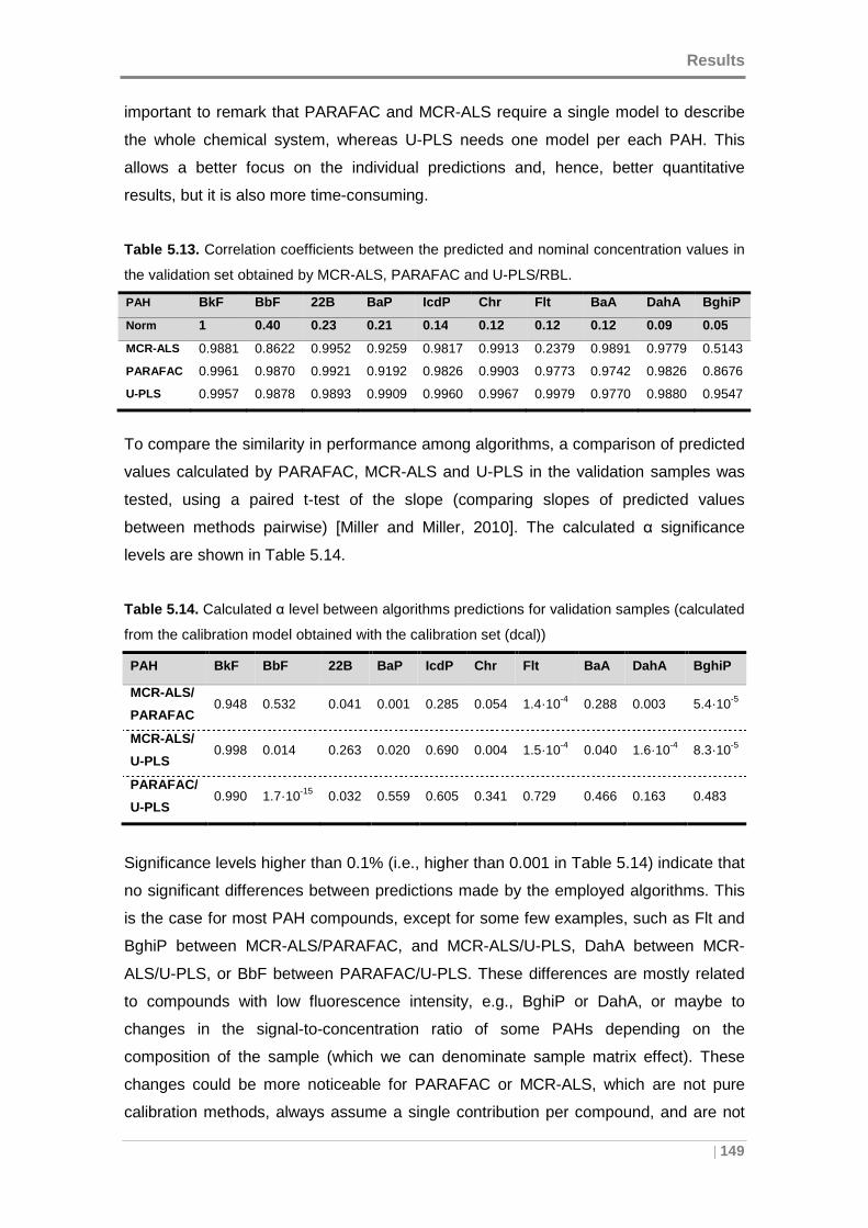
Results

| 149

important to remark that PARAFAC and MCR-ALS require a single model to describe

the whole chemical system, whereas U-PLS needs one model per each PAH. This

allows a better focus on the individual predictions and, hence, better quantitative

results, but it is also more time-consuming.

Table 5.13. Correlation coefficients between the predicted and nominal concentration values in

the validation set obtained by MCR-ALS, PARAFAC and U-PLS/RBL.


Norm 1 0.40 0.23 0.21 0.14 0.12 0.12 0.12 0.09 0.05

MCR-ALS 0.9881 0.8622 0.9952 0.9259 0.9817 0.9913 0.2379 0.9891 0.9779 0.5143

PARAFAC 0.9961 0.9870 0.9921 0.9192 0.9826 0.9903 0.9773 0.9742 0.9826 0.8676

U-PLS 0.9957 0.9878 0.9893 0.9909 0.9960 0.9967 0.9979 0.9770 0.9880 0.9547

To compare the similarity in performance among algorithms, a comparison of predicted

values calculated by PARAFAC, MCR-ALS and U-PLS in the validation samples was

tested, using a paired t-test of the slope (comparing slopes of predicted values

between methods pairwise) [Miller and Miller, 2010]. The calculated α significance

levels are shown in Table 5.14.

Table 5.14. Calculated α level between algorithms predictions for validation samples (calculated

from the calibration model obtained with the calibration set (dcal))


MCR-ALS/

PARAFAC 0.948 0.532 0.041 0.001 0.285 0.054 1.4·10-4 0.288 0.003 5.4·10-5

MCR-ALS/

U-PLS 0.998 0.014 0.263 0.020 0.690 0.004 1.5·10-4 0.040 1.6·10-4 8.3·10-5

PARAFAC/

U-PLS 0.990 1.7·10-15 0.032 0.559 0.605 0.341 0.729 0.466 0.163 0.483

Significance levels higher than 0.1% (i.e., higher than 0.001 in Table 5.14) indicate that

no significant differences between predictions made by the employed algorithms. This

is the case for most PAH compounds, except for some few examples, such as Flt and

BghiP between MCR-ALS/PARAFAC, and MCR-ALS/U-PLS, DahA between MCR-

ALS/U-PLS, or BbF between PARAFAC/U-PLS. These differences are mostly related

to compounds with low fluorescence intensity, e.g., BghiP or DahA, or maybe to

changes in the signal-to-concentration ratio of some PAHs depending on the

composition of the sample (which we can denominate sample matrix effect). These

changes could be more noticeable for PARAFAC or MCR-ALS, which are not pure

calibration methods, always assume a single contribution per compound, and are not

Chapter 5

150|

prepared to actively correct variations in signal-to-concentration ratio among samples.

U-PLS, instead, compensates better these differences among samples by adapting the

number of latent variables included in the model. This kind of effect will be further

analyzed in the following section 5.2.3, devoted to the study of samples with

interferences.

Results

| 151

5.2.3 Screening and determination of PAHs in presence of interferences

As discussed in Chapter 1, several authors have proven the efficiency of the selected

second-order calibration methods to quantify PAHs in the presence of unexpected

species which are absent in the calibration samples. However, few studies have been

conducted to simultaneously analyze a large number of PAHs in complex matrices with

a strong interference background. In fact, EEM matrices containing interfering species

and also sample matrix effects require the application of flexible methods, which can

successfully model qualitatively and quantitatively the different fluorescence

contributions. In this regard, sample matrix effects in second–order data of

multicomponent samples of PAHs have not yet been extensively studied and compared

with a wide range of datasets.

5.2.3.1 Objective

This section explores the feasibility of screening and determination of ten PAHs

through EEM in the presence of interferences and sample matrix effects, by using

different second-order data analysis algorithms: PARAFAC, MCR-ALS, and U-

PLS/RBL.

The scope of the proposed techniques is discussed for qualitative and quantitative

analysis of the selected PAHs. To understand the performance of PARAFAC, MCR-

ALS and U-PLS/RBL, and to propose a joint strategy of application, they were applied

to mixtures of standard reference materials containing interfering species such as the

16 US-EPA PAHs. Additionally, the importance of the complexity of the sample in

terms of number of target and interference compounds, and sample matrix effects, is

also discussed.

5.2.3.2 Data

Two sets of mixtures of the 16 US-EPA PAHs (dinterf ) were used as follows (section

3.5.4):

Set no.1. A total of 36 samples at 12 different concentration levels ranging from 1 - 20

ng mL-1.

Set no.2. 20 samples at 10 different concentration levels ranging from 0.2– 20 ng mL-1.

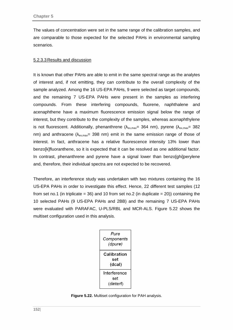
Chapter 5

152|

The values of concentration were set in the same range of the calibration samples, and

are comparable to those expected for the selected PAHs in environmental sampling

scenarios.


It is known that other PAHs are able to emit in the same spectral range as the analytes

of interest and, if not emitting, they can contribute to the overall complexity of the

sample analyzed. Among the 16 US-EPA PAHs, 9 were selected as target compounds,

and the remaining 7 US-EPA PAHs were present in the samples as interfering

compounds. From these interfering compounds, fluorene, naphthalene and

acenaphthene have a maximum fluorescence emission signal below the range of

interest, but they contribute to the complexity of the samples, whereas acenaphthylene

is not fluorescent. Additionally, phenanthrene (λex,max= 364 nm), pyrene (λex,max= 382

nm) and anthracene (λex,max= 398 nm) emit in the same emission range of those of

interest. In fact, anthracene has a relative fluorescence intensity 13% lower than

benzo[k]fluoranthene, so it is expected that it can be resolved as one additional factor.

In contrast, phenanthrene and pyrene have a signal lower than benzo[ghi]perylene

and, therefore, their individual spectra are not expected to be recovered.

Therefore, an interference study was undertaken with two mixtures containing the 16

US-EPA PAHs in order to investigate this effect. Hence, 22 different test samples (12

from set no.1 (in triplicate = 36) and 10 from set no.2 (in duplicate = 20)) containing the

10 selected PAHs (9 US-EPA PAHs and 2BB) and the remaining 7 US-EPA PAHs

were evaluated with PARAFAC, U-PLS/RBL and MCR-ALS. Figure 5.22 shows the

multiset configuration used in this analysis.

Figure 5.22. Multiset configuration for PAH analysis.

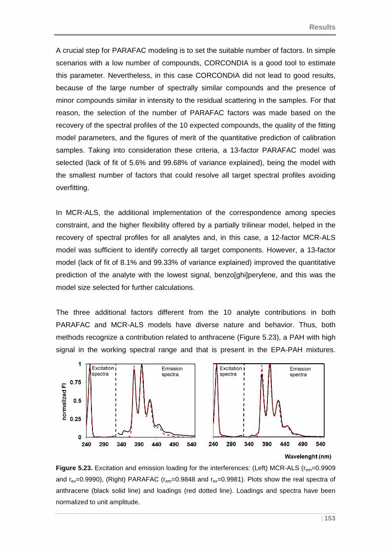
Results

| 153

A crucial step for PARAFAC modeling is to set the suitable number of factors. In simple

scenarios with a low number of compounds, CORCONDIA is a good tool to estimate

this parameter. Nevertheless, in this case CORCONDIA did not lead to good results,

because of the large number of spectrally similar compounds and the presence of

minor compounds similar in intensity to the residual scattering in the samples. For that

reason, the selection of the number of PARAFAC factors was made based on the

recovery of the spectral profiles of the 10 expected compounds, the quality of the fitting

model parameters, and the figures of merit of the quantitative prediction of calibration

samples. Taking into consideration these criteria, a 13-factor PARAFAC model was

selected (lack of fit of 5.6% and 99.68% of variance explained), being the model with

the smallest number of factors that could resolve all target spectral profiles avoiding

overfitting.

In MCR-ALS, the additional implementation of the correspondence among species

constraint, and the higher flexibility offered by a partially trilinear model, helped in the

recovery of spectral profiles for all analytes and, in this case, a 12-factor MCR-ALS

model was sufficient to identify correctly all target components. However, a 13-factor

model (lack of fit of 8.1% and 99.33% of variance explained) improved the quantitative

prediction of the analyte with the lowest signal, benzo[ghi]perylene, and this was the

model size selected for further calculations.

The three additional factors different from the 10 analyte contributions in both

PARAFAC and MCR-ALS models have diverse nature and behavior. Thus, both

methods recognize a contribution related to anthracene (Figure 5.23), a PAH with high

signal in the working spectral range and that is present in the EPA-PAH mixtures.

Figure 5.23. Excitation and emission loading for the interferences: (Left) MCR-ALS (rem=0.9909

and rex=0.9990), (Right) PARAFAC (rem=0.9848 and rex=0.9981). Plots show the real spectra of

anthracene (black solid line) and loadings (red dotted line). Loadings and spectra have been

normalized to unit amplitude.

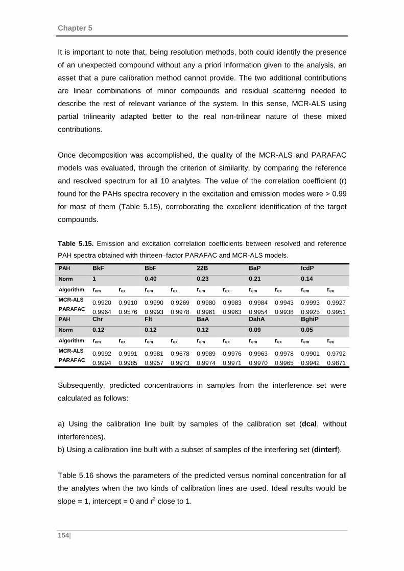
Chapter 5

154|

It is important to note that, being resolution methods, both could identify the presence

of an unexpected compound without any a priori information given to the analysis, an

asset that a pure calibration method cannot provide. The two additional contributions

are linear combinations of minor compounds and residual scattering needed to

describe the rest of relevant variance of the system. In this sense, MCR-ALS using

partial trilinearity adapted better to the real non-trilinear nature of these mixed

contributions.

Once decomposition was accomplished, the quality of the MCR-ALS and PARAFAC

models was evaluated, through the criterion of similarity, by comparing the reference

and resolved spectrum for all 10 analytes. The value of the correlation coefficient (r)

found for the PAHs spectra recovery in the excitation and emission modes were > 0.99

for most of them (Table 5.15), corroborating the excellent identification of the target

compounds.

Table 5.15. Emission and excitation correlation coefficients between resolved and reference

PAH spectra obtained with thirteen–factor PARAFAC and MCR-ALS models.


Norm 1 0.40 0.23 0.21 0.14


MCR-ALS 0.9920 0.9910 0.9990 0.9269 0.9980 0.9983 0.9984 0.9943 0.9993 0.9927 PARAFAC 0.9964 0.9576 0.9993 0.9978 0.9961 0.9963 0.9954 0.9938 0.9925 0.9951 PAH Chr Flt BaA DahA BghiP

Norm 0.12 0.12 0.12 0.09 0.05


MCR-ALS 0.9992 0.9991 0.9981 0.9678 0.9989 0.9976 0.9963 0.9978 0.9901 0.9792 PARAFAC 0.9994 0.9985 0.9957 0.9973 0.9974 0.9971 0.9970 0.9965 0.9942 0.9871

Subsequently, predicted concentrations in samples from the interference set were

calculated as follows:

a) Using the calibration line built by samples of the calibration set (dcal , without

interferences).

b) Using a calibration line built with a subset of samples of the interfering set (dinterf ).

Table 5.16 shows the parameters of the predicted versus nominal concentration for all

the analytes when the two kinds of calibration lines are used. Ideal results would be

slope = 1, intercept = 0 and r2 close to 1.

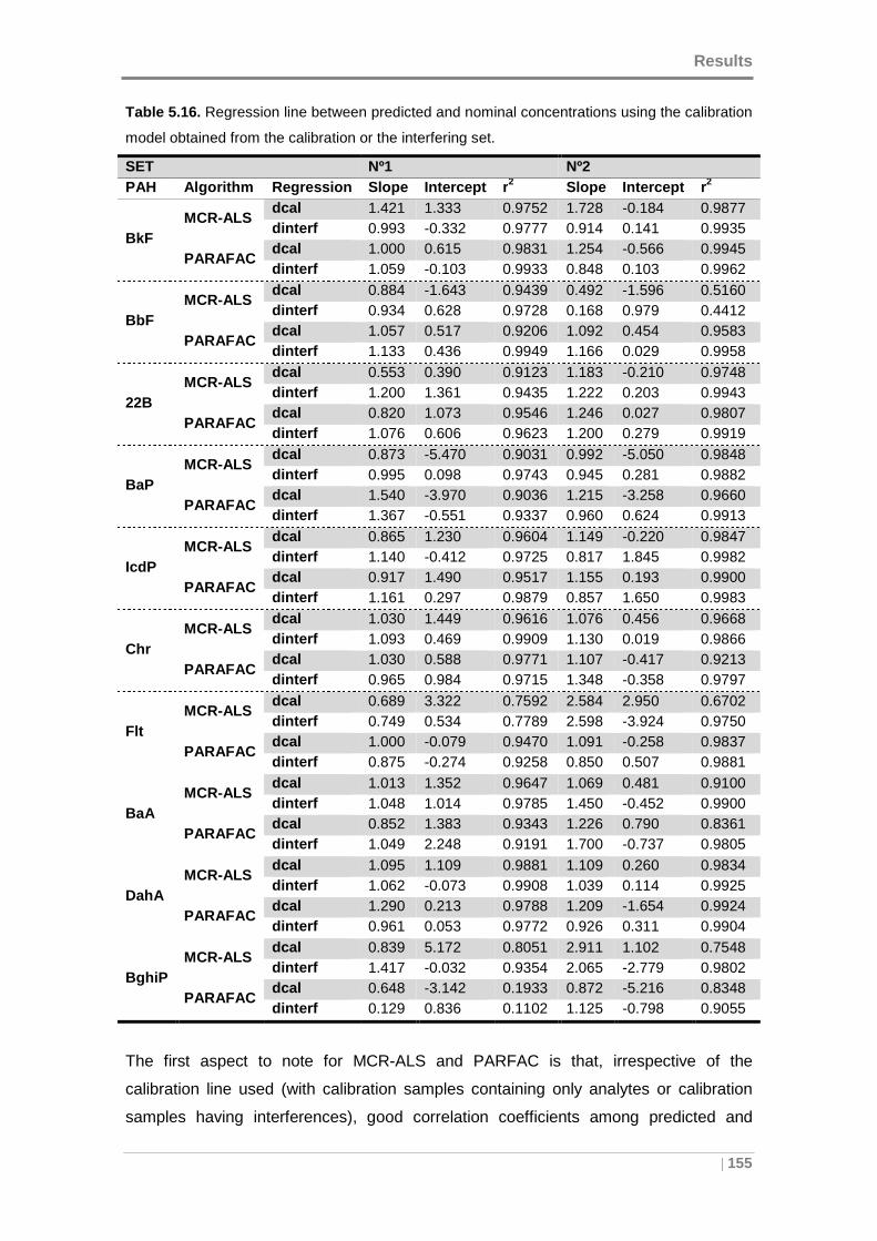
Results

| 155

Table 5.16. Regression line between predicted and nominal concentrations using the calibration

model obtained from the calibration or the interfering set.

SET Nº1 Nº2 PAH Algorithm Regression Slope Intercept r2 Slope Intercept r2

BkF MCR-ALS

dcal 1.421 1.333 0.9752 1.728 -0.184 0.9877 dinterf 0.993 -0.332 0.9777 0.914 0.141 0.9935

PARAFAC dcal 1.000 0.615 0.9831 1.254 -0.566 0.9945 dinterf 1.059 -0.103 0.9933 0.848 0.103 0.9962

BbF MCR-ALS

dcal 0.884 -1.643 0.9439 0.492 -1.596 0.5160 dinterf 0.934 0.628 0.9728 0.168 0.979 0.4412

PARAFAC dcal 1.057 0.517 0.9206 1.092 0.454 0.9583 dinterf 1.133 0.436 0.9949 1.166 0.029 0.9958

22B MCR-ALS

dcal 0.553 0.390 0.9123 1.183 -0.210 0.9748 dinterf 1.200 1.361 0.9435 1.222 0.203 0.9943


BaP MCR-ALS

dcal 0.873 -5.470 0.9031 0.992 -5.050 0.9848 dinterf 0.995 0.098 0.9743 0.945 0.281 0.9882

PARAFAC dcal 1.540 -3.970 0.9036 1.215 -3.258 0.9660 dinterf 1.367 -0.551 0.9337 0.960 0.624 0.9913

IcdP MCR-ALS

dcal 0.865 1.230 0.9604 1.149 -0.220 0.9847 dinterf 1.140 -0.412 0.9725 0.817 1.845 0.9982


Chr MCR-ALS

dcal 1.030 1.449 0.9616 1.076 0.456 0.9668 dinterf 1.093 0.469 0.9909 1.130 0.019 0.9866

PARAFAC dcal 1.030 0.588 0.9771 1.107 -0.417 0.9213 dinterf 0.965 0.984 0.9715 1.348 -0.358 0.9797

Flt MCR-ALS

dcal 0.689 3.322 0.7592 2.584 2.950 0.6702 dinterf 0.749 0.534 0.7789 2.598 -3.924 0.9750

PARAFAC dcal 1.000 -0.079 0.9470 1.091 -0.258 0.9837 dinterf 0.875 -0.274 0.9258 0.850 0.507 0.9881

BaA MCR-ALS

dcal 1.013 1.352 0.9647 1.069 0.481 0.9100 dinterf 1.048 1.014 0.9785 1.450 -0.452 0.9900

PARAFAC dcal 0.852 1.383 0.9343 1.226 0.790 0.8361 dinterf 1.049 2.248 0.9191 1.700 -0.737 0.9805

DahA MCR-ALS

dcal 1.095 1.109 0.9881 1.109 0.260 0.9834 dinterf 1.062 -0.073 0.9908 1.039 0.114 0.9925

PARAFAC dcal 1.290 0.213 0.9788 1.209 -1.654 0.9924 dinterf 0.961 0.053 0.9772 0.926 0.311 0.9904

BghiP MCR-ALS

dcal 0.839 5.172 0.8051 2.911 1.102 0.7548 dinterf 1.417 -0.032 0.9354 2.065 -2.779 0.9802

PARAFAC dcal 0.648 -3.142 0.1933 0.872 -5.216 0.8348 dinterf 0.129 0.836 0.1102 1.125 -0.798 0.9055

The first aspect to note for MCR-ALS and PARFAC is that, irrespective of the

calibration line used (with calibration samples containing only analytes or calibration

samples having interferences), good correlation coefficients among predicted and

Chapter 5

156|

nominal values are found for almost all analyzed compounds. The estimates of

concentration values show a general improvement (slight in some compounds) when

samples containing interferences are used as calibration set, but even if interferences

are absent in the calibration set, the information related to relative concentration among

samples is well defined. This is an important fact, since it gives a lot of value to

resolution methods when fast qualitative and quantitative screening of samples is the

main purpose, or when the evolution in relative concentrations among different

scenarios is the information sought, and not as much the exact concentration value of

the analytes in the sample.

Concerning the absolute quantitative predictions of analytes in samples, in most cases

there is a general worsening when predictions are performed with the calibration set

without interferences, a bit more noticeable in MCR-ALS calculations, perhaps because

of the more flexible underlying model used. However, even in this situation, good

results were obtained with REP values, less than 30% for several PAHs, e.g., Chr,

DahA and IcdP. The worst prediction was obtained for BghiP concentrations by both

algorithms, because of the very low signal of this analyte compared with the rest of

analytes, and some interfering species. When samples of the same interfering matrices

are used to build the calibration line, predictions improve significantly. In fact, for almost

all compounds, REP values were less than 30% except for BghiP, probably because of

the reason discussed above, and MCR-ALS had less satisfactory results for Flt and

BbF.

As a general result, PARAFAC and MCR-ALS are very suitable algorithms for

screening purposes, since they provide with a single model good qualitative and

relative quantitative information about the system analyzed. Nevertheless, one should

be aware that, for some compounds, these algorithms may be sensitive to potential

changes in signal-to-concentration ratio linked to the sample matrix and, therefore,

calibration sets without interferences might provide less accurate results, particularly

when the samples analyzed are extremely complex in terms of number of compounds

and signal overlap.

In the case of U-PLS model, the RBL step is required when samples with interferences

are analyzed, because they contain unexpected components absent in the set of

calibration samples. As a result, when U-PLS/RBL is used, two steps are required: a)

per each analyte, the number of latent variables in the U-PLS1 models is estimated

using the calibration set and b) per each sample to be predicted in the RBL step, an

Results

| 157

estimate of the additional number of factors corresponding to the unexpected

constituents is required. Because of the individual RBL step per each analyte in each

sample, it is important to note that the accurate estimation of the concentration implies

a dramatic increase of the computation time, since the number of models that must be

calculated is equal to: (number of samples × number of analytes), against the single

resolution model that is needed when PARAFAC or MCR-ALS algorithms are used.

Typically, the estimation of the number of factors in the RBL step is performed

comparing the RBL residuals (sRBL) of the decomposition, computed for different values

of unexpected components (Nunx) with the experimental noise (section 4.5.3). The

smallest number of factors that provides residuals at a value statistically comparable to

the experimental noise is chosen. But the number of RBL latent variables for real

samples is not easy to calculate, and mistakes in this step can lead to wrong predicted

concentrations.

For this reason, we compared the number of unexpected components for each PAH U-

plS model and sample calculated considering the methods described in [Braga et al.,

2010] and [Bortolato et al., 2008]. Braga et al. (2010) et al. propose a method to

compare the residuals of the U-PLS/RBL test samples with results of t-student

confidence intervals for the mean residuals of decomposition of the calibration

samples. In contrast, Bortotalo et al. estimate the number of optimum RBL factors

based on a ratio between the RBL residuals (sRBL):

s�� = ‖e��‖/h(¶ : N[ �$(¸ : N[ �$ : Al� =� (5.3)

and a penalized residual error (spen):

sv = s�� ¹(¶x¸$/h(¶ : N[ �$(¸ : N[ �$ : Al� =� º (5.4)

This ratio is computed for increasing values of unexpected components (Nunx) as

follows:

R = sv (N[ �$/hs��(N[ � : 1$] (5.5)

The first value of Nunx for which R did not exceed 1 was then selected as the number of

RBL components.

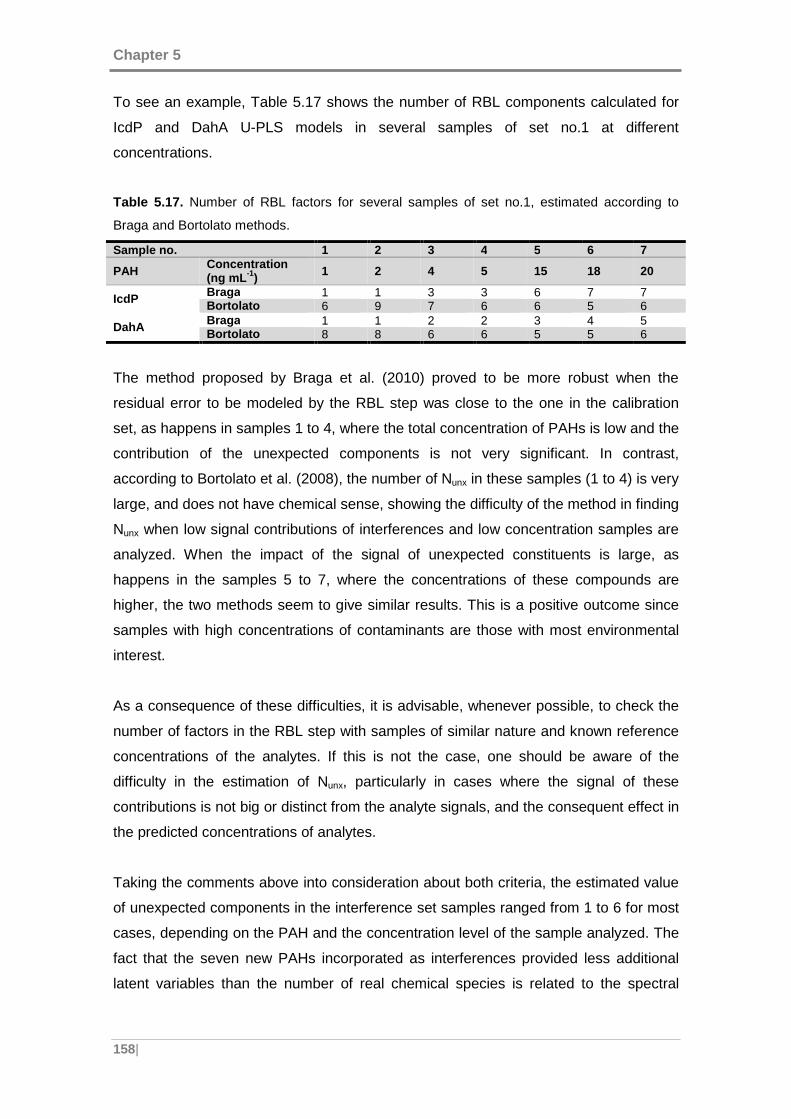
Chapter 5

158|

To see an example, Table 5.17 shows the number of RBL components calculated for

IcdP and DahA U-PLS models in several samples of set no.1 at different

concentrations.

Table 5.17. Number of RBL factors for several samples of set no.1, estimated according to

Braga and Bortolato methods.

Sample no. 1 2 3 4 5 6 7

PAH Concentration (ng mL -1) 1 2 4 5 15 18 20

IcdP Braga 1 1 3 3 6 7 7 Bortolato 6 9 7 6 6 5 6

DahA Braga 1 1 2 2 3 4 5 Bortolato 8 8 6 6 5 5 6

The method proposed by Braga et al. (2010) proved to be more robust when the

residual error to be modeled by the RBL step was close to the one in the calibration

set, as happens in samples 1 to 4, where the total concentration of PAHs is low and the

contribution of the unexpected components is not very significant. In contrast,

according to Bortolato et al. (2008), the number of Nunx in these samples (1 to 4) is very

large, and does not have chemical sense, showing the difficulty of the method in finding

Nunx when low signal contributions of interferences and low concentration samples are

analyzed. When the impact of the signal of unexpected constituents is large, as

happens in the samples 5 to 7, where the concentrations of these compounds are

higher, the two methods seem to give similar results. This is a positive outcome since

samples with high concentrations of contaminants are those with most environmental

interest.

As a consequence of these difficulties, it is advisable, whenever possible, to check the

number of factors in the RBL step with samples of similar nature and known reference

concentrations of the analytes. If this is not the case, one should be aware of the

difficulty in the estimation of Nunx, particularly in cases where the signal of these

contributions is not big or distinct from the analyte signals, and the consequent effect in

the predicted concentrations of analytes.

Taking the comments above into consideration about both criteria, the estimated value

of unexpected components in the interference set samples ranged from 1 to 6 for most

cases, depending on the PAH and the concentration level of the sample analyzed. The

fact that the seven new PAHs incorporated as interferences provided less additional

latent variables than the number of real chemical species is related to the spectral

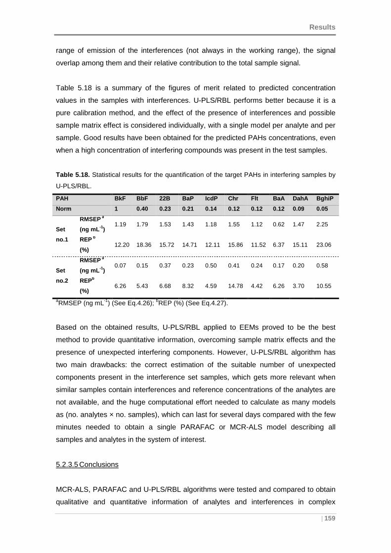
Results

| 159

range of emission of the interferences (not always in the working range), the signal

overlap among them and their relative contribution to the total sample signal.

Table 5.18 is a summary of the figures of merit related to predicted concentration

values in the samples with interferences. U-PLS/RBL performs better because it is a

pure calibration method, and the effect of the presence of interferences and possible

sample matrix effect is considered individually, with a single model per analyte and per

sample. Good results have been obtained for the predicted PAHs concentrations, even

when a high concentration of interfering compounds was present in the test samples.

Table 5.18. Statistical results for the quantification of the target PAHs in interfering samples by

U-PLS/RBL.


Norm 1 0.40 0.23 0.21 0.14 0.12 0.12 0.12 0.09 0.05

Set

no.1

RMSEP a

(ng mL -1) 1.19 1.79 1.53 1.43 1.18 1.55 1.12 0.62 1.47 2.25

REP b

(%) 12.20 18.36 15.72 14.71 12.11 15.86 11.52 6.37 15.11 23.06

Set

no.2

RMSEP a

(ng mL -1) 0.07 0.15 0.37 0.23 0.50 0.41 0.24 0.17 0.20 0.58

REPb

(%) 6.26 5.43 6.68 8.32 4.59 14.78 4.42 6.26 3.70 10.55

aRMSEP (ng mL-1) (See Eq.4.26); bREP (%) (See Eq.4.27).

Based on the obtained results, U-PLS/RBL applied to EEMs proved to be the best

method to provide quantitative information, overcoming sample matrix effects and the

presence of unexpected interfering components. However, U-PLS/RBL algorithm has

two main drawbacks: the correct estimation of the suitable number of unexpected

components present in the interference set samples, which gets more relevant when

similar samples contain interferences and reference concentrations of the analytes are

not available, and the huge computational effort needed to calculate as many models

as (no. analytes × no. samples), which can last for several days compared with the few

minutes needed to obtain a single PARAFAC or MCR-ALS model describing all

samples and analytes in the system of interest.

5.2.3.5 Conclusions

MCR-ALS, PARAFAC and U-PLS/RBL algorithms were tested and compared to obtain

qualitative and quantitative information of analytes and interferences in complex

Chapter 5

160|

samples of PAH mixtures analyzed by EEM fluorescence spectroscopy. Advantages

and drawbacks associated with these methods are related mainly to the main

resolution (MCR-ALS and PARAFAC) or calibration (U-PLS/RBL) purpose of the

algorithms.

Thus, MCR-ALS and PARAFAC are clearly the recommended methods for a fast

qualitative and quantitative screening of environmental samples. Even in samples

containing 10 analytes with overlapped signals and several interferences, the single

resolution model provided by both algorithms manages to recover the identity (spectral

profiles) of the analytes and is able to find out the identity of interfering compounds,

e.g., anthracene, when the signal of the unexpected compound is within the spectral

working range. It is important to note this capability for both methods, which are often

assumed to be able to work only with systems with a small number of compounds.

It is interesting to stress the effect of MCR-ALS constraints in the context of these

complex systems, notably the correspondence of species to identify more clearly the

analytes present in the sample and the partial trilinearity, which can provide a more

accurate description of the system behavior when deviations from ideal trilinearity due

to residual scattering exist. The active use of this kind of constraints is still not

sufficiently exploited and remains a point for which a more general diffusion within the

chemical community should be performed.

Quantitative information can also be extracted by both MCR-ALS and PARAFAC

algorithms, although predicted concentration values can be sometimes affected by

changes in the signal-to-concentration ratio (matrix effect) of the real samples when

compared with a calibration set without interferences. Since these algorithms are not

calibration-oriented methods, they are more sensitive to sample matrix effects.

However, relative concentration values are always correctly estimated and this

provides a good screening tool to obtain relative or approximate concentration values,

and to point out the most contaminated samples, which may deserve a more accurate

quantitative analysis. They would also be the algorithms of choice when environmental

trends in concentrations (due to seasonality, location or other factors) are the main

purpose of the study, rather than an exact determination of analyte concentration in

individual samples.

U-PLS/RBL, the only pure calibration method used here, provided the best quantitative

information for samples containing interferences and potential sample matrix effect,

Results

| 161

with low values of RMSEP and REP, below 1.8 ng mL-1 and 20% respectively,

comparable to those provided by separation and analysis techniques, more expensive

and time consuming. However, it presented as weak points the difficulty in estimating

the number of unexpected contributions in the RBL step (particularly for low

concentration samples) and the huge computation effort linked to calculate as many

models as (no. samples × no. analytes), which makes the algorithm unsuitable for fast

screening purposes.

From the above discussion, it seems recommendable a combined use of the presented

algorithms. A first application of PARAFAC or MCR-ALS for screening purposes, with

the added value of detecting unexpected compounds in the samples, and the capability

to point out the most contaminated samples, which are the most relevant from an

environmental point of view. For those samples, a second step using U-PLS/RBL can

be carried out to accurately estimate the concentrations of the analytes of interest,

knowing that the predicted concentration will be more reliable than the first estimation

provided by the screening resolution methodologies.

Chapter 5

162|

5.3. OPTIMIZATION OF THE EXTRACTION PROTOCOL

Extraction is one of the most crucial points in the analytical chain in the effort of

achieving a complete recovery of target compounds. It is also one of the most complex

steps and it rarely yields reproducible results. The standard extraction procedures for

sample preparation of particle-bound PAHs described in the standards listed in Table

1.5 recommend the incorporation of Soxhlet extraction methods that are labor

intensive (>8 h/sample), and consume large amounts of solvents (>150 mL/sample), to

achieve considerable PAH extraction efficiencies. Nonetheless, the Soxhlet extraction

is still the preferred method because of its comparative extraction results despite the

nature of matrix sample.

Automated Soxhlet extraction represents an improvement over the classic Soxhlet

extraction. The automated Soxhlet extraction design allows several samples to be

extracted simultaneously with its multiple extraction cells assembly while being cycle

and/or time monitoring for unattended operation, leading to a better reproducibility.

Since extraction is crucial in the sample preparation steps previous to fluorescence

analysis, the selection of the optimal operation parameters and the definition of the

most suitable extraction protocol according to the characteristics of the target PAHs is

thoughtfully studied in the following sections.

First, section 5.3.1 discusses the selection of the appropriate solvent and surrogate to

correct for the extraction efficiency, according to the extraction and fluorescence

analysis requirements.

In section 5.3.2 an examination with an automated extraction system is made to test

whether savings in time can be obtained in daily routine analysis. This system offers

the use of warm and hot extraction modes, which were developed to speed up the

classic Soxhlet extraction. Hence, a deeper study was undertaken to select the best

extraction mode.

Finally, section 5.3.3 explores the optimization of the extraction time, by analyzing a

standard reference material subjected to increasing extraction times required for later

aerosol analysis.

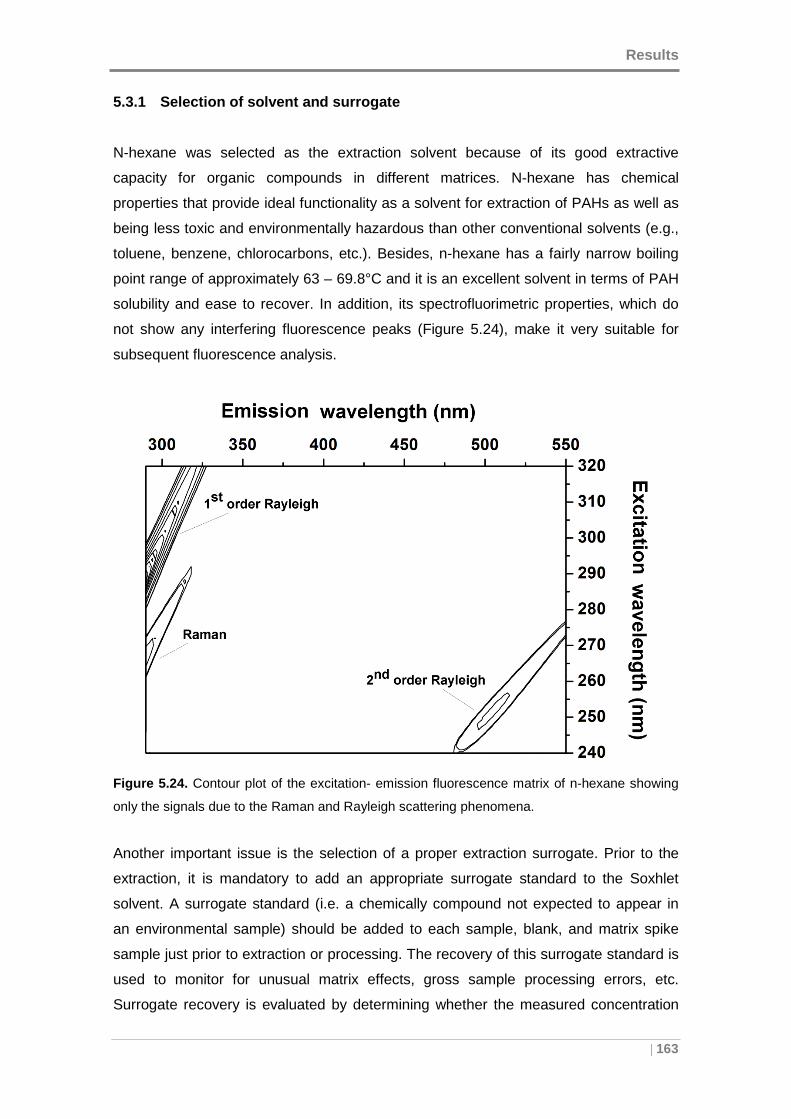
Results

| 163

5.3.1 Selection of solvent and surrogate

N-hexane was selected as the extraction solvent because of its good extractive

capacity for organic compounds in different matrices. N-hexane has chemical

properties that provide ideal functionality as a solvent for extraction of PAHs as well as

being less toxic and environmentally hazardous than other conventional solvents (e.g.,

toluene, benzene, chlorocarbons, etc.). Besides, n-hexane has a fairly narrow boiling

point range of approximately 63 – 69.8°C and it is an excellent solvent in terms of PAH

solubility and ease to recover. In addition, its spectrofluorimetric properties, which do

not show any interfering fluorescence peaks (Figure 5.24), make it very suitable for

subsequent fluorescence analysis.

Figure 5.24. Contour plot of the excitation- emission fluorescence matrix of n-hexane showing

only the signals due to the Raman and Rayleigh scattering phenomena.

Another important issue is the selection of a proper extraction surrogate. Prior to the

extraction, it is mandatory to add an appropriate surrogate standard to the Soxhlet

solvent. A surrogate standard (i.e. a chemically compound not expected to appear in

an environmental sample) should be added to each sample, blank, and matrix spike

sample just prior to extraction or processing. The recovery of this surrogate standard is

used to monitor for unusual matrix effects, gross sample processing errors, etc.

Surrogate recovery is evaluated by determining whether the measured concentration

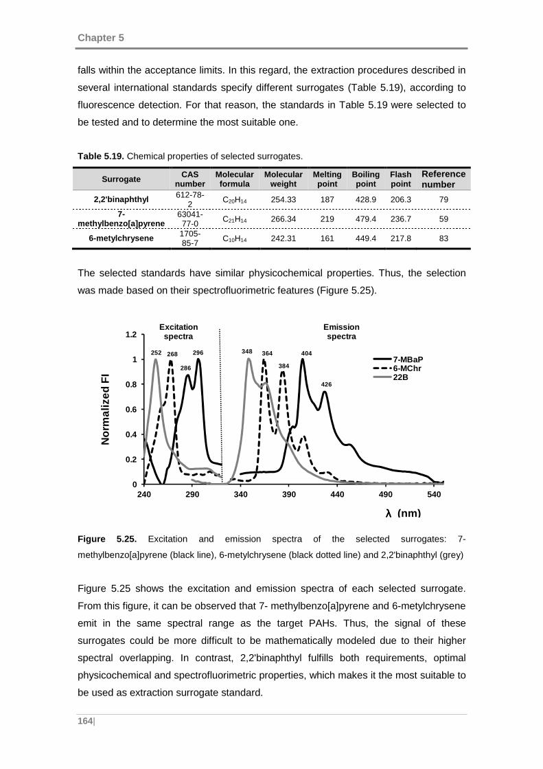
Chapter 5

164|

falls within the acceptance limits. In this regard, the extraction procedures described in

several international standards specify different surrogates (Table 5.19), according to

fluorescence detection. For that reason, the standards in Table 5.19 were selected to

be tested and to determine the most suitable one.

Table 5.19. Chemical properties of selected surrogates.

Surrogate CAS number

Molecular formula

Molecular weight

Melting point

Boiling point

Flash point

Reference number

2,2'binaphthyl 612-78-2 C20H14 254.33 187 428.9 206.3 79

7- methylbenzo[a]pyrene

63041-77-0 C21H14 266.34 219 479.4 236.7 59

6-metylchrysene 1705-85-7 C10H14 242.31 161 449.4 217.8 83

The selected standards have similar physicochemical properties. Thus, the selection

was made based on their spectrofluorimetric features (Figure 5.25).

Figure 5.25. Excitation and emission spectra of the selected surrogates: 7-

methylbenzo[a]pyrene (black line), 6-metylchrysene (black dotted line) and 2,2'binaphthyl (grey)

Figure 5.25 shows the excitation and emission spectra of each selected surrogate.

From this figure, it can be observed that 7- methylbenzo[a]pyrene and 6-metylchrysene

emit in the same spectral range as the target PAHs. Thus, the signal of these

surrogates could be more difficult to be mathematically modeled due to their higher

spectral overlapping. In contrast, 2,2'binaphthyl fulfills both requirements, optimal

physicochemical and spectrofluorimetric properties, which makes it the most suitable to

be used as extraction surrogate standard.

404

426

364

384

348

286

296268252

0

0.2

0.4

0.6

0.8

1

1.2

240 290 340 390 440 490 540

Nor

mal

ized

FI

λ λ λ λ (nm)

7-MBaP6-MChr22B

Excitation spectra

Emission spectra

Results

| 165

5.3.2 Optimization of the extraction mode

The optimization of the extraction conditions is usually assessed by systematic

alteration of one variable while the others are kept constant. However, this approach is

unable to determine interactions between parameters and predict extraction conditions.

In this regard, experimental designs (a.k.a. Design of Experiments, DoE) are

appropriate tools for this purpose. Furthermore, DoE allows efficient testing of the

method robustness. Among all plausible DoE types, the so-called full factorial designs

allow us to reveal the significance of the factors under investigation as well as the

interactions between them.

5.3.2.1 Objective

The objective of this section is the optimization of the Soxhlet extraction protocol by

means of DoE. The chosen DoE method was based on a two-level factorial design with

center points, applied to evaluate interactions between the selected Soxhlet factors as

well as to optimize them.

5.3.2.2 Data

PAH extraction samples (dextract). It consists of two sets of samples (section 3.5.5):

Set no.1. 36 samples obtained from 12 extraction tests in triplicate, constructed to test

the differences between the hot and warm operation mode.

Set no.2. 18 samples obtained from 6 extraction tests in triplicate, constructed to

compare the above obtained results with the standard Soxhlet method.

5.3.2.3 Method

To test the recovery of the extraction method, a half of 150 mm diameter quartz blank

filters were spiked with 150 µL of internal standard 22B at 10 ng µL-1 and 200 µL of the

16 US-EPA PAHs standard. Samples without drying step were extracted to a final

volume of 100 mL, whereas samples under drying conditions were concentrated to a

final volume of 10 mL and subsequently diluted to obtain extracts with concentrations in

the order of 10 ng mL-1.

For these preliminary experiments, filters spiked with standards were preferred over

extracting certified materials for two reasons. The first one was to homogenize the

Chapter 5

166|

matrix, since samples are collected onto filters and certified materials are normally

presented as a powder. The second one, the certified material SRM 1649b was more

expensive than the PAH standards solution. Therefore, the use of the standards

solution for method development and the use of the certified material for method

validation was preferred, considering the large number of tests performed to optimize

the extraction method.

In order to determine the influencing factors as well as their interactions, a 2 full

factorial design with center points was carried out for each set of samples. Center point

experiments were used to evaluate the response curvature. Three extraction factors

were selected for the experimental design: Soxhlet mode (X1), extraction time (X2) and

the use of the drying step (X3), in order to investigate their effect on the yield (Y) from

chemical PAHs extraction. As response, the percentage of recovery of each selected 9

PAHs and the surrogate used as internal standard (22B) was used. The recoveries

were compared and the robustness of the extraction method estimated.

It is also important to remark that the efficiencies of extraction of PAHs are also

dependent on the temperature. However, in our case, the extraction temperature is

controlled by the heating power of the heater. Thus, this was established according to

the manufacturer's specifications referring to the solvent used, n-hexane, as follows:

heating level below: 10; heating level above: 4.

The statistical significance of each experimental variable studied was established in

relation to the percentage of recovery of each target PAH (Y). Running the full

complement of all possible factor combinations means that all the main and interaction

effects can be estimated. Hence, there are three main effects (X1, X2, X3), three two-

factor interactions (X1X2, X1X3, X2X3), and one three-factor interaction (X1X2X3), all of

which appear in the full linear regression model as follows:

Y= β0 +β1X1 +β2X2 +β3X3 +β12X1X2 +β13X1X3 +β23X2X3 +β123X1X2X3 +ε (5.6)

where β0 represents the overall mean; β1, β2 and β3 represent the independent effect of

factor X1, X2 and X3 respectively; β12, β23 and β13 are related to the two factor

interaction effects, β123 represent the three factor interaction effect and ε is the random

error term. A full factorial design allows us to estimate all “beta” coefficients {β0,…,β123}

to investigate their effect on the response. These data were processed using Minitab

16.1 software package (Minitab Inc., UK).

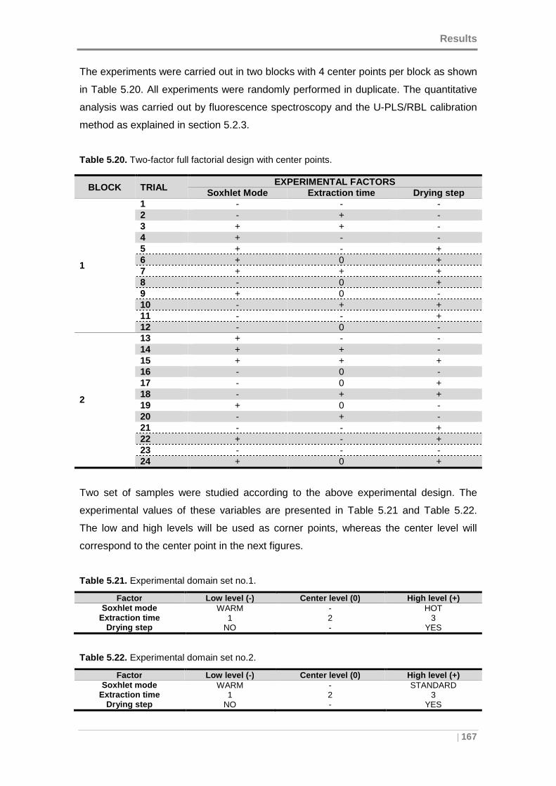
Results

| 167

The experiments were carried out in two blocks with 4 center points per block as shown

in Table 5.20. All experiments were randomly performed in duplicate. The quantitative

analysis was carried out by fluorescence spectroscopy and the U-PLS/RBL calibration

method as explained in section 5.2.3.

Table 5.20. Two-factor full factorial design with center points.

BLOCK TRIAL EXPERIMENTAL FACTORS Soxhlet Mode Extraction time Drying step

1

1 - - - 2 - + - 3 + + - 4 + - - 5 + - + 6 + 0 + 7 + + + 8 - 0 + 9 + 0 - 10 - + + 11 - - + 12 - 0 -

2

13 + - - 14 + + - 15 + + + 16 - 0 - 17 - 0 + 18 - + + 19 + 0 - 20 - + - 21 - - + 22 + - + 23 - - - 24 + 0 +

Two set of samples were studied according to the above experimental design. The

experimental values of these variables are presented in Table 5.21 and Table 5.22.

The low and high levels will be used as corner points, whereas the center level will

correspond to the center point in the next figures.

Table 5.21. Experimental domain set no.1.

Factor Low level ( -) Center level (0) High level (+) Soxhlet mode WARM - HOT

Extraction time 1 2 3 Drying step NO - YES

Table 5.22. Experimental domain set no.2.

Factor Low level ( -) Center level (0) High level (+) Soxhlet mode WARM - STANDARD

Extraction time 1 2 3 Drying step NO - YES

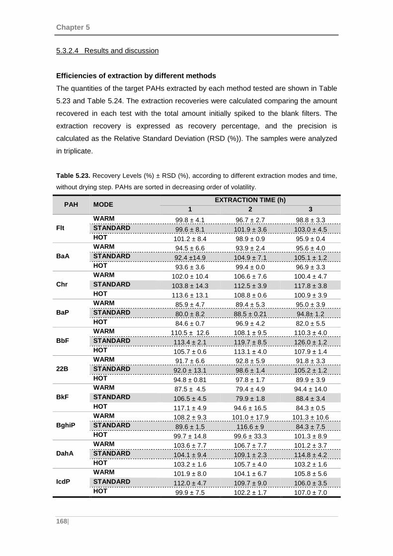
Chapter 5

168|


Efficiencies of extraction by different methods

The quantities of the target PAHs extracted by each method tested are shown in Table

5.23 and Table 5.24. The extraction recoveries were calculated comparing the amount

recovered in each test with the total amount initially spiked to the blank filters. The

extraction recovery is expressed as recovery percentage, and the precision is

calculated as the Relative Standard Deviation (RSD (%)). The samples were analyzed

in triplicate.

Table 5.23. Recovery Levels (%) ± RSD (%), according to different extraction modes and time,

without drying step. PAHs are sorted in decreasing order of volatility.

PAH MODE EXTRACTION TIME (h)

1 2 3

Flt WARM 99.8 ± 4.1 96.7 ± 2.7 98.8 ± 3.3 STANDARD 99.6 ± 8.1 101.9 ± 3.6 103.0 ± 4.5 HOT 101.2 ± 8.4 98.9 ± 0.9 95.9 ± 0.4

BaA WARM 94.5 ± 6.6 93.9 ± 2.4 95.6 ± 4.0 STANDARD 92.4 ±14.9 104.9 ± 7.1 105.1 ± 1.2 HOT 93.6 ± 3.6 99.4 ± 0.0 96.9 ± 3.3

Chr WARM 102.0 ± 10.4 106.6 ± 7.6 100.4 ± 4.7 STANDARD 103.8 ± 14.3 112.5 ± 3.9 117.8 ± 3.8 HOT 113.6 ± 13.1 108.8 ± 0.6 100.9 ± 3.9

BaP WARM 85.9 ± 4.7 89.4 ± 5.3 95.0 ± 3.9 STANDARD 80.0 ± 8.2 88.5 ± 0.21 94.8± 1.2 HOT 84.6 ± 0.7 96.9 ± 4.2 82.0 ± 5.5

BbF WARM 110.5 ± 12.6 108.1 ± 9.5 110.3 ± 4.0 STANDARD 113.4 ± 2.1 119.7 ± 8.5 126.0 ± 1.2 HOT 105.7 ± 0.6 113.1 ± 4.0 107.9 ± 1.4

22B WARM 91.7 ± 6.6 92.8 ± 5.9 91.8 ± 3.3 STANDARD 92.0 ± 13.1 98.6 ± 1.4 105.2 ± 1.2 HOT 94.8 ± 0.81 97.8 ± 1.7 89.9 ± 3.9

BkF WARM 87.5 ± 4.5 79.4 ± 4.9 94.4 ± 14.0 STANDARD 106.5 ± 4.5 79.9 ± 1.8 88.4 ± 3.4 HOT 117.1 ± 4.9 94.6 ± 16.5 84.3 ± 0.5

BghiP WARM 108.2 ± 9.3 101.0 ± 17.9 101.3 ± 10.6 STANDARD 89.6 ± 1.5 116.6 ± 9 84.3 ± 7.5 HOT 99.7 ± 14.8 99.6 ± 33.3 101.3 ± 8.9

DahA WARM 103.6 ± 7.7 106.7 ± 7.7 101.2 ± 3.7 STANDARD 104.1 ± 9.4 109.1 ± 2.3 114.8 ± 4.2 HOT 103.2 ± 1.6 105.7 ± 4.0 103.2 ± 1.6

IcdP WARM 101.9 ± 8.0 104.1 ± 6.7 105.8 ± 5.6 STANDARD 112.0 ± 4.7 109.7 ± 9.0 106.0 ± 3.5 HOT 99.9 ± 7.5 102.2 ± 1.7 107.0 ± 7.0

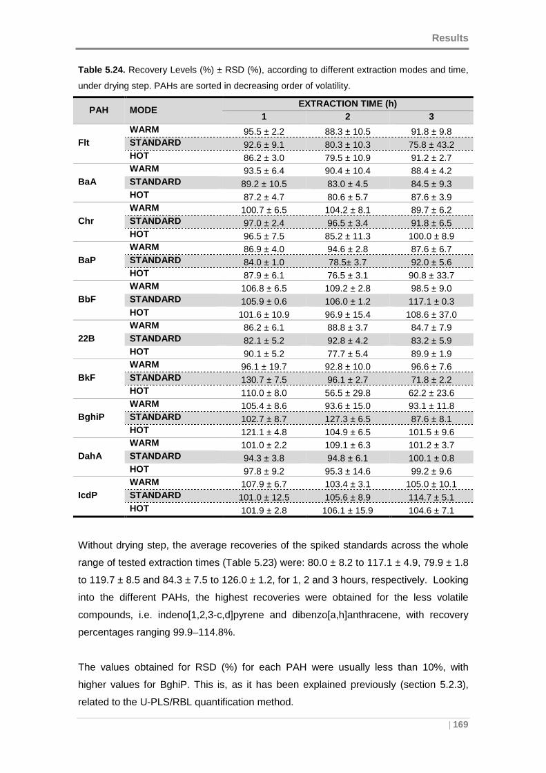
Results

| 169

Table 5.24. Recovery Levels (%) ± RSD (%), according to different extraction modes and time,

under drying step. PAHs are sorted in decreasing order of volatility.

PAH MODE EXTRACTION TIME (h)

1 2 3

Flt WARM 95.5 ± 2.2 88.3 ± 10.5 91.8 ± 9.8 STANDARD 92.6 ± 9.1 80.3 ± 10.3 75.8 ± 43.2 HOT 86.2 ± 3.0 79.5 ± 10.9 91.2 ± 2.7

BaA WARM 93.5 ± 6.4 90.4 ± 10.4 88.4 ± 4.2 STANDARD 89.2 ± 10.5 83.0 ± 4.5 84.5 ± 9.3 HOT 87.2 ± 4.7 80.6 ± 5.7 87.6 ± 3.9

Chr WARM 100.7 ± 6.5 104.2 ± 8.1 89.7 ± 6.2 STANDARD 97.0 ± 2.4 96.5 ± 3.4 91.8 ± 6.5 HOT 96.5 ± 7.5 85.2 ± 11.3 100.0 ± 8.9

BaP WARM 86.9 ± 4.0 94.6 ± 2.8 87.6 ± 6.7 STANDARD 84.0 ± 1.0 78.5± 3.7 92.0 ± 5.6 HOT 87.9 ± 6.1 76.5 ± 3.1 90.8 ± 33.7

BbF WARM 106.8 ± 6.5 109.2 ± 2.8 98.5 ± 9.0 STANDARD 105.9 ± 0.6 106.0 ± 1.2 117.1 ± 0.3 HOT 101.6 ± 10.9 96.9 ± 15.4 108.6 ± 37.0

22B WARM 86.2 ± 6.1 88.8 ± 3.7 84.7 ± 7.9 STANDARD 82.1 ± 5.2 92.8 ± 4.2 83.2 ± 5.9 HOT 90.1 ± 5.2 77.7 ± 5.4 89.9 ± 1.9

BkF WARM 96.1 ± 19.7 92.8 ± 10.0 96.6 ± 7.6 STANDARD 130.7 ± 7.5 96.1 ± 2.7 71.8 ± 2.2 HOT 110.0 ± 8.0 56.5 ± 29.8 62.2 ± 23.6

BghiP WARM 105.4 ± 8.6 93.6 ± 15.0 93.1 ± 11.8 STANDARD 102.7 ± 8.7 127.3 ± 6.5 87.6 ± 8.1 HOT 121.1 ± 4.8 104.9 ± 6.5 101.5 ± 9.6

DahA WARM 101.0 ± 2.2 109.1 ± 6.3 101.2 ± 3.7 STANDARD 94.3 ± 3.8 94.8 ± 6.1 100.1 ± 0.8 HOT 97.8 ± 9.2 95.3 ± 14.6 99.2 ± 9.6

IcdP WARM 107.9 ± 6.7 103.4 ± 3.1 105.0 ± 10.1 STANDARD 101.0 ± 12.5 105.6 ± 8.9 114.7 ± 5.1 HOT 101.9 ± 2.8 106.1 ± 15.9 104.6 ± 7.1

Without drying step, the average recoveries of the spiked standards across the whole

range of tested extraction times (Table 5.23) were: 80.0 ± 8.2 to 117.1 ± 4.9, 79.9 ± 1.8

to 119.7 ± 8.5 and 84.3 ± 7.5 to 126.0 ± 1.2, for 1, 2 and 3 hours, respectively. Looking

into the different PAHs, the highest recoveries were obtained for the less volatile

compounds, i.e. indeno[1,2,3-c,d]pyrene and dibenzo[a,h]anthracene, with recovery

percentages ranging 99.9–114.8%.

The values obtained for RSD (%) for each PAH were usually less than 10%, with

higher values for BghiP. This is, as it has been explained previously (section 5.2.3),

related to the U-PLS/RBL quantification method.

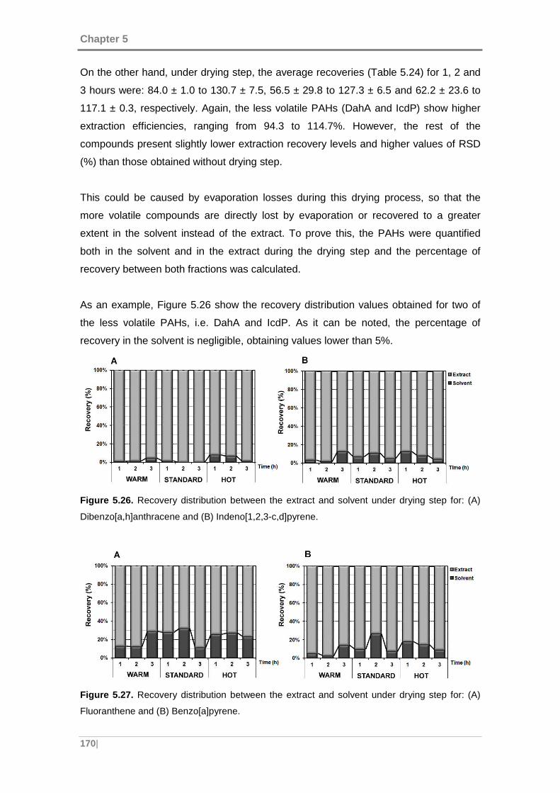
Chapter 5

170|

On the other hand, under drying step, the average recoveries (Table 5.24) for 1, 2 and

3 hours were: 84.0 ± 1.0 to 130.7 ± 7.5, 56.5 ± 29.8 to 127.3 ± 6.5 and 62.2 ± 23.6 to

117.1 ± 0.3, respectively. Again, the less volatile PAHs (DahA and IcdP) show higher

extraction efficiencies, ranging from 94.3 to 114.7%. However, the rest of the

compounds present slightly lower extraction recovery levels and higher values of RSD

(%) than those obtained without drying step.

This could be caused by evaporation losses during this drying process, so that the

more volatile compounds are directly lost by evaporation or recovered to a greater

extent in the solvent instead of the extract. To prove this, the PAHs were quantified

both in the solvent and in the extract during the drying step and the percentage of

recovery between both fractions was calculated.

As an example, Figure 5.26 show the recovery distribution values obtained for two of

the less volatile PAHs, i.e. DahA and IcdP. As it can be noted, the percentage of

recovery in the solvent is negligible, obtaining values lower than 5%.

Figure 5.26. Recovery distribution between the extract and solvent under drying step for: (A)

Dibenzo[a,h]anthracene and (B) Indeno[1,2,3-c,d]pyrene.

Figure 5.27. Recovery distribution between the extract and solvent under drying step for: (A)

Fluoranthene and (B) Benzo[a]pyrene.

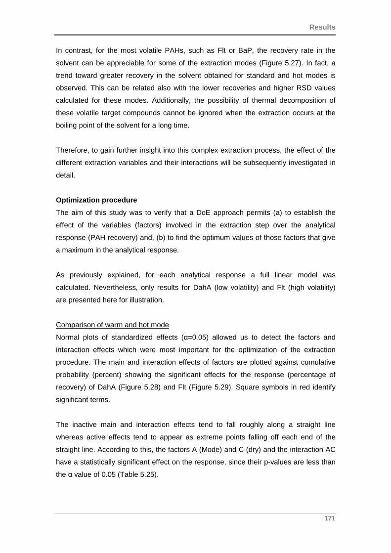
Results

| 171

In contrast, for the most volatile PAHs, such as Flt or BaP, the recovery rate in the

solvent can be appreciable for some of the extraction modes (Figure 5.27). In fact, a

trend toward greater recovery in the solvent obtained for standard and hot modes is

observed. This can be related also with the lower recoveries and higher RSD values

calculated for these modes. Additionally, the possibility of thermal decomposition of

these volatile target compounds cannot be ignored when the extraction occurs at the

boiling point of the solvent for a long time.

Therefore, to gain further insight into this complex extraction process, the effect of the

different extraction variables and their interactions will be subsequently investigated in

detail.

Optimization procedure

The aim of this study was to verify that a DoE approach permits (a) to establish the

effect of the variables (factors) involved in the extraction step over the analytical

response (PAH recovery) and, (b) to find the optimum values of those factors that give

a maximum in the analytical response.

As previously explained, for each analytical response a full linear model was

calculated. Nevertheless, only results for DahA (low volatility) and Flt (high volatility)

are presented here for illustration.

Comparison of warm and hot mode

Normal plots of standardized effects (α=0.05) allowed us to detect the factors and

interaction effects which were most important for the optimization of the extraction

procedure. The main and interaction effects of factors are plotted against cumulative

probability (percent) showing the significant effects for the response (percentage of

recovery) of DahA (Figure 5.28) and Flt (Figure 5.29). Square symbols in red identify

significant terms.

The inactive main and interaction effects tend to fall roughly along a straight line

whereas active effects tend to appear as extreme points falling off each end of the

straight line. According to this, the factors A (Mode) and C (dry) and the interaction AC

have a statistically significant effect on the response, since their p-values are less than

the α value of 0.05 (Table 5.25).

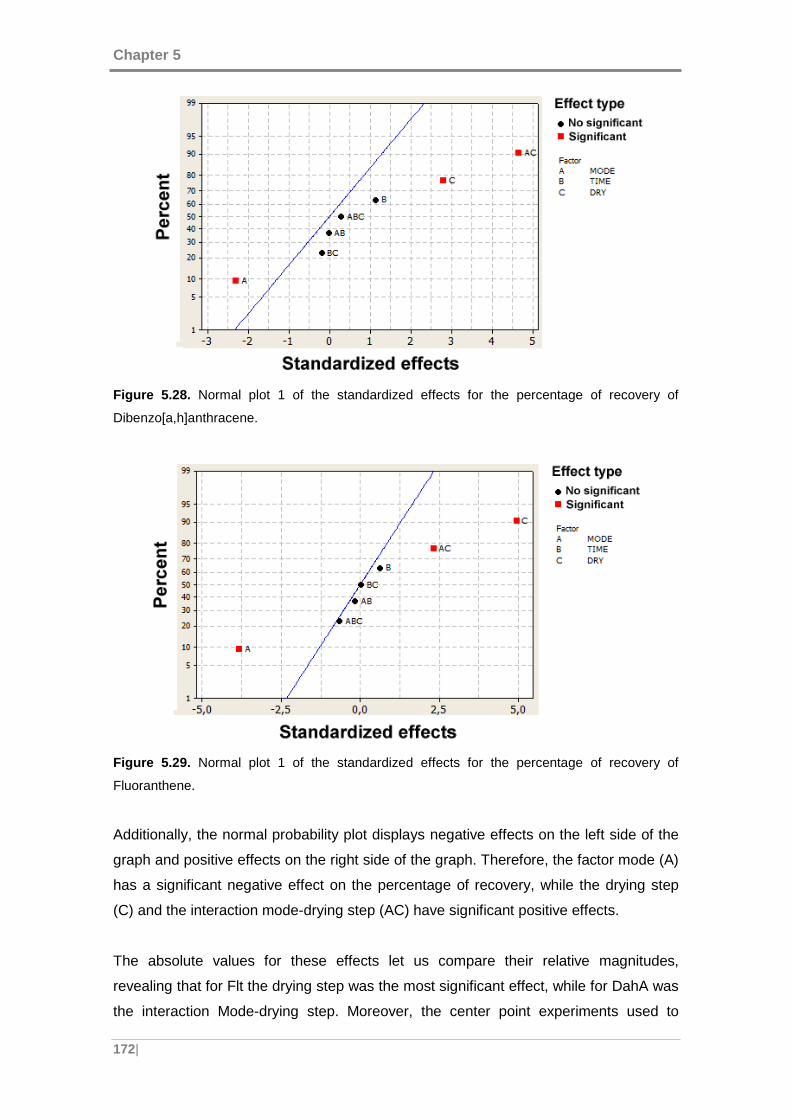
Chapter 5

172|


Dibenzo[a,h]anthracene.


Fluoranthene.

Additionally, the normal probability plot displays negative effects on the left side of the

graph and positive effects on the right side of the graph. Therefore, the factor mode (A)

has a significant negative effect on the percentage of recovery, while the drying step

(C) and the interaction mode-drying step (AC) have significant positive effects.

The absolute values for these effects let us compare their relative magnitudes,

revealing that for Flt the drying step was the most significant effect, while for DahA was

the interaction Mode-drying step. Moreover, the center point experiments used to

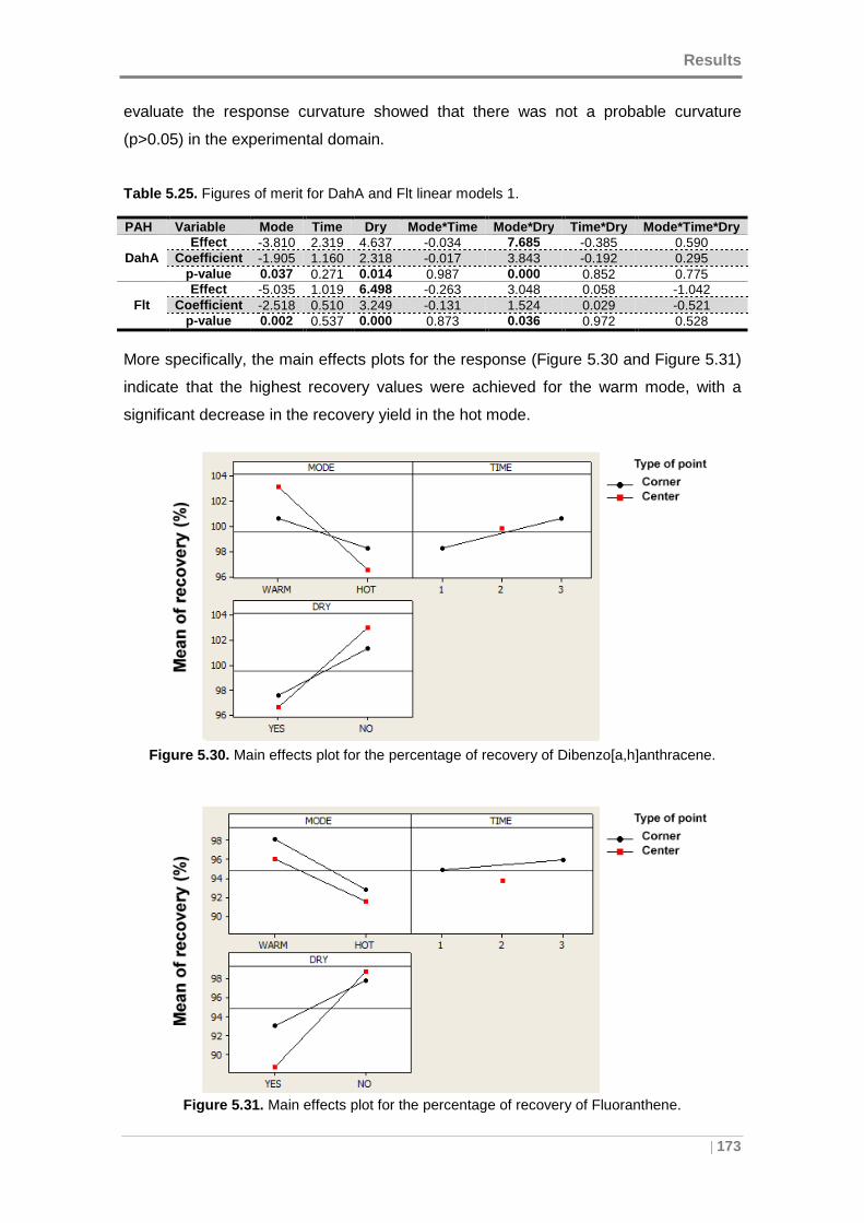
Results

| 173

evaluate the response curvature showed that there was not a probable curvature

(p>0.05) in the experimental domain.

Table 5.25. Figures of merit for DahA and Flt linear models 1.

PAH Variable Mode Time Dry Mode*Time Mode*Dry Time*Dry Mode*Time*Dry

DahA Effect -3.810 2.319 4.637 -0.034 7.685 -0.385 0.590

Coefficient -1.905 1.160 2.318 -0.017 3.843 -0.192 0.295 p-value 0.037 0.271 0.014 0.987 0.000 0.852 0.775

Flt Effect -5.035 1.019 6.498 -0.263 3.048 0.058 -1.042

Coefficient -2.518 0.510 3.249 -0.131 1.524 0.029 -0.521 p-value 0.002 0.537 0.000 0.873 0.036 0.972 0.528

More specifically, the main effects plots for the response (Figure 5.30 and Figure 5.31)

indicate that the highest recovery values were achieved for the warm mode, with a

significant decrease in the recovery yield in the hot mode.

Figure 5.30. Main effects plot for the percentage of recovery of Dibenzo[a,h]anthracene.

Figure 5.31. Main effects plot for the percentage of recovery of Fluoranthene.

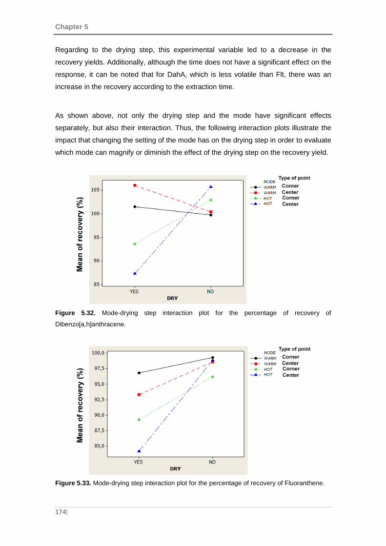
Chapter 5

174|

Regarding to the drying step, this experimental variable led to a decrease in the

recovery yields. Additionally, although the time does not have a significant effect on the

response, it can be noted that for DahA, which is less volatile than Flt, there was an

increase in the recovery according to the extraction time.

As shown above, not only the drying step and the mode have significant effects

separately, but also their interaction. Thus, the following interaction plots illustrate the

impact that changing the setting of the mode has on the drying step in order to evaluate

which mode can magnify or diminish the effect of the drying step on the recovery yield.



Figure 5.33. Mode-drying step interaction plot for the percentage of recovery of Fluoranthene.

Results

| 175

From the above figures it can be noted that the interaction between the hot mode and

the drying step is the highest one in magnitude. In contrast, the interaction between the

warm mode and the drying step is not so significant, since the lines tend to be more

parallel. In addition, the use of hot mode under drying conditions lead to a higher

decrease in the recovery yield, especially for fluoranthene. This may be related to its

higher volatility, being more susceptible to evaporation during the extraction at higher

temperatures.

As a result, the warm mode presented a better performance than the hot mode, and it

was consequently selected to be compared with the standard Soxhlet extraction

procedure.

Comparison of warm and standard mode

As before, the normal plots of standardized effects (α=0.05) plot the main and

interaction effects of factors against cumulative probability (percent) showing the

significant effects for the response (p-values < 0.05 (Table 5.26)) of DahA (Figure 5.34)

and Flt (Figure 5.35), where the square symbols in red identify significant terms.

In this case, the factors B (Time) and C (dry) as well as the interaction AC (mode*dry)

have a statistically significant effect on the response of DahA, whereas for the Flt

recovery the factor B (Time) has not a significant effect. Moreover, these significant

factors have a positive effect on both responses.



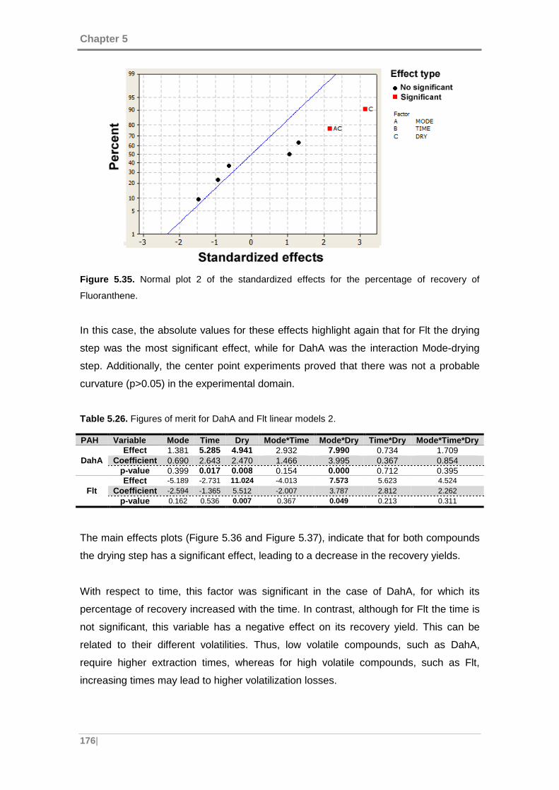
Chapter 5

176|


Fluoranthene.

In this case, the absolute values for these effects highlight again that for Flt the drying

step was the most significant effect, while for DahA was the interaction Mode-drying

step. Additionally, the center point experiments proved that there was not a probable

curvature (p>0.05) in the experimental domain.

Table 5.26. Figures of merit for DahA and Flt linear models 2.

PAH Variable Mode Time Dry Mode*Time Mode*Dry Time*Dry Mode*Time*Dry

DahA Effect 1.381 5.285 4.941 2.932 7.990 0.734 1.709

Coefficient 0.690 2.643 2.470 1.466 3.995 0.367 0.854 p-value 0.399 0.017 0.008 0.154 0.000 0.712 0.395

Flt Effect -5.189 -2.731 11.024 -4.013 7.573 5.623 4.524

Coefficient -2.594 -1.365 5.512 -2.007 3.787 2.812 2.262 p-value 0.162 0.536 0.007 0.367 0.049 0.213 0.311

The main effects plots (Figure 5.36 and Figure 5.37), indicate that for both compounds

the drying step has a significant effect, leading to a decrease in the recovery yields.

With respect to time, this factor was significant in the case of DahA, for which its

percentage of recovery increased with the time. In contrast, although for Flt the time is

not significant, this variable has a negative effect on its recovery yield. This can be

related to their different volatilities. Thus, low volatile compounds, such as DahA,

require higher extraction times, whereas for high volatile compounds, such as Flt,

increasing times may lead to higher volatilization losses.

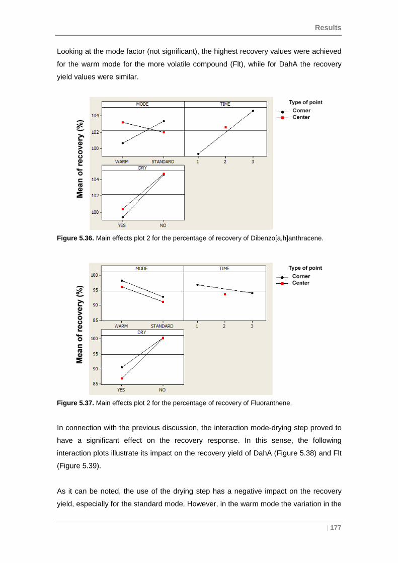
Results

| 177

Looking at the mode factor (not significant), the highest recovery values were achieved

for the warm mode for the more volatile compound (Flt), while for DahA the recovery

yield values were similar.

Figure 5.36. Main effects plot 2 for the percentage of recovery of Dibenzo[a,h]anthracene.

Figure 5.37. Main effects plot 2 for the percentage of recovery of Fluoranthene.

In connection with the previous discussion, the interaction mode-drying step proved to

have a significant effect on the recovery response. In this sense, the following

interaction plots illustrate its impact on the recovery yield of DahA (Figure 5.38) and Flt

(Figure 5.39).

As it can be noted, the use of the drying step has a negative impact on the recovery

yield, especially for the standard mode. However, in the warm mode the variation in the

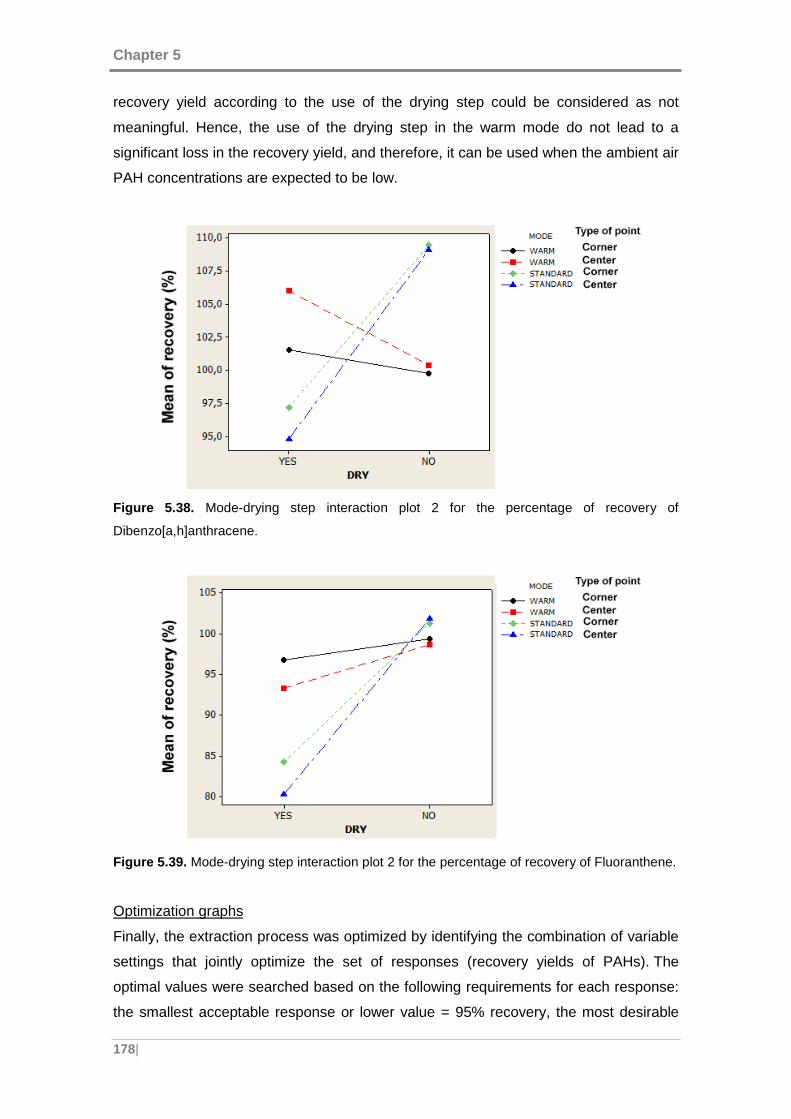
Chapter 5

178|

recovery yield according to the use of the drying step could be considered as not

meaningful. Hence, the use of the drying step in the warm mode do not lead to a

significant loss in the recovery yield, and therefore, it can be used when the ambient air

PAH concentrations are expected to be low.



Figure 5.39. Mode-drying step interaction plot 2 for the percentage of recovery of Fluoranthene.

Optimization graphs

Finally, the extraction process was optimized by identifying the combination of variable

settings that jointly optimize the set of responses (recovery yields of PAHs). The

optimal values were searched based on the following requirements for each response:

the smallest acceptable response or lower value = 95% recovery, the most desirable

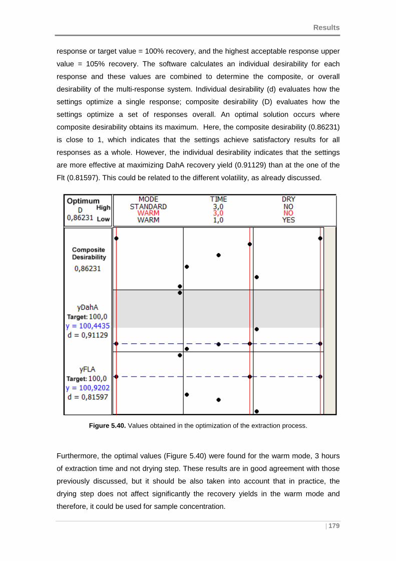
Results

| 179

response or target value = 100% recovery, and the highest acceptable response upper

value = 105% recovery. The software calculates an individual desirability for each

response and these values are combined to determine the composite, or overall

desirability of the multi-response system. Individual desirability (d) evaluates how the

settings optimize a single response; composite desirability (D) evaluates how the

settings optimize a set of responses overall. An optimal solution occurs where

composite desirability obtains its maximum. Here, the composite desirability (0.86231)

is close to 1, which indicates that the settings achieve satisfactory results for all

responses as a whole. However, the individual desirability indicates that the settings

are more effective at maximizing DahA recovery yield (0.91129) than at the one of the

Flt (0.81597). This could be related to the different volatility, as already discussed.

Figure 5.40. Values obtained in the optimization of the extraction process.

Furthermore, the optimal values (Figure 5.40) were found for the warm mode, 3 hours

of extraction time and not drying step. These results are in good agreement with those

previously discussed, but it should be also taken into account that in practice, the

drying step does not affect significantly the recovery yields in the warm mode and

therefore, it could be used for sample concentration.

Chapter 5

180|

5.3.2.5 Conclusions

The use of a full factorial DoE enabled the evaluation of the main significant factors and

interactions over the extraction process and the optimization of the extraction

conditions.

The results show that the warm mode is a valuable alternative to classical standard

extraction method, demonstrating advantages of robustness against conventional

Soxhlet extraction. Optimal extraction conditions were obtained for 3 hours of

extraction time and not drying step. However, the results obtained for warm mode

under drying conditions fulfilled also the requirements of good recovery yields and

therefore it could be used when low ambient air PAH concentrations are expected.

Among the different PAHs, the most volatile PAHs proved to be more sensitive to

volatility losses during the drying step, whereas for the low volatile PAHs the extraction

time had a more significant effect.

5.3.3 Optimization of the extraction time

Soxhlet extraction time strongly depends on matrix characteristics and particle size, as

the internal diffusion may be the limiting step during extraction. Thus, the efficiency of

the Soxhlet procedure to extract the target analytes was tested on other certified

matrix, the NIST (National Institute of Standards and Technology) SRM 1649b

reference material. This material has a variable PAHs content present in a powder

matrix similar to the one of the aerosol samples and hence, it can be considered useful

to optimize the Soxhlet extraction time, for which the previously optimized extraction

time of 3 hours was taken as the lower value.

5.3.3.1 Objective

This section explores the feasibility of applying the second-order data analysis methods

to optimize the extraction procedure for aerosol sample analysis by analyzing EEMs

obtained from a standard reference material, SRM 1649b urban dust, subjected to

increasing extraction times.

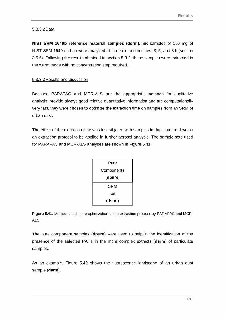
Results

| 181

5.3.3.2 Data

NIST SRM 1649b reference material samples (dsrm). Six samples of 150 mg of

NIST SRM 1649b urban were analyzed at three extraction times: 3, 5, and 8 h (section

3.5.6). Following the results obtained in section 5.3.2, these samples were extracted in

the warm mode with no concentration step required.


Because PARAFAC and MCR-ALS are the appropriate methods for qualitative

analysis, provide always good relative quantitative information and are computationally

very fast, they were chosen to optimize the extraction time on samples from an SRM of

urban dust.

The effect of the extraction time was investigated with samples in duplicate, to develop

an extraction protocol to be applied in further aerosol analysis. The sample sets used

for PARAFAC and MCR-ALS analyses are shown in Figure 5.41.

Figure 5.41. Multiset used in the optimization of the extraction protocol by PARAFAC and MCR-

ALS.

The pure component samples (dpure ) were used to help in the identification of the

presence of the selected PAHs in the more complex extracts (dsrm ) of particulate

samples.

As an example, Figure 5.42 shows the fluorescence landscape of an urban dust

sample (dsrm ).

Pure

Components

(dpure )

SRM

set

(dsrm )

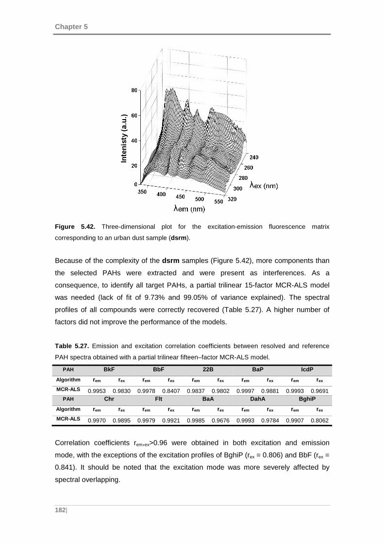
Chapter 5

182|


corresponding to an urban dust sample (dsrm ).

Because of the complexity of the dsrm samples (Figure 5.42), more components than

the selected PAHs were extracted and were present as interferences. As a

consequence, to identify all target PAHs, a partial trilinear 15-factor MCR-ALS model

was needed (lack of fit of 9.73% and 99.05% of variance explained). The spectral

profiles of all compounds were correctly recovered (Table 5.27). A higher number of

factors did not improve the performance of the models.


PAH spectra obtained with a partial trilinear fifteen–factor MCR-ALS model.



MCR-ALS 0.9953 0.9830 0.9978 0.8407 0.9837 0.9802 0.9997 0.9881 0.9993 0.9691 PAH Chr Flt BaA DahA BghiP


MCR-ALS 0.9970 0.9895 0.9979 0.9921 0.9985 0.9676 0.9993 0.9784 0.9907 0.8062

Correlation coefficients rem,ex>0.96 were obtained in both excitation and emission

mode, with the exceptions of the excitation profiles of BghiP (rex = 0.806) and BbF (rex =

0.841). It should be noted that the excitation mode was more severely affected by

spectral overlapping.

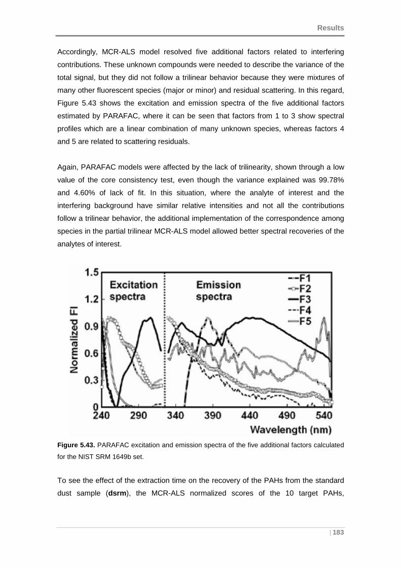
Results

| 183

Accordingly, MCR-ALS model resolved five additional factors related to interfering

contributions. These unknown compounds were needed to describe the variance of the

total signal, but they did not follow a trilinear behavior because they were mixtures of

many other fluorescent species (major or minor) and residual scattering. In this regard,

Figure 5.43 shows the excitation and emission spectra of the five additional factors

estimated by PARAFAC, where it can be seen that factors from 1 to 3 show spectral

profiles which are a linear combination of many unknown species, whereas factors 4

and 5 are related to scattering residuals.

Again, PARAFAC models were affected by the lack of trilinearity, shown through a low

value of the core consistency test, even though the variance explained was 99.78%

and 4.60% of lack of fit. In this situation, where the analyte of interest and the

interfering background have similar relative intensities and not all the contributions

follow a trilinear behavior, the additional implementation of the correspondence among

species in the partial trilinear MCR-ALS model allowed better spectral recoveries of the

analytes of interest.

Figure 5.43. PARAFAC excitation and emission spectra of the five additional factors calculated

for the NIST SRM 1649b set.

To see the effect of the extraction time on the recovery of the PAHs from the standard

dust sample (dsrm ), the MCR-ALS normalized scores of the 10 target PAHs,

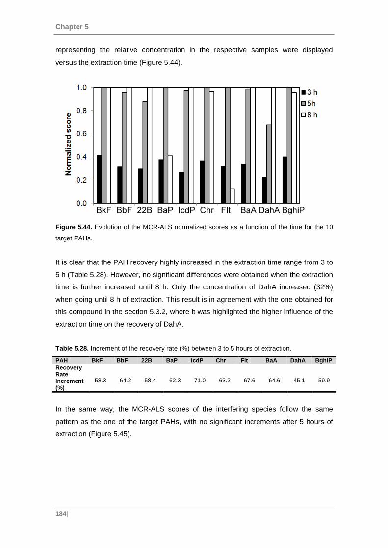
Chapter 5

184|

representing the relative concentration in the respective samples were displayed

versus the extraction time (Figure 5.44).

Figure 5.44. Evolution of the MCR-ALS normalized scores as a function of the time for the 10

target PAHs.

It is clear that the PAH recovery highly increased in the extraction time range from 3 to

5 h (Table 5.28). However, no significant differences were obtained when the extraction

time is further increased until 8 h. Only the concentration of DahA increased (32%)

when going until 8 h of extraction. This result is in agreement with the one obtained for

this compound in the section 5.3.2, where it was highlighted the higher influence of the

extraction time on the recovery of DahA.

Table 5.28. Increment of the recovery rate (%) between 3 to 5 hours of extraction.

PAH BkF BbF 22B BaP IcdP Chr Flt BaA DahA BghiP Recovery Rate Increment (%)

58.3 64.2 58.4 62.3 71.0 63.2 67.6 64.6 45.1 59.9

In the same way, the MCR-ALS scores of the interfering species follow the same

pattern as the one of the target PAHs, with no significant increments after 5 hours of

extraction (Figure 5.45).

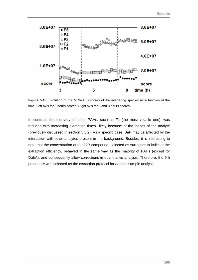
Results

| 185

Figure 5.45. Evolution of the MCR-ALS scores of the interfering species as a function of the

time. Left axis for 3 hours scores. Right axis for 5 and 8 hours scores.

In contrast, the recovery of other PAHs, such as Flt (the most volatile one), was

reduced with increasing extraction times, likely because of the losses of the analyte

(previously discussed in section 5.3.2). As a specific case, BaP may be affected by the

interaction with other analytes present in the background. Besides, it is interesting to

note that the concentration of the 22B compound, selected as surrogate to indicate the

extraction efficiency, behaved in the same way as the majority of PAHs (except for

DahA), and consequently allow corrections in quantitative analysis. Therefore, the 5-h

procedure was selected as the extraction protocol for aerosol sample analysis.

Chapter 5

186|

5.4 VALIDATION OF THE MODELS TO DETERMINE TARGET PA Hs IN

AEROSOL SAMPLES

In this section, a novel method based on the combination of EEMs and three second-

order algorithms: PARAFAC, MCR-ALS and U-PLS/RBL, is evaluated to identify and

quantify 9 US-EPA PAHs in extracts of urban aerosol samples, taking into account the

bases established in previous sections.

Aerosol samples comprise a particularly complex sample matrix because of the low

amount of PAHs and the numerous fluorescent interferences. Therefore, the

application of flexible methods that can successfully model the different fluorescence

contributions is required in order to achieve a good qualitative and quantitative

description of this kind of samples.

Consequently, in section 5.4.1, the global decomposition methods, i.e. PARAFAC and

MCR-ALS, were tested to describe the evolution of environmental patterns of variation

of PAHs in an urban ambient for routine environmental monitoring.

For quantitative analysis, in section 5.4.2, second-order calibration developed

methodologies were tested and compared with the conventional technique of liquid

extraction and analysis by GC-MS. Figures of merit related to the applicability of the

technique for the target PAHs are also defined. Moreover, the advantages and

drawbacks of each developed approach to determine PAHs in airborne samples are

highlighted.

Finally, taking into account the results obtained in the previous section, the presence of

a significant background signal associated with the complexity of the sample matrix,

and the presence of interferences, second-order standard addition methods were

tested also to carry out the quantitative analysis by PARAFAC and MCR-ALS, while U-

PLS/RBL predictions were carried out directly on the sample extracts. Thus, the

combination of standard addition methods and second-order data analysis algorithms

will be studied in the last section.

Section 5.4.3 presents the validation of the optimized extraction protocol and

quantitative methods, which was carried out by means of second-order standard

addition method on a standard certified material, in order to avoid sample matrix

effects.

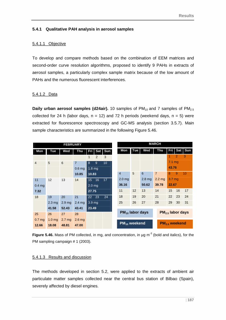
Results

| 187

5.4.1 Qualitative PAH analysis in aerosol samples

5.4.1.1 Objective

To develop and compare methods based on the combination of EEM matrices and

second-order curve resolution algorithms, proposed to identify 9 PAHs in extracts of

aerosol samples, a particularly complex sample matrix because of the low amount of

PAHs and the numerous fluorescent interferences.

5.4.1.2 Data

Daily urban aerosol samples (d24air). 10 samples of PM10 and 7 samples of PM2.5

collected for 24 h (labor days, n = 12) and 72 h periods (weekend days, n = 5) were

extracted for fluorescence spectroscopy and GC-MS analysis (section 3.5.7). Main

sample characteristics are summarized in the following Figure 5.46.

Figure 5.46. Mass of PM collected, in mg, and concentration, in µg m-3 (bold and italics), for the

PM sampling campaign # 1 (2003).


The methods developed in section 5.2, were applied to the extracts of ambient air

particulate matter samples collected near the central bus station of Bilbao (Spain),

severely affected by diesel engines.

MARCH

Mon Tue Wed Thu Fri Sat Sun

1 2 3

7.1 mg

43.76

4

2.0 mg

36.16

5 6

2.8 mg

50.62

7

2.2 mg

39.78

8 9 10

3.7 mg

22.67

11 12 13 14 15 16 17

18 19 20 21 22 23 24

25 26 27 28 29 30 31

FEBRUARY

Mon Tue Wed Thu Fri Sat Sun

1 2 3

4 5 6 7

0.6 mg

10.85

8 9 10

1.8 mg

10.83

11

0.4 mg

7.32

12

13

14 15 16 17

2.0 mg

27.75

18 19

2.3 mg

41.58

20

2.9 mg

52.43

21

2.4 mg

43.41

22 23 24

3.9 mg

23.49

25

0.7 mg

12.66

26

1.0 mg

18.08

27

2.7 mg

48.81

28

2.6 mg

47.00

PM10 labor days PM2.5 labor days

PM2.5 weekend PM10 weekend

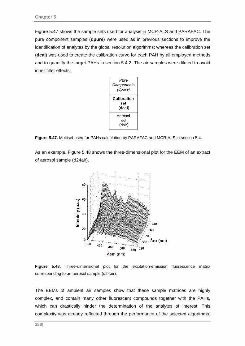
Chapter 5

188|

Figure 5.47 shows the sample sets used for analysis in MCR-ALS and PARAFAC. The

pure component samples (dpure ) were used as in previous sections to improve the

identification of analytes by the global resolution algorithms; whereas the calibration set

(dcal ) was used to create the calibration curve for each PAH by all employed methods

and to quantify the target PAHs in section 5.4.2. The air samples were diluted to avoid

inner filter effects.

Figure 5.47. Multiset used for PAHs calculation by PARAFAC and MCR-ALS in section 5.4.

As an example, Figure 5.48 shows the three-dimensional plot for the EEM of an extract

of aerosol sample (d24air).


corresponding to an aerosol sample (d24air).

The EEMs of ambient air samples show that these sample matrices are highly

complex, and contain many other fluorescent compounds together with the PAHs,

which can drastically hinder the determination of the analytes of interest. This

complexity was already reflected through the performance of the selected algorithms.

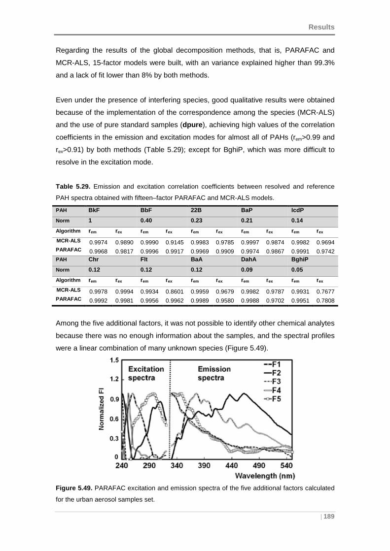
Results

| 189

Regarding the results of the global decomposition methods, that is, PARAFAC and

MCR-ALS, 15-factor models were built, with an variance explained higher than 99.3%

and a lack of fit lower than 8% by both methods.

Even under the presence of interfering species, good qualitative results were obtained

because of the implementation of the correspondence among the species (MCR-ALS)

and the use of pure standard samples (dpure ), achieving high values of the correlation

coefficients in the emission and excitation modes for almost all of PAHs (rem>0.99 and

rex>0.91) by both methods (Table 5.29); except for BghiP, which was more difficult to

resolve in the excitation mode.


PAH spectra obtained with fifteen–factor PARAFAC and MCR-ALS models.


Norm 1 0.40 0.23 0.21 0.14


MCR-ALS 0.9974 0.9890 0.9990 0.9145 0.9983 0.9785 0.9997 0.9874 0.9982 0.9694 PARAFAC 0.9968 0.9817 0.9996 0.9917 0.9969 0.9909 0.9974 0.9867 0.9991 0.9742 PAH Chr Flt BaA DahA BghiP

Norm 0.12 0.12 0.12 0.09 0.05


MCR-ALS 0.9978 0.9994 0.9934 0.8601 0.9959 0.9679 0.9982 0.9787 0.9931 0.7677 PARAFAC 0.9992 0.9981 0.9956 0.9962 0.9989 0.9580 0.9988 0.9702 0.9951 0.7808

Among the five additional factors, it was not possible to identify other chemical analytes

because there was no enough information about the samples, and the spectral profiles

were a linear combination of many unknown species (Figure 5.49).

Figure 5.49. PARAFAC excitation and emission spectra of the five additional factors calculated

for the urban aerosol samples set.

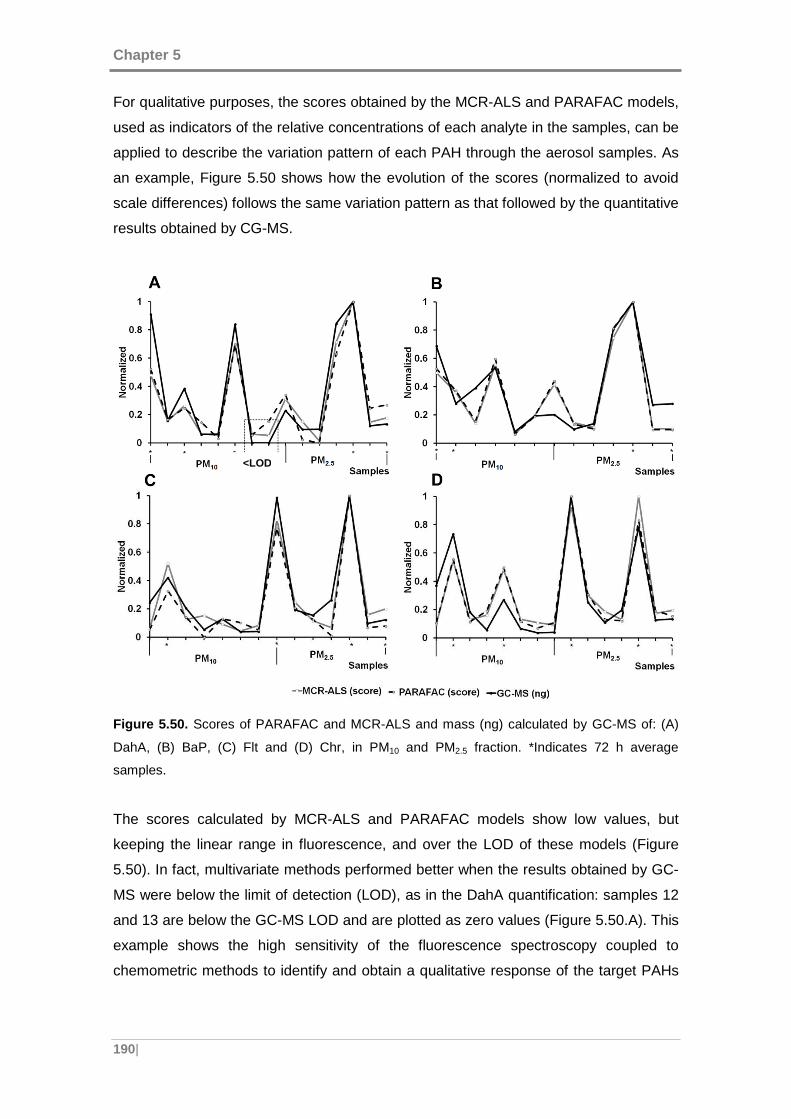
Chapter 5

190|

For qualitative purposes, the scores obtained by the MCR-ALS and PARAFAC models,

used as indicators of the relative concentrations of each analyte in the samples, can be

applied to describe the variation pattern of each PAH through the aerosol samples. As

an example, Figure 5.50 shows how the evolution of the scores (normalized to avoid

scale differences) follows the same variation pattern as that followed by the quantitative

results obtained by CG-MS.

Figure 5.50. Scores of PARAFAC and MCR-ALS and mass (ng) calculated by GC-MS of: (A)

DahA, (B) BaP, (C) Flt and (D) Chr, in PM10 and PM2.5 fraction. *Indicates 72 h average

samples.

The scores calculated by MCR-ALS and PARAFAC models show low values, but

keeping the linear range in fluorescence, and over the LOD of these models (Figure

5.50). In fact, multivariate methods performed better when the results obtained by GC-

MS were below the limit of detection (LOD), as in the DahA quantification: samples 12

and 13 are below the GC-MS LOD and are plotted as zero values (Figure 5.50.A). This

example shows the high sensitivity of the fluorescence spectroscopy coupled to

chemometric methods to identify and obtain a qualitative response of the target PAHs

<LOD

Results

| 191

in the PM10 and PM2.5 size fractions of urban aerosols, making them suitable for routine

monitoring instead of the chromatographic techniques.

5.4.1.4 Conclusions

PARAFAC and MCR-ALS algorithms may be recommended when a fast data analysis

providing qualitative information of the samples is required, which is the perfect

scenario for screening and monitoring of PAHs in aerosol samples.

5.4.2 Quantitative comparison with GC-MS

5.4.2.1 Objective

The second-order calibration developed methodologies were tested and compared with

the conventional technique of liquid extraction and analysis by GC-MS to quantify 9

PAHs in extracts of aerosol samples.

5.4.2.2 Data

The dataset used is the same specified in section 5.4.1.2, employing the multiset

structure defined in Figure 5.47 for PARAFAC and MCR-ALS quantification of target

PAHs. For U-PLS/RBL quantitative analysis, the rules defined in section 5.2.3 were

applied.

5.4.2.3. Results and discussion

As it has been highlighted in the previous section, the extracts of aerosol samples

contain a large number of compounds that contribute to a greater or lesser extent to

the total fluorescence signal (Figure 5.49). This may lead to inaccurate predictions

when the regression of the scores is made against the calibration curve obtained with a

set of calibration samples (dcal ) of different nature/sample matrix than the samples to

be analyzed (dair ).

Therefore, the quantitative results obtained (Table 5.30) were often in excess, because

of a false increase of the PAHs signals due to the presence of other interfering species

in the aerosol samples, except for PAHs with relative high intensities such as BkF or

BbF, which were in better agreement with the values obtained by GC-MS technique.

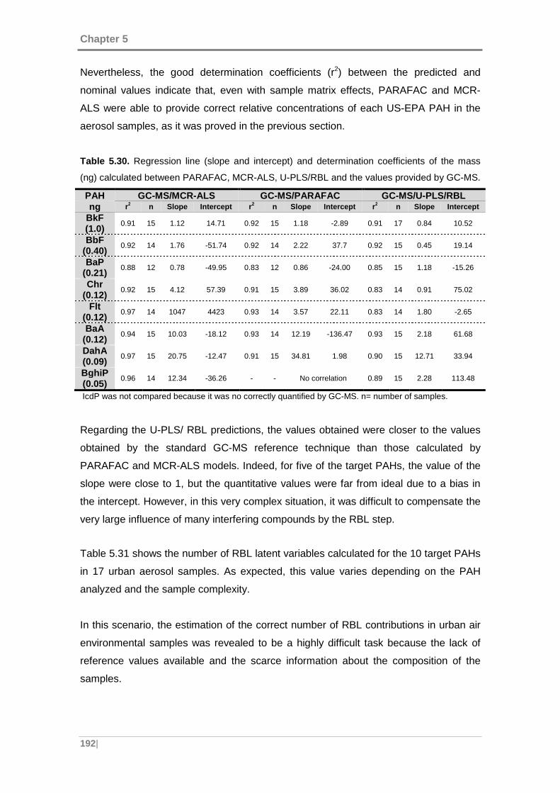
Chapter 5

192|

Nevertheless, the good determination coefficients (r2) between the predicted and

nominal values indicate that, even with sample matrix effects, PARAFAC and MCR-

ALS were able to provide correct relative concentrations of each US-EPA PAH in the

aerosol samples, as it was proved in the previous section.

Table 5.30. Regression line (slope and intercept) and determination coefficients of the mass

(ng) calculated between PARAFAC, MCR-ALS, U-PLS/RBL and the values provided by GC-MS.

PAH GC-MS/MCR-ALS GC-MS/PARAFAC GC-MS/U-PLS/RBL ng r2 n Slope Intercept r2 n Slope Intercept r2 n Slope Intercept

BkF (1.0)

0.91 15 1.12 14.71 0.92 15 1.18 -2.89 0.91 17 0.84 10.52

BbF (0.40)

0.92 14 1.76 -51.74 0.92 14 2.22 37.7 0.92 15 0.45 19.14

BaP (0.21)

0.88 12 0.78 -49.95 0.83 12 0.86 -24.00 0.85 15 1.18 -15.26

Chr (0.12)

0.92 15 4.12 57.39 0.91 15 3.89 36.02 0.83 14 0.91 75.02

Flt (0.12)

0.97 14 1047 4423 0.93 14 3.57 22.11 0.83 14 1.80 -2.65

BaA (0.12)

0.94 15 10.03 -18.12 0.93 14 12.19 -136.47 0.93 15 2.18 61.68

DahA (0.09)

0.97 15 20.75 -12.47 0.91 15 34.81 1.98 0.90 15 12.71 33.94

BghiP (0.05)

0.96 14 12.34 -36.26 - - No correlation 0.89 15 2.28 113.48

IcdP was not compared because it was no correctly quantified by GC-MS. n= number of samples.

Regarding the U-PLS/ RBL predictions, the values obtained were closer to the values

obtained by the standard GC-MS reference technique than those calculated by

PARAFAC and MCR-ALS models. Indeed, for five of the target PAHs, the value of the

slope were close to 1, but the quantitative values were far from ideal due to a bias in

the intercept. However, in this very complex situation, it was difficult to compensate the

very large influence of many interfering compounds by the RBL step.

Table 5.31 shows the number of RBL latent variables calculated for the 10 target PAHs

in 17 urban aerosol samples. As expected, this value varies depending on the PAH

analyzed and the sample complexity.

In this scenario, the estimation of the correct number of RBL contributions in urban air

environmental samples was revealed to be a highly difficult task because the lack of

reference values available and the scarce information about the composition of the

samples.

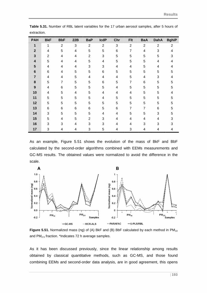
Results

| 193

Table 5.31. Number of RBL latent variables for the 17 urban aerosol samples, after 5 hours of

extraction.


1 1 2 3 2 2 3 2 2 2 2

2 4 5 4 5 5 6 7 4 3 4

3 2 4 4 2 3 5 5 5 5 3

4 5 4 4 5 4 5 5 5 4 4

5 4 4 4 3 3 4 4 5 4 4

6 6 4 5 5 6 5 5 5 5 5

7 4 4 5 4 4 4 5 4 3 4

8 5 7 5 5 6 5 7 6 5 5

9 4 6 5 5 5 4 5 5 5 5

10 4 5 4 5 4 4 4 5 5 4

11 5 5 5 5 4 5 5 5 5 5

12 5 5 5 5 5 5 5 5 5 5

13 6 6 6 6 5 6 7 7 6 5

14 3 5 5 5 4 4 5 5 3 5

15 5 4 5 2 3 4 4 4 4 3

16 3 3 4 3 3 4 4 3 3 3

17 3 4 4 3 5 4 3 4 4 4

As an example, Figure 5.51 shows the evolution of the mass of BkF and BbF

calculated by the second-order algorithms combined with EEMs measurements and

GC-MS results. The obtained values were normalized to avoid the difference in the

scale.

Figure 5.51. Normalized mass (ng) of (A) BkF and (B) BbF calculated by each method in PM10

and PM2.5 fraction. *Indicates 72 h average samples.

As it has been discussed previously, since the linear relationship among results

obtained by classical quantitative methods, such as GC-MS, and those found

combining EEMs and second-order data analysis, are in good agreement, this opens

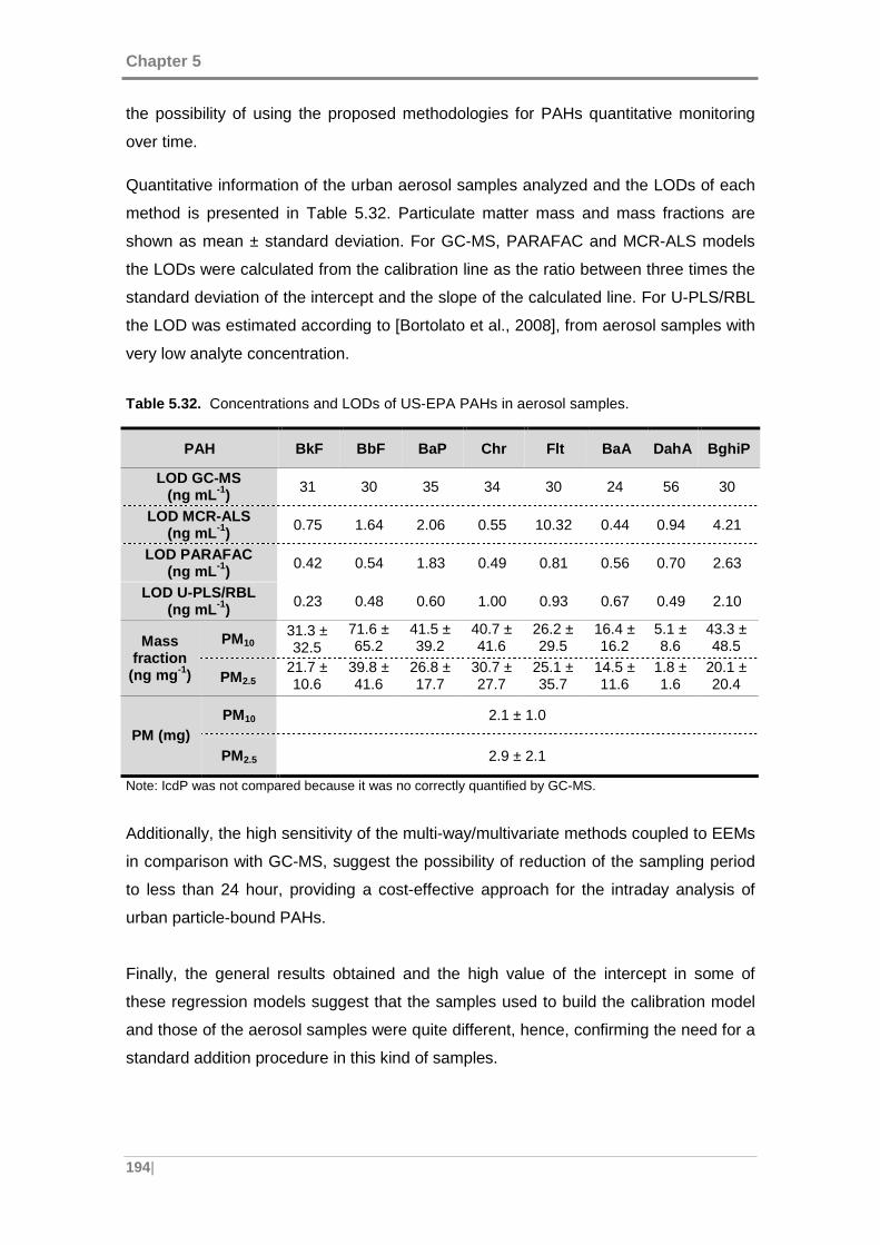
Chapter 5

194|

the possibility of using the proposed methodologies for PAHs quantitative monitoring

over time.

Quantitative information of the urban aerosol samples analyzed and the LODs of each

method is presented in Table 5.32. Particulate matter mass and mass fractions are

shown as mean ± standard deviation. For GC-MS, PARAFAC and MCR-ALS models

the LODs were calculated from the calibration line as the ratio between three times the

standard deviation of the intercept and the slope of the calculated line. For U-PLS/RBL

the LOD was estimated according to [Bortolato et al., 2008], from aerosol samples with

very low analyte concentration.

Table 5.32. Concentrations and LODs of US-EPA PAHs in aerosol samples.

PAH BkF BbF BaP Chr Flt BaA DahA BghiP

LOD GC-MS (ng mL -1) 31 30 35 34 30 24 56 30

LOD MCR-ALS (ng mL -1) 0.75 1.64 2.06 0.55 10.32 0.44 0.94 4.21

LOD PARAFAC (ng mL -1) 0.42 0.54 1.83 0.49 0.81 0.56 0.70 2.63

LOD U-PLS/RBL (ng mL -1) 0.23 0.48 0.60 1.00 0.93 0.67 0.49 2.10

Mass fraction

(ng mg -1)

PM10 31.3 ± 32.5

71.6 ± 65.2

41.5 ± 39.2

40.7 ± 41.6

26.2 ± 29.5

16.4 ± 16.2

5.1 ± 8.6

43.3 ± 48.5

PM2.5 21.7 ± 10.6

39.8 ± 41.6

26.8 ± 17.7

30.7 ± 27.7

25.1 ± 35.7

14.5 ± 11.6

1.8 ± 1.6

20.1 ± 20.4

PM (mg) PM10 2.1 ± 1.0

PM2.5 2.9 ± 2.1

Note: IcdP was not compared because it was no correctly quantified by GC-MS.

Additionally, the high sensitivity of the multi-way/multivariate methods coupled to EEMs

in comparison with GC-MS, suggest the possibility of reduction of the sampling period

to less than 24 hour, providing a cost-effective approach for the intraday analysis of

urban particle-bound PAHs.

Finally, the general results obtained and the high value of the intercept in some of

these regression models suggest that the samples used to build the calibration model

and those of the aerosol samples were quite different, hence, confirming the need for a

standard addition procedure in this kind of samples.

Results

| 195

5.4.2.4 Conclusions

A novel method for the determination of PAHs in ambient air aerosol samples, based

on the combination of EEMs and several second-order algorithms was evaluated and

compared with the results obtained with the standard technique of GC-MS.

MCR-ALS and PARAFAC proved to be fast methods to extract the target chemical

information of complex mixtures in presence of unknown and complex interference

contributions. The constraint of correspondence of species applied by MCR-ALS was a

decisive factor to achieve a better qualitative analysis when the analyte of interest and

the interfering background have similar relative signal intensities and high spectral

overlap. Because of the non-trilinear behavior of the unknown contributions present in

environmental samples, which are mixtures of many compounds and other interferents,

the partial trilinear model (MCR-ALS) was very well adapted to describe the behavior of

the dataset under study.

Even with very complex sample matrix effects, the analytical performance of PARAFAC

and MCR-ALS shows that they are suitable for monitoring PAHs patterns in the fine

particulate fraction (PM2.5) of ambient air. In addition, these methodologies could be

used when a high sensitivity is needed, as in studies of background atmospheres, or

when a fast analysis is required, because PARAFAC and MCR-ALS can describe a

large number of samples and analytes with a single model. Therefore, for qualitative

determinations or description of patterns of variation of PAHs, these methods are a

good alternative to the traditional methods of analysis, showing advantages in terms of

time of analysis, use of solvents, and sensitivity.

For quantitative analysis, U-PLS/RBL demonstrated a superior predictive capability as

long as no severe matrix effects are present. However, this algorithm is very time-

consuming, because a model is required per sample and per analyte, and the selection

of the correct number of RBL factors is a difficult task when many unexpected and

unknown compounds are present, as it happens in environmental samples. In this

situation, it could be worth exploring the combination of PARAFAC or MCR-ALS

algorithms with standard addition method and correction by a surrogate, which could

provide a faster quantitative analysis without needing prior information about the nature

of the unknown compounds in environmental samples.

Chapter 5

196|

5.4.3 Validation of the methods

The analytical method for PAH extraction and quantification is validated using the

Standard Reference Material NIST SRM 1649b (Urban Dust), determining the

accuracy of the quantification method and the recovery of the extraction method as

well.

As noted in sections 5.3.3 and 5.4.1, this standard reference material contains

interfering species, apart from the target PAHs and similar to the ones resolved in

aerosol samples (see Figure 5.43 and Figure 5.49), which can exhibit significant

spectral overlap and relative fluorescence intensities higher than those of the target

analytes. Additionally, sample matrix effects should be considered in the analysis of

SRM samples as well as atmospheric particulate matter, where other organic

compounds could affect the fluorescence emission of the PAHs, by leading to signal

enhancement or signal suppression. In this regard, quantification by standard addition

is employed to cope with background effects, which are usually due to a change in

analyte response due to interactions with the background. Therefore, because of the

complexity of SRM and aerosol samples, in this section the use of second-order

standard addition method was tested for quantitative analysis aiming at avoiding

plausible sample matrix effects.

5.4.3.1 Objective

This section explores the feasibility of applying second-order standard addition

methods to validate the extraction procedure for aerosol sample analysis, by analyzing

EEM spectra obtained from a Standard Reference Material (SRM) subject to increasing

extraction times, and to validate the method of quantification by the selected second-

order algorithms.

5.4.3.2 Data

NIST SRM 1649b reference material samples (dsrm). Two samples of 150 mg of

NIST SRM 1649b urban dust were extracted at different extraction times: 3, 5 and 8

hours. From five to seven additions of increasing amounts of known concentrations of

the 10 target PAHs were spiked in all extracts (section 3.5.6).

The sample sets used for PARAFAC and MCR-ALS analyses are shown in Figure

5.52.

Results

| 197

Figure 5.52. Multiset used for PAHs calculation by PARAFAC and MCR-ALS.


As highlighted in section 5.2.3, PARAFAC and MCR-ALS are more sensitive to sample

matrix effects. For this reason and due to the presence of a significant background

signal associated with the complexity of the sample matrix and the presence of

interferences (Figure 5.43), second-order standard addition methods were tested to

carry out the quantitative analysis by PARAFAC and MCR-ALS models [Peré-Trepat et

al., 2007].

Thus, the analyte scores related to the different additions of analytes over the extracted

samples were employed to build a pseudo-univariate standard addition calibration

model per analyte and sample, where the scores (from MCR-ALS or PARAFAC) were

regressed against the concentrations of added analyte taking into account the volume

of each added standard and its concentration in the stock solution prepared.

As an example, Figure 5.53 shows the plot of the PARAFAC scores for the two

extracted samples (1) and (2) at the three different extraction times (3, 5, and 8 h) for

the analyte BkF. As it has been mentioned in section 5.3.3, it is appreciable the

increment in the recovery rate between 3 and 5 hours and the no significant difference

for higher extraction times (8 hours). Thus, hereafter the results will be referred to the

ones related to 5 hours of extraction time.

Pure Components

(dpure )

SRM set with standard additions (dsrm )

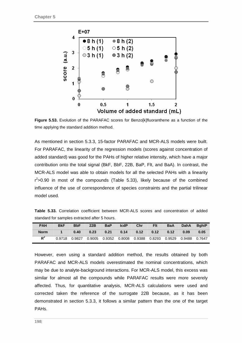
Chapter 5

198|

Figure 5.53. Evolution of the PARAFAC scores for Benzo[k]fluoranthene as a function of the

time applying the standard addition method.

As mentioned in section 5.3.3, 15-factor PARAFAC and MCR-ALS models were built.

For PARAFAC, the linearity of the regression models (scores against concentration of

added standard) was good for the PAHs of higher relative intensity, which have a major

contribution onto the total signal (BkF, BbF, 22B, BaP, Flt, and BaA). In contrast, the

MCR-ALS model was able to obtain models for all the selected PAHs with a linearity

r2>0.90 in most of the compounds (Table 5.33), likely because of the combined

influence of the use of correspondence of species constraints and the partial trilinear

model used.

Table 5.33. Correlation coefficient between MCR-ALS scores and concentration of added

standard for samples extracted after 5 hours.


Norm 1 0.40 0.23 0.21 0.14 0.12 0.12 0.12 0.09 0.05

R2 0.9718 0.9827 0.9005 0.9352 0.8008 0.9388 0.8293 0.9529 0.9488 0.7647

However, even using a standard addition method, the results obtained by both

PARAFAC and MCR-ALS models overestimated the nominal concentrations, which

may be due to analyte-background interactions. For MCR-ALS model, this excess was

similar for almost all the compounds while PARAFAC results were more severely

affected. Thus, for quantitative analysis, MCR-ALS calculations were used and

corrected taken the reference of the surrogate 22B because, as it has been

demonstrated in section 5.3.3, it follows a similar pattern than the one of the target

PAHs.

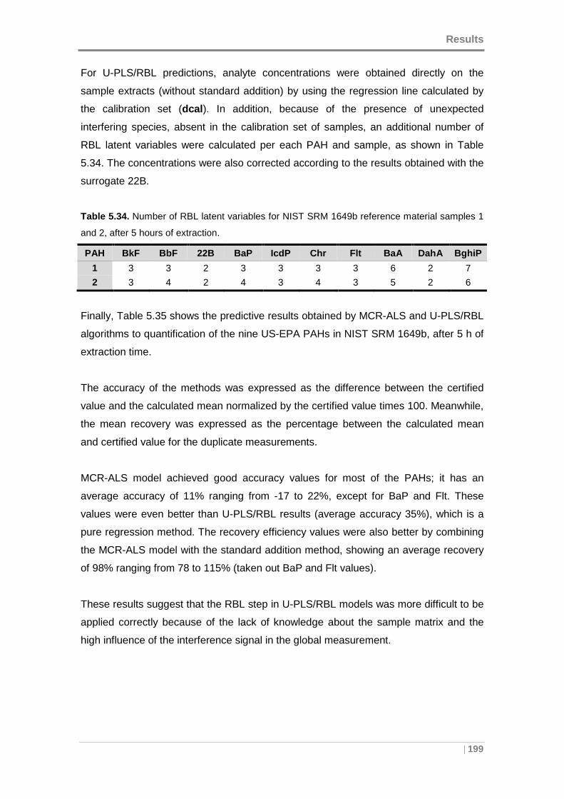
Results

| 199

For U-PLS/RBL predictions, analyte concentrations were obtained directly on the

sample extracts (without standard addition) by using the regression line calculated by

the calibration set (dcal ). In addition, because of the presence of unexpected

interfering species, absent in the calibration set of samples, an additional number of

RBL latent variables were calculated per each PAH and sample, as shown in Table

5.34. The concentrations were also corrected according to the results obtained with the

surrogate 22B.

Table 5.34. Number of RBL latent variables for NIST SRM 1649b reference material samples 1

and 2, after 5 hours of extraction.


1 3 3 2 3 3 3 3 6 2 7

2 3 4 2 4 3 4 3 5 2 6

Finally, Table 5.35 shows the predictive results obtained by MCR-ALS and U-PLS/RBL

algorithms to quantification of the nine US-EPA PAHs in NIST SRM 1649b, after 5 h of

extraction time.

The accuracy of the methods was expressed as the difference between the certified

value and the calculated mean normalized by the certified value times 100. Meanwhile,

the mean recovery was expressed as the percentage between the calculated mean

and certified value for the duplicate measurements.

MCR-ALS model achieved good accuracy values for most of the PAHs; it has an

average accuracy of 11% ranging from -17 to 22%, except for BaP and Flt. These

values were even better than U-PLS/RBL results (average accuracy 35%), which is a

pure regression method. The recovery efficiency values were also better by combining

the MCR-ALS model with the standard addition method, showing an average recovery

of 98% ranging from 78 to 115% (taken out BaP and Flt values).

These results suggest that the RBL step in U-PLS/RBL models was more difficult to be

applied correctly because of the lack of knowledge about the sample matrix and the

high influence of the interference signal in the global measurement.

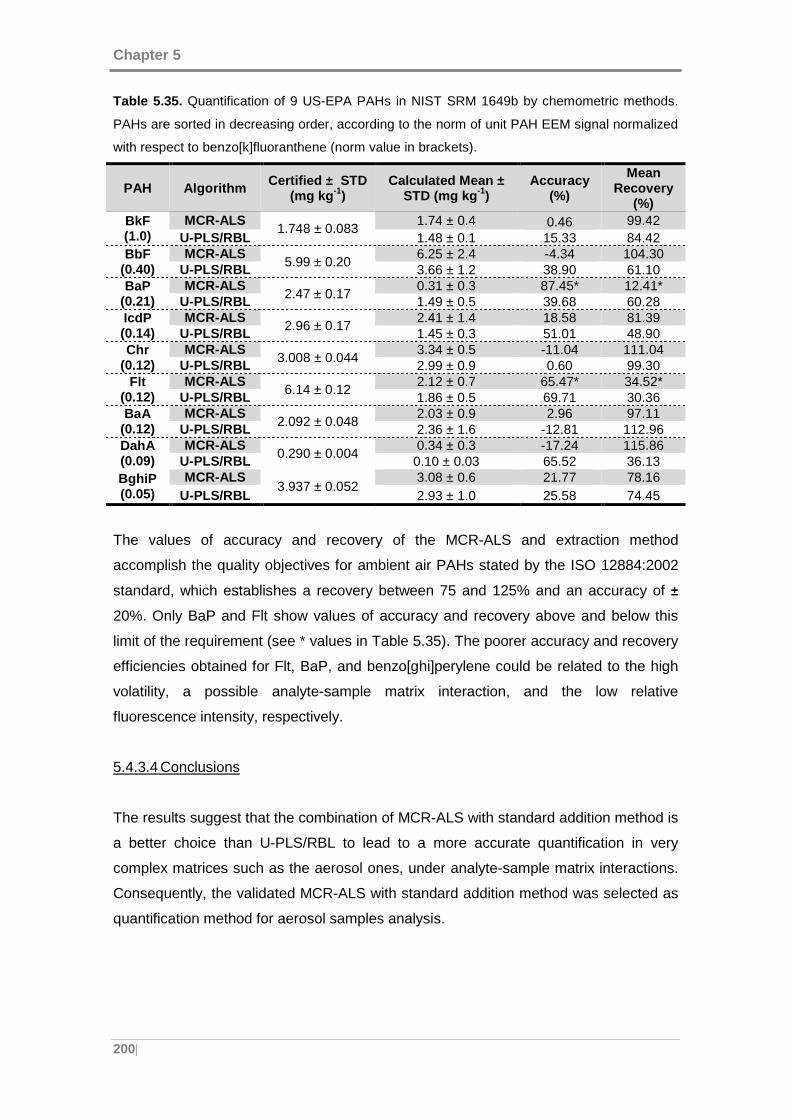
Chapter 5

200|

Table 5.35. Quantification of 9 US-EPA PAHs in NIST SRM 1649b by chemometric methods.

PAHs are sorted in decreasing order, according to the norm of unit PAH EEM signal normalized

with respect to benzo[k]fluoranthene (norm value in brackets).

PAH Algorithm Certified ± STD (mg kg -1)

Calculated Mean ± STD (mg kg -1)

Accuracy (%)

Mean Recovery

(%) BkF (1.0)

MCR-ALS 1.748 ± 0.083

1.74 ± 0.4 0.46 99.42 U-PLS/RBL 1.48 ± 0.1 15.33 84.42

BbF (0.40)

MCR-ALS 5.99 ± 0.20

6.25 ± 2.4 -4.34 104.30 U-PLS/RBL 3.66 ± 1.2 38.90 61.10

BaP (0.21)

MCR-ALS 2.47 ± 0.17

0.31 ± 0.3 87.45* 12.41* U-PLS/RBL 1.49 ± 0.5 39.68 60.28

IcdP (0.14)

MCR-ALS 2.96 ± 0.17

2.41 ± 1.4 18.58 81.39 U-PLS/RBL 1.45 ± 0.3 51.01 48.90

Chr (0.12)

MCR-ALS 3.008 ± 0.044

3.34 ± 0.5 -11.04 111.04 U-PLS/RBL 2.99 ± 0.9 0.60 99.30

Flt (0.12)

MCR-ALS 6.14 ± 0.12

2.12 ± 0.7 65.47* 34.52* U-PLS/RBL 1.86 ± 0.5 69.71 30.36

BaA (0.12)

MCR-ALS 2.092 ± 0.048

2.03 ± 0.9 2.96 97.11 U-PLS/RBL 2.36 ± 1.6 -12.81 112.96

DahA (0.09)

MCR-ALS 0.290 ± 0.004

0.34 ± 0.3 -17.24 115.86 U-PLS/RBL 0.10 ± 0.03 65.52 36.13

BghiP (0.05)

MCR-ALS 3.937 ± 0.052

3.08 ± 0.6 21.77 78.16 U-PLS/RBL 2.93 ± 1.0 25.58 74.45

The values of accuracy and recovery of the MCR-ALS and extraction method

accomplish the quality objectives for ambient air PAHs stated by the ISO 12884:2002

standard, which establishes a recovery between 75 and 125% and an accuracy of ±

20%. Only BaP and Flt show values of accuracy and recovery above and below this

limit of the requirement (see * values in Table 5.35). The poorer accuracy and recovery

efficiencies obtained for Flt, BaP, and benzo[ghi]perylene could be related to the high

volatility, a possible analyte-sample matrix interaction, and the low relative

fluorescence intensity, respectively.

5.4.3.4 Conclusions

The results suggest that the combination of MCR-ALS with standard addition method is

a better choice than U-PLS/RBL to lead to a more accurate quantification in very

complex matrices such as the aerosol ones, under analyte-sample matrix interactions.

Consequently, the validated MCR-ALS with standard addition method was selected as

quantification method for aerosol samples analysis.

Results

| 201

5.5 APPLICATION OF THE DEVELOPED METHODOLOGY TO URB AN AIR

SAMPLES

In previous sections, different methods for second-order calibration have been

validated and optimized in deep. Finally, the MCR-ALS method, in combination with

standard addition, was selected as the most suitable one for quantitative analysis of

PAHs in aerosol samples. Additionally, the extraction protocol was optimized and

validated, being selected the 5-h procedure in warm mode.

In this section, this methodology is applied to carry out a preliminary study for the

characterization of PAH pollution in an urban area, for several months. Due to the low

limit of detection of the method, a shorter-time monitoring (8 h sampling period) was

adopted. It is important to remark that there are very few studies quantifying PAHs in

PM10 size fraction with this temporal resolution, which can contribute to a better

understanding of the transformations, sources and fate of the PAHs in the atmosphere.

In this study, monthly and daily variation patterns are compared, discussed and related

to traffic patterns and other potential sources. The benzo[a]pyrene-equivalent toxicity

associated with ambient particle-bound PAHs is also evaluated, to discern the toxicity

contribution of other PAHs to the total toxicity and their relationships with the different

sampling periods. Additionally, diagnostic ratios are used for the assessment and

identification of the main contribution sources of particle-bound PAHs in the area.

Although most of the studies on particulate PAHs have been focused on source

identification, this study also includes the influence of meteorological conditions and

other conventional pollutants for a better understanding of the atmospheric fates of

particle-bound PAHs.

Then, multivariate approaches such as Principal Component Analysis is used to gain a

deeper characterization of the pollution scenarios, revealing different relationships

between the meteorology and pollution trends.

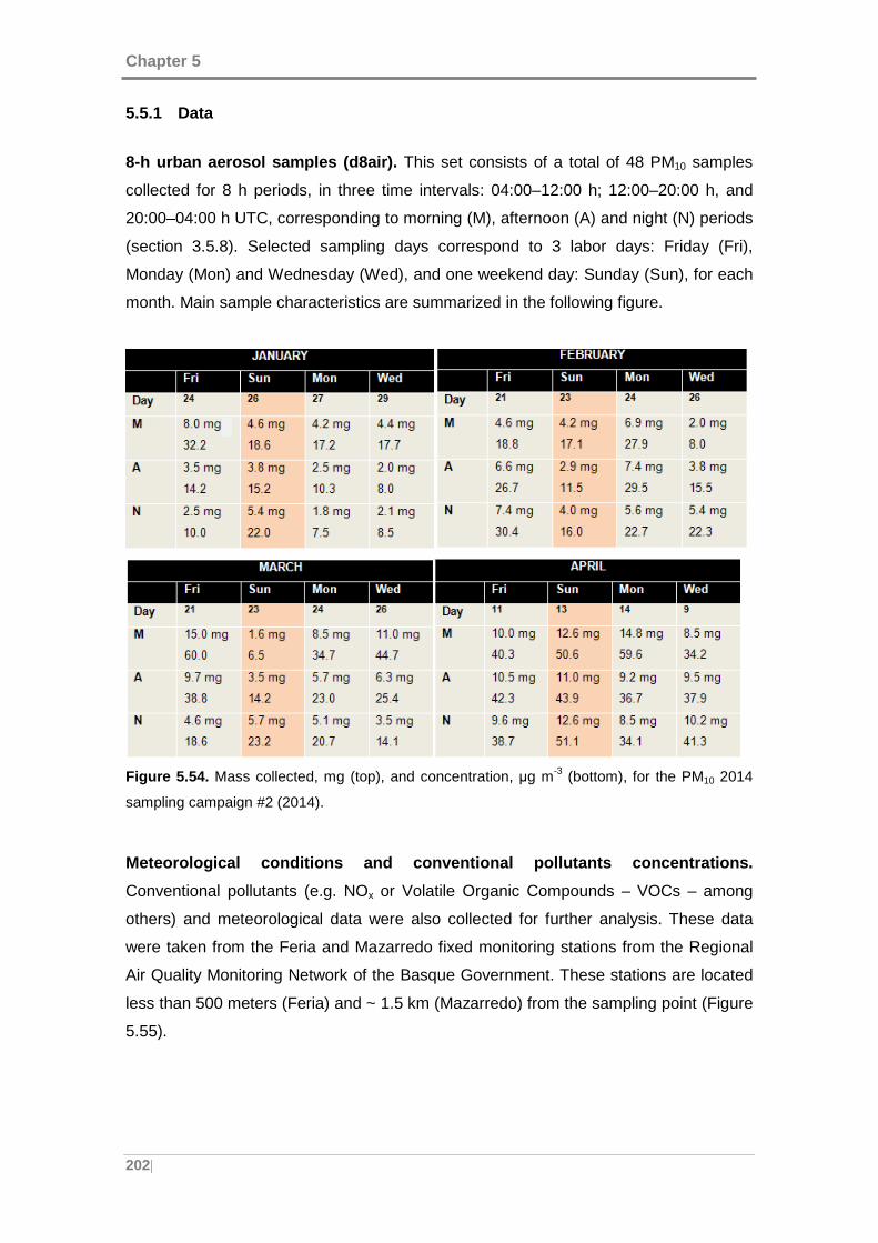
Chapter 5

202|

5.5.1 Data

8-h urban aerosol samples (d8air). This set consists of a total of 48 PM10 samples

collected for 8 h periods, in three time intervals: 04:00–12:00 h; 12:00–20:00 h, and

20:00–04:00 h UTC, corresponding to morning (M), afternoon (A) and night (N) periods

(section 3.5.8). Selected sampling days correspond to 3 labor days: Friday (Fri),

Monday (Mon) and Wednesday (Wed), and one weekend day: Sunday (Sun), for each

month. Main sample characteristics are summarized in the following figure.

Figure 5.54. Mass collected, mg (top), and concentration, µg m-3 (bottom), for the PM10 2014

sampling campaign #2 (2014).

Meteorological conditions and conventional pollutan ts concentrations.

Conventional pollutants (e.g. NOx or Volatile Organic Compounds – VOCs – among

others) and meteorological data were also collected for further analysis. These data

were taken from the Feria and Mazarredo fixed monitoring stations from the Regional

Air Quality Monitoring Network of the Basque Government. These stations are located

less than 500 meters (Feria) and ~ 1.5 km (Mazarredo) from the sampling point (Figure

5.55).

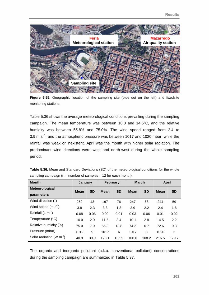
Results

| 203

Figure 5.55. Geographic location of the sampling site (blue dot on the left) and fixedsite

monitoring stations.

Table 5.36 shows the average meteorological conditions prevailing during the sampling

campaign. The mean temperature was between 10.0 and 14.5°C, and the relative

humidity was between 55.8% and 75.0%. The wind speed ranged from 2.4 to

3.9 m s−1, and the atmospheric pressure was between 1017 and 1020 mbar, while the

rainfall was weak or inexistent. April was the month with higher solar radiation. The

predominant wind directions were west and north-west during the whole sampling

period.

Table 5.36. Mean and Standard Deviations (SD) of the meteorological conditions for the whole

sampling campaign (n = number of samples = 12 for each month).

Month January February March April

Meteorological

parameters Mean SD Mean SD Mean SD Mean SD

Wind direction (°) 252 43 197 76 247 68 244 59

Wind speed (m s-1) 3.8 2.3 3.3 1.3 3.9 2.2 2.4 1.6 Rainfall (L m-2) 0.08 0.06 0.00 0.01 0.03 0.06 0.01 0.02

Temperature (°C) 10.0 2.9 11.6 3.4 10.1 2.8 14.5 2.2

Relative humidity (%) 75.0 7.9 55.8 13.8 74.2 6.7 72.6 9.3

Pressure (mbar) 1012 9 1017 6 1017 3 1020 2 Solar radiation (W m-2) 40.9 39.9 128.1 135.9 106.6 108.2 216.5 179.7

The organic and inorganic pollutant (a.k.a. conventional pollutant) concentrations

during the sampling campaign are summarized in Table 5.37.

Sampling site

Feria meteorological data

Mazarredo pollutants

Feria Meteorological station

Mazarredo Air quality station

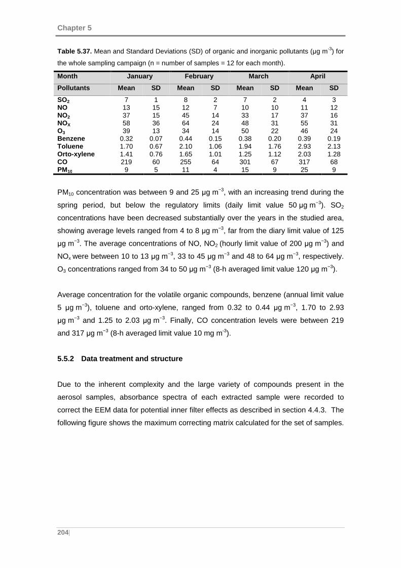
Chapter 5

204|

Table 5.37. Mean and Standard Deviations (SD) of organic and inorganic pollutants (µg m-3) for

the whole sampling campaign (n = number of samples = 12 for each month).

Month January February March April

Pollutants Mean SD Mean SD Mean SD Mean SD

SO2 7 1 8 2 7 2 4 3 NO 13 15 12 7 10 10 11 12 NO2 37 15 45 14 33 17 37 16 NOX 58 36 64 24 48 31 55 31 O3 39 13 34 14 50 22 46 24 Benzene 0.32 0.07 0.44 0.15 0.38 0.20 0.39 0.19 Toluene 1.70 0.67 2.10 1.06 1.94 1.76 2.93 2.13 Orto -xylene 1.41 0.76 1.65 1.01 1.25 1.12 2.03 1.28 CO 219 60 255 64 301 67 317 68 PM10 9 5 11 4 15 9 25 9

PM10 concentration was between 9 and 25 µg m−3, with an increasing trend during the

spring period, but below the regulatory limits (daily limit value 50 µg m−3). SO2

concentrations have been decreased substantially over the years in the studied area,

showing average levels ranged from 4 to 8 µg m−3, far from the diary limit value of 125

µg m−3. The average concentrations of NO, NO2 (hourly limit value of 200 µg m−3) and

NOx were between 10 to 13 µg m−3, 33 to 45 µg m−3 and 48 to 64 µg m−3, respectively.

O3 concentrations ranged from 34 to 50 µg m−3 (8-h averaged limit value 120 µg m−3).

Average concentration for the volatile organic compounds, benzene (annual limit value

5 µg m−3), toluene and orto-xylene, ranged from 0.32 to 0.44 µg m−3, 1.70 to 2.93

µg m−3 and 1.25 to 2.03 µg m−3. Finally, CO concentration levels were between 219

and 317 µg m−3 (8-h averaged limit value 10 mg m-3).

5.5.2 Data treatment and structure

Due to the inherent complexity and the large variety of compounds present in the

aerosol samples, absorbance spectra of each extracted sample were recorded to

correct the EEM data for potential inner filter effects as described in section 4.4.3. The

following figure shows the maximum correcting matrix calculated for the set of samples.

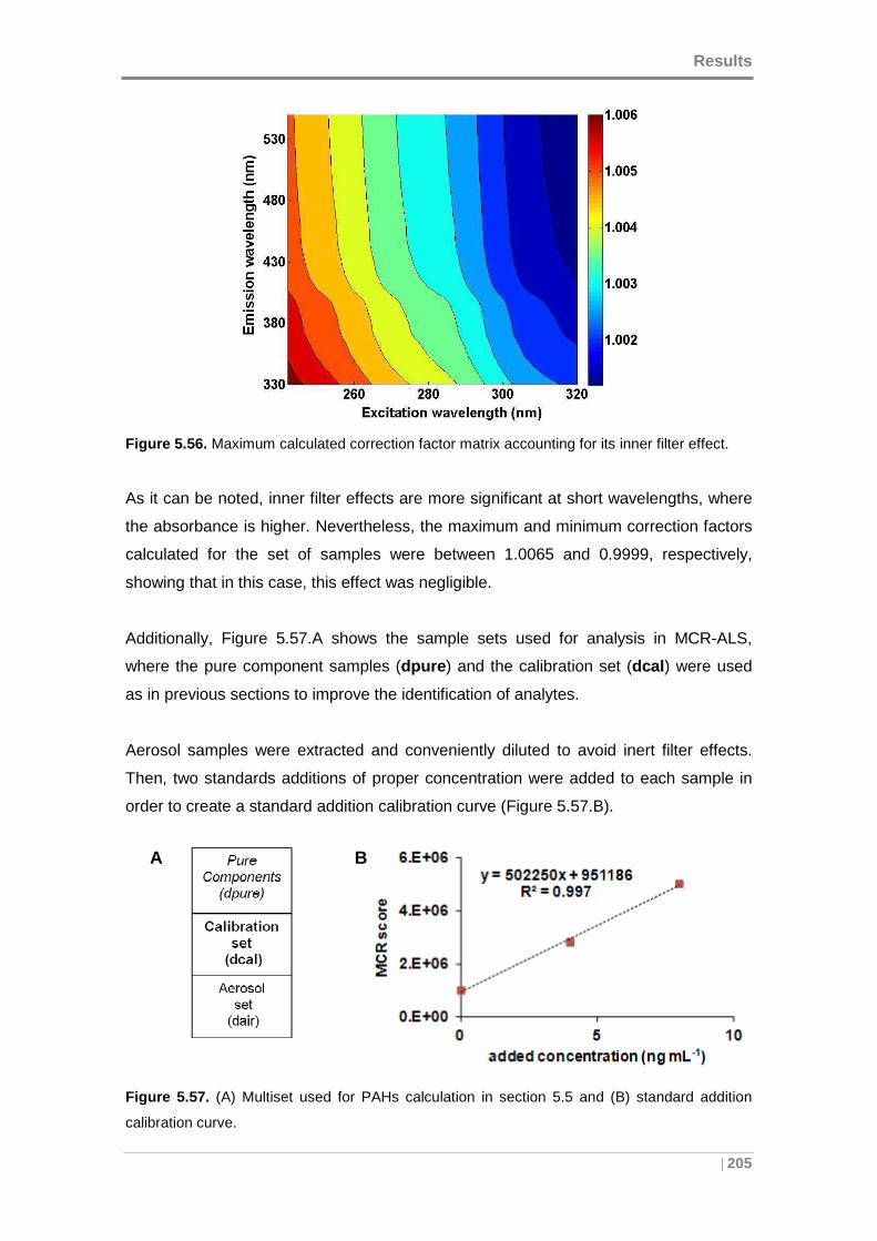
Results

| 205

Figure 5.56. Maximum calculated correction factor matrix accounting for its inner filter effect.

As it can be noted, inner filter effects are more significant at short wavelengths, where

the absorbance is higher. Nevertheless, the maximum and minimum correction factors

calculated for the set of samples were between 1.0065 and 0.9999, respectively,

showing that in this case, this effect was negligible.

Additionally, Figure 5.57.A shows the sample sets used for analysis in MCR-ALS,

where the pure component samples (dpure ) and the calibration set (dcal ) were used

as in previous sections to improve the identification of analytes.

Aerosol samples were extracted and conveniently diluted to avoid inert filter effects.

Then, two standards additions of proper concentration were added to each sample in

order to create a standard addition calibration curve (Figure 5.57.B).

Figure 5.57. (A) Multiset used for PAHs calculation in section 5.5 and (B) standard addition

calibration curve.

A B

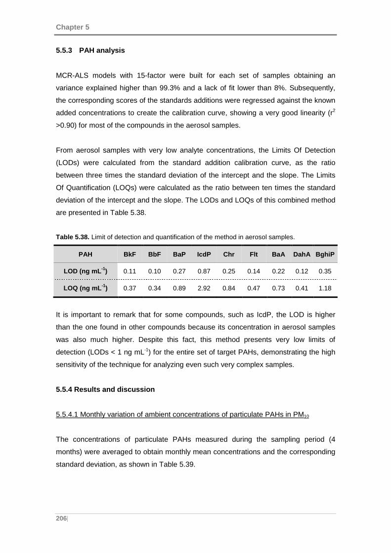
Chapter 5

206|

5.5.3 PAH analysis

MCR-ALS models with 15-factor were built for each set of samples obtaining an

variance explained higher than 99.3% and a lack of fit lower than 8%. Subsequently,

the corresponding scores of the standards additions were regressed against the known

added concentrations to create the calibration curve, showing a very good linearity (r2

>0.90) for most of the compounds in the aerosol samples.

From aerosol samples with very low analyte concentrations, the Limits Of Detection

(LODs) were calculated from the standard addition calibration curve, as the ratio

between three times the standard deviation of the intercept and the slope. The Limits

Of Quantification (LOQs) were calculated as the ratio between ten times the standard

deviation of the intercept and the slope. The LODs and LOQs of this combined method

are presented in Table 5.38.

Table 5.38. Limit of detection and quantification of the method in aerosol samples.

PAH BkF BbF BaP IcdP Chr Flt BaA DahA BghiP

LOD (ng mL -1) 0.11 0.10 0.27 0.87 0.25 0.14 0.22 0.12 0.35

LOQ (ng mL -1) 0.37 0.34 0.89 2.92 0.84 0.47 0.73 0.41 1.18

It is important to remark that for some compounds, such as IcdP, the LOD is higher

than the one found in other compounds because its concentration in aerosol samples

was also much higher. Despite this fact, this method presents very low limits of

detection (LODs < 1 ng mL-1) for the entire set of target PAHs, demonstrating the high

sensitivity of the technique for analyzing even such very complex samples.

5.5.4 Results and discussion

5.5.4.1 Monthly variation of ambient concentrations of particulate PAHs in PM10

The concentrations of particulate PAHs measured during the sampling period (4

months) were averaged to obtain monthly mean concentrations and the corresponding

standard deviation, as shown in Table 5.39.

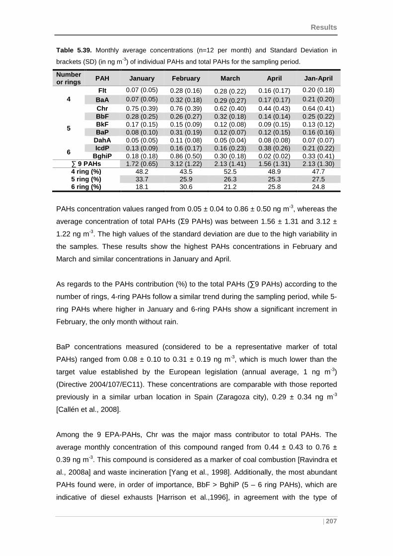
Results

| 207

Table 5.39. Monthly average concentrations (n=12 per month) and Standard Deviation in

brackets (SD) (in ng m-3) of individual PAHs and total PAHs for the sampling period.

Number or rings PAH January February March April Jan-April

4 Flt 0.07 (0.05) 0.28 (0.16) 0.28 (0.22) 0.16 (0.17) 0.20 (0.18)

BaA 0.07 (0.05) 0.32 (0.18) 0.29 (0.27) 0.17 (0.17) 0.21 (0.20) Chr 0.75 (0.39) 0.76 (0.39) 0.62 (0.40) 0.44 (0.43) 0.64 (0.41)

5

BbF 0.28 (0.25) 0.26 (0.27) 0.32 (0.18) 0.14 (0.14) 0.25 (0.22) BkF 0.17 (0.15) 0.15 (0.09) 0.12 (0.08) 0.09 (0.15) 0.13 (0.12) BaP 0.08 (0.10) 0.31 (0.19) 0.12 (0.07) 0.12 (0.15) 0.16 (0.16)

DahA 0.05 (0.05) 0.11 (0.08) 0.05 (0.04) 0.08 (0.08) 0.07 (0.07)

6 IcdP 0.13 (0.09) 0.16 (0.17) 0.16 (0.23) 0.38 (0.26) 0.21 (0.22)

BghiP 0.18 (0.18) 0.86 (0.50) 0.30 (0.18) 0.02 (0.02) 0.33 (0.41) ∑ 9 PAHs 1.72 (0.65) 3.12 (1.22) 2.13 (1.41) 1.56 (1.31) 2.13 (1.30) 4 ring (%) 48.2 43.5 52.5 48.9 47.7 5 ring (%) 33.7 25.9 26.3 25.3 27.5 6 ring (%) 18.1 30.6 21.2 25.8 24.8

PAHs concentration values ranged from 0.05 ± 0.04 to 0.86 ± 0.50 ng m-3, whereas the

average concentration of total PAHs (Σ9 PAHs) was between 1.56 ± 1.31 and 3.12 ±

1.22 ng m-3. The high values of the standard deviation are due to the high variability in

the samples. These results show the highest PAHs concentrations in February and

March and similar concentrations in January and April.

As regards to the PAHs contribution (%) to the total PAHs (∑9 PAHs) according to the

number of rings, 4-ring PAHs follow a similar trend during the sampling period, while 5-

ring PAHs where higher in January and 6-ring PAHs show a significant increment in

February, the only month without rain.

BaP concentrations measured (considered to be a representative marker of total

PAHs) ranged from 0.08 ± 0.10 to 0.31 ± 0.19 ng m -3, which is much lower than the

target value established by the European legislation (annual average, 1 ng m-3)

(Directive 2004/107/EC11). These concentrations are comparable with those reported

previously in a similar urban location in Spain (Zaragoza city), 0.29 ± 0.34 ng m-3

[Callén et al., 2008].

Among the 9 EPA-PAHs, Chr was the major mass contributor to total PAHs. The

average monthly concentration of this compound ranged from 0.44 ± 0.43 to 0.76 ±

0.39 ng m-3. This compound is considered as a marker of coal combustion [Ravindra et

al., 2008a] and waste incineration [Yang et al., 1998]. Additionally, the most abundant

PAHs found were, in order of importance, BbF > BghiP (5 – 6 ring PAHs), which are

indicative of diesel exhausts [Harrison et al.,1996], in agreement with the type of

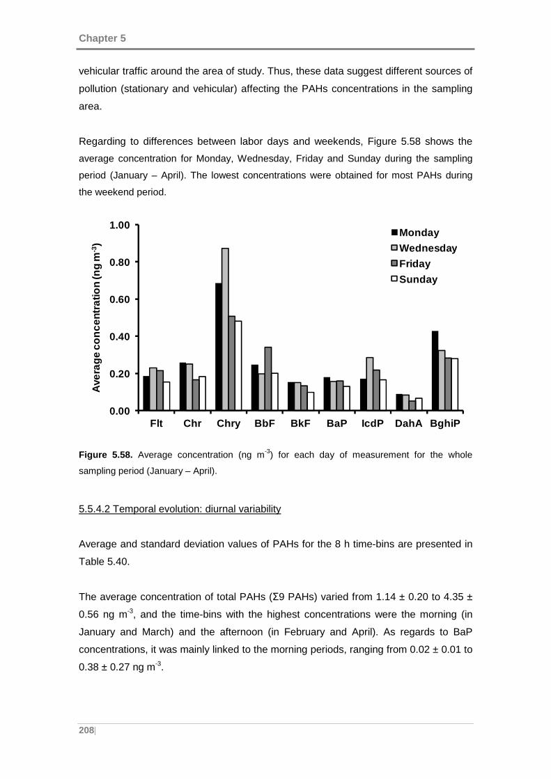
Chapter 5

208|

vehicular traffic around the area of study. Thus, these data suggest different sources of

pollution (stationary and vehicular) affecting the PAHs concentrations in the sampling

area.

Regarding to differences between labor days and weekends, Figure 5.58 shows the

average concentration for Monday, Wednesday, Friday and Sunday during the sampling

period (January – April). The lowest concentrations were obtained for most PAHs during

the weekend period.

Figure 5.58. Average concentration (ng m-3) for each day of measurement for the whole

sampling period (January – April).

5.5.4.2 Temporal evolution: diurnal variability

Average and standard deviation values of PAHs for the 8 h time-bins are presented in

Table 5.40.

The average concentration of total PAHs (Σ9 PAHs) varied from 1.14 ± 0.20 to 4.35 ±

0.56 ng m-3, and the time-bins with the highest concentrations were the morning (in

January and March) and the afternoon (in February and April). As regards to BaP

concentrations, it was mainly linked to the morning periods, ranging from 0.02 ± 0.01 to

0.38 ± 0.27 ng m-3.

0.00

0.20

0.40

0.60

0.80

1.00

Flt Chr Chry BbF BkF BaP IcdP DahA BghiP

Ave

rage

con

cent

ratio

n (n

g m

-3)

Monday

Wednesday

Friday

Sunday

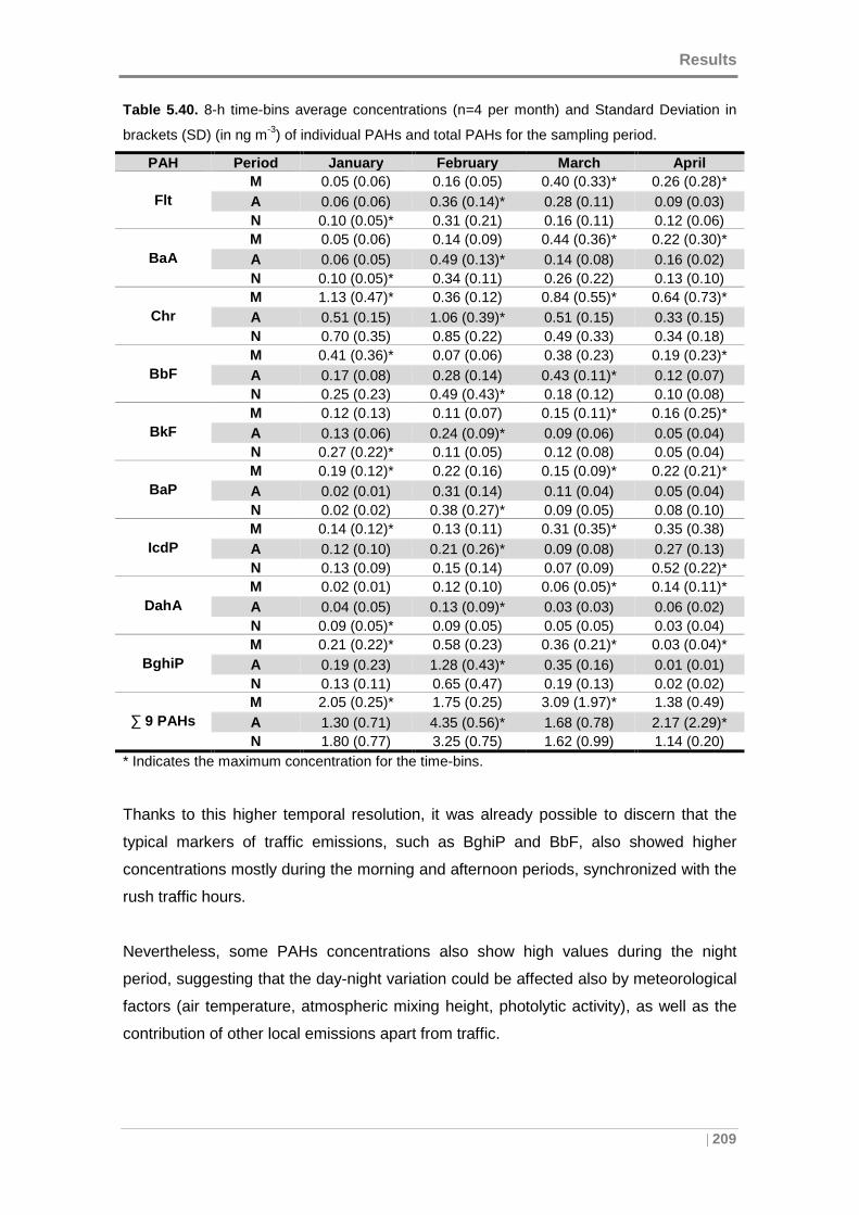
Results

| 209

Table 5.40. 8-h time-bins average concentrations (n=4 per month) and Standard Deviation in

brackets (SD) (in ng m-3) of individual PAHs and total PAHs for the sampling period.

PAH Period January February March April

Flt M 0.05 (0.06) 0.16 (0.05) 0.40 (0.33)* 0.26 (0.28)* A 0.06 (0.06) 0.36 (0.14)* 0.28 (0.11) 0.09 (0.03) N 0.10 (0.05)* 0.31 (0.21) 0.16 (0.11) 0.12 (0.06)

BaA M 0.05 (0.06) 0.14 (0.09) 0.44 (0.36)* 0.22 (0.30)* A 0.06 (0.05) 0.49 (0.13)* 0.14 (0.08) 0.16 (0.02) N 0.10 (0.05)* 0.34 (0.11) 0.26 (0.22) 0.13 (0.10)

Chr M 1.13 (0.47)* 0.36 (0.12) 0.84 (0.55)* 0.64 (0.73)* A 0.51 (0.15) 1.06 (0.39)* 0.51 (0.15) 0.33 (0.15) N 0.70 (0.35) 0.85 (0.22) 0.49 (0.33) 0.34 (0.18)

BbF M 0.41 (0.36)* 0.07 (0.06) 0.38 (0.23) 0.19 (0.23)* A 0.17 (0.08) 0.28 (0.14) 0.43 (0.11)* 0.12 (0.07) N 0.25 (0.23) 0.49 (0.43)* 0.18 (0.12) 0.10 (0.08)

BkF M 0.12 (0.13) 0.11 (0.07) 0.15 (0.11)* 0.16 (0.25)* A 0.13 (0.06) 0.24 (0.09)* 0.09 (0.06) 0.05 (0.04) N 0.27 (0.22)* 0.11 (0.05) 0.12 (0.08) 0.05 (0.04)

BaP M 0.19 (0.12)* 0.22 (0.16) 0.15 (0.09)* 0.22 (0.21)* A 0.02 (0.01) 0.31 (0.14) 0.11 (0.04) 0.05 (0.04) N 0.02 (0.02) 0.38 (0.27)* 0.09 (0.05) 0.08 (0.10)

IcdP M 0.14 (0.12)* 0.13 (0.11) 0.31 (0.35)* 0.35 (0.38) A 0.12 (0.10) 0.21 (0.26)* 0.09 (0.08) 0.27 (0.13) N 0.13 (0.09) 0.15 (0.14) 0.07 (0.09) 0.52 (0.22)*

DahA M 0.02 (0.01) 0.12 (0.10) 0.06 (0.05)* 0.14 (0.11)* A 0.04 (0.05) 0.13 (0.09)* 0.03 (0.03) 0.06 (0.02) N 0.09 (0.05)* 0.09 (0.05) 0.05 (0.05) 0.03 (0.04)

BghiP M 0.21 (0.22)* 0.58 (0.23) 0.36 (0.21)* 0.03 (0.04)* A 0.19 (0.23) 1.28 (0.43)* 0.35 (0.16) 0.01 (0.01) N 0.13 (0.11) 0.65 (0.47) 0.19 (0.13) 0.02 (0.02)

∑ 9 PAHs M 2.05 (0.25)* 1.75 (0.25) 3.09 (1.97)* 1.38 (0.49) A 1.30 (0.71) 4.35 (0.56)* 1.68 (0.78) 2.17 (2.29)* N 1.80 (0.77) 3.25 (0.75) 1.62 (0.99) 1.14 (0.20)

* Indicates the maximum concentration for the time-bins.

Thanks to this higher temporal resolution, it was already possible to discern that the

typical markers of traffic emissions, such as BghiP and BbF, also showed higher

concentrations mostly during the morning and afternoon periods, synchronized with the

rush traffic hours.

Nevertheless, some PAHs concentrations also show high values during the night

period, suggesting that the day-night variation could be affected also by meteorological

factors (air temperature, atmospheric mixing height, photolytic activity), as well as the

contribution of other local emissions apart from traffic.

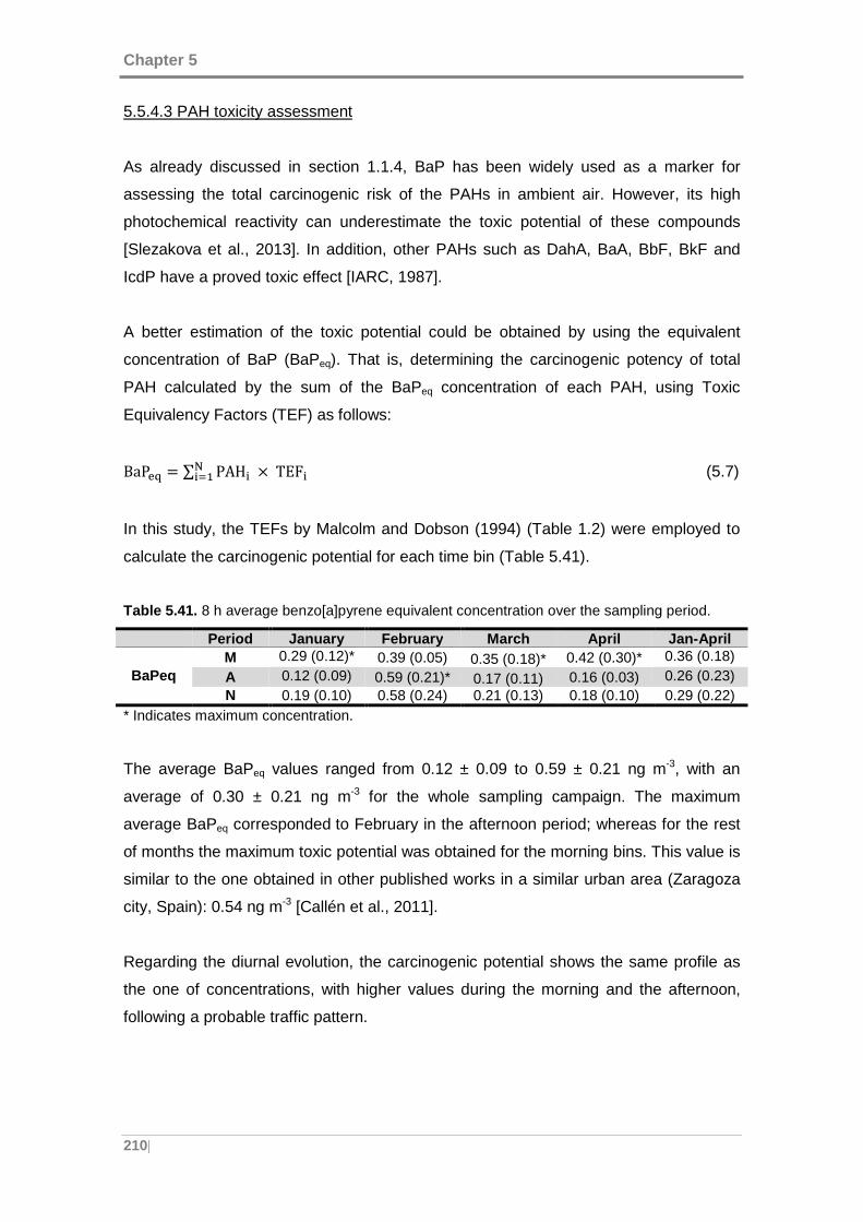
Chapter 5

210|

5.5.4.3 PAH toxicity assessment

As already discussed in section 1.1.4, BaP has been widely used as a marker for

assessing the total carcinogenic risk of the PAHs in ambient air. However, its high

photochemical reactivity can underestimate the toxic potential of these compounds

[Slezakova et al., 2013]. In addition, other PAHs such as DahA, BaA, BbF, BkF and

IcdP have a proved toxic effect [IARC, 1987].

A better estimation of the toxic potential could be obtained by using the equivalent

concentration of BaP (BaPeq). That is, determining the carcinogenic potency of total

PAH calculated by the sum of the BaPeq concentration of each PAH, using Toxic

Equivalency Factors (TEF) as follows:

BaP¼ = ∑ PAH�¾�� × TEF� (5.7)

In this study, the TEFs by Malcolm and Dobson (1994) (Table 1.2) were employed to

calculate the carcinogenic potential for each time bin (Table 5.41).

Table 5.41. 8 h average benzo[a]pyrene equivalent concentration over the sampling period.

Period January February March April Jan-April

BaPeq M 0.29 (0.12)* 0.39 (0.05) 0.35 (0.18)* 0.42 (0.30)* 0.36 (0.18)

A 0.12 (0.09) 0.59 (0.21)* 0.17 (0.11) 0.16 (0.03) 0.26 (0.23) N 0.19 (0.10) 0.58 (0.24) 0.21 (0.13) 0.18 (0.10) 0.29 (0.22)

* Indicates maximum concentration.

The average BaPeq values ranged from 0.12 ± 0.09 to 0.59 ± 0.21 ng m -3, with an

average of 0.30 ± 0.21 ng m-3 for the whole sampling campaign. The maximum

average BaPeq corresponded to February in the afternoon period; whereas for the rest

of months the maximum toxic potential was obtained for the morning bins. This value is

similar to the one obtained in other published works in a similar urban area (Zaragoza

city, Spain): 0.54 ng m-3 [Callén et al., 2011].

Regarding the diurnal evolution, the carcinogenic potential shows the same profile as

the one of concentrations, with higher values during the morning and the afternoon,

following a probable traffic pattern.

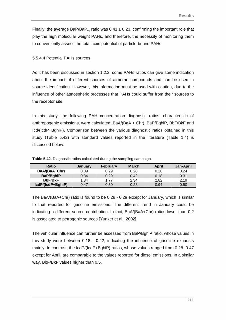
Results

| 211

Finally, the average BaP/BaPeq ratio was 0.41 ± 0.23, confirming the important role that

play the high molecular weight PAHs, and therefore, the necessity of monitoring them

to conveniently assess the total toxic potential of particle-bound PAHs.

5.5.4.4 Potential PAHs sources

As it has been discussed in section 1.2.2, some PAHs ratios can give some indication

about the impact of different sources of airborne compounds and can be used in

source identification. However, this information must be used with caution, due to the

influence of other atmospheric processes that PAHs could suffer from their sources to

the receptor site.

In this study, the following PAH concentration diagnostic ratios, characteristic of

anthropogenic emissions, were calculated: BaA/(BaA + Chr), BaP/BghiP, BbF/BkF and

Icd/(IcdP+BghiP). Comparison between the various diagnostic ratios obtained in this

study (Table 5.42) with standard values reported in the literature (Table 1.4) is

discussed below.

Table 5.42. Diagnostic ratios calculated during the sampling campaign.

Ratio January February March April Jan-April BaA/(BaA+Chr) 0.09 0.29 0.28 0.28 0.24

BaP/BghiP 0.34 0.29 0.42 0.18 0.31 BbF/BkF 1.84 1.77 2.34 2.82 2.19

IcdP/(IcdP+BghiP) 0.47 0.30 0.28 0.94 0.50

The BaA/(BaA+Chr) ratio is found to be 0.28 - 0.29 except for January, which is similar

to that reported for gasoline emissions. The different trend in January could be

indicating a different source contribution. In fact, BaA/(BaA+Chr) ratios lower than 0.2

is associated to petrogenic sources [Yunker et al., 2002].

The vehicular influence can further be assessed from BaP/BghiP ratio, whose values in

this study were between 0.18 - 0.42, indicating the influence of gasoline exhausts

mainly. In contrast, the IcdP/(IcdP+BghiP) ratios, whose values ranged from 0.28 -0.47

except for April, are comparable to the values reported for diesel emissions. In a similar

way, BbF/BkF values higher than 0.5.

Chapter 5

212|

It is also remarkable the different trend obtained in April for the BaP/BghiP and

IcdP/(IcdP+BghiP) ratios, which may be indicating the influence of a coal combustion

source [Yunker et al., 2002].

These results suggest the influence of multiple combustion sources, burning diesel,

gasoline, and coal as fuels. Thus, diagnosis of ratios can contribute qualitatively to the

identification of the main emission sources in the studied area.

Nevertheless, these ratios can also be altered due to the reactivity of some PAHs with

other atmospheric species, like ozone and/or oxides of nitrogen [Robinson et al., 2006

a]. For instance, The BaA/(BaA+Chr) ratio tends to change due to atmospheric

photoreactions, as a result of which BaA decays faster when adsorbed on soot,

resulting in strong shifts of the ratio towards low values [Kim et al., 2009].

Consequently, a further study including meteorological conditions and other

conventional pollutants was carried out and is presented in the following section.

5.5.4.5 Influence of physical-chemical and meteorological factors

PAHs determined in airborne particles are also influenced by several processes and

factors such as regional weather and source characteristics. Indeed, heterogeneous

reactions (photo-oxidations) and gas-particle partitioning, the main atmospheric

transformation processes for PAHs, are dependent on the meteorological conditions.

Thus the aim of this section was to analyze the simultaneous effects of the emission

sources (traffic and industrial sources), and parameters linked to the meteorological

conditions, on PAHs concentration patterns observed in the area under study.

Previous sections only involved the analysis of the variables in an independent manner

or using few combinations of specific PAHs (e.g. diagnostic ratios). However, this kind

of data analysis does not consider the plausible correlations between all the variables

at the same time. Hence, the use of multivariate data analysis is needed in order to

develop a more comprehensive study.

Principal Component Analysis (PCA) was selected as a pattern recognition technique.

By grouping variables with similar characteristics into Principal Components (PCs),

PCA transforms the original set of variables into a smaller set of linear combinations

that retain the original information as much as possible. Basically, the systematic

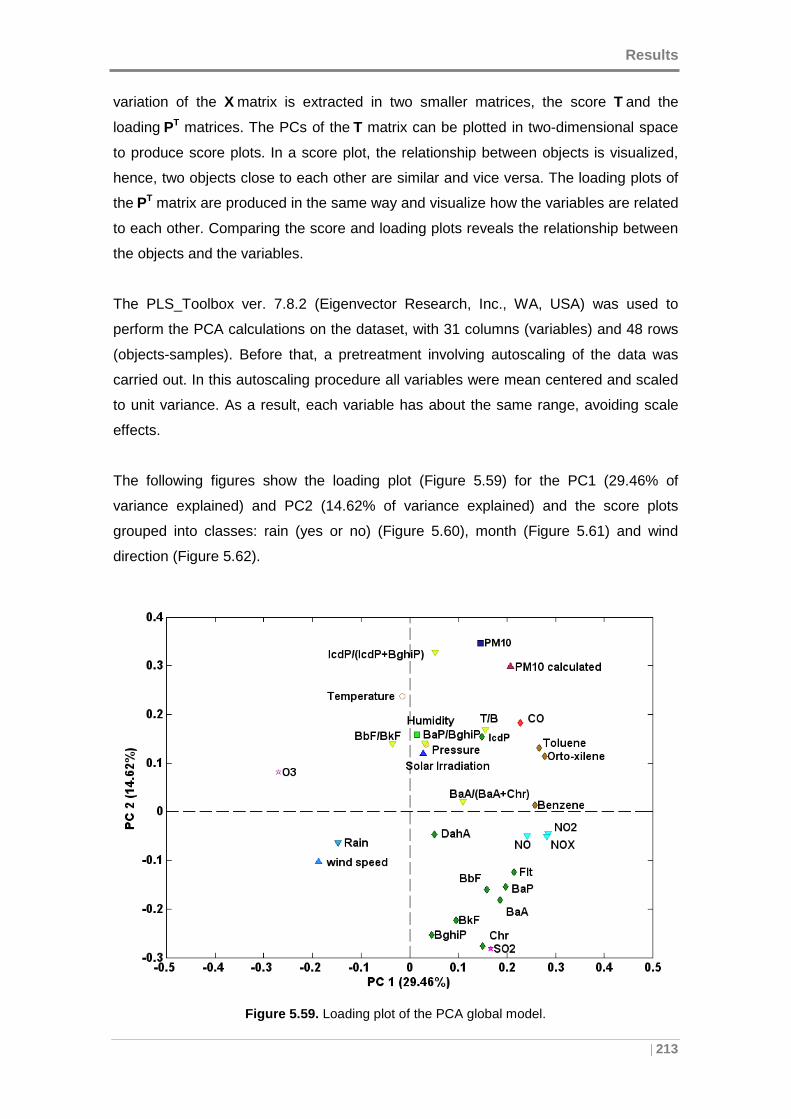
Results

| 213

variation of the X matrix is extracted in two smaller matrices, the score T and the

loading PT matrices. The PCs of the T matrix can be plotted in two-dimensional space

to produce score plots. In a score plot, the relationship between objects is visualized,

hence, two objects close to each other are similar and vice versa. The loading plots of

the PT matrix are produced in the same way and visualize how the variables are related

to each other. Comparing the score and loading plots reveals the relationship between

the objects and the variables.

The PLS_Toolbox ver. 7.8.2 (Eigenvector Research, Inc., WA, USA) was used to

perform the PCA calculations on the dataset, with 31 columns (variables) and 48 rows

(objects-samples). Before that, a pretreatment involving autoscaling of the data was

carried out. In this autoscaling procedure all variables were mean centered and scaled

to unit variance. As a result, each variable has about the same range, avoiding scale

effects.

The following figures show the loading plot (Figure 5.59) for the PC1 (29.46% of

variance explained) and PC2 (14.62% of variance explained) and the score plots

grouped into classes: rain (yes or no) (Figure 5.60), month (Figure 5.61) and wind

direction (Figure 5.62).

Figure 5.59. Loading plot of the PCA global model.

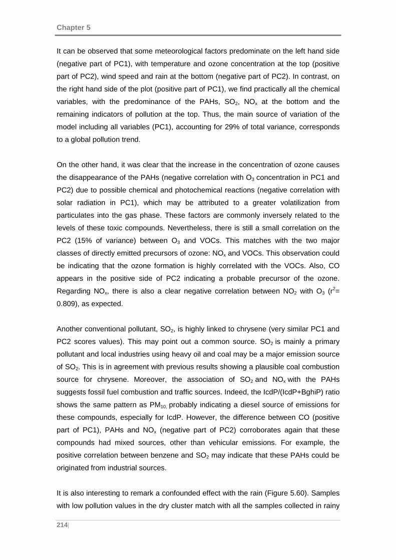
Chapter 5

214|

It can be observed that some meteorological factors predominate on the left hand side

(negative part of PC1), with temperature and ozone concentration at the top (positive

part of PC2), wind speed and rain at the bottom (negative part of PC2). In contrast, on

the right hand side of the plot (positive part of PC1), we find practically all the chemical

variables, with the predominance of the PAHs, SO2, NOx at the bottom and the

remaining indicators of pollution at the top. Thus, the main source of variation of the

model including all variables (PC1), accounting for 29% of total variance, corresponds

to a global pollution trend.

On the other hand, it was clear that the increase in the concentration of ozone causes

the disappearance of the PAHs (negative correlation with O3 concentration in PC1 and

PC2) due to possible chemical and photochemical reactions (negative correlation with

solar radiation in PC1), which may be attributed to a greater volatilization from

particulates into the gas phase. These factors are commonly inversely related to the

levels of these toxic compounds. Nevertheless, there is still a small correlation on the

PC2 (15% of variance) between O3 and VOCs. This matches with the two major

classes of directly emitted precursors of ozone: NOx and VOCs. This observation could

be indicating that the ozone formation is highly correlated with the VOCs. Also, CO

appears in the positive side of PC2 indicating a probable precursor of the ozone.

Regarding NOx, there is also a clear negative correlation between NO2 with O3 (r2=

0.809), as expected.

Another conventional pollutant, SO2, is highly linked to chrysene (very similar PC1 and

PC2 scores values). This may point out a common source. SO2 is mainly a primary

pollutant and local industries using heavy oil and coal may be a major emission source

of SO2. This is in agreement with previous results showing a plausible coal combustion

source for chrysene. Moreover, the association of SO2 and NOx with the PAHs

suggests fossil fuel combustion and traffic sources. Indeed, the IcdP/(IcdP+BghiP) ratio

shows the same pattern as PM10, probably indicating a diesel source of emissions for

these compounds, especially for IcdP. However, the difference between CO (positive

part of PC1), PAHs and NOx (negative part of PC2) corroborates again that these

compounds had mixed sources, other than vehicular emissions. For example, the

positive correlation between benzene and SO2 may indicate that these PAHs could be

originated from industrial sources.

It is also interesting to remark a confounded effect with the rain (Figure 5.60). Samples

with low pollution values in the dry cluster match with all the samples collected in rainy

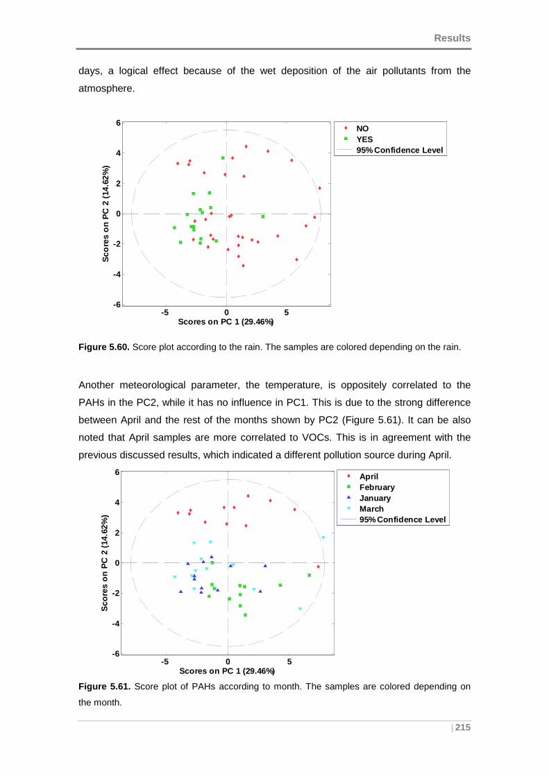
Results

| 215

days, a logical effect because of the wet deposition of the air pollutants from the

atmosphere.

Figure 5.60. Score plot according to the rain. The samples are colored depending on the rain.

Another meteorological parameter, the temperature, is oppositely correlated to the

PAHs in the PC2, while it has no influence in PC1. This is due to the strong difference

between April and the rest of the months shown by PC2 (Figure 5.61). It can be also

noted that April samples are more correlated to VOCs. This is in agreement with the

previous discussed results, which indicated a different pollution source during April.

Figure 5.61. Score plot of PAHs according to month. The samples are colored depending on

the month.

-5 0 5-6

-4

-2

0

2

4

6

Scores on PC 1 (29.46%)

Sco

res

on

PC

2 (

14.6

2%)

NOYES95% Confidence Level

-5 0 5-6

-4

-2

0

2

4

6


Sco

res

on P

C 2

(14

.62%

)

AprilFebruaryJanuaryMarch95% Confidence Level

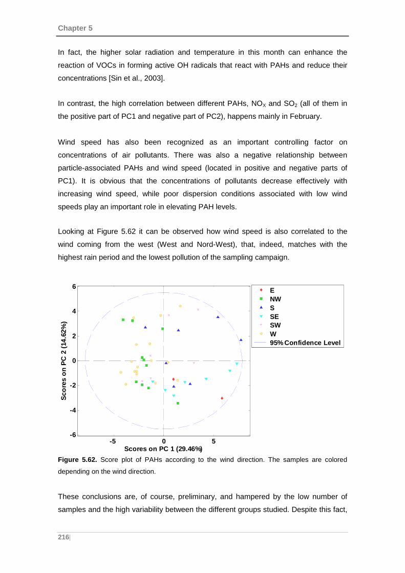
Chapter 5

216|

In fact, the higher solar radiation and temperature in this month can enhance the

reaction of VOCs in forming active OH radicals that react with PAHs and reduce their

concentrations [Sin et al., 2003].

In contrast, the high correlation between different PAHs, NOX and SO2 (all of them in

the positive part of PC1 and negative part of PC2), happens mainly in February.

Wind speed has also been recognized as an important controlling factor on

concentrations of air pollutants. There was also a negative relationship between

particle-associated PAHs and wind speed (located in positive and negative parts of

PC1). It is obvious that the concentrations of pollutants decrease effectively with

increasing wind speed, while poor dispersion conditions associated with low wind

speeds play an important role in elevating PAH levels.

Looking at Figure 5.62 it can be observed how wind speed is also correlated to the

wind coming from the west (West and Nord-West), that, indeed, matches with the

highest rain period and the lowest pollution of the sampling campaign.

Figure 5.62. Score plot of PAHs according to the wind direction. The samples are colored

depending on the wind direction.

These conclusions are, of course, preliminary, and hampered by the low number of

samples and the high variability between the different groups studied. Despite this fact,

-5 0 5-6

-4

-2

0

2

4

6


Sco

res

on

PC

2 (

14.6

2%)

ENWSSESWW95% Confidence Level

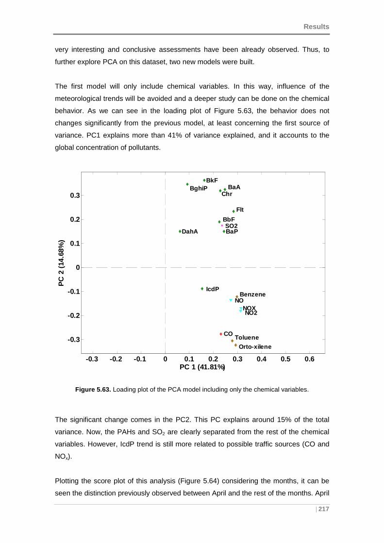
Results

| 217

very interesting and conclusive assessments have been already observed. Thus, to

further explore PCA on this dataset, two new models were built.

The first model will only include chemical variables. In this way, influence of the

meteorological trends will be avoided and a deeper study can be done on the chemical

behavior. As we can see in the loading plot of Figure 5.63, the behavior does not

changes significantly from the previous model, at least concerning the first source of

variance. PC1 explains more than 41% of variance explained, and it accounts to the

global concentration of pollutants.

Figure 5.63. Loading plot of the PCA model including only the chemical variables.

The significant change comes in the PC2. This PC explains around 15% of the total

variance. Now, the PAHs and SO2 are clearly separated from the rest of the chemical

variables. However, IcdP trend is still more related to possible traffic sources (CO and

NOx).

Plotting the score plot of this analysis (Figure 5.64) considering the months, it can be

seen the distinction previously observed between April and the rest of the months. April

-0.3 -0.2 -0.1 0 0.1 0.2 0.3 0.4 0.5 0.6

-0.3

-0.2

-0.1

0

0.1

0.2

0.3

PC 1 (41.81%)

PC

2 (

14.6

8%)

Flt

BaA Chr

BbF

BkF

BaP

IcdP

DahA

BghiP

Benzene NO

NO2 NOX

Orto-xilene

SO2

Toluene CO

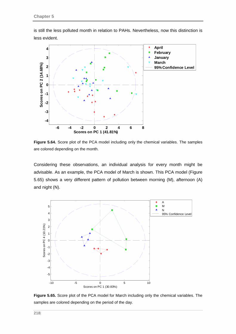
Chapter 5

218|

is still the less polluted month in relation to PAHs. Nevertheless, now this distinction is

less evident.

Figure 5.64. Score plot of the PCA model including only the chemical variables. The samples

are colored depending on the month.

Considering these observations, an individual analysis for every month might be

advisable. As an example, the PCA model of March is shown. This PCA model (Figure

5.65) shows a very different pattern of pollution between morning (M), afternoon (A)

and night (N).

Figure 5.65. Score plot of the PCA model for March including only the chemical variables. The

samples are colored depending on the period of the day.

-6 -4 -2 0 2 4 6 8

-4

-3

-2

-1

0

1

2

3

4


Sco

res

on P

C 2

(14

.68%

)

AprilFebruaryJanuaryMarch95% Confidence Level

-10 -5 0 5 10

-5

-4

-3

-2

-1

0

1

2

3

4

5


Sco

res

on P

C 4

(10

.21%

)

AMN95% Confidence Level

Results

| 219

According to this plot, the samples of the night period are the less polluted ones, while

the samples from the morning and afternoon are the ones suffering higher pollution

due to the PAHs.

These results must be taken with care, since only 48 samples have been analyzed

here. Nevertheless, there are three main conclusions to extract from the multivariate

perspective: the results match with the ones obtained in the previous sections. They

highlight new aspects, and there is still room for fostering a better understanding of the

behavior between the chemical and the meteorological variables, by applying more

dedicated methods, like canonical correlation analysis.

5.5.5 Conclusions

The MCR-ALS method coupled to standard addition was successfully applied for the

quantification of 9 particle-bound US-EPA PAHs in urban PM10 samples, with LODs < 1

ng mL-1.

The average concentration of total PAHs (Σ9 PAHs) was found between 1.56 ± 1.31

and 3.12 ± 1.22 ng m-3, showing the highest concentrations in February and March and

the lowest concentrations in January and April. Specifically, BaP concentration ranged

from 0.08 ± 0.10 to 0.31 ± 0.19 ng m -3, which is much lower than the target value

established by the European legislation (annual average, 1 ng m-3). Indeed, the

monthly average BaPeq values were between 0.12 ± 0.09 to 0.59 ± 0.21 ng m-3,

showing an average of 0.30 ± 0.21 ng m-3. Additionally, the average BaP/BaPeq ratio

obtained, 0.41 ± 0.23, confirmed that the only evaluation of BaP underestimates the

carcinogenic potential of the urban PAH mixtures.

Among the 9 EPA-PAHs, Chr was the major contributor, pointing out a plausible source

of coal combustion or waste incineration. This observation is corroborated by its strong

relationship with SO2, primary pollutant of local industries using heavy oil and coal. The

abundance of another PAHs species such as BbF and BghiP also indicates an

influence of vehicular traffic emissions on the site, lower during the weekend period.

Concerning the diurnal evolution, the time-bins with the highest concentrations were

the morning (in January and March) and the afternoon (in February and April),

following a probable traffic pattern. However, the day-night variation indicates that the

Chapter 5

220|

emissions could be highly affected by the meteorological factors as well as the

contribution of other local sources apart from traffic.

The use of diagnostic ratios confirmed the vehicular traffic presence (diesel and

gasoline exhaust), but pointed out also the influence of other stationary sources, like

the burning of coal, showing also a different trend between months.

The PCA analysis corroborated that, not only the vehicular emissions, but also

stationary sources were important sources of PAHs in the area of study. However, the

exact contribution of each source remains unclear due to the low number of samples

analyzed, which needs to be confirmed by further studies.

Conventional pollutants such as ozone showed a clear trend with the decrease of

PAHs, due to chemical and photochemical reactions.

Meteorological parameters also affected the air concentrations of PAHs, but their

influence was not independent. Indeed, it was shown that west and nord-west winds

were less polluted, but they also coincided with raining and higher wind speed periods.

Further, the temperature was oppositely correlated to the PAHs and positively

correlated with a different pollution source of VOCs during April, meanwhile the highest

correlation between the different PAHs, NOX and SO2, happened mainly in February.

Finally, the short-term monitoring of PAHs confirms the diurnal variation of the chemical

composition of the PM10, showing different trends for the morning, afternoon and night

periods, and helps on the source apportionment for air quality management.

CHAPTER 6

CONCLUSIONS

Conclusions

| 223

6. CONCLUSIONS

This Chapter collects the main conclusions in an itemized manner, so the reader can

follow all the achievements in a sequential way.

6.1 DEFINITION OF EEM DATA ADCQUISITION PROTOCOL

Setting the monochromators bandwidths at 5 nm, and the integration time to 0.1s

yielded the optimal amplification of the PMT, while minimizing the background noise.

The analysis of the fluorescence features of the target PAHs allowed us to reduce the

measurement spectral ranges to 240 – 320 nm (each 2 nm) and 330 – 550 nm (each 2

nm) for excitation and emission ranges, respectively. This allows for time savings in the

measurements (less than 35 minutes per sample), and to reduce the effects of

Rayleigh and Raman scattering.

The high overlapping of the broad spectral bands, and similarities in the spectral

features of the target PAHs, can be overcome coupling the EEM fluorescence

measurements with multivariate and three-way analysis.

6.2. DEVELOPMENT OF PRELIMINARY EEM DATA MODELS

The use of missing values to remove the scattering effects leads to problems related to

local minima in the built models, increases considerably the time of analysis, and

hinders the correct decomposition of very complex samples, contributing to the

appearance of spectral artifacts.

The use of interpolated data instead of missing values to remove the scattering effects

reduces the time of analysis and helps to build more robust models, being more

suitable as preprocessing method.

In the absence of interferences, the three algorithms (PARAFAC, MCR-ALS and

UPLS-RBL) lead to similar results, showing a good linear behavior (r2 > 0.99) and low

Limits Of Detection (LOD < 1 ng mL-1) for every target PAH.

The presence of non-trilinear contributions affects mostly to the performance of

PARAFAC models, whereas the use of partial trilinearity, and correspondence among

Chapter 6

224|

species as constraints in MCR-ALS models, provide a more accurate description of

complex samples. This is especially true if the relative signal of the analytes is at the

same level of other background contributions, and deviations from the ideal trilinearity

exist. The active use of this kind of constraints is still not sufficiently exploited.

Properly constrained MCR-ALS and PARAFAC models are able to recover the spectral

profiles of the analytes and other interfering compounds, even in samples containing a

great number of analytes with overlapped signals and several interferences, if the

signal of the unexpected compounds is within the spectral working range. This

challenges the common assumption that these models are only able to work with

samples with a small number of compounds.

As a first step, MCR-ALS and PARAFAC are the methods of choice for fast qualitative

and quantitative screening of environmental samples, although they are more sensitive

to changes in the signal-to-concentration ratio (matrix effects).

As a second step, U-PLS/RBL provides better quantitative information for samples

containing interferences and potential matrix effects, with low values of RMSEP and

REP, comparable to those achieved by other more expensive and time consuming

separation techniques.

6.3. OPTIMIZATION OF THE EXTRACTION PROTOCOL

N-hexane as solvent, and 2,2’binaphthyl as surrogate, fulfill the requirements of optimal

physicochemical and spectrofluorimetric properties for particle-bound PAHs extraction

and fluorescence analysis.

The results of a full factorial DoE pointed out that the warm mode is a valuable

alternative to the standard extraction methods, demonstrating advantage of robustness

against conventional Soxhlet extraction.

Desirability values of the multi-response system indicated 3 hours of extraction time

without drying step as the optimal extraction conditions for liquid PAH mixtures

standards. However, the variation in the recovery yield including the drying step in the

warm mode could be considered as meaningless and, therefore, it can be used when

the PAH concentrations are expected to be low.

Conclusions

| 225

The evaluation of the extraction protocol with standard reference material in particulate

phase proved the 5-h procedure as the optimum extraction time. The analysis also

highlighed the time dependence of some heavy PAHs (e.g. DahA); probably losses of

most volatile analytes (e.g. Flt), and plausible interactions between BaP and other

analytes present in the background, for increasing extraction times.

6.4 VALIDATION OF THE MODELS TO DETERMINE TARGET PA Hs IN

AEROSOL SAMPLES

Validation of the proposed models demonstrated that PARAFAC and MCR-ALS are

reliable methods for qualitative analysis, when a fast data analysis is required, which is

the perfect scenario for screening and monitoring of PAHs in aerosol samples.

Even with complex sample matrix effects, these curve resolution methodologies could

be used when a high sensitivity is needed, as in studies of background atmospheres,

overtaking other traditional methods of analysis -in terms of time, use of solvents, and

sensitivity- for qualitative analysis or monitoring patterns of variation of PAHs.

U-PLS/RBL exhibited better predictive capability for quantitative analysis, as long as no

severe matrix effects are present. Nevertheless, it is a very time-consuming method,

and the selection of the correct number of RBL factors becomes a difficult task when

many unexpected and unknown compounds are present in the environmental samples.

For quantitative analysis of complex environmental samples, the combination of MCR-

ALS with standard addition method is a better choice than U-PLS/RBL. It led to a more

accurate quantification, accomplishing the quality objectives for ambient air PAHs,

(recovery rates between 75 and 125% and accuracy values of ± 20%).

6.5 APPLICATION OF THE DEVELOPED METHODOLOGY TO URB AN AIR

SAMPLES

MCR-ALS coupled to standard addition for the quantification of 9 particle-bound US-

EPA PAHs in urban PM10 samples, achieves low limits of detection (< 1 ng mL-1), and

allows shorter time sampling periods.

BaP concentration values obtained were much lower than the target value established

in the EU (annual average, 1 ng m-3), and similar to other urban locations in Spain.

Chapter 6

226|

The average BaP/BaPeq ratio obtained confirms that the use of BaP alone

underestimates the carcinogenic potential of the PAH mix in ambient air.

The average concentration of total PAHs (Σ9 PAHs) did not show any clear temporal

trend. The diurnal evolution of PAHs concentrations revealed that their emissions could

be highly affected by meteorological factors and the contribution of local non-traffic

emission sources.

The analysis of individual PAH source markers, diagnostic ratios, and PCA

decomposition, confirmed the presence of traffic sources (diesel and gasoline

exhaust), pointed out the influence of other stationary sources burning coal, and

revealed also a different trend between months. However, the exact contribution of

each source remains unclear yet, due to the low number of samples analyzed.

Conventional pollutants such as ozone showed a clear influence on the decrease of

PAHs concentrations, due to chemical and photochemical reactions. Meteorological

parameters also affect the concentrations of PAHs, but their effects are not

independent, resulting from the combined impact of various meteorological conditions.

Finally, the use of shorter time sampling periods for PAHs, confirms the diurnal

variation of the PM10 chemical composition, showing different trends for the morning,

afternoon and night periods, and helps on the source apportionment tasks for air

quality management.

CHAPTER 7

BIBLIOGRAPHY

Bibliography

| 229

1. Agency for Toxic Substances and Disease Registry (ATSDR). Toxicological profile for polycyclic aromatic hydrocarbons (PAHs). US Department of Health and Human Services, Public Health Service. Atlanta, Georgia, 1995. http://www.atsdr.cdc.gov/toxprofiles/tp.asp?id=122&tid=25

2. Akyüz M, Çabuk H. Particle-associated polycyclic aromatic hydrocarbons in the atmospheric environment of Zonguldak, Turkey. Sci. Total Environ. 2008; 405: 62 -70.

3. Alarcón F, Báez ME, Bravo M, Ritcher P, Escandar GM, Olivieri AC, Fuentes E. Feasibility of the determination of polycyclic aromatic hydrocarbons in edible oils via unfolded partial least-squares/residual bilinearization and parallel factor analysis of fluorescence excitation emission matrices. Talanta 2013; 103: 361-370.

4. American Society for Testing and Materials (ASTM). Standard test method for determination of gaseous and particulate PAHs in ambient air (collection on sorbent-backed filters with GC/MS analysis). Designation: D6209-98; 2004.

5. Amigo JM, Marini F. Chapter 7. Multi-way methods. In Data handling in science and technology. Volume 28: chemometrics in food science, Marini F (ed.). Elsevier, UK, 2013; 265–313.

6. Amodio M, Caselli M, Gennaro G, Tutino M. Particulate PAHs in two urban areas

of Southern Italy: impact of the sources, meteorological and background conditions on air quality. Environ. Res. 2009; 109: 812–820.

7. Andersen CM, Bro R. Practical aspects of PARAFAC modelling of fluorescence excitation emission data. J. Chemometr. 2003; 17: 200–15.

8. Andersson CA, Bro R. The N-way toolbox for MATLAB. Chemom. Intell. Lab. Syst. 2000; 52: 1–4.

9. Andrade-Eiroa A, Canle M, Cerdá V. Environmental applications of excitation-

emission spectrofluorimetry; an in-depth review I. Appl. Spectrosc. Rev. 2013, 48: 1-49.

10. Arancibia JA, Boschetti CE, Olivieri AC, Escandar GM. Screening of oil samples

on the basis of excitation-emission room-temperature phosphorescence data and multi-way chemometric techniques. Introducing the second-order advantage in a classification study. Anal. Chem. 2008; 80: 2789–2798.

11. Armstrong B, Hutchinson E, Unwin J, Fletcher T. Lung cancer risk after exposure

to polycyclic aromatic hydrocarbons: a review and meta-analysis. Environ. Health Persp. 2004; 112: 970–978.

12. Baek SO, Goldstone ME, Kirk PWW, Lester JN, Perry R. Phase distribution and particle size dependency of polycyclic aromatic hydrocarbons in the urban environment. Chemosphere 1991a; 22: 503–520.

13. Baek SO, Field RA, Goldstone ME, Kirk PW, Lester JN, Perry R. A review of

atmospheric polycyclic aromatic hydrocarbons: sources, fate and behavior. Water Air Soil Poll. 1991b; 60: 279–300.

Chapter 7

230|

14. Bahram M, Bro R, Stedmon CA, Afkhami A. Handling of Rayleigh and Raman scatter for PARAFAC modeling of fluorescence data using interpolation. J. Chemometr. 2006; 20: 99–105.

15. Bark KM, Force RK. Analysis of polynuclear aromatic hydrocarbons mixtures in various environments by time-resolved fluorescence spectroscopy. Talanta 1991; 38: 181–188.

16. Barrado AI, García S, Castrillejo Y, Barrado E. Exploratory data analysis of PAH,

nitro-PAH and hydroxy-PAH concentrations in atmospheric PM10-bound aerosol particles. Correlations with physical and chemical factors. Atmos. Environ. 2013; 67: 385-393.

17. Barrero MA, Cantón L. Organic composition of atmospheric urban aerosol:

Variations and sources of aliphatic and polycyclic aromatic hydrocarbons. Atmos. Res. 2007; 85: 288-299.

18. Behymer TD, Hites RA. Photolysis of polycyclic aromatic hydrocarbons adsorbed

on fly ash. Environ. Sci. Technol. 1988; 22: 1311-1319. 19. Beltrán JL, Ferrer R, Guiteras J. Multivariate calibration of polycyclic aromatic

hydrocarbon mixtures from excitation-emission fluorescence spectra. Anal. Chim. Acta 1998; 373: 311-319.

20. Bohoyo D, Muñoz A, Arancibia JA, Escandar GM, Olivieri AC. Second-order

advantage achieved by unfolded-partial least-squares/residual bilinearization modeling of excitation-emission fluorescence data presenting inner filter effects. Anal. Chem. 2006; 78: 8051-8058.

21. Booksh KS, Kowalski BR. Theory of analytical chemistry. Anal. Chem. 1994; 66:

782-791.

22. Booksh KS, Muroski AR, Myrick ML. Single-measurement excitation/emission matrix spectrofluorometer for determination of hydrocarbons in ocean water. 2. Calibration and quantitation of naphthalene and styrene. Anal. Chem. 1996; 68: 3539-3544.

23. Bortolato SA, Arancibia JA, Escandar GM. Chemometrics-assisted excitation–

emission fluorescence spectroscopy on nylon membranes. Simultaneous determination of benzo[a]pyrene and dibenz[a,h]anthracene at parts-per-trillion levels in the presence of the remaining EPA PAH priority pollutants as interferences. Anal. Chem. 2008; 80: 8276–8286.

24. Bosco MV, Callao MP, Larrechi MS. Simultaneous analysis of the photocatalytic degradation of polycyclicaromatic hydrocarbons using three-dimensional excitation–emission matrix fluorescence and parallel factor analysis. Anal. Chim. Acta 2006; 576: 184–191.

25. Bosco MV, Larrechi MS. PARAFAC and MCR-ALS applied to the quantitative monitoring of the photodegradation process of polycyclic aromatic hydrocarbons using three-dimensional excitation emission fluorescent spectra: comparative results with HPLC. Talanta 2007; 71: 1703–1709.

26. Boström CE, Gerde P, Hanberg A, Jernström B, Johansson C, Kyrklund T,

Rannug A, Törnqvist M, Victorin K, Westerholm R. Cancer risk assessment,

Bibliography

| 231

indicators, and guidelines for polycyclic aromatic hydrocarbons in the ambient air. Environ. Health Persp. 2002; 110: 451-488.

27. Bourotte C, Forti MC, Taniguchi S, Bícego MC, Lotufo PA. A wintertime study of

PAHs in fine and coarse aerosols in Sao Paulo city, Brazil. Atmos. Environ. 2005; 39: 3799-3811.

28. Braga JWB, Carneiro RL, Poppi RJ. Evaluation of the number of factors needed

for residual bilinearization in BLLS and U-PLS models to achieve the second-order advantage. Chemom. Intell. Lab. Syst. 2010; 100: 99–109.

29. Brereton RG. Chapter 2.3.4. Partial factorials at several levels: calibration

designs. In Chemometrics: data analysis for the laboratory and chemical plant. John Wiley and Sons, Ltd. England, 2003; 69-76.

30. Bro R. Multi-way calibration. Multilinear PLS. J. Chemometr. 1996; 10: 47 – 61.

31. Bro R. PARAFAC. Tutorial and applications. Chemom. Intell. Lab. Syst. 1997; 38:

149–171.

32. Bro R, DeJong S. A fast non-negativity-constrained least squares algorithm. J. Chemometr. 1997; 11: 393–401.

33. Bro R. Multi-way analysis in the food industry: models, algorithms, and

applications; 1998. PhD Thesis monograph: Universiteit van Amsterdam.

34. Bro R, Sidiropoulos ND, Smilde AK. Maximum likelihood fitting using simple least squares algorithms. J. Chemometr. 2002; 16: 387–400.

35. Bro R. Multivariate calibration. What is in chemometrics for the analytical

chemist? Anal. Chim. Acta 2003; 500: 185–194. 36. Bro R, Kiers HAL. A new efficient method for determining the number of

components in PARAFAC models. J. Chemometr. 2003; 17: 274–286.

37. Brown AS, Brown RJC. Correlations in polycyclic aromatic hydrocarbon (PAH) concentrations in UK ambient air and implications for source apportionment. J. Environ. Monitor. 2012; 14: 2072 -2082.

38. Callén MS, de la Cruz MT, López JM, Murillo R, Navarro MV, Mastral AM. Some

interferences on the mechanism of atmospheric gas/particle partitioning of polycyclic aromatic hydrocarbons (PAH) at Zaragoza (Spain). Chemosphere 2008; 73: 1357-1365.

39. Callén MS, de la Cruz MT, López JM, Mastral AM. PAH in airborne particulate

matter: carcinogenic character of PM10 samples and assessment of the energy generation impact. Fuel Process. Technol. 2011; 92: 176–182.

40. Canadian Council of Ministers of the Environment (CCME). Canadian soil quality

guidelines for carcinogenic and other polycyclic aromatic hydrocarbons. Environmental and human health effects. Scientific criteria document. Winnipeg, 2010.

Chapter 7

232|

41. Caricchia AM, Chiavarini S, Pezza M. Polycyclic aromatic hydrocarbons in the urban atmospheric particulate matter in the city of Naples (Italy). Atmos. Environ. 1999; 33: 3731-3738.

42. Carroll JD, Chang JJ. Analysis of individual differences in multidimensional

scaling via and N-way generalization of and Eckart-Young decomposition. Psychometrika 1970; 35: 283-319.

43. Cattell RB. Parallel proportional profiles and other principles for determining the

choice of factors by rotation. Psychometrika 1944; 9: 267-283.

44. Chen SC, Liao CM. Health risk assessment on human exposed to environmental polycyclic aromatic hydrocarbons pollution sources. Sci. Total Environ. 2006; 366: 112–123.

45. Christensen J, Povlsen VT, Sørensen J. Application of fluorescence

spectroscopy and chemometrics in the evaluation of processed cheese during storage. J. Dairy Sci. 2003; 86: 1101-1107.

46. Christensen J, Nørgaard L, Bro R, Engelsen SB. Multivariate autofluorescence of

intact food systems. Chem. Rev. 2006; 106: 1979-1994.

47. Ciganek M, Neca J, Adamec V, Janosek J, Machala M. A combined chemical and bioassay analysis of traffic-emitted polycyclic aromatic hydrocarbons. Sci. Total Environ. 2004; 334-335: 141-148.

48. Cotham WE, Bidleman TF. Polycyclic aromatic hydrocarbons and polychlorinated

biphenyls in air at an urban and a rural site near Lake Michigan. Environ. Sci. Technol. 1995; 29: 2782–2789.

49. Council Decision 2004/259/EC of 19 February 2004 concerning the conclusion,

on behalf of the European Community, of the 1988 Protocol to the 1979 Convention on Long Range Transboundary Air Pollution on Persistent Organic Pollutants [OJ L 81 of 19.03.2004]. http://eur-lex.europa.eu/legal-content/EN/TXT/?uri=CELEX:32004D0259

50. De Juan A, Rutan SC, Tauler R, Massart DL. Comparison between the direct

trilinear decomposition and the multivariate curve resolution-alternating least squares methods for the resolution of three-way data sets. Chemom. Intell. Lab. Syst. 1998; 40: 19-32.

51. De Juan A, Tauler R. Comparison of three-way resolution methods for

nontrilinear chemical data sets. J. Chemometr. 2001; 15: 749-771.

52. De Juan A, Casassas E, Tauler R, Myers RA. Encyclopedia of Analytical Chemistry, Vol.11, Myers RA (ed). Wiley, Chichester, West Sussex, UK, 2002; 9800-9837.

53. De Juan A, Tauler R. Multivariate curve resolution (MCR) from 2000: progress in

concepts and applications. Crit. Rev. Anal. Chem. 2006; 36: 163-176.

54. Delgado-Saborit JM, Aquilina N, Baker S, Harrad S, Meddings C, Harrison RM. Determination of atmospheric particulate-phase polycyclic aromatic hydrocarbons from low volume air samples. Anal. Methods. 2010; 2: 231-242.

Bibliography

| 233

55. Ding X, Wang XM, Xie ZQ, Xiang CH, Mai BX, Sun LG, Zheng M, Sheng GY, Fu JM, Pöschl U. Atmospheric polycyclic aromatic hydrocarbons observed over the North Pacific Ocean and the Arctic area: spatial distribution and source identification. Atmos. Environ. 2007; 41: 2061-2072.

56. Dissanayake A, Galloway TS. Evaluation of fixed wavelength fluorescence and

synchronous fluorescence spectrophotometry as a biomonitoring tool of environmental contamination. Mar. Environ. Res. 2004; 58: 281–285.

57. Eiguren-Fernandez A, Miguel AH, Froines JR, Thurairatnam S, Avol EL.

Seasonal and spatial variation of polycyclic aromatic hydrocarbons in vapor-phase and PM2.5 in Southern California urban and rural communities. Aerosol Sci. Tech. 2004; 38: 447–455.

58. Escandar GM, Faber NKM, Goicoechea HC, Muñoz A, Olivieri AC, Poppi RJ.

Second- and third-order multivariate calibration: data, algorithms and applications. Trends Anal. Chem. 2007; 26: 752–765.

59. European Committee for Standardization (CEN). Standard method for the measurement of the concentration of BaP in ambient air. UNE-EN 15549. Brussels, 2008.

60. European Communities (EC). Ambient air pollution by polycyclic aromatic

hydrocarbons (PAH). Position Paper and Annexes. Office for Official Publications of the European Communities, Luxembourg, 2001.

61. European Environment Agency (EEA). European Union emission inventory report

1990–2011 under the UNECE Convention on Long-range Transboundary Air Pollution (LRTAP). Publications Office for Official Publications of the European Union, Luxembourg, 2013a.

62. European Environment Agency (EEA). Air quality in Europe – 2013 report. EEA

Report No 9/2013. Publications Office for Official Publications of the European Union, Luxembourg, 2013b.

63. European Union Directive (EUD). Directive 2004/107/EC of the European

parliament and of the council of 15 December 2004 relating to arsenic, cadmium, mercury, nickel and polycyclic aromatic hydrocarbons in ambient air. Off. J. Eur. Union L 2005; 23: 3–16.

64. Finlayson-Pitts BJ, Pitts JNJ. Chemistry of the upper and lower atmosphere:

theory, experiments, and applications. Academic Press, San Diego, 2000. 65. Galarneau E. Review. Source specificity and atmospheric processing of airborne

PAHs: Implications for source apportionment. Atmos. Environ. 2008; 42: 8139-8149.

66. Gianelle V, Colombi C, Caserini S, Ozgen S, Galante S, Marongiu A, Lanzani G.

Benzo(a)pyrene air concentrations and emission inventory in Lombardy region, Italy. Atmos. Pollut. Res. 2013; 4: 257-266.

67. Gogou A, Stratigakis N, Kanakidou M, Stephanou EG. Organic aerosols in

Eastern Mediterranean: components source reconciliation by using molecular markers and atmospheric back trajectories. Org. Geochem. 1996; 25: 79-96.

Chapter 7

234|

68. Goriaux M, Jourdain B, Temime B, Besombes JL, Marchand N, Albinet A, Leoz-Garziandia E, Wortham H. Field comparison of PAH measurements using a low flow denuder device and conventional sampling systems. Environ. Sci. Technol. 2006; 40: 6398-6404.

69. Grimmer G, Jacob J, Naujack KW. Profile of the polycyclic aromatic compounds

from crude oils-inventory by GC GC-MS. PAH in environmental materials, part 3. Fresen. J. Anal. Chem. 1983; 316: 29-36.

70. Guo H, Lee SC, Ho KF, Wang XM, Zou SC. Particle-associated polycyclic

aromatic hydrocarbons in urban air of Hong Kong. Atmos. Environ. 2003; 37: 5307-5317.

71. Gutiérrez-Dabán A, Fernández-Espinosa AJ, Ternero-Rodríguez M, Fernández-

Álvarez F. Particle-size distribution of polycyclic aromatic hydrocarbons in urban air in southern Spain. Anal. Bioanal. Chem. 2005; 381: 721-736.

72. Guzmán-Torres D, Eiguren-Fernández A, Cicero-Fernández P, Maubert-Franco

M, Retama-Hernández A, Ramos Villegas R, Miguel AH. Effects of meteorology on diurnal and nocturnal levels of priority polycyclic aromatic hydrocarbons and elemental and organic carbon in PM10 at a source and a receptor area in Mexico City. Atmos. Environ. 2009; 43: 2693-2699.

73. Haaland DM, Thomas EV. Partial least-squares methods for spectral analyses. 1.

Relation to other quantitative calibration methods and the extraction of qualitative information. Anal. Chem. 1988; 60: 1193-1202.

74. Harrison RM, Smith DJT, Luhana L. Source apportionment of atmospheric

polycyclic aromatic hydrocarbons collected from an urban location in Birmingham, UK. Environ. Sci. Technol. 1996; 30: 825–832.

75. Harshman RA. Foundations of the PARAFAC procedure: models and conditions

for an “explanatory” multi-mode factor analysis. UCLA Working Papers in Phonetics 1970; 16: 1-84.

76. Haynes BS. Soot and hydrocarbons in combustion. In Fossil fuel combustion,

Bartok W and Sarofim AF (Eds.). John Wiley and Sons, New York, 1991; 261–326.

77. Hoffmann R, Minkin VI, Carpenter BK. Ockham’s razor and chemistry. Bul. Soc.

Chim. France 1996; 133: 117-130; reprinted in Hyle 1997; 3: 3-28.

78. Hopke PK. The evolution of chemometrics. Anal. Chim. Acta 2003; 500: 365–377.

79. Instituto Nacional de Seguridad e Higiene en el Trabajo (INSHT). Determinación

de hidrocarburos policíclicos en aire. Método de captación en filtro y tubo adsorbente y detección fluorimétrica/cromatografía líquida de alta resolución. MTA/MA-039/A00.

80. International Agency for Research on Cancer (IARC). Monographs on the

Evaluation of the carcinogenic Risk of Chemicals to Humans. Polynuclear aromatic compounds. Part 1: chemical, environmental, and experimental data, Vol. 32. IARC, Lyon, France, 1983.

Bibliography

| 235

81. International Agency for Research on Cancer (IARC). Monographs on the evaluation of the carcinogenic risk of chemicals to humans. Overall evaluations of carcinogenicity: an updating of IARC Monographs, Vol. 1 to 42, Suppl. 7. IARC, Lyon, France, 1987.

82. International Organization for Standardization (ISO). Ambient air. Determination

of total (gas and particle-phase) PAHs. Collection on sorbent-backed filters with GC/MS analyses. ISO 12884:2000.

83. International Organization for Standardization (ISO). Stationary source emissions. Determination of gas and particle-phase PAHs. ISO 11338:2003.

84. International Organization for Standardization (ISO). Ambient air. Determination of particle-phase polycyclic aromatic hydrocarbons by high performance liquid chromatography. ISO 16362:2005.

85. Jamhari AA, Sahani M, Latif MT, Chan KM, Tan HS, Khan MF, Tahir NM.

Concentration and source identification of polycyclic aromatic hydrocarbons (PAHs) in PM10 of urban, industrial and semi-urban areas in Malaysia. Atmos. Environ. 2014; 86: 16-27.

86. Jaumot J, Gargallo R, De Juan A, Tauler R. A graphical user-friendly interface for

MCR–ALS: a new tool for multivariate curve resolution in MATLAB. Chemom. Intell. Lab. Syst. 2005; 76: 101-110.

87. Jaumot J, De Juan A, Tauler R. MCR-ALS GUI 2.0: new features and

applications. Chemom. Intell. Lab. Syst. 2015; 140: 1-12.

88. Jaward FM, Farrar NJ, Harner T, Sweetman AJ, Jones KC. Passive air sampling of polycyclic aromatic hydrocarbons and polychlorinated naphthalenes across Europe. Environ. Toxicol. Chem. 2004; 23: 1355-1364.

89. Jiji RD, Cooper GA, Booksh KS. Excitation-emission matrix fluorescence based

determination of carbamate pesticides and polycyclic aromatic hydrocarbons. Anal. Chim. Acta 1999; 397: 61-72.

90. Jiji RD, Andersson GG, Booksh KS. Application of PARAFAC for calibration with

excitation–emission matrix fluorescence spectra of three classes of environmental pollutants. J. Chemometr. 2000; 14: 171-185.

91. Johnson DW, Callis JB, Christian GD. Rapid scanning fluorescence

spectroscopy. Anal. Chem. 1977; 49: 747-757.

92. Kameda T, Akiyama A, Toriba A, Tang N, Hayakawa K. Atmospheric formation of hydroxynitropyrenes from a photochemical reaction of particle-associated 1-nitropyrene. Environ. Sci. Technol. 2011; 45: 3325–3332.

93. Kamens RM, Guo Z, Fulcher JN, Bell DA. Influence of humidity, sunlight and

temperature in the daytime decay of polyaromatic hydrocabons on atmospheric soot particles. Environ. Sci. Technol. 1998; 22:103–108.

94. Karcher W, Fordham RJ, Dubois JJ, Glaude PGJM, Lighart JAM. Spectral Atlas

of Polycyclic Aromatic Compounds, Vol.1. D. Reidel Publishing Company, Dordrecht ,The Netherlands, 1985.

Chapter 7

236|

95. Kaupp H, McLachlan MS. Gas-particle partitioning of PCDD/Fs, PCBs, PCNs and PAHs. Chemosphere 1999; 38: 3411–3421.

96. Kavouras IG, Lawrence J, Koutrakis P, Stephanou EG, Oyola P. Measurement of

particulate aliphatic and polynuclear aromatic hydrocarbons in Santiago de Chile: source reconciliation and evaluation of sampling artifacts. Atmos. Environ. 1999; 33: 4977-4986.

97. Khalili NR, Scheff PA, Holsen TM. PAH source fingerprints for coke ovens, diesel

and gasoline engines, highway tunnels, and wood combustion emissions. Atmos. Environ. 1995; 29: 533-542.

98. Kim D, Kumfer BM, Anastasio C, Kennedy IM, Young TM. Environmental ageing

of polycyclic aromatic hydrocarbons on soot and its effect on source identification. Chemosphere 2009; 76: 1075-1081.

99. Kim KH, Jahan SA, Kabir E, Brown RJC. A review of airborne polycyclic aromatic

hydrocarbons (PAHs) and their human health effects. Environ. Int. 2013; 60: 71-80.

100. Kim YC, Jordan JA, Nahorniak ML, Booksh KS. Photocatalytic degradation-

excitation-emission matrix fluorescence for increasing the selectivity of polycyclic aromatic hydrocarbon analyses. Anal. Chem. 2005; 77: 7679-7686.

101. Lakowicz JR. Principles of fluorescence spectroscopy, 3rd edition. Springer, New York, 2006.

102. Lee RGM, Coleman P, Jones JL, Jones KC, Lohmann R. Emission factors and importance of PCDD/Fs, PCBs, PCNs, PAHs and PM10 from the domestic burning of coal and wood in the UK. Environ. Sci. Technol. 2005; 39: 1436-1447.

103. Lewtas J. Complex mixtures of air pollutants: characterizing the cancer risk of

polycyclic organic matter. Environ. Health Persp. 1993; 100: 211–218.

104. Li CK, Kamens RM. The use of polycyclic aromatic hydrocarbons as sources signatures in receptor modeling. Atmos. Environ. 1993; 27A: 523-532.

105. Li J, Zhang G, Li XD, Qi SH, Liu GQ, Peng XZ. Source seasonality of polycyclic

aromatic hydrocarbons (PAHs) in a subtropical city, Guangzhou, South China. Sci. Total Environ. 2006; 355: 145-155.

106. Li Z, Sjodin A, Porter EN, Patterson DG, Needham LL, Lee S, Russell AG,

Wulholland JA. Characterization of PM2.5-bound polycyclic aromatic hydrocarbons in Atlanta. Atmos. Environ. 2009; 43: 1043–1050.

107. Linder M, Sundberg R. Second-order calibration: bilinear least squares regression and a simple alternative. Chemom. Intell. Lab. Syst. 1998; 42: 159-178.

108. Linder M, Sundberg R. Precision of prediction in second-order calibration, with

focus on bilinear regression methods. J. Chemometr. 2002; 16: 12-27.

109. Liu LB, Liu Y, Lin JM, Tang N, Hayakawa K, Maeda T. Development of analytical methods for polycyclic aromatic hydrocarbons (PAHs) in airborne particulates: a review. J. Environ. Sci. 2007; 19: 1-11.

Bibliography

| 237

110. Malcom HM, Dobson S. The calculation of an environmental assessment level (EAL) for atmospheric PAHs using relative potencies. Department of the Environment, London, UK, 1994; 34-46.

111. Mantis J, Chaloulakou A, Samara C. PM10-bound polycyclic aromatic hydrocarbons (PAHs) in the greater area of Athens, Greece. Chemosphere 2005; 59: 593-604.

112. Marr LC, Kirchstetter TW, Harley RA, Miguel AH, Hering SV, Hammond SK.

Characterization of polycyclic aromatic hydrocarbons in motor vehicles fuels and exhaust emissions. Environ. Sci. Technol. 1999; 33: 3091-3099.

113. Mas S, De Juan A, Tauler R, Olivieri AC, Escandar GM. Application of

chemometric methods to environmental analysis of organic pollutants: a review. Talanta 2010; 80: 1052-1067.

114. Masih A, Saini R, Singhvi R, Taneja A. Concentrations, sources, and exposure

profiles of polycyclic aromatic hydrocarbons (PAHs) in particulate matter (PM10) in the north central part of India. Environ. Monit. Assess. 2010; 163: 421-431.

115. Mastral AM, López JM, Callén MS, García T, Murillo R, Navarro MV. Spatial and

temporal PAH concentrations in Zaragoza, Spain. Sci. Total Environ. 2003; 307: 111-124.

116. McKnight DM, Boyer EW, Westerhoff PK, Doran PT, Kulbe T, Andersen DT.

Spectrofluorometric characterization of dissolved organic matter for indication of precursor organic material and aromaticity. Limnol. Oceanogr. 2001; 46: 38-48.

117. Menichini E, Iacovella N, Monfredini F, Turrio-Baldassarri L. Relationships

between indoor and outdoor air pollution by carcinogenic PAHs and PCBs. Atmos. Environ. 2007; 41: 9518-9529.

118. Menzie CA, Potocki BB, Santodonato J. Exposure to carcinogenic PAHs in the

environment. Environ. Sci. Technol. 1992; 26: 1278-1284.

119. Miguel AH, Kirchstetter TW, Harley RB, Hering RA. On-road emissions of particulate polycyclic aromatic hydrocarbons and black carbon from gasoline and diesel vehicles. Environ. Sci. Technol. 1998; 32: 450-455.

120. Miller JN, Miller JC. Statistics and chemometrics for analytical chemistry, 5th

edition. Pearson Education Limited, Edinburg Gate Harlow, England, 2010.

121. Moltó JG, Varea M, Galindo N, Crespo J. Application of an automatic thermal desorption-gas chromatography-mass spectrometry system for the analysis of polycyclic aromatic hydrocarbons in airborne particulate matter. J. Chromatogr. A 2009; 1216: 1285-1289.

122. Munck L, Nørgaard L, Engelsen SB, Bro R, Andersson CA. Chemometrics in food science-a demonstration of the feasibility of a highly exploratory, inductive evaluation strategy of fundamental scientific significance. Chemom. Intell. Lab. Syst. 1998; 44: 31-60.

123. Murphy KR, Stedmon CA, Graeber D, Bro R. Fluorescence spectroscopy and

multi-way techniques. PARAFAC. Anal. Methods. 2013; 5: 6557-6566.

Chapter 7

238|

124. Nahorniak ML, Booksh KS. Optimizing the implementation of the PARAFAC method for near-real time calibration of excitation-emission fluorescence analysis. J. Chemometr. 2003; 17: 608-617.

125. Nahorniak ML, Booksh KS. Excitation–emission matrix fluorescence

spectroscopy in conjunction with multi-way analysis for PAH detection in complex matrices. Analyst 2006; 131: 1308-1315.

126. National Institute for Occupational Safety and Health (NIOSH). Method: 5515,

Issue 2. Polynuclear aromatic hydrocarbons by GC. 1994.

127. National Institute for Occupational Safety and Health (NIOSH). Method: 5506, Issue 3. Polynuclear aromatic hydrocarbons by HPLC. 1998.

128. Neff JM. Polycyclic aromatic hydrocarbons in the aquatic environment: sources,

fates and biological effects. Applied Science Publishers, London, 1979; 1-262.

129. Oda J, Nomura S, Yasuhara A, Shibamoto T. Mobile sources of atmospheric polycyclic aromatic hydrocarbons in a roadway tunnel. Atmos. Environ. 2001; 35: 4819-4827.

130. Offenberg JH, Baker JE. The influence of aerosol size and organic carbon content on gas/particle partitioning of polycyclic aromatic hydrocarbons (PAHs). Atmos. Environ. 2002; 36: 1205-1220.

131. Office of the Federal Registration (OFR). Appendix A: priority pollutants. Fed.

Reg. 1982; 47: 52309. 132. Öhman J, Geladi P, Wold S. Residual bilinearization. Part 1: theory and

algorithms. J. Chemometr. 1990; 4: 79–90. 133. Ohura T, Amagai T, Sugiyama T, Fusaya M, Matsushita H. Characteristics of

particle matter and associated polycyclic aromatic hydrocarbons in indoor and outdoor air in two cities in Shizuoka, Japan. Atmos. Environ. 2004; 38: 2045–2054.

134. Olivieri AC. On a versatile second-order multivariate calibration method based on

partial least-squares and residual bilinearization: second-order advantage and precision properties. J. Chemometr. 2005; 19: 253-265.

135. Olivieri AC, Wu HL, Yu RQ. MVC2: a MATLAB graphical interface toolbox for

second-order multivariate calibration. Chemom. Intell. Lab. Syst. 2009; 96: 246–251.

136. Olivieri AC. Recent advances in analytical calibration with multi-way data. Anal.

Methods. 2012; 4: 1876-1886. 137. Omar NYMJ, Abas MRB, Ketuly KA, Tahir NM. Concentrations of PAHs in

atmospheric particles (PM10) and roadside particles collected in Kuala Lumpur, Malaysia. Atmos. Environ. 2002; 36: 247-254.

138. Omar NYMJ, Mon TC, Rahman NA, Abas MRB. Distributions and health risks of

polycyclic aromatic hydrocarbons (PAHs) in atmospheric aerosols of Kuala Lumpur, Malaysia. Sci. Total Environ. 2006; 369: 76-81.

Bibliography

| 239

139. Omar NYMJ, Abas MRB, Rahman NA, Tahir NM, Rushdi AI, Simoneit BRT. Levels and distributions of organic source tracers in air and roadside dust particles of Kuala Lumpur, Malaysia. Environ. Geol. 2007; 52: 1485-1500.

140. Owen CJ, Axler RP, Nordman DR, Sehubauer-Berigan M, Lodge KB, Sehubauer-

Berigan JP. Screening for PAHs by fluorescence spectroscopy: a comparison of calibrations. Chemosphere 1995; 31: 3345-3356.

141. Pandey SK, Kim KH, Brown RJC. A review of techniques for the determination of

polycyclic aromatic hydrocarbons in air. Trends Anal. Chem. 2011; 30: 1716-1739.

142. Patra D, Mishra AK. Recent developments in multi-component synchronous

fluorescence scan analysis. Trends Anal. Chem. 2002; 21: 787-798.

143. Patra D. Simple luminescence method for estimation of benzo[a]pyrene in a complex mixture of polycyclic aromatic hydrocarbons without a pre-separation procedure. J. Lumin. 2003; 18: 97-102.

144. Pengchai P, Chantara S, Sopajaree K, Wangkarn S, Tengcharoenkul U,

Rayanakorn M. Seasonal variation, risk assessment and source estimation of PM10 and PM10-bound PAHs in the ambient air of Chiang Mai and Lamphun, Thailand. Environ. Monit. Assess. 2009; 154: 197-218.

145. Peré-Trepat E, Lacorte S, Tauler R. Alternative calibration approaches for LC-MS

quantitative determination of coeluted compounds in complex environmental mixtures using multivariate curve resolution. Anal. Chim. Acta 2007; 595: 228–237.

146. Peters CA, Knightes CD, Brown DG. Long-term composition dynamics of PAH-

containing NAPLS and implications for risk assessment. Environ. Sci. Technol. 1999; 33: 4499-4507.

147. Poor N, Tremblay R, Kay H, Bhethanabotla V, Swartz E, Luther M, Campbell S.

Atmospheric concentrations and dry deposition rates of polycyclic aromatic hydrocarbons (PAHs) for Tampa Bay, Florida, USA. Atmos. Environ. 2004; 38: 6005–6015.

148. Poster DL, Schantz MM, Sander LC, Wise SA. Analysis of polycyclic aromatic

hydrocarbons (PAHs) in environmental samples: a critical review of gas chromatographic (GC) methods. Anal. Bioanal. Chem. 2006; 386: 859-881.

149. Ravindra K, Bencs L, Wauters E, de Hoog J, Deutsch F, Roekens E, Bleux N, Bergmans P, Van Grieken R. Seasonal and site specific variation in vapor and aerosol phase PAHs over Flanders (Belgium) and their relation with anthropogenic activities. Atmos. Environ. 2006; 40: 771-785.

150. Ravindra K, Sokhi R, Van Grieken R. Atmospheric polycyclic aromatic

hydrocarbons: source attribution, emission factors and regulation. Atmos. Environ. 2008a; 42: 2895-2921.

151. Ravindra K, Wauters E, Grieken RV. Variation in particulate PAHs levels and their relation with the transboundary movement of the air masses. Sci. Total Environ. 2008b; 396: 100-110.

Chapter 7

240|

152. Rehwagen M, Müller A, Massolo L, Herbarth O, Ronco A. Polycyclic aromatic hydrocarbons associated with particles in ambient air from urban and industrial areas. Sci. Total Environ. 2005; 348: 199–210.

153. Ringuet J, Albinet A, Leoz-Garziandia E, Budzinski H, Villenave E.

Diurnal/nocturnal concentrations and sources of particulate-bound PAHs, OPAHs and NPAHs at traffic and suburban sites in the region of Paris (France). Sci. Total Environ. 2012; 437: 297-305.

154. Rinnan Å, Booksh K, Bro R. First order Rayleigh as a separate component in the

decomposition of fluorescence landscapes. Anal. Chim. Acta 2005; 537: 349–358.

155. Robinson AL, Donahue NM, Rogge WF. Photochemical oxidation and changes in molecular composition of organic aerosol in the regional context. J. Geophys. Res-Oc. Atm. 2006a; 111: 1-15.

156. Robinson AL, Subramanian R, Donahue NM, Bernardo-Bricker A, Rogge WF.

Source apportionment of molecular markers and organic aerosols. 1. Polycyclic aromatic hydrocarbons and methodology for data visualization. Environ. Sci. Technol. 2006b; 40: 7803-7810.

157. Rodriguez JJS, Sanz CP. Fluorescence techniques for the determination of polycyclic aromatic hydrocarbons in marine environment: an overview. Analusis 2000; 28: 710-717.

158. Rogge WF, Hildemann LM, Mazurek MA, Cass GR, Simoneit BRT. Sources of fine organic aerosol: 2. Noncatalyst and catalyst-equipped automobiles and heavyduty diesel trucks. Environ. Sci. Technol. 1993; 27: 636-651.

159. Saarnio K, Sillanpaa M, Hillamo R, Sandel E, Pennanen AS, Salonen RO.

Polycyclic aromatic hydrocarbons in size–segregated particulate matter from six urban sites in Europe. Atmos. Environ. 2008; 42: 9087-9097.

160. Samanta SK, Singh OV, Jain RK. Polycyclic aromatic hydrocarbons:

environmental pollution and bioremediation. Trends Biotechnol. 2002; 20: 243-248.

161. Sanchez E, Kowalski BR. Generalized rank annihilation factor analysis. Anal.

Chem. 1986; 58: 496-499. 162. Sanchez E, Kowalski BR. Tensorial resolution: A direct trilinear decomposition. J.

Chemometr. 1990; 4: 29-45.

163. Sharma H, Jain VK, Khan ZH. Characterization and source identification of polycyclic aromatic hydrocarbons (PAHs) in the urban environment of Delhi. Chemosphere 2007; 66: 302-310.

164. Sicre MA, Marty JC, Saliot A, Aparicio X, Grimalt J, Albaiges S. Aliphatic and

aromatic hydrocarbons in different sized aerosols over the Mediterranean Sea: occurrence and origin. Atmos. Environ. 1987; 21: 2247-2259.

165. Sikalos TI, Paleologos EK, Karayannis MI. Monitoring of time variation and effect

of some meteorological parameters in polynuclear aromatic hydrocarbons in

Bibliography

| 241

Ioannina, Greece with the aid of HPLC-fluorescence analysis. Talanta 2002; 58: 497-510.

166. Simcik MF, Eisenreich SJ, Lioy PJ. Source apportionment and source/sink

relationships of PAHs in the coastal atmosphere of Chicago and Lake Michigan. Atmos. Environ. 1999; 33: 5071-5079.

167. Sin DWM, Wong YC, Choi YY, Lam CH, Louie PKK. Distribution of polycyclic

aromatic hydrocarbons in the atmosphere of Hong Kong. J. Environ. Monitor. 2003; 5: 989–996.

168. Singh DP, Gadi R, Mandal TK. D.P. Characterization of particulate-bound

polycyclic aromatic hydrocarbons and trace metals composition of urban air in Delhi, India. Atmos. Environ. 2011; 45: 7653-7663.

169. Sitaras IE, Bakeas EB, Siskos PA. Gas/particle partitioning of seven volatile

polycyclic aromatic hydrocarbons in a heavy traffic urban area. Sci. Total Environ. 2004; 327: 249-264.

170. Slezakova K, Castro D, Delerue-Matos C, Alvim–Ferraz MC, Morais S, Pereira

MC. Impact of vehicular traffic emissions on particulate-bound PAHs: levels and associated health risks. Atmos. Res. 2013; 127: 141-147.

171. Smilde A, Bro R, Geladi P. Chapter 2. Array definitions and properties. In Multi-

way analysis with applications in the chemical sciences. John Wiley and Sons, Ltd, England, 2004, 13-34.

172. Subramanyam V, Valsaraj KT, Thibodeaux LJ, Reible DD. Gas-to-particle partitioning of polycyclic aromatic hydrocarbons in an urban atmosphere. Atmos. Environ. 1994; 28: 3083–3091.

173. Tauler R. Multivariate curve resolution applied to second order data. Chemom.

Intell. Lab. Syst. 1995; 30: 133-146.

174. Tauler R, Smilde A, Kowalski B. Selectivity, local rank, three-way data analysis and ambiguity in multivariate curve resolution. J. Chemometr. 1995; 9: 31-58.

175. Tauler R, Maeder M, De Juan A. Chapter 2.24. Multiset data analysis: extended

multivariate curve resolution. In Comprehensive chemometrics, Brown SD, Tauler R, Walczak B (eds.). Elsevier, The Netherlands, 2009; 473–505.

176. Thygesen LG, Rinnan Å, Barsberg S, Møller JKS. Stabilizing the PARAFAC

decomposition of fluorescence spectra by insertion of zeros outside the data area. Chemom. Intell. Lab. Syst. 2004; 71: 97-106.

177. Tomasi G, Bro R. PARAFAC and missing values. Chemom. Intell. Lab. Syst. 2005; 75: 163-180.

178. Tsapakis M, Stephanou EG. Polycyclic aromatic hydrocarbons in the atmosphere of the Eastern Mediterranean. Environ. Sci. Technol. 2005; 39: 6584-6590.

179. United Nations Economic Commission for Europe (UNECE). Convention on long-range trans-boundary air pollution. United Nations Economic Commission for Europe, Geneva, 1979.

Chapter 7

242|

180. U.S. Environmental Protection Agency (US-EPA). Peer review and peer involvement at the U.S. Environmental Protection Agency, Science Policy Council, Office of the Science Advisor. Environmental Protection Agency. ID 2872, 1994.

181. U.S. Environmental Protection Agency (US-EPA). Method TO-13A.

Determination of polycyclic aromatic hydrocarbons (PAHs) in ambient air using gas chromatography/mass spectrometry (GC/MS). Cincinnati, Ohio, 1999.

182. Valeur B. Molecular fluorescence. Principles and applications. Wiley-VCH Verlag GmbH, Weinheim, Germany, 2001.

183. Vercauteren J, Matheeussen C, Wauters E, Roekens E, Van Grieken R, Krata A,

Makarovska C, Maenhaut W, Chi X, Geypens B. Chemkar PM10: an extensive look at the local differences in chemical composition of PM10 in Flanders, Belgium. Atmos. Environ. 2011; 45: 108-116.

184. Villar-Vidal M, Lertxundi A, Martinez MD, Alvarez JI, Santa Marina L, Ayerdi M,

Basterrechea M, Ibarluzea J. Air polycyclic aromatic hydrocarbons (PAHs) associated with PM2.5 in a North Cantabric coast urban environment. Chemosphere 2014; 99: 233-238.

185. Wang H, Zhang Y, Xiao X. Quantification of polycyclic aromatic hydrocarbons in

water: a comparative study based on three-dimensional excitation-emission matrix fluorescence. Anal Sci. 2010; 26: 1271-1276.

186. Wehry EL. Chapter 26. Molecular fluorescence and phosphorescence

spectrometry. In Handbook of instrumental techniques for analytical chemistry, Settle F (ed.). Prentice Hall Inc., New Jersey, 1997; 507-539.

187. Westerholm RN, Alsberg TR, Frommelin AB, Strandell ME, Rannug U, Winquist

L, Griporiadis V, Egebaeck KE. Effect of fuel polycyclic aromatic hydrocarbon content on the emissions of polycyclic aromatic hydrocarbons and other mutagenic substances from a gasoline-fueled automobile. Environ. Sci. Technol. 1988; 22: 925-930.

188. Wise BM, Gallagher NB. PLS Toolboox Version 1.5 for Use with Matlab,

Eigenvector Technologies, Manson, 1995. 189. Wold H. Path models with latent variables: the NIPALS approach. In Quantitative

sociology: international perspectives on mathematical and statistical model building, Blalock HM et al. (eds.). Academic Press. 1975; 307-357.

190. Wold S, Geladi P, Esbensen K, Øhman J. Multi-way principal components and

PLS-analysis. J. Chemometr. 1987; 1: 41-56. 191. World Health Organization (WHO). International Programme on Chemical Safety.

Selected non-heterocyclic polycyclic aromatic hydrocarbons. Environment Health Criteria No. 202. World Health Organization, Geneva, Switzerland, 1998.

192. World Health Organization (WHO). Health aspects of air pollution with particulate

matter, ozone and nitrogen dioxide: report on a WHO working group. World Health Organization, Bonn, Germany, 2003.

Bibliography

| 243

193. Wu HL, Shibukawa M, Oguma K. An alternating trilinear decomposition algorithm with application to calibration of HPLC-DAD for simultaneous determination of overlapped chlorinated aromatic hydrocarbons. J.Chemometr. 1998; 12: 1-26.

194. Yang HH, Lee WJ, Chen SJ, Lai SO. PAH emission from various industrial

stacks. J. Hazard. Mater. 1998; 60: 159-174. 195. Yunker MB, Macdonald RW, Vingarzan R, Mitchell RH, Goyette D, Sylvestre S.

PAHs in the Fraser River basin: a critical appraisal of PAH ratios as indicators of PAH source and composition. Org. Geochem. 2002; 33: 489-515.

196. Zhang X, Marcé R, Armengol J, Tauler R. Distribution of dissolved organic matter

in freshwaters using excitation emission fluorescence and multivariate curve resolution. Chemosphere 2014; 111: 120-128.

197. Zhang Y, Tao S. Global atmospheric emission inventory of polycyclic aromatic

hydrocarbons (PAHs) for 2004. Atmos. Environ. 2009; 43: 812-819. 198. Zhu L, Lu H, Chen S, Amagai T, Zhu L, Amagai T. Pollution level, phase

distribution and source analysis of polycyclic aromatic hydrocarbons in residential air in Hangzhou, China. J. Hazard. Mater. 2009; 162: 1165-1170.

APPENDIX

Appendix

| 247

LIST OF PUBLICATIONS

1. PARAFAC models of fluorescence data with scatter ing: a comparative study.

S. Elcoroaristizabal, R.Bro, J.A.García, L.Alonso. Chemometrics and Intelligent

Laboratory Systems 2015; 142: 124-130.

2. Comparison of second-order multivariate methods for screening and

determination of PAHs by total fluorescence spectro scopy.

S. Elcoroaristizabal, A. de Juan, J.A. García, N. Durana, L. Alonso. Chemometrics and

Intelligent Laboratory Systems 2014; 132: 63-74.

3. Chemometric determination of PAHs in aerosol sam ples by fluorescence

spectroscopy and second-order data analysis algorit hms.

S. Elcoroaristizabal, A. de Juan, J.A. García, I. Elorduy, N. Durana, L. Alonso. Journal

of Chemometrics 2014; 28(4): 260-271.

LIST OF PEER-REVIEWED PROCEEDINGS

1. Determination of PAHs by fluorescence spectrosco py and second-order

multivariate methods.

S. Elcoroaristizabal, A. de Juan, J.A. García, N. Durana, L. Alonso. V Chemometrics

Workshop for young researchers. Badajoz, Spain. October 2013. ISBN: 978-84-695-

7928-2.

2. Chemometric determination of PAHs in aerosol sam ples.

S. Elcoroaristizabal, J.A. García, N. Durana, L. Alonso, J.L. Ilardia, I. Elorduy, J. Iza.

Conferentia Chemometrica. Sopron, Hungary. September 2013. ISBN: 978-963-9970-

38-0.

LIST OF CONTRIBUTIONS TO CONFERENCES

1. Analysis of PAHs in airborne particles by therma l desorption-GC/MS in an

urban area.

I. Elorduy, N.Durana, S. Elcoroaristizabal, J.A. García, M.Navazo, M.C.Gómez, J. Iza,

L.Alonso. 38th International Symposium on Environmental Analytical Chemistry.

Lausanne, Switzerland. June 2014. Contribution: Poster.

Appendix

248|

2. Determination of PAHs by fluorescence spectrosco py and second-order

multivariate methods.

S. Elcoroaristizabal, A. de Juan, J.A. García, N. Durana, L. Alonso. V Chemometrics

Workshop for young researchers. Badajoz, Spain. October 2013. Contribution: Oral

presentation and poster.

3. Chemometric determination of PAHs in aerosol sam ples.

S. Elcoroaristizabal, J.A. García, N. Durana, L. Alonso, J.L. Ilardia, I. Elorduy, J. Iza.

Conferentia Chemometrica. Sopron, Hungary. September 2013. Contribution: Poster.

4. Development of thermal desorption and fluorescen ce techniques for

measuring ambient air PAHs.

I. Elorduy, S. Elcoroaristizabal, N. Durana, J.A. García, L. Alonso. GRACCIE

Workshop. Santander, Spain. December 2012. Contribution: Oral presentation.

5. Development and application of two sensitive met hods for determination of

PAH in urban areas.

S. Elcoroaristizabal, J.A. García, N. Durana, L. Alonso, J.L. Ilardia, J. Iza. Urban

Environmental Pollution. Amsterdam, Holland. June 2012. Contribution: Poster.

6. Identification and measurement of atmospheric PA Hs using fluorescence

techniques.

S. Elcoroaristizabal, J.A. García, L.Alonso, N.Durana, J.L.Ilardia. GRACCIE Workshop.

Salamanca, Spain. September 2011. Contribution: Oral presentation.

PAPER 01

PARAFAC models of fluorescence data with

scattering: A comparative study

Saioa Elcoroaristizabal, Rasmus Bro, Jose Antonio García,

Lucio Alonso

Chemometrics and Intelligent Laboratory Systems 142 (2015) 124-130

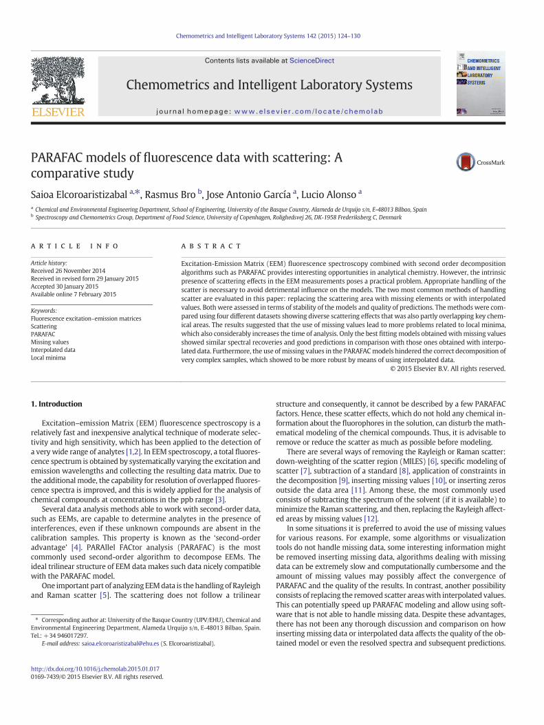
PARAFAC models of fluorescence data with scattering: Acomparative study

Saioa Elcoroaristizabal a,⁎, Rasmus Bro b, Jose Antonio García a, Lucio Alonso a

a Chemical and Environmental Engineering Department, School of Engineering, University of the Basque Country, Alameda de Urquijo s/n, E-48013 Bilbao, Spainb Spectroscopy and Chemometrics Group, Department of Food Science, University of Copenhagen, Rolighedsvej 26, DK-1958 Frederiksberg C, Denmark

a b s t r a c ta r t i c l e i n f o

Article history:Received 26 November 2014Received in revised form 29 January 2015Accepted 30 January 2015Available online 7 February 2015

Keywords:Fluorescence excitation–emission matricesScatteringPARAFACMissing valuesInterpolated dataLocal minima

Excitation-Emission Matrix (EEM) fluorescence spectroscopy combined with second order decompositionalgorithms such as PARAFAC provides interesting opportunities in analytical chemistry. However, the intrinsicpresence of scattering effects in the EEM measurements poses a practical problem. Appropriate handling of thescatter is necessary to avoid detrimental influence on the models. The two most common methods of handlingscatter are evaluated in this paper: replacing the scattering area with missing elements or with interpolatedvalues. Both were assessed in terms of stability of the models and quality of predictions. Themethodswere com-pared using four different datasets showing diverse scattering effects that was also partly overlapping key chem-ical areas. The results suggested that the use of missing values lead to more problems related to local minima,which also considerably increases the time of analysis. Only the best fitting models obtained withmissing valuesshowed similar spectral recoveries and good predictions in comparison with those ones obtained with interpo-lated data. Furthermore, the use of missing values in the PARAFACmodels hindered the correct decomposition ofvery complex samples, which showed to be more robust by means of using interpolated data.

© 2015 Elsevier B.V. All rights reserved.

1. Introduction

Excitation–emission Matrix (EEM) fluorescence spectroscopy is arelatively fast and inexpensive analytical technique of moderate selec-tivity and high sensitivity, which has been applied to the detection ofa very wide range of analytes [1,2]. In EEM spectroscopy, a total fluores-cence spectrum is obtained by systematically varying the excitation andemission wavelengths and collecting the resulting data matrix. Due tothe additional mode, the capability for resolution of overlapped fluores-cence spectra is improved, and this is widely applied for the analysis ofchemical compounds at concentrations in the ppb range [3].

Several data analysis methods able to work with second-order data,such as EEMs, are capable to determine analytes in the presence ofinterferences, even if these unknown compounds are absent in thecalibration samples. This property is known as the ‘second-orderadvantage’ [4]. PARAllel FACtor analysis (PARAFAC) is the mostcommonly used second-order algorithm to decompose EEMs. Theideal trilinear structure of EEM data makes such data nicely compatiblewith the PARAFAC model.

One important part of analyzing EEMdata is thehandling of Rayleighand Raman scatter [5]. The scattering does not follow a trilinear

structure and consequently, it cannot be described by a few PARAFACfactors. Hence, these scatter effects, which do not hold any chemical in-formation about the fluorophores in the solution, can disturb the math-ematical modeling of the chemical compounds. Thus, it is advisable toremove or reduce the scatter as much as possible before modeling.

There are several ways of removing the Rayleigh or Raman scatter:down-weighting of the scatter region (MILES) [6], specific modeling ofscatter [7], subtraction of a standard [8], application of constraints inthe decomposition [9], inserting missing values [10], or inserting zerosoutside the data area [11]. Among these, the most commonly usedconsists of subtracting the spectrum of the solvent (if it is available) tominimize the Raman scattering, and then, replacing the Rayleigh affect-ed areas by missing values [12].

In some situations it is preferred to avoid the use of missing valuesfor various reasons. For example, some algorithms or visualizationtools do not handle missing data, some interesting information mightbe removed inserting missing data, algorithms dealing with missingdata can be extremely slow and computationally cumbersome and theamount of missing values may possibly affect the convergence ofPARAFAC and the quality of the results. In contrast, another possibilityconsists of replacing the removed scatter areaswith interpolated values.This can potentially speed up PARAFAC modeling and allow using soft-ware that is not able to handle missing data. Despite these advantages,there has not been any thorough discussion and comparison on howinserting missing data or interpolated data affects the quality of the ob-tained model or even the resolved spectra and subsequent predictions.

Chemometrics and Intelligent Laboratory Systems 142 (2015) 124–130

⁎ Corresponding author at: University of the Basque Country (UPV/EHU), Chemical andEnvironmental Engineering Department, Alameda Urquijo s/n, E-48013 Bilbao, Spain.Tel.: +34 946017297.

E-mail address: [email protected] (S. Elcoroaristizabal).

http://dx.doi.org/10.1016/j.chemolab.2015.01.0170169-7439/© 2015 Elsevier B.V. All rights reserved.

Contents lists available at ScienceDirect

Chemometrics and Intelligent Laboratory Systems

j ourna l homepage: www.e lsev ie r .com/ locate /chemolab

http://crossmark.crossref.org/dialog/?doi=10.1016/j.chemolab.2015.01.017&domain=pdf

http://dx.doi.org/10.1016/j.chemolab.2015.01.017

mailto:[email protected]


http://www.sciencedirect.com/science/journal/01697439

www.elsevier.com/locate/chemolab

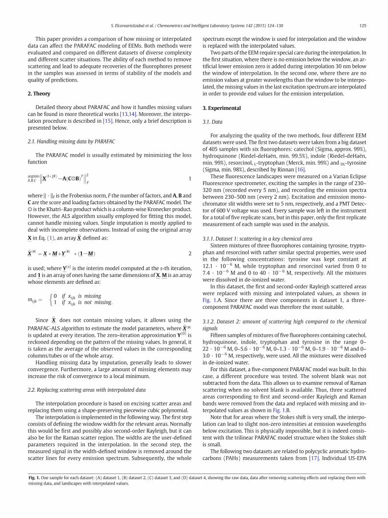
This paper provides a comparison of how missing or interpolateddata can affect the PARAFAC modeling of EEMs. Both methods wereevaluated and compared on different datasets of diverse complexityand different scatter situations. The ability of each method to removescattering and lead to adequate recoveries of the fluorophores presentin the samples was assessed in terms of stability of the models andquality of predictions.

2. Theory

Detailed theory about PARAFAC and how it handles missing valuescan be found in more theoretical works [13,14]. Moreover, the interpo-lation procedure is described in [15]. Hence, only a brief description ispresented below.

2.1. Handling missing data by PARAFAC

The PARAFAC model is usually estimated by minimizing the lossfunction

argminA;B;C X I� JKð Þ−A C⊙Bð ÞT

�� 2F

1

where ‖ · ‖F is the Frobenius norm, F the number of factors, and A, B andC are the score and loading factors obtained by the PARAFACmodel. The⊙ is the Khatri–Rao productwhich is a column-wise Kronecker product.However, the ALS algorithm usually employed for fitting this model,cannot handle missing values. Single imputation is mostly applied todeal with incomplete observations. Instead of using the original array

X in Eq. (1), an array eX defined as:

eX sð Þ ¼ X �MþY sð Þ � 1−Mð Þ 2

is used; where Y(s) is the interim model computed at the s-th iteration,and 1 is an array of ones having the same dimensions of X.M is an arraywhose elements are defined as:

mijk ¼0 if xi jk is missing1 if xi jk is not missing:

�

Since eX does not contain missing values, it allows using the

PARAFAC-ALS algorithm to estimate the model parameters, where eX sð Þ

is updated at every iteration. The zero-iteration approximation Y(0) isreckoned depending on the pattern of the missing values. In general, itis taken as the average of the observed values in the correspondingcolumns/tubes or of the whole array.

Handling missing data by imputation, generally leads to slowerconvergence. Furthermore, a large amount of missing elements mayincrease the risk of convergence to a local minimum.

2.2. Replacing scattering areas with interpolated data

The interpolation procedure is based on excising scatter areas andreplacing them using a shape-preserving piecewise cubic polynomial.

The interpolation is implemented in the followingway. Thefirst stepconsists of defining the window width for the relevant areas. Normallythis would be first and possibly also second-order Rayleigh, but it canalso be for the Raman scatter region. The widths are the user-definedparameters required in the interpolation. In the second step, themeasured signal in the width-defined window is removed around thescatter lines for every emission spectrum. Subsequently, the whole

spectrum except the window is used for interpolation and the windowis replaced with the interpolated values.

Two parts of the EEM require special care during the interpolation. Inthe first situation, where there is no emission below the window, an ar-tificial lower emission zero is added during interpolation 30 nm belowthe window of interpolation. In the second one, where there are noemission values at greater wavelengths than the window to be interpo-lated, themissing values in the last excitation spectrumare interpolatedin order to provide end values for the emission interpolation.

3. Experimental

3.1. Data

For analyzing the quality of the two methods, four different EEMdatasets were used. The first two datasets were taken from a big datasetof 405 samples with six fluorophores: catechol (Sigma, approx. 99%),hydroquinone (Riedel-deHaën, min. 99.5%), indole (Riedel-deHaën,min. 99%), resorcinol, L-tryptophan (Merck, min. 99%) and DL-tyrosine(Sigma, min. 98%), described by Rinnan [16].

These fluorescence landscapes were measured on a Varian EclipseFluorescence spectrometer, exciting the samples in the range of 230–320 nm (recorded every 5 nm), and recording the emission spectrabetween 230–500 nm (every 2 nm). Excitation and emission mono-chromator slit widths were set to 5 nm, respectively, and a PMT Detec-tor of 600 V voltage was used. Every sample was left in the instrumentfor a total of five replicate scans, but in this paper, only the first replicatemeasurement of each sample was used in the analysis.

3.1.1. Dataset 1: scattering in a key chemical areaSixteen mixtures of three fluorophores containing tyrosine, trypto-

phan and resorcinol with rather similar spectral properties, were usedin the following concentrations: tyrosine was kept constant at12.1 · 10−6 M, while tryptophan and resorcinol varied from 0 to7.4 · 10−6 M and 0 to 40 · 10−6 M, respectively. All the mixtureswere dissolved in de-ionized water.

In this dataset, the first and second-order Rayleigh scattered areaswere replaced with missing and interpolated values, as shown inFig. 1.A. Since there are three components in dataset 1, a three-component PARAFAC model was therefore the most suitable.

3.1.2. Dataset 2: amount of scattering high compared to the chemicalsignals

Fifteen samples of mixtures of five fluorophores containing catechol,hydroquinone, indole, tryptophan and tyrosine in the range 0–22 · 10−6 M, 0–5.6 · 10−6 M, 0–1.3 · 10−6 M, 0–1.9 · 10−6 M and 0–3.0 · 10−6 M, respectively, were used. All the mixtures were dissolvedin de-ionized water.

For this dataset, a five-component PARAFAC model was built. In thiscase, a different procedure was tested. The solvent blank was notsubtracted from the data. This allows us to examine removal of Ramanscattering when no solvent blank is available. Thus, three scatteredareas corresponding to first and second-order Rayleigh and Ramanbands were removed from the data and replaced with missing and in-terpolated values as shown in Fig. 1.B.

Note that for areas where the Stokes shift is very small, the interpo-lation can lead to slight non-zero intensities at emission wavelengthsbelow excitation. This is physically impossible, but it is indeed consis-tent with the trilinear PARAFAC model structure when the Stokes shiftis small.

The following two datasets are related to polycyclic aromatic hydro-carbons (PAHs) measurements taken from [17]. Individual US-EPA

Fig. 1. One sample for each dataset: (A) dataset 1, (B) dataset 2, (C) dataset 3, and (D) dataset 4, showing the raw data, data after removing scattering effects and replacing them withmissing data, and landscapes with interpolated values.

125S. Elcoroaristizabal et al. / Chemometrics and Intelligent Laboratory Systems 142 (2015) 124–130

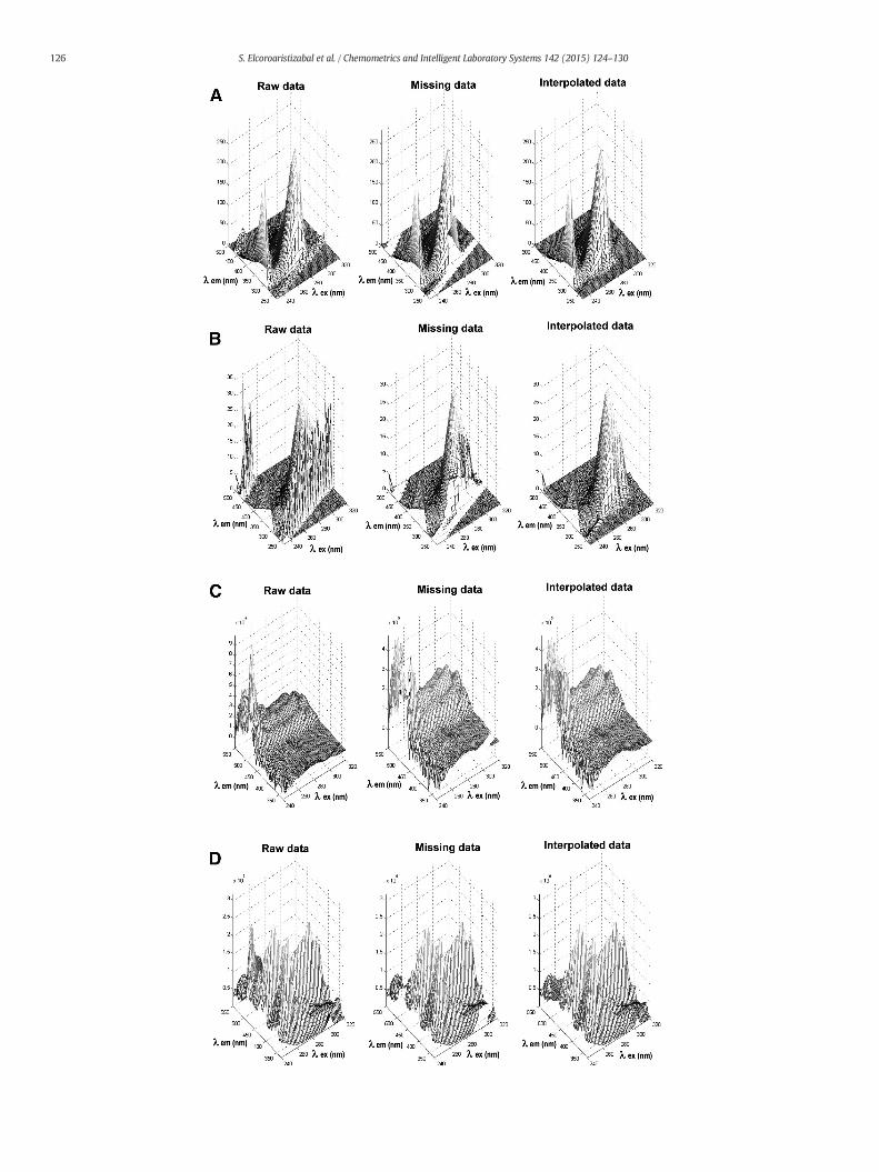
126 S. Elcoroaristizabal et al. / Chemometrics and Intelligent Laboratory Systems 142 (2015) 124–130

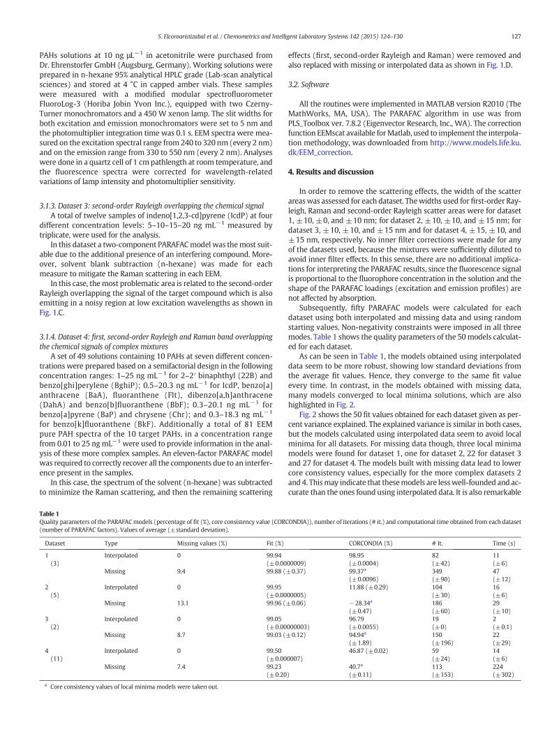
PAHs solutions at 10 ng μL−1 in acetonitrile were purchased fromDr. Ehrenstorfer GmbH (Augsburg, Germany). Working solutions wereprepared in n-hexane 95% analytical HPLC grade (Lab-scan analyticalsciences) and stored at 4 °C in capped amber vials. These sampleswere measured with a modified modular spectrofluorometerFluoroLog-3 (Horiba Jobin Yvon Inc.), equipped with two Czerny-Turner monochromators and a 450 W xenon lamp. The slit widths forboth excitation and emission monochromators were set to 5 nm andthe photomultiplier integration time was 0.1 s. EEM spectra were mea-sured on the excitation spectral range from 240 to 320 nm (every 2 nm)and on the emission range from 330 to 550 nm (every 2 nm). Analyseswere done in a quartz cell of 1 cm pathlength at room temperature, andthe fluorescence spectra were corrected for wavelength-relatedvariations of lamp intensity and photomultiplier sensitivity.

3.1.3. Dataset 3: second-order Rayleigh overlapping the chemical signalA total of twelve samples of indeno[1,2,3-cd]pyrene (IcdP) at four

different concentration levels: 5–10–15–20 ng mL−1 measured bytriplicate, were used for the analysis.

In this dataset a two-component PARAFACmodel was themost suit-able due to the additional presence of an interfering compound. More-over, solvent blank subtraction (n-hexane) was made for eachmeasure to mitigate the Raman scattering in each EEM.

In this case, themost problematic area is related to the second-orderRayleigh overlapping the signal of the target compound which is alsoemitting in a noisy region at low excitation wavelengths as shown inFig. 1.C.

3.1.4. Dataset 4: first, second-order Rayleigh and Raman band overlappingthe chemical signals of complex mixtures

A set of 49 solutions containing 10 PAHs at seven different concen-trations were prepared based on a semifactorial design in the followingconcentration ranges: 1–25 ng mL−1 for 2–2′ binaphthyl (22B) andbenzo[ghi]perylene (BghiP); 0.5–20.3 ng mL−1 for IcdP, benzo[a]anthracene (BaA), fluoranthene (Flt), dibenzo[a,h]anthracene(DahA) and benzo[b]fluoranthene (BbF); 0.3–20.1 ng mL−1 forbenzo[a]pyrene (BaP) and chrysene (Chr); and 0.3–18.3 ng mL−1

for benzo[k]fluoranthene (BkF). Additionally a total of 81 EEMpure PAH spectra of the 10 target PAHs, in a concentration rangefrom 0.01 to 25 ngmL−1 were used to provide information in the anal-ysis of these more complex samples. An eleven-factor PARAFAC modelwas required to correctly recover all the components due to an interfer-ence present in the samples.

In this case, the spectrum of the solvent (n-hexane) was subtractedto minimize the Raman scattering, and then the remaining scattering

effects (first, second-order Rayleigh and Raman) were removed andalso replaced with missing or interpolated data as shown in Fig. 1.D.

3.2. Software

All the routines were implemented in MATLAB version R2010 (TheMathWorks, MA, USA). The PARAFAC algorithm in use was fromPLS_Toolbox ver. 7.8.2 (Eigenvector Research, Inc., WA). The correctionfunction EEMscat available forMatlab, used to implement the interpola-tion methodology, was downloaded from http://www.models.life.ku.dk/EEM_correction.

4. Results and discussion

In order to remove the scattering effects, the width of the scatterareaswas assessed for each dataset. Thewidths used for first-order Ray-leigh, Raman and second-order Rayleigh scatter areas were for dataset1, ±10, ±0, and ±10 nm; for dataset 2, ±10, ±10, and ±15 nm; fordataset 3, ±10, ±10, and ±15 nm and for dataset 4, ±15, ±10, and±15 nm, respectively. No inner filter corrections were made for anyof the datasets used, because the mixtures were sufficiently diluted toavoid inner filter effects. In this sense, there are no additional implica-tions for interpreting the PARAFAC results, since the fluorescence signalis proportional to the fluorophore concentration in the solution and theshape of the PARAFAC loadings (excitation and emission profiles) arenot affected by absorption.

Subsequently, fifty PARAFAC models were calculated for eachdataset using both interpolated and missing data and using randomstarting values. Non-negativity constraints were imposed in all threemodes. Table 1 shows the quality parameters of the 50models calculat-ed for each dataset.

As can be seen in Table 1, the models obtained using interpolateddata seem to be more robust, showing low standard deviations fromthe average fit values. Hence, they converge to the same fit valueevery time. In contrast, in the models obtained with missing data,many models converged to local minima solutions, which are alsohighlighted in Fig. 2.

Fig. 2 shows the 50 fit values obtained for each dataset given as per-cent variance explained. The explained variance is similar in both cases,but the models calculated using interpolated data seem to avoid localminima for all datasets. For missing data though, three local minimamodels were found for dataset 1, one for dataset 2, 22 for dataset 3and 27 for dataset 4. The models built with missing data lead to lowercore consistency values, especially for the more complex datasets 2and 4. Thismay indicate that thesemodels are lesswell-founded and ac-curate than the ones found using interpolated data. It is also remarkable

Table 1Quality parameters of the PARAFACmodels (percentage of fit (%), core consistency value (CORCONDIA)), number of iterations (# it.) and computational time obtained from each dataset(number of PARAFAC factors). Values of average (±standard deviation).

Dataset Type Missing values (%) Fit (%) CORCONDIA (%) # It. Time (s)

1(3)

Interpolated 0 99.94(±0.0000009)

98.95(±0.0004)

82(±42)

11(±6)

Missing 9.4 99.88 (±0.37) 99.37a

(±0.0096)349(±90)

47(±12)

2(5)

Interpolated 0 99.95(±0.0000005)

11.88 (±0.29) 104(±30)

16(±6)

Missing 13.1 99.96 (±0.06) −28.34a

(±0.47)186(±60)

29(±10)

3(2)

Interpolated 0 99.05(±0.00000003)

96.79(±0.0055)

19(±0)

2(±0.1)

Missing 8.7 99.03 (±0.12) 94.94a

(±1.89)150(±196)

22(±29)

4(11)

Interpolated 0 99.50(±0.000007)

46.87 (±0.02) 59(±24)

14(±6)

Missing 7.4 99.23(±0.20)

40.7a

(±0.11)113(±153)

224(±302)

a Core consistency values of local minima models were taken out.


http://www.models.life.ku.dk/EEM_correction

http://www.models.life.ku.dk/EEM_correction

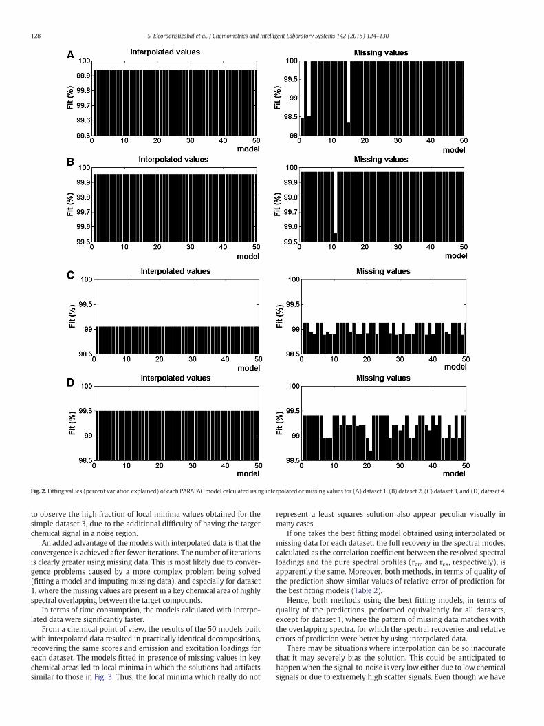
to observe the high fraction of local minima values obtained for thesimple dataset 3, due to the additional difficulty of having the targetchemical signal in a noise region.

An added advantage of themodels with interpolated data is that theconvergence is achieved after fewer iterations. The number of iterationsis clearly greater using missing data. This is most likely due to conver-gence problems caused by a more complex problem being solved(fitting a model and imputing missing data), and especially for dataset1, where themissing values are present in a key chemical area of highlyspectral overlapping between the target compounds.

In terms of time consumption, the models calculated with interpo-lated data were significantly faster.

From a chemical point of view, the results of the 50 models builtwith interpolated data resulted in practically identical decompositions,recovering the same scores and emission and excitation loadings foreach dataset. The models fitted in presence of missing values in keychemical areas led to local minima in which the solutions had artifactssimilar to those in Fig. 3. Thus, the local minima which really do not

represent a least squares solution also appear peculiar visually inmany cases.

If one takes the best fitting model obtained using interpolated ormissing data for each dataset, the full recovery in the spectral modes,calculated as the correlation coefficient between the resolved spectralloadings and the pure spectral profiles (rem and rex, respectively), isapparently the same. Moreover, both methods, in terms of quality ofthe prediction show similar values of relative error of prediction forthe best fitting models (Table 2).

Hence, both methods using the best fitting models, in terms ofquality of the predictions, performed equivalently for all datasets,except for dataset 1, where the pattern of missing data matches withthe overlapping spectra, for which the spectral recoveries and relativeerrors of prediction were better by using interpolated data.

There may be situations where interpolation can be so inaccuratethat it may severely bias the solution. This could be anticipated tohappenwhen the signal-to-noise is very low either due to low chemicalsignals or due to extremely high scatter signals. Even though we have

Fig. 2. Fitting values (percent variation explained) of each PARAFACmodel calculated using interpolated ormissing values for (A) dataset 1, (B) dataset 2, (C) dataset 3, and (D) dataset 4.


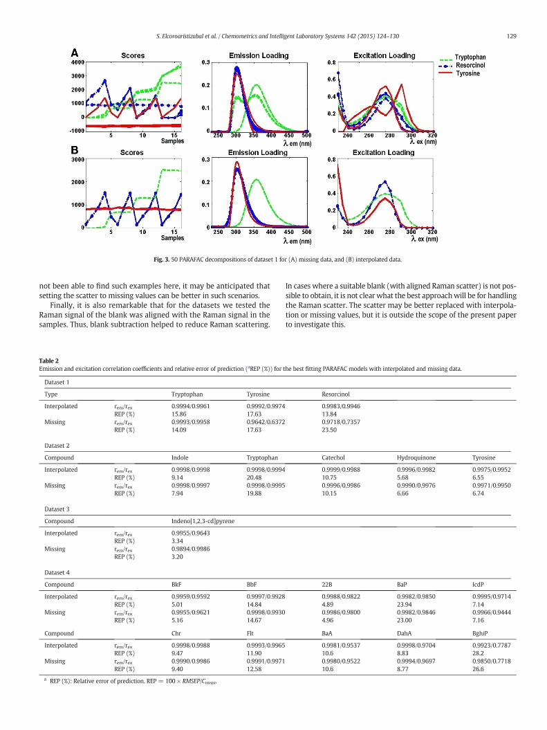
not been able to find such examples here, it may be anticipated thatsetting the scatter to missing values can be better in such scenarios.

Finally, it is also remarkable that for the datasets we tested theRaman signal of the blank was aligned with the Raman signal in thesamples. Thus, blank subtraction helped to reduce Raman scattering.

In cases where a suitable blank (with aligned Raman scatter) is not pos-sible to obtain, it is not clear what the best approachwill be for handlingthe Raman scatter. The scatter may be better replaced with interpola-tion or missing values, but it is outside the scope of the present paperto investigate this.

Table 2Emission and excitation correlation coefficients and relative error of prediction (aREP (%)) for the best fitting PARAFAC models with interpolated and missing data.

Dataset 1

Type Tryptophan Tyrosine Resorcinol

Interpolated rem/rex 0.9994/0.9961 0.9992/0.9974 0.9983/0.9946REP (%) 15.86 17.63 13.84

Missing rem/rex 0.9993/0.9958 0.9642/0.6372 0.9718/0.7357REP (%) 14.09 17.63 23.50

Dataset 2

Compound Indole Tryptophan Catechol Hydroquinone Tyrosine

Interpolated rem/rex 0.9998/0.9998 0.9998/0.9994 0.9999/0.9988 0.9996/0.9982 0.9975/0.9952REP (%) 9.14 20.48 10.75 5.68 6.55

Missing rem/rex 0.9998/0.9997 0.9998/0.9995 0.9996/0.9986 0.9990/0.9976 0.9971/0.9950REP (%) 7.94 19.88 10.15 6.66 6.74

Dataset 3

Compound Indeno[1,2,3-cd]pyrene

Interpolated rem/rex 0.9955/0.9643REP (%) 3.34

Missing rem/rex 0.9894/0.9986REP (%) 3.20

Dataset 4

Compound BkF BbF 22B BaP IcdP



Compound Chr Flt BaA DahA BghiP



a REP (%): Relative error of prediction. REP = 100 × RMSEP/Cmean.

Fig. 3. 50 PARAFAC decompositions of dataset 1 for (A) missing data, and (B) interpolated data.


5. Conclusions

Using interpolated values instead of missing values to removescattering areas helps PARAFAC to converge faster, and leads tosolutions that are physically and chemically meaningful.

Moreover, this approach is more advantageous because it preventsthe convergence to localminima, which is highly affected by themodelsbuilt using missing data.

Conflict of interest

All other authors declare that they have no conflicts of interest.

Acknowledgments

The authors gratefully thank the University of the Basque Country(UPV/EHU, UFI 11/47) and the Spanish Ministry of Science and Innova-tion (MICINN) for financing the projects PROMESHAP (CTM 2010-20607) and GRACCIE (CSD 2007-00067), co-financed with FEDERfounds. Saioa Elcoroaristizabal also wants to thank UPV/EHU for thedoctoral grant and the Spectroscopy and Chemometrics Group, Depart-ment of Food Science of the University of Copenhagen, for its supportduring her research stay.

Appendix A. Supplementary data

Supplementary data to this article can be found online at http://dx.doi.org/10.1016/j.chemolab.2015.01.017.

References

[1] R.D. JiJi, G.A. Cooper, K.S. Booksh, Excitation–emission matrix fluorescence baseddetermination of carbamate pesticides and polycyclic aromatic hydrocarbons,Anal. Chim. Acta 397 (1999) 61–72.

[2] C.A. Stedmon, S. Markager, R. Bro, Tracing dissolved organic matter in aquaticenvironments using a new approach to fluorescence spectroscopy, Mar. Chem. 82(2003) 239–254.

[3] A. Andrade-Eiroa, M. Canle, V. Cerdá, Environmental applications of excitation–emission spectrofluorimetry: an in-depth review II, Appl. Spectrosc. Rev. 48(2013) 77–141.

[4] J.A. Arancibia, C.E. Boschetti, A.C. Olivieri, G.M. Escandar, Screening of oil samples onthe basis of excitation–emission room-temperature phosphorescence data andmultiway chemometric techniques. Introducing the second-order advantage in aclassification study, Anal. Chem. 80 (2008) 2789–2798.

[5] J.R. Lakowicz, Principles of Fluorescence Spectroscopy, 3rd ed. SpringerScience + Business Media, New York, 2006.

[6] R. Bro, N.D. Sidiropoulos, A.K. Smilde, Maximum likelihood fitting using simple leastsquares algorithms, J. Chemom. 16 (2002) 387–400.

[7] Å. Rinnan, K. Booksh, R. Bro, First order Rayleigh as a separate component in the de-composition of fluorescence landscapes, Anal. Chim. Acta 537 (2005) 349–358.

[8] D.M. McKnight, E.W. Boyer, P.K. Westerhoff, P.T. Doran, T. Kulbe, D.T. Andersen,Spectrofluorometric characterization of dissolved organic matter for indication ofprecursor organic material and aromaticity, Limnol. Oceanogr. 46 (2001) 38–48.

[9] C.M. Andersen, R. Bro, Practical aspects of PARAFAC modeling of fluorescenceexcitation–emission data, J. Chemom. 17 (2003) 200–215.

[10] J. Christensen, V.T. Povlsen, J. Sørensen, Application of fluorescence spectroscopyand chemometrics in the evaluation of processed cheese during storage, J. DairySci. 86 (2003) 1101–1107.

[11] L.G. Thygesen, A. Rinnan, S. Barsberg, J.K.S. Møller, Stabilizing the PARAFAC decom-position of fluorescence spectra by insertion of zeros outside the data area,Chemom. Intell. Lab. Syst. 71 (2004) 97–106.

[12] L. Munck, L. Nørgaard, S.B. Engelsen, R. Bro, C.A. Andersson, Chemometrics in foodscience—a demonstration of the feasibility of a highly exploratory, inductive evalu-ation strategy of fundamental scientific significance, Chemom. Intell. Lab. Syst. 44(1998) 31–60.

[13] R. Bro, PARAFAC. Tutorial and applications, Chemom. Intell. Lab. Syst. 38 (1997)149–171.

[14] G. Tomasi, R. Bro, PARAFAC and missing values, Chemom. Intell. Lab. Syst. 75 (2005)163–180.

[15] M. Bahram, R. Bro, C.A. Stedmon, A. Afkhami, Handling of Rayleigh and Ramanscatter for PARAFAC modeling of fluorescence data using interpolation, J. Chemom.20 (2006) 99–105.

[16] Å. Rinnan, Application of PARAFAC on Spectral Data(Ph.D. thesis) Royal Veterinaryand Agricultural University, Denmark, 2004. (DK).

[17] S. Elcoroaristizabal, A. de Juan, J.A. García, N. Durana, L. Alonso, Comparison ofsecond-order multivariate methods for screening and determination of PAHs bytotal fluorescence spectroscopy, Chemom. Intell. Lab. Syst. 132 (2014) 63–74.




http://refhub.elsevier.com/S0169-7439(15)00028-3/rf0005














































PAPER 02

Comparison of second-order multivariate

methods for screening and determination of

PAHs by total fluorescence spectroscopy

Saioa Elcoroaristizabal, Anna de Juan, Jose Antonio García,

Nieves Durana, Lucio Alonso

Chemometrics and Intelligent Laboratory Systems 132 (2014) 63-74

Comparison of second-order multivariate methods for screening anddetermination of PAHs by total fluorescence spectroscopy

Saioa Elcoroaristizabal a,⁎, Anna de Juan b, Jose Antonio García a, Nieves Durana a, Lucio Alonso a

a Chemical and Environmental Engineering Department, School of Engineering, University of the Basque Country, Alameda de Urquijo s/n, E-48013 Bilbao, Spainb Chemometrics Group, Department of Analytical Chemistry, Universitat de Barcelona, Diagonal 645, E-08028 Barcelona, Spain

a b s t r a c ta r t i c l e i n f o

Article history:Received 14 November 2013Received in revised form 20 December 2013Accepted 6 January 2014Available online 16 January 2014

Keywords:Polycyclic aromatic hydrocarbonsFluorescence excitation–emission matricesPARAFACMCR–ALSU-PLS/RBL

Thiswork explores the feasibility of screening and determination of ten polycyclic aromatic hydrocarbons (PAHs)through excitation–emission fluorescence matrices (EEMs) and in the presence of interferences by usingdifferent second-order data analysis algorithms: parallel factor analysis (PARAFAC), multivariate curveresolution–alternating least squares (MCR–ALS), and unfolded partial least squares coupled to residualbilinearization (U-PLS/RBL).The scope of the proposed techniques is discussed for qualitative and quantitative analysis of the selected PAHs inthe presence of interferences and sample matrix effects. The target compounds were 9 of the 16 United StatesEnvironmental Protection Agency (US-EPA) priority PAHs: fluoranthene, benzo[a]anthracene, chrysene, benzo[b]fluoranthene, benzo[k]fluoranthene, benzo[a]pyrene, dibenzo[a,h]anthracene, benzo[ghi]perylene, indeno[1,2,3-cd]pyrene, and one internal standard: 2-2′ binaphthyl.The suitability of these methods was compared under different chemical situations, where they were demon-strated to be powerful tools to resolve complexmixtures of analytes of similar structure in the presence of unex-pected compounds. Qualitative and quantitative analysis of samples required the joint effort of the differentalgorithms to exploit the advantages of fast screening (PARAFAC andMCR–ALS) and accurate analyte determina-tion (U-PLS/RBL) provided by the different methods.

© 2014 Elsevier B.V. All rights reserved.

1. Introduction

Polycyclic aromatic hydrocarbons (PAHs) are complex organic com-pounds consisting of carbon and hydrogen atoms only, with two ormore fused aromatic rings. These compounds are primarily releasedduring incomplete combustion processes of organic material, being agroup of semi-volatile substances of high mobility among all environ-mental compartments [1–3].

PAHs are of environmental concern due to their persistence andproven toxic effects on human health and ecosystems; benzo[a]pyreneis classified as carcinogenic and other PAHs as potential carcinogenicagents [4]. Several international organisms have listed them as prioritypollutants. Thus, the US Environmental Protection Agency (EPA) regu-lates 16 unsubstituted PAHs (16 US-EPA PAHs) in wastewaters and 24in soils, sediments, hazardous wastes and groundwaters [5] and theWorld Health Organization (WHO) lists 31 parent PAHs plus two alkylderivatives [6]. Among the 16 most used in routine monitoring forregulatory purposes, only seven are considered as probable humancarcinogens [7]. Therefore, since the adverse effects depend on their

chemical structure, qualitative and quantitative speciation of PAHs isnecessary.

The standard procedures for PAH determination in complex envi-ronmental samples rely on chromatographic methods with specificdetectors (GC–MS,HPLC–UV/Vis orHPLC–FLD) [8]. Although the analyt-ical performance of these methods is widely accepted, PAH analysistends to be laborious, relatively expensive and time-consuming, sincethese substances require an intensive sample treatment, which makestheir use cumbersome for screening or routine analysis. For these rea-sons, the development of simpler and sensitive methods, or the im-provement of the existing ones is of great interest, for the detectionand determination of PAH compounds.

Fluorescence spectroscopy appears as an alternative, it allows de-tecting PAHs at sub-ppb levels, due to the luminescent properties ofthese compounds in the UV–Vis range, and provides a cheap and fastmeasurementmethod. Nevertheless, significant overlap between emis-sion and excitation bands of PAHs and other interfering compounds incomplex samples results in a lack of selectivity. Hence, fluorescencespectroscopy has been often limited to screening of environmentalexposures [9,10] or used in combination with separation techniques[11,12]. Recently, great developments in data acquisition systems,advanced chemometric tools [13–15], and related software [16–18] todeal with 2D fluorescence measurements havemade possible to identi-fy and quantify mixtures of compounds in fluorescent samples [19].

Chemometrics and Intelligent Laboratory Systems 132 (2014) 63–74

⁎ Corresponding author at: University of the Basque Country (UPV/EHU), Chemical andEnvironmental Engineering Department, Alameda Urquijo s/n, E-48013 Bilbao, Spain.Tel.:+34 946017297.

E-mail address: [email protected] (S. Elcoroaristizabal).

0169-7439/$ – see front matter © 2014 Elsevier B.V. All rights reserved.http://dx.doi.org/10.1016/j.chemolab.2014.01.005

Contents lists available at ScienceDirect

Chemometrics and Intelligent Laboratory Systems

j ourna l homepage: www.e lsev ie r .com/ locate /chemolab

http://crossmark.crossref.org/dialog/?doi=10.1016/j.chemolab.2014.01.005&domain=f


mailto:[email protected]


http://www.sciencedirect.com/science/journal/01697439

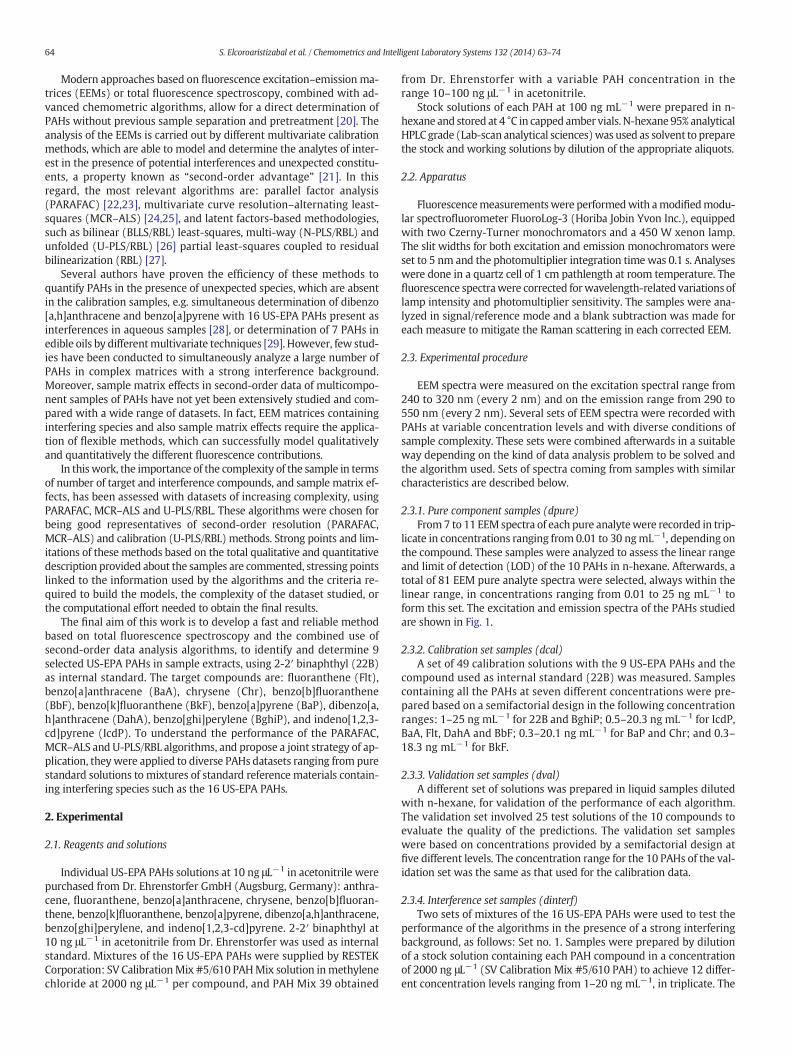
Modern approaches based on fluorescence excitation–emission ma-trices (EEMs) or total fluorescence spectroscopy, combined with ad-vanced chemometric algorithms, allow for a direct determination ofPAHs without previous sample separation and pretreatment [20]. Theanalysis of the EEMs is carried out by different multivariate calibrationmethods, which are able to model and determine the analytes of inter-est in the presence of potential interferences and unexpected constitu-ents, a property known as “second-order advantage” [21]. In thisregard, the most relevant algorithms are: parallel factor analysis(PARAFAC) [22,23], multivariate curve resolution–alternating least-squares (MCR–ALS) [24,25], and latent factors-based methodologies,such as bilinear (BLLS/RBL) least-squares, multi-way (N-PLS/RBL) andunfolded (U-PLS/RBL) [26] partial least-squares coupled to residualbilinearization (RBL) [27].

Several authors have proven the efficiency of these methods toquantify PAHs in the presence of unexpected species, which are absentin the calibration samples, e.g. simultaneous determination of dibenzo[a,h]anthracene and benzo[a]pyrene with 16 US-EPA PAHs present asinterferences in aqueous samples [28], or determination of 7 PAHs inedible oils by differentmultivariate techniques [29]. However, few stud-ies have been conducted to simultaneously analyze a large number ofPAHs in complex matrices with a strong interference background.Moreover, sample matrix effects in second-order data of multicompo-nent samples of PAHs have not yet been extensively studied and com-pared with a wide range of datasets. In fact, EEM matrices containinginterfering species and also sample matrix effects require the applica-tion of flexible methods, which can successfully model qualitativelyand quantitatively the different fluorescence contributions.

In thiswork, the importance of the complexity of the sample in termsof number of target and interference compounds, and sample matrix ef-fects, has been assessed with datasets of increasing complexity, usingPARAFAC, MCR–ALS and U-PLS/RBL. These algorithms were chosen forbeing good representatives of second-order resolution (PARAFAC,MCR–ALS) and calibration (U-PLS/RBL) methods. Strong points and lim-itations of these methods based on the total qualitative and quantitativedescription provided about the samples are commented, stressing pointslinked to the information used by the algorithms and the criteria re-quired to build the models, the complexity of the dataset studied, orthe computational effort needed to obtain the final results.

The final aim of this work is to develop a fast and reliable methodbased on total fluorescence spectroscopy and the combined use ofsecond-order data analysis algorithms, to identify and determine 9selected US-EPA PAHs in sample extracts, using 2-2′ binaphthyl (22B)as internal standard. The target compounds are: fluoranthene (Flt),benzo[a]anthracene (BaA), chrysene (Chr), benzo[b]fluoranthene(BbF), benzo[k]fluoranthene (BkF), benzo[a]pyrene (BaP), dibenzo[a,h]anthracene (DahA), benzo[ghi]perylene (BghiP), and indeno[1,2,3-cd]pyrene (IcdP). To understand the performance of the PARAFAC,MCR–ALS and U-PLS/RBL algorithms, and propose a joint strategy of ap-plication, theywere applied to diverse PAHs datasets ranging from purestandard solutions to mixtures of standard reference materials contain-ing interfering species such as the 16 US-EPA PAHs.

2. Experimental

2.1. Reagents and solutions

Individual US-EPA PAHs solutions at 10 ng μL−1 in acetonitrile werepurchased from Dr. Ehrenstorfer GmbH (Augsburg, Germany): anthra-cene, fluoranthene, benzo[a]anthracene, chrysene, benzo[b]fluoran-thene, benzo[k]fluoranthene, benzo[a]pyrene, dibenzo[a,h]anthracene,benzo[ghi]perylene, and indeno[1,2,3-cd]pyrene. 2-2′ binaphthyl at10 ng μL−1 in acetonitrile from Dr. Ehrenstorfer was used as internalstandard. Mixtures of the 16 US-EPA PAHs were supplied by RESTEKCorporation: SV CalibrationMix #5/610 PAHMix solution inmethylenechloride at 2000 ng μL−1 per compound, and PAH Mix 39 obtained

from Dr. Ehrenstorfer with a variable PAH concentration in therange 10–100 ng μL−1 in acetonitrile.

Stock solutions of each PAH at 100 ng mL−1 were prepared in n-hexane and stored at 4 °C in capped amber vials. N-hexane 95% analyticalHPLCgrade (Lab-scan analytical sciences)was used as solvent to preparethe stock and working solutions by dilution of the appropriate aliquots.

2.2. Apparatus

Fluorescencemeasurementswere performedwith amodifiedmodu-lar spectrofluorometer FluoroLog-3 (Horiba Jobin Yvon Inc.), equippedwith two Czerny-Turner monochromators and a 450 W xenon lamp.The slit widths for both excitation and emission monochromators wereset to 5 nm and the photomultiplier integration time was 0.1 s. Analyseswere done in a quartz cell of 1 cm pathlength at room temperature. Thefluorescence spectrawere corrected forwavelength-related variations oflamp intensity and photomultiplier sensitivity. The samples were ana-lyzed in signal/reference mode and a blank subtraction was made foreach measure to mitigate the Raman scattering in each corrected EEM.

2.3. Experimental procedure

EEM spectra were measured on the excitation spectral range from240 to 320 nm (every 2 nm) and on the emission range from 290 to550 nm (every 2 nm). Several sets of EEM spectra were recorded withPAHs at variable concentration levels and with diverse conditions ofsample complexity. These sets were combined afterwards in a suitableway depending on the kind of data analysis problem to be solved andthe algorithm used. Sets of spectra coming from samples with similarcharacteristics are described below.

2.3.1. Pure component samples (dpure)From7 to 11 EEM spectra of each pure analytewere recorded in trip-

licate in concentrations ranging from 0.01 to 30 ngmL−1, depending onthe compound. These samples were analyzed to assess the linear rangeand limit of detection (LOD) of the 10 PAHs in n-hexane. Afterwards, atotal of 81 EEM pure analyte spectra were selected, always within thelinear range, in concentrations ranging from 0.01 to 25 ng mL−1 toform this set. The excitation and emission spectra of the PAHs studiedare shown in Fig. 1.

2.3.2. Calibration set samples (dcal)A set of 49 calibration solutions with the 9 US-EPA PAHs and the

compound used as internal standard (22B) was measured. Samplescontaining all the PAHs at seven different concentrations were pre-pared based on a semifactorial design in the following concentrationranges: 1–25 ng mL−1 for 22B and BghiP; 0.5–20.3 ng mL−1 for IcdP,BaA, Flt, DahA and BbF; 0.3–20.1 ng mL−1 for BaP and Chr; and 0.3–18.3 ng mL−1 for BkF.

2.3.3. Validation set samples (dval)A different set of solutions was prepared in liquid samples diluted

with n-hexane, for validation of the performance of each algorithm.The validation set involved 25 test solutions of the 10 compounds toevaluate the quality of the predictions. The validation set sampleswere based on concentrations provided by a semifactorial design atfive different levels. The concentration range for the 10 PAHs of the val-idation set was the same as that used for the calibration data.

2.3.4. Interference set samples (dinterf)Two sets of mixtures of the 16 US-EPA PAHs were used to test the

performance of the algorithms in the presence of a strong interferingbackground, as follows: Set no. 1. Samples were prepared by dilutionof a stock solution containing each PAH compound in a concentrationof 2000 ng μL−1 (SV Calibration Mix #5/610 PAH) to achieve 12 differ-ent concentration levels ranging from 1–20 ng mL−1, in triplicate. The


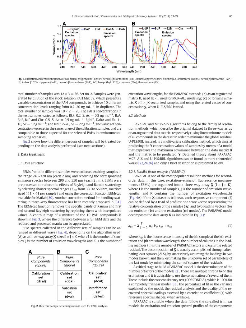
total number of samples was 12 × 3= 36. Set no. 2. Samples were gen-erated by dilution of the stock solution PAH Mix 39, which presents avariable concentration of the PAH compounds, to achieve 10 differentconcentration levels ranging from 0.2–20 ng mL−1, in duplicate. Thetotal number of samples was 10 × 2 = 20. The PAHs concentrations inthe test samples varied as follows: BkF: 0.2–2, Δc = 0.2 ng mL−1; BaA,BbF, BaP and Chr: 0.5–5, Δc = 0.5 ng mL−1; BghiP, DahA and Flt: 1–10,Δc=1ngmL−1; and IcdP: 2–20,Δc=2ngmL−1. The values of con-centrationwere set in the same range of the calibration samples, and arecomparable to those expected for the selected PAHs in environmentalsampling scenarios.

Fig. 2 shows how the different groups of samples will be treated de-pending on the data analysis performed (see next sections).

3. Data treatment

3.1. Data structure

EEMs from the different samples were collected exciting samples inthe range 240–320 nm (each 2 nm) and recording the correspondingemission spectra between 290 and 550 nm (each 2 nm). EEMs werepreprocessed to reduce the effects of Rayleigh and Raman scatteringsby selecting shorter spectral ranges (λem from 330 to 550 nm, matricessized 111 × 41 per sample) and using the correction function EEMscat,available for Matlab [30]. Another correction method for handling scat-tering in three-way fluorescence has been recently proposed in [31].The EEMscat function removes the specific bands of Raman and firstand second Rayleigh scattering by replacing them with interpolatedvalues. A contour map of a mixture of the 10 PAH compounds isshown in Fig. 3, where the difference between a full EEM data and thereduced and processed matrix can be appreciated.

EEM spectra collected in the different sets of samples can be ar-ranged in different ways (Fig. 4), depending on the algorithm used:(A) as a three-way arrayX, sized I × J × K, where I is the number of sam-ples, J is the number of emission wavelengths and K is the number of

excitation wavelengths, for the PARAFACmethod; (b) as an augmentedmatrixD, sized IK× J, used forMCR–ALSmodeling; (c) or forming ama-trix X of I × JK vectorized samples and using the related vector of con-centration y, when U-PLS/RBL is used.

3.2. Methods

PARAFAC and MCR–ALS algorithms belong to the family of resolu-tion methods, which describe the original dataset (a three-way arrayor an augmented datamatrix, respectively) using linearmixturemodelsof all compounds in the dataset in order tominimize the global residual.U-PLS/RBL, instead, is a multivariate calibration method, which aims atpredicting the Y concentration values of samples by means of a modelthat expresses the maximum covariance between the data matrix Xand the matrix to be predicted, Y. Detailed theory about PARAFAC,MCR–ALS and U-PLS/RBL algorithms can be found in more theoreticalworks [22,24,26] and only a brief description is presented below.

3.2.1. Parallel factor analysis (PARAFAC)PARAFAC is one of themost popular resolution methods for second-

order data. In this case, excitation–emission fluorescence measure-ments (EEMs) are organized into a three-way array X (I × J × K),where I is the number of samples, J is the number of emission wave-lengths, and K contains the number of excitation wavelengths(Fig. 4A). If the X dataset is trilinear, each responsive component (f)can be defined by a triad of profiles: one score vector representing therelative concentration of the samples (af) and two loading vectors (forthe emission (bf) and the excitation (cf) modes). The PARAFAC modeldecomposes the data array X as indicated in Eq. (1):

xijk ¼ Σ Ff ¼ 1 ai f b j f ck f þ ei jk ð1Þ

where xijk is the fluorescence intensity of the ith sample at the kth exci-tation and jth emissionwavelength, the number of columns in the load-ingmatrices (F) is the number of PARAFAC factors and eijk is the relatedresidual. The decomposition of X is usually accomplished through alter-nating least squares (ALS), by successively assuming the loadings in twomodes known and then, estimating the unknown set of parameters ofthe last mode by minimizing the sum of squares of the residuals.

A critical stage to build a PARAFACmodel is the determination of thenumber of factors of themodel [32]. There aremultiple criteria to do thisestimation and it is advisable to use the combination of several of them.These include the core consistency test (CORCONDIA), which is 100% fora completely trilinear model [33], the percentage of fit or the varianceexplained by the model, the residual analysis and the quality of the re-covered spectral loadings assessed by a correlation coefficient (r) withreference spectral shapes, when available.

PARAFAC is suitable when the data follow the so-called trilinearmodel: the excitation and emission spectral profiles of the components

Fig. 1. Excitation and emission spectra of (A) benzo[ghi]perylene (BghiP), benzo[k]fluoranthene (BkF), benzo[a]pyrene (BaP), dibenzo[a,h]anthracene (DahA), benzo[a]anthracene (BaA);(B) indeno[1,2,3-cd]pyrene (IcdP), benzo[b]fluoranthene (BbF), 2-2′ binaphthyl (22B), chrysene (Chr), fluoranthene (Flt).

Fig. 2. Different sample set configurations used for PAHs analysis.


image of Fig.�2

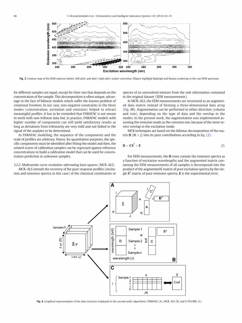
for different samples are equal, except for their size that depends on theconcentration of the sample. This decomposition is often unique, advan-tage in the face of bilinear models which suffer the known problem ofrotational freedom. In our case, non-negative constraints in the threemodes (concentration, excitation and emission) helped to extractmeaningful profiles. It has to be reminded that PARAFAC is not meantto work with non-trilinear data but, in practice, PARAFAC models withhigher number of components can still yield satisfactory results aslong as deviations from trilinearity are very mild and not linked to thesignal of the analytes to be determined.

In PARAFAC modeling, the sequence of the components and thescale of profiles are arbitrary. Hence, for quantitative purposes, the spe-cific componentsmust be identified after fitting themodel and then, therelated scores of calibration samples can be regressed against referenceconcentrations to build a calibrationmodel that can be used for concen-tration prediction in unknown samples.

3.2.2. Multivariate curve resolution–alternating least squares (MCR–ALS)MCR–ALS intends the recovery of the pure response profiles (excita-

tion and emission spectra in this case) of the chemical constituents or

species of an unresolved mixture from the sole information containedin the original dataset (EEM measurements).

In MCR–ALS, the EEMmeasurements are structured as an augment-ed data matrix instead of forming a three-dimensional data array(Fig. 4B). Augmentation can be performed in either direction (columnand row), depending on the type of data and the overlap in themodes. In the present work, the augmentation was implemented as-suming the emissionmode as the common one, because of themore se-vere overlap in the excitation mode.

MCR techniques are based on the bilinear decomposition of the ma-trix D (IK × J) into its pure contributions according to Eq. (2):

D ¼ CST þ E ð2Þ

For EEMmeasurements, the D rows contain the emission spectra asa function of excitation wavelengths and the augmented matrix con-taining the EEM measurements of all samples is decomposed into theproduct of the augmented Cmatrix of pure excitation spectra by the sin-gle ST matrix of pure emission spectra. E is the experimental error.

Fig. 3. Contour map of the EEMmatrices before (left plot) and after (right plot) scatter correction. Ellipses highlight Rayleigh and Raman scattering in the raw EEM spectrum.

Fig. 4. Graphical representation of the data structure employed in the second-order algorithms: PARAFAC (A), MCR–ALS (B) and U-PLS/RBL (C).


image of Fig.�3

image of Fig.�4

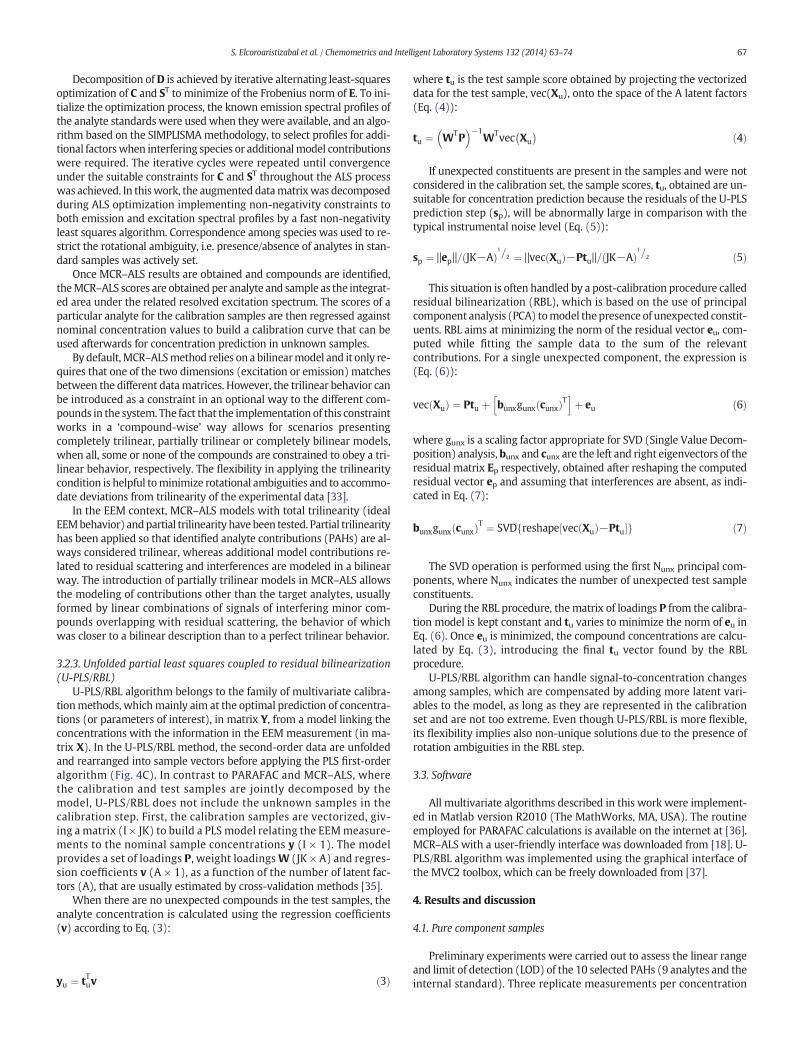
Decomposition ofD is achieved by iterative alternating least-squaresoptimization of C and ST to minimize of the Frobenius norm of E. To ini-tialize the optimization process, the known emission spectral profiles ofthe analyte standards were used when theywere available, and an algo-rithm based on the SIMPLISMAmethodology, to select profiles for addi-tional factorswhen interfering species or additionalmodel contributionswere required. The iterative cycles were repeated until convergenceunder the suitable constraints for C and ST throughout the ALS processwas achieved. In thiswork, the augmented datamatrixwas decomposedduring ALS optimization implementing non-negativity constraints toboth emission and excitation spectral profiles by a fast non-negativityleast squares algorithm. Correspondence among species was used to re-strict the rotational ambiguity, i.e. presence/absence of analytes in stan-dard samples was actively set.

Once MCR–ALS results are obtained and compounds are identified,theMCR–ALS scores are obtained per analyte and sample as the integrat-ed area under the related resolved excitation spectrum. The scores of aparticular analyte for the calibration samples are then regressed againstnominal concentration values to build a calibration curve that can beused afterwards for concentration prediction in unknown samples.

By default,MCR–ALSmethod relies on a bilinearmodel and it only re-quires that one of the two dimensions (excitation or emission) matchesbetween the different datamatrices. However, the trilinear behavior canbe introduced as a constraint in an optional way to the different com-pounds in the system. The fact that the implementation of this constraintworks in a ‘compound-wise’ way allows for scenarios presentingcompletely trilinear, partially trilinear or completely bilinear models,when all, some or none of the compounds are constrained to obey a tri-linear behavior, respectively. The flexibility in applying the trilinearitycondition is helpful tominimize rotational ambiguities and to accommo-date deviations from trilinearity of the experimental data [33].

In the EEM context, MCR–ALS models with total trilinearity (idealEEMbehavior) andpartial trilinearity have been tested. Partial trilinearityhas been applied so that identified analyte contributions (PAHs) are al-ways considered trilinear, whereas additional model contributions re-lated to residual scattering and interferences are modeled in a bilinearway. The introduction of partially trilinear models in MCR–ALS allowsthe modeling of contributions other than the target analytes, usuallyformed by linear combinations of signals of interfering minor com-pounds overlapping with residual scattering, the behavior of whichwas closer to a bilinear description than to a perfect trilinear behavior.

3.2.3. Unfolded partial least squares coupled to residual bilinearization(U-PLS/RBL)

U-PLS/RBL algorithm belongs to the family of multivariate calibra-tionmethods, whichmainly aim at the optimal prediction of concentra-tions (or parameters of interest), in matrix Y, from a model linking theconcentrations with the information in the EEM measurement (in ma-trix X). In the U-PLS/RBL method, the second-order data are unfoldedand rearranged into sample vectors before applying the PLS first-orderalgorithm (Fig. 4C). In contrast to PARAFAC and MCR–ALS, wherethe calibration and test samples are jointly decomposed by themodel, U-PLS/RBL does not include the unknown samples in thecalibration step. First, the calibration samples are vectorized, giv-ing a matrix (I × JK) to build a PLS model relating the EEMmeasure-ments to the nominal sample concentrations y (I × 1). The modelprovides a set of loadings P, weight loadingsW (JK × A) and regres-sion coefficients v (A × 1), as a function of the number of latent fac-tors (A), that are usually estimated by cross-validation methods [35].

When there are no unexpected compounds in the test samples, theanalyte concentration is calculated using the regression coefficients(v) according to Eq. (3):

yu ¼ tTuv ð3Þ

where tu is the test sample score obtained by projecting the vectorizeddata for the test sample, vec(Xu), onto the space of the A latent factors(Eq. (4)):

tu ¼ WTP� �−1

WTvec Xu� � ð4Þ

If unexpected constituents are present in the samples and were notconsidered in the calibration set, the sample scores, tu, obtained are un-suitable for concentration prediction because the residuals of the U-PLSprediction step (sp), will be abnormally large in comparison with thetypical instrumental noise level (Eq. (5)):

sp ¼ ‖ep‖= JK−Að Þ1=2 ¼ ‖vec Xuð Þ−Ptu‖= JK−Að Þ

1=2 ð5Þ

This situation is often handled by a post-calibration procedure calledresidual bilinearization (RBL), which is based on the use of principalcomponent analysis (PCA) tomodel thepresence of unexpected constit-uents. RBL aims at minimizing the norm of the residual vector eu, com-puted while fitting the sample data to the sum of the relevantcontributions. For a single unexpected component, the expression is(Eq. (6)):

vec Xuð Þ ¼ Ptu þ bunxgunx cunxð ÞTh i

þ eu ð6Þ

where gunx is a scaling factor appropriate for SVD (Single Value Decom-position) analysis,bunx and cunx are the left and right eigenvectors of theresidual matrix Ep respectively, obtained after reshaping the computedresidual vector ep and assuming that interferences are absent, as indi-cated in Eq. (7):

bunxgunx cunxð ÞT ¼ SVD reshape vec Xuð Þ−Ptu½ �f g ð7Þ

The SVD operation is performed using the first Nunx principal com-ponents, where Nunx indicates the number of unexpected test sampleconstituents.

During the RBL procedure, thematrix of loadings P from the calibra-tion model is kept constant and tu varies to minimize the norm of eu inEq. (6). Once eu is minimized, the compound concentrations are calcu-lated by Eq. (3), introducing the final tu vector found by the RBLprocedure.

U-PLS/RBL algorithm can handle signal-to-concentration changesamong samples, which are compensated by adding more latent vari-ables to the model, as long as they are represented in the calibrationset and are not too extreme. Even though U-PLS/RBL is more flexible,its flexibility implies also non-unique solutions due to the presence ofrotation ambiguities in the RBL step.

3.3. Software

All multivariate algorithms described in this work were implement-ed in Matlab version R2010 (The MathWorks, MA, USA). The routineemployed for PARAFAC calculations is available on the internet at [36].MCR–ALS with a user-friendly interface was downloaded from [18]. U-PLS/RBL algorithm was implemented using the graphical interface ofthe MVC2 toolbox, which can be freely downloaded from [37].

4. Results and discussion

4.1. Pure component samples

Preliminary experiments were carried out to assess the linear rangeand limit of detection (LOD) of the 10 selected PAHs (9 analytes and theinternal standard). Three replicate measurements per concentration


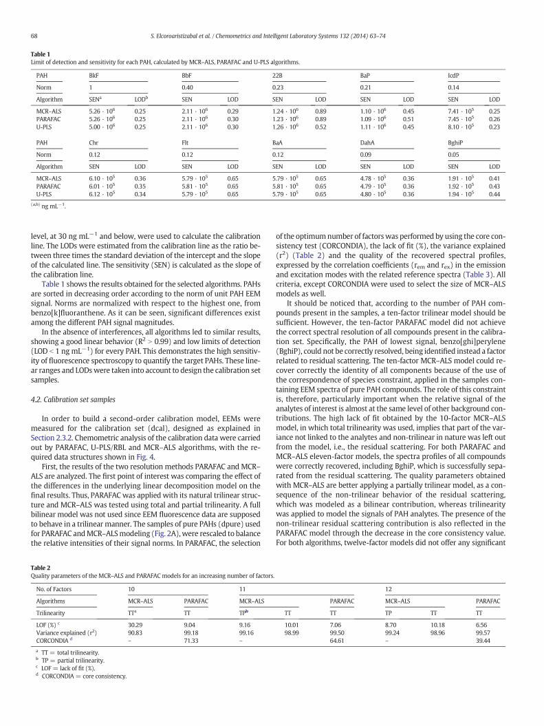
level, at 30 ng mL−1 and below, were used to calculate the calibrationline. The LODs were estimated from the calibration line as the ratio be-tween three times the standard deviation of the intercept and the slopeof the calculated line. The sensitivity (SEN) is calculated as the slope ofthe calibration line.

Table 1 shows the results obtained for the selected algorithms. PAHsare sorted in decreasing order according to the norm of unit PAH EEMsignal. Norms are normalized with respect to the highest one, frombenzo[k]fluoranthene. As it can be seen, significant differences existamong the different PAH signal magnitudes.

In the absence of interferences, all algorithms led to similar results,showing a good linear behavior (R2 N 0.99) and low limits of detection(LOD b 1 ng mL−1) for every PAH. This demonstrates the high sensitiv-ity of fluorescence spectroscopy to quantify the target PAHs. These line-ar ranges and LODswere taken into account to design the calibration setsamples.

4.2. Calibration set samples

In order to build a second-order calibration model, EEMs weremeasured for the calibration set (dcal), designed as explained inSection 2.3.2. Chemometric analysis of the calibration data were carriedout by PARAFAC, U-PLS/RBL and MCR–ALS algorithms, with the re-quired data structures shown in Fig. 4.

First, the results of the two resolution methods PARAFAC and MCR–ALS are analyzed. The first point of interest was comparing the effect ofthe differences in the underlying linear decomposition model on thefinal results. Thus, PARAFACwas applied with its natural trilinear struc-ture and MCR–ALS was tested using total and partial trilinearity. A fullbilinear model was not used since EEM fluorescence data are supposedto behave in a trilinear manner. The samples of pure PAHs (dpure) usedfor PARAFAC andMCR–ALSmodeling (Fig. 2A),were rescaled to balancethe relative intensities of their signal norms. In PARAFAC, the selection

of the optimumnumber of factorswas performed by using the core con-sistency test (CORCONDIA), the lack of fit (%), the variance explained(r2) (Table 2) and the quality of the recovered spectral profiles,expressed by the correlation coefficients (rem and rex) in the emissionand excitation modes with the related reference spectra (Table 3). Allcriteria, except CORCONDIA were used to select the size of MCR–ALSmodels as well.

It should be noticed that, according to the number of PAH com-pounds present in the samples, a ten-factor trilinear model should besufficient. However, the ten-factor PARAFAC model did not achievethe correct spectral resolution of all compounds present in the calibra-tion set. Specifically, the PAH of lowest signal, benzo[ghi]perylene(BghiP), could not be correctly resolved, being identified instead a factorrelated to residual scattering. The ten-factor MCR–ALS model could re-cover correctly the identity of all components because of the use ofthe correspondence of species constraint, applied in the samples con-taining EEM spectra of pure PAH compounds. The role of this constraintis, therefore, particularly important when the relative signal of theanalytes of interest is almost at the same level of other background con-tributions. The high lack of fit obtained by the 10-factor MCR–ALSmodel, in which total trilinearity was used, implies that part of the var-iance not linked to the analytes and non-trilinear in nature was left outfrom the model, i.e., the residual scattering. For both PARAFAC andMCR–ALS eleven-factor models, the spectra profiles of all compoundswere correctly recovered, including BghiP, which is successfully sepa-rated from the residual scattering. The quality parameters obtainedwith MCR–ALS are better applying a partially trilinear model, as a con-sequence of the non-trilinear behavior of the residual scattering,which was modeled as a bilinear contribution, whereas trilinearitywas applied to model the signals of PAH analytes. The presence of thenon-trilinear residual scattering contribution is also reflected in thePARAFAC model through the decrease in the core consistency value.For both algorithms, twelve-factor models did not offer any significant

Table 1Limit of detection and sensitivity for each PAH, calculated by MCR–ALS, PARAFAC and U-PLS algorithms.


Norm 1 0.40 0.23 0.21 0.14

Algorithm SENa LODb SEN LOD SEN LOD SEN LOD SEN LOD

MCR–ALS 5.26 · 106 0.25 2.11 · 106 0.29 1.24 · 106 0.89 1.10 · 106 0.45 7.41 · 105 0.25PARAFAC 5.26 · 106 0.25 2.11 · 106 0.30 1.23 · 106 0.89 1.09 · 106 0.51 7.45 · 105 0.26U-PLS 5.00 · 106 0.25 2.11 · 106 0.30 1.26 · 106 0.52 1.11 · 106 0.45 8.10 · 105 0.23


Norm 0.12 0.12 0.12 0.09 0.05

Algorithm SEN LOD SEN LOD SEN LOD SEN LOD SEN LOD

MCR–ALS 6.10 · 105 0.36 5.79 · 105 0.65 5.79 · 105 0.65 4.78 · 105 0.36 1.91 · 105 0.41PARAFAC 6.01 · 105 0.35 5.81 · 105 0.65 5.81 · 105 0.65 4.79 · 105 0.36 1.92 · 105 0.43U-PLS 6.12 · 105 0.34 5.79 · 105 0.65 5.79 · 105 0.65 4.80 · 105 0.36 1.94 · 105 0.44

(a,b) ng mL−1.

Table 2Quality parameters of the MCR–ALS and PARAFAC models for an increasing number of factors.

No. of Factors 10 11 12

Algorithms MCR–ALS PARAFAC MCR–ALS PARAFAC MCR–ALS PARAFAC

Trilinearity TTa TT TPb TT TT TP TT TT

LOF (%) c 30.29 9.04 9.16 10.01 7.06 8.70 10.18 6.56Variance explained (r2) 90.83 99.18 99.16 98.99 99.50 99.24 98.96 99.57CORCONDIA d – 71.33 – 64.61 – 39.44

a TT = total trilinearity.b TP = partial trilinearity.c LOF = lack of fit (%).d CORCONDIA = core consistency.


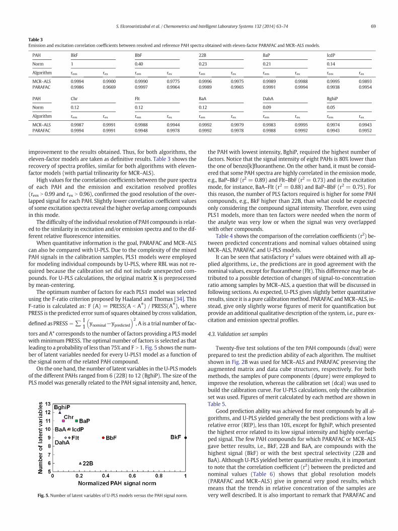
improvement to the results obtained. Thus, for both algorithms, theeleven-factor models are taken as definitive results. Table 3 shows therecovery of spectra profiles, similar for both algorithms with eleven-factor models (with partial trilinearity for MCR–ALS).

High values for the correlation coefficients between the pure spectraof each PAH and the emission and excitation resolved profiles(rem N 0.99 and rex N 0.96), confirmed the good resolution of the over-lapped signal for each PAH. Slightly lower correlation coefficient valuesof some excitation spectra reveal the higher overlap among compoundsin this mode.

The difficulty of the individual resolution of PAH compounds is relat-ed to the similarity in excitation and/or emission spectra and to the dif-ferent relative fluorescence intensities.

When quantitative information is the goal, PARAFAC and MCR–ALScan also be compared with U-PLS. Due to the complexity of the mixedPAH signals in the calibration samples, PLS1 models were employedfor modeling individual compounds by U-PLS, where RBL was not re-quired because the calibration set did not include unexpected com-pounds. For U-PLS calculations, the original matrix X is preprocessedby mean-centering.

The optimum number of factors for each PLS1 model was selectedusing the F-ratio criterion proposed by Haaland and Thomas [34]. ThisF-ratio is calculated as: F (A) = PRESS(A b A⁎) / PRESS(A⁎), wherePRESS is the predicted error sumof squares obtained by cross validation,

defined asPRESS ¼ ∑ I1 ynominal−ypredicted� �2

, A is a trial number of fac-

tors and A* corresponds to the number of factors providing a PLSmodelwith minimum PRESS. The optimal number of factors is selected as thatleading to a probability of less than 75% and F N 1. Fig. 5 shows the num-ber of latent variables needed for every U-PLS1 model as a function ofthe signal norm of the related PAH compound.

On the one hand, the number of latent variables in the U-PLSmodelsof the different PAHs ranged from 6 (22B) to 12 (BghiP). The size of thePLSmodel was generally related to the PAH signal intensity and, hence,

the PAH with lowest intensity, BghiP, required the highest number offactors. Notice that the signal intensity of eight PAHs is 80% lower thanthe one of benzo[k]fluoranthene. On the other hand, it must be consid-ered that some PAH spectra are highly correlated in the emissionmode,e.g., BaP–BkF (r2 = 0.89) and Flt–BbF (r2 = 0.73) and in the excitationmode, for instance, BaA–Flt (r2 = 0.88) and BaP–BbF (r2 = 0.75). Forthis reason, the number of PLS factors required is higher for some PAHcompounds, e.g., BkF higher than 22B, than what could be expectedonly considering the compound signal intensity. Therefore, even usingPLS1 models, more than ten factors were needed when the norm ofthe analyte was very low or when the signal was very overlappedwith other compounds.

Table 4 shows the comparison of the correlation coefficients (r2) be-tween predicted concentrations and nominal values obtained usingMCR–ALS, PARAFAC and U-PLS models.

It can be seen that satisfactory r2 values were obtained with all ap-plied algorithms, i.e., the predictions are in good agreement with thenominal values, except for fluoranthene (Flt). This differencemay be at-tributed to a possible detection of changes of signal-to-concentrationratio among samples by MCR–ALS, a question that will be discussed infollowing sections. As expected, U-PLS gives slightly better quantitativeresults, since it is a pure calibrationmethod. PARAFAC andMCR–ALS, in-stead, give only slightly worse figures of merit for quantification butprovide an additional qualitative description of the system, i.e., pure ex-citation and emission spectral profiles.

4.3. Validation set samples

Twenty-five test solutions of the ten PAH compounds (dval) wereprepared to test the prediction ability of each algorithm. The multisetshown in Fig. 2B was used for MCR–ALS and PARAFAC preserving theaugmented matrix and data cube structures, respectively. For bothmethods, the samples of pure components (dpure) were employed toimprove the resolution, whereas the calibration set (dcal) was used tobuild the calibration curve. For U-PLS calculations, only the calibrationset was used. Figures of merit calculated by each method are shown inTable 5.

Good prediction ability was achieved for most compounds by all al-gorithms, and U-PLS yielded generally the best predictions with a lowrelative error (REP), less than 10%, except for BghiP, which presentedthe highest error related to its low signal intensity and highly overlap-ped signal. The few PAH compounds for which PARAFAC or MCR–ALSgave better results, i.e., BkF, 22B and BaA, are compounds with thehighest signal (BkF) or with the best spectral selectivity (22B andBaA). Although U-PLS yielded better quantitative results, it is importantto note that the correlation coefficient (r2) between the predicted andnominal values (Table 6) shows that global resolution models(PARAFAC and MCR–ALS) give in general very good results, whichmeans that the trends in relative concentration of the samples arevery well described. It is also important to remark that PARAFAC and

Table 3Emission and excitation correlation coefficients between resolved and reference PAH spectra obtained with eleven-factor PARAFAC and MCR–ALS models.


Norm 1 0.40 0.23 0.21 0.14


MCR–ALS 0.9994 0.9900 0.9990 0.9775 0.9996 0.9975 0.9989 0.9988 0.9995 0.9893PARAFAC 0.9986 0.9669 0.9997 0.9964 0.9989 0.9965 0.9991 0.9994 0.9938 0.9954


Norm 0.12 0.12 0.12 0.09 0.05


MCR–ALS 0.9987 0.9991 0.9988 0.9944 0.9992 0.9979 0.9983 0.9995 0.9974 0.9943PARAFAC 0.9994 0.9991 0.9948 0.9978 0.9992 0.9978 0.9988 0.9992 0.9943 0.9952

Fig. 5. Number of latent variables of U-PLS models versus the PAH signal norm.


image of Fig.�5

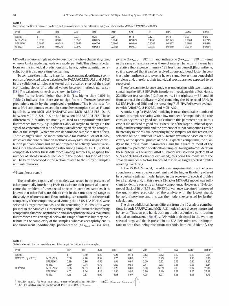
MCR–ALS require a singlemodel to describe thewhole chemical system,whereas U-PLSmodeling needs onemodel per PAH. This allows a betterfocus on the individual predictions and, hence, better quantitative re-sults, but it is also more time-consuming.

To compare the similarity in performance among algorithms, a com-parison of predicted values calculated by PARAFAC,MCR–ALS andU-PLSin the validation samples was tested using a paired t-test of the slope(comparing slopes of predicted values between methods pairwise)[38]. The calculated α levels are shown in Table 7.

Significance levels higher than 0.1% (i.e., higher than 0.001 inTable 7) indicate that there are no significant differences betweenpredictions made by the employed algorithms. This is the case formost PAH compounds, except for some few examples, such as Flt andBghiP between MCR–ALS/PARAFAC and MCR–ALS/U-PLS, DahAbetween MCR–ALS/U-PLS or BbF between PARAFAC/U-PLS. Thesedifferences in results are mostly related to compounds with lowfluorescence intensity, e.g., BghiP or DahA, or maybe to changes in thesignal-to-concentration ratio of some PAHs depending on the composi-tion of the sample (which we can denominate sample matrix effect).These changes could be more noticeable for PARAFAC or MCR–ALS,which are not pure calibration methods, always assume a single contri-bution per compound and are not prepared to actively correct varia-tions in signal-to-concentration ratio among samples. U-PLS, instead,compensates better these differences among samples by adapting thenumber of latent variables included in the model. This kind of effectwill be better described in the section related to the study of sampleswith interferences.

4.4. Interference study

The predictive capacity of the models was tested in the presence ofother potentially interfering PAHs to estimate their potential to over-come the problem of unexpected species in complex samples. It isknown that other PAHs are able to emit in the same spectral range asthe analytes of interest and, if not emitting, can contribute to the overallcomplexity of the sample analyzed. Among the 16 US-EPA PAHs, 9 wereselected as target compounds, and the remaining 7 US-EPA PAHs werepresent in the samples as interfering compounds. From the interferingcompounds,fluorene, naphthalene and acenaphthene have amaximumfluorescence emission signal below the range of interest, but they con-tribute to the complexity of the samples, whereas acenaphthylene isnot fluorescent. Additionally, phenanthrene (λexmax = 364 nm),

pyrene (λexmax = 382 nm) and anthracene (λexmax = 398 nm) emitin the same emission range as those of interest. In fact, anthracene hasa relative fluorescence intensity 13% less than benzo[k]fluoranthene,so it is expected that it can be resolved as one additional factor. In con-trast, phenanthrene and pyrene have a signal lower than benzo[ghi]perylene and, therefore, their individual spectra are not expected to berecovered.

Therefore, an interference study was undertaken with twomixturescontaining the 16US-EPA PAHs in order to investigate this effect. Hence,22 different test samples (12 from set no. 1 (in triplicate = 36) and 10from set no. 2 (in duplicate = 20)) containing the 10 selected PAHs (9US-EPA PAHs and 2BB) and the remaining 7 US-EPA PAHswere evaluat-ed with PARAFAC, U-PLS/RBL and MCR–ALS.

A crucial step for PARAFACmodeling is to set the suitable number offactors. In simple scenarios with a low number of compounds, the coreconsistency test is a good tool to estimate this parameter but, in thiscase, it did not lead to good results because of the large number of spec-trally similar compounds and the presence of minor compounds similarin intensity to the residual scattering in the samples. For that reason, theselection of the number of PARAFAC factors was made based on the re-covery of the spectral profiles of the 10 expected compounds, the qual-ity of the fitting model parameters, and the figures of merit of thequantitative prediction of calibration samples. Taking into considerationthese criteria, a 13-factor PARAFAC model was selected (lack of fit of5.6% and 99.68% of variance explained), this being the model with thesmallest number of factors that could resolve all target spectral profilesavoiding overfitting.

In the MCR–ALS model, the additional implementation of the corre-spondence among species constraint and the higher flexibility offeredby a partially trilinear model helped in the recovery of spectral profilesfor all analytes and, in this case, a 12-factor MCR–ALS model was suffi-cient to identify correctly all target components. However, a 13-factormodel (lack of fit of 8.1% and 99.33% of variance explained) improvedthe quantitative prediction of the analyte with the lowest signal,benzo[ghi]perylene, and this was the model size selected for furthercalculations.

The three additional factors different from the 10 analyte contribu-tions in both PARAFAC and MCR–ALS models have diverse nature andbehavior. Thus, on one hand, both methods recognize a contributionrelated to anthracene (Fig. 6), a PAH with high signal in the workingspectral range and that is present in the EPA-PAHmixtures. It is impor-tant to note that, being resolution methods, both could identify the

Table 4Correlation coefficient between predicted and nominal values in the calibration set (dcal) obtained by MCR–ALS, PARAFC and U-PLS.


Norm 1 0.40 0.23 0.21 0.14 0.12 0.12 0.12 0.09 0.05MCR–ALS 0.9778 0.9161 0.9965 0.8875 0.9849 0.9879 0.4666 0.9923 0.9861 0.7215PARAFAC 0.9935 0.9918 0.9959 0.9076 0.9907 0.9816 0.9745 0.9867 0.9844 0.8488U-PLS 0.9988 0.9976 0.9972 0.9984 0.9986 0.9993 0.9980 0.9980 0.9947 0.9964

Table 5Statistical results for the quantification of the target PAHs in validation samples.


Norm 1 0.40 0.23 0.21 0.14 0.12 0.12 0.12 0.09 0.05RMSEPa (ng mL−1) MCR–ALS 0.66 2.46 0.52 1.75 0.88 0.61 8.49 0.59 1.10 8.86

PARAFAC 0.39 0.86 0.56 1.91 0.99 0.60 0.92 0.92 0.80 3.25U-PLS 0.40 0.74 0.76 0.67 0.51 0.41 0.53 0.88 0.65 2.34

REPb (%) MCR–ALS 6.86 24.63 4.13 18.20 8.81 6.38 84.89 5.93 10.97 70.88PARAFAC 4.02 8.64 5.19 19.86 9.92 6.26 9.19 9.22 8.05 25.98U-PLS 4.18 7.37 6.07 6.98 5.07 4.25 5.27 8.81 6.46 18.73

a RMSEP (ng mL−1): Root mean square error of prediction. RMSEP ¼ 1=Ið Þ∑ I1 Cnominal−Cpredicted� �2#1=2

:

24

b REP (%): Relative error of prediction. REP = 100 × RMSEP / C mean.


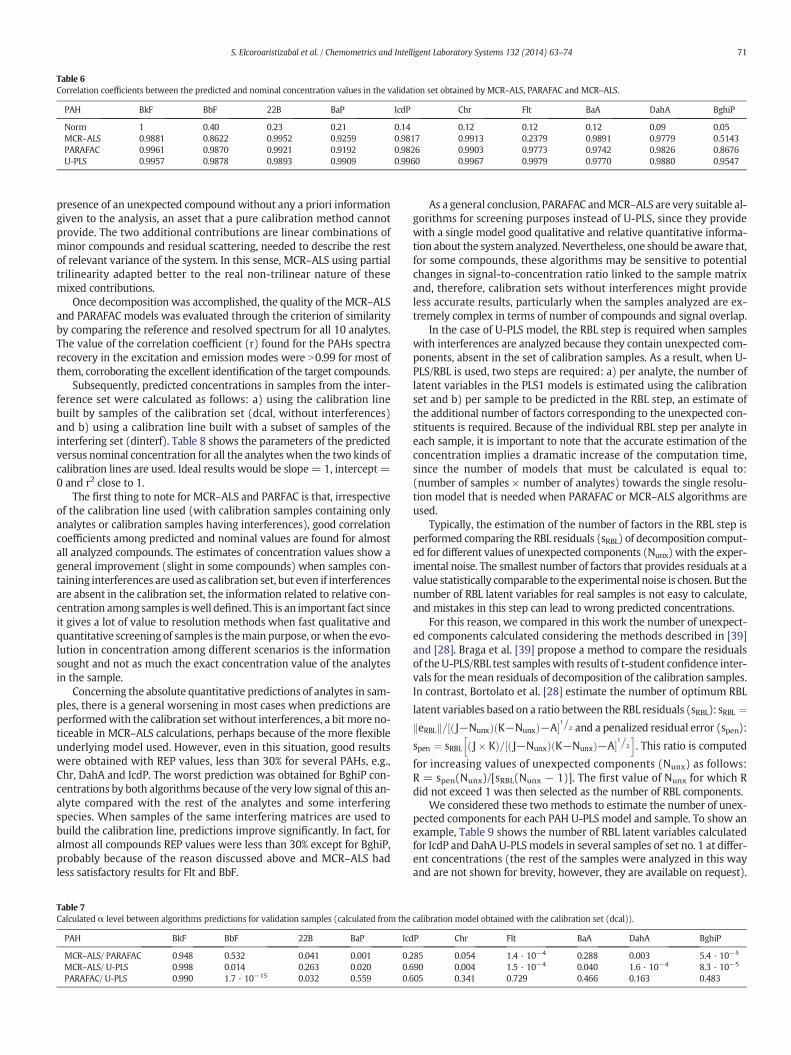
presence of an unexpected compound without any a priori informationgiven to the analysis, an asset that a pure calibration method cannotprovide. The two additional contributions are linear combinations ofminor compounds and residual scattering, needed to describe the restof relevant variance of the system. In this sense, MCR–ALS using partialtrilinearity adapted better to the real non-trilinear nature of thesemixed contributions.

Once decomposition was accomplished, the quality of the MCR–ALSand PARAFAC models was evaluated through the criterion of similarityby comparing the reference and resolved spectrum for all 10 analytes.The value of the correlation coefficient (r) found for the PAHs spectrarecovery in the excitation and emission modes were N0.99 for most ofthem, corroborating the excellent identification of the target compounds.

Subsequently, predicted concentrations in samples from the inter-ference set were calculated as follows: a) using the calibration linebuilt by samples of the calibration set (dcal, without interferences)and b) using a calibration line built with a subset of samples of theinterfering set (dinterf). Table 8 shows the parameters of the predictedversus nominal concentration for all the analytes when the two kinds ofcalibration lines are used. Ideal results would be slope= 1, intercept=0 and r2 close to 1.

The first thing to note for MCR–ALS and PARFAC is that, irrespectiveof the calibration line used (with calibration samples containing onlyanalytes or calibration samples having interferences), good correlationcoefficients among predicted and nominal values are found for almostall analyzed compounds. The estimates of concentration values show ageneral improvement (slight in some compounds) when samples con-taining interferences are used as calibration set, but even if interferencesare absent in the calibration set, the information related to relative con-centration among samples iswell defined. This is an important fact sinceit gives a lot of value to resolution methods when fast qualitative andquantitative screening of samples is themain purpose, orwhen the evo-lution in concentration among different scenarios is the informationsought and not as much the exact concentration value of the analytesin the sample.

Concerning the absolute quantitative predictions of analytes in sam-ples, there is a general worsening in most cases when predictions areperformedwith the calibration setwithout interferences, a bit more no-ticeable in MCR–ALS calculations, perhaps because of the more flexibleunderlying model used. However, even in this situation, good resultswere obtained with REP values, less than 30% for several PAHs, e.g.,Chr, DahA and IcdP. The worst prediction was obtained for BghiP con-centrations by both algorithms because of the very low signal of this an-alyte compared with the rest of the analytes and some interferingspecies. When samples of the same interfering matrices are used tobuild the calibration line, predictions improve significantly. In fact, foralmost all compounds REP values were less than 30% except for BghiP,probably because of the reason discussed above and MCR–ALS hadless satisfactory results for Flt and BbF.

As a general conclusion, PARAFAC andMCR–ALS are very suitable al-gorithms for screening purposes instead of U-PLS, since they providewith a single model good qualitative and relative quantitative informa-tion about the system analyzed. Nevertheless, one should be aware that,for some compounds, these algorithms may be sensitive to potentialchanges in signal-to-concentration ratio linked to the sample matrixand, therefore, calibration sets without interferences might provideless accurate results, particularly when the samples analyzed are ex-tremely complex in terms of number of compounds and signal overlap.

In the case of U-PLS model, the RBL step is required when sampleswith interferences are analyzed because they contain unexpected com-ponents, absent in the set of calibration samples. As a result, when U-PLS/RBL is used, two steps are required: a) per analyte, the number oflatent variables in the PLS1 models is estimated using the calibrationset and b) per sample to be predicted in the RBL step, an estimate ofthe additional number of factors corresponding to the unexpected con-stituents is required. Because of the individual RBL step per analyte ineach sample, it is important to note that the accurate estimation of theconcentration implies a dramatic increase of the computation time,since the number of models that must be calculated is equal to:(number of samples × number of analytes) towards the single resolu-tion model that is needed when PARAFAC or MCR–ALS algorithms areused.

Typically, the estimation of the number of factors in the RBL step isperformed comparing the RBL residuals (sRBL) of decomposition comput-ed for different values of unexpected components (Nunx) with the exper-imental noise. The smallest number of factors that provides residuals at avalue statistically comparable to the experimental noise is chosen. But thenumber of RBL latent variables for real samples is not easy to calculate,and mistakes in this step can lead to wrong predicted concentrations.

For this reason, we compared in this work the number of unexpect-ed components calculated considering the methods described in [39]and [28]. Braga et al. [39] propose a method to compare the residualsof the U-PLS/RBL test sampleswith results of t-student confidence inter-vals for themean residuals of decomposition of the calibration samples.In contrast, Bortolato et al. [28] estimate the number of optimum RBL

latent variables based on a ratio between the RBL residuals (sRBL): sRBL ¼eRBLk k= J−Nunxð Þ K−Nunxð Þ−A½ �1=2 and a penalized residual error (spen):

spen ¼ sRBL J� Kð Þ= J−Nunxð Þ K−Nunxð Þ−A½ �1=2

h i. This ratio is computed

for increasing values of unexpected components (Nunx) as follows:R = spen(Nunx)/[sRBL(Nunx − 1)]. The first value of Nunx for which Rdid not exceed 1 was then selected as the number of RBL components.

We considered these twomethods to estimate the number of unex-pected components for each PAH U-PLS model and sample. To show anexample, Table 9 shows the number of RBL latent variables calculatedfor IcdP and DahA U-PLSmodels in several samples of set no. 1 at differ-ent concentrations (the rest of the samples were analyzed in this wayand are not shown for brevity, however, they are available on request).

Table 6Correlation coefficients between the predicted and nominal concentration values in the validation set obtained by MCR–ALS, PARAFAC and MCR–ALS.


Norm 1 0.40 0.23 0.21 0.14 0.12 0.12 0.12 0.09 0.05MCR–ALS 0.9881 0.8622 0.9952 0.9259 0.9817 0.9913 0.2379 0.9891 0.9779 0.5143PARAFAC 0.9961 0.9870 0.9921 0.9192 0.9826 0.9903 0.9773 0.9742 0.9826 0.8676U-PLS 0.9957 0.9878 0.9893 0.9909 0.9960 0.9967 0.9979 0.9770 0.9880 0.9547

Table 7Calculated α level between algorithms predictions for validation samples (calculated from the calibration model obtained with the calibration set (dcal)).


MCR–ALS/ PARAFAC 0.948 0.532 0.041 0.001 0.285 0.054 1.4 · 10−4 0.288 0.003 5.4 · 10−5

MCR–ALS/ U-PLS 0.998 0.014 0.263 0.020 0.690 0.004 1.5 · 10−4 0.040 1.6 · 10−4 8.3 · 10−5

PARAFAC/ U-PLS 0.990 1.7 · 10−15 0.032 0.559 0.605 0.341 0.729 0.466 0.163 0.483


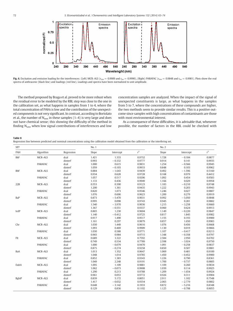
Themethod proposed by Braga et al. proved to bemore robustwhenthe residual error to be modeled by the RBL step was close to the one inthe calibration set, as what happens in samples from 1 to 4, where thetotal concentration of PAHs is low and the contribution of the unexpect-ed components is not very significant. In contrast, according to Bortolatoet al., the number of Nunx in these samples (1–4) is very large and doesnot have chemical sense; this showing the difficulty of the method infinding Nunx when low signal contributions of interferences and low

concentration samples are analyzed. When the impact of the signal ofunexpected constituents is large, as what happens in the samplesfrom 5 to 7, where the concentrations of these compounds are higher,the two methods seem to provide similar results. This is a positive out-come since sampleswith high concentrations of contaminants are thosewith most environmental interest.

As a consequence of these difficulties, it is advisable that, wheneverpossible, the number of factors in the RBL could be checked with

Fig. 6. Excitation and emission loading for the interferences: (Left) MCR–ALS (rem = 0.9909 and rex = 0.9990), (Right) PARAFAC (rem = 0.9848 and rex = 0.9981). Plots show the realspectra of anthracene (black line) and loadings (red line). Loadings and spectra have been normalized to unit amplitude.

Table 8Regression line between predicted and nominal concentrations using the calibration model obtained from the calibration or the interfering set.

SET No. 1 No. 2

PAH Algorithm Regression Slope Intercept r2 Slope Intercept r2

BkF MCR–ALS dcal 1.421 1.333 0.9752 1.728 −0.184 0.9877dinterf 0.993 −0.332 0.9777 0.914 0.141 0.9935

PARAFAC dcal 1.000 0.615 0.9831 1.254 −0.566 0.9945dinterf 1.059 −0.103 0.9933 0.848 0.103 0.9962

BbF MCR–ALS dcal 0.884 −1.643 0.9439 0.492 −1.596 0.5160dinterf 0.934 0.628 0.9728 0.168 0.979 0.4412

PARAFAC dcal 1.057 0.517 0.9206 1.092 0.454 0.9583dinterf 1.133 0.436 0.9949 1.166 0.029 0.9958

22B MCR–ALS dcal 0.553 0.390 0.9123 1.183 −0.210 0.9748dinterf 1.200 1.361 0.9435 1.222 0.203 0.9943


BaP MCR–ALS dcal 0.873 −5.470 0.9031 0.992 −5.050 0.9848dinterf 0.995 0.098 0.9743 0.945 0.281 0.9882

PARAFAC dcal 1.540 −3.970 0.9036 1.215 −3.258 0.9660dinterf 1.367 −0.551 0.9337 0.960 0.624 0.9913

IcdP MCR–ALS dcal 0.865 1.230 0.9604 1.149 −0.220 0.9847dinterf 1.140 −0.412 0.9725 0.817 1.845 0.9982


Chr MCR–ALS dcal 1.030 1.449 0.9616 1.076 0.456 0.9668dinterf 1.093 0.469 0.9909 1.130 0.019 0.9866

PARAFAC dcal 1.030 0.588 0.9771 1.107 −0.417 0.9213dinterf 0.965 0.984 0.9715 1.348 −0.358 0.9797

Flt MCR–ALS dcal 0.689 3.322 0.7592 2.584 2.950 0.6702dinterf 0.749 0.534 0.7789 2.598 −3.924 0.9750

PARAFAC dcal 1.000 −0.079 0.9470 1.091 −0.258 0.9837dinterf 0.875 −0.274 0.9258 0.850 0.507 0.9881

BaA MCR–ALS dcal 1.013 1.352 0.9647 1.069 0.481 0.9100dinterf 1.048 1.014 0.9785 1.450 −0.452 0.9900

PARAFAC dcal 0.852 1.383 0.9343 1.226 0.790 0.8361dinterf 1.049 2.248 0.9191 1.700 −0.737 0.9805

DahA MCR–ALS dcal 1.095 1.109 0.9881 1.109 0.260 0.9834dinterf 1.062 −0.073 0.9908 1.039 0.114 0.9925

PARAFAC dcal 1.290 0.213 0.9788 1.209 −1.654 0.9924dinterf 0.961 0.053 0.9772 0.926 0.311 0.9904

BghiP MCR–ALS dcal 0.839 5.172 0.8051 2.911 1.102 0.7548dinterf 1.417 −0.032 0.9354 2.065 −2.779 0.9802

PARAFAC dcal 0.648 −3.142 0.1933 0.872 −5.216 0.8348dinterf 0.129 0.836 0.1102 1.125 −0.798 0.9055


image of Fig.�6

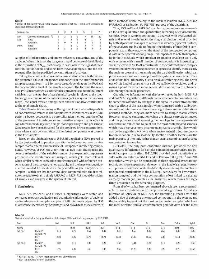
samples of similar nature and known reference concentrations of theanalytes.When this is not the case, one should be aware of the difficultyin the estimation of Nunx, particularly in cases where the signal of thesecontributions is not big or distinct from the analyte signals, and the con-sequent effect in the predicted concentrations of analytes.

Taking the comments above into consideration about both criteria,the estimated value of unexpected components in the interference setsamples ranged from 1 to 6 for most cases, depending on the PAH andthe concentration level of the sample analyzed. The fact that the sevennew PAHs incorporated as interferences provided less additional latentvariables than the number of real chemical species is related to the spec-tral range of emission of the interferences (not always in the workingrange), the signal overlap among them and their relative contributionto the total sample signal.

Table 10 collects a summary of thefigures ofmerit related to predict-ed concentration values in the samples with interferences. U-PLS/RBLperforms better because it is a pure calibration method, and the effectof the presence of interferences and possible sample matrix effect isconsidered individually with a singlemodel per analyte and per sample.Good results have been obtained for the predicted PAHs concentrations,even when a high concentration of interfering compounds was presentin the test samples.

Based on the obtained results, U-PLS/RBL applied to EEMs proved tobe the best method to provide quantitative information, overcomingsample matrix effects and presence of unexpected interfering compo-nents. However, U-PLS/RBL algorithm has two main drawbacks: thecorrect estimation of the suitable number of unexpected componentspresent in the interference set samples, which gets more relevantwhen similar samples containing interferences and with reference con-centrations of the analytes are not available, and the huge computation-al effort needed to calculate as many models as (nr. analytes × nr.samples), which can last for several days compared with the few mi-nutes needed to obtain a single PARAFAC orMCR–ALSmodel describingall samples and analytes in the system of interest.

5. Conclusions

MCR–ALS, PARAFAC and U-PLS/RBL algorithms were tested andcompared to obtain qualitative and quantitative information of analytesand interferences in complex samples of PAHmixtures analyzed by EEMfluorescence spectroscopy. Advantages and drawbacks associated with

these methods relate mainly to the main resolution (MCR–ALS andPARAFAC) or calibration (U-PLS/RBL) purpose of the algorithms.

Thus, MCR–ALS and PARAFAC are clearly the methods recommend-ed for a fast qualitative and quantitative screening of environmentalsamples. Even in samples containing 10 analytes with overlapped sig-nals and several interferences, the single resolution model providedby both algorithms manages to recover the identity (spectral profiles)of the analytes and is able to find out the identity of interfering com-pounds, e.g., anthracene, when the signal of the unexpected compoundis within the spectral working range. It is important to note this capabil-ity for both methods, which are often assumed to be able to work onlywith systems with a small number of compounds. It is interesting tostress the effect ofMCR–ALS constraints in the context of these complexsystems, notably the correspondence of species to identify more clearlythe analytes present in the sample and the partial trilinearity, which canprovide a more accurate description of the system behavior when devi-ations from ideal trilinearity due to residual scattering exist. The activeuse of this kind of constraints is still not sufficiently exploited and re-mains a point for which more general diffusion within the chemicalcommunity should be performed.

Quantitative information can also be extracted by both MCR–ALSand PARAFAC algorithms, although predicted concentration values canbe sometimes affected by changes in the signal-to-concentration ratio(matrix effect) of the real samples when compared with a calibrationset without interferences. Since these algorithms are not calibration-oriented methods, they are more sensitive to sample matrix effects.However, relative concentration values are always correctly estimatedand this provides a good screening methodology to have approximateconcentration values and to point out the most contaminated samples,which may deserve a more accurate quantitative analysis. They wouldalso be the algorithms of choice when environmental trends in concen-tration variation (due to seasonality, location or other factors) are themain purpose of the study rather than an exact determination of analyteconcentration in samples.

U-PLS/RBL, the only pure calibration method, provided the bestquantitative information for samples containing interferences and po-tential sample matrix effect. U-PLS/RBL provided good quantitative re-sults with low values of RMSEP and REP below 1.8 ng mL−1 and 20%respectively, which can be comparable to those provided by separationtechniques,more expensive and slower, in this kind of samples. Howev-er, it presented asweak points the difficulty in estimating the number ofunexpected contributions in the RBL step (particularly for low concen-tration samples) and the huge computation effort linked to calculateas many models (nr. samples × nr. analytes), which makes the algo-rithm unsuitable for fast screening purposes.

From all of what has been commented above, it seems recommend-able to use a combination of the presented algorithms. A first ap-plication of PARAFAC or MCR–ALS, for screening purposes, with theadded value of detecting unexpected compounds in the system, andthe capability to point out the most contaminated samples, which arethe most relevant from an environmental point of view. For the most

Table 10Statistical results for the quantification of the target PAHs in interfering samples by U-PLS/RBL.


Norm 1 0.40 0.23 0.21 0.14 0.12 0.12 0.12 0.09 0.05Set no. 1 RMSEPa

(ng mL−1)1.19 1.79 1.53 1.43 1.18 1.55 1.12 0.62 1.47 2.25

REPb

(%)12.20 18.36 15.72 14.71 12.11 15.86 11.52 6.37 15.11 23.06

Set no. 2 RMSEPa

(ng mL−1)0.07 0.15 0.37 0.23 0.50 0.41 0.24 0.17 0.20 0.58

REPb

(%)6.26 5.43 6.68 8.32 4.59 14.78 4.42 6.26 3.70 10.55

a RMSEP (ng mL−1): Root mean square error of prediction.b REP (%): Relative error of prediction.

Table 9Number of RBL latent variables for several samples of set no. 1, estimated according toBraga and Bortolato methods.

Samples no. 1 2 3 4 5 6 7

PAH Concentration (ng mL−1) 1 2 4 5 15 18 20IcdP Braga 1 1 3 3 6 7 7

Bortolato 6 9 7 6 6 5 6DahA Braga 1 1 2 2 3 4 5

Bortolato 8 8 6 6 5 5 6


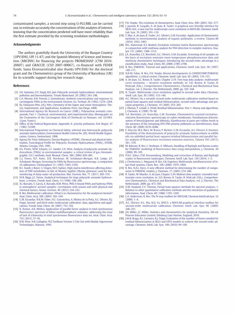
contaminated samples, a second step using U-PLS/RBL can be carriedout, to estimate accurately the concentrations of the analytes of interest,knowing that the concentration predicted will have more reliability thanthe first estimate provided by the screening resolution methodologies.

Acknowledgments

The authors gratefully thank the University of the Basque Country(UPV/EHU, UFI 11/47) and the Spanish Ministry of Science and Innova-tion (MICINN) for financing the projects PROMESHAP (CTM 2010-20607) and GRACCIE (CSD 2007-00067), co-financed with FEDERfunds. Saioa Elcoroaristizabal also thanks UPV/EHU for the doctoralgrant and the Chemometrics group of the University of Barcelona (UB)for its scientific support during her research stage.

References

[1] S.K. Samanta, O.V. Singh, R.K. Jain, Polycyclic aromatic hydrocarbons: environmentalpollution and bioremediation, Trends Biotechnol. 20 (2002) 243–248.

[2] C.A. Menzie, B.B. Potocki, J. Santodonato, Ambient concentrations and exposure tocarcinogenic PAHs in the environment, Environ. Sci. Technol. 26 (1992) 1278–1284.

[3] B.J. Finlayson-Pitts, J.N.J. Pitts, Chemistry of the Upper and Lower Atmosphere: The-ory, Experiments, and Applications, Academic Press, San Diego, 2000.

[4] International Agency for Research on Cancer (IARC), Polynuclear aromatic com-pounds, Part 1: Chemical, environmental, and experimental data, Monographs onthe Evaluation of the Carcinogenic Risk of Chemicals to Humans, vol. 321983.(Lyon, France).

[5] Office of the Federal Registration, Appendix A: priority pollutants, Fed. Regist. 47(1982) 52309.

[6] International Programme on Chemical Safety, selected non-heterocyclic polycyclicaromatic hydrocarbons, Environment Health Criteria No. 202,World Health Organi-zation, Geneva, Switzerland, 1998.

[7] Agency for Toxic Substances, Disease Registry (ATSDR), Chemical and physical infor-mation, Toxicological Profile for Polycyclic Aromatic Hydrocarbons (PAHs), ATSDR,Atlanta, Georgia, USA, 1995.

[8] D.L. Poster, M.M. Schantz, L.C. Sander, S.A. Wise, Analysis of polycyclic aromatic hy-drocarbons (PAHs) in environmental samples: a critical review of gas chromato-graphic (GC) methods, Anal. Bioanal. Chem. 386 (2006) 859–881.

[9] C.J. Owen, R.P. Axler, D.R. Nordman, M. Schubauer-Berigan, K.B. Lodge, J.P.Schubauer-Berigan, Screening for PAHs by fluorescence spectroscopy: a comparisonof calibrations, Chemosphere 31 (1995) 3345–3356.

[10] R.C. Sundt, J. Beyer, S. Vingen, M.O. Sydnes, Highmatrix interference affecting detec-tion of PAH metabolites in bile of Atlantic hagfish (Myxine glutinosa) used for bio-monitoring of deep-water oil production, Mar. Environ. Res. 71 (2011) 369–374.

[11] W.R. Biggs, J.C. Fetzer, Analytical techniques for large polycyclic aromatic hydrocar-bons: a review, Trends Anal. Chem. 15 (1996) 196–206.

[12] A.I. Barrado, S. García, E. Barrado, R.M. Pérez, PM2.5-bound PAHs and hydroxy-PAHsin atmospheric aerosol samples: correlations with season and with physical andchemical factors, Atmos. Environ. 49 (2012) 224–232.

[13] R. Bro, Multivariate calibration. What is in chemometrics for the analytical chemist?Anal. Chim. Acta. 500 (2003) 185–194.

[14] G.M. Escandar, N.K.M. Faber, H.C. Goicoechea, A. Muñoz de la Peña, A.C. Olivieri, R.J.Poppi, Second- and third-order multivariate calibration: data, algorithms and appli-cations, Trends Anal. Chem. 26 (2007) 752–765.

[15] K. Kumar, A.K. Mishra, Application of parallel factor analysis to total synchronousfluorescence spectrum of dilute multifluorophoric solutions: addressing the issueof lack of trilinearity in total synchronous fluorescence data set, Anal. Chim. Acta.755 (2012) 37–45.

[16] B.M.Wise, N.B. Gallagher, PLS Toolboox Version 1.5 for Use withMatlab, EigenvectorTechnologies, Manson, 1995.

[17] P.K. Hopke, The evolution of chemometrics, Anal. Chim. Acta. 500 (2003) 365–377.[18] J. Jaumot, R. Gargallo, A. de Juan, R. Tauler, A graphical user-friendly interface for

MCR–ALS: a new tool for multivariate curve resolution in MATLAB, Chemom. Intell.Lab. Syst. 76 (2005) 101–110.

[19] S. Mas, A. de Juan, R. Tauler, A.C. Olivieri, G.M. Escandar, Application of chemometricmethods to environmental analysis of organic pollutants: a review, Talanta 80(2010) 1052–1067.

[20] M.L. Nahorniak, K.S. Booksh, Excitation–emission matrix fluorescence spectroscopyin conjunction with multiway analysis for PAH detection in complex matrices, Ana-lyst 131 (2006) 1308–1315.

[21] J.A. Arancibia, C.E. Boschetti, A.C. Olivieri, G.M. Escandar, Screening of oil samples onthe basis of excitation–emission room-temperature phosphorescence data andmultiway chemometric techniques. Introducing the second-order advantage in aclassification study, Anal. Chem. 80 (2008) 2789–2798.

[22] R. Bro, PARAFAC. Tutorial and applications, Chemom. Intell. Lab. Syst. 38 (1997)149–171.

[23] N.K.M. Faber, R. Bro, P.K. Hopke, Recent developments in CANDECOMP/PARAFACalgorithms: a critical review, Chemom. Intell. Lab. Syst. 65 (2003) 119–137.

[24] A. de Juan, S.C. Rutan, R. Tauler, Chapter 2.19. Two-way data analysis: multivariatecurve resolution — iterative resolution methods, in: S.D. Brown, R. Tauler, B.Walczak (Eds.), Comprehensive Chemometrics, Chemical and Biochemical DataAnalysis, vol. 2, Elsevier, The Netherlands, 2009, pp. 325–344.

[25] R. Tauler, Multivariate curve resolution applied to second order data, Chemom.Intell. Lab. Syst. 30 (1995) 133–146.

[26] A.C. Olivieri, On a versatile second-order multivariate calibration method based onpartial least-squares and residual bilinearization: second-order advantage and pre-cision properties, J. Chemom. 19 (2005) 253–265.

[27] J. Öhman, P. Geladi, S. Wold, Residual bilinearization. Part 1: theory and algorithms,J. Chemom. 4 (1990) 79–90.

[28] S.A. Bortolato, J.A. Arancibia, G.M. Escandar, Chemometrics-assisted excitation–emission fluorescence spectroscopy on nylon membranes. Simultaneous determi-nation of benzo[a]pyrene and dibenz[a, h]anthracene at parts-per-trillion levels inthe presence of the remaining EPA PAH priority pollutants as intereferences, Anal.Chem. 80 (2008) 8276–8286.

[29] F. Alarcón, M.E. Báez, M. Bravo, P. Richter, G.M. Escandar, A.C. Olivieri, E. Fuentes,Feasibility of the determination of polycyclic aromatic hydrocarbons in edibleoils via unfolded partial least-squares/residual bilinearization and parallel fac-tor analysis of fluorescence excitation emission matrices, Talanta 103 (2013)361–370.

[30] M. Bahram, R. Bro, C. Stedmon, A. Afkhami, Handling of Rayleigh and Raman scatterfor PARAFAC modeling of fluorescence data using interpolation, J. Chemom. 20(2006) 99–105.

[31] P.H.C. Eilers, P.M. Kroonenberg, Modeling and correction of Raman and Rayleighscatter in fluorescence landscapes, Chemom. Intell. Lab. Syst. 130 (2014) 1–5.

[32] J. Christensen, L. Nørgaard, R. Bro, S.B. Engelsen, Multivariate autofluorescence of in-tact food systems, Chem. Rev. 106 (2006) 1979–1994.

[33] R. Bro, H.A.L. Kiers, A new efficient method for determining the number of compo-nents in PARAFAC models, J. Chemom. 17 (2003) 274–286.

[34] R. Tauler, M. Maeder, A. de Juan, Chapter 2.24. Multiset data analysis: extendedmul-tivariate curve resolution, in: S.D. Brown, R. Tauler, B. Walczak (Eds.), Comprehen-sive Chemometrics. Chemical and Biochemical Data Analysis, vol. 2, Elsevier, TheNetherlands, 2009, pp. 473–505.

[35] D.M. Haaland, E.V. Thomas, Partial least-squares methods for spectral analyses. 1.Relation to other quantitative calibration methods and the extraction of qualitativeinformation, Anal. Chem. 60 (1988) 1193–1202.

[36] C.A. Andersson, R. Bro, The N-way toolbox for MATLAB, Chemom.Intell.Lab.Syst. 52(2000) 1–4.

[37] A.C. Olivieri, H.L. Wu, R.Q. Yu, MVC2: a MATLAB graphical interface toolbox forsecond-order multivariate calibration, Chemom. Intell. Lab. Syst. 96 (2009)246–251.

[38] J.N. Miller, J.C. Miller, Statistics and chemometrics for analytical chemistry, 5th ed.Pearson Education Limited, Edinburg Gate Harlow, England, 2010.

[39] J.W.B. Braga, R.L. Carneiro, R.J. Poppi, Evaluation of the number of factors needed forresidual bilinearization in BLLS and UPLS models to achieve the second-order ad-vantage, Chemom. Intell. Lab. Syst. 100 (2010) 99–109.














































































































PAPER 03

Chemometric determination of PAHs in

aerosol samples by fluorescence

spectroscopy and second-order data analysis

algorithms

Saioa Elcoroaristizabal, Anna de Juan, Jose Antonio García,

Iñaki Elorduy, Nieves Durana, Lucio Alonso

Journal of Chemometrics 28:4 (2014) 260-271

Chemometric determination of PAHs in aerosolsamples by fluorescence spectroscopy andsecond-order data analysis algorithmsSaioa Elcoroaristizabala*, Anna de Juanb, Jose Antonio Garcíaa,Iñaki Elorduya, Nieves Duranaa and Lucio Alonsoa

The development of a method based on the combination of excitation–emission fluorescence matrices (EEMs) andsecond-order algorithms is proposed to identify and quantify 10 polycyclic aromatic hydrocarbons (PAHs) in extractsof aerosol samples, a particularly complex sample matrix because of the low amount of PAHs and the numerousfluorescent interferences. Parallel factor analysis, unfolded partial least squares coupled to residual bilinearization(RBL) and multivariate curve resolution – alternating least squares offered satisfactory results for their identificationand quantification andwere also helpful for the optimization of the extraction procedure for these substances bymeansof analysis of a standard reference material.Multivariate curve resolution – alternating least squares and parallel factor analysis combined with EEM proved to be

fast and cheap analysis methods that are able to do semiquantitative monitoring of PAHs patterns in the inhalable andrespirable fractions of atmospheric aerosols, important features for routine environmental monitoring. Accurate quan-tifications could also be achieved when the strategy of standard addition method was used.Unfolded partial least squares/RBL achieved slightly better quantitative results when sample matrices were moder-

ately complex; in aerosol sample analysis, the selection of number of RBL contributions turned particularly difficult—because of the lack of information on the sample composition—and the time-consuming application of the methoddid not suggest its use for routine environmental monitoring.Finally, results of EEM with second-order methods in agreement with gas chromatography-mass spectrometry

analysis of ambient air samples proved the suitability of the methodology proposed because of the sensitivity offluorescence measurements and the lower analytical cost and fast computation time comparedwith standard analyticalprocedures. Copyright © 2014 John Wiley & Sons, Ltd.

Keywords: particle-bound PAHs; fluorescence excitation–emission matrices; PARAFAC; MCR-ALS; U-PLS/RBL

1. INTRODUCTION

Polycyclic (or polynuclear) aromatic hydrocarbons (PAHs) arecomplex organic compounds that are primarily released to theatmosphere during incomplete combustion processes of organicmaterial. Major sources of PAHs are energy generation processes[1], including industrial combustion [2], traffic emissions, anddomestic heating systems [3]. Forest fires and volcanic eruptionsare also natural sources of PAHs [4]. PAHs are of environmentalconcern because of their persistence and toxicity, related tocarcinogenic and/or mutagenic properties [5]. After emission tothe atmosphere, PAHs are ubiquitously distributed and parti-tioned between the gaseous and the particulate phase [6], withthe most toxic PAHs linked to the respirable fraction of particu-late matter (aerodynamic diameter ≤2.5μm) [7]. Specifically, inurban and suburban areas, PAHs are present in the fine particulatefraction (PM2.5), and their emissions aremainly attributed to vehicleexhausts [8]. As a consequence, these compounds have been listedas priority pollutants. The United States Environmental Protec-tion Agency (US-EPA) regulates a series of 16 unsubstituted PAHs(16 US-EPA PAHs) [9], and the World Health Organization adds 17additional PAHs to make a total of 33 PAHs [10]. The EuropeanUnion Directive 2004/107/EC [11] on ambient air quality sets atarget value for benzo[a]pyrene (BaP) (1 ngm�3 in the PM10

fraction, annual average) taken as indicator for total particulatecarcinogenic PAHs. This Directive also mentions five more PAHsto assess the contribution of PAH in ambient air: benzo[a]anthra-cene (BaA), benzo[b]fluoranthene (BbF), benzo[j]fluoranthene,benzo[k]fluoranthene (BkF), indeno[1,2,3-cd]pyrene (IcdP), anddibenzo[a,h]anthracene (DahA). However, PAH data in urban airare still scarce, and most of the studies show large spatial andtemporal uncertainties because of the complex sampling andanalytical procedures required. In fact, the analysis of PAHs inaerosol samples faces many problems because of the very lowPAH concentrations in ambient air as well as the presence of other

* Correspondence to: Saioa Elcoroaristizabal, Chemical and Environmental Engi-neering Department, School of Engineering, University of the Basque Country(UPV/EHU) Alameda de Urquijo s/n, E-48013 Bilbao, Spain.E-mail: [email protected]

a S. Elcoroaristizabal, J. A. García, I. Elorduy, N. Durana, L. AlonsoChemical and Environmental Engineering Department, School of Engineering,University of the Basque Country (UPV/EHU), Alameda de Urquijo s/n, E-48013,Bilbao, Spain

b A. JuanChemometrics Group, Department of Analytical Chemistry, Universitat deBarcelona (UB), Diagonal 645, E-08028, Barcelona, Spain

Special Issue Article

Received: 4 November 2013, Revised: 20 January 2014, Accepted: 23 January 2014, Published online in Wiley Online Library

(wileyonlinelibrary.com) DOI: 10.1002/cem.2604

J. Chemometrics (2014) Copyright © 2014 John Wiley & Sons, Ltd.

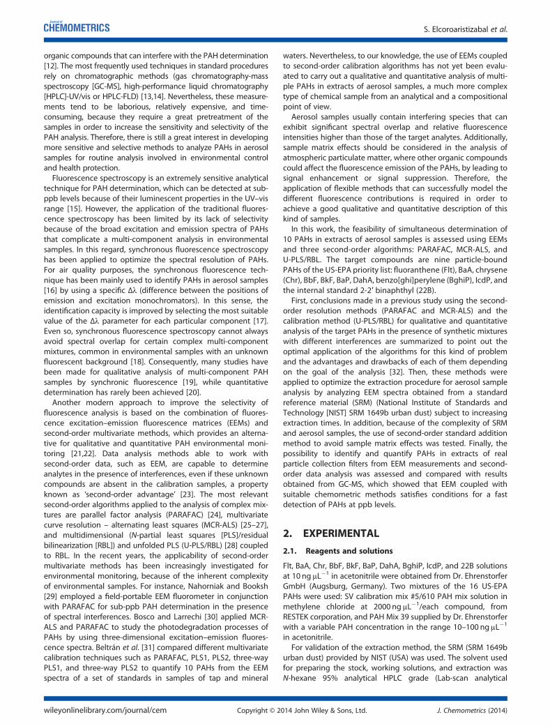
organic compounds that can interfere with the PAH determination[12]. The most frequently used techniques in standard proceduresrely on chromatographic methods (gas chromatography-massspectroscopy [GC-MS], high-performance liquid chromatography[HPLC]-UV/vis or HPLC-FLD) [13,14]. Nevertheless, these measure-ments tend to be laborious, relatively expensive, and time-consuming, because they require a great pretreatment of thesamples in order to increase the sensitivity and selectivity of thePAH analysis. Therefore, there is still a great interest in developingmore sensitive and selective methods to analyze PAHs in aerosolsamples for routine analysis involved in environmental controland health protection.

Fluorescence spectroscopy is an extremely sensitive analyticaltechnique for PAH determination, which can be detected at sub-ppb levels because of their luminescent properties in the UV–visrange [15]. However, the application of the traditional fluores-cence spectroscopy has been limited by its lack of selectivitybecause of the broad excitation and emission spectra of PAHsthat complicate a multi-component analysis in environmentalsamples. In this regard, synchronous fluorescence spectroscopyhas been applied to optimize the spectral resolution of PAHs.For air quality purposes, the synchronous fluorescence tech-nique has been mainly used to identify PAHs in aerosol samples[16] by using a specific Δλ (difference between the positions ofemission and excitation monochromators). In this sense, theidentification capacity is improved by selecting the most suitablevalue of the Δλ parameter for each particular component [17].Even so, synchronous fluorescence spectroscopy cannot alwaysavoid spectral overlap for certain complex multi-componentmixtures, common in environmental samples with an unknownfluorescent background [18]. Consequently, many studies havebeen made for qualitative analysis of multi-component PAHsamples by synchronic fluorescence [19], while quantitativedetermination has rarely been achieved [20].

Another modern approach to improve the selectivity offluorescence analysis is based on the combination of fluores-cence excitation–emission fluorescence matrices (EEMs) andsecond-order multivariate methods, which provides an alterna-tive for qualitative and quantitative PAH environmental moni-toring [21,22]. Data analysis methods able to work withsecond-order data, such as EEM, are capable to determineanalytes in the presence of interferences, even if these unknowncompounds are absent in the calibration samples, a propertyknown as ‘second-order advantage’ [23]. The most relevantsecond-order algorithms applied to the analysis of complex mix-tures are parallel factor analysis (PARAFAC) [24], multivariatecurve resolution – alternating least squares (MCR-ALS) [25–27],and multidimensional (N-partial least squares [PLS]/residualbilinearization [RBL]) and unfolded PLS (U-PLS/RBL) [28] coupledto RBL. In the recent years, the applicability of second-ordermultivariate methods has been increasingly investigated forenvironmental monitoring, because of the inherent complexityof environmental samples. For instance, Nahorniak and Booksh[29] employed a field-portable EEM fluorometer in conjunctionwith PARAFAC for sub-ppb PAH determination in the presenceof spectral interferences. Bosco and Larrechi [30] applied MCR-ALS and PARAFAC to study the photodegradation processes ofPAHs by using three-dimensional excitation–emission fluores-cence spectra. Beltrán et al. [31] compared different multivariatecalibration techniques such as PARAFAC, PLS1, PLS2, three-wayPLS1, and three-way PLS2 to quantify 10 PAHs from the EEMspectra of a set of standards in samples of tap and mineral

waters. Nevertheless, to our knowledge, the use of EEMs coupledto second-order calibration algorithms has not yet been evalu-ated to carry out a qualitative and quantitative analysis of multi-ple PAHs in extracts of aerosol samples, a much more complextype of chemical sample from an analytical and a compositionalpoint of view.Aerosol samples usually contain interfering species that can

exhibit significant spectral overlap and relative fluorescenceintensities higher than those of the target analytes. Additionally,sample matrix effects should be considered in the analysis ofatmospheric particulate matter, where other organic compoundscould affect the fluorescence emission of the PAHs, by leading tosignal enhancement or signal suppression. Therefore, theapplication of flexible methods that can successfully model thedifferent fluorescence contributions is required in order toachieve a good qualitative and quantitative description of thiskind of samples.In this work, the feasibility of simultaneous determination of

10 PAHs in extracts of aerosol samples is assessed using EEMsand three second-order algorithms: PARAFAC, MCR-ALS, andU-PLS/RBL. The target compounds are nine particle-boundPAHs of the US-EPA priority list: fluoranthene (Flt), BaA, chrysene(Chr), BbF, BkF, BaP, DahA, benzo[ghi]perylene (BghiP), IcdP, andthe internal standard 2-2′ binaphthyl (22B).First, conclusions made in a previous study using the second-

order resolution methods (PARAFAC and MCR-ALS) and thecalibration method (U-PLS/RBL) for qualitative and quantitativeanalysis of the target PAHs in the presence of synthetic mixtureswith different interferences are summarized to point out theoptimal application of the algorithms for this kind of problemand the advantages and drawbacks of each of them dependingon the goal of the analysis [32]. Then, these methods wereapplied to optimize the extraction procedure for aerosol sampleanalysis by analyzing EEM spectra obtained from a standardreference material (SRM) (National Institute of Standards andTechnology [NIST] SRM 1649b urban dust) subject to increasingextraction times. In addition, because of the complexity of SRMand aerosol samples, the use of second-order standard additionmethod to avoid sample matrix effects was tested. Finally, thepossibility to identify and quantify PAHs in extracts of realparticle collection filters from EEM measurements and second-order data analysis was assessed and compared with resultsobtained from GC-MS, which showed that EEM coupled withsuitable chemometric methods satisfies conditions for a fastdetection of PAHs at ppb levels.

2. EXPERIMENTAL

2.1. Reagents and solutions

Flt, BaA, Chr, BbF, BkF, BaP, DahA, BghiP, IcdP, and 22B solutionsat 10 ngμL�1 in acetonitrile were obtained from Dr. EhrenstorferGmbH (Augsburg, Germany). Two mixtures of the 16 US-EPAPAHs were used: SV calibration mix #5/610 PAH mix solution inmethylene chloride at 2000 ngμL�1/each compound, fromRESTEK corporation, and PAH Mix 39 supplied by Dr. Ehrenstorferwith a variable PAH concentration in the range 10–100 ngμL�1

in acetonitrile.For validation of the extraction method, the SRM (SRM 1649b

urban dust) provided by NIST (USA) was used. The solvent usedfor preparing the stock, working solutions, and extraction wasN-hexane 95% analytical HPLC grade (Lab-scan analytical

S. Elcoroaristizabal et al.

wileyonlinelibrary.com/journal/cem Copyright © 2014 John Wiley & Sons, Ltd. J. Chemometrics (2014)

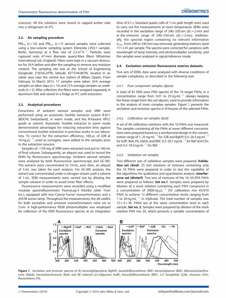
sciences). All the solutions were stored in capped amber vialsinto a refrigerator at 4°C.

2.2. Air sampling procedure

PM10 (n=10) and PM2.5 (n=7) aerosol samples were collectedusing a low-volume sampling system (Derenda LVS3.1 sampler,Berlin, Germany) at a flow rate of 2.3m3h�1. Particles werecaptured onto 47-mm diameter quartz-fiber filters (WhatmanInternational Ltd., England). Filters were kept in a vacuum desicca-tor for 24 h before and after the sampling to remove any moisturecontent. The sampling site was at the School of Engineering(longitude 2°56′56.24″W, latitude 43°15′44.86″N), located in anurban area near the central bus station of Bilbao (Spain). FromFebruary to March 2013, 17 samples were taken: 24 h averagesamples on labor days (n=12) and 72h average samples on week-ends (n=5). After collection, the filters were wrapped separately inaluminum foils and stored in a fridge at 4°C until extraction.

2.3. Analytical procedures

Extractions of ambient aerosol samples and SRM wereperformed using an automatic Soxhlet extractor system B-811(BÜCHI, Switzerland), in warm mode, and the N-hexane HPLCgrade as solvent. Automatic Soxhlet extractor in warm modedemonstrated advantages for reducing extraction time againstconventional Soxhlet extraction in previous works in our labora-tory. To correct for the extraction efficiency, 100μL of 22B at10 ngμL�1, used as surrogate, were added to the samples priorto the extraction process.Samples of ~150mg of SRM were extracted and put to 100mL

of final volume. Subsequently, an aliquot was used to record theEEMs by fluorescence spectroscopy. Ambient aerosol sampleswere analyzed by both fluorescence spectroscopy and GC-MS.The extracts were concentrated to 10mL, and, then, an aliquotof 5mL was taken for each analysis. For GC-MS analysis, theextract was concentrated under a nitrogen stream until a volumeof 1mL. EEM measurements were carried out by diluting thesample solution in order to avoid inner filter effects.Fluorescence measurements were recorded using a modified

modular spectrofluorometer FluoroLog-3 (Horiba Jobin YvonInc.), equipped with two Czerny-Turner monochromators and a450W xenon lamp. Throughout the measurements, the slit widthsfor both excitation and emission monochromators were set to5nm. A high-performance R928 photomultiplier was employedfor collection of the EEM fluorescence spectra at an integration

time of 0.1 s. Standard quartz cells of 1 cm path length were usedto carry out the measurements at room temperature. EEMs wererecorded in the excitation range of 240–320nm (Δλ =2nm) andin the emission range of 290–550 nm (Δλ = 2 nm). Addition-ally, the spectral region containing no relevant information(λem from 290 to 330nm) was removed, generatingmatrices sized111×41 per sample. The spectra were corrected for variations withwavelength of lamp intensity and photomultiplier sensitivity, andthe samples were analyzed in signal/reference mode.

2.4. Excitation–emission fluorescence matrice datasets

Five sets of EEMs data were analyzed with diverse conditions ofsample complexity, as described in the following text.

2.4.1. Pure component samples (dpure)

A total of 81 EEM pure PAH spectra of the 10 target PAHs, in aconcentration range from 0.01 to 25ngmL�1 (always keepingthe linear range) form this set (dpure), used to provide informationin the analysis of more complex samples. Figure 1 presents theexcitation and emission spectra in N-hexane of the selected PAHs.

2.4.2. Calibration set samples (dcal)

A set of 49 calibration solutions with the 10 PAHs was measured.The samples containing all the PAHs at seven different concentra-tions were prepared based on a semifactorial design in the concen-tration range of 1–25ngmL�1 for 22B and BghiP; 0.5–20.3ngmL�1

for IcdP, BaA, Flt, DahA, and BbF; 0.3–20.1ngmL�1 for BaP and Chr;and 0.3–18.3 ngmL�1 for BkF.

2.4.3. Validation set samples

Two different sets of validation samples were prepared. Valida-tion set (dval). 25 test solutions of mixtures containing onlythe 10 PAHs were prepared in order to test the capability ofthe algorithms for qualitative and quantitative analysis. Interfer-ence set (dinterf). Two sets of mixtures of the 16 US-EPA PAHswere prepared as follows: Set no.1. Samples were prepared bydilution of a stock solution containing each PAH compound ina concentration of 2000 ngμL�1 (SV calibration mix #5/610PAH) to achieve 12 different concentration levels ranging from1 to 20 ngmL�1, in triplicate. The total number of samples was12 × 3 = 36. PAHs are at the same concentration level in eachsample. Set no. 2. Samples were prepared by dilution of the stocksolution PAH mix 39, which presents a variable concentration of

Figure 1. Excitation and emission spectra of (A) benzo[ghi]perylene (BghiP), benzo[k]fluoranthene (BkF), benzo[a]pyrene (BaP), dibenzo[a,h]anthra-cene (DahA), benzo[a]anthracene (BaA) and (B) indeno[1,2,3-cd]pyrene (IcdP), benzo[b]fluoranthene (BbF), 2-2′ binaphthyl (22B), chrysene (Chr),fluoranthene (Flt).

Chemometric fluorescence determination of PAH

J. Chemometrics (2014) Copyright © 2014 John Wiley & Sons, Ltd. wileyonlinelibrary.com/journal/cem

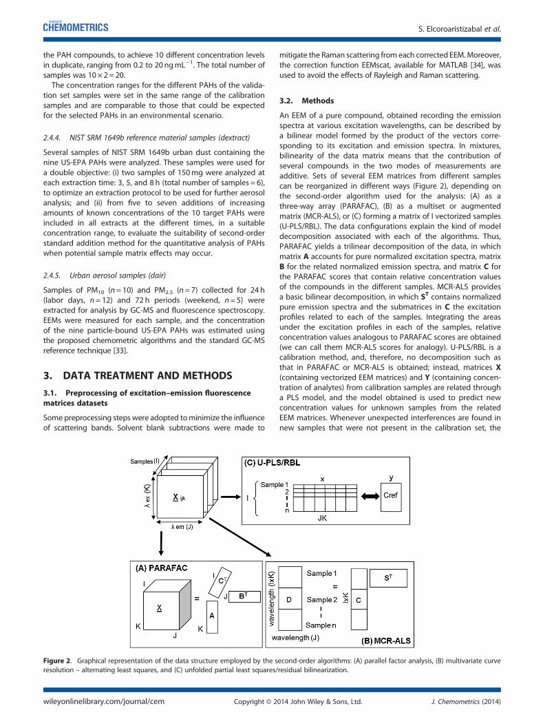
the PAH compounds, to achieve 10 different concentration levelsin duplicate, ranging from 0.2 to 20 ngmL�1. The total number ofsamples was 10×2=20.

The concentration ranges for the different PAHs of the valida-tion set samples were set in the same range of the calibrationsamples and are comparable to those that could be expectedfor the selected PAHs in an environmental scenario.

2.4.4. NIST SRM 1649b reference material samples (dextract)

Several samples of NIST SRM 1649b urban dust containing thenine US-EPA PAHs were analyzed. These samples were used fora double objective: (i) two samples of 150mg were analyzed ateach extraction time: 3, 5, and 8 h (total number of samples = 6),to optimize an extraction protocol to be used for further aerosolanalysis; and (ii) from five to seven additions of increasingamounts of known concentrations of the 10 target PAHs wereincluded in all extracts at the different times, in a suitableconcentration range, to evaluate the suitability of second-orderstandard addition method for the quantitative analysis of PAHswhen potential sample matrix effects may occur.

2.4.5. Urban aerosol samples (dair)

Samples of PM10 (n= 10) and PM2.5 (n=7) collected for 24 h(labor days, n=12) and 72 h periods (weekend, n=5) wereextracted for analysis by GC-MS and fluorescence spectroscopy.EEMs were measured for each sample, and the concentrationof the nine particle-bound US-EPA PAHs was estimated usingthe proposed chemometric algorithms and the standard GC-MSreference technique [33].

3. DATA TREATMENT AND METHODS

3.1. Preprocessing of excitation–emission fluorescencematrices datasets

Some preprocessing steps were adopted tominimize the influenceof scattering bands. Solvent blank subtractions were made to

mitigate the Raman scattering from each corrected EEM. Moreover,the correction function EEMscat, available for MATLAB [34], wasused to avoid the effects of Rayleigh and Raman scattering.

3.2. Methods

An EEM of a pure compound, obtained recording the emissionspectra at various excitation wavelengths, can be described bya bilinear model formed by the product of the vectors corre-sponding to its excitation and emission spectra. In mixtures,bilinearity of the data matrix means that the contribution ofseveral compounds in the two modes of measurements areadditive. Sets of several EEM matrices from different samplescan be reorganized in different ways (Figure 2), depending onthe second-order algorithm used for the analysis: (A) as athree-way array (PARAFAC), (B) as a multiset or augmentedmatrix (MCR-ALS), or (C) forming a matrix of I vectorized samples(U-PLS/RBL). The data configurations explain the kind of modeldecomposition associated with each of the algorithms. Thus,PARAFAC yields a trilinear decomposition of the data, in whichmatrix A accounts for pure normalized excitation spectra, matrixB for the related normalized emission spectra, and matrix C forthe PARAFAC scores that contain relative concentration valuesof the compounds in the different samples. MCR-ALS providesa basic bilinear decomposition, in which ST contains normalizedpure emission spectra and the submatrices in C the excitationprofiles related to each of the samples. Integrating the areasunder the excitation profiles in each of the samples, relativeconcentration values analogous to PARAFAC scores are obtained(we can call them MCR-ALS scores for analogy). U-PLS/RBL is acalibration method, and, therefore, no decomposition such asthat in PARAFAC or MCR-ALS is obtained; instead, matrices X(containing vectorized EEM matrices) and Y (containing concen-tration of analytes) from calibration samples are related througha PLS model, and the model obtained is used to predict newconcentration values for unknown samples from the relatedEEM matrices. Whenever unexpected interferences are found innew samples that were not present in the calibration set, the

Figure 2. Graphical representation of the data structure employed by the second-order algorithms: (A) parallel factor analysis, (B) multivariate curveresolution – alternating least squares, and (C) unfolded partial least squares/residual bilinearization.



additional RBL step has to be used for accurate prediction of theanalytes. Detailed theory about PARAFAC, MCR-ALS, and U-PLS/RBL algorithms can be found in several theoretical works[24–27]. Only some particular considerations taken into accountto build each model are presented in the succeeding text.

3.2.1. Parallel factor analysis and multivariate curve resolution –alternating least squares models

Parallel factor analysis and MCR-ALS algorithms were applied bycombining the EEM from different kinds of samples dependingon the problem to be solved, as shown in Figure 3. These sets ofsamples were organized as three-way data or multiset structures,depending on the algorithm used. Samples of individual PAHs(dpure) were always used to improve the identification of com-pounds in the results provided by these resolution methods andwere rescaled to balance the relative unit fluorescence intensitiesof the related PAHs. The calibration set (dcal) was used to createthe calibration curve and to carry out the predictions of the sam-ples analyzed (dval, dinterf, dair) except in the case of extractiondata (dextract) because standard addition method was used.To initialize MCR-ALS models, a combination of the known

spectral profiles of the analyte standards with additional spectralcontributions when interfering species that were present, foundby an algorithm based on SIMPLISMA [35], was used. PARAFACinitialization was made by using the best-fitting model of severalmodels fitted using a few iterations.Both algorithms applied non-negative constraints in all possi-

ble modes (concentration, excitation, and emission profiles) toobtain meaningful profiles. In addition, MCR-ALS model usedsupplementary constraints, such as correspondence amongspecies, that is, the presence/absence of certain compounds insamples was actively set. The trilinearity behavior was also appliedas an optional constraint by MCR-ALS model to the differentcomponents in the system. This allows for the implementation oftotal trilinearity or partial trilinearity [25,26]. In the partial trilinearmodel, the trilinear behavior was always applied to the contribu-tion of the analytes (PAHs), whereas the rest of components, whichcould include combinations of interferences and residual scatter-ing, were modeled as bilinear contributions.The selection of the number of components in PARAFAC or

MCR-ALS models was performed by building several models withan increasing number of factors. The core consistency test(CORCONDIA) [36], the percentage of fit (%), the variance explained(r2), and the recovery of spectra by emission and excitation correla-tion coefficients (rem and rex) were used to select the most suitablenumber of factors in PARAFAC models. All criteria, exceptCORCONDIA, were used to select the size of MCR-ALS models.

3.2.2. Unfolded partial least squares/residual bilinearizationmodels

Because of the high differences between fluorescence intensitiesand to the spectral overlap of the selected PAHs, U-PLS wasperformed by using PLS1 models, that is, by modeling separatelyeach individual PAH. For U-PLS predictions, the original matrix X—including only the calibration set samples (dcal)—is pre-processed by mean-centering. The optimum number of factorsin the calibration model for each PAH was selected by applica-tion of the F-ratio criterion proposed by Haaland and Thomas[37]. This F-ratio is calculated as F(A) = PRESS(A<A *)/PRESS(A *),where PRESS is the predicted error sum of squares, defined asPRESS ¼ ∑I1ðynominal � ypredicatedÞ2, A is a trial number of factors,and A* corresponds to the minimum PRESS. The number ofoptimum factors was selected as that leading to a probabilityof less than 75% with F> 1.

In the presence of unexpected components, U-PLS model wascombined with the post-processing RBL procedure. When usingU-PLS/RBL, in addition to the latent variables estimated to buildthe calibration model, setting an additional number of factorscorresponding to the unexpected constituents is required forthe RBL step. The number of RBL factors must be calculated foreach new sample and individual PAH model, and the final pre-diction is selected after testing different models with an increas-ing number of RBL factors. If the RBL procedure is successfullyapplied, the residual corresponding to the difference betweenthe test sample signal and that modeled after RBL processshould be comparable to the instrumental noise. The numberof unexpected components for the RBL step was calculated con-sidering the methods proposed by Bortolato et al. [38] and Bragaet al. [39]. Bortolato et al. [38] estimate the number of optimumRBL latent variables based on a ratio between the RBL residuals(SRBL): SRBL= ‖eRBL‖/[(J�Nunx)(K�Nunx)�A]1/2 and a penalized re-sidual error (Spen): Spen= SRBL[(JxK)/[(J�Nunx)(K�Nunx)�A]1/2].This ratio is computed for increasing values of unexpected com-ponents (Nunx) as follows: R= spen(Nunx)/[sRBL(Nunx� 1)]. The firstvalue of Nunx for which R did not exceed 1 was then selectedas the number of RBL components. In contrast, Braga et al. [39]proposed a method based on the comparison of the residualsof the U-PLS/RBL test samples with results of t-student confi-dence intervals for the mean residuals of decomposition of thecalibration samples. These two methods were considered toestimate the number of unexpected components for each PAHU-PLS model and sample.

3.3. Software

All the routines were implemented in MATLAB version R2010(The MathWorks, MA, USA). MCR-ALS with a graphical user-friendlyinterface was downloaded from [40]. The routine used forPARAFAC calculations is available at [41]. U-PLS/RBL algorithmwas implemented using the graphical interface of the MVC2 tool-box downloaded from [42].

4. RESULTS AND DISCUSSION

First of all, a summary of the main conclusions of the use of thethree second-order algorithms PARAFAC, MCR-ALS, and U-PLS/RBL on the set of synthetic validation samples with and withoutinterferences is presented to point out differences amongthese second-order methods when applied to the analytes

Figure 3. Multisets used for PAHs calculation by parallel factor analysisand multivariate curve resolution – alternating least squares.



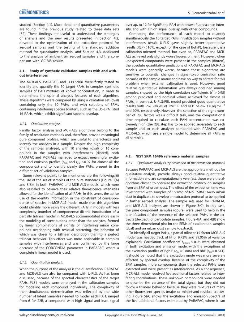
studied (Section 4.1). More detail and quantitative parametersare found in the previous study related to these data sets[32]. These findings are useful to understand the strategiesof analysis and the new results presented in Section 4.2,devoted to the optimization of the extraction protocol foraerosol samples and the testing of the standard additionmethod for quantitative analysis, and Section 4.3, dedicatedto the analysis of ambient air aerosol samples and the com-parison with GC-MS results.

4.1. Study of synthetic validation samples with and with-out interferences

The MCR-ALS, PARAFAC, and U-PLS/RBL were firstly tested toidentify and quantify the 10 target PAHs in complex syntheticsamples of PAH mixtures of known concentration, in order todeterminate the optimal analysis features of each algorithm.These algorithms were compared by using a validation set (dval)containing only the 10 PAHs, and with solutions of SRMscontaining interfering species (dinterf), such as the US-EPA listed16 PAHs, which exhibit significant spectral overlap.

4.1.1. Qualitative analysis

Parallel factor analysis and MCR-ALS algorithms belong to thefamily of resolution methods and, therefore, provide meaningfulpure compound profiles, which are useful to characterize andidentify the analytes in a sample. Despite the high complexityof the samples analyzed, with 10 analytes (dval) or 16 com-pounds in the samples with interferences (dinterf), bothPARAFAC and MCR-ALS managed to extract meaningful excita-tion and emission profiles (rem and rex >0.97 for almost all thecompounds) and to identify clearly the PAHs present in thedifferent set of validation samples.

Some relevant points to be mentioned are the following: (i)the use of the set of samples of the pure standards (Figure 3(A)and 3(B)), in both PARAFAC and MCR-ALS models, which werealso rescaled to balance their relative fluorescence intensitiesallowed for the identification of all PAHs; in this sense, the activeuse of the identity information in the constraint of correspon-dence of species in MCR-ALS model made that this algorithmcould identify more easily the different PAHs in models with lesscomplexity (number of components); (ii) the introduction of apartially trilinear model in MCR-ALS accommodated more easilythe modeling of contributions other than the analytes, formedby linear combinations of signals of interfering minor com-pounds overlapping with residual scattering, the behavior ofwhich was closer to a bilinear description than to a perfecttrilinear behavior. This effect was more noticeable in complexsamples with interferences and was confirmed by the largedecrease of the CORCONDIA parameter in PARAFAC, where acomplete trilinear model is used.

4.1.2. Quantitative analysis

When the purpose of the analysis is the quantification, PARAFACand MCR-ALS can also be compared with U-PLS. As has beendiscussed, because of the spectral characteristics of the targetPAHs, PLS1 models were employed in the calibration samplesfor modeling each compound individually. The complexity oftheir simultaneous determination was reflected by the widenumber of latent variables needed to model each PAH, rangedfrom 6 for 22B, a compound with high signal and least signal

overlap, to 12 for BghiP, the PAH with lowest fluorescence inten-sity, and with a high signal overlap with other compounds.Comparing the performance of each model to quantify

simultaneously the 10 target PAHs in validation samples withoutinterferences (dval), U-PLS gave slightly better quantitativeresults (REP< 10%, except for the case of BghiP), because it is acalibration-oriented method, but even so, PARAFAC and MCR-ALS achieved only slightly worse figures of merit. However, whenunexpected compounds were present in the samples (dinterf),the absolute quantitative predictions of PARAFAC and MCR-ALSmodels were generally worse, because these algorithms aresensitive to potential changes in signal-to-concentration ratiobecause of the sample matrix and have no way to correct for thisproblem when external calibration is used. However, goodrelative quantitative information was always obtained amongsamples, showed by the high correlation coefficients (r2> 0.95)among predicted and nominal values achieved for almost allPAHs. In contrast, U-PLS/RBL model provided good quantitativeresults with low values of RMSEP and REP below 1.8 ngmL�1

and 20%, respectively. However, the selection of the right num-ber of RBL factors was a difficult task, and the computationaltime required to calculate each PAH concentration was ex-tremely high (the RBL step has to be applied separately to eachsample and to each analyte) compared with PARAFAC andMCR-ALS, which use a single model to determine all PAHs inall samples.

4.2. NIST SRM 1649b reference material samples

4.2.1. Qualitative analysis (optimization of the extraction protocol)

Because PARAFAC and MCR-ALS are the appropriate methods forqualitative analysis, provide always good relative quantitativeinformation and are computationally very fast, these were the al-gorithms chosen to optimize the extraction protocol on samplesfrom an SRM of urban dust. The effect of the extraction time wasinvestigated with samples of 150mg of NIST SRM 1649b urbandust in duplicate to develop an extraction protocol to be appliedin further aerosol analysis. The sample sets used for PARAFACand MCR-ALS analyses are shown in Figure 3(C). In this case,the pure component samples (dpure) were used to help in theidentification of the presence of the selected PAHs in the ex-tracts (dextract) of particulate samples. Figure 4(A) and 4(B) showthe three-dimensional plot for the EEMs of a calibration samples(dcal) and an urban dust sample (dextract).To identify all target PAHs, a partial trilinear 15-factor MCR-ALS

model was needed (lack of fit of 9.73% and 99.05% of varianceexplained). Correlation coefficients rem,ex> 0.96 were obtainedin both excitation and emission mode, with the exceptions ofthe excitation profiles of BghiP (rex = 0.806) and BbF (rex = 0.841).It should be noted that the excitation mode was more severelyaffected by spectral overlap. Because of the complexity of theSRM samples, more components than the selected PAHs wereextracted and were present as interferences. As a consequence,MCR-ALS model resolved five additional factors related to inter-fering contributions. These unknown compounds were neededto describe the variance of the total signal, but they did notfollow a trilinear behavior because they were mixtures of manyother fluorescent species (major or minor) and residual scatter-ing. Figure 5(A) shows the excitation and emission spectra ofthe five additional factors estimated by PARAFAC, where it can



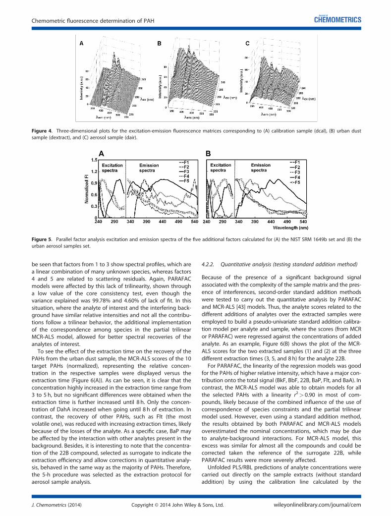
be seen that factors from 1 to 3 show spectral profiles, which area linear combination of many unknown species, whereas factors4 and 5 are related to scattering residuals. Again, PARAFACmodels were affected by this lack of trilinearity, shown througha low value of the core consistency test, even though thevariance explained was 99.78% and 4.60% of lack of fit. In thissituation, where the analyte of interest and the interfering back-ground have similar relative intensities and not all the contribu-tions follow a trilinear behavior, the additional implementationof the correspondence among species in the partial trilinearMCR-ALS model, allowed for better spectral recoveries of theanalytes of interest.To see the effect of the extraction time on the recovery of the

PAHs from the urban dust sample, the MCR-ALS scores of the 10target PAHs (normalized), representing the relative concen-tration in the respective samples were displayed versus theextraction time (Figure 6(A)). As can be seen, it is clear that theconcentration highly increased in the extraction time range from3 to 5 h, but no significant differences were obtained when theextraction time is further increased until 8 h. Only the concen-tration of DahA increased when going until 8 h of extraction. Incontrast, the recovery of other PAHs, such as Flt (the mostvolatile one), was reduced with increasing extraction times, likelybecause of the losses of the analyte. As a specific case, BaP maybe affected by the interaction with other analytes present in thebackground. Besides, it is interesting to note that the concentra-tion of the 22B compound, selected as surrogate to indicate theextraction efficiency and allow corrections in quantitative analy-sis, behaved in the same way as the majority of PAHs. Therefore,the 5-h procedure was selected as the extraction protocol foraerosol sample analysis.

4.2.2. Quantitative analysis (testing standard addition method)

Because of the presence of a significant background signalassociated with the complexity of the sample matrix and the pres-ence of interferences, second-order standard addition methodswere tested to carry out the quantitative analysis by PARAFACand MCR-ALS [43] models. Thus, the analyte scores related to thedifferent additions of analytes over the extracted samples wereemployed to build a pseudo-univariate standard addition calibra-tion model per analyte and sample, where the scores (from MCRor PARAFAC) were regressed against the concentrations of addedanalyte. As an example, Figure 6(B) shows the plot of the MCR-ALS scores for the two extracted samples (1) and (2) at the threedifferent extraction times (3, 5, and 8h) for the analyte 22B.

For PARAFAC, the linearity of the regression models was goodfor the PAHs of higher relative intensity, which have a major con-tribution onto the total signal (BkF, BbF, 22B, BaP, Flt, and BaA). Incontrast, the MCR-ALS model was able to obtain models for allthe selected PAHs with a linearity r2> 0.90 in most of com-pounds, likely because of the combined influence of the use ofcorrespondence of species constraints and the partial trilinearmodel used. However, even using a standard addition method,the results obtained by both PARAFAC and MCR-ALS modelsoverestimated the nominal concentrations, which may be dueto analyte-background interactions. For MCR-ALS model, thisexcess was similar for almost all the compounds and could becorrected taken the reference of the surrogate 22B, whilePARAFAC results were more severely affected.

Unfolded PLS/RBL predictions of analyte concentrations werecarried out directly on the sample extracts (without standardaddition) by using the calibration line calculated by the

Figure 4. Three-dimensional plots for the excitation-emission fluorescence matrices corresponding to (A) calibration sample (dcal), (B) urban dustsample (dextract), and (C) aerosol sample (dair).

Figure 5. Parallel factor analysis excitation and emission spectra of the five additional factors calculated for (A) the NIST SRM 1649b set and (B) theurban aerosol samples set.



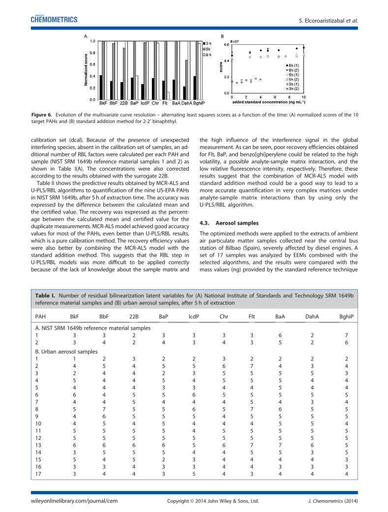
calibration set (dcal). Because of the presence of unexpectedinterfering species, absent in the calibration set of samples, an ad-ditional number of RBL factors were calculated per each PAH andsample (NIST SRM 1649b reference material samples 1 and 2) asshown in Table I(A). The concentrations were also correctedaccording to the results obtained with the surrogate 22B.

Table II shows the predictive results obtained by MCR-ALS andU-PLS/RBL algorithms to quantification of the nine US-EPA PAHsin NIST SRM 1649b, after 5 h of extraction time. The accuracy wasexpressed by the difference between the calculated mean andthe certified value. The recovery was expressed as the percent-age between the calculated mean and certified value for theduplicate measurements. MCR-ALSmodel achieved good accuracyvalues for most of the PAHs, even better than U-PLS/RBL results,which is a pure calibration method. The recovery efficiency valueswere also better by combining the MCR-ALS model with thestandard addition method. This suggests that the RBL step inU-PLS/RBL models was more difficult to be applied correctlybecause of the lack of knowledge about the sample matrix and

the high influence of the interference signal in the globalmeasurement. As can be seen, poor recovery efficiencies obtainedfor Flt, BaP, and benzo[ghi]perylene could be related to the highvolatility, a possible analyte-sample matrix interaction, and thelow relative fluorescence intensity, respectively. Therefore, theseresults suggest that the combination of MCR-ALS model withstandard addition method could be a good way to lead to amore accurate quantification in very complex matrices underanalyte-sample matrix interactions than by using only theU-PLS/RBL algorithm.

4.3. Aerosol samples

The optimized methods were applied to the extracts of ambientair particulate matter samples collected near the central busstation of Bilbao (Spain), severely affected by diesel engines. Aset of 17 samples was analyzed by EEMs combined with theselected algorithms, and the results were compared with themass values (ng) provided by the standard reference technique

Figure 6. Evolution of the multivariate curve resolution – alternating least squares scores as a function of the time: (A) normalized scores of the 10target PAHs and (B) standard addition method for 2-2′ binaphthyl.

Table I. Number of residual bilinearization latent variables for (A) National Institute of Standards and Technology SRM 1649breference material samples and (B) urban aerosol samples, after 5 h of extraction


A. NIST SRM 1649b reference material samples1 3 3 2 3 3 3 3 6 2 72 3 4 2 4 3 4 3 5 2 6

B. Urban aerosol samples1 1 2 3 2 2 3 2 2 2 22 4 5 4 5 5 6 7 4 3 43 2 4 4 2 3 5 5 5 5 34 5 4 4 5 4 5 5 5 4 45 4 4 4 3 3 4 4 5 4 46 6 4 5 5 6 5 5 5 5 57 4 4 5 4 4 4 5 4 3 48 5 7 5 5 6 5 7 6 5 59 4 6 5 5 5 4 5 5 5 510 4 5 4 5 4 4 4 5 5 411 5 5 5 5 4 5 5 5 5 512 5 5 5 5 5 5 5 5 5 513 6 6 6 6 5 6 7 7 6 514 3 5 5 5 4 4 5 5 3 515 5 4 5 2 3 4 4 4 4 316 3 3 4 3 3 4 4 3 3 317 3 4 4 3 5 4 3 4 4 4



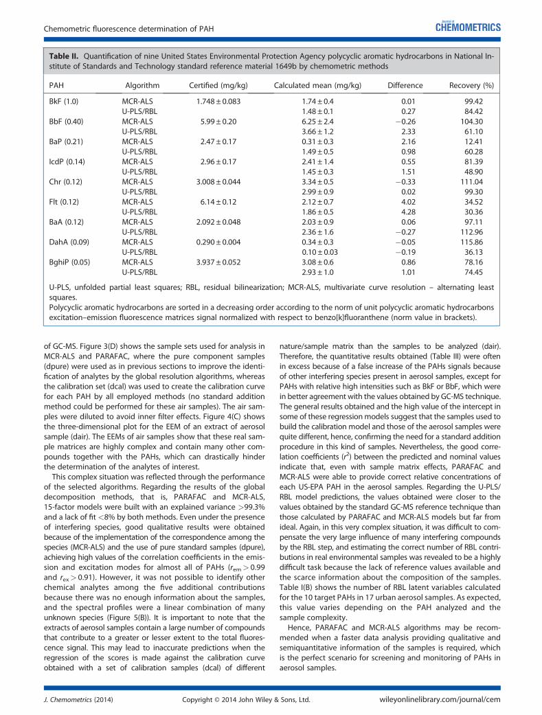
of GC-MS. Figure 3(D) shows the sample sets used for analysis inMCR-ALS and PARAFAC, where the pure component samples(dpure) were used as in previous sections to improve the identi-fication of analytes by the global resolution algorithms, whereasthe calibration set (dcal) was used to create the calibration curvefor each PAH by all employed methods (no standard additionmethod could be performed for these air samples). The air sam-ples were diluted to avoid inner filter effects. Figure 4(C) showsthe three-dimensional plot for the EEM of an extract of aerosolsample (dair). The EEMs of air samples show that these real sam-ple matrices are highly complex and contain many other com-pounds together with the PAHs, which can drastically hinderthe determination of the analytes of interest.This complex situation was reflected through the performance

of the selected algorithms. Regarding the results of the globaldecomposition methods, that is, PARAFAC and MCR-ALS,15-factor models were built with an explained variance >99.3%and a lack of fit <8% by both methods. Even under the presenceof interfering species, good qualitative results were obtainedbecause of the implementation of the correspondence among thespecies (MCR-ALS) and the use of pure standard samples (dpure),achieving high values of the correlation coefficients in the emis-sion and excitation modes for almost all of PAHs (rem> 0.99and rex> 0.91). However, it was not possible to identify otherchemical analytes among the five additional contributionsbecause there was no enough information about the samples,and the spectral profiles were a linear combination of manyunknown species (Figure 5(B)). It is important to note that theextracts of aerosol samples contain a large number of compoundsthat contribute to a greater or lesser extent to the total fluores-cence signal. This may lead to inaccurate predictions when theregression of the scores is made against the calibration curveobtained with a set of calibration samples (dcal) of different

nature/sample matrix than the samples to be analyzed (dair).Therefore, the quantitative results obtained (Table III) were oftenin excess because of a false increase of the PAHs signals becauseof other interfering species present in aerosol samples, except forPAHs with relative high intensities such as BkF or BbF, which werein better agreement with the values obtained by GC-MS technique.The general results obtained and the high value of the intercept insome of these regressionmodels suggest that the samples used tobuild the calibration model and those of the aerosol samples werequite different, hence, confirming the need for a standard additionprocedure in this kind of samples. Nevertheless, the good corre-lation coefficients (r2) between the predicted and nominal valuesindicate that, even with sample matrix effects, PARAFAC andMCR-ALS were able to provide correct relative concentrations ofeach US-EPA PAH in the aerosol samples. Regarding the U-PLS/RBL model predictions, the values obtained were closer to thevalues obtained by the standard GC-MS reference technique thanthose calculated by PARAFAC and MCR-ALS models but far fromideal. Again, in this very complex situation, it was difficult to com-pensate the very large influence of many interfering compoundsby the RBL step, and estimating the correct number of RBL contri-butions in real environmental samples was revealed to be a highlydifficult task because the lack of reference values available andthe scarce information about the composition of the samples.Table I(B) shows the number of RBL latent variables calculatedfor the 10 target PAHs in 17 urban aerosol samples. As expected,this value varies depending on the PAH analyzed and thesample complexity.

Hence, PARAFAC and MCR-ALS algorithms may be recom-mended when a faster data analysis providing qualitative andsemiquantitative information of the samples is required, whichis the perfect scenario for screening and monitoring of PAHs inaerosol samples.

Table II. Quantification of nine United States Environmental Protection Agency polycyclic aromatic hydrocarbons in National In-stitute of Standards and Technology standard reference material 1649b by chemometric methods

PAH Algorithm Certified (mg/kg) Calculated mean (mg/kg) Difference Recovery (%)

BkF (1.0) MCR-ALS 1.748 ± 0.083 1.74 ± 0.4 0.01 99.42U-PLS/RBL 1.48 ± 0.1 0.27 84.42

BbF (0.40) MCR-ALS 5.99 ± 0.20 6.25 ± 2.4 �0.26 104.30U-PLS/RBL 3.66 ± 1.2 2.33 61.10

BaP (0.21) MCR-ALS 2.47 ± 0.17 0.31 ± 0.3 2.16 12.41U-PLS/RBL 1.49 ± 0.5 0.98 60.28

IcdP (0.14) MCR-ALS 2.96 ± 0.17 2.41 ± 1.4 0.55 81.39U-PLS/RBL 1.45 ± 0.3 1.51 48.90

Chr (0.12) MCR-ALS 3.008 ± 0.044 3.34 ± 0.5 �0.33 111.04U-PLS/RBL 2.99 ± 0.9 0.02 99.30

Flt (0.12) MCR-ALS 6.14 ± 0.12 2.12 ± 0.7 4.02 34.52U-PLS/RBL 1.86 ± 0.5 4.28 30.36

BaA (0.12) MCR-ALS 2.092 ± 0.048 2.03 ± 0.9 0.06 97.11U-PLS/RBL 2.36 ± 1.6 �0.27 112.96

DahA (0.09) MCR-ALS 0.290 ± 0.004 0.34 ± 0.3 �0.05 115.86U-PLS/RBL 0.10 ± 0.03 �0.19 36.13

BghiP (0.05) MCR-ALS 3.937 ± 0.052 3.08 ± 0.6 0.86 78.16U-PLS/RBL 2.93 ± 1.0 1.01 74.45

U-PLS, unfolded partial least squares; RBL, residual bilinearization; MCR-ALS, multivariate curve resolution – alternating leastsquares.Polycyclic aromatic hydrocarbons are sorted in a decreasing order according to the norm of unit polycyclic aromatic hydrocarbonsexcitation–emission fluorescence matrices signal normalized with respect to benzo[k]fluoranthene (norm value in brackets).



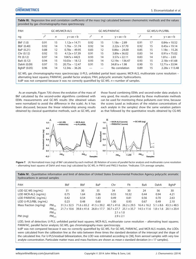
As an example, Figure 7(A) shows the evolution of the mass ofBkF calculated by the second-order algorithms combined withEEMs measurements and GC-MS results (the obtained valueswere normalized to avoid the difference in the scale). As it hasbeen discussed, because the linear relationship among resultsobtained by classical quantitative methods, such as GC-MS, and

those found combining EEMs and second-order data analysis isvery good, the results provided by these multivariate methodscan be used for monitoring these pollutants over time, becausethe scores (used as indicators of the relative concentrations ofeach analyte in the samples) show the same variation patternas that followed by the quantitative results obtained by CG-MS

Table III. Regression line and correlation coefficients of the mass (ng) calculated between chemometric methods and the valuesprovided by gas chromatography-mass spectroscopy

PAH GC-MS/MCR-ALS GC-MS/PARAFAC GC-MS/U-PLS/RBL

ng r2 n y= ax + b r2 n y = ax + b r2 n y = ax +b

BkF (1.0) 0.91 15 1.12x + 14.71 0.92 15 1.18x� 2.89 0.91 17 0.84x + 10.52BbF (0.40) 0.92 14 1.76x� 51.74 0.92 14 2.22x + 37.70 0.92 15 0.45x + 19.14BaP (0.21) 0.88 12 0.78x� 49.95 0.83 12 0.86x� 24.00 0.85 15 1.18x� 15.26Chr (0.12) 0.92 15 4.12x + 57.39 0.91 15 3.89x + 36.02 0.83 14 0.91x + 75.02Flt (0.12) 0.97 14 1047x + 4423 0.93 14 3.57x + 22.11 0.83 14 1.81x� 2.65BaA (0.12) 0.94 15 10.03x� 18.12 0.93 14 12.19x� 136.47 0.93 15 2.18x + 61.68DahA (0.09) 0.97 15 20.75x� 12.47 0.91 15 34.81x + 1.98 0.90 15 12.71x + 33.94BghiP (0.05) 0.96 14 12.34x� 36.26 — — No correlation 0.89 15 2.28x + 113.48

GC-MS, gas chromatography-mass spectroscopy; U-PLS, unfolded partial least squares; MCR-ALS, multivariate curve resolution –alternating least squares; PARAFAC, parallel factor analysis; PAH, polycyclic aromatic hydrocarbons.IcdP was not compared because it was no correctly quantified by GC-MS. n=number of samples.

Figure 7. (A) Normalized mass (ng) of BkF calculated by each method. (B) Relation of scores of parallel factor analysis and multivariate curve resolution– alternating least squares of DahA and mass (ng) calculated by GC-MS, in PM10 and PM2.5 fraction. *Indicates 72 h average samples.

Table IV. Quantitative information and limit of detection of United States Environmental Protection Agency polycyclic aromatichydrocarbons in aerosol samples

PAH BkF BbF BaP Chr Flt BaA DahA BghiP

LOD GC-MS (ng/mL) 31 30 35 34 30 24 56 30LOD MCR-ALS (ng/mL) 0.75 1.64 2.06 0.55 10.32 0.44 0.94 4.21LOD PARAFAC (ng/mL) 0.42 0.54 1.83 0.49 0.81 0.56 0.70 2.63LOD U-PLS/RBL (ng/mL) 0.23 0.48 0.60 1.00 0.93 0.67 0.49 2.10Mass fraction (ng/mg) PM10 31.3 ± 32.5 71.6 ± 65.2 41.5 ± 39.2 40.7 ± 41.6 26.2 ± 29.5 16.4 ± 16.2 5.1 ± 8.6 43.3 ± 48.5

PM2.5 21.7 ± 10.6 39.8 ± 41.6 26.8 ± 17.7 30.7 ± 27.7 25.1 ± 35.7 14.5 ± 11.6 1.8 ± 1.6 20.1 ± 20.4PM10 2.1 ± 1.0

PM (mg) PM2.5 2.9 ± 2.1

LOD, limit of detection; U-PLS, unfolded partial least squares; MCR-ALS, multivariate curve resolution – alternating least squares;PARAFAC, parallel factor analysis; GC-MS, gas chromatography-mass spectroscopy.IcdP was not compared because it was no correctly quantified by GC-MS. For GC-MS, PARAFAC, and MCR-ALS models, the LODswere calculated from the calibration line as the ratio between three times the standard deviation of the intercept and the slope ofthe calculated line. For U-PLS/residual bilinearization, the LOD was estimated according to [38], from aerosol samples with very lowanalyte concentration. Particulate matter mass and mass fractions are shown as mean± standard deviation (n=17 samples).



(Figure 7(B)). In fact, multivariate methods performed betterwhen the results obtained by GC-MS were below the limit of de-tection (LOD), as in the DahA quantification: samples 12 and 13are below the LOD and are plotted as zero values (Figure 7(B)).Quantitative information of the urban aerosol samples analyzedand the LOD of each method is presented in Table IV. It can beseen that the scores calculated by MCR-ALS and PARAFACmodels show low values, but keeping the linear range in fluores-cence, and over the LOD of these models. This demonstrates thehigh sensitivity of the fluorescence spectroscopy coupled tochemometric methods to identify and semiquantify the targetPAHs in the PM10 and PM2.5 fractions of urban aerosols, makingthem suitable for routine monitoring instead of the chromato-graphic techniques

5. CONCLUSIONS

A novel method for the determination of polycyclic aromatichydrocarbons in ambient air aerosol samples, based on thecombination of EEMs and several second-order algorithms, wasevaluated through samples of increasing complexity.Among the algorithms investigated, MCR-ALS and PARAFAC

proved to be fast methods to extract the target chemicalinformation of complex mixtures in presence of unknown andcomplex interference contributions. The constraint of corre-spondence of species applied by MCR-ALS was a decisive factorto achieve a better qualitative analysis when the analyte ofinterest and the interfering background have similar relativesignal intensities and high spectral overlap. Because of thenon-trilinear behavior of the unknown contributions presentin environmental samples, which are mixtures of many com-pounds and residual scattering, the partial trilinear model(MCR-ALS) was very well adapted to describe the behavior ofthe datasets under study.Even with very complex sample matrix effects, the analytical

performance of the second-order resolution methods,PARAFAC and MCR-ALS, shows that they are suitable to moni-tor PAHs patterns in the fine particulate fraction (PM2.5) ofambient air. In addition, these methodologies could be usedwhen a high sensitivity is needed, as in studies of backgroundatmospheres, because fluorescence measurements have thisproperty, or when a fast analysis is required, because PARAFACand MCR-ALS can describe a large number of samples andanalytes with a single model. Therefore, for semiquantitativedeterminations or description of evolution of environmentalpatterns of variation of PAHs, these methods could be a goodalternative to the traditional methods of analysis, showingadvantages in terms of time of analysis, use of solvents, andsensitivity.For quantitative analysis, U-PLS/RBL demonstrated a superior

predictive capability as long as no severe matrix effects arepresent. However, this algorithm is very time-consumingbecause a model is required per sample and per analyte, andthe selection of the correct number of RBL factors is a difficulttask when many unexpected and unknown compounds arepresent, as it happens in environmental samples. In this situa-tion, it has been proven that it is worth exploring further thecombination of MCR-ALS with standard addition method andcorrection by a surrogate, which could provide a faster quantita-tive analysis without needing prior information about the natureof the unknown compounds in environmental samples.

Acknowledgements

The authors gratefully thank the University of the BasqueCountry (UPV/EHU, UFI 11/47) and the Spanish Ministry of Scienceand Innovation (MICINN) for financing the projects PROMESHAP(CTM 2010-20607) and GRACCIE (CSD 2007-00067), co-financedwith FEDER founds. Saioa Elcoroaristizabal also wants to thankUPV/EHU for the doctoral grant and the Chemometrics Group,Department of Analytical Chemistry of the University of Barcelona,for its support during her research stay.

REFERENCES1. Mastral AM, Callén MS. A review on polycyclic aromatic hydrocarbon

(PAH) emissions from energy generation. Environ. Sci. Technol. 2000;34: 3051–3057.

2. Yang HH, Lee WJ, Chen SJ, Lai SO. PAH emission from various indus-trial stacks. J. Hazard. Mater. 1998; 60: 159–174.

3. Ravindra K, Sokhi R, Van Grieken R. Atmospheric polycyclic aromatichydrocarbons: source attribution, emission factors and regulation.Atmos. Environ. 2008; 42: 2895–2921.

4. European Communities. Ambient air pollution by polycyclic aromatichydrocarbons (PAH). Position Paper and Annexes. Office for OfficialPublications of the European Communities, Luxembourg, 2001.

5. International Agency for Research on Cancer. Polynuclear aromaticcompounds, part 1: chemical, environmental, and experimental data.Monographs on the Evaluation of the Carcinogenic Risk of Chemicalsto Humans. Vol. 32, Lyon, France, 1983.

6. Kaupp H, McLachlan MS. Gas/particle partitioning of PCDD/Fs, PCBs,PCNs and PAHs. Chemosphere 1999; 38: 3411–3421.

7. Sheu HL, Lee WJ, Lin SJ, Fang GC, Chang HC, You WC. Particle-boundPAH content in ambient air. Environ. Pollut. 1997; 96: 369–382.

8. Velasco E, Siegmann P, Siegmann HC. Exploratory study of particle-bound polycyclic aromatic hydrocarbons in different environmentsof Mexico City. Atmos. Environ. 2004; 38: 4957–4968.

9. Office of the Federal Registration. Appendix A: priority pollutants.Fed. Reg. 1982; 47: 52309.

10. International Programme on Chemical Safety. Selected non-heterocyclic polycyclic aromatic hydrocarbons. Environment HealthCriteria No. 202. World Health Organization, Geneva, Switzerland, 1998.

11. European Commission. Directive 2004/107/EC of the European par-liament and of the council of 15 December 2004 relating to arsenic,cadmium, mercury, nickel and polycyclic aromatic hydrocarbons inambient air. Off. J. Eur. Union L 2005; 23: 3–16.

12. Liu LB, Liu Y, Lin JM, Tang N, Hayakawa K, Maeda T. Development ofanalytical methods for polycyclic aromatic hydrocarbons (PAHs) inairborne particulates: a review. J. Environ. Sci. 2007; 19: 1–11.

13. Poster DL, Schantz MM, Sander LC, Wise SA. Analysis of polycyclicaromatic hydrocarbons (PAHs) in environmental samples: a criticalreview of gas chromatographic (GC) methods. Anal. Bioanal. Chem.2006; 386: 859–881.

14. International Organization for Standardization. Ambient air. Determi-nation of particle-phase polycyclic aromatic hydrocarbons by highperformance liquid chromatography. ISO 16362:2005.

15. Karcher W, Fordham RJ, Dubois JJ, Glaude PGJM, Ligthart JAM. SpectralAtlas of Polycyclic Aromatic Compounds Including Data on Occurrenceand Biological Activity. D. Reidel: Dordrecht, The Netherlands, 1985.

16. Sharma H, Jain VK, Khan ZH. Identification of polycyclic aromatichydrocarbons (PAHs) in suspended particulate matter by synchro-nous fluorescence spectroscopic technique. Spectrochim. Acta, PartA 2007; 68: 43–49.

17. Mastral AM, López JM, Callén MS, García T, Murillo R, Navarro MV.Spatial and temporal PAH concentrations in Zaragoza, Spain. Sci.Total Environ. 2003; 307: 111–124.

18. Sundt RC, Beyer J, Vingen S, Sydnes MO. High matrix interferenceaffecting detection of PAH metabolites in bile of Atlantic hagfish(Myxine glutinosa) used for biomonitoring of deep-water oil produc-tion. Mar. Environ. Res. 2011; 71: 369–374.

19. Patra D, Mishra AK. Recent developments inmulti-component synchro-nous fluorescence scan analysis. Trends Anal. Chem. 2002; 21: 787–798.

20. Mastral AM, Pardos C, Rubio B, Galbán J. Analytical determinationof polycyclic aromatic hydrocarbons in gases from coal conversion



by synchronous fluorescence spectrometry. Anal. Lett. 1995; 28:1883–1895

21. Nahorniak ML, Booksh KS. Excitation–emission matrix fluorescencespectroscopy in conjunction with multiway analysis for PAHdetection in complex matrices. Analyst 2006; 131: 1308–1315.

22. Jiji RD, Andersson GG, Booksh KS. Application of PARAFAC for calibrationwith excitation–emission matrix fluorescence spectra of three classes ofenvironmental pollutants. J. Chemometrics 2000; 14: 171–185.

23. Arancibia JA, Boschetti CE, Olivieri AC, Escandar GM. Screening of oilsamples on the basis of excitation—emission room-temperaturephosphorescence data and multiway chemometric techniques.Introducing the second-order advantage in a classification study.Anal. Chem. 2008; 80: 2789–2798.

24. Bro R. PARAFAC. Tutorial and applications. Chemom. Intell. Lab. Syst.1997; 38: 149–171.

25. Tauler R. Multivariate curve resolution applied to second order data.Chemom. Intell. Lab. Syst. 1995; 30: 133–146.

26. Tauler R, Maeder M, de Juan A. Chapter 2.24. Multiset data analysis:extended multivariate curve resolution. In ComprehensiveChemometrics, Brown SD, Tauler R, Walczak B (eds.). Elsevier, TheNetherlands, 2009; 473–505.

27. de Juan A, Tauler R. Multivariate curve resolution (MCR) from 2000:progress in concepts and applications. Crit. Rev. Anal. Chem. 2006;36: 163–176.

28. Olivieri AC. On a versatile second-order multivariate calibrationmethod based on partial least-squares and residual bilinearization:second-order advantage and precision properties. J. Chemometrics2005; 19: 253–265.

29. Nahorniak ML, Booksh KS. Optimizing the implementation of thePARAFAC method for near-real time calibration of excitation-emission fluorescence analysis. J. Chemometrics 2003; 17: 608–617.

30. Bosco MV, Larrechi MS. PARAFAC and MCR-ALS applied to thequantitative monitoring of the photodegradation process of polycy-clic aromatic hydrocarbons using three-dimensional excitation emis-sion fluorescent spectra: comparative results with HPLC. Talanta2007; 71: 1703–1709.

31. Beltrán JL, Ferrer R, Guiteras J. Multivariate calibration of polycyclicaromatic hydrocarbon mixtures from excitation–emission fluores-cence spectra. Anal. Chim. Acta. 1998; 373: 311–319.

32. Elcoroaristizabal S, de Juan A, García JA, Durana N, Alonso L.Comparison of second-order multivariate methods for screening

and determination of PAHs by total fluorescence spectroscopy.Chemom. Intell. Lab. Syst. 2014; 132: 63–74.

33. International Organization for Standardization. Ambient air.Determination of total (gas and particle-phase) polycyclic aromatichydrocarbons. Collection on sorbent-backed filters with gaschromatographic/mass spectrometric analyses. ISO 12884:2000, ISOGeneva, 2000.

34. Bahram M, Bro R, Stedmon C, Afkhami A. Handling of Rayleigh andRaman scatter for PARAFAC modeling of fluorescence data usinginterpolation. J. Chemometrics 2006; 20: 99–105.

35. Windig W, Guilment J. Interactive self-modeling mixture analysis.Anal. Chem. 1991; 63: 1425–1432.

36. Bro R, Kiers HAL. A new efficient method for determining thenumber of components in PARAFAC models. J. Chemometrics 2003;17: 274–286.

37. Haaland DM, Thomas EV. Partial least-squares methods for spectralanalyses. 1. Relation to other quantitative calibration methodsand the extraction of qualitative information. Anal. Chem. 1988;60: 1193–1202.

38. Bortolato SA, Arancibia JA, Escandar GM. Chemometrics-assistedexcitation-emission fluorescence spectroscopy on nylon mem-branes. Simultaneous determination of benzo[a]pyrene and dibenz[a,h]anthracene at parts-per-trillion levels in the presence of theremaining EPA PAH priority pollutants as interferences. Anal. Chem.2008; 80: 8276–8286.

39. Braga JWB, Carneiro RL, Poppi RJ. Evaluation of the number of factorsneeded for residual bilinearization in BLLS and UPLS models toachieve the second-order advantage. Chemom. Intell. Lab. Syst.2010; 100: 99–109.

40. Jaumot J, Gargallo R, de Juan A, Tauler R. A graphical user-friendlyinterface for MCR-ALS: a new tool for multivariate curve resolutionin MATLAB. Chemom. Intell. Lab. Syst. 2005; 76: 101–110.

41. Andersson CA, Bro R. The N-way toolbox for MATLAB. Chemom. Intell.Lab. Syst. 2000; 52: 1–4.

42. Olivieri AC, Wu HL, Yu RQ. MVC2: a MATLAB graphical interfacetoolbox for second-order multivariate calibration. Chemom. Intell.Lab. Syst. 2009; 96: 246–251.

43. Peré-Trepat E, Lacorte S, Tauler R. Alternative calibration approaches forLC-MS quantitative determination of coeluted compounds in complexenvironmentalmixtures usingmultivariate curve resolution.Anal. Chim.Acta. 2007; 595: 228–237.



Documents

Documento Tesis superdef_jmar - ADDI