Embed Size (px)
Citation preview

Divide-and-Conquer with Sequential Monte Carlo
Fredrik [email protected]
Dept. of EngineeringThe University of Cambridge
Cambridge, UK
Adam M. [email protected]
Dept. of StatisticsThe University of Warwick
Coventry, UK
Christian A. [email protected]. of Automatic Control
Linkoping UniversityLinkoping, Sweden
Bonnie [email protected]
Dept. of Computer ScienceUniversity of MiamiMiami, Florida, USA
Thomas B. [email protected]
Dept. of Information TechnologyUppsala UniversityUppsala, Sweden
John [email protected] Statistical Laboratory
The University of CambridgeCambridge, UK
Alexandre [email protected]
Dept. of StatisticsThe University of British Columbia
Vancouver, Canada
Abstract
We develop a Sequential Monte Carlo (SMC) procedure for inference in proba-bilistic graphical models using the divide-and-conquer methodology. The methodis based on an auxiliary tree-structured decomposition of the model of interestturning the overall inferential task into a collection of recursively solved sub-problems. Unlike a standard SMC sampler, the proposed method employs multi-ple independent populations of weighted particles, which are resampled, merged,and propagated as the method progresses. We illustrate empirically that this ap-proach can outperform standard methods in estimation accuracy. It also opensup novel parallel implementation options and the possibility of concentrating thecomputational effort on the most challenging sub-problems. The proposed methodis applicable to a broad class of probabilistic graphical models. We demonstrateits performance on a Markov random field and on a hierarchical Bayesian model.
1 Introduction
Sequential Monte Carlo (SMC) samplers [7] are a popular class of algorithms for simulating fromsome probability distribution of interest. The most well-known application of SMC is to the filteringproblem in general state-space hidden Markov models [12]. However, these methods are muchmore generally applicable and there has been much recent interest in using SMC for sampling fromprobabilistic models that are not defined sequentially. This typically involves using SMC to targeta sequence of auxiliary distributions which are constructed to admit the original distribution as anappropriate marginal [8]. Examples include annealing [8], data tempering [6], and sequential modeldecompositions [3, 22], to mention a few.
For many statistical models of interest, however, a sequential decomposition might not be the mostnatural nor computationally efficient way of approaching the inference problem. In this contributionwe propose an extension of the classical SMC framework, Divide-and-Conquer SMC (D&C-SMC),
1

which we believe will further widen the scope of SMC samplers and provide efficient computationaltools for Bayesian inference within a broad class of probabilistic models.
The idea behind D&C-SMC involves building an approximation by splitting the model into indepen-dent components and defining, for each of these, a suitable auxiliary target distribution. Samplingfrom these distributions can then be done in parallel, whereafter the results are merged to providea solution to the original problem of interest. By the divide-and-conquer methodology we can thenrepeat this procedure for each of the components. This corresponds to breaking the overall infer-ential task into a collection of simpler problems. We demonstrate that this strategy is effective notonly when the model has an obvious hierachical structure (for example, Figure 1), but also in caseswhere the hierarchical decomposition is artificial (Figure 2). In either case, one iteratively exploitscheap solutions to easy sub-problems as a first step in the solution of a more complex problem (forexample, as the first step of an SMC annealing sequence). The intuition behind the effectivenessof the method is that having C independent populations of N particles provide NC points in theparameter space which can be interpreted as a stratified sample with a storage cost O(NC).
Related work A number of related ideas have appeared in the literature although all have differedin key respects from the approach described herein. In [18] and [4, 26] belief propagation is ad-dressed using importance sampling and SMC, respectively, and these methods feature coalescenceof particle systems, although they do not provide samples targeting a distribution of interest in anexact [1] sense. Coalescence of particle systems in a different sense is employed by [16] which alsouses multiple populations of particles; here the state space of the full parameter vector is partitioned,rather than the parameter vector itself. The island particle model of [29] employs an ensemble ofparticle systems which themselves interact according to the usual rules of SMC with every particlesystem targetting the same distribution over the full set of variables. The local particle filtering ap-proach of [25] attempts to address degeneracy (in a hidden Markov model context) via an (inexact)localisation technique. Numerous authors have proposed SMC algorithms for tree-structured prob-lems [27, 3, 21]; these approaches depend upon the particular structure of the problems that theyaddress and generally employ a single particle population.
2 Divide-and-Conquer Sequential Monte Carlo
In this section we present the basic D&C-SMC method, which can be thought of as the analogueto the sequential importance resampling (SIR) method in the context of classical SMC. We alsoestablish some basic theoretical results for this sampler, namely consistency and unbiasedness of thenormalizing constant estimate. It should be noted that the D&C-SIR method is only the basic build-ing block of our proposed methodology. As with standard SMC algorithms, a range of techniquesare available to improve on D&C-SIR, and we discuss several possible extensions in Section 3.
2.1 Divide-and-Conquer Sequential Importance Resampling
Let γ(x) be a target probability density function of interest, defined on some measurable space(X,X ). A generic Monte Carlo procedure approximates γ by a collection of weighted samples(xi,wi)Ni=1 (which we call a population), in the sense that (
∑j w
j)−1∑iw
ih(xi) is an estima-tor of
∫h(x)γ(x)dx. In SMC, a sequence of intermediate target densities is used to sequentially
construct an approximation of γ. Instead of using a single sequence of auxiliary densities, how-ever, we propose a method that makes use of a tree of auxiliary densities. The specification of theintermediate distributions defined on the tree is a design choice—just as for the case of classicalSMC—guided by the structure of the model. This construction allows the application of SMC tomany models of interest without the identification of any natural sequential structure. Unlike a stan-dard SMC sampler, this method maintains multiple independent populations of weighted particles,which are propagated and merged as the algorithm progresses.
Formally, let T be an index set, which we interpret as organized on a tree using the followingnotation: for all t ∈ T , we let the list C(t) ⊂ T (with the obvious abuse of set-notation) denote thechildren of node t, with C(t) = ∅ if t is a leaf, and let r ∈ T denote the root of the tree. To eachnode t ∈ T , we associate an auxiliary target density γt(xt), defined on some set Xt. We assumethat γt(xt) = γt(xt)/Zt where γt can be evaluated point-wise, but Zt may be unknown. Thetarget density associated with the root of the tree is taken to be the original distribution of interest,
2

Algorithm 1 dc smc(t) // by convention∏c∈∅(·) = 1
1. For c ∈ C(t):
(a) ((xic,wic)Ni=1, Z
Nc )← dc smc(c).
(b) Resample (xic,wic)Ni=1 to obtain the equally weighted particle system (xic, 1)Ni=1.
2. For particle i = 1, . . . , N :
(a) Simulate xit ∼ qt(· | xic1 , . . . , xicC ) from some proposal kernel on Xt, and where
(c1, c2, . . . , cC) = C(t).(b) Set xit = (xic1 , . . . , x
icC , x
it).
(c) Compute wit =
γt(xit)∏
c∈C(t) γc(xic)
1
qt(xit | xic1 , . . . , xicC ).
3. Compute ZNt ={
1N
∑Ni=1 w
it
}∏c∈C(t) Z
Nc .
4. Return ((xit,wit)Ni=1, Z
Nt ).
Level 2:
Level 1:
Level 0:
y1 y2 y3
x1 x2 x3
y1 y2 y3
x1 x2 x3
x4
y1 y2 y3
x1 x2 x3
x4
x5
Figure 1: Decomposition of a hierarchical Bayesian model.
i.e. Xr = X and γr(x) ≡ γ(x). Furthermore, we assume that the spaces on which these targetdistributions are defined are constructed recursively as
Xt =(⊗c∈C(t)Xc
)× Xt
where the “incremental” set Xt can be chosen arbitrarily (in particular, Xt = ∅ is a valid choice).
The D&C-SMC algorithm uses a bottom-up approach to simulate from the auxiliary target distri-butions defined on the tree, by repeated resampling, propagation, and weighting steps, analogouslyto a standard SMC. The difference, as pointed out above, is that the D&C-SMC algorithm main-tains multiple independent populations of weighted particles which are recursively merged untilthe last iteration of the algorithm when all populations are merged at the root of the tree. We de-scribe the algorithm by specifying the operations that are carried out at each node of the tree. Fort ∈ T , we define a procedure dc smc(t) which returns, (1) a weighed particle system (xit,w
it)Ni=1
targeting γt, and (2) an estimator ZNt of the normalizing constant Zt, as in Algorithm 1. If theincremental set is empty (i.e. Xt = ∅), we omit step 2(a) and the division by the proposal density instep 2(c). Now, a particle system targeting γ(x) and an estimator of Z can be generated by calling((xi,wi)Ni=1, Z
N )← dc smc(r).
To illustrate the sampling procedure, consider the special case of inference in a hierarchical Bayesianmodel as shown in Figure 1. To use D&C-SMC for this model, we start by isolating the latent vari-ables at the bottom layer (Figure 1; left). By defining some arbitrary “pseudo-priors” for thesevariables, we can simulate from the resulting “pseudo-posteriors” (i.e., the auxiliary target distribu-tions) by importance sampling. This results in three independent particle populations (xit,w
it)Ni=1
for t = 1, 2, 3. Next, we introduce the parent node(s) at level 1 (Figure 1; middle). We simulate Nparticles from the product of the child populations and propagate these upward to target the auxiliarydistributions at this level. Finally, we repeat this procedure by introducing the root node at level 0,resulting in a weighted particle system targeting the joint posterior distribution of the full model.
3

In the example outlined above the graphical model is a tree, in which case the tree T can be obtaineddirectly from the model. However, we emphasize that this is not a requirement. Indeed, the D&C-SMC method can be applied to arbitrary decomposition of models: the tree T will then reflectthe model decomposition, rather than the model itself. In principle, D&C-SMC can be used forinference in rather general Bayesian networks, as well as for undirected Markov random fields (seeSection 4.1). Note also that D&C-SMC generalises the usual SMC framework; if |C(t)| = 1 for allinternal nodes, the D&C-SIR procedure described above reduces to a standard SIR method.
2.2 Theoretical Properties
As D&C-SMC consists of standard SMC steps combined with particle-system coalescence steps,it is possible with care to extend many of the results from the standard, and by now well-studied,SMC setting (see e.g., [7] for a comprehensive collection of theoretical results). The unbiasednessof the normalising constant estimate of standard SMC algorithms [7, Prop. 7.4.1] is inherited byD&C-SMC. For parsimony we consider a simplified case (the extension to the general case isstraightforward but cumbersome; the proof follows mutatis mutandis). A more general consistencyresult is also provided. The proofs of the two propositions stated below are given in Appendix A.Proposition 1. Assume that we employ a balanced binary tree decomposition, that appropriateabsolute continuity requirements are met, and that multinomial sampling is carried out for everypopulation and during every iteration. We then have that E[ZNr ] = Zr for any N ≥ 1.Proposition 2. Under regularity conditions detailed in Appendix A.2, the weighted particle sys-tem (xN,ir ,wN,i
r )Ni=1 generated by dc smc(r) is consistent in that for all non-negative, bounded,measurable functions f : X→ R:
N∑i=1
wN,it∑N
j=1 wN,jt
f(xN,ir )P−→∫f(x)γ(x)dx, as N →∞.
3 More Sophisticated Divide-and-Conquer SMC Algorithms
The simple D&C-SIR algorithm described above provides the basic structure of an algorithm whichrecursively applies sampling and resampling strategies to decompositions of arbitrary graphs. It islimited in scope, depending as it does on a single sampling of each variable combined with resam-pling steps, and was provided to demonstrate the idea in it simplest form. The extensions presentedhere comprise fundamental components of the general strategy introduced in this paper, and may berequired to obtain good performance in challenging settings.
3.1 Mitigating Degeneracy
The above algorithm is essentially an SIR algorithm and variables are not rejuvenated after their firstsampling. Inevitably, as in particle filtering, this will lead to degeneracy as repeated resampling stepsreduce the number of unique values of each variable represented within the sample. Techniquesemployed to ameliorate this problem in the particle filtering literature could be used — fixed lagtechniques [17] might make sense in some settings as could incorporating MCMC moves [15].However, here we focus upon more sophisticated methods which address the problem directly.
Merging Subpopulations via Mixture Sampling The resampling in Step 1b of the dc smc pro-cedure, which combines subpopulations to target a new distribution on a larger space, is critical.The independent multinomial resampling of child populations in the basic D&C-SIR procedure cor-responds to sampling N times with replacement from the product measure ⊗c∈C(t)γNc (dxc), whereγNc (dxc) := (
∑Nj=1 w
jc)−1∑Ni=1 w
icδxi
c(dxc) is the particle approximation of γc constructed at
node c. The low computational cost of this approach is appealing, but unfortunately it can leadto high variance when the product
∏c∈C(t) γc(xc) differs substantially from the corresponding
marginal of γt.
An alternative approach akin to the mixture proposal approach [5] or the auxiliary particle filter [24]might be particularly useful in the present setting, as it allows us to exploit the fact that the productmeasure has mass upon N |C(t)| points, in order to capture the dependencies among the variables
4
in the target distribution γt(xt). Let γt(xc1 , . . . ,xcC ) be some distribution which incorporates thisdependency (in the simplest case we might take γt ≈
∫γt(xc1 , . . . ,xcC , xt)dxt or, when Xt = ∅,
γt ≡ γt; see below for an alternative). We can then replace Step 1b of Algorithm 1 with simulating{(xic1 , . . . , x
icC )}Ni=1 from
Qt(dxc1 , . . . , dxcC ) :=
N∑i1=1
. . .
N∑iC=1
vt(i1, . . . , iC)δ(x
i1c1,...,x
iCcC
)(dxc1 , . . . , dxcC )∑N
j1=1 . . .∑NjC=1 vt(j1, . . . , jC)
, (1)
vt(i1, . . . , iC) :=
∏c∈C(t)
wicc
γt(xi1c1 , . . . ,x
iCcC )
/ ∏c∈C(t)
γc(xicc ),
with the weights of Step 2c computed using wit = γt(x
it)/[γt(x
i1c1 , . . . , x
iCcC )qt(x
it | xi1c1 , . . . , x
iCcC )].
Clearly, the computational cost of simulating from Qt will be O(N |C(t)|). However, we envisagethat both |C(t)| and the number of coalescence events (i.e. combinations of subpopulations via thisstep) are sufficiently small that this is not a problem in many cases. Furthermore, if this approach isemployed it significantly mitigates the impact of resampling and it is possible to reduce the branch-ing factor by introducing additional (dummy) internal nodes in T . For example, by introducingadditional nodes in order to obtain a binary tree (see Section 4.1), the merging of the child popula-tions will be done by coalescing pairs, gradually taking the dependencies between the variables intoaccount.
SMC Samplers & Tempering A common strategy when simulating from some complicated dis-tribution is to construct a synthetic sequence of distributions which moves from something tractableto the target distribution of interest, with proposal distributions corresponding to MCMC transi-tions. This idea underlies Annealed Importance Sampling (AIS; [23]) and a simple version of theSequential Monte Carlo (SMC; [8]) sampler which adds resampling steps to AIS.
Step 2 of Algorithm 1 corresponds essentially to a (sequential) importance sampling step: extend-ing an existing sample which is weighted to target the product of distributions
∏c∈C(t) γc(xc) by
sampling from qt(xt | xc1 , . . . ,xcC ) and then reweighting it to target γt(xt). We can straightfor-wardly replace this with several SMC sampler iterations, targeting distributions which bridge fromγt,0(xt) = {
∏c∈C(t) γc(xc)}qt(xt | xc1 , . . . ,xcC ) to γt,nt(xt) = γt(xt), typically by following a
geometric path γt,j ∝ γ1−αj
t,0 γαj
t,ntwith 0 < α1 < . . . < αnt
= 1. Step 2 is then replaced by:
2′. (a) For i = 1 to N , simulate xit ∼ qt(· | xic1 , . . . , xicC ).
(b) For i = 1 to N , set xit,0 = (xic1 , . . . , xicC , x
it) and wi
t,0 = 1.(c) For SMC sampler iteration j = 1 to nt:
i. For i = 1 to N , compute wit,j = wi
t,j−1γt,j(xit,j−1)/γt,j−1(xit,j−1).
ii. Optionally, resample (xit,j−1,wit,j)
Ni=1 and override the notation (xit,j−1,w
it,j)
Ni=1 to
refer to the resampled particle system.iii. For i = 1 to N , draw xit,j ∼ Kt,j(x
it,j−1, ·) using a γt,j-invariant Markov kernel Kt,j .
(d) Set xit = xit,ntand wi
t = wit,nt
.
The computation of normalising constant estimates has been omitted for brevity, but follows bystandard arguments. To enable efficient initialisation of each (node-specific) SMC sampler we cancombine this approach with the mixture resampling in (1), in which case the initial bridging distri-bution is given by γ′t,0(xt) = γt(xc1 , . . . ,xcC )qt(xt | xc1 , . . . ,xcC ) with, for α? ∈ (0, α1),
γt(xx1, . . . ,xcC ) ∝
∏c∈C(t)
γc(xc)
1−α? [∫γt,nt
(xx1, . . . ,xcC , xt)dxt
]α?
. (2)
The combination of tempering distributions in this way within this algorithm provides an algo-rithm class which allows us to bridge two standard strategies for employing SMC within the field ofBayesian inference: the trivial case in which the full graph is included from the outset corresponds tothe usual tempering approach and the case in which everything except the data is included from the
5

outset and these observed leaves are gradually included corresponds to [6]. Combining data temper-ing and the approach proposed here is straightforward and might be advantageous when likelihoodevaluation is costly.
Particle MCMC The seminal paper [1] demonstrated that SMC algorithms can be used to produceapproximations of idealised block-sampling proposals within Markov chain Monte Carlo (MCMC)algorithms. By interpreting these Particle MCMC (PMCMC) algorithms as standard algorithms onan extended space, incorporating all of the variables sampled during the running of these algorithms,they can be shown to be exact, in the sense that the apparent approximation does not change the in-variant distribution. Proposition 1, and in particular the construction used in its proof, demonstrateshow the class of D&C-SMC algorithms can be incorporated within the PMCMC framework. Suchtechniques are now essentially standard, once an appropriate auxiliary variable representation isobtained, we do not dwell on this approach here.
3.2 Improving Computational Efficiency
Section 3.1 focused on algorithmic improvements. This section summarises techniques to improvethe computational performance of the approach.
Adaptation Adaptive SMC algorithms have been the focus of much attention in recent years. In[9] comes the first formal validation of algorithms in which resampling is conducted only sometimesaccording to the value of some random quantity obtained from the algorithm itself. We advocate theuse of low variance resampling algorithms [10, e.g.] to be applied adaptively. Other adaptation ispossible within SMC algorithms. Two approaches are analyzed formally by [2]: the adaptation ofthe parameters of the MCMC kernels employed (step 2′(c)iii.) and of the number and location ofdistributions employed within tempering algorithms, i.e., nt and α1, . . . , αnt ; see e.g., [30] for oneapproach to this. Adaptation is especially appealing within dc smc: beyond the usual advantages itallows for the concentration of computational effort on the more challenging parts of the samplingprocess. Using adaptation will lead to more intermediate distributions for the sub-problems (i.e., thesteps of the D&C-SMC algorithm) for which the starting and ending distributions are more different.
Sample Size We have assumed throughout that all particle populations are of size N . This isnot necessary: naturally, fewer particles are required to represent simpler low-dimensional distribu-tions than to represent more complex distributions. Manually or adaptively adjusting the number ofparticles used within different steps of the algorithm remains a direction for future investigation.
4 Experiments
4.1 Markov Random Field - The Classical XY model
One model class for which the D&C-SMC algorithm can be potentially useful are Markov randomfields (MRFs). To illustrate this, we consider the square-lattice classical XY model of statisticalmechanics; see e.g. [20]. This model is a generalization of the well-known Ising model, in the sensethat each lattice site is described by the planar angle of its spin configuration, i.e. xk ∈ (−π, π].The configuration probability is given by p(x) ∝ e−βH(x), where β ≥ 0 is the inverse temperatureand H(x) = −
∑(k,`)∈E cos(xk − x`). Here, E denotes the edge set for the graphical model
which we assume correspond to nearest-neighbour interactions with periodic boundary conditions,see Figure 2 (rightmost figure).
Let the lattice size be M ×M , with M being a power of 2. The D&C-SMC method divides thecomplete inference problem over the M2 variables into a series of simpler problems over subsets ofthe variables. Specifically, we start by dividing the lattice into two halves, removing all the edgesbetween them. We then continue recursively, splitting each sub-model in two, until we obtain a col-lection of M2 disconnected nodes; see Figure 2. This decomposition of the model defines a binarytree T , on which the D&C-SMC algorithm operates. At the leaves we initialize M2 independentparticle populations by sampling uniformly over (−π, π]. These populations are then resampled,merged, and reweighted as we proceed up the tree, successively reintroducing the “missing” edgesof the model. This defines the basic D&C-SIR procedure for the MRF which we extend using the
6

Figure 2: The disconnected components correspond to the groups of variables that are targeted by the differentpopulations of the D&C-SMC algorithm. At the final iteration, corresponding to the rightmost figure, werecover the original, connected model.
9920
9925
9930
9935
9940
9945
9950
9955
(N,n) = (50, 5000) (N,n) = (500, 500) (N,n) = (5000, 50)
AIS
SMC
D&C-SMC (a)
D&C-SMC (b)10
−2
10−1
100
101
(N,n) = (50, 5000) (N,n) = (500, 500) (N,n) = (5000, 50)
Figure 3: Box-plots over 50 runs of each sampler, using N particles and a total of n annealing steps. D&C-SMC (b) uses fewer particles, N = 50, 309, and 475 in the three columns (left to right), respectively, to matchits computational cost to the other methods. Left: Estimates of log(Z). The horizontal lines correspond to minand max of 10 runs of AIS with (N,n) = (10, 100 000). Right: MSE (log-scale) for the estimates of E[xk](averaged over the grid).
tempering method discussed in Section 3.1: when the edges connecting two sub-graphs are reintro-duced this is done gradually according to an annealing schedule to avoid severe particle depletion atthe later stages of the algorithm.
We consider a grid of size 64 × 64 with β = 1 (close to the Kosterlitz-Thouless phase transitionat β ≈ 1.1 [28]). We compare the D&C-SMC algorithm with AIS [23] and with standard SMCsamplers [8]. We run two instances of D&C-SMC: (a) using independent resampling when mergingsubpopulations, and (b) using mixture resampling (see Section 3.1) with the target distribution de-fined as in (2). We run all methods for a varying number of particles N and annealing steps n. ForD&C-SMC the total budget of n annealing steps are divided among the generations of the algorithm.Furthermore, with N particles, D&C-SMC (b) has a rough computational cost of Nn + N2 (Nnfor the other methods) and therefore it is allowed fewer particles than its competitors. All in all, themethods take essentially the same amount of time to run for the different settings. We use linearannealing and single-site Gibbs updates within all methods. We also considered geometric sched-ules as suggested by [23], but we did not see any improvement of the results. Additional detailson the experimental setup are given in Appendix B. Note that for the classical XY model efficient,special-purpose, MCMC algorithms have been developed; see e.g. [28]. We do not compare againstthese as our purpose is to demonstrate the applicability of D&C-SMC to MRFs in general. However,D&C-SMC can employ any application-specific MCMC kernels available in particular contexts.
We consider first the estimates of the normalizing constant Z, a quantity of central interest for thesemodels. Note that all methods give rise to unbiased estimators of Z, but following standard practice,we compute log(Z), resulting in a negative bias. Therefore, larger values typically imply moreaccurate results. Box-plots for 50 independent runs of each method are reported in Figure 3 (left).When we use a comparatively large number of annealing steps n and few particles N , all methodsgive very similar results. If we decrease n (and instead increase N ), however, the performanceof both AIS and standard SMC samplers markedly degrade, but D&C-SMC continue to provideaccurate results, demonstrating robustness to these design parameters.
7

10 Particles 100 Particles 1 000 Particles 10k Particles
Bro
nx
−0.4 0.0 0.2 0.4
05
1015
−0.4 0.0 0.2 0.4
05
1015
−0.4 0.0 0.2 0.4
05
1015
−0.4 0.0 0.2 0.4
05
1015
-0.03(0.06) -0.05(0.04) -0.04(0.05) -0.04(0.05)
Que
ens
−0.4 0.0 0.2 0.4
05
1015
−0.4 0.0 0.2 0.4
05
1015
−0.4 0.0 0.2 0.4
05
1015
−0.4 0.0 0.2 0.4
05
1015
0.07(0.07) 0.03(0.04) 0.04(0.05) 0.04(0.04)
Figure 4: Approximation of the posterior distribution on δe for two boroughs (rows) and four computationalregimes (columns). A reasonable approximation can be obtained using 1 000 particles. The same observationis true for the other variables of the model (see Appendix C). The approximate posterior mean and standarddeviation are shown below each histogram.
Next, we consider the approximations of the target distribution p(x). We look at the mean estimatesof the lattice variables xk—quantities which are known to be zero by symmetry—and compute themean-squared errors (MSEs) over the lattice. The results are reported in Figure 3 (right). In thisrespect, D&C-SMC offers an order-of-magnitude improvement over AIS and a significant improve-ment over standard SMC samplers as well, for all the considered values of N and n.
4.2 Hierarchical Bayesian Model - New York State Mathematics Test
In this section, we demonstrate the scalability of our method by analysing a dataset containingNew York State Mathematics Test results for elementary and middle schools in New York City.The data (see Appendix C for specific details) consists of a table of test results, where each row tcontains the school code, the year, the number Mt of grade 3 students tested in that year and school,and the number mt of these Mt students that obtained a score higher than a fixed threshold. Wehave such information for a total of 278 399 test instances. Second, we have a set of hierarchicalrelationships defined on the school codes: each school code (there are 710 distinct schools in total)is given a unique school district number (there are 32 distinct districts in total), and each schooldistrict number is given a unique borough (from: Manhattan, The Bronx, Brooklyn, Queens, StatenIsland). Following standard practice in multi-level data analysis [14], we organize the data into atree (with nodes indexed by a set T ) where a path from the root to a leaf has the following form:NYC (root), borough of the school district, school district, school, year. Each leaf t ∈ T comes withan observation of mt successes out of Mt trials. We model these with a binomial distribution withsuccess probability parameter pt = logistic(θt), where θt are latent parameters. We attach latentvariables θt to internal nodes of the tree as well, and model the difference in values along an edgee = (t → t′) of the tree with the following expression θt′ = θt + ∆e, where, ∆e ∼ N(0, σ2
e).We can think of ∆e as describing the contribution of the information attached at t′ to the students’scores relative to the information attached at t. We put an improper prior (uniform on (−∞,∞)) onθr.1 We also make the variance random, but shared across siblings, σ2
e = σ2t ∼ Exp(1).
We apply the basic D&C-SIR to this problem, using the natural hierarchical structure provided bythe model. Note that conditionally on values for σ2
t and for the θt at the leaves, the other randomvariables are multivariate normal and can therefore be marginalised. The dimensionality of theremaining parameters in our dataset is 3 555; see Appendix C.2 for details. We varied the numberof particles, and assessed the quality of the D&C-SIR approximation of the posterior distributionof δe = (logistic(θt′) − logistic(θt))|m,M , where e = (t, t′) range over the top level edges, andm,M denotes the full set of observations. This can be interpreted as the difference in values ofprobabilities of success pt brought by the borough information. In Figure 4, we show the resultsfor the borough with the largest and smallest E[δe|m,M ], the results of the other boroughs are in
1When mt /∈ {0,Mt} for at least one leaf, this can be easily shown to yield a proper posterior.
8

Appendix C.3, where we also show results for the parameters σt. For all parameters, we can seethat a moderate number of particles—as few as 1 000—is sufficient to accurately approximate theposterior distribution.
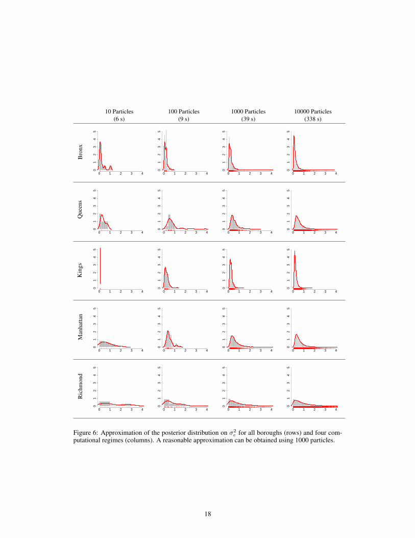
The qualitative results are in broad agreement with other socio-economic indicators. For example,among the five counties corresponding to each of the five boroughs, Bronx County has the highestfraction (41%) of children (under 18) living below poverty level.2 Queens has the second lowest(19.7%, after Richmond (Staten Island), 16.7%), however the fact that Staten Island contains a singleschool district means that our posterior distribution is much flatter for this borough (see Figure 6 inAppendix C).
A Theoretical Properties
A.1 Unbiasedness of the normalising constant estimate
We consider, in the unbiasedness result below, a simple case in which the sequence of subpopulationsis specified by a balanced binary tree. The extension to the general case is straightforward butnotationally cumbersome. Notationally, we assume that subpopulation h at depth d is obtainedfrom subpopulations 2h − 1 and 2h at depth d + 1. We also consider only the case of multinomialresampling during every iteration; again this may be straightforwardly relaxed. We note in particularthat the extension to balanced trees of degree greater than two is trivial and that unbalanced treesmay be addressed by the introduction of trivial dummy nodes (or directly, at the expense of furthercomplicating the notation).
First we specify sets in which multi-indices of particle populations live:
〈D〉2 =
D⋃d=0
{d} ⊗ {1, . . . , 2d}, 〈D〉′2 =〈D〉2 \ {0} ⊗ {1}.
Thus, population h at depth d, where the root of the tree is at a depth of 0, may be identified as(d, h) ∈ 〈D〉2 for any d ∈ {0, . . . , D}.Proposition 3. Provided that we employ a balanced binary tree decomposition andγ(d,h)(dx(d,h))� (γ(d+1,2h−1)⊗ γ(d+1,2h))(d(x(d,h) \ x(d,h)))q(d,h)(dx(d,h)|x(d,h) \ x(d,h)) (withthe obvious abuse of notation) for all (d, h) ∈ 〈D〉2, γ(D,h) � q(D,h) for all h ∈ {1, . . . , 2D} andmultinomial sampling is carried out for every population at every iteration, we have for any N ≥ 1:
E[Zr] = Zr =
∫γr(dxr).
Proof. We consider all of the random variables simulated in the running of the algorithm, followingthe approach of [1] for standard SIR algorithms. Let,
x1:N〈D〉2 := {xi(d,h) : (d, h) ∈ 〈D〉2, i ∈ {1, . . . , N}}
be the collection containing N particles within each sub-population and let
a1:N〈D〉′2
:= {ai(d,h) : (d, h) ∈ 〈D〉′2, i ∈ {1, . . . , N}}
be the ancestor indices associated with the resampling step; ai(d,h) is the ancestor of the ith particleobtained in the resampling step associated with subpopulation h at level d of the tree.
The joint distribution from which these variables are simulated during the running of the algorithmmay be written as:
q(dx1:N〈D〉2 , da
1:N〈D〉′2
)=
2D∏h=1
N∏i=1
q(D,h)(dxi(D,h))×
∏(d,h)∈〈D〉′2
N∏i=1
ωai(d,h)
(d,h) dai(d,h)
×∏
(d,h)∈〈D〉2
N∏i=1
δ(xai(d+1,2h−1)
(d+1,2h−1),x
ai(d+1,2h)
(d+1,2h)
)(d(xi(d,h) \ xi(d,h)))q(d,h)(dx
i(d,h)|x
i(d,h) \ x
i(d,h))
2Statistics from the New York State Poverty Report 2013, http://ams.nyscommunityaction.org/Resources/
Documents/News/NYSCAAs_2013_Poverty_Report.pdf
9

where ωi(d,h) denotes the normalised (to sum to one within the realized sample) importance weight
of particle i in subpopulation h of depth d. Note that this distribution is over(⊗(d,h)∈〈D〉2X(d,h)
)N⊗{1, . . . , N}|〈D〉′2|N and the da corresponds to a counting measure over the index set. We have in-cluded a singular transition (abusing density notation in the obvious manner) as no new particlevalues are simulated during the course of the algorithm described here (this isn’t essential but sim-plifies the keeping track of ancestries and emphasizes the similarity between this and standard SMCalgorithms).
It is convenient to define ancestral trees for our particles using the following recursive definition:
bi(0,1) = i bi(d,h) =
abi(d−1,(h+1)/2)
(d,h) d odd,
abi(d−1,h/2)
(d,h) d even,
the intention being that {bi(d,h) : (d, h) ∈ 〈D〉′2} contains the multi-indices of all particles which areancestral to the ith particle at the root.
It is also useful to define an auxiliary distribution over all of the samples variables and an additionalvariable k which indicates a selected ancestral tree from the collection of N , just as in the particleMCMC context, here we recall that γr := γr/Zr:
γr
(dx1:N〈D〉2 , da
1:N〈D〉′2
, dk)
=
γr(dxk(0,1))
∏(d,h)∈〈D〉2
δxbk(d,h)
(d,h)\x
bk(d,h)
(d,h)
(d
(xbk(d+1,2h−1)
(d+1,2h−1),xbk(d+1,2h)
(d+1,2h−1)
))N |〈D〉2|
×q(dx1:N〈D〉2 , da
1:N〈D〉′2
)2D∏h=1
q(D,h)(dxbk(D,h)
(D,h) )
( ∏(d,h)∈〈D〉′2
ωbk(d,h)
(d,h)
) ∏(d,h)∈〈D〉2
q(d,h)(dxbkd,h(d,h)|x
bkd,h(d,h) \ x
bkd,h(d,h))
×
∏(d,h)∈〈D〉2
δ(xbk(d+1,2h−1)
(d+1,2h−1),x
bk(d+1,2h)
(d+1,2h−1)
)(d(xbk(d,h)
(d,h) \ xbk(d,h)
(d,h)
))−1
which can be straightforwardly established to be a properly-normalised probability. Note that thedivision by a partially singular measure should be interpreted simply as removing the correspondingcomponent of q.
Augmenting the proposal distribution with k ∈ {1, . . . , N} obtained in the same way is convenient(and does not change the result which follows as Z does not depend upon k):
q(dx1:N〈D〉2 , da
1:N〈D〉′2
, dk)
= q(dx1:N〈D〉2 , da
1:N〈D〉′2
)ωk(0,1).
It’s straightforward to establish that γr is absolutely continuous with respect to q. Taking the Radon-Nikodym derivative yields the following useful result (the identification between xk(0,1) and it’s an-cestors is taken, somewhat abusively, to be implicit for brevity; as this equality holds with probabilityone under the proposal distribution, this is sufficient to define the quantity of interest almost every-where). We allow γr and q to denote the densities of the measures which they correspond to with
10

respect to an appropriate version of Lebesgue measure)
dγrdq
(x1:N〈D〉2 ,a
1:N〈D〉′2
, k)
=γr
(xk(0,1)
)N |〈D〉2|
12D∏h=1
q(D,h)(xbk(D,h)
(D,h) )∏
(d,h)∈〈D〉2q(d,h)(x
bkd,h(d,h)|x
bkd,h(d,h) \ x
bkd,h(d,h))
∏(d,h)∈〈D〉2
ωbk(d,h)
(d,h)
=γr
(xk(0,1)
)2D∏h=1
q(D,h)(xbk(D,h)
(D,h) )∏
(d,h)∈〈D〉2q(d,h)(x
bkd,h(d,h)|x
bkd,h(d,h) \ x
bkd,h(d,h))
∏(d,h)∈〈D〉2
wbk(d,h)
(d,h)1N
∑Ni=1 wi
(d,h)
where wi(d,h) denotes the unnormalized importance weight of particle i in subpopulation h at
depth d.
We can then identify the product∏
(d,h)∈〈D〉2 wbk(d,h)
(d,h) with the ratio of density γr to the assortedproposal densities evaluated at the appropriate ancestors of the surviving particle multiplied by thenormalising constant Zr (by construction; these are exactly the unnormalized weights). Further-more, we have that ∏
(d,h)∈〈D〉2
1
N
N∑i=1
wi(d,h) = Zr
which implies that γr = (Zr/Zr)q.
Consequently, we obtain the result as:
Eq[Zr] = Eq[Zrγr/q] = ZrEγr [1] = Zr.
A.2 Consistency
We now turn to consistency. Note that for simplicity we assume a perfect binary tree, C(t) =(l(t), r(t)), where l(t) and r(t) denote the left and right children of node t. The proof in thiscase captures the essential features of the general case. We base our argument on [11] (henceforth,DM08). We will use the following definitions and assumptions.
1. We require that the Radon-Nikodym derivative
dγtd γl(t) ⊗ γr(t) ⊗ qt
(xl, xr, xt) <∞, (3)
is well-defined and is finite almost everywhere.
2. We define the following class of test functions:
Ct = {f ∈ B(Xt) ≥ 0 : ∃C with f ≤ C ′}.
where B(Xt) denotes the Borel-measurable functions from Xt to R.
3. We also make the following assumption (which could be relaxed and which is too strongto cover some of the algorithms and applications discussed below but which simplifiesexposition): there exists a constant C such that for all t, xl, xr, xt:
dγtd γl(t) ⊗ γr(t) ⊗ qt
(xl, xr, xt) < C,
4. Assume multinomial or residual resampling is performed at every step.
11

Proposition 4. Under the above assumptions, the normalized weighted particles (xiN , wiN : i ∈
{1, . . . , N}), wiN = wiN/∑j w
jN , obtained from dc smc(r) are consistent with respect to (γ,Cr),
i.e.: for all test function f ∈ Cr, as the number of particles N →∞:∑i
wiNf(xiN )P−→∫f(x)π( dx).
Lemma 1. Let F denote a sigma-algebra generated by a semi-ring A, F = σ(A). Let π be afinite measure constructed using a Caratheodory extension based on A. Then, given ε > 0 andE ∈ F , there is a finite collection of disjoint simple sets R1, . . . , Rn that cover E and provide anε-approximation of its measure:
µ(A) ≤ µ(E) + ε,
A =
n⋃j=1
Rj ⊃ E.
Proof. From the definition of the Caratheodory outer measure, and the fact that it coincide with πon measure sets such as E, we have a countable cover R1, R2, . . . with:
µ(A) ≤ µ(E) +ε
2,
A =
∞⋃j=1
Rj ⊃ E.
Moreover, since µ(E) < ∞, the sum can be truncated to provide a finite ε-approximation. Finally,since A is a semi-ring, we can rewrite the finite cover as a disjoint finite cover.
Lemma 2. Let π1, π2 be finite measures, and f , a measurable function on the product sigma-algebraF1 ⊗F2. Then for all ε > 0, there is a measurable set B such that π1 ⊗ π2(B) < ε, and outside ofwhich f is uniformly approximated by simple functions on rectangles:
limM→∞
supx/∈B
∣∣∣∣∣f(x)−M∑m=1
cMm 1RMm
(x)
∣∣∣∣∣ = 0,
RMm = FMm ×GMm ,FMm ∈ F1, G
Mm ∈ F2.
Proof. Assume f ≥ 0 (if not, apply this argument to the positive and negative parts of f ) then thereexists simple functions fM that converge almost everywhere to f :
limM→∞
fM = f (a.s.)
fM =
M∑m=1
cMm 1EMm,
EMm ∈ F1 ⊗F2
Next, we apply Lemma 1 to each EMm , with µ = π1 ⊗ π2. We set an exponentially decreasingtolerance εMm = εM−12−M−1 so that:
µ(AMm ) ≤ µ(EMm ) + εM−12−M−1,
AMm =
nMm⋃
j=1
RMm,j ⊃ EMm .
12

Note that outside of some bad set B1, we now have pointwise convergence of simple functions onrectangles (since each AMm is a disjoint union of rectangles):
limM→∞
M∑m=1
cMm 1AMm
∣∣∣B1
c= f
∣∣∣B1
c(a.s.) (4)
B1 =
∞⋃M=1
M⋃m=1
(AMm \EMm ).
Note that:
π1 ⊗ π2(B1) ≤∞∑M=1
M∑m=1
εM−12−M−1
= ε
∞∑M=1
2−M−1 =ε
2.
Finally, pointwise convergence almost everywhere in Equation (4) implies by Egorov’s theorem theexistence of a set B2 with π1 ⊗ π2(B2) < ε/2 and such that convergence is uniform outside ofB = B1 ∪B2.
Lemma 3. Suppose x < y+β2. Then P(|X−x| > β1) < α implies that P(X > β1 +β2 +y) < α.
Proof. We prove that P(X > β1 +β2 + y) < P(|X −x| > β1) via the contrapositive on the events:
|X − x| ≤ β1 =⇒ X − x ≤ β1
=⇒ X ≤ β1 + β2 + y.
Proof. Let us label the nodes of the tree using a height function h defined to be equal to zero at theleaves, and to h(t) = 1 + max{h(tl), h(tr)} for the internal nodes.
We proceed by induction on h = 0, 1, 2, . . . , showing that for all t such that h(t) ≤ h, the normal-ized weighted particles (xit,N , w
it,N ) obtained from dc smc(t) are consistent with respect to (γt,Ct)
The base case it trivially true. Suppose t is one of the subtrees such that h(t) = h. Note that its twochildren tl and tr are such that h(tc) < h(t), so the induction hypothesis implies these two childrenpopulations of weighted particles (xil,N , w
il,N ), (xir,N , w
ir,N ) are consistent. We now show that we
adapt Theorem 1 of DM08 to establish that the weighted particles (xit,N , wit,N ) are consistent as
well.
Note that for each simple fM , we have:
N∑i=1
N∑j=1
wil,N wjr,Nf
M (xil,N , xir,N ) =
M∑m=1
(N∑i=1
wil,N1AMm
(xil,N )
) N∑j=1
wjr,N1BMm
(xjr,N )
P−→
M∑m=1
(∫1AM
m(xl)πl( dxl)
)(∫1BM
m(xr)πr( dxr)
)=
∫ ∫fM (xl, xr)(πl ⊗ πr)( dxl × dxr), (5)
where πl = πl(t) and πr = πr(t).
Next, we show that this convergence in probability can be lifted from simple fM to general boundedFl ⊗Fr-measurable functions . To shorten the notation, let:
µA(f) = πl ⊗ πr(1Af)
µNA (f) =
N∑i=1
N∑j=1
wil,N wjr,N1Af(xil,N , x
ir,N ),
13

(and µ(f), µN (f) are defined similarly but without the indicator restriction).
Let ε, δ > 0 be given. Using the result of Equation (5), first pick N¯> 0 such that for all N ≥ N
¯,
P(|µNBc(fM )− µBc(fM )| > ε) < δ/2.
Second, using Lemma 2 pick B ∈ Fl ⊗ Fr and M > 0 such that supx/∈B |fM (x) − f(x)| < ε/Cand µ(B) < ε/C. This implies that both |µBc(fM )−µBc(f)| and |µNBc(fM )−µNBc(f)| are boundedabove by ε.
Third, using Lemma 1, pick a coverA ofB, composed of a union of rectangles and such that µ(A) <µ(B)+ε/C. Using Equation (5) again, pickN
¯
′ > 0 such that for allN ≥ N¯
′, P(|µN (A)−µ(A)| >ε/C) < δ/2. Applying Lemma 3 with X = µN (A), β1 = β2 = ε/C, x = µ(A), α = δ/2 andy = µ(B), we get P(µN (A) > 3ε/C) < δ/2.
From these choices, we obtain that for all N > max{N¯, N
¯
′}:
P(|µN (f)− µ(f)| > 4ε) ≤ P(µNB (f) > 4ε
)+ P (D1 +D2 +D3 + µB(f) > 4ε) ,
where:
D1 = |µNBc(f)− µNBc(fM )|D2 = |µNBc(fM )− µBc(fM )|D3 = |µBc(fM )− µBc(f)|.
Therefore:
P(|µN (f)− µ(f)| > 4ε) ≤ P(µN (B) > 4ε/C) + P(D2 > ε)
≤ P(µN (A) > 3ε/C) + δ/2
≤ δ.
Next, we use the fact that resampling is performed at every iteration, condition 4, and Theorem 3from DM08, to view resampling as reducing the N2 particles into N unweighted particles. We plugin the following quantities in their notation:
MN = N2
MN = N
ξN,(i,j) = (xil,N , xjr,N )
ωN,(i,j) = wil,N wjr,N .
This yields that the N particles (xil,N , xjr,N ) obtained from resampling N time from the particle
approximation of πl × πr is consistent for non-negative bounded functions measurable with respectto the product σ-algebra.
Finally, Theorem 1 from DM08, applied on (xil,N , xjr,N ) closes the induction argument.
B Supplement on the classical XY model
In this section we present additional details on the implementation of the D&C-SMC algorithms forthe classical XY model.
As mentioned in the main text, AIS, the standard SMC sampler, and D&C-SMC (a) all have compu-tational costs scaling roughly as Nn, where N is the number of particles and n is the number of an-nealing steps. For D&C-SMC (b), we use mixture sampling (see Section 3.1 of the main text) whenmerging subpopulations. Since we have a binary tree T , by using N particles for D&C-SMC (b)this operation is of N2 computational complexity. However, since the coalescent events are com-paratively few and, in particular, independent of the number of annealing steps that are taken, this
14

additional computational cost is manageable. Specifically, for D&C-SMC (b) the computationalcost is roughly Nn + N2. To obtain a fair comparison with the other methods, we choose N tomatch this with Nn as:
(N,n) = (50, 5 000)⇒ N = 50,
(N,n) = (500, 500)⇒ N = 309,
(N,n) = (5 000, 50)⇒ N = 475.
Naturally, D&C-SMC (b) “suffers” the most when using a large number of particles and few an-nealing iterations for the other samplers. The actual execution times for the different methods andsettings were approximately the same.
For both of the D&C-SMC samplers, the total budget of n annealing steps is divided among the2 log2M generations (i.e., levels of the binary tree T ) of the algorithm. Specifically, we take thenumber of annealing steps at any level to be proportional to the square-root of the number of edgesthat are reintroduced at that level. For AIS, standard SMC, and D&C-SMC (a), the annealing is donewith equidistant increments from 0 to 1; linear annealing slightly outperformed geometric annealingfor all methods in our experiment.
For D&C-SMC (b), the mixture sampling approach allows us to better account for the influence ofthe missing edges already in the resampling stage; that is, we can exploit the fact that the productmeasure from which we draw N samples has support on N2 points in order to take the dependenciesbetween the variables of different subpopulations into account. This means that we can afford to“start” the annealing at a later stage. In particular, in the mixture sampling step we consider a targetdistribution as in Equation (2) (note that Xt = ∅ except at the leaves of T for this model). We selectα? = 0.1, 0.9, and 0.95, for n = 50, 500, and 5 000, respectively. Using a small value for α? whenn is large (and vice versa) reflects the fact that when n is large we can start from a small α and stillobtain small increments in the annealing procedure. Furthermore, we incorporated a simple form ofadaptation; if the specified value for α? gave rise to an effective sample size [19] smaller than 5N ,the parameter α? was decreased to satisfy this constraint. The effective sample size is computed forthe total of N2 distinct particles in the mixture γNc1(dxc1)⊗γNc2(dxc2), as:
ESS(N2;α) :=
N∑i1=1
N∑i2=1
(v(i1, i2;α)∑N
j1=1
∑Nj2=1 v(j1, j2;α)
)2−1
,
where v(·) are the resampling weights as defined in Section 3.1. Note that ESS(N2;α) ∈ [1, N2].In the continuation, we envision that more fully adaptive versions of D&C-SMC, as those discussedin the main text, will be preferable.
Finally, the standard SMC sampler and both of the D&C-SMC samplers used stratified resampling(see, e.g., [10]) and the resampling within the annealing procedure at each node was conductedwhenever the effective sample size fell below a threshold of 0.5N (or 0.5N for D&C-SMC (b)).
C Supplement on the hierarchical Bayesian model data analysis
C.1 Data pre-processing
The data was downloaded from https://data.cityofnewyork.us/Education/NYS-Math-Test-Results-By-Grade-2006-2011-School-Le/jufi-gzgp on May26, 2014. It contains New York City Results on the New York State Mathematics Tests, Grades 3-8.We used data from grade 3 only.
Data is available for the years 2006–2011. We removed years 2010 and 2011, since the documen-tation attached to the above URL indicates that: “Starting in 2010, NYSED changed the scale scorerequired to meet each of the proficiency levels, increasing the number of questions students neededto answer correctly to meet proficiency.”
Each row in the dataset contains a school code, a year, a grade, the number of students tested,and summary statistics on their grades. We use the last column of these summary statistics, whichcorresponds to the number of students that obtained a score higher than a fixed threshold.
15

Moreover, for each school code, we were able to extract its school district. We removed the datafrom the schools in School District 75. This is motivated by the specialized character of School Dis-trict 75: “District 75 provides citywide educational, vocational, and behavior support programs forstudents who are on the autism spectrum, have significant cognitive delays, are severely emotion-ally challenged, sensory impaired and/or multiply disabled.” (http://schools.nyc.gov/Academics/SpecialEducation/D75/AboutD75/default.htm)
For each school district we can also extract its county, one of Manhattan, Bronx, Kings, Queens,Richmond (note that some of these correspond to NYC boroughs with the same name, whileKings corresponds to Brooklyn; Richmond, to Staten Island; and Bronx, to The Bronx). Thepre-processing steps can be reproduced using the script scripts/prepare-data.sh in therepository.
C.2 D&C SMC implementation
As described in the main text, the D&C SMC needs to propose two kinds of parameters:values for θt at the leaves, and variance parameters σ2
t at internal nodes. Note that eachstep of D&C SMC will fall in exactly one of these two cases. We will now describe theproposals we use for each kind of variable. Note that these calculations are performed insrc/main/java/multilevel/smc/DivideConquerMCAlgorithm.java.
Leaves: We proceed by proposing a value for pt, which we map deterministically to θt = logit(pt).We propose using a Beta distribution with parameters 1 +mt and 1 +Mt −mt. Note thatthe weight update is constant by conjugacy.
Internal nodes: We propose a value for σ2t according to its prior, namely an exponential with rate
1. In this case, the weight update ratio involves factors obtained by evaluating the density ofmarginalized multivariate normal distributions (one for the proposed tree on the numerator,and one for each subtree on the denominator). We discuss these calculations next.
Given a subtree and all the values of σ2t , we need to compute the density of the imputed θt at the
leaves, marginalizing all the internal θt′ . Naively, this would require time O(L3) where L is thenumber of leaves, but using the tree structure, this can be done in timeO(L) using a simple messagepassing algorithm. To ensure correctness of the tree-structured multivariate normal marginalizationcode, we verified that it produces the same result as a reference implementation, CONTML [13].
Our Java implementation is open source and can be adapted to other multilevel Bayesiananalysis scenarios. The code and scripts used to perform our experiments are available athttps://github.com/[Anonymized].
C.3 Results
We show in Figure 5 and 6 additional plots on our experiments on the New YorkState Mathematics Test data. The experiments were executed using the scriptscripts/createNIPSPlots.sh in the repository, and code commit versione3aceb7031235cf6feb0025afd77abdaa1fb1acb. In the figures, we also report theoverall wall-clock times (in seconds) for the different number of particles, running on a 2.6GHzIntel Core i7 processor. These results were obtained using a single-thread implementation, and weleave for future work parallel extensions consisting in producing particles and/or populations inparallel.
References[1] C. Andrieu, A. Doucet, and R. Holenstein. Particle Markov chain Monte Carlo methods. Journal of the
Royal Statistical Society: Series B, 72(3):269–342, 2010.
[2] A. Beskos, A. Jasra, N. Kantas, and A. H. Thiery. On the convergence of adaptive sequential Monte Carloalgorithms. arxiv, arxiv:1306.6462v3, 2014.
[3] A. Bouchard-Cote, S. Sankararaman, and M. I. Jordan. Phylogenetic inference via sequential MonteCarlo. Systematic Biology, 61(4):579–593, 2012.
16

10 Particles 100 Particles 1000 Particles 10000 Particles(6 s) (9 s) (39 s) (338 s)
Bro
nx
−0.4 0.0 0.2 0.4
05
1015
−0.4 0.0 0.2 0.4
05
1015
−0.4 0.0 0.2 0.4
05
1015
−0.4 0.0 0.2 0.4
05
1015
Que
ens
−0.4 0.0 0.2 0.4
05
1015
−0.4 0.0 0.2 0.4
05
1015
−0.4 0.0 0.2 0.4
05
1015
−0.4 0.0 0.2 0.4
05
1015
Kin
gs
−0.4 0.0 0.2 0.4
05
1015
−0.4 0.0 0.2 0.4
05
1015
−0.4 0.0 0.2 0.4
05
1015
−0.4 0.0 0.2 0.40
510
15
Man
hatta
n
−0.4 0.0 0.2 0.4
05
1015
−0.4 0.0 0.2 0.4
05
1015
−0.4 0.0 0.2 0.4
05
1015
−0.4 0.0 0.2 0.4
05
1015
Ric
hmon
d
−0.4 0.0 0.2 0.4
05
1015
−0.4 0.0 0.2 0.4
05
1015
−0.4 0.0 0.2 0.4
05
1015
−0.4 0.0 0.2 0.4
05
1015
Figure 5: Approximation of the posterior distribution on δe for all boroughs (rows) and four compu-tational regimes (columns). A reasonable approximation can be obtained using 1000 particles.
17
10 Particles 100 Particles 1000 Particles 10000 Particles(6 s) (9 s) (39 s) (338 s)
Bro
nx
0 1 2 3 4
01
23
45
0 1 2 3 4
01
23
45
0 1 2 3 4
01
23
45
0 1 2 3 4
01
23
45
Que
ens
0 1 2 3 4
01
23
45
0 1 2 3 4
01
23
45
0 1 2 3 4
01
23
45
0 1 2 3 4
01
23
45
Kin
gs
0 1 2 3 4
01
23
45
0 1 2 3 4
01
23
45
0 1 2 3 4
01
23
45
0 1 2 3 40
12
34
5
Man
hatta
n
0 1 2 3 4
01
23
45
0 1 2 3 4
01
23
45
0 1 2 3 4
01
23
45
0 1 2 3 4
01
23
45
Ric
hmon
d
0 1 2 3 4
01
23
45
0 1 2 3 4
01
23
45
0 1 2 3 4
01
23
45
0 1 2 3 4
01
23
45
Figure 6: Approximation of the posterior distribution on σ2e for all boroughs (rows) and four com-
putational regimes (columns). A reasonable approximation can be obtained using 1000 particles.
18

[4] M. Briers, A. Doucet, and S. S. Singh. Sequential auxiliary particle belief propagation. In Proceedings ofthe 8th International Conference on Information Fusion, PA, USA, 2005.
[5] J. Carpenter, P. Clifford, and P. Fearnhead. Improved particle filter for nonlinear problems. IEE Proceed-ings Radar, Sonar and Navigation, 146(1):2–7, 1999.
[6] N. Chopin. A sequential particle filter method for static models. Biometrika, 89(3):539–551, 2002.
[7] P. Del Moral. Feynman-Kac Formulae - Genealogical and Interacting Particle Systems with Applications.Probability and its Applications. Springer, 2004.
[8] P. Del Moral, A. Doucet, and A. Jasra. Sequential Monte Carlo samplers. Journal of the Royal StatisticalSociety: Series B, 68(3):411–436, 2006.
[9] P. Del Moral, A. Doucet, and A. Jasra. On adaptive resampling procedures for sequential Monte Carlomethods. Bernoulli, 18(1):252–278, 2012.
[10] R. Douc, O. Cappe, and E. Moulines. Comparison of resampling schemes for particle filters. In Pro-ceedings of the 4th IEEE International Symposium on Image and Signal Processing and Analysis, pages64–69, Zagreb, Croatia, 2005.
[11] R. Douc and E. Moulines. Limit theorems for weighted samples with applications to sequential MonteCarlo. The Annals of Statistics, 36(5):2344–2376, 2008.
[12] A. Doucet and A. M. Johansen. A tutorial on particle filtering and smoothing. In D. Crisan and B. Ro-zovskii, editors, The Oxford Handbook of Nonlinear Filtering. OUP, 2011.
[13] J. Felsenstein. Maximum-likelihood estimation of evolutionary trees from continuous characters. Am. J.Hum. Genet., 25:471–492, 1973.
[14] A. Gelman and J. Hill. Data Analysis Using Regression and Multilevel/Hierarchical Models. CUP, 2006.
[15] W. R. Gilks and C. Berzuini. Following a moving target – Monte Carlo inference for dynamic Bayesianmodels. Journal of the Royal Statistical Society. Series B, 63(1):127–146, 2001.
[16] A. Jasra, A. Doucet, D. A. Stephens, and C. C. Holmes. Interacting sequential Monte Carlo samplers fortrans-dimensional simulation. Computational Statistics and Data Analysis, 52(4):1765–1791, 2008.
[17] G. Kitagawa. Monte Carlo filter and smoother for non-Gaussian nonlinear state space models. Journal ofComputational and Graphical Statistics, 5(1):1–25, 1996.
[18] D. Koller, U. Lerner, and D. Angelov. A general algorithm for approximate inference and its applicationto hybrid Bayes nets. In Conference on Uncertainty in Artificial Intelligence (UAI), volume 15, pages324–333, 1999.
[19] A. Kong, J. S. Liu, and W. H. Wong. Sequential imputations and Bayesian missing data problems. Journalof the American Statistical Association, 89(425):278–288, 1994.
[20] J. M. Kosterlitz and D. J. Thouless. Ordering, metastability and phase transitions in two-dimensionalsystems. Journal of Physics C: Solid State Physics, 6(7):1181–1203, 1973.
[21] B. Lakshminarayanan, D. M. Roy, and Y. W. Teh. Top-down particle filtering for Bayesian decision trees.In Proceedings of the 30th International Conference on Machine Learning, Atlanta, GA, USA, June 2013.
[22] C. A. Naesseth, F. Lindsten, and T. B. Schon. Sequential Monte Carlo methods for graphical models.arXiv.org, arXiv:1402.0330, 2014.
[23] R. M. Neal. Annealed importance sampling. Statistics and Computing, 11(2):125–139, 2001.
[24] M. K. Pitt and N. Shephard. Filtering via simulation: Auxiliary particle filters. Journal of the AmericanStatistical Association, 94(446):590–599, 1999.
[25] P. Rebeschini and R. van Handel. Can local particle filters beat the curse of dimensionality? arXiv.org,arXiv:1301.6585, January 2013.
[26] E. B. Sudderth, A. T. Ihler, M. Isard, W. T. Freeman, and A. S. Willsky. Nonparametric belief propagation.Communications of the ACM, 53(10):95–103, 2010.
[27] Y. W. Teh, H. Daume III, and D. Roy. Bayesian agglomerative clustering with coalescents. In Advancesin Neural Information Processing Systems (NIPS) 20, pages 1473–1480. MIT Press, 2008.
[28] Y. Tomita and Y. Okabe. Probability-changing cluster algorithm for two-dimensional xy and clock models.Physical Review B: Condensed Matter and Materials Physics, 65:184405, 2002.
[29] C. Verge, C. Dubarry, P. Del Moral, and E. Moulines. On parallel implementation of sequential montecarlo methods: the island particle model. Statistics and Computing, 2014+. In press.
[30] Y. Zhou, A. M. Johansen, and J. A. D. Aston. Towards automatic model comparison: An adaptivesequential Monte Carlo approach. arXiv.org, arXiv:1303.3123, 2013.
19


