Embed Size (px)
Citation preview
Distributed Spatio-Temporal Similarity Search
DemetriosZeinalipour-Yazti
Dept. of Computer ScienceUniversity of Cyprus
1678, Nicosia, Cyprus
Song Lin
Dept. of Comp. Sci. and Eng.Univ. of California, RiversideRiverside, CA 92521, USA
Dimitrios Gunopulos
Dept. of Comp. Sci. and Eng.Univ. of California, RiversideRiverside, CA 92521, USA
ABSTRACTIn this paper we introduce the distributed spatio-temporalsimilarity search problem: given a query trajectory Q, wewant to find the trajectories that follow a motion similar toQ, when each of the target trajectories is segmented acrossa number of distributed nodes. We propose two novel algo-rithms, UB-K and UBLB-K, which combine local computa-tions of lower and upper bounds on the matching betweenthe distributed subsequences and Q. Such an operation gen-erates the desired result without pulling together all thedistributed subsequences over the fundamentally expensivecommunication medium. Our solutions find applications ina wide array of domains, such as cellular networks, wildlifemonitoring and video surveillance. Our experimental evalu-ation using realistic data demonstrates that our frameworkis both efficient and robust to a variety of conditions.
Categories and Subject DescriptorsH.3 [Information Storage and Retrieval]:
General TermsAlgorithms, Design, Performance, Experimentation
KeywordsSpatio-temporal Similarity Search, Top-K Query Processing
1. INTRODUCTIONThe advances in networking technologies along with the
wide availability of GPS technology in commodity devices,make spatiotemporal records nowadays ubiquitous in manydifferent domains including cellular networks, wildlife moni-toring and video surveillance. The enormous growth in spa-tiotemporal records in conjunction with the emerging in-network storage model, constitute centralized spatiotempo-ral query processing techniques obsolete in many respects.
Permission to make digital or hard copies of all or part of this work forpersonal or classroom use is granted without fee provided that copies arenot made or distributed for profit or commercial advantage and that copiesbear this notice and the full citation on the first page. To copy otherwise, torepublish, to post on servers or to redistribute to lists, requires prior specificpermission and/or a fee.CIKM’06, November 5–11, 2006, Arlington, Virginia, USA.Copyright 2006 ACM 1-59593-433-2/06/0011 ...$5.00.
To stimulate our description consider the Enhanced 911(e911)1 service, which was recently enforced by the FederalCommunications Commission (FCC) to all US cellular ser-vice providers. In e911, each provider must be able to locatewireless 911 callers within a 50 to 300 meters accuracy, whenrequired. In order to satisfy the FCC requirements, carriershad the choice to either add GPS technology into their cellphones (the handset solution), or to estimate the position ofa caller using the timing of signals emitted from the phoneto the base station (the network solution). The bottom lineof both approaches, is that base stations scattered aroundUS neighborhoods must be able to provide the precise lo-cation of any cell phone user at any given moment. In theevent of a 911 call, the accurate location information will betransmitted towards the local state and government agen-cies that can take further action. An important point is thatthe generated data remains in-situ, at the base station thatgenerated the data, until some event of interest occurs.
The above example shows three important points : i)spatiotemporal data becomes available in an ever growingnumber of applications; ii) organizations realize that a dis-tributed data storage and query processing model is in manyoccasions more practical than storing everything centrally.A category of applications for which this is particularly true,are sensor and RFID-related technologies that try to capturethe physical world at a high fidelity; and iii) many of thegenerated spatiotemporal records might become outdatedbefore they are ever utilized (for instance a cell phone usermight never actually make a 911 call), which again showsthat centralization might be a wasteful approach.
In this paper we propose techniques to overcome the in-herent problems of the centralized scenario. Specifically, weformulate the Distributed Spatio-Temporal Similarity Searchproblem and devise techniques to solve this problem effi-ciently. To formalize our description, let A denote a spatio-temporal trajectory defined as a sequence of l multidimen-sional tuples {a1, ..., al}. Each tuple is characterized bytwo spatial dimensions and one temporal dimension (i.e.ai(xi, yi, ti), ∀i ∈ [1..l]). A segment or subsequence of a tra-jectory A, is defined as a collection of r consecutive tuples[ai..ai+r] (i+r≤ l). Note that the segments of each trajec-tory A, are located at different remote sites, depending onthe site that collected the data. In real applications a tra-jectory will usually span many such sites, depending on thecoverage provided by each access point.
1http://www.fcc.gov/911/enhanced/
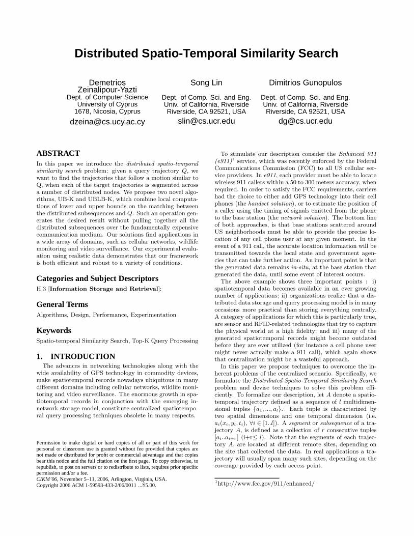
We denote the natural fragmentation of each trajectory asspatial fragmentation, because a trajectory is sliced up intoseveral disjoint subsequences which reside on spatially dis-tributed sites. Our objective is to answer the query: “Reportthe objects (i.e. trajectories) which follow a similar spatio-temporal motion with Q”, where Q is some query trajectory.The notion of similarity captures the trajectories which dif-fer only slightly, in the whole sequence, from the given searchquery Q. More formally, the tuples of each target trajectoryA, are compared with the points of Q within some tem-poral and spatial window. Other queries, such as patternqueries [12], which look at the pattern of a trajectory ratherthan individual points, are similarly interesting but outsideof the scope of this paper.
Research to this day, has focused on computing similarityqueries assuming that the querying entity has access to allthe trajectories in advance, or becomes aware of them in astreaming fashion (Section 2 provides an overview). Whilethe centralized model serves well many scenarios where thetransfer of data is inexpensive, it is not appropriate for en-vironments with expensive communication mediums, suchas wireless sensor networks [16], or environments where thedistributed sites generate large quantities of spatio-temporalrecords (e.g. the e911 scenario).
Our approach is optimized for retrieving the K most simi-lar trajectories to a query Q, for a user parameter K. There-fore the queries do not retrieve the whole universe of an-swers. Additionally, the techniques we propose employ tra-jectory matching techniques that have been shown to beaccurate and tolerant to noise and outliers while featuringan extremely low computational overhead. In this paper wemainly use the Longest Common Subsequence (LCSS) [9]as a distance measure, but the techniques can easily be ex-tended to work with Dynamic Time Warping (DTW) [5] aswell. Our main contributions are summarized as following:
1. We introduce and formalize the problem of findingthe most similar spatio-temporal trajectories in a dis-tributed environment.
2. We propose the UB-K and UBLB-K algorithms, whichare distributed query processing algorithms that findthe K most similar trajectories to a query trajectoryQ, by utilizing locally computed lower and upper boundson the trajectory similarity function.
3. We propose DUB LCSS and DLB LCSS, which aredistributed similarity approximation algorithms thatcan accurately upper and lower bound the LongestCommon Subsequence (LCSS) similarity.
The remainder of the paper is organized as follows: Sec-tion 2 provides an overview of related research, Section 3formulates the problem and our notation. Section 4 de-scribes our distributed query processing algorithms, UB-Kand UBLB-K, which utilize upper and lower bound scoreson a variety of distance measures in order to compute the Kmost similar trajectories to a query trajectory Q. The exactmechanism of generating the upper bounds (DUB LCSS)and lower bounds (DLB LCSS) is described in Section 5.In Section 6, we present an experimental study of our al-gorithms using 25,000 car trajectories moving in the city ofOldenburg (Denmark) and Section 7 concludes the paper.
G
trajectories
A 2
A 1
x
y
cell
Access Point moving object
Figure 1: The trajectories A1 and A2 of two moving
objects in space G. Each cell contains an access point
that records subsequences of A1 and A2.
2. RELATED WORKTo the best of our knowledge the distributed spatiotem-
poral similarity search problem has not been addressed inthe literature before. However spatio-temporal queries havebeen an intense area of research over the last years [1, 4,13, 19, 20, 22, 24, 26]. This resulted in the developmentof efficient access methods [13, 15, 22, 24] and similaritymeasures [5, 9, 24] for predictive [23], historical [24] andcomplex spatio-temporal queries [12]. All these techniques,as well as the frameworks for spatio-temporal queries [18,21, 25], work in a completely centralized setting. Our tech-niques on the other hand are decentralized and keep thedata in-situ, which is more appropriate for environmentswith expensive communication mediums and for large scaleapplications that generate huge amounts of spatiotemporalrecords.
One problem with the in-situ storage of trajectories is thatquery processing now becomes significantly more complex.Finding similar trajectories in a distributed fashion mightrequire sophisticated techniques and interactions to uncoverthe potentially very large number of answers. Note that aquery of the type “Find which other trajectories are similarto trajectory Q” yields fuzzy answers, thus it is meaning-ful to limit the cardinality of the answer set to some userdefined threshold K. Otherwise, the user would end up re-trieving a large number of less relevant answers. Solutions tothe above Top-K query processing problem, have tradition-ally been provided by the database community in a variety ofcontexts including middleware systems [10, 11], web accessi-ble databases [7, 17, 27], stream processors [2], peer-to-peersystems [3] and other distributed systems [8, 28].
In general, a Top-K query returns the K highest rankedanswers to a user defined similarity function. For instancethe query by example: ”Find the K=5 images that are mostsimilar to some query image Q”, returns the five picturesthat minimize the average distance for a set of given dimen-sions (e.g. using features such as color, texture, etc). Atop-k query returns a subset of the complete answer set, inorder to minimize some cost metric that is associated withthe retrieval of the complete answer set. Such a cost isusually measured in terms of disk accesses or network trans-missions, depending on where the data physically resides.
The TA [11] algorithm and its variants are well establishedand understood algorithms for computing top-k queries in acentralized setting. A fundamental assumption underlying
these algorithms is that the exact score is available for eachdimension of the similarity function. For instance, givensome image pi and some query image Q, we have a similarityscore associated with each of its dimensions (i.e. 0.7 simi-larity with respect to color, 0.94 similarity with respect totexture etc). The total similarity of pi and Q, is then simplybe the average of these scores (i.e. 0.82). Exact scores arealso the underlying assumption of distributed top-K queryprocessing algorithms proposed in recent literature, namelythe TPUT [8], TJA [28] and TPAT [14].
Unfortunately such exact scores are not available in oursetting and therefore none of the above top-k query pro-cessing solutions can be utilized in our case. To understandthis first assume that we map, using a 1:1 correspondence,each query dimension to a distributed site. The most similartrajectory A is the one that maximizes the similarity to Qacross all dimensions (i.e. all sites).
A naive solution would be to calculate some exact similar-ity score at each remote site and then combine these scoresusing any of the aforementioned top-k query processing al-gorithms. For instance, by utilizing the Euclidean distance
(L2), given as |Q−A| = 2
q
Pl
i=1|qi − ai|2, one can produce
a set of exact scores, which express the distance of Q to A.However the matching between Q and A, would only occurbetween points of identical time positions. As a result, itwould neither be flexible to out-of-phase matches (e.g. if wehave two identical trajectories but the first one moves earlierin time) nor tolerant to noisy data (e.g. we have two iden-tical trajectories but the first has some slight deviation inits spatial movement). Disregarding these parameters mightresult in an extremely poor similarity matching.
Therefore we opt for a multidimensional similarity mea-sure that takes into account out-of-phase matches and grace-fully handles noisy data. In particular, we use the LongestCommon Subsequence that will be described in Section 5.2.Using such a measure in a distributed environment limitsus to a lower and upper bound on the similarity score be-tween a query trajectory Q and Ai. For instance, we mightonly know that the similarity of Q to some subsequenceA1 is between 0.88 and 0.92 and that the similarity of Qto A2 is between 0.85 and 0.90. Thus, we can not deter-mine which of the two trajectories is more similar to Q. Forinstance if the real similarity is FullM(Q, A1) = 0.89 andFullM(Q, A2) = 0.90 then A2 is the most similar one; on thecontrary if FullM(Q, A1) = 0.89 and FullM(Q, A2) = 0.87then A1 is the most similar.
The above description shows that by having score bounds,rather than exact scores, is not enough to identify the mostsimilar trajectories. This creates a challenging problem:How to calculate the top-K answers if we have score boundsrather than exact scores? We will provide two novel al-gorithms that solve this problem in an iterative fashion.Such algorithms might potentially have many other applica-tions outside the spatiotemporal similarity search domain,although we will not explore these possibilities here.
3. PROBLEM FORMULATIONIn this section we provide the notation used throughout
the paper. Specifically, we formalize our data and querymodel. The main symbols and their respective definitionsare summarized in Table 1.
C1
: trajectories
A 1
A 2
access points x
y time C1
C2
C3
C4
A 1, A 2 C1,C2,C3,C4:
a) Map View b) Time View
C2
C3 C4
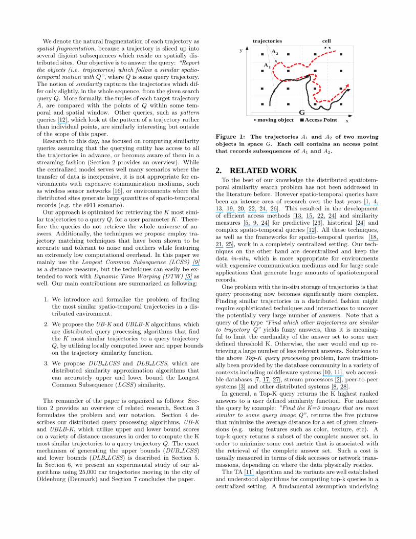
Figure 2: Two Spatially Fragmented Trajectories A1, A2
across four cells C1, C2, C3, C4.
Symbol Definition
G A Given Geographic AreaQN The Querying NodeQ A Spatio-Temporal Queryn Number of Cells in Gm Number of Trajectories (Objects)l Trajectory Length (discrete points)K Number of requested results
LowerM(Q,A), The Lower, Upper Bounding andUpperM(Q,A), Full Match between theFullM(Q,A) query Q and the trajectory A.
Larger Match means Smaller Distance
Table 1: Symbol Description.
3.1 The Data ModelLet G denote a 2-dimensional matrix of points in the
xy-plane that represents the coordinate space of some ge-ographic area. Without loss of generality, we assume thatthe points in G are logically organized into x ·y cells as illus-trated in Figure 2. Each cell contains an access point (AP )that is assumed to be in communication range from everypoint in its cell.2
Although the coordinate space is assumed to be parti-tioned in square cells, other geometric shapes such as vari-able size rectangles or Voronoi polygons are similarly appli-cable but outside the scope of this paper. This partitioningof the coordinate space simply denotes that in our setting,G is covered by a set of APs. Now let {A1, A2, ..., Am} de-note a set of m objects moving in G. At each discrete timeinstance, object Ai (∀i ≤ m) generates a spatio-temporalrecord r = {Ai, ti, xi, yi}, where ti denotes the timestampon which the record was generated, and (xi, yi) the coordi-nates of Ai at ti. The record r is then stored locally at theclosest AP for l discrete time moments after which it is dis-carded. Therefore at any given point every access point APmaintains locally the records of the last l time moments.
A trajectory can be conceptually thought of as a contin-uous sequence Ai = ((ax:1,y:1), ..., (ax:l,y:l)) (i ≤ m), whilephysically it is spatially fragmented across several cells (seeFigure 2). Similarly, the spatio-temporal query is also rep-resented as: Q = ((qx:1,y:1), ..., (qx:l,y:l)) but this sequence isnot spatially fragmented.
3.2 The Query ModelOur objective is to answer efficiently top-K queries of the
type: given a trajectory Q, retrieve the K trajectories which
2The terms access point and cell are used interchangeably.
A2,3,6 A0,4,8 A4,5,10 A7,7,9 A3,8,11 A9,8,9
....
A4,10,18 A2,13,19 A0,15,25 A3,20,27 A9,22,26 A7,30,35
....
c1
QN
c2 c3 c2
QN
c3
c1
2) Hierarchy 1) Star
m
Distributed Topologies
A4,4,5 A2,5,6 A0,5,7 A3,5,6 A9,8,10 A7,12,13
....
A4,1,3 A0,6,10 A2,5,7 A9,6,7 A3,7,10 A7,11,13
....
id,lb,ub C3
id,lb,ub C2
id,lb,ub C1
id,lb,ub METADATA
n
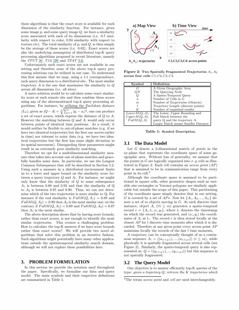
Figure 3: (a) METADATA: Lower and Upper bounds
computed for m trajectories. (b) Distributed Topologies.
are the most similar to Q. First note that the similarityquery Q is initiated by some querying node QN , which dis-seminates Q to all cells that intersect the query Q. Wecall the intersecting regions candidate cells. Upon receiv-ing Q, each candidate cell executes locally a lower boundingmatching function (LowerM) and an upper bounding func-tion (UpperM) on all its local subsequences (these functionswill be described in Section 5.2). This yields 2·m local dis-tance computations to Q by each cell (one for each bound).To speed up computations we could utilize spatiotemporalaccess methods similar to those proposed in [24]. The con-ceptual array of lower (LB) and upper bounds (UB) for anexample scenario of three nodes (C1, C2, C3) is illustrated inFigure 3a. We will refer to the sum of bounds from all cellsas METADATA and to the actual subsequence trajectoriesstored locally by each cell as DATA. Obviously, DATA isorders of magnitudes more expensive than METADATAto be transferred towards QN . Therefore we want to in-telligently exploit METADATA to identify the subset ofDATA that produces the K highest ranked answers. Fig-ure 3b illustrates two typical topologies between cells: starand hierarchy. Our proposed algorithms are equivalently ap-plicable to both of them although for the remainder of thepaper we use a star topology to simplify our description.
In order to find the K trajectories that are most similarto a query trajectory Q, QN can fetch all the DATA andthen perform a centralized similarity computation using theFullM(Q, Ai) (∀i ≤ m) method, which is one of the LCSS,DTW or other Lp-Norm distance measures presented in Sec-tion 5. Centralized is extremely expensive in terms of datatransfer and delay.
4. DISTRIBUTED QUERY PROCESSINGIn this section we present two novel distributed query pro-
cessing algorithms, UB-K and UBLB-K, which find the Kmost similar trajectories to a query trajectory Q. The UB-Kalgorithm uses an upper bound on the matching between Qand a target trajectory Ai, while UBLB-K uses both a lowerand an upper bound on the matching. The description onhow these bounds are acquired is delayed until Section 5.
4.1 The UB-K AlgorithmThe UB-K algorithm is an iterative algorithm for retriev-
ing the K most similar trajectories to a query Q. The algo-rithm minimizes the number of DATA entries transferred to-wards QN by exploiting the upper bounds from the META-DATA table. Notice that METADATA contains the boundsof many objects that will not be in the final top-K result.In order to minimize the cost of uploading the completeMETADATA table to QN we utilize a distributed top-K
Algorithm 1 : UB-K Algorithm
Input: Query Q, m Distributed Trajectories, Result Pa-rameter K, Iteration Step λ.Output: K trajectories with the largest match to Q.
1. Run any distributed top-K algorithm for Q and findthe Λ (Λ > K) trajectories with the highest UBs.
2. Fetch the (Λ − 1) trajectories from the cells and com-pute their full matching to Q using FullM(Q, Ai).
3. If the Λth UB is smaller or equal to the Kth largestfull match then stop; else goto step 1 with Λ=Λ + λ.
METADATA
id, ub
A4, 30
A2, 27
A0, 25
A3, 20
A9, 18
A7, 12
...
Λ=3
Λ=5
DATA
Q
A4, 23
A2, 22
A0, 16
A3, 18
A9, 15
A7, 10
...
FullM(Q, Ai)
A4
A2
A0
A3
A9
A7
C1 C2 C3
UB FullM
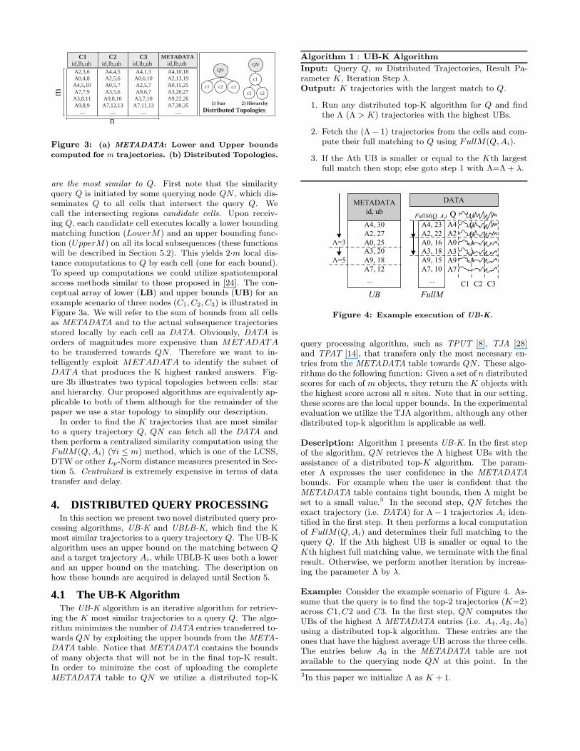
Figure 4: Example execution of UB-K.
query processing algorithm, such as TPUT [8], TJA [28]and TPAT [14], that transfers only the most necessary en-tries from the METADATA table towards QN . These algo-rithms do the following function: Given a set of n distributedscores for each of m objects, they return the K objects withthe highest score across all n sites. Note that in our setting,these scores are the local upper bounds. In the experimentalevaluation we utilize the TJA algorithm, although any otherdistributed top-k algorithm is applicable as well.
Description: Algorithm 1 presents UB-K. In the first stepof the algorithm, QN retrieves the Λ highest UBs with theassistance of a distributed top-K algorithm. The param-eter Λ expresses the user confidence in the METADATAbounds. For example when the user is confident that theMETADATA table contains tight bounds, then Λ might beset to a small value.3 In the second step, QN fetches theexact trajectory (i.e. DATA) for Λ− 1 trajectories Ai iden-tified in the first step. It then performs a local computationof FullM(Q, Ai) and determines their full matching to thequery Q. If the Λth highest UB is smaller or equal to theKth highest full matching value, we terminate with the finalresult. Otherwise, we perform another iteration by increas-ing the parameter Λ by λ.
Example: Consider the example scenario of Figure 4. As-sume that the query is to find the top-2 trajectories (K=2)across C1, C2 and C3. In the first step, QN computes theUBs of the highest Λ METADATA entries (i.e. A4, A2, A0)using a distributed top-k algorithm. These entries are theones that have the highest average UB across the three cells.The entries below A0 in the METADATA table are notavailable to the querying node QN at this point. In the
3In this paper we initialize Λ as K + 1.
second step QN will fetch the subsequences of the trajec-tories identified in the first step. Therefore QN has nowthe complete trajectories for A4 and A2 (right side of Fig-ure 4). QN then computes the following full matching:FullM(Q, A4) = 23, FullM(Q, A2) = 22 using the LongestCommon Subsequence described in Section 5. Since the Λthhighest UB (A0 = 25) is larger than the Kth highest fullmatch (A2 = 22), the termination condition is not satis-fied in the third step. To explain this, consider a trajec-tory X with a UB of 24 and a full match of 23. ObviouslyX is not retrieved yet (because it has a smaller UB than25). However, it is a stronger candidate for the top-2 resultthan (A2, 22), as X has a full match of 23 which is largerthan 22. Therefore we initiate the second iteration of theUB-K algorithm in which we compute the next λ (λ = 2)METADATA entries and full values FullM(Q, A0) = 16,FullM(Q, A3) = 18. Now the termination has been satis-fied because the Λth highest UB (A9, 18) is smaller than theKth highest full match (A2, 22). Finally we return as thetop-2 answer the trajectories with the highest full matches(i.e. {(A4, 23), (A2, 22)}).
Theorem 1.The UB-K algorithm always returns the mostsimilar objects to the query trajectory Q.
Proof: Let A denote some arbitrary object returned asan answer by the UB-K algorithm (A ∈ Result), and Bsome arbitrary object that is not among the returned re-sults (B /∈ Result). We want to show that FullM(Q, B) ≤FullM(Q, A) always holds.
Assume that FullM(Q, B) > FullM(Q, A). We will showthat such an assumption leads to a contradiction. SinceA ∈ Result and B /∈ Result it follows from the first stepof the algorithm that ubB ≤ ubA. In the second phaseof the algorithm we fetch the trajectory A and calculateFullM(Q, A). By using the assumption, we can now drawthe following conclusion: FullM(Q, A) < FullM(Q, B) ≤ubB ≤ ubA. When the algorithm terminates in the thirdstep, with A among its answers, we know that ubX , forsome object X, was smaller or equal to the Kth largest fullscore (i.e. ubX ≤ ... ≤ FullM(Q, A)). But it is also truethat ubB ≤ ubX (as object B was not chosen in the first stepof the algorithm), which yields ubB ≤ ubX ≤ FullM(Q, A)and subsequently FullM(Q, B) ≤ FullM(Q, A) (by defini-tion FullM(Q, B) ≤ ubB). This is a contradiction as weassumed that FullM(Q, B) > FullM(Q, A) �
4.2 The UBLB-K AlgorithmThe UBLB-K algorithm is, similarly to UB-K, an itera-
tive algorithm for retrieving the K most similar trajecto-ries. However it has two subtle differences: (i) It uses bothan upper bound (UB) and a lower bound (LB) in order todetermine whether the top K trajectories have been foundand (ii) It transfers the candidate trajectories in a final bulkstep rather than incrementally.
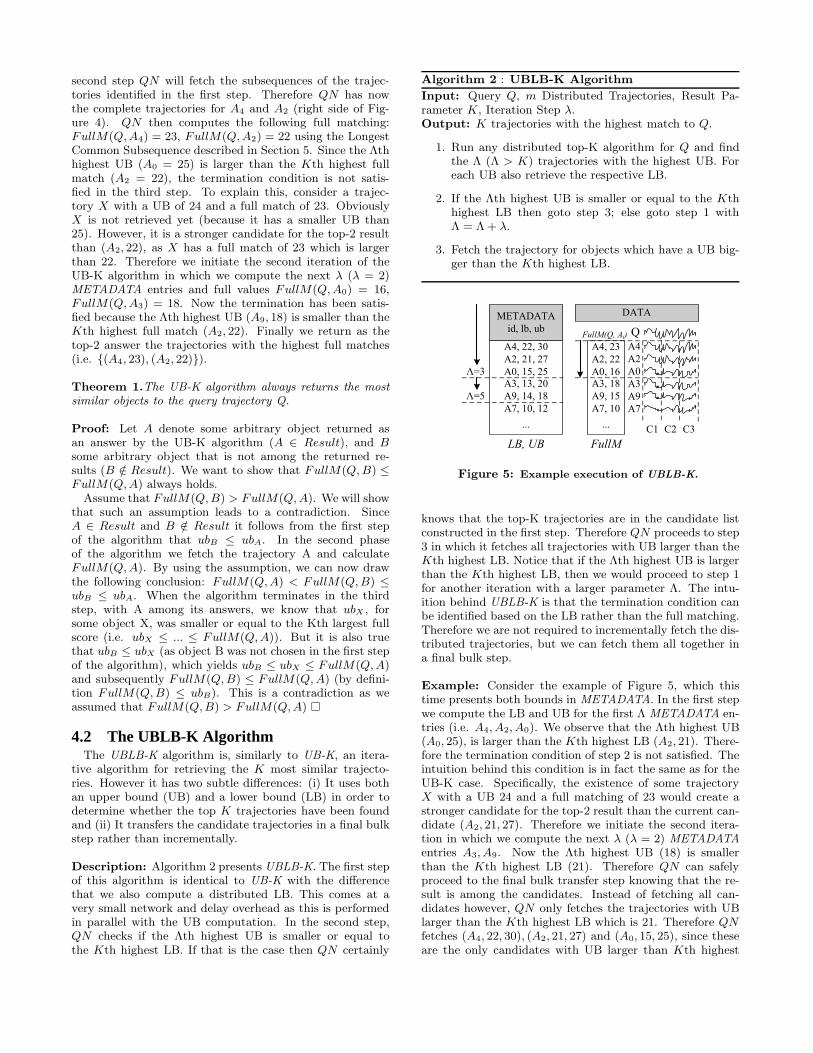
Description: Algorithm 2 presents UBLB-K. The first stepof this algorithm is identical to UB-K with the differencethat we also compute a distributed LB. This comes at avery small network and delay overhead as this is performedin parallel with the UB computation. In the second step,QN checks if the Λth highest UB is smaller or equal tothe Kth highest LB. If that is the case then QN certainly
Algorithm 2 : UBLB-K Algorithm
Input: Query Q, m Distributed Trajectories, Result Pa-rameter K, Iteration Step λ.Output: K trajectories with the highest match to Q.
1. Run any distributed top-K algorithm for Q and findthe Λ (Λ > K) trajectories with the highest UB. Foreach UB also retrieve the respective LB.
2. If the Λth highest UB is smaller or equal to the Kthhighest LB then goto step 3; else goto step 1 withΛ = Λ + λ.
3. Fetch the trajectory for objects which have a UB big-ger than the Kth highest LB.
METADATA
id, lb, ub
A4, 22, 30
A2, 21, 27
A0, 15, 25
A3, 13, 20
A9, 14, 18
A7, 10, 12
...
Λ=3
Λ=5
DATA
Q
A4, 23
A2, 22
A0, 16
A3, 18
A9, 15
A7, 10
...
FullM(Q, Ai)
A4
A2
A0
A3
A9
A7
C1 C2 C3
LB, UB FullM
Figure 5: Example execution of UBLB-K.
knows that the top-K trajectories are in the candidate listconstructed in the first step. Therefore QN proceeds to step3 in which it fetches all trajectories with UB larger than theKth highest LB. Notice that if the Λth highest UB is largerthan the Kth highest LB, then we would proceed to step 1for another iteration with a larger parameter Λ. The intu-ition behind UBLB-K is that the termination condition canbe identified based on the LB rather than the full matching.Therefore we are not required to incrementally fetch the dis-tributed trajectories, but we can fetch them all together ina final bulk step.
Example: Consider the example of Figure 5, which thistime presents both bounds in METADATA. In the first stepwe compute the LB and UB for the first Λ METADATA en-tries (i.e. A4, A2, A0). We observe that the Λth highest UB(A0, 25), is larger than the Kth highest LB (A2, 21). There-fore the termination condition of step 2 is not satisfied. Theintuition behind this condition is in fact the same as for theUB-K case. Specifically, the existence of some trajectoryX with a UB 24 and a full matching of 23 would create astronger candidate for the top-2 result than the current can-didate (A2, 21, 27). Therefore we initiate the second itera-tion in which we compute the next λ (λ = 2) METADATAentries A3, A9. Now the Λth highest UB (18) is smallerthan the Kth highest LB (21). Therefore QN can safelyproceed to the final bulk transfer step knowing that the re-sult is among the candidates. Instead of fetching all can-didates however, QN only fetches the trajectories with UBlarger than the Kth highest LB which is 21. Therefore QNfetches (A4, 22, 30), (A2, 21, 27) and (A0, 15, 25), since theseare the only candidates with UB larger than Kth highest

LB (A2, 21). After QN performs the final bulk transferringstep it calculates the full match of the retrieved candidatesand simply returns the top-2 trajectories with the highestmatch to the query (i.e. {(A4, 23), (A2, 22)}).
Theorem 2.The UBLB-K algorithm always returns the mostsimilar objects to the query trajectory Q.
Proof: Similar to Theorem 1 �
4.3 DiscussionUB-K vs. UBLB-K: Comparing the two algorithms wecan observe that in many cases (like our example), UBLB-Kmight terminate and retrieve less DATA entries at the ex-pense of an increased overhead of METADATA entries. Notethat the DATA entries are orders of magnitudes more expen-sive to be transferred than METADATA entries. The sav-ings increase when the LBs are tighter, which consequentlyallows QN to determine faster whether the top-K resultshave been found. The savings of UBLB-K are also increasedfor larger values of Λ. Note that UB-K has to always re-trieve Λ full trajectories while UBLB-K, based on the LBs,can be more selective. These observations are validated inSection 6.
Incremental Deepening into Top-K Results: Sinceboth our algorithms fetch the highest METADATA incre-mentally (e.g. they find the top K, Λ+λ, Λ+2λ, ... UBs atincreasing iterations), QN can cache the METADATA andDATA it has received in the previous iterations and onlyrequest for the new METADATA and DATA in a new it-eration. Consider for example Figure 4, where in the firstiteration, QN fetches the trajectories of {A4, A2}. In thesecond iteration, QN only needs to fetch the trajectories ofA0 and A3, since the top 2 trajectories have already beenfetched in the previous iteration.
Global Clock Independence: It is important to men-tion that our algorithms operate correctly in the absence ofa global clock. This is true because the various phases ofour algorithms are not defined as a function of time. How-ever, when nodes are not synchronized then this might resultin the computation of incorrect answers to the respectivequeries. We emphasize that this is not attributed to theoperation of our algorithms but rather to the out-of-ordertrajectories. In fact even the centralized algorithm would beaffected by the same problems in this case.
5. SIMILARITY MEASURES FOR SPATIO-TEMPORAL TRAJECTORIES
In the previous section we have discussed how our pro-posed distributed query processing algorithms work by uti-lizing locally computed lower and upper bound scores onthe matching between a query Q and the respective trajec-tories. In this section we describe how these bounds arecalculated. We start out by providing an overview of dis-tance measures that were proposed in a centralized setting,where the querying node has access to the complete trajec-tory of some moving object. We then provide extensions forcomputing these distances in a distributed setting. In par-ticular, we will focus on a distributed version of the LongestCommon Subsequence, which is utilized in this work.
5.1 Centralized Similarity MeasuresLet A((ax:1,y:1), ..., (ax:l1,y:l1)) and B((bx:1,y:1), ..., (bx:l2,y:l2))
denote two 2-dimensional trajectories with sizes l1 and l2respectively. The most straightforward way to compute thesimilarity between A and B is to use any of the Lp-Normdistances, such as the Manhattan (L1), Euclidean (L2) orChebyshev (L∞). Although this family of distances can becalculated very efficiently, it is not flexible to out-of-phasematches and not tolerant to noisy data because the pointsare only matched at identical time positions.
The Dynamic Time Warping (DTW) [5], solves some ofthe matching inefficiencies associated with the Lp-Norm dis-tances by allowing local stretching of the sequences to opti-mize the matching. However its performance might deteri-orate in the presence of noisy data in which outliers distortthe true distance between sequences.
The Longest Common Sub-Sequence (LCSS) similarity hasbeen extensively used in many 1-dimensional sequence prob-lems such as string matching. The 2-dimensional adaptationof LCSS using the L∞
4 is defined as following:Definition Given integers δ and ǫ, the Longest CommonSub-Sequence similarity LCSSδ,ǫ(A, B) between two sequencesA and B is defined as:
LCSSδ,ǫ(A, B) =
8
>
>
>
>
>
>
>
<
>
>
>
>
>
>
>
:
0, if A or B is empty
1 + LCSSδ,ǫ(Tail(A), Tail(B))
if |ax:l1 − bx:l2 | < ǫ and
|ay:l1 − by:l2 | < ǫ and |l1 − l2| < δ
max(LCSSδ,ǫ(Tail(A), B),LCSSδ,ǫ(A, Tail(B)))
otherwise
where the δ and ǫ are user defined thresholds that allowflexible matching in the time and the space domain respec-tively. LCSS can deal more efficiently with outliers, becauseoutliers are simply dropped from the matching and so largeoutliers do not skew the measure. Similar to DTW, LCSScan be computed by a dynamic programming algorithm witha time complexity of O(δ · (l1 + l2))[9].
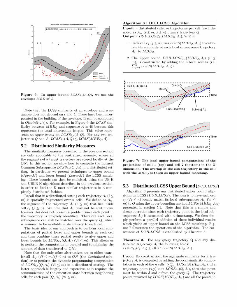
Even though LCSS offers many desirable properties, itstime complexity of O(δ · (l1 + l2)) might constitute it in-efficient for large values of l1, l2 or δ, so it is desirable togive a technique to upper bound the LCSS similarity. Theidea of the technique proposed in [24] is to encapsulate thequery trajectory Q within a bounding envelope and thenfind the intersection between the envelope and the trajecto-ries. For simplicity consider the 1-dimensional case whereQ= (qx:1, . . . , qx:l1) denotes a query and A= (ax:1, . . . , ax:l2)a trajectory. Suppose that we replicate each point Qi for δtime instances before and after time i and that we also repli-cate each point Qi for ǫ space instances above and below Qi
(see Figure 6). The area contained in the union of all thesepoints defines the Minimum Bounding Envelope (MBE) ofthe query trajectory Q. The notion of the bounding envelopecan be trivially extended to more dimensions.
The LCSS similarity between the envelope of Q and asequence A is defined as:
LCSS(MBEQ, A) =n
X
i=1
1 if A[i] within envelope0 otherwise
4We could also use L1 or L2 for the recursion step
0 20 40 60 80 100−1.5
−1
−0.5
0
0.5
1
1.5
2
2.5
3
3.5 Applying the Minimum Bounding Envelope (MBE) to the Query
x di
men
sion
Time
1 1 25
20
1
LCSS(MBEQ
, A) = ( 1 + 1 + 1 + 25 + 20) = 48
MBEQ
Trajectory AQuery Q
Figure 6: To upper bound LCSSδ,ǫ(A, Q), we use the
envelope MBE of Q
Note that the LCSS similarity of an envelope and a se-quence does not depend on ǫ and δ. These have been incor-porated in the building of the envelope. It can be computedin O(min(l1, l2)). For example, in Figure 6 the LCSS sim-ilarity between MBEQ and sequence A is 48 because thisrepresents the total intersection length. This value repre-sents an upper bound on LCSSδ,ǫ(A, Q). For any two tra-jectories Q and A, LCSSδ,ǫ(A, Q) ≤ LCSS(MBEQ, A).
5.2 Distributed Similarity MeasuresThe similarity measures presented in the previous section
are only applicable to the centralized scenario, where allthe segments of a target trajectory are stored locally at theQN . In this section we show how to compute the LongestCommon Subsequence LCSSδ,ǫ(Q,Ai) in a distributed set-ting. In particular we present techniques to upper bound(UpperM) and lower bound (LowerM) the LCSS match-ing. These bounds can then be exploited, using the UB-Kand UBLB-K algorithms described in the previous section,in order to find the K most similar trajectories in a com-pletely distributed fashion.
Recall that in a distributed setting each trajectory Ai (i ≤m) is spatially fragmented over n cells. We define as Aij ,the segment of the trajectory Ai (i ≤ m) that lies insidecell cj (j ≤ n). We note that Aij may not be continuous,however this does not present a problem since each point inthe trajectory is uniquely identified. Therefore each localsubsequence can still be matched over the query Q, whichis assumed to be available in its entirety to each cell.
The basic idea of our approach is to perform local com-putations of partial lower and upper bounds at each celland then combine these partial results to give upper andlower bounds for LCSSδ,ǫ(Q, Ai) (∀i ≤ m). This allows usto perform the computation in parallel and to minimize theamount of data transferred to QN .
Note that the only other alternatives are to either trans-fer all Aij (∀i ≤ m,∀j ≤ n) to QN (the Centralized solu-tion) or to perform the dynamic programming computationof LCSSδ,ǫ(Q,Ai) (∀i ≤ m) in a distributed setting. Thelatter approach is lengthy and expensive, as it requires thecommunication of the execution state between neighboringcells for each pair (Q,Ai) (∀i ≤ m).
Algorithm 3 : DUB LCSS Algorithm
Input: n distributed cells, m trajectories per cell (each de-noted as Aij (i ≤ m, j ≤ n)), query trajectory Q.Output: DUB LCSSδ,ǫ(MBEQ, Ai), ∀i ≤ m
1. Each cell cj (j ≤ n) uses LCSS(MBEQ, Aij) to calcu-late the similarity of each local subsequence trajectoryAij to MBEQ.
2. The upper bound DUB LCSSδ,ǫ(MBEQ, Ai) (i ≤m), is constructed by adding the n local results (i.e.Pn
j=1LCSS(MBEQ, Aij)).
Cell 1, ub(1)= 14
Time
Time
X
X
Cell 2, ub(2) = 22
Query QMBE(Q)
Sub−traj A1 LCSS matching
Figure 7: The local upper bound computations of the
projections of cell 1 (top) and cell 2 (bottom) in the X
dimension. The overlap of the sub-trajectory in the cell
with the MBEQ is taken as upper bound matching.
5.3 Distributed LCSS Upper Bound (DUB LCSS)Algorithm 3 presents our distributed upper bound algo-
rithm on LCSS (DUB LCSS). The idea is to have each cellcj (∀j ≤ n) locally match its local subsequences Aij (∀i ≤m) to Q using the upper bounding method LCSS(MBEQ, Aij)presented in section 5.1. Note that this is a simple andcheap operation since each trajectory point in the local sub-sequence Aij is associated with a timestamp. We then sim-ply perform a parallel addition of these individual resultswhich yields an upper bound on the LCSS matching. Fig-ure 7 illustrates the operations of the algorithm. The cor-rectness of DUB LCSS is established by Theorem 3.
Theorem 3. For any query trajectory Q and any dis-tributed trajectory Ai the following holds:LCSSδ,ǫ(Q, Ai) ≤ DUB LCSS(MBEQ, Ai).
Proof: By construction, the aggregate similarity for a tra-jectory Ai is computed by adding the local similarity compu-tation in each of the n cells:
Pn
j=1LCSS(MBEQ, Aij). If a
trajectory point (x,y) is in LCSSδ,ǫ(Q,Ai), then this pointmust be within δ and ǫ from the query Q. The trajectorypoints returned by LCSS(MBEQ, Aij) are all the points in
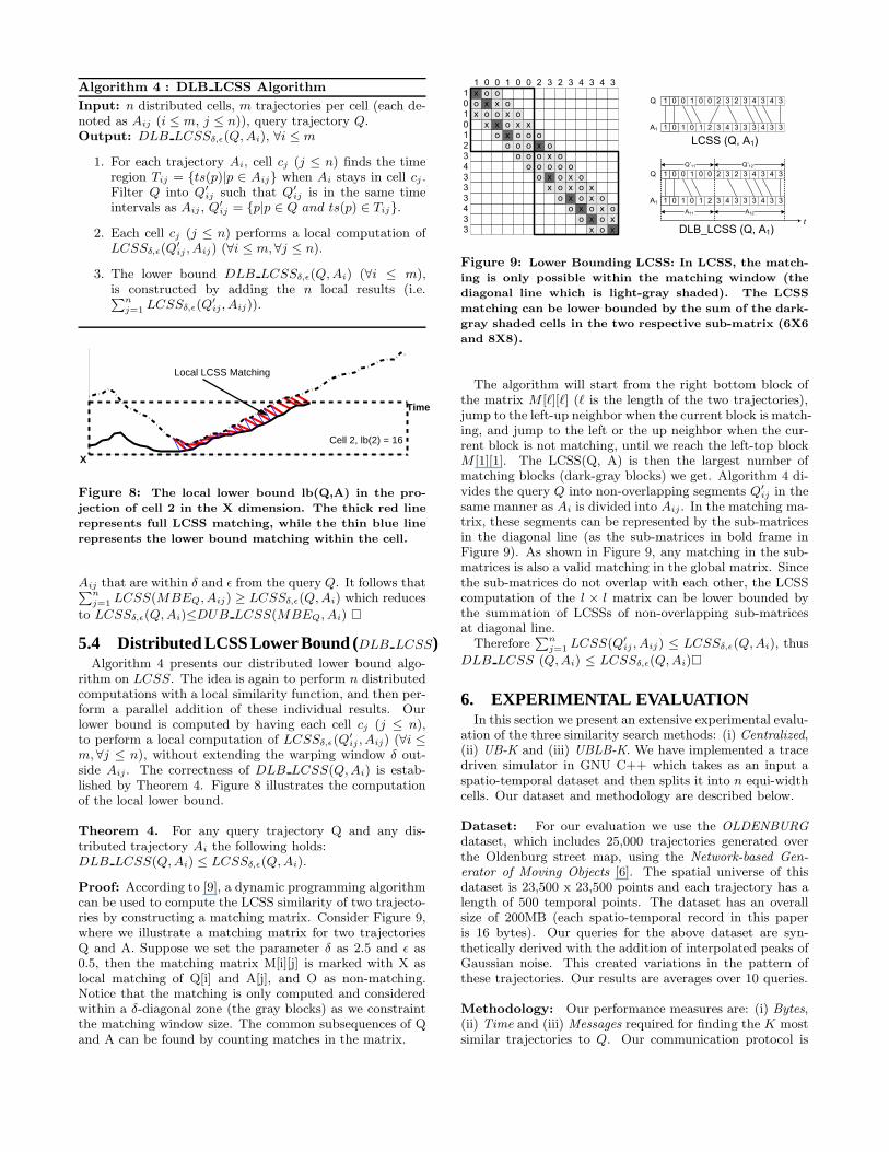
Algorithm 4 : DLB LCSS Algorithm
Input: n distributed cells, m trajectories per cell (each de-noted as Aij (i ≤ m, j ≤ n)), query trajectory Q.Output: DLB LCSSδ,ǫ(Q, Ai), ∀i ≤ m
1. For each trajectory Ai, cell cj (j ≤ n) finds the timeregion Tij = {ts(p)|p ∈ Aij} when Ai stays in cell cj .Filter Q into Q′
ij such that Q′
ij is in the same timeintervals as Aij , Q′
ij = {p|p ∈ Q and ts(p) ∈ Tij}.
2. Each cell cj (j ≤ n) performs a local computation ofLCSSδ,ǫ(Q
′
ij , Aij) (∀i ≤ m,∀j ≤ n).
3. The lower bound DLB LCSSδ,ǫ(Q, Ai) (∀i ≤ m),is constructed by adding the n local results (i.e.Pn
j=1LCSSδ,ǫ(Q
′
ij , Aij)).
Cell 2, lb(2) = 16
Local LCSS Matching
Time
X
Figure 8: The local lower bound lb(Q,A) in the pro-
jection of cell 2 in the X dimension. The thick red line
represents full LCSS matching, while the thin blue line
represents the lower bound matching within the cell.
Aij that are within δ and ǫ from the query Q. It follows thatPn
j=1LCSS(MBEQ, Aij) ≥ LCSSδ,ǫ(Q, Ai) which reduces
to LCSSδ,ǫ(Q, Ai)≤DUB LCSS(MBEQ, Ai) �
5.4 Distributed LCSS Lower Bound (DLB LCSS)Algorithm 4 presents our distributed lower bound algo-
rithm on LCSS. The idea is again to perform n distributedcomputations with a local similarity function, and then per-form a parallel addition of these individual results. Ourlower bound is computed by having each cell cj (j ≤ n),to perform a local computation of LCSSδ,ǫ(Q
′
ij , Aij) (∀i ≤m,∀j ≤ n), without extending the warping window δ out-side Aij . The correctness of DLB LCSS(Q, Ai) is estab-lished by Theorem 4. Figure 8 illustrates the computationof the local lower bound.
Theorem 4. For any query trajectory Q and any dis-tributed trajectory Ai the following holds:DLB LCSS(Q, Ai) ≤ LCSSδ,ǫ(Q, Ai).
Proof: According to [9], a dynamic programming algorithmcan be used to compute the LCSS similarity of two trajecto-ries by constructing a matching matrix. Consider Figure 9,where we illustrate a matching matrix for two trajectoriesQ and A. Suppose we set the parameter δ as 2.5 and ǫ as0.5, then the matching matrix M[i][j] is marked with X aslocal matching of Q[i] and A[j], and O as non-matching.Notice that the matching is only computed and consideredwithin a δ-diagonal zone (the gray blocks) as we constraintthe matching window size. The common subsequences of Qand A can be found by counting matches in the matrix.
1 0 0010
1
0
1
1
0
2
3
4
3
3
3
4
3
2 3 2 3 4 3 4 3
3
x
x
o
o
x
o
xo
xox
o
x
o
o
o
x
o
o
o
x
o
x
x
x
x
o
o
x
o
x
x
x
x
x
o
o
o
x
ox
o
o
o
o
o
o
o
o
o
o
o
x
o
o
o
o
x
o
o
x
o
x
o
Q
A1
001 1 0 0 42 3 32 33 4
101 0 1 2 33 4 43 33 3
Q
A1
A11 A12
Q’11 Q’12
t
001 1 0 0 42 3 32 33 4
101 0 1 2 33 4 43 33 3
LCSS (Q, A1)
DLB_LCSS (Q, A1)
Figure 9: Lower Bounding LCSS: In LCSS, the match-
ing is only possible within the matching window (the
diagonal line which is light-gray shaded). The LCSS
matching can be lower bounded by the sum of the dark-
gray shaded cells in the two respective sub-matrix (6X6
and 8X8).
The algorithm will start from the right bottom block ofthe matrix M [ℓ][ℓ] (ℓ is the length of the two trajectories),jump to the left-up neighbor when the current block is match-ing, and jump to the left or the up neighbor when the cur-rent block is not matching, until we reach the left-top blockM [1][1]. The LCSS(Q, A) is then the largest number ofmatching blocks (dark-gray blocks) we get. Algorithm 4 di-vides the query Q into non-overlapping segments Q′
ij in thesame manner as Ai is divided into Aij . In the matching ma-trix, these segments can be represented by the sub-matricesin the diagonal line (as the sub-matrices in bold frame inFigure 9). As shown in Figure 9, any matching in the sub-matrices is also a valid matching in the global matrix. Sincethe sub-matrices do not overlap with each other, the LCSScomputation of the l × l matrix can be lower bounded bythe summation of LCSSs of non-overlapping sub-matricesat diagonal line.
ThereforePn
j=1LCSS(Q′
ij , Aij) ≤ LCSSδ,ǫ(Q,Ai), thus
DLB LCSS (Q,Ai) ≤ LCSSδ,ǫ(Q, Ai)�
6. EXPERIMENTAL EVALUATIONIn this section we present an extensive experimental evalu-
ation of the three similarity search methods: (i) Centralized,(ii) UB-K and (iii) UBLB-K. We have implemented a tracedriven simulator in GNU C++ which takes as an input aspatio-temporal dataset and then splits it into n equi-widthcells. Our dataset and methodology are described below.
Dataset: For our evaluation we use the OLDENBURGdataset, which includes 25,000 trajectories generated overthe Oldenburg street map, using the Network-based Gen-erator of Moving Objects [6]. The spatial universe of thisdataset is 23,500 x 23,500 points and each trajectory has alength of 500 temporal points. The dataset has an overallsize of 200MB (each spatio-temporal record in this paperis 16 bytes). Our queries for the above dataset are syn-thetically derived with the addition of interpolated peaks ofGaussian noise. This created variations in the pattern ofthese trajectories. Our results are averages over 10 queries.
Methodology: Our performance measures are: (i) Bytes,(ii) Time and (iii) Messages required for finding the K mostsimilar trajectories to Q. Our communication protocol is
100000
1e+06
1e+07
1e+08
1e+09
10 20 30 40 50 60 70 80 90 100
Byt
es R
equi
red
n (Number of Cells)
Bytes for varying parameter n in OLDENBURG (m=25K, l=500, K=5, λ=5, δ=5,ε=90)
Centralized
UB-K
UBLB-K
1
10
100
1000
10000
10 20 30 40 50 60 70 80 90 100
Tim
e (s
econ
ds)
n (Number of Cells)
Time for varying parameter n in OLDENBURG (m=25K, l=500, K=5, λ=5, δ=5,ε=90)
Centralized
UB-K
UBLB-K
1
10
100
1000
10000
100000
1e+06
10 20 30 40 50 60 70 80 90 100
Mes
sage
s (V
aria
ble
Siz
e)
n (Number of Cells)
Messages for varying parameter n in OLDENBURG (m=25K, l=500, K=5, λ=5, δ=5,ε=90)
Centralized
UB-K
UBLB-K
Figure 10: Performance Evaluation, varying n (# cells) for the OLDENBURG dataset.
0
5
10
15
20
25
400 200 100 50 20
# of
Iter
eatio
ns
λ (% of K)
# of Iterations for varying parameter K and λ in OLDENBURG (m=25K, l=500, n=36, δ=5, ε=15)
UB-10UBLB-10
UB-50UBLB-50
UB-150UBLB-150
UB-250UBLB-250
0
2e+06
4e+06
6e+06
8e+06
1e+07
1.2e+07
400 200 100 50 20
Byt
es R
equi
red
λ (% of K)
Bytes for UB-K varying parameter K and λ in OLDENBURG (m=25K, l=500, n=36, δ=5, ε=15)
UB-10UB-50
UB-150UB-250
0
2e+06
4e+06
6e+06
8e+06
1e+07
1.2e+07
400 200 100 50 20
Byt
es R
equi
red
λ (% of K)
Bytes for UBLB-K varying parameter K and λ in OLDENBURG (m=25K, l=500, n=36, δ=5, ε=15)
UBLB-10UBLB-50
UBLB-150UBLB-250
Figure 11: Varying the Parameter K and λ using the OLDENBURG dataset.
structured in the following way: Each message is associatedwith a 40 byte header. This is augmented with an additional6 byte application layer header that includes: (i) The Cellidentifier (1 byte), (ii) the Message size (4 bytes) and thedepth of a cell from the querying node QN (1 byte). Wemeasure the total communication cost Bytes as a summa-tion of message cost (40 bytes header cost per message) andthe data cost (i.e. the cost of communicating DATA andMETADATA between QN and all the cells). In order toallow reproducible and comparable results we perform ourexperiments on a single host using a simulated dedicatedbandwidth of 128KBps for the edges between QN and thecells. Our edges have a random latency between 0-100mswhich is typical for Internet environments. Since the cellscan transmit their results back to QN in parallel, we con-sider only the longest time of each round.
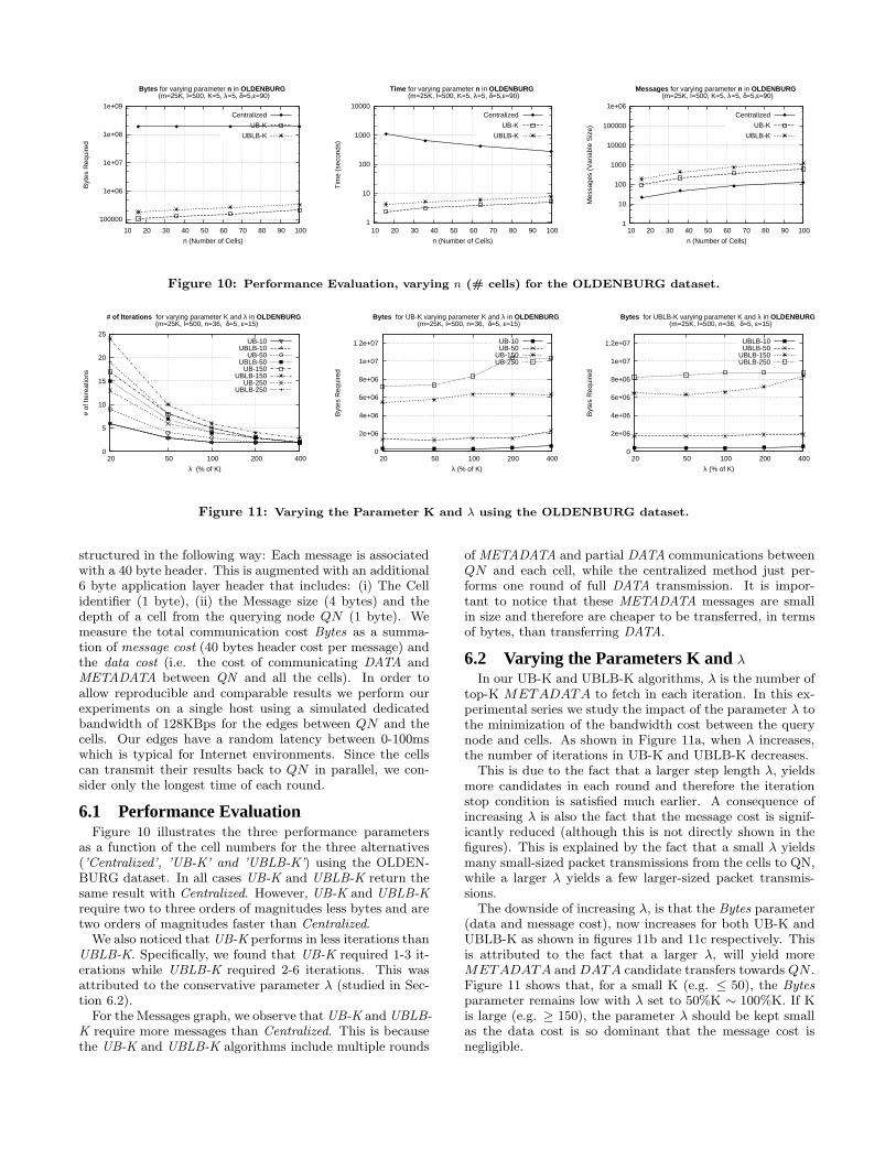
6.1 Performance EvaluationFigure 10 illustrates the three performance parameters
as a function of the cell numbers for the three alternatives(’Centralized’, ’UB-K’ and ’UBLB-K’) using the OLDEN-BURG dataset. In all cases UB-K and UBLB-K return thesame result with Centralized. However, UB-K and UBLB-Krequire two to three orders of magnitudes less bytes and aretwo orders of magnitudes faster than Centralized.
We also noticed that UB-K performs in less iterations thanUBLB-K. Specifically, we found that UB-K required 1-3 it-erations while UBLB-K required 2-6 iterations. This wasattributed to the conservative parameter λ (studied in Sec-tion 6.2).
For the Messages graph, we observe that UB-K and UBLB-K require more messages than Centralized. This is becausethe UB-K and UBLB-K algorithms include multiple rounds
of METADATA and partial DATA communications betweenQN and each cell, while the centralized method just per-forms one round of full DATA transmission. It is impor-tant to notice that these METADATA messages are smallin size and therefore are cheaper to be transferred, in termsof bytes, than transferring DATA.
6.2 Varying the Parameters K andλ
In our UB-K and UBLB-K algorithms, λ is the number oftop-K METADATA to fetch in each iteration. In this ex-perimental series we study the impact of the parameter λ tothe minimization of the bandwidth cost between the querynode and cells. As shown in Figure 11a, when λ increases,the number of iterations in UB-K and UBLB-K decreases.
This is due to the fact that a larger step length λ, yieldsmore candidates in each round and therefore the iterationstop condition is satisfied much earlier. A consequence ofincreasing λ is also the fact that the message cost is signif-icantly reduced (although this is not directly shown in thefigures). This is explained by the fact that a small λ yieldsmany small-sized packet transmissions from the cells to QN,while a larger λ yields a few larger-sized packet transmis-sions.
The downside of increasing λ, is that the Bytes parameter(data and message cost), now increases for both UB-K andUBLB-K as shown in figures 11b and 11c respectively. Thisis attributed to the fact that a larger λ, will yield moreMETADATA and DATA candidate transfers towards QN .Figure 11 shows that, for a small K (e.g. ≤ 50), the Bytesparameter remains low with λ set to 50%K ∼ 100%K. If Kis large (e.g. ≥ 150), the parameter λ should be kept smallas the data cost is so dominant that the message cost isnegligible.
7. CONCLUSIONThis paper introduces and formalizes the distributed tra-
jectory similarity search problem. We propose two noveldistributed query processing algorithms that provide an ef-ficient and exact solution to this problem. Our algorithmsexploit a partial lower and upper bounds on the LCSS sim-ilarity, which is computed locally by each node. Compre-hensive experiments with realistic data shows that UB-Kand UBLB-K are orders of magnitudes more efficient interms of network traffic and delay. Our approach can eas-ily be extended to lower bound the DTW distance as well.Since DTW is a distance, our distributed retrieval tech-niques would have to find the K trajectories with the small-est distances to the query. To do that we can modify ourUB-K algorithm to work with lower bounds instead.
AcknowledgementsWe would like to thank Michalis Vlachos (IBM TJ Watson)for his help in developing the spatiotemporal similarity mea-sures. We would also like to thank Eamonn Keogh (UCR)for the interesting discussions and ideas. This work wassupported by grants from NSF ITR #0220148, #0330481.
8. REFERENCES[1] Al-Taha K. , Snodgrass R., and Soo M.,
“Bibliography on Spatiotemporal Databases”, InSIGMOD Record, 22(1):59–67, March 1993.
[2] Babcock B. and Olston C., “Distributed Top-KMonitoring”, In SIGMOD’03, San Diego, CA, USA,pp. 28-39, 2003.
[3] Balke W.-T., Nejdl W., Siberski W., Thaden U.,“Progressive Distributed Top-K Retrieval inPeer-to-Peer Networks”, In ICDE’05, Tokyo, Japan,pp. 174-185, 2005.
[4] Basch J., Guibas L. and Hershberger J., “DataStructures for Mobile Data”, In SIAM Symposium onDiscrete Algorithms, New Orleans, Louisiana, pp.747-756, 1997.
[5] Berndt D., Clifford J., “Using Dynamic TimeWarping to Find Patterns in Time Series”, InKDD’94, Menlo Park, CA, pp. 229-248, 1994.
[6] Brinkhoff T., “A Framework for GeneratingNetwork-Based Moving Objects”. In GeoInformatica,6(2), 2002.
[7] Bruno N., Gravano L. and Marian A., “EvaluatingTop-K Queries Over Web Accessible Databases”, InICDE’02, San Jose, CA, Page 369, 2002.
[8] Cao P. and Wang Z., “Efficient Top-K QueryCalculation in Distributed Networks”, In PODC’04,St. John’s, Newfoundland, Canada, pp. 206-215,2004.
[9] Das G., Gunopulos D., Mannila H., “Finding SimilarTime Series”, In PKDD’97, Trondheim, Norway, pp.88-100, LNCS 1263, 1997.
[10] Fagin R., “Combining Fuzzy Information fromMultiple Systems”, In PODS’96, Montreal, Quebec,pp. 216-226, 1996.
[11] Fagin R., Lotem A. and Naor M., “OptimalAggregation Algorithms For Middleware”, InPODS’01, Santa Barbara, CA, pp. 102-113, 2001.
[12] Hadjieleftheriou M., Kollios G., Bakalov P., Tsotras
V.J., “Complex Spatio-Temporal Pattern Queries”,In VLDB’05, Trondheim, Norway, pp. 877-888, 2005.
[13] Kollios G., Gunopulos D., Tsotras V.J., “OnIndexing Mobile Objects”, In PODS’99,Philadelphia, PA, pp. 261-272, 1999.
[14] Yu H., Li H., Wu P., Agrawal D., Abbadi A.E.,“Efficient Processing of Distributed Top-k Queries”,In DEXA’05, Krakow, Poland, pp. 65-74, 2005.
[15] Kollios G., Gunopulos D., Tsotras V.J., Delis A.,Hadjieleftheriou M., “Indexing Animated ObjectsUsing Spatiotemporal Access Methods”, In IEEETKDE, Vol. 13, Iss. 5, pp. 758-777, 2001.
[16] Madden S.R., Franklin M.J., Hellerstein J.M., HongW., “TAG: a Tiny AGgregation Service for Ad-HocSensor Networks”, In OSDI’02, Boston, MA, pp.131-146, 2002.
[17] Bruno N., Gravano L. and Marian A., “EvaluatingTop-K Queries Over Web Accessible Databases”, InICDE’02, San Jose, CA, USA, Page 369, 2002.
[18] Mokbel M., Xiong X. and Aref W.G., “SINA:Scalable Incremental Processing of ContinuousQueries in Spatiotemporal Databases”, InSIGMOD’04, Paris, France, pp. 623-634, 2004.
[19] Papadias D., Mamoulis N., Delis V., “ApproximateSpatio-Temporal Retrieval”, In ACM TOIS, Vol. 19,Iss. 1, pp. 53-96, 2001.
[20] Saltenis S., Jensen C.S., “Indexing of Moving objectsfor Location-Based Services”, In ICDE’02,Washington, DC, Page 463, 2002.
[21] Saltenis S., Jensen C.S., Leutenegger S.T., LopezM.A., “Indexing the positions of continuouslymoving objects”, In SIGMOD’00, Dallas, Texas, pp.331-342, 2000.
[22] Tao Y., Papadias D., “The MV3R-Tree: ASpatio-Temporal Access Method for Timestamp andInterval Queries”, In VLDB’01, pp. 431-440, 2001.
[23] Tao Y., Sun J. and Papadias D., “Analysis ofPredictive Spatio-Temporal Queries” In ACMTODS, Vol. 28 , Iss. 4, pp. 295-336, 2003.
[24] Vlachos M., Hadjieleftheriou M., Gunopulos D.,Keogh E., “Indexing multi-dimensional time-serieswith support for multiple distance measures” InACM SIGKDD’03, Washington, D.C., pp. 216-225,2003.
[25] Xiong X., Mokbel M.F., Aref W.G., “SEA-CNN:Scalable Processing of Continuous K-NN Queries inSpatio-temporal Databases”, In ICDE’05, Tokyo,Japan, pp. 643-654, 2005.
[26] Xia T., Zhang D., Kanoulas E., Du Y., “OnComputing Top-t Most Influential Spatial Sites”, InVLDB’05, Trondheim, Norway, pp. 946-957, 2005.
[27] Xiong L. , Chitti S., Liu L., “Top-k Queries acrossMultiple Private Databases”, In ICDCS’05,Columbus, Ohio, pp. 145-154, 2005
[28] Zeinalipour-Yazti D., Vagena Z., Gunopulos D.,Kalogeraki V., Tsotras V., Vlachos M., Koudas N.,Srivastava D., “The Threshold Join Algorithm forTop-K Queries in Distributed Sensor Networks”, InDMSN (collocated with VLDB’05), Trondheim,Norway, 2005.


