Distributed generation system with PEM fuel cell for electrical power quality improvement

D. Ramirez , L.F. Beites , F. Blazquez , J.C. Ballesteros Department of Electrical Engineering, ETSII, Escuela de Ingenieros Industriaies, Uniuersidad Politecnica de Madrid,

C/ Jose Gutierrez Abascal 2, 28006 Madrid, Spain Endesa Generation, S.A. c/ Ribera de Loira 60, 28042 Madrid, Spain

Keywords: Distributed generation Power quality Fuel cell

A B S T R A C T

In this paper, a physical model for a distributed generation (DG) system with power quality improvement capability is presented. The generating system consists of a 5 kW PEM fuel cell, a natural gas reformer, hydrogen storage bottles and a bank of ultra-capacitors. Addi­tional power quality functions are implemented with a vector-controlled electronic converter for regulating the injected power. The capabilities of the system were experimentally tested on a scaled electrical network. It is composed of different lines, built with linear inductances and resistances, and taking into account both linear and non-linear loads. The ability to improve power quality was tested by means of different voltage and frequency perturbations produced on the physical model electrical network.

1. Introduction

Nowadays, the traditional centralized generation is slowly changing to a new paradigm, driven by environmental consid­erations and by the flexibility of the topology. This new model, usually known as distributed or embedded generation, is characterized by the small generation size, the proximity to the loads, and its connection to distribution networks. Usually, the generating equipment is renewable, or at least features clean and efficient energy systems.

The main purpose of this equipment is to generate the active power required by the loads. Besides, the flexibility of the generating systems allows their utilization as both voltage regulation devices, and as elements for power quality enhancement. The proper distribution of the different tech­nologies in the network also reduces losses and increases the reliability and efficiency of the electric system.

In addition to traditional generating equipment, like diesel or gas engines, new technologies have appeared, like micro turbines or fuel cells (FCs) With these systems, low power generation can reach a high efficiency. FCs appear as one of the most promising due to their good efficiency even at partial load, and especially due to their clean electric generation, with only water and heat as by-products. Also, their low noise and static operation allow them to be used even in domestic generation

Among all the different types of FC, the Proton Exchange Membrane Fuel Cells (PEMFCs) are one of the main choices for the range of powers used in distributed generation (DG). An interesting characteristic of this type of FC is its low operating temperature (less than 100 °C), which allows the system to be brought on-line rapidly and to install it close to the consumer.

In this paper, a DG system with power quality improve­ment functions is presented. It is based on a PEMFC with

a rated power of 5 kW. Its network behavior was evaluated on a scale model of an electrical grid constructed for this purpose. In addition to delivering active power to the grid, the system is designed to mitigate the following perturbations: voltage sags, voltage swells, voltage fluctuations, voltage collapse and frequency variations.

The paper is structured as follows: first, a general descrip­tion of the system is presented. The control algorithm is then explained, followed by a description of the main characteris­tics of the scale electrical grid. The paper concludes with the results of the perturbation compensation.

2. System description

Fuel cell systems, like any DC generating system, need an electronic converter to interface with the AC system. In DG applications, the converter is connected in parallel with the network, in the same way a traditional generator is connected. Compensation systems, on the other hand, can be connected using either a series or shunt topology.

The system in question was connected in parallel to the grid to allow it to inject active power as a DG system, while simultaneously acting as a compensating system.

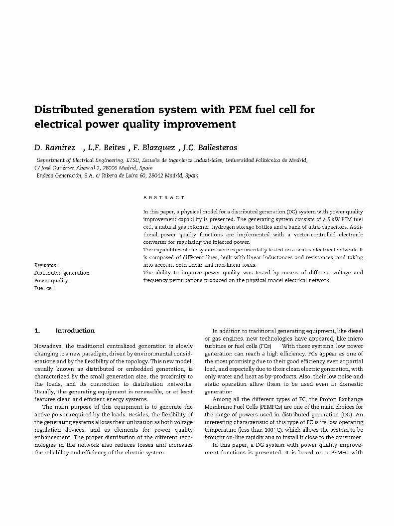
Fig. 1 shows the schematic diagram of the experimental set-up. The system is divided into 10 modules.

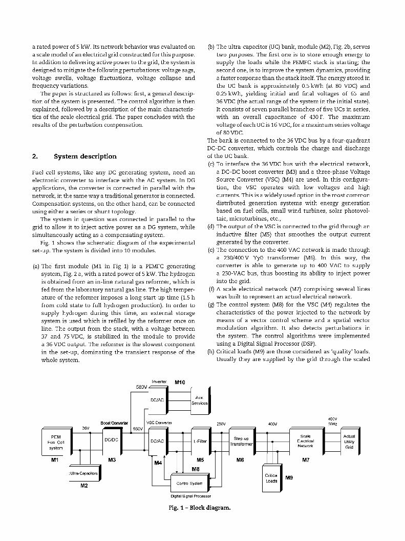
(a) The first module (Ml in Fig 1) is a PEMFC generating system, Fig. 2 a, with a rated power of 5 kW. The hydrogen is obtained from an in-line natural gas reformer, which is fed from the laboratory natural gas line. The high temper­ature of the reformer imposes a long start-up time (1.5 h from cold state to full hydrogen production). In order to supply hydrogen during this time, an external storage system is used which is refilled by the reformer once on line. The output from the stack, with a voltage between 37 and 75 VDC, is stabilized in the module to provide a 36 VDC output. The reformer is the slowest component in the set-up, dominating the transient response of the whole system.

(b) The ultra-capacitor (UC) bank, module (M2), Fig. 2b, serves two purposes. The first one is to store enough energy to supply the loads while the PEMFC stack is starting; the second one, is to improve the system dynamics, providing a faster response than the stack itself. The energy stored in the UC bank is approximately 0.5 kWh (at 80 VDC) and 0.25 kWh, yielding initial and final voltages of 65 and 36 VDC (the actual range of the system in the initial state). It consists of seven parallel branches of five UCs in series, with an overall capacitance of 430 F. The maximum voltage of each UC is 16 VDC, for a maximum series voltage of 80 VDC.

The bank is connected to the 36 VDC bus by a four-quadrant DC-DC converter, which controls the charge and discharge of the UC bank. (c) To interface the 36 VDC bus with the electrical network,

a DC-DC boost converter (M3) and a three-phase Voltage Source Converter (VSC) (M4) are used. In this configura­tion, the VSC operates with low voltages and high currents. This is a widely used option in the most common distributed generation systems with energy generation based on fuel cells, small wind turbines, solar photovol­taic, microturbines, etc.,

(d) The output of the VSC is connected to the grid through an inductive filter (M5) that smoothes the output current generated by the converter.

(e) The connection to the 400 VAC network is made through a 230/400 V YyO transformer (M6). In this way, the converter is able to generate up to 400 VAC to supply a 230-VAC bus, thus boosting its ability to inject power into the grid.

(f) A scale electrical network (M7) comprising several lines was built to represent an actual electrical network.

(g) The control system (M8) for the VSC (M4) regulates the characteristics of the power injected to the network by means of a vector control scheme and a spatial vector modulation algorithm. It also detects perturbations in the system. The control algorithms were implemented using a Digital Signal Processor (DSP).

(h) Critical loads (M9) are those considered as 'quality' loads. Usually they are supplied by the grid through the scaled

PEM Fuel Cell system

M1

E 3GV

Ultra-Capacitors •

M 9

oost Converter

DC/DC

M3

580V A

580V

Inverter

DC/AC

VSC Conve

DC/AC

M4

M10

ter

Aux, Services

L-Filter

M5

MS

230V

" •

Control System |

Step-up Transformer

M6

400V

Critical Loads

M9

IP

M7

400V 50Hz

Actual Utility Grid

Digital Signal Processor

Fig. 1 - Block diagram.

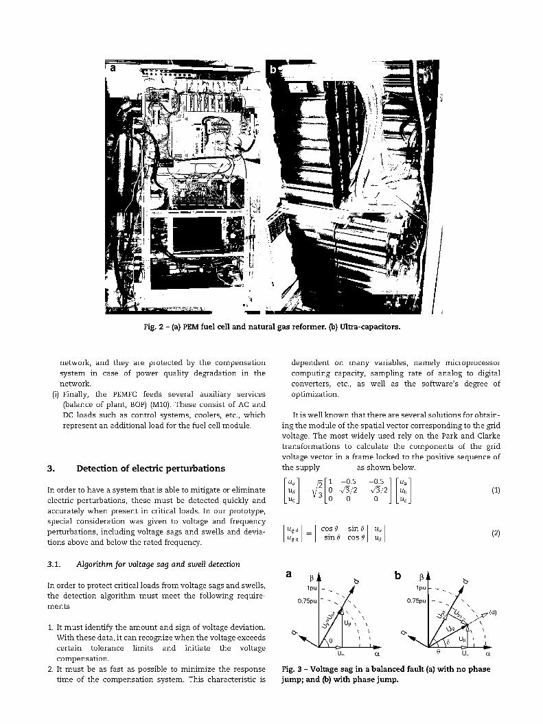
Fig. 2 - (a) PEM fuel cell and natural gas reformer, (b) Ultra-capacitors.

network, and they are protected by the compensation system in case of power quality degradation in the network.

(i) Finally, the PEMFC feeds several auxiliary services (balance of plant, BOP) (M10). These consist of AC and DC loads such as control systems, coolers, etc., which represent an additional load for the fuel cell module.

3. Detection of electric perturbations

In order to have a system that is able to mitigate or eliminate electric perturbations, these must be detected quickly and accurately when present in critical loads. In our prototype, special consideration was given to voltage and frequency perturbations, including voltage sags and swells and devia­tions above and below the rated frequency.

dependent on many variables, namely microprocessor computing capacity, sampling rate of analog to digital converters, etc., as well as the software's degree of optimization.

It is well known that there are several solutions for obtain­ing the module of the spatial vector corresponding to the grid voltage. The most widely used rely on the Park and Clarke transformations to calculate the components of the grid voltage vector in a frame locked to the positive sequence of the supply as shown below.

ua

Up

l_u°J

/?[ = v ^

U„d cos 6 -s in 6

0.5 3/2 0

-0.5 1 -V3/2

0

["a] Ub Uc

sin 6 cos 8

(1)

(2)

3.1. Algorithm for voltage sag and swell detection

In order to protect critical loads from voltage sags and swells, the detection algorithm must meet the following require­ments

1. It must identify the amount and sign of voltage deviation. With these data, it can recognize when the voltage exceeds certain tolerance limits and initiate the voltage compensation.

2. It must be as fast as possible to minimize the response time of the compensation system. This characteristic is

pj 1pu

0.75pu

\ &

"""• - y "*/ \

4A»s v ( d )

* \ \ o H Ua a

Fig. 3 - Voltage sag in a balanced fault (a) with no phase jump; and (b) with phase jump.

If the voltage sags or swells are not accompanied by a phase shift, Fig. 3a, then

P=cte

UP = + u; 2 _ q U„d (3)

since uq = 0, because 8 is the angle of the longitudinal axis, d, usually measured with a Phase-Locked Loop (PLL) system [6,7].

If, however, the balanced voltage variation is accompanied by a balanced phase jump, the PLL system initially loses synchronism, i.e. 8 ¥= 5, since the d-axis is in a new position (d) in Fig. 3b, which invalidates the results of the transforma­tions (2) and hence the value of (2).

Alternatively, if is calculated from the stationary coordi­nates and, by using the expression

Ua = \ ul + u2„ (4)

it is not necessary to know the transformation angle, and therefore the vector module is correctly calculated in each program cycle and with a lower computational effort because no trigonometric functions are used. This is why we opted for this approach.

Now it is possible to calculate the error in the utility grid voltage by using the expression

Err U = U0 -Vi (5)

where Ureference is the pre-sag (or swell) voltage value in the network.

Since the value of the spatial vector module is updated at the microprocessor sampling rate (0.2 ms in the prototype), the peak value of this voltage is available for the control system in each program cycle. In this way, the sag detection will occur in the initial phase of the perturbation, resulting in a very short compensation system response time.

The \Ug\ is a rippled signal due to imperfections in the measurement systems and even in the source voltages. To obtain a smooth value, the signal can be filtered out with a digital low-pass filter although this introduces a small delay in the detection system.

When the voltage error (5) is beyond a certain tolerance, a voltage perturbation (a sag for example) is considered to have taken place. It is important to note that the deeper the sag, the greater the magnitude of (5), which is a measure of the depth of the sag for the control system. The end of the sag is detected by using a hysteresis scheme in which the voltage is considered recovered when its value is above a fixed limit that is slightly greater than nominal. Then, once the fault is cleared, the amount of reactive power injected by the PEMFC-based compensator must be set to the pre-sag value to keep the PCC voltage from increasing above the rated value.

P+jQ 2f -

Uc ( Q (VSC)

©ug (gnd)

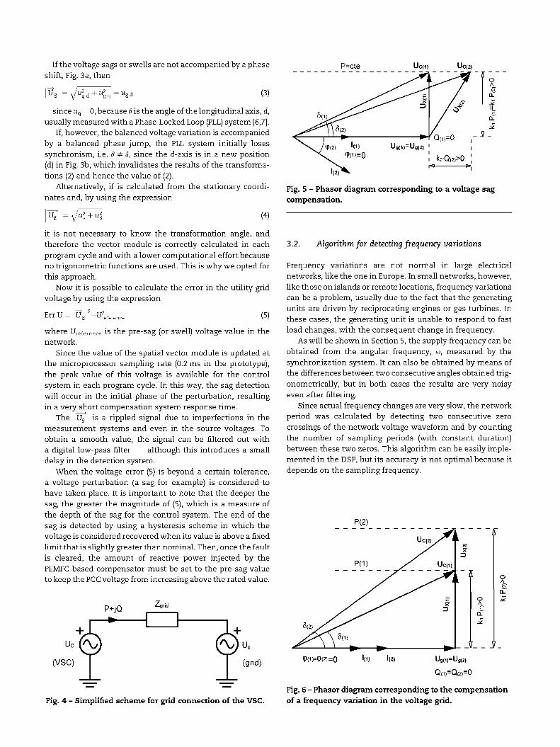
Fig. 5 - Phasor diagram corresponding to a voltage sag compensation.

3.2. Algorithm for detecting frequency variations

Frequency variations are not normal in large electrical networks, like the one in Europe. In small networks, however, like those on islands or remote locations, frequency variations can be a problem, usually due to the fact that the generating units are driven by reciprocating engines or gas turbines. In these cases, the generating unit is unable to respond to fast load changes, with the consequent change in frequency.

As will be shown in Section 5, the supply frequency can be obtained from the angular frequency, &>, measured by the synchronization system. It can also be obtained by means of the differences between two consecutive angles obtained trig-onometrically, but in both cases the results are very noisy even after filtering.

Since actual frequency changes are very slow, the network period was calculated by detecting two consecutive zero crossings of the network voltage waveform and by counting the number of sampling periods (with constant duration) between these two zeros. This algorithm can be easily imple­mented in the DSP, but its accuracy is not optimal because it depends on the sampling frequency.

<P(1)=P(2)=0 Ug(1)-UB(2|

Qd)=Q(2)=0

Fig. 4 - Simplified scheme for grid connection of the VSC. Fig. 6 - Phasor diagram corresponding to the compensation of a frequency variation in the voltage grid.

Electrical network

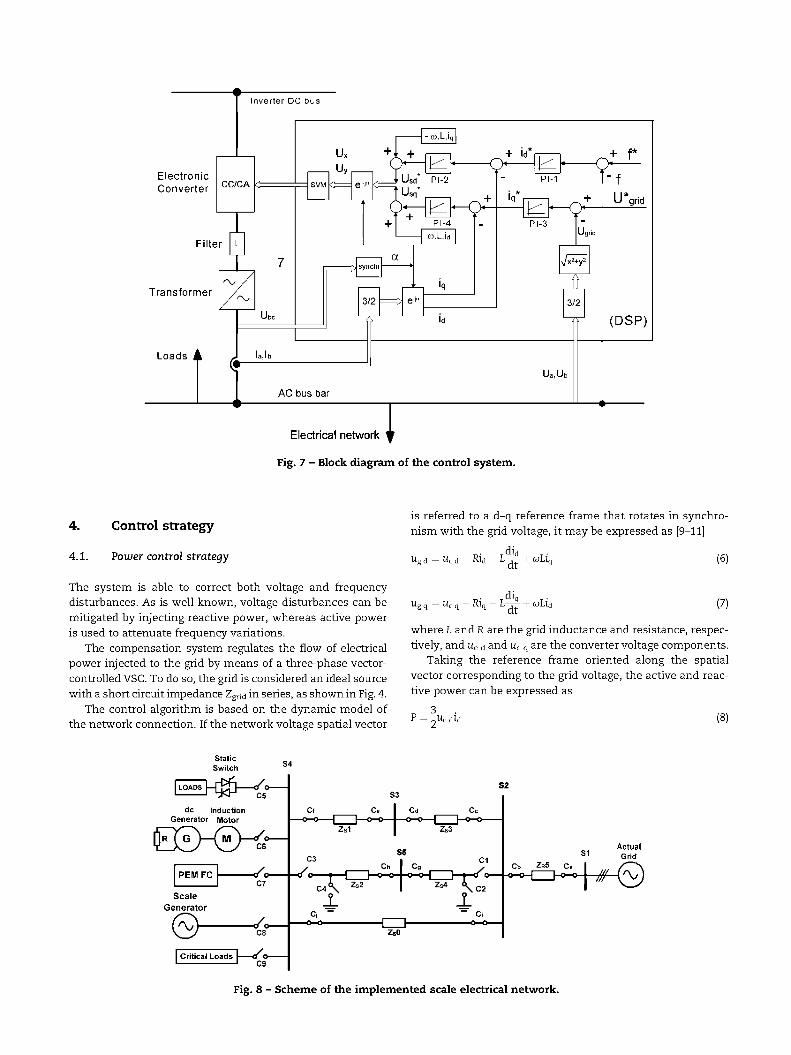
Fig. 7 - Block diagram of the control system.

4. Control strategy

4.1. Power control strategy

The system is able to correct both voltage and frequency disturbances. As is well known, voltage disturbances can be mitigated by injecting reactive power, whereas active power is used to attenuate frequency variations.

The compensation system regulates the flow of electrical power injected to the grid by means of a three-phase vector-controlled VSC. To do so, the grid is considered an ideal source with a short circuit impedance Zgnd in series, as shown in Fig. 4.

The control algorithm is based on the dynamic model of the network connection. If the network voltage spatial vector

is referred to a d-q reference frame that rotates in synchro­nism with the grid voltage, it may be expressed as [9-11]

u g d = uc d - Rid - L - j - + wLiq

^c q - Rlq - l - ^ + wLid

(6)

(7)

where L and R are the grid inductance and resistance, respec­tively, and uc d and uc q are the converter voltage components.

Taking the reference frame oriented along the spatial vector corresponding to the grid voltage, the active and reac­tive power can be expressed as

P = 2Uc did

Static Switch

:H#-£ dc Induction

Generator Motor

PEM FC

Scale Generator

© <r-Critical Loads M:̂

Actual

Fig. 8 - Scheme of the implemented scale electrical network.

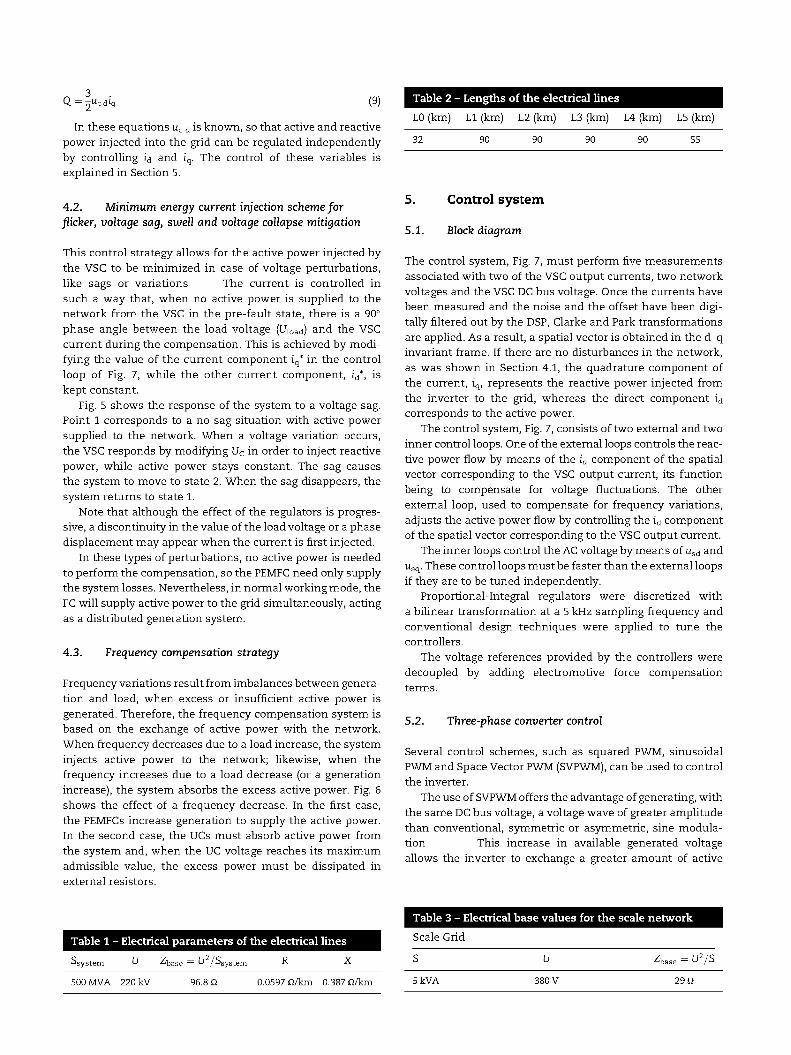
Q = ^ U c dlq (9)

In these equations uc d is known, so that active and reactive power injected into the grid can be regulated independently by controlling id and iq. The control of these variables is explained in Section 5.

4.2. Minimum energy current injection scheme for flicker, voltage sag, swell and voltage collapse mitigation

This control strategy allows for the active power injected by the VSC to be minimized in case of voltage perturbations, like sags or variations The current is controlled in such a way that, when no active power is supplied to the network from the VSC in the pre-fault state, there is a 90° phase angle between the load voltage (Uioad) and the VSC current during the compensation. This is achieved by modi­fying the value of the current component iq* in the control loop of Fig. 7, while the other current component, id*, is kept constant.

Fig. 5 shows the response of the system to a voltage sag. Point 1 corresponds to a no-sag situation with active power supplied to the network. When a voltage variation occurs, the VSC responds by modifying Uc in order to inject reactive power, while active power stays constant. The sag causes the system to move to state 2. When the sag disappears, the system returns to state 1.

Note that although the effect of the regulators is progres­sive, a discontinuity in the value of the load voltage or a phase displacement may appear when the current is first injected.

In these types of perturbations, no active power is needed to perform the compensation, so the PEMFC need only supply the system losses. Nevertheless, in normal working mode, the FC will supply active power to the grid simultaneously, acting as a distributed generation system.

4.3. Frequency compensation strategy

Frequency variations result from imbalances between genera­tion and load, when excess or insufficient active power is generated. Therefore, the frequency compensation system is based on the exchange of active power with the network. When frequency decreases due to a load increase, the system injects active power to the network; likewise, when the frequency increases due to a load decrease (or a generation increase), the system absorbs the excess active power. Fig. 6 shows the effect of a frequency decrease. In the first case, the PEMFCs increase generation to supply the active power. In the second case, the UCs must absorb active power from the system and, when the UC voltage reaches its maximum admissible value, the excess power must be dissipated in external resistors.

Table 2 -

L0 (km)

32

• Lengths of the electrical l ines

LI (km) L2 (km) L3 (km) L4 (km)

90 90 90 90

L5 (km)

55

5. Control system

5.1. Block diagram

The control system, Fig. 7, must perform five measurements associated with two of the VSC output currents, two network voltages and the VSC DC bus voltage. Once the currents have been measured and the noise and the offset have been digi­tally filtered out by the DSP, Clarke and Park transformations are applied. As a result, a spatial vector is obtained in the d-q invariant frame. If there are no disturbances in the network, as was shown in Section 4.1, the quadrature component of the current, iq, represents the reactive power injected from the inverter to the grid, whereas the direct component id

corresponds to the active power.

The control system, Fig. 7, consists of two external and two inner control loops. One of the external loops controls the reac­tive power flow by means of the iq component of the spatial vector corresponding to the VSC output current, its function being to compensate for voltage fluctuations. The other external loop, used to compensate for frequency variations, adjusts the active power flow by controlling the id component of the spatial vector corresponding to the VSC output current.

The inner loops control the AC voltage by means of usd and usq. These control loops must be faster than the external loops if they are to be tuned independently.

Proportional-Integral regulators were discretized with a bilinear transformation at a 5 kHz sampling frequency and conventional design techniques were applied to tune the controllers.

The voltage references provided by the controllers were decoupled by adding electromotive force compensation terms.

5.2. Three-phase converter control

Several control schemes, such as squared PWM, sinusoidal PWM and Space Vector PWM (SVPWM), can be used to control the inverter.

The use of SVPWM offers the advantage of generating, with the same DC bus voltage, a voltage wave of greater amplitude than conventional, symmetric or asymmetric, sine modula­tion This increase in available generated voltage allows the inverter to exchange a greater amount of active

Table 1 - Electrical parameters of the electrical lines

•^system u -̂•ba; •• u 2 / s ; 'system R

500 MVA 220 kV 96.8 Q 0.0597 Q/km 0.387 Q/km

Table 3 - Electrical base values for the scale network

Scale Grid

U2/S

5kVA 380 V 29 Q

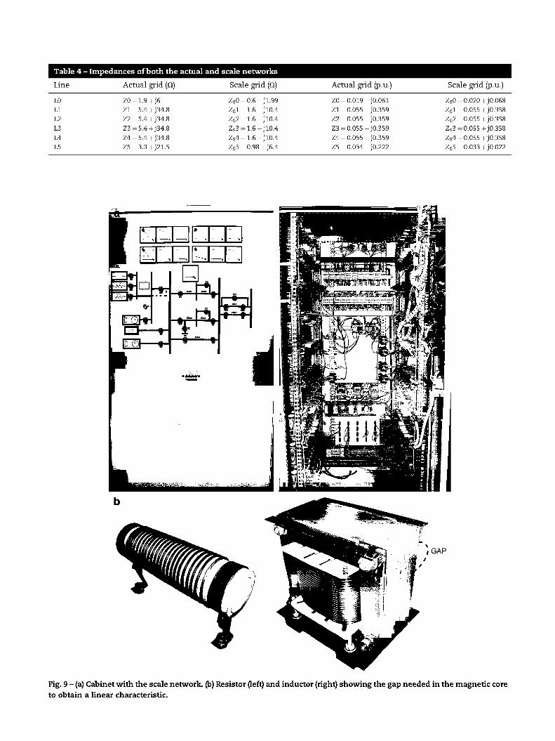
Table 4 •

Line

LO Ll L2 L3 L4 L5

- Impedances of both the actual and scale networks

Actual grid (Q)

Z0 = 1.9+j6 Zl = 5.4+j34.8 Z2 = 5.4+j34.8 Z3 = 5.4+j34.8 Z4 = 5.4+j34.8 Z5 = 3.3+j21.5

Scale grid (Q)

Zs0 = 0.6+jl.99 Zsl = 1.6+jl0.4 Zs2 = 1.6+jl0.4 Zs3 = 1.6+jl0.4 Zs4 = 1.6+jl0.4 Zs5 = 0.98+j6.4

Actual grid (p.u.)

Z0 = 0.019+J0.061 Zl = 0.055+J0.359 Z2 = 0.055+J0.359 Z3 = 0.055+J0.359 Z4 = 0.055+J0.359 Z5 = 0.034+J0.222

Scale grid (p.u.)

Zs0 = 0.020+J0.068 Zsl = 0.055 +J0.358 Zs2 = 0.055+J0.358 Zs3 = 0.055+J0.358 Zs4 = 0.055+J0.358 Zs5 = 0.033+J0.022

y ~ -:U~

»

i

—,

,

,

fc

Fig. 9 - (a) Cabinet with the scale network, (b) Resistor (left) and inductor (right) showing the gap needed in the magnetic core

to obtain a linear characteristic.

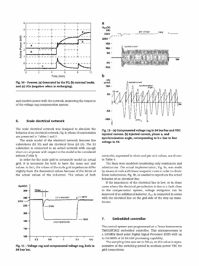
4 6 Time (min)

Fig. 10 - Powers, (a) Generated by the FC; (b) external loads; and (c) UCs (negative when is recharging).

and reactive power with the network, improving the response of the voltage sag compensation system.

6. Scale electrical network

The scale electrical network was designed to simulate the behavior of an electrical network, Fig. 8, whose characteristics are presented in Tables 1 and 2.

The scale model of the electrical network features five substations (S1-S5) and six electrical lines (L0-L5). The SI substation is connected to an actual network with enough short circuit power with respect to the model to be considered infinite (Table 3).

In order for the scale grid to accurately model an actual grid, it is necessary for both to have the same per unit values. In fact, the values of the scale grid impedances differ slightly from the theoretical values because of the limits of the actual values of the inductors. The values of both

Ugrid(V)

260 -

240 -235V — *

2 2 0 -

2 0 0 -

180 -

1 6 0 -

70ms

compensated i — 241V

f 218V

I uncompensated

I 0.2

I I I I I 0.6 1 1

183V

I 4 t(s)

a Ugrw(V)

i(A)

230V

2 0 9 V /

15A

10A

5A

-5A

-10A

grid voltage 240V -

injected current

Fig. 12 - (a) Compensated voltage sag in S4 bus bar and VSC injected current, (b) Injected current, phase a, and synchronization angle, corresponding to b-c line to line voltage in S4.

networks, expressed in ohms and per unit values, are shown in Table 4.

The lines were modeled considering only resistances and admittances. The actual implementation, Fig. 9a, was made by means of coils with linear magnetic cores in order to obtain linear inductances, Fig. 9b, as needed to reproduce the actual behavior of an electrical line.

If the impedance of the electrical line is low, or in those cases where the electrical perturbation is due to a fault close to the compensation system, voltage mitigation can be improved if an additional inductor, Xad, is connected in series with the electrical line on the grid side of the step-up trans­former

7. Embedded controller

Fig. 11 - Voltage sag and compensated voltage sag, both in S4 bus bar.

The control system was programmed on a Texas Instruments TMS320F2812 embedded controller. This microprocessor is a 150 MHz fixed point Digital Signal Processor (DSP) with up to 150 MIPS of 32-bit DSP processing capability.

The sampling time was set to 200 u,s, as this value is repre­sentative of the switching period in medium power VSC for grid connections.

a

frequency of grid voltage

compensated voltage

not compensated voltage

I u n 11

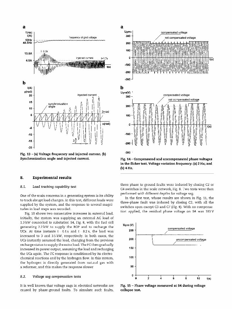
Fig. 13 - (a) Voltage frequency and injected current, (b) Synchronization angle and injected current.

b Ugrid(V)

300-compensated voltage

not compensated voltage

-300

Fig. 14 - Compensated and uncompensated phase voltages in the flicker test. Voltage variation frequency: (a) 2 Hz; and (b) 4 Hz.

8. Experimental results

8.1. Load tracking capability test

One of the main concerns in a generating system is its ability to track abrupt load changes. In this test, different loads were supplied by the system, and the response to several magni­tudes in load steps was recorded.

Fig. 10 shows two consecutive increases in external load. Initially, the system was supplying an external AC load of 1.3 kW connected to substation S4, Fig. 8, with the fuel cell generating 2.2 kW to supply the BOP and to recharge the UCs. At time instants t = 4.4s and t = 8.2s, the load was increased to 3 and 3.5 kW, respectively. In both cases, the UCs instantly assumed the load, changing from the previous recharge status to supply the extra load. The FC then gradually increased its power output, assuming the load and recharging the UCs again. The FC response is conditioned by its electro­chemical reactions and by the hydrogen flow. In this system, the hydrogen is directly generated from natural gas with a reformer, and this makes the response slower

8.2. Voltage sag compensation tests

It is well known that voltage sags in electrical networks are caused by phase-ground faults. To simulate such faults,

three-phase to ground faults were induced by closing C2 or C4 switches in the scale network, Fig. 8. Two tests were then performed with different depths for voltage sag.

In the first test, whose results are shown in Fig. 11, the three-phase fault was induced by closing C2, with all the switches open except C3 and C7 (Fig. 8). With no compensa­tion applied, the residual phase voltage on S4 was 183 V

Ugrid (V)

250

200

150

100

50

0

compensated voltage

uncompensated voltage

—r -

10 t(s)

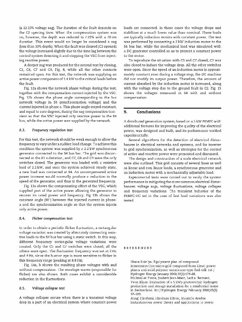
Fig. 15 - Phase voltage measured at S4 during voltage collapse test.

(a 22.13% voltage sag). The duration of the fault depends on the C2 opening time. When the compensation system was on, however, the depth was reduced to 7.23% with a 70 ms duration. This event would no longer be considered a sag (less than 10% depth). When the fault was cleared (C2 opened) the voltage increased slightly due to the time lag between the control system detecting it and stopping the VSC from inject­ing reactive power.

A deeper sag was produced for the second test by closing, CI, C4, C7 and C9, Fig. 8, while all the other contacts remained open. For this test, the network was supplying an active power component of 1.4 kW to the critical loads before the fault.

Fig. 12a shows the network phase voltage during the test, together with the compensation current injected by the VSC. Fig. 12b shows the phase angle corresponding to the b-c network voltage in S4 (synchronization voltage) and the current injected in phase a. This phase angle stayed constant, and equal to zero degrees, during the sag compensation tran­sient so that the VSC injected only reactive power to the S4 bus, while the active power was supplied by the network.

8.3. Frequency regulation test

For this test, the network should be weak enough to allow the frequency to vary under a sudden load change. To achieve this condition the system was supplied by a 2.2 kW synchronous generator connected to the S4 bus bar. The grid was discon­nected at the SI substation, and C7, C8 and C9 were the only switches closed. The generator was loaded with a resistive load of 2.2 kW, and once the system achieved steady state, a new load was connected at S4. An uncompensated active power increase would normally produce a reduction in the speed of the generator, and thus in the generated frequency.

Fig. 13a shows the compensating effect of the VSC, which supplied part of the active power allowing the generator to recover its rated power and frequency. Fig 13b shows the constant angle (90°) between the injected current in phase-a and the synchronization angle so that the system injects only active power.

8.4. Flicker compensation test

In order to obtain a periodic flicker fluctuation, a rectangular voltage variation was created by alternately connecting resis­tive loads to the S4 bus bar using a static switch. In this way, different frequency rectangular voltage variations were created. Only the C5 and C7 switches were closed; all the others were open. The fluctuation frequency was set at 2 Hz and 4 Hz, since the human eye is more sensitive to flicker in this frequency range (peaking at 8.8 Hz).

Fig. 14a, b shows the resulting phase voltages with and without compensation. The envelope waves (responsible for flicker) are also shown. Both cases exhibit a considerable reduction in the fluctuations.

8.5. Voltage collapse test

A voltage collapse occurs when there is a transient voltage drop in a part of an electrical system where constant power

loads are connected. In these cases the voltage drops and stabilizes at a much lower value than nominal. These loads are typically induction motors with constant power. The test was performed by connecting a 2 kW induction motor to the S4 bus bar, while the mechanical load was simulated with a DC generator controlled so as to present a constant power to the motor.

To reproduce the situation with C3 and C7 closed, C2 was also closed to induce the voltage drop. All the other switches were open. Since the speed of an induction motor is approxi­mately constant even during a voltage step, the DC machine did not modify its output power. Therefore, the amount of current absorbed by the induction motor is increased, along with the voltage step due to the ground fault in C2. Fig. 15 shows the voltages measured at S4 with and without compensation.

9. Conclusions

A distributed generation system, based on a 5 kW PEMFC with additional features for improving the quality of the electrical power, was designed and built, and its performance verified experimentally.

Several algorithms for the detection of electrical distur­bances in electrical networks and systems, and for inverter to grid synchronization, as well as strategies for the control of active and reactive power were presented and discussed.

The design and construction of a scale electrical network were also outlined. This grid consists of several lines as well as linear and non-linear loads, a synchronous generator and an induction motor with a mechanically adjustable load.

Experimental tests were carried out to verify the system performance in mitigating the most common electrical distur­bances: voltage sags, voltage fluctuations, voltage collapse and frequency variations. The transient behavior of the PEMFC-UC set in the case of fast load variations was also tested.

R E F E R E N C E S

Obara Shin'ya. Equipment plan of compound interconnection micro-grid composed from diesel power plants and solid polymer membrane-type fuel cell. Int J Hydrogen Energy January 2008;33(l):179-88. Hollmuller Pierre, Joubert Jean-Marc, Lachal Bernard, Yvon Klaus. Evaluation of a 5 kWp photovoltaic hydrogen production and storage installation for a residential home in Switzerland. Int J Hydrogen Energy February 2000;25(2): 97-109. Akagi Hirofumi, Hirokazu Edson, Mauricio Aredes. Instantaneous power theory and applications to power

conditioning. In: IEEE press series on power engineering. Hoboken, New Jersey: Wiley-Interscience; John Wiley & Sons, Inc., ISBN 978-0-470-10761-4; 2007. Montero-Hernandez Oscar, Enjeti Prasad N. A fast detection algorithm suitable for mitigation of numerous power quality disturbances. IEEE Trans Ind Appl November/December 2005; 41(No. 6). Fitzer Chris, Barnes Mike, Green Peter. Voltage sag detection technique for a dynamic voltage restorer. IEEE Trans Ind Appl January/February 2004;40(No. 1). Changjiang Zhan, Fitzer C, Ramachandaramurthy VK, Arulampalam A, Barnes M, Jenkins N. Software phase-locked loop applied to dynamic Voltage restorer (DVR). In: Proceedings of IEEE-PES Winter Meeting; 2001. p. 1033-1038. Neto Arruda Licia, Magalhaes Silva Sidelmo, Branz J, Filho Cardoso. PLL structures for utility connected systems. Industry Applications Conference, 2001. Thirty-Sixth IAS Annual Meeting. Conference Record of the 2001 IEEE 30 Sep-Oct 2001;4:2655-60. Macken Koen JP, Bollen Math HJ, Belmans Ronnie JM. Mitigation of voltage dips through distributed generation systems. IEEE Trans Ind Appl November/December 2004; 40(No. 6). Wang C, Nehrir MH, Gao H. Control of PEM fuel cell distributed generation systems. IEEE Trans Energy Convers June 2006;21(No. 2).

Li YH, Rajakaruna S, Choi SS. Control of a solid oxide fuel cell power plant in a grid-connected system. IEEE Trans Energy Convers June 2007;22(No. 2). Chinchilla Monica, Arnaltes Santiago, Burgos Juan Carlos. Control of permanent-magnet generators applied to variable-speed wind-energy systems connected to the grid. IEEE Trans Energy Convers March 2006;21(No. 1). Naetiladdanon S, Miura Y, Ise T. Current injection control scheme of voltage sag compensation by parallel type compensator with series inductor. IEEJ Trans Ind Appl 2006; 126(No. 10). Grahame Holmes D, Lipo Thomas A. Pulse width modulation for power converters. Principles and practice. IEEE Press, John Wiley & Sons, Inc., ISBN 0-471-20814-0; 2003. Staebler Martin. Reduced electromagnetic interference (EMI) with the TMS320C24x DSP. Application report SPRA501. Texas Instruments; December 1998. Field orientated control of 3-phase AC-motors. Literature number: BPRA073. Europe: Texas Instruments; February 1998. Implementing space vector modulation with the ADMC401. AN401-17. Analog Devices Inc; January 2000. Hamelin J, Agbossou K, Laperriere A, Laurencelle F, Bose TK. Dynamic behavior of a PEM fuel cell stack for stationary applications. Int J Hydrogen Energy June 2001; 26(6):625-9.