Embed Size (px)
Citation preview

DISSERTATION
Titel der Dissertation
Landslide analysis and early warning
Local and regional case study in the Swabian Alb, Germany
Verfasser
Dipl.-Geogr. Benjamin Thiebes
angestrebter akademischer Grad
Doktor der Naturwissenschaften (Dr. rer. nat.)
Wien, 2011
Studienkennzahl lt. Studienblatt: A 091 453
Dissertationsgebiet lt. Studienblatt: Dr.-Studium der Naturwissenschaften
Betreuer: Univ.Prof. Dipl.-Geogr. Dr. Thomas Glade


All visible objects, man, are but as pasteboard masks.
But in each event — in the living act, the undoubted
deed — there, some unknown but still reasoning thing
puts forth the mouldings of its features from behind the
unreasoning mask. If man will strike, strike through the
mask!
Captain Ahab in Moby Dick (Melville 1851)
There is a theory which states that if ever anyone dis-
covers exactly what the Universe is for and why it is
here, it will instantly disappear and be replaced by
something even more bizarre and inexplicable.
There is another theory which states that this has al-
ready happened.
Adams (1980)


i
ACKNOWLEDGMENT
First of all I want to thank my supervisor Prof. Dr. Thomas Glade, who encouraged
me to write a PhD thesis and who kindly offered me the chance to work in his new
working group established at the University of Vienna. Thank you for your support
and guidance! I would like to thank my colleague and friend Dr. Rainer Bell for the
great cooperation over the last few years; it has always been a great pleasure to work
with you, and our discussions have helped immensely to improve my thesis.
I am grateful to the entire ENGAGE working group at the Institute of Geography and
Regional Research in Vienna for comments and discussion. My special thanks go out
to my office colleagues. Your support and friendship helped me a lot on my way. I
also would like to thank the entire ILEWS project. These have been exciting and chal-
lenging years and I enjoyed working with you very much. Thank you for the wonder-
ful colleagueship. I would especially like to thank Stefan, Raik and Bernd from the
company Geomer for great cooperation in creating the technical early warning sys-
tems.
For help with bureaucracy and organisation I want to acknowledge the support tech-
nical staff at the institute, especially Helmut Slawik and Rudi Voit. Laboratory analy-
sis of soil samples could not have been carried out without the kind help of Christa
Hermann and Robert Petizka. I would also like to thank all the helping hands during
field work. Another person acknowledged here is Mr. Siegler; without his apprecia-
tion of our work the entire project would not have been possible. Furthermore, the
local administration of Lichtenstein-Unterhausen was very supportive which is highly
acknowledged.
Many thanks to Malcolm Anderson and Liz Holcombe from the University of Bristol
for providing the CHASM software and the helpful tips on how to use it most effec-
tively. Significant rainfall data was kindly provided by Prof. Dr. Clemens Simmer
(Uni Bonn), Dr. Armin Mathes (Uni Bonn), Dr. Antje Claussnitzer (Uni Berlin) and
Walter Koelschtzky (DWD). Additional data was kindly provided by the LUBW and
LGL. Many thanks also to Jean-Christophe Kohn for the landslide inventory data. The
financial support granted by the German Ministry of Education and Research (BMBF)
and the Geotechnologien Consortium is highly acknowledged.
For proof-reading of this thesis, I am grateful towards Rainer, Emma, Ronny, Catrin,
Helene and Melanie. I want to express my deepest thanks to all my friends in Vienna.
Thank you for the great times! Last but not least, thank you fide for your love and
support over the past challenging years. I think now there are some new adventures
waiting for us! To all of you and to all the people I might have forgotten to mention,
thank you!


iii
TABLE OF CONTENTS
1 INTRODUCTION . . . . . . . . . . . . . . . . . . . . . . . . . . . . . . . . . . . . . . . . . . . . . . . . . . . . . . . . . . . . . . . . . . . . . . . . . . . . . . . 1
1.1 PROBLEM STATEMENT ........................................................................................... 1
1.2 RESEARCH OBJECTIVES .......................................................................................... 2
1.3 THESIS OUTLINE ..................................................................................................... 3
2 THEORETICAL BACKGROUND . . . . . . . . . . . . . . . . . . . . . . . . . . . . . . . . . . . . . . . . . . . . . . . . . . . . . . . . . . . 5
2.1 LANDSLIDE PROCESSES ......................................................................................... 5
2.1.1 Definitions and classifications ........................................................................ 5
2.1.2 Principles of slope stability ............................................................................. 6
2.1.3 Systems theory considerations ..................................................................... 12
2.1.4 Landslide triggering ....................................................................................... 15
2.2 LANDSLIDE INVESTIGATION AND MONITORING................................................ 17
2.2.1 Mapping and inventory approaches ........................................................... 19
2.2.2 Displacement measurements ........................................................................ 21
2.2.3 Hydrological measurements ......................................................................... 24
2.2.4 Geophysical measurements .......................................................................... 25
2.3 LANDSLIDE MODELLING ..................................................................................... 27
2.3.1 Regional models ............................................................................................. 28
2.3.2 Local models ................................................................................................... 29
2.4 LANDSLIDE EARLY WARNING SYSTEMS .............................................................. 35
2.5 THE ILEWS PROJECT ........................................................................................... 57
3 STUDY AREA . . . . . . . . . . . . . . . . . . . . . . . . . . . . . . . . . . . . . . . . . . . . . . . . . . . . . . . . . . . . . . . . . . . . . . . . . . . . . . . . . 61
3.1 REGIONAL SETTING ............................................................................................. 61
3.1.1 Geology ............................................................................................................ 62
3.1.2 Climate ............................................................................................................. 65
3.1.3 Hydrology ....................................................................................................... 65
3.1.4 Geomorphology .............................................................................................. 68
3.1.5 Landslides........................................................................................................ 68
3.2 LOCAL STUDY AREA ............................................................................................ 70
3.2.1 Geology ............................................................................................................ 72
3.2.2 Geomorphology .............................................................................................. 72
3.2.3 Previous investigations.................................................................................. 75
4 DATA . . . . . . . . . . . . . . . . . . . . . . . . . . . . . . . . . . . . . . . . . . . . . . . . . . . . . . . . . . . . . . . . . . . . . . . . . . . . . . . . . . . . . . . . . . . . 77
5 METHODOLOGY . . . . . . . . . . . . . . . . . . . . . . . . . . . . . . . . . . . . . . . . . . . . . . . . . . . . . . . . . . . . . . . . . . . . . . . . . . . . 85
5.1 LOCAL SCALE ....................................................................................................... 85
5.1.1 Field work ........................................................................................................ 85
5.1.2 Data analysis ................................................................................................... 86
5.1.2.1 Core samples .......................................................................................... 87
5.1.2.2 Slope movement data ............................................................................. 87

iv
5.1.2.3 Hydrological data .................................................................................. 87
5.1.3 Landslide early warning modelling ............................................................ 87
5.1.3.1 Generation of input data ........................................................................ 91
5.1.3.2 Model application .................................................................................. 94
5.1.3.3 CHASM early warning model .............................................................. 95
5.1.3.4 CHASM decision-support tool .............................................................. 95
5.2 REGIONAL SCALE ................................................................................................. 96
5.2.1 Inventory analysis .......................................................................................... 96
5.2.2 Thresholds verification .................................................................................. 96
5.2.3 Early warning ................................................................................................. 97
6 RESULTS . . . . . . . . . . . . . . . . . . . . . . . . . . . . . . . . . . . . . . . . . . . . . . . . . . . . . . . . . . . . . . . . . . . . . . . . . . . . . . . . . . . . . . . . 99
6.1 LOCAL SCALE ....................................................................................................... 99
6.1.1 Field work ........................................................................................................ 99
6.1.2 Data analysis ................................................................................................. 101
6.1.2.1 Core samples ........................................................................................ 101
6.1.2.2 Slope movement data ........................................................................... 105
6.1.2.3 Hydrological data ................................................................................ 115
6.1.3 Landslide early warning modelling .......................................................... 134
6.1.3.1 Generation of input data ...................................................................... 134
6.1.3.2 Model application ................................................................................ 160
6.1.3.3 CHASM early warning model ............................................................ 170
6.1.3.4 CHASM decision-support tool ............................................................ 172
6.2 REGIONAL SCALE ............................................................................................... 177
6.2.1 Inventory analysis ........................................................................................ 177
6.2.2 Thresholds verification ................................................................................ 180
6.2.3 Early warning ............................................................................................... 189
7 INTEGRATIVE EARLY WARNING . . . . . . . . . . . . . . . . . . . . . . . . . . . . . . . . . . . . . . . . . . . . . . . . . . . . 193
8 DISCUSSION . . . . . . . . . . . . . . . . . . . . . . . . . . . . . . . . . . . . . . . . . . . . . . . . . . . . . . . . . . . . . . . . . . . . . . . . . . . . . . . . 197
9 PERSPECTIVES . . . . . . . . . . . . . . . . . . . . . . . . . . . . . . . . . . . . . . . . . . . . . . . . . . . . . . . . . . . . . . . . . . . . . . . . . . . . . 203
10 SUMMARY . . . . . . . . . . . . . . . . . . . . . . . . . . . . . . . . . . . . . . . . . . . . . . . . . . . . . . . . . . . . . . . . . . . . . . . . . . . . . . . . . . . 207
11 REFERENCES . . . . . . . . . . . . . . . . . . . . . . . . . . . . . . . . . . . . . . . . . . . . . . . . . . . . . . . . . . . . . . . . . . . . . . . . . . . . . . . . 213
12 APPENDIX . . . . . . . . . . . . . . . . . . . . . . . . . . . . . . . . . . . . . . . . . . . . . . . . . . . . . . . . . . . . . . . . . . . . . . . . . . . . . . . . . . . . 257

v
LIST OF FIGURES
Fig. 2.1: Stability states and destabilising factors (after Glade and Crozier 2005b, based on Crozier 1989) ........................................................................................................................ 7
Fig. 2.2: Stress vectors within a slope (based on Ahnert 2003) .......................................... 7
Fig. 2.3: Idealized stress-strain curves for brittle (A) and ductile (B) deformation (Petley and Allison 1997) ......................................................................................................... 9
Fig. 2.4: Idealized strain curves for the three stages of creep (after Petley et al. 2008) . 10
Fig. 2.5: Effects of external perturbations on a geomorphological system (based on Bull 1991) ................................................................................................................................. 13
Fig. 2.6: Simplified illustration of method of slices (based on Conolly 1997) ................ 31
Fig. 2.7: General risk management cycle (Alexander 2000; 2002) .................................... 36
Fig. 2.8: Number of landslide fatalities in Hong Kong (Wong and Ho 2000) ................ 45
Fig. 2.9: Comparison of warning curve and warning line thresholds and subsequent time spans for evacuation (Aleotti 2004) ............................................................................. 49
Fig. 2.10: Early warning system at Winkelgrat landslide equipped with automatic extensometers (left) and traffic light for road closure (right)........................................... 51
Fig: 2.11: General structure of ILEWS project (Bell et al. 2009) ........................................ 58
Fig. 3.1: Location of Swabian Alb and the local study area Lichtenstein-Unterhausen 61
Fig. 3.2: Geological features and fault lines in the Swabian Alb (based on Bell 2007) . 63
Fig. 3.3: Schematic profile across the South German cuesta landscape with indication of landslide susceptible areas and karst features (based on Wagenplast 2004) ............ 63
Fig. 3.4: Mean annual precipitation in the Swabian Alb region for period A (1941-1970) and period B (1971-2000) (based on Bell 2007) ................................................................... 66
Fig. 3.5: Annual rainfall for two selected weather stations from 1931 to 2004. Five year moving average and linear trend refer to Sonnenbühl-Genkingen ................................ 67
Fig. 3.6: Rainfall by month for selected years for Sonnenbühl-Genkingen station ....... 67
Fig. 3.7: Landslide susceptibility in the Swabian Alb (after Bell 2007). Magnified areas show Irrenberg (A) and Fils valley (B) ................................................................................ 69
Fig. 3.8: Photo of study area taken facing north east. Lines indicate the boundaries of the landslide bodies ............................................................................................................... 71
Fig. 3.9: Crack in a house due to slope movements ........................................................... 71
Fig. 3.10: Geological map (1:50,000) and landslide boundaries for the local study area Lichtenstein-Unterhausen (based on Bell 2007) ................................................................. 73
Fig. 3.11: Geomorphological map for the local study area Lichtenstein-Unterhausen (based on Bell 2007) ................................................................................................................ 74
Fig. 5.1: CHASM structure (based on Wilkinson et al. 2002b) ......................................... 90
Fig. 5.2: Overview on CHASM input data generation ...................................................... 91

vi
Fig. 6.1: Pictures taken with borehole camera in boreholelic05 drilling (from surface and depth of approximately 3.7 m depth) ........................................................................ 100
Fig. 6.2: Local monitoring system ...................................................................................... 101
Fig. 6.3: Photos of core samples from Lic04 and Lic05 boreholes .................................. 102
Fig. 6.4: Soil textures according to OENORM .................................................................. 104
Fig. 6.5: Soil suction characteristics in comparison to sand, silt and clay soils (Scheffer and Schachtschabel 2009) .................................................................................................... 105
Fig. 6.6: Cumulative geodetic displacement measurement from nine epochs (based on Aslan et al. 2010a) ................................................................................................................. 106
Fig. 6.7: Overview on periodic and permanent landslide monitoring ......................... 106
Fig. 6.8: Relative height change for points 201, 204 and 206 (based on Aslan et al. 2010a) ..................................................................................................................................... 107
Fig. 6.9: Selected records of Lic05 inclinometer measurements ..................................... 109
Fig. 6.10: Selected records of manual inclinometer measurements at Lic02 ................ 110
Fig. 6.11: Measured displacements of inclinometer chain for 2009, 2010 and 2009 to 2010 ......................................................................................................................................... 111
Fig. 6.12: Daily mean displacement changes measured by inclinometer chain for B direction ................................................................................................................................. 113
Fig. 6.13: Daily mean displacement changes measured by inclinometer chain for A direction ................................................................................................................................. 113
Fig. 6.14: Daily rainfall and daily mean temperature measured by ILEWS weather station ..................................................................................................................................... 116
Fig. 6.15: Comparison of monthly rainfall of ILEWS weather stations with stations in Reutlingen and Erpfingen ................................................................................................... 117
Fig. 6.16: Raw data from ultrasound distance measurement of snow height in comparison to daily mean temperature ............................................................................ 118
Fig. 6.17: Adjusted snow height and mean daily temperature ...................................... 118
Fig. 6.18: Hydrological monitoring at location p11 ......................................................... 121
Fig. 6.19: Hydrological monitoring at location p12 ......................................................... 121
Fig. 6.20: Hydrological monitoring at location p13 ......................................................... 123
Fig. 6.21: Hydrological monitoring at location p14 ......................................................... 123
Fig. 6.22: Hydrological monitoring at location p21 ......................................................... 125
Fig. 6.23: Hydrological monitoring at location p22 ......................................................... 125
Fig. 6.24: Hydrological monitoring at location p24 ......................................................... 126
Fig. 6.25: Hydrological monitoring at location p41 ......................................................... 127
Fig. 6.26: Snow height and temperature in February 2009 ............................................. 128
Fig. 6.27: Time-lapse inversion of geoelectrical monitoring data for period of 23.th to 26th of February (based on Wiebe et al. 2010) .................................................................. 130
Fig. 6.28: Volumetric water content at location p12 and p13 during February 2009 .. 131
vii
Fig. 6.29: Volumetric water content at location p12, p13 and p14 during May 2010 .. 132
Fig. 6.30: Drillings close to the local study area described in geological map (1:25,000) (Ohmert et al. 1988) .............................................................................................................. 136
Fig. 6.31: Estimated depth of debris for local study area ................................................ 137
Fig. 6.32: Results of geoseismic prospection and estimated bedrock interface depths (based on Bell et al. 2010) .................................................................................................... 139
Fig. 6.33: Assigned depth of debris from analysis of seismic prospection data .......... 140
Fig. 6.34: Interpolation of scree thickness ......................................................................... 141
Fig. 6.35: Stepwise interpolation of depth of landslide deposits ................................... 142
Fig. 6.36: Estimated thickness of landslide deposits by profile analysis ...................... 143
Fig. 6.37: Input data (A) and results (B) of spatial interpolation of debris cover thickness ................................................................................................................................ 145
Fig. 6.38: Subsurface model (DTM: LGL AZ: 2851.9-1/19) ............................................ 147
Fig. 6.39: Subsurface model for CHASM (DTM: LGL AZ: 2851.9-1/19) ...................... 148
Fig. 6.40: Spatially interpolated groundwater scenarios for dry (A) and wet (B) conditions .............................................................................................................................. 153
Fig. 6.41: Random slope profiles between 300 m and 600 m long ................................. 154
Fig. 6.42: Position of slip search grid and respective possible shear surfaces ............. 155
Fig. 6.43: KOSTRA rainfall intensities for 12 hour rainstorm with 1/10 year occurrence probability for Baden-Württemberg .................................................................................. 156
Fig. 6.44: Comparison of even, Euler1 and Euler2 rainfall distributions for a 12 hour rainstorm with 1/10 year probability ................................................................................ 158
Fig. 6.45: Main slope profile used for CHASM modelling ............................................. 161
Fig. 6.46: Sensitivity analysis for cohesion and angle of internal friction .................... 162
Fig. 6.47: Sensitivity analysis for Ksat scenarios ................................................................ 163
Fig. 6.48: Comparison of modelled FoS using soil suction curves estimated from SPAW model and interpolated laboratory values ........................................................... 164
Fig. 6.49: Comparison of modelled FoS using high and low groundwater table scenarios ................................................................................................................................ 164
Fig. 6.50: Locations of selected potential shear surfaces ................................................. 165
Fig. 6.51: Rainfall distribution for Euler 1, Euler 2 and block rainfall events (A) and resulting FoS (B) ................................................................................................................... 166
Fig. 6.52: Comparison of modelled FoS using normal, maximum and worst-case scenario rainfall events ........................................................................................................ 167
Fig. 6.53: Long duration simulation of slope stability using high and low groundwater scenarios and a 1 in 100 years rainfall with 48 hour duration ....................................... 169
Fig. 6.54: Comparison of modelled FoS using high and low groundwater scenarios and two consecutive rainfall events .................................................................................. 169
Fig. 6.55: Overview on the CHASM landslide early warning model ........................... 171

viii
Fig. 6.56: Overview on the CHASM decision-support application ............................... 173
Fig. 6.57: Screenshots of the web-based implementation of the CHASM decision-support application (DTM: LGL AZ: 2851.9-1/19) .......................................................... 176
Fig. 6.58: Selected landslide events with known date of occurrence. Magnified areas show (A) April 1994 events from Tübingen University inventory, and (B) April 1994 Filstal events .......................................................................................................................... 179
Fig. 6.59: Monthly distribution of selected landslide events .......................................... 179
Fig. 6.60: Daily rainfall and mean cumulative rainfall for April 1994 in Fils valley landslide locations (1 to 10) ................................................................................................. 181
Fig. 6.61: Comparison of 1994 Fils valley landslides to intensity-duration rainfall threshold accounting for two potential triggering dates and three potential triggering rainfalls (A to C) ................................................................................................................... 181
Fig. 6.62: Comparison of April 1994 Fils valley landslides to cumulative rainfall threshold accounting for two potentials triggering dates .............................................. 182
Fig. 6.63: Daily rainfall and mean cumulative rainfall for April 1994 landslide locations (11 to 14) ................................................................................................................ 182
Fig. 6.64: Comparison of 1994 Tübingen University landslide events to intensity-duration rainfall threshold for three potential triggering dates .................................... 183
Fig. 6.65: Comparison of April 1994 Tübingen inventory landslides with cumulative rainfall threshold accounting for two potentials triggering dates ................................ 183
Fig. 6.66: Comparison of presumably rainfall triggered landslides (18 to 34) to intensity-duration thresholds accounting for alternative triggering dates (18a to 34a) ................................................................................................................................................. 186
Fig. 6.67: Comparison of presumably rainfall triggered landslides (18 to 34) to cumulative thresholds accounting for alternative triggering dates (28a to 34a) ......... 186
Fig. 6.68: Comparison of presumably snow-melt triggered landslides (15 to 23) to intensity-duration thresholds including alternative triggering dates (15a to 23a) ..... 187
Fig. 6.69: Comparison of presumably snow melt triggered landslides (15 to 23) to cumulative rainfall threshold including alternative triggering date (15a to 23a) ....... 187
Fig. 6.70: Overview on the regional landslide early warning model ............................ 190
Fig. 7.1: Web-based visualisation of real-time inclinometer monitoring data and comparison to monitoring results ...................................................................................... 194
Fig. 7.2: Status control of real-time measurements with alert thresholds (A), alert level (B), alert sensors (C) and early warning signal (D) ......................................................... 194
Fig. 7.3: Signal light (based on Mayer and Pohl 2010) .................................................... 195
ix
LIST OF TABLES
Tab. 2.1: Mass movement classification based on process type and material (Cruden and Varnes 1996; Dikau et al. 1996) ....................................................................................... 5
Tab. 2.2: Mass movement classification based on velocity of displacement (Australian Geomechanics Society 2002 after Cruden and Varnes 1996).............................................. 6
Tab. 3.1: Jurassic strata in the Swabian Alb (based on Ohmert et al. 1988; Geyer and Gwinner 1997; Wagenplast 2005; Bell 2007) ....................................................................... 64
Tab. 3.2: Lithology and typical landslide processes at the Swabian Alb (based on Terhorst 1997) ......................................................................................................................... 69
Tab. 4.1: Overview of data used within this study ............................................................ 78
Tab. 5.1: Key input parameters required by CHASM (baed on Wilkinson et al. 2002a) ................................................................................................................................................... 90
Tab. 5.2: Rainfall thresholds tested within this study ....................................................... 97
Tab. 6.1: Installation depths (in cm) for hydrological sensors in relation to aspired depths ..................................................................................................................................... 101
Tab. 6.2: Upper limits of geological strata (based on Ohmert et al. 1988) .................... 135
Tab. 6.3: Analysed thickness of debris above bedrock (based on Ohmert et al. 1988) 136
Tab. 6.4: Elaborated geotechnical parameters (based on Meyenfeld 2010) .................. 149
Tab. 6.5: Initial geotechnical values used for CHASM modelling................................. 150
Tab. 6.6: Water content (in %) derived from SPAW model for suctions (pF) from -10 to -0.1 .......................................................................................................................................... 151
Tab. 6.7: Cumulative rainfall (in mm) for normal, maximum value and worst case scenarios for return periods between 1 and 100 years and storm duration between 1 hour and 72 hours ................................................................................................................ 157
Tab. 6.8: Ksat scenarios used for sensitivity analysis ........................................................ 162
Tab. 6.9: Preliminary rainfall threhsolds used for regional landslide early warning . 190

1 | Introduction 1
1 INTRODUCTION
1.1 PROBLEM STATEMENT
On the 8th of August 2010 a devastating mudslide occurred in the Chinese Gansu
Province after floods and torrential rainfall (BBC News 2010). Several landslides were
triggered by intense rainfall, transported gravel and mud into the river and built up a
temporary dam. The lake behind the dam grew to a length of 3 km before it finally
broke (BBC News 2010). An estimated 1.8 million cubic meter of debris swept through
three towns in Zhouqu county destroying homes and burying the area in mud several
meters deep (Bloomberg 2010). More than 10,000 soldiers and rescue staff members
were send to aid (Boston Globe 2010). According to Xinhua News Agency (2010) the
total death toll of the mudslide event was 1,471 with several hundreds of people still
missing.
Disasters like the one in Gansu Province demonstrate the devastating effects that
mass movements can have on society. However, the impacts of landslides are often
underestimated and damage is not accounted for. This is also due to the effect that
landslides are rarely sole events but mostly accompanying other natural hazards like
storms with intense rainfall or earthquakes which trigger mass movements. In these
cases damage is often accounted for the triggering event and not for the landslides.
An illustrative example is the 2008 Wenchuan earthquake in Sichuan Province, China,
which caused approximately 70,000 fatalities and was one of the worst natural disas-
ters in this year (MunichRe 2010b). Remarkably, 20,000 of those fatalities resulted
from more than 15,000 mass movements (Yin et al. 2009). A closer look at the 50 worst
disasters in 2008 listed by MunichRe (2010a) reveals that landslides processes are in
no case the sole cause of a disasters but accompany 20% of all catastrophic events.
Turner (1996) estimated the annual losses and fatalities from landslides and other
mass movement processes in the USA to US $ 1-2 billion and 25-50 deaths. Krauter
(1992) calculates the yearly economic damage for Germany alone as US $ 150 million.
According to Yin (2009) the damage due to landslides cause property losses in China
which add up to 10 billion RMB (approximately 1 billion EUR) and a death toll of 700
to 900 each year.
The occurrence of landslides is not only bound to the high-alpine regions of the world
but also many lower mountain ranges suffer from landslides if steep terrain, unfa-
vourable geological conditions and triggering factors are present (Dikau and Schmidt
2004; Van Den Eeckhaut et al. 2007). Moreover, it is not only fast landslide processes
that pose a problem for societies. Generally, slow moving landslides do not require
emergency actions like for example evacuation, but continuous displacement calls for

2 1 | Introduction
ongoing maintenance, adopted building codes and stabilisation works. Further on,
even if observed displacement rates are small there is still the imminent danger of
sudden acceleration which could lead to a catastrophic slope failure.
In general, there are four approaches to counter risk from landslides (Schuster and
Highland 2007): (1) avoiding hazards and restricting development in landslide-prone
areas; (2) securing potentially dangerous slopes by grading and excavation, and en-
forcement of adopted building codes; (3) protecting existing infrastructure by techni-
cal mitigation measures; and (4) implementing monitoring and early warning sys-
tems. Avoidance is in most cases the easiest and cheapest option to prevent damage
from mass movements, but is not possible in the case of already existing infrastruc-
ture. Excavation and protective measures are expensive and may not be technically or
economically possible or feasible for large landslides. Badoux et al. (2009) note that
communities threatened by mass movements are often also subject to other natural
hazards like floods which also need sufficient protective measures. Landslide moni-
toring and early warning systems have been developed in many parts of the world
but most cases consist of prototypic approaches as damage due to landslides is often
perceived as private losses which led to poor investments by the public sector and
only minor standardisation (Baum and Godt 2009).
Despite the fact, that predictive landslide simulation models are very common meth-
ods to forecast future behaviour, or as Janbu (1996) notes, one of the three general
tasks of slope stability practice along with investigative subsurface exploration and
experience driven safety assessment, this is only poorly reflected in recent landslide
early warning systems. Most technical systems rely on monitoring of external and
internal factors and utilise thresholds which are either based on expert experience or
model results. However, only very few examples exist where full advantage is taken
of the predictive possibilities of landslide simulation and prediction models.
Moreover, many regions which exhibit occurrences of mass movements are not
equipped with early warning systems, even though the necessary input data like
quantitative rainfall forecasts are widely available, and the technical advances in
computers and internet make basic warning service feasible.
1.2 RESEARCH OBJECTIVES
This thesis deals with landslide analysis and the subsequent development and im-
plementation of local and regional early warning systems in the Swabian Alb. The
local study area in Lichtenstein-Unterhausen comprises a extremely-slow reactivated
deep-seated landslide, for which a relation between hydrological processes and dis-
placement reactivation was assumed in earlier studies (Kruse 2006; Bell 2007); how-
ever, no detailed monitoring data was available to verify this. In this study, it is tried
to get deeper insights into slope hydrology by the installation of an extensive moni-

1 | Introduction 3
toring system. The application of landslide simulation software aims to simulate and
forecast landslide behaviour and consequently allow for early warning. On a regional
scale, it is tried to assess the potential for regional landslide early warning based on
rainfall thresholds.
In the following, research questions and the respective objectives for local and re-
gional investigations are summarised.
Local scale
How does slope hydrology contribute to the reactivation of landslide movements?
- Installation of a monitoring system for hydrology and slope movement - Combined analysis of hydrological and slope movement monitoring data
How can physically-based slope stability models be applied in landslide early warn-
ing?
- Simulation of landslide behaviour with a physically-based slope stability model
- Development and implementation of a decision-support and early warning model
Regional scale
Are landslide triggering rainfall thresholds applicable to regional early warning in the
Swabian Alb?
- Analysis of available landslide inventories - Comparison of landslide events to landslide triggering rainfall thresholds - Implementation of a regional landslide early warning model
The work presented is embedded into the ILEWS project in which a holistic approach
is pursuit. The overall goal is to develop and implement an integrative landslide early
warning system starting with the sensor in the field and ending with user-optimised
warning messages and action advice. Additional information on the ILEWS project is
provided in chapter 2.5. More detailed description of the results can be found in chap-
ter 7 and in Bell et al. (2010a).
1.3 THESIS OUTLINE
The thesis is designed to provide a systematic understanding of landslide early warn-
ing. Chapter 2 summarises the principles of landslides and the instability of slopes.
Further on, a comprehensive review on landslide detection and monitoring methods,
as well as applied landslide early warning systems is presented. The study area
Swabian Alb, its natural characteristics and previous research on landslides are pre-
sented in chapter 3. The data used within this study and their properties are described

4 1 | Introduction
in chapter 4. Chapter 5 presents the methodologies applied in this study. Therein, the
procedure of data analysis and the subsequent development and implementation of
early warning models on the local and regional scale are explained. Results of this
research are illustrated in chapter 6. Due to great diversity of the results, initial dis-
cussions are already provided in the respective subchapters. Some additional infor-
mation on the incorporation of the developed early warning models into an integra-
tive early warning system is given in chapter 7. Chapter 8 contains a concluding dis-
cussion in which the research questions are addressed. Perspectives for further re-
search and possible advancement of the developed early warning models, as well as
the potential for a transfer to other study areas are summarized in chapter 9. The the-
sis ends with a summary given in chapter 10. Some additional information, english
and german abstracts and a curriculum vitae are provided in the appendix.
2 | Theoretical background 5
2 THEORETICAL BACKGROUND
2.1 LANDSLIDE PROCESSES
2.1.1 Definitions and classifications
A very basic but widely accepted and used definition for landslide was established by
Cruden (1991) and Cruden and Varnes (1996) and defines a landslide as "the movement
of a mass of rock, debris or earth down a slope". However, the term can be confusing if the
parts of the word are considered. Cruden and Varnes (1996) note that it describes all
kinds of mass movements and is not limited to granular soil (as land might suggest)
or a sliding movement process. The term landslide is well established in the research
community and will therefore also be used in this thesis as an overarching term refer-
ring to all movement types and material properties. Further on, the term mass move-
ment is used interchangeably with landslide.
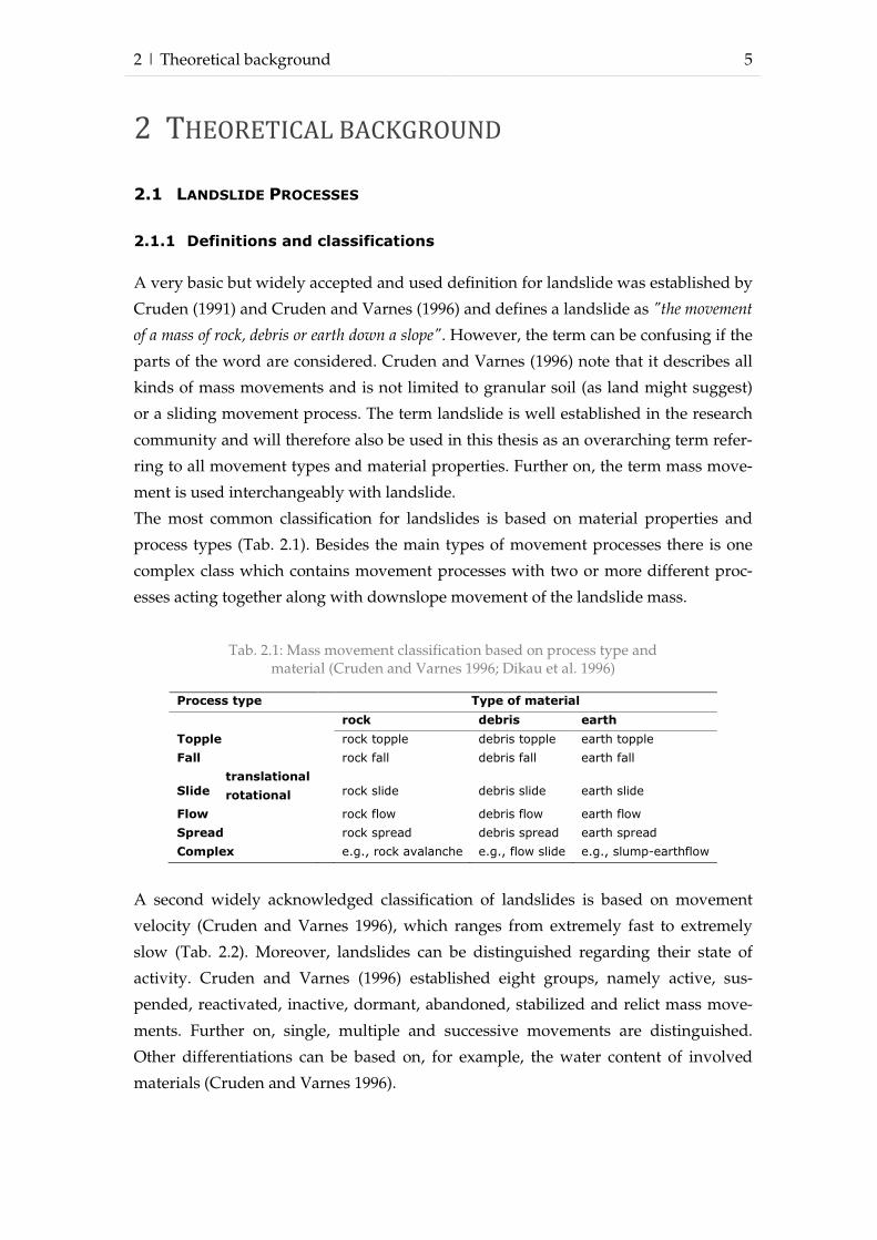
The most common classification for landslides is based on material properties and
process types (Tab. 2.1). Besides the main types of movement processes there is one
complex class which contains movement processes with two or more different proc-
esses acting together along with downslope movement of the landslide mass.
Tab. 2.1: Mass movement classification based on process type and material (Cruden and Varnes 1996; Dikau et al. 1996)
Process type Type of material
rock debris earth
Topple rock topple debris topple earth topple
Fall rock fall debris fall earth fall
Slide
translational rock slide
debris slide
earth slide rotational
Flow rock flow debris flow earth flow
Spread rock spread debris spread earth spread
Complex e.g., rock avalanche e.g., flow slide e.g., slump-earthflow
A second widely acknowledged classification of landslides is based on movement
velocity (Cruden and Varnes 1996), which ranges from extremely fast to extremely
slow (Tab. 2.2). Moreover, landslides can be distinguished regarding their state of
activity. Cruden and Varnes (1996) established eight groups, namely active, sus-
pended, reactivated, inactive, dormant, abandoned, stabilized and relict mass move-
ments. Further on, single, multiple and successive movements are distinguished.
Other differentiations can be based on, for example, the water content of involved
materials (Cruden and Varnes 1996).
6 2 | Theoretical background
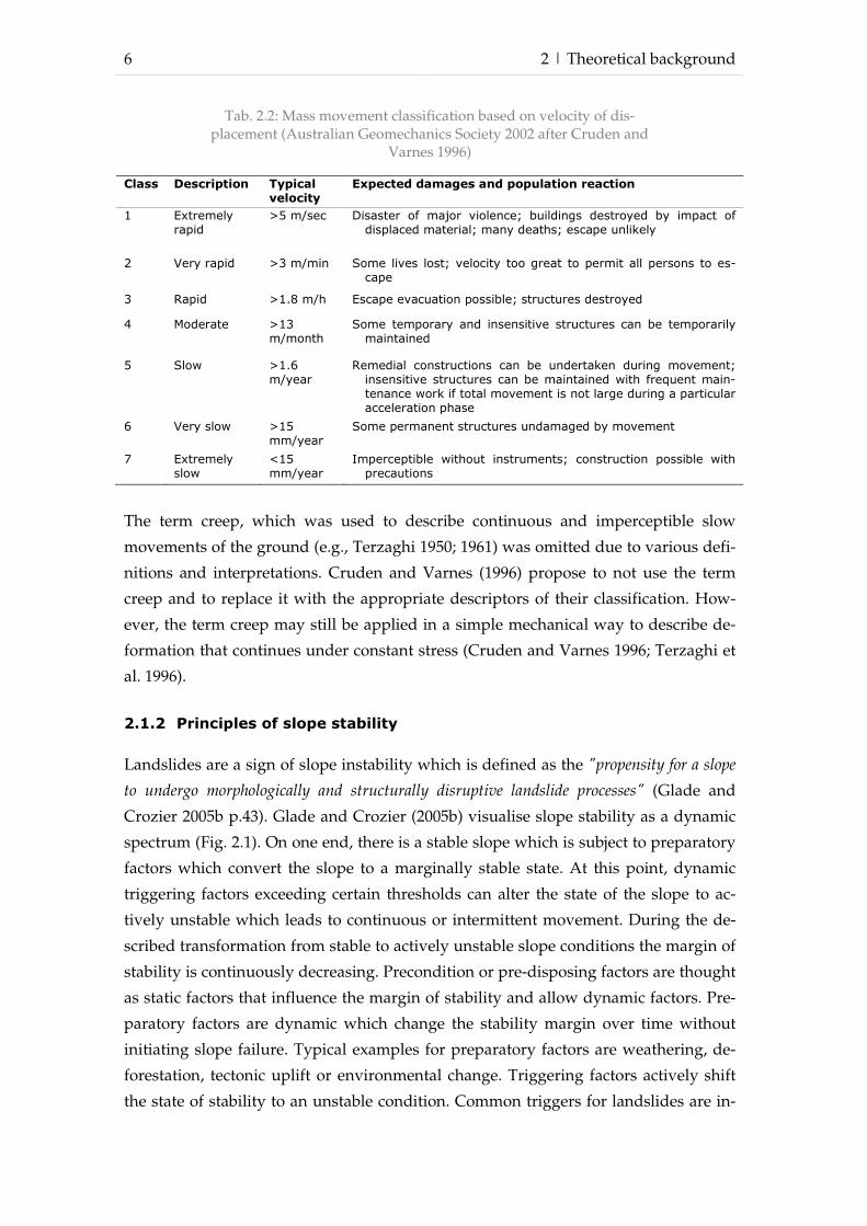
Tab. 2.2: Mass movement classification based on velocity of dis-placement (Australian Geomechanics Society 2002 after Cruden and
Varnes 1996)
Class Description Typical velocity
Expected damages and population reaction
1 Extremely rapid
>5 m/sec Disaster of major violence; buildings destroyed by impact of displaced material; many deaths; escape unlikely
2 Very rapid >3 m/min Some lives lost; velocity too great to permit all persons to es-cape
3 Rapid >1.8 m/h Escape evacuation possible; structures destroyed
4 Moderate >13 m/month
Some temporary and insensitive structures can be temporarily maintained
5 Slow >1.6 m/year
Remedial constructions can be undertaken during movement; insensitive structures can be maintained with frequent main-tenance work if total movement is not large during a particular acceleration phase
6 Very slow >15 mm/year
Some permanent structures undamaged by movement
7 Extremely slow
<15 mm/year
Imperceptible without instruments; construction possible with precautions
The term creep, which was used to describe continuous and imperceptible slow
movements of the ground (e.g., Terzaghi 1950; 1961) was omitted due to various defi-
nitions and interpretations. Cruden and Varnes (1996) propose to not use the term
creep and to replace it with the appropriate descriptors of their classification. How-
ever, the term creep may still be applied in a simple mechanical way to describe de-
formation that continues under constant stress (Cruden and Varnes 1996; Terzaghi et
al. 1996).
2.1.2 Principles of slope stability
Landslides are a sign of slope instability which is defined as the "propensity for a slope
to undergo morphologically and structurally disruptive landslide processes" (Glade and
Crozier 2005b p.43). Glade and Crozier (2005b) visualise slope stability as a dynamic
spectrum (Fig. 2.1). On one end, there is a stable slope which is subject to preparatory
factors which convert the slope to a marginally stable state. At this point, dynamic
triggering factors exceeding certain thresholds can alter the state of the slope to ac-
tively unstable which leads to continuous or intermittent movement. During the de-
scribed transformation from stable to actively unstable slope conditions the margin of
stability is continuously decreasing. Precondition or pre-disposing factors are thought
as static factors that influence the margin of stability and allow dynamic factors. Pre-
paratory factors are dynamic which change the stability margin over time without
initiating slope failure. Typical examples for preparatory factors are weathering, de-
forestation, tectonic uplift or environmental change. Triggering factors actively shift
the state of stability to an unstable condition. Common triggers for landslides are in-

2 | Theoretical background 7
tense rainstorms, seismic shaking or slope undercutting (Glade and Crozier 2005b).
Inherent in this concept is the theory of extrinsic and intrinsic thresholds (Schumm
1979). Sustaining factors control the behaviour of the actively unstable state and there-
fore dictate the duration of movement, form and run out distance of slope failure.
A similar concept is described by Leroueil (2004) who distinguishes four stages of
landslide movement: a pre-failure stage including deformation process leading to
failure, the onset of failure characterized by the formation of a continuous shear sur-
face through the entire soil mass, a post failure stage starting from failure until the
mass stops, and a reactivation phase when sliding occurs on a pre-existing shear sur-
face.
Stresses acting within a slope can be illustrated by vectors (Fig. 2.2), where a mass (m)
is subject to acceleration of gravity (g) which can be differentiated into a downslope
component (�) and a force acting perpendicular to slope surface (�). Distribution of
stresses depends on slope angle (β) and downslope force increases with higher slope
angles.
Fig. 2.2: Stress vectors within a slope (based on Ahnert 2003)
Fig. 2.1: Stability states and destabilising factors (after Glade and Crozier 2005b, based on Crozier 1989)
Preparatory
Factors
Sustaining
Factors
Triggering
FactorsStable
ActivelyUnstable
MarginallyStable
Precondition Factors
Margin of Stability
8 2 | Theoretical background
The potentially destructive effects of slope instability led to early research in predic-
tion of slope failures. Calculation of slope stability dates back to Coulomb (1776) and
his work on stability of retaining walls and determination of the most likely shear
surfaces with a wedge method, which are still valuable today (Ahnert 2003). Another
important advance of slope stability calculation was made by Terzaghi (1925), who
established the fundamental concept of effective stress. Therein, the effects of pore-
water pressure in slope stability are acknowledged. Pore-water pressure is the pres-
sure of water in the voids between solid particles of the soil (Casagli et al. 1999). As
water can not sustain shear stress, only the skeleton of solid particles at their contact
points can, slope stability decreases with a higher pore-water pressure. The stability
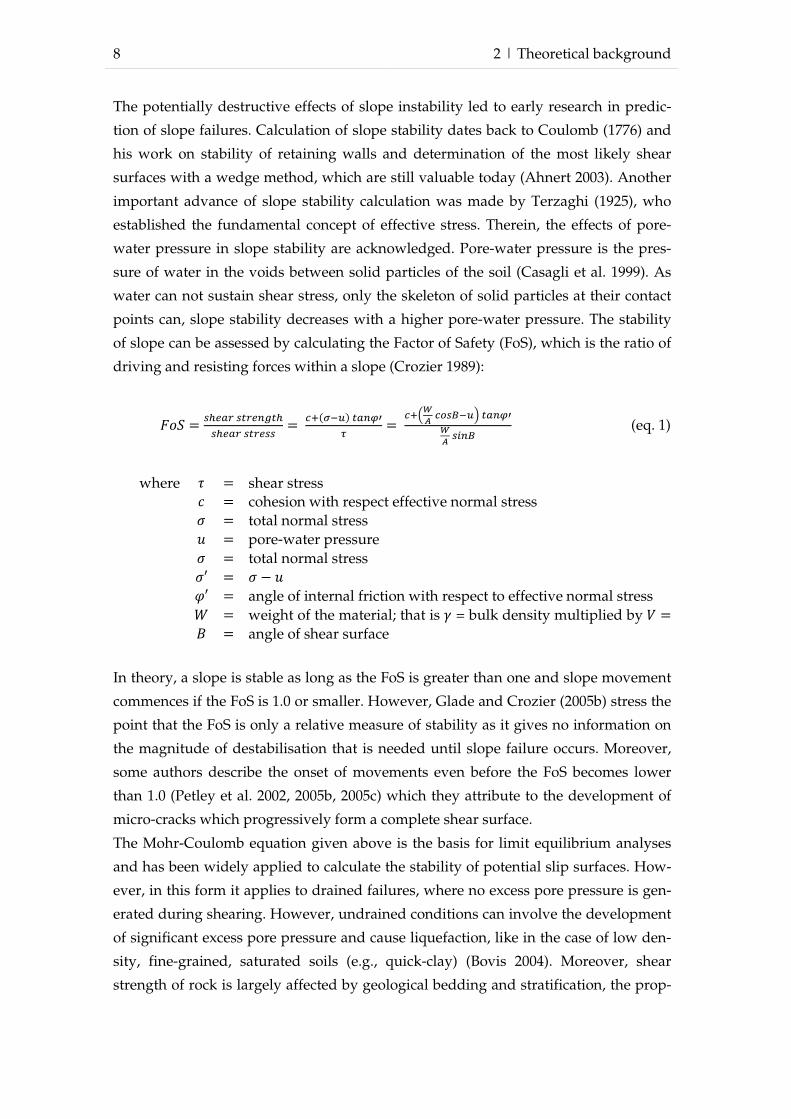
of slope can be assessed by calculating the Factor of Safety (FoS), which is the ratio of
driving and resisting forces within a slope (Crozier 1989):
��� = ����������������� = ������������
� = ����� ������ �����
�� �!��
(eq. 1)
where � = shear stress " = cohesion with respect effective normal stress � = total normal stress # = pore-water pressure � = total normal stress �′ = � − # &′ = angle of internal friction with respect to effective normal stress ' = weight of the material; that is ( = bulk density multiplied by ) = * = angle of shear surface
In theory, a slope is stable as long as the FoS is greater than one and slope movement
commences if the FoS is 1.0 or smaller. However, Glade and Crozier (2005b) stress the
point that the FoS is only a relative measure of stability as it gives no information on
the magnitude of destabilisation that is needed until slope failure occurs. Moreover,
some authors describe the onset of movements even before the FoS becomes lower
than 1.0 (Petley et al. 2002, 2005b, 2005c) which they attribute to the development of
micro-cracks which progressively form a complete shear surface.
The Mohr-Coulomb equation given above is the basis for limit equilibrium analyses
and has been widely applied to calculate the stability of potential slip surfaces. How-
ever, in this form it applies to drained failures, where no excess pore pressure is gen-
erated during shearing. However, undrained conditions can involve the development
of significant excess pore pressure and cause liquefaction, like in the case of low den-
sity, fine-grained, saturated soils (e.g., quick-clay) (Bovis 2004). Moreover, shear
strength of rock is largely affected by geological bedding and stratification, the prop-

2 | Theoretical background 9
erties of involved materials, and the morphology and complex interactions along dis-
continuities like cracks and joints during shearing (Prinz and Strauß 2006).
Examination of shear parameters and the stress-strain behaviour of materials are pri-
marily experimental, because of the technical difficulties to study the processes in
nature. Shear parameters are generally determined in the laboratory by undertaking
uniaxial or triaxial shear tests (Wu 1996). A relatively undisturbed soil sample is
placed into a shear box and stress is applied until the material fails. Applied loads and
subsequent strains are recorded. Idealized stress-strain curves for brittle and ductile
failure regimes are given in Fig. 2.3.
Fig. 2.3: Idealized stress-strain curves for brittle (A) and ductile (B) deformation (Petley and Allison 1997)
Most geological materials and engineering soils can display both brittle and ductile
failure modes depending on their confining pressure (Cristescu 1989). However, brit-
tle failure is dominant at low confining pressures representative for shallow failures
(Petley and Allison 1997). As stress or load is applied soil materials generally display
an initial phase of elastic and recoverable strain. The applied stress is loaded on the
grain-bonds within the material which deform but do not break. An increase of stress
causes the material's weakest bonds to break and an elastic-plastic phase can be ob-
served which is characterized by increasing strain rates. As more and more bonds
break, peak strength is exceeded and shear strength is significantly reduced. The
shear surface fully develops in the strain weakening phase in which shear strength
steadily reduces to a residual value. During this phase shear zone contraction or dila-
tion may occur which affects pore pressures and therefore strain rates (Iverson 2005).
Thereafter, strains primarily occur as displacement along the shear surface.
Ductile behaviour can be observed at high effective stresses prevalent in very deep-
seated landslides and in materials with little or no inter-particle bonding like weath-
ered clays (Petley and Allison 1997). The initial phases of elastic and elastic-plastic
strain are similar to the brittle failure regime. However, due to the high confining
stress no shear surface can develop. Increased load results in purely plastic deforma-
A B

10 2 | Theoretical background
tion at constant stresses as the material reforms. Moreover, a transition between duc-
tile and brittle behaviour was observed by (Petley and Allison 1997) at very high pres-
sures, which are present in very deep-seated landslides.
As mentioned above the term creep does not describe a certain landslide type but
refers to the mechanical behaviour of geological materials to constant stress. Some
creep takes place in almost all steep earth and rock slopes and may concentrate along
pre-existing or potential slip surfaces or distribute evenly across the landslide profile
(Fang 1990). Creep movements in landslide can be continuous or may vary seasonally
with hydrological conditions (Petley and Allison 1997). Creep can be maintained for
long periods, however, creep gradually decreases shear strength and a slope's margin
of stability (Fang 1990) and eventually the slope may fail.
A widely acknowledged concept of creep distinguishes between the phases of creep
movement (Okamoto et al. 2004; Petley et al. 2005b, 2005c; 2008). When constant stress
lower than peak strength is applied to a soil mass subsequent strains are time-
dependant and can be visualised as displacement versus time plot (Fig. 2.4). In the
primary creep stage strains are initially high due to elastic deformation but decrease
with time. During the secondary creep phase the material suffers diffuse damage but
strains are generally slow or almost steady (Okamoto et al. 2004), or may even stop
altogether (Petley et al. 2008). When diffuse micro-cracks start to interact to form a
shear surface, the critical point into the tertiary phase is reached (Reches and Lockner
1994; Main 2000). This phase is characterized by a rapid acceleration of displacement
until final failure.
Fig. 2.4: Idealized strain curves for the three stages of creep (after Petley et al. 2008)

2 | Theoretical background 11
The increasing displacement rates associated with rupture growth and micro-crack
interactions during the tertiary creep stage have been subject to research for a long
time in order to predict final failure (Saito 1965; Bjerrum 1967; Saito 1969; Voight 1989;
Fukuzono 1990) and volcanic eruptions (Voight 1988). The concept is frequently
termed progressive failure analysis and usually employs examination of movement
patterns by plotting movement in Λ − , space, where Λ = 1// (/ is velocity and , is
time) (Petley et al. 2002).
It has been observed in many shear experiments and real landslides that linear trends
in acceleration occur if failure is imminent. This was the case for first-time failures
and for failures in which brittle behaviour was dominant in the basal shear zone.
However, reactivated landslides and failures where ductile deformation is dominant
display asymptotic trend in Λ − , space which has been observed in several land-
slides, e.g., in Italy, New Zealand, California, Japan and the UK (Petley et al. 2002;
Carey et al. 2007).
The potential for prediction and early warning of landslide failures has been showed
by several case studies. Kilburn and Petley (2003) and Petley and Petley (2006) ana-
lysed displacement data from the famous Vaiont reservoir rockslide in Northern Italy,
which caused a flood wave that killed around 2000 people in 1963. The result of the
analysis was that at 30 days before final failure a transition to a linear trend in move-
ment acceleration was visible and final failure was therefore predictable. Moreover, in
the case of the artificial landslide experiment at the Selford slide (Selford Cutting
Slope Experiment) final failure could be predicted 50 days in advance (Petley et al.
2002).
Despite its potential, progressive failure analysis has not been integrated into an early
warning system yet. A test application to the slope under investigation in this study
failed because of slow movement rates and insufficient acceleration phases (Thiebes et
al. 2010).
Slow active landslides are widespread in many geomorphological contexts and mate-
rials, and can display steady movements over long periods of time, often along com-
pletely developed shear zones (Picarelli and Russo 2004). Changes in displacement
rates of slow or extremely slow landslides is in many cases related to varying pore-
water pressures (Leroueil 2004) and movements can be continuous or intermittent.
Especially in landslides of moderate depths pore pressures primarily drive displace-
ments, while in deeper landslides creep and erosion, as other phenomena of stress
relief, are the main influential factors (Picarelli and Russo 2004). While pore pressures
control landslide movement on short and medium time-scales, erosion, weathering,

12 2 | Theoretical background
progressive weakening due to strain are influencing on a larger time-scale (Picarelli
and Russo, 2004).
Seasonal variations of pore pressures close to surface are not necessarily reflected by
deeper layers if materials are rich in clay (Leroueil 2004). Moreover, clays also influ-
ence infiltration and slope stability by their swelling and drying behaviour. Very dry
clay may develop cracks which allow for quick percolation into depth along preferen-
tial flow paths. Preferential flow paths can have a positive effect on slope stability by
allowing quick drainage of potentially unstable areas, but can also have an adverse
effect by contributing additional water to areas where shear surfaces may develop
(Uchida et al. 2001). Infiltration in unsaturated materials is a complex process
(Leroueil 2004) and strongly dependant on initial conditions such as antecedent soil
water conditions, degree of saturation, pore pressure field, hydraulic conductivity
and amount of water required for saturation. As a result, it is extremely difficult to
relate rainfall conditions to pore-water pressures and to the occurrence of landslides.
Moreover, transferring one threshold to an entire landslide is extremely difficult
(Picarelli and Russo 2004).
Slow moving slopes often interact with infrastructure as movement rates are gener-
ally low, so that permanent avoidance or evacuation is not necessary (Picarelli and
Russo 2004). Still there is a danger of acceleration, as many catastrophic slope failures
are preceded by long periods of slow creep (Petley and Allison 1997). Geotechnical
stabilisation on the other hand would in many cases be too expensive or non-effective.
2.1.3 Systems theory considerations
Landslides are the results of complex interaction within the natural environment, and
if human intervention is present, the interactions and feedbacks become even more
complex (Armbruster 2002). A widely acknowledged approach in physical geography
was laid out by Chorley and Kennedy (1971) and aimed to provide a theoretical
framework which allows for analysis of form, material, and processes, as well as
interaction and feedbacks (Dikau 2005). Moreover, the conceptual approach
comprises variable space and time-scales of system evolution and external system
control, as well as early approaches to non-linear system response (Slaymaker 1991).
Four types of systems can be distinguished: morphological systems, cascading
systems, process-response systems and control systems (Chorley and Kennedy 1971).
Following Glade (1997) morphological systems can be used to describe the interaction
between landslide-prone regions and potentially landslide-triggering rainfall events.
Bell (2002) notes, that if research focuses on, for example, landsliding of periglacial
strata cascading systems may be more appropriate. Research on factors controlling
landslide behaviour can benefit from a process-response system point of view, while
control systems are important in geomorphological hazard research where direct
2 | Theoretical background 13
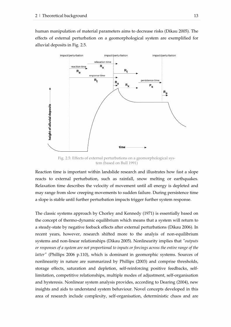
human manipulation of material parameters aims to decrease risks (Dikau 2005). The
effects of external perturbation on a geomorphological system are exemplified for
alluvial deposits in Fig. 2.5.
Fig. 2.5: Effects of external perturbations on a geomorphological sys-tem (based on Bull 1991)
Reaction time is important within landslide research and illustrates how fast a slope
reacts to external perturbation, such as rainfall, snow melting or earthquakes.
Relaxation time describes the velocity of movement until all energy is depleted and
may range from slow creeping movements to sudden failure. During persistence time
a slope is stable until further perturbation impacts trigger further system response.
The classic systems approach by Chorley and Kennedy (1971) is essentially based on
the concept of thermo-dynamic equilibrium which means that a system will return to
a steady-state by negative feeback effects after external perturbations (Dikau 2006). In
recent years, however, research shifted more to the analyis of non-equilibrium
systems and non-linear relationships (Dikau 2005). Nonlinearity implies that "outputs
or responses of a system are not proportional to inputs or forcings across the entire range of the
latter" (Phillips 2006 p.110), which is dominant in geomorphic systems. Sources of
nonlinearity in nature are summarized by Phillips (2003) and comprise thresholds,
storage effects, saturation and depletion, self-reinforcing positive feedbacks, self-
limitation, competitive relationships, multiple modes of adjustment, self-organisation
and hysteresis. Nonlinear system analysis provides, according to Dearing (2004), new
insights and aids to understand system behaviour. Novel concepts developed in this
area of research include complexity, self-organisation, deterministic chaos and are
14 2 | Theoretical background
reviewed and discussed in detail elsewhere (Phillips 1992a, Phillips 1992b; Richards
2002; Favis-Mortlock and De Boer 2003; Phillips 2003; Dikau 2006).
There is no single, precise definition of complexity (Favis-Mortlock and De Boer 2003).
However, complexity may loosely be delineated as the fact that systems can not be
described by the properties of its parts (Gallagher and Appenzeller 1999). According
to Phillips (1992a) complexity can arise from cumulative process-response
mechanisms which are far too numerous to be accounted for in individual details, or
due to multiple controls over process–response relationships that operate over a
range of spatial and temporal scales.
The studies of Bak et al. (1988) on sand-pile models provided some insights on
complex systems. In these models grains were dropped onto a sand pyramid. This
resulted either in no changes, or in landslides of various sizes. The landslide sizes
were found to follow a power-law distribution, but it was, however, not possible to
predict the size of the next landslide. The fact that the system drove itself to a critical
state was referred to as self-organised criticality, a concept that has been been widely
applied to geomorphological processes (Favis-Mortlock 1998; Phillips et al. 1999; Fon-
stad and Marcus 2003; Favis-Mortlock 2004).
Deterministic chaos describes the sensitivity of a system to initial conditions and
small perturbations, whereby initial differences or effects of minor perturbations tend
to persist and grow over time and may have unpredictable and apparently random
consequences (Phillips 2003). The basic principle of determinstic chaos has popularly
been described by the butterfly effect, where the flap of butterfly wings in one part of
the world may cause a hurricane at another place. Chaotic behavior was first
described by Lorenz (1963) who simulated meteorological processes and found
drastically differing model results depending on minimimal changes to small decimal
places. Prediction of model states was only possible for short time-spans.
These aspects of nonlinearity have drastic consequences for the predictability of
natural phenomena such as landslides (Von Elverfeldt 2010). However, this does not
mean that prediction is not possible as Dikau (2005) notes: nonlinear systems can be
simple and predictable, but this is not necessarily the case for complex systems. Most
landslide simulation programs, such as the models presented in chapter 2.3, can not
accomodate nonlinear system behaviour, such as complexity, self-organisation or
deterministic chaos. Some landslide related research projects, however, exploited for
example self-organised criticality for prediction of landslides and forest fires (Turcotte
and Malamud 2004), characterisation of landslide evolution (Huang et al. 2008) or
analyis of triggering conditions (Stähli and Bartelt 2007). Moreover cellular automa
have widely been used to simulate self-organising complex systems in geomorphic
2 | Theoretical background 15
research (Smith 1991; Avolio et al. 2000; D’Ambrosio et al. 2003; Iovine et al. 2005;
Fonstad 2006).
2.1.4 Landslide triggering
Even though landslides can occur without the impact of external factors, generally
their occurrence is connected to some kind of triggering event. Many factors can act as
triggers for landslides. The most common natural triggers are either related to geo-
logical events, such as seismic shaking due to volcanic eruptions or earthquakes, or
hydrological events such as intense rainfall, rapid snowmelt or water level changes in
rivers or lakes at the foot of slopes (Wieczorek 1996). Moreover, human interaction in
the form of loading or slope cutting can trigger landslide events. The most important
trigger, however, in both shallow and deep-seated landslides is intense rainfall (Cro-
sta and Frattini 2008). Infiltrating rain percolates within the soil, thus increasing pore
pressures at hydrologic boundaries, which subsequently decreases shear strength.
Positive pore-water pressure may occur directly caused by infiltration and percolation
(saturation from above), or may be the result of perched ground water tables (satura-
tion from below) (Terlien 1998). Important factors determining the evolution of satu-
ration are soil permeability and stratification, preferential flow paths, as well as me-
chanical characteristics (Berardi et al. 2005).
In the following landslide triggering, the efforts made to predict landslide occurrences
with respect to hydrological thresholds will briefly be described. More general re-
views on landslide triggering (Wieczorek 1996; Schuster and Wieczorek 2002; Wiec-
zorek and Glade 2005) and rainfall threshold determination (Terlien 1998; Wieczorek
and Guzzetti 1999; Polemio and Petrucci 2000; Aleotti 2004; Wieczorek and Glade
2005; Guzzetti et al. 2007; Guzzetti et al. 2008; Brunetti et al. 2010) can be found in the
respective literature.
Prediction of landslide triggering thresholds is one of the key issues in landslide re-
search (Berardi et al. 2005), and established thresholds have an important role in early
warning (Terlien 1998). One of the most influential works in this field was published
by Caine (1980) who worked on landslide triggering rainfall thresholds based on rain-
fall intensity and duration analyses. Since then, many research projects worked on
defining rainfall thresholds which trigger landslides. Triggering thresholds are pre-
dominantly expressed as rainfall intensity and duration, or cumulative and antece-
dent rainfall, and can be defined as the line fitting the minimum intensity of rainfall
associated with the occurrence of landslide in different areas (Caine 1980). However,
Terlien (1998) notes that rainfall events that did not cause landslides also should be
recognised. Therefore, minimum and maximum thresholds should be acquired,
16 2 | Theoretical background
where rainstorms below the minimum threshold never cause landslides, and storms
above maximum threshold always lead to landslides (Glade 1998; Crozier 1999). Be-
tween these thresholds landslides may occur under certain conditions.
Landslide triggering thresholds differ from one region to another based on hydro-
climatological and geophysical properties, such as regional and local rainfall charac-
teristics and patterns, slope morphometry, soil characteristics, lithology, morphology,
climate and geological history (Crosta 1998). Further on, landslide triggering thresh-
olds may also vary with time (Crozier 1999), for example due to seasonal changes of
vegetation (Wieczorek and Glade 2005). Moreover, Crozier and Preston (1999) note
that after movements have occurred resistance to further events may occur, if for ex-
ample., all material for future debris flows has already been transported.
Guzetti et al. (2007) distinguish between rainfall thresholds on three spatial scales, for
example, global, regional and local scale. A further distinction between landslide trig-
gering rainfall thresholds can be made between statistical or empirical and determi-
nistic thresholds (Guzzetti et al. 2007). When sufficient data on landslide occurrences
and rainfall conditions are available, thresholds can be determined in a statistical way.
With limited data deterministic models have to be applied to predict landslide behav-
iour under certain hydrological conditions (Terlien 1998).
Most case studies of rainfall thresholds relate to shallow landslides or debris flows.
Triggering of these landslide types generally refers to short and intense rain storms,
while the occurrence of deep-seated landslides is more affected by long-term rainfall
trends (Terranova et al. 2007). Deep-seated landslides share a more complex hydrol-
ogy compared to shallow landslides and simple correlations between rainfall and
deep-seated landslide triggering can not be determined (Terlien 1998). To establish
triggering rainfall thresholds in deep-seated landslides it is necessary to include rain-
fall, water infiltration and percolation, generally by means of modelling subsurface
hydrology (Ekanayake and Phillips 1999), and to determine the location of shear sur-
face, as well as the hydrological triggering mechanism (Terlien 1998).
The intensity-duration method first proposed by Caine (1980) has been applied in
many other studies (Pasuto and Silvano 1998; Jakob et al. 2006; Matsushi and Matsu-
kura 2007; Crosta and Frattini 2008; Guzzetti et al. 2008; Capparelli et al. 2009; Saito et
al. 2010). Rainfall duration generally refers to periods between 10 minutes and 35
days (Guzzetti et al. 2008), but some authors extended the time span analysed to sev-
eral months (Terranova et al. 2007; Marques et al. 2008). Long-term rainfall trends
have been integrated into threshold determination by relating intensity and duration
of rainstorms to mean annual precipitation (MAP) (Giannecchini 2006; Giannecchini
et al. 2007; Guzzetti et al. 2007; Sengupta et al. 2009).
2 | Theoretical background 17
Crozier and Eyles (1980) developed the Antecedent Daily Rainfall method to deter-
mine rainfall thresholds based on antecedent and daily rainfall. A decay factor de-
rived from discharge hydrographs controls the influence of antecedent soil water.
Several other case studies applied this methodology as well (e.g., Crozier 1999; Glade
2000; Glade et al. 2000; Strenger 2009).
Although rain is regarded as the prime factor of landslides triggering, infiltration and
the development of positive pressures at potential shear surfaces are initiating land-
slide processes (Reichenbach et al. 1998; Ekanayake and Phillips 1999; Leroueil 2004).
There is, however, no established standard procedure for calculation of pore pressure
in relation to rainfall events (Persson et al. 2007). A common procedure is to calculate
pore pressures conditions required for slope instability which are then compared to
observed pore pressures and checked for reasonability. Based on multiple regression
analysis of piezometric measurements Matsushi and Matsukura (2007) established
rainfall intensity duration thresholds. Godt et al. (2006) applied a similar approach
and derived rainfall thresholds by comparing rainfall data with measurements of
volumetric water content. Other authors utilise models to predict pore pressure in
response to rainfall events. Wilson (1989) presented a simple numerical model to in-
vestigate the build up of saturation and establish rainfall thresholds. The model
represents soils as leaky barrels, where additional water is added at one rate, while
water is lost by another rate. Wilson and Wieczorek (1995) combined the model with
measurements of piezometric levels and data on antecedent rainfall to derive rainfall
thresholds. A related approach has been performed by Terranova et al. (2007) who
derive critical rainfall situation for landslide triggering based on modelled infiltration
and comparison with piezometer data. Moreover, several other case studies also ap-
plied hydrological models to predict pore pressure evolution in response to rainfall
events to establish landslide triggering rainfall thresholds (Reid 1994; Crosta 1998;
Terlien 1998; Ekanayake and Phillips 1999; Iverson 2000; Frattini et al. 2009).
Coupled hydrology and stability models have been widely applied to predict the ef-
fects of rain storms, and to define critical situations. Examples for local scale (Buma
2000; Brooks et al. 2004; Berardi et al. 2005; Pagano et al. 2008), and regional scale
(Dhakal et al. 2002; Crosta and Frattini 2003) approaches can be found in the respec-
tive literature.
2.2 LANDSLIDE INVESTIGATION AND MONITORING
The occurrence of landslides is sometimes surprising for humans as they seem to oc-
cur without previous warning signs. However, (Terzaghi 1950) noted that if a land-
slide comes as a surprise to eyewitnesses, it would be more accurate to say that the
observers failed to detect the phenomena which preceded the slide. Therefore, dedi-
18 2 | Theoretical background
cated landslide analyses and monitoring methods have to be applied to be able to
recognise potential slope failures.
Many methodological approaches have been developed to reveal the occurrence of
landslides in space and time, to investigate processes acting within mass movements
and to monitor ground displacements. The wide range of possible methodological
approaches for landslide research stretch from field or desk-based mapping, to meas-
urements of surface and subsurface movement in field or by remotely acquired data
sources, recordings of triggering factors like rainfall or hydrological parameters, and
the use of simulation models.
Landslides can be assessed on various spatial scales (Glade and Crozier 2005a), but a
general distinction between local and regional approaches can be made. The initial
step of regional approaches is to define the spatial occurrence of landslides, com-
monly by preparing landslide inventories (Wieczorek et al. 2005). For local analyses
Nakamura (Nakamura 2004) argues that one of the first steps to understand the land-
slides under investigation are field investigations and boreholes to define the slip sur-
face. Regarding rockslides, but also applicable to other landslide phenomena, (Glawe
and Lotter 1996) stated that when instabilities can be expected geotechnical investiga-
tions, displacement monitoring and modelling techniques are generally applied. Fol-
lowing (Cornforth and Mikkelsen 1996) ideal features of a landslide monitoring sys-
tem are continuous measurements of pore-water pressure in the shear zone by auto-
mated sensors in order to correlate these with rainfall data.
In the following a review of methods for landslide detection, surface and sub-surface
investigations and monitoring techniques is given. The aim of this chapter is not to
provide a complete summary of all methods available for landslide research, but
rather to give a comprehensive overview on the methods most used in research prac-
tice and to highlight their advantages and disadvantages for monitoring. More infor-
mation on the methodological approaches to landslide investigation and monitoring
methods can be found in the sources given or in the general reviews (Franklin 1984;
Keaton and DeGraff 1996; McGuffey et al. 1996; Mikkelsen 1996; Soeters and Van
Westen 1996; Turner and McGuffey 1996; Olalla 2004; Van Westen 2007; Liu and
Wang 2008). No self-contained review on existing monitoring systems will be given as
many examples of monitoring systems are presented in the review on early warning
systems (chapter 2.4). It is however important to mention that many landslide moni-
toring systems employ several different techniques, such as methods for measuring
landslide movement and hydrology.
Regarding monitoring it should be made clear, that there is no obvious threshold that
determines what time intervals between repeated measurements are nevessary for it
to be classed as monitoring. Ollala (2004) points out that monitoring can range from,

2 | Theoretical background 19
for example, inclinometer measurements carried out once in a year, or automatic
measurements in intervals of seconds. Therefore, every repeated measurement could
be defined as monitoring. Automatic monitoring systems are however more conven-
ient than manual measurements as they do not require humans to regularly go to
study sites which may be remote or difficult to access. Another advantage of auto-
mated monitoring systems is the ability to control measures by time intervals, thresh-
olds or user input. Besides this, questions of data storage, transmission and security
arise with such automatic systems. Moreover, data should automatically be processed
and checked to prevent inconsistencies (Olalla 2004). However, issues of managing
automatic monitoring systems will not be discussed here.
2.2.1 Mapping and inventory approaches
A basic method to detect landslides in space and to prepare landslide inventories is
geomorphological mapping in the field. Geomorphological mapping requires expert
knowledge and experience of landslides and the study area. Results can vary drasti-
cally depending on the specialists who prepared the map, the knowledge on the study
area and the processes present (Guzzetti et al. 2000; Ardizzone et al. 2002). Repeated
mapping campaigns in the field without further measurements give rather qualitative
information on how processes have evolved over time but are essential for process
understanding. Important information could include cracks that open up due to
ground displacements, or damage to existing infrastructure.
Landslide maps and inventories are frequently prepared based on the analysis of re-
mote sensing data like stereographic aerial or space-borne images, and digital terrain
models (DTM) from, for example, LiDAR (Light Detection And Ranging) data. Gen-
eral reviews on landslide mapping and inventories can be found in various literature
sources (e.g., Soeters and Van Westen 1996; Malamud et al. 2004; Guzzetti et al. 2006;
Van Westen 2007).
The use of aerial photography is well established in landslide research (Soeters and
Van Westen 1996). Interpretation of aerial images is primarily qualitative; however
photogrammetric methods can be used to extract quantitative information. While
qualitative interpretation is common, quantitative studies are more rare, probably due
to limited availability of good quality photographs, adequately fixed control points
and cost (Morgenstern and Martin 2008). However, several landslide related quantita-
tive photogrammetric studies have been described (Maria et al. 2004; Mills et al. 2005;
Hu et al. 2008; Liu and Wang 2008; Smith et al. 2009).
Medium resolution satellite imagery, such as LANDSAT, SPOT, ASTER, IRIS-D etc.,
is today used routinely to create landuse maps and inventories of landslides (Van
Westen 2007). He also notes that Google Earth and other providers of high resolution

20 2 | Theoretical background
satellite data greatly facilitate mapping by offering capabilities of creating polygons
and exporting them to Geographic Information Systems (GIS). In several case studies
landslide inventories were created based on satellite imagery (Mondini et al. 2009;
Fiorucci et al. 2010; Santurri et al. 2010; Yang and Chen 2010) or Google Earth (Sato
and Harp 2009; Chigira et al. 2010).
In recent years the interpretation of Airborne Laser Scanning (ALS) DTM data has
been frequently applied for creation of landslide inventories (Van Westen 2007). By
removing vegetation and other objects from the DTM, Digital Surface Models (DSM)
can be created (Schulz 2004). This together with different modifiable angles of shad-
ing enable very detailed mapping of landslides and other geomorphological features
(Haneberg 2004; Thiebes 2006). Examples of ALS-based landslide maps are provided
by several authors (Chigira et al. 2004; Sekiguchi and Sato 2004; Ardizzone et al. 2007;
Eeckhaut et al. 2007).
By using multi-temporal remote sensing data sets landslides can be dated, and activ-
ity and evolution quantitatively investigated. Examples for multi-temporal landslide
inventories are provided by several authors (e.g., Cardinali et al. 2002; Dai and Lee
2003; Brennecke 2006; Imaizumi et al. 2008; Chiang and Chang 2009).
Several automatic landslide detection and mapping approaches have been developed
and are comprehensively reviewed by (Van Westen 2007). These approaches utilise
DTM subtraction analysis or multi-spectral analysis of satellite imagery. Fairly recent
applications of an automated landslide mapping system are presented by Tarantino et
al. (2005) and Booth et al. (2009).
Another remote-sensing method for mapping landslides and for detection rates and
extents of ground deformations is Synthetic Aperture Radar (SAR). SAR and the re-
lated methods of Interferometric SAR (InSAR), and their use for landslide research are
extensively reviewed by Rosen et al. (2002), Foese et al. (2004) and Morgenstern and
Martin (2008). SAR is based on microwave signals which are emitted by a satellite or
airplane and the back-scattered signals, which represent distance measurements, are
recorded. By processing two slightly offset images from the same flight paths InSAR
images can be created which can be used to create pixel-based images which form a
DTM. The benefits of this method are that radar measurements can be performed at
almost every weather condition and at day and night. Furthermore, large areas can be
analysed in a short period of time. Determination of displacements can be achieved
by analysing images from different flights. To further increase the accuracy of dis-
placement measurements Permanent or Persistent Scatterer Interferometric Synthetic
Aperture Radar (PS-InSAR) was introduced to landslide research (Morgenstern and
Martin 2008). Permanently fixed ground-points, in many cases buildings or other con-
structions, are determined in multiple InSAR images and relative movements of these
points can be measured. Best results, with accuracy of measurements in the sub-

2 | Theoretical background 21
centimetre range, can be obtained for movements along the line of sight (Rosen et al.
2002; Luzi et al. 2005). Several case studies have been performed utilising satellite-
based InSAR technology to detect and monitor ground movements (Colesanti and
Wasowski 2004; Ferretti et al. 2005; Meisina et al. 2006; Calcaterra et al. 2008; Vallone
et al. 2008; Yin et al. 2010b).
Also historic data such as newspaper articles, eyewitness records, road construction
office reports, city archives, old photographs and many more sources can be utilised
for landslide mapping. In many cases spatial and temporal information regarding
landslide occurrence can be found which are exceptionally useful for understanding
the magnitude-frequency behaviour of mass movements (Glade 2001). Examples of
landslide inventories based on historic data can be found in, for example, Calcaterra
et al. (2003), Carrara et al. (2003), Tropeano and Turconi (2004) and Kohn (2006).
2.2.2 Displacement measurements
Many field methods exist to measure ground displacements due to landslide move-
ments. A simple but convenient field method is the use of quadrilaterals (Keaton and
DeGraff 1996) which consist of four stakes that are fixed inside and outside the land-
slide body. Distances between the stakes can then be measured manually by tape.
Quadrilaterals have been applied within several research applications (Baum and
Fleming 1991; Bogaard 2000; Giraud 2002; Fernandez Merodo et al. 2004; Keaton and
Gailing 2004).
Standard theodolite geodetic measurements are frequently applied to measure and
monitor ground displacements (Reyes and Fernandez 1996; Walstra et al. 2004; Wa-
sowski et al. 2004; Burghaus et al. 2009) and available automatic systems have often
been used (Oboni 2005; Heincke et al. 2010). However, theodolite measurements re-
quire pre-defined ground points or prisms. Manual measurements are also cost and
time intensive.
The Global Positioning System (GPS) is another method that is often used to monitor
landslide movements (Bonnard et al. 1996; Wasowski et al. 2004; Mills et al. 2005;
Webster and Dias 2006; Yin et al. 2008; Zhang et al. 2008). Precision of measurements
is in the range of cm to mm. However, the applicability of this method depends on the
visibility of satellites which may not be the case in narrow valleys, densely forested
areas or on steep cliffs.
The methods described above are applicable to measure and monitor ground defor-
mation at the surface. In order to understand landslide behaviour subsurface meas-
urements are necessary. Basic approaches are pits and trenches which can be used to
investigate e.g., the depth of a landslide and the position of shear surfaces or to take
undisturbed material samples. Generally, pits and trenches can only be established on
shallow movements. Examples are given by Bromhead et al. (2000), Clark et al. (2000)
22 2 | Theoretical background
and Topal and Akin (2008). Penetration tests can also be performed to investigate
stiffness of subsurface materials. More often, drillings are utilised to investigate land-
slide bodies. An ample variety of drilling devices is available on the market from
simple handheld sounding poles to truck-sized rotary drilling machines. Besides the
advantage of directly probing the landslide body and having the opportunity to take
core samples, sensors can be applied within the boreholes to further investigate sub-
surface movement and hydrological processes.
In many cases inclinometers are used to determine subsurface movement of land-
slides (Borgatti et al. 2006; Bonnard et al. 2008; Bressani et al. 2008; Jongmans et al.
2008; Mihalinec and Ortolan 2008; Yin et al. 2008). General remarks on the use of in-
clinometers for landslides research are provided by Stark and Choi (2008). Inclinome-
ters consist of a flexible rilled pipe which is placed vertically into a drilled borehole. A
high-precision probe is inserted and the inclination of the pipe is measured in even
distances, for example, every e.g., 50 cm. Repeated measurements give information of
the occurred inclination changes in downslope and horizontal direction for the entire
length of the pipe. However, it is important that inclinometers are fixed into the stable
ground beneath the shear surface to prevent data bias. Automated inclinometers are
commercially available and usually consist of several inclinometer probes connected
to each other to a chain, or automatic systems where the probe automatically moves
within the pipe. Within landslide monitoring the use of automatic inclinometer and
inclinometer chains has been described by for example, Lollino et al. (2002) and Olalla
(2004), Volkmann and Schubert (2005) and Wienhöfer (2009). However, inclinometers
can only withstand a certain amount of displacement before pipes break. This makes
them especially applicable for monitoring of slow moving landslides, but also for de-
tection of shear processes in faster moving landslides.
A more recent method for the detection of subsurface movements and deformation is
Time Domain Reflectometry (TDR). Barendse and Machan (2009) note that inclinome-
ters can determine the magnitude and direction of ground deformation, while TDR is
primarily used to identify depths of active shearing. The TDR method has initially
been developed in the 1950s for locating discontinuities in power transmission cables
(Pasuto et al. 2000). TDR has first been used within landslide research in the 1980s in
underground coal mine monitoring (Olalla 2004) and since then applied to several
other case studies (Pasuto et al. 2000; Barendse and Machan 2009; Singer et al. 2009;
Yin et al. 2010a). The principle of TDR is based on an electric signal sent through a
coaxial cable. Shear movements deform the cable which creates a spike in cable signa-
ture and depth can be detected from the signal. Laboratory tests of TDR method for
detection of shear processes have been performed by Baek et al. (2004) and Blackburn
and Dowding (2004). Pasuto et al. (2000) compared TDR cables to inclinometer meas-
urements and extensometers. Their result was that TDR cables are less sensitive to
2 | Theoretical background 23
deformations but can withstand a larger displacement than usual inclinometers. The
higher stability of TDR cables make them a good choice for monitoring faster moving
processes like the Gschliefgraben flowslide in Austria (Marschallinger et al. 2009).
Wire or rod extensometers are used to monitor the distance between two points and
are frequently utilised in surface movement investigations (Furuya et al. 2000; An-
gerer et al. 2004; Barla et al. 2004; Willenberg et al. 2004; Wu et al. 2008). Extensom-
eters are in most cases applied to investigate surface movements but can also be in-
stalled within boreholes (Bloyet et al. 1989; Krauter et al. 2007). Accuracy of exten-
someters depends on the length measured and usually is in the sub-mm range.
Tiltmeters are able to give high resolution information on inclination and have been
applied to several landslide monitoring systems (Clark et al. 1996; Meidal and Moore
1996; Barton and McCosker 2000; Blikra 2008; García et al. 2010).
Crackmeters are used to monitor displacements in the sub-mm range at joints and
cracks in rocks, buildings and other structures. The application of crackmeters has
been described by several authors (e.g., Keaton and DeGraff 1996; Greif et al. 2004;
Olalla 2004; Vlcko 2004; Moore et al. 2010).
The mentioned field based methods only give information on ground displacements
for points or along lines. However, spatial methods are also available that give infor-
mation on displacement for entire slopes.
In recent years many studies utilised Terrestrial Laser Scanning (TLS) for monitoring
of geomorphological processes. The technique is similar to LiDAR, but ground-based.
In contrast to LiDAR it is appropriate for steep cliffs and rock faces as the scanner can
be placed in front of it. TLS scans are used to create three dimensional DTM which
can further be analysed quantitatively within GIS or CAD environments to assess e.g.,
the volume of displaced material between measurements. Precision of TLS is heavily
dependent on distance to the target and ranges from centimetres to mm, as well as
environmental conditions such as rain or vegetation. General remarks on TLS and its
usage for monitoring geomorphological processes are provided by (Prokop and Pan-
holzer 2009) and (Schaefer and Inkpen 2010). Many case studies applied TLS for land-
slide monitoring (e.g., Mikoš et al. 2005; Rosser et al. 2005; Rosser and Petley 2008;
Avian et al. 2009; Baldo et al. 2009; Oppikofer et al. 2009; Abellán et al. 2010).
SAR methods can also be applied in ground-based studies, which are frequently
termed Slope Stability Radar (SSR) (Van Westen 2007). The major advantages of this
method are that they provide high precision data in sub-millimetre range without
being affected by weather conditions and without the need to install reflectors or
ground marks. However, vegetation drastically decreases accuracy. Luzi et al. (2005)
used a ground-based DinSAR system to monitor displacement on the Italian Tessina
landslide and compared the measurements to regular theodolite surveys. Based on
24 2 | Theoretical background
comparable displacement results by both methods they conclude that InSAR is also
applicable for landslide early warning systems. Several other research projects in-
stalled SSR systems to monitor displacements of landslides (Canuti et al. 2002; An-
tonello et al. 2004; Casagali et al. 2004; Eberhardt et al. 2008; Bozzano et al. 2010;
Casagli et al. 2010).
Another method that has increasingly been used in recent years is Brillouin optical
time-domain reflectometer (BOTDR). These optical fibres can be used for measure-
ment of ground deformations along profiles. The principle of this method is based on
an interaction of pulsed beam and photons that are thermally excited within the light
propagation medium (Wang et al. 2008a), which are affected by temperature and
strains. Laboratory simulations to test the applicability of BOTDR (Dai et al. 2008;
Wang et al. 2008a), as well as field applications (Higuchi et al. 2007; Dai et al. 2008; Shi
et al. 2008a; Shi et al. 2008b; Moore et al. 2010) have been described.
2.2.3 Hydrological measurements
Given the great importance of rainfall and slope hydrology for landslide triggering,
these factors are frequently analysed and monitored within landslide research. Cli-
matic factors such as rain, snowfall, temperature and wind are usually measured at
climate stations, which are commercially available or in many cases provided by me-
teorological agencies. Measurement of ground-water conditions such as pore pres-
sures and soil water suction is usually accomplished by using piezometers and ten-
siometers. An overview on different types of these sensors can be found in (Kneale
1987). Piezometers are probably the most common hydrological sensor utilised for
landslide research (e.g., Wu et al. 2008; Yin et al. 2008; Calvello et al. 2008; Ching-
Chuan et al. 2009; Yin et al. 2010) and come as simple standpipe or more advanced
vibrating wire piezometers. Piezometers measure the pressure of water in saturated
soils and therefore give information on the height of the groundwater table within a
soil. Tensiometers measure matrix potentials and are frequently utilised to assess the
soil suction in the vadose zone (Li et al. 2004; Rinaldi et al. 2004; Montrasio and Valen-
tino 2007; Greco et al. 2010). Piezometers and tensiometers are usually installed within
boreholes or directly into the soil at trenches.
In recent years Time Domain Reflectometry (TDR) has also been applied to measure
volumetric soil water contents. (Greco et al. 2010) compared TDR sensors with ten-
siometers and concluded that TDR might be more useful for landslide monitoring and
early warning since TDR measurements of soil water content change smoothly, while
soil suction showed abrupt steep fronts. More examples of TDR application for assess-
ing soil water are presented by e.g., Hennrich (2000), Tohari et al. (Tohari et al. 2004)
and Kim (Kim 2008).

2 | Theoretical background 25
The chemical properties of ground and pore-water have a widely acknowledged ef-
fect on shear strength and affect slope stability (Di Maio and Onorati 2000; Angeli et
al. 2004) by for example, influencing the mechanical behaviour of clays (Leroueil
2004). However, monitoring of ground water composition is only rarely included in
landslide monitoring systems (Sakai and Tarumi 2000; Montety et al. 2007; Sakai
2008).
2.2.4 Geophysical measurements
Several methods from geophysics have been utilised for landslide research, mainly for
prospection of landslide bodies and for investigation of hydrological processes acting
within landslides. However, wider application of geophysics in landslide research
have been hindered for two reasons (Jongmans and Garambois 2007): geophysical
methods provide images of geophysical parameters which are not directly linked to
geological parameters required by geotechnical engineers and geomorphologists; and
the overestimation of the quality and reliability of results among some geophysicists.
The main advantages of geophysical methods compared to standard geotechnical
approaches are that they are non-invasive and can be applied to large areas for a low
cost. However, the main disadvantages are the decrease of resolution with depth, the
non-uniqueness of solutions for data inversion and interpretation, and the in-direct
information (Jongmans and Garambois 2007). Generally, geophysics are used for
prospection of landslide bodies, detection of discontinuities and shear surfaces, as
well as for investigation of hydrological regimes. Measurements are usually short-
term and only a few long-term monitoring exist (Supper and Römer 2003; Lebourg et
al. 2005)). Geophysical methods will only briefly be presented here, more detailed
reviews on geophysical application are provided by many introductive textbooks
(Telford et al. 1990; McGuffey et al. 1996; Parasnis 1997; Reynolds 1997; Kearey et al.
2002; Milsom 2003; Schrott et al. 2003; Knödel et al. 2005).
Seismic methods are based on the velocity measurements of seismic waves in subsur-
face materials. Generally, denser material causes faster wave propagation. At layer
interfaces waves are partly reflected, but also partly transferred into depth due to re-
fraction. In geomorphological applications seismic signal is usually induced by a
sledge hammer that is pounded on a steel plate. Penetration depths of more than 30 m
can be reached by more power sources e.g., drop weights or explosives) (Schrott and
Sass 2008). Measurements are taken by geophones which are located at even distances
along a profile. A number of different seismic techniques have been established, of
which seismic reflection, seismic refraction and seismic tomography are the most
common. Although seismic methods proved to be suitable for many geomorphologi-
cal studies which require definition of subsurface properties (Hecht 2001), such as
determination of active layer in permafrost or volumes of sediment bodies, problems

26 2 | Theoretical background
may occur if low velocity layers are sandwiched in high velocity layers (Schrott and
Sass 2008). Examples of dedicated landslide subsurface characterisation applying
seismic methods are provided by several authors (Schmutz et al. 2000; Willenberg et
al. 2002; Meric et al. 2004, Meric et al. 2005; Heincke et al. 2006; Heincke et al. 2010).
A variation of seismic method is applied to record fracture signals produced by de-
formation within landslides, and to locate fracture both in space and time. These
methods can be distinguished as micro-seismic, nano-seismic and passive seismic
(Joswig 2008). Instead of creating a seismic signal by e.g., a sledge hammer, these
methods use the acoustic signals emitted by deformation processes by "listening" to
ruptures. This method yields information on depth and mode of slope deformation
(Bláha 1996). An increasing number of studies employ such approaches in laboratory
tests (Dixon and Spriggs 2007; Ishida et al. 2010) and field applications (Merrien-
Soukatchoff et al. 2005; Amitrano et al. 2007; Meric et al. 2007; Häge and Joswig 2009;
Walter and Joswig 2009).
Ground penetrating radar (GPR) has increasingly been used in recent years in many
geomorphological research projects to investigate subsurface (Sass and Krautblatter
2007; Gomez et al. 2009). Advantages of the method include high resolution and wide
range of penetration depth (Jongmans and Garambois 2007). In landslide research,
GPR is generally used to determine landslide boundaries and discontinuities, such as
shear surfaces and cracks in rock, but GPR is also sensitive to groundwater. High-
frequency electromagnetic waves are emitted by an antenna and wave propagation is
determined by dielectric properties of the subsurface materials (Schrott and Sass
2008). Emitted pulses are reflected by inhomogeneities and received by a second an-
tenna. The antennas are usually moved along a profile, and travel times of pulses are
measured and subsequently inverted into 2D images. Penetration depth depends on
material properties and frequencies used, but can be up to 60 m if conditions are fa-
vourable (Schrott and Sass 2008). Landslide related research applying GPR are pro-
vided by (Bichler et al. 2004; Avila-Olivera and Garduño-Monroy 2008; Sass et al.
2008; Willenberg et al. 2008; Pueyo-Anchuela et al. 2009). However, GPR is generally
only applied for short-term measurement campaigns, and has not been employed in
monitoring projects. Still, Roch et al. (2006) propose repeated GPR monitoring for
rockfall monitoring.
Electrical resistivity and spontaneous potential are both geoelectrical methods. Self-
potential measurements investigate natural electrical potential by assessing potential
differences between pairs of electrodes. If electrochemical processes are absent within
a slope changes reflect changes of fluid flows, i.e. ground water. Spontaneous poten-
tial measurements can more easily be deployed and monitored compared to the resis-
tivity method (Jongmans and Garambois 2007); however, electrical resistivity meas-
urements are more common (Telford et al. 1990). This method is based on the meas-

2 | Theoretical background 27
urement of electrical potentials between an electrode pair while a direct current is
transmitted by another electrode pair (Schrott and Sass 2008). Several different proce-
dures and array setups exist for electrical resistivity measurements which have to be
chosen depending on the research question, study site properties and desired penetra-
tion depth. Electrical resistivity is affected by the nature of material, in particular clay
content, water content, as well as rock weathering and fracturing (Jongmans and
Garambois 2007). Geoelectric geophysical methods have frequently been used for
landslide prospection and determination of internal structure, such as the location of
shear surfaces and boundaries of landslide bodies (Jomard et al. 2007; Deparis et al.
2008; Sass et al. 2008; Heincke et al. 2010). However, sensitivity of resistivity to water
content also allows detection of ground water tables or preferential flow (Hiura et al.
2000; Kusumi et al. 2000; Lebourg et al. 2005). Geoelectrical methods are usually ap-
plied for short-term measurement campaigns, and only a few case studies describe
continuous monitoring (Supper and Römer 2003; Lebourg et al. 2004).
2.3 LANDSLIDE MODELLING
Landslide modelling is, along with experimental subsoil exploration and experience
driven safety assessment, one of the main tasks of slope stability practice (Janbu 1996).
Models are applied to analyse current stability status and to predict slope behaviour
under certain conditions such as rainfall events or scenarios for environmental
change. Moreover, models are used for the back analyses of already failed slopes and
for assessment of effectiveness of geotechnical stabilisation measures (Barla et al.
2004). However, when dealing with modelling it is important to keep in mind, that all
models are necessarily simplified generalisation and approximations of processes
which are occurring in nature (Favis-Mortlock and De Boer 2003).
Modelling of landslide failures can be either qualitative or quantitative (Carrara et al.
1999). Qualitative approaches integrate descriptive prediction and the opinion of ex-
perts, while quantitative applications are based on numerical simulations. Landslide
modelling approaches can broadly be separated into models that are focussing on
single landslide processes (i.e. local models), and models with greater spatial extent
(i.e. regional models) (Crozier and Glade 2005).
Local approaches to landslides have a long tradition within geotechnical engineering
slope stability practice, while regional applications have increasingly emerged since
the wide availability of powerful computers and GIS. A brief summary on regional
and local approaches to model landslides in order to predict slope failures is given in
the following sub-chapters.

28 2 | Theoretical background
2.3.1 Regional models
Regional landslide modelling methods generally focus on either landslide susceptibil-
ity or hazard, or eventually landslide risk. Landslide susceptibility is defined as the
"probability of spatial occurrence of slope failures, given a set of geo-environmental condi-
tions” (Guzzetti et al. 2005 p.113). Therefore landslide susceptibility modelling seeks
to delineate the terrains’ potential for landslide processes. In contrast, landslide haz-
ard is defined as "the probability of occurrence within a specified period of time and within a
given area of potentially damaging phenomenon” (Varnes 1984). The term hazard there-
fore also requires definition of magnitude of potential events, that is, affected area,
volume and velocity of expected landslide events (Reichenbach et al. 2005). The term
landslide risk refers to the outcomes of landslide events and is defined as "the expected
degree of loss due to a landslides and the expected number of lives lost, people injured, damage
to property and disruption of economic activity” (Varnes 1984). While landslide suscepti-
bility and hazard concentrate on the causes and properties of landslides, risk also re-
fers to the consequences and outcomes of such processes, which are strongly depend-
ant on the vulnerability of the effected people and infrastructure.
Soeters and Van Westen (1996) distinguish between four distinct approaches for re-
gional landslide hazard analysis, i.e. inventory-based, heuristic, statistic and determi-
nistic approaches.
Landslide inventory allow for detailed analyses of landslide distribution and in case
of multi-temporal inventories activity patterns and form the basis for regional model-
ling of landslide susceptibility, hazard and risk.
Heuristic methods integrate the knowledge and experience of geomorphological and
geotechnical experts to derive a regional map of landslide susceptibility and hazard.
Soeters and Van Westen (1996) distinguish between geomorphological analysis
(Kienholz et al. 1984; Cardinali et al. 2002; Reichenbach et al. 2005) and weighted
combination of thematic maps (Pachauri et al. 1998; Nagarajan et al. 2000; Dikau and
Glade 2003; Moreiras 2005; Petley et al. 2005a).
Statistical methods are the most frequently applied method to model regional land-
slide susceptibility and hazard, and to predict future slope failures (Armbruster 2002).
Herein, a statistical relationship between possible landslide causative factors and the
presence of existing landslides is established, and used for prediction of future land-
slide by spatial interpolation. A vast range of different methods has been developed.
Bell (2002) provides a extensive list of statistical methods, of which the most fre-
quently applied are bivariate regression (Ayalew et al. 2004; Süzen and Doyuran
2004), multiple regression (Carrara 1983; Chung et al. 1995), discriminant analyses
(Ardizzone et al. 2002; Carrara et al. 2003; Guzzetti et al. 2006), logistic regression (At-
kinson et al. 1998; Ohlmacher and Davis 2003; Süzen and Doyuran 2004; Brenning
2 | Theoretical background 29
2005), neural networks (Fernández-Steeger et al. 2002; Lee et al. 2003; Catani et al.
2005), support vector (Brenning 2005), bayesian statistic (Chung and Fabbri 1999; Lee
et al. 2002; Neuhäuser 2005), fuzzy logic (Tangestani 2003; Dewitte et al. 2006; Lee
2006) and likelihood ratio (Chung et al. 1995; Chung 2006; Demoulin and Chung
2007).
Regional deterministic models apply physically-based simulations to assess landslide
susceptibility expressed chiefly as FoS, and provide useful insights into landslide
causes (Carrara et al. 1992). The most frequently applied methodology for regional
deterministic modelling is based on distributed hydrological modelling and stability
calculation using a simplified approach, i.e. the infinite-slope model. Hydrological
modelling is essentially based on topographical flow routing and the simulated de-
velopment of soil saturation above an impermeable layer (O’Callaghan and Mark
1984; Fairfield and Leymarie 1991; Freeman 1991; Quinn et al. 1991; Lea 1992; Costa-
Cabral and Burges 1994; Terlien et al. 1995; Tarboton 1997). Calculation of slope stabil-
ity utilises geotechnical parameters such as cohesion and internal friction, which can
be measured in the field or laboratory (Soeters and Van Westen 1996; Westen et al.
1997). The infinite-slope model estimates stability for single grid-cells of a DTM and
neglects any effects of neighbouring areas. Moreover, deterministic methods are only
applicable when geomorphic and geologic conditions are fairly homogenous over the
entire study area and landslide types are simple (Soeters and Van Westen 1996). Due
to these limitations, regional deterministic models are only suitable for simple land-
slide processes, such as shallow translational landslides. The most widely used mod-
els for regional deterministic analyses are TOPMODEL (Montgomery and Dietrich
1994; Casadei et al. 2003; Meisina and Scarabelli 2007), SHALSTAB (Dietrich et al.
1998; Morrissey et al. 2001; Huang Jr et al. 2006), and SINMAP (Pack et al. 1998; Pack
et al. 2001; Zaitchik and van Es 2003; Pack and Tarboton 2004; Kreja and Terhorst
2005; Pack et al. 2005; Thiebes 2006; Deb and El-Kadi 2009), but similar studies have
also been performed by other authors (Hammond et al. 1992; Terlien et al. 1995; Wu
and Sidle 1995; van Westen et al. 1997; Wu and Sidle 1997; Sidle and Wu 1999; Xie et
al. 2004; Claessens et al. 2005).
2.3.2 Local models
Models for the analysis of single slope failures, i.e. local models, have a long tradition
in geotechnical slope stability practice. These models have frequently been applied to
assess the stability of human-made or natural slopes, and the design of slopes, such as
embankments, road cuts, open-pit mines etc. Moreover, physically-based models for
single slopes allow detailed investigation of failure processes, assessment effects of
triggering events, and assessment of the effectiveness of remedial measures and stabi-
lisation works.
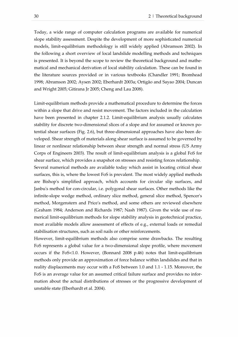
30 2 | Theoretical background
Today, a wide range of computer calculation programs are available for numerical
slope stability assessment. Despite the development of more sophisticated numerical
models, limit-equilibrium methodology is still widely applied (Abramson 2002). In
the following a short overview of local landslide modelling methods and techniques
is presented. It is beyond the scope to review the theoretical background and mathe-
matical and mechanical derivation of local stability calculation. These can be found in
the literature sources provided or in various textbooks (Chandler 1991; Bromhead
1998; Abramson 2002; Aysen 2002; Eberhardt 2003a; Ortigão and Sayao 2004; Duncan
and Wright 2005; Gitirana Jr 2005; Cheng and Lau 2008).
Limit-equilibrium methods provide a mathematical procedure to determine the forces
within a slope that drive and resist movement. The factors included in the calculation
have been presented in chapter 2.1.2. Limit-equilibrium analysis usually calculates
stability for discrete two-dimensional slices of a slope and for assumed or known po-
tential shear surfaces (Fig. 2.6), but three-dimensional approaches have also been de-
veloped. Shear strength of materials along shear surface is assumed to be governed by
linear or nonlinear relationship between shear strength and normal stress (US Army
Corps of Engineers 2003). The result of limit-equilibrium analysis is a global FoS for
shear surface, which provides a snapshot on stresses and resisting forces relationship.
Several numerical methods are available today which assist in locating critical shear
surfaces, this is, where the lowest FoS is prevalent. The most widely applied methods
are Bishop's simplified approach, which accounts for circular slip surfaces, and
Janbu's method for con-circular, i.e. polygonal shear surfaces. Other methods like the
infinite-slope wedge method, ordinary slice method, general slice method, Spencer's
method, Morgenstern and Price's method, and some others are reviewed elsewhere
(Graham 1984; Anderson and Richards 1987; Nash 1987). Given the wide use of nu-
merical limit-equilibrium methods for slope stability analysis in geotechnical practice,
most available models allow assessment of effects of e.g., external loads or remedial
stabilisation structures, such as soil nails or other reinforcements.
However, limit-equilibrium methods also comprise some drawbacks. The resulting
FoS represents a global value for a two-dimensional slope profile, where movement
occurs if the FoS<1.0. However, (Bonnard 2008 p.46) notes that limit-equilibrium
methods only provide an approximation of force balance within landslides and that in
reality displacements may occur with a FoS between 1.0 and 1.1 - 1.15. Moreover, the
FoS is an average value for an assumed critical failure surface and provides no infor-
mation about the actual distributions of stresses or the progressive development of
unstable state (Eberhardt et al. 2004).

2 | Theoretical background 31
Fig. 2.6: Simplified illustration of method of slices (based on Conolly 1997)
A second family of stability models on a local scale is concerned with continuum
modelling. The entire slope mass is divided into a finite number of elements and rep-
resented as a mesh. Continuum approaches include finite-difference and finite-
element methods. Finite-difference methods provide numerical approximations of
differential equations of equilibrium, strain-displacement relations or the stress-strain
equations (Eberhardt 2003a). In contrast, finite-element procedure exploits approxi-
mations to the connectivity of elements, and continuity of displacements and stresses
between elements (Eberhardt 2003a). However, in both methods the problem domain
is discretised into a set of sub-domains or elements. In contrast to limit-equilibrium
analysis, continuum modelling software allows for complex time-dependant landslide
analysis by including constitutive models such as elasticity, elasto-plasticity and
strain softening.
A third family of local landslides models are discontinuum methods, where slopes are
represented by distinct blocks which dynamically interact during movement or de-
formation. The underlying concept of these methods is that limit-equilibrium is re-
peatedly computed for each block, so that complex non-linear interaction can be ac-
counted for (Eberhardt 2003a).
Three variations of discrete-element variation can be distinguished. Distinct-element
methods are based on a force-displacement law to describe interaction between de-
formable elements, and a law of motion to numerically simulate displacements. Dis-
crete element methods are computationally intensive as many case studies involve a
very high number of interacting discrete objects. More detailed information is pro-
vided by (Hart 1993) and (Jing 1998). Discontinuous deformation analysis simulates
interaction of independent blocks along discontinuities, such as fractures and joints.
In contrast to distinct-elements methods, discontinuous deformation analysis ac-
counts for displacement instead of simulating forces (Cundall and Strack 1979). Parti-

32 2 | Theoretical background
cle flow methods represent slopes with spherical particles that interact through fric-
tional sliding contacts (Eberhardt 2003a).
Below, an overview of commercially available local landslide analysis and simulation
models is presented. This is, however, only a selection of models frequently applied in
landslide research as a complete summary is far beyond the scope of this study.
GGU is a CAD-based (Computer Aided Design) stability model which allows for pre-
dicting stability based on Bishop’s and Janbu’s, as well as general wedge and vertical
slice method. Moreover, stabilising factors such as anchors, soil nails and geosynthet-
ics can be included in the modelling process. However, the GGU stability software
does not account for dynamic hydrological modelling. Several applications utilising
the GGU stability software are available (Chok et al. 2004; Schneider-Muntau and
Zangerl 2005; Kupka et al. 2009; Hu et al. 2010).
Galena is another numerical software solution available which includes limit-
equilibrium analysis. It includes Bishop’s and Spencer-Wright method and Sarma
method, which utilises non-vertical slices for slope stability analysis. However, the
Galena software was developed mainly for slope design in open-pit mines, and only
few project applied it to analyse landslides (Kumar and Sanoujam 2006).
The program Xslope is capable of calculating slope stability based on Bishop's or
Morgenstern and Price's method, and is available through University of Sydney. It
does not include hydrological modelling, but pore-water pressure from an external
finite element steady-state seepage model can be integrated. Several case studies are
available that describe the application of Xslope (Lee et al. 2001; Hubble 2004; Cássia
de Brito Galvão et al. 2007)
Another model for limit-equilibrium analysis of soil and rock slopes is provided by
SLOPE/W which includes several methods (Morgenstern-Price, Spencer, Bishop, Or-
dinary, Janbu and more). Also, several soil strength models are available. Stability
analysis may be performed using deterministic or probabilistic input parameters.
However, dynamic hydrological modelling of pore pressures is not included in
SLOPE/W, but can be imported from SEEP/W, a finite-element software by the same
company. Moreover, external stresses by earthquakes for example, and also the effects
of reinforcements can be analysed. The use of SLOPE/W, also in combination with
SEEP/W is fairly widely acknowledged in recent landslide research (Anderson et al.
2000; Rahardjo et al. 2007; Cascini et al. 2008; Heng 2008; Yagoda-Biran et al. 2010;
Rahimi et al. 2010; Navarro et al. in press).
SVSlope is a slope stability software with a similar complexity and range of available
methods as SLOPE/W. However, three-dimensional limit-equilibrium analyses can
also be performed for which slopes are represented as columns to analyse stability by
2 | Theoretical background 33
a series of two-dimensional calculations. Moreover, a finite-element stability analysis
tools have been added to compute stresses and strains.
Several authors presented case studies applying SVSlope (Gitirana Jr 2005; Fredlund
2007; Gitirana Jr et al. 2008).
A similar program is Clara-W, which performs two and three-dimensional stability
limit-equilibrium analysis (Eberhardt 2003b; Stead et al. 2006; Cotza 2009; Montgom-
ery et al. 2009).
CHASM (Combined Hydrology And Stability Model) is a coupled hydrology and
slope stability model for limit-equilibrium analysis. The software program integrates
simulation of saturated and unsaturated hydrological processes to calculate pore-
water pressures, which are then incorporated into stability computation. CHASM is
essentially two-dimensional but hydrological simulations can be extended to account
for flow concentration at topographic hollows. Moreover, vegetation and stabilisation
measures can be integrated into Janbu and Bishop stability simulations. Furthermore,
a simple empirical-based run-out simulation is integrated into the model. CHASM
was also employed within this study and a more detailed review on CHASM meth-
odology is presented in chapter 5.1.3.2.
The CHASM model has been applied by several research projects, for example in
New Zealand (Wilkinson et al. 2000), Malaysia (Collison and Anderson 1996; Lateh et
al. 2008), Hong Kong (Wilkinson et al. 2002b), the Caribbean (Anderson et al. 2008),
Kuala Lumpur (Wilkinson et al. 2000; Wilkinson et al. 2002a), and Greece (Matziaris et
al. 2005; Ferentinou et al. 2006; Sakellariou et al. 2006). Common applications of
CHASM include investigations of effects of rainfall on slope hydrology and subse-
quently on slope stability (Matziaris et al. 2005; Ferentinou et al. 2006). Other studies
compared CHASM to other slope stability model and carried out sensitivity analyses
for rainfall, groundwater conditions and slope geometry (Lloyd et al. 2004).
Sensitivity analysis of CHASM has been carried out for geotechnical and hydrological
parameters (Hamm et al. 2006), hydraulic conductivity (Ibraim and Anderson 2003),
vegetation (Wilkinson et al. 2002b) and slope stability methods (Wilkinson et al. 2000).
Comparisons of field measurements of pore water pressures with modelled results
are provided by Anderson and Thallapally (1996) and Hennrich (2000). Other applica-
tions of CHASM include studies to improve criteria for geotechnical slope design
(Anderson et al. 1996), and validation of rainfall thresholds to enhance the perform-
ance of a landslide early warning system in Kuala Lumpur (Lloyd et al. 2001). Later
works of Wilkinson et al. (2002a) implemented a slope information system in which
pre-defined slopes can be modelled in CHASM using a variety of input parameter
constellations. Recent applications of CHASM include the work of Karnawati et al.
(2005) in which the aim was to provide guidance to local population in Java, Indone-
sia on how to judge stability and hazardousness of slopes. Back analysis of recent
34 2 | Theoretical background
landslides within CHASM was applied by Anderson et al. (2008) in the Caribbean.
Based on modelling results critical hydrological situations were determined and an
effective slope drainage system was designed.
Several models are available from RocScience for calculation of stability, stresses and
displacement for rock and soil. Phase² offers two-dimensional elasto-plastic finite-
element stress analysis for underground or surface excavations with integrated
groundwater seepage modelling (Hammah et al. 2008, Hammah et al. 2009). The pro-
gram Slide utilises two-dimensional limit-equilibrium analysis with built-in finite-
element hydrological modelling. Generally, capabilities of Slide are similar to other
limit-equilibrium programs described above. Case studies utilising Slide are de-
scribed by several authors (Kjelland et al. 2004; Hadjigeorgiou et al. 2006; Hammah et
al. 2006; Brandon et al. 2008; Topal and Akin 2008).
Plaxis is a collection of finite-element methods for numerical analysis of deformation
and stability in geotechnical engineering in two and three dimensions. Moreover, un-
saturated groundwater flow and pore pressures, as well as their effects on slope sta-
bility can be simulated. Static loads and dynamic loads and stability in response to
earthquakes, as well as non-linear, time-dependent and anisotropic behaviour of soils
and/or rock are more features of this complex software. Plaxis-aided research con-
cerned with landslides has been provided by several authors (e.g., Spickermann et al.
2003; Ausilio et al. 2004; Comegna et al. 2004; Kellezi et al. 2005; Keersmaekers et al.
2008; Majidi and Choobbasti 2008; Chang et al. 2010)
FLAC (Fast Lagrangian Analysis of Continua) is a two-dimensional explicit finite dif-
ference program widely acknowledged in analysis of plastic deformation (Cala et al.
2004; Maffei et al. 2004; Chugh and Stark 2005; Petley et al. 2005d; Jian et al. 2009).
Slopes are represented by elements which form a grid and behave according to a pre-
scribed linear or nonlinear stress and strain law. Deformation of the grid allows for
flowing and plastic-deformation, and large strain can be simulated. A simplified of
this model is FLAC/Slope, which is sold by the same company. Moreover, a three-
dimensional version, FLAC3D, is available and has frequently been applied within
research (Teoman et al. 2004; Pasculli and Sciarra 2006; Sitharam et al. 2007; Poisel et
al. 2009).
DAN, and its related version DAN-W and DAN3D, are software tools used for dy-
namic run-out analysis of rapid landslides processes such as rock avalanches (Hungr
1995). The core of the models is a Lagrangian solution of the integrated equations of
motion which is implemented for thin elements of the flowing mass. The model simu-
lates travel distance, velocity and flow depth and volumes in iterative time-steps.
Many case studies acknowledge the use of DAN codes (Hungr 1995; Sosio et al. 2008;
Hungr and McDougall 2009; Pirulli 2009).

2 | Theoretical background 35
UDEC (Universal Distinct Element Code) simulates the response of discontinuous
media such as jointed rock which subject to loading. The two-dimensional analysis
allows for rigid or deformable blocks. However, the related 3DEC model offers simi-
lar modelling capabilities but in three dimensions. Several case studies applied UDEC
on rock slopes (Bandis et al. 2000; Bozzano et al. 2000; Chen et al. 2000; Gunzberger et
al. 2004; Watson et al. 2004; Gong et al. 2005; Zhao et al. 2008), and 3DEC (Cheng et al.
2006; Ming-Gao et al. 2006; Lato et al. 2007; Bai et al. 2008).
2.4 LANDSLIDE EARLY WARNING SYSTEMS
In the following an introduction to early warning and the challenges of early warning
systems is presented. Therein, general aspects on social and technical aspects of early
warning are demonstrated. The focus, however, is put on landslide early warning.
More information regarding early warning systems for natural hazards in general is
provided by several other authors (e.g., Zschau et al. 2001; Zschau and Küppers 2003;
Dikau and Weichselgärtner 2005; Hall 2007; Schuster and Highland 2007; Felgentreff
and Glade 2007; Glantz 2009). In addition, a review of existing landslide early warn-
ing systems worldwide is presented. It is beyond the scope to give a complete sum-
mary of all existent systems, but to illustrate a wide range of technical applications
and to highlight integration of social components into early warning process.
Early warning can broadly be defined as the timely advice before a potentially haz-
ardous phenomenon occurs. Dikau and Weichselgärtner (2005) add that the effective
use of information for early warning is an important element of general risk manage-
ment which includes activities such as hazard zoning and prediction, warning com-
munication, disaster prevention and evacuation planning (Fig. 2.7). Good early warn-
ing systems therefore comprise identification and estimation of hazardous processes,
communication of warnings and adapted reaction of local population. Moreover,
early warning systems have to be embedded into local communities to ensure effec-
tiveness of the entire system.
A more pin-pointed definition is used by UNISDR (2009) where early warning system
are described as "the set of capacities needed to generate and disseminate timely and mean-
ingful warning information to enable individuals, communities and organizations threatened
by a hazard to prepare and to act appropriately and in sufficient time to reduce the possibility
of harm or loss".
Early warning systems have been developed for a wide range of natural hazards of
which extreme weather events, floods and tsunamis are maybe the best known. How-
ever, also for processes such as volcanic eruptions, droughts, snow avalanches, earth-
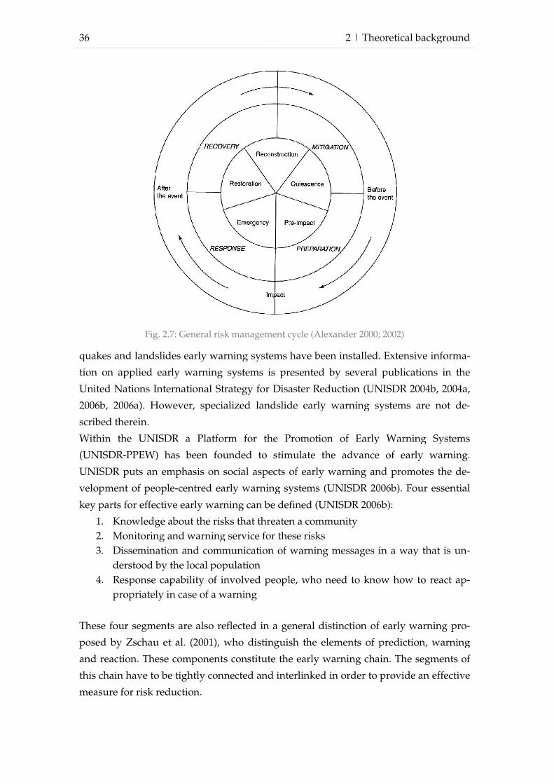
36
quakes and landslides early warning systems have been installed. Extensive inform
tion on applied early warning systems is presented by several publications
United Nations International Strategy for Disaster Reduction
2006b, 2006a). However, specialized landslide early warning systems are not d
scribed therein.
Within the UNISDR a Platform for the Promotion of Early Warning Systems
(UNISDR-PPEW) has been
UNISDR puts an emphasis on social aspects of early warning and promotes
velopment of people-centred early warning systems
key parts for effective early warning can be
1. Knowledge about the risks that2. Monitoring and warning service3. Dissemination and c
derstood by the local population4. Response capability
propriately in case of a warning
These four segments are also reflected in a general distinction of early warning pr
posed by Zschau et al. (2001)
and reaction. These components constitute the early
this chain have to be tightly connected and interlinked in order to provide an effective
measure for risk reduction.
Fig. 2.7: General risk management cycle
2 | Theoretical background
quakes and landslides early warning systems have been installed. Extensive inform
tion on applied early warning systems is presented by several publications
United Nations International Strategy for Disaster Reduction (UNISDR 2004b, 2004a,
. However, specialized landslide early warning systems are not d
Within the UNISDR a Platform for the Promotion of Early Warning Systems
has been founded to stimulate the advance of early
puts an emphasis on social aspects of early warning and promotes
centred early warning systems (UNISDR 2006b).
key parts for effective early warning can be defined (UNISDR 2006b):
about the risks that threaten a community arning service for these risks
Dissemination and communication of warning messages in a way that is uderstood by the local population Response capability of involved people, who need to know how to react
in case of a warning
These four segments are also reflected in a general distinction of early warning pr
(2001), who distinguish the elements of prediction, warning
These components constitute the early warning chain. The segments of
this chain have to be tightly connected and interlinked in order to provide an effective
measure for risk reduction.
: General risk management cycle (Alexander 2000; 2002)
Theoretical background
quakes and landslides early warning systems have been installed. Extensive informa-
tion on applied early warning systems is presented by several publications in the
(UNISDR 2004b, 2004a,
. However, specialized landslide early warning systems are not de-
Within the UNISDR a Platform for the Promotion of Early Warning Systems
to stimulate the advance of early warning.
puts an emphasis on social aspects of early warning and promotes the de-
. Four essential
way that is un-
of involved people, who need to know how to react ap-
These four segments are also reflected in a general distinction of early warning pro-
elements of prediction, warning
warning chain. The segments of
this chain have to be tightly connected and interlinked in order to provide an effective
(Alexander 2000; 2002)

2 | Theoretical background 37
Prediction is strongly influenced by a natural science and technological perspective
and aims to improve knowledge on the hazardous process itself and its timing, size,
extent, severity, duration etc. The time-span between warning and the occurrence of
the hazardous event is another important issue of prediction, and can last from sec-
onds (for e.g. earthquakes) to months (for e.g., droughts) (Zschau et al. 2001).
The second element, warning, can be regarded as the critical element within the early
warning chain (Dikau and Weichselgärtner 2005). Prediction has to be transferred into
an adequate warning message and distributed to the target population. Several com-
munication channels (e.g., SMS, Fax, Email, sirens) can be used to distribute warning
messages. However, effective warning is not only a technical problem, but is also de-
pendant on the social and political decisions and the legal framework (Zschau et al.
2001). Moreover, it is important that communication of warning is carefully planned
(Mayer and Pohl 2010). According to Kunz-Plapp (2007) warning messages should be
believable, clearly formulated, adapted to the context of the target group, and should
contain clear instructions on appropriate protection action.
Reaction is the third component of early warning, in which warning messages should
lead to appropriate action such as evacuation of hazardous areas. Decision makers
have to initiate protection actions based on the warning message. Effective reaction to
warning messages primarily depends on the administrative and organisational cir-
cumstances (Zschau et al. 2001).
Given the complex conditions of early warning it is obvious that purely technical ap-
proaches cannot provide effective early warning. It has already been noted by the
fathers of hazard research that it is important to know how technological advances in
early warning systems can be used to more efficiently trigger appropriate reactions of
populations to prevent losses from natural hazards (White and Haas 1975). Still, for a
long time advances in early warning systems were primarily related to the use of
more sophisticated monitoring equipment while social aspects of early warning were
neglected (Zschau et al. 2001). This is problematic, as many communities can not af-
ford expensive high-tech warning systems. Sorensen (2000 p.214) states that "better
local management and decision making about the warning process are more critical than pro-
moting more advanced technologies, although both would help". Many important social
aspects are not accounted for in technical approaches to early warning. However, the
importance of the hazard awareness can be illustrated by recent disaster events, such
as devastating the tsunami in the Indian Ocean in 2004 which caused more than
200,000 fatalities. Even though no early warning system was installed, this disaster
illustrates a major problem in early warning. As many people did not know that a
sudden decrease in sea-level precedes the occurrence of a tsunami, no appropriate
reaction could be initialised. If a threatened population is not informed about poten-

38 2 | Theoretical background
tial hazards, their consequences and suitable protective actions, early warning can not
be effective.
Although an early warning system could have enabled many people to evacuate
coastal areas, early warning systems can not provide full security from hazardous
events. An example of this took place in April 2010, when a train derailed in the Etsch
Valley, South Tyrol, Italy, because of a rockfall occurring above the track. Even
though an automatic early warning system existed to close the track in case of block-
ages, it failed in this event because the rockfall took place right above the passing
train (Murmelter 2010).
Moreover, it is important to keep in mind that only people and moveable objects can
benefit from early warnings and not stationary objects such as infrastructure. An
alarm can motivate people to escape from potentially dangerous situations, but it
does not stop the hazardous event itself (Hübl 2000). Therefore, early warning sys-
tems do not substantially decrease property damage (National Research Council
2004).
Although early warning systems can be an effective tool for risk reduction (Dikau and
Weichselgärtner 2005) they can also increase the risk. Increased risk may be due to a
false sense of security and building of higher value infrastructure in potentially haz-
ardous areas.
Uncertainties always prevail in hazard prediction and are also a major challenge for
early warning (UNISDR 2004b). Storms may change their track, or lose their strength
over time, earthquakes may be expected for a large area, but no exact location can be
determined. For many hazard events, only statistical forecasts, such as an El Niño
event probability for the next year of 60% can be made. In addition, uncertainties
within the social components complicate the prediction of the hazard consequences.
These include the reaction of the population to warnings and hazardous events, and
the functioning of evacuation plans and general disaster management. Baum and
Godt (2007) provide interesting examples where people were moving into warning
areas on purpose to secure their homes or save pets. Others misunderstand the warn-
ing and believe that if a warning is issued by for example the Department of Forestry
it only relates to areas with actual logging activities.
Moreover, the costs of unnecessary evacuations due to false alarms are a major con-
cern for decision makers. False alarms are a problem of early warning systems as they
can substantially compromise the credibility of early warning systems (Larsen 2008).
In 1982 the United States Geological Survey (USGS) issued a warning for the Mam-
moth Lakes Area because of an expected volcanic eruption potentially threatening a
ski resort on the slopes of the volcano. After the eruption did not occur the USGS was
mocked as the US Guessing Society (Die Zeit 2010). However, Sorenson (2000) argues,

2 | Theoretical background 39
that false alarms do not necessarily diminish the trust in early warning systems if the
reason for the false alarm is understood. The number of false alarms can be reduced
by pursuing a conservative strategy and by issuing generalised warnings. However,
the use of generalised warnings decreases with the size of the geographic area (Larsen
2008).
An interesting example of consequences of false warning took place in Italy in 2009
were a scientist had been measuring the emissions of radon gases which are associ-
ated with earthquakes. Based on his measurements he was expecting a major earth-
quake for the city of Sulmona two days before the devastating L’Aquila earthquake
(5.8 magnitude on Richter scale) which is located 70 km north-west. As his prediction
did not turn out to be accurate he was accused for creating panic but later absolved
(Die Zeit 2010).
On the other hand a group of seven Italian earthquake scientists who were assessing
the seismic activity in the L’Aquila region were accused of gross negligent man-
slaughter as they failed to predict the disaster. Only days before the earthquake they
had stated at a meeting with city officials that there were no grounds for believing a
major quake was on the way despite some smaller quakes in the previous days (Car-
tlidge 2010). The allegations gained much attention in the scientific community as
well as from general public, and a petition to end the investigations had been signed
by over 5000 scientists. In this open letter it was stated that at the moment there are no
scientific method to predict earthquake timing and that therefore, there is no ground
for the allegations (Die Zeit 2010). Warner Marzocchi, chief scientist at the Italian Na-
tional Institute for Geophysics and Vulcanology commented that "as scientists, we have
to focus on giving the best kind of scientific information" and that the decisions of what
actions need to be taken "is down to others to decide” (Cartlidge 2010). Thomas Jordan,
earth scientists who had also been working in the L’Aquila region added that the
costs of false alarms are too high compared to the low probabilities of an earthquake
occurring, so that there was no basis to initiate actions such as mass evacuations (Car-
tlidge 2010).
A similar case happened in the Italian community of Sarno, which was hit by devas-
tating landslides and a debris flood in 1998. Before the disaster event the mayor had
told the people to stay calm and to stay at home even though there were already
heavy rainfall and landslides occurring in the vicinity of the town (Die Zeit 2010). Af-
ter the event he was accused for negligent manslaughter but later absolved because
the event could not have been foreseen.
The previous examples clearly illustrate some of the problems and challenges of early
warning systems, arising from both natural and social components. Besides technical
difficulties of natural hazard prediction, legal, social and political dimensions add to
the complexity of early warning. Effective early warning systems must therefore be

40 2 | Theoretical background
carefully planned. Resulting from the work of the Integrative Landslide Early Warn-
ing Systems (ILEWS) project, issues have been identified that need to be addressed
when early warning systems are to be installed (Bell et al. 2010a). Important factors to
be accounted for include the process (flood, volcanic eruptions, landslides), time
(slowly developing or rapidly initiating hazards), forewarn time needed to provide
useful warning, financial aspects (private or public investments), communication of
warning (unidirectional, bidirectional), threatened human lives and infrastructure
(cost-effectiveness) and stakeholders to be warned (governmental agencies, emer-
gency services). Thus, early warning systems have to be demand-orientated and
adapted to local conditions (Twigg 2003). In addition, it is important that early warn-
ing systems are embedded into the local community to increase acceptance of warn-
ings (Mileti 1999; Greiving and Glade 2011).
Given the variety of hazards for which early warning systems have been installed it is
difficult to define clear categories. Some basic distinction, however, can be made (Bell
et al. 2010a):
- Monitoring systems are primarily installed to increase the understanding of natural processes but can also be utilised to plan further actions. These moni-toring systems differ by technologies applied, time intervals between meas-urements and degree of automation.
- Experts- or control-systems provide information on potentially hazardous events and are chiefly implemented to gain information on critical develop-ments and with the aim to guide scientists and decision makers.
- Alarm systems are based on monitoring systems and provoke an automatic warning if, for example, a predefined threshold is exceeded. Further differen-tiation of alarm systems can be made between pre- and post event systems and the forewarn time provided by the system. Moreover, these systems differ in their degree of integration of social aspects between purely technical appli-cations and integrative early warning systems.
Early warning systems have also been applied for landslide processes, e.g. rotational
and translational slides, debris flows and rock slides. Landslide early warning sys-
tems can be installed for single slopes, but also for entire regions. Also global land-
slide early warning systems have been proposed by applying methods such as rainfall
intensity and duration thresholds (Guzzetti et al. 2008) or satellite-based InSAR moni-
toring and progressive failure analysis (Petley et al. 2002).
Regional landslide early warning systems can only issue warnings, such as a 70%
probability of debris occurrence for a certain region; single slopes can not be identi-
fied (Wieczorek and Glade 2005). However, local or site-specific landslide early warn-
ing systems provide another quality of information. Exceedance of critical thresholds
may automatically lead to protective actions, such as alarms, road and bridge clo-

2 | Theoretical background 41
sures, evacuation and further disaster management actions. Local landslide early
warning systems have been frequently applied, partly because they can sometimes
replace structural measures of slope stabilisation while providing sufficient protection
(Palm et al. 2003). Site-specific systems generally apply monitoring systems for slope
movement or landslide triggering factors such as rainfall and pore-water pressure
(see Chapter 2.2) as the early basis of warning.
One of the first modern landslide early warning systems was installed in 1984 in
Utah, USA, after significant damage by debris flows initiated by snow melt (Baum
2007). Initially, monitoring of precipitation, temperature and slope movement on po-
tential landslides were used to alert local officials and issue a regional debris flow
early warning. Later works of (Ashland 2003) established groundwater thresholds for
instrumented potential landslides. Regional thresholds were determined based on
annual cumulative rainfall. Recent developments include snow monitoring to account
for landslide triggering by snow-melt (Baum 2007).
Based on the works of Campbell (1975), who established landslide and debris flow
triggering rainfall thresholds by intensity and duration analysis, a regional debris
flow early warning system was set up for the San Francisco Bay Area, USA in 1986
(Keefer et al. 1987; Wilson 2005). The system was developed and implemented as co-
operation between USGS and National Weather Service (NWS). Quantitative weather
forecasts issued by NWS two times a day for the upcoming 24 hours were provided to
the Landslide Initiation and Warning Project of USGS. Rainfall forecasts were com-
bined with data from automatic rainfall gauges and consequently checked against
pre-defined thresholds. Estimation of hazard level and final decision upon warning
was assessed cooperatively by experts from USGS and NWS. Initially, triggering
thresholds based on rainfall intensity in relation to annual rainfall (Cannon and Ellen
1988) were utilised. Later thresholds were adjusted to account for water storage ca-
pacity (Wieczorek 1987) and minimum thresholds for debris initiation (Wilson et al.
1993). Below the minimum rainfall threshold debris flow occurrences are unlikely
while above the upper threshold significant debris initiation in the region can be ex-
pected. In 1992 it was attempted to integrate radar data into the early warning system
to improve the spatial resolution of rainfall measurement. However, integration failed
because no reliable relations between radar reflectivity and ground based measure-
ment could be established. Along with technical problems the social aspects were a
major challenge for the early warning system. For instance, NWS and USGS had dif-
ferent expectations to the technical system. While USGS interpreted the system as an
experimental prototype of which warnings are by-products, NWS demanded reliable
predictions and warnings. Warning communication was another challenge for the
early warning system. USGS considered early warning as an entirely technical system
which ended with issuing an alarm. The population was expected to react appropri-
42 2 | Theoretical background
ately by avoiding dangerous areas. Yet, the population and also emergency services
were mostly unaware of debris hazards and their damage potential. In reality, many
people intentionally drove into hazardous areas in severe storm conditions trying to
get home to save the house or feed a pet (Wilson 2005). Eventually, the system was
shut down in 1995 because USGS could not afford to continue the service.
Based on the experiences in the San Francisco Bay Area, USGS and National Oceanic
and Atmospheric Administration (NOAA) cooperatively initiated a regional landslide
early warning system for burned areas in south California, which are prone to debris
flow initiation (NOAA-USGS Debris Flow Task Force 2005). An assessment of poten-
tial end-users and their demands towards landslide early warning were clarified be-
fore the system was set-up. Alert level terminology was overtaken from NWS severe
weather forecasts to increase the acceptance of the population. Dissemination of in-
formation and warning communication were adjusted to end-users needs. USGS also
developed an education program for involved meteorologists and interested public to
explain hydrological characteristics of debris flow initiation in areas with burned
vegetation (e.g., California Geological Survey 2003). Technical advances compared to
the previous system comprise improved quantitative rainfall forecasts, and imple-
mentation of test areas to improve the understanding of triggering groundwater con-
ditions. In addition, empirical and physically-based models were applied to assess
susceptibility to debris flows, their potential volume and run-out distance (NOAA-
USGS Debris Flow Task Force 2005).
Another regional debris flow early warning system for Oregon, USA, was developed
and implemented as a cooperation between Oregon Departments of Forestry (ODF),
Transportation (ODOT) and Geology and Mineral Industry (DOGAMI) with Oregon
Emergency Management (OEM) (Baum 2007). During periods of intense rainfall me-
teorologists of ODF monitor measured rainfall and forecasts and assess current haz-
ard level together with geotechnicians which are available 24 hours a day. Warning
messages are issued if thresholds are almost reached or exceeded. Thresholds used
within the system account for rainfall intensity and duration, but are modified in case
of significant antecedent rainfall or snow melting. Warning is spread via the emer-
gency channel of the National Weather Service. Within the developed system infor-
mation and education on debris flow hazards and early warning are also addressed
by for example, warning signs along the highway, advise to homeowners and infor-
mation on websites (Burns et al. 2008; Oregon Department of Geology and Mineral
Industry 2010).
2 | Theoretical background 43
A regional early warning system for shallow landslides is implemented for the Seattle
Area, USA since 2002 (Baum et al. 2005a; Baum and Godt 2009) and is jointly man-
aged by NWS, USGS and the city of Seattle. The technical system comprises a total
number of 17 automatic rain gauges with an average distance of 2-5 km between them
and quantitative weather forecasts. In addition, a test slope was instrumented to im-
prove understanding of pore-water pressure development and landslide triggering.
Furthermore, landslide mapping and probabilistic regional hazard modelling were
performed (Baum et al. 2005b). Detailed examination of rainfall data led to the estab-
lishment of a minimum threshold for landslide triggering based on intensity and du-
ration analysis and an antecedent water index calculated from cumulative rainfall of 3
days, and rain within the previous 15 days (Chleborad 2000; 2003; Chleborad et al.
2006). For the assignment of alert levels thresholds are used for both, intensity-
duration and antecedent water index. Rainfall exceeding intensity-duration thresh-
olds triggers a warning status at high antecedent water status. Watch level is issued,
in the occurrence of medium antecedent rainfall index values and observed or fore-
casted rainfalls above thresholds. Outlook level is activated if any of the rainfall
threshold is exceeded. In other cases the alert is null. In addition, warnings are only
provided if thresholds are exceeded for at least three gauges relating to an expected
number of three or more landslide events (Baum and Godt 2009). Warning thresholds
performed satisfactory in back-analysis with data from the 1978 to2003 period; only
eight storms caused landslides without previous threshold exceedance (Godt et al.
2006). 40% of all warnings were followed by landslides events and 85% off all land-
slides were triggered by rainfall above thresholds values. To increase the acceptance
of the early warning system and improve risk awareness of the local residents, USGS
provides educational material and information (USGS 2006).
In the USA, USGS is responsible for allocation of warnings related to geological
events, including landslides. To increase interoperability of warning systems and en-
sure smooth warning communication a common alerting protocol (CAP) was created
(Highland and Gori 2008). This data format is the same for many different kinds of
warnings including also man-made hazards and terrorism. Today it is widely used by
state agencies in the USA. Landslide related CAP warning have been adopted for all
study areas, for which reliable rainfall thresholds have been established, i.e. Seattle,
San Francisco Bay Area and burned areas and parts of the Appalachian mountain
areas of the eastern US. All alerts, including archived warnings, are presented on
USGS website. To increase the populations' awareness of landslide hazards and the
potential outcomes of landslide events, a documentary movie was produced, which is
also planned for school education (Highland and Gori 2008). Moreover, a wide range

44 2 | Theoretical background
of fact sheets, reports and other information on landslide hazards, consequences and
warnings is produced by USGS.
The most advanced and successful landslide early warning system may be that in-
stalled in Hong Kong, China (Schuster and Highland 2007). Hong Kong is densely
populated by seven million inhabitants and very prone to landslides occurrences and
damage consequences. The terrain is rugged, with hills rising up steeply, and less
than 30% of the densely populated areas are flat (0-5°) (Brand et al. 1984). The limited
availability of favourable land means that geotechnical slope construction works in-
cluding design of cut and fill slopes and slope stabilisation are frequently required.
Moreover, strong rainfalls with hourly intensities exceeding 150 mm occur along with
tropical cyclones and low pressure. After two catastrophic landslide events in 1972
and 1976 which together caused more than 100 fatalities, the Geotechnical Control
Office was established to reduce landslide consequences (Malone 1997). Later, the
agency was renamed the Geotechnical Engineering Office (GEO). GEO has many re-
sponsibilities, such as establishing instructions and guidelines for slope design, slope
stabilisation, quantitative risk management and early warning (Chan 2007). More-
over, education programs for the general population and homeowners aim to raise
awareness of landslides and related risks. Radio and television features, a telephone
hotline and a website provide a wide range of information and advice to local resi-
dents (Massey et al. 2001). Detailed information on integrative landslide risk man-
agement strategies in Hong Kong and the efforts and experiences of GEO is available
in a collection of scientific papers published for the 30th anniversary of GEO (Geo-
technical Engineering Office 2007). The great success of slope safety in Hong Kong is
also illustrated by significantly lower fatalities due to landslides after the establish-
ment of GEO's predecessor in 1977 (Fig. 2.8).
The Hong Kong regional landslide early warning system was launched in 1977 and is
managed cooperatively by GEO and Hong Kong Observatory. More than 100 auto-
matic rain gauges built the technical base for early warning. Rainfall thresholds trig-
gering landslides in Hong Kong were first established by Lumb (1975), but were
modified several times afterwards when improved real time rainfall and landslide
data became available. Initially, warning thresholds accounted for cumulative 24 hour
rainfall in relation to rainfall of the preceding 15 days. Warnings were issued if meas-
ured rainfall of the last 20 hours and the forecasted rain for the next 4 hours exceed
175 mm (Chan et al. 2003). In the 1980s an hourly rainfall threshold of 70 mm was
added to the warning scheme. Progressive analysis of landslide initiation and related
rainfall events led to prediction of the number of landslides expected for certain storm
events. Warnings were only issued if 15 or more landslides were expected to occur
(Chan et al. 2003). Since 2003 a GIS-based approach has been used for landslide pre-

2 | Theoretical background 45
diction (Yu et al. 2004). Therein, the entire area of Hong Kong is represented as grid
cells accounting for number of properties contained on the slopes. The number of ex-
pected landslides is then modelled according to a spatially variable susceptibility to
slope failure. A recent development of the landslide early warning system includes
the integration of radar data from the SWIRLS system (Short-range Warning of In-
tense Rainstorms in Localised Systems) to track storm cells and improve quantitative
prediction of localised storms (Cheung et al. 2006). Warning dissemination utilises
TV, radio and internet to inform the public. In addition, emergency forces and hospi-
tals are contacted if large numbers of landslide are expected. In early years warning
messages were mostly aimed at slum dwellers because they lived in most hazardous
areas. However, social and geotechnical developments since the 1980s changed the
focus. Today, the intention of early warning is to inform the entire population about
potentially hazardous events, thus to provoke cautious behaviour.
China is probably the country experiencing the highest landslide damage and number
of fatalities in the world (Tianchi 1994). China has begun to address the landslide
problem in the 1990s by starting a nationwide investigation program including land-
slide mapping, susceptibility zoning, risk analysis, rainfall threshold analysis, preven-
tion planning and engineering counter measures (Yin 2009) and early warning (Zhou
and Chen 2005). Since 2003 landslide warning based on rainfall forecasts are issued
after general weather reports on prime time TV shows (Yin 2009).
Fig. 2.8: Number of landslide fatalities in Hong Kong (Wong and Ho 2000)
46 2 | Theoretical background
A regional landslide early warning system based on susceptibility maps and rainfall
thresholds was installed for Zhejiang Province (Kunlong et al. 2007; Eng et al. 2009).
The system is based on rainfall forecasts and works as a WebGIS. Warnings are issued
if rainfall predictions exceed one of the two defined thresholds and near real-time
warnings are spread through various communication channels (internet, telephone,
etc.). The warning system is also combined with an assessment of economical risks
which aim to extend the system to landslide risk warning (Wu et al. 2009).
Zhong et al. (2009) provide detailed information of the precipitation based early
warning system for Hubei Province. The landslide early warning system was installed
in 2006 and represents a WebGIS. Critical rainfall thresholds have been determined by
analysing the statistic relationship between spatial distribution of occurred landslides
and rainfall data. Warning generation is based on 2 and 15 day antecedent rainfall,
which is compared to 24 hour rainfall forecast. If thresholds are exceeded in any of the
82 divisions in which Hubei is differentiated, the Meteorological Survey of Hubei
Province issues a warning on the internet. More information on the current situation
is freely accessible in the form of maps on the internet. In three years of operation the
system issued 11 warnings, of which 6 were followed by landslide events (Zhong et
al. 2009).
The Geotechnical Engineering Office of Rio de Janeiro, Brazil, implemented a regional
landslide early warning based on rainfall thresholds and rainfall monitoring in 1996
(Ortigao et al. 2002; Ortigao and Justi 2004). In early years the early warning system
was not entirely automated which resulted in a lack of warnings on for example,
weekends and holidays, as no experts were available (D’Orsi et al. 2004). Instead,
automated fax messages were sent without proper data analysis. However, due to
wide acceptance of the early warning system it was expanded in 1998, and since then
provides continuous service. At the same time a rainfall radar was included into the
technical input to increase forewarn time. In addition, a test slope was equipped with
piezometers and inclinometers to gain more insights into the failure processes. How-
ever, it was decided not to establish more site-specific monitoring systems as the costs
were too high. Two critical rainfall thresholds were determined which relate hourly
rainfall intensity to accumulated rainfall for 24 and 96 hours (D’Orsi 2006). Four
warning levels are used, e.g., low (landslides could happen), medium (occasional
landslides), high (scattered landslides) and very high (generalized landsliding). Cur-
rent information on warning levels is broadcasted by media and is also available
online. In addition, emergency services are informed by fax to prepare for potential
landslide events. In addition to the landslide early warning system, flash floods were
later integrated into forecasting activities (D’Orsi 2006).
2 | Theoretical background 47
A regional debris flow early warning system was installed in Combeima-Tolima Re-
gion in Colombia (Huggel et al. 2008; Huggel et al. 2009). The project was initiated by
the Swiss Agency for Development and Cooperation (SDC) which promoted invest-
ment into early warning, risk awareness education and disaster prevention training
instead of solely focussing on reconstruction. The automatic technical monitoring sys-
tem includes three rainfall stations and a series of geophones. At the Regional Emer-
gency Committee Centre data is collected and analysed 24 hours a day and is avail-
able online. Rainfall thresholds initiating debris flows were calculated based on inten-
sity and duration, and with respect to antecedent rainfall up to 30 days. If thresholds
are exceeded an emergency plan determines actions to be taken. Interestingly, Huggel
et al. (2009) analyse the performance of the developed system by a cost-effectiveness
calculation based on historic records. Therein, the costs of false alarms are compared
to losses in case of hazard events which can be used to adjust rainfall thresholds.
However, this approach is ethically questionable as it requires definition of monetary
costs of lost human lives.
The combined hydrology and slope stability model CHASM, which is applied within
this study, has also been used in another landslide early warning system. However,
instead of applying CHASM for continuous modelling of slope stability, rainfall
thresholds previously calculated were validated by detailed analyses for single slopes.
The system is located along the Kuala Lumpur Highway, Malaysia, and is in service
since 1996 (Lloyd et al. 2001). An automated monitoring system measures rainfall in-
tensity which is compared to pre-defined threshold values also accounting for antece-
dent rainfall conditions. A series of single slope CHASM simulations illustrated the
effect of high soil permeability on slope stability. In conclusion, rainfall longer than 6
days ago did not significantly influence slope stability and could be neglected in rain-
fall threshold determination in the study area.
An extensive early warning system for debris flows in Indonesia is presented by Apip
et al. (2009; 2010). Based on local rainfall threshold analyses accounting for rainfall
intensity and duration, as well as antecedent rainfall, design charts were created
which provide three warning levels (safe, watch, danger). Moreover, it is tried to
widen predictive power of the warning system by integrating spatially distributed
modelling of slope stability with physically-based hydrology and stability model.
Therein, quantitative rainfall forecasts by National Oceanic and Atmospheric Admini-
stration (NOAA) are utilised for real-time modelling of potential landslide initiation.
In addition, the model is planned to be further developed to provide forecasts of river
flows, sediment transport and debris flow run out.

48 2 | Theoretical background
A similar approach to early warning is provided by Liao et al. (2010), who also
worked on regional landslide early warning in Indonesia. The proposed system in-
cludes a physically-based hydrology and slope stability model, as well as integration
of quantitative rainfall forecasts. Modelling is performed in two steps. Initial calcula-
tions provide hot spots, which can then be modelled using data with higher resolu-
tion. However, the technical system represents a prototype development and further
research has to be accomplished in order to increase its predictive capacities.
Schmidt et al. (2008) present an innovative landslide early warning system for New
Zealand. Therein, probability of landslide failures is computed by combination of a
regional physical-based hydrology and stability model with quantitative weather
forecasts. However, landslide prediction is subject to large uncertainties which are
assessed by probabilistic methods. Unfortunately, the early warning system was only
a prototypic development and is currently not active.
Aleotti (2004) presents a prototype of a regional landslide early warning system for
shallow landslides in the Piedmont Region of north-western Italy. Rainfall thresholds
were determined by analysing intensity-duration, antecedent rainfall and mean an-
nual precipitation. Warning thresholds, however, were established lower than trigger-
ing thresholds to provide more safety. Instead of a warning threshold parallel to the
triggering threshold Aleotti (2004) applied a curve to account for different rain paths
(Fig. 2.9). By doing so time spans until landslide triggering threshold exceedance are
integrated, which are important for initiation of evacuations. The technical warning
system includes rainfall forecasts and station measurements. The system remains in
an ordinary attention state until thresholds are exceeded by rainfall forecasts. A pre-
ceding warning procedure is launched if landslide prone areas are affected by thresh-
old exceedance. Rainfall paths are then plotted according to antecedent and real-time
rainfall and an alert is issued according to the pre-defined thresholds.
Recent developments of the regional landslide early warning system concentrated on
the improvement of thresholds by including local properties, such as topography and
geological properties (Tiranti and Rabuffetti 2010). Consequently, three thresholds
were established, i.e. regional, sub-regional and a pragmatic threshold, which ac-
counts for multiple occurrences of landslide in single rain events. All thresholds were
tested for their performance in a back-analysis in terms of correct, false and missed
alarms. In addition, a technical system named SMART was developed which analyses
rainfall time series for each rain gauge in real time and identifies where thresholds are
exceeded. The current early warning system utilises rainfall forecast and real-time
measurements and applies the pragmatic threshold (Tiranti and Rabuffetti 2010).

2 | Theoretical background 49
The Åknes rockslide in Norway is one of the most intensely investigated and moni-
tored landslides worldwide (e.g., Derron et al. 2005; Ganerød et al. 2008; Kveldsvik et
al. 2008; Kveldsvik et al. 2009; Eidsvig et al. 2009; Heincke et al. 2010; Grøneng et al.
2010). The rockslide itself does not pose direct threat to a community, however, slope
failure is supposed to trigger a tsunami affecting ships and towns along the fjord. The
rockslide mass has a volume of 30-40 million m³ and displacements vary with seasons
and reach 3-10 cm/year with daily movements up to 1 mm (Blikra 2008). The techni-
cal monitoring system includes extensometers, inclinometers, crackmeters, tiltmeters,
geophones, piezometers, automated measurements by theodolites, laser and GPS and
ground based radar, and a climate station. All data is available in a web-based data-
base and supervised by experts 24 hours a day. Threshold values for displacement
velocity have been established which relate to five alert levels colour-coded from
green to red. In case of imminent slope failure sirens warn the population in poten-
tially affected towns. Other topics of the project include development and implemen-
tation of warning routines and evacuation planning (Blikra 2008).
Another example of an intensely monitored rock slide is the Frank Slide at Turtle
Mountain, Canada, which exhibited a catastrophic failure in 1903 causing 70 fatalities
(Froese et al. 2005). A landslide monitoring and early warning program was launched
in 2003 and commenced with detailed site investigations using InSAR, microseismic
surveys, ground penetrating radar, drilling and core sample analysis. Within the ac-
tual early warning system tiltmeters, extensometers and crack meters are used as
Fig. 2.9: Comparison of warning curve and warning line thresholds and subsequent time spans for evacuation (Aleotti 2004)
50 2 | Theoretical background
primary sensors as they provide high detail displacement data (Froese et al. 2006).
Secondary sensors include differential GPS and automatic theodolite measurements
which have higher fluctuations but improve understanding of the overall situation.
Background information is gained by tertiary sensors, i.e. climate station data and
microseismic monitoring. The early warning system comprises four elements (Froese
et al. 2005). A monitoring procedure was established to determine responsibilities for
measurements and their frequencies, which might change in response to trends and
anomalies in the data. Within the threshold development procedure value-based and
velocity-based thresholds two standard deviations above noise level were established.
Development of alert levels and notification protocols comprise the third element of
the early warning system. A standardised terminology and appropriate response to
trends in monitoring data were determined. Moreover, action advice was developed
for emergencies including procedures for communication and evacuation. The current
alert level is accessible on the internet and is presented in four colours. The green alert
level indicates normal situations where measurements are in the range of background
noise but may exhibit seasonal fluctuation. The watch level is active if multiple sen-
sors display unusual trends and leads to direct communication between technical
experts and local decision makers and municipal officials). The warning level is initi-
ated if multiple sensors demonstrate acceleration trends exceeding pre-defined
thresholds. If several sensors indicate accelerations and final failure is imminent (one
to three days to failure) then the alarm level is issued and the emergency response
procedure is executed. More detailed information on monitoring (Read et al. 2005),
modelling (Froese et al. 2009) and the information platform (Froese et al. 2006) is
given in the respective literature.
An early warning system for rockfall is installed at the Winkelgrat, also located at the
Swabian Alb in Germany (Fig. 2.10). The technical system consists of nine automatic
extensometers installed in 2002 (Ruch 2009). An automatic alarm message is sent to
the local emergency service if pre-defined thresholds are exceeded. The road below
the unstable rock mass is then closed by setting two traffic lights to red to prevent cars
from entering the hazardous area. At the same time road maintenance service, police,
rescue forces and the regional geological department are informed via SMS and fax.
Following field investigations by experts of the regional geological department it is
decided to initiate further protective measures, or in case of false alarms, to reopen the
road (GEOSENS 2009; Krause 2009).
Another landslide early warning system in Germany is described by Lauterbach et al.
(2002) and Krauter et al. (2007). This system relies primarily on technical solutions, for
example, GPS displacement measurements, and is installed at an autobahn in south-

2 | Theoretical background 51
west Germany. The slope under investigation is known to cause deformations to the
road surface since the 1960s. The landslide mass is calculated to be 700,000 m³ with
average annual movement rates of 1-2 cm. As structural measures were considered
uneconomical a GPS based warning system was installed. The system consists of 5
measured points of which the main station is based outside the landslide mass. Accu-
racy of the system is about 1 mm in location, and 2-3 mm in height. Two kinds of
alarms are implemented: one occurs when obviously false measurements are being
taken or maintenance works are necessary, the other if pre-defined thresholds of
movement rates are exceeded. If warning thresholds are exceeded the experts operat-
ing the system are informed via automatic telephone calls and immediately check the
situation in the field, which then can lead to emergency actions like, for example, road
closure.
Several slope monitoring and early warning systems have been installed in the United
Kingdom. An extensive technical monitoring and early warning was installed for the
coastal landslides on the Isle of Wight (Clark et al. 1996) where the first tiltmeter slope
early warning started in 1981 (Barton and McCosker 2000). Today, the technical sys-
tem comprises monitoring of surface and subsurface movements by theodolites, GPS,
inclinometers, tiltmeters and crackmeters. Weather stations and piezometers record
also rainfall and its effect on landslide triggering. Automatic alarms are issued if pre-
defined displacement thresholds are exceeded. Automatic monitoring systems were
preferred over manual systems even though initial costs are considerably higher.
Similar technical monitoring systems have also been installed in Lyme Regis, Scarbor-
ough and Cromer (Clark et al. 1996).
In Lyme Regis a series of inclinometers, piezometers and GPS ground markers are
continuously monitored and provide an alarm to experts and decision makers if an
Fig. 2.10: Early warning system at Winkelgrat landslide equipped with automatic extensometers (left) and traffic light for road closure
(right)

52 2 | Theoretical background
imminent threat is given (Clark et al. 2000). In addition, an increased monitoring fre-
quency can be initiated and emergency response is prepared.
At Cromer, automatic readings of field sensors activate an alarm by sending a mes-
sage by pager. Warning thresholds are based on a pre-determined movement velocity
of 3 mm per hour or 10 mm in 6 hours.
Landslide early warning on the Isle of Wight is part of an extensive general coastal
management scheme by the Isle of Wight Centre for Coastal Environment which
promotes a holistic approach. Coastal management comprises for example, allocation
of planning guidance maps, building codes, engineering measures, monitoring, fore-
casting and early warning. A wide range of information is available on the websites
(Isle of Wight Centre for the Coastal Environment 2010), such as a best practice guide
(McInnes 2000) providing detailed descriptions of monitoring and warning schemes,
as well as advice to homeowners on how to reduce risk of coastal erosion and instabil-
ity. In addition, the local management and information centre arranges workshops
and educational field trips.
An extensive technical monitoring system is installed along the slopes of Clyde Dam
Reservoir, New Zealand (Macfarlane et al. 1996). More than 5,500 theodolite observa-
tion points were installed to monitor displacements during dam construction and
reservoir filling. After filling was accomplished the number of observation points was
reduced. Further monitoring equipment includes borehole extensometers and incli-
nometers for subsurface movements and piezometers for slope hydrology. All data is
automatically stored in a database and alarms are raised automatically if pre-defined
thresholds are exceeded.
Given the great number of engineering works in China many applications of monitor-
ing and early warning systems are described in the literature. Since the 1990s much
attention has been paid to the landslide hazards along the Three Gorges Dam Reser-
voir, China, and many investigations have been performed by researchers on this
emerging topic (Fourniadis et al. 2007a, Fourniadis et al. 2007b; Li et al. 2008; Wang et
al. 2008c; Jian et al. 2009; Li et al. 2009a; Li et al. 2009b; Yin 2009). Several landslide
monitoring and early warning systems are located along the lake created by the Three
Gorges Dam. One of these was installed for the Shuping landslide, a reactivated mass
movement which accelerated after the impoundment of the lake. Several extensom-
eters are used to measure the landslide (Wang et al. 2008b; Wang et al. 2009). Dai et al.
(2008) describe a monitoring and warning system based on high resolution optical
fibres for the Yuhuangge landslide in the Three Gorges Area. Four alert levels were
determined which account for changes in velocity and pore-water pressure. Local
decision makers are informed about current alert levels and are obliged to issue final

2 | Theoretical background 53
warnings and initiate evacuation. Since 2004 the alert level was once set to yellow
level due to significant acceleration and damage on infrastructure (Yin et al. 2010a).
Later however, displacement rates decreased to former values and the alert level was
subsequently lowered.
Moreover, several more interesting papers on applied landslide early warning sys-
tems in China have been published, unfortunately, many are only available in Chi-
nese language with English abstracts (Jiang et al. 2009; Xu and Zeng 2009; Ye et al.
2009).
The Illgraben catchment (9.5 km²) in Switzerland has some one of the highest debris-
flow activity in the Alps. A monitoring and early warning system for debris flows
was installed and described in detail by (Badoux et al. 2009). The overarching early
warning concepts includes ongoing education and allocation of information for the
local population regarding debris flows and possible consequences, a monitoring sys-
tem, repeated field surveys to assess changes in the catchment, and integration of me-
teorological measurements to increase forewarn time (Graf et al. 2006). Several educa-
tion campaigns were performed to inform local population about potential hazards
and the early warning systems. In addition, children at elementary level learn about
debris flows in school. Tourists are provided information at local tourist information
centre. Along the debris flow channel warning signs were put up every 200 m ex-
plaining the threat of debris flow occurrences in five languages. Moreover, warning
lights and loud speakers were installed at three spots where hiking trails cross the
debris flow channel. The early warning system is managed and maintained by Illgra-
ben Security Commission and contacts local emergency task forces if potentially dan-
gerous situations emerge. The technical system includes several geophones located at
check dams, which can automatically trigger warning lights and speakers further
down the debris channel if a seismic signal lasts for more than five seconds. At the
same time SMS and emails are sent to local decision makers. A forewarn time of 5 to
15 minutes between measurement of debris flow by geophones and a debris flow
reaching settlement areas in the valley is provided by the system. Alarms can be can-
celled if geophones further downslope do not detect seismic signals 10 minutes after
the first signal. This is done to decrease chances of false alarms due to other potential
geophone triggers, e.g., rock fall, thunderstorms or earthquakes. Further technical
equipment of the Illgraben monitoring systems includes measurement of discharge by
ultrasonic sensors, laser and radar. Based on their experiences Badoux et al. (2009)
propose radar as the most suitable method for early warning, as it provides smooth
and reliable data on discharge even in situations of rapidly fluctuating discharge
amounts. The catchment is visited and mapped regularly to detect changes in the de-
bris flow source area, such as landslides that provide material for further debris flow

54 2 | Theoretical background
occurrences. Including meteorological forecasts into the early warning systems and
defining rainfall thresholds was also trialled. However, integration failed because
local thunderstorms in alpine areas are difficult to predict. The debris flow early
warning system at the Illgraben can be regarded successful. Since its implementation
20 alarms were issued, of which only one was a false alarms, and in only three cases a
warning was cancelled even though the debris flow had not stopped. The Illgraben
catchment is also part of the national IFKIS-Hydro early warning and information
platform, which provides monitoring data and event documentation (Romang et al.
2010).
In the North Italian community of Nals a local debris flow early warning system was
installed after devastating debris flow events in 2000 (Egger and Mair 2009). The aim
of the early warning system was to be an addition to structural protection measures.
Debris flow material is supplied by landslide processes in the upper catchment. How-
ever, due to the high activity it was decided not to install an automatic system there,
but to place a series of geophones into the debris flow channel to detect already initi-
ated events. Still, a forewarn time of 20 to 60 minutes between a geophone alarm and
the debris reaching settled areas is accomplished. Further technical equipment in-
cludes a piezometer, rainfall stations and a remote controlled video camera with flood
lights.
Another Italian case study on a debris flow warning system utilising geophones is
presented by Arratano (1999), however, it only was active for one summer.
A prototype of a mudflow early warning system for the Italian city Sarno is described
by Sirangelo and Braca (2004). Therein, the probabilistic hydrology model FLaIR
(Forecasting of Landslides Induced by Rainfall) was applied, which correlates rain-
falls with landslide occurrence. Warning thresholds were established by back analysis
and included the large 1998 event. According to these thresholds three warning levels
were determined, i.e. attention, alert and alarm.
The same model has been applied to Lanzo Valley of the Piedmont, Italy (Capparelli
and Tiranti 2010). Promising performance led to the current implementation of an
automatic early warning system.
Hübl (2000) describes the application of a prototypic early warning system for the
Wartschenbach catchment in Austria, which frequently experiences debris flows and
flash flood events. The developed early warning system is thought as a passive pro-
tection measure. The technical system is based on measurement of rainfall and flow
discharge by ultrasonic sensors in the upper catchment. If measurements exceed pre-
defined thresholds it is up to experts to decide whether to close lower lying roads to
prevent cars being hit by debris flows. By developing adequate response plans for

2 | Theoretical background 55
hazardous events they have tried to address the response of the local community. The
implemented system was planned and implemented as a prototype and should be
installed in other catchments which could potentially produce debris flows after a test
period.
A novel a landslide early warning system is described by Sakai (2008). Earlier re-
search (Sakai and Tarumi 2000) indicated that concentrations of sodium, calcium and,
sulphate ions in groundwater changed before phases of landslide activity. Landslide
failures could be predicted up to 90 days in advance. Therefore, a prototypic landslide
early warning system was set up which utilises automated ion-selective electrodes to
provide early warning to railroads in Japan. Data is transmitted from the sensors in
the field to train dispatchers and track maintenance engineers via mobile phone net-
works. Measurements are taken every 1 to 3 days, but frequency can be increased in
the case of unusual sensor readings.
Another example of an early warning system in Japan is presented by Chiba (2009).
The warning system strongly emphasises warning communication and is regarded as
an integral element of the local disaster prevention program against sediment-related
processes (debris flows and debris floods). Earlier research on local hazards provided
information on potential hazardous zones and return periods, which was utilised to
allocate warning and evacuation zones in the occurrence of debris flow events. Sev-
eral people were employed to carry out education programs in which local residents
were informed about potential hazards and appropriate reactions in case of a warn-
ing. If exceedance of pre-defined river flow thresholds occurs a disaster management
headquarter is assigned in which all information about the current hazard status is
collected. Information is gathered primarily by the employees by calling local resi-
dents by cell phone. Moreover, all data is updated to a GIS platform which is avail-
able online. Chiba (2009) illustrates the effectiveness of the warning system by com-
paring its performance to a neighbouring town, in which no early warning system
was installed, and no detailed hazard maps and evacuation plans were available.
During a debris flow event local disaster managers were overwhelmed by incoming
information and no efficient evacuation could be initialised. In contrast, disaster man-
agers of the town with a warning system were able to quickly determine where debris
flows had occurred and to initialise evacuation according to the pre-determined
schemes.
Flentje et al. (2005) present a real-time monitoring network for time pore-water pres-
sure, slope movement and rainfall in Wollongong, Australia, which aims to enhance
understanding of landslide triggering process and improve quantitative assessment of
56 2 | Theoretical background
landslide hazards. All data is automatically sent via a cell phone network to a web-
based database available online. Threshold values have been determined and current
measurements are colour-coded to allow for easy interpretation. However, the de-
scribed system is essentially technical and does not aim to provide a warning mes-
sages or initiate counter measures or evacuation.
Besides the ILEWS project several other research programs focussing on early warn-
ing systems for natural hazards were funded within the GEOTECHNOLOGIEN
framework. Three of these projects also concentrated on landslide processes, and will
briefly be described in the following.
The SLEWS (Sensor-based Early Warning System) project focused on three sensor
types measuring acceleration, inclination and pressure to monitor landslide initiation
(Fernandez-Steeger et al. 2009). The project emphasized technological developments
accounted for sensor development and laboratory testing. A large proportion of the
accomplished work concentrated on wireless sensor networks to ensure smooth data
transmission. Developed sensors were applied to several real case studies on the Bar-
colonette earthflow in France, and rockfall warning in Rathen, Germany. However,
besides the technical research, the integration of early warning in social decision mak-
ing process was another topic of the SLEWS project.
The main goal of the alpEWAS project was sensor-based monitoring and early warn-
ing in the Bavarian Alps (Singer et al. 2009; Thuro et al. 2009). Thereto, three main
methods were utilised to detect displacements, i.e. TDR measurements, prism-less
tachymetrie and low-cost GPS measurements. In addition, an information platform
was set up to collect all data and inform involved experts by email and SMS if pre-
defined thresholds were exceeded.
The EGIFF project adopted a technical approach and concentrated on the develop-
ment of new methods applicable within landslide early warning. A wide range of
geotechnical data for a test slope south of Munich, Germany, was compiled and mod-
elled by a finite element model (Breunig et al. 2009). In addition, 3D/4 D databases
were developed for effective data visualisation. Moreover, the project implemented
an automated system to interpret media news and extract landslide related informa-
tion.
From the examples of landslide early warning systems illustrated above some conclu-
sions can be drawn. Regional landslide early warning systems that focus on shallow
landslides or debris flows generally rely on rainfall thresholds derived by empirical or
physically-based methods. In some cases local test slopes are equipped with monitor-
ing systems to improve understanding of landslide triggering and consequently mod-
ify rainfall thresholds. Innovative approaches try to integrate sophisticated slope sta-
bility models and real time modelling of landslide initiation Local landslide early

2 | Theoretical background 57
warning systems however are installed for a wider range of processes. For debris
flows technical early warning systems can be fairly simple because it may take several
minutes until an initiated debris flow reaches settled areas. Forewarn time for other
landslide processes is often shorter and early warnings are more complex. For deep-
seated landslides and failures in rock more complex monitoring is applied to measure
displacements and processes related to movement triggering. Warning thresholds
may account for displacement or critical parameter values of triggering factors. Mod-
elling of slope behaviour by complex slope stability models is an important part of
landslide prediction and is frequently applied for landslide early warning. Most land-
slide early warning system are not fully automated but leave judgment of the current
situation and final warning to experts. Existing landslide early warning systems differ
substantially regarding the integration of social aspects. In some cases landslide early
warning is integrated into larger schemes for slope safety, risk management, disaster
prevention and hazard awareness, while other systems constitute simple technical
approaches.
2.5 THE ILEWS PROJECT
The work described within this thesis is embedded into the ILEWS project (Integra-
tive Landslide Early Warning Systems) which will be briefly introduced in the follow-
ing. Integrativity therein does not only refer to a strong interdisciplinary and coopera-
tive work between the project partners, but also to involvement of social sciences aim-
ing to cooperatively embed early warning into the prevalent political structures. Some
results are presented in chapter 7; more detailed information is provided in Bell et al.
(2010a). The ILEWS project was funded by the German Federal Ministry of Education
and Research (BMBF) and integrated into the GEOTECHNOLOGIEN research pro-
gram. The project started in 2007 and ran for three years.
It is important to note that the research carried out in the ILEWS project partly over-
laps with the topics of this thesis; however, several aspects are investigated in more
detail in this work while other aspects are not covered. While the analysis of slope
movement and hydrological monitoring data, and subsequent development of land-
slide early warning models are main goals of this thesis, the ILEWS project had a
wider scope. The overall goal of the ILEWS project was to develop and implement a
transferable early warning concept starting with sensors in the field and modelling of
early warning, and ending with user-optimized action advice embedded in a holistic
risk management strategy. To address the multiple issues arising from such a com-
prehensive approach project partners from various scientific backgrounds partici-
pated in the project, i.e. sensor technology, geoinformation, geomorphology, geodesy,
history, social geography and spatial planning. Altogether, 10 research partners coop-

58 2 | Theoretical background
erated within the ILEWS project, of which five were private companies, and five uni-
versity research groups. The general structure of the ILEWS project is illustrated in
Fig: 2.11.
Fig: 2.11: General structure of ILEWS project (Bell et al. 2009)
The project can be distinguished in three clusters, i.e. monitoring, modelling and im-
plementation. However, due to the complex mission of developing and implementing
integrative landslide early warning systems and the interlinked workflow of the in-
volved project partners, several tasks were carried out cooperatively.
Within the monitoring cluster the main goals were the prospection, and installation
and operation of an adapted monitoring system for hydrology and slope movement
on a landslide at the Swabian Alb, South-West Germany. Important milestones of the
monitoring cluster include:
- geophysical prospection and development of a technical monitoring system accounting for local geomorphology
- installation of hydrological sensors, inclinometers and geodetic network - continuous and periodic measurements of hydrology and slope movement - automated data storage, transmission and web-based visualisation - development of web-based data management platform allowing for analysis
and interpretation - archival research for analysis of frequency-magnitude behaviour of landslides
in the study areas The overall goal of the modelling cluster was to analyse the data, and provide reliable
information on future slope behaviour based on a range of modelling approaches.
Some of the main aims of this cluster were:
- data analysis and validation - application of empirical-based, physically-based and movement-based models - integration of models into an early warning system - modelling of early warning in real-time for both local and regional study areas

2 | Theoretical background 59
Within the cluster implementation cooperative risk management and end-user opti-
mised warning communication were the main objectives. Other goals include:
- clarification of local and regional demands towards landslide early warning - integration of warning into the respective social processes of decision making - cooperative definition of protection goals - development of alternative risk management strategies
The objective of ILEWS, to develop and implement an adaptive and integrative land-
slide early warning concept, was examined by a transfer to two studies of which one
is already equipped with a technical system.

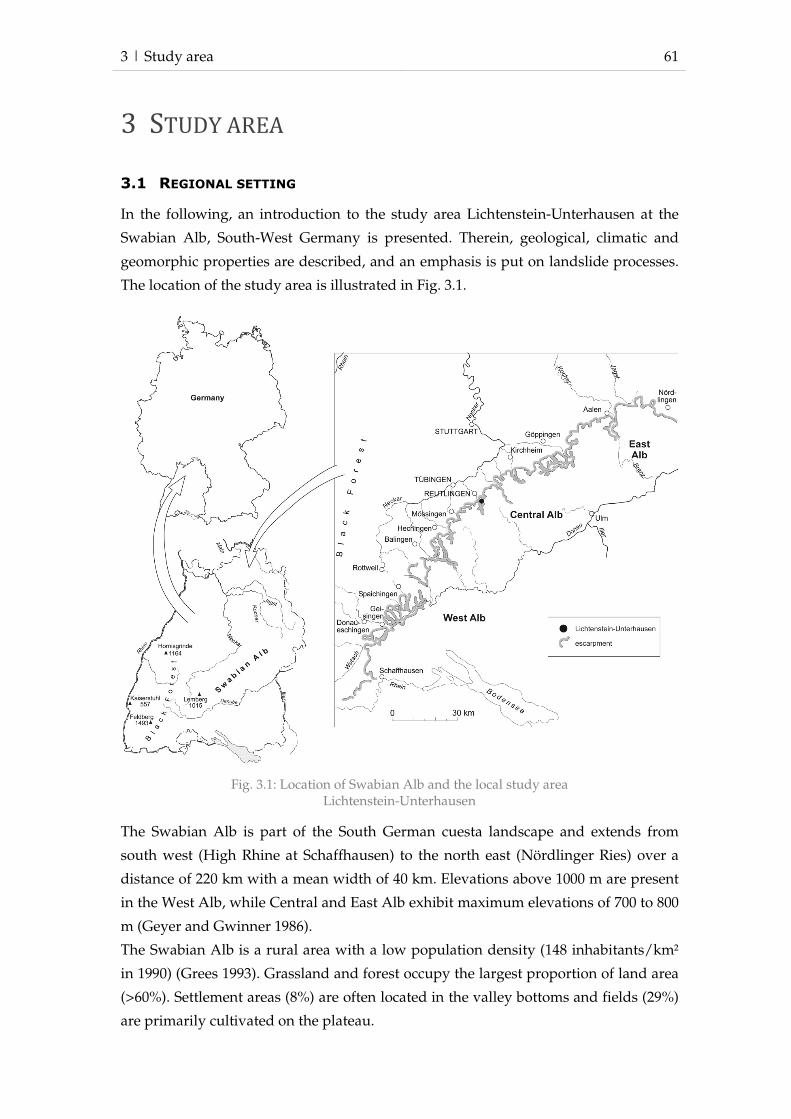
3 | Study area 61
3 STUDY AREA
3.1 REGIONAL SETTING
In the following, an introduction to the study area Lichtenstein-Unterhausen at the
Swabian Alb, South-West Germany is presented. Therein, geological, climatic and
geomorphic properties are described, and an emphasis is put on landslide processes.
The location of the study area is illustrated in Fig. 3.1.
Fig. 3.1: Location of Swabian Alb and the local study area Lichtenstein-Unterhausen
The Swabian Alb is part of the South German cuesta landscape and extends from
south west (High Rhine at Schaffhausen) to the north east (Nördlinger Ries) over a
distance of 220 km with a mean width of 40 km. Elevations above 1000 m are present
in the West Alb, while Central and East Alb exhibit maximum elevations of 700 to 800
m (Geyer and Gwinner 1986).
The Swabian Alb is a rural area with a low population density (148 inhabitants/km²
in 1990) (Grees 1993). Grassland and forest occupy the largest proportion of land area
(>60%). Settlement areas (8%) are often located in the valley bottoms and fields (29%)
are primarily cultivated on the plateau.

62 3 | Study area
3.1.1 Geology
The present landscape of the Swabian Alb is strongly influenced by Jurassic sedi-
ments, but also tertiary and quaternary processes influenced landscape development.
Leser (1982) emphasises the relationships of current and past climatic factors for land-
scape evolution, such as rainfall and temperature, and weathering, pedogenesis and
erosion processes, including landslides.
Lower Jurassic deposits are found in the foreland of the Swabian Alb, while Middle
Jurassic sediments are located more towards the cuesta ridge (Albtrauf) and the pla-
teau. The latter mainly consists of Upper Jurassic sediments (Geyer and Gwinner
1997). In addition, some 350 tuff diatremes of tertiary age illustrate volcanic activity in
the area around Urach (Rothe 2005). Other features include tertiary weathering prod-
ucts and quaternary deposits from limestone solution, as well as slope debris and de-
posits from landslides and fluvial processes. Tertiary deposits in the southern Alb
area are primarily molasse (Walter 1995). Fig. 3.2 illustrates the Geology of the
Swabian Alb. More detailed information on Jurassic strata is presented in Tab. 3.1.
Therein, strata are described by their German names instead of the English transla-
tion, to prevent confusion. Petrographic descriptions however, were translated to im-
prove understanding of strata properties.
In the Lower Jurassic strata, clays and marls are dominating, which also can be bitu-
minous, and are interstratified with lime and sandy materials. Middle Jurassic sedi-
ments are predominantly clays with fine sands and ferriferous lime sandstones hori-
zons, while Upper Jurassic strata comprise bedded layers of limestone and marls
(Geyer and Gwinner 1997). Strata are generally dipped towards south-east by 2.5-3°;
however, inclination may vary due to local folding features (Roth 2004). Fig. 3.3 illus-
trates the geological properties of South Germany's cuesta landscape as a cross sec-
tion, including the foreland, escarpment and plateau of the Swabian Alb.
Several tectonic fault lines are located in the Swabian Alb (Fig. 3.2), occasionally caus-
ing earthquakes. The strongest seismic events of the recent past include earthquakes
in 1911, 1943 and 1978 in the area of Albstadt which also triggered landslides (Rothe
2005). A recent study by Meyenfeld (2009) analysed the effects of earthquakes on
landslide triggering at the Swabian Alb and emphasized the importance of seismic
shaking for landslide initiation. The potential earthquake threat is accounted for in
spatial planning and adaptation of building codes according to earthquake zones
(Wirtschaftsministerium Baden-Württemberg 2001).

3 | Study area 63
Fig. 3.2: Geological features and fault lines in the Swabian Alb (based on Bell 2007)
Fig. 3.3: Schematic profile across the South German cuesta landscape with indication of landslide susceptible areas and karst features
(based on Wagenplast 2004)
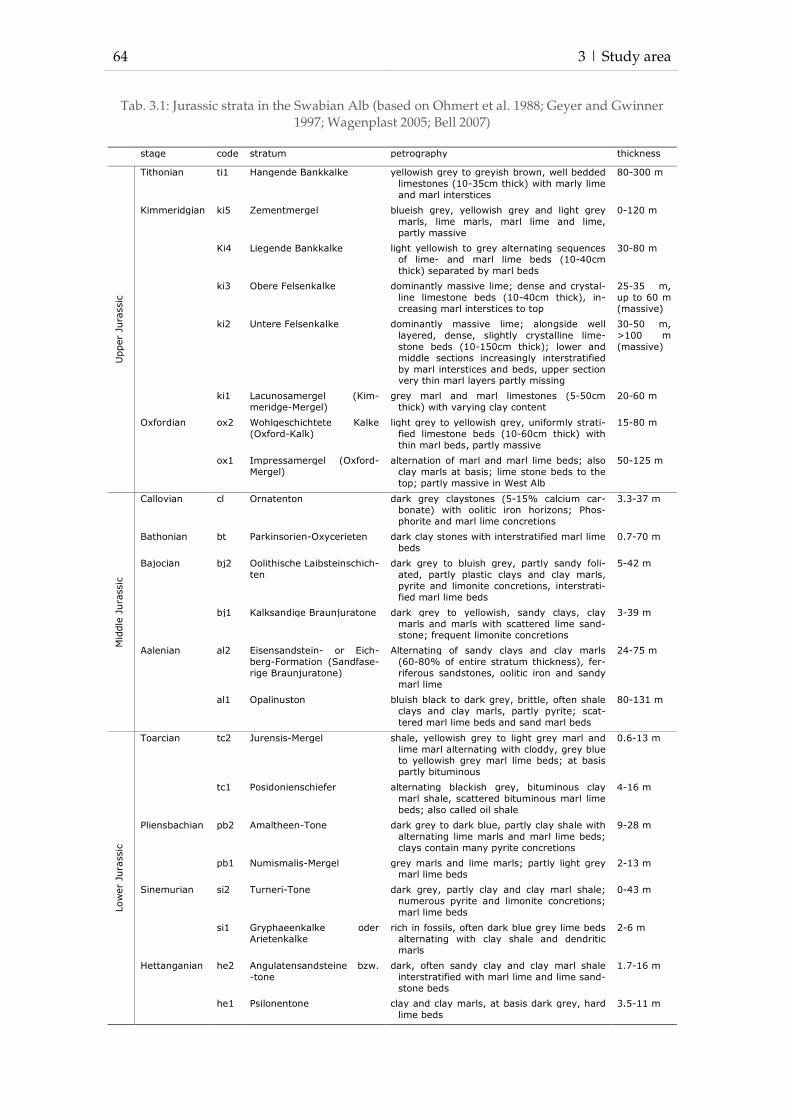
64 3 | Study area
Tab. 3.1: Jurassic strata in the Swabian Alb (based on Ohmert et al. 1988; Geyer and Gwinner 1997; Wagenplast 2005; Bell 2007)
stage code stratum petrography thickness
Upper
Jura
ssic
Tithonian ti1 Hangende Bankkalke yellowish grey to greyish brown, well bedded
limestones (10-35cm thick) with marly lime
and marl interstices
80-300 m
Kimmeridgian ki5 Zementmergel blueish grey, yellowish grey and light grey
marls, lime marls, marl lime and lime,
partly massive
0-120 m
Ki4 Liegende Bankkalke light yellowish to grey alternating sequences of lime- and marl lime beds (10-40cm
thick) separated by marl beds
30-80 m
ki3 Obere Felsenkalke dominantly massive lime; dense and crystal-
line limestone beds (10-40cm thick), in-
creasing marl interstices to top
25-35 m,
up to 60 m
(massive)
ki2 Untere Felsenkalke dominantly massive lime; alongside well
layered, dense, slightly crystalline lime-
stone beds (10-150cm thick); lower and
middle sections increasingly interstratified
by marl interstices and beds, upper section very thin marl layers partly missing
30-50 m,
>100 m
(massive)
ki1 Lacunosamergel (Kim-
meridge-Mergel)
grey marl and marl limestones (5-50cm
thick) with varying clay content
20-60 m
Oxfordian ox2 Wohlgeschichtete Kalke
(Oxford-Kalk)
light grey to yellowish grey, uniformly strati-
fied limestone beds (10-60cm thick) with
thin marl beds, partly massive
15-80 m
ox1 Impressamergel (Oxford-
Mergel)
alternation of marl and marl lime beds; also
clay marls at basis; lime stone beds to the
top; partly massive in West Alb
50-125 m
Mid
dle
Jura
ssic
Callovian cl Ornatenton dark grey claystones (5-15% calcium car-bonate) with oolitic iron horizons; Phos-
phorite and marl lime concretions
3.3-37 m
Bathonian bt Parkinsorien-Oxycerieten dark clay stones with interstratified marl lime
beds
0.7-70 m
Bajocian bj2 Oolithische Laibsteinschich-
ten
dark grey to bluish grey, partly sandy foli-
ated, partly plastic clays and clay marls,
pyrite and limonite concretions, interstrati-
fied marl lime beds
5-42 m
bj1 Kalksandige Braunjuratone dark grey to yellowish, sandy clays, clay
marls and marls with scattered lime sand-stone; frequent limonite concretions
3-39 m
Aalenian al2 Eisensandstein- or Eich-
berg-Formation (Sandfase-
rige Braunjuratone)
Alternating of sandy clays and clay marls
(60-80% of entire stratum thickness), fer-
riferous sandstones, oolitic iron and sandy
marl lime
24-75 m
al1 Opalinuston bluish black to dark grey, brittle, often shale
clays and clay marls, partly pyrite; scat-
tered marl lime beds and sand marl beds
80-131 m
Low
er
Jura
ssic
Toarcian tc2 Jurensis-Mergel shale, yellowish grey to light grey marl and
lime marl alternating with cloddy, grey blue to yellowish grey marl lime beds; at basis
partly bituminous
0.6-13 m
tc1 Posidonienschiefer alternating blackish grey, bituminous clay
marl shale, scattered bituminous marl lime
beds; also called oil shale
4-16 m
Pliensbachian pb2 Amaltheen-Tone dark grey to dark blue, partly clay shale with
alternating lime marls and marl lime beds;
clays contain many pyrite concretions
9-28 m
pb1 Numismalis-Mergel grey marls and lime marls; partly light grey marl lime beds
2-13 m
Sinemurian si2 Turneri-Tone dark grey, partly clay and clay marl shale;
numerous pyrite and limonite concretions;
marl lime beds
0-43 m
si1 Gryphaeenkalke oder
Arietenkalke
rich in fossils, often dark blue grey lime beds
alternating with clay shale and dendritic
marls
2-6 m
Hettanganian he2 Angulatensandsteine bzw.
-tone
dark, often sandy clay and clay marl shale
interstratified with marl lime and lime sand-
stone beds
1.7-16 m
he1 Psilonentone clay and clay marls, at basis dark grey, hard
lime beds
3.5-11 m

3 | Study area 65
3.1.2 Climate
The climate at the Swabian Alb is typical for Central European regions in the transi-
tion zone between oceanic and continental climate conditions (Leser 1982). Local relief
and the orientation of the Albtrauf escarpment, however, have strong effects on meso-
scale climate. Fig. 3.4 illustrates mean annual precipitation for the Swabian Alb for
two reference periods and the changes between them. Orographic effects on distribu-
tion of rainfall amounts can be observed by, for example, drier conditions one the lee
side of the Black Forest, and higher rainfall along the escarpment and on the plateau.
The variability of local climatic conditions can be illustrated by the comparison of two
weather stations, Sonnenbühl-Genkingen and Nehren, of which the former is located
on the plateau close to the escarpment, and the latter in the foreland (Fig. 3.5). The
distance between the stations is roughly 10 km. Precipitation trends are fairly similar;
however, Sonnenbühl-Genkingen receives significantly more rainfall. In addition,
annual rainfall maxima strongly vary for Sonnenbühl-Genkingen between a maxi-
mum of approximately 650 mm and more than 1450 mm with extremely wet years in
1941, 1965 and 2002. An overall trend of increased annual precipitation can be ob-
served.
Distribution of monthly precipitation is illustrated in Fig. 3.6 and demonstrates a high
variability. Most precipitation generally occurs in spring and early summer. How-
ever, comparison of two reference periods indicates a shift from two rainfall maxima
in June and August to one maximum in July.
Mean temperatures in the Swabian Alb vary between 6° and 9°C, with lower tempera-
tures associated with higher elevations on the plateau. Precipitation in winter often
occurs as snow, especially in higher elevation areas. Therefore, runoff is often delayed
until spring snow melt.
3.1.3 Hydrology
The Swabian Alb is located at the divide between the watersheds draining into the
rivers Rhine and Danube. Limestones of the Upper Jurassic, however, are strongly
affected by karst processes, thus phreatic watersheds vary from surficial ones. Ter-
horst (1997) distinguishes between shallow and deep karst. Shallow karst is found in
the vicinity of the Albtrauf escarpment and exhibits karst drainage above the eleva-
tion of the receiving river causing springs, whereas deep karst drainage occurs below.
Only few rivers can be found on the Swabian Alb plateau due to underground karst
drainage (Geyer and Gwinner 1997), thus, dry valleys are a common feature on the
plateau. Drainage density in the foreland of the Swabian Alb is higher due to less
permeable geological strata.

66 3 | Study area
Fig. 3.4: Mean annual precipitation in the Swabian Alb region for pe-riod A (1941-1970) and period B (1971-2000) (based on Bell 2007)
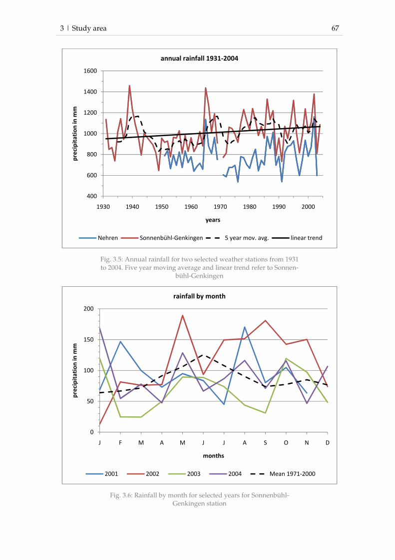
3 | Study area 67
Fig. 3.5: Annual rainfall for two selected weather stations from 1931 to 2004. Five year moving average and linear trend refer to Sonnen-
bühl-Genkingen
Fig. 3.6: Rainfall by month for selected years for Sonnenbühl-Genkingen station
400
600
800
1000
1200
1400
1600
1930 1940 1950 1960 1970 1980 1990 2000
pre
cip
ita
tio
n in
mm
years
annual rainfall 1931-2004
Nehren Sonnenbühl-Genkingen 5 year mov. avg. linear trend
0
50
100
150
200
J F M A M J J A S O N D
pre
cip
ita
tio
n in
mm
months
rainfall by month
2001 2002 2003 2004 Mean 1971-2000

68 3 | Study area
3.1.4 Geomorphology
The landscape of the Swabian Alb was essentially formed under climatic conditions
differing from the present (Blume 1971; Dongus 1977; Leser 1982; Brunotte et al. 2007).
18 million years ago, at the time of volcanic activity in the Urach-Kirchheim area. The
escarpment of the Swabian Alb was about 20 km further north than it is today (Geyer
and Gwinner 1986; Geyer and Gwinner 1997) which relates to an overall relocation of
1 m/1000 years (Kallinich 1999). Pleistocene relocation has been assessed to be 2-3
km/1000 years (Dongus 1977), although the involved processes are not entirely clari-
fied (Terhorst 1997). Detailed discussion of the relocation of the Albtrauf escarpment
is provided by Kallinich (1999). Blume (1971) regards solifluction and fluvial erosion
as the dominant processes, and rates landslide processes only of local importance for
relocation of the Albtrauf escarpment. In contrast, Dongus (1977) emphasizes land-
slides as one important erosion factor. For Holocene times, most authors assume low
geomorphological activity (Büdel 1944; Bleich 1960; Weippert 1960) apart from fluvial
erosion and sedimentation, soil erosion, karst processes and local landslides. A geo-
morphological map (1:100,000) for the Swabian Alb was established by Dongus
(1977), and a 1:25,000 map is available for the map sheet of Mössingen (Leser 1982).
3.1.5 Landslides
Several studies have focussed on landslide processes within the Swabian Alb. Early
extensive research include the works of Hölder (1953), Bleich (1960) and Reiff (1968).
Within the MABIS project carried out by the University Tübingen, a wide range of
methodological approaches were applied (e.g., Bibus 1985; Bibus 1986; Kraut 1995;
Wiegand 1996; Terhorst 1997; Kallinich 1999; Knipping 1999; Riedinger and Terhorst
1999; Kreja 2000; Thein 2000; Kreja and Terhorst 2005; Neuhäuser and Terhorst 2007).
Within the InterRISK project the focus was put onto local and regional landslide haz-
ard and risk analysis, with methodological approaches including analysis of historic
sources, geomorphological mapping, geophysical measurements and landslide mod-
elling (Armbruster 2002; Bell et al. 2006; Brennecke 2006; Kohn 2006; Kruse 2006;
Thiebes 2006; Holland 2007). A general relationship between lithology and landslide
activity was presented by Terhorst (1997) illustrated in Tab. 3.2.
Landslide inventories for subareas of the Swabian Alb were established e.g., by Kraut
(1995, 1999), Brennecke (2006) and Kohn (2006). Large scale geomorphological maps
(1:5,000 to 1:10,000) including landslide processes were established by Kößler (1997),
Terhorst (1997), Kallinich (1999), Kreja (2000) and Bell (2002). A more general map
(1:50,000) was developed by Kallinich (1999) for several study areas along the
Albtrauf escarpment.

3 | Study area 69
Tab. 3.2: Lithology and typical landslide processes at the Swabian Alb (based on Terhorst 1997)
lithology code landslide type
Mittel-Kimmeridge-Kalk ki2,3,4 rotational slides, rock and debris falls, rock top-ples, translational debris slides
Unter-Kimmeridge Mergel ki1 flows
Oxford-Kalke ox2 combined rotational slides, debris falls, transla-tional debris slides
Oxford-Mergel ox1 flows
Braunjuratone, especially Ornaten- and Opalinustone
cl, bt, bj2, al1
flows, translational slides
Braunjurakalke and –sandsteine bj1, al2 rotational slides, flows
A dendro-geomorphological investigation was carried out by Holland (2007) in which
phases of landslide activity were analysed for the Urselberg landslides in Pfullingen.
Several geophysical methods have been applied in local study areas, e.g. seismic
(Hecht 2001), geoelectric (Bell et al. 2006; Kruse 2006; Sass et al. 2008), radio-
magnetotellurics (Kruse 2006) and georadar (Sass et al. 2008). Kruse and Bell worked
on the same landslide, which is also investigated in this work.
Statistical models for delineation of landslide prone areas were established for several
areas of the Swabian Alb (Wiegand 1996; Thein 1999, Thein 2000; Armbruster 2002;
Neuhäuser et al. 2005; Neuhäuser and Terhorst 2007). Fig. 3.7 illustrates landslide
susceptibility for the Swabian Alb developed by Bell (2002), which later has been inte-
grated into regional planning.
Fig. 3.7: Landslide susceptibility in the Swabian Alb (after Bell 2007). Magnified areas show Irrenberg (A) and Fils valley (B)
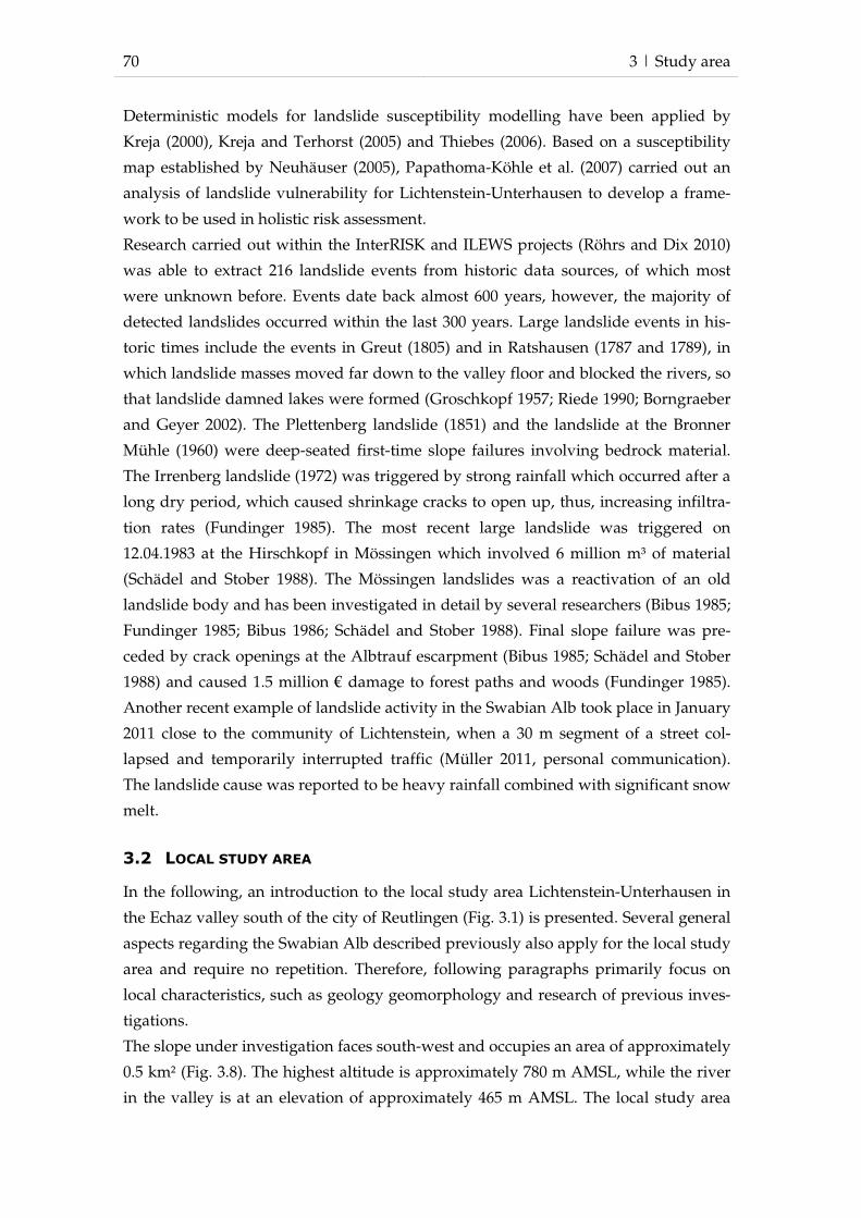
70 3 | Study area
Deterministic models for landslide susceptibility modelling have been applied by
Kreja (2000), Kreja and Terhorst (2005) and Thiebes (2006). Based on a susceptibility
map established by Neuhäuser (2005), Papathoma-Köhle et al. (2007) carried out an
analysis of landslide vulnerability for Lichtenstein-Unterhausen to develop a frame-
work to be used in holistic risk assessment.
Research carried out within the InterRISK and ILEWS projects (Röhrs and Dix 2010)
was able to extract 216 landslide events from historic data sources, of which most
were unknown before. Events date back almost 600 years, however, the majority of
detected landslides occurred within the last 300 years. Large landslide events in his-
toric times include the events in Greut (1805) and in Ratshausen (1787 and 1789), in
which landslide masses moved far down to the valley floor and blocked the rivers, so
that landslide damned lakes were formed (Groschkopf 1957; Riede 1990; Borngraeber
and Geyer 2002). The Plettenberg landslide (1851) and the landslide at the Bronner
Mühle (1960) were deep-seated first-time slope failures involving bedrock material.
The Irrenberg landslide (1972) was triggered by strong rainfall which occurred after a
long dry period, which caused shrinkage cracks to open up, thus, increasing infiltra-
tion rates (Fundinger 1985). The most recent large landslide was triggered on
12.04.1983 at the Hirschkopf in Mössingen which involved 6 million m³ of material
(Schädel and Stober 1988). The Mössingen landslides was a reactivation of an old
landslide body and has been investigated in detail by several researchers (Bibus 1985;
Fundinger 1985; Bibus 1986; Schädel and Stober 1988). Final slope failure was pre-
ceded by crack openings at the Albtrauf escarpment (Bibus 1985; Schädel and Stober
1988) and caused 1.5 million € damage to forest paths and woods (Fundinger 1985).
Another recent example of landslide activity in the Swabian Alb took place in January
2011 close to the community of Lichtenstein, when a 30 m segment of a street col-
lapsed and temporarily interrupted traffic (Müller 2011, personal communication).
The landslide cause was reported to be heavy rainfall combined with significant snow
melt.
3.2 LOCAL STUDY AREA
In the following, an introduction to the local study area Lichtenstein-Unterhausen in
the Echaz valley south of the city of Reutlingen (Fig. 3.1) is presented. Several general
aspects regarding the Swabian Alb described previously also apply for the local study
area and require no repetition. Therefore, following paragraphs primarily focus on
local characteristics, such as geology geomorphology and research of previous inves-
tigations.
The slope under investigation faces south-west and occupies an area of approximately
0.5 km² (Fig. 3.8). The highest altitude is approximately 780 m AMSL, while the river
in the valley is at an elevation of approximately 465 m AMSL. The local study area
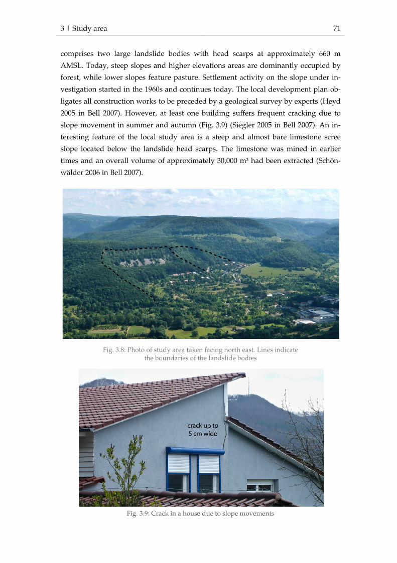
3 | Study area 71
comprises two large landslide bodies with head scarps at approximately 660 m
AMSL. Today, steep slopes and higher elevations areas are dominantly occupied by
forest, while lower slopes feature pasture. Settlement activity on the slope under in-
vestigation started in the 1960s and continues today. The local development plan ob-
ligates all construction works to be preceded by a geological survey by experts (Heyd
2005 in Bell 2007). However, at least one building suffers frequent cracking due to
slope movement in summer and autumn (Fig. 3.9) (Siegler 2005 in Bell 2007). An in-
teresting feature of the local study area is a steep and almost bare limestone scree
slope located below the landslide head scarps. The limestone was mined in earlier
times and an overall volume of approximately 30,000 m³ had been extracted (Schön-
wälder 2006 in Bell 2007).
Fig. 3.8: Photo of study area taken facing north east. Lines indicate the boundaries of the landslide bodies
Fig. 3.9: Crack in a house due to slope movements
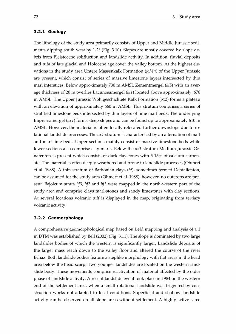
72 3 | Study area
3.2.1 Geology
The lithology of the study area primarily consists of Upper and Middle Jurassic sedi-
ments dipping south west by 1-2° (Fig. 3.10). Slopes are mostly covered by slope de-
bris from Pleistocene solifluction and landslide activity. In addition, fluvial deposits
and tufa of late glacial and Holocene age cover the valley bottom. At the highest ele-
vations in the study area Untere Massenkalk Formation (joMu) of the Upper Jurassic
are present, which consist of series of massive limestone layers intersected by thin
marl interstices. Below approximately 730 m AMSL Zementmergel (ki5) with an aver-
age thickness of 20 m overlies Lacunosamergel (ki1) located above approximately. 670
m AMSL. The Upper Jurassic Wohlgeschichtete Kalk Formation (ox2) forms a plateau
with an elevation of approximately 660 m AMSL. This stratum comprises a series of
stratified limestone beds intersected by thin layers of lime marl beds. The underlying
Impressamergel (ox1) forms steep slopes and can be found up to approximately 610 m
AMSL. However, the material is often locally relocated further downslope due to ro-
tational landslide processes. The ox1-stratum is characterised by an alternation of marl
and marl lime beds. Upper sections mainly consist of massive limestone beds while
lower sections also comprise clay marls. Below the ox1 stratum Medium Jurassic Or-
natenton is present which consists of dark claystones with 5-15% of calcium carbon-
ate. The material is often deeply weathered and prone to landslide processes (Ohmert
et al. 1988). A thin stratum of Bathonian clays (bt), sometimes termed Dentalienton,
can be assumed for the study area (Ohmert et al. 1988), however, no outcrops are pre-
sent. Bajoicum strata bj3, bj2 and bj1 were mapped in the north-western part of the
study area and comprise clays marl-stones and sandy limestones with clay sections.
At several locations volcanic tuff is displayed in the map, originating from tertiary
volcanic activity.
3.2.2 Geomorphology
A comprehensive geomorphological map based on field mapping and analysis of a 1
m DTM was established by Bell (2002) (Fig. 3.11). The slope is dominated by two large
landslides bodies of which the western is significantly larger. Landslide deposits of
the larger mass reach down to the valley floor and altered the course of the river
Echaz. Both landslide bodies feature a steplike morphology with flat areas in the head
area below the head scarp. Two younger landslides are located on the western land-
slide body. These movements comprise reactivation of material affected by the older
phase of landslide activity. A recent landslide event took place in 1984 on the western
end of the settlement area, when a small rotational landslide was triggered by con-
struction works not adapted to local conditions. Superficial and shallow landslide
activity can be observed on all slope areas without settlement. A highly active scree

3 | Study area 73
slope formed of loose limestone is located above the head of the oldest landslide de-
posit. Limestone rocks originating from the ox2 limestone stratum in the landslide
head scarp areas spread at the foot of the scree slope indicate high rockfall activity.
Fig. 3.10: Geological map (1:50,000) and landslide boundaries for the local study area Lichtenstein-Unterhausen (based on Bell 2007)

74 3 | Study area
Fig. 3.11: Geomorphological map for the local study area Lichten-stein-Unterhausen (based on Bell 2007)

3 | Study area 75
3.2.3 Previous investigations
The local study area investigated in this thesis has already been studied by the pre-
ceding research project InterRISK. Therein, an initial landslide monitoring system was
installed comprising inclinometers, geodetic levelling and temporary tiltmeter meas-
urements (Armbruster 2002). In addition, Kruse (2006) performed a series of geoelec-
trical measurements to investigate hydrological processes within the landslide bodies.
Based on monitoring results, Bell (2002) concluded that at least parts of the landslide
are seasonally reactivating leading to extremely slow displacement rates. Two distinct
patterns of movement were distinguished: a deep-seated sliding process down to the
bedrock in approximately -15.5 m depth, occurring in spring; and a flow or creep
movement of the upper 8.5 m in summer and autumn. Comparison of landslide
movement with rainfall data showed no clear relationship. However, a correlation
between snow melting and deep-seated sliding could be established. More extensive
interpretations of landslide behaviour were limited by the lack of detailed climatic
data, the small extent and short period of the slope monitoring, and extremely slow
movement rates close to the instruments' noise levels.
Four monthly geoelectrical surveys were performed by Kruse (2006). One of the main
results of the investigation was that the limestone scree allows for quick infiltration of
rainfall and melting snow, possibly an important factor for initiation of landslide
movement. It was, however, neither possible to establish a relationship between
geoelectrical monitoring data and landslide displacement, nor to fully describe sub-
surface hydrological processes.
A recently carried out study of potential damage related to a full reactivation of the
landslide bodies in Lichtenstein-Unterhausen (Greiving 2010) resulted in a maximum
loss of private property equal to 18.5 million EUR in addition to 1.7 million EUR dam-
age communal infrastructure.


4 | Data 77
4 DATA
Various data sources were used within this study. A compilation of all data and their
characteristics and sources is illustrated in Tab. 4.1. Additional information is pre-
sented in the following.
The Digital Terrain Model (DTM) provides detailed information on topography and
was acquired between 2002 and 2004 by airborne laserscanning during periods with
low vegetation cover (December to April) (Landesvermessungsamt Baden-
Württemberg 2010). Vegetation and infrastructure, such as houses and bridges were
removed by post-processing to produce a hydrological correct DTM with a spatial
resolution of 1 x 1 m.
Geological maps for the local study area are available in 1:25,000 and 1:50,000 scales,
however, only the latter exists as a digital version. Additional information on geologi-
cal characteristics of the local study area, including detailed description of several
drillings, is available from Ohmert et al. (1988).
Several sources of information on landslides in the Swabian Alb were available for
this study.
Kallinich (1999) mapped plateau areas of large rotational landslides and recent,
mostly small landslides located nearby. Field mapping was carried out at 1:25,000
scale, the final was presented in 1:50,000 scale.
A landslide inventory and database was established by Tübingen University and is
essentially based on the work of Kraut (1995). Data was acquired by an analysis of
literature sources, and geological and forestry site maps. The latter distinguish be-
tween active landslide susceptibility, inactive landslide and potentially susceptible to
landslides, and were produced for all state-owned forests in Baden-Württemberg.
Landslide locations are illustrated as point information, and timing is acknowledged.
Within the InterRISK and ILEWS projects, investigations using historical archives
have been carried out to extract information related to landslide occurrences in the
Swabian Alb. Data sources included several national and communal archives and
forestry records. Additional information is provided by Röhrs and Dix (2010).
Another landslide inventory was provided by Bell (2010, personal communication),
and contains information on a multiple landslide event in the Fils Valley in April
1994.
Brennecke (2006) created a landslide inventory based on interpretation of aerial pho-
tographs and hillshade analysis. Four landslide process types were distinguished, i.e.
rotational and translational slides, flows and complex landslides.

78 4 | Data
Tab. 4.1: Overview of data used within this study Data type Info Format Resolution Source
Topography
DTM1 (Digital Terrain Model)
airborne laser scans acquired between 2002
and 2004, available for
the entire Swabian Alb
ESRI grid 1 m x 1 m Umweltministerium Baden-Württemberg (UM BW), Landesanstalt für Messung, Umwelt und
Naturschutz (LUBW), Landesvermessungsamt
Baden-Württemberg (LV BW)
Geology
GK25 (Geological map)
map sheet 7521 (Reut-lingen)
printed map 1:25,000 Landesamt für Geologie, Rohstoffe und Bergbau Baden-Württemberg (LGRB BW)
GK50 (Geological
map)
map sheet 7520 (Reut-
lingen)
ESRI shape
files (polygons)
1:50,000 LGRB BW
Landslides
General landslide map
for parts of Swabian Alb printed map 1:25,000, 1:50,000
Kallinich (1999)
Inventory University
of Tübingen
for parts of Swabian Alb EXCEL table
with point
coordinates
working group Bibus and Terhorst, Institute
of Geography, University of Tübingen; For-
stliche Versuchs- und Forschungsanstalt
Baden-Württemberg (FVA) Inventory InterR-
SIK/ILEWS
historical research in
archives and forestry
records
text and EXCEL
files
InterRISK project (Röhrs and Dix 2010)
Inventory Filstal April 1994
event inventory ESRI shape files (polygons)
Bell (2010, personal communication)
Inventory Upper
Filstal
interpretation of aerial
photos and DTM
ESRI shape
files (polygons)
Brennecke (2006)
Inventory Depart-ment of Transporta-
tion Stuttgart
archive analysis and DTM mapping
ESRI shape files (points
and polygons)
Kohn (2006)
Climate
Station data temperature, precipita-
tion
EXCEL and text
files
30 minutes to
daily
DWD, LUBW
Regionalised rainfall data
interpolated rainfall and temperature, modelled
evaporation and snow
water equivalent
ESRI grid 500 x 500 m LUBW
ILEWS weather station
precipitation, humidity, temperature, air pres-
sure, wind, radiation,
snow height
raw data hourly measure-ment
Camek et al. (2010) (ILEWS)
COSMO-DE (rainfall forecasts)
2 cumulative model runs per day with 13 predic-
tions each
GRIB files hourly measure-ment
DWD
KOSTRA-DWD (rain-
fall intensity prob-abilities)
available for Baden-
Württemberg
software
program
8.45 km x 8.45
km
LUBW
Geophysical data
Geoelectric 1 profile analysed data monthly meas-
urement
Kruse (2006) and Bell (2007)
Geoelectric 2 profiles analysed data single measure-
ment
Wiebe and Krummel (2010) (ILEWS)
Geoseismic 4 profiles analysed data single measure-ment
Bell et al. (2010b) (ILEWS)
Movement monitoring
Geodetic monitoring geodetic network and
geodetic height
analysed data measurements
every 3 months
Aslan et al. (2010a) (ILEWS)
Inclinometers 3 inclinometers raw data measurements every 3 months
InterRISK project, Bell (2007), Bell and Thiebes (2010) (ILEWS)
Inclinometer chain 5 inclinometer between 3
and 15 meter depth
raw data measurements
every 30 minutes
Bell and Thiebes (2010) (ILEWS)
Hydrological monitoring
Tensiometers and TDR sensors
27 sensors each at 9 locations
raw data hourly measure-ments
Camek and Becker (2010) (ILEWS)
Geoelectrical monitor-
ing
2 profiles raw and
analysed data
measurements
every 2 hours
geoFact (ILEWS)
Drill cores
InterRISK 3 drill cores drill cores and
laboratory results
Bell (2007)
ILEWS project 2 drill cores drill cores and
laboratory
results
University of Vienna (ILEWS)
Geotechnical data
Laboratory analyses soil particle distribution,
water content, CaCO3,
soil water retention
curves
EXCEL file Christa Herrmann, University of Vienna
Substrate database collection of values from
literature
ACCESS data
base
Meyenfeld (2010, personal communication)
SPAW model geotechnical parameter
values
software
program
Saxton and Rawles (2006)
4 | Data 79
Kohn (2006) compiled a landslide inventory based on archive data from the Depart-
ment of Transportation of the administrative district Stuttgart. Parts of the archived
landslide were later mapped on a DTM. However, only a small part of its study area
covers the Swabian Alb and could be employed within this study.
Climatic data available for this study derives from three sources: National Meteoro-
logical Service Deutscher Wetterdienst (DWD), Landesanstalt für Messung, Umwelt
und Naturschutz Baden-Württemberg (LUBW), and data from a local weather station
installed and operated by the ILEWS project. Additional information on rainfall fore-
casts (Cosmo-DWD) and rainfall intensities for scenarios of various annual probabili-
ties (KOSTRA) was also utilised within this study.
Data on precipitation and temperature for 14 DWD and 16 LUBW stations within the
Swabian Alb covers the period until 2006 and provides a temporal resolution of 30
minutes to one hour. For two stations located close to the local study area Lichten-
stein-Unterhausen data extends to 2011. Additional rainfall data from all DWD
weather stations was provided by DWD for the period from 2006 to 2009.
For the period 1983 to 2003 regionalised climate data were provided by LUBW. Data
on precipitation, temperature, and modelled evaporation and snow height as water
equivalent are available as 500 x 500 m grid data with a daily resolution. Interpolated
precipitation and temperature data are considered to be very reliable by LUBW. Mod-
elling results, however, exhibit larger uncertainties as local characteristics such as
wind drift are not represented. For a 10 day period however, data is assumed to be
reliable (Gudera in Bell 2007). Additional information on regionalised climate data is
available in Ministerium für Umwelt und Verkehr (UVM) and Landesanstalt für
Umweltschutz (LfU) (2004).
A weather station was installed in the local study area by the ILEWS project in Au-
gust 2008. Measured parameters include:
- precipitation (two tipping bucket rain gauges of which one is heated)
- relative humidity (capacitative humidity sensor by polymer)
- air temperature (resistance temperature)
- air pressure (capacitative absolute pressure sensor)
- wind direction (potentiometer) and wind velocity (Reed switch)
- global radiation (thermopile)
- reflected radiation (thermopile)
- snow height (ultrasound)
- volumetric soil water content (TDR sensors)
- soil suction in 30 and 50 cm depth (tensiometer)
- soil temperature (semiconductor sensor in TDR probe)

80 4 | Data
All parameters are measured at intervals of 60 minutes and subsequently transferred
to a data server and parsed into the ILEWS project server available by ODBC. How-
ever, no data from the weather station is available from mid-September to mid-
November 2009 due to damage caused by animals, and for two weeks in July 2010
due to power failure. Additional information on climatic monitoring is provided by
Camek and Becker (2010).
COSMO-DE is the most complex weather forecasting model employed by DWD for
short-term prediction of weather conditions (Deutscher Wetterdienst (DWD) 2010b,
Deutscher Wetterdienst (DWD) 2010a). COSMO-DE is the German contribution to the
Consortium for Small-scale Modeling (COSMO) founded in 1998. The goal of
COSMO-DE is modelling of meteorological processes and prediction of parameters
such as air pressure, temperature, wind, water vapour, clouds and precipitation with
the aim to provide timely warning for severe weather conditions. Further information
on COSMO can be found on the consortium's website (Consortium for Small Scale
Modeling 2007). Within COSMO-DE meteorological processes are simulated in eight
daily model runs, each with prediction time of 18 hours. COSMO-DE predictions
have a very high spatial resolution of 0.025 degrees (2.8 km x 2.8 km grid cells) and 50
vertical levels, and cover Germany and parts of the surrounding countries. Rainfall
forecast from COSMO-DE model were provided by the DWD for the period from
September 2006 to December 2009 as cumulative simulation runs. For every day, two
simulations, each with a simulated length of 12 hours, are available in GRIB format.
Information on the probability of rainfall events was available from the KOSTRA atlas
distributed by the DWD. KOSTRA (Koordinierte Starkniederschlags-
Regionalisierungs-Auswertungen) represents a collection of maps implemented as an
interactive computer program. KOSTRA provides rainfall intensities for events of a
certain annual probability and was primarily developed for the design of technical
water management systems, e.g., urban drainage infrastructure. KOSTRA is based on
complex statistical regionalisation of precipitation data between 1951 and 2000 of 4500
climate stations in Germany. Annual rainfall probabilities vary between 0.5 and 100
years; storm duration between 5 minutes and 72 hours. Information on storm charac-
teristics can be retrieved for single grid cells of 8.45 km x 8.45 km and exported as
scenarios with varying rain intensities over the course of the storm events. Additional
information on KOSTRA is available in Bartels et al. (2005) and Malitz (2005).
Kruse (2006) carried out monthly geoelectrical surveys on the test slope in Lichten-
stein-Unterhausen from January to March 2006, which were later continued by Bell
(2007). Investigations utilised an ABEM Terrameter SAS 300 apparatus, and results

4 | Data 81
are available as inverted plots. Further information is available in Bell et al. (2006),
Kruse (2006), and Bell (2002).
In the initial phase of the ILEWS project, geophysical prospection were carried out
featuring geoelectrical and geoseismic surveys (Bell et al. 2010b). Two geoelectrical
profiles were acquired with an AGI STING/SWIFT R1 IP apparatus with Wenner and
Schlumberger plot configuration. Within a 24 h period 2 profiles were measured, each
126 m long (3 m electrode spacing and 42 electrodes with 3 m spacing) with an aver-
age penetration depth of approximately 20 m. Seismic prospection was carried out in
cooperation with partners from the ILEWS project applying a Bison 9048DIFP appara-
tus with 49 geophones with 4 metres spacing to measure 4 profiles. All geophysical
prospection data was analysed and processed by Heinrich Krummel from the com-
pany geoFact and is available as data inversion plots.
A geodetic network in the local study area, consisting of 15 installed points, was
measured every three months between November 2007 and December 2009 by a
working group within the ILEWS project (Aslan et al. 2010a). Measurements were
taken by a Leica TCRP 1201+ (SN 238310). In addition, geodetic heights were assessed
with a Trimble DiNi 12 (SN 700118). A total number of seven measurements are
available as maps displaying deformation. Unfortunately, most epochs do not include
measurement of stable points outside of the potential landslide area. Therefore, data
only provides information on relative deformation within the geodetic network.
Additional information on slope movement existed from five inclinometers posi-
tioned in the local study area, of which three have been installed within the InterRISK
project, and two during the ILEWS project. Manual measurements of inclinometers
began in 2004 (Bell 2007) and were continued periodically with a mobile NMG probe
by Glötzl with an accuracy of 0.01 to 0.1 mm per step. This relates to an error margin
of 0.2 to 0.3 mm for 10 and 15 m depths, respectively. In addition, an automated incli-
nometer chain by Glötzl (NMGD VP/2/10) with five sensors in depths from 3 to 15 m
in one borehole has been in operation since May 2009. Linearity of the automated sys-
tem is ±0.2%, and hysteresis ±0.02% of the final value. The error margin is approxi-
mately 1.5 - 3 mm at the surface (Glötzl 2010, personal communication). Measure-
ments are taken every hour and are processed by GLA software by Glötz, and conse-
quently retrieved by ILEWS data server. However, for some periods no measure-
ments were possible due to damage by construction works and electrical power fail-
ure. Additional information is also provided by Bell and Thiebes (2010).
The local monitoring system installed and operated by the ILEWS project included
tensiometers, TDR probes and two geoelectrical profiles to asses slope hydrology.

82 4 | Data
Management and maintenance of the technical slope hydrology monitoring system
were carried out by ILEWS project partners (Camek et al. 2010).
Tensiometers and TDR probes were in most cases connected to computers in the field
by cable; however, for one location wireless radio transmission was applied. T8 ten-
siometers from UMS were applied within the ILEWS project, measuring soil suction if
installed above the local ground water table. In addition, tensiometers can also be
utilised as piezometers if they are located within the phreatic zone. Measurement of
volumetric water content was achieved by TDR sensors (TRIME PICO probes by
IMKO). Tensiometers and TDR probes provide detailed data on soil hydrology with
hourly measurements available from August 2008 to July 2010. However, for certain
periods no data is available due to power failures. Moreover, tensiometers require
frequent refills with water to ensure correct measurements of soil suction. Unfortu-
nately, ongoing maintenance of tensiometers could not always be ensured which
caused some sensors to run dry.
Geoelectrical monitoring in the local study area Lichtenstein-Unterhausen is main-
tained by the ILEWS project partner geoFact (Wiebe and Krummel 2010) and started
in June 2008 with a vertical slope profile followed by a horizontal profile in August
2009. A LGM 4-Punkt light 10W apparatus by Lippmann Geophysikalische Messin-
strumente was applied for geoelectrical monitoring and took measurements every
two hours. Altogether, 48 electrodes were installed on the vertical profile, and 36 on
the horizontal profile. Measurement data is stored on the in-field computer and con-
sequently retrieved by the ILEWS data server. Data is available on the web-based
ILEWS data platform allowing for simple data analyses, such as visualisation of single
data points and resistivity pseudo-sections. More advanced data analyses including
time-lapse inversion of data were performed manually by geoFact.
From the InterRISK project, three bore logs originating from inclinometer installations
were available, including laboratory results reflecting water, CaCo3 content and soil
particle size distributions. Two additional bore logs were acquired during the ILEWS
project and subsequently analysed in the laboratory by Christa Herrmann, Institute
for Geography and Regional Research, University of Vienna. Soil particle size distri-
bution was carried out according to Austrian Norm (ÖNORM) by Köhn pipette
analysis. In addition, contents of water and CaCO3 were assessed. For a small number
of samples water retention curves were elaborated.
A collection of geotechnical parameter values (cohesion, angle of internal friction,
density etc.) based on experimental analysis in the literature was provided by
Meyenfeld (2010, personal communication). The database contains 1288 entries for a

4 | Data 83
large variety of rock and soil materials, often including minimum and maximum val-
ues.
Another source of information for geotechnical and hydrological parameterisation
was the soil database integrated into the SPAW (Soil-Plant-Air-Water) model that was
developed by (Saxton and Rawls 2006). The database was developed as a computer
program, in which soil hydrological parameters can be selected based on soil particle
size distributions as input parameters.


5 | Methodology 85
5 METHODOLOGY
A wide range of methods was applied within this study to investigate and model a
landslide in Lichtenstein-Unterhausen, and to develop and implement local and re-
gional scale technical landslide early warning systems as part of an integrated early
warning chain. In the following, the methodological approaches of this study are pre-
sented.
5.1 LOCAL SCALE
The methodological approach of this work includes planning and installation of a
monitoring system to assess slope movement and hydrological processes, data analy-
sis to investigate processes leading to landslide reactivation, simulation of slope be-
haviour by a coupled hydrology and slope stability model, and the design and im-
plementation of the model as a technical early warning and decision-support system.
5.1.1 Field work
Planning of a monitoring system for slope movement and hydrology was carried out
cooperatively with the other ILEWS project members during a field inspection. The
goal of an extended monitoring system was to gain more information on slope
movement and hydrological processes especially in the area where slope movement
had been causing cracking to a house, but also for the entire landslide mass. Addi-
tional criteria to be considered in the design of the monitoring systems were geomor-
phological features and the results of geophysical prospection of previous studies
(Armbruster 2002; Kruse 2006) and additional surveys carried out within the ILEWS
project (Bell et al. 2010b), as well as technical issues, such as accessibility of the loca-
tions with drilling equipment.
Most drillings were carried out with a percussion drilling machine (GTR 780V by
Geotool) mounted on a rubber chain crawler. The drilling rig uses a drop weight of
63.5 kg and a drop height of 75 cm. For locations impossible to access by the large
drilling machine, a pneumatic percussion cone penetrometer from Stitz GmbH with a
drop weight of 50 kg and a drop height of 50 cm was employed.
To increase the speed of drilling windowed 80 mm sampling tubes were utilised for
installation of hydrological sensors. However, no undisturbed samples could be ex-
tracted with these sampling tubes. Drillings for inclinometer installations were carried
out with closed 100 mm sampling tubes with plastic tubes that allowed extraction of
subsurface materials in a relatively undisturbed condition and the subsequent use for
later core interpretation and laboratory analyses.
86 5 | Methodology
In addition to the already existing tree inclinometers, two more inclinometers and one
inclinometer chain were installed. Since improved drilling equipment was available to
the ILEWS project in comparison to the preceding InterRISK project, additional incli-
nometers were placed close to the already existing ones and to an increased depth.
After borehole drilling, 55 mm inclinometer pipes were inserted into the boreholes
and fixed with a mixture of concrete and bentonite.
Periodic measurements of all inclinometers were carried out approximately every
three months with a mobile NMG probe by Glötzl. Each inclinometer was measured
in 50 cm steps in A and B directions to assess downslope and sideways displace-
ments. All inclinometer measurements were carried out twice to minimise errors.
An inclinometer chain was installed in the already existing borehole Lic02 with a
depth of approximately 15.50 m with the aim to increase the temporal resolution of
slope movement measurements. The inclinometer chain consisted of five inclinometer
probes located every 3 metres between 3 and 15 m depth. The inclinometer chain was
connected to the controlling computer located in field by cable, allowing remote con-
trol by a VPN tunnel.
Even though hydrological monitoring within the ILEWS project was managed by pro-
ject partners, drilling and installation of all tensiometers and TDR sensors were car-
ried out by the author with the help of field workers. Cooperatively, nine locations
were determined for installation of hydrological sensors. At each location boreholes
were brought down to depths of approximately 2, 5 and 10 meters for installation of
tensiometers and TDR probes. In each borehole one TDR probe and one tensiometer
located above were installed. After drilling to a desired depth, a 30 cm thick fill of
sieved soil material from the same depth was inserted to provide sufficient space for
the forks of the TDR probe. On top of this, 30 cm of sieved material was filled in be-
fore a tensiometer was installed into the borehole.
A low-cost infrared borehole camera provided by the ILEWS project partner IMKO
was used in the field to check subsurface conditions and to control correct sensor in-
stallation.
5.1.2 Data analysis
Core samples and data from laboratory investigations were analysed to improve un-
derstanding of subsurface conditions, which form an important element of slope sta-
bility modelling and subsequent landslide early warning. The variety of data on slope
movement and hydrological processes were analysed to investigate the processes
leading to landslide reactivation.
5 | Methodology 87
5.1.2.1 Core samples
Two core samples from inclinometer installations were available for further analyses.
Initially, cores were visually interpreted to differentiate layers based on material
characteristics, colour and water content. Samples of each layer were taken for labora-
tory analyses of soil water content, CaCO3 content and grain size distribution analysis
carried out by a laboratory technician. In addition, four samples were prepared for
elaboration of soil water retention curves. Soil skeleton was assessed by visual judg-
ment.
5.1.2.2 Slope movement data
Data from manual inclinometer measurements was compiled and plotted with soft-
ware by Glötzl (GLNP v4) to visualise displacements between single monitoring
campaigns.
Data from inclinometer chain was analysed on the ILEWS project online platform
where displacements between selectable points in time can be visualised. A more de-
tailed analysis of inclinometer chain data was carried out plotting the displacements
of each probe over time.
Data from geodetic measurements carried out by an ILEWS project partner were
available as maps displaying displacements and change of geodetic height between
single measurements, and were compared to inclinometer data. In addition, geodetic
information were utilised as a basis for interpretation of slope movements for a larger
area of the local study area.
5.1.2.3 Hydrological data
Data from local weather station and slope hydrology monitoring system was ex-
ported from the ILEWS database and plotted for further analysis of hydrological con-
ditions. Data were carefully checked for plausibility and possible errors or biases. In-
vestigation concentrated on the assessment of seasonal changes of groundwater con-
ditions for subsequent modelling of slope stability. A more detailed analysis of the
effects of rainfall and snow melting on soil water content and soil suction was carried
out for single events. For this, geoelectrical data in the form of time lapse inversions
from the ILEWS project partner geoFact and inclinometer chain data were also inte-
grated.
5.1.3 Landslide early warning modelling
Two approaches for the integration of the physical-based landslide simulation model
CHASM into a prototypic early warning system were developed in this work. The
first application was designed to continuously simulate slope stability for a pre-
defined slope profile integrating antecedent rainfall conditions, groundwater table

88 5 | Methodology
data based on monitoring results, and rainfall forecasts. A second application was
developed to aid decision-support and to allow quick assessment of slope stability for
freely selectable slope profiles using various rainfall and groundwater scenarios. As
noted before, technical solutions were implemented by the ILEWS project partners
(Jäger et al. 2010). However, design of the technical early warning system, and con-
figuration of CHASM, were part of the work achieved by the author of this study.
In this study, the physically-based landslide simulation model CHASM (Combined
Hydrology and Stability Model) was used to simulate the behaviour of the landslide
under investigation. This model was chosen because it combines slope hydrological
process simulation with slope stability calculation. Moreover, developers of CHASM
agreed on cooperation and a joint development. A brief description has already been
presented in chapter 2.3.2. More detailed information on CHASM is provided in the
following. Additional information, including derivation of equations applied in
CHASM is available elsewhere (Anderson and Richards 1987; Anderson et al. 1996;
Anderson and Thallapally 1996; Collison and Anderson 1996; Wilkinson et al. 2000;
Wilkinson et al. 2002a).
Within CHASM pore water pressures in response to individual rainfall events and the
effects on slope stability can be simulated. The model comprises two main elements:
hydrological and slope stability modelling. The first version of CHASM was devel-
oped in an UNIX environment using Fortran ’77, but has later been implemented
within a Microsoft Windows environment using C++ with the addition of a graphical
user-interface (GUI). The procedure for hydrological modelling adopted in CHASM is
a forward explicit finite difference scheme (Wilkinson et al. 2002a). The slope is di-
vided into a series of columns of which each is subdivided into regular cells. Deten-
tion storage, infiltration, evapotranspiration, and unsaturated and saturated flow re-
gimes are modelled within CHASM. Rainfall can infiltrate into the top cells and is
controlled by the infiltration capacity. Infiltration is calculated using Darcy’s Law
(Darcy 1856) with the conductivity being equal to the average of the saturated con-
ductivity and the hydraulic conductivity of the top two cells. Unsaturated vertical
flow within each column is computed using Richards equation (Richards 1931). Un-
saturated conductivity is defined by the Millington–Quirk (1959) procedure. Flow
between columns is simulated by Darcy’s equation for saturated flow, adopting the
Dupuit–Forcheimer (Forchheimer 1930) assumption. Numerical stability of the solu-
tion to the Richards equation depends on time step and iteration period and applies a
methodology proposed by Beven (1985) in which the required time step (iteration
period) is based on the distance between the computational nodes, the gradient of the
suction–moisture curve at a given suction value and the flow velocity. For most appli-
5 | Methodology 89
cations the commonly recommended spatial and temporal resolutions are an individ-
ual element size of 1 m × 1 m area, and 60s iteration period (Wilkinson et al. 2002a;
Wilkinson et al. 2002b). Slope curvature (convexity and concavity) can be integrated
by adjusting the column breadth to investigate the effects of three-dimensional topog-
raphy on pore pressure. Simulated hydrological conditions are then integrated into
standard two-dimensional stability analysis.
The stability assessment techniques used in CHASM are Bishop’s simplified circular
method (Bishop 1955) and Janbu’s non-circular method (Janbu 1954). These limit equi-
librium methods determine the shear strength along the failure surface, the mobilised
shear strength, and the ratio between these two (Factor of Safety); thus providing a
measure of the relative slope stability. On each hour of a CHASM simulation, pre-
dicted hydrological conditions are coupled to a limit equilibrium equation determin-
ing slope stability. Both negative and positive pore water pressures are incorporated
into the effective stress determination by the Mohr- Coulomb equation for soil shear
strength. A minimum FoS is computed of which temporal variations arise from hy-
drodynamic responses and changes in the position of the critical slip surface. Over-
view of the structure of the CHASM model (Fig. 5.1) and CHASM key input parame-
ters (Tab. 5.1) are presented below.
The main output of a CHASM run is the calculated minimum FoS for each hour of
simulation, along with the respective shear surface parameters. Additional output
files contain data on pore water pressure and soil moisture for each cell. For simula-
tion in which a FoS below 1.0 is calculated, an empirical relation (Finlay et al. 1999) of
slope height and slope angle is applied to simulate landslide run-out onto a horizontal
plain (CHASM 2008).
CHASM is continuously being developed and enhanced. One recent extension in-
cludes the integration of vegetation into hydrological simulations and computation of
slope stability (Collison and Anderson 1996). Effects of vegetation on hydrology and
slope stability, such as interception, evapotranspiration, root reinforcement and
changes to hydraulic conductivity and surcharge are incorporated into CHASM by
several routines. Test applications of the CHASM vegetation extension are provided
in for example Collison and Anderson (1996) and Wilkinson et al. (2002a).
Other features of CHASM include the integration of stabilising measures, such as geo-
textiles, geo-grids and earth nails. In addition, effects of seismicity on slope stability
can be assessed based on an empirical guideline (Charalambus 2003) to estimate the
horizontal seismic acceleration to induce instability.
Inherent in the structure and methodology of CHASM are limitations deriving from
the hydrology scheme and the method of stability analysis. Hydrological simulations
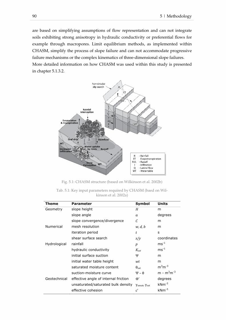
90 5 | Methodology
are based on simplifying assumptions of flow representation and can not integrate
soils exhibiting strong anisotropy in hydraulic conductivity or preferential flows for
example through macropores. Limit equilibrium methods, as implemented within
CHASM, simplify the process of slope failure and can not accommodate progressive
failure mechanisms or the complex kinematics of three-dimensional slope failures.
More detailed information on how CHASM was used within this study is presented
in chapter 5.1.3.2.
Fig. 5.1: CHASM structure (based on Wilkinson et al. 2002b)
Tab. 5.1: Key input parameters required by CHASM (baed on Wil-kinson et al. 2002a)
Theme Parameter Symbol Units
Geometry slope height H m
slope angle α degrees
slope convergence/divergence C m
Numerical mesh resolution w, d, b m
iteration period t s
shear surface search x/y coordinates
Hydrological rainfall p ms-1
hydraulic conductivity Ksat ms-1
initial surface suction Ψ m
initial water table height wt m
saturated moisture content θsat m3m-3
suction-moisture curve Ψ – θ m - m3m-3
Geotechnical effective angle of internal friction Φ’ degrees
unsaturated/saturated bulk density γunsat, γsat kNm-3
effective cohesion c’ kNm-3

5 | Methodology 91
5.1.3.1 Generation of input data
The methodological approach to create input data for CHASM modelling is illus-
trated in Fig. 5.2. and additional information is provided below.
Fig. 5.2: Overview on CHASM input data generation
Subsurface model
A general model combining surface and subsurface information, as well as geotechni-
cal parameters was developed to facilitate slope modelling in the local study area. The
subsurface model also formed the basis for the developed decision-support CHASM
application allowing free slope profile selection (chapter 5.1.3.4).
Information on geological conditions was extracted from available geological maps
(1:25,000 and 1:50,000). These maps show that large areas are covered by a layer of
slope debris ("Hangschutt") deriving primarily from solifluction (Ohmert et al. 1988
p.128), weathering, soil development, erosion and accumulation, as well as fluvial and
landslide processes. However, several outcrops of geologic strata allowed interpola-
tion of upper and lower limits of strata throughout the entire local study area under
the assumption that no strong features such as folding are present. In this study it was
assumed that boundaries of geological strata are parallel to contour lines, neglecting
the general dipping of geological strata quantified by Leser (1982) as 1-2°. Based on
altitude information Digital Terrain Models (DTM) for each stratum were computed
in GIS by a series of RASTERCALCULATOR commands (Appendix X) using the
DTM1 (1 m x 1 m resolution).
For estimation of slope debris thickness information available from drillings and data
from geophysical surveys were utilised. In general, a stepwise GIS approach was ap-
plied to create a realistic representation of slope debris cover for the local study. For
subareas assumed to exhibit similar geomorphological conditions, the depth of debris

92 5 | Methodology
cover was assessed using the available data, and stored as point data within GIS. Sub-
sequently, a smooth debris cover layer was computed by spatial interpolation tech-
niques.
Determination of slope debris thickness for the local study area utilised available
drilling data presented by Ohmert et al. (1988). However, most of the described drill-
ings were not carried out within the boundaries of the study area. Debris thickness
was therefore estimated, assuming that a similar debris cover is present in corre-
sponding relative slope positions.
Landslide deposits required a more elaborate approach to be realistically determined.
Five drillings were available from the InterRISK and ILEWS projects, however; only
one drilling (Lic02) penetrated the bedrock and gives an exact depth. As an additional
source of information, data from geoseismic prospection were utilised, which had
been carried out within the ILEWS project (Bell et al. 2010b) on the upper section of
the western landslide body. Inverted data plots from four surveyed profiles on the
upper western landslide deposits were interpreted and respective bedrock depths
were assessed. Therein, known depth at Lic02 was used for calibration. Derived
thickness of slope debris was stored as point data in GIS.
Neither drillings nor geophysical data were available for the eastern landslide body
and the lower part of the western landslide depositions. For these areas, landslide
deposits were assessed using an iterative GIS approach. A Triangulated Irregular
Network (TIN) was computed connecting points of the same height along landslide
boundaries to create a DTM without landslide deposits. In addition, topographical
analysis of landslide deposit height were integrated.
Another DTM was created for the limestone scree slope in the landslide head scarp
area. Determination of thickness was based on geoelectric measurements by Kruse
(2006) in which the monitored profile extended far upslope. Maximum depth and
bedrock boundary were assessed using inverted data plots, and measured depths
were stored as point data in GIS. Since geoelectric data for the limestone scree was
only available for one profile, thickness of loose material for the remaining areas had
to be assumed before spatial interpolation.
The final subsurface model was simplified for subsequent modelling in CHASM in
which only four material layers can be used. The selected layers include: Upper Juras-
sic, Middle Jurassic, slope debris, limestone scree slope.
Modelling slope stability with CHASM required determination of material parame-
ters, including effective angle of internal friction, effective cohesion, hydraulic con-
ductivity saturated and unsaturated bulk density, saturated moisture content, suction

5 | Methodology 93
moisture curve. Since no shear tests were available to this study, parameter values
were estimated from literature sources and software models.
Friction angle, cohesion and bulk density values were determined using a substrate
database created by Meyenfeld (2010, personal communication) containing a wide
selection of parameter values from literature sources. However, parameters in the
database exhibit large variations and value definition therefore required interpreta-
tion and subjective judgement. Still, during sensitivity analysis of CHASM, all values
were manipulated and adjusted to increase the predictive abilities of the model.
In addition to laboratory results, the SPAW model (Saxton and Willey 2006; Saxton
and Rawls 2006; Sung and Iba 2010) was utilised to define values for soil suction char-
acteristics, saturated moisture content and hydraulic conductivity for the materials in
the local study area. Essential input data for the SPAW model were soil particle dis-
tributions available from laboratory analyses.
As an additional source of information, primarily for determination of hydraulic con-
ductivity (Ksat) values, standard parameter values available in for example Bear (1972)
and DIN standard (DIN 18130) were used for orientation.
Groundwater scenarios
Hydrological monitoring data was utilised to create scenarios of ground water table
positions for subsequent modelling of slope stability in CHASM. Available ground
water data from each sensor location was analysed and annual variability was as-
sessed. For this, monitoring data until December 2009 was used. However, results
were verified against later monitoring data. Determination of groundwater table posi-
tions primarily exploited tensiometer data, which provide relative water table height
by measured excess pressure. Excess pore pressure was related to relative water table
height by
100 hPa = 102.15 cm
as proposed by the sensor manufacturer (UMS 2007).
Two groundwater table positions were generated to describe maximum and mini-
mum groundwater table position. Data was stored as point data in GIS and interpo-
lated to the entire study area by Inverse Distance Weighting, as this method provided
the results judged as the most realistic.
Rainfall scenarios
Rainfall scenarios for CHASM simulations were derived from the KOSTRA software
for the local study area Lichtenstein-Unterhausen. In addition, it was investigated
how KOSTRA rainfall intensities vary for neighbouring areas and for different time
spans, i.e. summer, winter, and entire year. KOSTRA was used to generate rainfall
scenarios of various storm durations, annual occurrence probabilities and rainfall in-

94 5 | Methodology
tensity distributions. Three types of scenarios, i.e. normal, maximum intensity and
worst case, were generated for subsequent CHASM modelling. Normal scenarios
were based on KOSTRA default settings for determination of rainfall intensities. In
maximum intensity scenarios KOSTRA default settings were increased to the maxi-
mum of the permitted range of approximately 4 to 12%, depending on annual occur-
rence probability and storm duration. A tolerance range for KOSTRA scenarios is ad-
vised within the model’s outputs if scenarios are to be used for planning purposes.
For annual probabilities of less than 5 years the advised tolerance range is ±10%, ±15%
for annual probabilities between 5 and 50 years, and ±20% for events of 50 to 100 year
reoccurrence intervals. These uncertainties were integrated as additional rainfall to
create worst-case scenarios. All rainfall scenarios created were transformed into text-
files in the format required for CHASM modelling.
Shear surface search
Calculation of slope stability within CHASM requires definition of shear surface pa-
rameters, which for single slope analysis can be ascertained by calibration. However,
development of the decision-support application of CHASM allowing free slope pro-
file selection required to establish rules for automatic slip surface search. Therefore,
the aim was to concentrate shear surface search into areas most prone to slope failure,
whilst still allowing for various possible shear surface positions in a reasonable
amount of time. In addition, time needed for calculation of stability conditions should
be acceptable for the usage within a web-based decision-support system. The basis for
the developed shear surface search was a procedure provided by Anderson (2009,
personal communication), which was modified to better fit slope conditions in the
local study area. The modified slip surface search procedure was tested on various
slope profiles and subsequently integrated into the web-based application (chapter
5.1.3.4).
5.1.3.2 Model application
In this study, the physically-based model CHASM was used to assess slope stability
for the local study area, with a focus on partial reactivation of an existing landslide
body. For subsequent integration of CHASM into an early warning system slope be-
haviour was simulated to attempt to predict landslide failure timing. For this study a
CHASM version including a GUI was available but was only used initially due to the
difficulties entering complex slope morphologies. Instead, the command-line based
version of CHASM (v4.12.5) was utilised for the majority of CHASM model runs.
CHASM simulations applied Bishop's methodology for circular shear surfaces, as the
available CHASM version did not include Janbu's procedure for non-circular shear
surface morphology. The effects of vegetation on slope stability were neglected in this
study and the respective CHASM extension was not used. The majority of CHASM

5 | Methodology 95
simulation computed slope stability for two dimensional slope profiles; however
three dimensional topography was integrated into some test simulation to investigate
possible improvements of the model results.
A sensitivity analysis for CHASM input parameters was carried out to assess their
influence on slope stability calculation, as well as to find the best suited parameter
combination to reflect real slope behaviour. Sensitivity analysis included geotechnical
parameters, rainfall conditions and groundwater table positions.
CHASM simulations were initially carried out to assess the areas and slope positions
most susceptible to future slope failures. Based on the results it was decided to focus
further simulations on a profile containing the damaged house in which slope move-
ments had been detected, and where monitoring data on slope movement and hydro-
logical processes were available. For this profile, slope stability was assessed for vari-
ous slip surface positions and subsequently integrated into an automated early warn-
ing system.
Analysis of CHASM results concentrated on the FoS as the prime output of CHASM.
Herein, the temporal development of the FoS as a response to rainfall and hydrologi-
cal processes was assessed. For a limited number of simulations hydrological outputs
of CHASM were analysed.
5.1.3.3 CHASM early warning model
Integration of CHASM into a prototypic landslide early warning system was based on
the experience of extensive model applications for the slope under investigation. For
early warning, the slope profile containing the damaged house was selected together
with the CHASM control parameters previously analysed to be the most appropriate.
An early warning procedure was designed which includes specifications on the inte-
gration of antecedent rainfall, hydrological monitoring data and rainfall forecasts.
However, since only historic rainfall forecasts were available to this study, all simu-
lated warnings are of hypothetical character. For integration of antecedent rainfall
conditions, data from the ILEWS weather station was used. Hydrological field condi-
tions were integrated in the form of groundwater scenarios developed beforehand,
which are chosen according to in-field measurements of the monitoring system.
Available rainfall forecast from the COSMO-DE were utilised for early warning and
integrated into the CHASM simulation as rainfall scenarios.
5.1.3.4 CHASM decision-support tool
The second application of CHASM as a decision-support tool also to be used in early
warning context was essentially based on all previously generated input data on rain-
fall, subsurface and hydrological conditions. In addition, the modified automated
shear surface procedure was integrated to ensure appropriate calculation of slope
stability. The cooperatively developed web-application was tested for several slope
96 5 | Methodology
profiles with the aim to detect bugs and optimise its performance. In addition, a step
by step guide explaining the usage of the developed application to end users was
prepared (see Appendix XII to XV).
5.2 REGIONAL SCALE
On a regional scale, the methodological approach of this work includes analysis of
available landslide inventory data, verification and testing of existing rainfall thresh-
olds for landslide initiation for the Swabian Alb, development and implementation of
a regional landslide early warning system.
Similar to other works, rainfall thresholds form the basis for regional early warning in
this study. However, in this study it was not the aim to establish a new rainfall
threshold for the Swabian Alb, as the data was judged inappropriate to derive reliable
threshold values. Instead, rainfall thresholds established for other regions that were
available were tested for their applicability in the Swabian Alb and implemented
within a technical warning system.
5.2.1 Inventory analysis
Data on landslide occurrences in the Swabian Alb was evaluated for its use for valida-
tion of rainfall thresholds. The most important criterion therefore was the availability
of information regarding the timing of slope failure, which had to be as exact as pos-
sible. In addition, events including multiple landslides are preferred for analysis, to
ensure that the landslides are not local phenomena such as results of inadequate con-
struction works but are the consequence of rainfall thresholds exceedance. Another
criterion for the selection of landslide events for threshold validation was the avail-
ability of rainfall data for the place and time of slope failure.
5.2.2 Thresholds verification
The applicability of existing rainfall thresholds to the Swabian Alb was evaluated for
the selected landslide events with known date of failure with rainfall records avail-
able as interpolated climate data with a daily resolution. Tab. 5.2 provides an over-
view on the thresholds tested in this study.
Four thresholds were tested for their performance in the Swabian Alb. Caine's (1980)
intensity-duration threshold was the first threshold established for landslide initia-
tion, and forms a benchmark for other, more recent intensity-duration relationships.
However, Caine (1980) could only use a limited data source of 73 landslide events for
rainfall threshold derivation. A more recently established global intensity-duration
rainfall threshold by Guzzetti et al. (2008) was based on a significantly larger database
of 2,626 rainstorm events that caused landslides. The third intensity-duration thresh-
5 | Methodology 97
old is the one applied in the landslide early warning system operating in Seattle
(Chleborad 2000; 2003; Chleborad et al. 2006). This system also utilises a threshold
based on cumulative rainfall of 3 and 15 days, and was also tested in this study.
Tab. 5.2: Rainfall thresholds tested within this study
Type Scale Value Landslide types Duration in
hours
Source
intensity-
duration
global I=14.82×D-0.39 all types 0.167<D<500 Caine 1980
intensity-
duration
global I=2.2×D-0.44 shallow land-
slides, debris
flows
0.1<D<1000 Guzzetti 2008
intensity-
duration
Seattle
area
I=3.257D–1.13 soil slides 20<D<55
Chleborad et
al. 2006
cumulative
rainfall
Seattle
area
P3=3.5–0.67P15 soil slides 72<D<360 Chleborad et
al. 2006
Analysis of intensity-duration relationship of landslide initiation required definition
of the rainfall event that triggered slope failure. Even if the date of landslide occur-
rence is known, triggering rainfall events may not easily be identified, for example in
cases where a strong storm event is preceded by only very low precipitation rates. In
this study, intensity and duration of triggering rainfall events were determined in
three ways: (1) only accounting for the precipitation on the day of landslide trigger-
ing, (2) for the days previous to landslide triggering on which a minimum rainfall
amount was recorded (amount determined by data analysis), and (3) for the time span
preceding landslide triggering up until the day where no rainfall was measured. In
addition to rainfall, snow melt was integrated in the threshold verification. Threshold
verification utilised regionalised weather data as the data source.
5.2.3 Early warning
The goal of the regional landslide early warning was to design and implement a pro-
totypic system for the Lichtenstein-Unterhausen region based on rainfall thresholds,
in which rainfall forecasts and actual measurements are integrated. Development of a
regional early warning system constituted a cooperative work of the author of this
thesis and of several individuals of the company of Geomer, who were partners in the
ILEWS project. It is important to mention, that all technical solutions were entirely
implemented by Geomer described in detail elsewhere (Jäger et al. 2010).
Design of a regional technical landslide early warning system included two main
elements: determination of rainfall thresholds, and implementation of a technical in-
formation and warning system integrating rainfall measurements and forecasts. Since
no reliable rainfall thresholds were available for the Swabian Alb, only preliminary
thresholds were implemented. Within this study, thresholds reflect measured precipi-

98 5 | Methodology
tation and forecasted rainfall. It was judged for the regional landslide early warning
system to be easily adjustable and extendable in case additional data becomes avail-
able, or other regions are to be integrated.
The technical regional landslide early warning system utilised rainfall measurements
from the ILEWS weather station and rainfall forecast by the DWD (COSMO-DE). An
information and warning platform implemented by Geomer (Jäger et al. 2010) was
developed to be able to assess current rainfall conditions and provide warnings in
case thresholds are exceeded.

6 | Results 99
6 RESULTS
6.1 LOCAL SCALE
6.1.1 Field work
The work in field constituted an important element of this study and required a con-
siderable amount of time. Altogether, over 9 weeks were spent in field during several
field campaigns between 2007 and 2008, primarily for drilling and subsequent sensor
installation. Additional field work included periodic manual inclinometers measure-
ments between 2007 and 2011.
Drillings had to negotiate difficult subsurface conditions, which hindered quick in-
stallation of sensors. In many cases, parts of the boreholes collapsed and had to be
drilled several times. Investigations of borehole properties with an infrared borehole
camera showed very heterogeneous subsurface material characteristics. Fig. 6.1 illus-
trates subsurface conditions in the Lic05 drilling down a depth of approximately 3.7
m. The uppermost material consists of loose material rich in limestone fragments,
which tended to collapse during drilling procedure (pictures 1 to 5). Pictures 6 to 12
show very smooth borehole walls consisting of compact clay. In contrast, the last
three pictures display the sudden change of material with large limestone blocks and
collapsed borehole walls opening to a cavity.
Altogether, nine locations were selected for the installation of hydrological sensors,
i.e. TDR sensors and tensiometers (Fig. 6.2). Sensors were primarily placed along a
cross and a longitudinal profile for which also geoelectrical monitoring surveys and a
seismic survey during initial prospection were carried out. Additional sensors were
placed on the meadow where inclinometer Lic04 was installed during the InterRISK
project and at a location in the forest (p41) above the road. Aspired depths of sensors
of 2, 5 and 10 m could not be achieved at all locations due to the difficult subsurface
conditions and the used drilling equipment. Installation depths of hydrological sen-
sors are summarised in Tab. 6.1. Additional sensors were installed at the ILEWS
weather station with TDR sensors in depths of 35 and 55 cm, tensiometers in 65 and
45 cm, and pf metres in 65 and 45 cm. A more detailed description of hydrological
monitoring results is presented in chapter 6.1.2.1.
Periodic manual inclinometer measurements commenced during the InterRISK pro-
ject were continued approximately every three months. However, after the project
ended in May 2010, measurements could only be carried out less frequently. Detailed
information on the results of inclinometer measurements are presented in chapter
6.1.2.2.

100 6 | Results
Fig. 6.1: Pictures taken with borehole camera in boreholelic05 drilling (from surface and depth of approximately 3.7 m depth)
7 8 9
10
1 2 3
4 5 6
11 12
13 14 15

6 | Results 101
Fig. 6.2: Local monitoring system
Tab. 6.1: Installation depths (in cm) for hydrological sensors in rela-tion to aspired depths
2 m 5 m 10 m
Location ID TDR Tensiometer TDR Tensiometer TDR Tensiometer
P11 195 175 470 450 880 860
P12 235 200 420 385 950 920
P13 165 135 355 330 840 775
P14 200 170 475 420 915 885
P21 160 130 450 440 730 715
P22 210 190 360 340 710 700
P24 210 185 480 450 950 935
P31 175 160 460 420 960 930
P41 190 170 390 370 710 695
6.1.2 Data analysis
6.1.2.1 Core samples
In this study, two core samples from drillings Lic04 and Lic05 were investigated in
detail. Both cores provide a continuous overview on subsurface conditions down to a
depth of approximately 11 m; however, for some sections material was lost during
core extraction.
A total number of 81 samples were prepared from cores for subsequent laboratory
analysis of grain size distribution, water content, CaCO3 content. Three additional

102 6 | Results
samples were extracted for laboratory analysis of soil suction behaviour. Core sam-
ples are presented in Fig. 6.3, and some results will be highlighted in the following. A
graphical representation of all laboratory results can be found in the appendix V.
Fig. 6.3: Photos of core samples from Lic04 and Lic05 boreholes

6 | Results 103
The first metre of the Lic04 contains plastic loamy material with a dark brown colour
indicating soil development processes. Between 1 m and 7 m depth layers of light
brown relatively plastic loam and dark fine-bedded marls, both with varying content
of limestone fragments, alternate. In addition several large limestone blocks can be
found in e.g. 3 m, 5.2 m, and 5.7 m depth. In 7 metre depth very soft and moist mate-
rial overlays compact clay. Drilling at Lic04 ended in a depth of 11.3 m when a hard
layer was reached, which could not be bored with the available drilling machine. The
last plastic bore log tube was broken due to high impact force and contains very soft
and slurry material.
A total number of 31 samples were prepared from Lic04 core sample for laboratory
analyses. Samples were classified according to Austrian OENORM standard as leh-
miger Ton, schluffiger Lehm, Lehm, and scattered Ton (Fig. 6.4). This relates to silty
clay and silty clay loam in the U.S. texture definition. Clay content varies between
34.6% and 49.6% with an average of approximately 43%. Sand content is generally
low with less than 1% and a maximum of 11% (average 3.7%). Visually assessed soil
skeleton content varies between 10% and approximately. 40 %; however, for sections
with large limestone blocks content rises to 90%. Content of CaCO3 in the analysed
fine material samples varies between 41.1% and a maximum of 77.18% (average 58%).
For water content, values between 6.7% and 38.2% were assessed, with the highest
values measured close to the surface, in a depth of approximately 9 m.
The first approximately 1.5 m of Lic05 core sample contains very light material with a
high content of limestone fragments. Deeper layers comprise more plastic materials,
and sections with very high content of soil skeleton including complete limestone
blocks, for example around 4.5 m depth, and between 6 m and 7 m. The drilling from
6 m to 7 m had to be repeated three times because borehole walls had col lapsed and
the borehole had been filled up with material. Similar materials characteristics as de-
scribed above can be found until 11 m. The last 30 cm drilled at Lic05 contain similar
material to Lic04, with very soft and moist soil. Again, the plastic bore log tube of the
last metre was partly burst due to the high forces that impacted when a hard material
layer was reached.
From Lic05 core sample a total number of 50 samples were prepared for laboratory
analyses. In OENORM these were defined as lehmiger Ton and schluffiger Lehm (Fig.
6.4), which relates to definition silty clay, silty clay loam, silt loam and clay loam in
U.S. texture classification.

104 6 | Results
Fig. 6.4: Soil textures according to OENORM
Clay content varies between 22.6% and 54.1% and averages 38%. Mean sand content
is low (7%) with a maximum value of 27.5% in a depth of 10.7 m. Soil skeleton content
varies strongly in the Lic05 borelog, with some sections entirely consisting of lime-
stone blocks, while others are almost free of any larger skeleton. A high mean content
CaCO3 of 67% in the fine grained material can be found throughout the core sample
with maximum values of over 80% closer to the surface. Water content varies between
4% and a maximum value of over 37% at the base of the borelog.
Three soil samples from Lic05 core sample were prepared from depths of 5.6 m, 7.7 m
and 10.5 m for elaboration of soil water retention characteristics in laboratory. Results
are presented in Fig. 6.5. All three samples show similar results with mean volumetric
water content of approximately 13 % to 16% for high suctions (pF 4.2 to 4.0, or 15,000
hPa to 8,000 hPa, respectively). For lower suctions (pF 2.5 to pF 1.5, or 300 hPa to 30
hPa) water content lies between 23% and 28%.
Discussion
Drilling cores and borehole camera investigations document heterogenic subsurface
conditions in the local study area. In all drill cores, layers of blocky limestones can be
found. However, similar conditions can not be expected for the entire local study area
since the material is disturbed due to former landslide activity.
Even though drillings carried out could not reach the bedrock, they provided some
interesting information. Both inclinometer drillings, i.e. Lic04 and Lic05 had to be

6 | Results 105
stopped, when a very hard layer was reached in approximately 11 m depth. In both
drill cores, moist material could be found at the greatest depths, which possibly indi-
cates the position of impermeable material layers, which could also act as shear sur-
faces. Still, without further drillings to greater depths using improved equipment it is
difficult to verify, if displacements occur along this material interface.
Laboratory analysis of soil properties provided essential information on material
characteristics in the local study area. However, since soil particle distribution analy-
sis only uses fine material, the influence of large particles on hydrological processes
and subsequently slope stability can easily be underestimated. Additional shear tests
could improve the understanding of geotechnical behaviour.
6.1.2.2 Slope movement data
Slope movement data from geodetic surveys carried out by Aslan et al. (2010a), and
inclinometers measurements including one inclinometer chain were available to ana-
lyse slope movements. An overview on the timing of displacement measurements is
presented in Fig. 6.7.
Tachymetry measurements by an ILEWS project partner (Aslan et al. 2010a) provided
some information on surface displacement between several epochs. In Fig. 6.6, rela-
tive deformation of geodetic network of all nine epochs between November 2007 and
December 2009 is displayed together with confidence ellipse indicating uncertainties
of measurements, i.e. noise levels. Measured displacements are generally extremely
Fig. 6.5: Soil suction characteristics in comparison to sand, silt and clay soils (Scheffer and Schachtschabel 2009)

106 6 | Results
low and are in the range of millimetres. Largest movements can be observed for point
201, located in the western part, and at points 205, 206, 207 and 306 in the East. For
these points, downslope displacements cumulate to 5 to 8 mm. Similar directions of
movement were also recorded further South at points 105 and 106. Other network
points, however, exhibited upslope movements for at least some of the epochs, e.g.
points 201, 202, 203, 101 and 304. The clearest movement trends can be observed for
the eastern part of the network. For points 101, 102, 104, and 203 movement rates are
small in relation to noise level and no clear movement trends can be found.
Fig. 6.6: Cumulative geodetic displacement measurement from nine epochs (based on Aslan et al. 2010a)
In Fig. 6.8, the change of geodetic height for three selected points, i.e. 201, 204 and 206
is illustrated. Measurements and subsequent calculation of height changes were
elaborated by (Aslan et al. 2010a), however, following description and interpretation
are made by the author of this thesis. Measurements show a seasonal variation of
Fig. 6.7: Overview on periodic and permanent landslide monitoring
2004 2005 2006 2007 2008 2009 2010 2011
manual inclinomter inclinometer chain geodetic surveys
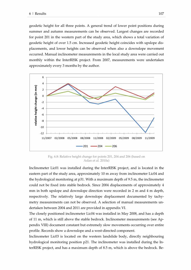
6 | Results 107
geodetic height for all three points. A general trend of lower point positions during
summer and autumn measurements can be observed. Largest changes are recorded
for point 201 in the western part of the study area, which shows a total variation of
geodetic height of over 1.5 cm. Increased geodetic height coincides with upslope dis-
placements, and lower heights can be observed when also a downslope movement
occurred. Manual inclinometer measurements in the local study area were carried out
monthly within the InterRISK project. From 2007, measurements were undertaken
approximately every 3 months by the author.
Fig. 6.8: Relative height change for points 201, 204 and 206 (based on Aslan et al. 2010a)
Inclinometer Lic01 was installed during the InterRISK project, and is located in the
eastern part of the study area, approximately 10 m away from inclinometer Lic04 and
the hydrological monitoring at p31. With a maximum depth of 9.5 m, the inclinometer
could not be fixed into stable bedrock. Since 2004 displacements of approximately 4
mm in both upslope and downslope direction were recorded in 2 m and 4 m depth,
respectively. The relatively large downslope displacement documented by tachy-
metry measurements can not be observed. A selection of manual measurements un-
dertaken between 2004 and 2011 are provided in appendix VI.
The closely positioned inclinometer Lic04 was installed in May 2008, and has a depth
of 11 m, which is still above the stable bedrock. Inclinometer measurements (see Ap-
pendix VIII) document constant but extremely slow movements occurring over entire
profile. Records show a downslope and a west-directed component.
Inclinometer Lic03 is located on the western landslide body, directly neighbouring
hydrological monitoring position p21. The inclinometer was installed during the In-
terRISK project, and has a maximum depth of 8.5 m, which is above the bedrock. Be-
-12
-10
-8
-6
-4
-2
0
2
4
6
11/2007 02/2008 05/2008 08/2008 11/2008 02/2009 05/2009 08/2009 11/2009
rela
tiv
e h
eig
ht
cha
ng
e (
in m
m)
201 204 206
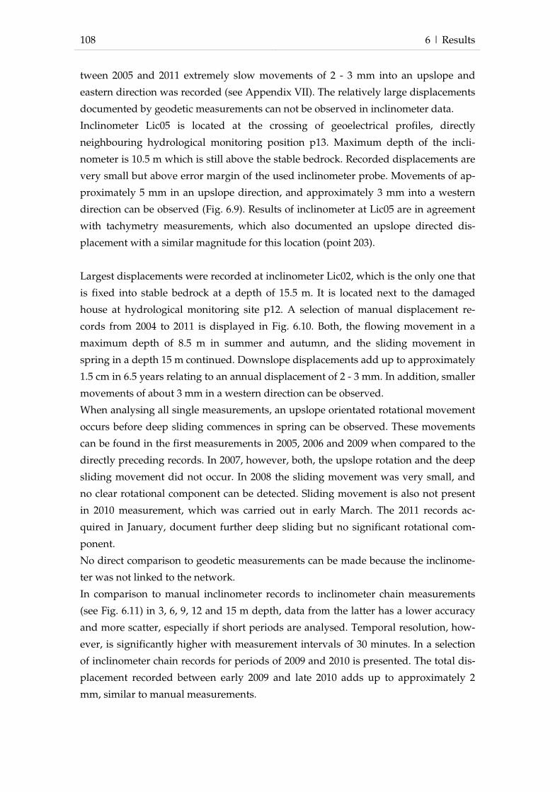
108 6 | Results
tween 2005 and 2011 extremely slow movements of 2 - 3 mm into an upslope and
eastern direction was recorded (see Appendix VII). The relatively large displacements
documented by geodetic measurements can not be observed in inclinometer data.
Inclinometer Lic05 is located at the crossing of geoelectrical profiles, directly
neighbouring hydrological monitoring position p13. Maximum depth of the incli-
nometer is 10.5 m which is still above the stable bedrock. Recorded displacements are
very small but above error margin of the used inclinometer probe. Movements of ap-
proximately 5 mm in an upslope direction, and approximately 3 mm into a western
direction can be observed (Fig. 6.9). Results of inclinometer at Lic05 are in agreement
with tachymetry measurements, which also documented an upslope directed dis-
placement with a similar magnitude for this location (point 203).
Largest displacements were recorded at inclinometer Lic02, which is the only one that
is fixed into stable bedrock at a depth of 15.5 m. It is located next to the damaged
house at hydrological monitoring site p12. A selection of manual displacement re-
cords from 2004 to 2011 is displayed in Fig. 6.10. Both, the flowing movement in a
maximum depth of 8.5 m in summer and autumn, and the sliding movement in
spring in a depth 15 m continued. Downslope displacements add up to approximately
1.5 cm in 6.5 years relating to an annual displacement of 2 - 3 mm. In addition, smaller
movements of about 3 mm in a western direction can be observed.
When analysing all single measurements, an upslope orientated rotational movement
occurs before deep sliding commences in spring can be observed. These movements
can be found in the first measurements in 2005, 2006 and 2009 when compared to the
directly preceding records. In 2007, however, both, the upslope rotation and the deep
sliding movement did not occur. In 2008 the sliding movement was very small, and
no clear rotational component can be detected. Sliding movement is also not present
in 2010 measurement, which was carried out in early March. The 2011 records ac-
quired in January, document further deep sliding but no significant rotational com-
ponent.
No direct comparison to geodetic measurements can be made because the inclinome-
ter was not linked to the network.
In comparison to manual inclinometer records to inclinometer chain measurements
(see Fig. 6.11) in 3, 6, 9, 12 and 15 m depth, data from the latter has a lower accuracy
and more scatter, especially if short periods are analysed. Temporal resolution, how-
ever, is significantly higher with measurement intervals of 30 minutes. In a selection
of inclinometer chain records for periods of 2009 and 2010 is presented. The total dis-
placement recorded between early 2009 and late 2010 adds up to approximately 2
mm, similar to manual measurements.

6 | Results
Fig. 6.9: Selected records of Lic05 inclinometer measurements: Selected records of Lic05 inclinometer measurements
109
: Selected records of Lic05 inclinometer measurements

110
Fig. 6.10: Selected records of manual inclinometer measurements at : Selected records of manual inclinometer measurements at Lic02
6 | Results
: Selected records of manual inclinometer measurements at
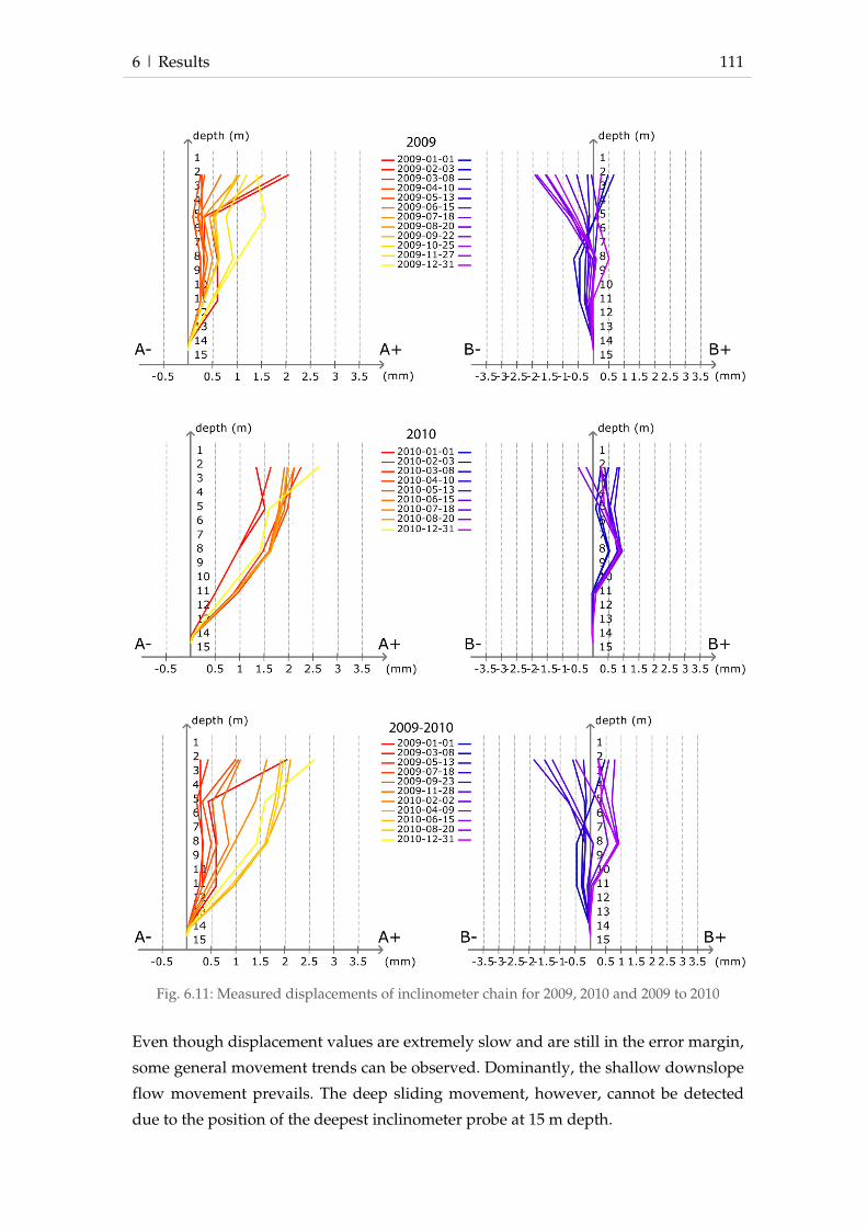
6 | Results 111
Fig. 6.11: Measured displacements of inclinometer chain for 2009, 2010 and 2009 to 2010
Even though displacement values are extremely slow and are still in the error margin,
some general movement trends can be observed. Dominantly, the shallow downslope
flow movement prevails. The deep sliding movement, however, cannot be detected
due to the position of the deepest inclinometer probe at 15 m depth.

112 6 | Results
To better understand the temporal dynamics of slope displacements, raw data was
analysed and thoroughly checked. It was found that extraction of the inclinometer
chain for manual measurements resulted in sudden jumps in displacements data last-
ing for some days, until records return to more stable values. All records from the
dates and the following four days, on which the inclinometer chain was extracted
were deleted from the data set. In addition, reference values which previously had in
some cases an offset of some days were adjusted. Results for A and B direction are
presented in Fig. 6.13 and Fig. 6.12, respectively.
Records start with some scatter during January 2009 but quickly adjust to more stable
conditions. The correction procedure described above reduced total displacements by
for example, 0.3 mm for the 3 m inclinometer probe. Still, a total downslope dis-
placement of 2 mm until September 2009 alone was recorded for this sensor. Move-
ment, however, was not continuous, but exhibited several phases of reversed direc-
tion. Periods of upslope movement can also be observed for the 6 m probe; but timing
of these does not reflect patterns similar to the 3 m sensor. Data from the probes lo-
cated in deeper positions is generally steadier. The probe in 15 m depth exhibited
three phases of larger movement, i.e. early 2009, between December 2009 and March
2010, and again in early 2011. However, the inclinometer chain was also removed
from the borehole during these times.
Similar to the A direction, no sudden changes can be observed in the daily mean dis-
placement changes of the inclinometer chains in B direction (Fig. 6.12). Records begin
with some initial scatter. However, from February 2009, relatively smooth changes
can be observed for 3 and 6 m sensors. A more step like course of displacement is
documented by the inclinometer probes in 12 m and 15 m depth.
For both A and B direction, greatest daily displacements variations documented by
the inclinometer chain are lower than 0.5 mm. Movements in this order of magnitude
are still in the margin of error and therefore have to be interpreted with great care.
Discussion
Based on geodetic measurements, three areas with similar movement trends can be
determined: the eastern part showing a general downslope displacement, the western
part moving into downslope and western direction, with certain epochs indicating
upslope movements, and the middle part moving slightly upslope in the upper sec-
tion downslope in the lower section. More detailed interpretation of the boundaries of
observed slope deformation requires integration of subsurface data provided by in-
clinometers.
Geodetic monitoring of surface displacements carried out by Aslan et al. (2010a) en-
hances the understanding of general landslide movement patterns. However, since
fixed points outside the landside body were only integrated into some of the epoch

6 | Results 113
Fig. 6.12: Daily mean displacement changes measured by inclinome-ter chain for B direction
Fig. 6.13: Daily mean displacement changes measured by inclinome-ter chain for A direction
-1
-0.5
0
0.5
1
1.5
01/2009 04/2009 07/2009 10/2009 01/2010 04/2010 07/2010 10/2010 01/2011 04/2011
dis
pla
cem
en
t in
mm
3 6 9 12 15
-1
-0.5
0
0.5
1
1.5
2
2.5
3
01/2009 04/2009 07/2009 10/2009 01/2010 04/2010 07/2010 10/2010 01/2011 04/2011
dis
pla
cem
en
t in
mm
3 6 9 12 15

114 6 | Results
measurements, only statements on relative deformation in the upper slope areas can
be made. Direct comparisons to inclinometer data is hindered by different dates of
measurements, and also because only three inclinometers were directly integrated
into the geodetic point network. For some parts, uncertainties are relatively large in
comparison to measured slope movements.
Observed variations of geodetic height of up to 1.2 cm can not only be explained by
rotational slope movements. Possibly, the measured variations are attributed to swell-
ing and drying of clay-rich subsurface materials. Lowest positions of geodetic points
generally coincide with the periods where the driest subsurface conditions were re-
corded. Higher positions were always recorded in early spring, when the wettest
conditions were measured. Continuation of geodetic measurements could aid to ver-
ify this hypothesis.
The extremely slow movements documented by the 6.5 years of inclinometer meas-
urements also continued during this study. For most inclinometers, displacements are
still smaller than the error margin of the applied sensors. However, at inclinometer
Lic02, measured displacements are clearly beyond the error margin by now. Previous
investigation by Bell (2007) showed a direct relation between the 8.5 m deep flowing
displacement with crack development at the house next to the inclinometer. High
precision tilt measurements (Bell 2007) were also able to verify rotational components
in the observed manual inclinometer measurements. Therefore, it can be assumed that
rotational movements documented within this study are also real.
Similar to previous studies in Lichtenstein-Unterhausen (Bell 2007; Bell and Thiebes
2010), two depths of slope displacements can be observed in data from manual meas-
urements in Lic02 which vary seasonally. These movements were described as a su-
perficial flow movement reaching down to a maximum depth of 8.5 m, and a deep
sliding movement occurring at approximately 15.5 m depth. In general, the same
statement can be made with respect to new data acquired in this study. However,
when taking into account all available manual inclinometer measurements some in-
teresting processes can be observed from approximately 2007 on. The flow-specific
gradual decrease of displacement with greater depths seems to slowly transition into
a more even horizontal movement, possibly indicating the onset of a progressive de-
velopment of a shear surface.
The rotational movements documented by monthly manual inclinometer measure-
ments carried out by Bell (2007) can still be observed in some of this study’s results;
however, lower monitoring frequency makes detection more difficult.
A direct comparison of displacements documented by inclinometer to results of the
geodetic monitoring can only be made for Lic01, Lic03 and Lic05 as these are incorpo-
rated in the geodetic network.

6 | Results 115
Lic01 and geodetic point 306 show similar displacements in B+ and B- direction. The
large total downslope displacements of the geodetic points however, can not be ob-
served in which might be attributed to the inclinometer installation above stable bed-
rock in 9.5 m.
Displacements documented by Lic03 are partly in agreement with geodetic measure-
ments at point 201; however the magnitude of movement is smaller in the inclinome-
ter data. Similar to geodetic data, also inclinometer data illustrates in B+, i.e. western
direction.
For the eastern part of the geodetic network, i.e. points 205 to 207, 306, 105 and 106, a
relatively strong downslope movement trend was observed, which is similarly ob-
servable in Lic04 inclinometer data, which is located between the respective points.
Still, the magnitude of displacement is smaller in Lic04, which is possibly related to
the installation above stable bedrock and a potential movement deeper than 11 m.
A comparison of data from inclinometer Lic05 and the geodetic network point 204 are
in agreement regarding the lack of any significant downslope movement. Rotational
movements of Lic05, however, can not be observed in geodetic data. Therefore, it has
to be questioned if the consistent rotational displacement component documented by
Lic05 and Lic02 are caused by the same movement process.
Unfortunately, the sliding movement documented by manual measurements of Lic02
can not be observed in the inclinometer chain data due to the positioning of the low-
est sensors. Due to limited project funding, further drillings to a great depth, and sub-
sequently deeper installations of the inclinometer chain could not be carried out.
However, general trends of movement documented by manual inclinometer meas-
urements are also visible in inclinometer chain data. Still, extremely slow movements
are in the range of the error margin and have to be interpreted carefully.
The very good temporal resolution of the automated inclinometer chain is potentially
of great value for the analysis of movement triggering events. However, no significant
displacement occurred during the project duration and single dates of the slope
movement initiation can not be determined. Instead, relatively steady displacements
are documented. Particularly regarding the deep sliding movement, no period of ac-
celerated movement can be defined.
6.1.2.3 Hydrological data
Within this study, climatic data from the ILEWS weather station posed an important
data source for the analysis of hydrological processes and landslide reactivation. Cli-
matic data is available from mid August 2008 to late March 2011, however due to
technical problems (power failures, damage induced by animals) no measurements
were recorded during some periods. Fig. 6.14 displays data for daily rainfall and
mean daily temperature from the ILEWS weather station. While temperature data
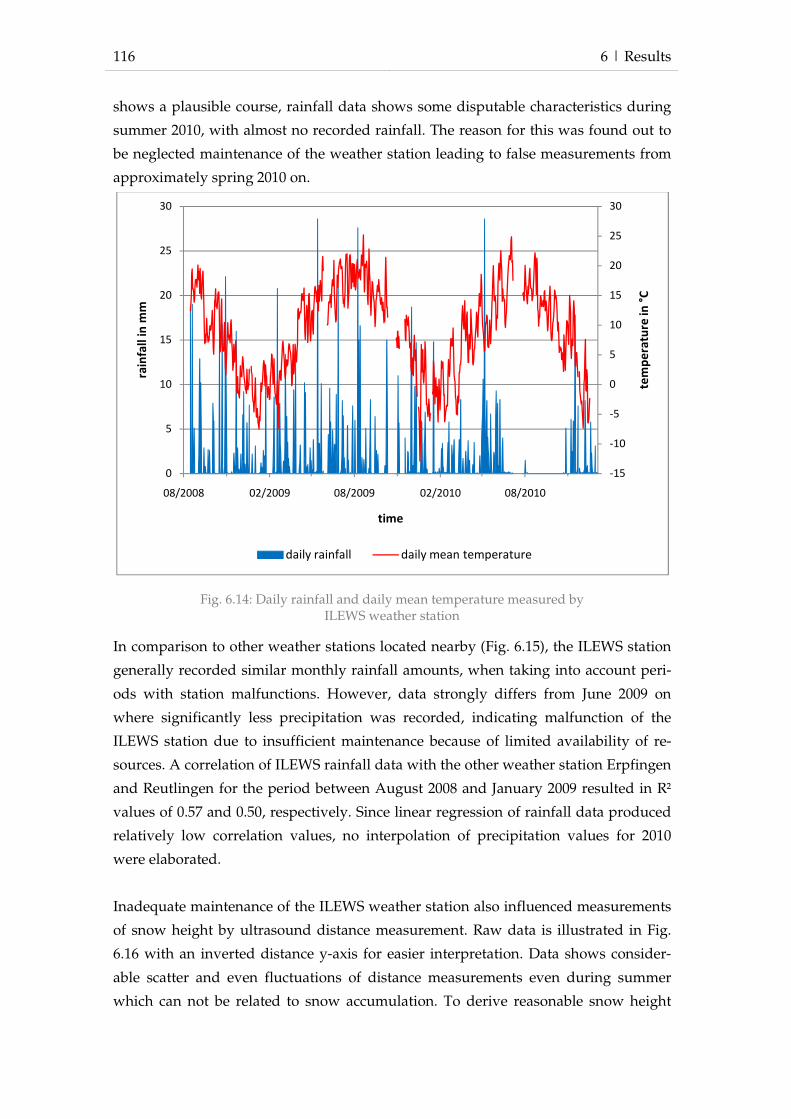
116 6 | Results
shows a plausible course, rainfall data shows some disputable characteristics during
summer 2010, with almost no recorded rainfall. The reason for this was found out to
be neglected maintenance of the weather station leading to false measurements from
approximately spring 2010 on.
Fig. 6.14: Daily rainfall and daily mean temperature measured by ILEWS weather station
In comparison to other weather stations located nearby (Fig. 6.15), the ILEWS station
generally recorded similar monthly rainfall amounts, when taking into account peri-
ods with station malfunctions. However, data strongly differs from June 2009 on
where significantly less precipitation was recorded, indicating malfunction of the
ILEWS station due to insufficient maintenance because of limited availability of re-
sources. A correlation of ILEWS rainfall data with the other weather station Erpfingen
and Reutlingen for the period between August 2008 and January 2009 resulted in R²
values of 0.57 and 0.50, respectively. Since linear regression of rainfall data produced
relatively low correlation values, no interpolation of precipitation values for 2010
were elaborated.
Inadequate maintenance of the ILEWS weather station also influenced measurements
of snow height by ultrasound distance measurement. Raw data is illustrated in Fig.
6.16 with an inverted distance y-axis for easier interpretation. Data shows consider-
able scatter and even fluctuations of distance measurements even during summer
which can not be related to snow accumulation. To derive reasonable snow height
-15
-10
-5
0
5
10
15
20
25
30
0
5
10
15
20
25
30
08/2008 02/2009 08/2009 02/2010 08/2010
tem
pe
ratu
re in
°C
rain
fall
in
mm
time
daily rainfall daily mean temperature

6 | Results 117
records, a detailed data analysis and correction was carried out for the following use
within analysis of snow melting and hydrological response.
Since the base distance at the beginning of each winter season varies in each period,
no single correction factor could be applied. Detailed data analysis considering tem-
perature and precipitation data led to determination of the three correction factors for
each winter season: 1.81 for winter 2008/2009, 1.78 for winter 2009/2010 and 1.79 for
winter 2010/2011.
In addition to correction factors, several records were deleted in the data set where
snow was considered unlikely due to daily mean temperatures. Adjusted snow height
data is presented in Fig. 6.17. Visual interpretation of plotted adjusted snow height
data indicate a relationship between daily mean temperatures and the variation of
snow height with a diametrically course of both factors.
In winter 2008/2009 the local study area experienced snow coverage from early De-
cember 2008 until early March with an period of snow melting due to higher tempera-
tures in late December and early January. The winter period of 2009/2010 exhibited
similar snow height conditions, with development of a snow cover in mid December
which lasted until March. Absolute snow height almost reached 20 cm in early winter
season. Additional snow fell during the winter season, but also melted during short
periods of high air temperatures. In winter 2010/2011 snow covered the local study
Fig. 6.15: Comparison of monthly rainfall of ILEWS weather stations with stations in Reutlingen and Erpfingen
0
20
40
60
80
100
120
140
160
08/2008 11/2008 02/2009 05/2009 08/2009 11/2009 02/2010 05/2010 08/2010 11/2010
rain
fall
in
mm
Erpfingen Reutlingen ILEWS

118 6 | Results
area between late November to early February with a maximum thickness of almost
20 cm. Warmer periods in late December and early January caused strong snow melt.
Fig. 6.16: Raw data from ultrasound distance measurement of snow height in comparison to daily mean temperature
Fig. 6.17: Adjusted snow height and mean daily temperature
-10
-5
0
5
10
15
20
25150
155
160
165
170
175
180
185
190
195
200
08/2008 02/2009 08/2009 02/2010 08/2010 02/2011
tem
pe
ratu
re in
°C
dis
tan
ce i
n c
m
snow height (raw data) mean daily temperature
-15
-10
-5
0
5
10
15
20
25
0
2
4
6
8
10
12
14
16
18
20
10/2008 04/2009 10/2009 04/2010 10/2010
tem
pe
ratu
re in
°C
sno
w h
eig
ht
in c
m
adjusted snow height daily mean temperature

6 | Results 119
In Fig. 6.18 to Fig. 6.25, data from hydrological monitoring, i.e. TDR sensors and ten-
siometers are presented along with daily rainfall data from the ILEWS weather sta-
tion. Unfortunately, no data from position p31 located in the eastern part of the moni-
toring system was available because this station was only connected to the monitoring
system at a very late state. In addition, some monitoring sensors are possibly dam-
aged during installation. Also vandalism, in particular to tensiometers was a problem;
in several cases rubber tubes were removed causing tensiometers to run dry until they
were repaired and refilled during later maintenance works.
Soil hydrology sensors at p11 are located in the south of the monitoring network, in
the garden below the house suffering cracking due to slope movements. Records from
the initial phase of monitoring in 2008 show no variations at (see Fig. 6.18). After
maintenance work by the project partner IMKO, in which the sensor software was
updated, real measurements commence in early 2009. Tensiometer measurements in
8.6 m depth describe positive values (up to >300 hPa) over the entire monitoring pe-
riod indicating that the sensor was permanently below the groundwater table. Similar
conditions are documented by TDR data from 8.8 m depth with constant volumetric
water content of around 50%. Tensiometer in 4.5 m depth reflects saturated conditions
for most times, and only negative values for summer and autumn 2009. The course of
the graph is similar to the deeper tensiometer, however, reaction to rainfall events is
quicker. Unfortunately, no TDR data is available from a similar depth because the
probe malfunctioned. Also measurements by the tensiometer in 1.75 m depth may be
influenced by a bad connection to the soil. From 2009 on, stable conditions close to
saturation were recorded without any significant influence of rainfall events. From
August 2009 on, measured pore pressure quickly decrease until October. Similar be-
haviour can also be observed for some other tensiometers. According to the project
partners IMKO who were responsible for the monitoring system, this behaviour is
related to drying of the ceramic contact. However, after refilling during maintenance
works, in this case around November 2009, records increased again and returned to
values similar to the initial conditions. TDR sensor in 1.95 metre depth describes a
strong increase of water content from below 30% to over 40% between February and
April 2009, followed by a decrease until approximately November. For 2010, also wa-
ter contents of over 45% were recorded indicating full saturation. Strong peaks for
deep tensiometers and the shallow TDR sensor can be observed after
February 2009. This event is highlighted in more detail in chapter 0. Groundwater
conditions for the following spatial interpolation of groundwater and subsequent
modelling were determined to vary between 2 m and 4.7 m for this location. Highest
groundwater positions referred to high saturation values measured at the shallowest

120 6 | Results
tensiometer (1.95 m depth), while lowest water table referred to minimum levels of
4.5 m tensiometer.
Hydrological sensors at p12 are located at the damaged house, only 2 metres away
from inclinometer chain in borehole Lic02. The TDR sensor in 9.5 m depth recorded
large fluctuations of volumetric water content which varied between approximately
35% and 45% (see Fig. 6.19). The amplitude of this sensor is the highest of all TDR
probes installed at this locations. Strong peaks can be observed for February 2009, and
from November 2009 on. Tensiometer data from similar depth (9.2 m) illustrates con-
ditions of high saturation but with lower fluctuations. Some stronger rainfall events
(e.g., May 2009) caused strong peaks relating to a location below groundwater table.
Phreatic conditions were also recorded by the tensiometer in 3.85 m depth for some
periods. Response to rainfall events by this sensor is relatively low. Records from ten-
siometer in 2.0 m depth only show small variations and lower response to rainfall
events than the tensiometer in 9.2 m. From August 2009 on massive drop of recorded
measurement in one month and increase afterwards, which likely to be caused by
drying of the tensiometer ceramics and refilling during maintenance works in October
2009. TDR sensors in 2.35 m and 4.2 m illustrate clear response of volumetric water
content to rainfall events. Both graphs describe similar trends, however, stronger
variations can be observed for the shallow TDR which also has higher mean water
content (~25% and ~20%). During late summer and early autumn 2009, TDR in 2.35 m
depth recorded quickly decreasing water contents, while the 4.2 m TDR sensor de-
scribes more steady conditions. However, after strong rainfall in December 2009, both
sensors return to initial value levels. Minimum and maximum groundwater table
depths for this location were determined to be 4.5 m and 2.0 m, respectively. The high
water table referred to almost saturated conditions at 2.0 m tensiometer. Low water
table definition followed measurements of the tensiometer in 3.85 m, which docu-
ments not saturated conditions for some periods.
Sensors at p13 are located in the centre of the monitoring system at inclinometer Lic05
and the container with monitoring equipment. For the TDR in 8.4 m depth, volumet-
ric water contents between approximately 20% and 25% can be observed (see Fig.
6.20). Strongest peaks occurred in spring 2009 and again in 2010, possibly related to
snow melting. However, no direct response to rainfall events can be found through-
out the monitoring campaign. Tensiometer in 7.75 m depth recorded no positive val-
ues, indicating that full saturation did not occur during monitoring campaign. Reac-
tion to rainfall events is relatively small, with the strongest peak occurring in Febru-
ary 2009.

6 | Results 121
Fig. 6.18: Hydrological monitoring at location p11
Fig. 6.19: Hydrological monitoring at location p12
-800
-600
-400
-200
0
200
400
0
10
20
30
40
50
60
08/2008 11/2008 02/2009 05/2009 08/2009 11/2009 02/2010 05/2010 08/2010
hP
a
wa
ter
con
ten
t (v
ol-
%)
am
d d
ail
y r
ain
fall
(in
mm
)
p11
daily rainfall TDR (1.95 m) TDR (8.8 m)
Tensio (1.75 m) Tensio (4.5 m) Tensio (8.6 m)
-800
-700
-600
-500
-400
-300
-200
-100
0
100
200
0
10
20
30
40
50
60
08/2008 11/2008 02/2009 05/2009 08/2009 11/2009 02/2010 05/2010 08/2010
hP
a
wa
ter
con
ten
t (v
ol-
%)
an
d d
ail
y r
ain
fall
(in
mm
)
p12
daily rainfall TDR (2.35 m) TDR (9.5 m) TDR (4.2 m)
Tensio (2.0 m) Tensio (3.85 m) Tensio (9.2 m)

122 6 | Results
Scattered data close to full saturation was recorded by tensiometer in 3.3 m depth
without any significant response to rainfall events. Similar to other tensiometers, re-
cords drop in summer 2008, likely to be related to drying of tensiometer ceramics.
More stable conditions are documented by tensiometer 1.35 m. Positive values indi-
cate saturation almost for the entire monitoring period. However, data from the shal-
lowest TDR sensor do not indicate fully saturated conditions with water content
variation between 15% and more than 30%. For location p13, groundwater minimum
levels were determined as 3.7 m, primarily based on 3.55 m tensiometer, which
documented unsaturated conditions during the entire monitoring period. A maxi-
mum groundwater table was determined to be 1.3 m using high saturation records
from 1.35 m tensiometer.
The most upslope sensor location is p14, which is positioned in the forest directly
neighbouring the geoelectrical monitoring profile. Tensiometer data from 8.85 m illus-
trates almost saturated conditions for the entire monitoring period, with only little
response to rainfall events (see Fig. 6.21). Relatively stable conditions are also docu-
mented by the adjacent TDR sensor in 9.15 m depth, with volumetric water contents
around 25% and no direct response to rainfall events. Tensiometers in 1.7 m and 4.2 m
depth recorded diametrical development of pressure measurements in the beginning
of monitoring period before documenting conditions close to saturation from Febru-
ary 2009 on. Afterwards, 1.7 m tensiometer reflects sudden drying which is likely to
be caused by damaged tensiometers. In August 2009 and October 2009, however, re-
cords increase again, possibly due to strong rainfall in August and maintenance
works in October. Shallow TDR sensors in 2.0 m and 4.75 m depth at p14, document
stable conditions without larger changes until February 2009 when water content in-
creases to more than 30% and 40% of volume, respectively. Afterwards, water con-
tents decrease until late 2009, with little response to rainfall events for the deeper sen-
sor. The shallow TDR in 2.0 m depth however reflects strong variations of more than
15% water content for spring periods. A maximum groundwater table of 1.8 m below
the surface was determined based on high saturation records of 1.7 m tensiometer.
The definition of a minimum water table was difficult due to possible malfunction of
tensiometers at this location. However, low water contents of 4.75 m TDR was used to
assume a minimum water table of 6 m.
In the western part of the study area, location p21 is adjacent to inclinometer Lic03.
Volumetric water contents of around 48% were recorded by deepest TDR in 7.3 m
with no great changes occurring throughout the monitoring campaign (see Fig. 6.22).
Phreatic conditions for long periods are also illustrated by tensiometer in a similar
depth (7.15 m) with variations in the range of -30 to +54 hPa. Large variations due to

6 | Results 123
Fig. 6.20: Hydrological monitoring at location p13
Fig. 6.21: Hydrological monitoring at location p14
-250
-200
-150
-100
-50
0
50
100
150
0
10
20
30
40
50
60
08/2008 11/2008 02/2009 05/2009 08/2009 11/2009 02/2010 05/2010 08/2010
hP
a
wa
ter
con
ten
t (v
ol-
%)
an
d d
ail
y r
ain
fall
(in
mm
)
p13
daily rainfall TDR (1.65 m) TDR (8.4 m) TDR (3.55 m)
Tensio (1.35 m) Tensio (3.3 m) Tensio (7.75 m)
-900
-800
-700
-600
-500
-400
-300
-200
-100
0
100
0
10
20
30
40
50
60
08/2008 11/2008 02/2009 05/2009 08/2009 11/2009 02/2010 05/2010 08/2010
hP
a
wa
ter
con
ten
t (v
ol-
%)
an
d d
ail
y r
ain
fall
(in
mm
)
p14
daily rainfall TDR (2.0 m) TDR (9.15 m) TDR (4.75 m)
Tensio (1.7 m) Tensio (4.2 m) Tensio (8.85 m)

124 6 | Results
rainfall events can be observed for the 4.4 m tensiometer with maximum positive
pressures relating to approximately 50 cm of groundwater above the sensor. Very
high water contents were also recorded by the adjacent TDR sensor in 4.5 m depth
with values above 40%. Driest conditions occurred during October and November
2009. Also TDR sensor located in 1.6 m depth illustrates relatively stable conditions
with water contents around 40% and only little response to rainfall events. For this
location, minimum and maximum groundwater levels of 4 m and 5 m were deter-
mined primarily based on the variations of tensiometer data from 4.4 m depth.
The installation of hydrological sensors at p22, located between inclinometer Lic03
and Lic05 directly next to the road was very difficult. Boreholes collapsed several
times during installation so that sensors might not be appropriately fixed into the soil.
Relatively stable conditions in depth are illustrated by the deepest sensors, with water
content around 23% by the TDR sensor in 7.1 m depth, and almost saturated condi-
tions (tensiometer in 7.0 m) (see Fig. 6.23). Both other tensiometers (in 1.9 m and 3.4 m
depth) document partly saturated periods during 2009 until August, when records
drop to very low values possibly due to drying of tensiometer ceramics. Data from the
shallow TDR in 2.1 m depth shows water content of approximately 10% with no
variations for two periods in 2008 and August 2009 to January 2010. For some time,
water content also drops to 0% which is very likely to be erroneous. More realistic
measurements and response to rainfall events were recorded from March 2009 on and
again in 2010. Definition of a groundwater levels for this location was difficult due to
problematic installation of sensors. However, a maximum groundwater table of 2 m
was determined based on high saturation values at the 1.9 m tensiometer. A mini-
mum level of 5 m was assumed using data from the 3.4 m tensiometer for orientation.
Sensors at p24 are located in the eastern part of the study area between inclinometer
Lic05, and the lawn with inclinometers Lic01 and Lic04. Saturated conditions are illus-
trated by deep tensiometer and TDR sensor in 9.35 m and 9.5 m, respectively (see Fig.
6.24). Volumetric water content was very constant throughout the monitoring cam-
paign, with values around 48 %. Tensiometer data describes positive pressures of up
to 100 hPa with some fluctuations. However, tensiometer data also includes meas-
urements of exactly 0 hPa very likely due to malfunction. More shallow tensiometers
data has some large scatter and also exhibits drying of tensiometer ceramics until re-
filling during maintenance works. Shallow TDR sensors show very little response to
rainfall events with relatively dry conditions (mean volumetric water content of 15%
for 2.0m, and 25% for 4.8 m). Partial saturation of the tensiometer in 1.85 m depth was
used to determine a maximum groundwater level as 1.9 m. Lowest groundwater posi-
tion was assumed to be 6 m based on interpretation of TDR and tensiometer from 4.8
m and 4.5 m depth, respectively, which reflect unsaturated conditions for some time.
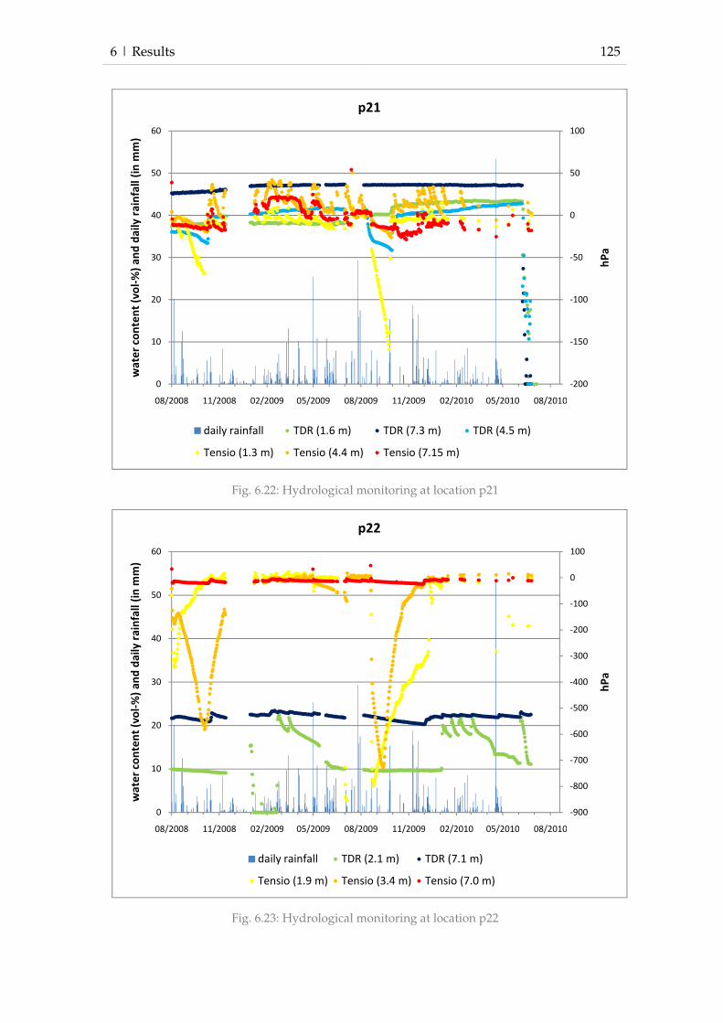
6 | Results 125
Fig. 6.22: Hydrological monitoring at location p21
Fig. 6.23: Hydrological monitoring at location p22
-200
-150
-100
-50
0
50
100
0
10
20
30
40
50
60
08/2008 11/2008 02/2009 05/2009 08/2009 11/2009 02/2010 05/2010 08/2010
hP
a
wa
ter
con
ten
t (v
ol-
%)
an
d d
ail
y r
ain
fall
(in
mm
)
p21
daily rainfall TDR (1.6 m) TDR (7.3 m) TDR (4.5 m)
Tensio (1.3 m) Tensio (4.4 m) Tensio (7.15 m)
-900
-800
-700
-600
-500
-400
-300
-200
-100
0
100
0
10
20
30
40
50
60
08/2008 11/2008 02/2009 05/2009 08/2009 11/2009 02/2010 05/2010 08/2010
hP
a
wa
ter
con
ten
t (v
ol-
%)
an
d d
ail
y r
ain
fall
(in
mm
)
p22
daily rainfall TDR (2.1 m) TDR (7.1 m)
Tensio (1.9 m) Tensio (3.4 m) Tensio (7.0 m)
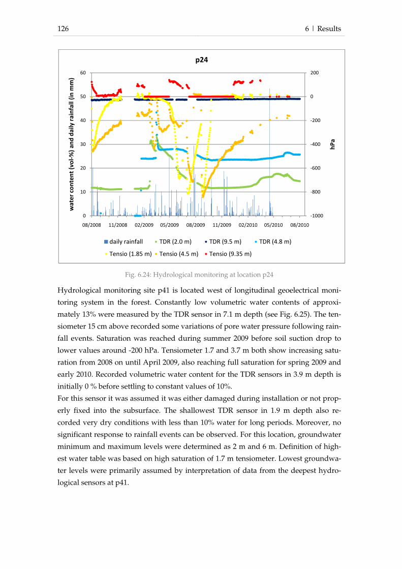
126 6 | Results
Fig. 6.24: Hydrological monitoring at location p24
Hydrological monitoring site p41 is located west of longitudinal geoelectrical moni-
toring system in the forest. Constantly low volumetric water contents of approxi-
mately 13% were measured by the TDR sensor in 7.1 m depth (see Fig. 6.25). The ten-
siometer 15 cm above recorded some variations of pore water pressure following rain-
fall events. Saturation was reached during summer 2009 before soil suction drop to
lower values around -200 hPa. Tensiometer 1.7 and 3.7 m both show increasing satu-
ration from 2008 on until April 2009, also reaching full saturation for spring 2009 and
early 2010. Recorded volumetric water content for the TDR sensors in 3.9 m depth is
initially 0 % before settling to constant values of 10%.
For this sensor it was assumed it was either damaged during installation or not prop-
erly fixed into the subsurface. The shallowest TDR sensor in 1.9 m depth also re-
corded very dry conditions with less than 10% water for long periods. Moreover, no
significant response to rainfall events can be observed. For this location, groundwater
minimum and maximum levels were determined as 2 m and 6 m. Definition of high-
est water table was based on high saturation of 1.7 m tensiometer. Lowest groundwa-
ter levels were primarily assumed by interpretation of data from the deepest hydro-
logical sensors at p41.
-1000
-800
-600
-400
-200
0
200
0
10
20
30
40
50
60
08/2008 11/2008 02/2009 05/2009 08/2009 11/2009 02/2010 05/2010 08/2010
hP
a
wa
ter
con
ten
t (v
ol-
%)
an
d d
ail
y r
ain
fall
(in
mm
)
p24
daily rainfall TDR (2.0 m) TDR (9.5 m) TDR (4.8 m)
Tensio (1.85 m) Tensio (4.5 m) Tensio (9.35 m)

6 | Results 127
Fig. 6.25: Hydrological monitoring at location p41
A more detailed analysis of hydrological response to rainfall and snow melting was
carried out for several shorter periods. Some examples of these will be presented in
the following.
The first event analysed in more detail is February 2009, where a strong raise of water
content and saturation was documented by several of the hydrological sensors. Cli-
matic data from the ILEWS weather station shows, that in February initially small
snow coverage increased to approximately 10 cm until 22nd February, when warmer
temperatures led to a quick decline of snow height (Fig. 6.26).
Precipitation records from the unheated rainfall gauge reflect the snow melting proc-
ess. Peaks in precipitation measurements can be observed for all periods in which the
temperatures is above 0° C. Total precipitation in February 2009 cumulates to 77 mm.
Snow height data, however, does not follow short-time temperature changes but re-
flects general trends. The strong decrease of snow height from 22nd February on, how-
ever, is only partly documented by precipitation records.
For the February 2009 period, a detailed time-lapse inversion of data from the longi-
tudinal geoelectrical profile was elaborated by Wiebe et al. (2010) which will be pre-
sented below. Though data processing was carried out by Wiebe et al. (2010), the fol-
lowing description and subsequent interpretation are made by the author of this the-
sis. Fig. 6.27 illustrates the time-lapse inversion, where changes between a reference
-1000
-800
-600
-400
-200
0
200
0
10
20
30
40
50
60
08/2008 11/2008 02/2009 05/2009 08/2009 11/2009 02/2010 05/2010 08/2010
hP
a
wa
ter
con
ten
t (v
ol-
%)
an
d d
ail
y r
ain
fall
(in
mm
)
p41
daily rainfall TDR (1.9 m) TDR (7.1 m) TDR (3.9 m)
Tensio (1.7 m) Tensio (3.7 m) Tensio (6.95 m)
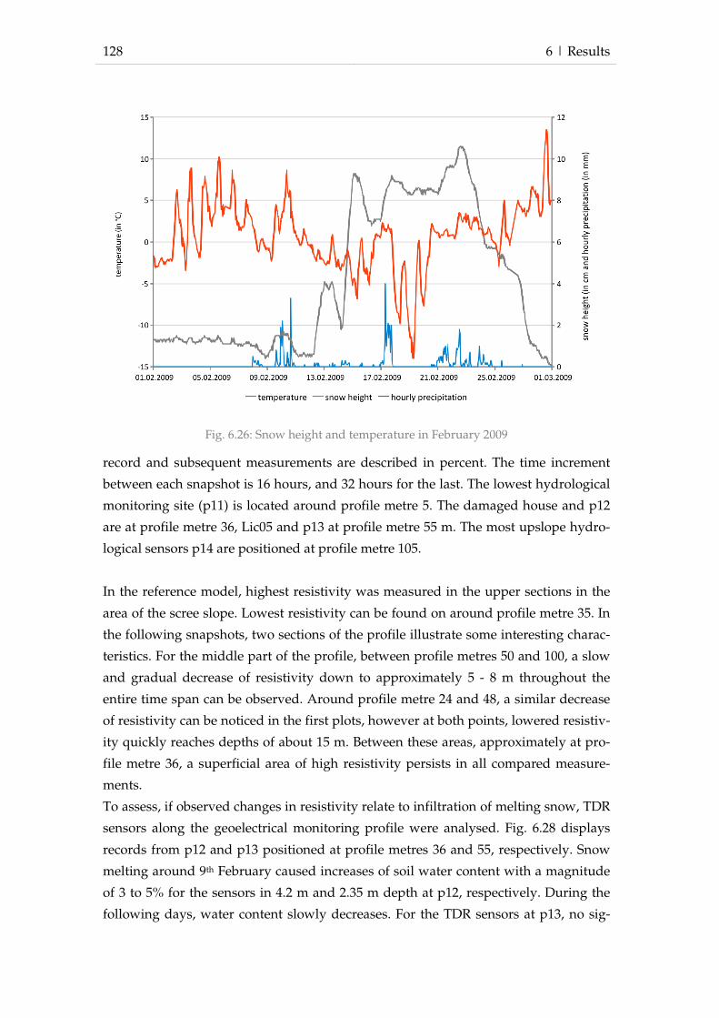
128 6 | Results
record and subsequent measurements are described in percent. The time increment
between each snapshot is 16 hours, and 32 hours for the last. The lowest hydrological
monitoring site (p11) is located around profile metre 5. The damaged house and p12
are at profile metre 36, Lic05 and p13 at profile metre 55 m. The most upslope hydro-
logical sensors p14 are positioned at profile metre 105.
In the reference model, highest resistivity was measured in the upper sections in the
area of the scree slope. Lowest resistivity can be found on around profile metre 35. In
the following snapshots, two sections of the profile illustrate some interesting charac-
teristics. For the middle part of the profile, between profile metres 50 and 100, a slow
and gradual decrease of resistivity down to approximately 5 - 8 m throughout the
entire time span can be observed. Around profile metre 24 and 48, a similar decrease
of resistivity can be noticed in the first plots, however at both points, lowered resistiv-
ity quickly reaches depths of about 15 m. Between these areas, approximately at pro-
file metre 36, a superficial area of high resistivity persists in all compared measure-
ments.
To assess, if observed changes in resistivity relate to infiltration of melting snow, TDR
sensors along the geoelectrical monitoring profile were analysed. Fig. 6.28 displays
records from p12 and p13 positioned at profile metres 36 and 55, respectively. Snow
melting around 9th February caused increases of soil water content with a magnitude
of 3 to 5% for the sensors in 4.2 m and 2.35 m depth at p12, respectively. During the
following days, water content slowly decreases. For the TDR sensors at p13, no sig-
Fig. 6.26: Snow height and temperature in February 2009

6 | Results 129
nificant response can be noticed. Further snow melting on the 17th is followed by only
smaller deviations of soil moisture, even though more precipitation is documented for
this period. More precipitation was recorded from the 21st on, which lead to signifi-
cant increase in soil water content. The earliest peak can be noticed for the shallowest
TDR at p12, approximately 24 hours after the precipitation peak. Shortly after, a small
increase of water content can be recognized for the 4.2 m deep TDR. The deepest TDR,
however, illustrates a very strong soil moisture increase of 6 – 8% starting on the 25th.
Sensors at p13 do not reflect any significant decrease in soil water content over the
entire period.
reference measurement
16 hours
32 hours

130 6 | Results
Fig. 6.27: Time-lapse inversion of geoelectrical monitoring data for period of 23.th to 26th of February (based on Wiebe et al. 2010)
The other sensors located along the geoelectrical profile, i.e. p11 and p14, also do not
show any sudden increases of soil moisture, except for the TDR probe in 4.2 m at p14.
Here, water content increases starting around 16th February from 20% to over 30% in 9
days, before a further rise to over 50% in only 4 days.
Inclinometer chain data from the same period were analysed to investigate if any in-
crease of movements were recorded during February 2009. After correction of raw
data, a total displacement of 0.2 - 0.5 mm can be observed. Magnitude of displace-
ments varies with installation depth of sensors, with larger movements occurring in
shallower locations. However, to carry out manual inclinometer measurements on
Lic02 borehole, the chain was extracted and later reinstalled on 12th February. There-
fore, it is not possible to assess if displacements describe real slope movements or
48 hours
64 hours
96 hours

6 | Results
originate from settling of the inclinometer probes after
hole. Manual measurements show no significant displacements between November
2008 and February 2009. Between February 2009 and the following manual measur
ment in November 2009, a movement of 1 mm occurring in approximately 15 m was
recorded. In addition, the more superficial displacement in approximately 8 m depth
also occurred with a total movement of 1.5 mm to 2.5 mm.
One of the strongest rainfall events during the period of monitoring occurred
2009, with a maximum hourly intensity of 27 mm. During this event, only shallow
sensors showed a quick response by increased soil moisture. Sensors located in
greater depths do not document significant increases of soil water content, except at
p12, where small reaction can be observed. Still, the response of the 9.5 m TDR sensor
is larger than the 4.2 m sensor at this location.
Inclinometer chain data from May 2009 show
sensor with a maximum displacement of
sors do not display any changes.
Another analysed period was November 2009 for which
records and hydrological data
were above 0° C making an influence of snow unlikely. Within the first five days,
approaximately 20 mm of precipitation were recorded, however, no signigcant
response by TDR sensors can be observed.
tensiometers, which do not reflect any significant changes
Fig. 6.28: Volumetric water content
originate from settling of the inclinometer probes after the extraction from
Manual measurements show no significant displacements between November
2008 and February 2009. Between February 2009 and the following manual measur
ment in November 2009, a movement of 1 mm occurring in approximately 15 m was
ddition, the more superficial displacement in approximately 8 m depth
also occurred with a total movement of 1.5 mm to 2.5 mm.
One of the strongest rainfall events during the period of monitoring occurred
2009, with a maximum hourly intensity of 27 mm. During this event, only shallow
sensors showed a quick response by increased soil moisture. Sensors located in
epths do not document significant increases of soil water content, except at
p12, where small reaction can be observed. Still, the response of the 9.5 m TDR sensor
is larger than the 4.2 m sensor at this location.
Inclinometer chain data from May 2009 shows some movements for the 3 m depth
sensor with a maximum displacement of approximately 1 mm, whereas deeper se
sors do not display any changes.
Another analysed period was November 2009 for which strong peaks in precipitation
records and hydrological data can be noticed. During this entire period, temperatures
making an influence of snow unlikely. Within the first five days,
approaximately 20 mm of precipitation were recorded, however, no signigcant
response by TDR sensors can be observed. Similar data was aquired fom
tensiometers, which do not reflect any significant changes in soil suctions and pore
: Volumetric water content at location p12 and p13 during February 2009
131
extraction from the bore-
Manual measurements show no significant displacements between November
2008 and February 2009. Between February 2009 and the following manual measure-
ment in November 2009, a movement of 1 mm occurring in approximately 15 m was
ddition, the more superficial displacement in approximately 8 m depth
One of the strongest rainfall events during the period of monitoring occurred in May
2009, with a maximum hourly intensity of 27 mm. During this event, only shallow
sensors showed a quick response by increased soil moisture. Sensors located in
epths do not document significant increases of soil water content, except at
p12, where small reaction can be observed. Still, the response of the 9.5 m TDR sensor
s some movements for the 3 m depth
1 mm, whereas deeper sen-
strong peaks in precipitation
During this entire period, temperatures
making an influence of snow unlikely. Within the first five days,
approaximately 20 mm of precipitation were recorded, however, no signigcant
Similar data was aquired fom
soil suctions and pore
at location p12 and p13 during

132
water pressure, except for the 9.2 m deep sensor at p12 for which an increase from
approximately 25 hPa to over 50 hPa was assessed. An increa
roughly relates to a rise of the ground water table by 30 cm.
For November 2009, no significant displacements were recorded by the inclinomter
chain.
More than 70 mm rainfall
followed by quick increase of soil water content (
respond to the precipitation event is the
moisture of 10% is documented.
sensor in medium depth, which is again smaller
TDR sensor. Here, water content reaches a maximum of
contrast, data from shallow TDR probes at p13 only show a slight increase after th
rainfall. The deepest TDR probe in 8.4 m depth shows the largest response to rainfall
with an increase of soil moisture from
hours. TDR sensors at p14 show the strongest increases for the two shallow sensors,
and a very smooth and slow rise of soil moisture for the deepest sensor in 9.15 m.
However, data from the inclinometer chain for this period does not reflect any
significant displacements.
Fig. 6.29: Volumetric
Discussion
In general, hydrological monitoring shows saturated conditions located in greatest
depths during the entire monitoring period, and responses to rainfall and snow mel
ing can mainly be observed for sensors in more surficial positions.
water pressure, except for the 9.2 m deep sensor at p12 for which an increase from
25 hPa to over 50 hPa was assessed. An increase of this magnitude
roughly relates to a rise of the ground water table by 30 cm.
For November 2009, no significant displacements were recorded by the inclinomter
0 mm rainfall are recorded in the first 10 days of May 2010
quick increase of soil water content (Fig. 6.29). At p12, the
respond to the precipitation event is the shallowest TDR for which a
is documented. Shortly after, a respronse can be observed
, which is again smaller than peak measured
TDR sensor. Here, water content reaches a maximum of approximately
contrast, data from shallow TDR probes at p13 only show a slight increase after th
rainfall. The deepest TDR probe in 8.4 m depth shows the largest response to rainfall
with an increase of soil moisture from 22% to approximately 35% in less than 48
hours. TDR sensors at p14 show the strongest increases for the two shallow sensors,
nd slow rise of soil moisture for the deepest sensor in 9.15 m.
However, data from the inclinometer chain for this period does not reflect any
: Volumetric water content at location p12, p13 and p14 duing May 2010
In general, hydrological monitoring shows saturated conditions located in greatest
depths during the entire monitoring period, and responses to rainfall and snow mel
observed for sensors in more surficial positions. Yet, for some rel
6 | Results
water pressure, except for the 9.2 m deep sensor at p12 for which an increase from
se of this magnitude
For November 2009, no significant displacements were recorded by the inclinomter
recorded in the first 10 days of May 2010 which was
). At p12, the first sensor the
for which a rise of soil
be observed at the
than peak measured by the 9.5 m
approximately 55%. In
contrast, data from shallow TDR probes at p13 only show a slight increase after the
rainfall. The deepest TDR probe in 8.4 m depth shows the largest response to rainfall
35% in less than 48
hours. TDR sensors at p14 show the strongest increases for the two shallow sensors,
nd slow rise of soil moisture for the deepest sensor in 9.15 m.
However, data from the inclinometer chain for this period does not reflect any
at location p12, p13 and p14 dur-
In general, hydrological monitoring shows saturated conditions located in greatest
depths during the entire monitoring period, and responses to rainfall and snow melt-
et, for some rela-

6 | Results 133
tively strong rainfall events, no significant response at all can be noticed. Relatively
dry conditions documented for location p41 are likely to be caused by the convergent
topography of the monitoring site. Overall, highest groundwater water contents are
recorded for spring, while lowest conditions occurred during summer and autumn.
Determination of groundwater positions from hydrological monitoring is also influ-
enced by subjective interpretation of monitoring data, and other experts could esti-
mate different groundwater levels. In theory, tensiometers can be used as piezometers
when installed within the phreatic zone, however, measured pressures could not eas-
ily be transferred to groundwater positions because of contradicting records. There-
fore, uncertainties prevail in the results which could be minimised by installation of
additional sensors.
Theoretically, the integration of geoelectrical monitoring data could also be used to
improve determination of groundwater table positions. Still, investigations of the rela-
tion of geoelectrical resistivity and measured soil water content carried out within the
ILEWS project (Wiebe et al. 2010) were not able to determine a simple relationship
between these parameters. Still, partial correlation were established for certain sensors
for relatively dry conditions (>50 ohm or <25% volumetric water content).
The influence of uncertainties due to partly subjective interpretation of hydrological
data on subsequent modelling has to be estimated by sensitivity analysis with
CHASM, which is described later (chapter 5.1.3.2).
The most interesting results in respect to hydrological response to rainfall and snow
melt derive from analysis of single events. In particular hydrological monitoring site
p12, located next to the house which frequently suffers crack development due to
slope movement, shows insightful characteristics. In general, hydrological sensors in
lower depths respond quicker to percolating water than sensors in greater depth.
However, at p12 analyses of several single rainfall and snow melt events show a con-
tradicting pattern. Here, the deepest TDR sensor in 9.5 m shows relatively quick and
large reactions to rainfall and snow melt, while the water content in medium depth
only varies slightly.
The observed variations of soil water content can be interpreted as a result of prefer-
ential flow paths by lateral influx of water. This assumption is supported by geoelec-
trical time-lapse inversions, which illustrate an even decrease of resistivity for most of
the measured profile following snow melt. For the area around monitoring site p12
however, low resistivity values in great depth develop without significant increases in
shallower depth above. Assuming variations in geoelectrical measurements for this
period are primarily related to infiltration and percolation of water, the observed re-
sistivity changes relate to a lateral influx on preferential flow paths.
134 6 | Results
Without any significant accelerations of slope movement hydrological triggering con-
ditions and thresholds can not be analysed adequately. Similar to the results of Bell
(2007) and Bell and Thiebes (2010), no simple correlation between rainfall or hydro-
logical conditions and shallow slope displacement can be found. The onset of the
deep-seated sliding, however, can be related to snow melting based on the timing of
these displacements. Also, deep-seated sliding can be observed for each spring season
except for 2007, when snow height in the previous months was relatively small.
Based on the results, it can be noted that tensiometers are of great value to estimate
the position of the groundwater table. An advantage of the TDR sensors is the quick
response time to rainfall events which make them particularly useful for low depth
installations.
Unfortunately, some of the installed tensiometers and TDR sensors seem to either
malfunction or may not be properly fixed to the soil. In addition, several tensiometers
are likely to have run dry due to low frequency of maintenance works.
Uncertainties of the weather data also have to be noted. Precipitation data from the
local weather station is questionable for at least summer 2010. In addition, also in ear-
lier periods, heated and unheated rainfall sensors differ in their records. Therefore,
rainfall data has to be interpreted with great care. Snow height data required some
correction processes to convert raw measurements into realistic snow depths. Cor-
rected snow height data can be assumed to describe general trends of snow accumula-
tion and melting realistically; however, some uncertainties remain regarding the exact
snow height.
6.1.3 Landslide early warning modelling
6.1.3.1 Generation of input data
In the following, results of generation of input data for following CHASM modelling
and early warning will be presented. These include the development of the general
subsurface model, modelling of groundwater scenarios, extraction of rainfall scenar-
ios, and design of an automated shear surface routine.
Subsurface model
A general subsurface model was generated by a combination of various data sources
(chapter 4) following a complex procedure (chapter 0) to facilitate subsequent model-
ling and early warning. Below, the results are presented.
Initially, positions of geological strata as upper limits were extracted from available
geological maps (1:25,000 and 1: 50,000) including information from described drill-
ings. Both maps contain similar information on positions and thickness for geological
strata. However, classification of the uppermost stratum differs between maps. In the

6 | Results 135
1:25,000 map, this is termed Kimmeridge Massenkalk, while the 1:50,000 map further
differentiates into the formations Kimmeridge Massenkalk and Lower Kimmeridge
Massenkalk. Tab. 6.2 shows the utilised strata classification of from the larger scale
map. Single DTM were created in GIS for each stratum with upper limit altitude as
grid cell information. At a later stage, these DTM blocks were merged with debris
thickness information to create a general subsurface model (see Fig. 6.38).
Tab. 6.2: Upper limits of geological strata (based on Ohmert et al. 1988)
series stage stratum code limit
Upper
Jurassic
Kimmeridgium Upper Kimmeridge limestone (Bank- and Fel-
senkalk)
ki2-3 790 m
Lower Kimmeridge marl (Lacunosamergel) k1 710 m
Oxfordian Oxfordian limestone (Oxfordkalk) ox2 670 m
Oxfordian marl (Impressamergel) ox1 610 m
Middle
Jurassic
Callovian Callovian clay (Ornatenton) cl 505 m
Bathonian Bathonian clay (Dentalienton) bt 475 m
Bajocian Bajocian clay (Hamitenton) bj3 465 m
Bajocian clay and marl (Stephanoceraten- and
Ostreenkalk)
bj2+ 440 m
Bajocian clay (Sonninien-Schichten) bj1 420 m
Drillings described by Ohmert (1988) were the first source of information for estima-
tion of debris thickness above bedrock. Fig. 6.30 displays drillings selected due to
their vicinity to the local study area. Depths of debris material, primarily termed soil,
alluvial loam and slope debris by the authors of core descriptions, were extracted, and
are summarized in Tab. 6.3. Holocene calcareous sinter and gravels from periglacial
periods found in some drillings, were neglected and therefore add to the geological
material which they overly.
Drillings 34 to 38 are located close to the river and describe a debris cover varying
between 3 m and almost 6.5 m, under which periglacial gravels and calcareous sinter
can be found. Almost 10 m loose material is attested at point 42. Several drillings are
in lower slope positions, i.e. 39 to 50. For these, a debris cover between 4.8 m and 13.8
m was measured, with the exception of drilling 41, where over 22 m of fluvial depos-
its and tufa sand overlie Callovian clay. Drilling 50 is located on landslide deposits
and attested a thickness of 24 m of slope debris above clay marl (cl). The drilling lo-
cated the furthest upslope is positioned at point 48. Here, 8 m of slope debris are over-
lying Oxfordian marl (ox1).

136 6 | Results
Fig. 6.30: Drillings close to the local study area described in geologi-cal map (1:25,000) (Ohmert et al. 1988)
Tab. 6.3: Analysed thickness of debris above bedrock (based on Oh-mert et al. 1988)
Drilling Position Debris thickness Description
34 River 3.8 m Soil, loam
35 River 4.3 m Soil, alluvial loam
36 River 6.4 m Soil, peat
37 River 3.0 m Soil, tufa sand
38 River 6.5 m Soil, tufa sand
42 River 9.9 m Soil, tufa sand, peat
39 Lower slope 12.0 m Soil, tufa sand, slope debris
40 Lower slope 13.8 m Soil, tufa sand, slope debris
41 River 21.7 m Fill, tufa sand
43 Lower slope 4.8 m Slope debris, loam
44 Lower slope 7.2 m Fill, slope debris, alluvial loam
47 Lower slope 17.8 m Fill, tufa sand, peat
50 Lower slope 24.0 m Landslide deposits
48 Middle slope 8.0 m Slope debris

6 | Results 137
From drillings 34, 35, 36, 37 and 38, a mean debris cover of 5 m was assumed for areas
located close to the river. Estimation of debris thickness for lower and middle slope
sections primarily referred to drillings 43 and 44, and 48 for orientation. Debris cover
was assumed to vary between 5 m and 7 m at similar slope positions. On the plateau
area, points were evenly distributed and a depth of bedrock of 1 m was assumed.
Variable debris thickness depending on local topography was not included for the
plateau area. No debris cover was supposed for the outcropping limestone at the
main landslide crown, and the upper scree slope. However, since evolution of the
scree took place after occurrence of the main landslide, debris was assumed to be lo-
cated underneath for lower sections. A bedrock depth of 1 m was assumed for this
area.
According to these findings, the estimated debris thickness for the local study area
was stored within GIS as point data and used for subsequent spatial interpolation
(Fig. 6.31). In addition to the previously described points, some others were added,
e.g. in the western part of the study area, and also for high slope positions, to ensure a
smoother interpolation and transition of debris thickness.
Fig. 6.31: Estimated depth of debris for local study area
138 6 | Results
In the core area of the local study area, the estimation of debris thickness was based
on data from seismic prospection elaborated with Rayfract by the company geoFact
(Bell et al. 2010b). Processing of seismic data was carried out by the project partner
geoFact, following interpretation and deduction of debris thickness is a result of the
author of this thesis. Seismic data and estimated depth of bedrock is presented in Fig.
6.32. Since one drilling, i.e. Lic02, penetrated the bedrock, it was used for calibration
of seismic results. In addition, the seismic profiles were compared and optimised to
each other at four intersections.
The western longitudinal profile intersects with lower and upper cross profiles at 79
m and 130 m, respectively. Inclinometers Lic02 and Lic05 are located at 42 m and 68
m, respectively. At Lic02, bedrock corresponds to a wave velocity of approximately
2000 m/s, displayed as the transition orange to red, which was subsequently used for
interpretation. The plot illustrated in Fig. 6.32 was combined from two single ana-
lysed profiles superimposed for interpretation. A refractor computed with plus-minus
method was calculated around 900 m/s, relating to a depth between 6 m to 8 m. Bell
et al. (2010b) interpreted the refractor as a weak zone. In general, the 2000 m/s line
was interpreted as the bedrock interface, relating to depths between 13 m to 16 m for
most parts of the profile. Considerable greater depths of over 20 m were estimated for
a spoon shaped hollow between profile metre 90 and 130.
The eastern longitudinal seismic prospection survey has a total length of almost 190 m
and was acquired in one measurement. At the maximum upslope location, the profile
intersects with the northern cross profile. Another intersection is positioned at profile
metre 140. The calculated refractor varies between 8 m and 14 m depth, and shows a
great variation in terms of wave velocity. For mid and low profile section, depth
ranges between 8 m and 16 m, respectively. For the upper profile maximum depths of
over 20 m were estimated, similar to the northern cross profile.
The northern cross profile has a length of 90 m and intersects with the western and
eastern longitudinal profiles at metre 47 and 66, respectively. The calculated refractor
is in a depth of approximately 12 m depth, corresponding to a seismic velocity be-
tween 1200 m/s and 1400 m/s. Estimation of bedrock depth followed the 2000 m/s
line, corresponding to depths of 10 m and 15 m for eastern and mid profile sections,
respectively. In the western part greater depths over 20 m were estimated in agree-
ment with data from the eastern longitudinal profile.
The southern cross profile was the longest, with a total length of 220 m and was pro-
duced by a combination of three single measurements. Intersections with the western
and eastern longitudinal profiles are located at metres 113 m and 148 m, respectively.
The refractor is in the range of 1000 m/s to 1200 m/s, corresponding to a depth of
approximately 8 m. For most areas, the 2000 m/s line was used for estimation of bed-
rock depth. Still, at around profile metre 90, one larger hollow was interpreted as arte-

6 | Results
fact of data inversion. Depth of bedrock ranges betwee
east, to slightly shallower values around 12 in mid and western profile.
Fig. 6.32: Results of geoseismic prospection and estimated bedrock interface depths
fact of data inversion. Depth of bedrock ranges between approximately
east, to slightly shallower values around 12 in mid and western profile.
: Results of geoseismic prospection and estimated bedrock interface depths (based on Bell et al. 2010)
139
approximately 16 m in the
east, to slightly shallower values around 12 in mid and western profile.
: Results of geoseismic prospection and estimated bedrock

140 6 | Results
After estimation of bedrock depths in seismic plots, data was transferred to GIS for
subsequent spatial interpolation. Depth information was extracted every 4 m, ana-
logue to the distance between the geophones during prospection, and stored within
GIS as point data (Fig. 6.33). Greatest debris thickness up to over 20 m was estimated
for the northern profile, especially on the western end, but also in the upper part of
the western longitudinal profile. Shallower positioning of bedrock was ascertained for
lower slope sections in general, and in particular for the western part.
Fig. 6.33: Assigned depth of debris from analysis of seismic prospec-tion data
After analysis of debris depth in the upper landslide area, the depth of material of the
scree slope was estimated. In GIS, outlines of scree slope were digitised and converted
to point data with scree depth information of zero. From interpretation of geoelectri-
cal monitoring data acquired by Bell (2007) and Kruse (2006), a maximum thickness of
8 m was assumed. Additional data points with the respective depth value were cre-
ated in GIS, positioned at approximately 60% of horizontal scree length. Further
points at the sides were added to ensure smooth spatial interpolation of scree depths.
Several interpolation methods (i.e. Kriging, Inverse Distance Weighting, and Nearest
Neighbour) were tested, of which the Natural Neighbour method was judged to gen-
erate the most realistic results (see Fig. 6.34).
Initial attempts of spatial interpolation of debris cover using the previously described
data demonstrated the need to improve representation of lower landslide deposits.
Since neither drillings nor geophysical data were available, an iterative GIS based
interpolation was carried out (see Fig. 6.35).
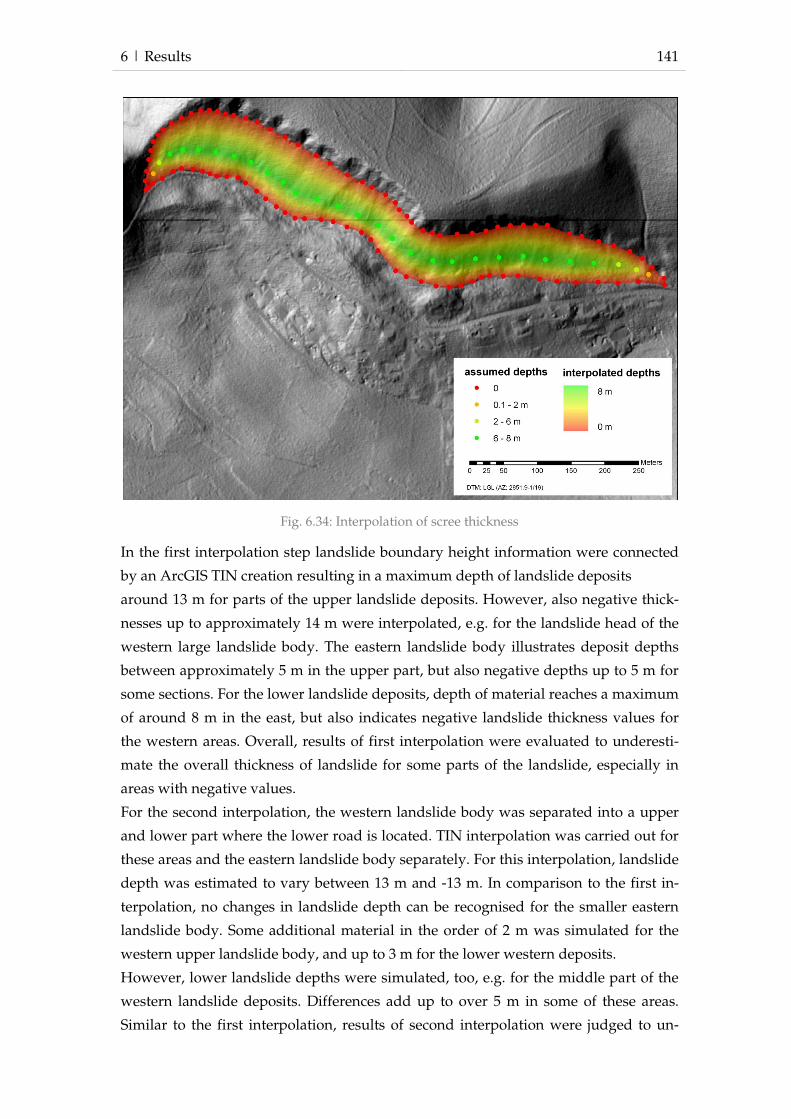
6 | Results 141
In the first interpolation step landslide boundary height information were connected
by an ArcGIS TIN creation resulting in a maximum depth of landslide deposits
around 13 m for parts of the upper landslide deposits. However, also negative thick-
nesses up to approximately 14 m were interpolated, e.g. for the landslide head of the
western large landslide body. The eastern landslide body illustrates deposit depths
between approximately 5 m in the upper part, but also negative depths up to 5 m for
some sections. For the lower landslide deposits, depth of material reaches a maximum
of around 8 m in the east, but also indicates negative landslide thickness values for
the western areas. Overall, results of first interpolation were evaluated to underesti-
mate the overall thickness of landslide for some parts of the landslide, especially in
areas with negative values.
For the second interpolation, the western landslide body was separated into a upper
and lower part where the lower road is located. TIN interpolation was carried out for
these areas and the eastern landslide body separately. For this interpolation, landslide
depth was estimated to vary between 13 m and -13 m. In comparison to the first in-
terpolation, no changes in landslide depth can be recognised for the smaller eastern
landslide body. Some additional material in the order of 2 m was simulated for the
western upper landslide body, and up to 3 m for the lower western deposits.
However, lower landslide depths were simulated, too, e.g. for the middle part of the
western landslide deposits. Differences add up to over 5 m in some of these areas.
Similar to the first interpolation, results of second interpolation were judged to un-
Fig. 6.34: Interpolation of scree thickness
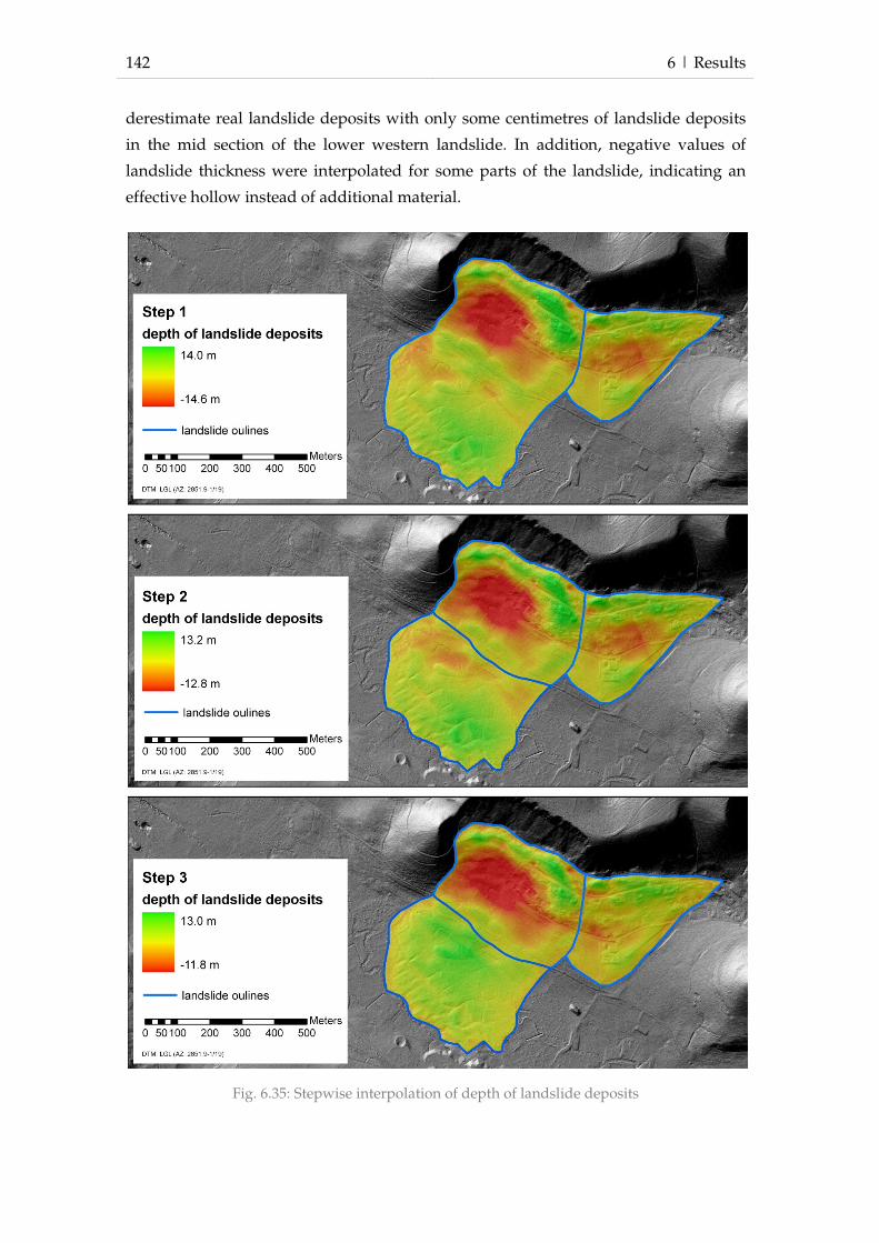
142 6 | Results
derestimate real landslide deposits with only some centimetres of landslide deposits
in the mid section of the lower western landslide. In addition, negative values of
landslide thickness were interpolated for some parts of the landslide, indicating an
effective hollow instead of additional material.
Fig. 6.35: Stepwise interpolation of depth of landslide deposits
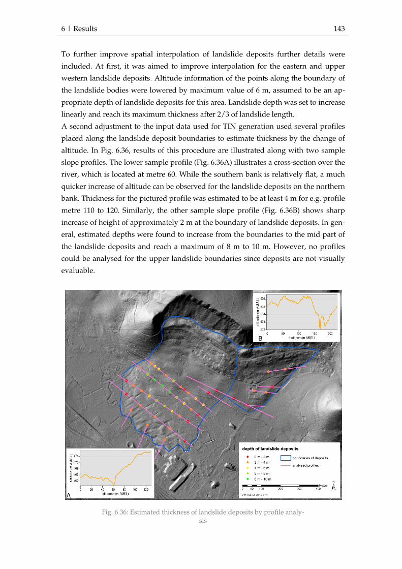
6 | Results 143
To further improve spatial interpolation of landslide deposits further details were
included. At first, it was aimed to improve interpolation for the eastern and upper
western landslide deposits. Altitude information of the points along the boundary of
the landslide bodies were lowered by maximum value of 6 m, assumed to be an ap-
propriate depth of landslide deposits for this area. Landslide depth was set to increase
linearly and reach its maximum thickness after 2/3 of landslide length.
A second adjustment to the input data used for TIN generation used several profiles
placed along the landslide deposit boundaries to estimate thickness by the change of
altitude. In Fig. 6.36, results of this procedure are illustrated along with two sample
slope profiles. The lower sample profile (Fig. 6.36A) illustrates a cross-section over the
river, which is located at metre 60. While the southern bank is relatively flat, a much
quicker increase of altitude can be observed for the landslide deposits on the northern
bank. Thickness for the pictured profile was estimated to be at least 4 m for e.g. profile
metre 110 to 120. Similarly, the other sample slope profile (Fig. 6.36B) shows sharp
increase of height of approximately 2 m at the boundary of landslide deposits. In gen-
eral, estimated depths were found to increase from the boundaries to the mid part of
the landslide deposits and reach a maximum of 8 m to 10 m. However, no profiles
could be analysed for the upper landslide boundaries since deposits are not visually
evaluable.
Fig. 6.36: Estimated thickness of landslide deposits by profile analy-sis
A
B
144 6 | Results
Results of third interpolation including points of the manipulated landslide boundary
between western and eastern landslide bodies, and data points from profile analysis
are presented in Fig. 6.35 as step 3. In comparison to the second interpolation, thicker
landslide deposits were simulated for most of the landslide areas. Especially for the
lower western landslide, the depth of material exceeds 9 m in the mid part. Also for
the smaller eastern landslide body, up to 7 m of additional material were calculated.
Fewer deposits were interpolated for some parts of the upper western landslide, and
for the eastern section of lower western landslide deposits. In this area, material depth
was estimated to be around 3 m lower than previously calculated in the second inter-
polation. Negative values of landslide thickness primarily occur in the upper part of
the western landslide. Lower landslide deposits are generally positive, besides some
points at the western edge. Still, the upper parts of the western landslide, but also the
eastern landslide body were evaluated to be unrealistic; with negative thickness val-
ues up to 12 m. For these areas, results were rejected, and subsequent interpolation of
debris thickness for the entire local study area was based on data estimated from
seismic data and some additional points. Results of the third simulation for the lower
landslide deposits of the large western landslide were judged to be an appropriate
representation of real landslide deposit depths and were accepted for further analysis.
However, to diminish the influence of negative landslide thickness, all values lower
than zero were increased to zero.
Interpolation of debris thickness for the entire local study area used all data previ-
ously generated. For the upper western and the eastern landslide body thickness was
interpolated from results of seismic data analysis. Some additional points were added
to ensure a smooth interpolation without large deviations occurring in small distances
(see Fig. 6.37A). For lower landslide deposits, regularly spaced points were created in
GIS and depth of landslide deposits were extracted from third interpolation. How-
ever, since interpolation for this area describes landslide deposits, and not total debris
depth, a mean thickness of 4 m for undisturbed material located below was assumed
and added to the point data. Similarly, points were added with a depth value of 4 m
along the landslide boundaries, assumed to be the mean thickness of debris material
for these slope positions if unaffected by landslide processes. For the rest of the study
area, point data from previously described analysis of drillings available in the geo-
logical map (1:25,000) was used. Some additional points were added to ensure smooth
transitions in subsequent interpolation of debris thickness with ArcGIS methods. Sev-
eral interpolation methods were tested (i.e. Inverse Distance Weighting, Ordinary and
Universal Kriging, Spline) of which Tension Spline method was evaluated to produce
the most realistic results (see Fig. 6.37B). From the plateau areas into a downslope
direction debris thickness smoothly increases from 1 m up to 7 m at the foot slope. No

6 | Results 145
Fig. 6.37: Input data (A) and results (B) of spatial interpolation of de-bris cover thickness

146 6 | Results
debris was interpolated for the outcropping limestone at the landslide crown and the
upper part of the scree slope. Calculated debris thickness for the landslide bodies has
a maximum of 22 m in the central landslide head area, and decreases to approxi-
mately 12 m in the western part. Into downslope direction, debris thickness decreases
in the mid part of the landslide to 5 m to 6 m, before increasing in the lower part
again. Here, interpolated thickness of debris reaches a maximum of 10 m to 14 m, and
levels out to the margins.
With debris depth stored as grid data, the complete subsurface model was created by
a series of RASTERCALCULATOR commands in ArcGIS. The scree slope and debris
grids were subtracted from the original DTM to derive the surface of geological strata.
Results are presented in Fig. 6.38. For the use within CHASM, the subsurface model
was simplified since CHASM can only integrate four material layers. The simplified
subsurface model contains Middle and Upper Jurassic, debris and scree slope (Fig.
6.39).

6 | Results 147
Fig. 6.38: Subsurface model (DTM: LGL AZ: 2851.9-1/19)
bj1 bj2+
bt cl
ox1
ki1 ki2-3
Debris Scree
ox2

148 6 | Results
Fig. 6.39: Subsurface model for CHASM (DTM: LGL AZ: 2851.9-1/19)
Upper
Jura
ssic
Scre
e
Mid
dle
Jura
ssic
Debri
s
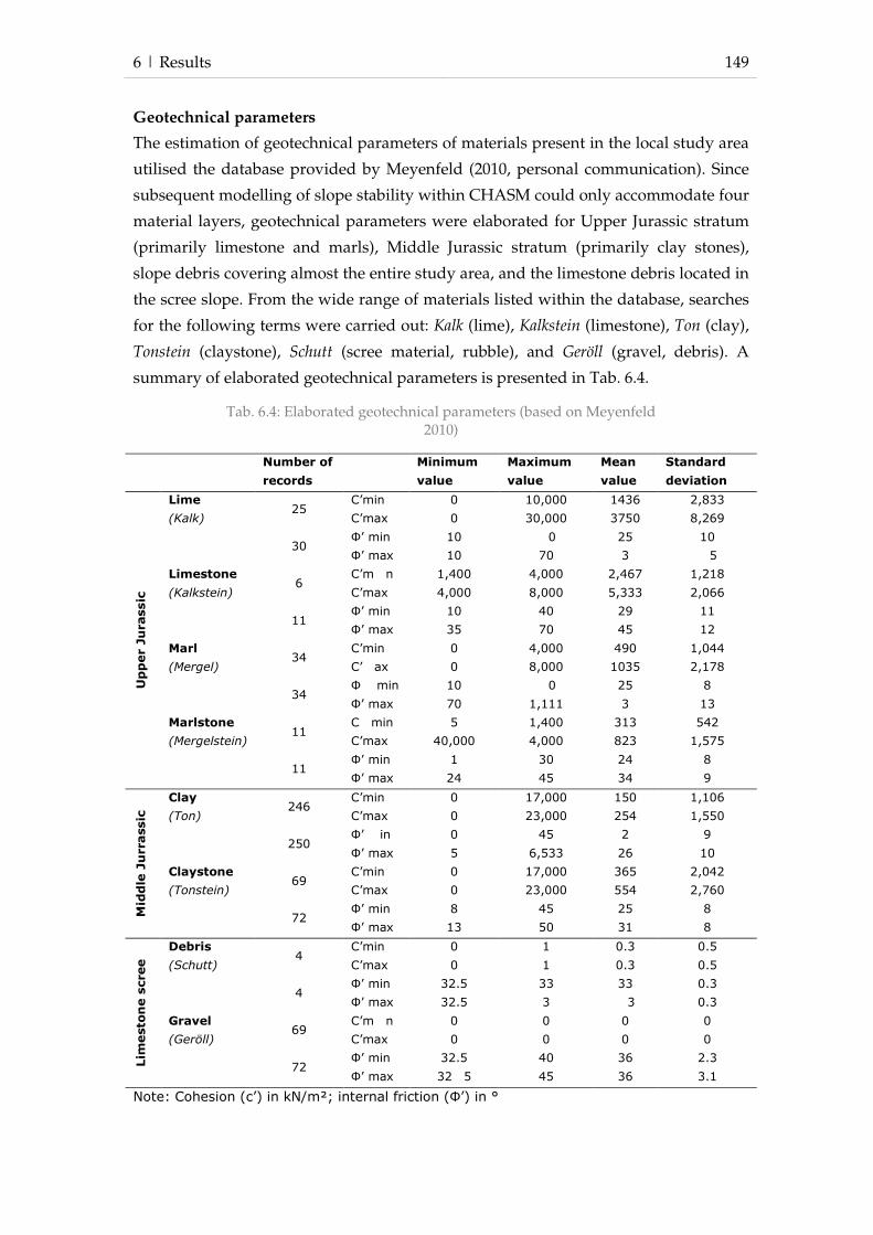
6 | Results 149
Geotechnical parameters
The estimation of geotechnical parameters of materials present in the local study area
utilised the database provided by Meyenfeld (2010, personal communication). Since
subsequent modelling of slope stability within CHASM could only accommodate four
material layers, geotechnical parameters were elaborated for Upper Jurassic stratum
(primarily limestone and marls), Middle Jurassic stratum (primarily clay stones),
slope debris covering almost the entire study area, and the limestone debris located in
the scree slope. From the wide range of materials listed within the database, searches
for the following terms were carried out: Kalk (lime), Kalkstein (limestone), Ton (clay),
Tonstein (claystone), Schutt (scree material, rubble), and Geröll (gravel, debris). A
summary of elaborated geotechnical parameters is presented in Tab. 6.4.
Tab. 6.4: Elaborated geotechnical parameters (based on Meyenfeld 2010)
Number of
records
Minimum
value
Maximum
value
Mean
value
Standard
deviation
Upper Jurassic
Lime 25
C’min 0 10,000 1436 2,833
(Kalk) C’max 0 30,000 3750 8,269
30
Φ’ min 10 0 25 10
Φ’ max 10 70 3 5
Limestone 6
C’m n 1,400 4,000 2,467 1,218
(Kalkstein) C’max 4,000 8,000 5,333 2,066
11
Φ’ min 10 40 29 11
Φ’ max 35 70 45 12
Marl 34
C’min 0 4,000 490 1,044
(Mergel) C’ ax 0 8,000 1035 2,178
34
Φ min 10 0 25 8
Φ’ max 70 1,111 3 13
Marlstone 11
C min 5 1,400 313 542
(Mergelstein) C’max 40,000 4,000 823 1,575
11
Φ’ min 1 30 24 8
Φ’ max 24 45 34 9
Middle Jurrassic
Clay 246
C’min 0 17,000 150 1,106
(Ton) C’max 0 23,000 254 1,550
250
Φ’ in 0 45 2 9
Φ’ max 5 6,533 26 10
Claystone 69
C’min 0 17,000 365 2,042
(Tonstein) C’max 0 23,000 554 2,760
72
Φ’ min 8 45 25 8
Φ’ max 13 50 31 8
Limestone scree
Debris 4
C’min 0 1 0.3 0.5
(Schutt) C’max 0 1 0.3 0.5
4
Φ’ min 32.5 33 33 0.3
Φ’ max 32.5 3 3 0.3
Gravel 69
C’m n 0 0 0 0
(Geröll) C’max 0 0 0 0
72
Φ’ min 32.5 40 36 2.3
Φ’ max 32 5 45 36 3.1
Note: Cohesion (c’) in kN/m²; internal friction (Φ’) in °

150 6 | Results
Search for the terms Kalk and Kalkstein, Mergel and Mergelstein delivered 30 and 34
records with information on cohesion or friction, respectively. However, some records
were excluded from the selection because they were judged inappropriate. Excluded
records include records describing for example, materials located in very deep under-
ground conditions (1000 m to 2000 m) and weathered debris. The parameter range for
both, cohesion and friction is very large. For example, records for Kalk contain mini-
mum cohesion values of 0 kN/m², and a maximum of 30,000 kN/m². The highest
number of records was available for Ton for and Tonstein with 250 and 72 records on
cohesion or friction, respectively. Again, the range of geotechnical parameters is very
large with cohesion varying between 0 kN/m² and 23,000 kN/m². Only a small num-
ber of records were found for Schutt and Geröll. In controversy to the previously de-
scribed search terms, parameters are less dispersed. Cohesion is very low for all re-
cords, ranging between 0 kN/m² and 1 kN/m² , and friction between 33° and
45°.Values of cohesion and internal friction for slope debris could not be elaborated
from the database but instead used typical values from literature, which were later
checked during sensitivity analysis.
Estimated values for cohesion and friction used for initial CHASM modelling are pre-
sented in Tab. 6.5. For estimation of geotechnical characteristics of the Upper Jurassic
layer, Kalkstein and Mergelstein records were preferred since they focus on intact rock
materials. Similar for Middle Jurassic, Tonstein was favoured since the Middle Jurassic
in the study area is covered by slope debris.
Tab. 6.5: Initial geotechnical values used for CHASM modelling
Upper Jurassic Middle Jurassic Debris Scree
Cohesion 300 1500 20 0
Internal friction 35 15 20 33
Ksat 1e-6 1e-9 6,78e-7 1e-1
Moisture Content (sat) 40.7 44.7 52.6 48.3
Bulk density(sat) 25 23 16 16
Bulk density (unsat) 23 21 15 15
CHASM also required determination of soil suction values and saturated moisture
content for materials involved in CHASM modelling. Values for these parameters
were elaborated based on the soil database integrated into the SPAW model (Saxton
and Rawls 2006). Even though, laboratory analysis provided some initial information
on soil suctions and related water contents (chapter 6.1.2.1), tests only involved a rela-
tively small range of suctions compared to CHASM requirements. Also, laboratory
suction analyses concerned only materials from slope debris, but not for the other
materials of the subsurface model. For landslide debris, mean values for clay, silt and
sand content were calculated from results of laboratory analysis and used as input for
SPAW. In addition, a relatively high gravel content of 40% was assumed, based on

6 | Results 151
experience during drilling and analysis of available borelogs. In comparison to the
soil suction data acquired in laboratory analyses, SPAW values describe significantly
higher water contents for the entire range of applied suctions. Soil suction behaviour
of the limestone scree material was elaborated using assumed values for grain size
distribution. High permeability was reflected by 96% sand content and 50% of gravel,
as well as a decreased compaction factor of 0.9. In comparison to limestone scree ma-
terial, Upper Jurassic material was assumed to be denser and less permeable. Soil suc-
tion curves were determined using assumed contents of 20% sand, 40% clay, no
gravel and dense compaction (1.1). Middle Jurassic materials were assumed to be
even less permeable, and soil suction curves were elaborated using 60% clay, 2%
sand, no gravel and maximum compaction (1.26). Resulting soil suction points for the
described materials are presented in Tab. 6.6.
Parameter values for hydraulic conductivity (Ksat) for the materials involved in
CHASM modelling used standard values provided in DIN standard (18130) and lit-
erature values (Bear 1972). For limestone scree material, a very high hydraulic con-
ductivity of 10-1 m/s was estimated, relating to pervious conditions similar to gravel.
The SPAW model was used to establish Ksat values for debris material. Hydraulic
conductivity of Upper Medium Jurassic materials were determined referring to pervi-
ous and semi-pervious materials, respectively. Estimated values for hydraulic con-
ductivity initially used for CHASM simulations are presented along with the other
geotechnical parameters in Tab. 6.5.
Tab. 6.6: Water content (in %) derived from SPAW model for suc-tions (pF) from -10 to -0.1
pF -10 -8 -6 -4 -3 -2 -1.6 -1.2 -0.8 -0.4 -0.2 -0.1
Scree 0.2 0.3 0.4 0.4 6.9 0.9 1.2 1.53 2.2 4 21.8 35.5
Debris 0 0 0 0 0 0 0 0 0 0 0 0
Upper
Jurassic 25.9 26.6 27.6 29.1 30.2 31.8 32.7 34 35.8 39.2 45.7 50
Middle
Jurassic 0 0 0 0 0 0 0 0 0 0 0 0
Groundwater scenarios
In Fig. 6.40, results of spatial interpolation of groundwater positions by Inverse Dis-
tance Weighting method are illustrated. In addition to the data points describing the
positions of hydrological monitoring sensors, several points were included to ensure a
smooth and more realistic interpolation of groundwater positions. For these,
groundwater table positions had to be assumed since no information was available.
Mean groundwater table positions for dry and wet seasons were assumed as 4 m and
6 m, respectively.
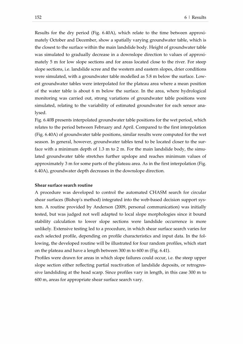
152 6 | Results
Results for the dry period (Fig. 6.40A), which relate to the time between approxi-
mately October and December, show a spatially varying groundwater table, which is
the closest to the surface within the main landslide body. Height of groundwater table
was simulated to gradually decrease in a downslope direction to values of approxi-
mately 5 m for low slope sections and for areas located close to the river. For steep
slope sections, i.e. landslide scree and the western and eastern slopes, drier conditions
were simulated, with a groundwater table modelled as 5.8 m below the surface. Low-
est groundwater tables were interpolated for the plateau area where a mean position
of the water table is about 6 m below the surface. In the area, where hydrological
monitoring was carried out, strong variations of groundwater table positions were
simulated, relating to the variability of estimated groundwater for each sensor ana-
lysed.
Fig. 6.40B presents interpolated groundwater table positions for the wet period, which
relates to the period between February and April. Compared to the first interpolation
(Fig. 6.40A) of groundwater table positions, similar results were computed for the wet
season. In general, however, groundwater tables tend to be located closer to the sur-
face with a minimum depth of 1.3 m to 2 m. For the main landslide body, the simu-
lated groundwater table stretches further upslope and reaches minimum values of
approximately 3 m for some parts of the plateau area. As in the first interpolation (Fig.
6.40A), groundwater depth decreases in the downslope direction.
Shear surface search routine
A procedure was developed to control the automated CHASM search for circular
shear surfaces (Bishop's method) integrated into the web-based decision support sys-
tem. A routine provided by Anderson (2009, personal communication) was initially
tested, but was judged not well adapted to local slope morphologies since it bound
stability calculation to lower slope sections were landslide occurrence is more
unlikely. Extensive testing led to a procedure, in which shear surface search varies for
each selected profile, depending on profile characteristics and input data. In the fol-
lowing, the developed routine will be illustrated for four random profiles, which start
on the plateau and have a length between 300 m to 600 m (Fig. 6.41).
Profiles were drawn for areas in which slope failures could occur, i.e. the steep upper
slope section either reflecting partial reactivation of landslide deposits, or retrogres-
sive landsliding at the head scarp. Since profiles vary in length, in this case 300 m to
600 m, areas for appropriate shear surface search vary.
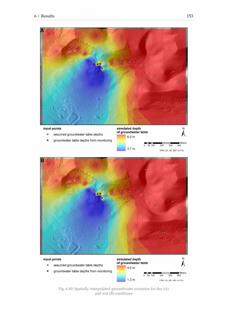
6 | Results 153
Fig. 6.40: Spatially interpolated groundwater scenarios for dry (A) and wet (B) conditions

154 6 | Results
Fig. 6.41: Random slope profiles between 300 m and 600 m long
Parallel to Andersons procedure, the position of the grid, in which the centres of ana-
lysed slip circles are located, were defined by geometrical characteristics of the ana-
lysed slope profile (slope length and height). For slope profiles shorter than 450 m, the
lower upslope corner of the search grid was defined at two-thirds of slope height and
half of slope length. Longer profiles used two-thirds of slope height and one-third of
slope length, effectively, moving the grid box further upslope. In Fig. 6.42 the four
profiles and the position of grid search box are illustrated along with resulting poten-
tial shear surfaces.
For the first two profiles, grid box is positioned at 50% of slope length, for profile 3
and 4, at one-third of profile length. For all profiles, potential shear surfaces reflect
slope failures within the head of former landslide deposits or within the steeper up-
slope area. Retrogressive failure at the plateau can only be analysed when very large
radiuses are used.
Apart from position of the grid search box, other settings included its spacing and
size, and the incremental increase of the search radius between iterations. The spacing
of the grid search box was set to the same dimension as the general mesh, relating to
the resolution of the DTM used for profile generation. Since the number of maximum
cells in CHASM simulations is limited to 300, maximum profile length is 300 m and
600 m for 1 m and 2 m DTM, respectively. The size of the grid search box was chosen
to be relatively large with 10 m by 10 m to increase the number of possible shear sur-
6 | Results 155
face locations. However, incremental increase of the radius between simulation steps
was set to a relatively high value of 1 m to limit the total number of iterations and
shorten simulation time.
Fig. 6.42: Position of slip search grid and respective possible shear surfaces

156 6 | Results
Rainfall scenarios
KOSTRA rainfall intensity probabilities were extracted for the grid cell containing the
local study area Lichtenstein-Unterhausen and subsequently used to derive CHASM
input files. To enhance the understanding of KOSTRA, spatial and temporal variabil-
ity of rainfall intensities were investigated. KOSTRA data in map format (Fig. 6.43)
shows, that the cell directly neighbouring the local study area to the west contains
higher rainfall intensities for many scenarios. Higher cumulative rainfall for this area
can be observed for all annual probabilities and storm durations. Largest deviations
can be identified for rainstorm events of long durations, where cumulative rainfall is
over 20% higher.
Comparison of summer (May to September) and winter (October to April) rainfall
intensities to the values of the entire year illustrate some interesting features. Summer
rainfall intensities are higher than winter rainfalls for almost all rainfall durations and
occurrence probabilities, with largest deviations occurring for short storm durations.
For these events summer rainfall intensities are up to 400% higher. Only for rainfall
events with 72 h duration and bi-annual probability slightly smaller (7%) rainfall in-
tensity is described by KOSTRA. KOSTRA rainfall intensities derived for the entire
year are the same as for the summer period for almost all rainfall durations and oc-
Fig. 6.43: KOSTRA rainfall intensities for 12 hour rainstorm with 1/10 year occurrence probability for Baden-Württemberg

6 | Results 157
currence probabilities, except for very long durations with high probability of occur-
rence (>1 per year). Winter rainfall intensities are in all cases lower than values for the
entire year, with largest deviations detectable for short duration scenarios (>80%).
Tab. 6.7: Cumulative rainfall (in mm) for normal, maximum value and worst case scenarios for return periods between 1 and 100 years
and storm duration between 1 hour and 72 hours
Normal values Maximum values Worst case
Return period in years
Duration in
hours
1 10 50 100
1 10 50 100
1 10 50 100
1 18 37 50 56 18 38 52 58 20 44 60 70
6 27 48 63 69 29 51 66 73 31 58 76 87
12 32 54 69 75 34 57 73 80 37 66 84 96
24 38 64 82 90 40 70 91 100 44 81 105 120
48 45 73 92 100 50 80 101 110 55 92 116 132
72 55 83 102 110 60 90 111 120 66 104 128 144
KOSTRA was used to derive rainfall intensity probabilities for storm durations of 1, 6,
12, 24, 48 and 72 hours, and for return periods of 1, 10, 50 and 100 years (Tab. 6.7).
Moreover, standard parameter values within CHASM were altered to derive maxi-
mum value scenarios, and uncertainties were integrated as additional rainfall within
worst case scenarios. Maximum value scenarios differ from normal value scenarios
between approximately 1% and over 11%, with largest deviations occurring for long
duration rainstorm events. Worst case scenarios include the fixed uncertainties de-
scribed within KOSTRA which range between 10 and 20% depending on probability
of occurrence. In comparison to normal values maximum values and uncertainties
add up to an increased cumulative rainfall of over 30% for long duration and low an-
nual probability scenarios.
Scenarios with varying intensities over the course of a rainfall event were created to
describe storm characteristics more realistically. KOSTRA includes Euler1 and Euler2
model rainstorms only for rainfall duration ≤12 h; for longer storms, rainfall intensity
distributions were computed manually. Fig. 6.44 exemplifies the differences between
scenarios of even intensity distributions to Euler1 and Euler2 scenarios. Euler1 scenar-
ios start with a very high rainfall peak which is followed by an even decrease of
hourly intensities. In contrast, Euler2 scenarios reach highest hourly intensities after
one third of the storm duration.
A total number of 192 rainfall scenarios were created for subsequent use in CHASM
and the web-based applications of slope stability assessment. All scenarios were
transferred to text-files conform to CHASM requirements. In these files, onset of rain-
storm in relation to CHASM simulation length had to be defined. After thorough test-
ing of CHASM (chapter 6.1.3.2), onset of rainfall was set to hour 10.
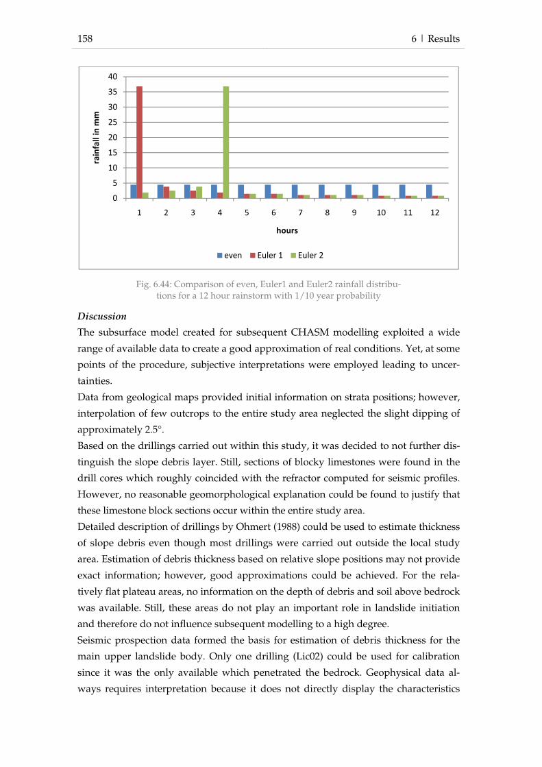
158 6 | Results
Fig. 6.44: Comparison of even, Euler1 and Euler2 rainfall distribu-tions for a 12 hour rainstorm with 1/10 year probability
Discussion
The subsurface model created for subsequent CHASM modelling exploited a wide
range of available data to create a good approximation of real conditions. Yet, at some
points of the procedure, subjective interpretations were employed leading to uncer-
tainties.
Data from geological maps provided initial information on strata positions; however,
interpolation of few outcrops to the entire study area neglected the slight dipping of
approximately 2.5°.
Based on the drillings carried out within this study, it was decided to not further dis-
tinguish the slope debris layer. Still, sections of blocky limestones were found in the
drill cores which roughly coincided with the refractor computed for seismic profiles.
However, no reasonable geomorphological explanation could be found to justify that
these limestone block sections occur within the entire study area.
Detailed description of drillings by Ohmert (1988) could be used to estimate thickness
of slope debris even though most drillings were carried out outside the local study
area. Estimation of debris thickness based on relative slope positions may not provide
exact information; however, good approximations could be achieved. For the rela-
tively flat plateau areas, no information on the depth of debris and soil above bedrock
was available. Still, these areas do not play an important role in landslide initiation
and therefore do not influence subsequent modelling to a high degree.
Seismic prospection data formed the basis for estimation of debris thickness for the
main upper landslide body. Only one drilling (Lic02) could be used for calibration
since it was the only available which penetrated the bedrock. Geophysical data al-
ways requires interpretation because it does not directly display the characteristics
0
5
10
15
20
25
30
35
40
1 2 3 4 5 6 7 8 9 10 11 12
rain
fall
in
mm
hours
even Euler 1 Euler 2
6 | Results 159
analysed, which in this study was position of bedrock, but geophysical conditions
which can be used as proxy information. Uncertainties related to the use of seismic
data in this study can be estimated preliminarily by comparison of single inversion
plots along the same profile. Therein, measured seismic velocity can differ signifi-
cantly which relates to differences of bedrock position of several meters. Still, at four
intersections of the available seismic profiles estimated bedrock depths could be com-
pared and resulted in similar debris thickness. Interpretation of bedrock depths based
on seismic data would benefit from additional drillings to exactly determine the
depth of bedrock and calibrate measured seismic velocities.
The GIS procedure to assess the thickness of landslide deposits in the lower landslide
body was carried out iteratively. Simple TIN creation could not be applied to create a
realistic representation of real conditions. Addition of results from topographic analy-
sis of deposits’ height significantly improved delineation of the landslide deposits.
Though, assessment of landslide deposits’ depths is more uncertain for areas further
away from the landslide boundaries.
Final interpolation of the slope debris layer resulted in relatively realistic depths for
the areas most important for potential landslide initiation.
Geotechnical parameterisation subsurface material required interpretation and subjec-
tive judgement since the range of values described in literature sources is very large.
Still, the best-fitting parameter settings were also chosen with respect to their influ-
ence on slope stability modelling assessed during subsequent sensitivity analysis.
Further shear tests could help to minimise uncertainties associated with the use of
literature values of geotechnical parameters.
Spatial interpolation of groundwater tables for the entire local study area relied on a
limited number of hydrological sensors, which exhibited a great variety even though
sensors were located relatively close to each other. For large parts of the local study
area, no monitoring data was available and interpolation of groundwater table posi-
tions required addition of assumed water table heights. Since spatial interpolation
neglected process simulation but rather relied on general spatial interpolation tech-
niques, results lack a physically based justification. Still, this kind of interpolation
would require more detailed information on subsurface conditions, such as material
properties and preferential flow paths that would require much more intense field
surveys. Estimation of the influence of uncertainties inherent in the applied method-
ology requires detailed analysis within CHASM. Altogether, the groundwater scenar-
ios can be assumed to be good approximations of real conditions for the area in which
hydrological monitoring was carried out, which is also the most important for slope
stability analysis. For other areas, estimated groundwater scenarios are more specula-
tive.
160 6 | Results
The developed shear surface search routine effectively concentrates search procedure
to the upper slope areas, which are assumed to be most likely influenced by potential
landslide initiation. In order to increase the modelling speed it was necessary to limit
the number of potential shear surfaces analysed by the search procedure. The devel-
oped procedure reduces the number of possible shear surface positions by a relatively
large radius increment of Bishop’s shear circles, while at the same time allowing for a
large number of possible positions in a horizontal direction. By the current settings,
shear surfaces are primarily assumed to be located in the upper slope areas reflecting
potential reactivation of at least parts of the landslide deposits. Retrogressive slope
failures involving the massive Upper Jurassic limestone can also be modelled, how-
ever, they were not given priority in this work. Since only circular shear surfaces are
integrated, more complex landslide morphologies can not adequately be recognised
by the shear surface search.
The shear surface search procedure is adjusted to the slope morphology in the local
study area and can not be transferred to other areas without further modifications.
Further improvements of the developed shear surface search procedure could employ
additional threshold values, to enhance the positioning of the grid search box depend-
ing on profile lengths.
In this study, rainfall events were deduced from the KOSTRA atlas, which represents
the most advanced available data source for precipitation intensity probabilities. Still,
data is only available for 8.45 km x 8.45 km grid cells and therefore includes simplifi-
cations. For example, local topography, which can have a significant influence on
rainfall distributions as illustrated in this thesis, is only regarded for the relatively
large grid cells. Comparison to neighbouring grid cells shows that rainfall could po-
tentially be higher.
In addition, snow melt is not included in KOSTRA data. However, uncertainties in-
herent in KOSTRA included as additional precipitation in this study can also be re-
garded as the effect of snow melting.
Integration of Euler 1 and Euler 2 rainfall scenarios aimed to include more realistic
rainfall distributions with distinct peak rainfalls.
6.1.3.2 Model application
Modelling slope stability with CHASM mostly focussed on the longitudinal slope
profile on which four hydrological monitoring sites and geoelectrical monitoring are
located. Also, the house experiencing damage due to slope movements is located
along the profile. The position of the main profile and its subsurface conditions are
illustrated in Fig. 6.45. Other slope profiles were also tested, however, since modelling
results did not significantly differ from the main profile, they will not be presented
herein.
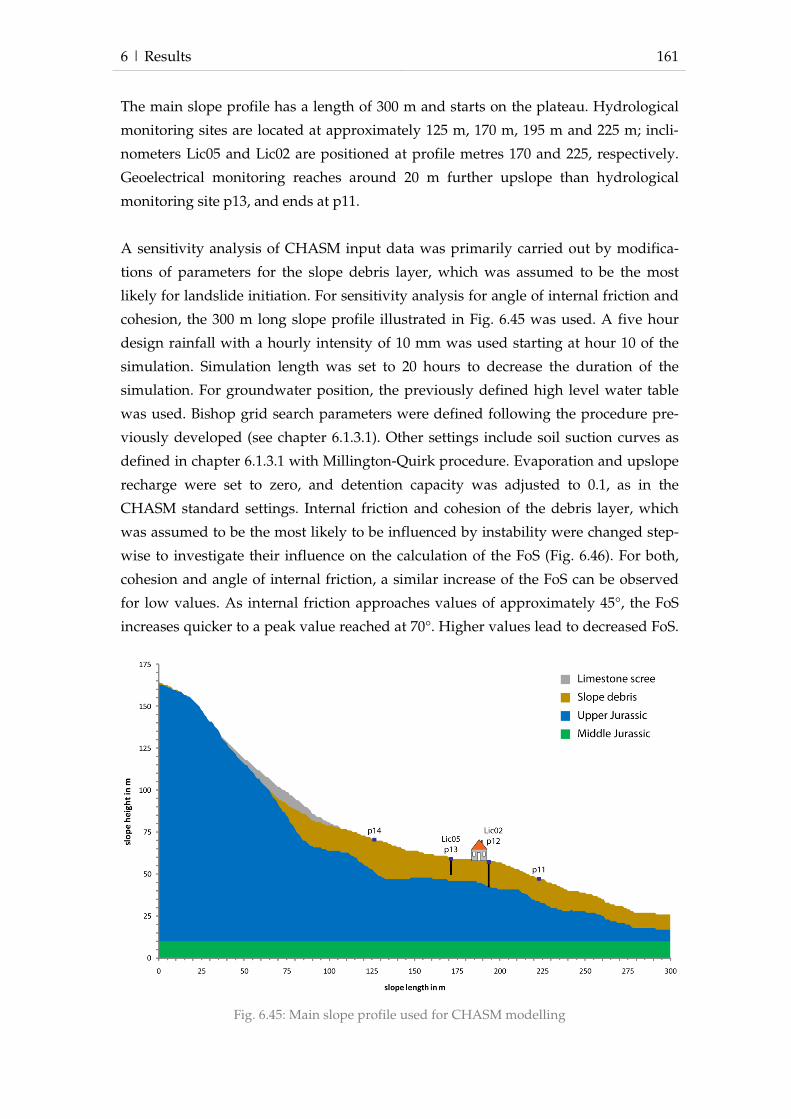
6 | Results 161
The main slope profile has a length of 300 m and starts on the plateau. Hydrological
monitoring sites are located at approximately 125 m, 170 m, 195 m and 225 m; incli-
nometers Lic05 and Lic02 are positioned at profile metres 170 and 225, respectively.
Geoelectrical monitoring reaches around 20 m further upslope than hydrological
monitoring site p13, and ends at p11.
A sensitivity analysis of CHASM input data was primarily carried out by modifica-
tions of parameters for the slope debris layer, which was assumed to be the most
likely for landslide initiation. For sensitivity analysis for angle of internal friction and
cohesion, the 300 m long slope profile illustrated in Fig. 6.45 was used. A five hour
design rainfall with a hourly intensity of 10 mm was used starting at hour 10 of the
simulation. Simulation length was set to 20 hours to decrease the duration of the
simulation. For groundwater position, the previously defined high level water table
was used. Bishop grid search parameters were defined following the procedure pre-
viously developed (see chapter 6.1.3.1). Other settings include soil suction curves as
defined in chapter 6.1.3.1 with Millington-Quirk procedure. Evaporation and upslope
recharge were set to zero, and detention capacity was adjusted to 0.1, as in the
CHASM standard settings. Internal friction and cohesion of the debris layer, which
was assumed to be the most likely to be influenced by instability were changed step-
wise to investigate their influence on the calculation of the FoS (Fig. 6.46). For both,
cohesion and angle of internal friction, a similar increase of the FoS can be observed
for low values. As internal friction approaches values of approximately 45°, the FoS
increases quicker to a peak value reached at 70°. Higher values lead to decreased FoS.
Fig. 6.45: Main slope profile used for CHASM modelling

162 6 | Results
The linear rise of the FoS with increasing cohesion values continues until values of 85,
and larger values do not influence the FoS.
CHASM sensitivity to changed hydraulic conductivity values could not be tested the
same way as for cohesion and internal friction, since not only Ksat values of the poten-
tially unstable debris layer influences the results, but also the hydraulic conductivity
of the other material layers. In addition, hydraulic conductivity parameter values
stretch over several orders of magnitudes, leading to an infinite number of possible
combinations of Ksat values for all materials involved in modelling. Several combina-
tions of hydraulic conductivity values for debris and the Upper Jurassic material be-
low were tested with a wide range of rainfall scenarios and groundwater scenarios. In
Tab. 6.8, a selection of hydraulic conductivity scenarios modelled is presented. In all
these scenarios except for the first one, the Upper Jurassic layer has a lower hydraulic
conductivity than for the slope debris layer to allow for an increase of pore water
pressures above the bedrock. For the other settings of CHASM, the same values were
applied as in the previous model run. CHASM results using a range of hydraulic con-
ductivity scenarios are presented in Fig. 6.47.
Fig. 6.46: Sensitivity analysis for cohesion and angle of internal fric-tion
Tab. 6.8: Ksat scenarios used for sensitivity analysis
Limestone scree Slope debris Upper Jurassic Middle Jurassic
Scenario 1 1e-1 6.78e-7 1e-6 1e-9
Scenario 2 1e-1 6.78e-6 1e-7 1e-9
Scenario 3 1e-1 6.78e-5 1e-6 1e-9
Scenario 4 1e-1 6.78e-5 1e-7 1e-9
Scenario 5 1e-1 6.78e-7 1e-8 1e-9
Scenario 6 1e-1 6.78e-6 1e-8 1e-9
0
0.5
1
1.5
2
2.5
3
3.5
0 20 40 60 80 100
Fo
S
parameter values
Internal friction Cohesion

6 | Results 163
Fig. 6.47: Sensitivity analysis for Ksat scenarios
In all scenarios, the FoS is on a similar level of approximately 1.12 at the beginning of
the simulation run. From hour 5 on, general trends can be observed. For scenarios 1, 2
and 6, the FoS gradually decreases until the end of the simulation. Scenario 5 how-
ever, shows an increase of stability with and no destabilising effect of the rainfall
event. Results of scenario 3 and 4 show an increasing FoS for the initial hours of the
simulation which then drops during the rainfall event. For further modelling and
subsequent early warning modelling, Ksat values from scenario 2 were selected.
Since soil moisture curve points used for CHASM modelling were not determined by
detailed laboratory analysis but by the SPAW model, the influence of this input pa-
rameter on stability calculation was examined. The limited number of records on
pressures and related water content from laboratory analysis were interpolated to the
range required for CHASM analysis, and then used for modelling. These values are
significantly lower with water contents approximately 40% to 50% lower than esti-
mated from SPAW. Estimated values are presented in the appendix X and results of
CHASM simulation are illustrated in Fig. 6.48. The largest differences between the
model runs can be observed in the initial hours of the simulations. Over the course of
the simulation, the graphs gradually converge and reach a similar FoS level of ap-
proximately 1.05 towards the end. During the initial three hours of the rainfall event
the FoS slightly increases, before dropping to lower values for approximately 10
hours.
0
2
4
6
8
10
12
1
1.05
1.1
1.15
1.2
0 5 10 15 20
rain
fall
in
mm
Fo
S
hour of simulation
rainfall 1 2 3 4 5 6

164 6 | Results
Fig. 6.48: Comparison of modelled FoS using soil suction curves es-timated from SPAW model and interpolated laboratory values
The influence of groundwater positions on CHASM stability calculation was tested
for the elaborated high and low groundwater scenarios (see chapter 6.1.3.1), and also
for various designed scenarios in which groundwater was assumed to be located at an
equal depth below the surface. Results of CHASM modelling using high and low
groundwater table scenarios, and artificial groundwater positions of 2 m and 5 m be-
low the surface are presented Fig. 6.49. These simulations were carried out with all
other settings being the same as in the previous simulations. The high groundwater
scenario and the even 2 m below surface setting both result in very similar FoS of ap-
proximately 1.1 in the beginning of the simulation, and gradually decreasing to values
of 1.06 towards the end. Lower groundwater tables, i.e. low groundwater scenario
0
2
4
6
8
10
12
1
1.05
1.1
1.15
1.2
0 5 10 15 20 25 30
rain
fall
in
mm
Fo
S
hour of simulation
rainfall SPAW vlaues interpolated values
Fig. 6.49: Comparison of modelled FoS using high and low groundwater table scenarios
0
2
4
6
8
10
12
1
1.1
1.2
1.3
1.4
1.5
0 5 10 15 20 25 30
rain
fall
in
mm
Fo
S
hour of simulation
rainfall high groundwater low groundwater
5 m below surface 2 m below surface

6 | Results 165
and the designed groundwater scenario with an equal depth of groundwater of 5 m
below the surface, result in higher FoS which decrease during the entire the simula-
tion. No significant accelerated decrease of the FoS can be observed during the rainfall
event.
Several potential shear surface positions were investigated within this study. In Fig.
6.50, a selection of four analysed slip surfaces is presented in which the Bishop
method integrated in CHASM was used. For the upper most shear surface (green),
indicating a initiation of a slope failure below the scree slope a FoS of 0.78 and 0.75
with low and high groundwater table scenarios was calculated, respectively. The slip
surface located further downslope (pink), starting at the lower end of the scree slope,
resulted in a FoS of 1.52 and 1.4 for low and high groundwater scenarios, respectively.
For the third slip surface (yellow), with a shear plane affecting the house at its lower
end, a FoS of 1.15 for low groundwater conditions, and 1.05 using the high groundwa-
ter positions was simulated. This shear surface was also the same, which was used for
previous CHASM simulations and is the result of shear surface definitions described
in chapter 6.1.3.1. The highest FoS was calculated for the potential shear surface lo-
cated below the damaged house (teal). For low groundwater conditions, the FoS was
simulated as 1.78, and 1.61 using the high groundwater scenario. Other shear surfaces
not displayed here were also tested, including failures comprising bedrock. However,
the FoS for such shear surfaces was significantly higher with FoS values between 3.0
to over 6.0.
Fig. 6.50: Locations of selected potential shear surfaces

166 6 | Results
The influence of rainfall events on slope stability was tested with several rainfall dis-
tribution and intensities. In the following, results of three rainfall events with differ-
ent distributions of rainfall intensities will be presented (Fig. 6.51). Therein, Euler 1
and 2 rainfall events are compared to a block rainfall using previous CHASM setting
and the high groundwater scenario. All rainfall scenarios comprise the same sum and
only differ in their hourly distribution. For this comparison, the 24 hour rainfall was
used with an annual occurrence probability of 100 years. In all scenarios, rainfall
commenced at hour 10 of simulation and lasted until hour 34. The block rainfall has a
steady precipitation intensity of 3.8 mm/h. The Euler 1 scenario has a hourly maxi-
mum intensities of 56 mm and 44 mm in the first and second hours of the rainfall
event, respectively. Afterwards, rainfall continues with relatively low hourly intensi-
ties of 1.25 mm/h for the rest of the simulation. Similarly, the Euler 2 rainfall has dis-
tinct precipitation peaks, however, these occurs in hour 7 and 8.
Fig. 6.51: Rainfall distribution for Euler 1, Euler 2 and block rainfall events (A) and resulting FoS (B)
0
20
40
60
rain
fall
in
mm
Euler 1 Euler 2 block rain
1
1.05
1.1
1.15
0 5 10 15 20 25 30 35 40
Fo
S
hour of simulation
Euler1 Euler2 block rain
A
B

6 | Results 167
The course of the graphs is identical until hour 10 of the simulation, when the rain-
storm commences. Euler 1 rainfall (blue line) shows the lowest FoS at hour 16 of the
simulation caused by the high intensity rainfall occurring in the first two hours of the
rainfall event. A similar drop of FoS can not be observed for the Euler 2 (red line)
which has its maximum intensity at hour seven to eight. Between hour 20 and 24, the
lowest FoS can be observed for the block rain with constant hourly rainfall intensity.
For the later simulation time, all tested rainfall distributions result in similar FoS of
approximately 1.05. Overall, only very small deviations of the FoS between the simu-
lation runs using different rainfall distributions can be observed documenting to a
relatively low sensitivity to rainfall distributions.
Normal, maximum value and worst-case rainfall scenarios derived from KOSTRA
were also tested for their influence on slope stability calculation in CHASM. Fig. 6.52
shows the CHASM results using a 24 hour duration rainfall with annual occurrence
probability of 100 years beginning at hour 10 of the simulation. Total rainfall for these
scenarios is 91.2 mm, 100.8 mm and 120 mm for normal, maximum value and worst-
case rainfall scenarios, respectively.
Fig. 6.52: Comparison of modelled FoS using normal, maximum and worst-case scenario rainfall events
Until hour 10 of the simulation, when rainfall commences, FoS for all model runs is
the same in all simulations. Afterwards, the worst-case scenario shows slightly lower
FoS values for the following seven hours; however, the difference between the model
runs is very small with FoS deviations of approximately 0.05. For the rest of the
CHASM simulation, all three simulations produced very similar FoS values with only
1.02
1.04
1.06
1.08
1.1
1.12
1.14
1.16
0 5 10 15 20 25 30 35 40
Fo
S
hour of simulation
normal values maximum value worst-case values
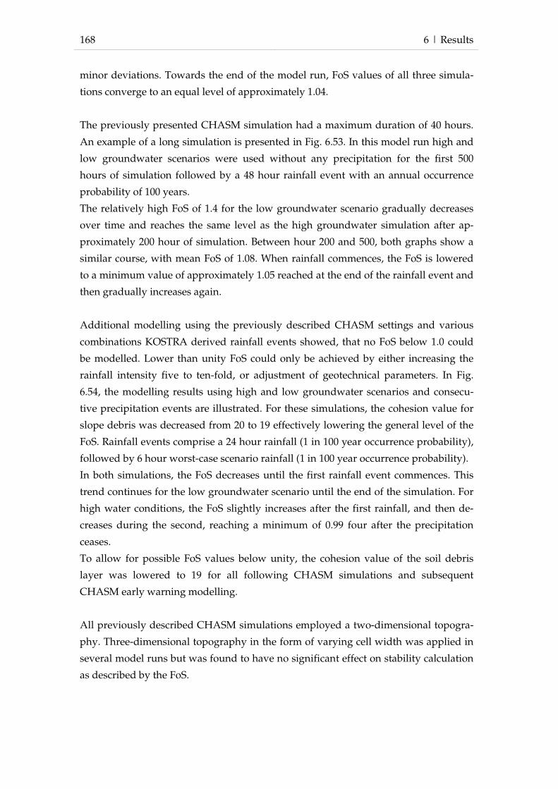
168 6 | Results
minor deviations. Towards the end of the model run, FoS values of all three simula-
tions converge to an equal level of approximately 1.04.
The previously presented CHASM simulation had a maximum duration of 40 hours.
An example of a long simulation is presented in Fig. 6.53. In this model run high and
low groundwater scenarios were used without any precipitation for the first 500
hours of simulation followed by a 48 hour rainfall event with an annual occurrence
probability of 100 years.
The relatively high FoS of 1.4 for the low groundwater scenario gradually decreases
over time and reaches the same level as the high groundwater simulation after ap-
proximately 200 hour of simulation. Between hour 200 and 500, both graphs show a
similar course, with mean FoS of 1.08. When rainfall commences, the FoS is lowered
to a minimum value of approximately 1.05 reached at the end of the rainfall event and
then gradually increases again.
Additional modelling using the previously described CHASM settings and various
combinations KOSTRA derived rainfall events showed, that no FoS below 1.0 could
be modelled. Lower than unity FoS could only be achieved by either increasing the
rainfall intensity five to ten-fold, or adjustment of geotechnical parameters. In Fig.
6.54, the modelling results using high and low groundwater scenarios and consecu-
tive precipitation events are illustrated. For these simulations, the cohesion value for
slope debris was decreased from 20 to 19 effectively lowering the general level of the
FoS. Rainfall events comprise a 24 hour rainfall (1 in 100 year occurrence probability),
followed by 6 hour worst-case scenario rainfall (1 in 100 year occurrence probability).
In both simulations, the FoS decreases until the first rainfall event commences. This
trend continues for the low groundwater scenario until the end of the simulation. For
high water conditions, the FoS slightly increases after the first rainfall, and then de-
creases during the second, reaching a minimum of 0.99 four after the precipitation
ceases.
To allow for possible FoS values below unity, the cohesion value of the soil debris
layer was lowered to 19 for all following CHASM simulations and subsequent
CHASM early warning modelling.
All previously described CHASM simulations employed a two-dimensional topogra-
phy. Three-dimensional topography in the form of varying cell width was applied in
several model runs but was found to have no significant effect on stability calculation
as described by the FoS.

6 | Results 169
For most simulations, only the FoS as the prime output of CHASM simulation was
analysed. However, CHASM also provides hydrological results, i.e. soil moisture con-
tent and pore water pressures for each cell, which can be exported for single-time
steps as graphic or text files. Since analysis of hydrological results for long slope pro-
files is very time-intensive, this was only done for few simulations. Hydrological re-
sults for most modelled CHASM scenarios illustrate fully saturated conditions for all
but the top cells, for which the saturation gradually increases during rainfall events.
Fig. 6.53: Long duration simulation of slope stability using high and low groundwater scenarios and a 1 in 100 years rainfall with 48 hour
duration
Fig. 6.54: Comparison of modelled FoS using high and low groundwater scenarios and two
consecutive rainfall events
0
1
2
3
1
1.1
1.2
1.3
1.4
0 100 200 300 400 500 600
rain
fall
in
mm
Fo
S
hour of simulation
rainfall low groundwater scenario high groundwater scenario
0
1
2
3
4
0.95
1
1.05
1.1
1.15
1.2
1.25
1.3
1.35
0 10 20 30 40 50 60 70
rain
fall
in
mm
Fo
S
hour of simulation
rainfall high ground water low groundwater

170 6 | Results
Discussion
Sensitivity analysis of geotechnical parameters yielded some interesting results which
help to estimate the influence of the respective factors. Cohesion and angle of internal
friction have a similarly strong linear influence on CHASM stability calculation. Hy-
draulic conductivity (Ksat) is an important factor which strongly controls simulation of
the FoS. If these values are not carefully chosen, hydrological simulations can not re-
sult in positive pore pressures essential for destabilisation. Soil moisture curves and
groundwater table positions have a strong effect on stability calculation, however,
during long duration simulations the differences gradually level out.
All modelled slope profiles and shear surface positions show low FoS values illustrat-
ing potential slope failure. The lowest stability was calculated for the upper slope
area. CHASM results demonstrate that potential shear surfaces are most likely located
at the interface of slope debris and the underlying bedrock. Shear surfaces also includ-
ing bedrock material have a significantly higher FoS and no CHASM simulation pro-
duced shear surfaces within the debris material. CHASM simulations therefore reflect
deep-seated sliding slope movements as monitored in Lic02 inclinometer, which have
a depth of approximately 15.5 m at this point. The shallower displacements recorded
in approximately 8.5 m depth, which shows characteristics of a flowing movements
and possibly the progressive development of a shear surface, is not detected by
CHASM simulations. Still, limit-equilibrium analysis can only be used to simulate
failure processes, in which a rigid body slides along a shear surface, so progressive
failure, flow processes and slow creep of material can not be modelled.
A very low influence of rainfall in general, and specifically for rainfall distributions
and intensities is documented by the CHASM simulation results. Even very high pre-
cipitation events do not significantly lower the FoS. A possible explanation for the low
influence of rainfall on CHASM stability calculation might be that the model is often
used in tropical and sub-tropical environments and is possibly optimised for excep-
tionally strong rainfall. FoS values lower than 1.0, which in theory represent the initia-
tion of slope movements, can only be simulated by modified geotechnical parameters,
high groundwater conditions, and strong consecutive rainfall events.
6.1.3.3 CHASM early warning model
In the following, the general procedure and technical implementation of the web-
processing service application of CHASM for local landslide early warning is pre-
sented. The CHASM early warning model is a result of the work presented before,
and the technical implementation carried out by the ILEWS project partner Geomer
(Jäger et al. 2010).
The developed CHASM landslide early warning system uses a combination of fixed
and variable data inputs to simulate hydrological processes and their influence on
slope stability for one profile every 24 hours. An overview on the CHASM early
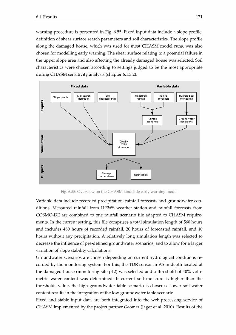
6 | Results 171
warning procedure is presented in Fig. 6.55. Fixed input data include a slope profile,
definition of shear surface search parameters and soil characteristics. The slope profile
along the damaged house, which was used for most CHASM model runs, was also
chosen for modelling early warning. The shear surface relating to a potential failure in
the upper slope area and also affecting the already damaged house was selected. Soil
characteristics were chosen according to settings judged to be the most appropriate
during CHASM sensitivity analysis (chapter 6.1.3.2).
Fig. 6.55: Overview on the CHASM landslide early warning model
Variable data include recorded precipitation, rainfall forecasts and groundwater con-
ditions. Measured rainfall from ILEWS weather station and rainfall forecasts from
COSMO-DE are combined to one rainfall scenario file adapted to CHASM require-
ments. In the current setting, this file comprises a total simulation length of 560 hours
and includes 480 hours of recorded rainfall, 20 hours of forecasted rainfall, and 10
hours without any precipitation. A relatively long simulation length was selected to
decrease the influence of pre-defined groundwater scenarios, and to allow for a larger
variation of slope stability calculations.
Groundwater scenarios are chosen depending on current hydrological conditions re-
corded by the monitoring system. For this, the TDR sensor in 9.5 m depth located at
the damaged house (monitoring site p12) was selected and a threshold of 40% volu-
metric water content was determined. If current soil moisture is higher than the
thresholds value, the high groundwater table scenario is chosen; a lower soil water
content results in the integration of the low groundwater table scenario.
Fixed and stable input data are both integrated into the web-processing service of
CHASM implemented by the project partner Geomer (Jäger et al. 2010). Results of the

172 6 | Results
simulation are stored in the database for later access. CHASM early warning model-
ling is connected to an alarm sensor on the ILEWS website which changes its status
depending on the results of the simulation and provides notification to involved ex-
perts. More detailed information on ILEWS alarm sensors and subsequent issuing of
early warnings is provided in chapter 7. However, since no real-time data is available
on rainfall forecasts the connection to the alarm sensor is currently disabled.
Discussion
The developed prototypic CHASM early warning model applies the program fixed
settings found to be the most appropriate during earlier model application and sensi-
tivity analysis. Variable input data for early warning modelling combines measured
and forecasted rainfall into one CHASM readable scenario file.
Groundwater scenarios depend on hydrological monitoring data, however, in a sim-
plified form of minimum and maximum scenarios. Direct integration of each hydro-
logical sensors’ measurements are hindered by CHASM structure, which can only
accommodate simplified groundwater conditions. Complex groundwater conditions,
for example increasing groundwater positions in a downslope direction, and prefer-
ential flow paths can not be represented. Still, determination of an exact groundwater
table position based on hydrological monitoring is difficult and can not be carried out
without subjective interpretation (see chapter 6.1.2.3). Without further modifications
of CHASM, improvements of the integration of groundwater conditions can mainly
be achieved by the addition of more groundwater scenarios and respective threshold
determination. To decrease the influence of simplified groundwater conditions, a long
duration for early warning modelling was selected.
The developed CHASM early warning model procedure represents a prototypic de-
velopment, which at the moment can only provide theoretical early warnings. How-
ever, if local stakeholders demand realistic early warning, the technical system can be
adjusted with little efforts.
The notification service set-up by Jäger et al. (2010) to inform the involved experts on
potentially dangerous slope stability changes is based on CHASM modelling results.
Still, without the possibility to validate CHASM simulation with real slope displace-
ment events, the notification thresholds can only be determined hypothetically.
6.1.3.4 CHASM decision-support tool
The web-based CHASM decision-support tool was developed to be able to quickly
assess slope stability for freely selectable profiles using a variety of input parameters.
The general procedure is a results of this work, technical implementation, however,
was carried out by the ILEWS project partner Geomer (Jäger et al. 2010). A graphical
overview on the developed CHASM decision-support web-processing service appli-

6 | Results 173
cation is presented in Fig. 6.56. Screenshots of each step of the web-based CHASM
simulation are presented in Fig. 6.57.
Fig. 6.56: Overview on the CHASM decision-support application
The slope profile for which stability is to be calculated can be selected by clicking on
the DTM of the local study area (1). Automatically, the CHASM slope file is produced
taking into account the simplified subsurface model with a two metre resolution. Ac-
cording to profile length, the slip surface search (chapter 6.1.3.1) is selected. In the
next step (2), the user can enter a name for the simulation and set model parameters,
i.e. simulation length and iteration period. All rainfall scenarios derived from
KOSTRA can be selected for slope stability calculation from a drop down menu (3).
Currently, all rainfall events start at the hour 10 of the simulation. High and low
groundwater scenarios are available as input data. For soil characteristics, either the
CHASM standard parameter or the parameter values developed in this study can be
chosen. CHASM is executed on the ILEWS server and takes approximately one min-
ute for most simulations (4). The selected slope profile is colour-coded according to
the simulated FoS of the last hour of the simulation, with green for FoS larger than 1.3,
orange for FoS between 1.0 and 1.3, and red for FoS lower than 1.0 (5). Further infor-
mation, for example, the course of the FoS throughout the simulation or the position
of the shear surface can be accessed (6). In addition, all previous simulations are
stored in the database can be selected for analysis. Sample results are presented in
screenshots 7 and 8. Therein, rainfall is marked as a blue area and the course of the
FoS can be viewed. While in the first of these figures, the FoS decreases during rainfall
and stabilises afterwards, the second graph drops to much lower values for some
steps of the simulation. This was found to be related to a changed position of shear
surfaces parameters in the respective time-steps of the simulation.

174 6 | Results
1
2
3

6 | Results 175
4
5
6

176 6 | Results
Fig. 6.57: Screenshots of the web-based implementation of the
CHASM decision-support application (DTM: LGL AZ: 2851.9-1/19)
The CHASM decision-support application is available in German and English lan-
guage. In addition, a bilingual step-by-step tutorial explaining the functionality of the
service and basic terms of slope stability calculation were developed to increase us-
ability (see Appendix XII to Appendix XV).
Discussion
The aim of the CHASM decision-support system was to allow quick calculation of
slope stability without the need to elaborate slope profile and shear surface definition
files. It was not the goal to convert the entire CHASM stability software into a web-
based simulation program; however, if this is demanded by the CHASM developers,
further works could be based on the work described in this thesis. In addition to the
previously described uncertainties inherent in CHASM modelling, the developed
CHASM decision-support system is subject to uncertainties arising from automated
7
8

6 | Results 177
shear surface search which causes the slip search to be located at different positions
for some hours of the simulation.
Concluding the results of this work, it can be noted, that the developed CHASM deci-
sion-support system enables quick judgement on slope stability for various slope pro-
files and variable input data. This can be potentially of great help to stakeholders that
require assessing slope stability situation for larger areas in a short amount of time.
However, the slope under investigation did not show any significant phase of in-
creased movement speed and CHASM simulations could not be sufficiently vali-
dated. Application of the decision-support system in more active study areas could
improve the overall performance and aid to assess its value in the context of landslide
risk management and early warning.
6.2 REGIONAL SCALE
6.2.1 Inventory analysis
Not all landslide inventories available for the Swabian Alb could be employed for
verification of rainfall thresholds because they did not meet the defined criteria.
The general landslide map by Kallinich (1999) provides extensive information on the
spatial distribution of slope failures, but does not contain information on the date of
occurrence.
The Tübingen University inventory contains over 600 landslide events and informa-
tion about geological and geomorphological characteristics of slope failure sites.
However, only for a fraction of 36 events the date of occurrence is acknowledged.
Earliest records date back to 1851; still, the majority of landslide took place in the last
50 years. Information on timing of slope failures varies between exact dates, year, or
rough information like "approximately 15 years ago". From all dated events, only four
landslides could be used for further investigations, since only these occurred during
the period for which rainfall data is available. The selected landslide events describe
the "second half of April 1994" as triggering date. To be able to investigate if these
landslides followed the exceedance of rainfall thresholds, further analyses of rainfall
events during this period were required.
The landslide inventory created by analysis of historic documents within the Inter-
RISK and ILEWS projects (Röhrs and Dix 2010) includes a total number of 216 events,
of which the earliest date to the year 1416. The majority of events, however, took place
within the last 200 years. For most slope failures date of occurrence is only acknowl-
edgements in terms of years. No events from this inventory could be employed for
subsequent threshold analysis.

178 6 | Results
The landslide event inventory provided by Bell (2010, personal communication) lists
10 slope failures that occurred after strong rainfalls in April 1994 in the Fils valley.
Since rainfall data in the form of regionalised climate data is available for this period,
the entire inventory could be used for threshold verification.
Another inventory for the Fils valley produced by Brennecke (2006) only includes
relative information of landslide age, making threshold verification for these events
impossible.
The most detailed information on temporal occurrence of landslides is available in the
inventory of the Department of Transportation of the administrative district Stuttgart
created by Kohn (2006). A total number of 389 landslides are included, of which 250
were localised in GIS. However, many landslides are not located in the Swabian Alb
but can still be used to ensure recorded landslides were not singular slope failures but
the result of rainfall threshold exceedance. Altogether, 10 events of increased land-
slide activity between 1 and 44 days long were determined, in which a total number
62 landslides occurred. However, only 15 of these took place within the Swabian Alb.
In total, 29 landslides were judged to be adequate for the use within rainfall threshold
verification for the Swabian Alb. An overview on these landslide events is presented
in Fig. 6.58. Therein, not only the 29 selected events, but also the other slope failures
outside the Swabian Alb are displayed.
The monthly distribution of the selected 29 slope failures shows a strong peak in
April, primarily due to the event inventories by Bell (2010, personal communication)
and Tübingen University (Fig. 6.59).
Discussion
Results of inventory analysis illustrate some general problems associated with rainfall
thresholds, i.e. the availability of information on temporal and spatial occurrence of
slope failures. In most cases, the exact date of landslide triggering is not acknowl-
edged and can not easily be ascertained by analysis of potential triggering rainfall
events. From all available data sources, the inventory of the Department of Transpor-
tation of the administrative district Stuttgart (Kohn 2006) provides the most reliable
data on temporal landslide occurrence, since road damage can be expected to be re-
ported shortly after slope failures. However, these failures are often associated with
bank failures and therefore may not reflect the conditions which lead to failures of
natural slopes.
In addition, the triggering agents are not always recorded in the inventories and un-
certainties remain whether landslides are initiated by for example rainfall, earth-
quakes or inadequate construction works. The integration of landslides which are
located outside the Swabian Alb aimed to reduce these uncertainties.

6 | Results 179
Fig. 6.58: Selected landslide events with known date of occurrence. Magnified areas show (A) April 1994 events from Tübingen Univer-
sity inventory, and (B) April 1994 Filstal events
Fig. 6.59: Monthly distribution of selected landslide events
0
5
10
15
20
Jan Feb Mar Apr May Jun Jul Aug Sep Oct Nov Dec
nu
me
r o
f la
nd
slid
es

180 6 | Results
Since the availability of rainfall data with a high temporal resolution was limited, not
all landslide failures available in inventories could be used for the verification of rain-
fall thresholds. If additional data became available, more landslides events could be
integrated into threshold verification.
6.2.2 Thresholds verification
For two landslide events comprising 14 landslide failures in total, the exact date of
occurrence is unknown. These include 10 landslides in the Fils valley triggered on 12th
or 13th February 1994, and four slope failures acknowledged to have occurred in the
"second half of April 1994". To estimate rainfall thresholds, rainfall data was analysed
and different potential dates of slope failures were assumed based on rainfall records.
Fig. 6.60 illustrates daily rainfall for each landslide location in the six weeks preceding
landslide failures in Fils valley.
Several rainfall events exceeding 10 mm/day occurred during March and April.
Strongest peaks were recorded for 12th and 13th April, for which a total of approxi-
mately 120 mm was measured. According to KOSTRA rainfall intensity atlas, rainfall
intensities of this magnitude have recurrence intervals of 50 to 100 years.
Since it is unsure on which day landslides were triggered, rainfalls for both potential
dates were analysed. Comparison to intensity-duration thresholds also required iden-
tification of the landslide triggering rainfall event. Fig. 6.61 displays Fils valley land-
slides with three assumed triggering rainfall events, beginning (A) on the day of po-
tential slope failure, (B) after a day with low precipitation of less than 1 mm, and (C)
after the last day with no precipitation. For all potential triggering dates and assumed
triggering rainfall events, precipitation exceeded the thresholds of Guzzetti et al.
(2008) and Chleborad et al. (2006), Caines' (1980) threshold however, is not reached by
the records.
A comparison of rainfall records for the Fils valley landslides to the cumulative rain-
fall threshold by Chleborad et al. (2006) is illustrated in Fig. 6.62. For this, both poten-
tial dates of landslide occurrence, i.e. 12th and 13th April were considered. Cumulative
rainfall was higher for all landslides than threshold values, independent from date of
occurrence.
For the four landsides from Tübingen University inventory, the exact date of slope
failure was also unknown. Rainfall records for April 1994 (see Fig. 6.63) show a strong
rainfall peak on the 12th and 13th April, similar to that in the Fils valley that had trig-
gered multiple landslides. A second rainfall peak can be observed on the 25th April;
however, rainfall intensities on that day are about 50% lower than the previous peaks.
Both dates were assumed to be potential dates of landslide occurrences and were
used to verify rainfall threshold values.
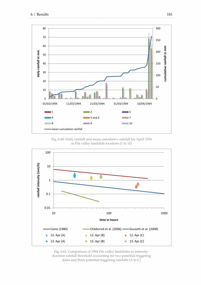
6 | Results 181
Fig. 6.60: Daily rainfall and mean cumulative rainfall for April 1994 in Fils valley landslide locations (1 to 10)
Fig. 6.61: Comparison of 1994 Fils valley landslides to intensity-duration rainfall threshold accounting for two potential triggering
dates and three potential triggering rainfalls (A to C)
0
50
100
150
200
250
300
0
10
20
30
40
50
60
70
80
01/03/1994 11/03/1994 21/03/1994 31/03/1994 10/04/1994
cum
ula
tiv
e r
ain
fall
in
mm
da
ily
ra
infa
ll i
n m
m
1 2 3
4 5 and 6 7
8 9 10
mean cumulative rainfall
0.01
0.1
1
10
100
10 100 1000
rain
fall
in
ten
sity
(m
m/h
)
time in hours
Caine (1980) Chleborad et al. (2006) Guzzetti et al. (2008)
12. Apr (A) 12. Apr (B) 12. Apr (C)
13. Apr (A) 13. Apr (B) 13. Apr (C)
182 6 | Results
Fig. 6.62: Comparison of April 1994 Fils valley landslides to cumula-tive rainfall threshold accounting for two potentials triggering dates
Fig. 6.63: Daily rainfall and mean cumulative rainfall for April 1994 landslide locations (11 to 14)
For comparison of rainfall records for the four landslides from Tübingen University
inventory, two potential dates of slope failures were analysed to be the most likely,
i.e. 12th/13th April and 25th April. For this analysis, triggering rainfall event was de-
termined to begin on the day following low precipitation record of less than 0.1
mm/day. Results are presented in Fig. 6.64 and show that for all tested potential dates
of landslide occurrence thresholds of Chleborad et al. (2006) and Guzzetti et al. (2008)
are exceeded, while Caines’ (1980) threshold is not reached. Similar results were
0
20
40
60
80
100
120
140
160
0 50 100 150 200
3 d
ay
cu
mu
lati
ve
ra
infa
ll i
n m
m
15 day cumulative rainfall in mm
Chleborad et al. (2006) 12-Apr 13-Apr
0
50
100
150
200
250
300
350
400
0
10
20
30
40
50
60
70
80
01/03/1994 15/03/1994 29/03/1994 12/04/1994 26/04/1994
cum
ula
tiv
e d
ail
y r
ain
fall
in
mm
da
ily
ra
infa
ll i
n m
m
11 12 13 14 mean cumulative rainfall

6 | Results 183
elaborated when taking into account only the rainfall on the days of potential slope
failures.
Cumulative rainfall thresholds (Chleborad et al. 2006) were exceeded using 13th and
25th April as potential landslide failures (Fig. 6.65). For the 25th April, threshold ex-
ceedance is primarily influenced by 15-day cumulative rainfall, while for the 13th the
3-day cumulative rainfall has a greater influence.
Fig. 6.64: Comparison of 1994 Tübingen University landslide events to intensity-duration rainfall threshold for three potential triggering
dates
Fig. 6.65: Comparison of April 1994 Tübingen inventory landslides with cumulative rainfall threshold accounting for two potentials
triggering dates
0.01
0.1
1
10
100
10 100 1000
rain
fall
in
ten
sity
(m
m/h
)
time in hours
Caine (1980) Chleborad et al. (2006) Guzzetti et al. (2008)
12-Apr 13-Apr 25-Apr
0
20
40
60
80
100
120
140
160
0 50 100 150 200 250
3 d
ay
cu
mu
lati
ve
ra
infa
ll i
n m
m
15 day cumulative rainfall in mm
Chleborad et al. (2006) 13-Apr 25-Apr
184 6 | Results
For the April 1994 landslides the triggering factor was known to be strong rainfall.
This is however not the case for the other selected landslide events which could also
be initiated by for example snow melting. Regionalised climate data including snow
water equivalent and temperature records were integrated into threshold analysis for
all landslides where data was available. Slope failure records without data on snow
cover changes and temperature include seven events with a total number of nine
landslides which had occurred in the Swabian Alb.
Two landslides (ID 18 and 19) were triggered on 30th July 1987 close to Schwäbisch
Gmünd. According to inventory information the landslides were both triggered on a
day with only 6.8 mm precipitation, a total sum occurring very often. However, rain-
fall events up to four times stronger occurred some days earlier and later. Since the
recorded triggering date may be inaccurate, alternative triggering dates were consid-
ered.
Two more landslides (ID 24 and 25) were triggered in the same area on the 15th Octo-
ber 1988.
Between 26th May and 9th June 1983, seven landslides are listed in the inventory, of
which one (ID 31) is located in the northern Swabian Alb. Even though snow data was
available for this period, no snow was recorded.
Four landslides were recorded between 11th and 22nd April 1994 of which one is lo-
cated in the study area (ID 32). The total size of the landslide was 625 m² and it was
triggered on a day with relatively low precipitation of only 8.5 mm. However, a much
stronger rainfall event (>50 mm) occurred one day later, and was considered as a po-
tentially more accurate triggering date.
For late March 2002, the inventory contains four landslides of which one (ID 34) is in
the Swabian Alb. The slope failure covered an area of 450 m² and had a depth of 3 m.
No rainfall was recorded for the day of landslide initiation or the day before. An ex-
tremely strong rainfall event of almost 70 mm occurred six days earlier and was
checked as an alternative triggering date.
The inventory contains one record (ID 28) for the 29th August 1990 on which several
landslides had occurred close to Neidlingen; though, only one coordinate is provided.
Rainfall data describes only 2.8 mm of precipitation for the day of landslide occur-
rence. As an alternative triggering date, the subsequent day was considered, on which
more than 11 mm precipitation were recorded.
At the boundary of the Swabian Alb, close to Kirchheim, one landslide (ID 33) was
recorded for the 6th November 1998. Two more landslides occurred outside the study
area on the preceding day.

6 | Results 185
A low total precipitation of only 1 mm was recorded for the triggering day; however,
a very strong rainfall event with over 70 mm six days earlier might have been the cor-
rect initiation day and was therefore considered as an alternative.
Results of intensity-duration threshold analysis of landslides for which only rainfall
data was available are presented in Fig. 6.66.
All landslides are above the intensity-duration threshold used in the Seattle landslide
early warning system. From the landslides for which the recorded triggering date was
used four lie below Guzzetti et al. (2008) threshold. Caines’ threshold was not ex-
ceeded by any of the slope failures. Alternative triggering dates generally increased
intensity-duration values and led to two landslides being raised above Guzzetti et al.
(2008) threshold; however, slope failures of the Neidlingen event (ID 28) remain be-
low.
Results of cumulative threshold analysis of landslides for which only rainfall data was
available are presented in Fig. 6.67. Therein, recorded and alternative landslide trig-
gering dates were considered.
When using recorded triggering dates, five of seven landslides analysed were located
below threshold values. Generally, these show relatively low values for 3-day cumu-
lative precipitation. Only landslides 33 and 34 exceed the threshold due to high cumu-
lative rainfall of more than 150 mm. Alternative triggering dates generally have
higher cumulative rainfall values, however, only for landslide 31 the threshold was
thereby exceeded.
Landslide events, for which also snow data was available, include three events in
March 1987, March and April 1988 and February 2005.
On 27th March 1987 three landslides (ID 15 to 17) occurred at the border of the
Swabian Alb close to Ellwangen. Slope failures were between 20 and 40 m and had a
maximum depth of 4.5 m.
The highest number of landslides occurred in March and April 1988. However, of 33
landslides listed in the inventory, only four were triggered in the study area. Three of
these landslides (ID 20 to 23) were classified as failures in natural slopes, and one as
rockfall. The largest of the landslides had a total size of 2,500 m² and required con-
crete injection for stabilisation. In the days preceding the described slope failures
snow height quickly decreased by approximately 60 cm occurred.
Two failures in embankments (ID 29 and 30) are listed for 17th February 2005. Even
though data on snow cover and temperature were available, no threshold analysis
could be performed. According to weather data, temperature was below zero
throughout the triggering period, and all precipitation was stored as snow.
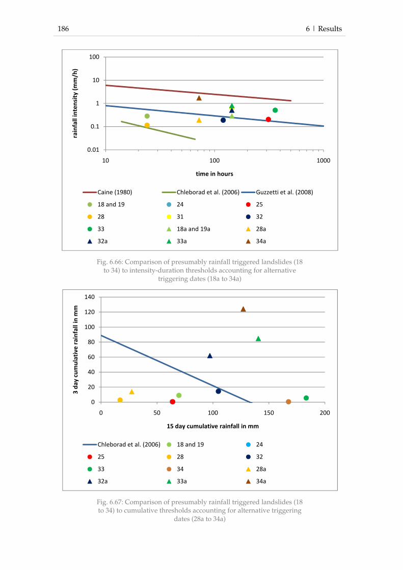
186 6 | Results
Fig. 6.66: Comparison of presumably rainfall triggered landslides (18 to 34) to intensity-duration thresholds accounting for alternative
triggering dates (18a to 34a)
Fig. 6.67: Comparison of presumably rainfall triggered landslides (18 to 34) to cumulative thresholds accounting for alternative triggering
dates (28a to 34a)
0.01
0.1
1
10
100
10 100 1000
rain
fall
in
ten
sity
(m
m/h
)
time in hours
Caine (1980) Chleborad et al. (2006) Guzzetti et al. (2008)
18 and 19 24 25
28 31 32
33 18a and 19a 28a
32a 33a 34a
0
20
40
60
80
100
120
140
0 50 100 150 200
3 d
ay
cu
mu
lati
ve
ra
infa
ll i
n m
m
15 day cumulative rainfall in mm
Chleborad et al. (2006) 18 and 19 24
25 28 32
33 34 28a
32a 33a 34a

6 | Results 187
Results of intensity-duration and cumulative threshold analysis of landslides for
which snow height data was integrated are presented in Fig. 6.68 and Fig. 6.69, re-
spectively.
Fig. 6.68: Comparison of presumably snow-melt triggered landslides (15 to 23) to intensity-duration thresholds including alternative trig-
gering dates (15a to 23a)
Fig. 6.69: Comparison of presumably snow melt triggered landslides (15 to 23) to cumulative rainfall threshold including alternative trig-
gering date (15a to 23a)
0.01
0.1
1
10
100
10 100 1000rain
fall
in
ten
sity
(m
m/h
)
time in hours
Caine (1980) Chleborad et al. (2006) Guzzetti et al. (2008)
15 16 17
20 21 22
23 15a 16a
17a 20a 21a
22a 23a
0
20
40
60
80
100
0 50 100 150 200 250
3 d
ay
cu
mu
lati
ve
pre
cip
ita
tio
n i
n m
m
15 day cumulative precipitation in mm
Chleborad et al. (2006) 15 16
17 20 21
22 23 15a
16a 17a 20a
21a 22a 23a

188 6 | Results
All landslides analysed have intensity-duration values lying between the thresholds
by Guzzetti et al. (2008)and Caine (1980). In general, longer duration precipitation
events were considered since snow melting occurred over periods up to 18 days.
When neglecting additional rainfall while using the same precipitation event dura-
tions, results show slightly lower intensity-duration values; however, these are still
above the values of Guzzetti et al. (2008).
Results of cumulative rainfall threshold analysis show that four landslides are above,
and three below the threshold by Chleborad et al. (2006). In general, threshold ex-
ceedance is strongly influenced by long term 15-day cumulative precipitation and
only to a lower extent by 3-day cumulative precipitation.
Integration of snow data generally raised cumulative rainfall values. When snow
melting is not considered only one landslide (22a) is clearly above threshold values,
and two others (20a and 21a) are very close to threshold line.
Some interesting characteristics can be observed for landslide 23, which shows a sig-
nificant difference depending on the integration of snow melting. When snow melting
is considered, it results in the highest cumulative precipitation values of all landslides.
When only measured precipitation is used, no 3-day cumulative precipitation can be
observed resulting in values below the threshold.
Most landslides occurred between intensity-duration values between thresholds by
Caine (1980), which was never exceeded by landslides analysed, and Guzzetti et al.
(2008), which was exceeded by a large proportion of the landslides. The lowest inten-
sity-duration threshold from the Seattle landslide early warning system was exceeded
by all analysed landslides. Similarly, the cumulative rainfall threshold by Chleborad
et al. (2006) was exceeded in most cases; still some landslides occurred below.
For some cases, the recorded landslide triggering date did not coincide with highest
rainfall intensities and alternative dates were considered. In general, this resulted in
higher index values and more landslides being above threshold levels.
Discussion
Limited availability of data on landslide occurrences and related initiating rainfall
events hindered the establishment of rainfall thresholds specifically for the Swabian
Alb. Tested rainfall intensity and duration thresholds proposed in the literature, how-
ever, performed satisfactorily. In general, Caines’ (1980) threshold seems too high for
the Swabian Alb, since no landslide exceeded its critical values. In contrast, the
threshold proposed by Chleborad et al. (2006) appears to be too low, since most land-
slides triggering rainfall events significantly exceeded critical values. Still, further
analysis integrating rainfall events that did not cause landslides should be tested to
verify this assumption. From all tested intensity duration thresholds, the one pro-
6 | Results 189
posed by Guzzetti et al. (2009) performed most satisfactorily, with a high number of
landslides exceeding critical values.
Cumulative rainfall thresholds tested in this study (Chleborad et al. 2006) can be con-
sidered adequate since a large number of landslides occurred above threshold values.
In comparison to intensity-duration thresholds, a slightly higher number of landslides
occurred below threshold rainfall.
Still, some uncertainties remain in the results. The exact date of landslide triggering is
not known for all landslides. Analysis of additional potential triggering dates, as car-
ried out in this thesis, can help to ascertain these, however validation can not be car-
ried out. Similarly, triggering rainfall events are difficult to determine but can have a
significant influence on threshold verification.
Results illustrate the need to integrate data on snow data melting into thresholds de-
termination, especially due to the frequent landslide occurrence in spring.
Regionalised climate data used within this study is subject to uncertainties. In particu-
lar snow melt does not represent real measurements but results of modelling. Integra-
tion of real snow height measurements could significantly improve the results and
make threshold verification more reliable.
6.2.3 Early warning
The regional early warning system was designed in cooperation with the company of
Geomer which was also responsible for technical implementation (QUOTE). In the
following, the design of the regional early warning system will be presented. Detailed
information on the technical implementation is provided by Jäger et al. (2010). Addi-
tional information on the warning procedure initiated once a threshold is exceeded is
described in chapter 7.
The early warning scheme of the developed prototypic regional system integrates
measured precipitation, rainfall forecasts and thresholds. Since only historic rainfall
forecasts were available, the system represents a technical solution without realistic
early warning capabilities at this stage. However, the regional landslide early warning
system was planned to be modifiable and extendable when additional data becomes
available.
The regional landslide early warning system for the Swabian Alb was designed as a
spatially distributed system where rainfall thresholds and warning levels may vary
throughout the focus area. In the current state of the system technical implementation,
only the area of Lichtenstein-Unterhausen is integrated, which is also the local project
area in this study. An overview on the early warning procedure is presented in Fig.
6.70.

190 6 | Results
Fig. 6.70: Overview on the regional landslide early warning model
Precipitation recorded by the ILEWS weather station is utilised to describe antecedent
rainfall conditions of the past 15 days. Rainfall forecasts for the next 20 hours are ex-
tracted from regionalised climate modelling results of COSMO-DWD for the grid cell
containing Lichtenstein-Unterhausen. The combination of antecedent precipitation
and forecasted rainfall is then compared to defined threshold values. Five preliminary
thresholds values were determined (Tab. 6.9) using Chleborad et al. (2006) as a refer-
ence.
Tab. 6.9: Preliminary rainfall threhsolds used for regional landslide early warning
Antecedent rainfall (in mm) Forecasted rainfall (in mm)
130 0
90 30
50 50
20 70
0 80
The regional early warning system is also connected to alarm sensors on the web-
based ILEWS early warning platform. If any threshold is exceeded, an alarm sensor is
activated and a notification is sent to the involved experts for evaluation of the cur-
rent situation. More information on the actual early warning procedure is provided in
chapter . However, since no real-time rainfall forecasts were available for this study,
early warnings only have a hypothetical character and the alarm sensor is currently
disabled.

6 | Results 191
Discussion
The developed regional landslide early warning system represents a prototype appli-
cation which can not issue realistic warning at the current state due to the lack of real-
time rainfall forecasts. The technical system however, can be used for realistic early
warnings, once real-time rainfall forecasts become available.
Rainfall thresholds currently implemented in the regional early warning model are
determined in reference to the values proposed by Chleborad et al. (2006). However,
threshold values can easily be modified in the web-based warning platform (see chap-
ter 7) once more results become available.
In its current layout, the regional warning system accounts for the Lichtenstein-
Unterhausen area. Extension of the system to the entire Swabian Alb region as a fully-
fledged regionalised early warning model can be based upon the prototype devel-
oped in this thesis. Further developments could also include spatially varying rainfall
thresholds once these are investigated in more detail.


7 | Integrative early warning 193
7 INTEGRATIVE EARLY WARNING
Local and regional early warning models developed in this thesis forecast future
landslide behaviour and are embedded into the integrative landslide early warning
system elaborated by the ILEWS project. In the following, the web-based information
and warning platform, as well as the process of transformation of alarm notifications
into early warnings are presented. More detailed descriptions are provided by Jäger
et al. (2010) and Mayer and Pohl (2010), respectively. Since the developed early warn-
ing chain is a result of the cooperative risk management and communication carried
out in the ILEWS project, additional information on the challenges of the integration
of early warning systems into the social and administrative framework and decision
making processes are summarized.
The main goal of the web-based platform is to store and visualise monitoring and
modelling results based on standardised geo-data services to ensure interoperability.
In addition, notifications to experts are provided in case pre-defined alarm thresholds
are exceeded, which then can lead to an early warning. The GIS-based visualisation of
real-time monitoring data is managed by a complex geodata infrastructure described
in detail by Jäger et al. (2010). Latest measurements can be viewed by hovering the
mouse over the sensor on a map (Fig. 7.1). Several settings can be changed for data
analysis. For the automated inclinometer, these include analysed time-frame, scale of
visualised data, and also direct comparison to hydrological monitoring results.
Similar visualisation capabilities are implemented for all continuously and periodi-
cally measured monitoring data. Single and groups of hydrological sensor records can
be visualised and directly compared to climate data from the ILEWS weather station.
Geoelectrical monitoring data can be displayed for single or groups of measurement
points. In addition, resistivity pseudo-sections with a time-lapse function can be com-
puted. Movement data from periodic tachymetry and inclinometer measurements in
the form of interactive maps but can also be downloaded for further analysis. Fur-
thermore, the CHASM early warning and decision-support systems are implemented
on the ILEWS platform. For quick evaluation of the current situation, a status control
system was set-up illustrated in Fig. 7.2.
Alert thresholds are implemented for each continuously measuring sensor in the field,
accounting for changes of measurement values for varying time periods (Fig. 7.2 A).
Additional alert thresholds are implemented for the CHASM early warning model,
and regional rainfall thresholds. Latest measurements are compared to threshold val-
ues and displayed as an alert level (Fig. 7.2 B). In addition, the current status of the
alert thresholds is visualised as coloured alert lights (Fig. 7.2 C), which change from
green to yellow if a pre-defined

194 7 | Integrative early warning
Fig. 7.1: Web-based visualisation of real-time inclinometer monitor-ing data and comparison to monitoring results
Fig. 7.2: Status control of real-time measurements with alert thresh-olds (A), alert level (B), alert sensors (C) and early warning signal (D)
C
A
D
B

7 | Integrative early warning 195
threshold is exceeded. Ultimately, the alert thresholds influence the three-coloured
early warning signal light (Fig. 7.2 D).
The ILEWS landslide early warning system was set up as an expert-system, in which
registered users can only view the data, but only experts can edit the system and for
example modify thresholds values, adjust frequency of measurements and change the
early warning level. The current early warning level of the signal light is controlled by
a procedure illustrated in Fig. 7.3.
Fig. 7.3: Signal light (based on Mayer and Pohl 2010)
As long as real-time measurements are below alert thresholds, the signal light is on a
green level, indicating that no critical situation is expected. Once an alert threshold is
exceeded, respective alarm senor and the early warning signal light change to yellow.
Simultaneously, SMS and emails are sent to the involved experts (e.g. scientists) and
registered users (e.g. local and regional administration, local population, media), in-
forming that a pre-defined monitoring or modelling threshold has been exceeded.
Experts are requested to check the situation and decide whether the situation is poten-
tially dangerous or a false alarm. Depending on the experts' decision, the early warn-
ing signal light is either set back to green, or upgraded to red. Red early warning level
is directly followed by automated messages with action advises to registered users
and emergency forces are informed by the experts.
196 7 | Integrative early warning
The ILEWS early warning chain is the result of cooperative risk assessment and com-
munication with local and regional stakeholders and was developed during several
discussions and round-table meetings to ensure the early warning system is opti-
mised to the end-users (Mayer and Pohl 2010). The local community represented by
the local administration and the mayor were the first potential end-user interviewed
about the demands towards a landslide early warning system. On a local level how-
ever, landslide hazards and early warning are of low interest partly due to the admin-
istrative framework which regulates the responsibilities between local, regional and
national political entities. At the current state, the situation in the local study is not
regarded an imminent hazard but only as potentially dangerous (Gefahrenverdacht) for
which the political framework does not foresee any compulsory actions. The local
administration has no interest in detailed visualisation of monitoring data and other
scientific products. Instead, only short information is required in case any emergency
actions have to be initiated. Therefore, management of the landslide early warning
system can not be undertaken by local administration, but has to be embedded into
higher-level institution responsible for civil protection.
Round-table meetings with regional decision-makers included three administrative
levels which share responsibilities for risk management of natural hazards including
landslides. Early warning however, is not directly integrated into the federal system
of Baden-Württemberg and the other federal states of Germany. On the lowest re-
gional level of civil protection (Untere Katastrophenschutzbehörde) the district office
(Landratsamt) is factually responsible and carries out measures in cooperation with
specialist authorities (Fachämter), e.g. geological survey. The local community only
acts as a connecting authority between local population and regional decision-makers.
On the medium level (Obere Katastrophenschutzbehörde) the regional councils
(Regierungspräsidien) deals with civil protection issues affecting technical infrastruc-
ture and for affairs which exceed the lowest level responsibilities. On the highest level
(Oberste Katastrophenschutzbehörde), the Ministry of Interior of the federal state Baden-
Württemberg is responsible for planning of civil protection measures; localised phe-
nomena such landslides however, do not play an important role for this agency. None
of the regional stakeholders responsible for civil protection and risk management of
natural hazards wanted to be in charge of the developed early warning system and
act as the managing expert. However, each authority named other agencies, which to
their position were dedicated to fulfil the role of the expert. These results show that
the inexplicit administrative and political structures of responsibilities hinder an ef-
fective application of landslide early warning systems. Successful integration of land-
slide early warning into the decision-making process therefore requires modifications
of the political framework in Baden-Württemberg to ensure responsibilities are clearly
defined.
8 | Discussion 197
8 DISCUSSION
During the monitoring campaign, small slope movements have been recorded by sur-
face and subsurface measurements which are extremely-slow according to the defini-
tion by Cruden and Varnes (1996). In particular with regard to inclinometer Lic02,
these displacements can be interpreted as a continuation of the displacement previ-
ously described by Bell (2007). In contrast to this earlier study, the research described
in this thesis could employ geodetic measurements carried out by Aslan et al. (2010a)
for interpretation of large scale movement trends.
According to geodetic monitoring, three blocks of similar movement trends can be
distinguished: relatively large downslope movements in the eastern part, relatively
low displacements rates in the middle part, and alternating movement directions in
the western part. These movement trends are partly affirmed by inclinometer meas-
urements. Exact boundaries of current landslide displacement, however, can not be
determined. Still, geodetic measurements lack fixed points outside the potential land-
slide which limits their informative power.
Most important landslide movement data was recorded at inclinometer Lic02, and in
particular by manual measurements. Two depths of seasonally varying slope dis-
placements can be observed: a deep seated-sliding occurring in 15.5 m depth in
spring, and a flow-like movement in 8.5 m depth in summer and autumn. The latter
movements are also recorded by other inclinometers, however, deep-seated sliding
can not be assessed due to the positioning above stable bedrock. When taking into
account all manual measurements of inclinometer Lic02, it seems as the shallower
displacement gradually transformed into a more slide-like movement, possibly indi-
cating the progressive development of a shear surface.
While manual inclinometer measurements provide superior data on spatial distribu-
tion of movements, temporal resolution is higher for the automated inclinometer
chain. However, the deep-seated movement is not appropriately detectable with the
inclinometer chain due to the position of the lowest sensor. During the monitoring
campaign, no distinct accelerations phases could be observed. Such continuous low
displacements rates can possibly be interpreted as secondary creep as described by
Okamoto et al. (2004) and Petley et al. (2005b, 2005c; 2008), in which diffuse micro-
cracks develop. Therefore, an increase of movement speed during a tertiary creep
phase is a potential future scenario, which should be controlled by continued moni-
toring. In particular, the inclinometer chain is of great value for this task since notifi-
cations by the ILEWS early warning system are provided if displacement thresholds
are exceeded. In addition, continued monitoring could provide the data required to
improve definition of triggering conditions.

198 8 | Discussion
The hydrological monitoring by tensiometers, TDR and geoelectrical monitoring pro-
vided indications for preferential flow paths leading to a quick rise of water content in
great depths at the damaged house, i.e. monitoring site p12. This is not surprising
given the heterogenic subsurface conditions documented by the drillings. Even
though no direct contribution of preferential flow to slope instability can be ap-
pointed, it is likely that some effect is present given the recorded displacements in
inclinometer Lic02 and the crack development at the house. Further investigations are
necessary to assess the influence of preferential flow paths since they are important
for slope stability and should be integrated into early warning (Uchida 2004). In par-
ticular, geoelectrical monitoring could aid to estimate the complex subsurface hydro-
logical processes. Unfortunately, hydrological monitoring data could not be analysed
in full detail by Wiebe and Krummel (2010) and Wiebe et al. (2010) due to limited re-
sources.
With regard to these results, the first research question, "How does slope hydrology con-
tribute to the reactivation of landslide movements?", can not easily be answered. Without
any periods of pronounced slope movement, preferably larger than error margin of
the monitoring equipment, no exact triggering conditions can be determined. Instead,
only broad statements on hydrological influence on slope stability can be made, for
example that some correlation between snow melting in spring and deep-seated slid-
ing exist.
The generation of a subsurface model aimed to describe real surface and subsurface
conditions as realistic as possible to facilitate slope stability and early warning model-
ling with CHASM. In general, a good approximation of real conditions could be
achieved even though subjective interpretation was required at some points of the
applied methodology. For estimation of slope debris thickness, for example, the drill-
ings by Ohmert (1988) provided accurate data for some points and were interpolated
to the entire study area based on relative slope positions. Similarly, estimation of
landslide deposit thickness from seismic prospection data included personal judg-
ment but greatly enhanced representation of real conditions. Topographic analysis for
the lower landslide deposits significantly improved the subsurface model. Geotechni-
cal parameters estimated from literature sources provided good initial information on
the possible range of real values. Subsequent sensitivity analysis helped to assess the
influence of the parameters and allowed for calibration of CHASM stability calcula-
tion.
Based on the available information from drillings and the interpretation of seismic
prospection data, the slope debris layer could not further be distinguished. Still, drill
cores demonstrated heterogenic subsurface conditions which in reality can not be
assumed to behave uniformly. In particular in terms of hydrological conditions, this is

8 | Discussion 199
a significant simplification of real conditions. Still, preferential flow paths as indicated
by hydrological monitoring data, for example, cannot be accommodated within the
current simulation approach implemented in CHASM.
Results of CHASM analysis show a generally low stability for the entire slope profile
along the damaged house, with the lowest stability occurring in the upper slope sec-
tions, thus indicating a potential slope failure similar to the medium-age landslide
located in the western part of the study area. Drill cores from borehole Lic05 provided
some indication for the existence of a potential shear surface in the upper slope area;
however, to verify this assumption, continued monitoring or the installation of addi-
tional inclinometers, preferably stably fixed into the bedrock is required. Still, it
should also be questioned if additional costly installations are justified in regard to
the extremely slow displacement recorded over the last 6.5 years. From a scientific
point of view, an extended monitoring system could not only facilitate the under-
standing of the processes occurring at the slope under investigation in this thesis, but
also provide important information regarding slow moving slopes in the Swabian Alb
in general.
According to CHASM simulations, shear surfaces are most likely positioned at the
boundary of slope debris and the bedrock below. In contrast, shear surfaces also in-
cluding the bedrock material have a significantly higher FoS and are therefore less
probable. A shear surface position at the bedrock interface reflects a deep-seated slid-
ing, similar to the movements recorded in approximately 15.5 m at inclinometer
Lic02. The shallower displacement measured at this location, which also shows char-
acteristics of a flowing movement, cannot be simulated by CHASM due to the limita-
tions of the limit-equilibrium method. Future applications of dedicated simulation
models, for example finite-element software, could provide more insights into the
displacement process. Some promising initial tests have already been carried out by
Aslan et al. (2010b) and further research is currently being performed.
Two CHASM-based applications were developed to address the second research
question: "How can physically-based slope stability models be applied in landslide early warn-
ing?".
With the CHASM early warning model slope stability is continuously simulated
based on current groundwater conditions and measured and forecasted rainfall. Sen-
sitivity analysis of CHASM provided some interesting results regarding the influence
of rainfall events which is also important for subsequent modelling of early warning.
Surprisingly, rainfall distribution and rainfall intensity have a very low influence on
slope stability calculation which limits the predictive power of the CHASM early
warning model. Possibly, further adjustment of CHASM parameters could increase
the sensitivity to rainfall; however, this would preferably require a distinct onset of
displacement to be able to appropriately validate the input data. In its current state of

200 8 | Discussion
development, the notification service can only issue hypothetic early warnings since
real-time rainfall forecasts are not available. However, if these became accessible, the
technical system could easily be adjusted. Nevertheless, the developed CHASM early
warning application is a prototype with a high potential for the further applications.
The second CHASM application for the use in the context of early warning is a deci-
sion-support tool for quick calculation of slope stability without time-consuming
elaboration of a slope profile and the respective shear surface parameters. In addition,
the effect of a variety of input data can be tested which is a significant improvement
in comparison to the standard single profile analysis. The integrated shear surface
search routine effectively concentrates search procedure to the upper slope areas
which are the most landslide prone areas according to CHASM simulations. How-
ever, the decision-support system represents a prototype development which does
not include all capabilities of CHASM and cannot replace more detailed investiga-
tions. Overall, the ability to quickly initiate CHASM simulations for freely-selectable
slope profiles has great potential for future applications.
Available landslide inventories for the Swabian Alb contain several hundred land-
slide events with the earliest records dating back to the 15th century. However, esti-
mation and verification of rainfall thresholds can not in all cases benefit from this data
since the exact day of initiation and the triggering agents are not accounted for. Still,
landslide inventories are essential data sources for other research objectives besides
early warning, for example determination of geomorphological activity, landslide
hazard and risk management, and spatial planning in general. Therefore, efforts for
recording of landslide events and investigation of available data sources should be
continued and increased in the future.
With the limited number of dated landslide events it was not tried to determine rain-
fall thresholds for the Swabian Alb, but to verify the applicability of thresholds pro-
posed in the literature. Comparison of landslide events to intensity-duration and cu-
mulative rainfall thresholds was carried out for all events for which the date of initia-
tion was recorded, and regionalised climate data was available. For some landslide
events, the exact date of occurrence was unknown but could be ascertained by assum-
ing potential triggering dates. In general, tested intensity-duration and cumulative
rainfall threshold performed satisfactorily and affirm the applicability of such an ap-
proach in the Swabian Alb. Still, not all landslides can be explained by the applied
rainfall thresholds and subsequently early warning cannot be expected to be able to
predict all future slope failures.
The importance of snow melting for the initiation of slope failures in the Swabian Alb
is demonstrated by the temporal clustering of landslide events in spring. In addition,
the integration of snow melting into verification of rainfall thresholds was able to ex-

8 | Discussion 201
plain some of the landslide events, which could not have been predicted by rainfall
alone.
The technical regional early warning system implemented by Jäger et al. (2010) em-
ploys preliminary rainfall thresholds which can be expected to be able to predict the
majority of landslide events. Once more appropriate threshold values become avail-
able alarm levels can easily be modified on the web-based warning platform. In its
current state, early warnings are only hypothetical since no real-time rainfall forecasts
are available; still, from a technical point of view, the system is capable of providing
notifications to the experts in charge. However, before realistic early warnings can be
issued, decision-makers have to define the desired warning levels in regard to possi-
ble false alarms and missed warnings. The regional early warning system has a great
potential for a transfer to larger areas. By relatively small modifications, the early
warning system could be developed into a fully-fledged regional system accounting
for spatially varying threshold values, similar to the system in Hong Kong.
Based on the presented threshold verification and the implemented regional landslide
early warning prototype, the research question raised in the beginning - "Are landslide
triggering rainfall thresholds applicable to regional early warning in the Swabian Alb?" - can
be answered in the affirmative.


9 | Perspectives 203
9 PERSPECTIVES
The results of this thesis raise new questions for future investigations in the Swabian
Alb in general and in particular for the landslide in Lichtenstein-Unterhausen. In ad-
dition, some refinements could improve local and regional early warning applications
and their landslide forecasting capabilities. In the following, potential improvements
are presented, and the prospects for a transfer of the developed early warning appli-
cations and the ILEWS warning system in general are discussed.
On a local scale, a continuation and expansion of the slope monitoring system could
improve the understanding of slope hydrology and the process of landslide reactiva-
tion. In particular additional inclinometers installed into stable bedrock could help to
define the boundaries of measured slope displacements and enhance the subsurface
model. The integration of fixed points outside the landslide area in tachymetry meas-
urements could enable a more accurate interpretation of large scale movement trends
and the verification of possible deep-seated displacement for inclinometers Lic04 and
Lic05. Definition of distinct triggering condition requires the continuation of meas-
urements, in particular by the automated inclinometer. Results of hydrological moni-
toring indicate preferential flow paths in the area of the damaged house. Future re-
search could install additional hydrological sensors to assess the characteristics of
subsurface hydrology and the contribution to slope instability. Furthermore, geoelec-
trical monitoring data has not been analysed in full detail and could aid understand-
ing of subsurface hydrology. Moreover, the application of hydrological simulation
software could improve the interpolation of groundwater conditions for subsequent
stability modelling. Possibly, analysis of chemical properties of groundwater compo-
sition could provide interesting insights and help to predict future accelerations.
Early warning modelling with CHASM could benefit from an improved subsurface
representation and more detailed study in groundwater table positions. The applica-
tion of designated models, for example the Sloping Local base Level approach
(Jaboyedoff et al. 2004) could improve the approximation of the subsurface morphol-
ogy. Hydrological simulation models could be used to create more realistic and so-
phisticated groundwater scenarios for subsequent modelling. In addition, shear tests
and more complex hydrological laboratory tests of soil samples could improve the
overall performance of slope stability simulation. CHASM capabilities not tested in
this study, such as Janbu's non-circular shear surface methodology could potentially
enhance simulation of landslide behaviour. Furthermore, other physically-based
landslide simulation models could be applied on the slope in Lichtenstein-
Unterhausen. In particular finite-elements models could help to understand the proc-

204 9 | Perspectives
esses of landslide movement reactivation. It would also be interesting to see how
other landslide simulation models perform in early warning systems.
The CHASM early warning procedure would benefit from the integration of real-time
rainfall forecasts instead of historic records so that real warnings can be issued. In
addition, the integration of snow melting could increase the accuracy of slope stability
predictions.
The transfer of the developed CHASM decision-support and early warning applica-
tions to other study areas are attractive prospects. Appropriate study areas should
include deep-seated landslides with a known shear surface depth. Ideally, hydrologi-
cal monitoring should be available to be able to estimate groundwater tables. How-
ever, the monitoring system could be significantly smaller if subsurface conditions are
more homogeneous. To take full advantage of quick slope stability calculation capa-
bilities of the developed CHASM decision-support system, an ideal study area would
comprise similar slope morphologies within the focus area. For example slopes along
roads or railway lines would be suitable for an effective application.
For future regional scale research on landslides, an improvement of the landslide in-
ventory by further exploration of data sources currently not available to science is
desirable. Therefore, ongoing recording of landslide events in addition to continued
research in historic archives and media reports is required. The application of hydro-
logical models could help to define triggering dates for landslides for which the exact
date is unknown and thus provide the data needed for more sophisticated verification
of rainfall thresholds.
In this work, a limited number of landslide triggering rainfall thresholds was ana-
lysed. Future investigations could possibly benefit from an examination of other
threshold concepts; in particular approaches in which long-term conditions are inte-
grated, for example taking into account mean annual precipitation or the antecedent
soil water status. Also, deterministic models could be used to enhance determination
of landslide triggering rainfall threshold, since these approaches have lower require-
ments regarding landslide inventory data (Terlien 1998).
The regional landslide early warning system would benefit from real-time weather
forecasts which would enable to issue real early warnings. Prediction of landslide
events could be enhanced by an automated integration of snow melting data into the
regional early warning model. One of the most promising improvement of the re-
gional landslide early warning application could be achieved by further development
into a spatially distributed system similar to the system implemented in Hong Kong.
Such a system could accommodate both regional and local landslide triggering rain-
fall thresholds for which additional research is required.
9 | Perspectives 205
A transfer of the developed regional landslide early warning procedure could be car-
ried out with very little technical modifications. In particular the availability of rain-
fall forecasts with a high spatial and temporal resolution in the form COSMO-DE
simulations could be used as the basis for further implementation of regional land-
slide early warning systems in central Europe. However, without additional studies
on landside initiating rainfall thresholds, only generic alarm levels could be em-
ployed. In addition, warning thresholds had to be determined by cooperative discus-
sions to meet the end-users requirements towards the early warning system.
Even though the technical feasibility of local and regional landslide early warning
system in the Swabian Alb has been confirmed, effective early warning also requires
integration into political and social structures. In the federal system of Germany,
competences are currently not clearly defined and local and regional decision-makers
are reluctant to overtake responsibilities for early warnings. It is therefore essential to
inform policy makers about the benefits of early warning systems within integrative
risk management strategies.

10 | Summary 207
10 SUMMARY
Landslides are among the most hazardous natural hazards and can have disastrous
effects on society as demonstrated by recent large slope failures for example in China.
In places, where landslide prone areas cannot be avoided or slopes cannot be stabi-
lised, early warning systems can be a useful counter-measure to effectively protect the
local population and also act as an integral element of risk management. Despite the
common use of slope stability simulation software for landslide analysis and forecast-
ing in geotechnical practice, landslide early warning systems rarely take full advan-
tage of these models. Moreover, regional landslide early warning systems are mostly
implemented as prototype applications even though necessary input data like quanti-
tative rainfall forecasts and rainfall thresholds are widely available.
The main objectives of this thesis are the analysis of landslide characteristics and the
subsequent development and implementation of local and regional early warning
models in the Swabian Alb. In the local study area, a reactivated deep-seated land-
slide is equipped with an extensive monitoring system to investigate the contribution
of slope hydrology to the process of displacement reactivation. A physically-based
slope stability model is applied to simulate and forecast landslide behaviour and sub-
sequently implemented as a decision-support and early warning model. On the re-
gional scale, available landslide inventories are analysed and dated mass movements
are compared to rainfall thresholds elaborated in other studies. Consequently, a pro-
totypic early warning application is implemented based on the results.
The work is embedded in the ILEWS project, in which the entire early warning chain
from the sensors in the field to user-optimised action advises is addressed.
Forecasting of slope failures, and in particular slow moving landslides is extremely
difficult. For such processes, long phases of slow and steady displacements, fre-
quently termed creep, can be observed prior to final failure. Changes of displacement
rates may occur due to variations of hydrological conditions and progressive weaken-
ing of the soil material. Difficulties of landslide forecasting also arise from the com-
plex nature of landslide processes, in which feedback processes and non-linear behav-
iour hamper predictions. Landslide prediction usually employs thresholds of trigger-
ing factors such as rainfall. In particular thresholds accounting for rainfall characteris-
tics such as intensity-duration have frequently been applied on a regional scale. A
wide range of methods can be applied for landslide investigation and monitoring of
hydrology and slope displacements, and several simulation models are available for
landslide modelling of which limit-equilibrium methods are possibly the most fre-
quently applied. Effective early warning of landslides is not only a technical challenge
208 10 | Summary
but also requires integration into the society’s political framework and processes of
decision-making. A review on landslide early warning systems worldwide shows that
most systems have prototypic character and that no simple best-practice approach is
available. Landslide early warning systems for single slopes generally apply extensive
monitoring systems of displacement and potential triggering factors to predict slope
failure; or are implemented as post-event systems which issue an alarm once a land-
slide process has been initiated. In most cases, regional landslide early warning sys-
tems rely on rainfall measurement and forecasts which are compared to pre-defined
threshold values.
The study area of this thesis is the lower mountain range of the Swabian Alb in
southwest Germany, an area which is frequently affected by landslides. The region’s
geology consists of Jurassic, clays, marls and limestones, of which the latter form a
steep escarpment (Albftrauf). In the local study area Lichtenstein-Unterhausen, a reac-
tivated landslide body which has also been investigated in previous research projects,
regularly causes cracking to a house.
A wide range of data was used in this study. On the local scale these include geologi-
cal maps and drillings, geotechnical parameters from literature values, slope hydrol-
ogy and movement monitoring data acquired within the ILEWS project. For regional
scale analysis climate data and landslide inventories are the most important data
sources.
Extensive field work including drillings, drill core extraction, and the installation of
inclinometers and hydrological sensors were an essential part for the research carried
out in this thesis, as well as for the ILEWS project. Data analysis included comparative
examination of movement monitoring records in the form of tachymetry measure-
ments, manual and automated inclinometers records. Hydrological data was analysed
to investigate the response of slope hydrology to rainfall events. The deterministic
limit-equilibrium software was CHASM used to simulate slope behaviour, and fore-
cast future behaviour. Subsequently, two novel applications were developed for land-
slide decision-support and early warning. To facilitate landslide modelling, a general
subsurface model combining geological data, drillings, results of geophysical prospec-
tion and geotechnical parameters was created by a step-wise and iterative GIS proce-
dure. Groundwater scenarios were elaborated based on analysis of hydrological data
and spatially interpolated for subsequent CHASM modelling. In addition, rainfall
scenarios were generated using the KOSTRA atlas. Furthermore, a procedure was
developed to control the automated shear surface search implemented within
CHASM. Simulation of slope behaviour with CHASM investigated the influence of a

10 | Summary 209
variety of input parameters including rainfall, groundwater, and geotechnical pa-
rameters during a sensitivity analysis. CHASM was subsequently implemented as an
early warning model to continuously calculated slope stability. A CHASM decision-
support system allowing for quick calculation of slope stability for freely selectable
slope profiles was developed based on previously generated input data. On the re-
gional scale, the applied methodology focussed on analysis of landslide inventories in
the Swabian Alb to select slope failures appropriate for the verification of landslide
initiating rainfall thresholds. Three intensity-duration and one cumulative rainfall
thresholds were tested for their applicability in the Swabian Alb, based on regional-
ised climate data reflecting daily rainfall intensities and snow height. Subsequently, a
regional early warning concept was developed, which was then technically imple-
mented by Jäger et al. (2010).
Results of drill core analysis illustrate heterogenic subsurface conditions with an al-
ternation of dense clays and sections of large limestone blocks. A hydrological moni-
toring system was installed including a total number of 27 tensiometers and TDR sen-
sors located at nine locations in three different depths. In addition, two inclinometer
pipes were installed and one automated inclinometer chain was put into an existing
borehole. Tachymetry measurements carried out by Aslan et al. (2010a) illustrate a
maximum downslope movement of up to 8 mm, and variations of geodetic height of
up to 1.2 cm. Extremely slow slope movements are also documented by inclinometer
measurements; however, displacements are for most inclinometers still in the error
margin. Inclinometer Lic02, which is fixed into stable bedrock recorded a total
downslope displacement of approximately 1.5 cm in 6.5 years. Two displacement pat-
terns can be observed: a sliding movement in 15.5 m depth in spring, and a flowing
movement in 8.5 m depth occurring in late summer and autumn. Single dates or short
periods of accelerated displacement can not be determined based on the inclinometer
chain data. Hydrological data illustrate seasonal variation of groundwater conditions
and were estimated to vary between 1.3 m and 6 m metres depending on location and
season. In general, only small fluctuations and little response to rainfall events can be
observed for the deepest hydrological sensors. However, at the monitoring site lo-
cated at the damaged house strong peaks in hydrological data demonstrate quick per-
colation of precipitation. Similarly, geoelectrical data describes anomalous character-
istics for this site during a period of strong snow melting. The subsurface model cre-
ated combines several geological strata, limestone scree and mixed slope debris.
Based on drillings and interpretation of seismic data, the thickness of the slope debris
layer was estimated to reach maximum values of over 20 m for the landslide head
area, and approximately 8 m for the lower deposits. Analysis of geotechnical parame-
ter values in the literature for the materials present in the study area illustrates a very

210 10 | Summary
large range which was later partly tested during CHASM sensitivity analysis. The
developed grid search routine is based on slope geometry and effectively focuses
slope stability calculation on the upper slope areas. Rainfall scenarios created from
KOSTRA account for normal, maximum and worst-case scenarios. Rainfall events
have annual exceedance probabilities between 1 to 100 years and cover durations
from 1 hour to 72 hours. CHASM sensitivity analysis documents a linear influence of
angle of friction and cohesion for lower value range. Groundwater conditions have a
strong influence on slope stability calculation. In contrast, rainfall intensities and rain-
fall distributions do only slightly affect the Factor of Safety (FoS). According to the
results, a potential slope failure is most likely in the upper slope area where the FoS
only slightly above unity. Computed shear surfaces are located at the interface of
slope debris and the bedrock below. The developed CHASM early warning model
combines monitored groundwater conditions with measured and forecasted rainfall
to forecast future landslide behaviour. The CHASM decision-support represents an
entirely web-based application based on the input data generated in this thesis. The
user can chose a profile and select from various rainfall and groundwater conditions
for calculation of slope stability. A total number of 29 appropriate landslide events
were selected for regional verification of rainfall thresholds. Most landslide events
exceeded two of the three tested intensity-duration and the cumulative rainfall
threshold. The regional early warning procedure developed in this thesis and techni-
cally implemented by Jäger et al. (2010) employs rainfall threshold values in reference
to the cumulative rainfall thresholds proposed by Chleborad et al. (2006).
The developed local and regional early warning applications are integrated into the
web-based information and early warning platform implemented within the ILEWS
project (Jäger et al. 2010). An early warning chain was elaborated (Mayer and Pohl
2010) in which experts can issue an early warning after being notified about the ex-
ceedance of pre-defined thresholds. However, the topic of early warning is not explic-
itly regulated in the political framework of Baden-Württemberg and responsibilities
are not clearly defined, thus hindering the effective application of the developed sys-
tem.
The installed monitoring system provides essential information on slope hydrology
and also indicates the occurrence of preferential flow in the area of the damaged
house. However, extremely slow slope movements showed no acceleration phase
during the monitoring campaign which could be attributed to hydrological condi-
tions. Continuous manual inclinometer measurements supply evidence for the transi-
tion from a flowing slope movement to a sliding process along a progressively devel-
oping shear surface.
10 | Summary 211
Physically-based modelling of slope behaviour with CHASM based on a detailed rep-
resentation of subsurface conditions showed only little response to rainfall events
hindering forecasting of landslide prediction. Nevertheless, the developed CHASM
early warning application represents a novel approach to landslide early warning in
which a physically-based model is directly incorporated. In addition, the CHASM
decision-support tool is a major advancement to the simulation model and allows
quick assessment of stability for various slope profiles.
With the limited information available on landslide occurrences, only a small number
of landslides events could be compared to rainfall threshold values. Still, tested rain-
fall thresholds performed satisfactorily and forecasting landslides can be expected to
predict a large proportion of future landslide events. The developed regional land-
slide early warning application represents a prototype but demonstrates the feasibil-
ity of threshold-based early warning in the Swabian Alb.
Future research should include continuation of local slope monitoring and recording
of landslide occurrences on a regional scale. Additional investigations are required to
assess the contribution of preferential flow on slope instability and landslide reactiva-
tion in Lichtenstein-Unterhausen. The regional early warning system could be ex-
tended to a fully distributed regional system with very little efforts. Both landslide
early warning applications developed in this thesis offer a great potential for a trans-
fer to other study areas. In particular the CHASM decision-support system could be
effectively used for landslide risk management for example along linear traffic lines
such as roads and railway lines.

11 | References 213
11 REFERENCES
Abellán, A., Calvet, J., Vilaplana, J.M., Blanchard, J., 2010. Detection and spatial pre-diction of rockfalls by means of terrestrial laser scanner monitoring. Geomor-phology 119 (3-4), 162-171.
Abramson, L.W., 2002. Slope stability and stabilization methods. John Wiley and Sons, 744 p.
Adams, D., 1980. The Restaurant at the End of the Universe. Ballantine, 255 p. Ahnert, F., 2003. Einführung in die Geomorphologie. Ulmer, Stuttgart, Germany, 477
p. Aleotti, P., 2004. A warning system for rainfall-induced shallow failures. Engineering
Geology 73 (3-4), 247–265. Alexander, D., 2002. Principles of Emergency Planning and Management, 1st ed. Ox-
ford University Press, USA, 340 p. Alexander, D.E., 2000. Confronting catastrophe: new perspectives on natural disas-
ters. Oxford University Press, 292 p. Amitrano, D., Gaffet, S., Malet, J.-P., Maquaire, O., 2007. Understanding mudslides
through micro-seismic monitoring: The Super-Sauze (South French Alps) case study. Bulletin de la Société Géologique de France 178 (2), 149-157.
Anderson, H., Bengtsson, P.-E., Berglund, C., Larsson, C., Larsson, R., Sällfors, G., Öberg-Högsta, A.-L., 2000. The Landslide at Vagnharad in Sweden, in: Brom-head, E., Dixon, N., Ibsen, M.-L. (Eds.), Landslides in Research, Theory and Practice. 8th International Symposium on Landslides. T. Telford, London, Cardiff, Wales, pp. 65-70.
Anderson, M.G., Lloyd, D.M., Park, A., Hartshorne, J., Hargraves, S., Othman, A., 1996. Establishing new design dynamic modelling criteria for tropical cut slopes., in: Senneset, K. (Ed.), Landslides. 7th International Symposium on Landslides. Balkema, Rotterdam, Trondheim, Norway, pp. 1067-1072.
Anderson, M.G., Richards, K., 1987. Modelling slope stability: the complementary nature of geotechnical and geomorphological approaches, in: Anderson, M.G. (Ed.), Slope Stability: Geotechnical Engineering and Geomorphology. John Wiley & Sons Ltd, pp. 1-9.
Anderson, M., Holcombe, L., Flory, R., Renaud, J.-P., 2008. Implementing low-cost landslide risk reduction: a pilot study in unplanned housing areas of the Car-ibbean. Natural Hazards 47 (3), 297-315.
Anderson, S.A., Thallapally, L.K., 1996. Hydrologic response of a steep tropical slope to heavy rainfall, in: Senneset, K. (Ed.), Landslides. 7th International Sympo-sium on Landslides. Balkema, Rotterdam, Trondheim, Norway, pp. 1489-1495.
Angeli, M.-G., Gasparetto, P., Bromhead, E., 2004. Strength-regain mechanisms in intermittently moving slides, in: Lacerda, W., Ehrlich, M., Fontoura, S.A.B., Sayao, A.S.F. (Eds.), Landslides: Evaluation and stabilization. 9th International Symposium on Landslides. A.A. Balkema Publishers, Leiden, Rio de Janeiro, Brazil, pp. 689-696.
Angerer, H., Hermann, S.W., Kittl, H., Poisel, R., Roth, W., 2004. Monitoring, mechan-ics and risk assessrnent of the landslide Lärchberg Galgenwald (Austria), in: Lacerda, W., Ehrlich, M., Fontoura, S.A.B., Sayao, A.S.F. (Eds.), Landslides: Evaluation and stabilization. 9th International Symposium on Landslides. A.A. Balkema Publishers, Leiden, Rio de Janeiro, Brazil, pp. 821-826.
Antonello, G., Casagli, N., Farina, P., Leva, D., Nico, G., Sieber, A.J., Tarchi, D., 2004.

214 11 | References
Ground-based SAR interferometry for monitoring mass movements. Land-slides 1 (1), 21-28.
Apip, K., Takara, K., Yamashina, S., Ibrahim, A.B., 2009. Study on Early Warning Sys-tems for Shallow Landslide in the Upper Ciarum River catchment, Indonesia. Annuals of Disaster Prevention Research Institute Kyoto University, Japan (52B), 9-17.
Apip, Takara, K., Yamashiki, Y., Sassa, K., Ibrahim, A.B., Fukuoka, H., 2010. A dis-tributed hydrological–geotechnical model using satellite-derived rainfall esti-mates for shallow landslide prediction system at a catchment scale. Landslides 7 (3), 237-258.
Arattano, M., 1999. On the use of seismic detectors as monitoring and warning sys-tems for debris flows. Natural Hazards 20 (2), 197–213.
Ardizzone, F., Cardinali, M., Carrara, A., Guzzetti, F., Reichenbach, P., 2002. Impact of mapping errors on the reliability of landslide hazard maps. Natural Hazards and Earth System Sciences 2, 3-14.
Ardizzone, F., Cardinali, M., Galli, M., Guzzetti, F., Reichenbach, P., 2007. Identifica-tion and mapping of recent rainfall-induced landslides using elevation data collected by airborne Lidar. Natural Hazards and Earth System Sciences 7, 637-650.
Armbruster, V., 2002. Grundwasserneubildung in Baden-Württemberg, Dissertation. Freiburger Schriften zur Hydrologie. University of Bonn, 305 p.
Ashland, F.X., 2003. Characteristics, causes, and implications of the 1998 Wasatch Front landslides. Utah: Utah Geological Survey Special Study 105, 49 p.
Aslan, A.M., Burghaus, S., Li, L., Schauerte, W., Kuhlmann, H., 2010a. Bewegungen an der Oberfläche, in: Bell, R., Pohl, J., Glade, T., Mayer, J., Greiving, S. (Eds.), In-tegrative Frühwarnsysteme für gravitative Massenbewegungen (ILEWS) Monitoring, Modellierung, Implementierung. pp. 74-84.
Aslan, A.M., Schauerte, W., Kuhlmann, H., 2010b. Empirisches Frühwarnmodell, in: Bell, R., Pohl, J., Glade, T., Mayer, J., Greiving, S. (Eds.), Integrative Frühwarn-systeme für gravitative Massenbewegungen (ILEWS) Monitoring, Model-lierung, Implementierung. pp. 140-150.
Atkinson, P., Jiskoot, H., Massari, R., Murray, T., 1998. Generalized linear modelling in geomorphology. Earth Surface Processes and Landforms 23 (13), 1185–1195.
Ausilio, E., Cairo, R., Dente, G., 2004. Role of viscous soil properties on landslide movement triggered by pore water fluctuations, in: Lacerda, W., Ehrlich, M., Fontoura, S.A.B., Sayao, A.S.F. (Eds.), Landslides: Evaluation and stabilization. 9th International Symposium on Landslides. A.A. Balkema Publishers, Leiden, Rio de Janeiro, Brazil, pp. 1195-1200.
Australian Geomechanics Society, 2002. Landslide risk management concepts and guidelines. Australian Geomechanics Society Sub-committee on Landslide Risk Management 51-70.
Avian, M., Kellerer-Pirklbauer, A., Bauer, A., 2009. LiDAR for monitoring mass movements in permafrost environments at the cirque Hinteres Langtal, Aus-tria, between 2000 and 2008. Natural Hazards and Earth System Sciences 9, 1087–1094.
Avila-Olivera, J.A., Garduño-Monroy, V.H., 2008. A GPR study of subsidence-creep-fault processes in Morelia, Michoacán, Mexico. Engineering Geology 100 (1-2), 69–81.
Avolio, M.V., Di Gregorio, S., Mantovani, F., Pasuto, A., Rongo, R., Silvano, S., Spataro, W., 2000. Simulation of the 1992 Tessina landslide by a cellular auto-mata model and future hazard scenarios. International Journal of Applied

11 | References 215
Earth Observation and Geoinformation 2 (1), 41–50. Ayalew, L., Yamagishi, H., Ugawa, N., 2004. Landslide susceptibility mapping using
GIS-based weighted linear combination, the case in Tsugawa area of Agano River, Niigata Prefecture, Japan. Landslides 1 (1), 73-81.
Aysen, A., 2002. Soil mechanics: basic concepts and engineering applications. Taylor & Francis, 480 p.
Badoux, A., Graf, C., Rhyner, J., Kuntner, R., McArdell, B.W., 2009. A debris-flow alarm system for the Alpine Illgraben catchment: design and performance. Natural Hazards 49 (3), 517-539.
Baek, Y., Koo, H.B., Bae, G.J., 2004. Study on developement monitoring system of slope using the optical fibre sensor, in: Lacerda, W., Ehrlich, M., Fontoura, S.A.B., Sayao, A.S.F. (Eds.), Landslides: Evaluation and stabilization. 9th Inter-national Symposium on Landslides. A.A. Balkema Publishers, Leiden, Rio de Janeiro, Brazil, pp. 755-758.
Bai, Y., Huang, R., Ju, N., Zhao, J., Huo, Y., 2008. 3DEC stability analysis of high and steep rock slope. Journal of Engineering Geology (5).
Bak, P., Tang, C., Wiesenfeld, K., 1988. Self-organized criticality. Phys. Rev. A 38 (1), 364.
Baldo, M., Bicocchi, C., Chiocchini, U., Giordan, D., Lollino, G., 2009. LIDAR monitor-ing of mass wasting processes: The Radicofani landslide, Province of Siena, Central Italy. Geomorphology 105 (3-4), 193–201.
Bandis, S., Colombini, V., Delmonaco, G., Margottini, C., 2000. New Typology of Low Environmental Impact Consolidation for Rockfall Prone Cliffs Through Inter-ventions from the Underground, in: Bromhead, E., Dixon, N., Ibsen, M.-L. (Eds.), Landslides in Research, Theory and Practice. 8th International Sympo-sium on Landslides. T. Telford, London, Cardiff, Wales, pp. 107-112.
Barendse, M.B., Machan, G., 2009. In-place Microelectromechanical System Inclinome-ter Strings: Evaluation of an Evolving Technology - Publications Index, in: TRB 88th Annual Meeting Compendium of Papers DVD. Presented at the Trans-portation Research Board 88th Annual Meeting, Washington, DC, p. 12. http://pubsindex.trb.org/view.aspx?id=881568 [Accessed: 21 September 2010]
Barla, G., Amici, R., Vai, L., Vanni, A., 2004. Investigation, monitoring and modelling of a landslide in porphyry in a public safety perspective, in: Lacerda, W., Ehr-lich, M., Fontoura, S.A.B., Sayao, A.S.F. (Eds.), Landslides: Evaluation and sta-bilization. 9th International Symposium on Landslides. A.A. Balkema Publish-ers, Leiden, Rio de Janeiro, Brazil, pp. 623-628.
Bartels, H., Dietzer, B., Malitz, G., Albrecht, F.M., Guttenberg, J., 2005. KOSTRA-DWD-2000. Starkniederschlagshöhen für Deutschland (1951-2000). Fortschreibungsbericht. Deutscher Wetterdienst (DWD), Abteilung Hydrome-teorologie, Offenbach, Germany, 53 p.
Barton, M.E., McCosker, M., 2000. Inclinometer and Tiltmeter Monitoring of a High Chalk Cliff, in: Bromhead, E., Dixon, N., Ibsen, M.-L. (Eds.), Landslides in Re-search, Theory and Practice. 8th International Symposium on Landslides. T. Telford, London, Cardiff, Wales, pp. 127-132.
Baum, R.L., 2007. Landslide Warning Capabilities in the United States - 2006, in: Pro-ceedings of the 1st North America Landslide Conference. Association of Engi-neering Geologists Special Publication 23, Vail Colorado, USA, p. 1–14.
Baum, R.L., Godt, J.W., Harp, E.L., McKenna, J.P., McMullen, S.R., 2005a. Early warn-ing of landslide for rail traffic between Seattle and Washington, USA, in: Hungr, O., Fell, R., Couture, R., Eberhardt, E. (Eds.), International Conference
216 11 | References
on Landslide Risk Management. Taylor & Francis Ltd., Vancouver, Canada, pp. 731-740.
Baum, R.L., Coe, J.A., Godt, J.W., Harp, E.L., Reid, M.E., Savage, W.Z., Schulz, W.H., Brien, D.L., Chleborad, A.F., McKenna, J.P., Michael, J.A., 2005b. Regional landslide-hazard assessment for Seattle, Washington, USA. Landslides 2 (4), 266-279.
Baum, R.L., Fleming, R.W., 1991. Use of longitudinal strain in identifying driving and resisting elements of landslides. Geological Society of America Bulletin 103 (8), 1121-1132.
Baum, R.L., Godt, J.W., 2009. Early warning of rainfall-induced shallow landslides and debris flows in the USA. Landslides 7 (3), 259-272.
BBC News, 2010. BBC News - Dozens killed in landslides in China’s Gansu province. http://www.bbc.co.uk/news/world-asia-pacific-10905399 [Accessed: 23 Sep-tember 2010]
Bear, J., 1972. Dynamics of fluids in porous media. Dover, New York, 784 p. Bell, R., 2007. Lokale und regionale Gefahren- und Risikoanalyse gravitativer Mas-
senbewegungen an der Schwäbischen Alb. University of Bonn, Germany, 305 p.
Bell, R., Glade, T., Thiebes, B., Jäger, S., Krummel, H., Janik, M., Holland, R., 2009. Modelling and web processing of early warning, in: Malet, J.-P., Remaître, A., Bogaard, T. (Eds.), Landslide Processes, From Geomorphic Mapping To Dy-namic Modelling. CERG Editions, Strasbourg, France, p. 249 – 252.
Bell, R., Kruse, J.-E., Garcia, A., Glade, T., Hördt, A., 2006. Subsurface investigations of landslides using geophysical methods - geoelectrical applications in the Swabian Alb (Germany). Geographica Helvetica (3), 201-208.
Bell, R., Mayer, J., Pohl, J., Greiving, S., Glade, T. (Eds.), 2010a. Integrative Frühwarn-systeme für Gravitative Massenbewegungen (ILEWS) - Monitoring, Model-lierung, Implementierung. Klartext Verlag, Essen, 272 p.
Bell, R., Thiebes, B., 2010. Untergrundbewegungen, in: Bell, R., Pohl, J., Glade, T., Mayer, J., Greiving, S. (Eds.), Integrative Frühwarnsysteme für gravitative Massenbewegungen (ILEWS) Monitoring, Modellierung, Implementierung. pp. 84-92.
Bell, R., Wiebe, H., Krummel, H., 2010b. Vorerkundung, in: Bell, R., Pohl, J., Glade, T., Mayer, J., Greiving, S. (Eds.), Integrative Frühwarnsysteme für gravitative Massenbewegungen (ILEWS) Monitoring, Modellierung, Implementierung. pp. 62-69.
Berardi, R., Mercurio, G., Bartolini, P., Cordano, E., 2005. Dynamics of saturation phe-nomena and landslide triggering by rain infiltration in a slope, in: Hungr, O., Fell, R., Couture, R., Eberhardt, E. (Eds.), International Conference on Land-slide Risk Management. Taylor & Francis Ltd., Vancouver, Canada, pp. 212-219.
Beven, K.J., 1985. Distributed models, in: Anderson, M.G., Burt, T.B. (Eds.), Hydro-logical Forecasting. Wiley, New York, p. 405–435.
Bibus, E., 1985. Massenverlagerung im Wald und ihre Folgeschäden am Beispiel des Hirschkopfes beiMössingen. Allgemeine Forstzeitschrift (35), 901-910.
Bibus, E., 1986. Die Rutschung am Hirschkopf bei Mössingen (Schwäbische Alb).Geowissenschaftliche Rahmenbedingungen - Geoökologische Folgen. Geoökodynamik (7), 333-360.
Bichler, A., Bobrowsky, P., Best, M., Douma, M., Hunter, J., Calvert, T., Burns, R., 2004. Three-dimensional mapping of a landslide using a multi-geophysical approach: the Quesnel Forks landslide. Landslides 1 (1), 29-40.
11 | References 217
Bishop, A.W., 1955. The use of the slip circle in the stability analysis of slopes. Geo-technique 5 (1), 7–17.
Bjerrum, L., 1967. Progressive Failure in Slopes of Overconsolidated Plastic Clay and Clay Shales. Journal of the Soil Mechanics and Foundations Division of the American Society of Civil Engineers 93, 1–49.
Blackburn, J.T., Dowding, C.H., 2004. Finite-Element Analysis of Time Domain Reflec-tometry Cable-Grout-Soil Interaction. Journal of Geotechnical and Geoenvi-ronmental Engineering 130 (3), 231-239.
Bláha, P., 1996. Geoacoustic method and slope deformations, in: Senneset, K. (Ed.), Landslides. 7th International Symposium on Landslides. Balkema, Rotterdam, Trondheim, Norway, pp. 1521-1524.
Bleich, K.E., 1960. Das Alter des Albtraufs. Jahreshefte des Vereins für Vaterländische Naturkunde in Württemberg 115, 39-92.
Blikra, L.H., 2008. The Aknes rockslide; monitoring, threshold values and early-warning, in: Landslides and Engineered Slopes. From the Past to the Future Proceedings of the 10th International Symposium on Landslides and Engi-neered Slopes. p. 1089–1094.
Bloomberg, 2010. Death Toll of China’s Gansu Mudslide May Rise, Disaster Relief Chief Says - Bloomberg [online]. http://www.bloomberg.com/news/2010-08-11/death-toll-of-china-s-gansu-mudslide-may-rise-disaster-relief-chief-says.html [Accessed: 23 September 2010]
Bloyet, J., Beghoul, N., Ricard, Y., Froidevaux, C., 1989. In situ test of a borehole ex-tensometer. Rock Mechanics and Rock Engineering 22 (4), 289-297.
Blume, H., 1971. Probleme der Schichtstufenlandschaft, Erträge der Forschung. Wis-senschaftliche Buchgesellschaft, Darmstadt, Germany, 117 p.
Bogaard, T., 2000. The slope movements within the Mondorès graben (Drôme, France); the interaction between geology, hydrology and typology. Engineer-ing Geology 55 (4), 297-312.
Bonnard, C., 2008. Introduction to Lanslide: Mechanisms of Landslides and Specifici-ties of Large Landslides. Presented at the Landslide Risk Assessment and Mitigation Summerschool 2008 (LARAM), Ravello, Italy.
Bonnard, C., Noverraz, F., Dupraz, H., 1996. Long-term movement of substabilized versants and climatic changes in the Swiss Alps, in: Senneset, K. (Ed.), Land-slides. 7th International Symposium on Landslides. Balkema, Rotterdam, Trondheim, Norway, pp. 1525-1530.
Bonnard, C., Tacher, L., Beniston, M., 2008. Prediction of landslide movements caused by climate change: Modelling the behaviour of a mean elevation large slide in the Alps and assessing its uncertainties, in: Proceedings of the Tenth Interna-tional Symposium on Landslides and Engineered Slopes (Volume 1).
Booth, A.M., Roering, J.J., Perron, J.T., 2009. Automated landslide mapping using spectral analysis and high-resolution topographic data: Puget Sound low-lands, Washington, and Portland Hills, Oregon. Geomorphology 109 (3-4), 132-147.
Borgatti, L., Corsini, A., Barbieri, M., Sartini, G., Truffelli, G., Caputo, G., Puglisi, C., 2006. Large reactivated landslides in weak rock masses: a case study from the Northern Apennines (Italy). Landslides 3 (2), 115-124.
Borngraeber, O., Geyer, M., 2002. Geologische Karte von Baden-Württemberg, Blatt 7324 Geislingen a.d. Steige-West. Landesamt für Geologie, Rohstoffe und Bergbau, Freiburg im Breisgau, Germany.
Boston Globe, 2010. Landslides strike Zhouqu County, China - The Big Picture - Bos-ton.com [online].

218 11 | References
http://www.boston.com/bigpicture/2010/08/landslides_strike_zhouqu_count.html [Accessed: 23 September 2010]
Bovis, M.J., 2004. Failure, in: Goudie, A. (Ed.), Encyclopedia of Geomorphology. pp. 360-361.
Bozzano, F., Gaeta, M., Scarascia Mugnozza, G., Valentini, G., 2000. Numerical Model-ling of Slopes Surrounding Ignimbrite Plateaux, in: Bromhead, E., Dixon, N., Ibsen, M.-L. (Eds.), Landslides in Research, Theory and Practice. 8th Interna-tional Symposium on Landslides. T. Telford, London, Cardiff, Wales, pp. 177-182.
Bozzano, F., Mazzanti, P., Prestininzi, A., Scarascia Mugnozza, G., 2010. Research and development of advanced technologies for landslide hazard analysis in Italy. Landslides 7 (3), 381-385.
Brand, E.W., Premchitt, J., Philipson, H.B., 1984. Relationship between rainfall and landslides in Hong Kong, in: Proceedings of the Fourth International Sympo-sium on Landslides. Toronto, pp. 377-384.
Brandon, T.L., Wright, S.G., Duncan, J.M., 2008. Analysis of the Stability of I-Walls with Gaps between the I-Wall and the Levee Fill. Journal of Geotechnical and Geoenvironmental Engineering 134 (5), 692.
Brennecke, M., 2006. Erstellung einer Inventarkarte gravitativer Massenbewegungen an der Schwäbischen Alb - Kartierung aus Luftbildern und einem digitalen Höhenmodell (unpublished Dimplomarbeit).
Brenning, A., 2005. Spatial prediction models for landslide hazards: review, compari-son and evaluation. Natural Hazards and Earth System Sciences 5 (6), 853–862.
Bressani, L.A., Pinheiro, R.J.B., Eisenberger, C.N., Soares, J.M.D., 2008. Movements of a large urban slope in the town of Santa Cruz do Sul (RGS), Brazil. Landslides and Engineered Slopes. From the Past to the Future 1, 293-298.
Breunig, M., Schilberg, B., Kupfer, P.V., Jahn, M., Reinhardt, W., Nuhn, E., Boley, C., Trauner, F.-X., Wiesel, J., Richter, D., Abecker, A., Gallus, D., Kazakos, W., Bartels, A., 2009. EGIFF - Developing Advanced GI Methods for Early Warn-ing in Mass Movement Scenarios, in: Stroink, L. (Ed.), GEOTECHNOLOGIEN Science Report 13. Early Warning System in Earth Management. pp. 49-72.
Bromhead, E.N., 1998. Stability of Slopes. Taylor & Francis, 428 p. Bromhead, E., Huggins, M., Ibsen, M.-L., 2000. Shallow Landslides in Wadhurst Clay
at Robertsbridge, Sussex, UK, in: Bromhead, E., Dixon, N., Ibsen, M.-L. (Eds.), Landslides in Research, Theory and Practice. 8th International Symposium on Landslides. T. Telford, London, Cardiff, Wales, pp. 183-188.
Brooks, S.M., Crozier, M.J., Glade, T.W., Anderson, M.G., 2004. Towards Establishing Climatic Thresholds for Slope Instability: Use of a Physically-based Combined Soil Hydrology-slope Stability Model. Pure and Applied Geophysics 161 (4), 881-905.
Brunetti, M.T., Peruccacci, S., Rossi, M., Luciani, S., Valigi, D., Guzzetti, F., 2010. Rain-fall thresholds for the possible occurrence of landslides in Italy. Natural Haz-ards and Earth System Sciences 10, 447–458.
Brunotte, E., Glaser, R., Radtke, U., Reuber, P., 2007. Schichtstufen und Schicht-kämme, in: Gebhardt, H. (Ed.), Geographie. Physische Geographie und Hu-mangeographie. Elsevier, Munich, Germany, pp. 323-325.
Büdel, J., 1944. Die morphologischen Wirkungen des Eiszeitklimas im gletscherfreien Gebiet. Beiträge zur Geomorphologie der Klimazonen und Vorzeitklimate I. Geologische Rundschau (34), 482-519.
Bull, W.B., 1991. Geomorphic responses to climatic change. Oxford University Press, 360 p.
11 | References 219
Buma, J., 2000. Finding the most suitable slope stability model for the assessment of the impact of climate change on a landslide in southeast France. Earth Surface Processes and Landforms 25 (6), 565–582.
Burghaus, S., Bell, R., Kuhlmann, H., 2009. Improvement of a Terrestric Network for Movement Analysis ofa Complex Landslide. Presented at the FIG Working Week 2009, Eilat, Israel.
Burns, S.F., Harden, T.M., Andrew, C.J. (Eds.), 2008. Homeowner’s Guide to Land-slides - Recognition, Prevention, Control and Mitigation, Federal Emergency Management Agency Region 10. Portland State University, 12 p.
Caine, N., 1980. The Rainfall Intensity: Duration Control of Shallow Landslides and Debris Flows. Geografiska Annaler. Series A, Physical Geography 62 (1/2), 23-27.
Cala, M., Flisiak, J., Tajdus, A., 2004. Slopc stability analysis with modified shear strength reduction technique, in: Lacerda, W., Ehrlich, M., Fontoura, S.A.B., Sayao, A.S.F. (Eds.), Landslides: Evaluation and stabilization. 9th International Symposium on Landslides. A.A. Balkema Publishers, Leiden, Rio de Janeiro, Brazil, pp. 1085-1090.
Calcaterra, D., Parise, M., Palma, B., 2003. Combining historical and geological data for the assessment of the landslide hazard: a case study from Campania, Italy. Natural Hazards and Earth System Sciences (3), 3-16.
Calcaterra, D., Ramondini, M., Calò, F., Longobardi, V., Parise, M., Galzerano, C.M., 2008. DInSAR techniques for monitoring slow moving-landslides, in: Chen, Z., Zhang, J.-M., Ho, K., Wu, F.-Q., Li, Z.-K. (Eds.), Landslides and Engineered Slopes. From the Past to the Future Proceedings of the 10th International Sym-posium on Landslides and Engineered Slopes. p. 1089–1094.
California Geological Survey, 2003. Hazards From “Mudslides”...Debris Avalanches and Debris Flows in Hillslide and Wildfire Areas ( No. CGS Note 33). U.S. Geological Survey Open File Report 2006-1064.
Calvello, M., Cascini, L., Sorbino, G., 2008. A numerical procedure for predicting rain-fall-induced movements of active landslides along pre-existing slip surfaces. International Journal for Numerical and Analytical Methods in Geomechanics 32 (4), 327-351.
Camek, T., Becker, R., 2010. Klima, in: Bell, R., Pohl, J., Glade, T., Mayer, J., Greiving, S. (Eds.), Integrative Frühwarnsysteme für gravitative Massenbewegungen (ILEWS) Monitoring, Modellierung, Implementierung. pp. 69-74.
Camek, T., Becker, R., Öhl, S., 2010. Bodenfeuchte (TDR, Tensiometer), in: Bell, R., Pohl, J., Glade, T., Mayer, J., Greiving, S. (Eds.), Integrative Frühwarnsysteme für gravitative Massenbewegungen (ILEWS) Monitoring, Modellierung, Im-plementierung. pp. 92-100.
Campbell, R.H., 1975. Soil slips, debris flows, and rainstorms in the Santa Monica Mountains and vicinity, southern California. US Geological Survey Profes-sional Paper 851, 51 p.
Cannon, S.H., Ellen, S.D., 1988. Rainfall that resulted in abundant debris flow activity during the storm, in: Ellen, S.D., Wieczorek, G.F. (Eds.), Landslides, floods, and marine effects of the storm of January 3-5, 1982, in the San Francisco Bay region, California. US Geological Survey Professional Paper, pp. 27-33.
Canuti, P., Casagali, N., Moretti, S., Leva, D., Sieber, A.J., Tarchi, D., 2002. Landslide monitoring by using ground-based radar differential interferometry, in: Rybá?, J., Stemberk, J., Wagner, P. (Eds.), First European Conference on Land-slides. Balkema Publishers, Prague, Czech Republic, pp. 523-528.
Capparelli, G., Biondi, D., De Luca, D.L., Versace, P., 2009. Hydrological and complete

220 11 | References
models for forecasting landslides triggered by rainfalls, in: Rainfall–induced landslides. Mechanisms monitoring techniques and nowcasting models for early warning systems. Proceedings of the 1st Italian Workshop on Landslides. p. 8–10.
Capparelli, G., Tiranti, D., 2010. Application of the MoniFLaIR early warning system for rainfall-induced landslides in Piedmont region (Italy). Landslides 4 (7), 401-410.
Cardinali, M., Reichenbach, P., Guzzetti, F., Ardizzone, F., Antonini, G., Galli, M., Cacciano, M., Castellani, M., Salvati, P., 2002. A geomorphological approach to the estimation of landslide hazards and risks in Umbria, Central Italy. Natural Hazards and Earth System Sciences 2 (1/2), 57–72.
Carey, J.M., Moore, R., Petley, D.N., Siddle, H.J., 2007. Pre-failure behaviour of slope materials and their significance in the progressive failure of landslides, in: McInnes, R., Jakeways, J., Fairbank, H., Mathie, E. (Eds.), Landslide and Cli-mate Change – Challenges and Solutions. London, pp. 217-226.
Carrara, A., 1983. Multivariate models for landslide hazard evaluation. Mathematical Geology 15 (3), 403–426.
Carrara, A., Cardinali, M., Guzzetti, F., 1992. Uncertainty in Accessing Landslide Hazard Risk. ITC Journal 2, 172-183.
Carrara, A., Guzzetti, F., Cardinali, M., Reichenbach, P., 1999. Use of GIS technology in the prediction and monitoring of landslide hazard. Natural Hazards 20 (2), 117–135.
Carrara, A., Crosta, G., Frattini, P., 2003. Geomorphological and historical data in as-sessing landslide hazard. Earth Surface Processes and Landforms 28 (10), 1125-1142.
Cartlidge, E., 2010. Scientists face trial over L’Aquila quake [online]. phys-icsworld.com. http://physicsworld.com/cws/article/news/43001 [Accessed: 13 September 2010]
Casadei, M., Dietrich, W.E., Miller, N.L., 2003. Testing a model for predicting the tim-ing and location of shallow landslide initiation in soil-mantled landscapes. Earth Surface Processes and Landforms 28 (9), 925-950.
Casagali, N., Farina, P., Leva, D., Tarchi, D., 2004. Landslide monitoring on the Stromboli volcano through SAR interferometry, in: Lacerda, W., Ehrlich, M., Fontoura, S.A.B., Sayao, A.S.F. (Eds.), Landslides: Evaluation and stabilization. 9th International Symposium on Landslides. A.A. Balkema Publishers, Leiden, Rio de Janeiro, Brazil, pp. 803-808.
Casagli, N., Rinaldi, M., Gargini, A., Curini, A., 1999. Pore water pressure and streambank stability: results from a monitoring site on the Sieve River, Italy. Earth Surface Processes and Landforms 24 (12), 1095–1114.
Casagli, N., Catani, F., Del Ventisette, C., Luzi, G., 2010. Monitoring, prediction, and early warning using ground-based radar interferometry. Landslides 7 (3), 291-301.
Cascini, L., Cuomo, S., Pastor, M., 2008. The role played by mountain tracks on rain-fall-induced shallow landslides: a case study, in: Proc. of the iEMSs Fourth Bi-ennial Meeting: International Congress on Environmental Modelling and Software (iEMSs 2008). 7-10 July 2008, Barcelona, Spain. p. 1484–1491.
Cássia de Brito Galvão, T., Parizzi, M.G., Sobreira, F.G., Elmiro, T., Beirigo, E.A., 2007. Landslide in Belo Horizonte, Brazil. Presented at the International Conference “Waste Management, Environmental Geotechnology and Global Sustainable Development (ICWMEGGSD’07 - GzO’07).”
Catani, F., Casagli, N., Ermini, L., Righini, G., Menduni, G., 2005. Landslide hazard
11 | References 221
and risk mapping at catchment scale in the Arno River basin. Landslides 2 (4), 329-342.
Chan, R.K.S., 2007. Challenges in slope engineering in Hong Kong, in: Proceedings of the Sixteenth Southeast Asian Geotechnical Conference, Southeast Asian Geo-technical Society, Malaysia. pp. 137-151.
Chan, R.K.S., Pang, P.L.R., Pun, W.K., 2003. Recent developments in the Landslip WarningSystem in Hong Kong, in: Proceedings of the Fourteenth Southeast Asian Geotechnical Conference, Southeast Asian Geotechnical Society, Hong Kong. pp. 219-224.
Chandler, R.J., 1991. Slope stability engineering: developments and applications : pro-ceedings of the International Conference on Slope Stability. Thomas Telford, 464 p.
Chang, K.-T., Wan, S., Lei, T.-C., 2010. Development of a spatial decision support sys-tem for monitoring earthquake-induced landslides based on aerial photo-graphs and the finite element method. International Journal of Applied Earth Observation and Geoinformation 12 (6), 448-456.
Charalambus, S., 2003. Methodology development for the stability evaluation of natu-ral and man-made slopes against static and seismic loads in a GIS environ-ment. Technical University of Athens, Athens, Greece.
CHASM, 2008. CHASM Software - Combined Hydrology & Slope Stability Model [online]. http://chasm.info/ [Accessed: 14 February 2011]
Chen, S.G., Cai, J.G., Zhao, J., Zhou, Y.X., 2000. Discrete element modelling of an un-derground explosion in a jointed rock mass. Geotechnical and Geological En-gineering 18 (2), 59–78.
Cheng, D.X., Pan, W., Liu, D.A., Feng, S.R., Guo, H.F., Ding, E.B., 2006. 3 DEC model-ing of equivalent mechanical parameters in anchoredjointed rock mass. Yantu Lixue(Rock and Soil Mechanics) 27 (12), 2127–2132.
Cheng, Y.M., Lau, C.K., 2008. Slope stability analysis and stabilization: new methods and insight. Routledge, 260 p.
Cheung, P.Y., Wong, M.C., Yeung, H.Y., 2006. Application of Rainstorm Nowcast to Real-time Warning of Landslide Hazards in Hong Kong, in: WMO PWS Workshop on Warnings of Real-Time Hazards by Using Nowcasting Technol-ogy. p. 9–13.
Chiang, S., Chang, K., 2009. Application of radar data to modeling rainfall-induced landslides. Geomorphology 103 (3), 299-309.
Chiba, M., 2009. Warning and evacuation in response to sediment-related disasters. Natural Hazards 2 (56), 499-507.
Chigira, M., Wu, X., Inokuchi, T., Wang, G., 2010. Landslides induced by the 2008 Wenchuan earthquake, Sichuan, China. Geomorphology 3-4 (118), 225-238.
Chigira, M., Duan, F., Yagi, H., Furuya, T., 2004. Using an airborne laser scanner for the identification of shallow landslides and susceptibility assessment in an area of ignimbrite overlain by permeable pyroclastics. Landslides 1 (3), 203-209.
Ching-Chuan, H., Yih-Jang, J., Lih-Kang, H., Jin-Long, L., 2009. Internal soil moisture and piezometric responses to rainfall-induced shallow slope failures. Journal of Hydrology 370 (1-4), 39–51.
Chleborad, 2000. Preliminary method for anticipating the occurrence of precipitation-induced landslides in Seattle, Washington. U.S. Geological Survey Open-File Report 03-463, 31 p. http://pubs.usgs.gov/of/2000/ofr-00-0469/ofr-00-0469.html [Accessed: 8 February 2011]
Chleborad, A.F., 2003. Preliminary evaluation of a precipitation threshold for antici-

222 11 | References
pating the occurrence of landslides in the Seattle, Washington, area, U.S. Geo-logical Survey open-file report ; 03-463. U.S. Dept. of the Interior, U.S. Geologi-cal Survey, Denver, Colorado, US, 13 p.
Chleborad, A.F., Baum, R.L., Godt, J.W., 2006. Rainfall Thresholds for Forecasting Landslide in the Seattle. Washington, Area - Exceedance and Probability. U.S. Geological Survey Open File Report 2006-1064, 35 p.
Chok, Y.H., Kaggwa, W., Jaksa, M.B., Griffiths, D.V., 2004. Modelling the effects of vegetation on stability of slopes, in: Proceedings of the 9th Australia New Zea-land Conference on Geomechanics. Auckland, New Zealand, pp. 391-397.
Chorley, R.J., Kennedy, B.A., 1971. Physical Geography - A Systems Approach. Pren-tice-Hall International Inc, London, UK, 370 p.
Chugh, A.K., Stark, T.D., 2005. Permanent seismic deformation analysis of a landslide. Landslides 3 (1), 2-12.
Chung, C.J., 2006. Using likelihood ratio functions for modeling the conditional prob-ability of occurrence of future landslides for risk assessment. Computers & Geosciences 32 (8), 1052–1068.
Chung, C.J.F., Fabbri, A.G., 1999. Probabilistic prediction models for landslide hazard mapping. Photogrammetric Engineering and Remote Sensing 65 (12), 1389–1399.
Chung, C., Fabbri, A.G., Van Westen, C.J., 1995. Multivariate regression analysis for landslide hazard zonation, in: Carrara, A., Guzzetti, F. (Eds.), Geographical In-formation Systems in Assessing Natural Hazards. Kluwer Academic Publish-ers, Dordrecht, pp. 107-134.
Claessens, L., Heuvelink, G.B.M., Schoorl, M.J., Veldkamp, A., 2005. DEM resolution effects on shallow landslide hazard and soil redistribution modelling. Earth Surface Processes and Landforms 30, 461-477.
Clark, A.R., Fort, D.S., Davis, G.M., 2000. The Strategy, Management and Investiga-tion of Coastal Landslides at Lyme Regis, Dorset, in: Bromhead, E., Dixon, N., Ibsen, M.-L. (Eds.), Landslides in Research, Theory and Practice. 8th Interna-tional Symposium on Landslides. T. Telford, London, Cardiff, Wales, pp. 279-286.
Clark, A.R., Moore, R., Palmer, J.S., 1996. Slope monitoring and early warning sys-tems: Application to coastal landslide on the south and east coast of England, UK, in: Senneset, K. (Ed.), Landslides. 7th International Symposium on Land-slides. Balkema, Rotterdam, Trondheim, Norway, pp. 1531-1538.
Colesanti, C., Wasowski, J., 2004. Satellite SAR interferometry for wide-area slope hazard detection and site-specific monitoring of sloe landslides, in: Lacerda, W., Ehrlich, M., Fontoura, S.A.B., Sayao, A.S.F. (Eds.), Landslides: Evaluation and stabilization. 9th International Symposium on Landslides. A.A. Balkema Publishers, Leiden, Rio de Janeiro, Brazil, pp. 795-802.
Collison, A.J.C., Anderson, M.G., 1996. Using a combined slope hydrology/stability model to identify suitable conditions for landslide prevention by vegetation in the humid tropics. Earth Surface Processes and Landforms 21 (8), 737–747.
Comegna, L., Urciuoli, G., Picarelli, L., 2004. The role of pore pressures on the me-chanics of mudslides, in: Lacerda, W., Ehrlich, M., Fontoura, S.A.B., Sayao, A.S.F. (Eds.), Landslides: Evaluation and stabilization. 9th International Sym-posium on Landslides. A.A. Balkema Publishers, Leiden, Rio de Janeiro, Bra-zil, pp. 1183-1188.
Conolly, H., 1997. World Wide Web Pages for Slope Design, MEeng final year project report. School of Engineering, University of Durham, UK, 43 p.
Consortium for Small Scale Modeling, 2007. Operations at DWD - COSMO-DE

11 | References 223
[online]. http://www.cosmo-model.org/content/tasks/operational/dwd/default_de.htm [Accessed: 24 January 2011]
Cornforth, D.H., Mikkelsen, P.E., 1996. Continuous Monitoring of the Slope above an Excavation within a Marginally Stable Landslide, in: Senneset, K. (Ed.), Land-slides. 7th International Symposium on Landslides. Balkema, Rotterdam, Trondheim, Norway, pp. 1539-1544.
Costa-Cabral, M.C., Burges, S.J., 1994. Digital Elevation Model Networks (DEMON): A model of flow over hillslopes for computation of contributing and dispersal areas. Water Resources Research 30 (6), 1681-1692.
Cotza, G., 2009. Geologische und geotechnische Verhältnisse der Massenbewegungen bei Pontives (Grödnertal, Südtirol), Diplomarbeit. University of Vienna, 140 p.
Coulomb, C.A., 1776. Essai sur une application des regles des maximis et minimis a quelques problemes de statique relatifs a l’architecture. Memoires de l’Academie Royale pres Divers Savants 7, 343–387.
Cristescu, N., 1989. Rock rheology. Springer, 350 p. Crosta, G., 1998. Regionalization of rainfall thresholds: an aid to landslide hazard
evaluation. Environmental Geology 35 (2), 131–145. Crosta, G.B., Frattini, P., 2003. Distributed modelling of shallow landslides triggered
by intense rainfall. Natural Hazards and Earth System Sciences 3, 81–93. Crosta, G.B., Frattini, P., 2008. Rainfall-induced landslides and debris flows. Hydro-
logical Processes 22 (4), 473-477. Crozier, M.J., 1999. Prediction of rainfall-triggered landslides: a test of the antecedent
water status model. Earth Surface Processes and Landforms 24 (9), 825–833. Crozier, M.J., Eyles, R.J., 1980. Assessing the probability of rapidmass movement, in:
Proceedings of the 3rd Australia and New Zealand conference on Geomechan-ics. New Zealand Institute of Engineers, pp. 247-251.
Crozier, M.J., Glade, T., 2005. Landslide Hazard and Risk: Issues, Concepts, and ap-proach, in: Glade, T., Anderson, M., Crozier, M.J. (Eds.), Landslide hazard and risk. John Wiley and Sons, pp. 1-40.
Crozier, M.J., Preston, N.J., 1999. Modelling changes in terrain resistance as a compo-nent of landform evolution in unstable hill country, in: Hergarten, S., Neuge-bauer, H.J. (Eds.), Process Modelling and Landform Evolution. Springer, Ber-lin/Heidelberg, pp. 267-284.
Crozier, M.J., 1989. Landslides: Causes, Consequences and Environment. Routledge, 272 p.
Cruden, D.M., 1991. A very simple definition for a landslide. IAEG Bulletin, 43 27-29. Cruden, D.M., Varnes, D.J., 1996. Landslide types and processes, in: Turner, A.K.,
Schuster, R.L. (Eds.), Landslides: Investigation and Mitigation (Special Re-port). National Research Council, Transportation and Research Board Special Report 247, Washington, D.C., USA, pp. 36-75.
Cundall, P.A., Strack, O.D.L., 1979. A discrete numerical model for granular assem-blies. Géotechnique 29 (1), 47-65.
D’Ambrosio, D., Di Gregorio, S., Iovine, G., Lupiano, V., Rongo, R., Spataro, W., 2003. First simulations of the Sarno debris flows through cellular automata model-ling. Geomorphology 54 (1-2), 91–117.
D’Orsi, R., 2006. Alerta Rio - The Rio de Janeiro Warning System Against Severe Weather and Mass Movements. Presented at the Landslide Risk Assessment and Mitigation Summerschool 2006 (LARAM), Ravello, Italy.
D’Orsi, R., Feijo, R.L., Paes, N.M., 2004. 2,500 operational days of Alerta Rio System - History, in: Lacerda, W., Ehrlich, M., Fontoura, S.A.B., Sayao, A.S.F. (Eds.),
224 11 | References
Landslides: Evaluation and stabilization. 9th International Symposium on Landslides. A.A. Balkema Publishers, Leiden, Rio de Janeiro, Brazil, pp. 549-555.
Dai, F.C., Lee, C.F., 2003. A spatiotemporal probabilistic modelling of storm-induced shallow landsliding using aerial photographs and logistic regression. Earth Surface Processes and Landforms 28 (5), 527-545.
Dai, Z.-Y., Liu, Y., Zhang, L.-X., Ou, Z.-H., Zhou, C., Liu, Y.-Z., 2008. Landslide Moni-toring Based on High-Resolution Distributed Fiber Optic Stress Sensor. Journal of Electronic Science and Technology of China 6 (4), 416-419.
Darcy, H., 1856. Les fontaines publiques de la ville de Dijon. Victor Dalmont, Paris, France, 647 p.
Dearing, J., 2004. Non-linear Dynamics, in: Goudie, A. (Ed.), Encyclopedia of Geo-morphology. pp. 721-725.
Deb, S.K., El-Kadi, A.I., 2009. Susceptibility assessment of shallow landslides on Oahu, Hawaii, under extreme-rainfall events. Geomorphology 108 (3-4), 219-233.
Demoulin, A., Chung, C.J.F., 2007. Mapping landslide susceptibility from small data-sets: A case study in the Pays de Herve (E Belgium). Geomorphology 89 (3-4), 391–404.
Deparis, J., Fricout, B., Jongmans, D., Villemin, T., Effendiantz, L., Mathy, A., 2008. Combined use of geophysical methods and remote techniques for characteriz-ing the fracture network of a potentially unstable cliff site (the’Roche du Midi’, Vercors massif, France). Journal of Geophysics and Engineering 5, 147.
Derron, M.H., Blikra, L.H., Jaboyedoff, M., 2005. High resolution digital elevation model analysis for landslide hazard assessment (Åkerneset, Norway), in: Sen-neset, K., Flaate, K., Larsen, J.O. (Eds.), Landslide and Avalanches, ICFL 2005, Norway. Taylor & Francis Group, London, UK, pp. 101-106.
Deutscher Wetterdienst (DWD), 2010a. Wettervorhersagemodelle [online]. http://www.dwd.de/sid_D31WN9NSVwLdMVZnCBnG6ppbNKJTvH6pMsg3sSWmRmVHMvscH7T1!-183911575!-240204644!1295863186793/bvbw/appmanager/bvbw/dwdwwwDesktop?_nfpb=true&_pageLabel=_dwdwww_spezielle_nutzer_forschung_analyse&T12203837091139841917821gsbDocumentPath=Content%2FForschung%2FFE1%2FNu-merische__Vorhersagemodelle%2FFU__Numerische__Vorhersagemodelle__teaser.html&_state=maximized&_windowLabel=T12203837091139841917821&lastPageLabel=_dwdwww_spezielle_nutzer_forschung_analyse [Accessed: 24 January 2011]
Deutscher Wetterdienst (DWD), 2010b. COSMO [online]. http://www.dwd.de/sid_T1MhMx2KB2L6TQDG8c2s8CgyWLG6vd2H4M46N37j5N8wb2tMxzHr!626907054!791452674!1290927658132/bvbw/appmanager/bvbw/dwdwwwDesktop?_nfpb=true&_pageLabel=_dwdwww_spezielle_nutzer_forschung_analyse&T20409056401154674533726gsbDocumentPath=Naviga-tion%2FForschung%2FAnalyse__Modellierung%2FFU__koop__proj__COSMO__node.html%3F__nnn%3Dtrue&_state=maximized&_windowLabel=T20409056401154674533726 [Accessed: 24 January 2011]
Dewitte, O., Chung, C., Demoulin, A., 2006. Reactivation hazard mapping for ancient landslides in West Belgium. Natural Hazards and Earth System Sciences 6 (4), 653–662.
Dhakal, G., Yoneda, T., Kato, M., Kaneko, K., 2002. Slake durability and mineralogical

11 | References 225
properties of some pyroclastic and sedimentary rocks. Engineering Geology 65 (1), 31–45.
Di Maio, C., Onorati, R., 2000. Influence of Pore Liquid Composition on the Shear Strength of an Active Clay, in: Bromhead, E., Dixon, N., Ibsen, M.-L. (Eds.), Landslides in Research, Theory and Practice. 8th International Symposium on Landslides. T. Telford, London, Cardiff, Wales, pp. 463-468.
Die Zeit, H., 2010. Erdbeben in Italien: “Trinken Sie lieber einen!” [online]. Die Zeit. http://www.zeit.de/2010/37/T-Erdbeben [Accessed: 13 September 2010]
Dietrich, W.E., Real de Asua, R., Coyle1, J., Orr, B., Trso, M., 1998. A validation study of the shallow slope stability model, SHALSTAB, in forested lands of Northern California. Stillwater Ecosystem, Watershed & Riverine Sciences, Berkley, USA, 59 p.
Dikau, R., 2005. Geomorphologische Perspektiven integrativer Forschungsansätze in Physischer Geographie und Humangeographie, in: Wardenga, U., Müller-Mahn, D. (Eds.), Möglichkeiten und Grenzen integrativer Forschungsansätze in Physischer Geographie und Humangeographie. forum ifl. Leibniz-Institut für Länderkunde, Leipzig, p. 91–108.
Dikau, R., 2006. Komplexe Systeme in der Geomorphologie. Mitteilungen der Österreichischen Geographischen Gesellschaft 148, 125-150.
Dikau, R., Brunsden, D., Schrott, L., 1996. Landslide Recognition: Identification, Movement and Causes: Identification, Movement and Courses. John Wiley & Sons, 274 p.
Dikau, R., Glade, T., 2003. Nationale Gefahrenhinweiskarte gravitativer Massen-bewegungen, in: Liedtke, H., Mäusbacher, R., Schmidt, K.-H. (Eds.), Relief, Boden und Wasser. Nationalatlas Bundesrepublik Deutschland. Spektrum Akademischer Verlag, Heidelberg, pp. 98-99.
Dikau, R., Schmidt, J., 2004. Modeling historical climate variability and slope stability. Geomorphology 60 (3-4), 433-447.
Dikau, R., Weichselgärtner, J., 2005. Der unruhige Planet. Der Mensch und die Natur-gewalten, 1st ed. Primus Verlag.
Dixon, N., Spriggs, M., 2007. Quantification of slope displacement rates using acoustic emission monitoring. Canadian Geotechnical Journal 44 (8), 966-976.
Dongus, H., 1977. Die Oberflächenformen der Schwäbischen Alb und ihres Vorlandes. Marburger Geographische Schriften, Marburg, Germany, 486 p.
Duncan, J.M., Wright, S.G., 2005. Soil strength and slope stability. John Wiley & Sons, 320 p.
Eberhardt, E., 2003a. Rock Slope Stability Analysis - Utilization of Advanced Numeri-cal Techniques. University of British Columbia, Vancouver, Canada, 41 p. http://www.eos.ubc.ca/personal/erik/e-papers/EE-SlopeStabilityAnalysis.pdf
Eberhardt, E., 2003b. Rock Slope Stability Analysis-Utilization of Advanced Numeri-cal Techniques, in: University of British Columbia.
Eberhardt, E., Spillmann, T., Maurer, H., Willenberg, H., Loew, S., Stead, D., 2004. The Randa Rockslide Laboratory: establishing brittle and ductile instabilty mecha-nisms using numerical modelling and microseismicity, in: Lacerda, W., Ehr-lich, M., Fontoura, S.A.B., Sayao, A.S.F. (Eds.), Landslides: Evaluation and sta-bilization. 9th International Symposium on Landslides. A.A. Balkema Publish-ers, Leiden, Rio de Janeiro, Brazil, pp. 481-488.
Eberhardt, E., Watson, A.D., Loew, S., 2008. Improving the interpretation of slope monitoring and early warning data through better understanding of complex deep-seated landslide failure mechanisms, in: Chen, Z., Zhang, J.-M., Ho, K.,

226 11 | References
Wu, F.-Q., Li, Z.-K. (Eds.), Landslides and Engineered Slopes: From the Past to the Future, Proceedings of the 10th International Symposium on Landslides and Engineered Slopes. Taylor & Francis, Xi’an, China, pp. 39-51.
Eeckhaut, M.V.D., Poesen, J., Verstraeten, G., Vanacker, V., Nyssen, J., Moeyersons, J., Beek, L.P.H. van, Vandekerckhove, L., 2007. Use of LIDAR-derived images for mapping old landslides under forest. Earth Surface Processes and Landforms 32 (5), 754-769.
Egger, P., Mair, V., 2009. Innovative Maßnahmen zur gefahrenreducktion am beispiel Grissianerbach. Journal für Wildbach-, Lawinen-, Erosion- und Steinschlagschutz 161, 1-15.
Eidsvig, U.M., Medina-Cetina, Z., Kveldsvik, V., Glimsdal, S., Harbitz, C.B., Sander-sen, F., 2009. Risk assessment of a tsunamigenic rockslide at Åknes. Natural Hazards.
Ekanayake, J.C., Phillips, C.J., 1999. A model for determining thresholds for initiation of shallow landslides under near-saturated conditions in the East Coast region, New Zealand. Journal of Hydrology (NZ) 38 (1), 1-28.
Eng, H.J., Li, W., Ma, T.H., Li, C.J., 2009. Geological disaters early warning and fore-cast information-releasing system: A new generation of releasing system based on ann and gis. Journal of Natural Disasters 18 (1), 187-193.
Fairfield, J., Leymarie, P., 1991. Drainage networks from grid digital elevation models. Water Resources Research 27 (5), 709-717.
Fang, H.-Y., 1990. Foundation engineering handbook. Springer, 954 p. Favis-Mortlock, D., 1998. A self-organizing dynamic systems approach to the simula-
tion of rill initiation and development on hillslopes. Computers & Geosciences 24 (4), 353–372.
Favis-Mortlock, D., 2004. Self-Organization and Cellular Automata Models, in: Wainwright, J., Mulligan, M. (Eds.), Environmental modelling: finding sim-plicity in complexity. John Wiley & Sons, pp. 349-370.
Favis-Mortlock, D., De Boer, D., 2003. Simple at heart? Landscape as a self-organizing complex system, in: Trudgill, S., Roy, A. (Eds.), Contemporary meanings in physical geography. Oxford University Press, USA, p. 127–172.
Felgentreff, C., Glade, T., 2007. Naturrisiken und Sozialkatastrophen, 1st ed. Spek-trum Akademischer Verlag, 454 p.
Ferentinou, M.D., Sakellariou, M., Matziaris, V., Charalambous, S., 2006. An Intro-duced Methodology for Estimating Landslide Hazard for Seismic and Rainfall Induced Landslides in a Geographical Information System Environment, in: Nadim, F., Pöttler, R., Einstein, H., Klapperich, H., Kramer, S. (Eds.), Geohaz-ards, Proceedings of the ECI Conference on Geohazards. Lillehammer, Nor-way, pp. 1-8.
Fernandez Merodo, J.A., Pastor, M., Mira, P., Tonni, L., Herreros, M.I., Gonzalez, E., Tamagnini, R., 2004. Modelling of diffuse failure mechanisms of catastrophic landslides. Computer Methods in Applied Mechanics and Engineering 193 (27-29), 2911–2939.
Fernández-Steeger, T.M., Rohn, J., Czurda, K., 2002. Identification of landslide areas with neuralnets for hazard analysis, in: Rybář, J., Stemberk, J., Wagner, P. (Eds.), Landslides: proceedings of the First European Conference on Land-slides, Prague, Czech Republic, June 24-26, 2002. Taylor & Francis, pp. 163-168.
Fernandez-Steeger, T.M., Arnhardt, C., Hass, S., Niemayer, F., Nakaten, B., Homfeld, S.D., Asch, K., Azzam, R., Bill, R., Ritter, H., 2009. SLEWS - A Prototype Sys-temfor Flexible Real Time Monitoring of Landslide Using on Open Spatial Data Infrastructure and Wireless Sensor Networks, in: GEOTECHNOLOGIEN
11 | References 227
Science Report 13. Early Warning System in Earth Management. pp. 3-15. Ferretti, A., Prati, C., Rocca, F., Casagli, N., Farina, P., Young, B., 2005. Permanent
Scatterers technology: a powerful state of the art tool for historic and future monitoring of landlsides and other terrain instability phenomena., in: Hungr, O., Fell, R., Couture, R., Eberhardt, E. (Eds.), International Conference on Landslide Risk Management. Taylor & Francis Ltd., Vancouver, Canada, pp. 389-397.
Finlay, P.J., Mostyn, G.R., Fell, R., 1999. Landslide risk assessment: prediction of travel distance. Canadian Geotechnical Journal 36 (3), 556–562.
Fiorucci, F., Cardinali, M., Carlà, R., Mondini, A., Santurri, L., Guzzetti, F., 2010. Comparison of event-based landslide inventory maps obtained interpreting satellite images and aerial photographs. Geophysical Research Abstracts 12.
Flentje, P.N., Chowdhury, R.N., Tobin, P., Brizga, V., 2005. Towards real-time land-slide risk management in an urban area, in: Hungr, O., Fell, R., Couture, R., Eberhardt, E. (Eds.), International Conference on Landslide Risk Management. Taylor & Francis Ltd., Vancouver, Canada, pp. 741-751.
Fonstad, M.A., 2006. Cellular automata as analysis and synthesis engines at the geo-morphology-ecology interface. Geomorphology 77 (3-4), 217–234.
Fonstad, M., Marcus, W.A., 2003. Self-Organized Criticality in Riverbank Systems. Annals of the Association of American Geographers 93 (2), 281-296.
Forchheimer, P., 1930. Hydraulik. Teubner, Leipzig and Berlin, 566 p. Fourniadis, I.G., Liu, J.G., Mason, P.J., 2007a. Landslide hazard assessment in the
Three Gorges area, China, using ASTER imagery: Wushan-Badong. Geomor-phology 84 (1-2), 126–144.
Fourniadis, I.G., Liu, J.G., Mason, P.J., 2007b. Regional assessment of landslide impact in the Three Gorges area, China, using ASTER data: Wushan-Zigui. Landslides 4 (3), 267-278.
Franklin, J.A., 1984. Slope instrumentation and monitoring, in: Brunsden, D., Prior, D.B. (Eds.), Slope instability. Wiley and Sons, New York, p. 143–170.
Frattini, P., Crosta, G., Sosio, R., 2009. Approaches for defining thresholds and return periods for rainfall-triggered shallow landslides. Hydrological Processes 23 (10), 1444-1460.
Fredlund, D.G., 2007. Slope stability hazard management systems. Journal of Zhejiang University. Science A 8 (11), 1695-1711.
Freeman, T., 1991. Calculating catchment area with divergent flow based on a regular grid. Computers & Geosciences 17 (3), 413-422.
Froese, C.R., Jaboyedoff, M., Pedrazzini, A., Hungr, O., Moreno, F., 2009. Hazard mapping for the eastern face of Turtle Mountain, adjacent to the Frank Slide, Alberta, Canada. Landslide Processes 283–289.
Froese, C.R., Carter, G., Langenberg, W., Morena, F., 2006. Emergency Response Plan-ning for a Second Catastrophic Rock Slide at Turtle Mountain, Alberta, in: 1st Specialty Conference on Disaster Mitigation. Calgary, Canada, pp. 1-10. http://www.ags.gov.ab.ca/activities/conferences/Emergency_Response_Turtle_Mountain.pdf
Froese, C.R., Murray, C., Cavers, D.S., Anderson, W.S., Bidwell, A.K., Read, R.S., Cruden, D.M., Langenberg, W., 2005. Development and implementation of a warning system for the South Peak of Turtle Mountain, in: Hungr, O., Fell, R., Couture, R., Eberhardt, E. (Eds.), International Conference on Landslide Risk Management. Taylor & Francis Ltd., Vancouver, Canada, pp. 705-12.
Froese, C.R., Van der Kooij, M., Kosar, K., 2004. Advances in the application of inSAR to complex, slowly moving landslides in dry and vegetated terrain, in:

228 11 | References
Lacerda, W., Ehrlich, M., Fontoura, S.A.B., Sayao, A.S.F. (Eds.), Landslides: Evaluation and stabilization. 9th International Symposium on Landslides. A.A. Balkema Publishers, Leiden, Rio de Janeiro, Brazil, pp. 1255-1264.
Fukuzono, T., 1990. Recent studies on time prediction of slope failure. Landslide News (4), 9-12.
Fundinger, A., 1985. Ingenieurgeologische Untersuchung und geologische Kartierung (Dogger/Malm) der näheren Umgebung der Rutschungen am Hirschkopf bei Mössingen und am Irrenberg bei Thanheim (Baden-Würrtemberg), Diplomar-beit. Geowissenschaftliche Fakultät, University Tübingen, Germany, 125 p.
Furuya, G., Sassa, K., Fukuoka, H., Hiura, H., Wang, J., Yang, Q., 2000. Monitoring of Slope Deformation in Lishan Landsiide, Xi’an, China, in: Bromhead, E., Dixon, N., Ibsen, M.-L. (Eds.), Landslides in Research, Theory and Practice. 8th Inter-national Symposium on Landslides. T. Telford, London, Cardiff, Wales, pp. 591-596.
Gallagher, R., Appenzeller, T., 1999. Beyond reductionism. Science 284 (5411), 79. Ganerød, G.V., Grøneng, G., Rønning, J.S., Dalsegg, E., Elvebakk, H., Tønnesen, J.F.,
Kveldsvik, V., Eiken, T., Blikra, L.H., Braathen, A., 2008. Geological model of the \AAknes rockslide, western Norway. Engineering Geology 102 (1-2), 1–18.
García, A., H\ördt, A., Fabian, M., 2010. Landslide monitoring with high resolution tilt measurements at the Dollendorfer Hardt landslide, Germany. Geomor-phology.
GEOSENS, 2009. Felsmonitor Winkelgrat. Alarm- und Überwachungssystem zur Si-cherung der Kreisstraße 7145 gegen Felssturz. Messsystem- und Software-entwicklung, Ebringen, Germany, 4 p. http://www.geosens.de/geosens/ref/winkelgrat_geosens.pdf [Accessed: 25 November 2010]
Geotechnical Engineering Office (Eds.), 2007. Thirty Years of Slope Safety Practice in Hong Kong. Hong Kong, China, 639 p.
Geyer, O.F., Gwinner, M.P., 1997. Sammlung geologischer Führer, Bd.67, Die Schwäbische Alb und ihr Vorland, 3rd ed. Borntraeger, Stuttgart, Germany, 275 p.
Geyer, O., Gwinner, M.P., 1986. Geologie von Baden-Wurttemberg. E. Schweizerbart, Stuttgart, Germany, 472 p.
Giannecchini, R., 2006. Relationship between rainfall and shallow landslides in the southern Apuan Alps (Italy). Natural Hazards and Earth System Sciences 6, 357–364.
Giannecchini, R., Naldini, D., D’Amato Avanzi, G., Puccinelli, A., 2007. Modelling of the initiation of rainfall-induced debris flows in the Cardoso basin (Apuan Alps, Italy). Quaternary International 171-172, 108-117.
Giraud, R.E., 2002. Movement history and prelimanary hazard assessment of the Heather Drive Landslides, Layton, Davis County, Utah, Utah Geological Sur-vey Report of Investigation 251. Utah Geological Survey. Utah Department of Natural Resources., 27 p.
Gitirana Jr, G., 2005. Weather-related geo-hazard assessment model for railway em-bankment stability, Dissertation. Department of Civil and Geological Engi-neering, University of Saskatchewan, Saskatoon, Canada, 411 p.
Gitirana Jr, G., Santos, M.A., Fredlund, M.D., 2008. Three-Dimensional Analysis or the Lodalen Landslide, in: Geosustainability and geohazard mitigation, Proceed-ings of Geocongress 2008. New Orleans, Louisiana, USA, pp. 1-5.
Glade, T., 1997. The temporal and spatial occurrence of rainstorm-triggered landslide events in New Zealand, Dissertation. School of Earth Science, Institute of Ge-
11 | References 229
ography, Victoria University of Welington, New Zealand, 380 p. Glade, T., 1998. Establishing the frequency and magnitude of landslide-triggering
rainstorm events in New Zealand. Environmental Geology 35 (2), 160–174. Glade, T., 2000. Modelling landslide-triggering rainfalls in different regions of New
Zealand - the soil water status model. Zeitschrift für Geomorphologie Suppl.-Bd. 122, 63-84.
Glade, T., Crozier, M., Smith, P., 2000. Applying probability determination to refine landslide-triggering rainfall thresholds using an empirical “Antecedent Daily Rainfall Model”. Pure and Applied Geophysics 157 (6), 1059–1079.
Glade, T., Crozier, M.J., 2005a. The nature of landslide hazard impact, in: Glade, T., Anderson, M., Crozier, M.J. (Eds.), Landslide hazard and risk. John Wiley and Sons, pp. 43-74.
Glade, T., Crozier, M.J., 2005b. A review of Scale Dependency in Landslide Hazard and Risk Analysis, in: Glade, T., Anderson, M., Crozier, M.J. (Eds.), Landslide hazard and risk. John Wiley and Sons, pp. 75-138.
Glade, T., 2001. Landslide hazard assessment and historical landslide data - an in-separable couple?, in: Glade, T., Albini, P., Francés, F. (Eds.), The use of his-torical data in natural hazard assessments. Springer, pp. 153-167.
Glantz, M.H., 2009. Heads Up!: Early Warning Systems for Climate-, Water- And Weather-Related Hazards. United Nations University Press, Tokyo, Japan, 190 p.
Glawe, U., Lotter, M., 1996. Time prediction of rocl slope failures based on monitoring results, in: Senneset, K. (Ed.), Landslides. 7th International Symposium on Landslides. Balkema, Rotterdam, Trondheim, Norway, pp. 1551-1555.
Godt, J.W., Baum, R.L., Chleborad, A.F., 2006. Rainfall characteristics for shallow landsliding in Seattle, Washington, USA. Earth Surface Processes and Land-forms 31 (1), 97-110.
Gomez, C., Lavigne, F., Hadmoko, D.S., Lespinasse, N., Wassmer, P., 2009. Block-and-ash flow deposition: A conceptual model from a GPR survey on pyroclastic-flow deposits at Merapi Volcano, Indonesia. Geomorphology 110 (3-4), 118–127.
Gong, Q.M., Zhao, J., Jiao, Y.Y., 2005. Numerical modeling of the effects of joint orien-tation on rock fragmentation by TBM cutters. Tunnelling and underground space technology 20 (2), 183–191.
Graf, C., Badoux, A., MacArdell, B., Dufour, F., Rhyner, J., Kuntner, R., 2006. A warn-ing system for natural hazards in summer at the Illgraben, in: Proceedings of the 4th Swiss Geoscience Meeting. Bern, Switzerland, p. A warning system for natural hazards in summer at the Illgraben.
Graham, J., 1984. Methods of Slope Stability Analysis, in: Brunsden, D., Prior, D.B. (Eds.), Slope instability. Wiley and Sons, New York, p. 171–215.
Greco, R., Guida, A., Damiano, E., Olivares, L., 2010. Soil water content and suction monitoring in model slopes for shallow flowslides early warning applications. Physics and Chemistry of the Earth 35 (3-5), 127-136.
Grees, H., 1993. Die Schwäbische Alb, in: Borcherdt, C. (Ed.), Geographische Lan-deskunde von Baden-Württemberg, Schriften zur politischen Landeskunde Baden-Württembergs, Band 8. W. Kohlhammer GmbH, Stuttgart, Germany, pp. 332-362.
Greif, V., Sassa, K., Fukuoka, H., 2004. Monitoring of rock displacement at Bitchu-Matsuyama Rock Slope in Japan using Linear Variable Differential Trans-former (LVDT) Sensors, in: Lacerda, W., Ehrlich, M., Fontoura, S.A.B., Sayao, A.S.F. (Eds.), Landslides: Evaluation and stabilization. 9th International Sym-
230 11 | References
posium on Landslides. A.A. Balkema Publishers, Leiden, Rio de Janeiro, Bra-zil, pp. 773-779.
Greiving, S., 2010. Risikomanagement, in: Bell, R., Pohl, J., Glade, T., Mayer, J., Greiv-ing, S. (Eds.), Integrative Frühwarnsysteme für gravitative Massenbewegun-gen (ILEWS) Monitoring, Modellierung, Implementierung. pp. 203-230.
Greiving, S., Glade, T., 2011. Risk Governance, in: Bobrowsky, P. (Ed.), Encyclopedia of natural hazards. Springer, Berlin.
Grøneng, G., Christiansen, H.H., Nilsen, B., Blikra, L.H., 2010. Meteorological effects on seasonal displacements of the Åknes rockslide, western Norway. Land-slides 1 (8), 1-15.
Groschkopf, P., 1957. Der große Bergsturz von 1805 bei Hausen-Fils. Geschichtliche Mitteilungen von Geislingen und Umgebung (15), 81-83.
Gunzberger, Y., Merrien-Soukatchoff, V., Senfaute, G., Piguet, J.-P., 2004. Field inves-tigations, monitoring and modeling in the identification of rock fall causes, in: Lacerda, W., Ehrlich, M., Fontoura, S.A.B., Sayao, A.S.F. (Eds.), Landslides: Evaluation and stabilization. 9th International Symposium on Landslides. A.A. Balkema Publishers, Leiden, Rio de Janeiro, Brazil, pp. 557-563.
Guthrie, R.H., Hockin, A., Colquhoun, L., Nagy, T., Evans, S.G., Ayles, C., 2009. An examination of controls on debris flow mobility: Evidence from coastal British Columbia. Geomorphology (114), 601-613.
Guzzetti, Cardinali, Reichenbach, Carrara, 2000. Comparing Landslide Maps: A Case Study in the Upper Tiber River Basin, Central Italy. Environmental Manage-ment 25 (3), 247-263.
Guzzetti, F., Peruccacci, S., Rossi, M., Stark, C.P., 2007. Rainfall thresholds for the ini-tiation of landslides in central and southern Europe. Meteorology and Atmos-pheric Physics 98 (3-4), 239-267.
Guzzetti, F., Reichenbach, P., Ardizzone, F., Cardinali, M., Galli, M., 2006. Estimating the quality of landslide susceptibility models. Geomorphology 81 (1-2), 166–184.
Guzzetti, F., Peruccacci, S., Rossi, M., Stark, C.P., 2008. The rainfall intensity–duration control of shallow landslides and debris flows: an update. Landslides 5 (1), 3-17.
Guzzetti, F., Reichenbach, P., Cardinali, M., Galli, M., Ardizzone, F., 2005. Probabilis-tic landslide hazard assessment at the basin scale. Geomorphology 72 (1-4), 272-299.
Hadjigeorgiou, J., Kyriakou, E., Papanastasiou, P., 2006. A road embankment failure near Pentalia in southwest Cyprus, in: International Conference on the Stabil-ity of Rock Slopes in Open Pit Mining and Civil Engineering. The South Afri-can Institute of Mining and Metallurgy, Cape Town, South Africa, pp. 343-352.
Häge, M., Joswig, M., 2009. Microseismic study using small arrays in the swarm area of Nový Kostel: Increased detectability during an inter-swarm period. Studia Geophysica et Geodaetica 52 (4), 651-660.
Hall, P., 2007. Early Warning Systems: Reframing the Discussion. The Australian Journal of Emergency Management 22 (2), 32-36.
Hamm, N.A.S., Hall, J.W., Anderson, M.G., 2006. Variance-based sensitivity analysis of the probability of hydrologically induced slope instability. Computers & Geosciences 32 (6), 803–817.
Hammah, R.E., Yacoub, T.E., Curran, J.H., 2008. Probabilistic Slope Analysis with the Finite Element Method, in: Proceedings of the 41st U.S. Symposium on Rock Mechanics and the 4th U.S.-Canada Rock Mechanics Symposium. Asheville, North Carolina, USA.

11 | References 231
Hammah, R.E., Yacoub, T.E., Curran, J.H., 2009. Numerical modelling of slope uncer-tainty due to rock mass jointing, in: Proceedings of the International Confer-ence on Rock Joints and Jointed Rock Masses. p. 7–8.
Hammah, R., Yacoub, T., Curran, J., 2006. Investigating the performance of the shear strength reduction (SSR) method on the analysis of reinforced slopes, in: Pro-ceedings of the 59th Canadian Geotechnical and 7th Joint CGS/IAH-CNC Groundwater Specialty Conference. Vancouver, British Columbia, Canada.
Hammond, C., Hall, D., Miller, S., Swetik, P., 1992. Level I stability analysis (LISA), Documentation for version 2.0. General Technical Report INT-285. U.S. De-partment of Agriculture, Forest Service, Intermountain Research Station, 190 p.
Haneberg, W.C., 2004. The ins and outs of airborne LIDAR: An introduction for prac-ticing engineering geologists. AEG News 48 (1), 16-19.
Hart, R.D., 1993. An introduction to Discint Element Modelleing for Rock Engineer-ing, in: Proceedings of the 7th International Congress on Rock Mechanics. Per-gamon Press, Aachen, Germany, pp. 1881-1892.
Hecht, S., 2001. Anwendung refraktionsseismischer Methoden zur Erkundung des oberflächennahen Untergrundes: Mit acht Fallbeispielen aus Südwestdeutsch-land, Stuttgarter geographische Studien 131. University of Stuttgart, Germany, 165 p.
Heincke, B., Günther, T., Dalsegg, E., Ronning, J.S., Ganerod, G.V., Elvebakk, H., 2010. Combined three-dimensional electric and seismic tomography study on the Aknes rockslide in western Norway. Journal of Applied Geophysics (70), 292-306.
Heincke, B., Maurer, H., Green, A.G., Willenberg, H., Spillmann, T., Burlini, L., 2006. Characterizing an unstable mountain slope using shallow 2D and 3D seismic tomography. Geophysics 71 (6), 241-256.
Heng, M., 2008. Comparative Study of Rock Slope Stability Analysis Based on SLOPE/W and Fuzzy Evaluation. Express Information of Mining Industry (9).
Hennrich, K., 2000. Modelling Critical Water Contents for Slope Stability and Associ-ated Rainfall Thresholds using Computer Simulations, in: Bromhead, E., Dixon, N., Ibsen, M.-L. (Eds.), Landslides in Research, Theory and Practice. 8th International Symposium on Landslides. T. Telford, London, Cardiff, Wales, pp. 713-718.
Highland, L.M., Gori, P.L., 2008. Two approaches for public landslide awareness in the United States - U.S. geological survey warning system and a landslide film documentary, in: Chen, Z., Zhang, J.-M., Ho, K., Wu, F.-Q., Li, Z.-K. (Eds.), Landslides and Engineered Slopes. From the Past to the Future Proceedings of the 10th International Symposium on Landslides and Engineered Slopes. pp. 1173-1176.
Higuchi, K., Fujisawa, K., Asai, K., Pasuto, A., Marcato, G., 2007. Application of new landslide monitoring technique using optical fiber sensor at Takisaka Land-slide, Japan, in: AEG Special Publication, Proceedings of the 1st North Ameri-can Landslide Conference. Vail, Colorado, pp. 1074-1083.
Hiura, H., Furuya, G., Fukuoka, H., Sassa, K., 2000. Investigation of the Groundwater Distribution in a Crystalline Schist Landslide Zentoku, Shikoku Island, Japan, in: Bromhead, E., Dixon, N., Ibsen, M.-L. (Eds.), Landslides in Research, The-ory and Practice. 8th International Symposium on Landslides. T. Telford, Lon-don, Cardiff, Wales, pp. 719-724.
Hölder, H., 1953. Erosionsformen am Trauf der Schwäbischen Alb. Neues Jahrbuch fürGeologie und Paläontologie (97), 345-378.
232 11 | References
Holland, R., 2007. Dendrogeomorphologische Untersuchungen an einem Rutschhang am Ursulaberg, Pfullingen, Schwäbische Alb, Diplomarbeit. University of Bonn, Germany.
Hu, H., Fernandez-Steeger, T.M., Dong, M., Nguyen, H.T., Azzam, R., 2010. 3D Mod-eling using LiDAR data and its geological and geotechnical applications, in: Geoinformatics, 18th International Conference on Geoinformatics. Beijing, China, pp. 1-6.
Hu, X.W., Tang, H.M., Li, J.S., 2008. General digital camera-based experiments for large-scale landslide physical model measurement. Landslides and Engi-neered Slopes: From the Past to the Future Proceedings of the 10th Interna-tional Symposium on Landslides and Engineered Slopes, 249-255.
Huang Jr, C., Kao, S.J., Hsu, M.L., Lin, J.C., 2006. Stochastic procedure to extract and to integrate landslide susceptibility maps: an example of mountainous water-shed in Taiwan. Natural Hazards and Earth System Sciences (6), 803-815.
Huang, Z., Law, K.T., Liu, H., Jiang, T., 2008. The chaotic characteristics of landslide evolution: a case study of Xintan landslide. Environmental Geology 1585-1591.
Hubble, T.C.T., 2004. Slope stability analysis of potential bank failure as a result of toe erosion on weir-impounded lakes: an example from the Nepean River, New South Wales, Australia. Marine and Freshwater Research 55 (1), 57-65.
Hübl, H., 2000. Frühwarnsysteme als passive Schutzmaßnahmen in Wild-bacheinzugsgebieten, in: Wildbach und Lawinenverbauung (Eds.), Jahres-bericht 2000 des Bundesministeriums für Landwirtschaft, Forst, Wasser und Umwelt. p. 46.
Huggel, C., Ramírez, J.M., Calvache, M., González, H., Gutierrez, C., Krebs, R., 2008. A Landslide Early Warning System within an Integral Risk Management Strategy for the Combeima-Tolima Region, Colombia, in: The International Disaster and Risk Conferences. IDRC Davos, Switzerland, pp. 273-276.
Huggel, C., Khabarov, N., Obersteiner, M., Ramírez, J.M., 2009. Implementation and integrated numerical modeling of a landslide early warning system: a pilot study in Colombia. Natural Hazards 52 (2), 501-518.
Hungr, O., 1995. A model for the runout analysis of rapid flow slides, debris flows and avalanches. Canadian Geotechnical Journal 32 (4), 610-623.
Hungr, O., McDougall, S., 2009. Two numerical models for landslide dynamic analy-sis. Computers & Geosciences 35 (5), 978–992.
Ibraim, I., Anderson, M.G., 2003. A new approach to soil characterisation for hydrol-ogy-stability analysis models. Geomorphology 49 (3-4), 269–279.
Imaizumi, F., Sidle, R.C., Kamei, R., 2008. Effects of forest harvesting on the occur-rence of landslides and debris flows in steep terrain of central Japan. Earth Surface Processes and Landforms 33 (6), 827-840.
Iovine, G., D’Ambrosio, D., Di Gregorio, S., 2005. Applying genetic algorithms for calibrating a hexagonal cellular automata model for the simulation of debris flows characterised by strong inertial effects. Geomorphology 66 (1-4), 287–303.
Ishida, T., Kanagawa, T., Kanaori, Y., 2010. Source distribution of acoustic emissions during an in-situ direct shear test: Implications for an analog model of seis-mogenic faulting in an inhomogeneous rock mass. Engineering Geology 110 (3-4), 66–76.
Isle of Wight Centre for the Coastal Environment, 2010. Isle of Wight Centre for the Coastal Environment [online]. http://www.coastalwight.gov.uk/index.html [Accessed: 2 December 2010]
Iverson, R.M., 2000. Landslide triggering by rain infiltration. Water Resources Re-

11 | References 233
search 36 (7), 1897–1910. Iverson, R.M., 2005. Regulation of landslide motion by dilatancy and pore pressure
feedback. Journal of geophysical research (110), 1-17. Jaboyedoff, M., Baillifard, F., Couture, R., Locat, J., Locat, P., Rouiller, J.-D., 2004. To-
ward preliminary hazard assessment using DEM topographic analysis and simple mechanic modeling, in: Lacerda, W., Ehrlich, M., Fontoura, S.A.B., Sayao, A.S.F. (Eds.), Landslides: Evaluation and stabilization. 9th International Symposium on Landslides. A.A. Balkema Publishers, Leiden, Rio de Janeiro, Brazil, p. 191–197.
Jäger, S., Paulsen, H., Mayer, C., Huber, B., Dietz, R., Greve, K., Camek, T., 2010. In-formationstechnik in der Frühwarnmodellierung, in: Bell, R., Pohl, J., Glade, T., Mayer, J., Greiving, S. (Eds.), Integrative Frühwarnsysteme für gravitative Massenbewegungen (ILEWS) Monitoring, Modellierung, Implementierung. pp. 155-179.
Jakob, M., Holm, K., Lange, O., Schwab, J.W., 2006. Hydrometeorological thresholds for landslide initiation and forest operation shutdowns on the north coast of British Columbia. Landslides 3 (3), 228-238.
Janbu, N., 1954. Application of composite slip surface for stability analysis, in: Pro-ceedings of the European conference on the stability of earth slopes. p. 43–49.
Janbu, N., 1996. Slope stability evaluations in engineering practice, in: Senneset, K. (Ed.), Landslides. 7th International Symposium on Landslides. Balkema, Rot-terdam, Trondheim, Norway, pp. 17-34.
Jian, W., Wang, Z., Yin, K., 2009. Mechanism of the Anlesi landslide in the Three Gorges Reservoir, China. Engineering Geology 108 (1-2), 86–95.
Jiang, T., Wang, W., Cui, J.L., Chen, X.T., 2009. Landslide forecast based on state vec-tor method. Yantu Lixue/Rock and Soil Mechanics 30 (6), 1747-1752.
Jing, L., 1998. Formulation of discontinuous deformation analysis (DDA)–an implicit discrete element model for block systems. Engineering Geology 49 (3-4), 371–381.
Jomard, H., Lebourg, T., Binet, S., Tric, E., Hernandez, M., 2007. Characterization of an internal slope movement structure by hydrogeophysical surveying. Terra Nova 19 (1), 48-57.
Jongmans, D., Garambois, S., 2007. Geophysical investigation of landslides: a review. Bulletin de la Société Géologique de France 178 (2), 101-112.
Jongmans, D., Renalier, F., Kniess, U., Bièvre, G., Schwartz, S., Pathier, E., Orengo, Y., Villemin, T., Delacourt, C., 2008. Characterisation of the Avignonnet landslide (French Alps) using seismic techniques, in: Chen, Z., Zhang, J.-M., Ho, K., Wu, F.-Q., Li, Z.-K. (Eds.), Landslides and Engineered Slopes: From the Past to the Future, Proceedings of the 10th International Symposium on Landslides and Engineered Slopes. Taylor & Francis, Xi’an, China, pp. 395-401.
Joswig, M., 2008. Nanoseismic monitoring fills the gap between microseismic net-worls and passive seismic. first break 26, 81-88.
Kallinich, J., 1999. Verbreitung, Alter und Ursachen von Massenverlagerungen an der Schwäbischen Alb auf der Grundlage von geomorphologischen Kartierungen, in: Bibus, E., Terhorst, B. (Eds.), Angewandte Studien zu Massenbewegungen, Tübinger Geowissenschaftliche Arbeiten. pp. 59-82.
Karnawati, D., Ibriam, I., Anderson, M.G., Holcombe, E.A., Mummery, G.T., Renaud, J.-P., Wang, Y., 2005. An Initial Approach to Identifying Slope Stability Con-trols in SouthernJava and to Providing Community-based Landslide Warning Information, in: Glade, T., Anderson, M., Crozier, M.J. (Eds.), Landslide haz-ard and risk. John Wiley and Sons, pp. 733-763.

234 11 | References
Kearey, P., Brooks, M., Hill, I., 2002. An introduction to geophysical exploration. Wiley-Blackwell, 282 p.
Keaton, J.R., DeGraff, J.V., 1996. Surface observation and geologic mapping, in: Turner, A.K., Schuster, R.L. (Eds.), Landslides: Investigation and Mitigation (Special Report). National Research Council, Transportation and Research Board Special Report 247, Washington, D.C., USA, pp. 178-230.
Keaton, J.R., Gailing, R.W., 2004. Monitoring Slope Deformation With Quadrilaterals for Pipeline Risk Management, in: ASME Conference Proceedings, Proceed-ings of the 2004 International Pipeline Conference (IPC). Calgary, Canada, pp. 269-274. http://link.aip.org/link/abstract/ASMECP/v2004/i41766/p269/s1 [Accessed: 20 September 2010]
Keefer, D.K., Wilson, R.C., Mark, R.K., Brabb, E.E., BROWN III, W.M., Ellen, S.D., Harp, E.L., Wieczorek, G.F., Alger, C.S., Zatkin, R.S., 1987. Real-time landslide warning during heavy rainfall. Science 238 (4829), 921.
Keersmaekers, R., Maertens, J., Van Gemert, D., Haelterman, K., 2008. Modeling land-slide triggering in layered soils, in: Chen, Z.-Y., Zhang, J.-M., Ho, K. (Eds.), Landslides and Engineered Slopes: From the Past to the Future, Proceedings of the 10th International Symposium on Landslides and Engineered Slopes. Tay-lor & Francis, Xi’an, China, pp. 761-767.
Kellezi, L., Allkja, S., Hansen, P.B., 2005. Landslide FE Stability Analysis, in: Proceed-ings of the IACMAG. Italy, p. 545–553.
Kienholz, H., Hafner, H., Schneider, G., Zimmermann, M., 1984. Methods for the as-sessment of mountain hazards and slope stability in Nepal. Erdwissen-schaftliche Forschung 18, 147-160.
Kilburn, C.R.J., Petley, D.N., 2003. Forecasting giant, catastrophic slope collapse: les-sons from Vajont, Northern Italy. Geomorphology 54 (1-2), 21–32.
Kim, H.W., 2008. Development of wireless sensor node for landslide detection, in: Chen, Z., Zhang, J.-M., Ho, K., Wu, F.-Q., Li, Z.-K. (Eds.), Landslides and En-gineered Slopes: From the Past to the Future, Proceedings of the 10th Interna-tional Symposium on Landslides and Engineered Slopes. Taylor & Francis, Xi’an, China, pp. 1183-1187.
Kjelland, N.H., Hutchinson, D.J., Diederichs, M.S., Lawrence, M.S., Harrap, R., 2004. Development of GIS-based decision support systems for stability analysis of slow moving, active landslides using geotechnical modeling, in: Lacerda, W., Ehrlich, M., Fontoura, S.A.B., Sayao, A.S.F. (Eds.), Landslides: Evaluation and stabilization. 9th International Symposium on Landslides. A.A. Balkema Pub-lishers, Leiden, Rio de Janeiro, Brazil, pp. 1299-1304.
Kneale, P.E., 1987. Instrumentation of pore pressure and soil water suction, in: Ander-son, M.G. (Ed.), Slope Stability: Geotechnical Engineering and Geomorphol-ogy. John Wiley & Sons Ltd, pp. 77-112.
Knipping, M., 1999. Pollenanalytische Datierungen an Feuchtsedimenten auf Han-grutschungen in Südwestdeutschland, in: Bibus, E., Terhorst, B. (Eds.), Ange-wandte Studien zu Massenbewegungen, Tübinger Geowissenschaftliche Ar-beiten. pp. 117-128.
Knödel, K., Krummel, H., Lange, G., 2005. Handbuch zur Erkundung des Untergrun-des von Deponien: Geophysik. Springer, Berlin, 1134 p.
Kohn, J.-C., 2006. Potenzial der Auswertung des Archivs der Straßenbauverwaltung für die Risikoforschung - Nutzung des Archivs der Baustoff und Bodenprüf-stelle Ludwigsburg als historische Quelle, Diplomarbeit. University of Bonn, Germany.
Kößler, U., 1997. Relief, Böden und Deckschichten in ausgewählten Gebieten der Ju-
11 | References 235
rastufe bei Göppingen, Diplomarbeit. University Tübingen, Germany. Krause, R., 2009. Felsmonitor Winkelgrat - Erfahrungen mit einem sensorbasierten
Frühwarnsystem zum Schutz vor Bergsturz. Presented at the SLEWS und ILEWS Workshop Warn- und Risikomanagement bei Massenbewegungen, Hannover, Germany.
Kraut, C., 1995. Der Einfluß verschiedener Geofaktoren auf die Rutschempfindlichkeit an derSchichtstufe der Schwäbischen Alb, Zulasungsarbeit. University Tübin-gen, Germany, 109 p.
Kraut, C., 1999. Der Einfluss verschiedener Geofaktoren auf die Rutschempfindlich-keit an der Schichtstufe der Schwäbischen Alb, in: Bibus, E., Terhorst, B. (Eds.), Angewandte Studien zu Massenbewegungen, Tübinger geowissenschaftliche Arbeiten. pp. 129-148.
Krauter, E., 1992. Hangrutschungen – ein Umweltproblem, in: Ingenieurvermessung ’92. XI. Internationaler Kurs für Ingenieurvermessung. Zürich, Switzerland, pp. 1-12.
Krauter, E., Lauterbach, M., Feuerbach, J., 2007. Hangdeformationen–Beobachtungsmethoden und Risikoanalyse. geo-international & For-schungsstelle Rutschungen 1-6.
Kreja, R., Terhorst, B., 2005. GIS-gestützte Ermittlung rutschungsgefährdeter Gebiete am Schönberger Kapf bei Öschingen (Schwäbische Alb). Die Erde 136 (4), 395-412.
Kreja, R., 2000. Die Entwicklung einer Gefährdungskarte für Rutschungen am Schön-berger Kapf bei Öschingen unter Anwendung eines Geographischen Informa-tionssystems, Diplomarbeit. University Tübingen, Germany.
Kruse, J.E., 2006. Untergrunderkundung und Monitoring von gravitativenMassen-bewegungen mit Gleichstromgeoelektrik undRadiomagnetotellurik. Univer-sity of Bonn, Germany, 151 p.
Kumar, A., Sanoujam, M., 2006. Landslide studies along the national highway (NH 39) in Manipur. Natural Hazards 40 (3), 603-614.
Kunlong, Y.I.N., Lixia, C., Guirong, Z., 2007. Regional Landslide Hazard Warning and Risk Assessment. Earth Science Frontiers 14 (6).
Kunz-Plapp, T., 2007. Vorwarnung, Vohersage und Frühwarnung, in: Felgentreff, C., Glade, T. (Eds.), Naturrisiken und Sozialkatastrophen. Spektrum Akademischer Verlag, pp. 213-223.
Kupka, M., Herle, I., Arnold, M., 2009. Advanced calculations of safety factors for slope stability. International Journal of Geotechnical Engineering 3 (4), 509-515.
Kusumi, H., Nakamura, M., Nishida, K., 2000. Monitoring of Groundwater Behaviour Caused by Rainfall in Fracture Zone of Rock Slope using Electric Resistivity Method, in: Bromhead, E., Dixon, N., Ibsen, M.-L. (Eds.), Landslides in Re-search, Theory and Practice. 8th International Symposium on Landslides. T. Telford, London, Cardiff, Wales, pp. 871-876.
Kveldsvik, V., Kaynia, A.M., Nadim, F., Bhasin, R., Nilsen, B., Einstein, H.H., 2009. Dynamic distinct-element analysis of the 800 m high Aknes rock slope. Inter-national Journal of Rock Mechanics and Mining Sciences 46 (4), 686–698.
Kveldsvik, V., Einstein, H.H., Nilsen, B., Blikra, L.H., 2008. Numerical Analysis of the 650,000 m2 Åknes Rock Slope based on Measured Displacements and Geo-technical Data. Rock Mechanics and Rock Engineering 42 (5), 689-728.
Landesvermessungsamt Baden-Württemberg, 2010. Geodaten [online]. Landesamt für Geoinformation und Landentwicklung. http://www.lv-bw.de/lvshop2/index.htm [Accessed: 22 March 2011]

236 11 | References
Larsen, M.C., 2008. Rainfall-triggered landslides, anthropogenic hazards, and mitiga-tion strategies. Advances in Geosciences 14, 147–153.
Lateh, H., Anderson, M.G., Ahmad, F., 2008. CHASM - The Model to Predict Stability of Gully Walls Along the East-West Highway in Malaysia: A Case Study, in: Proceeding of The First World Landslide Forum. ISDR, Tokyo, Japan, pp. 340-343.
Lato, M., Hutchinson, J., Diederichs, M., Kalenchuk, K., 2007. Evaluating block shape and block volume distributions of rock faces using LiDAR and 3DEC, in: Geo-physical Research Abstracts.
Lauterbach, M., Krauter, E., Feuerbach, J., 2002. Satellitengestütztes Monitoring einer Großrutschung im Bereich eines Autobahndammes bei Landstuhl/Pfalz. Geo-technik 25 (2), 97-100.
Lea, N.L., 1992. An aspect driven kinematic routine algorithm, in: Parsons, A.J. (Ed.), Overland flow: hydraulics and erosion mechanics. Taylor & Francis, pp. 374-388.
Lebourg, T., Binet, S., Jomard, H., E., T., El Bedoui, S., 2004. 3D Geophysical survey ofthc “La Clapiere” landslide, southeastern France, in: Lacerda, W., Ehrlich, M., Fontoura, S.A.B., Sayao, A.S.F. (Eds.), Landslides: Evaluation and stabiliza-tion. 9th International Symposium on Landslides. A.A. Balkema Publishers, Leiden, Rio de Janeiro, Brazil, pp. 851-856.
Lebourg, T., Binet, S., Tric, E., Jomard, H., El Bedoui, S., 2005. Geophysical survey to estimate the 3D sliding surface and the 4D evolution of the water pressure on part of a deep seated landslide. Terra Nova 17 (5), 399-406.
Lee, C.F., Kwong, A.K.L., Ghazavi, M., Emami, N. (Eds.), 2001. Analysis of failed slope in saturated soft soils: A case study, in: Soft Soil Engineering. Taylor & Francis, pp. 11-116.
Lee, S., Ryu, J.H., Lee, M.J., Won, J.S., 2003. Use of an artificial neural network for analysis of the susceptibility to landslides at Boun, Korea. Environmental Ge-ology 44 (7), 820–833.
Lee, S., 2006. Application and verification of fuzzy algebraic operators to landslide susceptibility mapping. Environmental Geology 52 (4), 615-623.
Lee, S., Choi, J., Min, K., 2002. Landslide susceptibility analysis and verification using the Bayesian probability model. Environmental Geology 43 (1-2), 120-131.
Leroueil, S., 2004. Geotechnics of slopes before failure, in: Lacerda, W., Ehrlich, M., Fontoura, S.A.B., Sayao, A.S.F. (Eds.), Landslides: Evaluation and stabilization. 9th International Symposium on Landslides. A.A. Balkema Publishers, Leiden, Rio de Janeiro, Brazil, pp. 863-884.
Leser, H., 1982. Erläuterungen zur Geomorphologischen Karte 1:25,000 der Bundesre-publik Deutschland. GMK 25 Blatt 9 7520 Mössingen Geomorphologische De-tailkartierung in der Bundesrepublik Deutschland. Geo Center, Stuttgart, Germany.
Li, A.G., Tham, L.G., Lee, C.F., Yue, Q.Z., Law, K.T., Deng, J.H., 2004. Field instru-mentation for a saprolite cut slope, in: Lacerda, W., Ehrlich, M., Fontoura, S.A.B., Sayao, A.S.F. (Eds.), Landslides: Evaluation and stabilization. 9th Inter-national Symposium on Landslides. A.A. Balkema Publishers, Leiden, Rio de Janeiro, Brazil, pp. 571-576.
Li, C., Knappett, J., Feng, X., 2008. Centrifuge Modelling of Reservoir Landslides in Three, in: Proceedings of the International Conference on Landslide Risk Man-agement. Vancouver, Canada, pp. 732-735.
Li, D., Yin, K., Gao, H., Liu, C., 2009a. Design and application analysis of prediction system of geo-hazards based on GIS in the three gorges reservoir, in: Liu, Y.,

11 | References 237
Tang, X. (Eds.), International Symposium on Spatial Analysis, Spatial-Temporal Data Modeling, and Data Mining, Proceedings of SPIE - The Inter-national Society for Optical Engineering. Wuhan, Hubei, China.
Li, D., Yin, K., Leo, C., 2009b. Analysis of Baishuihe landslide influenced by the effects of reservoir water and rainfall. Environmental Earth Sciences 60 (4), 677-687.
Liao, Z., Hong, Y., Wang, J., Fukuoka, H., Sassa, K., Karnawati, D., Fathani, F., 2010. Prototyping an experimental early warning system for rainfall-induced land-slides in Indonesia using satellite remote sensing and geospatial datasets. Landslides 7 (3), 317-324.
Liu, S., Wang, Z., 2008. Choice of surveying methods for landslides monitoring, in: Chen, Z., Zhang, J.-M., Ho, K., Wu, F.-Q., Li, Z.-K. (Eds.), Landslides and En-gineered Slopes: From the Past to the Future, Proceedings of the 10th Interna-tional Symposium on Landslides and Engineered Slopes. Taylor & Francis, Xi’an, China.
Lloyd, D.M., Anderson, M.G., Renaud, J.P., Wilkinson, P., Brooks, S.M., 2004. On the need to determine appropriate domains for hydrology-slope stability models. Advances in Environmental Research 8 (3-4), 379–386.
Lloyd, D.M., Wilkinson, P.L., Othmann, M.A., Anderson, M.G., 2001. Predicting land-slides: assessment of an automated rainfall based landslide warnings systems, in: Ho, K.K.S., Li, K.S. (Eds.), Geotechnical Engineering - Meeting Society’s Needs. Taylor & Francis, pp. 135-139.
Lollino, G., Arattano, M., Cuccureddu, M., 2002. The use of the automatic inclinomet-ric system for landslide early warning: the case of Cabella Ligure (North-Western Italy). Physics and Chemistry of the Earth 27 (36), 1545–1550.
Lorenz, E.N., 1963. Deterministic Non-periodic Flow. Journal of Atmospheric Sciences 20, 130-141.
Lumb, P., 1975. Slope failures in Hong Kong. Quarterly Journal of Engineering Geol-ogy & Hydrogeology 8 (1), 31.
Luzi, G., Pieraccini, M., Macaluso, G., Mecatti, D., Noferini, L., Atzeni, C., Galgaro, A., Teza, G., 2005. Ground based microwave interferometry for estimating the movement of landslides, in: Hungr, O., Fell, R., Couture, R., Eberhardt, E. (Eds.), International Conference on Landslide Risk Management. Taylor & Francis Ltd., Vancouver, Canada, pp. 309-314.
Macfarlane, D.F., Silvester, P.K., Benck, J.M., Whiford, N.D., 1996. Monitoring strategy and performance of instrumentation int the clyde power project landslide, New Zealand, in: Senneset, K. (Ed.), Landslides. 7th International Symposium on Landslides. Balkema, Rotterdam, Trondheim, Norway, pp. 1557-1564.
Maffei, A., Martino, S., Prestininzi, A., Scarascia Mugnozza, G., Pellegriono, A., 2004. The impact of alteration on DSGSD in crystalline-metamorphic rocks: the case of Mt. Granieri-Salineriti (Calabria - Italy), in: Lacerda, W., Ehrlich, M., Fon-toura, S.A.B., Sayao, A.S.F. (Eds.), Landslides: Evaluation and stabilization. 9th International Symposium on Landslides. A.A. Balkema Publishers, Leiden, Rio de Janeiro, Brazil, pp. 1247-1253.
Main, I.G., 2000. A damage mechanics model for power-law creep and earthquake aftershock and foreshock sequences. Geophysical Journal International 142 (1), 151-161.
Majidi, A., Choobbasti, A.J., 2008. Numerical Analysis of Hollar Landslide. Electronic Journal of Geotechnical Engineering 13 (B), 1-10.
Malamud, B.D., Turcotte, D.L., Guzzetti, F., Reichenbach, P., 2004. Landslide invento-ries and their statistical properties. Earth Surface Processes and Landforms 29 (6), 687-711.
238 11 | References
Malitz, G., 2005. KOSTRA-DWD-2000. Starkniederschlagshöhen für Deutschland (1951-2000). Grundlagenbericht. Deutscher Wetterdienst (DWD), Hydromete-orologie, Offenbach, Germany, 32 p.
Malone, A.W., 1997. Risk management and slope safety in Hong Kong. Transaction of the Hong Kong Institution of Engineers 4 (2-3), 12-21.
Maria, F.A., GGianfranco, F., Hélène, V.I., 2004. Rock slope stability analysis based on photogrammetric surveys., in: Lacerda, W., Ehrlich, M., Fontoura, S.A.B., Sayao, A.S.F. (Eds.), Landslides: Evaluation and stabilization. 9th International Symposium on Landslides. A.A. Balkema Publishers, Leiden, Rio de Janeiro, Brazil, pp. 789-794.
Marques, R., Zêzere, J., Trigo, R., Gaspar, J., Trigo, I., 2008. Rainfall patterns and criti-cal values associated with landslides in Povoação County (São Miguel Island, Azores): relationships with the North Atlantic Oscillation. Hydrological Proc-esses 22 (4), 478-494.
Marschallinger, R., Eichkitz, C., Gruber, H., Heibl, K., Hofmann, R., Schmid, K., 2009. The Gschliefgraben Landslide (Austria): A Remediation Approach involving Torrent and Avalanche Control, Geology, Geophysics, Geotechnics and Geoin-formatics. Austrian Journal of Earth Sciences 102 (2), 36-51.
Massey, J.B., Mak, S.H., Yim, K.P., 2001. Community based approach to landslide risk reduction, in: Proceedings of the Fourteenth Southeast Asian Geotecnical Con-ference. Hong Kong, China, pp. 141-147.
Matsushi, Y., Matsukura, Y., 2007. Rainfall thresholds for shallow landsliding derived from pressure-head monitoring: cases with permeable and impermeable bed-rocks in Boso Peninsula, Japan. Earth Surface Processes and Landforms 32 (9), 1308-1322.
Matziaris, V.G., Ferentinou, M., Sakellariou, M.G., 2005. Slope stability assessment in unsaturated soils under rainfall conditions. Ovidius University Annals Series: Civil Engineering 1 (7), 103-110.
Mayer, J., Pohl, W., 2010. Risikokommunikation, in: Bell, R., Pohl, J., Glade, T., Mayer, J., Greiving, S. (Eds.), Integrative Frühwarnsysteme für gravitative Massen-bewegungen (ILEWS) Monitoring, Modellierung, Implementierung. pp. 180-202.
McGuffey, V., Modeer, J., Victor, A., Turner, A.K., 1996. Subsurface exploration, in: Turner, A.K., Schuster, R.L. (Eds.), Landslides: Investigation and Mitigation (Special Report). National Research Council, Transportation and Research Board Special Report 247, Washington, D.C., USA, p. 231–277.
McInnes, R.G., 2000. Managing ground instability in urban areas - A guide to best practice. Isle of Wight Centre for the Coastal Environment, UK, 80 p.
Meidal, K.M., Moore, D.P., 1996. Long-term performance of instrumentation at Dutchman’s Ridge, in: Senneset, K. (Ed.), Landslides. 7th International Sympo-sium on Landslides. Balkema, Rotterdam, Trondheim, Norway, pp. 1565-1577.
Meisina, C., Scarabelli, S., 2007. A comparative analysis of terrain stability models for predicting shallow landslides in colluvial soils. Geomorphology 87 (3), 207–223.
Meisina, C., Zucca, F., Fossati, D., Ceriani, M., Allievi, J., 2006. Ground deformation monitoring by using the permanent scatterers technique: the example of the Oltrepo Pavese (Lombardia, Italy). Engineering Geology 87, 240-259.
Melville, H., 1851. Moby Dick. Oxford University Press, USA, 656 p. Meric, O., Garambois, S., Jongmans, D., Wathelet, M., Chatelain, J.L., Vengeon, J.M.,
2005. Application of geophysical methods for the investigation of the large gravitational mass movement of Séchilienne, France. Canadian Geotechnical

11 | References 239
Journal 42 (4), 1105-1115. Meric, O., Jongmans, D., Garambois, S., Giraud, A., Vengeon, J.-M., 2004. Investiga-
tion of the gravitational movement of Séchilienne by geophysical methods, in: Lacerda, W., Ehrlich, M., Fontoura, S.A.B., Sayao, A.S.F. (Eds.), Landslides: Evaluation and stabilization. 9th International Symposium on Landslides. A.A. Balkema Publishers, Leiden, Rio de Janeiro, Brazil, pp. 629-634.
Meric, O., Garambois, S., Malet, J.-P., Cadet, H., Gueguen, P., Jongmans, D., 2007. Seismic noise-based methods for soft-rock landslide characterization. Bulletin de la Societe Geologique de France 178 (2), 137-148.
Merrien-Soukatchoff, V., Clément, C., Senfaute, G., Gunzburger, Y., 2005. Monitoring of a potential rockfall zone: The case of “Rochers de Valabres” site, in: Hungr, O., Fell, R., Couture, R., Eberhardt, E. (Eds.), International Conference on Landslide Risk Management. Taylor & Francis Ltd., Vancouver, Canada, pp. 416-422.
Meyenfeld, H., 2009. Modellierungen seismisch ausgelöster gravitativer Massen-bewegungen für die Schwäbische Alb und den Raum Bonn und Erstellen von Gefahrenhinweiskarten, Dissertation. University of Bonn, Germany, 241 p.
Mihalinec, Z., Ortolan, Ž., 2008. Landslide “‘Granice’”in Zagreb (Croatia), in: Chen, Z., Zhang, J.-M., Ho, K., Wu, F.-Q., Li, Z.-K. (Eds.), Landslides and Engineered Slopes: From the Past to the Future, Proceedings of the 10th International Symposium on Landslides and Engineered Slopes. Taylor & Francis, Xi’an, China, p. 1587–1593.
Mikkelsen, P.E., 1996. Field instrumentation, in: Turner, A.K., Schuster, R.L. (Eds.), Landslides: Investigation and Mitigation (Special Report). National Research Council, Transportation and Research Board Special Report 247, Washington, D.C., USA, p. 278–316.
Mikoš, M., Vidmar, A., Brilly, M., 2005. Using a laser measurement system for moni-toring morphological changes on the Strug rock fall, Slovenia. Natural Haz-ards and Earth System Sciences 5, 143–153.
Mileti, D.S., 1999. Disasters by Design: A Reassessment of Natural Hazards in the United States, Natural Hazards and Disasters: Reducing Loss and Building Sustainability in a Hazardous World: A Series. Joseph Henry Press, 376 p.
Millington, R.J., Quirk, J.P., 1959. Permeability of porous media. Nature 183, 387-388. Mills, J.P., Buckley, S.J., Mitchell, H.L., Clarke, P.J., Edwards, S.J., 2005. A geomatics
data integration technique for coastal change monitoring. Earth Surface Proc-esses and Landforms 30 (6), 651-664.
Milsom, J., 2003. Field geophysics. John Wiley and Sons, 250 p. Ming-Gao, T., Qiang, X.U., Huang, R.Q., Ming, Y.A.N., 2006. 3DEC analysis on 6#
high rock slope with joints in Xiaowan Hydropower Project. Hydrogeology & Engineering Geology (3).
Ministerium für Umwelt und Verkehr (UVM), Landesanstalt für Umweltschutz (LfU) (Eds.), 2004. Wasser- und Bodenatlas Baden-Württemberg. Stuttgart, Karlsruhe, Germany.
Mondini, A., Carlà, R., Reichenbach, P., Cardinali, M., Guzzetti, F., 2009. use of remote sensing approach to detect landslide thermal behaviour. Geophysical Research Abstracts (11).
Montety, V. de, Marc, V., Emblanch, C., Malet, J.-P., Bertrand, C., Maquaire, O., Bogaard, T.A., 2007. Identifying the origin of groundwater and flow processes in complex landslides affecting black marls: insights from a hydrochemical survey. Earth Surface Processes and Landforms 32 (1), 32-48.
Montgomery, D.R., Dietrich, W.E., 1994. A physically based model for the Topog-

240 11 | References
raphic control on shallow landsliding. Water Resources Research 30 (4), 1153 - 1171.
Montgomery, D.R., Schmidt, K.M., Dietrich, W.E., McKean, J., 2009. Instrumental re-cord of debris flow initiation during natural rainfall: Implications for modeling slope stability. Journal of Geophysical Research 114, 1-16.
Montrasio, L., Valentino, R., 2007. Experimental analysis and modelling of shallow landslides. Landslides 4 (3), 291-296.
Moore, J.R., Gischig, V., Button, E., Loew, S., 2010. Rockslide deformation monitoring with fiber optic strain sensors. Natural Hazards and Earth System Sciences 10, 191–201.
Moreiras, S.M., 2005. Landslide susceptibility zonation in the Rio Mendoza Valley, Argentina. Geomorphology 66 (1-4), 345-357.
Morgenstern, N.R., Martin, C.D., 2008. Landslides: Seeing the ground, in: Chen, Z., Zhang, J.-M., Ho, K., Wu, F.-Q., Li, Z.-K. (Eds.), Landslides and Engineered Slopes: From the Past to the Future, Proceedings of the 10th International Symposium on Landslides and Engineered Slopes. Taylor & Francis, Xi’an, China, p. 3–24.
Morrissey, M.M., Wieczorek, G.F., Morgan, B.A., 2001. A Comparative Analysis of Hazard Models for Predicting Debris Flows in Madison County, Virginia, Open-File Report 01-0067. U.S. Department of the Interior, U.S. Geological Survey, Washington, D.C., USA, 17 p.
MunichRe, 2010a. Topics Geo - Natural catastrophes 2008, Knowledge Series. Mu-nichRe NatCatService, 50 p.
MunichRe, 2010b. Great natural Catastrophes 1950-2009., Knowledge Series. Mu-nichRe NatCatService.
Murmelter, G., 2010. Erdrutsch löste Zugunglück im Vinschgau aus. Der Standard, 13.04.2010 6.
Nagarajan, R., Roy, A., Vinod Kumar, R., Mukherjee, A., Khire, M.V., 2000. Landslide hazard susceptibility mapping based on terrain and climatic factors for tropi-cal monsoon regions. Bulletin of Engineering Geology and the Environment 58 (4), 275-287.
Nakamura, H., 2004. Field instrumentation and laboratory investigation, in: Lacerda, W., Ehrlich, M., Fontoura, S.A.B., Sayao, A.S.F. (Eds.), Landslides: Evaluation and stabilization. 9th International Symposium on Landslides. A.A. Balkema Publishers, Leiden, Rio de Janeiro, Brazil, pp. 541-548.
Nash, D.F.T., 1987. A comparatice review of limit equilibrium methods of stability analysis, in: Anderson, M.G. (Ed.), Slope Stability: Geotechnical Engineering and Geomorphology. John Wiley & Sons Ltd, pp. 11-75.
National Research Council, 2004. Partnerships for Reducing Landslide Risk: Assess-ment of the National Landslide Hazards Mitigation Strategy. The National Academies Press, Washington, D.C., 131 p.
Navarro, V., Yustres, A., Candel, M., López, J., Castillo, E., 2010. Sensitivity analysis applied to slope stabilization at failure. Computers and Geotechnics 37 (7-8), 837-845.
Neuhäuser, B., 2005. Probabilistische Beurteilung der Rutschanfälligkeit zur Einsch\ätzung der Gefährdung durch Hangrutschungen am Beispiel Schwäbische Alb, in: Angewandte Geoinformatik, Beiträge zum 17. AGIT-Symposium. Salzburg, Austria, p. 129–137.
Neuhäuser, B., Strobl, J., Blaschke, T., Griesebner, G., 2005. Probabilistische Beurteilung der Rutschanfälligkeit zur Einschätzung der Gefährdung durch Hangrutschungen am Beispiel Schwäbische Alb (Probabilistic Assessment of
11 | References 241
Landslide Susceptibility for Landlside Hazard Estimation in the Swabian Alb), in: Angewandte Geoinformatik 2005 – Beiträge zum 17. AGIT-Symposium Salzburg. Wichmann Verlag, Heidelberg, Germany, p. 129–137.
Neuhäuser, B., Terhorst, B., 2007. Landslide susceptibility assessment using. Geomor-phology 86 (1-2), 12–24.
NOAA-USGS Debris Flow Task Force, 2005. NOAA-USGS Debris-Flow Warning Sys-tem - Final Report. US Geological Survey Open File Report 2006-1064, 47 p.
O’Callaghan, J.F., Mark, D.M., 1984. The extraction of drainage networks from digital elevation data. Computer Vision Graphics and Image Processing 28 (3), 323-344.
Oboni, F., 2005. Velocity-rain relationship at the Cassas Landslide, in: Hungr, O., Fell, R., Couture, R., Eberhardt, E. (Eds.), International Conference on Landslide Risk Management. Taylor & Francis Ltd., Vancouver, Canada, pp. 280-284.
Ohlmacher, G.C., Davis, J.C., 2003. Using multiple logistic regression and GIS tech-nology to predict landslide hazard in northeast Kansas, USA. Engineering Ge-ology 69 (3-4), 331–343.
Ohmert, W., Von Koenigswald, W., Münzing, K., Villinger, E., 1988. Geologische Karte 1:25.000 von Baden Württemberg. Erläterungen zu Blatt 7521 Reut-lingen.
Okamoto, T., Larsen, J.O., Matsuura, S., Asano, S., Takeuchi, Y., Grande, L., 2004. Dis-placement properties of landslide masses at the initiation of failure in quick clay deposits and the effects of meteorological and hydrological factors. Engi-neering Geology 72 (3-4), 233–251.
Olalla, C., 2004. Recent developements in landslide monitoring, in: Lacerda, W., Ehr-lich, M., Fontoura, S.A.B., Sayao, A.S.F. (Eds.), Landslides: Evaluation and sta-bilization. 9th International Symposium on Landslides. A.A. Balkema Publish-ers, Leiden, Rio de Janeiro, Brazil, pp. 549-555.
Oppikofer, T., Jaboyedoff, M., Blikra, L., Derron, M.H., Metzger, R., 2009. Characteri-zation and monitoring of the Aknes rockslide using terrestrial laser scanning. Natural Hazards and Earth System Sciences 9, 1003–1019.
Oregon Department of Geology and Mineral Industry, 2010. Debris flow warnings [online]. http://www.oregongeology.com/sub/Landslide/debrisflow.htm [Accessed: 3 December 2010]
Ortigao, B., Justi, M.G., 2004. Geotechnical Instrumentation News. Geotechnical News 22 (3), 28-31.
Ortigão, J.A.R., Sayao, A.S.F.J., 2004. Handbook of slope stabilisation. Birkhäuser, 512 p.
Ortigao, J.A.R., Justi, M.G., D’Orsi, R., Brito, H., 2002. Rio-Watch 2001: the Rio de Ja-neiro landslide alarm system, in: Ho, K.K.S., Li, K.S. (Eds.), Proceedings, 14th Southeast Asian geotechnics Conference - Geotechnical Engineering: Meeting Society’s Needs. pp. 237-241.
Pachauri, A.K., Gupta, P.V., Chander, R., 1998. Landslide zoning in a part of the Garhwal Himalayas. Environmental Geology 36 (3-4), 325-334.
Pack, R.T., Tarboton, D.G., Goodwin, C.N., 2001. Assessing Terrain Stability in a GIS using SINMAP, in: GIS 2001, 15th annual GIS conference. Vancouver, British Columbia, pp. 1-9.
Pack, R.T., Tarboton, D.G., Goodwin, C.N., Prasad, A., 2005. SINMAP 2 - A Stability Index Approach to Terrain Stability Hazard Mapping, SINMAP User Manual 2.00. 73 p.
Pack, R., Tarboton, D., 2004. Stability Index Mapping (SINMAP) Applied to the Pre-diction of Shallow Translational Landsliding. Geophysical Research Abstracts

242 11 | References
(6). Pack, R.T., Tarboton, D.G., Goodwin, C.N., 1998. SINMAP - A stability index ap-
proach to terrain stability hazard mapping, SINMAP User Manual 1.00. 75 p. http://www.neng.usu.edu/cee/faculty/dtarb/sinmap.pdf
Pagano, L., Rianna, G., Zingariello, M.C., Urciuoli, G., Vinale, F., 2008. An early warn-ing system to predict flowslides in pyroclastic deposits, in: Chen, Z., Zhang, J.-M., Ho, K., Wu, F.-Q., Li, Z.-K. (Eds.), Landslides and Engineered Slopes: From the Past to the Future, Proceedings of the 10th International Symposium on Landslides and Engineered Slopes. Taylor & Francis, Xi’an, China, pp. 1259-1264.
Palm, H., Staab, S., Schmitz, R., 2003. Verkehrsicherheiten an klassifizierten Straßen im Hinblick auf Steinschlag- und Felssturzgefahr, in: Rutschungen in Rheinland-Pfalz. Erkennen, Erkunden und Sanieren. Felssicherung und Sanierung von Stützmauern, Weiterbildungsseminar III. Mainz, Germany, pp. 16-22.
Papathoma-Köhle, M., Neuhäuser, B., Ratzinger, K., Wenzel, H., Dominey-Howes, D., 2007. Elements at risk as a framework for assessing the vulnerability of com-munities to landslides. Natural Hazards and Earth System Science 7 (6), 765-779.
Parasnis, D.S., 1997. Principles of applied geophysics. Springer, 460 p. Pasculli, A., Sciarra, N., 2006. A 3D landslide analyses with constant mechanical pa-
rameters compared with the results of a probabilistic approach assuming se-lected heterogeneities at different spatial scales. Giornale di Geologia Appli-cata 3, 269–280.
Pasuto, A., Silvano, S., 1998. Rainfall as a trigger of shallow mass movements. A case study in the Dolomites, Italy. Environmental Geology 35 (2), 184–189.
Pasuto, A., Silvano, S., Berlasso, G., 2000. Application of Time Domain Reflectometry (TDR) Technique in Monitoring the Pramollo Pass Landslide (Province of Udine, Italy), in: Bromhead, E., Dixon, N., Ibsen, M.-L. (Eds.), Landslides in Research, Theory and Practice. 8th International Symposium on Landslides. T. Telford, London, Cardiff, Wales, pp. 1189-1194.
Persson, H., Alén, C., Lind, B.B., 2007. Development of a pore pressure prediction model: In, in: McInnes, R., Jakeways, J., Fairbanks, J., Mathie, E. (Eds.), Land-slides and Climate Change. Challenges and solutions, Proceedings of the In-ternational Conference on Landslides and Climate Change. Taylor & Francis, Isle of Wight, UK, p. 21–24.
Petley, D.N., Allison, R.J., 1997. The mechanics of deep-seated landslides. Earth Sur-face Processes and Landforms 22 (8), 747–758.
Petley, D.N., Bulmer, M.H., Murphy, W., 2002. Patterns of movement in rotational and translational landslides. Geology 30 (8), 719.
Petley, D.N., Hearn, G.J., Hart, A., 2005a. Towards the Development of a Landslide RiskAssessment for Rural Roads in Nepal, in: Glade, T., Anderson, M., Crozier, M.J. (Eds.), Landslide hazard and risk. John Wiley and Sons, pp. 597-619.
Petley, D.N., Higuchi, T., Dunning, S., Rosser, N.J., Petley, D.J., Bulmer, M.H., Carey, J., 2005b. A new model for the development of movement in progressive land-slides, in: Hungr, O., Fell, R., Couture, R., Eberhardt, E. (Eds.), International Conference on Landslide Risk Management. Taylor & Francis Ltd., Vancouver, Canada, pp. 350-358.
Petley, D.N., Higuchi, T., Petley, D.J., Bulmer, M.H., Carey, J., 2005c. Development of progressive landslide failure in cohesive materials. Geology 33 (3), 201-204.

11 | References 243
Petley, D.N., Mantovani, F., Bulmer, M.H., Zannoni, A., 2005d. The use of surface monitoring data for the interpretation of landslide movement patterns. Geo-morphology 66 (1-4), 133–147.
Petley, D.N., Petley, D.J., 2006. On the initiation of large rockslides: Perspectives from a new analysis of the Vaiont movement record. Earth and Environmental Sci-ence 49 (2), 77-84.
Petley, D.N., Petley, D.J., Allison, R.J., 2008. Temporal prediction in landslides – Un-derstanding the Saito effect, in: Chen, Z., Zhang, J.-M., Ho, K., Wu, F.-Q., Li, Z.-K. (Eds.), Landslides and Engineered Slopes: From the Past to the Future. Taylor & Francis, Xi’an, China, pp. 794-800.
Phillips, J., 1992a. Nonlinear dynamical systems in geomorphology: revolution or evo-lution? Geomorphology 5 (3-5), 219-229.
Phillips, J., 1992b. The end of equilibrium? Geomorphology 5 (3-5), 195-201. Phillips, J.D., 2003. Sources of nonlinearity and complexity in geomorphic systems.
Progress in Physical Geography 27 (1), 1. Phillips, J.D., 2006. Deterministic chaos and historical geomorphology: a review and
look forward. Geomorphology 76 (1-2), 109–121. Phillips, J.D., Golden, H., Cappiella, K., Andrews, B., Middleton, T., Downer, D., Kelli,
D., Padrick, L., 1999. Soil redistribution and pedologic transformations in coastal plain croplands. Earth Surface Processes and Landforms 24 (1), 23–39.
Picarelli, L., Russo, C., 2004. Remarks on the mechanics of slow active landslides and the interaction with man-made works, in: Lacerda, W., Ehrlich, M., Fontoura, S.A.B., Sayao, A.S.F. (Eds.), Landslides: Evaluation and stabilization. 9th Inter-national Symposium on Landslides. A.A. Balkema Publishers, Leiden, Rio de Janeiro, Brazil, pp. 1141-1176.
Pirulli, M., 2009. The Thurwieser rock avalanche (Italian Alps): Description and dy-namic analysis. Engineering Geology 109 (1-2), 80–92.
Poisel, R., Angerer, H., P\öllinger, M., Kalcher, T., Kittl, H., 2009. Mechanics and ve-locity of the L\ärchberg-Galgenwald landslide (Austria). Engineering Geology 109 (1-2), 57–66.
Polemio, M., Petrucci, O., 2000. Rainfall as a Landslide Triggering Factor: An Ove-wiew of Recent International Research, in: Bromhead, E., Dixon, N., Ibsen, M.-L. (Eds.), Landslides in Research, Theory and Practice. 8th International Sym-posium on Landslides. T. Telford, London, Cardiff, Wales, pp. 1219-1226.
Prinz, H., Strauß, R., 2006. Abriss der Ingenieurgeologie. Spektrum Akademischer Verlag, 674 p.
Prokop, A., Panholzer, H., 2009. Assessing the capability of terrestrial laser scanning for monitoring slow moving landslides. Natural Hazards and Earth System Sciences 9, 1921–1928.
Pueyo-Anchuela, Ó., Pocoví Juan, A., Soriano, M.A., Casas-Sainz, A.M., 2009. Charac-terization of karst hazards from the perspective of the doline triangle using GPR–Examples from Central Ebro Basin (Spain). Engineering Geology 108 (3-4), 225–236.
Quinn, P., Beven, K., Chevallier, P., Planchon, O., 1991. The prediction of hillslope flow paths for distributed hydrological modelling using digital terrain models. Hydrological Processes 5 (1), 59-79.
Rahardjo, H., Ong, T.H., Rezaur, R.B., Leong, E.C., 2007. Factors Controlling Instabil-ity of Homogeneous Soil Slopes under Rainfall. Journal of Geotechnical and Geoenvironmental Engineering 133 (12), 1532-1543.
Rahimi, A., Rahardjo, H., Leong, E.-C., 2010. Effect of hydraulic properties of soil on rainfall-induced slope failure. Engineering Geology 114 (3-4), 135-143.

244 11 | References
Read, R.S., Langenberg, W., Cruden, D., Field, M., Stewart, R., Bland, H., Chen, Z., Froese, C.R., Cavers, D.S., Bidwell, A.K., Murray, C., Anderson, W.S., Jones, A., Chen, J., McIntyre, D., Kenway, D., Bingham, D.K., Weir-Jones, I., Sera-phim, J., Freeman, J., Spratt, D., Lamb, M., Herd, E., Martin, D., McLellan, P., Pana, D., 2005. Frank Slide a century later: The Turtle Mountain monitoring project, in: Hungr, O., Fell, R., Couture, R., Eberhardt, E. (Eds.), International Conference on Landslide Risk Management. Balkema Publishers, p. 713–723.
Reches, Z., Lockner, D.A., 1994. Nucleation and growth of faults in brittle rocks. Jour-nal of Geophysical Research 99 (B9), 18159-18173.
Reichenbach, P., Cardinali, M., De Vita, P., Guzzetti, F., 1998. Regional hydrological thresholds for landslides and floods in the Tiber River Basin (central Italy). Environmental Geology 35 (2), 146–159.
Reichenbach, P., Galli, M.J., Cardinali, M., Guzzetti, F., Ardizzone, F., 2005. Geomor-phological Mapping to Assess Landslide Risk: Concepts, Methods and Appli-cations in the Umbria Region of Central Italy, in: Glade, T., Anderson, M., Crozier, M.J. (Eds.), Landslide hazard and risk. John Wiley and Sons, pp. 429-468.
Reid, M.E., 1994. A Pore-Pressure Diffusion Model for Estimating Landslide-Inducing Rainfall. The Journal of Geology 102 (6), 709-717.
Reiff, H.-J., 1968. Die Bergrutsche und Bergschlipfe am Trauf der Schwäbischen Alb, Zulassungsarbeit. University Tübingen, Germany.
Reyes, C.A., Fernandez, L.C., 1996. Monitoring of surface movements in excavated slopes, in: Senneset, K. (Ed.), Landslides. 7th International Symposium on Landslides. Balkema, Rotterdam, Trondheim, Norway, pp. 1579-1584.
Reynolds, J.M., 1997. An introduction to applied and environmental geophysics. John Wiley, 816 p.
Richards, A., 2002. Complexity in Physical Geography. Geography 87 (2), 99-107. Richards, L.A., 1931. Capillary conduction of liquids through porous mediums. Phys-
ics 1, 318–333. Riede, G., 1990. Heimat-Chronik Ratshausen, Beiträge zur Ortsgeschichte. Eigenver-
lag, 586 p. Riedinger, R., Terhorst, B., 1999. Vegetationsökologische Befunde in Rutschgebieten
der Mittleren Schwäbischen Alb, in: Bibus, E., Terhorst, B. (Eds.), Angewandte Studien zu Massenbewegungen, Tübinger Geowissenschaftliche Arbeiten. pp. 97-116.
Rinaldi, M., Casagli, N., Dapporto, S., Gargini, A., 2004. Monitoring and modelling of pore water pressure changes and riverbank stability during flow events. Earth Surface Processes and Landforms 29 (2), 237-254.
Roch, K.-H., Chwatal, W., Brückl, E., 2006. Potentials of monitoring rock fall hazards by GPR: considering as example the results of Salzburg. Landslides 3 (2), 87-94.
Röhrs, M., Dix, H., 2010. Rekonstruktion historischer Ereignisse, in: Bell, R., Pohl, J., Glade, T., Mayer, J., Greiving, S. (Eds.), Integrative Frühwarnsysteme für gravitative Massenbewegungen (ILEWS) Monitoring, Modellierung, Imple-mentierung. pp. 46-61.
Romang, H., Zappa, M., Hilker, N., Gerber, M., Dufour, F., Frede, V., Bérod, D., Oplatka, M., Hegg, C., Rhyner, J., 2010. IFKIS-Hydro: an early warning and in-formation system for floods and debris flows. Natural Hazards 2 (56), 509-527.
Rosen, P.A., Hensley, S., Joughin, I.R., Li, F.K., Madsen, S.N., Rodriguez, E., Gold-stein, R.M., 2002. Synthetic aperture radar interferometry. Proceedings of the IEEE 88 (3), 333–382.

11 | References 245
Rosser, N.J., Petley, D.N., 2008. Monitoring and modeling of slope movement on rock cliffs prior to failure, in: Chen, Z., Zhang, J.-M., Ho, K., Wu, F.-Q., Li, Z.-K. (Eds.), Landslides and Engineered Slopes: From the Past to the Future, Pro-ceedings of the 10th International Symposium on Landslides and Engineered Slopes. Taylor & Francis, Xi’an, China, pp. 1265-1271.
Rosser, N.J., Dunning, S.A., Lim, M., Petley, D.N., 2005. Terrestrial laser scanning for quantitative rockfall hazard assessment, in: Hungr, O., Fell, R., Couture, R., Eberhardt, E. (Eds.), International Conference on Landslide Risk Management. Taylor & Francis Ltd., Vancouver, Canada, pp. 359-368.
Roth, R., 2004. Das Ermstal zwischen Neckartenzlingen und Bad Urach : eine Studie zur Erd- und Landschaftsgeschichte eines schwabischen Flusstals. Theiss Ver-lag, Stuttgart, Germany, 184 p.
Rothe, P., 2005. Die Geologie Deutschlands. 48 Landschaften im Portrait, 2nd ed. Pri-mus Verlag, Darmstadt, Germany, 240 p.
Ruch, C., 2009. Georisiken. Aktive Massenbewegungen am Albtrauf. LGRB-Nachrichten 8 (2), 1-2.
Saito, H., Nakayama, D., Matsuyama, H., 2010. Relationship between the initiation of a shallow landslide and rainfall intensity--duration thresholds in Japan. Geo-morphology 118 (1-2), 167-175.
Saito, M., 1965. Forecasting the time of occurence of a slope failure, in: Proceedings of the 6th International Conference on Soil Mechnics and Foundation Engineer-ing. Montreal, Canada, pp. 537-541.
Saito, M., 1969. Forecasting time of slope failure by tertiary creep, in: 7th International Conference on Soil Mechanics and Foundation Engineering. p. 677–683.
Sakai, H., 2008. A warning system using chemical sensors and telecommunication-technologies to protect railroad operation from landslide disaster, in: Chen, Z., Zhang, J.-M., Ho, K., Wu, F.-Q., Li, Z.-K. (Eds.), Landslides and Engineered Slopes: From the Past to the Future, Proceedings of the 10th International Symposium on Landslides and Engineered Slopes. Taylor & Francis, Xi’an, China, pp. 1277-1281.
Sakai, H., Tarumi, H., 2000. Estimation of the Next Happening of a Landslide by Ob-serving the Change in Groundwater Composition, in: Bromhead, E., Dixon, N., Ibsen, M.-L. (Eds.), Landslides in Research, Theory and Practice. 8th Inter-national Symposium on Landslides. T. Telford, London, Cardiff, Wales, pp. 1289-1294.
Sakellariou, M., Ferentinou, M., Charalambous, S., 2006. An integrated tool for seismic induced landslide hazards mapping, in: Agioutantis, Z., Komnitsas, K. (Eds.), First European Conference on Earthquake Engineering and Seismology, Pro-ceedings of the joint event of 13th ECEE & 30th General Assembly of the ESC. Geneva, Switzerland, pp. 1365-1375.
Santurri, L., Carlà, R., Fiorucci, F., Aiazzi, B., Baronti, S., 2010. Assessment of very high resolution satellite data fusion techniques for landslide recognition, in: Wagner, W., Székely, B. (Eds.), ISPRS TC VII Symposium - 100 years if ISPRS. Vienna, Austria, pp. 493-497.
Sass, O., Bell, R., Glade, T., 2008. Comparison of GPR, 2D-resistivity and traditional techniques for the subsurface exploration of the Öschingen landslide, Swabian Alb (Germany). Geomorphology 93 (1-2), 89–103.
Sass, O., Krautblatter, M., 2007. Debris flow-dominated and rockfall-dominated talus slopes: Genetic models derived from GPR measurements. Geomorphology 86 (1-2), 176–192.
Sato, H.P., Harp, E.L., 2009. Interpretation of earthquake-induced landslides triggered
246 11 | References
by the 12 May 2008, M7.9 Wenchuan earthquake in the Beichuan area, Sichuan Province, China using satellite imagery and Google Earth. Landslides 6 (2), 153-159.
Saxton, K.E., Willey, M.P.H., 2006. The SPAW model for agricultural field and pond hydrologic simulation, in: Singh, V.P., Frevert, D. (Eds.), Mathematical Model-ing of Watershed Hydrology. CRC Press, pp. 401-435.
Saxton, K.E., Rawls, W.J., 2006. Soil Water Characteristic Estimates by Texture and Organic Matter for Hydrologic Solutions. Soil Science Society of America Journal 5 (70), 1569-1578.
Schädel, K., Stober, I., 1988. Rezente Großrutschungen an der Schwäbischen Alb. Jahreshefte des Geologischen Landesamtes Baden-Württemberg (30), 431-439.
Schaefer, M., Inkpen, R., 2010. Towards a protocol for laser scanning of rock surfaces. Earth Surface Processes and Landforms (35), 417–423.
Scheffer, F., Schachtschabel, P., 2009. Lehrbuch der Bodenkunde, 15th ed. Spektrum Akademischer Verlag, Stuttgart, Germany, 593 p.
Schmidt, J., Turek, G., Clark, M.P., Uddstrom, M., Dymond, J.R., 2008. Probabilistic forecasting of shallow, rainfall-triggered landslides using real-time numerical weather predictions. Natural Hazards and Earth System Sciences (8), 349-357.
Schmutz, M., Guerin, R., Schott, J.J., Maquaire, O., Descloitres, M., Albouy, Y., 2000. Geophysical Method Contribution to the Super Sauze (South France) Flow-slide Knowledge, in: Bromhead, E., Dixon, N., Ibsen, M.-L. (Eds.), Landslides in Research, Theory and Practice. 8th International Symposium on Landslides. T. Telford, London, Cardiff, Wales, pp. 1321-1326.
Schneider-Muntau, B., Zangerl, C., 2005. Numerical Modelling of a Slowly Creeping Landslide in Crystalline Rock–a Case Study, in: Impact of the Human Activity on the Geological Environment, Proceedings of the 5th ISRM Regional Sympo-sium Eurock. International Society for Rock Mechanics, Brno, Czech Republic, p. 535–540.
Schrott, L., Sass, O., 2008. Application of field geophysics in geomorphology: ad-vances and limitations exemplified by case studies. Geomorphology 93 (1-2), 55–73.
Schrott, L., Hördt, A., Dikau, R. (Eds.), 2003. Geophysical applications in geomor-phology, Zeitschrift für Geomorphologie. Borntraeger, Berlin, Stuttgart, 190 p.
Schulz, W.H., 2004. Landslides mapped using LIDAR imagery, Seattle, Washington, U.S. Geological Survey Open-File Report 2004-1396. U.S. Department of the In-terior, U.S. Geological Survey, 11 p.
Schumm, S.A., 1979. Geomorphic Thresholds: The Concept and Its Applications. http://www.jstor.org/stable/622211 [Accessed: 28 September 2010]
Schuster, R.L., Wieczorek, G.F., 2002. Landslide triggers and types, in: Rybář, J., Stem-berk, J., Wagner, P. (Eds.), Landslides: proceedings of the First European Con-ference on Landslides, Prague, Czech Republic, June 24-26, 2002. Taylor & Francis, pp. 59-78.
Schuster, R.L., Highland, L.M., 2007. The Third Hans Cloos Lecture. Urban landslides: socioeconomic impacts and overview of mitigative strategies. Bulletin of Engi-neering Geology and the Environment 66 (1), 1-27.
Sekiguchi, T., Sato, H.P., 2004. Mapping of micro topography using airborne laser scanning. Landslides 1 (3), 195-202.
Sengupta, A., Gupta, S., Anbarasu, K., 2009. Rainfall thresholds for the initiation of landslide at Lanta Khola in north Sikkim, India. Natural Hazards 52 (1), 31-42.
Shi, B., Wang, B., Li, K., Haibo, H., Wei, G., Piao, C., 2008a. Distributive monitoring of the slope engineering, in: Chen, Z., Zhang, J.-M., Ho, K., Wu, F.-Q., Li, Z.-K.
11 | References 247
(Eds.), Landslides and Engineered Slopes: From the Past to the Future, Pro-ceedings of the 10th International Symposium on Landslides and Engineered Slopes. Taylor & Francis, Xi’an, China, p. 61–68.
Shi, Y.X., Zhang, Q., Meng, X.W., 2008b. Optical fiber sensing technology used in landslide monitoring, in: Chen, Z., Zhang, J.-M., Ho, K., Wu, F.-Q., Li, Z.-K. (Eds.), Landslides and Engineered Slopes: From the Past to the Future, Pro-ceedings of the 10th International Symposium on Landslides and Engineered Slopes. Taylor & Francis, Xi’an, China, pp. 921-925.
Sidle, R.C., Wu, W., 1999. Simulating effects of timber harvesting on the temporal and spatial distribution of shallow landslides. Zeitschrift für Geomorphologie 43, 15-201.
Singer, J., Schuhbäck, S., Wasmeier, P., Thuro, K., Heunecke, O., Wunderlich, T., Glabsch, J., Festl, J., 2009. Monitoring the Aggenalm Landslide using Economic De-formation Measurement Techniques_. Austrian Journal of Earth Sciences 102 (2), 20-34.
Sirangelo, B., Braca, G., 2004. Identification of hazard conditions for mudflow occur-rence by hydrological model:: Application of FLaIR model to Sarno warning system. Engineering Geology 73 (3-4), 267–276.
Sitharam, T.G., Maji, V.B., Verma, A.K., 2007. Practical Equivalent Continuum Model for Simulation of Jointed Rock Mass Using FLAC3D. International Journal of Geomechanics 7, 389.
Slaymaker, O., 1991. Mountain geomorphology: A theoretical framework for meas-urement programmes. Catena 18 (5), 427-437.
Smith, M.J., Chandler, J., Rose, J., 2009. High spatial resolution data acquisition for the geosciences: kite aerial photography. Earth Surface Processes and Landforms 34 (1), 155-161.
Smith, R., 1991. The application of cellular automata to the erosion of landforms. Earth Surface Processes and Landforms 16 (3), 273–281.
Soeters, R., Van Westen, C.J., 1996. Slope instability recognition, analysis, and zona-tion, in: Turner, A.K., Schuster, R.L. (Eds.), Landslides: Investigation and Miti-gation (Special Report). National Research Council, Transportation and Re-search Board Special Report 247, Washington, D.C., USA, pp. 129 - 177.
Sorensen, J.H., 2000. Hazard warning systems: review of 20 years of progress. Natural Hazards Review 1 (2), 119–125.
Sosio, R., Crosta, G.B., Hungr, O., 2008. Complete dynamic modeling calibration for the Thurwieser rock avalanche (Italian Central Alps). Engineering Geology 100 (1-2), 11-26.
Spickermann, A., Schanz, T., Datcheva, M., 2003. Numerical study of a potential land-slide in the Swiss Alps, in: Aifantis, E.C. (Ed.), 5th EUROMECH Solid Mechan-ics Conference. Thessaloniki, Greece, pp. 17-22.
Stähli, M., Bartelt, P., 2007. Von der Auslösung zur Massenbewegung, in: Hegg, C., Rhyner, J. (Eds.), Warnung bei aussergewöhnlichen Naturereignissen, Forum für Wissen. p. 33–38.
Stark, T.D., Choi, H., 2008. Slope inclinometers for landslides. Landslides 5 (3), 339-350.
Stead, D., Eberhardt, E., Coggan, J.S., 2006. Developments in the characterization of complex rock slope deformation and failure using numerical modelling tech-niques. Engineering Geology 83 (1-3), 217-235.
Strenger, M.P., 2009. Niederschlagsschwellenwerte bei der Auslösung von Muren, Diplomarbeit. University Vienna, Austria, 96 p.
Sung, C.T.B., Iba, J., 2010. Accuracy of the Saxton-Rawls Method for Estimating the

248 11 | References
Soil Water Characteristics for Mineral Soils of Malaysia. Pertanika Journal of Tropical Agricicultural Science 33 (2), 297–302.
Supper, R., Römer, A., 2003. New achievments in development of a high-speed geoelectrical monitoring system for landslide monitoring, in: Proceedings of the Environmental and Engineering Geophysical Society. Prague, Czech Re-public, pp. 1-6.
Süzen, M.L., Doyuran, V., 2004. A comparison of the GIS based landslide susceptibil-ity assessment methods: multivariate versus bivariate. Environmental Geology 45 (5), 665-679.
Tangestani, M.H., 2003. Landslide susceptibility mapping using the fuzzy gamma operation in a GIS, Kakan catchment area, Iran, in: Disaster Management, Pro-ceeding of the Map India 2003 conference. New Delhi, India, pp. 107-134.
Tarantino, C., Blonda, P., Pasquariello, G., 2004. Application of change detection tech-niques for monitoring man-induced landslide causal factors, in: Geoscience and Remote Sensing, Proceedings of the IGARSS Symposium. p. 1103–1106.
Tarboton, D., 1997. A new method for the determination of flow directions and up-slope areas in grid digital elevation models. Water Resources Research 33 (2), 11.
Telford, W.M., Telford, W.M., Geldart, L.P., Sheriff, R.E., Sheriff, R.E., 1990. Applied geophysics. Cambridge University Press, 796 p.
Teoman, M.B., Topal, T., Işık, N.S., 2004. Assessment of slope stability in Ankara clay: a case study along E90 highway. Environmental Geology 45 (7), 963–977.
Terhorst, B., 1997. Formenschatz, Alter und Ursachenkomplexe von Massenver-lagerungen an der schwäbischen Juraschichtstufe unter besonderer Berücksi-chtigung von Boden- und Deckschichtenentwicklung, Tübinger Geowissen-schaftliche Arbeiten, Reihe D2. Tübingen, Germany, 212 p.
Terlien, M.T.J., Van Westen, C.J., Van Asch, T., 1995. Deterministic modelling in GIS-based landslide hazard assessment, in: Carrara, A., Guzzetti, F. (Eds.), Geo-graphical Information Systems in Assessing Natural Hazards. Kluwer, pp. 57-77.
Terlien, M.T.J., 1998. The determination of statistical and deterministic hydrological landslide-triggering thresholds. Environmental Geology 35 (2), 124–130.
Terranova, O., Antronico, L., Gullą, G., 2007. Landslide triggering scenarios in homo-geneous geological contexts: The area surrounding Acri (Calabria, Italy). Geomorphology 87 (4), 250–267.
Terzaghi, K., 1925. Erdbaumechanik auf bodenphysikalischer Grundlage. F. Deuticke, Vienna, Austria.
Terzaghi, K., 1950. Mechanisms of landslides, in: Paige, S. (Ed.), Application of geol-ogy to engineering practice. Geological Society of America, Berkley, USA, pp. 83-123.
Terzaghi, K., 1961. Die Bodenmechanik in der Baupraxis. Springer, Berlin. Terzaghi, K., Peck, R.B., Mesri, G., 1996. Soil mechanics in engineering practice. Wiley
and Sons, 604 p. Thein, S., 1999. Massenverlagerungen an der Schwäbischen Juraschichtstufe - sta-
tistische Bewertungsmodelle und Entwicklung von Gefährdungskarten unter Anwendung eines Geographischen Informationssystems, in: Bibus, E., Ter-horst, B. (Eds.), Angewandte Studien zu Massenbewegungen, Tübinger Ge-owissenschaftliche Arbeiten. pp. 59-82.
Thein, S., 2000. Massenverlagerungen an der Schwäbischen Alb - Statistische Vorher-sagemodelle und regionale Gefährdungskarten unter Anwendung eines Geographischen Informationssystems, Tübinger Geowissenschaftliche Ar-
11 | References 249
beiten, Reihe D, Geoökologie und Quartärforschung. Tübingen, Germany, 187 p.
Thiebes, B., 2006. Räumliche Gefährdungsmodellierung flachgründiger Han-grutschungen - GIS gestützte Analyse an der Schwäbischen Alb, Diplomarbeit. University of Bonn, Germany, 147 p.
Thiebes, B., Bell, R., Glade, T., 2010. Bewegungsanalyse-Frühwarnmodell, in: Bell, R., Pohl, J., Glade, T., Mayer, J., Greiving, S. (Eds.), Integrative Frühwarnsysteme für gravitative Massenbewegungen (ILEWS) Monitoring, Modellierung, Im-plementierung. pp. 150-151.
Thuro, K., Wunderlich, T., Heunecke, O., Singer, J., Schuhbäck, S., Wasmeier, P., Glabsch, J., Festl, J., 2009. Low cost 3D early warning system for unstable al-pine slopes - the Aggenalm Landslide monitoring system. Geomechanics and Tunnelling 2 (3), 221–237.
Tianchi, L., 1994. Landslide Disasters and Human Responses in China. Mountain Re-search and Development 4 (14), 341-346.
Tiranti, D., Rabuffetti, D., 2010. Estimation of rainfall thresholds triggering shallow landslides for an operational warning system implementation. Landslides 4 (7), 471-481.
Tohari, A., Nishigaki, M., Komatsu, M., Kankam-Yeboah, K., Daimuru, S., 2004. Field monitoring of hydrological response of a residual soil slope to rainfall, in: Lacerda, W., Ehrlich, M., Fontoura, S.A.B., Sayao, A.S.F. (Eds.), Landslides: Evaluation and stabilization. 9th International Symposium on Landslides. A.A. Balkema Publishers, Leiden, Rio de Janeiro, Brazil, pp. 749-754.
Topal, T., Akin, M., 2008. Investigation of a landslide along a natural gas pipeline (Ka-racabey-Turkey), in: Chen, Z., Zhang, J.-M., Ho, K., Wu, F.-Q., Li, Z.-K. (Eds.), Landslides and Engineered Slopes: From the Past to the Future, Proceedings of the 10th International Symposium on Landslides and Engineered Slopes. Tay-lor & Francis, Xi’an, China, pp. 1647-1652.
Tropeano, D., Turconi, L., 2004. Using historical documents for landslide, debris flow and stream flood prevention. Applications in Northern Italy. Natural Hazards 31 (3), 663–679.
Turcotte, D.L., Malamud, B.D., 2004. Landslides, forest fires, and earthquakes: exam-ples of self-organized critical behavior. Physica A: Statistical Mechanics and its Applications 340 (4), 580–589.
Turner, A.K., 1996. Socioeconomic significance of landslides, in: Turner, A.K., Schus-ter, R.L. (Eds.), Landslides: Investigation and Mitigation (Special Report). Transportation Research Board, pp. 12-35.
Turner, A.K., McGuffey, V.C., 1996. Organization of investigation process, in: Turner, A.K., Schuster, R.L. (Eds.), Landslides: Investigation and Mitigation (Special Report). National Research Council, Transportation and Research Board Spe-cial Report 247, Washington, D.C., USA, pp. 121-128.
Twigg, J., 2003. The human factor in early warning: risk perception and appropriate communications, in: Zschau, J., Küppers, A.N. (Eds.), Early warning systems for natural disaster reduction. Springer, pp. 19-27.
Uchida, T., 2004. Clarifying the role of pipe flow on shallow landslide initiation. Hy-drol. Process. 18 (2), 375-378.
UMS, 2007. Bedienungsanleitung T8 Langzeitmonitoring-Tensiometer. UMS GmbH, München, 56 p.
UNISDR, 2004a. Living with Risk, A global review of disaster reduction initiatives. UN/ISDR, Geneva, Switzerland.
UNISDR, 2004b. Early Warning Systems, in: Living with Risk. UN/ISDR, Geneva,

250 11 | References
Switzerland, pp. 358-383. http://www.unisdr.org/eng/about_isdr/bd-lwr-2004-eng.htm [Accessed: 15 September 2010]
UNISDR, 2004c. ISDR: Platform for the Promotion of Early Warning [online]. http://www.unisdr.org/ppew/whats-ew/ew-made.htm [Accessed: 19 No-vember 2010]
UNISDR, 2006a. Global Survey of Early Warning Systems. UN/ISDR, 56 p. UNISDR, 2006b. Compendium of Early Warning Systems, EWC III, Third National
Conference on Early Warning. UN/ISDR, Bonn, Germany, 47 p. UNISDR, 2009. ISDR : Terminology [online].
http://www.unisdr.org/eng/library/lib-terminology-eng%20home.htm [Ac-cessed: 15 September 2010]
US Army Corps of Engineers, 2003. Slope Stabiliy, Engineering and Design Manual. Washington, D.C., USA, 205 p. http://140.194.76.129/publications/eng-manuals/em1110-2-1902/entire.pdf
USGS, 2006. Landslide Hazards in the Seattle, Washington, Area, USGS Fact Sheet 2007-3005. Department of the Interior and U.S. Geological Survey, 4 p.
Vallone, P., Giammarinaro, M.S., Crosetto, M., Agudo, M., Biescas, E., 2008. Ground motion phenomena in Caltanissetta (Italy) investigated by InSAR and geologi-cal data integration. Engineering Geology 98 (3-4), 144–155.
Van Den Eeckhaut, M., Poesen, J., Dewitte, O., Demoulin, A., De Bo, H., Vanmaercke-Gottigny, M.C., 2007. Reactivation of old landslides: lessons learned from a case-study in the Flemish Ardennes (Belgium). Soil Use and Management 23 (2), 200–211.
Van Westen, C.J., 2007. Mapping landslides: recent developments in the use of digital information., in: Turner, A., Schuster, R.L. (Eds.), Landslides and society : pro-ceedings of the First North American Conference on Landslides, Vail, Colo-rado, U.S.A., June 3-8, 2007. Association of Environmental and Engineering Geologists, Vail Colorado, USA, pp. 221-238.
Varnes, D.J., 1984. Landslide Hazard Zonation: A Review of Principles and Practice, IAEG Comission on Landslides and other Mass Movements. UNESCP Press, Paris, France, 63 p.
Vlcko, J., 2004. Extremely slow slope movements influencing the stability of Spis Cas-tle, UNESCO site. Landslides 1 (1), 67-71.
Voight, B., 1989. A relation to describe rate-dependent material failure. Science 243 (4888), 200.
Voight, B., 1988. A method for prediction of volcanic eruptions. Nature 332 (6160), 125-130.
Volkmann, G., Schubert, W., 2005. The Use of Horizontal Inclinometers for the Opti-mization of the Rock Mass–Support Interaction, in: Erdem, Y., Solak, T. (Eds.), Underground Space Use-Analysis of the past and lessons for the future. Taylor & Francis, pp. 967-972.
Von Elverfeldt, K., 2010. Systemtheorie in der Geomorphologie. Problemfelder, erk-enntnistheoretische Konsequenzen und praktische Implikationen, Disserta-tion. University Vienna, Austria, 195 p.
Wagenplast, P., 2005. Ingenieurgeologische Gefahren in Baden-Württemberg, Infor-mationen 16. Landesamt für Geologie, Rohstoffe und Bergbau, Freiburg, Ger-many.
Walstra, J., Chandler, J.H., Dixon, N., Dijkstra, T.A., 2004. Extracting landslide move-ments from historical aerial photographs, in: Lacerda, W., Ehrlich, M., Fon-toura, S.A.B., Sayao, A.S.F. (Eds.), Landslides: Evaluation and stabilization. 9th International Symposium on Landslides. A.A. Balkema Publishers, Leiden, Rio

11 | References 251
de Janeiro, Brazil, pp. 843-850. Walter, M., Joswig, M., 2009. Seismic characterization of slope dynamics caused by
softrock-landslides: The Super-Sauze case study, in: Malet, J.-P., Remaître, A., Bogaard, T. (Eds.), Landslide Processes: From Geomorphic Mapping To Dy-namic Modelling, Proceedings of the Landslide Processes Conference. CERG Editions, Strasbourg, France, pp. 215-220.
Walter, R., 1995. Geologie von Mitteleuropa, 6th ed. Schweizerbart’Sche Verlagsbuch-handlung, 566 p.
Wang, B.-jun, Li, K., Shi, B., Wei, G.-qing, 2008a. Test on application of distributed fiber optic sensing technique into soil slope monitoring. Landslides 6 (1), 61-68.
Wang, F., Zhang, Y., Huo, Z., Peng, X., 2009. Monitoring on Shuping Landslide in the Three Gorges Dam Reservoir, China, in: Wang, F., Li, T. (Eds.), Landslide Dis-aster Mitigation in Three Gorges Reservoir, China. Springer, p. 257–273.
Wang, F.W., Wang, G., Zhang, Y.M., Huo, Z.T., Peng, X.M., Araiba, K., Tekeuchi, A., 2008b. Displacement monitoring on Shuping landslide in the Three Gorges Dam Reservoir area, China from August 2004 to July 2007, in: Chen, Z., Zhang, J.-M., Ho, K., Wu, F.-Q., Li, Z.-K. (Eds.), Landslides and Engineered Slopes: From the Past to the Future, Proceedings of the 10th International Symposium on Landslides and Engineered Slopes. Taylor & Francis, Xi’an, China, pp. 1321-1327.
Wang, H., Harvey, A.M., Xie, S., Kuang, M., Chen, Z., 2008c. Tributary-junction fans of China’s Yangtze Three-Gorges valley: Morphological implications. Geo-morphology 100 (1-2), 131–139.
Wasowski, J., Lollino, P., Limoni, P.P., Del Gaudio, V., Lollino, G., Gostelow, P., 2004. Towards an integrated field and EO-based approach for monitoring peri-urban slope instability, in: Lacerda, W., Ehrlich, M., Fontoura, S.A.B., Sayao, A.S.F. (Eds.), Landslides: Evaluation and stabilization. 9th International Sym-posium on Landslides. A.A. Balkema Publishers, Leiden, Rio de Janeiro, Bra-zil, pp. 809-816.
Watson, A.D., Moore, D.P., Stewart, T.W., 2004. Temperature influence on rock slope movements at Checkerboard Creek, in: Lacerda, W., Ehrlich, M., Fontoura, S.A.B., Sayao, A.S.F. (Eds.), Landslides: Evaluation and stabilization. 9th Inter-national Symposium on Landslides. A.A. Balkema Publishers, Leiden, Rio de Janeiro, Brazil, pp. 1293-1298.
Webster, T.L., Dias, G., 2006. An automated GIS procedure for comparing GPS and proximal LiDAR elevations. Computers & Geosciences 32 (6), 713–726.
Weippert, D., 1960. Zur Gliederung, Bildung und Altersstellung des Kalksteinschutts am Trauf derwestlichen Schwäbischen Alb. Eiszeitalter und Gegenwart (11), 24-30.
Westen, C.J. van, Rengers, N., Terlien, M.T.J., Soeters, R., 1997. Prediction of the oc-currence of slope instability phenomenal through GIS-based hazard zonation. Geologische Rundschau 86 (2), 404-414.
van Westen, C.J., Rengers, N., Terlien, M.T.J., Soeters, R., 1997. Prediction of the oc-currence of slope instability phenomena through GIS-based hazard zonation. Geologische Rundschau 86, 404-414.
White, G., Haas, J.E., 1975. Assessment of Research on Natural Hazards. MIT Press, 487 p.
Wiebe, H., Krummel, H., 2010. Bodenfeuchte (Geoelektrik), in: Bell, R., Pohl, J., Glade, T., Mayer, J., Greiving, S. (Eds.), Integrative Frühwarnsysteme für gravitative Massenbewegungen (ILEWS) Monitoring, Modellierung, Implementierung.
252 11 | References
pp. 100-116. Wiebe, H., Krummel, H., Camek, T., Thiebes, B., 2010. Kombinierte Auswertung der
Bodenfeuchte, in: Bell, R., Pohl, J., Glade, T., Mayer, J., Greiving, S. (Eds.), In-tegrative Frühwarnsysteme für gravitative Massenbewegungen (ILEWS) Monitoring, Modellierung, Implementierung. pp. 116-129.
Wieczorek, G.F., Glade, T., 2005. Climatic factors influencing occurrence of debris flows, in: Jakob, M., Hungr, O. (Eds.), Debris-flow hazards and related phe-nomena. Springer, Berlin, Germany, p. 325–362.
Wieczorek, G.F., Guzzetti, F., 1999. A review of rainfall thresholds for triggering land-slides, in: Claps, P., Siccardi, F. (Eds.), Mediterranean Storms, Proceedings Plinius Conference ’99. Maratea, Italy, p. 407–414.
Wieczorek, G.F., 1987. Effect of rainfall intensity and duratiopn on debris flows on the central Santa Cruz mountains, California, in: Costa, J.E., Wieczorek, G.F. (Eds.), Debris flows/avalanches: process, recognition, and mitigation, Reviews in Engineering Geology 7. Geological Society of America, Boulder, pp. 93-104.
Wieczorek, G.F., 1996. Landslide triggering mechanisms, in: Turner, A.K., Schuster, R.L. (Eds.), Landslides: Investigation and Mitigation (Special Report). National Research Council, Transportation and Research Board Special Report 247, Washington, D.C., USA, p. 76–90.
Wieczorek, G.F., Gori, P.L., Highland, L.M., 2005. Reducing landslide hazards and risk in the United States: The role of the US Geological Survey, in: Glade, T., Anderson, M., Crozier, M.J. (Eds.), Landslide hazard and risk. John Wiley and Sons, pp. 351-375.
Wiegand, T., 1996. Modellierung von Massenverlagerungen und ihre Darstellung in Gefährdungskarten auf Blatt 7719 Balingen mit Hilfe von Geographischen In-formationssystemen (unpublished Dimplomarbeit).
Wienhöfer, J., Lindenmaier, 2009. Temporal variability of a slow-moving landslide: the Heumöser case study in Vorarlberg, Austria, in: Malet, J.P., Remaître, A., Bogaard, T. (Eds.), Landslide Processes: From geomorphological mapping to dynamic modelling, Proceedings of the International Conference on Landslide Processes. CERG Editions, Strasbourg, France, pp. 221-226.
Wilkinson, P.L., Anderson, M.G., Lloyd, D.M., Renaud, J.P., 2002a. Landslide hazard and bioengineering: towards providing improved decision support through integrated numerical model development. Environmental Modelling & Soft-ware 17 (4), 333–344.
Wilkinson, P.L., Anderson, M.G., Lloyd, D.M., 2002b. An integrated hydrological model for rain-induced landslide prediction. Earth Surface Processes and Landforms 27 (12), 1285-1297.
Wilkinson, P.L., Brooks, S.M., Anderson, M.G., 2000. Design and application of an automated non-circular slip surface search within a combined hydrology and stability model (CHASM). Hydrological Processes 14 (11-12), 2003–2017.
Willenberg, H., Loew, S., Eberhardt, E., Evans, K., Spillmann, T., Heincke, B., Maurer, H., Green, A., 2008. Internal structure and deformation of an unstable crystal-line rock mass above Randa (Switzerland): Part I — Internal structure from in-tegrated geological and geophysical investigations. Engineering Geology 101 (1-2), 1-14.
Willenberg, H., Evans, K.F., Eberhardt, E., Loew, S., Spillmann, T., Maurer, H.R., 2004. Geological, geophysical and geotechnical investigations into the internal struc-ture and kinematics of an unstable, complex sliding mass in crystalline rock, in: Lacerda, W., Ehrlich, M., Fontoura, S.A.B., Sayao, A.S.F. (Eds.), Landslides: Evaluation and stabilization. 9th International Symposium on Landslides.

11 | References 253
A.A. Balkema Publishers, Leiden, Rio de Janeiro, Brazil, pp. 489-494. Willenberg, H., Spillmann, T., Eberhardt, E., Evans, K.F., Loew, H., Maurer, H., 2002.
Multidisciplinary monitoring of progressive failure process in brittle rock slopes – concepts and system design, in: Rybá?, J., Stemberk, J., Wagner, P. (Eds.), First European Conference on Landslides. Balkema Publishers, Prague, Czech Republic, pp. 477-483.
Wilson, R.C., 1989. Rainstorms, pore pressures, and debris flows: A theoretical framework., in: Sadler, P.M., Morton, D.M. (Eds.), Landslides in Semi-Arid Environment. Inland Geological Society, Riverside, California, USA, pp. 101-117.
Wilson, R.C., 2005. The Rise and Fall of a Debris-Flow Warning System for the San Francisco Bay Region, California, in: Glade, T., Anderson, M., Crozier, M.J. (Eds.), Landslide hazard and risk. John Wiley and Sons, pp. 493-516.
Wilson, R.C., Mark, R.K., Barbato, G., 1993. Operation of a real-time warning system for debris flows in the San Franciso Bay area, California, in: Shen, H.W., Su, S.T., Wen, F. (Eds.), Proceedings of the 1993 Conference on Hydraulic Engi-neering. pp. 1908-1913.
Wilson, R.C., Wieczorek, G.F., 1995. Rainfall thresholds for the initiation of debris flows at La Honda, California. Environmental and Engineering Geoscience 1 (1), 11-27.
Wirtschaftsministerium Baden-Württemberg, 2001. Erdbebensicheres Bauen. Planun-shilfe für Bauherren, Architekten und Ingenieure. Stuttgart, Germany, 107 p.
Wong, H.N., Ho, K.K.S., 2000. Learning from slope failures in Hong Kong, in: Brom-head, E., Dixon, N., Ibsen, M.-L. (Eds.), Landslides in Research, Theory and Practice, Proceedings of the 8th International Symposium on Landslides. Thomas Telford, Cardiff, Wales, UK.
Wu, M.J., Li, Z.C., Yuan, P.J., Jiang, Y.H., 2008. Twenty years of safety monitoring for the landslide of Hancheng PowerStation, in: Chen, Z., Zhang, J.-M., Ho, K., Wu, F.-Q., Li, Z.-K. (Eds.), Landslides and Engineered Slopes: From the Past to the Future, Proceedings of the 10th International Symposium on Landslides and Engineered Slopes. Taylor & Francis, Xi’an, China, pp. 1335-1341.
Wu, T.H., 1996. Soil strength properties and their measurement, in: Turner, A.K., Schuster, R.L. (Eds.), Landslides: Investigation and Mitigation (Special Re-port). National Research Council, Transportation and Research Board Special Report 247, Washington, D.C., USA, pp. 319-336.
Wu, W., Sidle, R.C., 1997. Application of a distributed Shallow Landslide Analysis Model (dSLAM) to managed forested catchments in Oregon, USA, in: Human Impact on Erosion and Sedimentation, Proceedings of the Rabat Symposium. IAHS Publication 245, p. 213–222.
Wu, W., Sidle, R.C., 1995. A Distributed Slope Stability Model for Steep Forested Ba-sins. Water Resources Research 31 (8), 2097-2110.
Wu, Y.P., Yin, K.L., Jiang, W., 2009. Early warning of landslide risk in Yongjia County, Zhejiang Province. Journal of Natural Disasters 18 (2), 124-130.
Xie, M., Esaki, T., Zhou, G., 2004. GIS-Based Probabilistic Mapping of Landslide Haz-ard Using a Three-Dimensional Deterministic Model. Natural Hazards 33 (2), 265-282.
Xinhua News Agency, 2010. Death toll from NW China mudslides rises to 1,471; 294 still missing [online]. http://news.xinhuanet.com/english2010/china/2010-09/02/c_13474994.htm [Accessed: 23 September 2010]
Xu, Q., Zeng, Y., 2009. Research on acceleration variation characteristics of creep land-slide and early-warning prediction indicator of critical sliding. Yanshilixue Yu

254 11 | References
Gongcheng Xuebao/Chinese Journal of Rock Mechanics and Engineering 28 (6), 1099-1106.
Yagoda-Biran, G., Hatzor, Y.H., Amit, R., Katz, O., 2010. Constraining regional paleo peak ground acceleration from back analysis of prehistoric landslides: Exam-ple from Sea of Galilee, Dead Sea transform. Tectonophysics 490 (1-2), 81-92.
Yang, X., Chen, L., 2010. Using multi-temporal remote sensor imagery to detect earth-quake-triggered landslides. International Journal of Applied Earth Observa-tion and Geoinformation 6 (12), 487-495.
Ye, Y., Mu, Q., Zhang, C., 2009. Tunnel construction multivariate information fore-warning and safety management system research. Yanshilixue Yu Gongcheng Xuebao/Chinese Journal of Rock Mechanics and Engineering 28 (5), 900-907.
Yin, J.H., Zhu, H.H., Jin, W., 2008. Monitoring of soil nailed slopes and dams using innovative technologies, in: Chen, Z., Zhang, J.-M., Ho, K., Wu, F.-Q., Li, Z.-K. (Eds.), Landslides and Engineered Slopes: From the Past to the Future, Pro-ceedings of the 10th International Symposium on Landslides and Engineered Slopes. Taylor & Francis, Xi’an, China, pp. 1361-1366.
Yin, Y., 2009. Landslide mitigation strategy and implementation in China, in: Sassa, K., Canuti, P. (Eds.), Landslides-Disaster Risk Reduction. Springer, Berlin, Germany, pp. 482-484.
Yin, Y., Wang, F., Sun, P., 2009. Landslide hazards triggered by the 2008 Wenchuan earthquake, Sichuan, China. Landslides 6 (2), 139-152.
Yin, Y., Wang, H., Gao, Y., Li, X., 2010a. Real-time monitoring and early warning of landslides at relocated Wushan Town, the Three Gorges Reservoir, China. Landslides 7 (3), 339-349.
Yin, Y., Zheng, W., Liu, Y., Zhang, J., Li, X., 2010b. Integration of GPS with InSAR to monitoring of the Jiaju landslide in Sichuan, China. Landslides 7 (3), 359-365.
Yu, Y.F., Lam, J.S., Siu, C.K., Pun, W.K., 2004. Recent advance in Landslip Warning System, in: Recent Advances in Geotechnical Engineering, Proceedings of the Twenty-fourth Geotechnical Division Annual Seminar. Institution of Engi-neers, Hong Kong, pp. 139-147.
Zaitchik, B.F., van Es, H.M., 2003. Applying a GIS slope-stability model to site-specific landslide prevention in Honduras. Journal of Soil and Water Conservation 58 (1), 45-53.
Zhang, Q., Wang, L., Zhang, X.Y., Huang, G.W., Ding, X.L., Dai, W.J., Yang, W.T., 2008. Application of multi-antenna GPS technique in the stability monitoringof roadside slopes, in: Chen, Z., Zhang, J.-M., Ho, K., Wu, F.-Q., Li, Z.-K. (Eds.), Landslides and Engineered Slopes: From the Past to the Future, Proceedings of the 10th International Symposium on Landslides and Engineered Slopes. Tay-lor & Francis, Xi’an, China, pp. 1367-1372.
Zhao, X.B., Zhao, J., Cai, J.G., Hefny, A.M., 2008. UDEC modelling on wave propaga-tion across fractured rock masses. Computers and Geotechnics 35 (1), 97–104.
Zhong, L., Xiao, S., Zhou, Y., 2009. Research on the Early Warning and Forecast Sys-tem of Geologic Hazards in Hubei Province Based on WEBGIS, in: First Inter-national Workshop on Education Technology and Computer Science. Wuhan, Hubei, China, pp. 602-606.
Zhou, P.G., Chen, H.Q., 2005. Research on Geologic Hazard Risk Management in China Based on Geologic Hazard Survey and Zoning, in: Hungr, O., Fell, R., Couture, R., Eberhardt, E. (Eds.), International Conference on Landslide Risk Management. Taylor & Francis, Vancouver, Canada, pp. 54-60.
Zschau, J., Merz, B., Plate, E.J., Goldammer, J.G., 2001. Vorhersage und Frühwarnung, in: Plate, E.J., Merz, B. (Eds.), Naturkatastrophen. Schweizerbart’Sche Verlags-

11 | References 255
buchhandlung, pp. 273-350. Zschau, J., Küppers, A.N., 2003. Early warning systems for natural disaster reduction.
Springer, Berlin, Germany, 834 p.


12 | Appendix 257
12 APPENDIX
Appendix I: Affidavit .......................................................................................................... 258
Appendix II: English abstract ............................................................................................. 259
Appendix III: German abstract ........................................................................................... 260
Appendix IV: List of abbreviations .................................................................................... 261
Appendix V: Borehole plots for Lic04 and Lic05 drillings ............................................. 262
Appendix VI: Inclinometer measurements for Lic01 ...................................................... 263
Appendix VII: Inclinometer measurements for Lic04 ..................................................... 264
Appendix VIII: Inclinometer measurements for Lic03 ................................................... 265
Appendix IX: Slip search grid location definition ........................................................... 266
Appendix X: ArcGIS RASTERCALCULATOR commands for computation of the subsurface model ................................................................................................................. 266
Appendix XI: Soil suction curves defined by SPAW model in comparison to laboratory measurements with interpolated values ....................................................... 267
Appendix XII: English tutorial for web-based CHASM decission-support system ... 268
Appendix XIII: Englsih frequently asked questions (FAQ) ........................................... 269
Appendix XIV: German tutorial for web-based CHASM decission-support system. 272
Appendix XV: German frequently asked questions (FAQ) ........................................... 273
Appendix XVI: Curriculum vitae ....................................................................................... 275

258 12 | Appendix
Appendix I: Affidavit
Erklärung
Hiermit versichere ich, dass die ich die vorliegende Dissertation selbstständig ver-
fasst, andere als die angegebenen Quellen und Hilfsmittel nicht benutzt und mich
auch sonst keiner unerlaubter Hilfe bedient habe,
dass ich dieses Dissertationsthema bisher weder im In- noch im Ausland in irgendei-
ner Form als Prüfungsarbeit vorgelegt habe
und dass diese Arbeit mit der vom Begutachter beurteilten Arbeit vollständig über-
einstimmt.
Wien, den 30.05.2010
12 | Appendix 259
Appendix II: English abstract
Landslide analysis and early warning
– Local and regional case studies in the Swabian Alb, Germany
Recent landslide events demonstrate the need to improve landslide forecasting and
early warning capabilities in order to reduce related risks and protect human lives. In
this thesis, local and regional investigations were carried out to analyse landslide
characteristics in the Swabian Alb region, and to develop prototypic landslide early
warning systems.
In the local study area, an extensive hydrological and slope movement monitoring
system was installed on a seasonally reactivated landslide body located in Lichten-
stein-Unterhausen. Monitoring data was analysed to assess the influence of rainfall
and snow-melt on groundwater conditions, and the initiation of slope movements.
The coupled hydrology-slope stability model CHASM was applied to detect areas
most prone to slope failures, and to simulate slope stability using a variety of input
data. Subsequently, CHASM was refined and two web-based applications were de-
veloped: a technical early warning system to constantly simulate slope stability inte-
grating rainfall measurements, hydrological monitoring data and weather forecasts;
and a decision-support system allowing for quick calculation of stability for freely
selectable slope profiles.
On the regional scale, available landslide inventory data were analysed for their use
in evaluation of rainfall thresholds proposed in other studies. Adequate landslide
events were selected and their triggering rainfall and snow-melting conditions were
compared to intensity-duration and cumulative thresholds. Based on the results, a
regional landslide early warning system was developed and implemented as a web-
based application.
Both, the local and the regional landslide early warning systems are part of a holistic
and integrative early warning chain developed by the ILEWS project, and could easily
be transferred to other landslide prone areas.

260 12 | Appendix
Appendix III: German abstract
Analyse und Frühwarnung gravitativer Massenbewegungen
Lokale und regionale Fallstudie an der Schwäbischen Alb, Deutschland
In jüngerer Vergangenheit aufgetretene gravitative Massenbewegungen verdeutli-
chen die Notwendigkeit die Vorhersagemöglichkeiten von und die Frühwarnung vor
gravitativen Massenbewegungen zu verbessern, um die damit verbundenen Risiken
zu reduzieren und Menschenleben zu schützen. Die vorliegende Arbeit beschäftigt
sich mit lokalen und regionalen Analysen der auslösenden Bedingungen gravitativer
Massenbewegungen an der Schwäbischen Alb, und der Entwicklung von Frühwarn-
system Prototypen.
Im lokalen Untersuchungsgebiet wurde ein extensives hydrologisches und Hangbe-
wegungsmonitoringsystem auf einem saisonal reaktivierten Hangrutschungskörper
in Lichtenstein-Unterhausen installiert. Basierend auf der Analyse von Monitoringda-
ten wurde der Einfluss von Niederschlag und Schneeschmelze auf die Grundwasser-
bedingungen und die Initiierung von Hangbewegungen untersucht. Das kombinierte
Hydrologie und Stabilitätsmodell CHASM wurde verwendet, um Hangbereiche aus-
zuweisen, für die ein Versagen wahrscheinlich ist, und die Auswirkungen einer Viel-
zahl von Einflussfaktoren auf die Hangstabilität zu simulieren. Auf den Ergebnissen
aufbauend wurden zwei Internet-basierte Anwendungen entwickelt. Die erste Appli-
kation stellt ein technisches Frühwarnsystem dar, in dem die Hangstabilität unter
Verwendung von gemessenem Niederschlag, hydrologischen Monitoringdaten und
Wettervorhersagen fortlaufend simuliert wird. Die zweite Anwendung dient der Ent-
scheidungsunterstützung und erlaubt eine schnelle Berechnung der Hangstabilität für
frei wählbare Profile.
Auf der regionalen Ebene wurden verfügbare Inventare gravitativer Massenbewe-
gungen analysiert und hinsichtlich einer Bewertung von Niederschlagsschwellenwer-
te anderer Studien ausgewertet. Adäquate gravitative Massenbewegungen wurden
ausgewählt und deren auslösende Niederschlags- und Schneeschmelzekonditionen
mit Intensität-Dauer und kumulativen Schwellenwerten verglichen. Aufbauend auf
den Ergebnissen wurde ein regionales Frühwarnsystem für gravitative Massenbewe-
gungen entwickelt und als Internet-basiertes Anwendung implementiert.
Die entwickelten lokalen und regionalen Frühwarnsysteme sind Teil einer holisti-
schen und integrativen Frühwarnkette, welche durch das ILEWS Project implemen-
tiert wurde, und können auch auf andere von gravitativen Massenbewegungen be-
troffene Gebiete übertragen werden.

12 | Appendix 261
Appendix IV: List of abbreviations
ALS = Airborne Laser Scanning AMSL = Above Mean Sea Level BOTDR = Brillouin Optical Time-Domain Reflectometry CAD = Computer Aided Design CHASM = Combined Hydrology and Stability Model DOGAMI = Oregon Department of Geology and Mineral Industry DSM = Digital Surface Model DTM = Digital Terrain Model DWD = Deutscher Wetterdienst FLaIR = Forecasting of Landslides Induced by Rainfall FoS = Factor of Safety FVA = Forstliche Versuchs- und Forschungsanstalt GEO = Geotechnical Engineering Office GIS = Geographic Information System GPR = Ground Penetrating Radar GPS = Global Positioning System ILEWS = Integrative Landslide Early Warning Systems (D)InSAR = (Differential) Interferential Synthetic Aperture Radar KOSTRA = Koordinierte Starkniederschlags-Regionalisierungs-Auswertungen LGL = Landesamt für Geoinformation und Landentwicklung Baden-
Württemberg LGRB = Landesamt für Geologie, Rohstoffe und Bergbau Baden-Württemberg LiDAR = Light Detection and Ranging LUBW = Landesanstalt für Messung, Umwelt und Naturschutz Baden-
Württemberg LV BW = Landesvermessungsamt Baden-Württemberg NOAA = National Oceanic and Atmospheric Administration ODF = Oregon Department of Forestry ODOT = Oregon Department of Transportation OEM = Oregon Emergency Management SAR = Synthetic Aperture Radar TDR = Time Domain Reflectometry TIN = Triangulated Irregular Network TLS = Terrestrial Laser Scanning UM BW = Umweltministerium Baden-Württemberg USGS = United States Geological Survey WPS = Web-processing service
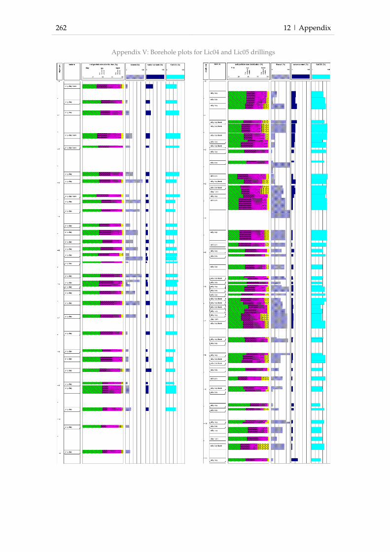
262 12 | Appendix
Appendix V: Borehole plots for Lic04 and Lic05 drillings

12 | Appendix
Appendix Appendix VI: Inclinometer measurements for Lic01
263

264
Appendix Appendix VII: Inclinometer measurements for Lic04
12 | Appendix

12 | Appendix
Appendix endix VIII: Inclinometer measurements for Lic03
265
266 12 | Appendix
Appendix IX: Slip search grid location definition
SLIP SEARCH GRID LOCATION
1.1. Define coordinates of the lower left hand corner of the grid: at one-third of the
profile length and at two-thirds height for profiles longer than 450 metres; half the
height and two-thirds of length
1.2. If grid overlaps with slope surface, move right 1 mesh coordinate
1.3. Define grid spacing as the same as mesh size, and grid dimensions as 10 by 10
1.4. Set minimum radius as 10 metres and radius increment as the same as mesh size
Appendix X: ArcGIS RASTERCALCULATOR commands for compu-tation of the subsurface model
Command to create DTM segments for geological strata in ESRI ArcGIS RASTER-
CALCULATOR based on maximum elevation. The procedure involves two com-
mands to be executed in RASTERCALCULATOR. In this example nine segments are
created, of which the lowest is below the level of the DTM
Step 1:
step1_elevation2 = con([DTM] > elevation3, [DTM])
step1_elevation3 = con([DTM] > elevation4, [DTM])
step1_elevation4 = con([DTM] > elevation5, [DTM])
step1_elevation5 = con([DTM] > elevation6, [DTM])
step1_elevation6 = con([DTM] > elevation7, [DTM])
step1_elevation7 = con([DTM] > elevation8, [DTM])
Step 2:
step2_elevation1 = con([DTM] > elevation2, [DTM])
step2_elevation2 = con([elevation2_1] >= elevation2, elevation2, [elevation2_1])
step2_elevation3 = con([elevation3_1] >= elevation3, elevation3, [elevation3_1])
step2_elevation4 = con([elevation4_1] >= elevation4, elevation4, [elevation4_1])
step2_elevation5 = con([elevation5_1] >= elevation5, elevation5, [elevation5_1])
step2_elevation6 = con([elevation6_1] >= elevation6, elevation6, [elevation6_1])
step2_elevation7 = con([elevation7_1] >= elevation7, elevation7, [elevation7_1])
step2_elevation8 = con([DTM] < elevation8, [DTM])
step2_elevation9 = con([DTM] > elevation9, elevation9)

12 | Appendix 267
Appendix XI: Soil suction curves defined by SPAW model in com-parison to laboratory measurements with interpolated values
Pf Laboratory values SPAW values Interpolated values
15 0.13486667 0.245 0.13486667
10 0.259 0.14915
8 0.15643333 0.266 0.15643333
6 0.276 0.16625416
4 0.291 0.176075
3 0.302 0.18589583
2 0.318 0.19571667
1.6 0.327 0.2055375
1.2 0.34 0.21535833
0.8 0.358 0.22517917
0.4 0.392 0.235
0.3 0.235 0.235
0.2 0.457 0.24
0.1 0.2587 0.5 0.2587
0.06 0.26413333 0.26413333
0.03 0.27656667 0.27656667

268 12 | Appendix
Appendix XII: English tutorial for web-based CHASM decission-support system
1. Welcome to the web-processing service by the ILEWS project! On this website you
can calculate slope stabiltiy for our test slope in Lichtenstein-Unterhausen at the
Swabian Alb, Germany. To start please activate the pencil symbol in the upper left
corner and create a slope profile for the calculation by clicking on the map.
2. Please select a name for your chosen profile. You can change some model parame-
ters like the length of the simulation and the timesteps. Please select the output in-
formation that you would like to receive. Please select the rainfall scenarios by
clicking on RS.
3. Please select a rainfall scenario for you simulation.
o Scenario type: normal, worst case and maximal worst case
o rainfall distribution pattern: equally distributed rainfall distribution, Euler 1
and Euler
o rainfall duration: 6h, 12h, 24h, 48h oder 72h Niederschlagsverteilung: gleich-
verteilt, Euler 1 oder Euler 2
o likelihood of occurence: 1 in 1, 1 in 10, 1 in 50, 1 in 100 and click OK
4. Click on „Create model“ to save the your simulation settings to the database, or
click “create model and calculate” to also start the simulation.
5. Your simulation is beeing processed on the server. Please wait until calculation is
finished.
6. The slope profile is calculated with respect to your settings and the profile is col-
oured regarding the calculated stability. The FoS of the last simulation step is
shown next to the profile. Please select Simulation>model resuls>show results for
further information for your simulation.
7. Please select your simulation or any other simulation created before .
8. Clicking on the curve symbol behind your simulation opens a graphical presen-
tion of the FoS in the course of the simulation
9. Congratulation! You have completed a CHASM WPS simulation!

12 | Appendix 269
Appendix XIII: Englsih frequently asked questions (FAQ)
General information
The web-processing service of CHASM enables the user to calculate slope stability for
the study area of the project ILEWS. For further information please read the FAQ and
visit the websites.
CHASM
CHASM is an integrated slope hydrology/slope stability software package. The soft-
ware has been written to assist in the estimation of controls on slope stability and to
be of value to a wide range of potential users ranging from pre-site investigation en-
gineering applications to evaluations concerned with the impact of bioengineering on
slope stability.
Source and additional information: http://chasm.info/
WPS
A Web Processing Service (WPS) is designed to standardize the way that GIS calcula-
tions are made available to the Internet. WPS can describe any calculation (i.e. proc-
ess) including all of its inputs and outputs, and trigger its execution as a Web Service.
Source and additional information:
http://en.wikipedia.org/wiki/Web_Processing_Service
CHASM-WPS
The CHASM WPS is a pivotal development in the ILEWS project as has been jointly
designed by the company Geomer (Germany) and the Workgroup on Geomor-
phological Systems and Risk Research (ENGAGE), Institute of Geography and Re-
gional Research, University of Vienna (Austria).
For further information: http://www.geomer.de/ and
http://geomorph.univie.ac.at/?L=2
KOSTRA
Kostra (also KOSTRA-2000-DWD) is a storm rainfall event catalogue published by the
Deutscher Wetter Dienst (DWD) (German Weather Service).
Source and additional information: http://de.wikipedia.org/wiki/Kostra and
http://www.itwh.de/S_kostra.htm
Factor of Safety (FoS)
A measure of slope stability. With FoS>1 a slope is defined stable and FoS<1 as unsta-
ble
For more information: http://en.wikipedia.org/wiki/Factor_of_safety

270 12 | Appendix
ILEWS
The ILEWS project is is concerned with the development and implementation of
modular and transferable landslide early warning systems for local and regional
scales which can also be adapted to other localities and processes. Within ILEWS early
warning systems are regarded as a chain starting from the sensor in field as the piv-
otal part of a robust monitoring system, reliable data transmission, innovative model-
ling and communication of possible actions with stakeholders.
For more information: http://www.ilews.eu
Rainfall scenarios
Rainfall scenarios are based on the KOSTRA atlas. From the statistical modelling of
the rainfall intensities performed within KOSTRA three types of scenarios were cre-
ated for.
Normal: These scenario are based on the standard intensities given by KOSTRA
Maximum: As KOSTRA rainfall events are based on probability calculation upper and
lower limits are given. Max scenarios are bases on the upper limit given in KOSTRA.
Max-worst: Rainfall intensities given in KOSTRA are subject to uncertainties and
these are also quantified (up to 20%). In max-worst scenarios the uncertainties are
added to the maximum rainfall intensities.
Rainfall distributions
Three kinds of rainfall distributions are available:
Equally distributed: same intensities for the entire course of the rainfall event
Euler 1: a statistically derived rainfall distribution used within drainage planning.
Euler 1 events have the highest rainfall intensities in the beginning of the rainfall
event and decreasing intensities afterwards
Euler 2: similar to Euler 1 scenarios but the highest intensities occur after one third of
the duration of the rainfall.
Disclaimer
Slope stability calculation presented here is for informational use only. Calculations
are based on simplified models and no recommendations for possible actions should
be deduced of the CHASM WPS without the consultancy of experts. Neither the pro-
ject ILEWS nor the owner of the website are responsible for inappropriate use of the
CHASM WPS.
Contact
For questions regarding the implementation of CHASM as WPS please contact
[email protected] For questions concerning the calculation of slope stability, data used

12 | Appendix 271
and other model parameters please contact [email protected] For questions
on CHASM please contact [email protected]

272 12 | Appendix
Appendix XIV: German tutorial for web-based CHASM decission-support system
1. Willkommen zum web-processing service des Projekts ILEWS! Auf dieser Websei-
te können Sie die Hangstabilität für unseren Untersuchungshang in Lichtenstein-
Unterhausen an der Schwäbischen Alb, Deutschland ermitteln. Um zu beginnen
aktivieren Sie bitte das Stiftsymbol oben links und klicken Sie bitte an zwei Stellen
auf die Karte um ein Profil für die Berechnung zu erstellen.
2. Bitte wählen Sie einen Namen für das gewählte Profil. Sie können weitere Model-
paramter wie z.B. die Laufzeit der Modellierung und die Länge der Zeitschritte
verändern. Bitte wählen Sie die gewünschten Ausgabeinformationen. Bitte wählen
Sie die gewünschten Niederschlagsszenarien, indem Sie auf RS klicken.
3. Bitte wählen Sie ein Niederschlagsszenario für Ihre Modellierung.
o Szenariotyp: normal, worst case und maximal worst case Szenario
o Niederschlagsverteilung: gleichverteilt, Euler 1 oder Euler 2
o Dauer des Niederschlagsereignisses: 6h, 12h, 24h, 48h oder 72h
o Jährlichkeit des Ereignisses: 1 in 1, 1 in 10, 1 in 50, 1 in 100 und klicken Sie an-
schließend OK
4. Klicken Sie “Modell erstellen” um die Simulationseinstellungen in der Datenbank
abzuspeichern, oder klicken Sie “Modell erstellen und berechnen” um auch direkt
die Modellierung zu starten.
5. Ihre Modellierung wird grade auf dem Server berechnet, bitte warten Sie bis die
Kalkulation abgeschlossen ist.
6. Das von Ihnen gewählte Hangprofil wird anhand der ermittelten Stabilität einge-
färbt und der FoS des letzten Modellierungsschrittes wird neben dem Profil ange-
geben Wählen sie unter Simulation>Modell Ergebnisse> Ergebnisse anzeigen um
weitere Informationen zur Modellierung zu erhalten
7. Wählen Sie ihr selbst erstellte Simulation aus, oder eine zuvor berechnete Simula-
tion.
8. Mit einem Klick auf das Kurvensymbol hinter Ihrer Modellierung erhalten Sie
eine grafische Darstellung des Verlaufs des FoS
9. Gratulation! Sie haben die zentralen Funktionen des CHASM WPS durchgeführt!

12 | Appendix 273
Appendix XV: German frequently asked questions (FAQ)
Einführende Informationen
Der web-processing service von CHASM ermöglicht die Ermittlung der Hangstabili-
tät für das Untersuchungsgebiet des Projekts ILEWS. Für weitere Informationen lesen
Sie bitte die FAQ und besuchen Sie die Websites.
CHASM
CHASM ist eine interiertes Hanghydrologie und -stabilitäts Softwarepaket. Das Pro-
gramm wurde entwickelt um den Einfluss unterschiedlicher Faktoren auf die Hang-
stabilität abzuschätzen. Es dient unter anderem der Vorerkundung für für bauliche
Maßnahmen und zur Ermittlung des Effekts von bioengineering Maßnahmen.
Quelle und weitere Informationen: http://chasm.info/
WPS
Ein Web processing service ist eine standardisierte Form mit der GIS Berechnungen
im Internet zur Verfügung gestellt werden. WPS können jegliche Berechnungen (Pro-
zesse) mit allen Inputs und Outputs als Web Service durchführen.
Quelle und weitere Informationen:
http://en.wikipedia.org/wiki/Web_Processing_Service
CHASM-WPS
Der CHASM WPS ist eine zentrale Entwicklung des ILEWS Projekts und wurde ge-
meinschaftlich durch die Firma Geomer (Deutschland) und der Arbeitsgruppe Geo-
morphologische Systeme und Risikoforschung (ENGAGE), Institute für Geographie
und Regionalforschung, Universität Wien (Österreich) aufgebaut.
Für weitere Informationen: http://www.geomer.de/ und
http://geomorph.univie.ac.at/
KOSTRA
Kostra (auch KOSTRA-2000-DWD) ist ein vom Deutschen Wetterdienst (DWD) he-
rausgegebener Starkregenkatalog und steht für Koordinierte Starkniederschlags-
Regionalisierungs Auswertungen.
Quelle und weitere Informationen: http://de.wikipedia.org/wiki/Kostra und
http://www.itwh.de/S_kostra.htm
Factor of Safety (FoS)
Ein Maß der Hangstbilität. Ein FoS>1 ist demnach stabil und mit FoS<1 instabil.
Für weitere Informationen: http://de.wikipedia.org/wiki/Reservefaktor

274 12 | Appendix
ILEWS
Das Projekt ILEWS beschäftigt sich mit der Entwicklung und Implementierung von
modularen und transferierbaren Frühwarnsysteme für gravitative Massenbewegun-
gen für lokale und regionale Skalen, welches sich auch auf andere Lokalitäten und
Prozesse adaptieren lässt. In ILEWS werden Frühwarnsysteme als eine Kette betrach-
tet, welche mit dem Sensor im Feld als zentralen Teil eines robusten Monitorings-
systems beginnt und ebenso zuverlässige Datenübermittlung, innovative Modellie-
rungen und Kommunikation der Warnung, sowie Bereitstellung von Handlungsal-
ternativen für die Entscheidungsträgern umfasst.
Für weitere Informationen: http://www.ilews.eu
Niederschlagszenarien
Die Niederschlagsereignisse basieren auf dem KOSTRA Atlas. Aufgrund der statisti-
schen Modellierung von Niederschlagsintensitäten innerhalb von KOSTRA wurden
drei Typen von Niederschlagsereignissen gebildet:
o Normal: Diese Szenarien beruhen auf den Standardintensitäten laut KOSTRA
o Max: Da die Niederschlagsintensitäten in KOSTRA auf probabilitischen Mo-
dellierungen basieren werden obere und untere Klassengrenzen angegeben.
Die max Szenarien basieren auf den oberen Klassengrenzen von KOSTRA.
o Max-worst: Die Niederschlagsintensitäten in KOSTRA unterliegen Unsicher-
heiten, welche auch quantifiziert sind (bis zu 20%). In den max-worst Szena-
rien wurden diese Unsicherheiten den maximalen Szenarien zugeschlagen.
Niederschlagsverteilung
Drei unterschiedliche Niederschlagsverteilungen stehen zur Auswahl:
o gleichverteilt: gleiche Niederschlagsintensitäten während des gesamten Nie-
derschlagsereignisses
o Euler 1: ein statistisch ermittelter Modellregen der in der häufig in der Pla-
nung von Entwässerungssystemen Verwendung findet. Euler 1 Verteilungen
weisen die höchste intensität des niederschlags zu Beginn des Ereinisses auf,
anschliessend nimmt die Intensität ab.
Euler 2: ähnlich wie Euler 1 Verteilungen. Der Unterschied besteht darin, dass die höchste intensität nach einem Drittel der Niederschlagsdauer erreicht wird.

12 | Appendix 275
Appendix XVI: Curriculum vitae
Personal Dates
Name Benni Thiebes
Date of birth 3. November 1980
Place of Birth
Siegburg, Germany
Address Adolfstraße 80, 53111 Bonn, Deutschland
Email [email protected]
Research interests
Geomorphology, natural hazards and risks, early warning systems, landslide processes, modelling, global change
Education
May 2007 – June 2011
PhD student at the Department of Geography and Regional Research, University of Vienna, Austria Topic of PhD-thesis: Landslide analysis and early Warning – Local and regional case study in the Swabian Alb, Germany
July 2006 Diploma in Geographies at University of Bonn, Germany (Grade: 1.2) Master Thesis: Spatial Susceptibility Analysis of Shallow Landslides - GIS based Analysis in the Swabian Alb (in German, Grade: 1.0)
Oct 2002 Intermediate Diploma in Geography at University of Bonn, Germany (Grade: 1.4)
Oct 2000 Begin of Studies of Geography, Soil Science and Agricultural Engineer-ing, Rheinische Friedrich-Wilhelm University of Bonn, Germany
June 2000 General Qualification for university entrance (Abitur) at Integrierte Ge-samtschule, Bonn-Beuel, Germany
Practical Experiences
June 2009 Workshop: Geotechnologien für instabilie Hänge (Geotechnics for unst-able slopes). Technical University Munich, Germany(2 days)
Sep 2009 Summer school: “Landslide Risk Assessment and Mitigation (LARAM)”, University of Salerno, Italien (14 days)
Aug 2006 Summer school: „Environmental Hazards and Sustainable Development in Mountain Regions“, Institute of Geography, Romanian Academy, Rumänien (7 days)
Nov 2005 – May 2006
Student assistant in the InterRISK project (Integrative Risk Analysis and Assessment of Mass Movements in the Swabian Alb) at Department of Geography, University of Bonn, Germany
Oct 2003 – Dec 2003
Internship at Institute of Geological and Nuclear Sciences (GNS), Wel-lington, New Zealand
Aug 2003 Field work seminar, “High Mountain Geomorphology”, Turtmanntal, Wallis, Switzerland
276 12 | Appendix
Further Qualifications
Languages German (first language), English (very good), French (basic knowledge), Mandarin Chinese (beginner)
Computer skills
Extensive general computer skills (e.g. MS Office, OpenOffice, Free-Hand, Photoshop), slope stability analysis (e.g. CHASM, GeoStudio)
GIS Extensive knowledge in GIS software (ArcView 3.x, ArcGIS 9.x, ArcInfo, Golden Surfer, Global Mapper), geomorphic modelling based on digital elevation models, regional landslide susceptibility and hazard model-ling (e.g. SINMAP, SHALSTAB, statistical models )
Field me-thods
Geomorphological mapping, drilling, geophysical methods (geolectric, seismic), geodetic surveying, terrestrial laserscanning, hydrological analysis, sensor installation, soil analysis
Licenses Driving License for cars, trucks (max. 7,5 t) and motorcycles, PADI Open Water licence
Publications
Mayer, J., Glade, T., Thiebes, B., Bell, R. (2010): Integrative Frühwarnsysteme. In: Bell, R., Glade, T., Greiving, S., Mayer, J., Pohl, J. (eds): Integrative Frühwarnsys-teme für gravitative Massenbewegungen (ILEWS) - Monitoring, Modellierung, Implementierung.17-31.
Bell, R., Greiving, S., Pohl, J., Röhrs, M., Glade, T., Thiebes, B., Mayer, J. (2010): Unter-suchungsgebiete. In: Bell, R., Glade, T., Greiving, S., Mayer, J., Pohl, J. (eds): In-tegrative Frühwarnsysteme für gravitative Massenbewegungen (ILEWS) - Monitoring, Modellierung, Implementierung. 32-45.
Bell, R., Wiebe, H., Krummel, H., Camek, T., Becker, R., Öhl, S., Aslan, A. M., Burghaus,S., Li, L., Schauerte, W., Kuhlmann, H., Thiebes , B. (2010): Monitor-ing. In: Bell, R., Glade, T., Greiving, S., Mayer, J., Pohl, J. (eds): Integrative Frühwarnsysteme für gravitative Massenbewegungen (ILEWS) - Monitoring, Modellierung, Implementierung. 62-129.
Thiebes, B., Bell, R., Glade, T., Aslan, A. M., Schauerte, W., Kuhlmann, H. (2010): Frühwarnmodellierung. In: Bell, R., Glade, T., Greiving, S., Mayer, J., Pohl, J. (eds): Integrative Frühwarnsysteme für gravitative Massenbewegungen (ILEWS) - Monitoring, Modellierung, Implementierung. 130-154.
Bell, R., Mayer, J., Pohl, J., Greiving, S., Paulsen, H., Röhrs, M., Jäger, S., Wiebe, H., Thiebes, B. (2010): Erfahrungen aus dem integrativen Projekt. In: Bell, R., Glade, T., Greiving, S., Mayer, J., Pohl, J. (eds): Integrative Frühwarnsysteme für gravitative Massenbewegungen (ILEWS) - Monitoring, Modellierung, Im-plementierung. 231-237.
Bell, R., Mayer, J., Pohl, J., Greiving, S., Paulsen, H., Röhrs, M., Jäger, S., Wiebe, H., Thiebes, B., Aslan, A. M. (2010): Transferierbarkeit des integrativen Frühwarn-systems. In: Bell, R., Glade, T., Greiving, S., Mayer, J., Pohl, J. (eds): Integrative Frühwarnsysteme für gravitative Massenbewegungen (ILEWS) - Monitoring, Modellierung, Implementierung. 238-243.
Bell, R., Becker, R., , Burghaus, S., Dix, A., Flex, F., Glade, T. Greiving, S., Greve, K., Jaeger, S., Janik, M., Kuhlmann, H., Krummel, H., Lang, A., Li, L., Mayer, C., Mayer, J., Padberg, A., Paulsen, H., Pohl, J., Roehrs, M., Schauerte, W., Thie-bes, B. & Wiebe, H. (2009): ILEWS - Integrative Landslides Early Warning Sys-tems. In: Stroink, L. (editor): Geotechnologien Science Report (Conference Pro-
12 | Appendix 277
ceeding), Early Warning Systems in Earth Management, No. 13. Technical University Munich, Germany. 16 - 32.
Bell, R., Glade, T., Thiebes, B., Jaeger, S., Krummel, H., Janik, M. & Holland, R. (2009): Modelling and web processing of early warning. In: J.-P. Malet, A. Remaître, T. Bogaard (Editors): Landslide Processes, From Geomorphic Mapping To Dynamic Modelling (Conference Proceeding), CERG Editions, Strasbourg, France. 249 – 252.
Bell, R., Thiebes, B., Glade, T., Becker, R., Kuhlmann, H., Schauerte, W., Burghaus, S., Krummel, H., Janik, M. & Paulsen, H. (2008): The technical concept within the Integrative Landslide Early Warning Systems (ILEWS) project. 10th Interna-tional Symposium on Landslides And Engineered Slopes (Conference Pro-ceeding). Xi'an, China. 293 – 298.
Thiebes, B., Bell, R. & Glade, T. (2007): Determinitische Analyse flachgruendiger Han-grutschungen mit SINMAP - Fallstudie an der Schwaebischen Alb (Determi-nistic landslide susceptibility analysis using SINMAP - case study in the Swabian Alb, Germany). In: Geomorphology for the Future (Conference Pro-ceeding). Obergurgl, Austria. (in German with English abstract). 177 – 184.
Glade, T., Becker, R., Bell, R., Burghaus, S., Danscheid, M., Dix, A., Greiving, S., Greve, K., Jaeger, S., Krummel, H., Kuhlmann, H., Paulsen, H., Pohl, J., Roehrs, M. & Thiebes, B. (2007): Integrative Landslides Early Warning Systems. In: Stroink, L. (editor): Geotechnologien Science Report (Conference Proceeding), Early Warning Systems in Earth Management, No. 10. Technical University, Karlsruhe, Germany. 89 - 100.
Thiebes, B. (2006): Raeumliche Gefaehrdungsanalyse flachgruendiger Hang-rutschungen - GIS gestuetzte Analyse an der Schwaebischen Alb. (Spatial Sus-ceptibility Assessment of Shallow Landslides – GIS Based Analysis in the Swabian Alb). Unpublished Master Thesis. Department of Geographies, Uni-versity of Bonn, Bonn, Germany. (in German). 124 p.
Thiebes, B. (2003): Analysis of landslide effects in the Paekakariki area from 3. Oct. 2003 rainstorm. Institute of Geological and Nuclear Sciences File Report LD5/941. Wellington, New Zealand. 14 p.
Presentations
Modelling landslide early warning - experiences from the ILEWS project . Normal University Nanjing, China. 28.08.2010.
Landslide early-warning using CHASM as a web processing service. European Geo-sciences Union General Assembly (EGU), Vienna, Austria. Geophysical Re-search Abstracts, Vol. 11, EGU2009-6228. 21.04.2009.
Fruehwarnsystem an der Schwaebischen Alb. Nutzen fuer Suedtirol? Workshop with local agents of the administration of the Autonomous Province of South Tyrol, Bolzano, South Tyrol. 07.04.2009.
Quantitative Risk Assessment. Presentation in colloquium Geomorphology, Institute of Geography and Regional Research, University of Vienna, Austria. 20.01.2009.
SINMAP Stability Index Mapping – Determinische Gefaehrdungsanalyse flachgru-endiger Hangrutschungen. Presentation for agents of the government of Lower Austria, Vienna, Austria. 30.09.2008
Local and Regional Early Warning Systems. International School on "Landslide Risk Assessment and Mitigation (LARAM)", University of Salerno, Ravello, Italy. 12.09.2008.
278 12 | Appendix
Landslide Monitoring and Modelling. Presentation of PhD thesis in Research Semi-nar. Institute of Geography and Regional Research, University of Vienna, Aus-tria. 23.06.2008
Determinitische Analyse flachgruendiger Hangrutschungen mit SINMAP - Fallstudie an der Schwaebischen Alb. At: Geomorphology for the Future, Meeting of the Austrian Research Association on Geomorphology and Global Change, Ober-gurgl, Austria. 05.09.2008
Spatial landslide susceptibility assessment - GIS-based study in the Swabian Alb. Summer School 'Environmental Hazards and Sustainable Development in Mountain Regions'. Romanian Academy, Institute of Geography Bucarest, Romania. Patarlagele, Romania. 19.07.2006
Deterministische Analyse flachgruendiger Hangrutschungen mit SINMAP. Presenta-tion of Master thesis in colloqium of the Prof. Dikau working group. Depart-ment of Geography, University of Bonn, Germany. 20.06.2006
Posters
Thiebes, B., Bell, R., Glade, T., Aslan, A. M., Jaeger, S., Anderson, L. & Holcombe, L.: Landslide early warning models – five applicartion within the ILEWS project. Geophysical Research Abstracts, Vol. 12, EGU2010-2503. European Geo-sciences Union General Assembly (EGU), Vienna, Austria. 05.05.2010.
Bai, S., Thiebes, B., Bell, R., Glade, T., Wang, J.: A comparison of susceptibility maps created with logistic regression and SINMAP for spatial planning in the Lan-zhou City, China. Geophysical Research Abstracts, Vol. 12, EGU2010-6130-1. European Geosciences Union General Assembly (EGU), Wien, Österreich. 05.05.2010.
Thiebes, B., Jaeger, S., Bell, R., Janik, M., Krummel, H., Becker, R., Paulsen, H., Glade, T., Holcombe, L., Anderson, M.: Fruehwarnung gravitativer Massenbewegun-gen als web-processing service. Statusseminar Geotechnologien, Early Warn-ing Systems in Earth Management. Munich, Germany. 12. - 13.10.2009.
Thiebes, B., Becker, R., Bell, R., Burghaus, S., Dix, A., Glade, T., Greiving, S., Greve, K., Jaeger, S., Krummel, H., Kuhlmann, H., Mayer, J., Paulsen, H., Pohl, J., Roehrs, M. & Schauerte, W.: Integrative Fruehwarnsysteme fuer gravitative Massen-bewegungen. Deutscher Geographentag, Vienna, Austria. 20.09.2009.
Thiebes, B., Jaeger, S., Bell, R., Janik, M., Krummel, H., Becker, R., Paulsen, H., Glade, T., Holcombe, L. & Anderson, M.: Fruehwarnung gravitativer Massen-bewegungen als web-processing service. Workshop Warn- und Risikoman-agement bei Massenbewegungen, Hannover, Germany. 25.06.2009.
Bell, R., Glade, T., Krummel, H., Kuhlmann, H., Mayer, J., Becker, R., Dix, A., Greiv-ing, S., Burghaus, S., Greve, K., Jaeger, S., Paulsen, H., Pohl, J., Roehrs, M., Schauerte, W. & Thiebes, B.: Integrative Fruehwarnsysteme fuer gravitative Massenbewegungen. Monitoring, Modellierung, Implementierung. Workshop Warn- und Risikomanagement bei Massenbewegungen, Hannover, Germany. 25.06.2009.
Thiebes, B., Becker, R., Bell, R., Burghaus, S., Dix, A., Glade, T., Greiving, S., Greve, K., Jaeger, S., Krummel, H., Kuhlmann, H., Mayer, J., Paulsen, H., Pohl, J., Roehrs, M. & Schauerte, W.: Integrative Landslide Early Warning Systems within the ILEWS Project. Geophysical Research Abstracts, Vol. 11, EGU2009-6212. Euro-pean Geosciences Union General Assembly (EGU), Vienna, Austria. 21.04.2009.
Thiebes, B., Bell, R., Glade, T., Jaeger, S. & Anderson, M.: Near-Real Time Early Warn-

12 | Appendix 279
ing Modelling im Projekt ILEWS. 3rd Central-European Congress on Geomor-phology, Salzburg, Austria. 24.09.2008.
Bell, R., Thiebes, B., Becker, R., Burghaus, S., Dix, A.,Glade, T., Greiving, S., Jaeger, S., Krummel, H., Paulsen, H., Greve, K., Pohl, J., Roehrs, M. & Schauerte, W.: ILEWS – Integrative Landslide Early Warning System. 3rd Central-European Congress on Geomorphology, Salzburg, Austria. 24.09.2008.
Thiebes, B., Bell, R., Becker, R., Burghaus, S., Dix, A., Glade, T., Janik, M., Kuhlmann, H., Paulsen, H. & Schauerte, W.: Landslide monitoring and modelling within the Integrative Landslide Early Warning Systems (ILEWS). Geophysical Re-search Abstracts, Vol. 10, EGU2008-A-10030. European Geosciences Union General Assembly (EGU), Vienna, Austria. 18.04.2008.
Danscheid, M., Becker, R., Bell, R., Burghaus, S., Dix, A., Glade, T., Greiving, S., Greve, K., Jaeger, S., Krummel, H., Kuhlmann, H., Paulsen, H., Pohl, J., Roehrs, M., Schauerte, W. & Thiebes, B.: Integrative landslide early warning systems (ILEWS). Geophysical Research Abstracts, Vol. 10, EGU2008-A-09998. Euro-pean Geosciences Union General Assembly (EGU), Vienna, Austria. 15.04.2008.
Thiebes, B., Bell, R. & Glade, T.: Deterministic landslide susceptibility analysis using SINMAP - a case study in the Swabian Alb. Geophysical Research Abstracts, Vol. 9, 11199. European Geosciences Union General Assembly (EGU), Vienna, Austria. 20.04.2007.
Thiebes, B., Bell, R. & Glade, T.: GIS gestuetzte Gefaehrdungsmodellierung flachgru-endiger Hangrutschungen mit SINMAP. 17th Meeting of Working Group Natural Hazards, GIS in Natural Hazard Analysis and Risk Management, Augsburg, Germany. 14.12.2006.
Teaching
Underground investigations of landslides. Intensive Course for the MountainRisks Project, Les Diablerets, Switzerland. 22. - 24.06.2009.
Field and Laboratory Methods in Physical Geography. Lecture (in German), WS 2008/2009, Institute for Geography and Regional Research, University of Vienna, Austria.
Exercises - Field and Laboratory Methods in Physical Geography . Practical course (in German), WS 2008/2009, Institute for Geography and Regional Research, University of Vienna, Austria.
Affiliation
o European Geosciences Union (EGU) o AK Naturgefahren/Naturrisiken (Working Group Natural hazards/Natural
Risks) o AK Geomorphologie (Working Group Geomorphology) o Österreichische Geographische Gesellschaft (ÖGG) (Austrian Geographical Socie-
ty) / Austrian Research Association on Geomorpholgy and Environmental Change (Geomorph.at)


