Direct and adjoint global modes of a recirculation bubble: lift-up and convective non-normalities

J. Fluid Mech. (2009), vol. 622, pp. 1–21. c© 2009 Cambridge University Press

doi:10.1017/S0022112008004023 Printed in the United Kingdom

1

Direct and adjoint global modes of arecirculation bubble: lift-up andconvective non-normalities

OLIVIER MARQUET1, MATTEO LOMBARDI1,JEAN-MARC CHOMAZ1,2, DENIS SIPP1

AND LAURENT JACQUIN1

1Departement d’Aerodynamique Fondamentale et Experimentale, ONERA, 92190 Meudon, France2Laboratoire d’Hydrodynamique (LadHyx), CNRS - Ecole Polytechnique, 91128 Palaiseau, France

(Received 29 April 2007 and in revised form 20 July 2008)

The stability of the recirculation bubble behind a smoothed backward-facing stepis numerically computed. Destabilization occurs first through a stationary three-dimensional mode. Analysis of the direct global mode shows that the instabilitycorresponds to a deformation of the recirculation bubble in which streamwise vorticesinduce low- and high-speed streaks as in the classical lift-up mechanism. Formulationof the adjoint problem and computation of the adjoint global mode show thatboth the lift-up mechanism associated with the transport of the base flow by theperturbation and the convective non-normality associated with the transport ofthe perturbation by the base flow explain the properties of the flow. The lift-upnon-normality differentiates the direct and adjoint modes by their component: thedirect is dominated by the streamwise component and the adjoint by the cross-stream component. The convective non-normality results in a different localizationof the direct and adjoint global modes, respectively downstream and upstream.The implications of these properties for the control problem are considered. Passivecontrol, to be most efficient, should modify the flow inside the recirculation bubblewhere direct and adjoint global modes overlap, whereas active control, by for exampleblowing and suction at the wall, should be placed just upstream of the separationpoint where the pressure of the adjoint global mode is maximum.

1. IntroductionFor many years the problem of transition to turbulence in shear flows has been

addressed by studying the exponential growth of linear perturbations developing ona base flow. However this linear modal analysis failed to predict the transitionalReynolds number determined experimentally in parallel shear flows such as Couetteand Poiseuille flows since those flows are linearly stable at this transitional Reynoldsnumber. In the past decade a transition scenario based on the concept of receptivityhas been considered that completes the modal analysis. The flow receptivity definesthe ability of stable flows to amplify perturbation energy in a transient manner. Thisnon-modal amplification is due to the non-normality of the linearized Navier–Stokesoperator (Trefethen et al. 1993). The non-normality of parallel shear flows wasfirst explored by Butler & Farrell (1992) who described the physical mechanismunderlying the non-normality of parallel shear flows as the so-called lift-up mechanism

2 O. Marquet, M. Lombardi, J.-M. Chomaz, D. Sipp and L. Jacquin

(Landahl 1980) which creates large streamwise perturbations through transport of thebase-flow momentum by cross-stream velocity perturbations. Transition to turbulenceis then due (see the review by Schmid 2007) to a nonlinear feedback betweenstreamwise streaks and streamwise vortices and only a nonlinear weak feedbackis sufficient since the linear non-normal amplification of vortices into streaks isextremely large and increases with the Reynolds number.

Open flows are usually strongly non-parallel and analysing their stability requires, inthe case of a flow homogeneous in the spanwise direction, solving a two-dimensionaleigenvalue problem for which both the streamwise and cross-stream directions areeigendirections. Thanks to increasing computational capacity, the so-called globalstability analysis has recently received substantial attention. Theofilis, Hein & Dallman(2000), Barkley, Gomes & Henderson (2002), Gallaire, Marquillie & Ehrenstein(2007) – among many others – have determined the spectrum of the linearizedNavier–Stokes operator for different two-dimensional base flows. Only a few studies(Schmid & Henningson 2002; Ehrenstein & Gallaire 2005; Giannetti & Luchini 2007;Akervik et al. 2007) have started to analyse the dynamics resulting from thenon-normality of this operator. Most of them have focused on the descriptionof the amplifier dynamics, i.e. the short-time dynamics resulting from a transientamplification of the perturbation energy. As shown by Schmid & Henningson 2002 orEhrenstein & Gallaire (2005), this transient growth may be viewed as the superpositionof global modes since they are non-orthogonal when the operator is non-normal. Assuggested by Chomaz (2005), examining the non-normality of the evolution operatoris also of interest to better understand the destabilization of the flow close to thebifurcation. To our knowledge, only Giannetti & Luchini (2003, 2007) have perfomedsuch an analysis, in the case of a circular cylinder flow. They have computed boththe direct and adjoint leading global modes that describe the occurrence of the vonKarman street and commented, as did Chomaz Huerre & Redekopp (1990) and Cossu& Chomaz (1997) when studying the Ginzburg–Landau envelop equation with varyingcoefficients, on the dissymmetry due to the transport of perturbations by the baseflow.

The objective of the present paper is to generalize this consideration to the three-dimensional destabilization of a two-dimensional flow and to apply it to a recirculationbubble in S-shaped geometry modelling an air intake. In other configurations, Theofiliset al. (2000) for a flow separating on a flat plate, Barkley et al. (2002) for a backward-facing-step flow and Gallaire et al. (2007) for separating flow over a bump, havefound that the first destabilization, on increasing the Reynolds parameter, is three-dimensional and steady. By computing both the direct global mode associated withthe leading eigenvalue of the linearized Navier–Stokes operator and the adjoint globalmode solution of the corresponding adjoint problem we discuss the non-normality ofthe flow and point out the interplay between the lift-up mechanism and the convectivenon-normality due to the transport of the perturbation by the base flow. For a studyof the non-normality and the resulting amplifier dynamics for the present recirculationflow, we refer to Marquet et al. (2008).

The paper is organized as follows. In § 2 we formulate the problem of the directand adjoint global mode analysis, distinguish two origins of the non-normality byexamining the direct and adjoint operators and thereby we extend the considerationdeveloped in the review by Chomaz (2005). In § 3 we present the numerical methodsand convergence tests. In § 4 we present the results of the direct and adjoint globalstability analysis. In particular we discuss the impact of the two distinct originsof the non-normality pointed out in § 2 on the direct and adjoint leading global

Direct and adjoint global modes of a recirculation bubble 3

1(a)

(b)

0y

–1

0.02

0.01Cf

xs xr

0

–0.01

–6 –4 –2 0 2 4 6 8 10 12

–6 –4 –2 0x

2 4 6 8 10 12

Figure 1. Flow configuration and base-flow characterization. (a) Streamlines of the base flowshowing the recirculation region. (b) Skin-friction coefficient on the lower wall (solid curve)and upper wall (dashed curve) as a function of the non-dimensional longitudinal coordinatex; the separation (xs = 0.46) and reattachment (xr = 0.55) points defining the length of therecirculation bubble are shown. Parameter settings: Re = 800, computational mesh Mb1.

modes. Finally, we give a physical interpretation of the adjoint global mode in termsof receptivity of the global mode to initial conditions and forcing, as well as itssensitivity to local modification of the recirculation bubble, both properties beingcrucial when control is concerned.

2. Problem formulation2.1. Geometry and base flow

A recirculation bubble is a separated flow reattaching downstream of the separationpoint, thus forming a recirculation region. To obtain such a flow configuration anS-shaped geometry (figure 1) has been designed. The shape of the lower wall is arounded backward-facing step, defined by its height h and its length L, and theshape of the upper wall has been chosen to prevent any recirculation region on thiswall. Further details about the geometry are provided in Appendix A. Coordinatesx, y and z denote respectively the longitudinal, vertical and transverse directionswith origin taken at the rounded-step edge. Those Cartesian coordinate are madenon-dimensional with the step height h. The computational domain is denoted Ω anddelimited by the boundaries Γi , Γo, Γu, Γl which correspond respectively to the inlet,the outlet and the upper and lower solid walls.

The motion of a viscous fluid governed by the non-dimensional incompressibleNavier–Stokes equations is considered:

∂t u + (u · ∇)u = −∇p + Re−1∇2u, (2.1a)

∇ · u = 0, (2.1b)

where u = (u, v, w) is the non-dimensional velocity field, p is the pressure field scaledby ρU 2

0 and the Reynolds number is defined as Re = U0h/ν; ν is the kinematicviscosity of the fluid and U0 is the maximum inlet centreline velocity which has been


used to scale the velocities. The following boundary conditions are imposed:

u =4y(hi − y)

h2i

, v = w = 0 on Γi, (2.2a)

u = v = w = 0 on Γu ∪ Γl, (2.2b)

p − Re−1∂xu = 0, ∂xv = ∂xw = 0 on Γo. (2.2c)

They correspond respectively to a parabolic velocity profile at the inlet, no-slipconditions on the solid walls and a free outflow condition at the outlet. The coefficienthi in the definition of the parabolic profile is the inlet height.

2.2. Base-flow computation and global modes analysis

The velocity and pressure fields are decomposed into a two-dimensional base flowQ(x, y) = (U, P )T = (U, V, 0, P )T and a three-dimensional disturbance flow, denotedby the quadrivector εq ′(x, y, z, t) = (u′, v′, w′, p′)T , where ε is the amplitude of theperturbation. The base flow is assumed to be a solution of the stationary two-dimensional incompressible Navier–Stokes equations

(U · ∇)U = −∇P + Re−1∇2U, (2.3a)

∇ · U = 0, (2.3b)

associated with the boundary conditions (2.2a–c). At leading order in ε theperturbation q ′ is a solution of the linearized Navier–Stokes equations and sincethe base flow is stationary and homogeneous in the transverse direction z, the three-dimensional perturbations may be sought as a normal mode

q ′(x, y, z, t) = 12{(u, v, w, p)T (x, y) exp[ikz + σ t] + c.c.}, (2.4)

where k is the real spanwise wavenumber, σ the complex growth rate and c.c. standsfor the complex conjugate of the preceding expression. The imaginary part σi of theglobal mode growth rate σ is related to the frequency of the mode, and its real partσr to the temporal growth rate. In particular, σr > 0 denotes exponential growth ofthe mode q ′ in time t .

Use of this normal mode decomposition in the Navier–Stokes equation linearizedaround the base flow Q gives that the growth rate is solution of the generalizedeigenvalue problem that may be written in the form:

A · q = σB · q, (2.5)

where q = (u, p)T = (u, v, iw, p)T is the complex eigenvector, the so-called globalmode, associated with the complex eigenvalue σ , the global growth rate. As noticedby Theofilis (2000), the particular form of q with the w component in quadraturewith the three others allows the solution of a generalized eigenvalue problem (2.5)with real matrices A and B defined as:

A =

⎛⎜⎝

D − C − ∂xU −∂yU 0 −∂x

−∂xV D − C − ∂yV 0 −∂y

0 0 D − C k

∂x ∂y k 0

⎞⎟⎠ ; B =

⎛⎜⎝

1 0 0 00 1 0 00 0 1 00 0 0 0

⎞⎟⎠ , (2.6)

where D = Re−1(∂x2 + ∂y2 − k2

)accounts for the viscous diffusion of the perturbation

and C = U∂x + V ∂y for its advection by the base flow.


The boundary conditions associated with (2.5) are

(u, v, iw) = (0, 0, 0) on Γu ∪ Γl ∪ Γi, (2.7a)

p − Re−1∂xu = 0, ∂xv = ∂xw = 0 on Γo. (2.7b)

To simplify the discussion the eigenmodes, solutions of (2.5) and (2.7), will be assumeddiscrete and non-degenerate. They will be indexed by an integer l and ranked indecreasing order of the real part of their temporal growth rate.

2.3. Non-normality and adjoint analysis

We define A+, the adjoint operator of A, as the operator such that, for any vectors qfulfilling the boundary conditions (2.7) and q+, with respect to boundary conditionsto be determined,

(q+, A · q) = (A+ · q+

, q), (2.8)

where q+ = (u+, p

+)T = (u+, v

+, iw+

, p+)T and (. , .) corresponds to the inner product

(q+, q) =

∫Ω

q+t · q dΩ. (2.9)

The superscript t denotes the transconjugate and the centred dot refers to theusual scalar product of two vectors. If the instantaneous energy density of a three-dimensional perturbation is defined as

E(q ′) =1

LzΩ

∫ +Lz/2

−Lz/2

∫Ω

(u′2 + v′2 + w′2) dx dy dz, (2.10)

where Lz = 2π/k is the transverse wavelength, Ω being the computational domainpreviously defined, it can be expressed using the normal mode decomposition (2.4)as

E(q ′) = 12E(q) exp[2σrt], (2.11a)

with

E(q) = (q, B · q) . (2.11b)

By successively integrating the left-hand side of (2.8) by parts, we obtain

A+ =

⎛⎜⎝

D + C − ∂xU −∂xV 0 −∂x

−∂yU D + C − ∂yV 0 −∂y

0 0 D + C k

∂x ∂y k 0

⎞⎟⎠ , (2.12)

and the adjoint boundary conditions:

(u+, v+, iw+) = (0, 0, 0) on Γu ∪ Γl ∪ Γi, (2.13a)

p+ − Re−1∂xu+ = −u+U

Re−1∂xv+ = v+U

Re−1∂xw+ = w+U

⎫⎬⎭ on Γo. (2.13b)

appropriate to cancel all of the boundary terms appearing during the integration byparts. The adjoint eigenproblem is then

A+ · q+ = σ+B · q+, (2.14)

σ+ and q+ being the adjoint growth rate and the adjoint global mode. It may beshown (see Schmid & Henningson 2001) that all the adjoint complex eigenvalues,


1

(a)0y

–1

–6 –4 –2 0 2 4 6 8 10 12

1

(b)

0y

–1

–6 –4 –2 0 2 4x

6 8 10 12

30

18

6

–6

–18

–30

1.5

0.9

0.3

–0.3

–0.9

–1.5

Figure 2. Spatial distribution of the derivatives of the base flow. The black line in the flowshows the dividing streamlines linking the separation point to the reattachment point. (a) ∂yU ,(b) ∂xV . Parameter settings: Re = 800, mesh Mb1.

ordered with the same rule as the direct ones, are the complex conjugates of adirect eigenvalue (σ+

l = σ ∗l ) and that the direct and adjoint global modes respect the

bi-orthogonality condition:

(q+m, B · q l) = Clδlm, (2.15)

which indicates that a particular adjoint global mode indexed by m is orthogonal toall the direct global modes indexed by l, except the one associated with the sameeigenvalue. From the expressions for A and A+ (2.6)–(2.12), we easily verify that Aand A+ do not commute, meaning that direct and adjoint global mode bases are notidentical and implying that for at least one l

(q+l B · q l) �= 1, (2.16)

if both q l and q+l are normalized to unit energy. Properties (2.15) and (2.16) imply

that direct eigenmodes are not normal to each other and therefore the energy ofa perturbation is not the sum of the squared coefficients of its decomposition ontothe base of eigenmodes. This offers the possibility of a transient growth of theperturbation energy even if all the coefficients of the decomposition into eigenmodesdecrease in time as is the case for stable flows. For parallel shear flows, transientgrowth is associated in particular with the lift-up mechanism, i.e. the creation of alarge streamwise velocity perturbation through transport of the base-flow momentumby a cross-stream velocity perturbation (see Schmid & Henningson 2001). In thepresent formalism, this mechanism corresponds to the off-diagonal terms of A thatreduce to −∂yU if the V component of the base flow is negligible, as is the case whenthe flow is parallel. This lift-up term transposes from the u to the v+ component whencomparing A and A+. As a result of the lift-up, the direct mode presents large values ofu′ whereas the adjoint mode should have large v′. As seen on figure 2, the lift-up term−∂yU dominates −∂xV by two orders of magnitude everywhere in the flow except inthe close vicinity of the separation point where the ratio increases to one order ofmagnitude. This non-normal effect, similar to the lift-up, is local and non-isotropicsince at each location in the flow the direct A and adjoint A+ operators differ byoff-diagonal terms and therefore affect the components of the vector differently. Byextension this effect coming from the transport of the base flow by the perturbationwill be referred to hereafter as lift-up non-normality even though it also accounts


for the Orr and the Kelvin–Helmholtz mechanisms, in particular when k = 0. Assuggested by Chomaz (2005) in open flow a second type of non-normality arisesfrom the transport of the perturbation by the base flow and complements the lift-upnon-normality coming from the base flow transport. This convective non-normalityis here expressed in the convective term C that is diagonal and therefore respectsisotropy but changes sign between the direct A and adjoint A+ operators. Physically,it corresponds to downstream transport for the direct perturbations and upstreamtransport for the adjoint perturbations. As noticed by Chomaz et al. (1990) whenanalysing the Ginzburg–Landau model equation, this non-normality is specific to openflows and tends to spatially separate the perturbation velocity fields, downstream forthe direct perturbations and upstream for the adjoint perturbations.

3. Numerical resolutionThe two-dimensional stationary Navier–Stokes equations (2.3), and the direct (2.5)

and adjoint (2.14) generalized eigenvalue problems are numerically solved by a finite-element method. The spatial discretization is a mixed finite-element formulation usingP2-P1 Hood–Taylor elements: six-node quadratic triangular elements with quadraticinterpolation for velocities (P2) and three-node linear triangular elements for pressure(P1) (see Ding & Kawahara 1999 for details). The meshes as well as the discretematrices resulting from the variational formulation of the problems (2.3), (2.5) and(2.14) projected onto those meshes are generated with the software FreeFem++(http://www.freefem.org).

3.1. Base flow

To compute the base flow, we proceed as in Barkley et al. (2002): a time-dependentsimulation of the two-dimensional Navier–Stokes equations is first used to obtainan approximate solution of the steady solution at low Reynolds number where it isstable to two-dimensional perturbations. A Newton iteration method is then appliedto solve the stationary Navier–Stokes equations (2.3), starting the procedure with theapproximate steady solution as a guess. The Newton algorithm requires the inversionof a non-symmetrical sparse matrix of size Nb ×Nb where Nb = 2N2b +N1b is the totalnumber of nodes and N2b and N1b denote respectively the number of nodes associatedwith the P2 and P1 elements. This inversion is carried out by a direct method, theUMFPACK library being used to perform a sparse LU factorization. Solution atlarger Reynolds number is followed by continuity using the Newton method andstarting the iterative process with the solution at smaller Reynolds number as a guess.Steady solutions may be computed for any Reynolds number by this procedure evenwhen the flow is unstable in two dimensions. Figure 1(a) shows streamlines of thebase flow computed for Re = 800 which gives a qualitative representation of therecirculation bubble. The skin-friction coefficient Cf is defined here as

Cf (x) = − 2

Ret · (∇U + ∇U t ) · n (3.1)

where t and n are respectively the tangent oriented downstream and the normaloriented outward from the solid walls. The skin-friction coefficients on the lower andupper walls are respectively depicted in figure 1 by the solid and dashed lines. On thelower wall the skin friction changes sign inside the recirculation bubble. The separationand reattachment points are located at the abscissae xs = 0.46 and xr = 5.50, forwhich the skin friction coefficient is nil (vertical lines). Since the reattachment length


Mesh Lo N2b N1b xs xr Lb

Mb3 14 102201 25874 0.46152 5.50580 5.04428Mb2 14 185722 46884 0.46108 5.50567 5.04459Mb1 14 256572 64699 0.46107 5.50553 5.04446Lb1 22 258342 65164 0.46052 5.50571 5.04519

Table 1. Results of the convergence test on the base-flow calculations. Re = 800.

Mesh N2s N1s σ1 σ2r σ2i

Ms3 94613 23978 0.00344581 −0.04097234 −0.10552459Ms2 125580 31775 0.00344550 −0.04097274 −0.10552477Ms1 145602 36836 0.00344539 −0.04097288 −0.10552485Ls1 142736 36135 0.00345051 −0.04096535 −0.10553184

Table 2. Results of the convergence test on the stability calculations. Re = 800, k = 1.92.

is known to be particularly sensitive to the numerical resolution, it has been used tocheck the convergence of the base-flow calculations when the grid resolution and thedimensions of the computational domain Ω are varied. The convergence with respectto grid resolution has been checked on the meshes denoted Mb1 to Mb3 in table 1.The reference mesh being the low-resolution grid Mb3, the convergence test consistedof doubling the number of points close to the separation (Mb2) and reattachmentpoints (Mb1). The convergence with respect to external dimensions has been checkedby varying the distance Lo of the outlet boundary. In table 1 it corresponds to themeshes denoted by Mb1 and Lb1. The results of the convergence test are reported intable 1 and show that the low-resolution grid Mb3 is sufficiently accurate to computethe separation bubble properly.

3.2. Stability calculations

Once the base flow Q has been computed on the mesh Mb, it is then interpolatedon a coarser mesh Ms on which the three-dimensional stability problems (2.5) and(2.14) are solved. The size of the discrete matrix is now Ns × Ns where the totalnumber of nodes is Ns = 3N2s + N1s and N2s and N1s denote respectively the numberof nodes associated with the P2 and P1 elements of the mesh Ms . To compute theeigenvalues of largest real part, which are responsible for the bifurcation, a shift-and-invert strategy is used as in Ehrenstein & Gallaire (2005). The resulting generalizedeigenvalue problems are then solved using the Implicitly Restarted Arnoldi method ofthe library. Since the bifurcation is found to be steady as in Barkley et al. (2002), a realshift parameter has been used in most of the computations. However complex shiftparameters have also been investigated to obtain the spectrum along the imaginaryaxis in the (σi ,σr )-plane. By doing this, we checked that all eigenvalues associated withnon-zero frequency are stable. For each value of the transverse wavenumber k, thegeneralized eigenvalue problem is solved by computing a selection of about 20 leadingeigenvalues. A typical example of the computed eigenvalue spectrum is depicted infigure 3(a). All the values plotted are independent of the mesh used and are thereforenot spurious. As for the base-flow computation, convergence tests with varying gridresolution Ms and domain size Ls have been performed. The corresponding twoleading eigenvalues σ1 (real) and σ2 (complex) are reported in table 2 for the differentmeshes. Only the fifth digit varies on the grid, showing that the grid Ms3 is accurateenough for the stability computation. The leading eigenvalue σ1, denoted by an open


σi

σr

–0.2 –0.1 0 0.1 0.2

–0.3

–0.2

–0.1

0

(a)

k

σ1

0 1 2 3 4

–0.02

–0.01

0

(b)

Figure 3. Results of the stability calculations. (a) Typical eigenvalue spectrum in the(σi ,σr )-plane for the transverse wavenumber k = 1.92, the base flow being first computed onthe mesh Mb1 and then extrapolated on the mesh Ms1. Open circle indicates the eigenvalue ofmaximal temporal growth rate σ1 at this wavenumber k. (b) Temporal growth rate of the leadingeigenmode σ1 (in the present case σ1 is real) as a function of the transverse wavenumber k.Parameter settings: Re = 800.

circle in figure 3(a), is plotted as a function of the transverse wavenumber k onfigure 3(b) for the Reynolds number value Re = 800. For high (k > 2.5) and low(k < 1.5) values of the transverse wavenumber, all the eigenmodes are damped. On thecontrary, for intermediate values of k, σ1 is positive indicating that this wavenumberis unstable. The maximum temporal growth rate σ1max = 0.00345 is reached for thetransverse wavenumber value k1 = 1.92 which corresponds to transverse wavelengthLz = 2π/k1 = 3.27. The associated mode is therefore three-dimensional; it is alsonon-oscillating since σ1i = 0 and will be referred to as the leading global mode.Hereafter we will focus our attention on this leading mode, considering that allinitial perturbations must converge towards it at large time. Its velocity components,described in the next section, have a spatial structure very similar to the leadingglobal mode found in other separated flows as discussed by Barkley et al. (2002) inthe case of a backward-facing-step flow and by Gallaire et al. (2005) in the case of adetached boundary layer over a bump.

To determine the leading adjoint eigenmode, we solve the adjoint problem (2.14)for the value of the transverse wavenumber k1 = 1.92 by computing a selection ofleading eigenvalues using the same procedure as for the direct problem resolution.Therefore the numerical implementation of the differential operators A and A+ leadsto discrete operators that are not adjoint to each other. Note that in the computationwe do not assume that the adjoint eigenvalues σ+

l are complex conjugated with thedirect eigenvalues σl . This property and the bi-orthogonality relation (2.15) are aposteriori used to check that our numerical procedure accurately estimates the directand adjoint global modes. We find that the adjoint eigenvalue with the largest realpart is σ+

1 = 0.00344540 (computed on the mesh Ms3), the difference with σ1 being oforder 10−7, and that (q l , B · q+

m) is smaller than 10−6 for the 20 leading normed modes.

4. Global and adjoint modesFigure 4(a) represents the amplitude of the direct global mode defined as the

square-root of the energy density field. The separation line of the base flow isalso plotted (black curve) in order to compare the position of the global mode


1(a)

(b)

0y

–1

–6 –4 –2 0 2 4 6 8 10 12

–6 –4 –2 0 2x

4 6 8 10 12

4.5

3.6

2.7

1.8

0.9

0

10

8

6

4

x-am

pli

tude

2

0

Figure 4. Leading direct global mode. (a) Spatial distribution of the velocity magnitude |u1|.The separation line is also shown by a black line. (b) Magnitude of the velocity and of itscomponents integrated over y: ——– (

∫|u1|2dy)1/2, − − − (

∫|u1|2dy)1/2, ——– (

∫|v1|2dy)1/2,

− · − (∫

|w1|2dy)1/2, as a function of the longitudinal position x. Parameter settings: Re = 800,k = 1.92

with the recirculation bubble. The amplitude of the direct global mode reaches amaximum slightly below the free shear layer detached from the separation point andslightly upstream of the reattachment point. It also extends downstream from therecirculation bubble. The amplitude of the direct global mode versus x – which willbe called hereafter the x-amplitude – is computed as the square-root of the densityenergy integrated over a vertical cross-section for each streamwise position and ispresented on figure 4(b) as a thick solid line. The thin dashed, dashed-dotted andsolid lines in figure 4(b) represent respectively the contribution of the longitudinal,vertical and transverse velocity components to this x-amplitude distribution of thedirect global mode. Three zones can be distinguished on this figure. In the first zoneextending from the inlet to nearly the separation point (x < xs) the direct global modeis almost nil. In the second region extending from the separation point (x � xs) tonearly the reattachment point (x = xr ) the global mode amplitude is maximum. Themaximum x-amplitude is reached close to the longitudinal location x = 4. In the thirdregion that extends down from the reattachment point to the outlet, the x-amplitudeis one order of magnitude smaller than its maximum value and decreases extremelyslowly in x. Strikingly the u-contribution to the direct global mode dominates theentire field except in the close vicinity of the separation point. This suggests that thelift-up mechanism is predominant in the energy production of the direct global mode,as exemplified below.

Figure 5(a) presents a three-dimensional view of the fictitious flow Q +βq1′ defined

as the base flow perturbed by the global mode with an arbitrary finite amplitude β .This procedure was classically used in mixing layer or jet stability analysis to charac-terize the physical mechanism underlying the instability (see Maslowe & Kelly 1970).The flow is viewed from downstream, the spanwise direction is from right to left and itsextent corresponds to two wavelengths of the global mode. Isovalues of the streamwisecomponent of the skin friction Cf of the total flow are plotted for the lower wall. Notethat in this three-dimensional flow the skin-friction coefficient is no longer a scalar buta vector that may be decomposed into a spanwise and a streamwise component. How-ever, since the streamwise component is dominant over the transverse component byone order of magnitude almost everywhere on the walls, we will hereafter identify the


(a)

(b)

y

xz

1.5E-021.3E-021.1E-029.0E-037.0E-035.0E-033.0E-031.0E-03–1.0E-03–3.0E-03–5.0E-03

0

–0.4y

–0.8

0 1.63 3.26 4.89 6.52

(c)

0

–0.4

–0.8

0 1.63 3.26 4.89 6.52

(d)

–0.2

–0.6

–0.4

y

–0.8

–1.0

–0.2

–0.6

–0.4

–0.8

–1.00 1.63 3.26

z z4.89 6.52

(e)

0 1.63 3.26 4.89 6.52

Figure 5. Three-dimensional view of the total flow Q + βq1′ where β is an arbitrary finite

amplitude here chosen equal to β = 0.05. The visualized portion of the flow extends twoglobal mode wavelengths along the span. The streamwise component of the total skin-frictionon the lower wall is indicated by coloured isolines with negative values in blue. A particularthree-dimensional streamline is depicted by the solid black line. Cross-stream sections upstreamof the reattachment, at x = 4, and downstream, at x = 8, are indicated as long rectangles in (a).Fields are shown in (b) and (c) for x = 4 and in (d) and (e) for x = 8. (b, d) Contours of thestreamwise vorticity (dotted lines standing for negative values) with superimposed streamwisevelocity of the base flow visualized by colours, from white (negative values) to red (highpositive values). In (b) a particular contour (U = 0.298) corresponding to the separation lineof the base flow is indicated by a horizontal dashed line. (c, e) Contours of the streamwisevelocity of the total flow (dotted lines stand for negative values). The dashed line marks theedge of the deformed separation bubble (it is also plotted in (b) for comparison). Parametersettings: Re = 800, k1 = 1.92, Lz = 3.26, β = 0.05.

skin friction with its streamwise component. A particular three-dimensional streamlineof the total flow is also depicted in figure 5(a) by a solid black line. The locations of twocross-stream sections respectively upstream and downstream of the reattachment lineare shown by elongated rectangles. Figure 5(b, d) depicts the total streamwise vorticityin these two planes and figure 5(c, e) depicts the total streamwise velocity. Starting thedescription of the figure 5(a) from upstream, the skin friction on the lower wall has notransverse variation. The three-dimensional global mode hardly alters the base flowin this region and has approximately no effect on the position of the separation line


1(a)

(b)

0y

–1

–6 –4 –2 0 2 4 6 8 10 12

–6 –4 –2 0 2x

4 6 8 10 12

10

12

8

6

4

x-am

pli

tude

2

0

10

8

6

4

2

0

Figure 6. As figure 4 but for the leading adjoint global modes q+1 .

marked by the inversion of the sign of the skin friction along x. Inside the recirculationbubble is a dead-flow region characterized by low negative values of the skin friction.The skin friction of the total flow is altered in the reattachment region and thereattachment line is displaced alternately downstream and upstream. Downstreamof the reattachment line the deformation of skin friction remains. Higher valuescorrespond to high-speed streaks (see the cross-section in figure 5e). In figure 5(a)the streamline indicates the trajectory of a particular particle released close to thesymmetry plane of the perturbation, one period Lz away from z = 0. Once it enters therecirculation bubble the particle circles around several times before exiting the bubblewith a lateral displacement of half a period, at a position near where the reattachmentline is most displaced downstream. In figure 5(b) are depicted the streamwise vorticityof the total flow (isocontours) and the streamwise velocity of the base flow (shading) inthe cross-stream section located upstream from the reattachment line (see figure 5a).The base flow being two-dimensional, the streamwise vorticity is that of theperturbation flow. Weak self-sustained streamwise vortices depicted by the isocontoursare generated inside the shear layer of the recirculation bubble. These streamwisevortices are of opposite sign and thus induce alternate vertical velocity perturbations.For instance the vertical velocity perturbation, represented schematically by arrowson figure 5(b), is positive in the half-wavelength plane (z = 1.63) and negative inthe wavelength plane (z = 3.26). In the half-wavelength plane low-speed fluid in theshear layer of the recirculation bubble (white region) is transported by the verticalvelocity perturbation towards regions of higher speed in the shear layer (red regionsin figure 5b), and vice versa in the wavelength plane. This lift-up mechanism thusgenerates low- and high-speed streaks in the longitudinal direction. A typical patternof those streaks in a cross-section is shown in figure 5(c) where the u-velocity ofthe total flow is plotted. The dotted and solid lines show respectively negative andpositive isovalues of the streamwise velocity. This deformation of the recirculationbubble has the effect of displacing upstream and downstream the reattachment line(see figure 5a). Downstream of the reattachment line a similar but weaker lift-upmechanism is active with weak streamwise vortices (see figure 5c) associated withlow- and high-speed streaks (see figure 5e). On both figures 5(b) and 5(d) streamwisevortices are separated from the wall by opposite sign vorticity at the wall.

We turn now to the characteristics of the adjoint global mode q+1 depicted in

figures 6(a) and 6(b) which show respectively the amplitude of the adjoint global


mode |u+1 | in the computational domain and its x-amplitude (i.e. (

∫|u+

1 |2dy)1/2) asa function of the streamwise position x. Like the direct global mode, three regionscan be identified. Since the advection by the base flow is reversed in the adjointevolution operator A+ we start the description from downstream. From the outletto the reattachment point the adjoint global mode is nil. It is most intense in therecirculation bubble and reaches its maximum at the separation point. Upstream ofthat point its x-amplitude is one order of magnitude smaller and concentrated on thew+ component. A comparison of figures 4 and 6 indicates a spatial separation of thedirect and adjoint global modes related to the convective non-normality due to thebase-flow advection as discussed in § 2.3. The direct global mode is nil upstream ofthe separation and the adjoint is nil downstream of the reattachment. Both the directand adjoint global modes are maximum inside the recirculation bubble and only theirmaxima are separated. The direct mode is maximum close to the reattachment andthe adjoint is maximum close to the separation.

The direct and adjoint global modes also reflect characteristics of the lift-up non-normality since, as discussed in § 2, the direct mode is dominated by streamwiseperturbation (figure 4) and the adjoint mode by cross-stream perturbation (figure 6),respectively downstream of the reattachment point and upstream of the separationpoint. Close to the reattachment and separation points, all the components contributeto the dynamics of both the direct and adjoint global modes, suggesting a closeinterplay between convective and lift-up non-normalities.

As discussed in Chomaz (2005), close to the bifurcation the leading global modedefines the slow manifold and on that slow time scale the adjoint global modecharacterizes the sensitivity to initial conditions, the receptivity to forcing and thesensitivity to base flow modification.

An initial perturbation q0 may be decomposed on the eigenmode base and thecoefficient of this decomposition on a particular mode is equal to the scalar productof this initial perturbation with the adjoint of that mode, divided by the scalar productof that mode with its adjoint:

Al =(B · q+

l , q0)

(q+l , B · q l)

. (4.1)

It depends only on the direct and adjoint velocities and not on the associated pressurefield. Before or at the bifurcation the flow converges at large time towards the leadingglobal mode, so that only the coefficient A1 of this decomposition for the leadingglobal mode q1 is of interest (see Schmid & Henningson 2001). If the direct and adjointglobal modes are of unit norm, the coefficient A1 exp[σ1t] represents the amplitudeof the global mode at large time. For an initial perturbation localized in space (forexample of delta function form δ(x − x0, y − y0)), the coefficient A1 is the value of theadjoint global mode at (x0, y0). The spatial distribution of the adjoint global modeshows the region of the flow where the global mode is sensitive (or receptive) toa localized initial perturbation. From figure 6(b) we see that the sensitivity to theinitial perturbation is the highest close to the wall inside the recirculation bubbleand reaches a maximum in the vicinity of the separation point. From (4.1), the mostdangerous initial perturbation, i.e. the initial perturbation of unit norm that leads tothe highest global mode amplitude, is the adjoint global mode (q0 = q+

1 ). Figure 7(a)is a magnified visualization of the adjoint global mode in the region of the separationpoint where the dividing streamline of the recirculation bubble is depicted by thethick dashed line. The streamlines show that the direction of the optimal initial


0.1

0.6

0.4

0.2

0

–0.2

–0.4

–0.6

(a) (b)

0

–0.1

y

y

–0.2

0.4 0.5 0.6 0.4 0.5 0.6 0.7

0.1

(c) (d)

0

–0.1

–0.2

0.1

0

–0.1

–0.2

0.4 0.5x x

0.6 0.4 0.5 0.6

Figure 7. Physical interpretation of the optimal initial perturbation. (a) Magnifiedvisualization of the adjoint velocity field u+

1 close to the separation point in a spanwiseplane one period Lz away from z = 0. Red and white regions correspond respectively to highand low values of the amplitude of the adjoint global mode, its orientation being shown bythe streamlines. (c, d) Streamlines of the total flow q = Q + α(q+

1 exp[ik1z] + c.c.) close tothe separation point in spanwise planes (c) half a period Lz/2 and (d) one period Lz awayfrom z = 0. (b) Streamwise component of the skin-friction coefficient of the total flow asa function of the longitudinal position x for three spanwise planes. Dashed line, z = Lz/2;solid lines, z = 3Lz/4; dashed-dotted line z = Lz. The dashed lines in (a), (c) and (d) showthe separation line of the unperturbed flow, i.e. the base flow. Parameter settings: Re = 800,k = k1 , α = 0.001.

perturbation, close to the separation point, is parallel to the lower wall and orienteddownstream. The strength of this vector field is indicated by the colour shadingwhere red regions denote high perturbation velocities. The effect of the optimal initialperturbation may be physically interpreted by considering, as we did for the directglobal mode, the flow reconstructed as the linear superposition of the base flow Qand the adjoint global mode q+

1 with an arbitrary finite amplitude α. Figure 7(c, d)depicts the streamlines of the total flow close to the separation point in two spanwiseplanes with opposite phase z = Lz/2 and z = Lz. The lower wall is marked bythe thick solid line and the dividing streamline of the base flow is the thick dashedline. We see that the separation point is displaced upstream and downstream and the


recirculation region deflates and inflates as we move along the z-axis. This is confirmedby computing the skin-friction coefficient of the total flow, plotted in figure 7(b)as a function of the longitudinal coordinate x. The solid line corresponds to the skin-friction coefficient on the lower wall in the spanwise plane z = 3Lz/4 which, sincethe longitudinal and vertical velocity components of the optimal perturbation are nilthere, is identical to the skin-friction coefficient of the base flow. The dashed anddashed-dotted lines represent respectively the skin-friction coefficient in the planesz = Lz/2 and z = Lz. The optimal initial perturbation, given by the adjoint globalmode, physically corresponds to a streamwise displacement of the separation pointvarying along the span.

For stable flow, the adjoint global mode also quantifies the response to forcing. Inthe present case, when stationary forcing is considered, the forcing term may be eithera momentum or a mass forcing term, the receptivity of the global mode to volumicforcing being evaluated by

Af =(u+

1 , f )

(q+1 , B · q1)

, Am =(p+

1 , m)

(q+1 , B · q1)

, (4.2)

where the same notation (, ) is used for the three-dimensional and one-dimensionalinner products. Af and Am stand for the amplitude of the global mode q1 when it

is forced by, respectively, a body force f = ( f x, f y, f z) or a mass source m withthe same spanwise wavelength as the global mode. Therefore the velocity field ofthe adjoint global mode u+

1 determines regions of the flow receptive to momentumforcing and the amplitude of the global mode Af will be large, and thus the forcingefficient, when the body force is applied in regions where u+

1 is large, here closeto the separation point. Equivalently the adjoint pressure field indicates regions ofreceptivity to mass forcing. Figure 8 depicting the pressure distribution of the leadingadjoint global mode indicates that a volumic mass forcing should be placed justupstream of the separation point to have a large impact on the leading globalmode.

In the case of forcing through blowing or suction at the wall (or eventually at theinlet), Giannetti & Luchini (2007) recently expressed the dependence of the globalmode amplitude on the velocity uw at the wall Γ , as

Aw =〈p+

1 n + Re−1∇u+1 · n, uw〉Γ(

q+1 , B · q1

) , (4.3)

where 〈. , .〉Γ corresponds to integration along the wall

〈α, α′〉Γ =

∫Γ

αt.α′dΓ, (4.4)

for three-component vector fields α and α′.The amplitude of the global mode Aw when forced by a velocity at the wall is

determined by the wall pressure p+1 and the velocity gradient tensor ∇u+

1 weightedby the inverse of the Reynolds number. The latter term may be neglected comparedto the former when the Reynolds number is large and at Re = 800 it is already oneorder of magnitude smaller than the pressure. The orientation of the forcing velocitywith respect to the wall also influences the response of the global mode since, whenthe viscous term in (4.3) is neglected, for a given magnitude of the wall velocity |uw|,


2 (a)

(b)

(c)

1

0y

–1

4

2

0

Wal

l pre

ssure

Vis

cous

tenso

r

–2

–4

0.4

0.2

0

–0.2

–0.4

–4 –2 0 2 4 6 8 10 12

12

12

–4–6

–6

–2 0 2 4 6 8 10

–4 –2 0 2x

4 6 8 10

3.20

1.92

0.64

–0.64

–1.92

–3.20

Figure 8. Receptivity to mass and boundary forcing. (a) Spatial distribution of the pressureof the adjoint global mode, with a magnified view of the separation region in the top rightcorner. (b) Wall pressure of the adjoint global mode p+

1 on the lower wall as a function ofthe longitudinal position x. (c) Components of the adjoint viscous tensor Re−1∇u+

1 on thelower wall as a function of the longitudinal position x. ——– , Re−1∂xu

+1 , -- -- -- Re−1∂yu

+1 ,

-- · -- Re−1∂xv+1 , ---- ---- ---- , Re−1∂yv

+1 . Parameter settings: Re = 800, k = k1.

the closer the orientation to the normal vector to the wall, the larger the amplitudeAw . The adjoint pressure and the four components of the velocity gradient tensorweighted by the Reynolds number (the adjoint viscous tensor) are evaluated on thelower wall and respectively plotted in figures 8(b) and 8(c) as a function of thestreamwise position. Upstream from x = −1 and downstream from x = 1 the adjointpressure p

+ is almost zero whereas in the close vicinity of the separation point, itreaches a maximum. The four components of the tensor have a similar shape buttheir maximum value is one order of magnitude smaller than for the adjoint pressure.At this Reynolds number, the dominant term in evaluating the amplitude of theresponse of the global mode to a wall velocity forcing is the adjoint wall pressure.

To determine the region of the flow where feedback processes at the origin of a self-sustained instability are active, Chomaz (2005) and Giannetti & Luchini (2003, 2007)have examined the sensitivity of the leading eigenvalue to structural perturbations ofthe linear evolution operator (respectively on the Ginzburg–Landau model equationand for the two-dimensional circular cylinder flow configuration). For clarity ofpresentation, mathematical details of the structural analysis leading to the definitionof the sensitivity are given in Appendix B.

The sensitivity Sl of a particular eigenvalue σl is defined as a bound of the eigenvaluevariation |δσl | which is induced by a local structural perturbation δA0 of the linearizedNavier–Stokes operator (2.6). If structural perturbations of unit norm are considered,the sensitivity is given by (see Appendix B for details)

Sl(x0, y0) = |(q+l , B · q l)|−1|ul (x0, y0)| · |u+

l (x0, y0)| (4.5)


1 (a)

(b)

0y

–1

102

101

100

10–1

–6 –4

x-am

pli

tude

–2 0 2 4 6 8 10 12

–6 –4 –2 0

x2 4 6 8 10 12

109764310

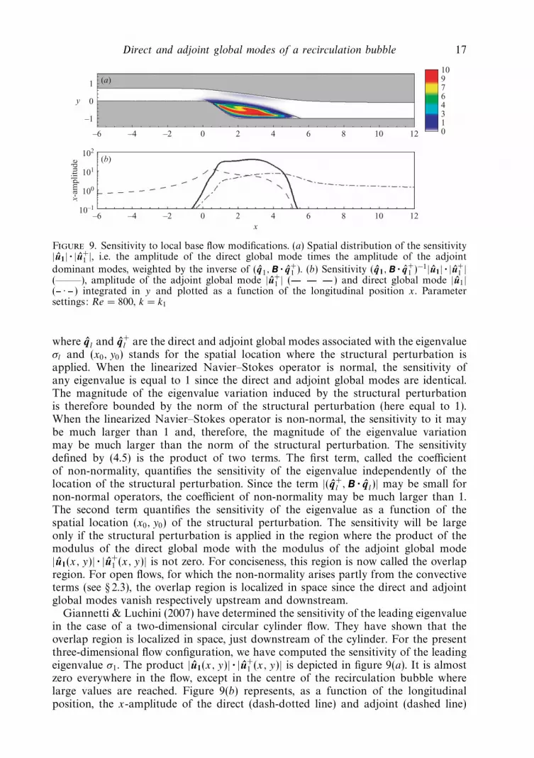
Figure 9. Sensitivity to local base flow modifications. (a) Spatial distribution of the sensitivity|u1| · |u+

1 |, i.e. the amplitude of the direct global mode times the amplitude of the adjoint

dominant modes, weighted by the inverse of (q1,B · q+1 ). (b) Sensitivity (q1,B · q+

1 )−1|u1| · |u+1 |

(——–), amplitude of the adjoint global mode |u+1 | (---- ---- ---- ) and direct global mode |u1|

(-- · -- ) integrated in y and plotted as a function of the longitudinal position x. Parametersettings: Re = 800, k = k1

where q l and q+l are the direct and adjoint global modes associated with the eigenvalue

σl and (x0, y0) stands for the spatial location where the structural perturbation isapplied. When the linearized Navier–Stokes operator is normal, the sensitivity ofany eigenvalue is equal to 1 since the direct and adjoint global modes are identical.The magnitude of the eigenvalue variation induced by the structural perturbationis therefore bounded by the norm of the structural perturbation (here equal to 1).When the linearized Navier–Stokes operator is non-normal, the sensitivity to it maybe much larger than 1 and, therefore, the magnitude of the eigenvalue variationmay be much larger than the norm of the structural perturbation. The sensitivitydefined by (4.5) is the product of two terms. The first term, called the coefficientof non-normality, quantifies the sensitivity of the eigenvalue independently of thelocation of the structural perturbation. Since the term |(q+

l , B · q l)| may be small fornon-normal operators, the coefficient of non-normality may be much larger than 1.The second term quantifies the sensitivity of the eigenvalue as a function of thespatial location (x0, y0) of the structural perturbation. The sensitivity will be largeonly if the structural perturbation is applied in the region where the product of themodulus of the direct global mode with the modulus of the adjoint global mode|u1(x, y)| · |u+

1 (x, y)| is not zero. For conciseness, this region is now called the overlapregion. For open flows, for which the non-normality arises partly from the convectiveterms (see § 2.3), the overlap region is localized in space since the direct and adjointglobal modes vanish respectively upstream and downstream.

Giannetti & Luchini (2007) have determined the sensitivity of the leading eigenvaluein the case of a two-dimensional circular cylinder flow. They have shown that theoverlap region is localized in space, just downstream of the cylinder. For the presentthree-dimensional flow configuration, we have computed the sensitivity of the leadingeigenvalue σ1. The product |u1(x, y)| · |u+

1 (x, y)| is depicted in figure 9(a). It is almostzero everywhere in the flow, except in the centre of the recirculation bubble wherelarge values are reached. Figure 9(b) represents, as a function of the longitudinalposition, the x-amplitude of the direct (dash-dotted line) and adjoint (dashed line)


global modes, taken from figures 4(b) and 6(b), as well as the product of thesetwo quantities (solid line) given by the coefficient of non-normality |(q+

1 , B · q1)|−1.The x-amplitude of the direct (respectively adjoint) global mode vanishing upstream(respectively downstream) of the recirculation bubble, and the overlap region is clearlylocalized inside the recirculation bubble.

In physical terms, this overlap region is crucial in determining the wavemaker regionof a self-sustained hydrodynamic instability, i.e. the region of the flow where thehydrodynamic feedback process is active. Indeed, if we assume that the hydrodynamicfeedback process may be modelled by a forcing of the momentum equations fproportional to the local instability velocity, i.e. f (x, y) = δA0ulδ(x − x0, y − y0),then the sensitivity of an eigenvalue to such a local feedback is given by (4.5) (seeGiannetti & Luchini (2007) for more details). The overlap region depicted in figure 9(a)thus identifies the region of the flow where a local feedback will have a large impacton the leading eigenvalue σ1. Conversely, any local feedback applied outside thisoverlap region only slightly modifies this eigenvalue, indicating that these regionsdo not play a significant role in the process giving rise to the global instability. Forthe present flow configuration, we may conclude that the recirculation bubble is thewavemaker region of the three-dimensional instability.

5. ConclusionIn this paper we have studied the linear dynamics of a two-dimensional flow in

an S-shaped duct. A global stability analysis has been performed to account for thenon-parallelism of the recirculation bubble and has been numerically solved using afinite-element formulation. The primary bifurcation has been shown to be steady andthree-dimensional. A detailed analysis of the structure of the leading global modesuggested that a lift-up mechanism was responsible for the energy production of theinstability. The physical effect of this three-dimensional instability on the recirculationbubble has been characterized as a deformation of the reattachment line. The non-normality of the linearized Navier–Stokes operator has been outlined and discussedin terms of a lift-up non-normality resulting from the transport of the base flowby the perturbation which is characteristic of shear flows, and a convective non-normality resulting from the transport of the perturbations by the base flow which ischaracteristic of open flows. By computing the adjoint global mode associated withthe direct global mode, this distinction between the two types of non-normality hasthen been discussed for the present case corresponding to a real open shear flow. Thespatial separation of the direct and adjoint global modes has been interpreted as aresult of the convective non-normality, whereas the separation in components, thedirect global mode being dominated by the streamwise component and the adjointglobal mode by crossflow components almost everywhere, as an effect of the lift-upnon-normality. A detailed analysis of the adjoint global mode has allowed a completephysical interpretation of the instability close to the bifurcation and the distinguishingof different regions of the flow. The vicinity of the separation point is where the three-dimensional global mode is most receptive to initial perturbations and local forcing.This region is distinct from the wavemaker region which has been identified as thewhole recirculation bubble by considering the overlap of the direct and adjoint globalmodes. In the perspective of controlling the instability close to the bifurcation thisanalysis suggests different locations of the actuator depending on the control method.In the case of a passive control for which a small device is introduced in the flowand induces local modifications of the base flow, it should be placed where both the


direct and adjoint global modes are not zero, i.e. in the recirculation bubble, to obtaina large impact on the instability development. In the active control framework, theunderlying idea being to produce a large effect in the flow by introducing only asmall amount of energy, the adjoint global mode is essential (Akervik et al. 2007).For example if the actuator imposes either a small wall displacement or wall blowingand suction, the adjoint pressure field shows that maximum efficiency is achieved byplacing the actuator just upstream of the separation point.

Appendix A. Shape of the lower and upper wallsThe shapes of the lower and upper walls are presented in the non-dimensional

Cartesian coordinate system. The lower wall is a rounded backward-facing stepcomposed of three different parts:

y = p1l(x) =AB

2hπ

(sin

(hπx

B

)− hπx

B

), x ∈

[0,

B

h

], (A 1)

y = p2l(x) =AB

2h

(1 − 2hx

B

), x ∈

[B

h,B

h+

M

h√

1 + A2

], (A 2)

y = p3l(x) =AC

2hπ

(− sin

(π

C

(hx − B − M√

1 + A2

))− π

C

(hx − B − M√

1 + A2

))

− A

2h

(C + B +

2M√1 + A2

), x ∈

[B

h+

M

h√

1 + A2,L

h

]. (A 3)

The step length is denoted by L and the step height by h. The value of the parametersused to define the lower wall are h = 0.2025, L = 0.5, A = 0.75, B = 0.15, C = 0.31and M = 0.31. In order to design the curved upper wall preliminary calculations havebeen carried out. A flat plate was first considered as the upper wall and its distancefrom the lower wall was increased in order to prevent separation from occurring onthe flat upper wall. The streamline emerging from the inlet boundary at the verticalcoordinate y = 0.723605 was then extracted and the upper wall finally defined byusing interpolated functions of this streamline. The absence of separation on thatwall is then verified numerically by computing the skin friction on the upper wall(figure 1) and checking that it never vanishes.

Appendix B. Structural stability and sensitivityThe structural stability analysis of a linear operator A consists of investigating how

structural perturbations of the operator modify its spectrum. Let us consider that Ais the linearized Navier–Stokes operator (2.6). Introducing a structural perturbationεδA (of norm ε) in the perturbation equations (2.5) yields

(A + εδA)(q l + εδq l) = (σl + εδσl)B(q l + εδq l) (B 1)

where δσl and δq l are the eigenvalue and eigenvector variations induced by thestructural perturbation. If only infinitesimal structural perturbation are consideredε � 1, we obtain the expression

(A − σlB)δq l + δAq l = δσlBq l (B 2)

by using that (σl, q l) solves the perturbations equations (2.5). The above expressionis then projected onto the adjoint global mode q+

l

(q+l , (A − σlB)δq l) + (q+

l , δAq l) = δσl(q+l , Bq l). (B 3)


The first term on the left-hand side of (B3) is equal to zero:

(q+l , (A − σlB)δq l) =

((A+ − σ ∗

l B)q+l︸︷︷︸

=0

, δq i

)(B 4)

since the adjoint global mode q+l solves the adjoint equation perturbations (2.14).

The eigenvalue variation is then related to the structural perturbation δA through

δσl =(q+

l , δA · q l)

(q+l , B · q l)

. (B 5)

Let us now consider a specific structural perturbation δA, which is spatially localizedin (x0, y0) and acts only on the momentum equations, i.e.

δA(x, y) =

(δA0 00 0

)δ(x − x0, y − y0) (B 6)

where δ is the Kronecker symbol, and δA0 is the local structural perturbation actingon the momentum equations. The magnitude of the eigenvalue variation may thenbe bounded as follows:

|δσl | � ||δA0|| |(q+l , B · q l)|−1(|ul (x0, y0)||u+

l (x0, y0)|)︸︷︷︸Sl (x0,y0)

(B 7)

where ||δA0|| is the norm of the structural perturbation. The quantity Sl(x0, y0) definesthe sensitivity of the eigenvalue σl to a local structural perturbation δA0.

REFERENCES

Akervik, E., Hoepffner, J., Ehrenstein, U. & Henningson, D. S. 2007 Optimal growth, modelreduction and control in a separated boundary-layer flow using global modes. J. Fluid Mech.579, 305–314.

Barkley, D., Gomes, M. G. M. & Henderson, R. D. 2002 Three-dimensional instability in flowover a backward-facing step. J. Fluid Mech. 473, 167–190.

Butler, K. M. & Farrell, B. F. 1992 Three-dimensional optimal perturbations in viscous shearflow. Phys. Fluids A 4, 1637–1650.

Chomaz, J. M. 2005 Global instabilities in spatially developping flows: non-normality andnonlinearity Annu. Rev. Fluid Mech. 37, 357–392.

Chomaz, J. M., Huerre, P. & Redekopp, L. G. 1990 The effect of nonlinearity and forcing onglobal modes. In New Trends in Nonlinear Dynamcs and Pattern-Forming Phenomena (ed.P. Coulet & P. Huerre), p. 259. Plenum.

Cossu, C. & Chomaz, J. M. 1997 Global measures of local convective instabilities Phys. Rev. Lett.78, 4387–4390.

Ding, Y. & Kawahara, M. 1999 Three-dimensional linear stability analysis of incompressibleviscous flows using the finite element method Intl J. Numer. Meth. Fluids 31, 451–479.

Ehrenstein, U. & Gallaire, F. 2005 On two-dimensional temporal modes in spatially evolvingopen flows: the flat-plate boundary layer. J. Fluid Mech. 536, 209–218.

Gallaire, F., Marquillie, M. & Ehrenstein, U. 2007 Three-dimensional transverse instabilities indetached boundary layers. J. Fluid Mech. 571, 221–233.

Giannetti, F. & Luchini, P. 2003 Receptivity of the circular cylinder’s first instability. Proc. 5thEur. Fluid Mech. Conf. Toulouse.

Giannetti, F. & Luchini, P. Structural sensitivity of the first instability of the cylinder wake. J. FluidMech. 581, 167–197.


Griffith, M. D., Thompson, M. C., Leweke, T. , Hourigan, K. & Anderson, W. P. 2007 Wakebehaviour and instability of flow through a partially blocked channel. J. Fluid Mech. 582,319–340.

Huerre, P. & Monkewitz, P. A. 1990 Local and global instabilities in spatially developing flowsAnnu. Rev. Fluid Mech. 22, 473–537.

Landahl, M. T. 1980 A note on an algebraic instability of inviscid parallel shear flows. J. FluidMech. 98, 243–251.

Lehoucq, R. B., Masschhoff, K., Sorensen, D. & Yang, C. 1996 ARPACK Software Package,http://www.caam.rice.edu/software/ARPACK/

Lehoucq, R. B., Sorensen, D. C. & Yang, C. 1998 ARPACK Users’s Guide. SIAM.

Marquet, O., Sipp, D., Chomaz, J.-M. & Jacquin, L. 2008 Amplifier and resonator dynamicsof a low-Reynolds number recirculation bubble in a global framework. J. Fluid Mech. 605,429–443.

Maslowe, S. A. & Kelly, R. E. 1970 Finite-amplitude oscillations in a Kelvin-Helmholtz flow. IntlJ. Non-Linear Mech. 5, 427–435.

Schmid, P. J. 2007 Nonmodal stability theory. Annu. Rev. Fluid Mech. 39, 129–162.

Schmid, P. J. & Henningson, D. S. 2001 Stability and Transition in Shear Flows . Springer.

Schmid, P. J. & Henningson, D. S. 2002 On the stability of a falling liquid curtain. J. Fluid Mech.463, 163–171.

Theofilis, V. 2000 Globally unstable flows in open cavities. AIAA Paper 2000-1965.

Theofilis, V., Hein, S. & Dallmann, U. 2000 On the origins of unsteadiness and three-dimensionality in a laminar separation bubble. Phil. Trans. R. Soc. Lond. A 358, 3229–3246.

Trefethen, L. N., Trefethen, A. E., Reddy, S. C. & Driscoll, T. A. 1993 Hydrodynamic stabilitywithout eigenvalues. Science 261, 578–584.

Documents

Direct and adjoint global modes of a recirculation bubble: lift-up and convective non-normalities