Dimer problem on the cylinder and torus

Physica A 387 (2008) 6069–6078

Contents lists available at ScienceDirect

Physica A

journal homepage: www.elsevier.com/locate/physa

Dimer problem on the cylinder and torusWeigen Yan a, Yeong-Nan Yeh b, Fuji Zhang c,∗

a School of Sciences, Jimei University, Xiamen 361021, Chinab Institute of Mathematics, Academia Sinica, Taipei 11529, Taiwanc School of Mathematical Science, Xiamen University, Xiamen 361005, China

a r t i c l e i n f o

Article history:Received 11 March 2008Received in revised form 16 June 2008Available online 3 July 2008

Keywords:Dimer problem8.8.4 lattice8.8.6 latticeHexagonal latticeCylindrical and toroidal boundaryconditions

a b s t r a c t

Weobtain explicit expressions of the number of close-packed dimers and entropy for threetypes of lattices (the so-called 8.8.6, 8.8.4, andhexagonal lattices)with cylindrical boundarycondition and the entropy of the 8.8.6 lattice with toroidal boundary condition. Our resultsand the one on 8.8.4 and hexagonal lattices with toroidal boundary condition by Salinasand Nagle [S.R. Salinas, J.F. Nagle, Theory of the phase transition in the layered hydrogen-bonded SnCl2·2H2O crystal, Phys. Rev. B 9 (1974) 4920–4931] and Wu [F.Y. Wu, Dimerson two-dimensional lattices, Inter. J. Modern Phys. B 20 (2006) 5357–5371] imply that the8.8.6 (or 8.8.4) lattices with cylindrical and toroidal boundary conditions have the sameentropy whereas the hexagonal lattices have not. Based on these facts we propose thefollowing problem: under which conditions do the lattices with cylindrical and toroidalboundary conditions have the same entropy?

© 2008 Elsevier B.V. All rights reserved.

1. Introduction

In 1961, Kasteleyn [14] found a formula for the number of close-packed dimers (perfect matchings) of anm×n quadraticlattice graph. Temperley and Fisher [34] used a different method and arrived at the same result at almost exactly the sametime. Both lines of calculation showed that the logarithm of the number of close-packed dimers, divided by mn

2 , convergesto 2c/π ≈ 0.5831 as m, n → ∞, where c is Catalan’s constant. This limit is called the entropy of the quadratic latticegraph and the corresponding problem was called the dimer problem by the statistical physicists. In 1992, Elkies et al. [6]studied the enumeration of close-packed dimers of regions called Aztec diamonds, and showed that the entropy equalslog 22 ≈ 0.35. Different methods for counting close-packed dimers of Aztec diamonds were considered by many authors

(see for example Refs. [19,28,42]). The problem involving enumeration of close-packed dimers of another type of quadraticlattices with different boundary conditions was studied by Sachs and Zeritz [31] and a different entropy was obtained.These facts showed that the entropy of the quadratic lattice is strongly dependent on their boundary conditions. It shouldbe pointed out that the dimer model on the hexagonal (Kasteleyn or brick) lattice has a ‘‘frozen’’ ground state, which sortof resembles the ground state of the ferromagnetic six-vertex model. It has been shown that the entropy of the six-vertexmodel does depend on the boundary conditions [18]. See also the works of chemists cited in [10].

Cohn, Kenyon, and Propp [4] demonstrated that the behavior of randomperfectmatchings (close-packed dimers) of largeregions R was determined by a variational (or entropy maximization) principle, as was conjectured in Section 8 of Ref. [6],and they gave an exact formula for the entropy of simply-connected regions of arbitrary shape. Particularly, they showedthat computation of the entropy is intimately linked with an understanding of long-range variations in the local statistics ofrandom domino tilings. Kenyon, Okounkov, and Sheffield [17] considered the problem of enumerating close-packed dimers

∗ Corresponding author.E-mail addresses:[email protected] (W. Yan), [email protected] (Y.-N. Yeh), [email protected] (F. Zhang).

0378-4371/$ – see front matter© 2008 Elsevier B.V. All rights reserved.doi:10.1016/j.physa.2008.06.042

http://www.elsevier.com/locate/physa

http://www.elsevier.com/locate/physa

mailto:[email protected]



http://dx.doi.org/10.1016/j.physa.2008.06.042

6070 W. Yan et al. / Physica A 387 (2008) 6069–6078

of the doubly period bipartite graph on a torus, which generalized the results in Ref. [4]. They proved that the number ofclose-packed dimers of the doubly period plane bipartite graph G can be expressed in terms of four determinants and theyexpressed the entropy of G as a double integral.

The exact solution of the dimer problem was obtained for many lattices such as the quadratic lattice, 8.8.4 lattice,hexagonal lattice, triangular lattice, kagome lattice, 3-12-12 lattice, union Jack lattice, and etc. with toroidal boundarycondition [8,14,32,37]. The exact solution of the dimer problem has been extended to the cylindrical condition [22,26].Wu and Wang [36] obtained the exact result on the enumeration of close-packed dimers on a finite kagome lattice withgeneral asymmetric dimer weights under the cylindrical boundary condition. The result by Wu and Wang implies that thekagome lattices with the cylindrical and toroidal boundary conditions have the same entropy. This phenomenon also tookplace for some other lattices with the cylindrical and toroidal boundary conditions [9].

Some related work about the dimer problem can be found in, for example, Refs. [7,8,10,14–16,23,27,32,34,39,40] byphysicists and chemists and Refs. [2–4,17,29,33,41–43] by mathematicians.

In this paper, we consider three types of lattices—8.8.6, 8.8.4, and hexagonal lattices. We obtain explicit expressions ofthe number of close-packed dimers and entropy for these three types of lattices with cylindrical boundary condition. Basedon the result by Kenyon, Okounkov, and Sheffield [17], we compute the entropy of the 8.8.6 lattice with toroidal boundarycondition. Combining our results and the one on 8.8.4 and hexagonal lattices with toroidal boundary condition [32,37], wecan see that the 8.8.6 (or 8.8.4) lattices with cylindrical and toroidal boundary conditions have the same entropy whereasthe effect of the boundary for the hexagonal lattices is not trivial (that is, the hexagonal lattices with cylindrical and toroidalboundary conditions have different entropies). Based on these facts we would propose the following problem: under whichconditions do the lattices with cylindrical and toroidal boundary conditions have the same entropy?

2. Pfaffians

The Pfaffian method enumerating close-packed dimers of plane graphs was independently discovered by Fisher [8],Kasteleyn [14], and Temperley [34]. Given a plane graph G, the method produces a skew symmetric matrix A such thatthe number of close-packed dimers of G can be expressed by the Pfaffian of the matrix A. Alternatively, the Pfaffian can bereplaced by the square root of the determinant of A. By using this method, Fisher [8], Kasteleyn [14], and Temperley [34]solved independently a famous problemon enumerating close-packed dimers of anm×nquadratic lattice graph in statisticalphysics–Dimer problem. Given a simple graph G = (V (G), E(G)) with vertex set V (G) = {v1, v2, . . . , vn}, let Ge be anarbitrary orientation. The skew adjacency matrix of Ge, denoted by A(Ge), is defined as follows:

A(Ge) = (aij)n×n,

where

aij =

{1 if (vi, vj) is an arc of Ge,−1 if (vj, vi) is an arc of Ge,0 otherwise.

Obviously, A(Ge) is a skew symmetric matrix.Let D be an orientation of a graph G. A cycle C of even length in D is said to be oddly oriented in D if for either choice

of the two directions of traversal around C , the number of edges of C directed in the direction of the traversal is odd (notethat this definition is independent of the choice of traversal, since C has an even length). A cycle C in D is said to be niceif the subgraph D–C (obtained from D by deleting all vertices of C) has a close-packed dimer. We say that D is a Pfaffianorientation of G if every nice cycle of even length of G is oddly oriented in D. It is well known that if a bipartite graph Gcontains no subdivision of K3,3 then G has a Pfaffian orientation (see Little [20]). McCuaig [24], andMcCuaig, Robertson et al.[25], and Robertson, Seymour et al. [30] found a polynomial-time algorithm to showwhether a bipartite graph has a Pfaffianorientation. Stembridge [33] proved that the number (or generating function) of nonintersecting r-tuples of paths from aset of r vertices to a specified region in an acyclic digraph D can, under favorable circumstances, be expressed as a Pfaffian.For a recent survey of Pfaffian orientations of graphs, please see Thomas [35]. Throughout this paper, we denote by M(G)the number of close-packed dimers of a graph G.

Lemma 2.1 (Lovász et al. [21]). If Ge is a Pfaffian orientation of a graph G, then

M(G) =

√det(A(Ge)),

where A(Ge) is the skew adjacency matrix of Ge.

Lemma 2.2 (Lovász et al. [21]). If a plane graph G has an orientation Ge such that every boundary face – except possibly theinfinite face – has an odd number of edges oriented clockwise, then in every cycle the number of edges oriented clockwise is ofopposite parity to the number of vertices of Ge inside the cycle. Consequently, Ge is a Pfaffian orientation.

W. Yan et al. / Physica A 387 (2008) 6069–6078 6071

Fig. 1. (a) The 8.8.6 lattice G∗

1(m, 2n). (b) The 8.8.4 lattice G∗

2(m, 2n).

3. Three types of cylinders

Two bulk lattices, denoted by G∗

1(m, 2n) and G∗

2(m, 2n), are illustrated in Fig. 1(a) and Fig. 1(b), respectively, whereG∗

1(m, 2n) is a finite subgraph of an edge-to-edge tiling of the plane with two types of vertices—8.8.6 and 8.8.4 vertices,and G∗

2(m, 2n) is a finite subgraph of 8.8.4 tiling in the Euclidean plane which has been used to describe phase transitionsin the layered hydrogen-bonded SnCl2·2H2O crystal [32] in physical systems [1,27,32]. The 8.8.6 lattice G∗

1(m, 2n), whosefundamental part is a hexagon, is composed of 2mn hexagons. Similarly, The 8.8.4 lattice G∗

2(m, 2n), whose fundamentalpart is a quadrangle, is composed of 2mn quadrangles. Each of such bulk graphs is called ‘‘an (m, 2n)-bipartite graph withfree boundary condition’’ (see Ref. [23]).

If we add edges (ai, a∗

i ), (bi, b∗

i ) for 1 ≤ i ≤ m and (cj, c∗

j ) for 1 ≤ j ≤ 2n in G∗

1(m, 2n), we obtain an (m, 2n)-bipartitegraph with toroidal boundary condition, denoted by Gt

1(m, 2n). Similarly, if we add edges (ai, a∗

i ) for 1 ≤ i ≤ m and (bj, b∗

j )

for 1 ≤ j ≤ 2n in G∗

2(m, 2n), then an (m, 2n)-bipartite graph with toroidal boundary condition, denoted by Gt2(m, 2n), is

obtained. For some relatedwork on the plane bipartite graphs with the toroidal boundary condition, see Kenyon, Okounkov,and Sheffield [17] andCohn, Kenyon, andPropp [4]. Salinas andNagle [32] andWu [37] showed that the entropy ofGt

2(m, 2n),that is limn,m→∞

28mn log[M(Gt

2(m, 2n))], equals

12π

∫ π/2

0log

[5 +

√25 − 16 cos2 θ

2

]dθ ≈ 0.3770. (1)

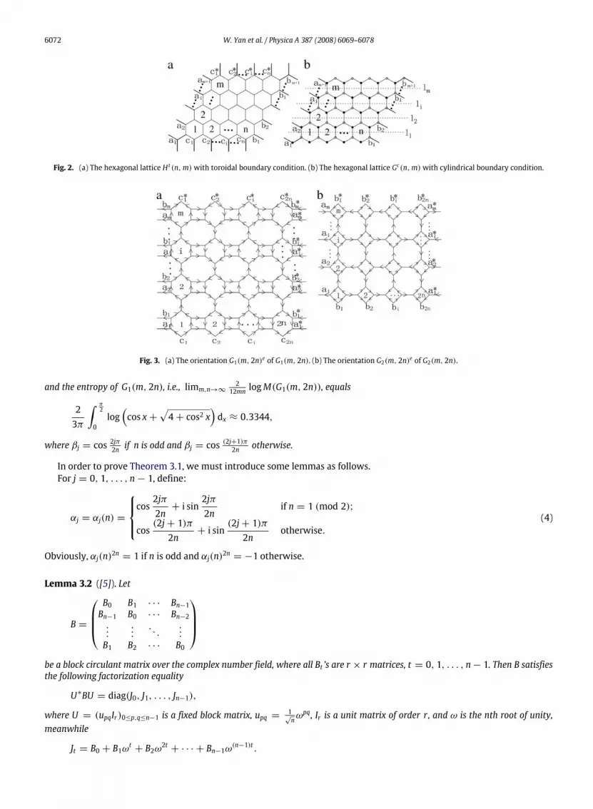
The hexagonal lattices with toroidal and cylindrical boundary conditions, denoted by H t(n,m) and Hc(n,m), areillustrated in Fig. 2(a) and Fig. 2(b), where (a1, b1), (a2, b2), . . . , (am+1, bm+1), (a1, c∗

1 ), (c1, c∗

2 ), (c2, c∗

3 ), . . . , (cn−1, c∗n ),

(cn, bm+1) are edges in H t(n,m), and (a1, b1), (a2, b2), . . . , (am+1, bm+1) are edges in Hc(n,m). Wu [37–39] showed thatthe entropy of H t(n,m), i.e.,

limn,m→∞

2(n + 1)(2m + 2)

log[M(H t(n,m))] =2π

∫ π/3

0log(2 cos θ)dθ ≈ 0.3230. (2)

In this section, we enumerate close-packed dimers of the 8.8.6, 8.8.4, and hexagonal lattices G1(m, 2n),G2(m, 2n),and Hc(n,m) with cylindrical boundary condition, where G1(m, 2n) (resp. G2(m, 2n)) is obtained from G∗

1(m, 2n) (resp.G∗

2(m, 2n)) by adding extra edges (ai, a∗

i ), (bi, b∗

i ) for 1 ≤ i ≤ m (resp. (ai, a∗

i ) for 1 ≤ i ≤ m) between each pair of oppositevertices of both sides of them.We call each ofG1(m, 2n) andG2(m, 2n) ‘‘an (m, 2n)-bipartite graphwith cylindrical boundarycondition’’ (simply cylinder). We also obtain the exact solutions for the entropies of the 8.8.6 lattice G1(m, 2n), 8.8.4 latticeG2(m, 2n), and hexagonal lattice Hc(n,m) with cylindrical boundary condition.

3.1. The cylinder G1(m, 2n)

Let G1(m, 2n)e be the orientation of G1(m, 2n) illustrated in Fig. 3(a). For G1(m, 2n)e, all hexagons in the first column havethe same orientation, all hexagons in the second column have the inverse of the orientation of hexagons in the first column,and so on. Obviously, G1(m, 2n)e satisfies the conditions in Lemma 2.2 and hence is a Pfaffian orientation.

Theorem 3.1. For the cylinder G1(m, 2n), the number of close-packed dimers of G1(m, 2n) can be expressed by

M(G1(m, 2n)) =12n

n−1∏j=0

1√4 + β2

j

[(√4 + β2

j + βj

)2m+1+

(√4 + β2

j − βj

)2m+1]

, (3)


Fig. 2. (a) The hexagonal lattice H t (n,m) with toroidal boundary condition. (b) The hexagonal lattice Gc(n,m) with cylindrical boundary condition.

Fig. 3. (a) The orientation G1(m, 2n)e of G1(m, 2n). (b) The orientation G2(m, 2n)e of G2(m, 2n).

and the entropy of G1(m, 2n), i.e., limm,n→∞2

12mn logM(G1(m, 2n)), equals

23π

∫ π2

0log

(cos x +

√4 + cos2 x

)dx ≈ 0.3344,

where βj = cos 2jπ2n if n is odd and βj = cos (2j+1)π

2n otherwise.

In order to prove Theorem 3.1, we must introduce some lemmas as follows.For j = 0, 1, . . . , n − 1, define:

αj = αj(n) =

cos

2jπ2n

+ i sin2jπ2n

if n = 1 (mod 2);

cos(2j + 1)π

2n+ i sin

(2j + 1)π2n

otherwise.(4)

Obviously, αj(n)2n = 1 if n is odd and αj(n)2n = −1 otherwise.

Lemma 3.2 ([5]). Let

B =

B0 B1 · · · Bn−1

Bn−1 B0 · · · Bn−2...

.... . .

...B1 B2 · · · B0

be a block circulant matrix over the complex number field, where all Bt ’s are r × r matrices, t = 0, 1, . . . , n − 1. Then B satisfiesthe following factorization equality

U∗BU = diag(J0, J1, . . . , Jn−1),

where U = (upqIr)0≤p,q≤n−1 is a fixed block matrix, upq =1

√nω

pq, Ir is a unit matrix of order r, and ω is the nth root of unity,meanwhile

Jt = B0 + B1ωt+ B2ω

2t+ · · · + Bn−1ω

(n−1)t .


A direct consequence of Lemma 3.2 is the following:

Corollary 3.3. Let

B =

A R 0 · · · 0 RT

RT A R · · · 0 00 RT A · · · 0 0...

.... . .

. . .. . .

...0 0 0 · · · A RR 0 0 · · · RT A

n×n

be a block circulant matrix over the real number field, where both A and R are r× r matrices. Then there exists an invertible matrixU of order nr such that

U−1BU = diag(J0, J1, . . . , Jn−1),

where Jt = A + ωtR + ω−tRT, t = 0, 1, . . . , n − 1, and ω is the nth root of unity.

Lemma 3.4. Let

B =

A R 0 · · · 0 −RT

RT A R · · · 0 00 RT A · · · 0 0...

.... . .

. . .. . .

...0 0 0 · · · A R

−R 0 0 · · · RT A

n×n

be a block circulant matrix over the real number field, where both A and R are r× r matrices. Then there exists an invertible matrixU of order nr such that

U−1BU = diag(J0, J1, . . . , Jn−1),

where Jt = A + ωtR + ω−1t RT, and ωt = cos (2t+1)π

n + i sin (2t+1)πn , t = 0, 1, . . . , n − 1.

Proof. Note that the set of roots of equation xn = −1 is exactly {ω0, ω1, . . . , ωn−1}. Let U = (Uij)n×n and U∗= (U∗

ij )n×n be

two n × n block matrices such that Uij =ωij

√n Ir and U∗

ij =ω

−ji√n Ir for 0 ≤ i, j ≤ n − 1, where Ir is the identity matrix of order

r . It is not difficult to show that U∗U = Inr . Hence U∗= U−1. It suffices to prove that U∗BU = diag(J0, J1, . . . , Jn−1). For

convenience, let B = (Bst)n×n and U∗BU = (Xst)n×n, where Bst and Xst are r × r matrices. Note that, for 0 ≤ i, j ≤ n − 1,

Xij =

∑0≤s,t≤n−1

U∗

isBstUtj =1n

∑0≤s,t≤n−1

ω−si Bstω

tj

=1n

[n−1∑k=0

(ω−1i ωj)

kA +

n−1∑k=0

ωj(ω−1i ωj)

kR +

n−1∑k=0

ω−1j (ω−1

i ωj)kRT

]

=

{Ji if i = j,0 otherwise.

Hence we have finished the proof of the lemma. �

Proof of Theorem 3.1. By a suitable labelling of vertices of G1(m, 2n)e, the skew adjacency matrix of G1(m, 2n)e, denotedby A1(Ge), has the following form:

A1(Ge) =

A R 0 · · · 0 RT

−RT−A R · · · 0 0

0 −RT A · · · 0 0...

.... . .

. . .. . .

...0 0 0 · · · A R

−R 0 0 · · · −RT−A

2n×2n

,

where A denotes the skew adjacencymatrix of the part in first column ofG1(m, 2n)e, and R is the adjacency relation betweenthe two parts in the first and second columns of G1(m, 2n)e.


Set

M1 =

A R 0 · · · 0 RT

RT A R · · · 0 00 RT A · · · 0 0...

.... . .

. . .. . .

...0 0 0 · · · A RR 0 0 · · · RT A

2n×2n

and

M2 =

A R 0 · · · 0 −RT

RT A R · · · 0 00 RT A · · · 0 0...

.... . .

. . .. . .

...0 0 0 · · · A R

−R 0 0 · · · RT A

2n×2n

.

Multiplying by −1 to rows 2 and 3 of the block matrix A1(Ge), then to columns 3 and 4, then to rows 6 and 7, then tocolumns 7 and 8, and so on and so forth, finally we obtain the matrix M1 when n = 1 (mod 2), or the matrix M2 whenn = 0 (mod 2). Clearly we have

det(A1(Ge)) =

{| det(M1)| if n = 1 (mod 2),| det(M2)| if n = 0 (mod 2).

Note that, by Corollary 3.3 and Lemma 3.4, we have

det(M1) =

2n−1∏j=0

det(A + ωjR + ω−jRT) =

(n−1∏j=0

det(A + ωjR + ω−jRT)

)2

and

det(M2) =

2n−1∏j=0

det(A + ωjR + ω−1j RT) =

(n−1∏j=0

det(A + ωjR + ω−1j RT)

)2

,

where ω = cos 2π2n + i sin 2π

2n (i.e., ω is the 2nth root of unity) and ωj = cos (2j+1)π2n + i sin (2j+1)π

2n .Nowwe construct nweighted digraphsDj’s with 6m vertices from G1(m, 2n)e which are illustrated in Fig. 3(a), where αj’s

satisfy (1), and each arc (vs, vt) in Dj whose weight is neither αj nor α−1j must be regarded as two arcs (vs, vt) and (vt , vs)

with weights 1 and −1, respectively.By the definitions of αj’s and Dj’s, it is not difficult to see that the adjacency matrix Aj of weighted digraph Dj defined

above equals exactly A + ωjR + ω−jRT if n = 1 (mod 2) and A + ωjR + ω−1j RT otherwise. Thus, by Lemma 2.1, we have

M(G1(m, 2n)) =

√det(A(Ge

1)) =

n−1∏j=0

| det(Aj)|, (5)

where Aj is the adjacency matrix of Dj.Let D′

j be the digraph obtained from Dj by deleting vertex c∗

1 (see Fig. 4(b)). For j = 0, 1, . . . , n − 1, set

Lm(j) = det(Aj), L′

m(j) = det(A′

j),

where Aj (resp. A′

j) is the adjacencymatrix of the digraphDj (resp.D′

j). It is not difficult to prove that {Lm(j)}m≥0 and {L′m(j)}m≥0

satisfy the following recurrences:Lm(j) = (4 + 4β2j )Lm−1(j) + 4βjL′

m−1(j) form ≥ 1,L′

m(j) = 4βjLm−1(j) + 4L′

m−1(j) form ≥ 1,L0(j) = 1, L′

0(j) = 0.

Then we have{Lm(j) = (8 + 4β2

j )Lm−1(j) − 16Lm−2(j) form ≥ 2,L0(j) = 1, L1(j) = 4 + 4β2

j ,


Fig. 4. (a) The digraphs Dj ’s. (b) The digraph D′

j obtained from Dj by deleting vertex c∗

1 shown in Fig. 4(a). (c) The digraphs Cj ’s. (d) The digraph C ′

j obtainedfrom Dj by deleting vertex b∗

1 shown in Fig. 4(c).

which implies the following:

Lm(j) =1

2√4 + β2

j

[(√4 + β2

j + βj

)2m+1+

(√4 + β2

j − βj

)2m+1]

. (6)

Hence the equality (3) follows from (5) and (6). So the entropy of G1(m, 2n)

limm,n→∞

212mn

logM(G1(m, 2n))

= limm,n→∞

16mn

{−n log 2 −

12

n−1∑j=0

log(4 + β2j ) +

n−1∑j=0

log[(√

4 + β2j + βj

)2m+1+

(√4 + β2

j − βj

)2m+1]}

=23π

∫ π/2

0log

(cos x +

√4 + cos2 x

)dx ≈ 0.3344

and this completes the proof. �

In order to prove the following corollary, we need to introduce a formula of the entropy for an (n, n)-bipartite graphwithtoroidal boundary condition obtained by Kenyon, Okounkov, and Sheffield [17]. Let G be a Z2-period bipartite graph whichis embedded in the plane so that translations in the plane act by color-preserving isomorphisms of G—isomorphisms whichmap black vertices to black vertices andwhite to white. Let Gn be the quotient of G by the action of nZ2. Then Gn is a bipartitegraph with the doubly period condition. Let P(z, w) be the characteristic polynomial of G (see the definition in page 1029in Ref. [17]). Authors of Ref. [17] showed that the entropy of Gn

limn→∞

2n2|G1|

logM(Gn) =2

|G1|(2π i)2

∫Dlog |P(z, w)|

dz

zdw

w, (7)

where D = {(z, w) ∈ C2: |z| = |w| = 1} and i2 = −1.

Corollary 3.5. Both G1(m, 2n) and Gt1(m, 2n) have the same entropy, that is,

limm,n→∞

212mn

log(M(G1(m, 2n))) = limm,n→∞

212mn

log(M(Gt1(m, 2n))) ≈ 0.3344.

Proof. Note that by the definition in Ref. [17] the fundamental domain of Gt1(m, 2n) is composed of two hexagons (see

Fig. 5). Otherwise, if we use a hexagon as the fundamental domain, then it does not satisfy the condition ‘‘color-preservingisomorphisms’’. It is not difficult to show that the characteristic polynomial of Gt

1(m, 2n)

P(z, w) = 10 − 4(z + z−1) − (w + w−1).


Fig. 5. The fundamental domain of Gt1(m, 2n).

Hence, by (7), we have

limm,n→∞

212mn

log(M(Gt1(m, 2n))) =

212(2π)2

∫ 2π

0

∫ 2π

0log(10 − 8 cos x − 2 cos y)dxdy

=1

24π2

∫ 2π

0

∫ 2π

0log(10 − 8 cos x − 2 cos y)dxdy.

It is not difficult to see that

124π2

∫ 2π

0

∫ 2π

0log(10 − 8 cos x − 2 cos y)dxdy =

23π

∫ π/2

0log

(cos x +

√4 + cos2 x

)dx.

The corollary has thus been proved. �

3.2. The cylinder G2(m, 2n)

Let G2(m, 2n)e be the orientation of G2(m, 2n) illustrated in Fig. 3(b). For G2(m, 2n)e, all quadrangles in the first columnhave the same orientation, all quadrangles in the second column have the inverse of the orientation of quadrangles in thefirst column, and so on. Obviously, G2(m, 2n)e satisfies the conditions in Lemma 2.2 and hence is a Pfaffian orientation.

Theorem 3.6. For the cylinder G2(m, 2n), the number of close-packed dimers of G2(m, 2n) can be expressed by

M(G2(m, 2n)) =

n−1∏j=0

√9 + 16β2

j + 3

2√9 + 16β2

j

5 +

√9 + 16β2

j

2

m

+

√9 + 16β2

j − 3

2√9 + 16β2

j

5 −

√9 + 16β2

j

2

m , (8)

and the entropy, i.e., limm,n→∞2

8mn logM(G2(m, 2n)), equals

12π

∫ π/2

0log

[5 +

√25 − 16 cos2 θ

2

]dθ ≈ 0.3770,

where βj = cos jπn if n is odd and βj = cos (2j+1)π

2n otherwise.

Proof. We can prove easily the statement in the theorem on the entropy from (8). Hence it suffices to prove that (8) holds.For the orientation G2(m, 2n)e of the cylinder G2(m, 2n) shown in Fig. 3(b). Let Cj denote the digraph illustrated in Fig. 4(c)for 0 ≤ j ≤ n − 1. Similarly to the proof of Theorem 3.1, we can prove that

M(G2(m, 2n)) =

n−1∏j=0

| det(Fj)|, (9)

where Fj is the adjacency matrix of Cj.Let C ′

j be the digraph obtained from Cj by deleting vertex b∗

1 (see Fig. 4(d)) and F ′

j the adjacency matrix of C ′

j .For j = 0, 1, . . . , n − 1, set

Pm(j) = det(Fj), P ′

m(j) = det(F ′

j ),

where Fj (resp. F ′

j ) is the adjacency matrix of the digraph Cj (resp. C ′

j ) illustrated in Fig. 4(c) (resp. Fig. 4(d)). It is not difficultto prove that {Pm(j)}m≥0 and {P ′

m(j)}m≥0 satisfy the following recurrences:P2m+1(j) = 4P2m(j) + 2βjP ′

2m(j), P ′

2m+1(j) = −2βjP2m(j) − P ′

2m(j) m ≥ 0,P2m(j) = 4P2m−1(j) − 2βjP ′

2m−1(j), P ′

2m(j) = 2βjP2m−1(j) − P ′

2m−1(j) m ≥ 1,P0(j) = 1, P ′

0(j) = 0, P1(j) = 4, P ′

1(j) = −2βj.

Then we have(P2m+1(j)P ′

2m+1(j)

)=

(16 + 4β2

j −10βj

−10βj 4β2j + 1

)(P2m−1(j)P ′

2m−1(j)

)(10)


and (P2m(j)P ′

2m(j)

)=

(16 + 4β2

j 10βj

10βj 4β2j + 1

)(P2(m−1)(j)P ′

2(m−1)(j)

). (11)

Let am = P2m+1(j) and bm = P2m(j) for j ≥ 0. Hence we haveam = (18β2

j + 17)am−1 − 16(1 − β2j )

2am−2 form ≥ 2,bm = (18β2

j + 17)bm−1 − 16(1 − β2j )

2bm−2 form ≥ 2,a0 = 4, a1 = 64 + 36β2

j , b0 = 1, b1 = 16 + 4β2j .

(12)

By solving the recurrences in (12), then we have

am =

n−1∏j=0

√9 + 16β2

j + 3

2√9 + 16β2

j

5 +

√9 + 16β2

j

2

2m+1

+

√9 + 16β2

j − 3

2√9 + 16β2

j

5 −

√9 + 16β2

j

2

2m+1 ,

and

bm =

n−1∏j=0

√9 + 16β2

j + 3

2√9 + 16β2

j

5 +

√9 + 16β2

j

2

2m

+

√9 + 16β2

j − 3

2√9 + 16β2

j

5 −

√9 + 16β2

j

2

2m .

Hence (8) has been proved and the theorem follows. �

From (1) and Theorem 3.6, the 8.8.4 lattices with cylindrical and toroidal boundary conditions have the same entropywhich is approximately 0.3770.

3.3. The cylinder Hc(n,m)

Note that the hexagonal lattice Hc(n,m) with cylindrical boundary condition is a finite bipartite graph whose vertex setcan be colored by two colors black and white (see Fig. 2(b)). One can see that no edge intersected by the cut segment li(i = 1, 2, . . . ,m) illustrated in Fig. 2(b) can belong to one close-packed dimers, since the the upper (or bottom) vertices ofedges intersected by the cut segment li have the same color. Thus the number of close-packed dimers ofHc(n,m) equals thenumber of close-packed dimers ofm + 1 cycles with 2n + 2 vertices. Hence we have the following:

Theorem 3.7. The number of close-packed dimers of Hc(n,m) can be expressed by

M(Hc(n,m)) = 2m+1

and the entropy equals zero.

From (2) and the above theorem, we have the following:

Remark 3.8. The hexagonal latticesH t(n,m) andHc(n,m)with toroidal and cylindrical boundary conditions have differententropies. That is, for the hexagonal lattices, the entropy is dependent on boundary conditions.

4. Concluding remarks

In statistical mechanics some examples implied that the thermodynamic limit of the free energy (including the entropy)is independent of boundary conditions [9]. Kasteleyn [14] discussed the related problem of the m × n quadratic latticeswith the free and toroidal boundary conditions. The results by Wu [37,22] and by Wu and Wang [36] also imply that thekagome lattices with toroidal and cylindrical boundary conditions have the same entropy. In this paper, we computed theentropies of the 8.8.6, 8.8.4, and hexagonal lattices with cylindrical boundary condition and the entropy of the 8.8.6 latticewith toroidal boundary condition. We showed that the 8.8.6 lattices with the cylindrical and toroidal boundary conditionshave the same entropy. Comparing with the result by Salinas and Nagle [32] and Wu [37] we can see that the 8.8.4 latticeshave the same property. But, for the hexagonal lattices, the entropy is dependent on the boundary conditions. Based onthese results, it is natural to pose the following

Problem 4.1. Let Gc(m, n) and Gt(m, n) be the lattices with the cylindrical and toroidal boundary conditions, where theirfundamental domain is a plane bipartite graphGwith close-packeddimers. Underwhich conditions doGc(m, n) andGt(m, n)have the same entropy?

In Refs. [11–13] the finite-size corrections for the dimer model on the square and triangular lattices have been studied.It is an interesting problem to study the finite-size corrections of the dimer model on 8.8.6 and 8.8.4 lattices and comparethe results with the present paper.


Acknowledgements

We are grateful to the referees for providing many helpful revising suggestions (one of them called our attention to Refs.[11–13], and one of them told us that the results by Korepin and Zinn-Justin [18] may shed a light on Problem 4.1). Wewould like to thank Professor Z. Chen for providing many suggestions for revising this paper. The third author Fuji Zhangthanks Institute of Mathematics, Academia Sinica for its financial support and hospitality. The first author was supported inpart by NSFC Grant #10771086 and by Program for New Century Excellent Talents in Fujian Province University. The secondauthorwas supported in part by NSCGrant #NSC96-2115-M-001-005. The third authorwas supported in part by NSFCGrant#10671162.

References

[1] G.R. Allen, Dimer models for the antiferroelectric transition in copper formate tetrahydrate, J. Chem. Phys. 60 (1974) 3299–3309.[2] M. Ciucu, Enumeration of perfect matchings in graphs with reflective symmetry, J. Combin. Theory Ser. A 77 (1997) 67–97.[3] H. Cohn, N. Elkies, J. Propp, Local statistics for random domino tilings of the Aztec diamond, Duke Math. J. 85 (1996) 117–166.[4] H. Cohn, R. Kenyon, J. Propp, A variational principle for domino tilings, J. Amer. Math. Soc. 14 (2001) 297–346.[5] P.J. Davis, Circulant Matrices, Wiley, New York, 1979.[6] N. Elkies, G. Kuperberg, M. Larsen, J. Propp, Alternating sign matrices and domino tilings, J. Alg. Combin. 1 (1992) 111–132 and 219–234.[7] V. Elser, Solution of the dimer problem on a hexagonal lattice with boundary, J. Phys. A 17 (1984) 1509–1513.[8] M.E. Fisher, Statistical mechanics of dimers on a plane lattice, Phys. Rev. 124 (1961) 1664–1672.[9] M.E. Fisher, J.L. Lebowitz, Asymptotic free energy of a system with periodic boundary conditions, Commun. Math. Phys. 19 (1970) 251–272.

[10] I. Gutman, S.J. Cyvin, Kekulé Structures in Benzenoid Hydrocarbons, Springer, Berlin, 1988.[11] N.Sh. Izmailian, K.B. Oganesyan, C.-K. Hu, Exact finite-size corrections of the free energy for the square lattice dimer model under different boundary

conditions, Phys. Rev. E 67 (2003) 066114.[12] N.Sh. Izmailian, K.B. Oganesyan, M.-C. Wu, C.-K. Hu, Finite-size corrections and scaling for the triangular lattice dimer model with periodic boundary

conditions, Phys. Rev. E 73 (2006) 016128.[13] N.Sh. Izmailian, V.B. Priezzhev, P. Ruelle, C.-K. Hu, Logarithmic conformal field theory and boundary effects in the Dimer model, Phys. Rev. Lett. 95

(2005) 260602.[14] P.W. Kasteleyn, The statistics of dimers on a lattice I: The number of dimer arrangements on a quadratic lattice, Physica 27 (1961) 1209–1225.[15] P.W. Kasteleyn, Dimer statistics and phase transitions, J. Math. Phys. 4 (1963) 287–293.[16] P.W. Kasteleyn, Graph theory and crystal physics, in: F. Harary (Ed.), Graph Theory and Theoretical Physics, Academic Press, 1967, pp. 43–110.[17] R. Kenyon, A. Okounkov, S. Sheffield, Dimers and amoebae, Ann. Math. 163 (2006) 1019–1056.[18] V. Korepin, P. Zinn-Justin, Thermodynamic limit of the six-vertex model with domain wall boundary conditions, J. Phys. A 33 (2000) 7053.[19] E.H. Kuo, Applications of graphical condensation for enumerating matchings and tilings, Theoret. Comput. Sci. 319 (2004) 29–57.[20] C.H.C. Little, A characterization of convertible (0, 1)-matrices, J. Combin. Theory Ser. B 18 (1975) 187–208.[21] L. Lovász, M.D. Plummer, Matching Theory, Elsevier, Amsterdam, New York, 1986.[22] W.T. Lu, F.Y. Wu, Physica A 258 (1998) 157–170.[23] W.T. Lu, F.Y. Wu, Dimer statistics on the Mobius strip and the Klein bottle, Phys. Lett. A 259 (1999) 108–114.[24] W. McCuaig, Polyá’s permanent problem, Electron. J. Combin. 11 (2004) R79.[25] W. McCuaig, N. Robertson, P.D. Seymour, R. Thomas, Permanents, Pfaffian orientations, and even directed circuits (Extended abstract), in: Proc. Symp.

on the Theory of Computing, STOC’97, 1997.[26] M. McCoy, T.T. Wu, The Two-dimensional Ising Model, Harvard University Press, Cambridge, 1973.[27] J.F. Nagle, C.S.O. Yokoi, S.M. Bhattacharjee, Dimer models on anisotropic lattices, in: C. Domb, J.L. Lebowitz (Eds.), Phase Transitions and Critical

Phenomena, vol. 13, Academic Press, New York, 1989.[28] J. Propp, Generalized domino-shuffling, Theoret. Comput. Sci. 303 (2003) 267–301.[29] J. Propp, Enumerations of matchings: Problems and progress, in: New Perspectives in Geometric Combinatorics, in: MSRI Publications, vol. 38,

Cambridge University Press, Cambridge, UK, 1999, pp. 255–291.[30] N. Robertson, P.D. Seymour, R. Thomas, Permanents, Pfaffian orientations, and even directed circuits, Ann. Math. 150 (1999) 929–975.[31] H. Sachs, H. Zeritz, Remark on the dimer problem, Discrete Appl. Math. 51 (1994) 171.[32] S.R. Salinas, J.F. Nagle, Theory of the phase transition in the layered hydrogen-bonded SnCl2·2H2O crystal, Phys. Rev. B 9 (1974) 4920–4931.[33] J.R. Stembridge, Nonintersecting paths, pfaffians, and plane partitions, Adv. Math. 38 (1990) 96–131.[34] H.N.V. Temperley, M.E. Fisher, Dimer problem in statistical mechanics—An exact result, Philos. Magazine 6 (1961) 1061–1063.[35] R. Thomas, A Survey of Pfaffian Orientations of Graphs, ICM, 2006.[36] F.Y. Wu, F. Wang, Dimers on the kagome lattice I: Finite lattices, Physica A 387 (2008) 4148–4156.[37] F.Y. Wu, Dimers on two-dimensional lattices, Internat. J. Modern Phys. B 20 (2006) 5357–5371.[38] F.Y. Wu, Exactly soluble model of the ferroelectric phase transition in two dimensions, Phys. Rev. Lett. 18 (1967) 605.[39] F.Y. Wu, Remarks on the modified potassium dihydrogen phosphate model of a ferroelectric, Phys. Rev. 168 (1968) 539–543.[40] F.Y. Wu, X.N. Wu, H.W.J. Blóte, Critical frontier of the antiferromagnetic Ising model in a magnetic field: The honeycomb lattice, Phys. Rev. Lett. 62

(1989) 2773–2776.[41] W.G. Yan, F.J. Zhang, Enumeration of perfect matchings of graphs with reflective symmetry by Pfaffians, Adv. Appl. Math. 32 (2004) 655–668.[42] W.G. Yan, F.J. Zhang, Graphical condensation for enumerating perfect matchings, J. Combin. Theory Ser. A 110 (2005) 113–125.[43] W.G. Yan, F.J. Zhang, Enumeration of perfect matchings of a type of Cartesian products of graphs, Disrete Appl. Math. 154 (2006) 145–157.

Documents

Dimer problem on the cylinder and torus