Diagnosing performance changes

in distributed systems

by comparing request °owsCMU-PDL-13-105

Submitted in partial ful�llment for the requirements forthe degreee of

Doctor of Philosophyin

Electrical & Computer Engineering

Raja Raman SambasivanB.S., Electrical & Computer Engineering, Carnegie Mellon UniversityM.S., Electrical & Computer Engineering, Carnegie Mellon University

Carnegie Mellon UniversityPittsburgh, PA

May 2013

Copyright © 2013 Raja Raman Sambasivan

To my parents and sister.

Keywords: distributed systems, performance diagnosis, request-�ow comparison

AbstractDiagnosing performance problems in modern datacenters and distributed

systems is challenging, as the root cause could be contained in any one of thesystem’s numerous components or, worse, could be a result of interactionsamong them. As distributed systems continue to increase in complexity, di-agnosis tasks will only become more challenging. �ere is a need for a newclass of diagnosis techniques capable of helping developers address problemsin these distributed environments.

As a step toward satisfying this need, this dissertation proposes a novel tech-nique, called request-�ow comparison, for automatically localizing the sourcesof performance changes from the myriad potential culprits in a distributed sys-tem to just a few potential ones. Request-�ow comparison works by contrastingthe work�ow of how individual requests are serviced within and among everycomponent of the distributed system between two periods: a non-problem pe-riod and a problem period. By identifying and ranking performance-a�ectingchanges, request-�ow comparison provides developers with promising startingpoints for their diagnosis e�orts. Request work�ows are obtained with lessthan 1% overhead via use of recently developed end-to-end tracing techniques.

To demonstrate the utility of request-�ow comparison in various distributedsystems, this dissertation describes its implementation in a tool called Spectro-scope and describes how Spectroscope was used to diagnose real, previouslyunsolved problems in the Ursa Minor distributed storage service and in selectGoogle services. It also explores request-�ow comparison’s applicability to theHadoop File System. Via a 26-person user study, it identi�es e�ective visualiza-tions for presenting request-�ow comparison’s results and further demonstratesthat request-�ow comparison helps developers quickly identify starting pointsfor diagnosis.�is dissertation also distills design choices that will maximizean end-to-end tracing infrastructure’s utility for diagnosis tasks and other usecases.

v

vi

AcknowledgmentsMany people have helped me throughout my academic career and I owe

my success in obtaining a Ph.D. to them. Most notably, I would like to thankmy advisor, Greg Ganger, for his unwavering support, especially during thelong (and frequent) stretches during which I was unsure whether my researchideas would ever come to fruition. His willingness to let me explore my ownideas, regardless of whether they ultimately failed or succeeded, and his abilityto provide just the right amount of guidance when needed, have been the keydriving forces behind my growth as a researcher.

I would also like to thank the members of my thesis committee for theirtime and support. My committee consisted of Greg Ganger (Chair), ChristosFaloutsos, and Priya Narasimhan from Carnegie Mellon University, RodrigoFonseca from Brown University, and Ion Stoica from the University of Califor-nia, Berkeley. Rodrigo’s insights (o�en conveyed over late-night discussions)on tracing distributed-system activities have proven invaluable and helpedshape the latter chapters of this dissertation. Christos’s insights on machinelearning and mechanisms for visualizing graph di�erences have also been in-valuable. Priya and Ion’s detailed feedback during my proposal and defensehelped greatly improve the presentation of this dissertation.

Of course, I am greatly indebted to mymany friends and collaborators withwhom I shared many long hours, both at CMU and at internships. At CMU,Andrew Klosterman, Mike Mesnier, and Eno�ereska’s guidance when I wasa new graduate student was especially helpful. I learned how to rigorouslyde�ne a research problem, break the problem down into manageable pieces,and make progress on solving those pieces from them. I o�en �nd myselflooking back fondly on the 3 A.M. Eat & Park dinners Mike and I would go onto celebrate successful paper submissions—never have I been so exhausted andso happy at the same time. Alice Zheng helpedme realize the tremendous valueof inter-disciplinary research. Working with her convinced me to strengthenmy background in statistics and machine learning, a decision I am gratefulfor today. At Google, Michael De Rosa and Brian McBarron spent long hourshelping me understand the intricacies of various Google services in the span

vii

of a few short months.Elie Krevat, Michelle Mazurek and Ilari Shafer have been constant compan-

ions during my last few years of graduate school, and I am happy to say thatwe have collaborated on multiple research projects. �eir friendship helpedme stay sane during the most stressful periods of graduate school. I have alsogreatly valued the friendship and research discussions I shared with JamesHendricks, Matthew Wachs, Brandon Salmon, Alexey Tumanov, Jim Cipar,Michael Abd-El-Malek, Chuck Cranor, and Terrence Wong. Of course, anylist of my Parallel Data Lab cohorts would not be complete without mentionof Karen Lindenfelser and Joan Digney. Joan was invaluable in helping im-prove the presentation of my work and Karen provided everything I neededto be happy while in the lab, including pizza, administrative help, and goodconversations.

�ough I have been interested in science and engineering as far back asI can remember, it was my high school physics teacher, Howard Myers, whogave my interests substance. His obvious love for physics and his enthusiasticteaching methods are qualities I strive to emulate with my own research andteaching.

I am especially grateful to my parents and sister for their unconditionalhelp and support throughout my life.�eir unwavering con�dence in me hasgiven me the strength to tackle challenging and daunting tasks.

My research would not have been possible without the gracious supportof the members and companies of the Parallel Data Laboratory consortium(including Acti�o, APC, EMC, Emulex, Facebook, Fusion-io, Google, Hewlett-Packard Labs, Hitachi, Intel, Microso� Research, NEC Laboratories, NetApp,Oracle, Panasas, Riverbed, Samsung, Seagate, STEC, Symantec, VMware, andWestern Digital). My research was also sponsored in part by two Googleresearch awards, by the National Science Foundation, under grants #CCF-0621508, #CNS-0326453, and #CNS-1117567, by the Air Force Research Lab-oratory, under agreement #F49620-01-1-0433, by the Army Research O�ce,under agreements #DAAD19-02-1-0389 and #W911NF-09-1-0273, by the De-partment of Energy, under award #DE-FC02-06ER25767, and by Intel via theIntel Science and Technology Center for Cloud Computing.

viii

Contents

1 Introduction 1

1.1 �esis statement and key results . . . . . . . . . . . . . . . . . . . . . . . . . . 41.2 Goals & non-goals . . . . . . . . . . . . . . . . . . . . . . . . . . . . . . . . . . 51.3 Assumptions . . . . . . . . . . . . . . . . . . . . . . . . . . . . . . . . . . . . . 61.4 Dissertation organization . . . . . . . . . . . . . . . . . . . . . . . . . . . . . 7

2 Request-�ow comparison 9

2.1 Overview . . . . . . . . . . . . . . . . . . . . . . . . . . . . . . . . . . . . . . . 92.2 End-to-end tracing . . . . . . . . . . . . . . . . . . . . . . . . . . . . . . . . . 102.3 Requirements from end-to-end tracing . . . . . . . . . . . . . . . . . . . . . 112.4 Work�ow . . . . . . . . . . . . . . . . . . . . . . . . . . . . . . . . . . . . . . . 122.5 Limitations . . . . . . . . . . . . . . . . . . . . . . . . . . . . . . . . . . . . . . 142.6 Implementation in Spectroscope . . . . . . . . . . . . . . . . . . . . . . . . . 16

2.6.1 Categorization . . . . . . . . . . . . . . . . . . . . . . . . . . . . . . . 162.6.2 Identifying response-time mutations . . . . . . . . . . . . . . . . . . 172.6.3 Identifying structural mutations and their precursors . . . . . . . . 182.6.4 Ranking . . . . . . . . . . . . . . . . . . . . . . . . . . . . . . . . . . . 212.6.5 Visualization . . . . . . . . . . . . . . . . . . . . . . . . . . . . . . . . 222.6.6 Identifying low-level di�erences . . . . . . . . . . . . . . . . . . . . . 232.6.7 Limitations of current algorithms & heuristics . . . . . . . . . . . . 24

3 Evaluation & case studies 25

3.1 Overview of Ursa Minor & Google services . . . . . . . . . . . . . . . . . . . 253.2 Do requests w/the same structure have similar costs? . . . . . . . . . . . . . 283.3 Ursa Minor case studies . . . . . . . . . . . . . . . . . . . . . . . . . . . . . . 31

3.3.1 MDS con�guration change . . . . . . . . . . . . . . . . . . . . . . . . 31

ix

3.3.2 Read-modify-writes . . . . . . . . . . . . . . . . . . . . . . . . . . . . 333.3.3 MDS prefetching . . . . . . . . . . . . . . . . . . . . . . . . . . . . . . 343.3.4 Create behaviour . . . . . . . . . . . . . . . . . . . . . . . . . . . . . . 353.3.5 Slowdown due to code changes . . . . . . . . . . . . . . . . . . . . . 363.3.6 Periodic spikes . . . . . . . . . . . . . . . . . . . . . . . . . . . . . . . 37

3.4 Google case studies . . . . . . . . . . . . . . . . . . . . . . . . . . . . . . . . . 383.4.1 Inter-cluster performance . . . . . . . . . . . . . . . . . . . . . . . . 383.4.2 Performance change in a large service . . . . . . . . . . . . . . . . . 39

3.5 Extending Spectroscope to HDFS . . . . . . . . . . . . . . . . . . . . . . . . . 393.5.1 HDFS & workloads applied . . . . . . . . . . . . . . . . . . . . . . . 393.5.2 Handling very large request-�ow graphs . . . . . . . . . . . . . . . . 403.5.3 Handling category explosion . . . . . . . . . . . . . . . . . . . . . . . 42

3.6 Summary & future work . . . . . . . . . . . . . . . . . . . . . . . . . . . . . . 44

4 Advanced visualizations for Spectroscope 47

4.1 Related work . . . . . . . . . . . . . . . . . . . . . . . . . . . . . . . . . . . . . 484.2 Interface design . . . . . . . . . . . . . . . . . . . . . . . . . . . . . . . . . . . 50

4.2.1 Correspondence determination . . . . . . . . . . . . . . . . . . . . . 514.2.2 Common features . . . . . . . . . . . . . . . . . . . . . . . . . . . . . 534.2.3 Interface Example . . . . . . . . . . . . . . . . . . . . . . . . . . . . . 54

4.3 User study overview & methodology . . . . . . . . . . . . . . . . . . . . . . . 544.3.1 Participants . . . . . . . . . . . . . . . . . . . . . . . . . . . . . . . . . 544.3.2 Creating before/a�er graphs . . . . . . . . . . . . . . . . . . . . . . . 554.3.3 User study procedure . . . . . . . . . . . . . . . . . . . . . . . . . . . 564.3.4 Scoring criteria . . . . . . . . . . . . . . . . . . . . . . . . . . . . . . . 584.3.5 Limitations . . . . . . . . . . . . . . . . . . . . . . . . . . . . . . . . . 59

4.4 User study results . . . . . . . . . . . . . . . . . . . . . . . . . . . . . . . . . . 594.4.1 Quantitative results . . . . . . . . . . . . . . . . . . . . . . . . . . . . 604.4.2 Side-by-side . . . . . . . . . . . . . . . . . . . . . . . . . . . . . . . . 624.4.3 Di� . . . . . . . . . . . . . . . . . . . . . . . . . . . . . . . . . . . . . . 634.4.4 Animation . . . . . . . . . . . . . . . . . . . . . . . . . . . . . . . . . 64

4.5 Future work . . . . . . . . . . . . . . . . . . . . . . . . . . . . . . . . . . . . . 664.6 Summary . . . . . . . . . . . . . . . . . . . . . . . . . . . . . . . . . . . . . . . 68

x

5 �e importance of predictability 69

5.1 How to improve distributed system predictability? . . . . . . . . . . . . . . . 695.2 Diagnosis tools & variance . . . . . . . . . . . . . . . . . . . . . . . . . . . . . 70

5.2.1 How real tools are a�ected by variance . . . . . . . . . . . . . . . . . 715.3 �e three I’s of variance . . . . . . . . . . . . . . . . . . . . . . . . . . . . . . . 735.4 VarianceFinder . . . . . . . . . . . . . . . . . . . . . . . . . . . . . . . . . . . 74

5.4.1 Id’ing functionality & �rst-tier output . . . . . . . . . . . . . . . . . 755.4.2 Second-tier output & resulting actions . . . . . . . . . . . . . . . . . 75

5.5 Discussion . . . . . . . . . . . . . . . . . . . . . . . . . . . . . . . . . . . . . . 765.6 Conclusion . . . . . . . . . . . . . . . . . . . . . . . . . . . . . . . . . . . . . . 77

6 Related work on performance diagnosis 79

6.1 Problem-localization tools . . . . . . . . . . . . . . . . . . . . . . . . . . . . . 806.1.1 Anomaly detection . . . . . . . . . . . . . . . . . . . . . . . . . . . . 816.1.2 Behavioural-change detection . . . . . . . . . . . . . . . . . . . . . . 836.1.3 Dissenter detection . . . . . . . . . . . . . . . . . . . . . . . . . . . . 856.1.4 Exploring & �nding problematic behaviours . . . . . . . . . . . . . 856.1.5 Distributed pro�ling & debugging . . . . . . . . . . . . . . . . . . . 866.1.6 Visualization . . . . . . . . . . . . . . . . . . . . . . . . . . . . . . . . 86

6.2 Root-cause identi�cation tools . . . . . . . . . . . . . . . . . . . . . . . . . . 876.3 Problem-recti�cation tools . . . . . . . . . . . . . . . . . . . . . . . . . . . . . 886.4 Performance-optimization tools . . . . . . . . . . . . . . . . . . . . . . . . . 886.5 Single-process tools . . . . . . . . . . . . . . . . . . . . . . . . . . . . . . . . . 89

7 Systemizing end-to-end tracing knowledge 91

7.1 Background . . . . . . . . . . . . . . . . . . . . . . . . . . . . . . . . . . . . . 927.1.1 Use cases . . . . . . . . . . . . . . . . . . . . . . . . . . . . . . . . . . 927.1.2 Approaches to end-to-end tracing . . . . . . . . . . . . . . . . . . . . 947.1.3 Anatomy of end-to-end tracing . . . . . . . . . . . . . . . . . . . . . 95

7.2 Sampling techniques . . . . . . . . . . . . . . . . . . . . . . . . . . . . . . . . 977.3 Causal relationship preservation . . . . . . . . . . . . . . . . . . . . . . . . . 98

7.3.1 �e submitter-preserving slice . . . . . . . . . . . . . . . . . . . . . . 1007.3.2 �e trigger-preserving slice . . . . . . . . . . . . . . . . . . . . . . . 1017.3.3 Is anything gained by preserving both? . . . . . . . . . . . . . . . . . 102

xi

7.3.4 Preserving concurrency, forks, and joins . . . . . . . . . . . . . . . . 1027.3.5 Preserving inter-request slices . . . . . . . . . . . . . . . . . . . . . . 103

7.4 Causal tracking . . . . . . . . . . . . . . . . . . . . . . . . . . . . . . . . . . . 1037.4.1 What to propagate as metadata? . . . . . . . . . . . . . . . . . . . . . 1047.4.2 How to preserve forks and joins . . . . . . . . . . . . . . . . . . . . . 105

7.5 Trace visualization . . . . . . . . . . . . . . . . . . . . . . . . . . . . . . . . . 1067.6 Putting it all together . . . . . . . . . . . . . . . . . . . . . . . . . . . . . . . . 108

7.6.1 Suggested choices . . . . . . . . . . . . . . . . . . . . . . . . . . . . . 1097.6.2 Existing tracing implementations’ choices . . . . . . . . . . . . . . . 111

7.7 Challenges & opportunities . . . . . . . . . . . . . . . . . . . . . . . . . . . . 1127.8 Conclusion . . . . . . . . . . . . . . . . . . . . . . . . . . . . . . . . . . . . . . 113

8 Conclusion 115

8.1 Contributions . . . . . . . . . . . . . . . . . . . . . . . . . . . . . . . . . . . . 1158.2 �oughts on future work . . . . . . . . . . . . . . . . . . . . . . . . . . . . . . 116

8.2.1 Generalizing request-�ow comparison to more systems . . . . . . . 1168.2.2 Improving request-�ow comparison’s presentation layer . . . . . . . 1188.2.3 Building more predictable systems . . . . . . . . . . . . . . . . . . . 1198.2.4 Improving end-to-end tracing . . . . . . . . . . . . . . . . . . . . . . 120

Bibliography 121

xii

List of Figures

1.1 �e problem diagnosis work�ow . . . . . . . . . . . . . . . . . . . . . . . . . 21.2 Request-�ow comparison . . . . . . . . . . . . . . . . . . . . . . . . . . . . . 3

2.1 A request-�ow graph . . . . . . . . . . . . . . . . . . . . . . . . . . . . . . . . 122.2 �e request-�ow comparison work�ow . . . . . . . . . . . . . . . . . . . . . 132.3 How the precursor categories of a structural-mutation category are identi�ed 202.4 Contribution to the overall performance change by a category containing

mutations of a given type . . . . . . . . . . . . . . . . . . . . . . . . . . . . . . 212.5 Example of how initial versions of Spectroscope visualized categories con-

taining mutations . . . . . . . . . . . . . . . . . . . . . . . . . . . . . . . . . . 22

3.1 5-component Ursa Minor constellation used during nightly regression tests 263.2 CDF of C2 for large categories induced by three workloads run on Ursa Minor 303.3 CDF ofC2 for large categories induced by Bigtable instances in three Google

datacenters . . . . . . . . . . . . . . . . . . . . . . . . . . . . . . . . . . . . . . 303.4 Visualization of create behaviour . . . . . . . . . . . . . . . . . . . . . . . . . 363.5 Timeline of inter-arrival times of requests at the NFS Server . . . . . . . . . 383.6 Graph of a small 320KB write operation in HDFS . . . . . . . . . . . . . . . 413.7 Expected number of categories that will be generated for di�erent-sized

HDFS clusters . . . . . . . . . . . . . . . . . . . . . . . . . . . . . . . . . . . . 43

4.1 �ree visualization interfaces . . . . . . . . . . . . . . . . . . . . . . . . . . . 524.2 Completion times for all participants . . . . . . . . . . . . . . . . . . . . . . . 604.3 Precision/recall scores . . . . . . . . . . . . . . . . . . . . . . . . . . . . . . . 614.4 Likert responses, by condition . . . . . . . . . . . . . . . . . . . . . . . . . . . 62

xiii

5.1 Example of how a VarianceFinder implementation might categorize re-quests to identify functionality with high variance . . . . . . . . . . . . . . . 76

7.1 Anatomy of end-to-end tracing . . . . . . . . . . . . . . . . . . . . . . . . . . 967.2 Traces for two storage system write requests when preserving di�erent

slices of causality . . . . . . . . . . . . . . . . . . . . . . . . . . . . . . . . . . 1017.3 Comparison of various approaches for visualizing traces . . . . . . . . . . . 107

xiv

List of Tables

3.1 Requests sampled and average request-�ow graph sizes for Ursa Minorworkloads . . . . . . . . . . . . . . . . . . . . . . . . . . . . . . . . . . . . . . . 27

3.2 Distribution of requests in the categories induced by three Ursa Minorworkloads . . . . . . . . . . . . . . . . . . . . . . . . . . . . . . . . . . . . . . . 30

3.3 Distribution of requests in the categories induced by three instances ofBigtable over a 1-day period . . . . . . . . . . . . . . . . . . . . . . . . . . . . 30

3.4 Overview of the Ursa Minor case studies . . . . . . . . . . . . . . . . . . . . 323.5 �e three workloads used for my HDFS explorations . . . . . . . . . . . . . 403.6 Request-�ow graph sizes for the HDFS workloads . . . . . . . . . . . . . . . 413.7 Category sizes and average requests per category for the workloads when

run on the test HDFS cluster . . . . . . . . . . . . . . . . . . . . . . . . . . . . 44

4.1 Participant demographics . . . . . . . . . . . . . . . . . . . . . . . . . . . . . 554.2 Before/a�er graph-pair assignments . . . . . . . . . . . . . . . . . . . . . . . 574.3 Most useful approaches for aiding overall comprehension and helping

identify the various types of graph di�erences contained in the user studyassignments . . . . . . . . . . . . . . . . . . . . . . . . . . . . . . . . . . . . . 65

5.1 How the predictions made by automated performance diagnosis tools area�ected by high variance . . . . . . . . . . . . . . . . . . . . . . . . . . . . . . 72

6.1 Localization tools that identify anomalies . . . . . . . . . . . . . . . . . . . . 826.2 Localization tools that identify behavioural changes . . . . . . . . . . . . . . 836.3 Localization tools that identify dissenters in tightly coupled systems . . . . 856.4 Localization tools that explore potential system behaviours to �nd problems 866.5 Localization tools that pro�le distributed system performance . . . . . . . . 866.6 Localization tools that visualize important metrics . . . . . . . . . . . . . . . 87

xv

7.1 Main uses of end-to-end tracing . . . . . . . . . . . . . . . . . . . . . . . . . 937.2 Suggested intra-�ow slices to preserve for various intended uses . . . . . . 1007.3 Tradeo�s between trace visualizations . . . . . . . . . . . . . . . . . . . . . . 1067.4 Suggested design choices for various use cases and choices made by existing

tracing implementations . . . . . . . . . . . . . . . . . . . . . . . . . . . . . . 110

xvi

Chapter 1

Introduction

Modern clouds and datacenters are rapidly growing in scale and complexity. Datacenterso�en contain an eclectic set of hardware and networks, on which they run many diverseapplications. Distributed applications are increasingly built upon other distributed services,which they share with other clients. All of these factors cause problem diagnosis in theseenvironments to be especially challenging. For example, Google engineers diagnosing adistributed application’s performance o�en must have intricate knowledge of the applica-tion’s components, the many services it depends upon (e.g., Bigtable [28], GFS [55], andthe authentication mechanism), its con�guration (e.g., the machines on which it’s runningand its resource allocations), its critical paths, the network topology, and the many co-located applications that might be interfering with it. Many researchers believe increasedautomation is necessary to keep management tasks in these environments from becominguntenable [38, 49, 50, 80, 95, 120, 127].

�e di�culty of diagnosis in cloud computing environments is borne out by the manyexamples of failures observed in them over the past few years and engineers’ herculeane�orts to diagnose these failures [11, 107, 133]. In some cases, outages were exacerbatedbecause of unaccounted for dependencies between a problematic service and other services.For example, in 2011, a network miscon�guration in a single Amazon Elastic Block Store(EBS) cluster resulted in an outage of all EBS clusters. Analysis eventually revealed that thethread pool responsible for routing user requests to individual EBS clusters used an in�nitetimeout and thus transformed a local problem into a global outage [129].

1

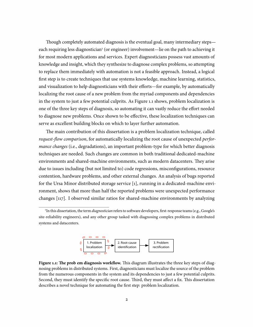
�ough completely automated diagnosis is the eventual goal, many intermediary steps—each requiring less diagnostician1 (or engineer) involvement—lie on the path to achieving itfor most modern applications and services. Expert diagnosticians possess vast amounts ofknowledge and insight, which they synthesize to diagnose complex problems, so attemptingto replace them immediately with automation is not a feasible approach. Instead, a logical�rst step is to create techniques that use systems knowledge, machine learning, statistics,and visualization to help diagnosticians with their e�orts—for example, by automaticallylocalizing the root cause of a new problem from the myriad components and dependenciesin the system to just a few potential culprits. As Figure 1.1 shows, problem localization isone of the three key steps of diagnosis, so automating it can vastly reduce the e�ort neededto diagnose new problems. Once shown to be e�ective, these localization techniques canserve as excellent building blocks on which to layer further automation.

�e main contribution of this dissertation is a problem localization technique, calledrequest-�ow comparison, for automatically localizing the root cause of unexpected perfor-mance changes (i.e., degradations), an important problem-type for which better diagnosistechniques are needed. Such changes are common in both traditional dedicated-machineenvironments and shared-machine environments, such as modern datacenters.�ey arisedue to issues including (but not limited to) code regressions, miscon�gurations, resourcecontention, hardware problems, and other external changes. An analysis of bugs reportedfor the Ursa Minor distributed storage service [1], running in a dedicated-machine envi-ronment, shows that more than half the reported problems were unexpected performancechanges [117]. I observed similar ratios for shared-machine environments by analyzing

1In this dissertation, the term diagnostician refers to so�ware developers, �rst-response teams (e.g., Google’ssite-reliability engineers), and any other group tasked with diagnosing complex problems in distributedsystems and datacenters.

1. Problem localization

2. Root-cause identi!cation

3. Problem recti!cation

Figure 1.1: �e problem diagnosis work�ow. �is diagram illustrates the three key steps of diag-nosing problems in distributed systems. First, diagnosticians must localize the source of the problemfrom the numerous components in the system and its dependencies to just a few potential culprits.Second, they must identify the speci�c root cause.�ird, they must a�ect a �x.�is dissertationdescribes a novel technique for automating the �rst step: problem localization.

2

Hadoop File System (HDFS) [134] bug reports, obtained from the JIRA [135] and conversa-tions with developers.

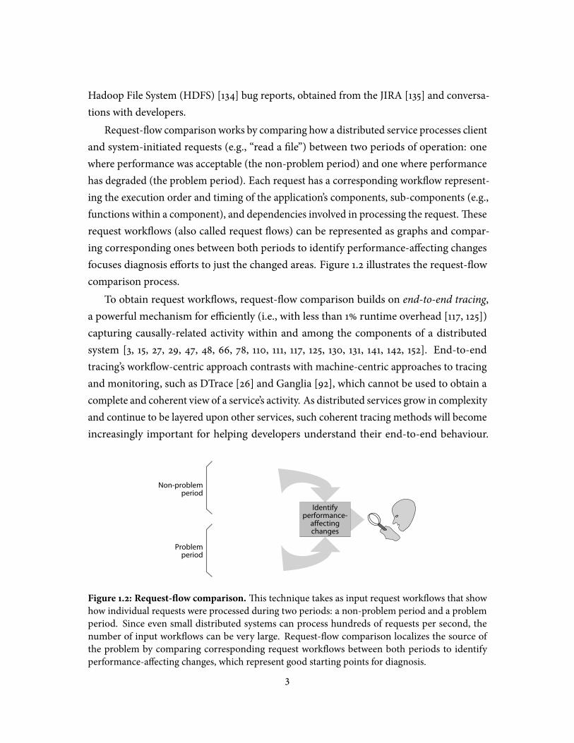
Request-�ow comparison works by comparing how a distributed service processes clientand system-initiated requests (e.g., “read a �le”) between two periods of operation: onewhere performance was acceptable (the non-problem period) and one where performancehas degraded (the problem period). Each request has a corresponding work�ow represent-ing the execution order and timing of the application’s components, sub-components (e.g.,functions within a component), and dependencies involved in processing the request.�eserequest work�ows (also called request �ows) can be represented as graphs and compar-ing corresponding ones between both periods to identify performance-a�ecting changesfocuses diagnosis e�orts to just the changed areas. Figure 1.2 illustrates the request-�owcomparison process.

To obtain request work�ows, request-�ow comparison builds on end-to-end tracing,a powerful mechanism for e�ciently (i.e., with less than 1% runtime overhead [117, 125])capturing causally-related activity within and among the components of a distributedsystem [3, 15, 27, 29, 47, 48, 66, 78, 110, 111, 117, 125, 130, 131, 141, 142, 152]. End-to-endtracing’s work�ow-centric approach contrasts with machine-centric approaches to tracingand monitoring, such as DTrace [26] and Ganglia [92], which cannot be used to obtain acomplete and coherent view of a service’s activity. As distributed services grow in complexityand continue to be layered upon other services, such coherent tracing methods will becomeincreasingly important for helping developers understand their end-to-end behaviour.

Figure 1.2: Request-�ow comparison.�is technique takes as input request work�ows that showhow individual requests were processed during two periods: a non-problem period and a problemperiod. Since even small distributed systems can process hundreds of requests per second, thenumber of input work�ows can be very large. Request-�ow comparison localizes the source ofthe problem by comparing corresponding request work�ows between both periods to identifyperformance-a�ecting changes, which represent good starting points for diagnosis.

3

Indeed, there are already a growing number of industry implementations, includingGoogle’sDapper [125], Cloudera’s HTrace [33], Twitter’s Zipkin [147], and others [36, 143]. Lookingforward, end-to-end tracing has the potential to become the fundamental substrate forproviding a global view of intra- and inter-datacenter activity in cloud environments.

1.1 Thesis statement and key results

�is dissertation explores the following thesis statement:

Request-�ow comparison is an e�ective technique for helping developers localize the source ofperformance changes in many request-based distributed services.

To evaluate this thesis statement, I developed Spectroscope [117], a tool that implementsrequest-�ow comparison, and used it to diagnose real, previously undiagnosed performancechanges in the Ursa Minor distributed storage service [1] and select Google services. Ialso explored Spectroscope’s applicability to the Hadoop File System [134] and identi�edneeded extensions. Since problem localization techniques like request-�ow comparisondo not directly identify the root cause of a problem, but rather help diagnosticians in theire�orts, their e�ectiveness depends on how well they present their results. To identify goodpresentations, I explored three approaches for visualizing Spectroscope’s results and rana 26-person user study to identify which ones are best for di�erent problem types [116].Finally, based on my experiences, I conducted a design study illustrating the propertiesneeded from end-to-end tracing for it to be useful for various use cases, including diagnosis.My thesis statement is supported by the following:

1. I demonstrated the usefulness of request-�ow comparison by using Spectroscope todiagnose six performance changes in a 6-component con�guration of Ursa Minor,running in a dedicated-machine environment. Four of these problems were real andpreviously undiagnosed—the root cause was not known a priori. One problem hadbeen previously diagnosed and was re-injected into the system.�e last problem wassynthetic and was injected into the system to evaluate a broader spectrum of problemtypes diagnosable by request-�ow comparison. �e problems diagnosed includedthose due to code regressions, miscon�gurations, resource contention, and externalchanges.

2. I demonstrated that request-�ow comparison is useful in other environments by using4

a version of Spectroscope to diagnose two real, previously undiagnosed performancechanges within select Google services, running in a shared-machine environment.�e Google version of Spectroscope was implemented as an addition to Dapper [125],Google’s end-to-end tracing infrastructure. I also explored Spectroscope’s applicabilityto HDFS and identi�ed extensions needed to the algorithms and heuristics it uses forit to be useful in this system.

3. I further demonstrated that diagnosticians can successfully use request-�ow compar-ison to identify starting points for diagnosis via a 26-person user study that includedGoogle and Ursa Minor developers. I also used this user study to identify the visual-ization approaches that best convey request-�ow comparison’s results for di�erentproblem types and users.

4. Via a design study, I determined how to design end-to-end tracing infrastructuresso that they are maximally e�ective for supporting diagnosis tasks. In the study, Idistilled the key design axes that dictate an end-to-end tracing infrastructure’s utilityfor di�erent use cases, such as diagnosis and resource attribution. I identi�ed gooddesign choices for di�erent use cases and showedwhere prior tracing implementationsfall short.

1.2 Goals & non-goals

�e key goal of this dissertation is to develop and show the e�ectiveness of a technique forautomating one key part of the problem diagnosis work�ow: localization of problems thatmanifest as steady-state-performance changes (e.g., changes to the 50th or 60th percentile ofsome important performance metric’s distribution). In doing so, it aims to address threefacets of developing an automation tool that helps developers perform management tasks.First, it describes algorithms and heuristics for the proposed automation and evaluatesthem. Second, it presents a user study evaluating three approaches for e�ectively presentingthe automation tool’s results to diagnosticians. �ird, it describes the properties neededfrom the underlying data source (end-to-end tracing) for success.

By describing an additional application for which end-to-end tracing is useful (diagnos-ing performance changes), this dissertation also aims to further strengthen the argumentfor implementing this powerful data source in datacenters and distributed systems.�oughend-to-end tracing has already been shown to be useful for a variety of use cases, includ-

5

ing diagnosis of certain correctness and performance problems [29, 47, 48, 110, 117, 125],anomaly detection [15, 29], pro�ling [27, 125], and resource usage attribution [15, 141], addi-tional evidence showing its utility is important so as to prove the signi�cant e�ort requiredto implement and maintain it is warranted.

A signi�cant non-goal of this dissertation is localizing performance problems thatmanifest as anomalies (e.g., requests that show up in the 99th percentile of some importantperformance metric’s distribution). Other techniques exist for localizing such problems [15].�is dissertation also does not aim to help diagnose correctness problems, though request-�ow comparison could be extended to do so.

Another important non-goal of this dissertation is complete automation. Request-�owcomparison automatically localizes the root cause of an performance change; it does notautomatically identify the root cause or automatically perform corrective actions. Muchadditional research is needed to understand how to automate other other phases of thediagnosis work�ow.

�is dissertation also does not attempt to quantitatively show that request-�ow compar-ison is better than other automated problem localization techniques. Such an evaluationwould require a user study in which many expert diagnosticians are asked to diagnose realproblems observed in a common system using di�erent localization techniques. But, it isextraordinarily di�cult to obtain a large enough pool of expert diagnosticians for the lengthof time needed to complete such a study. Instead, this dissertation demonstrates request-�ow comparison’s e�ectiveness by illustrating how it helped diagnosticians identify the rootcauses of real, previously undiagnosed problems. It also qualitatively argues that request-�owcomparison is more useful than many other localization techniques because it uses a datasource (end-to-end traces) that provides a coherent, complete view of a distributed system’sactivity.

A �nal non-goal is this dissertation is online diagnosis. Instead, this dissertation focuseson demonstrating the e�ectiveness of request-�ow comparison and leaves implementingonline versions of it to future work.

1.3 Assumptions

To work, request-�ow comparison relies on four key assumptions. First, it assumes thatdiagnosticians can identify two distinct periods of activity, one where performance wasacceptable (the non-problem period) and another where performance has degraded (the

6

problem period). Doing so is usually easy for steady-state-performance changes. Sincerequest-�ow comparison simply identi�es changes in request work�ows, it is indi�erent tothe number of distinct problems observed in the problem period, as long as they do not existin the non-problem period. Also, the problem period need not be a tight bound aroundthe performance degradation being diagnosed, but simply needs to contain it. However,for many implementations, the e�ectiveness of request-�ow comparison will increase withtighter problem-period bounds.

Second, request-�ow comparison assumes that theworkload (e.g., percentage of di�erentrequest types) observed in both the non-problem and problem periods are similar. If theyare signi�cantly di�erent, there is no basis for comparison, and request-�ow comparisonmay identify request work�ow changes that are a result of the di�ering workloads ratherthan problems internal to the distributed system. To avoid such scenarios, diagnosticianscould use change-point detection algorithms [31, 99] to determine whether the non-problemand problem period workloads di�er signi�cantly before applying request-�ow comparison.

�ird, request-�ow comparison assumes that users possess the domain expertise nec-essary to identify a problem’s root cause given evidence showing how it a�ects requestwork�ows. As such, request-�ow comparison is targeted toward distributed systems devel-opers and �rst-response teams, not end users or most system administrators. Chapters 3.6and 8.2.2 suggest that future work should consider how to incorporate more domain knowl-edge into request-�ow comparison tools, so as to reduce the amount of domain knowledgeusers must possess to make use of their results.

Fourth, request-�ow comparison assumes the availability of end-to-end traces (i.e.,traces that show the work�ow of how individual requests are serviced within and amongthe components of the distributed system being diagnosed). Request-�ow comparison willwork best when these traces exhibit certain properties (e.g., they distinguish concurrentactivity from sequential activity), but will work with degraded e�ectiveness when some arenot met.

1.4 Dissertation organization

�is dissertation contains eight chapters. Chapter 2 introduces request-�ow comparison,provides a high-level overview of it, and describes the algorithms and heuristics used toimplement request-�ow comparison in Spectroscope. Chapter 3 describes case studies ofusing Spectroscope to diagnose real, previously undiagnosed changes in Ursa Minor [1]

7

and in select Google services. It also describes extensions needed to Spectroscope for it tobe useful for diagnosing problems in HDFS [134]. Most of the content of these chapters waspublished in NSDI in 2011 [117], WilliamWang’s Master’s thesis in 2011 [150], and HotAC in2007 [118].

Chapter 4 describes the user study I ran to identify promising approaches for visualizingrequest-�ow comparison’s results. Most of this chapter was previously published in atechnical report in 2013 (CMU-PDL-13-104) [116].

Chapter 5 highlights a stumbling block on the path to automated diagnosis: lack ofpredictability in distributed systems (i.e., high variance in key metrics). It shows how Spec-troscope and other diagnosis tools are limited by high variance and suggests a framework forhelping developers localize high variance sources in their systems. In addition to increasingthe e�ectiveness of automation, eliminating unintended variance will increase distributedsystem performance [16]. Most of this chapter was published in HotCloud in 2012 [115].

Chapter 6 presents related work about performance diagnosis tools. Chapter 7 describesproperties needed from end-to-end tracing for it to be useful for various use cases, such asdiagnosis and resource attribution. Finally, chapter 8 concludes.

8

Chapter 2

Request-°ow comparison

�is chapter presents request-�ow comparison and its implementation in a diagnosis tool Ibuilt called Spectroscope. Section 2.1 presents a high-level overview of request-�ow com-parison and the types of performance problems for which it is useful. Section 2.2 providesrelevant background about end-to-end tracing and describes the properties request-�owcomparison needs from it. Section 2.4 describes the work�ow that any tool that imple-ments request-�ow comparison will likely have to incorporate. Di�erent tools may choosedi�erent algorithms to implement the work�ow, depending on their goals. Section 2.5discusses request-�ow comparison’s key limitations. Section 2.6 describes the algorithmsand heuristics used by Spectroscope, which were chosen for their simplicity and ability tolimit false positives.

2.1 Overview

Request-�ow comparison helps diagnosticians localize performance changes that manifestasmutations or changes in the work�ow of how client requests and system-initiated activitiesare processed. It is most useful in work-evident distributed systems, for which the worknecessary to service a request, as measured by its response time or aggregate throughput,is evident from properties of the request itself. Examples of such systems include mostdistributed storage systems (e.g., traditional �lesystems, key/value stores, and table stores)and three-tier web applications.

Request-�ow comparison, as described in this dissertation, focuses on helping diagnosesteady-state-performance changes (also known as behavioural changes). Such changesdi�er from performance problems caused by anomalies. Whereas anomalies are a small

9

number of requests that di�er greatly from others with respect to some important metricdistribution, steady-state changes o�en a�ect many requests, but perhaps only slightly. Moreformally, anomalies a�ect only the tail (e.g., 99th percentile) of some important metric’sdistribution, whereas steady-state changes a�ect the entire distribution (e.g., they changethe 50th or 60th percentile). Both anomalies and steady-state performance changes areimportant problem types for which advanced diagnosis tools are needed. However, mostexisting diagnosis tools that use end-to-end traces focus only on anomaly detection forperformance problems [15] or correctness problems [29, 78].

Since request-�ow comparison only aims to identify performance-a�ectingmutations, itis indi�erent to the actual root cause. A such, many types of problems can be localized usingrequest-�ow comparison, including performance changes due to con�guration changes,code changes, resource contention, and failovers to slower backup machines. Request-�owcomparison can also be used to understand why a distributed application performs di�er-ently in di�erent environments (e.g., di�erent datacenters) and to rule out the distributedsystem as the cause of an observed problem (i.e., by showing request work�ows have notchanged).�ough request-�ow comparison can be used in both production and testingenvironments, it is exceptionally suited to regression testing, since such tests always yieldwell-de�ned periods for comparison.

2.2 End-to-end tracing

To obtain graphs showing the work�ow of individual requests, request-�ow comparisonuses end-to-end tracing, which identi�es the �ow of causally-related activity (e.g., a request’sprocessing) within and among the components of a distributed system. Many approachesexist, but the most common ismetadata-propagation-based tracing [27, 29, 46, 47, 48, 110,117, 125, 141]. With this approach, trace points, which are similar to log statements, areautomatically or manually inserted in key areas of the distributed system’s so�ware. Usually,they are automatically inserted in commonly-used libraries, such as RPC libraries, andmanually inserted in other important areas. During runtime, the tracing mechanismpropagates an unique ID with each causal �ow and uses it to stitch together executed tracepoints, yielding end-to-end traces. �e runtime overhead of end-to-end tracing can belimited to less than 1% by using head-based sampling, in which a random decision is madeat the start of a causal �ow whether or not to collect any trace points for it [117, 125].

Other approaches to end-to-end tracing include black-box-based tracing [3, 21, 78, 83, 111,

10

130, 131, 152] and schema-based tracing [15, 66].�e �rst is used in un-instrumented systems,in which causally-related activity is inferred based on externally observable events (e.g.,network activity). With the second, IDs are not propagated. Instead, an external schemadictates how to stitch together causally-related trace points. Chapter 7 further describesdi�erent end-to-end tracing approaches and discusses design decisions that a�ect a tracinginfrastructure’s utility for di�erent use cases.�e rest of this section focuses on propertiesneeded from end-to-end tracing for request-�ow comparison.

2.3 Requirements from end-to-end tracing

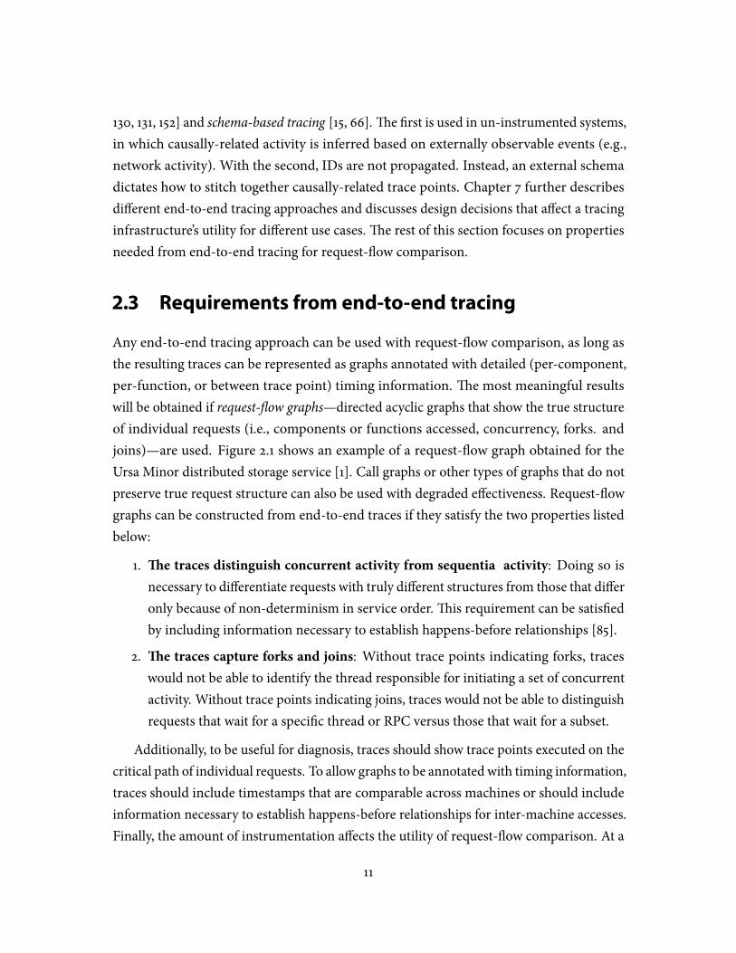
Any end-to-end tracing approach can be used with request-�ow comparison, as long asthe resulting traces can be represented as graphs annotated with detailed (per-component,per-function, or between trace point) timing information. �e most meaningful resultswill be obtained if request-�ow graphs—directed acyclic graphs that show the true structureof individual requests (i.e., components or functions accessed, concurrency, forks. andjoins)—are used. Figure 2.1 shows an example of a request-�ow graph obtained for theUrsa Minor distributed storage service [1]. Call graphs or other types of graphs that do notpreserve true request structure can also be used with degraded e�ectiveness. Request-�owgraphs can be constructed from end-to-end traces if they satisfy the two properties listedbelow:

1. �e traces distinguish concurrent activity from sequential activity: Doing so isnecessary to di�erentiate requests with truly di�erent structures from those that di�eronly because of non-determinism in service order.�is requirement can be satis�edby including information necessary to establish happens-before relationships [85].

2. �e traces capture forks and joins: Without trace points indicating forks, traceswould not be able to identify the thread responsible for initiating a set of concurrentactivity. Without trace points indicating joins, traces would not be able to distinguishrequests that wait for a speci�c thread or RPC versus those that wait for a subset.

Additionally, to be useful for diagnosis, traces should show trace points executed on thecritical path of individual requests. To allow graphs to be annotated with timing information,traces should include timestamps that are comparable across machines or should includeinformation necessary to establish happens-before relationships for inter-machine accesses.Finally, the amount of instrumentation a�ects the utility of request-�ow comparison. At a

11

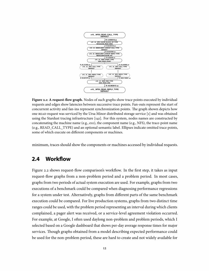
Figure 2.1: A request-�ow graph. Nodes of such graphs show trace points executed by individualrequests and edges show latencies between successive trace points. Fan-outs represent the start ofconcurrent activity and fan-ins represent synchronization points. �e graph shown depicts howone read request was serviced by the Ursa Minor distributed storage service [1] and was obtainedusing the Stardust tracing infrastructure [141]. For this system, nodes names are constructed byconcatenating the machine name (e.g., e10), the component name (e.g., NFS), the trace-point name(e.g., READ_CALL_TYPE) and an optional semantic label. Ellipses indicate omitted trace points,some of which execute on di�erent components or machines.

minimum, traces should show the components or machines accessed by individual requests.

2.4 Work°ow

Figure 2.2 shows request-�ow comparison’s work�ow. In the �rst step, it takes as inputrequest-�ow graphs from a non-problem period and a problem period. In most cases,graphs from two periods of actual system execution are used. For example, graphs from twoexecutions of a benchmark could be compared when diagnosing performance regressionsfor a system under test. Alternatively, graphs from di�erent parts of the same benchmarkexecution could be compared. For live production systems, graphs from two distinct timeranges could be used, with the problem period representing an interval during which clientscomplained, a pager alert was received, or a service-level agreement violation occurred.For example, at Google, I o�en used daylong non-problem and problem periods, which Iselected based on a Google dashboard that shows per-day average response times for majorservices.�ough graphs obtained from a model describing expected performance couldbe used for the non-problem period, these are hard to create and not widely available for

12

Categorization

Response-time mutation identi!cation

Structural mutation identi!cation

Problemperiod grap

Problem period graphs

Ranking

Visualization

Non-problem period graphs

Problem period graphs

Ranked list of categories with mutations

1. Structural2. Response time

Optional extensions

Low-level difference

identification

Diagnostician interface

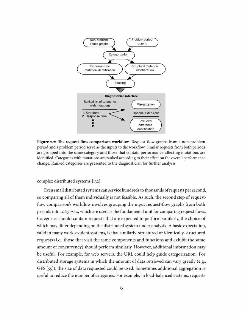
Figure 2.2: �e request-�ow comparison work�ow. Request-�ow graphs from a non-problemperiod and a problem period serve as the inputs to the work�ow. Similar requests from both periodsare grouped into the same category and those that contain performance-a�ecting mutations areidenti�ed. Categories with mutations are ranked according to their e�ect on the overall performancechange. Ranked categories are presented to the diagnostician for further analysis.

complex distributed systems [132].

Even small distributed systems can service hundreds to thousands of requests per second,so comparing all of them individually is not feasible. As such, the second step of request-�ow comparison’s work�ow involves grouping the input request-�ow graphs from bothperiods into categories, which are used as the fundamental unit for comparing request �ows.Categories should contain requests that are expected to perform similarly, the choice ofwhich may di�er depending on the distributed system under analysis. A basic expectation,valid in many work-evident systems, is that similarly-structured or identically-structuredrequests (i.e., those that visit the same components and functions and exhibit the sameamount of concurrency) should perform similarly. However, additional information maybe useful. For example, for web servers, the URL could help guide categorization. Fordistributed storage systems in which the amount of data retrieved can vary greatly (e.g.,GFS [55]), the size of data requested could be used. Sometimes additional aggregation isuseful to reduce the number of categories. For example, in load-balanced systems, requests

13

that exhibit di�erent structures only because they visit di�erent replicas should be groupedinto the same category.

�e third step of request-�ow comparison’s work�ow involves identifying which cate-gories contain mutations and precursors. Mutations are expensive requests observed in theproblem period that have mutated or changed from less expensive requests observed inthe non-problem period. Conversely, precursors are requests from the non-problem periodthat have mutated into more expensive requests in the problem period. Two very commontypes of mutations are response-time mutations and structural mutations. Response-timemutations are requests whose structure remains identical between both periods, but whoseresponse times have increased. Comparing them to their precursors localizes the problemto the components or functions responsible for the slowdown and focuses diagnosis e�orts.Structural mutations are requests whose performance has decreased because their structureor work�ow through the distributed system has changed. Comparing them to their pre-cursors identi�es the changed substructures, which are good locations to start diagnosise�orts.

�e fourth step of request-�ow comparison’s work�ow is to focus diagnosticians’ e�orton the most performance-a�ecting mutations by ranking them according to their contri-bution to the performance change. In the ��h and �nal �nal step, ranked categories arepresented to the diagnostician for further analysis.

Many additional work�ow steps are possible. For example, additional localization maybe possible by identifying the low-level parameters (e.g., function variables, client-sentparameters) that best di�erentiate mutations and their precursors. As such, Spectroscopeincludes an optional work�ow step for such identi�cation. For two case studies, thisadditional step immediately revealed the root cause (see the case studies described inChapter 3.3.1 and 3.3.2). Also, Spectroscope could be extended to detect anomalies byidentifying requests in the tails of intra-category, intra-period, response-time distributions.

2.5 Limitations

Despite its usefulness, there are �ve key limitations to request-�ow comparison’s work�ow.Most notably, request-�ow comparison’s method of localizing performance changes byidentifying mutations may not identify the most direct problem sources. For example, inone case study, described in Chapter 3.3.1, my implementation of request-�ow comparison,Spectroscope, was used to help diagnose a performance degradation whose root cause was

14

a miscon�guration.�ough Spectroscope was able to localize the problem to a change inthe storage node used by one component of the service and to speci�c variables used in thecodebase, it did not localize the problem to the problematic con�guration �le. Similarly,when diagnosing problems such as contention, request-�ow comparison may localize theproblem by identifying a change in per-component timing, but will not localize it to thespeci�c competing process or request. I believe additional work�ow steps could be used toincrease the directness of localization.�is is exempli�ed by Spectroscope’s additional work-�ow step, which seeks to localize performance changes to low-level parameter di�erencesbetween mutations and precursors.

�e number of categories identi�ed by request-�ow comparison as containing muta-tions will likely greatly exceed the number of problems present in the system.�is is partlybecause a single problem will o�en a�ect many di�erent request types, each with di�erentperformance expectations. For example, a single performance problem may a�ect bothattribute requests and write requests. Since these two request types are expected to exhibitfundamentally di�erent performance characteristics, they will be assigned to di�erent cate-gories and identi�ed as separate mutations, even though both show the same underlyingproblem. To cope, a�er �xing the problem identi�ed by a highly-ranked mutation cate-gory, diagnosticians should always re-run the request-�ow comparison tool to see if othermutations were caused by the same problem. If so, they will not appear in the new results.

�e granularity at which request-�ow comparison can localize problems is limited bythe granularity of tracing. For example, if the traces only show inter-component activity(e.g., RPCs or messages passed between components), then request-�ow comparison will belimited to localizing problems to entire components. Component-level localization is alsopossible for black-box components (i.e., components that export no trace data whatsoever)if traces in surrounding components document accesses to them.

Request-�ow comparison, as presented in this dissertation, will be of limited valuein dynamic environments (i.e., ones in which applications can be moved while they areexecuting or between comparable executions). To be useful in such environments, extrawork�ow steps would be needed to determine whether an observed performance changeis the expected result of an infrastructure-level change or is representative of a real prob-lem [119].

Finally, many distributed systems mask performance problems by diverting additionalresources to the problematic application or job. For example, many map-reduce imple-mentations, such as Hadoop [8], limit the performance impact of stragglers by aggressively

15

duplicating or restarting slow-to-complete tasks [6, 155]. Request-�ow comparison will beless useful in these systems, since they may exhibit no discernible performance slowdownin some cases.

2.6 Implementation in Spectroscope

I implemented request-�ow comparison in two versions of Spectroscope. �e �rst wasused to diagnose problems in Ursa Minor [1] and to explore the utility of Spectroscope’salgorithms and heuristics in HDFS [134]. It was written using a combination of Perl, Matlab,and C.�e secondwas used to diagnose select Google services andwas implemented in C++as an extension to Google’s end-to-end tracing infrastructure, Dapper [125]. Speci�cally,the Google version of Spectroscope uses Dapper’s aggregation pipeline to obtain call graphs.Both versions implement request-�ow comparison’s work�ow using the same algorithmsand heuristics, which were chosen for their simplicity, ability to use unlabeled data, andability to regulate false positives. As such, they are not di�erentiated in this dissertationunless necessary.�e second constraint is necessary because labels indicating whether indi-vidual requests performed well or poorly are uncommon in many systems.�e period label(problem or non-problem) is not su�cient because both periods may contain both types ofrequests. I included the third constraint because Facebook and Google engineers indicatedthat false positives are the worst failure mode of an automated diagnosis tool because ofthe amount of diagnostician e�ort wasted [107]. However, when running user studies toevaluate visualizations for Spectroscope (see Chapter 4), I found that false negatives are justas troublesome, because they reduce diagnosticians’ con�dence in automation.

In addition to comparing request �ows between two periods, Spectroscope can alsobe used to categorize requests observed in a single period. In such cases, Spectroscopewill output the list of categories observed, each annotated with relevant metrics, such asaverage response time and response time variance. Categories can be ranked by any metriccomputed for them.�e remainder of this section describes the algorithms and heuristicsused by Spectroscope for request-�ow comparison.

2.6.1 Categorization

Spectroscope creates categories composed of identically-structured requests. It uses a stringrepresentation of individual request-�ow graphs, as determined by a depth-�rst traversal,to identify which category to assign a given request.�ough this method will incorrectly

16

assign requests with di�erent structures, yet identical string representations, to the samecategory, I have found it works well in practice. For requests with parallel substructures,Spectroscope computes all possible string representations when determining the categoryin which to bin them.�e exponential cost is mitigated by imposing an order on parallelsubstructures (i.e., by always traversing children in lexographic order) and by the fact thatmost requests we observed in Ursa Minor and Google exhibited limited parallelism.

Creating categories that consist of identically-structured requests may result in a largenumber of categories. To reduce the number, I explored using unsupervised clusteringalgorithms, such as those used in Magpie [15], to group similar, but not identical, requestsinto the same category [118]. But, I found that o�-the-shelf clustering algorithms createdcategories that were too coarse-grained and unpredictable. O�en, they would assign re-quests with important di�erences into the same category, masking their existence.�oughthere is potential for improving Spectroscope’s categorizing step by using clustering algo-rithms, improvements are needed, such as specialized distance metrics that better alignwith diagnosticians’ notions of request similarity.

2.6.2 Identifying response-time mutations

Since response-time mutations and their precursors have identical structures, they will beassigned to the same category, but will have di�erent period labels. As such, categories thatcontain them will have signi�cantly di�erent non-problem and problem-period responsetimes. To limit false positives, which result in wasted diagnostician e�ort, Spectroscopeuses the Kolmogorov-Smirnov two-sample hypothesis test [91] instead of raw thresholds toidentify such categories.

�e Kolmogorov-Smirnov test takes as input two empirical distributions and determineswhether there is enough evidence to reject the null hypothesis that both represent the sameunderlying distribution (i.e., they di�er only due to chance or natural variance).�e null hy-pothesis is rejected only if the expected false-positive rate of declaring the two distributionsas di�erent—i.e., the p-value—is less than a pre-set value, almost always 5%. Spectroscoperuns the Kolmogorov-Smirnov hypothesis test on a category’s observed non-problem andproblem-period response-time distributions and marks it as containing response-time mu-tations if the test rejects the null hypothesis. Since the test will yield inaccurate results if thefollowing condition is true: non−probl em period requests ⋅ probl em period requests

non−probl em period requests + probl em period requests ≤ 4, such categoriesare summarily declared not to contain mutations.�e Kolmogorov-Smirnov test’s runtime

17

is O(N), where N is the number samples in the distributions being compared (i.e., thenumber of non-problem and problem-period requests).

�e Kolmogorov-Smirnov test is non-parametric, which means it does not assume aspeci�c distribution type, but yields increased false negatives compared to tests that operateon known distributions. I chose a non-parametric test because I observed per-categoryresponse-time distributions are not governed by well-known distributions. For example,inadequate instrumentation might result in requests with truly di�erent structures andbehaviours being grouped into the same category, yielding multi-modal response-timedistributions.

Once categories containing response-timemutations have been identi�ed, Spectroscoperuns the Kolmogorov-Smirnov test on the category’s edge latency distributions to localizethe problem to the speci�c areas responsible for the overall response time change.

2.6.3 Identifying structural mutations and their precursors

Since structural mutations are requests that have changed in structure, they will be assignedto di�erent categories than their precursors during the problem period. Spectroscope usestwo steps to identify structural mutations and their precursors. First, Spectroscope identi�esall categories that contain structural mutations and precursors. Second, it determines amapping showing which precursor categories are likely to have donated requests to whichstructural-mutation category during the problem period.

Step 1: Identifying categories containing mutations and precursors

To identify categories containing structural mutations and their precursors, Spectroscopeassumes that the loads observed in both the non-problem and problem periods were similar(but not necessarily identical). As such, structural-mutation categories can be identi�edas those that are assigned signi�cantlymore problem-period requests than non-problem-period ones. Conversely, categories containing precursors can be identi�ed as those thatare assigned signi�cantly fewer problem-period requests than non-problem ones.

Since workload �uctuations and non-determinism in service order dictate that per-category counts will always vary slightly between periods, Spectroscope uses a raw thresholdto identify categories that contain structural mutations and their precursors. Categoriesthat contain SM_P_THRESHOLDmore requests from the problem period than from the non-problemperiod are labeled as containingmutations and those that containSM_P_THRESHOLD

18

fewer are labeled as containing precursors. Unlike for response-time mutations, Spec-troscope does not use non-parametric hypothesis tests to identify categories containingstructural mutations because multiple runs of the non-problem and problem period wouldbe needed to obtain the required input distributions of category counts. Also, Googleengineers indicated that request structures change frequently at Google due to frequentso�ware changes from independent teams, discouraging the use of approaches that requirelong-lived models.

Choosing a good threshold for a workload may require some experimentation, as it issensitive to both the number of requests issued and the sampling rate. Fortunately, it iseasy to run Spectroscope multiple times, and it is not necessary to get the threshold exactlyright. Choosing a value that is too small will result in more false positives, but the rankingscheme will assign them a low rank, and so will not mislead diagnosticians.

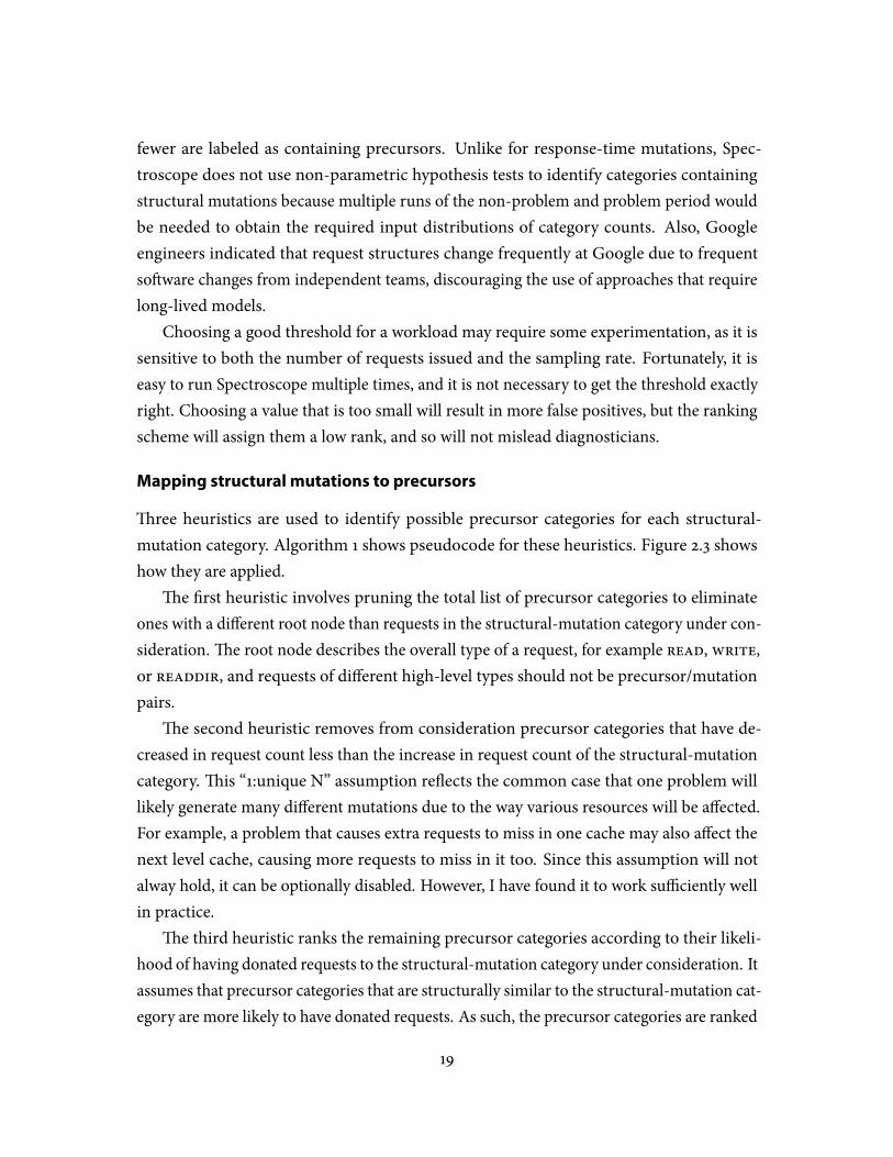
Mapping structural mutations to precursors

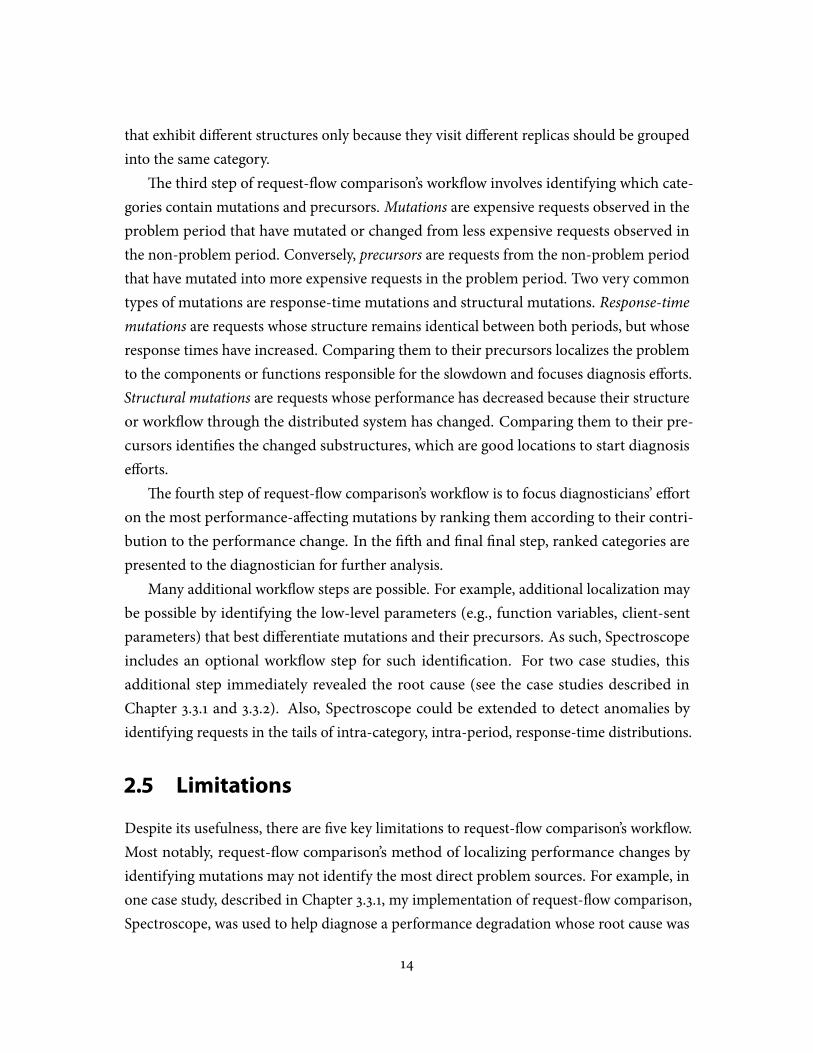
�ree heuristics are used to identify possible precursor categories for each structural-mutation category. Algorithm 1 shows pseudocode for these heuristics. Figure 2.3 showshow they are applied.

�e �rst heuristic involves pruning the total list of precursor categories to eliminateones with a di�erent root node than requests in the structural-mutation category under con-sideration.�e root node describes the overall type of a request, for example read, write,or readdir, and requests of di�erent high-level types should not be precursor/mutationpairs.

�e second heuristic removes from consideration precursor categories that have de-creased in request count less than the increase in request count of the structural-mutationcategory. �is “1:unique N” assumption re�ects the common case that one problem willlikely generate many di�erent mutations due to the way various resources will be a�ected.For example, a problem that causes extra requests to miss in one cache may also a�ect thenext level cache, causing more requests to miss in it too. Since this assumption will notalway hold, it can be optionally disabled. However, I have found it to work su�ciently wellin practice.

�e third heuristic ranks the remaining precursor categories according to their likeli-hood of having donated requests to the structural-mutation category under consideration. Itassumes that precursor categories that are structurally similar to the structural-mutation cat-egory are more likely to have donated requests. As such, the precursor categories are ranked

19

Input : List of precursor categories and structural-mutation categoriesOutput :Ranked list of candidate precursor categories for each structural-mutation categoryfor i ← 1 to length(sm_list) do

candidates [i]← find_same_root_node_precursors(precursor_list, sm_list [i]);if apply_1_n_heuristic then

candidates [i]← prune_unlikely_precursors( candidates [i], sm_list [i]);end

// Re-arrange in order of inverse normalized string-edit distancecandidates [i]← rank_by_inverse_nsed( candidates [i], sm_list [i]);

end

Algorithm 1: Heuristics used to identify and rank precursor categories that could have do-

nated requests to a structural-mutation category. �e “1:unique N” heuristic assumes that oneprecursor category will likely donate requests to many structural-mutation categories and elimi-nates precursor categories that cannot satisfy this assumption.�e �nal output list is ranked byinverse normalized string-edit distance, which is used to approximate the probability that a givenprecursor category donated requests.�e cost of these heuristics is dominated by the string-editdistance calculation, which costs O(N2), where N is the length of each string.

Read

Mutation Precursor categoriesRead Read Read

Lookup

NP: 700P: 1,000

NP: 300P: 200

NP: 550 P: 150

NP: 650 P: 100

ReadDir

NP: 200P: 100

NP: 1,100P: 600

Figure 2.3: How the precursor categories of a structural-mutation category are identi�ed. Onestructural-mutation category and �ve precursor categories are shown, each with their correspondingrequest counts from the non-problem (NP) and problem (P) periods. For this case, the shadedprecursor categories will be identi�ed as those that could have donated requests to the structural-mutation category. �e precursor categories that contain lookup and readdir requests cannothave donated requests, because their constituent requests are not reads.�e top le�-most precursorcategory contains reads, but the 1:N heuristic eliminates it. Due to space constraints, mocked-upgraphs are shown in which di�erent node shapes represent the types of components accessed.

20

by the inverse of their normalized Levenshtein string-edit distance from the structural-mutation category.�e string-edit distance implementation used by the Ursa Minor/HDFSversion of Spectroscope has runtime O(N2

) in the number of graph nodes. As such, itdominates runtime when input request-�ow graphs do not exhibit much concurrency.Runtime could be reduced by using more advanced edit-distance algorithms, such as theO(ND) algorithm described by Berghel and Roach [19], where N is the number of graphnodes and D is the edit distance computed. Sub-polynomial approximation algorithms forcomputing edit distance also exist [7].

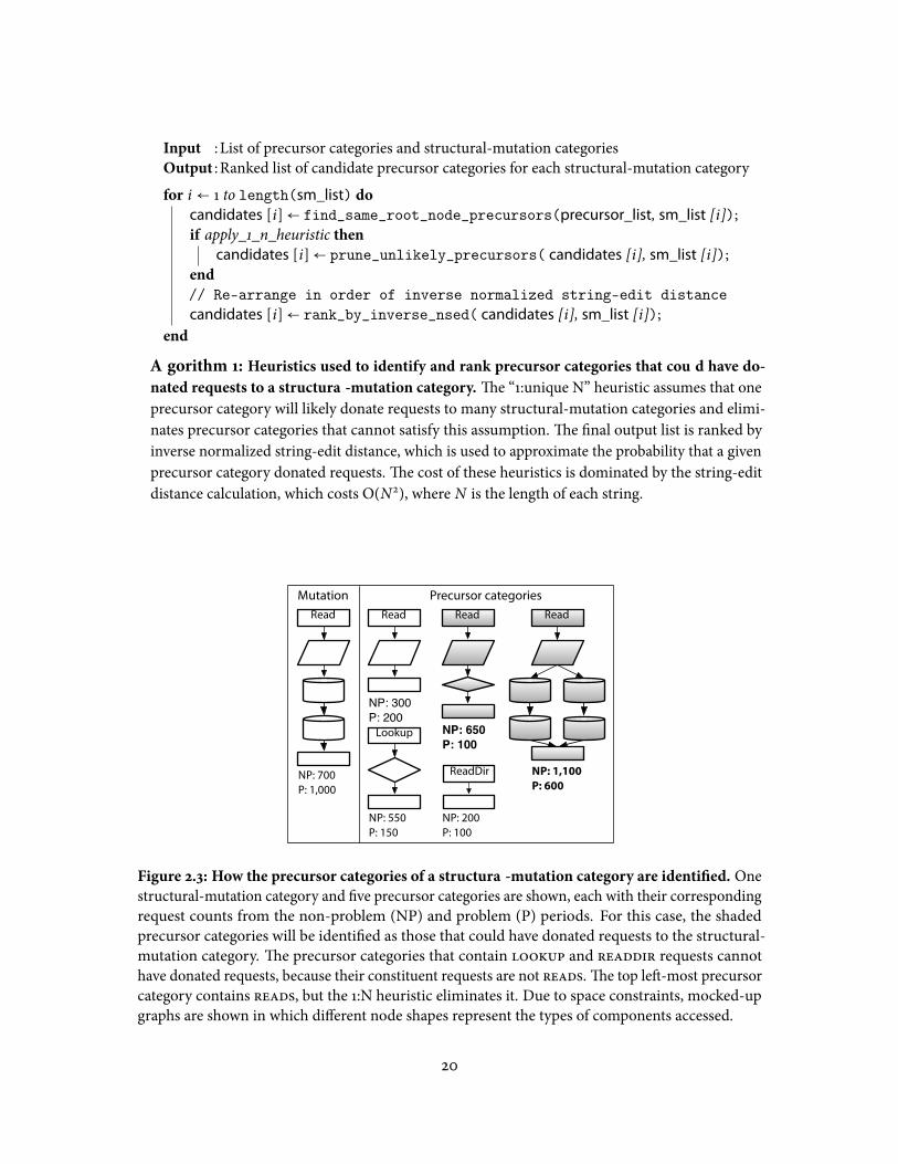
2.6.4 Ranking

Spectroscope ranks categories containing mutations according to their contribution tothe overall performance change. �e contribution for a category containing response-time mutations is calculated as the number of non-problem-period requests assigned to itmultiplied by the change in average response time between both periods.�e contributionfor a category containing structural mutations is calculated as the number of extra problem-period requests assigned to it times the average change in response time between it andits precursor category. If more than one candidate precursor category exists, an averageof their response times are used, weighted by structural similarity. Figure 2.4 shows theequations used for ranking.

Spectroscope will split categories containing structural mutations and response-time

Response timei = (NPrequests i)(̇Presponse time i − NPresponse time i)

Structural mutationi = (Prequests i − NPrequests i)C∑j=1

Presponse time i −1

nsed(i , j)∑C

j=11

nsed(i , j)Presponse time j

Figure 2.4: Contribution to the overall performance change by a category containingmutations

of a given type.�e contribution for a category containing response-time mutations is calculatedas the number of non-problem-period requests it contains times the category’s change in averageresponse time between both periods.�e contribution for a category containing structural mutationsis calculated as the number of extra problem-period requests it contains times the change in averageresponse time between it and its precursor category. If multiple candidate precursor categoriesexist, an average weighted by structural similarity is used. For the equations above, NP refers to thenon-problem period, P refers to the problem period, nsed refers to normalized string-edit distance,and C refers to the number of candidate precursor categories.

21

mutations into separate virtual categories and rank each separately. I also explored rankingsuch categories based on the combined contribution from both mutation types. Notethat category ranks are not independent of each other. For example, precursor categoriesof a structural-mutation category may themselves contain response-time mutations, so�xing the root cause of the response-time mutation will a�ect the rank assigned to thestructural-mutation category.

2.6.5 Visualization

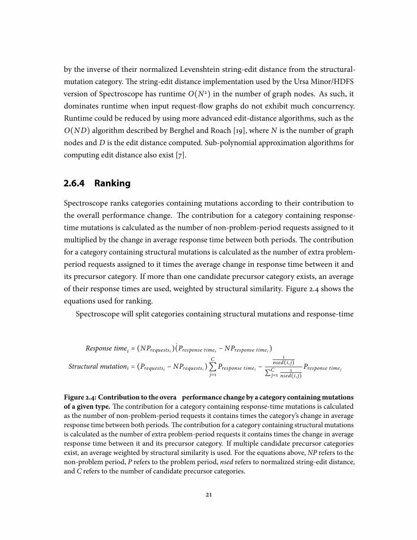
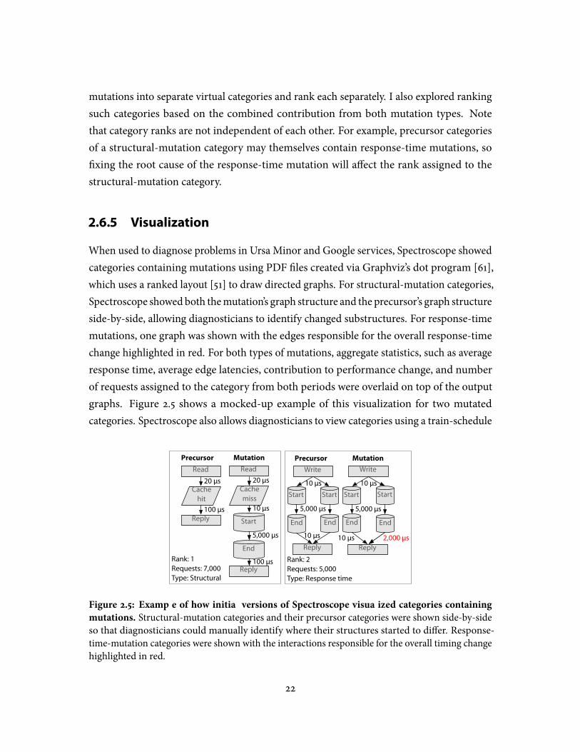
When used to diagnose problems in Ursa Minor and Google services, Spectroscope showedcategories containing mutations using PDF �les created via Graphviz’s dot program [61],which uses a ranked layout [51] to draw directed graphs. For structural-mutation categories,Spectroscope showed both themutation’s graph structure and the precursor’s graph structureside-by-side, allowing diagnosticians to identify changed substructures. For response-timemutations, one graph was shown with the edges responsible for the overall response-timechange highlighted in red. For both types of mutations, aggregate statistics, such as averageresponse time, average edge latencies, contribution to performance change, and numberof requests assigned to the category from both periods were overlaid on top of the outputgraphs. Figure 2.5 shows a mocked-up example of this visualization for two mutatedcategories. Spectroscope also allows diagnosticians to view categories using a train-schedule

Cachehit

Reply

Read

Cachemiss

Start

Reply

Read20 μs

10 μs

5,000 μs

20 μs

100 μs

Precursor Mutation Precursor

End

100 μs

Reply

Write

Start Start

End End

10 μs

Rank: 1Requests: 7,000Type: Structural

Rank: 2Requests: 5,000Type: Response time

5,000 μs

Reply

Write

Start Start

End End

10 μs

10 μs

5,000 μs

Mutation

2,000 μs

10 μs

Figure 2.5: Example of how initial versions of Spectroscope visualized categories containing

mutations. Structural-mutation categories and their precursor categories were shown side-by-sideso that diagnosticians could manually identify where their structures started to di�er. Response-time-mutation categories were shown with the interactions responsible for the overall timing changehighlighted in red.

22

visualization (also called a swimlane visualization) [146].For Spectroscope to be useful to diagnosticians, it must present its results as clearly

as possible. My experiences using Spectroscope’s initial visualizations convinced me theyare not su�cient. Chapter 4 describes a user study I ran with real distributed systemsdevelopers comparing three advanced approaches for presenting Spectroscope’s results.

2.6.6 Identifying low-level diªerences

Identifying the di�erences in low-level parameters between a mutation and precursor cano�en help developers further localize the source of the problem. For example, the rootcause of a response-time mutation might be further localized by identifying that it is causedby a component that is sending more data in its RPCs than during the non-problem period.

Spectroscope allows developers to pick a mutation category and candidate precursorcategory for which to identify low-level di�erences. Given these categories, Spectroscopeinduces a regression tree [20] showing the low-level parameters that best separate requestsin these categories. Each path from root to leaf represents an independent explanation ofwhy the mutation occurred. Since developers may already possess some intuition aboutwhat di�erences are important, the process is meant to be interactive. If the developer doesnot like the explanations, he can select a new set by removing the root parameter fromconsideration and re-running the algorithm.

�e regression tree is induced as follows. First, a depth-�rst traversal is used to extract atemplate describing the parts of request structures that are common between both categories,up until the �rst observed di�erence. Portions that are not common are excluded, sincelow-level parameters cannot be compared for them.

Second, a table in which rows represent requests and columns represent parametersis created by iterating through each of the categories’ requests and extracting parametersfrom the parts that fall within the template. Each row is labeled as precursor or mutationdepending on the category to which the corresponding request was assigned. Certainparameter values, such as the thread ID and timestamp, must always be ignored, asthey are not expected to be similar across requests. Finally, the table is fed as input tothe C4.5 algorithm [108], which creates the regression tree and has worst-case runtime ofO(MN2

), where M is the number of problem and non-problem requests in the precursorand mutations categories and N is the number of parameters extracted. To reduce runtime,only parameters from a randomly sampled subset of requests are extracted from the database,

23

currently a minimum of 100 and a maximum of 10% of the total number of input requests.Parameters only need to be extracted the �rst time the algorithm is run; subsequent iterationscan modify the table directly.

2.6.7 Limitations of current algorithms & heuristics

�is section describes some current limitations with the algorithms and heuristics imple-mented in Spectroscope.

Load observed in both periods must be similar: �ough request-�ow comparisonexpects that the workloads (i.e., percentage of request types) observed in both periods willbe similar, Spectroscope’s algorithms could be improved to better tolerate di�erences inload. For example, Spectroscope could be extended to use queuing theory to predict whena latency increase is the expected result of a load change.

Utility is limited when diagnosing problems due to contention: Such problems willresult in increased variance, limiting the Kolmogorov-Smirnov’s tests to identify distributionchanges and, hence, Spectroscope’s ability to identify response-time mutations. Chapter 3.2further describes how Spectroscope is a�ected by variance.

Utility is limited for systems that generate very large graphs and those that generate

many unique graph structures: Spectroscope’s algorithms, especially theO(N2) algorithm

it uses for calculating structural similarity between structural mutations and precursors,will not scale to extremely large graphs. Also, systems that generate many unique requeststructures may result in too many categories with too few requests in each to accuratelyidentify mutations. Chapter 3.5 describes how these two problems occur for HDFS [134]and describes the two extensions to Spectroscope’s algorithms that address them.

Requests that exhibit a large amount of parallelism will result in slow runtimes:Spectroscope must determine which request-�ow graphs (i.e., directed acyclic graphs)are isomorphic during its categorization phase. Doing so is trivial for purely sequentialgraphs, but can require exponential time for graphs that contain fan-outs due to parallelism.Unless the cost of categorization can be reduced for them (e.g., by traversing children inlexographic order), Spectroscope will be of limited use for workloads that generate suchgraphs.

24

Chapter 3

Evaluation & case studies

�is chapter evaluates Spectroscope in three ways. First, using workloads run on UrsaMinor [1] and Google’s Bigtable [28], it evaluates the validity of Spectroscope’s expectationthat requests with the same structure should perform similarly. Second, it presents casestudies of using Spectroscope to diagnose real and synthetic problems in Ursa Minor andselect Google services. Not only do these case studies illustrate real experiences of usingSpectroscope to diagnose real problems, they also illustrate how Spectroscope �ts intodiagnosticians’ work�ows when debugging problems. �ird, it explores Spectroscope’sapplicability to even more distributed systems by describing extensions necessary for it’salgorithms to be useful in helping diagnose problems in HDFS [134]. Section 3.1 describesUrsa Minor, the Google services used for the evaluation, and the workloads run on them.Section 3.2 evaluates the validity of Spectroscope’s same structures/similar performanceexpectation. Section 3.3 describes the Ursa Minor case studies, and Section 3.4 describesthe Google ones. Section 3.5 describes extensions needed for Spectroscope to be useful forHDFS and Section 3.6 concludes.

3.1 Overview of Ursa Minor & Google services

�eUrsaMinor distributed storage service: UrsaMinor is an object-based storage serviceand is based on the network attached secure disk architecture (NASD) [57]. An Ursa Minorinstance (called a “constellation”) consists of potentially many NFS servers (which serve asproxies for unmodi�edNFS clients and, as such, are responsible for translating NFS requeststo native Ursa Minor client ones), storage nodes (SNs), metadata servers (MDSs), and end-to-end trace servers. To access data, the NFS server (or a native UrsaMinor client) must �rst

25

send a request to the metadata server to obtain the appropriate permissions and the namesof the storage nodes that contain the data. Once the NFS server knows the names of thestorage nodes, it is free to access them directly. Ursa Minor was actively developed between2004 and 2011 and contains about 230,000 lines of code. More than 20 graduate studentsand sta� have contributed to it over its lifetime. More details about its implementation canbe found in Abd-El-Malek et al. [1]. It is normally run in a dedicated-machine environment,with di�erent components run on di�erent machines.

Ursa Minor’s tracing services are provided by a version of Stardust [141] revised to beuseful for diagnosis. Stardust’s architecture is similar to other metadata propagation-basedtracing infrastructures [27, 29, 46, 47, 48, 110, 117, 125, 141]. �e revised version outputsrequest-�ow graphs, which are the type of graphs Spectrocope works best with. Stardust’sdefault head-based sampling percentage is 10% and Ursa Minor itself contains about 200trace points, 124 manually inserted as well as automatically generated ones for each sendand receive RPC.

Figure 3.1 shows the 5-component Ursa Minor constellation used to evaluate Spectro-scope. It consists of one NFS server, one metadata server, two storage nodes, and oneend-to-end tracing server. Each component runs on its own dedicated machine in a ho-mogeneous cluster, which consists of machines with 3.0GhZ processors and 2GB of RAM.�ough Ursa Minor could be run with an arbitrary number of components in either sharedmachine or dedicated machine environments, the con�guration listed above is the oneused during its nightly regression tests, during which all of the case study problems were

Client request

Application

NFS

ser

ver

SN

Metadata server

Trace server

Data request

NFS client

Metadata request

Ursa Minor constellation

Figure 3.1: 5-component Ursa Minor constellation used during nightly regression tests. �econstellation consists of one NFS server, one metadata server, two storage nodes (one reserved fordata and one for metadata), and one end-to-end tracing server.

26

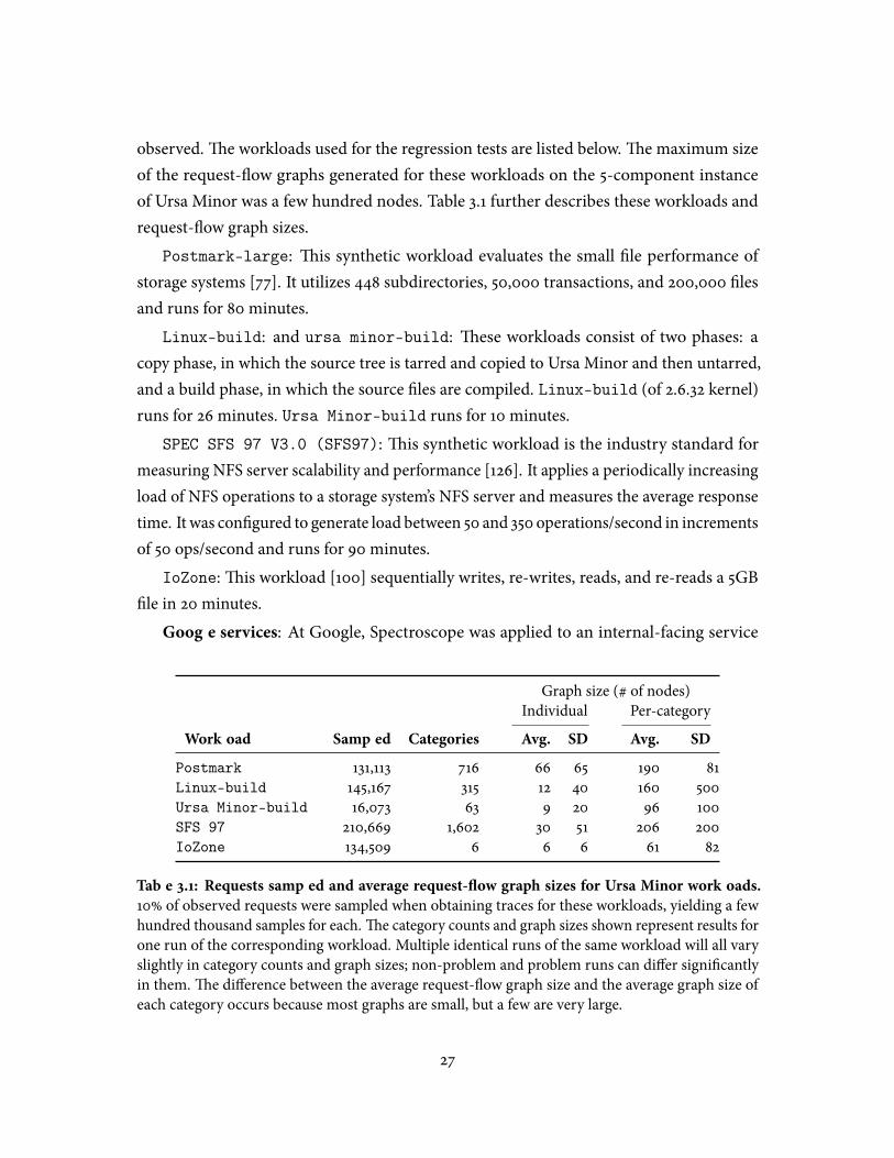
observed.�e workloads used for the regression tests are listed below.�e maximum sizeof the request-�ow graphs generated for these workloads on the 5-component instanceof Ursa Minor was a few hundred nodes. Table 3.1 further describes these workloads andrequest-�ow graph sizes.

Postmark-large: �is synthetic workload evaluates the small �le performance ofstorage systems [77]. It utilizes 448 subdirectories, 50,000 transactions, and 200,000 �lesand runs for 80 minutes.

Linux-build: and ursa minor-build: �ese workloads consist of two phases: acopy phase, in which the source tree is tarred and copied to Ursa Minor and then untarred,and a build phase, in which the source �les are compiled. Linux-build (of 2.6.32 kernel)runs for 26 minutes. Ursa Minor-build runs for 10 minutes.

SPEC SFS 97 V3.0 (SFS97): �is synthetic workload is the industry standard formeasuring NFS server scalability and performance [126]. It applies a periodically increasingload of NFS operations to a storage system’s NFS server and measures the average responsetime. It was con�gured to generate load between 50 and 350 operations/second in incrementsof 50 ops/second and runs for 90 minutes.

IoZone:�is workload [100] sequentially writes, re-writes, reads, and re-reads a 5GB�le in 20 minutes.

Google services: At Google, Spectroscope was applied to an internal-facing service

Graph size (# of nodes)Individual Per-category

Workload Sampled Categories Avg. SD Avg. SD

Postmark 131,113 716 66 65 190 81Linux-build 145,167 315 12 40 160 500Ursa Minor-build 16,073 63 9 20 96 100SFS 97 210,669 1,602 30 51 206 200IoZone 134,509 6 6 6 61 82

Table 3.1: Requests sampled and average request-�ow graph sizes for Ursa Minor workloads.

10% of observed requests were sampled when obtaining traces for these workloads, yielding a fewhundred thousand samples for each.�e category counts and graph sizes shown represent results forone run of the corresponding workload. Multiple identical runs of the same workload will all varyslightly in category counts and graph sizes; non-problem and problem runs can di�er signi�cantlyin them.�e di�erence between the average request-�ow graph size and the average graph size ofeach category occurs because most graphs are small, but a few are very large.

27

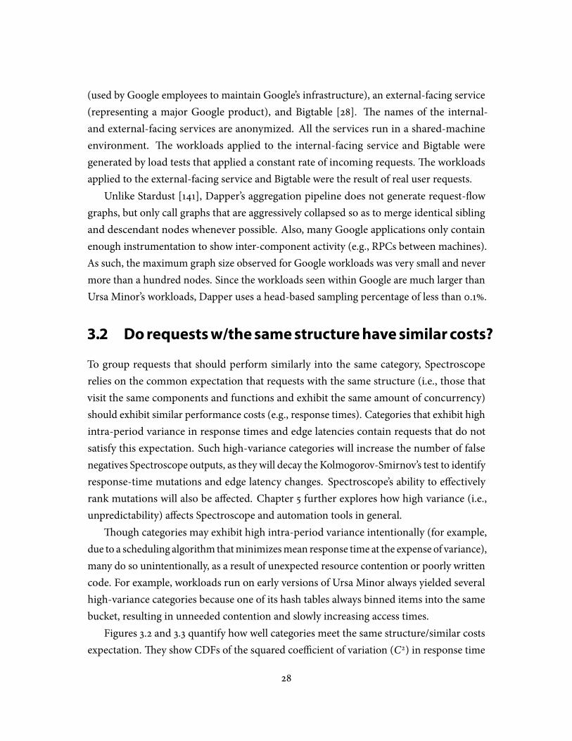
(used by Google employees to maintain Google’s infrastructure), an external-facing service(representing a major Google product), and Bigtable [28]. �e names of the internal-and external-facing services are anonymized. All the services run in a shared-machineenvironment. �e workloads applied to the internal-facing service and Bigtable weregenerated by load tests that applied a constant rate of incoming requests.�e workloadsapplied to the external-facing service and Bigtable were the result of real user requests.

Unlike Stardust [141], Dapper’s aggregation pipeline does not generate request-�owgraphs, but only call graphs that are aggressively collapsed so as to merge identical siblingand descendant nodes whenever possible. Also, many Google applications only containenough instrumentation to show inter-component activity (e.g., RPCs between machines).As such, the maximum graph size observed for Google workloads was very small and nevermore than a hundred nodes. Since the workloads seen within Google are much larger thanUrsa Minor’s workloads, Dapper uses a head-based sampling percentage of less than 0.1%.

3.2 Do requests w/the same structurehave similarcosts?

To group requests that should perform similarly into the same category, Spectroscoperelies on the common expectation that requests with the same structure (i.e., those thatvisit the same components and functions and exhibit the same amount of concurrency)should exhibit similar performance costs (e.g., response times). Categories that exhibit highintra-period variance in response times and edge latencies contain requests that do notsatisfy this expectation. Such high-variance categories will increase the number of falsenegatives Spectroscope outputs, as they will decay the Kolmogorov-Smirnov’s test to identifyresponse-time mutations and edge latency changes. Spectroscope’s ability to e�ectivelyrank mutations will also be a�ected. Chapter 5 further explores how high variance (i.e.,unpredictability) a�ects Spectroscope and automation tools in general.

�ough categories may exhibit high intra-period variance intentionally (for example,due to a scheduling algorithm thatminimizesmean response time at the expense of variance),many do so unintentionally, as a result of unexpected resource contention or poorly writtencode. For example, workloads run on early versions of Ursa Minor always yielded severalhigh-variance categories because one of its hash tables always binned items into the samebucket, resulting in unneeded contention and slowly increasing access times.

Figures 3.2 and 3.3 quantify how well categories meet the same structure/similar costsexpectation.�ey show CDFs of the squared coe�cient of variation (C2) in response time

28

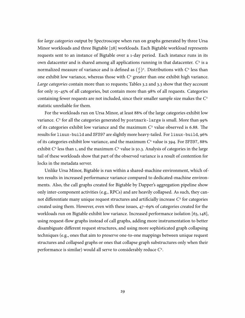
for large categories output by Spectroscope when run on graphs generated by three UrsaMinor workloads and three Bigtable [28] workloads. Each Bigtable workload representsrequests sent to an instance of Bigtable over a 1-day period. Each instance runs in itsown datacenter and is shared among all applications running in that datacenter. C2 is anormalized measure of variance and is de�ned as ( σµ)2. Distributions with C2 less thanone exhibit low variance, whereas those with C2 greater than one exhibit high variance.Large categories contain more than 10 requests; Tables 3.2 and 3.3 show that they accountfor only 15–45% of all categories, but contain more than 98% of all requests. Categoriescontaining fewer requests are not included, since their smaller sample size makes the C2

statistic unreliable for them.For the workloads run on Ursa Minor, at least 88% of the large categories exhibit low

variance. C2 for all the categories generated by postmark-large is small. More than 99%of its categories exhibit low variance and the maximum C2 value observed is 6.88. �eresults for linux-build and SFS97 are slightly more heavy-tailed. For linux-build, 96%of its categories exhibit low variance, and the maximum C2 value is 394. For SFS97, 88%exhibit C2 less than 1, and the maximum C2 value is 50.3. Analysis of categories in the largetail of these workloads show that part of the observed variance is a result of contention forlocks in the metadata server.

Unlike Ursa Minor, Bigtable is run within a shared-machine environment, which of-ten results in increased performance variance compared to dedicated-machine environ-ments. Also, the call graphs created for Bigtable by Dapper’s aggregation pipeline showonly inter-component activities (e.g., RPCs) and are heavily collapsed. As such, they can-not di�erentiate many unique request structures and arti�cially increase C2 for categoriescreated using them. However, even with these issues, 47–69% of categories created for theworkloads run on Bigtable exhibit low variance. Increased performance isolation [63, 148],using request-�ow graphs instead of call graphs, adding more instrumentation to betterdisambiguate di�erent request structures, and using more sophisticated graph collapsingtechniques (e.g., ones that aim to preserve one-to-one mappings between unique requeststructures and collapsed graphs or ones that collapse graph substructures only when theirperformance is similar) would all serve to considerably reduce C2.

29

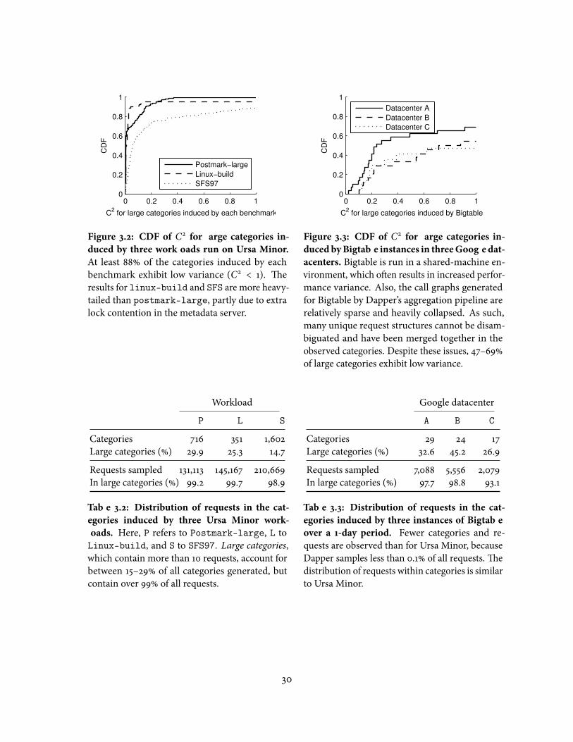
0 0.2 0.4 0.6 0.8 10

0.2

0.4

0.6

0.8

1

C2 for large categories induced by each benchmark

CD

F

Postmark−large

Linux−build

SFS97

Figure 3.2: CDF of C2 for large categories in-

duced by three workloads run on Ursa Minor.

At least 88% of the categories induced by eachbenchmark exhibit low variance (C2 < 1). �eresults for linux-build and SFS are more heavy-tailed than postmark-large, partly due to extralock contention in the metadata server.

0 0.2 0.4 0.6 0.8 10

0.2

0.4

0.6

0.8

1

C2 for large categories induced by Bigtable

CD

F

Datacenter A

Datacenter B

Datacenter C

Figure 3.3: CDF of C2 for large categories in-

duced byBigtable instances in threeGoogle dat-

acenters. Bigtable is run in a shared-machine en-vironment, which o�en results in increased perfor-mance variance. Also, the call graphs generatedfor Bigtable by Dapper’s aggregation pipeline arerelatively sparse and heavily collapsed. As such,many unique request structures cannot be disam-biguated and have been merged together in theobserved categories. Despite these issues, 47–69%of large categories exhibit low variance.

Workload

P L S

Categories 716 351 1,602Large categories (%) 29.9 25.3 14.7

Requests sampled 131,113 145,167 210,669In large categories (%) 99.2 99.7 98.9

Table 3.2: Distribution of requests in the cat-

egories induced by three Ursa Minor work-

loads. Here, P refers to Postmark-large, L toLinux-build, and S to SFS97. Large categories,which contain more than 10 requests, account forbetween 15–29% of all categories generated, butcontain over 99% of all requests.

Google datacenter

A B C

Categories 29 24 17Large categories (%) 32.6 45.2 26.9

Requests sampled 7,088 5,556 2,079In large categories (%) 97.7 98.8 93.1

Table 3.3: Distribution of requests in the cat-

egories induced by three instances of Bigtable

over a 1-day period. Fewer categories and re-quests are observed than for Ursa Minor, becauseDapper samples less than 0.1% of all requests.�edistribution of requests within categories is similarto Ursa Minor.

30

3.3 Ursa Minor case studies

I used Spectroscope to diagnose �ve real performance problems and one synthetic problemin UrsaMinor. All of the real problems were observed during nightly regression tests, whichperhaps represent the best use case for Spectroscope due to the well-de�ned problem andnon-problem periods they create. Four of the real problems were previously undiagnosed,so the root cause was not known a priori.�e remaining real problem had been diagnosedpreviously using traditional diagnosismethods andwas re-injected intoUrsaMinor to gaugeSpectroscope’s usefulness for it.�e sole synthetic problem was injected into Ursa Minorto explore a wider range of problems diagnosable using Spectroscope.�ree quantitativemetrics were used to evaluate the quality of the ranked list of categories containingmutationsthat Spectroscope outputs:

�e percentage of the 10 highest-ranked categories that are relevant: �is is themost important metric, since diagnosticians will naturally investigate the highest-rankedcategories �rst. Relevant categories are ones that were useful in helping diagnose theproblem.

�e percentage of false-positive categories: �is metric evaluates the quality of theentire ranked list by identifying the percentage of all results that are not relevant.

Request coverage:�is metric provides an alternate means for evaluating ranked listquality. It shows the percentage of all requests a�ected by the problem contained in theranked list’s categories.

Table 3.4 summarizes Spectroscope’s performance using thesemetrics.1 Unless otherwisenoted, I used a default value of 50 as the threshold at which a category was deemed to containstructural mutations or associated precursors (SM_P_THRESHOLD). When necessary, Ilowered it to further explore the space of possible structural mutations. For all of the casestudies, I used the default sampling percentage of 10%.

3.3.1 MDS con®guration change

A�er a particular large code check-in, performance of postmark-large decayed signif-icantly, from 46tps to 28tps. To diagnose this problem, I used Spectroscope to comparerequest �ows between two runs of postmark-large, one from before the check-in andone from a�er. �e results showed many categories that contained structural mutations.

1�e results shown in Table 3.4 have been slightly revised from those presented in my NSDI’11 paper dueto a minor bug I found in Spectroscope a�er the paper’s publication.

31

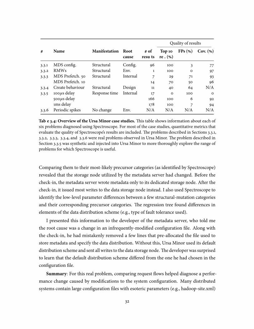
Quality of results

# Name Manifestation Root # of Top 10 FPs (%) Cov. (%)

cause results rel. (%)

3.3.1 MDS con�g. Structural Con�g. 96 100 3 773.3.2 RMWs Structural Env. 1 100 0 973.3.3 MDS Prefetch. 50 Structural Internal 7 29 71 93

MDS Prefetch. 10 14 70 50 963.3.4 Create behaviour Structural Design 11 40 64 N/A3.3.5 100µs delay Response time Internal 17 0 100 0

500µs delay 166 100 6 921ms delay 178 100 7 94

3.3.6 Periodic spikes No change Env. N/A N/A N/A N/A

Table 3.4: Overview of the Ursa Minor case studies.�is table shows information about each ofsix problems diagnosed using Spectroscope. For most of the case studies, quantitative metrics thatevaluate the quality of Spectroscope’s results are included.�e problems described in Sections 3.3.1,3.3.2, 3.3.3, 3.3.4, and 3.3.6 were real problems observed in Ursa Minor.�e problem described inSection 3.3.5 was synthetic and injected into Ursa Minor to more thoroughly explore the range ofproblems for which Spectroscope is useful.

Comparing them to their most-likely precursor categories (as identi�ed by Spectroscope)revealed that the storage node utilized by the metadata server had changed. Before thecheck-in, the metadata server wrote metadata only to its dedicated storage node. A�er thecheck-in, it issued most writes to the data storage node instead. I also used Spectroscope toidentify the low-level parameter di�erences between a few structural-mutation categoriesand their corresponding precursor categories. �e regression tree found di�erences inelements of the data distribution scheme (e.g., type of fault tolerance used).

I presented this information to the developer of the metadata server, who told methe root cause was a change in an infrequently-modi�ed con�guration �le. Along withthe check-in, he had mistakenly removed a few lines that pre-allocated the �le used tostore metadata and specify the data distribution. Without this, Ursa Minor used its defaultdistribution scheme and sent all writes to the data storage node.�e developer was surprisedto learn that the default distribution scheme di�ered from the one he had chosen in thecon�guration �le.

Summary: For this real problem, comparing request �ows helped diagnose a perfor-mance change caused by modi�cations to the system con�guration. Many distributedsystems contain large con�guration �les with esoteric parameters (e.g., hadoop-site.xml)

32

that, if modi�ed, can result in perplexing performance changes. Spectroscope can pro-vide guidance in such cases by showing how modi�ed con�guration options a�ect systembehaviour.

Quantitative analysis: For the evaluation in Table 3.4, results in the ranked list weredeemed relevant if they included metadata accesses to the data storage node and theirmost-likely precursor category included metadata accesses to the metadata storage node.

3.3.2 Read-modify-writes

�is problem was observed and diagnosed before development on Spectroscope began; Ire-injected it in Ursa Minor to show how Spectroscope could have helped diagnosticianseasily debug it.

A few years ago, performance of IoZone declined from22MB/s to 9MB/s a�er upgradingthe Linux kernel from 2.4.22 to 2.6.16.11. I originally discovered the root cause by manuallyexamining Stardust traces. I found that the new kernel’s NFS client was no longer honouringthe NFS server’s preferred read and write I/O sizes, which were set to 16KB.�e smallerI/O sizes used by the new kernel forced the NFS server to performmany read-modify-writes(RMWs), which severely a�ected performance. To remedy this issue, support for smallerI/O sizes was added to the NFS server and counters were added to track the frequency ofRMWs.

To show how comparing request �ows and identifying low-level parameter di�erencescould have helped developers quickly identify the root cause, I used Spectroscope to comparerequest �ows between a run of IoZone in which the Linux client’s I/O size was set to 16KBand another during which the Linux client’s I/O size was set to 4KB. All of the categoriesoutput by Spectroscope in its ranked list were structural-mutation categories that containedRMWs.

I next used Spectroscope to identify the low-level parameter di�erences between thehighest-ranked result and its most-likely precursor category.�e resulting regression treeshowed that the count parameter perfectly separated precursors andmutations. Speci�cally,requests with count parameter values less than or equal to 4KBwere classi�ed as precursors.

Summary: Diagnosis of this problem demonstrates how comparing request �ows canhelp diagnosticians identify performance problems that arise due to a workload change. Italso showcases the utility of highlighting relevant low-level parameter di�erences.

33

Quantitative analysis: For Table 3.4, results in the ranked list were deemed relevant ifthey contained RMWs and their most-likely precursor category did not.

3.3.3 MDS prefetching

A few years ago, several Ursa Minor developers and I tried to add server-driven metadataprefetching [67] to Ursa Minor. �is feature was supposed to improve performance byprefetching metadata to clients on every metadata server access, in hopes of minimizingthe total number of accesses necessary. However, when implemented, this feature actuallyreduced overall performance. �e developers spent a few weeks (o� and on) trying tounderstand the reason for this unexpected result but eventually moved on to other projectswithout an answer.

To diagnose this problem, I compared two runs of linux-build, one with prefetchingdisabled and another with it enabled. I chose linux-build, because it is more likely to seeperformance improvements due to prefetching than the other workloads.

When I ran Spectroscope with SM_P_THRESHOLD set to 50, several categories wereidenti�ed as containing mutations. �e two highest-ranked results immediately piquedmy interest, as they containedwrites that exhibited an abnormally large number of lockacquire/release accesses within the metadata server. All of the remaining results containedresponse-time mutations from regressions in the metadata prefetching code path, whichhad not been properly maintained. To further explore the space of structural mutations, Idecreased SM_P_THRESHOLD to 10 and re-ran Spectroscope.�is time, many more resultswere identi�ed; most of the highest-ranked ones now exhibited an abnormally high numberof lock accesses and di�ered only in the exact number.

Analysis revealed that the additional lock/unlock calls re�ected extra work performedby requests that accessed the metadata server to prefetch metadata to clients. To verifythis as the root cause, I added instrumentation around the prefetching function to con�rmthat it was causing the database accesses. Altogether, this information provided me withthe intuition necessary to determine why server-driven metadata prefetching decreasedperformance: the extra time spent in the DB calls by metadata server accesses outweighedthe time savings generated by the increase in client cache hits.

Summary:�is problem demonstrates how comparing request �ows can help develop-ers account for unexpected performance loss when adding new features. In this case, theproblem was due to unanticipated contention several layers of abstraction below the feature

34

addition. Note that diagnosis with Spectroscope is interactive—for example, in this case, Ihad to iteratively modify SM_P_THRESHOLD to gain additional insight.

Quantitative analysis: For Table 3.4, results in the ranked list were deemed relevant ifthey contained at least 30 LOCK_ACQUIRE→ LOCK_RELEASE edges. Results for the outputwhen SM_P_THRESHOLD was set to 10 and 50 are reported. In both cases, response-timemutations caused by decay of the prefetching code path are conservatively considered falsepositives, since these regressions were not the focus of this diagnosis e�ort.

3.3.4 Create behaviour

Performance graphs of postmark-large showed that the response times of creates wereincreasing signi�cantly during its execution. To diagnose this performance degradation, Iused Spectroscope to compare request �ows between the �rst 1,000 creates issued and thelast 1,000. Due to the small number of requests compared, I set SM_P_THRESHOLD to 10.

Spectroscope’s results showed categories that contained both structural and response-time mutations, with the highest-ranked one containing the former. �e response-timemutations were the expected result of data structures in the NFS server and metadata serverwhose performance decreased linearly with load. Analysis of the structural mutations,however, revealed two architectural issues, which accounted for the degradation.

First, to serve a create, the metadata server executed a tight inter-component loopwith a storage node. Each iteration of the loop required a few milliseconds, greatly a�ectingresponse times. Second, categories containing structural mutations executed this loopmore times than their precursor categories.�is inter-component loop can be seen easilyif the categories are zoomed out to show only component traversals and plotted in a trainschedule, as in Figure 3.4.

Conversations with the metadata server’s developer led me to the root cause: recursiveB-Tree page splits needed to insert the new item’s metadata. To ameliorate this problem, thedeveloper increased the page size and changed the scheme used to pick the created item’skey.

Summary:�is problem demonstrates how request-�ow comparison can be used todiagnose performance degradations, in this case due to a long-lived design problem.�oughsimple counters could have shown that creates were very expensive, they would not haveshown that the root cause was excessive metadata server/storage node interaction.

Quantitative analysis: For Table 3.4, results in the ranked list were deemed relevant if

35

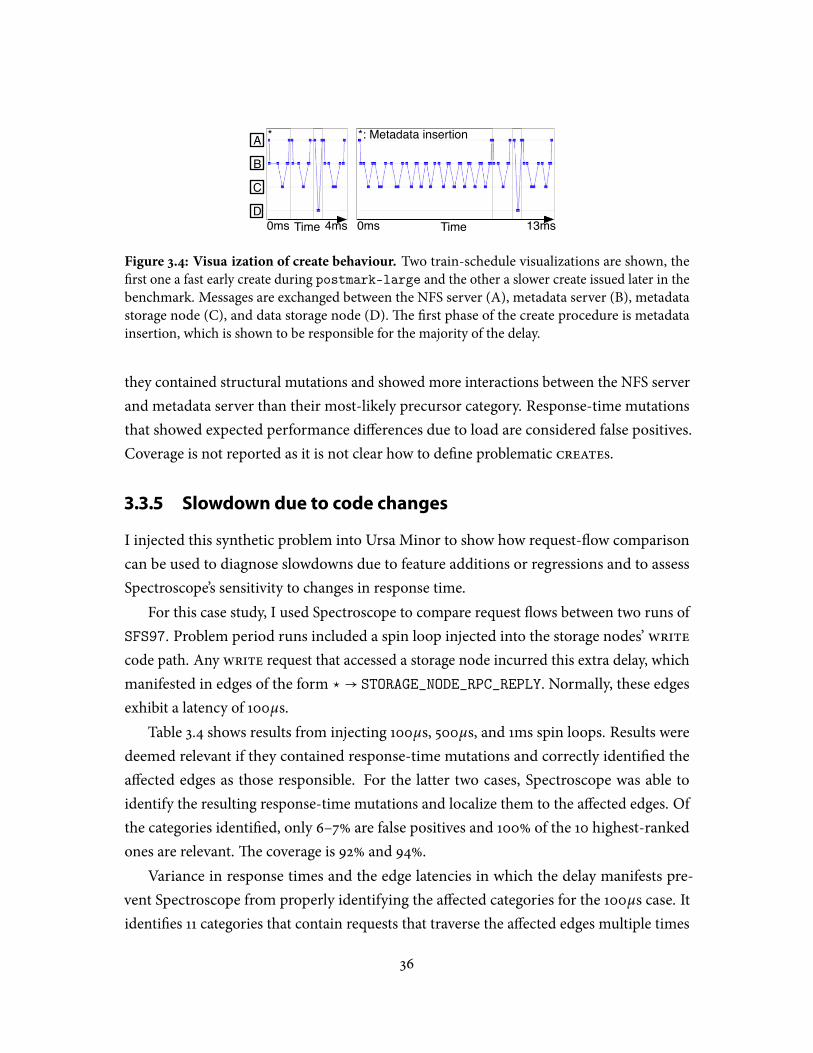
A

B

C

D

Time Time0ms 4ms 0ms 13ms

*: Metadata insertion*

Figure 3.4: Visualization of create behaviour. Two train-schedule visualizations are shown, the�rst one a fast early create during postmark-large and the other a slower create issued later in thebenchmark. Messages are exchanged between the NFS server (A), metadata server (B), metadatastorage node (C), and data storage node (D).�e �rst phase of the create procedure is metadatainsertion, which is shown to be responsible for the majority of the delay.

they contained structural mutations and showed more interactions between the NFS serverand metadata server than their most-likely precursor category. Response-time mutationsthat showed expected performance di�erences due to load are considered false positives.Coverage is not reported as it is not clear how to de�ne problematic creates.

3.3.5 Slowdown due to code changes

I injected this synthetic problem into Ursa Minor to show how request-�ow comparisoncan be used to diagnose slowdowns due to feature additions or regressions and to assessSpectroscope’s sensitivity to changes in response time.

For this case study, I used Spectroscope to compare request �ows between two runs ofSFS97. Problem period runs included a spin loop injected into the storage nodes’writecode path. Any write request that accessed a storage node incurred this extra delay, whichmanifested in edges of the form ⋆→ STORAGE_NODE_RPC_REPLY. Normally, these edgesexhibit a latency of 100µs.

Table 3.4 shows results from injecting 100µs, 500µs, and 1ms spin loops. Results weredeemed relevant if they contained response-time mutations and correctly identi�ed thea�ected edges as those responsible. For the latter two cases, Spectroscope was able toidentify the resulting response-time mutations and localize them to the a�ected edges. Ofthe categories identi�ed, only 6–7% are false positives and 100% of the 10 highest-rankedones are relevant.�e coverage is 92% and 94%.

Variance in response times and the edge latencies in which the delay manifests pre-vent Spectroscope from properly identifying the a�ected categories for the 100µs case. Itidenti�es 11 categories that contain requests that traverse the a�ected edges multiple times

36

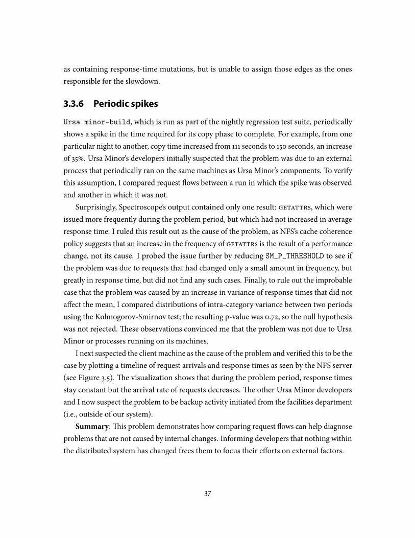
as containing response-time mutations, but is unable to assign those edges as the onesresponsible for the slowdown.

3.3.6 Periodic spikes

Ursa minor-build, which is run as part of the nightly regression test suite, periodicallyshows a spike in the time required for its copy phase to complete. For example, from oneparticular night to another, copy time increased from 111 seconds to 150 seconds, an increaseof 35%. Ursa Minor’s developers initially suspected that the problem was due to an externalprocess that periodically ran on the same machines as Ursa Minor’s components. To verifythis assumption, I compared request �ows between a run in which the spike was observedand another in which it was not.

Surprisingly, Spectroscope’s output contained only one result: getattrs, which wereissued more frequently during the problem period, but which had not increased in averageresponse time. I ruled this result out as the cause of the problem, as NFS’s cache coherencepolicy suggests that an increase in the frequency of getattrs is the result of a performancechange, not its cause. I probed the issue further by reducing SM_P_THRESHOLD to see ifthe problem was due to requests that had changed only a small amount in frequency, butgreatly in response time, but did not �nd any such cases. Finally, to rule out the improbablecase that the problem was caused by an increase in variance of response times that did nota�ect the mean, I compared distributions of intra-category variance between two periodsusing the Kolmogorov-Smirnov test; the resulting p-value was 0.72, so the null hypothesiswas not rejected.�ese observations convinced me that the problem was not due to UrsaMinor or processes running on its machines.

I next suspected the client machine as the cause of the problem and veri�ed this to be thecase by plotting a timeline of request arrivals and response times as seen by the NFS server(see Figure 3.5).�e visualization shows that during the problem period, response timesstay constant but the arrival rate of requests decreases.�e other Ursa Minor developersand I now suspect the problem to be backup activity initiated from the facilities department(i.e., outside of our system).

Summary:�is problem demonstrates how comparing request �ows can help diagnoseproblems that are not caused by internal changes. Informing developers that nothing withinthe distributed system has changed frees them to focus their e�orts on external factors.

37

Time0s 5s

...

...

A:

B:

Figure 3.5: Timeline of inter-arrival times of requests at the NFS Server. A 5s sample of requests,where each rectangle represents the process time of a request, reveals long periods of inactivity dueto lack of requests from the client during spiked copy times (B) compared to periods of normalactivity (A).

3.4 Google case studies

I used the Google version of Spectroscope to diagnose two real problems observed in twoservices. Unlike for the Ursa Minor case studies, my experiences diagnosing problems atGoogle are purely qualitative.

3.4.1 Inter-cluster performance

A team responsible for an internal-facing service at Google observed that load tests runon their so�ware in two di�erent datacenters exhibited signi�cantly di�erent performance.However, they believed that performance should be similar because the machines con�gu-rations they were using in both datacenters were almost the same.�ey wanted to knowif the performance di�erence was an artifact of their so�ware or was due to some otherproblem.

I used Spectroscope to compare request �ows between the two load test instances.�eresults showed many categories that contained response-time mutations; many were causedby latency changes not only within the service itself, but also within RPCs and within severaldependencies, such as the shared Bigtable instance running in the lower-performing cluster.�is led me to hypothesize that the performance di�erence was due to a pervasive problemin the slower load test’s datacenter and that the team’s so�ware was not at fault. Googleengineers con�rmed this hypothesis by determining that the Bigtable instance in the slowerload test’s datacenter was not working properly.�is experience is a further example of howcomparing request �ows can help developers rule out the distributed system (in this case, aspeci�c Google service) as the cause of the problem.

38

3.4.2 Performance change in a large service

To help identify performance problems, Google keeps per-day records of average requestlatencies for major services. I used Spectroscope to compare two day-long periods for onesuch external-facing service, which exhibited a signi�cant performance deviation, but only asmall di�erence in load, between the periods compared.�oughmany interestingmutationswere identi�ed, I was unable to identify the root cause due to my limited knowledge of theservice, highlighting the importance of domain knowledge in interpreting Spectroscope’sresults.

3.5 Extending Spectroscope to HDFS

To understand how the algorithms and heuristics used by Spectroscope would have tochange for di�erent distributed systems, I also tried applying Spectroscope to HDFS [134].�e traces obtained forHDFS fromX-Trace [47] aremuchmore detailed than those obtainedfor GFS [55] from Dapper’s aggregation pipeline. As such, they capture more of the uniquesemantics of HDFS/GFS-like �lesystems. HDFS’s write semantics, in particular, cause twoproblems for Spectroscope’s algorithms: very large request-�ow graphs and an extremelylarge number of categories. Section 3.5.1 describes HDFS, its write semantics, and theworkloads used for this exploration. Section 3.5.2 describes the large graph problem andhow their size can be reduced by collapsing them. Section 3.5.3 describes the categoryexplosion problem and presents ways Spectroscope could be extended to handle it.

3.5.1 HDFS & workloads applied

HDFS is the �lesystem used by the open source implementation of Map Reduce [40],Hadoop [8]. It is modeled a�er the Google File System (GFS) [55], which is itself based ontheNASD [57] architecture. As such, it consists of ametadata server (called a namenode) andmany storage nodes (called datanodes). HDFS is usually run in both shared and dedicated-machine environments. Unlike Ursa Minor, whose block size—i.e., the granularity atwhich data is read and written—is relatively small, HDFS’s block size is 64MB. Larger sizesare possible via a con�guration parameter. When writing a block (i.e., when servicing anew_block or append_block request), HDFS ensures reliability by using a pipeline toreplicate each 64KB portion to a con�gurable number of datanodes. �e �rst datanodein the pipeline is the one that receives the write operation and the remaining ones are

39

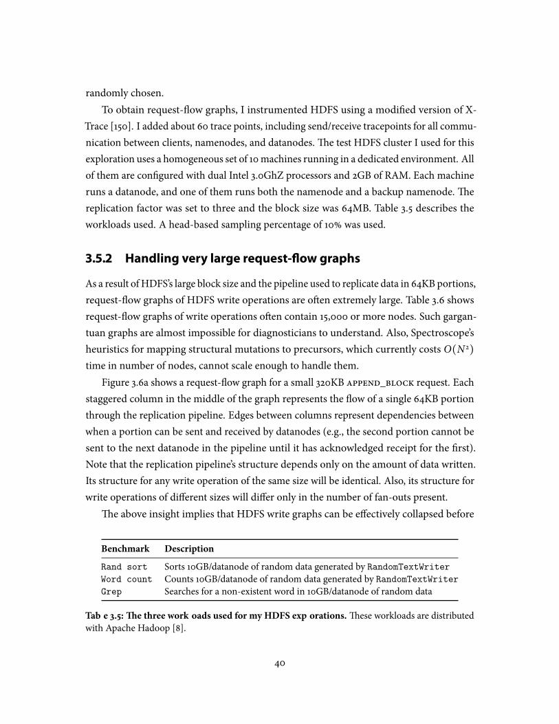
randomly chosen.To obtain request-�ow graphs, I instrumented HDFS using a modi�ed version of X-

Trace [150]. I added about 60 trace points, including send/receive tracepoints for all commu-nication between clients, namenodes, and datanodes.�e test HDFS cluster I used for thisexploration uses a homogeneous set of 10machines running in a dedicated environment. Allof them are con�gured with dual Intel 3.0GhZ processors and 2GB of RAM. Each machineruns a datanode, and one of them runs both the namenode and a backup namenode.�ereplication factor was set to three and the block size was 64MB. Table 3.5 describes theworkloads used. A head-based sampling percentage of 10% was used.

3.5.2 Handling very large request-°ow graphs

As a result of HDFS’s large block size and the pipeline used to replicate data in 64KB portions,request-�ow graphs of HDFS write operations are o�en extremely large. Table 3.6 showsrequest-�ow graphs of write operations o�en contain 15,000 or more nodes. Such gargan-tuan graphs are almost impossible for diagnosticians to understand. Also, Spectroscope’sheuristics for mapping structural mutations to precursors, which currently costs O(N2

)

time in number of nodes, cannot scale enough to handle them.Figure 3.6a shows a request-�ow graph for a small 320KB append_block request. Each

staggered column in the middle of the graph represents the �ow of a single 64KB portionthrough the replication pipeline. Edges between columns represent dependencies betweenwhen a portion can be sent and received by datanodes (e.g., the second portion cannot besent to the next datanode in the pipeline until it has acknowledged receipt for the �rst).Note that the replication pipeline’s structure depends only on the amount of data written.Its structure for any write operation of the same size will be identical. Also, its structure forwrite operations of di�erent sizes will di�er only in the number of fan-outs present.

�e above insight implies that HDFS write graphs can be e�ectively collapsed before

Benchmark Description

Rand sort Sorts 10GB/datanode of random data generated by RandomTextWriterWord count Counts 10GB/datanode of random data generated by RandomTextWriterGrep Searches for a non-existent word in 10GB/datanode of random data

Table 3.5: �e three workloads used for my HDFS explorations.�ese workloads are distributedwith Apache Hadoop [8].

40

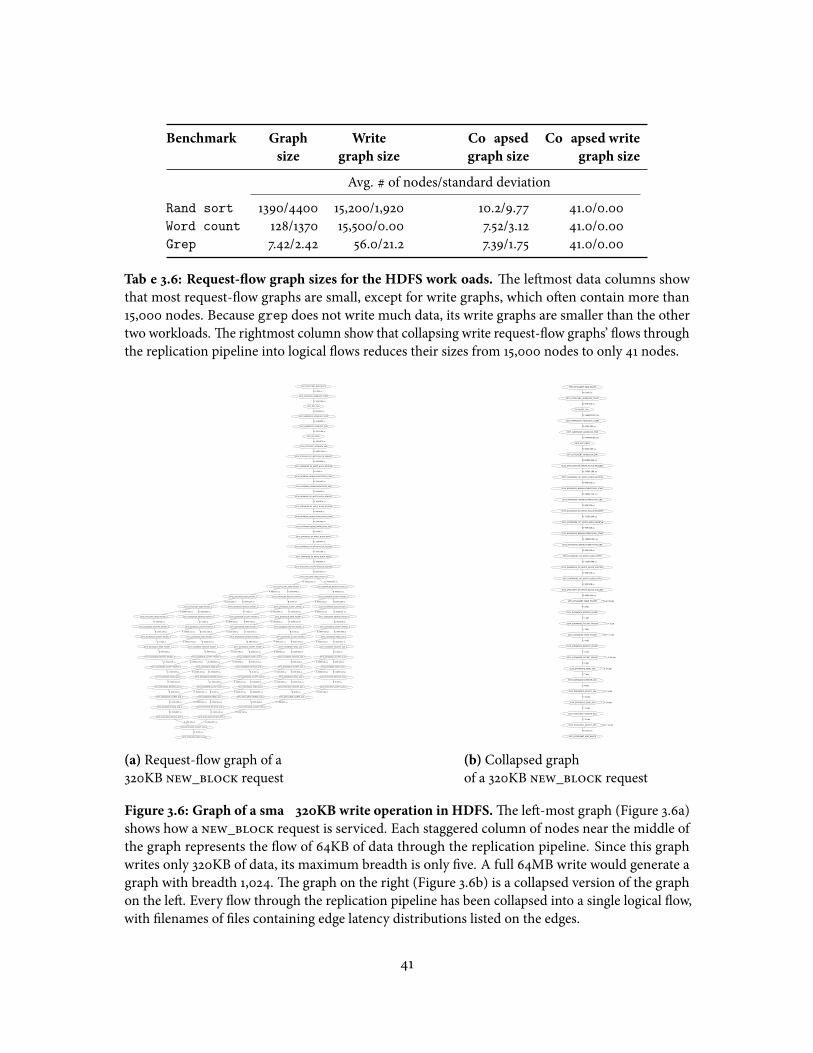
Benchmark Graph Write Collapsed Collapsed write

size graph size graph size graph size

Avg. # of nodes/standard deviation

Rand sort 1390/4400 15,200/1,920 10.2/9.77 41.0/0.00Word count 128/1370 15,500/0.00 7.52/3.12 41.0/0.00Grep 7.42/2.42 56.0/21.2 7.39/1.75 41.0/0.00

Table 3.6: Request-�ow graph sizes for the HDFS workloads. �e le�most data columns showthat most request-�ow graphs are small, except for write graphs, which o�en contain more than15,000 nodes. Because grep does not write much data, its write graphs are smaller than the othertwo workloads.�e rightmost column show that collapsing write request-�ow graphs’ �ows throughthe replication pipeline into logical �ows reduces their sizes from 15,000 nodes to only 41 nodes.

SS70_DFSCLIENT_NEW_BLOCK

SS70_DFSCLIENT_ADDBLOCK_START

R: 0.000 us

SS70_RPC_CALL

R: 1000.166 us

SS70_NAMENODE_ADDBLOCK_START

R: 999.928 us

SS70_NAMENODE_ADDBLOCK_END

R: 1999.855 us

SS70_RPC_REPLY

R: 1000.166 us

SS70_DFSCLIENT_ADDBLOCK_END

R: 4999.876 us

SS70_DFSCLIENT_OP_WRITE_BLOCK_REQUEST

R: 49000.025 us

SS70_DATANODE_OP_WRITE_BLOCK_RECEIVE

R: 6999.969 us

SS70_DATANODE_NEWBLOCKRECEIVER_START

R: 0.000 us

SS70_DATANODE_NEWBLOCKRECEIVER_END

R: 2000.093 us

SS70_DATANODE_OP_WRITE_BLOCK_REQUEST

R: 999.928 us

SS74_DATANODE_OP_WRITE_BLOCK_RECEIVE

R: 1999.974 us

SS74_DATANODE_NEWBLOCKRECEIVER_START

R: 999.928 us

SS74_DATANODE_NEWBLOCKRECEIVER_END

R: 2000.093 us

SS74_DATANODE_OP_WRITE_BLOCK_REPLY

R: 0.000 us

SS70_DATANODE_OP_WRITE_BLOCK_SUCCESS

R: 1999.974 us

SS70_DATANODE_OP_WRITE_BLOCK_REPLY

R: 1000.166 us

SS70_DFSCLIENT_OP_WRITE_BLOCK_SUCCESS

R: 1999.855 us

SS70_DFSCLIENT_SEND_PACKET_0

R: 3000.021 us

SS70_DFSCLIENT_SEND_PACKET_1

R: 16000.032 us

SS70_DATANODE_RECEIVE_PACKET_0

R: 16000.032 us

SS70_DFSCLIENT_SEND_PACKET_2

R: 999.928 us

SS70_DATANODE_RECEIVE_PACKET_1

R: 3999.949 us

SS70_DFSCLIENT_SEND_PACKET_3

R: 1000.166 us

SS70_DATANODE_RECEIVE_PACKET_2

R: 5000.114 us

SS70_DFSCLIENT_SEND_PACKET_4

R: 33999.920 us

SS70_DATANODE_RECEIVE_PACKET_3

R: 5999.804 us

SS70_DATANODE_RECEIVE_PACKET_4

R: 999.928 us

SS70_DATANODE_ACCEPT_PACKET_4

R: 1000.166 us

SS70_DATANODE_SEND_PACKET_4

R: 0.000 us

SS74_DATANODE_RECEIVE_PACKET_4

R: 999.928 us

SS74_DATANODE_ACCEPT_PACKET_4

R: 1000.166 us

SS74_DATANODE_SEND_ACK_4

R: 1999.855 us

SS70_DATANODE_RECEIVE_ACK_4

R: 1500.010 us

SS70_DATANODE_ACCEPT_ACK_4

R: 999.928 us

SS70_DATANODE_SEND_ACK_4

R: 7000.208 us

SS70_DFSCLIENT_RECEIVE_ACK_4

R: 7999.897 us

SS70_DFSCLIENT_ACCEPT_ACK_4

R: 999.928 us

SS70_DFSCLIENT_END_BLOCK

R: 0.000 us

SS70_DATANODE_ACCEPT_PACKET_3

R: 0.000 us

R: 30000.210 us

SS70_DATANODE_SEND_PACKET_3

R: 1000.166 us

R: 29000.044 us

SS74_DATANODE_RECEIVE_PACKET_3

R: 2500.057 us

SS74_DATANODE_ACCEPT_PACKET_3

R: 999.928 us

R: 26000.023 us

SS74_DATANODE_SEND_ACK_3

R: 4999.876 us

R: 23000.002 us

SS70_DATANODE_RECEIVE_ACK_3

R: 4999.995 us

SS70_DATANODE_ACCEPT_ACK_3

R: 1000.166 us

R: 15999.794 us

SS70_DATANODE_SEND_ACK_3

R: 0.000 us

R: 23000.002 us

SS70_DFSCLIENT_RECEIVE_ACK_3

R: 5999.804 us

SS70_DFSCLIENT_ACCEPT_ACK_3

R: 1000.166 us

R: 24999.857 us

SS70_DATANODE_ACCEPT_PACKET_2

R: 0.000 us

R: 1999.855 us

SS70_DATANODE_SEND_PACKET_2

R: 999.928 us

R: 2000.093 us

SS74_DATANODE_RECEIVE_PACKET_2

R: 5500.078 us

SS74_DATANODE_ACCEPT_PACKET_2

R: 999.928 us

R: 2000.093 us

SS74_DATANODE_SEND_ACK_2

R: 6000.042 us

R: 999.928 us

SS70_DATANODE_RECEIVE_ACK_2

R: 4500.031 us

SS70_DATANODE_ACCEPT_ACK_2

R: 0.000 us

R: 3000.021 us

SS70_DATANODE_SEND_ACK_2

R: 999.928 us

R: 2000.093 us

SS70_DFSCLIENT_RECEIVE_ACK_2

R: 6999.969 us

SS70_DFSCLIENT_ACCEPT_ACK_2

R: 999.928 us

R: 1000.166 us

SS70_DATANODE_ACCEPT_PACKET_1

R: 0.000 us

R: 2000.093 us

SS70_DATANODE_SEND_PACKET_1

R: 1000.166 us

R: 1999.855 us

SS74_DATANODE_RECEIVE_PACKET_1

R: 4499.912 us

SS74_DATANODE_ACCEPT_PACKET_1

R: 0.000 us

R: 3000.021 us

SS74_DATANODE_SEND_ACK_1

R: 8000.135 us

R: 999.928 us

SS70_DATANODE_RECEIVE_ACK_1

R: 3499.985 us

SS70_DATANODE_ACCEPT_ACK_1

R: 999.928 us

R: 2000.093 us

SS70_DATANODE_SEND_ACK_1

R: 999.928 us

R: 2000.093 us

SS70_DFSCLIENT_RECEIVE_ACK_1

R: 8000.135 us

SS70_DFSCLIENT_ACCEPT_ACK_1

R: 0.000 us

R: 1999.855 us

SS70_DATANODE_ACCEPT_PACKET_0

R: 999.928 us

R: 3000.021 us

SS70_DATANODE_SEND_PACKET_0

R: 1000.166 us

R: 3000.021 us

SS74_DATANODE_RECEIVE_PACKET_0

R: 3000.021 us

SS74_DATANODE_ACCEPT_PACKET_0

R: 999.928 us

R: 3999.949 us

SS74_DATANODE_SEND_ACK_0

R: 9999.990 us

R: 2000.093 us

SS70_DATANODE_RECEIVE_ACK_0

R: 3000.021 us

SS70_DATANODE_ACCEPT_ACK_0

R: 0.000 us

R: 3999.949 us

SS70_DATANODE_SEND_ACK_0

R: 999.928 us

R: 3999.949 us

SS70_DFSCLIENT_RECEIVE_ACK_0

R: 10999.918 us

SS70_DFSCLIENT_ACCEPT_ACK_0

R: 0.000 us

R: 1000.166 us

(a) Request-�ow graph of a320KB new_block request

SS74_DFSCLIENT_NEW_BLOCK

SS74_DFSCLIENT_ADDBLOCK_START

R: 0.000 us

SS74_RPC_CALL

R: 999.928 us

SS70_NAMENODE_ADDBLOCK_START

R: 2444999.933 us

SS70_NAMENODE_ADDBLOCK_END

R: 2000.093 us

SS74_RPC_REPLY

R: 2444999.933 us

SS74_DFSCLIENT_ADDBLOCK_END

R: 9000.063 us

SS74_DFSCLIENT_OP_WRITE_BLOCK_REQUEST

R: 82999.945 us

SS74_DATANODE_OP_WRITE_BLOCK_RECEIVE

R: 24000.168 us

SS74_DATANODE_NEWBLOCKRECEIVER_START

R: 999.928 us

SS74_DATANODE_NEWBLOCKRECEIVER_END

R: 28000.116 us

SS74_DATANODE_OP_WRITE_BLOCK_REQUEST

R: 999.928 us

SS70_DATANODE_OP_WRITE_BLOCK_RECEIVE

R: 12500.048 us

SS70_DATANODE_NEWBLOCKRECEIVER_START

R: 999.928 us

SS70_DATANODE_NEWBLOCKRECEIVER_END

R: 108000.040 us

SS70_DATANODE_OP_WRITE_BLOCK_REPLY

R: 999.928 us

SS74_DATANODE_OP_WRITE_BLOCK_SUCCESS

R: 12500.048 us

SS74_DATANODE_OP_WRITE_BLOCK_REPLY

R: 999.928 us

SS74_DFSCLIENT_OP_WRITE_BLOCK_SUCCESS

R: 999.928 us

SS74_DFSCLIENT_SEND_PACKET

R: 6000.042 us

F: 18.dat

SS74_DATANODE_RECEIVE_PACKET

F: 0.dat

SS74_DATANODE_ACCEPT_PACKET

F: 1.dat

F: 2.dat

SS74_DATANODE_SEND_PACKET

F: 3.dat

F: 17.dat

SS70_DATANODE_RECEIVE_PACKET

F: 4.dat

SS70_DATANODE_ACCEPT_PACKET

F: 5.dat

F: 16.dat

SS70_DATANODE_SEND_ACK

F: 6.dat

F: 15.dat

SS74_DATANODE_RECEIVE_ACK

F: 7.dat

SS74_DATANODE_ACCEPT_ACK

F: 8.dat

F: 9.dat

SS74_DATANODE_SEND_ACK

F: 10.dat

F: 14.dat

SS74_DFSCLIENT_RECEIVE_ACK

F: 11.dat

SS74_DFSCLIENT_ACCEPT_ACK

F: 12.dat

F: 13.dat

SS74_DFSCLIENT_END_BLOCK

R: 0.000 us

(b) Collapsed graphof a 320KB new_block request

Figure 3.6: Graph of a small 320KB write operation in HDFS.�e le�-most graph (Figure 3.6a)shows how a new_block request is serviced. Each staggered column of nodes near the middle ofthe graph represents the �ow of 64KB of data through the replication pipeline. Since this graphwrites only 320KB of data, its maximum breadth is only �ve. A full 64MB write would generate agraph with breadth 1,024.�e graph on the right (Figure 3.6b) is a collapsed version of the graphon the le�. Every �ow through the replication pipeline has been collapsed into a single logical �ow,with �lenames of �les containing edge latency distributions listed on the edges.

41

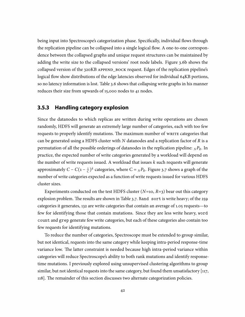
being input into Spectroscope’s categorization phase. Speci�cally, individual �ows throughthe replication pipeline can be collapsed into a single logical �ow. A one-to-one correspon-dence between the collapsed graphs and unique request structures can be maintained byadding the write size to the collapsed versions’ root node labels. Figure 3.6b shows thecollapsed version of the 320KB append_bock request. Edges of the replication pipeline’slogical �ow show distributions of the edge latencies observed for individual 64KB portions,so no latency information is lost. Table 3.6 shows that collapsing write graphs in his mannerreduces their size from upwards of 15,000 nodes to 41 nodes.

3.5.3 Handling category explosion

Since the datanodes to which replicas are written during write operations are chosenrandomly, HDFS will generate an extremely large number of categories, each with too fewrequests to properly identify mutations.�e maximum number of write categories thatcan be generated using a HDFS cluster with N datanodes and a replication factor of R is apermutation of all the possible orderings of datanodes in the replication pipeline: NPR. Inpractice, the expected number of write categories generated by a workload will depend onthe number of write requests issued. A workload that issues k such requests will generateapproximately C − C(1 − 1

C )k categories, where C = NPR. Figure 3.7 shows a graph of the

number of write categories expected as a function of write requests issued for various HDFScluster sizes.

Experiments conducted on the test HDFS cluster (N=10, R=3) bear out this categoryexplosion problem.�e results are shown in Table 3.7. Rand sort is write heavy; of the 259categories it generates, 132 are write categories that contain an average of 1.05 requests—tofew for identifying those that contain mutations. Since they are less write heavy, wordcount and grep generate few write categories, but each of these categories also contain toofew requests for identifying mutations.

To reduce the number of categories, Spectroscope must be extended to group similar,but not identical, requests into the same category while keeping intra-period response-timevariance low. �e latter constraint is needed because high intra-period variance withincategories will reduce Spectroscope’s ability to both rank mutations and identify response-time mutations. I previously explored using unsupervised clustering algorithms to groupsimilar, but not identical requests into the same category, but found them unsatisfactory [117,118].�e remainder of this section discusses two alternate categorization policies.

42

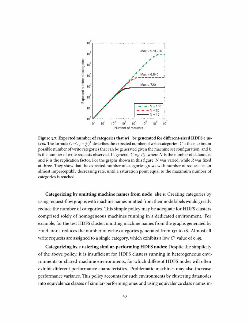
100

101

102

103

104

105

106

107

100

101

102

103

104

105

106

107

Number of requests

Expecte

d n

um

ber

of cate

gories

N = 100

N = 20

N = 10

Max = 720

Max = 6,840

Max = 970,200

Figure 3.7: Expected number of categories that will be generated for di�erent-sized HDFS clus-

ters.�e formulaC−C(̇1− 1C )

k describes the expected number of write categories. C is themaximumpossible number of write categories that can be generated given the machine set con�guration, and kis the number of write requests observed. In general, C =N PR , where N is the number of datanodesand R is the replication factor. For the graphs shown in this �gure, N was varied, while R was �xedat three. �ey show that the expected number of categories grows with number of requests at analmost imperceptibly decreasing rate, until a saturation point equal to the maximum number ofcategories is reached.

Categorizing by omitting machine names from node labels: Creating categories byusing request-�ow graphs withmachine names omitted from their node labels would greatlyreduce the number of categories. �is simple policy may be adequate for HDFS clusterscomprised solely of homogeneous machines running in a dedicated environment. Forexample, for the test HDFS cluster, omitting machine names from the graphs generated byrand sort reduces the number of write categories generated from 132 to 16. Almost allwrite requests are assigned to a single category, which exhibits a low C2 value of 0.45.

Categorizing by clustering similar-performing HDFS nodes: Despite the simplicityof the above policy, it is insu�cient for HDFS clusters running in heterogeneous envi-ronments or shared-machine environments, for which di�erent HDFS nodes will o�enexhibit di�erent performance characteristics. Problematic machines may also increaseperformance variance.�is policy accounts for such environments by clustering datanodesinto equivalence classes of similar-performing ones and using equivalence class names in-

43

Benchmark # of # of Avg. # of # of write # of write Avg. # of

requests categories requests requests categories requests

Rand sort 1,530 259 5.90 139 132 (126) 1.05Wordcount 1,025 116 8.84 8 7 (8) 1.14Grep 1,041 116 8.97 2 2 (2) 1.00

Table 3.7: Category sizes and average requests per category for the workloads when run on the

test HDFS cluster. HDFS’s write semantics, which speci�es that data be replicated to three randomlychosen datanodes, generates a large number of write categories.�ese categories contain too fewrequests to accurately identify response-time or structural mutations. For example, rand sort, themost write intensive of the benchmarks above generates 132 write categories with an average of 1.05requests in each. Numbers listed in parentheses indicate the expected number of write categories forthe given benchmark.

stead of machine names in individual request-�ow graphs.�e speci�c clustering algorithmused for this approach will depend on the amount of performance variance that is expected.For clusters that exhibit only a small amount of variance, perhaps due to a small numberof problematic machines in a homogeneous dedicated-machine environment, simple ap-proaches, such as peer comparison [75, 76] may be su�cient. For clusters that exhibit morevariance, such as those running within Amazon’s EC2, more advanced techniques maybe necessary. One promising technique is semi-supervised learning, in which developerfeedback is incorporated in choosing what category to assign a request.

3.6 Summary & future work

By showing how real problems were diagnosed using Spectroscope in both Ursa Minor andselect Google services, this chapter demonstrates the utility of request-�ow comparison andthe e�cacy of the algorithms and heuristics Spectroscope uses to implement it. By exploringhow Spectroscope could be extended to work with HDFS, this chapter also demonstrateshow graph collapsing, applied carefully, can be e�ective in reducing the graph sizes input toSpectroscope so as to reduce its runtime overhead.

�e experiences described in this chapter also reveal promising avenues for future work.Most the Google case studies show that even with Spectroscope’s automation, domainknowledge is still an important factor when diagnosing problems. However, for distributedservices built upon many other distributed services, each owned by a di�erent set of devel-opers, no single person may possess the required knowledge. To help, future work should

44

focus on incorporating more domain knowledge into diagnosis tools, such as SpectroscopeFor example, machine learning techniques could be used to learn the semantic meaningof request-�ow graphs and such meanings could be displayed along with Spectroscope’soutput. My HDFS explorations also reveal the need for future work to mitigate categoryexplosion in systems that can generate many unique request-�ow graphs.

45

46

Chapter 4

Advanced visualizations forSpectroscope

Myexperiences diagnosing performance problems using Spectroscope’s [117] initial Graphviz-based [61] visualizations convinced me that they were inadequate. For example, theGraphviz-based visualizations required diagnosticians to manually and painstakingly com-pare structuralmutations and corresponding precursors to identify di�erences. For response-time mutations and general timing changes, dot’s ranked layout could not be easily usedto draw edges proportional to observed latencies, complicating analyses of where time isspent. Unfortunately, existing literature does not provide guidance on how to improveSpectroscope’s visualizations.�ough much systems research has focused on techniquesfor automated problem localization [14, 15, 29, 72, 76, 88, 98, 103, 117, 122, 144], apart froma few select instances [86, 90], little research has focused on how best to present theirresults. Likewise, in the visualization community, little research has focused on identifyingvisualizations that are useful for distributed systems developers and diagnosticians.

To address the need for more research on visualizations for distributed systems diag-nosis tasks, this chapter describes a 26-person user study that compares three promisingapproaches for helping developers compare graphs of precursor categories (called “beforegraphs” in this chapter) and graphs of mutation categories (called “a�er graphs” in thischapter). �e user study comprises 13 professionals (i.e., developers of Ursa Minor andso�ware engineers fromGoogle) and 13 graduate students taking distributed systems classes.I did not expect a single approach to be best for every user study task, so my goal withthis study was to identify which approaches work best for di�erent usage modes and fordiagnosing di�erent types of problems.

�e approaches compared in this chapter were chosen based on my intuition and the

47

recommendations of those developers who helped me diagnose problems in Ursa Minor [1]and Google services.�e side-by-side approach is nearly a “juxtaposition,” which presentsindependent layouts of both before and a�er graphs. Di� is an “explicit encoding,” whichhighlights the di�erences between the two graphs. Animation is closest to a “superposition”design that guides attention to changes that “blink.” All of the approaches automatically iden-tify correspondences between matching nodes in both graphs so as to focus diagnosticianson relevant structural di�erence—i.e., those without correspondences.

Despite the large body of work on comparing graphs [9, 10, 44], I found no existingimplementations of side-by-side, di�, and animation suitable for request-�ow comparison’sdomain-speci�c needs. For example, since correspondences between nodes of before-and-a�er graphs are not known a priori, they must be identi�ed algorithmically.�erefore, Ibuilt my own interfaces. For this study, categories containing both structural mutationsand response-time mutations were not split into multiple virtual categories. Rather, theresulting edge latency and structural changes are displayed together in the same graph.

Overall, the user study results show that side-by-side is the best approach for helpingdiagnosticians obtain an overall understanding of an observed performance change. Anima-tion is best for helping diagnose problems that are caused by structural mutations alone (e.g.,by a change in the amount of concurrent activity or by a slower thread of activity replacing afaster thread). Di� is best for helping diagnose problems caused by response-timemutationsalone.

�e rest of this chapter is organized as follows. Section 4.1 describes related work.Section 4.2 describes the interfaces. Section 4.3 describes the user study methodology andSection 4.4 presents results. Based on my experiences with this study, Section 4.5 describeslessons learned and opportunities for future work. Finally, Section 4.6 concludes.

4.1 Related work

Recent research has explored a number of approaches, including some akin to side-by-side,di�, and animation, to help users identify di�erences in graphs, but no single one hasemerged as the clear winner [9, 10, 113].�e choice depends on the domain, the types ofgraphs being compared, and the di�erences of interest, thus motivating the need for thestudy presented in this chapter.

Archambault et al. [9] suggest that animation may be more e�ective for helping usersunderstand the evolution of nodes and edges in a graph, whereas small multiples (akin to

48

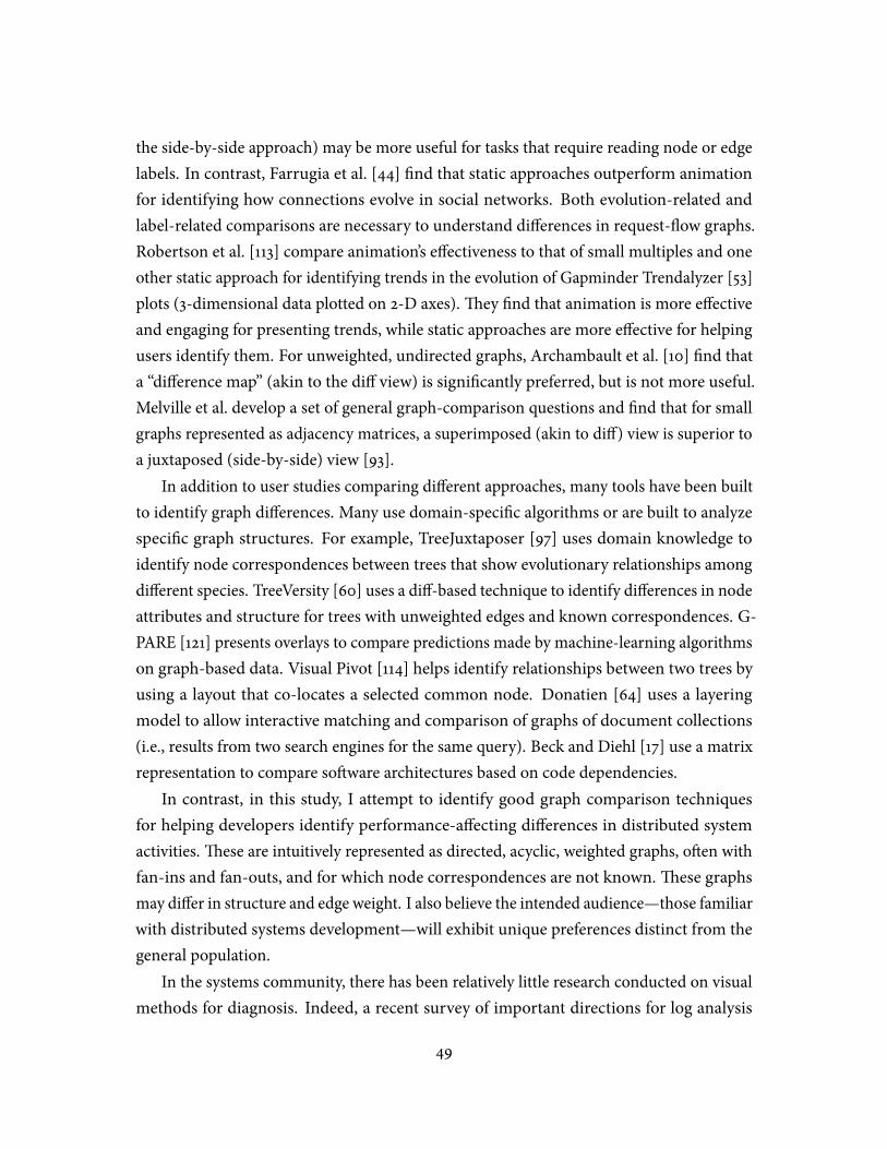
the side-by-side approach) may be more useful for tasks that require reading node or edgelabels. In contrast, Farrugia et al. [44] �nd that static approaches outperform animationfor identifying how connections evolve in social networks. Both evolution-related andlabel-related comparisons are necessary to understand di�erences in request-�ow graphs.Robertson et al. [113] compare animation’s e�ectiveness to that of small multiples and oneother static approach for identifying trends in the evolution of Gapminder Trendalyzer [53]plots (3-dimensional data plotted on 2-D axes).�ey �nd that animation is more e�ectiveand engaging for presenting trends, while static approaches are more e�ective for helpingusers identify them. For unweighted, undirected graphs, Archambault et al. [10] �nd thata “di�erence map” (akin to the di� view) is signi�cantly preferred, but is not more useful.Melville et al. develop a set of general graph-comparison questions and �nd that for smallgraphs represented as adjacency matrices, a superimposed (akin to di�) view is superior toa juxtaposed (side-by-side) view [93].

In addition to user studies comparing di�erent approaches, many tools have been builtto identify graph di�erences. Many use domain-speci�c algorithms or are built to analyzespeci�c graph structures. For example, TreeJuxtaposer [97] uses domain knowledge toidentify node correspondences between trees that show evolutionary relationships amongdi�erent species. TreeVersity [60] uses a di�-based technique to identify di�erences in nodeattributes and structure for trees with unweighted edges and known correspondences. G-PARE [121] presents overlays to compare predictions made by machine-learning algorithmson graph-based data. Visual Pivot [114] helps identify relationships between two trees byusing a layout that co-locates a selected common node. Donatien [64] uses a layeringmodel to allow interactive matching and comparison of graphs of document collections(i.e., results from two search engines for the same query). Beck and Diehl [17] use a matrixrepresentation to compare so�ware architectures based on code dependencies.

In contrast, in this study, I attempt to identify good graph comparison techniquesfor helping developers identify performance-a�ecting di�erences in distributed systemactivities.�ese are intuitively represented as directed, acyclic, weighted graphs, o�en withfan-ins and fan-outs, and for which node correspondences are not known.�ese graphsmay di�er in structure and edge weight. I also believe the intended audience—those familiarwith distributed systems development—will exhibit unique preferences distinct from thegeneral population.

In the systems community, there has been relatively little research conducted on visualmethods for diagnosis. Indeed, a recent survey of important directions for log analysis

49

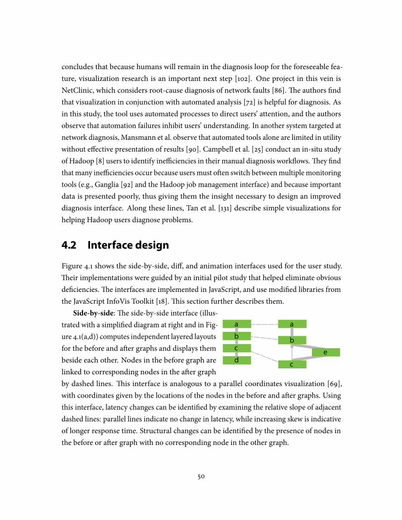
concludes that because humans will remain in the diagnosis loop for the foreseeable fea-ture, visualization research is an important next step [102]. One project in this vein isNetClinic, which considers root-cause diagnosis of network faults [86].�e authors �ndthat visualization in conjunction with automated analysis [72] is helpful for diagnosis. Asin this study, the tool uses automated processes to direct users’ attention, and the authorsobserve that automation failures inhibit users’ understanding. In another system targeted atnetwork diagnosis, Mansmann et al. observe that automated tools alone are limited in utilitywithout e�ective presentation of results [90]. Campbell et al. [25] conduct an in-situ studyof Hadoop [8] users to identify ine�ciencies in their manual diagnosis work�ows.�ey �ndthat many ine�ciencies occur because users must o�en switch betweenmultiple monitoringtools (e.g., Ganglia [92] and the Hadoop job management interface) and because importantdata is presented poorly, thus giving them the insight necessary to design an improveddiagnosis interface. Along these lines, Tan et al. [131] describe simple visualizations forhelping Hadoop users diagnose problems.

4.2 Interface design

Figure 4.1 shows the side-by-side, di�, and animation interfaces used for the user study.�eir implementations were guided by an initial pilot study that helped eliminate obviousde�ciencies.�e interfaces are implemented in JavaScript, and use modi�ed libraries fromthe JavaScript InfoVis Toolkit [18].�is section further describes them.

Side-by-side:�e side-by-side interface (illus-trated with a simpli�ed diagram at right and in Fig-ure 4.1(a,d)) computes independent layered layoutsfor the before and a�er graphs and displays thembeside each other. Nodes in the before graph arelinked to corresponding nodes in the a�er graphby dashed lines. �is interface is analogous to a parallel coordinates visualization [69],with coordinates given by the locations of the nodes in the before and a�er graphs. Usingthis interface, latency changes can be identi�ed by examining the relative slope of adjacentdashed lines: parallel lines indicate no change in latency, while increasing skew is indicativeof longer response time. Structural changes can be identi�ed by the presence of nodes inthe before or a�er graph with no corresponding node in the other graph.

50

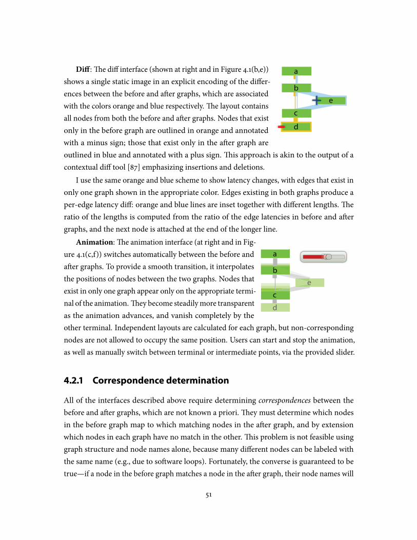
Di� :�e di� interface (shown at right and in Figure 4.1(b,e))shows a single static image in an explicit encoding of the di�er-ences between the before and a�er graphs, which are associatedwith the colors orange and blue respectively.�e layout containsall nodes from both the before and a�er graphs. Nodes that existonly in the before graph are outlined in orange and annotatedwith a minus sign; those that exist only in the a�er graph areoutlined in blue and annotated with a plus sign. �is approach is akin to the output of acontextual di� tool [87] emphasizing insertions and deletions.

I use the same orange and blue scheme to show latency changes, with edges that exist inonly one graph shown in the appropriate color. Edges existing in both graphs produce aper-edge latency di�: orange and blue lines are inset together with di�erent lengths.�eratio of the lengths is computed from the ratio of the edge latencies in before and a�ergraphs, and the next node is attached at the end of the longer line.

Animation:�e animation interface (at right and in Fig-ure 4.1(c,f)) switches automatically between the before anda�er graphs. To provide a smooth transition, it interpolatesthe positions of nodes between the two graphs. Nodes thatexist in only one graph appear only on the appropriate termi-nal of the animation.�ey become steadilymore transparentas the animation advances, and vanish completely by theother terminal. Independent layouts are calculated for each graph, but non-correspondingnodes are not allowed to occupy the same position. Users can start and stop the animation,as well as manually switch between terminal or intermediate points, via the provided slider.

4.2.1 Correspondence determination

All of the interfaces described above require determining correspondences between thebefore and a�er graphs, which are not known a priori.�ey must determine which nodesin the before graph map to which matching nodes in the a�er graph, and by extensionwhich nodes in each graph have no match in the other.�is problem is not feasible usinggraph structure and node names alone, because many di�erent nodes can be labeled withthe same name (e.g., due to so�ware loops). Fortunately, the converse is guaranteed to betrue—if a node in the before graph matches a node in the a�er graph, their node names will

51

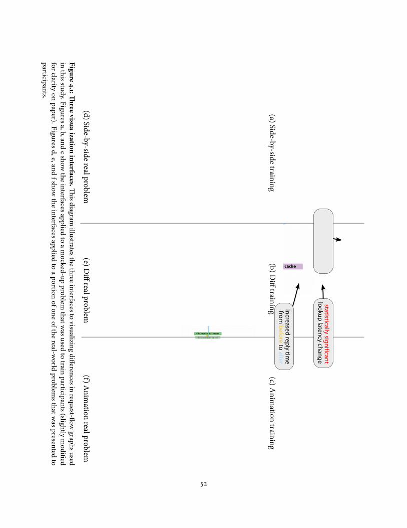
(a)Side-by-sidetraining(b)D

i�training

(c)Anim

ationtraining

(d)Side-by-siderealproblem(e)D

i�realproblem

(f)Anim

ationrealproblem

Figure

4.1:

�ree

visu

alizatio

ninterfa

ces.�isdiagram

illustratesthethreeinterfacestovisualizing

di�erencesinrequest-�ow

graphsusedin

thisstudy.Figuresa,b,andcshow

theinterfacesappliedto

amocked-up

problemthatw

asusedto

trainparticipants(slightly

modi�ed

forclarityon

paper).Figuresd,e,andfshow

theinterfacesapplied

toaportion

ofoneofthe

real-world

problemsthatw

aspresentedto

participants.

52

be the same.�e interfaces exploit this property to obtain approximate correspondences.�e approximation technique runs in O(N2

) time in the number of nodes. First, ituses a lexically-ordered depth-�rst traversal to transform both graphs into strings. Next,it keeps track of the insertions, deletions, and mutations made by a string-edit distancetransformation of one string into another. Finally, it maps these edits back onto the appro-priate interface. Items that were not inserted, deleted, or removed are ones that correspondin both graphs. Despite the limitations of this approach, I have found it to work well inpractice. Gao et al. survey a variety of related algorithms [52]; because the problem is hard(in the formal sense), these algorithms are limited in applicability, approximate, or both.�ough this approximation technique was implemented independently of Spectroscope’sheuristics for identifying corresponding mutations and precursors, both could be combinedto reduce overall runtime.

4.2.2 Common features

All three of the interfaces incorporate some common features, tailored speci�cally forrequest-�ow graphs. All graphs are drawn with a layered layout based on the techniqueby Sugiyama et al [128]; layouts that modify this underlying approach enjoy widespreaduse [42].

To navigate the interface, users can pan the graph view by clicking and dragging or byusing a vertical scroll bar. In large graphs, this allows for movement in the neighborhood ofthe current view or rapid traversal across the entire graph. By using the wheel on a mouse,users can zoom in and out, up to a limit.�e interfaces employ rubber-banding for both thetraversal and zoom features to prevent the graphs from moving o� the screen or becomingsmaller than the viewing window.

For all of the interfaces, edge lengths are drawn using a sigmoid-based scaling functionthat allows both large and small edge latencies to be visible on the same graph. Statisticallysigni�cant edge latency changes are highlighted with a bold red outline. To distinguish waittime from actual latency for threads involved in join operations, the interfaces use thinnerlines for the former and thicker lines for the latter (see the “write in cache” to “MDSCLIENTlookup call” edge in Figures 4.1(a-c) for an example).

Each interface also has an annotation mechanism that allows users to add marks andcomments to a graph comparison.�ese annotations are saved as an additional layer onthe interface and can be restored for later examination.

53

4.2.3 Interface Example

To better illustrate how these interfaces show di�erences, the example of di� shown inFigure 4.1(b) is annotated with the three key di�erences it is meant to reveal. First, the a�ergraph contains an extra thread of concurrent activity (outlined in blue and marked witha plus sign). Second, there is a statistically signi�cant change in metadata lookup latency(highlighted in red).�ird, there is a large latency change between the lookup of metadataand the request’s reply that is not identi�ed as statistically signi�cant (perhaps becauseof high variance). �ese observations localize the problem to those system componentsinvolved in the changes and thus provide starting points for diagnosticians’ diagnosise�orts.

4.3 User study overview & methodology

I compared the three approaches via a between-subjects user study, in which I askedparticipants to complete �ve assignments using the interfaces. Each assignment askedparticipants to �nd key performance-a�ecting di�erences for a before/a�er request-�owgraph pair obtained from Ursa Minor [1].�ree of the �ve assignments used graphs derivedfrom real problems (see Chapter 3.3) observed in the system.

4.3.1 Participants

�e interfaces’ target users are developers and diagnosticians of the distributed system beingdiagnosed. As the performance problems used for the user study come from Ursa Minor,I recruited the seven Ursa Minor developers to whom I had access as expert participants.In addition, I recruited six professional distributed-system developers from Google.�ischapter refers to the Ursa Minor and Google developers collectively as professionals.

Many of the professional participants are intimately familiar with more traditionaldiagnosis techniques, perhaps biasing their responses to the user-study questions somewhat.To obtain a wider perspective, I also recruited additional participants by advertising inundergraduate and graduate classes on distributed systems and posting �iers on and aroundCarnegie Mellon University’s campus. Potential participants were required to demonstrate(via a pre-screening questionnaire) knowledge of key undergraduate-level distributed sys-tems concepts. Of the 33 volunteers who completed the questionnaire, 29 were deemedeligible; I selected the �rst 13 to respond as participants. Because all of the selected partici-

54

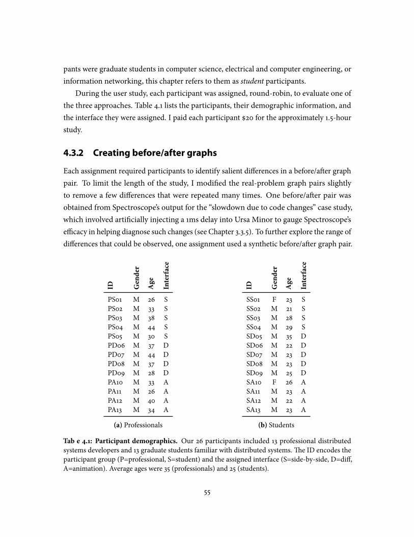
pants were graduate students in computer science, electrical and computer engineering, orinformation networking, this chapter refers to them as student participants.

During the user study, each participant was assigned, round-robin, to evaluate one ofthe three approaches. Table 4.1 lists the participants, their demographic information, andthe interface they were assigned. I paid each participant $20 for the approximately 1.5-hourstudy.

4.3.2 Creating before/after graphs

Each assignment required participants to identify salient di�erences in a before/a�er graphpair. To limit the length of the study, I modi�ed the real-problem graph pairs slightlyto remove a few di�erences that were repeated many times. One before/a�er pair wasobtained from Spectroscope’s output for the “slowdown due to code changes” case study,which involved arti�cially injecting a 1ms delay into Ursa Minor to gauge Spectroscope’se�cacy in helping diagnose such changes (see Chapter 3.3.5). To further explore the range ofdi�erences that could be observed, one assignment used a synthetic before/a�er graph pair.

ID Gender

Age

Interface

PS01 M 26 SPS02 M 33 SPS03 M 38 SPS04 M 44 SPS05 M 30 SPD06 M 37 DPD07 M 44 DPD08 M 37 DPD09 M 28 DPA10 M 33 APA11 M 26 APA12 M 40 APA13 M 34 A

(a) Professionals

ID Gender

Age

Interface

SS01 F 23 SSS02 M 21 SSS03 M 28 SSS04 M 29 SSD05 M 35 DSD06 M 22 DSD07 M 23 DSD08 M 23 DSD09 M 25 DSA10 F 26 ASA11 M 23 ASA12 M 22 ASA13 M 23 A

(b) Students

Table 4.1: Participant demographics. Our 26 participants included 13 professional distributedsystems developers and 13 graduate students familiar with distributed systems.�e ID encodes theparticipant group (P=professional, S=student) and the assigned interface (S=side-by-side, D=di�,A=animation). Average ages were 35 (professionals) and 25 (students).

55

It was created by modifying a real request-�ow graph observed in Ursa Minor. Table 4.2describes the various assignments and their properties.

To make the before/a�er graphs easier for participants to understand, I changed nodelabels, which describe events observed during request processing, to more human-readableversions. For example, I changed the label “e10__t3__NFS_CACHE_READ_HIT” to “Readthat hit in the NFS server’s cache.”�e original labels were written by UrsaMinor developersand only have meaning to them. Finally, I omitted numbers indicating edge lengths fromthe graphs to ensure participants used visual properties of the interfaces to �nd importantdi�erences.

4.3.3 User study procedure

�e study consisted of four parts: training, guided questions, emulation of real diagnoses,and interface comparison. Participants were encouraged to think aloud throughout thestudy.

Training

In the training phase, participants were shown an Ursa Minor architecture diagram (similarto the one in Figure 3.1).�ey were only required to understand that the system consists of�ve components that can communicate over the network. I also provided a sample request-�ow graph and described themeaning of nodes and edges. Finally, I trained each participanton her assigned interface by showing her a sample/before a�er graph (identical to thoseshown in Figures 4.1(a-c)) and guiding her through tasks she would have to complete inlatter parts of the study. Participants were given ample time to ask questions and were toldI would be unable to answer further questions a�er the training portion.

Finding diªerences via guided questions

In this phase of the study, I guided participants through the process of identifying di�erences,asking them to complete �ve focused tasks for each of three assignments. Rows 1–3 ofTable 4.2 describe the graphs used for this part of the study.

Task 1: Find any edges with statistically signi�cant latency changes.�is task required par-ticipants to �nd all of the graph edges highlighted in red (i.e., those automatically identi�edby the Spectroscope as having statistically signi�cant changes in latency distribution).

Task 2: Find any other edges with latency changes worth investigating. Spectroscope will

56

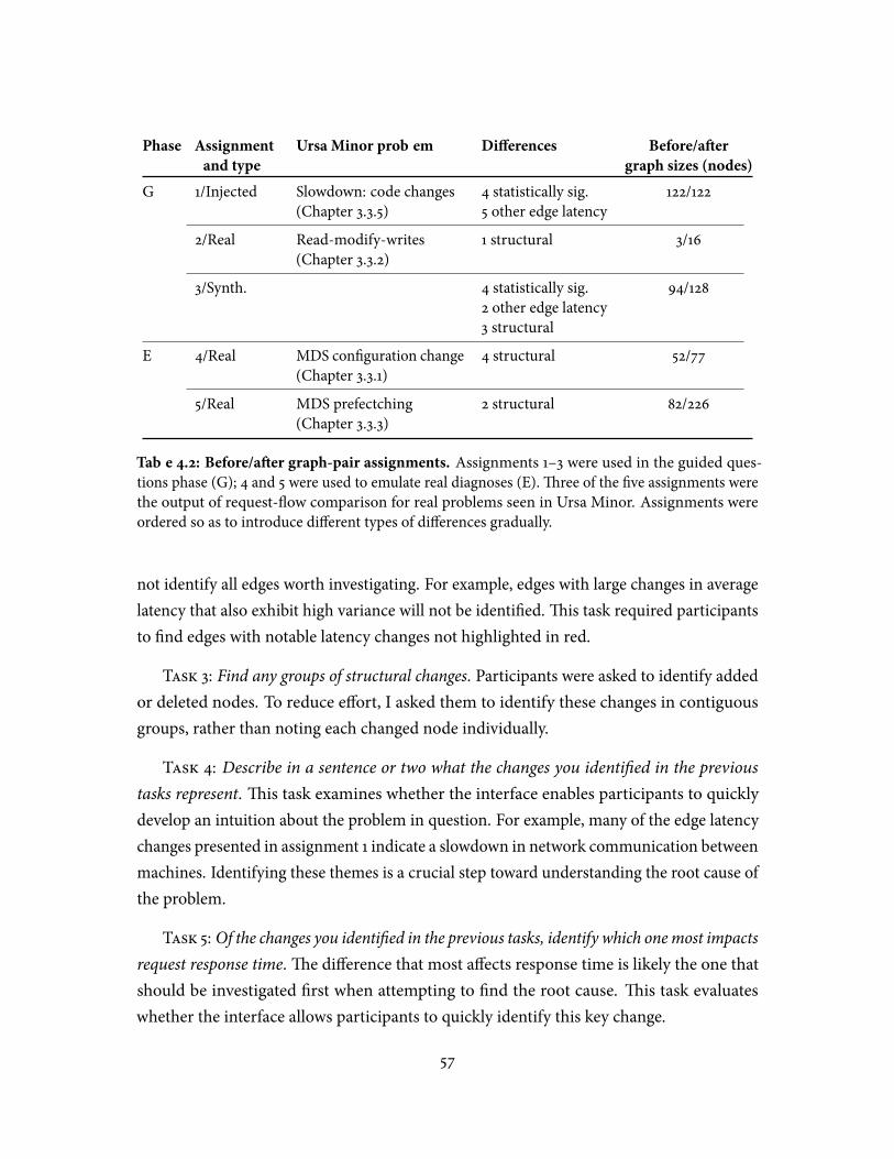
Phase Assignment Ursa Minor problem Di�erences Before/a�er

and type graph sizes (nodes)

G 1/Injected Slowdown: code changes 4 statistically sig. 122/122(Chapter 3.3.5) 5 other edge latency

2/Real Read-modify-writes 1 structural 3/16(Chapter 3.3.2)

3/Synth. 4 statistically sig. 94/1282 other edge latency3 structural

E 4/Real MDS con�guration change 4 structural 52/77(Chapter 3.3.1)

5/Real MDS prefectching 2 structural 82/226(Chapter 3.3.3)

Table 4.2: Before/a�er graph-pair assignments. Assignments 1–3 were used in the guided ques-tions phase (G); 4 and 5 were used to emulate real diagnoses (E).�ree of the �ve assignments werethe output of request-�ow comparison for real problems seen in Ursa Minor. Assignments wereordered so as to introduce di�erent types of di�erences gradually.

not identify all edges worth investigating. For example, edges with large changes in averagelatency that also exhibit high variance will not be identi�ed.�is task required participantsto �nd edges with notable latency changes not highlighted in red.

Task 3: Find any groups of structural changes. Participants were asked to identify addedor deleted nodes. To reduce e�ort, I asked them to identify these changes in contiguousgroups, rather than noting each changed node individually.

Task 4: Describe in a sentence or two what the changes you identi�ed in the previoustasks represent. �is task examines whether the interface enables participants to quicklydevelop an intuition about the problem in question. For example, many of the edge latencychanges presented in assignment 1 indicate a slowdown in network communication betweenmachines. Identifying these themes is a crucial step toward understanding the root cause ofthe problem.

Task 5: Of the changes you identi�ed in the previous tasks, identify which onemost impactsrequest response time.�e di�erence that most a�ects response time is likely the one thatshould be investigated �rst when attempting to �nd the root cause. �is task evaluateswhether the interface allows participants to quickly identify this key change.

57

Emulating real diagnoses

In the next phase, participants completed two additional assignments.�ese assignmentswere intended to emulate how the interfaces might be used in the wild, when diagnosing anew problem for the �rst time. For each assignment, the participant was asked to completetasks 4 and 5 only (as described above). I selected these two tasks because they most closelyalign with the questions a developer would ask when diagnosing an unknown problem.

A�er this part of the study, participants were asked to agree or disagree with twostatements using a �ve-point Likert scale: “I am con�dent my answers are correct” and“�is interface was useful for solving these problems.” I also asked them to comment onwhich features of the interface they liked or disliked, and to suggest improvements.

Interface comparison

Finally, to get a more direct sense of what aspects of each approach were useful, I showedparticipants an alternate interface. To avoid fatiguing participants and training e�ects, Idid not ask them to complete the assignments and tasks again; instead I asked them tobrie�y consider (using assignments 1 and 3 as examples) whether the tasks would be easieror harder to complete with the second interface, and to explain which features of bothapproaches they liked or disliked. Because the pilot study suggested animation was mostdi�cult to use, I focused this part of the study on comparing side-by-side and di�.

4.3.4 Scoring criteria

I evaluated participants’ responses by comparing them to an “answer key” that I created.Tasks 1–3, which asked for multiple answers, were scored using precision/recall. Precisionmeasures the fraction of a participant’s answers that were also in the key. Recallmeasuresthe fraction of all answers in the key identi�ed by the participant. Note that is possible tohave high precision and low recall—for example, by identifying only one change out of tenpossible ones. For task 3, participants who marked any part of a correct group were givencredit.

Tasks 4 and 5 were graded as correct or incorrect. For both, I accepted multiple possibleanswers. For example, for task 4 (“identify what changes represent”), I accepted an answeras correct if it was close to one of several possibilities, corresponding to di�erent levelsof background knowledge. In one assignment, several students identi�ed the changes asrepresenting extra cache misses in the a�er graph, which I accepted. Some participants

58

with more experience explicitly identi�ed that the a�er graph showed a read-modify write,a well-known bane of distributed storage system performance.

I also captured completion times for the �ve quantitative tasks. For completion timesas well as precision/recall, I used the Kruskal-Wallis test to establish di�erences among allthree interfaces, then pairwise Wilcoxon Rank Sum tests (chosen a priori) to separatelycompare the animation interface to each of side-by-side and di�. I recorded and analyzedparticipants’ comments from each phase as a means to better understand the strengths andweaknesses of each approach.

4.3.5 Limitations

My user study methodology has several limitations. Most importantly, it is di�cult to fullyevaluate visualization approaches for helping developers diagnose problems without askingthem to go through the entire process of debugging a real, complex problem. However, suchproblems are o�en unwieldy and can take hours or days to diagnose. As a compromise, Idesigned the user study tasks to test whether the interfaces enable participants to understandthe gist of the problem and identify starting points for diagnosis.

De�ciencies in the interface implementations may skew participants’ notions of whichapproaches work best for various scenarios. I explicitly identify such cases in the evaluationand suggest ways for improving the interfaces so as to avoid them in the future.

I stopped recruiting participants for the study when their qualitative comments con-verged, leading me to believe I had enough information to identify the useful aspects ofeach interface. However, the study’s small sample size may limit the generalizability of ourquantitative results.

Many of the participants were not familiar with statistical signi�cance and, as such,were confused by the wording of some of the tasks (especially tasks 1 and 2). I discuss thisin more detail in the Future Work section.

�e participants skewed young and male. To some extent this re�ects the populationof distributed-systems developers and students, but it may limit the generalizability of theresults somewhat.

4.4 User study results

No single approach was best for all participants and types of graph di�erences. For example,side-by-side was preferred by novices, and di� was preferred by advanced users and experts.

59

Similarly, where side-by-side and di� provedmost useful for most types of graph di�erences,animation proved better than side-by-side and di� for two very common types. When oneof the participants (PD06) was asked to pick his preferred interface, he said, “If I had tochoose between one and the other without being able to �ip, I would be sad.” When askedto contrast side-by-side with di�, SS01 said, “�is is more clear, but also more confusing.”Section 4.4.1 compares the approaches based on participants’ quantitative performanceon the user study tasks. Sections 4.4.2 to 4.4.4 describe my observations and participants’comments about the various interfaces and, based on this data, distill the approaches bestsuited for speci�c graph di�erence types and usage modes.

4.4.1 Quantitative results

Figure 4.2: Completion times for all partici-

pants.�e boxplots show completion times forindividual tasks, aggregated across all assign-ments.

Figure 4.2 shows completion times for eachof the three interfaces. Results for individualtasks, aggregated over all assignments, areshown (note that assignments, as shown inTable 4.2, may contain one or multiple typesof di�erences). Participants who used anima-tion took longer to complete all tasks com-pared to those who used side-by-side or di�,corroborating the results of several previousstudies [9, 44, 113]. Median completion timesfor side-by-side and di� are similar for mosttasks.�e observed di�erences between an-imation and the other interfaces are statisti-cally signi�cant for task 1 (“identify statistically signi�cant changes”)1 and task 4 (“whatchanges represent”).2 �e observed trends are similar when students and professionalsare considered separately, except that the di�erences between animation and the otherinterfaces are less pronounced for the latter.

Figure 4.3a shows the precision, recall, and accuracy results for each of the three inter-faces.�e results are not statistically signi�cant, but do contain artifacts worth describing.Overall, both side-by-side and di� fared well, and their median scores for most tasks are

1p-value=0.03 (side-by-side vs. anim), p-value=0.02 (di� vs. anim)2p-value=0.003 (side-by-side vs. anim), p-value=0.03 (di� vs. anim)

60

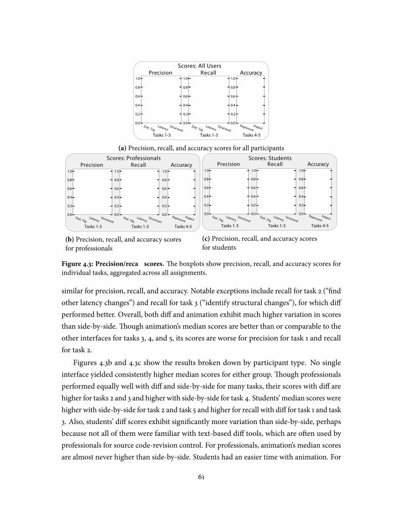
(a) Precision, recall, and accuracy scores for all participants

(b) Precision, recall, and accuracy scoresfor professionals

(c) Precision, recall, and accuracy scoresfor students

Figure 4.3: Precision/recall scores. �e boxplots show precision, recall, and accuracy scores forindividual tasks, aggregated across all assignments.

similar for precision, recall, and accuracy. Notable exceptions include recall for task 2 (“�ndother latency changes”) and recall for task 3 (“identify structural changes”), for which di�performed better. Overall, both di� and animation exhibit much higher variation in scoresthan side-by-side.�ough animation’s median scores are better than or comparable to theother interfaces for tasks 3, 4, and 5, its scores are worse for precision for task 1 and recallfor task 2.

Figures 4.3b and 4.3c show the results broken down by participant type. No singleinterface yielded consistently higher median scores for either group.�ough professionalsperformed equally well with di� and side-by-side for many tasks, their scores with di� arehigher for tasks 2 and 3 and higher with side-by-side for task 4. Students’ median scores werehigher with side-by-side for task 2 and task 5 and higher for recall with di� for task 1 and task3. Also, students’ di� scores exhibit signi�cantly more variation than side-by-side, perhapsbecause not all of them were familiar with text-based di� tools, which are o�en used byprofessionals for source code-revision control. For professionals, animation’s median scoresare almost never higher than side-by-side. Students had an easier time with animation. For

61

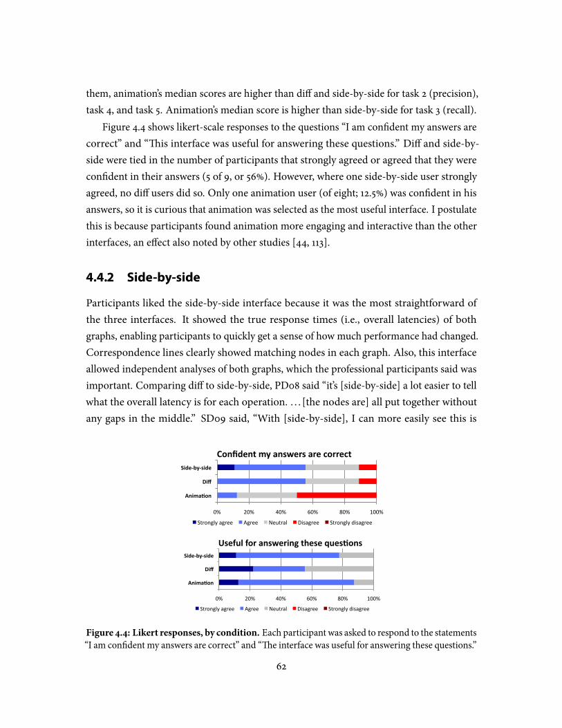
them, animation’s median scores are higher than di� and side-by-side for task 2 (precision),task 4, and task 5. Animation’s median score is higher than side-by-side for task 3 (recall).

Figure 4.4 shows likert-scale responses to the questions “I am con�dent my answers arecorrect” and “�is interface was useful for answering these questions.” Di� and side-by-side were tied in the number of participants that strongly agreed or agreed that they werecon�dent in their answers (5 of 9, or 56%). However, where one side-by-side user stronglyagreed, no di� users did so. Only one animation user (of eight; 12.5%) was con�dent in hisanswers, so it is curious that animation was selected as the most useful interface. I postulatethis is because participants found animation more engaging and interactive than the otherinterfaces, an e�ect also noted by other studies [44, 113].

4.4.2 Side-by-side

Participants liked the side-by-side interface because it was the most straightforward ofthe three interfaces. It showed the true response times (i.e., overall latencies) of bothgraphs, enabling participants to quickly get a sense of how much performance had changed.Correspondence lines clearly showed matching nodes in each graph. Also, this interfaceallowed independent analyses of both graphs, which the professional participants said wasimportant. Comparing di� to side-by-side, PD08 said “it’s [side-by-side] a lot easier to tellwhat the overall latency is for each operation. . . . [the nodes are] all put together withoutany gaps in the middle.” SD09 said, “With [side-by-side], I can more easily see this is

0%   20%   40%   60%   80%   100%  

Anima&on  

Diff  

Side-­‐by-­‐side  

Confident  my  answers  are  correct  

Strongly  agree   Agree   Neutral   Disagree   Strongly  disagree  

0%   20%   40%   60%   80%   100%  

Anima&on  

Diff  

Side-­‐by-­‐side  

Useful  for  answering  these  ques&ons  

Strongly  agree   Agree   Neutral   Disagree   Strongly  disagree  

Figure 4.4: Likert responses, by condition. Each participant was asked to respond to the statements“I am con�dent my answers are correct” and “�e interface was useful for answering these questions.”

62

happening here before and a�er. Without the dashed lines, you can’t see which event in theprevious trace corresponds to the a�er trace.”�ese sentiments were echoed by many otherparticipants (e.g., SD06, SD07, PD07).

�e side-by-side interface su�ers from two key drawbacks. First, it is di�cult to identifydi�erences when before/a�er graphs di�er signi�cantly because corresponding ones becomefurther apart. PS01 complained that “the points that should be lining up are getting fartherand farther away, so it’s getting more di�cult to compare the two.” PD06 complained that itwas more di�cult to match up large changes since the other one could be o� the screen.Similar complaints were voiced by other participants (e.g., PS02, SS02, PS04). Adding theability to pin one graph relative to another to my side-by-side implementation would limitvertical distance between di�erences. However, horizontal distance, which increases withthe number of concurrent threads in each request, would remain.

Second, when nodes are very close to another, correspondence lines became too clutteredand di�cult to use.�is led to complaints from several participants (e.g., PS03, SS01, SS03,PA13). To cope, SS03 and PS05 gave up trying to identify corresponding nodes betweenthe graphs and instead identi�ed structural di�erences by determining if the number ofcorrespondence lines on the screen matched the number of nodes visible in both the beforeand a�er graph. Modifying the side-by-side interface to draw correspondence lines only atthe start of a contiguous run of corresponding nodes would help reduce clutter, but wouldcomplicate edge latency comparisons.

Based on participants’ comments above and my observations, Table 4.3 shows the usecases for which I believe side-by-side is the best of the three approaches. As shown inTable 4.3, side-by-side’s simple approach works best for aiding comprehension. However,due to potential for horizontal skew and clutter, it is not the best approach for identifyingany type of di�erence.

4.4.3 Diª

Participants’ comments about the di� interface were polarized. Professionals and moreadvanced students preferred di� ’s compactness, whereas others were less decisive. Forexample, PS03 claimed di� ’s compact representation made it easier for him to draw deduc-tions. Indeed, unlike side-by-side, di� always shows di�erences right next to each other,making it easier to �nd di�erences when before and a�er graphs have diverged signi�cantly.Also, by placing di�erences right next to each other, di� allows for easier identi�cation of

63

smaller structural and edge latency changes. In contrast, SS04 said, “[Side-by-side] may bemore helpful than [di�], because this is not so obvious, especially for structural changes.”

�ough participants rarely made explicit comments about �nding di� di�cult to use,I found that it encouraged incorrect mental models in student participants. For example,SD08 and SD09 confused structural di�erences within a single thread of activity with achange in the amount of concurrency. It is easy to see why participants might confuse thetwo, as both are represented by fan-outs in the graph.

I believe that participants’ comments about di� vary greatly because its compact repre-sentation requires more knowledge about so�ware development and distributed systemsthan that required by the more straightforward side-by-side interface. Additionally, manyof the professionals are familiar with di� tools for text, which would help them understandmy graph-based di� technique more easily.

Since it places di�erences close together, Table 4.3 lists di� as the best approach forshowing edge latency changes. However, because it encourages poor mental models formany structural di�erences, it is not the best approach for showing concurrency changesand intra-thread event changes.

4.4.4 Animation

My user study participants o�en struggled when using the animation interface. With thisinterface, all di�erences between the two graphs appear and disappear at the same time.�iscombined movement confused participants when multiple types of changes were presentin the same thread of activity, an e�ect also noticed by Ghani et al. [54]. In such cases,edge latency changes would cause existing nodes to move down and, as they were doing so,trample over nodes that were fading in or out due to structural changes. PA11 complained,“Portions of graphs where calls are not being made in the a�er trace are fading away whileother nodes move on top of it and then above it . . . it is confusing.”�ese sentiments wereechoed by many other participants (e.g., SA11, PA12, SA10, PA13).

�e combined movement of nodes and edges also prevented participants from estab-lishing static reference points for gauging the impact of a given di�erence. SA10 told us:“I want to. . .pick one node and switch it between before and a�er. [But the same node] inbefore/a�er is in a di�erent location completely.” SA12 said he did not like the animationinterface because of the lack of consistent reference points. “If I want to measure the size ofan edge, if it was in the same position as before. . . then it’d be easy to see change in position

64

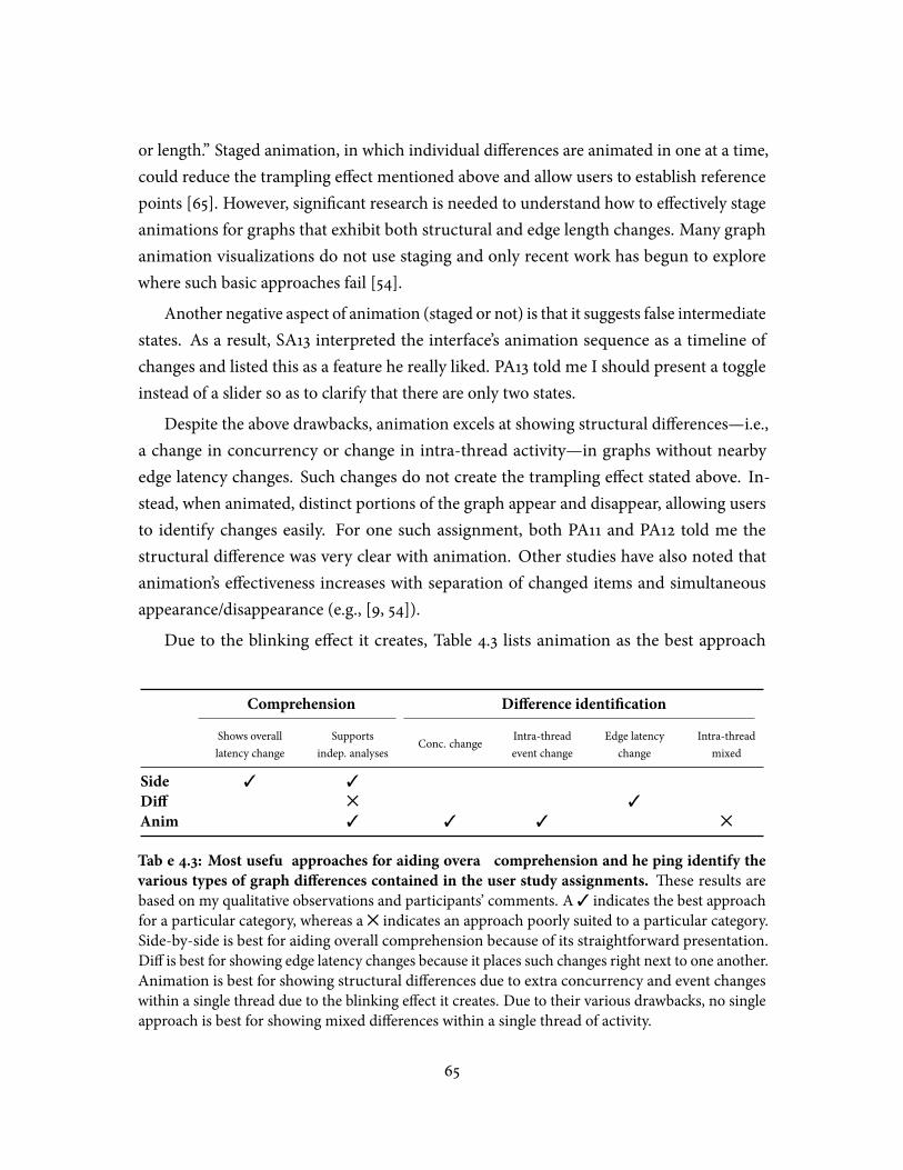
or length.” Staged animation, in which individual di�erences are animated in one at a time,could reduce the trampling e�ect mentioned above and allow users to establish referencepoints [65]. However, signi�cant research is needed to understand how to e�ectively stageanimations for graphs that exhibit both structural and edge length changes. Many graphanimation visualizations do not use staging and only recent work has begun to explorewhere such basic approaches fail [54].

Another negative aspect of animation (staged or not) is that it suggests false intermediatestates. As a result, SA13 interpreted the interface’s animation sequence as a timeline ofchanges and listed this as a feature he really liked. PA13 told me I should present a toggleinstead of a slider so as to clarify that there are only two states.

Despite the above drawbacks, animation excels at showing structural di�erences—i.e.,a change in concurrency or change in intra-thread activity—in graphs without nearbyedge latency changes. Such changes do not create the trampling e�ect stated above. In-stead, when animated, distinct portions of the graph appear and disappear, allowing usersto identify changes easily. For one such assignment, both PA11 and PA12 told me thestructural di�erence was very clear with animation. Other studies have also noted thatanimation’s e�ectiveness increases with separation of changed items and simultaneousappearance/disappearance (e.g., [9, 54]).

Due to the blinking e�ect it creates, Table 4.3 lists animation as the best approach

Comprehension Di�erence identi�cation

Shows overalllatency change

Supportsindep. analyses

Conc. change Intra-threadevent change

Edge latencychange

Intra-threadmixed

Side 3 3

Di� 5 3

Anim 3 3 3 5

Table 4.3: Most useful approaches for aiding overall comprehension and helping identify the

various types of graph di�erences contained in the user study assignments. �ese results arebased on my qualitative observations and participants’ comments. A 3 indicates the best approachfor a particular category, whereas a 5 indicates an approach poorly suited to a particular category.Side-by-side is best for aiding overall comprehension because of its straightforward presentation.Di� is best for showing edge latency changes because it places such changes right next to one another.Animation is best for showing structural di�erences due to extra concurrency and event changeswithin a single thread due to the blinking e�ect it creates. Due to their various drawbacks, no singleapproach is best for showing mixed di�erences within a single thread of activity.

65

for showing di�erences due to concurrency changes and intra-thread event changes.�epotential for trampling means it is the worst of the three for showing both latency andstructural di�erences within a single thread of activity.

4.5 Future work

Comparing these three interfaces has yielded insights about which approaches are usefulfor di�erent circumstances. Performing this study also produced a number of directions forimproving each of the interfaces. Here I highlight a few that participants found importantand that are complex enough to warrant further research.

Addressing skew, horizontal layout, and trampling: Many users struggled with theincreasing skew in the side-by-side layout, as well as the inability to quickly trace a corre-spondence from one graph to another (e.g., PS02, SA10, and PS05).�e animation interface,which produces a trampling e�ect as all changes are animated together, also made it di�cultto focus on individual di�erences. A future interface might anchor the comparison inmultiple or user-selectable locations to mitigate this problem. However, there are subtletiesinvolved in choosing and using anchor points.

One option, as requested by most participants (e.g., PA12 and PD08), is to anchorthe comparison at a user-selectable location. Another is to re-center the graph as usersscroll through it. However, both techniques distort the notion that time �ows downward,and neither would reduce horizontal distance or clutter. Approaches that restructure thecomparison to minimize the horizontal distance between corresponding nodes are aninteresting opportunity.

For the animation technique, anchoring in multiple locations could be achieved bystaging changes. Questions of ordering immediately arise: structural changes might bepresented before, a�er, or between latency changes.�e choice is non-obvious. For example,it is not clear whether to animate structural and latency changes together when the structuralchange causes the latency change or even how to algorithmically determine such cases.

Exploring semantic zooming: Participants found the larger graphs used for this study,which were about 200 nodes in size, unwieldy and di�cult to understand. �ough thestraightforward zooming approach used by my interfaces allowed entire graphs to be seen,zooming out resulted in nodes, edges, and correspondence lines that were too small tobe interpreted. As a result, participants needed to scroll through graphs while zoomed in,making it di�cult for them to obtain a high-level understanding of the problem. Several

66

participants complained about this issue (e.g., SD05, SA10). Further work is needed toinvestigate ways to semantically zoom the graphs being compared so as to preserve inter-pretability. One option is to always coalesce portions of the comparison that are the samein both graphs and progressively coalesce portions that contain di�erences.

Exploiting annotation: Annotation was used in this study to record answers. But, italso has the potential to be a valuable tool for collaborative debugging, especially in largedistributed systems with components developed by independent teams. In such systems,it is likely that no single person will have the end-to-end knowledge required to diagnosea complex problem that a�ects several components. For this reason, several professionalparticipants from Google listed the interfaces’ annotation mechanism as a strength of theinterfaces (e.g., PA13, PS04, and PD08). PS04 said “[I] really like the way you added theannotation. . . .So other people who are later looking at it can get the bene�t of your analysis.”Supporting cooperative diagnosis work with an annotation interface, such as used that usedin Rietveld [112] for code reviews, is an interesting avenue of future work.

Matching automation to users’ expectations: Like many other diagnosis tools [72, 88,98], Spectroscope uses statistical tests to automatically identify di�erences, since they limitexpensive false positives. However, many of the user study participants did not have astrong background in statistics and so mistook “statistically signi�cant” to mean “largechanges in latency.”�ey did not know that variance a�ects whether an edge latency changeis deemed statistically signi�cant.�is generated confusion and accounted for lower thanexpected scores for some tasks. For example, some participants (usually students) failedto di�erentiate between task 1 and task 2, and a few students and professionals refused tomark a change as having the most impact unless it was highlighted in red (as statisticallysigni�cant). Trying to account for why one particularly large latency change was nothighlighted, SA10 said, “I don’t know what you mean by statistically signi�cant. Maybeit’s signi�cant to me.” �ese concerns were echoed by almost all of the participants, anddemonstrate that automationmustmatch users’mentalmodels and that diagnosis toolsmustlimit both false positives and false negatives. Statistics and machine learning techniques canprovide powerful automation tools, but to take full advantage of this power—which becomesincreasingly important as distributed systems become more complex—diagnosticians musthave the right expectations about how theywork. Both better techniques andmore advancedtraining may be needed to achieve this goal.

67

4.6 Summary

For tools that automate aspects of problem diagnosis to be useful, they must present theirresults in a manner developers �nd clear and intuitive.�is chapter investigates improvedvisualizations for Spectroscope, one particular automated problem localization tool. Itcontrasts three approaches for presenting Spectroscope’s results through a 26-participantuser study, and �nd thats each approach has unique strengths for di�erent usage modes,graph di�erence types, and users. Moving forward, I expect that these strengths and theresearch directions inspired by their weaknesses will inform the presentation of futurerequest-�ow comparison tools and other diagnosis tools.

68

Chapter 5

The importance of predictability

�ough Spectroscope has proven useful for automatically localizing performance changes, ithas been unable to reach its full potential because most distributed systems do not satisfy akey property needed for automation—predictability (i.e., low variance in key metrics).�ischapter highlights this important stumbling block toward increased automation. Section 5.1describes how high variance a�ects predictability and discusses potential solutions forlowering variance. Section 5.2 describes how existing automated diagnosis tools are a�ectedby high variance. Section 5.3 describes a nomenclature for helping system builders disam-biguate wanted and unwanted variance sources in their distributed systems, and Section 5.4describes a tool for helping system builders �nd such variance sources. Section 5.5 discussesopen questions, and Section 5.6 concludes.

5.1 How to improve distributed system predictability?

�e predictability of a distributed system is a�ected by variance in the metrics used to makedeterminations about it. As variance increases, predictability decreases, and it becomesharder for automation tools to make con�dent, or worse, correct determinations.�oughvariance cannot be eliminated completely due to fundamental non-determinism (e.g.,actions of a remote system and bit errors), it can be reduced, improving predictability.

To aid automation, system builders could be encouraged to always minimize variance inkeymetrics.�is policy dovetails nicely with areas in which predictability is paramount. Forexample, in the early 1990s, the US Postal Service slowed down mail delivery because theydecided consistency of delivery times was more important than raw speed. When askedwhy this tradeo� was made, the postmaster general responded: “I began to hear complaints

69

frommailers and customers about inconsistent �rst-class mail delivery. . . .We learned howimportant consistent, reliable delivery is to our customers” [24]. In scienti�c computing,inter-node variance can drastically limit performance due to frequent synchronizationbarriers. In real-time systems, it is more important for programs to meet each deadlinethan run faster on average. Google has recently identi�ed low response-time variance ascrucial to achieving high performance in warehouse-scale computing [16].

Of course, inmany cases, variance is a side e�ect of desirable performance enhancements.Caches, amainstay ofmost distributed systems, intentionally trade variance for performance.Many scheduling algorithms do the same. Also, reducing variance blindly may lead tosynchronized “bad states,” which may result in failures or drastic performance problems.For example, Patil et al. describe an emergent property in which load-balancing in GIGA+,a distributed directory service, leads to a large performance dropo� as compute-intensivehash bucket splits on various nodes naturally become synchronized [105].

Some variance is intrinsic to distributed systems and cannot be reduced without whole-sale architectural changes. For example, identical components, such as disks from thesame vendor, can di�er signi�cantly in performance due to fault-masking techniques andmanufacturing e�ects [12, 84]. Also, it may be di�cult to design complex systems to exhibitlow variance because it is hard to predict their precise operating conditions [62, 94].

In practice, there is no easy answer in deciding how to address variance to aid automation.�ere is, however, a wrong answer—ignoring it, as is too o�en being done today. Instead,for the highly touted goal of automation to become a reality, system builders must treatvariance as a �rst-class metric. �ey should strive to localize the sources of variance intheir systems and make conscious decisions about which ones should be reduced. Suchexplicit decisions about variance properties will result in more robust systems and willvastly improve the utility of automation tools that rely on low variance to work.

5.2 Diagnosis tools & variance

Tools that automate aspects of performance diagnosis each assume a unique model ofsystem behaviour and use deviations from it to predict diagnoses. Most do not identify theroot cause directly, but rather automatically localize the source of the problem from anyof the numerous components in the system to just the speci�c components or functionsresponsible. Di�erent tools exhibit di�erent failure modes when variance is high, dependingon the underlying techniques they use.

70

Tools that rely on thresholds make predictions when important metrics chosen byexperts exceed pre-determined values. �eir failure mode is the most unpredictable, asthey will return more false positives (inaccurate diagnoses) or false negatives (diagnosesnot made when they should have been), depending on the value of the threshold. A lowthreshold will result in more false positives, whereas increasing it to accommodate thehigh variance will mask problems, resulting in more false negatives. My conversationswith Facebook and Google engineers indicate that false positives are perhaps the worstfailure mode, due to the amount of developer e�ort wasted [107]. However, my experiencesrunning the visualization user study presented in Chapter 4 indicate that false negativesmay be just as nefarious because they decay developers’ con�dence in the tool’s ability.

To avoid false positives, some tools use statistical techniques to avoid predicting whenthe expected false positive rate exceeds a pre-set one (e.g., 5%).�e cost of high variancefor them is an increase in false negatives. Some statistical tools use adaptive techniques toincrease their con�dence before making predictions—e.g., by collecting more data samples.�e cost of high variance for them is increased storage/processing cost and an increase intime required before predictions can be made.

Many tools use machine learning to automatically learn the model (e.g., metrics andvalues) that best predicts performance. �e false positive rate and false negative rate arecontrolled by selecting the model that best trades generality (which usually results inmore false negatives) with speci�city (which results in either more false positives or falsenegatives).

5.2.1 How real tools are aªected by variance

Real tools use a combination of the techniques described above to make predictions.�issection lists four such tools and how they are a�ected by variance. Table 5.1 provides asummary and lists additional tools.

Magpie [15]:�is tool uses an unsupervised machine learning algorithm (clustering)to identify anomalous requests in a distributed system. Requests are grouped togetherbased on similarity in request structure, performance metrics, and resource usage. Magpieexpects that most requests will fall into one of several “main” clusters of behaviour, so itidenti�es small ones as anomalies. A threshold is used to decide whether to place a requestin the cluster deemed most similar to it or whether to create a new one. High variance inthe values of the features used and use of a low threshold will yield many small clusters,

71

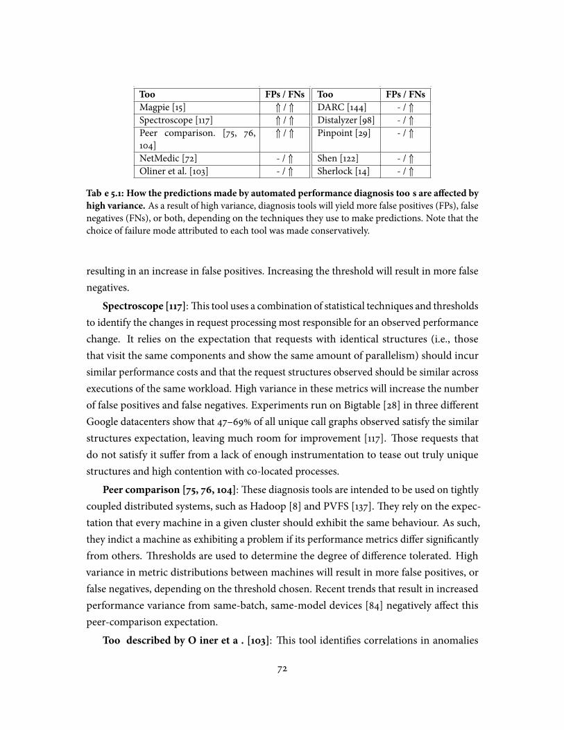
Tool FPs / FNs Tool FPs / FNs

Magpie [15] ⇑ / ⇑ DARC [144] - / ⇑Spectroscope [117] ⇑ / ⇑ Distalyzer [98] - / ⇑Peer comparison. [75, 76,104]

⇑ / ⇑ Pinpoint [29] - / ⇑

NetMedic [72] - / ⇑ Shen [122] - / ⇑Oliner et al. [103] - / ⇑ Sherlock [14] - / ⇑

Table 5.1: How the predictions made by automated performance diagnosis tools are a�ected by

high variance. As a result of high variance, diagnosis tools will yield more false positives (FPs), falsenegatives (FNs), or both, depending on the techniques they use to make predictions. Note that thechoice of failure mode attributed to each tool was made conservatively.

resulting in an increase in false positives. Increasing the threshold will result in more falsenegatives.

Spectroscope [117]:�is tool uses a combination of statistical techniques and thresholdsto identify the changes in request processing most responsible for an observed performancechange. It relies on the expectation that requests with identical structures (i.e., thosethat visit the same components and show the same amount of parallelism) should incursimilar performance costs and that the request structures observed should be similar acrossexecutions of the same workload. High variance in these metrics will increase the numberof false positives and false negatives. Experiments run on Bigtable [28] in three di�erentGoogle datacenters show that 47–69% of all unique call graphs observed satisfy the similarstructures expectation, leaving much room for improvement [117]. �ose requests thatdo not satisfy it su�er from a lack of enough instrumentation to tease out truly uniquestructures and high contention with co-located processes.

Peer comparison [75, 76, 104]:�ese diagnosis tools are intended to be used on tightlycoupled distributed systems, such as Hadoop [8] and PVFS [137].�ey rely on the expec-tation that every machine in a given cluster should exhibit the same behaviour. As such,they indict a machine as exhibiting a problem if its performance metrics di�er signi�cantlyfrom others. �resholds are used to determine the degree of di�erence tolerated. Highvariance in metric distributions between machines will result in more false positives, orfalse negatives, depending on the threshold chosen. Recent trends that result in increasedperformance variance from same-batch, same-model devices [84] negatively a�ect thispeer-comparison expectation.

Tool described by Oliner et al. [103]: �is tool identi�es correlations in anomalies

72

across components of a distributed system. To do so, it �rst calculates an anomaly scorefor discrete time intervals by comparing the distribution of some signal—e.g., averagelatency—during the interval to the overall distribution.�e strength of this calculation isdependent on low variance in the signal. High variance will yield lower scores, resulting inmore false negatives.�e authors themselves state this fact: “�e [anomaly] signal shouldusually take values close to the mean of its distribution—this is an obvious consequence ofits intended semantics” [103].

5.3 The three I’s of variance

Variance in distributed systems is an important metric that directly a�ects potential forautomated diagnosis. To reduce it, two complementary courses of action are necessary.During the design phase, system builders should make conscious decisions about whichareas of the distributed system should be more predictable (exhibit low variance with regardto important metrics). Since the complexity of distributed systems makes it unlikely theywill be able to identify all of the sources of variance during design [12, 62, 94], they mustalso work to identify sources of variance during development and testing. To help withthe latter, this section describes a nomenclature for variance sources that can help systembuilders reason about them and understand for which ones’ variance should be reduced.

Intentional variance sources:�ese are a result of a conscious tradeo�made by systembuilders. For example, such variance may emanate from a scheduling algorithm that lowersmean response time at the expense of variance. Alternatively, it may result from explicitanti-correlation added to a component to prevent it from entering synchronized, stuck states(e.g., Microreboots [106]). Labeling a source as intentional indicates the system builder willnot try to reduce its variance.

Inadvertent variance sources:�ese are o�en the result of poorly designed or imple-mented code; as such, their variance should be reduced or eliminated. For example, suchvariance sources may include functions that exhibit extraordinarily varied response timesbecause they contain many di�erent control paths (spaghetti code). In a recent paper [75],Kasick et al. describe how such high variance functions were problematic for an automateddiagnosis tool developed for PVFS [137]. Such variance can also emanate from unforeseeninteractions between components, or may be the result of extreme contention for a so�-ware resource (e.g., locks).�e latter suggests that certain contention-related performanceproblems can be diagnosed directly by localizing variance. In fact, while developing Spec-

73

troscope [117], I found that high variance was o�en a good predictor of such problems (seeChapter 3.2).

Intrinsic variance sources:�ese sources are o�en a result of fundamental propertiesof the distributed system or datacenter—for example, the hardware in use. Short of archi-tectural changes, their variance cannot be reduced. Examples include non-�at topologieswithin a datacenter or disks that exhibit high variance in bandwidth between their innerand outer zones [12].

Variance from intentional and intrinsic sources may be a given, so the quality of pre-dictions made by automation tools in these areas will su�er. However, it is important toguarantee their variance does not impact predictions made for other areas of the system.�is may be the case if the data granularity used by an automation tool to make predic-tions is not high enough to distinguish between a high-variance source and surroundingareas. For example, problems in the so�ware stack of a component may go unnoticedif an automation tool does not distinguish it from a high-variance disk. To avoid suchscenarios, system builders should help automation tools account for high-variance sourcesdirectly—for example, by adding markers around them that are used by automation toolsto increase their data granularity.

5.4 VarianceFinder

To illustrate a variance-oriented mindset, this section proposes one potential mechanism,called VarianceFinder, for helping system builders identify the main sources of variance intheir systems during development and testing.�e relatively simple design outlined herefocuses on reducing variance in response times for distributed storage systems such as UrsaMinor [1], Bigtable [28], and GFS [55]. However, I believe this basic approach could beextended to include other performance metrics and systems.

VarianceFinder utilizes request-�ow graphs obtained from end-to-end tracing (seeChapter 2.2) and follows a two-tiered approach. First, it shows the variance associatedwith aspects of the system’s overall functionality that should exhibit similar performance(Section 5.4.1). Second, it allows system builders to select functionality with high varianceand identi�es the components, functions, or RPCs responsible, allowing them to takeappropriate action (Section 5.4.2). I believe this tiered approach will allow system buildersto expend e�ort where it is most needed.

74

5.4.1 Id’ing functionality & ®rst-tier output

To identify functionality that should exhibit similar performance, VarianceFinder employsthe expectation that requests with identical structures should incur similar performancecosts. Like Spectroscope, VarianceFinder groups request-�ow graphs that exhibit the samestructure—i.e., those that represent identical activities and execute the same trace points—into categories and calculates average response times, variances, and squared coe�cients ofvariation (C2) for each. C2, which is measured as ( σµ)2, is a normalized measure of variance.It captures the intuition that categories whose standard deviation is much greater than themean are worse o�enders than those whose standard deviation is less than or close to themean. In practice, categories with C2

> 1 are said to have high variance around the mean,whereas those with C2

< 1 exhibit low variance around the mean.�e �rst-tier output from VarianceFinder consists of the list of categories ranked by C2

value. System builders can click through highly-ranked categories to see a graph view ofthe request structure, allowing them to determine whether it is important. For example,a highly-ranked category that contains read requests likely will be deemed important,whereas one that contains rare requests for the names of mounted volumes likely will not.

5.4.2 Second-tier output & resulting actions

Once the system builder has selected an important highly-ranked category, he can useVarianceFinder to localize its main sources of variance. �is is done by highlighting thehighest-variance edges along the critical path of the category’s requests. Figure 5.1 illustratesthe overall process. In some cases, an edge may exhibit high variance, because of anotheredge—for example, an edge spanning a queue might display high variance because thecomponent to which it sends data also does so. To help system builders understand thesedependencies, clicking on a highlighted edge will reveal other edges that have non-zerocovariance with it.

Knowing the edges responsible for the high variance allows the system builder toinvestigate the relevant areas of the system. Variance from sources that he deems inadvertentshould be reduced or eliminated. Alternatively, he might decide that variance from certainsources should not or cannot be reduced because they are intentional or intrinsic. In suchcases, he should add tight instrumentation points around the source to serve as markers.Automation tools that use these markers to increase their data granularity—especially those,like Spectroscope [117], that use end-to-end traces directly [15, 29, 117, 125]—will be able to

75

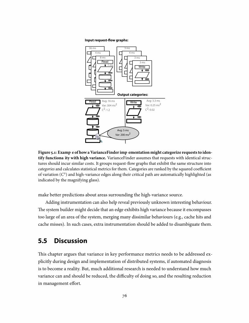
Write3 ms

Write4 ms

Write3 ms1 ms

Read36 ms

1 msRead4 ms

Read8 ms

1 ms

Read Avg: 16 ms

Var: 304 ms2

C2: 1.2

Write Avg: 3.3 ms

Var: 0.25 ms2

C2: 0.02

Avg: 5 ms

Var: 200 ms2

Write3 ms

Input request-!ow graphs:

Output categories:

Figure 5.1: Example of how aVarianceFinder implementationmight categorize requests to iden-

tify functionality with high variance. VarianceFinder assumes that requests with identical struc-tures should incur similar costs. It groups request-�ow graphs that exhibit the same structure intocategories and calculates statistical metrics for them. Categories are ranked by the squared coe�cientof variation (C2) and high-variance edges along their critical path are automatically highlighted (asindicated by the magnifying glass).

make better predictions about areas surrounding the high-variance source.Adding instrumentation can also help reveal previously unknown interesting behaviour.

�e system builder might decide that an edge exhibits high variance because it encompassestoo large of an area of the system, merging many dissimilar behaviours (e.g., cache hits andcache misses). In such cases, extra instrumentation should be added to disambiguate them.

5.5 Discussion

�is chapter argues that variance in key performance metrics needs to be addressed ex-plicitly during design and implementation of distributed systems, if automated diagnosisis to become a reality. But, much additional research is needed to understand how muchvariance can and should be reduced, the di�culty of doing so, and the resulting reductionin management e�ort.

76

To answer the above questions, it is important that we work to identify the breakdownof intentional, inadvertent, and intrinsic variance sources in distributed systems and data-centers. To understand if the e�ort required to reduce variance is worthwhile, the bene�tsof better automation must be quanti�ed by how real people utilize and react to automationtools, not via simulated experiments or fault injection. If this tradeo� falls strongly in favourof automation, and intrinsic variance sources are the largest contributers, architecturalchanges to datacenter and hardware design may be necessary. For example, system buildersmay need to increase the rate at which they adopt and develop strong performance isola-tion [63] or insulation [148] techniques. Also, hardware manufacturers, such as disk drivevendors, may need to incorporate performance variance as a �rst-class metric and strive tominimize it.

Similarly, if (currently) intentional sources are the largest contributors, system buildersmay need to re-visit key design tradeo�s. For example, they may need to consider usingdatacenter schedulers that emphasize predictability and low variance in job completiontimes [45] instead of ones that dynamically maximize resource utilization at the cost ofpredictability and low variance [56].

Finally, automated performance diagnosis is just one of many reasons why low varianceis important in distributed systems and datacenters. For example, strong service-levelagreements are di�cult to support without expectations of low variance. As such, many ofthe arguments posed in this chapter are applicable in a much broader sense.

5.6 Conclusion

�ough automation in large distributed systems is a desirable goal, it cannot be achievedwhen variance is high.�is chapter presents a framework for understanding and reducingvariance in performance metrics so as to improve the quality of automated performancediagnosis tools. I imagine that there are many other tools and design patterns for reducingvariance and enhancing predictability. In the interim, those building automation tools mustconsider whether the underlying system is predictable enough for their tools to be e�ective.

77

78

Chapter 6

Related work on performancediagnosis

�ere has been a proliferation of research in the past several years on how to diagnosedistributed systems problems. Due to the many di�erent types of systems (e.g., distributedstorage, dynamic hash tables, those for high-performance computing, those for cloudcomputing), available data sources (e.g., end-to-end traces, logs, performance counters),and potential problems (e.g., performance anomalies, behavioural changes, correctnessissues), it is likely that there is no single “magic bullet” solution. Rather, the likely outcomeof these research e�orts is a toolbox of diagnosis techniques, each serving their own uniqueand useful purpose.�is chapter samples the constituents of this toolbox for performancediagnosis.

Tools for performance diagnosis can be categorized on many axes. For example, theycould be categorized according to the type of instrumentation they use (see Oliner’s dis-sertation [101]) or the techniques they use to diagnose relevant problems (e.g., statistics,machine learning, mathematical modeling). In this related work chapter, tools are catego-rized according to their intended functionality. Viewed through this lens, most diagnosistools are designed to help diagnosticians with a speci�c phase of the diagnosis work�ow:problem localization, root-cause identi�cation, or problem recti�cation (see Figure 1.1).Most research has focused on tools for helping diagnosticians localize the source of a newproblem; they are described in Section 6.1. Some tools are designed to help identify theroot cause directly and are described in Section 6.2. Tools in this category are limited tosuggesting previously observed root causes, but doing so allows diagnosticians to skip theproblem localization step. A few tools attempt to automatically �x an observed problem byapplying simple actions, such as rebooting or re-imaging an o�ending machine; examples

79

are described in Section 6.3.Recent research has also focused on tools for helping optimize distributed system

performance when no “problem” has been explicitly identi�ed—for example, tools thathelp administrators with decisions about con�guration choices. Such tools are describedin Section 6.4. A signi�cant amount of research has also focused on diagnosis tools forsingle-process systems; examples of such tools are described in Section 6.5.

6.1 Problem-localization tools

Tools that localize performance problems can be divided into six main categories: toolsthat automatically identify anomalies, tools that automatically identify behavioural changes(i.e., steady-state changes), tools that automatically identify dissenting nodes in tightlycoupled distributed systems (e.g., PVFS [137]), tools that aid in distributed pro�ling, toolsthat exhaustively explore potential behaviours to �nd potential problems, and tools that helplocalize problems by visualizing trends amongst important metrics. Tables 6.1, 6.2, 6.3, 6.4,6.5, and 6.6 summarize these tools in terms of their functionality, the comparative approachthey use to identify problems, and their building blocks (i.e., the fundamental techniquesand data source they use). End-to-end traces are the most detailed and comprehensivedata source, but require distributed systems to be modi�ed to generate them. To work withunmodi�ed systems, many tools use more commonly available data sources, such as logs.However, in practice, the potential of these tools is o�en limited because the data sourcesthey use are not speci�cally designed to support their intended use cases. To help, someresearch e�orts focus on mechanisms to automatically retro�t existing distributed systemswith the instrumentation necessary to support speci�c diagnosis tasks [154].

Many tools that localize performance problems work by comparing expected distributedsystem behaviour to poorly-performing runtime behaviour. Expected behaviour can beexpressed in a variety of ways, including via:

Current runtime behaviour: When determining whether a problem should be lo-calized to a given distributed system component or request, expected behaviour can beexpressed in terms of that of other nodes, components, or requests observed during thesame execution.�is comparison approach is most commonly used for anomaly detectionor for detecting dissenters in tightly coupled distributed systems in which all nodes areexpected to perform similarly.

Previous runtimebehaviour: In systems inwhich all nodes are not expected to perform

80

similarly, behaviour from previous time periods during which performance was acceptablecan be stored and used as expected behaviour. Such tools may use machine learning tolearn a model from previous behaviour or may use previous behaviour directly.

Look-back window: �is approach is similar to the previous one, except instead ofusing a distinct speci�c period or execution as expected behaviour, a look-back window ofthe previous N minutes is used. Look-back windows are most commonly used by tools thatoperate on time-series data built from performance counters or other key metrics.

Mathematical models: Some tools use models derived from �rst principles, such asqueuing theory, as expected behaviour. Compared to using runtime behaviour directly,as in the approaches described above, mathematical models can more completely andcorrectly express desired behaviour. For example, expected behaviour derived from aprevious execution may itself contain latent performance problems and is limited in scopeto what was observed. Despite these advantages, many tools do not use mathematicalmodels because they are very di�cult to create and scale [132].

Expectations: Another approach involves asking diagnosticians to explicitly specifyexpected behaviour, for example via a custom language [110]. Manually written expectationsare di�cult to specify for large systems that exhibit many complex behaviours.

Diagnostician’s intuition: In some cases, especially for distributed pro�ling and vi-sualization, expected behaviour is not explicitly speci�ed; rather, these tools rely on thediagnostician’s intuition to judge where the problem lies. For example, a diagnosticianusing a pro�ling tool, such as Whodunit [27], must himself decide whether a large latencyobserved for a function is acceptable, whereas this decision can be made automatically bytools that use explicit models.

�e rest of this section describes various localization tools.

6.1.1 Anomaly detection

Table 6.1 summarizes tools intended to help diagnosticians localize problems that manifestas anomalies—components, requests, or other behaviours that show up in the tail of someimportant performance metric’s distribution. More generally, anomalies are rare and ex-tremely di�erent from what has been observed before. Mapgie [15] uses end-to-end tracesand unsupervised machine learning to identify request �ows that exhibit very di�erentstructures or resource utilizations compared to other requests. Xu et al. [152] attempt toreplicate Magpie’s functionality for systems without native end-to-end tracing support by

81

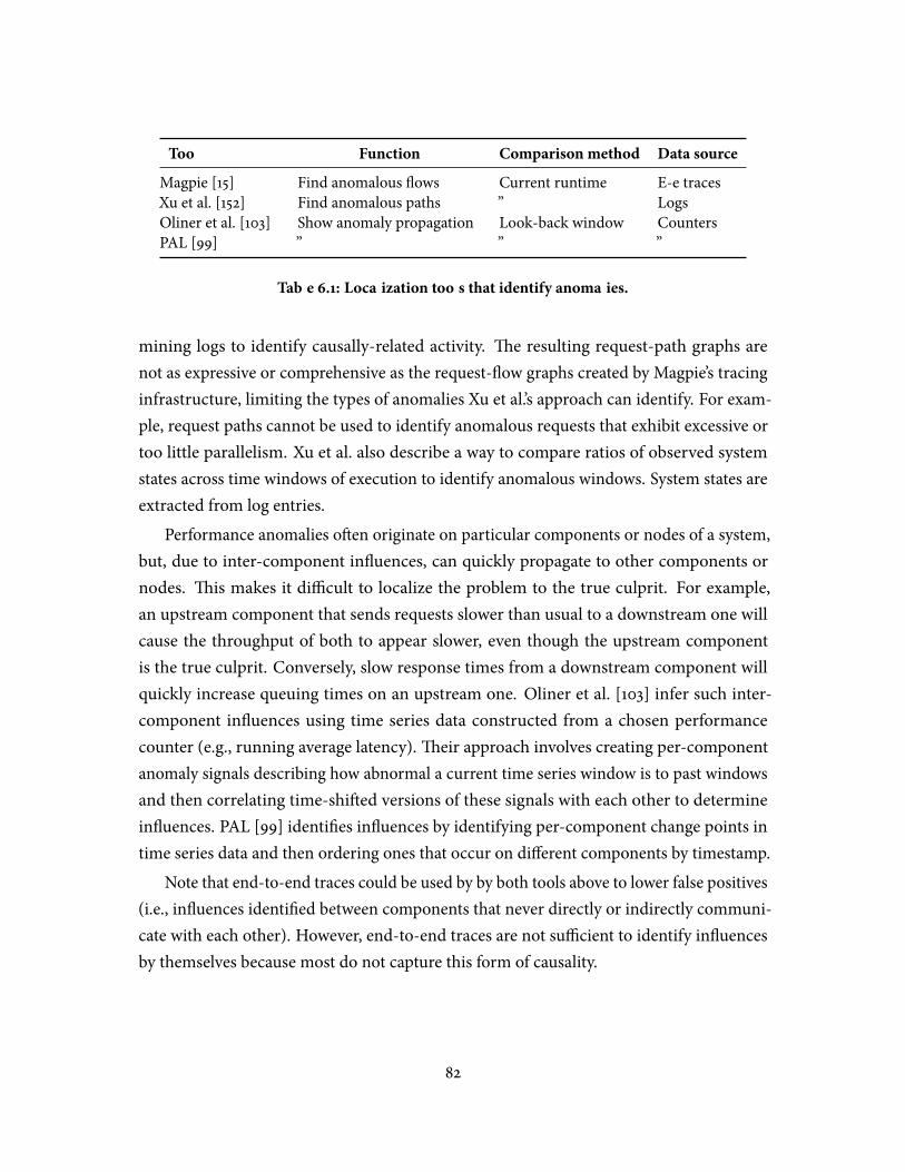
Tool Function Comparison method Data source

Magpie [15] Find anomalous �ows Current runtime E-e tracesXu et al. [152] Find anomalous paths ” LogsOliner et al. [103] Show anomaly propagation Look-back window CountersPAL [99] ” ” ”

Table 6.1: Localization tools that identify anomalies.

mining logs to identify causally-related activity. �e resulting request-path graphs arenot as expressive or comprehensive as the request-�ow graphs created by Magpie’s tracinginfrastructure, limiting the types of anomalies Xu et al.’s approach can identify. For exam-ple, request paths cannot be used to identify anomalous requests that exhibit excessive ortoo little parallelism. Xu et al. also describe a way to compare ratios of observed systemstates across time windows of execution to identify anomalous windows. System states areextracted from log entries.

Performance anomalies o�en originate on particular components or nodes of a system,but, due to inter-component in�uences, can quickly propagate to other components ornodes. �is makes it di�cult to localize the problem to the true culprit. For example,an upstream component that sends requests slower than usual to a downstream one willcause the throughput of both to appear slower, even though the upstream componentis the true culprit. Conversely, slow response times from a downstream component willquickly increase queuing times on an upstream one. Oliner et al. [103] infer such inter-component in�uences using time series data constructed from a chosen performancecounter (e.g., running average latency).�eir approach involves creating per-componentanomaly signals describing how abnormal a current time series window is to past windowsand then correlating time-shi�ed versions of these signals with each other to determinein�uences. PAL [99] identi�es in�uences by identifying per-component change points intime series data and then ordering ones that occur on di�erent components by timestamp.

Note that end-to-end traces could be used by by both tools above to lower false positives(i.e., in�uences identi�ed between components that never directly or indirectly communi-cate with each other). However, end-to-end traces are not su�cient to identify in�uencesby themselves because most do not capture this form of causality.

82

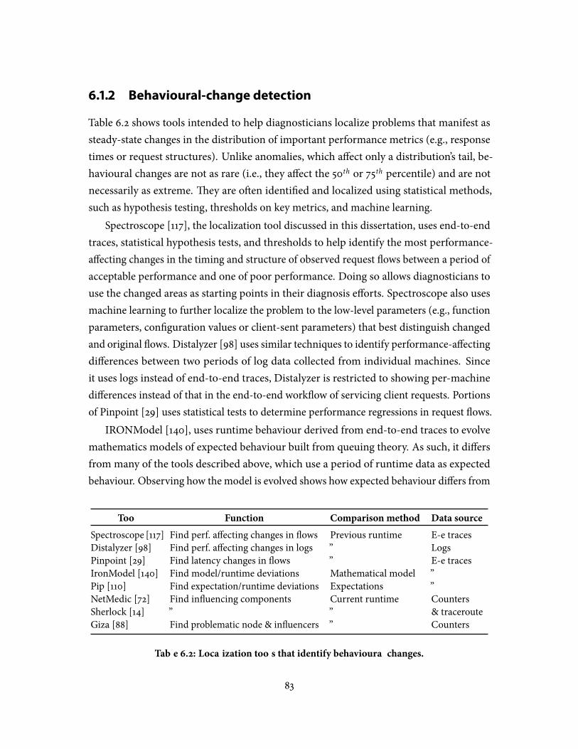
6.1.2 Behavioural-change detection

Table 6.2 shows tools intended to help diagnosticians localize problems that manifest assteady-state changes in the distribution of important performance metrics (e.g., responsetimes or request structures). Unlike anomalies, which a�ect only a distribution’s tail, be-havioural changes are not as rare (i.e., they a�ect the 50th or 75th percentile) and are notnecessarily as extreme. �ey are o�en identi�ed and localized using statistical methods,such as hypothesis testing, thresholds on key metrics, and machine learning.

Spectroscope [117], the localization tool discussed in this dissertation, uses end-to-endtraces, statistical hypothesis tests, and thresholds to help identify the most performance-a�ecting changes in the timing and structure of observed request �ows between a period ofacceptable performance and one of poor performance. Doing so allows diagnosticians touse the changed areas as starting points in their diagnosis e�orts. Spectroscope also usesmachine learning to further localize the problem to the low-level parameters (e.g., functionparameters, con�guration values or client-sent parameters) that best distinguish changedand original �ows. Distalyzer [98] uses similar techniques to identify performance-a�ectingdi�erences between two periods of log data collected from individual machines. Sinceit uses logs instead of end-to-end traces, Distalyzer is restricted to showing per-machinedi�erences instead of that in the end-to-end work�ow of servicing client requests. Portionsof Pinpoint [29] uses statistical tests to determine performance regressions in request �ows.

IRONModel [140], uses runtime behaviour derived from end-to-end traces to evolvemathematics models of expected behaviour built from queuing theory. As such, it di�ersfrom many of the tools described above, which use a period of runtime data as expectedbehaviour. Observing how the model is evolved shows how expected behaviour di�ers from

Tool Function Comparison method Data source

Spectroscope [117] Find perf. a�ecting changes in �ows Previous runtime E-e tracesDistalyzer [98] Find perf. a�ecting changes in logs ” LogsPinpoint [29] Find latency changes in �ows ” E-e tracesIronModel [140] Find model/runtime deviations Mathematical model ”Pip [110] Find expectation/runtime deviations Expectations ”NetMedic [72] Find in�uencing components Current runtime CountersSherlock [14] ” ” & tracerouteGiza [88] Find problematic node & in�uencers ” Counters

Table 6.2: Localization tools that identify behavioural changes.

83

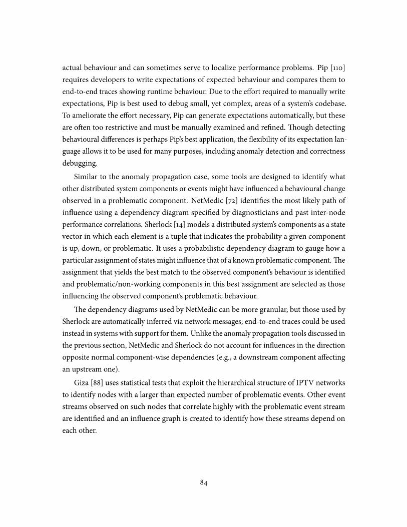
actual behaviour and can sometimes serve to localize performance problems. Pip [110]requires developers to write expectations of expected behaviour and compares them toend-to-end traces showing runtime behaviour. Due to the e�ort required to manually writeexpectations, Pip is best used to debug small, yet complex, areas of a system’s codebase.To ameliorate the e�ort necessary, Pip can generate expectations automatically, but theseare o�en too restrictive and must be manually examined and re�ned. �ough detectingbehavioural di�erences is perhaps Pip’s best application, the �exibility of its expectation lan-guage allows it to be used for many purposes, including anomaly detection and correctnessdebugging.

Similar to the anomaly propagation case, some tools are designed to identify whatother distributed system components or events might have in�uenced a behavioural changeobserved in a problematic component. NetMedic [72] identi�es the most likely path ofin�uence using a dependency diagram speci�ed by diagnosticians and past inter-nodeperformance correlations. Sherlock [14] models a distributed system’s components as a statevector in which each element is a tuple that indicates the probability a given componentis up, down, or problematic. It uses a probabilistic dependency diagram to gauge how aparticular assignment of statesmight in�uence that of a known problematic component.�eassignment that yields the best match to the observed component’s behaviour is identi�edand problematic/non-working components in this best assignment are selected as thosein�uencing the observed component’s problematic behaviour.

�e dependency diagrams used by NetMedic can be more granular, but those used bySherlock are automatically inferred via network messages; end-to-end traces could be usedinstead in systemswith support for them. Unlike the anomaly propagation tools discussed inthe previous section, NetMedic and Sherlock do not account for in�uences in the directionopposite normal component-wise dependencies (e.g., a downstream component a�ectingan upstream one).

Giza [88] uses statistical tests that exploit the hierarchical structure of IPTV networksto identify nodes with a larger than expected number of problematic events. Other eventstreams observed on such nodes that correlate highly with the problematic event streamare identi�ed and an in�uence graph is created to identify how these streams depend oneach other.

84

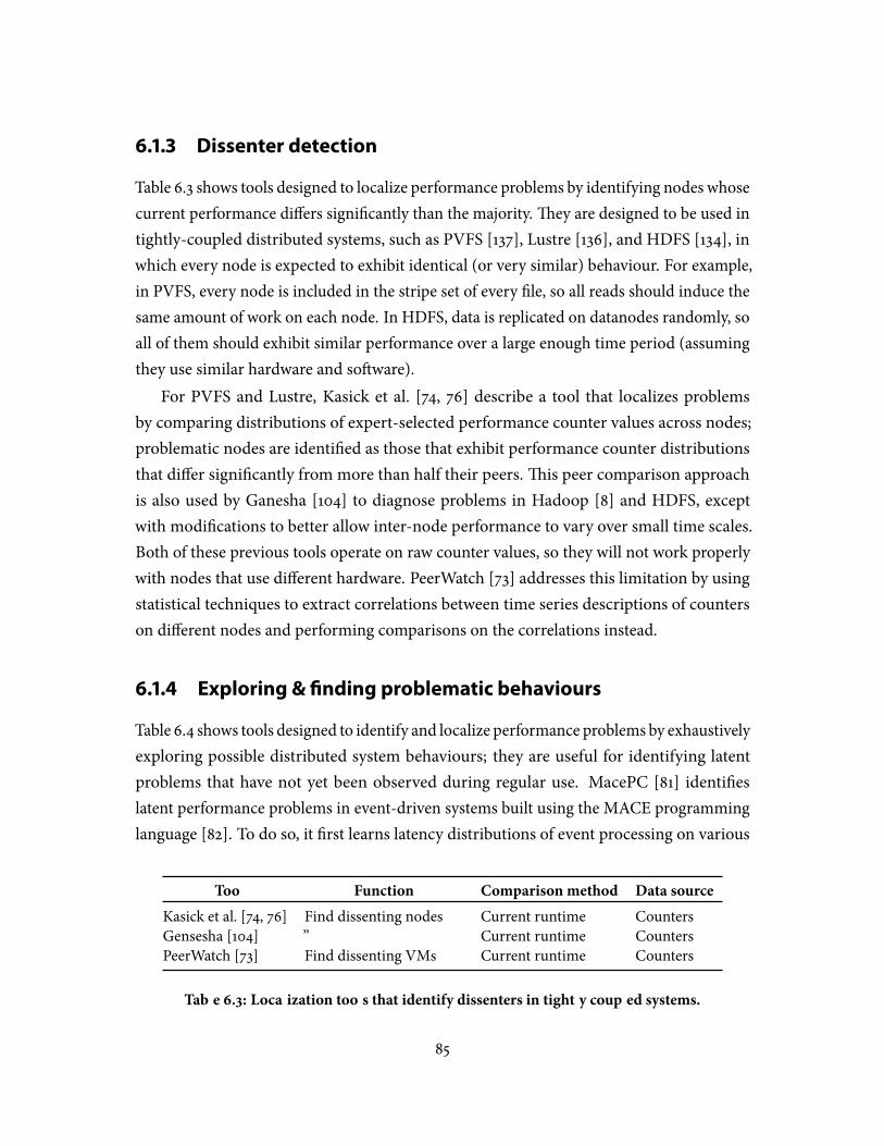
6.1.3 Dissenter detection

Table 6.3 shows tools designed to localize performance problems by identifying nodes whosecurrent performance di�ers signi�cantly than the majority.�ey are designed to be used intightly-coupled distributed systems, such as PVFS [137], Lustre [136], and HDFS [134], inwhich every node is expected to exhibit identical (or very similar) behaviour. For example,in PVFS, every node is included in the stripe set of every �le, so all reads should induce thesame amount of work on each node. In HDFS, data is replicated on datanodes randomly, soall of them should exhibit similar performance over a large enough time period (assumingthey use similar hardware and so�ware).

For PVFS and Lustre, Kasick et al. [74, 76] describe a tool that localizes problemsby comparing distributions of expert-selected performance counter values across nodes;problematic nodes are identi�ed as those that exhibit performance counter distributionsthat di�er signi�cantly from more than half their peers.�is peer comparison approachis also used by Ganesha [104] to diagnose problems in Hadoop [8] and HDFS, exceptwith modi�cations to better allow inter-node performance to vary over small time scales.Both of these previous tools operate on raw counter values, so they will not work properlywith nodes that use di�erent hardware. PeerWatch [73] addresses this limitation by usingstatistical techniques to extract correlations between time series descriptions of counterson di�erent nodes and performing comparisons on the correlations instead.

6.1.4 Exploring & ®nding problematic behaviours

Table 6.4 shows tools designed to identify and localize performance problems by exhaustivelyexploring possible distributed system behaviours; they are useful for identifying latentproblems that have not yet been observed during regular use. MacePC [81] identi�eslatent performance problems in event-driven systems built using the MACE programminglanguage [82]. To do so, it �rst learns latency distributions of event processing on various

Tool Function Comparison method Data source

Kasick et al. [74, 76] Find dissenting nodes Current runtime CountersGensesha [104] ” Current runtime CountersPeerWatch [73] Find dissenting VMs Current runtime Counters

Table 6.3: Localization tools that identify dissenters in tightly coupled systems.

85

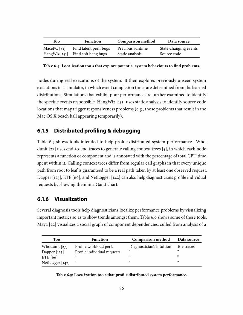
Tool Function Comparison method Data source

MacePC [81] Find latent perf. bugs Previous runtime State-changing eventsHangWiz [151] Find so� hang bugs Static analysis Source code

Table 6.4: Localization tools that explore potential system behaviours to �nd problems.

nodes during real executions of the system. It then explores previously unseen systemexecutions in a simulator, in which event completion times are determined from the learneddistributions. Simulations that exhibit poor performance are further examined to identifythe speci�c events responsible. HangWiz [151] uses static analysis to identify source codelocations that may trigger responsiveness problems (e.g., those problems that result in theMac OS X beach ball appearing temporarily).

6.1.5 Distributed pro®ling & debugging

Table 6.5 shows tools intended to help pro�le distributed system performance. Who-dunit [27] uses end-to-end traces to generate calling context trees [5], in which each noderepresents a function or component and is annotated with the percentage of total CPU timespent within it. Calling context trees di�er from regular call graphs in that every uniquepath from root to leaf is guaranteed to be a real path taken by at least one observed request.Dapper [125], ETE [66], and NetLogger [142] can also help diagnosticians pro�le individualrequests by showing them in a Gantt chart.

6.1.6 Visualization

Several diagnosis tools help diagnosticians localize performance problems by visualizingimportant metrics so as to show trends amongst them; Table 6.6 shows some of these tools.Maya [22] visualizes a social graph of component dependencies, culled from analysis of a

Tool Function Comparison method Data source

Whodunit [27] Pro�le workload perf. Diagnostician’s intuition E-e tracesDapper [125] Pro�le individual requests ” ”ETE [66] ” ” ”NetLogger [142] ” ” ”

Table 6.5: Localization tools that pro�le distributed system performance.

86

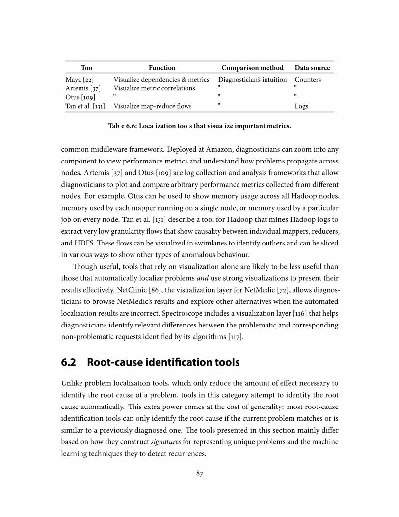
Tool Function Comparison method Data source

Maya [22] Visualize dependencies & metrics Diagnostician’s intuition CountersArtemis [37] Visualize metric correlations ” ”Otus [109] ” ” ”Tan et al. [131] Visualize map-reduce �ows ” Logs

Table 6.6: Localization tools that visualize important metrics.

common middleware framework. Deployed at Amazon, diagnosticians can zoom into anycomponent to view performance metrics and understand how problems propagate acrossnodes. Artemis [37] and Otus [109] are log collection and analysis frameworks that allowdiagnosticians to plot and compare arbitrary performance metrics collected from di�erentnodes. For example, Otus can be used to show memory usage across all Hadoop nodes,memory used by each mapper running on a single node, or memory used by a particularjob on every node. Tan et al. [131] describe a tool for Hadoop that mines Hadoop logs toextract very low granularity �ows that show causality between individual mappers, reducers,and HDFS.�ese �ows can be visualized in swimlanes to identify outliers and can be slicedin various ways to show other types of anomalous behaviour.

�ough useful, tools that rely on visualization alone are likely to be less useful thanthose that automatically localize problems and use strong visualizations to present theirresults e�ectively. NetClinic [86], the visualization layer for NetMedic [72], allows diagnos-ticians to browse NetMedic’s results and explore other alternatives when the automatedlocalization results are incorrect. Spectroscope includes a visualization layer [116] that helpsdiagnosticians identify relevant di�erences between the problematic and correspondingnon-problematic requests identi�ed by its algorithms [117].

6.2 Root-cause identi®cation tools

Unlike problem localization tools, which only reduce the amount of e�ect necessary toidentify the root cause of a problem, tools in this category attempt to identify the rootcause automatically. �is extra power comes at the cost of generality: most root-causeidenti�cation tools can only identify the root cause if the current problem matches or issimilar to a previously diagnosed one. �e tools presented in this section mainly di�erbased on how they construct signatures for representing unique problems and the machinelearning techniques they to detect recurrences.

87

SLIC [35] constructs signatures of past problems using bit vectors in which the ith

element indicates whether some observed performance counter’s running average valuewas more likely to come from a period of service-level objective violation or compliance.Probabilities are learned from past behaviour using a tree-augmented Bayesian network [34].Since the same problemmay manifest as many similar, yet distinct signatures, unsupervisedclustering is used to group similar signatures and a new problem is identi�ed as a recurrenceof the cluster to which it is assigned. Bodik et al. [23] improve upon SLIC’s technique byusing more robust data (e.g., quantiles instead of averages) and more e�ective machinelearning techniques. Finally, instead of using performance counters, Yuan et al. [153] usesignatures constructed from n-grams of system-call invocations observed during a problemoccurrence. Support vector machines, each trained to detect whether a new signature isrepresentative of a previously observed problem, are used to detect recurrences.

6.3 Problem-recti®cation tools

A small number of tools explore how to automatically take corrective actions to �x anobserved problem. For example, Autopilot [59, 70] uses data from past automated actionsto compute a survivor function describing how long a failed machine or device will lastgiven a certain recovery action is performed. Given a desired survival time, it picks the bestaction and performs it. Only simple recovery actions, such as rebooting or re-imaging areconsidered. Netprints [2] crowdsources problem instances and network con�guration dataand uses both to create regression trees that identify potential �xes for a given problem. Ifpossible, these �xes are applied automatically.

6.4 Performance-optimization tools

Many of the tools described in the previous section are meant to be used to �x an observedproblem. Some tools help developers understand how to improve performance even whenno overt problem has been identi�ed. “What-if analysis” [132, 138, 139, 141] allows developersto explore the e�ect on performance of con�guration changes (e.g., “What would theresponse time be if I upgraded the hard disks on one server?”). Where many of these toolsuse mathematical models derived from queuing theory [138, 141], WISE [132], designedto answer what-if questions about large-scale CDNs, eschews models derived from �rstprinciples for easier to specify ones derived from machine learning. Another class of tools

88

allows users to explore con�guration changes in sandboxed environments [156] or viaspeculative execution that can be rolled back [13]. Note that the pro�ling tools, discussed inSection 6.1.5, could also be included in this category.

6.5 Single-process tools

�ere are also many single-process diagnosis tools that inform diagnosis techniques fordistributed systems. For example, conceptually similar to Spectroscope [117], OptiScope [96]compares the code transformations made by di�erent compilers to help developers identifyimportant performance-a�ecting di�erences. Delta analysis [145] compares multiple failingand non-failing runs to identify di�erences responsible for failures.�e tool described byShen et al. [122] compares two executions of Linux workloads using statistical techniquesto identify unexpected performance changes. In another paper, Shen et al. [123] describe atool that identi�es performance problems in I/O subsystems by comparing an analyticalmodel of the subsystem to observed runtime behaviour. DARC [144] creates histograms ofLinux system call latencies and automatically pro�les selected peaks to identify the mostdominant latency contributors.

89

90

Chapter 7

Systemizing end-to-end tracingknowledge

�is dissertation focuses primarily on request-�ow comparison, a diagnosis techniquethat uses end-to-end traces as its data source. However, in the process of developing andevaluating this technique, I had to design, engineer, and maintain two of the most well-known tracing infrastructures (i.e., Stardust [117, 141] and the version of X-Trace [47] Iused for my HDFS explorations [150]). I also worked on Google’s end-to-end tracinginfrastructure, Dapper [125], in the context of building Spectroscope [117] and other toolsas extensions to it.�ese experiences have given me considerable insight into end-to-endtracing.

Most notably, I have learned that end-to-end tracing is not a one-size-�ts-all solution.For example, when developing Spectroscope, my collaborators and I initially thought thatthe original version of Stardust [141], which had been designed for resource attribution (i.e.,to charge work done deep in the distributed system to the client responsible for submittingit), would also be useful for diagnosis. However, I quickly found that the traces it yieldedwere of little value for most diagnosis tasks, leadingme to create a revised version of Stardustuseful speci�cally for diagnosis [117]. More generally, I have found that key design axesdictate a tracing infrastructure’s utility for each of the various use cases generally attributedto end-to-end tracing. Since e�ciency concerns make it impractical to support all use cases,designers of a tracing infrastructure must be careful to choose options for these axes thatare best suited to the infrastructure’s intended purposes. Otherwise, it will fail to satisfyexpectations.

Unfortunately, despite the strong interest in end-to-end tracing from both the researchcommunity [3, 15, 27, 29, 47, 48, 66, 78, 110, 111, 117, 130, 131, 141, 142, 152] and industry [36,

91

125, 143, 147], there exists little information to help designers make informed choices aboutend-to-end tracing’s design axes. Since these axes are not well understand, somewell-knowntracing infrastructures have indeed failed to live up to expectations.

�is dissertation chapter seeks to help. Based on my experiences and the previousten years of research on end-to-end tracing, it distills the key design axes and explainstrade-o�s associated with the options for each. Beyond describing the degrees of freedom, itsuggests speci�c design points for each of several key tracing use cases and identi�es whichprevious tracing infrastructures do and do not match up. Overall, I believe this chapterrepresents the �rst attempt to bring together a coherent view of the range of end-to-endtracing implementations and provide system designers a roadmap for integrating it.

�e remainder of this chapter is organized as follows. Section 7.1 discusses use cases forand the basic anatomy of end-to-end tracing. Sections 7.2 to 7.5 describe key design axes andtradeo�s for them.�ese axes include the sampling strategy, which causal relationships arecaptured, how causal relationships are tracked, and how end-to-end traces are visualized.Section 7.6 applies these insights to suggest speci�c design choices for each of severaluse cases. It also compares my suggestions to that of existing tracing infrastructures toshow where prior infrastructures fall short. Section 7.7 discusses some challenges andopportunities that remain in realizing the full potential of end-to-end tracing, and Section 7.8concludes.

7.1 Background

�is section describes relevant background about end-to-end tracing. Section 7.1.1 describesits key use cases from the literature. Section 7.1.2 lists the three commonly used approachesto end-to-end tracing, and Section 7.1.3 describes the architecture of the approach advocatedin this paper.

7.1.1 Use cases

Table 7.1 summarizes the key use cases of end-to-end tracing.�ey are described below.Anomaly detection:�is diagnosis-related use case involves detecting rare �ows that

incur signi�cant latency and/or have extremely di�erent structures than other �ows andunderstanding why they occur. Anomalies may be related to correctness (e.g., timeouts orcomponent failures) or performance (e.g., slow requests that fall in the 99.9th percentileof observed response times). Magpie [15] identi�es both types by �nding requests that

92

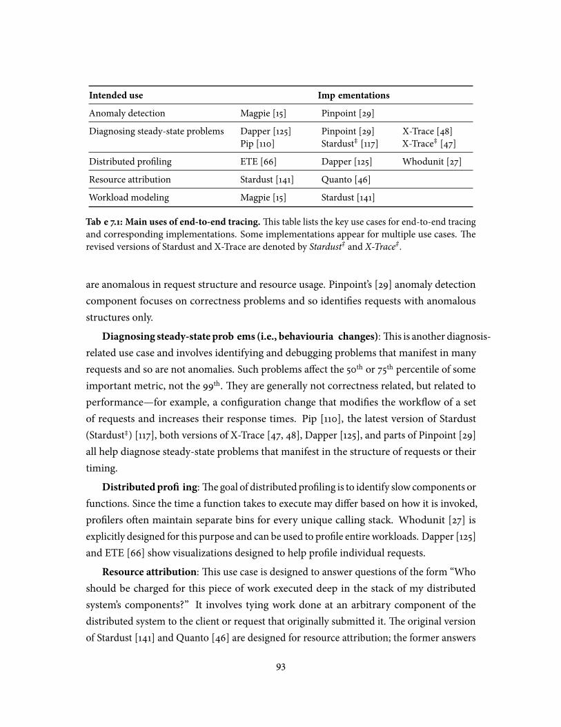
Intended use Implementations

Anomaly detection Magpie [15] Pinpoint [29]

Diagnosing steady-state problems Dapper [125]Pip [110]

Pinpoint [29]Stardust‡ [117]

X-Trace [48]X-Trace‡ [47]

Distributed pro�ling ETE [66] Dapper [125] Whodunit [27]

Resource attribution Stardust [141] Quanto [46]

Workload modeling Magpie [15] Stardust [141]

Table 7.1: Main uses of end-to-end tracing.�is table lists the key use cases for end-to-end tracingand corresponding implementations. Some implementations appear for multiple use cases. �erevised versions of Stardust and X-Trace are denoted by Stardust‡ and X-Trace‡.

are anomalous in request structure and resource usage. Pinpoint’s [29] anomaly detectioncomponent focuses on correctness problems and so identi�es requests with anomalousstructures only.

Diagnosing steady-state problems (i.e., behaviourial changes):�is is another diagnosis-related use case and involves identifying and debugging problems that manifest in manyrequests and so are not anomalies. Such problems a�ect the 50th or 75th percentile of someimportant metric, not the 99th. �ey are generally not correctness related, but related toperformance—for example, a con�guration change that modi�es the work�ow of a setof requests and increases their response times. Pip [110], the latest version of Stardust(Stardust‡) [117], both versions of X-Trace [47, 48], Dapper [125], and parts of Pinpoint [29]all help diagnose steady-state problems that manifest in the structure of requests or theirtiming.

Distributedpro�ling:�e goal of distributed pro�ling is to identify slow components orfunctions. Since the time a function takes to execute may di�er based on how it is invoked,pro�lers o�en maintain separate bins for every unique calling stack. Whodunit [27] isexplicitly designed for this purpose and can be used to pro�le entire workloads. Dapper [125]and ETE [66] show visualizations designed to help pro�le individual requests.

Resource attribution:�is use case is designed to answer questions of the form “Whoshould be charged for this piece of work executed deep in the stack of my distributedsystem’s components?” It involves tying work done at an arbitrary component of thedistributed system to the client or request that originally submitted it.�e original versionof Stardust [141] and Quanto [46] are designed for resource attribution; the former answers

93

“what-if ” questions (e.g., “What would happen to the performance of workload A if Ireplaced the CPU on a certain distributed system component with a faster one?”) and thelatter tracks energy usage in distributed embedded systems. Note that resource attribution-based tracing can be especially useful for accounting and billing purposes, especially indistributed services shared by many clients, such as HDFS or Amazon’s EC2 [149].

Workload modeling: End-to-end tracing can also be used to model workloads. Forexample, Magpie [15] clusters its traces to identify those that are representative of the entireworkload. Stardust [141] can be used to create queuing models that served to answer its“what-if ” analyses.

7.1.2 Approaches to end-to-end tracing

Most end-to-end tracing infrastructures use one of three approaches to identify causally-related �ows: metadata propagation, schemas, or black-box inference.�is paper focuseson design decisions for tracing infrastructures that use the �rst, as they are more scalableand produce more accurate traces than those that use the other two. However, many of myanalyses are also applicable to the other approaches.

Metadata propagation: Like security, end-to-end tracingworks best when it is designedas part of the distributed system. As such, many implementations are designed for usewith white-box systems, for which the distributed system’s components can be modi�ed topropagate metadata (e.g., an ID) delineating causally-related �ows [27, 29, 46, 47, 48, 110,117, 125, 141]. All of them identify causality between individual functions or trace points,which resemble log messages and record the fact that a �ow reached a particular pointin the system. However, Dapper [125] chooses to emphasize causality between individualRPCs. To keep runtime overhead (e.g., slowdown in response time and throughput) to aminimum so that tracing can be “always on,” most tracing infrastructures in this categoryuse sampling to collect only a small number of trace points or �ows.

Schema-based: A few implementations, such as ETE [66] and Magpie [15] do not prop-agate metadata, but rather require developers to write temporal join-schemas that establishcausal relationships among variables exposed in individual log messages. Developers mustmodify the distributed system to expose appropriate variables. A temporal join de�nes avalid time interval during which trace-point records that store speci�c identical variablevalues should be considered causally-related. For example, in most systems, a worker threadpulling an item o� of a queue de�nes the start of a valid time interval during which all

94

log messages that store the same thread ID should be considered causally related. Schema-based approaches are not compatible with sampling, since they delay determining whatis causally related until a�er all logs are collected. �erefore, they are less scalable thanmetadata-propagation approaches.

Black-box inference: Several implementations try to create traces for black-box systems—i.e., systems for which source code cannot or will not be modi�ed [3, 21, 78, 83, 111, 130, 131,152]. Some try to infer causality by correlating variables exposed in pre-existing log state-ments [21, 78, 131, 152]. Others use simplifying assumptions. For example, Tak et al. [130]assume synchronous behaviour between components and, within components, that a singleworker thread will be responsible for synchronously performing all work for a given request,including sending/receiving sub-requests and responding to the original client. Aguilera etal. [3] and Reynolds et al. [111] observe only send/receive events between components anduse models of expected delay between causally-related events to infer causality.�ough thepromise of obtaining end-to-end traces without so�ware modi�cation is appealing, theseapproaches cannot properly attribute causality in the face of asynchronous behaviour (e.g.,caching, event-driven systems), concurrency, aggregation, or code-speci�c design patterns(e.g., 2-of-3 storage encodings), all of which are common in distributed systems.

7.1.3 Anatomy of end-to-end tracing

Figure 7.1 shows the anatomy of most end-to-end tracing infrastructures that use metadatapropagation. Two conceptual design choices dictate its functionality and the design of itsphysical components: how to decide what �ows or trace points to sample and what observedcausal relationships to preserve. Section 7.2 describes the tradeo�s between various samplingtechniques, and Section 7.3 describes what causal relationships should be preserved forvarious end-to-end tracing use cases. �e sampling technique used a�ects the types ofcausal relationships that can be preserved with low overhead, so care must be taken tochoose compatible ones.

�e so�ware components of the tracing infrastructure work to implement the chosensampling technique, preserve desired causal relationships, optionally store this information,and create traces.�ey include individual trace points, the causal-tracking mechanism, thestorage component, trace construction code, and the presentation layer.

Individual trace points record locations in the codebase accessed by individual �ows.�ey are o�en embedded in commonly used libraries (e.g., RPC libraries) and manu-

95

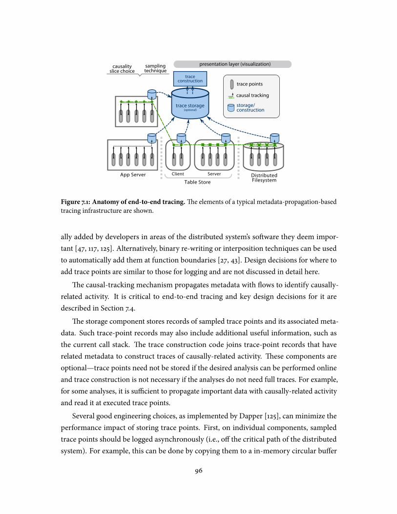
Figure 7.1: Anatomy of end-to-end tracing.�e elements of a typical metadata-propagation-basedtracing infrastructure are shown.

ally added by developers in areas of the distributed system’s so�ware they deem impor-tant [47, 117, 125]. Alternatively, binary re-writing or interposition techniques can be usedto automatically add them at function boundaries [27, 43]. Design decisions for where toadd trace points are similar to those for logging and are not discussed in detail here.

�e causal-tracking mechanism propagates metadata with �ows to identify causally-related activity. It is critical to end-to-end tracing and key design decisions for it aredescribed in Section 7.4.

�e storage component stores records of sampled trace points and its associated meta-data. Such trace-point records may also include additional useful information, such asthe current call stack. �e trace construction code joins trace-point records that haverelated metadata to construct traces of causally-related activity. �ese components areoptional—trace points need not be stored if the desired analysis can be performed onlineand trace construction is not necessary if the analyses do not need full traces. For example,for some analyses, it is su�cient to propagate important data with causally-related activityand read it at executed trace points.

Several good engineering choices, as implemented by Dapper [125], can minimize theperformance impact of storing trace points. First, on individual components, sampledtrace points should be logged asynchronously (i.e., o� the critical path of the distributedsystem). For example, this can be done by copying them to a in-memory circular bu�er

96

(or discarding them if the bu�er is full) and using a separate thread to write trace pointsfrom this bu�er to local disk or to a table store. A map-reduce job can then be used toconstruct traces. Both Stardust [141] and Dapper [125] suggest storing traces for two weeksfor post-hoc analyses before discarding them.

�e �nal aspect of an end-to-end tracing infrastructure is the presentation layer. Itis is responsible for showing constructed traces to users and is important for diagnosis-related tasks. Various ways to visualize traces and tradeo�s between them are discussed inSection 7.5.

7.2 Sampling techniques

Sampling determines what trace points are collected by the tracing infrastructure. It isthe most important technique used by end-to-end tracing infrastructures to limit runtimeand storage overhead [27, 47, 117, 125, 141]. For example, even though Dapper writes tracepoints records to stable storage asynchronously (i.e., o� the critical path of the distributedsystem), it still imposes a 1.5% throughput and 16% response time overhead when capturingall trace points executed by a web search workload [125]. When using sampling to capturejust 0.01% of all trace points, the slowdown in response times is reduced to 0.20% and inthroughput to 0.06% [125]. Even when trace points need not be stored because the requiredanalyses can be performed online, sampling is useful to limit the sizes of analysis-speci�cdata structures [27].

�ere are three commonly-used options with regards to deciding what trace pointsto sample.�e �rst two are necessary if traces showing causally-related activity are to beconstructed.

Head-based coherent sampling: In order to construct a trace of causally-related activity,all trace points executed on its behalf must be sampled. Coherent sampling satis�es thisrequirement by sampling all or none of the trace points executed on behalf of a �ow.With head-based sampling, the decision to collect a �ow is made at its start (e.g., when arequest enters the system) and metadata is propagated along with the the �ow indicatingwhether to collect its trace points. �is method of coherent sampling is used by severalimplementations [47, 117, 125]. Using this method to preserve certain causality slices willresult in high overheads (see Section 7.3).

Tail-based coherent sampling:�is method is similar to the previous one, except thatthe sampling decision is made at the end of causally-related �ows, instead of at their start.

97

Delaying the sampling decision allows for more intelligent sampling—for example, thetracing infrastructure can examine a �ow’s properties (e.g., response time) and chooseonly to collect anomalous ones. But, trace point records for every �ow must be cachedsomewhere until the sampling decision is made for it. Since many requests can executeconcurrently and because each request can execute many trace points, such temporarycollection is not always feasible. Whodunit [27], the only tracing implementation that usestail-based sampling, caches trace points by propagating them as metadata with individual�ows.

Unitary sampling: With this method, the sampling decision is made at the level ofindividual trace points. No attempt is made at coherence (i.e., capturing all trace pointsassociated with a given �ow), so traces cannot be constructed using this approach. �ismethod is best used when coherent sampling is unnecessary or infeasible. For example, forsome use cases, the information needed for analysis can be propagated with casual �owsand retrieved at individual trace points without having to having to construct traces.

In addition to deciding how to sample trace points, developers must decide howmany ofthem to sample. Many infrastructures choose to randomly sample a small, set percentage—o�en between 0.01% and 10%—of trace points or causal �ows [27, 47, 117, 125, 141]. However,this approach will capture only a few trace points for small workloads, limiting its use forthem. Using per-workload sampling percentages can help, but requires knowing workloadsizes a priori. A more robust solution, proposed by Sigelman at al. [125], is an adaptivescheme, in which the tracing infrastructure aims to always capture a set rate of trace pointsor causal �ows (e.g., 500 trace points/second or 100 causal �ows/second) and dynamicallyadjusts the sampling percentage to accomplish this set goal.�ough promising, care mustbe taken to avoid biased results when the captured data is used for statistical purposes. Fordistributed services built on top of shared services, the adaptive sampling rate should bebased on the tracing overhead the lowest-tier shared service can support (e.g., Bigtable [28])and proportionately propagated backward to top-tier services.

7.3 Causal relationship preservation

Since preserving causality is the ultimate goal of end-to-end tracing, the ultimate tracinginfrastructure would preserve all true or necessary causal relationships. It would preservethe work�ow of servicing individual requests and background activities, read a�er writeaccesses to memory, caches, �les, and registers, provenance of stored data, inter-request

98

causal relationships due to resource contention (e.g., for caches) or built-up state, and so on.Lamport’s happens-before relationship (→) [85], states that if a and b are events and a → b,then a may have in�uenced b.�us, b might be causally dependent on a, and capturing allsuch relationships allows one to create a happens-before graph, showing all possible channelsof in�uence.

Unfortunately, the general happens-before graph is not su�cient for two reasons. First,it may be infeasible to capture all possible relations—even the most e�cient so�ware tainttracking mechanisms yield a 2x to 8x slowdown [79]. It may also be impossible to know allpossible channels of in�uence [30]. Second, it is too indiscriminate: in most cases, we areinterested in a stronger, ‘is necessary for’, or ‘cannot happen without’ relationship, whichis a subset of the full happens-before relationship. To help alleviate the �rst issue, tracinginfrastructures o�en ask developers to explicitly instrument parts of the distributed systemthey know to be important. To account for the second, most tracing infrastructures useknowledge about the system to remove spurious edges in the happens-before graph. Forexample, by assuming a memory protection model the system may exclude edges betweenevents in di�erent processes, or even between di�erent events in a single-threaded event-based system. By removing selected edges from this graph, one creates slices of the fullrelation that can be more useful for speci�c purposes. A tracing infrastructure choosesslices that are most useful for how its output will be used and works to preserve them.�issection describes slices that have proven useful for various use cases.

When choosing slices, developers must �rst identify one that de�nes the work�owof a request as it is being serviced by a distributed system. �ough any request will in-duce a certain set of activities that must be performed eventually, latent ones need notbe considered part of its �ow, but rather part of the request that forces that work to beexecuted.�is observation forms the basis for two potential intra-request slices—submitterand trigger preserving—that preserve di�erent information and are useful for di�erent usecases. Section 7.3.1 and Section 7.3.2 describe the tradeo�s involved in preserving these slicesin more detail. Section 7.3.3 lists the advantages of preserving both submitter causality andtrigger causality. Section 7.3.4 discusses the bene�ts of delineating concurrent behaviourfrom sequential behaviour and preserving forks and joins in individual traces. Table 7.2shows intra-request slices most useful for the key uses of end-to-end tracing.

Developers may also want to preserve important dependencies between individualrequests. Two such inter-request slices are discussed in Section 7.3.5.

99

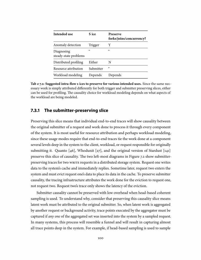
Intended use Slice Preserve

forks/joins/concurrency?

Anomaly detection Trigger Y

Diagnosingsteady-state problems

” ”

Distributed pro�ling Either N

Resource attribution Submitter ”

Workload modeling Depends Depends

Table 7.2: Suggested intra-�ow slices to preserve for various intended uses. Since the same nec-essary work is simply attributed di�erently for both trigger and submitter preserving slices, eithercan be used for pro�ling.�e causality choice for workload modeling depends on what aspects ofthe workload are being modeled.

7.3.1 The submitter-preserving slice

Preserving this slice means that individual end-to-end traces will show causality betweenthe original submitter of a request and work done to process it through every componentof the system. It is most useful for resource attribution and perhaps workload modeling,since these usage modes require that end-to-end traces tie the work done at a componentseveral levels deep in the system to the client, workload, or request responsible for originallysubmitting it. Quanto [46], Whodunit [27], and the original version of Stardust [141]preserve this slice of causality. �e two le�-most diagrams in Figure 7.2 show submitter-preserving traces for twowrite requests in a distributed storage system. Request one writesdata to the system’s cache and immediately replies. Sometime later, request two enters thesystem and must evict request one’s data to place its data in the cache. To preserve submittercausality, the tracing infrastructure attributes the work done for the eviction to request one,not request two. Request two’s trace only shows the latency of the eviction.

Submitter causality cannot be preserved with low overhead when head-based coherentsampling is used. To understand why, consider that preserving this causality slice meanslatent work must be attributed to the original submitter. So, when latent work is aggregatedby another request or background activity, trace points executed by the aggregator must becaptured if any one of the aggregated set was inserted into the system by a sampled request.In many systems, this process will resemble a funnel and will result in capturing almostall trace points deep in the system. For example, if head-based sampling is used to sample

100

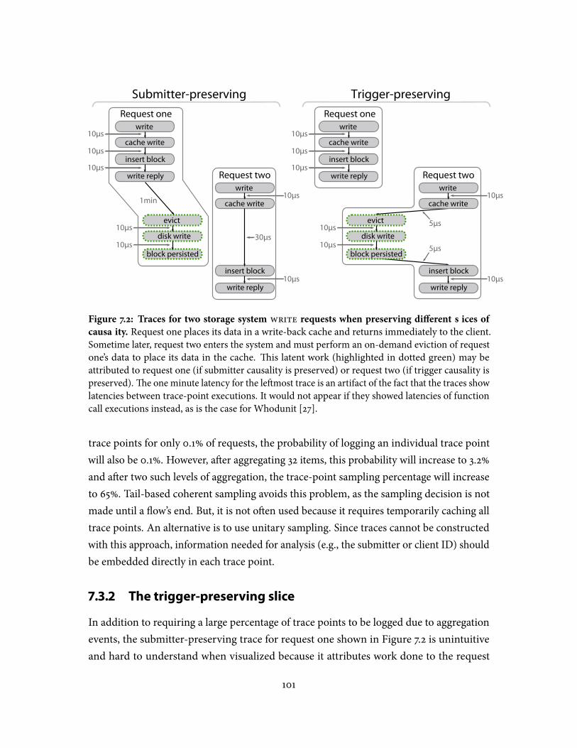
Figure 7.2: Traces for two storage system write requests when preserving di�erent slices of

causality. Request one places its data in a write-back cache and returns immediately to the client.Sometime later, request two enters the system and must perform an on-demand eviction of requestone’s data to place its data in the cache. �is latent work (highlighted in dotted green) may beattributed to request one (if submitter causality is preserved) or request two (if trigger causality ispreserved).�e one minute latency for the le�most trace is an artifact of the fact that the traces showlatencies between trace-point executions. It would not appear if they showed latencies of functioncall executions instead, as is the case for Whodunit [27].

trace points for only 0.1% of requests, the probability of logging an individual trace pointwill also be 0.1%. However, a�er aggregating 32 items, this probability will increase to 3.2%and a�er two such levels of aggregation, the trace-point sampling percentage will increaseto 65%. Tail-based coherent sampling avoids this problem, as the sampling decision is notmade until a �ow’s end. But, it is not o�en used because it requires temporarily caching alltrace points. An alternative is to use unitary sampling. Since traces cannot be constructedwith this approach, information needed for analysis (e.g., the submitter or client ID) shouldbe embedded directly in each trace point.

7.3.2 The trigger-preserving slice

In addition to requiring a large percentage of trace points to be logged due to aggregationevents, the submitter-preserving trace for request one shown in Figure 7.2 is unintuitiveand hard to understand when visualized because it attributes work done to the request

101

a�er the client reply has been sent. Also, latent work attributed to this request (i.e., tracepoints executed a�er the reply is sent) is performed in the critical path of request two. Incontrast, trigger causality guarantees that a trace of a request will show all work that mustbe performed before a client response can be sent, including another client’s latent workif it is in its critical path.�e right two traces in Figure 7.2 show the same two requests asin the submitter-preserving example, with trigger causality preserved instead. Since thesetraces are easier to understand when visualized (they always end with a client reply) andalways show all work done on requests’ critical paths, trigger causality should be preservedfor diagnosis tasks, which o�en involve answering questions of the form “Why is thisrequest so slow?” Indeed, trigger causality is explicitly preserved by the revised versionof Stardust [117]. Since it takes less e�ort to preserve than submitter causality, many othertracing implementations implicitly preserve this slice of causality [15, 29, 47, 110, 125]. Triggercausality can be used with head-based coherent sampling without in�ating the trace-pointsampling percentage, since only the sampling decision made for the request that forceslatent work to be executed determines whether trace points a�er aggregation points aresampled.

7.3.3 Is anything gained by preserving both?

�e slices suggested above are the most important ones that should be preserved for varioususe cases, not the only ones that should be preserved. Indeed, preserving both submittercausality and trigger causality will enable a deeper understanding of the distributed systemthan what is possible by preserving only one of them. For example, for diagnosis, preservingsubmitter causality in addition to trigger causality will allow the tracing infrastructure toanswer questions such as “Who was responsible for evicting my client’s cached data?” or,more generally, “Which clients tend to interfere with each other most?”

7.3.4 Preserving concurrency, forks, and joins

For both submitter-preserving causality and trigger-preserving causality, delineating con-current activity from sequential activity and preserving forks and joins is optional. Doingso o�en requires more e�ort on the part of developers (e.g., �nding forks and joins in thesystem and instrumenting them) and additional metadata, but enables developers to viewactual request structure, and diagnose problems that arise as a result of excessive paral-lelism, not enough parallelism, or excessive waiting at synchronization points. It also allows

102

for easier automated critical-path identi�cation. As such, diagnosis tasks bene�t greatlyfrom preserving these causal relationships.�e revised versions of both Stardust [117] andX-Trace [47] explicitly delineate concurrency and explicitly identify forks and joins. Forother use cases, such as pro�ling and resource attribution, delineating concurrency is notnecessary, and most pro�lers (including Whodunit [27] and gprof [58]) do not do so.

7.3.5 Preserving inter-request slices

In addition to relationships within a request, many types of causal relationships may existbetween requests.�is section describes the two most common ones.

�e contention-preserving slice: Requests may compete with each other for resources,such as access to a shared variable. Preserving causality between requests holding a resourcelock and those waiting for it can help explain unexpected performance slowdowns ortimeouts. Only Whodunit [27] preserves this slice.

�e read a�er write-preserving slice: Requests that read data (e.g., from a cache or�le) written by others may be causally a�ected by the contents. For example, a request thatperforms work dictated by the contents of a �le—e.g., a map-reduce job [40]—may dependon that �le’s original writer. Preserving read-a�er-write dependencies can help explain suchrequests’ behaviour.

7.4 Causal tracking

All end-to-end tracing infrastructures must employ a mechanism to track the slices ofintra-request and inter-request causality most relevant to their intended use cases. Toavoid capturing super�uous relationships, tracing infrastructures “thread” metadata alongwith individual �ows and establish happens-before relationships only to items with thesame (or related) metadata [27, 29, 47, 48, 110, 117, 125, 141, 142]. Section 7.4.1 describesdi�erent options for what to propagate as metadata and tradeo�s between them. In general,metadata can be propagated by storing them in thread-local variables when a single threadis performing causally-related work and encoding logic to propagate metadata acrossboundaries (e.g., across threads or components) in commonly used libraries.

�ough any of the approaches discussed below can preserve concurrency by establishinghappens-before relationships, additional instrumentation is needed to capture forks andjoins, which are needed to properly order concurrency-related causal relationships. Forexample, if joins are not preserved, a trace point may erroneously be deemed causally

103

dependent on the last thread to synchronize, rather than on multiple concurrent activities.Section 7.4.2 further discusses how to preserve forks and joins.

7.4.1 What to propagate as metadata?

Most tracing infrastructures propagate one of the options listed below. �ey di�er insize, whether they are �xed or variable width, and how they establish happens-beforerelationships to order causally-related activity and distinguish concurrent behaviour fromsequential behaviour. Perhaps surprisingly, all of them are equivalent in functionality, exceptfor the case of event-based systems, for which mutable breadcrumbs are needed.

An immutable, �xed-width trace ID (TID):�e trace ID identi�es causally-relatedwork and could be a unique value chosen at the start of such activity (e.g., when a requestis received or at the start of background activity). Tracing implementations that use thismethod must rely on visible clues to establish happens-before relationships between tracepoints. For example, since network messages must always be sent by a client before beingreceived by a server, tracing infrastructures that do not rely on synchronized clocks mightestablish happens-before relationships between client and server work using network sendand receive trace points on bothmachines. Similarly, to order causally-related activity withina single thread, they must rely on an external clock. To identify concurrent work withincomponents, they might establish happens-before relationship via thread IDs. Pip [110],Pinpoint [29], and Quanto [46] use an immutable �xed-width trace ID as metadata.

An immutable �xed-width trace ID and a mutable, �xed-width breadcrumb (TID

& BC): Like the previous method, the trace ID allows all causally-related activity to beidenti�ed and quickly extracted. Instead of relying on external clues or trace points, mutablebreadcrumbs are used to encode happens-before relationships. For example, to show that agiven trace point occurs a�er another, the latter will be assigned a new breadcrumb anda happens-before relationship will be created between it and the previous trace point’sbreadcrumb. Similarly, when sending an RPC, the tracing infrastructure will assign theserver a di�erent breadcrumb than the client and establish “client breadcrumb happensbefore server breadcrumb.” In contrast to the previous approach, this metadata-propagationapproach relies less on externally observable clues. For example, if thread IDs are not visible,the previous approach might not be able to identify concurrent activity within a component.Also, mutable breadcrumbs are needed to identify di�erent causally-related �ows �owsin event-based systems, in which a single thread performs all work. Both versions of X-

104

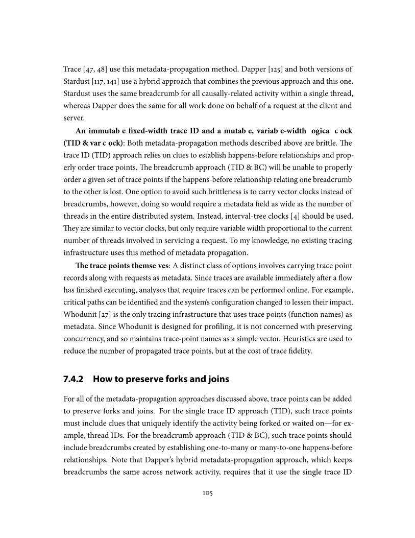
Trace [47, 48] use this metadata-propagation method. Dapper [125] and both versions ofStardust [117, 141] use a hybrid approach that combines the previous approach and this one.Stardust uses the same breadcrumb for all causally-related activity within a single thread,whereas Dapper does the same for all work done on behalf of a request at the client andserver.

An immutable �xed-width trace ID and a mutable, variable-width logical clock

(TID & var clock): Both metadata-propagation methods described above are brittle.�etrace ID (TID) approach relies on clues to establish happens-before relationships and prop-erly order trace points.�e breadcrumb approach (TID & BC) will be unable to properlyorder a given set of trace points if the happens-before relationship relating one breadcrumbto the other is lost. One option to avoid such brittleness is to carry vector clocks instead ofbreadcrumbs, however, doing so would require a metadata �eld as wide as the number ofthreads in the entire distributed system. Instead, interval-tree clocks [4] should be used.�ey are similar to vector clocks, but only require variable width proportional to the currentnumber of threads involved in servicing a request. To my knowledge, no existing tracinginfrastructure uses this method of metadata propagation.

�e trace points themselves: A distinct class of options involves carrying trace pointrecords along with requests as metadata. Since traces are available immediately a�er a �owhas �nished executing, analyses that require traces can be performed online. For example,critical paths can be identi�ed and the system’s con�guration changed to lessen their impact.Whodunit [27] is the only tracing infrastructure that uses trace points (function names) asmetadata. Since Whodunit is designed for pro�ling, it is not concerned with preservingconcurrency, and so maintains trace-point names as a simple vector. Heuristics are used toreduce the number of propagated trace points, but at the cost of trace �delity.

7.4.2 How to preserve forks and joins

For all of the metadata-propagation approaches discussed above, trace points can be addedto preserve forks and joins. For the single trace ID approach (TID), such trace pointsmust include clues that uniquely identify the activity being forked or waited on—for ex-ample, thread IDs. For the breadcrumb approach (TID & BC), such trace points shouldinclude breadcrumbs created by establishing one-to-many or many-to-one happens-beforerelationships. Note that Dapper’s hybrid metadata-propagation approach, which keepsbreadcrumbs the same across network activity, requires that it use the single trace ID

105

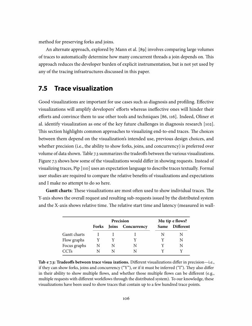
method for preserving forks and joins.An alternate approach, explored by Mann et al. [89] involves comparing large volumes

of traces to automatically determine how many concurrent threads a join depends on.�isapproach reduces the developer burden of explicit instrumentation, but is not yet used byany of the tracing infrastructures discussed in this paper.

7.5 Trace visualization

Good visualizations are important for use cases such as diagnosis and pro�ling. E�ectivevisualizations will amplify developers’ e�orts whereas ine�ective ones will hinder theire�orts and convince them to use other tools and techniques [86, 116]. Indeed, Oliner etal. identify visualization as one of the key future challenges in diagnosis research [102].�is section highlights common approaches to visualizing end-to-end traces.�e choicesbetween them depend on the visualization’s intended use, previous design choices, andwhether precision (i.e., the ability to show forks, joins, and concurrency) is preferred overvolume of data shown. Table 7.3 summarizes the tradeo�s between the various visualizations.Figure 7.3 shows how some of the visualizations would di�er in showing requests. Instead ofvisualizing traces, Pip [110] uses an expectation language to describe traces textually. Formaluser studies are required to compare the relative bene�ts of visualizations and expectationsand I make no attempt to do so here.

Gantt charts:�ese visualizations are most o�en used to show individual traces.�eY-axis shows the overall request and resulting sub-requests issued by the distributed systemand the X-axis shows relative time.�e relative start time and latency (measured in wall-

Precision Multiple �ows?

Forks Joins Concurrency Same Di�erent

Gantt charts I I I N NFlow graphs Y Y Y Y NFocus graphs N N N Y NCCTs N N N Y Y

Table 7.3: Tradeo�s between trace visualizations. Di�erent visualizations di�er in precision—i.e.,if they can show forks, joins and concurrency (“Y”), or if it must be inferred (“I”).�ey also di�erin their ability to show multiple �ows, and whether those multiple �ows can be di�erent (e.g.,multiple requests with di�erent work�ows through the distributed system). To our knowledge, thesevisualizations have been used to show traces that contain up to a few hundred trace points.

106

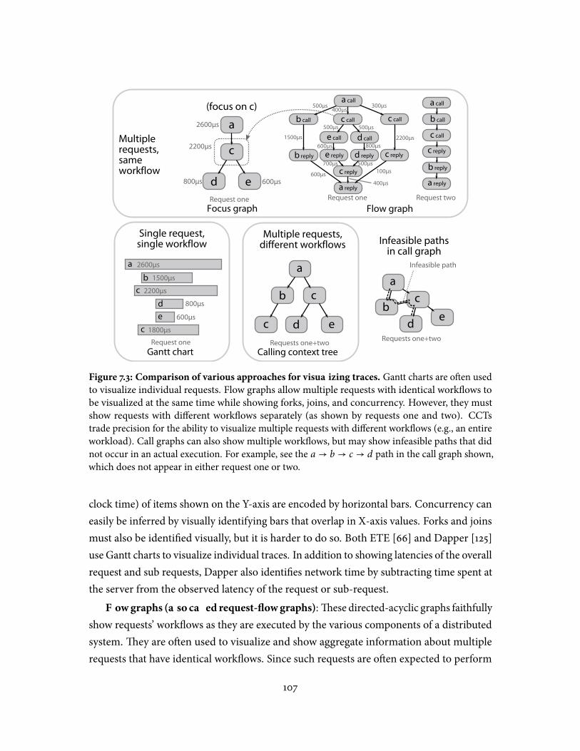
Figure 7.3: Comparison of various approaches for visualizing traces. Gantt charts are o�en usedto visualize individual requests. Flow graphs allow multiple requests with identical work�ows tobe visualized at the same time while showing forks, joins, and concurrency. However, they mustshow requests with di�erent work�ows separately (as shown by requests one and two). CCTstrade precision for the ability to visualize multiple requests with di�erent work�ows (e.g., an entireworkload). Call graphs can also show multiple work�ows, but may show infeasible paths that didnot occur in an actual execution. For example, see the a → b → c → d path in the call graph shown,which does not appear in either request one or two.

clock time) of items shown on the Y-axis are encoded by horizontal bars. Concurrency caneasily be inferred by visually identifying bars that overlap in X-axis values. Forks and joinsmust also be identi�ed visually, but it is harder to do so. Both ETE [66] and Dapper [125]use Gantt charts to visualize individual traces. In addition to showing latencies of the overallrequest and sub requests, Dapper also identi�es network time by subtracting time spent atthe server from the observed latency of the request or sub-request.

Flowgraphs (also called request-�owgraphs):�ese directed-acyclic graphs faithfullyshow requests’ work�ows as they are executed by the various components of a distributedsystem.�ey are o�en used to visualize and show aggregate information about multiplerequests that have identical work�ows. Since such requests are o�en expected to perform

107

similarly, �ow graphs are a good way to preserve precision, while still showing multiplerequests. Fan-outs in the graph represent the start of concurrent activity (forks), events ondi�erent branches are concurrent, and fan-ins represent synchronization points (joins).�erevised version of Stardust [117] and the revised version of X-Trace [47] visualize traces via�ow graphs. Note that for �ow graphs to be used, the underlying causal trackingmechanismmust preserve concurrency, forks, and joins. If these properties are not preserved, CCTscould be used instead.

Call graphs and focus graphs:�ese visualizations are also o�en used to showmultipletraces, but do not preserve concurrency, forks, or joins, and so are not precise. Call graphsuse fan-outs to show functions accessed by a parent function. Focus graphs show the callstack to a chosen component or function, called the “focus node,” and the call graph thatresults from treating the focus node as its root. In general, focus graphs are best usedfor diagnosis tasks for which developers already knows which functions or componentsare problematic. Dapper [125] uses focus graphs to show multiple request with identicalwork�ows, but owing to its RPC-oriented nature, nodes do not represent components orfunctions, but rather all work done to execute an RPC at the client and server. Note thatwhen used to visualize multiple requests with di�erent work�ows, call graphs can showinfeasible paths [5]. �is is demonstrated by the a → b → c → d path for the call graphshown in Figure 7.3.

Calling Context Trees (CCTs) [5]:�ese visualizations are best used to show multipletraces with di�erent workloads, as they guarantee that every path from root to leaf is a validpath through the distributed system. To do so in a compact way, they use fan-outs to showfunction invocations, not forks, and, as such, are not precise. CCTs can be constructed inamortized constant time and are best used for tasks for which a high-level summary ofsystem behaviour is desired (e.g., pro�ling). Whodunit [27] uses CCTs to show pro�linginformation for workloads.

7.6 Putting it all together

Based on the tradeo�s described in previous sections and my own experiences, this sectionidenti�es good design choices for the key uses of end-to-end tracing. I also show previousimplementations’ choices and contrast them to my suggestions.

108

7.6.1 Suggested choices

�e italicized rows of Table 7.4 show suggested design choices for key use cases of end-to-endtracing. To preserve concurrent behaviour, I suggest the hybrid �xed-width immutablethread ID and �xed-width mutable breadcrumb (TID & BC) approach used by Stardust [117,141], because it o�ers the best tradeo�s among the various approaches. Speci�cally, it is ofconstant size, does not rely much on external clues (except for a timestamp to order intra-component trace points), and is less brittle than the straightforward TID & BC approach(since it only switches breadcrumbs between components). However, the immutable, �xed-width thread ID (TID) approach is also a good choice if the needed external clues will alwaysbe available. I also suggest developers should consider using variable-width approaches iffeasible. For use cases that require coherent sampling, I conservatively suggest the head-based version when it is su�cient, but tail-based based coherent sampling should also beconsidered since it subsumes the former and allows for a wider range of uses.�e rest ofthis section explains design choices for the various use cases.

Anomaly detection: �is use case involves identifying and recording rare �ows thatare extremely di�erent from others so that developers can analyze them. As such, tail-basedcoherent sampling should be used so that traces can be constructed and so that the tracinginfrastructure can gauge whether a �ow is anomalous before deciding whether or not tosample it. Either trigger causality or submitter causality can be preserved with low overhead,but the former should be preferred since it shows critical paths and because they are easier tounderstand when visualized. To identify anomalies that result due to excessive parallelism,too little parallelism, or excessive waiting for one of many concurrent operations to �nish,implementations should preserve forks, joins, and concurrent behaviour. Flow graphs arebest for visualizing anomalies because they are precise and because anomaly detectionwill, by de�nition, not generate many results. Gantt charts can also be used to visualizeindividual �ows.

Diagnosing steady-state problems: �is use case involves diagnosing performanceand correctness problems that can be observed in many requests. Design choices for it aresimilar to anomaly detection, except that head-based sampling can be used, since even withlow sampling rates it is unlikely that problems will go unnoticed.

Distributed pro�ling:�is use case involves sampling function (or inter-trace point)latencies.�e inter- and intra-component call stacks to a function must be preserved so thatsampled times can be grouped together based on context, but complete traces need not be

109

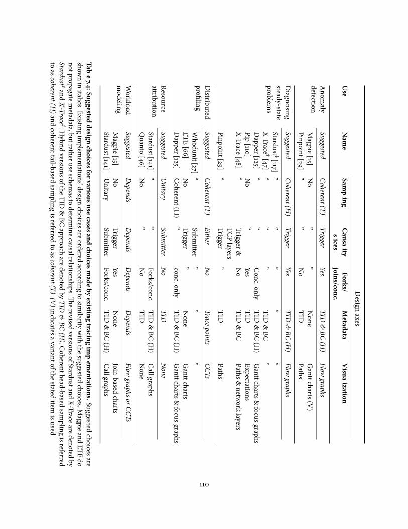
Design

axes

Use

Name

Samplin

gCau

sality

slices

Forks/

joins/co

nc.

Meta

data

Visu

alizatio

n

Anom

alydetection

SuggestedCoherent(T)

TriggerYes

TID&BC

(H)

Flowgraphs

Magpie[15]

No

””

None

Ganttcharts(V

)Pinpoint[29]

””

No

TIDPaths

Diagnosing

steady-stateproblem

s

SuggestedCoherent(H

)Trigger

YesTID

&BC

(H)

Flowgraphs

Stardust ‡[117]”

””

””

X-Trace ‡[47]”

””

TID&BC

”Dapper[125]

””

Conc.only

TID&BC

(H)

Ganttcharts&

focusgraphsPip

[110]No

”Yes

TIDExpectations

X-Trace[48]”

Trigger&TCP

layersNo

TID&BC

Paths&netw

orklayers

Pinpoint[29]”

Trigger”

TIDPaths

Distributed

pro�lingSuggested

Coherent(T)

EitherNo

TracepointsCCTs

Whodunit[27]

”Subm

itter”

””

ETE[66]

No

Trigger”

None

Ganttcharts

Dapper[125]

Coherent(H

)”

conc.onlyTID

&BC

(H)

Ganttcharts&

focusgraphs

Resourceattribution

SuggestedUnitary

Submitter

No

TIDNone

Stardust[141]”

”Forks/conc.

TID&BC

(H)

CallgraphsQuanto

[46]No

”No

TIDNone

Workload

modeling

SuggestedDepends

Depends

Depends

Depends

FlowgraphsorC

CTs

Magpie[15]

No

TriggerYes

None

Join-basedcharts

Stardust[141]Unitary

Submitter

Forks/conc.TID

&BC

(H)

Callgraphs

Table7.4

:Suggested

desig

nchoices

forvario

ususe

cases

andchoices

madebyexistin

gtra

cingim

plem

entatio

ns.Suggested

choicesareshow

nin

italics.Existingim

plementations’design

choicesareorderedaccording

tosim

ilaritywith

thesuggestedchoices.M

agpieandETE

donotpropagatem

etadata,butratheruseschemasto

determinecausalrelationships.�

erevisedversionsofStardustand

X-Tracearedenotedby

Stardust ‡andX-Trace ‡.H

ybridversionsoftheTID

&BC

approacharedenoted

byTID

&BC

(H).C

oherenthead-basedsam

plingisreferred

toascoherent(H

)andcoherenttail-based

sampling

isreferredto

ascoherent(T).(V)indicatesavariantofthestated

itemisused

110

constructed.�ese requirements align well with tail-based coherent sampling (where “tail”is de�ned to be the current function being executed) and carrying trace points as metadata.Together, these options will allow pro�les to be collected online. Call stacks do not needto preserve forks, joins, or concurrency. CCTs are best for visualizing distributed pro�les,since they can show entire workloads and infeasible paths do not appear.

Resource attribution:�is use case involves attributing work done at arbitrary levelsof the system to the original submitter, so submitter causality must be preserved. Unitarysampling is su�cient, since submitter IDs can be propagated with requests and stored withtrace points. It is not important to preserve forks, joins, or concurrency, so the TID approachto causal tracking is su�cient. Since traces need not be constructed, trace visualization isnot necessary.

Workload modeling:�e design decisions for this use case depend on what propertiesof the workload are being modeled. For example, when used to model workloads, Mag-pie [15] aims to identify a set of �ows and associated resource usages that are representativeof an entire workload. As such, it is useful for Magpie to preserve forks, joins, and concur-rent behaviour. If traces for this use case are to be visualized, �ow graphs or CCTs shouldbe used since they allow for visualizing multiple traces at one time.

7.6.2 Existing tracing implementations’ choices

Table 7.4 also shows existing tracing implementations and the choices they make. Existingimplementations are qualitatively ordered by similarity in design choices to my suggestedones. Inmany cases, the design choicesmade by existing tracing implementations are similarto my suggestions. However, in cases where di�erences exist, existing implementationso�en fall short of their intended range of uses or achieve needed functionality via ine�cientmeans.

For anomaly detection, I suggest tail-based sampling, but both Magpie [15] and Pin-point [29] do not use any sampling techniques whatsoever. Collecting and storing tracepoints for every request guarantees that both implementations will not miss capturing anyrare events (anomalies), but alsomeans they cannot scale to handle large workloads. Magpiecannot use sampling, because it does not propagate metadata. Pinpoint is concerned mainlywith correctness anomalies, and so does not bother to preserve concurrency, forks, or joins.

For diagnosing steady-state problems, the design choices made by the revised version ofStardust [117] and the revised version of X-Trace [47] are identical to my suggested choices.

111

I originally tried to use the original version of Stardust, which was designed for resourceaccounting, for diagnosis, but found it insu�cient, motivating the need for the revisedversion. X-Trace was originally designed to help with diagnosis tasks by showing causalitywithin and across network layers, but over time its design was evolved to re�ect my currentchoices because they proved to be more useful.

Pip [110] di�ers from many other tracing infrastructures in that it uses an expectationlanguage to show traces. Pip’s expectation language describes howother components interactwith a component of interest and so is similar in functionality to Dapper’s component-basedgraphs. Both are best used when developers already have a component-of-interest in mind,not for problem localization tasks.

For the most part, for distributed pro�ling and resource attribution, existing infrastruc-tures either meet or exceed my suggestions.

7.7 Challenges & opportunities

�ough end-to-end tracing has proven useful, many important challenges remain beforeit can reach its full potential. Most are a result of the complexity and volume of tracesgenerated by today’s large-scale distributed systems.�is section summarizes them.

As instrumented systems scale both in size and workload, tracing infrastructures mustaccommodate larger, more complex, traces at higher throughput, while maintaining rele-vance of tracing data.�ough head-based sampling meets the �rst two criteria of this keychallenge, it does not guarantee trace relevance. For example, it complicates diagnosticson speci�c traces and will not capture rare bugs (i.e., anomalies). Conversely, tail-basedsampling, in which trace points are cached until requests complete, meets the relevancecriteria, but not the �rst two.

An in-between approach, in which all trace points for requests are discarded as soon asthe request is deemed uninteresting, seems a likely solution, but important research into�nding the trace attributes that best determine when a trace can be discarded is neededbefore this approach can be adopted. An alternate approachmay be to collect low-resolutiontraces in the common case and to increase resolution only when a given trace is deemedinteresting. However, this approach also requires answering similar research questions asthat required for the in-between approach.

Another challenge, which end-to-end tracing shares with logging, involves trace inter-pretability. In many cases, the developers responsible for instrumenting a distributed system

112

are not the same as those tasked with using the resulting traces. �is leads to confusionbecause of di�erences in context and expertise. For example, in a recent user study, Samba-sivan et al. had to manually translate the trace-point names within end-to-end traces fromdeveloper-created ones to ones more readily understood by general distributed systemsexperts [116]. To help, key research must be conducted on how to de�ne good instrumenta-tion practices, how to incentivize good instrumentation, and how to educate users on howto interpret instrumented traces or logs. Research into automatic instrumentation and onthe �y re-instrumentation (e.g., as in DTrace [26]) can also help reduce instrumentationburden and help interpretability.

A third important challenge lies in the integration of di�erent end-to-end tracing in-frastructures. Today’s distributed services are composed of many independently-developedparts, perhaps instrumented with di�erent tracing infrastructures (e.g., Dapper [125], Star-dust [117, 141], Tracelytics [143], X-Trace [47, 48], or Zipkin [147]). Unless they are modi�edto be interoperable, we miss the opportunity to obtain true end-to-end traces of composedservices.�e provenance community has moved forward in this direction by creating theOpen Provenance Model [32], which deserves careful examination.

7.8 Conclusion

End-to-end tracing can be implemented in many ways, and the choices made dictate theutility of the resulting traces for di�erent development and management tasks. Based onmy experiences developing tracing infrastructures and the past ten years of research onthe topic, this chapter provides guidance to designers of such infrastructures and identi�esopen questions for researchers.

113

114

Chapter 8

Conclusion

Performance diagnosis in distributed systems is extremely challenging, because the problemcould be contained in any of the system’s numerous components or dependencies or maybe an artifact of interactions among them. As distributed services continue to grow incomplexity and in the number of other distributed services upon which they depend,performance diagnosis will only become more challenging. �is dissertation exploresthe use of a novel technique, called request-�ow comparison [117], for helping diagnoseproblems in distributed systems. Request-�ow comparison uses end-to-end traces, whichshow the entire work�ow of individual requests through the distributed service and itsdependencies, to automatically localize the problem from the many possible culprits tojust a few potential ones.�e results presented in this dissertation show the usefulness ofrequest-�ow comparison and the e�cacy of the algorithms used to implement it.

8.1 Contributions

�e key contributions of this dissertation are the request-�ow comparison work�ow andthe case studies demonstrating its usefulness in helping diagnose real, previously unsolveddistributed systems problems. To enable these contributions, this dissertation addressesall aspects of building a request-�ow comparison diagnosis tool. For example, it describesalgorithms and heuristics for implementing request-�ow comparison and where thesealgorithms fall short. Also, via a 26-person user study involving real distributed systemsdevelopers, it identi�es promising approaches for visualizing request-�ow comparison.

Another important contribution is the observation that distributed systems’ potentialfor automation will always be limited unless they are built to bemore predictable. To demon-

115

strate the validity of this observation, this dissertation shows how existing automation toolsare a�ected by unpredictability, or high variance in key performance metrics. It suggeststhat to make systems more predictable, system builders must incorporate performancevariance as an important metric and strive to minimize it where appropriate. To helpsystem builders lower performance variance, it conceptually describes a tool for identifyingsources of variance in distributed systems and a nomenclature for helping system buildersunderstand what to do about di�erent variance sources.

�e �nal major contribution of this dissertation is a design study of end-to-end tracing.It aims to guide designers of tracing infrastructures by distilling key design axes that dictatea tracing infrastructure’s utility for di�erent use cases, such as resource attribution anddiagnosis. Existing literature [3, 15, 27, 29, 47, 48, 66, 78, 110, 111, 117, 125, 130, 131, 141, 142, 152]treats end-to-end tracing as a one-size-�ts-all solution and so does not identify theseaxes. Since the axes are not well understood, many existing tracing infrastructures do note�ectively support some desired use cases.

8.2 Thoughts on future work

I believe my work on request-�ow comparison has helped identify a wealth of future workopportunities, some of which were described in previous chapters.�is section highlightsthe most important ones.

8.2.1 Generalizing request-°ow comparison to more systems

�is dissertation describes algorithms and heuristics for implementing request-�ow com-parison’s work�ow that proved e�ective for Ursa Minor and select Google services. It alsodescribed modi�cations needed for these algorithms to be useful in HDFS [134]. However,due to the wide variety of request-based distributed systems in existence, di�erent (ormodi�ed) request-�ow comparison algorithms may be needed for di�erent distributedsystems and problem types.

Before developing request-�ow comparison algorithms for a candidate distributedsystem, developers must �rst ensure that end-to-end traces showing request work�ows canbe obtained for it. Developers must carefully consider what constitutes the work�ow ofan “individual request” (i.e., a fundamental unit of work) and guarantee that individualtraces show this information. Doing so may be easy for some systems (e.g., storage systems)and di�cult for others (e.g., batch-processing systems). Chapter 7.3 provides guidance on

116

what causal relationships to preserve when de�ning the work�ow of individual requestsfor diagnosis tasks. Most notably, for request-�ow comparison to be e�ective, requestwork�ows must show work done on the critical path of the request. Note that if end-to-endtraces will be obtained via a metadata-propagation-based tracing infrastructure, the designchoices suggested in Chapter 7.6.1 for diagnosing steady-state problems may be of value inchoosing how to de�ne request work�ows, how to avoid high tracing overheads, and howto present trace data.

When creating a request-�ow-comparison tool for a candidate system, developersmust carefully consider which algorithms to use to implement request-�ow comparison’scategorization step.�is work�ow step is responsible for grouping requests that are expectedto perform similarly into the same category. I believe Spectroscope’s expectation thatrequests with similar or identical structures should perform similarly is fundamental andvalid in many systems. However, additional or looser constraints may be needed for othersystems. For example, Chapter 3.5.3 demonstrated that a straightforward interpretationof the same structures/similar cost expectation is too strict for HDFS, as using it resultsin too many categories with too few requests in each to identify mutations. �e chaptersuggested ways to loosen the expectation by removing certain structural details while stillguaranteeing that categories will contain requests that are expected to perform similarly.For example, for homogeneous, dedicated-machine environments, in which all machinesare expected to perform similarly, it suggested removing machine names from node labels.For heterogeneous or shared-machine environments, it suggested grouping individualmachines into equivalence classes of similarly-performing ones and using equivalence classnames instead of machine names in node labels.

In practice, it may be di�cult to know up-front which properties of requests dictateperformance. To help, I believe additional research is needed to investigate semi-supervisedmethods for categorization. With such methods, the request-�ow-comparison tool woulduse basic expectations (such as the same structures/similar performance one) and observedperformance to present an initial categorization of requests. Diagnosticians could then usea visual interface to specify which groupings align with their intuition of what requests areexpected to perform similarly.�e comparison tool could then use diagnosticians’ feedbackto, over time, learn what request properties dictate performance and improve the results ofits categorization step. Note that di�erences between automatically-learned groupings anddiagnosticians’ intuition may themselves indicate important performance problems.

I believe the algorithms used by Spectroscope to identify response-time mutations and

117

structural mutations are be applicable to a broad range of distributed systems. However,there is room for improvement. For response-time mutations, research is needed to identifywhether alternate algorithms exist that are more robust to high variance caused by resourcecontention. Opportunities also exist to further reduce diagnostician burden when compar-ing structural mutations to their precursors—for example, by automating the identi�cationof changed substructures between mutations and precursors. It remains to be seen whetheralgorithms, such as graph kernels [124], frequent-graph mining [71], or advanced structuralanomaly detection [41] can be used to enable such additional automation.

In addition to determining what algorithms will work best when implementing request-�ow comparison’s basic work�ow for a new distributed system, developers should alsoconsider whether additional work�ow steps would be useful. For example, additionalwork�ow steps that directly identify contending requests or processes would be a valuableaddition for distributed services that operate in shared-machine environments. However,additional research is needed to identify how best to identify competing activities andwhether modi�cations to the underlying tracing infrastructure are necessary to do so.

In the long term, it is important to consider whether request-�ow comparison (or otherexisting diagnosis techniques) can be extended to work in newly emerging adaptive cloudenvironments [68]. To increase resource utilization, these environments use schedulersthat dynamically move workloads and change resource allocations. For example, to satisfyglobal constraints, they may move a running application to a di�erent set of machineswith very di�erent hardware. If only a few applications are running, they may bless therunning ones with very high resource allocations, only to steal back these resources later.Unfortunately, such dynamism reduces the e�ectiveness of most existing diagnosis tools,because they are not built to expect it and because increasing resource utilization o�enalso increases performance variance. I believe that a �rst step toward extending existingdiagnosis techniques to adaptive clouds will involve making them privy to datacenterscheduler decisions, so that they can determine whether or not an observed performancechange is the expected result of a scheduler decision [119].

8.2.2 Improving request-°ow comparison’s presentation layer

�ough the systems research community has created many problem localization tech-niques [14, 15, 29, 72, 76, 98, 103, 117, 122, 144], it has performed very little research on howto e�ectively present their results. �is is unfortunate because the e�ectiveness of such

118

tools is limited by how easily diagnosticians can understand their results.�e user study Iran comparing three approaches for visualizing Spectroscope’s results (see Chapter 4) isbut a �rst step. Participants’ comments during this study, and my own experiences withSpectroscope, have revealed many insights that can guide future visualization work.

Most important is the insight that, by themselves, comparisons of full request-�owgraphs are not su�cient for helping diagnosticians’ interpret request-�ow comparison’sresults. Even though the graphs presented to the user study participants o�en containedless than 200 nodes, participants o�en complained about their size. Worse, in complexdistributed services—for example, ones built upon other distributed services—it is likely thatno single person will have complete knowledge of the entire system. As such, diagnosticiansof such systems will not possess the expertise to determine whether a performance changeobserved deep in the bowels of the systems represents valid behaviour or an an unexpectedperformance problem.

Semantic zooming, annotation mechanisms (as suggested by the user study partici-pants), and graph collapsing (as discussed in Chapter 3.5.2) can somewhat help. But, Ido not believe they are su�cient. Ideally, diagnosis tools should be able to identify themeaning of an observed problem automatically. For example, request-�ow-comparisontools, like Spectroscope, could learn the textual meaning of individual graphs, enablingthem to output both observed mutations and what they represent. One promising methodfor enabling such learning is crowdsourcing. As a game, developers of individual distributedsystems components could be presented with graph substructures relevant only to theircomponent and asked to name them. When presenting mutations and precursors, the diag-nosis tool could display their meanings by combining the names given to their constituentsubstructures.

8.2.3 Building more predictable systems

Without increased predictability, automation techniques, such as request-�ow comparison,will never reach their full potential. But, it is not clear how best to increase predictabilityfor most distributed systems. Research is needed to identify good techniques for localizinginadvertent variance sources. Research to understand the dominant sources of variance indistributed systems would also help.

An alternate approach, suggested by Dean et al. [39], is to treat unpredictability as agiven and build systems that are naturally resilient to it. I believe this approach and that of

119

reducing variance merit comparison, especially with regards to their implications towardautomation and future diagnosis techniques.

8.2.4 Improving end-to-end tracing

Despite end-to-end tracing’s usefulness, many organizations are still wary of it because ofthe enormous storage overhead it can impose when head-based sampling is used. Evenfor Ursa Minor [1], traces collected for its regression tests were a few gigabytes in size.For large organizations, such as Google, storage overhead could balloon to petabytes evenwith minimal sampling.�ough tail-based sampling reduces storage overhead, it increasesmemory cost. A very pertinent area of research involves creating tracing techniques thatcan capture interesting traces while minimizing storage-related overhead.

120

Bibliography

[1] Michael Abd-El-Malek, William V. Courtright II, Chuck Cranor, Gregory R. Ganger,James Hendricks, Andrew J. Klosterman, Michael Mesnier, Manish Prasad, BrandonSalmon, Raja R. Sambasivan, Shafeeq Sinnamohideen, John Strunk, Eno�ereska,Matthew Wachs, and Jay Wylie. Ursa minor: versatile cluster-based storage. InFAST’05: Proceedings of the 4th USENIX Conference on File and Storage Technologies,2005. Cited on pages 2, 4, 7, 11, 12, 16, 25, 26, 48, 54, 74, and 120.

[2] Bhavish Aggarwal, Ranjita Bhagwan, Tathagata Das, Siddarth Eswaran, Venkata N.Padmanabhan, and Geo�rey M. Voelker. NetPrints: diagnosing home network mis-con�gurations using shared knowledge. In NSDI’09: Proceedings of the 6th USENIXSymposium on Networked Systems Design and Implementation, 2009. Cited on page88.

[3] Marcos K. Aguilera, Je�rey C. Mogul, Janet L. Wiener, Patrick Reynolds, and AthichaMuthitacharoen. Performance debugging for distributed systems of black boxes. InSOSP’03: Proceedings of the 19th ACM Symposium on Operating Systems Principles,2003. Cited on pages 3, 10, 91, 95, and 116.

[4] Paulo Sérgio Almeida, Carlos Baquero, and Victor Fonte. Interval tree clocks. InOPODIS’08: Proceedings of the 12th International Conference on Principles of Dis-tributed Systems, 2008. Cited on page 105.

[5] Glenn Ammons,�omas Ball, and James R. Larus. Exploiting hardware performancecounters with �ow and context sensitive pro�ling. In PLDI’97: Proceedings of the 11th

ACM SIGPLAN Conference on Programming Language Design and Implementation,1997. Cited on pages 86 and 108.

[6] Ganesh Ananthanarayanan, Srikanth Kandula, Albert Greenberg, Ion Stoica, Yi Lu,Bikas Saha, and Edward Harris. Reining in the outliers in Map-Reduce clusters usingMantri. In OSDI’10: Proceedings of the 9th USENIX Symposium on Operating Systems

121

Design and Implementation, 2010. Cited on page 16.

[7] Alexandr Andoni and Krzysztof Onak. Approximating edit distance in near-lineartime. In STOC’09: Proceedings of the 41st Annual ACM Symposium on �eory ofcomputing, 2009. Cited on page 21.

[8] Apache hadoop. http://hadoop.apache.org. Cited on pages 15, 39, 40, 50, 72,and 85.

[9] Daniel Archambault, Helen C. Purchase, and Bruno Pinaud. Animation, smallmultiples, and the e�ect of mental map preservation in dynamic graphs. IEEETransactions on Visualization and Computer Graphics, 17(4):539–552, April 2011. Citedon pages 48, 60, and 65.

[10] Daniel Archambault, Helen C. Purchase, and Bruno Pinaud. Di�erence map read-ability for dynamic graphs. In GD’10: Proceedings of the 18th International Conferenceon Graph Drawing, 2011. Cited on pages 48 and 49.

[11] Michael Armbrust, Armando Fox, Rean Gri�th, Anthony D. Joseph, Randy H. Katz,Andy Konwinski, Gunho Lee, David Patterson, Ariel Rabkin, Ion Stoica, and MateiZaharia. A view of cloud computing. Communications of the ACM, 53(4), April 2010.Cited on page 1.

[12] RemziH. Arpaci-Dusseau andAndrea C. Arpaci-Dusseau. Fail-stutter fault tolerance.InHotOS’01: Proceedings of the 8th IEEEWorkshop on Hot Topics in Operating Systems,2001. Cited on pages 70, 73, and 74.

[13] Mona Attariyan and Jason Flinn. Automating con�guration troubleshooting withdynamic information �ow analysis. In OSDI’10: Proceedings of the 9th USENIXSymposium on Operating Systems Design and Implementation, 2010. Cited on page89.

[14] Paramvir Bahl, Ranveer Chandra, Albert Greenberg, Srikanth Kandula, David A.Maltz, and Ming Zhang. Towards highly reliable enterprise network services viainference of multi-level dependencies. In SIGCOMM’07: Proceedings of the 2007ACM SIGCOMM Conference on Data Communications, 2007. Cited on pages 47, 72,83, 84, and 118.

[15] Paul Barham, Austin Donnelly, Rebecca Isaacs, and Richard Mortier. Using Magpiefor request extraction and workload modelling. In OSDI’04: Proceedings of the 6th

USENIX Symposium on Operating Systems Design and Implementation, 2004. Cited

122

on pages 3, 6, 10, 11, 17, 47, 71, 72, 75, 81, 82, 91, 92, 93, 94, 102, 110, 111, 116, and 118.

[16] Luiz A. Barroso. Warehouse-scale computing: entering the teenage decade, August2011. Cited on pages 8 and 70.

[17] Fabian Beck and Stephan Diehl. Visual comparison of so�ware architectures. InSOFTVIS’10: Proceedings of the 5th International Symposium on So�ware Visualization,2010. Cited on page 49.

[18] Nicolas Garcia Belmonte.�e Javascript Infovis Toolkit. http://www.thejit.org.Cited on page 50.

[19] Hal Berghel and David Roach. An extension of Ukkonen’s enhanced dynamicprogramming ASM algorithm. Transactions on Information Systems (TOIS, 14(1),January 1996. Cited on page 21.

[20] Christopher M. Bishop. Pattern recognition and machine learning. Springer Science+ Business Media, LLC, �rst edition, 2006. Cited on page 23.

[21] Ledion Bitincka, Archana Ganapathi, Stephen Sorkin, and Steve Zhang. Optimizingdata analysis with a semi-structured time series database. In SLAML’10: Proceedingsof the 2010 ACMWorkshop onManaging Large-scale Systems via the Analysis of SystemLogs and the Application of Machine Learning Techniques, 2010. Cited on pages 10and 95.

[22] Peter Bodik, Armando Fox, Michael Jordan, and David Patterson. Advanced toolsfor operators at Amazon.com. In HotAC’06: Proceedings of the 1st Workshop on HotTopics in Autonomic Computing, 2006. Cited on pages 86 and 87.

[23] Peter Bodik, Moises Goldszmidt, Armando Fox, Dawn B.Woodard, and Hans Ander-sen. Fingerprinting the datacenter: automated classi�cation of performance crises.In EuroSys’10: Proceedings of the 5th ACM SIGOPS European Conference on ComputerSystems, 2010. Cited on page 88.

[24] James Bovard. Slower is better:�e new postal service. Cato Policy Analysis, February1991. Cited on page 70.

[25] Jason D. Campbell, Arun B. Ganesan, Ben Gotow, Soila P. Kavulya, James Mulhol-land, Priya Narasimhan, Sriram Ramasubramanian, Mark Shuster, and Jiaqi Tan.Understanding and improving the diagnostic work�ow of MapReduce users. InCHIMIT’11: Proceedings of the 5th ACM Symposium on Computer Human Interactionfor Management of Information Technology, 2011. Cited on page 50.

123

[26] Bryan M. Cantrill and Michael W. Shapiro. Dynamic instrumentation of productionsystems. In ATC’04: Proceedings of the 2004 USENIX Annual Technical Conference,2004. Cited on pages 3 and 113.

[27] Anupam Chanda, Alan L. Cox, and Willy Zwaenepoel. Whodunit: transactionalpro�ling for multi-tier applications. In EuroSys’07: Proceedings of the 2nd ACMSIGOPS European Conference on Computer Systems, 2007. Cited on pages 3, 6, 10, 26,81, 86, 91, 93, 94, 96, 97, 98, 100, 101, 103, 105, 108, 110, and 116.

[28] Fay Chang, Je�rey Dean, Sanjay Ghemawat, Wilson C. Hsieh, Deborah A. Wallach,Michael Burrows, Tushar Chandra, Andrew Fikes, and Robert E. Gruber. Bigtable:a distributed storage system for structured data. In OSDI’06: Proceedings of the 7th

USENIX Symposium on Operating Systems Design and Implementation, 2006. Citedon pages 1, 25, 28, 29, 72, 74, and 98.

[29] Mike Y. Chen, Anthony Accardi, Emre Kiciman, Jim Lloyd, David Patterson, Ar-mando Fox, and Eric Brewer. Path-based failure and evolution management. InNSDI’04: Proceedings of the 1st USENIX Symposium on Networked Systems Design andImplementation, 2004. Cited on pages 3, 6, 10, 26, 47, 72, 75, 83, 91, 93, 94, 102, 103,104, 110, 111, 116, and 118.

[30] David R. Cheriton and Dale Skeen. Understanding the limitations of causally andtotally ordered communication. In SOSP’93: Proceedings of the 14th ACM Symposiumon Operating Systems Principles, 1993. Cited on page 99.

[31] Ludmila Cherkasova, KivancOzonat, NingfangMi, Julie Symons, and Evgenia Smirni.Anomaly? Application change? or Workload change? towards automated detectionof application performance anomaly and change. In DSN’08: Proceedings of the 38th

Annual IEEE/IFIP International Conference on Dependable Systems and Networks,2008. Cited on page 7.

[32] Ben Cli�ord, Juliana Freire, Joe Futrelle, Yolanda Gil, Paul Groth, Natalia Kwas-nikowska, Simon Miles, Paolo Missier, Jim Myers, Beth Plale, Yogesh Simmhan, EricStephan, and Jan Van den Bussche. �e open provenance model core speci�cation(v1.1). Future Generation Computer Systems, 27(6):743–756, June 2011. Cited on page113.

[33] Cloudera Htrace. http://github.com/cloudera/htrace. Cited on page 4.

[34] Ira Cohen, Moises Goldszmidt, and Terence Kelly. Correlating instrumentation

124

data to system states: a building block for automated diagnosis and control. InOSDI’04: Proceedings of the 6th USENIX Symposium on Operating Systems Design andImplementation, 2004. Cited on page 88.

[35] Ira Cohen, Steve Zhang, Moises Goldszmidt, Julie Symons, Terence Kelly, and Ar-mando Fox. Capturing, indexing, clustering, and retrieving system history. InSOSP’05: Proceedings of the 20th ACM Symposium on Operating Systems Principles,2005. Cited on page 88.

[36] Compuware dynaTrace PurePath. http://www.compuware.com. Cited on pages 4and 91.

[37] Gabriela F. Creţu-Ciocârlie, Mihai Budiu, and Moises Goldszmidt. Hunting forproblems with Artemis. InWASL’08: Proceedings of the 1st USENIX conference onAnalysis of System Logs, 2008. Cited on page 87.

[38] L. Dailey Paulson. Computer system, heal thyself. Computer, 35(8):20–22, 2002.Cited on page 1.

[39] Je�rey Dean and Luiz A. Barroso. �e tail at scale. Communications of the ACM,56(2):74–80, February 2013. Cited on page 119.

[40] Je�rey Dean and Sanjay Ghemawat. MapReduce: simpli�ed data processing on largeclusters. In OSDI’04: Proceedings of the 6th USENIX Symposium on Operating SystemsDesign and Implementation, 2004. Cited on pages 39 and 103.

[41] William Eberle and Lawrence B. Holder. Discovering structural anomalies in graph-based data. In ICDMW’07: Proceedings of the 7th IEEE International Conference onData Mining Workshops, 2007. Cited on page 118.

[42] John Ellson, Emden R. Gansner, Ele�herios Koutso�os, Stephen C North, and Gor-don Woodhull. Graphviz and Dynagraph – static and dynamic graph drawing tools.In Graph Drawing So�ware. Springer-Verlag, 2003. Cited on page 53.

[43] Ulfar Erlingsson, Marcus Peinado, Simon Peter, and Mihai Budiu. Fay: extensibledistributed tracing from kernels to clusters. In SOSP’11: Proceedings of the 23rd ACMSymposium on Operating Systems Principles, 2011. Cited on page 96.

[44] Michael Farrugia and Aaron Quigley. E�ective temporal graph layout: a comparativestudy of animation versus static display methods. Information Visualization, 10(1):47–64, January 2011. Cited on pages 48, 49, 60, and 62.

[45] Andrew D. Ferguson, Peter Bodik, Srikanth Kandula, Eric Boutin, and Rodrigo

125

Fonseca. Jockey: guaranteed job latency in data parallel clusters. In EuroSys’12:Proceedings of the 7th ACM SIGOPS European Conference on Computer Systems, 2012.Cited on page 77.

[46] Rodrigo Fonseca, Prabal Dutta, Philip Levis, and Ion Stoica. Quanto: trackingenergy in networked embedded systems. In OSDI’08: Proceedings of the 8th USENIXSymposium on Operating Systems Design and Implementation, 2008. Cited on pages10, 26, 93, 94, 100, 104, and 110.

[47] Rodrigo Fonseca, Michael J. Freedman, and George Porter. Experiences with tracingcausality in networked services. In INM/WREN’10: Proceedings of the 1st InternetNetwork Management Workshop/Workshop on Research on Enterprise Monitoring,2010. Cited on pages 3, 6, 10, 26, 39, 91, 93, 94, 96, 97, 98, 102, 103, 105, 108, 110, 111,113, and 116.

[48] Rodrigo Fonseca, George Porter, Randy H. Katz, Scott Shenker, and Ion Stoica. X-Trace: a pervasive network tracing framework. In NSDI’07: Proceedings of the 4th

USENIX Symposium on Networked Systems Design and Implementation, 2007. Citedon pages 3, 6, 10, 26, 91, 93, 94, 103, 105, 110, 113, and 116.

[49] Foundations for future clouds. Intel Labs, August 2011. http://www.istc-cc.

cmu.edu/publications/papers/2011/ISTC-Cloud-Whitepaper.pdf. Citedon page 1.

[50] Gregory R. Ganger, John D. Strunk, and Andrew J. Klosterman. Self-* Storage: brick-based storage with automated administration. Technical Report CMU-CS-03-178,Carnegie Mellon University, September 2003. Cited on page 1.

[51] Emden R. Gansner, Ele�herios E. Koutso�os, Stephen C. North, and Kiem-Phong Vo.A technique for drawing directed graphs. IEEE Transactions on So�ware Engineering,19(3):214–230, 1993. Cited on page 22.

[52] Xinbo Gao, Bing Xiao, Dacheng Tao, and Xuelong Li. A survey of graph edit distance.Pattern Analysis and Applications, 13(1):113–129, January 2009. Cited on page 53.

[53] Gapminder. http://www.gapminder.org. Cited on page 49.

[54] Sohaib Ghani, Niklas Elmqvist, and Ji S. Yi. Perception of animated node-linkdiagrams for dynamic graphs. Computer Graphics Forum, 31(3), June 2012. Cited onpages 64 and 65.

[55] Sanjay Ghemawat, Howard Gobio�, and Shun-Tak Leung. �e Google �le system.

126

In SOSP’03: Proceedings of the 19th ACM Symposium on Operating Systems Principles,2003. Cited on pages 1, 13, 39, and 74.

[56] Ali Ghodsi, Matei Zaharia, Benjamin Hindman, Andy Konwinski, Scott Shenker,and Ion Stoica. Dominant resource fairness: fair allocation of multiple resource types.In NSDI’11: Proceedings of the 8th USENIX Symposium on Networked Systems Designand Implementation, 2011. Cited on page 77.

[57] Garth A. Gibson, David F. Nagle, Khalil Amiri, Je� Butler, Fay W. Chang, HowardGobio�, Charles Hardin, Erik Riedel, David Rochberg, and Jim Zelenka. A cost-e�ective, high-bandwidth storage architecture. In ASPLOS’98: Proceedings of the 8th

ACM International Conference on Architectural Support for Programming Languagesand Operating Systems, 1998. Cited on pages 25 and 39.

[58] GNU gprof. http://www.cs.utah.edu/dept/old/texinfo/as/gprof_toc.

html. Cited on page 103.

[59] MoisesGoldszmidt,Mihai Budiu, Yue Zhang, andMichael Pechuk. Toward automaticpolicy re�nement in repair services for large distributed systems. ACM SIGOPSOperating Systems Review, 44(2):47–51, April 2010. Cited on page 88.

[60] John Alexis Guerra Gomez, Audra Buck-Coleman, Catherine Plaisant, and BenShneiderman. Interactive visualizations for comparing two trees with structure andnode value changes. Technical Report HCIL-2012-04, University of Maryland, 2012.Cited on page 49.

[61] Graphviz. http://www.graphviz.org. Cited on pages 22 and 47.

[62] Steven D. Gribble. Robustness in complex systems. In HotOS’01: Proceedings of the8th IEEE Workshop on Hot Topics in Operating Systems, 2001. Cited on pages 70and 73.

[63] Ajay Gulati, Arif Merchant, and Peter J. Varman. mClock: handling throughputvariability for hypervisor IO scheduling. In OSDI’10: Proceedings of the 9th USENIXSymposium on Operating Systems Design and Implementation, 2010. Cited on pages29 and 77.

[64] Mountaz Hascoët and Pierre Dragicevic. Visual comparison of document collec-tions using multi-layered graphs. Technical report, Laboratoire d’Informatique, deRobotique et de Microèlectronique de Montpellier (LIRMM), 2011. Cited on page49.

127

[65] Je�rey Heer and George G. Robertson. Animated Transitions in Statistical DataGraphics. IEEE Transactions on Visualization and Computer Graphics, 13(6):1240–1247, 2007. Cited on page 65.

[66] Joseph L. Hellerstein, Mark M. Maccabe, W. Nathaniel Mills III, and John J. Turek.ETE: a customizable approach to measuring end-to-end response times and theircomponents in distributed systems. In ICDCS’99: Proceedings of the 19th IEEE Inter-national Conference on Distributed Computing Systems, 1999. Cited on pages 3, 11,86, 91, 93, 94, 107, 110, and 116.

[67] James Hendricks, Raja R. Sambasivan, Shafeeq Sinnamohideen, and Gregory R.Ganger. Improving small �le performance in object-based storage. Technical ReportCMU-PDL-06-104, Carnegie Mellon University, 2006. Cited on page 34.

[68] BenjaminHindman, AndyKonwinski, Matei Zaharia, Ali Ghodsi, AnthonyD. Joseph,Randy H. Katz, Scott Shenker, and Ion Stoica. Mesos: a platform for �ne-grainedresource sharing in the data center. In NSDI’11: Proceedings of the 8th USENIXSymposium on Networked Systems Design and Implementation, 2011. Cited on page118.

[69] Alfred Inselberg. Parallel coordinates: Visual multidimensional geometry and itsapplications. Springer-Verlag, 2009. Cited on page 50.

[70] Michael Isard. Autopilot: automatic data center management. ACM SIGOPS Operat-ing Systems Review, 41(2):60–67, April 2007. Cited on page 88.

[71] Ruoming Jin, Chao Wang, Dmitrii Polshakov, Srinivasan Parthasarathy, and GaganAgrawal. Discovering frequent topological structures from graph datasets. InKDD’05:Proceedings of the 11th ACM International Conference on Knowledge Discovery in DataMining, 2005. Cited on page 118.

[72] Srikanth Kandula, Ratul Mahajan, Patrick Verkaik, Sharad Agarwal, Jitendra Padhye,and Paramvir Bahl. Detailed diagnosis in enterprise networks. In SIGCOMM’09:Proceedings of the 2009 ACM SIGCOMM Conference on Data Communications, 2009.Cited on pages 47, 50, 67, 72, 83, 84, 87, and 118.

[73] Hui Kang, Haifeng Chen, and Guofei Jiang. PeerWatch: a fault detection and diagno-sis tool for virtualized consolidation systems. In ICAC’10: Proceedings of the 7th IEEEInternational Conference on Autonomic Computing, 2010. Cited on page 85.

[74] Michael P. Kasick, Keith A. Bare, Eurene E. Marinelli III, Jiaqi Tan, Rajeev Gandhi,

128

and Priya Narasimhan. System-call based problem diagnosis for PVFS. InHotDep’09:Proceedings of the 5th USENIXWorkshop on Hot Topics in System Dependability, 2009.Cited on page 85.

[75] Michael P. Kasick, Rajeev Gandhi, and Priya Narasimhan. Behavior-based problemlocalization for parallel �le systems. In HotDep’10: Proceedings of the 6th USENIXWorkshop on Hot Topics in System Dependability, 2010. Cited on pages 44, 72, and 73.

[76] Michael P. Kasick, Jiaqi Tan, Rajeev Gandhi, and Priya Narasimhan. Black-boxproblem diagnosis in parallel �le systems. In FAST’10: Proceedings of the 8th USENIXConference on File and Storage Technologies, 2010. Cited on pages 44, 47, 72, 85,and 118.

[77] Je�rey Katcher. Postmark: a new �le system benchmark. Technical Report TR3022,Network Applicance, 1997. Cited on page 27.

[78] Soila P. Kavulya, Scott Daniels, Kaustubh Joshi, Matt Hultunen, Rajeev Gandhi, andPriya Narasimhan. Draco: statistical diagnosis of chronic problems in distributedsystems. InDSN’12: Proceedings of the 42nd Annual IEEE/IFIP International Conferenceon Dependable Systems and Networks, 2012. Cited on pages 3, 10, 91, 95, and 116.

[79] Vasileios P. Kemerlis, Georgios Portokalidis, Kangkook Jee, andAngelosD.Keromytis.libd�: practical dynamic data �ow tracking for commodity systems. In VEE’12:Proceedings of the 8th ACM SIGPLAN/SIGOPS conference on Virtual Execution Envi-ronments, 2012. Cited on page 99.

[80] Je�rey O. Kephart and David M. Chess. �e vision of autonomic computing. Com-puter, 36(1):41–50, 2003. Cited on page 1.

[81] Charles Killian, Karthik Nagaraj, Salman Pervez, Ryan Braud, James W. Anderson,and Ranjit Jhala. Finding latent performance bugs in systems implementations. InFSE’10: Proceedings of the 18th ACM SIGSOFT Symposium on Foundations of So�wareEngineering, 2010. Cited on pages 85 and 86.

[82] Charles E. Killian, James W. Anderson, Ryan Braud, Ranjit Jhala, and Amin M.Vahdat. Mace: language support for building distributed systems. In PLDI’07:Proceedings of the 2007 ACM SIGPLAN Conference on Programming Language Designand Implementation, 2007. Cited on page 85.

[83] Eric Koskinen and John Jannotti. Borderpatrol: isolating events for black-box tracing.In EuroSys’08: Proceedings of the 3rd ACM SIGOPS European Conference on Computer

129

Systems, 2008. Cited on pages 10 and 95.

[84] Elie Krevat, Joseph Tucek, and Gregory R. Ganger. Disks are like snow�akes: no twoare alike. In HotOS’11: Proceedings of the 13th USENIX Workshop on Hot Topics inOperating Systems, 2011. Cited on pages 70 and 72.

[85] Leslie Lamport. Time, clocks, and the ordering of events in a distributed system.Communications of the ACM, 21(7), July 1978. Cited on pages 11 and 99.

[86] Zhicheng Liu, Bongshin Lee, Srikanth Kandula, and Ratul Mahajan. NetClinic:interactive visualization to enhance automated fault diagnosis in enterprise networks.In VAST’10: Proceedings 2010 IEEE Conference on Visual Analytics Science and Tech-nology, 2010. Cited on pages 47, 50, 87, and 106.

[87] David MacKenzie, Paul Eggert, and Richard Stallman. Comparing and merging �leswith GNU di� and patch. Network�eory Ltd, 2002. Cited on page 51.

[88] Ajay A. Mahimkar, Zihui Ge, Aman Shaikh, Jia Wang, Jennifer Yates, Yin Zhang,and Qi Zhao. Towards automated performance diagnosis in a large IPTV network.In SIGCOMM’09: Proceedings of the 2009 ACM SIGCOMM Conference on DataCommunications, 2009. Cited on pages 47, 67, 83, and 84.

[89] Gideon Mann, Mark Sandler, Darja Krushevskaja, Sudipto Guha, and Eyal Even-dar.Modeling the parallel execution of black-box services. InHotCloud’11: Proceedings ofthe 2011 USENIX Workshop on Hot Topics in Cloud Computing, 2011. Cited on page106.

[90] Florian Mansmann, Fabian Fischer, Daniel A. Keim, and Stephen C. North. Visualsupport for analyzing network tra�c and intrusion detection events using TreeMapand graph representations. In CHIMIT’09: Proceedings of the 3rd ACM Symposiumon Computer Human Interaction for Management of Information Technology, 2009.Cited on pages 47 and 50.

[91] Frank J. Massey, Jr. �e Kolmogorov-Smirnov test for goodness of �t. Journal of theAmerican Statistical Association, 46(253):66–78, 1951. Cited on page 17.

[92] Matthew L. Massie, Brent N. Chun, and David E. Culler. �e Ganglia distributedmonitoring system: design, implementation, and experience. Parallel Computing,30(7):817–840, July 2004. Cited on pages 3 and 50.

[93] Alan G. Melville, Martin Graham, and Jessie B. Kennedy. Combined vs. separateviews in matrix-based graph analysis and aomparison. In IV’11: Proceedings of the

130

15th International Conference on Information Visualisation, 2011. Cited on page 49.

[94] Je�rey Mogul. Emergent (mis)behavior vs. complex so�ware systems. In EuroSys’06:Proceedings of the 1st ACM SIGOPS European Conference on Computer Systems, 2006.Cited on pages 70 and 73.

[95] Hossein Momeni, Omid Kashe�, and Mohsen Shari�. How to realize self-healingoperating systems? In ICTTA’08: Proceedings of the 3rd International Conference onInformation and Communication Technologies, 2008. Cited on page 1.

[96] Tipp Moseley, Dirk Grunwald, and Ramesh Peri. Optiscope: performance account-ability for optimizing compilers. In CGO’09: Proceedings of the 7th Annual IEEE/ACMInternational Symposium on Code Generation and Optimization, 2009. Cited on page89.

[97] Tamara Munzner, François Guimbretière, Serdar Tasiran, Li Zhang, and YunhongZhou. Treejuxtaposer: scalable tree comparison using focus+context with guaranteedvisibility. In SIGGRAPH’03: Proceedings of the 30th International Conference onComputer Graphics and Interactive Techniques, 2003. Cited on page 49.

[98] Karthik Nagaraj, Charles Killian, and Jennifer Neville. Structured comparativeanalysis of systems logs to diagnose performance problems. In NSDI’12: Proceedingsof the 9th USENIX Symposium on Networked Systems Design and Implementation,2012. Cited on pages 47, 67, 72, 83, and 118.

[99] Hiep Nguyen, Yongmin Tan, and Xiaohui Gu. PAL: propogation-aware anomalylocalization for cloud hosted distributed applications. In SLAML’11: Proceedings ofthe 2011 ACMWorkshop on Managing Large-scale Systems via the Analysis of SystemLogs and the Application of Machine Learning Techniques, 2011. Cited on pages 7and 82.

[100] William Norcott and Don Capps. Iozone �lesystem benchmark program, 2002.http://www.iozone.org. Cited on page 27.

[101] Adam J. Oliner. Using In�uence to Understand Complex Systems. PhD thesis, StanfordUniversity, 2011. Cited on page 79.

[102] Adam J. Oliner, Archana Ganapathi, and Wei Xu. Advances and challenges in loganalysis. Communications of the ACM, 55(2), February 2012. Cited on pages 50and 106.

[103] Adam J. Oliner, Ashutosh V. Kulkarni, and Alex Aiken. Using correlated surprise

131

to infer shared in�uence. In DSN’10: Proceedings of the 40th Annual IEEE/IFIPInternational Conference on Dependable Systems and Networks, 2010. Cited on pages47, 72, 73, 82, and 118.

[104] Xinghao Pan, Jiaqi Tan, Soila P. Kavulya, Rajeev Gandhi, and Priya Narasimhan.Ganesha: black-box diagnosis of MapReduce systems. SIGMETRICS PerformanceEvaluation Review, 37(3), 2010. Cited on pages 72 and 85.

[105] Swapnil Patil and Garth Gibson. Scale and concurrency of GIGA+: �le systemdirectories withmillions of �les. In FAST’11: Proceedings of the 9th USENIXConferenceon File and Storage Technologies, 2011. Cited on page 70.

[106] David Patterson, Arron Brown, Pete Broadwell, George Candea, Mike Y. Chen,James Cutler, Patricia Enriquez, Armando Fox, Emre Kiciman, Matthew Merzbacher,David Oppenheimer, Naveen Sastry, William Tetzla�, Jonathon Traupman, and NoahTreuha�. Recovery oriented computing (ROC): motivation, de�nition, techniques,and case studies. Technical Report UCB/CSD-02-1175, University of California,Berkeley, 2002. Cited on page 73.

[107] Personal communications with Facebook and Google engineers. Cited on pages 1,16, and 71.

[108] John R. Quinlan. Bagging, boosting, and C4.5. In ICAI’96: Proceedings of the 13th

National Conference on Arti�cial Intelligence, 1996. Cited on page 23.

[109] Kai Ren, Julio López, and Garth Gibson. Otus: resource attribution in data-intensiveclusters. InMapReduce’11: Proceedings of the 2nd International Workshop on MapRe-duce and its Applications, 2011. Cited on page 87.

[110] Patrick Reynolds, Charles Killian, Janet L. Wiener, Je�rey C. Mogul, Mehul Shah,and Amin M. Vahdat. Pip: detecting the unexpected in distributed systems. InNSDI’06: Proceedings of the 3rd USENIX Symposium on Networked Systems Designand Implementation, 2006. Cited on pages 3, 6, 10, 26, 81, 83, 84, 91, 93, 94, 102, 103,104, 106, 110, 112, and 116.

[111] Patrick Reynolds, JanetWiener, Je�reyMogul, Marcos K. Aguilera, andAminM. Vah-dat. WAP5: black-box performance debugging for wide-area systems. InWWW’06:Proceedings of the 15th International World Wide Web Conference, 2006. Cited onpages 3, 10, 91, 95, and 116.

[112] Rietveld code review system. http://code.google.com/p/rietveld/. Cited

132

on page 67.

[113] G. Robertson, R. Fernandez, D. Fisher, B. Lee, and J. Stasko. E�ectiveness of animationin trend visualization. IEEE Transactions on Visualization and Computer Graphics,14(6):1325–1332, November 2008. Cited on pages 48, 49, 60, and 62.

[114] George Robertson, Kim Cameron, Mary Czerwinski, and Daniel Robbins. Polyarchyvisualization: visualizing multiple intersecting hierarchies. In CHI’02: Proceedings ofthe 2002 ACM SIGCHI Conference on Human Factors in Computing Systems, 2002.Cited on page 49.

[115] Raja R. Sambasivan andGregory R. Ganger. Automated diagnosis without predictabil-ity is a recipe for failure. In HotCloud’12: Proceedings of the 2012 USENIX Workshopon Hot Topics in Cloud Computing, 2012. Cited on page 8.

[116] Raja R. Sambasivan, Ilari Shafer, Michelle L Mazurek, and Gregory R. Ganger. Visu-alizing request-�ow comparison to aid performance diagnosis in distributed systems.Technical Report CMU-PDL-13-104, Carnegie Mellon University, 2013. Cited onpages 4, 8, 87, 106, and 113.

[117] Raja R. Sambasivan, Alice X. Zheng, Michael De Rosa, Elie Krevat, SpencerWhitman,Michael Stroucken, William Wang, Lianghong Xu, and Gregory R. Ganger. Diag-nosing performance changes by comparing request �ows. In NSDI’11: Proceedings ofthe 8th USENIX Symposium on Networked Systems Design and Implementation, 2011.Cited on pages 2, 3, 4, 6, 8, 10, 26, 42, 47, 72, 74, 75, 83, 87, 89, 91, 93, 94, 96, 97, 98,102, 103, 105, 108, 109, 110, 111, 113, 115, 116, and 118.

[118] Raja R. Sambasivan, Alice X. Zheng, Eno�ereska, and Gregory R. Ganger. Cate-gorizing and di�erencing system behaviours. In HotAC’07: Proceedings of the 2nd

Workshop on Hot Topics in Autonomic Computing, 2007. Cited on pages 8, 17, and 42.

[119] Ilari Shafer, Snorri Gylfason, and Gregory R. Ganger. vQuery: a platform for con-necting con�guration and performance. VMWare Technical Journal, 1:1–8, December2012. Cited on pages 15 and 118.

[120] Michael W. Shapiro. Self-healing in modern operating systems. ACM Queue, 2(9),December 2004. Cited on page 1.

[121] Hossam Sharara, Awalin Sopan, Galileo Namata, Lise Getoor, and Lisa Singh. G-PARE: a visual analytic tool for comparative analysis of uncertain graphs. In VAST’11:Proceedings 2011 IEEE Conference on Visual Analytics Science and Technology, 2011.

133

Cited on page 49.

[122] Kai Shen, Christopher Stewart, Chuanpeng Li, and Xin Li. Reference-driven perfor-mance anomaly identi�cation. In SIGMETRICS’09: Proceedings of the 2009 ACMSIGMETRICS International Conference on Measurement and Modeling of ComputerSystems, 2009. Cited on pages 47, 72, 89, and 118.

[123] Kai Shen, Ming Zhong, and Chuanpeng Li. I/O system performance debuggingusing model-driven anomaly characterization. In FAST’05: Proceedings of the 4th

USENIX Conference on File and Storage Technologies, 2005. Cited on page 89.

[124] Nino Shervashidze, Pascal Schweitzer, Erik Jan van Leeuwen, Kurt Mehlhorn, andKarsten M. Borgwardt. Weisfeiler-Lehman graph kernels. �e Journal of MachineLearning Research, 12, feb 2011. Cited on page 118.

[125] Benjamin H. Sigelman, Luiz A. Barroso, Michael Burrows, Pat Stephenson, ManojPlakal, Donald Beaver, Saul Jaspan, and Chandan Shanbhag. Dapper, a large-scaledistributed systems tracing infrastructure. Technical Report dapper-2010-1, Google,2010. Cited on pages 3, 4, 5, 6, 10, 16, 26, 75, 86, 91, 92, 93, 94, 96, 97, 98, 102, 103, 105,107, 108, 110, 113, and 116.

[126] SPEC SFS97 (2.0). http://www.spec.org/sfs97. Cited on page 27.

[127] Roy Sterritt and Maurice G. Hinchey. Why computer-based systems should beautonomic. In ECBS’05: Proceedings of the 12th IEEE International Conference andWorkshops on the Engineering of Computer-Based Systems, 2005. Cited on page 1.

[128] Kozo Sugiyama, Shojiro Tagawa, and Mitsuhiko Toda. Methods for visual under-standing of hierarchical system structures. IEEE Transactions on Systems, Man andCybernetics, 11(2):109–125, 1981. Cited on page 53.

[129] Summary of the Amazon EC2 and Amazon RDS service disruption in the US eastregion, April 2011. http://aws.amazon.com/message/65648. Cited on page 1.

[130] Byung Chul Tak, Chunqiang Tang, Chun Zhang, Sriram Govindan, Bhuvan Ur-gaonkar, and Rong N. Chang. vPath: precise discovery of request processing pathsfrom black-box observations of thread and network activities. InATC’09: Proceedingsof the 2009 USENIX Annual Technical Conference, 2009. Cited on pages 3, 11, 91, 95,and 116.

[131] Jiaqi Tan, Soila P. Kavulya, Rajeev Gandhi, and Priya Narasimhan. Visual, log-basedcausal tracing for performance debugging of MapReduce systems. In ICDCS’10:

134

Proceedings of the 30th IEEE International Conference on Distributed Computing, 2010.Cited on pages 3, 11, 50, 87, 91, 95, and 116.

[132] Mukarram Tariq, Amgad Zeitoun, Vytautas Valancius, Nick Feamster, and MostafaAmmar. Answering what-if deployment and con�guration questions with WISE.In SIGCOMM’08: Proceedings of the 2008 ACM SIGCOMM Conference on DataCommunications, 2008. Cited on pages 13, 81, and 88.

[133] �e 10 worst cloud outages (and what we can learn from them),June 2011. http://www.infoworld.com/d/cloud-computing/

the-10-worst-cloud-outages-and-what-we-can-learn-them-902. Citedon page 1.

[134] �e Apache Hadooop File System. http://hadoop.apache.org/hdfs/. Citedon pages 3, 4, 8, 16, 24, 25, 39, 85, and 116.

[135] �e HDFS JIRA. https://issues.apache.org/jira/browse/HDFS. Cited onpage 3.

[136] �e Lustre �le system. http://wiki.lustre.org. Cited on page 85.

[137] �e Parallel Virtual File System. http://www.pvfs.org. Cited on pages 72, 73, 80,and 85.

[138] Eno �ereska, Michael Abd-El-Malek, Jay J. Wylie, Dushyanth Narayanan, andGregory R. Ganger. Informed data distribution selection in a self-predicting storagesystem. In ICAC’06: Proceedings of the 3rd IEEE International Conference onAutonomicComputing, 2006. Cited on page 88.

[139] Eno�ereska, BjoernDoebel, AliceX. Zheng, andPeterNobel. Practical performancemodels for complex, popular applications. In SIGMETRICS’10: Proceedings of the2010 ACM SIGMETRICS International Conference on Measurement and Modeling ofComputer Systems, 2010. Cited on page 88.

[140] Eno�ereska and Gregory R. Ganger. IRONModel: robust performance models inthe wild. In SIGMETRICS’08: Proceedings of the 2008 ACM SIGMETRICS Interna-tional Conference on Measurement and Modeling of Computer Systems, 2008. Citedon page 83.

[141] Eno �ereska, Brandon Salmon, John Strunk, Matthew Wachs, Michael Abd-El-Malek, Julio Lopez, andGregory R. Ganger. Stardust: tracking activity in a distributedstorage system. In SIGMETRICS’06: Proceedings of the 2006 ACM SIGMETRICS

135

International Conference on Measurement and Modeling of Computer Systems, 2006.Cited on pages 3, 6, 10, 12, 26, 28, 88, 91, 93, 94, 97, 98, 100, 103, 105, 109, 110, 113,and 116.

[142] Brian Tierney, William Johnston, Brian Crowley, Gary Hoo, Chris Brooks, and DanGunter. �e NetLogger methodology for high performance distributed systemsperformance analysis. In HPDC’98: Proceedings of the 7th International Symposiumon High Performance Distributed Computing, 1998. Cited on pages 3, 86, 91, 103,and 116.

[143] Tracelytics. http://www.tracelytics.com. Cited on pages 4, 92, and 113.

[144] Avishay Traeger, Ivan Deras, and Erez Zadok. DARC: dynamic analysis of rootcauses of latency distributions. In SIGMETRICS’08: Proceedings of the 2008 ACMSIGMETRICS International Conference on Measurement and Modeling of ComputerSystems, 2008. Cited on pages 47, 72, 89, and 118.

[145] JosephTucek, Shan Lu, ChengduHuang, Spiros Xanthos, andYuanyuanZhou. Triage:diagnosing production run failures at the user’s site. In SOSP’07: Proceedings of 21st

ACM Symposium on Operating Systems Principles, 2007. Cited on page 89.

[146] Edward R. Tu�e. �e visual display of quantitative information. Graphics Press,Cheshire, Connecticut, 1983. Cited on page 23.

[147] Twitter Zipkin. https://github.com/twitter/zipkin. Cited on pages 4, 92,and 113.

[148] Matthew Wachs, Michael Abd-El-Malek, Eno �ereska, and Gregory R. Ganger.Argon: performance insulation for shared storage servers. In FAST’07: Proceedingsof the 5th USENIX conference on File and Storage Technologies, 2007. Cited on pages29 and 77.

[149] MatthewWachs, Lianghong Xu, Arkady Kanevsky, and Gregory R. Ganger. Exertion-based billing for cloud storage access. InHotCloud’11: Proceedings of the 2011 USENIXWorkshop on Hot Topics in Cloud Computing, 2011. Cited on page 94.

[150] William Wang. End-to-end tracing in HDFS. Master’s thesis, Carnegie MellonUniversity, 2011. Cited on pages 8, 40, and 91.

[151] Xi Wang, Zhenyu Guo, Xuezheng Liu, Zhilei Xu, Haoxiang Lin, Xiaoge Wang, andZheng Zhang. Hang analysis: �ghting responsiveness bugs. InEuroSys’08: Proceedingsof the 3rd ACM SIGOPS European Conference on Computer Systems, 2008. Cited on

136

page 86.

[152] Wei Xu, Ling Huang, Armando Fox, David Patterson, andMichael Jordan. Detectinglarge-scale system problems by mining console logs. In SOSP’09: Proceedings of 22nd

ACM Symposium on Operating Systems Principles, 2009. Cited on pages 3, 11, 81, 82,91, 95, and 116.

[153] Chun Yuan, Ni Lao, Ji-Rong Wen, Jiwei Li, Zheng Zhang, Yi-Min Wang, and Wei-Ying Ma. Automated known problem diagnosis with event traces. In EuroSys’06:Proceedings of the 1st ACM SIGOPS European Conference on Computer Systems, 2006.Cited on page 88.

[154] Ding Yuan, Jin Zheng, Soyeon Park, Yuanyuan Zhou, and Stefan Savage. Improvingso�ware diagnosability via log enhancement. In ASPLOS’11: Proceedings of the 16th

International Conference on Architectural Support for Programming Languages andOperating Systems, 2011. Cited on page 80.

[155] Matei Zaharia, Andy Konwinski, Anthony D. Joseph, Randy H. Katz, and Ion Stoica.Improving MapReduce performance in heterogeneous environments. In OSDI’08:Proceedings of the 8th USENIX Symposium on Operating Systems Design and Imple-mentation, 2008. Cited on page 16.

[156] Wei Zheng, Ricardo Bianchini, G. John Janakiraman, Jose Renato Santos, and YoshioTurner. JustRunIt: experiment-based management of virtualized data centers. InATC’09: Proceedings of the 2009 USENIX Annual Technical Conference, 2009. Citedon page 89.

137