1

Device-to-Device Communication Underlaying aFinite Cellular Network Region

Jing Guo, Student Member, IEEE, Salman Durrani, Senior Member, IEEE, Xiangyun Zhou, Member,IEEE and Halim Yanikomeroglu, Senior Member, IEEE

Abstract—Underlay in-band device-to-device (D2D) communi-cation can improve the spectrum efficiency of cellular networks.However, the coexistence of D2D and cellular users causes inter-cell and intra-cell interference. The former can be effectivelymanaged through inter-cell interference coordination and, there-fore, is not considered in this work. Instead, we focus on theintra-cell interference and propose a D2D mode selection schemeto manage it inside a finite cellular network region. The potentialD2D users are controlled by the base station (BS) to operate inD2D mode based on the average interference generated to theBS. Using stochastic geometry, we study the outage probabilityexperienced at the BS and a D2D receiver, and spectrumreuse ratio, which quantifies the average fraction of successfullytransmitting D2D users. The analysis shows that the outageprobability at the D2D receiver varies for different locations.Additionally, without impairing the performance at the BS, ifthe path-loss exponent on the cellular link is slightly lower thanthat on the D2D link, the spectrum reuse ratio can have negligibledecrease while the D2D users’ average number of successfultransmissions increases with increasing D2D node density. Thisindicates that an increasing level of D2D communication can bebeneficial in future networks.

Index Terms—Device-to-device communication, intra-cell in-terference, spectrum reuse ratio, stochastic geometry, location-dependent performance.

I. INTRODUCTION

A. Background

Device-to-device (D2D) communication, allowing directcommunication between nearby users, is envisioned as aninnovative feature of 5G cellular networks [1]–[3]. Differentfrom ad-hoc networks, the D2D communication is generallyestablished under the control of the base station (BS). In D2D-enabled cellular networks, the cellular and D2D users canshare the spectrum resources in two ways: in-band whereD2D communication utilizes the cellular spectrum and out-of-band where D2D communication utilizes the unlicensedspectrum [4]. In-band D2D can be further divided into twocategories: overlay where the cellular and D2D communica-tions use orthogonal (i.e., dedicated) spectrum resources andunderlay where D2D users share the same spectrum resourcesoccupied by the cellular users. Note that the spectrum sharingin in-band D2D is controlled by the cellular network, whichis different than the spectrum sharing in cognitive radio

J. Guo, S. Durrani and X. Zhou are with the Research School ofEngineering, The Australian National University, Canberra, ACT 2601,Australia (Emails: {jing.guo, salman.durrani, xiangyun.zhou}@anu.edu.au).H. Yanikomeroglu is with the Department of Systems and Computer En-gineering, Carleton University, Ottawa, ON K1S 5B6, Canada (E-mail:halim@sce.carleton.ca).

networks [5], [6]. Underlay in-band D2D communication cangreatly improve the spectrum efficiency of cellular networksand is considered in this paper.

B. Motivation and related work

A key research challenge in underlay in-band D2D is howto deal with the interference between D2D users and cellularusers. For traditional cellular networks with universal reusefrequency, the inter-cell interference coordination (ICIC) andits enhancements can be used to effectively manage the inter-cell interference. Thus, dealing with intra-cell interference inD2D-enabled cellular networks becomes a key issue. Existingworks have proposed many different approaches to manage theinterference, which have been summarized in [1]. The maintechniques include: (i) Using network coding to mitigate inter-ference [7]. However, this increases the implementation com-plexity at the users. (ii) Using interference aware/avoidenceresource allocation methods [8]–[12]. These can involve ad-vanced mathematical techniques such as optimization theory,graph theory or game theory. (iii) Using mode selection whichinvolves choosing to be in underlay D2D mode or not. In thisregard, different mode selection schemes have been proposedand analyzed in infinite regions using stochastic geometryin [13]–[17]. These schemes generally require knowledge ofthe channel between cellular and D2D users. (iv) Using otherinterference management techniques such as advanced receivertechniques, power control, etc. [18]–[22].

Since D2D communication is envisaged as short-rangedirect communication between nearby users, it is also veryimportant to model the D2D-enabled cellular networks asfinite regions as opposed to infinite regions. The considerationof finite regions allows modeling of the location-dependentperformance of users (i.e., the users at cell-edge experiencedifferent interference compared with users in the center).In this regard it is a highly challenging open problem toanalytically investigate the intra-cell interference in a D2D-enabled cellular network and the performance of underlayD2D communication when the users are confined in a finiteregion.

C. Contributions

In this paper, we model the cellular network region as afinite size disk region and assume that multiple D2D usersare confined inside this finite region, where their locationsare modeled as a Poisson Point Process (PPP). The D2Dusers share the uplink resources occupied by cellular users.

arX

iv:1

510.

0316

2v4

[cs

.IT

] 2

7 O

ct 2

016

2

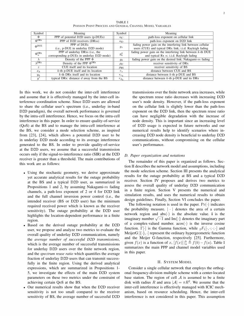
TABLE IPOISSON POINT PROCESS AND GENERAL CHANNEL MODEL VARIABLES

Symbol Meaning Symbol MeaningΦ PPP of potential D2D users (p-DUEs) αC path-loss exponent on cellular link

ΦDRx PPP of D2D receivers (DRxs) αD path-loss exponent on D2D link

ΦDUE PPP of DUEs(i.e., p-DUE in underlay D2D mode) gz

fading power gain on the interfering link between cellularusers (CUE) and typical DRx link; i.i.d. Rayleigh fading

ΦDRxu

PPP of underlay DRxs (i.e., thecorresponding p-DUEs in underlay D2D mode) gκk

fading power gain on the interfering link between k-th DUEand typical Rx κ; i.i.d. Rayleigh fading

λ Density of the PPP Φ g0 fading power gain on the desired link; Nakagami-m fadingλDRx Density of the PPP ΦDRx ρD receiver sensitivity of DRxz CUE itself and its location ρBS receiver sensitivity of BSxk k-th p-DUE itself and its location rz distance between CUE and BSyk k-th DRx itself and its location rck distance between k-th p-DUE and BSy′ typical DRx: distance d away from the BS rdk distance between k-th p-DUE and its DRx

In this work, we do not consider the inter-cell interferenceand assume that it is effectively managed by the inter-cell in-terference coordination scheme. Since D2D users are allowedto share the cellular user’s spectrum (i.e., underlay in-bandD2D paradigm), the overall network performance is governedby the intra-cell interference. Hence, we focus on the intra-cellinterference in this paper. In order to ensure quality-of-service(QoS) at the BS and to manage the intra-cell interference atthe BS, we consider a mode selection scheme, as inspiredfrom [23], [24], which allows a potential D2D user to bein underlay D2D mode according to its average interferencegenerated to the BS. In order to provide quality-of-serviceat the D2D users, we assume that a successful transmissionoccurs only if the signal-to-interference ratio (SIR) at the D2Dreceiver is greater than a threshold. The main contributions ofthis work are as follows:

• Using the stochastic geometry, we derive approximateyet accurate analytical results for the outage probabilityat the BS and a typical D2D user, as summarized inPropositions 1 and 2, by assuming Nakagami-m fadingchannels, a path-loss exponent of 2 or 4 for D2D linkand the full channel inversion power control (i.e., theintended receiver (BS or D2D user) has the minimumrequired received power which is known as the receiversensitivity). The outage probability at the D2D userhighlights the location-dependent performance in a finiteregion.

• Based on the derived outage probability at the D2Duser, we propose and analyze two metrics to evaluate theoverall quality of underlay D2D communication, namelythe average number of successful D2D transmissions,which is the average number of successful transmissionsfor underlay D2D users over the finite network region,and the spectrum reuse ratio which quantifies the averagefraction of underlay D2D users that can transmit success-fully in the finite region. Using the derived analyticalexpressions, which are summarized in Propositions 1-5, we investigate the effects of the main D2D systemparameters on these two metrics under the constraint ofachieving certain QoS at the BS.

• Our numerical results show that when the D2D receiversensitivity is not too small compared to the receiversensitivity of BS, the average number of successful D2D

transmissions over the finite network area increases, whilethe spectrum reuse ratio decreases with increasing D2Duser’s node density. However, if the path-loss exponenton the cellular link is slightly lower than the path-lossexponent on the D2D link, then the spectrum reuse ratiocan have negligible degradation with the increase ofnode density. This is important since an increasing levelof D2D usage is expected in future networks and ournumerical results help to identify scenarios where in-creasing D2D node density is beneficial to underlay D2Dcommunications, without compromising on the cellularuser’s performance.

D. Paper organization and notations

The remainder of this paper is organized as follows. Sec-tion II describes the network model and assumptions, includingthe mode selection scheme. Section III presents the analyticalresults for the outage probability at BS and a typical D2Dreceiver. Section IV proposes and derives two metrics toassess the overall quality of underlay D2D communicationin a finite region. Section V presents the numerical andsimulation results, and uses the numerical results to obtaindesign guidelines. Finally, Section VI concludes the paper.

The following notation is used in the paper. Pr(·) indicatesthe probability measure. | · | denotes the area of a certainnetwork region and abs(·) is the absolute value. i is theimaginary number

√−1 and Im{·} denotes the imaginary part

of a complex-valued number. acos(·) is the inverse cosinefunction. Γ[·] is the Gamma function, while 2F1[·, ·; ·; ·] andMeijerG [{·}, ·] represent the ordinary hypergeometric functionand the Meijer G-function, respectively [25]. Furthermore,given f(x) is a function of x, [f(x)] |ba , f(b)−f(a). Table Isummarizes the main PPP and channel model variables usedin this paper.

II. SYSTEM MODEL

Consider a single cellular network that employs the orthog-onal frequency-division multiple scheme with a center-locatedbase station. The region of cell A is assumed to be a finitedisk with radius R and area |A| = πR2. We assume that theinter-cell interference is effectively managed with ICIC mech-anism, based on resource scheduling. Hence, the inter-cellinterference is not considered in this paper. This assumption

3

rc

rd

θ

dR

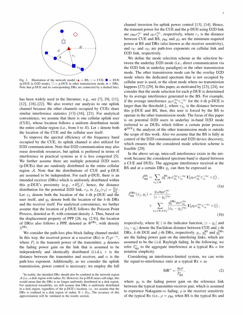
Fig. 1. Illustration of the network model (N = BS, ◦ = CUE, � = DUE(p-DUE in D2D mode), � = p-DUE in other transmission mode, • = DRx.Note that p-DUE and its corresponding DRx are connected by a dashed line).

has been widely used in the literature, e.g., see [7], [9], [11],[12], [18]–[22]. We also restrict our analysis to one uplinkchannel because the other channels occupied by CUEs sharesimilar interference statistics [13]–[16], [21]. For analyticalconvenience, we assume that there is one cellular uplink user(CUE), whose location follows a uniform distribution insidethe entire cellular region (i.e., from 0 to R). Let z denote boththe location of the CUE and the cellular user itself.

To improve the spectral efficiency of the frequency bandoccupied by the CUE, its uplink channel is also utilized forD2D communication. Note that D2D communication may alsoreuse downlink resources, but uplink is preferred in terms ofinterference in practical systems as it is less congested [5].We further assume there are multiple potential D2D users(p-DUEs) that are randomly distributed in the entire cellularregion A. Note that the distributions of CUE and p-DUEare assumed to be independent. For each p-DUE, there is anintended receiver (DRx) which is uniformly distributed withinthis p-DUE’s proximity (e.g., πR2

D)1, hence, the distancedistribution for the potential D2D link, rd, is fRd(rd) = 2rd

R2D

.Let xk denote both the location of the k-th p-DUE and theuser itself, and yk denote both the location of the k-th DRxand the receiver itself. For analytical convenience, we furtherassume that the location of p-DUE follows the Poisson PointProcess, denoted as Φ, with constant density λ. Thus, based onthe displacement property of PPP [26, eq. (2.9)], the locationof DRxs also follows a PPP, denoted as ΦDRx, with densityλDRx.

We consider the path-loss plus block fading channel model.In this way, the received power at a receiver (Rx) is Ptgr−α,where Pt is the transmit power of the transmitter, g denotesthe fading power gain on the link that is assumed to beindependently and identically distributed (i.i.d.), r is thedistance between the transmitter and receiver, and α is thepath-loss exponent. Additionally, as we consider the uplinktransmission, power control is necessary; we employ the full

1In reality, the intended DRx should also be confined in the network regionA (i.e., a disk region with radius R). However, for p-DUE nears cell-edge, thiswould mean that the DRx is no longer uniformly distributed in a disk region.For analytical tractability, we still assume that DRx is uniformly distributedin a disk region, regardless of the p-DUE’s location, i.e., we assume that theDRx is confined in a disk region of radius R + RD . The accuracy of thisapproximation will be validated in the results section.

channel inversion for uplink power control [13], [14]. Hence,the transmit power for the CUE and the p-DUE using D2D linkare ρBSr

αCz and ρDrαDd , respectively, where rz is the distance

between CUE and BS, ρBS and ρD are the minimum requiredpower at BS and DRx (also known as the receiver sensitivity),and αC and αD are path-loss exponents on cellular link andD2D link, respectively.

We define the mode selection scheme as the selection be-tween the underlay D2D mode (i.e., direct communication viathe D2D link in underlay paradigm) or the other transmissionmode. The other transmission mode can be the overlay D2Dmode where the dedicated spectrum that is not occupied bycellular user is used, or the silent mode where no transmissionhappens [27]–[29]. In this paper, as motivated by [23], [24], weconsider that the mode selection for each p-DUE is determinedby its average interference generated to the BS. For example,if the average interference ρDrαDdk r

−αCck

for the k-th p-DUE islarger than the threshold ξ, where rdk is the distance betweenthis p-DUE and BS, then, this user is forced by the BS tooperate in the other transmission mode. The focus of this paperis on potential D2D users in underlay in-band D2D mode(referred to as DUEs which follow a certain point processΦDUE); the analysis of the other transmission mode is outsidethe scope of this work. Also we assume that the BS is fully incontrol of the D2D communication and D2D device discovery,which ensures that the considered mode selection scheme isfeasible [29].

In the above set-up, intra-cell interference exists in the net-work because the considered spectrum band is shared betweena CUE and DUEs. The aggregate interference received at theBS and at a certain DRx yj can then be expressed as

IBSagg =

∑xk∈Φ

gBSk ρDr

αDdkr−αCck

1(ρDr

αDdkr−αCck

<ξ),

(1a)

IDRxagg (xj , yj) =

gzρBSrαCz

|z − yj |αD

+∑

xk∈Φ,k 6=j

gDRxk ρDr

αDdk

|xk − yj |αD1(ρDr

αDdkr−αCck

<ξ),

(1b)

respectively, where 1(·) is the indicator function, |z− yj | and|xk−yj | denote the Euclidean distance between CUE and j-thDRx, k-th DUE and j-th DRx, respectively. gz , gBS

k and gDRxk

are the fading power gain on the interfering links, which areassumed to be the i.i.d. Rayleigh fading. In the following, werefer Iκagg to the aggregate interference at a typical Rx κ fornotation simplicity.

Considering an interference-limited system, we can writethe signal-to-interference ratio at a typical Rx κ as

SIRκ =g0ρ

Iκagg, (2)

where g0 is the fading power gain on the reference linkbetween the typical transmitter-receiver pair, which is assumedto exprience Nakagami-m fading, ρ is the receiver sensitivityof the typical Rx (i.e., ρ = ρBS when BS is the typical Rx and

4

ρ = ρD if DRx is the typical Rx)2.

III. OUTAGE PROBABILITY ANALYSIS

To evaluate the network performance, we first considerand compute the outage probability experienced at a typicalreceiver.

A. Mathematical framework

Our considered outage probability for a typical Rx at agiven location is averaged over the fading power gain andthe possible locations of all interfering users. Mathematically,the outage probability at a typical Rx can be written as

Pκout(γ) = EIκagg,g0

{Pr

(g0ρ

Iκagg< γ

)}, (3)

where EIκagg,g0{·} is the expectation operator with respect to

Iκagg and g0.We leverage the reference link power gain-based frame-

work [30] to work out the outage probability. For the casethat the reference link suffers from the Nakagami-m fadingwith integer m, the outage expression in (3) can be rewrittenas (see proof in Appendix A)

Pκout(γ) =1−m−1∑t=0

(−s)t

t!

dt

dstMIκagg

(s)

∣∣∣∣s=m γ

ρ

, (4)

where MIκagg(s) = EIκagg

[exp(−sIκagg)

]is the moment gen-

erating function (MGF) of Iκagg. Note that this fading modelcovers Rayleigh fading (i.e., by setting m = 1) and can alsoapproximate Rician fading [30], [31]. Hence, it is adopted inthis paper.

As shown in (4), the computation of outage probabilityrequires the MGF results for the aggregate interference at thetypical Rx, which will be presented in the following.

B. MGF of the aggregate interference at the BS

The aggregate interference at the BS is generally in theform of

∑xk∈Φ

IBSk , where IBS

k is the interference from the k-

th p-DUE. Note that IBSk = 0 if k-th p-DUE is in the other

transmission mode. Due to the independently and uniformlydistributed (i.u.d.) property of p-DUEs and the i.i.d. propertyof the fading channels, the interference from a p-DUE is alsoi.i.d.. In the following, we drop the index k in rck , rdk , gkand IBS

k . As such, the aggregate interference can be writtenas(IBS)M

, where M is the number of p-DUEs following thePoisson distribution with density λ(|A|). Based on the MGF’sdefinition (stated below (4)), the MGF of IBS

agg is given by

MIBSagg

(s) =EM[EIBS

[exp

(−s(IBS)M)∣∣∣M]]

= exp(λ(|A|)

(MIBS(s)− 1

)), (5)

2According to (1b), when the typical Rx is a DRx, the SIR relies onthe location of DRx yj . Hence, the SIR at yj should be expressed asSIRDRx(xj , yj). But in this paper, we will sometimes ignore xj and yj ,and refer it simply as SIRDRx. This notation is also adopted for the outageprobability at yj , where the full notation would be Pκout(γ, yj).

where MIBS(s) denotes the MGF of the interference at theBS from a p-DUE, which is presented as follows.

Proposition 1. For the underlay in-band D2D communicationwith the considered mode selection scheme in a disk-shapedcellular network region, following the system model in Sec-tion II, the MGF of the interference from an i.u.d. p-DUEreceived at the BS can be expressed as (6), as shown at the

top of next page, where R̃D , min(RD, R

αCαD

(ξρD

) 1αD

)and

ξ is the mode selection threshold.Proof: See Appendix B.

Note that the result in (6) is expressed in terms of theordinary hypergeometric function and the MeijerG function,which are readily available in standard mathematical packagessuch as Mathematica.

C. MGF of the aggregate interference at a typical DRx

The point process of DUEs ΦDUE is in fact an independentthinning process of the underlaying PPP Φ, which is also aPPP with a certain density [26]. Similarly, in terms of thelocation of underlay DRxs (i.e., whose corresponding p-DUEis in underlay D2D mode), it is also a PPP ΦDRx

u , which is anindependent thinning process of DRxs ΦDRx.

For analytical convenience, we condition on an underlayDRx y′, which is located at a distance d away from the BS,and its corresponding DUE is denoted as x′. Because of theisotropic network region and PPP’s rotation-invariant property,the outage probability derived at y′ is the same for thoseunderlay DRxs whose distance to BS is d. Then, accordingto the Slivnyak’s Theorem, we can have the MGF of theaggregate interference received at y′ as

MIDRxagg

(s, d) = EIDRxC

{exp

(−sIDRx

C

)}× EΦ\x′

exp

−s ∑xk∈Φ\x′

IDRxk (y′)

=MIDRx

C(s, d)EΦ

{exp

(−s∑xk∈Φ

IDRxk (y′)

)}=MIDRx

C(s, d) exp

(λ(|A|)

(MIDRx(s, d)− 1

)), (7)

where IDRxC is the interference from CUE, MIDRx

C(s, d) is the

corresponding MGF, IDRxk (y′) is the interference from k-th p-

DUE, and MIDRx(s, d) is the MGF of the interference froma p-DUE. The results for these two MGFs are presented asfollows.

Proposition 2. For the underlay in-band D2D communicationwith the considered mode selection scheme in a disk-shapedcellular network region, following the system model in Sec-tion II, with the path-loss exponent αC = αD = 2 or 4, theMGF of the interference from an i.u.d. p-DUE received at aDRx, which is a distance d away from the BS can be givenas (8), as shown at the top of next page, where Ψ1(x, ·, ·, ·) isgiven in (25). Note that for other αC values, the semi-closed-form of MIDRx(s, d) is available in (24a) (αD = 2) and (26a)(αD = 4).

5

MIBS(s) =1 +2F1

[1, 2

αC; 1 + 2

αC; −1sξ

]R2DR

2R̃D−2− 2αD

αC (ξ/ρD)2αC

αCαD + αC

−

[αC 2F1

[1, 2αC

;1+ 2αC

; −RαC

sρDxαD

]+αD 2F1

[1,−2αD

;1− 2αD

; −RαC

sρDxαD

]x−2R2

D(αC+αD)

]∣∣∣∣∣R̃D

0

, αD 6= 2;

2R̃D2MeijerG

[{{0,αC−2

αC

},{2}

},{{0,1},

{−2αC

}}, RαC

sρDR̃D2

]R2DαC

, αD = 2;

(6)

MIDRx(s, d) = 1−

sρD [Ψ1(x2,sρD,R

2−d2,4d2sρD)−Ψ1(x2,sρD+ρDξ ,−d

2,4d2sρD)]|R̃D0

R2DR

2 , αC = αD = 2;

Im{[

Ψ1(x2,−i√sρD,R2−d2,−4i√sρDd2)−Ψ1

(x2,√ρDξ −i√sρD,−d2,−4i√sρDd2

)]∣∣∣R̃D0

}(√sρD)−1R2

DR2 , αC = αD = 4;

(8)

Proof: See Appendix C.

Corollary 1. For the underlay in-band D2D communicationwith the considered mode selection scheme in a disk-shapedcellular network region, following the system model in Sec-tion II, with the path-loss exponent αC = αD = 2 or 4, theMGF of the interference from an i.u.d. cellular user receivedat a DRx, which is distance d away from the BS, can be givenas (9), as shown at the top of next page, where β2(x, a, b, c) =√

(ax+ b)2 + c−b ln(ax+ b+

√(ax+ b)2 + c

). For other

αC values, theMIDRxC

(s, d) expression is given in (27b) (αD =2) and (28a) (αD = 4).Proof: See Appendix D.

Note that although (8) and (9) contain terms with theimaginary number, the MGF results are still real because ofthe Im(·) function.

IV. D2D COMMUNICATION PERFORMANCE ANALYSIS

Generally, the outage probability reflects the performanceat a typical user. In order to characterize the overall networkperformance, especially when the users are confined in a finiteregion, metrics other than the outage probability need to beconsidered. In this section, we consider two metrics: averagenumber of successful D2D transmissions and spectrum reuseratio. Their definitions and formulations are presented below.

A. Average number of successful D2D transmissions

1) Mathematical framework: In this paper, the averagenumber of successful D2D transmissions is defined as theaverage number of underlay D2D users that can transmit suc-cessfully over the network region A. Therein, the successfultransmission is defined as the event that the SIR at a DRxis greater than the threshold γ. For the considered scenario,we obtain the expression of the average number of successtransmissions in the following.

Proposition 3. For the underlay in-band D2D communicationwith the considered mode selection scheme in a disk-shapedcellular network region, following the system model in Sec-tion II, the average number of successful D2D transmissionsis

M̄ =

∫ R+RD

0

(1− PDRx

out (γ, d))pD2D(d)λDRx(d)2πd dd, (10)

where pD2D(d) is the probability that p-DUE is in D2D modegiven its corresponding DRx’s distance to BS is d, λDRx(d) isthe node density of DRxs, and PDRx

out (γ, d) is outage probabilityat the corresponding DRx.Proof: See Appendix E.

According to Proposition 3, the average number of success-ful D2D transmissions is determined by the outage probabilityexperienced at the underlay DRxs, the density function ofDRx, and the probability that the DRx is an underlay DRx.The outage probability has been derived in Section III. In thissection, we present the results for the remaining two factors,which will then allow the computation of average number ofsuccessful D2D transmissions using (10).

2) Density function of DRxs: Before showing the exactdensity function, we define one lemma as follows.

Lemma 1. For two disk regions with radii r1 and r2, respec-tively, which are separated by distance d, the area of theiroverlap region is given by [32], [33]

ψ(d, r1, r2) =r21acos

(d2+r2

1−r22

2dr1

)+ r2

2acos(d2+r2

2−r21

2dr2

)−√

2r22(r2

1 +d2)−r22−(r2

1−d2)2

2. (11)

Using Lemma 1, we can express the node density of DRxsas shown in the following proposition.

Proposition 4. For a disk-shaped network region with radiusR, assume that there are multiple p-DUEs that are randomlyindependently and uniformly distributed inside the region, andtheir location is modeled as a PPP with density λ. For each p-DUE, there is an intended DRx which is uniformly distributedinside the disk region formed around the p-DUE with radiusRD. Then, the location of DRxs also follows a PPP, with thedensity

λDRx(d) =

{λ, 0 ≤ d < R−RD;

λψ(d,R,RD)πR2

D, R−RD ≤ d ≤ R+RD;

(12)

where ψ(·, ·, ·) is defined in Lemma 1.Proof: See Appendix F.

The node density result in (12) can in fact be applied toa broader class of networks adopting the Poisson bi-polarnetwork model. To the best of our knowledge, this result for

6

MIDRxC

(s, d) = 1−

sρBS [β2(x2,(sρBS+1)2,d2(sρBS−1),4d4sρBS)]|R

0

R2(sρBS+1)3 , αC = αD = 2;

Im

√sρBS

[β2

(x2,1−i√sρBS,−d2

1+i√sρBS1−i√sρBS

,−4i√sρBSd

4

(1−i√sρBS)2

)]∣∣∣∣R0

R2(1−i√sρBS)2

, αC = αD = 4;(9)

the node density of receivers for the bi-polar network modelin a disk region has not been presented before in the literature.

3) Probability of being in D2D mode:

Proposition 5. For the underlay in-band D2D communicationwith the considered mode selection scheme in a disk-shapedcellular network region, following the system model in Sec-tion II, when the path-loss exponents for cellular link andD2D link are the same, the probability that a p-DUE is inunderlay D2D mode given that its DRx’s distance to BS is d,is given by

pD2D(d) =

1(ξ>ρD)− ξ2α d2(−1)1(ξ>ρD)+1(ξ1α−ρ

1αD

)2R2D

, 0 ≤ d < RD1;

1(ξ>ρD)−ψ

abs

ξ2α d

ξ2α −ρ

2αD

,RD,abs

ξ1α ρ

1αDd

ξ2α −ρ

2αD

πR2

D(−1)1(ξ>ρD)+1 ,

RD1 ≤ d < RD2;

1, d ≥ RD2;

(13)

where RD1 = abs(

1−(ρDξ

)1α

)RD, RD2 =

(1+(ρDξ

)1α

)RD,

ξ is the mode selection threshold and ψ(·, ·, ·) is definedin (11) in Lemma 1. For ξ = ρD, we have pD2D(d) = 1 −R2Dacos

(d

2RD

)− d2√R2D−

d2

4

πR2D

when d < 2RD, while pD2D(d) = 1

if d ≥ 2RD.Under the different path-loss exponent scenario, this prob-

ability can be approximated by

pD2D(d) ≈1 +

N∑n=1

(−1)n

(N

n

)2d

2αCαD (nNξ)

2αD

R2DαD

((N !)1/NρD

) 2αD

× Γ

[− 2

αD,

dαCnNξ

(N !)1/NρDRαDD

], (14)

where N is the parameter of a Gamma distribution which isused to formulate the approximation3.Proof: See Appendix G.

B. Spectrum reuse ratio

Since we have employed the mode selection scheme, notall p-DUEs are in D2D mode. To evaluate the efficiency ofour considered mode selection scheme, we propose a metric,namely the spectrum reuse ratio, which quantifies the averagefraction of DUEs that can successfully transmit among all

3By comparing with simulation results, we have verified that the averagenumber of successful D2D transmissions obtained using this approximationis accurate when N = 6.

DUEs. For analytical tractability4, spectrum reuse ratio isgiven by

τ =average number of successful D2D transmissions

average number of DUEs

=M̄

M̄D2D, (15)

where M̄ is given in (10), and M̄D2D is the average numberof DUEs, which can be obtained as

M̄D2D = EΦ,rd

{∑x∈Φ

1(ρDrαDd < ξrαCc )

}

=

∫ RD

0

(∫ R

0

1(ρDrαDd < ξrαCc ) 2πrcλ drc

)fRd(rd) drd

= λπ

∫ R̃D

0

∫ R

r

αDαCd (ρDξ )

1αC

2rcfRd(rd) drc drd

= λπR2

R̃D2

R2D

− αCαC + αD

(ρD/ξ)2αC R̃D

2αDαC

+2

R2R2D

. (16)

C. Summary

Summarizing, for the underlay in-band D2D communicationwith the considered mode selection scheme in a disk-shapedcellular network region, following the system model in Sec-tion II, we can calculate:

(i) outage probability at the BS by combining (5) and (6) inProposition 1 and substituting into (4);

(ii) conditional outage probability at a DRx by combin-ing (7), (8) in Proposition 2 and (9) in Corollary 1 andsubstituting into (4);

(iii) average number of successful D2D transmissions by sub-stituting the conditional outage probability at a DRx, (12)in Proposition 4 and (13) (or (14)) in Proposition 5,into (10) in Proposition 3;

(iv) spectrum reuse ratio by finding the ratio of averagenumber of successful D2D transmissions and M̄D2Din (16).

Note that the evaluation of the analytical results requiresthe differentiation and integration of the MGFs, which canbe easily implemented using mathematical packages such asMathematica.

4Note that a more accurate metric is the average of the rationumber of successful D2D transmissions

number of DUEs . However, such a metric is very difficult toobtain. Instead, we consider the metric in (15). It can be numerically verifiedthat the values for these two metrics are very close to each other.

7

TABLE IIMAIN SYSTEM PARAMETER VALUES.

Parameter Symbol Valuep-DUE’s node density λ 5 ∗ 10−5 users/m2

p-DUE’s transmission range RD 35 mReceiver sensitivity for BS ρBS −80 dBmReceiver sensitivity for DRx ρD −70 dBmSIR threshold γ 0 dB

V. RESULTS

In this section, we present the numerical results to studythe impact of the D2D system parameters (i.e., the p-DUE’snode density λ and the receiver sensitivity of DRx ρD) onthe outage probability, the average number of successful D2Dtransmissions and spectrum reuse ratio. To validate our derivedresults, the simulation results are generated using MATLAB,which are averaged over 106 simulation runs. Note that in thesimulations, all DRxs are confined in the region A. Unlessspecified otherwise, the values of the main system parametersshown in Table II are used. We assume a cell region radiusof R = 500 m. The vast majority of the D2D literature hasconsidered either αC = αD (i.e., [13]–[15], [17], [19]–[22])or αC is slightly smaller than αD (i.e., [11], [16], [34]–[36]).Hence we adopt the following path-loss exponent values whengenerating the main results: αC = 3.5, 3.75, 4 and αD = 4.5

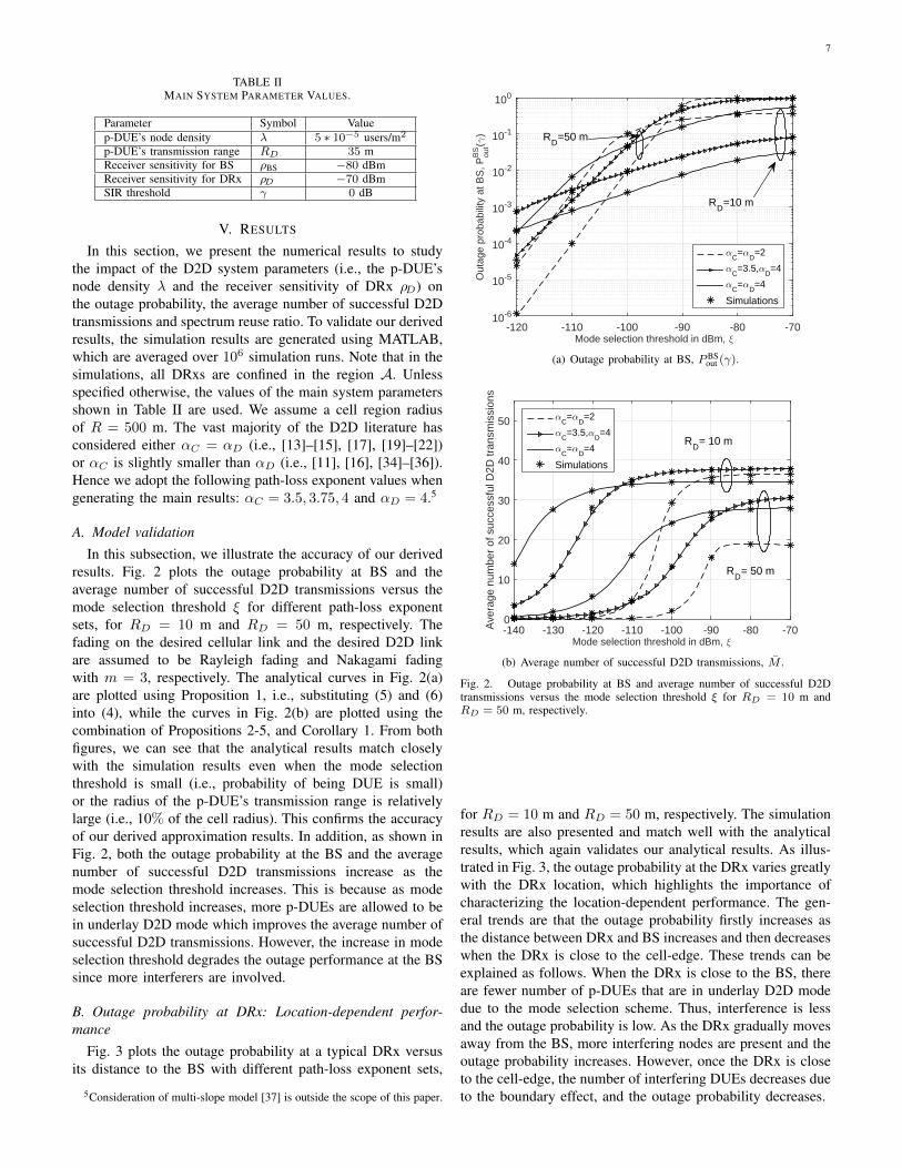
A. Model validationIn this subsection, we illustrate the accuracy of our derived

results. Fig. 2 plots the outage probability at BS and theaverage number of successful D2D transmissions versus themode selection threshold ξ for different path-loss exponentsets, for RD = 10 m and RD = 50 m, respectively. Thefading on the desired cellular link and the desired D2D linkare assumed to be Rayleigh fading and Nakagami fadingwith m = 3, respectively. The analytical curves in Fig. 2(a)are plotted using Proposition 1, i.e., substituting (5) and (6)into (4), while the curves in Fig. 2(b) are plotted using thecombination of Propositions 2-5, and Corollary 1. From bothfigures, we can see that the analytical results match closelywith the simulation results even when the mode selectionthreshold is small (i.e., probability of being DUE is small)or the radius of the p-DUE’s transmission range is relativelylarge (i.e., 10% of the cell radius). This confirms the accuracyof our derived approximation results. In addition, as shown inFig. 2, both the outage probability at the BS and the averagenumber of successful D2D transmissions increase as themode selection threshold increases. This is because as modeselection threshold increases, more p-DUEs are allowed to bein underlay D2D mode which improves the average number ofsuccessful D2D transmissions. However, the increase in modeselection threshold degrades the outage performance at the BSsince more interferers are involved.

B. Outage probability at DRx: Location-dependent perfor-mance

Fig. 3 plots the outage probability at a typical DRx versusits distance to the BS with different path-loss exponent sets,

5Consideration of multi-slope model [37] is outside the scope of this paper.

Mode selection threshold in dBm, ξ-120 -110 -100 -90 -80 -70

Out

age

prob

abili

ty a

t BS

, Pou

tB

S(γ

)

10-6

10-5

10-4

10-3

10-2

10-1

100

αC=α

D=2

αC=3.5,α

D=4

αC=α

D=4

Simulations

RD

=10 m

RD

=50 m

(a) Outage probability at BS, PBSout (γ).

Mode selection threshold in dBm, ξ-140 -130 -120 -110 -100 -90 -80 -70A

vera

ge n

umbe

r of

suc

cess

ful D

2D tr

ansm

issi

ons

0

10

20

30

40

50 αC=α

D=2

αC=3.5,α

D=4

αC=α

D=4

Simulations

RD

= 50 m

RD

= 10 m

(b) Average number of successful D2D transmissions, M̄ .

Fig. 2. Outage probability at BS and average number of successful D2Dtransmissions versus the mode selection threshold ξ for RD = 10 m andRD = 50 m, respectively.

for RD = 10 m and RD = 50 m, respectively. The simulationresults are also presented and match well with the analyticalresults, which again validates our analytical results. As illus-trated in Fig. 3, the outage probability at the DRx varies greatlywith the DRx location, which highlights the importance ofcharacterizing the location-dependent performance. The gen-eral trends are that the outage probability firstly increases asthe distance between DRx and BS increases and then decreaseswhen the DRx is close to the cell-edge. These trends can beexplained as follows. When the DRx is close to the BS, thereare fewer number of p-DUEs that are in underlay D2D modedue to the mode selection scheme. Thus, interference is lessand the outage probability is low. As the DRx gradually movesaway from the BS, more interfering nodes are present and theoutage probability increases. However, once the DRx is closeto the cell-edge, the number of interfering DUEs decreases dueto the boundary effect, and the outage probability decreases.

8

Distance between DRx and BS, d0 100 200 300 400 500

Out

age

Pro

babi

lity

at D

Rx,

Pou

tD

Rx (γ

,d)

10-5

10-4

10-3

10-2

10-1

100

Analytical (RD=10 m)

Analytical (RD=50 m)

Simulations

αC

=3.5, αD

=4

αC

=αD

=2

αC

= αD

=4

Fig. 3. Outage probability at DRx, PDRxout (γ, d), versus the distance between

BS and DRx d for RD = 10 m and RD = 50 m, respectively.

C. Effects of D2D user’s density

In this subsection, we investigate the effect of p-DUE’s nodedensity λ on the average number of successful D2D transmis-sions and spectrum reuse ratio (i.e., the average fraction ofDUEs that can successfully transmit among all DUEs). Sinceboth the outage probability at the BS and the average numberof successful D2D transmissions are increasing functions ofthe mode selection threshold ξ, as shown in Fig. 2, we haveadopted the following method to investigate the effects of D2Duser’s density:

• Given a QoS at the BS, for each p-DUE’s node densityλ, using (4), (5) and (6), we can find the mode selectionthreshold ξ satisfying the QoS at the BS;

• Using the mode selection threshold ξ that satisfies theQoS at BS, the average number of successful D2Dtransmissions M̄ can be calculated for each λ. Thisobtained M̄ value can be regarded as the maximumaverage number of successful underlay D2D transmissionachieved by the system. We can then work out thecorresponding spectrum reuse ratio.

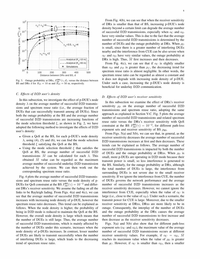
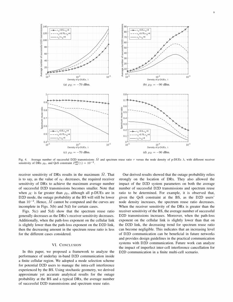
Fig. 4 plots the average number of successful D2D transmis-sions and spectrum reuse ratio versus the node density of p-DUEs for QoS constraint at the BS PBS

out (γ) = 10−2 and differ-ent DRx’s receiver sensitivity. We assume the fading on all thelinks to be Rayleigh fading. From Figs. 4(a) and 4(c), we cansee that the average number of successful D2D transmissionsincreases with increasing node density of p-DUE, however thespectrum reuse ratio decreases. This trend can be explained asfollows. When the node density is higher, the probability ofbeing in D2D mode is reduced to maintain the QoS at the BS.However, the overall node density is large which means thatthe number of DUEs is still large. Thus, the average numberof successful D2D transmissions, which is mainly affected bythe number of DUEs under this scenario, increases when thenode density of p-DUEs increases. In contrast, lesser numberof DUEs are likely to transmit successfully when the numberof interfering DUEs is large, which leads to the decreasingtrend of spectrum reuse ratio.

From Fig. 4(b), we can see that when the receiver sensitivityof DRx is smaller than that of BS, increasing p-DUE’s nodedensity beyond a certain limit can degrade the average numberof successful D2D transmissions, especially when αC and αDhave very similar values. This is due to the fact that the averagenumber of successful D2D transmissions is determined by thenumber of DUEs and the outage probability at DRx. When ρDis small, since there is a greater number of interfering DUEsnearby and the interference from CUE can be also severe whenαC and αD have very similar values, the outage probability atDRx is high. Thus, M̄ first increases and then decreases.

From Fig. 4(c), we can see that if αC is slightly smallerthan αD and ρD is greater than ρC , the decreasing trend forspectrum reuse ratio is almost negligible. In other words, thespectrum reuse ratio can be regarded as almost a constant andit does not degrade with increasing node density of p-DUE.Under such a case, increasing the p-DUE’s node density isbeneficial for underlay D2D communication.

D. Effects of D2D user’s receiver sensitivity

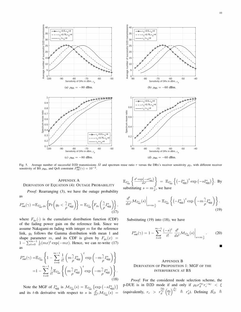
In this subsection we examine the effect of DRx’s receiversensitivity ρD on the average number of successful D2Dtransmissions and spectrum reuse ratio, adopting the sameapproach as explained in Section V-C. Fig. 5 plots the averagenumber of successful D2D transmissions and related spectrumreuse ratio versus the DRx’s receiver sensitivity with QoSconstraint at the BS PBS

out (γ) = 10−2, for different path-lossexponent sets and receiver sensitivity of BS ρBS.

From Figs. 5(a) and 5(b), we can see that, in general, as thereceiver sensitivity decreases the average number of successfulD2D transmissions increases at first and then decreases. Thesetrends can be explained as follows. The average number ofsuccessful D2D transmissions is impacted by both the numberof DUEs and the outage probability at DRxs. When ρD issmall, more p-DUEs are operating in D2D mode because theirtransmit power is small, so less interference is generated tothe BS. Similarly, for the outage probability at DRx, althoughthe total number of DUEs is large, the interference fromsurrounding DUEs is not severe due to the small receiversensitivity. If we ignore the interference from CUE, the numberof DUEs governs the network performance and the averagenumber of successful D2D transmissions increases as thereceiver sensitivity decreases. However, we cannot ignore theinterference from CUE, especially when the value of αC islarge (i.e., close to the value of αD). Under such a scenario, thetransmit power for CUE is large. Moreover, due to the smallerreceiver sensitivity at DRxs, DRxs are more likely to be inoutage. Consequently, the interplay of the number of DUEsand the outage probability at the DRx causes the averagenumber of successful D2D transmissions to first increase andthen decrease as the receiver sensitivity decreases.

Figs. 5(a) and 5(b) also show that for different path-lossexponent sets (αC and αD), the maximum value of the averagenumber of successful D2D transmissions occurs at differentreceiver sensitivity values. For example, if αC = αD, M̄reaches its maximum value when the value of ρD is greaterthan ρC . However, if αC is smaller than αD, then a smaller

9

Density of p-DUEs, λ10-5 10-4 10-3A

vera

ge n

umbe

r of

suc

cess

ful D

2D tr

ansm

issi

ons

0

20

40

60

80

100

120

140α

C=3.5,α

D=4

αC=3.75,α

D=4

αC=α

D=4

(a) ρD = −70 dBm.

Density of p-DUEs, λ10-5 10-4 10-3A

vera

ge n

umbe

r of

suc

cess

ful D

2D tr

ansm

issi

ons

0

10

20

30

40

50

60

70

80

90α

C=3.5,α

D=4

αC=3.75,α

D=4

αC=α

D=4

(b) ρD = −90 dBm.

Density of p-DUEs, λ10-5 10-4 10-3

Spe

ctru

m r

euse

rat

io

0.4

0.5

0.6

0.7

0.8

0.9

1

αC=3.5,α

D=4

αC=3.75,α

D=4

αC=α

D=4

(c) ρD = −70 dBm.

Density of p-DUEs, λ10-5 10-4 10-3

Spe

ctru

m r

euse

rat

io

0

0.1

0.2

0.3

0.4

0.5

0.6

0.7

0.8

αC=3.5,α

D=4

αC=3.75,α

D=4

αC=α

D=4

(d) ρD = −90 dBm.

Fig. 4. Average number of successful D2D transmissions M̄ and spectrum reuse ratio τ versus the node density of p-DUEs λ, with different receiversensitivity of DRx ρD , and QoS constraint PBS

out (γ) = 10−2.

receiver sensitivity of DRx results in the maximum M̄ . Thatis to say, as the value of αC decreases, the required receiversensitivity of DRx to achieve the maximum average numberof successful D2D transmissions becomes smaller. Note thatwhen ρC is far greater than ρD, although all p-DUEs are inD2D mode, the outage probability at the BS will still be lowerthan 10−2. Hence, M̄ cannot be computed and the curves areincomplete in Figs. 5(b) and 5(d) for certain cases.

Figs. 5(c) and 5(d) show that the spectrum reuse ratiogenerally decreases as the DRx’s receiver sensitivity decreases.Additionally, when the path-loss exponent on the cellular linkis slightly lower than the path-loss exponent on the D2D link,then the decreasing amount in the spectrum reuse ratio is lessfor the different cases considered.

VI. CONCLUSION

In this paper, we proposed a framework to analyze theperformance of underlay in-band D2D communication insidea finite cellular region. We adopted a mode selection schemefor potential D2D users to manage the intra-cell interferenceexperienced by the BS. Using stochastic geometry, we derivedapproximate yet accurate analytical results for the outageprobability at the BS and a typical DRx, the average numberof successful D2D transmissions and spectrum reuse ratio.

Our derived results showed that the outage probability reliesstrongly on the location of DRx. They also allowed theimpact of the D2D system parameters on both the averagenumber of successful D2D transmissions and spectrum reuseratio to be determined. For example, it is observed that,given the QoS constraint at the BS, as the D2D users’node density increases, the spectrum reuse ratio decreases.When the receiver sensitivity of the DRx is greater than thereceiver sensitivity of the BS, the average number of successfulD2D transmissions increases. Moreover, when the path-lossexponent on the cellular link is slightly lower than that onthe D2D link, the decreasing trend for spectrum reuse ratiocan become negligible. This indicates that an increasing levelof D2D communication can be beneficial in future networksand provides design guidelines in the practical communicationsystems with D2D communication. Future work can analyzethe impact of imperfect inter-cell interference cancellation forD2D communication in a finite multi-cell scenario.

10

Sensitivity of DRx in dBm, ρd

-100 -90 -80 -70 -60 -50Ave

rage

num

ber

of s

ucce

ssfu

l D2D

tran

smis

sion

s

0

5

10

15

20

25

30

35

40α

C=3.5,α

D=4

αC=3.75,α

D=4

αC=α

D=4

(a) ρBS = −80 dBm.

Sensitivity of DRx in dBm, ρd

-90 -80 -70 -60 -50 -40Ave

rage

num

ber

of s

ucce

ssfu

l D2D

tran

smis

sion

s

0

5

10

15

20

25

30

35

40α

C=3.5,α

D=4

αC=3.75,α

D=4

αC=α

D=4

(b) ρBS = −60 dBm.

Sensitivity of DRx in dBm, ρd

-100 -90 -80 -70 -60 -50

Spe

ctru

m r

euse

rat

io

0.1

0.2

0.3

0.4

0.5

0.6

0.7

0.8

0.9

1

αC=3.5,α

D=4

αC=3.75,α

D=4

αC=α

D=4

(c) ρBS = −80 dBm.

Sensitivity of DRx in dBm, ρd

-90 -80 -70 -60 -50 -40

Spe

ctru

m r

euse

rat

io

0

0.2

0.4

0.6

0.8

1α

C=3.5,α

D=4

αC=3.75,α

D=4

αC=α

D=4

(d) ρBS = −60 dBm.

Fig. 5. Average number of successful D2D transmissions M̄ and spectrum reuse ratio τ versus the DRx’s receiver sensitivity ρD , with different receiversensitivity of BS ρBS, and QoS constraint PBS

out (γ) = 10−2.

APPENDIX ADERIVATION OF EQUATION (4): OUTAGE PROBABILITY

Proof: Rearranging (3), we have the outage probabilityas

Pκout(γ) =EIκagg,g0

{Pr

(g0 <

γ

ρIκagg

)}= EIκagg

{Fg0

(γ

ρIκagg

)},

(17)

where Fg0(·) is the cumulative distribution function (CDF)of the fading power gain on the reference link. Since weassume Nakagami-m fading with integer m for the referencelink, g0 follows the Gamma distribution with mean 1 andshape parameter m, and its CDF is given by Fg0(x) =1 −

∑m−1t=0

1t! (mx)t exp(−mx). Hence, we can re-write (17)

as

Pκout(γ) =EIκagg

{1−

m−1∑t=0

1

t!

(mγ

ρIκagg

)texp

(−mγ

ρIκagg

)}

=1−m−1∑t=0

1

t!EIκagg

{(mγ

ρIκagg

)texp

(−mγ

ρIκagg

)}.

(18)

Note the MGF of Iκagg is MIκagg(s) = EIκagg

{exp

(−sIκagg

)}and its t-th derivative with respect to s is dt

dstMIκagg(s) =

EIκagg

{dt exp(−sIκagg)

dst

}= EIκagg

{(−Iκagg

)texp

(−sIκagg

)}. By

substituting s = mγρ , we have

dt

dstMIκagg

(s)

∣∣∣∣s=m γ

ρ

= EIκagg

{(−Iκagg

)texp

(−mγ

ρIκagg

)}.

(19)

Substituting (19) into (18), we have

Pκout(γ) = 1−m−1∑t=0

(−s)t

t!

dt

dstMIκagg

(s)

∣∣∣∣s=m γ

ρ

. (20)

APPENDIX BDERIVATION OF PROPOSITION 1: MGF OF THE

INTERFERENCE AT BS

Proof: For the considered mode selection scheme, thep-DUE is in D2D mode if and only if ρDr

αDd r−αCc < ξ

(equivalently, rc > rαDαC

d

(ρDξ

) 1αC , r′d). Defining R̃D ,

11

min(RD, R

αCαD

(ξρD

) 1αD

), we can then express IBS as

IBS =

gρDr

αDd r−αCc , (r′d ≤ rc < R, 0 ≤ rd < R̃D);

0, (0 ≤ rc < r′d, 0 ≤ rd < R̃D);

0, (0 ≤ rc < R, R̃D ≤ rd < RD);

(21)

Using the definition of MGF, we have (22) as shown at thetop of next page, where the final result is obtained using [25]and Mathematica software.

APPENDIX CDERIVATION OF PROPOSITION 2: MGF OF THE

INTERFERENCE FROM P-DUEProof: For a DRx located at distance d away from

the BS, the interference from an i.u.d. p-DUE, IDRx, issimilar to (21) except that gρDr

αDd r−αCc is replaced by

gρDrαDd

(r2c + d2 − 2rcd cos θ

)−αD2 , where θ is the angleformed between the y′-BS line and p-DUE-BS line, whichis uniformly distributed between 0 and 2π (see Fig. 1). Usingthe definition of MGF and simplifying, we have

MIDRx(s, d)=

∫ R̃D

0

∫ R

r′d

∫ 2π

0

∫ ∞0

exp

(−sgρDrαDd

(r2c+d2−2rcd cos θ)αD2

)× fG(g)

1

2πfRc(rc)fRd(rd) dg dθ drc drd

+

∫ R̃D

0

∫ r′d

0

∫ 2π

0

∫ ∞0

fG(g)1

2πfRc(rc)fRd(rd) dg dθ drcdrd

+

∫ RD

R̃D

∫ R

0

∫ 2π

0

∫ ∞0

fG(g)1

2πfRc(rc)fRd(rd) dg dθ drcdrd

=1−∫ R̃D

0

∫ R

r′d

∫ π

0

sρDrαDd

sρDrαDd +(r2c+d2−2rcd cos θ)

αD2

× 1

πfRc(rc)fRd(rd) dθ drc drd, (23)

where r′d , rαDαC

d

(ρDξ

) 1αC .

Due to the complicated expression of IDRx, the closed-formresults (or semi-closed form) exist only for the cases of αD = 2or αD = 4.• Case of αD = 2: Substituting αD = 2 into (23), we

get (24) as shown at the top of next page, where thesecond and third steps come from (2.553) and (2.261)in [25], respectively, and last step is obtained using Math-ematica. β1(x, a, b, c) = ax + b +

√(ax+ b)2 + cx,∫

xxβ1(x, a, b, c)dx = Ψ1(x, a, b, c) and

Ψ1(x, a, b, c) =−x2

8+

(10ab+ 3c− 2a2x)√

(ax+ b)2 + cx

16

+x2

2ln(β1(x, a, b, c))−

ln(c+2a2x+2a

(b+√

(ax+b)2+cx))

32a4(16a2b2 + 16abc+ 3c2)−1.

(25)

• Case of αD = 4: Similar to αD = 2 case, via substitutingαD = 4 into (23) and using (2.553) and (2.261) in [25], wehave (26) as shown at the top of next page, where the thirdstep comes from the fact that the two integrated terms in thesecond step are conjugated such that a−a∗

2i = Im{a}.Thus, we arrive at the result in Proposition 2.

APPENDIX DDERIVATION OF COROLLARY 1: MGF OF THE

INTERFERENCE FROM CUE

Proof: Since there is no constraint on the CUE, thei.u.d. CUE will always generate interference (e.g., IDRx

C =

gρBSrαCz

(r2z + d2 − 2rzd cos θ

)−αD2 ) to this typical DRx. Asbefore, we can only derive the analytical result for αD = 2 or4.• Case of αD = 2: According to the definition of MGF and

the expression of IDRxC , we have

MIDRxC

(s, d)= 1−∫ R

0

∫ π

0

sρBSrαCz 2rz/(πR

2)

sρBSrαCz +(r2z+d2−2rzd cos θ)

αD2

dθ drz

(27a)

= 1− sρBS

R2

∫ R

0

2rαC+1z√

(sρBSrαCz + r2z + d2)2 − 4r2zd2

drz (27b)

= 1−sρBS

[β2(x2, (sρBS + 1)2, d2(sρBS − 1), 4d4sρBS

)]∣∣R0

R2(sρBS + 1)3,

(αC = 2),(27c)

where β2(x, a, b, c) =√

(ax+ b)2 + c −b ln

(ax+ b+

√(ax+ b)2 + c

).

• Case of αD = 4: Similarly, substituting αD = 4into (27a), we get

MIDRxC

(s, d)= 1−∫ R

0

Im

rαC/2z√(

r2z+d2−i√sρBSr

αCz

)2−4r2zd2

×

2rz√sρBS

R2drz (28a)

=1−Im

√sρBS

[β2(x2, 1−i√sρBS,−d2 1+i√sρBS

1−i√sρBS,−4i√sρBSd

4

(1−i√sρBS)2

)]∣∣∣R0

R2(1− i√sρBS)2

,

(αC = 4). (28b)

Note the step in (27c) and step in (28b) come from [25,(2.264)].

APPENDIX EDERIVATION OF PROPOSITION 3: AVERAGE NUMBER OF

SUCCESSFUL D2D TRANSMISSIONS

Proof: Using the definition in Section IV-A1, the averagenumber of successful D2D transmissions can be mathemati-cally written as

M̄ =EΦ

{∑xi∈Φ

1(xj ∈ΦDUE)1(SIRDRx(xj , yj)>γ)

}. (29)

As mentioned in Section III-C, the location of underlayDRxs (i.e., whose corresponding p-DUE is in underlay D2Dmode) follows the PPP. According to the reduced Campbell

12

MIBS(s) =

∫ R̃D

0

∫ R

r′d

∫ ∞0

exp(−sgρDrαDd r−αCc

)fG(g)fRc(rc)fRd(rd) dg drc drd

+

∫ R̃D

0

∫ r′d

0

∫ ∞0

fG(g)fRc(rc)fRd(rd) dg drc drd +

∫ RD

R̃D

∫ R

0

∫ ∞0

fG(g)fRc(rc)fRd(rd) dg drc drd

= 1−∫ R̃D

0

2F1

[1,

2

αC, 1 +

2

αC,− RαC

sρDrαDd

]−r2αDαC

d 2F1

[1, 2

αC, 1 + 2

αC,− 1

sξ

]R2(ξ/ρD)

2αC

fRd(rd) drd

= 1+2F1

[1, 2

αC; 1 + 2

αC; −1sξ

]R2DR

2R̃D−2− 2αD

αC (ξ/ρD)2αC

αCαD + αC

−

[αC 2F1

[1, 2αC

;1+ 2αC

; −RαC

sρDxαD

]+αD 2F1

[1,−2αD

;1− 2αD

; −RαC

sρDxαD

]x−2R2

D(αC+αD)

]∣∣∣∣∣R̃D

0

, αD 6= 2;

2R̃D2MeijerG

[{{0,αC−2

αC

},{2}

},{{0,1},

{−2αC

}}, RαC

sρDR̃D2

]R2DαC

, αD = 2;

(22)

MIDRx(s, d) = 1−∫ R̃D

0

∫ R

r′d

∫ π

0

sρDr2d

sρDr2d+r2

c+d2−2rcd cos θ

1

πfRc(rc)fRd(rd) dθ drc drd

= 1−∫ R̃D

0

∫ R

r′d

sρDr2d√

(sρDr2d + r2

c + d2)2 − 4r2cd

2

2rcR2

fRd(rd) drc drd

=1−∫ R̃D

0

sρDr2d

R2ln

β1

(r2d, sρD, R

2 − d2, 4d2sρD)√((

r2dρDξ

) 2αC +sρDr2

d−d2

)2

+4d2sρDr2d+(r2dρDξ

) 2αC +sρDr2

d−d2

2rdR2D

drd (24a)

=1−sρD

[Ψ1

(x2, sρD, R

2 − d2, 4d2sρD)−Ψ1

(x2, sρD + ρD

ξ ,−d2, 4d2sρD

)]∣∣∣R̃D0

R2DR

2, (αC = 2). (24b)

MIDRx (s, d)=1−∫ R̃D

0

∫ R

r′d

∫ π

0

sρDr4d

2i√sρDr4d

(1

r2c+d2−2rcd cos θ−i√sρDr4d

− 1

r2c+d2−2rcd cos θ+i√sρDr4d

)2rc dθ drcπR2

fRd(rd) drd

=1−∫ R̃D

0

√sρDr4d2iR2

∫ R

r′d

2rc√(r2c+d2−i

√sρDr4d)

2−4r2cd2− 2rc√

(r2c+d2+i√sρDr4d)

2−4r2cd2

drcfRd(rd) drd

=1−∫ R̃D0

√sρDr4dR2

Im

lnβ1(r2d,−i√sρD, R2−d2,−4i√sρDd2

)√((r4dρDξ

) 2αC−i√sρDr2d−d2

)2−4i√sρDd2r2d+

(r4dρDξ

) 2αC−i√sρDr2d−d2

2rdR2D

drd (26a)

=1−Im{[

Ψ1

(x2,−i√sρD, R2−d2,−4i√sρDd2

)−Ψ1

(x2,√

ρDξ−i√sρD,−d2,−4i√sρDd2

)]∣∣∣R̃D0

}(√sρD)−1R2

DR2

, (αC = 4). (26b)

measure [26], we can rewrite (29) as

M̄ =

∫A

1(x′∈ΦDUE)Pr!x′(SIRDRx(x′, y′)>γ

)λ dx′

=

∫ADRx

1(y′∈ΦDRxu )

(1− PDRx

out (γ, y′))λDRx(y′) dy′

=

∫ R+RD

0

pD2D(d)(1− PDRx

out (γ, d))λDRx(d)2πd dd, (30)

where Pr!x(·) is the reduced Palm distribution, ADRx is thenetwork region for DRxs (e.g., a disk region with radiusR+RD). The second step in (30) results from the Slivnyak’stheorem and the fact that we interpret this reduced Campbellmeasure from the point view of DRx, while the last step in (30)is based on the isotropic property of the underlay networkregion and the independent thinning property of PPP.

13

R

d d

RD

B1 = φ(d,R,RD)

B1 = πR2D

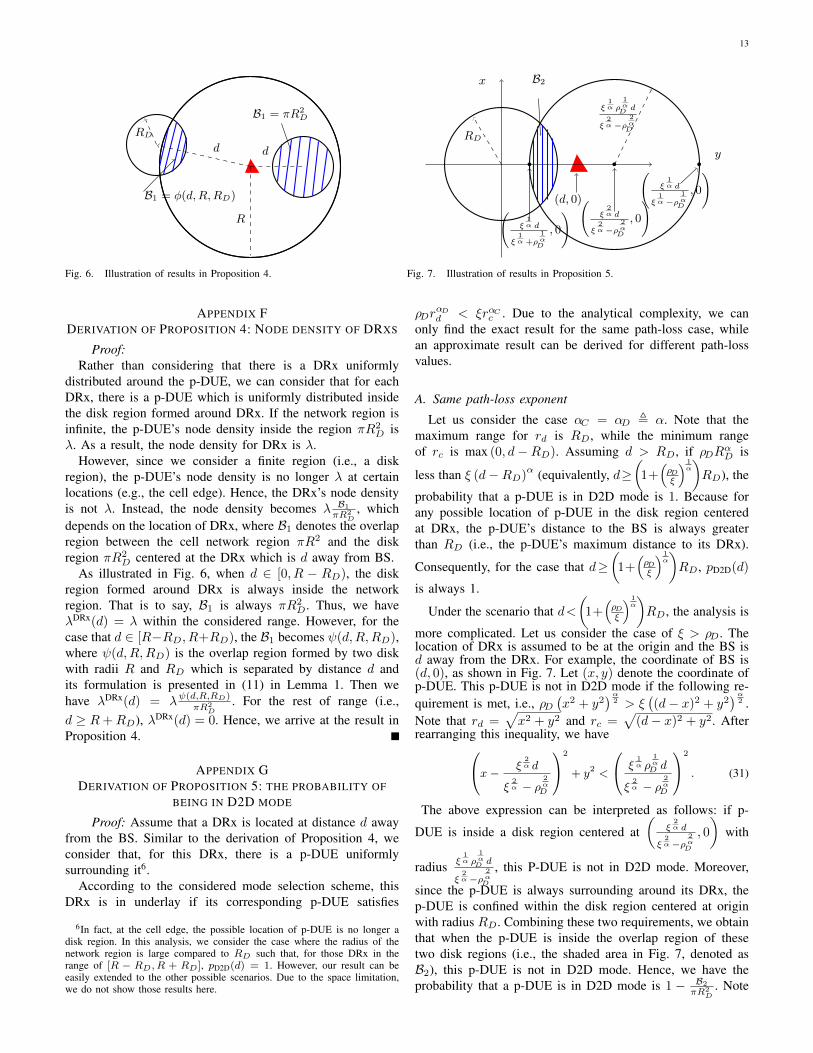
Fig. 6. Illustration of results in Proposition 4.

x

y

(d, 0)(ξ

2α d

ξ2α−ρ

2αD

, 0

)

ξ1α ρ

1αDd

ξ2α−ρ

2αD

(ξ

1α d

ξ1α−ρ

1αD

, 0

)(

ξ1α d

ξ1α +ρ

1αD

, 0

)

RD

B2

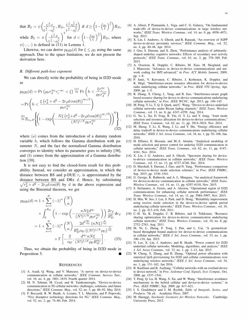
Fig. 7. Illustration of results in Proposition 5.

APPENDIX FDERIVATION OF PROPOSITION 4: NODE DENSITY OF DRXS

Proof:Rather than considering that there is a DRx uniformly

distributed around the p-DUE, we can consider that for eachDRx, there is a p-DUE which is uniformly distributed insidethe disk region formed around DRx. If the network region isinfinite, the p-DUE’s node density inside the region πR2

D isλ. As a result, the node density for DRx is λ.

However, since we consider a finite region (i.e., a diskregion), the p-DUE’s node density is no longer λ at certainlocations (e.g., the cell edge). Hence, the DRx’s node densityis not λ. Instead, the node density becomes λ B1

πR2D

, whichdepends on the location of DRx, where B1 denotes the overlapregion between the cell network region πR2 and the diskregion πR2

D centered at the DRx which is d away from BS.As illustrated in Fig. 6, when d ∈ [0, R − RD), the disk

region formed around DRx is always inside the networkregion. That is to say, B1 is always πR2

D. Thus, we haveλDRx(d) = λ within the considered range. However, for thecase that d ∈ [R−RD, R+RD), the B1 becomes ψ(d,R,RD),where ψ(d,R,RD) is the overlap region formed by two diskwith radii R and RD which is separated by distance d andits formulation is presented in (11) in Lemma 1. Then wehave λDRx(d) = λψ(d,R,RD)

πR2D

. For the rest of range (i.e.,d ≥ R+RD), λDRx(d) = 0. Hence, we arrive at the result inProposition 4.

APPENDIX GDERIVATION OF PROPOSITION 5: THE PROBABILITY OF

BEING IN D2D MODE

Proof: Assume that a DRx is located at distance d awayfrom the BS. Similar to the derivation of Proposition 4, weconsider that, for this DRx, there is a p-DUE uniformlysurrounding it6.

According to the considered mode selection scheme, thisDRx is in underlay if its corresponding p-DUE satisfies

6In fact, at the cell edge, the possible location of p-DUE is no longer adisk region. In this analysis, we consider the case where the radius of thenetwork region is large compared to RD such that, for those DRx in therange of [R − RD, R + RD], pD2D(d) = 1. However, our result can beeasily extended to the other possible scenarios. Due to the space limitation,we do not show those results here.

ρDrαDd < ξrαCc . Due to the analytical complexity, we can

only find the exact result for the same path-loss case, whilean approximate result can be derived for different path-lossvalues.

A. Same path-loss exponent

Let us consider the case αC = αD , α. Note that themaximum range for rd is RD, while the minimum rangeof rc is max (0, d−RD). Assuming d > RD, if ρDRαD is

less than ξ (d−RD)α (equivalently, d≥

(1+(ρDξ

)1α

)RD), the

probability that a p-DUE is in D2D mode is 1. Because forany possible location of p-DUE in the disk region centeredat DRx, the p-DUE’s distance to the BS is always greaterthan RD (i.e., the p-DUE’s maximum distance to its DRx).

Consequently, for the case that d≥(

1+(ρDξ

)1α

)RD, pD2D(d)

is always 1.

Under the scenario that d<(

1+(ρDξ

)1α

)RD, the analysis is

more complicated. Let us consider the case of ξ > ρD. Thelocation of DRx is assumed to be at the origin and the BS isd away from the DRx. For example, the coordinate of BS is(d, 0), as shown in Fig. 7. Let (x, y) denote the coordinate ofp-DUE. This p-DUE is not in D2D mode if the following re-quirement is met, i.e., ρD

(x2 + y2

)α2 > ξ

((d− x)2 + y2

)α2 .

Note that rd =√x2 + y2 and rc =

√(d− x)2 + y2. After

rearranging this inequality, we havex− ξ2α d

ξ2α − ρ

2αD

2

+ y2 <

ξ1α ρ

1αD d

ξ2α − ρ

2αD

2

. (31)

The above expression can be interpreted as follows: if p-

DUE is inside a disk region centered at(

ξ2α d

ξ2α−ρ

2αD

, 0

)with

radius ξ1α ρ

1αD d

ξ2α−ρ

2αD

, this P-DUE is not in D2D mode. Moreover,

since the p-DUE is always surrounding around its DRx, thep-DUE is confined within the disk region centered at originwith radius RD. Combining these two requirements, we obtainthat when the p-DUE is inside the overlap region of thesetwo disk regions (i.e., the shaded area in Fig. 7, denoted asB2), this p-DUE is not in D2D mode. Hence, we have theprobability that a p-DUE is in D2D mode is 1 − B2

πR2D

. Note

14

that B2 = ψ

(ξ

2α d

ξ2α−ρ

2αD

, RD,ξ

1α ρ

1αD d

ξ2α−ρ

2αD

)if d≥

(1−(ρDξ

)1α

)RD,

while B2 = π

(ξ

1α d

ξ1α−ρ

1αD

)2

for d <(

1−(ρDξ

)1α

)RD, where

ψ(·, ·, ·) is defined in (11) in Lemma 1.Likewise, we can derive pD2D(d) for ξ ≤ ρD using the same

approach. Due to the space limitation, we do not present thederivation here.

B. Different path-loss exponent

We can directly write the probability of being in D2D modeas

pD2D(d) = Pr(ρDr

αDd r−αCc < ξ

) (a)≈ Pr

(h <

ξrαCcρDr

αDd

)=Pr

(h <

ξ(r2d + d2 − 2rdd cos(θ)

)αC/2ρDr

αDd

)(b)≈ Erd,θ

(

1− exp

(−Nξ(r2d+d2−2rdd cos(θ)

)αC/2(N !)1/NρDr

αDd

))N ,

(32)

where (a) comes from the introduction of a dummy randomvariable h, which follows the Gamma distribution with pa-rameter N , and the fact the normalized Gamma distributionconverges to identity when its parameter goes to infinity [38],and (b) comes from the approximation of a Gamma distribu-tion [39].

It is not easy to find the closed-form result for this prob-ability. Instead, we consider an approximation, in which thedistance between BS and p-DUE rc is approximated by thedistance between BS and DRx d. Hence, by substituting√r2d + d2 − 2rdd cos(θ) by d in the above expression and

using the Binomial theorem, we get

pD2D(d) ≈ 1 +

N∑n=1

(−1)n

(N

n

)×∫ RD

0

(1− exp

(− nNξdαC

(N !)1/NρDrαDd

))2rdR2D

drd

= 1 +

N∑n=1

(−1)n

(N

n

)2d

2αCαD (nNξ)

2αD

R2DαD

((N !)1/NρD

) 2αD

× Γ

[− 2

αD,

dαCnNξ

(N !)1/NρDRαDD

]. (33)

Thus, we obtain the probability of being in D2D mode inProposition 5.

REFERENCES

[1] A. Asadi, Q. Wang, and V. Mancuso, “A survey on device-to-devicecommunication in cellular networks,” IEEE Commun. Surveys Tuts.,vol. 16, no. 4, pp. 1801–1819, Fourth quarter 2014.

[2] M. N. Tehrani, M. Uysal, and H. Yanikomeroglu, “Device-to-devicecommunication in 5G cellular networks: challenges, solutions, and futuredirections,” IEEE Commun. Mag., vol. 52, no. 5, pp. 86–92, May 2014.

[3] F. Boccardi, R. W. Heath, A. Lozano, T. L. Marzetta, and P. Popovski,“Five disruptive technology directions for 5G,” IEEE Commun. Mag.,vol. 52, no. 2, pp. 74–80, Feb. 2014.

[4] A. Altieri, P. Piantanida, L. Vega, and C. G. Galarza, “On fundamentaltrade-offs of device-to-device communications in large wireless net-works,” IEEE Trans. Wireless Commun., vol. 14, no. 9, pp. 4958–4971,Sep. 2015.

[5] X. Lin, J. Andrews, A. Ghosh, and R. Ratasuk, “An overview of 3GPPdevice-to-device proximity services,” IEEE Commun. Mag., vol. 52,no. 4, pp. 40–48, Apr. 2014.

[6] J. Guo, S. Durrani, and X. Zhou, “Performance analysis of arbitrarily-shaped underlay cognitive networks: Effects of secondary user activityprotocols,” IEEE Trans. Commun., vol. 63, no. 2, pp. 376–389, Feb.2015.

[7] A. Osseiran, K. Doppler, C. Ribeiro, M. Xiao, M. Skoglund, andJ. Manssour, “Advances in device-to-device communications and net-work coding for IMT-advanced,” in Proc. ICT Mobile Summit, 2009,pp. 1–8.

[8] P. Janis, V. Koivunen, C. Ribeiro, J. Korhonen, K. Doppler, andK. Hugl, “Interference-aware resource allocation for device-to-deviceradio underlaying cellular networks,” in Proc. IEEE VTC-Spring, Apr.2009, pp. 1–5.

[9] R. Zhang, X. Cheng, L. Yang, and B. Jiao, “Interference-aware graphbased resource sharing for device-to-device communications underlayingcellular networks,” in Proc. IEEE WCNC, Apr. 2013, pp. 140–145.

[10] M. Peng, Y. Li, T. Q. S. Quek, and C. Wang, “Device-to-device underlaidcellular networks under Rician fading channels,” IEEE Trans. WirelessCommun., vol. 13, no. 8, pp. 4247–4259, Aug. 2014.

[11] G. Yu, L. Xu, D. Feng, R. Yin, G. Y. Li, and Y. Jiang, “Joint modeselection and resource allocation for device-to-device communications,”IEEE Trans. Commun., vol. 62, no. 11, pp. 3814–3824, Nov. 2014.

[12] M. Sheng, Y. Li, X. Wang, J. Li, and Y. Shi, “Energy efficiency anddelay tradeoff in device-to-device communications underlaying cellularnetworks,” IEEE J. Sel. Areas Commun., vol. 34, no. 1, pp. 92–106, Jan.2016.

[13] H. ElSawy, E. Hossain, and M.-S. Alouini, “Analytical modeling ofmode selection and power control for underlay D2D communication incellular networks,” IEEE Trans. Commun., vol. 62, no. 11, pp. 4147–4161, Nov. 2014.

[14] X. Lin, J. G. Andrews, and A. Ghosh, “Spectrum sharing for device-to-device communication in cellular networks,” IEEE Trans. WirelessCommun., vol. 13, no. 12, pp. 6727–6740, Dec. 2014.

[15] D. Marshall, S. Durrani, J. Guo, and N. Yang, “Performance comparisonof device-to-device mode selection schemes,” in Proc. IEEE PIMRC,Sep. 2015, pp. 1536–1541.

[16] G. George, K. Ratheesh, and A. L. Mungara, “An analytical frameworkfor device-to-device communication in cellular networks,” IEEE Trans.Wireless Commun., vol. 14, no. 11, pp. 6297–6310, Nov. 2015.

[17] S. Stefanatos, A. Gotsis, and A. Alexiou, “Operational region of D2Dcommunications for enhancing cellular network performance,” IEEETrans. Wireless Commun., vol. 14, no. 11, pp. 5984–5997, Nov. 2015.

[18] H. Min, W. Seo, J. Lee, S. Park, and D. Hong, “Reliability improvementusing receive mode selection in the device-to-device uplink periodunderlaying cellular networks,” IEEE Trans. Wireless Commun., vol. 10,no. 2, pp. 413–418, Feb. 2011.

[19] C.-H. Yu, K. Doppler, C. B. Ribeiro, and O. Tirkkonen, “Resourcesharing optimization for device-to-device communication underlayingcellular networks,” IEEE Trans. Wireless Commun., vol. 10, no. 8, pp.2752–2763, Aug. 2011.

[20] M. Ni, L. Zheng, F. Tong, J. Pan, and L. Cai, “A geometrical-based throughput bound analysis for device-to-device communicationsin cellular networks,” IEEE J. Sel. Areas Commun., vol. 33, no. 1, pp.100–110, Jan. 2015.

[21] N. Lee, X. Lin, J. Andrews, and R. Heath, “Power control for D2Dunderlaid cellular networks: Modeling, algorithms, and analysis,” IEEEJ. Sel. Areas Commun., vol. 33, no. 1, pp. 1–13, Jan. 2015.

[22] W. Cheng, X. Zhang, and H. Zhang, “Optimal power allocation withstatistical QoS provisioning for D2D and cellular communications overunderlaying wireless networks,” IEEE J. Sel. Areas Commun., vol. 34,no. 1, pp. 151–162, Jan 2016.

[23] B. Kaufman and B. Aazhang, “Cellular networks with an overlaid deviceto device network,” in Proc. Asilomar Conf. Signals, Syst. Comput., Oct.2008, pp. 1537–1541.

[24] T. Peng, Q. Lu, H. Wang, S. Xu, and W. Wang, “Interference avoidancemechanisms in the hybrid cellular and device-to-device systems,” inProc. IEEE PIMRC, Sep. 2009, pp. 617–621.

[25] I. S. Gradshteyn and I. M. Ryzhik, Table of Integrals, Series, andProducts, 7th ed. Academic Press, 2007.

[26] M. Haenggi, Stochastic Geometry for Wireless Networks. CambridgeUniversity Press, 2012.

15

[27] Z. Liu, T. Peng, S. Xiang, and W. Wang, “Mode selection for device-to-device (D2D) communication under LTE-advanced networks,” in Proc.IEEE ICC, Jun. 2012, pp. 5563–5567.

[28] P. Phunchongharn, E., Hossain, and D. I. Kim, “Resource allocation fordevice-to-device communications underlaying lte-advanced networks,”IEEE Trans. Wireless Commun., vol. 20, no. 4, pp. 91–100, Aug. 2013.

[29] P. Mach, Z. Becvar, and T. Vanek, “In-band device-to-device communi-cation in OFDMA cellular networks: A survey and challenges,” IEEECommun. Surveys Tuts., vol. 17, no. 4, pp. 1885–1922, Fourthquarter2015.

[30] J. Guo, S. Durrani, and X. Zhou, “Outage probability in arbitrarily-shaped finite wireless networks,” IEEE Trans. Commun., vol. 62, no. 2,pp. 699–712, Feb. 2014.

[31] M. K. Simon and M.-S. Alouini, Digital Communication over FadingChannels, 2nd ed. Wiley, 2005.

[32] E. W. Weisstein, “Circle-circle intersection,” MathWorld. [Online].Available: http://mathworld.wolfram.com/Circle-CircleIntersection.html

[33] K. Huang, M. Kountouris, and V. O. K. Li, “Renewable powered cellularnetworks: Energy field modeling and network coverage,” IEEE Trans.Wireless Commun., vol. 14, no. 8, pp. 4234–4247, Aug. 2015.

[34] S. Ali, N. Rajatheva, and M. Latva-aho, “Full duplex device-to-devicecommunication in cellular networks,” in Proc. EuCNC, 2014, pp. 1–5.

[35] L. Wei, R. Q. Hu, Y. Qian, and G. Wu, “Energy efficiency and spectrumefficiency of multihop device-to-device communications underlayingcellular networks,” IEEE Trans. Veh. Technol., vol. 65, no. 1, pp. 367–380, Jan. 2016.

[36] A. Al-Hourani, S. Kandeepan, and A. Jamalipour, “Stochastic geometrystudy on device-to-device communication as a disaster relief solution,”IEEE Trans. Veh. Technol., vol. 65, no. 5, pp. 3005–3017, May 2016.

[37] X. Zhang and J. G. Andrews, “Downlink cellular network analysis withmulti-slope path loss models,” IEEE Trans. Commun., vol. 63, no. 5,pp. 1881–1894, May 2015.

[38] T. Bai and R. W. Heath, “Coverage and rate analysis for millimeter-wavecellular networks,” IEEE Trans. Wireless Commun., vol. 14, no. 2, pp.1100–1114, Feb. 2015.

[39] H. Alzer, “On some inequalities for the incomplete gamma function,”Math. Comput., vol. 66, no. 218, pp. 771–778, Apr. 1997.