Development of an Intelligent Sprayer to Optimize Pesticide

Development of an Intelligent Sprayer to Optimize Pesticide Applications in Nurseries

and Orchards

DISSERTATION

Presented in Partial Fulfillment of the Requirements for the Degree Doctor of Philosophy

in the Graduate School of The Ohio State University

By

Yu Chen

Graduate Program in Food, Agricultural and Biological Engineering

The Ohio State University

2010

Dissertation Committee:

Dr. H. Erdal Ozkan, Adviser

Dr. Heping Zhu, Co-Adviser

Dr. Richard C. Derksen

Dr. Peter P. Ling

Copyright by

Yu Chen

2010

ii

Abstract

Variable rate spray applications using intelligent control systems can greatly

reduce pesticide use and off-target contamination of environment in nursery and orchard

productions. The current equipment with variable rate functions for tree crops is limited

to ultrasonic sensor based control systems that only detect tree occurrence to switch

nozzles on or off and measure tree width in low accuracy to change spray application

rates. However, the size and foliage density of canopies can vary greatly with trees even

in the same orchard or nursery. The goal of this study was to develop an intelligently

functioned sprayer prototype with utilization of a high precision laser scanner controlled

system to deliver variable-rate spray outputs that match the canopy sectional structures in

real time, in an effort to improve pesticide spray efficiency without reducing the level of

crop protection expected from pesticides.

A high speed laser scanner was used to acquire data on the geometry, density

characteristics and occurrence of the canopy on-the-go. A fast algorithm was developed

to calculate tree canopy characteristic parameters using the data from the laser sensor.

The algorithm also performed automatic detection of the ground surface, the tree row

centerline, and tree width, height, volume and foliage density. A flow rate control unit

was designed with Pulse Width Modulation (PWM) signals to adjust the flow rate from

each individual nozzle in accordance with the detected tree sectional canopy size and

density in real time. A back pressure bypass device was assembled into the spraying

iii

system to minimize the pressure fluctuations caused by operating solenoid valves at 10Hz

frequency. A mathematic model was developed to calculate the optimal spray rate for

each of 20 individual nozzles on one side of the sprayer based on the concept that the

spray volume equals the effective canopy volume multiplied by a recommended spray

constant.

A commercially available vineyard sprayer base was used for the development of

the intelligent sprayer prototype. The laser sensor and flow rate controller circuits for

sensing trees and controlling variable rate were implemented into the automatic control

system for the sprayer prototype development. Four five-port air assisted nozzles with

one 8002 XR flat fan nozzle in each port were constructed and mounted on each side of

the intelligent sprayer prototype. System response time was determined with a high speed

camera system.

Field tests were conducted in an apple orchard to spray trees at three growth

stages for comparison of spray performances of three sprayers: the intelligent sprayer

with automatic control, the intelligent sprayer without automatic control, and a

conventional air blast sprayer.

Both laboratory and field tests verified that the algorithm developed for the

intelligent sprayer was able to detect a wide variety of foliage canopy density changes,

and the electro-mechanical controllers were fast enough to activate the sprayer to achieve

desired coverage uniformity regardless of foliage canopy variations.

Field spray deposition tests in the orchard also illustrated that compared to the

intelligent sprayer without automatic control and the conventional air blast sprayer, the

iv

intelligent sprayer with automatic control did not produce excessive sprays inside tree

canopies. Also, the intelligent sprayer with automatic control provided relatively uniform

spray coverage and deposition inside canopies with different foliage densities at different

growth stages. In addition, compared to the other two sprayers, the intelligent sprayer

with automatic control reduced spray volume by 47% to 73% with much less off-target

loss on the ground, through tree gaps and in the air.

By automatically spraying the optimal amount of spray mixtures into tree

canopies and stopping spraying beyond target areas, the intelligent sprayer with

automatic control can significantly reduce the amount and cost of pesticides for growers,

reduce the risk of environmental pollution by pesticides, and provide safer and healthier

working conditions for workers.

v

Dedication

This document is dedicated to my parents.

vi

Acknowledgments

I want to thank my co-advisors, Dr. Erdal Ozkan and Dr. Heping Zhu, who

provided me with numerous guidance throughout my Ph.D. study. I am grateful to Dr.

Ozkan for inspiring me from the first day I started my Ph.D. program. His strong support,

patience and trust in me are invaluable to this research and will never be forgotten. I am

also fortunate to have Dr. Heping Zhu as my co-adviser, who spent countless hours with

me providing strong technical and intellectual support for the progress and development

of this research program and myself.

I would also like to thank Dr. Richard Derksen and Dr. Peter Ling for serving as

my research committee members, offering great insights and suggestions and helping me

make this work more complete.

I want to express my appreciation to Dr. Robert Fox for reviewing my dissertation

and giving important comments. Special thanks are extended to Adam Clark, Keith

Williams and Barry Nudd for their valuable technical assistance during the course of this

work. I want to thank USDA-ARS Application Technology Research Unit for providing

facilities and support required for this study, and Dr. Harold Keener for coordinating

additional lab space for my indoor experiments. I am also grateful to the technical

support from Mike Klingman, Mike Sciarini, Chris Gecik, Carl Cooper and Bryon Hand.

vii

I wish to thank Dr. Reza Ehsani from University of Florida and Bradley

Farnsworth from Case Western Reserve University for answering my technical questions

about the Laser scanning sensor at the beginning of this research. I am thankful to Jeff

Grimm of Capstan Ag System for allowing me the opportunity to spend a few days in

their shop, providing us some equipment used in my research, and giving me technical

support. I would also like to acknowledge Hongyoung Jeon, Andy Doklovic, Leslie

Morris, Leona Horst, Mike Sward, Jiabing Gu, Dan Troyer, Alex Sigler, Marcelo

Gimenes, Rone Oliveira and Colwyn Headley for helping me with the field tests; and

Peggy Christman, Candy McBride, Carol Moody, Lori Bowman, Kay Elliott, Kevin

Davison, Carolyn Heydon and Janeen Polen for helping me with all the paperwork and

procedures which allowed me more time to focus on my work.

I would like to thank all my friends at The Ohio state University for their

friendship, help, support and love, which made my stay in Columbus and Wooster filled

with many good memories.

Finally, I would like to express my gratitude to my parents and my brother for

their constant love, trust and support which keeps me moving forward.

viii

Vita

June 20, 1983 .................................................Born – Anhui, P.R. China

2004................................................................B.S. Engineering, China Agricultural

University, P.R. China

2006................................................................M.S. Engineering, China Agricultural

University, P.R. China

2006 to 2008 .................................................Graduate Teaching Associate, Department

of Food, Agricultural and Biological

Engineering, The Ohio State University

2008 to present ..............................................Graduate Research Associate, Department

of Food, Agricultural and Biological

Engineering, The Ohio State University

Fields of Study

Major Field: Food, Agricultural and Biological Engineering

ix

Table of Contents

Page

Abstract ............................................................................................................................... ii

Dedication ........................................................................................................................... v

Acknowledgments.............................................................................................................. vi

Vita ................................................................................................................................... viii

List of Tables ................................................................................................................... xiv

List of Figures ................................................................................................................. xvii

Chapter 1: Introduction ....................................................................................................... 1

1.1 Background of research ............................................................................................. 1

1.2 Literature review ....................................................................................................... 7

1.2.1 Importance of pesticide applications in nurseries and orchards ......................... 7

1.2.2 Sprayer used for orchard and nursery applications ............................................ 8

1.2.3 Variable rate sprayer development for nursery and orchard applications ........ 14

1.2.4 Sensors used for tree crop structure detection .................................................. 17

1.3 Objectives of research ............................................................................................. 21

1.4 Description of contents............................................................................................ 22

x

Chapter 2: Research Methods and Design ........................................................................ 23

2.1 Data Acquisition System ......................................................................................... 27

2.1.1 Hardware components ...................................................................................... 27

2.1.2 Software design ................................................................................................ 31

2.2 Algorithm to characterize tree canopy .................................................................... 34

2.2.1 Basic terms and definitions used in the algorithm design ................................ 34

2.2.2 Algorithm design .............................................................................................. 39

2.2.3 Evaluation of the algorithm .............................................................................. 50

2.3 Flow-Rate Control System ...................................................................................... 56

2.3.1 Controller components ..................................................................................... 56

2.3.2 Software design for generating PWM signals .................................................. 58

2.3.3 Switching/amplification circuit using PWM signals ........................................ 58

2.3.4 Experiment station for one five-port air assisted nozzle .................................. 60

2.3.5 Pressure transducer and flow sensor ................................................................. 63

2.3.6 Pressure fluctuation caused by the variable flow rate ...................................... 65

2.4 Spray model for optimal flow rate calculation ........................................................ 67

2.4.1 Spray model derivation ..................................................................................... 67

2.4.2 Laboratory (indoor) sprayer evaluation of the intelligent sprayer .................... 69

2.5 Sprayer Modification............................................................................................... 73

xi

2.5.1 Nozzle replacement .......................................................................................... 73

2.5.2 Sensor and controller mounting ........................................................................ 74

2.5.3 Pressure regulating (back pressure bypass) ...................................................... 74

2.5.4 System response calibration using high speed camera system ......................... 74

2.6 Field Evaluations of intelligent sprayer .................................................................. 76

2.6.1 Artificial targets mounting................................................................................ 76

2.6.2 Sprayer settings................................................................................................. 83

2.7 Sprayer test on container trees ................................................................................ 86

2.7.1 Location of water sensitive paper mounting..................................................... 86

2.7.2 Sprayer setup .................................................................................................... 87

2.8 Calculations of liquid consumption ........................................................................ 89

Chapter 3: Results and discussion..................................................................................... 92

3.1 Validation result on wooden block (artificial target) density .................................. 93

3.2 Nozzle calibration results ........................................................................................ 97

3.2.1 Flow rate sensor calibration .............................................................................. 97

3.2.2 Calibration of pulse width modulated solenoid valve ...................................... 97

3.2.3 Relationship between duty cycle and nozzle flow rate ..................................... 98

3.3 Back pressure effect comparison result ................................................................. 101

3.4 Indoor spray rate test ............................................................................................. 106

xii

3.5 Calibration of sprayer components ....................................................................... 112

3.5.1 Air velocity and droplet size from the intelligent sprayer .............................. 112

3.5.2 Sprayer system response time ......................................................................... 113

3.6 Field tests............................................................................................................... 116

3.6.1 Uniformity of spray deposition and coverage inside tree canopies ................ 116

3.6.2 Spray loss on to the ground ............................................................................ 137

3.6.3 Spray loss through tree gaps between tree canopies and above tree canopies 140

3.6.4 The transition of spray deposition between two trees .................................... 143

3.6.5 Downwind spray drift ..................................................................................... 148

3.7 Sprayer outdoor tests with container trees ............................................................ 150

3.8 Liquid savings ....................................................................................................... 160

3.8.1 Field tests ........................................................................................................ 160

3.8.2 Container tree test ........................................................................................... 162

Chapter 4: Conclusions and Recommendations ............................................................. 164

4.1 Conclusions ........................................................................................................... 164

4.2 Unique contributions of this study to the intelligent sprayer development........... 169

4.3 Recommendations for future study ....................................................................... 171

References ....................................................................................................................... 174

Appendix A: Block diagram for Data Acquisition program using Laser Scanner ........ 181

xiii

Appendix B: Schematic of switching circuit for controlling 10 channels of low power

PWM signals ................................................................................................................... 183

Appendix C: Block diagram for generating 10 channels of independent PWM signals

with specified 10 duty cycle values ................................................................................ 185

Appendix D: Block diagram for New Spray controller program ................................... 187

Appendix E: Canopy size and density calculation algorithms source code .................... 189

xiv

List of Tables

Table Page

Table 2.1. Specifications of LMS291 laser scanning sensor ............................................ 30

Table 2.2. Weather data during the field tests .................................................................. 76

Table 2.3. Sprayer field test settings ................................................................................. 84

Table 2.4. Sprayer settings for container tree tests ........................................................... 88

Table 3.1. Tree and container heights and nozzles necessary to spray these trees for the

tree volume evaluation test ............................................................................................. 110

Table 3.2. Average spray constant (L/m3), calculated by the algorithm for each section of

the tree covered by its corresponding nozzle .................................................................. 111

Table 3.3. Droplet sizes from 8002 nozzle tip operated at 207 kPa pressure, 50 m/s air

velocity and various duty cycles. .................................................................................... 112

Table 3.4. Spray coverage on water sensitive papers within different X location sections

inside Tree 1 canopy for the field tests in April, May and June using three sprayers .... 119





Table 3.7. Spray deposits collected by nylon screens within different X location sections

inside Tree 1 canopy for the field tests in April, May and June using three sprayers. ... 122

xv





Table 3.10. Spray coverage on water sensitive papers within different Y location sections






Table 3.13. Spray deposits collected by nylon screens within different Y location sections






Table 3.16. Spray coverage on water sensitive papers within different Z location sections






xvi

Table 3.19. Spray deposits collected by nylon screens within different Z location sections






xvii

List of Figures

Figure Page

Figure 1.1. An apple orchard with different sizes of tree canopies .................................... 3

Figure 1.2. A typical nursery production plot with different canopy sizes and shapes ...... 4

Figure 1.3. Overspray of a nursery sprayer when using the same setting to treat different

size crops in the same production line ................................................................................ 4

Figure 1.4. Conventional air-blast sprayer .......................................................................... 9

Figure 1.5. Tower sprayer ................................................................................................. 10

Figure 1.6. Cannon sprayer ............................................................................................... 11

Figure 1.7. Tunnel sprayer ................................................................................................ 11

Figure 1.8. Custom – designed or modified air-blast sprayers ......................................... 13

Figure 2.1. Intelligent sprayercontrol system - overview ................................................. 25

Figure 2.2. Intelligent sprayer control system – detail ...................................................... 26

Figure 2.3. Flow chart of hardware for laser communication........................................... 27

Figure 2.4. Laser scanner and fast baud rate gateway DeviceMaster 500 ........................ 28

Figure 2.5. Time-of-Flight measurement with SICK LMS2XX series ............................ 29

Figure 2.6. Laser communication software flow chart ..................................................... 33

Figure 2.7. Two segments with different densities ........................................................... 37

Figure 2.8. Illustration of definitions used in the algorithm ............................................. 38

Figure 2.9. Density algorithm design flow chart .............................................................. 39

xviii

Figure 2.10. Conversion from polar coordinates to Cartesian coordinates....................... 40

Figure 2.11. Illustration of data segmentation .................................................................. 44

Figure 2.12. Illustration of a segment in a transition slice ................................................ 47

Figure 2.13. Potential wind effect on spray path .............................................................. 49

Figure 2.14. Lumber block as artificial target ................................................................... 52

Figure 2.15. Lumber blocks with different densities ........................................................ 54

Figure 2.16. USB-4304 board ........................................................................................... 57

Figure 2.17. Flow chat for generating PWM signals ........................................................ 59

Figure 2.18. Schematic for five port nozzle experiment station ....................................... 61

Figure 2.19. USB-1608FS data acquisition board ............................................................ 61

Figure 2.20. Computer interface for calibration of five port nozzle ................................. 62

Figure 2.21. Control circuits for generating and amplifying PWM signals...................... 62

Figure 2.22. The volume of a canopy segment sprayed by one nozzle within time t ....... 68

Figure 2.23. Illustration of the manual tree section measurement .................................... 72

Figure 2.24. Arrangement of the orchard used in the field tests ....................................... 77

Figure 2.25. Coordinate system for sample locations in trees (April and June, 2010) ..... 79

Figure 2.26. Coordinate system for sample locations in trees (May, 2010) ..................... 80

Figure 2.27. Artificial targets on the ground and poles – side view ................................. 81

Figure 2.28. Artificial targets on the ground and poles – top view .................................. 82

Figure 2.29. Artificial target mounting positions.............................................................. 83

Figure 2.30. Water sensitive paper locations for container trees ...................................... 87

xix

Figure 3.1. Regression result of calculated density (%) using laser data and density

algorithm over known density (%) of section 1 of the lumber block ............................... 95







Figure 3.5. Calibration of flow rate as a function of frequency from DFS-2 flow rate

sensor (with 8002 XR tip at 207 kPa) ............................................................................... 99

Figure 3.6. Calibration of frequency as a function of duty cycle for the PWM solenoid

valve controlled 8002 XR nozzle tip used on the sprayer .............................................. 100

Figure 3.7. Pressure fluctuation observed using a check valve in the back pressure unit to

manipulate two operating multi-port nozzles ................................................................. 102

Figure 3.8. Pressure fluctuation observed using an adjustable valve in the back pressure

unit to manipulate two operating multi-port nozzles ...................................................... 103


manipulate four operating multi-port nozzles ................................................................. 104


unit to manipulate four operating multi-port nozzles ..................................................... 105

Figure 3.11. Pictures of trees used for the tree volume evaluation and their images

scanned by laser .............................................................................................................. 107

xx

Figure 3.12. Screenshots from high speed video camera for measurement of sprayer

system response time ...................................................................................................... 115

Figure 3.13. Mean spray coverage (%) on water sensitive papers placed on the ground for

tests with three sprayers .................................................................................................. 138

Figure 3.14. Mean deposition (µL/cm2) on the plastic plates placed on the ground for

tests with three sprayers .................................................................................................. 139

Figure 3.15. Mean spray coverage (%) on water sensitive papers mounted on the poles

behind tree canopy for tests with three sprayers ............................................................. 141

Figure 3.16. Mean spray deposition (µL/cm2) on the nylon screens mounted on the poles

behind tree canopy for tests with three sprayers ............................................................. 142

Figure 3.17. Spray deposits on long water sensitive paper strips placed between two trees

for the test on April 12. ................................................................................................... 145


for the test on May 3. ...................................................................................................... 146


for the test on June 8. ...................................................................................................... 147

Figure 3.20. Airbore drift (µL/cm2) on the nylon screens mounted on the poles 5, 15 and

35 m downwind from the centerline of the test row when using three sprayers ............ 149

Figure 3.21. Spray coverage (%) and its standard deviation at different locations inside

the canopy of Tree 1 for the intelligent sprayer at 3.22 km/h travel speed. .................... 152



xxi






the canopy of Tree 3 for the intelligent sprayerat 3.22 km/h travel speed. ..................... 156







Figure 3.29. Liquid consumption of three sprayers for spraying a row of 21 trees in an

apple orchard in April, May and June. ............................................................................ 161

Figure 3.30. Comparison of spray mixture consumptions between intelligent sprayer with

automatic control and intelligent sprayer without automatic control for spraying four

container trees with dense canopies at travel speeds of 3.22 km/h and 6.44 km/h. ........ 163

1

Chapter 1: Introduction

1.1 Background of research

Spray applications are an important tool in the agricultural industry for the

protection of crops. They have helped produce an abundance of fruit crops which are

equally important as field crops to feed and clothe the world‟s growing population. They

have also helped produce an abundance of flowers and nursery shrubs and trees to

beautify our environment and improve our lifestyle. Applications of pesticides have

ensured high quality products from the fruit and nursery industries to meet stringent

market requirements. Pesticides include insecticides, fungicides, herbicides and various

other substances. Although there are concerns about potential risks to human health and

the environment from pesticides use, the practice of pesticide-free crop production is not

practical with present technologies (Oerke et al., 1994; Oerke, 2006). Also, the reports

indicate that anticipated maximum yield for a variety of crops would be reduced by 20 to

40 percent if pesticides are not used during production.

The fruit and ornamental nursery industries are major enterprises in U.S.

agriculture. The contribution that fruits and tree nuts production add to the U.S. economy

has exceeded $17.2 billion each year from 2005 to 2009 (Harris et al., 2009). Total floral

and nursery sales reached $16.9 billion at wholesale prices in 2006, a $52 million

increase from 2005, producing over 10% of all income from agricultural products,

ranking third in gates receipts behind corn and soybean field crops (Jerardo, 2007). In

2

nurseries and orchard production, no alternative methods can be found for the spray

technology to effectively protect trees from pests and thus preventing production loss due

to pest infection and infestation. However, existing spray systems are not efficient. The

level of inefficiency and inaccuracy is even higher in orchard and nursery applications

than field crop sprayers. When using conventional spray equipment and flow rate

estimation, most nursery crops are over sprayed. Less than 30% of pesticide sprayed

actually reaches nursery canopies while the rest are lost (Zhu et al., 2006). Typically,

nurseries spend approximately $500 to $1000 on pesticides per acre per year (H. Zhu,

personal communication, August, 2010). Lack of proper spray equipment and technology

is blamed as the reason for this high chemical input. In contrast to other field crops,

orchard and nursery crops have great diversity in their form, size, canopy structure and

density and can vary greatly with production circumstances. There is no universal

delivery equipment or method that can address all these complex diversities. Most of the

pesticides applied using current sprayers is being wasted in the form of off target losses

such as airborne drift, sedimental drift, runoff, and evaporation. It is common to see a

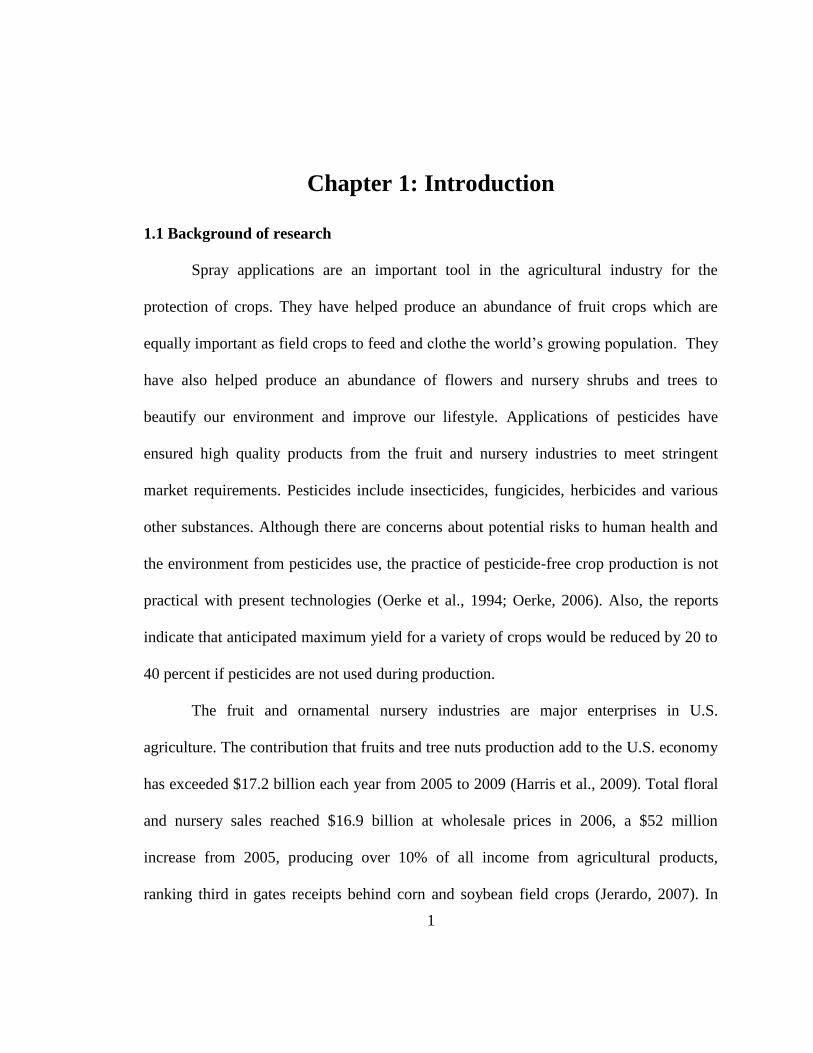
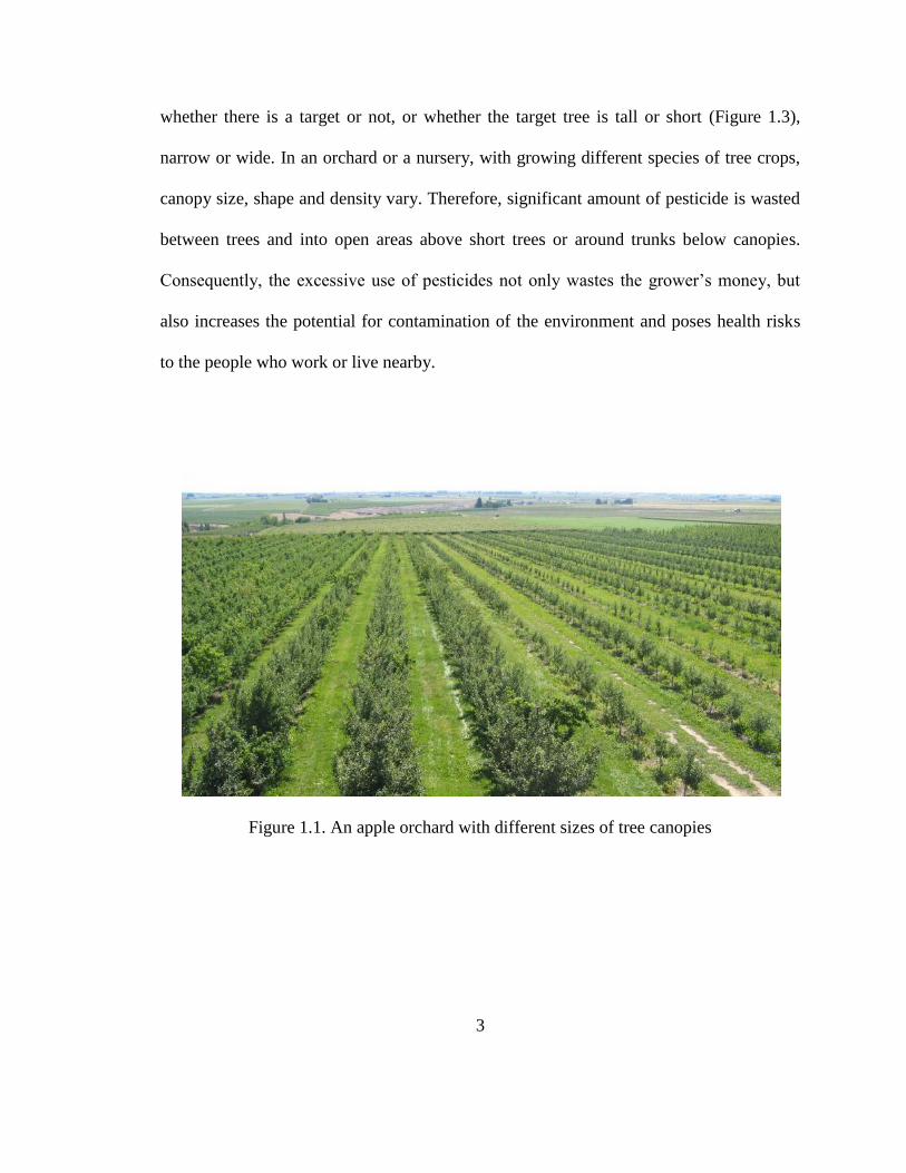
mix of different sizes of trees in an orchard or a nursery, such as shown in Figures 1.1

and 1.2. Often, there are huge gaps between these young trees. When treating these

orchards and nurseries using the conventional sprayers, much of the pesticide will be

wasted because it is impractical for applicators to manually adjust sprayer settings to

match target tree canopy size and shape after application starts, due to the demands of

pest pressure and labor costs. The spray output of a conventional sprayer cannot be

adjusted once the sprayer is turned on; a constant amount of liquid is sprayed regardless

3

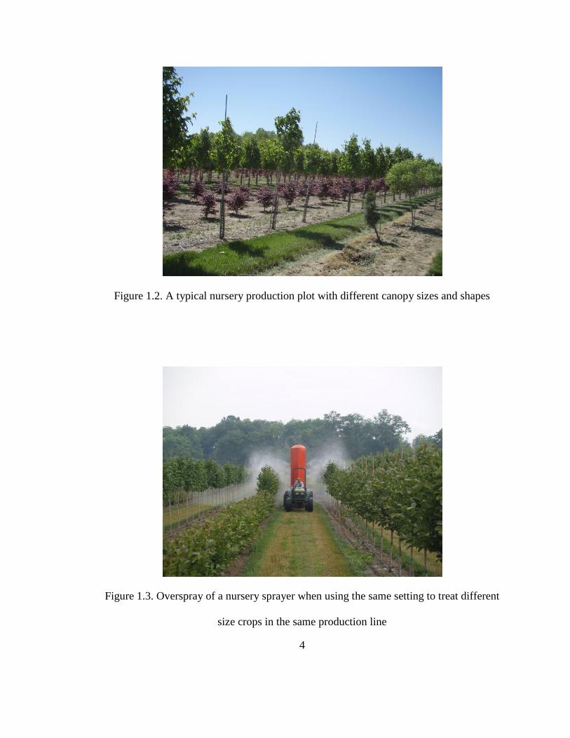
whether there is a target or not, or whether the target tree is tall or short (Figure 1.3),

narrow or wide. In an orchard or a nursery, with growing different species of tree crops,

canopy size, shape and density vary. Therefore, significant amount of pesticide is wasted

between trees and into open areas above short trees or around trunks below canopies.

Consequently, the excessive use of pesticides not only wastes the grower‟s money, but

also increases the potential for contamination of the environment and poses health risks

to the people who work or live nearby.

Figure 1.1. An apple orchard with different sizes of tree canopies

4

Figure 1.2. A typical nursery production plot with different canopy sizes and shapes

Figure 1.3. Overspray of a nursery sprayer when using the same setting to treat different

size crops in the same production line

5

With the rising cost of pesticides and growing public concerns about the potential

contamination of the environment caused by excessive use of pesticides, new pesticide

application equipment and strategies have been consistently demanded to reduce the

consumption of pesticides.

Turning off sprayers when there is no target, or adjusting application rates based

on canopy size and density have been considered by researchers and sprayer

manufacturers in the past. Since 1970s this concept has been seriously considered by

researchers and sprayer manufacturers because of the significant advances in sensor and

control technologies (Reichard and Ladd, 1981). Precision spraying technology was first

introduced in boom sprayers by manufacturers in late 1980‟s (Bode, 2008). Variable rate

technology using GPS and GIS technologies has been integrated into several boom

sprayers and became commercially available (e.g. John Deere 30-series sprayers).

Ultrasonic sensors were integrated into orchard sprayers to detect the presence and

absence of a tree and to switch nozzles on or off as necessary (SmartSpray, Durand-

Wayland, LaGrange, GA). Although it was a major step towards reducing applied

pesticide, this technology can be further improved by developing a control system based

on a variable rate function that incorporates information about the tree canopy height,

shape and foliage density.

Therefore, to fully meet the requirements for effective and efficient treatments of

fruit and nursery crops, it is necessary to develop sensor-controlled intelligent or semi-

intelligent spraying systems that deliver pesticides more economically, accurately, timely

6

and in an environmentally sustainable manner with minimum human involvement before,

during and after applications.

7

1.2 Literature review

1.2.1 Importance of pesticide applications in nurseries and orchards

To insure yield and the quality of production, growers rely heavily on application

of pesticides. Without crop protection, the potential loss can range from 43-50% in food

crops, and 53-68% in cash crops (Oerke and Dehne, 2004). Fruit production requires

repeated pesticide applications while nursery crops are often associated with even higher

pesticide use than any other crops because consumers‟ quality standards for ornamentals

are higher (Oerke, and Dehne, 2004).

The use of synthetic pesticides is often unavoidable. Recently, some pesticides

have even been classified as irreplaceable by the US National Research Council

(Anonymous, 2000). Pesticide-free production often results in a reduction in yield and

quality of field crops produced. These problems are even more apparent in fruit

production (Knutson et al., 1997), because (1) genetic resistance is often overcomed by

animal pests and pathogens, (2) the efficacy and reliability of biocontrol agents is limited,

and (3) today manual weed control cannot be expected from most growers. However, an

increase in the efficacy of pest control does not depend on an increase in the amount of

pesticide used, but primarily on the targeted application of suitable products when

needed.

The goal of pesticide application is to deliver effective and uniform dose of

chemicals to the target areas in a safe and timely manner. Conventional spray equipment

used in nurseries and orchards has some problems with spray efficiency and safety. For

example, usually high percentage of chemicals is wasted in the form of drift of droplets,

8

over spraying, run-off, and off-target deposition. This misdirected pesticide not only

reduces the effectiveness of the application and waste growers‟ money, it also increases

the potential of environmental contamination (Deveau, 2009).

1.2.2 Sprayer used for orchard and nursery applications

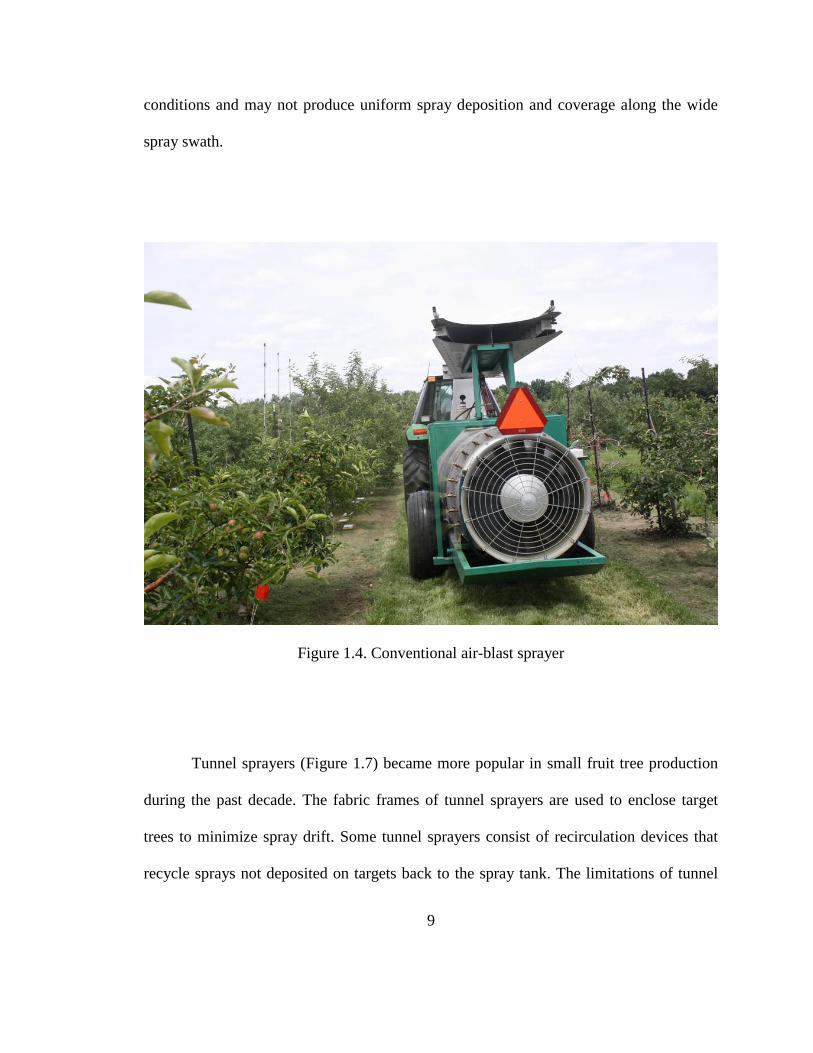
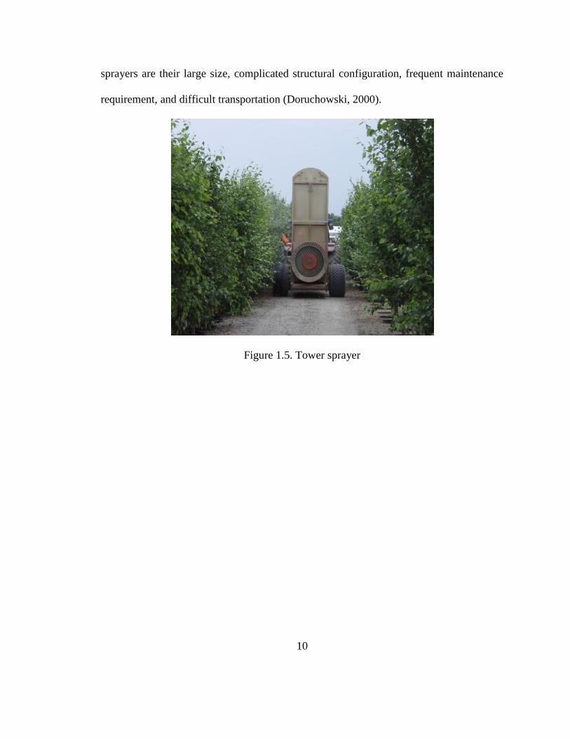
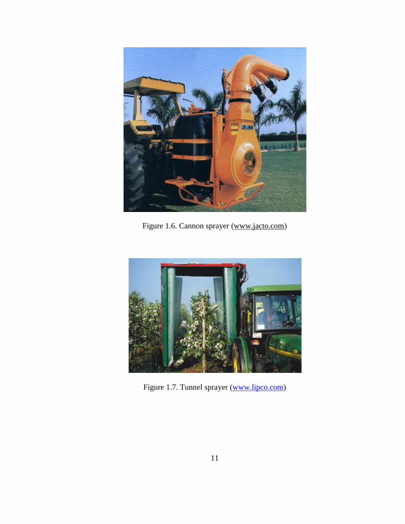
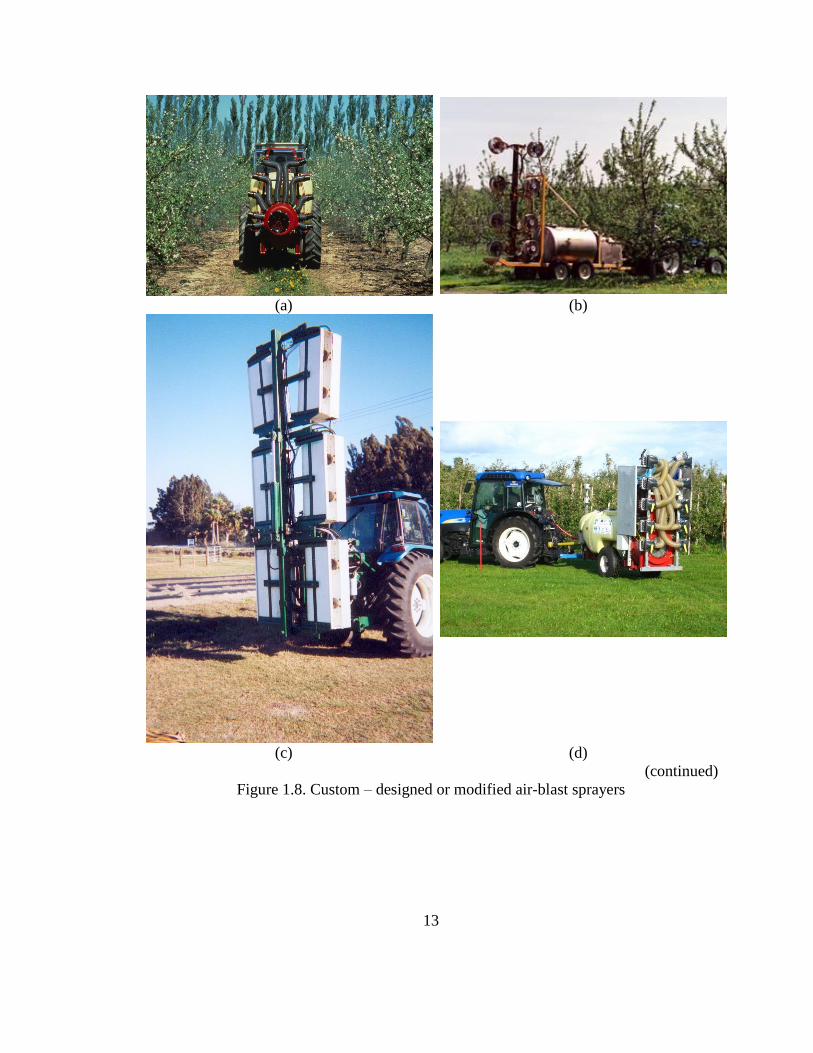
Air-blast sprayers are commonly used in orchards and nurseries. They include

conventional axial-fan air-blast sprayers (Figure 1.4), tower sprayers (Figure 1.5), cannon

sprayer (Figure 1.6), tunnel sprayers (Figure 1.7), and custom-designed or modified air-

blast sprayers (Figure 1.8 (a) to (e)). Tower sprayers are the air-assisted sprayers that

discharge sprays horizontally by directing the airflow from a fan into horizontal ducts on

a vertical plane. Tower sprayers are used in nurseries and orchards where horizontal

spray trajectory is preferred for the trees with consistent heights.

Air-assisted cannon sprayers consist of cylindrical outlets that create high air

velocity jets that break spray mixtures into fine droplets and carries them long distance

downwind. The cylindrical spray outlet can be tilted downward, upward, forward or

backward to aim the spray at the canopy. The cannon sprayers can cover very wide spray

swaths and are often used in nursery fields where conventional air-blast sprayers are not

feasible to deliver sprays to the crops. Because of high air velocity, the sprayers can

penetrate canopies and create turbulence that disturb plants and increase spray deposition

on both leaf surfaces. Compared with air-blast sprayers, the cannon sprayer is generally

small in size, easily transported and stored, and only requires a small path for spray

application. However, cannon sprayer performances are greatly influenced by wind

9

conditions and may not produce uniform spray deposition and coverage along the wide

spray swath.

Figure 1.4. Conventional air-blast sprayer

Tunnel sprayers (Figure 1.7) became more popular in small fruit tree production

during the past decade. The fabric frames of tunnel sprayers are used to enclose target

trees to minimize spray drift. Some tunnel sprayers consist of recirculation devices that

recycle sprays not deposited on targets back to the spray tank. The limitations of tunnel

10

sprayers are their large size, complicated structural configuration, frequent maintenance

requirement, and difficult transportation (Doruchowski, 2000).

Figure 1.5. Tower sprayer

11

Figure 1.6. Cannon sprayer (www.jacto.com)

Figure 1.7. Tunnel sprayer (www.lipco.com)

http://www.jacto.com/

http://www.lipco.com/

12

Sensor-controlled variable rate application technology for air-assisted orchard

sprayers also has been reported. Giles et al. (1987; 1988; 1989) developed a

microcomputer-based sprayer control system with ultrasonic transducers to detect foliage

volume, resulting in a commercially available sensor-controlled air-assisted orchard

sprayer (i.e. SmartSpray, Durand-Wayland, LaGrange, GA). The sprayer system detects

the presence or absence of a tree and switches the nozzles on or off, but it cannot detect

the canopy size and foliage density. Because of limited sensor resolution or response

speed of the spray-control system, none of the sensor-controlled sprayers has fully

achieved variable rates to match tree-canopy shape and density (Fox et al., 2008).

13

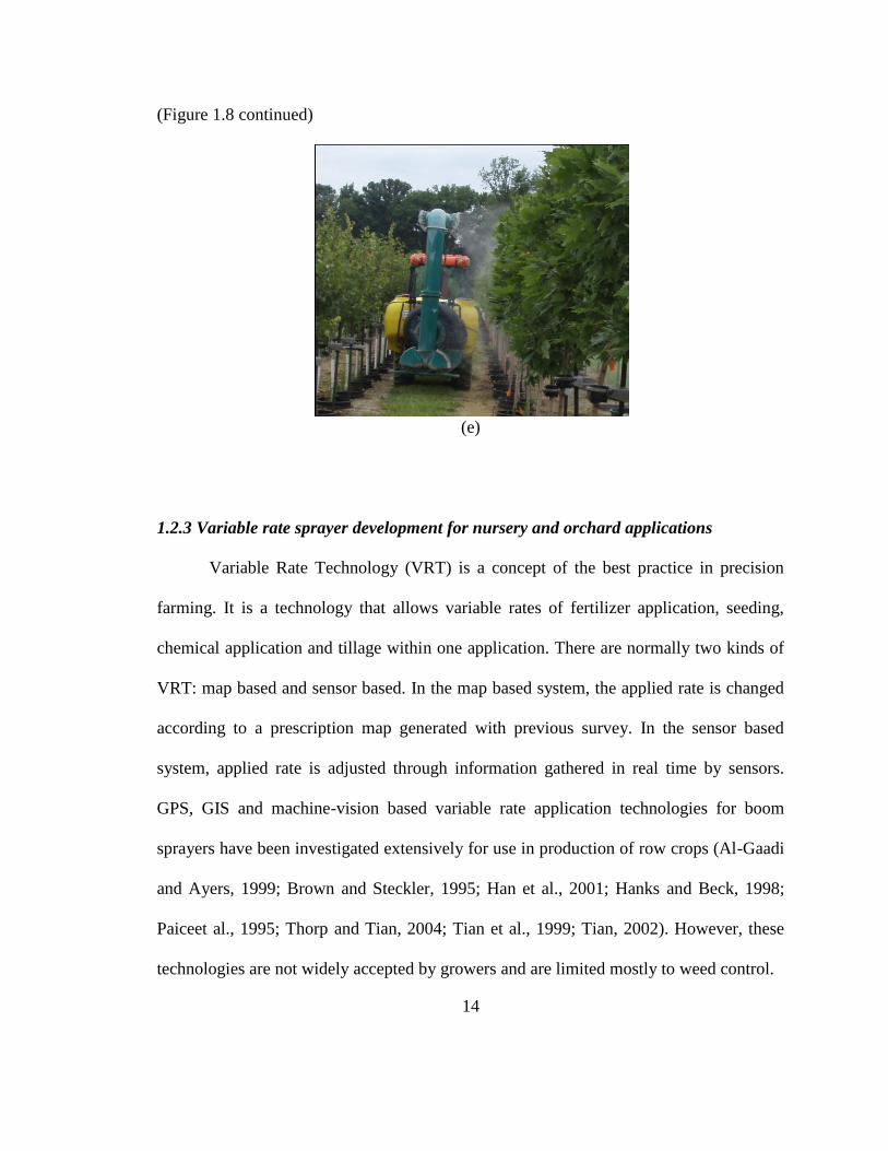
(a) (b)

(c) (d) (continued)

Figure 1.8. Custom – designed or modified air-blast sprayers

14

(Figure 1.8 continued)

(e)

1.2.3 Variable rate sprayer development for nursery and orchard applications

Variable Rate Technology (VRT) is a concept of the best practice in precision

farming. It is a technology that allows variable rates of fertilizer application, seeding,

chemical application and tillage within one application. There are normally two kinds of

VRT: map based and sensor based. In the map based system, the applied rate is changed

according to a prescription map generated with previous survey. In the sensor based

system, applied rate is adjusted through information gathered in real time by sensors.

GPS, GIS and machine-vision based variable rate application technologies for boom

sprayers have been investigated extensively for use in production of row crops (Al-Gaadi

and Ayers, 1999; Brown and Steckler, 1995; Han et al., 2001; Hanks and Beck, 1998;

Paiceet al., 1995; Thorp and Tian, 2004; Tian et al., 1999; Tian, 2002). However, these

technologies are not widely accepted by growers and are limited mostly to weed control.

15

Because the crop characteristics of nurseries and orchards change considerably during a

growing season and the crop life cycle, prescription maps for variable application rates

need to be updated frequently, thus making map based VRT very expensive (Mooney et

al., 2009). With sensor based VRT, sensors mounted on the application equipment detect

crop structure information that controllers process and use to control spray outputs as

needed, in real time. Thus sensor based VRT is better suited in nurseries and orchard

chemical applications than map based VRT.

There are two major steps in variable rate sprayer development. The first step is to

utilize different types of sensors such as ultrasonic sensor and laser sensor to detect target

crops or tree characteristics. This step includes data acquisition and data processing to

obtain target characteristic information. The second step is to develop variable rate

delivery equipment by modifying commercially available sprayers by implementing

sensors and controllers.

As mentioned above, with the advancement of sensor and control technologies it

is possible to develop variable rate sprayers for the nursery and orchard applications.

Researchers have designed several variable rate sprayers using ultrasonic sensors.

Giles et al. (1987, 1988 and 1989) retrofitted a conventional air-blast orchard

sprayer by integrating ultrasonic sensor technology into a sprayer control system to

measure foliage volume and then control the spray output. Spray savings ranging from

28% to 35% and 36% to 52% were reported in peaches and apples, respectively. In

addition, compared with a standard sprayer, the sensor-controlled sprayer had a

significant reduction in off-target loss.

16

Escola et al. (2003) reported research on modifying a sprayer for adjusting spray rate

proportional to tree volume. Later an experimental electronic control system was

developed and was able to change application rate based on tree canopy width (Solanelles

et al., 2006). Ultrasonic sensors were used to measure the distance between the sensor

and the outside edge of the canopy and the canopy width at the same height as the

ultrasonic sensors. With known values of tree row spacing, sensor position on the tractor

and travel speed, the optimal spray volume was calculated and was used to trigger

electro-valves for control of the nozzle flow rate. Liquid savings of 70%, 28% and 39%

were reported in the olive, pear and apple orchards respectively from the variable rate

sprayer compared to a conventional application. Lower spray deposition on the canopy

but a higher ratio between the total spray deposit and the liquid spray output (i.e. better

application efficiency) were also reported.

Following the work of Escola et al. (2003), Gil et al. (2007) modified a multi-

nozzle air-blast sprayer with three ultrasonic sensors and three electro-valves. The nozzle

flow rate was modulated in real time as a function of crop width in a vineyard, as

measured with the ultrasonic sensors. The canopy in vineyard was divided into three

height sections, each covered by one ultrasonic sensor and one electro-valve controlled

nozzle. A saving of 58% percent was reported compared with conventional constant rate

application while deposition quality on leaves, uniformity of liquid distribution and

capability to reach the inner parts of the crop remained similar.

17

Using the same sprayer tested by Gil et al. (2007), Llorens et al. (2010) compared

conventional spray application and variable rate application in three vine varieties at

different crop growing stages. The variable rate application was reported to have an

average of 58% savings in application volume with similar or even better leaf deposition.

1.2.4 Sensors used for tree crop structure detection

So far, only ultrasonic sensors have been extensively used for developing variable

rate sprayers or orchard, nurseries and vineyards. However, there is a growing number of

investigation on using ultrasonic sensors and other types of sensor to measure tree crop

canopy structure and characteristics, which is a very important step in developing

variable rate sprayer for tree crops.

Giles et al. (1988) used a commercially available ultrasonic sensor to detect apple

trees. Field tests reported that the sensor was relatively precise in measuring tree width

(with less than 10% average error). Tests at ground speeds of 2, 4 and 6 km/h found no

significant effect of the ground speed on the sensor detection accuracy. However, it

tended to overestimate the tree width due to the conical shape of the ultrasonic pattern.

A crop adapted application system has been proposed, as a result of ISAFRUIT

(Increasing fruit consumption through a trans disciplinary approach leading to high

quality produce from environmentally safe, sustainable methods) project launched in

2006 in Europe, to improve the efficiency and safety of spray application in orchards

based on the actual needs and respect to the environment (Van de Zande et al., 2007).

The system will consist of three components: crop identification system (Balsari et al.,

18

2007), environmentally dependent application system (Doruchowski, 2007) and crop

health detection system (Van de Zande et al., 2007).The crop identification system uses

ultrasonic sensors to assess canopy width and vegetation density (defined as the number

of leaf layers). The environmentally dependent application system identifies

environmental circumstances (such as wind velocity and direction, orchard boundary and

other sensitive areas from GIS) and adjusts application parameters accordingly. The crop

health detection system measures spectral wavelength distribution of picked leaves and

identify the water stress, nutrient stress, cultivar and disease stress of the fruit trees.

Wei and Salyani (2004 and 2005) used a laser scanner with an offline processing

algorithm to scan the citrus canopy. Based on the scanning data they calculated the

canopy characteristics such as tree height, width, canopy volume, foliage density and tree

boundary profile. An artificial target was tested and the results showed an accuracy of

97% for the length measurement. The density estimation was found to have good

correlation with the visual assessments.

Palacin et al. (2007 and 2008) used a laser scanner to measure canopy volume and

to estimate tree foliage area in real time. The validation tests with pear trees concluded

there was a linear relationship between canopy volume and the foliage surface area with a

coefficient of correlation (R) of 0.81. However, they also reported that the accuracy of

the estimation was closely related to tree species and tree truck size could influence the

estimation result.

Lee and Ehsani (2008) used a laser scanner to scan citrus trees and designed a

program using the saved data to estimate the tree canopy height, width and volume. The

19

height estimation was compared with manual measurement and the error was found to be

less than 1 cm. The width estimation was found to have an error of about 15 cm and its

accuracy was believed to be dependent on the accuracy of the tractor speed measurement.

The error of the volume estimation varied with the definition of the profile polygon in the

algorithm. A minimum error of 0.09% was found for the volume estimation.

Rosell et al. (2009a and 2009b) used a laser scanner mounted on a tractor to scan

selected trees of a vineyard and a pear orchard several times before and after defoliation.

The scanned data was then used to build 3D images to determine geometrical and

structural parameters of the vegetation such as volume and leaf area of trees. These

geometrical and structural parameters were compared with crop leaf surface values

obtained by manual measurements in which leaves were picked and one-sided projected

area of the leaves was measured via shadowgraph measurement techniques. Results have

shown a good linear correlation between the canopy volume calculated from the laser

measurement and the total foliage area from the manual measurement.

As evident from this review of literature, the sensors most commonly used to

measure tree canopy characteristics are one of two types: ultrasonic sensors or laser

scanners. Ultrasonic sensors have the advantage of being simple to use and low cost;

however, due to the divergence angle of sound waves, its error increases with the

increases in distance measured. Also, their accuracy can be affected by the ambient

temperature, humidity and even the tractor ground speed. Laser scanning is relatively

more expensive but has advantages such as higher accuracy, scanning mode rather than

the single point measurement as is the case when using ultrasonic sensors. With laser

20

scanners, more target information can be gathered in a short period of time, and they are

not influenced as much by weather and field environment as the ultrasonic sensors.

Based on previous studies by other researchers, it can be concluded that a laser

scanner can characterize more crop structure information with higher accuracy than an

ultrasonic sensor. Because the laser sensor can offer acceptable precision and reliability

to measure tree structures regardless of weather or lighting conditions, they have greater

potentials to be used for the variable-rate sprayer development for orchard and nursery

applications than other types of sensors.

21

1.3 Objectives of research

The overall goals of this study are to develop an intelligent sprayer prototype with

automatic control that can match spray outputs to the canopy sectional structures and

improve pesticide spray efficiency without reducing the level of crop protection expected

from pesticides when compared to the performance of conventional sprayers.

Specific objectives are:

1) Develop an automatic controller to enable the variable spray outputs without changing

the spray pressure at the nozzle, and consequently the droplet size.

2) Modify a conventional sprayer to improve spray penetration capability and spray

deposition uniformity by newly designed five-port air assisted nozzles.

3) Develop a set of algorithms to calculate tree canopy parameters (such as tree width,

height, canopy volume and foliage density) employing a fast speed laser scanning

sensor and controller.

4) Develop a spray model for the newly developed variable-rate sprayer to optimize its

flow rate based on the sensor data.

5) Conduct field experiments to evaluate performances of the newly developed variable-

rate sprayer.

22

1.4 Description of contents

This study is focused on the development of a variable-rate air-assisted sprayer

which integrates a high speed laser scanning system, a custom-designed sensor-data

analyzer and variable-rate controller and a multi-channel air-assisted delivery system.

The sprayer will have the capability to achieve variable spray rates for different canopy

volumes and densities with nozzles of one size. Different flow rates will be obtained with

one nozzle size instead of requiring a change of nozzles to change flow rate. A laser

scanner (SICK LMS291, SICK Inc., Germany) was chosen as the detecting sensor

because of its many advantages over other types of sensors, as explained in detail in the

following chapter. A computational algorithm is designed to process signals from the

laser and to calculate tree canopy characteristics such as tree height, width, and canopy

volume and density. A spray model specifically designed for this sprayer is used to

determine the optimal flow rate needed. The model output is sent to the controller circuit

boards that convert these control decisions to hardware signals for activating solenoid

valves and then modulating nozzle discharge rates. A series of field experiments were

conducted to compare spray deposition and coverage inside tree canopies between

conventional and the sprayer prototype.

23

Chapter 2: Research Methods and Design

The ultimate goal of the intelligent sprayer is to reduce pesticide consumption by

turning the sprayer off when there is no target to spray (by detecting the gaps between

trees) and by applying the optimum level of spray mixture in accordance with the

characteristics of the target tree (size, shape and foliage density). Several tasks are

required to achieve this goal:

1) Collect data representing the characteristics of tree canopies in a reliable and real-time

manner as the sprayer moves along the tree rows. This data-acquisition mechanism

should be very robust since the sprayers work in uneven terrain and harsh outdoor

environmental conditions in orchards or nurseries. The data transfer rate should be

sufficient to satisfy different sprayer travel speeds.

2) While data are being collected by the data-acquisition system, an on-line algorithm

performs computation on the stream of real-time data to calculate the parameters that

characterize the tree canopy. Based on the computed parameters, an optimal sprayer

flow rate is derived to be used by the mechanical control mechanism. This on-line

algorithm works on the real-time data stream collected by the data-acquisition system,

therefore it must be highly efficient to produce real-time control signals, and very

robust to manage a wide spectrum of data input in an outdoor field environment.

3) Given the spray flow-rate decision, a dedicated control mechanism is needed to

convert the digital signals (possibly in TTL (transistor–transistor logic) level

24

voltages) into electrical control signals required to power the solenoid controlled

valves that modulate the flow rate from the sprayer nozzles. This control mechanism

should respond to the variable rate output of the online algorithm very quickly to

change to state of the solenoid valves. Since it is working with very strong current to

control the solenoid valves, the control mechanism must be able to tolerate the

electrical interference caused by frequent switching. It also must be able to handle

the dramatic change of hydraulic pressure while it is changing the state of solenoid

valves.

The control system consists of three major components, as shown in Figure 2.1:

1) Sensing component. A fast response laser scanning sensor is used to scan the target

tree canopy and collect data representing tree canopy characteristics. The original

data produced by the sensor is accumulated in a buffer and transferred to next stage

for data processing.

2) Data Processing component. An intelligent algorithm is designed to calculate the tree

canopy characteristics using data input from the sensor component. Based on the

computed canopy characteristics, an optimal spray flow rate is calculated for the

control action.

3) Control Component. This component converts the optimal flow-rate decision into

actual Pulse Width Modulation (PWM) signals that was used to activate sprayer

nozzles in order to spray the optimal flow rate.

25

SensingData

processingControl

Figure 2.1. Intelligent sprayer control system - overview

Within this research, the procedure as shown in Figure 2.2 was followed. A data-

acquisition system using a laser scanner to scan a target and acquire data representing the

characteristics of the target was designed (section 2.1). Then an intelligent algorithm was

designed to calculate tree shape and density (section 2.2). In the meantime, the

performance of the solenoid valves and the nozzles to be used in the intelligent sprayer

system were evaluated and calibrated using a specially designed experiment station. An

electronic circuit was designed to drive the electronic valves (section 2.3). To use the

data generated by the sensor to adjust the controller for varying spray output, a spray

model was established (section 2.4). The output from the spray model was used to match

the variable flow-rate control of the sprayer to the spray target. A mechanical prototype

of the intelligent sprayer was also developed (modified from a commercially available

sprayer) to be used for field tests and to demonstrate the effectiveness of our approach

(section 2.5). Comprehensive field tests (section 2.6) and an outdoor test on container

trees (section 2.7) were conducted to evaluate the performance of the intelligent sprayer

prototype in terms of spray uniformity, spray loss off the target, downwind drift and

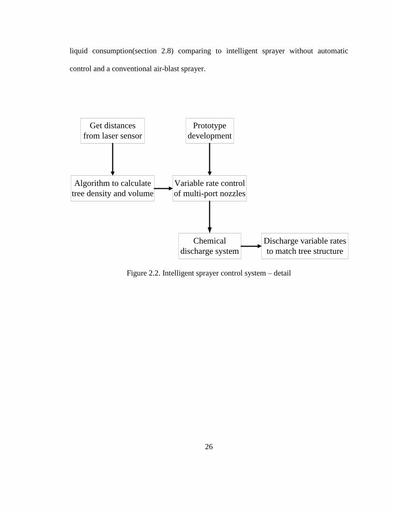
26

liquid consumption(section 2.8) comparing to intelligent sprayer without automatic

control and a conventional air-blast sprayer.

Figure 2.2. Intelligent sprayer control system – detail

Get distances

from laser sensor

Algorithm to calculate

tree density and volume

Chemical

discharge system

Prototype

development

Discharge variable rates

to match tree structure

Variable rate control

of multi-port nozzles

27

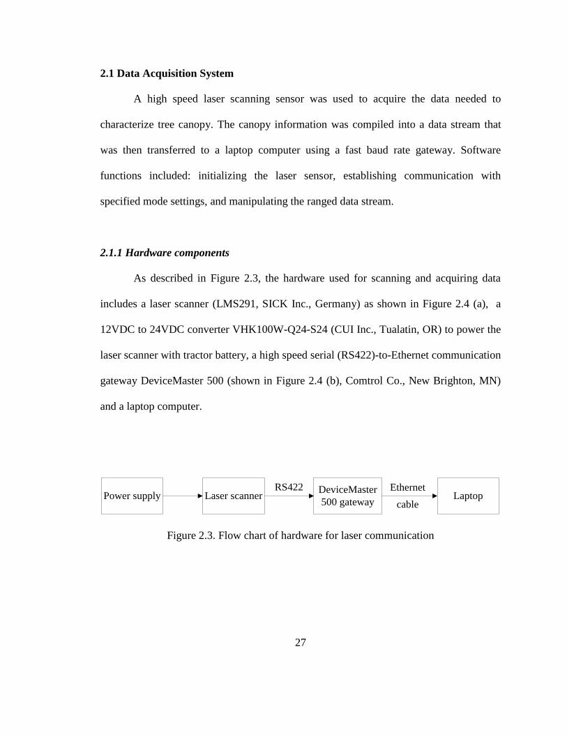
2.1 Data Acquisition System

A high speed laser scanning sensor was used to acquire the data needed to

characterize tree canopy. The canopy information was compiled into a data stream that

was then transferred to a laptop computer using a fast baud rate gateway. Software

functions included: initializing the laser sensor, establishing communication with

specified mode settings, and manipulating the ranged data stream.

2.1.1 Hardware components

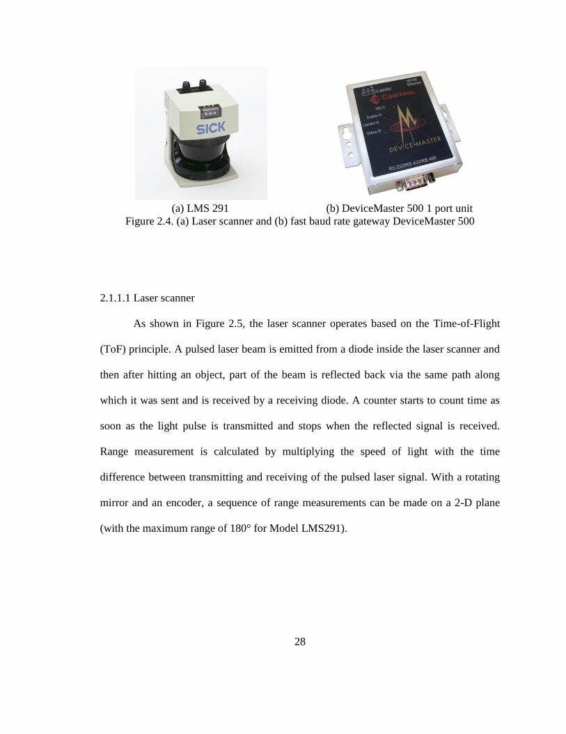
As described in Figure 2.3, the hardware used for scanning and acquiring data

includes a laser scanner (LMS291, SICK Inc., Germany) as shown in Figure 2.4 (a), a

12VDC to 24VDC converter VHK100W-Q24-S24 (CUI Inc., Tualatin, OR) to power the

laser scanner with tractor battery, a high speed serial (RS422)-to-Ethernet communication

gateway DeviceMaster 500 (shown in Figure 2.4 (b), Comtrol Co., New Brighton, MN)

and a laptop computer.

Figure 2.3. Flow chart of hardware for laser communication

Laser scannerDeviceMaster

500 gatewayLaptop

RS422 EthernetPower supply

cable

28

(a) LMS 291 (b) DeviceMaster 500 1 port unit

Figure 2.4. (a) Laser scanner and (b) fast baud rate gateway DeviceMaster 500

2.1.1.1 Laser scanner

As shown in Figure 2.5, the laser scanner operates based on the Time-of-Flight

(ToF) principle. A pulsed laser beam is emitted from a diode inside the laser scanner and

then after hitting an object, part of the beam is reflected back via the same path along

which it was sent and is received by a receiving diode. A counter starts to count time as

soon as the light pulse is transmitted and stops when the reflected signal is received.

Range measurement is calculated by multiplying the speed of light with the time

difference between transmitting and receiving of the pulsed laser signal. With a rotating

mirror and an encoder, a sequence of range measurements can be made on a 2-D plane

(with the maximum range of 180° for Model LMS291).

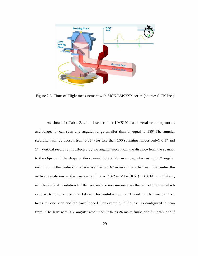
29

Figure 2.5. Time-of-Flight measurement with SICK LMS2XX series (source: SICK Inc.)

As shown in Table 2.1, the laser scanner LMS291 has several scanning modes

and ranges. It can scan any angular range smaller than or equal to 180°.The angular

resolution can be chosen from 0.25° (for less than 100°scanning ranges only), 0.5° and

1°. Vertical resolution is affected by the angular resolution, the distance from the scanner

to the object and the shape of the scanned object. For example, when using 0.5° angular

resolution, if the center of the laser scanner is 1.62 m away from the tree trunk center, the

vertical resolution at the tree center line is: ( ) ,

and the vertical resolution for the tree surface measurement on the half of the tree which

is closer to laser, is less than 1.4 cm. Horizontal resolution depends on the time the laser

takes for one scan and the travel speed. For example, if the laser is configured to scan

from 0° to 180° with 0.5° angular resolution, it takes 26 ms to finish one full scan, and if

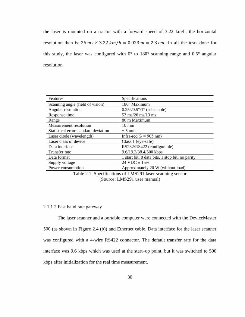
30

the laser is mounted on a tractor with a forward speed of 3.22 km/h, the horizontal

resolution then is: ⁄ . In all the tests done for

this study, the laser was configured with 0° to 180° scanning range and 0.5° angular

resolution.

Features Specifications

Scanning angle (field of vision) 180° Maximum

Angular resolution 0.25°/0.5°/1° (selectable)

Response time 53 ms/26 ms/13 ms

Range 80 m Maximum

Measurement resolution 10 mm

Statistical error standard deviation ± 5 mm

Laser diode (wavelength) Infra-red (λ = 905 nm)

Laser class of device Class 1 (eye-safe)

Data interface RS232/RS422 (configurable)

Transfer rate 9.6/19.2/38.4/500 kbps

Data format 1 start bit, 8 data bits, 1 stop bit, no parity

Supply voltage 24 VDC ± 15%

Power consumption Approximately 20 W (without load)

Table 2.1. Specifications of LMS291 laser scanning sensor

(Source: LMS291 user manual)

2.1.1.2 Fast baud rate gateway

The laser scanner and a portable computer were connected with the DeviceMaster

500 (as shown in Figure 2.4 (b)) and Ethernet cable. Data interface for the laser scanner

was configured with a 4-wire RS422 connector. The default transfer rate for the data

interface was 9.6 kbps which was used at the start–up point, but it was switched to 500

kbps after initialization for the real time measurement.

31

2.1.2 Software design

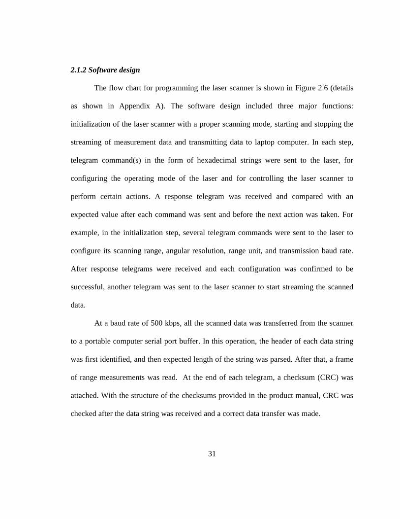
The flow chart for programming the laser scanner is shown in Figure 2.6 (details

as shown in Appendix A). The software design included three major functions:

initialization of the laser scanner with a proper scanning mode, starting and stopping the

streaming of measurement data and transmitting data to laptop computer. In each step,

telegram command(s) in the form of hexadecimal strings were sent to the laser, for

configuring the operating mode of the laser and for controlling the laser scanner to

perform certain actions. A response telegram was received and compared with an

expected value after each command was sent and before the next action was taken. For

example, in the initialization step, several telegram commands were sent to the laser to

configure its scanning range, angular resolution, range unit, and transmission baud rate.

After response telegrams were received and each configuration was confirmed to be

successful, another telegram was sent to the laser scanner to start streaming the scanned

data.

At a baud rate of 500 kbps, all the scanned data was transferred from the scanner

to a portable computer serial port buffer. In this operation, the header of each data string

was first identified, and then expected length of the string was parsed. After that, a frame

of range measurements was read. At the end of each telegram, a checksum (CRC) was

attached. With the structure of the checksums provided in the product manual, CRC was

checked after the data string was received and a correct data transfer was made.

32

In addition, error handlers were created and were used throughout every step. If

the program ran into exceptions, actions such as stop data streaming were taken and the

operator notified.

33

Figure 2.6. Laser communication software flow chart

Initialize laser

scanner

Send command

and set laser to

start data streaming

Read data

from laser

scanner

Convert data from Polar to

Cartesian coordinate system

Display

intensity chart

Input file

name from

keyboard

Save file to

hard disk

Display data?

Save data?

Stop?

Yes

Stop data

streaming

No

Yes

No

No

Yes

34

2.2 Algorithm to characterize tree canopy

The core of the software component for the intelligent sprayer is an intelligent

algorithm to characterize a tree canopy based on the laser sensor detection and for

calculating an optimal output flow rate in correspondence to the computed canopy profile

and density.

2.2.1 Basic terms and definitions used in the algorithm design

The data collected by the laser sensor reflects the distance of individual points on

the canopy surface to the sensor‟s central point. This distance is then used to determine

the distance between the tree vertical center line and the detected point on the canopy

surface. The tree vertical center line is determined beforehand by using the “top point

rule” which will be explained in the following sections. However, obtaining foliage

density information from range values can be more challenging and will be discussed

first.

The major part of the work in this canopy characterization algorithm is to predict

foliage density using distance/range measurements from the laser scanner. The density

algorithm was designed based on two assumptions:

1) In a short/limited height h (height range covered by one nozzle), the densest possible

canopy of a tree will appear to be a flat surface, parallel to the plane defined by the

tractor forward direction and tree vertical center line.

35

2) For a small volume of the canopy viewed from the sensor, the surface topology will

vary but there is no empty space or hollowness inside of the canopy.

To describe the design of the algorithm, especially the design of density

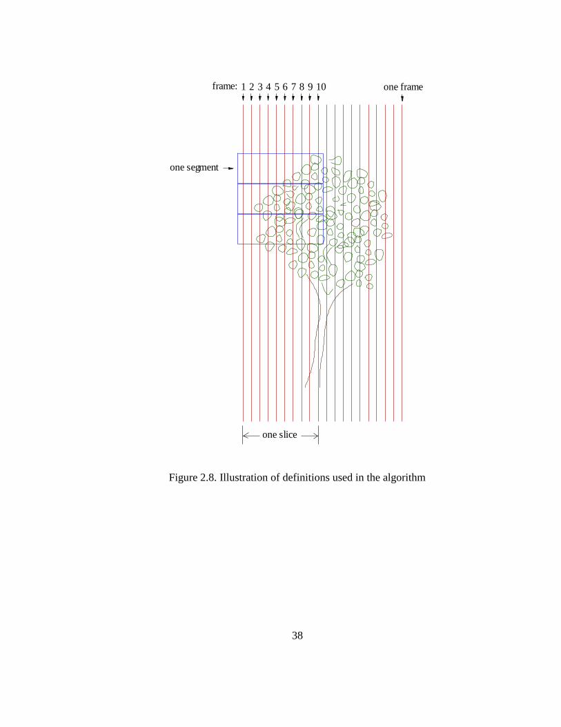
calculation, several terms are defined below. Figure 2.8 presents a graphical illustration

of these terms.

Frame: During canopy detection, the laser scanner spins and scans 180° vertically

to obtain an array of distance data, and each data point represents a distance between the

scanner and the point detected on the canopy surface for a certain angular interval. This

array of data is called a Frame. For example, in the 180° range and 0.5° angular

resolution scanning mode, one frame of data contains 361 data points, and each data point

represents the distance between the scanner and the canopy surface for the angular

intervals of 0 , 0.5 , 1 , 1.5 … 179.5 and 180 .

Slice: A Frame is a basic unit of data collection. However, it cannot be directly

utilized to do computation because canopy characteristics must be derived from a

contiguous space range, and a single frame cannot provide sufficient information about

the space topology of the canopy. Therefore, multiple contiguous Frames (such as 10

frames) is concatenated into a bigger 2-D array, called a Slice which represents a

contiguous space range in the tree canopy, and is used as the unit of calculation to

compute the tree canopy parameters over a contiguous space.

Segment: A slice of data points is equally divided into 20 height groups of points

from the ground upward across the height with an increment of the height covered by the

spray discharged from one nozzle (e.g. 13.5 cm). Each of such a group of points is called

36

a Segment. Each segment may not contain the same number of data points but has the

same height. A segment is physically covered by its corresponding spray nozzle.

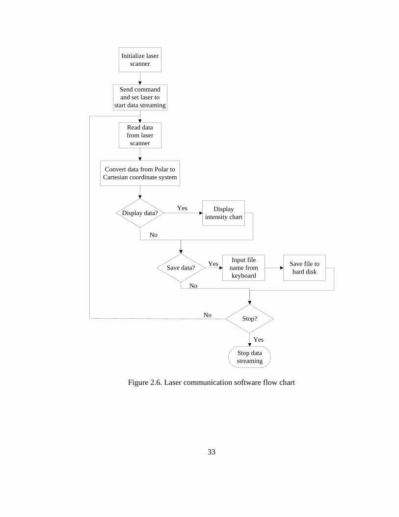
Density: Density in this scenario is defined with the assumption that, the ideal

segment of the densest canopy should be 100% filled with tree-substances (leaves, twigs,

branches, etc.) from the canopy surface inward to the trunk of the tree. Looking from the

laser sensor, this segment will appear as a cube with purely flat surface and with a depth

equal to the cross-section width of the canopy from the surface perpendicular to tree

vertical center line. The density of a segment is defined as the ratio between actual

volume filled with tree substances and the maximum possible volume.

For an ideal segment with density equal to 100%, all points on the canopy surface

have the same distance to the tree vertical center line equal to the cross-segment width of

the tree. In reality, a segment may have some holes and hollows on its surface (due to the

lack of leaves, etc.). As a result, the volume of substances inside the segment is less than

the maximum possible volume which corresponds to 100% density. This is illustrated in

Figure 2.7. In the figure each data point is represented by a bar, with the length of the bar

equal to the distance of that point to the tree vertical center line. Each bar in a same

segment has the same normalized bottom area, so that its volume can be calculated by

multiplying the bottom area with its depth. Summing up all bars in a segment yields the

total volume of that segment. The maximum volume of a segment can be computed by

filling that segment using the bar with the largest depth in that segment. The segment‟s

density is derived by dividing its actual volume over the maximum possible volume of

that segment.

37

Figure 2.7. Two segments with different densities

An ideal segment with density=100% A real segment with density < 100%

38

Figure 2.8. Illustration of definitions used in the algorithm

one slice

1 2 3 4 5 6 7 8 9 10frame: one frame

one segment

39

2.2.2 Algorithm design

The density-calculation algorithm consists of multiple stream-lined components

that form a cascade of processing, as is shown in Figure 2.9 (details as shown in

Appendix D and E).

Figure 2.9. Density algorithm design flow chart

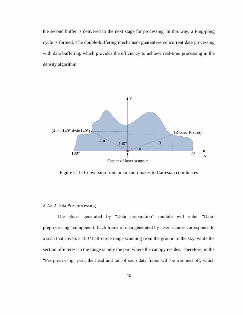
2.2.2.1 Data preparation

Since data from the laser scanner is formatted in polar coordinates, a conversion is

needed before data can be processed further. As shown in Figure 2.10, range values are

converted to Cartesian coordinates using their angles. Converted data points are saved in

two buffers and then delivered to the computation module.

The computational module accepts input in unit of frame. In the data-preparation

component, a double-buffer is prepared to accommodate the input frames. Each of the

double buffers has the same size as a slice. The data frames are concatenated into the

first buffer. Once the accumulated frames form a complete slice, this slice is delivered to

the next stage in the chain, while input frames are redirected to the second buffer. By the

time the second buffer is filled up, the data processing in the first buffer will be

completed. Then, the first buffer will be switched to receive new data while the data in

Pre-processingData

preparationCalculation

Slide window

filter

Duty cycle

generator

40

the second buffer is delivered to the next stage for processing. In this way, a Ping-pong

cycle is formed. The double-buffering mechanism guarantees concurrent data processing

with data buffering, which provides the efficiency to achieve real-time processing in the

density algorithm.

Figure 2.10. Conversion from polar coordinates to Cartesian coordinates

2.2.2.2 Data Pre-processing

The slices generated by “Data preparation” module will enter “Data-

preprocessing” component. Each frame of data generated by laser scanner corresponds to

a scan that covers a 180° half-circle range scanning from the ground to the sky, while the

section of interest in the range is only the part where the canopy resides. Therefore, in the

“Pre-processing” part, the head and tail of each data frame will be trimmed off, which

140°

x

α

y

(R∙cosα,R∙sinα)

R4m

0°180°

(4∙cos140°,4∙sin140°)

Center of laser scanner

41

leaves the main body of a frame corresponding to the tree canopy. In an outdoor

environment, the data frames usually contain some “outlier” values caused by

environment noises such as sun glare. If not filtered out, they will bring some uncertainty

into the density computation. The “Pre-processing” part also eliminates these “outliers”

by resetting their values to 0.

The value of each data point represents the distance from laser sensor to that point

detected on the canopy. However, the calculation of canopy density is based on each

point‟s distance from the canopy surface to the tree center. In order to derive this

distance, the position of the tree center needs to be calculated first. A simple yet effective

procedure to find tree center distance from the laser sensor was designed as below:

1) After trimming off head and tail of each data frame and filtering out outlier values,

each data frame was scanned from the top, and the first point with non-zero value was

found. This point was regarded as the “top-of-canopy” for that frame. Each point was

captured in a pair of values: the height of that point, and the distance from that point

to laser sensor.

2) All the “top-of-canopy” points within one slice were then compared to find the point

with the greatest height value. That point becomes the “center point” for the current

slice, and its “distance to the laser sensor” was used as that slice‟s “center distance” to

the laser sensor.

3) A sliding window which contains the center points for the past 5 slices was

maintained in the memory. Once the “center point” for the current slice was found, it

was shifted into the sliding window and the oldest point was retired from the sliding

42

window. Then the 5 points was compared in this sliding window and the largest

distance value to the laser sensor was found. This value was output as the “distance

from the laser sensor to the tree center” for the current slice.

After acquiring the tree center distance for a slice, all surface data points in the

slice was subtracted from the center distance to get their distances to the tree center.

These distance values were then pipelined to the next stage to be used to calculate tree

canopy density.

2.2.2.3 Calculation

After pre-processing, the data slice is split into multiple segments (each segment

corresponding to one nozzle‟s height) and computation is performed on each segment to

calculate its density. The calculation can be divided into the following stages.

1) Data segmentation

Since the intelligent sprayer has multiple nozzles to cover different parts of the tree

canopy, the tree canopy needs to be split into multiple segments of equal height that are

covered by the spray from one nozzle. Given the number of nozzles, the height that one

nozzle covers and distance from laser sensor to the tree center, the split strategy to divide

one data slice into multiple segments can be derived. For each working mode (e.g.

different angular resolution mode and angular range mode) of the intelligent sprayer this

split strategy is different, and this strategy is called a template.

43

Given a working mode (such as 0° to 180° scanning range with 0.5° angular

resolution mode used in the field tests including in this dissertation) of the intelligent

sprayer, the template remains the same and does not need to be computed for every data

frame. Therefore templates for every possible working mode of the intelligent sprayer are

calculated and prepared beforehand. Before the sprayer starts to work, its working mode

will be predetermined and sent to the algorithm, and the algorithm will pick the data split

template appropriately for that specific mode. For a slice of data, the split template is

applied into each frame and then each frame is divided it into multiple sub-frames. All

the sub-frames in the same position of a slice form a segment.

From basic geometry, the radius covered by each segment is different since each

segment is of the same height. However, the laser sensor generates data points at equal

angle intervals. As a result, each segment covers varied number of data points.

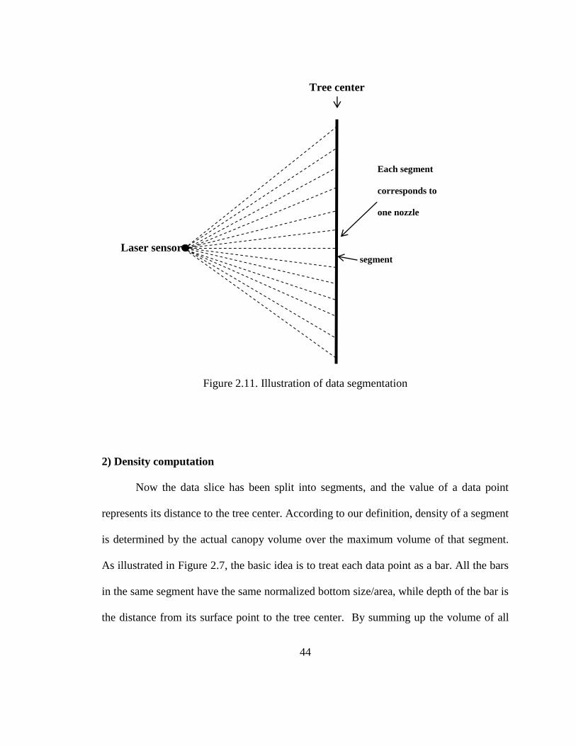
44

Figure 2.11. Illustration of data segmentation

2) Density computation

Now the data slice has been split into segments, and the value of a data point

represents its distance to the tree center. According to our definition, density of a segment

is determined by the actual canopy volume over the maximum volume of that segment.

As illustrated in Figure 2.7, the basic idea is to treat each data point as a bar. All the bars

in the same segment have the same normalized bottom size/area, while depth of the bar is

the distance from its surface point to the tree center. By summing up the volume of all

segment

Each segment

corresponds to

one nozzle

Laser sensor

Tree center

line

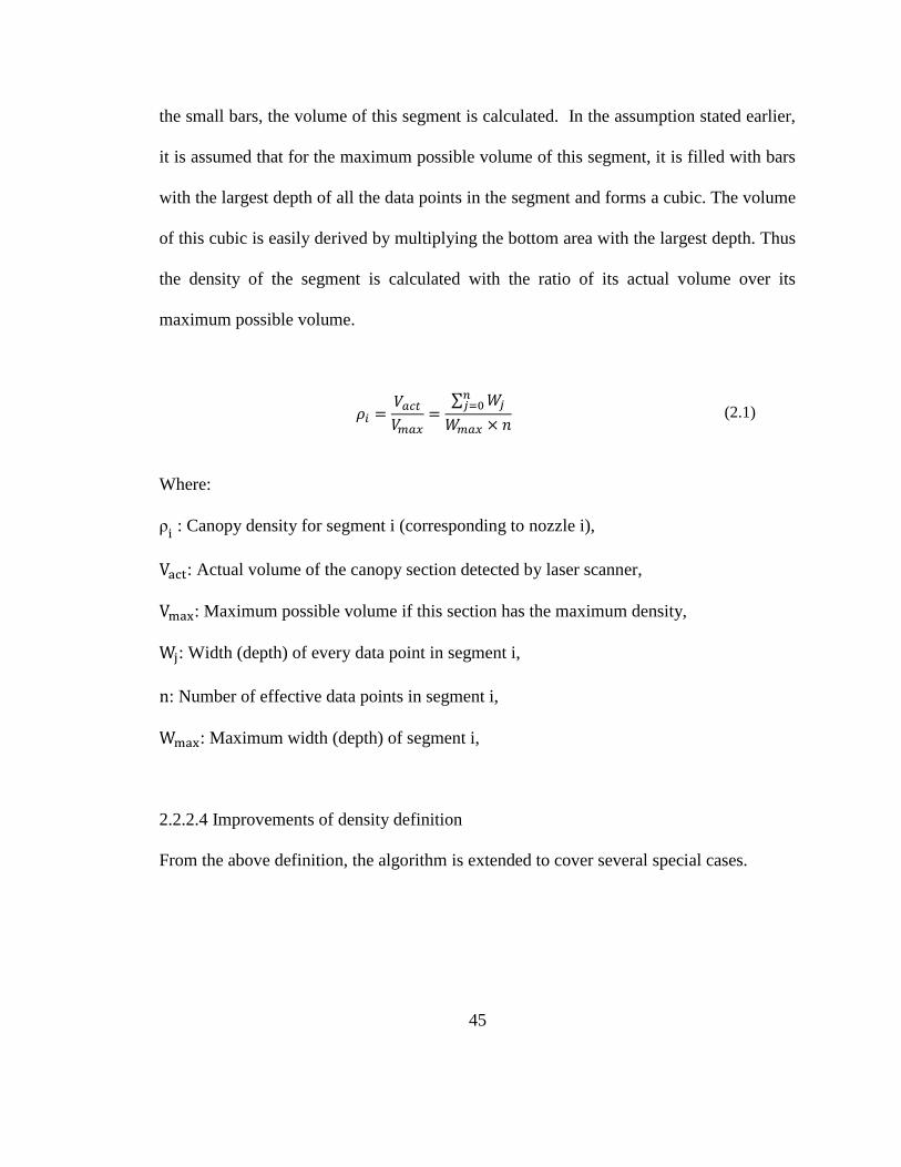
45

the small bars, the volume of this segment is calculated. In the assumption stated earlier,

it is assumed that for the maximum possible volume of this segment, it is filled with bars

with the largest depth of all the data points in the segment and forms a cubic. The volume

of this cubic is easily derived by multiplying the bottom area with the largest depth. Thus

the density of the segment is calculated with the ratio of its actual volume over its

maximum possible volume.

∑

(2.1)

Where:

: Canopy density for segment i (corresponding to nozzle i),

: Actual volume of the canopy section detected by laser scanner,

: Maximum possible volume if this section has the maximum density,

: Width (depth) of every data point in segment i,

: Number of effective data points in segment i,

: Maximum width (depth) of segment i,

2.2.2.4 Improvements of density definition

From the above definition, the algorithm is extended to cover several special cases.

46

1) To handle a transition slice

As the sprayer moves along the tree row line, the laser sensor will detect

consecutive tree canopies interspersed with empty spaces. When the sensor moves from

an empty space to an area covered by canopy or from canopy area to empty space, the

slice will be a partially empty; this is called a transition slice. Figure 2.12 illustrates a

segment in a transition slice. This segment consists of 4 sub-frames. The sub-frame 0 is

at the transition area from empty space to canopy, and it contains only 1 valid data point.

If sub-frame 0 is included in calculation, it will expand the bottom area of this segment

and hence increase the maximum volume of this segment, which results in a smaller

computed density than a typical human being would perceive.

In order to improve the accuracy of density computation, any highly sparse sub-

frame that contains too few valid data points from a segment was filtered out. A

threshold value Tt was chosen, and if number of valid data points in a sub-frame is

smaller than this threshold number, this sub-frame is excluded from the segment. In the

example in Figure 2.12, if Tt is set to be 2, then sub-frame 0 will be eliminated, and the

bottom area of this segment becomes 4×3 instead of 4×4. This filtering mechanism

helps to preclude polluted data at the transition area from the computation, and hence

improve the density accuracy.

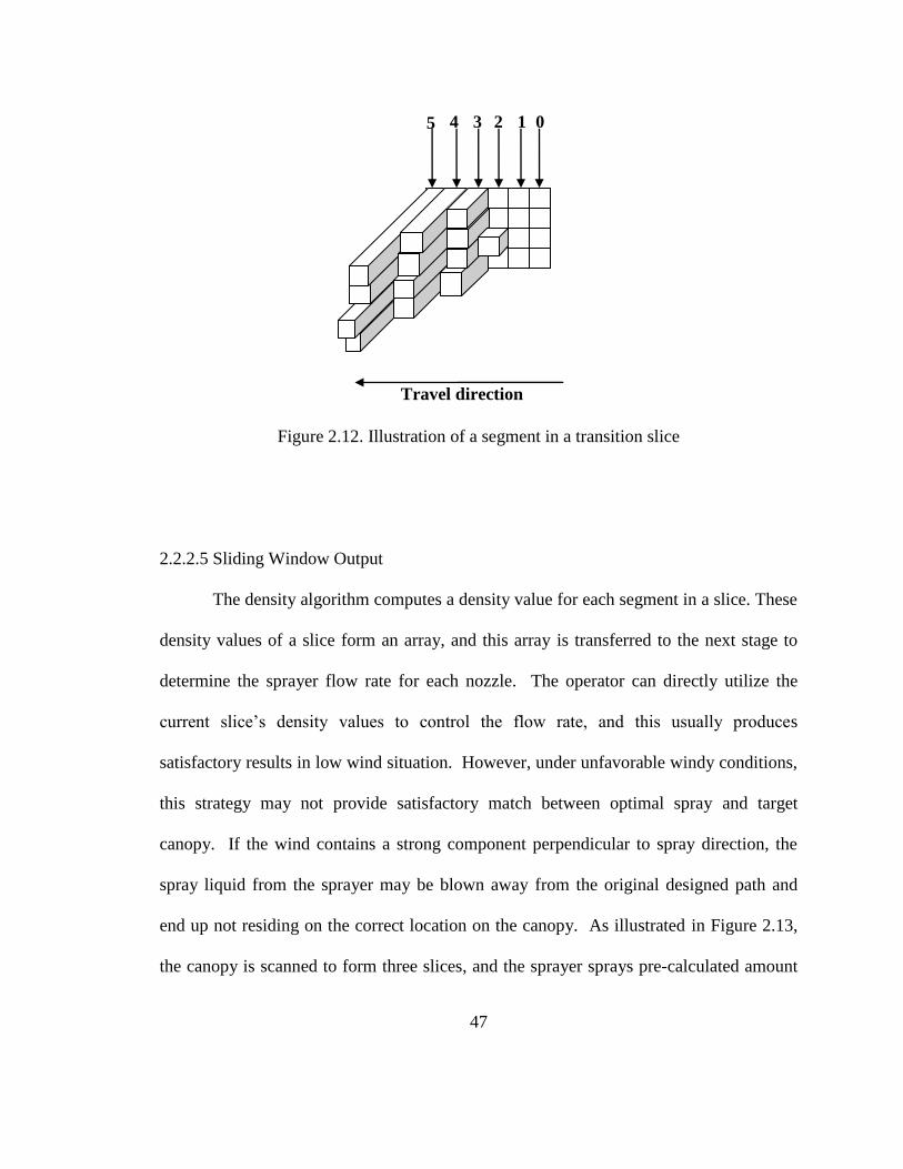
47

Figure 2.12. Illustration of a segment in a transition slice

2.2.2.5 Sliding Window Output

The density algorithm computes a density value for each segment in a slice. These

density values of a slice form an array, and this array is transferred to the next stage to

determine the sprayer flow rate for each nozzle. The operator can directly utilize the

current slice‟s density values to control the flow rate, and this usually produces

satisfactory results in low wind situation. However, under unfavorable windy conditions,

this strategy may not provide satisfactory match between optimal spray and target

canopy. If the wind contains a strong component perpendicular to spray direction, the

spray liquid from the sprayer may be blown away from the original designed path and

end up not residing on the correct location on the canopy. As illustrated in Figure 2.13,

the canopy is scanned to form three slices, and the sprayer sprays pre-calculated amount

3 4 5 2 1 0

Travel direction

48

of liquid for each slice. Due to the strong wind component perpendicular to the spray

direction, however, the liquid aimed at slice 1 is blown toward to 1‟, liquid for slice 2

ends up on slice 1, and slice 3 cannot receive any spray.

To overcome this mis-targeting problem caused by wind conditions, a sliding

window mechanism to offset possible negative impacts is designed. A sliding window at

the output side of the computation is prepared. This sliding window contains a circular

buffer to hold the density results for the past three slices including current slice. The

computed density from section 2.2.2.3 is shifted into this slide window as current slice,

and the oldest slice in the buffer is retired and replaced by the newest result. Then the

three arrays in the sliding window are compared to form a new output array. Every

element in this output array is the largest value of the three elements at corresponding

positions from the three past arrays. Eventually, this sliding window will provide the

capability of “remembering” the computation result in the past. Consequently, the mis-

targeting problem is compensated by adjusting the delay unit (described in section 2.5),

and opening the nozzles ahead of time for one slice and delay the turning-off for one

slice.

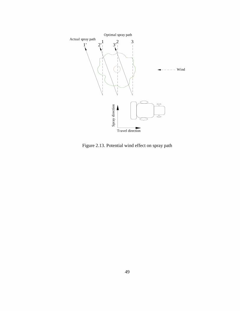
49

Figure 2.13. Potential wind effect on spray path

Wind

1 2 31' 2' 3'

Sp

ray

dir

ecti

on

Travel direction

Actual spray path

Optimal spray path

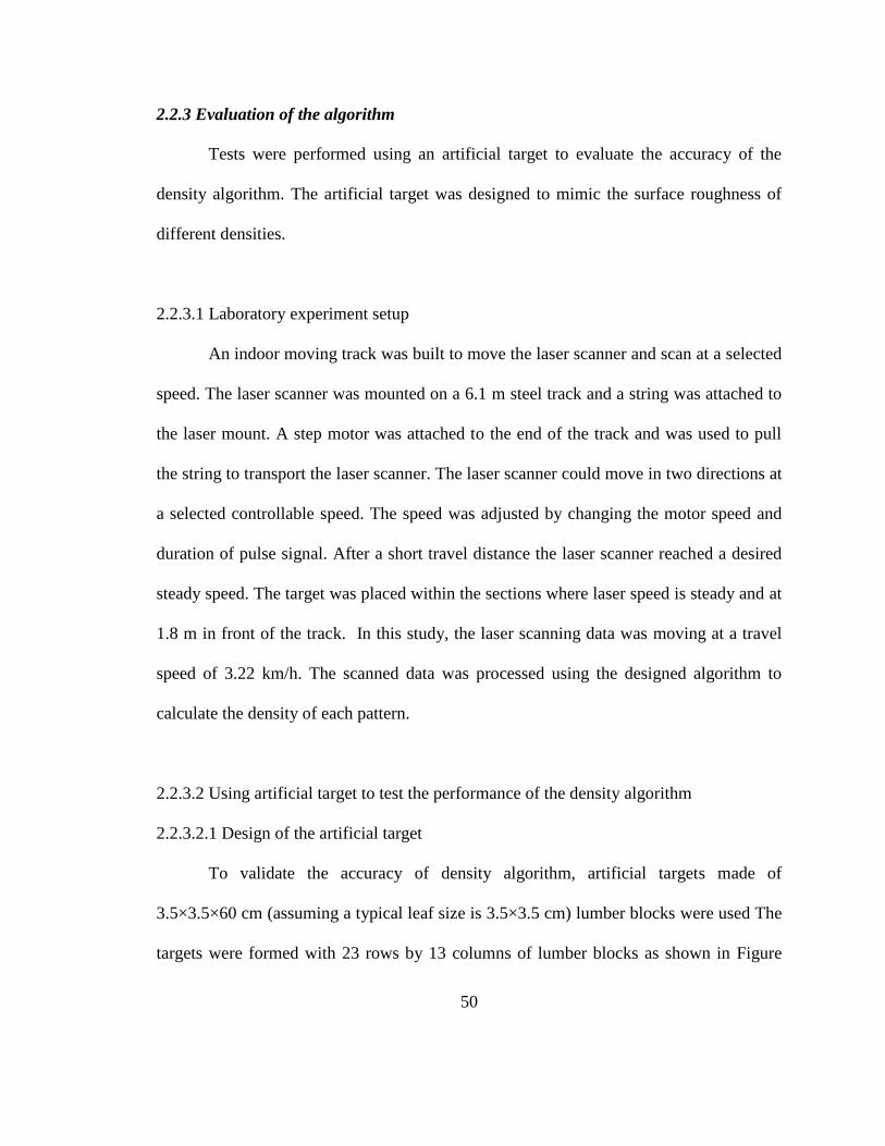
50

2.2.3 Evaluation of the algorithm

Tests were performed using an artificial target to evaluate the accuracy of the

density algorithm. The artificial target was designed to mimic the surface roughness of

different densities.

2.2.3.1 Laboratory experiment setup

An indoor moving track was built to move the laser scanner and scan at a selected

speed. The laser scanner was mounted on a 6.1 m steel track and a string was attached to

the laser mount. A step motor was attached to the end of the track and was used to pull

the string to transport the laser scanner. The laser scanner could move in two directions at

a selected controllable speed. The speed was adjusted by changing the motor speed and

duration of pulse signal. After a short travel distance the laser scanner reached a desired

steady speed. The target was placed within the sections where laser speed is steady and at

1.8 m in front of the track. In this study, the laser scanning data was moving at a travel

speed of 3.22 km/h. The scanned data was processed using the designed algorithm to

calculate the density of each pattern.

2.2.3.2 Using artificial target to test the performance of the density algorithm

2.2.3.2.1 Design of the artificial target

To validate the accuracy of density algorithm, artificial targets made of

3.5×3.5×60 cm (assuming a typical leaf size is 3.5×3.5 cm) lumber blocks were used The

targets were formed with 23 rows by 13 columns of lumber blocks as shown in Figure

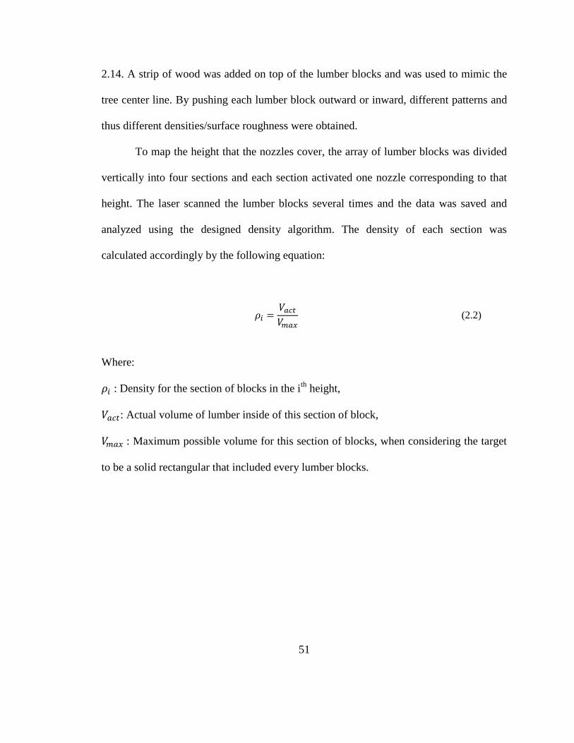
51

2.14. A strip of wood was added on top of the lumber blocks and was used to mimic the

tree center line. By pushing each lumber block outward or inward, different patterns and

thus different densities/surface roughness were obtained.

To map the height that the nozzles cover, the array of lumber blocks was divided

vertically into four sections and each section activated one nozzle corresponding to that

height. The laser scanned the lumber blocks several times and the data was saved and

analyzed using the designed density algorithm. The density of each section was

calculated accordingly by the following equation:

(2.2)

Where:

: Density for the section of blocks in the ith

height,

: Actual volume of lumber inside of this section of block,

: Maximum possible volume for this section of blocks, when considering the target

to be a solid rectangular that included every lumber blocks.

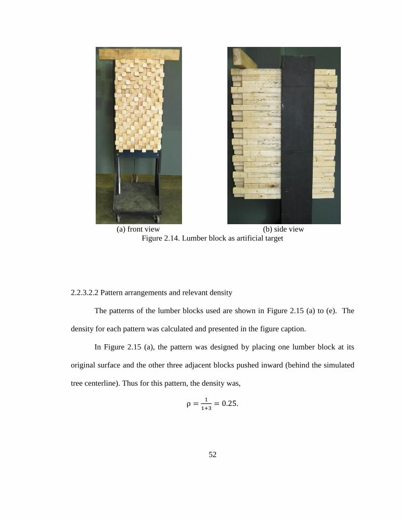
52

(a) front view (b) side view

Figure 2.14. Lumber block as artificial target

2.2.3.2.2 Pattern arrangements and relevant density

The patterns of the lumber blocks used are shown in Figure 2.15 (a) to (e). The

density for each pattern was calculated and presented in the figure caption.

In Figure 2.15 (a), the pattern was designed by placing one lumber block at its

original surface and the other three adjacent blocks pushed inward (behind the simulated

tree centerline). Thus for this pattern, the density was,

.

53

In Figure 2.15 (b), for each block on its original surface, two adjacent blocks were

pushed inward behind the center line (created by the wood board on top of the blocks).

Thus for this pattern, the density was,

.

Similarly, in Figure 2.15 (c), the density was,

.

In Figure 2.15 (d), the density was,

.

In Figure 2.15 (e), the density was,

.

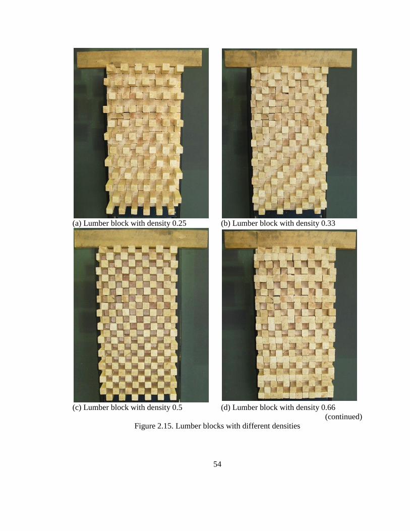
54

(a) Lumber block with density 0.25 (b) Lumber block with density 0.33

(c) Lumber block with density 0.5 (d) Lumber block with density 0.66

(continued)

Figure 2.15. Lumber blocks with different densities

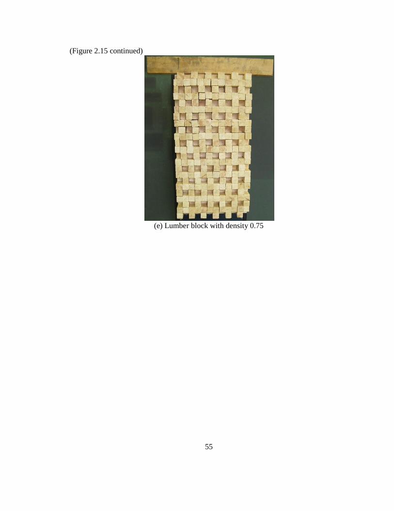
55


(e) Lumber block with density 0.75

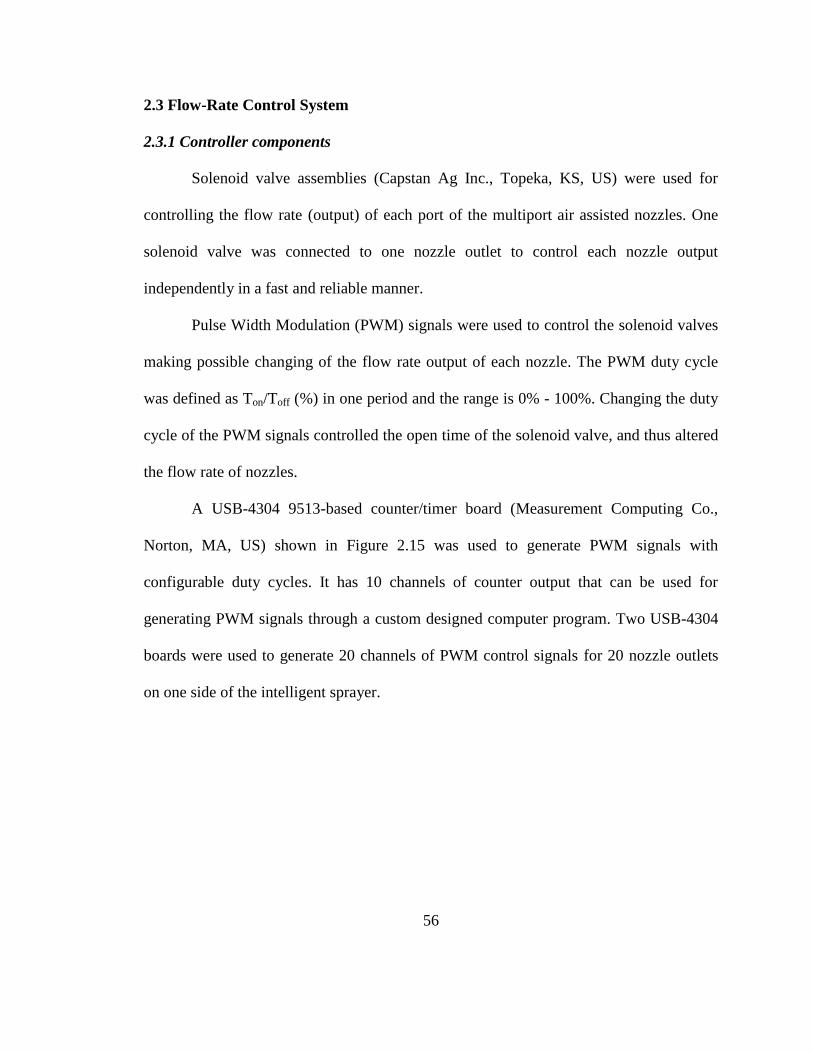
56

2.3 Flow-Rate Control System

2.3.1 Controller components

Solenoid valve assemblies (Capstan Ag Inc., Topeka, KS, US) were used for

controlling the flow rate (output) of each port of the multiport air assisted nozzles. One

solenoid valve was connected to one nozzle outlet to control each nozzle output

independently in a fast and reliable manner.

Pulse Width Modulation (PWM) signals were used to control the solenoid valves

making possible changing of the flow rate output of each nozzle. The PWM duty cycle

was defined as Ton/Toff (%) in one period and the range is 0% - 100%. Changing the duty

cycle of the PWM signals controlled the open time of the solenoid valve, and thus altered

the flow rate of nozzles.

A USB-4304 9513-based counter/timer board (Measurement Computing Co.,

Norton, MA, US) shown in Figure 2.15 was used to generate PWM signals with

configurable duty cycles. It has 10 channels of counter output that can be used for

generating PWM signals through a custom designed computer program. Two USB-4304

boards were used to generate 20 channels of PWM control signals for 20 nozzle outlets

on one side of the intelligent sprayer.

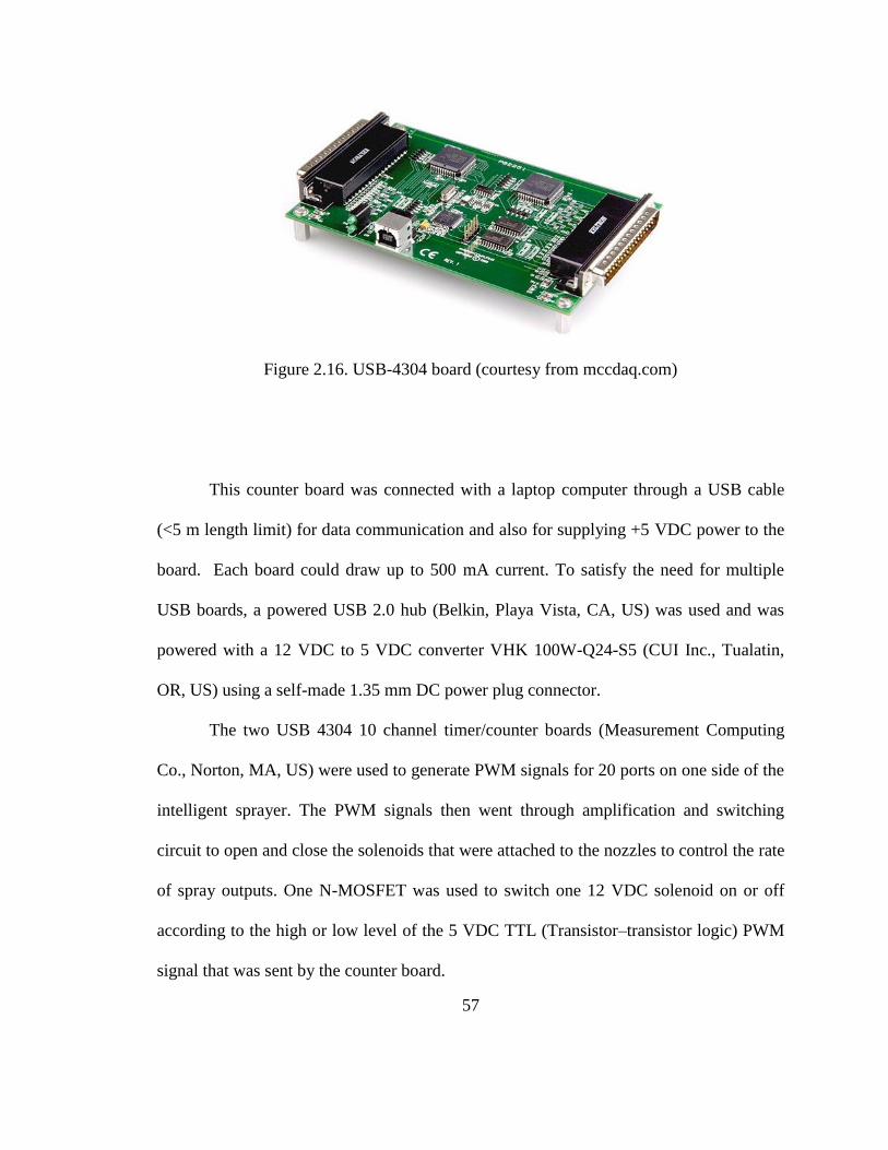
57

Figure 2.16. USB-4304 board (courtesy from mccdaq.com)

This counter board was connected with a laptop computer through a USB cable

(<5 m length limit) for data communication and also for supplying +5 VDC power to the

board. Each board could draw up to 500 mA current. To satisfy the need for multiple

USB boards, a powered USB 2.0 hub (Belkin, Playa Vista, CA, US) was used and was

powered with a 12 VDC to 5 VDC converter VHK 100W-Q24-S5 (CUI Inc., Tualatin,

OR, US) using a self-made 1.35 mm DC power plug connector.

The two USB 4304 10 channel timer/counter boards (Measurement Computing

Co., Norton, MA, US) were used to generate PWM signals for 20 ports on one side of the

intelligent sprayer. The PWM signals then went through amplification and switching

circuit to open and close the solenoids that were attached to the nozzles to control the rate

of spray outputs. One N-MOSFET was used to switch one 12 VDC solenoid on or off

according to the high or low level of the 5 VDC TTL (Transistor–transistor logic) PWM

signal that was sent by the counter board.

58

2.3.2Software design for generating PWM signals

A logic program was specially developed to control USB 4304 counter board to

generate 10 channels of PWM signals with independent duty cycles using LabVIEW

software (National Instruments Co., Austin, TX, USA). Figure 2.17 shows the flow chart

for generating PWM signals with the desired duty cycle and frequency (details as shown

in Appendix C).

2.3.3 Switching/amplification circuit using PWM signals

Since the PWMs signals generated from the counter board are +5 VDC TTL

(Transistor–transistor logic) signals, they are required to be amplified in order to be able

to control the solenoid valves that are powered at 12 VDC. Custom

switching/amplification circuits designed for four functions: 1) supporting +12 VDC

power from external tractor battery and also receiving +5 VDC power from USB port

through USB 4304 power pins; 2) connecting 10 channels of independent PWM signals

generated from USB 4304 board to the corresponding program; 3) switching from +5 V

TTL to +12 V signals to activate solenoid valves; 4) limiting the reverse kick-back

current from solenoid coil using Zener diodes (details as shown in Appendix B).

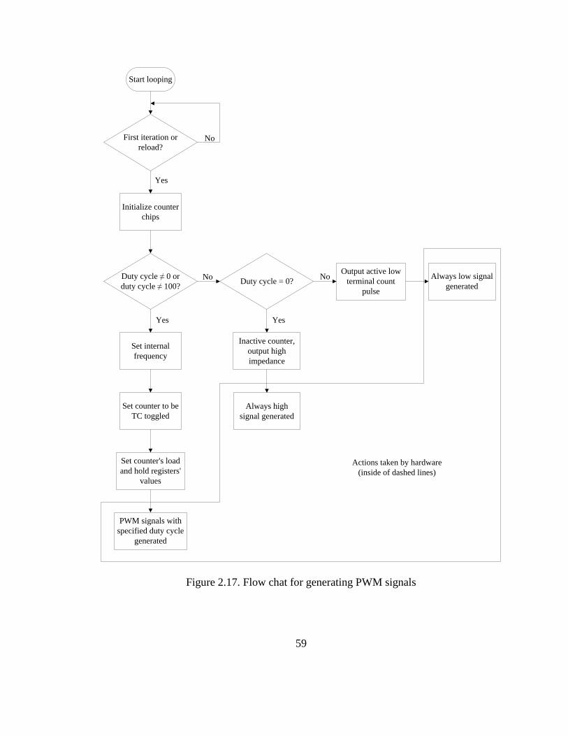
59

Figure 2.17. Flow chat for generating PWM signals

Start looping

First iteration or

reload?

Initialize counter

chips

Duty cycle ≠ 0 or

duty cycle ≠ 100?Duty cycle = 0?

Set counter to be

TC toggled

Set internal

frequency

Set counter's load

and hold registers'

values

PWM signals with

specified duty cycle

generated

Inactive counter,

output high

impedance

Always high

signal generated

Output active low

terminal count

pulse

Always low signal

generated

No

Yes

No

Yes Yes

No

Actions taken by hardware

(inside of dashed lines)

60

2.3.4 Experiment station for one five-port air assisted nozzle

An experiment station was built to test the variable rate control software and

hardware and also to calibrate the five-port air-assisted nozzle. Figure 2.18 shows the

schematic of the design of the experiment station for independent control of one five-port

air-assisted nozzle.

The experiment station included a tank and a pump for supplying liquid, a

pressure regulator and a mechanical pressure gauge for adjusting the liquid pressure

manually, a pressure transducer and a flow sensor connected to a data acquisition board

(USB-1608FS, Measurement Computing Co., Norton, MA, US) shown in Figure 2.19.

The acquisition board was used for acquiring real time pressure and flow rate values and

also for storing them in a portable computer. A five-port nozzle (air was not supplied for

all tests done with this experiment station) was connected and controlled by five solenoid

valves, one for each port. An operator used a custom computer program designed with

LabVIEW (interface shown in Figure 2.20) to change the duty cycle of 5 independent

channels of PWM signals generated and amplified by the control circuits (shown in

Figure 2.21) to drive five individual solenoid valves.

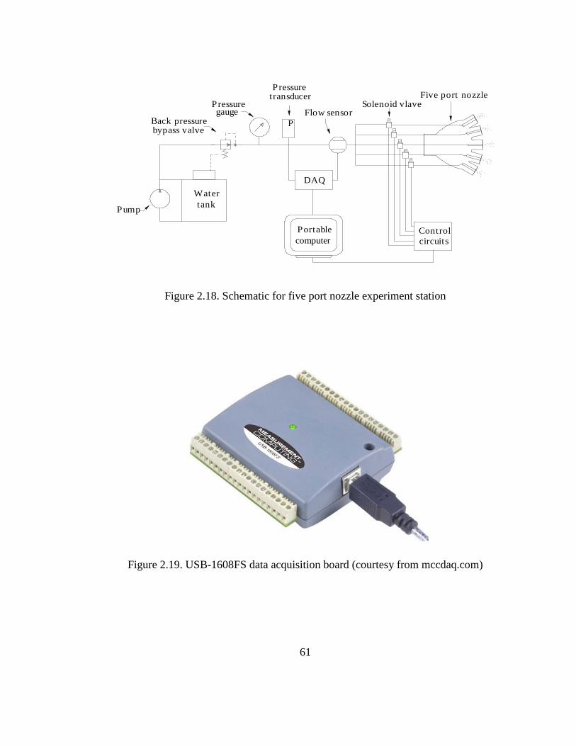
61

Figure 2.18. Schematic for five port nozzle experiment station

Figure 2.19. USB-1608FS data acquisition board (courtesy from mccdaq.com)

Portable

computer

DAQ

Control

circuits

Water

tankPump

Back pressurebypass valve

Solenoid vlavePressure

Pressuretransducer

Flow sensor

Five port nozzle

P

gauge

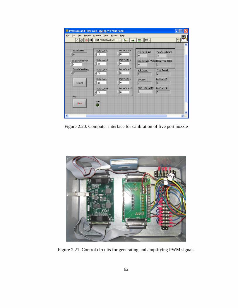
62

Figure 2.20. Computer interface for calibration of five port nozzle

Figure 2.21. Control circuits for generating and amplifying PWM signals

63

2.3.5 Pressure transducer and flow sensor

2.3.5.1 Pressure transducer

A pressure transducer (model MSP-400-100-P-4-N-1, Measurement Specialties

Inc., Hampton, VA) was used in the experiment system to monitor and log the pressure

change in real time. When supplied with 12 VDC power, this pressure transducer outputs

1 ~ 5 VDC voltage signal which is proportional to 0 ~ 690 kPa operating pressure.

The analog to digital (A/D) converter was a 16 bit USB-1608FS analog to digital

converter and -5 V to +5 V was chosen as the full scale range, the resolution of the A/D

converter was:

( )

( ) (2.3)

Where,

:Resolution, ,

: Full scale range, ,

N: Bits resolution, .

Thus the pressure sensitivity of the pressure transducer is:

( ) (2.4)

Where,

64

: Pressure sensitivity, ,

: Output high voltage, ,

: Output low voltage, ,

: Highest pressure to measure, ,

: Lowest pressure to measure, .

Thus the smallest pressure change that the A/D converter can measure is:

( ) (2.5)

Where,

: The pressure resolution that the A/D converter can measure, .

Thus, the pressure measured can be calculated from digital counts converted by analog

voltage input.

( )

2.3.5.2 Flow sensor

A flow sensor (model DFS-2 Digiflow Systems, Hudson, MA) was used to

calibrate the relationship between the duty cycle of the PWM control signal and the flow

rate output from the ports on the five-port nozzle. The resolution (also called K-factor)

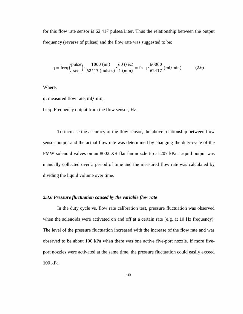
65

for this flow rate sensor is 62,417 pulses/Liter. Thus the relationship between the output

frequency (reverse of pulses) and the flow rate was suggested to be:

(

)

( )

( ) ( )

( )

( ) (2.6)

Where,

: measured flow rate, ,

: Frequency output from the flow sensor, Hz.

To increase the accuracy of the flow sensor, the above relationship between flow

sensor output and the actual flow rate was determined by changing the duty-cycle of the

PMW solenoid valves on an 8002 XR flat fan nozzle tip at 207 kPa. Liquid output was

manually collected over a period of time and the measured flow rate was calculated by

dividing the liquid volume over time.

2.3.6 Pressure fluctuation caused by the variable flow rate

In the duty cycle vs. flow rate calibration test, pressure fluctuation was observed

when the solenoids were activated on and off at a certain rate (e.g. at 10 Hz frequency).

The level of the pressure fluctuation increased with the increase of the flow rate and was

observed to be about 100 kPa when there was one active five-port nozzle. If more five-

port nozzles were activated at the same time, the pressure fluctuation could easily exceed

100 kPa.

66

The intelligent sprayer prototype, described in more detail in the later chapters,

consisted of 20 solenoid valves on each side. Turning all the nozzles on and off to

achieve variable rate for matching target characteristics will eventually create the

pressure fluctuation greater than 100 kPa. Since the nozzle flow rate is directly affected

by the operating pressure, the pressure fluctuation should be minimized to obtain a

constant flow rate for the same control signals. Therefore, to limit the pressure fluctuation

at the nozzle tips, and to minimize the error of the nozzle flow rate, a back pressure

bypass unit consisting of a pressure regulator was added in the spray line to stabilize the

pressure by discharging excessive fluid back to the tank, as shown in Figure 2.18.

The adjustable pressure regulating valve and the check valve were tested to

compare their performance in reducing pressure fluctuation caused by flow rate changes.

When conducting tests to determine the effect of two back pressure bypass valves, all the

nozzles were fully open for 300 ms and then close for 300 ms all at the same time.

Pressure was acquired from the pressure transducer every 50 ms using USB-1608FS data

acquisition board and was saved to a portable computer using the program interface

shown in Figure 2.20. This represents the most extreme case for the intelligent sprayer to

face while in operation, though it is unlikely to happen. However, testing under this

condition could provide a reference for the upper limits of pressure fluctuation when

using a check valve or an adjustable valve for the back pressure path.

67

2.4 Spray model for optimal flow rate calculation

2.4.1 Spray model derivation

As shown in Figure 2.22, for each segment of the tree canopy corresponding to

one nozzle port on the intelligent sprayer, the volume of the canopy segment is:

(2.7)

The effective volume of this tree canopy segment is:

(2.8)

Where,

: Width (depth) of the canopy section (segment maximum width), m,

: Tractor forward speed, m/s,

: Time passed, s,

: Density of the canopy segment, 0 ~ 1,

: Average height that each nozzle covers, m, (0.12 to 0.135 cm based on sprayer

dimension measured).

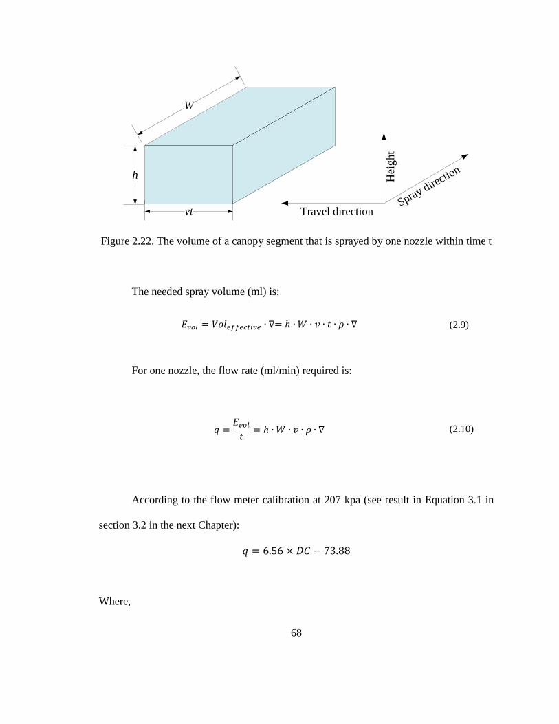
68

Figure 2.22. The volume of a canopy segment that is sprayed by one nozzle within time t

The needed spray volume (ml) is:

(2.9)

For one nozzle, the flow rate (ml/min) required is:

(2.10)

According to the flow meter calibration at 207 kpa (see result in Equation 3.1 in

section 3.2 in the next Chapter):

Where,

h

vt

W

Spray directio

n

Travel direction

Hei

ght

69

DC is the duty cycle of the flow rate control signal, and is the spray rate or the amount

of spray to treat a unit of tree canopy volume (L/m3).

Thus to match the need of the effective volume of the tree canopy segment, the

required Duty cycle of the control signal should be:

(2.11)

The recommended optimal spray rates for orchards are 0.1 L and 0.13 L of spray

mixture per 1.0 m3

of tree canopy for pruned and unpruned trees, respectively (Jenkins

and Hines, 2003). For the tests conducted in this study, was chosen to be 0.1.

Therefore, the duty cycle of the control signal can be determined with the known segment

height that one nozzle port covers (h), the tractor speed (v), the calculated maximum

segment width (W) and the density of the canopy segment ( ).

2.4.2 Laboratory (indoor) sprayer evaluation of the intelligent sprayer

To evaluate the accuracy of using the laser scanner and computational algorithm

to measure tree canopy characteristics and to assess the performance of the spray model

designed for the Intelligent sprayer, sectional volume of four trees with two different

species was measured by the laser scanner and then was compared with manual

measurements.

The two tree species were Tsuga Canadensis and Emerald Green Thuja (Figure

3.11), and they were purchased from local commercial nurseries. The two Tsuga

70

Canadensis trees were 228 cm and 320 cm high and were designated as Tree 1 and Tree

2, respectively. The two Emerald Green Thuja trees were 271 cm and 263 cm high and

were designated as Tree 3 and Tree 4, respectively.

The widths at a 12 cm height interval of each tree were manually measured to

calculate sectional volume. Trees were also scanned by the laser scanner to determine the

sectional volume for comparison. Sectional density and optimal spray rate for each

nozzle corresponding to that section were then calculated by the computer program using

the density algorithm and the spray model described earlier. For each of the 20

sections/nozzles, density calculated from laser data was multiplied by the sectional

volume based on the manual measurement to obtain effective tree volume corresponding

to each nozzle. The optimal spray rate calculated by the algorithm was then divided by

the effective tree volume to obtain the actual spray constant (Equation 2.12) used for each

nozzle.

The procedure for this indoor evaluation test was:

1. Manually measure the tree width at every 12 cm height interval (the height for each

nozzle to cover, assumed) for all four trees (shown in Figure 2.23).

2. Calculate the canopy volume for each height section (corresponding to one nozzle)

using the following equation:

( ) (2.12)

Where,

71

: Volume for the ith section of canopy,

: Height interval, equals to 12 cm in this experiment,

: Radius of the lower part of the section, also equals to half the lower part width (

)

: Radius of the upper part of the section, also equals to half the upper part width (

).

3. Scan all trees with laser scanner and save the range data.

4. Use the algorithm to calculate tree maximum width and each sectional canopy density

from the range data.

5. Use the spray model to calculate the flow rate for each canopy section, calculate the

spray volume by multiplying flow rate with time.

6. Divide spray volume result by the effective canopy volume (or manually- measured

volume multiplies by the calculated canopy density) for each canopy section.

(2.13)

Where,

: The canopy section number, 1 to 20 (from bottom to top),

: Spray rate for the ith section of the canopy (L/m3),

: Flow rate for the ith nozzle, L/min,

: Time used for spraying the ith section of canopy, min,

: Volume for the ith section of canopy, m3,

: Density for the ith section of canopy, calculated by the density algorithm.

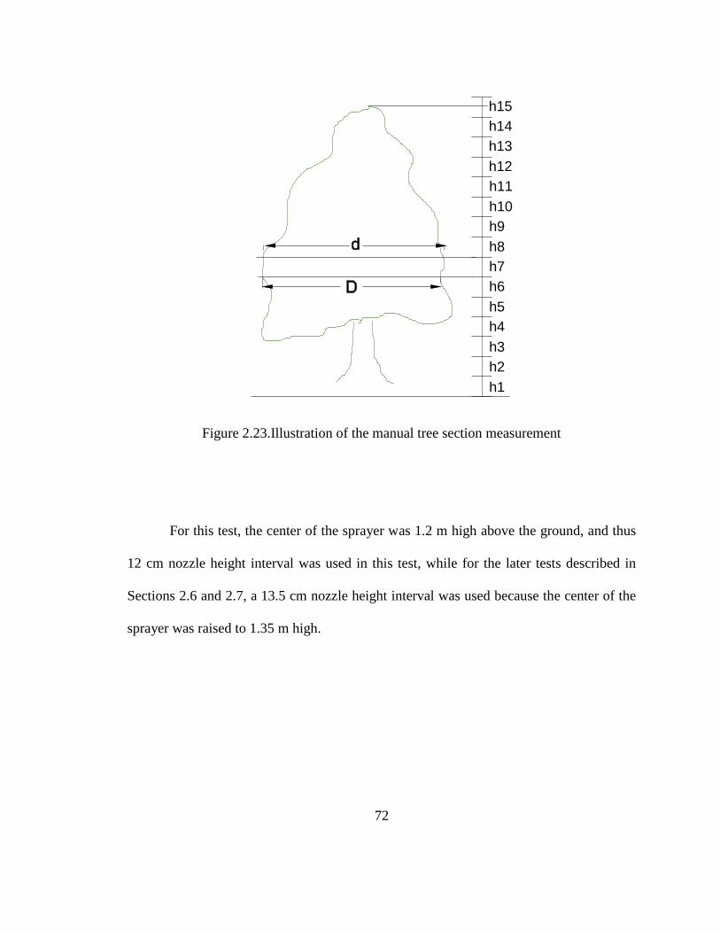
72

h1

h2

h3

h4

h5

h6

h7

h8

h9

h10

h11

h12

h13

h14

h15

Figure 2.23.Illustration of the manual tree section measurement

For this test, the center of the sprayer was 1.2 m high above the ground, and thus

12 cm nozzle height interval was used in this test, while for the later tests described in

Sections 2.6 and 2.7, a 13.5 cm nozzle height interval was used because the center of the

sprayer was raised to 1.35 m high.

73

2.5 Sprayer Modification

The intelligent sprayer was modified from a vineyard sprayer (model ZENIT B11,

HARDI Inc., Davenport, IA) with a 0.81 m axial fan to deliver air to eight spray

dischargers on both sides of the sprayer. The modifications to the sprayer were done in

three steps: nozzle replacement, sensor and controller mounting, pressure regulating and

system response calibration.

2.5.1 Nozzle replacement

The original eight spray dischargers on two sides of the sprayer were replaced

with eight, five-port air-assisted nozzles, and each nozzle consisted of five ports to

discharge five streams of sprays. The nozzle tip in each port was a modified Teejet

11003VB flat fan tip (Spraying Systems, Wheaton, IL) and was mounted at the center of

each port. Details of the modified nozzle tips for the five-port nozzle were given by Zhu

et al., (2006). These nozzles were used for the intelligent sprayer development to

potentially improve spray penetration and spray deposition uniformity over conventional

spray delivery design.

The maximum air velocity of five-port air assisted nozzles was measured with

constant temperature anemometer (CTA) employing 0.15 mm cylindrical hot-film

sensors (Model 1210-60, TSI Inc., St. Paul, MN). The sensors were located at 1 cm away

from the port outlets. During the air velocity measurement, the fan was set at the high

speed mode (same as field test setting).

74

2.5.2 Sensor and controller mounting

The laser scanner was mounted on the spray tank frame between the tractor cab

and spray nozzles. Both the scanner and nozzles on the same side were pointed to the

same direction. The distance between the laser scanner and the nozzles was 1.45 m. This

distance was chosen because it was easy for the connection between the sensor and the

spray tank frame. The error caused by the distance was compensated by adding a delay in

the controller and thus not affecting the real-time matching of the flow rate to the target.

A water proof controller box was mounted beneath the water tank of the intelligent

sprayer. All electrical circuits, power converters and cables were mounted inside the

secured controller box and were sealed from water leakage damage.

2.5.3 Pressure regulating (back pressure bypass)

As indicated previously, the spray pressure near the nozzle tip fluctuates when the

solenoid valves were switched on and off at a 10 Hz rate. The pressure fluctuation could

cause unintended changes in flow rate output and droplet size. To reduce the pressure

fluctuation near the nozzle tip, a back pressure regulating unit described in section 2.3

was added to discharge extra fluids through the bypass to the spray tank.

2.5.4 System response calibration using high speed camera system

Real-time automatic spray application is the one of the major goals in the design

of the intelligent sprayer. Because it takes time for the laser scanner to scan the target, the

data buffer to accumulate frames for calculation, the algorithm to calculate canopy width,

75

density and optimal flow rate for each nozzle, and the hydraulic-mechanical response to

the control signal, there is a time delay between the target being detected by the laser

scanner and the liquid actually being sprayed. Knowing this system delay time is very

important because it is a reference to determine minimum distance between the laser

scanner and nozzle outlets. It is also used to calculate the control delay needed for

matching the correct spray flow rate to the target structure.

A SILICON VIDEO® 642M camera (EPIX, Inc., Buffalo Grove, IL, USA) was

used to measure the system response time. This high speed camera can capture an image

sequence with a time mark on each frame. This enables one to determine the time

difference between any two images by simple subtraction of times associated with two

images.

A laser pointer was mounted beside the camera in a position such that it would

produce a dot on a recognizable location on the laser scanner at the exact time when the

laser beam aligned with the edge of the target tree. In this way, the “seeing” of the target

was identified by capturing the laser pointer dot on the specific location (calibrated

beforehand) on the laser scanner. Following this, the time of actual spraying was captured

in the camera and recorded. Therefore the system response was the time between the

actions captured when laser “sees” the target and when the liquid began to flow.

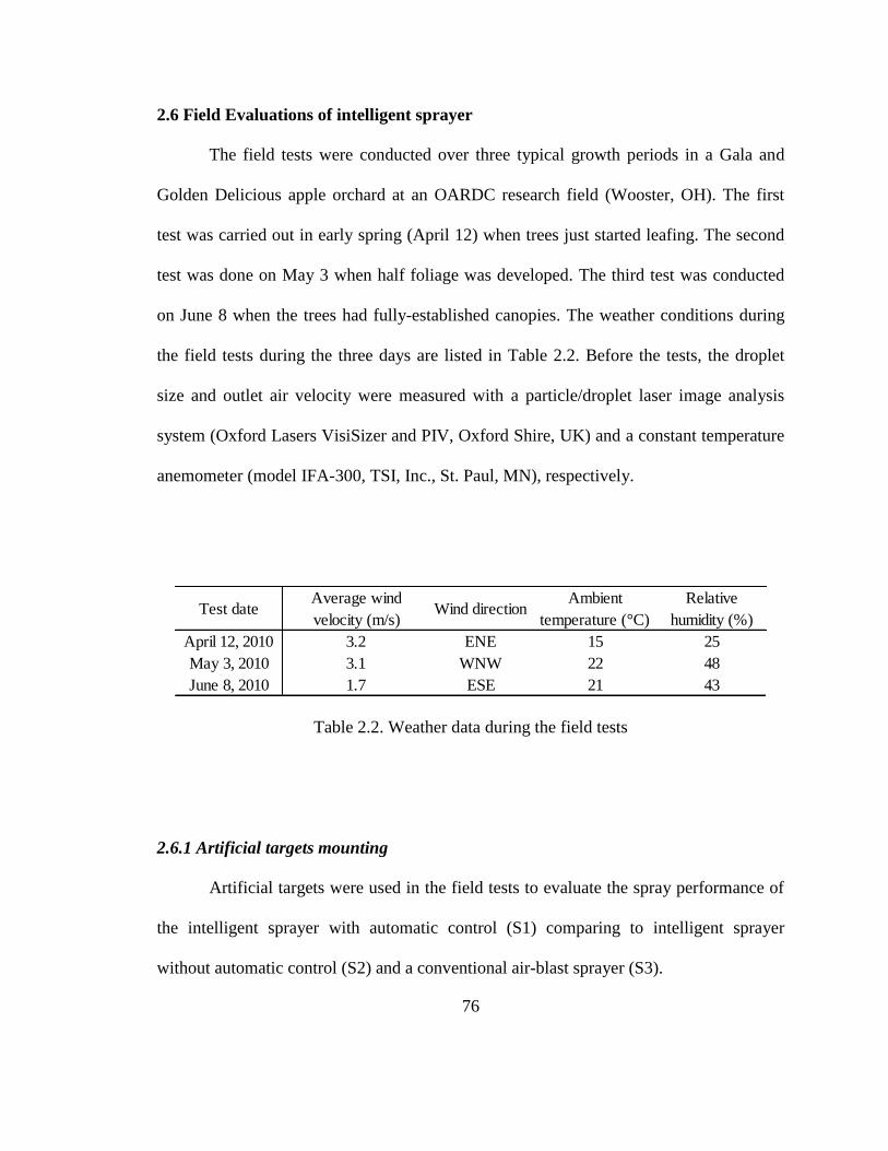
76

2.6 Field Evaluations of intelligent sprayer

The field tests were conducted over three typical growth periods in a Gala and

Golden Delicious apple orchard at an OARDC research field (Wooster, OH). The first

test was carried out in early spring (April 12) when trees just started leafing. The second

test was done on May 3 when half foliage was developed. The third test was conducted

on June 8 when the trees had fully-established canopies. The weather conditions during

the field tests during the three days are listed in Table 2.2. Before the tests, the droplet

size and outlet air velocity were measured with a particle/droplet laser image analysis

system (Oxford Lasers VisiSizer and PIV, Oxford Shire, UK) and a constant temperature

anemometer (model IFA-300, TSI, Inc., St. Paul, MN), respectively.

Table 2.2. Weather data during the field tests

2.6.1 Artificial targets mounting

Artificial targets were used in the field tests to evaluate the spray performance of

the intelligent sprayer with automatic control (S1) comparing to intelligent sprayer

without automatic control (S2) and a conventional air-blast sprayer (S3).

Test dateAverage wind

velocity (m/s)Wind direction

Ambient

temperature (°C)

Relative

humidity (%)

April 12, 2010 3.2 ENE 15 25

May 3, 2010 3.1 WNW 22 48

June 8, 2010 1.7 ESE 21 43

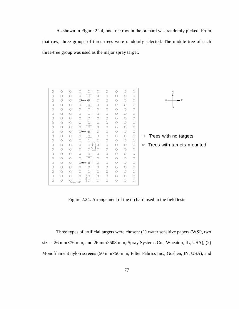
77

As shown in Figure 2.24, one tree row in the orchard was randomly picked. From

that row, three groups of three trees were randomly selected. The middle tree of each

three-tree group was used as the major spray target.

Figure 2.24. Arrangement of the orchard used in the field tests

Three types of artificial targets were chosen: (1) water sensitive papers (WSP, two

sizes: 26 mm×76 mm, and 26 mm×508 mm, Spray Systems Co., Wheaton, IL, USA), (2)

Monofilament nylon screens (50 mm×50 mm, Filter Fabrics Inc., Goshen, IN, USA), and

Trees with no targets

Trees with targets mounted

2.6m

S

EW

N

4.6m

Tree 1

Tree 2

Tree 3

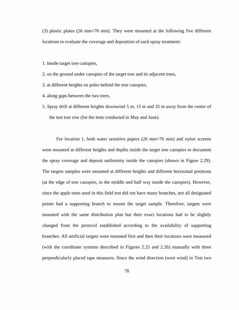
78

(3) plastic plates (26 mm×76 mm). They were mounted at the following five different

locations to evaluate the coverage and deposition of each spray treatment:

1. Inside target tree canopies,

2. on the ground under canopies of the target tree and its adjacent trees,

3. at different heights on poles behind the tree canopies,

4. along gaps between the two trees,

5. Spray drift at different heights downwind 5 m, 15 m and 35 m away from the center of

the test tree row (for the tests conducted in May and June).

For location 1, both water sensitive papers (26 mm×76 mm) and nylon screens

were mounted at different heights and depths inside the target tree canopies to document

the spray coverage and deposit uniformity inside the canopies (shown in Figure 2.29).

The targets samples were mounted at different heights and different horizontal positions

(at the edge of tree canopies, in the middle and half way inside the canopies). However,

since the apple trees used in this field test did not have many branches, not all designated

points had a supporting branch to mount the target sample. Therefore, targets were

mounted with the same distribution plan but their exact locations had to be slightly

changed from the protocol established according to the availability of supporting

branches. All artificial targets were mounted first and then their locations were measured

(with the coordinate systems described in Figures 2.25 and 2.26) manually with three

perpendicularly placed tape measures. Since the wind direction (west wind) in Test two

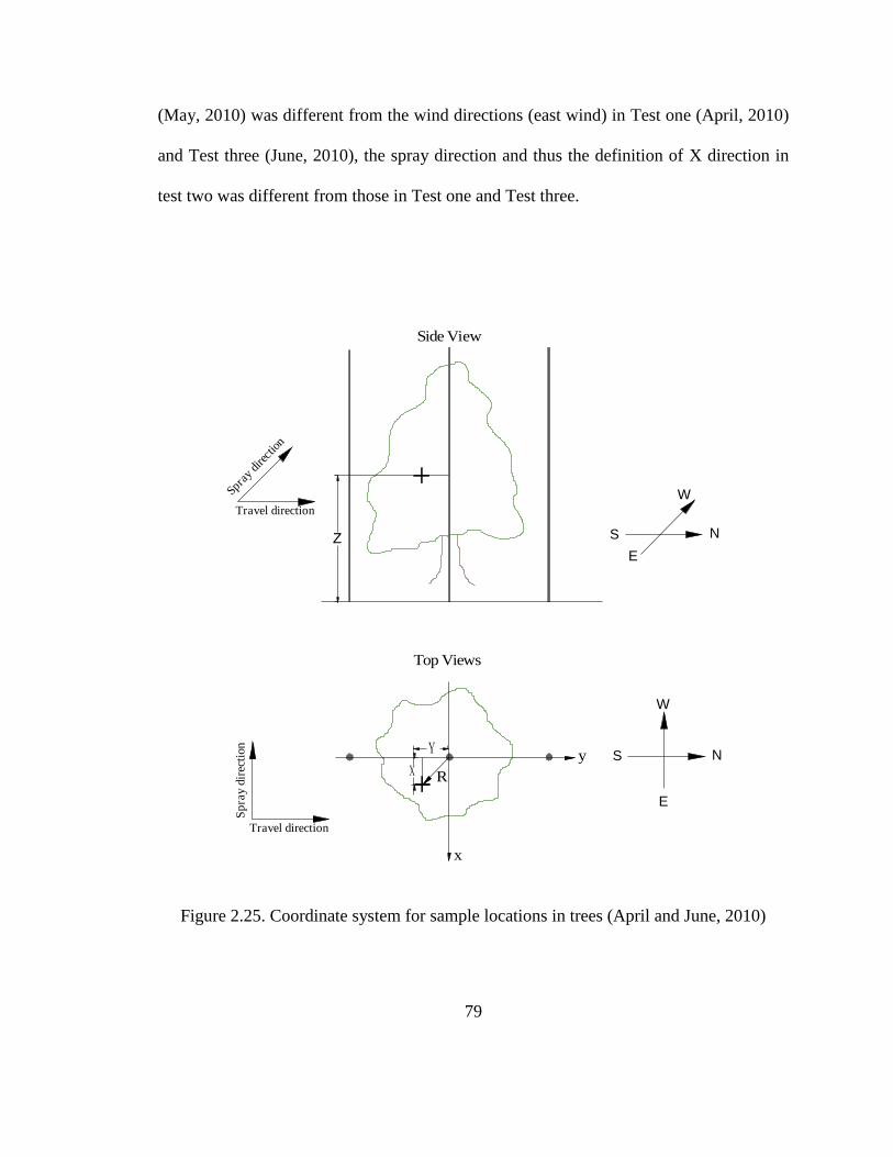
79

(May, 2010) was different from the wind directions (east wind) in Test one (April, 2010)

and Test three (June, 2010), the spray direction and thus the definition of X direction in

test two was different from those in Test one and Test three.

Figure 2.25. Coordinate system for sample locations in trees (April and June, 2010)

Top Views

Side View

Travel direction

Travel direction

Sp

ray d

irec

tion

Spray

dire

ctio

n

NS

E

W

NS

E

W

RX

x

y

Z

Y

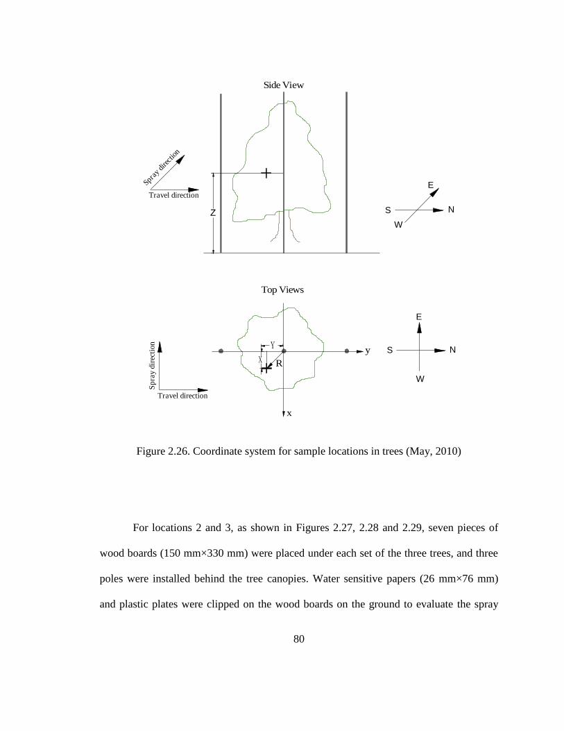
80

Figure 2.26. Coordinate system for sample locations in trees (May, 2010)

For locations 2 and 3, as shown in Figures 2.27, 2.28 and 2.29, seven pieces of

wood boards (150 mm×330 mm) were placed under each set of the three trees, and three

poles were installed behind the tree canopies. Water sensitive papers (26 mm×76 mm)

and plastic plates were clipped on the wood boards on the ground to evaluate the spray

Top Views

Side View

Travel direction

Travel direction

Sp

ray d

irec

tion

Spray

dire

ctio

n

NS

W

E

NS

W

E

RX

x

y Z

Y

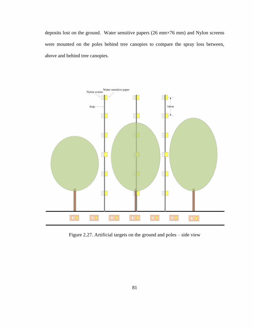
81

deposits lost on the ground. Water sensitive papers (26 mm×76 mm) and Nylon screens

were mounted on the poles behind tree canopies to compare the spray loss between,

above and behind tree canopies.

Figure 2.27. Artificial targets on the ground and poles – side view

Nylon screenWater sensitive paper

Pole 54cm

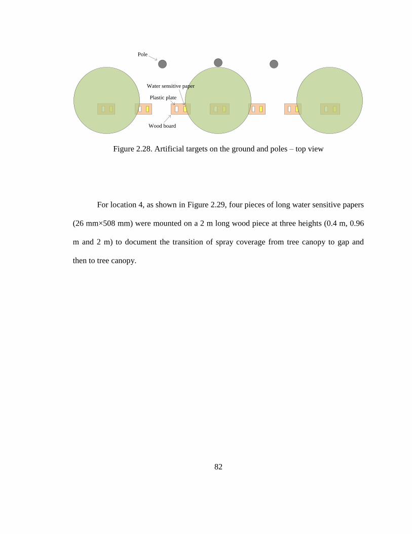
82

Pole

Wood board

Plastic plate

Water sensitive paper

Figure 2.28. Artificial targets on the ground and poles – top view

For location 4, as shown in Figure 2.29, four pieces of long water sensitive papers

(26 mm×508 mm) were mounted on a 2 m long wood piece at three heights (0.4 m, 0.96

m and 2 m) to document the transition of spray coverage from tree canopy to gap and

then to tree canopy.

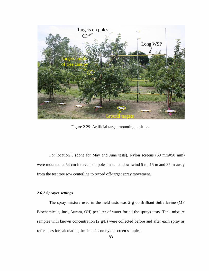
83

Figure 2.29. Artificial target mounting positions

For location 5 (done for May and June tests), Nylon screens (50 mm×50 mm)

were mounted at 54 cm intervals on poles installed downwind 5 m, 15 m and 35 m away

from the test tree row centerline to record off-target spray movement.

2.6.2 Sprayer settings

The spray mixture used in the field tests was 2 g of Brilliant Sulfaflavine (MP

Biochemicals, Inc., Aurora, OH) per liter of water for all the sprays tests. Tank mixture

samples with known concentration (2 g/L) were collected before and after each spray as

references for calculating the deposits on nylon screen samples.

Long WSP

Targets on poles

Ground targets

Targets inside

of tree canopy

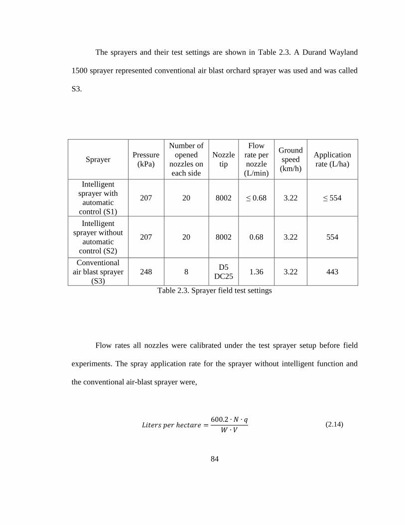
84

The sprayers and their test settings are shown in Table 2.3. A Durand Wayland

1500 sprayer represented conventional air blast orchard sprayer was used and was called

S3.

Sprayer Pressure

(kPa)

Number of

opened

nozzles on

each side

Nozzle

tip

Flow

rate per

nozzle

(L/min)

Ground

speed

(km/h)

Application

rate (L/ha)

Intelligent

sprayer with

automatic

control (S1)

207 20 8002 ≤ 0.68 3.22 ≤ 554

Intelligent

sprayer without

automatic

control (S2)

207 20 8002 0.68 3.22 554

Conventional

air blast sprayer

(S3)

248 8 D5

DC25 1.36 3.22 443

Table 2.3. Sprayer field test settings

Flow rates all nozzles were calibrated under the test sprayer setup before field

experiments. The spray application rate for the sprayer without intelligent function and

the conventional air-blast sprayer were,

(2.14)

85

Where:

Number of the nozzles used,

Flow rate of one nozzle, L/min,

Distance between two tree row centerlines, m, 4.575 m in the test field,

Ground speed, km/h.

Thus for intelligent sprayer without automatic control (S2), the application rate

(L/ha) is:

.

For the Conventional air blast sprayer (S3), the application rate (L/ha) is:

.

86

2.7 Sprayer test on container trees

The four container trees used in the indoor tests described in section 2.4 had

denser canopies than the apple trees used in the field tests. The container plants were used

in an outdoor test to evaluate the performance of the intelligent sprayer for dense

canopies.

The container trees were placed side by side from north to south. During this

outdoor test, the average wind velocity was 3.5 m/s from northwest, the ambient

temperature was 8.5 °C, and the relative humidity was 50%.

2.7.1 Location of water sensitive paper mounting

Water sensitive papers (26 mm by 76 mm) were mounted inside each container

tree canopy to measure spray coverage at different locations inside tree canopies. The

guideline for mounting of the water sensitive papers was shown in Figure 2.30. With this

design, tree canopy was divided into five sections in two horizontal directions (e.g. from

spray direction and sprayer travel direction). Water sensitive papers were distributed

along the tree height directions with a height interval of 27 cm. In this way, spray

deposition could be evaluated from three directions. Since these trees had different

heights and structures, the total number of water sensitive papers was not the same for all

trees.

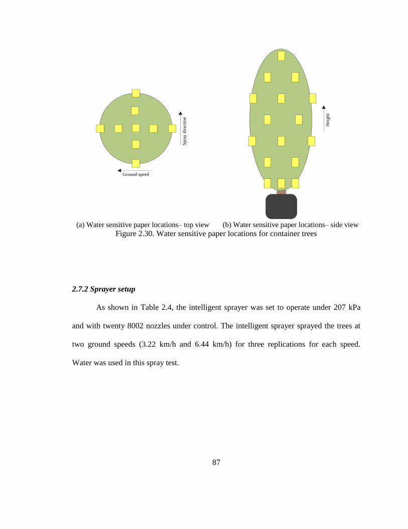
87

Sp

ray

dir

ecti

on

Ground speed

Hei

gh

t

(a) Water sensitive paper locations– top view (b) Water sensitive paper locations– side view

Figure 2.30. Water sensitive paper locations for container trees

2.7.2 Sprayer setup

As shown in Table 2.4, the intelligent sprayer was set to operate under 207 kPa

and with twenty 8002 nozzles under control. The intelligent sprayer sprayed the trees at

two ground speeds (3.22 km/h and 6.44 km/h) for three replications for each speed.

Water was used in this spray test.

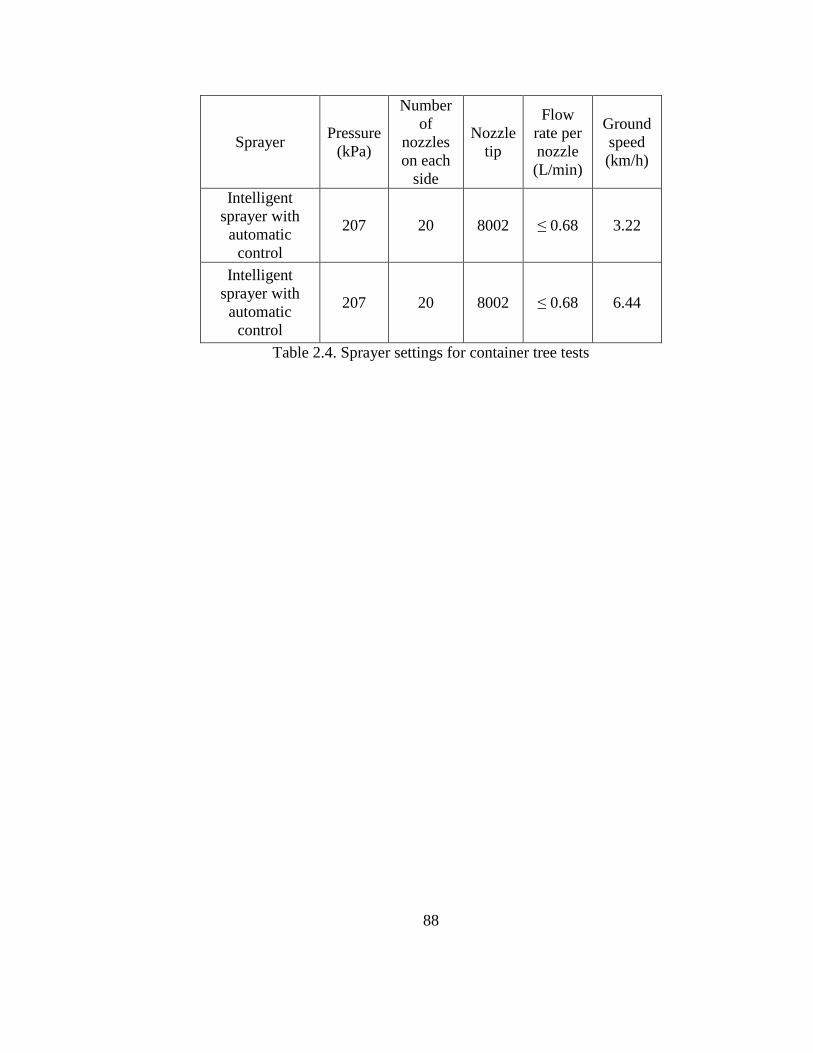
88

Sprayer Pressure

(kPa)

Number

of

nozzles

on each

side

Nozzle

tip

Flow

rate per

nozzle

(L/min)

Ground

speed

(km/h)

Intelligent

sprayer with

automatic

control

207 20 8002 ≤ 0.68 3.22

Intelligent

sprayer with

automatic

control

207 20 8002 ≤ 0.68 6.44

Table 2.4. Sprayer settings for container tree tests

89

2.8 Calculations of liquid consumption

One of the major goals of this study to determine if the intelligent sprayer

operation would result in considerable reductions in pesticide consumption by better

targeting and variable rate application. Tests were conducted to document the savings in

spray mixture containing water and chemicals, when using the intelligent sprayer.

For the intelligent sprayer without automatic control and the conventional air-

blast sprayer, the flow rate discharged from each nozzle remained the same after liquid

pressure was set, and the total spray volume could be calculated by multiplying flow rate

by the spray time. Thus, for the non-variable rate sprayer, the liquid consumption is:

(2.15)

Where:

: Total liquid volume sprayed, ml

: Number of nozzles used during spray,

: Flow rate for each nozzle used, ml/min

: Sprayed time, min.

For the Intelligent sprayer, the data associated with duty cycles of nozzles was

saved after each application. The actual flow rate of each nozzle, and the total spray

volume of the sprayer was calculated using the saved duty cycles of control signals for

each spray, the calibrated relationship between duty cycle, flow rate for the nozzles used,

and the time interval used for each control signal.

90

From the nozzle calibration result described in Equation 3.1 in section 3.3, the

relationship between duty cycle and output flow rate of the nozzles is:

Where,

: Flow rate of one nozzle, ml/min,

: Duty cycle of the spray control PWM signal (0~100).

Therefore the total liquid consumption is:

∑∑

(2.16)

: Total volume of liquid sprayed by the intelligent sprayer, mL,

: Flow rate of the ith

nozzle (out of the total of 20) at the jth

slice, mL/min

: Time interval of the control signals. The control signal refreshes every 0.26 second

for all tests in this dissertation, so

(minutes).

The liquid savings were calculated by dividing the liquid consumption from the

intelligent sprayer by the amount discharged from the intelligent sprayer without control

or from the conventional air-blast sprayer. Of course the “liquid” mentioned here

includes water as carrier, and pesticides and other chemicals added to the spray mixture

to enhance the efficiency of a spray application. Therefore, any savings in spray liquid

91

consumption should lead to higher net income and less impact on the environment and

human safety.

92

Chapter 3: Results and discussion

In the previous chapter, components of the intelligent sprayer that can adjust its

spray flow rate in accordance with the canopy characteristics were described. A

prototype of the intelligent sprayer has been implemented, including a laser sensor to

scan the foliage canopy, a real time algorithm to calculate the canopy characteristics

using the data from the laser sensor, and a variable rate controller to convert the

computation results into PWM control signals to activate solenoid valves to change the

nozzle flow rate. A series of tests were designed and conducted to validate each part of

the design. Both field and controlled outdoor tests were also conducted to evaluate

performance of the entire intelligent sprayer system. In this chapter, all tests results are

presented and analyzed.

93

3.1 Validation result on wooden block (artificial target) density

An indoor experiment was designed (described in section 2.2) using an artificially

target to evaluate the accuracy of the density calculation algorithm. In this test, lumber

blocks were assembled together to form shapes with pre-defined density. Then the

artificial target with known density was scanned using a laser sensor. Measurement data

was then sent to the proposed intelligent algorithm to compute the density created by

these artificial targets. The computation results were compared with the corresponding

known density of that arrangement of the artificial target.

Since the intelligent sprayer prototype has 20 nozzles on one side to be controlled,

the algorithm divides the laser scanning range into 20 groups corresponding to the 20

nozzles. The lumber blocks with known densities used in this density validation test had a

height that could be covered by four nozzles. Thus, the lumber blocks were divided into

four sections: sections 1, 2, 3 and 4.

After the laser sensor scanned the lumber blocks 30 times, the densities of each

section were calculated for these 30 runs, and the calculated densities for each section

were averaged (Figures 3.1 through 3.4). Figures 3.1 through 3.4 also illustrate the

relationship between the calculated density from laser scanner data and the actually

known density of the artificial target (lumber block section). The regression equations

were:

, with R2=0.9817 for section 1,


94


, with R2=0.9942 for section 4.

From the linear regression equations, the slopes for the four sections were 0.9544,

0.9418, 0.9784, and 1.0066. All the slopes were very close to one. Although the

calculated density is slightly larger than the known density, their difference was very

small. Therefore, the designed density algorithm was effective in estimating density of a

three dimensional object using the roughness of its surface.

95


algorithm over known density (%) of section 1 of the lumber block



Calculated density = 0.9544·Known density + 7.8555R² = 0.9817

0

10

20

30

40

50

60

70

80

90

0 10 20 30 40 50 60 70 80

Ca

lcu

late

d d

en

sity

, %

Known density, %

Section 1

Calculated density = 0.9418·Known density + 7.8184

R² = 0.9799

0

10

20

30

40

50

60

70

80

90

0 10 20 30 40 50 60 70 80

Ca

lcu

late

d d

en

sity

, %

Known density, %

Section 2

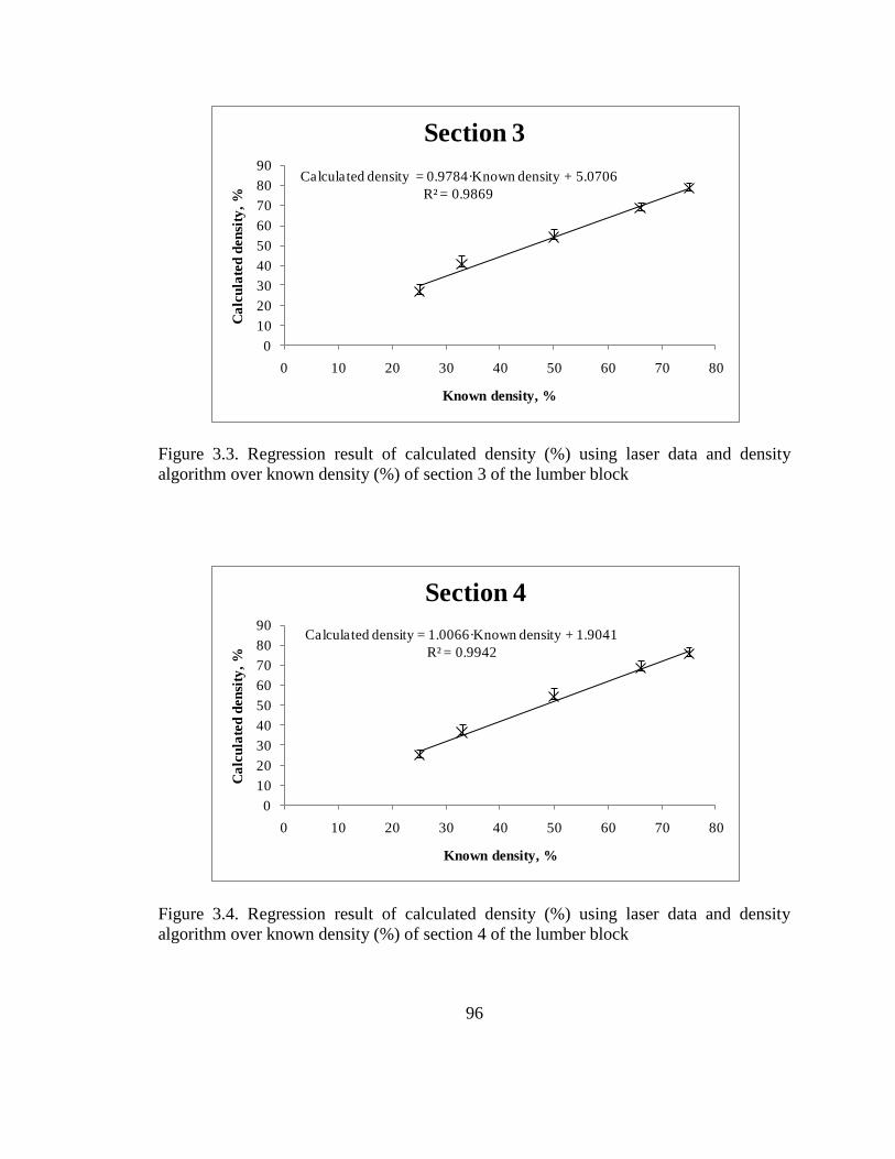
96






R² = 0.9869

0

10

20

30

40

50

60

70

80

90

0 10 20 30 40 50 60 70 80

Ca

lcu

late

d d

en

sity

, %

Known density, %

Section 3


R² = 0.9942

0

10

20

30

40

50

60

70

80

90

0 10 20 30 40 50 60 70 80

Ca

lcu

late

d d

en

sity

, %

Known density, %

Section 4

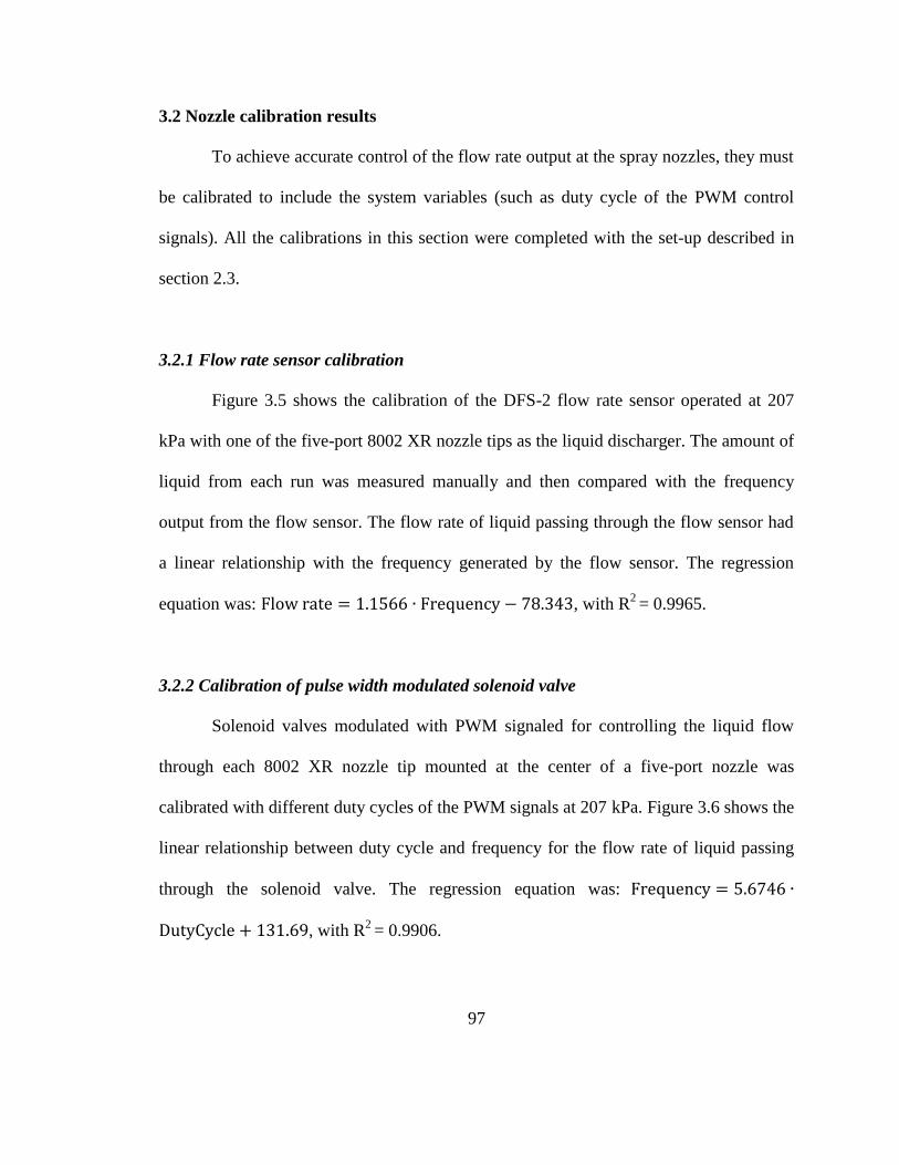
97

3.2 Nozzle calibration results

To achieve accurate control of the flow rate output at the spray nozzles, they must

be calibrated to include the system variables (such as duty cycle of the PWM control

signals). All the calibrations in this section were completed with the set-up described in

section 2.3.

3.2.1 Flow rate sensor calibration

Figure 3.5 shows the calibration of the DFS-2 flow rate sensor operated at 207

kPa with one of the five-port 8002 XR nozzle tips as the liquid discharger. The amount of

liquid from each run was measured manually and then compared with the frequency

output from the flow sensor. The flow rate of liquid passing through the flow sensor had

a linear relationship with the frequency generated by the flow sensor. The regression

equation was: , with R2 = 0.9965.

3.2.2 Calibration of pulse width modulated solenoid valve

Solenoid valves modulated with PWM signaled for controlling the liquid flow

through each 8002 XR nozzle tip mounted at the center of a five-port nozzle was

calibrated with different duty cycles of the PWM signals at 207 kPa. Figure 3.6 shows the

linear relationship between duty cycle and frequency for the flow rate of liquid passing

through the solenoid valve. The regression equation was:

, with R2

= 0.9906.

98

3.2.3 Relationship between duty cycle and nozzle flow rate

From the calibration results presented in Figures 3.5 and 3.6, the relationship

between flow rate and duty cycle was:

(3.1)

Where,

Liquid flow rate from 8002 XR nozzle tip, ml/min.

Duty cycle of the input PWM control signal.

Equation 3.1 was used in section 2.4 when deriving the spray model for the intelligent

sprayer.

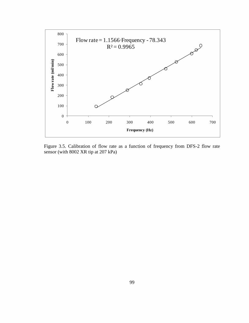
99

Figure 3.5. Calibration of flow rate as a function of frequency from DFS-2 flow rate

sensor (with 8002 XR tip at 207 kPa)

Flow rate = 1.1566·Frequency - 78.343

R² = 0.9965

0

100

200

300

400

500

600

700

800

0 100 200 300 400 500 600 700

Flo

w r

ate

(m

l/m

in)

Frequency (Hz)

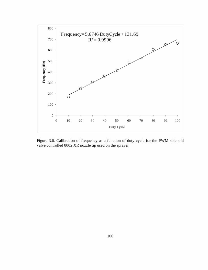
100

Figure 3.6. Calibration of frequency as a function of duty cycle for the PWM solenoid

valve controlled 8002 XR nozzle tip used on the sprayer

Frequency= 5.6746·DutyCycle + 131.69

R² = 0.9906

0

100

200

300

400

500

600

700

800

0 10 20 30 40 50 60 70 80 90 100

Freq

uen

cy

(H

z)

Duty Cycle

101

3.3 Back pressure effect comparison result

As describe in section 2.3, pressure fluctuation was observed when operating the

solenoid valves using PWM signals. Pressure fluctuation can induce error in flow rate

output and droplet size that the nozzle produces. A back pressure bypass test unit was

designed and described in section 2.3. The adjustable valve and check valves were tested

to compare their ability to limit pressure fluctuations.

Figures 3.7 and 3.8 show the change of nozzle pressure when using the check

valve and the adjustable valve in the back pressure unit to manipulate two five-port

nozzles. Figure 3.7 shows that, when using the check valve to manipulate two five-port

nozzles, the pressure fluctuation might reach 85 kPa. Figure 3.8 shows that, when using

the adjustable valve to manipulate two five-port nozzles, the pressure fluctuation could

go up to 35 kPa.

Figures 3.9 and 3.10 show the change in nozzle pressure with using the check

valve and the adjustable valve in the back pressure unit to manipulate four five-port

nozzles. Figure 3.9 shows that, when using the check valve to manipulate four five-port

nozzles the pressure fluctuation could go up to 89 kPa. Figure 3.10 shows that, when

using the adjustable valve to manipulate four five-port nozzles the pressure fluctuation

could go up to 66 kPa.

Figures 3.7 to 3.11 indicate that the adjustable valve performs better than the

check valve in limiting the pressure fluctuation and is more suitable to be used in the

back pressure unit to minimize the nozzle pressure changes caused by the constant

pulsing of the solenoid valves.

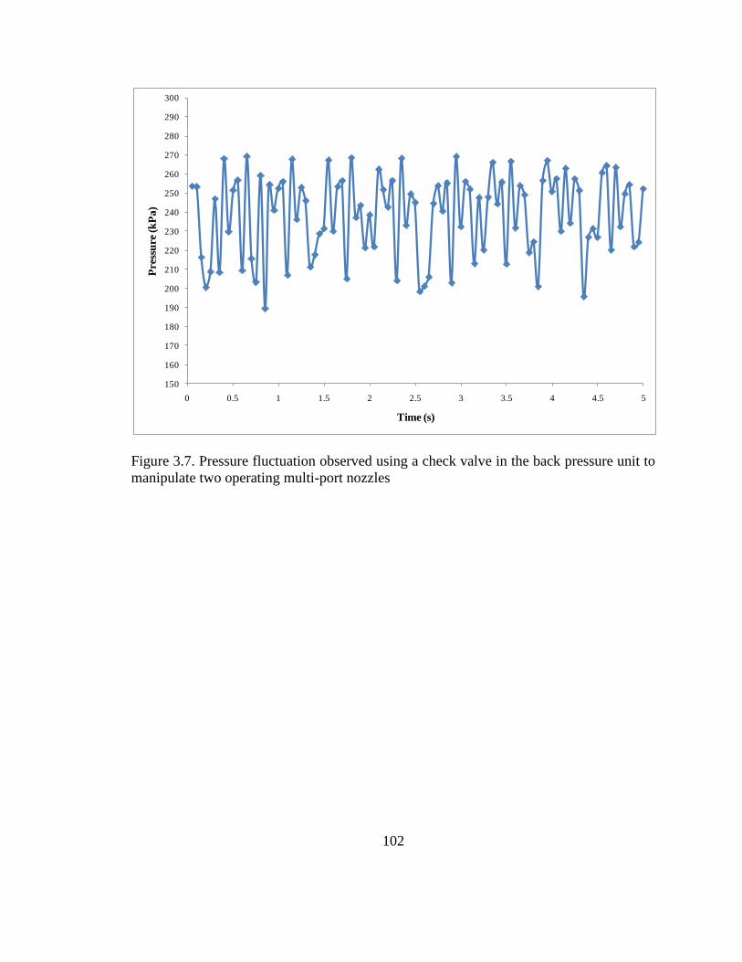
102


manipulate two operating multi-port nozzles

150

160

170

180

190

200

210

220

230

240

250

260

270

280

290

300

0 0.5 1 1.5 2 2.5 3 3.5 4 4.5 5

Pre

ssu

re (k

Pa

)

Time (s)

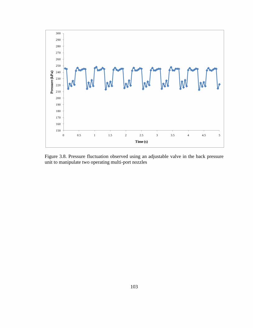
103


unit to manipulate two operating multi-port nozzles

150

160

170

180

190

200

210

220

230

240

250

260

270

280

290

300

0 0.5 1 1.5 2 2.5 3 3.5 4 4.5 5

Pre

ssu

re (k

Pa

)

Time (s)

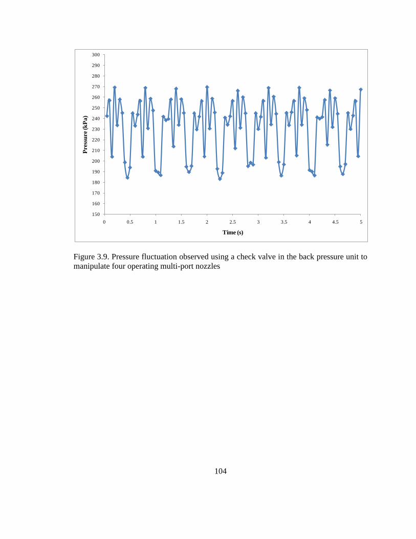
104


manipulate four operating multi-port nozzles

150

160

170

180

190

200

210

220

230

240

250

260

270

280

290

300

0 0.5 1 1.5 2 2.5 3 3.5 4 4.5 5

Pre

ssu

re (k

Pa)

Time (s)

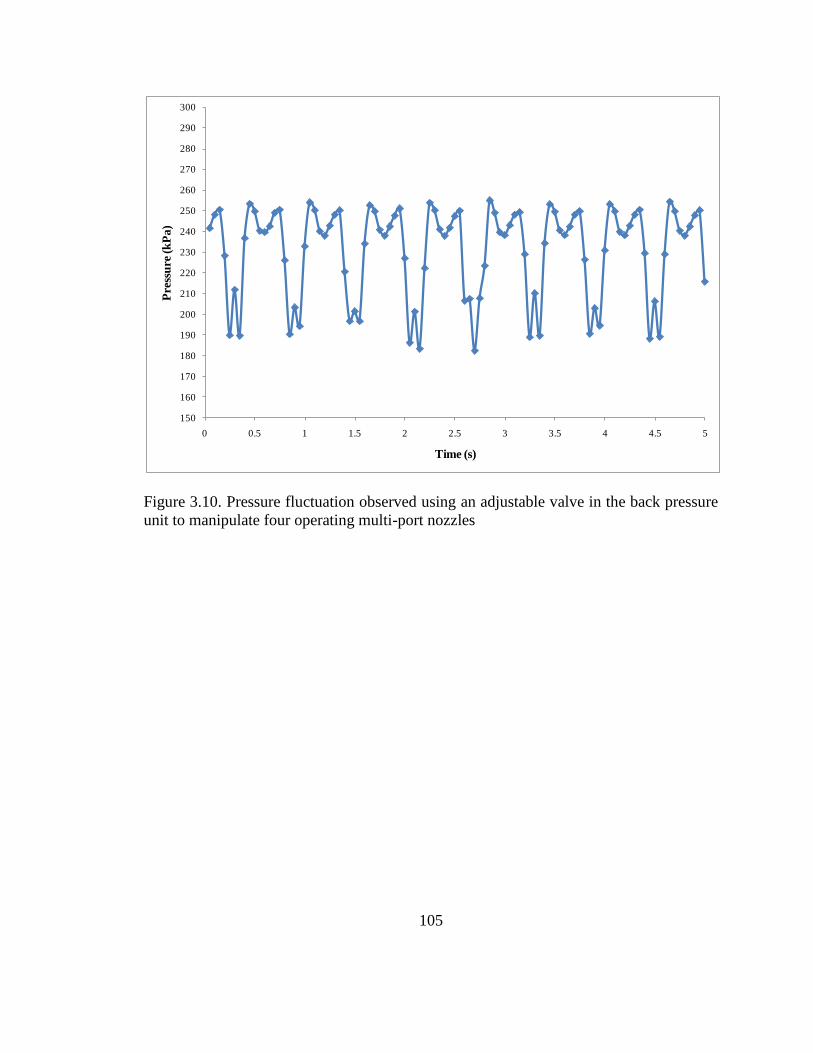
105


unit to manipulate four operating multi-port nozzles

150

160

170

180

190

200

210

220

230

240

250

260

270

280

290

300

0 0.5 1 1.5 2 2.5 3 3.5 4 4.5 5

Pre

ssu

re (k

Pa)

Time (s)

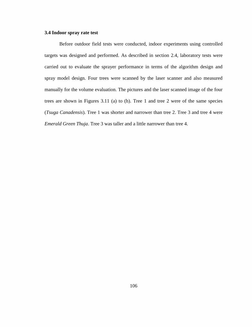
106

3.4 Indoor spray rate test

Before outdoor field tests were conducted, indoor experiments using controlled

targets was designed and performed. As described in section 2.4, laboratory tests were

carried out to evaluate the sprayer performance in terms of the algorithm design and

spray model design. Four trees were scanned by the laser scanner and also measured

manually for the volume evaluation. The pictures and the laser scanned image of the four

trees are shown in Figures 3.11 (a) to (h). Tree 1 and tree 2 were of the same species

(Tsuga Canadensis). Tree 1 was shorter and narrower than tree 2. Tree 3 and tree 4 were

Emerald Green Thuja. Tree 3 was taller and a little narrower than tree 4.

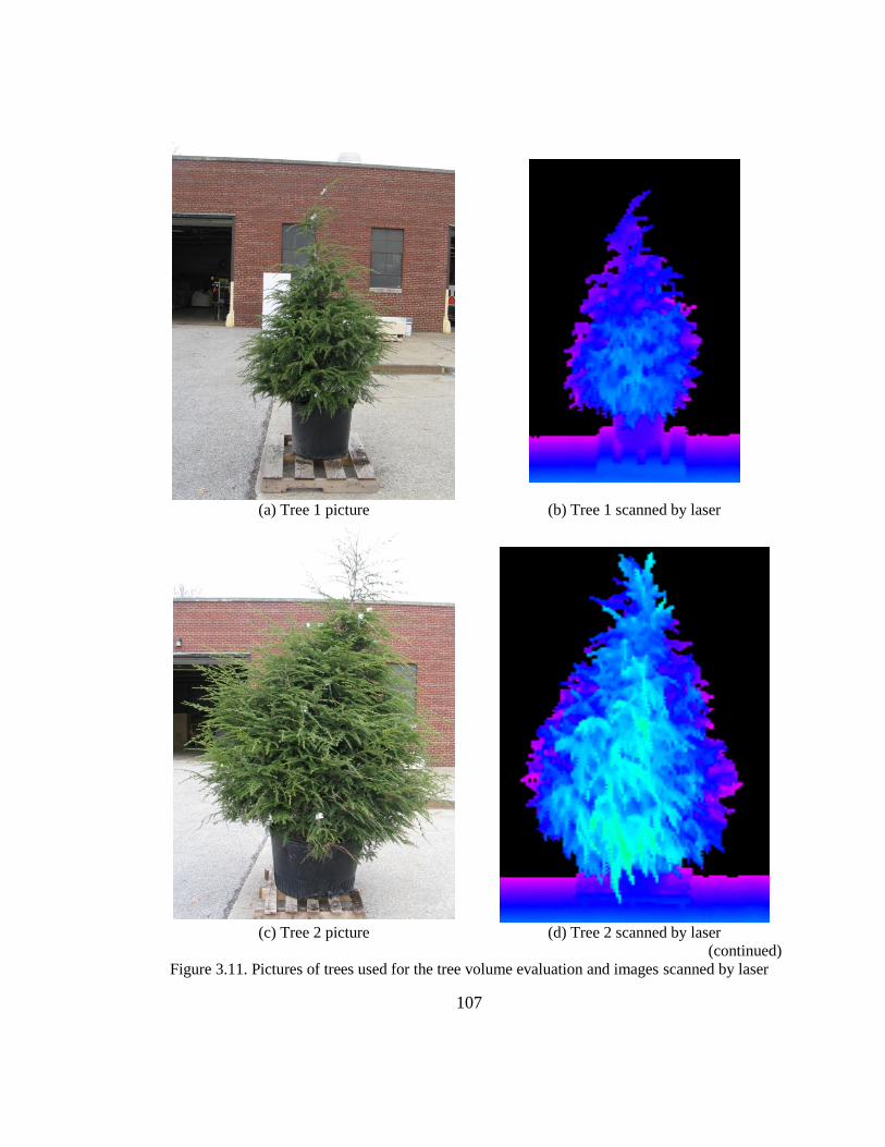
107

(a) Tree 1 picture (b) Tree 1 scanned by laser

(c) Tree 2 picture (d) Tree 2 scanned by laser

(continued)

Figure 3.11. Pictures of trees used for the tree volume evaluation and images scanned by laser

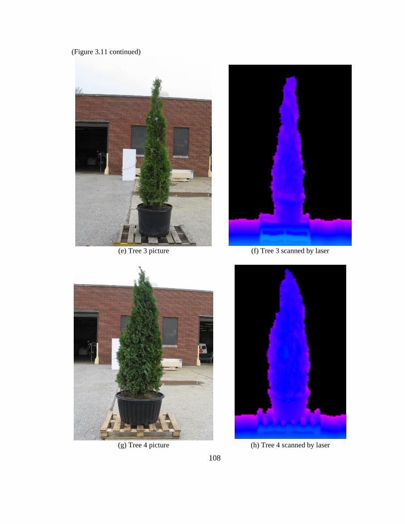
108


(e) Tree 3 picture (f) Tree 3 scanned by laser

(g) Tree 4 picture (h) Tree 4 scanned by laser

109

Table 3.1 shows the actual heights of each tree and the container in which the tree

was planted. In this test, only tree canopies were of the interest, so the result on the height

of containers were not discussed. The nozzles that should be opened to spray tree canopy

for each tree are also listed in Table 3.1. This was verified by the calculated results from

the algorithm.

Table 3.2 shows the result of spray constants calculated by the algorithm for each

section of the tree covered by one nozzle, nozzles are ordered 1 to 20 from bottom to the

top. The bottom few nozzles that faced the tree containers were not considered. Spray

constants, as defined in section 2.4, were Liters of spray liquid per m3 of effective tree

volume (volume times density). The effective tree volume in this test was calculated from

the manually measured volume multiplied by the density factor calculated from the

density algorithm. The average spray constants were 0.155, 0.142, 0.251 and 0.194 L/m3

for trees 1, 2, 3 and 4, respectively, and they all were greater than 0.1 L/m3. The reason

for this over estimation is explained as below.

Targeted, variable-rate application of pesticides is expected to result in savings in

consumption of pesticides. However, the amount of savings may be a critical issue for

some growers who may not want to take the risk of not spraying enough chemicals on the

target. The main goal behind development of the intelligent sprayer was that it should

apply the optimum amount of chemicals while achieving satisfactory efficacy expected

from the products applied. As a safety measure, to make sure that sprayed product

reaches deep into the canopy, and coverage is more than adequate, the density algorithm

used for the intelligent sprayer was designed such that the densities predicted would be

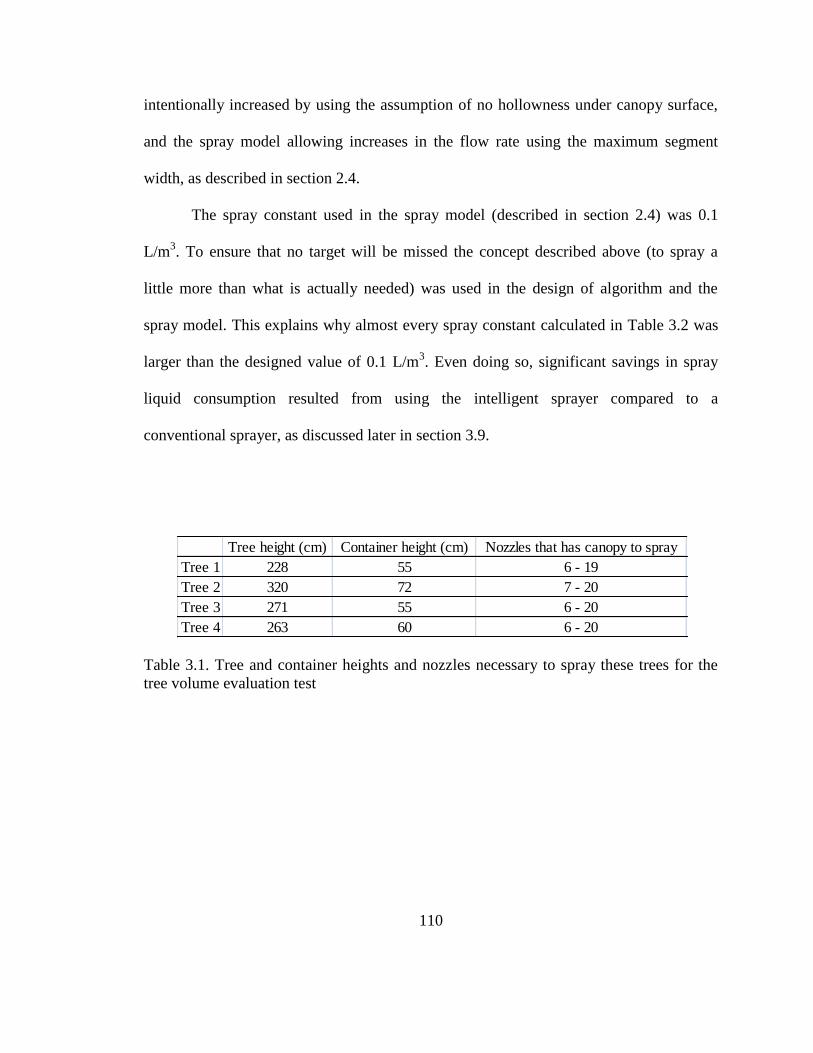
110

intentionally increased by using the assumption of no hollowness under canopy surface,

and the spray model allowing increases in the flow rate using the maximum segment

width, as described in section 2.4.

The spray constant used in the spray model (described in section 2.4) was 0.1

L/m3. To ensure that no target will be missed the concept described above (to spray a

little more than what is actually needed) was used in the design of algorithm and the

spray model. This explains why almost every spray constant calculated in Table 3.2 was

larger than the designed value of 0.1 L/m3. Even doing so, significant savings in spray

liquid consumption resulted from using the intelligent sprayer compared to a

conventional sprayer, as discussed later in section 3.9.

Table 3.1. Tree and container heights and nozzles necessary to spray these trees for the

tree volume evaluation test

Tree height (cm) Container height (cm) Nozzles that has canopy to spray

Tree 1 228 55 6 - 19

Tree 2 320 72 7 - 20

Tree 3 271 55 6 - 20

Tree 4 263 60 6 - 20

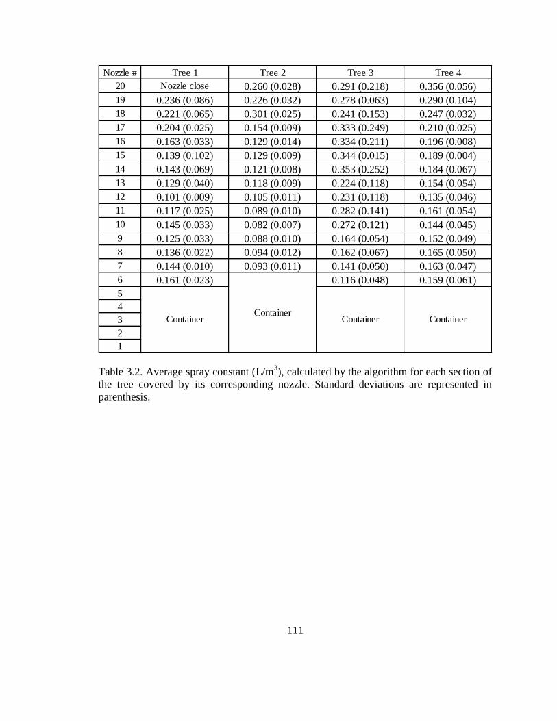
111

Table 3.2. Average spray constant (L/m3), calculated by the algorithm for each section of

the tree covered by its corresponding nozzle. Standard deviations are represented in

parenthesis.

Nozzle # Tree 1 Tree 2 Tree 3 Tree 4

20 Nozzle close 0.260 (0.028) 0.291 (0.218) 0.356 (0.056)

19 0.236 (0.086) 0.226 (0.032) 0.278 (0.063) 0.290 (0.104)

18 0.221 (0.065) 0.301 (0.025) 0.241 (0.153) 0.247 (0.032)

17 0.204 (0.025) 0.154 (0.009) 0.333 (0.249) 0.210 (0.025)

16 0.163 (0.033) 0.129 (0.014) 0.334 (0.211) 0.196 (0.008)

15 0.139 (0.102) 0.129 (0.009) 0.344 (0.015) 0.189 (0.004)

14 0.143 (0.069) 0.121 (0.008) 0.353 (0.252) 0.184 (0.067)

13 0.129 (0.040) 0.118 (0.009) 0.224 (0.118) 0.154 (0.054)

12 0.101 (0.009) 0.105 (0.011) 0.231 (0.118) 0.135 (0.046)

11 0.117 (0.025) 0.089 (0.010) 0.282 (0.141) 0.161 (0.054)

10 0.145 (0.033) 0.082 (0.007) 0.272 (0.121) 0.144 (0.045)

9 0.125 (0.033) 0.088 (0.010) 0.164 (0.054) 0.152 (0.049)

8 0.136 (0.022) 0.094 (0.012) 0.162 (0.067) 0.165 (0.050)

7 0.144 (0.010) 0.093 (0.011) 0.141 (0.050) 0.163 (0.047)

6 0.161 (0.023) 0.116 (0.048) 0.159 (0.061)

5

4

3

2

1

Container ContainerContainerContainer

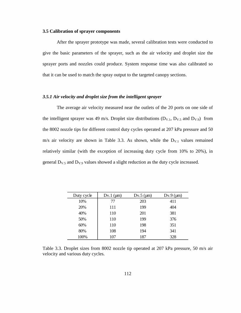
112

3.5 Calibration of sprayer components

After the sprayer prototype was made, several calibration tests were conducted to

give the basic parameters of the sprayer, such as the air velocity and droplet size the

sprayer ports and nozzles could produce. System response time was also calibrated so

that it can be used to match the spray output to the targeted canopy sections.

3.5.1 Air velocity and droplet size from the intelligent sprayer

The average air velocity measured near the outlets of the 20 ports on one side of

the intelligent sprayer was 49 m/s. Droplet size distributions (DV.1, DV.5 and DV.9) from

the 8002 nozzle tips for different control duty cycles operated at 207 kPa pressure and 50

m/s air velocity are shown in Table 3.3. As shown, while the DV.1 values remained

relatively similar (with the exception of increasing duty cycle from 10% to 20%), in

general DV.5 and DV.9 values showed a slight reduction as the duty cycle increased.

Table 3.3. Droplet sizes from 8002 nozzle tip operated at 207 kPa pressure, 50 m/s air

velocity and various duty cycles.

Duty cycle Dv.1 (µm) Dv.5 (µm) Dv.9 (µm)

10% 77 203 411

20% 111 199 404

40% 110 201 381

50% 110 199 376

60% 110 198 351

80% 108 194 341

100% 107 187 328

113

3.5.2 Sprayer system response time

The intelligent sprayer consists of many different aspects, ranging from

computational algorithms to hydraulic mechanics. Different components are cascaded to

form a complete system. Each component introduces certain latency into the whole

system. In this experiment, the overall response time of the intelligent sprayer system

was measured.

As described in section 2.5, videos were recorded to document the response time

from when the sprayer starts spraying targets, until the laser detected the target. Figures

3.12 (a) to (d) show the four frames taken from video files of the response time

measurement. The time difference of 0.119 s (0.196 s – 0.076 s) between Figures 3.12 (a)

and (c) is the lag time between the time when laser detected the target and the time liquid

discharged from the nozzle. This lag time included software computation time, electronic

response time and hydraulic-mechanical response time.

Since the laser was mounted 1.45 m ahead of nozzles (half-way between the cab

location and the nozzles), there was sufficient time between when the laser “sees” the

target and when the sprayer is operated under the typical travel speeds. Therefore, to

match the optimal spray to the intended target canopy, a delay was added to the model

between the point when the software performs all the necessary calculations and develops

an output, and when the solenoid valve control was reloaded. The delay count was

calculated as:

114

(3.2)

Where,

: Distance from the center of the laser to the center of the nozzle port, which was

measured to be 1.45 m.

: Tractor forward speed, which was 3.22 km/h (0.89 m/s).

: System response time, which was calibrated above (0.119 s).

: Refresh time for the solenoid valves, which was 0.26 s for all the tests

performed in this study.

Substituting values of parameters into equation (3.2) yields . Thus, a delay count of

6 was used in the field tests so that the highest amount of the spray solution discharged

from the intelligent sprayer is intercepted by the target canopy.

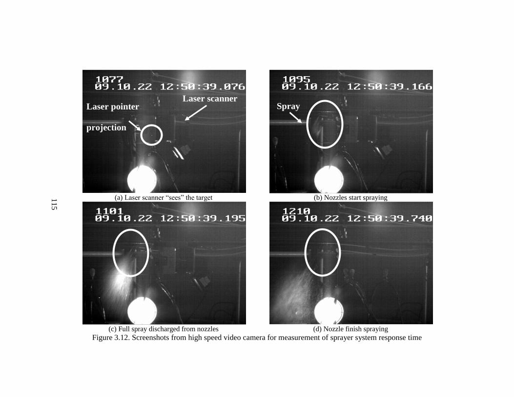
115

(a) Laser scanner “sees” the target (b) Nozzles start spraying

(c) Full spray discharged from nozzles (d) Nozzle finish spraying

Figure 3.12. Screenshots from high speed video camera for measurement of sprayer system response time

Spray

115

Laser scanner Laser pointer

projection

116

3.6 Field tests

3.6.1 Uniformity of spray deposition and coverage inside tree canopies

As described in section 2.6, a 3D Cartesian coordinate system was defined for

locating each sample mounted inside the tree canopy. With the defined 3D Cartesian

coordinate system, every water sensitive paper and nylon screen mounted inside tree

canopies was given one set of X, Y and Z values based on manual measurement.

Accordingly, the samples collected from each tree were grouped in three directions: tree

height direction (vertically), spray direction (horizontally), and tractor travel direction

(horizontally). In this way, the uniformity of spray deposition and coverage from each

direction could be evaluated separately. For example, target locations were grouped into

four X sections (Tables 3.4 to 3.9) with about equal width according to the samples‟ X

coordinates (as shown in Figures 2.25 and 2.26). The “front” is closest to the spray

nozzle, and the “back” section is the furthest away from the spray nozzles. Similarly,

“middle front and middle back” represents the sections located in the middle parts of the

canopy with “middle front” closer to the spray nozzles and “middle back” away from the

spray nozzles. Due to the change in spray direction in the spray test performed in May

and the growing of tree width, actual range of the four X location sections varies for each

test. In the same way, target locations were grouped into four Y sections and three Z

sections. “Right, middle right, middle left and right” (Tables 3.10 to 3.15) represent four

horizontal location sections along the tractor travel direction with “right” having the

largest Y values and “left” having the smallest Y values. “High, middle and low” (Tables

117

3.16 to 3.21) represent three vertical sections with “high” having the largest Z values and

low having the smallest Z value.

For the first test conducted in April when trees were just starting to leaf out, the

average coverage inside canopies were 41%, 88% and 70%, and the average deposit

inside the canopies were 1.31, 6.61 , and 3.91 µL/cm2

for S1, S2 and S3, respectively.

For the second test conducted in May when the apple trees canopies were at half

of the full foliage, the average coverage inside canopies were 39%, 74% and 53%, and

the average deposit inside the canopies were 0.87, 3.64, and 1.56 µL/cm2

for S1, S2 and

S3, respectively.

For the third test conducted in June when the foliage was fully developed, the

average coverage inside canopies were 36%, 56% and 42%, and the average deposit

inside the canopies were 0.92, 2.96 , and 1.27 µL/cm2

for S1, S2 and S3, respectively.

Tables 3.4 to 3.9 show the coverage and deposition result for the samples

mounted at different X locations inside the tree canopies. In earlier months when the tree

canopies were not fully developed, both values of spray coverage and deposit for S1 were

significantly lower than those for S2 and S3. In June when the canopies were fully

developed, the three sprayers do not have significant differences in spray coverage and

deposit performance. These tables also show that in general S2 has the best uniformity

(fewest differences in deposit and coverage) along the X direction (spray direction) and

S1 has the second best. When just looking at the half of canopies closer to the spray

nozzles, S1 has uniform spray coverage and deposition along the spray direction for all

118

tests and all trees. Therefore, it suggests that S1 works better when used to spray every

row than when used in alternative row spraying.


mounted at different Y locations inside the tree canopies. The uniformity of S1 and S2 on

Y direction (parallel to spray travel direction) are better than that of S3 which S1 has

better uniformity on Tree 1 and 2, while S2 has better uniformity on Tree 3.


mounted at different Z locations inside the tree canopies. It is shown that S1 generally has

the best uniformity along the Z direction (vertical direction) among three sprayers.

It is also shown from Tables 3.4 to 3.21 that for the first two tests while the tree

canopies were not fully developed, almost all the coverage and deposit values for S2 and

S3 were significantly larger than those for S1. Many samples sprayed by S2 and S3 in the

first two tests, had coverage from 80% to 100%, which are more than what the canopies

needed. However, the results of S1 were sufficient for all tests, and were not too high.

The spray coverage and deposit from S1 were sufficient except for one position

on Tree 2 in May test (Table 3.5 at the back location of the tree) where the average

coverage was 3% and was lower than the recommended 15% (based on Dr. Heping Zhu‟s

experience with visual observation of spray coverage on water sensitive papers). The

results from the other two sprayers, S2 and S3, at this location were also lower than 15%,

which indicates that this location was hard to reach by itself (on the back of the canopy,

farthest from spray nozzles), especially when the trees reached about half-full canopies.

119

Table 3.4. Spray coverage on water sensitive papers within different X location sections inside Tree 1 canopy for the field tests

in April, May and June using intelligent sprayer with automatic spray control, intelligent sprayer without automatic control and

conventional air blast sprayer. Standard deviations are given in parentheses.

[1] Means in a row followed by different lowercase letters are significantly different (p < 0.05). Means in a column followed by different uppercase letters are

significantly different (p < 0.05).

[2] S1 = Intelligent sprayer with automatic control.

[3] S2 = Intelligent sprayer without automatic control.

[4] S3 = Conventional air blast sprayer.

Target location

on tree canopy S1[2]

S2[3]

S3[4] S1 S2 S3 S1 S2 S3

Front 53 (20) cdA 100 (0) aA 86 (16) abAB 38 (12) dAB 89 (15) abA 71 (18) bcA 75 (18) bcA 88 (14) abA 83 (11) abA

Middle front 41 (20) dA 96 (12) aA 75 (17) abcAB 45 (18) dA 82 (28) abA 52 (21) cdAB 45 (32) dAB 65 (36) bcdA 59 (28) bcdAB

Middle back 48 (22) bcA 100 (0) aA 87 (16) aA 25 (23) dB 65 (16) bA 40 (15) cdBC 47 (21) bcAB 58 (31) bcA 37 (21) cdBC

Back 46 (28) bcdA 93 (15) aA 64 (22) abcB 19 (19) dB 72 (35) abA 26 (19) cdC 32 (29) cdB 52 (35) bcdA 18 (20) dC

Average Spray Coverage (%)[1]

JuneApril May

119

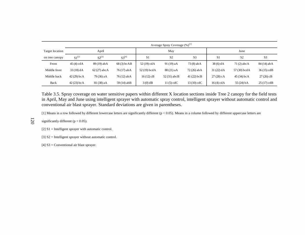
120









Target location


S2[3]

S3[4] S1 S2 S3 S1 S2 S3

Front 45 (4) cdA 89 (19) abA 68 (3) bcAB 52 (19) cdA 91 (19) aA 73 (8) abA 38 (6) dA 71 (2) abcA 84 (14) abA

Middle front 33 (18) dA 62 (27) abcA 76 (17) abA 52 (19) bcdA 88 (21) aA 72 (26) abA 31 (22) dA 57 (30) bcdA 36 (15) cdB

Middle back 42 (29) bcA 79 (36) aA 76 (12) abA 16 (12) cB 52 (31) abcB 41 (22) bcB 27 (28) cA 45 (34) bcA 27 (26) cB

Back 42 (23) bcA 81 (38) aA 59 (14) abB 3 (0) dB 11 (5) cdC 13 (10) cdC 16 (4) cdA 55 (24) bA 25 (17) cdB


April May June

120

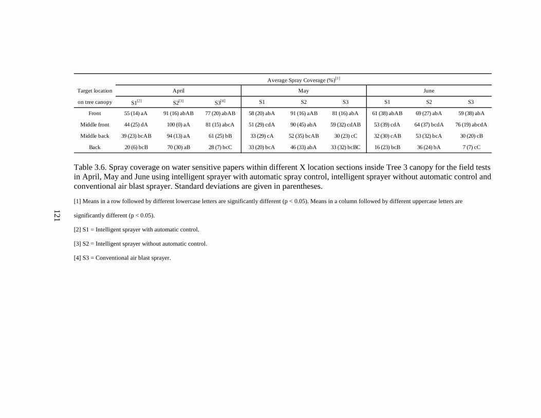
121









Target location


S2[3]

S3[4] S1 S2 S3 S1 S2 S3

Front 55 (14) aA 91 (16) abAB 77 (20) abAB 58 (20) abA 91 (16) aAB 81 (16) abA 61 (38) abAB 69 (27) abA 59 (38) abA

Middle front 44 (25) dA 100 (0) aA 81 (15) abcA 51 (29) cdA 90 (45) abA 59 (32) cdAB 53 (39) cdA 64 (37) bcdA 76 (19) abcdA

Middle back 39 (23) bcAB 94 (13) aA 61 (25) bB 33 (29) cA 52 (35) bcAB 30 (23) cC 32 (30) cAB 53 (32) bcA 30 (20) cB

Back 20 (6) bcB 70 (30) aB 28 (7) bcC 33 (20) bcA 46 (33) abA 33 (32) bcBC 16 (23) bcB 36 (24) bA 7 (7) cC

April May June


121

122

Table 3.7. Spray deposits collected by nylon screens within different X location sections inside Tree 1 canopy for the field tests








Target location


S2[3]

S3[4] S1 S2 S3 S1 S2 S3

Front 1.16 (0.51) efA 7.69 (2.89) aA 4.11 (1.53) bcA 0.61 (0.36) fA 3.16 (1.53) bcdeA 1.77 (0.64) defA 2.37 (0.84) cdefA 4.81 (1.74) bA 3.53 (1.3) bcdA

Middle front 0.93 (0.32) cA 8.67 (3.78) aA 4.64 (0.83) bA 0.55 (0.32) cA 3.74 (1.9) bA 1.27 (0.52) cAB 1.6 (1.4) cAB 4.06 (1.58) bA 1.19 (0.76) cB

Middle back 1.42 (0.84) cA 8.91 (2.58) aA 4.72 (1.49) bA 0.6 (0.62) cA 3.63 (2.73) bA 0.89 (0.55) cB 0.95 (0.47) cBC 3.85 (2.96) bA 0.99 (0.55) cB

Back 1.6 (1.12) cA 7.4 (2.04) aA 4.46 (1.24) bA 0.44 (0.63) cA 5.74 (5.15) abA 0.73 (0.48) cB 0.37 (0.16) cC 1.8 (1.27) cA 0.52 (0.44) cB

Average Spray Deposit (µL/cm2)[1]

April May June

122

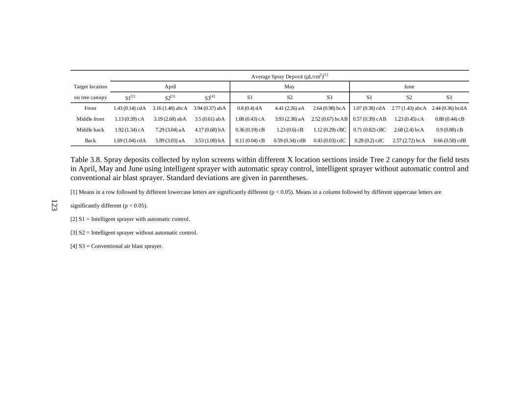
123









Target location


S2[3]

S3[4] S1 S2 S3 S1 S2 S3

Front 1.43 (0.14) cdA 3.16 (1.48) abcA 3.94 (0.37) abA 0.8 (0.4) dA 4.41 (2.26) aA 2.64 (0.98) bcA 1.07 (0.38) cdA 2.77 (1.43) abcA 2.44 (0.36) bcdA

Middle front 1.13 (0.39) cA 3.19 (2.68) abA 3.5 (0.61) abA 1.08 (0.43) cA 3.93 (2.38) aA 2.52 (0.67) bcAB 0.57 (0.39) cAB 1.23 (0.45) cA 0.88 (0.44) cB

Middle back 1.92 (1.34) cA 7.29 (3.04) aA 4.17 (0.68) bA 0.36 (0.19) cB 1.23 (0.6) cB 1.12 (0.29) cBC 0.71 (0.82) cBC 2.68 (2.4) bcA 0.9 (0.88) cB

Back 1.69 (1.04) cdA 5.89 (3.03) aA 3.53 (1.08) bA 0.11 (0.04) cB 0.59 (0.34) cdB 0.43 (0.03) cdC 0.28 (0.2) cdC 2.57 (2.72) bcA 0.66 (0.58) cdB

April May June


123

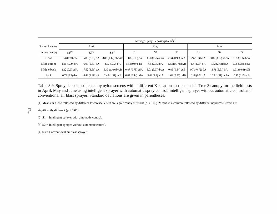
124









Target location


S2[3]

S3[4] S1 S2 S3 S1 S2 S3

Front 1.4 (0.73) cA 5.85 (3.05) aA 3.82 (1.12) abcAB 1.88 (1.13) cA 4.28 (1.25) abA 2.34 (0.99) bcA 2 (2.11) bcA 3.05 (3.12) abcA 2.55 (0.36) bcA

Middle front 1.21 (0.79) dA 6.07 (2.63) aA 4.07 (0.92) bA 1.54 (0.97) dA 4.5 (2.35) bA 1.63 (0.77) dAB 1.4 (1.29) dA 3.32 (2.48) bcA 2.08 (0.88) cdA

Middle back 1.12 (0.6) cdA 7.52 (3.66) aA 3.43 (1.49) bAB 0.87 (0.78) cdA 3.01 (3.07) bcA 0.89 (0.84) cdB 0.71 (0.72) dA 3.71 (3.51) bA 1.01 (0.68) cdB

Back 0.73 (0.2) dA 4.48 (2.89) aA 2.49 (1.31) bcB 0.87 (0.44) bdA 3.43 (2.2) abA 1.04 (0.56) bdB 0.48 (0.5) dA 1.22 (1.31) bcdA 0.47 (0.45) dB

April May June


124

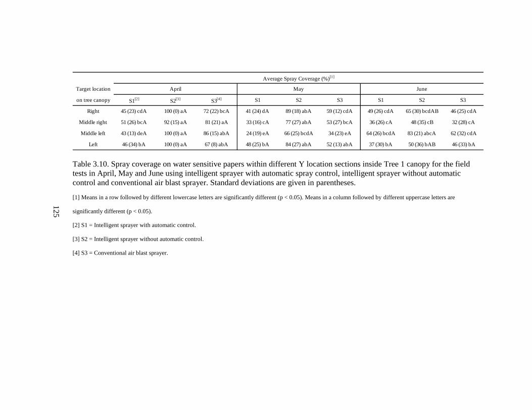
125

Table 3.10. Spray coverage on water sensitive papers within different Y location sections inside Tree 1 canopy for the field

tests in April, May and June using intelligent sprayer with automatic spray control, intelligent sprayer without automatic

control and conventional air blast sprayer. Standard deviations are given in parentheses.






Target location


S2[3]

S3[4] S1 S2 S3 S1 S2 S3

Right 45 (23) cdA 100 (0) aA 72 (22) bcA 41 (24) dA 89 (18) abA 59 (12) cdA 49 (26) cdA 65 (30) bcdAB 46 (25) cdA

Middle right 51 (26) bcA 92 (15) aA 81 (21) aA 33 (16) cA 77 (27) abA 53 (27) bcA 36 (26) cA 48 (35) cB 32 (28) cA

Middle left 43 (13) deA 100 (0) aA 86 (15) abA 24 (19) eA 66 (25) bcdA 34 (23) eA 64 (26) bcdA 83 (21) abcA 62 (32) cdA

Left 46 (34) bA 100 (0) aA 67 (8) abA 48 (25) bA 84 (27) abA 52 (13) abA 37 (30) bA 50 (36) bAB 46 (33) bA


April May June

125

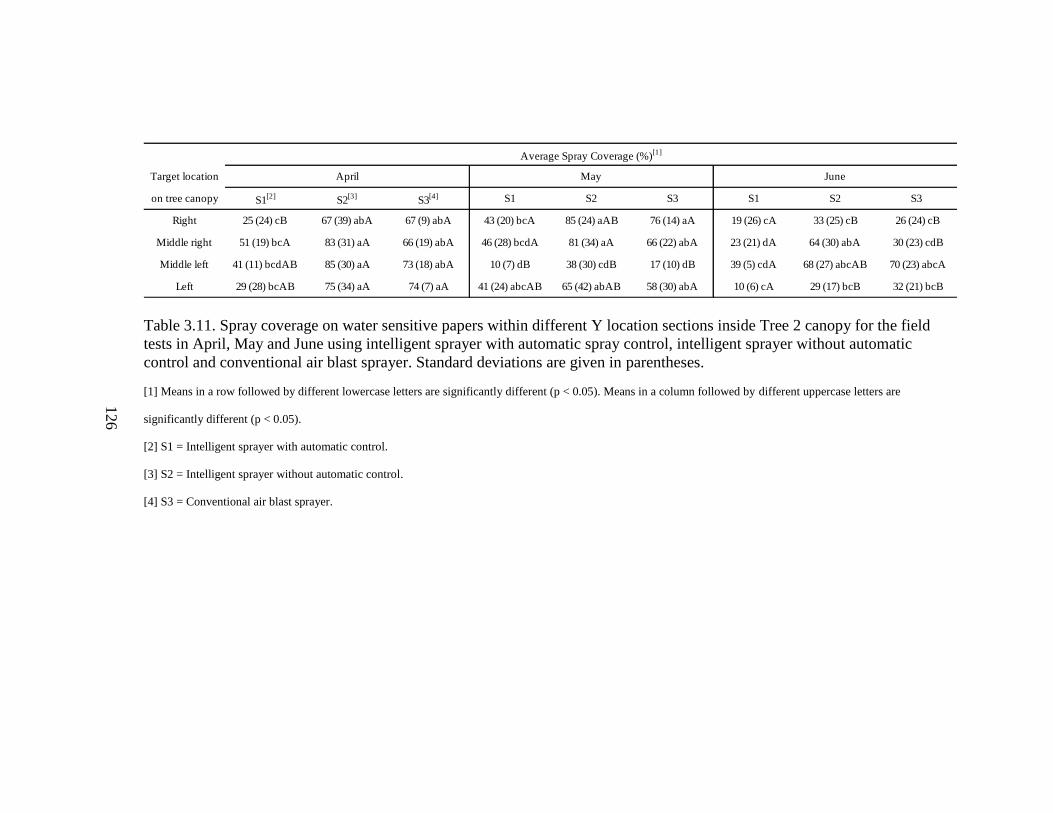
126









Target location


S2[3]

S3[4] S1 S2 S3 S1 S2 S3

Right 25 (24) cB 67 (39) abA 67 (9) abA 43 (20) bcA 85 (24) aAB 76 (14) aA 19 (26) cA 33 (25) cB 26 (24) cB

Middle right 51 (19) bcA 83 (31) aA 66 (19) abA 46 (28) bcdA 81 (34) aA 66 (22) abA 23 (21) dA 64 (30) abA 30 (23) cdB

Middle left 41 (11) bcdAB 85 (30) aA 73 (18) abA 10 (7) dB 38 (30) cdB 17 (10) dB 39 (5) cdA 68 (27) abcAB 70 (23) abcA

Left 29 (28) bcAB 75 (34) aA 74 (7) aA 41 (24) abcAB 65 (42) abAB 58 (30) abA 10 (6) cA 29 (17) bcB 32 (21) bcB

April May June


126

127









Target location


S2[3]

S3[4] S1 S2 S3 S1 S2 S3

Right 57 (23) bA 100 (0) aA 79 (32) abA 48 (31) bA 80 (19) abA 60 (20) bA 76 (36) abA 84 (22) abA 71 (16) abA

Middle right 30 (18) cdB 84 (22) aA 52 (29) bcA 52 (25) bcA 83 (44) aA 60 (30) bA 29 (30) cdB 57 (24) bAB 24 (23) dB

Middle left 33 (24) bAB 86 (27) aA 61 (24) abA 44 (29) bA 61 (41) abA 41 (42) bA 35 (31) bB 29 (35) bB 41 (36) bAB

Left 44 (22) bAB 100 (0) aA 67 (8) abA 25 (25) bA 55 (38) abA 37 (32) bA 19 (28) bB 48 (38) bAB 63 (42) abA

April May June


127

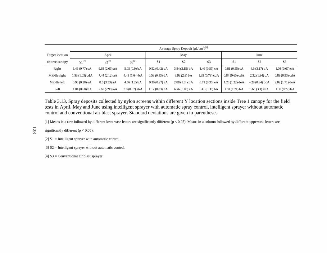
128

Table 3.13. Spray deposits collected by nylon screens within different Y location sections inside Tree 1 canopy for the field








Target location


S2[3]

S3[4] S1 S2 S3 S1 S2 S3

Right 1.49 (0.77) cA 9.68 (2.65) aA 5.05 (0.9) bA 0.52 (0.42) cA 3.84 (2.15) bA 1.46 (0.55) cA 0.81 (0.55) cA 4.6 (3.17) bA 1.08 (0.67) cA

Middle right 1.53 (1.03) cdA 7.44 (2.12) aA 4.43 (1.64) bA 0.53 (0.33) dA 3.93 (2.8) bA 1.35 (0.78) cdA 0.84 (0.65) cdA 2.32 (1.94) cA 0.89 (0.93) cdA

Middle left 0.96 (0.28) eA 8.5 (3.53) aA 4.56 (1.2) bA 0.39 (0.27) eA 2.88 (1.6) cdA 0.71 (0.35) eA 1.76 (1.22) deA 4.28 (0.94) bcA 2.02 (1.71) deA

Left 1.04 (0.68) bA 7.67 (2.98) aA 3.8 (0.07) abA 1.17 (0.83) bA 6.76 (5.05) aA 1.41 (0.39) bA 1.81 (1.71) bA 3.65 (3.1) abA 1.37 (0.77) bA


April May June

128

129









Target location


S2[3]

S3[4] S1 S2 S3 S1 S2 S3

Right 1.28 (1.24) bcA 4.65 (3.31) aA 3.47 (0.68) abA 0.84 (0.49) cA 3.48 (2.59) abAB 2.14 (0.76) bcA 0.6 (0.94) cA 1.8 (2.47) bcA 0.83 (0.72) cB

Middle right 2.01 (0.94) cdeA 6.01 (3.31) aA 3.69 (0.8) bcA 0.84 (0.54) deA 3.87 (2.74) bA 2.36 (1.28) bcdA 0.42 (0.38) eA 2.49 (2.4) bcdA 0.81 (0.77) deB

Middle left 1.25 (0.29) bcA 3.73 (2.4) aA 3.96 (1.22) aA 0.24 (0.16) cB 1.13 (0.49) bcB 0.63 (0.35) bcB 0.85 (0.44) bcA 3.2 (2.02) aA 2.19 (0.63) abA

Left 1.21 (1.2) bcA 6.55 (2.66) aA 4.01 (0.97) abA 0.61 (0.23) cAB 2.77 (1.73) abcAB 1.86 (0.78) bcA 0.3 (0.26) cA 1.76 (2.51) bcA 1.05 (0.8) cB

April May June


129

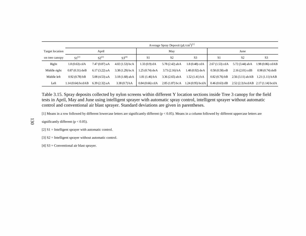
130









Target location


S2[3]

S3[4] S1 S2 S3 S1 S2 S3

Right 1.8 (0.63) cdA 7.47 (0.87) aA 4.02 (1.53) bcA 1.33 (0.9) dA 5.78 (2.42) abA 1.8 (0.48) cdA 2.67 (1.53) cdA 5.72 (3.44) abA 1.98 (0.86) cdAB

Middle right 0.87 (0.31) deB 6.17 (3.22) aA 3.38 (1.29) bcA 1.25 (0.74) deA 3.73 (2.16) bA 1.48 (0.92) deA 0.58 (0.58) eB 2.16 (2.01) cdB 0.98 (0.74) deB

Middle left 0.92 (0.78) bB 5.08 (4.53) aA 3.18 (1.68) abA 1.81 (1.46) bA 3.36 (2.65) abA 1.52 (1.41) bA 0.82 (0.76) bB 2.56 (3.11) abAB 1.21 (1.11) bAB

Left 1.14 (0.64) bcdAB 6.39 (2.32) aA 3.38 (0.7) bA 0.84 (0.66) cdA 2.85 (1.87) bcA 1.24 (0.95) bcdA 0.46 (0.63) dB 2.52 (2.3) bcdAB 2.17 (1.14) bcdA

April May June


130

131

Table 3.16. Spray coverage on water sensitive papers within different Z location sections inside Tree 1 canopy for the field








Target location


S2[3]

S3[4] S1 S2 S3 S1 S2 S3

High 49 (23) cA 100 (0) aA 72 (20) bcA 23 (16) dA 88 (23) abA 52 (18) cAB 69 (10) bcA 100 (0) aA 61 (13) cA

Middle 51 (22) cdA 100 (0) aA 83 (20) abA 27 (14) dA 68 (23) bcA 35 (24) dB 47 (35) cdA 69 (29) bcAB 38 (35) dA

Low 43 (22) bA 95 (12) aA 79 (19) aA 42 (23) bA 79 (26) aA 56 (21) bA 42 (25) bA 49 (29) bB 48 (30) bA


April May June

131

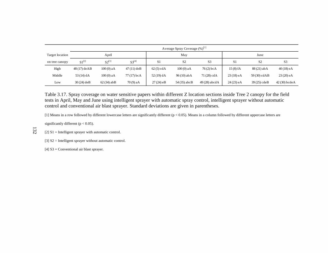
132









Target location


S2[3]

S3[4] S1 S2 S3 S1 S2 S3

High 48 (17) deAB 100 (0) aA 47 (11) deB 62 (5) cdA 100 (0) aA 76 (2) bcA 15 (8) fA 88 (21) abA 40 (18) eA

Middle 53 (14) dA 100 (0) aA 77 (17) bcA 52 (19) dA 96 (10) abA 71 (28) cdA 23 (18) eA 59 (30) cdAB 23 (20) eA

Low 30 (24) deB 62 (34) abB 70 (9) aA 27 (24) eB 54 (35) abcB 49 (28) abcdA 24 (23) eA 39 (25) cdeB 42 (30) bcdeA

April May June


132

133









Target location


S2[3]

S3[4] S1 S2 S3 S1 S2 S3

High 28 (11) cdB 100 (0) aA 29 (7) cdC 44 (19) bcAB 66 (29) bA 51 (28) bcA 29 (23) cdB 54 (11) bcA 10 (6) dB

Middle 59 (9) cdA 100 (0) aA 85 (12) abcA 71 (17) bcdA 91 (15) abA 54 (33) dA 71 (31) bcdA 70 (38) bcdA 50 (15) dAB

Low 32 (23) aB 84 (23) aA 60 (26) aB 38 (27) aB 65 (34) aA 52 (34) aA 28 (32) aB 48 (33) aA 46 (37) aA

April May June


133

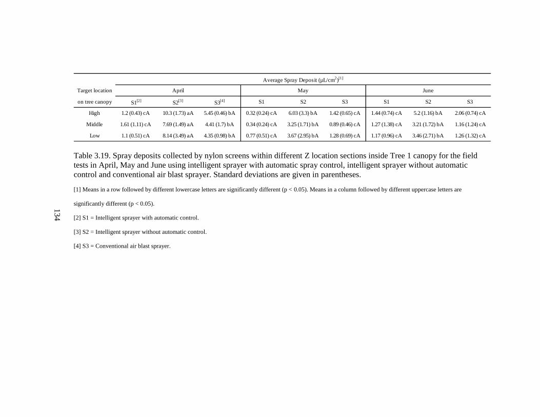
134

Table 3.19. Spray deposits collected by nylon screens within different Z location sections inside Tree 1 canopy for the field








Target location


S2[3]

S3[4] S1 S2 S3 S1 S2 S3

High 1.2 (0.43) cA 10.3 (1.73) aA 5.45 (0.46) bA 0.32 (0.24) cA 6.03 (3.3) bA 1.42 (0.65) cA 1.44 (0.74) cA 5.2 (1.16) bA 2.06 (0.74) cA

Middle 1.61 (1.11) cA 7.69 (1.49) aA 4.41 (1.7) bA 0.34 (0.24) cA 3.25 (1.71) bA 0.89 (0.46) cA 1.27 (1.38) cA 3.21 (1.72) bA 1.16 (1.24) cA

Low 1.1 (0.51) cA 8.14 (3.49) aA 4.35 (0.98) bA 0.77 (0.51) cA 3.67 (2.95) bA 1.28 (0.69) cA 1.17 (0.96) cA 3.46 (2.71) bA 1.26 (1.32) cA


April May June

134

135









Target location


S2[3]

S3[4] S1 S2 S3 S1 S2 S3

High 2.18 (1.19) cdeA 7.92 (1.13) aA 3.58 (1.37) bcdA 1.05 (0.04) deA 5.78 (1.11) abA 2.93 (0.11) cdeA 0.22 (0.12) eA 4.77 (3.77) bcA 1.22 (0.96) deA

Middle 1.85 (0.51) cdA 7.1 (1.42) aA 4.08 (1.01) bA 0.9 (0.47) dA 3.95 (2.05) bAB 2.85 (1.09) cA 0.5 (0.36) dA 2.75 (1.91) bcAB 0.83 (0.75) dA

Low 1.3 (1.13) bcA 3.78 (3.15) aB 3.59 (0.64) aA 0.53 (0.46) cA 2.16 (2.27) bB 1.42 (0.84) bcB 0.59 (0.69) cA 1.58 (1.81) bcB 1.18 (0.93) bcA


April May June

135

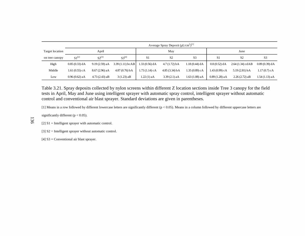
136









Target location


S2[3]

S3[4] S1 S2 S3 S1 S2 S3

High 0.85 (0.33) dA 9.19 (2.59) aA 3.39 (1.11) bcAB 1.33 (0.56) dA 4.7 (1.72) bA 1.18 (0.44) dA 0.8 (0.52) dA 2.64 (1.34) cdAB 0.89 (0.39) dA

Middle 1.61 (0.55) cA 8.67 (2.96) aA 4.87 (0.76) bA 1.73 (1.14) cA 4.85 (3.34) bA 1.35 (0.89) cA 1.43 (0.99) cA 5.19 (2.81) bA 1.17 (0.7) cA

Low 0.96 (0.62) aA 4.73 (2.43) aB 3 (1.23) aB 1.22 (1) aA 3.39 (2.1) aA 1.63 (1.08) aA 0.89 (1.28) aA 2.26 (2.72) aB 1.54 (1.13) aA

April May June


136

137

3.6.2 Spray loss on to the ground

As shown in Figures 3.13 and 3.14, S1 had the smallest amount of spray loss on

the ground, and S3 had the most. The differences are significant between three sprayers.

Even though the lowest nozzle on S3 was manually closed during all three spray tests, the

conventional sprayer (S3) still had much greater spray deposition on the ground than the

intelligent sprayer prototype (S1 and S2). This result shows that, the spray trajectories

from the intelligent sprayer were more toward the canopies than the radial spray pattern

from the conventional air blast sprayer.

As for each individual sprayer itself, the spray loss on the ground had very little

variation among the three tests conducted in April, May and June.

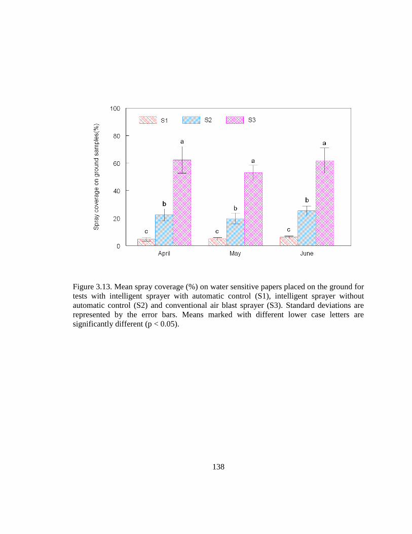
138

Figure 3.13. Mean spray coverage (%) on water sensitive papers placed on the ground for

tests with intelligent sprayer with automatic control (S1), intelligent sprayer without

automatic control (S2) and conventional air blast sprayer (S3). Standard deviations are

represented by the error bars. Means marked with different lower case letters are


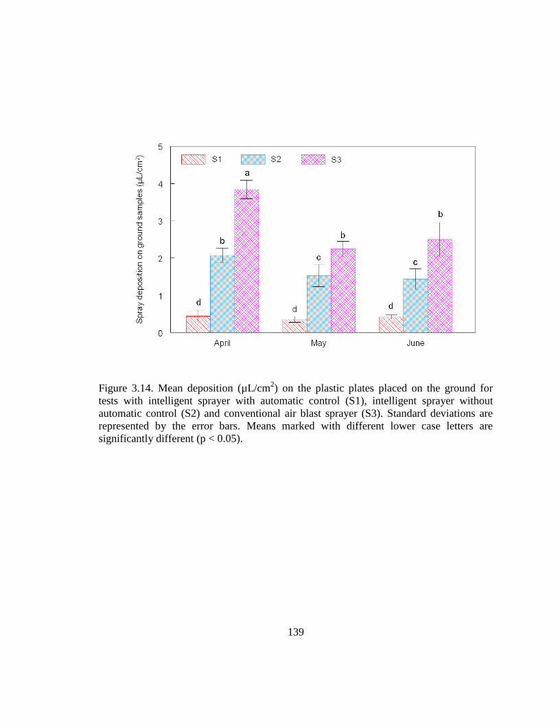
139

Figure 3.14. Mean deposition (µL/cm2) on the plastic plates placed on the ground for

tests with intelligent sprayer with automatic control (S1), intelligent sprayer without

automatic control (S2) and conventional air blast sprayer (S3). Standard deviations are

represented by the error bars. Means marked with different lower case letters are


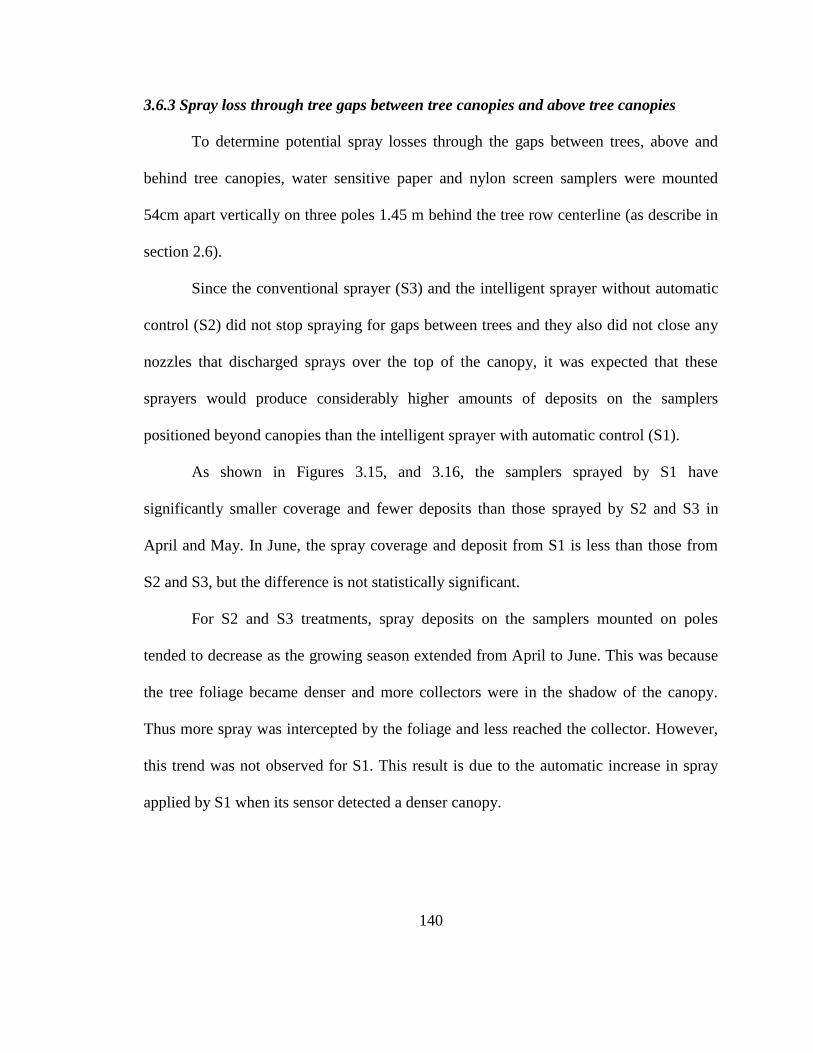
140

3.6.3 Spray loss through tree gaps between tree canopies and above tree canopies

To determine potential spray losses through the gaps between trees, above and

behind tree canopies, water sensitive paper and nylon screen samplers were mounted

54cm apart vertically on three poles 1.45 m behind the tree row centerline (as describe in

section 2.6).

Since the conventional sprayer (S3) and the intelligent sprayer without automatic

control (S2) did not stop spraying for gaps between trees and they also did not close any

nozzles that discharged sprays over the top of the canopy, it was expected that these

sprayers would produce considerably higher amounts of deposits on the samplers

positioned beyond canopies than the intelligent sprayer with automatic control (S1).

As shown in Figures 3.15, and 3.16, the samplers sprayed by S1 have

significantly smaller coverage and fewer deposits than those sprayed by S2 and S3 in

April and May. In June, the spray coverage and deposit from S1 is less than those from

S2 and S3, but the difference is not statistically significant.

For S2 and S3 treatments, spray deposits on the samplers mounted on poles

tended to decrease as the growing season extended from April to June. This was because

the tree foliage became denser and more collectors were in the shadow of the canopy.

Thus more spray was intercepted by the foliage and less reached the collector. However,

this trend was not observed for S1. This result is due to the automatic increase in spray

applied by S1 when its sensor detected a denser canopy.

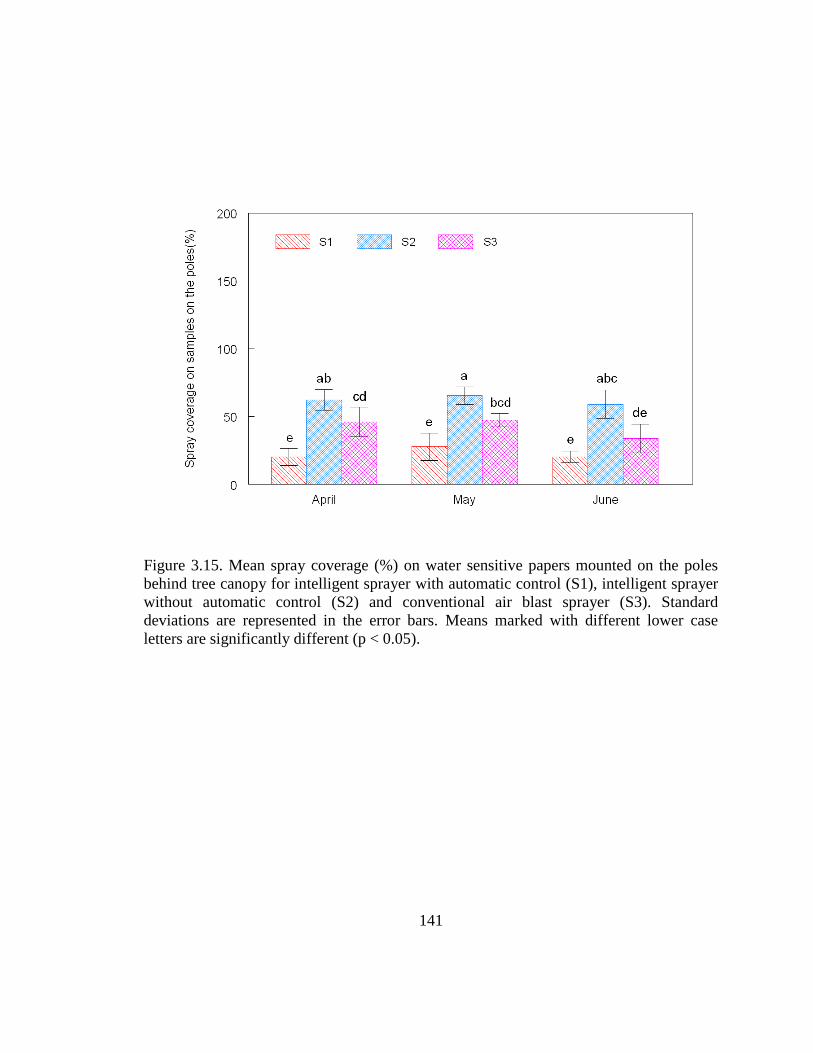
141

Figure 3.15. Mean spray coverage (%) on water sensitive papers mounted on the poles

behind tree canopy for intelligent sprayer with automatic control (S1), intelligent sprayer

without automatic control (S2) and conventional air blast sprayer (S3). Standard

deviations are represented in the error bars. Means marked with different lower case

letters are significantly different (p < 0.05).

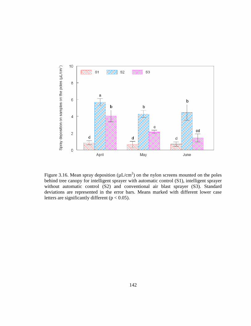
142

Figure 3.16. Mean spray deposition (µL/cm2) on the nylon screens mounted on the poles

behind tree canopy for intelligent sprayer with automatic control (S1), intelligent sprayer

without automatic control (S2) and conventional air blast sprayer (S3). Standard

deviations are represented in the error bars. Means marked with different lower case

letters are significantly different (p < 0.05).

143

3.6.4 The transition of spray deposition between two trees

To document the transition of spray deposition from one tree canopy to another,

three long strips of water sensitive papers were used to collect spray deposits between

two trees. The strips were mounted horizontally on three narrow wood bars at three

different heights (0.4, 0.9 and 2.0 m above the ground). The three bars were supported by

three vertical poles installed behind and between two trees. Each strip of water sensitive

papers was formed with four 26mm×508mm water sensitive papers connected together.

In this test, part of each strip at both sides was behind part of two tree canopies, and the

middle part of the strip was behind the tree gap. The detailed setup of poles and the

mounting of long water sensitive paper strips were described in section 2.6.

Figures 3.17 to 3.19 show the coverage results on the long water sensitive paper

strips between two trees for the test conducted in April, May and June, respectively. In

each figure there are nine rows of long water sensitive paper strips. Each row represents

the actual row that was sprayed. Nine rows were grouped into three sets of three rows,

and each set was sprayed by one of the three sprayers S1, S2 and S3. The top set of three

rows was sprayed with S1, the middle set was sprayed with S2, and the bottom set was

sprayed with S3. Within each set, the first and the third rows were placed at heights of 2

m and 0.4 m, where the tree gaps were very large; the second row was placed at 0.9 m

height, where the tree gap was narrow.

Figures 3.17 to 3.19 illustrate that S1 had the lowest sprays through tree gaps

among all the three sprayer treatments. This result was evidenced by the observation of

images shown in Figure 3.17. Obviously, S2 and S3 delivered considerably higher

144

amount of sprays on three long strips of water sensitive papers at three different heights

than S1, even behind trees.

In Figure 3.18 which shows the result from the May test when trees had half

foliage, the three rows of long water sensitive paper strips for S2 and S3 had less

coverage than there were in April test. This is because there were more leaves on the

trees in May and they blocked more spray liquid than the trees in April. Contrarily, the

three rows of long water sensitive paper sprayed by S1 had more coverage than those

were sprayed in April. This is because S1 automatically increased spray volume as a

result of denser canopies in May.

Figure 3.19 shows the result from the June test when trees had fully grown

canopies. The very dense foliage at the edge of trees blocked considerable amount of

sprays from reaching the long strips of water sensitive papers from S2 and S3. The

yellow areas with very few blue dots on the two ends of the strips show that these areas

were shadowed by very dense canopies. For S1, the increase of spray coverage on long

strips across the wide gap at 0.4 and 2.0 m heights was not visible while this increase was

visible at the 0.96 m height where the gap was narrow. This is because there were a few

small outward branches triggering nozzles to spray with higher flow rate than in the

earlier tests. Also, there were not many leaves on the edge of the trees to intercept spray

deposits, so an excessive portion of the sprays reached the water sensitive paper strips.

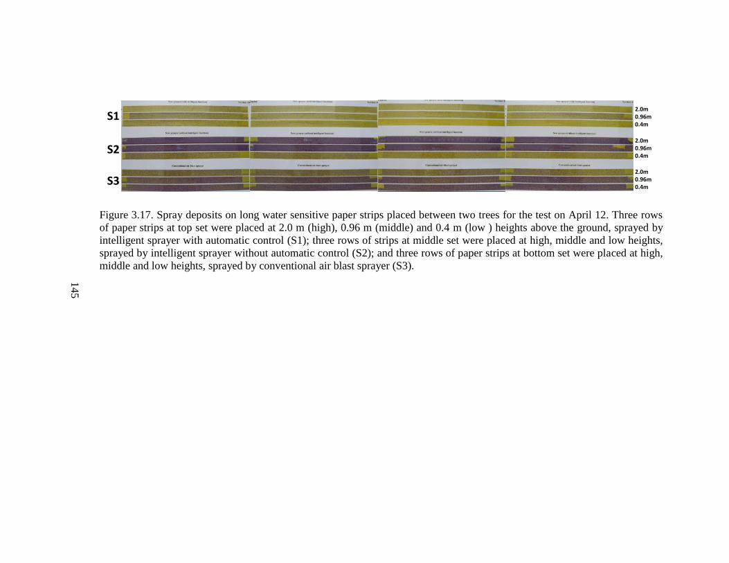
145

Figure 3.17. Spray deposits on long water sensitive paper strips placed between two trees for the test on April 12. Three rows

of paper strips at top set were placed at 2.0 m (high), 0.96 m (middle) and 0.4 m (low ) heights above the ground, sprayed by

intelligent sprayer with automatic control (S1); three rows of strips at middle set were placed at high, middle and low heights,

sprayed by intelligent sprayer without automatic control (S2); and three rows of paper strips at bottom set were placed at high,

middle and low heights, sprayed by conventional air blast sprayer (S3).

S1

S2

S3

2.0m0.96m0.4m

2.0m0.96m0.4m

2.0m0.96m0.4m

145

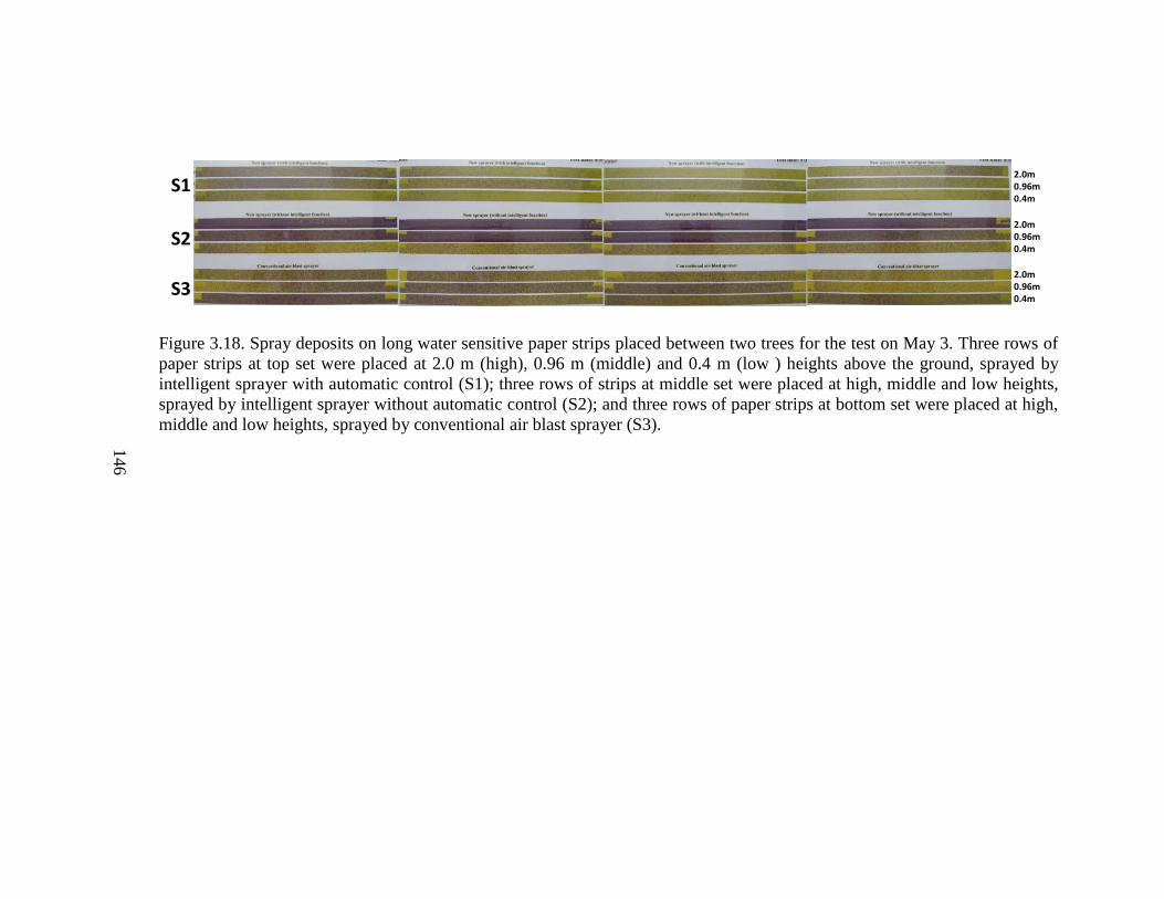
146

Figure 3.18. Spray deposits on long water sensitive paper strips placed between two trees for the test on May 3. Three rows of

paper strips at top set were placed at 2.0 m (high), 0.96 m (middle) and 0.4 m (low ) heights above the ground, sprayed by




S1

S2

S3

2.0m0.96m0.4m

2.0m0.96m0.4m

2.0m0.96m0.4m

146

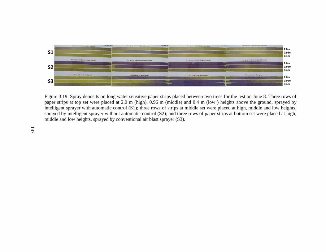
147

Figure 3.19. Spray deposits on long water sensitive paper strips placed between two trees for the test on June 8. Three rows of

paper strips at top set were placed at 2.0 m (high), 0.96 m (middle) and 0.4 m (low ) heights above the ground, sprayed by




S1

S2

S3

2.0m0.96m0.4m

2.0m0.96m0.4m

2.0m0.96m0.4m

147

148

3.6.5 Downwind spray drift

Tests were conducted to measure airborne drift from spray treatments only during

2nd

and 3rd

tests conducted in May and June, respectively. Nylon screens were placed

54cm apart at six heights on poles located downwind 5, 15 and 35 m downwind from the

centerline of the trees sprayed.

Results for airborne drift from experiments conducted in May are presented in

Figure 3.20. Targets on poles 15 and 35 m downwind had extremely low amount of drift

deposits. The drift data from the pole nearest to the sprayer (5 m away) showed that

among the sprayers tested, sprayer S1 (intelligent sprayer with automatic control)

produced the least amount of drift, while S2, the same sprayer without the intelligent

function turned to produce the highest amount of airborne drift. The differences are

statistically significant. The major reason for S2 to produce the most of amount of drift

was that all the nozzles on S2 discharge droplets in a horizontal trajectory, allowing a

high volume of spray material moving downwind at a height not much different from the

height of the poles. Thus more droplets are likely candidates to be captured by the

samplers. Such result corresponds to the result shown in section 3.6.2, where S3 had the

most spray lost on the ground, due to its radial spray pattern. In May, significant less drift

was created from S1 than S2 and S3. This is because the spray rate of S1 was

automatically reduced to match the canopy and thus less liquid was produced to go

beyond tree canopy.

Results from the experiments conducted in June shows that there is no significant

difference in the airborne drift created from three sprayers and at all three downwind

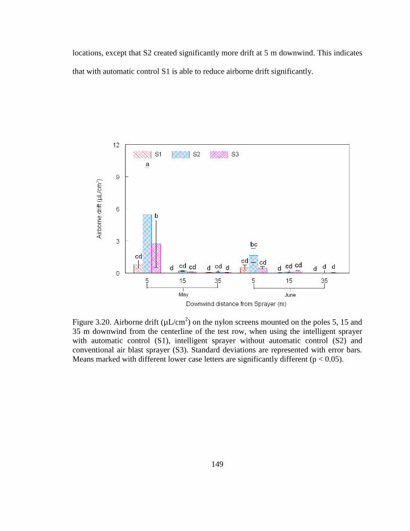
149

locations, except that S2 created significantly more drift at 5 m downwind. This indicates

that with automatic control S1 is able to reduce airborne drift significantly.

Figure 3.20. Airborne drift (µL/cm2) on the nylon screens mounted on the poles 5, 15 and

35 m downwind from the centerline of the test row, when using the intelligent sprayer

with automatic control (S1), intelligent sprayer without automatic control (S2) and

conventional air blast sprayer (S3). Standard deviations are represented with error bars.

Means marked with different lower case letters are significantly different (p < 0.05).

150

3.7 Sprayer outdoor tests with container trees

Four container trees (placed 2 m apart from tree center to tree center) were used to

determine the intelligent sprayer performance on very dense and thick canopies. The four

trees were the same ones used in the indoor spray rate test described in section 3.4. All

the four trees had fully grown and very dense canopies. The spray constant used in this

test was 0.05.

Among all the water sensitive papers sprayed by the intelligent sprayer with

automatic control at 3.2 km/h travel speed, 67% of them had coverage greater than 15%

which is considered sufficient coverage. In addition to the coverage data, droplet density

data were also calculated. This is especially meaningful for those samples with coverage

values lower than 15%. It was found that 87% of the water sensitive papers either had

coverage greater than 15% or have droplet density greater than 70 deposits/cm2

(recommended droplet density for fungicides by Syngenta Crop Protection AG located at

CH-4002 Basel, Switzerland), and 94% of the total water sensitive papers either had

coverage greater than 15% or had droplet density greater than 30 deposits/cm2

(recommended droplet density for insecticides by Syngenta Crop Protection AG located

at CH-4002 Basel, Switzerland).

For the test conducted at 6.44 km/h, 55% of the water sensitive papers had

coverage greater than 15%, 72% of the water sensitive papers either had coverage greater

than 15% or had droplet density greater than 70 deposits/cm2, and 85% of the total water

sensitive papers either had coverage greater than 15% or had droplet density greater than

30 deposits/cm2.

151

Figures 3.21 to 3.28 show the mean percentage of coverage on the water sensitive

papers mounted on different positions inside tree canopies sprayed by the intelligent

sprayer with automatic control. Figures 3.21, 3.23, 3.25 and 3.27 show the coverage data

when the sprayer was operated at a travel speed of 3.2 km/h, while Figures 3.22, 3.24,

3.26 and 3.28 show the coverage data for travel speed of 6.4 km/h. Comparing the results

for the same tree between lower and higher speeds illustrates that the coverage at lower

speed was higher.

Data presented on Figures 3.21 to 3.28 also indicates that at both ground speeds

there was uniform spray distribution along vertical direction. However, uniformity of

horizontal spray distribution (both along the spray direction and travel speed direction)

was not good, especially for the positions that were far away from the nozzles. This

means that the sprayer was not able to provide conditions that are conducive to

penetration of droplets into inner parts of the canopy. This was very likely the result of

the sprayer being operated at a relatively low air velocity and low air volume, which is

not strong enough to open the canopy sufficiently.

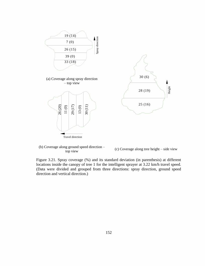
152

33 (18)

39 (0)

26 (15)

7 (0)

19 (14)

Spra

y d

irec

tio

n

25 (16)

28 (19)

30 (6)

Hei

ght

(a) Coverage along spray direction

– top view

(b) Coverage along ground speed direction –

top view (c) Coverage along tree height – side view

Figure 3.21. Spray coverage (%) and its standard deviation (in parenthesis) at different

locations inside the canopy of tree 1 for the intelligent sprayer at 3.22 km/h travel speed.

(Data were divided and grouped from three directions: spray direction, ground speed

direction and vertical direction.)

30 (

11

)

13 (

0)

29 (

17

)

11 (

0)

26 (

20

)

Travel direction

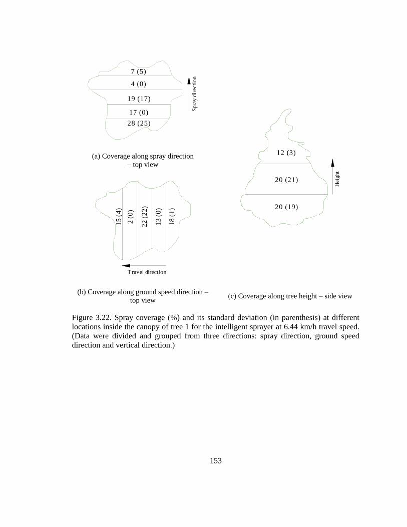
153

28 (25)

19 (17)

4 (0)

7 (5)

17 (0)

Spra

y d

irec

tio

n

20 (19)

20 (21)

12 (3)

Hei

ght


– top view







13

(0

)

22

(2

2)

2 (

0)

15

(4

)

18

(1

)

Travel direction

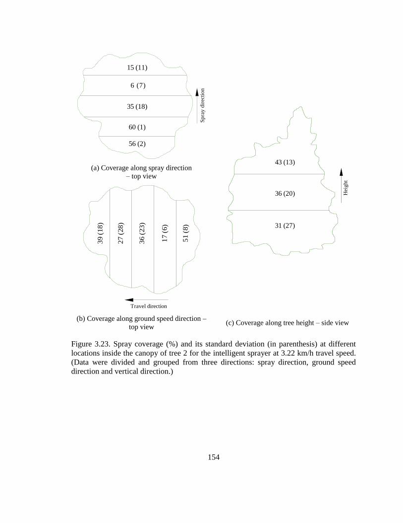
154

56 (2)

15 (11)

35 (18)

6 (7)

60 (1)

Sp

ray

dir

ecti

on

31 (27)

36 (20)

43 (13)

Hei

ght


– top view







51 (

8)

17 (

6)

36 (

23

)

27 (

28

)

39 (

18

)

Travel direction

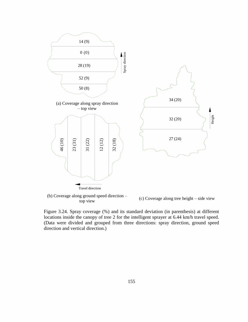
155

50 (8)

14 (9)

28 (19)

0 (0)

52 (9)

Sp

ray

dir

ecti

on

27 (24)

32 (20)

34 (20)

Hei

ght


– top view







32 (

18)

12 (

12)

31 (

22)

23 (

31)

46 (

10)

Travel direction

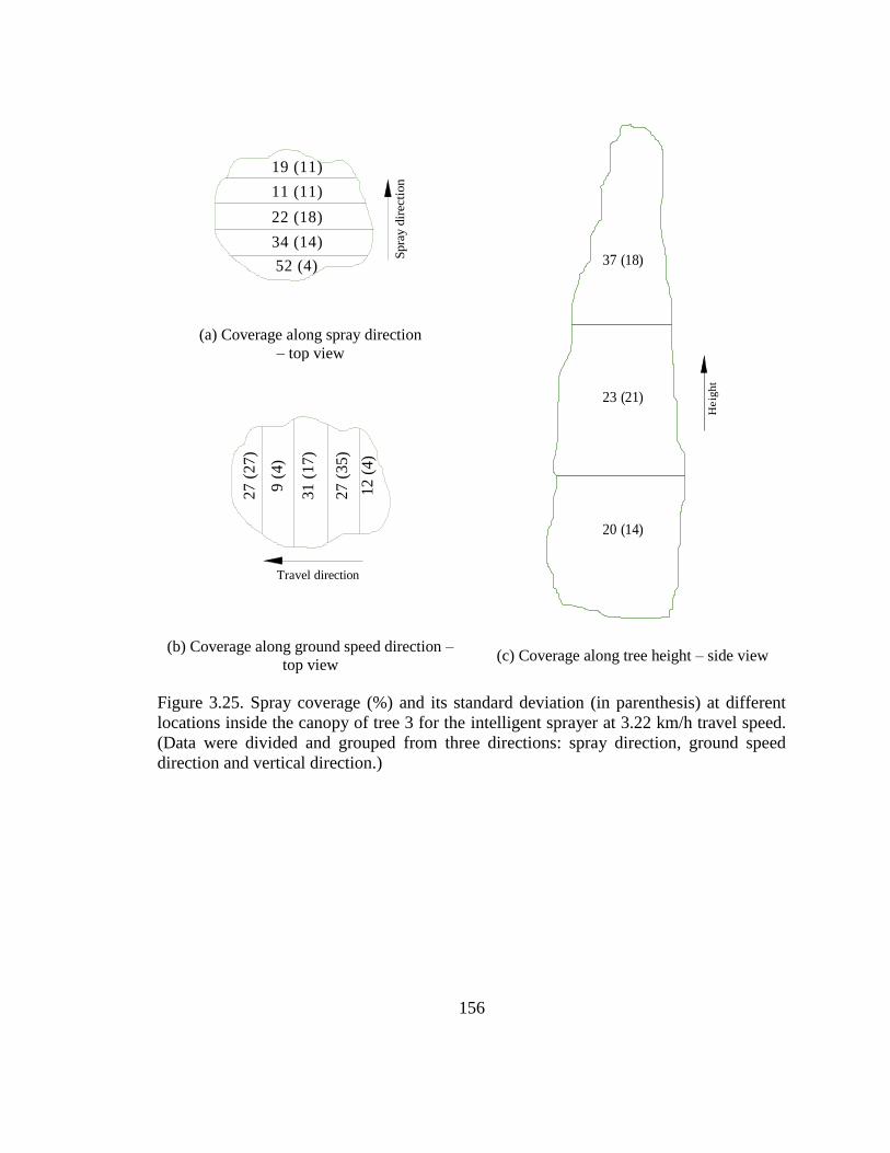
156

52 (4)

34 (14)

22 (18)

11 (11)

19 (11)

Spra

y d

irecti

on

20 (14)

23 (21)

37 (18)

He

igh

t


– top view







12 (

4)

27 (

35)

31 (

17)

9 (

4)

27 (

27)

Travel direction

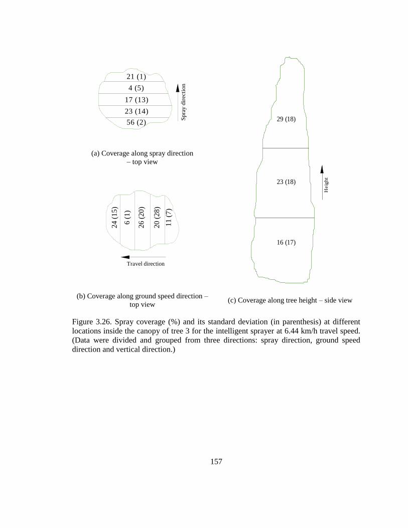
157

56 (2)

23 (14)

17 (13)

4 (5)

21 (1)

Spra

y d

irec

tion

16 (17)

23 (18)

29 (18)

Heig

ht


– top view







11 (

7)

20 (

28

)

26 (

20

)

6 (

1)

24 (

15

)

Travel direction

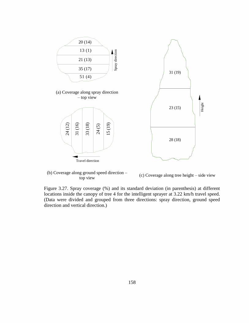
158

51 (4)

35 (17)

21 (13)

13 (1)

20 (14)

Spra

y d

irec

tion

28 (18)

23 (15)

31 (19)

Heig

ht


– top view







15 (

19)

24 (

5)

33 (

18)

31 (

16)

24 (

12)

Travel direction

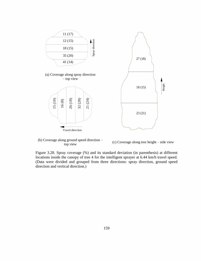
159

41 (14)

35 (20)

18 (15)

12 (15)

11 (17)

Spra

y d

irec

tio

n

23 (21)

18 (15)

27 (18)

Heig

ht


– top view







21

(2

4)

32

(2

8)

26

(1

8)

15

(1

0)

16

(8

)

Travel direction

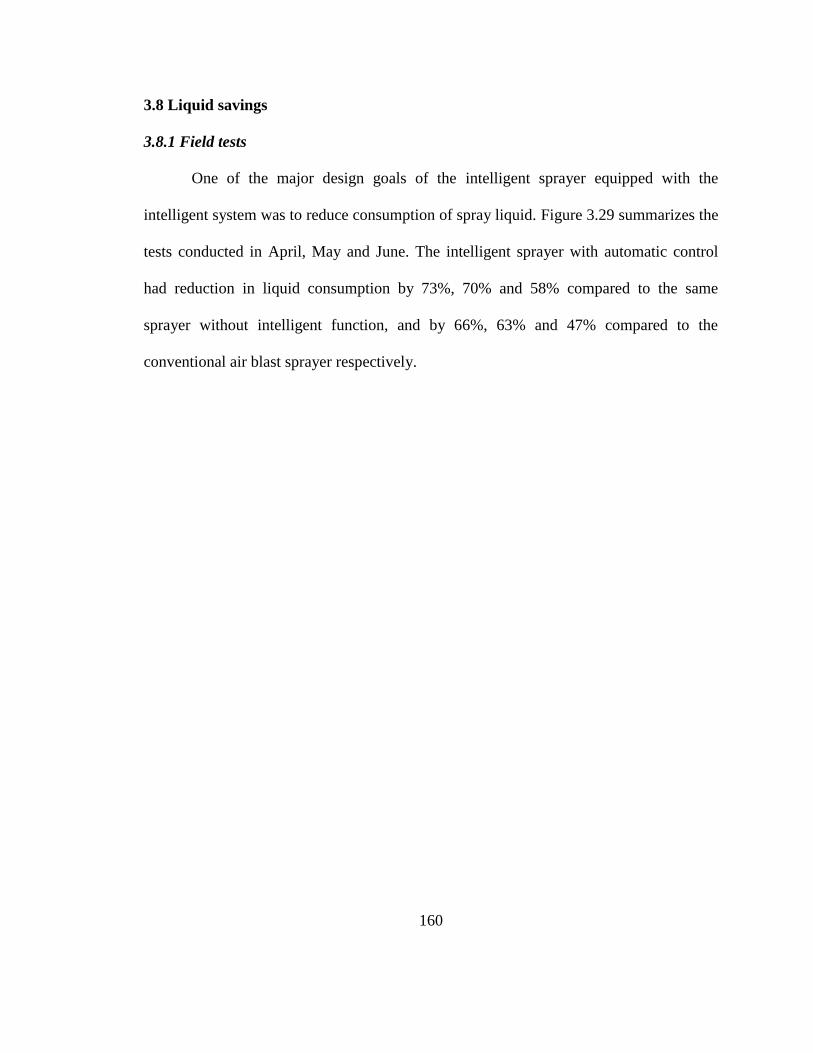
160

3.8 Liquid savings

3.8.1 Field tests

One of the major design goals of the intelligent sprayer equipped with the

intelligent system was to reduce consumption of spray liquid. Figure 3.29 summarizes the

tests conducted in April, May and June. The intelligent sprayer with automatic control

had reduction in liquid consumption by 73%, 70% and 58% compared to the same

sprayer without intelligent function, and by 66%, 63% and 47% compared to the

conventional air blast sprayer respectively.

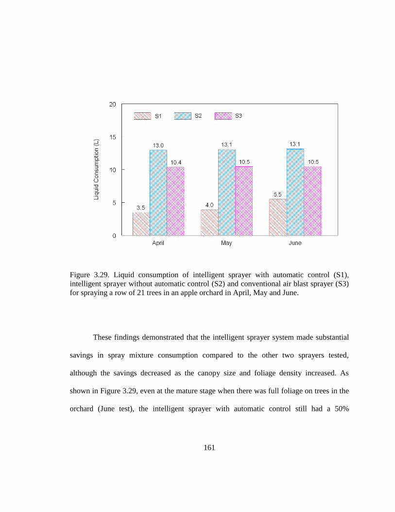
161

Figure 3.29. Liquid consumption of intelligent sprayer with automatic control (S1),

intelligent sprayer without automatic control (S2) and conventional air blast sprayer (S3)

for spraying a row of 21 trees in an apple orchard in April, May and June.

These findings demonstrated that the intelligent sprayer system made substantial

savings in spray mixture consumption compared to the other two sprayers tested,

although the savings decreased as the canopy size and foliage density increased. As

shown in Figure 3.29, even at the mature stage when there was full foliage on trees in the

orchard (June test), the intelligent sprayer with automatic control still had a 50%

162

reduction in spray mixture consumption compared to the conventional air assisted

sprayer.

3.8.2 Container tree test

Savings in spray mixture consumption were also evaluated for the four trees

grown in containers, in the spray test described in section 3.7 (tree measurements were

shown in Table 3.1). During the test, the four trees were placed 2 m apart from tree center

to center, which was a relatively close spacing for trees with their fully grown canopies.

As shown in Figure 3.30, intelligent sprayer with automatic control had spray

consumption savings of 51% and 38% for the four container trees at travel speed of 3.22

km/h and 6.44 km/h, respectively, compared to intelligent sprayer without automatic

control.

The main reason for the decrease in the percent savings when the travel speed was

increased to 6.44 km/h is that the intelligent sprayer without automatic control could not

adjust the application rate according to the travel speed. That is, the nozzle flow rate was

the same for the two tests with the sprayer without the intelligent function travelling at

both speeds. As the travel speed doubles, the application rate decreased by half.

However, when its intelligent function was turned on, the intelligent sprayer was able to

adjust the application rate automatically to compensate the speed difference since the

travel speed was included in the spray output model.

The decrease in spray consumption of intelligent sprayer with automatic control at

a higher travel speed was a result of the decrease of sensor resolution along the travel

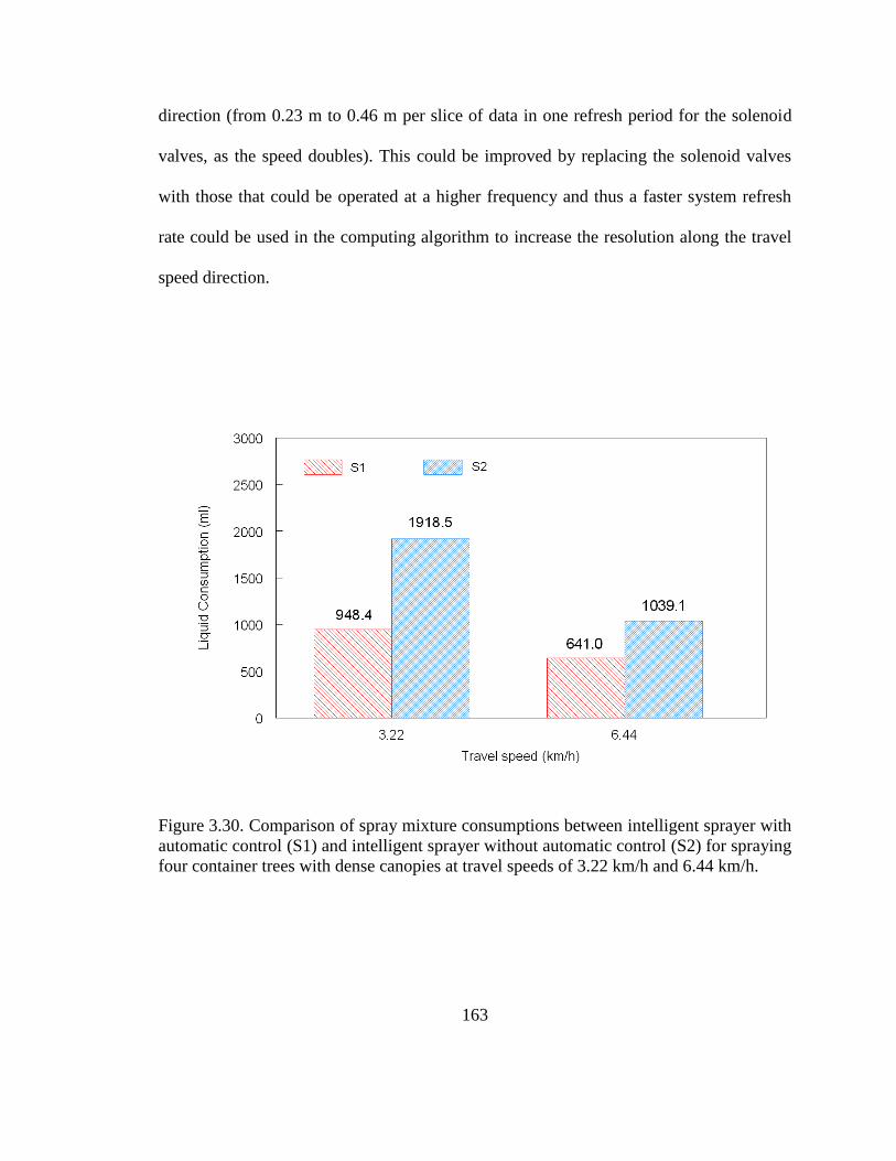
163

direction (from 0.23 m to 0.46 m per slice of data in one refresh period for the solenoid

valves, as the speed doubles). This could be improved by replacing the solenoid valves

with those that could be operated at a higher frequency and thus a faster system refresh

rate could be used in the computing algorithm to increase the resolution along the travel

speed direction.

Figure 3.30. Comparison of spray mixture consumptions between intelligent sprayer with

automatic control (S1) and intelligent sprayer without automatic control (S2) for spraying

four container trees with dense canopies at travel speeds of 3.22 km/h and 6.44 km/h.

164

Chapter 4: Conclusions and Recommendations

4.1 Conclusions

The intelligent sprayer prototype with intelligent functions for nurseries and

orchards developed in this research has several advantages over conventional chemical

application systems. By using laser sensing and variable rate control technologies to

adjust the amount of spray output based on the need of target canopies, it can not only

reduce chemical cost for the growers, but also reduce the risk of potential environmental

contamination due to a significant reduction in the chemicals that miss the targets. Other

advantages of the intelligent sprayer prototype are that:

1) It implements real-time tree shape and foliage density measurement information into

the real-time spray control. It achieves fully automatic variable-rate spray tasks,

without human involvement during spray applications.

2) It automatically detects tree row center, which eliminates the requirement to measure

and input distance from tractor to the tree center by the operator. When the tractor

makes a turn to spray a new row of trees, the tree center will be updated as the tractor

goes down the row.

3) It has versatility to treat many varieties of tree crops with different heights and shapes

by turning on and off appropriate nozzles, and by adjusting flow rate of nozzles based

on canopy size and density. This is especially useful in nurseries where a variety of

tree crops are commonly planted together in the same field.

165

4) The intelligent algorithm inside the control component can handle a wide variety of

foliage canopy density changes, and the electro-mechanical controllers are fast

enough to activate the sprayer to achieve desired coverage regardless of foliage

canopy variations.

However, the limitation of the current intelligent sprayer prototype is that the air

velocity is not strong enough to carry spray droplets inside large and dense nursery

canopies such as Tsuga Canadensis.

A high speed laser scanner was used to acquire data on the geometry, density

characteristics and occurrence of the canopy on-the-go. The laser was able to scan the

target crops and transfer the measurement data to a laptop computer for further

processing. For the laser scanning sensor used and its operation mode chosen in this

study, the tree structure measurement had resolution of 1.4 cm vertically and 2.3 cm

horizontally.

A fast algorithm was developed to calculate tree canopy characteristic parameters

using the data from the laser sensor. The algorithm could also automatically detect the

ground surface, and the tree row centerline to assist in the calculations of tree width,

height, volume and foliage density. Indoor tests with artificial targets were conducted to

validate the algorithm used for calculation of canopy density. Results showed that the

calculated density values were very close to the actual densities. The relationship

between the calculated and actual densities was linear with correlation coefficients (R2)

ranging from 0.98 to 0.99.

166

A flow rate control unit was designed with Pulse Width Modulation (PWM)

signals to adjust the spray output of nozzles in accordance with the detected tree canopy

density in a real-time manner. An experiment station was built to calibrate the nozzle

flow rates and to validate the accuracy of hardware and software used for the variable

rate controller. During the experiments, pressure fluctuations were observed when

operating solenoid valves at 10 Hz frequency and were minimized by a back pressure

bypass device added to the spraying system.

A mathematic model was developed to calculate the optimal spray rate for each of

20 individual nozzles based on the concept that spray volume equals the effective canopy

volume multiplied by a recommended spray constant. Laboratory tests were conducted to

validate the effectiveness of the spray model as well as the performance of the data

processing algorithm. Results showed that the spray model was effective in generating

an optimal amount of spray that can ensure adequate spray coverage on targets.

A commercially available vineyard sprayer base was used for the development of

the intelligent sprayer prototype. The laser sensor and flow rate controller circuits for

sensing trees and controlling variable rate were implemented into the sprayer prototype.

Four five-port air assisted nozzles with one 8002 XR flat fan nozzle in each port were

assembled and mounted on each side of the Intelligent sprayer. Air velocity from each

port was measured when the axial fan on the sprayer was running at the high speed mode.

The sizes of droplets discharged from the nozzles at different modulation rate of the

PWM control signals were also measured at the same air velocity as it was at the port.

System response time was determined with a high speed camera system. The latency

167

between when laser “sees” the target and when the nozzle starts spraying liquid was

measured to be approximately 0.119 seconds which includes the time for the software to

complete the calculation, and for the electronic, hydraulic and mechanical components to

respond in accordance with the computation results.

Field tests were conducted on apple trees in an orchard at three growth stages of

tree canopy to compare the spray performances of three sprayers: intelligent sprayer with

automatic control, intelligent sprayer without automatic control, and conventional air

blast sprayer. Results from the field tests highlighted following important conclusions:

1) Unlike the intelligent sprayer without automatic control and the conventional air blast

sprayer, intelligent sprayer with automatic control did not provide excessive sprays on

the tree canopies.

2) Intelligent sprayer with automatic control was able to spray the tree canopies with

relatively uniform coverage throughout the tree at different growth stages. However,

the spray uniformity from the other two sprayers was not as good as that produced by

the intelligent sprayer.

3) Unlike the other two sprayers which generally showed significantly lower spray

coverage when spraying trees with denser canopies, the spray coverage achieved by

the intelligent sprayer varied very little with the foliage density.

4) Intelligent sprayer with automatic control had the least spray loss to the ground, while

the conventional air blast spray had the most. This result not only proves that

intelligent sprayer with automatic control is able to shut off the nozzles when there is

no canopy to spray, but also supports the assumption that the intelligent sprayer

168

prototype equipped with intelligently-controlled five-port nozzles has a better spray

trajectory control than the conventional air blast sprayer.

5) Intelligent sprayer with automatic control had the lowest spray loss through tree gaps

and beyond tree canopies than the other two sprayers.

6) Intelligent sprayer with automatic control had the least airborne drift than the other two

sprayers.

7) In addition to the advantages listed above, field experiments demonstrated that the

intelligent sprayer with automatic control could reduce spray volume by 47% to 73%

compared to the other two sprayers and still provide adequate coverage and

deposition.

To evaluate the spray coverage achieved from the intelligent sprayer with

automatic control when spraying dense canopies such as evergreen trees found in

nurseries, spray tests were conducted in four container trees with much denser canopies

than the apple trees used in field tests explained above. Results from tests with four

dense container-grown nursery trees showed that the uniformity of the spray coverage

from the intelligent sprayer was not stable along the horizontal directions (both travel

direction and spray direction). The primary reason for this ineffectiveness was that the air

velocity and volume from the sprayer was not strong enough to open the dense canopy

and help spray droplets penetrate into inner parts of the canopy. Therefore, an improved

air-delivery subsystem with more powerful air output is needed for the intelligent sprayer

prototype to treat very dense and thick canopies.

169

4.2 Unique contributions of this study to the intelligent sprayer development

As the evidence from the literature review presented in Chapter 1, in recent years

some other researchers also have conducted research with objectives somewhat similar to

the objectives of the study described in this dissertation. Although the ultimate goal of all

of these studies was to design intelligent sprayers to apply pesticides at optimum rates,

the Intelligent Sprayer described in this dissertation has following unique features that set

it apart from the other sprayers designed with similar objectives in mind.

1. A commercially available sprayer base was fitted with a high precision laser sensor to

determine tree canopy characteristics and occurrence in real time. Others have relied

on ultrasonic sensor to acquire canopy occurrence only. The intelligent sprayer

described here is able to acquire much more information on canopy structures in a

real-time manner with higher accuracy than other sprayers.

2. Working with a rich set of real-time data from the high speed laser sensor, intelligent

algorithms were designed and developed to capture the tree canopy characteristics

and occurrence to manipulate spray outputs. Compared to the algorithms used by

others, the algorithms presented in this study 1) are able to precisely sketch the tree

canopy characteristics for a specific section covered by one individual nozzle; 2) do

not require original data from laser sensor to be saved and thus reduce overhead in

data collection; and 3) they do not require any offline data processing on other

computer software such as Matlab (MathWorks Co. Natick, MA), which is often used

in similar research.

170

3. The intelligent sprayer prototype can detect the foliage density in addition to canopy

height, width, volume and occurrence, and can adjust flow rate of each nozzle

according to the canopy structure measurements and complete the spray decision

management on-the-go.

4. It is the first sprayer of its kind that is able to automatically identify the ground surface,

the tree row center and tree spacing. No prior orchard or nursery measurement data is

required for the application and no human involvement is needed to run the system.

The operator only needs to turn on the sprayer with intelligent functions selected and

drive the tractor.

5. The intelligent sprayer prototype is the first sprayer system that has the capability to

divide a whole tree canopy into many small sections and each section is sprayed with

variable rate by an individual nozzle based on the sectional canopy structure

measurements. It is the first orchard and nursery sprayer that uses specially designed

five-port air assisted nozzles which have better trajectory control than other nozzles.

6. It is also the first sprayer of its kind that employs a back pressure bypass mechanism to

limit the pressure fluctuation caused by the modulation of solenoid valves at 10 Hz

frequency.

171

4.3 Recommendations for future study

The main goal of this study was to design and develop software and hardware for

an intelligent sprayer that can control variable-rate spray outputs through the nozzles

based on availability of a target in sight, and density level of the canopy sprayed. This has

been accomplished to a large degree. However, there is still some ineffectiveness

associated with the operation of this sprayer that can be addressed by future studies.

Following are some of the areas where further research is needed:

1. The height of tree section treated by each nozzle was assumed to be equal to simplify

the parameters used in the system. However, in the future research, the height covered

by each nozzle (with their specific orientation) should be calibrated and compared

with what is done in this study to determine if the sprayer performance can be

improved by using the calibrated height treated by each nozzle.

2. Currently the sprayer only has one laser scanner to control one side of the nozzles on

the sprayer. It is necessary to investigate spraying from two sides of the sprayer when

traveling in the same path by using either a laser scanner with wider field of view or

two laser scanners mounted on the sprayer .

3. Currently the intelligent sprayer does not have a speed sensor to measure the travel

speed in real time; speed information is manually entered in the computer before the

sprayer is operated. Real time speed measurement should be included in the system to

improve the accuracy of matching the flow rate to the target regardless of variations

in travel speed.

172

4. A direct injection system should be added to the intelligent sprayer to reduce the

possibility of leftover pesticide and water mixture in the tank after the field is

sprayed. This will further protect the environment by eliminating the improper

practice of dumping leftover spray mixture somewhere in the field after completion of

spraying.

5. A GPS and management control logic should be added in the intelligent sprayer. By

doing so, the orchard or nursery manager can select pesticide type for a specific field

location and GPS will verify that no spraying will take place unless the sprayer is in

the right location. This will ensure that chemicals will only be applied to their

designated plots.

6. Currently centerlines of all five-port nozzles are oriented horizontally. The current

design can be improved so that an optimal orientation can be determined for each

nozzle for specific tasks or preferences, such as to spray trees mostly from top down,

or bottom up.

7. An air controller should be added to the intelligent sprayer to adjust the air velocity

and air volume based on the volume and density of the tree canopy to achieve

adequate and uniform spray coverage on targets.

8. The spray model should incorporate with more parameters including weather data,

environment information and user preferences for better management of the fate of

pesticides applied. This can be achieved by automatic adjustment of the spray rate

and air velocity of the sprayer based on environmental conditions such as

temperature, wind speed and direction, and proximity of the area to water resources

173

and other sensitive areas to avoid their contamination and risk to safety and health of

nearby people and animals.

174

References

Al-Gaadi, K. A., Ayers, P. D. (1999). Integrating GIS and GPS into a spatially variable

rate herbicide application system. Applied Engineering in Agriculture, 15(4), 255-

262.

Anonymous. (2000). In National Research Council (Ed.), The future role of pesticides in

US agriculture National Academy Press, Washington.

Balsari, P., Doruchowski, G., Marucco, P., Tamagnone M., Van de Zande, J. (2007). The

development of a crop identification system (CIS) able to adjust spray application to

target characteristics. SuProFruit 2007, 9th Workshop on Spray Application

Techniques in Fruit Growing, Alnarp, Sweden. 17-18.

Bode, L. E. (2008). Agricultural chemical application technology: A remarkable past and

an amazing future. Transactions of the ASABE, 51(2), 391-395.

Brown, R.B., Steckler, J.P.G.A. (1995). Prescription maps for spatially variable herbicide

application in no-till corn. Transactions of the ASAE, 38(6), 1659-1666.

Deveau, J. (2009). Six elements of effective spraying in orchards and vineyards. Ministry

of Agriculture, Food and Rural Affairs, Ontario.

175

Doruchowski, G., Jedrachowicz, T., Holownicki, R., Godyn, A., Swlechowski, W.,

Balsari, P., ... Wenneker, M. (2007). Environmentally dependent application system

(EDAS) for adjusting the spray application parameters according to the

environmental circumstances in orchards - ISAFRUIT project. SuProFruit 2007, 9th

Workshop on Spray Application Techniques in Fruit Growing, Alnarp, Sweden. 15-

16.

Doruchowski, G. (2000). Environmentally friendly spray techniques for tree crops. Crop

Protection, 19(8-10), 617-622.

Escola, A., Camp, F., Solanelles, F., Planas, S, Rosell, J. R. (2003). Tree crop

proportional spraying according to the vegetation volume. first results. Proceedings

of the 7th Workshop on Spray Application Techniques in Fruit Growing, Cuneo,

Italy, 43-49.

Fox, R. D., Derksen, R.C., Zhu, H., Brazee, R.D., Svensson, S.A. (2008). A history of

air-blast sprayer development and future prospects. Transactions of the ASABE,

51(2), 405-410.

Gil, E., Escola, A., Rosell, J. R., Planas, S., Val, L. (2007). Variable rate application of

plant protection products in vineyard using ultrasonic sensors. Crop Protection,

26(8), 1287-1297.

176

Giles, D.K., Delwiche, M.J., Dodd, R.B. (1987). Control of orchard spraying based on

electronic sensing of target characteristics. Transactions of the ASAE, 30(6), 1624-

1630.

Giles, D. K., Delwiche, M.J., Dodd, R.B. (1988). Electronic measurement of tree canopy

volume. Transactions of the ASAE, 31(1), 264-272.

Giles, D. K., Delwiche, M. J., Dodd, R. B. (1989). Sprayer control by sensing orchard

crop characteristics: Orchard architecture and spray liquid savings. Journal of

Agricultural Engineering Research, 43(4), 271-289.

Han, S., Hendrickson, L. L., Ni, B., Zhang, Q. (2001). Modification and testing of a

commercial sprayer with PWM solenoids for precision spraying. Applied

Engineering in Agriculture, 17(5), 591-594.

Hanks, J. E., Beck, J. L. (1998). Sensor-controlled hooded sprayer for row crops. Weed

Technology, 12(2), 308-314.

Harris, M.J., Erickson, K., Johnson, J., Morehart, M., Strickland, R., Covey, T., …

Dubman, R. 2009 agricultural income and finance outlook / AIS-88 / december

2009. http://usda.mannlib.cornell.edu/usda/ers/AIS//2000s/2009/AIS-12-22-2009.pdf

Jenkins, E., Hines, R. (2003). Chapter 4: Spraying fruit. Fruit crop pest management. A

guide for commercial applicators category 1C. Michigan St. Univ. 124pp.

http://usda.mannlib.cornell.edu/usda/ers/AIS/2000s/2009/AIS-12-22-2009.pdf

177

Jerardo, A. (2007). Floriculture and nursery crops yearbook/FLO-2007/September 2007.

http://www.ers.usda.gov/Publications/Flo/2007/09Sep/FLO2007.pdf

Knutson, R.D., Hall, C.R., Smith, E.G., Contner, S.D., Miller, J.W. (1997). Pesticide-free

production a „disaster‟. Commercial Grower, 52, 8-10.

Lee, K. H., Ehsani, R. (2008). A laser scanner based measurement system for

quantification of citrus tree geometric characteristics. ASABE Paper no. 083980, St.

Joseph, Mich.: ASABE.

Llorens, J., Gil, E., Llop, J.,Escola, A. (2010). Variable rate dosing in precision

viticulture: Use of electronic devices to improve application efficiency. Crop

Protection, 29, 239-248.

Mooney, D. F., Larson, J. A., Roberts, R. K. English, B. C. (2009).When does variable

rate technology for agricultural sprayers pay? A case study for cotton production in

tennessee. http://economics.ag.utk.edu/publications/precisionag/313_Mooney.pdf

Oerke, E. C. (2006). Crop losses to pests. The Journal of Agricultural Science, 144(1),

31.

Oerke, E. C., Dehne, H.W. (2004). Safeguarding production--losses in major crops and

the role of crop protection. Crop Protection, 23(4), 275-285.

http://www.ers.usda.gov/Publications/Flo/2007/09Sep/FLO2007.pdf

http://economics.ag.utk.edu/publications/precisionag/313_Mooney.pdf

178

Oerke, E. C., Dehne, H.W., Schonbeck, F., Weber, A. (1994). Crop production and crop

protection: Estimated losses in major food and cash crops. Amsterdam: Elsevier

Science.

Paice, M. E. R., Miller, P. C. H., Bodle, J. D. (1995). An experimental sprayer for the

spatially selective application of herbicides. Journal of Agricultural Engineering

Research, 60(2), 107-116.

Palacin, J., Palleja, T., Tresanchez, M., Teixido, M., Sanz, R., Llorens, J.,...Rosell, J. R.

(2008). Difficulties on tree volume measurement from a ground laser scanner.

Instrumentation and Measurement Technology Conference Proceedings, Victoria,

Vancouver Island, Canada, , 1997-2002.

Palacin, J., Palleja, T., Tresanch, M., Sanz, R., Llorens, J., Ribes-Dasi, M.,... Rosell, J. R.

(2007). Real-time tree-foliage surface estimation using a ground laser scanner. Ieee

Transactions on Instrumentation and Measurement, 56(4), 1377-1383.

Reichard, D. L., Ladd, T. L. (1981). An automatic intermittent sprayer. Transactions of

the ASABE.24 (4), 893-896

Rosell, J.R., Sanz, R., Llorens, J., Arno, J., Escola, A., Ribes-Dasi, M.,...Palacin, J.

(2009a). A tractor-mounted scanning LIDAR for the non-destructive measurement

of vegetative volume and surface area of tree-row plantations: A comparison with

conventional destructive measurements. Biosystems Engineering, 102(2), 128-134.

179

Rosell, J. R., Llorens, J., Sanz, R., Arno, J., Ribes-Dasi, M., Masip, J.,... Palacin, J.

(2009b). Obtaining the three-dimensional structure of tree orchards from remote 2D

terrestrial LIDAR scanning. Agricultural and Forest Meteorology, 149(9), 1505-

1515.

Salyani, M., Wei, J. (2005).Effect of travel speed on characterizing citrus canopy

structure with a laser scanner. Precision Agriculture'05. Papers Presented at the 5th

European Conference on Precision Agriculture, Uppsala, Sweden, 185-192.

Solanelles, F., Escola, A., Planas, S., Rosell, J., Camp, F., Gracia, F. (2006). An

electronic control system for pesticide application proportional to the canopy width

of tree crops. Biosystems Engineering, 95(4), 473-481.

Thorp, K. R., Tian, L. (2004). Performance study of variable-rate herbicide applications

based on remote sensing imagery. Biosystems Engineering, 88(1), 35-47.

Tian, L., Reid, J.F., Hummel, J.W. (1999). Development of a precision sprayer for site-

specific weed management. Transactions of the ASAE, 42(4), 893-900.

Tian, L. (2002). Development of a sensor-based precision herbicide application system.

Computers and Electronics in Agriculture, 36(2-3), 133-149.

Van de Zande, J.C., Wenneker, M., Meuleman, J., Achten, V., Balsari, P., Doruchowski,

G. (2007).Development of a crop health sensor (CHS) to minimise spray

180

applications in apple. SuProFruit 2007, 9th Workshop on Spray Application

Techniques in Fruit Growing, Alnarp, Sweden. 13-14.

Wei, J., Salyani, M. (2004). Development of a laser scanner for measuring tree canopy

characteristics: Phase 1. prototype development. Transactions of the ASAE, 47(6),

2101-2107.

Wei, J., Salyani, M. (2005). Development of a laser scanner for measuring tree canopy

characteristics: Phase 2. foliage density measurement. Transactions of the ASAE,

48(4), 1595-1601.

Zhu, H., Derksen, R.C., Guler, H., Krause, C.R., Ozkan, H.E. (2006). Foliar deposition

and off-target loss with different spray techniques in nursery applications.

Transactions of the ASABE, 49(2), 325-334.

Zhu, H. (2006). A specially designed air-assisted sprayer to improve spray penetration

and air jet velocity distribution inside dense nursery crops. Transactions of the

ASABE, 49(5), 1285-1294.

181

Appendix A

Block diagram for Data Acquisition program using LMS 291 Laser Scanner (LabVIEW)

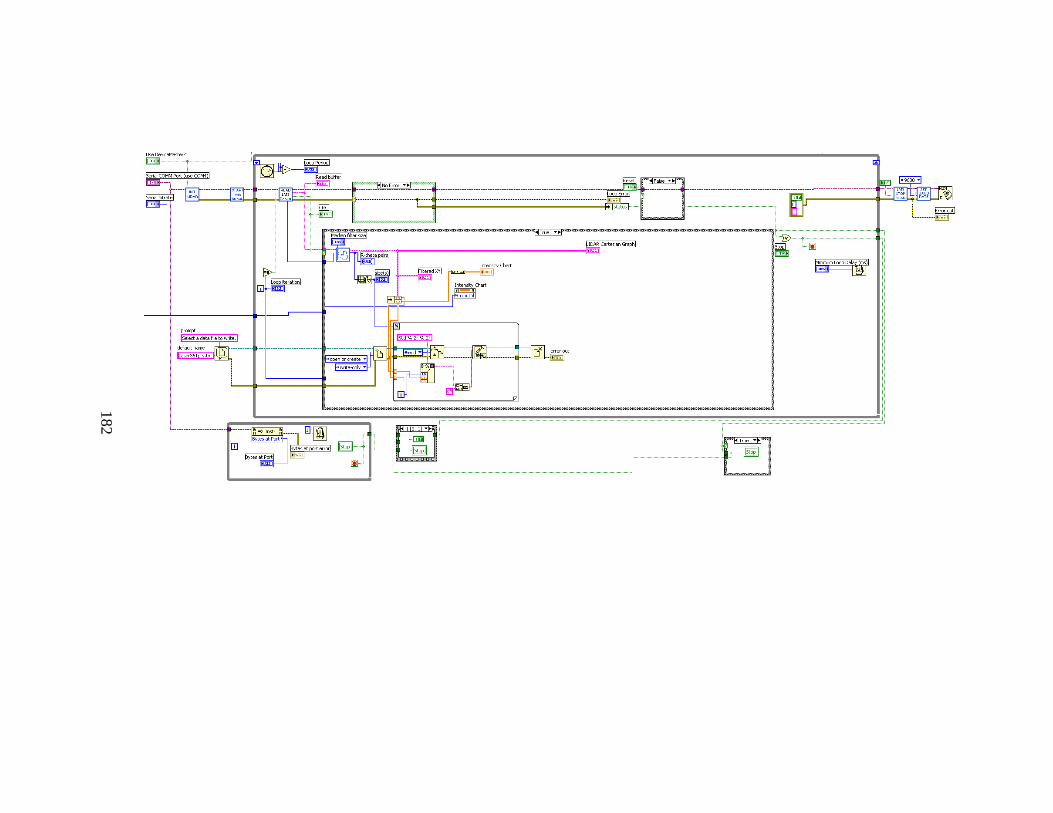
182

182

183

Appendix B

Schematic of switching circuit for controlling 10 channels of low power PWM signals

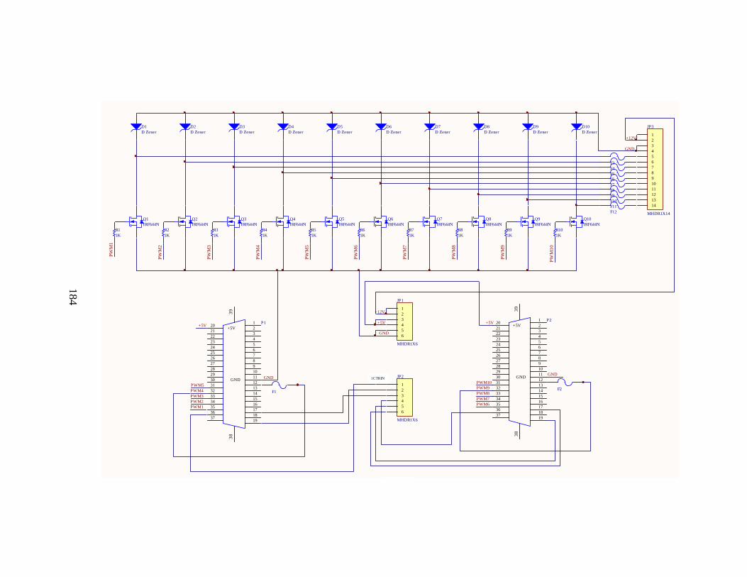
184

1

1

2

2

3

3

4

4

5

5

6

6

D D

C C

B B

A A

Title

Number RevisionSize

B

Date: 3/3/2010 Sheet of

File: D:\DXP\Valve driver08\VD2Apr.SchDoc Drawn By :

1K

R9

IRF644N

Q9

1K

R10

IRF644N

Q10

1K

R8

IRF644N

Q8

1K

R7

IRF644N

Q7

1K

R6

IRF644N

Q6

PWM5

PWM4

PWM3

PWM2

PWM1

1K

R4

IRF644N

Q4

1K

R5

IRF644N

Q5

1K

R3

IRF644N

Q3

1K

R2

IRF644N

Q2

1K

R1

IRF644N

Q1

1

2

3

4

5

6

7

8

9

10

11

12

13

14

MHDR1X14

JP3

PW

M1

PW

M2

PW

M3

PW

M4

PW

M5

PW

M6

PW

M7

PW

M8

PW

M9

PW

M1

0

1

2

3

4

5

6

7

8

9

10

GND11

12

13

14

15

16

17

18

19

+5V20

21

22

23

24

25

26

27

28

29

30

31

32

33

34

35

36

37

38

39

P1

PWM10

PWM9

PWM8

PWM7

PWM6

1

2

3

4

5

6

7

8

9

10

GND11

12

13

14

15

16

17

18

19

+5V20

21

22

23

24

25

26

27

28

29

30

31

32

33

34

35

36

37

38

39

P2

D Zener

D1

D Zener

D2

D Zener

D3

D Zener

D4

D Zener

D5

D Zener

D6

D Zener

D7

D Zener

D8

D Zener

D9

D Zener

D10

F1F2

F3

F4

F5

F6

F7

F8

F9

F10

F11

F12

GND

1

2

3

4

5

6

MHDR1X6

JP1

1

2

3

4

5

6

MHDR1X6

JP2

GND

GNDGND

+5V+5V

+12V

+5V

+12V

1CTRIN

184

185

Appendix C

Block diagram for generating 10 channels of independent PWM signals with specified 10

duty cycle values (LabVIEW)

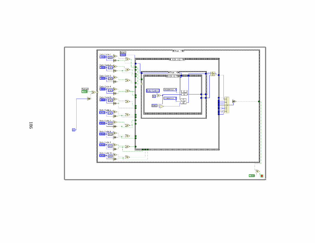
186

186

187

Appendix D

Block diagram for New Spray controller program (LabVIEW)

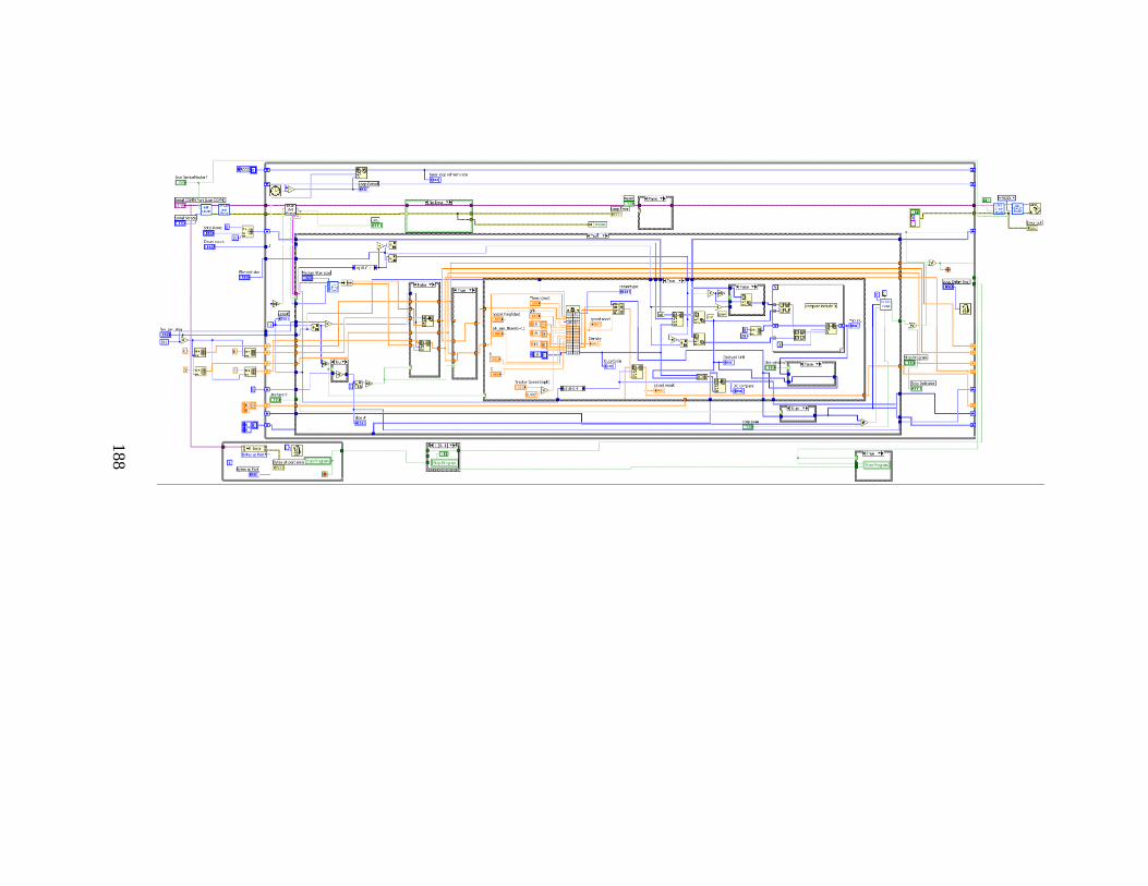
188

188

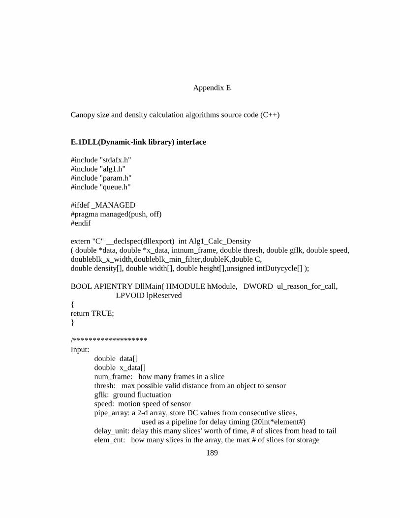
189

Appendix E

Canopy size and density calculation algorithms source code (C++)

E.1DLL(Dynamic-link library) interface

#include "stdafx.h"

#include "alg1.h"

#include "param.h"

#include "queue.h"

#ifdef _MANAGED

#pragma managed(push, off)

#endif

extern "C" __declspec(dllexport) int Alg1_Calc_Density

( double *data, double *x_data, intnum_frame, double thresh, double gflk, double speed,

doubleblk_x_width,doubleblk_min_filter,doubleK,double C,

double density[], double width[], double height[],unsigned intDutycycle[] );

BOOL APIENTRY DllMain( HMODULE hModule, DWORD ul_reason_for_call,

LPVOID lpReserved

{

return TRUE;

}

/*******************

Input:

double data[]

double x_data[]

num_frame: how many frames in a slice

thresh: max possible valid distance from an object to sensor

gflk: ground fluctuation

speed: motion speed of sensor

pipe_array: a 2-d array, store DC values from consecutive slices,

used as a pipeline for delay timing (20int*element#)

delay_unit: delay this many slices' worth of time, # of slices from head to tail

elem_cnt: how many slices in the array, the max # of slices for storage

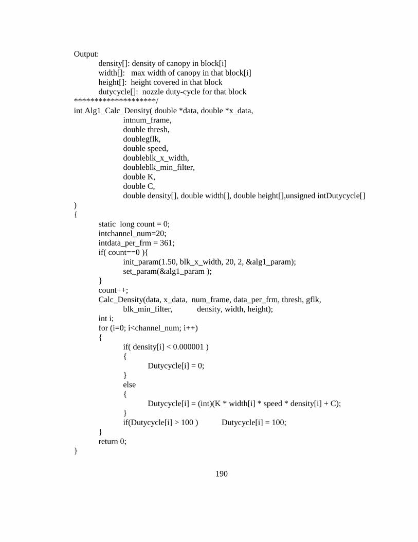
190

Output:

density[]: density of canopy in block[i]

width[]: max width of canopy in that block[i]

height[]: height covered in that block

dutycycle[]: nozzle duty-cycle for that block

********************/

int Alg1_Calc_Density( double *data, double *x_data,

intnum_frame,

double thresh,

doublegflk,

double speed,

doubleblk_x_width,

doubleblk_min_filter,

double K,

double C,

double density[], double width[], double height[],unsigned intDutycycle[]

)

{

static long count = 0;

intchannel_num=20;

intdata_per_frm = 361;

if( count==0 ){

init_param(1.50, blk_x_width, 20, 2, &alg1_param);

set_param(&alg1_param );

}

count++;

Calc_Density(data, x_data, num_frame, data_per_frm, thresh, gflk,

blk_min_filter, density, width, height);

int i;

for (i=0; i<channel_num; i++)

{

if( density[i] < 0.000001 )

{

Dutycycle[i] = 0;

}

else

{

Dutycycle[i] = (int)(K * width[i] * speed * density[i] + C);

}

if(Dutycycle[i] > 100 ) Dutycycle[i] = 100;

}

return 0;

}

191

#ifdef _MANAGED

#pragma managed(pop)

#endif

192

E.2 Compute the parameters for a chosen working mode

#ifndef __PARAM_H__

#define __PARAM_H__

#define MAX_BLK 20

#define MAX_DATA_PER_BLK 32

typedefstructs_CalcParam

{

double d;

double h;

int blk_num;

intang_res;

intstart_pos;

intnum_pts;

intpts_unit[MAX_BLK];

doublepts_width[MAX_BLK][MAX_DATA_PER_BLK];

}CalcParam_t;

void init_param(double d, double h, intnum_h, intang_res, CalcParam_t* param ) ;

#endif

#include "stdafx.h"

#include "string.h"

#include "math.h"

#include <stdio.h>

#include "param.h"

void init_param(double d, double h, intnum_h, intang_res, CalcParam_t* param )

{

double pi = 3.14159265;

doublestart_ang, ang2;

int i,j, k;

inttotal_pts;

double degree;

doubleang_inc;

intpts_per_degree;

memset(param, 0, sizeof(CalcParam_t) );

start_ang = atan(d/(h*num_h/2));

degree = start_ang * 180/pi;

193

if(ang_res == 1 ){

total_pts = 181;

pts_per_degree = 1;

i = (int)(degree * 1);

ang_inc = pi/180;

}

else if(ang_res == 2){

total_pts = 361;

pts_per_degree = 2;

i = (int)(degree*2);

ang_inc = pi/180/2;

}

else if( ang_res == 3){

total_pts = 401;

pts_per_degree = 4;

i = (int) ((degree - 40) * 4);

ang_inc = pi/180/4;

}

else{

printf("Error: unknown angular-resolution %d\n", ang_res);

return;

}

if( i<0 ) i = 0;

param->start_pos = i;

param->num_pts = (total_pts- i*2);

param->d = d;

param->h = h;

param->blk_num = num_h;

param->ang_res = ang_res;

intlast_pt = i;

for(i=1; i<num_h/2; i++)

{

ang2 = atan( d / ((num_h/2-i)*h) );

if(ang_res == 3 ) {

j = ( (ang2*180/pi) - 40) * 4;

}

else{

j = (ang2 * 180/pi) * pts_per_degree;

}

param->pts_unit[i-1] = j - last_pt;

194

last_pt = j;

}

param->pts_unit[i-1] = total_pts/2 - last_pt;

for(i=num_h/2; i<num_h; i++ )

{

param->pts_unit[i] = param->pts_unit[num_h-1-i];

}

double tmp[401];

doublelast_ang = start_ang;

doublelast_x = h*num_h/2 * 1000;

doublecurrent_x;

doublecurrent_ang = last_ang;

for(i=1; i<= param->num_pts/2; i++)

{

current_ang += ang_inc;

current_x = 1000 * d * cos(current_ang)/sin(current_ang);

last_x = current_x;

}

tmp[i-1] = tmp[i-2];

for(i=param->num_pts/2; i<param->num_pts; i++)

{

tmp[i] = tmp[ param->num_pts - 1 - i ];

}

j = 0;

for(i=0; i<num_h; i++ )

{

for(k=0; k<param->pts_unit[i]; k++, j++)

param->pts_width[i][k] = tmp[j];

if( i == num_h/2-1 )

j++;

}

}

195

E.3 Algorithm to calculate canopy width and foliage density

#include "stdafx.h"

#include "string.h"

#include "math.h"

#include <stdio.h>

#include "alg1.h"

#include "param.h"

#define FRAME_PER_SLICE 50

#define DATA_PER_FRAME 401

static double glb_slice_data[FRAME_PER_SLICE][DATA_PER_FRAME];

static double glb_x_data[FRAME_PER_SLICE][DATA_PER_FRAME];

staticintglb_data_per_frame = 361;

staticintglb_trunk_len;

staticintglb_blk_per_frm = 20;

double glb_gnd_fluc;

intglb_centermode;

typedefstructwidth_s

{

intidx;

double width;

}width_t;

CalcParam_t alg1_param;

CalcParam_t *cur_param;

#define CENT_WIND_SIZE 5

width_tglb_cent_width[CENT_WIND_SIZE];

intglb_cent_width_cnt = 0;

doublecenter_width = -1;

void set_param(CalcParam_t* param)

{

cur_param = param;

196

}

voidinternal_quickSort(double a[], int lo, int hi)

{

int i=lo, j=hi, h;

double x=a[(lo+hi)/2];

do

{

while (a[i]<x) i++;

while (a[j]>x) j--;

if (i<=j)

{

h=a[i]; a[i]=a[j]; a[j]=h;

i++; j--;

}

} while (i<=j);

if (lo<j) internal_quickSort(a, lo, j);

if (i<hi) internal_quickSort(a, i, hi);

}

void quick_sort(double* data, intnum)

{

internal_quickSort(data, 0, num-1);

}

double get_min_dist( double* data, intnum, double percent )

{

int n, i = 0;

double min = 0;

while( i<num )

{

if( data[i] > 0.01 )

break;

i++;

}

n = num - i;

if( n > 0 )

{

197

min = data[i + (int)(n*percent)];

}

return min;

}

doubleget_average(double* data, intnum)

{

double sum = 0;

int n, i = 0;

while( i<num )

{

if( data[i] > 0.01 )

break;

i++;

}

n=0;

for(; i<num; i++)

{

sum += data[i];

n++;

}

return sum/n;

}

voidTruncate_Data(double *data, double *x_data, intnum_frame, double thresh)

{

intflen = glb_data_per_frame;

int i, j, k;

intstart_pos;

start_pos = cur_param->start_pos;

glb_trunk_len = 0;

for(i=0; i<glb_blk_per_frm; i++ )

{

glb_trunk_len += cur_param->pts_unit[i];

}

198

doublegnd_high;

for(i=0; i<num_frame; i++)

{

k = i*flen + start_pos;

gnd_high = *(x_data+i*flen);

memcpy(glb_slice_data[i], data+k, glb_trunk_len*sizeof(double));

memcpy(glb_x_data[i], x_data+k, glb_trunk_len*sizeof(double));

for(j=0; j<glb_trunk_len; j++ )

{

if(fabs( *(x_data+k+j)-gnd_high )<= glb_gnd_fluc )

{

glb_slice_data[i][j] = 0;

}

else if( glb_slice_data[i][j] >= thresh )

{


}

else if(glb_slice_data[i][j] < 0 )

{


}

}

}

}

doubleGet_Row_Center(intnum_frame, intflen)

{

staticwidth_ttop_distance[64];

memset((void*)top_distance, 0, 64*sizeof(width_t));

int i, j;

if(glb_cent_width_cnt == 0 )

{

memset(glb_cent_width, 0, CENT_WIND_SIZE*sizeof(width_t) );

}


{

for(j=flen-1; j>=0; j--)

{

199

if(glb_slice_data[i][j] > 0 )

{

top_distance[i].idx = j;

top_distance[i].width = glb_slice_data[i][j];

break;

}

}

}

double max = -1;

inttop_idx = -1;


{

if(top_distance[i].idx>top_idx )

{

top_idx = top_distance[i].idx;

max = top_distance[i].width;

}

else if( top_distance[i].idx == top_idx )

{

if(top_distance[i].width > max )

{

top_idx = top_distance[i].idx;

max = top_distance[i].width;

}

}

}

i = glb_cent_width_cnt%CENT_WIND_SIZE;

glb_cent_width[i].idx = top_idx;

glb_cent_width[i].width = max;

glb_cent_width_cnt++;

max = -1;

for(i=0; i<CENT_WIND_SIZE; i++)

{

if(glb_cent_width[i].width > max )

max = glb_cent_width[i].width;

}

return max;

}

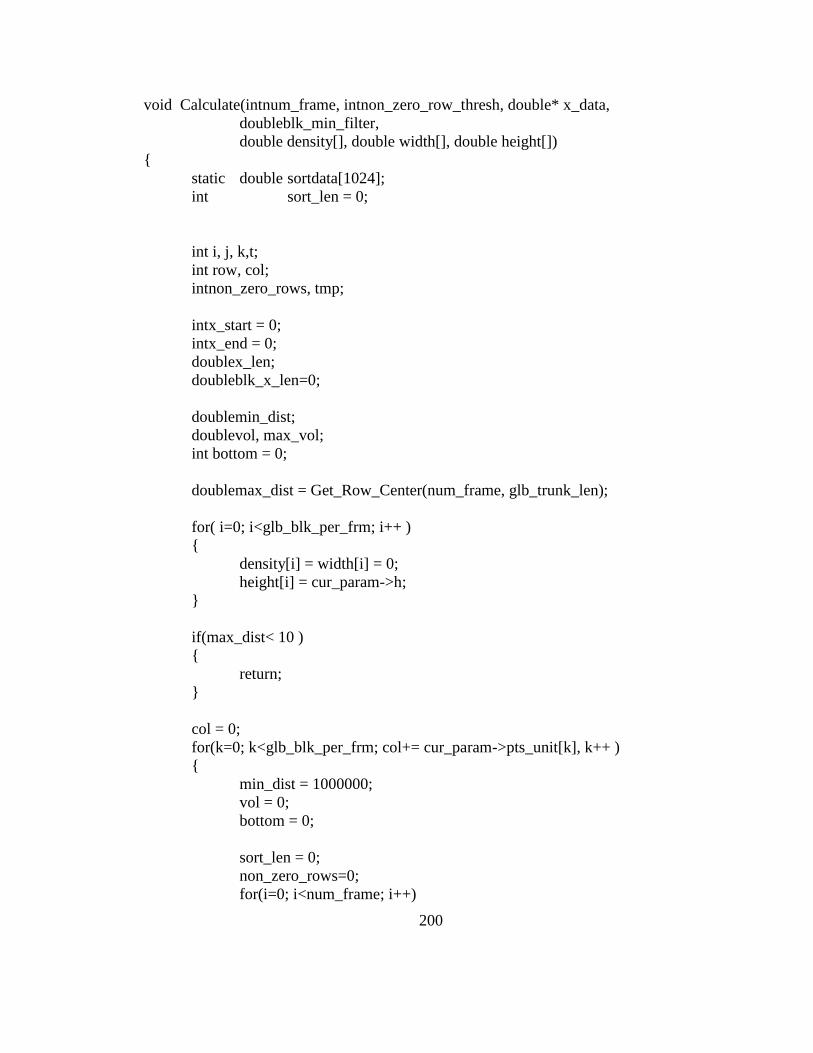
200

void Calculate(intnum_frame, intnon_zero_row_thresh, double* x_data,


double density[], double width[], double height[])

{

static double sortdata[1024];

int sort_len = 0;

int i, j, k,t;

int row, col;

intnon_zero_rows, tmp;

intx_start = 0;

intx_end = 0;

doublex_len;

doubleblk_x_len=0;

doublemin_dist;

doublevol, max_vol;

int bottom = 0;

doublemax_dist = Get_Row_Center(num_frame, glb_trunk_len);

for( i=0; i<glb_blk_per_frm; i++ )

{

density[i] = width[i] = 0;

height[i] = cur_param->h;

}

if(max_dist< 10 )

{

return;

}

col = 0;

for(k=0; k<glb_blk_per_frm; col+= cur_param->pts_unit[k], k++ )

{

min_dist = 1000000;

vol = 0;

bottom = 0;

sort_len = 0;

non_zero_rows=0;


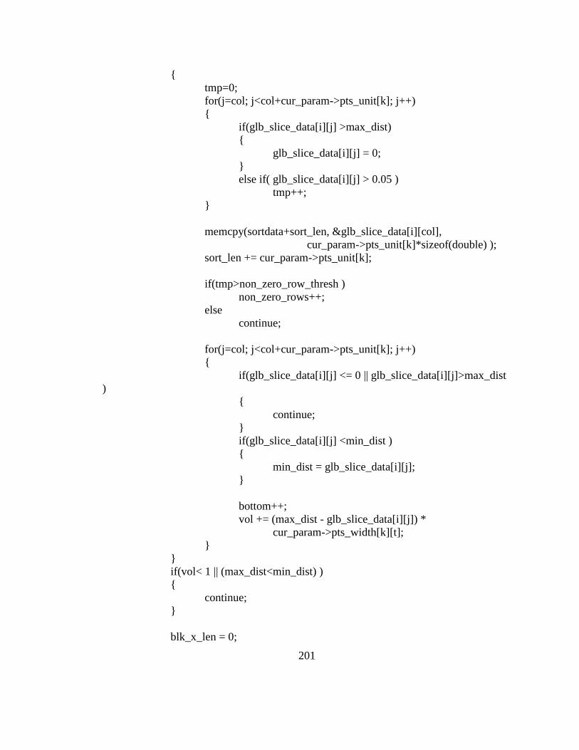
201

{

tmp=0;

for(j=col; j<col+cur_param->pts_unit[k]; j++)

{

if(glb_slice_data[i][j] >max_dist)

{


}

else if( glb_slice_data[i][j] > 0.05 )

tmp++;

}

memcpy(sortdata+sort_len, &glb_slice_data[i][col],

cur_param->pts_unit[k]*sizeof(double) );

sort_len += cur_param->pts_unit[k];

if(tmp>non_zero_row_thresh )

non_zero_rows++;

else

continue;

for(j=col; j<col+cur_param->pts_unit[k]; j++)

{

if(glb_slice_data[i][j] <= 0 || glb_slice_data[i][j]>max_dist

)

{

continue;

}

if(glb_slice_data[i][j] <min_dist )

{

min_dist = glb_slice_data[i][j];

}

bottom++;

vol += (max_dist - glb_slice_data[i][j]) *

cur_param->pts_width[k][t];

}

}

if(vol< 1 || (max_dist<min_dist) )

{

continue;

}

blk_x_len = 0;

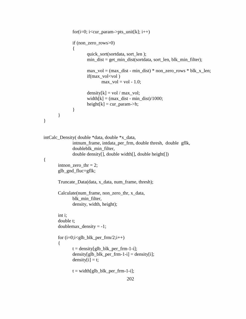
202

for(i=0; i<cur_param->pts_unit[k]; i++)

if (non_zero_rows>0)

{

quick_sort(sortdata, sort_len );

min_dist = get_min_dist(sortdata, sort_len, blk_min_filter);

max_vol = (max_dist - min_dist) * non_zero_rows * blk_x_len;

if(max_vol<vol )

max_vol = vol - 1.0;

density[k] = vol / max_vol;

width[k] = (max_dist - min_dist)/1000;

height[k] = cur_param->h;

}

}

}

intCalc_Density( double *data, double *x_data,

intnum_frame, intdata_per_frm, double thresh, double gflk,


double density[], double width[], double height[])

{

intnon_zero_thr = 2;

glb_gnd_fluc=gflk;

Truncate_Data(data, x_data, num_frame, thresh);

Calculate(num_frame, non_zero_thr, x_data,

blk_min_filter,

density, width, height);

int i;

double t;

doublemax_density = -1;

for (i=0;i<glb_blk_per_frm/2;i++)

{

t = density[glb_blk_per_frm-1-i];

density[glb_blk_per_frm-1-i] = density[i];

density[i] = t;

t = width[glb_blk_per_frm-1-i];

203

width[glb_blk_per_frm-1-i] = width[i];

width[i] = t;

t = height[glb_blk_per_frm-1-i];

height[glb_blk_per_frm-1-i] = height[i];

height[i] = t;

}

return 0;}

Documents

Development of an Intelligent Sprayer to Optimize Pesticide