Embed Size (px)
Citation preview
Development of a Torsion Balance Facility and a search for
Temporal Variations in the Newtonian Gravitational
Constant.
by
Hasnain Panjwani
A thesis submitted to
The University of Birmingham
for the degree of
DOCTOR OF PHILOSOPHY
Astrophysics and Space Research Group
School of Physics and Astronomy
College of Engineering and Physical Sciences
The University of Birmingham
July 2012

University of Birmingham Research Archive
e-theses repository This unpublished thesis/dissertation is copyright of the author and/or third parties. The intellectual property rights of the author or third parties in respect of this work are as defined by The Copyright Designs and Patents Act 1988 or as modified by any successor legislation. Any use made of information contained in this thesis/dissertation must be in accordance with that legislation and must be properly acknowledged. Further distribution or reproduction in any format is prohibited without the permission of the copyright holder.
Abstract
The torsion balance is one of the key pieces of apparatus used in experimental searches
for weak forces. In the search for an understanding of a Unified Theory, physicists have
suggested a number of signatures that are detectable in laboratory measurements.
This thesis describes the development of a new torsion balance facility, relocated from
the BIPM (Bureau International des Poids et Mesures) [1], which has excellent environ-
mental stability and benefits from a new compact interferometric readout for measuring
angular motion which has been characterised and installed onto the torsion balance. The
interferometer has sensitivities of 5 × 10⁻¹¹ radians/√
Hz between 10−1 Hz and 10 Hz,
an angular range of over ±1 and significantly reduces sensitivity to ground tilt. With
the new facility the first experiment searching for temporal variations in the Newtonian
gravitational constant has been undertaken with a null result for δG/G0 for both sidereal
and half sidereal signals at magnitudes greater than 5×10⁻⁶. These results have been used
to set an upper limit on some of the parameters within the Standard Model Extension
framework [2].
The thesis also reports on the design and manufacture of prototype test masses with a
high electron-spin density of approximately 1024 and negligible external magnetic field ≤
10−4T. These test masses can be used within the facility to potentially make it sensitive
enough to conduct future spin-coupling experiments.
Acknowledgements
In the name of God the Beneficial the Merciful.
Firstly I would like to thank Professor Clive. C. Speake for giving me the opportunity
to undertake this work. His support throughout the project but specifically near the
end when things were particularly difficult was much appreciated. I thank him for always
giving me his time even when I randomly turned up outside his office. Secondly my thanks
to Dr. Ludovico Carbone who I had the pleasure of working with for a couple of years. His
knowledge of the apparatus and practicality when undertaking experimental measurements
was an inspiration for me. I can’t thank Ludovico enough for his continued support and
guidance even after his time with this experiment, it will always be remembered. A big
thanks also to Dr. Fabian Pena-Arellano who was greatly supportive during the time of
the interferometer development. I thoroughly enjoyed working with him and hope our
communication will continue into the future. It has also been a pleasure to work with
some of the other colleagues within the group, Dr. Chris Collins, Dr Stuart Aston, Mr
John Bryant and Mr Dave Hoyland all of whom have contributed to this work whether
through discussions or helping with the apparatus. For his help and support during the
many computer failures and for always trying his best to meet some of my difficult requests
I must thank Mr Dave Stops, our computer systems manager.
Finally I cannot forget my parents who have always guided and supported me during this
project and I would like to dedicate this thesis to them - thank you.
Contents
1 Introduction 2
1.1 Lorentz Violation and the SME . . . . . . . . . . . . . . . . . . . . . . . . . 3
1.2 Variation in the Newtonian Gravitational Constant . . . . . . . . . . . . . . 5
1.3 Tests with Polarised Electrons . . . . . . . . . . . . . . . . . . . . . . . . . . 7
2 Experimental Apparatus 9
2.1 The Torsion Balance . . . . . . . . . . . . . . . . . . . . . . . . . . . . . . . 9
2.2 Experimental Procedure . . . . . . . . . . . . . . . . . . . . . . . . . . . . . 14
2.3 Vacuum System . . . . . . . . . . . . . . . . . . . . . . . . . . . . . . . . . . 14
2.4 Optical Sensors . . . . . . . . . . . . . . . . . . . . . . . . . . . . . . . . . . 17
2.5 Environmental Controls . . . . . . . . . . . . . . . . . . . . . . . . . . . . . 18
2.5.1 Thermal Stability . . . . . . . . . . . . . . . . . . . . . . . . . . . . 18
2.5.2 Tilt . . . . . . . . . . . . . . . . . . . . . . . . . . . . . . . . . . . . 20
2.6 Data Acquisition . . . . . . . . . . . . . . . . . . . . . . . . . . . . . . . . . 21
3 Spin Test Masses 23
3.1 Magnetism - A brief introduction . . . . . . . . . . . . . . . . . . . . . . . . 23
3.2 Previous Test Mass Designs . . . . . . . . . . . . . . . . . . . . . . . . . . . 30
3.3 New Test Mass Design . . . . . . . . . . . . . . . . . . . . . . . . . . . . . . 31
3.3.1 Test Mass Geometry . . . . . . . . . . . . . . . . . . . . . . . . . . . 33
3.3.2 Magnetic Materials . . . . . . . . . . . . . . . . . . . . . . . . . . . . 36
3.4 Magnetostatic Analysis . . . . . . . . . . . . . . . . . . . . . . . . . . . . . 36
ii
Contents iii
3.4.1 FEA Software and Preliminary Studies . . . . . . . . . . . . . . . . 37
3.4.2 Analysis of test compensated masses . . . . . . . . . . . . . . . . . . 38
3.5 Final Design and manufacture . . . . . . . . . . . . . . . . . . . . . . . . . . 43
3.5.1 Material determination . . . . . . . . . . . . . . . . . . . . . . . . . 46
3.5.2 Dimension Design . . . . . . . . . . . . . . . . . . . . . . . . . . . . 47
3.5.3 Spin Content . . . . . . . . . . . . . . . . . . . . . . . . . . . . . . . 50
3.5.4 Manufactured Prototype . . . . . . . . . . . . . . . . . . . . . . . . . 54
4 Iliad - Angle Interferometric Device 56
4.1 Basics of Optical Interferometry . . . . . . . . . . . . . . . . . . . . . . . . 57
4.2 Mirror Tilt Immunity and the Cat’s Eye Retroreflector . . . . . . . . . . . . 59
4.3 ILIAD - Innovative Laser Interferometric Angular Device . . . . . . . . . . 59
4.4 Experimental Realisation . . . . . . . . . . . . . . . . . . . . . . . . . . . . 63
4.5 Performance Characterisation . . . . . . . . . . . . . . . . . . . . . . . . . . 67
4.5.1 Dynamical Angular Range . . . . . . . . . . . . . . . . . . . . . . . . 68
4.5.2 Device Calibration . . . . . . . . . . . . . . . . . . . . . . . . . . . . 69
4.5.3 Linearity Tests . . . . . . . . . . . . . . . . . . . . . . . . . . . . . . 71
4.5.4 Angular Sensitivity . . . . . . . . . . . . . . . . . . . . . . . . . . . . 74
4.6 Iliad on the Torsion Balance . . . . . . . . . . . . . . . . . . . . . . . . . . . 82
4.7 Conclusions . . . . . . . . . . . . . . . . . . . . . . . . . . . . . . . . . . . . 82
5 Data Analysis and Systematics 85
5.1 Data Collection and Conversion . . . . . . . . . . . . . . . . . . . . . . . . . 85
5.2 Least Squares Fit . . . . . . . . . . . . . . . . . . . . . . . . . . . . . . . . . 87
5.3 Expected Torque Model . . . . . . . . . . . . . . . . . . . . . . . . . . . . . 90
5.4 Temperature Systematic . . . . . . . . . . . . . . . . . . . . . . . . . . . . . 91
5.5 Tilt Systematic . . . . . . . . . . . . . . . . . . . . . . . . . . . . . . . . . . 91
6 Results 95
Contents iv
7 Conclusion and Discussion 100
7.1 δG/G Results . . . . . . . . . . . . . . . . . . . . . . . . . . . . . . . . . . . 100
7.2 Summary . . . . . . . . . . . . . . . . . . . . . . . . . . . . . . . . . . . . . 102
References 104
References . . . . . . . . . . . . . . . . . . . . . . . . . . . . . . . . . . . . . . . . 104
Appendices 112
A Magnetic Properties for SmCo5 and Nd2Fe14B final pieces 113
B CAD Drawings of Iliad mechanical holder 118
List of Figures
1.1 Sun-centred reference frame[3] . . . . . . . . . . . . . . . . . . . . . . . . . . 6
2.1 Current best angular sensitivity of the balance (red). . . . . . . . . . . . . . 13
2.2 Image of core torsion balance apparatus. . . . . . . . . . . . . . . . . . . . . 15
2.3 Image of torsion strip before installation into the apparatus. . . . . . . . . . 15
2.4 Image of Torsion Balance apparatus within the inner foam box. . . . . . . . 16
2.5 Source Mass position calibration showing the pendulum mean angle as a
function of source mass position. The two blue lines signify the positions
of maximum deflection, ≈ ±18.8. . . . . . . . . . . . . . . . . . . . . . . . 17
2.6 Temperature change of experiment over typical 50 hr timescale. . . . . . . . 19
2.7 Tilt output before control (blue), after control (red) . . . . . . . . . . . . . 21
2.8 High Pass Filter. . . . . . . . . . . . . . . . . . . . . . . . . . . . . . . . . . 22
2.9 Integrator Control Loop. . . . . . . . . . . . . . . . . . . . . . . . . . . . . . 22
3.1 Spin-Orbit interaction vector model[4] . . . . . . . . . . . . . . . . . . . . . 25
3.2 Application of Hund’s rule to find the ground state multiplet of Sm3++ ion 27
3.3 Typical permenant magnet hysteresis curve, image from [5] . . . . . . . . . 29
3.4 Demagnetisation curve for bonded Nd2Fe14B MPQ-14-12. . . . . . . . . . . 30
3.5 University of Washington spin pendulum [6]. Upper Left: top view of single
’puck’, arrows signify the relative densities and direction of magnetisation.
The net spin moment points to the right. Lower right: assembled pendulum
of 4 pucks. Arrows show direction of B field. . . . . . . . . . . . . . . . . . 32
v
List of Figures vi
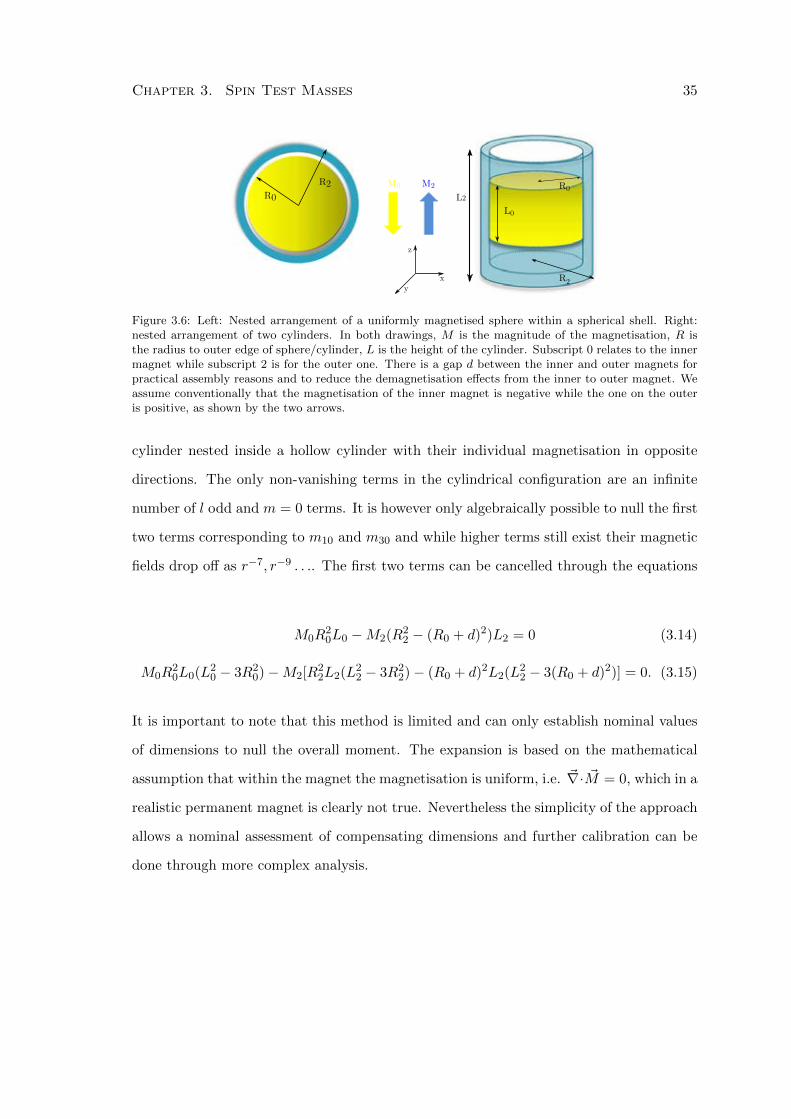
3.6 Left: Nested arrangement of a uniformly magnetised sphere within a spher-
ical shell. Right: nested arrangement of two cylinders. In both drawings,
M is the magnitude of the magnetisation, R is the radius to outer edge
of sphere/cylinder, L is the height of the cylinder. Subscript 0 relates to
the inner magnet while subscript 2 is for the outer one. There is a gap d
between the inner and outer magnets for practical assembly reasons and to
reduce the demagnetisation effects from the inner to outer magnet. We as-
sume conventionally that the magnetisation of the inner magnet is negative
while the one on the outer is positive, as shown by the two arrows. . . . . . 35
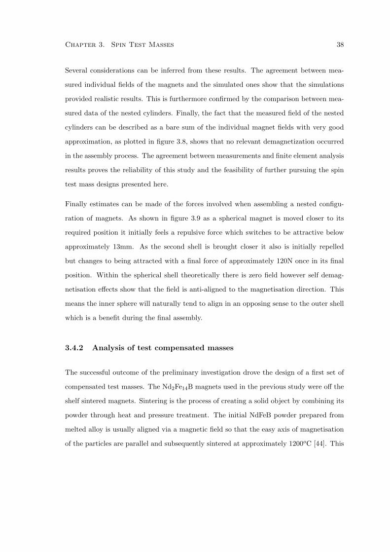
3.7 Field measurements in z direction (black dots) at varying distances along
magnet symmetry axis compared with results from FEMM software (red) . 39
3.8 (Left)Field measurements in z direction (black dots) at varying distances
along nested assembly symmetry axis compared with linear sum of individ-
ual field measurements (magenta) and FEMM estimates (green). (Right)Zoom
in of previous plot at its knee. . . . . . . . . . . . . . . . . . . . . . . . . . . 39
3.9 Plot of forces (as a function of axial distance between centres) and torques
acting on the magnets. Top left: force acting on the solid inner sphere
as it is brought towards the bottom hemisphere of the shell (final design
dimensions). Top right: force on the top hemisphere as it is brought to-
wards the assembled inner sphere + bottom hemisphere (final design di-
mensions). Bottom left: torque on the sphere, surrounded by the spherical
shell, as function of the angle between the magnetic moments. (This data
has been obtained using the software ANSYS(TM) [7] for a smaller com-
pensated sphere than the final design). Bottom right: force on inner solid
cylinder as it is brought towards hollow one (m10 bonded cylinder test di-
mensions. . . . . . . . . . . . . . . . . . . . . . . . . . . . . . . . . . . . . . 40
List of Figures vii
3.10 FEMM estimates of Bz field around final test mass assembly. Colourmap
is an order of magnitude value in units of Tesla. . . . . . . . . . . . . . . . . 42
3.11 Comparison of measurements and theoretical estimates from FEMM simu-
lations and multipole moment expansion of axial Bz field. . . . . . . . . . . 42
3.12 Cumulative plot showing contribution of multipole moments to total axial
Bz field. . . . . . . . . . . . . . . . . . . . . . . . . . . . . . . . . . . . . . . 42
3.13 FEMM estimates of Bz field around final test mass assembly, Outer radius
is 26.98mm. Colourmap is an order of magnitude value in units of Tesla. . . 49
3.14 Crystal structure SmCo5 (Image from [8]). Two layers of the Co(2c) site
atoms (blue) sandwich the Co(3g) atoms (green). The Sm atoms lie in the
middle of the hexagons (red) . . . . . . . . . . . . . . . . . . . . . . . . . . 51
3.15 Images of final test mass pieces. . . . . . . . . . . . . . . . . . . . . . . . . . 55
4.1 Michelson Interferometer Schematic . . . . . . . . . . . . . . . . . . . . . . 58
4.2 Iliad Optical Layout (The image is inverted to its operational orientation.
The second arm of the layout has also been visually removed.) . . . . . . . 60
4.3 One arm of Iliad optical layout . . . . . . . . . . . . . . . . . . . . . . . . . 61
4.4 Iliad optical layout front . . . . . . . . . . . . . . . . . . . . . . . . . . . . . 61
4.5 CAD images of Iliad assembly . . . . . . . . . . . . . . . . . . . . . . . . . . 64
4.6 Photographs of machined mechanical holder pieces . . . . . . . . . . . . . . 65
4.7 Image of aligned device on bench top during performance tests. . . . . . . . 66
4.8 Iliad mechanical holder installed into the torsion balance apparatus (centre).
Image taken before all optics aligned. . . . . . . . . . . . . . . . . . . . . . . 67
4.9 Setup for measuring dynamic range of Iliad. Central mirror is rotated out
to the limits of Iliad sensitivity and the angle is independently measured by
an optical level using a He-Ne laser. . . . . . . . . . . . . . . . . . . . . . . 69
4.10 Visibility of Iliad output as a function of mirror rotation angle. . . . . . . . 70
List of Figures viii
4.11 Method of assessing linearity. Left: Plot of raw and corrected Lissajous
pattern. Centre: Typical mirror movement tracked by autocollimator and
Iliad. Right: Data from autocollimator plotted against Iliad and the fit. . . 71
4.12 Setup for measuring linearity at large rotation angles. Size of angle between
Iliad and test mirror exaggerated for visual purposes. He-Ne laser, via
optical lever method, used to measure this angle. . . . . . . . . . . . . . . . 73
4.13 Photo of setup for measuring linearity at large rotation angles. The mirror
and He-Ne laser used to independently measure the Iliad angle is not shown
here. . . . . . . . . . . . . . . . . . . . . . . . . . . . . . . . . . . . . . . . . 73
4.14 Calibration factor of Iliad repeated 14 times at the sweet spot. Mean =
0.9960, Std = 1.3 × 10⁻³ . . . . . . . . . . . . . . . . . . . . . . . . . . . . 74
4.15 Calibration factor as a function of mirror distance. Sweet spot is at 59mm . 75
4.16 Calibration factor as a function of mirror angle. . . . . . . . . . . . . . . . . 75
4.17 Lissajous patterns for differing input intensity using the old photodiode
subtraction method and the new intensity rejection method . . . . . . . . . 79
4.18 Sensitivity of Iliad and its components. Blue - Iliad Device with rigid mirror,
Green - Laser and photodiode setup through USB ADC, Brown - Laser and
photodiode setup through new module box, Orange - Intrinsic electronic
noise of USB ADC, Purple - Intrinsic electronic noise of new module box.
Note: New electronics module has internal filter producing the roll off above
50Hz. . . . . . . . . . . . . . . . . . . . . . . . . . . . . . . . . . . . . . . . 81
4.19 Calibration on Torsion Balance. Left: Example of windowing of time se-
ries data. Centre: Linear Calibration coefficients for each window. Right:
Histogram of residuals from mean calibration coefficient and Gaussian fit. . 83
4.20 Calibration factor with respect to Iliad angle on Torsion Balance. Red:
Torsion Balance Data. Blue: Theoretical using eq 4.11 . . . . . . . . . . . . 83
List of Figures ix
5.1 Schematic example of autocollimator output before and after adjusting for
rotation. . . . . . . . . . . . . . . . . . . . . . . . . . . . . . . . . . . . . . . 86
5.2 Experimental data from top, motor position, pendulum torque, tilt X read-
ing, tilt Y reading. All data have been interpolated to the same timebase.
Green points signify the time while the source masses are stationary. Red
dots are the average of these points (excluding 25 seconds from the start
and 5 seconds from the end.) . . . . . . . . . . . . . . . . . . . . . . . . . . 88
5.3 Tilt readings showing the impulse felt by the table, particularly noticeable
in the tilt X, when the motor moves. . . . . . . . . . . . . . . . . . . . . . . 92
5.4 Tilt calibration run. Top: output data of torque points from the autocol-
limaotr (blue) and Iliad (orange), middle: tilt X readings, bottom: tilt Y
readings. . . . . . . . . . . . . . . . . . . . . . . . . . . . . . . . . . . . . . . 93
6.1 δG/G0 amplitudes of autocollimator data. Top: full 55 day data set, bot-
tom: Approximately 1500 data points and a dummy sidereal fit (red) for
comparison. Error bars removed for visual purposes. . . . . . . . . . . . . . 96
6.2 Spectrum of torque amplitude for each data set individually. Green line is
the position of the sidereal frequency. . . . . . . . . . . . . . . . . . . . . . . 96
7.1 Torsion Balance angular sensitivity when motor running (red) and when
it was not (black). The noise at the 800 second signal frequency is more
than an order of magnitude higher when the motor is modulating the source
masses. . . . . . . . . . . . . . . . . . . . . . . . . . . . . . . . . . . . . . . 101
A.1 Demagnetisation Curve for SmCo5 material used for the inner sphere. . . . 114
A.2 Demagnetisation Curve for bonded Nd2Fe14B material, MQP-14-12, used
for the outer shells. . . . . . . . . . . . . . . . . . . . . . . . . . . . . . . . . 115
A.3 Magnetic Moment measurements of final SmCo5 sphere made by MPUSA[9].116

List of Figures x
A.4 Magnetic Moment measurements of final bonded Nd2Fe14B half shells made
by MPUSA[9]. . . . . . . . . . . . . . . . . . . . . . . . . . . . . . . . . . . 117
B.1 CAD drawing of front piece housing two 45 beam splitters and cat’s eyes. . 119
B.2 CAD drawing of back piece housing the interfering optics and the photodi-
odes. The template with grooves to position optics is a separate piece fixed
onto the back part. . . . . . . . . . . . . . . . . . . . . . . . . . . . . . . . . 120
B.3 CAD drawing of collimator kinematic mount which screws onto the top of
the front part. . . . . . . . . . . . . . . . . . . . . . . . . . . . . . . . . . . . 121
List of Tables
2.1 Positions of 9 PT100 RTDs. . . . . . . . . . . . . . . . . . . . . . . . . . . . 20
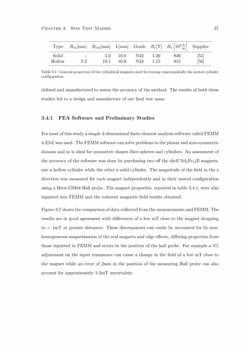
3.1 General properties of the cylindrical magnets used for testing experimen-
tally the nested cylinder configuration. . . . . . . . . . . . . . . . . . . . . . 37
3.2 Dimensions of m10 and m30 compensated bonded magnets. . . . . . . . . . 41
3.3 Nominal magnetic properties of final test mass materials. In the FEMM
designs a non-linear B-H profile was used. . . . . . . . . . . . . . . . . . . . 49
3.4 Dimensions of final test mass design. . . . . . . . . . . . . . . . . . . . . . . 49
3.5 Summary of moment contributions for each material. . . . . . . . . . . . . . 54
3.6 Summary of spin content for different pendulum designs. Our torsion bal-
ance can hold up to 4.8kg thus reported is the upper limit. . . . . . . . . . 54
5.1 Estimated systematic effects from to apparatus tilt. Parameters as per
equation 5.12. Coefficient errors are obtained from the calibration test run
oscillating the Y axis tilt every 20 hours. Estimated sidereal amplitudes
obtained by fitting sidereal sinusoid to full experimental data set. . . . . . . 94
6.1 Fit coefficients for sidereal signal. Errors reported include those from both
statistical and systematic uncertainties . . . . . . . . . . . . . . . . . . . . . 97
1
Chapter 1
Introduction
General Relativity (GR) and the Standard Model (SM) are two giants within modern
physics. The strong, weak and electromagnetic interactions are described through the
exchange of quantum particles while gravity is explained through the classical curvature
of spacetime. Independently they have withstood a number of experimental tests. However
attempts to combine both theories to explain all interactions have been unsuccessful. It
is thought that both are low-energy limits of a more fundamental unified theory which is
expected to merge the fundamental forces at the Planck scale, mp ≈ 1019 GeV. Although
experimentally verifying physics at these scales is currently out of our reach probing some
of the low-energy signatures of candidate theories are possible.
This thesis describes the development of an experimental facility benefiting from good
environmental stability and which can be used to search for some of the signatures as-
sociated with new theories of quantum gravity. The heart of the apparatus is a torsion
balance, a device which has been used in a variety of scientific endeavours [10] since its first
construction in 1777 and is described in chapter 2. Torsion balances, if well balanced, can
be free from serious seismic interference and, due to its orthogonal relationship, the signal
of interest is decoupled from the Earth’s gravitational force. This makes it very sensitive
in detecting small perturbations occurring from new non-Newtonian physics or Lorentz
violating effects. In recent years the apparatus has been used in tests of the equivalence
2
Chapter 1. Introduction 3
principle, short-range tests of the gravitational inverse-square law and searches for new
types of interacting particles [11]. Some of the theoretical motivations for using a torsion
balance are described later in this chapter.
Chapter 3 and Chapter 4 outline two novel additions to the apparatus. The first is
the development of a test mass containing a large number of aligned electrons. This
test mass can be used to probe some of the spin dependent effects predicted by new
theories and potentially make the facility sensitive to set new limits on these forces. The
second is a new interferometer to measure angles with an immunity to the orthogonal tilt.
The interferometer has been assembled, characterised and installed into the facility and
subsequently used when undertaking the first experimental campaign looking for temporal
changes in the Newtonian gravitational constant.
1.1 Lorentz Violation and the SME
The combination of SM and GR currently provide a highly successful description of na-
ture. However there are some situations where even these theories break down. Both are
unable to describe phenomena at high energies such as just after the Big Bang while also
not always being compatible. GR is a classical theory which does not describe quantum
phenomena but it can be used to predict effects on short length scales, for example, pre-
dicting a singularity at the centre of a black hole. The SM is a quantum field theory which
should therefore be able to accurately describe short distance physics. However it cannot,
in its present form, explain these black hole singularities. It is therefore expected that
a more fundamental theory exists incorporating a quantum description of gravity. Some
of the more successful candidates are string theory and loop quantum gravity. In 1989
Kostelecky and Samuel [12, 13] showed that natural mechanisms for Lorentz symmetry
breaking exist in unified theories at the Planck scale. Lorentz symmetry is a postulate
Chapter 1. Introduction 4
requiring experimental results to be independent of the orientation or boost velocity of
the laboratory through space. This idea, that physics is the same for all observers, is the
basis of GR and is a key feature of the Standard Model used to classify certain particles
and their interaction within groups. These violations of Lorentz symmetry in the early
Universe would manifest today as small relic background fields interacting with elemen-
tary particles causing them to have a preferred direction in space. In 1998 Colladay and
Kostelecky [14] developed the Standard Model Extension (SME) which aimed to catalogue
and predict observable signatures in various types of low-energy experiments. The SME
includes all the predictions of the Standard Model and is also observer Lorentz invariant,
which means that the laws of physics are the same for all inertial observers. However
the SME is not invariant to particle Lorentz symmetry which describes the movement of
particles with respect to a fixed inertial frame. This means that the physical properties of
a particle, such as its energy and momentum, will change as the motion or spin orientation
of the particle changes with respect to the background field. The SME provides a generic
framework and formalism for the interpretation and comparison of various types of ex-
periments. Various theoretical and experimental results so far have been published in the
Lorentz and CPT violation data tables [15]. To date a large number of different tests have
been carried out to search for leading order signals of Lorentz violation. Although there
have been no signs of violation these tests have set stringent limits on the SME parameters.
For example, in the neutron sector, Brown et al. [16] use a K-3He co-magnetometer to look
at neutron spin interactions with the background field setting a limit for the equatorial
components of |bn⊥| < 3.7× 10⁻³³ GeV at the 68% confidence level. In the photon sector
several tests have set limits through Michelson-Morley type experiments. Using a rotating
cryogenic sapphire oscillator Hohensee et al. [17] have constrained κtr with a precision of
7.4 × 10⁻⁹. Torsion balances have also been used to set limits on parameters within the
electron sector. Heckel et al. [6] used a novel spin pendulum to search for preferred frame
interactions with electron spin. They set stringent limits on the b and d parameters of ≈
Chapter 1. Introduction 5
10−31 GeV and 10−27 GeV respectively.
1.2 Variation in the Newtonian Gravitational Constant
The SME also provides the framework for a large number of gravitational matter couplings
in the presence of Lorentz violation. Kostelecky and Tasson [2] have outlined a general
approach to the search for possible signals within a number of scenarios. In the laboratory
these signals can take the form of a time variation of the Newtonian gravitational constant,
GN , for measurements of gravitational acceleration, or, time-varying differences in the
coefficients associated with different matter when undertaking Weak EP tests. The original
aim of our torsion balance apparatus was to conduct precision measurements of GN which
intrinsically lends itself to a search for these Lorentz violating effects. The Lagrangian
in the SME includes the conventional Newtonian kinetic and potential terms along with
corrections that depend on extra coefficients. In a laboratory the force acting in the z
direction on a test particle is given by [2]
Fz = −mT g
[1 +
2α
mT(aTeff )t +
2α
mS(aSeff )t) + (cT )tt + (cS) +
3
2stt +
1
2ztz
], (1.1)
where aTeff and aSeff are 4-vector coupling to the species of fermion with T and S being
the test and sources masses respectively while m is their effective inertial mass. With our
experimental apparatus we are only sensitive to the first two corrective terms [18].
The SME uses a standardised Sun-centred co-ordinate system [19]. For a laboratory fixed
to the Earth the standard frame (t, x, y, z) is such that the x axis points south, the y
axis points east and the z axis points vertically upwards. In the Sun-centred system
(T⊕,X,Y ,Z), the X axis points along the direction from the centre of the Earth towards
the Sun at the vernal equinox and the Z axis is aligned with the rotation axis of the Earth.
The time T⊕ is taken when the laboratory y axis coincides with the Sun-centred Y axis.
Chapter 1. Introduction 6
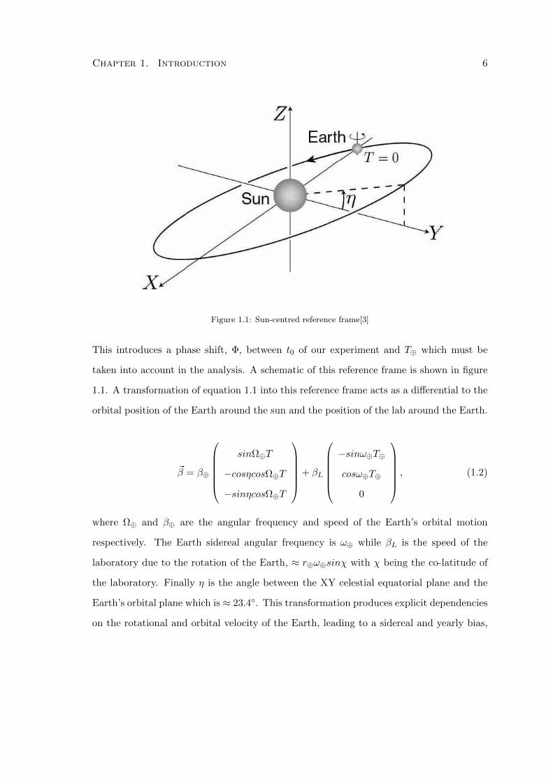
Figure 1.1: Sun-centred reference frame[3]
This introduces a phase shift, Φ, between t0 of our experiment and T⊕ which must be
taken into account in the analysis. A schematic of this reference frame is shown in figure
1.1. A transformation of equation 1.1 into this reference frame acts as a differential to the
orbital position of the Earth around the sun and the position of the lab around the Earth.
~β = β⊕
sinΩ⊕T
−cosηcosΩ⊕T
−sinηcosΩ⊕T
+ βL
−sinω⊕T⊕
cosω⊕T⊕
0
, (1.2)
where Ω⊕ and β⊕ are the angular frequency and speed of the Earth’s orbital motion
respectively. The Earth sidereal angular frequency is ω⊕ while βL is the speed of the
laboratory due to the rotation of the Earth, ≈ r⊕ω⊕sinχ with χ being the co-latitude of
the laboratory. Finally η is the angle between the XY celestial equatorial plane and the
Earth’s orbital plane which is ≈ 23.4. This transformation produces explicit dependencies
on the rotational and orbital velocity of the Earth, leading to a sidereal and yearly bias,
Chapter 1. Introduction 7
δG in the measurement of the gravitational constant
~δG
G' −2α
(∑w
NTwa
wJ
MT+∑
w
NSwa
wJ
MS
)(~β), (1.3)
where N is the number of fermions and J refers to the spatial coordinates in the Sun-
centred frame.
An initial run of our experiment has set the first experimental limits on these parameters
[20, 21] and we hope modifications to the apparatus explained in this thesis will improve
these results.
1.3 Tests with Polarised Electrons
The SME also provides mechanisms for the interaction between intrinsic electron spin and
a Lorentz violating background field which breaks rotational symmetry. This potential
is developed in the SME when taking the electron coupling terms in the non-relativistic
limit appropriate for torsion-balance experiments as
Ve = −~σ · ~be (1.4)
where σ is the spin of the electron and be is the combination of CPT-even and CPT-odd
parameters. Torsion balance experiments can be conducted through measuring sidereal
torque perturbations on spin test masses. Recently measurements on this interaction have
been carried out by Hou et al. [22] and Heckel et al. [6] with the most stringent limits on
the strength of this interaction being set by the latter of 10−31 GeV.
There is also a large amount of theoretical work considering the role of spin in gravity, for
a review see [23]. A number of experiments have therefore set out to probe some of these
Chapter 1. Introduction 8
interactions specifically in the electron sector, some of which use torsion balances. Moody
and Wilczek [24] discuss the forces produced by the exchange of low-mass spin-0 parti-
cles and describe two spin-dependent interactions. Firstly a ‘monopole-dipole’ interaction
between polarised electrons and an unpolarised atom
V (r) = h(gSgP )σ · r
8πMP
[1
λr+
1
r2
]e−r/λ, (1.5)
where λ is the range of interaction, σh/2 is the spin of the electron, gP and gS are the
coupling constants at the polarised and unpolarised particles respectively, Mp is the mass
of the polarised particle and r is the distance between interacting particles. Similarly a
second ‘dipole-dipole’ interaction involving two sets of polarised electrons can be given by
V (r) =h(g1P g
2P )
16πM1PM
2P
[( ~σ1 · ~σ2)
(1
λr2+
1
r3+
4
3π∂3r
)
−( ~σ1 · r)( ~σ2 · r)(
1
λ2r+
3
λr2+
3
r3δ3r
)e−r/λ
], (1.6)
where definitions are the same as before. Recently Dobrescu and Mocioiu [25] have clas-
sified the kinds of potentials that might arise from the exchange of low-mass bosons,
constrained only by rotational and translational invariance. Experiments already con-
ducted searching for these types of interactions include Ritter et al. in 1993 [26], Ni et
al. in 1999 [27] and Heckel et al. in 2008 [6] who used traditional torsion balances while
Hammond et al. in 2007/2008 modified the apparatus to use a superconducting levitating
torsion balance setup [28, 29].
The experimental search for these spin dependent interactions in the electron sector was
the motivation towards the development of a new spin-test mass as described in chapter
3.
Chapter 2
Experimental Apparatus
This chapter describes the torsion balance facility set up in order to undertake experimen-
tal campaigns and make precision measurements giving insights into some of the suggested
theoretical signals. The heart of the facility is the torsion balance itself, particularly the
use of a torsion strip which has been used and described in previous measurements. Here,
we summarise the main advantages of this setup and the various other items of apparatus
used to develop the whole experimental facility. The two main upgrades, the spin test
masses and the angular sensor are discussed in detail in chapters 3 and 4 respectively.
2.1 The Torsion Balance
Although the torsion balance concept is now widely used in multiple disciplines with
differing designs [10], the setup for this experiment has remained largely similar to the
original design. A suspension, usually a round fibre or in this case a strip, is used to
support a load and is extremely sensitive to lateral deflections, specifically its torsional
mode. The equation of motion for a torsion pendulum can be given as
τ(t) = Iθ(t) + βθ(t) + kθ(t) (2.1)
9
Chapter 2. Experimental Apparatus 10
where τ(t) is an external torque, I is the pendulum moment of inertia, β is any viscous
damping constant, k is the torsion constant of the suspension material and θ is the angle
of deflection. Usually torsion balance experiments are conducted within a vacuum so as to
minimise the gas damping β term, although there are still internal sources of dissipation[30,
31, 32, 33].
The internal dissipation in materials can be approximated as an extension of Hooke’s law
with a complex spring constant,
knew = −k(1 + iφ) (2.2)
where φ is a lag term indicating that the response of the material will lag the torque
applied. In many cases this lag is frequency independent [33, 34] and by comparing to a
viscous effect can be given as the reciprocal of the quality factor, i.e. φ = 1/Q.
We can define the pendulum’s transfer function by converting equation 2.1 into the fre-
quency domain
τ(ω) =θ(ω)
H(ω)(2.3)
with H(ω) being the transfer function given as
H(ω) = (k(1− (ω/ω0)2 + i/Q))−1 (2.4)
where ω0 = 2πf0 =√k/I is the pendulum’s resonance and Q is the mechanical quality
factor. The maximum torque sensitivity of a pendulum is reached when limited by intrinsic
thermal noise of the system. This limit can be derived by using the fluctuation dissipation
theorem [30]
Chapter 2. Experimental Apparatus 11
S1/2τth
=
√4kBT
k
ωQ(2.5)
where kB is the Boltzmann constant and T is the temperature. When designing a torsion
pendulum the intrinsic thermal noise can be reduced by increasing the Q and reducing
the stiffness, k. However, for example, it is not just a simple case of making the sus-
pension thinner, thus reducing the stiffness, since this also reduces the suspendable load
and subsequently the detectable signal. Ultimately the problem lies in the signal to noise
ratio where various trade-offs must be considered depending on the type of experiment
one wishes to undertake.
The apparatus and torsion pendulum design for this facility was originally developed by
Quinn et al. for measurements of the gravitational constant, G [35, 36, 1]. The design
is based on a torsion strip being the suspension system as opposed to the more common
circular cross section fibre. The torsion strip was chosen for two major benefits with
detailed descriptions given in [35, 36, 37]. The torsion constant of a strip with width b,
thickness t and length L, where L b t is given by
ks =bt3F
3L+Mgb2
12L(2.6)
where F is the modulus of rigidity, M the loaded mass and g the local acceleration due to
gravity. This is in contrast to the equation for a round fibre given by
kw =πr4F
2L+Mgr2
2L(2.7)
where r is the radius of the wire. In wide, heavily loaded strips, the torsion constant is
dominated by the gravitation term which is not a function of the strip’s elastic properties
and confirmed to be lossless [37]. This means, strips are not subject to significant anelastic
Chapter 2. Experimental Apparatus 12
effects and its associated noise as circular fibres are and thus leads to a higher Qpend of
the system since
Qpend = Qelastkelast
kgrav + kelast(2.8)
where subscript ‘elast’ signifies the elastic contribution and ‘grav’, the gravitational con-
tribution [38]. Secondly the possible load on the strip is a function of its dimensions which
can be adjusted such as to increase the load and thus any detection signal without the
need to increase the stiffness in the same way as a round fibre. This benefit can be shown
by comparing the signal to noise ratios of the strip and wire
snstripsnwire
=
(3
2π
b
t
)1/2
(2.9)
which in the case of our current torsion strip is over a factor of 6 better. There is also a
further benefit in that any experimental modulation can be done at a higher frequency,
due to a higher pendulum resonance frequency, thus taking advantage of the lower noise.
The increased stiffness does however mean a smaller deflection angle for any equivalent
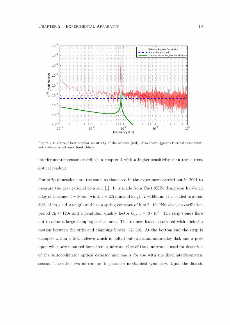
torque. Figure 2.1 shows the theoretical thermal noise angular sensitivity of the balance,
obtained by using the transfer function to convert from torque to angle, and its current
best sensitivity after carefully mounting the system and ensuring proper experimental
conditions, for example; no ground loops, proper levelling of the table and stable vacuum
pressure. Also plotted is the intrinsic limit of autocollimator, one of our optical sensors,
obtained by placing a fixed mirror infront of the device. Clearly at higher frequencies
we are limited by the optical readout and with further environmental control this may
also be the case at lower frequencies. In order to therefore take advantage of the torsion
strip setup and achieve an overall performance that is closer to the thermal noise limit
a higher-resolution detector is required. This is one of the major drives to develop the
Chapter 2. Experimental Apparatus 13
10−4
10−3
10−2
10−1
100
10−11
10−10
10−9
10−8
10−7
10−6
10−5
10−4
10−3
S1/
2 (ra
dian
s/√H
z)
Frequency (Hz)
Balance Angular SensitivityAutocollimator LimitThermal Noise Angular Sensitivity
Figure 2.1: Current best angular sensitivity of the balance (red). Also shown (green) thermal noise limitautocollimator intrinsic limit (blue)
interferometric sensor described in chapter 4 with a higher sensitivity than the current
optical readout.
Our strip dimensions are the same as that used in the experiment carried out in 2001 to
measure the gravitational constant [1]. It is made from Cu-1.8%Be dispersion hardened
alloy of thickness t = 30µm, width b = 2.5 mm and length L=160mm. It is loaded to about
80% of its yield strength and has a spring constant of k ≈ 2 · 10−4Nm/rad, an oscillation
period T0 ≈ 120s and a pendulum quality factor Qpend ≈ 3 · 105. The strip’s ends flare
out to allow a large clamping surface area. This reduces losses associated with stick-slip
motion between the strip and clamping blocks [37, 39]. At the bottom end the strip is
clamped within a BeCu sleeve which is bolted onto an aluminium-alloy disk and a post
upon which are mounted four circular mirrors. One of these mirrors is used for detection
of the Autocollimator optical detector and one is for use with the Iliad interferometric
sensor. The other two mirrors are in place for mechanical symmetry. Upon the disc sit
Chapter 2. Experimental Apparatus 14
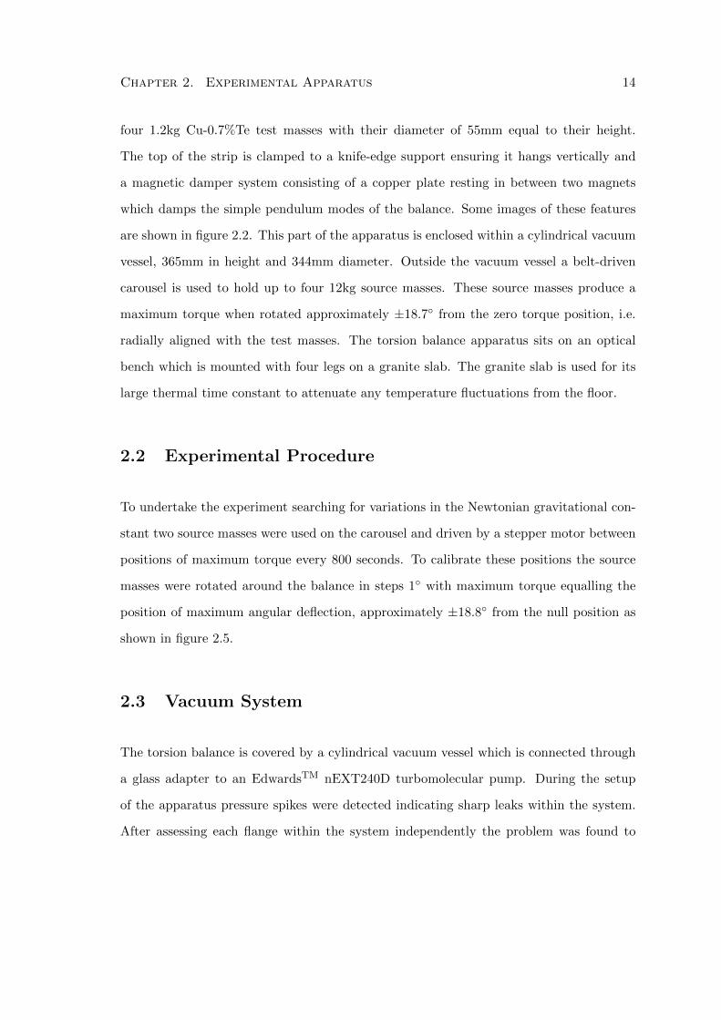
four 1.2kg Cu-0.7%Te test masses with their diameter of 55mm equal to their height.
The top of the strip is clamped to a knife-edge support ensuring it hangs vertically and
a magnetic damper system consisting of a copper plate resting in between two magnets
which damps the simple pendulum modes of the balance. Some images of these features
are shown in figure 2.2. This part of the apparatus is enclosed within a cylindrical vacuum
vessel, 365mm in height and 344mm diameter. Outside the vacuum vessel a belt-driven
carousel is used to hold up to four 12kg source masses. These source masses produce a
maximum torque when rotated approximately ±18.7 from the zero torque position, i.e.
radially aligned with the test masses. The torsion balance apparatus sits on an optical
bench which is mounted with four legs on a granite slab. The granite slab is used for its
large thermal time constant to attenuate any temperature fluctuations from the floor.
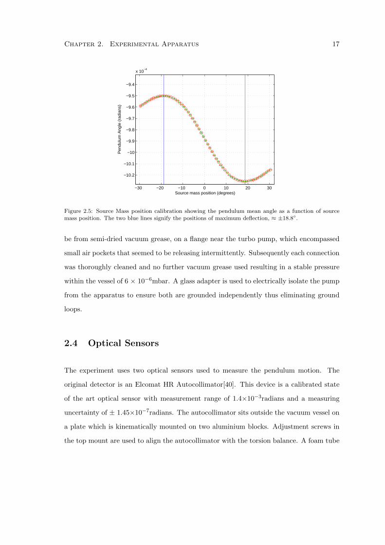
2.2 Experimental Procedure
To undertake the experiment searching for variations in the Newtonian gravitational con-
stant two source masses were used on the carousel and driven by a stepper motor between
positions of maximum torque every 800 seconds. To calibrate these positions the source
masses were rotated around the balance in steps 1 with maximum torque equalling the
position of maximum angular deflection, approximately ±18.8 from the null position as
shown in figure 2.5.
2.3 Vacuum System
The torsion balance is covered by a cylindrical vacuum vessel which is connected through
a glass adapter to an EdwardsTM nEXT240D turbomolecular pump. During the setup
of the apparatus pressure spikes were detected indicating sharp leaks within the system.
After assessing each flange within the system independently the problem was found to
Chapter 2. Experimental Apparatus 15
Test Masses
Base Plate
Knife Edge Support
Torsion Strip and Mirrors
Copper plate for magnetic dampers
Figure 2.2: Image of core torsion balance apparatus.
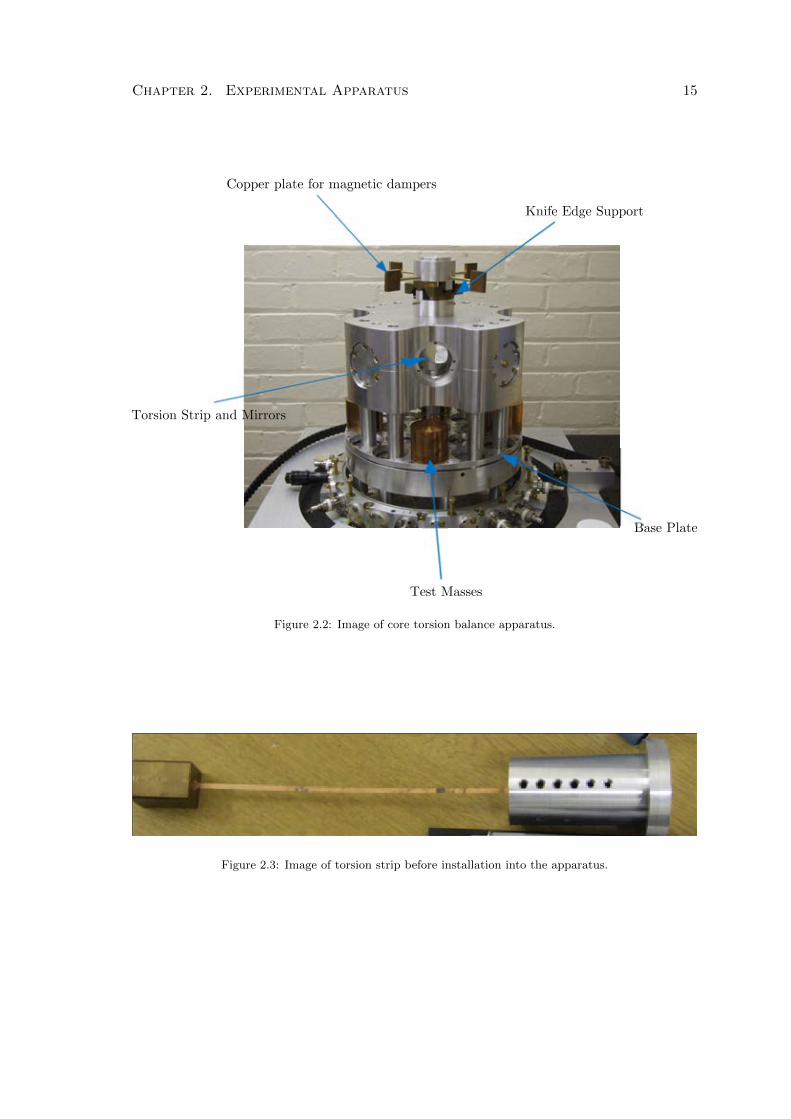
Figure 2.3: Image of torsion strip before installation into the apparatus.
Chapter 2. Experimental Apparatus 16
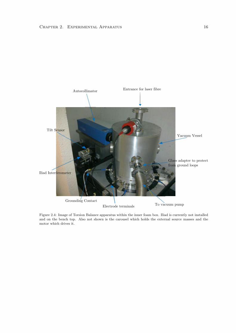
Electrode terminalsTo vacuum pump
Vacuum Vessel
Grounding Contact
Iliad Interferometer
Tilt Sensor
AutocollimatorEntrance for laser fibre
Glass adapter to protect
from ground loops
Figure 2.4: Image of Torsion Balance apparatus within the inner foam box. Iliad is currently not installedand on the bench top. Also not shown is the carousel which holds the external source masses and themotor which drives it.
Chapter 2. Experimental Apparatus 17
−30 −20 −10 0 10 20 30
−10.2
−10.1
−10
−9.9
−9.8
−9.7
−9.6
−9.5
−9.4
x 10−4
Source mass position (degrees)
Pen
dulu
m A
ngle
(ra
dian
s)
Figure 2.5: Source Mass position calibration showing the pendulum mean angle as a function of sourcemass position. The two blue lines signify the positions of maximum deflection, ≈ ±18.8.
be from semi-dried vacuum grease, on a flange near the turbo pump, which encompassed
small air pockets that seemed to be releasing intermittently. Subsequently each connection
was thoroughly cleaned and no further vacuum grease used resulting in a stable pressure
within the vessel of 6 × 10⁻⁶mbar. A glass adapter is used to electrically isolate the pump
from the apparatus to ensure both are grounded independently thus eliminating ground
loops.
2.4 Optical Sensors
The experiment uses two optical sensors used to measure the pendulum motion. The
original detector is an Elcomat HR Autocollimator[40]. This device is a calibrated state
of the art optical sensor with measurement range of 1.4×10⁻³radians and a measuring
uncertainty of ± 1.45×10⁻⁷radians. The autocollimator sits outside the vacuum vessel on
a plate which is kinematically mounted on two aluminium blocks. Adjustment screws in
the top mount are used to align the autocollimator with the torsion balance. A foam tube
Chapter 2. Experimental Apparatus 18
encloses the air between the autocollimator and the vacuum vessel to reduce noise from
air turbulence affecting the detection of the reflected LED light. On a static mirror the
autocollimator has a sensitivity limit of 5× 10⁻⁹rad/√Hz which corresponds to approx-
imately 9 × 10⁻¹³Nm/√Hz when used with our torsion balance system. This is almost
four times higher than the thermal noise of the balance. The size of the autocollimator
also requires it to be mounted externally to the vacuum vessel and torsion balance setup.
This makes it susceptible to differential motion, due to thermal and other effects, which
may introduce noise into the data. For both these reasons a second optical readout has
been developed and is described in detail in chapter 4.
2.5 Environmental Controls
For any precision measurement it is important to ensure the environment does not intro-
duce sources of noise into the data. Periodic changes in parameters such as the tempera-
ture and tilt of the apparatus will be detected as a false signal from the torsion balance.
For example a temperature oscillation may change the properties of the strip reducing
or increasing its amplitude of deflection. If this temperature change happens at similar
frequencies to the signal we are searching for, i.e. daily, it will be very difficult to de-
couple this environmental effect from any real one. This section describes some of the
efforts taken to ensure that these disturbances are measured and minimised, especially on
timescales associated with our signal.
2.5.1 Thermal Stability
The temperature is monitored by a number of PT100 resistance temperature detectors
(RTD) placed at various points around the laboratory as listed in table 2.5.1. Temperature
changes within the system may be detected by the readout originating from two effects.
Chapter 2. Experimental Apparatus 19
0 5 10 15 20 25 30 35 40 45 50−0.2
−0.15
−0.1
−0.05
0
0.05
0.1
0.15
0.2
Time [hours]
∆Tem
p [K
]
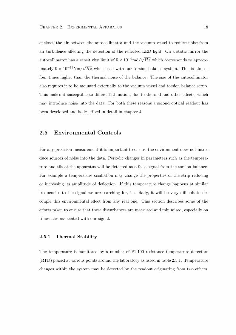
Figure 2.6: Temperature change of experiment over typical 50 hr timescale. Black: Air temperatureof laboratory, Cyan: Air temperature of outer foam layer, Green: Air temperature of inner foam layer,Magenta: Temperature of butterfly piece inside vacuum, Yellow: Temperature of autocollimator mount.
An apparent motion will be seen due to a drift in the output caused by physical thermal
changes, for example the expansion of the autocollimator mount mimicking a change in the
torsion balance equilibrium angle. The other more subtle, but real, effect is due to changes
to the properties of the torsion strip which may increase or decrease its deflection angle.
To mitigate these effects the apparatus was enclosed in two layers of thermal shielding
made of foam panels. A thermally stable water bath [41] pumps water through copper
pipes welded to a large copper plate. This thermally controlled plate was initially designed
to be heat-sunk to the optical bench to regulate its temperature. However it was found
that mechanical noise from the flow of water coupled into the balance. The plate was
thus placed onto the granite slab and used to radiatively regulate the air temperature
within the inner thermal box. The stabilised water is also pumped in parallel to a heat
exchanger located in between the inner and outer thermal boxes. Fans are used to pass
the air through the heat exchanger and stabilise the air temperature of the outer box.
This system results in an attenuation between any change in the room temperature and
the inner box by a factor of almost 10 as shown in figure 2.6 where the temperature inside
the vacuum vessel has not fluctuated by more than 0.03K. Over much longer periods we
did not notice a change in the temperature of more than a peak-to-peak of 0.1K.
Chapter 2. Experimental Apparatus 20
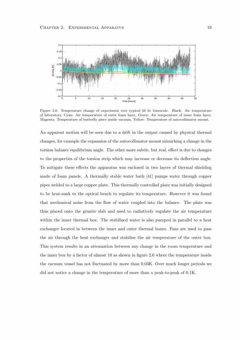
Number Position Standard Colour when plotted
1 Middle of optical table Red2 Front leg of table Blue3 Inner Box air Green4 Inside Vacuum Magenta5 Room air Black6 End leg of table Orange7 Copper pipes Grey8 Autocollimator stand Yellow9 Outer box air Cyan
Table 2.1: Positions of 9 PT100 RTDs.
2.5.2 Tilt
An Applied Geomechanics 755 miniature tilt sensor mounted on the optical bench mea-
sures the tilt, in two orthogonal axis, of the experimental setup. We found that along
the long axis of the optical bench there was a daily oscillation in the tilt signal. In the
summer months the peak-to-peak oscillation was approximately 4µradian over 24 hours
and approximately 1µradian in the winter months. This effect is most likely due to the
heating and cooling of the building from the day/night cycles. To compensate for this
daily variation which may mimic a gravitational signal a stack of piezo electric discs were
fitted in between the optical bench and the granite slab. These piezos were driven by a
PID controlled high voltage power supply which adjusted the supplied voltage depending
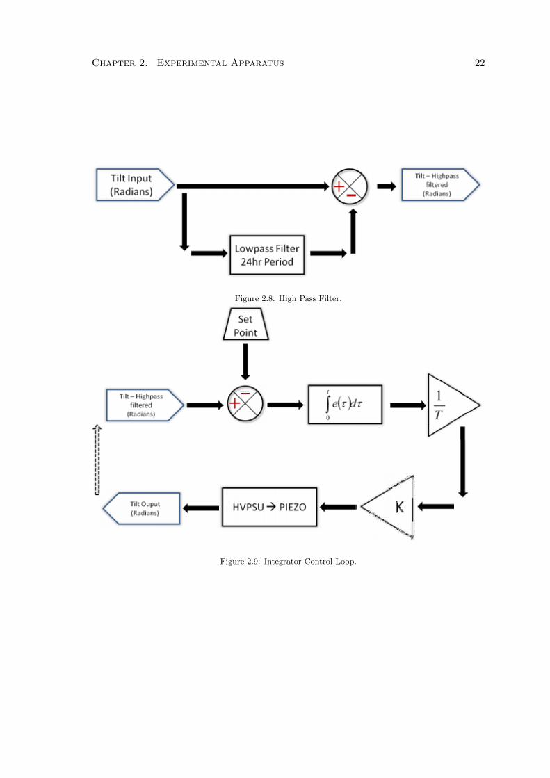
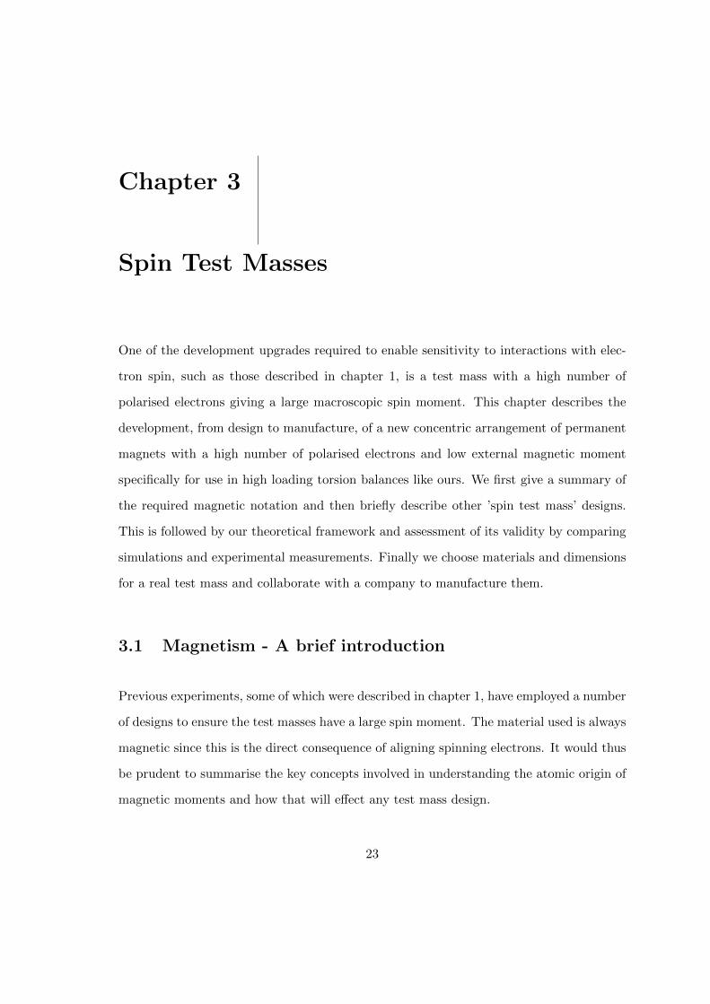
on the tilt monitored by the tilt sensor. A schematic of the control loop is shown in figure
2.7. There are two stages to the control loop. Initially, to ensure the piezo stays within
its operating range, the long term drift in the tilt is discarded by high-pass filtering. This
is done, as shown in figure 2.8, by averaging over a 24 hour period and subtracting this
from the original data. The filtered tilt readings are subsequently sent to the second stage,
shown in figure 2.9. Here the input is compared to the setpoint, in our case zero, and the
error logged in an integrator buffer. The time constant is given by the parameter T , set
for 700 seconds, while the gain for conversion to voltage is given by K. Data from the
Chapter 2. Experimental Apparatus 21
0 20 40 60 80 100 120 140−8
−6
−4
−2
0
2x 10
−6
Time [hours]
Tilt
[rad
ians
]
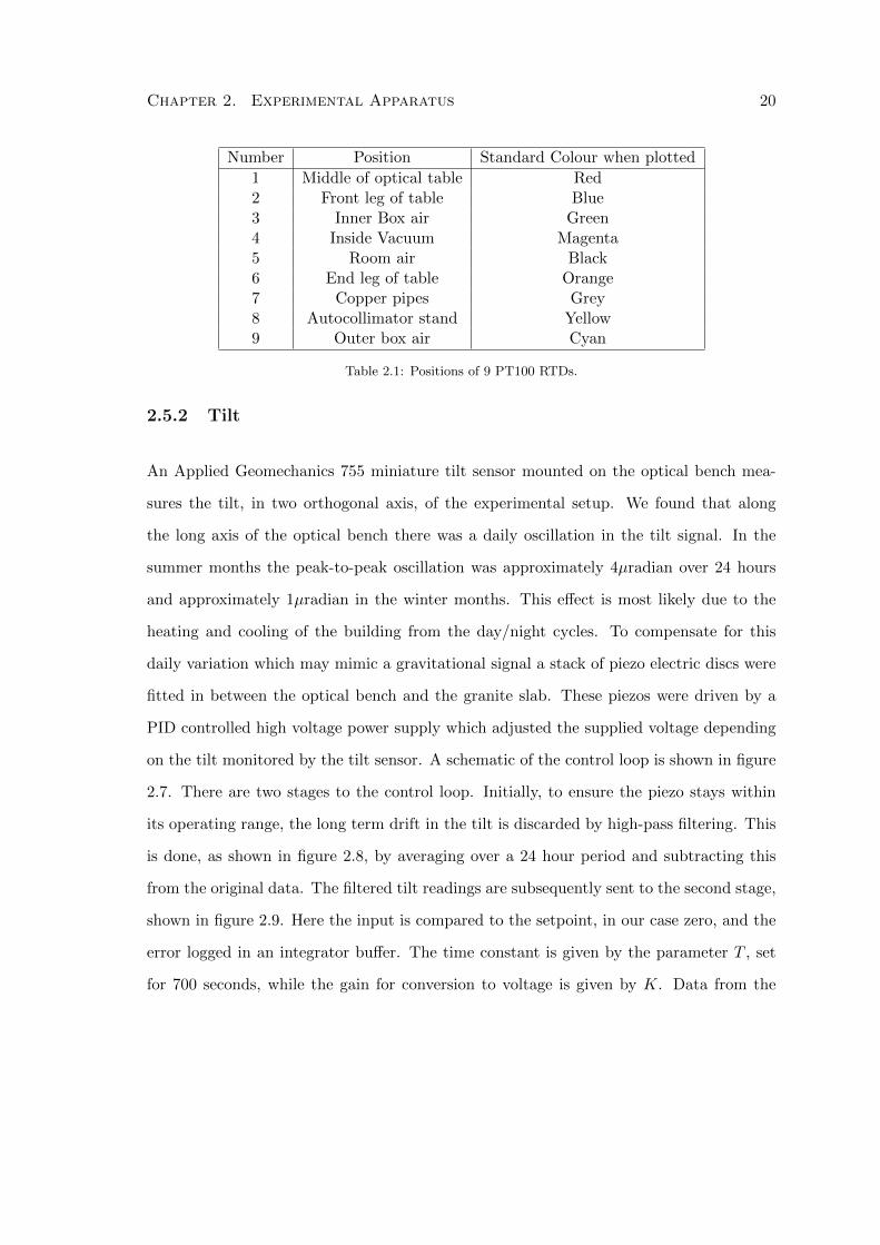
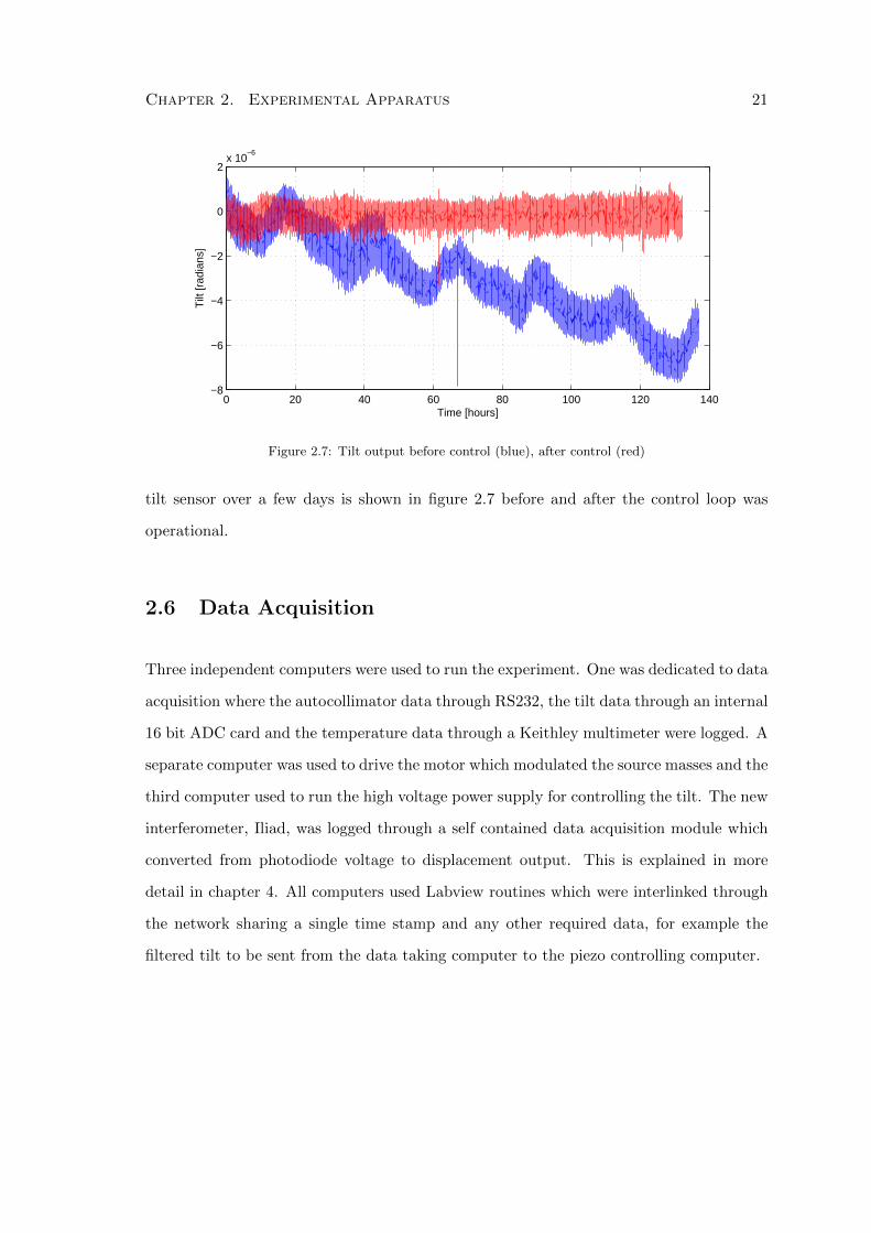
Figure 2.7: Tilt output before control (blue), after control (red)
tilt sensor over a few days is shown in figure 2.7 before and after the control loop was
operational.
2.6 Data Acquisition
Three independent computers were used to run the experiment. One was dedicated to data
acquisition where the autocollimator data through RS232, the tilt data through an internal
16 bit ADC card and the temperature data through a Keithley multimeter were logged. A
separate computer was used to drive the motor which modulated the source masses and the
third computer used to run the high voltage power supply for controlling the tilt. The new
interferometer, Iliad, was logged through a self contained data acquisition module which
converted from photodiode voltage to displacement output. This is explained in more
detail in chapter 4. All computers used Labview routines which were interlinked through
the network sharing a single time stamp and any other required data, for example the
filtered tilt to be sent from the data taking computer to the piezo controlling computer.
Chapter 2. Experimental Apparatus 22
Figure 2.8: High Pass Filter.
Figure 2.9: Integrator Control Loop.
Chapter 3
Spin Test Masses
One of the development upgrades required to enable sensitivity to interactions with elec-
tron spin, such as those described in chapter 1, is a test mass with a high number of
polarised electrons giving a large macroscopic spin moment. This chapter describes the
development, from design to manufacture, of a new concentric arrangement of permanent
magnets with a high number of polarised electrons and low external magnetic moment
specifically for use in high loading torsion balances like ours. We first give a summary of
the required magnetic notation and then briefly describe other ’spin test mass’ designs.
This is followed by our theoretical framework and assessment of its validity by comparing
simulations and experimental measurements. Finally we choose materials and dimensions
for a real test mass and collaborate with a company to manufacture them.
3.1 Magnetism - A brief introduction
Previous experiments, some of which were described in chapter 1, have employed a number
of designs to ensure the test masses have a large spin moment. The material used is always
magnetic since this is the direct consequence of aligning spinning electrons. It would thus
be prudent to summarise the key concepts involved in understanding the atomic origin of
magnetic moments and how that will effect any test mass design.
23
Chapter 3. Spin Test Masses 24
A quantum mechanical treatment of atoms leads to information on the energy levels as-
sociated with the electrons that are characterised by four quantum numbers, n, l,ml,ms.
The principal quantum number, n, determines the electron shell and defines its energy.
The orbital angular momentum, l, describes the angular momentum of the orbital motion
and equals h√l(l + 1). The final two numbers describe the orbital angular momentum and
spin angular momentum of one component of the total. According to the Pauli exclusion
principle the states of two electrons are characterised by different sets of quantum number.
The magnetic moment of an individual electron from its angular momentum around the
nucleus, µL, can be derived as the product of a circular current, I, around a closed area
δA, ~µL = I · δ ~A. The current is a function of electron velocity, v, and radius from the
nucleus, r, such that I = −ep·r2mer2
. The moment is therefore
~µL =−e2me
~L, (3.1)
where e is the charge on an electron and me is the electron mass. The value −e2me
h is known
as the Bohr magneton, the natural unit for electronic magnetism, µB. A constant can be
defined called the gyromagnetic ratio
γ =e
2me= ge
µBh, (3.2)
where ge is known as the Lande g-factor associated with the quantum nature of the elec-
tron. The gyromagnetic ratio defines the angular velocity for Larmour precession where
the magnetic moment will precess around an homogeneous magnetic field as ~ω = γ ~B. The
moment in the z-component can therefore be written as
µlz = −γmlh = −glµBml, (3.3)
Chapter 3. Spin Test Masses 25
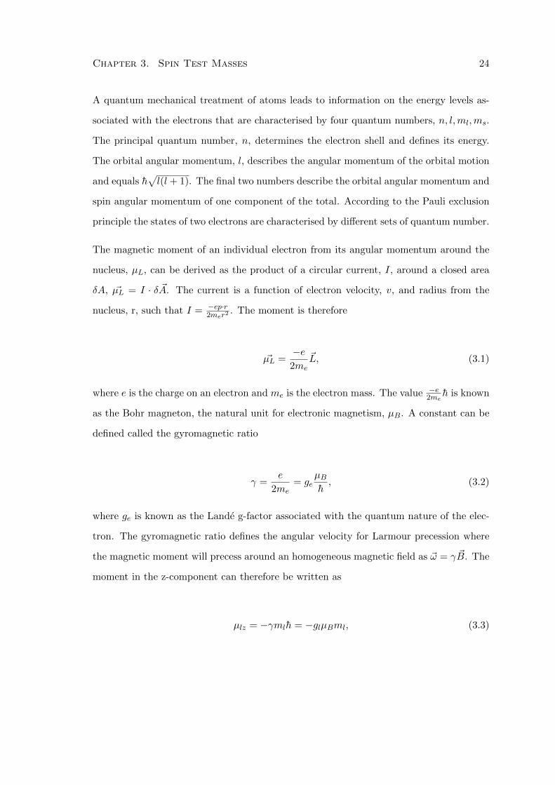
Figure 3.1: Spin-Orbit interaction vector model[4]
where the value ml can take up to (2l + 1) integral values. For the orbital moment
the value of the g-factor is equivalent to 1. A further magnetic moment also exists and
is associated with the intrinsic spin angular momentum of the electron with quantum
number ms = ±1/2.
µsz = gsµBmsh. (3.4)
The g-factor for spin, gs, is approximately equal to 2 [42] and has been extensively mea-
sured. It is associated with the quantum nature of the electron and is predicted very
accurately by quantum electrodynamics (QED). A vector model of this is shown in figure
3.1.
Both the orbital and spin motions of the electrons can be taken together to form a resultant
total angular momentum vector. This type of coupling is known as the Russell-Saunders
interaction and has been proved to be applicable to most magnetic atoms [43]
~J = ~L+ ~S, (3.5)
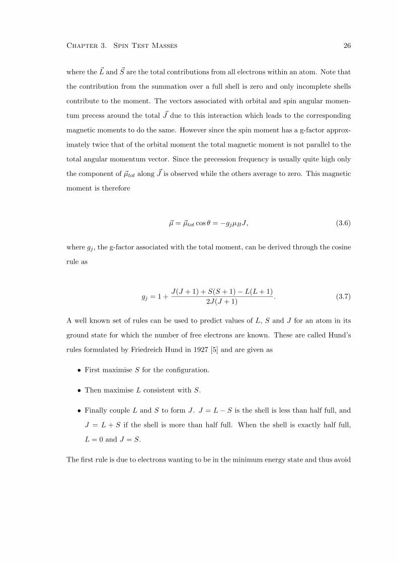
Chapter 3. Spin Test Masses 26
where the ~L and ~S are the total contributions from all electrons within an atom. Note that
the contribution from the summation over a full shell is zero and only incomplete shells
contribute to the moment. The vectors associated with orbital and spin angular momen-
tum precess around the total ~J due to this interaction which leads to the corresponding
magnetic moments to do the same. However since the spin moment has a g-factor approx-
imately twice that of the orbital moment the total magnetic moment is not parallel to the
total angular momentum vector. Since the precession frequency is usually quite high only
the component of ~µtot along ~J is observed while the others average to zero. This magnetic
moment is therefore
~µ = ~µtot cos θ = −gjµBJ, (3.6)
where gj , the g-factor associated with the total moment, can be derived through the cosine
rule as
gj = 1 +J(J + 1) + S(S + 1)− L(L+ 1)
2J(J + 1). (3.7)
A well known set of rules can be used to predict values of L, S and J for an atom in its
ground state for which the number of free electrons are known. These are called Hund’s
rules formulated by Friedreich Hund in 1927 [5] and are given as
• First maximise S for the configuration.
• Then maximise L consistent with S.
• Finally couple L and S to form J . J = L− S is the shell is less than half full, and
J = L + S if the shell is more than half full. When the shell is exactly half full,
L = 0 and J = S.
The first rule is due to electrons wanting to be in the minimum energy state and thus avoid
Chapter 3. Spin Test Masses 27
ml= 3
2
1
0
-1
-2
-3
L=5S=5/2J=5/2
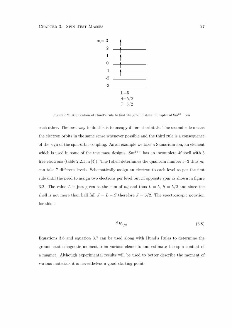
Figure 3.2: Application of Hund’s rule to find the ground state multiplet of Sm3++ ion
each other. The best way to do this is to occupy different orbitals. The second rule means
the electron orbits in the same sense whenever possible and the third rule is a consequence
of the sign of the spin-orbit coupling. As an example we take a Samarium ion, an element
which is used in some of the test mass designs. Sm3++ has an incomplete 4f shell with 5
free electrons (table 2.2.1 in [4]). The f shell determines the quantum number l=3 thus ml
can take 7 different levels. Schematically assign an electron to each level as per the first
rule until the need to assign two electrons per level but in opposite spin as shown in figure
3.2. The value L is just given as the sum of ml and thus L = 5, S = 5/2 and since the
shell is not more than half full J = L− S therefore J = 5/2. The spectroscopic notation
for this is
6H5/2 (3.8)
Equations 3.6 and equation 3.7 can be used along with Hund’s Rules to determine the
ground state magnetic moment from various elements and estimate the spin content of
a magnet. Although experimental results will be used to better describe the moment of
various materials it is nevertheless a good starting point.
Chapter 3. Spin Test Masses 28
The interaction between many atoms in a solid gives rise to different magnetic effects. One
of these effects is a persistent magnetic field which keeps an ordering within the materials’
electrons. These materials are called permanent magnets and include iron, nickel, cobalt
and alloys of rare-earth metals. We will briefly give here a description of the mechanism
and established nomenclature associated with permanent magnets since they will be of
use in the later sections.
A good description of the various types of modern permanent magnets can be found in
[43, 44, 45]. Principal materials used today are AlNiCo (which are a family of ferromagnetic
alloys composed mainly of Aluminium, Nickel and Cobalt), Ferrites, chemical compounds
consisting of ceramic materials with iron(III) oxide (Fe2O3) as their principal component
and rare-earth alloys mixing with cobalt or iron base. These permanent magnets are
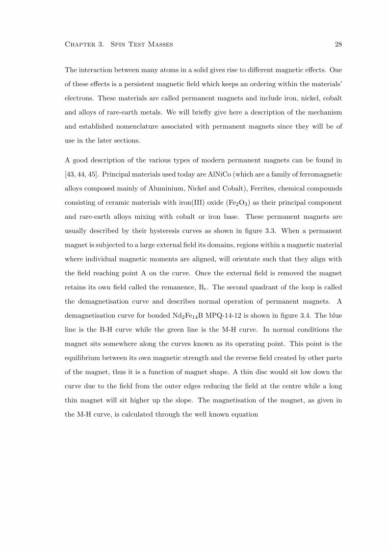
usually described by their hysteresis curves as shown in figure 3.3. When a permanent
magnet is subjected to a large external field its domains, regions within a magnetic material
where individual magnetic moments are aligned, will orientate such that they align with
the field reaching point A on the curve. Once the external field is removed the magnet
retains its own field called the remanence, Br. The second quadrant of the loop is called
the demagnetisation curve and describes normal operation of permanent magnets. A
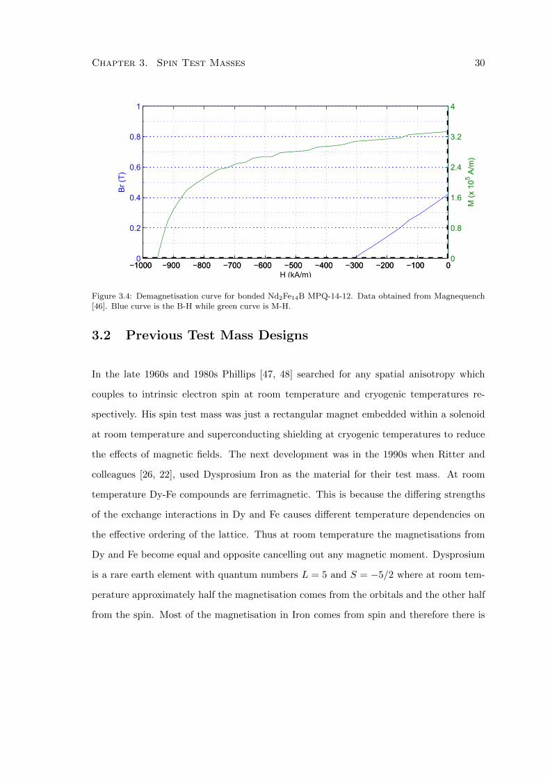
demagnetisation curve for bonded Nd2Fe14B MPQ-14-12 is shown in figure 3.4. The blue
line is the B-H curve while the green line is the M-H curve. In normal conditions the
magnet sits somewhere along the curves known as its operating point. This point is the
equilibrium between its own magnetic strength and the reverse field created by other parts
of the magnet, thus it is a function of magnet shape. A thin disc would sit low down the
curve due to the field from the outer edges reducing the field at the centre while a long
thin magnet will sit higher up the slope. The magnetisation of the magnet, as given in
the M-H curve, is calculated through the well known equation
Chapter 3. Spin Test Masses 29
Figure 3.3: Typical permenant magnet hysteresis curve, image from [5]
~B = µ0( ~H + ~M). (3.9)
The point the B-H curve crosses the x-axis is known as the coercivity of the magnet, the
reverse field required to render its magnetic flux, B, to zero. However this is just a mere
cancellation of the two fields and does not affect the internal magnetisation properties.
The point the M-H curve crosses the x-axis is more important and is known as its intrinsic
coercivity, Hci. This is the reverse field necessary to intrinsically demagnetise the material
after which it will not return to a previous state. The intrinsic coercivity is important
when choosing a magnetic material as it will define the maximum field the outer magnet
in our design can withstand and guides the choice of both internal and external magnet
size.
Chapter 3. Spin Test Masses 30
−1000 −900 −800 −700 −600 −500 −400 −300 −200 −100 00
0.2
0.4
0.6
0.8
1
Br
(T)
−1000 −900 −800 −700 −600 −500 −400 −300 −200 −100 00
0.8
1.6
2.4
3.2
4
H (kA/m)
M (
x 1
05
A/m
)
Figure 3.4: Demagnetisation curve for bonded Nd2Fe14B MPQ-14-12. Data obtained from Magnequench[46]. Blue curve is the B-H while green curve is M-H.
3.2 Previous Test Mass Designs
In the late 1960s and 1980s Phillips [47, 48] searched for any spatial anisotropy which
couples to intrinsic electron spin at room temperature and cryogenic temperatures re-
spectively. His spin test mass was just a rectangular magnet embedded within a solenoid
at room temperature and superconducting shielding at cryogenic temperatures to reduce
the effects of magnetic fields. The next development was in the 1990s when Ritter and
colleagues [26, 22], used Dysprosium Iron as the material for their test mass. At room
temperature Dy-Fe compounds are ferrimagnetic. This is because the differing strengths
of the exchange interactions in Dy and Fe causes different temperature dependencies on
the effective ordering of the lattice. Thus at room temperature the magnetisations from
Dy and Fe become equal and opposite cancelling out any magnetic moment. Dysprosium
is a rare earth element with quantum numbers L = 5 and S = −5/2 where at room tem-
perature approximately half the magnetisation comes from the orbitals and the other half
from the spin. Most of the magnetisation in Iron comes from spin and therefore there is
Chapter 3. Spin Test Masses 31
a net spin moment. Their test mass was approximately 29g in mass and contained about
9×10²² spins.
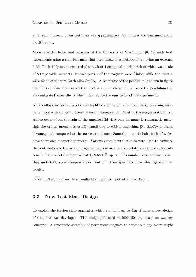
More recently Heckel and collegues at the University of Washington [6, 49] undertook
experiments using a spin test mass that used shape as a method of removing an external
field. Their 107g mass consisted of a stack of 4 octagonal ‘pucks’ each of which was made
of 8 trapezoidal magnets. In each puck 4 of the magnets were Alnico, while the other 4
were made of the rare-earth alloy SmCo5. A schematic of the pendulum is shown in figure
3.5. This configuration placed the effective spin dipole at the centre of the pendulum and
also mitigated other effects which may reduce the sensitivity of the experiment.
Alnico alloys are ferromagnetic and highly coercive, can with stand large opposing mag-
netic fields without losing their intrinsic magnetisation. Most of the magnetisation from
Alnico occurs from the spin of the unpaired 3d electrons. In many ferromagnetic mate-
rials the orbital moment is usually small due to orbital quenching [5]. SmCo5 is also a
ferromagnetic composed of the rare-earth element Samarium and Cobalt, both of which
have their own magnetic moments. Various experimental studies were used to estimate
the contribution to the overall magnetic moment arising from orbital and spin components
concluding in a total of approximately 9.6×10²² spins. This number was confirmed when
they undertook a gyrocompass experiment with their spin pendulum which gave similar
results.
Table 3.5.3 summarises these results along with our potential new design.
3.3 New Test Mass Design
To exploit the torsion strip apparatus which can hold up to 5kg of mass a new design
of test mass was developed. This design published in 2009 [50] was based on two key
concepts. A concentric assembly of permanent magnets to cancel out any macroscopic
Chapter 3. Spin Test Masses 32
4 Pucks of SmCo5
4 Pucks of Alnico
Figure 3.5: University of Washington spin pendulum [6]. Upper Left: top view of single ’puck’, arrowssignify the relative densities and direction of magnetisation. The net spin moment points to the right.Lower right: assembled pendulum of 4 pucks. Arrows show direction of B field.
Chapter 3. Spin Test Masses 33
magnetic moment and the use of different materials with varying ratios of orbital and spin
contribution. This section will describe the steps undertaken to confirm such a design
while the next section will explain the manufacturing process.
3.3.1 Test Mass Geometry
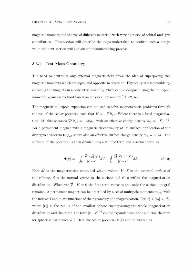
The need to neutralise any external magnetic field drove the idea of superposing two
magnetic moments which are equal and opposite in direction. Physically this is possible by
enclosing the magnets in a concentric assembly which can be designed using the multipole
moment expansion method based on spherical harmonics [51, 52, 53].
The magnetic multipole expansion can be used to solve magnetostatic problems through
the use of the scalar potential such that ~H = −~∇ΦM . Where there is a fixed magnetisa-
tion, ~M , this becomes ∇2ΦM = −4πρM with an effective charge density ρM = −~∇ · ~M .
For a permanent magnet with a magnetic discontinuity at its surface, application of the
divergence theorem to ρM shows also an effective surface charge density σM = ~n · ~M . The
solution of the potential is then divided into a volume term and a surface term as
Φ(~r) = −∫V
~∇′ · ~M(~r′)
|~r − ~r′|dV +
∮s
~M(~r) · ~n′(~r′)|~r − ~r′|
dS. (3.10)
Here ~M is the magnetisation contained within volume V , S is the external surface of
the volume, ~n is the normal vector to the surface and ~r′ is within the magnetisation
distribution. Whenever ~∇ · ~M = 0 the first term vanishes and only the surface integral
remains. A permanent magnet can be described by a set of multipole moments mlm, with
the indexes l andm are functions of their geometry and magnetisation. For |~r| > |~r0| > |~r′|,
where |~r0| is the radius of the smallest sphere encompassing the whole magnetisation
distribution and the origin, the term |~r − ~r′|−1 can be expanded using the addition theorem
for spherical harmonics [51]. Here the scalar potential Φ(~r) can be written as
Chapter 3. Spin Test Masses 34
Φ(r, θ, φ) =∞∑l=0
l∑m=−l
4π
2l + 1mlm
Ylm(θ, φ)
rl+1, (3.11)
where Ylm(θ, φ) is the spherical harmonic function of order l and m and (r, θ, φ) are
spherical coordinates. The magnetic multipole moment mlm of order l and m is defined
as
mlm =
∮S
(r′)lY ∗lm(θ′, φ′) ~M · d~S. (3.12)
The magnetic field in the surrounding space is derived from equation 3.11 through ~B =
−µ0~∇Φ resulting in a linear combination of terms ~Blm = −µ0mlm~∇(Ylm(θ, φ)r−(l+1))
whose amplitude decays with distance as r−(l+2). Magnetic multipole moments are ad-
ditive, so, by making the mlm of the individual elements equal and opposite nulls the
resulting magnetic field.
The multipole expansion is particularly appropriate for simple geometries for example the
sphere and cylinder. The simplest nested geometry is that of a sphere contained within
a concentric spherical shell, both with uniform magnetisation but in opposite direction.
For such spheres and spherical shells the only non-vanishing moment is m10, which is
proportional to their respective volumes and magnetisations. Referring to the drawing in
figure 3.6, a proper choice of materials and volumes such that m10(in) + m10(out) = 0.
i.e.
M0R30 −M2
[R3
2 − (R0 + d)3]
= 0, (3.13)
allows the overall magnetic moment of the test mass to be zero leading to the magnetic
field vanishing in the outer regions. Another configuration, while slightly more complex
to describe mathematically but easier to manufacture, are concentric cylinders. A solid
Chapter 3. Spin Test Masses 35
R0
R2
R2
R0
L0
L2
M0 M2
z
x
y
Figure 3.6: Left: Nested arrangement of a uniformly magnetised sphere within a spherical shell. Right:nested arrangement of two cylinders. In both drawings, M is the magnitude of the magnetisation, R isthe radius to outer edge of sphere/cylinder, L is the height of the cylinder. Subscript 0 relates to the innermagnet while subscript 2 is for the outer one. There is a gap d between the inner and outer magnets forpractical assembly reasons and to reduce the demagnetisation effects from the inner to outer magnet. Weassume conventionally that the magnetisation of the inner magnet is negative while the one on the outeris positive, as shown by the two arrows.
cylinder nested inside a hollow cylinder with their individual magnetisation in opposite
directions. The only non-vanishing terms in the cylindrical configuration are an infinite
number of l odd and m = 0 terms. It is however only algebraically possible to null the first
two terms corresponding to m10 and m30 and while higher terms still exist their magnetic
fields drop off as r−7, r−9 . . .. The first two terms can be cancelled through the equations
M0R20L0 −M2(R
22 − (R0 + d)2)L2 = 0 (3.14)
M0R20L0(L
20 − 3R2
0)−M2[R22L2(L
22 − 3R2
2)− (R0 + d)2L2(L22 − 3(R0 + d)2)] = 0. (3.15)
It is important to note that this method is limited and can only establish nominal values
of dimensions to null the overall moment. The expansion is based on the mathematical
assumption that within the magnet the magnetisation is uniform, i.e. ~∇· ~M = 0, which in a
realistic permanent magnet is clearly not true. Nevertheless the simplicity of the approach
allows a nominal assessment of compensating dimensions and further calibration can be
done through more complex analysis.
Chapter 3. Spin Test Masses 36
3.3.2 Magnetic Materials
There are two requirements that drive the choice of material to be used in a concentric
test mass arrangement, a high net spin content and an ability to withstand large magnetic
fields, or ‘hardness’. Firstly in order to have a net spin moment the magnetisation of the
two materials should develop from differing ratios of spin and orbital components. In the
perfect scenario one material’s magnetic moment should occur entirely from spin while
the other entirely from orbitals. The second requirement however restricts the type of
material to those with high coercivities. The coercivity is a measure of the ability of a
magnet to withstand an opposing magnetic field. In any concentric assembly in which each
magnet is oppositely aligned, their respective fields will interact with the other magnet.
If the magnets have low coercivities these opposing fields will tend to assert a torque on
the polarised electrons and thus demagnetise the magnet. The usefulness and accuracy of
the multipole expansion will then start to diminish. We have chosen rare-earth magnets
as the basis of the design since they satisfy both these requirements. The well known and
readily available rare-earth magnets of Samarium Cobalt, SmCo5 and Neodymium Iron
Boron, Nd2Fe14B, provided two of the best solutions. Both are permanent magnets and
thus are intrinsically difficult to demagnetise. Secondly most of the magnetic moment in
the Nd2Fe14B comes from the spin in Fe14 while the SmCo5 owes most of its magnetisation
to the spin and orbitals in the Co5. Further analysis of the specific magnetic content of
each of these materials will be discussed in a subsequent section.
3.4 Magnetostatic Analysis
The feasibility study of the design described in the previous section was undertaken in two
parts. Firstly a suitable finite element analysis software was chosen and its effectiveness
checked against measurements of real magnets. Secondly a test cylindrical assembly was
Chapter 3. Spin Test Masses 37
Type Rin[mm] Rout[mm] L[mm] Grade Br[T] Hc
[103 A
m
]Supplier
Solid - 5.0 10.0 N42 1.30 836 [55]Hollow 5.2 10.1 10.9 N33 1.15 915 [56]
Table 3.1: General properties of the cylindrical magnets used for testing experimentally the nested cylinderconfiguration.
defined and manufactured to assess the accuracy of the method. The results of both these
studies led to a design and manufacture of our final test mass.
3.4.1 FEA Software and Preliminary Studies
For most of this study a simple 2-dimensional finite element analysis software called FEMM
4.2[54] was used. The FEMM software can solve problems in the planar and axis-symmetric
domain and so is ideal for symmetric shapes likes spheres and cylinders. An assessment of
the accuracy of the software was done by purchasing two off the shelf Nd2Fe14B magnets,
one a hollow cylinder while the other a solid cylinder. The magnitude of the field in the z
direction was measured for each magnet independently and in their nested configuration
using a Hirst-GM04 Hall probe. The magnet properties, reported in table 3.4.1, were also
inputted into FEMM and the coherent magnetic field results obtained.
Figure 3.7 shows the comparison of data collected from the measurements and FEMM. The
results are in good agreement with differences of a few mT close to the magnet dropping
to < 1mT at greater distances. These discrepancies can easily be accounted for by non-
homogeneous magnetisation of the real magnets and edge effects, differing properties from
those inputted in FEMM and errors in the position of the hall probe. For example a 5%
adjustment on the input remanence can cause a change in the field of a few mT close to
the magnet while an error of 2mm in the position of the measuring Hall probe can also
account for approximately 1-2mT uncertainty.
Chapter 3. Spin Test Masses 38
Several considerations can be inferred from these results. The agreement between mea-
sured individual fields of the magnets and the simulated ones show that the simulations
provided realistic results. This is furthermore confirmed by the comparison between mea-
sured data of the nested cylinders. Finally, the fact that the measured field of the nested
cylinders can be described as a bare sum of the individual magnet fields with very good
approximation, as plotted in figure 3.8, shows that no relevant demagnetization occurred
in the assembly process. The agreement between measurements and finite element analysis
results proves the reliability of this study and the feasibility of further pursuing the spin
test mass designs presented here.
Finally estimates can be made of the forces involved when assembling a nested configu-
ration of magnets. As shown in figure 3.9 as a spherical magnet is moved closer to its
required position it initially feels a repulsive force which switches to be attractive below
approximately 13mm. As the second shell is brought closer it also is initially repelled
but changes to being attracted with a final force of approximately 120N once in its final
position. Within the spherical shell theoretically there is zero field however self demag-
netisation effects show that the field is anti-aligned to the magnetisation direction. This
means the inner sphere will naturally tend to align in an opposing sense to the outer shell
which is a benefit during the final assembly.
3.4.2 Analysis of test compensated masses
The successful outcome of the preliminary investigation drove the design of a first set of
compensated test masses. The Nd2Fe14B magnets used in the previous study were off the
shelf sintered magnets. Sintering is the process of creating a solid object by combining its
powder through heat and pressure treatment. The initial NdFeB powder prepared from
melted alloy is usually aligned via a magnetic field so that the easy axis of magnetisation
of the particles are parallel and subsequently sintered at approximately 1200oC [44]. This
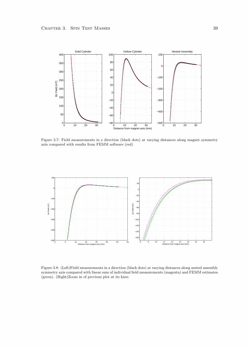
Chapter 3. Spin Test Masses 39
0 10 20 300
50
100
150
200
250
300
350
400B
z F
ield
(m
T)
Solid Cylinder
0 10 20 30−80
−60
−40
−20
0
20
40
60
80
100Hollow Cylinder
Distance from magnet axis (mm)0 10 20 30
−500
−400
−300
−200
−100
0
100Nested Assembly
Figure 3.7: Field measurements in z direction (black dots) at varying distances along magnet symmetryaxis compared with results from FEMM software (red)
0 5 10 15 20 25 30 35−500
−400
−300
−200
−100
0
100
Distance from magnet axis (mm)
Bz
Fie
ld (
mT
)
8 9 10 11 12 13 14 15 16
−160
−140
−120
−100
−80
−60
−40
−20
0
20
Distance from magnet axis (mm)
Bz
Fie
ld (
mT
)
Figure 3.8: (Left)Field measurements in z direction (black dots) at varying distances along nested assemblysymmetry axis compared with linear sum of individual field measurements (magenta) and FEMM estimates(green). (Right)Zoom in of previous plot at its knee.
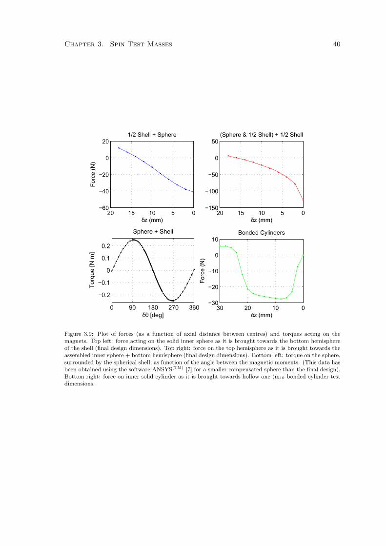
Chapter 3. Spin Test Masses 40
05101520−60
−40
−20
0
20
δz (mm)
Forc
e (
N)
1/2 Shell + Sphere
05101520−150
−100
−50
0
50
δz (mm)
(Sphere & 1/2 Shell) + 1/2 Shell
0102030−30
−20
−10
0
10Bonded Cylinders
δz (mm)
Fo
rce (
N)
0 90 180 270 360
−0.2
−0.1
0
0.1
0.2
Torq
ue [N
m]
δθ [deg]
Sphere + Shell
Figure 3.9: Plot of forces (as a function of axial distance between centres) and torques acting on themagnets. Top left: force acting on the solid inner sphere as it is brought towards the bottom hemisphereof the shell (final design dimensions). Top right: force on the top hemisphere as it is brought towards theassembled inner sphere + bottom hemisphere (final design dimensions). Bottom left: torque on the sphere,surrounded by the spherical shell, as function of the angle between the magnetic moments. (This data hasbeen obtained using the software ANSYS(TM) [7] for a smaller compensated sphere than the final design).Bottom right: force on inner solid cylinder as it is brought towards hollow one (m10 bonded cylinder testdimensions.
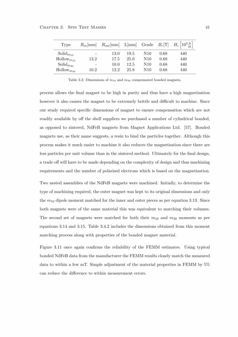
Chapter 3. Spin Test Masses 41
Type Rin[mm] Rout[mm] L[mm] Grade Br[T] Hc
[103 A
m
]Solidm10 - 13.0 19.5 N10 0.68 440
Hollowm10 13.2 17.5 25.0 N10 0.68 440Solidm30 - 10.0 12.5 N10 0.68 440
Hollowm30 10.2 12.2 25.8 N10 0.68 440
Table 3.2: Dimensions of m10 and m30 compensated bonded magnets.
process allows the final magnet to be high in purity and thus have a high magnetisation
however it also causes the magnet to be extremely brittle and difficult to machine. Since
our study required specific dimensions of magnet to ensure compensation which are not
readily available by off the shelf suppliers we purchased a number of cylindrical bonded,
as opposed to sintered, NdFeB magnets from Magnet Applications Ltd. [57]. Bonded
magnets use, as their name suggests, a resin to bind the particles together. Although this
process makes it much easier to machine it also reduces the magnetisation since there are
less particles per unit volume than in the sintered method. Ultimately for the final design,
a trade off will have to be made depending on the complexity of design and thus machining
requirements and the number of polarised electrons which is based on the magnetisation.
Two nested assemblies of the NdFeB magnets were machined. Initially, to determine the
type of machining required, the outer magnet was kept to its original dimensions and only
the m10 dipole moment matched for the inner and outer pieces as per equation 3.13. Since
both magnets were of the same material this was equivalent to matching their volumes.
The second set of magnets were matched for both their m10 and m30 moments as per
equations 3.14 and 3.15. Table 3.4.2 includes the dimensions obtained from this moment
matching process along with properties of the bonded magnet material.
Figure 3.11 once again confirms the reliability of the FEMM estimates. Using typical
bonded NdFeB data from the manufacturer the FEMM results closely match the measured
data to within a few mT. Simple adjustment of the material properties in FEMM by 5%
can reduce the difference to within measurement errors.
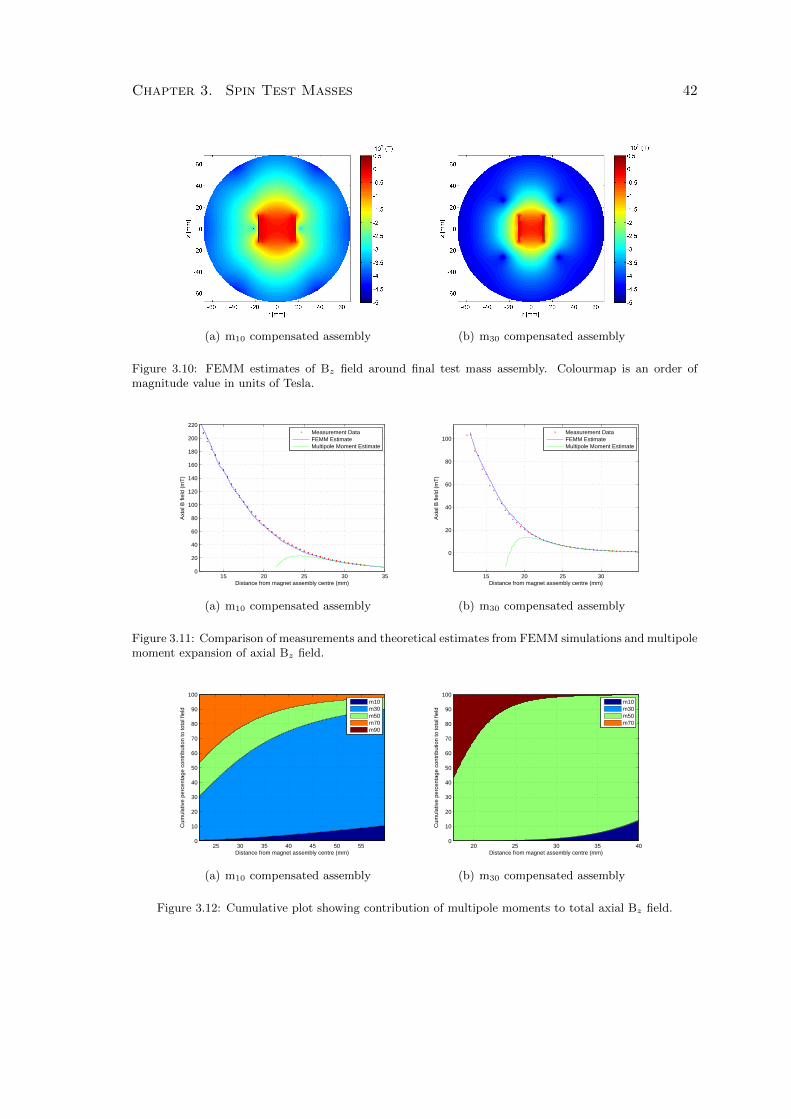
Chapter 3. Spin Test Masses 42
(a) m10 compensated assembly (b) m30 compensated assembly
Figure 3.10: FEMM estimates of Bz field around final test mass assembly. Colourmap is an order ofmagnitude value in units of Tesla.
15 20 25 30 350
20
40
60
80
100
120
140
160
180
200
220
Distance from magnet assembly centre (mm)
Axi
al B
fiel
d (m
T)
Measurement DataFEMM EstimateMultipole Moment Estimate
(a) m10 compensated assembly
15 20 25 30
0
20
40
60
80
100
Distance from magnet assembly centre (mm)
Axi
al B
fiel
d (m
T)
Measurement DataFEMM EstimateMultipole Moment Estimate
(b) m30 compensated assembly
Figure 3.11: Comparison of measurements and theoretical estimates from FEMM simulations and multipolemoment expansion of axial Bz field.
Distance from magnet assembly centre (mm)
Cum
ulat
ive
perc
enta
ge c
ontr
ibut
ion
to to
tal f
ield
25 30 35 40 45 50 550
10
20
30
40
50
60
70
80
90
100m10m30m50m70m90
(a) m10 compensated assembly
Distance from magnet assembly centre (mm)
Cum
ulat
ive
perc
enta
ge c
ontr
ibut
ion
to to
tal f
ield
20 25 30 35 400
10
20
30
40
50
60
70
80
90
100m10m30m50m70
(b) m30 compensated assembly
Figure 3.12: Cumulative plot showing contribution of multipole moments to total axial Bz field.
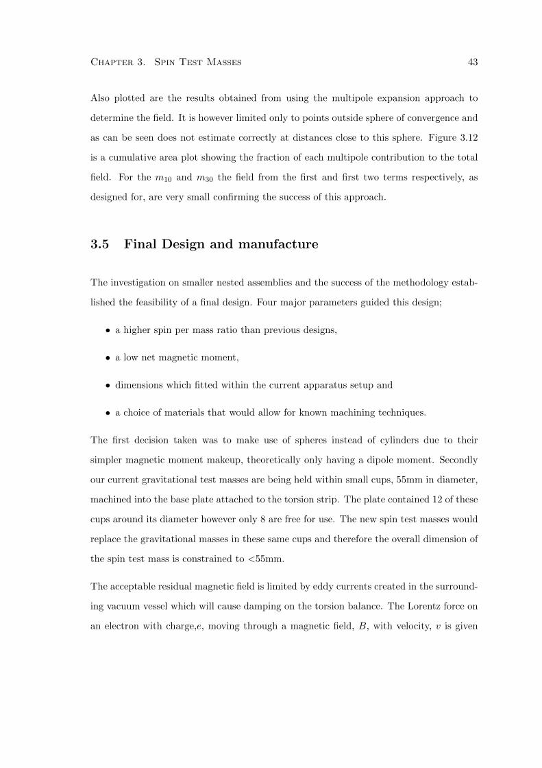
Chapter 3. Spin Test Masses 43
Also plotted are the results obtained from using the multipole expansion approach to
determine the field. It is however limited only to points outside sphere of convergence and
as can be seen does not estimate correctly at distances close to this sphere. Figure 3.12
is a cumulative area plot showing the fraction of each multipole contribution to the total
field. For the m10 and m30 the field from the first and first two terms respectively, as
designed for, are very small confirming the success of this approach.
3.5 Final Design and manufacture
The investigation on smaller nested assemblies and the success of the methodology estab-
lished the feasibility of a final design. Four major parameters guided this design;
• a higher spin per mass ratio than previous designs,
• a low net magnetic moment,
• dimensions which fitted within the current apparatus setup and
• a choice of materials that would allow for known machining techniques.
The first decision taken was to make use of spheres instead of cylinders due to their
simpler magnetic moment makeup, theoretically only having a dipole moment. Secondly
our current gravitational test masses are being held within small cups, 55mm in diameter,
machined into the base plate attached to the torsion strip. The plate contained 12 of these
cups around its diameter however only 8 are free for use. The new spin test masses would
replace the gravitational masses in these same cups and therefore the overall dimension of
the spin test mass is constrained to <55mm.
The acceptable residual magnetic field is limited by eddy currents created in the surround-
ing vacuum vessel which will cause damping on the torsion balance. The Lorentz force on
an electron with charge,e, moving through a magnetic field, B, with velocity, v is given
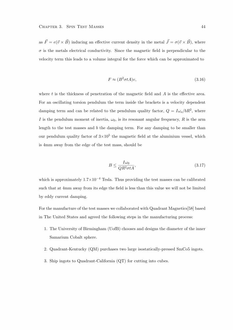
Chapter 3. Spin Test Masses 44
as ~F = e(~v × ~B) inducing an effective current density in the metal ~J = σ(~v × ~B), where
σ is the metals electrical conductivity. Since the magnetic field is perpendicular to the
velocity term this leads to a volume integral for the force which can be approximated to
F ≈ (B2σtA)v, (3.16)
where t is the thickness of penetration of the magnetic field and A is the effective area.
For an oscillating torsion pendulum the term inside the brackets is a velocity dependent
damping term and can be related to the pendulum quality factor, Q = Iωo/bR2, where
I is the pendulum moment of inertia, ω0, is its resonant angular frequency, R is the arm
length to the test masses and b the damping term. For any damping to be smaller than
our pendulum quality factor of 3×10⁵ the magnetic field at the aluminium vessel, which
is 4mm away from the edge of the test mass, should be
B ≤ Iω0
QR2σtA, (3.17)
which is approximately 1.7×10⁻⁴ Tesla. Thus providing the test masses can be calibrated
such that at 4mm away from its edge the field is less than this value we will not be limited
by eddy current damping.
For the manufacture of the test masses we collaborated with Quadrant Magnetics[58] based
in The United States and agreed the following steps in the manufacturing process:
1. The University of Birmingham (UofB) chooses and designs the diameter of the inner
Samarium Cobalt sphere.
2. Quadrant-Kentucky (QM) purchases two large isostatically-pressed SmCo5 ingots.
3. Ship ingots to Quadrant-California (QT) for cutting into cubes.
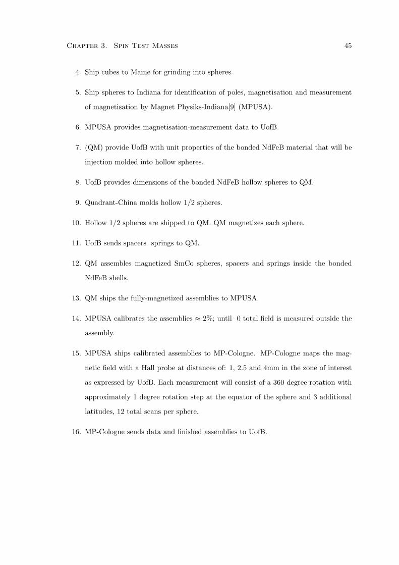
Chapter 3. Spin Test Masses 45
4. Ship cubes to Maine for grinding into spheres.
5. Ship spheres to Indiana for identification of poles, magnetisation and measurement
of magnetisation by Magnet Physiks-Indiana[9] (MPUSA).
6. MPUSA provides magnetisation-measurement data to UofB.
7. (QM) provide UofB with unit properties of the bonded NdFeB material that will be
injection molded into hollow spheres.
8. UofB provides dimensions of the bonded NdFeB hollow spheres to QM.
9. Quadrant-China molds hollow 1/2 spheres.
10. Hollow 1/2 spheres are shipped to QM. QM magnetizes each sphere.
11. UofB sends spacers springs to QM.
12. QM assembles magnetized SmCo spheres, spacers and springs inside the bonded
NdFeB shells.
13. QM ships the fully-magnetized assemblies to MPUSA.
14. MPUSA calibrates the assemblies ≈ 2%; until 0 total field is measured outside the
assembly.
15. MPUSA ships calibrated assemblies to MP-Cologne. MP-Cologne maps the mag-
netic field with a Hall probe at distances of: 1, 2.5 and 4mm in the zone of interest
as expressed by UofB. Each measurement will consist of a 360 degree rotation with
approximately 1 degree rotation step at the equator of the sphere and 3 additional
latitudes, 12 total scans per sphere.
16. MP-Cologne sends data and finished assemblies to UofB.
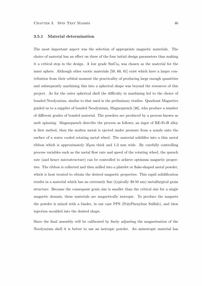
Chapter 3. Spin Test Masses 46
3.5.1 Material determination
The most important aspect was the selection of appropriate magnetic materials. The
choice of material has an effect on three of the four initial design parameters thus making
it a critical step in the design. A low grade SmCo5 was chosen as the material for the
inner sphere. Although other exotic materials [59, 60, 61] exist which have a larger con-
tribution from their orbital moment the practicality of producing large enough quantities
and subsequently machining this into a spherical shape was beyond the resources of this
project. As for the outer spherical shell the difficulty in machining led to the choice of
bonded Neodymium, similar to that used in the preliminary studies. Quadrant Magnetics
guided us to a supplier of bonded Neodymium, Magnequench [46], who produce a number
of different grades of bonded material. The powders are produced by a process known as
melt spinning. Magnequench describe the process as follows; an ingot of RE-Fe-B alloy
is first melted, then the molten metal is ejected under pressure from a nozzle onto the
surface of a water cooled rotating metal wheel. The material solidifies into a thin metal
ribbon which is approximately 35µm thick and 1-3 mm wide. By carefully controlling
process variables such as the metal flow rate and speed of the rotating wheel, the quench
rate (and hence microstructure) can be controlled to achieve optimum magnetic proper-
ties. The ribbon is collected and then milled into a platelet or flake-shaped metal powder,
which is heat treated to obtain the desired magnetic properties. This rapid solidification
results in a material which has an extremely fine (typically 30-50 nm) metallurgical grain
structure. Because the consequent grain size is smaller than the critical size for a single
magnetic domain, these materials are magnetically isotropic. To produce the magnets
the powder is mixed with a binder, in our case PPS (PolyPhenylene Sulfide), and then
injection moulded into the desired shape.
Since the final assembly will be calibrated by finely adjusting the magnetisation of the
Neodymium shell it is better to use an isotropic powder. An anisotropic material has
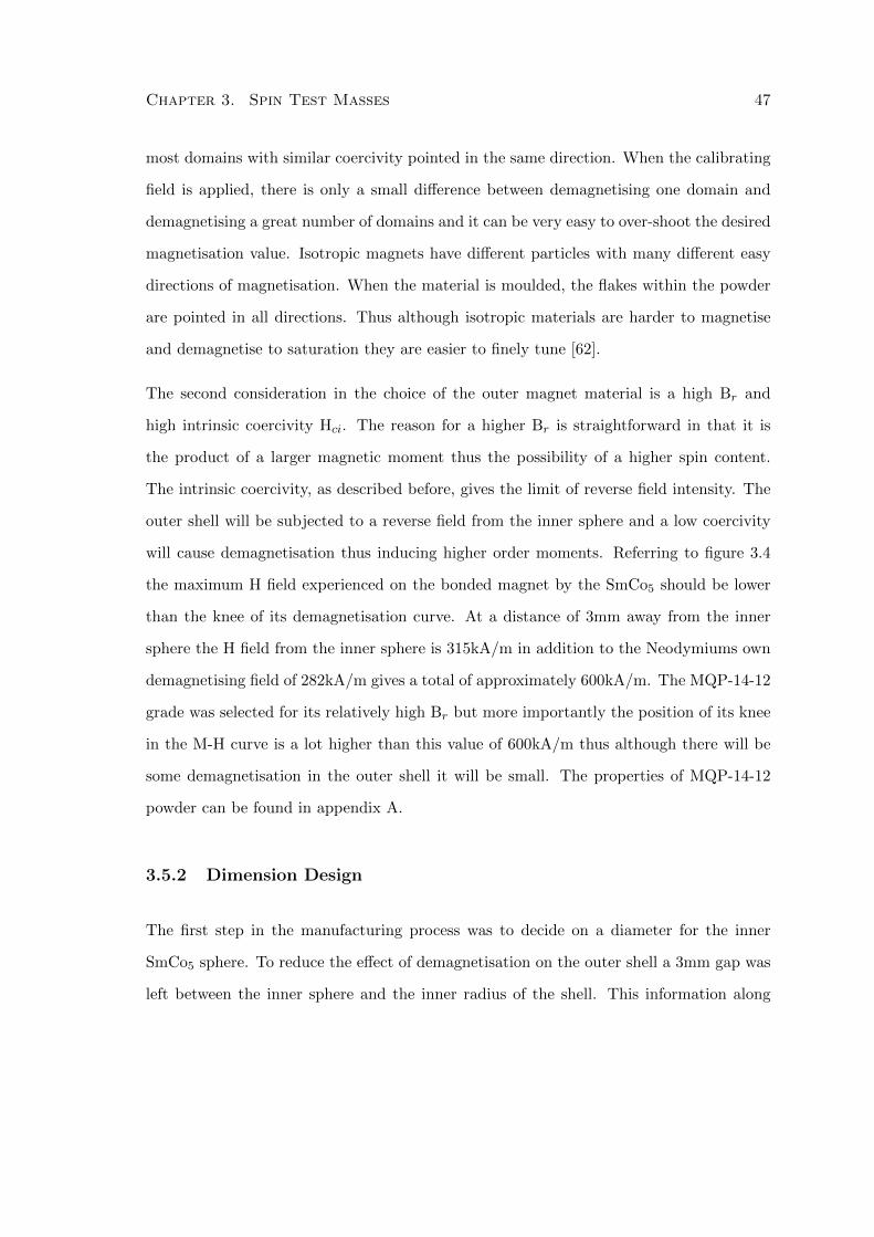
Chapter 3. Spin Test Masses 47
most domains with similar coercivity pointed in the same direction. When the calibrating
field is applied, there is only a small difference between demagnetising one domain and
demagnetising a great number of domains and it can be very easy to over-shoot the desired
magnetisation value. Isotropic magnets have different particles with many different easy
directions of magnetisation. When the material is moulded, the flakes within the powder
are pointed in all directions. Thus although isotropic materials are harder to magnetise
and demagnetise to saturation they are easier to finely tune [62].
The second consideration in the choice of the outer magnet material is a high Br and
high intrinsic coercivity Hci. The reason for a higher Br is straightforward in that it is
the product of a larger magnetic moment thus the possibility of a higher spin content.
The intrinsic coercivity, as described before, gives the limit of reverse field intensity. The
outer shell will be subjected to a reverse field from the inner sphere and a low coercivity
will cause demagnetisation thus inducing higher order moments. Referring to figure 3.4
the maximum H field experienced on the bonded magnet by the SmCo5 should be lower
than the knee of its demagnetisation curve. At a distance of 3mm away from the inner
sphere the H field from the inner sphere is 315kA/m in addition to the Neodymiums own
demagnetising field of 282kA/m gives a total of approximately 600kA/m. The MQP-14-12
grade was selected for its relatively high Br but more importantly the position of its knee
in the M-H curve is a lot higher than this value of 600kA/m thus although there will be
some demagnetisation in the outer shell it will be small. The properties of MQP-14-12
powder can be found in appendix A.
3.5.2 Dimension Design
The first step in the manufacturing process was to decide on a diameter for the inner
SmCo5 sphere. To reduce the effect of demagnetisation on the outer shell a 3mm gap was
left between the inner sphere and the inner radius of the shell. This information along
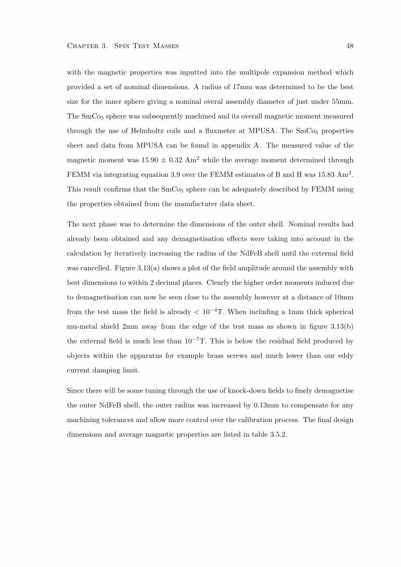
Chapter 3. Spin Test Masses 48
with the magnetic properties was inputted into the multipole expansion method which
provided a set of nominal dimensions. A radius of 17mm was determined to be the best
size for the inner sphere giving a nominal overal assembly diameter of just under 55mm.
The SmCo5 sphere was subsequently machined and its overall magnetic moment measured
through the use of Helmholtz coils and a fluxmeter at MPUSA. The SmCo5 properties
sheet and data from MPUSA can be found in appendix A. The measured value of the
magnetic moment was 15.90 ± 0.32 Am2 while the average moment determined through
FEMM via integrating equation 3.9 over the FEMM estimates of B and H was 15.83 Am2.
This result confirms that the SmCo5 sphere can be adequately described by FEMM using
the properties obtained from the manufacturer data sheet.
The next phase was to determine the dimensions of the outer shell. Nominal results had
already been obtained and any demagnetisation effects were taking into account in the
calculation by iteratively increasing the radius of the NdFeB shell until the external field
was cancelled. Figure 3.13(a) shows a plot of the field amplitude around the assembly with
best dimensions to within 2 decimal places. Clearly the higher order moments induced due
to demagnetisation can now be seen close to the assembly however at a distance of 10mm
from the test mass the field is already < 10−4T. When including a 1mm thick spherical
mu-metal shield 2mm away from the edge of the test mass as shown in figure 3.13(b)
the external field is much less than 10−7T. This is below the residual field produced by
objects within the apparatus for example brass screws and much lower than our eddy
current damping limit.
Since there will be some tuning through the use of knock-down fields to finely demagnetise
the outer NdFeB shell, the outer radius was increased by 0.13mm to compensate for any
machining tolerances and allow more control over the calibration process. The final design
dimensions and average magnetic properties are listed in table 3.5.2.
Chapter 3. Spin Test Masses 49
(a) No shield (b) Including a mu-metal shield
Figure 3.13: FEMM estimates of Bz field around final test mass assembly, Outer radius is 26.98mm.Colourmap is an order of magnitude value in units of Tesla.
Type Grade Br[T] Hc
[103 A
m
]SmCo5 22 0.970 762
Nd2Fe14B MPQ-14-12 0.446 311
Table 3.3: Nominal magnetic properties of final test mass materials. In the FEMM designs a non-linearB-H profile was used.
Type Rin[mm] Rout[mm] Density[10−3 g
mm3
]Volume
[104mm3
]Mass[g]
SmCo5 - 17.0 8.5 2.06 171Nd2Fe14B 20.0 27.1 5 4.99 249
Table 3.4: Dimensions of final test mass design.
Chapter 3. Spin Test Masses 50
3.5.3 Spin Content
The final parameter to be discussed, however probably the most important in terms of
scientific value, is the net spin density within these newly designed magnets. To success-
fully estimate the proportions of spin and orbit contribution to the overall magnetisation
of each of the materials it will be required to assess previous experimental data on these
materials. The net spin densities Σ can be estimated through
Σ =αinµin + αoutµout
µBmt, (3.18)
where mt is the total mass, α is the spin contribution to the magnetic moment, µ, of each
magnet, which can be estimated to good accuracy via FEMM and through measurements.
SmCo5
RCo5 materials, where R is a rare-earth element, were developed due to the complicated
range of stoichometric compounds that are made when mixed with a transition metal,
in this case Cobalt [44]. This interaction causes a strong magnetic anisotropy in both
atoms thus giving a strong permanent magnetism. SmCo5 has been extensively studied
using a number of techniques including neutron scattering and nuclear magnetic resonance
[63, 64, 65]. The crystal structure of SmCo5, shown in figure 3.14, is that of CaCu5 and
the cobalt sites are separated into two sets of inequivalent atoms, 2 atoms in the 2c site
and 3 atoms in the 3g site [8, 66, 67, 68]. Polarised neutron studies [66] have determined
that the cobalt in YCo5 exhibits large differences in the moment densities between the two
localised crystallographic sites. This study determined that the Co2c site has a localised
moment of 1.77µB while the Co3g site has a moment of 1.72µB with a spin proportion of
0.74 and 0.85 respectively. In a second study [65] reported for SmCo5 the cobalt moments
are shown to be 1.86µB and 1.75µB at the respective sites. As for the spin fraction,
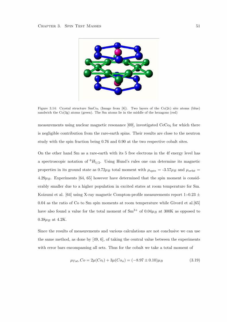
Chapter 3. Spin Test Masses 51
Figure 3.14: Crystal structure SmCo5 (Image from [8]). Two layers of the Co(2c) site atoms (blue)sandwich the Co(3g) atoms (green). The Sm atoms lie in the middle of the hexagons (red)
measurements using nuclear magnetic resonance [69], investigated CeCo5 for which there
is negligible contribution from the rare-earth spins. Their results are close to the neutron
study with the spin fraction being 0.76 and 0.90 at the two respective cobalt sites.
On the other hand Sm as a rare-earth with its 5 free electrons in the 4f energy level has
a spectroscopic notation of 6H5/2. Using Hund’s rules one can determine its magnetic
properties in its ground state as 0.72µB total moment with µspin = -3.57µB and µorbit =
4.29µB. Experiments [64, 65] however have determined that the spin moment is consid-
erably smaller due to a higher population in excited states at room temperature for Sm.
Koizumi et al. [64] using X-ray magnetic Compton-profile measurements report 1:-0.23 ±
0.04 as the ratio of Co to Sm spin moments at room temperature while Givord et al.[65]
have also found a value for the total moment of Sm3+ of 0.04µB at 300K as opposed to
0.38µB at 4.2K.
Since the results of measurements and various calculations are not conclusive we can use
the same method, as done by [49, 6], of taking the central value between the experiments
with error bars encompassing all sets. Thus for the cobalt we take a total moment of
µTot, Co = 2µ(Coi) + 3µ(Coii) = (−8.97± 0.10)µB (3.19)
Chapter 3. Spin Test Masses 52
µS , Co = 2µS(Coi) + 3µS(Coii) = (−7.14± 0.39)µB, (3.20)
and for Samarium using the ratio determined by Koizumi [64] the spin moment would be
µS , Sm = (−7.14± 0.39)× (−0.23± 0.04) = (+1.64± 0.37).. (3.21)
Heckel [6] also makes a calculation of the Sm spin moment at room temperature as µS ,Sm
= +3.56µB. We can once again take an average with error bars encompassing both values
as
µS , Sm(av) = +2.60± 0.96µB. (3.22)
With this value the total spin fraction in SmCo5 is estimated to be
µSfrac, SmCo5 =µS , SmCo5µTot, SmCo5
=(−7.14 + 2.6)
(−8.97 + 0.04)= 0.51± 0.05. (3.23)
Nd2Fe14B
There is a similar amount of literature detailing efforts on understanding the makeup and
magnetic properties of Nd2Fe14B as a whole and its constituents individually. However due
to discrepancies in experimental data there is considerable doubt in the exact effects of ex-
change interactions between Nd and Fe at room temperature. Initially it was assumed that
by studying Yttrium, which is non magnetic, in place of neodymium the Fe moment could
be determined. Givord et al. [70] reports that at 4.2K the value of the spontaneous mag-
netisation of Y2Fe14B corresponds to 2.10µB/Fe atom. On the other hand measurements
by Tokuhara [71] determine a total magnetisation of 31.1µB/fu giving 2.22µB/Fe atom,
very close to 2.20µB measured in pure iron. Accordingly using this value in Nd2Fe14B re-
sults in a Nd moment of 3.40µB/atom which is close to that of Nd3+ obtained from Hund’s
Chapter 3. Spin Test Masses 53
rules but lower than 3.75µB from Givords measurement. However Givord et al.[72] carried
out a subsequent measurement using polarised neutrons and reports a Nd2Fe14B moment
at 4.2K of 37.90µB/fu with Nd contributing 2.20µB/atom, well below the ground state
value [73]. This corresponds to an iron moment of 2.40µB. The study also measures a
drop in the moment of Y2Fe14B from 29.50µB/fu at 4.2K to 28.20µB/fu at 300K. This
is in good agreement with Koon [74] who mentioned a similar 12% drop in the moment
between the two temperatures. We can assume [75] that the relative variation in Fe for
Nd2Fe14B should be very similar and thus taking the Givord value of Nd2Fe14B at 4.2K
and removing the Nd moment gives 33.50µB for the iron moment. A 12% reduction at
room temperature results in an Fe moment of 2.11µB. The average moment of a number
of room temperature measurements on Nd2Fe14B [74, 76, 77, 78, 79] is 32.50µB resulting
in a 300K Nd moment of 1.55µB.
Finally we must assess the spin and orbital contribution to these moments. A small orbital
moment has been reported for iron [80, 81] and we take here a conservative estimate of
0.1µB/Fe atom. We also assume [82] that the ratio of orbital and spin contribution to the
total moment for Nd remains constant over the temperature range [75]. Since the spins in
Nd are antiparallel to the Fe this gives a final spin ratio for Nd2Fe14B of αN = 0.79± 0.04
1. Table 3.5 summarises the results for both materials.
µSfrac, Nd2Fe14B =µS , Nd2Fe14B
µTot, Nd2Fe14B=
(28.00− 2.34)
(29.48 + 3.10)= 0.79± 0.04. (3.24)
Total Spin Content
The total number of spins can be estimated by using the moment measurement of the
SmCo5 sphere of 15.90±0.32Am2. In the perfect scenario the outer Nd2Fe14B shell should
1We assign a 5% error to this result as reported in Garcia for experimental measurements
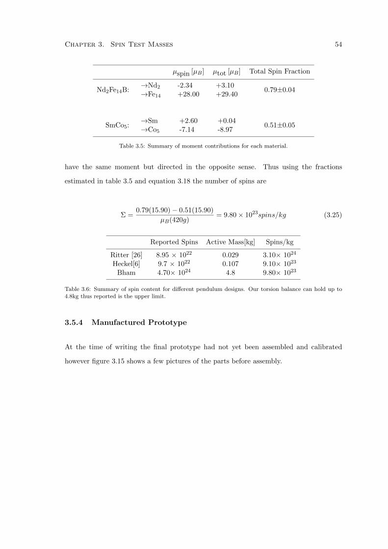
Chapter 3. Spin Test Masses 54
µspin [µB] µtot [µB] Total Spin Fraction
Nd2Fe14B:→Nd2
→Fe14
-2.34+28.00
+3.10+29.40
0.79±0.04
SmCo5:→Sm→Co5
+2.60-7.14
+0.04-8.97
0.51±0.05
Table 3.5: Summary of moment contributions for each material.
have the same moment but directed in the opposite sense. Thus using the fractions
estimated in table 3.5 and equation 3.18 the number of spins are
Σ =0.79(15.90)− 0.51(15.90)
µB(420g)= 9.80× 10²³spins/kg (3.25)
Reported Spins Active Mass[kg] Spins/kg
Ritter [26] 8.95 × 10²² 0.029 3.10× 1024
Heckel[6] 9.7 × 10²² 0.107 9.10× 10²³
Bham 4.70× 1024 4.8 9.80× 10²³
Table 3.6: Summary of spin content for different pendulum designs. Our torsion balance can hold up to4.8kg thus reported is the upper limit.
3.5.4 Manufactured Prototype
At the time of writing the final prototype had not yet been assembled and calibrated
however figure 3.15 shows a few pictures of the parts before assembly.
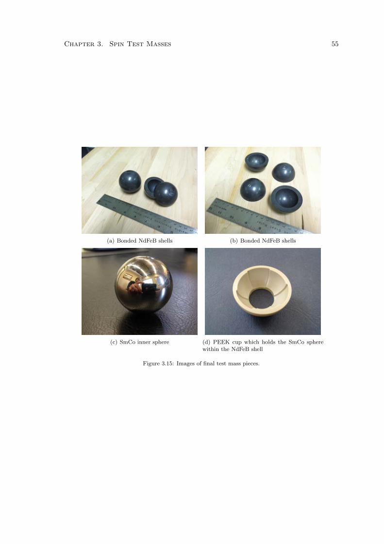
Chapter 3. Spin Test Masses 55
(a) Bonded NdFeB shells (b) Bonded NdFeB shells
(c) SmCo inner sphere (d) PEEK cup which holds the SmCo spherewithin the NdFeB shell
Figure 3.15: Images of final test mass pieces.
Chapter 4
Iliad - Angle
Interferometric Device
As discussed in chapter 2 the torsion strip balance can provide a better signal to noise
ratio than round fibres due to its ability to hang a larger mass and the higher mechanical
quality factor. However, in order to fully take advantage of these two features a sensor that
is able to detect the smaller angular deflection produced for the equivalent torque from a
round fibre is required. Our current readout, the autocollimator, has a sensitivity limit
of 5 × 10⁻⁹rad/√Hz which corresponds to a torque of few 10−12Nm/
√Hz at 10−3Hz.
This level makes it difficult for our experimental setup to be competitive with other ex-
periments searching for weak interactions. For example the University of Washington spin
coupling experiment achieved results equivalent to a torque of approximately 1×10⁻¹⁵Nm
at 10−3Hz 1. Another restriction of the Autocollimator is that due to its size it needs
to be mounted externally on a large platform. This platform can be very susceptible to
environmental factors like temperature which would shift the autocollimator position with
respect to the Torsion Balance giving false signals. A small integrated readout device
would improve the experimental facility greatly.
1Using values given in [6]
56
Chapter 4. Iliad - Angle Interferometric Device 57
4.1 Basics of Optical Interferometry
Optical interferometers are widely used to measure displacements with high resolution
and accuracy. In a standard Michelson interferometric configuration monochromatic light
of wavelength λ, usually from a stable laser source, is sent through beam splitting optics
which divide the beam into two arms of the interferometer, a reference arm and a mea-
surement arm. The electromagnetic waves propagating in the two arms can be represented
as
Eref = A1 exp i(ωt− φ1) (4.1)
Emeas = A2 exp i(ωt− φ2) (4.2)
where An is the amplitude, ω is the angular frequency, t is the time and φn is the phase
given by 2π/λxn; n = 1, 2. The beams travel to their respective mirrors and reflect back
to the splitting optics where they are recombined and detected as an interference pattern
with intensity
I(∆φ) = |(Eref + Emeas)|2 = A1 +A2 + 2A1A2cos(∆φ) (4.3)
Here ∆φ = 2π/λδx with δx being the difference in path lengths travelled in each arm.
It can be seen that I(∆φ) varies sinusoidally with φ and goes through a complete cycle
(maximum - minimum - maximum) every time ∆φ changes by 2π. Each one of these cycles
is called a fringe and accurately counting fringes, or fractions of the fringe, can determine
the distance displaced by the mirror. If ∆l is the displacement of the measurement mirror,
i.e. the difference in length between the two arms, then
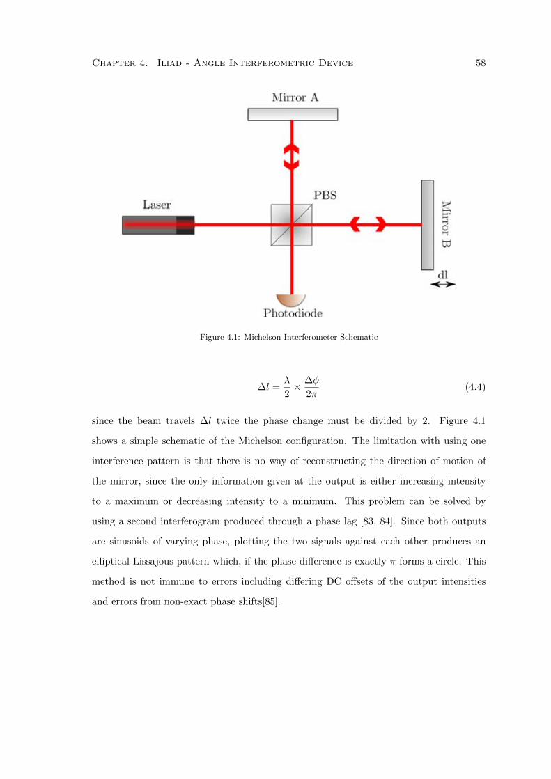
Chapter 4. Iliad - Angle Interferometric Device 58
Figure 4.1: Michelson Interferometer Schematic
∆l =λ
2× ∆φ
2π(4.4)
since the beam travels ∆l twice the phase change must be divided by 2. Figure 4.1
shows a simple schematic of the Michelson configuration. The limitation with using one
interference pattern is that there is no way of reconstructing the direction of motion of
the mirror, since the only information given at the output is either increasing intensity
to a maximum or decreasing intensity to a minimum. This problem can be solved by
using a second interferogram produced through a phase lag [83, 84]. Since both outputs
are sinusoids of varying phase, plotting the two signals against each other produces an
elliptical Lissajous pattern which, if the phase difference is exactly π forms a circle. This
method is not immune to errors including differing DC offsets of the output intensities
and errors from non-exact phase shifts[85].
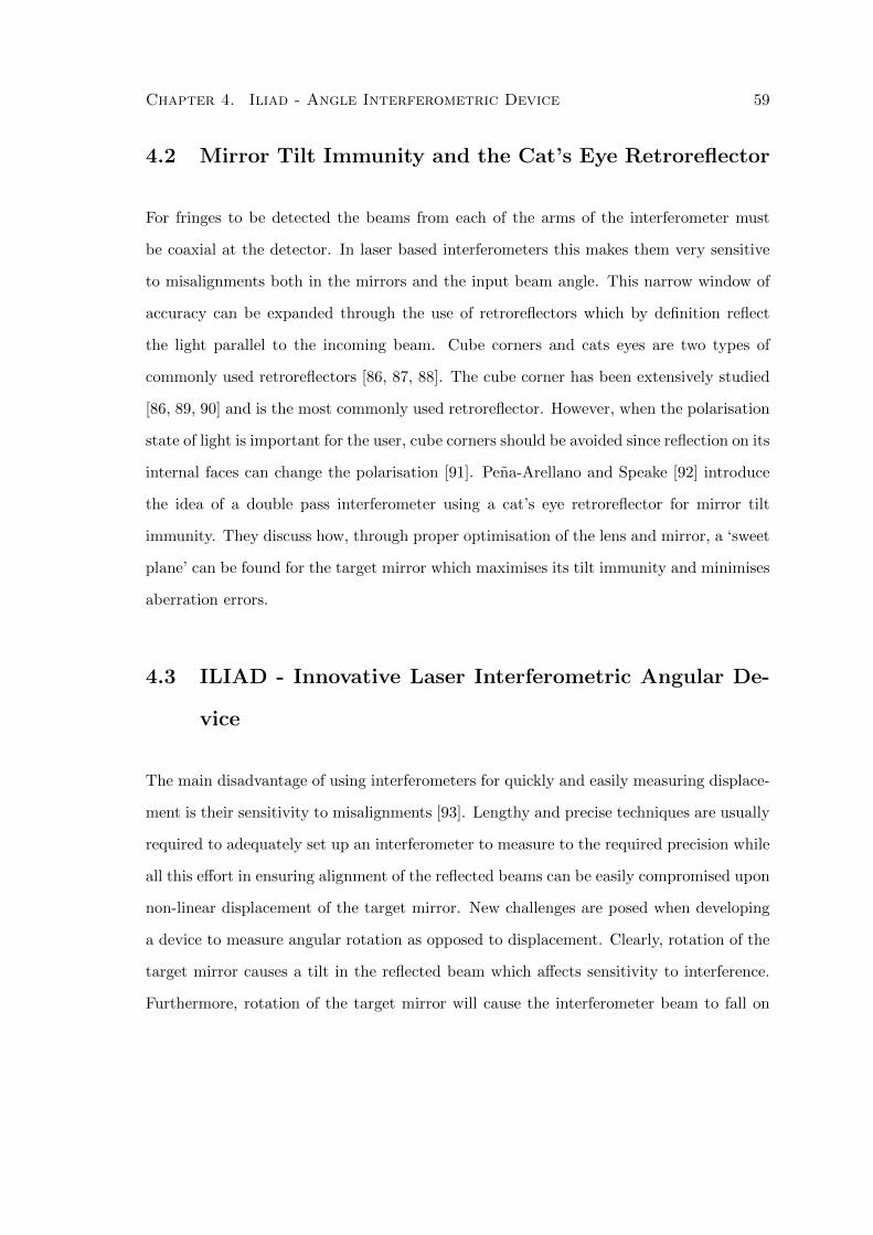
Chapter 4. Iliad - Angle Interferometric Device 59
4.2 Mirror Tilt Immunity and the Cat’s Eye Retroreflector
For fringes to be detected the beams from each of the arms of the interferometer must
be coaxial at the detector. In laser based interferometers this makes them very sensitive
to misalignments both in the mirrors and the input beam angle. This narrow window of
accuracy can be expanded through the use of retroreflectors which by definition reflect
the light parallel to the incoming beam. Cube corners and cats eyes are two types of
commonly used retroreflectors [86, 87, 88]. The cube corner has been extensively studied
[86, 89, 90] and is the most commonly used retroreflector. However, when the polarisation
state of light is important for the user, cube corners should be avoided since reflection on its
internal faces can change the polarisation [91]. Pena-Arellano and Speake [92] introduce
the idea of a double pass interferometer using a cat’s eye retroreflector for mirror tilt
immunity. They discuss how, through proper optimisation of the lens and mirror, a ‘sweet
plane’ can be found for the target mirror which maximises its tilt immunity and minimises
aberration errors.
4.3 ILIAD - Innovative Laser Interferometric Angular De-
vice
The main disadvantage of using interferometers for quickly and easily measuring displace-
ment is their sensitivity to misalignments [93]. Lengthy and precise techniques are usually
required to adequately set up an interferometer to measure to the required precision while
all this effort in ensuring alignment of the reflected beams can be easily compromised upon
non-linear displacement of the target mirror. New challenges are posed when developing
a device to measure angular rotation as opposed to displacement. Clearly, rotation of the
target mirror causes a tilt in the reflected beam which affects sensitivity to interference.
Furthermore, rotation of the target mirror will cause the interferometer beam to fall on
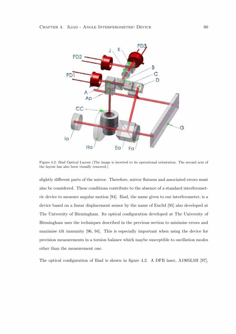
Chapter 4. Iliad - Angle Interferometric Device 60
Figure 4.2: Iliad Optical Layout (The image is inverted to its operational orientation. The second arm ofthe layout has also been visually removed.)
slightly different parts of the mirror. Therefore, mirror flatness and associated errors must
also be considered. These conditions contribute to the absence of a standard interferomet-
ric device to measure angular motion [94]. Iliad, the name given to our interferometer, is a
device based on a linear displacement sensor by the name of Euclid [95] also developed at
The University of Birmingham. Its optical configuration developed at The University of
Birmingham uses the techniques described in the previous section to minimise errors and
maximise tilt immunity [96, 94]. This is especially important when using the device for
precision measurements in a torsion balance which maybe susceptible to oscillation modes
other than the measurement one.
The optical configuration of Iliad is shown in figure 4.2. A DFB laser, A1905LMI [97],
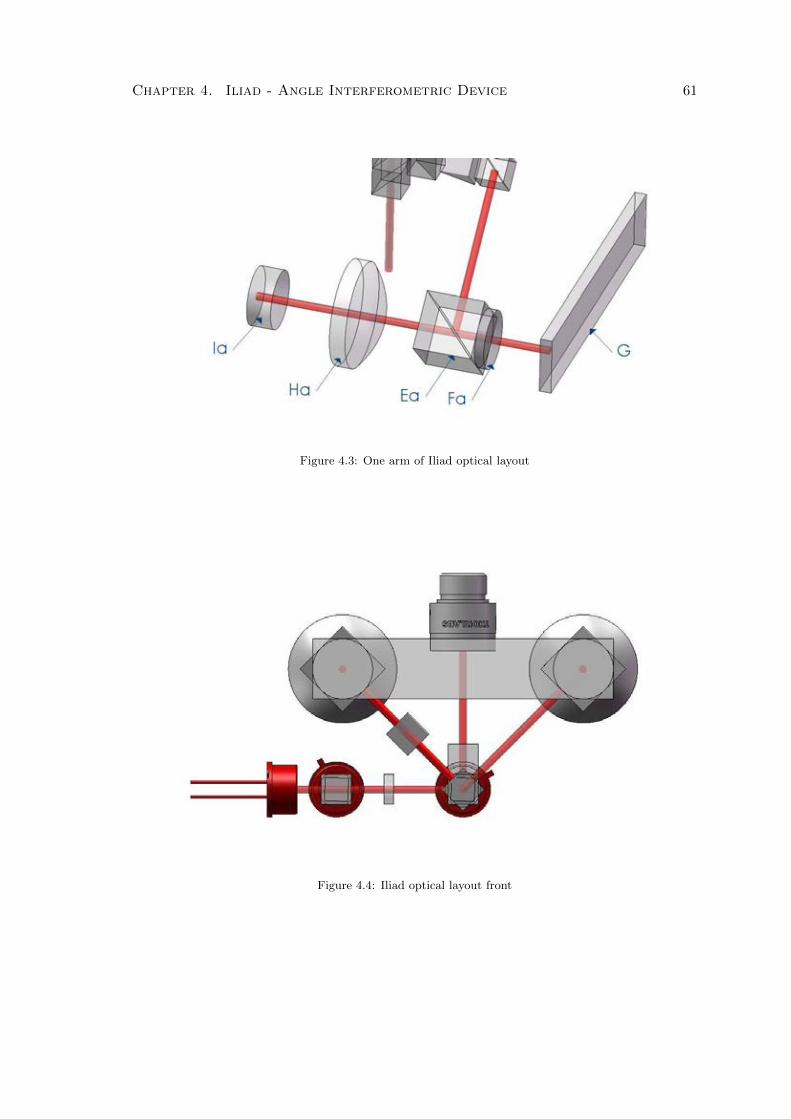
Chapter 4. Iliad - Angle Interferometric Device 61
Figure 4.3: One arm of Iliad optical layout
Figure 4.4: Iliad optical layout front
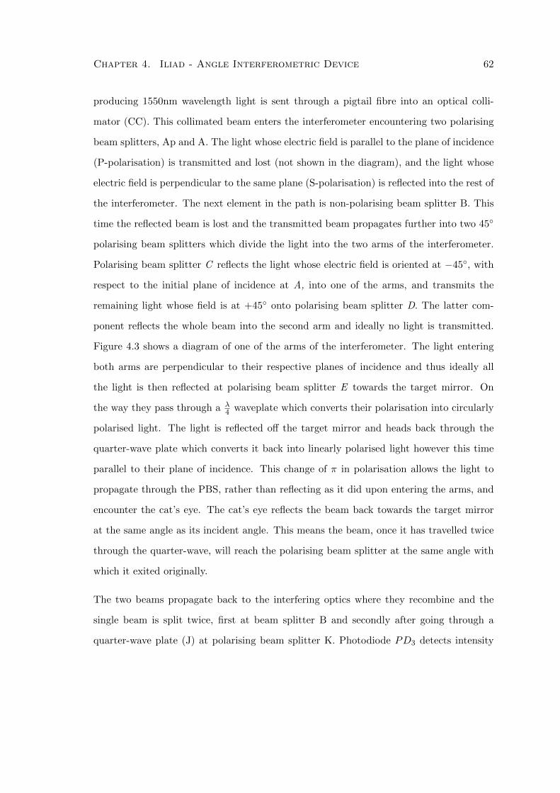
Chapter 4. Iliad - Angle Interferometric Device 62
producing 1550nm wavelength light is sent through a pigtail fibre into an optical colli-
mator (CC). This collimated beam enters the interferometer encountering two polarising
beam splitters, Ap and A. The light whose electric field is parallel to the plane of incidence
(P-polarisation) is transmitted and lost (not shown in the diagram), and the light whose
electric field is perpendicular to the same plane (S-polarisation) is reflected into the rest of
the interferometer. The next element in the path is non-polarising beam splitter B. This
time the reflected beam is lost and the transmitted beam propagates further into two 45
polarising beam splitters which divide the light into the two arms of the interferometer.
Polarising beam splitter C reflects the light whose electric field is oriented at −45, with
respect to the initial plane of incidence at A, into one of the arms, and transmits the
remaining light whose field is at +45 onto polarising beam splitter D. The latter com-
ponent reflects the whole beam into the second arm and ideally no light is transmitted.
Figure 4.3 shows a diagram of one of the arms of the interferometer. The light entering
both arms are perpendicular to their respective planes of incidence and thus ideally all
the light is then reflected at polarising beam splitter E towards the target mirror. On
the way they pass through a λ4 waveplate which converts their polarisation into circularly
polarised light. The light is reflected off the target mirror and heads back through the
quarter-wave plate which converts it back into linearly polarised light however this time
parallel to their plane of incidence. This change of π in polarisation allows the light to
propagate through the PBS, rather than reflecting as it did upon entering the arms, and
encounter the cat’s eye. The cat’s eye reflects the beam back towards the target mirror
at the same angle as its incident angle. This means the beam, once it has travelled twice
through the quarter-wave, will reach the polarising beam splitter at the same angle with
which it exited originally.
The two beams propagate back to the interfering optics where they recombine and the
single beam is split twice, first at beam splitter B and secondly after going through a
quarter-wave plate (J) at polarising beam splitter K. Photodiode PD3 detects intensity
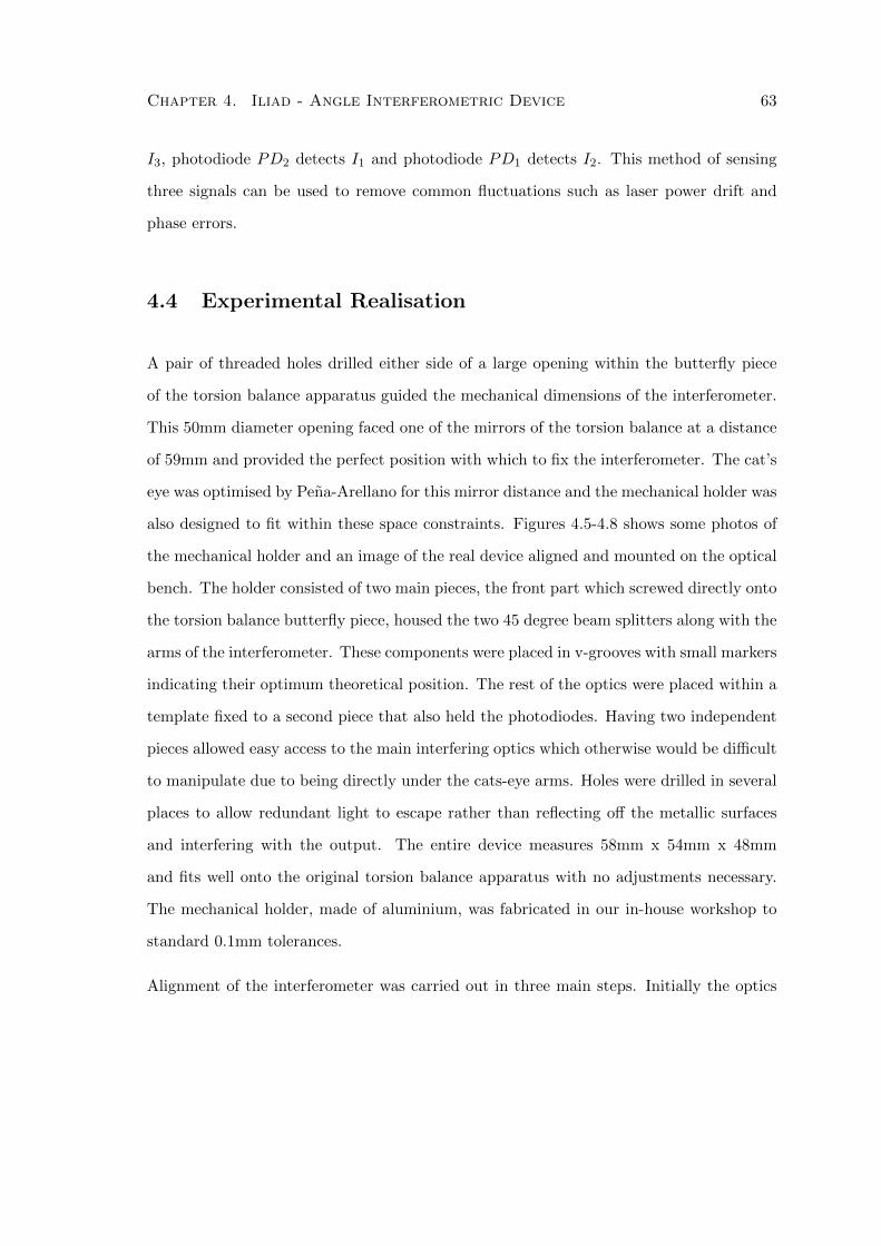
Chapter 4. Iliad - Angle Interferometric Device 63
I3, photodiode PD2 detects I1 and photodiode PD1 detects I2. This method of sensing
three signals can be used to remove common fluctuations such as laser power drift and
phase errors.
4.4 Experimental Realisation
A pair of threaded holes drilled either side of a large opening within the butterfly piece
of the torsion balance apparatus guided the mechanical dimensions of the interferometer.
This 50mm diameter opening faced one of the mirrors of the torsion balance at a distance
of 59mm and provided the perfect position with which to fix the interferometer. The cat’s
eye was optimised by Pena-Arellano for this mirror distance and the mechanical holder was
also designed to fit within these space constraints. Figures 4.5-4.8 shows some photos of
the mechanical holder and an image of the real device aligned and mounted on the optical
bench. The holder consisted of two main pieces, the front part which screwed directly onto
the torsion balance butterfly piece, housed the two 45 degree beam splitters along with the
arms of the interferometer. These components were placed in v-grooves with small markers
indicating their optimum theoretical position. The rest of the optics were placed within a
template fixed to a second piece that also held the photodiodes. Having two independent
pieces allowed easy access to the main interfering optics which otherwise would be difficult
to manipulate due to being directly under the cats-eye arms. Holes were drilled in several
places to allow redundant light to escape rather than reflecting off the metallic surfaces
and interfering with the output. The entire device measures 58mm x 54mm x 48mm
and fits well onto the original torsion balance apparatus with no adjustments necessary.
The mechanical holder, made of aluminium, was fabricated in our in-house workshop to
standard 0.1mm tolerances.
Alignment of the interferometer was carried out in three main steps. Initially the optics
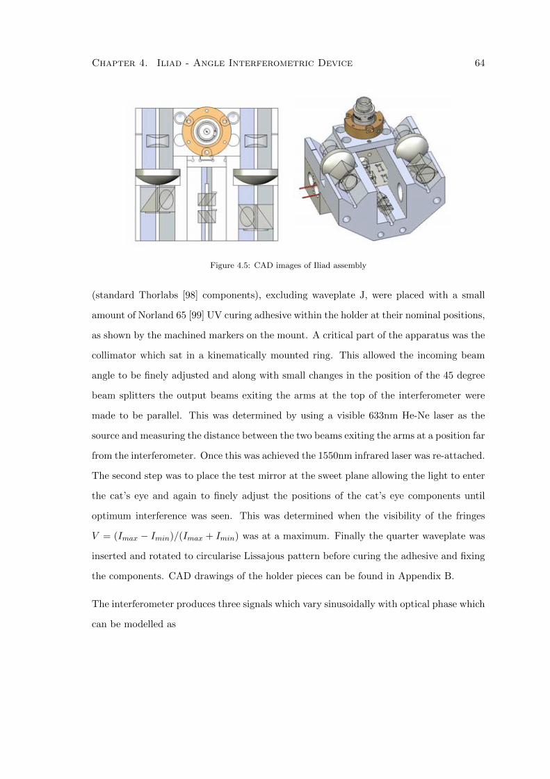
Chapter 4. Iliad - Angle Interferometric Device 64
Figure 4.5: CAD images of Iliad assembly
(standard Thorlabs [98] components), excluding waveplate J, were placed with a small
amount of Norland 65 [99] UV curing adhesive within the holder at their nominal positions,
as shown by the machined markers on the mount. A critical part of the apparatus was the
collimator which sat in a kinematically mounted ring. This allowed the incoming beam
angle to be finely adjusted and along with small changes in the position of the 45 degree
beam splitters the output beams exiting the arms at the top of the interferometer were
made to be parallel. This was determined by using a visible 633nm He-Ne laser as the
source and measuring the distance between the two beams exiting the arms at a position far
from the interferometer. Once this was achieved the 1550nm infrared laser was re-attached.
The second step was to place the test mirror at the sweet plane allowing the light to enter
the cat’s eye and again to finely adjust the positions of the cat’s eye components until
optimum interference was seen. This was determined when the visibility of the fringes
V = (Imax − Imin)/(Imax + Imin) was at a maximum. Finally the quarter waveplate was
inserted and rotated to circularise Lissajous pattern before curing the adhesive and fixing
the components. CAD drawings of the holder pieces can be found in Appendix B.
The interferometer produces three signals which vary sinusoidally with optical phase which
can be modelled as
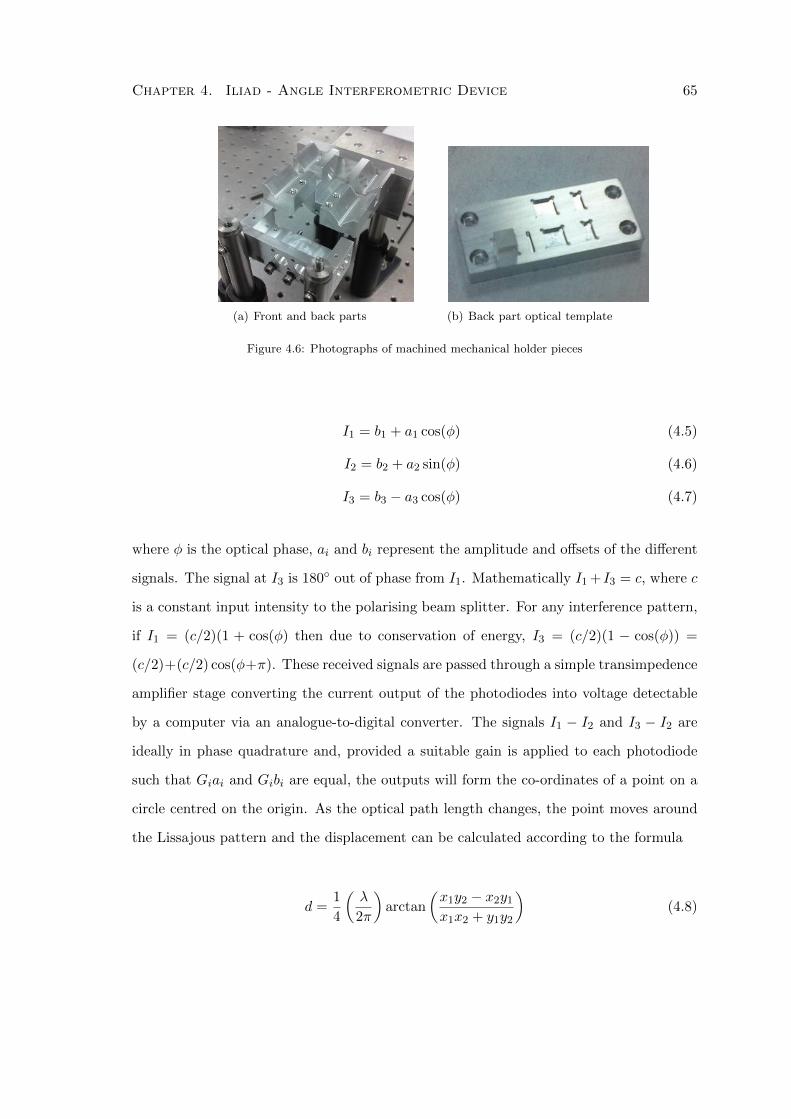
Chapter 4. Iliad - Angle Interferometric Device 65
(a) Front and back parts (b) Back part optical template
Figure 4.6: Photographs of machined mechanical holder pieces
I1 = b1 + a1 cos(φ) (4.5)
I2 = b2 + a2 sin(φ) (4.6)
I3 = b3 − a3 cos(φ) (4.7)
where φ is the optical phase, ai and bi represent the amplitude and offsets of the different
signals. The signal at I3 is 180 out of phase from I1. Mathematically I1 + I3 = c, where c
is a constant input intensity to the polarising beam splitter. For any interference pattern,
if I1 = (c/2)(1 + cos(φ) then due to conservation of energy, I3 = (c/2)(1 − cos(φ)) =
(c/2)+(c/2) cos(φ+π). These received signals are passed through a simple transimpedence
amplifier stage converting the current output of the photodiodes into voltage detectable
by a computer via an analogue-to-digital converter. The signals I1 − I2 and I3 − I2 are
ideally in phase quadrature and, provided a suitable gain is applied to each photodiode
such that Giai and Gibi are equal, the outputs will form the co-ordinates of a point on a
circle centred on the origin. As the optical path length changes, the point moves around
the Lissajous pattern and the displacement can be calculated according to the formula
d =1
4
(λ
2π
)arctan
(x1y2 − x2y1x1x2 + y1y2
)(4.8)
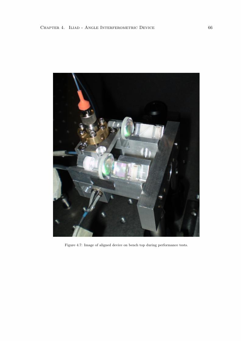
Chapter 4. Iliad - Angle Interferometric Device 66
Figure 4.7: Image of aligned device on bench top during performance tests.
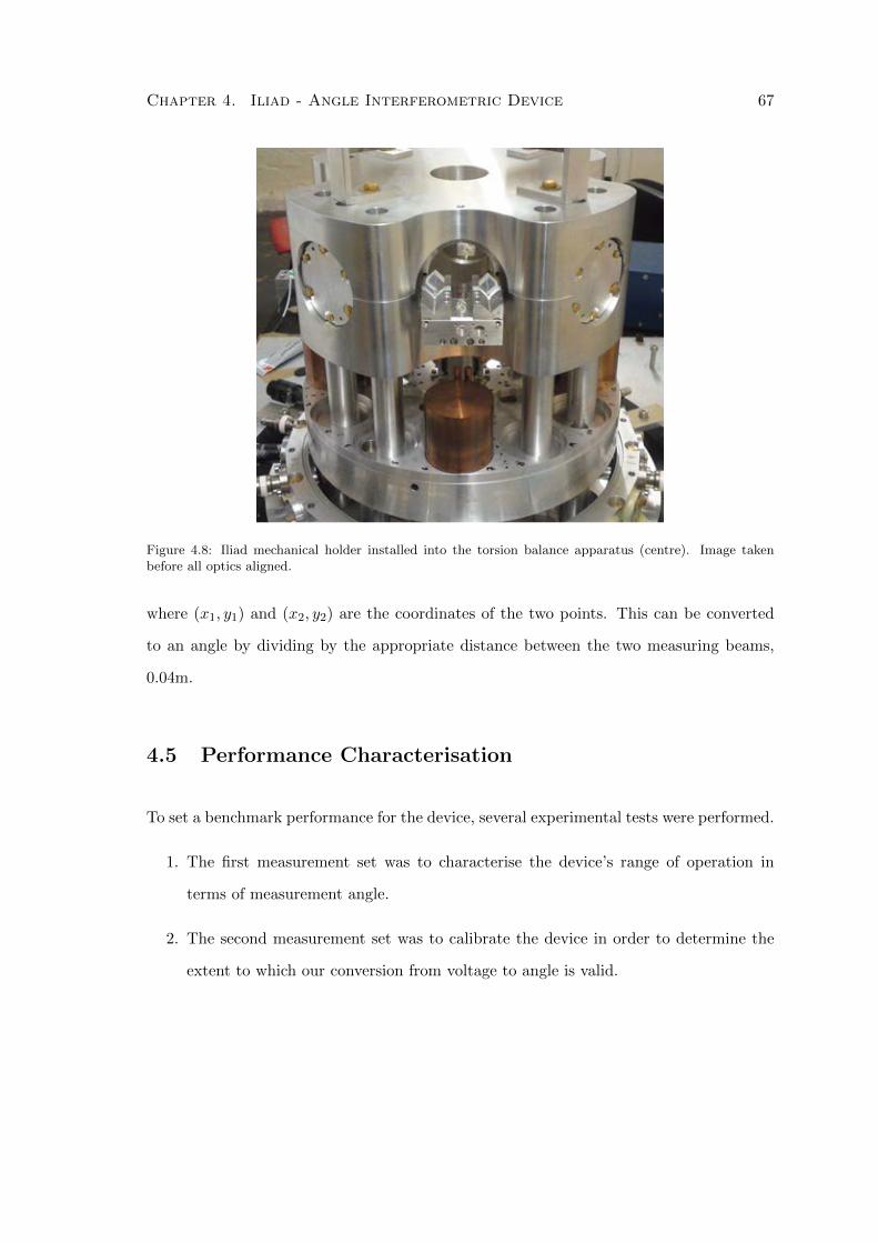
Chapter 4. Iliad - Angle Interferometric Device 67
Figure 4.8: Iliad mechanical holder installed into the torsion balance apparatus (centre). Image takenbefore all optics aligned.
where (x1, y1) and (x2, y2) are the coordinates of the two points. This can be converted
to an angle by dividing by the appropriate distance between the two measuring beams,
0.04m.
4.5 Performance Characterisation
To set a benchmark performance for the device, several experimental tests were performed.
1. The first measurement set was to characterise the device’s range of operation in
terms of measurement angle.
2. The second measurement set was to calibrate the device in order to determine the
extent to which our conversion from voltage to angle is valid.
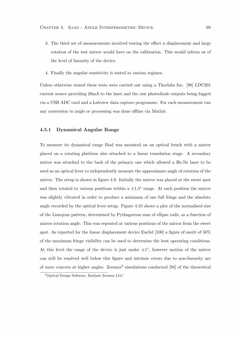
Chapter 4. Iliad - Angle Interferometric Device 68
3. The third set of measurements involved testing the effect a displacement and large
rotation of the test mirror would have on the calibration. This would inform us of
the level of linearity of the device.
4. Finally the angular sensitivity is tested in various regimes.
Unless otherwise stated these tests were carried out using a Thorlabs Inc. [98] LDC201
current source providing 20mA to the laser and the raw photodiode outputs being logged
via a USB ADC card and a Labview data capture programme. For each measurement run
any conversion to angle or processing was done offline via Matlab.
4.5.1 Dynamical Angular Range
To measure its dynamical range Iliad was mounted on an optical bench with a mirror
placed on a rotating platform also attached to a linear translation stage. A secondary
mirror was attached to the back of the primary one which allowed a He-Ne laser to be
used as an optical lever to independently measure the approximate angle of rotation of the
mirror. The setup is shown in figure 4.9. Initially the mirror was placed at the sweet spot
and then rotated to various positions within a ±1.5 range. At each position the mirror
was slightly vibrated in order to produce a minimum of one full fringe and the absolute
angle recorded by the optical lever setup. Figure 4.10 shows a plot of the normalised size
of the Lissajous pattern, determined by Pythagorean sum of ellipse radii, as a function of
mirror rotation angle. This was repeated at various positions of the mirror from the sweet
spot. As reported for the linear displacement device Euclid [100] a figure of merit of 50%
of the maximum fringe visibility can be used to determine the best operating conditions.
At this level the range of the device is just under ±1, however motion of the mirror
can still be resolved well below this figure and intrinsic errors due to non-linearity are
of more concern at higher angles. Zeemax2 simulations conducted [94] of the theoretical
2Optical Design Software, Radiant Zeemax LLC
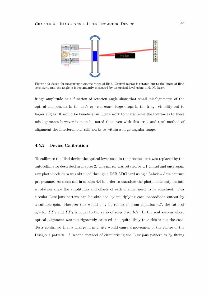
Chapter 4. Iliad - Angle Interferometric Device 69
Figure 4.9: Setup for measuring dynamic range of Iliad. Central mirror is rotated out to the limits of Iliadsensitivity and the angle is independently measured by an optical level using a He-Ne laser.
fringe amplitude as a function of rotation angle show that small misalignments of the
optical components in the cat’s eye can cause large drops in the fringe visibility out to
larger angles. It would be beneficial in future work to characterise the tolerances to these
misalignments however it must be noted that even with this ‘trial and test’ method of
alignment the interferometer still works to within a large angular range.
4.5.2 Device Calibration
To calibrate the Iliad device the optical lever used in the previous test was replaced by the
autocollimator described in chapter 2. The mirror was rotated by±1.5mrad and once again
raw photodiode data was obtained through a USB ADC card using a Labview data capture
programme. As discussed in section 4.4 in order to translate the photodiode outputs into
a rotation angle the amplitudes and offsets of each channel need to be equalised. This
circular Lissajous pattern can be obtained by multiplying each photodiode output by
a suitable gain. However this would only be robust if, from equation 4.7, the ratio of
ai’s for PD1 and PD3 is equal to the ratio of respective bi’s. In the real system where
optical alignment was not rigorously assessed it is quite likely that this is not the case.
Tests confirmed that a change in intensity would cause a movement of the centre of the
Lissajous pattern. A second method of circularising the Lissajous pattern is by fitting
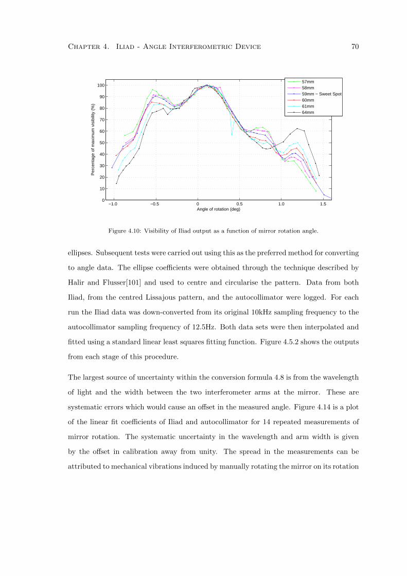
Chapter 4. Iliad - Angle Interferometric Device 70
−1.0 −0.5 0 0.5 1.0 1.50
10
20
30
40
50
60
70
80
90
100
Angle of rotation (deg)
Per
cent
age
of m
axim
um v
isib
ility
(%
)
57mm58mm59mm − Sweet Spot60mm61mm64mm
Figure 4.10: Visibility of Iliad output as a function of mirror rotation angle.
ellipses. Subsequent tests were carried out using this as the preferred method for converting
to angle data. The ellipse coefficients were obtained through the technique described by
Halir and Flusser[101] and used to centre and circularise the pattern. Data from both
Iliad, from the centred Lissajous pattern, and the autocollimator were logged. For each
run the Iliad data was down-converted from its original 10kHz sampling frequency to the
autocollimator sampling frequency of 12.5Hz. Both data sets were then interpolated and
fitted using a standard linear least squares fitting function. Figure 4.5.2 shows the outputs
from each stage of this procedure.
The largest source of uncertainty within the conversion formula 4.8 is from the wavelength
of light and the width between the two interferometer arms at the mirror. These are
systematic errors which would cause an offset in the measured angle. Figure 4.14 is a plot
of the linear fit coefficients of Iliad and autocollimator for 14 repeated measurements of
mirror rotation. The systematic uncertainty in the wavelength and arm width is given
by the offset in calibration away from unity. The spread in the measurements can be
attributed to mechanical vibrations induced by manually rotating the mirror on its rotation
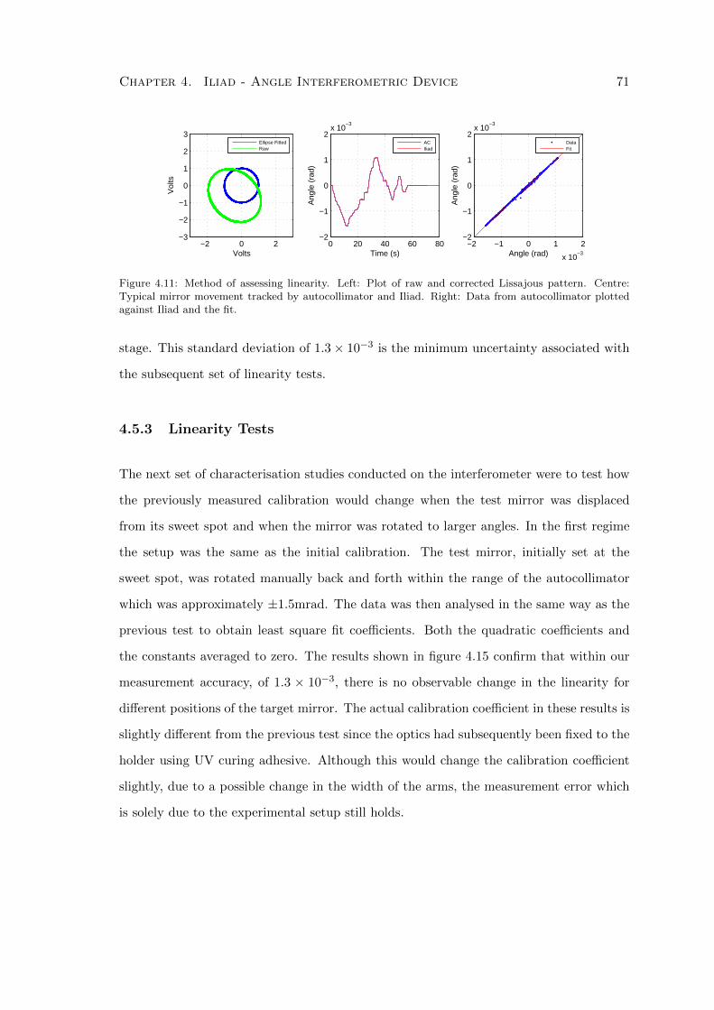
Chapter 4. Iliad - Angle Interferometric Device 71
−2 0 2−3
−2
−1
0
1
2
3
Volts
Vol
ts
0 20 40 60 80−2
−1
0
1
2x 10
−3
Time (s)
Ang
le (
rad)
−2 −1 0 1 2
x 10−3
−2
−1
0
1
2x 10
−3
Angle (rad)
Ang
le (
rad)
ACIliad
Ellipse FittedRaw
DataFit
Figure 4.11: Method of assessing linearity. Left: Plot of raw and corrected Lissajous pattern. Centre:Typical mirror movement tracked by autocollimator and Iliad. Right: Data from autocollimator plottedagainst Iliad and the fit.
stage. This standard deviation of 1.3× 10⁻³ is the minimum uncertainty associated with
the subsequent set of linearity tests.
4.5.3 Linearity Tests
The next set of characterisation studies conducted on the interferometer were to test how
the previously measured calibration would change when the test mirror was displaced
from its sweet spot and when the mirror was rotated to larger angles. In the first regime
the setup was the same as the initial calibration. The test mirror, initially set at the
sweet spot, was rotated manually back and forth within the range of the autocollimator
which was approximately ±1.5mrad. The data was then analysed in the same way as the
previous test to obtain least square fit coefficients. Both the quadratic coefficients and
the constants averaged to zero. The results shown in figure 4.15 confirm that within our
measurement accuracy, of 1.3 × 10⁻³, there is no observable change in the linearity for
different positions of the target mirror. The actual calibration coefficient in these results is
slightly different from the previous test since the optics had subsequently been fixed to the
holder using UV curing adhesive. Although this would change the calibration coefficient
slightly, due to a possible change in the width of the arms, the measurement error which
is solely due to the experimental setup still holds.
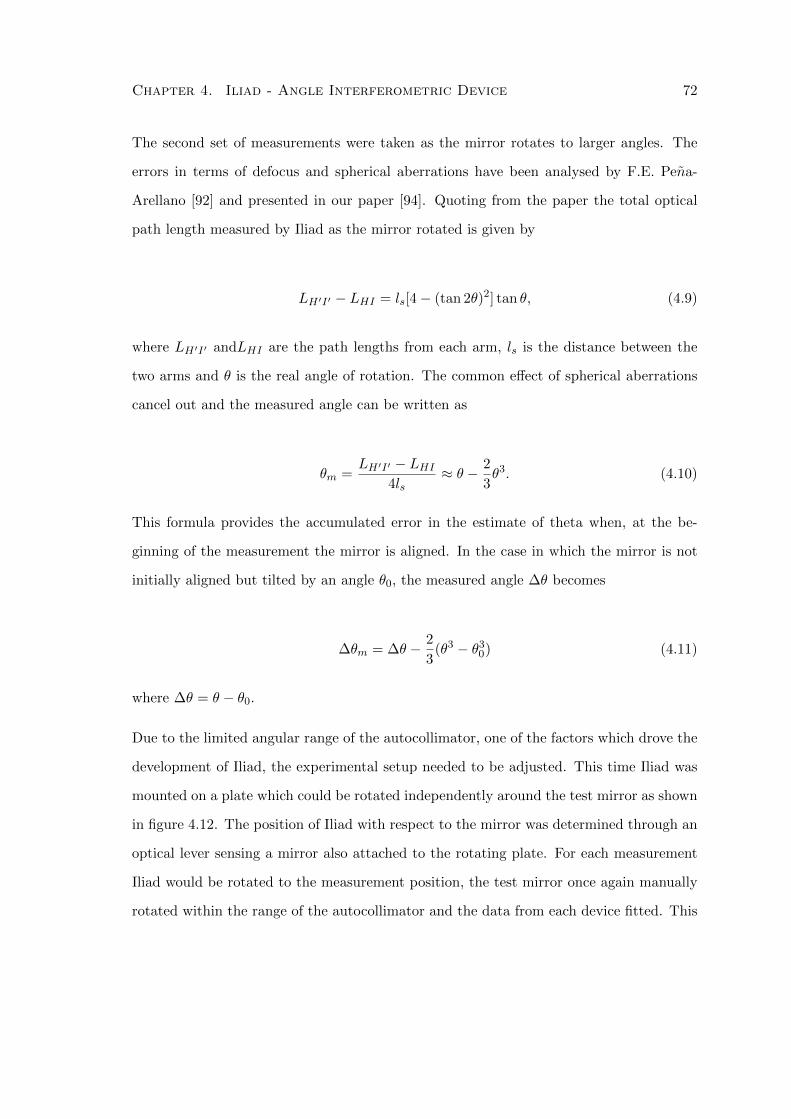
Chapter 4. Iliad - Angle Interferometric Device 72
The second set of measurements were taken as the mirror rotates to larger angles. The
errors in terms of defocus and spherical aberrations have been analysed by F.E. Pena-
Arellano [92] and presented in our paper [94]. Quoting from the paper the total optical
path length measured by Iliad as the mirror rotated is given by
LH′I′ − LHI = ls[4− (tan 2θ)2] tan θ, (4.9)
where LH′I′ andLHI are the path lengths from each arm, ls is the distance between the
two arms and θ is the real angle of rotation. The common effect of spherical aberrations
cancel out and the measured angle can be written as
θm =LH′I′ − LHI
4ls≈ θ − 2
3θ3. (4.10)
This formula provides the accumulated error in the estimate of theta when, at the be-
ginning of the measurement the mirror is aligned. In the case in which the mirror is not
initially aligned but tilted by an angle θ0, the measured angle ∆θ becomes
∆θm = ∆θ − 2
3(θ3 − θ30) (4.11)
where ∆θ = θ − θ0.
Due to the limited angular range of the autocollimator, one of the factors which drove the
development of Iliad, the experimental setup needed to be adjusted. This time Iliad was
mounted on a plate which could be rotated independently around the test mirror as shown
in figure 4.12. The position of Iliad with respect to the mirror was determined through an
optical lever sensing a mirror also attached to the rotating plate. For each measurement
Iliad would be rotated to the measurement position, the test mirror once again manually
rotated within the range of the autocollimator and the data from each device fitted. This
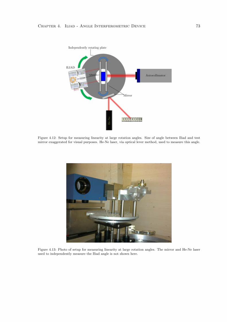
Chapter 4. Iliad - Angle Interferometric Device 73
Figure 4.12: Setup for measuring linearity at large rotation angles. Size of angle between Iliad and testmirror exaggerated for visual purposes. He-Ne laser, via optical lever method, used to measure this angle.
Figure 4.13: Photo of setup for measuring linearity at large rotation angles. The mirror and He-Ne laserused to independently measure the Iliad angle is not shown here.
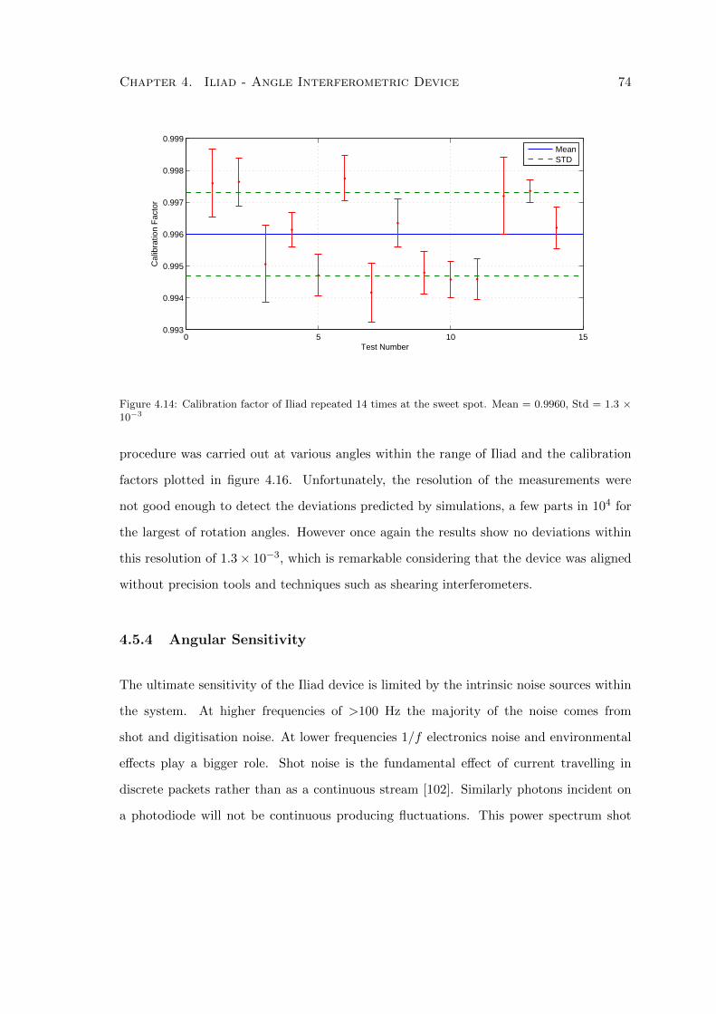
Chapter 4. Iliad - Angle Interferometric Device 74
0 5 10 150.993
0.994
0.995
0.996
0.997
0.998
0.999
Test Number
Cal
ibra
tion
Fac
tor
MeanSTD
Figure 4.14: Calibration factor of Iliad repeated 14 times at the sweet spot. Mean = 0.9960, Std = 1.3 ×10⁻³
procedure was carried out at various angles within the range of Iliad and the calibration
factors plotted in figure 4.16. Unfortunately, the resolution of the measurements were
not good enough to detect the deviations predicted by simulations, a few parts in 104 for
the largest of rotation angles. However once again the results show no deviations within
this resolution of 1.3× 10⁻³, which is remarkable considering that the device was aligned
without precision tools and techniques such as shearing interferometers.
4.5.4 Angular Sensitivity
The ultimate sensitivity of the Iliad device is limited by the intrinsic noise sources within
the system. At higher frequencies of >100 Hz the majority of the noise comes from
shot and digitisation noise. At lower frequencies 1/f electronics noise and environmental
effects play a bigger role. Shot noise is the fundamental effect of current travelling in
discrete packets rather than as a continuous stream [102]. Similarly photons incident on
a photodiode will not be continuous producing fluctuations. This power spectrum shot
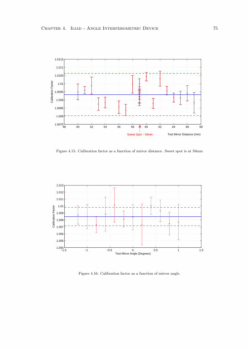
Chapter 4. Iliad - Angle Interferometric Device 75
48 50 52 54 56 58 60 62 64 66 681.0075
1.008
1.0085
1.009
1.0095
1.01
1.0105
1.011
1.0115
Test Mirror Distance (mm)
Cal
ibra
tion
Fac
tor
Sweet Spot − 59mm
Figure 4.15: Calibration factor as a function of mirror distance. Sweet spot is at 59mm
−1.5 −1 −0.5 0 0.5 1 1.51.004
1.005
1.006
1.007
1.008
1.009
1.01
1.011
1.012
1.013
Test Mirror Angle (Degrees)
Cal
ibra
tion
Fac
tor
Figure 4.16: Calibration factor as a function of mirror angle.
Chapter 4. Iliad - Angle Interferometric Device 76
noise of the photocurrent, Ic, is given by
S1/2shot(f) =
√2eIc ×Rf (4.12)
in units of V/√Hz, where e is the charge on the electron and Rf is the feedback resistor
within the transimpedence amplifier stage. Noise also occurs from the digitisation of the
signal through the ADC card. This is given by
S1/2ADC(f) = Lrms ×
Vrange2N
×√
1
(fs/2)(4.13)
where Lrms is the least significant bit RMS of the ADC, Vrange is the voltage range, N is
the number of bits and fs is the sampling rate. Most data described were logged through
a transimpedence stage which used an Rf of 69kΩ, with 8 times gain, and the 16 bit ADC
card previously mentioned. A typical photocurrent produced when the laser was set to
an intensity of 20mA was 2µA. This gives a shot noise level of 10−6V/√Hz. The limiting
factor is the ADC board which if using a voltage range of ±5V and a sampling rate of
990Hz, higher sampling rates produced files sizes which were very large to analyse, gave a
noise limit of 1× 10⁻⁵V/√Hz. Initial measurements of Iliad with a static mirror showed
noise levels higher than this limit and causes of these errors were investigated.
Laser Frequency Fluctuations
Instabilities in the frequency of the laser due to spontaneous emission into the resonator
modes will propagate through the interferometer as a phase delay if the arms of the device
are unequal. Intrinsically the design of Iliad creates unequal path lengths between the arms
due to the requirement of one of the beams to travel through an extra beam splitter. A
further optical component of the same material and dimension as this extra beam splitter
Chapter 4. Iliad - Angle Interferometric Device 77
was therefore added in the path of that arm. In our case we used a polarising beam
splitter of the same kind as PBS A placed in the optical line connecting PBS C and PBS
Eb. The effect of these fluctuations can be determined by first considering the path length
difference, equation 4.4. The phase measured for a mirror displacement, d, is given by
∆φ =8πd
λ(4.14)
Any erroneous displacement at this distance can be interpreted as an extra phase change
δx = δφλ
8π(4.15)
which can be brought about by a change in the laser wavelength
d(∆φ) = −−8πd
λ
dλ
λ(4.16)
δx = −dλδλ (4.17)
The spectrum of the intrinsic frequency fluctuations is given by Owens [103] as
δf2(ν) =D
π(4.18)
δf
f= −δλ
λ(4.19)
where D is the intrinsic linewidth of the laser. The coherence length of a laser is given as
L ≈ λ2
∆λ=
c
D(4.20)
where δλ is the linewidth in terms of wavelength. These can be substituted into equation
(4.15) to give the spectrum of displacement errors due to frequency fluctuations.

Chapter 4. Iliad - Angle Interferometric Device 78
δx = λd
√1
cLπ(4.21)
with units of m/√Hz. It has been reported3 that the coherence length of our 1550nm
DFB laser is given as being between 6m - 10m. This gives an upper limit of δx ≈
d · 2 × 10⁻¹¹m/√Hz. Thus even for large angles up to the maximum range of Iliad of
±1.5 the displacement noise due to frequency fluctuations is less than 1×10⁻¹⁴rad/√Hz,
well below the other limiting factors within the system.
Laser Intensity Noise
The laser may also experience fluctuations in its output intensity due to thermal and
acoustic effects along with fundamental quantum properties [102]. This may also propa-
gate into displacement noise through the differing properties of the photodiodes. A more
accurate model than those of equations 4.7 can be given for the signal on the photodiodes
I1 = α(γb1 + a1β cos(φ)) (4.22)
I2 = α(γb2 + a2β sin(φ)) (4.23)
I3 = α(γb3 − a3β cos(φ)) (4.24)
where the addition of β and γ are effects due to mirror rotation and α are intensity
fluctuations from the laser. Since alignment of beams on each photodiode are not identical
a change in laser intensity, α, will cause a different change in each photodiode. The
ellipse fitting method described earlier fits an ellipse to the data as a whole. If over
longer timescales temperature fluctuations caused intensity changes these would manifest
themselves as a shift in the centre of the Lissajous pattern causing the initial ellipse fit
parameters to be wrong. Real time ellipse fitting could be used however when sensing
3Reported in Distributed-feedback (DFB) Laser Coherence and Linewidth Broadening -http://dspace.dsto.defence.gov.au/dspace/bitstream/1947/3355/1/DSTO-RR-0263%20PR.pdf
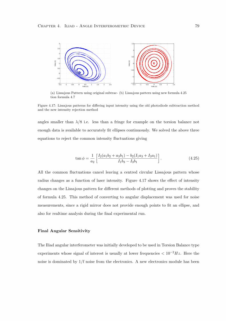
Chapter 4. Iliad - Angle Interferometric Device 79
−1.5 −1 −0.5 0 0.5 1 1.5 2 2.5−1
−0.5
0
0.5
1
1.5
2
2.5
3
Volts (V)
Vol
ts (
V)
(a) Lissajous Pattern using original subtrac-tion formula 4.7
−1.5 −1 −0.5 0 0.5 1 1.5−1.5
−1
−0.5
0
0.5
1
1.5
Volts (V)
Vol
ts (
V)
(b) Lissajous pattern using new formula 4.25
Figure 4.17: Lissajous patterns for differing input intensity using the old photodiode subtraction methodand the new intensity rejection method
angles smaller than λ/8 i.e. less than a fringe for example on the torsion balance not
enough data is available to accurately fit ellipses continuously. We solved the above three
equations to reject the common intensity fluctuations giving
tanφ =1
a2
[I2(a1b2 + a3b1)− b2(I1a3 + I3a1)
I1b3 − I3b1
]. (4.25)
All the common fluctuations cancel leaving a centred circular Lissajous pattern whose
radius changes as a function of laser intensity. Figure 4.17 shows the effect of intensity
changes on the Lissajous pattern for different methods of plotting and proves the stability
of formula 4.25. This method of converting to angular displacement was used for noise
measurements, since a rigid mirror does not provide enough points to fit an ellipse, and
also for realtime analysis during the final experimental run.
Final Angular Sensitivity
The Iliad angular interferometer was initially developed to be used in Torsion Balance type
experiments whose signal of interest is usually at lower frequencies < 10−2Hz. Here the
noise is dominated by 1/f noise from the electronics. A new electronics module has been
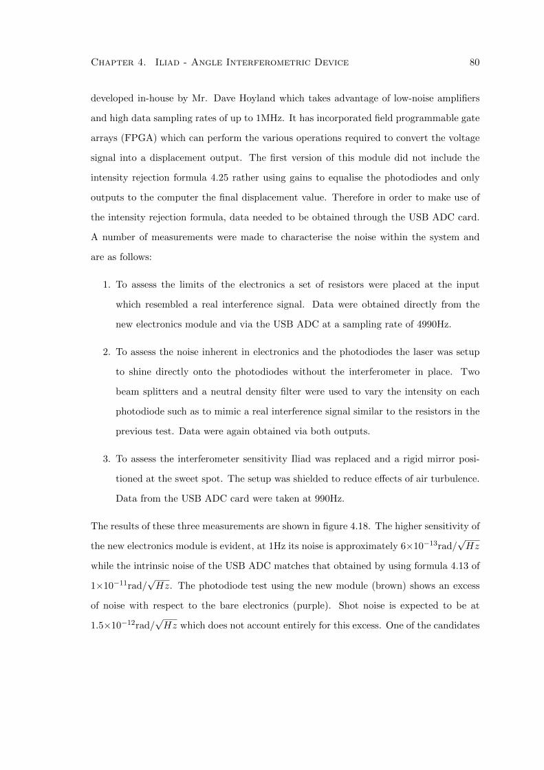
Chapter 4. Iliad - Angle Interferometric Device 80
developed in-house by Mr. Dave Hoyland which takes advantage of low-noise amplifiers
and high data sampling rates of up to 1MHz. It has incorporated field programmable gate
arrays (FPGA) which can perform the various operations required to convert the voltage
signal into a displacement output. The first version of this module did not include the
intensity rejection formula 4.25 rather using gains to equalise the photodiodes and only
outputs to the computer the final displacement value. Therefore in order to make use of
the intensity rejection formula, data needed to be obtained through the USB ADC card.
A number of measurements were made to characterise the noise within the system and
are as follows:
1. To assess the limits of the electronics a set of resistors were placed at the input
which resembled a real interference signal. Data were obtained directly from the
new electronics module and via the USB ADC at a sampling rate of 4990Hz.
2. To assess the noise inherent in electronics and the photodiodes the laser was setup
to shine directly onto the photodiodes without the interferometer in place. Two
beam splitters and a neutral density filter were used to vary the intensity on each
photodiode such as to mimic a real interference signal similar to the resistors in the
previous test. Data were again obtained via both outputs.
3. To assess the interferometer sensitivity Iliad was replaced and a rigid mirror posi-
tioned at the sweet spot. The setup was shielded to reduce effects of air turbulence.
Data from the USB ADC card were taken at 990Hz.
The results of these three measurements are shown in figure 4.18. The higher sensitivity of
the new electronics module is evident, at 1Hz its noise is approximately 6×10⁻¹³rad/√Hz
while the intrinsic noise of the USB ADC matches that obtained by using formula 4.13 of
1×10⁻¹¹rad/√Hz. The photodiode test using the new module (brown) shows an excess
of noise with respect to the bare electronics (purple). Shot noise is expected to be at
1.5×10⁻¹²rad/√Hz which does not account entirely for this excess. One of the candidates
Chapter 4. Iliad - Angle Interferometric Device 81
10−1
100
101
102
10−13
10−12
10−11
10−10
10−9
Frequency [Hz]
Ang
ular
Rea
dout
Noi
se [r
ad H
z−1/
2 ]
Figure 4.18: Sensitivity of Iliad and its components. Blue - Iliad Device with rigid mirror, Green - Laserand photodiode setup through USB ADC, Brown - Laser and photodiode setup through new module box,Orange - Intrinsic electronic noise of USB ADC, Purple - Intrinsic electronic noise of new module box.Note: New electronics module has internal filter producing the roll off above 50Hz.
at lower frequencies could be air turbulence however the origin of the noise above 1Hz is
still unknown. Finally the blue curve shows the sensitivity of the Iliad device on an
optical bench in air. In the range between 10−1Hz and 10Hz the noise spectrum is
almost flat, and is about 5× 10⁻¹¹ radians/√Hz. Below 10−1Hz the signal is most likely
limited by effects induced by thermal drifts and air currents, whereas at higher frequencies
(≈ 10Hz and above) the features indicate it is limited by mechanical vibration in the
measurement apparatus. The exact source of the broadband excess noise seen between
the measurements of the intereferometer and photodiodes alone is not fully understood. It
is quite possible that mechanical vibrations are the only cause of this and a better assembly
within a vacuum environment may produce better results. However it is important to note
that these measurements confirm an upper limit on the Iliad device angular sensitivity of
5× 10⁻¹¹ radians/√Hz between 10−1Hz and 10Hz.
Chapter 4. Iliad - Angle Interferometric Device 82
4.6 Iliad on the Torsion Balance
Once the characterisation studies were complete, Iliad was installed onto the torsion bal-
ance apparatus. The smooth oscillatory motion of the torsion balance also provided a good
platform to further test the device linearity. Data from Iliad and the autocollimator was
logged for a number of oscillations and subsequently split into small 140 second windows.
Each section was fitted with the same procedure as previously employed. The results,
plotted in figure 4.19, show that the standard deviation of fit coefficients in this setup was
2 × 10⁻⁴, small enough to compare to the theoretical predictions. Since the range of the
autocollimator is smaller than our testing parameters, these measurements were slightly
more complicated to perform. To rotate the torsion balance with respect to Iliad one
set of damping electrodes were used to bias the equilibrium position of the balance. The
autocollimator was then rotated manually to the necessary position and then the second
set of electrodes were used to damp the oscillations down to the range of the autocolli-
mator ±1.5mrad. At each angle the torsion balance was allowed to oscillate a number of
times and the same data procedure described previously was used to assess the linearity
coefficients. The results, shown in figure 4.20, are surprising due to the assymetry of the
coefficients. Indeed the amplitude error agrees with the theoretical results, also plotted in
blue, however since there was no quantifiable assessment of the alignment of the device it
is difficult to predict a reason for these results. Further discussion and analysis is required
although it is only of concern to users who require a relative error of better than 1×10⁻³
and measuring angles out to the limit of the device.
4.7 Conclusions
The development and characterisation of the first prototype Iliad device has been a sub-
stantial part of the overall project. The increased sensitivity over the current state of the
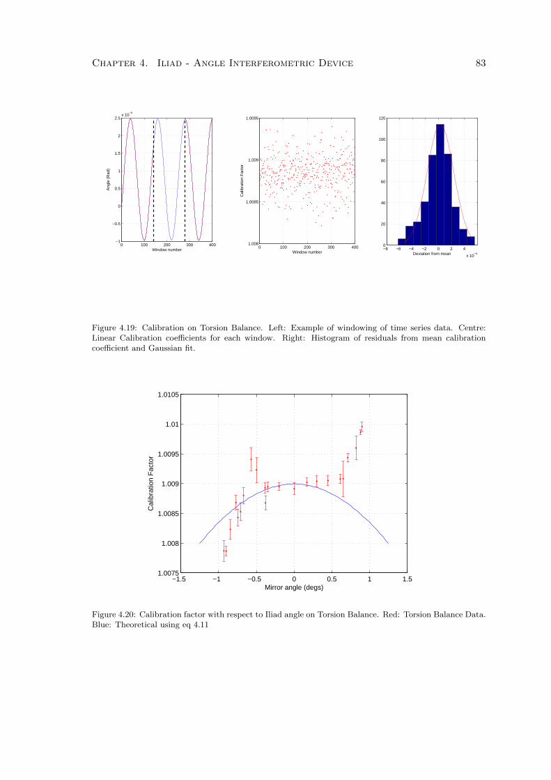
Chapter 4. Iliad - Angle Interferometric Device 83
0 100 200 300 400−1
−0.5
0
0.5
1
1.5
2
2.5x 10
−5
Window number
Ang
le (
Rad
)
0 100 200 300 4001.008
1.0085
1.009
1.0095
Window number
Cal
ibra
tion
Fac
tor
−8 −6 −4 −2 0 2 4
x 10−4
0
20
40
60
80
100
120
Deviation from mean
Figure 4.19: Calibration on Torsion Balance. Left: Example of windowing of time series data. Centre:Linear Calibration coefficients for each window. Right: Histogram of residuals from mean calibrationcoefficient and Gaussian fit.
−1.5 −1 −0.5 0 0.5 1 1.51.0075
1.008
1.0085
1.009
1.0095
1.01
1.0105
Mirror angle (degs)
Cal
ibra
tion
Fac
tor
Figure 4.20: Calibration factor with respect to Iliad angle on Torsion Balance. Red: Torsion Balance Data.Blue: Theoretical using eq 4.11
Chapter 4. Iliad - Angle Interferometric Device 84
art autocollimator allows the benefits of using torsion strip balance to be fully exploited.
Its compact design also makes it less sensitive to environmental effects for example ther-
mal drifts which couple into the autocollimator signal due to its large size and mounting
requirements. The device also has a great degree of tilt immunity both in its assembly and
operational alignment which makes it ideal for use in these types of experiments. Although
the drive to develop this instrument was for the use in our torsion balance experiment its
application is much wider. Our studies showed that even through a non quantitative align-
ment process the device showed remarkable properties, having a large dynamical range
of over ±1 and still being linear to within 1 part in 103 out to large rotational angles.
Further tests should however be carried out to understand the origin of some of the dif-
ferences from simulations, for example the ‘wings’ seen in figure 4.10. This effect could
be due to back reflection into the laser and can be tested by checking for any erroneous
displacement signal with only one arm sensing the mirror. Also a thorough investigation
into the alignment process should be carried out using proper techniques such as shearing
interferometers so that theory and experiment can be quantitatively compared.
Chapter 5
Data Analysis and
Systematics
As described previously two source masses were modulated every 800 seconds between
positions of maximum torque on the torsion balance. This section describes the analysis
procedure to convert from the measured angle to a torque signal and systematic effects
which may interfere with the detection of a real signal.
5.1 Data Collection and Conversion
Each of the five sets of experimental and environmental data; autocollimator detected
angle θac, Iliad detected angle θil, temperature, tilt and motor position were logged to
separate files every 12 hours. Although the sampling rate varied for each set the reference
time was equivalent for all the data.
The autocollimator senses the position of the reflected beam in both X and Y co-ordinates
and thus gives information on the rotation and tilt of the balance. However, since the
autocollimator is not positioned exactly parallel to the base plate of the torsion balance
there will be some mixing between the two signals depending on offset angle θ. A schematic
of this is shown in figure 5.1. To remove this effect the data was subjected to a rotation
85
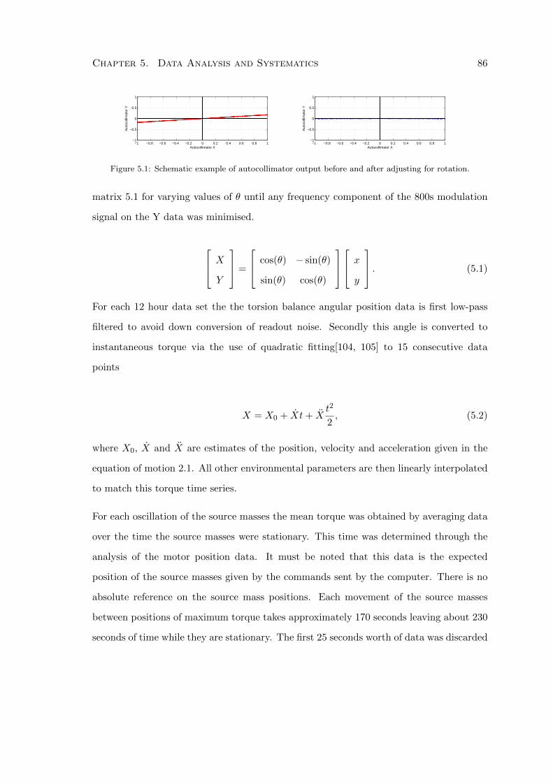
Chapter 5. Data Analysis and Systematics 86
−1 −0.8 −0.6 −0.4 −0.2 0 0.2 0.4 0.6 0.8 1−1
−0.5
0
0.5
1
Autocollimator X
Aut
ocol
limat
or Y
−1 −0.8 −0.6 −0.4 −0.2 0 0.2 0.4 0.6 0.8 1−1
−0.5
0
0.5
1
Autocollimator X
Aut
ocol
limat
or Y
Figure 5.1: Schematic example of autocollimator output before and after adjusting for rotation.
matrix 5.1 for varying values of θ until any frequency component of the 800s modulation
signal on the Y data was minimised.
X
Y
=
cos(θ) − sin(θ)
sin(θ) cos(θ)
x
y
. (5.1)
For each 12 hour data set the the torsion balance angular position data is first low-pass
filtered to avoid down conversion of readout noise. Secondly this angle is converted to
instantaneous torque via the use of quadratic fitting[104, 105] to 15 consecutive data
points
X = X0 + Xt+ Xt2
2, (5.2)
where X0, X and X are estimates of the position, velocity and acceleration given in the
equation of motion 2.1. All other environmental parameters are then linearly interpolated
to match this torque time series.
For each oscillation of the source masses the mean torque was obtained by averaging data
over the time the source masses were stationary. This time was determined through the
analysis of the motor position data. It must be noted that this data is the expected
position of the source masses given by the commands sent by the computer. There is no
absolute reference on the source mass positions. Each movement of the source masses
between positions of maximum torque takes approximately 170 seconds leaving about 230
seconds of time while they are stationary. The first 25 seconds worth of data was discarded
Chapter 5. Data Analysis and Systematics 87
at the beginning of each of these 230 seconds sets to allow the damping of the pendulum
and a further 5 seconds of data discarded at the end of the set to ensure fluctuations
in the starting time of the motor were ignored. For each set the coherent torque and
environmental data were saved and averaged to output a single point associated with each
movement of the source masses. Figure 5.2 shows an example of this process.
5.2 Least Squares Fit
The torque model and any systematics can be fitted using a general least squares fitting
procedure which minimises the squared error between the observed data and a number of
fit parameters [106]. For example
Y = f(X) + ε, (5.3)
where Y is our observed variable, f(X) is a function of our correlation variables and ε the
excess noise. For yi data points each with σi standard deviation and bj variables with xj,i
points we attempt to minimise the χ-square function
χ2 =n∑i=1
(yi − fi(xj,i))2
σi
2
. (5.4)
We can rewrite this equation in matrix notation. Consider our N observables as a vector
y = (y1, ...., yN ) and let X be an N × P matrix of
X =
x1,1 x1,2 . . x1,P
x2,1. x2,2 . . .
. . . . .
xN,1 xN,2 . . xN,P
. (5.5)
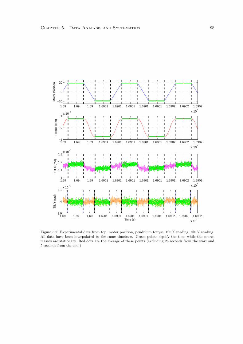
Chapter 5. Data Analysis and Systematics 88
1.69 1.69 1.69 1.6901 1.6901 1.6901 1.6901 1.6901 1.6902 1.6902 1.6902
x 107
3.9
4
4.1x 10
−5
Tilt
Y (
rad)
Time (s)
1.69 1.69 1.69 1.6901 1.6901 1.6901 1.6901 1.6901 1.6902 1.6902 1.6902
x 107
−20
0
20
Mot
or P
ositi
on
1.69 1.69 1.69 1.6901 1.6901 1.6901 1.6901 1.6901 1.6902 1.6902 1.6902
x 107
−1
0
1x 10
−8
Tor
que
(Nm
)
1.69 1.69 1.69 1.6901 1.6901 1.6901 1.6901 1.6901 1.6902 1.6902 1.6902
x 107
1
1.1
1.2
1.3x 10
−5
Tilt
X (
rad)
Figure 5.2: Experimental data from top, motor position, pendulum torque, tilt X reading, tilt Y reading.All data have been interpolated to the same timebase. Green points signify the time while the sourcemasses are stationary. Red dots are the average of these points (excluding 25 seconds from the start and5 seconds from the end.)
Chapter 5. Data Analysis and Systematics 89
Each of the columns in X represents our parameters and rows are the data points. We
also define a vector, A = (a1, ...., aP ) which are the coefficients to be fitted. The minimum
occurs by differentiating with respect to each coefficient obtaining a set of P equations
N∑i=1
yiXkxiσ2i
−P∑j=1
ajXj(xi)Xk(xi)
σ2i= 0, (5.6)
where k = 1, ..., P . In matrix form this is given as
XTV−1y y = (XTV−1y X)A, (5.7)
where V−1y is a diagonal matrix of the errors associated with the data points. The standard
uncertainties related to the fitted parameters can be given by
σ2(aj) =N∑i=1
σ2i
(δajδyi
)2
, (5.8)
which leads to
σ2(aj) = (XTV −1y X)−1jj . (5.9)
The inverse matrix (XT Vy−1 X)−1 is known as the covariance matrix and its diagonal
components are the standard errors on the fit parameters which are intrinsically linked
to the original data variance. For each of our data points we allocate an error, σi as the
mean standard error associated with the averaging procedure. Thus the reduced chi-square
statistic, equation 5.4 divided by the degrees of freedom, gives a measure of the goodness
of fit. A value of 1 indicates a good match since the variance of the residuals matches the
variance given in the fit. This indicator can be used when fitting for various systematics.
Chapter 5. Data Analysis and Systematics 90
5.3 Expected Torque Model
Any temporal signatures in the Newtonian constant will manifest as an amplitude change
in the detected torque on the balance which is an uncalibrated measurement of G, the
gravitational constant. We can model the torque as
τM = τN + σ, (5.10)
where τM is the measured torque, τN is the Newtonian torque and σ are any real sources
of fluctuations or systematic effects. Modulating the source masses can separate out
amplitude signals with drift signals reducing the sources of noise within the experiment.
Referring to our analysis technique, each torque point can be described as
τMi = α+ (±)(τN + σsignal + σsystematic) + γ(θ) + ε, (5.11)
where α is an offset, σsignal and σsystematic are the additions associated with any signal
and systematic event and ε is the statistical uncertainty on each point. The ± refers to
each change in the source mass position defining the amplitude of the torque signal. Any
signal or systematic that couples to the torque amplitude must also be allocated a ± to
their data points. The final term is the mean pendulum angle where γ would be equal to
the torsional coefficient of the pendulum and is included to account for any drifts. A least
squares fit is used to obtain values of α, τN and γ and once subtracted gives the δG/G
residuals.
Chapter 5. Data Analysis and Systematics 91
5.4 Temperature Systematic
The first source of systematic errors are temperature changes and gradients that can
cause unknown changes in the apparatus. Although as described in chapter 2 efforts have
been taken to ensure temperature fluctuations within the laboratory are minimised it is
still nonetheless important to assess its impact. To establish a calibration coefficient the
temperature was oscillated by manually adjusting the set point of the Julabo stabilised
water tank by ±1K every 10 hours. A second measurement at a different frequency, 9
hour oscillation, and a smaller amplitude, ±0.15K, was conducted by heating a length of
copper pipe in which the water passed through before going into the two thermal boxes via
the control of current through a thin wire wrapped around the pipe. The small amplitude
was due to the limitation of the current source output power. The torque output data was
fitted against the temperature for both these two measurements and longer 5 and 25 day
runs. In all cases the coefficient associated with the vacuum temperature lay within the
bounds 5×10⁻¹² to 8×10⁻¹³. The fact that the coefficient was the same for both Iliad and
the autocollimator suggests that, at this level, the temperature is directly affecting the
torsion balance as opposed to an artefact from the autocollimator mounting. An estimate
into systematic error associated with the temperature can be determined by fitting the
full temperature profile over the experimental run to a sidereal sinusoid. The obtained
amplitude was 4.4±2×10⁻⁴. When using the upper limit for the coefficient this amplitude
relates to a signal in δG/G of 3±1×10⁻⁷, an order of magnitude smaller than our current
noise levels.
5.5 Tilt Systematic
Although the tilt in the long axis (Y axis) of the optical bench is stabilised via the con-
trolled piezo as described in chapter 2 there are still a number of tilt effects which may
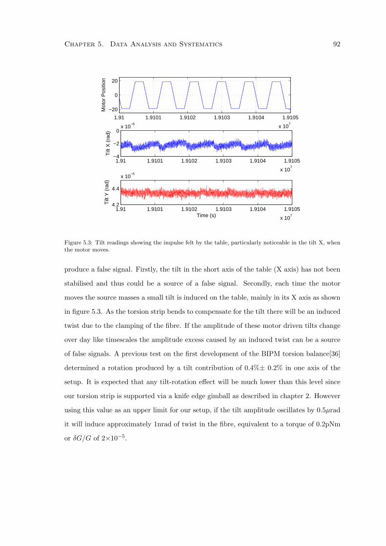
Chapter 5. Data Analysis and Systematics 92
1.91 1.9101 1.9102 1.9103 1.9104 1.9105
x 107
−20
0
20
Mot
or P
ositi
on
1.91 1.9101 1.9102 1.9103 1.9104 1.9105
x 107
−4
−2
0x 10
−6
Tilt
X (
rad)
1.91 1.9101 1.9102 1.9103 1.9104 1.9105
x 107
4.2
4.4
x 10−5
Time (s)
Tilt
Y (
rad)
Figure 5.3: Tilt readings showing the impulse felt by the table, particularly noticeable in the tilt X, whenthe motor moves.
produce a false signal. Firstly, the tilt in the short axis of the table (X axis) has not been
stabilised and thus could be a source of a false signal. Secondly, each time the motor
moves the source masses a small tilt is induced on the table, mainly in its X axis as shown
in figure 5.3. As the torsion strip bends to compensate for the tilt there will be an induced
twist due to the clamping of the fibre. If the amplitude of these motor driven tilts change
over day like timescales the amplitude excess caused by an induced twist can be a source
of false signals. A previous test on the first development of the BIPM torsion balance[36]
determined a rotation produced by a tilt contribution of 0.4%± 0.2% in one axis of the
setup. It is expected that any tilt-rotation effect will be much lower than this level since
our torsion strip is supported via a knife edge gimball as described in chapter 2. However
using this value as an upper limit for our setup, if the tilt amplitude oscillates by 0.5µrad
it will induce approximately 1nrad of twist in the fibre, equivalent to a torque of 0.2pNm
or δG/G of 2×10⁻⁵.
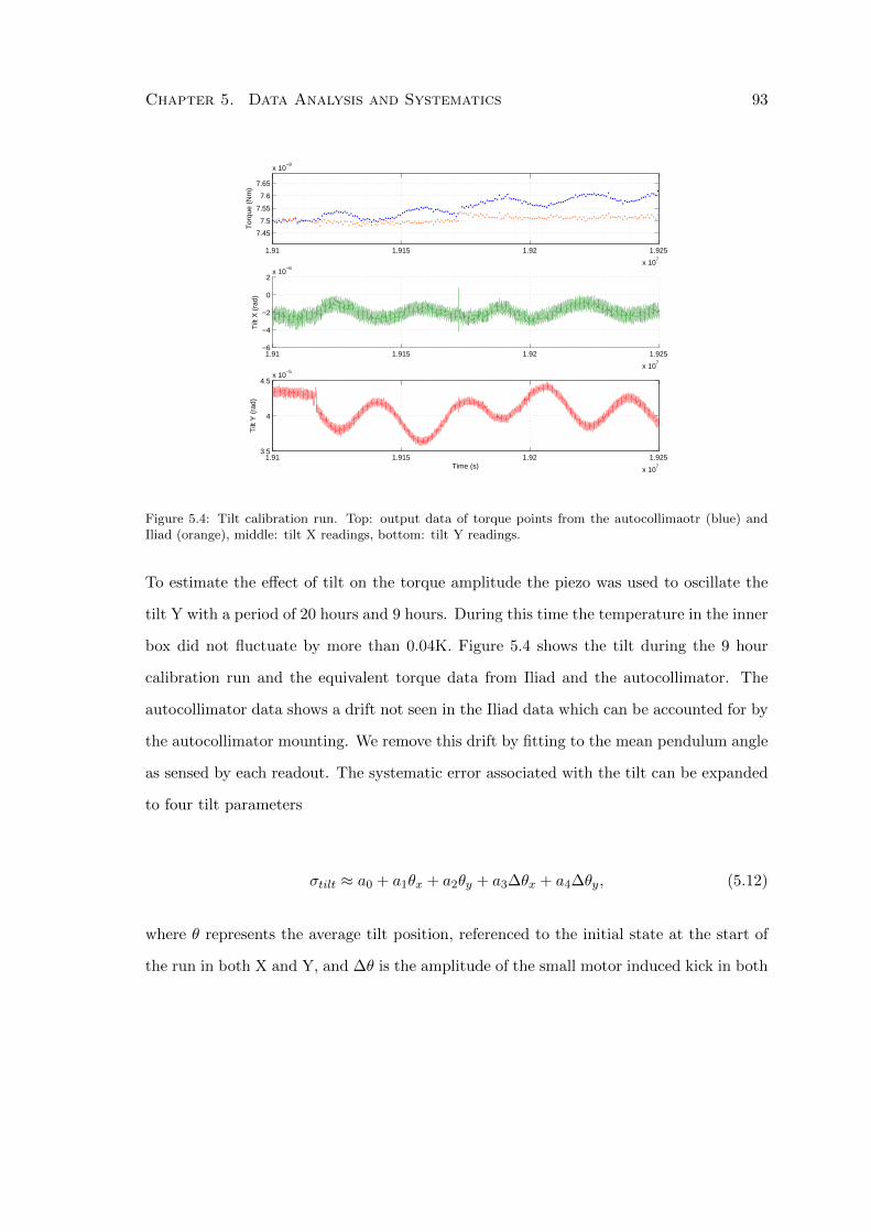
Chapter 5. Data Analysis and Systematics 93
1.91 1.915 1.92 1.925
x 107
7.45
7.5
7.55
7.6
7.65
x 10−9
Tor
que
(Nm
)
1.91 1.915 1.92 1.925
x 107
−6
−4
−2
0
2x 10
−6
Tilt
X (
rad)
1.91 1.915 1.92 1.925
x 107
3.5
4
4.5x 10
−5
Tilt
Y (
rad)
Time (s)
Figure 5.4: Tilt calibration run. Top: output data of torque points from the autocollimaotr (blue) andIliad (orange), middle: tilt X readings, bottom: tilt Y readings.
To estimate the effect of tilt on the torque amplitude the piezo was used to oscillate the
tilt Y with a period of 20 hours and 9 hours. During this time the temperature in the inner
box did not fluctuate by more than 0.04K. Figure 5.4 shows the tilt during the 9 hour
calibration run and the equivalent torque data from Iliad and the autocollimator. The
autocollimator data shows a drift not seen in the Iliad data which can be accounted for by
the autocollimator mounting. We remove this drift by fitting to the mean pendulum angle
as sensed by each readout. The systematic error associated with the tilt can be expanded
to four tilt parameters
σtilt ≈ a0 + a1θx + a2θy + a3∆θx + a4∆θy, (5.12)
where θ represents the average tilt position, referenced to the initial state at the start of
the run in both X and Y, and ∆θ is the amplitude of the small motor induced kick in both
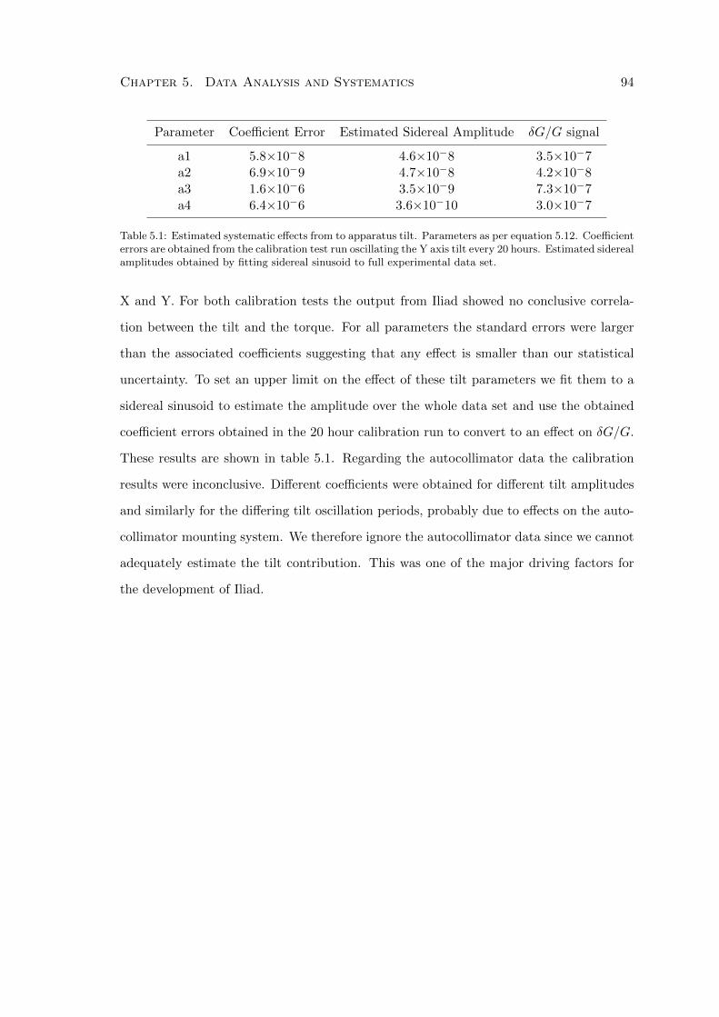
Chapter 5. Data Analysis and Systematics 94
Parameter Coefficient Error Estimated Sidereal Amplitude δG/G signal
a1 5.8×10⁻⁸ 4.6×10⁻⁸ 3.5×10⁻⁷a2 6.9×10⁻⁹ 4.7×10⁻⁸ 4.2×10⁻⁸a3 1.6×10⁻⁶ 3.5×10⁻⁹ 7.3×10⁻⁷a4 6.4×10⁻⁶ 3.6×10⁻¹⁰ 3.0×10⁻⁷
Table 5.1: Estimated systematic effects from to apparatus tilt. Parameters as per equation 5.12. Coefficienterrors are obtained from the calibration test run oscillating the Y axis tilt every 20 hours. Estimated siderealamplitudes obtained by fitting sidereal sinusoid to full experimental data set.
X and Y. For both calibration tests the output from Iliad showed no conclusive correla-
tion between the tilt and the torque. For all parameters the standard errors were larger
than the associated coefficients suggesting that any effect is smaller than our statistical
uncertainty. To set an upper limit on the effect of these tilt parameters we fit them to a
sidereal sinusoid to estimate the amplitude over the whole data set and use the obtained
coefficient errors obtained in the 20 hour calibration run to convert to an effect on δG/G.
These results are shown in table 5.1. Regarding the autocollimator data the calibration
results were inconclusive. Different coefficients were obtained for different tilt amplitudes
and similarly for the differing tilt oscillation periods, probably due to effects on the auto-
collimator mounting system. We therefore ignore the autocollimator data since we cannot
adequately estimate the tilt contribution. This was one of the major driving factors for
the development of Iliad.
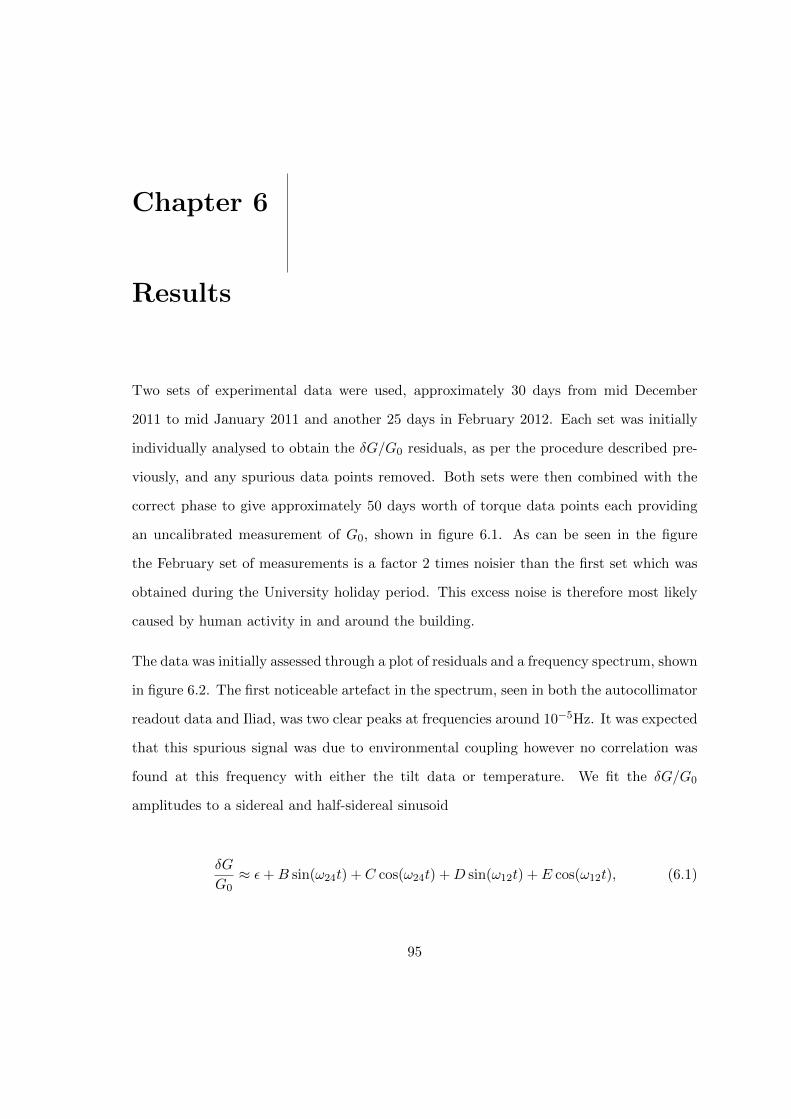
Chapter 6
Results
Two sets of experimental data were used, approximately 30 days from mid December
2011 to mid January 2011 and another 25 days in February 2012. Each set was initially
individually analysed to obtain the δG/G0 residuals, as per the procedure described pre-
viously, and any spurious data points removed. Both sets were then combined with the
correct phase to give approximately 50 days worth of torque data points each providing
an uncalibrated measurement of G0, shown in figure 6.1. As can be seen in the figure
the February set of measurements is a factor 2 times noisier than the first set which was
obtained during the University holiday period. This excess noise is therefore most likely
caused by human activity in and around the building.
The data was initially assessed through a plot of residuals and a frequency spectrum, shown
in figure 6.2. The first noticeable artefact in the spectrum, seen in both the autocollimator
readout data and Iliad, was two clear peaks at frequencies around 10−5Hz. It was expected
that this spurious signal was due to environmental coupling however no correlation was
found at this frequency with either the tilt data or temperature. We fit the δG/G0
amplitudes to a sidereal and half-sidereal sinusoid
δG
G0≈ ε+B sin(ω24t) + C cos(ω24t) +D sin(ω12t) + E cos(ω12t), (6.1)
95
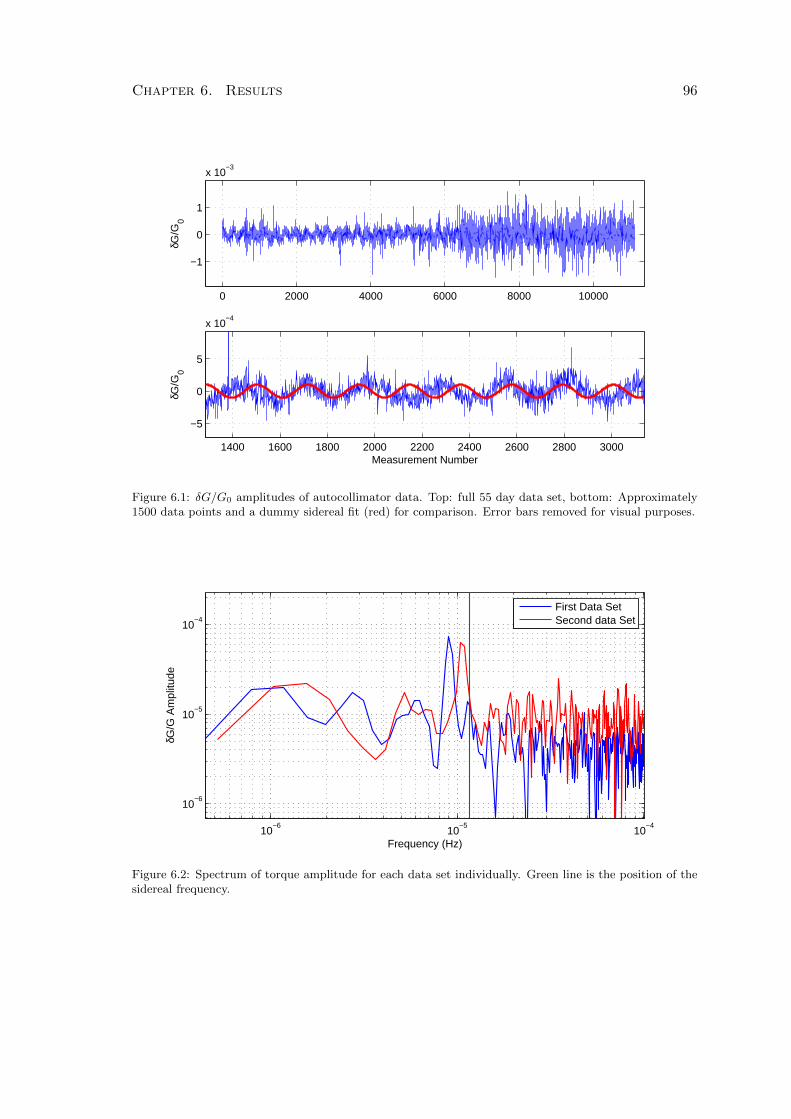
Chapter 6. Results 96
0 2000 4000 6000 8000 10000
−1
0
1
x 10−3
δG/G
0
1400 1600 1800 2000 2200 2400 2600 2800 3000
−5
0
5
x 10−4
Measurement Number
δG/G
0
Figure 6.1: δG/G0 amplitudes of autocollimator data. Top: full 55 day data set, bottom: Approximately1500 data points and a dummy sidereal fit (red) for comparison. Error bars removed for visual purposes.
10−6
10−5
10−4
10−6
10−5
10−4
Frequency (Hz)
δG/G
Am
plitu
de
First Data SetSecond data Set
Figure 6.2: Spectrum of torque amplitude for each data set individually. Green line is the position of thesidereal frequency.
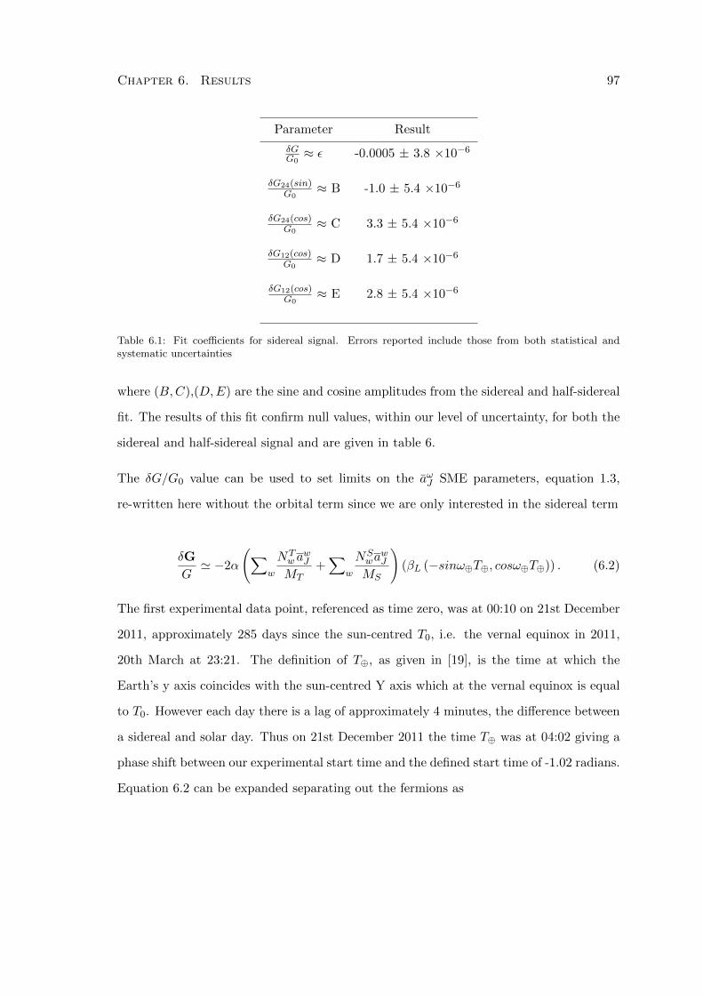
Chapter 6. Results 97
Parameter Result
δGG0≈ ε -0.0005 ± 3.8 ×10⁻⁶
δG24(sin)G0
≈ B -1.0 ± 5.4 ×10⁻⁶
δG24(cos)G0
≈ C 3.3 ± 5.4 ×10⁻⁶
δG12(cos)G0
≈ D 1.7 ± 5.4 ×10⁻⁶
δG12(cos)G0
≈ E 2.8 ± 5.4 ×10⁻⁶
Table 6.1: Fit coefficients for sidereal signal. Errors reported include those from both statistical andsystematic uncertainties
where (B,C),(D,E) are the sine and cosine amplitudes from the sidereal and half-sidereal
fit. The results of this fit confirm null values, within our level of uncertainty, for both the
sidereal and half-sidereal signal and are given in table 6.
The δG/G0 value can be used to set limits on the aωJ SME parameters, equation 1.3,
re-written here without the orbital term since we are only interested in the sidereal term
δG
G' −2α
(∑w
NTwa
wJ
MT+∑
w
NSwa
wJ
MS
)(βL (−sinω⊕T⊕, cosω⊕T⊕)) . (6.2)
The first experimental data point, referenced as time zero, was at 00:10 on 21st December
2011, approximately 285 days since the sun-centred T0, i.e. the vernal equinox in 2011,
20th March at 23:21. The definition of T⊕, as given in [19], is the time at which the
Earth’s y axis coincides with the sun-centred Y axis which at the vernal equinox is equal
to T0. However each day there is a lag of approximately 4 minutes, the difference between
a sidereal and solar day. Thus on 21st December 2011 the time T⊕ was at 04:02 giving a
phase shift between our experimental start time and the defined start time of -1.02 radians.
Equation 6.2 can be expanded separating out the fermions as
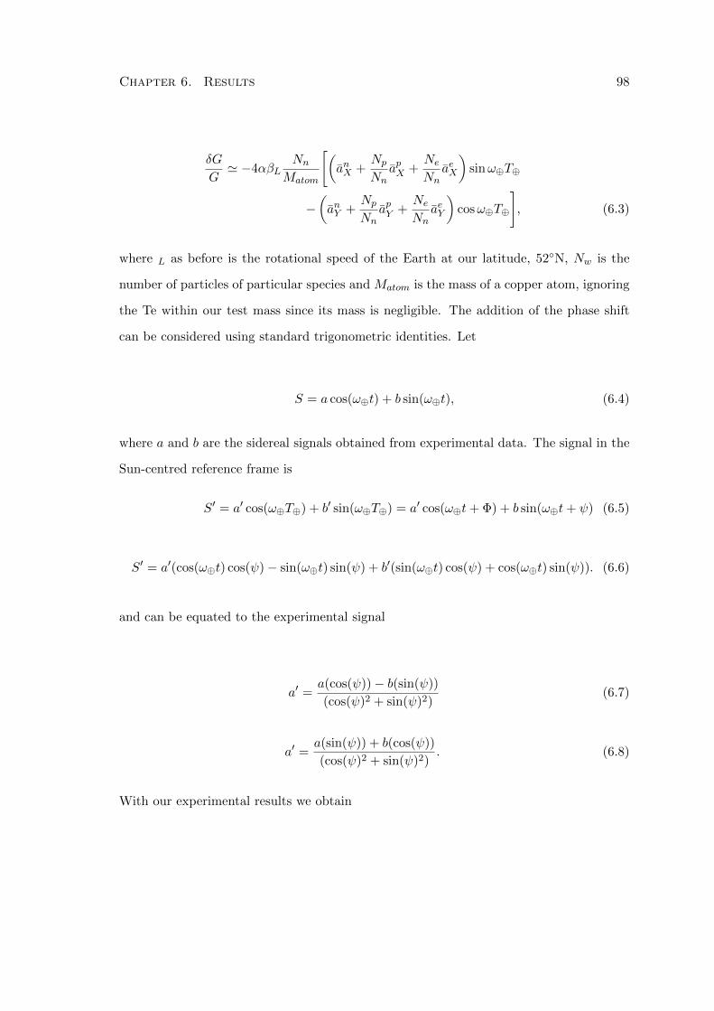
Chapter 6. Results 98
δG
G' −4αβL
Nn
Matom
[(anX +
Np
NnapX +
Ne
NnaeX
)sinω⊕T⊕
−(anY +
Np
NnapY +
Ne
NnaeY
)cosω⊕T⊕
], (6.3)
where L as before is the rotational speed of the Earth at our latitude, 52N, Nw is the
number of particles of particular species and Matom is the mass of a copper atom, ignoring
the Te within our test mass since its mass is negligible. The addition of the phase shift
can be considered using standard trigonometric identities. Let
S = a cos(ω⊕t) + b sin(ω⊕t), (6.4)
where a and b are the sidereal signals obtained from experimental data. The signal in the
Sun-centred reference frame is
S′ = a′ cos(ω⊕T⊕) + b′ sin(ω⊕T⊕) = a′ cos(ω⊕t+ Φ) + b sin(ω⊕t+ ψ) (6.5)
S′ = a′(cos(ω⊕t) cos(ψ)− sin(ω⊕t) sin(ψ) + b′(sin(ω⊕t) cos(ψ) + cos(ω⊕t) sin(ψ)). (6.6)
and can be equated to the experimental signal
a′ =a(cos(ψ))− b(sin(ψ))
(cos(ψ)2 + sin(ψ)2)(6.7)
a′ =a(sin(ψ)) + b(cos(ψ))
(cos(ψ)2 + sin(ψ)2). (6.8)
With our experimental results we obtain
Chapter 6. Results 99
|α [anX + 0.83(apX + aeX)] | ≤ 1.3 GeV,
|α [anY + 0.83(apY + aeY )] | ≤ 1.6 GeV. (6.9)
This limit is higher than that achieved in our previous experimental run as presented in
[21] which gave constraints that were several times smaller. However it must be noted
that the current results were obtained from 55 days worth of data as opposed to almost
80 days for the previous set and in a noisier environment as confirmed by a comparison
of torsion balance spectra. Our current data also contained the spurious signals around
10−5Hz which are yet to be understood.

Chapter 7
Conclusion and Discussion
7.1 δG/G Results
Although we have rejected any sidereal variation of magnitude greater than 5×10⁻⁶ the
origin of the two spurious signals were still unknown. For the current experiment we
used two source masses positioned along the short-axis of the optical bench. We therefore
considered the effect of rotating these masses so they would oscillate around the long-
axis of the table which was tilt controlled by the piezo device. There was no discernible
difference between a 5 day run with the source masses in this position against a previous
5 day run with the 10−5Hz signal still appearing in the data. The source of the signal
was also not an aliasing effect since changing the modulation period of the masses to
1000 seconds and filtering out the pendulum resonance did not eliminate the signal. The
difference in frequencies of the two peaks in the spectrum is also peculiar suggesting a
shift in the periodicity between December and February. During the experimental run
there were major building works being carried out a few hundred metres away however
the signal was still apparent during the Christmas and new year break where building
works would have stopped. We have therefore yet to determine the origin of this spurious
signal.
A possible source of noise in the system could be due to non perfect movement of the
100
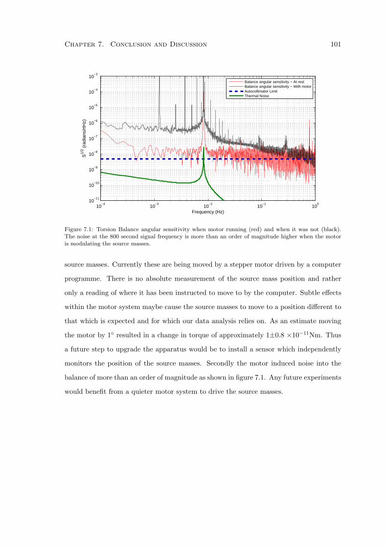
Chapter 7. Conclusion and Discussion 101
10−4
10−3
10−2
10−1
100
10−11
10−10
10−9
10−8
10−7
10−6
10−5
10−4
10−3
S1/
2 (ra
dian
s/rt
Hz)
Frequency (Hz)
Balance angular sensitivity − At restBalance angular sensitivity − With motorAutocollimator LimitThermal Noise
Figure 7.1: Torsion Balance angular sensitivity when motor running (red) and when it was not (black).The noise at the 800 second signal frequency is more than an order of magnitude higher when the motoris modulating the source masses.
source masses. Currently these are being moved by a stepper motor driven by a computer
programme. There is no absolute measurement of the source mass position and rather
only a reading of where it has been instructed to move to by the computer. Subtle effects
within the motor system maybe cause the source masses to move to a position different to
that which is expected and for which our data analysis relies on. As an estimate moving
the motor by 1 resulted in a change in torque of approximately 1±0.8 ×10⁻¹¹Nm. Thus
a future step to upgrade the apparatus would be to install a sensor which independently
monitors the position of the source masses. Secondly the motor induced noise into the
balance of more than an order of magnitude as shown in figure 7.1. Any future experiments
would benefit from a quieter motor system to drive the source masses.
Chapter 7. Conclusion and Discussion 102
7.2 Summary
This thesis has described the development of a laboratory apparatus used to undertake
experiments searching for weak interactions which could give insights into the validity of
new theoretical frameworks. The first experiment undertaken in this new setup was to
search for variations in the Newtonian Gravitational constant which obtained a null result
for a sidereal signal at the few ppm level. Along with a previous similar test set the first
limits on one of the parameters of the Standard Model Extension.
The work carried out on assembling and characterising a new interferometric readout has
also been reported. This readout, Iliad, which can measure angles accurately to ± 1, is
also immune to orthogonal tilts and thus is ideal for use in a torsion balance system. Its
current measured sensitivity, 5×10⁻¹¹ radians/√Hz between 10−1Hz and 10Hz, is more
than an order of magnitude better than the current state of the art autocollimator device
and its compactness, an overall cube shape measuring about 5cm3 in volume, allows it
to be fitted inside the vacuum system giving it immunity from environmental noise that
affects the autocollimator.
Finally the design and manufacture of a new spin test mass has been described. Using
a nested arrangement of rare-earth magnets it has been shown that the external mag-
netic field can be compensated while still keeping a net spin moment. These test masses,
although not complete at the time of writing, have been designed so they can directly re-
place the current CuTe test masses and new spin-coupling experiments can be undertaken.
The number of polarised electrons per kilogram in this design equals that used by Heckel
et al. [6, 49] to achieve the best current limits on some of the spin interactions. With
the use of a torsion strip our balance can potentially carry 50 times more spin than on
The University of Washington design [6, 49]. Although there is much further work to be
carried out on the torsion balance apparatus to reduce the noise and establish the origin
of spurious signals, and on the test masses to calibrate and prepare them for installation

Chapter 7. Conclusion and Discussion 103
into the torsion balance the feasibility of running new and exciting experiments in our
laboratory has been shown.
REFERENCES 104
References
[1] T.J. Quinn et al. A New Determination of G Using Two Methods. Phys. Rev. Lett.,
87(11):111101, 2001.
[2] V. A. Kostelecky and J. Tasson. Matter gravity couplings and Lorentz violation.
Phys. Rev. D, 83:016013, 2011.
[3] Q.G. Bailey and V.A. Kostelecky. Signals for Lorentz violation in post-newtonian
gravity. Phys. Rev. D, 74:045001, 2006.
[4] K.H. Buschow and F.R. De Boer. Physics of Magnetism and Magnetic Materials.
Kluwer Academic Publishers, New York, 2004.
[5] C. Kittel. Introduction to Solid State Physics. John Wiley and Sons, London, seventh
edition, 1995.
[6] B.R. Heckel et al. Preferred-frame and CP-violation tests with polarized electrons.
Phys. Rev. D, 78:092006, Nov 2008.
[7] ANSYS(TM). http://www.ansys.com.
[8] P. Larson et al. Calculation of magnetic anisotropy energy in SmCo5. Phys. Rev.
B, 67:214405, 2003.
[9] Magnet-Physik GmbH USA. Indianapolis, Indiana, US.
[10] G.T. Gillies and R.C. Ritter. Torsion balances, torsion pendulums, and related
devices. Rev. Sci. Instrum., 64:283, 1993.
[11] E.G. Adelberger et al. Torsion balance experiments: A low-energy frontier of particle
physics. Prog. Part. Nucl. Phys., 62:102, 2009.
[12] V.A. Kostelecky and S. Samuel. Spontaneous breaking of lorentz symmetry in string
REFERENCES 105
theory. Phys. Rev. D, 39:683, 1989.
[13] V.A. Kostelecky and R. Potting. CPT and strings. Nucl. Phys. B., 359:545, 1991.
[14] V.A. Kostelecky and D. Colloday. Lorentz-violating extension of the standard model.
Phys. Rev. D, 58:116002, 1998.
[15] V.A.Kostelecky and N. Russell. Data tables for Lorentz and CPT violation. Rev.
Mod. Phys., 83:11, 2011.
[16] J.M. Brown et al. New limit on lorentz- and cpt-violating neutron spin interactions.
Phys. Rev. Lett., 105(15):151604, 2010.
[17] M.A. Hohensee et al. Improved constraints on isotropic shift and anisotropies of
the speed of light using rotating cryogenic sapphire oscillators. Phys. Rev. D,
82(7):076001, 2010.
[18] V.A. Kostelecky. Private Communication.
[19] V.A. Kostelecky and M. Mewes. Signals for Lorentz violation in electrodynamics.
Phys. Rev. D, 66:056005, 2002.
[20] L. Carbone et al. A Torsion Balance Search for Temporal Variations in the Newto-
nian Constant. In R.T. Jantzen T. Damour and eds. R. Ruffini, editors, Proceedings
of the Twelfth Marcel Grossmann Meeting on General Relativity. World Scientific,
Singapore, 2010.
[21] H. Panjwani et al. Laboratory searches for preferred frame effects: Ongoing work
and results at birmingham. In V. Alan Kostelecky ed., editor, Proceedings of the
Fifth Meeting on CPT and Lorentz Symmetry. World Scientific, Singapore, 2010.
[22] L-S Hou et al. Test of cosmic spatial isotropy for polarized electrons using a rotatable
torsion balance. Phys. Rev. Lett., 90:201101, 2003.
REFERENCES 106
[23] W-T. Ni. Searches for the role of spin and polarization in gravity. Rep. Prog. Phys,
73:056901, 2010.
[24] J.E. Moody and F. Wilczek. New macroscopic forces? Phys. Rev. D, 30:130, 1984.
[25] B.A. Dobrescu and I. Mocioiu. Spin-dependent macroscopic forces from new particle
exchange. J. High Energy Phys., 5:0611, 2006.
[26] R.C. Ritter et al. Search for anomalous spin-dependent forces with a polarized-mass
torsion pendulum. Phys. Rev. Lett., 70:701, 1993.
[27] W-T. Ni et al. Search for an axionlike spin coupling using a paramagnetic salt with
a dc squid. Phys. Rev. Lett., 82:2439, 1999.
[28] G.D. Hammond et al. New constraints on short-range forces coupling mass to in-
trinsic spin. Phys. Rev. Lett., 98:081101, 2007.
[29] G.D. Hammond et al. Development of a second generation torsion balance based on
a spherical superconducting suspension. Rev. Sci. Instrum., 79(2):025103, 2008.
[30] P. Saulson. Thermal noise in mechanical experiments. Phys. Rev. D, 42(8):2437,
1990.
[31] K. Kuroda. Anelasticity in G experiments. Meas. Sci. Technol., 10:435, 1999.
[32] C. Zenar. Internal friction in solids. Phys. Rev., 53:90, 1938.
[33] C.C. Speake et al. Experiment and theory in anelasticity. Meas. Sci. Technol.,
10:430, 1999.
[34] A.L. Kimball and D.E. Lovell. Internal friction in solids. Phys. Rev., 30:948, 1927.
[35] S.J. Richman et al. Preliminary determination of G using BIPM torsion strip bal-
ance. Meas. Sci. Technol., 10:430, 1999.
REFERENCES 107
[36] T.J. Quinn et al. Novel torsion balance for the measurement of the Newtonian
gravitational constant. Metrologia, 34:245, 1997.
[37] T.J. Quinn et al. The restoring torque and damping in wide Cu-Be torsion strips.
Phys. Lett. A, 238:36, 1997.
[38] P.R. Saulson. Fundamentals of interferometric gravitational wave detectors. World
Scientific Publishing Co, Singapore, 1994.
[39] T.J. Quinn et al. Stress-dependent damping in Cu-Be torsion and flexure suspensions
at stresses up to 1.1 GPa. Phys. Lett. A, 197(3):197, 1995.
[40] Moller-Wedel Optical. http://www.moeller-wedel-optical.com/.
[41] Julabo. F33-EH. http://www.julabo.de/.
[42] B. Odom et al. New measurement of the electron magnetic moment using a one-
electron quantum cyclotron. Phys. Rev. Lett., 97(3), 2006.
[43] J.M.D. Coey. Magnetism and Magnetic Materials. Cambridge University Press,
Cambridge, 2010.
[44] M. McCaig. Permanent magnets in theory and in practice. Pentech, London, second
edition, 1987.
[45] K.J Strnat. Modern Permanent Magnets for Applications in Electro-Technology.
Proceedings of the IEEE, 78(6):923, 1990.
[46] Material Technologies Inc. Singapore.
[47] P. Phillips and D. Woolum. A test of Lorentz invariance using a torsion pendulum.
Nuovo. Cimento., 64B:28, 1969.
[48] P. Phillips. Test of Spatial Isotropy Using a Cryogenic Torsion Balance. Phys. Rev.
REFERENCES 108
Lett., 59(15):1784, 1987.
[49] C.E. Cramer. A Torsion Balance Search for Spin-Coupled Forces. PhD thesis,
University of Washington, 2007.
[50] L.C. Carbone et al. Design of high-density electron spin-polarized test masses. Class.
Quantum Grav., 26, 2009.
[51] J.D. Jackson. Classical Electrodynamics. Wiley, New York; London, second edition,
1975.
[52] J.B. Bronzan. The magnetic scalar potential. American Journal of Physics, 39:1359,
1971.
[53] C.G. Gray. Magnetic multipole expantion using the scalar potential. American
Journal of Physics, 47(5):457, 1979.
[54] D.C. Meeker. Finite element method magnetics (femm), Version 4.2 (23-05-2008).
http://femm.foster-miller.net/wiki.
[55] First4Mag. http://www.first4magnets.co.uk.
[56] MagsUK. http://www.magnetsukonline.co.uk.
[57] Magnetic Applications LTD. http://www.magnetapplications.com.
[58] Quadrant Magnetics LLC. Louisville, Kentucky, US.
[59] F.L. Pratt et al. Ferromagnetism with zero intrinsic magnetization: µSR on Gd-
doped SmAl2. Physica B, 34:374, 2006.
[60] H. Adachi and H. Ino. A ferromagnet having no net magnetic moment. Nature,
401:148, 1999.
[61] K.J. Strnat and A. Tauber. Internal temperature compensation of rare earth-cobalt
REFERENCES 109
permanent magnets for microwave devices by adding heavy lanthanides. Journal of
the Less-Common Metals, 93:269, 1983.
[62] Mike Guthrie. Quadrant Magnetics LLC, Private Communication.
[63] P. Tils et al. Crystal and exchange fields in SmCo5 studied by inelastic neutron
scattering. Journal of Alloys and Compounds, 289:28, 1999.
[64] A. Koizumi et al. X-ray magnetic Compton-profile measurements on SmCo5 by
using pulsed high magnetic field. J. Phys. Soc. Japan, 66(2):318, 1997.
[65] D. Givord et al. Temperature dependence of the samarium magnetic form factor in
SmCo5. J. App. Phys., 50(3):2008, 1979.
[66] J. Schweizer et al. Polarised neutron study of the RCo5 intermetallic compounds: I.
the cobalt magnetisation in YCo5. J. Phys. F: Metal Phys., 10:2799, 1980.
[67] D. Givord et al. Different contributions of the two cobalt sites to the magnetocrys-
talline anisotropy of YCo5 and related compounds. IEEE Transactions on Magnet-
ics, Mag-12(6):1000, 1976.
[68] L. Nordstom et al. Calculation of orbital magnetism and magnetocrystalline
anisotropy energy in YCo5. J. Phys. Condens. Matter, 4:3261, 1992.
[69] H. Yoshie et al. Nuclear magnetic resonance of RCo5. iii. R=Ce and Sm. J. Phys.
Soc. Japan, 57:2525, 1988.
[70] D. Givord et al. Magnetic properties of Y2Fe14B and Nd2Fe14B single crystals.
Solid State Communications, 51(11):857–860, 1984.
[71] K. Tokuhara et al. Magnetization and torque measurements on Nd2Fe14B single
crystals. Solid State Communications, 56(4):333–336, 1985.
[72] D. Givord et al. Polarized neutron study of the compounds Y2Fe14B and Nd2Fe14B.
REFERENCES 110
J. Appl. Phys, 57(1), 1985.
[73] H. Onodera et al. Mssbauer study of the intermetallic compound Nd2Fe14B. II. Tem-
perature dependence and spin reorientation. Journal of Magnetism and Magnetic
Materials, 68(1):15, 1987.
[74] N.C. Koon et al. Magnetic properties of R2Fe14B single crystals. J. Appl. Phys,
57(1), 1985.
[75] D. Givord et al. Private Communication.
[76] M. Sagawa et al. Permanent magnet materials based on the rare earth-iron-boron
tetragonal compounds. IEEE Trans. Mag., Mag-20(5):1584, 1984.
[77] S. Hirosawa et al. Magnetisation and magnetic anisotropy of R2Fe14B measured on
single crystals. J. App. Phys., 59(3):873, 1986.
[78] J.F. Herbst et al. Relationships between crystal structure and magnetic properties
in Nd2Fe14B. Phys. Rev. B, 29:4176, 1984.
[79] J. Chaboy et al. 57Fe Mossbauer and x-ray magnetic circular dichroism study of
magnetic compensation of the rare-earth sublattice in Nd2-xHoxFe14B compounds.
Phys. Rev. B, 79:134408, 2007.
[80] L.M Garcia et al. Soft x-ray magnetic circular dichroism investigation of the spin
reorientation transition in Nd2Fe14B. J. Appl. Phys., 87:6567, 2000.
[81] R.A Reck and D.L. Fry. Orbital and spin magnetization in Fe-Co, Fe-Ni and Ni-Co.
Phys. Rev., 184(2), 1969.
[82] L.M Garcia, J. Chaboy, and F.Bartolome. Orbital magnetic moment instability at
the spin reorientation transition of Nd2Fe14B. Phys. Rev. Lett., 85(2), 2000.
[83] E. R. Peck and S. Wendell Obetz. Wavelength or Length Measurement by Reversible
REFERENCES 111
Fringe Counting. J. Opt. Soc. Am., 43(6):505, 1953.
[84] M.J. Downs and K.W. Raines. Beam-splitter coatings for producing phase quadra-
ture interferometer outputs. J. Mod. Opt., 25(7), 1978.
[85] V. Greco et al. Multiphase homodyne interferometry: analysis of some error sources.
App. Opt., 34(13):2207, 1995.
[86] E.R. Peck. Theory of the cube-corner interferometer. J. Opt. Soc. Am, 38:1015,
1948.
[87] J.J. Snyder. Paraxial ray analysis of a cat’s-eye retroreflector. Appl. Opt., 14(8):1825,
1975.
[88] M.L. Biermann et al. Design and analysis of a diffraction-limited cat’s eye retrore-
flector. Opt. Eng., 41:1655, 2002.
[89] R.F. Chang et al. Far-field diffraction pattern for corner reflectors with complex
reflection coefficients. J. Opt. Soc. Am., 61(4):432, 1971.
[90] H.D. Eckhardt. Simple model of corner reflector phenomena. App. Opt, 10(1):1559,
1971.
[91] M.A. Player. Polarization properties of a cube-corner reflector. J. Mod. Opt, 35:1813,
1988.
[92] F.E. Pena-Arellano and C.C. Speake. Mirror tilt immunity interferometry with a
cat’s eye retroreflector. App. Opt., 50(7):981, 2011.
[93] N. Bobroff. Recent advances in displacement measuring interferometry. Meas. Sci.
Tech., 4:907, 1953.
[94] F.E. Pena-Arellano et al. An interferometer for measuring angular motion. In
Preparation.
REFERENCES 112
[95] C.C. Speake and S.M. Aston. An interferometric seonsor for satellite drag-free con-
trol. Class. Quantum Grav., 22:S269, 2005.
[96] F.E. Pena-Arellano. Characterisation of polarization homodyne interferometers.
PhD thesis, University of Birmingham, 2008.
[97] Laser 2000. http://http://www.laser2000.co.uk/.
[98] Thorlabs Inc. http://www.thorlabs.com.
[99] Norland Products. http://www.norlandprod.com/adhesives/noa2065.html.
[100] S.M. Aston. Optical Read-out Techniques for the Control of Test-masses in Gravi-
tational Wave Observatories. PhD thesis, University of Birmingham, 2011.
[101] R. Halir and J. Flusser. Numerically stable direct least squares fitting of ellipses.
In Proceedings of the 6th International Conference in Central Europe on Computer
Graphics and Visualization. WSCG, 1998.
[102] S.B. Alexander. Optical Communication Receiver Design. SPIE - The International
Society for Optical Engineering, Washington, 1997.
[103] D.K. Owens and R. Weiss. Measurement of the phase fluctuations in a He-Ne Zeeman
laser. Rev. Sci. Instrum., 45:1060, 1974.
[104] L. Carbone et al. Upper limits to surface-force disturbances on lisa proof masses
and the possibility of observing galactic binaries. Phys. Rev. D, 75:042001, 2007.
[105] L. Ferraioli et al. Discrete derivative estimation in lisa pathfinder data reduction.
Class. Quantum Grav., 26:094013, 2009.
[106] W.H. Press et al. Numerical Recipes: The Art of Scientific Computing. Cambridge
University Press, Cambridge, 1986.

Appendix
A
Magnetic Properties for
SmCo5 and Nd2Fe14B final
pieces
113
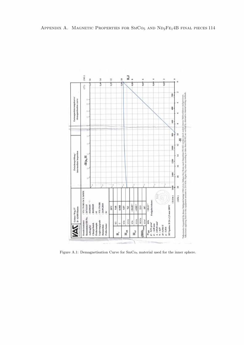
Appendix A. Magnetic Properties for SmCo5 and Nd2Fe14B final pieces 114
Figure A.1: Demagnetisation Curve for SmCo5 material used for the inner sphere.
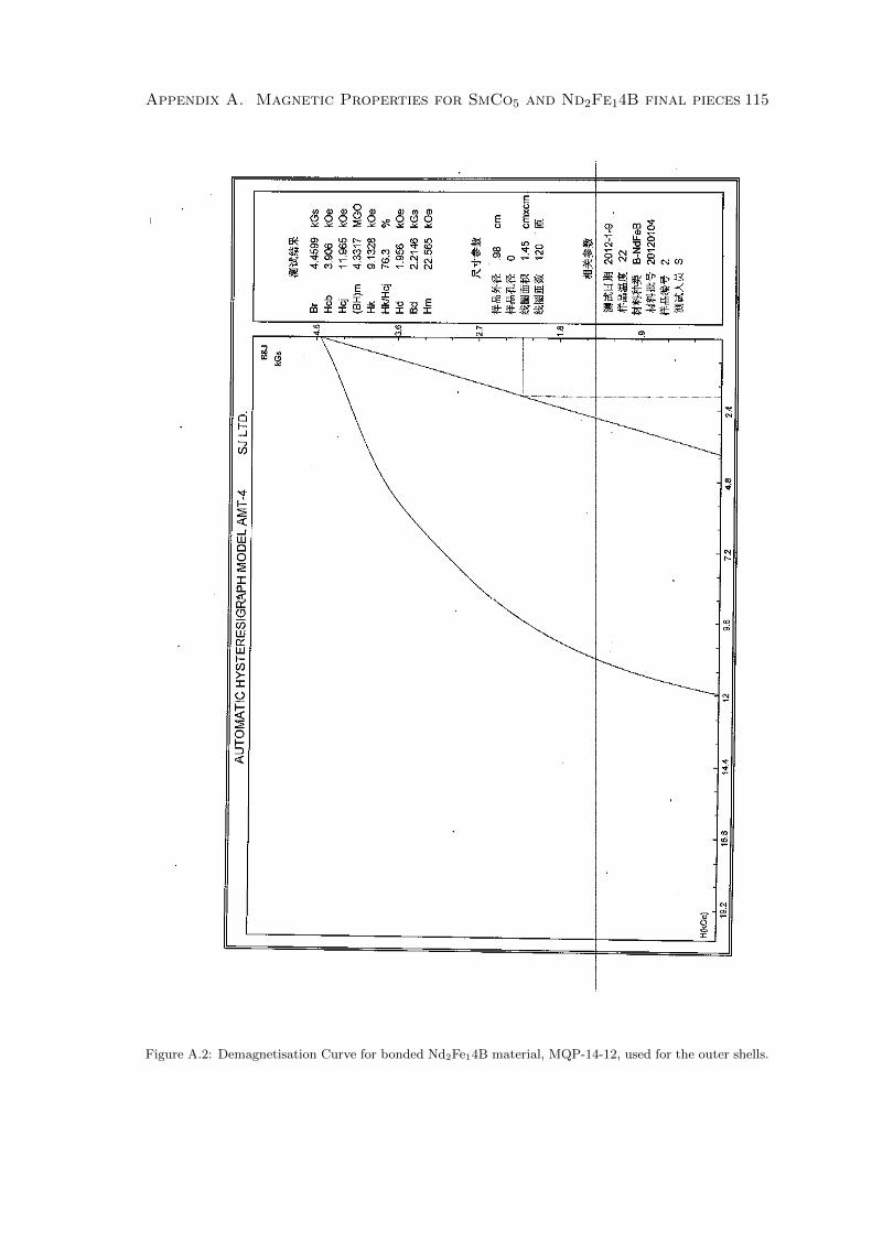
Appendix A. Magnetic Properties for SmCo5 and Nd2Fe14B final pieces 115
Figure A.2: Demagnetisation Curve for bonded Nd2Fe14B material, MQP-14-12, used for the outer shells.
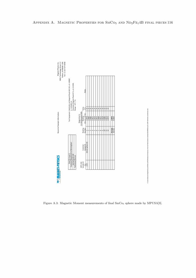
Appendix A. Magnetic Properties for SmCo5 and Nd2Fe14B final pieces 116
Rec
ord
of
Sam
ple
Info
rmat
ion
Mag
net
-Ph
ysic
s In
c.
90
01
Tec
hn
olo
gy D
rive
C-2
Fish
ers,
IN 4
60
38
USA
Tel:
+1 3
17
57
7 8
70
0
Dat
e:3
1-A
ug-
11
Test
Eq
uip
men
t:H
elm
ho
ltz
coil
Mag
net
-Ph
ysik
MS
21
0, s
/n 1
09
98
7.
Cu
sto
mer
:Q
uad
ran
t/U
.of
Bir
min
gham
k =
0.0
14
04
cm
Job
No
:u
s10
-12
0Fl
uxm
eter
Mag
net
-Ph
ysik
EF
5, s
/n 1
11
95
0.
Tech
nic
ian
:R
strn
atR
ange
= 1
0^-
7 V
s
Mag
net
ized
inM
PS-
USA
2 x
50
kO
e p
uls
e fi
eld
.Sa
mp
le ID
Cu
sto
mer
Rea
din
gR
ead
ing
Tem
p.
mu
-Sa
mp
le ID
Nu
mb
er[V
s-cm
x 1
0^-
3]
[°C
]N
ote
s1
75
7Sm
Co
5 s
ph
ere
#21
1.9
97
82
42
1.9
98
02
43
1.9
98
02
44
1.9
97
22
45
1.9
97
02
46
1.9
97
32
47
1.9
96
82
48
1.9
97
52
49
1.9
97
82
41
01
.99
80
24
11
1.9
97
92
41
21
.99
79
24
Average
1.9976
Std
Dev
0.0
00
4
C:\
Use
rs\H
asn
ain
\Ap
pD
ata\
Loca
l\M
icro
soft
\Win
do
ws\
Tem
po
rary
Inte
rnet
File
s\C
on
ten
t.O
utl
oo
k\S4
LIW
8G
K\u
s10
-12
0B
Hel
mh
olt
z w
ork
shee
t.xl
sx
Figure A.3: Magnetic Moment measurements of final SmCo5 sphere made by MPUSA[9].
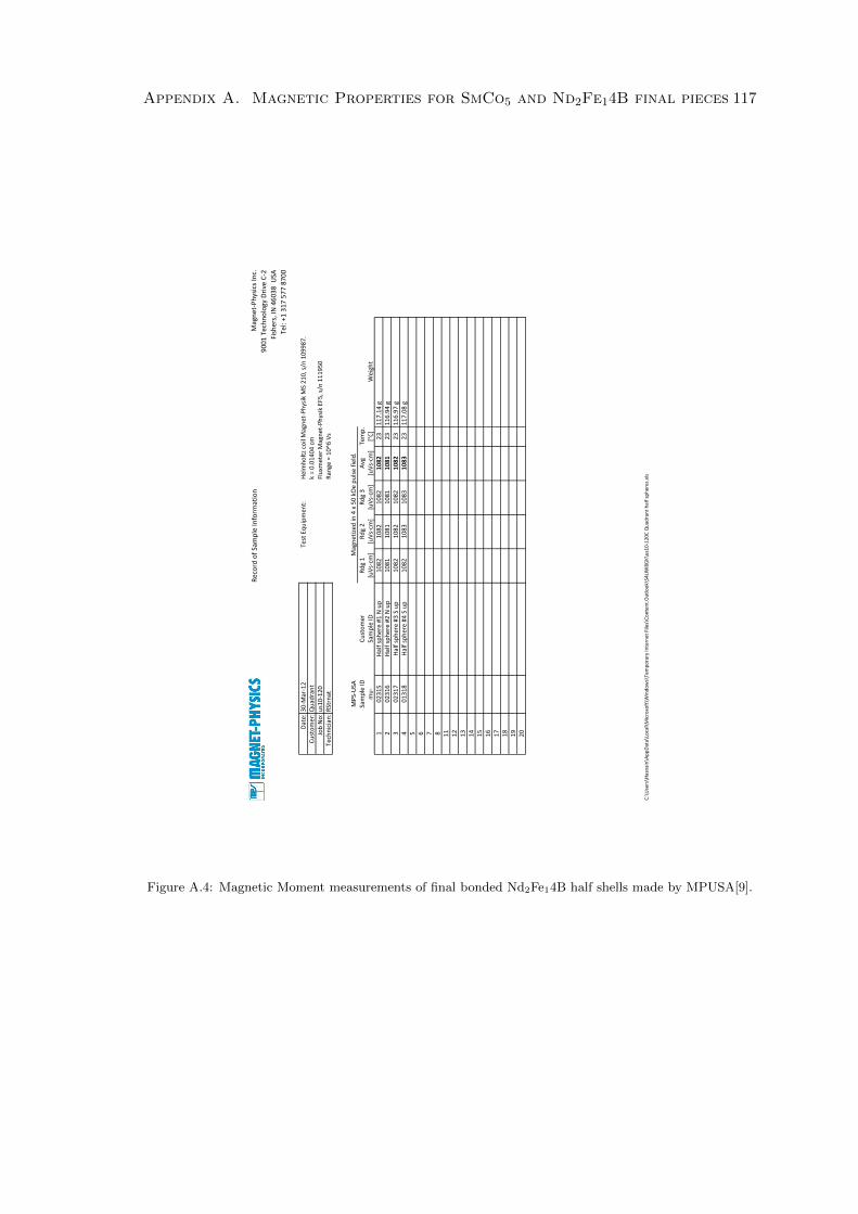
Appendix A. Magnetic Properties for SmCo5 and Nd2Fe14B final pieces 117
Rec
ord
of
Sam
ple
Info
rmat
ion
Mag
net
-Ph
ysic
s In
c.
90
01
Tec
hn
olo
gy D
rive
C-2
Fish
ers,
IN 4
60
38
USA
Tel:
+1 3
17
57
7 8
70
0
Dat
e:3
0-M
ar-1
2Te
st E
qu
ipm
ent:
Hel
mh
olt
z co
il M
agn
et-P
hys
ik M
S 2
10
, s/n
10
99
87
.C
ust
om
er:
Qu
adra
nt
k =
0.0
14
04
cm
Job
No
:u
s10
-12
0Fl
uxm
eter
Mag
net
-Ph
ysik
EF5
, s/n
11
19
50
Tech
nic
ian
:R
Strn
atR
ange
= 1
0^6
Vs
MP
S-U
SASa
mp
le ID
Cu
sto
mer
Rd
g 1
Rd
g 2
Rd
g 3
Avg
Tem
p.
mu
-Sa
mp
le ID
[uV
s-cm
][u
Vs-
cm]
[uV
s-cm
][u
Vs-
cm]
[°C
]W
eigh
t1
02
31
5H
alf
sph
ere
#1 N
up
10
82
10
82
10
82
1082
23
11
7.1
4 g
20
23
16
Hal
f sp
her
e #2
N u
p1
08
11
08
11
08
11081
23
11
6.9
4 g
30
23
17
Hal
f sp
her
e #3
S u
p1
08
21
08
21
08
21082
23
11
6.9
7 g
40
13
18
Hal
f sp
her
e #4
S u
p1
08
21
08
31
08
31083
23
11
7.0
8 g
5 6 7 8 11
12
13
14
15
16
17
18
19
20
Mag
net
ized
in 4
x 5
0 k
Oe
pu
lse
fiel
d.
C:\
Use
rs\H
asn
ain
\Ap
pD
ata\
Loca
l\M
icro
soft
\Win
do
ws\
Tem
po
rary
Inte
rnet
File
s\C
on
ten
t.O
utl
oo
k\S4
LIW
8G
K\u
s10
-12
0C
Qu
adra
nt
hal
f sp
her
es.x
ls
Figure A.4: Magnetic Moment measurements of final bonded Nd2Fe14B half shells made by MPUSA[9].

Appendix
B
CAD Drawings of Iliad
mechanical holder
118
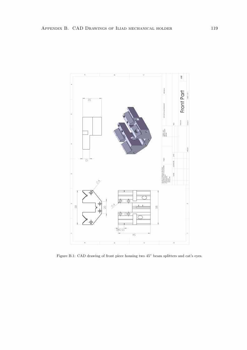
Appendix B. CAD Drawings of Iliad mechanical holder 119
58
4
20
54
58
4
10.340
32
12
B C D
12
A
32
14
BA
56
SCA
LE:1
:1SH
EET 1
OF
1
C
WEI
GHT
:
Fron
t Par
tA
4D
WG
NO
.
TITLE
:
REVI
SIO
ND
O N
OT
SCA
LE D
RAW
ING
DA
TESI
GN
ATU
REN
AM
E
DEB
UR A
ND
BR
EAK
SHA
RP
EDG
ES
UNLE
SS O
THER
WIS
E SP
ECIF
IED
:D
IMEN
SIO
NS
ARE
IN M
ILLIM
ETER
SSU
RFA
CE
FIN
ISH:
TOLE
RAN
CES
:
LINEA
R:
AN
GUL
AR:
FINIS
H:
Figure B.1: CAD drawing of front piece housing two 45 beam splitters and cat’s eyes.
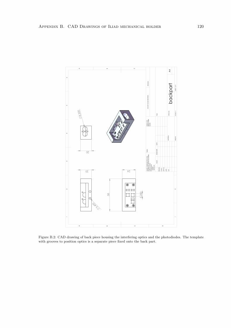
Appendix B. CAD Drawings of Iliad mechanical holder 120
20
3.400
58
24
5.20
0
20
8.30
0
B C D
12
A
32
14
BA
56
DRA
WN
CHK
'D
APP
V'D
MFG
Q.A
UNLE
SS O
THER
WIS
E SP
ECIF
IED
:D
IMEN
SIO
NS
ARE
IN M
ILLIM
ETER
SSU
RFA
CE
FIN
ISH:
TOLE
RAN
CES
:
LINEA
R:
AN
GUL
AR:
FINIS
H:D
EBUR
AN
D
BREA
K SH
ARP
ED
GES
NA
ME
SIG
NA
TURE
DA
TE
MA
TERI
AL:
DO
NO
T SC
ALE
DRA
WIN
GRE
VISI
ON
TITLE
:
DW
G N
O.
SCA
LE:1
:1SH
EET 1
OF
1
A4
C
WEI
GHT
:
back
part
Figure B.2: CAD drawing of back piece housing the interfering optics and the photodiodes. The templatewith grooves to position optics is a separate piece fixed onto the back part.
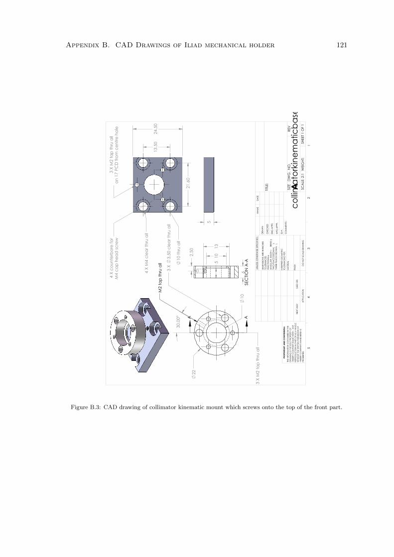
Appendix B. CAD Drawings of Iliad mechanical holder 121
on 1
7 PC
D fr
om c
entre
hol
e3
X M
2 ta
p th
ru a
ll
4 X
M4
clea
r thr
u al
l
M4
cap
head
scre
w4
X co
unte
rbor
e fo
r
13.5
0
21.6
0
24.5
0
10 th
ru a
ll
3 X
3.50
cle
ar th
ru a
ll
3 X
M2
tap
thru
all
22
10
30.0
0° A A
M2
tap
thru
all
5
1013
5
6
2.50
SEC
TION
A-A
DO
NO
T SC
ALE
DRA
WIN
G
collim
ator
kine
mat
icba
seSH
EET 1
OF
1
UNLE
SS O
THER
WIS
E SP
ECIF
IED
:
SCA
LE: 2
:1W
EIG
HT:
REV
DW
G.
NO
.
ASIZE
TITLE
:
NA
ME
DA
TE
CO
MM
ENTS
:
Q.A
.
MFG
APP
R.
ENG
APP
R.
CHE
CKE
D
DRA
WN
FIN
ISH
MA
TERI
AL
INTE
RPRE
T G
EOM
ETRI
CTO
LERA
NC
ING
PER
:
DIM
ENSI
ON
S A
RE IN
INC
HES
TOLE
RAN
CES
:FR
AC
TION
AL
AN
GUL
AR:
MA
CH
B
END
TW
O P
LAC
E D
ECIM
AL
TH
REE
PLA
CE
DEC
IMA
L
APP
LICA
TION
USED
ON
NEX
T A
SSY
PRO
PRIE
TARY
AN
D C
ON
FIDE
NTIA
LTH
E IN
FORM
ATIO
N C
ON
TAIN
ED IN
THI
SD
RAW
ING
IS T
HE S
OLE
PRO
PERT
Y O
F<I
NSE
RT C
OM
PAN
Y N
AM
E HE
RE>.
AN
Y RE
PRO
DUC
TION
IN P
ART
OR
AS
A W
HOLE
WITH
OUT
THE
WRI
TTEN
PER
MIS
SIO
N O
F<I
NSE
RT C
OM
PAN
Y N
AM
E HE
RE>
IS
PRO
HIBI
TED
.
54
32
1
Figure B.3: CAD drawing of collimator kinematic mount which screws onto the top of the front part.


