Developing Indian grain supplychain cost model: a system

dynamics approachAmit Sachan, B.S. Sahay and Dinesh SharmaManagement Development Institute, Gurgaon, India

Abstract

Purpose – The objective of the present study is to model the total supply chain cost (TSCC) of anIndian grain chain in order to understand and predict the future outcome of each supply chain model indifferent situations and to devise policies accordingly to reduce TSCC.

Design/methodology/approach – The system dynamics (SD) approach is used to model the TSCCmodel of an Indian grain chain, which takes care of the dynamic interaction of the cost variables.

Findings – The major findings of the paper are the reduced cost ratios in the different scenarios.A total of nine scenarios are evaluated, which are the cooperative model, contract farming and acollaborative supply chain based on optimistic, pessimistic and most likely views.

Practical implications – The practical implications are the action plans suggested to reduce TSCCin each of the future scenarios of the supply chain model that are developed in the paper.

Originality/value – The TSCC model is beneficial not only for organizations entering into the foodbusiness, but also for economic policy makers.

Keywords Supply chain management, Dynamics, Food crops, India

Paper type Research paper

IntroductionThe agriculture sector in India accounts for about 25 percent of gross domestic product(GDP) and employs close to 70 percent of the country’s work force. However, it isplagued by multitude of problems which hinder its efficient operation. India has seenrapid developments in several areas, most notably in manufacturing industry and theservice sector (e.g. information technology). But, in the agriculture sector, the grainsupply chain has remain unchanged: over 90 percent of food is sold in unorganisedmarkets, with organised business accounting for just 2 percent of the market(Economic Times Intelligence Group, 2003). According to the Indian Ministry of Tradeand Industry, approximately 20 percent of food produced in India is wasted (see www.etfoodprocessing.com). Various research studies by the Economic Times IntelligenceGroup (ETIG) and the Investment Information and Credit Rating Agency (ICRA) havedetailed the weaknesses and problems present in the Indian grain chain (InvestmentInformation and Credit Rating Agency, 2001). First, tonnes of grain are wasted due toimproper handling and storage, pest infestation, poor logistics, inadequate storage andtransportation infrastructure. Second, intermediaries take large portions of theearnings which should go to farmers. Third, post-harvest losses are about 25-30percent in India. Even marginal reductions in these losses are bound to bring greatrelief on the food security front as well as improve the income level of the farmers.Fourth, Indian consumers pay three to four times the farm gate price, as compared to

The Emerald Research Register for this journal is available at The current issue and full text archive of this journal is available at

www.emeraldinsight.com/researchregister www.emeraldinsight.com/1741-0401.htm

Indian grainsupply chain

187

Received October 2003Revised January 2004;

November 2004Accepted December 2004

International Journal of Productivityand Performance Management

Vol. 54 No. 3, 2005pp. 187-205

q Emerald Group Publishing Limited1741-0401

DOI 10.1108/17410400510584901

developed countries where the consumer pays one and a half to two times the farm gateprice. Also, 60-80 percent of the price that consumers pay goes to traders, commissionagents, traders, wholesalers and retailers (Economic Times Intelligence Group, 2003).These intermediaries (also called commission agents) lead to poor coordination andcollaboration in the supply chain, which in turn leads to inefficient information flow.

Seeing the inefficiencies in the Indian grain chain and the opportunity of makinggood profits, some private and public sector companies entered into this organised foodbusiness. These companies were based on three types of model:

(1) the cooperative supply chain model;

(2) the collaborative supply chain model; and

(3) contract farming.

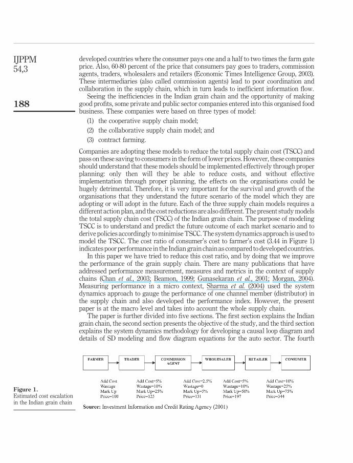
Companies are adopting these models to reduce the total supply chain cost (TSCC) andpass on these saving to consumers in the form of lower prices. However, these companiesshould understand that these models should be implemented effectively through properplanning: only then will they be able to reduce costs, and without effectiveimplementation through proper planning, the effects on the organisations could behugely detrimental. Therefore, it is very important for the survival and growth of theorganisations that they understand the future scenario of the model which they areadopting or will adopt in the future. Each of the three supply chain models requires adifferent action plan, and the cost reductions are also different. The present study modelsthe total supply chain cost (TSCC) of the Indian grain chain. The purpose of modelingTSCC is to understand and predict the future outcome of each market scenario and toderive policies accordingly to minimise TSCC. The system dynamics approach is used tomodel the TSCC. The cost ratio of consumer’s cost to farmer’s cost (3.44 in Figure 1)indicates poor performance in the Indian grain chain as compared to developed countries.

In this paper we have tried to reduce this cost ratio, and by doing that we improvethe performance of the grain supply chain. There are many publications that haveaddressed performance measurement, measures and metrics in the context of supplychains (Chan et al., 2003; Beamon, 1999; Gunasekaran et al., 2001; Morgan, 2004).Measuring performance in a micro context, Sharma et al. (2004) used the systemdynamics approach to gauge the performance of one channel member (distributor) inthe supply chain and also developed the performance index. However, the presentpaper is at the macro level and takes into account the whole supply chain.

The paper is further divided into five sections. The first section explains the Indiangrain chain, the second section presents the objective of the study, and the third sectionexplains the system dynamics methodology for developing a causal loop diagram anddetails of SD modeling and flow diagram equations for the auto sector. The fourth

Figure 1.Estimated cost escalationin the Indian grain chain

IJPPM54,3

188

section presents the scenarios of the Indian grain chain, and the paper ends with adiscussion and conclusions.

Indian grain supply chainA supply chain has been described as a system whose constituent parts includematerial suppliers, production facilities, distribution services and customers linkedtogether via the feed-forward flow of materials and the feedback flow of information(Stevens, 1989). Recently there has been a shift of focus in supply chain managementtowards a more integrated approach (Towill, 1996). Integrated supply chainmanagement is a process-oriented, integrated approach to procuring, producing, anddelivering products and services to customers. Integrated supply chain managementcovers the management of materials, information, and fund flows (Metz, 1998).

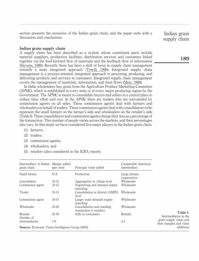
In India wholesalers buy grain from the Agriculture Produce Marketing Committee(APMC), which is established in every state or in every major producing region by theGovernment. The APMC is meant to consolidate buyers and sellers in a central place toreduce time, effort and cost. In the APMC there are traders who are surrounded bycommission agents on all sides. These commission agents deal with farmers andwholesalers on behalf of traders. These commission agents deal with consolidators (whorepresent the small farmer) on the farmer’s side and wholesalers on the retailer’s side(Table I). These consolidators and commission agents charge their fees as a percentage ofthe transaction. This number of people varies across the markets, and their percentagesalso vary. In this study we have considered five major players in the Indian grain chain:

(1) farmers;

(2) traders;

(3) commission agents;

(4) wholesalers; and

(5) retailers (also considered in the ICRA report).

Intermediary in Indiangrain chain

Margin added(per cent) Principal value added

Comparable Americanintermediary

Small farmer N/A Production Large farmer,cooperatives

Consolidator 10-15 Aggregation at village level WholesalerCommission agent 10-15 Negotiating and demand supply

matchingWholesaler

Trader 10-15 Consolidation at district (AMPC)level

Wholesaler

Commission agent 10-15 Larger scale demand supplymatching

Wholesaler

Wholesaler 25-30 Consolidation and resellingtransaction to retailers

Wholesaler

Retailer 25-30 Sells to consumers RetailerNumber ofintermediaries 7-8 3-4

Source: Economic Times Intelligence Group (2003)

Table I.Intermediaries in the

grain supply chain andtheir margins and value

additions

Indian grainsupply chain

189

Figure 1 clearly reflects that if the farmer sells grain at 100 rupees then by the time itreaches the trader its price becomes 125. Then the commission agent further adds to itand the price rises to 131. Then the wholesaler increases the price by 50 percent, and itrises to 197. The wholesaler adds no value to the grain, except that he breaks them intosmall parts. Finally the retailer adds his own cost and the final cost rises to 344. Theend consumer on average pays more than three times the farm gate price for grain. Theadditional cost, wastage and mark-up of these participants (trader, commission agent,and wholesaler) drastically increase the cost, by up to almost 3.5 times. The data inFigure 1 clearly show the effect that the number of participants has on the price forboth farmers and consumers. Table I presents the Indian intermediaries andcomparable American intermediaries along with the margins and value additionsmade by them.

Some of the reasons for the existence of these intermediaries in the grain supplychain are:

. age-old historical loyalty of farmers to their agents, because these agents providedebt to the farmer;

. local understanding and relationships with transporters;

. lethargy on the part of government and NGOs to educate farmers regardingother options;

. lack of guidelines and rules in the development and supply of produce staples;

. organised cartels between commission agents, wholesalers and transporters;

. lack of scale in terms of what each farmer produces, sheer numbers of smallfarmers drive down bargaining power; and

. lack of effort in development from front-end players (retailers) and institutions.

ObjectiveThe objective of the present study is to model the total supply chain cost (TSCC) of theIndian grain chain. The purpose of modeling TSCC is to understand and predict thefuture outcome of each market scenario and to devise policies accordingly to minimiseTSCC. Each of the nine scenarios suggests improvement in the performance of thesupply chain by decreasing the cost ratio. The paper presents nine scenarios for thecooperative model, contract farming and collaborative supply chain based onoptimistic, pessimistic and most likely situations.

System dynamics methodologyThe system dynamics (SD) approach is used to model the TSCC. The application ofsystem dynamics modeling to supply chain management has its roots in industrialdynamics (Forrester, 1958, 1961). SD is a methodology for understanding the behaviorof complex, dynamic social-technological-economic-political (STEP) systems to showhow system structures and the policies used in decision making govern the behavior ofthe system. SD focuses on the structure and behavior of systems composed ofinteracting feedback loops. The objective of the SD approach is to capture the dynamicinteraction of different system variables and to analyze their impact on policy decisionsover a long-term horizon.

IJPPM54,3

190

Procedural steps in system dynamics modelingThe objective of the SD study is to attain some desired goals through modifications ofthe system. For this, a system boundary is defined and a model of the system is built.The systematic procedural steps in SD modeling are as follows (Roberts, 1978):

(1) define the problems to be solved and goals to be achieved;

(2) describe the system with a causal loop/influence diagram;

(3) formulate the structure of the model (i.e. develop the flow diagram forsystematizing symbols, arrow designator and the format of system dynamicmodeling in the form of DYNAMO equations);

(4) collect the initial data/base data needed for model operation either fromhistorical data and/or from discussion with executives/planners who haveknowledge and experience of the system under study – these are the initialvalue of all the level variables, constants and policy data;

(5) validate the model on some suitable criteria to establish sufficient confidence inthe model; and

(6) use the model to test various policy actions to find the best way to achieveprescribed goals.

SD procedural steps as explained above were used in developing the SD model for theIndian grain chain.

System dynamics model of the grain supply chain costMorecroft (1988) emphasized that model conceptualization begins with causal loopsand moves to rate/level flow diagrams and finally to explicit equations capturing thediagram structure. Thus, the objective of the SD model is to capture the dynamicinteraction of different variables that the system has and to analyze the policy decisionover a long-term time horizon. Causal loop diagramming is an important tool, whichhelps the modeler to conceptualize the real world system in terms of feedback loops. Itis very important to identify the key variables of TSCC before developing a causal loopdiagram for the Indian grain chain. To model the grain chain, we consider Figure 1.The major cost components of the grain supply chain are the farmer’s price, additionalcosts, wastage and mark-ups.

Farmer’s priceThe farmer’s price (FP) is the starting point of the grain supply chain. This pricecontains the cost of growing and processing the grain at farmer’s end and margins ofthe farmers. The farmer’s price has a proportional effect on the supply chain cost.These costs are affected by the total farm production (TFP), yield per hectare (YPH) ofland and cost of inputs (COI).

WastageTotal wastage (TW) may be due to three reasons:

(1) obsolesce losses (OL);

(2) transit losses (TL); and

(3) pilferage losses (PL).

Indian grainsupply chain

191

This wastage depends on the number of intermediaries in the chain. Wastage has aproportional effect on the supply chain cost. This wastage depends on how many timesthe grain is handled or transported in the chain, so wastage also depends on thenumber of intermediaries.

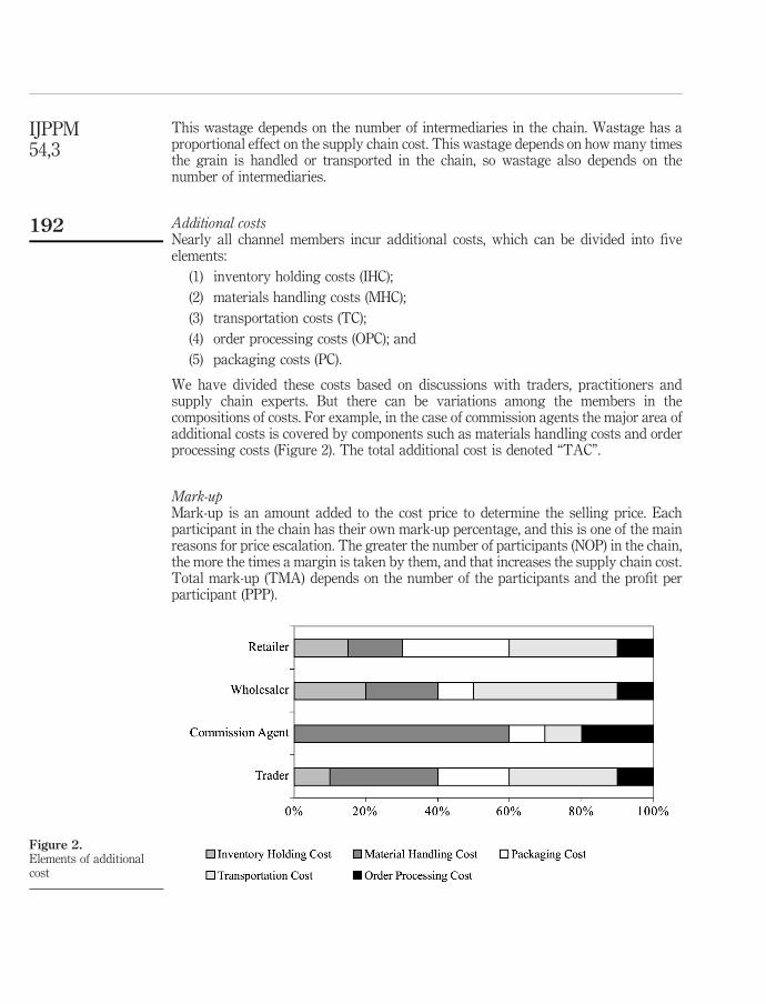
Additional costsNearly all channel members incur additional costs, which can be divided into fiveelements:

(1) inventory holding costs (IHC);

(2) materials handling costs (MHC);

(3) transportation costs (TC);

(4) order processing costs (OPC); and

(5) packaging costs (PC).

We have divided these costs based on discussions with traders, practitioners andsupply chain experts. But there can be variations among the members in thecompositions of costs. For example, in the case of commission agents the major area ofadditional costs is covered by components such as materials handling costs and orderprocessing costs (Figure 2). The total additional cost is denoted “TAC”.

Mark-upMark-up is an amount added to the cost price to determine the selling price. Eachparticipant in the chain has their own mark-up percentage, and this is one of the mainreasons for price escalation. The greater the number of participants (NOP) in the chain,the more the times a margin is taken by them, and that increases the supply chain cost.Total mark-up (TMA) depends on the number of the participants and the profit perparticipant (PPP).

Figure 2.Elements of additionalcost

IJPPM54,3

192

Causal loop diagramAn integrated causal loop diagram of this model reflecting the interactions of the abovevariables was developed, and is shown in Figure 3. The causal loop diagram is animportant tool which helps the modeler to conceptualize the real-world system in termsof feedback loops. In a causal loop diagram, the arrows indicate the direction ofinfluence, and the plus or minus sign the type of influence. All other things being equal,if a change in one variable generates a change in the same direction in the secondvariable, relative to its prior value, the relationship between the two variables isreferred to as positive. If the change in the second variable takes place in the oppositedirection, the relationship is negative. Causal loop diagrams characterize the initialview of the system and basically serve the purpose of communication between themodeler and the policy maker. However, the formulation of an operational model of thesystem is based on more specific structural details, like rates or policy variables,accumulation of level, auxiliaries, constants, information flows and delays.

In the causal diagram of total supply chain cost there are ten negative feedbackloops. Four of them are between the supply chain cost and the total additional cost,total wastage, total mark-up and farmer’s price, which means that an increase in anyone of these costs will increase the total supply chain cost. When the supply chain costincreases, people try to reduce the one of these costs. For example, many farmers havenow started selling direct to the retailer, bypassing traders, commission agents andwholesalers. In this way they both are sharing the mark-up and the other costs thatthese participants make. In some cases retailers are also integrating backwards andremoving one or two participants in the chain and increasing their margins orproviding more value to customers.

The other five negative loops are between the total additional cost and the inventoryholding cost, the transportation cost, the materials handling cost, the packaging cost

Figure 3.Causal diagram of total

supply chain cost

Indian grainsupply chain

193

and the order processing cost. Increasing any one of these costs will lead to increases inadditional costs. When additional costs increase, then channel members try to reducethese costs. Transportation costs are usually reduced by transporting the material inbulk, and channel members attempt to reduce costs per kg in this way. In the case oforder processing, in some places channel participants have started using computersand information technology. Using standard packaging material throughout the chainalso reduces packaging costs.

One of the most important variables in the causal diagram is the number ofparticipants (NOP). This increases the total supply chain cost in a number of ways. Itcan easily be seen what role the number of participants (NOP) plays in the grain supplychain in India. The NOP also includes “intermediaries” or “middlemen” in the grainchain. The formulation of an operational model of the TSCC system is based on specificstructural details, like rates or policy variables, accumulation of levels, auxiliaries,constants, information flows and delays. Flow diagrams represent such details andspecific aspects of the model structure (Richardson and Pugh, 1981).

Flow diagramThe causal loop for the TSCC model has been converted into a flow diagram with thehelp of ithink 7.0.2 ANALYST software (Richmond, 2001). Level variables, ratevariables, decision factors and decision points are inter-connected. The SD equationshave been generated in the model, and represents the dynamics of the systemsencapsulating the rate of changes with complex interactions.

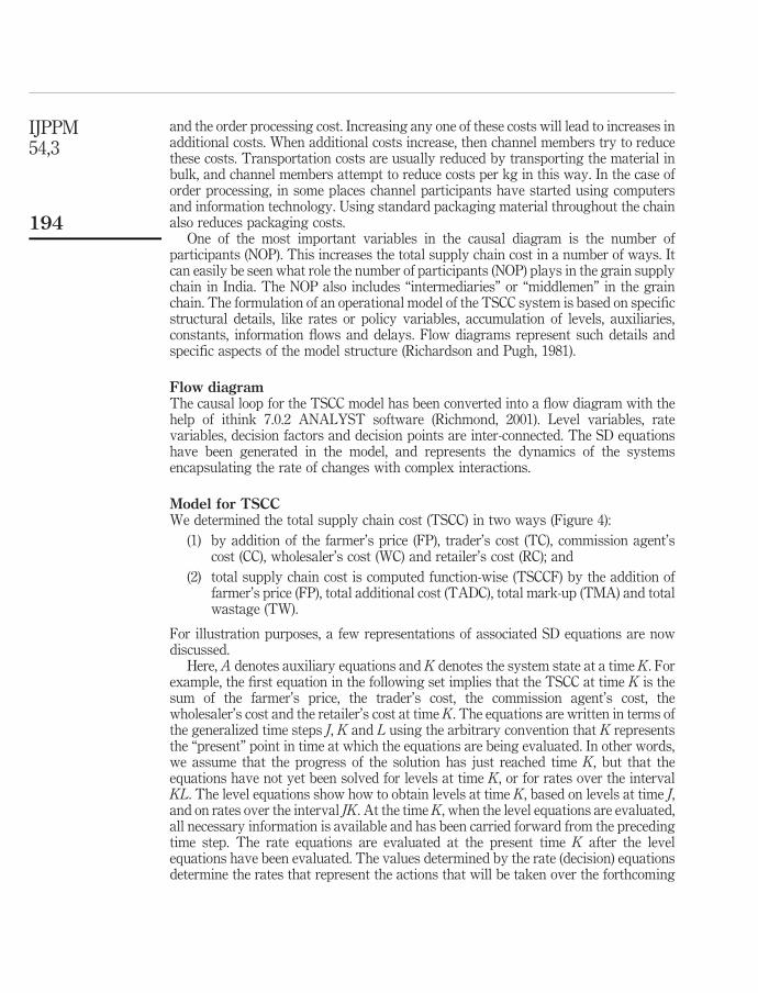
Model for TSCCWe determined the total supply chain cost (TSCC) in two ways (Figure 4):

(1) by addition of the farmer’s price (FP), trader’s cost (TC), commission agent’scost (CC), wholesaler’s cost (WC) and retailer’s cost (RC); and

(2) total supply chain cost is computed function-wise (TSCCF) by the addition offarmer’s price (FP), total additional cost (TADC), total mark-up (TMA) and totalwastage (TW).

For illustration purposes, a few representations of associated SD equations are nowdiscussed.

Here, A denotes auxiliary equations and K denotes the system state at a time K. Forexample, the first equation in the following set implies that the TSCC at time K is thesum of the farmer’s price, the trader’s cost, the commission agent’s cost, thewholesaler’s cost and the retailer’s cost at time K. The equations are written in terms ofthe generalized time steps J, K and L using the arbitrary convention that K representsthe “present” point in time at which the equations are being evaluated. In other words,we assume that the progress of the solution has just reached time K, but that theequations have not yet been solved for levels at time K, or for rates over the intervalKL. The level equations show how to obtain levels at time K, based on levels at time J,and on rates over the interval JK. At the time K, when the level equations are evaluated,all necessary information is available and has been carried forward from the precedingtime step. The rate equations are evaluated at the present time K after the levelequations have been evaluated. The values determined by the rate (decision) equationsdetermine the rates that represent the actions that will be taken over the forthcoming

IJPPM54,3

194

interval KL. Constant rates imply a constant rate of change in levels during a timeinterval.

After evaluation of the levels at time K and the rates for the interval KL, time is“indexed”. That is, the J, K, L positions are moved one time interval to the right. The Klevels just calculated are re-labeled as J levels. The KL rates become the JK rates. TimeK, “the present”, is thus advanced by one interval of time of DT length. The entirecomputation sequence can then be repeated to obtain a new state of the system at atime that is one DT later than the previous state. By definition this DT interval must beshort enough so that it represents constant rates of flow over the interval as asatisfactory approximation to continuously varying rates in the actual system.

Total supply chain cost (TSCC) is an auxiliary variable which is determined by theaddition of the farmer’s sales value (FP), the trader’s cost (TC), the commission agent’scost (CC), the wholesaler’s cost (WC) and the retailer’s cost (RC). Total supply chaincost function-wise (TSCCF) is an auxiliary variable, which is determined by theaddition of farmer’s sales value (FP), total additional cost (TADC), total mark-up(TMA) and total wastage (TW).

Additional cost can be also calculated in two ways, i.e. functional-wise and channelmember-wise. Channel member-wise, total additional cost (TAC) is an auxiliaryvariable which is determined by summation of the additional cost of the trader (ACT),the additional cost of the commission agent (ACC), the additional cost of the wholesaler(ACW) and the additional cost of retailer (ACR). Functional-wise, total additional cost(TADC) is an auxiliary variable which is determined by summation of the totalinventory holding cost (TIHC), the total materials handling cost (TMHC), the totaltransportation cost (TOTC), the total order processing cost (TOPC) and the total

Figure 4.Components of total

supply chain cost (TSCC)

Indian grainsupply chain

195

packaging cost (TPC). Elements of additional cost (i.e. TIHC, TMHC, TOTC, TOPC andTPC) are determined from participant: for example, the total inventory holding cost(TIHC) is determined by the inventory holding cost of the trader, the commission agent,the wholesaler and the retailer. Similarly, total wastage (TW) and total mark-up (TMA)are calculated:

A TSCC:K ¼ FP:K þ TC:K þ CC:K þ WC:K þ RC:K;

A TSCCF:K ¼ TADC:K þ TMA:K þ FP:K þ TW:K;

A TAC:K ¼ ACT:K þ ACC:K þ ACW:K þ ACR:K;

A TADC:K ¼ TIHC:K þ TMHC:K þ TOTC:K þ TOPC:K þ TPC:K;

A TIHC:K ¼ IHCT:K þ IHCC:K þ IHCW:K þ IHCR:K;

A TMHC:K ¼ MHCT:K þ MHCC:K þ MHCW:K þ MHCR:K;

A TOTC:K ¼ TCT:K þ TRCC:K þ TCW:K þ TCR:K;

A TOPC:K ¼ OPCT:K þ OPCC:K þ OPCW:K þ OPCR:K;

A TPC:K ¼ PCT:K þ PCC:K þ PCW:K þ PCR:K;

A TW:K ¼ WR:K þ WW:K þ WCA:K þ WT:K;

A TMA:K ¼ MUT:K þ MUC:K þ MUW:K þ MUR:K;

where TSCC is the total supply chain cost (in rupees), TSCCF is the total supply chaincost function-wise, FP is the farmer’s price (in rupees), TC is the trader’s cost (inrupees), CC is the commission agent’s cost (in rupees), WC is the wholesaler’s cost (inrupees), RC is the retailer’s cost (in rupees), TW is total wastage, TMA is the total markup, TAC is the total additional cost, TADC is the total add cost, TIHC is the totalinventory holding cost, TMHC is the total materials handling cost, TOTC is the totaltransportation cost, TOPC is the total order processing cost, and TPC is the totalpackaging cost.

Farmer’s costThe time interval taken in the model is one year and the level variables are the cost atthe farmer’s end and the wheat production volume. The rate is taken on the basis of thepast ten years of available data for wheat production and cost. Wheat production isincreasing at a rate (GPM) of 2.5 percent and the cost of production is increasing at arate (PIM) of 8 percent. The quantity of grain produced (QG) and the cost of production(COI) in 2001 were taken:

IJPPM54,3

196

A FP:K ¼ QG:K*COI:K;

L QG:K ¼ QG:J þ ðDTÞðRIQG:JKÞ;

N QG ¼ 6:85e8;

R RIQG:KL ¼ QG:K*GPM

C GPM ¼ 0:025;

L COI:K ¼ COI:J þ ðDTÞðPI:JKÞ

N COI ¼ 497:9;

R PI:KL ¼ COI:K* PIM;

C PIM ¼ 0:08;

where QG is the quantity required (quintals), FP is the farmer’s price (in rupees), COI isthe cost of inputs (in rupees/quintal), PI is the price increase, and PIM is the priceincrement multiplier (fraction).

Trader’s costThe trader’s cost is a summation of all the costs that the trader incurs. They are theadditional costs of the trader, the total wastage of trader and the mark-up of the trader.The total trader’s cost (TTC) is an auxiliary variable which is a summation of theadditional cost of trader (ACT), the wastage of the trader (WT) and the mark-up of thetrader (MUT). The additional cost of the trader (ACT) is an auxiliary variable which isa summation of the inventory holding cost (IHCT), the materials handling cost(MHCT), the transportation cost (TCT), the order processing cost (OPCT) and thepackaging cost (PCT) of the trader. These elements are the product of the farmer’s priceand the percentage of these components (Figure 3). The wastage of the trader (WT) isan auxiliary variable which is a product of the farmer’s price and the percentage ofwastage of the trader (PWT). The percentage of wastage of the trader is a constant andis taken as being 10 percent. Mark-up by trader (MUT) is an auxiliary variable which isproduct of the farmer’s price and the percentage of mark-up of the trader (PMUT). Thepercentage of mark-up of the trader is a constant, and is taken as being 10 percent:

A TTC:K ¼ ACT:K þ WT:K þ MUT:K þ FP:K;

A ACT:K ¼ IHCT:K þ MHCT:K þ TCT:K þ OPCT:K þ PCT:K;

A IHCT:K ¼ FP:K*PIHCT;

Indian grainsupply chain

197

C PIHCT ¼ 0:005;

A MHCT:K ¼ FP:K*PMHCT;

C PMHCT ¼ 0:015;

A TCT:K ¼ FP:K*PTCT;

C PTCT ¼ 0:015;

A OPCT:K ¼ FP:K*POPCT;

C POPCT ¼ 0:005;

A PCT:K ¼ FP:K*PPCT;

C PPCT ¼ 0:01;

A WT:K ¼ FP:K*PWT;

C PWT ¼ 0:10;

A MUT:K ¼ FP:K*PMUT;

C PMUT ¼ 0:10;

A TC:K ¼ TTC:K 2 FP:K;

where TTC is the total trader’s cost (in rupees), ACT is the additional cost for the trader(in rupees), WT is the wastage for the trader ( in rupees), MUT is the mark-up by thetrader (in rupees), IHCT is the inventory holding cost of the trader, MHCT is thematerials handling cost of the trader, TCT is the transportation cost of the trader,OPCT is the order processing cost of the trader, TC is the trader’s cost, PCT is thepackaging cost of the trader, PIHCT is the percentage inventory holding cost of thetrader (dimensionless), PMHCT is the percentage materials handling cost of the trader(dimensionless), PTCT is the percentage transportation cost of the trader(dimensionless), POPCT is the percentage order processing cost of the trader(dimensionless), PPCT is the percentage packaging cost of the trader (dimensionless),PWT is the percentage wastage of the trader (dimensionless), and PMUT is thepercentage mark-up of the trader (dimensionless).

Similarly, other sets of equations of commission agent, wholesaler and retailer havebeen developed across the range of factors and interactions that impact on the TSCCand TSCCF. This builds a “model” of the situation that can be used to explore theefficacy of alternative improvement strategies.

IJPPM54,3

198

Altogether there are 73 variables in the model. For the purposes of validation of themodel, three important variables were selected. The three variables selected were thepackaging cost, transportation cost and materials handling cost. The packaging cost,transportation cost and materials handling cost per quintal were Rs. 35.35, Rs. 37.55and Rs. 53, respectively. Then the model was subjected to some statistical tests to lendadded credence to the work. This was carried out by deriving the mean and standarddeviation of the model and actual values followed by a t-test for two means and anF-test for two variances, as summarised in Table II. The tabulated values of the t-testwith 20 degrees of freedom and F test with (10,10) are 2.086 and 2.98 respectively. Thecalculated values for packaging cost, transportation cost and materials handling costare within 95 percent confidence limits for the t-tests and F-tests. On the above basis,the model can be considered valid and hence the model can be used for projectingfuture costs.

Future projectionFuture projection of total supply chain cost is done by generating three scenarios (i.e.cooperative models, contract farming and collaborative supply chain). The optimistic,pessimistic and most likely views of the above mentioned three scenarios areconsidered for analysis. In total, nine scenarios generated. The present simulationmodel was changed and run nine times – once for each scenario – to get the finalresults. The three models are explained briefly below.

Cooperative modelThe cooperative model of farming is an improvement over individual farming(Figure 5). In the cooperative pattern farmers come together and form a cooperative. Insome parts of India milk is collected and sold by cooperatives. The cooperativemovement for milk was initiated by the National Dairy Development Board (NDDB)(Chakravarty, 2000). Due to these milk cooperatives, the efficiency, transparency andfairness of the system have improved (see www.digitaldividend.org/pdf/akashganga.pdf). In the case of grain, the domain of cooperative arrangements can range acrossvarious activities of the supply chain like procurement, storage, processing andmarketing. The government’s attitude towards the cooperative system is positive,especially after the success of the milk sector.

As mentioned previously in this paper we take three views – optimistic, pessimisticand most likely – in all three grain supply chain models. In the pessimistic view of thecooperative model we remove the commission agent, mark-up and additional cost. Herewe are assuming that the cooperative will at least be able to overcome the commissionagent. The variables changed in the model are percentage mark-up of the commission

Mean Standard deviationVariable Actual Model Actual Model t-test F-test

Packaging cost 1:74E þ 10 1:70E þ 10 5:17E þ 09 6:42E þ 09 0.1523 0.5065Transportation cost 2:48E þ 10 2:832E þ 10 8:21E þ 09 9:00E þ 09 0.2716 0.7784Materials handling cost 1:76E þ 10 1:759E þ 10 5:82E þ 09 5:82E þ 09 20.0045 0.6820

Table II.Validation of model

based on comparison ofactual and SD model

results from 1991 to 2001

Indian grainsupply chain

199

agent (PMUC) and the additional cost of the commission agent (ACC). In the most likelyview, we remove the trader’s and the commission agent’s margins. The variableschanged in the model are PMUC and the percentage mark-up of the trader (PMUT). Inthe optimistic view we removing the trader, commission agent and wholesalerwastage, mark-up and handling cost. The variables changed in the model are PMUC,PMUT, the percentage markup of the wholesaler (PMUW), PMHCT, PWT, percentagematerials handling cost of the commission agent (PMHCC), the percentage wastage ofthe commission agent (PWC), the percentage materials handling cost of the wholesaler(PMHCW) and the percentage wastage of the wholesaler (PWW). The changes weremade in the equations of the SD model developed in accordance with each view of thecooperative model, and the results are shown in Figure 6.

Figure 5.Co-operative supply chainmodel

Figure 6.Total supply chain cost inthe cooperative model

IJPPM54,3

200

Collaborative supply chainOne of the models of the grain supply chain is collaborative (Figure 7). At present everyretailer striving for scale and quality is creating distinct and separate supply chains,which are basically the same, i.e. farmer-AMPC-retailer. The collaborative effortalready visible in consumer durables and FMCG can also be applied here. In thisarrangement the third party manages the system, i.e. he takes the grain from thefarmer, consolidates and then perform cross docking for retailers. In essence there arevertical silos which do not allow the scaling up of the grain supply chain. Experts andacademics believe that the collaborative effort already visible in consumer durablesand FMCG would give the food supply chain exactly the scale and consolidation that itneeds to attract more investment, technology and people. This could give the grainsupply chain exactly the scale and consolidation that it wants.

In the pessimistic view of the collaborative supply chain model there will be areduction in the wastage and mark-up of to 25 percent for intermediaries. The variableschanged in the model are PMUC, PMUT, percentage mark-up of the wholesaler(PMUW) PWT, percentage wastage of the commission agent (PWC), and thepercentage wastage of the wholesaler (PWW). In the most likely view, the wastage andmark-up of the intermediaries are reduced by 50 percent. The variables changed in themodel are PMUC, PMUT, PMUW, PWT, PWC and PWW. In the optimistic view wehave removed the commission agent and mark-up and wastage are reduced by 50percent for the other intermediaries. The variables changed in the model are PMUC,PMUT, PMUW, PWT, PWC and PWW. The changes were made in the equations ofeach model according to each scenario, and the results are shown in Figure 8.

Contract farmingContract farming is the next option (Figure 9). Farmers under forward contracts candefine contract farming as a system for the production and supply of grain with anindustrial partner. The contract will include a commitment from the farmer to provide

Figure 7.Collaborative supply chain

model

Indian grainsupply chain

201

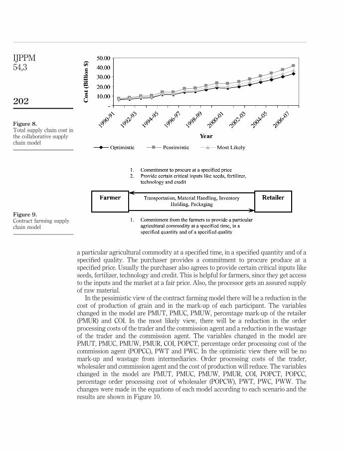
a particular agricultural commodity at a specified time, in a specified quantity and of aspecified quality. The purchaser provides a commitment to procure produce at aspecified price. Usually the purchaser also agrees to provide certain critical inputs likeseeds, fertilizer, technology and credit. This is helpful for farmers, since they get accessto the inputs and the market at a fair price. Also, the processor gets an assured supplyof raw material.

In the pessimistic view of the contract farming model there will be a reduction in thecost of production of grain and in the mark-up of each participant. The variableschanged in the model are PMUT, PMUC, PMUW, percentage mark-up of the retailer(PMUR) and COI. In the most likely view, there will be a reduction in the orderprocessing costs of the trader and the commission agent and a reduction in the wastageof the trader and the commission agent. The variables changed in the model arePMUT, PMUC, PMUW, PMUR, COI, POPCT, percentage order processing cost of thecommission agent (POPCC), PWT and PWC. In the optimistic view there will be nomark-up and wastage from intermediaries. Order processing costs of the trader,wholesaler and commission agent and the cost of production will reduce. The variableschanged in the model are PMUT, PMUC, PMUW, PMUR, COI, POPCT, POPCC,percentage order processing cost of wholesaler (POPCW), PWT, PWC, PWW. Thechanges were made in the equations of each model according to each scenario and theresults are shown in Figure 10.

Figure 8.Total supply chain cost inthe collaborative supplychain model

Figure 9.Contract farming supplychain model

IJPPM54,3

202

Discussion and conclusionAs compared to developed countries, the Indian grain supply chain is more complexand difficult to manage because of an unorganised grain market, price escalation andlarge number of intermediaries. In order to manage the grain supply chain, the IndianGovernment established APMC. APMC acts as a marketing exchange where traderspurchase grain from farmers and sell it to wholesalers or retailers. But due to poorconnectivity of villages, small land holding size and low education levels of farmers,commission agents (intermediaries) appear in the chain. With time these intermediarieshave become powerful and have formed cartels. These cartels becomecounter-productive for the farmers who are left with no choice but have to sell theirgrain through these commission agents. Similarly, wholesalers or retailers have topurchase through these commission agents. This disruption in the selling and buyingprocess leads to price escalation and high transaction costs (three to four times theactual price). Coase (1937) observed that under this condition, the cost of conductingeconomic exchange in a market may exceed the cost of organising the exchange withina firm. In order to manage the high transaction cost, a great deal of cooperation andcollaboration is required in the grain supply chain.

The purpose of this paper was to develop different models (cooperative model,contract farming model and collaborative model) to minimise the total supply chaincost (TSCC) under different scenarios – optimistic, most likely and pessimistic – todevise policies accordingly. This paper has proposed nine scenarios which may help inmanaging total supply chain cost. As discussed in the nine scenarios, we haveproposed to reduce some of the intermediaries in the three suggested models of thegrain supply chain. The results of the cost ratios of all nine scenarios are summarizedin Table III. The optimistic scenario in cooperative model and in contract farming

Figure 10.Total supply chain cost in

the contract farmingmodel

Scenario Optimistic Pessimistic Most likely

Cooperative supply chain 1.90 3.31 2.74Contract farming 1.95 1.90 2.58Collaborative supply chain 2.44 3.06 2.70

Table III.Cost ratio of the cost at

the consumer’s end to thecost at the farmer’s end

Indian grainsupply chain

203

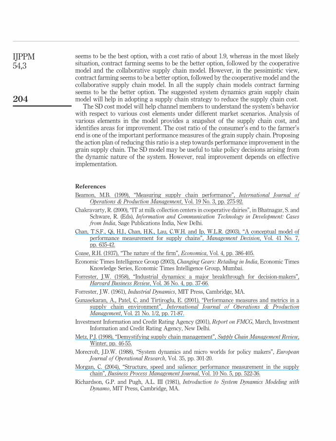
seems to be the best option, with a cost ratio of about 1.9, whereas in the most likelysituation, contract farming seems to be the better option, followed by the cooperativemodel and the collaborative supply chain model. However, in the pessimistic view,contract farming seems to be a better option, followed by the cooperative model and thecollaborative supply chain model. In all the supply chain models contract farmingseems to be the better option. The suggested system dynamics grain supply chainmodel will help in adopting a supply chain strategy to reduce the supply chain cost.

The SD cost model will help channel members to understand the system’s behaviorwith respect to various cost elements under different market scenarios. Analysis ofvarious elements in the model provides a snapshot of the supply chain cost, andidentifies areas for improvement. The cost ratio of the consumer’s end to the farmer’send is one of the important performance measures of the grain supply chain. Proposingthe action plan of reducing this ratio is a step towards performance improvement in thegrain supply chain. The SD model may be useful to take policy decisions arising fromthe dynamic nature of the system. However, real improvement depends on effectiveimplementation.

References

Beamon, M.B. (1999), “Measuring supply chain performance”, International Journal ofOperations & Production Management, Vol. 19 No. 3, pp. 275-92.

Chakravarty, R. (2000), “IT at milk collection centers in cooperative dairies”, in Bhatnagar, S. andSchware, R. (Eds), Information and Communication Technology in Development: Casesfrom India, Sage Publications India, New Delhi.

Chan, T.S.F., Qi, H.J., Chan, H.K., Lau, C.W.H. and Ip, W.L.R. (2003), “A conceptual model ofperformance measurement for supply chains”, Management Decision, Vol. 41 No. 7,pp. 635-42.

Coase, R.H. (1937), “The nature of the firm”, Economica, Vol. 4, pp. 386-405.

Economic Times Intelligence Group (2003), Changing Gears: Retailing in India, Economic TimesKnowledge Series, Economic Times Intelligence Group, Mumbai.

Forrester, J.W. (1958), “Industrial dynamics: a major breakthrough for decision-makers”,Harvard Business Review, Vol. 36 No. 4, pp. 37-66.

Forrester, J.W. (1961), Industrial Dynamics, MIT Press, Cambridge, MA.

Gunasekaran, A., Patel, C. and Tirtiroglu, E. (2001), “Performance measures and metrics in asupply chain environment”, International Journal of Operations & ProductionManagement, Vol. 21 No. 1/2, pp. 71-87.

Investment Information and Credit Rating Agency (2001), Report on FMCG, March, InvestmentInformation and Credit Rating Agency, New Delhi.

Metz, P.J. (1998), “Demystifying supply chain management”, Supply Chain Management Review,Winter, pp. 46-55.

Morecroft, J.D.W. (1988), “System dynamics and micro worlds for policy makers”, EuropeanJournal of Operational Research, Vol. 35, pp. 301-20.

Morgan, C. (2004), “Structure, speed and salience: performance measurement in the supplychain”, Business Process Management Journal, Vol. 10 No. 5, pp. 522-36.

Richardson, G.P. and Pugh, A.L. III (1981), Introduction to System Dynamics Modeling withDynamo, MIT Press, Cambridge, MA.

IJPPM54,3

204

Richmond, B. (2001), An Introduction to Systems Thinking, High Performance Systems, Hanover,NH.

Roberts, E.B. (1978), Managerial Applications of System Dynamics, MIT Press, Cambridge, MA.

Sharma, D., Sahay, B.S. and Sachan, A. (2004), “Modeling distributors performance index usingsystem dynamics approach”, Asia Pacific Journal of Marketing and Logistics, Vol. 16 No. 3,pp. 37-67.

Stevens, G.C. (1989), “Integrating the supply chain”, International Journal of Physical Distribution& Logistics Management, Vol. 19 No. 8, pp. 3-8.

Towill, D.R. (1996), “Industrial dynamics modeling of supply chains”, Logistics InformationManagement, Vol. 9 No. 4, pp. 43-56.

Indian grainsupply chain

205