Energies 2014, 7, 7348-7367; doi:10.3390/en7117348

energies ISSN 1996-1073

www.mdpi.com/journal/energies

Article

Design Optimization of Heat Wheels for Energy Recovery in

HVAC Systems

Stefano De Antonellis 1,*, Manuel Intini 1, Cesare Maria Joppolo 1 and Calogero Leone 2

1 Department of Energy, Politecnico di Milano, Via Lambruschini 4, Milano 20156, Italy;

E-Mails: manuel.intini@polimi.it (M.I.); cesare.joppolo@polimi.it (C.M.J.) 2 Recuperator S.p.A., Via Valfurva 13, Rescaldina (MI) 20027, Italy;

E-Mail: leone@recuperator.eu

* Author to whom correspondence should be addressed; E-Mail: stefano.deantonellis@polimi.it;

Tel.: +39-02-2399-3823; Fax: +39-02-2399-3863.

External Editor: Chi-Ming Lai

Received: 31 July 2014; in revised form: 13 September 2014 / Accepted: 4 November 2014 /

Published: 14 November 2014

Abstract: Air to air heat exchangers play a crucial role in mechanical ventilation

equipment, due to the potential primary energy savings both in case of refurbishment of

existing buildings or in case of new ones. In particular, interest in heat wheels is increasing

due to their low pressure drop and high effectiveness. In this paper a detailed optimization

of design parameters of heat wheels is performed in order to maximize sensible

effectiveness and to minimize pressure drop. The analysis is carried out through a one

dimensional lumped parameters heat wheel model, which solves heat and mass transfer

equations, and through appropriate correlations to estimate pressure drop. Simulation

results have been compared with experimental data of a heat wheel tested in specific

facilities, and good agreement is attained. The device optimization is performed through

the variation of main design parameters, such as heat wheel length, channel base, height

and thickness and for different operating conditions, namely the air face velocity and the

revolution speed. It is shown that the best configurations are achieved with small channel

thickness and, depending on the required sensible effectiveness, with appropriate values of

wheel length and channel base and height.

OPEN ACCESS

Energies 2014, 7 7349

Keywords: heat wheel optimization; heat wheel effectiveness; simulation; experimental data;

heat exchanger design

1. Introduction

It is well known that buildings are responsible for around 40% of primary energy consumption in

developed countries and for 20%–40% in developing countries [1]. In case of refurbishment of existing

buildings or in new ones, the introduction of a heat exchanger between exhaust and fresh air streams

play a crucial role due to relevant achievable energy savings [2–8]. In particular, interest in heat

wheels is increasing due to their low pressure drop and high effectiveness compared to conventional

plate heat exchangers [9].

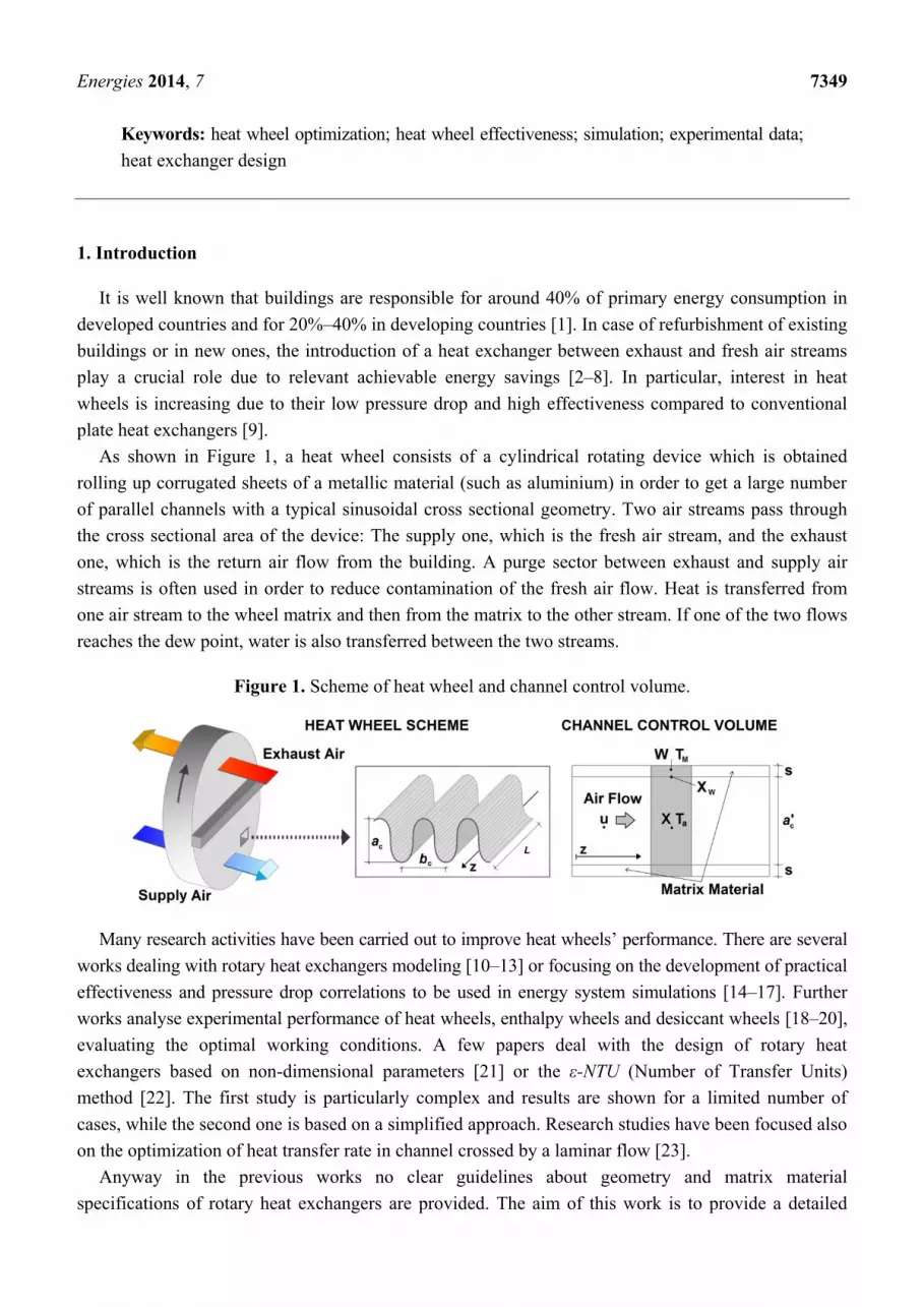
As shown in Figure 1, a heat wheel consists of a cylindrical rotating device which is obtained

rolling up corrugated sheets of a metallic material (such as aluminium) in order to get a large number

of parallel channels with a typical sinusoidal cross sectional geometry. Two air streams pass through

the cross sectional area of the device: The supply one, which is the fresh air stream, and the exhaust

one, which is the return air flow from the building. A purge sector between exhaust and supply air

streams is often used in order to reduce contamination of the fresh air flow. Heat is transferred from

one air stream to the wheel matrix and then from the matrix to the other stream. If one of the two flows

reaches the dew point, water is also transferred between the two streams.

Figure 1. Scheme of heat wheel and channel control volume.

Many research activities have been carried out to improve heat wheels’ performance. There are several

works dealing with rotary heat exchangers modeling [10–13] or focusing on the development of practical

effectiveness and pressure drop correlations to be used in energy system simulations [14–17]. Further

works analyse experimental performance of heat wheels, enthalpy wheels and desiccant wheels [18–20],

evaluating the optimal working conditions. A few papers deal with the design of rotary heat

exchangers based on non-dimensional parameters [21] or the ε-NTU (Number of Transfer Units)

method [22]. The first study is particularly complex and results are shown for a limited number of

cases, while the second one is based on a simplified approach. Research studies have been focused also

on the optimization of heat transfer rate in channel crossed by a laminar flow [23].

Anyway in the previous works no clear guidelines about geometry and matrix material

specifications of rotary heat exchangers are provided. The aim of this work is to provide a detailed

Energies 2014, 7 7350

analysis and optimization of heat wheel design, maximizing sensible effectiveness and minimizing

pressure drop. In particular the effects of channel geometry, wheel length and revolution speed on

component performance are evaluated.

The analysis of the rotary heat exchanger has been performed through a lumped parameter model

based on heat and mass transfer equations and on appropriate correlations to evaluate pressure drop.

The model has been previously validated through the comparison with the performance of a rotary

device tested in the lab facilities, showing good agreements in all the conditions.

2. Mathematical Model

2.1. Heat Wheel Description and Model Assumptions

The rotating wheel, which is characterized by a diameter D and a length L, is divided into two

sections: the first for supply air and the second for exhaust air in a counter current flow arrangement.

The wheel rotates at constant speed N and each channel is periodically exposed to the two streams.

In this model the purge section is not considered.

As shown in Figure 1, the geometry of the channel cross section is assumed sinusoidal in the upper

part and flat in the remaining one. Duct height and base are respectively referred to as ac and bc.

The physical model and the numerical analysis are based on the following assumptions:

- Temperature and velocity profiles in the channels are fully developed.

- Channels are equal and uniformly distributed throughout the wheel.

- Temperature, humidity ratio and velocity of each inlet flow are uniform at the inlet face of the wheel.

- Heat and mass transfer between adjacent channels is negligible.

- Heat and mass transfer from the wheel to the surroundings is negligible.

- Axial heat conduction and water vapour diffusion in the air stream are negligible.

- Temperature gradient through the channel thickness is negligible.

- Density and velocity variation of air along the channel are negligible.

- Specific heat and thermal conductivity of dry air, water vapour and liquid water are assumed constant.

- Air leakages between the two streams are negligible.

2.2. Governing Equations

The following equations are applied to an infinitesimal element of the channel: Conservation of

water and energy in the solid side (matrix material and condensed water), conservation of water and

energy in the wet air stream.

Conservation of water in the air stream:

( )ρ

mw

da c

P hX Xu X X

t z A

(1)

where X is the humidity ratio of the air stream, XW is the humidity ratio of air on the channel wall,

P the perimeter and Ac the cross sectional area of the channel and hm the mass transfer coefficient.

Conservation of water on the channel surface:

Energies 2014, 7 7351

M

wm

f

PXXh

t

W )(

(2)

where W is the amount of condensed water on the channel surface and fM is the metallic material mass

per unit of length in the channel.

Energy balance in the system made up of the matrix material and the condensed water:

2

2( ) ( λ) ( ) ( )M M

M M M w v a w M m w T a M M M

T Tf cp f cp W cp T cp T h X X P h T T P A k

t z

(3)

where Ta and TM are respectively the air and channel material temperature, λ is the vaporization latent

heat of water, cpw and cpM are respectively the specific heat of the liquid water and of the channel

material, hT is the heat transfer coefficient, kM and AM are respectively the thermal conductivity and the

cross sectional area of the matrix thickness.

Energy balance in the air stream:

( ) ( )

ρ ρ

a a T a M m W v a

c da wa c da wa

T T h T T P h X X Pcp Tu

t z A cp A cp

(4)

where cpwa is the specific heat of wet air defined as cpwa = cpda + X·cpv.

Further equations are necessary to solve the system. The humidity ratio on the surface of the

channel structure can be expressed in the form reported in the following. If water condensation occurs

on the surface (W > 0) or the surface temperature is below the dew point of the air stream (TM < Tdew):

;φ 100%W W MX X T (5a)

In all other conditions:

XXW (5b)

The relation between relative and absolute humidity is:

φ0.622

φtot

sat

Xp

p

(6)

where ptot is the atmospheric pressure, assumed constant and equal to 101,325 Pa, and psat is the steam

saturation pressure, calculated through the following equation:

13.4615.273

44.3816196.23

aT

sat ep (7)

The Nusselt number of the fully developed flow depends on the sinusoidal channel geometry [24]:

432

'

'4966.0

'

'9975.1

'

'1901.3

'

'7701.211791.1

c

c

c

c

c

c

c

c

b

a

b

a

b

a

b

aNu (8)

where a'c is the inner channel height and b'c is the inner channel base.

The Sherwood number is calculated through the Chilton-Colburn analogy:

Nu

ShLe 3/1 (9)

Energies 2014, 7 7352

The Lewis number is assumed constant and equal to 1 and therefore Nu is equal to Sh.

The heat transfer coefficient hT can be calculated from local Nusselt number in this way:

a

eqT

k

DhNu (10)

where ka is the thermal conductivity of the wet air. The mass transfer coefficient hm is obtained from

the Sherwood number:

ρ

M eq

DA v

h DSh

D (11)

where Dv is the mass diffusivity of vapour in air.

The actual velocity of air in the channel is assumed to be:

σ

fvu (12)

where σ is the wheel porosity calculated in this form:

σ c

M c

A

A A

(13)

Finally the following correlations are used to calculate respectively: The equivalent diameter of the

inner channel [24], the inner channel height and base, the inner channel cross section area, perimeter

and the cross section area of the matrix layer:

432

'

'0436.0

'

'1794.0

'

'1180.0

'

'4670.00542.1'

c

c

c

c

c

c

c

c

ceqb

a

b

a

b

a

b

aaD (14)

22'

saa cc (15)

22'

sbb cc (16)

2

'' ccc

baA (17)

2

2 2

2

23

π2 π

2 2 24

π

c

cc cc

c

c

b

ab aP b

b

a

(18)

2

sPAM (19)

2.3. Boundary and Initial Conditions

The following conditions are set to solve the system of equations discussed above:

Energies 2014, 7 7353

Initial conditions:

0

0

0

0,

,0

,0

,0

,0

WzW

XzX

TzT

TzT

MM

aa

(20)

Boundary conditions supply air period:

insu

insua

XtX

TtT

,

,

0,

0, (21)

And during the exhaust air period:

inex

inexa

XtX

TtT

,

,

0,

0, (22)

The system of PDE (Partial Differential Equations) is solved with the Implicit Euler Method.

Convergence is achieved when water mass and heat transferred from air during the supply air period

are equal to water mass and heat exchanged during the exhaust air period plus a prefixed error.

2.4. Pressure Drop

Pressure drop is calculated through the following equation:

2 21 1ξ ρ 4 ρ

2 2C wa wa

eq

Lp u f u

D (23)

where ξc is the loss coefficient which takes into account the contraction and expansion of the air flow

at the inlet and outlet of the wheel, assumed equal to 0.2 [25], and f is the Fanning friction factor,

which is expressed in the following form [24]:

5432

'

'0338.0

'

'2907.0

'

'8314.0

'

'8619.0

'

'0772.015687.9Re

c

c

c

c

c

c

c

c

c

c

b

a

b

a

b

a

b

a

b

af (24)

In Equation (24), Reynolds number of each air stream is evaluated at average conditions between

the channel inlet and outlet.

3. Experimental Methodology

3.1. Experimental Setup Description

A rotary heat exchanger was tested in two different test rigs: In the first one the sensible

effectiveness has been evaluated, while in the second one pressured drop has been measured. The two

test rigs are described in detail in Sections 3.2 and 3.3.

Energies 2014, 7 7354

3.2. Heat Transfer Test Rig

The facility is designed according to ASHRAE standards [26], in order to provide the rotary heat

exchanger with two air streams at balanced and controlled flow rates. Supply and exhaust air flows

pass through the heat wheel in a counter current arrangement. A schematic representation of the

experimental setup is shown at the top of Figure 2.

Supply air is provided at outdoor temperature, while exhaust air temperature is properly controlled

through an electric heater. Humidity ratio of both air streams is not controlled and is equal to outside air

humidity ratio. Temperature is measured by calibrated thermocouples (type T Copper/Constantan) with

±0.5 °C uncertainty. Sensors are installed across the heat wheel, at the inlet and outlet of each air stream.

Figure 2. Heat transfer and pressure drop test rigs.

Mass flow rates of the supply and exhaust air streams are equal. Flow rates are set by a variable speed

fan and are measured through calibrated nozzles, constructed according to ASHRAE standards [26].

Air flow rate can be adjusted in the range between 1000 and 3000 m3·h−1. Pressure drop and

temperature at calibrated nozzles inlet and outlet are measured through a water U-tube manometer

(uncertainty of 1% of reading) and by a calibrated thermocouple (uncertainty of ±0.5 °C) respectively.

Heat wheel revolution speed is controlled through an AC inverter motor in the range between 10

and 20 rev·min−1. All calibrated sensors are connected to a specific data logger and samples are

collected every 5 s. Air handling unit and ducts are properly insulated with mineral wool panels.

3.3. Pressure Drop Test Rig

A specific facility has been designed to measure the pressure drop across the heat wheel, as shown

in Figure 2. In a typical experimental setup used to evaluate heat wheels performance, the measured

pressure drop includes the effect of the cross section variation of the ducts which supply the air stream

to the device. In fact, the wheel face area has a semi-circular geometry and connecting ducts have a

Energies 2014, 7 7355

rectangular cross section. Air pressure drop related to this cross section variation does not depend on

the heat wheel channels geometry but on the air handling unit and heat exchanger frame design.

In order to exclude the contribution of the aforementioned effect, in this pressure drop test rig a

circular duct has been sealed directly to the heat wheel face area. In this way only distributed and local

pressure drop at inlet and outlet of the heat wheel channels have been properly measured.

The pressure drop test rig is part of a complex unit that is used to evaluate desiccant wheel

performance. Outside air is properly controlled through heating coils, cooling coils and evaporative

coolers in order to match the required temperature and humidity.

Air flow rate is set by variable speed fans and is measured across orifice plates installed in two

different parallel ducts. Each duct can be excluded in case of low volumetric air flow tests to limit

measurement uncertainty. Orifice plates and ducts apparatus are constructed according to DIN EN ISO

5167-2 standards [27]. The maximum air flow rate is 2000 m3·h−1. A part of the heat wheel face is

directly connected to a 20 cm-diameter duct.

Pressure drop across the rotative heat exchanger and across orifice plate is measured by

piezoelectric transmitters (uncertainty of ±0.5% of reading ±1 Pa) while temperature is measured

by calibrated RTD PT100 1/3 class B (IEC 751) sensors (uncertainty of ±0.2 °C) and relative humidity

by capacitive sensors (uncertainty of ±1%).

3.4. Experimental Procedure

Each test is carried out in steady state conditions and in each session at least 100 samples of each

physical quantity are logged. Representative values for each working point are obtained as average of

the collected data.

At the end of each test the following quantities are calculated:

outsuinsuaasus TTcpmQ ,,,

(25)

inexoutexaaexs TTcpmQ ,,,

(26)

Performance of heat wheel is determined through sensible effectiveness, defined as:

, ,

.

, ,

ε

2 ( )

s su s ex

s

a a ex in su in

Q Q

m cp T T

(27)

The experimental uncertainty uxi of each monitored variable xi is:

,

2 2

95( σ )i i inst i

x x xu u t (28)

where uxi,inst is the instrument uncertainty of the generic measured parameter, t95 is the Student test

multiplier at 95% confidence and σix is the standard deviation of the mean.

The combined uncertainty of sensible effectiveness uεs is calculated as [28]:

2 2

, 95

ε εσ

i is x inst x

i ii i

u u tx x

(29)

Energies 2014, 7 7356

Pressure drop has been measured through a specific test, as reported in Section 3.2. Even in this

case pressure drop of each test condition has been calculated as the average of the measured values and

its uncertainty evaluated through Equation (28).

4. Model Validation

Model results have been compared with experimental data of a commercial heat wheel tested in the

two experimental rigs described in Section 3.2 and 3.3. Main data of the tested device are summarized

in Table 1.

Table 1. Main data of tested heat wheel.

Parameter Data

ac (mm) 2.0

bc (mm) 3.8

s (mm) 0.055

D (m) 0.6

Dhub (m) 0.06

L (m) 0.2

Matrix Material Aluminium *

Purge Sector None

* Assumed ρM = 2700 kg·m−3; cpM = 900 kJ·kg−1 °C−1; kM = 220 W·m−1·°C−1.

4.1. Sensible Effectiveness

The heat wheel has been tested in several working conditions, as summarized in Table 2, in particular

with different revolution speed and air face velocity and inlet temperature of both air streams.

Table 2. Experimental sensible effectiveness: Test conditions and measured data.

Test A1 A2 A3 B1 B2 B3 C1 C2 C3 D1 D2 D3 E1 E2 E3 F1 F2 F3

vf (m s−1) 2.09 2.11 2.11 2.87 2.92 2.92 3.76 3.72 3.71 4.44 4.45 4.40 5.21 5.18 5.17 5.75 5.76 5.80

N (rev min−1) 10 15 20 10 15 20 10 15 20 10 15 20 10 15 20 10 15 20

Tsu,in (°C) 25.8 26.2 25.0 24.2 23.8 24.3 22.3 23.3 24.8 22.5 22.6 23.8 20.2 20.1 20.3 21.8 21.3 20.9

Tex,in (°C) 64.5 64.0 62.6 57.3 56.9 55.5 47.4 51.4 53.2 51.8 49.7 49.7 47.3 58.1 59.7 59.6 60.7 59.8

Xin (g kg−1) 9.1 7.8 8.2 8.2 8.0 8.1 9.8 11.1 9.9 9.3 9.5 9.6 9.8 9.7 9.8 10.5 10.2 10.1

φsu,in (%) 44.3 37.2 42.0 44.2 44.0 43.3 59.1 62.6 51.1 55.3 56.3 52.9 67.2 67.0 66.8 65.1 65.3 66.1

φex,in (%) 6.0 5.3 5.9 7.5 7.5 8.1 14.5 13.4 11.0 11.1 12.5 12.7 14.6 8.5 8.0 8.6 8.0 8.2

εs (-) 0.79 0.79 0.79 0.74 0.74 0.74 0.68 0.69 0.69 0.65 0.65 0.65 0.61 0.62 0.62 0.58 0.59 0.60

Q,s (kW) 11.1 10.9 10.9 12.3 12.5 11.8 11.0 12.3 12.5 14.3 13.5 12.8 14.7 20.9 21.8 21.8 23.2 23.1

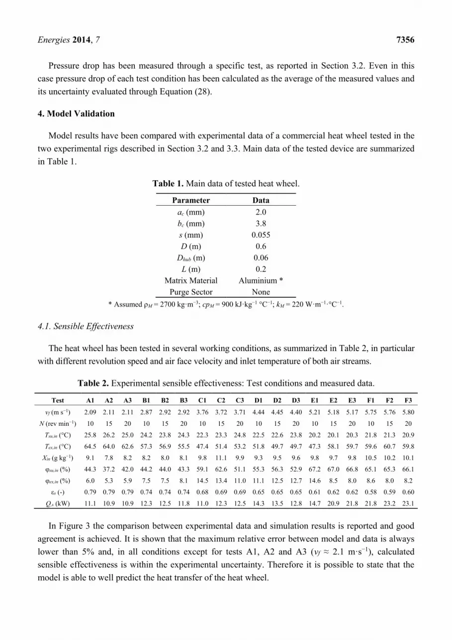
In Figure 3 the comparison between experimental data and simulation results is reported and good

agreement is achieved. It is shown that the maximum relative error between model and data is always

lower than 5% and, in all conditions except for tests A1, A2 and A3 (vf ≈ 2.1 m·s−1), calculated

sensible effectiveness is within the experimental uncertainty. Therefore it is possible to state that the

model is able to well predict the heat transfer of the heat wheel.

Energies 2014, 7 7357

Figure 3. Sensible effectiveness: Experimental data and simulation results. Refer to

Tables 1 and 2 for heat wheel data and test conditions.

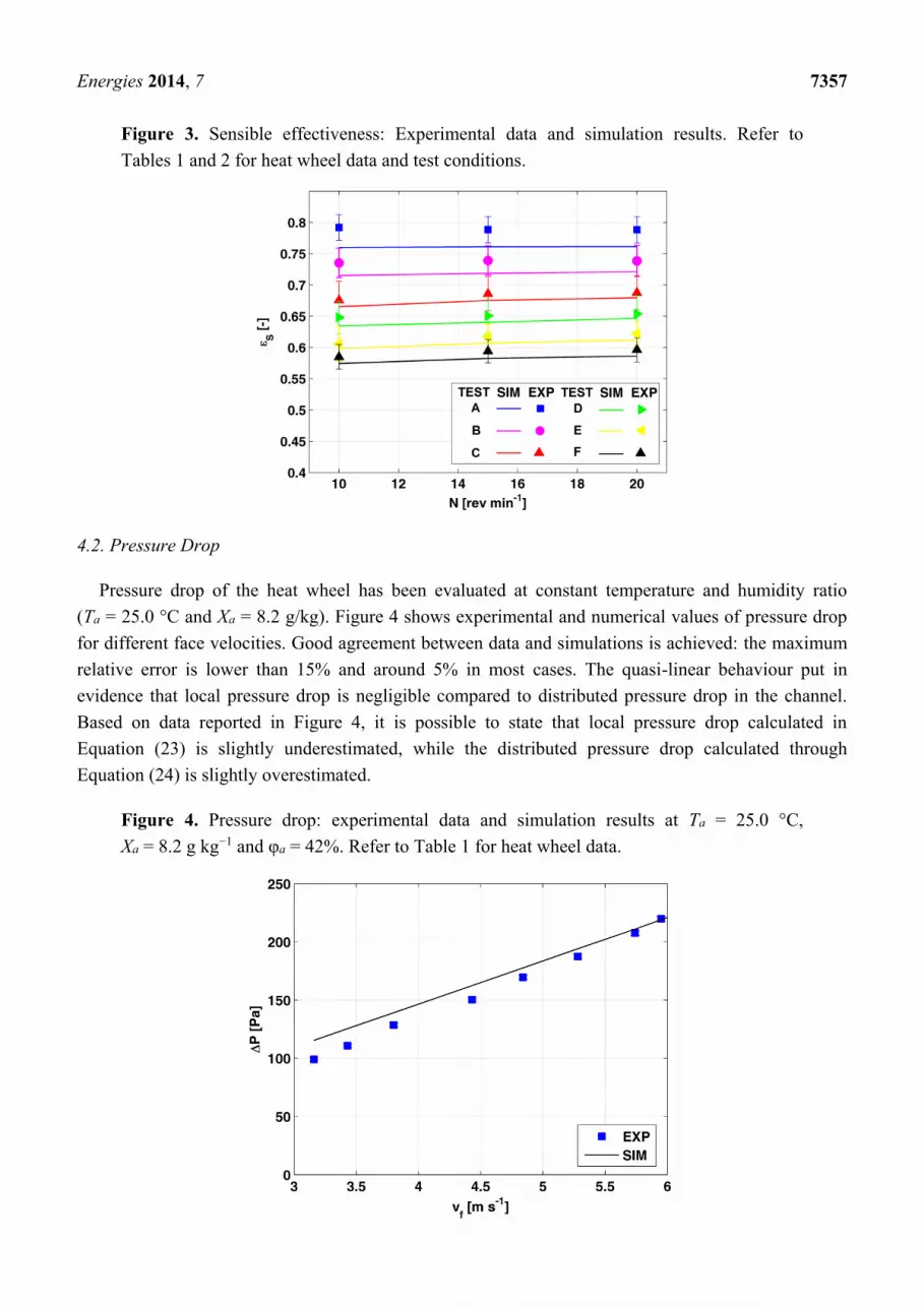
4.2. Pressure Drop

Pressure drop of the heat wheel has been evaluated at constant temperature and humidity ratio

(Ta = 25.0 °C and Xa = 8.2 g/kg). Figure 4 shows experimental and numerical values of pressure drop

for different face velocities. Good agreement between data and simulations is achieved: the maximum

relative error is lower than 15% and around 5% in most cases. The quasi-linear behaviour put in

evidence that local pressure drop is negligible compared to distributed pressure drop in the channel.

Based on data reported in Figure 4, it is possible to state that local pressure drop calculated in

Equation (23) is slightly underestimated, while the distributed pressure drop calculated through

Equation (24) is slightly overestimated.

Figure 4. Pressure drop: experimental data and simulation results at Ta = 25.0 °C,

Xa = 8.2 g kg−1 and φa = 42%. Refer to Table 1 for heat wheel data.

Figure 4. Pressure drop: experimental data and simulation results at

Ta=25.0 °C and Xa=8.2 g kg-1

. Refer to Table 1 for heat wheel data

Figure 4. Pressure drop: experimental data and simulation results at

Ta=25.0 °C and Xa=8.2 g kg-1

. Refer to Table 1 for heat wheel data

Energies 2014, 7 7358

5. Heat Wheel Optimization

5.1. Preliminary Analysis of Performance

In this section the effect of boundary conditions and design parameters on heat wheel sensible

effectiveness is evaluated. These effects are investigated for a rotary heat exchanger crossed by

balanced supply and exhaust air flows. In all simulations face air velocity is an input and results are

reported at constant face area. It is assumed the heat wheel is made of aluminium, whose properties are

reported in Table 1. Although the model is able to predict latent heat recovery due to water

condensation on channel walls, in this work only sensible effectiveness is analysed and therefore

appropriate boundary conditions have been selected.

In Figure 5 it is shown the effect of revolution speed, inlet temperature and face velocity on

component effectiveness. It is possible to state that if inlet temperature of air streams varies within the

range of HVAC applications, the rotary heat exchanger performance does not change significantly.

On the other side, effects due to revolution speed and face velocity variation are important and they

can be explained in the following way:

- If the heat wheel rotates too slowly, the matrix material average temperature becomes close to

the air stream and, therefore, heat transfer decreases due to limited temperature difference. On

the other side, if the wheel rotates too fast, the effect of carryover, i.e., the cross contamination

between the two streams due to the amount of air trapped in the wheel channel, becomes

relevant. Therefore an optimal revolution speed exists: It is typically around 10–20 rev·min−1,

depending on air flow rates and heat exchanger geometry.

- If the face air velocity vf of both streams increases (and consequently the velocity in the channel u),

the sensible effectiveness decreases because air heat capacity rate is bigger at constant heat

transfer area.

All the aforementioned considerations are in agreement with previous research works,

such as [13,17,18].

Figure 5. Effect of revolution speed, inlet temperature and face velocity on sensible

effectiveness (ac = bc = 2 mm, s = 0.06 mm, L = 0.2 m, Xa,in = 3.0 g/kg).

Figure 5. Effect of revolution speed, inlet temperature and face velocity on

sensible effectiveness (ac = bc = 2 mm, s = 0.06 mm, L = 0.2 m, Xa,in= 3 g/kg)

Energies 2014, 7 7359

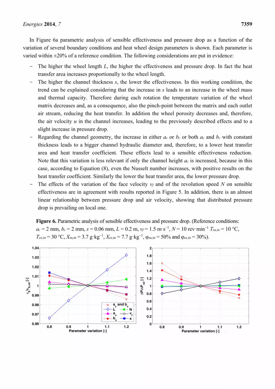
In Figure 6a parametric analysis of sensible effectiveness and pressure drop as a function of the

variation of several boundary conditions and heat wheel design parameters is shown. Each parameter is

varied within ±20% of a reference condition. The following considerations are put in evidence:

- The higher the wheel length L, the higher the effectiveness and pressure drop. In fact the heat

transfer area increases proportionally to the wheel length.

- The higher the channel thickness s, the lower the effectiveness. In this working condition, the

trend can be explained considering that the increase in s leads to an increase in the wheel mass

and thermal capacity. Therefore during each rotation the temperature variation of the wheel

matrix decreases and, as a consequence, also the pinch-point between the matrix and each outlet

air stream, reducing the heat transfer. In addition the wheel porosity decreases and, therefore,

the air velocity u in the channel increases, leading to the previously described effects and to a

slight increase in pressure drop.

- Regarding the channel geometry, the increase in either ac or bc or both ac and bc with constant

thickness leads to a bigger channel hydraulic diameter and, therefore, to a lower heat transfer

area and heat transfer coefficient. These effects lead to a sensible effectiveness reduction.

Note that this variation is less relevant if only the channel height ac is increased, because in this

case, according to Equation (8), even the Nusselt number increases, with positive results on the

heat transfer coefficient. Similarly the lower the heat transfer area, the lower pressure drop.

- The effects of the variation of the face velocity vf and of the revolution speed N on sensible

effectiveness are in agreement with results reported in Figure 5. In addition, there is an almost

linear relationship between pressure drop and air velocity, showing that distributed pressure

drop is prevailing on local one.

Figure 6. Parametric analysis of sensible effectiveness and pressure drop. (Reference conditions:

ac = 2 mm, bc = 2 mm, s = 0.06 mm, L = 0.2 m, vf = 1.5 m·s−1, N = 10 rev·min−1 Tsu,in = 10 °C,

Tex,in = 30 °C, Xsu,in = 3.7 g·kg−1, Xex,in = 7.7 g·kg−1, φsu,in = 50% and φex,in = 30%).

Figure 6. Parametric analysis of sensible effectiveness and pressure drop. (Reference conditions:

ac = 2 mm, bc = 2 mm, s = 0.06 mm, L = 0.2 m, vf = 1.5 m s-1

N = 10 rev min-1

Xa,in= 3 g kg-1

)

Energies 2014, 7 7360

5.2. Optimization Results

5.2.1. Preliminary Simulations

In this section the heat wheel design is optimized in order to maximize effectiveness and minimize

pressure drop, which is directly related to ventilation power consumption. The power required to rotate

the device (around 30 W for a 60 cm-diameter wheel) is not considered. According to the preliminary

investigation reported in Section 5.1, the analysis is performed at fixed inlet temperature and humidity

ratio of both air streams. Note that inlet air conditions are not strictly representative of a specific site

but they have been fixed in order to avoid water condensation on the wheel channel. Many parameters

affecting heat exchanger sensible effectiveness and pressure drop have been varied, namely: Channel

height, base and thickness, revolution speed, wheel length and face air velocity.

Each of the aforementioned parameters has been varied in the range reported in Table 3. According

to Equations (8) and (9) typical values of Nu and Sh are in the range between 2.1 and 2.6 while Re

varies between 100 and 550 (vf = 2.5 m s−1).

Table 3. Minimum and maximum value of each parameter adopted in the simulations.

Parameter Min Max

N (rev·min−1) 5 20

ac (mm) 1 6

bc (mm) 1 6

s (mm) 0.05 0.12

L (m) 0.05 0.4

vf (m·s−1) 1.5 3.5

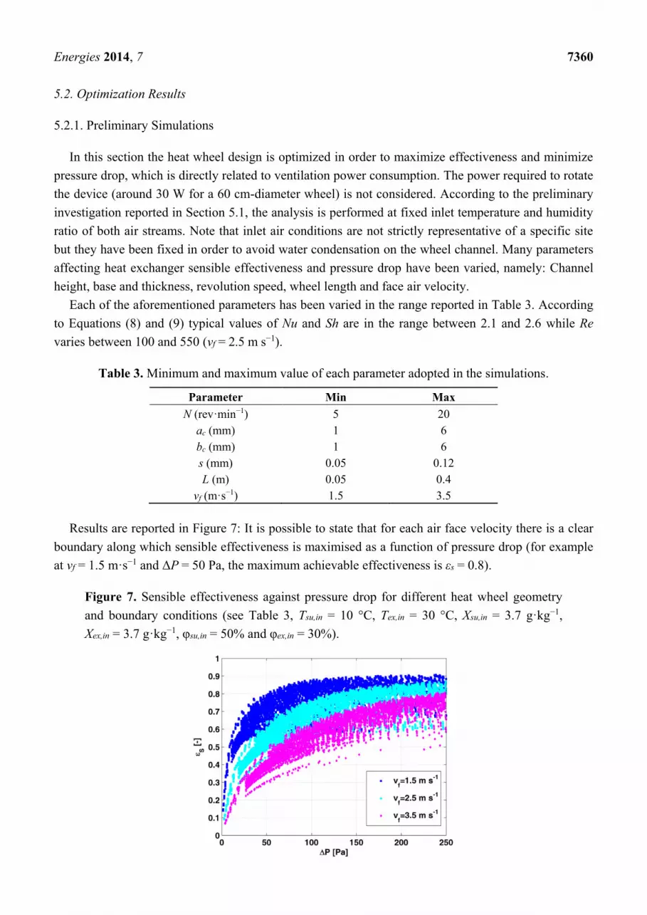
Results are reported in Figure 7: It is possible to state that for each air face velocity there is a clear

boundary along which sensible effectiveness is maximised as a function of pressure drop (for example

at vf = 1.5 m·s−1 and ΔP = 50 Pa, the maximum achievable effectiveness is εs = 0.8).

Figure 7. Sensible effectiveness against pressure drop for different heat wheel geometry

and boundary conditions (see Table 3, Tsu,in = 10 °C, Tex,in = 30 °C, Xsu,in = 3.7 g·kg−1,

Xex,in = 3.7 g·kg−1, φsu,in = 50% and φex,in = 30%).

Figure 7. Effectiveness against pressure drop for different heat wheel geometry and

boundary conditions (see Table 3, Tsu,in=10°C, Tex,in=30°C, Xin=7 g kg-1

)

Energies 2014, 7 7361

It is of primary interest to identify the values that design parameters should assume in order to

match the Pareto front. It is outlined that points on Pareto front are marked out by small channel

thickness and are almost independent of revolution speed, that is generally around 8–12 rev·min−1. In

order to evaluate properly the effect of other parameters, a detailed analysis has been performed in case

of vf = 2.5 m·s−1, which represents a common operating condition in air handling units.

5.2.2. Performance at Constant Heat Wheel Length L = 0.2 m

It is put in evidence that the length of most commercial rotary heat exchangers is usually equal to

0.2 m [9], according to air handling units’ manufacturer requirements. Therefore a preliminary

investigation deals with such a configuration: In Figure 8 the optimal heat wheel arrangements with

L = 0.2 m are shown. Based on the preliminary analysis of Section 5.2.1, in all cases the best channel

thickness is s = 0.05 mm, that is the minimum value adopted in the simulations. A thinner channel is

not considered because of its lack of mechanical resistance.

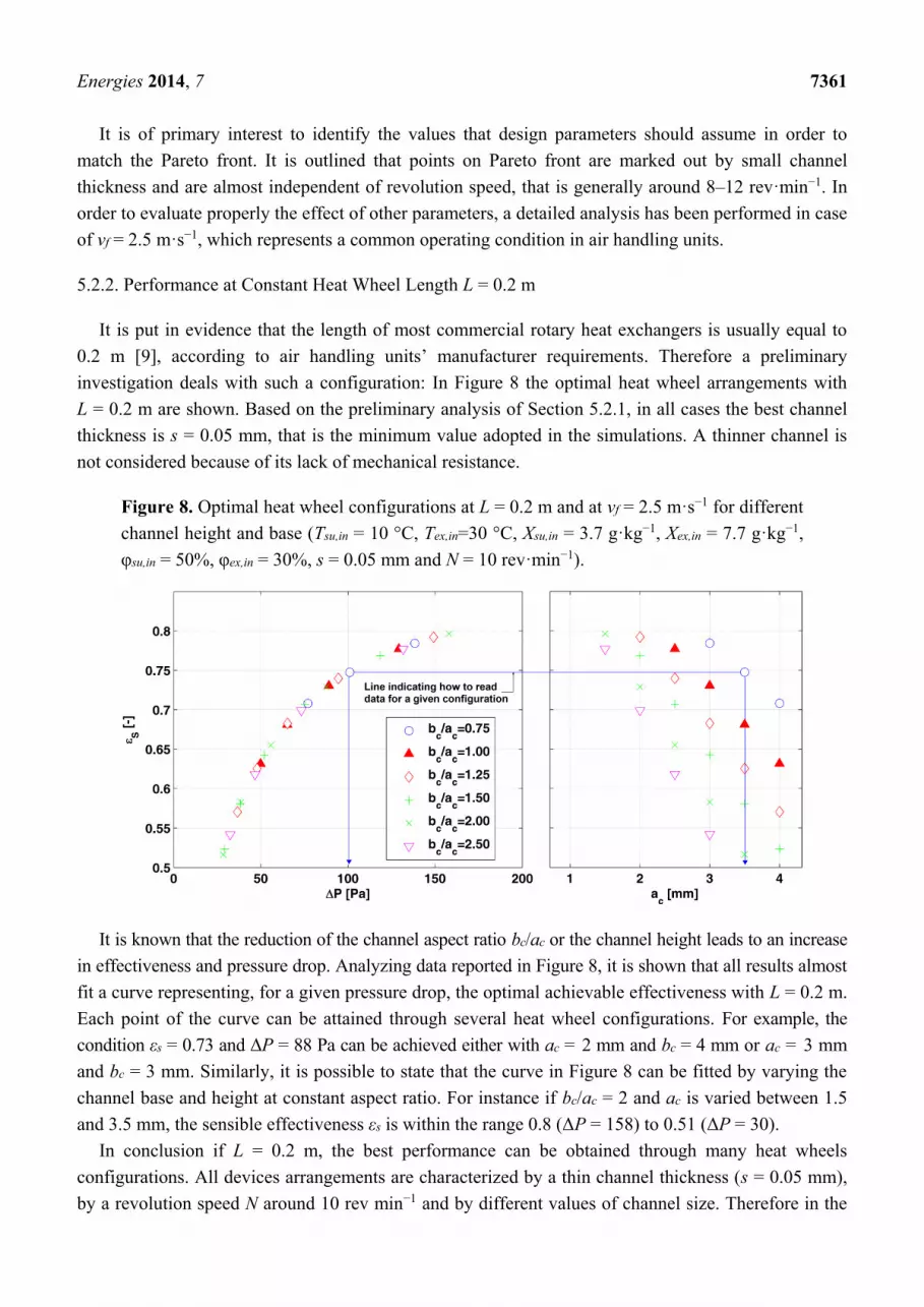
Figure 8. Optimal heat wheel configurations at L = 0.2 m and at vf = 2.5 m·s−1 for different

channel height and base (Tsu,in = 10 °C, Tex,in=30 °C, Xsu,in = 3.7 g·kg−1, Xex,in = 7.7 g·kg−1,

φsu,in = 50%, φex,in = 30%, s = 0.05 mm and N = 10 rev·min−1).

It is known that the reduction of the channel aspect ratio bc/ac or the channel height leads to an increase

in effectiveness and pressure drop. Analyzing data reported in Figure 8, it is shown that all results almost

fit a curve representing, for a given pressure drop, the optimal achievable effectiveness with L = 0.2 m.

Each point of the curve can be attained through several heat wheel configurations. For example, the

condition εs = 0.73 and ΔP = 88 Pa can be achieved either with ac = 2 mm and bc = 4 mm or ac = 3 mm

and bc = 3 mm. Similarly, it is possible to state that the curve in Figure 8 can be fitted by varying the

channel base and height at constant aspect ratio. For instance if bc/ac = 2 and ac is varied between 1.5

and 3.5 mm, the sensible effectiveness εs is within the range 0.8 (ΔP = 158) to 0.51 (ΔP = 30).

In conclusion if L = 0.2 m, the best performance can be obtained through many heat wheels

configurations. All devices arrangements are characterized by a thin channel thickness (s = 0.05 mm),

by a revolution speed N around 10 rev min−1 and by different values of channel size. Therefore in the

Energies 2014, 7 7362

analysis reported in the next section, only the aspect ratio bc/ac = 2 is considered in order to limit the

amount of cases to be analyzed.

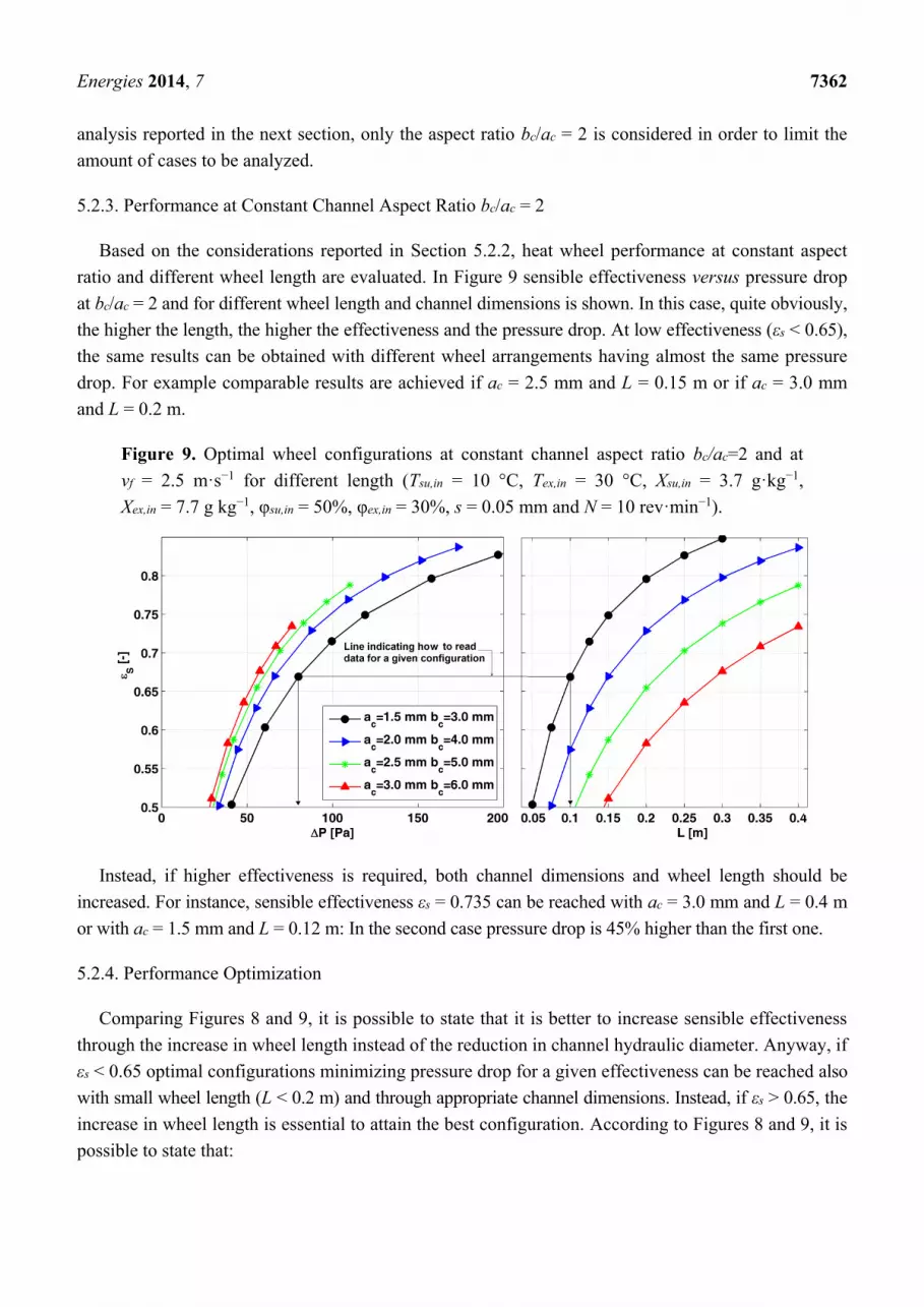
5.2.3. Performance at Constant Channel Aspect Ratio bc/ac = 2

Based on the considerations reported in Section 5.2.2, heat wheel performance at constant aspect

ratio and different wheel length are evaluated. In Figure 9 sensible effectiveness versus pressure drop

at bc/ac = 2 and for different wheel length and channel dimensions is shown. In this case, quite obviously,

the higher the length, the higher the effectiveness and the pressure drop. At low effectiveness (εs < 0.65),

the same results can be obtained with different wheel arrangements having almost the same pressure

drop. For example comparable results are achieved if ac = 2.5 mm and L = 0.15 m or if ac = 3.0 mm

and L = 0.2 m.

Figure 9. Optimal wheel configurations at constant channel aspect ratio bc/ac=2 and at

vf = 2.5 m·s−1 for different length (Tsu,in = 10 °C, Tex,in = 30 °C, Xsu,in = 3.7 g·kg−1,

Xex,in = 7.7 g kg−1, φsu,in = 50%, φex,in = 30%, s = 0.05 mm and N = 10 rev·min−1).

Instead, if higher effectiveness is required, both channel dimensions and wheel length should be

increased. For instance, sensible effectiveness εs = 0.735 can be reached with ac = 3.0 mm and L = 0.4 m

or with ac = 1.5 mm and L = 0.12 m: In the second case pressure drop is 45% higher than the first one.

5.2.4. Performance Optimization

Comparing Figures 8 and 9, it is possible to state that it is better to increase sensible effectiveness

through the increase in wheel length instead of the reduction in channel hydraulic diameter. Anyway, if

εs < 0.65 optimal configurations minimizing pressure drop for a given effectiveness can be reached also

with small wheel length (L < 0.2 m) and through appropriate channel dimensions. Instead, if εs > 0.65, the

increase in wheel length is essential to attain the best configuration. According to Figures 8 and 9, it is

possible to state that:

Energies 2014, 7 7363

- When L = 0.2, the heat wheel is almost optimized if bc > 3.8–4.0 mm and bc/ac > 1. In other

arrangements, for a given effectiveness, pressure drop is higher than the value attained with the

best configuration.

- If there are no restrictions on wheel length, a large hydraulic diameter should be selected

(for example with bc = 6.0 mm and bc/ac = 2) and the increase in effectiveness should be

obtained through the increase in wheel length. When wheel length cannot be further increased

(for example L = 0.4), the increase in effectiveness should be achieved through a reduction in bc

and bc/ac. In this way pressure drop is minimized for a given sensible effectiveness.

Note that a similar analysis has been performed also with vf = 1.5 m·s−1 and vf = 3.5 m·s−1,

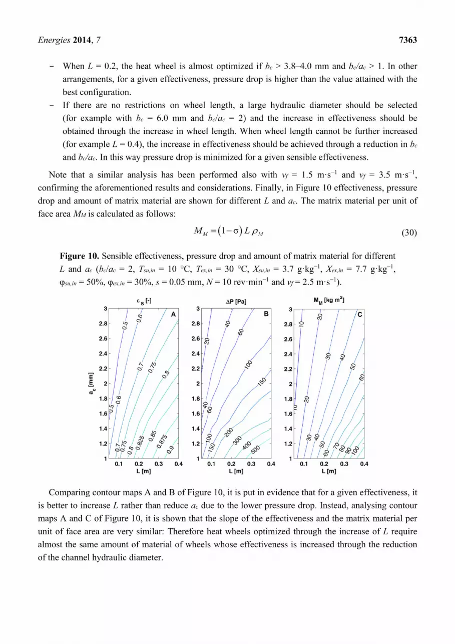
confirming the aforementioned results and considerations. Finally, in Figure 10 effectiveness, pressure

drop and amount of matrix material are shown for different L and ac. The matrix material per unit of

face area MM is calculated as follows:

1 σM MM L (30)

Figure 10. Sensible effectiveness, pressure drop and amount of matrix material for different

L and ac (bc/ac = 2, Tsu,in = 10 °C, Tex,in = 30 °C, Xsu,in = 3.7 g·kg−1, Xex,in = 7.7 g·kg−1,

φsu,in = 50%, φex,in = 30%, s = 0.05 mm, N = 10 rev·min−1 and vf = 2.5 m·s−1).

Comparing contour maps A and B of Figure 10, it is put in evidence that for a given effectiveness, it

is better to increase L rather than reduce ac due to the lower pressure drop. Instead, analysing contour

maps A and C of Figure 10, it is shown that the slope of the effectiveness and the matrix material per

unit of face area are very similar: Therefore heat wheels optimized through the increase of L require

almost the same amount of material of wheels whose effectiveness is increased through the reduction

of the channel hydraulic diameter.

Figure 10. Effectiveness, pressure drop and amount of matrix material for different L and ac

(bc/ac=2, Tsu,in=10°C, Tex,in=30°C, Xin=7 g kg-1

, s=0.05 mm, N=10 rev min-1

, vf=2.5 m s-1

)

Energies 2014, 7 7364

6. Conclusions

In this paper a detailed optimization of heat wheels design parameters is performed in order to

maximize sensible effectiveness and to minimize pressure drop. The analysis is carried out through a

validated one dimensional lumped parameters heat wheel model and through appropriate correlations

to estimate pressure drop. The device optimization is performed through the variation of main design

parameters and operating conditions: Wheel length, channel base, height and thickness, air face

velocity and revolution speed. As a result of the optimization process, the following considerations

should be underlined:

- The best configurations are characterized by a small channel thickness (for example s = 0.05 mm).

- Revolution speed barely affects wheel performance and, therefore, N should be within

10–15 rev·min−1.

- Heat wheels with large channel hydraulic diameters should be preferred (for example

bc = 5.0–6.0 mm and bc/ac = 1.5–2) and the increase in sensible effectiveness should be reached

through the increase in the wheel length.

- If the wheel length is equal to 0.2 m due to air handling units manufacturer restrictions, the

component is almost optimized if bc > 3.8–4.0 mm and bc/ac > 1.

- Heat wheels optimized through the increase in L do not require more matrix material than

wheels optimized through the reduction of the channel hydraulic diameter.

Acknowledgments

Funding for this work from Italian Cassa Conguaglio Sistema Elettrico under agreement No. 6562 is

acknowledged (project STAR-Sidera Trigenerazione Alto Rendimento).

Author Contributions

All the authors have previous experience on heat wheels that have been shared in order to reach the

results discussed in the paper. In particular Stefano De Antonellis, Manuel Intini and Cesare Maria Joppolo

contributed to the development of the heat wheel model and to the optimization analysis while

Calogero Leone contributed to the technical development of the experimental set-up. All the authors

equally contributed to the preparation and to the critical revision of the paper.

Nomenclature

ac channel height (m)

a'c inner channel height (m)

Ac channel cross section area (m2)

AM matrix layer cross section area (m2)

bc channel base (m)

b'c inner channel base (m)

cp isobaric specific heat (J·kg−1·K−1)

D external wheel diameter (m)

Energies 2014, 7 7365

Dhub wheel hub diameter (m)

Dv diffusivity of water vapour in air (m2·s−1)

Deq hydraulic channel diameter (m)

EXP experiment

f Fanning friction factor (-)

fM matrix mass per unit of length (kg·m−1)

hm mass transfer coefficient (kg·m−2·s−1)

hT heat transfer coefficient (W·m−2·K−1)

k thermal conductivity (W·m−1·K−1)

L wheel length (m)

Le Lewis number (-)

ṁ mass flow of dry air (kg·s−1)

M mass per unit of face area (kg·m−2)

N wheel rotational speed (rev·min−1)

p pressure (Pa)

P channel perimeter (m)

Qs heat transfer rate (W)

Re Reynolds number (-)

s channel thickness (m)

Sh Sherwood number (-)

SIM simulation

t time (s)

T temperature (°C)

u air velocity in the channel (m·s−1)

vf face air velocity (m·s−1)

W water content (kg·kg−1)

X air humidity ratio (kg·kg−1)

xi monitored physical variable (-)

z axial direction (m)

Greek letters

ΔP pressure drop (Pa)

εs sensible effectiveness (-)

λ latent heat of vaporization (kJ·kg−1)

ξC local pressure drop coefficient (-)

ρ density (kg m−3)

σ wheel porosity (-)

φ relative humidity (-)

Subscripts

0 initial condition

a air

da dry air

dew air dew point

Energies 2014, 7 7366

ex exhaust air

in inlet

inst instrumental

M channel material

out outlet

sat saturated vapour

su supply air

tot total

v water vapour

w liquid water

W channel wall

wa wet air

Conflicts of Interest

The authors declare no conflict of interest.

References

1. Mardiana, A.; Riffat, S.B. Review on physical and performance parameters of heat recovery

systems for building applications. Renew. Sustain. Energy Rev. 2013, 28, 174–190.

2. Valancius, R.; Jurelionis, A.; Dorosevas, V. Method for cost-benefit analysis of improved indoor

climate conditions and reduced energy consumption in office buildings. Energies 2013, 6,

4591–4606.

3. Airaksinen, M. Energy use in day care centers and schools. Energies 2011, 4, 998–1009.

4. Tommerup, H.; Svendsen, S. Energy savings in Danish residential building stock. Energy Build.

2006, 38, 618–626.

5. Rasouli, M.; Simonson, C.J.; Besant, R.W. Applicability and optimum control strategy of energy

recovery ventilators in different climatic conditions. Energy Build. 2010, 42, 1376–1385.

6. Leone, C.; Liberati, P. Designing the comfort and the energy savings through the heat recovery

use. In Proceedings of the AICARR National Conference 2014, Padua, Italy, 5 June 2014.

7. Dall’O’, G.; Belli, V.; Brolis, M.; Mozzi, I. Fasano, M. Nearly Zero-Energy Buildings of the

Lombardy Region (Italy), a Case Study of High-Energy Performance Buildings. Energies 2013, 6,

3506–3527.

8. Airaksinen, M.; Matilainen, P. A Carbon Footprint of an Office Building. Energies 2011, 4,

1197–1210.

9. Eurovent Certified Performance. Available online: http://www.eurovent-certification.com

(accessed on 1 September 2014).

10. Nóbrega, C.E.L.; Brum, N.C.L. Modeling and simulation of heat and enthalpy recovery wheels.

Energy 2009, 34, 2063–2068.

11. Wu, Z.; Melnik, R.V.; Borup, F. Model-based analysis and simulation of regenerative heat wheel.

Energy Build. 2006, 38, 502–514.

Energies 2014, 7 7367

12. Simonson, C.J.; Besant, R.W. Energy wheel effectiveness: Part I-development of dimensionless

groups. Int. J. Heat Mass Transf. 1999, 42, 2161–2170.

13. Zhang, L.Z.; Niu, J.L. Performance comparisons of desiccant wheels for air dehumidification and

enthalpy recovery. Appl. Therm. Eng. 2002, 22, 1347–1367.

14. Simonson, C.J.; Besant, R.W. Energy wheel effectiveness: Part II–correlations. Int. J. Heat

Mass Transf. 1999, 42, 2171–2185.

15. Sphaier, L.A.; Worek, W.M. Parametric analysis of heat and mass transfer regenerators using a

generalized effectiveness-NTU method. Int. J. Heat Mass Transf. 1999, 52, 2265–2272.

16. De Antonellis, S.; Intini, M.; Joppolo, C.M.; Pedranzini, F. Experimental analysis and practical

effectiveness correlations of enthalpy wheels. Energy Build. 2014, 84, 316–323.

17. Jeong, J.W.; Mumma, S.A. Practical thermal performance correlations for molecular sieve and

silica gel loaded enthalpy wheels. Appl. Therm. Eng. 2005, 25, 719–740.

18. Rabah, A.A.; Fekete, A.; Kabelac, S. Experimental Investigation on a Rotary Regenerator

Operating at Low Temperatures. J. Therm. Sci. Eng. Appl. 2009, 1, 041004:1–041004:9.

19. Tu, R.; Liu, X.H.; Jiang, Y. Performance comparison between enthalpy recovery wheels and

dehumidification wheels. Int. J. Refrig. 2013, 36, 2308–2322.

20. Enteria, N.; Yoshino, H.; Satake, A.; Mochida, A.; Takaki, R.; Yoshie, R.; Mitamura, T.; Baba, S.

Experimental heat and mass transfer of the separated and coupled rotating desiccant wheel and

heat wheel. Exp. Therm. Fluid Sci. 2010, 34, 603–615.

21. Mioralli, P.C.; Ganzarolli, M.M. Thermal analysis of a rotary regenerator with fixed pressure drop

or fixed pumping power. Appl. Therm. Eng. 2013, 52, 187–197.

22. Swanepoel, D.C.; Kröger, D.G. Rotary regenerator design theory and optimisation. Res. Dev. J.

Afr. Inst. Mech. Eng. 1996, 12, 90–97.

23. Yilmaz, A.; Büyükalaca, O.; Yilmaz, T. Optimum shape and dimensions of ducts for convective

heat transfer in laminar flow at constant wall temperature. Int. J. Heat Mass Transf. 2000, 43,

767–775.

24. Kakac, S.; Shah, R.K.; Aung, W. Handbook of Single Phase Convective Heat Transfer;

John Wiley & Sons: New York, NY, USA, 1987.

25. Niu, J.L.; Zhang, L.Z. Heat transfer and friction coefficient in corrugated ducts confined by

sinusoidal and arc curves. Int. J. Heat Mass Transf. 2002, 45, 571–578.

26. Method of Testing Air-to-Air Heat/Energy Exchangers; ANSI/ASHRARE 84-2008; American

Society of Heating, Refrigerating and Air Conditioning Engineers (ASHRAE): Atlanta, GA,

USA, 2008.

27. Measurement of Fluid Flow by Means of Pressure Differential Devices Inserted in Circular

Cross-Section Conduits Running Full-Part 2: Orifice Plates; DIN EN ISO 5167–2 Standards

(ISO 5167–2:2003); International Organization for Standardization: Geneva, Switzerland, 2003.

28. Moffat, R.J. Describing the uncertainties in experimental results. Exp. Therm. Fluid Sci. 1988, 1,

3–10.

© 2014 by the authors; licensee MDPI, Basel, Switzerland. This article is an open access article

distributed under the terms and conditions of the Creative Commons Attribution license

(http://creativecommons.org/licenses/by/4.0/).