DESIGN AND IMPLEMENTATION OF PARALLEL AND RANDOMIZED APPROXIMATION ALGORITHMS

DESIGN AND IMPLEMENTATION OF

PARALLEL AND RANDOMIZED

APPROXIMATION ALGORITHMS

A Project Report Submitted

in Partial Fulfilment of the Requirements

for the Degree of

BACHELOR OF TECHNOLOGY

in

Mathematics and Computing

by

Ajay Shankar Bidyarthy

(Roll No. 09012305)

to the

DEPARTMENT OF MATHEMATICS

INDIAN INSTITUTE OF TECHNOLOGY GUWAHATI

GUWAHATI - 781039, INDIA

April 2013

CERTIFICATE

This is to certify that the work contained in this project report entitled “Design and im-

plementation of parallel and randomized approximation algorithms” submitted

by Ajay Shankar Bidyarthy (Roll No.: 09012305) to Indian Institute of Technology

Guwahati towards partial requirement of Bachelor of Technology in Mathematics and

Computing has been carried out by him under my supervision and that it has not been

submitted elsewhere for the award of any degree.

Guwahati - 781 039 (Dr. Gautam K. Das)

April 2013 Project Supervisor

ii

ABSTRACT

The multiplicative weights algorithm is a well known technique for solving packing-

covering linear program (LP) and semidefinite programs (SDP) approximately. There

has been considerable recent research building on this technique and developing fast and

approximate solutions to packing-covering linear as well as semi-definite programs [1],

[2], [8], [12], [7].

In this article we have implemented these technique. The performance of our program

outperforms the best known semidefinite programming solvers in the literature. Our al-

gorithms run much faster for moderately small approximation factors and large instances

(5000× 5000 dense real matrices), compared to SeDuMi [11] (a well-known LP and SDP

solver) and GLPK.

These algorithms are a building-block for solving large-scale combinatorial optimiza-

tion problems approximately, for example Lovasz ϑ, control and system theory, sparsest

cut etc. Our algorithms have been implemented in MATLAB and have been tested on

multiple modern 2-core machines.

We also compare our results with the matrix multiplicative weights algorithm for com-

puting approximate solutions to packing-covering semidefinite programs [7], and present

results on problems in SDPLIB [4].

Keywords: convex optimization, approximation algorithm, packing-covering semidef-

inite programs, positive semidefinite programming, multiplicative weights, online algo-

rithm, experimental analysis.

iii

Contents

List of Figures vii

List of Tables viii

1 Fast Algorithms for Approximate Packing Semidefinite Programs using

the Multiplicative - Weights Update Techniques 1

1.1 Introduction . . . . . . . . . . . . . . . . . . . . . . . . . . . . . . . . . . 1

1.2 Primal only approach for approximately solving SDPs . . . . . . . . . . . 2

1.2.1 Overview of algorithm . . . . . . . . . . . . . . . . . . . . . . . . 3

1.3 Algorithm . . . . . . . . . . . . . . . . . . . . . . . . . . . . . . . . . . . 4

1.3.1 ORACLE implementation . . . . . . . . . . . . . . . . . . . . . . 6

1.4 Correctness . . . . . . . . . . . . . . . . . . . . . . . . . . . . . . . . . . 8

1.4.1 Techniques for correctness . . . . . . . . . . . . . . . . . . . . . . 10

1.4.2 Example . . . . . . . . . . . . . . . . . . . . . . . . . . . . . . . . 11

1.5 Converting a feasibility engine into an optimizer . . . . . . . . . . . . . . 12

1.6 Experimental results . . . . . . . . . . . . . . . . . . . . . . . . . . . . . 13

1.6.1 AHK versus SeDuMi . . . . . . . . . . . . . . . . . . . . . . . . . 13

1.7 Conclusions . . . . . . . . . . . . . . . . . . . . . . . . . . . . . . . . . . 15

2 Solving Optimization problems using AHK optimizer 16

2.1 Introduction . . . . . . . . . . . . . . . . . . . . . . . . . . . . . . . . . . 16

iv

2.2 Techniques to solve relaxed SDPs . . . . . . . . . . . . . . . . . . . . . . 17

2.3 Experimental results . . . . . . . . . . . . . . . . . . . . . . . . . . . . . 18

2.4 Conclusions and future work . . . . . . . . . . . . . . . . . . . . . . . . . 20

3 The Multiplicative - Weights Update Techniques: Survey 21

3.1 Introduction . . . . . . . . . . . . . . . . . . . . . . . . . . . . . . . . . . 21

3.2 The Weighted Majority Algorithm . . . . . . . . . . . . . . . . . . . . . . 22

3.3 The Multiplicative - Weights Update Techniques . . . . . . . . . . . . . . 23

3.4 Conclusions . . . . . . . . . . . . . . . . . . . . . . . . . . . . . . . . . . 26

3.5 Remarks . . . . . . . . . . . . . . . . . . . . . . . . . . . . . . . . . . . . 26

4 Data Streaming and Online Algorithm: Matrix Multiplicative - Weights

Update technique 27

4.1 Introduction . . . . . . . . . . . . . . . . . . . . . . . . . . . . . . . . . . 27

4.2 Data Streaming and Online Problems . . . . . . . . . . . . . . . . . . . . 28

4.2.1 2-Player Zero-Sum Game . . . . . . . . . . . . . . . . . . . . . . . 28

4.2.2 Matrix Multiplicative - Weights Update Algorithm . . . . . . . . 30

4.2.3 Data Streaming and Online Algorithm . . . . . . . . . . . . . . . 31

4.3 Experiments and Analysis . . . . . . . . . . . . . . . . . . . . . . . . . . 33

4.3.1 Problem . . . . . . . . . . . . . . . . . . . . . . . . . . . . . . . . 33

4.3.2 Experimental Results . . . . . . . . . . . . . . . . . . . . . . . . . 34

4.3.3 Experimental Analysis . . . . . . . . . . . . . . . . . . . . . . . . 36

4.4 Conclusions . . . . . . . . . . . . . . . . . . . . . . . . . . . . . . . . . . 41

4.5 Remarks . . . . . . . . . . . . . . . . . . . . . . . . . . . . . . . . . . . . 42

5 Fast Algorithms for Approximate Packing-Covering Semidefinite Pro-

grams using the Multiplicative - Weights Update Techniques 43

5.1 Introduction . . . . . . . . . . . . . . . . . . . . . . . . . . . . . . . . . . 43

v

5.2 Algorithm . . . . . . . . . . . . . . . . . . . . . . . . . . . . . . . . . . . 44

5.2.1 Computation of vector y . . . . . . . . . . . . . . . . . . . . . . . 47

5.3 Examples . . . . . . . . . . . . . . . . . . . . . . . . . . . . . . . . . . . 48

5.3.1 Example 1 . . . . . . . . . . . . . . . . . . . . . . . . . . . . . . . 49

5.3.2 Example 2 . . . . . . . . . . . . . . . . . . . . . . . . . . . . . . . 49

5.4 Conclusions . . . . . . . . . . . . . . . . . . . . . . . . . . . . . . . . . . 50

5.5 Remarks . . . . . . . . . . . . . . . . . . . . . . . . . . . . . . . . . . . . 50

Bibliography 51

vi

List of Figures

1.1 CPU Time tradeoff versus n (problem size) of AHK Algorithm . . . . . . 14

1.2 CPU Time tradeoff versus n (problem size) of AHK Algorithm and of

SeDuMi . . . . . . . . . . . . . . . . . . . . . . . . . . . . . . . . . . . . 15

4.1 Total payoff and worst payoff Vs. number of rounds . . . . . . . . . . . 34

4.2 upperbound, random payoff and random payoff Div. total payoff Vs. num-

ber of rounds . . . . . . . . . . . . . . . . . . . . . . . . . . . . . . . . . 35

4.3 Total actual payoff Vs. size of PSD matrices . . . . . . . . . . . . . . . . 37

4.4 Random payoff Vs. size of PSD matrices . . . . . . . . . . . . . . . . . . 37

4.5 Random payoff div. total actual payoff Vs. size of PSD matrices . . . . . 38

4.6 Worst payoff Vs. size of PSD matrices . . . . . . . . . . . . . . . . . . . 38

4.7 Upper bound Vs. size of PSD matrices . . . . . . . . . . . . . . . . . . . 39

4.8 Total actual payoff Vs. ε error accuracy . . . . . . . . . . . . . . . . . . . 39

4.9 Random payoff Vs. ε error accuracy . . . . . . . . . . . . . . . . . . . . . 40

4.10 Random payoff div. total actual payoff Vs. ε error accuracy . . . . . . . 40

4.11 Worst payoff Vs. ε error accuracy . . . . . . . . . . . . . . . . . . . . . . 41

4.12 Upper bound Vs. ε error accuracy . . . . . . . . . . . . . . . . . . . . . . 41

vii

List of Tables

2.1 SDP lower bound for Lovasz ϑ functions . . . . . . . . . . . . . . . . . . 19

2.2 SDP upper bound for Lovasz ϑ functions . . . . . . . . . . . . . . . . . . 19

viii

Chapter 1

Fast Algorithms for Approximate

Packing Semidefinite Programs

using the Multiplicative - Weights

Update Techniques

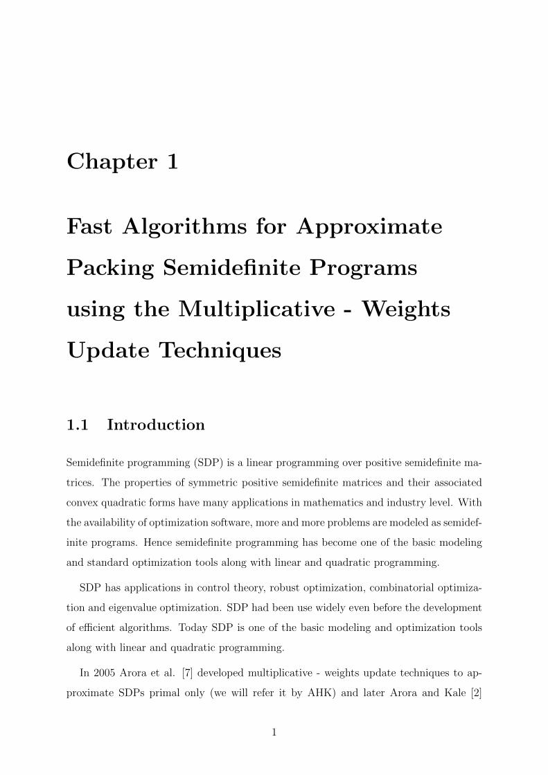
1.1 Introduction

Semidefinite programming (SDP) is a linear programming over positive semidefinite ma-

trices. The properties of symmetric positive semidefinite matrices and their associated

convex quadratic forms have many applications in mathematics and industry level. With

the availability of optimization software, more and more problems are modeled as semidef-

inite programs. Hence semidefinite programming has become one of the basic modeling

and standard optimization tools along with linear and quadratic programming.

SDP has applications in control theory, robust optimization, combinatorial optimiza-

tion and eigenvalue optimization. SDP had been use widely even before the development

of efficient algorithms. Today SDP is one of the basic modeling and optimization tools

along with linear and quadratic programming.

In 2005 Arora et al. [7] developed multiplicative - weights update techniques to ap-

proximate SDPs primal only (we will refer it by AHK) and later Arora and Kale [2]

1

developed same technique to approximate primal-dual SDPs (we will refer it by AK).

A recent paper by Raman et al. [12] developed a fast approximations to solve packing-

covering LPs and constant-sum games via multiplicative-weights technique.

We will strongly follow algorithms proposed by AHK and AK to design multiplicative-

weights update algorithms and we will implement it for computing approximate solutions

to packing-covering semidefinite programs. From now on we refer multiplicative weights

update method algorithms framework as the MW framework.

1.2 Primal only approach for approximately solving

SDPs

Semidefinite programming (SDP) solves the following problem:

min c •X

subject to Aj •X ≥ bj for j = 1, 2, ...,m

X � 0. (1.1)

Where X ∈ Rn×n is a matrix of variables and A1, A2, ..., Am ∈ Rn×n. For n × n

matrices A and B, A • B is their inner product (A • B =∑

ij AijBij) treating them as

vector in Rn2, and A � 0 is notation for A is positive semidefinite. Our implementation

contributes the modified multiplicative weights technique to handle some of high-width

SDPs and technique used is the multiplicative weights technique. Here we have implicitly

performed a binary search on the optimum and the objective is converted to a constraint

in the standard way (in later section we will give technique to do it). Here one additional

constraint has been assumed, a bound on the trace of the solution (∑

iXii):

Aj •X ≥ bj for j = 1, 2, ...,m.∑i

Xii ≤ R

X � 0. (1.2)

2

Here we have added one additional constraint i.e. the upper bound on trace Tr(x) =∑iXii ≤ R. For SDPs relaxation it is natural to put an upper bounds on trace, Tr(X) =∑iXii. We solve the SDP approximately up to a given tolerance ε, by which we mean

that either we find a solution X which satisfies all the constraints up to an additive error

of ε, i.e.

Aj •X − bj ≥ −ε for j = 1, 2, ...,m,

or conclude correctly that the SDP is infeasible.

1.2.1 Overview of algorithm

The Multiplicative Weights Update idea for solving SDPs is to perform several iterations,

indexed by time t as follows:

According to AHK, associate a non-negative weight w(t)j with constraint j, where

∑j w

(t)j =

1. A high current weight for a constraint indicates that it was not satisfied too well in the

past, and therefore should receive higher priority in the next step. Thus the optimization

problem to the next step is to

max∑j

w(t)j (Aj •X − bj)∑

i

Xii ≤ R

X � 0.

Which represents an eigenvalue problem, since the optimum is attained at an X that

has rank 1. The Lagrangian relaxation idea would be to solve this eigenvalue problem,

and update the weights wi according to the usual multiplicative update rule, for some

constant β:

w(t+1)j = w

(t)j (1− β(AjXt − bj))/St.

Where Xt was the solution to the eigenvalue problem, expressed as a rank 1 PSD

matrix, at a time t, and St is the normalization factor to make the weights sum to 1, can

3

be written as:

St =

(t)∑j

(1− β(Aj •Xt − bj)).

If β is small enough, the average 1T

∑Tt=1 Xt is guaranteed to converge to a near-feasible

solution to the original SDP if we assume a feasible solution exists, assuming a feasible

solution exists.

1.3 Algorithm

Objective is to

min c •X

subject to Aj •X ≥ bj for j = 1, 2, ...,m

X � 0.

Let n be the size of matrices Aj, where j = 1, 2, 3, ...,m, m being the number of

constraints. Let R be the upper bound on the Tr(X), i.e. Tr(x) =∑

iXii ≤ R.

Assuming Aj is symmetric, i.e. Aj = Aᵀj for each j = 1, 2, 3, ...,m. Let N ≥ n be the

number of nonzero entries of Aj for each j = 1, 2, , 3, ...,m.

Algorithm 1 checks the feasibility of given SDP problems. To get the optimal solution

of a given particular SDP problem, we implicitly perform a binary search on the optimum

and the objective is converted to a constraint in the standard way. In the next section we

provide detail on binary search technique on the optimum and we also provide conversion

of objective function to a constraint for AHK algorithm. Since this algorithm uses multi-

plicative weights update techniques and checks the feasibility of given SDP therefore we

call this algorithm as decision making algorithm AHK primal only multiplicative weights

SDP solver.

Let C be the weighted cumulative constraint matrix (as C defined by AHK) and it

is used to calculate the eigenvector, V (largest eigenvector), corresponding to the largest

eigenvalue λ by the lanczos method and adding V ᵀ × V to the current solution XCur.

4

Algorithm 1 returns feasible/infeasible solution PSD matrixX and corresponding num-

ber of satisfiable/unsatisfiable constraints (feasible/infeasible constraints) Aj •X ≥ bj for

j = 1, 2, ...,m.

Theorem 1.3.1. (Theorem 1 [Arora et al. [7]])

Consider the SDP (1.2). Let P = {X � 0,∑

iXii ≤ R}. Assume that for any j, Aj •X−

bj lies in one of the ranges [−l, ρ] or [−ρ, l] where 1 ≤ l ≤ ρ. Then ρ is called the width of

constraint. Also assume that there is an algorithm (ORACLE) which runs in time Toracle,

and given any set of non-negative weights w1, w2, ..., wm on the constraints summing to 1,

either finds an X ∈ P which makes the weighted combination∑m

j=1wJ(Aj •X−bj) ≥ − ε2

or declares correctly that no X ∈ P makes this combination non-negative. Then there is

an algorithm which runs in O( lρε2

(Toracle +m)) time and either gets an ε solution to SDP

(1.2) or concludes that it is infeasible.


With the setup as in previous theorem, there is an algorithm which produces an ε approx-

imate solution to the SDP (1.2) or declares correctly its infeasibility in time

O(m log(ρ)Toracle +m log(ρ)M(m log(ρ)))

where M(m) = O(m2.3) is time needed to multiply two m × m matrices (m is the

number of constraints). The O notation is used to suppress polylog(mnε

).

5

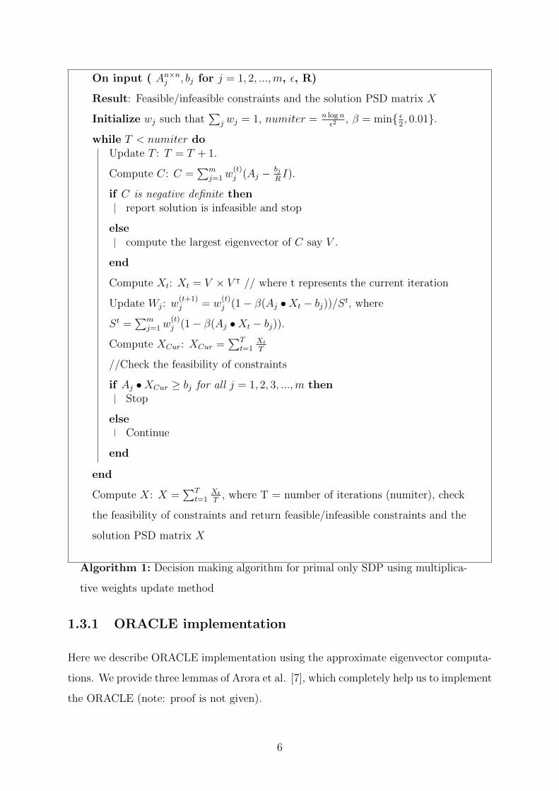
On input ( An×nj , bj for j = 1, 2, ...,m, ε, R)

Result: Feasible/infeasible constraints and the solution PSD matrix X

Initialize wj such that∑

j wj = 1, numiter = n lognε2

, β = min{ ε2, 0.01}.

while T < numiter doUpdate T : T = T + 1.

Compute C: C =∑m

j=1 w(t)j (Aj − bj

RI).

if C is negative definite thenreport solution is infeasible and stop

elsecompute the largest eigenvector of C say V .

end

Compute Xt: Xt = V × V ᵀ // where t represents the current iteration

Update Wj: w(t+1)j = w

(t)j (1− β(Aj •Xt − bj))/St, where

St =∑m

j=1 w(t)j (1− β(Aj •Xt − bj)).

Compute XCur: XCur =∑T

t=1XtT

//Check the feasibility of constraints

if Aj •XCur ≥ bj for all j = 1, 2, 3, ...,m thenStop

elseContinue

end

end

Compute X: X =∑T

t=1XtT

, where T = number of iterations (numiter), check

the feasibility of constraints and return feasible/infeasible constraints and the

solution PSD matrix X

Algorithm 1: Decision making algorithm for primal only SDP using multiplica-

tive weights update method

1.3.1 ORACLE implementation

Here we describe ORACLE implementation using the approximate eigenvector computa-

tions. We provide three lemmas of Arora et al. [7], which completely help us to implement

the ORACLE (note: proof is not given).

6

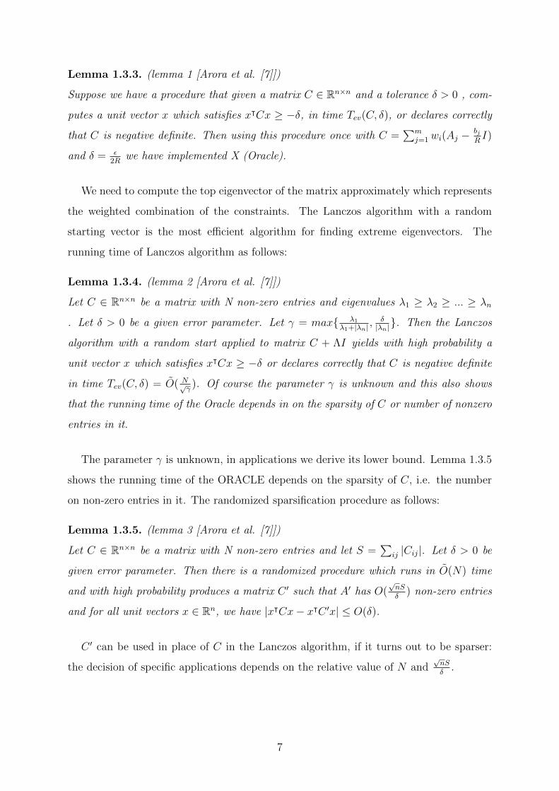
Lemma 1.3.3. (lemma 1 [Arora et al. [7]])

Suppose we have a procedure that given a matrix C ∈ Rn×n and a tolerance δ > 0 , com-

putes a unit vector x which satisfies xᵀCx ≥ −δ, in time Tev(C, δ), or declares correctly

that C is negative definite. Then using this procedure once with C =∑m

j=1 wi(Aj −bjRI)

and δ = ε2R

we have implemented X (Oracle).

We need to compute the top eigenvector of the matrix approximately which represents

the weighted combination of the constraints. The Lanczos algorithm with a random

starting vector is the most efficient algorithm for finding extreme eigenvectors. The

running time of Lanczos algorithm as follows:


Let C ∈ Rn×n be a matrix with N non-zero entries and eigenvalues λ1 ≥ λ2 ≥ ... ≥ λn

. Let δ > 0 be a given error parameter. Let γ = max{ λ1λ1+|λn| ,

δ|λn|}. Then the Lanczos

algorithm with a random start applied to matrix C + ΛI yields with high probability a

unit vector x which satisfies xᵀCx ≥ −δ or declares correctly that C is negative definite

in time Tev(C, δ) = O( N√γ). Of course the parameter γ is unknown and this also shows

that the running time of the Oracle depends in on the sparsity of C or number of nonzero

entries in it.

The parameter γ is unknown, in applications we derive its lower bound. Lemma 1.3.5

shows the running time of the ORACLE depends on the sparsity of C, i.e. the number

on non-zero entries in it. The randomized sparsification procedure as follows:


Let C ∈ Rn×n be a matrix with N non-zero entries and let S =∑

ij |Cij|. Let δ > 0 be

given error parameter. Then there is a randomized procedure which runs in O(N) time

and with high probability produces a matrix C ′ such that A′ has O(√nSδ

) non-zero entries

and for all unit vectors x ∈ Rn, we have |xᵀCx− xᵀC ′x| ≤ O(δ).

C ′ can be used in place of C in the Lanczos algorithm, if it turns out to be sparser:

the decision of specific applications depends on the relative value of N and√nSδ

.

7

1.4 Correctness

We have checked correctness of decision making algorithm AHK primal only multiplicative

weights update SDP solver implemented in matlab. By verifying the solutions with those

obtained from other SDP solvers like Sedumi, SDPA, SDPLR, CSDP etc. All agree for a

given SDP optimization problem with objective min/max and m constraints of size n×n.

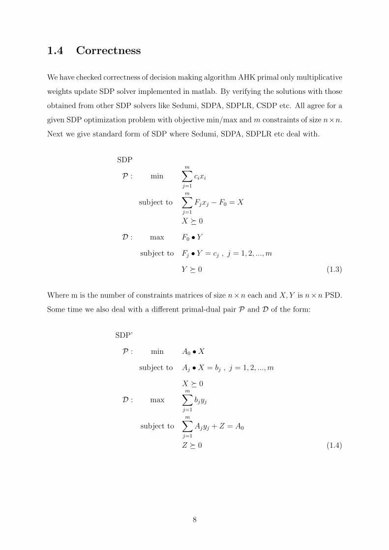
Next we give standard form of SDP where Sedumi, SDPA, SDPLR etc deal with.

SDP

P : minm∑j=1

cixi

subject tom∑j=1

Fjxj − F0 = X

X � 0

D : max F0 • Y

subject to Fj • Y = cj , j = 1, 2, ...,m

Y � 0 (1.3)

Where m is the number of constraints matrices of size n×n each and X, Y is n×n PSD.

Some time we also deal with a different primal-dual pair P and D of the form:

SDP’

P : min A0 •X

subject to Aj •X = bj , j = 1, 2, ...,m

X � 0

D : maxm∑j=1

bjyj

subject tom∑j=1

Ajyj + Z = A0

Z � 0 (1.4)

8

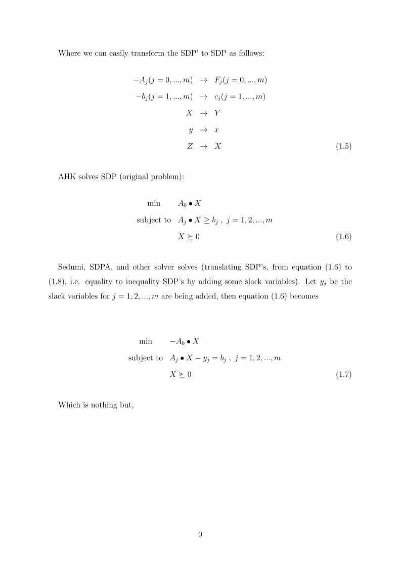
Where we can easily transform the SDP’ to SDP as follows:

−Aj(j = 0, ...,m) → Fj(j = 0, ...,m)

−bj(j = 1, ...,m) → cj(j = 1, ...,m)

X → Y

y → x

Z → X (1.5)

AHK solves SDP (original problem):

min A0 •X

subject to Aj •X ≥ bj , j = 1, 2, ...,m

X � 0 (1.6)

Sedumi, SDPA, and other solver solves (translating SDP’s, from equation (1.6) to

(1.8), i.e. equality to inequality SDP’s by adding some slack variables). Let yj be the

slack variables for j = 1, 2, ...,m are being added, then equation (1.6) becomes

min −A0 •X

subject to Aj •X − yj = bj , j = 1, 2, ...,m

X � 0 (1.7)

Which is nothing but,

9

max A0 •X

subject to Aj •X − yj ≤ bj , j = 1, 2, ...,m

X � 0

OR

min −A0 •X

subject to −Aj •X + yj ≥ −bj , j = 1, 2, ...,m

X � 0 (1.8)

Note that we are keeping equation (1.8) in equality SDP’s, since it is being solved by

Sedumi, SDPA etc solver which solves equality SDP’s only. After transformation the new

constraint matrices and objective Aj look like (let it is represented by Mj)

Mj =

Aj 0n×m

0m×n yj

, for j = 0, 1, 2, ...,m

and the new solution PSD X will look like (let it is represented by Y)

Y =

Xn×n 0n×m

0m×n yj

� 0, for j = 1, 2, ...,m

and thus Y � 0, Y is (n+m)× (n+m) PSD. Y PSD ensures y1, y2, ..., ym are all positive

and X is PSD. This is because det(Y −λI) = (λ−y1)(λ−y2)...(λ−ym).det(X−λI) = 0.

All roots non-negative imply y1 ≥ 0, y2 ≥ 0, ..., ym ≥ 0 and all roots of det(X − λI) ≥ 0,

as X is PSD.

1.4.1 Techniques for correctness

The following steps represents the technique to check correctness of the decision making

algorithm AHK SDP solver:

1. Solve SDP optimization problem using decision making algorithm AHK SDP solver

and check how many constraints are satisfiable (feasible). (say K)

10

2. Solve SDP optimization problem using SDPA, SeDuMi and others with exactly K

constraint and an A0 objective. Find Optimal value (say α?).

3. Now give SDP optimization problem return back to the decision making algorithm

AHK SDP solver with exactly K constraints plus add an extra constraint A0 to

AHK SDP solver (i.e. A0 •X ≥ α?).

Thus now we have: K constraints + A0 • X ≥ α? ± δ, for small δ > 0. Thus the

decision making algorithm AHK should give

A0 •X ≥ α? − δ : feasible (satisfiable) and

A0 •X ≥ α? + δ : infeasible (not satisfiable). (1.9)

Feasible A0 •X ≥ α? − δ and infeasible A0 •X ≥ α? + δ guarantee that the decision

making algorithm AHK SDP solver returns ε-optimal and δ-feasible optimum value of

optimization problems.

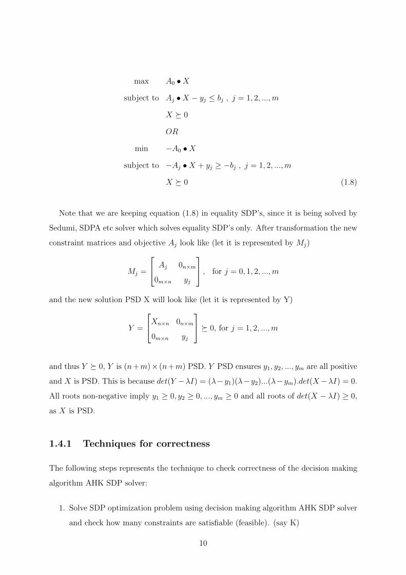
1.4.2 Example

Input for decision making algorithm AHK:

n = 2,m = 3, A0 =

−11 0

0 23

, A1 =

10 4

4 0

, A2 =

0 0

0 −8

, A3 =

0 −8

−8 −2

,

b =

−48

−8

−20

.

Decision making algorithm AHK output: K = 3 (all three constraints satisfiable (feasi-

ble)). Give this SDP optimization problem to SDPA, Sedumi and other solvers. SDPA,

SeDuMi, etc. Output is:

objValPrimal = +2.3000000262935881e+ 01

objValDual = +2.2999999846605416e+ 01

Now give SDP optimization problem back to the decision making algorithm AHK SDP

solver with 4 constraints, AHK. Outputs: For n = 2,m = 3+1 = K+1, ε = 0.01, R ≥ 11,

11

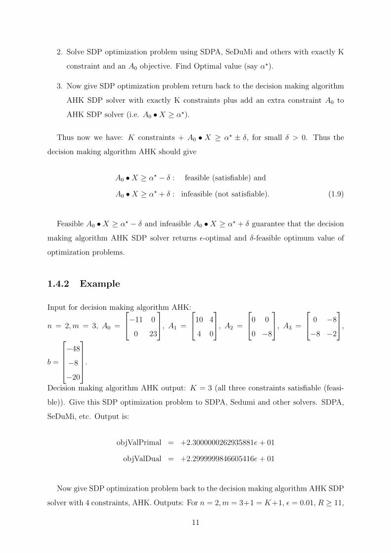
(since Tr(X) ≤ R, δ = 0.01 and α? = 23.0, we get

A0 •X ≥ α? + δ : infeasible (not satisfiable)

A0 •X ≥ α? − δ : feasible (satisfiable).

1.5 Converting a feasibility engine into an optimizer

In this section we explain technique to convert a feasibility engine into an optimizer.

Let lb be the expected lower bound of minima and ub be the expected upper bound of

minima. Here constraints + objective we mean that Aj • X ≥ bj for j = 0, 1, 2, ...,m

i.e. AHK decision making SDP solver handle with m + 1 constraints (objective A0 also

included in constraints). In order to get optima of a given problem we formulate the

objective function into (m+ 1)th constraint as: A0 •X ≥ lb or A0 •X ≥ ub.

In the next algorithm 2 in each step we move from lb towards ub and from ub towards

lb. If ub− lb < ε then we get optima-ε approximation and return lb as optimum of a given

optimization problem. Here we are calling Algorithm 1 by a function call AHKFeasibil-

ity(constraint + objective (A0), α?) whose input arguments are constraints Aj •X ≥ bj

and objective in terms of constant i.e. A0 • X ≥ α?, where α? = ub+lb2

. We have given

binary search technique to minimize a given optimization problem using decision making

AHK SDP solver.

12

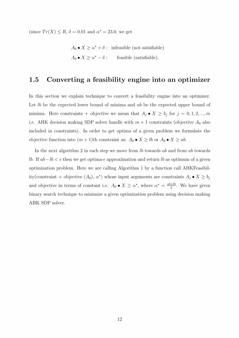
AHKOptimizer(Aj for j = 0, 1, 2, ...,m, lb, ub)

α? = ub+lb2

AHKFeasibility(Aj for j = 0, 1, 2, ...,m, α?)

if Aj •X ≥ bj for all j = 0, 1, 2, ...,m, where X we get from algorithm 1

thenub = α?


elselb = α?


end

if ub− lb ≤ ε thenreturn lb as optima-ε approximation and stop

elsecontinue

end

Algorithm 2: Converting a feasibility engine (decision making AHK SDP

solver) into an optimizer.

1.6 Experimental results

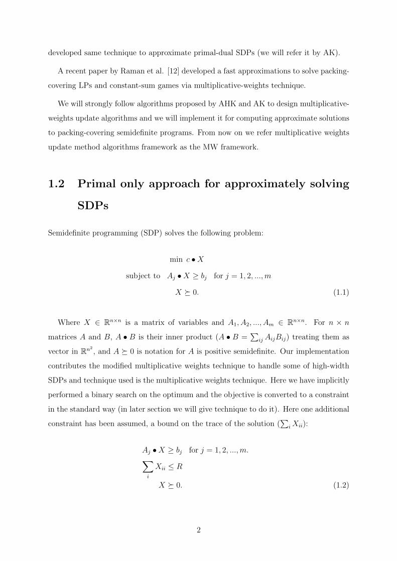
Figure 4.3 represents the CPU time tradeoff versus n (problem size i.e. the size of the

constraint matrices) of the AHK algorithm. For a given constraints m, an objective and

its size n, CPU time is the time required to get a minimum optimum value of objective

function of a given SDP.

1.6.1 AHK versus SeDuMi

We have performed experimental analysis to compare the performance of our implemen-

tation versus SeDuMi in MATLAB. SeDuMi (Self-Dual-Minimization) is an add-on for

Matlab, which let us solve optimization problems with linear, quadratic and semidefi-

niteness constraints. It implements the self- dual embedding technique for optimization

over self-dual homogeneous cones. The self-dual embedding technique essentially makes

it possible to solve certain optimization problems in a single phase, leading either to an

13

100 200 300 400 500 600 700 800 9000

20

40

60

80

100

120

140

160

180

200

n: Problem Size−−−−−−−−−−−>

CP

U T

ime (

seco

nd

s)−

−−

−−

−−

−>

Time Vs Problem size with ε = 0.01 (m = number of constraints)

m = 100

m = 200

m = 300

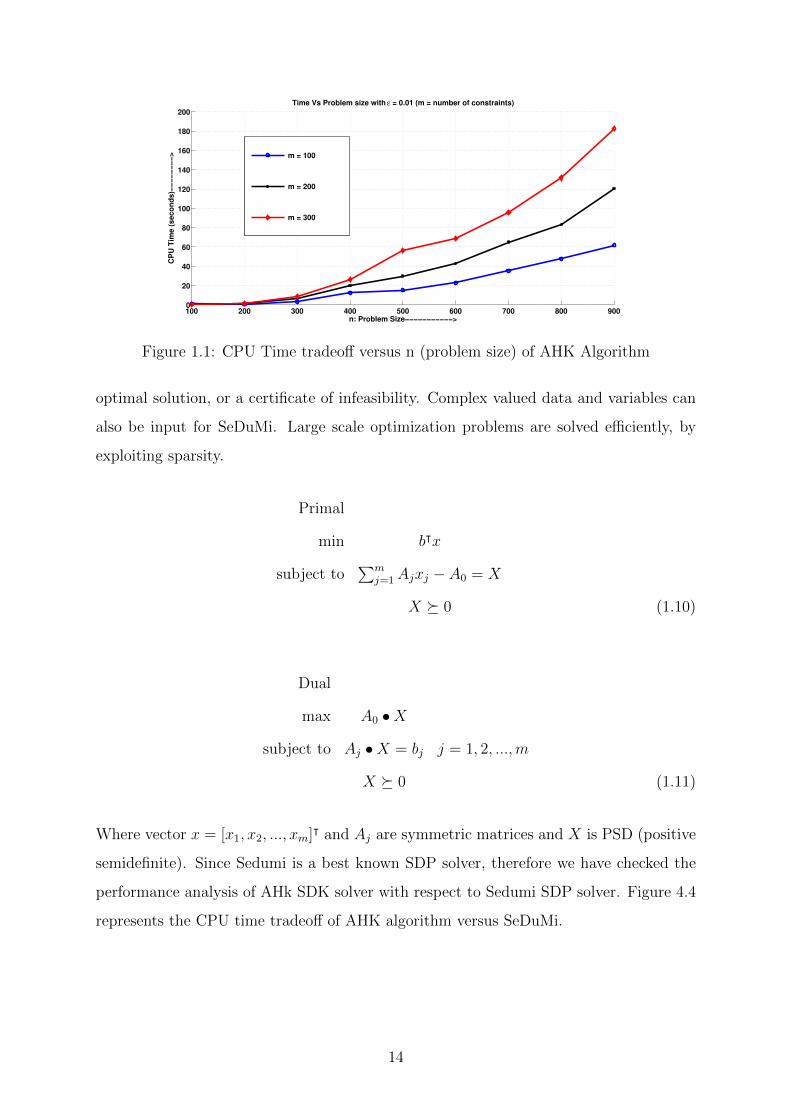
Figure 1.1: CPU Time tradeoff versus n (problem size) of AHK Algorithm

optimal solution, or a certificate of infeasibility. Complex valued data and variables can

also be input for SeDuMi. Large scale optimization problems are solved efficiently, by

exploiting sparsity.

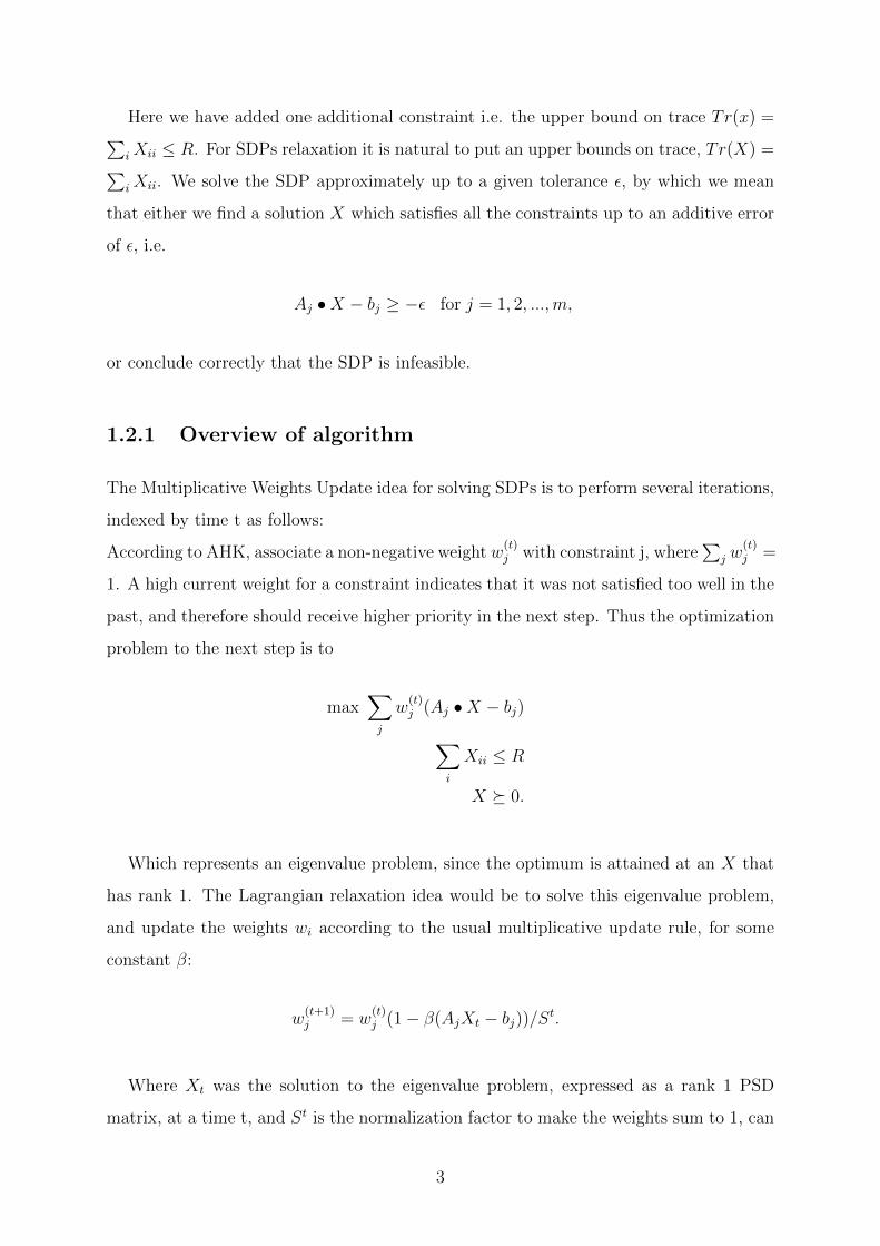
Primal

min bᵀx

subject to∑m

j=1Ajxj − A0 = X

X � 0 (1.10)

Dual

max A0 •X

subject to Aj •X = bj j = 1, 2, ...,m

X � 0 (1.11)

Where vector x = [x1, x2, ..., xm]ᵀ and Aj are symmetric matrices and X is PSD (positive

semidefinite). Since Sedumi is a best known SDP solver, therefore we have checked the

performance analysis of AHk SDK solver with respect to Sedumi SDP solver. Figure 4.4

represents the CPU time tradeoff of AHK algorithm versus SeDuMi.

14

100 200 300 400 500 600 700 800 9000

100

200

300

400

500

600

700

800

900

1000

n: Problem size−−−−−−−−>

CP

U T

ime (

seco

nd

s)−

−−

−−

−−

−−

−−

>

CPU Time Tradeoff of AHK Algorithm versus SeDuMi with ε = 0.1 (Gaps)

m = 100 "AHK"

m = 200 "AHK"

m = 300 "AHK"

m = 100 "SeDuMi"

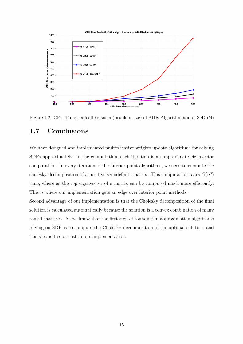
Figure 1.2: CPU Time tradeoff versus n (problem size) of AHK Algorithm and of SeDuMi

1.7 Conclusions

We have designed and implemented multiplicative-weights update algorithms for solving

SDPs approximately. In the computation, each iteration is an approximate eigenvector

computation. In every iteration of the interior point algorithms, we need to compute the

cholesky decomposition of a positive semidefinite matrix. This computation takes O(n3)

time, where as the top eigenvector of a matrix can be computed much more efficiently.

This is where our implementation gets an edge over interior point methods.

Second advantage of our implementation is that the Cholesky decomposition of the final

solution is calculated automatically because the solution is a convex combination of many

rank 1 matrices. As we know that the first step of rounding in approximation algorithms

relying on SDP is to compute the Cholesky decomposition of the optimal solution, and

this step is free of cost in our implementation.

15

Chapter 2

Solving Optimization problems using

AHK optimizer

2.1 Introduction

In the previous chapter we have given an algorithm to check the feasibility of a given

SDP problems. We call it feasibility engine or decision making algorithm. Since it only

decides whether a given SDP problem is feasible or not. Later we gave technique how to

convert this decision making algorithm or feasibility engine to an optimizer.

In this chapter we use this technique to solve some of the SDP problems listed in

SDPLib [4]. In this SDP library several SDP problems are well designed. This library

has equality constraints SDPs. But our optimizer solves inequality constraints SDPs.

To resolve this issue we relax these equality constraints SDPs to inequality constraints

SDPs. Due to relaxation we get relaxed optimal (lower and upper bound of minima),

since inequality constraints will have more freedom to search the optimum solution in

compare to equality constraints (since the feasible region will increase). We solved some

selected SDPs listed in SDPLib. Next we give technique to relax these problems and

finally we give our experimental results.

16

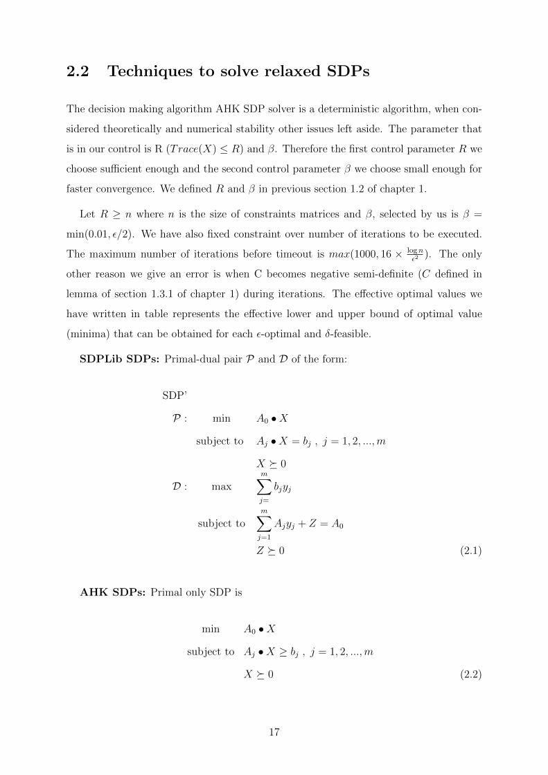
2.2 Techniques to solve relaxed SDPs

The decision making algorithm AHK SDP solver is a deterministic algorithm, when con-

sidered theoretically and numerical stability other issues left aside. The parameter that

is in our control is R (Trace(X) ≤ R) and β. Therefore the first control parameter R we

choose sufficient enough and the second control parameter β we choose small enough for

faster convergence. We defined R and β in previous section 1.2 of chapter 1.

Let R ≥ n where n is the size of constraints matrices and β, selected by us is β =

min(0.01, ε/2). We have also fixed constraint over number of iterations to be executed.

The maximum number of iterations before timeout is max(1000, 16 × lognε2

). The only

other reason we give an error is when C becomes negative semi-definite (C defined in

lemma of section 1.3.1 of chapter 1) during iterations. The effective optimal values we

have written in table represents the effective lower and upper bound of optimal value

(minima) that can be obtained for each ε-optimal and δ-feasible.

SDPLib SDPs: Primal-dual pair P and D of the form:

SDP’

P : min A0 •X

subject to Aj •X = bj , j = 1, 2, ...,m

X � 0

D : maxm∑j=

bjyj

subject tom∑j=1

Ajyj + Z = A0

Z � 0 (2.1)

AHK SDPs: Primal only SDP is

min A0 •X

subject to Aj •X ≥ bj , j = 1, 2, ...,m

X � 0 (2.2)

17

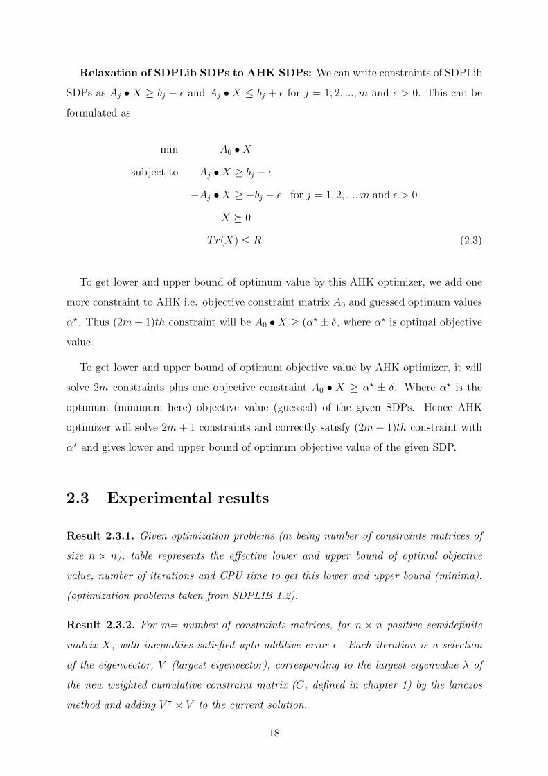
Relaxation of SDPLib SDPs to AHK SDPs: We can write constraints of SDPLib

SDPs as Aj •X ≥ bj − ε and Aj •X ≤ bj + ε for j = 1, 2, ...,m and ε > 0. This can be

formulated as

min A0 •X

subject to Aj •X ≥ bj − ε

−Aj •X ≥ −bj − ε for j = 1, 2, ...,m and ε > 0

X � 0

Tr(X) ≤ R. (2.3)

To get lower and upper bound of optimum value by this AHK optimizer, we add one

more constraint to AHK i.e. objective constraint matrix A0 and guessed optimum values

α?. Thus (2m+ 1)th constraint will be A0 •X ≥ (α? ± δ, where α? is optimal objective

value.

To get lower and upper bound of optimum objective value by AHK optimizer, it will

solve 2m constraints plus one objective constraint A0 • X ≥ α? ± δ. Where α? is the

optimum (minimum here) objective value (guessed) of the given SDPs. Hence AHK

optimizer will solve 2m + 1 constraints and correctly satisfy (2m + 1)th constraint with

α? and gives lower and upper bound of optimum objective value of the given SDP.

2.3 Experimental results

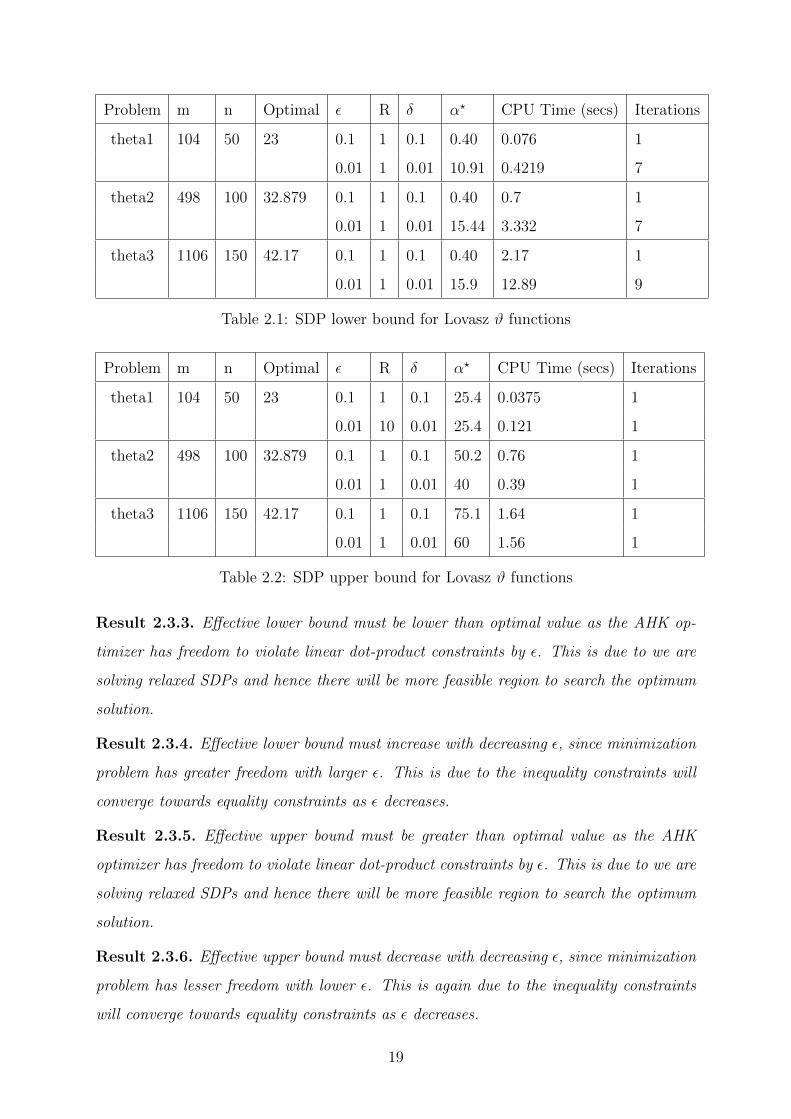
Result 2.3.1. Given optimization problems (m being number of constraints matrices of

size n × n), table represents the effective lower and upper bound of optimal objective

value, number of iterations and CPU time to get this lower and upper bound (minima).

(optimization problems taken from SDPLIB 1.2).

Result 2.3.2. For m= number of constraints matrices, for n × n positive semidefinite

matrix X, with inequalties satisfied upto additive error ε. Each iteration is a selection

of the eigenvector, V (largest eigenvector), corresponding to the largest eigenvalue λ of

the new weighted cumulative constraint matrix (C, defined in chapter 1) by the lanczos

method and adding V ᵀ × V to the current solution.

18

Problem m n Optimal ε R δ α? CPU Time (secs) Iterations

theta1 104 50 23 0.1 1 0.1 0.40 0.076 1

0.01 1 0.01 10.91 0.4219 7

theta2 498 100 32.879 0.1 1 0.1 0.40 0.7 1

0.01 1 0.01 15.44 3.332 7

theta3 1106 150 42.17 0.1 1 0.1 0.40 2.17 1

0.01 1 0.01 15.9 12.89 9

Table 2.1: SDP lower bound for Lovasz ϑ functions

Problem m n Optimal ε R δ α? CPU Time (secs) Iterations

theta1 104 50 23 0.1 1 0.1 25.4 0.0375 1

0.01 10 0.01 25.4 0.121 1

theta2 498 100 32.879 0.1 1 0.1 50.2 0.76 1

0.01 1 0.01 40 0.39 1

theta3 1106 150 42.17 0.1 1 0.1 75.1 1.64 1

0.01 1 0.01 60 1.56 1

Table 2.2: SDP upper bound for Lovasz ϑ functions

Result 2.3.3. Effective lower bound must be lower than optimal value as the AHK op-

timizer has freedom to violate linear dot-product constraints by ε. This is due to we are

solving relaxed SDPs and hence there will be more feasible region to search the optimum

solution.

Result 2.3.4. Effective lower bound must increase with decreasing ε, since minimization

problem has greater freedom with larger ε. This is due to the inequality constraints will

converge towards equality constraints as ε decreases.

Result 2.3.5. Effective upper bound must be greater than optimal value as the AHK

optimizer has freedom to violate linear dot-product constraints by ε. This is due to we are

solving relaxed SDPs and hence there will be more feasible region to search the optimum

solution.

Result 2.3.6. Effective upper bound must decrease with decreasing ε, since minimization

problem has lesser freedom with lower ε. This is again due to the inequality constraints

will converge towards equality constraints as ε decreases.

19

2.4 Conclusions and future work

In this chapter we have presented our experimental results on solving relaxed SDPs Lo-

vasz ϑ functions and presented how we approach towards the optimum one. Our results

are good in quality and efficient in compare to existing one. Presently our implementation

runs sequentially, which may not be good for considerable large combinatorial optimiza-

tion problems. In future I am willing to implement these multiplicative weights update

algorithms in a distributed setup. This will give us faster results in compare to existing

one. Distributed setup implementation will also have good quality of results as we have

know. There has been considerable recent research building on this work, developing fast

and parallel approximate algorithms to approximate solutions to packing-covering linear

as well as semi-definite programs. This research direction seem to be more interesting

and can have reasonable payoff and hence it can not be ignored.

20

Chapter 3

The Multiplicative - Weights Update

Techniques: Survey

3.1 Introduction

The multiplicative - weights method is a an idea which has been repeatedly discovered

in the field of machine learning, optimization and game theory.

The idea of multiplicative - weights update technique can be understood in the follow-

ing setting. A decision maker has a choice of n decisions, and needs to repeatedly make

a decision and obtain an associated payoff. The decision maker’s goal, in the long run,

is to achieve a total payoff which is comparable to the payoff of that fixed decision that

maximizes the total payoff with the benefit of hindsight. While this best decision may

not be known a priori, it is still possible to achieve this goal by maintaining weights on

the decisions, and choosing the decisions randomly with probability proportional to the

weights. In each successive round, the weights are updated by multiplying them with

factors which depend on the payoff of the associated decision in that round.

Intuitively, this scheme works because it tends to focus higher weight on higher payoff

decisions in the long run.

21

3.2 The Weighted Majority Algorithm

The weighted majority algorithm also known as the prediction from expert advice problem.

Let us assume the process of picking good times to invest in a stock. Assume there is

a single stock of interest. Assume its daily price movement is modeled as a sequence of

binary events: 1 : price goes up

0 : price goes down

(3.1)

Each morning we try to predict whether the price will go up or down that day:if our prediction happens to be wrong then we lose a dollar that day

and if it is correct then we lose nothing

(3.2)

The stock movements can be arbitrary and even adversarial. In order to balance out this

assumption, we assume that while making our predictions we are allowed to watch the

predictions of n ”experts.” These experts could be arbitrarily correlated, and they may

or may not know what they are talking about. The Weighted Majority Algorithm’s goal

is to limit its cumulative losses, that is the bad predictions, to roughly the same as the

best of these experts.

The first and trivial technique is to compute each day’s up and down prediction by

going with the majority opinion among the experts that day. But this technique does

not work, because a majority of experts may be consistently wrong on every single day.

The weighted majority algorithm corrects the trivial algorithm. It maintains a weight-

ing of the experts. Initially all experts have equal weight. As time goes on, some experts

are seen as making better predictions than others, and the weighted majority algorithm

increases their weight proportionately. The weighted majority algorithm’s prediction of

up and down for each day is computed by going with the opinion of the weighted majority

of the experts for that day. Now consider the following algorithm 3, which is called the

weighted majority algorithm.

22

Initialization: Fix an ε ≤ 12. With each expert i, associate the weight

w(1)i := 1.

for t = 1, 2, ..., T : do1. Make the prediction that is the weighted majority of the experts’

predictions based on the weights w(t)1 , ..., w

(t)n . That is, predict ”up” or

”down” depending on which prediction has a higher total weight of

experts advising it (if there is ties break it arbitrarily).

2. For every expert i who predicts wrongly, decrease his weight for

the next round by multiplying it by a factor of (1− ε) :

w(t+1)i = (1− ε)w(t)

i (update rule). (3.3)

end

Algorithm 3: Weighted Majority Algorithm

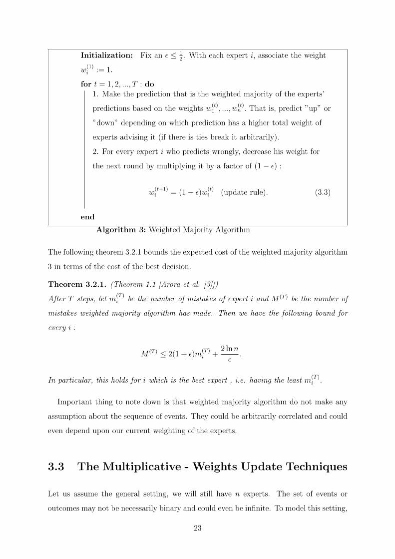
The following theorem 3.2.1 bounds the expected cost of the weighted majority algorithm

3 in terms of the cost of the best decision.

Theorem 3.2.1. (Theorem 1.1 [Arora et al. [3]])

After T steps, let m(T )i be the number of mistakes of expert i and M (T ) be the number of

mistakes weighted majority algorithm has made. Then we have the following bound for

every i :

M (T ) ≤ 2(1 + ε)m(T )i +

2 lnn

ε.

In particular, this holds for i which is the best expert , i.e. having the least m(T )i .

Important thing to note down is that weighted majority algorithm do not make any

assumption about the sequence of events. They could be arbitrarily correlated and could

even depend upon our current weighting of the experts.

3.3 The Multiplicative - Weights Update Techniques

Let us assume the general setting, we will still have n experts. The set of events or

outcomes may not be necessarily binary and could even be infinite. To model this setting,

23

we dispense with the notion of predictions altogether, and instead suppose that in each

round, every expert recommends a course of action, and our task is to pick an expert and

use his advice. Basically we have a set of n decisions and each round, we are required to

select one decision from the set. In each run each decision incurs a certain cost, which

is determined by nature or an adversary. All the costs are revealed after we choose our

decision, and we incur the cost of the decision that we choose.

For example: in the prediction from expert advice problem, each decision corresponds

to a choice of an expert, and the cost of an expert is 1 if the expert makes a mistake, and

0 otherwise.

In order to understand the multiplicative - weights (MW) technique. Consider the

naive strategy. In each iteration, simply picks a decision at random. The expected

penalty will be that of the average decision. Suppose now that a few decisions are clearly

better in the long run. This is easy to spot as the costs are revealed over time, and so

it is sensible to reward them by increasing their probability of being picked in the next

round, hence it is called the multiplicative - weights update technique.

Automatically, being in complete ignorance about the decisions at the outset, we select

them uniformly at random. This maximum entropy starting rule reflects our ignorance.

As we learn which ones are the good decisions and which ones are bad, we lower the

entropy to reflect our increased knowledge. The multiplicative weight update technique

is our means of skewing the distribution.

Let, t = 1, 2, 3, ..., T denote the current round. Let i be a generic decision. In each

round t, we select a distribution p(t) over the set of decisions, and select a decision i

randomly from it. At this point, the costs of all the decisions are revealed by nature in

the form of the vector m(t) such that decision i incurs cost m(t)i . Assume that the costs

lie in the range [−1, 1]. This is the only assumption to make on the costs. Nature is

completely free to choose the cost vector as long as these bounds are respected, even with

full knowledge of the distribution that we choose our decision from.

The expected cost to the algorithm for sampling a decision i from the distribution p(t)

is

Ei∈p(t) [m(t)i ] = m(t) · p(t).

24

The total expected cost over all rounds is therefore:

T∑t=1

m(t) · p(t).

Just as before, we want to achieve a total expected cost not too much more than the cost

of the best decision in hindsight i.e.

mini

T∑t=1

m(t)i .

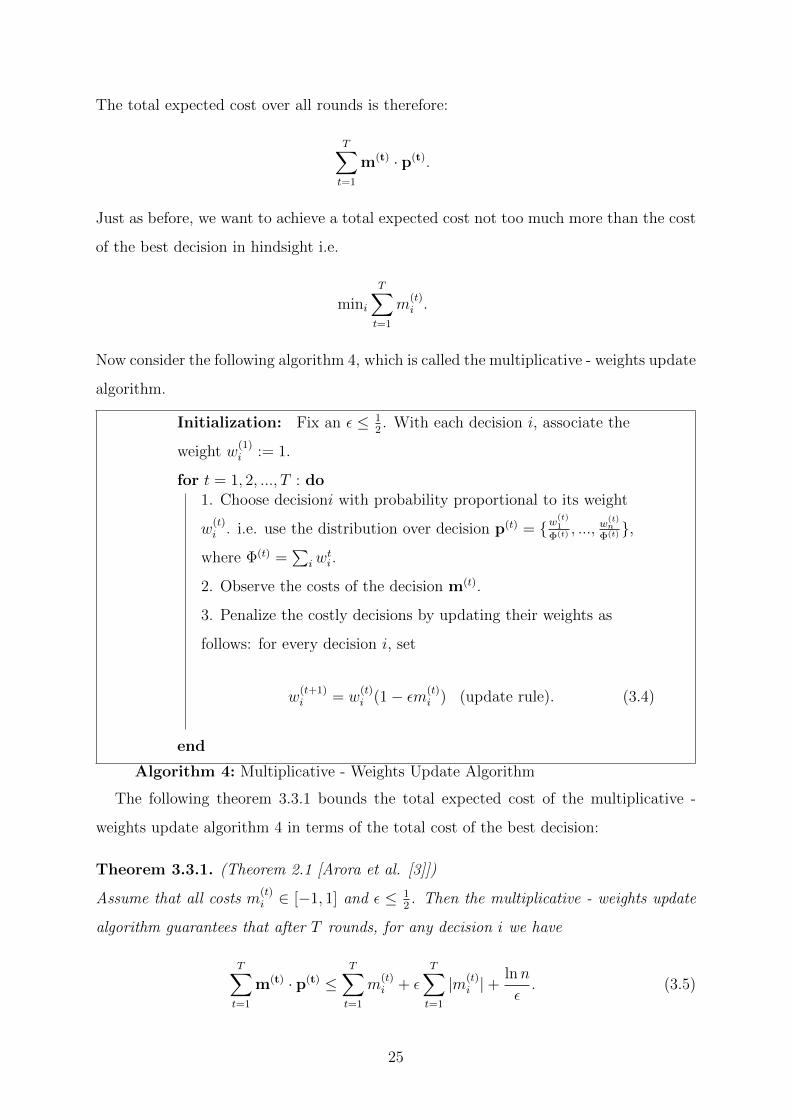
Now consider the following algorithm 4, which is called the multiplicative - weights update

algorithm.

Initialization: Fix an ε ≤ 12. With each decision i, associate the

weight w(1)i := 1.

for t = 1, 2, ..., T : do1. Choose decisioni with probability proportional to its weight

w(t)i . i.e. use the distribution over decision p(t) = {w

(t)1

Φ(t) , ...,w

(t)n

Φ(t)},

where Φ(t) =∑

iwti .

2. Observe the costs of the decision m(t).

3. Penalize the costly decisions by updating their weights as

follows: for every decision i, set

w(t+1)i = w

(t)i (1− εm(t)

i ) (update rule). (3.4)

end

Algorithm 4: Multiplicative - Weights Update Algorithm

The following theorem 3.3.1 bounds the total expected cost of the multiplicative -

weights update algorithm 4 in terms of the total cost of the best decision:

Theorem 3.3.1. (Theorem 2.1 [Arora et al. [3]])

Assume that all costs m(t)i ∈ [−1, 1] and ε ≤ 1

2. Then the multiplicative - weights update

algorithm guarantees that after T rounds, for any decision i we have

T∑t=1

m(t) · p(t) ≤T∑t=1

m(t)i + ε

T∑t=1

|m(t)i |+

lnn

ε. (3.5)

25

3.4 Conclusions

In this chapter we have presented a survey on the multiplicative - weights update tech-

niques, which was proposed in game theory in the early 1950s. First we have presented the

weighted majority algorithm followed by the multiplicative - weights algorithm. These

algorithms mostly used in solving machine learning, data streaming and online problems.

These algorithms tries to increase knowledge about input after every round. Based on

present knowledge about input it updates weights and then tries to construct strategy

such that cost is minimized and profit is maximized.

3.5 Remarks

We have not given proofs of theorem 3.2.1 and 3.3.1 for the weighted majority algorithm

and the multiplicative - weights algorithm. Proofs of these two theorems are available in

Arora et. al [3] paper.

26

Chapter 4

Data Streaming and Online

Algorithm: Matrix Multiplicative -

Weights Update technique

4.1 Introduction

The multiplicative - weights update techniques is being used in areas of combinatorial op-

timization, Game theory and machine learning. For example the multiplicative - weights

update techniques can be used to solve a constrained optimization problems, data stream-

ing online problems, 2-player zero-sum games problem and etc.

Let us consider constrained optimization problem. Let a decision represent each con-

straint in the problem, where costs specified by the points in the domain of interest. For

a given point, the cost of a decision is made proportional to how well the corresponding

constraint is satisfied on the point.

About weights update mechanism, we reduce a decision’s weight depending on its

penalty, and if a constraint is well satisfied on points then we want its weight to be

smaller, so that the algorithm focuses on constraints that are poorly satisfied.

Overall, the choice of points is also under our control (but not for all applications).

We need to generate the maximally adversarial point, i.e. the point that maximizes

the expected cost. In order to apply the multiplicative - weights update technique in

27

constraints optimization problems, we require to go through following two phases:

1. An oracle for generating the maximally adversarial point at each step, and

2. The multiplicative - weights update technique for updating the weights of the de-

cision.

4.2 Data Streaming and Online Problems

Online algorithms represent a theoretical framework for studying problems in interactive

computing. They model, in particular, that the input in an interactive system does not

arrive as a batch but as a sequence on input portions and that the system must react

in response to each incoming portion. They take into account that at any point in time

future input is unknown. Online algorithms consider the algorithmic aspects of interactive

systems. The problem is to design strategies that always compute good output and keep

a given system in good state. One do not make any assumptions about the input streams.

The input can even be generated by an adversary that creates new input portions based

on the system’s reaction to previous one.

In an online decision problem, one has to make a sequence of decisions without knowl-

edge of the future. One version of this problem is the case with n experts corresponding

to decisions. Each period we pick one expert and then observe the cost ∈ [0, 1] for each

expert. Our cost is that of the chosen expert. Our basic goal is to ensure that total

cost is not much larger than the minimum total cost of any expert. This is a version

of the predicting from expert advice problem. The exponential weighting schemes for

this problem have been discovered and rediscovered in many years. Here we use matrix

multiplicative - weights update technique to solve data streaming online problem and

give results based on experimental analysis.

4.2.1 2-Player Zero-Sum Game

The strategic form, or normal from of a two-player zero-sum game is given by a triplet

(X, Y,A), where

28

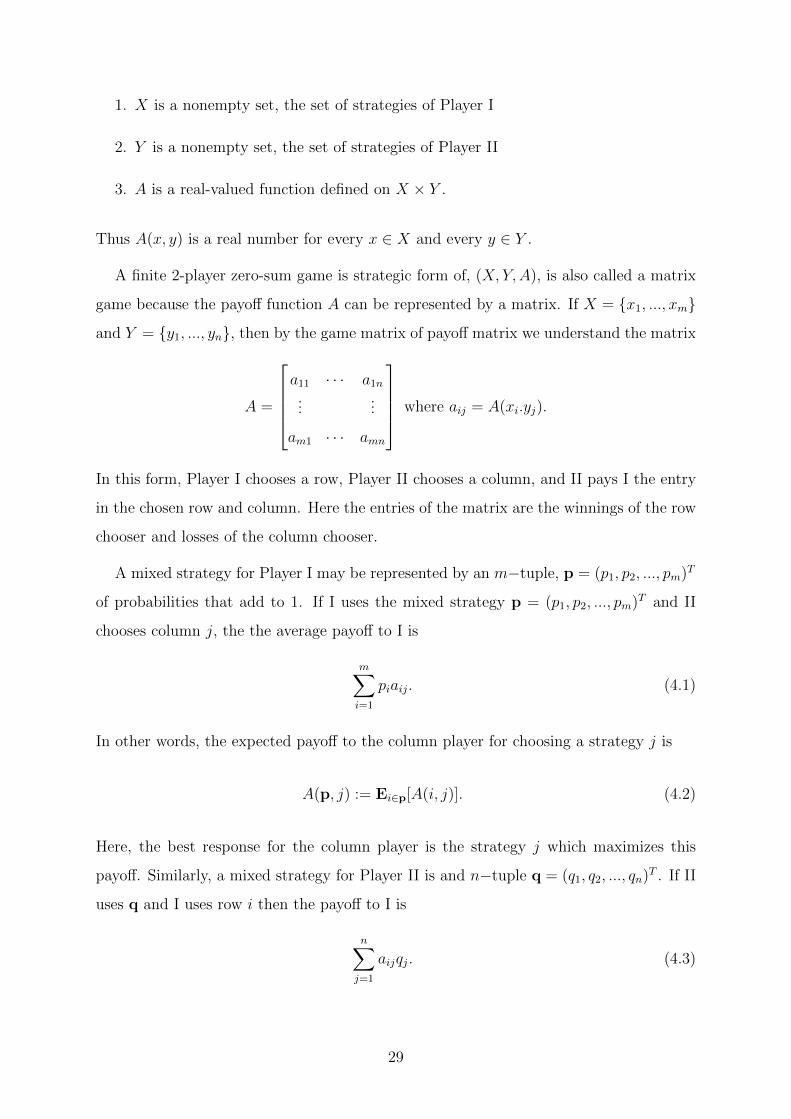
1. X is a nonempty set, the set of strategies of Player I

2. Y is a nonempty set, the set of strategies of Player II

3. A is a real-valued function defined on X × Y .

Thus A(x, y) is a real number for every x ∈ X and every y ∈ Y .

A finite 2-player zero-sum game is strategic form of, (X, Y,A), is also called a matrix

game because the payoff function A can be represented by a matrix. If X = {x1, ..., xm}

and Y = {y1, ..., yn}, then by the game matrix of payoff matrix we understand the matrix

A =

a11 · · · a1n

......

am1 · · · amn

where aij = A(xi.yj).

In this form, Player I chooses a row, Player II chooses a column, and II pays I the entry

in the chosen row and column. Here the entries of the matrix are the winnings of the row

chooser and losses of the column chooser.

A mixed strategy for Player I may be represented by an m−tuple, p = (p1, p2, ..., pm)T

of probabilities that add to 1. If I uses the mixed strategy p = (p1, p2, ..., pm)T and II

chooses column j, the the average payoff to I is

m∑i=1

piaij. (4.1)

In other words, the expected payoff to the column player for choosing a strategy j is

A(p, j) := Ei∈p[A(i, j)]. (4.2)

Here, the best response for the column player is the strategy j which maximizes this

payoff. Similarly, a mixed strategy for Player II is and n−tuple q = (q1, q2, ..., qn)T . If II

uses q and I uses row i then the payoff to I is

n∑j=1

aijqj. (4.3)

29

In other words, the expected payoff column player gets if the row player chooses the

strategy i is

A(i,q) := Ej∈q[A(i, j)]. (4.4)

Here, the best response for the row player is the strategy i which minimizes this payoff.

In general if I uses the mixed strategy p and II uses the mixed strategy q, the average

payoff to I is

pTAq =m∑i=1

n∑j=1

piaijqj. (4.5)

4.2.2 Matrix Multiplicative - Weights Update Algorithm

Let A be a symmetric matrix. let λ1(A) ≥ λ2(A) ≥ ... ≥ λn(A) denote eigenvalues of

matrix A. Let a matrix generalization of the usual 2-player zero-sum game. The first

player chooses a unit vector v ∈ Sn−1. The second player chooses a matrix M such that

0 �M � I. The first player has to pay the second player

vᵀMv = M • vvᵀ. (4.6)

For n× n matrices A and B, A •B is their inner product (A •B =∑

ij AijBij) treating

them as vector in Rn2. Let the first player to choose his vector from a distribution D over

Sn−1, then the expected loss of the first player is

ED[vᵀMv] = M • ED[vvᵀ] (4.7)

The matrix Let P = ED[vvᵀ] is a density matrix, it is positive semidefinite and has trace

1, (for example, density matrices which appear in quantum computation). Let us consider

an online version of this game. The first player has to react to an external adversary who

picks a matrix M at each step; this is called an observed event. An online algorithm for

the first player chooses a density matrix P (t), and observe the event matrix M (t) in each

round t = 1, 2, ..., T . After T rounds, the best fixed vector for the first player in hindsight

30

is the unit vector v which minimizes the total loss

T∑t=1

vᵀM (t)v. (4.8)

This is minimized when v is the unit eigenvector of∑T

t=1M(t) corresponding to the

smallest eigenvalue.

Next our goal is to design and implement the matrix multiplicative - weights update

algorithm, whose total expected loss over the T rounds is not much more than the mini-

mum loss λn(∑T

t=1 M(t)). Consider the algorithm 5, is the matrix multiplicative - weights

algorithm, which uses matrix multiplicative - weights update technique to update weights

in every round.

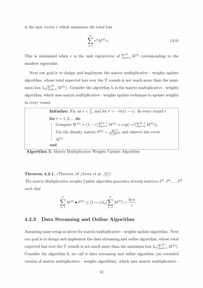
Initialize: Fix an ε < 12, and let ε′ = −ln(1− ε). In every round t

for t = 1, 2, ... do

Compute W (t) = (1− ε)∑t−1

i=1 M(i) = exp(−ε′(

∑t−1i=1 M

(i))).

Use the density matrix P (t) = W (t)

Tr(W (t) and observe the event

M (t).

end

Algorithm 5: Matrix Multiplicative Weights Update Algorithm


The matrix Multiplicative weights Update algorithm generates density matrices P 1, P 2, ..., P T

such that

T∑t=1

M (t) • P (t) ≤ (1 + ε)λn(T∑t=1

M (t)) +lnn

ε.

4.2.3 Data Streaming and Online Algorithm

Assuming same setup as above for matrix multiplicative - weights update algorithm. Next

our goal is to design and implement the data streaming and online algorithm, whose total

expected loss over the T rounds is not much more than the minimum loss λn(∑T

t=1M(t)).

Consider the algorithm 6, we call it data streaming and online algorithm (an extended

version of matrix multiplicative - weights algorithm), which uses matrix multiplicative -

31

weights update technique to update weights in every round. Here our goal includes the

minimum payoff, total payoff, upper bound on payoff, worst payoff and random payoff to

be calculated. Our goal also includes to do analysis on these payoffs which has be given

in next section. Let T be the maximum number of observations. We introduce a new

matrix in the algorithm that we describe here is N (T ), which is defined as follows:

N (T ) =T∑t=1

M (t) (4.9)

Next actual total payoff calculated as follows:

payoff(t)total = payoff

(t−1)total + P (t) •M (t) (4.10)

Then we calculate largest eigenvector V1 and smallest eigenvector Vn corresponding to

largest and smallest eigenvalue of N (T ) respectively. We calculate the minimum payoff as

follows:

payoffmin = V ′nN(T )Vn (4.11)

We calculate the worst payoff as follows:

payoffworst = V ′1N(T )V1 (4.12)

We calculate the upper bound on minimum payoff as follows:

payoffubound = payoffmin(1 + ε) +log n

ε(4.13)

Next our target is to calculate the random payoff. We calculate it as follows: Fix k, find

a random vector, r = r||r|| , of normally distributed pseudorandom numbers of length n,

then the random payoff is

payoffrandom =1

k

k∑i=1

r′N (T )r. (4.14)

32

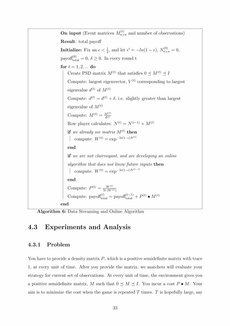
On input (Event matrices M(t)n×n and number of observations)

Result: total payoff

Initialize: Fix an ε < 12, and let ε′ = −ln(1− ε), N (0)

n×n = 0,

payoff(0)total = 0, δ ≥ 0. In every round t

for t = 1, 2, ... do

Create PSD matrix M (t) that satisfies 0 �M (t) � I

Compute: largest eigenvector, V (t) corresponding to largest

eigenvalue d(t) of M (t)

Compute: d(t) = d(t) + δ, i.e. slightly greater than largest

eigenvalue of M (t)

Compute: M (t) = M(t)

d(t)

Row player calculates: N (t) = N (t−1) +M (t)

if we already see matrix M (t) then

compute: W (t) = exp− ln(1−ε)N(t)

end

if we are not clairvoyant, and are developing an online

algorithm that does not know future inputs then

compute: W (t) = exp− ln(1−ε)N(t−1)

end

Compute: P (t) = W (t)

Tr (W (t))

Compute: payoff(t)total = payoff

(t−1)total + P (t) •M (t)

end

Algorithm 6: Data Streaming and Online Algorithm

4.3 Experiments and Analysis

4.3.1 Problem

You have to provide a density matrix P , which is a positive semidefinite matrix with trace

1, at every unit of time. After you provide the matrix, we matchers will evaluate your

strategy for current set of observations. At every unit of time, the environment gives you

a positive semidefinite matrix, M such that 0 � M � I. You incur a cost P •M . Your

aim is to minimize the cost when the game is repeated T times. T is hopefully large, say

33

hundred at least usually.

4.3.2 Experimental Results

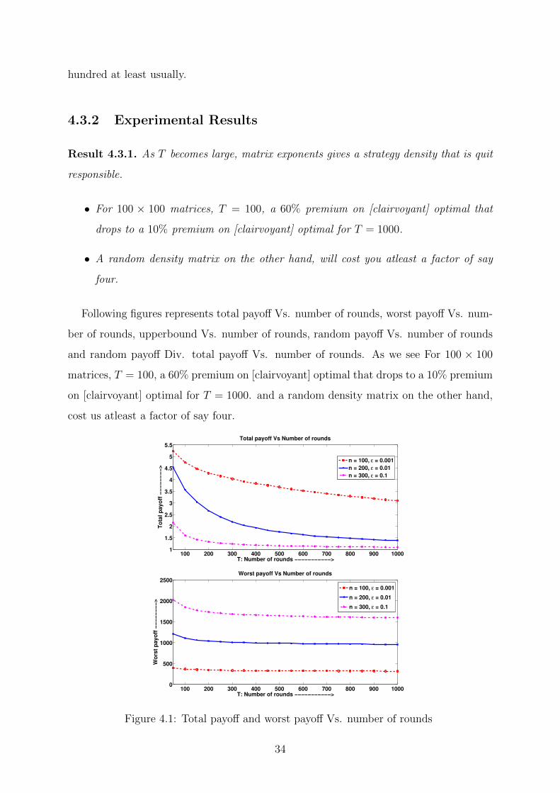
Result 4.3.1. As T becomes large, matrix exponents gives a strategy density that is quit

responsible.

• For 100 × 100 matrices, T = 100, a 60% premium on [clairvoyant] optimal that

drops to a 10% premium on [clairvoyant] optimal for T = 1000.

• A random density matrix on the other hand, will cost you atleast a factor of say

four.

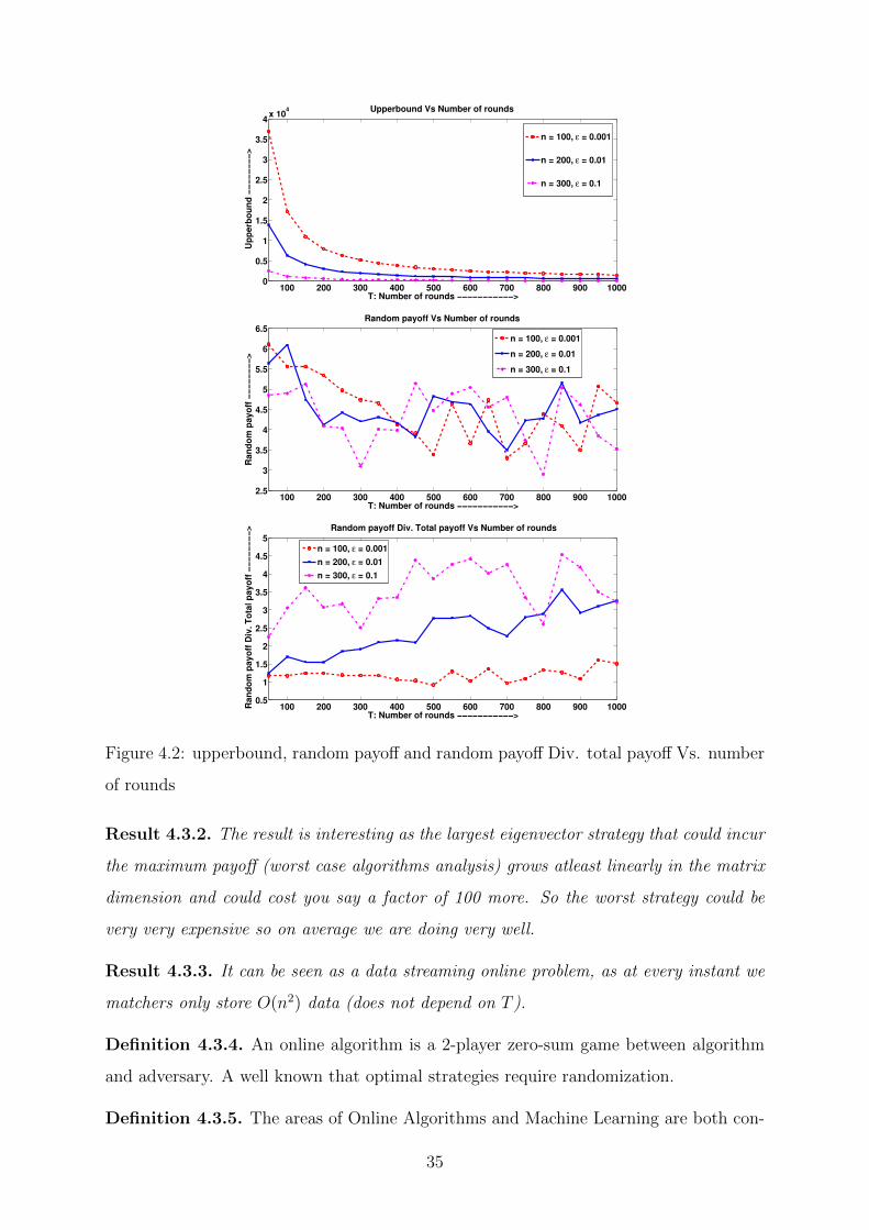
Following figures represents total payoff Vs. number of rounds, worst payoff Vs. num-

ber of rounds, upperbound Vs. number of rounds, random payoff Vs. number of rounds

and random payoff Div. total payoff Vs. number of rounds. As we see For 100 × 100

matrices, T = 100, a 60% premium on [clairvoyant] optimal that drops to a 10% premium

on [clairvoyant] optimal for T = 1000. and a random density matrix on the other hand,

cost us atleast a factor of say four.

100 200 300 400 500 600 700 800 900 10001

1.5

2

2.5

3

3.5

4

4.5

5

5.5

T: Number of rounds −−−−−−−−−−−>

To

tal p

ayo

ff −

−−

−−

−−

−>

Total payoff Vs Number of rounds

n = 100, ε = 0.001

n = 200, ε = 0.01

n = 300, ε = 0.1

100 200 300 400 500 600 700 800 900 10000

500

1000

1500

2000

2500


Wo

rst

payo

ff −

−−

−−

−−

−>

Worst payoff Vs Number of rounds

n = 100, ε = 0.001

n = 200, ε = 0.01

n = 300, ε = 0.1

Figure 4.1: Total payoff and worst payoff Vs. number of rounds

34

100 200 300 400 500 600 700 800 900 10000

0.5

1

1.5

2

2.5

3

3.5

4x 10

4


Up

perb

ou

nd

−−

−−

−−

−−

>

Upperbound Vs Number of rounds

n = 100, ε = 0.001

n = 200, ε = 0.01

n = 300, ε = 0.1

100 200 300 400 500 600 700 800 900 10002.5

3

3.5

4

4.5

5

5.5

6

6.5


Ran

do

m p

ayo

ff −

−−

−−

−−

−>

Random payoff Vs Number of rounds

n = 100, ε = 0.001

n = 200, ε = 0.01

n = 300, ε = 0.1

100 200 300 400 500 600 700 800 900 10000.5

1

1.5

2

2.5

3

3.5

4

4.5

5


Ran

do

m p

ayo

ff D

iv. T

ota

l p

ayo

ff −

−−

−−

−−

−> Random payoff Div. Total payoff Vs Number of rounds

n = 100, ε = 0.001

n = 200, ε = 0.01

n = 300, ε = 0.1

Figure 4.2: upperbound, random payoff and random payoff Div. total payoff Vs. number

of rounds

Result 4.3.2. The result is interesting as the largest eigenvector strategy that could incur

the maximum payoff (worst case algorithms analysis) grows atleast linearly in the matrix

dimension and could cost you say a factor of 100 more. So the worst strategy could be

very very expensive so on average we are doing very well.

Result 4.3.3. It can be seen as a data streaming online problem, as at every instant we

matchers only store O(n2) data (does not depend on T ).

Definition 4.3.4. An online algorithm is a 2-player zero-sum game between algorithm

and adversary. A well known that optimal strategies require randomization.

Definition 4.3.5. The areas of Online Algorithms and Machine Learning are both con-

35

cerned with problems of making decisions about the present based only on knowledge of

the past, hence we see the online Algorithms in machine learning.

Definition 4.3.6. A problem where goal is to predict whether or not to invest in a stock

that day. Input is the advice of n ”experts” Each day, each expert predicts yes or no.

The learning algorithm must use this information in order to make its own prediction,

assuming we make no assumptions about the quality or independence of the experts.

This is called predicting from Expert Advice.

Definition 4.3.7. An algorithm which is used to solve the problem, where we only have

a limited amount of storage is called streaming algorithms.

4.3.3 Experimental Analysis

Under competitive analysis (worst case), for any input, the cost of our online algorithm is

never worse than c (constant) times the cost of the optimal offline algorithm. If we knew

whole input in advance it is easy to optimize. Pros: it can make very robust statements

about the performance of a strategy. Cons: its results tend to be pessimistic.

Under probabilistic analysis, we have assumed a distribution generating the input. We

have designed an algorithm which minimizes the expected cost of the algorithm. Pros:

it can incorporate information predicting the future. Cons: can be difficult to determine

probability distributions accurately.

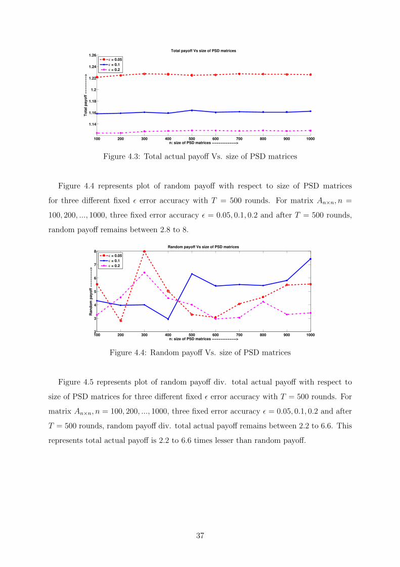
Figure 4.3 represents plot of total actual payoff with respect to size of PSD matrices

for three different fixed ε error accuracy with T = 500 rounds. For matrix An×n, n =

100, 200, ..., 1000, three fixed error accuracy ε = 0.05, 0.1, 0.2 and after T = 500 rounds,

total actual payoff remains between 1.12 to 1.23.

36

100 200 300 400 500 600 700 800 900 1000

1.14

1.16

1.18

1.2

1.22

1.24

1.26

n: size of PSD matrices −−−−−−−−−−−>

To

tal p

ayo

ff −

−−

−−

−−

−>

Total payoff Vs size of PSD matrices

ε = 0.05

ε = 0.1

ε = 0.2

Figure 4.3: Total actual payoff Vs. size of PSD matrices

Figure 4.4 represents plot of random payoff with respect to size of PSD matrices

for three different fixed ε error accuracy with T = 500 rounds. For matrix An×n, n =


random payoff remains between 2.8 to 8.

100 200 300 400 500 600 700 800 900 10002

3

4

5

6

7

8


Ran

do

m p

ayo

ff −

−−

−−

−−

−>

Random payoff Vs size of PSD matrices

ε = 0.05

ε = 0.1

ε = 0.2

Figure 4.4: Random payoff Vs. size of PSD matrices

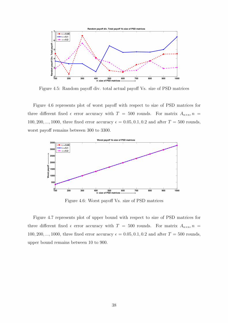
Figure 4.5 represents plot of random payoff div. total actual payoff with respect to

size of PSD matrices for three different fixed ε error accuracy with T = 500 rounds. For

matrix An×n, n = 100, 200, ..., 1000, three fixed error accuracy ε = 0.05, 0.1, 0.2 and after

T = 500 rounds, random payoff div. total actual payoff remains between 2.2 to 6.6. This

represents total actual payoff is 2.2 to 6.6 times lesser than random payoff.

37

100 200 300 400 500 600 700 800 900 10002

3

4

5

6

7


Ran

do

m p

ayo

ff D

iv. T

ota

l p

ayo

ff −

−−

−−

−−

−>

Random payoff div. Total payoff Vs size of PSD matrices

ε = 0.05

ε = 0.1

ε = 0.2

Figure 4.5: Random payoff div. total actual payoff Vs. size of PSD matrices

Figure 4.6 represents plot of worst payoff with respect to size of PSD matrices for

three different fixed ε error accuracy with T = 500 rounds. For matrix An×n, n =


worst payoff remains between 300 to 3300.

100 200 300 400 500 600 700 800 900 10000

500

1000

1500

2000

2500

3000

3500


Wo

rst

payo

ff −

−−

−−

−−

−>

Worst payoff Vs size of PSD matrices

ε = 0.05

ε = 0.1

ε = 0.2

Figure 4.6: Worst payoff Vs. size of PSD matrices

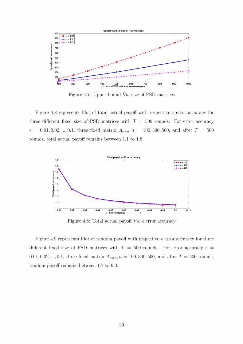
Figure 4.7 represents plot of upper bound with respect to size of PSD matrices for

three different fixed ε error accuracy with T = 500 rounds. For matrix An×n, n =


upper bound remains between 10 to 900.

38

100 200 300 400 500 600 700 800 900 10000

100

200

300

400

500

600

700

800

900

1000


Up

perb

ou

nd

−−

−−

−−

−−

>

Upperbound Vs size of PSD matrices

ε = 0.05

ε = 0.1

ε = 0.2

Figure 4.7: Upper bound Vs. size of PSD matrices

Figure 4.8 represents Plot of total actual payoff with respect to ε error accuracy for

three different fixed size of PSD matrices with T = 500 rounds. For error accuracy

ε = 0.01, 0.02, ..., 0.1, three fixed matrix An×n, n = 100, 300, 500, and after T = 500

rounds, total actual payoff remains between 1.1 to 1.8.

0.01 0.02 0.03 0.04 0.05 0.06 0.07 0.08 0.09 0.1 0.111.1

1.2

1.3

1.4

1.5

1.6

1.7

1.8

1.9

ε : Error accuracy −−−−−−−−−−−>

To

tal p

ayo

ff −

−−

−−

−−

−>

Total payoff Vs Error accuracy

n = 100

n = 300

n = 500

Figure 4.8: Total actual payoff Vs. ε error accuracy

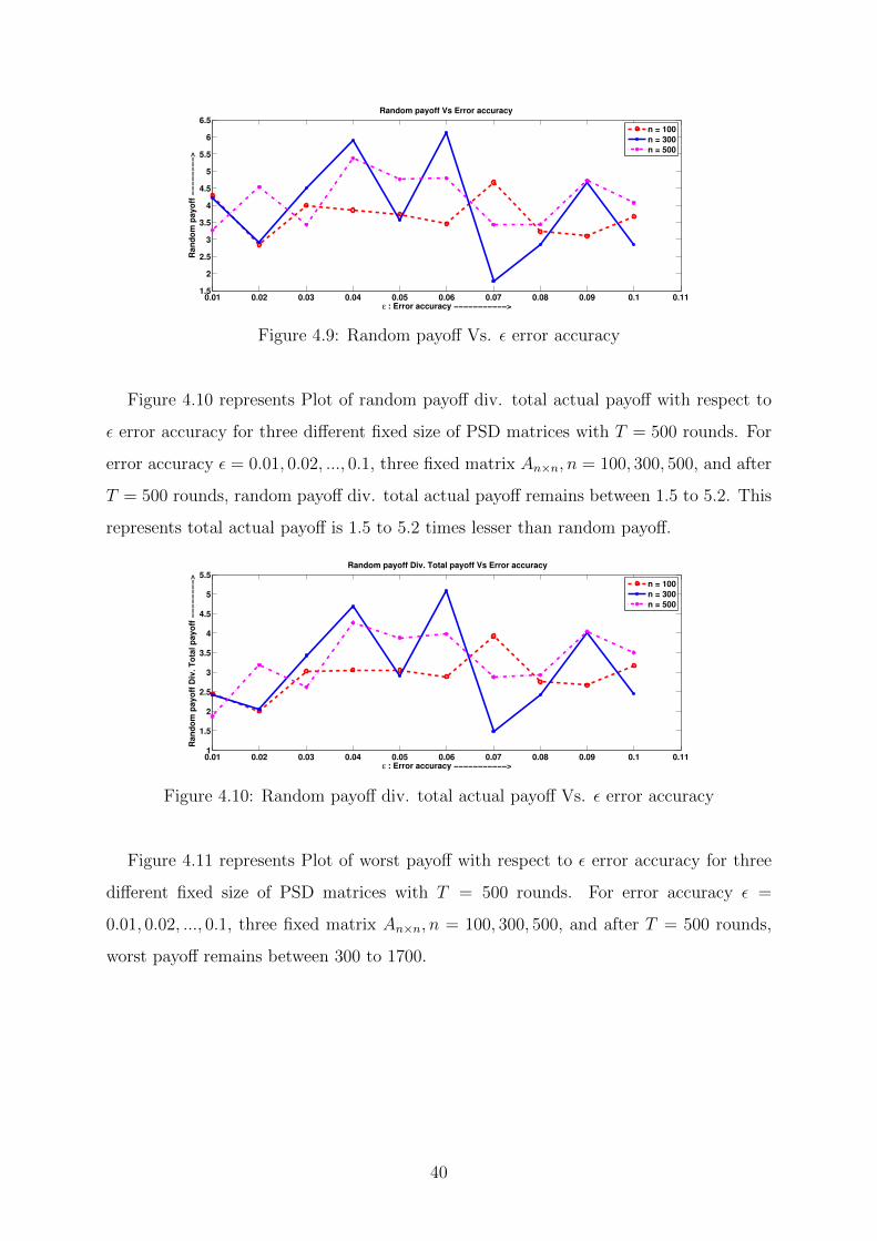
Figure 4.9 represents Plot of random payoff with respect to ε error accuracy for three

different fixed size of PSD matrices with T = 500 rounds. For error accuracy ε =

0.01, 0.02, ..., 0.1, three fixed matrix An×n, n = 100, 300, 500, and after T = 500 rounds,

random payoff remains between 1.7 to 6.3.

39

0.01 0.02 0.03 0.04 0.05 0.06 0.07 0.08 0.09 0.1 0.111.5

2

2.5

3

3.5

4

4.5

5

5.5

6

6.5


Ran

do

m p

ayo

ff −

−−

−−

−−

−>

Random payoff Vs Error accuracy

n = 100

n = 300

n = 500

Figure 4.9: Random payoff Vs. ε error accuracy

Figure 4.10 represents Plot of random payoff div. total actual payoff with respect to

ε error accuracy for three different fixed size of PSD matrices with T = 500 rounds. For

error accuracy ε = 0.01, 0.02, ..., 0.1, three fixed matrix An×n, n = 100, 300, 500, and after

T = 500 rounds, random payoff div. total actual payoff remains between 1.5 to 5.2. This

represents total actual payoff is 1.5 to 5.2 times lesser than random payoff.

0.01 0.02 0.03 0.04 0.05 0.06 0.07 0.08 0.09 0.1 0.111

1.5

2

2.5

3

3.5

4

4.5

5

5.5


Ran

do

m p

ayo

ff D

iv. T

ota

l p

ayo

ff −

−−

−−

−−

−>

Random payoff Div. Total payoff Vs Error accuracy

n = 100

n = 300

n = 500

Figure 4.10: Random payoff div. total actual payoff Vs. ε error accuracy

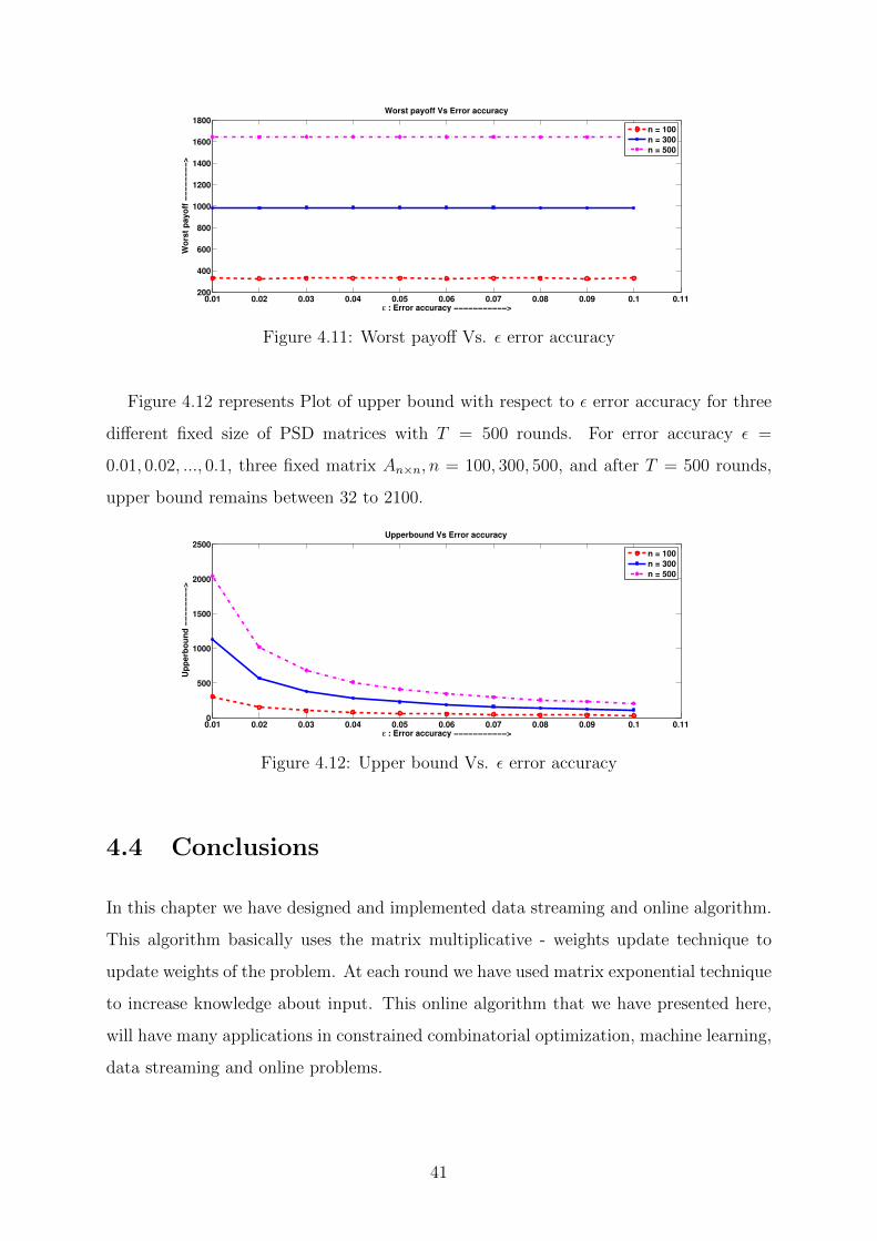
Figure 4.11 represents Plot of worst payoff with respect to ε error accuracy for three



worst payoff remains between 300 to 1700.

40

0.01 0.02 0.03 0.04 0.05 0.06 0.07 0.08 0.09 0.1 0.11200

400

600

800

1000

1200

1400

1600

1800


Wo

rst

payo

ff −

−−

−−

−−

−>

Worst payoff Vs Error accuracy

n = 100

n = 300

n = 500

Figure 4.11: Worst payoff Vs. ε error accuracy

Figure 4.12 represents Plot of upper bound with respect to ε error accuracy for three



upper bound remains between 32 to 2100.

0.01 0.02 0.03 0.04 0.05 0.06 0.07 0.08 0.09 0.1 0.110

500

1000

1500

2000

2500


Up

perb

ou

nd

−−

−−

−−

−−

>

Upperbound Vs Error accuracy

n = 100

n = 300

n = 500

Figure 4.12: Upper bound Vs. ε error accuracy

4.4 Conclusions

In this chapter we have designed and implemented data streaming and online algorithm.

This algorithm basically uses the matrix multiplicative - weights update technique to

update weights of the problem. At each round we have used matrix exponential technique

to increase knowledge about input. This online algorithm that we have presented here,

will have many applications in constrained combinatorial optimization, machine learning,

data streaming and online problems.

41

4.5 Remarks

We have not given any theorem and proofs for data streaming and online algorithm

6. Since theorems of matrix multiplicative - weights update algorithm can be directly

mapped to data streaming and online algorithm 6 [3].

42

Chapter 5

Fast Algorithms for Approximate

Packing-Covering Semidefinite

Programs using the Multiplicative -

Weights Update Techniques

5.1 Introduction

In chapter 1 we have presented primal only approach to approximate SDPs. Here we

present primal-dual approach to approximate SDPs. Our main objective of this chapter

is to design and implement general primal-dual algorithm to compute a near-optimal

solution to any SDP.

A general SDP with n2 variables, an n× n matrix variable X and m constraints and

43

its dual can be written as follows:

Max C •X

subject to Aj •X ≤ bj, forj = 1, 2, ...,m

X � 0 (Primal) (5.1)

Min b.y

subject to∑m

j=1Ajyj � C

y ≥ 0 (Dual) (5.2)

Where, y = {y1, y2, ..., ym} are the dual variables and b = {b1, b2, ..., bm}. A linear

program is the special case of SDPs. We can see this by replacing all entries of all

matrices by zero other than diagonal entries. Hence we say than SDP’s are more general

form of LPs.

Assume A1 = I and b1 = R. This assumption helps in trace bounding i.e. Trace(X) ≤

R. Where Trace(X) ≤ R is a scaling constraint bound on trace of optimum value X.

We assume as in the case of primal only approach to approximate SDPs, that our imple-

mentation of SDP primal-dual algorithm uses binary search on α to reduce optimization

to feasibility. Let α be the algorithm’s current guess for the optimum value of the SDP.

Implementation is trying to either construct a PSD matrix that is primal feasible and has

value > α. or a dual feasible solution whose value is at most (1 + δ)α for some arbitrary

small δ > 0.

5.2 Algorithm

The algorithm starts with a trivial candidate for a primal solution X, where X is PSD

matrix possibly infeasible of trace equals R. Let X(1) = RnI. Then algorithm iteratively

generates candidate primal solutions X(1), X(2), .... At every step it tries to improve X(t)

to obtain X(t+1). In order to apply the multiplicative - weights update technique in

constraints combinatorial optimization problems, we require to go through following two

phases:

44

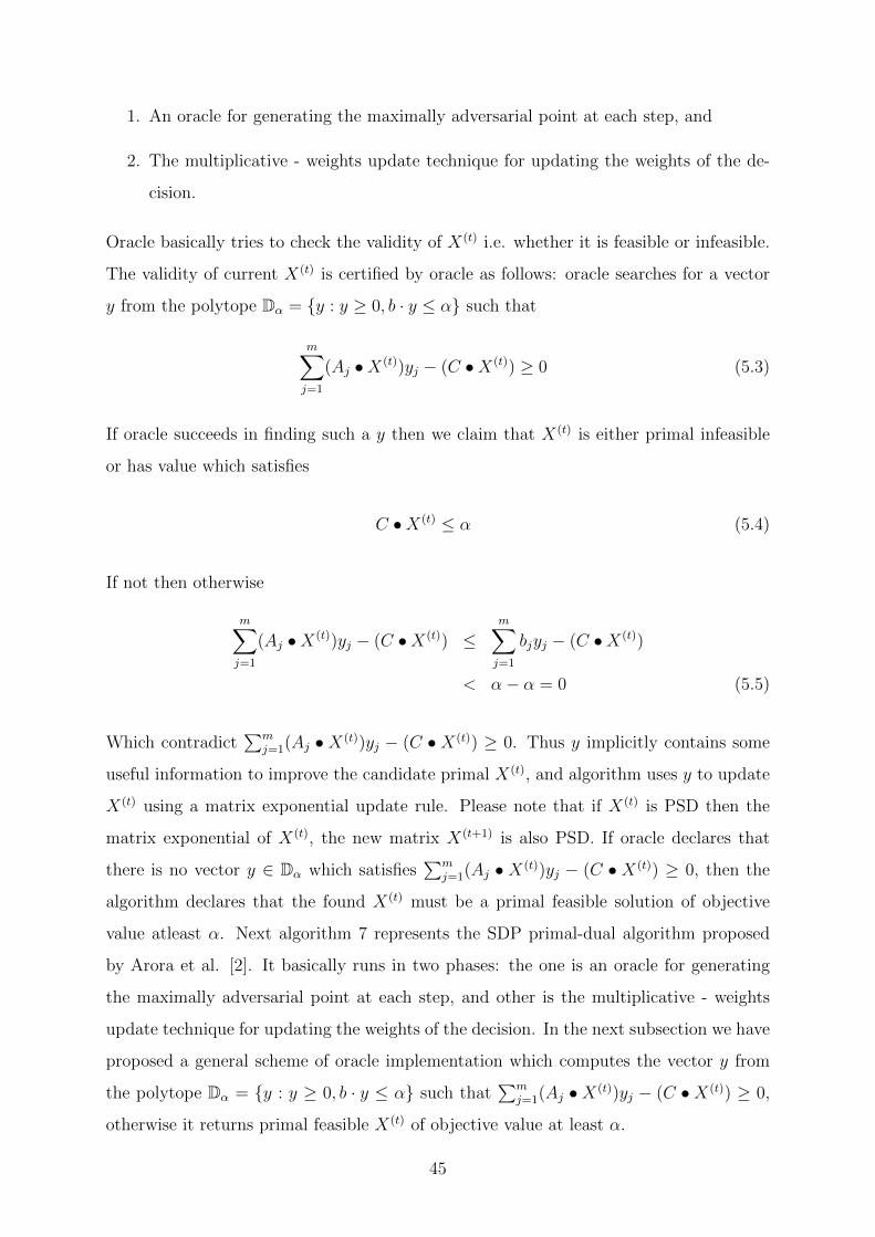
1. An oracle for generating the maximally adversarial point at each step, and

2. The multiplicative - weights update technique for updating the weights of the de-

cision.

Oracle basically tries to check the validity of X(t) i.e. whether it is feasible or infeasible.

The validity of current X(t) is certified by oracle as follows: oracle searches for a vector

y from the polytope Dα = {y : y ≥ 0, b · y ≤ α} such that

m∑j=1

(Aj •X(t))yj − (C •X(t)) ≥ 0 (5.3)

If oracle succeeds in finding such a y then we claim that X(t) is either primal infeasible

or has value which satisfies

C •X(t) ≤ α (5.4)

If not then otherwise

m∑j=1

(Aj •X(t))yj − (C •X(t)) ≤m∑j=1

bjyj − (C •X(t))

< α− α = 0 (5.5)

Which contradict∑m

j=1(Aj • X(t))yj − (C • X(t)) ≥ 0. Thus y implicitly contains some

useful information to improve the candidate primal X(t), and algorithm uses y to update

X(t) using a matrix exponential update rule. Please note that if X(t) is PSD then the

matrix exponential of X(t), the new matrix X(t+1) is also PSD. If oracle declares that

there is no vector y ∈ Dα which satisfies∑m

j=1(Aj • X(t))yj − (C • X(t)) ≥ 0, then the

algorithm declares that the found X(t) must be a primal feasible solution of objective

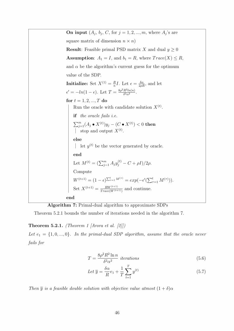
value atleast α. Next algorithm 7 represents the SDP primal-dual algorithm proposed

by Arora et al. [2]. It basically runs in two phases: the one is an oracle for generating

the maximally adversarial point at each step, and other is the multiplicative - weights

update technique for updating the weights of the decision. In the next subsection we have

proposed a general scheme of oracle implementation which computes the vector y from

the polytope Dα = {y : y ≥ 0, b · y ≤ α} such that∑m

j=1(Aj •X(t))yj − (C •X(t)) ≥ 0,

otherwise it returns primal feasible X(t) of objective value at least α.

45

On input (Aj, bj, C, for j = 1, 2, ...,m, where Aj’s are

square matrix of dimension n× n)

Result: Feasible primal PSD matrix X and dual y ≥ 0

Assumption: A1 = I, and b1 = R, where Trace(X) ≤ R,

and α be the algorithm’s current guess for the optimum

value of the SDP.

Initialize: Set X(1) = RnI. Let ε = δα

2ρR, and let

ε′ = −ln(1− ε). Let T = 8ρ2R2ln(n)δ2α2 .

for t = 1, 2, ..., T do

Run the oracle with candidate solution X(t).

if the oracle fails i.e.∑mj=1(Aj •X(t))yj − (C •X(t)) < 0 then

stop and output X(t).

else

let y(t) be the vector generated by oracle.

end

Let M (t) = (∑m

j=1Ajy(t)j − C + ρI)/2ρ.

Compute

W (t+1) = (1− ε)∑tτ=1M

(τ)= exp(−ε′(

∑tτ=1M

(τ))).

Set X(t+1) = RW (t+1)

Trace(W (t+1))and continue.

end

Algorithm 7: Primal-dual algorithm to approximate SDPs

Theorem 5.2.1 bounds the number of iterations needed in the algorithm 7.


Let e1 = {1, 0, ..., 0}. In the primal-dual SDP algorithm, assume that the oracle never

fails for

T =8ρ2R2 lnn

δ2α2iterations (5.6)

Let y =δα

Re1 +

1

T

T∑t=1

y(t) (5.7)

Then y is a feasible double solution with objective value atmost (1 + δ)α

46

5.2.1 Computation of vector y

Here we give a proposed idea for implementation of oracle for primal-dual SDPs. This

implementation calculates the vector y from the polytope Dα = {y : y ≥ 0, b · y ≤ α}

such that∑m

j=1(Aj •X(t))yj − (C •X(t)) ≥ 0, otherwise it returns primal feasible X(t) of

objective value at least α. The search for vector y is as follows:

y ≥ 0, b1y1 + b2y2 + ...+ bmym ≤ α (5.8)m∑j=1

(Aj •X(t))yj − (C •X(t)) ≥ 0 (5.9)

from equation (5.8)

y1 =α−

∑mj=2 bjyj − εb1

(5.10)

substitute (5.10) in (5.9)

(A1 •X(t))y1 +m∑j=2

(Aj •X(t))yj ≥ C •X(t)

(A1 •X(t))(α−

∑mj=2 bjyj − εb1

) +m∑j=2


(A1 •X(t))α

b1

−(A1 •X(t))

∑mj=2 bjyj

b1

− ε(A1 •X(t))

b1

+m∑j=2


m∑j=2

(Aj •X(t))yj −(A1 •X(t))

∑mj=2 bjyj

b1

≥ C •X(t) +ε(A1 •X(t))

b1

− (A1 •X(t))α

b1

m∑j=2

(Aj •X(t) − (A1 •X(t))bjb1

)yj ≥ C •X(t) +ε(A1 •X(t))

b1

− (A1 •X(t))α

b1

Let,

dj = (Aj •X(t) − A1 •X(t)bjb1

)

c? =ε(A1 •X(t))

b1

− (A1 •X(t))α

b1

47

therefore,

m∑j=2

djyj ≥ C •X(t) + c? = CNew. (5.11)

For all dj < 0, set,

yj = 0, 2 ≤ j ≤ m (5.12)

let K of the dj’s 2 ≤ j ≤ m be ≥ 0, say dl1 , dl2 , ..., dlk , then let S = dl1 + dl2 + ...+ dlk ,

set

yl1 = yl2 = ... = ylk =CNewS

+ ε (5.13)

others were set to zero in (5.12). Calculate y1 from (5.10). Hence (5.10), (5.12) and (5.13)

gives vector y.

The primal-dual SDP algorithm depends on the width parameter of the oracle. This

is the smallest ρ ≥ 0 such that for every primal candidate X, the vector y ∈ Dα returned

by the oracle satisfies

||Ajyj − C|| ≤ ρ. (5.14)

Theorem 5.2.2. (Theorem V.1 [Chan et al. [5]])

There exists such an oracle with access time O(n2), and for candidate value α, it has

width ρα = O(αn).

5.3 Examples

Consider the SDP’s primal (5.1) and dual (5.2)

48

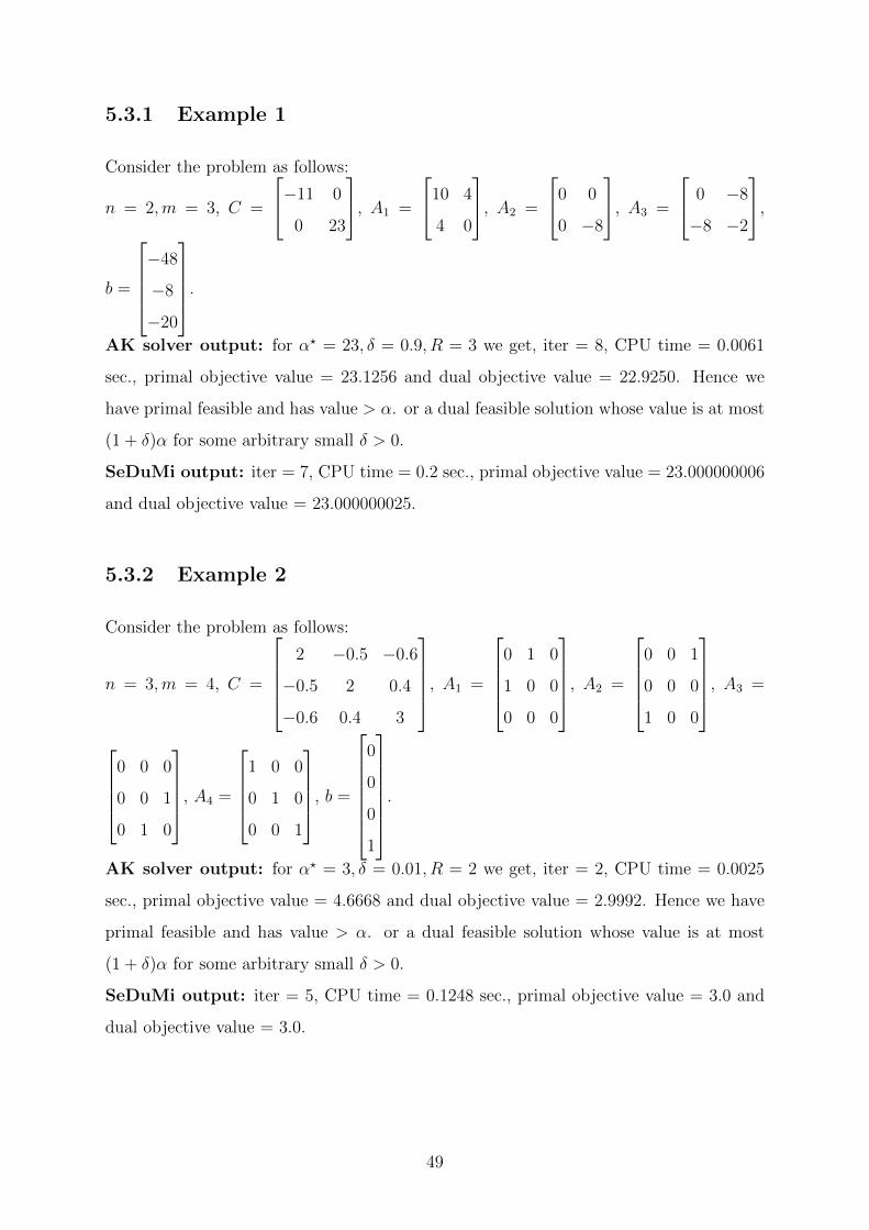
5.3.1 Example 1

Consider the problem as follows:

n = 2,m = 3, C =

−11 0

0 23

, A1 =

10 4

4 0

, A2 =

0 0

0 −8

, A3 =

0 −8

−8 −2

,

b =

−48

−8

−20

.

AK solver output: for α? = 23, δ = 0.9, R = 3 we get, iter = 8, CPU time = 0.0061

sec., primal objective value = 23.1256 and dual objective value = 22.9250. Hence we

have primal feasible and has value > α. or a dual feasible solution whose value is at most

(1 + δ)α for some arbitrary small δ > 0.

SeDuMi output: iter = 7, CPU time = 0.2 sec., primal objective value = 23.000000006

and dual objective value = 23.000000025.

5.3.2 Example 2

Consider the problem as follows:

n = 3,m = 4, C =

2 −0.5 −0.6

−0.5 2 0.4

−0.6 0.4 3

, A1 =

0 1 0

1 0 0

0 0 0

, A2 =

0 0 1

0 0 0

1 0 0

, A3 =

0 0 0

0 0 1

0 1 0

, A4 =

1 0 0

0 1 0

0 0 1

, b =

0

0

0

1

.

AK solver output: for α? = 3, δ = 0.01, R = 2 we get, iter = 2, CPU time = 0.0025

sec., primal objective value = 4.6668 and dual objective value = 2.9992. Hence we have

primal feasible and has value > α. or a dual feasible solution whose value is at most

(1 + δ)α for some arbitrary small δ > 0.

SeDuMi output: iter = 5, CPU time = 0.1248 sec., primal objective value = 3.0 and

dual objective value = 3.0.

49

5.4 Conclusions

In this chapter we have given an overview of AK algorithm. AK algorithm runs in

basically two parts. One as oracle computations and other is matrix multiplicative -

weights update method. Matrix multiplicative - weights update method is very trivial, it

is easy to implement. The first part i.e. oracle computation (computation of vector y) of

AK algorithm is the root of this algorithm. Hence we have given a different approach to

compute this vector y, a very general one. This oracle computation is likely to work for

all general SDP’s problems. Then we have given two examples and compared our results

with SeDuMi, a well known SDP solver. Thus we are doing well in computation time.

5.5 Remarks

Please not that we have not modified AK SDP algorithm presented in algorithm 7. We

have given a general approach to compute vector y at each round. Proofs of related

theorems are available in Arora et al. [2] paper.

50

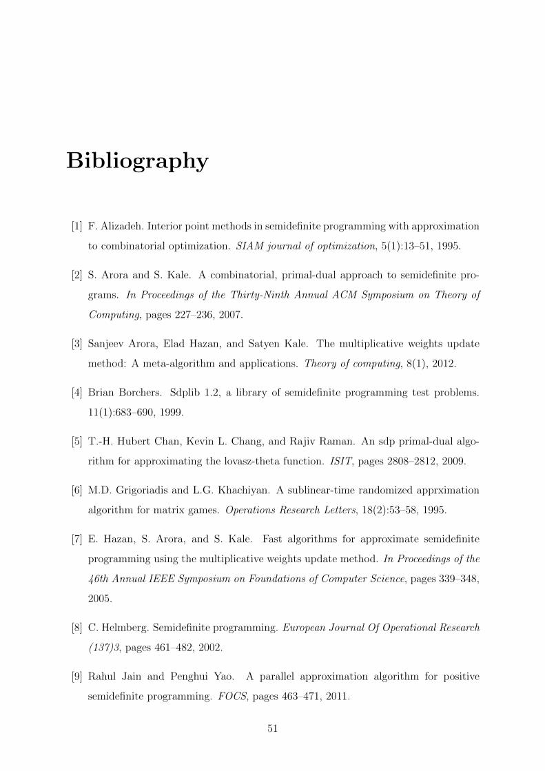
Bibliography

[1] F. Alizadeh. Interior point methods in semidefinite programming with approximation

to combinatorial optimization. SIAM journal of optimization, 5(1):13–51, 1995.

[2] S. Arora and S. Kale. A combinatorial, primal-dual approach to semidefinite pro-

grams. In Proceedings of the Thirty-Ninth Annual ACM Symposium on Theory of

Computing, pages 227–236, 2007.

[3] Sanjeev Arora, Elad Hazan, and Satyen Kale. The multiplicative weights update

method: A meta-algorithm and applications. Theory of computing, 8(1), 2012.

[4] Brian Borchers. Sdplib 1.2, a library of semidefinite programming test problems.

11(1):683–690, 1999.

[5] T.-H. Hubert Chan, Kevin L. Chang, and Rajiv Raman. An sdp primal-dual algo-

rithm for approximating the lovasz-theta function. ISIT, pages 2808–2812, 2009.

[6] M.D. Grigoriadis and L.G. Khachiyan. A sublinear-time randomized apprximation

algorithm for matrix games. Operations Research Letters, 18(2):53–58, 1995.

[7] E. Hazan, S. Arora, and S. Kale. Fast algorithms for approximate semidefinite

programming using the multiplicative weights update method. In Proceedings of the

46th Annual IEEE Symposium on Foundations of Computer Science, pages 339–348,

2005.

[8] C. Helmberg. Semidefinite programming. European Journal Of Operational Research

(137)3, pages 461–482, 2002.

[9] Rahul Jain and Penghui Yao. A parallel approximation algorithm for positive

semidefinite programming. FOCS, pages 463–471, 2011.

51

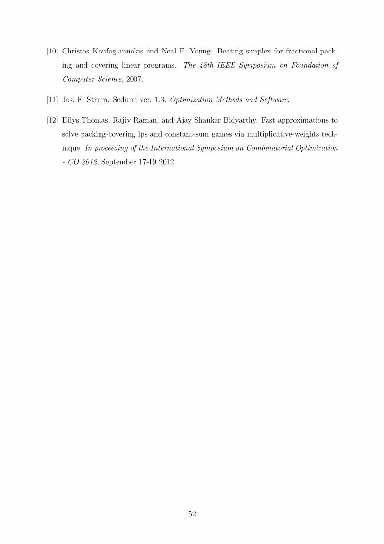
[10] Christos Koufogiannakis and Neal E. Young. Beating simplex for fractional pack-

ing and covering linear programs. The 48th IEEE Symposium on Foundation of

Computer Science, 2007.

[11] Jos. F. Strum. Sedumi ver. 1.3. Optimization Methods and Software.

[12] Dilys Thomas, Rajiv Raman, and Ajay Shankar Bidyarthy. Fast approximations to

solve packing-covering lps and constant-sum games via multiplicative-weights tech-

nique. In proceeding of the International Symposium on Combinatorial Optimization

- CO 2012, September 17-19 2012.

52

Documents

DESIGN AND IMPLEMENTATION OF PARALLEL AND RANDOMIZED APPROXIMATION ALGORITHMS