Embed Size (px)
Citation preview
Implementation of Multiplicative weights and Multi-Commodity Flows Parallel
and Randomized Approximation Algorithms
BY
Ajay Shankar Bidyarthy
ON
16th July 2012
Report
Submitted in Systems Research Laboratory
TATA Research Development and Design Center (TRDDC)
54-B, Hadapsar Industrial Estate, Pune, MH, 411013, India.
Under the Guidance
of
Dr. Rajiv Raman
TATA Research Development and Design Center, Pune
Dr. Dilys Thomas
TATA Research Development and Design Center, Pune
1
1 Implementation of parallel and randomized algorithm for skew-
symmetric matrix game
1.1 Problem Statement
Given a (m,n)-matrix game A = [aij ] ∈ [−1, 1], we give a serial implementation to a parallel
randomized algorithm which computes a pair of ε-optimal strategies in 4ε2
log n number of iter-
ations where n is size of the matrix A. For any accuracy ε > 0, the expected sequential running
time of the suggested algorithm is O( 1ε2n log n). If we assume m = n the randomized algorithm
achieves an almost quadratic expected speedup relative to any deterministic method [1].
1.2 Introduction
Let A = [aij ] be an (m,n)-matrix game of value v? = min {v | Ax ≤ ve, eᵀx = 1, x ≥ 0} =
max {v | Aᵀy ≥ ve, eᵀy = 1, y ≥ 0}, where e is the vector of all ones. This value is always
achieved for a pair of optimal strategies x? ∈ Rn, y? ∈ Rm. Let the elements of the payoff
matrix A lie in some interval, say A = [aij ] ∈ [−1, 1] .
A pair of strategies x, y is ε− optimal for A if
Ax ≤ (v? + ε)e, eᵀx = 1, x ≥ 0 and Aᵀy ≥ (v? + ε)e, eᵀy = 1, y ≥ 0 ..........(?)
Define U(t) = AX(t) ∈ <m, and for symmetric matrix games (A = −Aᵀ) V (t) = −U(t)
for all tth iteration. The algorithm is a simple randomized variant of the deterministic method
(where players play pure best response) in which indices i(t) ∈ {1, ..., n} or j(t) ∈ {1, ...,m} are
selected with probability propotional to exp{−εVi(t)/2} or exp{+εUj(t)/2} for the minimizing
and maximizing player, respectively. For symmetric games, the probability of selcting an index
i(t) is given by the Gibbs distribution pi(t) = exp{εUi(t)/2}/∑n
j=1 exp{εUj(t)/2}.
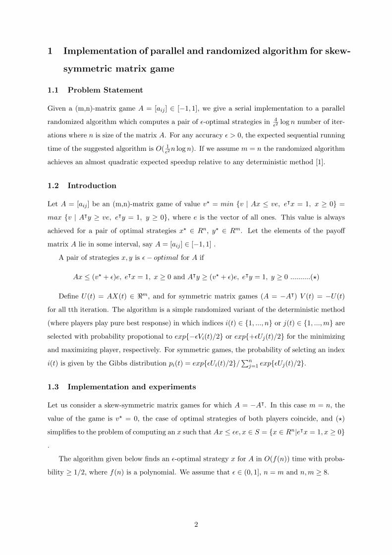
1.3 Implementation and experiments
Let us consider a skew-symmetric matrix games for which A = −Aᵀ. In this case m = n, the
value of the game is v? = 0, the case of optimal strategies of both players coincide, and (?)
simplifies to the problem of computing an x such that Ax ≤ εe, x ∈ S = {x ∈ Rn|eᵀx = 1, x ≥ 0}
.
The algorithm given below finds an ε-optimal strategy x for A in O(f(n)) time with proba-
bility ≥ 1/2, where f(n) is a polynomial. We assume that ε ∈ (0, 1], n = m and n,m ≥ 8.
2
Result: ε-optimal strategy vector x
Initialize: X = 0, U = 0, X,U ∈ Rn, p = e/n, t = 0.
repeatIteration count: t = t+ 1.
Random direction: pick a random k ∈ {1, ..., n} with probability pk.
X − update:
Xk = Xk + 1.
U − update:
for i = 1, ..., n do
do in parallel Ui = Ui + aik.
end
p− update:
for i = 1, ..., n do
do in parallel pi = piexp{ ε2aik}/∑n
j=1 pjexp{ε2ajk}.
end
Stopping criterion:
if U/t ≤ εe then
Output: x = X/t and halt.
end
until;
Algorithm 1: Parallel and randomized apprximation algorithm for skew-symmetric
matrix games
Result: k ∈ {1, ..., n} with probability pk
for i = 1, ..., n do
calculate cummulative sum Si = p1 + p2 + ...+ pi.
end
Generate an uniform random number z ∈ [0, 1]
Pick a random number k ∈ {1, ..., n} such that Sk−1 < z ≤ Sk.Algorithm 2: Algorithm for picking a random k ∈ {1, ..., n} with probability pk
Theorem:
1. The stopping criterion U/t ≤ εe guarantees the ε− optimality of the output vector x i.e.
x = X/t [1].
2. Algorithm halts in t? = 4ε−2ln(n) iterations with probability ≥ 1/2 [1].
3
Corollary:
An ε-optimal strategy for a symmetric matrix game An×n ∈ [−1, 1] can be computed in
O(ε−2 log n) expected number of iterations of this algorithm. Since this algorithm runs re-
peatedly for at most t? = 4ε−2 lnn iterations succeeding each time with probability at least 1/2,
until the stopping criterion is satisfied.
Let f(n) = 1ε2
lnn. E[t?] = 12 × f(n) + 1
4 × 2× f(n) + 18 × 3× f(n) + ...+ 1
2i× i× f(n) + ...
=∑∞
i=1i2if(n) = f(n)
∑∞i=1
i2i≤ 4 × f(n). Since we know that 1 + x + x2 + x3 + ... = 1
1−x .
Differentiating both side w.r.t. x we get 0 + 1 + 2x+ 3x2 + ... = ddx( 1
1−x) = 1(1−x)2 = 1
(1− 12)2
= 4
at x = 1/2. �
Theorem:
An ε-optimal solution for a given symmetric n × n matrix game A = [aij ] ∈ [−1, 1] can be
computed in O(ε−2 log2 n) expected time on an n/log n-processor EREW PRAM ([1] Theorem
2.).
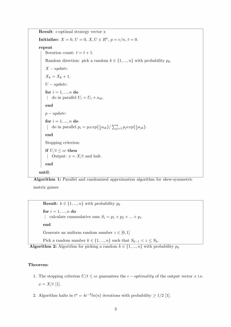
1.4 Analysis and results
log n dependence:
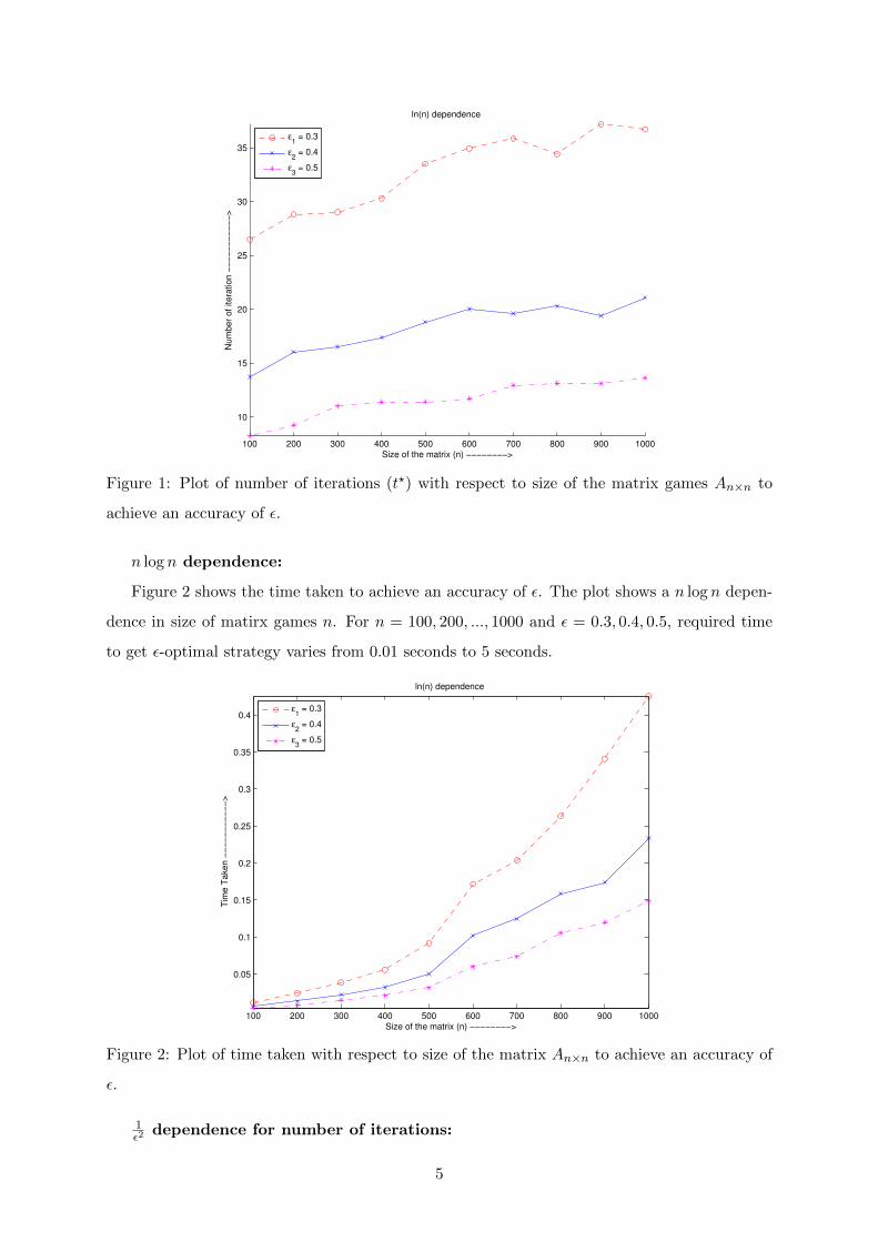
Figure 1 shows the number of iterations required to achieve an accuracy of ε. The plot shows
a log growth in size of matrix games n. For n = 100, 200, ..., 1000 and ε = 0.3, 0.4, 0.5, required
number of iterations varies from 7 to 40. Algorithm outputs ε-optimal strategy (output vector
x) atmost in 4ε2
log n iterations.
4
100 200 300 400 500 600 700 800 900 1000
10
15
20
25
30
35
Num
ber
of itera
tion −
−−
−−
−−
−−
−−
>
Size of the matrix (n) −−−−−−−−>
ln(n) dependence
ε1 = 0.3
ε2 = 0.4
ε3 = 0.5
Figure 1: Plot of number of iterations (t?) with respect to size of the matrix games An×n to
achieve an accuracy of ε.
n log n dependence:
Figure 2 shows the time taken to achieve an accuracy of ε. The plot shows a n log n depen-
dence in size of matirx games n. For n = 100, 200, ..., 1000 and ε = 0.3, 0.4, 0.5, required time
to get ε-optimal strategy varies from 0.01 seconds to 5 seconds.
100 200 300 400 500 600 700 800 900 1000
0.05
0.1
0.15
0.2
0.25
0.3
0.35
0.4
Tim
e T
aken −
−−
−−
−−
−−
−−
>
Size of the matrix (n) −−−−−−−−>
ln(n) dependence
ε1 = 0.3
ε2 = 0.4
ε3 = 0.5
Figure 2: Plot of time taken with respect to size of the matrix An×n to achieve an accuracy of
ε.
1ε2
dependence for number of iterations:
5
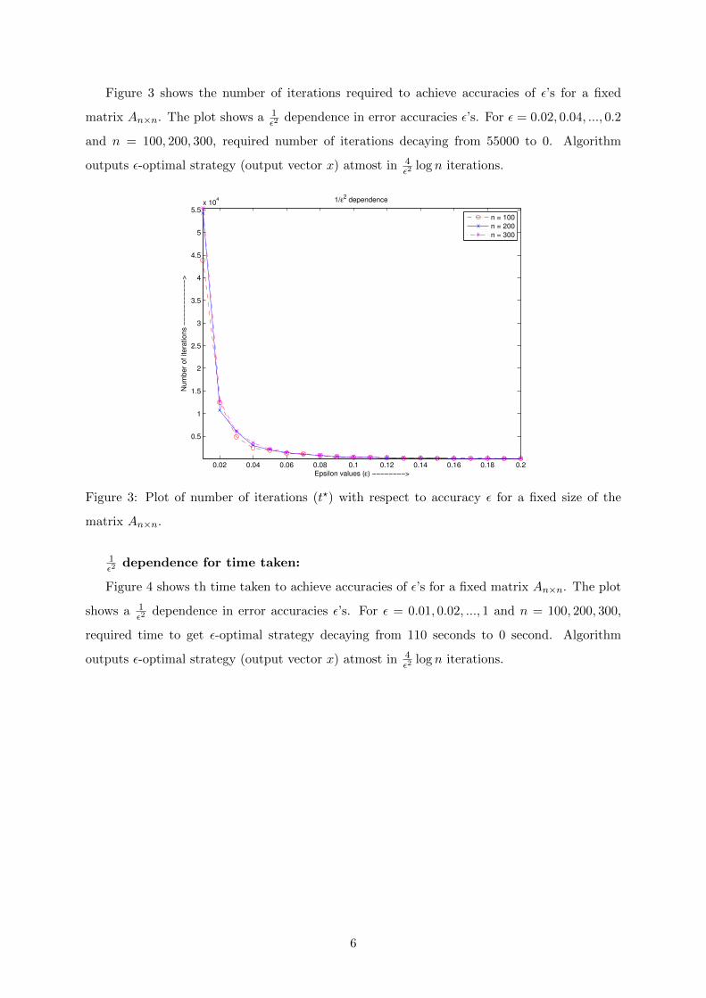
Figure 3 shows the number of iterations required to achieve accuracies of ε’s for a fixed
matrix An×n. The plot shows a 1ε2
dependence in error accuracies ε’s. For ε = 0.02, 0.04, ..., 0.2
and n = 100, 200, 300, required number of iterations decaying from 55000 to 0. Algorithm
outputs ε-optimal strategy (output vector x) atmost in 4ε2
log n iterations.
0.02 0.04 0.06 0.08 0.1 0.12 0.14 0.16 0.18 0.2
0.5
1
1.5
2
2.5
3
3.5
4
4.5
5
5.5x 10
4
Num
ber
of
itera
tions −
−−
−−
−−
−−
−−
>
Epsilon values (ε) −−−−−−−−>
1/ε2 dependence
n = 100
n = 200
n = 300
Figure 3: Plot of number of iterations (t?) with respect to accuracy ε for a fixed size of the
matrix An×n.
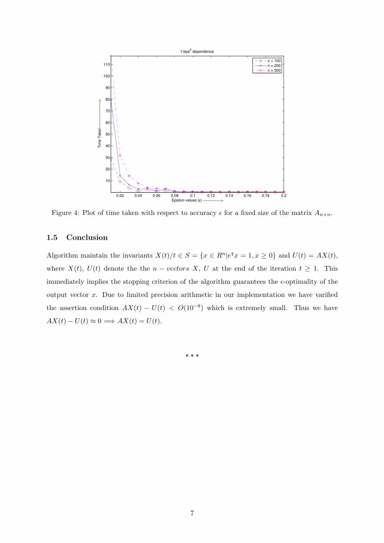
1ε2
dependence for time taken:
Figure 4 shows th time taken to achieve accuracies of ε’s for a fixed matrix An×n. The plot
shows a 1ε2
dependence in error accuracies ε’s. For ε = 0.01, 0.02, ..., 1 and n = 100, 200, 300,
required time to get ε-optimal strategy decaying from 110 seconds to 0 second. Algorithm
outputs ε-optimal strategy (output vector x) atmost in 4ε2
log n iterations.
6
0.02 0.04 0.06 0.08 0.1 0.12 0.14 0.16 0.18 0.2
10
20
30
40
50
60
70
80
90
100
110
Tim
e T
aken −
−−
−−
−−
−−
−−
>
Epsilon values (ε) −−−−−−−−>
1/eps2 dependence
n = 100
n = 200
n = 300
Figure 4: Plot of time taken with respect to accuracy ε for a fixed size of the matrix An×n.
1.5 Conclusion
Algorithm maintain the invariants X(t)/t ∈ S = {x ∈ Rn|eᵀx = 1, x ≥ 0} and U(t) = AX(t),
where X(t), U(t) denote the the n − vectors X, U at the end of the iteration t ≥ 1. This
immediately implies the stopping criterion of the algorithm guarantees the ε-optimality of the
output vector x. Due to limited precision arithmetic in our implementation we have varified
the assertion condition AX(t) − U(t) < O(10−8) which is extremely small. Thus we have
AX(t)− U(t) ≈ 0 =⇒ AX(t) = U(t).
? ? ?
7
2 Performance analysis of M.D. Grigoriadis and L.G. Khachiyan
algorithm Vs SeDuMi in Matlab of A sublinear-time random-
ized apprximation algorithm for matrix games.
2.1 Introduction
SeDuMi (Self-Dual-Minimization) is an add-on for Matlab, which let us solve optimization
problems with linear, quadratic and semidefiniteness constraints. It implements the self- dual
embedding technique for optimization over self-dual homogeneous cones. The self-dual embed-
ding technique essentially makes it possible to solve certain optimization problems in a single
phase, leading either to an optimal solution, or a certificate of infeasibility. Complex valued
data and variables can also be input for SeDuMi. Large scale optimization problems are solved
efficiently, by exploiting sparsity.
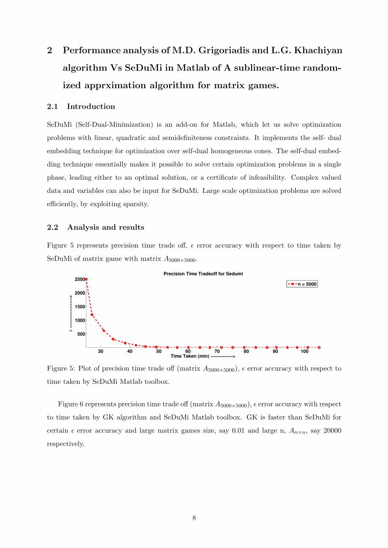
2.2 Analysis and results
Figure 5 represents precision time trade off, ε error accuracy with respect to time taken by
SeDuMi of matrix game with matrix A5000×5000.
30 40 50 60 70 80 90 100
500
1000
1500
2000
2500
ε −
−−
−−
−−
−−
−−
>
Time Taken (min) −−−−−−−−>
Precision Time Tradeoff for Sedumi
n = 5000
Figure 5: Plot of precision time trade off (matrix A5000×5000), ε error accuracy with respect to
time taken by SeDuMi Matlab toolbox.
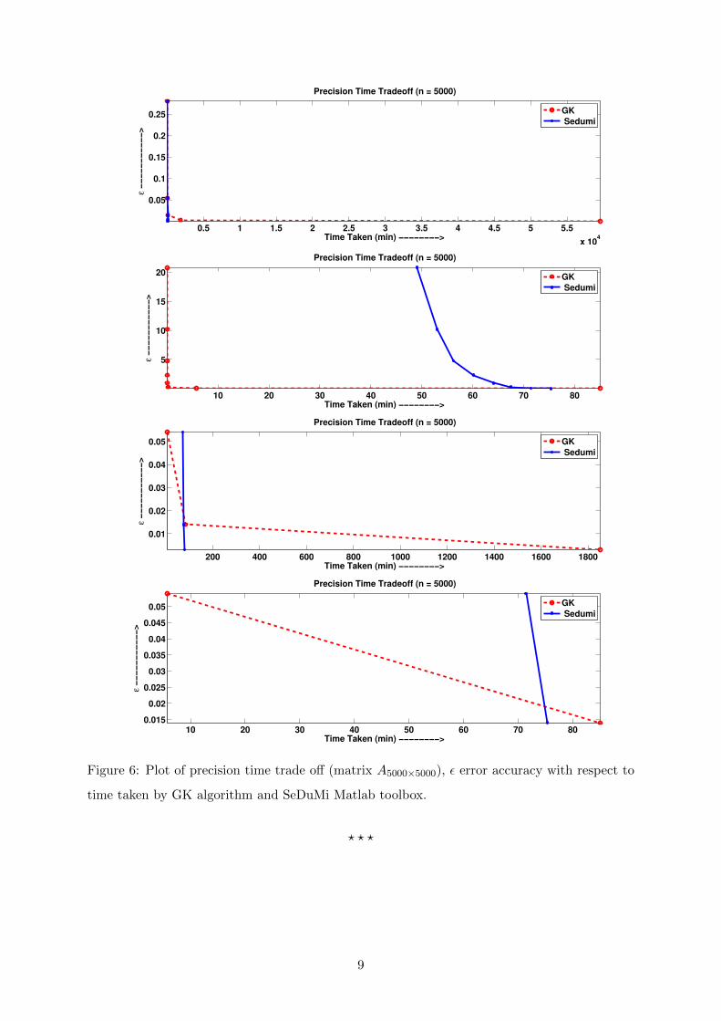
Figure 6 represents precision time trade off (matrix A5000×5000), ε error accuracy with respect
to time taken by GK algorithm and SeDuMi Matlab toolbox. GK is faster than SeDuMi for
certain ε error accuracy and large matrix games size, say 0.01 and large n, An×n, say 20000
respectively.
8
0.5 1 1.5 2 2.5 3 3.5 4 4.5 5 5.5
x 104
0.05
0.1
0.15
0.2
0.25
ε −
−−
−−
−−
−−
−−
>
Time Taken (min) −−−−−−−−>
Precision Time Tradeoff (n = 5000)
GK
Sedumi
10 20 30 40 50 60 70 80
5
10
15
20
ε −
−−
−−
−−
−−
−−
>
Time Taken (min) −−−−−−−−>
Precision Time Tradeoff (n = 5000)
GK
Sedumi
200 400 600 800 1000 1200 1400 1600 1800
0.01
0.02
0.03
0.04
0.05
ε −
−−
−−
−−
−−
−−
>
Time Taken (min) −−−−−−−−>
Precision Time Tradeoff (n = 5000)
GK
Sedumi
10 20 30 40 50 60 70 800.015
0.02
0.025
0.03
0.035
0.04
0.045
0.05
ε −
−−
−−
−−
−−
−−
>
Time Taken (min) −−−−−−−−>
Precision Time Tradeoff (n = 5000)
GK
Sedumi
Figure 6: Plot of precision time trade off (matrix A5000×5000), ε error accuracy with respect to
time taken by GK algorithm and SeDuMi Matlab toolbox.
? ? ?
9
3 Beating simplex for fractional packing and covering linear
programs
3.1 Introduction
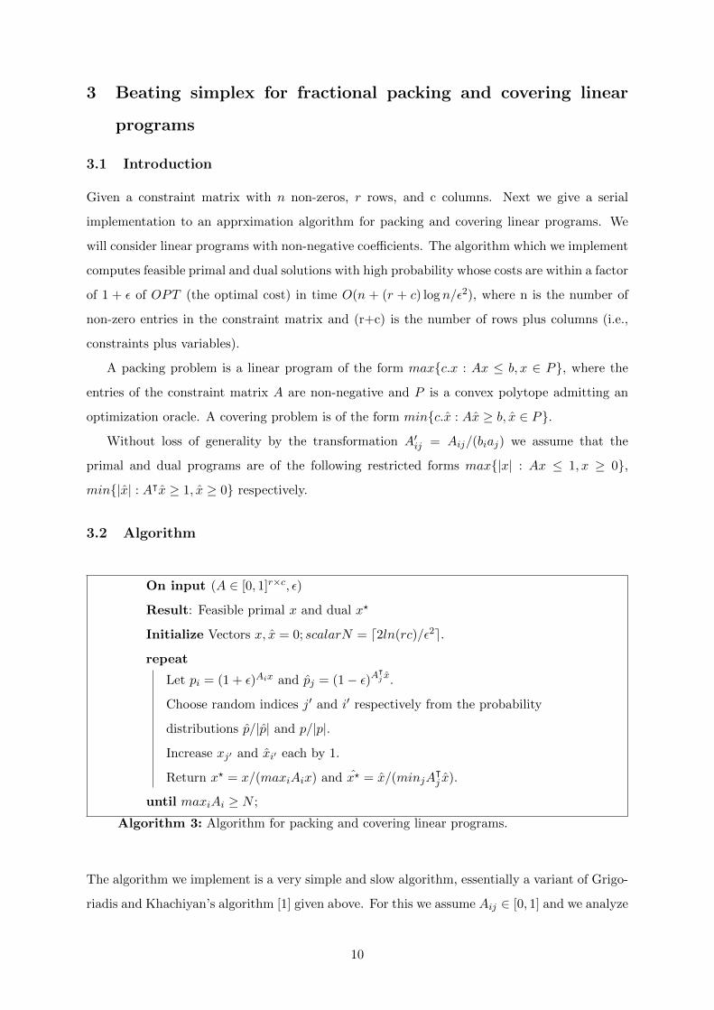
Given a constraint matrix with n non-zeros, r rows, and c columns. Next we give a serial
implementation to an apprximation algorithm for packing and covering linear programs. We
will consider linear programs with non-negative coefficients. The algorithm which we implement
computes feasible primal and dual solutions with high probability whose costs are within a factor
of 1 + ε of OPT (the optimal cost) in time O(n + (r + c) log n/ε2), where n is the number of
non-zero entries in the constraint matrix and (r+c) is the number of rows plus columns (i.e.,
constraints plus variables).
A packing problem is a linear program of the form max{c.x : Ax ≤ b, x ∈ P}, where the
entries of the constraint matrix A are non-negative and P is a convex polytope admitting an
optimization oracle. A covering problem is of the form min{c.x : Ax ≥ b, x ∈ P}.
Without loss of generality by the transformation A′ij = Aij/(biaj) we assume that the
primal and dual programs are of the following restricted forms max{|x| : Ax ≤ 1, x ≥ 0},
min{|x| : Aᵀx ≥ 1, x ≥ 0} respectively.
3.2 Algorithm
On input (A ∈ [0, 1]r×c, ε)
Result: Feasible primal x and dual x?
Initialize Vectors x, x = 0; scalarN = d2ln(rc)/ε2e.
repeat
Let pi = (1 + ε)Aix and pj = (1− ε)Aᵀj x.
Choose random indices j′ and i′ respectively from the probability
distributions p/|p| and p/|p|.
Increase xj′ and xi′ each by 1.
Return x? = x/(maxiAix) and x? = x/(minjAᵀj x).
until maxiAi ≥ N ;
Algorithm 3: Algorithm for packing and covering linear programs.
The algorithm we implement is a very simple and slow algorithm, essentially a variant of Grigo-
riadis and Khachiyan’s algorithm [1] given above. For this we assume Aij ∈ [0, 1] and we analyze
10
the ruuning time. This algorithm demonstrates the use of coupled random increments to the
primal and dual. At the end of the iteration the algorithm returns a (1 − 2ε)-approximate
primal-dual pair with high probability.
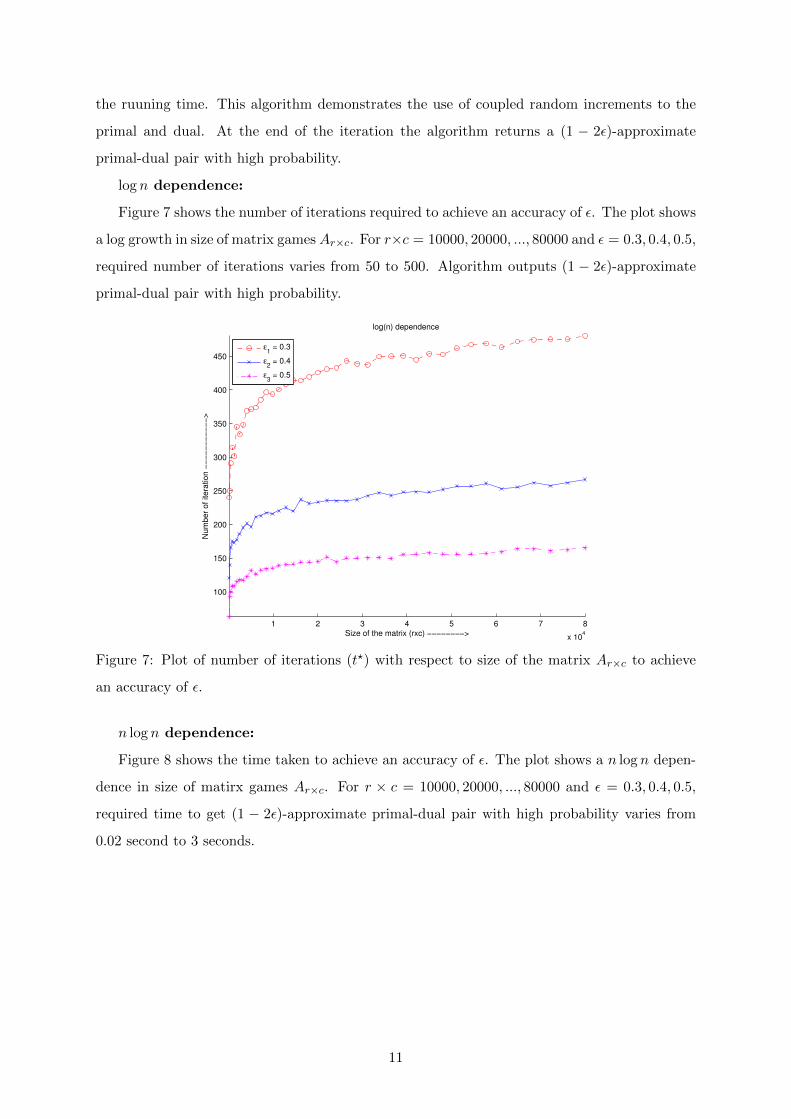
log n dependence:
Figure 7 shows the number of iterations required to achieve an accuracy of ε. The plot shows
a log growth in size of matrix gamesAr×c. For r×c = 10000, 20000, ..., 80000 and ε = 0.3, 0.4, 0.5,
required number of iterations varies from 50 to 500. Algorithm outputs (1 − 2ε)-approximate
primal-dual pair with high probability.
1 2 3 4 5 6 7 8
x 104
100
150
200
250
300
350
400
450
Num
ber
of itera
tion −
−−
−−
−−
−−
−−
>
Size of the matrix (rxc) −−−−−−−−>
log(n) dependence
ε1 = 0.3
ε2 = 0.4
ε3 = 0.5
Figure 7: Plot of number of iterations (t?) with respect to size of the matrix Ar×c to achieve
an accuracy of ε.
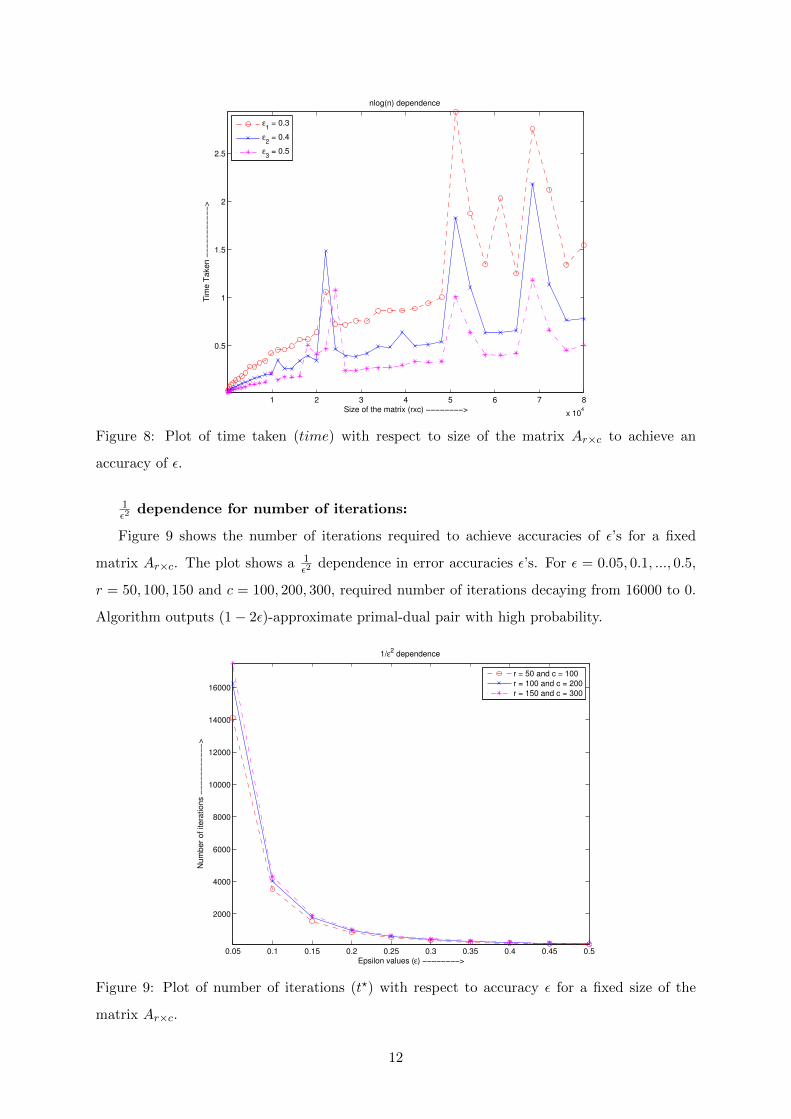
n log n dependence:
Figure 8 shows the time taken to achieve an accuracy of ε. The plot shows a n log n depen-
dence in size of matirx games Ar×c. For r × c = 10000, 20000, ..., 80000 and ε = 0.3, 0.4, 0.5,
required time to get (1 − 2ε)-approximate primal-dual pair with high probability varies from
0.02 second to 3 seconds.
11
1 2 3 4 5 6 7 8
x 104
0.5
1
1.5
2
2.5
Tim
e T
aken −
−−
−−
−−
−−
−−
>
Size of the matrix (rxc) −−−−−−−−>
nlog(n) dependence
ε1 = 0.3
ε2 = 0.4
ε3 = 0.5
Figure 8: Plot of time taken (time) with respect to size of the matrix Ar×c to achieve an
accuracy of ε.
1ε2
dependence for number of iterations:
Figure 9 shows the number of iterations required to achieve accuracies of ε’s for a fixed
matrix Ar×c. The plot shows a 1ε2
dependence in error accuracies ε’s. For ε = 0.05, 0.1, ..., 0.5,
r = 50, 100, 150 and c = 100, 200, 300, required number of iterations decaying from 16000 to 0.
Algorithm outputs (1− 2ε)-approximate primal-dual pair with high probability.
0.05 0.1 0.15 0.2 0.25 0.3 0.35 0.4 0.45 0.5
2000
4000
6000
8000
10000
12000
14000
16000
Num
ber
of itera
tions −
−−
−−
−−
−−
−−
>
Epsilon values (ε) −−−−−−−−>
1/ε2 dependence
r = 50 and c = 100
r = 100 and c = 200
r = 150 and c = 300
Figure 9: Plot of number of iterations (t?) with respect to accuracy ε for a fixed size of the
matrix Ar×c.
12
1ε2
dependence for time taken:
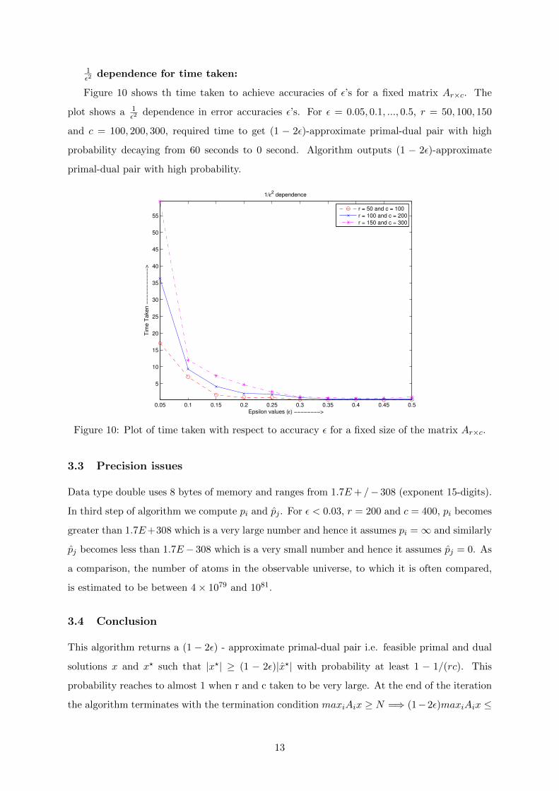
Figure 10 shows th time taken to achieve accuracies of ε’s for a fixed matrix Ar×c. The
plot shows a 1ε2
dependence in error accuracies ε’s. For ε = 0.05, 0.1, ..., 0.5, r = 50, 100, 150
and c = 100, 200, 300, required time to get (1 − 2ε)-approximate primal-dual pair with high
probability decaying from 60 seconds to 0 second. Algorithm outputs (1 − 2ε)-approximate
primal-dual pair with high probability.
0.05 0.1 0.15 0.2 0.25 0.3 0.35 0.4 0.45 0.5
5
10
15
20
25
30
35
40
45
50
55
Tim
e T
aken −
−−
−−
−−
−−
−−
>
Epsilon values (ε) −−−−−−−−>
1/ε2 dependence
r = 50 and c = 100
r = 100 and c = 200
r = 150 and c = 300
Figure 10: Plot of time taken with respect to accuracy ε for a fixed size of the matrix Ar×c.
3.3 Precision issues
Data type double uses 8 bytes of memory and ranges from 1.7E+ /− 308 (exponent 15-digits).
In third step of algorithm we compute pi and pj . For ε < 0.03, r = 200 and c = 400, pi becomes
greater than 1.7E+308 which is a very large number and hence it assumes pi =∞ and similarly
pj becomes less than 1.7E− 308 which is a very small number and hence it assumes pj = 0. As
a comparison, the number of atoms in the observable universe, to which it is often compared,
is estimated to be between 4× 1079 and 1081.
3.4 Conclusion
This algorithm returns a (1 − 2ε) - approximate primal-dual pair i.e. feasible primal and dual
solutions x and x? such that |x?| ≥ (1 − 2ε)|x?| with probability at least 1 − 1/(rc). This
probability reaches to almost 1 when r and c taken to be very large. At the end of the iteration
the algorithm terminates with the termination condition maxiAix ≥ N =⇒ (1−2ε)maxiAix ≤
13
minjAᵀj x. Due to limited precision arithmetic in our implementation we have verified the
assertion condition with yes instance and |x| = |x| =⇒ the perfomance guarantee.
? ? ?
14
4 Implementation of Fast Algorithm for Approximate Semidef-
inite Programming using the Multiplicative Weights Update
Method
4.1 Introduction
Semidefinite programming SDP solves the following problem:
min c •X
such that Aj •X ≥ bj , for j = 1, 2, ...,m.
and X � 0. —— (1)
Where X ∈ Rn×n is a matrix of variables and A1, A2, ..., Am ∈ Rn×n. For n× n matrices A
and B, A • B is their inner product (A • B =∑
ij AijBij) treating them as vector in Rn2, and
A � 0 is notation for A is positive semidefinite.
The first polynomial time algorithm, an apprximation algorithm that computes the solu-
tion up to any desired accuracy ε in polynomial time in log 1ε was via the Ellipsoid method.
Faster running time interior point methods were later given by Alizadeh [8] with running time
O(√m(m + n3)L), (O suppress polylog(mnε ) factor), where L is an input size parameter, and
Nesterov and Nemirovskii [9].
Our implementation contributes the modified multiplicative weights technique to handle
some of high-width SDPs and technique used is the multiplicative weights technique. Algorithm
we have implemented assume a feasibility version of the SDP (1). Here we have implicitly
performed a binary search on the optimum and the objective is converted to a constraint in the
standard way. Here one additional constraint has been assumed, a bound on the trace of the
solution:
Aj •X ≥ bj for j = 1, 2, ...,m.∑iXii ≤ R
X � 0. ———— (2)
For SDPs relaxation it is natural to put an upper bounds on trace, Tr(X) =∑
iXii. We have
solved the SDP approximately up to a given tolerance ε, by which we mean that either we find
a solution X which satisfies all the constraints up to an additive error of ε, i.e. Aj •X− bj ≥ −ε
for j = 1, 2, ...,m, or conclude correctly that the SDP is infeasible.
15
Multiplicative weights update method: We perform several iterations, indexed by time
t. Associate a non-negative weight w(t)j with constraint j, where
∑j w
(t)j = 1. A high current
weight for a constraint indicated that it was not satisfied too well in the past, and therefore
should receive higher priority in the next step. Thus the optimization problem to the next step
is to
max∑
j w(t)j (Aj •X − bj)∑iXii ≤ R
X � 0
Which represents an eigenvalue problem, since the optimum is attained at an X that has rank
1. Update the weights wi according to the usual multiplicative update rule, for some constant
β:
w(t+1)j = w
(t)j (1− β(AjXt − bj))/St.
Where Xt was the solution to the eigenvalue problem, expressed as a rank 1 PSD matrix, at a
time t, and St is the normalization factor to make the weights sum to 1, can be written as:
St =∑(t)
j (1− β(Aj •Xt − bj))
If β is small enough, the average 1T
∑Tt=1Xt is guaranteed to converge to a near-feasible solution
to the original SDP if we asuume a feasible solution exists.
4.2 Algorithm
Objective: maxA •X
Xii ≤ 1 for i = 1, 2, ..., n
X � 0
Assuming diag(A) ≥ 0. Let N ≥ n be the number of nonzero entries of A, our implementation
get a multiplicative 1−O(ε) apprximation to the optimum value of the SDP.
16
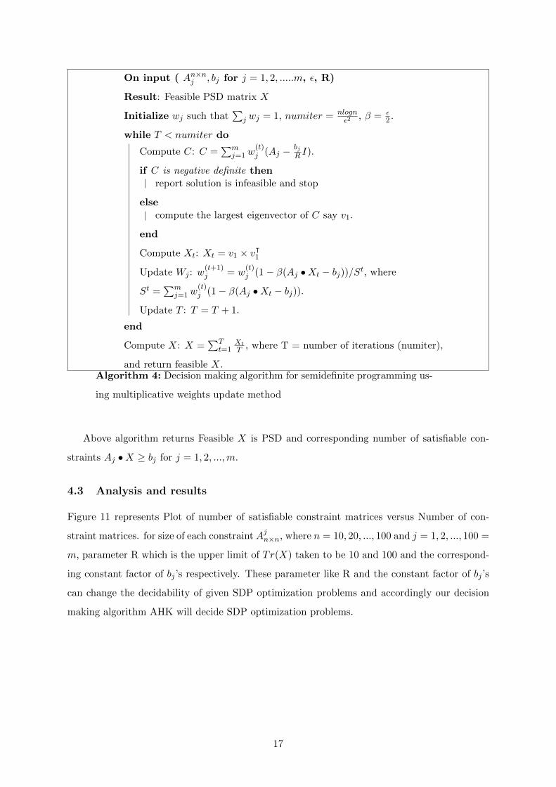
On input ( An×nj , bj for j = 1, 2, .....m, ε, R)
Result: Feasible PSD matrix X
Initialize wj such that∑
j wj = 1, numiter = nlognε2
, β = ε2 .
while T < numiter do
Compute C: C =∑m
j=1w(t)j (Aj − bj
R I).
if C is negative definite then
report solution is infeasible and stop
else
compute the largest eigenvector of C say v1.
end
Compute Xt: Xt = v1 × vᵀ1Update Wj : w
(t+1)j = w
(t)j (1− β(Aj •Xt − bj))/St, where
St =∑m
j=1w(t)j (1− β(Aj •Xt − bj)).
Update T : T = T + 1.
end
Compute X: X =∑T
t=1XtT , where T = number of iterations (numiter),
and return feasible X.Algorithm 4: Decision making algorithm for semidefinite programming us-
ing multiplicative weights update method
Above algorithm returns Feasible X is PSD and corresponding number of satisfiable con-
straints Aj •X ≥ bj for j = 1, 2, ...,m.
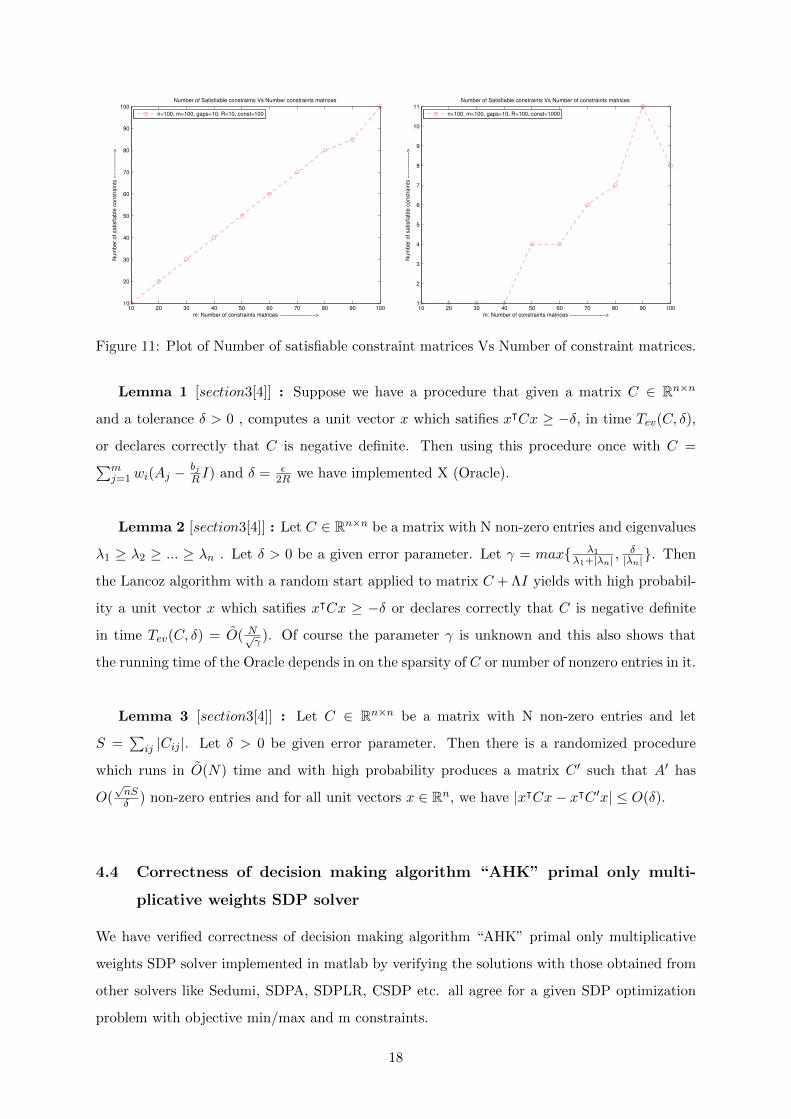
4.3 Analysis and results
Figure 11 represents Plot of number of satisfiable constraint matrices versus Number of con-
straint matrices. for size of each constraint Ajn×n, where n = 10, 20, ..., 100 and j = 1, 2, ..., 100 =
m, parameter R which is the upper limit of Tr(X) taken to be 10 and 100 and the correspond-
ing constant factor of bj ’s respectively. These parameter like R and the constant factor of bj ’s
can change the decidability of given SDP optimization problems and accordingly our decision
making algorithm AHK will decide SDP optimization problems.
17
10 20 30 40 50 60 70 80 90 10010
20
30
40
50
60
70
80
90
100
m: Number of constraints matrices −−−−−−−−−−−>
Nu
mb
er
of
sa
tisfia
ble
co
nstr
ain
ts −
−−
−−
−−
−>
Number of Satisfiable constraints Vs Number constraints matrices
n=100, m=100, gaps=10, R=10, const=100
10 20 30 40 50 60 70 80 90 1001
2
3
4
5
6
7
8
9
10
11
m: Number of constraints matrices −−−−−−−−−−−>
Nu
mb
er
of
sa
tisfia
ble
co
nstr
ain
ts −
−−
−−
−−
−>
Number of Satisfiable constraints Vs Number of constraints matrices
n=100, m=100, gaps=10, R=100, const=1000
Figure 11: Plot of Number of satisfiable constraint matrices Vs Number of constraint matrices.
Lemma 1 [section3[4]] : Suppose we have a procedure that given a matrix C ∈ Rn×n
and a tolerance δ > 0 , computes a unit vector x which satifies xᵀCx ≥ −δ, in time Tev(C, δ),
or declares correctly that C is negative definite. Then using this procedure once with C =∑mj=1wi(Aj −
bjR I) and δ = ε
2R we have implemented X (Oracle).
Lemma 2 [section3[4]] : Let C ∈ Rn×n be a matrix with N non-zero entries and eigenvalues
λ1 ≥ λ2 ≥ ... ≥ λn . Let δ > 0 be a given error parameter. Let γ = max{ λ1λ1+|λn| ,
δ|λn|}. Then
the Lancoz algorithm with a random start applied to matrix C + ΛI yields with high probabil-
ity a unit vector x which satifies xᵀCx ≥ −δ or declares correctly that C is negative definite
in time Tev(C, δ) = O( N√γ ). Of course the parameter γ is unknown and this also shows that
the running time of the Oracle depends in on the sparsity of C or number of nonzero entries in it.
Lemma 3 [section3[4]] : Let C ∈ Rn×n be a matrix with N non-zero entries and let
S =∑
ij |Cij |. Let δ > 0 be given error parameter. Then there is a randomized procedure
which runs in O(N) time and with high probability produces a matrix C ′ such that A′ has
O(√nSδ ) non-zero entries and for all unit vectors x ∈ Rn, we have |xᵀCx− xᵀC ′x| ≤ O(δ).
4.4 Correctness of decision making algorithm “AHK” primal only multi-
plicative weights SDP solver
We have verified correctness of decision making algorithm “AHK” primal only multiplicative
weights SDP solver implemented in matlab by verifying the solutions with those obtained from
other solvers like Sedumi, SDPA, SDPLR, CSDP etc. all agree for a given SDP optimization
problem with objective min/max and m constraints.
18
SDP:
Max A0 •X
subject to Aj •X = bj , j = 1, 2, ...,m
X � 0, X is n× n PSD.
Where m is the number of constraint matrices and n is size of constraint square matrices
Aj ’s and X.
“AHK” solves (original problem):
Max A0 •X
Subject to Aj •X ≥ bj for j = 1, 2, ...,m
X ≥ 0, X is n× n PSD.
SDPA, Sedumi and other solver solves (Translating SDP’s):
Max A0 •X
Subject to Aj •X − yj = bj
Where new PSD Y will look like
Y =
Xn×n 0n×m
0m×n yj
� 0, for j = 1, 2, ...,m
and thus Y � 0, Y is (n+m)× (n+m) PSD. Y PSD ensures y1, y2, ..., ym are all positive and
X is PSD. This is becaouse det(Y − λI) = (λ − y1)(λ − y2)...(λ − ym).det(X − λI) = 0. All
roots non-negative imply y1 ≥ 0, y2 ≥ 0, ..., ym ≥ 0 and all roots of det(X−λI) ≥ 0, as X is PSD.
Things to be done to check correctness of the decision making algorithm “AHK”:
1. Solve SDP optimization problem using decision making algorithm “AHK” and check how
many constraints are satisfiable (feasible). (say K)
2. Solve SDP optimization problem using SDPA, SeDuMi and others with exactly K con-
straint and an A0 objective. Find Optimal value (say A0Opt).
3. Now give SDP optimization problem to the decision making algorithm “AHK” with ex-
actly K constraints plus add an extra constraint A0 to AHK (i.e. Max A0 •X = A0Opt).
Thus now we have:
K constraints + A0 •X ≥ A0Opt ± δ, for small δ ≥ 0, we may assume δ = ε. Thus the decision
making algorithm “AHK” should give
19
A0 •X ≥ A0Opt − δ : feasible (satisfiable) and
A0 •X ≥ A0Opt + δ : infeasible (not satisfiable).
Feasible A0 •X ≥ A0Opt− δ and infeasible A0 •X ≥ A0Opt+ δ guarantee that the decision mak-
ing algorithm “AHK” is correct and gives correct primal objective optimal solution of SDP’s
optimization problems.
Checking the decision making algorithm “AHK”’s correctness with following example.
Input for decision making algorithm “AHK”:
n = 2,m = 3, A0 =
−11 0
0 23
, A1 =
10 4
4 0
, A2 =
0 0
0 −8
, A3 =
0 −8
−8 −2
, b =
−48
−8
−20
.
Decision making algorithm “AHK” output: K = 3 (all three constraints satisfiable (feasible))
Give this SDP optimization problem to SDPA, Sedumi and other solvers. SDPA, SeDuMi,
etc output:
objValPrimal = +2.3000000262935881e+01
objValDual = +2.2999999846605416e+01
Now give SDP optimization problem back to the decision making algorithm “AHK” with 4
constraints, “AHK” outputs:
For n = 2,m = 3 + 1 = K + 1, ε = 0.01, R ≥ 11, (since Trace(X) ≤ R, δ = 0.01 and
A0Opt = 23.0, we get
A0 •X ≥ A0Opt + δ : infeasible (not satisfiable)
A0 •X ≥ A0Opt − δ : feasible (satisfiable).
4.5 Solving Optimization problems using decision making algorithm AHK
The decision making algorithm AHK is a deterministic algorithm, when considered theoretically
(numerical stability other issues left aside).
The only parameter that was in our control is R (Trace(X) ≤ R). We have selected R=100
in all the experiments.
The β, for the multiplicative weights, paper AHK05, Section 1.1 page 3, column 1 is se-
lected by us as β = min(0.01, ε/2) and maximum number of iterations before timeout is
20
max(1000, 16 × lognε2
). The only other reason we give an error is when C becomes negative
semi-definite [C is on page 6 in AHK05] during iterations. The effective optimal values we have
written in table represents the effective lower bound of optimal value that we can be obtained
for each epsilon accuracy.
SDPA package SDP:
Min b.x
subject to∑Aj .xA0 = X, for j = 1, 2, ...,m
X � 0, X is PSD, n× n (Primal)
and
Max A0 • Y
subject to Aj • Y = bj , for j = 1, 2, ...,m
Y � 0, Y is PSD, n× n (Dual)
Decision making algorithm AHK SDP:
Max A0 •X
Subject to Aj •X ≥ bj , for j = 1, 2, ...,m
X � 0
Trace(X) ≤ R, X is n× n PSD.
SDPA package SDP to decision making algorithm AHK SDP:
Min −A0 •X
subject to
Aj •X ≥ bj − ε
−Aj •X ≥ −bj − ε,
for j = 1, 2, ...,m
X � 0
Trace(X) ≤ R, X is n× n PSD.
To get lower bound of optimum value by this decision making algorithm AHK, we add one
more constraint to AHK i.e. Objective constraint matrix.
(2m +1)th constraint will be −A0 •X ≥ −(A0Opt ± δ), where A0Opt is optimal objective value.
To get lower bound of optimum objective value by AHK decision making algorithm, AHK
will decide 2m constraints + one objective constraint −A0 •X ≥ −(A0Opt ± δ). Where A0Opt
is the optimum (minimum here) objective value (guessed) of the given SDP.
21
Hence AHK decision algorithm will solve and decide 2m + 1 constraints and correctly satisfy
with A0Opt and correctly gives lower bound of optimum objective value of a given SDP.
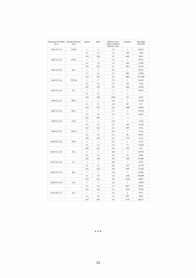
Given optimization problems (m is number of constraints and n is size of each constraints
square matrices) table represents the effective lower bound of optimal objective value, number
of iterations and time taken to get this lower bound. (optimization problems taken from SD-
PALIB 1.2)
Results:
(m= number of constraints, for nxn PSD matrix X, with inequalties satisfied upto additive
error eps) each iteration is a selection of the eigenvector, e, corresponding to the largest eigen-
value λ of the new weighted cumulative constraint matrix by the lanczos method and adding
eᵀ × e to the current solution.
22
Optimization Problem (m, n)
Optimal Objective value
Epsilon Delta Effective Lower bound of Optimal Objective value
Iterations Time taken (Seconds)
hinf1 (13, 14) 2.0326 1 1 -1.5 1 0.0175
0.1 0.1 1.6 190 1.286
0.01 0.01 4.7 2442 28.61
hinf2 (13, 16) 10.967 1 1 -1.5 1 0.0131
0.1 0.1 1.6 180 1.2995
0.01 0.01 4.7 2407 31.433
hinf3 (13, 16) 56.9 1 1 -5.9 1 0.0137
0.1 0.1 -2.7 884 8.1968
0.01 0.01 -0.2 4882 125.5089
hinf4 (13, 16) 274.764 1 1 -17.2 1 0.0143
0.1 0.1 -2.7 145 1.055
0.01 0.01 -0.2 2434 32.034
hinf5 (13, 16) 363 1 1 -1 1 0.0137
0.1 0.1 ----- ---- ----
0.01 0.01 188.8 131 0.947
hinf6 (13, 14) 449.0 1 1 -10.7 1 0.0138
0.1 0.1 -2.6 187 1.37
0.01 0.01 14.6 1088 10.6997
hinf7 (13, 16) 391.0 1 1 -27 1 0.0134
0.1 0.1 -2.6 74 0.4967
0.01 0.01 ---- ----- ---
hinf8 (13, 16) 116.0 1 1 -17.6 1 0.130
0.1 0.1 -2.7 149 1.0176
0.01 0.01 -0.2 2507 32.55
hinf9 (13, 16) 236.25 1 1 -26.2 1 0.129
0.1 0.1 -2.7 96 0.6517
0.01 0.01 -0.2 1775 19.53
hinf10 (21, 18) 109.0 1 1 -35.1 1 0.278
0.1 0.1 -4.3 75 0.6218
0.01 0.01 -0.4 1375 16.8
hinf11 (31, 22) 65.9 1 1 -40.8 1 0.0279
0.1 0.1 -6.3 76 0.805
0.01 0.01 -0.6 1344 21.089
hinf12 (43, 24) 0.2 1 1 -16.5 1 0.272
0.1 0.1 -8.6 703 10.794
0.01 0.01 -0.8 2876 73.204
hinf13 (57, 30) 46.0 1 1 -3.8 1 0.0363
0.1 0.1 -1.8 3540 160.998
0.01 0.01 -0.5 21493 4390.1
hinf14 (73, 34) 13.0 1 1 -2.9 1 0.0483
0.1 0.1 -1.3 4821 381.61
0.01 0.01 -0.1 7819 734.56
hinf15 (91, 37) 25.0 1 1 -3.2 1 0.071
0.1 0.1 -1.5 3567 296.6
0.01 0.01 -0.1 6734 924.75
? ? ?
23
5 Data Streaming and Online Algorithms: Matrix Multiplica-
tive weights
5.1 Introduction
For a symmetric matrix A, we let λ1(A) ≥ λ2(A) ≥ ... ≥ λn(A) denote its eigenvalues. Imag-
ine a matrix generalization of the usual 2-player zero-sum game. one player chooses a unit
vector v ∈ Sn−1. The other player chooses a matrix M such that 0 � M � I. The first
player has to pay the second vᵀMv = M • vvᵀ. We allow the first player to choose his vector
from a distribution D over Sn−1. We are interested in expected loss of the first player, that is
ED[vᵀMv] = M • ED[vvᵀ]. The matrix P = ED[vvᵀ] is a density matrix, it is positive semidefi-
nite and has trace 1. (Density matrices which appear in quantum computation). Consider an
online version of this game where the first player has to react to an external adversary who
picks a matrix M at each step; this is called an observed event. An online algorithm for the
first player chooses a density matrix P (t), and observe the event matrix M (t) in each round
t = 1, 2, ..., T . After T rounds, the best fixed vector for the first player in hindsight is the
unit vector v which minimizes the total loss∑T
t=1 vᵀM (t)v. This minimized when v is the unit
eigenvector of∑T
t=1M(t) corresponding to the smallest eigenvalue.
Our goal is to implement an algorithm whose total expected loss over the T rounds is not much
more than the minimum loss λn(∑T
t=1M(t)).
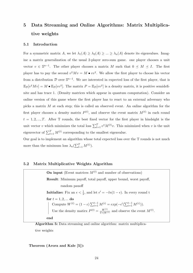
5.2 Matrix Multiplicative Weights Algorithm
On input (Event matrices M (t) and number of observations)
Result: Minimum payoff, total payoff, upper bound, worst payoff,
random pauoff
Initialize: Fix an ε < 12 , and let ε′ = −ln(1− ε). In every round t
for t = 1, 2, ... do
Compute W (t) = (1− ε)∑t−1
i=1M(i) = exp(−ε′(
∑t−1i=1M
(i))).
Use the density matirx P (t) = W (t)
Tr(W (t) and observe the event M (t).
end
Algorithm 5: Data streaming and online algorithm: matrix multiplica-
tive weights
Theorem (Arora and Kale [5]):
24
The matrix Multiplicative weights Update algorithm generates density matrices P 1, P 2, ..., P T
such that∑T
t=1M(t) • P (t) ≤ (1 + ε)λn(
∑Tt=1M
(t)) + lnnε .
We have implemented natrix multiplicative weights algorithm with the matrix exponent
function.
Problem:
You have to provide a density matrix P ( a positive semidefinite matrix PSD with trace 1 that
appears in quantum computation) at every unit of time.
After you provide the matrix, we matchers will evaluate your strategy for current set of obser-
vations.
At every unit of time, the environment gives you a positive semidefinite matrix,M, 0 ≤M ≤
I.
You incure a cost P ?M .
Your aim is to minimize the cost when the game is repeated T times. T is hopefully large, say
hundred at least usually.
5.3 Our experimental results
1. As T becomes large matrix exponents gives a strategy density that is quit responsible.
• For 100× 100 matrices T = 100, a 60% premium on [clairvoyant] optimal that drops
to a 10% premium on [clairvoyant] optimal for T = 1000.
• A random density matrix on the other hand, will cost you atleast a factor of say four.
2. The result is interesting as the largest eigenvector strategy that could incure the maximum
payoff (worst case algorithms analysis) grows atleast linearly in the matrix dimension and
could cost you say a factor of 100 more. So the worst strategy could be very very expensive
so on average we are doing very well.
It can be seen a data streaming online problem, as at every instant we matchers only store
O(n2) data (does not depend on T).
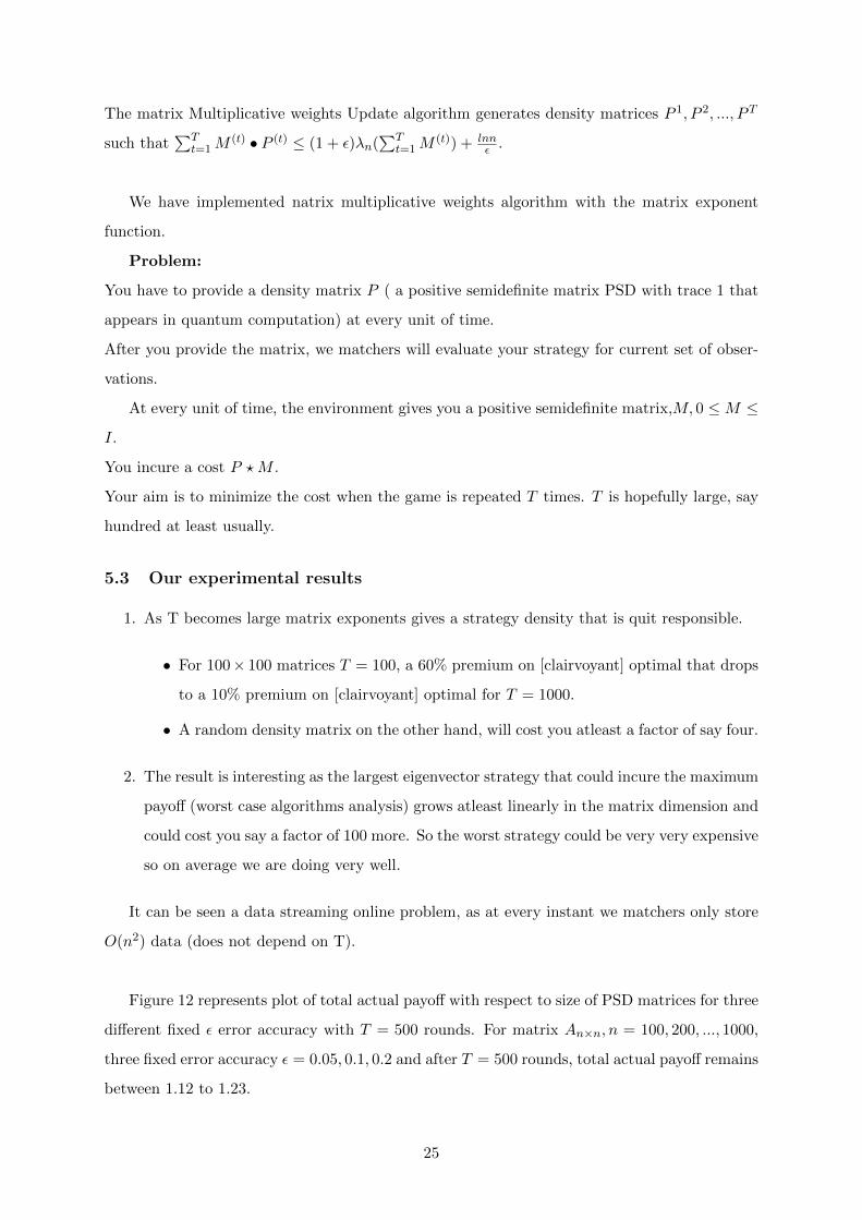
Figure 12 represents plot of total actual payoff with respect to size of PSD matrices for three
different fixed ε error accuracy with T = 500 rounds. For matrix An×n, n = 100, 200, ..., 1000,
three fixed error accuracy ε = 0.05, 0.1, 0.2 and after T = 500 rounds, total actual payoff remains
between 1.12 to 1.23.
25
100 200 300 400 500 600 700 800 900 1000
1.14
1.16
1.18
1.2
1.22
1.24
1.26
n: size of PSD matrices −−−−−−−−−−−>
To
tal p
ayo
ff −
−−
−−
−−
−>
Total payoff Vs size of PSD matrices
ε = 0.05
ε = 0.1
ε = 0.2
Figure 12: Plot of total actual payoff with respect to size of PSD matrices for three different
fixed ε error accuracy with T = 500 rounds.
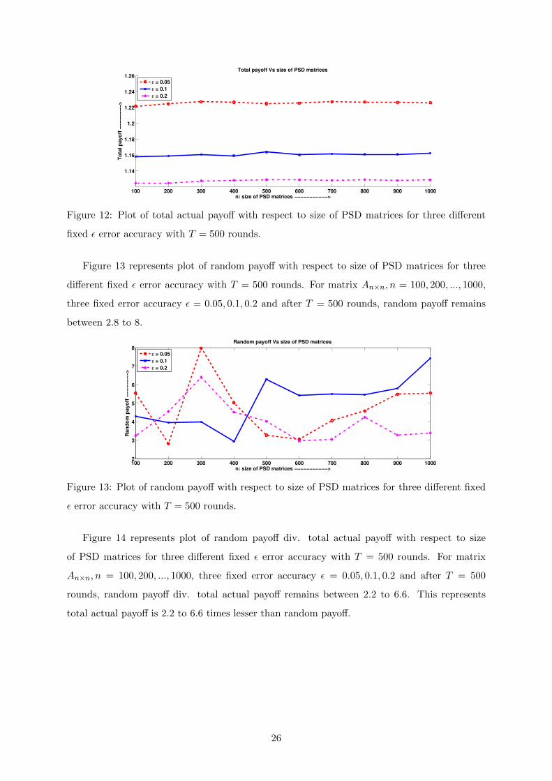
Figure 13 represents plot of random payoff with respect to size of PSD matrices for three
different fixed ε error accuracy with T = 500 rounds. For matrix An×n, n = 100, 200, ..., 1000,
three fixed error accuracy ε = 0.05, 0.1, 0.2 and after T = 500 rounds, random payoff remains
between 2.8 to 8.
100 200 300 400 500 600 700 800 900 10002
3
4
5
6
7
8
n: size of PSD matrices −−−−−−−−−−−>
Ran
do
m p
ayo
ff −
−−
−−
−−
−>
Random payoff Vs size of PSD matrices
ε = 0.05
ε = 0.1
ε = 0.2
Figure 13: Plot of random payoff with respect to size of PSD matrices for three different fixed
ε error accuracy with T = 500 rounds.
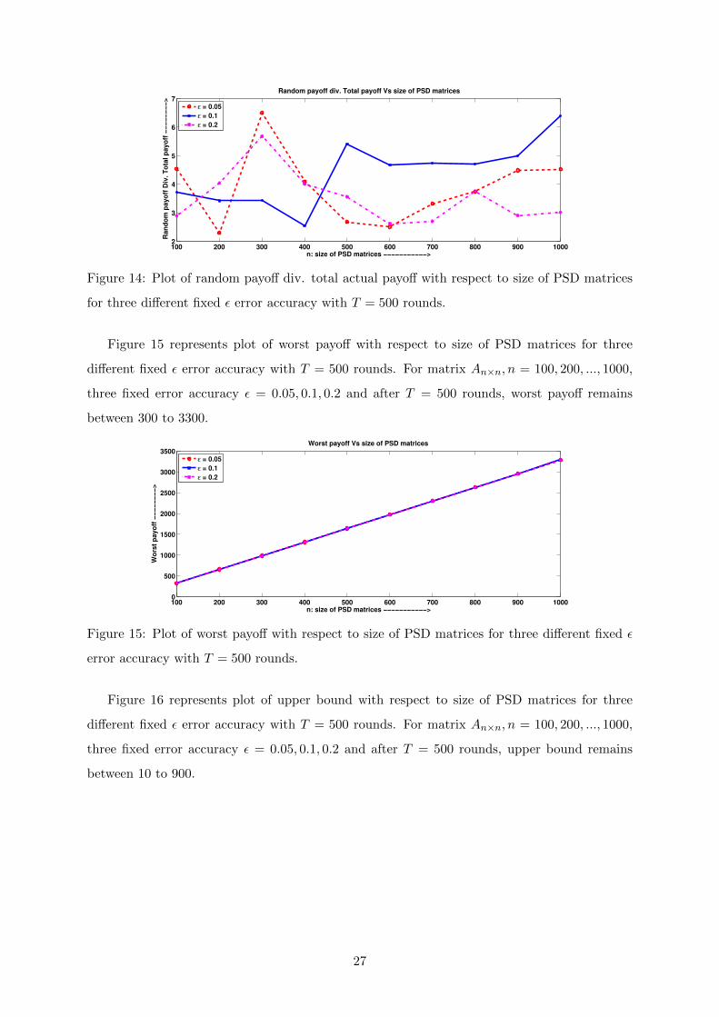
Figure 14 represents plot of random payoff div. total actual payoff with respect to size
of PSD matrices for three different fixed ε error accuracy with T = 500 rounds. For matrix
An×n, n = 100, 200, ..., 1000, three fixed error accuracy ε = 0.05, 0.1, 0.2 and after T = 500
rounds, random payoff div. total actual payoff remains between 2.2 to 6.6. This represents
total actual payoff is 2.2 to 6.6 times lesser than random payoff.
26
100 200 300 400 500 600 700 800 900 10002
3
4
5
6
7
n: size of PSD matrices −−−−−−−−−−−>
Ran
do
m p
ayo
ff D
iv. T
ota
l p
ayo
ff −
−−
−−
−−
−>
Random payoff div. Total payoff Vs size of PSD matrices
ε = 0.05
ε = 0.1
ε = 0.2
Figure 14: Plot of random payoff div. total actual payoff with respect to size of PSD matrices
for three different fixed ε error accuracy with T = 500 rounds.
Figure 15 represents plot of worst payoff with respect to size of PSD matrices for three
different fixed ε error accuracy with T = 500 rounds. For matrix An×n, n = 100, 200, ..., 1000,
three fixed error accuracy ε = 0.05, 0.1, 0.2 and after T = 500 rounds, worst payoff remains
between 300 to 3300.
100 200 300 400 500 600 700 800 900 10000
500
1000
1500
2000
2500
3000
3500
n: size of PSD matrices −−−−−−−−−−−>
Wo
rst
payo
ff −
−−
−−
−−
−>
Worst payoff Vs size of PSD matrices
ε = 0.05
ε = 0.1
ε = 0.2
Figure 15: Plot of worst payoff with respect to size of PSD matrices for three different fixed ε
error accuracy with T = 500 rounds.
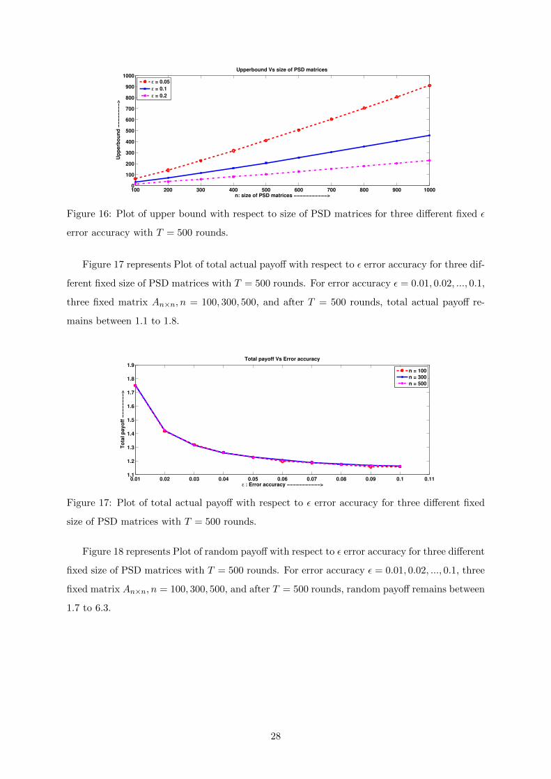
Figure 16 represents plot of upper bound with respect to size of PSD matrices for three
different fixed ε error accuracy with T = 500 rounds. For matrix An×n, n = 100, 200, ..., 1000,
three fixed error accuracy ε = 0.05, 0.1, 0.2 and after T = 500 rounds, upper bound remains
between 10 to 900.
27
100 200 300 400 500 600 700 800 900 10000
100
200
300
400
500
600
700
800
900
1000
n: size of PSD matrices −−−−−−−−−−−>
Up
perb
ou
nd
−−
−−
−−
−−
>
Upperbound Vs size of PSD matrices
ε = 0.05
ε = 0.1
ε = 0.2
Figure 16: Plot of upper bound with respect to size of PSD matrices for three different fixed ε
error accuracy with T = 500 rounds.
Figure 17 represents Plot of total actual payoff with respect to ε error accuracy for three dif-
ferent fixed size of PSD matrices with T = 500 rounds. For error accuracy ε = 0.01, 0.02, ..., 0.1,
three fixed matrix An×n, n = 100, 300, 500, and after T = 500 rounds, total actual payoff re-
mains between 1.1 to 1.8.
0.01 0.02 0.03 0.04 0.05 0.06 0.07 0.08 0.09 0.1 0.111.1
1.2
1.3
1.4
1.5
1.6
1.7
1.8
1.9
ε : Error accuracy −−−−−−−−−−−>
To
tal p
ayo
ff −
−−
−−
−−
−>
Total payoff Vs Error accuracy
n = 100
n = 300
n = 500
Figure 17: Plot of total actual payoff with respect to ε error accuracy for three different fixed
size of PSD matrices with T = 500 rounds.
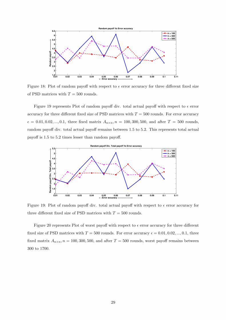
Figure 18 represents Plot of random payoff with respect to ε error accuracy for three different
fixed size of PSD matrices with T = 500 rounds. For error accuracy ε = 0.01, 0.02, ..., 0.1, three
fixed matrix An×n, n = 100, 300, 500, and after T = 500 rounds, random payoff remains between
1.7 to 6.3.
28
0.01 0.02 0.03 0.04 0.05 0.06 0.07 0.08 0.09 0.1 0.111.5
2
2.5
3
3.5
4
4.5
5
5.5
6
6.5
ε : Error accuracy −−−−−−−−−−−>
Ran
do
m p
ayo
ff −
−−
−−
−−
−>
Random payoff Vs Error accuracy
n = 100
n = 300
n = 500
Figure 18: Plot of random payoff with respect to ε error accuracy for three different fixed size
of PSD matrices with T = 500 rounds.
Figure 19 represents Plot of random payoff div. total actual payoff with respect to ε error
accuracy for three different fixed size of PSD matrices with T = 500 rounds. For error accuracy
ε = 0.01, 0.02, ..., 0.1, three fixed matrix An×n, n = 100, 300, 500, and after T = 500 rounds,
random payoff div. total actual payoff remains between 1.5 to 5.2. This represents total actual
payoff is 1.5 to 5.2 times lesser than random payoff.
0.01 0.02 0.03 0.04 0.05 0.06 0.07 0.08 0.09 0.1 0.111
1.5
2
2.5
3
3.5
4
4.5
5
5.5
ε : Error accuracy −−−−−−−−−−−>
Ran
do
m p
ayo
ff D
iv. T
ota
l p
ayo
ff −
−−
−−
−−
−>
Random payoff Div. Total payoff Vs Error accuracy
n = 100
n = 300
n = 500
Figure 19: Plot of random payoff div. total actual payoff with respect to ε error accuracy for
three different fixed size of PSD matrices with T = 500 rounds.
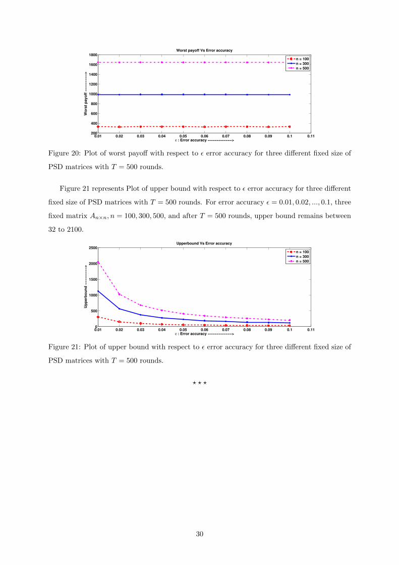
Figure 20 represents Plot of worst payoff with respect to ε error accuracy for three different
fixed size of PSD matrices with T = 500 rounds. For error accuracy ε = 0.01, 0.02, ..., 0.1, three
fixed matrix An×n, n = 100, 300, 500, and after T = 500 rounds, worst payoff remains between
300 to 1700.
29
0.01 0.02 0.03 0.04 0.05 0.06 0.07 0.08 0.09 0.1 0.11200
400
600
800
1000
1200
1400
1600
1800
ε : Error accuracy −−−−−−−−−−−>
Wo
rst
payo
ff −
−−
−−
−−
−>
Worst payoff Vs Error accuracy
n = 100
n = 300
n = 500
Figure 20: Plot of worst payoff with respect to ε error accuracy for three different fixed size of
PSD matrices with T = 500 rounds.
Figure 21 represents Plot of upper bound with respect to ε error accuracy for three different
fixed size of PSD matrices with T = 500 rounds. For error accuracy ε = 0.01, 0.02, ..., 0.1, three
fixed matrix An×n, n = 100, 300, 500, and after T = 500 rounds, upper bound remains between
32 to 2100.
0.01 0.02 0.03 0.04 0.05 0.06 0.07 0.08 0.09 0.1 0.110
500
1000
1500
2000
2500
ε : Error accuracy −−−−−−−−−−−>
Up
perb
ou
nd
−−
−−
−−
−−
>
Upperbound Vs Error accuracy
n = 100
n = 300
n = 500
Figure 21: Plot of upper bound with respect to ε error accuracy for three different fixed size of
PSD matrices with T = 500 rounds.
? ? ?
30
6 Implementation of primal-dual approach for approximately
solving SDPS
6.1 Introduction
Tis section implements a general primal-dual algorithm to compute a near-optimal solution to
any SDP and not just SDPs used in apprximation algorithms.
A general SDP with n2 variables, an n×n matrix variable X and m constraints and its dual
can be written as follows:
Max C •X
subject to Aj •X ≤ bj , for j = 1, 2, ...,m
X � 0 (Primal)
and
Min b.y
subject to∑m
j=1Ajyj � C
y ≥ 0 (Dual)
Where y = {y1, y2, ..., ym} are the dual variables and b = {b1, b2, ..., bm}. As in the case of
LP’s, strong duality holds for SDP’s under very mild conditions, always satisfied by the SDPs
here, and the optima of the two programs coincide. A leanear program is the special case
whereby all the matrices involved are diagonal.
For notational ease we assume that A1 = I and b1 = R. This serves to bound the trace
of the solution: Trace(X) ≤ R and is thus a simple scaling constraint. It is very naturally
present in SDP relaxations for combinatorial optimization problems. We assume that our
implementation of this algorithm uses binary search to reduce optimization to feasibility. Let
α be the algorithm’s current guess for the optimum value of the SDP. Implementation is trying
to either construct a PSD matrix that is primal feasible and has value > α. or a dual feasible
solution whose value is at most (1 + δ)α for some arbitrary small δ > 0.
6.2 Algorithm
As in usual in primal-dual algorithms, the algorithm starts with a trivial condidate for a primal
solution, in this case the trivial PSD matrix, possibly infeasible, of trace R, X(1) = Rn I. Then it
iteratively generates condidate primal solutions X(1), X(2), .... At every step it tries to improve
X(t) to obtain X(t+1), and in this it has help from ans auxiliary algorithm, called the ORACLE,
31
that tries to certify the validity of the current X(t) as follows: ORACLE searches for a vector
y from the polytope Dα = {y : y ≥ 0, b.y ≤ α} such that∑mj=1(Aj •X(t))yj − (C •X(t)) ≥ 0 ———— (?)
If ORACLE succeeds in finding such a y then we claim X(t) is either primal infeasible or
has value C •X(t) ≤ α. the reason is that otherwise∑mj=1(Aj •X(t))yj − (C •X(t)) ≤
∑mj=1 bjyj − (C •X(t)) < α− α = 0,
which would contradict (?). Thus y implicitly contains some usefull information to improve the
condidate primal X(t), and we use y to update X(t) using a matrix exponential update rule.
Our observation about matrix exponentials ensures that the new matrix X(t+1) is also PSD. If
ORACLE declares that there is no vector y ∈ Dα which satisfies ?, then it can be easily checked
using leanear programming duality that X(t) must be a primal feasible solution of objective
value atleast α.
Implementing ORACLE for Primal-Dual SDP: Calculating y using ORACLE
search
y ≥ 0, b1y1 + b2y2 + ...+ bmym ≤ α (1)
m∑j=1
(Aj •X(t))yj − (C •X(t)) ≥ 0 (2)
from (1)
y1 =α−
∑mj=2 bjyj − εb1
(3)
substitute (3) in (2)
(A1 •X(t))y1 +
m∑j=2
(Aj •X(t))yj ≥ C •X(t)
(A1 •X(t))(α−
∑mj=2 bjyj − εb1
) +m∑j=2
(Aj •X(t))yj ≥ C •X(t)
(A1 •X(t))α
b1−
(A1 •X(t))∑m
j=2 bjyj
b1− ε(A1 •X(t))
b1+
m∑j=2
(Aj •X(t))yj ≥ C •X(t)
m∑j=2
(Aj •X(t))yj −(A1 •X(t))
∑mj=2 bjyj
b1≥ C •X(t) +
ε(A1 •X(t))
b1− (A1 •X(t))
α
b1
m∑j=2
(Aj •X(t) − A1 •X(t)bjb1
)yj ≥ C •X(t) +ε(A1 •X(t))
b1− (A1 •X(t))
α
b1
32
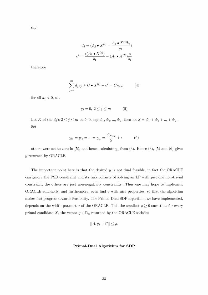
say
dj = (Aj •X(t) − A1 •X(t)bjb1
)
c? =ε(A1 •X(t))
b1− (A1 •X(t))
α
b1
therefore
m∑j=2
djyj ≥ C •X(t) + c? = CNew (4)
for all dj < 0, set
yj = 0, 2 ≤ j ≤ m (5)
Let K of the dj ’s 2 ≤ j ≤ m be ≥ 0, say dl1 , dl2 , ..., dlk , then let S = dl1 + dl2 + ...+ dlk .
Set
yl1 = yl2 = ... = ylk =CNewS
+ ε (6)
others were set to zero in (5), and hence calculate y1 from (3). Hence (3), (5) and (6) gives
y returned by ORACLE.
The important point here is that the desired y is not dual feasible, in fact the ORACLE
can ignore the PSD constraint and its task consists of solving an LP with just one non-trivial
constraint, the others are just non-negativity constraints. Thus one may hope to implement
ORACLE efficiently, and furthermore, even find y with nice properties, so that the algorithm
makes fast progress towards feasibility. The Primal-Dual SDP algorithm, we have implemented,
depends on the width parameter of the ORACLE. This the smallest ρ ≥ 0 such that for every
primal condidate X, the vector y ∈ Dα returned by the ORACLE satisfies
||Ajyj − C|| ≤ ρ.
Primal-Dual Algorithm for SDP
33
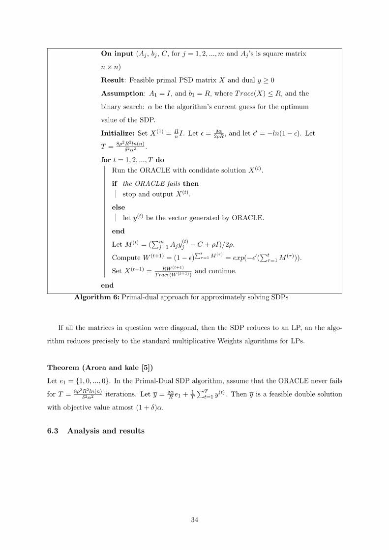
On input (Aj , bj , C, for j = 1, 2, ...,m and Aj ’s is square matrix
n× n)
Result: Feasible primal PSD matrix X and dual y ≥ 0
Assumption: A1 = I, and b1 = R, where Trace(X) ≤ R, and the
binary search: α be the algorithm’s current guess for the optimum
value of the SDP.
Initialize: Set X(1) = Rn I. Let ε = δα
2ρR , and let ε′ = −ln(1− ε). Let
T = 8ρ2R2ln(n)δ2α2 .
for t = 1, 2, ..., T do
Run the ORACLE with condidate solution X(t).
if the ORACLE fails then
stop and output X(t).
else
let y(t) be the vector generated by ORACLE.
end
Let M (t) = (∑m
j=1Ajy(t)j − C + ρI)/2ρ.
Compute W (t+1) = (1− ε)∑tτ=1M
(τ)= exp(−ε′(
∑tτ=1M
(τ))).
Set X(t+1) = RW (t+1)
Trace(W (t+1))and continue.
end
Algorithm 6: Primal-dual approach for approximately solving SDPs
If all the matrices in question were diagonal, then the SDP reduces to an LP, an the algo-
rithm reduces precisely to the standard multiplicative Weights algorithms for LPs.
Theorem (Arora and kale [5])
Let e1 = {1, 0, ..., 0}. In the Primal-Dual SDP algorithm, assume that the ORACLE never fails
for T = 8ρ2R2ln(n)δ2α2 iterations. Let y = δα
R e1 + 1T
∑Tt=1 y
(t). Then y is a feasible double solution
with objective value atmost (1 + δ)α.
6.3 Analysis and results
34
6.4 Correctness of primal-dual approach for approximately solving SDPS
“AK” multiplicative weights SDP solver
6.5 Solving Optimization problems using primal-dual approach for approxi-
mately solving SDPS “AK” multiplicative weights SDP solver
? ? ?
7 References
1. M.D. Grigoriadis and L.G. Khachiyan. A sublinear-time randomized apprximation algo-
rithm for matrix games. Operations Research Letters, 18(2):53-58, 1995.
2. Christos Koufogiannakis and Neal E. Young. Beating simplex for fractional packing and
covering linear programs. The 48th IEEE Symposium on Foundation of Computer Science
(FOCS 2007) (corrected version FOCS 2008).
3. Michael Luby and Noam Nisan. A parallel apprximation algorithm for positive linear
programming. In proceedings of the twenty-fifth annual ACM symposium on Theory of
computing, STOC ’93, pages 448-457, New York, NY, USA, 1993. ACM.
35
4. S. Arora, E. Hazan and S. Kale. Fast algorithms for approximate semidefinite program-
ming using the multiplicative weights update method. In Proceedings of the 46th Annual
IEEE Symposium on Foundations of Computer Science, pages 339-348, 2005.
5. S. Arora and S. Kale. A combinatorial, prima-dual approach to semidefinite programs.
In Proceedings of the Thirty-Ninth Annual ACM Symposium on Theory of Computing,
pages 227-236, 2007.
6. Rahul Jain and Penghui Yao. A parallel apprximation algorithm for positive semidefinite
programming. In FOCS, pages 463-471, 2011.
7. Rechard Peng and Kanat Tangwongsan. Faster and simpler width-independent parallel
algorithms for positive semidefinite programming. In CoRR abs/1201.5135, 2012.
8. F. Alizadeh. Interior Point Methods in Semidefinite Programming with Apprximation to
Combinatorial Optimization. SIAM J. Optim., 5(1):13-51, 1995.
9. Y. Nesterov and A. Nemirovskii. Interior Point Polynomial Methods in Convex Program-
ming: Theory and Applications. SIAM , Philadelphia, 1994.
10. Paul Christiano, Jonathan A. Kelner, Aleksander Madry, Daniel Spielman and Shang-
Huam Teng. Electrical flows, laplacian Systems, and faster apprximation of maximum
flow in undirected graphs. CoRR abs/1010.2921, 2010.
36


