Deriving Traffic-Performance Measures and Levels of Service from Second-Order Statistical Features of Spatiotemporal Traffic Contour Maps

Deriving Traffic Performance Measures and Levels of Service from Second-Order Statistical Features of Spatiotemporal Traffic Contour Maps

By Sherif Ishak

Department of Civil and Environmental Engineering Louisiana State University Baton Rouge, LA 70803 Phone: (225)-578-4846

Fax: (225)-578-8652 Email: [email protected]

Paper submitted for presentation at the Transportation Research Board

82nd Annual Meeting Washington, D.C. 2003

and for publication in the Transportation Research Record journal

Revised and Re-Submitted on November 7, 2002

TRB 2003 Annual Meeting CD-ROM Paper revised from original submittal.

Ishak, S. 2

ABSTRACT Currently, little information has been successfully extracted from the wealth of data collected by intelligent transportation systems (ITS). Such information is critical to maximize the efficiency of operation and management functions of traffic management centers (TMC). This research study presents a new set of second-order statistical measures that are derived from texture characterization techniques in the field of digital image analysis. The main objective of the study is to improve the data analysis tools used in performance monitoring systems and assessment of level of service. The new measures are capable of extracting properties such as smoothness, homogeneity, regularity, and randomness in traffic operations directly from constructed spatiotemporal traffic contour maps. To avoid information redundancy, a correlation matrix was examined for nearly 14,000 15-minute speed contour maps generated for a section of 3.4 miles of the freeway over a period of 5 weekdays. The process resulted in retaining a set of three second-order measures: angular second moment (ASM), contrast (CON), and entropy (ENT). Each measure was further analyzed to examine its sensitivity to various traffic conditions, expressed by the overall speed mean of each contour map. The study also presented a tentative approach, similar to the conventional one used in the highway capacity manual, to evaluate the level of service for each contour map. The new set of level of service criteria can be applied in real time using a standalone module that was developed in this study. The module can be readily implemented online and provides TMC operators with the flexibility of tuning a large set of related parameters.

KEYWORDS Freeway operations, performance measures, level of service, information extraction, texture characterization, contour maps, and second-order statistics.


Ishak, S. 3

INTRODUCTION As the ITS instrumentation efforts continue to pervade our urban freeway system nationwide, real-time data from hundreds of miles is simply being either archived or disposed of. Currently, little information has been utilized from the tremendous wealth of information that can be potentially extracted from this data. This is primarily due to the lack of advanced data mining methods that are specifically developed to maximize the utility of information extraction from existing surveillance systems. Such methods must be capable of manipulating large amounts of data for the purpose of extracting the most useful information while suppressing data redundancies. Essentially, the need for new methods was not justified in the past when real time transportation data acquisition in today’s quality and quantity was once a technological challenge. Today, we face another challenge; that is how to extract the most useful information from the plethora of data and maximize the efficiency of operation and management functions of traffic management centers (TMC). This can only be achieved through advanced analytical techniques and performance measures that have the capability to extract the most valuable information from real-time and archived data while reducing the overwhelming level of redundancies therein.

DATA MINING ISSUES The interest in knowledge discovery and data mining tools is continuously growing to face challenges in real-world applications (1,2). Many state-of-the-art techniques have been introduced to boost the capabilities of existing data mining tools. Even with today’s remarkable computer advancements, knowledge discovery from data is still intrinsically cumbersome. Yet, we continue to rely more and more on computers to accumulate data, process data, and make use of data while seeking intelligent tools to accomplish those tasks. Data preprocessing is an essential part of the knowledge discovery process and is vital to subsequent algorithms. For instance, incident detection algorithms rely on data collected from traffic patterns in the neighborhood of the incident time and location. Such algorithms are deemed sensitive to irrelevant and / or redundant features in the constructed traffic patterns. Today, we continue to face the challenge of dealing with ever-growing amounts of data, along with the limitations of data analysis tools and representations (3). Essentially, to get more useful findings from our data, we must first remove redundancies and make the data less. By doing so, we emphasize the concept “less is more” (4). This study focuses on improving knowledge discovery and data mining tools for performance assessment of freeway traffic operations under ITS. In the area of traffic operations and control under ITS, traffic management and control functions undertaken by traffic management centers and other related agencies are conducted through a series of sequential and parallel tasks that involve processing information and making decisions. Two major challenges face researchers and practitioners today. First, how can we extract the most relevant information for traffic management centers and other interested transportation agencies from the vast amount of data despite the tremendous redundancies therein? Second, how can we use such wealth of data to advance our level of understanding of the stochastic traffic behavior and to build robust decision support systems? To answer the first question, this research study presents new tools for extracting information from traffic patterns with the purpose of advancing the current performance measures on freeway systems. The new performance measures attempt to reveal properties undetectable by ordinary first-order statistical measures. In other words, the new measures characterize traffic operations in terms of smoothness,


Ishak, S. 4

homogeneity, regularity, etc., in a manner analogous to textural characterization of digital images.

BACKGROUND Conventional performance measures are usually selected to answer a few basic questions (5). For a highway facility, the questions are “how good was my trip?”, “how many of us did the system serve?”, “how well did the system move us?”, “how much of the system resources were used up in the process?”, and “are there deficiencies in the infrastructure?” The common measures used to answer the previous questions include travel time, speed, delay, volume, demand-to-capacity ratio, congestion extent and duration, and average vehicle occupancies. Those first-order statistical measures are used individually or collectively to evaluate the level of service on highway facilities (5-12). While those measures reveal common properties of the system operation, several other properties go undetected, and therefore, are the focus of this research study. Several research studies were conducted in the past on performance measures of freeway operations. However, only a few have addressed the problem at large scale operation, yet with first-order statistical measures only. For instance, a recent study in the area of freeway performance monitoring systems was conducted by Choe et al. (13) and emphasized the importance of using operational analysis tools in the context of PeMS (Freeway Performance Measurement System) in California. The study presented a comprehensive system that is capable of providing traffic management centers with uniform and comprehensive assessment of freeway performance in real time. The authors showed how the system can benefit several entities in transportation including both transportation system users and providers (planners, operators, etc.). The study emphasized a few applications such as bottleneck identification and analysis, level of service characterization, incident impacts, and assessment of ATMIS strategies. Another recent study attempted to capture special features and trends in travel times from day to day (14). In that study, the authors highlighted some issues related to feature extraction and proposed an unusualness measure for each day by comparing it with the average.

METHODOLOGY The methodology used in this study relies on the identification of a viable set of measures that is capable of extracting important features from spatiotemporal traffic contour maps in a manner analogous to extracting features from digital images in the field of image analysis and pattern recognition. Similar concept was applied to freeway operational analysis in the past to distinguish between incident and incident-free traffic patterns using artificial neural networks (see for instance; 15, 16). However, the feature extraction process in the context of this study is not primarily intended for pattern recognition application, but rather for revealing texture characteristics of spatiotemporal contour maps. The latest edition of the highway capacity manual (HCM) (11) describes the use of time-space domain contour maps (speed or density) in performance measures for freeway facilities. Contour maps can be used to identify valleys of low-speed or high-density regions. Consequently, contour maps can simply be considered pictorial representations of traffic conditions in time and space. With this concept in mind, spatiotemporal traffic contour maps can be analyzed using techniques developed for digital image analysis.


Ishak, S. 5

Several common techniques have been developed in the field of image analysis (17-20) to characterize image textures. Generally, texture description can be addressed using one of three approaches: structural, statistical, and combinations of both (18). Traditional structural approaches generate Fourier transforms of images and then derive measurements such as entropy, energy, inertia, etc. from the grouped transform data. Other popular approaches include wavelet transform and Gabor wavelet. The second alternative to analyze image details is the statistical approach (17, 18). The most recognized method is the co-occurrence matrix, which is built from pair-wise pixel information at different distances and relative inclination. The co-occurrence matrix measures spatial relationships, as opposed to frequency contents in structural approaches. Essentially, measures of entropy, energy, inertia, and others can be likewise derived from co-occurrence matrices. The third approach is a combination of the structural and statistical approaches. A recent approach was cited in (18) and combines geometrical structures with statistical ones. The approach is called statistical geometric features (SGF) and leads to measures of irregularity. In this study, we utilize the statistically based approach for its simplicity. The approach yields second-order statistical measures that will be described in detail later. Each measure quantifies a certain property of a spatiotemporal traffic contour map.

ASSUMPTIONS AND LIMITATIONS There are a few fundamental assumptions and limitations of the adopted approach. Since the approach draws on the subject of image analysis and feature extraction/generation, the term “traffic contour map” will be adopted throughout the paper to represent a spatiotemporal image of traffic conditions. Example of a traffic speed contour map plotted for the morning peak period in the eastbound direction of I-4 on April 3rd, 2001 is shown in FIGURE 1(a). Each contour map is composed of artificially constructed pixels in two dimensions: time and space. As shown in FIGURE 1(b), a pixel is defined as a single point measurement in the time space domain of the contour map and is generated from one data collection device (e.g. inductive loop detector or radar detector) at the end of fixed time intervals (usually in the order of 20 to 30 seconds). The intensity at each pixel can be expressed in terms of one of three traffic parameters (speed, volume, and lane occupancy) that are observed in real time. The approach has a limitation that should also be pointed out. The point measurements along a freeway system are often taken at distances in the order of one third to half a mile to reduce the instrumentation costs. This relatively large separation between data collection stations leads to lower spatial resolution in the constructed traffic contour map. In other words, variations in traffic conditions in the sections amid stations will be virtually impossible to capture. However, the emphasis of this study will be placed on relatively long segments of the freeway system (at least four or five miles long), and therefore, the details compromised by the low spatial resolution may not have a significant impact on the overall efficiency of the approach being proposed. Using contour maps with relatively small spatiotemporal dimensions, e.g. four miles by 15 minutes, leads to properties characterizing the texture of traffic at local levels, a scenario that is recommended for monitoring the local variations in spatiotemporal properties only. For system-wide monitoring, one contour map can be constructed for the entire freeway segment and the overall peak period, where the effect of coarse sampling is of less significance. In such case, the boundaries of an entire bottleneck will be encompassed within the boundaries of the contour map and the measured properties will reflect the overall performance of the system for a large time-space domain.


Ishak, S. 6

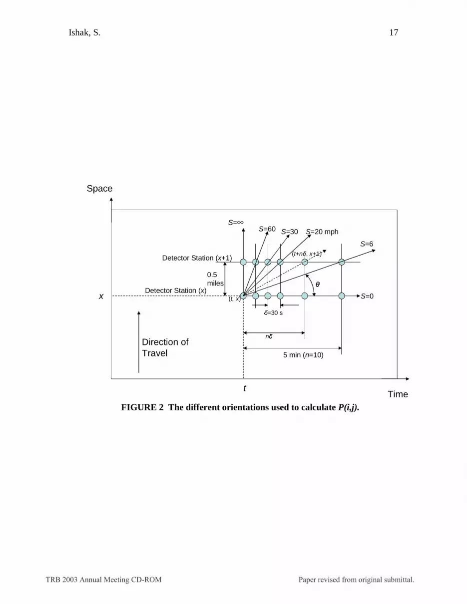
TEXTURE CHARACTERIZATION OF CONTOUR MAPS The study draws on the subject of image texture characterization to establish similar measures for traffic texture characterization in order to reveal high-resolution properties of the evolution of traffic conditions that cannot be otherwise detected by first-order statistical measures. The statistical approach adopted here relies on the construction of the co-occurrence matrices for relative distances and relative orientations between a point and all of its surroundings in the time-space domain of a traffic contour map as illustrated in FIGURE 2. The figure shows that the relative differences between each point (t,x) and its surroundings are taken at angles in the range from 0° to 360°. The angular variation was chosen such that a wide range of shockwave speeds is covered, when emanating from or into (t,x). Given that the spacing between two consecutive stations is nearly half a mile and that traffic measurements are taken every 30 seconds, it was found that the inclusion of 10 point measurements in the temporal dimension would result in the following shockwave speeds 0, 6, 6.7, 7.5, 8.6, 10, 12, 15, 20, 30, and 60 mph, starting from 0° and moving to 90° anticlockwise. Although the figure shows one quarter only (0° to 90°), the three remaining quarters (from 90° to 360°) can be similarly constructed as mirrors of the first quarter. Each point will be compared to each of the neighboring points as shown in FIGURE 2 in all orientations from 0° to 360°. For each angle (θ) (possible shockwave speed), a co-occurrence matrix can be constructed as follows:

(0,0) (0,1) . . (0, )

(1,0) (1,1) . . .1

. . . . .

. . . . .

( ,0) . . . ( , )

N

AR

N N N

θ

η η ηη η

η η

=

(1)

Where η(i,j) is the number of point pairs at angle θ that have values i and j, respectively. Mathematically,

,( , ) ( , ) 0,..., ; 0,...,i j t xt x

i j f t x t N x Nη = ∀ ∈ ∈∑∑ (2)

And

,

1 ( , ) ( , 1)( , )

0i j

if I t x i and I t n x jf t x

Otherwise

δ= ± ± ==

(3)

Where I(t,x) = the intensity at time t and location x, measured by one of the three traffic parameters (speed in this study). The value of I(t,x) was rounded off to multiples of 5 mph to suppress the effect of noise and minor disturbances in traffic conditions. Nt = Number of observations in the temporal dimension of the contour map Nx = Number of observations in the spatial dimension of the contour map n = Number of 30-second observations in reference to time t δ = Temporal resolution of the contour map (30 seconds in this study) R = the total number of possible pairs N = the depth of the traffic contour map, measured by the number of discrete levels of the representative traffic parameter (speed in this study)


Ishak, S. 7

P(i,j) = η(i,j)/R and is the basis for calculating each of the selected measures that are applied to nonlinear transforms of images. Next, we explain the set of measures proposed to explore the second-order properties of spatiotemporal speed contour maps.

Angular Second Moment (ASM) ASM is a measure of texture smoothness of digital images. If all point measurements in a spatiotemporal traffic contour map are identical, then the texture of the map can be characterized as “smooth” in the time-space domain considered. “Smoothness” in this context does not imply free-flow conditions, but rather uniform transitions or minor perturbations. On the other hand, low ASM indicates non-uniform transitions or high perturbations in traffic operations. ASM is mathematically defined as

1 12

0 0

( , )N N

i j

ASM P i j− −

= =

=∑∑ (4)

Where, P(i,j) = the probability of observing adjacent pairs of traffic contour map pixels with values i and j in all possible orientations; i.e. spatially, temporally, and spatiotemporally, as shown in FIGURE 2.

Contrast (CON) The measure of contrast is typically used to indicate the local color level variations in a digital image. Similarly, in a spatiotemporal traffic contour map, contrast emphasizes local variations in traffic conditions. Degree of local variations indicates the severity of disturbance in the region considered. Since traffic contour maps are spatiotemporal in nature, the local variations can be temporal (horizontal), spatial (vertical), or spatiotemporal (angular), in reference to FIGURE 2. High contrasts exhibit severe local disturbances that could be attributed to heavy weaving or merging maneuvers and abrupt changes in demand or capacity as a result of lane-blocking incidents. Mathematically, the contrast measure can be quantified as

1 1 12

0 0 0

( , )N N N

n i ji j n

CON n P i j− − −

= = =− =

=

∑ ∑∑ (5)

The contrast measure parameters are as defined before. n refers to the difference in the intensity levels of a pair of pixels in a digital image. For a spatiotemporal traffic contour map, this refers to the difference in the traffic parameter values of two adjacent point measurements either temporally, spatially, or spatiotemporally.

Inverse Difference Moment (IDF) IDF is a complimentary measure that relates inversely to the contrast measure. It is also a direct measure of the local homogeneity of a digital image. Low IDF is associated with low homogeneity and vice versa. For a traffic contour map, this property can be similarly measured to quantify the degree of homogeneity in traffic conditions in the time space domain. In mathematical terms, IDF is measured as

1 1

20 0

( , )

1 ( )

N N

i j

P i jIDF

i j

− −

= =

=+ −∑∑ (6)


Ishak, S. 8

Entropy (ENT) Entropy is a quantity widely used in information theory and is based on probability theory (19). It is often used to quantify the expected amount of surprise or uncertainty in a random variable. In information theory, entropy is considered to be the average amount of information received when a random variable is observed. Also, entropy can be used to measure the amount of randomness in a digital image. For a spatiotemporal traffic contour map, entropy can be defined mathematically as

1 1

20 0

( , ) log ( , )N N

txi j

ENT P i j P i j− −

= =

= −∑∑ (7)

Where, x and t refer to the spatial and temporal dimensions of the traffic contour map, respectively. High values of ENT indicate high randomness in traffic conditions and vice versa.

Additional Measures Additional second-order statistical measures have also been applied to quantify other properties including:

CORRELATION (CORR) = ( ) ( , ) x t

i j

x t

ij P i j µ µ

σ σ

−

∑∑

(8)

SUM ENTROPY (SUMENT) = 2 2

0

( ) log ( )N

x t x ti

P i P i−

+ +=∑ (9)

DIFFERENCE ENTROPY (DIFFENT) = 2 2

0

( ) log ( )N

x t x ti

P i P i−

− −=

−∑ (10)

INFORMATION MEASURE (INFO) = 1

max( , )tx tx

x t

ENT ENT

ENT ENT

− (11)

Where ,x tµ µ = The speed mean observed over x and t, respectively

,x tσ σ = The speed standard deviation observed over x and t, respectively; and 1 1

1

0 0

( , ) log[ ( ) ( )]N N

tx x ti j

ENT P i j P i P j− −

= =

= −∑∑ (12)

1 1

0 0

( ) ( , ) ( ) ( , )N N

x tj i

P i P i j P i P i j− −

= =

= =∑ ∑ (13)

1 1

0 0

( ) ( , )N N

x ti j

i j k

P k P i j− −

±= =

± =

=∑∑ (14)

1 1

0 0

( ) log ( ) ( ) log ( )N N

x x x t t ti j

ENT P i P i ENT P j P j− −

= =

= − = −∑ ∑ (15)

DATA COLLECTION The analysis was conducted on a segment of I-4 in Orlando, Florida using data collected from five consecutive weekdays in both directions. The selected segment is 3.4 miles long and lies in


Ishak, S. 9

the middle of a 40-mile corridor that is equipped with traffic surveillance devices. The segment has 8 inductive dual loop detector stations measuring speed, lane occupancy, and volume every 30 seconds on each of the six lanes. Data for the period of April 2nd, 2001 to April 6th, 2001 was extracted from the data archival system of the freeway, which is located on the web server at http://trafficinfo.engr.ucf.edu. The data was used to demonstrate how the proposed measures are evaluated and how to interpret the results in terms of evaluating the level of service in real time from the traffic contour maps.

QUANTIFYING INFORMATION REDUNDANCY In order to quantify any possible information redundancies in the selected set of measures, a correlation matrix was constructed among second-order statistical measures and between second-order measures and first-order measures. The correlation matrix is shown in TABLE 1 and was derived from a total of 14,270 spatiotemporal contour maps, each constructed for a 15-minute window over a 3.4-mile segment. The contour maps were generated from observations taken from 5 successive 24-hour periods. The correlation coefficient between a pair of measures was used to indicate the degree of association between both measures, and therefore, can be effectively used to eliminate information redundancies. Measures with high correlation coefficient strongly indicate that they both quantify the same property, and therefore, should not be used simultaneously. The identification of strongly correlated measures requires establishing a threshold value for information redundancy to be detected. This value can be arbitrarily selected (say 0.9). When exceeded, one of the two measures should be eliminated due to information redundancy. To facilitate the process of information redundancy elimination, a redundancy score was used to count the number of times the correlation coefficient exceeded the threshold value 0.9 for each measure. Measures with high scores indicate high contribution to information redundancy, and therefore, should be eliminated first. As shown in the table, the information measure (INFO), defined by Equation (11), received the highest score (4), and thus, should be eliminated first. This is followed by a score of (3) for the three measures (ENT, SUMENT, and DIFFENT). Since the three measures were strongly inter-correlated, only one of them should be retained. Again, for simplification, we will retain ENT and eliminate both SUMENT and DIFFENT. The next measure, IDF, has a score of (2), with strong correlation with both INFO and ASM. Since INFO has been already eliminated, we now have the choice between ASM and IDF, and will arbitrarily eliminate IDF. The next two measures with a score of (1) and are inter-correlated are the MEAN and CORR, defined by Equation (8). For simplification, we will choose to eliminate the other measure (CORR) from the analysis. The last two measures that did not exhibit any strong correlation with any other measures are the speed variance (VAR) and CON. Therefore, both measures will be retained. In summary, the process of eliminating information redundancies has resulted in narrowing down the set of measures to a total of five measures, which are MEAN and VAR, from first-order statistics, and ASM, CON, and ENT, from second-order statistics. A conclusion can also be made that the five measures are sufficient to express the most relevant features that are quantifiable by both first-order and second-order statistical measures. The emphasis of the remainder of the paper will be on how the selected measures can be applied to measure the performance in real time and the sensitivity of the second-order measures to variations in traffic conditions that are often quantified by first-order measures.


Ishak, S. 10

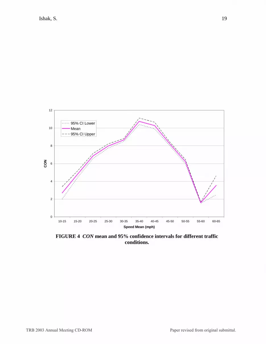
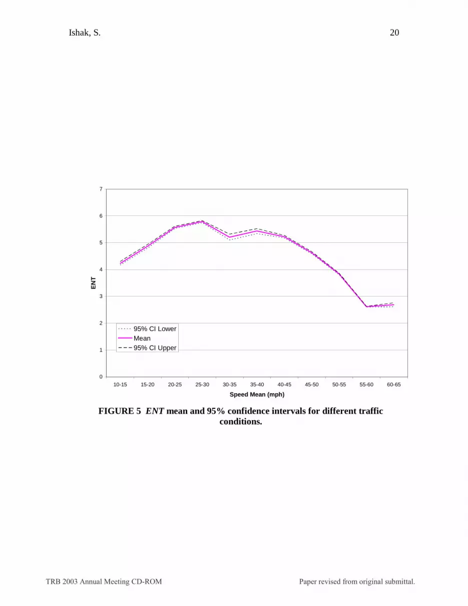
SENSITIVITY ANALYSIS This section presents the sensitivity analysis of each of the second-order statistical measures to various traffic conditions that are quantified by the speed mean (MEAN) of each contour map. The purpose of this analysis is to detect relationships between first-order and second-order properties of traffic conditions. Using the same set of 14,270 constructed contour maps, the observations were grouped by MEAN over 5-mph intervals. For each interval, the descriptive statistics (mean and 95% confidence intervals) of ASM, CON, and ENT, were calculated. The profile of the mean and 95% confidence bounds for each of the second-order measures was plotted against MEAN. FIGURE 3 shows the effect on ASM as a measure of smoothness. The figure shows the ASM mean and lower and upper 95% confidence limits to indicate whether significant differences exist across different speed mean intervals. The figure shows that the lowest ASM is observed when the speed mean is in the range o f 25 to 30 mph, indicating that this speed interval marks the coarsest texture of traffic contour maps. This is followed by slightly higher ASM in the range of 20-25 mph. Since the ASM confidence bounds do not overlap with other limits in the figure, it can be concluded that the differences are statistically significant. This indicates that the highest level of non-uniformity in traffic conditions is very likely to be observed in that speed range. In the meantime, the highest ASM mean (very smooth) is observed in the range of 55 to 60 mph, when traffic operates at or near free-flow conditions and speeds are likely to be more uniform. A slight drop in ASM is also observed in the speed range of 60 to 65 mph, which is possibly caused by variations in speeds under free-flow conditions where drivers have the freedom of choosing their own desired speeds. In FIGURE 4, we examine the effect of MEAN on the variable CON. The figure shows that the maximum local variations, measured by CON, are observed at speeds in the range of 35 to 45 mph and that the difference in CON between the 35-40 mph interval and the 40-45 mph interval was not statistically significant. Such observation suggests that the lowest level of homogeneity in traffic conditions is detected between 35 to 45 mph. Essentially, this range marks transient states from and into congested conditions, where high levels of local disturbances due to traffic breakdowns are often encountered. As traffic conditions assume away from transient stages, the level of homogeneity increases, as exhibited by the decrease in the values of CON. A slight increase in CON was also observed in the 60 to 65 mph speed interval and can be attributed similarly to the drivers’ ability to choose their desired speeds under extremely unconstrained conditions. Similarly, the relationship between traffic conditions and the ENT measure is illustrated in FIGURE 5. The figure shows that the maximum ENT (highest randomness) is observed at speed range of 25 to 30 mph, with statistically significant differences from neighboring observations. This is consistent with the other results from ASM and CON. Lower randomness is observed during heavy congestion (20 mph and less) where traffic has already plunged into extreme forced-flow conditions. The lowest levels of randomness are observed during conditions of 55 mph and higher.

LEVEL OF SERVICE (LOS) In order to describe the quality of traffic operations qualitatively, we will have to establish level of service criteria, similar to those used with conventional measures in the highway capacity manual (e.g. density). Since each of the three measures emphasizes a different property, the level of service will be established for each measure separately. Following the conventions of the highway capacity manual for estimating the level of service on basic freeway segments, we may


Ishak, S. 11

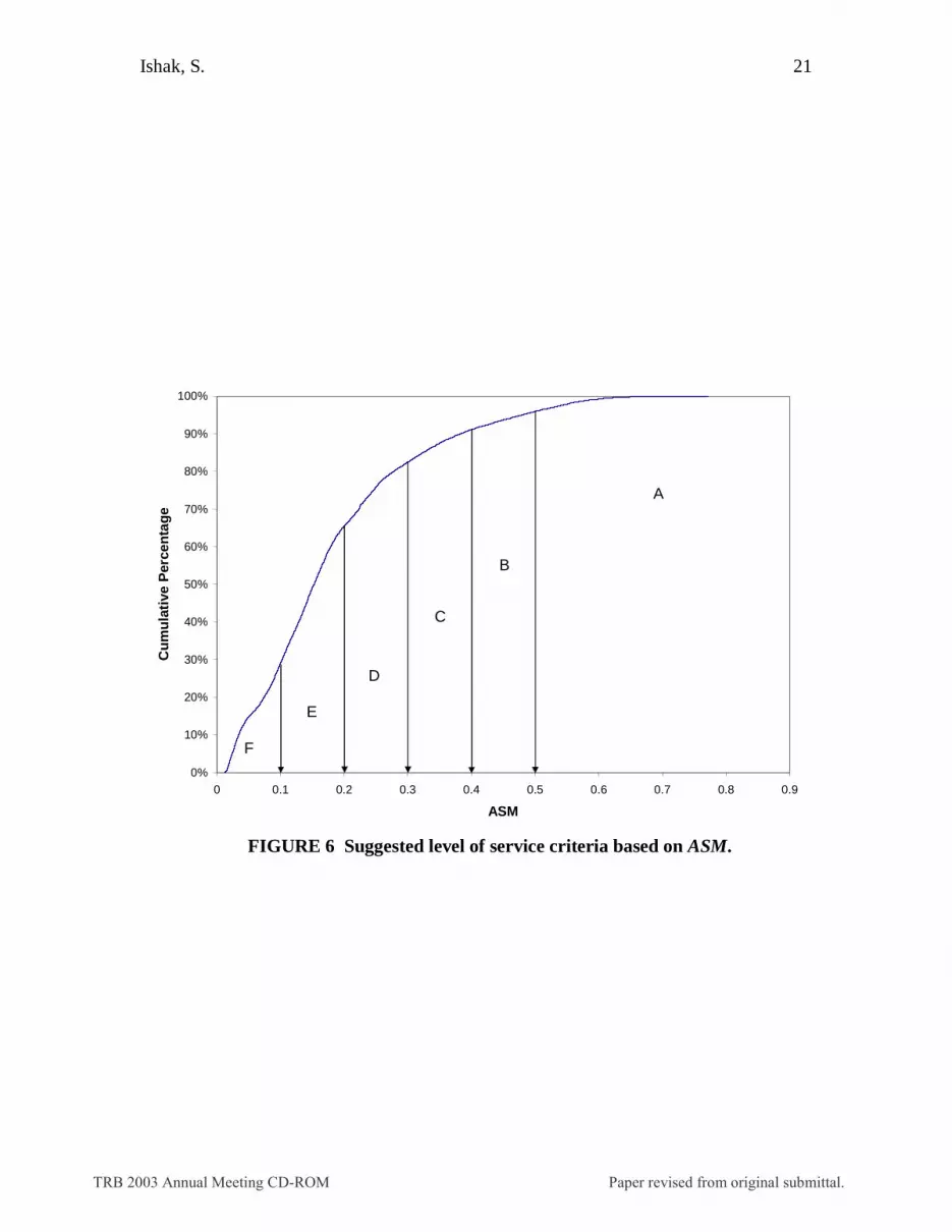
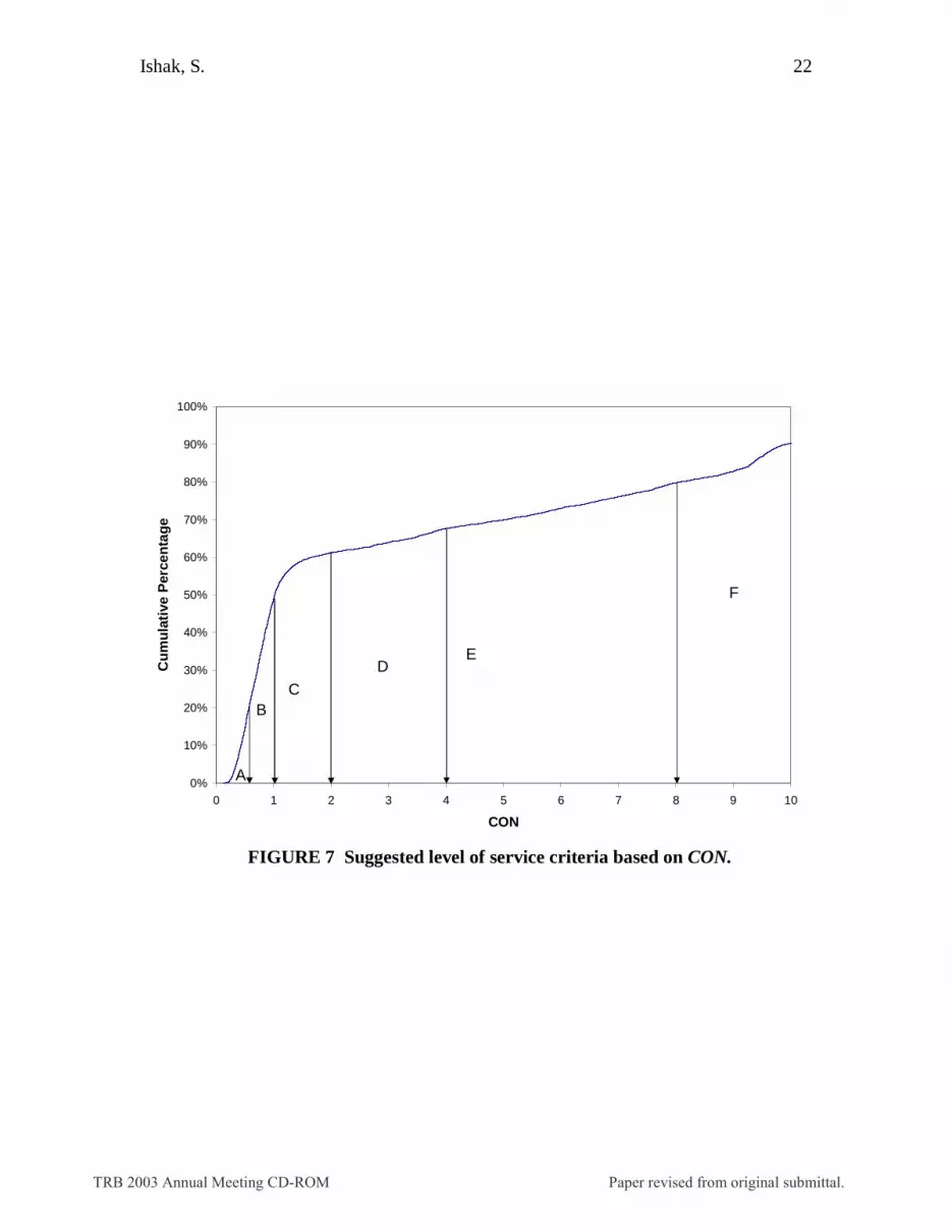
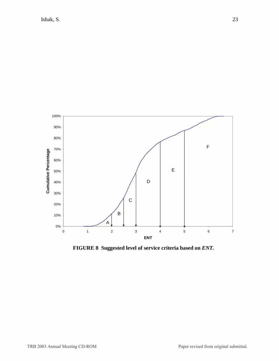
divide the plausible range of each measure into 6 distinct categories: A through F. For smoothness, ASM was arbitrarily divided into 6 categories as shown in FIGURE 6. LOS A indicates very smooth operation of traffic with values greater than or equal to 0.5. On the other side, LOS F is characterized with very coarse operation with values less than or equal to 0.1. Intermediate values of ASM reflect gradual variation between the two extremes. Similarly, the LOS criteria were arbitrarily established for homogeneity and randomness as shown in FIGURE 7 and FIGURE 8, respectively. For homogeneity, CON was also divided into 6 regions (A though F). LOS A is defined by CON ≤ 0.5 and indicates very homogeneous traffic conditions, as opposed to LOS F, with CON ≥ 8. Similar description may apply to the amount of randomness in traffic operations using the level of service criteria shown in FIGURE 8.

ON-LINE PERFORMANCE ASSESSMENT The on-line implementation of the second-order statistical measures can be accomplished by specifying the dimensions of the time-space window of the contour maps. The spatial dimension is determined by the length of the freeway section where performance needs monitoring. The temporal dimension can be arbitrarily chosen, but should not be less than 15 minutes to ensure that the constructed contour maps are large enough to support the calculations of the second-order measures. The constructed contour map can be updated in real time by moving the time-space window incrementally over time. To facilitate the online implementation process, a standalone module was developed and used to conduct the analysis presented in this study. The module can be executed in real time and allows the user to specify the following parameters: direction of travel (eastbound, westbound, or both), the parameter(s) used to construct the contour map (speed, occupancy, or volume), the beginning and end of the freeway section, the spatial dimension (number of sensors or stations) and temporal dimension (minutes) of the contour map, and the level of discretization of the traffic parameter (e.g. 5 mph in this study).

CONCLUSIONS This study presented an approach to characterize traffic contour maps in a manner analogous to texture characterization of digital images in the field of image analysis. The concept is similar to that applied to incident detection using pattern recognition techniques such as artificial neural networks. However, the approach presented here focused on extracting features or properties from spatiotemporal traffic contour maps that quantify special characteristics such as smoothness, regularity, homogeneity, and randomness. Several advanced techniques are available in this area, the simplest of which are derived from second-order statistics. In this study, several second-order statistical measures were applied to quantify properties of nearly 14,000 spatiotemporal traffic contour maps that were constructed from a 3.4 mile section of I-4 over 15-minute time windows. To detect information redundancies between first-order and second-order measures, as well as among second-order measures, a correlation matrix was examined. Strongly inter-correlated measures were eliminated to avoid information redundancy. This has resulted in retaining three second-order measures: ASM, CON, and ENT. To investigate the sensitivity of the three measures (ASM, CON, and ENT) to traffic conditions, the speed means were divided incrementally into 5-mph intervals and the mean and confidence bounds for each measure were calculated. The lowest ASM was observed in the range of 25 to 30 mph, indicating that this speed category marks the coarsest texture of traffic contour maps. This indicates that the highest level of non-uniformity in traffic conditions is observed in that speed


Ishak, S. 12

range. The maximum local variations (CON) were observed at speeds in the range of 35 to 45 mph. Essentially, this speed range marks transient stages in traffic conditions with high levels of local disturbances. The maximum ENT (highest randomness) was observed in the speed range of 25 to 30 mph. This was consistent with the results of the other measures. The study also showed the possibility of deploying the second order measures in performance assessment and level of service estimation. An approach similar to the one used for evaluating the level of service on freeway segments in the highway capacity manual was devised by dividing the range of feasible values for each measure into 6 distinct categories, namely A through F. The tentatively defined levels of service can be readily used to assess qualitatively the levels of smoothness, homogeneity, and randomness. An online implementation module was also developed to process traffic contour maps in real time and provides traffic management centers with enough flexibility to specify a large set of relevant parameters.

FUTURE WORK Future research in this area may include more sophisticated tools for textural characterization such as structural approaches (Fourier transforms, wavelet transforms, and Gabor wavelets) and a combination of both (statistical geometric features). Such approaches can further enhance the performance measures and reveal additional properties of traffic behavior. Further research can investigate the degree of correlation between new performance measures and accident frequency and severity. Certain properties can be used to improve the performance of incident detection algorithms and to advance the current procedures for evaluating the level of service on freeways.

ACKNOWLEDGEMENT This research is supported by the National Science Foundation (NSF) through grant CMS/0230216 to Louisiana State University. The research award was granted under a joint program between NSF and USDOT on information and communication systems for surface transportation (ICSST).


Ishak, S. 13

REFERENCES 1. Witten, I. and E. Frank. (2000) Data Mining: Practical Machine Learning Tools and

Techniques with Java Implementations. Academic Press. 2. Mallach, E.G. (2000). Decision Support and Data Warehouse Systems. McGraw Hill. 3. McNeil, S., W. Wallace, and T. Humphrey. (2000) Developing an Information

Technology-Oriented Basic Research Program for Surface Transportation Systems. Report to the NSF and USDOT, Workshop at the University of Illinois at Chicago.

4. Liu, H. and H. Motoda. (2001) Feature Extraction Construction and Selection, a Data Mining Perspective. Kluwer Academic Publishers, Second Edition.

5. Roess, R., W. McShane, and E. Prassas. (1998) Traffic Engineering. Prentice Hall. 6. Khisty, C. and B. Lall. (1990) Transportation Engineering: An Introduction. Prentice

Hall. 7. May, A. (1990) Traffic Flow Fundamentals. Prentice Hall. 8. Papacostas, C. and P. Prevedouros. (2001) Transportation Engineering and Planning.

Prentice Hall. 9. Garber, N. and L. Hoel. (1999). Traffic and Highway Engineering. Brooks/Cole

Publishing Company. 10. Wright, P. (1996) Highway Engineering. John Wiley & Sons, Inc. 11. Highway Capacity Manual. (2000). Transportation Research Board, National Research

Council, Washington, DC. 12. Banks, J. (2000). Introduction to Transportation Engineering. McGraw Hill. 13. Choe, T., A. Skabardonis, and P. Varaiya. (2002). “Freeway Performance Measurement

System (PeMS): An Operational Analysis Tool” 81st Annual Meeting of the Transportation Research Board, Pre-print CD-ROM, Washington D.C.

14. Kwon, J., Coifman B., and Bickel P. (2000) "Day-to-Day Travel Time Trends and Travel Time Prediction from Loop Detector Data", Transportation Research Record No. 1717, 120-129.

15. Ishak, S. and H. Al-Deek. (1998). “Applying Fuzzy ART to Freeway Incident Detection.” Transportation Research Record. No. 1634.

16. Ishak, S. and H. Al-Deek. (1999). “Performance of Automatic Ann-Based Incident Detection on Freeways.” Journal of Transportation Engineering, ASCE, 125(4), 281-290.

17. Theodoridis, S. and K. Koutroumbas. (1999) Pattern Recognition. Academic Press. 18. Nixon, M. and A. Aguado. (2002) Feature Extraction and Image Processing. Newnes. 19. Micheli-Tzanakou E. (2000) Supervised and Unsupervised Pattern Recognition, Feature

Extraction and Computational Intelligence. CRC Press LLC. 20. Seul, M., L. O’Gorman, and M. Sammon. (2000) Practical Algorithms for Image

Analysis. Cambridge University Press.


Ishak, S. 14

LIST OF TABLES TABLE 1 Correlation Matrix between Measures ....................................................................... 15

LIST OF FIGURES FIGURE 1 Illustration of spatiotemporal traffic contour maps................................................... 16 FIGURE 2 The different orientations used to calculate P(i,j). .................................................... 17 FIGURE 3 ASM mean and 95% confidence intervals for different traffic conditions................. 18 FIGURE 4 CON mean and 95% confidence intervals for different traffic conditions. ............... 19 FIGURE 5 ENT mean and 95% confidence intervals for different traffic conditions. ................ 20 FIGURE 6 Level of service criteria based on ASM. ................................................................... 21 FIGURE 7 Level of service criteria based on CON. ................................................................... 22 FIGURE 8 Level of service criteria based on ENT. .................................................................... 23


Ishak, S. 15

TABLE 1 Correlation Matrix between Measures

MEAN VAR ASM CON IDF CORR ENT SUMENT DIFFENT INFO

Overall Redundancy Score

MEAN 1.000 -0.618 0.472 -0.545 0.605 0.937 -0.780 -0.748 -0.741 -0.705 1

VAR -0.618 1.000 -0.475 0.749 -0.500 -0.652 0.608 0.692 0.660 0.643 0

ASM 0.472 -0.475 1.000 -0.492 0.907 0.625 -0.820 -0.811 -0.798 -0.858 1

CON -0.545 0.749 -0.492 1.000 -0.560 -0.635 0.689 0.744 0.785 0.692 0

IDF 0.605 -0.500 0.907 -0.560 1.000 0.775 -0.890 -0.851 -0.883 -0.922 2

CORR 0.937 -0.652 0.625 -0.635 0.775 1.000 -0.847 -0.816 -0.829 -0.813 1

ENT -0.780 0.608 -0.820 0.689 -0.890 -0.847 1.000 0.984 0.974 0.974 3

SUMENT -0.748 0.692 -0.811 0.744 -0.851 -0.816 0.984 1.000 0.972 0.971 3

DIFFENT -0.741 0.660 -0.798 0.785 -0.883 -0.829 0.974 0.972 1.000 0.965 3

INFO -0.705 0.643 -0.858 0.692 -0.922 -0.813 0.974 0.971 0.965 1.000 4


Ishak, S. 16

(a) Example of a traffic speed contour map taken for the eastbound morning

peak (7:30 AM to 9:30 AM) on April 3rd, 2001 over a 4-mile section of I-4.

Dis

tanc

e

Time

X=a

X=b

T=t1T=t2

X=x

T=t

I(t,x)

Pixel (t,x)

(B) SPATIOTEMPORAL TRAFFIC CONTOUR LAYOUT REPRESENTED

BY TRAFFIC PARAMETER I.

FIGURE 1 Illustration of spatiotemporal traffic contour maps.


Ishak, S. 17

Time

Space

t

x

δ=30 s

Detector Station (x)

Detector Station (x+1)

0.5miles

Direction ofTravel

S=60 S=30 S=20 mph

S=6

S=0

S=∞

5 min (n=10)

θ

nδ

(t, x)

(t+nδ, x+1)

FIGURE 2 The different orientations used to calculate P(i,j).


Ishak, S. 18

0

0.05

0.1

0.15

0.2

0.25

0.3

10-15 15-20 20-25 25-30 30-35 35-40 40-45 45-50 50-55 55-60 60-65

Speed Mean (mph)

AS

M

95% CI LowerMean95% CI Upper

FIGURE 3 ASM mean and 95% confidence intervals for different traffic

conditions.


Ishak, S. 19

0

2

4

6

8

10

12

10-15 15-20 20-25 25-30 30-35 35-40 40-45 45-50 50-55 55-60 60-65

Speed Mean (mph)

CO

N


FIGURE 4 CON mean and 95% confidence intervals for different traffic

conditions.


Ishak, S. 20

0

1

2

3

4

5

6

7

10-15 15-20 20-25 25-30 30-35 35-40 40-45 45-50 50-55 55-60 60-65

Speed Mean (mph)

EN

T


FIGURE 5 ENT mean and 95% confidence intervals for different traffic

conditions.


Ishak, S. 21

0%

10%

20%

30%

40%

50%

60%

70%

80%

90%

100%

0 0.1 0.2 0.3 0.4 0.5 0.6 0.7 0.8 0.9

ASM

Cu

mu

lati

ve P

erce

nta

ge

A

C

D

E

F

B

FIGURE 6 Suggested level of service criteria based on ASM.


Ishak, S. 22

0%

10%

20%

30%

40%

50%

60%

70%

80%

90%

100%

0 1 2 3 4 5 6 7 8 9 10

CON

Cu

mu

lati

ve P

erce

nta

ge

F

E

CB

A

D

FIGURE 7 Suggested level of service criteria based on CON.


Ishak, S. 23

0%

10%

20%

30%

40%

50%

60%

70%

80%

90%

100%

0 1 2 3 4 5 6 7

ENT

Cu

mu

lati

ve P

erce

nta

ge

A

B

C

D

F

E

FIGURE 8 Suggested level of service criteria based on ENT.


Documents

Deriving Traffic-Performance Measures and Levels of Service from Second-Order Statistical Features of Spatiotemporal Traffic Contour Maps