Embed Size (px)
Citation preview

DEFINING PRIORITIES AND TIMESCALES FOR SEISMIC INTERVENTION IN SCHOOL
BUILDINGS IN ITALY
Damian Grant
Post-Doctoral Researcher EUCENTRE, Pavia, Italy
Julian J. Bommer
Reader in Earthquake Hazard Assessment Imperial College London, UK
Rui Pinho
Assistant Professor University of Pavia, Italy
Gian Michele Calvi
Professor of Structural Design University of Pavia, Italy
July 2006


PREFACE
This report presents the development of a risk-management framework for the seismic safety of school buildings in Italy. The primary objectives of the decision-making framework are to identify the most high-risk schools, prioritise the allocation of resources to these schools for seismic strengthening, and to assign timescales and target safety levels for the strengthening, in accordance with the new Italian seismic design code. While the steps in the method are clearly outlined and described, the fundamental parameters of the framework, such as tolerable risk levels and resources available to carry out the operation, must be defined by the relevant authorities. With an appropriate selection of these parameters, the framework described herein is able to provide a rational distribution of both technical and financial resources to reduce the seismic risk of Italian school buildings over realistic timescales that reflect the urgency of these measures for protecting the next generation of Italian citizens.
The authors would like to acknowledge the following individuals for their valuable contributions to this study:
• Massimiliano Stucchi, Valentina Montaldo, Carlo Meletti and Fabrizio Meroni, for providing INGV hazard data and guidance on all aspects of Italian seismic hazard.
• Giacomo di Pasquale and Agostino Goretti for providing information on Italian risk management studies and on previous Italian seismic zonations and seismic design provisions, and for reviewing the manuscript.
• Andrea Penna and Lorenza Petrini, for discussion of Italian legislative situation and seismic vulnerability assessment.
• Helen Crowley, for help with loss estimation methods, discussion of many concepts on the definition of tolerable seismic risk, and for reviewing draft versions of parts of this report.
• Laura Peruzza for making available the time-dependent hazard data, and for reviewing the manuscript.
• Richard Fenwick, John Berrill, Nigel Priestley and Simon Grant, for providing information about New Zealand seismic design codes.
The authors also acknowledge the financial support provided by the Italian Department of Civil Protection (DPC – Dipartimento della Protezione Civile), through the financing of the ProCiv-INGV 2004-06 applied research programme, under the framework of which this work has been partially funded (as part of Sub-Project S1 activities).


TABLE OF CONTENTS
PREFACE..................................................................................................................................................... iii TABLE OF CONTENTS........................................................................................................................... v LIST OF FIGURES ................................................................................................................................... vii LIST OF TABLES....................................................................................................................................... xi 1. INTRODUCTION .............................................................................................................................. 1
1.1 BACKGROUND ............................................................................................................................... 1 1.2 CONCEPTS AND TERMINOLOGY ................................................................................................ 4 1.3 SCOPE OF THE PROJECT.............................................................................................................. 8
2. REVIEW OF LOSS ESTIMATION METHODS ....................................................................... 11 2.1 SCORE- AND INDEX-BASED METHODS................................................................................... 12 2.2 ATC-13 METHOD ....................................................................................................................... 16 2.3 HAZUS METHOD....................................................................................................................... 18 2.4 THE CATANIA PROJECT ............................................................................................................. 24 2.5 ORDAZ ET AL. [2000] LOSS ESTIMATION MODEL................................................................. 29 2.6 COSENZA ET AL. [2005] VULNERABILITY ASSESSMENT METHOD ...................................... 31 2.7 DISPLACEMENT-BASED EARTHQUAKE LOSS ASSESSMENT (DBELA)................................ 34
3. DEFINING TOLERABLE LEVELS OF SEISMIC RISK........................................................ 43 3.1 BASE DEFINITION OF TOLERABLE SEISMIC RISK IN DESIGN CODES................................ 43 3.2 ADJUSTMENT TO TOLERABLE RISK FOR BUILDING IMPORTANCE AND PERFORMANCE47 3.3 TOLERABLE RISK FOR SEISMIC ASSESSMENT AND REHABILITATION OF EXISTING STRUCTURES......................................................................................................................................... 50 3.4 PERFORMANCE-BASED EARTHQUAKE ENGINEERING ......................................................... 56 3.5 IMPORTANCE FACTORS IN A PBEE FRAMEWORK ................................................................ 58
4. SEISMIC HAZARD IN ITALY ...................................................................................................... 67 4.1 ITALIAN SEISMICITY.................................................................................................................... 67 4.2 HISTORY OF ITALIAN SEISMIC PROVISIONS ........................................................................... 68 4.3 ITALIAN HAZARD DATA ............................................................................................................ 71
D. N. Grant, J. J. Bommer, R. Pinho & G. M. Calvi
vi
4.4 COMPARISON OF REGIONAL HAZARD CURVES .....................................................................73 4.5 TIME-DEPENDENT CHARACTERISATION OF ITALIAN HAZARD..........................................78
5. RISK MANAGEMENT DECISION-MAKING FRAMEWORKS.........................................89 5.1 REVIEW OF RETROFIT PRIORITISATION PROJECTS ...............................................................90 5.2 REVIEW OF RISK MANAGEMENT PROJECTS IN ITALY ..........................................................92 5.3 ATC 3-06 METHODOLOGY........................................................................................................95
5.3.1 Qualitative evaluation .....................................................................................................97 5.3.2 Analytical evaluation .......................................................................................................99 5.3.3 Required capacity and permissible times for retrofit ................................................100
5.4 NZSEE ACTIVE RISK REDUCTION PROGRAMME ................................................................101 5.4.1 Initial evaluation procedure..........................................................................................102 5.4.2 Detailed assessment procedure....................................................................................106 5.4.3 Prioritising detailed assessment and timetables for improvement..........................106
6. PROPOSED FRAMEWORK FOR ITALIAN SCHOOLS......................................................111 6.1 GENERAL CONSIDERATIONS...................................................................................................111 6.2 ADAPTABILITY OF EXISTING METHODOLOGIES .................................................................113 6.3 OBJECTIVES OF ASSESSMENT PROCEDURE AND SEISMIC INTERVENTION......................117 6.4 PROPOSED MULTIPLE-LEVEL SCREENING METHODOLOGY .............................................119
6.4.1 First ranking: assessment based on desk study..........................................................119 6.4.2 Second ranking: vulnerability rating by visual inspection ........................................131 6.4.3 Third ranking: Simplified mechanics-based structural assessment, and priorities
and timescales for detailed assessment and retrofit ..........................................133 6.5 EXAMPLE APPLICATION OF PROPOSED METHODOLOGY..................................................141
REFERENCES .........................................................................................................................................145 APPENDIX A. POISSON MODEL OF EARTHQUAKE AND GROUND MOTION RECURRENCE ........................................................................................................................................157 APPENDIX B. PGA DEFICIT CALCULATIONS ..........................................................................159

LIST OF FIGURES
Figure 1.1. Damage states of buildings in downtown Kobe affected by the 1995 Hyogo-ken Nanbu earthquake, as proportions of those buildings constructed according to the 1952 code and the 1981 code [K. Takiguchi, Pers. Comm., 1996]..................................1
Figure 1.2. Effect of a new seismic design code in reducing the earthquake vulnerability of the building stock over time [Coburn and Spence, 1992]........................................................2
Figure 1.3. Collapsed elementary school in San Giuliano di Puglia where 27 children and one teacher were killed [Bazzurro and Maffei, 2004]. ...............................................................3
Figure 1.4. Hazard curves for PGA corresponding to a 10% probability of exceedance in different regions of the United States [Kramer, 1996]. .....................................................7
Figure 2.1. Structural damage assessment form for use following earthquakes [Anagnastopoulos et al., 1989].............................................................................................13
Figure 2.2. Categories and codes used to define building usage in the building evaluation form shown in Figure 2.1 [Anagnostopoulos et al., 1989]. .......................................................14
Figure 2.3. Categories and codes used to define structural type and load bearing system in the building evaluation form shown in Figure 2.1 [Anagnostopoulos et al., 1989]. ...........14
Figure 2.4. Seismic indices in longitudinal (L) and transverse (T) direction of seven RC buildings (identified by letters) affected by the 1968 Tokachi-oki earthquake and the levels of damage experienced [Aoyama, 1981]. ................................................................16
Figure 2.5. Flowchart of the HAZUS earthquake loss estimation methodology [FEMA, 2003]..19 Figure 2.6. Demand spectra and capacity curves in HAZUS methodology [FEMA, 2003]. .........21 Figure 2.7. Example building inventory for HAZUS methodology [Kircher et al., 1997a].
“Floor area” refers to total floor area over entire inventory. .........................................22 Figure 2.8. Example fragility curves for different damage states [Kircher et al., 1997a].................24 Figure 2.9. Distribution of buildings by height and age class for (a) masonry buildings (sample
of 5500 buildings) and (b) reinforced concrete (RC) buildings (sample of 2200 buildings). Data from the comprehensive survey of central Catania, at 33% complete stage [Faccioli et al., 1999]. .................................................................................26
Figure 2.10. Statistical distributions of the vulnerability index, Iv, for masonry and RC buildings for the Catania building inventory [Faccioli et al., 1999]. ................................................27
Figure 2.11. Relationship between damage factor and peak ground acceleration for different values of the vulnerability index (shown on the curves), for masonry and RC buildings [adapted from Guagenti and Petrini, 1989]......................................................27

D. N. Grant, J. J. Bommer, R. Pinho & G. M. Calvi
viii
Figure 2.12. Example of second vulnerability assessment procedure from Catania project, for limit state 1 (yield), beam-sway reinforced concrete frames, PGA=0.3g; SD = “structural damage” and NSD = “non-structural damage” [Calvi, 1999]. ........ 29
Figure 2.13. Non-linear analytical model used in the evaluation of structural capacity in the Cosenza et al. method [Cosenza et al., 2005]..................................................................... 33
Figure 2.14. Capacity curves for 3-storey building models, for low-order, medium-order and high-order parameter definitions; (a) base shear coefficient and (b) inter-storey drift ratio [Cosenza et al., 2005]................................................................................................... 34
Figure 2.15. Example building inventory for the application of the DBELA method in Marmara Region, Turkey [Crowley et al., 2005]. ............................................................................... 37
Figure 2.16. Deterministic representation of DBELA method [Glaister and Pinho, 2003]............ 38 Figure 2.17. Definition of effective height coefficient in DBELA method [Glaister and Pinho,
2003]. ..................................................................................................................................... 39 Figure 3.1. Seismic performance categories and definition of tolerable risk for existing
buildings [Brunsdon, 2004; adapted from NZSEE, 2003]............................................. 52 Figure 3.2. Relationship between annual frequency of exceedance and displacement capacity-
demand ratio [adapted from Priestley, 1997]. .................................................................. 53 Figure 3.3. Relative risk of existing to new structures [NZSEE, 2003]. .......................................... 53 Figure 3.4. Matrix of recommended performance objectives, adapted from (a) Vision 2000
[SEAOC, 1995], (b) FEMA 273/274 and FEMA 356 [ATC, 1997; ASCE, 2000] (c) FEMA 302/303 [BSSC, 1997]. .......................................................................................... 57
Figure 3.5. Treatment of building importance with scalar importance factor on Vision 2000 [SEAOC, 1995] performance matrix (see Figure 3.4a). (a) Increasing hazard for same performance level, (b) improving performance for same design hazard............ 59
Figure 3.6. Dependence of performance objectives on seismicity and structural type. Annual frequency of exceedance (AFE) and peak drift values from Vision 2000 [SEAOC, 1995] ...................................................................................................................................... 61
Figure 3.7. Implications of (a) k-dependent, and (b) performance-dependent importance factors for design, following from the design approaches illustrated in Figure 3.5(a) and (b), respectively. ............................................................................................................ 61
Figure 3.8. Alternative interpretation of building importance factors: improving confidence in either performance level or hazard level........................................................................... 64
Figure 3.9. Dependence of performance objectives on confidence level of either hazard or performance.......................................................................................................................... 65
Figure 4.1. Historical seismicity from the Catalogue of Strong Italian Earthquakes [Boschi et al., 2000] and instrumental seismicity from INGV bulletin [Valensise et al., 2003]. ......... 67
Figure 4.2. Median peak ground acceleration (units of g) for return periods of (a) 100 years, (b) 475 years, (c) 1000 years, and (d) 2500 years. Data from INGV [2005]....................... 72

Defining Priorities and Timescales for Seismic Intervention
ix
Figure 4.3. Linear regression for slope of hazard curve (k) for median PGA values, calibrated for 100, 475, 1000 and 2500-year return period data. (a) Best-fit k-values, and (b) r2 values......................................................................................................................................74
Figure 4.4. Hazard curves for three locations in Italy: (a) PGA, and (b) PGA normalised to 475-year return period value. ..............................................................................................74
Figure 4.5. Relationship between gradient of log-log hazard curve (k) and 475-year PGA value for all grid points in Figure 4.3. ..........................................................................................76
Figure 4.6. Grouped data from Figure 4.5. Rectangles show median and median plus/minus one standard deviation of k-values for PGA in a 0.01g interval....................................77
Figure 4.7. Best-fit slope of hazard curve (k) for spectral acceleration, median-plus-one-standard-deviation values, calibrated for 95-, 475-, 975- and 2475-year return period data [SSN, 2001]; (a) response period = 0.2 sec, and (b) response period = 1.0 sec. .78
Figure 4.8. Locations of potential “seismic gaps” in Italy [adapted from Valensise and Pantosti, 2001].......................................................................................................................................80
Figure 4.9. Mean peak ground acceleration (units of g); Poisson earthquake recurrence for a 10% probability of exceedance in (a) 30 years, (b) 50 years, and time-dependent earthquake recurrence model for a 10% probability of exceedance in (c) 30 years, and (d) 50 years. Data from Peruzza [2005a]....................................................................82
Figure 4.10. Ratio of time-dependent mean PGA values to Poisson mean values for a 10% probability of exceedance in (a) 30 years, and (b) 50 years. Data from Peruzza [2005a]....................................................................................................................................83
Figure 4.11. Residuals between observed Italian seismicity data and Poissonian recurrence model, versus the time elapsed since the last significant earthquake [Cinti et al., 2004].......................................................................................................................................85
Figure 5.1. Outline of steps in ATC 3-06 risk reduction methodology [based on ATC, 1978]. ...96 Figure 5.2. (a) Minimum acceptable rc values, before and after retrofit, for Category C buildings,
and (b) permissible time to strengthen or demolish building for αt = 12 [both adapted from ATC, 1978]. ............................................................................................... 100
Figure 5.3. Outline of steps in an active risk reduction programme, using NZSEE methodology [NZSEE, 2003].......................................................................................... 103
Figure 5.4. Initial Evaluation Procedure (IEP) in NZSEE methodology [NZSEE, 2003]......... 104 Figure 5.5. Occupancy classifications for non-essential buildings; for essential buildings
OC = 1 [NZSEE, 2003].................................................................................................... 107 Figure 6.1. Summary of advantages and disadvantages of different levels of detail in
vulnerability assessment for large-scale seismic intervention. ..................................... 112 Figure 6.2. Outline of steps in proposed risk reduction methodology. ......................................... 120 Figure 6.3. PGA deficit (units of g) for Italy, for buildings designed prior to 18/04/1909. ...... 126

D. N. Grant, J. J. Bommer, R. Pinho & G. M. Calvi
x
Figure 6.4. PGA deficit (units of g) for Italy, for buildings designed between 18/04/1909 and 5/11/1916........................................................................................................................... 126
Figure 6.5. PGA deficit (units of g) for Italy, for buildings designed between 5/11/1916 and 13/03/1927. ....................................................................................................................... 127
Figure 6.6. PGA deficit (units of g) for Italy, for buildings designed between 13/03/1927 and 25/03/1935. ....................................................................................................................... 127
Figure 6.7. PGA deficit (units of g) for Italy, for buildings designed between 25/03/1935 and 10/03/1969. ....................................................................................................................... 128
Figure 6.8. PGA deficit (units of g) for Italy, for buildings designed between 10/03/1969 and 3/03/1975........................................................................................................................... 128
Figure 6.9. PGA deficit (units of g) for Italy, for buildings designed between 3/03/1975 and 3/06/1981........................................................................................................................... 129
Figure 6.10. PGA deficit (units of g) for Italy, for buildings designed between 3/06/1981 and 19/06/1984. ....................................................................................................................... 129
Figure 6.11. PGA deficit (units of g) for Italy, for buildings designed between 19/06/1984 and Ordinanza 3274/2003 (not currently compulsory). ...................................................... 130
Figure 6.12. PGA deficit (units of g) for Italy, for new buildings designed according to Ordinanza 3274/2003 (not currently compulsory). ...................................................... 130
Figure 6.13. Relationship between frequency of occurrence of different levels of PGA, based on assumption of a linear log-log hazard curve with gradient −k. ................................... 132
Figure 6.14. Relationship between normalised number of children and relative risk rating, for different values of exponent a.......................................................................................... 134
Figure 6.15. Two linear log-log hazard curves with gradient −k1 and −k2, and k2 > k1. Annual probability of collapse is greater for hazard curve 2. .................................................... 136
Figure 6.16. (a) Time permitted for seismic intervention, t, versus capacity ratio, CR; (b) maximum time permitted for high capacity ratio buildings, tmax, versus the number of children in the school, Nc............................................................................................. 139
Figure 6.17. Time permitted for seismic intervention as a function of capacity ratio, for (a) the three k-values shown in Figure 4.4, and (b) three values of Nc. .................................. 140

LIST OF TABLES
Table 2.1. Damage matrix for high-rise steel moment-resisting frames [adapted from ATC, 1985].......................................................................................................................................18
Table 2.2. Typical loss rates for single-family residences of light-frame wood construction located in California (dollars per square foot) [Kircher et al., 1997b]. ...........................25
Table 4.1. Summary of horizontal seismic design forces and seismic zonations in Italian seismic provisions, and intermediate changes to zonation in between new code releases. Partly adapted from Di Pasquale et al. [1999b]..................................................69
Table 4.2. Annual frequency of exceedance (AFE) and return periods (TR) for different values of k (from Figure 4.3), for Building Categories I and II in the draft Italian seismic design code [OPCM, 2003]. ................................................................................................75
Table 4.3. Values of PGA and k for seismic zones in Italy. .............................................................77 Table 5.1. Function exposure factors for California hospital retrofit programme [Holmes,
2002].......................................................................................................................................92 Table 5.2. Suggested occupation densities per floor, expressed as square feet per occupant
(SFPO) from ATC [1978], and converted to square metres per occupant (SMPO). ...98 Table 5.3. Grading system and relative risk of existing buildings; adapted from NZSEE [2003].
............................................................................................................................................. 106 Table 5.4. Modification factor (K1) to consider occupancy in prioritising detailed evaluation
and determining time frame for rehabilitation according to NZSEE (2003) methodology. ..................................................................................................................... 108
Table 5.5. Modification factor (K2) to consider risk to people outside building in prioritising detailed evaluation and determining time frame for rehabilitation according to NZSEE [2003] methodology........................................................................................... 108
Table 6.1. Dates considered for the presentation of PGA deficit maps, and the key developments in effective PGA, that motivate their inclusion (see also Table 4.1). ......................... 124
Table 6.2. Prioritisation scheme based on risk rating, number of children (Nc) and, if necessary, time-dependent hazard factor.. ........................................................................................ 138
Table 6.3. Building inventory, PGA deficit and 1st risk ranking for example application. ........ 142 Table 6.4. GNDT vulnerability index and 2nd risk ranking for example application.................. 143 Table 6.5. Assumed simplified structural analysis results, 3rd risk ranking and timescales
allowed for seismic intervention for example application. .......................................... 143 Table B.1. Effective design PGA values (g) for Italian seismic design provisions..................... 160


1. INTRODUCTION
1.1 BACKGROUND
The single most effective tool in reducing earthquake risk is a sound seismic design code, rigorously and effectively enforced at both the design and construction stages. The provisions of the code, in terms of specified design levels of earthquake shaking and performance criteria (expressed as stresses and displacements) for buildings to meet under the expected ground motions, can ensure that the majority of structures built after the publication of the code will not collapse during future earthquakes. The code may thus prevent loss of life and also limit business and social disruption, direct and indirect monetary losses, and the numbers of injured or homeless people due to future earthquakes.
The effectiveness of a well-implemented modern seismic design code is clearly illustrated in Figure 1.1, which shows the proportions of building stock in downtown Kobe affected by the 1995 Hyogo-ken Nanbu earthquake in Japan. The data are separated into those buildings constructed up to 1981 and those built after the introduction of a new seismic
Figure 1.1. Damage states of buildings in downtown Kobe affected by the 1995 Hyogo-ken Nanbu
earthquake, as proportions of those buildings constructed according to the 1952 code and the 1981 code [K. Takiguchi, Pers. Comm., 1996].

D. N. Grant, J. J. Bommer, R. Pinho & G. M. Calvi
2
design code in June 1981, to replace the Standard Building Law, which had been in effect for many years. A significant feature of the 1981 code was the explicit inclusion, for the first time in Japan, of force reduction factors to allow for inelastic behaviour of buildings subjected to strong earthquakes [Elnashai et al., 1995].
Although the application of a good seismic design code may effectively increase the earthquake resistance of a new building conforming to the code requirements, the impact of a new seismic code on the risk in an urban area in a seismically active region may initially be low. Figure 1.2 illustrates schematically how the introduction of a seismic design code alters the vulnerability of the building stock in an urban area with time. Note that Figure 1.2 only shows the damage states as proportions of the two sets of building stock; the 1995 earthquake occurred 14 years after the introduction of the 1981 regulations, hence a very large proportion of the affected buildings were still those that had been built according to the 1952 standards.
Figure 1.2. Effect of a new seismic design code in reducing the earthquake vulnerability of the
building stock over time [Coburn and Spence, 1992].
Since seismic design codes are generally not applicable retrospectively (i.e. their provisions only apply to new construction), it is clear that several decades may need to pass before a new seismic code makes a very significant impact on the level of risk in a major town or city. Paradoxically, the process can be accelerated by a strong earthquake removing a large part of the most vulnerable building stock, which could then be replaced by new structures conforming to a new or improved seismic design code. The social and economic effects of a damaging earthquake can also influence public perception of seismic risk, and encourage communities to investigate the vulnerability of structures in other localities that were not affected by the earthquake. If the loss of life and property is to be prevented in the short-to-medium-term, then it is clearly the existing building stock

Defining Priorities and Timescales for Seismic Intervention
3
that will be the most important factor in controlling the risk. This fact underlies the importance of assessing the existing building stock and, where necessary, upgrading the levels of earthquake resistance.
The effects of a moderate-sized earthquake on an under-prepared community were demonstrated clearly and tragically in the Mw = 5.7 Molise earthquake that occurred in southern Italy in October 2002. Thirty people were killed in the earthquake, including 27 children and one teacher in a school which collapsed in the town of San Giuliano di Puglia, shown in Figure 1.3. Despite a 1998 proposal for seismic zonation re-classifying San Giuliano from “Zone 4” to “Zone 2” (where 1 is the highest and 4 the lowest), seismic design provisions were not adopted for the region until after the earthquake, meaning that a second storey addition to the school in 2000 did not require seismic design [Bazzurro and Maffei, 2004]. The delay in adopting the new seismic zonation meant that almost an entire generation of six- and seven-year-old children in San Giuliano was killed.
Figure 1.3. Collapsed elementary school in San Giuliano di Puglia where 27 children and one teacher
were killed [Bazzurro and Maffei, 2004].
A problem for the earthquake engineering community is that it is difficult to communicate technical information about seismic risk to the public. The probabilistic nature of seismic hazard definitions in design codes and the unpredictability of earthquake recurrence imply that it is generally impossible to design an “earthquake-proof” building. Even “deterministic” definitions of seismic hazard almost invariably involve decisions with a probabilistic basis [Bommer, 2002b], and maximum levels of

D. N. Grant, J. J. Bommer, R. Pinho & G. M. Calvi
4
ground shaking for a site elude the current capabilities of engineering seismology [Bommer et al., 2004a]. Perhaps more importantly, the allocation of resources to the management of seismic risk must be balanced with other expenditure and with resources allocated to other sources of risk to the population. Preventing loss of life in earthquakes is often expensive compared to sources of risk such as traffic accidents and smoking-related deaths. The definition of tolerable seismic risk to the population will necessarily be a compromise, and involve pragmatic and economic decisions as well as social and technical ones.
Nevertheless, the consideration of public opinion is important: following the Molise earthquake, the mother of an eight-year-old killed in San Giuliano said “I ask only one thing of everyone, that all schools be made safe. I don't want any mama or daddy, any one, ever to weep for their children” [CBS News, 2002]. The Organisation for Economic Co-operation and Development has recently recognised the problem of seismic safety in schools, releasing a report entitled “Keeping Schools Safe in Earthquakes” [OECD, 2004]. Approximately 20,000 Italian schools were built before the application of national seismic design provisions, and presumably many if not most of these would be considered inadequate by current standards. With limited resources available to them, and the lack of reliable earthquake-prediction methods, earthquake engineers may not be able to prevent a future tragedy such as San Giuliano with complete certainty, but they can work together with policy makers to ensure that the probability of it occurring is sufficiently low.
Since the Molise earthquake, a new seismic design code [OPCM, 2003] and a new seismic zonation map [INGV, 2005] have been developed for Italy. To address the inadequacy of a large portion of Italian building stock, and to avoid future collapses such as in San Giuliano, this code is to be applicable retroactively, and a large scale assessment and rehabilitation project is to be carried out. This report investigates the application of the new code and seismic zonation to existing Italian building stock, and presents a framework in which to consider the various social, technical, political and pragmatic decisions involved.
1.2 CONCEPTS AND TERMINOLOGY
Seismic risk can be defined as the possibility or probability of losses due to earthquakes, whether these losses are human, social or economic. Qualitatively, seismic risk may be expressed as the convolution of four factors:
Seismic Risk = Seismic Hazard * Exposure * Vulnerability * Cost (1.1)
The seismic hazard represents the potential effects of an earthquake at a particular site, including surface rupture, liquefaction, landslides, tsunami and ground shaking. Of these, the effect of ground shaking, which is also related to the potential for liquefaction and

Defining Priorities and Timescales for Seismic Intervention
5
landslides, is the cause of the vast majority of damage and loss of life in earthquakes [Bird and Bommer, 2004], the recent devastating tsunami in the Indian Ocean notwithstanding. The exposure refers to the human activity located in zones of seismic hazard, in terms of population density and the built environment. The vulnerability represents the susceptibility of the exposed elements to earthquake effects, or, equivalently, the lack of earthquake resistance of a structure. The final term in Eq. (1.1) represents the monetary repair and restoration costs as a proportion of the cost of demolition and replacement cost of a structure. Extending the cost term to human casualties can be more difficult, even if the delicate and controversial issue of assigning monetary values to human lives is avoided, as the relationship between building damage and deaths or injuries is often not well defined. Indirect costs such as loss of business and downtime can also be incorporated into seismic risk assessment. The quantitative application of Eq. (1.1) for a geographical area is the basis of earthquake loss estimation models, discussed in Chapter 2.
Seismic risk mitigation can theoretically be achieved by reducing any of the components of the risk in Eq. (1.1). Of these, however, the seismic hazard cannot generally be altered, only assessed, and the exposure is generally governed by issues that are more compelling than the regulation of seismic risk. The latter fact explains the large and growing population in many seismic areas of the world, and the subsequent increase in monetary loss and human casualties in recent earthquakes. Structural vulnerability can be reduced by the actions of engineers, although seismic design will generally increase the cost of a structure. Depending on the seismic hazard and local construction practice, this increase may be of the order of 5% of the cost for new buildings [Holmes, 1998]. Earthquake engineering, therefore, seeks the optimal balance between the vulnerability and cost terms of Eq. (1.1), in reducing the overall seismic risk.
Understanding of the concepts of seismic hazard and risk is hampered by widespread confusion, in no small part the result of ambiguous and poorly defined terminology. The term “earthquake” is sometimes used in the literature in the place of “ground motion”; a measure of ground shaking for design applications, for example, may be referred to as the “design earthquake”. This usage is misleading, and the terms should not be interchanged – “earthquake” should refer to the release of energy at the source, while “ground motion” is shaking at a particular site. A “design earthquake”, therefore, may be expressed as the magnitude and location of an earthquake appropriate for design. Probabilistic definitions of ground motion combine the effects of many different possible earthquake scenarios, and a value of design ground motion from a hazard map does not represent the effects of a single “design earthquake”. Deterministic earthquake scenarios are more closely related to the ground motions they produce, although even in this case, the distinction between the two is important. For example, a scenario earthquake may be identical for a number of engineering projects in a region, in terms of magnitude and location, although the level

D. N. Grant, J. J. Bommer, R. Pinho & G. M. Calvi
6
of ground motion at each site could be very different. Ground motion is a function of the travel path from the source, and the soil conditions at the site, in addition to the earthquake source characteristics implied by the term “earthquake”.
Probabilistic measures of ground-motion levels are often defined in terms of a fixed probability of exceedance, q, for an exposure time, L years. Assuming a Poisson model of recurrence, the return period of the ground motion may be defined by (see Appendix A):
)1ln( q
LTR −−= (1.2)
The return period is the average time interval between occurrences of the given level of ground motion; the ground-motion level that has a 10% probability of exceedance in 50 years, for example, has a return period equal to 475 years. It is important to realise that the return period does not imply that ground motions exceeding a certain level will occur every TR years, nor that during a period of TR, the ground motion of that level will definitely occur. For this reason, some authors refer to TR as the mean return period, as an attempt to eliminate the implication of periodicity. A better solution is to remove the emphasis on intervals of time altogether, and express different levels of ground motion in terms of their annual frequencies of exceedance (AFE). The advantages of AFE as a measure of ground motion recurrence are discussed in Chapter 3.
The AFE is sometimes referred to as the annual probability of exceedance (APE), although the two concepts are not identical. For extremely low levels of ground motion, with return periods of less than one year, the AFE is greater than unity; i.e. this level of shaking is expected more than once per year on average. Even for these very low levels of ground motion, the APE is always less than unity, as there remains a finite probability of non-exceedance. Although this distinction is important from a conceptual point of view, the actual numerical difference is small for AFE values considered in practice. This point is illustrated further in Appendix A.
The recurrence interval, Tr, is the reciprocal of the annual rate of occurrence of earthquakes of a given magnitude. Although recurrence interval and return period are often used interchangeably, the two terms should be distinguished, for the same reasons discussed above for “earthquake” and “ground motion”. An example from Bommer [2003] clearly illustrates the distinction between the two:
Consider an earthquake with a recurrence interval of 100 years...combined with the median plus two standard deviations of the chosen ground-motion parameter. This ground motion, for a given magnitude-distance couple, corresponds to a 97.7 percentile,

Defining Priorities and Timescales for Seismic Intervention
7
which is approximately the 1-in-40 level; combined with the 1-in-100 year earthquake, a return period of 4000 years is comfortably achieved.
This provides further justification for the use of AFE instead of return period to measure the frequency of occurrence of a level of ground motion, to remove the confusion with the recurrence interval.
Figure 1.4. Hazard curves for PGA corresponding to a 10% probability of exceedance in different
regions of the United States [Kramer, 1996].
As with the distinctions between “ground motion” and “earthquake”, and between “return period” and “recurrence interval”, the term “hazard” should be reserved for the level of ground motion at a site or its corresponding AFE, and should not be used to refer to the recurrence of earthquakes. Hazard curves show the AFE for a given ground motion parameter. Figure 1.4, for example, shows hazard curves for different regions of the United States for peak ground acceleration (PGA), although in this case the curves are plotted in terms of exposure time for a 10% probability of exceedance, related to AFE through Eq. (1.2). A hazard curve is a particularly useful representation of seismic hazard at a site, as it contains probabilistic measures of ground motion for a range of return periods. In many cases, the logarithm of a ground-motion parameter and the logarithm of

D. N. Grant, J. J. Bommer, R. Pinho & G. M. Calvi
8
the corresponding annual frequency of exceedance can be assumed to be linearly-related, at least for return periods of engineering interest. The negative gradient of the log-log hazard curve is referred to as k in this report, following the definition in Part 1 of Eurocode 8 [CEN, 2004]; note, however, that Part 2 of Eurocode 8 confusingly (and inconsistently) uses k to refer to the inverse of this gradient. The parameter k is used in Section 4.4, along with hazard maps of PGA for a given return period (Section 4.2), to describe more completely the seismic hazard in Italy.
In contrast to the hazard curve, the term “hazard function” is often used in the time-dependent characterisation of earthquake recurrence (Section 4.5) to refer to the rate at which earthquakes of a given magnitude are expected to occur given that none have occurred for a fixed time period. Since this rate is actually related to the recurrence of earthquakes rather than ground motions, however, the term “earthquake recurrence function” is used in this report.
1.3 SCOPE OF THE PROJECT
The purpose of this project is to devise a decision-making framework for seismic strengthening of public buildings in Italy that are judged to have inadequate resistance according to the specifications of the new Italian seismic design code. For this preliminary phase of work, the scope is limited only to school buildings, since protection of the next generations of citizens should be amongst the highest priorities of any society. The framework could be adapted to other buildings with other functions – and in this respect those related to emergency response such as hospitals, fire stations and civil defence offices, would be logical candidates for the next phase of work – and possibly also to infrastructure.
This project is being carried out for the Dipartimento di Protezione Civile (DPC) in Italy and an important assumption is that the project is therefore for implementation of a programme at national level. It may be the case that the implementation of programmes of seismic assessment and strengthening will actually be executed at regional or municipal level, but the decision-making framework developed herein assumes application at national level.
The basic elements of the decision-making framework are two-fold:
1. Prioritisation of school buildings for strengthening (if needed) 2. Definition of timescales and target safety levels for strengthening
The project does not aim to provide a formulaic procedure that obviates the need for the relevant authorities to make informed decisions, since the implementation of the

Defining Priorities and Timescales for Seismic Intervention
9
strengthening programme must take full account of the finite resources (financial, human and technical) available for the task. The first part of the decision-making process, which simply ranks school buildings in terms of their seismic risk (i.e. the relative threat to the occupants of injury or death due to earthquakes), can be based on technical considerations related to factors such as the structural vulnerability of the building, the level of seismic hazard in the area, and the number of children using the school. A procedure is therefore developed to define a hierarchy of schools identifying those presenting the greatest risk as having highest priority for strengthening. In this part of the procedure, however, the framework resists the widespread practice of combining indices in a way that results in arbitrarily defined numerical indicators of risk that obscure the influence of different factors. Maintaining a transparent presentation of the factors involved in the prioritization scheme not only allows the physical basis for the rankings to be viewed, it also enables the user to easily alter the scheme by explicitly and independently adjusting the relative influence of different factors.
The second part of the decision-making process, which focuses on the actual measures to be taken, necessarily involves technical, political and financial considerations. Options range from immediate evacuation and demolition of unsafe school buildings to no action at all for those judged to be of low risk. For most schools judged to have inadequate seismic resistance, the most likely response will be some form of structural intervention to reduce the vulnerability. The authorities will need to determine the resources that will be dedicated to these measures and how these resources are to be distributed amongst the schools identified as representing some higher-than-tolerable level of risk, which may mean large investment for extensive strengthening in the most susceptible schools or more modest measures in a greater number of schools. The project aims to provide a framework that facilitates making decisions on these issues, but clearly cannot be expected to produce a formula whereby the decisions are made without executive judgement.
The same applies to the difficult but vital question of timescales for interventions, especially in the schools most at risk. While it would be easy to recommend that all schools passing a certain risk threshold should be immediately evacuated and not re-occupied until strengthening work is completed, this is unlikely to be feasible to implement in practice and could also result in spending a large proportion of the available resources in a way that makes little medium- and long-term impact on the real seismic risk. Therefore, for purely pragmatic reasons, the decision-making framework considers timescales as well as relative priorities, but these will be accompanied by clear warnings about the dangers of misinterpreting concepts such as the use of ground motion return periods to define shorter intervals during which the threat can be neglected.

D. N. Grant, J. J. Bommer, R. Pinho & G. M. Calvi
10
With the above objectives in mind, the remainder of this report discusses quantitative and qualitative measures of seismic risk and risk management strategies for prioritising and assigning timescales for seismic intervention of Italian school buildings. Chapter 2 discusses the quantitative definition of seismic risk in individual loss estimation studies and general methodologies. Although a full loss estimation study is beyond the scope of this report, these methodologies include numerical evaluations of each of the elements of the risk equation, and therefore provide important insight into the seismic risk assessment process. Chapter 3 considers various definitions of “tolerable” seismic risk in building codes and seismic design provisions, for new and existing structures, including the Performance-Based Earthquake Engineering framework. Chapter 4 investigates the seismic hazard throughout Italy, in terms of the peak ground acceleration (PGA) values provided in the new seismic zonation, as well as the gradient of hazard curves throughout the country and the possible adjustment of the design hazard for time-dependency of earthquake recurrence. Chapter 5 reviews several risk management frameworks which address the issue of prioritising buildings or infrastructure for seismic rehabilitation, and possibly to assign timescales within which the rehabilitation must be performed. Finally, in Chapter 6, such a framework is proposed for Italian schools, and a flowchart of the steps in the process and example applications are provided.
2. REVIEW OF LOSS ESTIMATION METHODS
Earthquake loss estimation methods are used to obtain a quantitative measure of the seismic risk in a geographical area, effectively providing a framework with which to evaluate the qualitative relationship given in Eq. (1.1). Some methods consider the elements of the risk equation as independent modules, and make the convolution of these elements explicit; others combine the components of the seismic risk implicitly. Some other studies investigate only one of the elements of risk, without considering how it will interact with the other modules in an overall loss estimation framework. To obtain meaningful results, however, each of the components must be able to “communicate” with the others – through consistent input and output parameters – and involve a comparable degree of sophistication and reliability, or “consistent crudeness” [Elms, 1985].
The input and output of a given loss estimation procedure will depend on the application and scale of the project, including the timeframe, the geographical area and the subset of the built environment that is to be considered. Loss may be estimated for a particular earthquake scenario, or over a fixed period of exposure, such as 1 year (for the expected annual loss, EAL) or 50 years, as a nominal useful life of the buildings. The geographical area considered may vary in size from a town or city [e.g. Faccioli et al., 1999] to an entire country [e.g. Bommer et al., 2002], and include buildings, bridges and other lifelines. At the conclusion of the study, the seismic risk may be reported in terms of monetary loss (including direct and indirect economic sources), human casualties and other forms of social impact. Considering the large amount of decision making and data collection required, and the inevitable limitation of both time and resources available, it will be important to clearly define the objectives and scope of any loss estimation project, and to ensure that data collection, manipulation and reporting is carried out with these in mind.
In this chapter, a number of loss estimation methods are briefly reviewed. For each methodology, the intended application is identified, and each component of the risk equation, Eq. (1.1), is discussed individually. The primary purposes of this review are to further clarify the quantitative treatment of seismic risk, and to select an appropriate framework for the assessment of Italian school buildings, to aid in retrofit decision making.

D. N. Grant, J. J. Bommer, R. Pinho & G. M. Calvi
12
2.1 SCORE- AND INDEX-BASED METHODS
Qualitative methods of vulnerability assessment generally assign descriptive ratings or indices to the buildings to indicate their level of seismic safety. One example, the Field Evaluation Method [Culver et al., 1975], is based on five forms that are completed by an engineer, covering the following aspects: vertical resistance elements, horizontal resistance elements, capacity ratio, intensity level, and overall judgement of building adequacy. The information collected on the forms is then used to classify the building as good, fair, poor or very poor. Another example of field evaluation forms for structural assessment is shown in Figure 2.1–2.3 [Anagnastopolous et al., 1989]; these forms are actually for the specific purpose of assessing the damage to structures following an earthquake in order to guide decisions on continued occupancy, but it serves to illustrate the general format of such forms and some of the data that is sought.
A vulnerability evaluation method using indices to define the earthquake resistance of existing buildings is that presented by Aoyama [1981]. The first component of the index is the seismic protection index, Eo, given by the equation:
FCEo ⋅⋅= φ (2.1)
The first term is the storey index, which is related to the ratio of the total base shear on the structure of n degrees of freedom to the shear at the i th storey under consideration, which is estimated from the following simple equation:
)(3)12(2
inn++
=φ (2.2)
assuming a uniform distribution of mass and of storey heights.
The second term in Eq. (2.1) is the strength index, and is estimated from the ratio of the storey shear capacity to the weight of the building above the i th storey:
∑
=
= n
ijj
i
W
VC
where Vi is the storey shear capacity of the i th storey, and Wj is the weight of the j th storey.

Defining Priorities and Timescales for Seismic Intervention
13
Figure 2.1. Structural damage assessment form for use following earthquakes [Anagnastopoulos
et al., 1989].

D. N. Grant, J. J. Bommer, R. Pinho & G. M. Calvi
14
Figure 2.2. Categories and codes used to define building usage in the building evaluation form
shown in Figure 2.1 [Anagnostopoulos et al., 1989].
Figure 2.3. Categories and codes used to define structural type and load bearing system in the
building evaluation form shown in Figure 2.1 [Anagnostopoulos et al., 1989].

Defining Priorities and Timescales for Seismic Intervention
15
The final term is the ductility index, defined by:
)05.01(75.0
12µ
µ+
−=F (2.3)
where µ is the ductility capacity. This expression relates the maximum inelastic force to the maximum elastic force, and is a modified form of the equal energy approximation [Veletsos and Newmark, 1960] for reinforced concrete hysteresis properties.
The seismic protection index is then multiplied by three other factors to obtain the seismic index, Is, of the structure, which represents the earthquake resistant capacity of a particular storey of the structure:
TSGEI Dos ⋅⋅⋅= (2.4)
The second term, G, is the geological index, which represents the potential for the site response to amplify or attenuate the ground shaking. The third term, SD, is the structural design index and takes values between 0.4 and 1.2 depending on the degree of eccentricity in stiffness in plan and elevation, and the complexity or irregularity of the architectural configuration. Finally, T is a time index that represents the loss of quality and strength with age due to deterioration, settlements and cracking due to shrinkage; it takes a value between 0.5 and 1.0.
The method of Aoyama [1981] allows the engineer to calculate Is in three different ways, each representing an increased level of complexity. The physical significance of the index is illustrated by Figure 2.4, which compares the damage in 7 RC buildings affected by the 1968 Tokachi-oki earthquake in Japan to the Is values. Those buildings having Is values less than 0.5 suffered medium or major damage, whereas those with an index greater than 0.7 were undamaged.
Generally, retrofit or upgrade decisions will not be made directly on the basis of the outcome of a qualitative evaluation; rather, the outcome will determine whether further analysis is required and possibly even indicate the analytical methods that would be most appropriate to apply. This is the specific purpose of the Decision Factor Analysis Method [Public Building Services, 1978], for example, in which a Decision Factor Sum is calculated based on seismicity, building performance, location and confidence in the decision. The value of the Sum is then used to decide whether further analysis should be carried out by applying one of the following: (i) the simplified procedures of the Uniform Building Code (UBC); (ii) the UBC procedure with a modified equation for the natural period; or (iii) dynamic analysis.

D. N. Grant, J. J. Bommer, R. Pinho & G. M. Calvi
16
Figure 2.4. Seismic indices in longitudinal (L) and transverse (T) direction of seven RC buildings
(identified by letters) affected by the 1968 Tokachi-oki earthquake and the levels of damage experienced [Aoyama, 1981].
The methods discussed above provide relative measures of building vulnerability which may be of some use for retrofit or emergency management applications. They may also be useful for the present application, as a simple method of assigning priorities for seismic rehabilitation of a large building inventory. For this purpose, the GNDT method of vulnerability assessment, which uses forms and numerical indices to estimate the seismic vulnerability of Italian building stock, is particularly appropriate, and is discussed further in Section 5.2.
To make use of vulnerability indices in loss estimation, generally an empirical correlation between the indices and building damage or human casualties will be required. The ATC-13 method [ATC, 1985], for example, provides damage estimates for different building types, conditioned on the level of ground shaking experienced at a site. This method is reviewed in the next section.
2.2 ATC-13 METHOD
The method proposed by the Applied Technology Council [ATC, 1985], and published as ATC-13, is conceptually and computationally simple, while still remaining relevant for

Defining Priorities and Timescales for Seismic Intervention
17
practical application. The method is based on the definition of statistical damage matrices, which relate the probabilistic distribution of building damage to the intensity of ground shaking, for a number of different building categories. Since these damage matrices were developed primarily on the basis of expert opinion, the method may not be considered as rigorous as those discussed in subsequent sections. The consideration of observed earthquake damage data in their definition, however, suggests that at least the results of this procedure have some basis in reality, and may be applicable for the California building stock, ground conditions and seismicity for which they were intended.
Seismic hazard: The seismic hazard component of the method is based on the Modified Mercalli Intensity (MMI) scale. This representation of hazard has the advantage that it is directly correlated with building damage, as the observation of damage in different types of buildings is included explicitly in its definition. A disadvantage of this approach, however, is that it ignores the relationship between ground-motion frequency content and the dominant period of buildings in the estimation of building damage. Furthermore, the estimation of intensity at a site will require the use of attenuation relationships that involve the arithmetical manipulation of intensity indices as if they were continuous variables, rather than discrete variables with non-uniform intervals. Finally, the use of these discrete MMI values results in a relatively coarse quantification of the seismic hazard, although this effect will be reduced when the procedure is applied over the entire building inventory.
Exposure: The characterisation of building inventory is carried out by categorising buildings into one of 40 types, based on structural material, structural system and height (low, medium and high rise). Although monetary losses are included explicitly in the description of damage (see below), building occupancy is not included in the building inventory data collection. The effect of age – particularly with regard to buildings designed before the introduction of seismic codes – is included only in the distinction between “ductile” and “non-ductile” moment-resisting reinforced concrete frames. Clearly, this approach will not be suitable for Italian building stock, for which the age of a building could be expected to be particularly relevant for the calculation of its vulnerability, and damage predictions based on building stock in the United States will not be appropriate.
Vulnerability: Building vulnerability is presented in tabular form in damage matrices, which indicate the probability of a building reaching a certain damage level for each MMI value and building class. Damage is measured in terms of damage factors (DF), which are each defined as the ratio of the cost of repair to the replacement cost of the damaged building, and damage levels, which are defined by a range of damage factors. Each damage level and building class combination is accompanied by a brief description of expected damage, again based on expert opinion. An example damage matrix, for high-rise steel moment-

D. N. Grant, J. J. Bommer, R. Pinho & G. M. Calvi
18
resisting frames, is presented in Table 2.1. Finally, for a given building inventory, the distribution of damage may be calculated based on the relative proportions of buildings of each building type for each intensity level, for the specified earthquake scenario.
Cost: With the use of damage factors to define the structural vulnerability, damage and monetary cost are correlated directly. The monetary loss for a given building type may be determined from the distribution of damage factors and an estimation of total building cost. The latter can vary significantly based on building use, and an accurate estimate will require a thorough building inventory collection.
Table 2.1. Damage matrix for high-rise steel moment-resisting frames [adapted from ATC, 1985].
Modified Mercalli Intensity Damage
description DF
range VI VII VIII IX X XI XII
None 0 26.8 0.5 – – – – – Slight 0–1 60.0 22.5 2.7 – – – – Light 1–10 13.2 77.1 92.3 58.8 14.7 5.9 0.8
Moderate 10–30 – 0.2 5.0 41.2 83.0 67.1 42.3 Heavy 30–60 – – – – 2.3 26.9 55.7 Major 60–100 – – – – – 0.1 1.2
Collapse 100 – – – – – – –
The ATC-13 method provides estimates of building damage and monetary losses that may be useful in preliminary emergency planning applications or loss estimation studies. A loss estimation study has recently been carried out for Italy, based on the damage matrix approach of the ATC-13 method [Di Pasquale et al., 2005]. In the last decade, however, several more sophisticated methods, with a basis in engineering analysis rather than expert judgement, have been proposed. Some of these methods are summarised in the following sections.
2.3 HAZUS METHOD
The HAZUS approach, developed by the National Institute of Building Sciences (NIBS) and the Federal Emergency Management Agency [FEMA, 2003; Whitman et al., 1997; Kircher et al., 1997b], is the most comprehensive and documented methodology in the field of earthquake loss estimation. Its modular nature allows the user to consider different components of the risk equation separately, and to include or exclude individual contributions to the overall seismic risk, as appropriate. The HAZUS software is

Defining Priorities and Timescales for Seismic Intervention
19
implemented in a Geographical Information System (GIS) environment, in which layers representing the constituents of the model are superimposed, permitting ready visual interpretation of the loss framework. Programming languages, such as C++, and database software are also employed to more efficiently manage and manipulate inventory data. The modules in the HAZUS methodology, and the relationships between each of the modules, are summarised in Figure 2.5.
Figure 2.5. Flowchart of the HAZUS earthquake loss estimation methodology [FEMA, 2003].
Numbers refer to chapters in HAZUS documentation.
D. N. Grant, J. J. Bommer, R. Pinho & G. M. Calvi
20
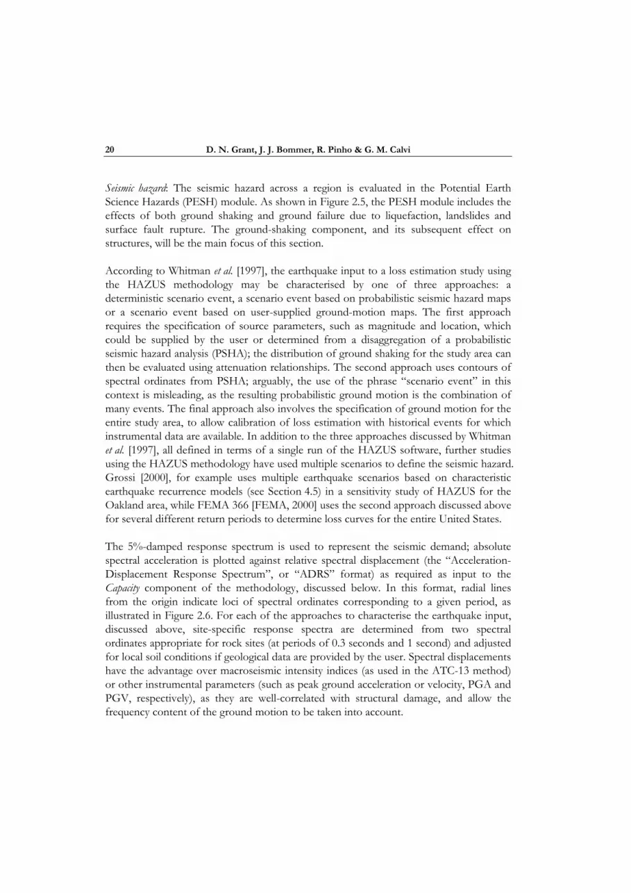
Seismic hazard: The seismic hazard across a region is evaluated in the Potential Earth Science Hazards (PESH) module. As shown in Figure 2.5, the PESH module includes the effects of both ground shaking and ground failure due to liquefaction, landslides and surface fault rupture. The ground-shaking component, and its subsequent effect on structures, will be the main focus of this section.
According to Whitman et al. [1997], the earthquake input to a loss estimation study using the HAZUS methodology may be characterised by one of three approaches: a deterministic scenario event, a scenario event based on probabilistic seismic hazard maps or a scenario event based on user-supplied ground-motion maps. The first approach requires the specification of source parameters, such as magnitude and location, which could be supplied by the user or determined from a disaggregation of a probabilistic seismic hazard analysis (PSHA); the distribution of ground shaking for the study area can then be evaluated using attenuation relationships. The second approach uses contours of spectral ordinates from PSHA; arguably, the use of the phrase “scenario event” in this context is misleading, as the resulting probabilistic ground motion is the combination of many events. The final approach also involves the specification of ground motion for the entire study area, to allow calibration of loss estimation with historical events for which instrumental data are available. In addition to the three approaches discussed by Whitman et al. [1997], all defined in terms of a single run of the HAZUS software, further studies using the HAZUS methodology have used multiple scenarios to define the seismic hazard. Grossi [2000], for example uses multiple earthquake scenarios based on characteristic earthquake recurrence models (see Section 4.5) in a sensitivity study of HAZUS for the Oakland area, while FEMA 366 [FEMA, 2000] uses the second approach discussed above for several different return periods to determine loss curves for the entire United States.
The 5%-damped response spectrum is used to represent the seismic demand; absolute spectral acceleration is plotted against relative spectral displacement (the “Acceleration-Displacement Response Spectrum”, or “ADRS” format) as required as input to the Capacity component of the methodology, discussed below. In this format, radial lines from the origin indicate loci of spectral ordinates corresponding to a given period, as illustrated in Figure 2.6. For each of the approaches to characterise the earthquake input, discussed above, site-specific response spectra are determined from two spectral ordinates appropriate for rock sites (at periods of 0.3 seconds and 1 second) and adjusted for local soil conditions if geological data are provided by the user. Spectral displacements have the advantage over macroseismic intensity indices (as used in the ATC-13 method) or other instrumental parameters (such as peak ground acceleration or velocity, PGA and PGV, respectively), as they are well-correlated with structural damage, and allow the frequency content of the ground motion to be taken into account.

Defining Priorities and Timescales for Seismic Intervention
21
Figure 2.6. Demand spectra and capacity curves in HAZUS methodology [FEMA, 2003].
Exposure: Within the HAZUS methodology, buildings are classified according to both their use (“occupancy class”) and structural system and height (“model building type”). Twenty-eight occupancy classes and 36 model building types are defined. Both aspects of building classification affect the assessment of monetary loss, while building capacity is determined solely by the model building type. An example building inventory, showing the total floor area for different occupancy classes and structural systems (both reduced in number for simplicity), is presented in Figure 2.7.
In addition to the occupancy class and model building type, the vulnerability of the building stock is also a function of the seismic design level; code design levels corresponding to the 1994 Uniform Building Code seismic zones 4, 2B and 1 are included, in addition to a “Pre-Code” level for buildings not designed for earthquake loading. This latter aspect of Exposure is accounted for by including the building age in the inventory classification, and determining what level of seismic resistance was required at the time that the building was constructed. Treating the building classification in this manner ignores the issue of possible code non-compliance in design and construction – perhaps less of a problem in the United States than in other parts of the world, including Italy.
As with the PESH module described earlier, default building stock inventories are included in the HAZUS software. Although of some use for preliminary loss assessment, the default inventories will generally be too coarse for in-depth loss estimation studies in the United Sates, and of even less applicability for building stock in other parts of the

D. N. Grant, J. J. Bommer, R. Pinho & G. M. Calvi
22
Figure 2.7. Example building inventory for HAZUS methodology [Kircher et al., 1997a]. “Floor area”
refers to total floor area over entire inventory.
world. For this reason, the collection of data for the HAZUS methodology is particularly demanding; it has been suggested that the preparation of a detailed inventory may require up to two years [FEMA, 2003]. In addition to time constraints in the preparation of the building stock inventory, computational time may also limit the resolution of data that can be included in the loss estimation: in determining an earthquake loss model for Turkey, Bommer et al. [2002] reduced an initial draft list of 38 building types, based on expected differences in seismic vulnerability, to just 14 types, to reduce the run-time required by the analyses.
Vulnerability: Building stock vulnerability is characterised in HAZUS by two sets of “building damage functions”: capacity curves and fragility curves [Kircher et al., 1997a], defined for each model building type. The capacity curves provide an estimate of peak lateral load resistance (divided by mass to give units of acceleration) as a function of peak displacement, which allows the visual comparison with seismic demand on the ADRS plot, as in the Capacity Spectrum method [Freeman et al., 1975; Freeman, 1978]. Fragility curves represent the predicted probability of reaching each damage state for a given earthquake response level. The Vulnerability module in the HAZUS methodology determines a performance point for each model building type as the intersection of the demand and capacity curves, and uses this estimate of performance as an input to the fragility curves to determine the expected structural or non-structural damage. Although non-structural damage – both displacement- and acceleration-sensitive components [Kircher et al., 1997a] – is considered in the same framework within HAZUS, only structural damage is discussed in the following.

Defining Priorities and Timescales for Seismic Intervention
23
Building capacity curves are fully defined by two control points, representing yield- and ultimate-level response, respectively, determined from code design levels and expected material and structural overstrength values. The curves are essentially elastic-perfectly plastic, except for a non-linear transition region defined between the two control points. Capacity curves represent the “pushover” response of each building type, and enhanced non-linear static analysis techniques [e.g. ATC, 2005; Antoniou and Pinho, 2004] could be expected to provide a more accurate estimation of building capacity if incorporated into the methodology.
The definition of building capacity in the same framework as seismic demand allows the building performance to be evaluated graphically as the intersection of these curves. However, because the building non-linearity described by the capacity curve is accompanied by additional energy dissipation (beyond the 5% viscous damping assumed in the Seismic Hazard module) the demand curve must be modified. In HAZUS, this modification is carried out by the definition of an equivalent viscous damping, consistent with the secant stiffness defined from the origin to the performance point. The demand curve is also adjusted for the duration of the ground motion, where this can be established from a deterministic hazard scenario or disaggregation of PSHA. Finally, the expected performance point for each building type may be determined from the intersection of the capacity and adjusted demand curves; equivalent linear properties are response-dependent, as they are a function of the attained ductility, and an iterative procedure is required to obtain this point. The determination of the performance point is illustrated in Figure 2.6.
Once the expected spectral response has been determined, this information may be used with building fragility curves to determine the distribution of damage expected for the building stock in each model building type category. Fragility curves are probability distributions for the boundary between damage states, defined in terms of a median value and a lognormal standard deviation. The median for each damage state threshold, shown as a circle in each of the example fragility curves in Figure 2.8, is calculated from drift ratios corresponding to damage for each material and building type, and effective building height to translate drift ratios into spectral displacements. The lognormal standard deviation accounts for aleatory and epistemic uncertainty in the capacity curve properties, damage states, and definition of ground shaking; the uncertainty in the latter is assumed to be independent of the other two sources of uncertainty. Since the capacity and the demand are correlated in the definition of the performance point, however, a convolution process is required to appropriately consider their joint probability distribution [Kircher et al., 1997a]. The probability that each damage state threshold is exceeded for each model building type may then be determined from the fragility curves, and the distribution of buildings in each damage state is calculated from the difference between these probabilities. Finally, this distribution of damage may be convolved with the building inventory, to determine the total damage over the entire region.

D. N. Grant, J. J. Bommer, R. Pinho & G. M. Calvi
24
Figure 2.8. Example fragility curves for different damage states [Kircher et al., 1997a].
Cost: Building loss functions are defined in HAZUS in terms of loss rates, in dollars per square foot, for each combination of damage state, model building type and occupancy class, and for different categories of damage [Kircher et al., 1997b]. An example matrix of loss rates, for a given model building type and occupancy class, and for different damage states and sources of damage, is shown in Table 2.2. Although the numerical values are not important for this study, the table illustrates how loss rates are defined in the methodology, and gives an indication of the quantity of data necessary to define them for all building types and occupancy classes. This is particularly relevant in applications of the HAZUS methodology outside the United States, in which customised building inventory definitions may be required, and US dollar values will not apply. The loss functions may be convolved with the building inventory, seismic hazard and building damage functions to determine the total direct monetary losses for a region. Modules also exist within HAZUS for the determination of direct losses resulting from damage to lifelines and ground failure, induced damages (caused by, for example, fire following a seismic event), indirect losses (considering long-term economic effects), and social losses (for example, human casualties).
2.4 THE CATANIA PROJECT A comprehensive loss estimation study was carried out on the city of Catania in eastern Sicily, Italy [Faccioli et al., 1999]. Two different methods were used to characterise the vulnerability of the building stock: the first was a score-based assessment method (see Section 5.2), widely used in Italy [Benedetti and Petrini, 1984; Angeletti et al., 1988; CNR-GNDT, 1993], based on the determination of a vulnerability score, and the correlation of this score with damage based on real earthquake damage observations; the second was

Defining Priorities and Timescales for Seismic Intervention
25
Table 2.2. Typical loss rates for single-family residences of light-frame wood construction located in California (dollars per square foot) [Kircher et al., 1997b].
Damage State
Structural System
Non-structural
(Drift-sensitive)
Non-structural
(Acceleration-sensitive)
Total Building Contents
Building Plus
Contents
Slight 0.38 0.8 0.43 1.6 0.4 2
Moderate 1.88 2 2.13 8 2 10
Extensive 9.38 20 10.63 40 10 50
Complete 18.75 40 21.25 80 20 100
based on a comparison of the displacement capacity for given limit states with the displacement response spectrum defining the seismic hazard [Calvi, 1999]. The latter approach holds some features in common with the HAZUS methodology, described in the previous section, and provided the initial framework for the development of the DBELA method, discussed in Section 2.7. Since the aim of the study was to determine the expected damage distribution for a given earthquake scenario, the Cost component of the risk equation, in terms of monetary and social losses, is not considered here. For the first method, where damage factors are used to define the loss, the damage and monetary loss are related in the same manner as in the ATC-13 method (Section 2.2). In the second method, damage is expressed in damage states, requiring further calibration to provide monetary loss.
Seismic hazard: The study aimed to determine damage scenarios for the city area of Catania, for a deterministic seismic event: an earthquake of magnitude, M = 7+, rupturing a 70 km portion of a mapped fault, 10 to 12 km from Catania city centre. This scenario is believed to be similar to a large event that occurred in 1693, which, following another large event two days previously, almost completely destroyed the entire city [Azzaro et al., 1999]. Attenuation relationships for median PGA and spectral displacement values (at periods of 0.4 seconds and 1 second, and for a viscous damping ratio of 2%) were employed, using GIS software, to obtain maps of ground motion for the Catania area [Pessina, 1999]. Peak ground acceleration maps were used in the first vulnerability assessment approach, and displacement spectral ordinates were used in the second. Both assessment methods are described in the Vulnerability section, below.
Exposure: The Catania project included building inventory data from three different surveys: national census data, a survey of the central city carried out in the 1980s by Catania city planning office, and a comprehensive survey of Catania building stock

D. N. Grant, J. J. Bommer, R. Pinho & G. M. Calvi
26
performed specifically to assess building vulnerability. The buildings were primarily constructed from masonry or reinforced concrete, and were classified according to their age and height. Age is a particularly important parameter for characterising structural vulnerability, with a large portion of the historic centre dating from the reconstruction of the city following the 1693 earthquake, and seismic code provisions enforced only since 1981. The distribution of building inventory, from the first stage of the building vulnerability survey (with 33% of Catania building stock included), is shown in Figure 2.9.
15
9
13<1
919
-45
46-6
061
-71
72-8
1>8
1
0
20
40
60
80
100
120
no. of bldgs
no. of stories
age class
RC
14
7
<19
19-4
5
46-6
0
61-7
1
72-8
0
>80
0
200
400
600
800
1000
1200
1400no. of bldgs
no. of stories
age class
Masonry
(a) (b)
Figure 2.9. Distribution of buildings by height and age class for (a) masonry buildings (sample of 5500 buildings) and (b) reinforced concrete (RC) buildings (sample of 2200 buildings). Data from the comprehensive survey of central Catania, at 33% complete stage [Faccioli et al., 1999].
Vulnerability: As discussed above, the vulnerability of Catania building stock was assessed using two distinct approaches. The first vulnerability assessment approach was based on field observation, and the assignment of a vulnerability index, Iv, to each building. An initial preliminary assessment was carried out based on an Italian national database of seismic vulnerability data, followed by a more detailed study in which all residential buildings in the city were assigned vulnerability indices based on a field survey, expert judgement and the data from the initial assessment. The statistical distributions of the vulnerability indices for masonry and reinforced concrete (RC) buildings based on this procedure are shown in Figure 2.10. These vulnerability indices have been calibrated based on damage observations from the 1976 Friuli and 1984 Abruzzo earthquakes, to provide a relationship between the expected damage factor (defined in Section 2.2) with the ground shaking (measured in terms of PGA) for different values of the vulnerability index. This relationship is illustrated in Figure 2.11. Finally, the total damage using this approach may be determined by superimposing the distribution of vulnerability indices on the ground shaking PGA maps, and obtaining a deterministic estimate of damage factors for the earthquake scenario.

Defining Priorities and Timescales for Seismic Intervention
27
0
50%
100%
5 15 25 35 45 55 65 75 85 95
Iv
Masonry
< 1919> 1919all bldgs
0
50%
100%
-15 -5 5 15 25 35 45 55 65 75 85 95
Iv
RC
< 1980> 1980all bldgs
Figure 2.10. Statistical distributions of the vulnerability index, Iv, for masonry and RC buildings for
the Catania building inventory [Faccioli et al., 1999].
Iv = 80 60 40 20 10 5
0
0.2
0.4
0.6
0.8
1
0 0.2 0.4 0.6 0.8 1
a_max
Dam
age
fact
or, d
Figure 2.11. Relationship between damage factor and peak ground acceleration for different values
of the vulnerability index (shown on the curves), for masonry and RC buildings [adapted from Guagenti and Petrini, 1989].
The second approach employed in the Catania project for the assessment of building vulnerability is based on the definition of structural damage limit states corresponding to specific levels of inter-storey drift [Calvi, 1999]. For the first limit state, the structure is assumed to behave elastically, with a deformed shape that is linear with height. Beyond the structural yield level, response is categorised by either “soft-storey” or “distributed damage” behaviour, referred to in the following as “column-sway” and “beam-sway” response, respectively. For a column-sway mechanism, all inelastic deformation is concentrated in the ground level; limit state thresholds are defined in terms of concrete and steel strain limits (or other appropriate material strain limits for non-RC structures), structure and member geometry, and estimated plastic hinge lengths. The collapse limit state for the column-sway mechanism is limited by an approximate storey displacement

D. N. Grant, J. J. Bommer, R. Pinho & G. M. Calvi
28
ductility limit of 3. The calculations for a beam-sway mechanism are similar, with an assumed linear deformation profile up the height of the building, and a collapse ductility limit of 4. For each limit state, equivalent linear properties based on the substitute structure approach [Shibata and Sozen, 1976] are used to determine the reduction in the demand spectrum to take into account the additional inelastic energy dissipation, and the effective period of vibration, for each limit state.
To account for the variability in geometric and material properties of the buildings in each building class, and uncertainty in the modelling approach, lower and upper bounds for each displacement limit and effective period are determined, and the building properties are assumed to be distributed uniformly within these bounds. When the displacement capacity and effective period bounds are superimposed on the displacement response spectrum, adjusted for the equivalent viscous damping level, the distribution of buildings in each limit state can be determined. The fraction of the rectangular area which lies below the demand spectrum represents the fraction of the buildings for which demand is greater than capacity – i.e. the limit state is exceeded.
Figure 2.12 shows an example application for RC frames forming a beam-sway mechanism, for the yield limit state and a PGA of 0.3g. Demand spectra corresponding to firm and soft soil are shown, along with the performance bounds corresponding to structural (SD) and non-structural (NSD) damage. Considering just the structural damage (lower displacement spectrum in Figure 2.12) in the example application, it can be observed that, in firm soil conditions (solid boxes), approximately 8%, 5% and 2% of 4-, 8- and 12-storey buildings (left, middle, and right boxes), respectively, exceed the yield limit state. For soft soil conditions (dashed boxes), these percentages increase to 20%, 35% and 30%.
Both of the vulnerability assessment procedures used in the Catania project have some advantages and limitations. The vulnerability index approach has been used extensively throughout Italy, and calibrated with data from two damaging earthquakes. As discussed in Section 2.3, however, the peak ground acceleration is not correlated well with damage, and does not take into account the frequency content of the ground motion and the fundamental frequency of the structure. This suggests that correlated damage functions may be specific to the type of ground motion experienced in the Friuli and Abruzzo earthquakes and the building stock in those two regions, and may not be applicable for future earthquake scenarios. Furthermore, the method does not take into account the uncertainty in the estimation of seismic hazard or structural vulnerability. The second approach has the advantage that it is based on spectral displacement, which is better correlated with both structural and displacement-sensitive non-structural damage. Furthermore, the variability in the building stock is considered in the estimation of both drift limits and structural vibration periods, although a uniform distribution is assumed

Defining Priorities and Timescales for Seismic Intervention
29
Figure 2.12. Example of second vulnerability assessment procedure from Catania project, for limit
state 1 (yield), beam-sway reinforced concrete frames, PGA=0.3g; SD = “structural damage” and NSD = “non-structural damage” [Calvi, 1999].
for simplicity. Uncertainty is not taken into account in the evaluation of the equivalent viscous damping, nor in the determination of the seismic hazard across the region. The DBELA method, which also uses spectral displacement as a measure of capacity and demand, addresses a number of these shortcomings, and is discussed in Section 2.7.
2.5 ORDAZ ET AL. [2000] LOSS ESTIMATION MODEL
Ordaz et al. [2000] present an earthquake loss estimation model specifically developed to evaluate seismic risk for Mexico City; the general approach of the method, however, could be adopted for other study areas.
Seismic hazard: The seismic hazard is represented for the entire city by hazard curves of spectral acceleration values, computed for fundamental periods of 0, 1 and 3 seconds using PSHA. Three separate attenuation relationships are assumed in the PSHA, which were developed for firm sites in Mexico City for subduction events, intermediate-depth events and areas of diffuse seismicity. Site amplification effects are taken into account by empirical transfer functions (ETF), which relate the expected ground motion for any site to a reference stiff soil site. These functions were developed based on microtremor measurements and strong motion data for instrumented sites, comparing the spectral

D. N. Grant, J. J. Bommer, R. Pinho & G. M. Calvi
30
response at the reference site to instrumental data; the transfer functions for non-instrumented sites were determined by interpolation. Ground motion is considered in north-south and east-west components to account for the expected orientation of ground shaking in Mexico City.
Exposure: Ordaz et al. [2000] give little information about the building inventory characterisation used in the loss estimation study. However, according to the paper “the system includes an expert procedure to characterise buildings, which infers structural parameters (predominant period, structural type, etc.) using the level of information furnished by the user, be it rough or very detailed”. As described below, the calculation of building vulnerability requires the following parameters: structural type, the number of storeys, typical inter-storey height, location, soil type and age. These parameters, at minimum, are required in the building inventory description. Ordaz et al. [2000] also refer to modifications to the vulnerability based on geometrical irregularities, proximity of neighbouring structures to take into account pounding potential, existence of previous damage, and the presence of short columns. These penalty factors are presumably included in a “very detailed” characterisation of building inventory.
Vulnerability: As with the method of Calvi [1999], the vulnerability assessment procedure is based on the relationship between spectral displacements and peak inter-storey drift ratios. The spectral displacement is obtained from the spectral acceleration by an assumed relationship between the fundamental period and the number of storeys in the structure. The parameters in this relationship were calibrated for different structural types, taking into account the variation in structural stiffness due to location, soil type, and age of construction. The peak inter-storey drift ratio is obtained from the spectral displacement by multiplying by four pre-calibrated factors, which represent:
1. The ratio between maximum roof displacement and spectral displacement for linear-elastic behaviour.
2. The “lateral deflected shape factor”, which is the ratio between the peak inter-storey drift ratio and global distortion, where the latter is defined as the ratio of maximum roof displacement to total height of the structure.
3. The ratio of inelastic to elastic lateral displacement – effectively the behaviour factor, R, from US design codes.
4. The ratio of inelastic to elastic lateral deflected shape factors, defined according to point 2, above.
The four factors are all expressed as functions of different structural properties, based on a number of semi-empirical studies by the authors.

Defining Priorities and Timescales for Seismic Intervention
31
Cost: Mean damage ratios, and therefore expected monetary loss for a given structure, are determined through a non-linear function of peak inter-storey drift, structural system and date of construction. For loss estimation over a building inventory, the probability density function (PDF) of the loss is required. An expression for the variance of the damage ratio was assumed as a function of structural type, based on ATC-13 damage matrices (Section 2.2) and simulations of simple structures. The mean and variance of the damage ratio allow the full PDF to be described, and the gross loss to be calculated. The probable maximum loss (PML), defined as the 1500-year return period loss in this study, is calculated by summing the expected losses for each structure and for each seismic source. The use of a 1500-year return period to represent “the largest loss that can be suffered during an individual event” [Ordaz et al., 2000] seems to have been selected fairly arbitrarily – arguably, the use of time intervals consistent with the characteristic earthquake model assumed in the development of hazard curves [Ordaz and Reyes, 1999] may have been more appropriate.
2.6 COSENZA ET AL. [2005] VULNERABILITY ASSESSMENT METHOD
Cosenza et al. [2005] recently proposed an approach for the capacity assessment of a building inventory, for use in loss estimation studies. The approach uses the response surface method and Monte Carlo simulation to estimate the probability distribution of building capacity in an inventory, which may then be convolved with a consistent measure of seismic hazard to determine the expected loss. The characterisation of seismic demand and the transition from damage limit states to monetary losses are not addressed by the study.
Exposure: A specific aim of the method is to account for the various levels of information that may be available for a given inventory characterisation in the final specification of structural vulnerability. The parameters required for the vulnerability assessment are divided into three categories, based on the difficulty with which they may be obtained for a given building inventory, referred to as low-, medium- and high-order parameters, in increasing order of difficulty. Low-order parameters are related to the overall geometry of the structure, and may be obtained from an exterior survey. Medium-order parameters require interior inspection of buildings, and include frame dimensions and the number of sets of stairs. Finally, high-order parameters include material properties that must be determined from building codes, construction standards and regional databases. By categorising parameters in this manner, the effect of reducing the epistemic uncertainty can be quantitatively evaluated. The aleatory uncertainty, which is related to the actual variability of building stock within building classes, can also be reduced by refining building class definitions, and the effect on the building class vulnerability can then be evaluated.

D. N. Grant, J. J. Bommer, R. Pinho & G. M. Calvi
32
Vulnerability: Monte Carlo simulation is used to generate randomly-sampled building models from the probabilistic definition of each of the structural parameters. The different aspects of the modelling process are summarised in Figure 2.13. The building frame system is idealised as a three-dimensional line model (top of Figure 2.13), and beams and columns are dimensioned and designed for the building code that was in place at the time of construction (middle). For each element, member moment–rotation behaviour is defined in terms of yield moment, yield curvature and ultimate curvature capacity (bottom). The ultimate capacity of each simulated building is determined using a plastic analysis approach; it is assumed that building capacity corresponds to the development of a plastic mechanism, and that seismic forces may be represented by a linear distribution over the height of the building. A number of collapse mechanisms are postulated, based on column-sway, beam-sway or combined beam/column-sway behaviour, and the base shear and total roof drift are determined for each. The governing collapse mechanism is the one with the lowest base shear capacity. Finally, from the individual building capacities for each of the simulated modes, an estimation of the overall vulnerability of the building stock is obtained from the Response Surface method. The final output from the method is a “capacity curve” which shows the probability distribution of the base shear and total roof drift capacity for the building inventory. Example capacity curves are shown for a 3-storey building model in Figure 2.14(a) and (b), for the base shear coefficient and inter-storey drift ratio, respectively. The curves are shown for three parameter sets, described as low-, medium- and high-order, which relate to the parameter groupings described previously. The sensitivity studies to which these capacity curves relate, described in Cosenza et al. [2005], show that reducing the uncertainty on the input parameters reduces the spread in the final estimation of vulnerability.
Although the method is proposed solely for the assessment of building vulnerability, it is implied that the capacity curve may be convolved with a probabilistic distribution of expected demand to determine damage and possibly monetary loss distributions in a scenario earthquake. This may be possible to a limited extent, although the consideration of only a single limit state (the development of a full plastic mechanism) limits the applicability for large-scale loss estimation studies. Extending the plastic analysis approach to other limit states based on inter-storey drifts or material strains would not be possible. Furthermore, the capacity curves determined for full plastic mechanism arereported in terms of base shear capacity and roof drift; it would be difficult to convolve such curves with any measure of seismic demand other than PGA. As discussed in Section 2.3, spectral measures of demand are better correlated with the damage potential of earthquakes than PGA. Finally, the use of a triangular equivalent earthquake force distribution for the assessment of potential plastic mechanisms severely limits the applicability of the results. Equivalent earthquake forces are determined by the

Defining Priorities and Timescales for Seismic Intervention
33
Figure 2.13. Non-linear analytical model used in the evaluation of structural capacity in the Cosenza
et al. method [Cosenza et al., 2005].

D. N. Grant, J. J. Bommer, R. Pinho & G. M. Calvi
34
(a) (b)
Figure 2.14. Capacity curves for 3-storey building models, for low-order, medium-order and high-order parameter definitions; (a) base shear coefficient and (b) inter-storey drift ratio [Cosenza et al., 2005].
distribution of mass and stiffness in the building. The latter varies with inelasticity, and is therefore a function of the plastic mechanism developed. Overall, the method seems to require a disproportionate amount of computational effort for the accuracy and utility of the final results.
These limitations notwithstanding, the framework proposed by Cosenza et al. [2005] provides valuable information about the sensitivity of building vulnerability to various parameters. Furthermore, the authors recognise that “a more refined structural model and/or method could be introduced without influencing the applicability of the proposed approach” [Cosenza et al., 2005], although some of the limitations discussed above may be difficult to address.
2.7 DISPLACEMENT-BASED EARTHQUAKE LOSS ASSESSMENT (DBELA)
As discussed in Section 2.3, the HAZUS method and associated software represents the state of the art in the field of earthquake loss estimation. Several shortcomings of the method were identified in Section 2.3, however; in particular, a large amount of time is required to compile the inventory data required for effective loss estimation and subsequent computational effort is also significant.
Based on the original framework of Calvi [1999], Pinho et al. [2002] proposed a displacement-based earthquake loss assessment (DBELA) procedure, which is particularly suitable for earthquake loss modelling due to its computational efficiency, without loss of accuracy. The method was further developed by Glaister and Pinho [2003], and extended to a probabilistic framework by Crowley et al. [2004]. The DBELA method is used to provide an estimate of the distribution of building damage, in terms of discrete damage bands, following a number of scenario earthquakes. No guidance is provided, as yet, for

Defining Priorities and Timescales for Seismic Intervention
35
translating these damage distributions into monetary loss or human casualties. The method is currently able to consider the effects of direct structural damage, drift-sensitive non-structural damage [Crowley et al., 2004], and liquefaction [Bird et al., 2005], although only structural damage is discussed in the following.
Seismic hazard: As discussed above, the seismic demand in the DBELA method is based on displacement spectral ordinates, in the form of a displacement response spectrum. The response spectrum must be adjusted for the equivalent viscous damping used in the definition of the substitute structure (see Vulnerability, below).
The displacement demand spectrum that might be used in a loss estimation study could take the form of a code spectrum or else a uniform hazard spectrum derived from PSHA for one or more annual frequencies of exceedance. Both of these options have drawbacks in being obtained from PSHA wherein the contributions from all relevant sources of seismicity are combined into a single rate of occurrence for each level of a particular ground-motion parameter. The consequence is that if the hazard is calculated in terms of a range of parameters, such as spectral ordinates at several periods, the resulting spectrum will sometimes not be compatible with any physically feasible earthquake scenario [Bommer, 2002a]. Furthermore, if additional ground-motion parameters, such as duration of shaking, are to be incorporated – as they are in HAZUS, in the definition of the inelastic demand spectrum – then it is more rational not to combine all sources of seismicity into a single response spectrum but rather to treat individual earthquakes separately, notwithstanding the computational penalty that this entails. Compelling arguments against using PSHA for loss assessment arise also from the treatment of the scatter in the attenuation relationship [Bommer and Crowley, 2005].
The approach recommended therefore is to use multiple earthquake scenarios, each with an annual frequency of occurrence determined from recurrence relationships. For each triggered scenario, the resulting spectra are found from a ground-motion prediction equation. In this way, the aleatory uncertainty, as represented by the standard deviation of the lognormal residuals, can be directly accounted for in each spectrum. Following the suggestion of Bommer and Crowley [2005], it may also be appropriate to separate the uncertainty into “inter-event” and “intra-event” components, so that the proper correlation of uncertainty at different sites is taken into account. The cumulative distribution function (CDF) of the displacement demand can then be compared with the joint probability density functions of displacement capacity and the annual probability of failure for a class of buildings can be found by integrating the failure probabilities for all the earthquake scenarios. There are many benefits in using a multiple earthquake scenario approach, not least amongst which is the facility to obtain clear and reliable disaggregations of the calculated losses. The probabilistic implementation of the method

D. N. Grant, J. J. Bommer, R. Pinho & G. M. Calvi
36
enables scenario-based loss calculations, which take full account of the ground-motion variability, to be performed efficiently.
Exposure: The initial step required in this method is the division of the building population into separate building classes. A building class is to be considered as a group of buildings which share the same construction material, failure mechanism and number of storeys. The building classes currently considered within this methodology comprise the following structural types:
1. Reinforced concrete beam-sway moment-resisting frames 2. Reinforced concrete column-sway moment-resisting frames 3. Reinforced concrete structural wall buildings 4. Unreinforced masonry buildings exhibiting an out-of-plane failure mechanism 5. Unreinforced masonry buildings exhibiting an in-plane failure mechanism
Within each structural type, further building classes may be defined to separate, for example, buildings with different number of storeys, buildings designed with distinct steel grades or those built without adequate confining reinforcement. A decision regarding whether a moment-resisting frame will exhibit a beam-sway (class 1) or a column-sway (class 2) mechanism may be made considering the construction type, construction year and evidence of a weak ground storey. Many buildings constructed before the inclusion of sound seismic design philosophy (i.e. capacity design) into a country’s seismic design code and those with a weak ground floor storey will generally adopt a soft-storey (column-sway) mechanism. The treatment of classes 4 and 5, relating to unreinforced masonry structures, have been dealt with by Restrepo-Vélez and Magenes [2004]; classes 1 and 2 are discussed briefly below, and in more detail by Crowley et al. [2004]. Building class 3 has not yet been addressed in the DBELA method.
A simplified loss estimation study was carried out for the Marmara region in Turkey using the DBELA method [Crowley et al., 2005], primarily to assess the sensitivity of the losses to uncertainties in the ground-motion and vulnerability models. Turkish building census data was used to classify over 750,000 buildings in Istanbul, Kocaeli and Tekirdag. For the purposes of this study, buildings were classified based on the number of storeys, and a qualitative assessment (“Good” or “Poor”) of expected seismic performance, based on age and construction quality. All “Good” buildings and one third of all “Poor” buildings were expected to form a beam-sway mechanism in an earthquake; the remainder were assumed to form a column-sway mechanism (see below). The building inventory for the study region is summarised in Figure 2.15.

Defining Priorities and Timescales for Seismic Intervention
37
Number of Storeys
1 2 3 4 5 6 7-9
Prop
ortio
n of
RC
Fra
me
Bui
ldin
g St
ock
0.00
0.05
0.10
0.15
0.20
0.25
'Poor'_Column-sway'Poor'_Beam-sway'Good'_Beam-sway
Figure 2.15. Example building inventory for the application of the DBELA method in Marmara
Region, Turkey [Crowley et al., 2005]. “Good” and “Poor” building descriptions are correlated with expected building geometry, material properties, and global behaviour. All “Good” buildings, and one third of “Poor” buildings, are assumed to form a beam-sway mechanism, with the remainder displaying a column-sway mechanism.
Building geometry, in terms of column and beam dimensions, and material properties, in terms of limiting material strains for each limit state, were assumed for “Good” and “Poor” Turkish buildings, based on consultation with local engineers and published data on Turkish construction practice [EERI, 2000]. Mean values for every parameter, as well as probabilistic distributions and coefficients of variation, were assumed. Although a more in-depth study may require a more refined representation of Turkish building stock, the simplified study of Crowley et al. [2005] gives some indication of a building classification scheme, and parameters required, to carry out a loss estimation study with the DBELA method.
Vulnerability: The procedure uses mechanically-derived formulae to describe the displacement capacity of classes of buildings at three different limit states. These equations are given in terms of material and geometrical properties, including the average height of buildings in the class. By substituting this average through a formula relating height to the limit state period, displacement capacity functions in terms of period are attained; the advantage being that a direct comparison can now be made at any period between the displacement capacity of a building class and the displacement demand predicted from a response spectrum. The original concept is illustrated in Figure 2.16,

D. N. Grant, J. J. Bommer, R. Pinho & G. M. Calvi
38
Height
cumulative frequency
HLS1 HLS2HLS3
PLS3
0
PLS2
PLS1
PLSi – percentage of buildings failing LSi
effectiveperiod
disp
lace
men
t
LS1
LS2
LS3
Demand Spectra
TLS1TLS2 TLS3
HLSi = f (TLsi , LSi)
ηLS1
ηLS2
ηLS3
Figure 2.16. Deterministic representation of DBELA method; LS = limit state [Glaister and Pinho,
2003].
whereby the range of periods with displacement capacity below the displacement demand is obtained and transformed into a range of heights using the aforementioned relationship between limit state period and height. This range of heights is then superimposed onto the CDF of building stock to find the proportion of buildings failing the given limit state.
Building response is represented by an equivalent linear, single-degree-of-freedom (SDOF) system, according to the substitute structure approach [Shibata and Sozen, 1976]. The height (Hcsf) to the centre of seismic force, and an effective SDOF height (HSDOF) are defined in Figure 2.17. The latter is related to the total height (HT) by a coefficient, efh, which may be used to determine the total roof displacements from the SDOF system displacements. Values of efh are ductility- and mechanism-dependent, and are calculated based on building displacement profiles proposed by Priestley [2003].
The fundamental period appropriate to describe building response up to first yield is assumed to be solely a function of building height. Crowley and Pinho [2004] determined a simple, linear expression for the yield period as a function of building height, based on several analytical evaluations of European building stock. Such an expression is an essential element in the DBELA methodology, as it provides the means to relate the two halves of Figure 2.16. Although uncertainty is not included explicitly in the Crowley and Pinho [2004] relationship, it must be recognised that several sources of uncertainty are inherently incorporated. In particular, the variability in stiffness and mass of European building stock would be expected to affect the period-height relationship. Since the uncertainty in concrete strength and section geometries – directly related to building stiffness – is included explicitly in the evaluation of capacity, to avoid double counting the uncertainty in stiffness it would formally be necessary to evaluate the correlation.

Defining Priorities and Timescales for Seismic Intervention
39
θ
HT
HCSF
HSDOF T
SDOFh H
Hef =
Deformation profile of actual structure
Deformation profile of equivalent SDOF
Figure 2.17. Definition of effective height coefficient in DBELA method [Glaister and Pinho, 2003].
Beyond the yield limit, the SDOF dynamic properties are based on an equivalent linearisation approach. The period related to the secant stiffness is expressed as a function of ductility, assuming an elastic-perfectly plastic (EPP) backbone curve. Equivalent viscous damping ratios consistent with the secant period – ideally representative of real structural energy dissipation rather than EPP dynamic response – are also defined as a function of ductility. It is also recognised that spectral displacement adjustment factors for damping ratios other than 5% are influenced by the duration of the input motion [Bommer and Mendis, 2005], although this has not been incorporated into the method as yet.
Damage to the structural (load-bearing) system of the building class is estimated using three limit states of the displacement capacity. The building class may thus fall within one of four discrete bands of structural damage: none to slight, moderate, extensive or complete. Quantitative suggestions for the definition of each limit state and qualitative descriptions of expected damage under each limit state are provided in Crowley et al. [2004], taken from the work of Priestley [1997] and Calvi [1999]. The first structural limit state is defined as the yield point of the structure and the second and third structural limit states are attained when the sectional steel and concrete strains reach pre-defined strain limits. Two alternative pairs of sectional strains for the third limit state have been reported because the ultimate sectional strains that can be reached depend on the level of confinement of the structural members. Nevertheless, it should be noted that one is not constrained to employ the limit state steel and concrete strains provided by Crowley et al. [2004], and these, and other, parameters may be varied in the building class capacity calculations, if appropriate.

D. N. Grant, J. J. Bommer, R. Pinho & G. M. Calvi
40
By considering the yield strain of the reinforcing steel and the geometry of the beam and column sections used in a building class, yield section curvatures can be defined using the relationships suggested by Priestley [2003]. These beam and column yield curvatures are then multiplied by empirical coefficients to account for shear and joint deformation to obtain a formula for the yield chord rotation. This chord rotation is equated to base rotation and multiplied by the total building height and the effective height coefficient, as introduced in Figure 2.17, to produce the yield displacement capacity of a SDOF substitute structure. Sound, rational and deformation-based equations of displacement capacity can thus be derived through first principles and mechanical considerations. These capacity equations are derived based on the development of a column-sway or beam-sway mechanism. Note, however, that because the equations are ductility-dependent and material strain limits are defined, limit states other than the development of a full plastic mechanism may be assumed; this is not possible in the vulnerability assessment method of Cosenza et al. [2005], discussed previously.
A given building class within a selected urban area may comprise a large number of structures that present the same number of storeys and failure mode, but that feature varying geometrical properties (e.g. beam height, beam length, column depth, column/storey height), due to the diverse architectural and loading constraints that drove their original design and construction. Since such uncertainty does affect in a significant manner the results of loss assessment studies (see Glaister and Pinho, [2003]), it is duly accounted for in the current method by means of the probabilistic modelling described below. The probability density functions of the limit state displacement capacity and period are found using the first-order reliability method (FORM). Essentially, FORM can be used to compute the approximate CDF of a non-linear function of correlated parameters, such as the limit state displacement capacity function and limit state period function. The reader is referred for example to Pinto et al. [2004] for a description of the theory of FORM, as well as Restrepo-Vélez [2004] for a detailed description of the application of FORM to the displacement capacity equations for unreinforced masonry structures. Probabilistic distributions for geometrical parameters, limit state thresholds, and the parameters used in empirical relationships, are recommended in Crowley et al. [2004].
Based on the probabilistic representation of capacity parameters, the joint probability density function (JPDF) may be defined, which describes the correlation between the distributions. Finally, the JPDF can be convolved with a probabilistic representation of demand to find the probability of exceeding each of the three limit states described above. The probability of a building class being in each of the four structural damage bands, can then simply be found from the difference between the exceedance probabilities of the bordering limit states to the damage band in question. This probability is equated to the proportion of buildings falling within each damage band.

Defining Priorities and Timescales for Seismic Intervention
41
An interesting comparison can be made among the final performance points in the HAZUS, Cosenza et al. [2005], and DBELA loss estimation methods, neglecting any probabilistic considerations. HAZUS and DBELA are both based on spectral measures of capacity and demand, and their performance points, whether shown on a capacity spectrum or displacement response spectrum, have the same physical significance, although various assumptions in the procedure may be different. HAZUS provides a continuous representation of capacity through a pushover curve, while DBELA calculates only the performance levels that correspond to the attainment of limit states, although more limit states could be considered in the latter method, and an effective pushover curve of performance points could be constructed on an ADRS plot. Since both HAZUS and DBELA are based on an equivalent linearisation approach, the performance points would be similar. The fundamental difference between the two approaches, however, is the manner in which dynamic response is approximated statically; the former uses an assumed distribution of equivalent static force in the pushover analysis, which may or may not be adjusted with ductility, while the latter uses a relationship between fundamental period and building height and functions describing the displacement profile in terms of ductility. The method of Cosenza et al. [2005] considers only one limit state, corresponding to the development of a full plastic collapse mechanism. The earthquake forces in this method are also represented by an equivalent static force profile; the performance point in this case would be similar to the final limit state in the HAZUS method, although because of the plastic analysis approach adopted, it would not be possible to determine intermediate limit states using this method.

3. DEFINING TOLERABLE LEVELS OF SEISMIC RISK
The mitigation of seismic risk has become an essential part of the design and assessment of structures in earthquake-prone regions. As expressed in Eq. (1.1), seismic risk is a function of the seismic hazard, exposure, vulnerability and cost. Since the hazard cannot be controlled, and the exposure is generally dictated by other requirements, seismic design is a process of balancing the vulnerability and cost components. Guidelines, pre-standards and codes for seismic design therefore specify acceptable levels of vulnerability, as a function of the hazard at the site, adjusted for the use and occupancy of the structure.
In this chapter, the specification of tolerable seismic risk in design and assessment codes and guidelines, and within the new Performance-Based Earthquake Engineering (PBEE) framework, is summarised.
3.1 BASE DEFINITION OF TOLERABLE SEISMIC RISK IN DESIGN CODES
The definition of a consistent level of seismic risk for new building construction in a country is usually the role of seismic design provisions in building codes. These provisions prescribe maximum values of material strains, local and global ductility limits, and general detailing requirements, for a given ground-motion intensity. The various capacity requirements are generally selected to represent an Ultimate Limit State (ULS) building performance, under which significant structural and non-structural damage may occur, but loss of life is prevented. Clearly, this degree of damage would not be tolerable in small seismic events occurring perhaps many times over the life of the building. For this reason, ULS design is generally carried out for a level of ground motion expected in earthquakes which occur much less frequently. The issue of what is considered sufficiently “rare” or “unlikely” is a contentious one, and is fundamental to the definition of tolerable seismic risk in modern design codes.
Seismic design provisions have generally been developed in terms of a single limit state; until relatively recently, only the seismic codes of Japan and New Zealand included multiple limit states for different levels of ground motion [Uang, 1993]. Code commentaries recognise, however, that this single explicit check is expected to also provide adequate performance under more and less frequent seismic events. Hamburger [1998], for example, suggests that the implicit performance objectives included the following:

D. N. Grant, J. J. Bommer, R. Pinho & G. M. Calvi
44
1. Resist minor earthquakes without damage. 2. Resist moderate earthquakes without structural damage but with some non-
structural damage. 3. Resist major earthquakes with significant structural and non-structural damage. 4. Resist the most severe earthquakes ever likely to affect the building, without
collapse.
As discussed in Section 1.2, the use of the term “earthquakes” to refer to the hazard levels in these methodologies is inexact; “ground motion” should be used when referring to the expected level of ground shaking from a probabilistic hazard assessment.
Capacity design philosophy, developed in the 1970s [Park and Paulay, 1975] and first adopted in seismic codes in the 1980s [NZS, 1982], addresses the fourth of these objectives, by ensuring that ductile plastic mechanisms may develop under extreme ground motions. For moment-frame systems, for example, a “weak beam-strong column” design philosophy is adopted, whereby beams are detailed for the development of plastic hinges, and columns are prevented from hinging by the provision of sufficient overstrength. One of the principal intentions of capacity design is to desensitise the structure to the intensity of the ground motion. Priestley and Amaris [2002] have demonstrated, however, that for capacity-designed structural wall systems, extreme ground motion may cause yielding outside designated plastic hinge zones. To maintain the capacity design objective of concentrating plasticity at the base of the wall, overstrength design actions must therefore be defined that are a function of the level of input ground motion. This suggests that the rather ambiguously-defined “most severe” ground motion that is “ever likely to affect the building” requires more careful definition, particularly in safety-critical applications such as the design of nuclear power plants [Bommer et al., 2004a].
More recently, performance-based approaches have explicitly considered multiple objectives similar to those given above, with more rigorously defined hazard levels and performance targets. Modern design codes [CEN, 2004; OPCM, 2003] are beginning to specify more than one limit state for design, and future codes can be expected to make further use of Performance-Based Earthquake Engineering concepts (Section 3.4).
In most seismic codes throughout the world, design ground-motion levels, corresponding to the “major earthquake” listed in the third performance objective above, are defined probabilistically. The first probabilistic seismic hazard maps, for PGA values with a return period of 475 years, appeared in ATC 3-06 [ATC, 1978], and were based on the work of Algermissen and Perkins [1976]. The 475-year return period selected is equivalent to an annual frequency of exceedance of 0.21%, or a probability of exceedance

Defining Priorities and Timescales for Seismic Intervention
45
of 10% over an assumed 50-year design life. Bommer and Pinho [2005] show that both the 10% probability and 50-year design life were selected fairly arbitrarily, and were retained principally because the resulting hazard maps were similar to those that had already been developed based on expert judgement. The 475-year hazard maps were subsequently adopted in the 1988 edition of UBC [ICBO, 1988], and the same return period was used in probabilistic hazard assessments in most of the next generation of seismic design codes throughout the world. An exception is the 1986 Costa Rican code [IAEE, 1996], which provides PGA maps for return periods of 50, 100, 500 and 1000 years, and allows the designer to calculate the appropriate return period based on the importance, design life and ductility of the structure.
The commentary to ATC 3-06 [ATC, 1978] acknowledges that “the use of a 50-year interval to characterize the probability is a rather arbitrary convenience, and does not imply that all buildings are thought to have a useful life of 50 years”. In fact, the specification of design ground motion in terms of a given probability of exceedance in a fixed design life is generally used to implicitly define a design action with an annual frequency of exceedance (AFE) that is deemed tolerable for new construction. A building that has been designed for a 10%-in-25-year hazard (AFE = 0.42%), for example, represents twice the annual risk to its occupants or the general public as a building designed for the same exceedance probability for a 50-year design life (AFE = 0.21%). Although there may be other reasons for reducing design motions, based on limited exposure of inventory or human lives (Section 3.2) or an increased cost-to-benefit ratio for the retrofit of existing construction (Section 3.3), this reduction cannot be justified in terms of a reduced design life. The arbitrariness in the selection of the design life led to the unusual legislation in New Zealand for the assessment of existing structures, in which a 50-year design life “will allow unlimited life to the structure [; however] if a different design life is assumed, [the design hazard] can be modified accordingly but the structure shall be demolished upon expiration of the time span assumed in the assessment.” [NZSEE, 2003]. This attempt to enforce the design life through legislation – although providing an incentive for targeting the standard code hazard level in seismic retrofit projects – ignores the fact that it is the annual frequency of exceedance that is important in the definition of tolerable levels of seismic risk. The issue of reducing the design life for the assessment of existing structures is investigated further in Section 3.2.
Although the 50-year design life has become a sacred cow of earthquake engineering, the 10% probability of exceedance has been subjected to modification over recent decades. Holmes [1998] reports that “the mystique of the [10%-in-50 year] event was first broken during development of the code for seismic isolation, where collapse of the isolation system was considered catastrophic and a larger event was specified to check the stability of the isolation bearings.” In this case, the global consequences of bearing stability failure were much more severe than those implied under standard ULS design procedures. Code developers believed that a 2%-in-50-year hazard – equivalent to a return period of 2475 years, or annual frequency of
D. N. Grant, J. J. Bommer, R. Pinho & G. M. Calvi
46
exceedance of 0.04% – was more representative of a tolerable frequency of collapse, while the 475-year hazard was retained for the standard, ultimate limit state design requirements.
Subsequently, the 2%-in-50-year hazard was also adopted for a collapse prevention limit state in the development of the 1997 NEHRP Recommended Provisions for Seismic Regulations for New Buildings, FEMA 302/303 [BSSC, 1997]. The Maximum Considered Earthquake (MCE) was defined as the “the maximum level of earthquake ground shaking that is considered as reasonable to design normal structures to resist” [Leyendecker et al., 2000]. The subtle change in emphasis from the “Maximum Credible Earthquake” or “Maximum Capable Earthquake” terminology defined in previous studies means that the issue of defining a worst possible ground motion, discussed by Bommer et al. [2004a], is avoided here. Furthermore, as discussed in Chapter 1, the use of the word “earthquake” in this context is misleading, as it actually refers to a ground motion. The MCE is defined by hazard maps, which were developed for the minimum of the 2%-in-50-year probabilistic ground motion, and 1.5 times a deterministic ground motion based on characteristic earthquake models. Since standard design was carried out to the same ultimate limit state requirements as before – such as material strain limits and capacity design guidelines – the MCE hazard was adjusted by a factor of 2/3, based on expected building performance beyond the design level prior to collapse. The justification for such an adjustment is discussed in more detail in the following section. Finally, the new Canadian seismic code has also adopted 2475-year hazard as the standard level for new design, with an adjustment factor of two-thirds which only applies to short period structures [Heidebrecht, 2003]. Without comparing all aspects of building design in the United States and Canada, including material strain and ductility limits, and detailing requirements, it is difficult to determine if long-period Canadian buildings are expected to reach a higher performance level, consistent with the use of a probability level that “represents the approximate structural failure rate deemed acceptable” [Adams and Halchuk, 2003].
From the above discussion, it is clear that it is not possible to select the return period which defines the code seismic demand independently of the performance levels implied by the code. For example, if the Canadian building code allows much higher ductility levels to develop under a design seismic action that is 1.5 times larger for long period structures, then it is possible that US and Canadian seismic provisions represent a similar level of risk. Furthermore, a level of seismic risk that is considered tolerable for one country may not be appropriate for another. Construction types, relative importance of other hazards, and other social and economic factors may all influence the level of seismic risk that may be considered acceptable for an individual country. Bommer et al. [2005] have argued that the methods described in Chapter 2 could be used to determine the expected monetary loss and loss of life under scenario events, based on different code design assumptions. This iterative loss modelling approach would then provide a rational

Defining Priorities and Timescales for Seismic Intervention
47
basis for the selection of structural design levels for future generations of seismic design codes.
3.2 ADJUSTMENT TO TOLERABLE RISK FOR BUILDING IMPORTANCE AND PERFORMANCE
Seismic codes typically specify more severe design ground motion for structures which may contain a large number of people (e.g. meeting halls), those whose function may be particularly important following an earthquake (e.g. hospitals), and those for which the consequences of collapse may be particularly grave (e.g. schools). Similarly, a reduction factor may be applied to the base design hazard for structures of a secondary nature, such as farm buildings, warehouses and temporary construction. The relative importance of a structure is taken into account by an importance factor, which is multiplied by the appropriate zone factor to obtain the design hazard. This design process ostensibly targets the same building performance for a ground motion with a longer return period; implicitly, this also serves to provide a greater design performance under the basic design level ground motion. When identical importance factors are specified across a large region characterised by varying seismicity, such as in the 2000 International Building Code [ICC, 2000], the return period of the design ground motion will vary accordingly, even if the implicit target performance level remains the same. For example, Figure 1.4 shows PGA values with a 10% probability of exceedance for a number of areas in the United States. As discussed in Section 1.2, given a fixed probability of exceedance, the exposure time on the horizontal axis is proportional to the return period of the ground motion. For a site in San Francisco, a factor of 1.07 is required to scale the 10%-in-50-year ground motion (TR = 475 years) to the 10%-in-250-year level (TR = 2375 years). In the New Madrid area, however, the same importance factor would result in a 10%-in-55-year hazard, with a return period of only 525 years.
On the other hand, some modern design codes ― e.g. Eurocode 8 [CE4, 2003] – allow the importance factor to be adjusted with the gradient of the hazard curve, which implies that the performance level under the standard design ground motion will also vary. Eurocode 8 states that “wherever feasible this factor should be derived so as to correspond to a higher or lower value of the return period of the seismic event”. With the log-log hazard curve gradient, k, defined as in Section 1.2 (the Eurocode 8, Part 1 definition), the importance factor, γI, may be estimated from:
( ) kLRLI PP /1/ −=γ (3.1)
where PL is the desired probability of exceedance in TL years, and PLR is the reference probability of exceedance with respect to the same design life [CEN, 2004]. As an alternative to Eq. (3.1), importance factors may also be specified by the National Annex,

D. N. Grant, J. J. Bommer, R. Pinho & G. M. Calvi
48
independently of k. Since recommended values of γI rather than PL are provided in the code, most National Annexes could be expected to adopt the simpler approach. A more rational consideration of building importance is provided by the PBEE framework (Section 3.4), in which the desired performance level under different return periods of ground motion may be specified for design.
As discussed above, many design codes assign importance factors for buildings with increased occupancy, such as schools or meeting halls, reflecting the increased exposure of human lives to the seismic hazard. Generally, only two levels are recognised: normal occupancy for an importance factor of one, or greater than normal occupancy for an importance factor greater than one. The difference between, for example, a school with 100 students and one with 1000 students is not generally taken into account. The retrofit prioritisation scheme described in ATC 3-06 [ATC, 1978] includes a continuous definition of occupancy through the “Occupancy Potential” (OP). This risk management framework is discussed in more detail in Section 5.3.
In addition to importance factors, the 1992 New Zealand Loadings Standard [NZS, 1992] introduces a structural performance factor, Sp, to reduce the seismic actions specified for design. According to the code commentary, the structural performance factor takes into account the fact that damage is related to sustained cyclic response rather than the peak values reported in hazard maps, and other factors that need to be accounted for in the design process such as material and member overstrengths, contribution of non-structural elements to building strength, and structural redundancy. Reduction of elastic design forces for structural ductility is considered separately. As with importance factors, discussed above, performance factors are more related to building capacity than seismic hazard, and logically a factor of 1/Sp should be applied to a structure’s design capacity. Note that several of these considerations are taken into account, together with structural ductility, in the behaviour factor, R, in US codes.
The performance factor is assigned a value of 0.67 in the code, although it is recognised that different values may be appropriate for different structural materials. Jury [2004] reports the use of different values of Sp, ranging from the code-specified 0.67 to a conservative value of 1.0 for important projects (e.g. Auckland’s Sky Tower). Rather than scaling the design actions to adjust for expected building performance, it appears that different values of the performance factor have been specified in lieu of (or possibly in addition to) an importance factor. Given that the maximum importance factor assigned in the 1992 NZ Loadings Standard is 1.3, for “buildings dedicated to the preservation of human life or for which the loss of function would have a severe impact on society” [NZS, 1992], the use of a 1.0/0.67 = 1.5 adjustment through the performance factor seems rather arbitrary. Although the name given to such an adjustment of design actions is irrelevant, the rather ad hoc way in which the performance factor is defined, and its presence in the definition
Defining Priorities and Timescales for Seismic Intervention
49
of demand rather than capacity, obscure the risk considerations involved. The commentary to the Loadings Standard reports that the gradient of the hazard curve is essentially independent of location within New Zealand, which does provide some justification for the use of a constant performance or importance factor in this manner. According to Jury [2004], the performance factor has remained controversial from the time of its introduction, and at least one commentator has suggested that the value of 1/1.5 derives from the fact that the seismic hazard assessment used in the construction of the 450-year return period hazard map led to peak ground accelerations approximately 50% higher than the 150-year hazard specified in the previous code, and code developers were unwilling to propose a change of this magnitude [Heidebrecht, 1995]. Given that the previous code hazard level was originally proposed based on “the intuitive feeling of a majority of the [Discussion Group on Bridge Design] that most bridges should be designed for ground motions with a 150-year return period” [Berrill et al., 1981], this decision has very little technical justification.
As discussed in the previous section, the definition of seismic hazard in FEMA 302/303 [BSSC, 1997], and subsequently adopted in the International Building Code [ICC, 2000], involves a similar adjustment for expected building performance. The “seismic margin” against collapse in buildings designed according to the provisions was conservatively estimated as 1.5 times the design earthquake motion, although the actual margin would depend on the type of structure and detailing [Leyendecker et al., 2000]. The developers of FEMA 302/303 recognised that the variation in the shape of the hazard curve for different regions in the United States implied a non-uniform margin against collapse across the country. The ratio between the 0.2 second spectral acceleration for 2%-in-50-year and 10%-in-50-year hazard levels is approximately 1.5 in San Francisco and Los Angeles, and varies from 2.0 to 5.0 in other parts of the US [Leyendecker et al., 2000]. To maintain a similar level of seismic risk in coastal California compared to previous hazard maps based on 475-year return period, and to adjust the hazard accordingly in the rest of the country to obtain a uniform margin against collapse, a 2%-in-50-year hazard was specified for design with the corresponding ground motions then adjusted by a factor of two-thirds.
There are several similarities in the adjustment factors proposed in the 1992 New Zealand Loadings Standard and FEMA 302/303, and the policy decisions that were involved in their development. Both documents adjust the seismic hazard by an identical factor to account for the margin of safety against collapse in well-designed buildings (although different features underlying this margin are highlighted in each case). The former document, however, adjusts the seismic hazard level corresponding to a 450-year return period, whereas the latter adjusts a 2475-year hazard. Other differences in the definition of building capacity in each approach may account for this discrepancy, however: in particular, it seems that the ultimate limit state requirements of the New Zealand

D. N. Grant, J. J. Bommer, R. Pinho & G. M. Calvi
50
Loadings Standard, “to protect life and ensure that the structure will not collapse” [NZS, 1992], are a combination of the “life safety” and “near collapse” limit states adopted in more recent guidelines in the United States and elsewhere (see Section 3.4). In each case, the desire to not deviate excessively from previous standards influenced the risk management process, even if, as discussed above, the commonly adopted 10%-in-50-year hazard has a fairly arbitrary basis. As can be observed in these examples, and in examples presented in the previous section, recent changes to seismic-risk levels in codes have generally placed more emphasis on the reduction of the variability of the risk across a region than on the definition of a rational basis for tolerable risk levels.
3.3 TOLERABLE RISK FOR SEISMIC ASSESSMENT AND REHABILITATION OF EXISTING STRUCTURES
As discussed in Chapter 1, a large fraction of building stock throughout the world was designed and built before the introduction of modern seismic provisions. Based on modern knowledge of structural behaviour in earthquakes, the seismic performance of these structures could be expected to be significantly worse than that of new designs. It is apparent that to reduce the seismic risk of existing buildings to a tolerable level, as specified by modern codes or guidelines, will in many cases require rehabilitation. As with the design of new buildings, however, the definition of tolerable levels of risk for existing structures is a contentious issue.
Considered from a cost-benefit point of view, the tolerable level of seismic risk for existing structures should be higher than that specified in design codes for new construction. A statistical study carried out by FEMA [1994] reports that the rehabilitation of existing building stock for seismic safety may be expected to cost around 10–25% of the total cost of the building; comparable costs for new construction may be 5% or less [Holmes, 1998]. Seismic rehabilitation costs also tend to exhibit more variability than new construction, and cost estimations taking into account this variation, for example for the median cost plus a number of standard deviations, will be even higher. In the framework of the risk equation, Eq. (1.1), the Cost term is higher for existing buildings, to maintain the Vulnerability at the same level. To achieve the same tolerable seismic-risk level, therefore, the assessment of existing construction may be carried out with respect to less stringent criteria for the structural vulnerability, or, alternatively, lower levels of seismic hazard for the same target performance. The implications of these alternative approaches to adjusting tolerable seismic risk are investigated in Section 3.5.
Despite the above discussion, many international codes and guidelines for the assessment and rehabilitation of existing buildings specify the same design hazard levels and corresponding performance requirements as for new construction. For example, Parts 1

Defining Priorities and Timescales for Seismic Intervention
51
and 3 of Eurocode 8 (for new and existing buildings, respectively) recommend the same return period seismic action for both ultimate and damage limitation limit states 1 , although these return periods may be redefined in the National Annex. Eurocode 8 also defines an additional “near collapse” limit state, corresponding to a greater level of structural damage that must also be checked for a higher level of seismic demand (a return period of 2475 years is specified, although this and other hazard levels may be redefined in National Annexes). The explicit consideration of multiple performance objectives for different seismic hazard levels is the cornerstone of the Performance-Based Earthquake Engineering methodology, which will be discussed in more detail in Section 3.4.
The new Italian seismic code [OPCM, 2003] does allow for lower levels of ground motion for the evaluation and retrofit of existing buildings. A ground motion as low as 65% of the new design level is permitted, although regional authorities must set this value based on local construction types. The code does not, however, provide guidance on how this value should be selected for a given region.
Another assessment code that does specify less stringent performance criteria for existing structures is the draft New Zealand code for assessment and rehabilitation of earthquake risk buildings [NZSEE, 2003]. Figure 3.1 summarises the definition of acceptable seismic risk for new construction according to this document, whereby a building with capacity below 33% of the new building design level requires retrofit, and below 67% retrofit is recommended. The lower limit is the same as that imposed by the Wellington City Council in over 30 years of retrofit of unreinforced masonry buildings, while the higher limit is more likely to be recommended by engineers involved in rehabilitation projects and may be considered more defensible from a risk point of view [Hopkins, 2000]. Although rehabilitation is mandatory only for a capacity ratio lower than 33%, the new code specifies that buildings found to be deficient must be retrofitted to at least the 67% new design level. The New Zealand Society for Earthquake Engineering [NZSEE, 2003] has also developed a building grading system to provide quantitative estimates of seismic
1 The terminology used for performance requirements and limit states in Eurocode 8, Parts 1 and 3 (CEN, 2003) is somewhat confusing and inconsistent. In Part 1, for new design, the “no-collapse requirement’ specifies that the “ultimate limit state” is maintained for a given return period; the “damage limitation requirement” is specified similarly for the “damage limitation state”. In Part 3, the fundamental performance requirements are unnamed, and the limit states (LS) are referred to as “LS of Near Collapse”, “LS of Significant Damage” and “LS of Damage Limitation”. The latter two limit states correspond to the two defined in Part 1; the “LS of Near Collapse” refers to a greater degree of damage in the structure.

D. N. Grant, J. J. Bommer, R. Pinho & G. M. Calvi
52
risk to owners, and recommendations for the prioritisation of seismic intervention; these risk management procedures are discussed in more detail in Section 5.4.
Figure 3.1. Seismic performance categories and definition of tolerable risk for existing buildings
[Brunsdon, 2004; adapted from NZSEE, 2003].
According to the code, the limiting values of 33% and 67% represent a seismic-risk level for New Zealand building stock of 20 and 3 times that of new construction, respectively. Figure 3.2 and Figure 3.3 show how the quantitative measures of risk, based on a ratio of annual exceedance probabilities, are obtained. The former, adapted from the work of Priestley [1997], allows the annual frequency of exceedance corresponding to a reduced level of capacity to be calculated from the known seismic hazard of a region. The capacity of a building is assessed, and then normalised with respect to the new design level. The demand required to reach this capacity is used, along with the hazard curve, to determine the annual frequency of exceedance. Figure 3.3, from the draft New Zealand code [NZSEE, 2003], contains the same information as Figure 3.2, but normalised with respect to the 0.002% design level hazard, with a k-value of approximately 3. According to Eurocode 8 [CEN, 2004, p. 16], this gradient also represents an average value for Europe, and Figure 3.1 should therefore be applicable to Italy. However, note that the hazard curve can vary significantly across a region or for different response quantities; this issue is investigated for Italian seismic hazard in Chapter 4.
The relatively high tolerable risk level in the draft NZ code, corresponding to around 20 times the risk of new construction, is justified on the basis of political pragmatism. The

Defining Priorities and Timescales for Seismic Intervention
53
1.0
2.0
∆u / ∆d
0.2%0.02% annual probability of exceedance (p)pmax
unsa
fesa
fe
Return period = 500 yearsDesign life of structure = 50 years
Figure 3.2. Relationship between annual frequency of exceedance and displacement capacity-
demand ratio [adapted from Priestley, 1997].
Figure 3.3. Relative risk of existing to new structures [NZSEE, 2003]. ULS = “Ultimate limit state”
design strength for new structures.

D. N. Grant, J. J. Bommer, R. Pinho & G. M. Calvi
54
document frequently states that the threshold of 33% of the new design level is a trade-off between feasibility and safety, as the cost of requiring full compliance to modern standards would be excessive. Furthermore, the priority is on identifying the most deficient buildings for retrofit in the immediate future, and possibly raising the threshold over time. In any case, the code suggests that buildings with less than 67% of new design capacity should be recommended for retrofit, and the starting point of any discussions between engineers and clients should, where possible, be a target of 100% of new design requirements. The acceptance in New Zealand of higher seismic risk for existing building stock may also be related to the seismicity in the recent past: only seven lives have been lost in earthquakes over the country in the last 70 years [Brunsdon, 2004]. This makes the risk communication process difficult for the earthquake engineering community, and also suggests that “this perception of acceptability/unacceptability of earthquake risk is very likely to change after the next damaging earthquake involving loss of life in New Zealand” [Brunsdon, 2004]. The death of 27 school children in the 2002 Molise earthquake in Italy [Bazzurro and Maffei, 2004] is an unfortunate reminder for the Italian community of the need to reduce the vulnerability of existing buildings.
The NEHRP Guidelines for the Seismic Rehabilitation of Buildings, FEMA 273/274 [ATC, 1997] also recognise that higher levels of risk may be acceptable for existing structures. Unlike the New Zealand approach, the design ground motion is not adjusted by a constant factor, although the definition of the “Basic Safety Earthquake” is slightly different from the recommended approach for new structures [BSSC, 1997]. Instead, the target performance level, still referred to as “life safe” performance, is reduced. For existing structures, life safety is defined as having a 33% margin against collapse, as compared to a 50% margin for new structures. The life safe performance level is therefore defined as 1/1.33 times, and 1/1.5 times the “near collapse” level, for existing and new structures, respectively. The issue is further complicated by the fact that existing structures may be expected to exhibit less ductile response, and therefore the “near collapse” will be different in each case. This approach is, however, consistent with the philosophy of the NEHRP guidelines for new structures, which target a uniform margin against collapse across the United States.
Although not strictly relevant to the discussion of existing buildings, it is interesting to consider here the definition of the construction phase seismic event for new bridge design in Part 2 of Eurocode 8 [CEN, 2004]. Annex A states that a reduced design hazard may be specified by replacing the design life of the bridge with the duration of the construction phase in the calculation of the design return period. From this reduced return period, the appropriate design ground acceleration may be scaled from the 475-year value using the slope of the hazard curve. This lower value of PGA, corresponding to a much more frequent seismic event, may then be used in construction phase design checks for the bridge.
Defining Priorities and Timescales for Seismic Intervention
55
It has been suggested that the concept of a reduced design life could also be applied to existing building stock, to define an allowable remaining life for structures with inadequate capacity. For example, if the building capacity is half that required to resist a 10%-in-50-year design ground motion, then it will be necessary to retrofit the building within a timeframe of 25 years, maintaining the same probability of exceedance of 10% for the reduced building life. As discussed in the previous section, this is an irrational approach to reducing the tolerable risk for existing construction, as only the annual probability of failure represents the true risk to the public. As noted by Priestley [1997], if the specified remaining life expires without the occurrence of a damaging earthquake, then the same arguments could be invoked to extend it again, which “makes a mockery of the risk process”. Although this approach is flawed from a strictly probabilistic point of view, the specification of relative timeframes for the rehabilitation of inadequate buildings may be justified in a risk management framework, when limited resources must be distributed over a large building stock. This issue is discussed further in Chapters 5 and 6.
Despite the lack of technical justification for the Eurocode 8 [CEN, 2004] construction phase earthquake approach, it may be justified for pragmatic reasons: although the calculation involved over-emphasises the importance of design life in the risk process, it does provide a simple method to reduce the design hazard to more appropriate levels for the construction phase of the bridge. An interesting observation is that the text of Annex A refers to the reference return period of 475 years as an event with “a probability of exceedance ranging between 0.10 and 0.19 for a design life ranging between 50 years and 100 years respectively”. In other words, for standard bridge design the 475-year event is retained even for a design life other than 50 years, with an adjustment to the tolerable probability of exceedance over this duration. For the construction phase event, it is also stated in Annex A that the probability of exceedance over the relatively short duration should not exceed 5% – not the value of 10% used for the 50 year design life. In fact, the relatively simple calculation of the reduced design return period takes into account not just the lower duration of exposure, but the consequences of failure over this time period, and possibly different performance targets for construction phase events.
The current generation of seismic design and assessment codes have begun to adopt a performance-based approach to control the seismic risk in new and existing construction, and future codes may be expected to embrace the performance-based seismic design philosophy completely. Due to the different requirements of this new design philosophy, the development of these codes will require the reconsideration of specified earthquake actions, and the development of design and analysis methods to ensure that target performance levels can be achieved.

D. N. Grant, J. J. Bommer, R. Pinho & G. M. Calvi
56
3.4 PERFORMANCE-BASED EARTHQUAKE ENGINEERING
Performance-based earthquake engineering (PBEE) is a relatively new framework for design and assessment of structures in which elements of seismic risk are made more explicit, and engineers and other stakeholders have more flexibility in the definition of tolerable risk levels. Although a performance-based philosophy has been inherent in seismic design for a number of years, the first formal treatment of the PBEE approach was contained in the Vision 2000 report [SEAOC, 1995]. This document defines a performance objective as “a coupling of expected performance level with expected levels of ground motions” – essentially the same as those design goals implicitly assumed in existing seismic design codes, discussed in Section 3.1. By describing these couples explicitly, however, PBEE allows performance objectives to be “made by the client, in consultation with the design professional, based on consideration of client’s expectations, the seismic hazard exposure, economic analysis, and acceptable risk” [SEAOC, 1995]. The framework therefore simplifies the risk communication procedure, and allows tolerable risk levels to be defined on a project-by-project basis. On a technical level, Vision 2000 also expresses a principal aim of PBEE as “designing structures for predictable and definable seismic performance”. During the last decade, it has been recognised that predictable performance in seismic design may require the abandonment of traditional force-based procedures, in favour of design methods that focus on displacements [e.g. Priestley, 1993].
Vision 2000 proposed the matrix of performance objectives illustrated in Figure 3.4(a). The “Basic Objective” line refers to design goals that may be expected for normal structures; the “Essential/Hazardous Objective” and “Safety Critical Objective” refer to enhanced objectives that may be appropriate for hospitals and chemical plants, respectively. Each building performance level, from “Fully Operational” to “Near Collapse”, is defined in Vision 2000 in terms of expected damage to structural and non-structural elements, for different building materials and lateral-load resisting systems. These definitions provide the translation from engineering jargon to language that other stakeholders can understand, to aid in the risk communication process. Finally, earthquake design levels, from “Frequent” to “Very Rare” are defined in terms of return period. The return periods shown in Figure 3.4(a) were selected to correspond to probabilities of exceedance of 50% in 30 years, 50% in 50 years, 10% in 50 years, and 10% in 100 years. Clearly, these design ground motion definitions are as arbitrary as the 475-year return period introduced in ATC 3-06 (ATC, 1978), discussed in Section 3.1.
The NEHRP Guidelines for the Seismic Rehabilitation of Buildings, FEMA 273/274 [ATC, 1997], and the subsequent pre-standard, FEMA 356 [ASCE, 2000], also adopted the PBEE framework for use in the seismic rehabilitation of buildings. The performance

Defining Priorities and Timescales for Seismic Intervention
57
(a)
Frequent
(43 years)
Occasional
(72 years)
Rare
(475 years)
Very Rare
(970 years)
Eart
hqua
ke H
azar
d Le
vel
Fully Operational Operational Life Safe Near Collapse
Basic Objective
Essential/Hazardous Objective
Safety Critical Objective
Building Performance Level
(b)
(72 years)
(224 years)
BSE-1
(475 years OR 2/3 * BSE-2)
Operational Immediate Occupancy Life Safety Collapse
Prevention
Limited Objective
Enhanced Objective: (2 x ) + at least (1 x )
Basic Objective
Building Performance Level
Eart
hqua
ke H
azar
d Le
vel
BSE-2
(2475 years OR 1.5*deterministic)
(c)
Frequent
(72 years)
Eart
hqua
ke H
azar
d Le
vel
Life Safe Near Collapse
Performance for Group I Buildings
Performance for Group II Buildings
Performance for Group III Buildings
Building Performance Level
Operational Immediate Occupancy
MCE
(2475 years OR 1.5*deterministic)
Design
(2/3 * MCE)
Figure 3.4. Matrix of recommended performance objectives, adapted from (a) Vision 2000 [SEAOC,
1995], (b) FEMA 273/274 and FEMA 356 [ATC, 1997; ASCE, 2000] (c) FEMA 302/303 [BSSC, 1997]. Return periods shown in parentheses; BSE = “Basic Safety Earthquake”, MCE = “Maximum Considered Event”. Seismic Use Groups I, II and III apply for normal buildings, those with increased occupancy or important use, and those with essential post-earthquake function, respectively [BSSC, 1997]. Dashed lines in part (b) indicate that at least one of these performance points must be considered for the Enhanced Objective.
objectives, in terms of earthquake hazard levels and performance levels, are summarised in Figure 3.4(b). In this case, “Basic Objective” rehabilitation considers only two hazard-performance pairs, while an “Enhanced Objective” considers either the “Basic Objective” plus one or more additional pairs (dotted lines in Figure 3.4b), or improved performance at the highest considered hazard level. Finally, the “Limited Objective” targets less stringent performance levels than the “Basic Objective”, for projects in which resources are limited, and some minimal improvement is desired by the client. Both the labels and technical descriptions of hazard and performance levels are different from those adopted in Vision 2000. The difference between the most extreme earthquake hazard considered in each performance matrix is particularly notable: Vision 2000 proposes a 970-year return period, while the NEHRP guidelines and pre-standard adopt

D. N. Grant, J. J. Bommer, R. Pinho & G. M. Calvi
58
the MCE definition from FEMA 302/303 [BSSC, 1997], which in most parts of the United States corresponds to a 2475-year return period, as discussed in Section 3.1. The “Basic Safety Earthquake”, BSE-1, corresponds to a return period of 475 years, although a limit of two-thirds the MCE is imposed, to ensure that ground motion demand for existing structures does not exceed the values for new construction proposed in FEMA 302/303. As discussed in Chapter 1, the term “earthquake” in this context is inappropriate, as seismic design levels are defined in terms of ground motions. Clearly, a full comparison of the risk implications of the two performance matrices illustrated in Figure 3.4(a) and (b) would also require an evaluation of the material strain limits and damage descriptions for each of the performance levels.
Recent work on PBEE has focussed on both the definition of appropriate ground-motion levels for design [Bommer and Pinho, 2005], and increasing the reliability of analysis [e.g. ATC, 2005] and design [e.g. Priestley, 2003] methods to ensure that design performance targets are achieved. The Pacific Earthquake Engineering Research (PEER) Center has developed a cohesive and formal mathematical framework for PBEE [Deierlein, 2004; Krawinkler et al., 2004], which allows more flexibility in the definition of performance objectives for design and assessment applications. Within the next few years of development, it should be possible to express performance goals in terms of minimising annual expected loss [Hamburger, 2004] or ensuring that the probability of a certain demand limit being exceeded is less than a specified percentage value [Krawinkler et al., 2004]. Although these developments have the potential to obscure the risk considerations in technical jargon and numbers, if treated pragmatically they should allow building owners and engineers to communicate tolerable levels of seismic risk more readily.
3.5 IMPORTANCE FACTORS IN A PBEE FRAMEWORK
The PBEE approach takes into account building importance directly, and therefore should theoretically obviate the need to adjust the seismic demand by a scalar importance factor. Several preliminary code applications of PBEE, however, do not abandon the importance factor approach, such as the 1997 NEHRP Recommended Provisions for Seismic Regulations for New Buildings, discussed in previous sections. The performance matrix contained therein is illustrated in Figure 3.4(c) – although it should be noted that two of the design ground motion and performance levels are defined inter-dependently, so only two design checks are implied by the figure. It is interesting, in any case, to assess the risk implications of current design codes, which generally do prescribe the use of importance factors, within the PBEE framework. The matrix of performance objectives from the Vision 2000 document (Figure 3.4a) is used to illustrate these concepts, and the examples are based on the improvement from the “Basic Objective” to the “Essential/Hazardous Objective”. It is recognised, however, that the numerical values of

Defining Priorities and Timescales for Seismic Intervention
59
(a) Eart
hqua
ke H
azar
d Le
vel
Building Performance Level
Same performance for
less likely ground motion
(b)
Improved performance for
same design ground motion
Eart
hqua
ke H
azar
d Le
vel
Building Performance Level
Figure 3.5. Treatment of building importance with scalar importance factor on Vision 2000 [SEAOC,
1995] performance matrix (see Figure 3.4). (a) Increasing hazard for same performance level, and (b) improving performance for same design hazard.
hazard and peak inter-storey drift recommended in Vision 2000 are different from those provided in other documents [e.g. ATC, 1997], and that the nature of the PBEE approach is to allow the input of a number of stakeholders in the decision process to define performance objectives on a project-by-project basis.
As discussed in Section 3.2, scalar importance factors increase the seismic demand for the design of buildings with an important post-earthquake function, an expensive inventory, a high concentration of people, or grave consequences of failure. As for the design of regular buildings (Section 3.1), the explicit consideration of a single level of performance is used to provide a building design that will meet a number of other implicit performance objectives. This is illustrated on the Vision 2000 performance matrix in Figure 3.5(a). The design demand is increased by a constant factor, corresponding to an annual frequency of exceedance, AFE, that depends on the slope of the hazard curve in the region. If, for example, the “Essential/Hazardous Objective” in the Vision 2000 performance matrix and design guidelines [SEAOC, 1995] is considered an appropriate target, a design drift limit of 1.5% will still be specified, but for a seismic hazard with AFE reduced from 0.2% to 0.1%. The base performance objective is unchanged, while ideally the other objectives on the Vision 2000 matrix, not checked explicitly in normal code design, are also maintained for increased hazard levels. The Vision 2000 requirements are used for illustrative purposes only, and it is recognised that the “Essential/Hazardous Objective” will not correspond exactly to the use of importance factors in existing design codes.
The above interpretation of the importance factor approach is consistent with discussion in existing seismic design codes and their commentaries. Eurocode 8 [CEN, 2004], for example, recommends that “wherever feasible, this factor should be derived so as to correspond to a higher or lower value of the return period of the seismic event”. Further guidance is provided on the

D. N. Grant, J. J. Bommer, R. Pinho & G. M. Calvi
60
manner in which the factor may be determined based on a target ground motion return period and a given hazard curve (see Section 4.2). Similarly, the commentary to the 1992 New Zealand Loadings Standard justifies the use of constant importance factors based on the relative homogeneity of the normalised shape of the hazard curve for New Zealand [NZS, 1992, p. 32], implying that importance factors that vary with the gradient of the hazard curve would be required if this were not the case. Finally, part of the reason that the 1986 Costa Rican code [IAEE, 1996] provides maps of PGA for several different return periods (see Section 3.1) is to allow the designer to adjust the design hazard based on building importance, an approach which Eurocode 8 approximates with the use of k-dependent importance factors in Eurocode 8. As shown below, the consideration of k-dependent importance factors in seismic design provisions is only compatible with the interpretation of the importance factor according to Figure 3.5(a).
An alternative, and perhaps more logical, manner in which to consider the use of the importance factor is illustrated in Figure 3.5(b). In this case, the intention of the increase in the design demand is actually to target an improved performance for the same baseline design hazard. For the “Essential/Hazardous Objective”, this could, for example, correspond to a reduction in the allowable drift limit from 1.5% to 0.5%, for AFE held constant at 0.2%. Bommer and Pinho [2005] argue that this is the main intention of importance factors in design codes, even when code commentaries suggest otherwise. This argument seems particularly convincing when one considers that one of the primary applications of importance factors is for buildings with a critical post-earthquake function, such as hospitals; for these types of buildings in particular, the emphasis should be on improving the performance in the design earthquake, rather than adjusting the return period of the earthquake that will produce “life safe” response. Even the Eurocode 8 definition of an importance factor as a “factor which relates to the consequence of a structural failure” suggests that the focus should be on reducing the damage under baseline design ground motion, in spite of the adjustment for the shape of the hazard curve, discussed above.
Figure 3.6 and Figure 3.7 illustrate further the implication of importance factors in the PBEE framework. The right-hand side of Figure 3.6 shows generic hazard curves for two different sites (labelled “1” and “2”), presented in terms of a general spectral ordinate, and normalised with respect to the value corresponding to a return period of 475 years. This spectral ordinate could be PGA, spectral displacement or acceleration at the fundamental period of the structure being considered, or any other measure of ground motion. Although the hazard curves do not correspond to any particular region, the log-hazard axis is shown to scale to provide a visual comparison of the annual exceedance frequencies adopted in the Vision 2000 document. The bottom plot of Figure 3.6 shows generic relationships between peak storey drifts and the same ground-motion intensity
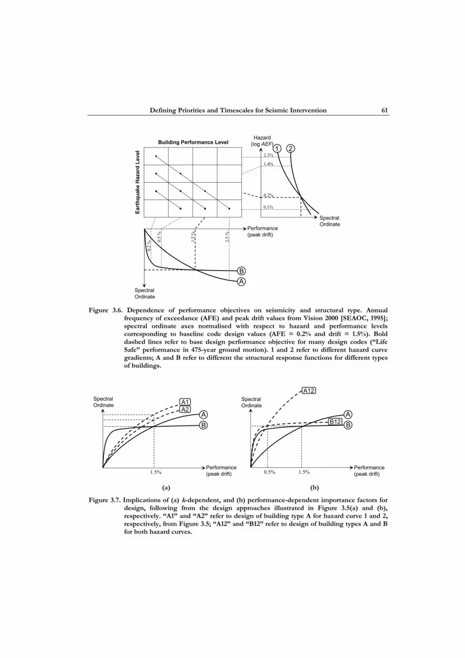
Defining Priorities and Timescales for Seismic Intervention
61
Spectral Ordinate
Performance (peak drift)
Spectral Ordinate
0.2
% 0.5
%
1.5
%
2.5
%
2.3%
1.4%
0.2%
0.1%
Eart
hqua
ke H
azar
d Le
vel
Building Performance Level1 2
BA
Hazard (log AEF)
Figure 3.6. Dependence of performance objectives on seismicity and structural type. Annual
frequency of exceedance (AFE) and peak drift values from Vision 2000 [SEAOC, 1995]; spectral ordinate axes normalised with respect to hazard and performance levels corresponding to baseline code design values (AFE = 0.2% and drift = 1.5%). Bold dashed lines refer to base design performance objective for many design codes (“Life Safe” performance in 475-year ground motion). 1 and 2 refer to different hazard curve gradients; A and B refer to different the structural response functions for different types of buildings.
BA
A1A2
Performance (peak drift)
Spectral Ordinate
1.5%
BA
A12
B12
Performance (peak drift)
Spectral Ordinate
1.5%0.5% (a) (b)
Figure 3.7. Implications of (a) k-dependent, and (b) performance-dependent importance factors for design, following from the design approaches illustrated in Figure 3.5(a) and (b), respectively. “A1” and “A2” refer to design of building type A for hazard curve 1 and 2, respectively, from Figure 3.5; “A12” and “B12” refer to design of building types A and B for both hazard curves.

D. N. Grant, J. J. Bommer, R. Pinho & G. M. Calvi
62
measure discussed above for two different structural systems (labelled “A” and “B”), normalised with respect to the “Life Safe” performance level (drift = 1.5%). This type of plot is equivalent to the “structural response function” considered in the PEER framework for PBEE [Hamburger, 2004]; although similar, it is not identical to the capacity curve of HAZUS (Section 2.3), as a spectral quantity is related to the peak inter-storey drift in this case. Again, the curves do not represent any particular structural types, but the drift axis is shown to scale for illustrative purposes. Note that the spectral ordinate scale is shown as linear in both plots for visual comparison; if a logarithmic axis were used for the hazard curves, a linear relationship would be expected, with a gradient of negative k. Clearly, k is greater for hazard curve 1 than for hazard curve 2.
Based on the generic hazard curves and structural response functions, various design decisions can be illustrated on Figure 3.6 and Figure 3.7. For the baseline seismic hazard (importance factor = 1) the design approach is to provide a structure with adequate capacity given a certain seismic demand. The process can be represented on Figure 3.6 as multiplying the structural response function by a constant scaling factor so that the demand is equal to the capacity at the desired hazard level and performance level. This is a simplification of real design, as the shape of the structural response function may be expected to vary with the strength. In terms of the Vision 2000 document and the relationships illustrated in Figure 3.6, the design for normal importance is therefore carried out as follows:
1. Determine spectral demand from hazard curve (1 or 2) with AFE = 0.2%. 2. Scale structural response function (A or B) such that spectral capacity for a peak
drift of 1.5% (“Life Safe”) is equal to the spectral demand.
The hazard curves and spectral response functions in Figure 3.6 have been scaled to the same spectral ordinates for AFE = 0.2% and drift = 1.5%; the standard design process is therefore the same for all combinations of hazard curves 1 and 2, and response functions A and B. The response functions in Figure 3.6, therefore, represent the baseline design level, and any further scaling factors required for higher performance objectives are equivalent to importance factors in the normal code approach.
The second design option to consider is for the “Essential/Hazardous objective”, following the approach of Figure 3.5(a). In this case, the hazard is increased, while maintaining the target performance at the “Life Safe” level. The design process is therefore:
1. Determine spectral demand from hazard curve (1 or 2) with AFE = 0.1%. 2. Scale structural response function (A or B) such that spectral capacity for a peak
drift of 1.5% (“Life Safe”) is equal to the spectral demand.

Defining Priorities and Timescales for Seismic Intervention
63
This process is illustrated in Figure 3.7(a), in which “A1” and “A2” refer to design for response function A with hazard curves 1 and 2, respectively. Since hazard curve 1 has a higher spectral demand for AFE = 0.1%, the scaling factor required to scale response function A (which represents standard design) to A1 is higher than the corresponding factor for A2. Although “B1” and “B2” (design for response function B with hazard curves 1 and 2, respectively) are not shown on Figure 3.7(a), it is apparent that the scaling factors for A1 and B1, and A2 and B2 are identical, as the spectral ordinate values at 1.5% drift are equal. As discussed above, these scaling factors are equivalent to scalar importance factors in normal code design. Since the importance factor for the Figure 3.5(a) approach varies with the gradient of the hazard curve and does not depend on the structural type, it may be referred to as “k-dependent”.
The final design option considered is also for the “Essential/Hazardous objective”, but following the approach shown in Figure 3.5(b). In this case, the hazard is maintained at the base level, while the target drift is reduced to the “Operational” performance level. The procedure follows as before:
1. Determine spectral demand from hazard curve (1 or 2) with AFE = 0.2%. 2. Scale structural response function (A or B) such that spectral capacity for a peak
drift of 0.5% (“Operational”) is equal to the spectral demand.
This design procedure is illustrated in Figure 3.7(b), in which “A12” and “B12” represent design for either hazard curve, with response functions A and B, respectively. In this case, the scaling factor required to meet the performance objectives is independent of the hazard, as the design spectral ordinate is constant. The scaling factor is, however, higher for structural type A than for structural type B, as the ratio of the “Operational” to “Life Safe” spectral ordinates is smaller. If the intention of importance factors is as interpreted in Figure 3.5(b), it will therefore be necessary to specify values that depend on the type of structure, and in particular the shape of its response function. Since the structural response function is a measure of performance across a range of spectral demand values, importance factors for the approach of Figure 3.5(b) may be referred to as “performance-dependent”.
These arguments, developed specifically for the code treatment of building importance, can also be extended to other adjustments of the base tolerable seismic risk. For example, in the previous section, the New Zealand [NZSEE, 2003] and United States [ATC, 1997] approaches to increasing the tolerable risk for existing structures were contrasted – the former reduces the design hazard and the latter reduces the margin against collapse, and therefore the target performance level. Similarly, for the construction phase ground motion proposed for bridges in Eurocode 8, Part 2 [CEN, 2004], a reduction of the design hazard is used, although different performance objectives are also implied by the

D. N. Grant, J. J. Bommer, R. Pinho & G. M. Calvi
64
fact that the check is carried out with respect to an incomplete structure. Clearly, each of these adjustments to the base design risk may be considered in the framework illustrated in Figure 3.5, with the corresponding adjustments for the gradient of the hazard curve and the structural type.
An alternative interpretation of the importance factor adjustment, outside the scope of the standard Vision 2000 matrix of performance objectives, is illustrated in Figure 3.8. In this case, the hazard level and performance level for baseline design are not adjusted; instead, the increased design demand is used to simulate an improved level of confidence that the performance level or hazard level will not be exceeded. This is shown by a third axis in Figure 3.7, although a four dimensional plot in which performance and hazard confidence were separated onto separate axes may be more appropriate. The axis labels CL1 and CL2 are confidence levels, defined as percentiles, where CL1 represents the standard design confidence level and CL2 a higher percentile value. For the ground motion, appropriate values may be CL1 = 50% (median hazard curve) and CL1 = 84% (median plus one standard deviation); for the performance, values of CL1 = 90% and CL1 = 95% may be appropriate, based on nominal versus median material strength definitions. This interpretation is consistent with the work of Elms [1980], who developed importance factors compatible with the New Zealand Loading Code based on the concept of lowering the probability of attaining a given limit state (failure) for more important buildings.
Confidence Level
CL1
CL2
Earthquake Hazard Level
Improved confidence in
performance or hazard level
Building Performance Level
Figure 3.8. Alternative interpretation of building importance factors: improving confidence in either
performance level or hazard level. Confidence level is shown on a single axis, although performance and hazard components are independent. CL1 and CL2 represent percentile levels of confidence.

Defining Priorities and Timescales for Seismic Intervention
65
The implication of this interpretation of importance factors is illustrated in Figure 3.9. Seismic hazard curves, labelled “3” and “4”, are shown in the right-hand plot for two regions, for which the median (CL1) curves are identical but the uncertainty is greater and therefore the 84th percentile (CL2) curves gives higher spectral ordinates for curve 4. Using arguments similar to those given above for k-dependent and performance-dependent importance factors, it can be observed that targeting an increased confidence level in the design hazard would imply a greater scaling factor for hazard curve 4 than for hazard curve 3. Similarly, the bottom plot shows two building types, represented by structural response functions, “C” and “D”, with identical 90th percentile (CL1) structural response functions and different 95th percentile (CL2) functions due to a higher uncertainty in the response of building type D. In this case, it is evident that increasing the confidence level from CL1 to CL2 would require a higher importance factor for building type D than for building type C. Since the value required to achieve the same increase in confidence depends on the uncertainty in both of these cases, these importance factors may be referred to as “uncertainty-dependent”.
D CL2
4 CL1
Spectral Ordinate
Performance (peak drift)
Spectral Ordinate
1.5
%
2.3%
1.4%
0.2%
0.1%
Eart
hqua
ke H
azar
d Le
vel
Building Performance Level
3
C CL2
C
Hazard (log AEF)
D CL1
2.5
%
3 CL2
4 CL2
Figure 3.9. Dependence of performance objectives on confidence level of either hazard or
performance. Annual frequency of exceedance (AFE) and peak drift values from Vision 2000 [SEAOC, 1995]; spectral ordinate axes normalised with respect to hazard and performance levels corresponding to baseline code design values (AFE = 0.2% and drift = 1.5%) and base confidence level, CL1. 3 and 4 refer to the same hazard curve with two different levels of uncertainty; C and D refer to the same structural response function for two different levels of uncertainty. In both cases, CL2 is a percentile value higher than CL1.

D. N. Grant, J. J. Bommer, R. Pinho & G. M. Calvi
66
As shown above, in many cases, the use of a constant importance factor to decrease the tolerable level of seismic risk for a new structure may not provide for constant risk for all structural types and seismic zones. For state-of-the-art design carried out in the PBEE framework, this issue would ideally be avoided by the specification of appropriate performance objectives, and seismic zonation that includes hazard levels other than the baseline 475-year return period hazard [Bommer and Pinho, 2005]. For the assessment and rehabilitation of existing buildings, it will be necessary to consider both the treatment of importance in the design code in place at the time of construction, and the statutory requirements of current seismic provisions. In the context of the current project, the structural response functions for the school buildings considered may not vary significantly, although this may require further investigation. Italian seismic hazard, however, is relatively heterogeneous. This is illustrated in the next chapter, in which seismic hazard curves are constructed for the entire country, and the risk implications of importance factors in the context of Italy are investigated further.

4. SEISMIC HAZARD IN ITALY
4.1 ITALIAN SEISMICITY
Italy is a region of moderate to high seismicity characterised by its tectonic complexity. Figure 4.1 illustrates the locations of past earthquakes from the Catalogue of Strong Italian Earthquakes [Boschi et al., 2000]. From the figure, it is apparent that most of Italy is seismically active, except for areas in the north and south-east, and Sardinia and southern Sicily. Particularly active areas include a subduction zone off the coast of Calabria, much of Sicily including the Messina Straits, the Friuli region, and the length of the Appenines mountain range, especially the southern branch [Valensise et al., 2003].
Figure 4.1. Historical seismicity from the Catalogue of Strong Italian Earthquakes [Boschi et al.,
2000] and instrumental seismicity from INGV bulletin; squares represent historical events and circles represent instrumental events [Valensise et al., 2003].

D. N. Grant, J. J. Bommer, R. Pinho & G. M. Calvi
68
Valensise et al. [2003] observe two particularly notable features of Italian seismicity, based on paleoseismological and archeoseismological evidence. The first observation is that Italian seismic sources typically exhibit recurrence intervals of the order of 1000–3000 years, suggesting that the reliable historical record of around 700 years may not be sufficient to describe the recurrence of all sources accurately. The second observation is that Italian earthquakes tend to cluster in both time and space, due to stress triggering on adjacent seismic sources. A recent example of this is the Umbria-Marche earthquakes of September and October 1997. This clustering phenomenon is discussed in more detail in Section 4.5.
4.2 HISTORY OF ITALIAN SEISMIC PROVISIONS
The representation of seismic hazard in Italy has undergone a number of changes since the first seismic design provisions were adopted in 1909. Major earthquakes have often motivated such changes, largely due to a change in public perception of seismic risk as well as an increased technical understanding of the seismic hazard. In this section, a summary of the history of Italian seismic provisions is provided, mostly adapted from Di Pasquale et al. [1999a; 1999b]. Table 4.1 provides a summary of horizontal seismic forces and seismic zonations specified in each seismic design code, as well as the date of any intermediate changes to seismic zones in between the release of new seismic provisions. Note that most of these intermediate changes affect only a few municipalities.
The first Italian seismic provisions were passed by royal decree in April 1909, following the Messina Straits earthquake in December of the previous year. Seismic zonation consisted of a list of the municipalities most damaged in the 1908 event, for which seismic design was made obligatory. Within these municipalities, construction of buildings was forbidden on unsuitable building sites, and buildings were limited to 10 metres in height. Other rules, related to the structural types and member dimensions were also implemented. Vertical and horizontal seismic forces were prescribed, although numerical values for these forces were not given; a scientific commission, however, concluded that horizontal building forces of the order of 8% of the building weight were appropriate. Following large earthquakes in 1911 and 1915 in Sicily and Marsica (central Italy), respectively, several more municipalities were added to the seismic classification, and this practice of adding (and also removing) municipalities in between changes in the seismic code continued throughout the 20th century based on the occurrence of damaging earthquakes and on political pressure (see Table 4.1). In 1916, numerical values were assigned for the seismic forces, as a fraction of the floor weight at each level.
In 1927, a second category (seismic zone) was introduced, corresponding to a lower level of seismic hazard. Seismic design forces for the Category II buildings were lower than Category I buildings, and other design requirements were less stringent. For the next five

Defining Priorities and Timescales for Seismic Intervention
69
Table 4.1. Summary of horizontal seismic design forces and seismic zonations in Italian seismic provisions, and intermediate changes to zonation in between new code releases. Partly adapted from Di Pasquale et al. [1999b] (continued overleaf).
Date of application Horizontal seismic action Seismic
zonation Intermediate changes
to zonation 18/04/1909 Undefined weight-proportional
forces (Fhi = 0.08 Wi recommended by expert commission)
Municipalities in single seismic
zone defined by decree
15/7/1909, 6/9/1912, 11/10/1914, 7/2/1915,
29/4/1915
5/11/1916 First floor, Fh1 = 1/8 W1 Other floors, Fhi = 1/6 Wi
– –
23/10/1924 Essentially unchanged – – 13/3/1927 I cat. Fh1 = 1/8 W1
Fhi = 1/6 Wi II cat. Fhi = 1/10 Wi (I ≥ 1)
Two different seismic zones
introduced (I and II cat.).
2/4/1930
25/03/1935 I cat. Fhi = 0.1 Wi II cat. Fhi = 0.07 Wi Sliveloads = 0.33
– 22/11/1937
25/11/1962 I cat. Fhi = 0.1 Wi II cat. Fhi = 0.07 Wi Sliveloads = 1 (warehouses etc) Sliveloads = 0.33
– 23/8/1965, 26/9/1968, 10/3/1969
3/03/1975 Fhi = ki Wi = C R ε β γi Wi I cat. C = 0.10 II cat. C = 0.07 R = normalised response spectrum Sliveloads = 1 (warehouses etc) Sliveloads = 1/2 (hospitals etc) Sliveloads = 1/3 (civil buildings)
– 15/9/1976, 21/2/1979, 8/7/1980, 22/9/1980,
7/3/1981
3/6/1981 Essentially unchanged, except: III cat. C = 0.04
Third seismic zone (III cat.)
introduced for a small number of
municipalities
26/6/1981, 23/9/1981, 9/10/1981, 11/1/1982, 4/2/1982, 19/3/1982, 14/5/1982, 27/7/1982, 13/9/1982, 10/2/1983, 1/4/1983, 23/7/1983, 29/2/1984, 5/3/1984

D. N. Grant, J. J. Bommer, R. Pinho & G. M. Calvi
70
Table 4.1. Continued from previous page.
19/6/1984 Adopts importance factor: = 1.4 for strategic buildings = 1.2 for buildings with grave consequences of collapse
– 14/7/1984
16/1/1996 Introduces γE factor, although according to 10/04/1997 circular, should be taken as 1.0 for masonry
– –
Ordinanza 3274/2003
Not yet enforced
Fi = Fh (zi Wi) / Σ(zj Wj) where Fh = Sd(T1) W λ /(q g) Sd(T1) is design spectrum, anchored to PGA values: Zone 1: 0.35g Zone 2: 0.25g Zone 3: 0.15g Zone 4: 0.05g
New zonation based on 1998 proposal, but
with 800 municipalities maintained in 1984 zone for
political reasons. Previous “not
classified” becomes Zone 4.
–
decades, very few changes were made to Italian seismic design: the seismic zonation was modified slightly (including a significant number of municipalities removed from seismic classification in 1937) and live loads were introduced to the seismic weight calculations, but the horizontal seismic forces and design philosophy remained essentially unchanged.
The first Italian seismic code to include seismic design based on a design response spectrum was released in March 1975. According to this document, floor seismic forces were a function of seismic zonation, building period, soil type, type of structural system, structural geometry and seismic weight. The seismic zonation was not changed significantly at this time. Subsequent modifications to Italian seismic design in the years following included the introduction of a third seismic category for a small number of municipalities in 1981, and the introduction of importance factors (see Section 3.2) in the 1984 design provisions. More importantly, the 1984 provisions expanded seismic category II significantly, such that almost half of the geographical area of Italy was classified for seismic design.
The zonation map was further updated in 2003, essentially following a proposal based on probabilistic seismic hazard assessment made in 1998. The principal difference between the 1998 proposal and the map adopted in 2003 is that approximately 800 municipalities

Defining Priorities and Timescales for Seismic Intervention
71
that would have been reduced in seismic category in the proposal were instead maintained at their current level. The 2003 seismic design code, Ordinanza 3274/2003 [OPCM, 2003], also introduced a fourth seismic zone, which replaced the unclassified regions in previous zonations, such that a minimal level of seismic design is now specified for the entire country, although individual regions in Zone 4 may choose not to adopt the new seismic design requirements.
Since political motivations have had such a significant effect on seismic zonation proposals, code zonation maps may not be the best measure of seismic hazard available. Even if a code zonation is based completely on a probabilistic seismic hazard assessment, it will necessarily be a coarser representation of the hazard: for example, the four seismic zones in the most recent Italian zonation map represent ranges of PGA of up to 0.10g. For this reason, the seismic hazard assessment conducted by the Istituto Nazionale di Geofisica e Vulconologia [INGV, 2005], discussed in the following section, is used to represent seismic hazard in the present study. Historical seismic zonations, however, provide a general indication of the variation in seismic design requirements over the last century, and therefore the vulnerability of the existing building stock. Assuming consistent code compliance, both in time and over the entire country, approximate vulnerability estimates may be obtained for a large building inventory, based solely on geographical location and year of design. This concept is employed in the proposed risk management framework, discussed in Section 6.4.
4.3 ITALIAN HAZARD DATA
A new seismic zonation for Italy has recently been completed by the Istituto Nazionale di Geofisica e Vulconologia, based on a probabilistic seismic hazard assessment of the country [Gruppo di Lavoro, 2004]. Maps of peak ground acceleration (PGA) for return periods of 100, 475, 1000, and 2500 years from this study are presented in Figure 4.2. These maps are based on preliminary data: the values for the islands of Pantelleria, Stromboli, Panarea, Ustica, Alicudi and Filicudi should be considered underestimates of the real hazard, and no data are currently available for Sardinia. The use of 475-year PGA values for the design hazard is mandated by Italian law, and Figure 4.2(b) is therefore used in the specification of seismic zones for design. Figure 4.2(a), (c) and (d) give an indication of the different ordinates of the hazard curve for different regions in Italy. Hazard curves for the entire country are developed in the following section, which will be useful when the seismic hazard is adjusted from the baseline design level.
Although the design hazard is given in terms of PGA, it is recognised that this measure of ground-motion intensity is not well-correlated with structural damage. Spectral ordinates (of either acceleration or displacement) would provide a more representative measure of potentially damaging ground motion throughout the country. These data, however, would not be consistent with Italian design provisions for new construction, and, in any case,

D. N. Grant, J. J. Bommer, R. Pinho & G. M. Calvi
72
are not available in the current phase of the INGV project. The code acceleration spectrum, anchored on the PGA value from the seismic zonation at the zero-period ordinate, provides an approximation to the uniform hazard spectrum, although it does not take into account possible variation in the spectral shape throughout the country.
Figure 4.2. Median peak ground acceleration (units of g) for return periods of (a) 100 years, (b) 475
years, (c) 1000 years, and (d) 2500 years. Data from INGV [Gruppo di Lavoro, 2004].

Defining Priorities and Timescales for Seismic Intervention
73
4.4 COMPARISON OF REGIONAL HAZARD CURVES
As discussed in Section 1.2, the hazard curve can often be approximated as a straight line on log-log axes with a gradient equal to minus k, at least for return periods of engineering interest. Eurocode 8 [CEN, 2004] allows the use of this assumption to determine importance factors which vary with the gradient of the hazard curve, as discussed in Section 3.4. The code suggests that the k-value is approximately equal to 3 for Europe; the same value seems to have been used in the construction of Figure 3.3 for New Zealand seismicity. Based on this representation, two hazard maps – one for a ground-motion parameter at a fixed annual frequency of exceedance, and the second for the corresponding k-value – are sufficient to determine the seismic hazard across a region for all return periods of interest [Grases et al., 1992].
To provide a full representation of Italian hazard, k-values were calculated from hazard maps presented in Figure 4.2(a)–(d), to be used in conjunction with Figure 4.2(b). For each grid point in the GIS data plotted in Figure 4.2, a linear regression was carried out on the logarithms of PGA and annual frequency of exceedance (AFE). The values of k determined from this procedure are presented in Figure 4.3(a). From the figure, it can be observed that k varies significantly within Italy’s boundaries, with minimum and maximum values of 1.8 and 4.7, respectively. The mean and standard deviation of k for all grid points shown in Figure 4.3(a) are 3.0 and 0.6, respectively; these statistical measures may, however, be skewed by the extreme data that are included in the GIS grid but do not lie within Italy’s borders, such as the high values off the east and west coasts of Italy, and the low values at the edges of the area considered. The goodness-of-fit parameter from each linear regression, r2, is shown in Figure 4.3(b). For the entire country, r2 is greater than 0.990, which suggests that the linear hazard curve assumption is justified for the return periods considered.
Three sample hazard curves, for grid points indicated by stars on Figure 4.3, are plotted on logarithmic axes in Figure 4.4. The three curves were selected as representative of a low, medium and high value of k: the southern, northern and central stars in Figure 4.3, respectively. The linear hazard curves have best-fit k-values of 1.8, 3.0 and 4.7, with regression r2 parameters of 0.996, 0.998, and 0.997, respectively. The curves are provided in terms of absolute PGA values (Figure 4.4a), and PGA normalised with respect to the 475-year return period value (Figure 4.4b). Considering the logarithmic axes on Fig. 4.4(b), it is apparent that the level of variation of k-values throughout Italy has important implications when return periods other than 475 years are considered.
The effect of different values of k can be evaluated for the three building categories, and corresponding importance factors, defined in the Italian seismic design code [OPCM, 2003]. Category I buildings are those for which post-earthquake function is important, such as hospitals, fire departments and civil defence facilities. Category II buildings are

D. N. Grant, J. J. Bommer, R. Pinho & G. M. Calvi
74
(a) (b)
Figure 4.3. Linear regression for slope of hazard curve (k) for median PGA values, calibrated for 100, 475, 1000 and 2500-year return period data. (a) Best-fit k-values, and (b) r2 values. Hazard curves are plotted in Figure 4.4 for points marked with stars.
0.0001
0.001
0.01
0.1
0.01 0.1 1
PGA (g)
AFE
Low kAverage kHigh k
0.0001
0.001
0.01
0.1
0.1 1 10
Normalised PGA
AFE
Low kAverage kHigh k
(a) (b)
Figure 4.4. Hazard curves for three locations in Italy: (a) PGA, and (b) PGA normalised to 475-year return period value. Symbols refer to INGV data, and lines are best-fit linear relationship.
those of increased importance due to the consequences of collapse, such as schools and theatres. Finally, normal buildings not included in the other two categories are designated Category III. The design level hazard, specified in terms of a 475-year return period, is defined for the third building category; Category I and II buildings are assigned importance factors of 1.4 and 1.2, which multiply the design spectral ordinates, respectively. As discussed in Section 3.5, the geographical variation in seismicity must be taken into account if the intention of the factor is to reduce the probability of exceedance of the design ground motion. Adjustments that are k-dependent are not appropriate, however, if the intention of the importance factor is to improve the seismic performance under the design level hazard.

Defining Priorities and Timescales for Seismic Intervention
75
Table 4.2 shows the implied seismic hazard, under the assumption that a k-dependent adjustment is appropriate, in terms of both annual frequency of exceedance (AFE) and return period (TR), for the importance factors given in the Italian seismic design code (OPCM, 2003), and a range of values of k. These values are consistent with the thresholds for each contour in Figure 4.3. As is evident from Figure 4.3 and Table 4.2, the implied hazard is a function of both geographical location and building importance, assuming that PGA is an appropriate representation of ground-motion intensity. As an example, a school building (importance factor 1.2) on a site with k = 3.0 in Figure 4.3(a), will be designed for a 821-year seismic hazard according to the draft Italian seismic design code. If the same building were to be used for post-earthquake civil defence activities, and was therefore assigned to Category I (importance factor 1.4), the Italian code would imply a 1303-year hazard for design.
Since only PGA values are available from code seismic zonation, it may be desirable to determine an approximate relationship between k and PGA for Italy, in lieu of mapped values of k for the entire country. To this end, the k-values for each grid point in Figure 4.3 are plotted against their respective 475-year PGA values in Figure 4.5. For PGA Table 4.2. Annual frequency of exceedance (AFE) and return periods (TR) for different values of k
(from Figure 4.3), for Building Categories I and II in the draft Italian seismic design code [OPCM, 2003]. Bold line refers to average value of k for Italy. Note that AFE(PGA475) = 0.21%; TR(PGA475) = 475 years
Building Category I Building Category II k AFE TR AFE TR
1.6 0.12% 814 years 0.16% 636 years 1.8 0.11% 870 0.15% 660 2 0.11% 931 0.15% 684
2.2 0.10% 996 0.14% 709 2.4 0.09% 1065 0.14% 736 2.6 0.09% 1139 0.13% 763 2.8 0.08% 1219 0.13% 791 3 0.08% 1303 0.12% 821
3.2 0.07% 1394 0.12% 851 3.4 0.07% 1491 0.11% 883 3.6 0.06% 1595 0.11% 916 3.8 0.06% 1706 0.11% 950 4 0.05% 1825 0.10% 985
4.2 0.05% 1952 0.10% 1022 4.4 0.05% 2088 0.09% 1059 4.6 0.04% 2233 0.09% 1099 4.8 0.04% 2388 0.09% 1140

D. N. Grant, J. J. Bommer, R. Pinho & G. M. Calvi
76
0
1
2
3
4
5
0.00 0.05 0.10 0.15 0.20 0.25
PGA (g)
k
Figure 4.5. Relationship between gradient of log-log hazard curve (k) and 475-year PGA value for all
grid points in Figure 4.3.
greater than 0.05g, k shows a generally decreasing trend, although there is considerable scatter. Most data points with PGA less than 0.05g lie outside the Italian borders (Figure 4.2b), and the k-values may also be less well-constrained by the linear regression discussed above (Figure 4.3b). For this reason, the increasing trend of k for 0 < PGA < 0.05g may be considered dubious.
The data from Figure 4.5 were grouped into 0.01g PGA intervals, and median values and standard deviations were determined for each interval. The plus/minus one standard deviation intervals are shown as rectangles in Figure 4.6. A simple piecewise linear relationship was fitted to the data, and is shown as a solid line in Figure 4.6. The positive gradient portion for 0 < PGA < 0.05g was ignored. The four branches of the piecewise linear curve are defined by:
( )( )
⎪⎪⎩
⎪⎪⎨
⎧
+−+−
=
4.21.3/7.25.4/16
6.3
gPGAgPGA
k
PGAggPGAggPGAg
gPGA
<<<<<<<
26.026.011.011.0056.0056.00
(4.1)
Equation (4.1) may be used to provide estimates of k for all of Italy, based on mapped PGA values for a return period of 475 years. The relationship involves a significant amount of scatter, however, and where possible mapped values of k in Figure 4.3 should

Defining Priorities and Timescales for Seismic Intervention
77
0
1
2
3
4
5
0.00 0.05 0.10 0.15 0.20 0.25
PGA (g)
k
0
50 0.28
Figure 4.6. Grouped data from Figure 4.5. Rectangles show median and median plus/minus one
standard deviation of k-values for PGA in a 0.01g interval. Solid line shows piecewise linear approximation to median values, from Eq. (4.1).
be favoured. For the four zones in the seismic zonation of Italy, the PGA and corresponding k-values from Eq. (4.1) are given in Table 4.3. Note that for seismic zone I, the PGA of 0.35g lies outside the range of available data; the value of k is extrapolated from the fourth branch of the piecewise linear relationship.
Table 4.3. Values of PGA and k for seismic zones in Italy.
Seismic Zone Code PGA (g) k I 0.35 2.4 II 0.25 2.4 III 0.15 2.7 IV 0.05 3.6
The k-values determined in this section correspond to the slope of the hazard curve for PGA only, and may be expected to vary for different ground-motion measures. A preliminary study was conducted using spectral acceleration data from the Servizio Sismico Nazionale project [SSN, 2001], for structural periods of 0.2 seconds and 1.0 second. The spectral ordinates were determined based on the median-plus-one-standard-deviation values from two attenuation relationships. Data for Sardinia and 1.0-second data for a small region in the north-west of Italy were not available. The k-values

D. N. Grant, J. J. Bommer, R. Pinho & G. M. Calvi
78
determined using the regression procedure described above are shown for the two spectral ordinates in Figure 4.7. Although the data from the SSN study may not be directly compatible with the data used in Figure 4.3 [Gruppo di Lavoro, 2004], it is evident from Figure 4.5 that k varies significantly with structural period. The hazard curve for other ground-motion parameters may be expected to show similar variation.
(a) (b)
Figure 4.7. Best-fit slope of hazard curve (k) for spectral acceleration, median-plus-one-standard-deviation values, calibrated for 95-, 475-, 975- and 2475-year return period data [SSN, 2001]; (a) response period = 0.2 sec, and (b) response period = 1.0 sec.
4.5 TIME-DEPENDENT CHARACTERISATION OF ITALIAN HAZARD
The Poisson model of earthquake recurrence, one of the primary assumptions of most probabilistic seismic hazard analysis, ignores the variation in seismic hazard over time. Although this assumption may be conservative for design purposes [Cornell and Winterstein, 1988], it ignores evidence that seismic hazard may be more accurately characterised by time-dependent models, at least in some parts of the world. The elastic rebound theory [Reid, 1910] suggests that, for an individual seismic source, the hazard should increase with time after an earthquake, as the elastic strain in the crust approaches the rupture limit. Consistent with this model, characteristic earthquakes, of an approximately constant magnitude and inter-event time, have been identified in some regions [Schwartz and Coppersmith, 1984]. Clustering models [e.g. Faenza et al., 2003], on the other hand, propose that earthquakes tend to group in both space and time due to the interaction of seismogenic sources within a seismic source zone. Neither of these models – in which the seismic hazard increases or decreases with time, respectively – is compatible with the assumption that earthquake recurrence is a Poisson process with a stationary earthquake recurrence function. A large body of literature exists on the time-dependent characterisation of seismic hazard; some relevant models, applicable to Italian

Defining Priorities and Timescales for Seismic Intervention
79
seismic hazard data, are discussed below. For further information, the review by Anagnos and Kiremidjian [1988] on earthquake occurrence models, and that of Utsu [2002] on statistical features of seismicity in general, are useful resources.
The inclusion of time-dependence in this present study is motivated by the need to prioritise rehabilitation over a large quantity of building stock. For this purpose, the results of the study of Cornell and Winterstein [1988], in which it was shown that “the Poisson model provides a sufficient engineering hazard estimate (i.e., either conservative or unconservative by a factor of no more than three)”, are less relevant. In the present study, it will be useful to distinguish between the conservative and unconservative cases, in a quantitative manner, if possible on the basis of the existing data. For example, if time-dependent models of Italian seismicity suggest that the hazard increases with time, then it would be prudent to assign a lower priority to buildings in the Umbria-Marche region, which experienced a cluster of relatively large earthquakes in 1997, than in “seismic gap” regions, which have not experienced any seismic events in recent times. Figure 4.8, adapted from the study of Valensise and Pantosti [2001], shows the location of potential seismic gaps in Italy. Even if the seismicity data only support an increase or decrease of the seismic hazard of the order of 10%, this factor will allow the distinction between otherwise identical buildings, and permit priorities for seismic rehabilitation to be more readily assigned. The implicit assumption here, as outlined in Chapter 1, is that this project is to be carried out at the national level, and time-dependent characterisation of hazard may not be applicable in studies for smaller areas.
As alluded to above, the time-dependence of seismic hazard in a region will be affected by the characterisation of the earthquake sources. Depending on the level of historical knowledge and geological data available, earthquake sources may be assigned to mapped faults or fault segments, point sources at the location of previous large earthquakes, or areal seismic source zones. The latter model, in which the rate of earthquake occurrence and faulting type is assumed to be constant over a given geological area, is commonly used in time-independent probabilistic seismic hazard assessment, including the recent assessment carried out by the INGV [2005], described in the previous section. The former two approaches were used in the study carried out under the coordination of Peruzza [2005a] to obtain time-dependent hazard estimates for Italy. Although these studies were conducted by different researchers, under different assumptions – including, but not limited to, the description of the seismic sources – their results can be compared to obtain approximate quantitative estimates of the importance of the time-dependence of Italian seismic hazard.
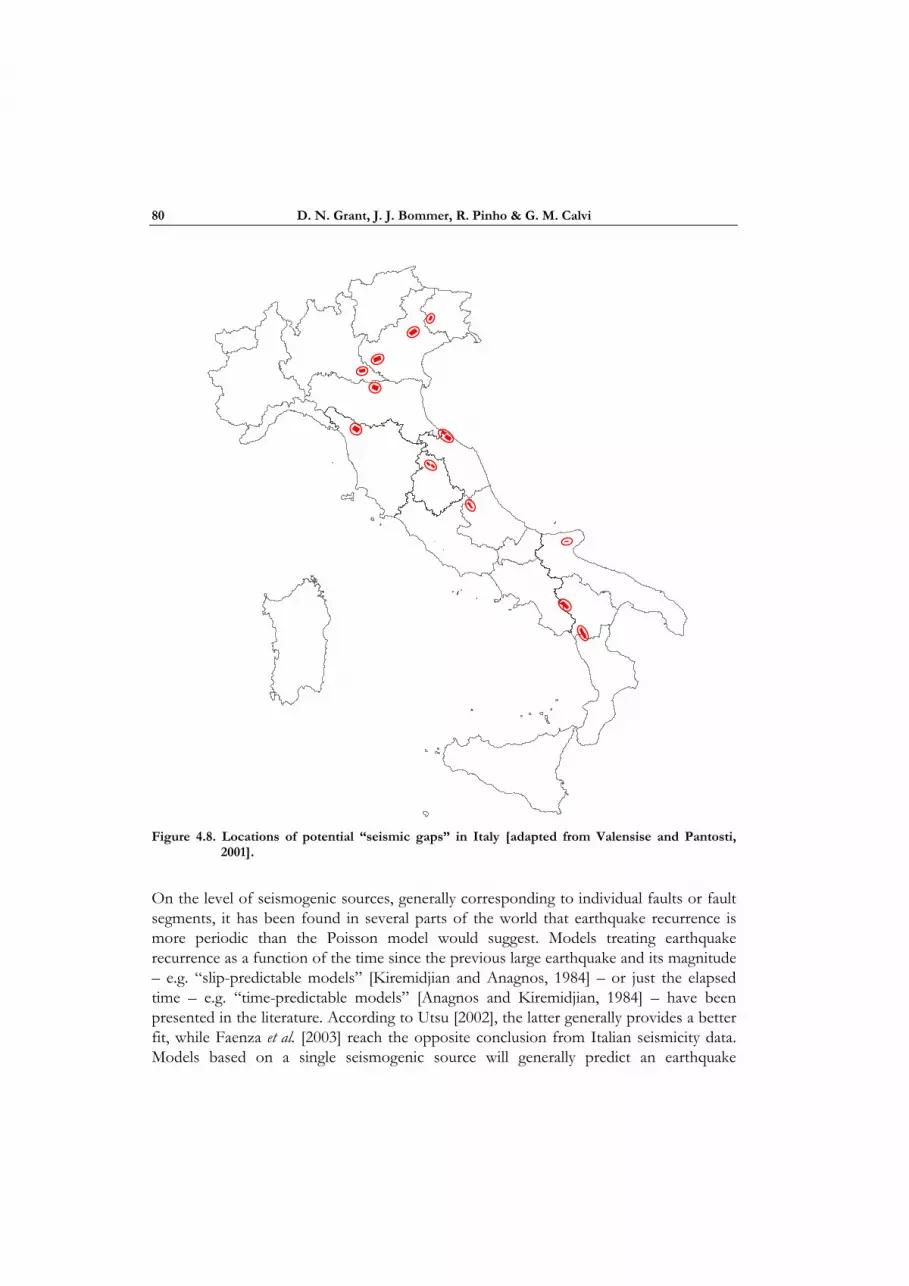
D. N. Grant, J. J. Bommer, R. Pinho & G. M. Calvi
80
Figure 4.8. Locations of potential “seismic gaps” in Italy [adapted from Valensise and Pantosti,
2001].
On the level of seismogenic sources, generally corresponding to individual faults or fault segments, it has been found in several parts of the world that earthquake recurrence is more periodic than the Poisson model would suggest. Models treating earthquake recurrence as a function of the time since the previous large earthquake and its magnitude – e.g. “slip-predictable models” [Kiremidjian and Anagnos, 1984] – or just the elapsed time – e.g. “time-predictable models” [Anagnos and Kiremidjian, 1984] – have been presented in the literature. According to Utsu [2002], the latter generally provides a better fit, while Faenza et al. [2003] reach the opposite conclusion from Italian seismicity data. Models based on a single seismogenic source will generally predict an earthquake

Defining Priorities and Timescales for Seismic Intervention
81
recurrence function that increases with time after a large earthquake, which has been shown to provide a good fit of earthquake catalogues for some regions.
Peruzza and co-authors carried out assessment of Italian seismic hazard based on time-dependent earthquake recurrence models, initially for the Calabrian arc [Peruzza et al., 1997] and other individual regions [Peruzza, 1999; Peruzza and Pace, 2002; Pace et al., 2005], but recently extended to the rest of the country [Amatoa and Selvaggi, 2004; Peruzza, 2005a; 2005b]. The assessment is based on a hybrid approach, in which the CPTI database [Boschi et al., 1999] is used to define potential sources of earthquakes with M > 5.5, and seismic source zones are used to represent background seismicity associated with smaller earthquakes. The former are divided into geological and historical sources, and are assigned characteristic magnitudes and recurrence intervals based on fault geometry, slip rate and seismic moment rate considerations. Earthquake recurrence is modelled by a characteristic earthquake model [Schwartz and Coppersmith, 1984], with a Brownian passage time relationship used to describe the inter-event time; Poissonian recurrence is also considered for comparison, which leads to an exponential distribution of inter-event times. The background seismicity is modelled with the Gutenberg-Richter relationship and an exponential distribution for the inter-event times. This hybrid approach to modelling seismic hazard allows the consideration of time dependence for the larger magnitude earthquakes, while retaining the influence of background seismicity on the probabilistic ground motions.
For the purposes of this report, the results for a 10% probability of exceedance in a reference period of 30 years and 50 years were available from both the time-independent (Poissonian) and time-dependent studies. The time-independent data are illustrated for 30-year and 50-year reference periods in Figure 4.9(a) and (b), respectively, while the corresponding data from the time-dependent study are illustrated in Figure 4.9(c) and (d). Note that the GIS model was based on municipalities rather than the regular grid used in Figure 4.2, and it is therefore not possible to directly compare Figure 4.9(b) and Figure 4.2(b), which were both evaluated with time-independent seismicity models for a return period of 475 years, on a grid-point basis. In any case, the results of Peruzza [2005a] were obtained using different source models and attenuation relationships, and the uncertainty in the attenuation relationships was not considered. For this reason, Figure 4.9 may be considered incompatible with both the current Italian seismic zonation and the INGV hazard maps [Gruppo di Lavoro, 2004]. Nevertheless, a quantitative comparison of parts (a) and (b) of Figure 4.9 with parts (c) and (d), respectively, can be used to give an indication of the effects of time-dependent recurrence models on the assessment of probabilistic ground motions.

D. N. Grant, J. J. Bommer, R. Pinho & G. M. Calvi
82
Figure 4.9. Mean peak ground acceleration (units of g); Poisson earthquake recurrence for a 10%
probability of exceedance in (a) 30 years, (b) 50 years, and time-dependent earthquake recurrence model for a 10% probability of exceedance in (c) 30 years, and (d) 50 years. Data from Peruzza [2005a].
To carry out this comparison, the ratios of time-dependent to time-independent data were calculated on a point-by-point basis in the GIS model. The results from this

Defining Priorities and Timescales for Seismic Intervention
83
(a) (b)
Figure 4.10. Ratio of time-dependent mean PGA values to Poisson mean values for a 10% probability of exceedance in (a) 30 years, and (b) 50 years. Data from Peruzza [2005a].
procedure are illustrated in Figure 4.10, in which part (a) shows the ratio of Figure 4.9 (c) to (a), and part (b) shows the ratio of Figure 4.9 (d) to (b). From the plots, it is apparent that time-dependent hazard modelling has relatively little impact throughout a large part of the country, and generally leads to ground motion estimates within 10% of time-independent data. Ground motions ratios are also similar between the two exposure times considered, although the 10%-in-50-year results are slightly more spread about the median. Although the exposure time of 50 years is consistent with the code ground-motion definition, 30 years may be closer to the total time frame over which school retrofit will be carried out in the present application, and is therefore more relevant in identifying regions which are more or less likely to experience large earthquake ground motions in the near future. Figure 4.10 (a) may therefore be used to determine priorities for intervention in different regions throughout the country. Since the study of Peruzza [2005a] was based on significantly different assumptions to the INGV [2005] study, it may not be appropriate to use the numerical values illustrated in (a) to directly multiply the code seismic zone factors (Table 4.3); the most appropriate use of the time-dependent ratios is to prioritise intervention within each seismic zone individually.
As pointed out by Cornell and Winterstein [1988], with theoretical justification originally attributed to Khintchine [1960], the sum of non-Poissonian processes tends to a Poisson process in the limit. For this reason, even if individual sources exhibit time- and magnitude-dependent recurrence behaviour, the average of this behaviour over an entire seismic source zone representing many seismogenic sources may be approximated by a Poisson model. This “summation” of earthquake recurrence over several faults, however,

D. N. Grant, J. J. Bommer, R. Pinho & G. M. Calvi
84
ignores the interdependence of the strain accumulation and release process that underlies the observed seismicity. The presence of foreshocks and aftershocks for large events, and “swarms” or “clusters” of moderate to large events, may in some cases be attributable to stress transfer from one seismogenic source to another – “stress triggering” [e.g. King et al., 1994] – leading Faenza et al. [2003] to conclude from Italian data that “the interaction between faults seems to be more relevant for earthquake forecasting purposes, than the behaviour of a single seismogenic fault”. If moderate to large earthquakes tend to occur in clusters, then the earthquake recurrence function should decrease with time, at least over a short time interval following the last significant event.
Faenza and co-authors have conducted studies on earthquake clustering in Italy with the assumption of a regular grid seismic source zonation [Faenza et al., 2003] and seismically homogeneous source zones based on tectonics [Cinti et al., 2004]. The studies adopt a non-parametric model of earthquake recurrence, in which the actual observed seismicity with a magnitude greater than or equal to 5.5 in a 403-year earthquake catalogue is compared with the Poisson model, and the residual is presented as a function of time since the last significant seismic event. Faenza et al. [2003] showed that the form of the residual function adopted in these studies has a trend comparable to the earthquake recurrence function, with a gradient of zero on a plot of the residual versus time implying Poissonian recurrence. The residual function obtained by Cinti et al. [2004], illustrated in Figure 4.11, clearly indicates that, for Italian seismicity, the earthquake recurrence function decreases with time since the last event up to around 10 years. On the logarithmic scale presented in Figure 4.11, it is difficult to draw conclusions for time greater than 100 years, and impossible to extrapolate beyond the maximum inter-event time observed in any seismic source zone, which is approximately 150 years. Cinti et al. [2004] conclude from Figure 4.11 that the Italian earthquake catalogue is characterised by clustering for a period of a few years following an event, and Poissonian recurrence thereafter. Although the former conclusion seems justified by Figure 4.11, it appears that the 403-year earthquake catalogue may be inadequate to support the latter conclusion with much confidence.
A few limitations are apparent in the methodology presented by Faenza et al. [2003] and Cinti et al. [2004]. The method assumes an earthquake recurrence function in terms of the time since the last event, x*,of the form:
( ) ( ) βλλ zz exx **, 0= (4.2)
where z and β are vectors related to the spatial distribution of the hazard, and λ0 is a discrete baseline earthquake recurrence function which is determined directly from the data. The temporal component of the earthquake recurrence function is therefore defined

Defining Priorities and Timescales for Seismic Intervention
85
Figure 4.11. Residuals between observed Italian seismicity data and Poissonian recurrence model,
versus the time elapsed since the last significant earthquake [Cinti et al., 2004]. Faenza et al. [2003] show that the form of the residual function adopted here shows the same trend as the earthquake recurrence function, with zero gradient implying Poissonian recurrence.
independently of the spatial component. As discussed by Faenza et al. [2003], this implies that the mechanism of earthquake occurrence is the same for different geographical areas in the region under consideration. Although this assumption may be justifiable from a practical standpoint – the coupling of spatial and temporal dependence would require significantly more data and computational effort to quantify – it appears to be an overly simplistic model of the time-dependence of seismic hazard in Italy. As discussed above, the grouping of seismogenic sources into seismic source zones already obscures the observations of “seismic gaps” and “characteristic events”; in this case, the source zones have been combined into a single large source zone accounting for the time-dependence of the hazard for the entire country. Of course, this limitation only makes the observation of significant clustering more remarkable, and does not invalidate the principal conclusions of the studies based on this approach [Faenza et al., 2003; Cinti et al., 2004]. It does, however, imply that any time-dependence specific to a certain geographical area will not have been captured in the baseline earthquake recurrence function.
A second limitation with the study of Cinti et al. [2004] is that only seismic source zones for which at least one earthquake of magnitude greater than 5.5 occurred in the 403-year catalogue were included in the model calibration. If the assumption of an increasing earthquake recurrence function were appropriate, any source zones that have been

D. N. Grant, J. J. Bommer, R. Pinho & G. M. Calvi
86
excluded would be expected to have a higher probability of experiencing an earthquake in the immediate future. If it were possible to incorporate paleoseismological data into the procedure, an earthquake recurrence function which decreases initially but increases for large values of elapsed time, may be obtained. Although this observation is speculative and somewhat circular (an increasing earthquake recurrence function is postulated to justify the possibility of an increasing earthquake recurrence function), it does suggest that a systematic bias may be present in the determination of the baseline function for large elapsed times.
The final problem with the study of Cinti et al. [2004], as applied to the present project, is that the results are presented as maps of probability of earthquake recurrence in a 10-year time interval, and not as probabilistic estimates of ground shaking throughout Italy. Although it is possible to compare such maps to similar results in which a Poisson process was assumed to obtain estimates of the time-dependence of the hazard, quantitative results are much more readily obtained from a comparison of PGA maps.
From the studies of Peruzza [2005a] and Cinti et al. [2004], it is difficult to conclude what is the most effective way to characterise the time-dependence of Italian seismicity. The two studies use the same data to draw opposite conclusions, which could have a large effect on the rehabilitation prioritisation scheme developed herein. For example, the former study assigns a decreased hazard to the Umbria-Marche region, while the latter assigns an increased hazard, in both cases due to recent seismic activity in the region. Essentially, the difference between the two is the level on which the seismic sources are considered: individual faults in the former and seismic source zones in the latter. Fault-level representations that use separate recurrence models to describe the occurrence of seismic events along each fault do not take into account the interaction between different seismogenic sources; seismic source zones average the behaviour of many sources, and cannot include possible “characteristic events” or “seismic gaps” that may apply to an individual fault. Taking into account the timescales considered in each of the studies, it seems likely that a two-level approach would be required to describe the time-dependent hazard accurately. The outcome of such an approach may be earthquake recurrence functions for regions in Italy that decrease for a few years after a moderate event, and increase for timescales of the order of the average inter-event time of individual seismogenic sources. Such a study is beyond the scope of this report, and herein we make use of the Peruzza [2005a] results and the time-dependent ratios presented in Figure 4.10. Given the uncertainty in the results, however, time-dependent data is given low importance in the prioritisation scheme discussed in Section 6.4.
As discussed above, earthquake clustering has been ignored in the development of Figure 4.9. Although this may be appropriate for determining the 475-year seismic hazard (AFE = 0.21%), and a single application of the resulting motions, the fact that Italian

Defining Priorities and Timescales for Seismic Intervention
87
seismicity is characterised by clustering of large events in time may influence the apparent vulnerability of Italian buildings. Buildings may be subjected to the ground-motion levels in Figure 4.9 multiple times within a relatively short time period, due to the occurrence of several large events. For well-designed structures, this should not be an issue; for poorly-designed structures, progressive collapse may occur over multiple earthquakes. This effect is similar to the influence of duration on degrading structures (Bommer et al., 2004b), except that repair is possible between distinct events. Overall, the effect of earthquake clustering is to further separate the apparent vulnerability of well-designed and poorly-designed buildings.


5. RISK MANAGEMENT DECISION-MAKING FRAMEWORKS
As has been discussed in previous chapters, a rational approach to the reduction of seismic risk requires the consideration of each of the four elements of the risk equation: seismic hazard, exposure, vulnerability and cost (Section 1.2). A fully quantitative treatment of these elements is possible by carrying out seismic loss estimation for the study area, as described in Chapter 2. Risk decisions – such as the definition of acceptable levels of seismic capacity for existing buildings versus new design requirements and time frames for seismic intervention – could be assessed by multiple loss estimation iterations, as suggested for the development of new design codes by Bommer et al. [2005]. An optimum risk reduction framework could be developed in which expected loss of life is limited to tolerable levels, and expected monetary losses are balanced with expenditure. A similar approach was used to compare proposals for seismic risk mitigation in California, following the 1994 Northridge Earthquake [Seligson et al., 1998].
Although loss estimation is a valuable tool for quantitatively assessing seismic risk, it will not always be feasible to gather the technical data required for an accurate study, and the results may be difficult to interpret. For this reason, various risk management frameworks have been developed to provide measures of seismic risk, and aid in decision making. These frameworks may include any or all of the following:
• Multiple stages of vulnerability and hazard assessment • A prioritisation scheme to rank structures in order of seismic risk • Minimum capacity levels below which intervention is required • Minimum performance objectives for retrofit designs • Time frames within which rehabilitation or demolition must be carried out.
In this chapter, several of these risk management methodologies are reviewed, including several that were developed for a single project, a general review of Italian risk management projects, and two proposals for regulation that are therefore intended for more general application.

D. N. Grant, J. J. Bommer, R. Pinho & G. M. Calvi
90
5.1 REVIEW OF RETROFIT PRIORITISATION PROJECTS
Several examples of large scale seismic retrofit projects are available in the literature, particularly for the rehabilitation of bridges [e.g. Vasishth et al., 1995; Chapman et al., 2000] and hospitals [e.g. Holmes, 2002]. For these individual projects, generally a simple screening procedure is adequate to determine priorities, and possibly time frames, for seismic intervention. Some of these projects are briefly reviewed in this section; procedures based solely on economic considerations [e.g. Albanesi et al., 2004], and bridge retrofit projects based on network theory [e.g. Cherng and Wen, 1994] are not particularly relevant to this report, and are not discussed further.
Bridges are often owned and maintained by local, regional or national authorities, which means that seismic upgrading may be carried out on a large scale. Vasishth et al. [1995] describe a seismic prioritisation scheme developed for bridges in Washington State. An initial screening was carried out based on structural type, in which bridges with in-span hinges and those with simply supported superstructures were assigned the highest priority, followed by single-column piers, multiple-column piers and, finally, bridges already programmed for retrofitting. A Prioritisation Index was then defined, as the product of a Criticality Factor and Vulnerability Factor. The former factor was a weighted combination of various other factors describing the importance of the bridge to the road network; the latter factor considered the hazard at the site, remaining service life of the bridge and superstructure and substructure deficiencies. The Prioritisation Index was used to prioritise bridges in the network for further elastic and inelastic analysis, and subsequently for retrofit.
A similar prioritisation and rehabilitation procedure was carried out in New Zealand [Chapman et al., 2000]. Initially, two major bridges – the Thorndon bridge in Wellington and the Auckland Harbour bridge – were selected for retrofit, followed by the development of a screening procedure for the assessment of the country’s remaining bridges. The screening process was based on a series of 11 stages in increasing order of engineering specialisation, to gradually reduce the inventory under consideration, and gather information about the bridges that represent the highest risk. The first four stages consist of the elimination of bridges for which the seismic vulnerability or consequences of failure are sufficiently low, and the collection of data for the remaining bridges, including design drawings, aerial photographs, and the effects of traffic disruption. In stage 5, a Seismic Attributes Grade (SAG) is defined, which is a weighted score of factors related to hazard, importance and vulnerability, and is used to identify bridges which require site inspection in stages 6 to 8. In stage 9, a risk assessment is carried out by a specialist bridge engineer, who must identify potential seismic weaknesses, and estimate their likelihood and consequences of occurring. Stage 10 is an economic analysis, including the effects of traffic disruption and an estimation of the cost of retrofit. Finally,
Defining Priorities and Timescales for Seismic Intervention
91
the information from stages 5, 9 and 10 is collected into a single Ranking for Further Analysis for each bridge, and bridges are ranked in order of decreasing priority.
The hospital programme in California is another example of a risk management methodology for seismic rehabilitation [Holmes, 2002]. Hospitals fulfil an important function following a moderate-to-large earthquake, and the poor performance of hospitals in the 1971 San Fernando earthquake was of particular concern to state officials. The Hospital Safety Act was passed in 1972, although its provisions did not apply retroactively, and the rate of replacement of existing facilities did not match the expectations of the Building Safety Board. A numerical scheme was proposed, which specified deadlines for compliance with the Hospital Safety Act for existing hospitals, based on vulnerability, cost and function of non-structural contents and occupancy. Under this proposal, a Compliance Priority Rating, P, was defined for each building as:
EDP ×= (5.1)
In Eq. (5.1), D is a Structure Deficiency Index, equal to 9.0 for structures representing the highest risk, 2.25 for intermediate structures, and 1.0 for non-complying structures deemed “life safe”. The second factor, E, is an Essential Function Exposure, defined as:
∑+=i
ieE 5.0 (5.2)
where ei values are defined in Table 5.1 based on the presence of critical equipment and the number of beds available.
Finally, the number of years to compliance from the year of inspection is given by the following expression:
P
Y 440= (5.3)
Assuming E = 0.5, Eq. (5.2) gives time frames of 10, 20 and 30 years for the three possible values of D; for E ≥ 0.5, the permissible time for compliance is reduced.
Although the proposed scheme was not adopted for the retrofit of California hospitals, a bill was passed in 1994 that requires all hospitals to comply with the Hospital Safety Act by 2030. Under the bill, hospitals are classified into one of five Structural Performance Categories (SPCs) and one of five Non-structural Performance Categories (NPCs), mainly based on vulnerability and exposure, although also including information about proximity to a fault. Retrofit or demolition of high-risk structures (representing

D. N. Grant, J. J. Bommer, R. Pinho & G. M. Calvi
92
approximately 40% of hospitals in California) must be carried out by 2008; various non-structural performance requirements are also defined for the years 2002 and 2008. Holmes [2002] reports that the implementation of the programme has significantly improved seismic performance of hospitals in California overall, although some owners of high-risk facilities are expected to have difficulty in meeting the 2008 objective.
Table 5.1. Function exposure factors for California hospital retrofit programme [Holmes, 2002].
Function or occupancy Function exposure factor, ei
Emergency room 0.20 Surgery 0.20 Labour and delivery 0.20 Critical care beds, per 12 beds 0.20 Emergency generator 0.20 Laboratory 0.15 Radiology 0.15 Beds other than critical care, per 50 beds 0.10 Pharmacy 0.05 Dietary 0.05 Required general storage 0.05 Boilers 0.05 Medical gases 0.05 Transformers, main switchgear 0.05
5.2 REVIEW OF RISK MANAGEMENT PROJECTS IN ITALY
In addition to the Catania project, reviewed in Section 2.4, a large amount of information related to the vulnerability of Italian building stock has been collected in the last two decades, and used for seismic risk assessment and risk management applications. This data has been collected and used for allocating funds in regions for which the seismic risk is high [e.g. Di Pasquale et al., 2001], assessing damage and necessary repair following an earthquake [e.g. Goretti and Di Pasquale, 2004], and for general awareness of the relative seismic risk throughout the country [e.g. Martinelli and Corazza, 1999]. Given that data collection is a particularly time-consuming stage of any risk evaluation, it will be important to ensure that the methodology proposed in the present project is compatible with the information available from previous studies.

Defining Priorities and Timescales for Seismic Intervention
93
The vulnerability assessment forms published by the Gruppo Nazionale per la Difesa dai Terremoti [CNR-GNDT, 1993] have been used as the basis for a number of these Italian studies, including the Catania project discussed in Section 2.4. The forms were developed in conjunction with the vulnerability assessment method of Benedetti and Petrini [1984] and Angeletti et al. [1988], to ensure that all the data required to numerically evaluate the vulnerability in that method are obtained from routine building inspection. The assessment forms are provided in two levels of detail, referred to as Level I and Level II, with separate forms for reinforced concrete and masonry structures. The data provided in the Level II assessment can be used to calculate a vulnerability index, variously referred to as Iv or V.
For masonry buildings, the value of V is calculated as the weighted sum of 11 parameters, related to the type and configuration of the structural system, and the quality of the construction and materials. Each parameter is assigned a value between 0 (for low vulnerability) to 45 (for high vulnerability), and a weighting between 0.25 and 1.0. The weighted parameters are added together, and the resulting sum is normalised on a scale of 0 to 100 (low to high vulnerability). The value of PGA expected to cause collapse in the structure, PGAC, is then given by the following expression [CNR-GNDT, 1993]:
( )γβα VPGA
ccC +
= 1 (5.4)
where αc, βc and γ are parameters of the model that have been calibrated from the performance of buildings in previous earthquakes.
The vulnerability index, V, is also defined in a compatible manner for reinforced concrete buildings, with possible values between −25 and 100. The negative lower bound is defined such that V values for reinforced concrete and masonry structures should be comparable. Since the least vulnerable reinforced concrete buildings are generally less likely to collapse in an earthquake than the least vulnerable masonry buildings, values less than zero are permitted. For this reason, Eq. (5.4) is replaced with the following expression [Zonno et al., 1999]:
( )( )γβα 251
++=
VPGA
ccC (5.5)
where the three parameters of the model must be re-calibrated based on earthquake data. The values obtained by Zonno et al. [1999] for these parameters are: αc = 1.5371, βc = 0.000974 and γ = 1.8087.

D. N. Grant, J. J. Bommer, R. Pinho & G. M. Calvi
94
Vulnerability assessment using the GNDT assessment forms has been carried out on a regional basis for a large number of Italian buildings. By February 1997, for example the Vulnerability Survey Data Bank included over 13,000 buildings for which Level I and Level II GNDT forms had been completed [SERGISAI Working Group, 1997]. Over half of these were public buildings from the regions of Piemonte, Emilia Romagna, Toscana, Marche and Abruzzo, including city halls, schools and public transportation stations. This extensive data set, extrapolated for the whole of Italy, has been used to develop probabilistic distributions of vulnerability, which allowed the development of seismic risk maps for Italy as part of the SERGISAI project [SERGISAI Working Group, 1997]. The Catania project, described in Section 2.4, also benefited from the information contained in the Data Bank, using detailed information from previous studies to supplement a more rapid building survey carried out in Catania.
Further vulnerability assessment has been carried out for public buildings, and buildings considered strategic or special, by the Dipartimento di Protezione Civile (DPC), based on the GNDT assessment forms. In the framework of the LSU-1 project [AA.VV, 1999], buildings were inspected in the regions of Abruzzo, Molise, Campania, Basilicata, Puglia, Calabria and Sicilia. Approximately 40,000 buildings were inspected, of which approximately 18,500 were schools. According to the seismic zonation in place at the time of assessment (see Section 4.2), around 28% of the buildings were in Zone 1, 63% in Zone 2 and 9% in Zone 3. As a result of the study, buildings were grouped into one of five vulnerability classes, high, medium-high, medium, medium-low and low, based on the GNDT vulnerability index. The marginal distribution of school vulnerability class and the joint probability distribution of vulnerability class and seismic zonation were also computed. It is interesting to note that the school in San Giuliano that collapsed in the Molise earthquake (Section 1.1) had been assigned to the medium-low vulnerability class.
Following the collection of building vulnerability data, a DPC Working Group was established in April 2000, to carry out risk analysis for the 40,000 buildings [AA.VV, 2000]. Fragility curves calculated using the GNDT approach were convolved with hazard data represented as macroseismic intensity. Discrete damage probabilities, conditional upon macroseismic intensities and vulnerability class, were then obtained. For each building, the following quantities were calculated:
• Annual probability of non-usability • Annual probability of non-repairability • Annual probability of collapse • Individual annual probability of death • Individual annual probability of injury • Mean annual damage ratio (see Section 2.2) • Cost of upgrading structure for seismic safety.

Defining Priorities and Timescales for Seismic Intervention
95
Risk calculations for building performance were based on collected data from previous Italian earthquakes; calculations related to injury or death were based on international data, as few Italian data were available.
In 2003 a decree was issued which formalised the vulnerability assessment procedure for strategic bridges and lifelines and for buildings with an important post-earthquake function or with grave consequences of collapse. As part of the decree, three levels of assessment were defined, referred to as Level 0, Level 1 and Level 2, in increasing order of detail. For buildings, Level 0 forms include the location, number of storeys and mean storey heights, floor area, structural material, year of design and construction, year of any subsequent upgrade, site morphology and mean occupancy. The lack of technical details in the Level 0 forms allows the assessment to be carried out by non-engineers, although it also means that any vulnerability evaluation from the data will be very approximate. Level 1 and Level 2 assessment are of a similar order of detail to the GNDT Level II assessment forms; the difference between Levels 1 and 2 is that the former is based on linear evaluation methods, while the latter is based on non-linear analysis. The assessment of all public buildings in Italy according to the new three-level framework is not a trivial exercise; current work at the DPC is focussing on the compilation of a database of information from all assessments that have been carried out using both the GNDT and 2003 decree forms.
Balbi et al. [2004] adopted very similar levels of assessment in the evaluation of school buildings in the Sanremo municipality, in the region of Imola. In this case, Level 0 assessment involved the construction of a GIS database, and did not include a numerical evaluation of vulnerability. Following this initial stage, Level 1 assessment used the vulnerability evaluation methodology of Giovinazzi and Lagomarsino [2003] to evaluate a vulnerability index similar to the GNDT index, discussed above. Level 2 assessment followed a similar approach to the method of Cosenza et al. [2005], discussed in Section 2.6, using analytical structural models and assumed collapse mechanisms to evaluate structural capacity.
5.3 ATC 3-06 METHODOLOGY
Chapter 13 of ATC 3-06 [ATC, 1978] provides recommendations for assessment methods, criteria for tolerable risk, and priorities and timescales for seismic intervention. Unlike the risk management frameworks discussed in Section 5.1 which were developed for a single project, the ATC 3-06 guidelines are applicable for all existing buildings. Historical buildings of special significance, however, may justify additional studies if it is difficult to meet all of the strengthening requirements of the document “without loss of character which distinguishes them” [ATC, 1978].

D. N. Grant, J. J. Bommer, R. Pinho & G. M. Calvi
96
The steps required by the Cognizant Jurisdiction (CJ) to assess and reduce the seismic risk for a community are outlined in Figure 5.1. In the figure, seismic zones 1 to 4 refer to the code seismic zonation, with 1 the lowest and 4 the highest hazard; seismic hazard exposure groups represent building importance, where Group III buildings are essential for post-earthquake recovery, Group II buildings are expected to contain a large number of occupants, and all other buildings are classified as Group I. Note that only Zone 4 buildings require assessment according to Figure 5.1. ATC 3-06 suggests that buildings in areas of lower seismic hazard will generally have additional lateral strength due to the
Retrofit building to required capacity, within specified
timeframe
Identify types of buildings which require evaluation
Design and detailing
adequate?
Perform qualitative evaluation
Seismic Hazard
Exposure Group?
Capacity ratio greater than minimum?
I, II
III
Yes
No
Yes
No
Seismic Zone?
1,2,3
4
Building Category C Building Category D
Perform analytical evaluation
No further action required
Figure 5.1. Outline of steps in ATC 3-06 risk reduction methodology [based on ATC, 1978]. Seismic
hazard exposure groups related to building importance (explained in text).

Defining Priorities and Timescales for Seismic Intervention
97
consideration of wind loading, and will therefore have adequate capacity to resist design earthquake forces. Although the strength of these buildings may be sufficient, the shift of focus from strength to ductility in the years following the publication of ATC 3-06, and the adoption of capacity design principles throughout the world, suggest that at least a qualitative evaluation of buildings in zones 1 to 3 may be prudent.
The commentary to Chapter 13 of ATC 3-06 recognises that “the primary purpose of the evaluation is to prevent human injury and to protect life safety” [ATC, 1978]. For this reason, the occupancy potential of the building, OP, is a crucial parameter in the assessment and rehabilitation process. Occupancy potential is determined based on the average occupancy density for the building use, expressed as square feet per occupant (SFPO) and square metres per occupant (SMPO) in Table 5.2. Finally, OP is obtained from the following equation:
SMPO
floors all of area TotalOP = (5.4)
where the total floor area is expressed in square metres.
As discussed above, buildings outside seismic zone 4 are exempt from further assessment. For buildings within zone 4, buildings are assigned to either category C (for exposure groups I and II) or category D (exposure group III). For category C buildings, the required assessment is determined from the occupancy potential: for OP > 100, qualitative evaluation is required for the entire building, while for OP ≤ 100, only exterior non-structural elements must be evaluated. In both cases, subsequent analytical evaluation may be required if the design and detailing is deemed to be inadequate. For category D buildings, an analytical evaluation is required.
Each of the steps in the assessment and rehabilitation process is discussed in the following sub-sections.
5.3.1 Qualitative evaluation
Qualitative evaluation of a building is carried out based on the construction drawings and original design calculations, if available, and on-site inspection. Based on the available information, the primary structural system is identified, and a sketch of the load path for equivalent earthquake forces is prepared. Serious deficiencies that may warrant a full analytical evaluation include [ATC, 1978]:

D. N. Grant, J. J. Bommer, R. Pinho & G. M. Calvi
98
Table 5.2. Suggested occupation densities per floor, expressed as square feet per occupant (SFPO) from ATC [1978], and converted to square metres per occupant (SMPO). Note bold lines for school classrooms, workshops and vocational rooms.
Use SFPO SMPO Aircraft hangers (no repair) 500 46.5 Auction rooms 7 0.7 Assembly areas, concentrated use (without fixed seats): Auditoriums, bowling alleys, churches and chapels, dance floors, lodge rooms, reviewing stands, stadiums
7 0.7
Assembly areas, less-concentrated use: Conference rooms, dining rooms, drinking establishments, exhibit rooms, gymnasiums, lounges, skating rinks, stages
15 1.4
Children’s homes and homes for the aged 80 7.4 Classrooms 20 1.9 Dormitories 50 4.6 Dwellings 300 27.9 Garage, parking 200 18.6 Hospitals and sanitariums, nursing homes 80 7.4 Hotels and apartments 200 18.6 Kitchen – commercial 200 18.6 Library reading room 50 4.6 Locker rooms 50 4.6 Mechanical equipment room 300 27.9 Nurseries for children (day care) 50 4.6 Offices 100 9.3 School workshops and vocational rooms 50 4.6 Stores, retail sales rooms Basement 20 1.9 Ground floor 30 2.8 Upper floors 50 4.6 Warehouses 300 27.9 All others 100 9.3
Defining Priorities and Timescales for Seismic Intervention
99
1. A primary structural system that differs significantly from construction drawings, is incomplete or non-existent, or has a discontinuity in stiffness along its height that could affect earthquake performance.
2. The building has a highly irregular layout in plan. 3. The primary structural system has been damaged by previous fire, earthquake,
foundation settlements or alterations, or there is visual evidence of deterioration of the primary structural system.
4. Soft-storey behaviour is likely, or, for reinforced concrete frame buildings, the elements in the frame have not been designed to ensure adequate ductility.
5. Columns are restrained by walls over part of their length (“short column effect”). 6. Masonry or reinforced concrete structural walls lack sufficient reinforcement, or
detailing of precast concrete element connections is inadequate.
Interior non-structural elements are assumed to be adequate if the primary structural system is also adequate; exterior non-structural elements must be assessed, however, to determine if there is any risk to people outside the building.
5.3.2 Analytical evaluation
Analytical evaluation is used to assess the earthquake resistance of the primary structural system and non-structural components of a building; force-based evaluation techniques are described in ATC 3-06 for the former, while it is recognised that non-structural elements are more difficult to assess analytically. The assessment is carried out with respect to the code requirements for new buildings, with adjustments for in situ material properties and connection details that may not be employed in modern design. Seismic capacity is evaluated for each structural element, in terms of moment, axial force and shear forces. Seismic demand is calculated based on equivalent static earthquake forces appropriate for new design, and is added to the dead, live and snow loads; from a static analysis, corresponding member moments, axial forces and shear forces are determined. Finally, earthquake capacity ratios are calculated for each section and for each of the design actions, and the minimum ratio for all sections and design actions is taken as the earthquake capacity ratio, rc, of the structure.
As discussed in Section 3.3, tolerable risk levels for an existing building are a balance between the reduction of vulnerability and the cost of rehabilitation. For this reason, existing building capacity less than that required for new design (i.e. rc < 1) may be permissible. ATC 3-06 specifies the following minimum earthquake capacity ratios:

D. N. Grant, J. J. Bommer, R. Pinho & G. M. Calvi
100
5.0
5.0700
100125.0
,
,
=
≤⎟⎠⎞
⎜⎝⎛ −+=
minc
minc
r :D Category
OPr :C Category
The same minimum capacity ratios apply for structural and non-structural elements, with the exception that rc,min should be taken as 0.5 for non-structural walls and attachments that may pose a risk to people outside the building.
Equation (5.5a) is illustrated in Figure 5.2(a). For rc < rc,min, retrofit is required, based on the criteria defined in Section 5.3.3.
0.00
0.25
0.50
0.75
1.00
100 300 500 700 900
Occupancy Potential
r c,min
Minimum r c
after strengthening
Minimum r c
before strengthening
0
10
20
0 0.1 0.2 0.3 0.4 0.5
r c
t x
(years)
Category CCategory D
OP = 100
OP = 800
(a) (b)
Figure 5.2. (a) Minimum acceptable rc values, before and after retrofit, for Category C buildings, and (b) permissible time to strengthen or demolish building for αt = 12 [both adapted from ATC, 1978].
5.3.3 Required capacity and permissible times for retrofit
When a building is determined to be inadequate, retrofit or demolition must be carried out within a length of time, tx, in years. Clearly, the rate at which buildings can be rehabilitated depends on economic and logistical considerations; the maximum permissible time frame for retrofit is given by the following expressions:
- Category D buildings, non-conforming primary structural system:
151 ≤=≤ ctx rt α (5.6)
- Category D buildings, non-conforming internal non-structural components:
2=xt (5.7)
(5.5a)
(5.5b)

Defining Priorities and Timescales for Seismic Intervention
101
- Category C buildings, non-conforming primary structural system:
1520012 ≤⎟⎠⎞
⎜⎝⎛ +=≤ ctx r
OPt α (5.8)
- External non-structural components on all buildings:
1=xt (5.9)
where αt is a parameter to be specified by the Regulatory Agency. ATC 3-06 suggests that a value of 12 may be typical; tx is plotted from Eqs. (5.6) and (5.8) for αt = 12 and OP = 100 and 800 in Figure 5.2(b).
For category D buildings, category C buildings with OP ≥ 800, and external non-structural elements on any building, the objective of seismic rehabilitation should be full compliance with new design requirements (i.e. rc,min = 1). For category C buildings with OP < 800, values of rc lower than unity are permitted, according to the following expression:
0.1700
10015.0, ≤⎟⎠⎞
⎜⎝⎛ −+= OPr minc (5.10)
Equation (5.10) is plotted in Figure 5.2(a).
5.4 NZSEE ACTIVE RISK REDUCTION PROGRAMME
The New Zealand Society for Earthquake Engineering [NZSEE] draft guidelines for the Assessment and Improvement of the Structural Performance of Buildings in Earthquakes [NZSEE, 2003] include recommendations for prioritising seismic rehabilitation. In addition to technical guidelines for determining retrofit priorities and timeframes, the document also includes a building grading scheme to increase awareness of the risk that inadequate buildings can pose to the community. The NZSEE intend that the guidelines may be nominated as a “means of compliance” with the recently amended New Zealand Building Act, which obligates territorial authorities (TAs, equivalent to CJs in Section 5.3) to consider the earthquake risk of their building stock and empowers them to enforce seismic upgrade, where appropriate. Territorial authorities may adopt a passive or active risk reduction programme; in the former, assessment and rehabilitation are only required if a building owner applies for an alteration or change of use, while, in the latter, evaluation and upgrade are carried out for all buildings. The active risk reduction programme is of most relevance for this study, and is considered in the following.

D. N. Grant, J. J. Bommer, R. Pinho & G. M. Calvi
102
The steps required in the implementation of an active risk reduction programme are outlined in Figure 5.3. Initially, the TA carries out an initial evaluation procedure (IEP) for the entire building stock, to provide a preliminary prioritisation for further assessment. For each building, the seismic capacity is defined as a percentage of the required capacity for new construction, and the appropriate label from Figure 3.1 is applied. For “Low Risk” buildings, with capacity greater than 67% of new design requirements, no further work is required. “Moderate Risk” buildings, with capacity between 33% and 67% of new design, are considered acceptable, provided that a change of use or building alteration consent is not required. In the latter case, Figure 5.3 refers to the passive risk reduction programme, which is not considered in this report. Finally, a “High Risk” level, for capacity less than 33% of new design, obliges the owner to carry out a more detailed assessment, in which a “Low” or “Moderate” rating carries the same implications as in the initial evaluation, and a “High” rating means the building must be retrofitted. As discussed in Section 3.3, although the 33% level is considered just tolerable for an existing building, “Low Risk”, or 67% of new design capacity, should be the objective of any rehabilitation project.
In the following sub-sections, the initial evaluation and detailed assessment steps of the active risk reduction programme are discussed in more detail. In Section 5.3.3, priorities assigned for detailed assessment and maximum timescales for rehabilitation are also discussed.
5.4.1 Initial evaluation procedure
The first box in Figure 5.3, the initial evaluation procedure (IEP), is outlined in further detail in Figure 5.4. Since the IEP is intended to be a simple, preliminary screening, it is clear that a conservative estimate of building capacity is desirable to ensure that inadequate building stock is correctly identified as “High Risk”. Excessive conservatism in the screening process, however, would result in large expenditure of time and money on detailed building assessments, albeit at the expense of the building owner rather than the TA. The IEP process, therefore, involves sufficient, although not excessive, technical detail to accurately describe building capacity, and is intended to be carried out by an experienced engineer.
Each step in the IEP refers to a form provided in the NZSEE [2003] document: Tables IEP-1 to IEP-3 (see Figure 5.4). These forms must be completed for two directions of earthquake attack, if the worst-case direction is not immediately obvious, with the structural performance score (SPS) taken as the smaller of the two values. The main considerations in each step of the process are discussed below:

Defining Priorities and Timescales for Seismic Intervention
103
Figure 5.3. Outline of steps in an active risk reduction programme, using NZSEE methodology
[NZSEE, 2003]. IEP = Initial Evaluation Procedure (see Figure 5.4); TA = Territorial Authority; Anairp = “As near as is reasonably practicable”; Low, Medium and High Risk defined in Figure 3.1. For the passive programme outline, required for alteration or change of use consent applications, refer to NZSEE [2003].
Step 1: Determine baseline percent new building standard (%NBS)b. This value provides the expected building strength for the appropriate building type and age, assuming it complies with the building code in place at the time of construction and has no apparent critical structural weaknesses (CSWs). It is determined from the product of five factors:
( )fpb
fgenb ZSRNBSNBS
µ1167.0)(%% ××××= (5.11)

D. N. Grant, J. J. Bommer, R. Pinho & G. M. Calvi
104
The first factor, (%NBS)gen, refers to the generic design strength expected based on the building age, seismic zone, soil type and fundamental period, normalised for unit risk scaling factor (Rf), zone factor (Z) and ductility scaling factor (µf). The factor therefore takes into account the changes in the design response spectrum in past New Zealand building codes for different structural periods and soil types, and the change from working stress to limit state design in the 1976 code. The value is normalised to allow changes in risk factors (equivalent to the importance factors discussed in Sections 3.2 and 3.5), seismic zonation and allowable ductility to be taken into account. The remaining four factors in Eq. (5.11) then adjust this generic value for building importance, expected performance, seismic zone and maximum allowable ductility. The baseline structural performance factor, Spb, is assigned a value of 0.67, consistent with the code of practice for existing structures (see Section 3.2), and the third factor in Eq. (5.11) is thus equal to one.
Initial Evaluation Procedure
% NBS Direction 1 % NBS Direction 2
PAR Direction 1 PAR Direction 2
(%NBS)b x PAR(Direction 1)
(%NBS)b x PAR(Direction 2)
SPS for Building(Take lower value)
Building Not Safe inEarthquake?
Seismic Grade for Building
Table IEP-1
Table IEP-2
Table IEP-3
Table IEP-3
Table IEP-3
Figure 5.4. Initial Evaluation Procedure (IEP) in NZSEE methodology [NZSEE, 2003]. %NBS =
Percentage of New Building Strength; PAR = Performance Achievement Ratio; SPS = Structural Performance Score; (%NBS)b = Baseline %NBS; table numbers refer to NZSEE [2003] document. All terms are explained in the text.

Defining Priorities and Timescales for Seismic Intervention
105
Step 2: Determine performance achievement ratio, PAR. The PAR is a factor that adjusts the baseline building capacity for critical structural weaknesses (CSWs), pounding potential and site characteristics. CSWs include vertical and plan irregularity and the presence of short columns; these three items are assigned descriptions of “Severe”, “Significant” or “Insignificant”, corresponding to reduction factors of 0.4, 0.7 or 1.0, respectively. The pounding potential is evaluated based on building separation, and differences in floor alignment and height in adjacent buildings, and assigned a factor between 0.4 and 1.0. Site characteristics, including potential for site instability, and landslide and liquefaction potential are also evaluated, and a factor of 0.5, 0.7 or 1.0 is assigned. For each of these factors, guidance is provided on which of the discrete values is appropriate and interpolation is not permitted. Finally, the PAR is given by the product of all the factors, and will generally take a value between 0.013 (with the minimum value assigned to every factor) and 1.0.
Step 3: Determine structural performance score, SPS. The SPS is determined from the following equation:
( )bNBSPARSPS %×= (5.12)
As shown in Figure 5.4, Steps 1 and 2 are carried out independently for two directions of earthquake attack; the final SPS is the minimum of each direction from Eq. (5.12). As discussed above, if the SPS is less than 33%, then a more detailed evaluation is required, at the expense of the building owner. If SPS is greater than 33%, no further action is required, although a building grade may still be appropriate (see Step 4) to inform owners of the actual level of risk represented by their buildings.
Step 4: Assign building grade. As part of the assessment procedure, NZSEE [2003] proposed a building grading scheme, whereby the level of risk can be communicated to the building owner and other stakeholders. The building grades are assigned based on the SPS rating, according to Table 5.3. Approximate risk levels relative to a new building are also provided in the scheme, and are determined directly from Figure 3.3. Although the grading scheme is not an essential part of the assessment and risk management procedure, it is “intended to assist in raising awareness of the existence of earthquake risk, and to provide an underlying motivation for owners to improve their buildings” [NZSEE, 2003]. Although the initial grade is determined based on the IEP, the grade may be re-evaluated based on more detailed analyses. The grading scheme could arguably be more consistent with the NZSEE methodology, and therefore more useful, if the thresholds between grades were more directly related to the “High Risk”, “Medium Risk” and “Low Risk” descriptions from Figure 3.1. In particular, a building assigned a grade of “B” may be “Low” or “Medium” risk, as the 67% value lies within the 50% and 80% boundaries of grade B.

D. N. Grant, J. J. Bommer, R. Pinho & G. M. Calvi
106
Table 5.3. Grading system and relative risk of existing buildings; adapted from NZSEE [2003].
Percentage of New Building Strength,
SPS
Building Grade
Approximate Risk Relative to New Building
>100 A+ < 1 time 80 to 100 A 1 to 2 times 50 to 80 B 2 to 8 times 33 to 50 C 8 to 20 times 20 to 33 D 20 to 40 times
<20 E > 40 times
5.4.2 Detailed assessment procedure
As discussed above, if the structural performance score determined from the IEP is lower than 33%, then a detailed assessment is required. NZSEE [2003] outlines three possible assessment methods, and suggests that the appropriate approach will depend on the circumstances. The three approaches are:
1. Force-based assessment procedure. 2. Displacement-based assessment procedure. 3. Time-history analysis.
A discussion of each of the assessment procedures is beyond the scope of this report. Any of the methods may be used to determine a more accurate value of SPS; as illustrated in Figure 5.3, a value of SPS lower than 33% means that retrofit will be required, while SPS between 33% and 67% means that retrofit is recommended.
5.4.3 Prioritising detailed assessment and timetables for improvement
The NZSEE document recognises that “it is probably not realistic to expect many territorial authorities to carry out a complete evaluation of their entire building stock in the short term, even where they have a genuine commitment to upgrading their buildings” [NZSEE, 2003]. Furthermore, the New Zealand Building Act lists several factors that territorial authorities must consider when specifying timescales for seismic rehabilitation, including several related to the consequences of failure. Although the consequence of failure is included in the definition of risk factors, these do not take into account the number of occupants in a building (except in a very coarse manner), nor the risk posed to people outside the building. For this reason, Appendix A2 of the NZSEE guidelines includes recommendations for prioritising detailed assessment (as described in Section 5.3.2) and subsequent

Defining Priorities and Timescales for Seismic Intervention
107
rehabilitation, based on the initial evaluation (Section 5.3.1), and other consequence-based factors.
The occupancy classification (OC) is defined in terms of both occupancy load (OL) and the occupancy Intensity (OI). Occupancy load is defined as the maximum number of people exposed to earthquake risk during the normal functioning of the building, while the occupancy intensity is defined as the average number of people per 100 m2. The latter is given by the following expression:
hours40
occupancy normal of hours Weekly)m of (100s Area FloorGross
LoadOccupantO 2I ×= (5.13)
For essential buildings, the occupancy class is equal to one; for non-essential buildings, the occupancy class is determined from Figure 5.5. The first priority factor, K1, is then determined from Table 5.4. The second priority factor, K2, related to the expected number of people outside the building who may be injured in the event of collapse, is determined from Table 5.5.
Figure 5.5. Occupancy classifications for non-essential buildings; for essential buildings OC = 1
[NZSEE, 2003].
The prioritised structural performance score, PS, may then be used to rank buildings based on their SPS values and priority factors:
21 KK
SPSPS×
= (5.14)

D. N. Grant, J. J. Bommer, R. Pinho & G. M. Calvi
108
Table 5.4. Modification factor (K1) to consider occupancy in prioritising detailed evaluation and determining time frame for rehabilitation according to NZSEE (2003) methodology.
Occupancy Classification (refer Figure 5.5) K1
1 1.2 2 1.0 3 0.9 4 0.8
Table 5.5. Modification factor (K2) to consider risk to people outside building in prioritising detailed evaluation and determining time frame for rehabilitation according to NZSEE [2003] methodology.
Risk to people outside K2 High: inner city retail shopping areas adjacent to busy footpath, exitways, malls and public places.
1.1
Medium: inner and outer city commercial business areas with street frontage. 1.0
Low: outer city/suburb industrial warehouse areas not frequented by pedestrians. 0.9
Finally, the maximum time (in years) allowed to complete performance improvement, Tc, is given by the following expression:
years T whereKK
SPST cc 2015
(%)
21
<<××
= (5.15)
In this case, the SPS value obtained from either the initial evaluation procedure or detailed assessment may be used. Note that if rehabilitation is required as part of a change-of-use application, then the retrofit work should proceed immediately as part of the consent.
The NZSEE guidelines stress that the priority factors should only be used for prioritising and time management, and not for adjusting the structural performance score to determine whether or not the building is safe. This is primarily to maintain consistency with the ultimate limit state (ULS) requirements of the seismic design provisions for new structures, such that the SPS retains its interpretation as the ratio of existing building strength to the strength of a new structure. The procedure is also not intended for

Defining Priorities and Timescales for Seismic Intervention
109
comparison of buildings in different earthquake zones, even though the SPS value does take into account the seismic hazard in the definition of both new and existing building strength. Presumably, this limitation is due to different consequences of failure for different levels of ground motion, although, given the approximate nature of the procedure it seems justifiable to compare PS values defined in Eq. (5.14) across seismic zones to assign rehabilitation priorities.


6. PROPOSED FRAMEWORK FOR ITALIAN SCHOOLS
6.1 GENERAL CONSIDERATIONS
As is evident from the previous chapter, a risk management framework for seismic retrofit decision making cannot be reduced to a simple formula or recipe. Every decision must consider the availability of resources – both monetary and logistical – and must balance the reduction of seismic risk within these limitations. For example, a community with a large allotment of resources available for the mitigation of seismic risk and few buildings requiring intervention can specify very strict minimum strength requirements and timescales for retrofit. In the case of an especially vulnerable building inventory and limited resources, it is more important to identify and upgrade the buildings that represent the largest portion of the total seismic risk in the short term, and saving less vulnerable buildings until more resources become available. The present application is much closer to the latter case; indeed, the problem of mitigating the seismic risk of all Italian public buildings has already been reduced in scope for this report to primarily consider schools, which in itself is an example of prioritisation based on the consequences of collapse.
Aside from the balance between building vulnerability and the limitation of resources, the public perception of the potential danger of earthquakes must also be taken into account when establishing a seismic risk management framework for a region. This is especially evident following an earthquake that involves loss of life; the collapse of a school in San Giuliano in the 2002 Molise earthquake means that the Italian public should be supportive of efforts to mitigate the seismic risk in schools. In New Zealand, on the other hand, only seven lives have been lost in earthquakes in the last 70 years [Brunsdon, 2004], and the public perception of seismic risk could be expected to change dramatically following a large earthquake involving loss of life.
Given the need to balance available resources with technical information and public opinion about seismic risk, a key element in large-scale seismic rehabilitation is determining the level of detail required in the vulnerability assessment. Figure 6.1 summarises the advantages and disadvantages of different levels of detail, from “crude” through to “detailed” assessment. A crude assessment may be based on a qualitative assessment of buildings by an engineer or some other basic screening procedure, to rapidly determine the buildings most urgently in need of intervention. Since the level of information available is limited, capacity estimates are necessarily approximate in nature, and retrofit decisions must generally be made conservatively. A detailed assessment, on

D. N. Grant, J. J. Bommer, R. Pinho & G. M. Calvi
112
the other hand, may require quantitative evaluation of building capacity, and could involve the original building drawings, thorough building inspection, and laboratory or in situ testing of materials. Clearly, the latter extreme involves a large expenditure of both time and monetary resources, with the benefit of allowing a less conservative assessment of building capacity, and therefore less expenditure on unnecessary intervention. The delay in implementation of eventual seismic intervention, however, could compromise public safety in the short term. The selection of an assessment procedure must therefore balance short-term and long-term safety and expenditure, with tolerable risk levels and available resources.
Increasing level of detail in assessment
Crude assessment
• Rapid implementation
• Short-term safety
• Could lead to unnecessary intervention
Detailed assessment
• Delay in implementation
• Unnecessary cost
• Better targeting of upgrade required
Figure 6.1. Summary of advantages and disadvantages of different levels of detail in vulnerability assessment for large-scale seismic intervention.
The above discussion assumes a single assessment stage is carried out and used in the decision-making framework. Both of the general assessment procedures considered in detail in Sections 5.3 and 5.4, however, use a multiple-level procedure to determine buildings for which intervention is required, essentially removing the disadvantages of both single-level approaches summarised in Figure 6.1. In this case, a crude assessment is used to identify the most critical building stock rapidly for urgent intervention, while a more detailed assessment may be carried out for other vulnerable buildings to better target upgrade requirements and to assist in retrofit design. Carrying out a multiple-level assessment allows a more effective short-term and long-term distribution of resources, and a more accurate evaluation of the seismic risk posed by existing buildings.
The results of an assessment procedure must be compared with the levels of seismic risk considered tolerable, and buildings for which intervention is necessary must be identified. To this end, the following components must be defined by policy makers in the implementation of a seismic risk mitigation framework:
1. A minimum capacity ratio threshold for existing structures, pre-intervention (CRpre), below which seismic intervention – either retrofit or demolition – is required. The capacity ratio (CR) is generally defined as a ratio of existing

Defining Priorities and Timescales for Seismic Intervention
113
building capacity to that required for new buildings according to current seismic design provisions. The threshold value, CRpre, can take a value between zero (for no intervention required) and one (where intervention is required for all buildings that do not meet current design requirements).
2. A minimum capacity threshold for existing structures, post-intervention (CRpost), as a target level for structures requiring retrofit. This threshold, again defined as a ratio of new building capacity, is generally greater than or equal to CRpre, and less than or equal to one. For values of CRpost > CRpre, some extra seismic risk is tolerated for buildings with intermediate capacity values, to take into account the cost of initiating a retrofit design and its implementation, while for CRpost = CRpre, all inadequate buildings are upgraded to a constant minimum capacity level. This concept is well-illustrated in Figure 3.1, which refers to the New Zealand Society for Earthquake Engineering guidelines [NZSEE, 2003] in which CRpre = 33% and CRpost = 67%.
3. Specified timescales within which buildings must be upgraded to CRpost, or demolished. The time allowed may be constant for all buildings, or it may be a function of the current seismic capacity and possibly other features such as consequences of failure and building occupancy.
Timescales are an inevitable component of any large-scale risk management framework, as it is not possible from a practical point of view to enforce immediate compliance with capacity thresholds. Timescales are a purely pragmatic means to prioritise intervention based on relative seismic risk, and to provide a reasonable length of time within which to carry out rehabilitation of a large building inventory. They should not be interpreted as an exposure time within which the building is safe from destructive earthquakes, nor that an earthquake will occur immediately after the time limit expires. Clearly, changing the exposure time over which the building is allowed to remain vulnerable does not alter the annual probability that the building will collapse in an earthquake within that time period. Since timescales are defined for purely pragmatic reasons, they must be determined by policy makers based on the availability of resources and the extent of building inventory that may require intervention.
6.2 ADAPTABILITY OF EXISTING METHODOLOGIES
Each of the risk management frameworks reviewed in Chapter 5 was developed with a specific goal in mind, whether it involved application to a specific type of structure in an area (such as the projects discussed in Section 5.1) or for all existing buildings in a region or entire country (Sections 5.2, 5.3 and 5.4). Since the goals and scope of the projects and methodologies are varied, it is hardly surprising that different decisions and recommendations are made in each. For the same reason, the methods would require various degrees of adaptation for application to Italian school buildings.

D. N. Grant, J. J. Bommer, R. Pinho & G. M. Calvi
114
Furthermore, in many cases the technical decisions underlying the seismic risk decisions are poorly documented, or are obscured by over-simplification. For example, several of the methods are based around the calculation of a single risk factor, which may include any or all of the components of the qualitative risk expression, Eq. (1.1). The Washington State bridge retrofit project [Vasishth et al., 1995] is an example of a simple index-based approach for prioritisation, while the California hospital programme [Holmes, 2002] uses a seismic risk index to assign both priorities and timescales for retrofit. The latter does have the advantage of providing timescales that have clearly been developed based on the availability of resources and a desirable maximum time frame for all retrofit applications (Eq. (5.3) gives time limits up to 30 years), and prioritisation based on vulnerability and exposure of important facilities. As discussed in Section 1.3, however, there are advantages to keeping various components of risk separated so that territorial authorities can manipulate this information based on technical decisions, public perception of risk, and available resources. From a technical point of view, it may be possible to explain why an emergency room is “worth” the same as four pharmacies (Table 5.1); it is more difficult to explain why, in Eq. (5.1), a high-risk structure with low exposure of essential functions (e.g. D = 9.0, E = 1.0) should have the same priority as an intermediate-risk structure with high exposure (e.g. D = 2.25, E = 4.0, say).
Risk management methodologies developed for a single project may also not be applicable to the present application due to the size of the inventory of structures considered. The New Zealand bridge screening programme, for example, involves multiple stages of assessment, many of which require technical input from an experienced engineer. This would not be directly practicable for Italian school buildings for several reasons:
1. There are many more Italian schools than New Zealand bridges. 2. Bridges are arguably a simpler structural system than buildings, and assessment
may not be as time consuming. 3. Variability in the vulnerability of New Zealand bridge stock could be expected to
be less than that of Italian schools, and it should be easier to eliminate large portions of the inventory through selective screening in the initial stages of the assessment.
4. Probably most importantly, the risk of loss of life in a bridge failure is not as high as in school buildings. Consequently, the need for intervention in New Zealand bridges is not as urgent from a life safety perspective.
The Italian building inventory collection and risk assessments described in Section 5.2 are of particular relevance to the present project. Given the large body of information that is already available, it is particularly important that the proposed risk management framework is compatible with this data. It should, however, be recognised that the

Defining Priorities and Timescales for Seismic Intervention
115
GNDT assessment method gives a relatively crude estimation of building vulnerability, particularly when compared to more recent approaches based on mechanics, such as the DBELA method (Section 2.7). Ideally, mechanics-based methods could be used in conjunction with existing data from either the GNDT or 2003 decree assessment forms. It is beyond the scope of this report to develop a new vulnerability method based on the available data; the GNDT vulnerability index is used as a preliminary assessment stage in the proposed methodology in Section 6.4, but it is recognised that this could be replaced with an alternative approach which requires the same level of information at a later stage.
The more general retrofit prioritisation schemes discussed in Chapter 5 – the ATC 3-06 method [ATC, 1978] and the NZSEE active risk reduction programme [NZSEE, 2003] – are also applicable to the present project. Both methodologies were developed for application on a regional or national level to upgrade a large building inventory to modern seismic design requirements, as near as reasonably possible. Each of the references provides a multiple-level screening programme, and guidelines on the three components discussed in Section 6.1 (pre- and post-retrofit capacity thresholds and timescales for intervention). Although some of the risk decisions may not be entirely appropriate for application to Italian schools, the general frameworks are used as the basis of the framework developed in this report. A critical review of the adaptability of the methodologies and a comparison of some of the specific recommendations are presented in the following.
Both the ATC 3-06 and NZSEE approaches comprise essentially two phases of assessment, of increasing level of detail. In the former case, this is preceded by an initial screening based on the seismic zone and importance of the building; of particular interest is that only buildings located in the highest seismic hazard zone are considered for further assessment and potential intervention. Initial screening based on seismic zonation, coupled with some consideration of vulnerability, is an effective means of prioritising further assessment and intervention based on a rough measure of seismic risk. As discussed in Section 5.3, however, it does not seem prudent to ignore completely buildings outside the highest seismic zone in the seismic risk mitigation framework, as is suggested in the ATC 3-06 methodology. A method that addresses high-vulnerability buildings in medium-hazard zones along with medium-vulnerability buildings in high-hazard zones is required for the present application.
An initial simplified evaluation is recommended for normal importance buildings in the ATC 3-06 methodology, and for all buildings in the NZSEE methodology. In the former method, this takes the form of a qualitative evaluation of structural deficiencies, based on design drawings or on-site inspection; in the latter, a simplified quantitative evaluation is carried out which includes an estimation of structural capacity based on the seismic design provisions for which the building was designed, and an adjustment based on

D. N. Grant, J. J. Bommer, R. Pinho & G. M. Calvi
116
apparent structural deficiencies. Both of these methods require individual treatment of each building – a luxury which probably cannot be accommodated when around 60,000 schools must be evaluated for retrofit. Ironically, the quantitative assessment of the NZSEE guidelines is simpler to carry out than the qualitative assessment of ATC 3-06, as most of the numerical calculation is based on historical seismic design requirements rather than building inspection. The concept of evaluating the deficit of building capacity with respect to current design provisions by assuming the building complies with the seismic code enforced at the time of design is a useful one, and is particularly suitable as a first filter to reduce the initial building inventory to a more manageable size. Essentially, this implies that for this project the percentage of new building strength (%NBS) rather than the structural performance score (SPS) may be adapted in a simplified manner from the NZSEE guidelines, as the latter index required more building-specific information which would be time-consuming to compile.
Following the initial simplified assessment, both the NZSEE and ATC 3-06 methodologies require a more detailed assessment for high-risk buildings. In each case, this serves the dual purpose of determining the capacity with some accuracy to compare with tolerable capacity thresholds, and providing further information about structural weaknesses for the retrofit design, where needed. The NZSEE guidelines are particularly notable in their inclusion of a displacement-based assessment procedure, based on similar assumptions to the DBELA loss estimation methodology discussed in Section 2.7. The output from both detailed assessment procedures is expressed in terms of a ratio of the existing building capacity to that required by current seismic design requirements. This capacity ratio provides a simple measure of the seismic risk of existing buildings relative to new construction.
Finally, the capacity ratio is used by both methods, along with a measure of building occupancy, to determine whether seismic intervention is necessary, and the timeframe within which it must be carried out. Both methods propose an intervention time that is linear with the capacity ratio, in addition to a maximum and minimum time for very high and very low capacity ratios, respectively. The ATC 3-06 method allows the gradient of this relationship to vary with a parameter, αt, which may be defined by the policymakers. This parameterisation is well-suited to the current project, as it allows authorities to define realistic timescales based on budgetary and logistical concerns. Since the minimum and maximum timescales proposed in each of the methods are also defined arbitrarily in the documents, these values could also be assigned by authorities based on a feasible minimum time for design and implementation of retrofit, and a reasonable maximum time over which seismically-inadequate construction is tolerable. The NZSEE method also includes a prioritisation score for ranking buildings for further assessment and retrofit; the ranking is based almost completely on the capacity ratio, with slight adjustments to the prioritisation score based on occupancy capacity, occupancy density,

Defining Priorities and Timescales for Seismic Intervention
117
and the potential risk to people outside the building in the case of collapse. This is a simple approach, although it combines information about the relative importance of building vulnerability, occupancy and outside risk that has no technical basis and is non-transparent. A principle objective of this project is to avoid the use of factors involving arbitrary combinations of different parameters, and it would be preferable to develop a ranking scheme without this limitation.
6.3 OBJECTIVES OF ASSESSMENT PROCEDURE AND SEISMIC INTERVENTION As summarised in Chapter 1, the principal objective of the proposed risk management framework is to define priorities and timescales for seismic intervention for Italian school buildings in a manner that is transparent, technically sound and pragmatic. Keeping in mind the discussion of the previous two sections, the most effective means of implementing such a procedure is through multiple levels of screening, of increasing engineering complexity and accuracy, through which the building inventory under consideration is gradually reduced to a manageable number of highest-risk buildings. To maintain transparency, the final implementation of the framework must include input from the relevant authorities, as not all decisions can be made from a strictly technical point of view. In this report, these decisions are reduced to a number of parameters for which values must be assigned, preferably at the level of national government. Suggested values of these parameters are provided, based on international practice and the authors’ judgement, although further refinement is recommended based on the available budget for retrofit, engineering resources, time available for implementation, and by comparing tolerable levels of seismic risk to other risks that are posed to individuals or society.
More specifically, the objectives of the risk management framework are:
1. To identify school buildings that are appreciably unsafe with respect to the seismic design requirements of the new code.
2. To prioritise unsafe schools for intervention in a way that maximises the benefit from available resources in terms of reducing the largest numbers of school children at risk.
3. To define timescales for the upgrading of the most unsafe school buildings.
One of the major decisions that must be made in the implementation of the proposed framework is whether or not existing buildings must comply fully with modern seismic design provisions. The first objective listed above refers to “appreciably unsafe” school buildings with respect to new design requirements, which implies that some tolerance may be made for school buildings that are within a certain range of the new design capacity. Figure 3.3 provides a good justification for this viewpoint: the most vulnerable buildings with respect to new design requirements represent a much greater annual risk to the public, and therefore resources should be focussed on rehabilitating as many of these buildings as possible rather than increasing the capacity of a more limited number of
D. N. Grant, J. J. Bommer, R. Pinho & G. M. Calvi
118
them to fully comply with new design standards. As discussed in Section 3.3, reduced tolerable capacity levels can also be justified on the basis of cost-benefit analysis, which in this case reduces to a comparison of “cost per life saved” for new and existing construction. The cost of complying with modern design provisions is higher for existing structures, and therefore, in crude terms, the risk of higher loss of life may be considered tolerable. On the other hand, this would be a difficult decision to justify to the mother of a victim of the school collapse in San Giuliano in the 2002 Molise earthquake (Section 1.1), for whom probabilities of collapse and cost-benefit analyses are of little relevance.
The second objective listed above is perhaps the most controversial, as it implies that larger schools should receive higher priorities than smaller ones. This may again be justified by a comparison of the “cost per life saved” for schools in the inventory: although it costs more to retrofit a larger school, the increase in cost is not proportional to the occupancy, and therefore larger schools are more cost effective to retrofit. Consideration of the occupancy in the definition of seismic risk leads to what may be referred to as “social risk” [Di Pasquale et al., 2001]. An alternative viewpoint is to compare the risk posed to each individual child, or the “individual risk” [Di Pasquale et al., 2001]. In this case, the occupancy of the school is irrelevant, and children who attend smaller schools are not discriminated against. In the ATC 3-06 methodology (Section 5.3), occupancy is considered in both permissible capacity thresholds, before and after retrofit, and timescales for intervention, except for buildings in the highest importance class for which occupancy is not considered. In contrast to this, the NZSEE active risk reduction programme (Section 5.4) considers occupancy in the determination of priorities and timescales for intervention only, but does not adjust capacity thresholds. The proposed methodology must include elements of both social and individual risk, and combine them in a rational and transparent manner in the definition of priorities, timescales and capacity thresholds for seismic intervention.
The pragmatic intent of the third objective has been discussed in Section 6.1. In general, it is not possible to define a technical basis for assigning timescales for retrofit, despite some proposals to the contrary based on reducing the design life of the building (Section 3.3). Timescales are defined in the framework as a time within which intervention – either retrofit, relocation of students and change of use, or demolition – must take place, based on the level of risk that the building represents. Timescales are also implicitly built into the framework through multiple levels of screening and prioritisation rankings, which ensure that high-risk buildings are identified immediately for further vulnerability assessment, while buildings representing a lower seismic risk may be considered later.
Finally, it should be noted that comparison of existing building capacity with new code requirements will primarily focus on forces rather than displacements and deformations, at least at the initial levels of screening. This is only because the code is force-based, and

Defining Priorities and Timescales for Seismic Intervention
119
does not imply that factors such as member ductility capacities and inter-storey drift limits do not matter in the intervention. In any case, the more detailed levels of assessment are based on more mechanically-based methods, which involve displacement capacity as the fundamental measure of building vulnerability. For these methods, the implied displacement spectrum can be inferred from the code acceleration spectrum anchored to the 475-year PGA map.
6.4 PROPOSED MULTIPLE-LEVEL SCREENING METHODOLOGY
Based on the above considerations, the proposed risk reduction methodology, summarised in Figure 6.2, is described in this section. The method is based on multiple stages of risk assessment of increasing level of detail, with each stage designed to make best use of the available information to rank buildings in order of seismic risk. To ensure that the more detailed levels of assessment do not need to be carried out over the entire building inventory, each stage includes only those buildings which were identified as “high-risk” in the previous ranking. The number of buildings eliminated at each stage of assessment must be decided by the relevant authorities, based on the budget and other resources available for retrofit projects. It will probably be necessary to set the number of buildings eliminated at each stage after a significant portion of the assessment for that stage has already been carried out. For example, if preliminary results indicate that a large portion of the building stock is inadequate, then few buildings should be eliminated from more detailed assessment, and either extra funding must be found for retrofit, or several buildings must be abandoned. When the high-risk buildings have been addressed, successive sweeps of the screening methodology may be carried out to include buildings which represent a lower risk. Each of the steps in Figure 6.2 is discussed in the following sub-sections.
6.4.1 First ranking: assessment based on desk study
As discussed in previous sections, the initial stage of a multiple-level screening procedure should be carried out as rapidly as possible, to make the most efficient use of time and other resources. Vulnerability assessment on an individual basis of approximately 80,000 Italian school buildings would not satisfy this objective, and it is therefore necessary to develop a simplified method for estimating the seismic risk. Ideally, a simple risk assessment could be carried out using only simple inventory data – such as age and geographical location – to rank schools in decreasing order of risk. Based on such a preliminary evaluation, a smaller number of schools, X, may be considered for subsequent levels of more detailed assessment.
Following the basic philosophy of the initial evaluation procedure in the NZSEE methodology (Section 5.4.1), an approximate estimate of relative seismic risk of school buildings throughout Italy may be obtained by assuming that all buildings were designed

D. N. Grant, J. J. Bommer, R. Pinho & G. M. Calvi
120
1st ranking: Evaluate PGA deficit for building inventory
2nd ranking: Evaluate vulnerability index and risk rating
3rd ranking: Carry out simplified mechanics-based structural assessment
and evaluate capacity ratio, CR, and risk rating
Carry out detailed evaluation and retrofit within a specified timescale, to
a capacity ratio target of 0.8
X schools with highest PGA deficit
Y schools with highest risk rating
All schools with CR < 0.8
Figure 6.2. Outline of steps in proposed risk reduction methodology.
according to the code in place at the time of design. Assuming uniform and consistent code compliance, both in time and across the entire country, building capacity can be assumed to be equal to code demand. Converting to units of PGA, this measure of expected building vulnerability may be compared with the hazard data presented in Figure 4.2(b) and modern seismic design requirements, to obtain a relative measure of seismic risk based solely on building age and location. Local soil conditions are not considered at this assessment stage. The difference between current PGA and the effective design PGA from historical seismic codes gives the PGA deficit:
PGA deficit = Current PGA − Design PGA (6.1)
Although the intent of the PGA deficit is to measure the inadequacy of old buildings with respect to modern design requirements, the most up-to-date seismic hazard assessment

Defining Priorities and Timescales for Seismic Intervention
121
(Figure 4.2b) is used for the “Current PGA” term, rather than the most recent code zonation. As discussed in Section 4.2, seismic zonations are influenced significantly by political considerations, and do not represent the best estimate of seismic hazard available. Furthermore, the use of only four seismic zones with associated PGA values, may make it difficult to distinguish between a large number of buildings, and it may be difficult to select the top X highest-risk schools for the next level of assessment; for example, all buildings in Zone 1 designed under a certain design code would have the same PGA deficit score. The use of the probabilistic hazard map rather than the current code zonation also implies that the PGA deficit will not necessarily be equal to zero for new buildings, and may also be negative in parts of Italy where the code zonation overestimates the seismic hazard. Although it is unlikely that new buildings will be in the highest-risk category, the PGA deficit allows the margin of safety for new and old buildings to be evaluated consistently throughout Italy.
Since PGA values have only been defined explicitly in Italian seismic design provisions since the 2003 Ordinanza, effective “Design PGA” terms must be defined for older codes for use in Eq. (6.1). Until 1975, seismic design forces were specified as a percentage of floor weights, with different percentages for different seismic zones. For each of the historic seismic codes, the equivalent PGA based on modern design requirements, including the adjustment for ductility capacity and building importance, may be evaluated by equating seismic forces. This calculation is carried out for historical Italian seismic codes in Appendix B.
For buildings designed before the introduction of seismic design requirements in a municipality, the Design PGA is assumed to be zero. Given that Design PGA is used as a proxy for seismic capacity, this is a conservative assumption, which neglects the contribution to lateral resistance from wind and gravity design. Pre-code buildings will not have been subjected to maximum height and other geometry requirements that have been included in Italian seismic design requirements since 1909. Consequently, for a quantitative comparison between pre-code and seismically-designed buildings, some conservatism is justified in the former case. In a study of Italian seismic risk, Bazzurro et al. [2005] assume a base shear coefficient of 0.08–0.10 for Italian reinforced concrete frame buildings designed for gravity load requirements only, which corresponds to an effective PGA of 0.10g–0.12g (see Appendix B). Given that this is applied for all buildings designed prior to 1975 in the present seismic zone 1, it is possible that this range of building capacity was selected to coincide with seismic design requirements from 1909–1975, as outlined in Table 4.1. In any case, unreinforced masonry buildings designed for gravity loads only may have significantly less lateral resistance than reinforced concrete buildings under the same loading conditions, and the zero Design PGA used here appears justified.

D. N. Grant, J. J. Bommer, R. Pinho & G. M. Calvi
122
The PGA deficit has a number of advantages for an approximate estimate of relative seismic risk across Italy. The principal advantage is that it provides a rapid evaluation of relative seismic risk, taking into account actual seismic hazard and expected building vulnerability. The only requirements for this calculation are the age and location of buildings in the inventory. Since seismic zonation is uniform across a municipality, PGA deficit is also calculated on a municipality basis, and the location of each school can therefore be defined in a relatively coarse manner. The relative vulnerability of different building materials should already be included in seismic design provisions, and taken into account directly by assuming that seismic capacity is proportional to seismic demand. Note, however, that some historical Italian codes provide different demand levels for different building materials, based on different ductility capacity and consequences of failure. Overall, the ranking should provide a consistent measure of risk across the country, and a relative measure with which to compare, in a quantitative manner, high-vulnerability buildings in medium-hazard zones with medium-vulnerability buildings in high-hazard zones. Buildings in low-hazard zones will generally have a low PGA deficit rating, which reflects the fact that the seismic risk is also low.
In most seismic design provisions, different seismic design requirements are defined for different structural systems, building materials and building geometry. Consequently, a number of assumptions must be made to determine an effective “Design PGA” term for use in Eq. (6.1) that is representative of a large number of buildings. The principal assumptions, summarised below, are used in the calculation of PGA deficit outlined in Appendix B:
• Uniform and consistent code compliance in time and location in Italy. Clearly, this is the fundamental assumption, and yet it is almost certainly not valid for a large number of Italian schools. Nevertheless, the assumption is required to make use of the PGA deficit concept, and should give a general indication of municipalities for which seismic design provisions have been inadequate in the past, relative to the seismic hazard. If the assumption is clearly not valid for a certain time period or region of Italy, then it would be appropriate to replace the Design PGA with a value of zero in calculating the PGA deficit.
• Live loads are small relative to dead loads. The seismic weight is obtained from the dead load plus a percentage of the live load of a building. The percentage of live load to consider, however, has changed several times in Italian seismic design provisions (Table 4.1), and it is therefore difficult to assess seismic weights for Italian school buildings of different time periods. For masonry buildings, dead loads are expected to dominate the seismic weight, and therefore the assumption that live loads are small, and that seismic weights have remained constant, is justified. In any case, the inclusion of live loads where required by the seismic design code would reduce the PGA deficit for older construction, for which live

Defining Priorities and Timescales for Seismic Intervention
123
loads were not considered; since code compliance may also be less likely for older codes, these assumptions may balance out.
• For post-1984 construction, the building was originally designed as a school, or for any other important function for which an importance factor of 1.2 is specified. Many schools in Italy were originally used for a different purpose, for which an importance factor would not be appropriate. Note, however, that this observation principally applies for older buildings, while the importance factor was only introduced in 1984. The importance factor increases the Design PGA level, and therefore decreases the PGA deficit for post-1984 school buildings.
• The building is built on rock or very stiff soil, such that the hazard reported in Figure 4.2(b) is not subject to site-amplification effects, and seismic design (post-1975 when soil effects were introduced) did not include amplification for site effects.
• The fundamental period of the building is relatively short, such that the appropriate response spectral ordinate is found on the “plateau” of the response spectrum, and is given by 2.5 PGA.
• In the case of the 1916 and 1927 seismic design provisions, the seismic forces are different for the bottom storey, and to calculate the total base shear coefficient it was assumed that the building is two storeys in height.
• In some historical Italian seismic codes different building materials and structural types are subjected to different seismic design forces, to take into account difference in ductility capacity. The PGA deficit calculations in Appendix B assume that the building is constructed from unreinforced masonry.
The PGA deficit for a municipality changes whenever seismic design forces are modified, or when seismic zonation is updated. Since seismic forces have changed several times since 1909, and municipalities have been added or removed from seismic zones with some regularity (Table 4.1), it is not practical to provide maps of PGA deficit for every time period in which a change occurs somewhere in Italy. For a study conducted on a smaller scale – such as a region or municipality – it may be more appropriate to consider every small change in zoning. For the purposes of this study, however, the time periods shown in Table 6.1 have been selected. The reason for selecting each date is also shown in the table, although the dates correspond to when the law was first passed, and not necessarily to when uniform compliance may be assumed. For example, the 2003 Ordinanza is still not obligatory for new construction, and is included here only for comparison with earlier seismic design guidelines, and not to represent the seismic risk of all buildings designed since 2003. Most of the dates relate to a change of seismic design forces, usually combined with a large number of changes in zonation since the previous design code. The 1969 date was also included, despite no change in design forces taking place, to include the large number of municipalities that had changed zonation since 1935.

D. N. Grant, J. J. Bommer, R. Pinho & G. M. Calvi
124
The date of construction may be used in lieu of the date of design if the latter is not available in the building inventory. In this case, it would be appropriate to adjust the time periods in Table 6.1 slightly to take into account buildings that were designed just before the introduction of new seismic design provisions.
From the calculations in Appendix B, the time periods in Table 6.1, and the hazard data in Figure 4.2, the values of PGA deficit were calculated for all of Italy, and are presented in Figure 6.3 to Figure 6.11. Figure 6.3, for buildings constructed prior to 1909, is identical to Figure 4.2(b), as the Design PGA is equal to zero prior to the introduction of seismic design requirements. As more municipalities are incorporated into the seismic zonation, and seismic design forces change, the maps of PGA deficit gradually change. As discussed previously, seismic design was not required for a large percentage of municipalities prior to the 2003 Ordinanza, and therefore a large fraction of the PGA deficit map is constant throughout all the maps until that date. This is particularly evident in the post-1984 map (Figure 6.11), in which the PGA deficit is decreased substantially over all the areas for which seismic design is required, but some high-risk areas remain. It is interesting to observe that San Giuliano di Puglia, in which a school collapsed in the 2002 Molise earthquake, was not seismically classified prior to the 2003 Ordinanza, and the PGA deficit is therefore equal to the Current PGA of 0.21g for all time periods. Table 6.1. Dates considered for the presentation of PGA deficit maps, and the key developments in
effective PGA, that motivate their inclusion (see also Table 4.1).
Date Developments pre-1909– No seismic design; Design PGA = 0 everywhere
18/04/1909– Introduction of design provisions for 367 municipalities 5/11/1916– Change of seismic forces; change of seismic classification for 416
municipalities since 1909 13/03/1927– Change of seismic forces; change of seismic classification for 951
municipalities since 1916, including introduction of Category II 25/03/1935– Change of seismic forces; change of seismic classification for 174
municipalities since 1927 10/03/1969– Change of seismic classification for 267 municipalities since 1935 3/03/1975 Complete change of seismic design philosophy; change of seismic
classification for 153 municipalities since 1969
3/06/1981– Change of seismic classification for 239 municipalities since 1975, including introduction of Category III
19/06/1984– Introduction of importance factor (=1.2 for schools); change of seismic classification for 1533 municipalities since 1981
Ordinanza 3274/2003
Complete change of seismic design philosophy based on 4 Seismic Zones, with associated PGA values

Defining Priorities and Timescales for Seismic Intervention
125
PGA deficit values are also presented for buildings designed according to the 2003 Ordinanza in Figure 6.12. The Ordinanza is still not compulsory for new building construction, and therefore it is not possible to assume code compliance for buildings designed since 2003. However, it is interesting to evaluate the Ordinanza on the basis of the PGA deficit, to assess the uniformity of seismic risk for the next generation of Italian building stock. The legend of Figure 6.12 is different from the previous figures, to show the negative values of PGA deficit over most of the country. Note, however, that not all PGA deficit values are negative, and for some municipalities in the north of Italy, values in excess of 0.05g are obtained.
Following the calculation of the PGA deficit for all (or most) school buildings in Italy, the buildings must be ranked in order of decreasing deficit. From this approximate assessment of seismic risk, a number of schools, X, must be selected from the top of the list for further assessment. The next stage of assessment could involvee the GNDT vulnerability calculation, and if this is the case the value of X may be defined based on the completeness of the GNDT database for these top-ranked schools. Although the target of the PGA deficit ranking is to substantially reduce the number of buildings to be considered – from around 60,000 to a number of the order of a few thousand – if very little further assessment is required to evaluate the second ranking, a larger value of X could be considered.
Another consideration in the selection of the value of X is that the PGA deficit ranking is a very crude estimation of seismic risk, in terms of the shortfall of design capacity in light of modern design requirements and current understanding of seismic hazard. As discussed in Section 6.1, a crude assessment procedure should be coupled with a relatively conservative filter, such that buildings that are assigned a medium-risk rating but actually represent a high level of risk are not omitted from further assessment. This is especially important given that the PGA deficit makes the assumption that buildings were designed, constructed and maintained in full compliance with the contemporary seismic design code which for many buildings may not be the case. The second ranking and subsequent structural assessments may give a more accurate measure of the level of seismic risk that the building represents, and may reduce the building inventory more substantially.
The final, and most important, consideration in setting the number of buildings for further assessment is the availability of resources. Subsequent levels of assessment require an additional investment of time, money and engineering personnel, which can be minimised by considering smaller values for X. Selecting a smaller value for X also ensures that further assessment and eventual retrofit can take place much sooner for the most high-risk schools; if resources are still available following the first sweep of Figure 6.2, a second iteration may be carried out on another group of schools.

D. N. Grant, J. J. Bommer, R. Pinho & G. M. Calvi
126
Figure 6.3. PGA deficit (units of g) for Italy, for buildings designed prior to 18/04/1909. Note that
since the Design PGA is zero throughout Italy for this period, this figure is comparable to Figure 4.2(b).
Figure 6.4. PGA deficit (units of g) for Italy, for buildings designed between 18/04/1909 and
5/11/1916.

Defining Priorities and Timescales for Seismic Intervention
127
Figure 6.5. PGA deficit (units of g) for Italy, for buildings designed between 5/11/1916 and
13/03/1927.
Figure 6.6. PGA deficit (units of g) for Italy, for buildings designed between 13/03/1927 and
25/03/1935.

D. N. Grant, J. J. Bommer, R. Pinho & G. M. Calvi
128
Figure 6.7. PGA deficit (units of g) for Italy, for buildings designed between 25/03/1935 and
10/03/1969.
Figure 6.8. PGA deficit (units of g) for Italy, for buildings designed between 10/03/1969 and
3/03/1975.

Defining Priorities and Timescales for Seismic Intervention
129
Figure 6.9. PGA deficit (units of g) for Italy, for buildings designed between 3/03/1975 and
3/06/1981.
Figure 6.10. PGA deficit (units of g) for Italy, for buildings designed between 3/06/1981 and
19/06/1984.

D. N. Grant, J. J. Bommer, R. Pinho & G. M. Calvi
130
Figure 6.11. PGA deficit (units of g) for Italy, for buildings designed between 19/06/1984 and
Ordinanza 3274/2003 (not currently compulsory).
Figure 6.12. PGA deficit (units of g) for Italy, for new buildings designed according to Ordinanza
3274/2003 (not currently compulsory).

Defining Priorities and Timescales for Seismic Intervention
131
6.4.2 Second ranking: vulnerability rating by visual inspection
The second ranking of seismic risk is evaluated based on visual inspection of buildings, or the use of existing databases of vulnerability data and aims to reduce the inventory of X buildings carried over from the first ranking to a more manageable number, Y, for simplified assessment. The GNDT vulnerability index, which has been used extensively in Italy and is familiar to a number of Italian engineers, may be convenient for this purpose. As with the PGA deficit, the GNDT vulnerability index provides a relatively crude measure of seismic vulnerability (Section 5.2). The familiarity of the GNDT method within Italy implies that inspection and evaluation can be carried out relatively quickly for the high-risk buildings from the first ranking that are not already included in the GNDT database. Furthermore, although the GNDT index may be crude, it has the advantage that it is evaluated for each building individually, and therefore addresses obvious structural deficiencies and irregularities, and provides a quantitative estimation of their effect on building vulnerability. This is in contrast to the previous ranking, which idealised the structural capacity based on the seismic code that was in place at the time of design, and does not take into account deficiencies in design or construction.
Equation (5.5) provides the value of PGA expected to cause collapse in a structure with GNDT vulnerability index V, and is repeated here for convenience:
( ) ( )( )γβα 251
++=
VVPGA
ccC (6.2)
where the three parameters are given by Zonno et al. [1999]: αc = 1.5371, βc = 0.000974 and γ = 1.8087.
If the vulnerability index, V, and collapse model parameters, αc, βc and γ, are considered to be fully deterministic, then a ground motion with peak ground acceleration PGA ≥ PGAc(V) will cause collapse of all buildings with vulnerability index ≥ V. Under this assumption, the only stochastic component remaining is the ground motion recurrence, represented by its hazard curve with log-log gradient of −k. Further assuming that the annual probability of exceedance p(PGAC) of a ground motion with PGAC is approximately equal to its annual frequency of exceedance (AFE; see Appendix A), the annual probability of collapse may be estimated by:
( ) ( )k
C
DDC PGA
PGAPGApPGApCollapsep ⎟⎟
⎠
⎞⎜⎜⎝
⎛== )( (6.3)
where PGAD is the PGA value from the current seismic hazard map (Figure 4.2b), with

D. N. Grant, J. J. Bommer, R. Pinho & G. M. Calvi
132
log(PGA)
log(AFE)
PGAC PGAD
−k
p(PGAC)
p(PGAD)
Figure 6.13. Relationship between frequency of occurrence of different levels of PGA, based on
assumption of a linear log-log hazard curve with gradient −k.
an annual probability of exceedance, p(PGAD) = 0.21%. The derivation of Eq. (6.3) follows from the definition of the log-log gradient, k, and is further illustrated in Figure 6.13.
Since p(PGAD) is constant for all buildings, the following expression gives a relative measure of the annual probability of collapse:
( )( )( )kccD
k
C
D VPGAPGAPGA
Risk Individual γβα 25++×=⎟⎟⎠
⎞⎜⎜⎝
⎛= (6.4)
Following the distinction of Di Pasquale et al. [2001], the relative risk rating in Eq. (6.4) is referred to as “individual risk”, as it represents the risk posed to an individual student who attends a school assigned a vulnerability rating of V. As discussed in Section 6.3, the “social risk” is more consistent with the objective of prioritising resources to protect the most number of lives. The total social risk for a school is related to the expected number of deaths per year, assuming the death of all occupants in a collapse, and no deaths in no collapse. Since the individual risk is identical for all the children (Nc) in a particular school building, a relative measure of social risk is given by multiplying Eq. (6.4) by Nc:
( )( )( ) ck
ccD NVPGARisk Social ×++×= γβα 25 (6.5)
The prioritisation of school buildings based on Eq. (6.5) implies, for example, that a school with 500 students with an annual collapse probability of 0.1% would be assigned an identical priority rating to one with 50 students and an annual collapse probability of 1%.

Defining Priorities and Timescales for Seismic Intervention
133
As stated above, the social risk is most compatible with the objective of protecting lives from seismic risk. The use of Eq. (6.5) for prioritising further assessment and retrofit, however, discriminates against schools with a small number of students, and ignores the individual risk of the students in these small schools. For this reason, the following relationship is proposed for the second risk rating:
( )( )( ) ( )ac
kccD NVPGARatingRisk ×++×= γβα 25 (6.6)
where a is an exponent, with 0 ≤ a ≤ 1, that must be selected by the governing authorities. Taking a as 0 and 1 returns Eqs. (6.4) and (6.5) respectively, while an intermediate value provides a balance between individual and social risk.
Equation (6.6) provides a numerical rating which may be used to rank schools in decreasing order of risk, and to select the Y highest risk schools for subsequent assessment. Since different values of a will result in very different numerical values of risk, it may also be worthwhile to normalise the number of children with respect to the highest occupancy in the building inventory, Nc,max. This normalisation allows the relative effect of different values of a to be assessed, and may assist authorities in selecting an appropriate value. The effect of different exponents on the risk rating, in terms of Nc/Nc,max is illustrated in Figure 6.14. The appropriate value of a could be determined, for example, by taking the ratio of the number of children in the smallest and largest schools in the building inventory (i.e. Nc,min/Nc,max), and consulting Figure 6.14. If the largest school is ten times the size of the smallest school, and a relative priority of 0.5 is desired by the authorities, then from the figure an exponent of approximately 0.25 should be specified.
6.4.3 Third ranking: Simplified mechanics-based structural assessment, and priorities and timescales for detailed assessment and retrofit
The first two rankings are based on very simple risk assessments, with very little individual building inspection required: the first ranking may be determined solely from the age and location of the buildings in the inventory, while the second ranking is based on information which has already been collected for a large portion of Italian school buildings. Although these screening methods may be adequate for reducing the size of the building inventory from around 60,000 schools to a more manageable number, a more accurate assessment of vulnerability is required before retrofit decisions can be made. For this purpose, the DBELA method for reinforced concrete frame buildings [Crowley et al., 2004], and the MeBaSe method [Restrepo-Vélez and Magenes, 2004] for masonry buildings provide a good balance between simplicity of assessment and calculation and accuracy of results. The DBELA method was discussed in Section 2.7,

D. N. Grant, J. J. Bommer, R. Pinho & G. M. Calvi
134
0
0.5
1
0 0.5 1(N c /N c,max )
(Nc/N
c,m
ax)a
a = 0
a = 1
0.25
0.5
0.75
Figure 6.14. Relationship between normalised number of children and relative risk rating, for
different values of exponent a.
related to the seismic loss assessment over a large building inventory, but the method is equally applicable to a single structure. MeBaSe is also based on similar principles, and the two methods should provide a consistent evaluation of seismic vulnerability for reinforced concrete and masonry structures.
The DBELA and MeBaSe methods are both based on simplified structural analysis using assumed failure mechanisms and equivalent linearisation of structural response. In both cases, the seismic demand is represented by a displacement response spectral ordinate, calculated at the effective period and equivalent viscous damping of the structure. For the present application, a displacement design spectrum can be obtained by converting the acceleration design spectrum from the Italian code [OPCM, 2003] anchored to the PGA value in Figure 4.3(b). To assess building capacity, the DBELA method requires the following geometric and material properties:
• Number of storeys • Height of storeys – ground floor and regular storey • Depth of columns • Length and depth of beams • Steel yield strain (can be determined based on steel grade) • Adequacy of confinement (adequate or not).

Defining Priorities and Timescales for Seismic Intervention
135
The MeBaSe method uses a modified version of the GNDT Level 1 vulnerability assessment form for masonry, which includes more detailed geometrical data, and information related to likely collapse mechanisms based on existing damage.
Both assessment methods have been implemented into a fully stochastic framework, using the First Order Reliability Method (FORM). Using this method, the annual frequency of collapse can be evaluated directly, based on assumed probabilistic distributions and standard deviations of the input parameters. While this approach is justified when considering the expected damage or monetary losses for a large building inventory, for individual building assessment a deterministic application of the DBELA and MeBaSe methods should be sufficient.
Results from the simplified structural analysis may be presented as a ratio of structural capacity to seismic demand:
( )
( )damping viscous t Equivalenperiod, EffectiveSparameters material and GeometricS
CR Ratio, CapacityD
C= (6.7)
where SC is the displacement capacity at the life safety limit state, evaluated as a function of geometric and material parameters, and SD is the spectral displacement for the equivalent linear properties of the structure.
Since the seismic demand is also representative of the capacity of structures designed to modern codes, with the code zonation replaced by a seismic hazard map, the capacity-demand ratio is equivalent to the capacity ratios employed by the ATC 3-06 and NZSEE methodologies (Sections 5.3 and 5.4, respectively). A capacity ratio, CR, of 1 implies that the building meets modern seismic design requirements based on the INGV 2003 hazard map, while values lower than 1 imply that the building is inadequate. Since the hazard map [Gruppo di lavoro, 2004] is not identical to the modern code zonation, the denominator of the capacity ratio is not strictly equivalent to modern building capacity requirements; the difference between the two is well-illustrated in the PGA deficit map corresponding to the 2003 Ordinanza, shown in Figure 6.12.
A rating of individual risk, proportional to the annual probability of collapse, can be derived from the log-log hazard curve (Figure 6.13) in the same manner as for Eq. (6.4). This gives the following risk rating:
kk
CRCapacityDemandRatingRisk ⎟
⎠⎞
⎜⎝⎛=⎟⎟
⎠
⎞⎜⎜⎝
⎛= 1 (6.8)

D. N. Grant, J. J. Bommer, R. Pinho & G. M. Calvi
136
As with Eq. (6.4), this may be interpreted as the annual probability that the collapse-level PGA is exceeded, which is approximately equal to the annual frequency of collapse. The rationale behind Eq. (6.8) is further illustrated in Figure 6.15, which shows two linear log-log hazard curves, with gradients of −k1 and −k2, with k2 > k1. For levels of collapse PGA lower than the design level, PGAD, the annual frequency of exceedance is greater for the steeper hazard curve. The risk rating defined in Eq. (6.8), proportional to the annual probability of collapse, includes this k-dependence, for values of CR < 1. Note that if PGA values in excess of the design level were being considered, implying that CR > 1, both Eq. (6.8) and Figure 6.15 show that a larger value of k results in a lower annual frequency of exceedance and consequently a lower risk rating. This observation is consistent with the discussion of k-dependent modifications to the design PGA, discussed with regard to importance factors in Section 3.5.
log(PGA)
log(AFE)
PGAC PGAD
−k1
p1(PGAC)
p(PGAD)
−k2
p2(PGAC)
Figure 6.15. Two linear log-log hazard curves with gradient −k1 and −k2, and k2 > k1. Annual
probability of collapse is greater for hazard curve 2.
Based on the capacity ratio and risk rating, defined in Eqs. (6.7) and (6.8), building seismic risk may be classified as acceptable or unacceptable, and priorities and timescales may be defined for seismic intervention. As discussed in Section 3.3, the new Italian seismic design code [OPCM, 2003] allows regional authorities to set ground-motion levels for existing construction as low as 65% of that required for new design. Since building importance has not been considered in the calculation of the capacity ratio, this should also be accounted for in the tolerable capacity thresholds; an importance factor of 1.2 for school buildings gives capacity thresholds pre- and post-retrofit of CRpre = CRpost = 0.78, which may be rounded up to a value of 0.8 (it is noted that if the building importance factor has been already considered in the calculation of CR, then the capacity threshold remains as 0,65). Regional authorities may select capacity thresholds higher than this, with a reasonable upper limit of 1.2 (1.0 multiplied by the importance factor for schools). In

Defining Priorities and Timescales for Seismic Intervention
137
any case, 0.8 provides a lower-bound threshold for the capacity ratio, defined according to Eq. (6.7). Schools with CR < 0.8 must be either abandoned or retrofitted; schools with CR > 0.8 may be considered acceptable, depending on the region.
To aid in the distribution of funds and other resources, priorities and timescales for seismic intervention can be defined. The proposed prioritisation scheme is illustrated in Table 6.2. In the proposed scheme, schools are first grouped by the risk rating, in discrete bands as shown in the figure. Within each band of risk ratings, the schools are further grouped into bands based on the number of children, Nc. Finally, each occupancy band is ranked in order of decreasing time-dependent hazard factor, from Figure 4.10(a), to distinguish between schools with similar risk rating and occupancy. Prioritisation is then defined by the arrows shown in Table 6.2, in decreasing order of the time-dependent hazard factor within each band. Therefore, all schools with a risk rating greater than 500 and Nc > 1000 are ranked first, in order of time-dependent hazard factor, then those schools with risk rating greater than 500 and between 500 and 1000 children, and so on. Following this scheme, high-risk schools are given higher priority than low-risk schools, regardless of occupancy. Within a given risk-rating band, schools are ranked primarily based on occupancy, and secondly based on the immediacy of the hazard. Note that the upper and lower bounds for each of the discrete bands may be re-defined by the authorities based on the number of buildings remaining in the inventory, and the range of risk ratings and building occupancies present.
By not using arbitrarily-defined risk indices or prioritisation ratings to define priorities, the proposed scheme achieves the desired goal of transparency. Of the three components of the scheme, only the risk rating involves any degree of mathematical manipulation, and that is defined to be proportional to the annual frequency of exceedance of the collapse ground motion. The scheme also combines the individual risk and social risk represented by each school, discussed in Section 6.4.2, in a politically- and technically-sound manner: the highest-risk schools are ranked highest, regardless of occupancy, although within a risk band, the larger schools are ranked higher than the smaller schools. The time-dependent hazard factor is used to give an indication of the locations where the hazard maps [Gruppo di Lavoro, 2004] underestimate the immediate hazard, although this is only used to distinguish between schools with similar risk and occupancy. Finally, because the scheme is defined in a transparent manner, each of the components may be modified independently, and with a clear understanding of what each component represents.
Timescales for seismic intervention may also be defined based on the risk rating. The ATC 3-06 and NZSEE methodologies both specified linear relationships between the time allowed for seismic intervention, t, and the capacity ratio, with minimum and maximum timescales defined for low and high capacity ratios, respectively. The gradient of this relationship is influenced by the building occupancy in both methodologies. For

D. N. Grant, J. J. Bommer, R. Pinho & G. M. Calvi
138
the present application, timescales based on the risk rating, rather than the capacity ratio, are more appropriate, to take into account the variation in hazard curve gradient throughout Italy. To retain the linear relationship between timescales and capacity ratio for a constant value of k = 3, t is defined to be proportional to the cube root of the risk rating, referred to as the “effective capacity ratio” in the following:
( ) ( ) 3/3/1 kCRRatingRisk Ratio Capacity Effective == (6.9)
Table 6.2. Prioritisation scheme based on risk rating, number of children (Nc) and, if necessary, time-dependent hazard factor. Arrows signify decreasing time-dependent hazard factor within occupancy bands.
Final ranking according to time-dependent hazard factor
500 – 1000250 – 500100 – 25050 – 100
100 – 500
40 – 100
20 – 40
10 – 20
5 – 10
3 – 5
> 1000
< 50
…
…
…
…
…
…
…
> 1000
< 50> 1000
< 50
> 1000
< 50> 1000
< 50
Risk Rating
> 500
< 3
Nc
> 1000
< 50> 1000
< 50> 1000
< 50

Defining Priorities and Timescales for Seismic Intervention
139
The relationship between timescales for intervention, risk rating (through the effective capacity ratio) and the number of children in the school is fully defined by five independent parameters – CRmin, CRmax, tmin, t0 and α – as illustrated in Figure 6.16. As shown in Figure 6.16(a), for effective capacity ratios lower than a value CRmin, the time allowed for intervention is given by the minimum value, tmin, which is independent of the building occupancy. For effective capacity ratios exceeding a value CRmax, the allowable time is bounded by a maximum tmax which is a function of the number of children in the school, as illustrated in Figure 6.16(b). This relationship is governed by the remaining parameters, t0 and α, and should also be bound by a minimum value, tmin. To ensure that the time permitted for large schools is not governed entirely by the occupancy, the value of Nc for which tmax is equal to tmin should be of the order of twice the largest school occupancy in the building inventory. Finally, for intermediate values of effective capacity ratio, a linear relationship is defined between the two limits.
0
5
10
15
20
0 0.25 0.5 0.75 1
Effective Capacity Ratio, CR k/3
Tim
e fo
r int
erve
ntio
n, t
(yea
rs)
(CR min ,t min)
(CR max,t max(N c ))
0
5
10
15
20
0 500 1000 1500 2000
Number of children, N c
t max
(yea
rs)
(0, t 0)
((t 0−t min)/α , t min)
−α
(a) (b)
Figure 6.16. (a) Time permitted for seismic intervention, t, versus capacity ratio, CR; (b) maximum time permitted for high capacity ratio buildings, tmax, versus the number of children in the school, Nc.
The proposed relationship for determining timescales for seismic intervention is investigated further in Figure 6.17. In contrast to Figure 6.16(a), the timescales are plotted with respect to the capacity ratio rather than the effective capacity ratio, to show the effective of different values of k more clearly. The following parameters are used in the figure as an example: CRmin = 0.25, CRmax = 0.75, tmin = 1 year, t0 = 20 years and α = 0.01 years/child. Note that these parameters are used for illustrative purposes only, and should be defined by the authorities based on the overall logistics of the rehabilitation programme. Figure 6.17(a) shows the relationship between t and CR for different values of k, for a school with 50 children. The three values of k – 1.8, 3.0 and 4.7 – are representative of lower-bound, mean, and upper-bound values for Italy, as discussed in Section 4.4. The figure shows that for a steeper hazard curve, corresponding to a larger value of k, less time is permitted for intervention due to the greater annual frequency of

D. N. Grant, J. J. Bommer, R. Pinho & G. M. Calvi
140
0
5
10
15
20
0 0.25 0.5 0.75 1
Capacity Ratio, CR
Tim
e fo
r int
erve
ntio
n, t
(yea
rs)
k = 1.8k = 3.0 k = 4.7
0
5
10
15
20
0 0.25 0.5 0.75 1
Capacity Ratio, CR
Tim
e fo
r int
erve
ntio
n, t
(yea
rs)
N c = 50N c = 500 N c = 1000
(a) (b)
Figure 6.17. Time permitted for seismic intervention as a function of capacity ratio, for (a) the three k-values shown in Figure 4.4, and (b) three values of Nc. This figure is for example parameters only (in text), and should not be used without proper calibration of controlling parameters.
exceedance of the collapse ground-motion level (Figure 6.15). Since t is defined with respect to capacity ratio to the power of k/3, the curve between tmin and tmax is non-linear for values of k other than 3.0, although the curvature is not significant.
The following expressions summarise the relationship illustrated in Figure 6.16:
( ) ( )cc
k
NtttNtCRCRCRCR
tt maxminmaxminmax
min3/
min , ≤≤⋅⎟⎟⎠
⎞⎜⎜⎝
⎛
−−
+= (6.10)
where tmax(Nc) is given by:
( ) minmax0max , ttNtNt cc ≥−= α (6.11)
Figure 6.17(b) shows the relationship between t and CR for schools with 50, 500 and 1000 students, a constant k-value of 3.0, and the parameters defined above. As illustrated in Figure 6.16(b), larger schools have lower values of tmax, and therefore for all effective capacity ratios greater than CRmin the time allowed for rehabilitation is less. The dependence of t on the building occupancy increases with CR, such that for very vulnerable schools, the number of children does not influence t, and for less vulnerable schools, Nc is of increasing importance. This is consistent with the objective of the prioritisation procedure to not discriminate against a small school if the seismic vulnerability is high. For very large schools, the value of tmax approaches tmin; for the parameters used here, tmax = tmin for Nc = 1900. If the largest school in the building inventory is of this order, then either a larger t0 or a smaller α should be used.

Defining Priorities and Timescales for Seismic Intervention
141
Following the definition of priorities and timescales, detailed assessment must be carried out for each building to assess specific structural deficiencies, and to select and design the seismic intervention, if appropriate. Detailed evaluation should be carried out according to Chapter 11 of Ordinanza 3274/2003, summarised specifically for school buildings by Dolce [2003]. The capacity threshold defined above, with a suggested value of 0.8, may also be applied here: clearly, if the detailed assessment reveals that intervention is not required according to this threshold, then no further action is necessary. Detailed assessment, and design and implementation of seismic retrofit, should be carried out in the order of priorities and within the timescales defined above.
The capacity thresholds, risk ratings for prioritisation, and timescales for retrofit developed in this section are effectively adjustments to the tolerable level of seismic risk and can therefore be interpreted within the framework discussed in Section 3.5. According to that framework, adjustments to the baseline seismic demand can be interpreted as k-dependent, performance-dependent, or uncertainty-dependent, based on the objectives of the modification. The minimum capacity ratio threshold of 0.8, for example, corresponds to a multiplication of the required seismic capacity by a factor of 80%. In this case, the objective of a lower seismic demand level is to allow a slightly lower confidence level that “life safe” performance will be achieved under the baseline design ground motion, and therefore an uncertainty-dependent adjustment – which does not depend on the hazard curve gradient k – is appropriate. On the other hand, the risk rating and effective capacity ratios defined in Eqs. (6.8) and (6.9) are k-dependent measures of risk, with values greater than unity representing a higher seismic risk than that specified for new construction in modern seismic design codes. Here the focus is on identifying schools for which “life safe” performance is expected under more frequent ground motions, and therefore the k-dependent risk rating is used as a basis for defining priorities and timescales for intervention.
6.5 EXAMPLE APPLICATION OF PROPOSED METHODOLOGY
The multiple-level screening procedure discussed above is intended for application on a national level, for a large building inventory. To illustrate the calculations involved in each step, however, this section provides an example application on a much smaller building inventory of five schools in the municipalities of Bonefro and Colletorto, located near San Giuliano di Puglia. Since simplified structural assessment has not been carried out for these schools, according to the guidelines in Section 6.4.3, results are assumed for this stage for the evaluation of priorities and timescales for seismic intervention.
The schools included in the example application are briefly described in Table 6.3. Inventory data for Table 6.3 and subsequent tables were obtained from the GNDT vulnerability database, and provided by Fabrizio Meroni [Pers. Comm., 2005]. Three of the schools are located in Bonefro, and two in Colletorto. The date of construction is also

D. N. Grant, J. J. Bommer, R. Pinho & G. M. Calvi
142
provided in the table, as a proxy for the date of design used in the evaluation of PGA deficit; however, since Bonefro and Colletorto were both not seismically-classified until the 2003 Ordinanza, the PGA deficit is unaffected by the building age. Both municipalities lie in the 0.200g–0.225g range in the PGA deficit maps; from the original data, the actual PGA deficit value of 0.21g – equal to the PGA demand and the same for both municipalities – is reported in Table 6.3. Since all schools have the same PGA deficit value, it is not possible to rank them in decreasing order of seismic risk to select the X most high-risk schools. Clearly, in a larger building inventory including a larger geographical spread of buildings, this would not be the case. Schools 4 and 5 have been seismically-upgraded since construction. If this information is available in the building inventory it could be used to assign a different date for the evaluation of PGA deficit; in this case, it is not possible to evaluate the level of seismic capacity following retrofit, as no seismic design provisions were enforced in these municipalities until the 2003 Ordinanza.
Table 6.3. Building inventory, PGA deficit and 1st risk ranking for example application.
ID Description Date of construction
PGA Deficit (g)
1 Middle school in Bonefro post-1981 0.21
2 Middle school in Bonefro post-1981 0.21
3 Primary school in Bonefro 1961–1971 0.21
4 Pre-school in Colletorto 1961–1971 0.21
5 Primary/Middle school Colletorto 1946–1960 0.21
Table 6.4 shows the data required for the 2nd ranking: GNDT vulnerability index, mean occupancy (assumed to be equal to the number of children), and the value of k obtained from Figure 4.3(a). The demand PGA is equal to the PGA deficit reported in Table 6.3. Again note that there would be more variation in the demand PGA and k-value for a more geographically-spread building inventory. From this information, the individual risk, and risk rating is calculated, assuming values of the exponent, a, of 0.25 and 0.75. According to the vulnerability index, building 4 is the most vulnerable, and consequently the individual risk is highest. The much larger occupancy of building 5, however, leads to a higher risk rating for both values of a. It is also interesting to note that the ranking of all five schools is different according to the two values of the exponent, based on the implied weighting of individual and social risk: for a = 0.25, the schools are ranked 5, 4, 2, 1, 3 (from highest to lowest risk), while for a = 0.75, the ranking is 5, 4, 2, 3, 1. The ranking is relatively insensitive to a in this example, but this may not be the case over a larger building inventory. Once a value of a has been selected by the authorities, the ranking may be used to select the Y most high-risk schools for simplified assessment.

Defining Priorities and Timescales for Seismic Intervention
143
Table 6.4. GNDT vulnerability index and 2nd risk ranking for example application.
ID GNDT
Vulnerability Index, V
Mean Occupancy,
Nc
Log-log hazard curve
slope, k
Individual Risk
Risk rating,
a = 0.25
Risk rating,
a = 0.75 1 28.1 30 2.8 0.23 0.54 3.0 2 27.8 50 2.8 0.23 0.61 4.3 3 24.8 50 2.8 0.20 0.53 3.8 4 31.4 60 2.8 0.27 0.74 5.8 5 27.8 125 2.8 0.23 0.76 8.5
Assumed structural assessment results for the five buildings are reported in Table 6.5, and the corresponding risk ratings are calculated from the k-values reported in Table 6.4. Based on the capacity threshold of 0.8, all five of the buildings require seismic intervention of some kind. Time-dependent hazard factors are also reported from Figure 4.10(a), although the geographical proximity of the schools results in identical values for the entire inventory. The data in Table 6.5 allow priority rankings to be assessed from the scheme discussed above. In this example, the ranking is essentially in order of decreasing risk rating due to the relatively small building inventory. Schools 1 and 2 lie within the same risk rating band, and therefore the latter school is assigned higher priority due to the larger occupancy. Timescales for seismic intervention are also calculated according to Eq. (6.10) and the parameters assumed above. Timescales ranging from 1 year, for the most high-risk school, to 15 years, for the lowest-risk school, are obtained. Within this time, the school buildings must be either retrofitted to a capacity level equal to 0.8 of that required for new building construction or abandoned. Once again, it should be
Table 6.5. Assumed simplified structural analysis results, 3rd risk ranking and timescales allowed for seismic intervention for example application.
ID Capacity
ratio (assumed)
Risk rating
Time-dependent
hazard factor
Priority ranking
Time allowed for intervention
(years) 1 0.4 13.0 1.0 4th 8 2 0.4 13.0 1.0 3rd 8 3 0.6 4.2 1.0 5th 15 4 0.2 90.6 1.0 1st 1 5 0.3 29.1 1.0 2nd 4

D. N. Grant, J. J. Bommer, R. Pinho & G. M. Calvi
144
emphasised that the example in this section is purely for illustrative purposes, based on a small sample inventory of data, assumed values for the parameters required for the framework, and assumed capacity ratios. Actual application of the framework to a full building inventory will require further calibration of parameters and assessment of actual building capacity, as outlined in the previous section.

REFERENCES
AA.VV. [1999] Censimento di Vulnerabilità degli Edifici Pubblici, Strategici e Speciali nelle Regioni Abruzzo, Basilicata, Calabria, Campania, Molise, Puglia e Sicilia, Dipartimento della Protezione Civile, Rome.
AA.VV. [2000] Censimento di Vulnerabilità a Campione dell’Edilizia Corrente dei Centri Abitati, nelle Regioni Abruzzo, Basilicata, Calabria, Campania, Molise, Puglia e Sicilia, Dipartimento della Protezione Civile, Rome.
Adams, J. and Halchuk, S. [2003] “Fourth generation seismic hazard maps of Canada: Values for over 650 Canadian localities intended for the 2005 National Building Code of Canada,” Geological Survey of Canada Open File 4459, 155 pp.
Albanesi, T., Nuti, C., Vanzi, I. [2004] “Should we retrofit structures for earthquake protection?” Proceedings of the Thirteenth World Conference on Earthquake Engineering, Vancouver, Canada, Paper No. 2562.
Algermissen, S. T. and Perkins, D. M. [1976] “A probabilistic estimate of maximum acceleration in rock in the contiguous United States,” US Geological Survey, Open-File Report 76-416.
Amato, A., and Selvaggi, G. [2004] “Terremoti probabili in Italia tra l’anno 2000 e il 2030: elementi per la definizione di priorità degli interventi di riduzione del rischio sismico,” in Scientific Reports – 3rd Year of Activities, GNDT, Roma.
Anagnostopoulos, S. A., Petrovski, J., and Bouwkamp, J. G. [1989] “Emergency earthquake damage and usability assessment of buildings,” Earthquake Spectra, Vol. 5, No. 3, pp. 461–476.
Anagnos, T. and Kiremidjian, A. S. [1984] “Stochastic time-predictable model for earthquake occurrences,” Bulletin of the Seismological Society of America, Vol. 74, No. 6, pp. 2593–2611.
Anagnos, T. and Kiremidjian, A. S. [1988] “A review of earthquake occurrence models for seismic hazard analysis,” Probabilistic Engineering Mechanics, Vol. 3, No. 1, pp. 3–11.
Angeletti, P., Bellina, A., Guagenti, E., Moretti, A. and Petrini, V. [1988] “Comparison between vulnerability assessment and damage index,” Proceedings of the Ninth World Conference on Earthquake Engineering, Tokyo-Kyoto, Japan, pp. 181–186.

D. N. Grant, J. J. Bommer, R. Pinho & G. M. Calvi
146
Antoniou, S. and Pinho, R. [2004] “Development and verification of a displacement-based adaptive pushover procedure,” Journal of Earthquake Engineering, Vol. 8, No. 5.
Aoyama, H. [1981] “A method for the evaluation of the seismic capacity of existing reinforced concrete buildings in Japan,” Bulletin of the New Zealand National Society for Earthquake Engineering, Vol. 14, No. 3, pp. 105–131.
ASCE [2000] “Pre-standard and commentary for the seismic rehabilitation of buildings,” Report No, FEMA-356, American Society of Civil Engineers, Reston, Virginia.
ATC [1978] “Tentative provisions for the development of seismic regulations for buildings,” Report No. ATC 3-06, Applied Technology Council, Redwood City, California.
ATC [1985] “Earthquake damage evaluation data for California,” Report No. ATC-13, Applied Technology Council, Redwood City, California.
ATC [1997] “NEHRP guidelines for the seismic rehabilitation of buildings,” Report No. FEMA-273, Federal Emergency Management Agency, Washington D.C.
ATC [2005] “Improvement of nonlinear static seismic analysis procedures,” Report No. FEMA-440, Federal Emergency Management Agency, Washington D.C.
Azzaro, R., Barbano, M. S., Moroni, A., Mucciarelli, M. and Stucchi, M. [1999] “The seismic history of Catania,” Journal of Seismology, Vol. 3, pp. 235–242.
Balbi, A., Frumento, S., Lagomarsino, S. and Penna, A. [2004] “Una procedura integrata per la valuatzione della vulnerabilità sismica degli edifici scolastici,” X! Congresso Nazionale L’ingegneria Sismica in Italia, Genova [in Italian].
Bazzurro, P., De Sortis, A. and Mollaioli, F. [2005] “Seismic risk of Italian reinforced concrete frame buildings,” International Conference on Structural Safety and Reliability, Rome.
Bazzurro, P. and Maffei, J., eds [2004] “2002 Molise, Italy, Earthquake Reconnaissance Report,” Earthquake Spectra, Vol. 20, Special Issue 1.
Benedetti, D. and Petrini, V. [1984] “On seismic vulnerability of masonry buildings: proposal of an evaluation procedure,” L’industria delle Costruzioni, Vol. 18, pp. 66–78 [in Italian].
Berrill, J. B., Priestley, M. J. N. and Peek, R. [1981] “Further comments on seismic design loads for bridges,” Bulletin of the New Zealand Society for Earthquake Engineering, Vol. 14, No. 1, pp. 3–11.

Defining Priorities and Timescales for Seismic Intervention
147
Bird, J. F. and Bommer, J. J. [2004] “Earthquake losses due to ground failure,” Engineering Geology, Vol. 75, pp. 147–179.
Bird, J. F., Crowley, H., Pinho, R. and Bommer, J. J. [2005] “Assessment of liquefaction-induced building damage,” Bulletin of the New Zealand Society for Earthquake Engineering [in press].
Bommer, J. J. [2002a]. Basics of seismology and seismic hazard assessment. Notes from European School for Advanced Studies in Reduction of Seismic Risk, Pavia, Italy.
Bommer, J. J. [2002b] “Deterministic vs. probabilistic seismic hazard assessment: an exaggerated and obstructive dichotomy,” Journal of Earthquake Engineering, Vol. 6, Special Issue 1, pp. 43–73.
Bommer, J. J. [2003] “Uncertainty about the uncertainty in seismic hazard analysis,” Engineering Geology, Vol. 70, pp. 165–168.
Bommer, J. J., Abrahamson, N. A., Strasser, F. O., Pecker, A., Bard, P.-Y., Bungum, H., Cotton, F., Fäh, D., Sabetta, F., Scherbaum, F. and Studer, J. [2004a] “The challenge of defining upper bounds on earthquake ground motions,” Seismological Research Letters, Vol. 75, No. 1, pp. 82–95.
Bommer, J. J., Magenes, G., Hancock, J. and Penazzo, P. [2004b] “The Influence of Strong-Motion Duration on the Seismic Response of Masonry Structures,” Bulletin of Earthquake Engineering, Vol. 2, No. 1, pp. 1–26.
Bommer, J. J. and Crowley, H. [2005] “The influence of ground-motion variability in earthquake loss modelling,” Bulletin of Earthquake Engineering [in press].
Bommer, J. J. and Mendis, R. [2005] “Scaling of displacement spectral ordinates with damping ratios,” Earthquake Engineering and Structural Dynamics, Vol. 34, No. 2, pp. 145–165.
Bommer, J. J. and Pinho, R. [2005] “Adapting earthquake actions in Eurocode 8 for performance-based seismic design,” Earthquake Engineering and Structural Dynamics, Vol. 34, No. 14, pp. 1653–1685.
Bommer, J. J., Pinho, R. and Crowley, H. [2005] “Using displacement-based earthquake loss assessment in the selection of seismic code design levels,” International Conference on Structural Safety and Reliability, Rome.
D. N. Grant, J. J. Bommer, R. Pinho & G. M. Calvi
148
Bommer, J. J., Spence, R., Erdik, M., Tabuchi, S., Aydinoglu, N., Booth, E., del Re, D. and Peterken, O. [2002] “Development of an earthquake loss model for Turkish catastrophe insurance,” Journal of Seismology, Vol. 6, pp. 431–446.
Boschi, E., Gasperini, P., Valensise, G., Camassi, R., Castelli, V., Stucchi, M., Rebez, A., Monachesi, G., Barbano, M. S., Albini, P., Guidoboni, E., Ferrari, G., Mariotti, D., Comastri, A. and Molin, D. [1999] Catalogo Parametrico dei Terremoti Italiani, ING, GNDT, SGA, Bologna, 92 pp.
Boschi, E., Guidabondi, E., Graziano, F., Mariotti, D., Valensise, G. and Gasperini, P., eds. [2000] “Catalogue of strong Italian earthquakes from 461 B.C. to 1997, version 3,” Annali di Geofisica, Vol. 43, No. 4, pp. 609–868.
Brunsdon, D. R. [2004] “Establishing the linkages between structural engineering and risk management,” Symposium to Celebrate the Lifetime Contributions of Professors Emeriti Tom Paulay and Bob Park, Christchurch, New Zealand, pp. 115–126.]
BSSC [1997] “1997 Edition NEHRP Recommended Provisions for Seismic Regulations for New Buildings, Parts I and II”, FEMA 302/303, Building Seismic Safety Council, Washington D.C.
Calvi, G. M. [1999] “A displacement-based approach for vulnerability evaluation of classes of buildings,” Journal of Earthquake Engineering, Vol. 3, No. 3, pp. 411–438.
CBS News [2002] “Anger at Italian quake funeral,” CBS News Report, 3 November 2002, online at http://www.cbsnews.com/stories/2002/11/04/world/main528036.shtml.
CEN [2004] Eurocode 8: Design of Structures for Earthquake Resistance. Comité Européen de Normalisation, Brussels.
Chapman, H. E., Oakden, G. J. and Lauder, M. K. [2000] “Seismic screening of bridges in New Zealand,” Proceedings of the Twelfth World Conference on Earthquake Engineering, Auckland, New Zealand, Paper No. 2083.
Cherng, R.-H. and Wen, Y. K. [1994] “Reliability-based cost-effective retrofit of highway bridge systems,” Proceedings of the Fifth U.S. National Conference on Earthquake Engineering, Chicago, Illinois, pp. 891–900.
Cinti, F. R., Faenza, L., Marzocchi, W. and Montone, P. [2004] “Probability map of the next M ≥ 5.5 earthquakes in Italy,” Geochemistry Geophysics Geosystems, Vol. 5, No. Q11003.

Defining Priorities and Timescales for Seismic Intervention
149
CNR-GNDT [1993] “Seismic risk of public buildings. Vol. 1: Methodological aspects,” Research Report, Rome [in Italian].
Coburn, A. and Spence, R. [1992]. Earthquake Protection. John Wiley & Sons.
Cornell, C. A. and Winterstein, S. R. [1988] “Temporal and magnitude dependence in earthquake recurrence models,” Bulletin of the Seismological Society of America, Vol. 78, No. 4, pp. 1522–1537.
Cosenza, E., Manfredi, G., Polese, M. and Verderame, G. M. [2005] “A multilevel approach to the capacity assessment of existing RC buildings,” Journal of Earthquake Engineering, Vol. 9, No. 1, pp. 1–22.
Crowley, H., Bommer, J. J., Pinho, R. and Bird, J. [2005] “The impact of epistemic uncertainty on an earthquake loss model,” Earthquake Engineering and Structural Dynamics, Vol. 34 [in press].
Crowley, H. and Pinho, R. [2004] “Period-height relationship for existing European reinforced concrete buildings,” Journal of Earthquake Engineering, Vol. 8, Special Issue 1, pp. 93–119.
Crowley, H., Pinho, R. and Bommer, J. J. [2004] “A probabilistic displacement-based vulnerability assessment procedure for earthquake loss estimation,” Bulletin of Earthquake Engineering, Vol. 2, pp. 173–219.
Culver, C., Lew, H. S., Hart, G. C. and Pinkham, C. W. [1975] “Natural hazards evaluation of existing buildings,” Building Science Series, National Bureau of Standards, Washington D.C.
Deierlein, G. G. [2004] “A framework for performance-based earthquake engineering,” Performance-Based Seismic Design: Concepts and Implementation, Proceedings of an International Workshop, PEER 2004/05, Pacific Earthquake Engineering Research Center, pp. 15–26.
Di Pasquale, G., Fralleone, A., Pizza, A. G., Serra, C. [1999a] “Synthesis of the code evolution from the Royal Decree issued after the Messina and Reggio earthquake up to the first Ministry decree issued after the law n. 64/74,” in La classificazione e la normativa sismica italiana dal 1909 al 1984, De Marco, R. and Martini, M. G. [eds.] Istituto Poligrafico e Zecca dello Stato, Roma
Di Pasquale, G., Fralleone, A., Pizza, A. G., Serra, C. [1999b] “Relevant changes to the Italian Seismic Code from 1909 to 1975 – a synoptic table,” in La classificazione e la normativa sismica italiana dal 1909 al 1984, De Marco, R. and Martini, M. G. [eds.] Istituto Poligrafico e Zecca dello Stato, Roma

D. N. Grant, J. J. Bommer, R. Pinho & G. M. Calvi
150
Di Pasquale, G., Orsini, G. and Romeo, R. W. [2005] “New developments in seismic risk assessment in Italy,” Bulletin of Earthquake Engineering, Vol. 3, No. 1, pp. 101–128.
Di Pasquale, G., Orsini, G. and Severino, M. [2001] “Modello di valutazione di un indice di rischio sismico per edifici,” X Congresso Nazionale L’ingegneria Sismica in Italia, Potenza-Matera [in Italian].
Dolce, M., coord [2003] Linea Guida per la Valutazione della Vulnerabilità degli Edifici Scolastici, CNR-DAST Unità Operativa Ingegneristico Geologico, L’Aquila [in Italian].
EERI [2000] “1999 Kocaeli, Turkey, earthquake reconnaissance report,” Earthquake Spectra, Vol. 16, supplement A.
Elms, D. G. [1980] “Reliability-based risk factors,” Bulletin of the New Zealand National Society for Earthquake Engineering, Vol. 13, No. 1, pp. 3–13.
Elms, D. G. [1985] “Principle of consistent crudeness,” Workshop on Civil Engineering Application of Fuzzy Sets, Purdue University, West Lafayette, Indiana.
Elnashai, A. S., Bommer, J. J., Baron, C. I., Lee, D. and Salama, A. I. [1995] “Selected engineering seismology and structural engineering studies of the Hyogo-ken Nanbu (Great Hanshin) earthquake of 17 January 1995,” ESEE Research Report No. 95-2, Department of Civil Engineering, Imperial College, London, U.K.
Faccioli, E., Pessina, V., Calvi, G. M. and Borzi, B. [1999] “A study on damage scenarios for residential buildings in Catania city,” Journal of Seismology, Vol. 3, pp. 327–343.
Faenza, L., Marzocchi, W. and Boschi, E. [2003] “A non-parametric hazard model to characterize the spatio-temporal occurrence of large earthquakes; an application to the Italian catalogue,” Geophysical Journal International, Vol. 155, pp. 521–531.
FEMA [1994] “Typical costs for seismic rehabilitation of buildings, second edition,” Report No. FEMA-273, Federal Emergency Management Agency, Washington D.C.
FEMA [2000] “HAZUS estimated earthquake losses for the United States,” Report No. FEMA-366, Federal Emergency Management Agency. Washington D.C.
FEMA [2003] Multihazard Earthquake Loss Estimation Methodology: Technical Manual, Federal Emergency Management Agency, Washington D.C.

Defining Priorities and Timescales for Seismic Intervention
151
Freeman, S. A., Nicoletti, J. P., and Tyrell, J. V. [1975] “Evaluations of existing buildings for seismic risk – a case study of Puget Sound Naval Shipyard, Bremerton, Washington,” Proceedings of First U.S. National Conference on Earthquake Engineering, EERI, Berkeley, 113–122.
Freeman, S. A. [1978] “Prediction of response of concrete buildings to severe earthquake motion,” Publication SP-55, American Concrete Institute, Detroit, Michigan, pp. 589–605.
Giovinazzi, S. and Lagomarsino, S. [2001] “Una metodologia per l’analisi di vulnerabilità sismica del costruito,” X Congresso Nazionale L’ingegneria Sismica in Italia, Potenza-Matera [in Italian].
Glaister, S. and Pinho, R. [2003] “Development of a simplified deformation-based vulnerability assessment procedure for earthquake loss estimation,” Journal of Earthquake Engineering, Vol. 7, special issue 1, pp. 107–140.
Goretti, A. and Di Pasquale, G. [2004] “Building inspection and damage data for the 2002 Molise, Italy, earthquake,” Earthquake Spectra, Vol. 20, No. S1, pp. S167–S190.
Grases, J., Cascante, G. and Gajardo, E. [1992] “Earthquake hazard mapping for seismic design: a new approach,” Proceedings of the Tenth World Conference on Earthquake Engineering, Madrid, Vol. 1, pp. 5777–5782.
Grossi, P. [2000] “Quantifying the uncertainty in seismic risk and loss estimation,” Proceedings of the Second EuroConference on Global Change and Catastrophe Risk Management: Earthquake Risks in Europe, Austria.
Gruppo di Lavoro [2004] “Redazione della mappa di pericolosità sismica prevista dall’Ordinanza PCM del 20 marzo 2003 n. 3274”, All.1. Rapporto conclusivo per il Dipartimento della Protezione Civile. INGV, Milano-Roma, aprile 2004, 65 pp. + 5 appendici. (in Italian).
Hamburger, R. O. [1998] “A reliability basis for design performance objectives,” Structural Engineers World Congress, San Francisco, California, Paper Ref. T166-1.
Hamburger, R. O. [2004] “Development of next-generation performance-based seismic design guidelines,” Performance-Based Seismic Design: Concepts and Implementation, Proceedings of an International Workshop, PEER 2004/05, Pacific Earthquake Engineering Research Center, pp. 89–100.
Heidebrecht, A. C. [1995] “Insights and challenges associated with determining seismic design forces in a loading code,” Bulletin of the New Zealand Society for Earthquake Engineering, Vol. 28, No. 3.

D. N. Grant, J. J. Bommer, R. Pinho & G. M. Calvi
152
Heidebrecht, A. C. [2003] “Seismic design implications of revisions to the National Building Code of Canada,” Proceedings of the Pacific Conference on Earthquake Engineering, Christchurch, New Zealand, Paper No. 148.
Holmes, W. T. [1998] “The need for performance based engineering in seismic rehabilitation,” Structural Engineers World Congress, San Francisco, California, Paper Ref. T187-1.
Holmes, W. T. [2002] “Background and history of the seismic hospital program in California,” Proceedings of the Seventh U.S. National Conference on Earthquake Engineering, Boston, Massachusetts.
Hopkins, D. C. [2000] “The value of earthquake engineering,” SESOC Journal, Vol. 13, No. 2, pp. 40–43.
IAEE, [1996] Regulations for Seismic Design: A World List, International Association for Earthquake Engineering, Tokyo.
ICBO [1988] Uniform Building Code, International Conference of Building Officials, Whittier, California, USA.
ICC [2000] International Building Code, International Code Council, Birmingham, Alabama, USA.
INGV [2005] Progetto S1 - Proseguimento della assistenza a DPC per il completamento e la gestione della mappa di pericolosità sismica prevista dall’Ordinanza PCM 3274 e progettazione di ulteriori sviluppi, Istituto Nazionale di Geofisica e Vulcanologia (Milan), Work-in-progress, Personal Communication.
Jury, R. D. [2004] “The prediction of building performance during earthquakes – an art or a science?,” Symposium to Celebrate the Lifetime Contributions of Professors Emeriti Tom Paulay and Bob Park, Christchurch, New Zealand, pp. 87–92.
Khintchine, A. J. [1960] Mathematical Methods in the Theory of Queuing, Griffin, London, 120 pp.
King, G. C. P., Stein, R. S. and Lin, J. [1994] “Static stress changes and the triggering of earthquakes,” Bulletin of the Seismological Society of America, Vol. 84, No. 3, pp. 935–953.
Kircher, C. A., Nassar, A. A., Kustu, O. and Holmes, W. T. [1997a] “Development of building damage functions for earthquake loss estimation,” Earthquake Spectra, Vol. 13, No. 4, pp. 663–682.

Defining Priorities and Timescales for Seismic Intervention
153
Kircher, C. A., Reitherman, R. K., Whitman, R. V. and Arnold, C. [1997b] “Estimation of earthquake losses to buildings,” Earthquake Spectra, Vol. 13, No. 4, pp. 703–720.
Kiremidjian, A. S. and Anagnos, T. [1984] “Stochastic slip-predictable model for earthquake occurrences,” Bulletin of the Seismological Society of America, Vol. 74, No. 2, pp. 739–755.
Kramer, S. L. [1996] Geotechnical Earthquake Engineering, Prentice-Hall, New Jersey.
Krawinkler, H., Zareian, F., Medina, R. and Ibarra, L. [2004] “Contrasting performance-based design with performance assessment,” Performance-Based Seismic Design: Concepts and Implementation, Proceedings of an International Workshop, PEER 2004/05, Pacific Earthquake Engineering Research Center, pp. 505–516.
Leyendecker, E. V., Hunt, R. J., Frankel, A. D. and Rukstales, K. S. [2000] “Development of maximum considered earthquake ground motion maps,” Earthquake Spectra, Vol. 16, No. 1.
NZS [1982] New Zealand Standard Code of Practice for the Design of Concrete Structures, NZS 3101, Standards New Zealand, Wellington, New Zealand.
NZS [1992] Code of practice for general structural design and design loadings for buildings, NZS 4203:1992, Volumes 1 and 2, Standards New Zealand, Wellington, New Zealand.
NZSEE [2003] Assessment and Improvement of the Structural Performance of Buildings in Earthquakes [draft]” New Zealand Society for Earthquake Engineering, Wellington.
OECD [2004] Keeping Schools Safe in Earthquakes, Organisation for Economic Co-operation and Development, http://www.oecd.org.
OPCM [2003] Primi elementi in materia di criteri generali per la classificazione sismica del territorio nazionale e di normative tecniche per le costruzioni in zona sismica, OPCM n. 3274/2005, 20 marzo 2003, Ordinanza del Presidente del Consiglio dei Ministri, Italy. (in Italian)
Ordaz, M., Miranda, E., Reinose, E. and Pérez-Rocha, L. E. [2000] “Seismic loss estimation model for Mexico City,” Proceedings of the Twelfth World Conference on Earthquake Engineering, Auckland, New Zealand, Paper No. 1902.
Ordaz, M. and Reyes, C. [1999] “Seismic hazard in Mexico City: observations vs. computations,” Bulletin of the Seismological Society of America, Vol. 89, No. 5, pp. 1379–1383.

D. N. Grant, J. J. Bommer, R. Pinho & G. M. Calvi
154
Pace, B., Peruzza, L., Lavecchia, G. and Boncio, P. [2005] “Layered seismogenic source model and probabilistic seismic hazard analyses in Central Italy,” Bulletin of the Seismological Society of America [in press].
Park, R. and Paulay, T. [1975] Reinforced Concrete Structures, John Wiley & Sons, New York.
Peruzza, L., ed. [1999] Progetto MISHA. Metodi Innovativi per la Stima dell'HAzard – Applicazione all'Italia Centrale, Trieste, Studio Gamma, 176 pp.
Peruzza, L. [2005a] “Mappe di pericolosità time-dependent,” Istituto Nazionale di Oceanografia e di Geofisica Sperimentale (Trieste), Work-in-progress, Personal Communication.
Peruzza, L. [2005b] “Probable shakings in Italy in 50 years since 2003: trials, perspectives and limitations for the 3rd generation seismic hazard maps,” Bollettino di Geofisica Teorica e Applicata, [submitted for publication].
Peruzza, L. and Pace, B. [2002] “Sensitivity analysis for seismic source characteristics to probabilistic seismic hazard assessment in central Apennines (Abruzzo area),” Bollettino di Geofisica Teorica ed Applicata, Vol. 43, No. 1-2, pp. 79–100.
Peruzza, L., Pantosti, D., Slejko, D. and Valensise, L. [1997] “Testing a new hybrid approach to seismic hazard assessment; an application to the Calabrian Arc (southern Italy),” Natural Hazards, Vol. 14, pp. 113–126.
Pessina, V. [1999] “Empirical prediction of the ground shaking scenario for the Catania area,” Journal of Seismology, Vol. 3, pp. 265–277.
Pinho, R., Bommer, J. J. and Glaister, S. [2002] “A simplified approach to displacement-based earthquake loss estimation analysis,” Proceedings of the Twelfth European Conference on Earthquake Engineering, London, Paper No. 738.
Pinto, P. E., Giannini, R. and Franchin, P. [2004]. Methods for Seismic Reliability Analysis of Structures, IUSS Press, Pavia, Italy.
Priestley, M. J. N. [1993] “Myths and fallacies in earthquake engineering: conflicts between design and reality,” Proceedings of Tom Paulay Symposium: Recent Developments in Lateral Force Transfer in Buildings, La Jolla, California, pp. 231–254.
Priestley, M. J. N. [1997] “Displacement-based assessment of reinforced concrete buildings,” Journal of Earthquake Engineering, Vol. 1, No. 1, pp. 157–192.

Defining Priorities and Timescales for Seismic Intervention
155
Priestley, M. J. N. [2003] “Myths and fallacies in earthquake engineering: revisited,” Ninth Mallet-Milne Lecture, IUSS Press, Pavia, Italy.
Priestley, M. J. N. and Amaris, A. D. [2002] “Dynamic amplification of seismic moments and shear forces in cantilever walls,” Report No. ROSE 2002/01, European School for Advanced Studies in Reduction of Seismic Risk, IUSS Press, Pavia, Italy.
Public Building Services [1978]. Earthquake Resistance of Buildings. Volume II: Evaluation of Existing Structures. General Services Administration, Washington D.C.
Reid, H. F. [1910] “The California earthquake of April 18, 1906: Report of the State Earthquake Investigation Commission. Volume II: The mechanics of the earthquake,” The Carnegie Institution of Washington, Washington D.C. [reprinted in 1965].
Restrepo-Vélez, L. F. [2004] “Seismic risk of unreinforced masonry buildings,” Individual Study, European School for Advanced Studies in Reduction of Seismic Risk, Pavia, Italy.
Restrepo-Vélez, L. F. and Magenes G. [2004] “Simplified procedure for the seismic risk assessment of unreinforced masonry buildings,” Proceedings of the Thirteenth World Conference on Earthquake Engineering, Vancouver, Canada, Paper No. 2561.
Schwartz, D. P. and Coppersmith, K. J. [1984] “Fault behaviour and characteristic earthquakes: examples from the Wasatch and San Andreas fault zones,” Journal of Geophysical Research, Vol. 89, No. B7, pp. 5681–5698.
SEAOC [1995] “Vision 2000 – a framework for performance based earthquake engineering,” Structural Engineers Association of California, Sacramento, CA.
Seligson, H. A., Blais, N. C., Eguchi, R. T., Flores, P. J. and Bortugno, E. [1998] “Regional benefit-cost analysis for earthquake hazard mitigation: application to the Northridge earthquake,” Proceedings of the Sixth U.S. National Conference on Earthquake Engineering, Seattle, Washington, Paper No. 429.
SERGISAI Working Group [1997] "First Year Progress Report of the SERGISAI Project " European Commission Directorate General XII for Science, Research and Development Environment and Climate 1994–1998, Climatology and Natural Hazards.
Shibata, A. and Sozen, M. A. [1976] “Substitute-structure method for seismic design in R/C,” Journal of the Structural Division, ASCE, Vol. 102, No. 1, pp. 1–18.
SSN [2001] Rischio Sismico Nazionale 2001, Servizio Sismico Nazionale, CD-ROM [in Italian].

D. N. Grant, J. J. Bommer, R. Pinho & G. M. Calvi
156
Uang, C.-M. [1993] “An evaluation of two-level seismic design procedures,” Earthquake Spectra, Vol. 9, No. 1, pp. 121–135.
Utsu, T. [2002] “Statistical features of seismicity,” in: Lee, W. H. K., Kanamori, H., Jennings, P. C. and Kisslinger, C., eds. International Handbook of Earthquake and Engineering Seismology, Academic Press, London, U.K.
Valensise, G., Amato, A., Montone, P. and Pantosti, D. [2003] “Earthquakes in Italy: past, present and future,” Episodes, Journal of International Geoscience, Vol. 26, n. 3, pp. 245–249.
Valensise, G. and Pantosti, D., eds. [2001] “Database of potential sources for earthquakes larger than M 5.5 in Italy, version 2.0,” Annali di Geofisica, supplement to Vol. 44, n. 4.
Vasishth, U. C., Murray, R. H. and Jacobson, J. S. [1995] “Seismic prioritization and retrofit of bridges in Washington State,” Proceedings of the Fifth International Conference on Seismic Zonation, Nice, France, pp. 518–525.
Veletsos, A. S. and Newmark, N. M. [1960] “Effect of inelastic behavior on the response of simple systems to earthquake motions,” Proceedings of the Second World Conference on Earthquake Engineering, Tokyo and Kyoto, Japan, Vol. 2, pp. 895–912.
Whitman, R. V., Anagnos, T., Kircher, C. A., Lagorio, H. J., Lawson, R. S. and Schneider, P. [1997] “Development of a national earthquake loss estimation methodology,” Earthquake Spectra, Vol. 13, No. 4, pp. 643–661.
Zonno, G., coord. [1998] Rapporto Finale CNR-IRRS alla Commissione Europea, Contratto ENV4-CT96-0279, pp. 95–102.

APPENDIX A. POISSON MODEL OF EARTHQUAKE AND GROUND MOTION RECURRENCE
As discussed in Section 1.2, probabilistic measures of earthquake recurrence and ground-motion levels are often defined in terms of a fixed probability of exceedance, q, for an exposure time, L years. A Poisson model is commonly assumed for earthquake recurrence, considering each year to be an individual trial with a frequency of occurrence, N, of an earthquake of magnitude greater than or equal to M. Using this model, the probability of x events with magnitude greater than M in L trials (years) is then given by:
!
)()(x
eLNxPLNx −
= (A.1)
The probability of exceedance is defined as the probability that at least one earthquake of magnitude greater than M occurs during the design life, or, equivalently, the difference between unity and the probability that no earthquakes occur:
LNePq −−=−= 1)0(1 (A.2)
where P(0) is substituted from Eq. (A.1).
The recurrence interval, Tr, may be defined for earthquakes exceeding magnitude M as the reciprocal of the annual frequency of exceedance:
N
Tr1= (A.3)
Substituting Eq. (A.3) into Eq. (A.2), and solving for Tr allows the recurrence interval to be expressed in terms of the probability of exceedance and the exposure time, as given by Eq. (1.2). As discussed in Section 1.2, the recurrence interval does not imply that earthquakes of a particular size will occur every Tr years, nor does it imply that during a period of time Tr an earthquake of a particular size will definitely occur.
Since the Poisson model is used for earthquake recurrence modelling in probabilistic seismic hazard analysis (PSHA), probabilistic ground motion definitions will also be governed by Eqs. (A.1)–(A.3), and Eq. (1.2). In this case, a “successful” trial refers to the exceedance of a specified ground-motion level in a year. As with the definition of earthquake recurrence, probabilistic ground motions from PSHA are usually defined in terms of a probability q of exceedance in an exposure time of L years. This approach has

D. N. Grant, J. J. Bommer, R. Pinho & G. M. Calvi
158
been the basis of code seismic hazard definitions since the late 1970s, and is discussed in detail in Chapter 3. When the Poisson model is used to describe ground motion rather than earthquake recurrence, the recurrence interval in Eq. (A.3) should be replaced with TR, the return period. The ground-motion level that has a 10% probability of exceedance in 50 years, for example, has a return period equal to 475 years, from Eq. (1.2). Recurrence interval and return period are often used interchangeably, although as discussed in Section 1.2, they are conceptually different.
The value of using the annual frequency of exceedance (AFE) rather than the return period of a ground motion was also discussed in Section 1.2. The AFE is sometimes referred to as the annual probability of exceedance (APE or q), although the two concepts are not identical; the former may be greater than unity for extremely low levels of ground motion, while the latter is always less than unity. Substituting L = 1 into Eq. (1.3), an replacing N and q with AFE and APE, respectively, the annual probability of exceedance is given by:
AFEeAPE −−= 1 (A.4)
Replacing the exponential term with its Taylor series expansion at AFE = 0 (MacLaurin series) gives the following expression:
)(!3!2!1
11 232
AFEOAFEAFEAFEAFEAPE +=⎟⎟⎠
⎞⎜⎜⎝
⎛+−+−−= K (A.5)
where O(AFE2) represents terms of order AFE2 and higher. Therefore, the annual probability of exceedance is equal to the annual frequency of exceedance for small values of AFE, but diverges for larger values. Although this distinction is important from a conceptual point of view, the actual numerical difference is small for AFE values considered in practice. The lowest level of ground motion considered by the Vision 2000 document [SEAOC, 1995; see Section 3.4], for example, is for a return period of 43 years, or AFE = 2.33%. From Eq. (A.6), the corresponding APE = 2.30%.

APPENDIX B. PGA DEFICIT CALCULATIONS
Effective PGA values for use in Eq. (6.1) are determined for all previous Italian seismic design provisions by evaluating the total base shear force, F, normalised with respect to the total structural weight, W. This may be compared with seismic forces specified in the current code as a function of PGA, and consistent values of effective design PGA may be obtained. The calculations for each date listed in Table 6.1 are summarised in this appendix. Where necessary, it is assumed that the building has two storeys, a relatively short fundamental period and is constructed of unreinforced masonry (URM).
18/04/1909: Although quantitative values are not specified in the code, horizontal seismic forces of 8% of the weight of the building were recommended by an expert commission. Therefore:
F / W = 0.08 (B.1)
5/11/1916: Seismic forces equal to one eighth of the first floor weight, and one sixth of higher floor weights are specified. Assuming two storeys of equal weight, this gives a ratio of:
F / W = (1/8 + 1/6) / 2 = 0.146 (B.2)
13/03/1927: Seismic category II introduced, for which seismic forces are equal to 10% of floor weights for all storeys. Therefore, base shear forces are given by:
F / W = 0.146 for cat. I; F / W = 0.10 for cat. II (B.3)
25/03/1935: Seismic forces are reduced to 10% for seismic category I, and 7% for seismic category II, for all floors:
F / W = 0.10 for cat. I; F / W = 0.07 for cat. II (B.4)
3/03/1975: Response spectrum-based approach is introduced. Seismic forces are given by the product of the weight, a seismic zone factor (C = 0.1 for cat. I; 0.07 for cat. II), a normalised response spectrum factor (R = 1 for period < 0.8 sec.), a foundation coefficient (ε = 1 for normal soil), and a structure coefficient (β = 2 for URM, similar to the behaviour factor in current codes). Therefore, the seismic forces are given by:
F / W = 0.20 for cat. I; F / W = 0.14 for cat. II (B.4)
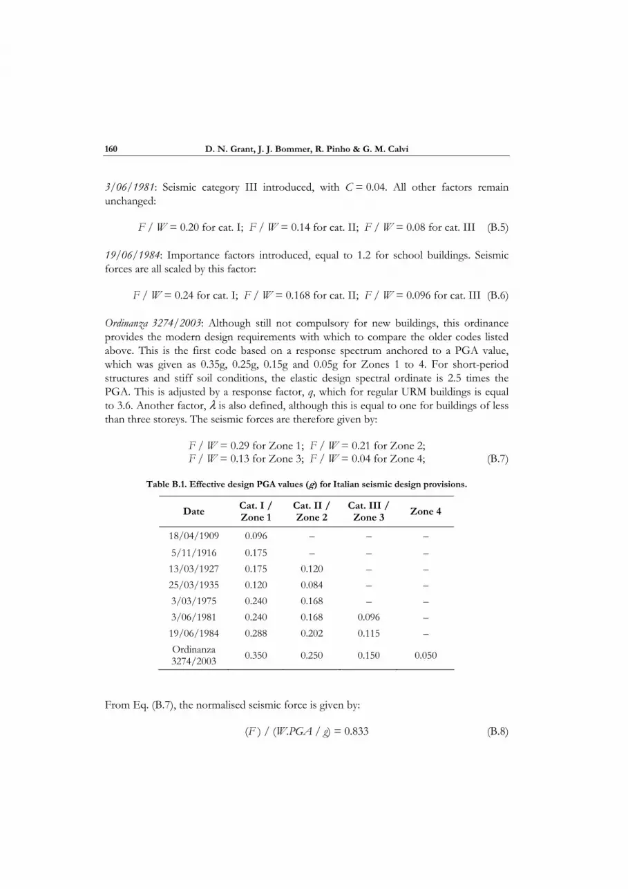
D. N. Grant, J. J. Bommer, R. Pinho & G. M. Calvi
160
3/06/1981: Seismic category III introduced, with C = 0.04. All other factors remain unchanged:
F / W = 0.20 for cat. I; F / W = 0.14 for cat. II; F / W = 0.08 for cat. III (B.5)
19/06/1984: Importance factors introduced, equal to 1.2 for school buildings. Seismic forces are all scaled by this factor:
F / W = 0.24 for cat. I; F / W = 0.168 for cat. II; F / W = 0.096 for cat. III (B.6)
Ordinanza 3274/2003: Although still not compulsory for new buildings, this ordinance provides the modern design requirements with which to compare the older codes listed above. This is the first code based on a response spectrum anchored to a PGA value, which was given as 0.35g, 0.25g, 0.15g and 0.05g for Zones 1 to 4. For short-period structures and stiff soil conditions, the elastic design spectral ordinate is 2.5 times the PGA. This is adjusted by a response factor, q, which for regular URM buildings is equal to 3.6. Another factor, λ is also defined, although this is equal to one for buildings of less than three storeys. The seismic forces are therefore given by:
F / W = 0.29 for Zone 1; F / W = 0.21 for Zone 2; F / W = 0.13 for Zone 3; F / W = 0.04 for Zone 4; (B.7)
Table B.1. Effective design PGA values (g) for Italian seismic design provisions.
Date Cat. I / Zone 1
Cat. II / Zone 2
Cat. III / Zone 3 Zone 4
18/04/1909 0.096 – – – 5/11/1916 0.175 – – – 13/03/1927 0.175 0.120 – – 25/03/1935 0.120 0.084 – – 3/03/1975 0.240 0.168 – – 3/06/1981 0.240 0.168 0.096 – 19/06/1984 0.288 0.202 0.115 – Ordinanza 3274/2003 0.350 0.250 0.150 0.050
From Eq. (B.7), the normalised seismic force is given by:
(F ) / (W.PGA / g) = 0.833 (B.8)

Defining Priorities and Timescales for Seismic Intervention
161
Finally, the effective design PGA values for each of the codes discussed above can be obtained by dividing each of Eqs. (B.1)–(B.7) by Eq. (B.8). This gives the design PGA values reported in Table B.1. Clearly, for modern design according to Ordinanza 3274/2003, effective PGA values are as specified for the seismic zones in the code.


![[Re]Defining Chandigarh - CORE](https://img.dokumen.tips/doc/110x75/6316371b6ebca169bd0b755d/redefining-chandigarh-core.jpg)


