Decision trees with optimal joint partitioning

Decision Trees with OptimalJoint PartitioningDjamel A. Zighed,1,* Gilbert Ritschard,2,† Walid Erray,1,‡

Vasile-Marian Scuturici1,§

1ERIC Laboratory, University of Lyon 2, C.P.11 F-69676 Bron Cedex,France2Department of Econometrics, University of Geneva, CH-1211 Geneva 4,Switzerland

Decision tree methods generally suppose that the number of categories of the attribute to bepredicted is fixed. Breiman et al., with their Twoing criterion in CART, considered gathering thecategories of the predicted attribute into two supermodalities. In this article, we propose anextension of this method. We try to merge the categories in an optimal unspecified number ofsupermodalities. Our method, called Arbogodaï, allows during tree growing for grouping cat-egories of the target variable as well as categories of the predictive attributes. It handles bothcategorical and quantitative attributes. At the end, the user can choose to generate either a set ofsingle rules or a set of multiconclusion rules that provide interval-like predictions. © 2005 WileyPeriodicals, Inc.

1. INTRODUCTION

Induction trees are among the most popular supervised methods proposed inthe literature. They are appreciated for the simplicity and the high efficacy of thealgorithms, for their ease of use, and for the easily interpretable results they pro-vide. Hastie et al. ~Ref. 1, p. 313! designate them as the learning tool that comesclosest to the requirements of an “off-the-shelf” method.

Many induction tree methods have been proposed so far in the literature. Some,like ID3,2 C4.5,3 and CHAID,4,5 build n-ary trees; others like CART6 producebinary trees or, like SIPINA,7,8 latticed graphs that generalize trees by allowingthe merging of nodes.

All these methods were originally intended for categorical attributes andrequire therefore that quantitative variables be discretized. This discretization canbe done at once before growing the tree. Most of the tree growing methods,

*Author to whom all correspondence should be addressed: e-mail: [email protected].†e-mail: [email protected].‡e-mail: [email protected].§e-mail: [email protected].

INTERNATIONAL JOURNAL OF INTELLIGENT SYSTEMS, VOL. 20, 693–718 ~2005!© 2005 Wiley Periodicals, Inc. Published online in Wiley InterScience~www.interscience.wiley.com!. • DOI 10.1002/int.20091

nevertheless, handle quantitative variables in an automatic manner by dynami-cally choosing the optimal discretization thresholds at each node.9–11 Some meth-ods also attempt to reduce the number of categories of nominal attributes bypartitioning them into a smaller number of classes. CART, for example, mergesthe categories into two new supermodalities at each new split. This has the advan-tage of avoiding uselessly increasing the number of nodes. Indeed, the higher thenumber of nodes, the greater are the chances that some of them will have too fewcases to get reliable estimates of the response classes probabilities.

There are two main ways for partitioning the values of the nominal predictiveattributes:

1. The first is, for instance, a characteristic feature of CHAID.4 At each node, the localdiscriminating power of each categorical attribute is tested using all possible partitionsof its values. Partitions in two or more groups are explored. Thus, for each split, apredictor is selected simultaneously with its locally best partition.

2. The second strategy is used, for instance, by Breiman et al.6 in their CART method. Ateach node, CART looks only for the best bipartition of each predictor. It generates thusonly binary trees.

With their Twoing criterion, the authors of CART, however, also propose a strat-egy that extends their principle to the response variable. When the response ismultivalued, using Twoing is equivalent to seeking, for every predictor, simulta-neously the best bipartition of its values and the best bipartition of the responsevalues. The Twoing is the value of the Gini impurity for the best couple of biparti-tions and is used for selecting the split variable at each node.

In this article, we extend the principle of a simultaneous search of a doublebipartition. We combine the CHAID and CART approaches. Like CHAID we lookat each step for the best not necessarily binary partition of the attributes. LikeCART with Twoing we explore also the partitioning of the values of the targetvariable. Unlike CART, we do not, however, restrict ourself to bipartitions. Ateach step we look for the simultaneous grouping of the predictor values and of thetarget variable values that optimizes the chosen criterion. This gives rise to a newinduction tree method that we call Arbogodaï. This kind of tree is characterized bya number of value classes of the target variable that varies from one node to theother. It is dynamically determined at each new split. When the majority class in aleaf contains several response values, the corresponding prediction rule becomes amultiple conclusion rule. For instance, we can get a rule like “a female customeraged between 30 and 40 with a monthly income ranging from 4000 to 5000 euroswill choose a red or blue car.” Indeed, we can easily compute which of the twocolors is more frequent in the leaf. Hence, we can also derive classical simplerules. With Arbogodaï, the user has the possibility to chose the kind of rule thatbest suits her/his needs.

The article is organized as follows. Section 2 sets the framework and recallsthe goal and principle of induced decision trees. In Section 3, we motivate thesimultaneous n-ary partitioning of the target and predictor values. Section 4describes the simultaneous row–column merging heuristic. The Arbogodaï tree

694 ZIGHED ET AL.

growing process that seeks at each step the optimal joint merging of target andpredictor values is described in Section 5. Section 6 discusses the multiple conclu-sion nature of the generated rules and how to measure their prediction error rates.It reports also some experiments with a set of benchmark datasets. In Section 7,we propose an in-depth study of the simultaneous merging heuristic. Further devel-opments are briefly discussed in the concluding section.

2. PRINCIPLE OF INDUCTION TREES AND NOTATIONS

Let V be the population concerned by the learning problem. The profile ofany member v of V is described by p variables, X1, . . . , Xp , called either exog-enous variables, predictive attributes, or predictors. These variables can be quali-tative or quantitative. The set of values taken by Xj is denoted by Xj . Each variableXj , j �1, . . . , p can be seen as a mapping Xj :Vr Xj , where Xj , the domain of thevalues of Xj , is any not necessarily finite set. We consider also a target attribute C,sometimes called the response, endogenous, or dependent variable, and designateby C the set of response values. Like the Xj ’s, C can be qualitative or quantitative.Because the attributes Xj and the target variable C take only a finite number ofdifferent values in a given dataset, the sets Xj and C are finite. We denote by mj thenumber of different values taken by the attribute Xj and by � the number of differ-ent response values ci . Thus, C � $c1, . . . , c� % .

The goal of induction trees is then to generate a model f~X1, . . . , Xp ! in theform of a decision tree for predicting the value of C from the knowledge of thevalues taken by the predictive attributes. The tree f is induced from a trainingsample VL � V. The validation of the predictive model is done on a test sampleVT � V distinct from the former, VL � VT � �.

The growing process of the tree is quite simple. As illustrated in Figure 1, theset VL is iteratively split by means of, at each step, one of the predictive attributesX1, . . . , Xp .

Figure 1. An induced tree.

TREES WITH JOINT PARTITIONING 695

The leaves of the tree obtained at each step t of the growing process define apartition St of VL that becomes finer and finer with t. The root of the tree corre-sponds to the trivial partition S0 � $VL % .

The goal is to get a partition with each leaf ~class of the partition! as pure aspossible, a pure leaf being one in which all the individuals have the same value forthe predicted attribute. The leaf must indeed contain enough individuals to bereliable.

The tree given in Figure 1 partitions VL in three subsets corresponding to thenodes s2, s3, and s4. In leaf s3, for example, we have the set of cases of VL that takevalues X1 � male and X2 � 5000. At step t, the partition St is derived from theprevious one St�1 by seeking the best leaf-attribute couple ~sk , Xj !, that is, that forwhich the splitting of sk � St�1 according to the values of Xj maximizes the gainof information on the target variable between St�1 and St . Formally, lettingG~St�1, sk , Xj ! be the gain of information when sk is split with attribute Xj , weseek at step t the leaf-attribute couple ~sv , Xu ! such that

G~St�1, sv , Xu ! � maxk; j

G~St�1, sk , Xj !

The gain of information is usually measured as the reduction in uncertainty for thetarget variable or as the increase in the strength of association between the parti-tion and the target variable. The growing process stops when the criterion can nolonger be improved, that is, when G~St�1, sv , Xu ! � 0, or when some other stop-ping criterion is reached.

Let n be the grand total of cases in node s, nik the number of cases with valueci for the target variable in the class ~leaf ! sk of the partition S of the cases in s, n.k

the total number of cases in leaf sk , and ni. the total number of cases with value ci

in s. The corresponding observed frequencies are denoted respectively by fik , f.k ,and fi. , and fi6k � nik /n.k stands for the conditional frequency of value ci in the leafsk . To be rigorous, the ns and fs should be indexed by the node label s. We omit itto avoid cumbersome notations.

At any node s of a tree, an attribute Xj defines a partition of the cases in s.This partition is described by the columns of the l � mj contingency table ~Table I!that cross-tabulates the target variable ~rows! with Xj ~columns!.

The criteria used to measure the gain of information brought by a split definedby Xj are computed from this table. For instance, some methods try to maximize

Table I. Contingency table defined by Xj at a node s.

xj1 . . . xjk . . . xjmjTotal

c1 n11 . . . n1k . . . n1mjn1.

I I L I I Ici ni1 . . . nik . . . nimj

ni.

I I I L I Ic� n�1 . . . n�k . . . n�mj

n�.

Total n.1 . . . n.k . . . n.mjn

696 ZIGHED ET AL.

the reduction in uncertainty as measured by entropies. In this case, the uncertaintyafter the split is defined as the weighted mean of the uncertainty of the columns ofthe contingency Table I:

I ~S! � (k�1

mj n.k

nh~ f16k ; . . . ; fi 6k ; . . . ; f�6k ! ~1!

where h~ ! is, for example, the Shannon entropy, �(i�1� fi 6k log2 fi 6k , or the

quadratic entropy, also known as the Gini diversity index, (i�1� fi 6k~1 � fi6k !.

Alternatively, some methods, like CHAID, optimize the strength or the statisticalsignificance of the association between the resulting partition ~columns of Table I!and the target variable ~rows of Table I!.

Let us recall that CHAID tries, at each step, to merge the columns of cross-tables like Table I to find the best grouping of values for each candidate attribute,that is, the grouping that optimizes the criterion. CHAID makes no change, how-ever, on the values of the target variable. Arbogodaï, like the Twoing approach inCART, considers merging both columns and rows. Unlike the Twoing rule thatlooks for the best solution among 2 � 2 tables only, we seek however the bestcross-partition without constraints on the number of rows and columns. Section 4discusses this joint row–column partitioning issue. Before turning to it, we moti-vate the approach in Section 3.

3. MOTIVATIONS FOR A JOINT n-ARY PARTITIONING

Consider the contingency Table II. The best bipartition of its columns is Sbin �$$a, b%, $d, e%% , whether we use the Gini, the Twoing, the significance of Pearson’sChi-squares, or an association measure like the t of Tschuprow. Now, the best three-way partition is S3way � $$a%, $b, d %, $e%% with any of the criteria except Twoing,which is not applicable. Clearly S3way cannot be obtained by splitting the classesof Sbin . This proves that multiple binary partitions are not equivalent to n-ary par-titions and can sometime miss optimal solutions.

The merging of response values is different in nature from that of the valuesof a predictive attribute. Indeed, the partition of the response values does not trans-late into a split of the node. Considering such mergings in the optimization pro-cess merits, therefore, some further justification. This is given by simply extendingthe argument of Breiman et al. ~Ref. 6, p. 105!, who argue that searching for

Table II. A n-ary solution different from that of successive binary splits.

a b d e Total

c1 200 100 10 1 311c2 10 150 150 10 320c3 1 10 100 200 311

Total 211 260 260 211 942


superclasses ~the groups of the partitions of the response values! provides strate-gic information on the similarities of responses. When two or more responses, redcar and blue car, for example, are almost equally frequent it may be a better strat-egy to predict that the customer will buy a red or a blue car than explicitly a redone. Simultaneously, it may be useful to know that yellow and pink colors aremuch less probable than all other nonred and nonblue proposed colors. There isthus no reason to limit the argument to two superclasses only. Multisupermodali-ties provide a more refined strategic information.

Now, the grouping on one variable ~say the row variable!may obviously affectthe optimal grouping on the other attribute ~the column variable!. For example,grouping first rows c1 and c2 in Table II we get the reduced table

�210 250 160 1

1 10 100 200�The most similar columns in this new table are obviously the first two. Hence, thebest column partitioning would be $$a, b%, $d %, $e%% or $$a, b, d %, $e%% , but clearlynot the one found without grouping the rows. Due to this relationship between thepartitions of the rows and the columns, it is then essential to determine themsimultaneously.

4. SIMULTANEOUS ROW AND COLUMN PARTITIONING

In this section, we introduce the method adopted for determining the bestsimultaneous partition of the rows and the columns. First, we specify the objec-tives and briefly review related works. We then define the formal setting anddescribe our merging heuristic.

4.1. Objectives

Although the univariate optimal grouping of values has been abundantly stud-ied since the pioneering work of Walter Fisher,12 the literature about the simulta-neous grouping of rows and columns of a table is less rich. We can mention therelated work by Fisher13,14 about the optimal grouping of the unknowns and equa-tions of predictive economic models. The simultaneous partitioning of the cases~rows! and the variables ~columns! in a data matrix has been studied by Ander-berg,15 Bock,16 and Govaert,17 among others. In Refs. 17 and 18, Govaert investi-gates the special case of binary tables. In the framework of contingency tables thatwe are interested in, the optimal partitioning problem has been studied from dif-ferent points of view. Benzécri19 is interested in the partition in a fixed number ofgroups that maximizes the Pearson Chi-square. A solution to this problem is givenin Ref. 20 in the form of an iterative heuristic that clusters alternatively the rowsand the columns. Gilula and Krieger21 study how the Pearson Chi-square behaveswhen the table is reduced by aggregation. Hirotsu22 and Greenacre23 are inter-ested in finding the most homogeneous tables. As already mentioned, Breiman

698 ZIGHED ET AL.

et al.6 have considered with their Twoing approach the joint dichotomization oftwo variables.

Our objective is to find both the number of groups and the joint partition ofrows and columns of a contingency table that maximizes the row–column associ-ation. None of the works cited gives a satisfactory solution to this problem. Some,like those done after Benzécri19 or those by Breiman et al.,6 assume the number ofgroups fixed a priori. The others either do not consider the case of contingencytables or consider criteria, homogeneity for example, that are hardly transposablein our setting.

Clearly, the exhaustive scanning of all combinations of partitions of each ofthe variable is not practicable for large tables. We show in Section 7.1 that thesearch of the optimal solution becomes untractable when the number of values ofthe predictive and/or target variable exceeds 5 or 6. We consider therefore a heu-ristic, first introduced in Ref. 24, that successively looks for the optimal groupingof two row or column categories. We recall the principle of the algorithm hereafterand will propose an in-depth study of its behavior and performance in Section 7.

4.2. Formal Framework

Let X be a predictive attribute. From hereon we shall drop the subscripts jwhen there is no ambiguity. Cross-tabulating variable C with X generates a contin-gency table T��m with � rows and m columns.

Let uCX � u~T��m ! denote a generic association criterion for table T��m .This criterion uCX may thus be a Chi-square-based association measure like Cram-er’s v or Tschuprow’s t, an asymmetrical PRE measure like Goodman-Kruskal’stCX or Theil’s uncertainty coefficient uCX , or, when both variables are ordinal, anordinal association index like Kendall’s tb or Somers’ dCX .

Let Pc be a partition of the values of the row variable C, and Px a partition ofthe states of X. Each couple ~Pc , Px ! defines then a contingency table T~Pc , Px !.The optimization problem considered is then the maximization of the associationuCX among the set of couples ~Pc , Px ! of partitions

maxPc , Px

u~T~Pc , Px !!

For ordinal variables, hence for interval or ratio variables, only partitionsobtained by merging adjacent categories make sense. We consider then the restrictedprogram

�maxPc , Px

u~T~Pc , Px !!

u.c. Pc � Ac and Px � Ay

where Ac and Ax stand for the sets of partitions obtained by grouping adjacentvalues of C and X. Letting Pc and Px be the unrestricted sets of partitions, we havefor �, m � 2, Ac � Pc and Ax � Px . Finally, note that ordinal association measuresmay take negative values. Then, for maximizing the strength of the association,


the objective function u~T~Pc , Px !! should be the absolute value of the ordinalassociation measure.

4.3. The Heuristic

The heuristic is an iterative greedy process that successively merges the tworows or columns that most improve the association criteria u~T!.

Such a heuristic may indeed not end up with the optimal solution, but perhapsonly with a quasi-optimal solution. See Section 7.3 for empirical insights on thissuboptimality. Formally, the configuration ~Pc

k , Pxk ! obtained at step k is the solu-

tion of

�maxPc , Px

u~T~Pc , Px !!

u.c. Pc � Pc~k�1! and Px � Px

~k�1!

or

Pc � Pc~k�1! and Px � Px

~k�1!

~2!

where Pc~k�1! stands for the set of partitions on C resulting from the grouping of

two classes of the partition Pc~k�1! . For ordinal variables, Pc

~k�1! and Px~k�1! should

be replaced by the sets Ac~k�1! and Ax

~k�1! of partitions resulting from the aggrega-tion of two adjacent elements.

Let T0 � T��m be the table associated with the finest partition of the catego-ries of C and X. Starting with T0 , the algorithm successively determines the tablesTk, k �1,2, . . . corresponding to the partitions solution of Equation 2. The processcontinues while u~Tk !� u~T~k�1! ! and is stopped when the best grouping of twocategories leads to a reduction of the criteria.

The quasi-optimal grouping is the couple ~Pck , Px

k ! solution of Equation 2 atthe step k where

u~T~k�1! !� u~Tk ! � 0 and u~Tk !� u~T~k�1! !� 0

By convention, we set the value of the association criteria u~T! to zero forany table with a single row or column. The algorithm then ends up with such asingle value table if and only if all rows ~columns! are equivalently distributed.

5. ARBOGODAÏ: A NEW DECISION TREE APPROACH

We now introduce the new Arbogodaï tree growing method. We first explainthe principle of the Arbogodaï algorithm and, then, describe how it works on anexample.

5.1. Principle of the Algorithm

Arbogodaï follows the general principle of tree growing presented in Sec-tion 2. Its specificity is an additional preparatory step before testing the attributes

700 ZIGHED ET AL.

at a node. This step consists of optimally reducing the size of the table that cross-tabulates the target variable with the tested attribute. The splitting criterion is thencomputed using the found partitions of both the attribute and the target variablevalues. The splitting of the selected node is done according to the found classes ofvalues of the selected predictive attribute.

This additional step plays a role similar to discretization. The merging ofvalues can indeed be assimilated to some sort of discretization that works also onnominal variables. Remember, however, that the merging is done here simulta-neously at each step on the target and the predictive attribute.

The reduction of the table is that for which the row–column association u ismaximized. Indeed, we use the heuristic of Section 4.3 and measure the associa-tion u with the t of Tschuprow: t � $n�1 @~� � 1!~m � 1!#�1/2x2 %1/2 , where x2 �

(i�1� (k�1

m ~nni. n.k !�1~nnik � ni. n.k !

2 is the Pearson Chi-square statistic. Unlikesome other association measures, the t of Tschuprow always increases with themerging of equivalently distributed rows or columns ~see Ref. 25 and Section 7.2!.

The splitting criterion is the reduction in uncertainty ~gain in purity! achievedwith the columns of the reduced table as compared to its margin. The uncertaintyafter the split is computed for every Xj by applying formula 1 on the optimal reducedtable for Xj at the considered node s.

More specifically, we use Laplace estimates of the column distributions afterthe split; that is, the proportion of cases that take the ith value of C in column k isestimated by:

fi 6k*~l! �

nik* � l

n.k* � �*l

where the asterisk denotes values for the reduced table.Using the quadratic ~Gini! entropy, the gain in uncertainty considered by Arbo-

godaï then reads

h~C * !� h~C * 6Xj* ! � 1 �(

i

fi.*2 �(

k

f.k*�1 �(

i

~ fi 6k*~l! !2�

�(i��(

k

f.k* ~ fi 6k

*~l! !2�� fi.*2�

The use of Laplace estimates penalizes the gain of uncertainty obtained atnodes with small counts. With very small counts, that is, when l represents a sig-nificant proportion of the count, a split may even deteriorate the uncertainty crite-rion ~see Ref. 8, p. 76!.

5.2. Example

We now describe the Arbogodaï algorithm through an example. We considerthe Flags dataset from the UCI repository.26 The response variable C takes sixnominal values C � $c1, c2, c3, c4, c5, c6 % and there are 29 mixed categorical and


quantitative predictive attributes X1, . . . , X29. The dataset contains 194 cases. Fig-ure 2 shows an extract of the two first levels of the Arbogodaï tree for these data.

Step 1. At the root of the tree, we have the distribution of all 194 casesamong the six values of the response C. The 29 predictive attributes are succes-sively tested. For every attribute, we first determine the optimal reduced cross-table with the target variable. We then select the attribute for which the gain inuncertainty computed on the reduced table is maximal. The winner is X7, whichtakes eight values: X7 � $a, b, c, d, e, f, g, h% . The two simultaneous groupingsfound by the heuristic of Section 4.3 are X7

* � $$c, d, e, h%;$a, b, g%;$ f %% and C* �$$c1%;$c2, c4, c5, c6 %;$c3 %% . The corresponding cross-table is shown in Table IIItogether with the table of the derived conditional frequencies fi 6k

*~l! . The latterhave been computed by setting l � 1. The marginal uncertainty is h~C * ! � 1 �0.2012 � 0.5302 � 0.2682 � 0.605 and the uncertainty after the split, which isthe weighted average of the uncertainty of each column, is h~C * 6X3

* ! � 0.314.The gained information is thus 0.291. This is the maximal value achievable withany of the 29 attributes.

Step 2. The process is repeated on every terminal node of the previouslyobtained tree. Notice that we try to merge the original set of values X and C andnot the set of previously merged classes. In our example, the next best split occursat the middle node ~X7 � $a, b, g%!. The attribute selected for splitting this node isX3. The six values of the target C were merged to form four target classes. How-ever, no merging of the attribute values could improve the association between X3

and the target C. The node is therefore split into four new classes corresponding tothe four values of X3. This leads to the tree with six leaves shown in Figure 2.

Following steps. In our example, the tree growing process is stopped afterstep 2. Without explicit stopping rules, the growing continues until the criterion

Figure 2. Example of an Arbogodaï tree.

702 ZIGHED ET AL.

can no longer be improved. At step 3, Arbogodaï would scan the six leaves of thepreviously grown tree.

Two further remarks should be made: ~1! At a same level, nodes that do notresult from a same parent may have different partitions of the set C of responsevalues. ~2!When the same attribute is used as the splitting variable at more thanone node, its values are not necessarily partitioned the same way for each split.For example, growing the tree of Figure 2 one level further leads to splitting eachof the two leftmost leaves of level 2 with the same attribute X29. The correspond-ing cross-tables are given in Table IV. It can be seen that the values of C are oncepartitioned as $$c1, c2, c4%, $c3%, $c5, c6%% and once as $$c3%, $c4%, $c1, c2, c5, c6%% . Like-wise, attribute X29 is used once with the partition $$a, b, d, e%, $ f %% and once with$$a, e, d %, $b, f %% .

6. THE INDUCED RULES AND THEIR ACCURACY

Arbogodaï can generate two types of classification rules: ~1! classical rulesby disregarding the merged classes of response values in the final leaves, and~2! multiple conclusion rules for leaves with merged response values. This sectionspecifies the nature of these rules, defines error rates adapted for them, and presentsexperimentation results.

Table IV. Cross-table for splitting the two leftmost leaves with X29.

$a, b, d, e% $ f %

$c1, c2, c4 % 38 1c3 0 3Other 0 0

$a, d, e% $b, f %

c3 2 2c4 8 0Other 0 0

Table III. Step 1 optimal cross-table and Laplace estimates ofcolumn distributions.

CX7 $c, d, e, h% $a, b, g% $ f %

$c1% 33 6 0$c2, c4, c5, c6 % 2 100 1$c3 % 17 9 26

Total 52 115 27

fi 6k*~l! $c, d, e, h% $a, b, g% $ f % fi.

*

$c1% 0.618 0.059 0.033 0.201$c2, c4, c5, c6 % 0.055 0.855 0.067 0.530$c3 % 0.327 0.084 0.900 0.268

f.k* 0.268 0.592 0.139 1


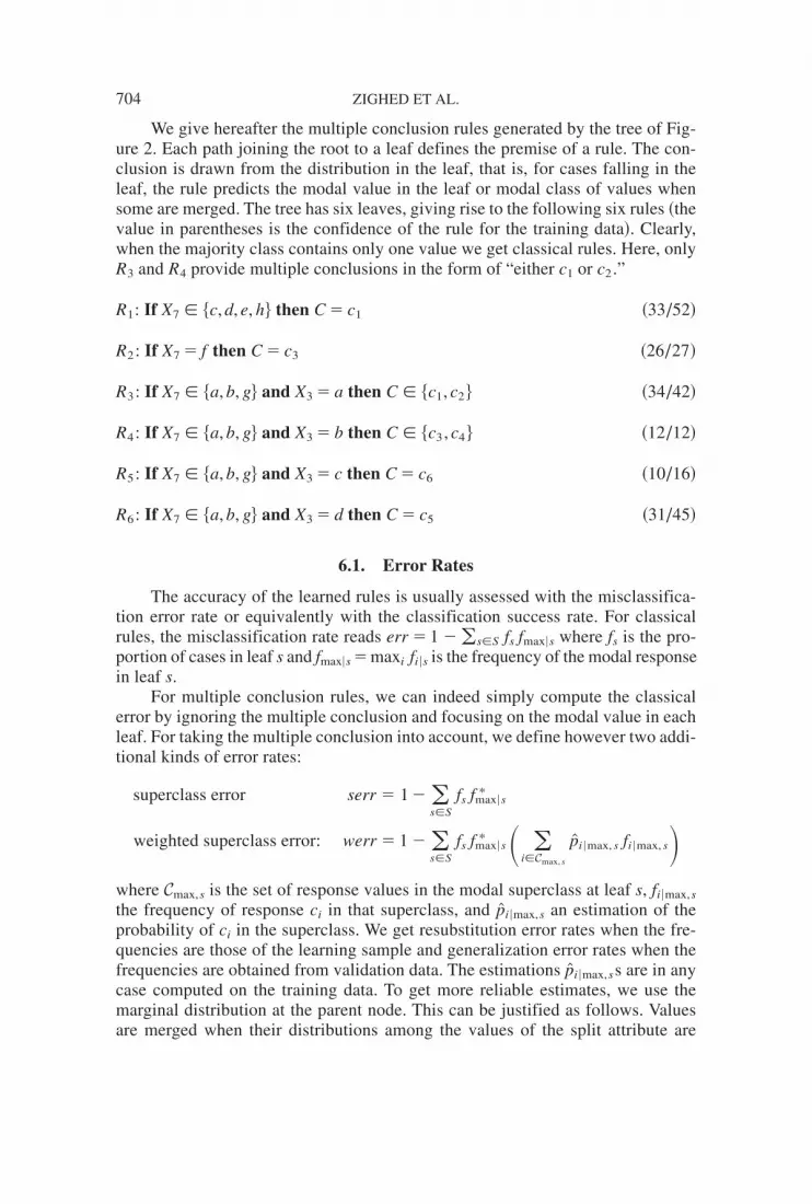
We give hereafter the multiple conclusion rules generated by the tree of Fig-ure 2. Each path joining the root to a leaf defines the premise of a rule. The con-clusion is drawn from the distribution in the leaf, that is, for cases falling in theleaf, the rule predicts the modal value in the leaf or modal class of values whensome are merged. The tree has six leaves, giving rise to the following six rules ~thevalue in parentheses is the confidence of the rule for the training data!. Clearly,when the majority class contains only one value we get classical rules. Here, onlyR3 and R4 provide multiple conclusions in the form of “either c1 or c2.”

R1: If X7 � $c, d, e, h% then C � c1 ~33/52!

R2: If X7 � f then C � c3 ~26/27!

R3: If X7 � $a, b, g% and X3 � a then C � $c1, c2 % ~34/42!

R4: If X7 � $a, b, g% and X3 � b then C � $c3, c4 % ~12/12!

R5: If X7 � $a, b, g% and X3 � c then C � c6 ~10/16!

R6: If X7 � $a, b, g% and X3 � d then C � c5 ~31/45!

6.1. Error Rates

The accuracy of the learned rules is usually assessed with the misclassifica-tion error rate or equivalently with the classification success rate. For classicalrules, the misclassification rate reads err � 1 �(s�S fs fmax6s where fs is the pro-portion of cases in leaf s and fmax6s � maxi fi6s is the frequency of the modal responsein leaf s.

For multiple conclusion rules, we can indeed simply compute the classicalerror by ignoring the multiple conclusion and focusing on the modal value in eachleaf. For taking the multiple conclusion into account, we define however two addi-tional kinds of error rates:

superclass error serr � 1 �(s�S

fs fmax6s*

weighted superclass error: werr � 1 �(s�S

fs fmax6s* � (

i�Cmax, s

[pi 6max, s fi 6max, s�where Cmax,s is the set of response values in the modal superclass at leaf s, fi6max,s

the frequency of response ci in that superclass, and [pi6max,s an estimation of theprobability of ci in the superclass. We get resubstitution error rates when the fre-quencies are those of the learning sample and generalization error rates when thefrequencies are obtained from validation data. The estimations [pi6max,ss are in anycase computed on the training data. To get more reliable estimates, we use themarginal distribution at the parent node. This can be justified as follows. Valuesare merged when their distributions among the values of the split attribute are

704 ZIGHED ET AL.

similar. Hence, their distributions inside the superclass are similar too, and, there-fore, similar to the marginal distribution.

The superclass error, serr, is computed as for classical rules but with thesuperclass frequencies fi 6s

* instead of the single response frequencies fi6s . Doing so,we do not care indeed about classification error inside the modal superclasses.This may have sense independently for each rule. We cannot compare, however,the error rate of a rule that predicts for instance c1 with that of a rule that predictsc1 or c2. Hence, the global superclass error does not make much sense.

The weighted superclass error, werr, takes the uncertainty inside the major-ity class into account. It assumes that each case falling in a leaf is randomly assignedto a value in the modal superclass. The supposed random assignment is done accord-ing to the learned distribution inside Cmax,s . For instance, for our example tree, acase ~X7 � a, X3 � a,C � c2 ! is correctly classified in the modal superclass ofleaf 3. In that leaf, the estimated proportion of cases taking C � c2 in the super-class is 85%. Thus, we weight this correct classification down and count it as a0.85 correct classification. In resubstitution, if we use [pi6max,s � fi6max,s , this isequivalent to weighting down the success rates with the Gini uncertainty of thedistribution inside the superclass: werr �(s @1 � ~1 � serrs !Gini~Cmax,s !# , whereserrs is the superclass error for rule s.

It is well known that the learning error rate suffers from an optimistic bias. Itunderestimates the generalization error rate. For validation, it is then common prac-tice to compute the classification error rate on a validation dataset distinct fromthe data used in the learning phase. Alternatively, and perhaps more frequently, across-validation error rate is computed. A 10-fold cross-validation ~10CV!, forinstance, consists of splitting the learning sample into 10 approximately equallysized parts. Dropping each time a different part we get 10 learning datasets fromwhich 10 trees are induced. For each of them we compute the error rate on thedropped-out data. The cross-validation error rate is the mean values of the 10 result-ing error rates.

6.2. Experimentation

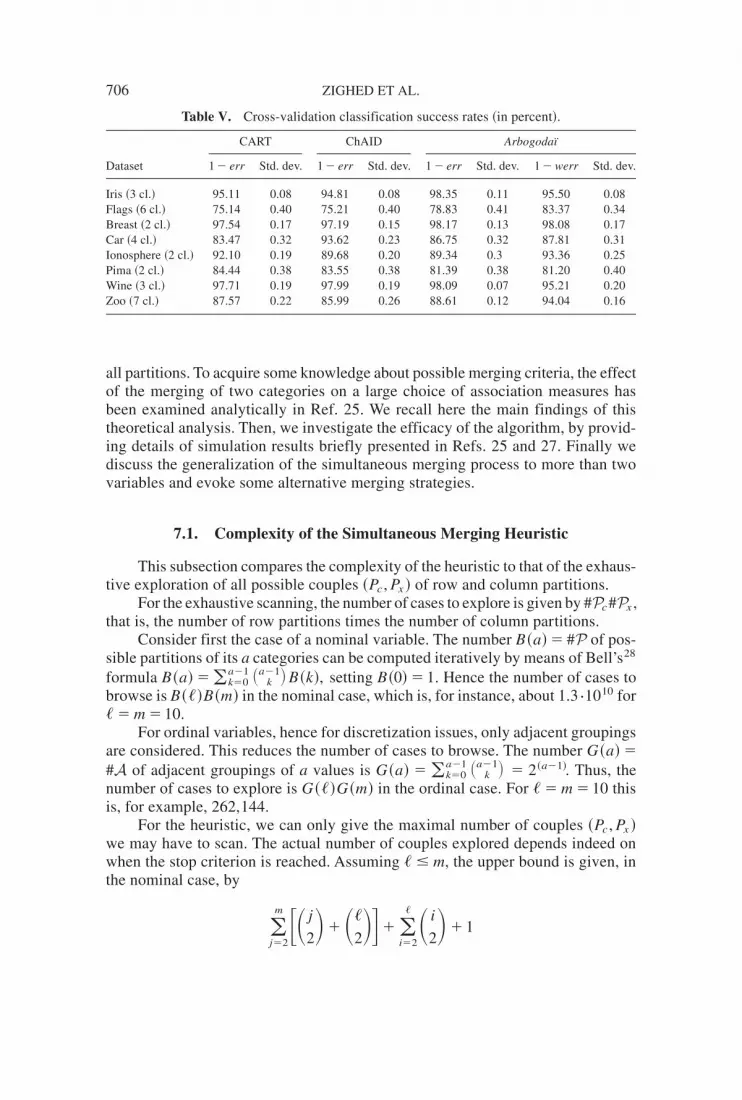
We have experimented with our approach on eight benchmark datasets. Table Vgives the cross-validation success rates obtained for each dataset with Arbogodaïand, for the sake of comparison, with CART and CHAID. For Arbogodaï, we givethe rate derived from both the classical and the weighted superclass error. Arbo-godaï ranks first for five of the eight datasets whatever error is considered. Unsur-prisingly, its superiority is mostly significant when the number of values of thetarget variable is large.

7. ADVANCED STUDY OF THE MERGING HEURISTIC

The joint response and predictive attribute partitioning is done with the heu-ristic described in Section 4.3. We propose here an in-depth study of this greedyalgorithm that successively seeks the best merge of two row or column categories.First, we examine its complexity and compare it with the exhaustive scanning of


all partitions. To acquire some knowledge about possible merging criteria, the effectof the merging of two categories on a large choice of association measures hasbeen examined analytically in Ref. 25. We recall here the main findings of thistheoretical analysis. Then, we investigate the efficacy of the algorithm, by provid-ing details of simulation results briefly presented in Refs. 25 and 27. Finally wediscuss the generalization of the simultaneous merging process to more than twovariables and evoke some alternative merging strategies.

7.1. Complexity of the Simultaneous Merging Heuristic

This subsection compares the complexity of the heuristic to that of the exhaus-tive exploration of all possible couples ~Pc , Px ! of row and column partitions.

For the exhaustive scanning, the number of cases to explore is given by #Pc#Px ,that is, the number of row partitions times the number of column partitions.

Consider first the case of a nominal variable. The number B~a!� #P of pos-sible partitions of its a categories can be computed iteratively by means of Bell’s28

formula B~a!�(k�0a�1 �a�1

k � B~k!, setting B~0!� 1. Hence the number of cases tobrowse is B~�!B~m! in the nominal case, which is, for instance, about 1.3{1010 for� � m � 10.

For ordinal variables, hence for discretization issues, only adjacent groupingsare considered. This reduces the number of cases to browse. The number G~a!�#A of adjacent groupings of a values is G~a! � (k�0

a�1 �a�1k � � 2~a�1!. Thus, the

number of cases to explore is G~�!G~m! in the ordinal case. For � � m � 10 thisis, for example, 262,144.

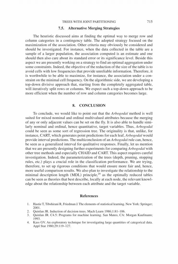
For the heuristic, we can only give the maximal number of couples ~Pc , Px !we may have to scan. The actual number of couples explored depends indeed onwhen the stop criterion is reached. Assuming � � m, the upper bound is given, inthe nominal case, by

(j�2

m �� j

2��

2��(i�2

� � i

2�� 1

Table V. Cross-validation classification success rates ~in percent!.

CART ChAID Arbogodaï

Dataset 1 � err Std. dev. 1 � err Std. dev. 1 � err Std. dev. 1 � werr Std. dev.

Iris ~3 cl.! 95.11 0.08 94.81 0.08 98.35 0.11 95.50 0.08Flags ~6 cl.! 75.14 0.40 75.21 0.40 78.83 0.41 83.37 0.34Breast ~2 cl.! 97.54 0.17 97.19 0.15 98.17 0.13 98.08 0.17Car ~4 cl.! 83.47 0.32 93.62 0.23 86.75 0.32 87.81 0.31Ionosphere ~2 cl.! 92.10 0.19 89.68 0.20 89.34 0.3 93.36 0.25Pima ~2 cl.! 84.44 0.38 83.55 0.38 81.39 0.38 81.20 0.40Wine ~3 cl.! 97.71 0.19 97.99 0.19 98.09 0.07 95.21 0.20Zoo ~7 cl.! 87.57 0.22 85.99 0.26 88.61 0.12 94.04 0.16

706 ZIGHED ET AL.

that is

�~�2 � 1!� m~m2 � 1!

6�~m � 1!�~� � 1!

2� 1

In the ordinal case, it reads

~� � m � 1!~� � m � 2!

2� 1

For m � � � 10, these bounds are, respectively, 736 and 172.Figure 3 and Table VI show how the relative efficacy of the heuristic increases

with the number of initial categories. The values reported concern square tables. Itis worth mentioning that the seemingly exponential increase in the number of casesreported for the heuristic concerns the upper bound. Practically, the effective num-ber of cases browsed will be much lower.

7.2. Summary of Analytical Results

Because the heuristic merges at each step two categories only, we studied inRef. 25 the effect of such a grouping on a choice of association measures, namelyPearson’s X 2 and the Likelihood Ratio G2 Chi-square statistics, Tschuprow’s t,

Figure 3. Complexity versus size of the square table ~for heuristic, values reported are upperbounds!.


Cramer’s v, Goodman and Kruskal’s t, Theil’s u, Goodman and Kruskal’s g, Ken-dall’s tb , and Somers’ d. The latter three are ordinal measures and apply thereforeonly to ordinal variables. The formula of the indexes are recalled in the Appendix.

Table VII summaries the results established in Ref. 25. For the ordinal mea-sures that take their values in @�1,1# , we report effects on the absolute value of themeasure and consider, indeed, only the merging of two adjacent categories.

For our purpose, we expect an improvement of the criteria when two equiva-lently distributed values are merged. We do not recommend, therefore, criteria thatcan remain unchanged after such a merge. Thus, Chi-square statistics that cannotbe increased with a merge, but also the Cramer v and the asymmetrical PRE mea-sures ~the Goodman–Kruskal t and the Theil u! are not suited for our needs. Among

Table VI. Number of configurations explored.

Nominal case Ordinal case

� � m Exhaustive Heuristic Exhaustive Heuristic

2 4 4 4 43 25 15 16 114 225 39 64 225 2,704 81 256 376 41,209 146 1,024 567 769,129 239 4,096 798 17,139,600 365 16,384 1069 447,195,609 529 65,536 137

10 1.345{1010 736 262,144 17220 2.675{1027 6,271 2.749{1011 46650 3.449{1094 101,676 3.169{1029 4,852

100 2.264{10231 823,351 4.017{1059 19,702

Table VII. Effect of a merge of two categories on a choice of association measures.

Merge of response values Merge of predictor values

Criteria Asym. Not eq. dist. Equiv. dist. Not eq. dist. Equiv. dist.

Chi-square statisticsX 2 , G2 � � � �

Nominal association measuresCramer’s v �/� �/� �/� �/�Tschuprow’s t �/� � �/� �G-K t * �/� � � �Theil’s u * �/� � � �

Ordinal association measuresG-K g �/� � �/� �Kendall’s tb �/� � �/� �Kendall’s tc �/� �/� �/� �/�Somers’ d * �/� � �/� �

708 ZIGHED ET AL.

the ordinal measures, only the Goodman–Kruskal g and the Kendall tb satisfy therequested condition. Among the measures studied, the t of Tschuprow that fits thecondition and can be used with both ordered and unordered values is our preferredchoice.

7.3. Reliability of the Joint Merging Heuristic

The purpose of this section is to assess the reliability of the results providedby the heuristic. A series of simulation studies have been run to investigate twoaspects: ~1! the proportion of global optima missed by the heuristic and ~2! howfar the solution of the heuristic is from the global optimum.

Several association measures have been examined. We report outcomes forthe t of Tschuprow, the t of Goodman and Kruskal, and the tb of Kendall. Amongthe measures considered ~simulations have been run for all the measures listed inTable VII! the t of Tschuprow has been retained because it provides the worsescores for both the proportion of missed optima and the deviations from the globaloptima. The t of Goodman and Kruskal has been selected as a representative ofthe asymmetrical PRE ~proportion of reduction in error of prediction! measures.Likewise, the tb of Kendall has been selected to represent the ordinal measures.

The comparison between quasi and global optima is done for square tables ofsize 4, 5, and 6. Above 6, the global optimum can no longer be obtained in areasonable time.

For the t of Tschuprow and the t of Goodman and Kruskal, we report respec-tively in Tables VIII and IX results for the nominal case as well as for the ordinalcase. The tb of Kendall being an ordinal measure, Table X exhibits only figures forthe ordinal case.

For each measure, size, and variable type, 200 contingency tables have beenrandomly generated. Each table was obtained by distributing 10,000 cases among

Table VIII. Simulations: t of Tschuprow.

Tschuprow Nominal Ordinal

Size 4 � 4 5 � 5 6 � 6 4 � 4 5 � 5 6 � 6Nonzero deviations 39.5% 62.5% 74.5% 23.5% 36% 46.5%

Maximum 0.073 0.074 0.077 0.077 0.063 0.108Mean 0.025 0.023 0.028 0.019 0.019 0.012Standard deviation 0.015 0.014 0.016 0.014 0.016 0.015Skewness 0.986 0.979 0.598 1.674 0.972 3.394

With zero deviationsMean 0.010 0.015 0.021 0.005 0.007 0.006Standard deviation 0.016 0.016 0.018 0.011 0.013 0.012Skewness 1.677 1.062 0.615 3.168 2.211 4.457

Relative deviationsMaximum 0.168 0.198 0.221 0.179 0.194 0.307Mean 0.079 0.077 0.093 0.063 0.066 0.046

Mean initial association 0.260 0.240 0.226 0.263 0.244 0.228Mean global optimum 0.340 0.316 0.303 0.301 0.275 0.250


its � � m cells with a random uniform process. This differs from the solution usedto generate the results given in Ref. 25, which were obtained by distributing thecases with nested conditional uniform distributions: First a random percentage ofthe cases is attributed to the first row, then a random percentage of the remainingcases is affected to the second row and so on until the last row; the total of eachrow is then likewise distributed among the columns. The solution retained hereindeed generates tables that are closer to the uniform distribution and should there-fore exhibit lower association. As will be shown, low associations are the lessfavorable situations for the heuristic. Thus, we can expect the results obtained

Table IX. Simulations: t of Goodman and Kruskal.

G&K t Nominal Ordinal

Size 4 � 4 5 � 5 6 � 6 4 � 4 5 � 5 6 � 6Nonzero deviations 5% 6.5% 12% 6% 19% 32.5%

Maximum 0.013 0.031 0.029 0.076 0.077 0.059Mean 0.007 0.010 0.008 0.025 0.016 0.013Standard deviation 0.004 0.009 0.009 0.021 0.016 0.012Skewness �0.308 1.004 1.181 1.107 2.361 1.908

With zero deviationsMean 0.0004 0.0007 0.0010 0.0015 0.003 0.004Standard deviation 0.0018 0.0033 0.004 0.008 0.009 0.009Skewness 5.323 6.471 5.137 6.685 5.040 3.255

Relative deviationsMaximum 0.142 0.296 0.318 0.420 0.518 0.401Mean 0.062 0.091 0.079 0.216 0.168 0.149

Mean initial association 0.074 0.060 0.048 0.073 0.060 0.050Mean global optimum 0.148 0.128 0.113 0.118 0.098 0.084

Table X. Simulations: tb of Kendall.

Kendall tb Ordinal

Size 4 � 4 5 � 5 6 � 6Nonzero deviations 19% 24.5% 32%

Maximum 0.596 0.597 0.542Mean 0.235 0.182 0.140Standard deviation 0.195 0.190 0.157Skewness 0.076 0.598 0.652

With zero deviationsMean 0.045 0.045 0.045Standard deviation 0.125 0.123 0.111Skewness 2.775 2.849 2.445

Relative deviationsMaximum 1.954 1.970 1.982Mean 0.355 0.259 0.074

Mean initial association ~abs. value! 0.094 0.078 0.064Mean global optimum ~abs. value! 0.256 0.236 0.215

710 ZIGHED ET AL.

with this random uniform generating process to provide some upper bounds forthe deviations from the global optima.

Tables VIII–X exhibit, for each series of tables generated, the proportion ofoptima missed and characteristic values ~maximum, mean value, standard devia-tion, skewness! of the distribution of the deviations between global and quasioptima. Relative deviations, of which the maximum and the mean value arereported, are the ratios between deviations and global optima. The last two rowsgive, respectively, the average of the initial values of the criterion and the meanvalue of the global optima. In Table X, these two last figures are means of absolutevalues because the tbs may be negative.

Additional insight for the Tschuprow’s t and Goodman and Kruskal’s t casesis provided by Figures 4 and 5. Figure 4 shows plots of the 200 initial values, quasioptima, and global optima for 6 � 6 cases. Figure 5 plots the 200 deviations againstthe global optima.

Looking at Tables VIII–X, we see that the proportion of optima missed by theheuristic is relatively important and tends to increase with the size of the table.The proportion is somewhat lower for PRE measures ~the t of Goodman andKruskal!. This is probably due to the fact that PRE measures cannot be improvedby merging values of the predictor ~see Table VII!, which means that the group-ings are, in this case, almost exclusively made on one ~the target! variable. Curi-ously, however, the percentages of missed optima are, for PRE measures, larger inthe ordinal case than in the nominal one.

This high percentage of missed optima is luckily balanced by the small devi-ation between the quasi and global optima. The mean value of the nonzero devia-tions is roughly less than half the difference between the initial value of the criterionand the global optimum. In the case of stronger initial associations than those gen-erated here with a uniform random distribution, this ratio becomes largely morefavorable, that is, smaller. The level and dispersion of the nonzero deviations seemsto remain stable when the size of the table increases. These deviations tend natu-rally to be larger when the association measure provides larger values. Inversely,the relative deviations take larger values when the association measure tends tozero.

Finally, let us recall that the tb of Kendall takes its values in @�1,1# . Thedeviations may thus exceed the absolute value of the global optimum when thequasi and global optima are of opposite signs. This explains why some maximalrelative deviations are greater than one.

Globally, the outcomes of these simulation studies show that the cost in termsof reliability of the heuristic remains moderate when compared with the dramaticincrease of performance.

7.4. Multidimensional Grouping

In supervised learning we are interested in the best way of using the predic-tors to discriminate between the values of the response variable. Arbogodaï, likeother tree algorithms, proceeds by partitioning the predictor values in order toreduce as much as possible the uncertainty on future responses in each class. At


Fig

ure

4.In

itia

l,qu

asi,

and

glob

alop

tim

a.

712 ZIGHED ET AL.

Fig

ure

5.D

evia

tion

sve

rsus

glob

alop

tim

a.


each step of the growing process, a node is split according to a single predictor.Interaction effects are introduced by successive splits along a stem. This has theadvantage of generating an easily described partition. Some interactions, how-ever, are not representable by trees. Hence, to allow for additional interactioneffects, it may make sense to consider splits defined simultaneously on severalpredictors. Generalizing Arbogodaï in this way would indeed require extendingthe simultaneous row-column merging process to the more general multidimen-sional joint merging case.

At the limit, if we consider all predictors simultaneously with the response,the multidimensional merging process, assuming it is practicable, would providesome optimal partition without resorting to a tree.

Our heuristic is intended for the simultaneous partitioning of two variablesonly. There is no straightforward way to extend it to the general multivariate casewith more than two variables. On the one hand, it would require the definition of asuitable multivariate association measure, that is, an index for a multiway contin-gency table. Coefficients like the multiple correlation measure the associationbetween one ~target! variable and the set of predictors. Hence, they do not mea-sure globally the association between all variables. On the other hand, multiplyingthe dimensions of the table would dramatically increase the complexity of the heu-ristic and, hence, render it unusable.

A solution seems practicable, nevertheless, when we are in presence of onetarget variable and a set of predictors. In the spirit of the multiple correlation, themultivariate case can, in this setting, be handled by taking as column variable thecomposite variable defined by cross-tabulating the predictors. The optimal group-ing of the row target variable and the composite predictor provides then simulta-neously the optimal conditional partitions of the predictors and the target variable.

Let us illustrate with an example. The target variable y is dresses’ quality~high, poor! and the predictors are x1 the type of dresses ~W � women, M � men,C � children! and x2 the family income ~L � low, M � medium, H � high!. Anoptimal solution may then look as depicted in Table XI.

In this example, we see that medium and low family incomes are groupedtogether for men and children whereas medium and high family incomes aregrouped for women. Likewise, all three categories, women, men, and children, aregrouped together for either high income or low income. The interactions betweentype and income that define these two classes clearly cannot be represented in treeform. This demonstrates the usefulness of such a multivariate approach.

Table XI. An aggregated multivariate table.

Type: W W M C W M M C CQuality Income: M H H H L L M L M

High 50 10Poor 5 100

714 ZIGHED ET AL.

7.5. Alternative Merging Strategies

The heuristic discussed aims at finding the optimal way to merge row andcolumn categories in a contingency table. The adopted strategy focused on themaximization of the association. Other criteria may obviously be considered andshould be investigated. For instance, when the data collected in the table are asample of a larger population, the association computed is an estimate and oneshould then also care about its standard error or its significance level. Beside thisaspect we are presently working on a strategy to find an optimal aggregation undersome constraints. Indeed, the objective of the reduction of the size of the table is toavoid cells with low frequencies that provide unreliable information. Therefore, itis worthwhile to be able to maximize, for instance, the association under a con-straint on the minimal cell frequency. On the algorithmic side, we are developing atop-down divisive approach that, starting from the completely aggregated table,will iteratively split rows or columns. We expect such a top-down approach to bemore efficient when the number of row and column categories becomes large.

8. CONCLUSION

To conclude, we would like to point out that the Arbogodaï method is wellsuited for mixed nominal and ordinal multivalued attributes because the mergingof any or only adjacent values can be set on the fly. It is also able to handle simi-larly nominal and ordinal, hence quantitative, target variables. Thus, Arbogodaïcould be seen as some sort of regression tree. The originality is that, unlike, forinstance, CART, which generates point predictions for each leaf, Arbogodaï wouldprovide interval predictions. The multiconclusion of an Arbogodaï rule can, hence,be seen as a generalized interval for qualitative responses. Finally, let us mentionthat we are presently designing further experiments for comparing Arbogodaï withother tree methods and especially CHAID and CART. This aspect requires carefulinvestigation. Indeed, the parameterization of the trees ~depth, pruning, stoppingrules, etc.! plays a crucial role in the classification performance. We are trying,therefore, to set up rigorous conditions that would ensure more fair and, hence,more useful comparison results. We also plan to investigate the relationship to theminimal description length ~MDL! principle,29 as the optimally reduced tablescan be seen as theories that best describe, locally at each node, the relevant knowl-edge about the relationship between each attribute and the target variable.

References

1. Hastie T, Tibshirani R, Friedman J. The elements of statistical learning. New York: Springer;2001.

2. Quinlan JR. Induction of decision trees. Mach Learn 1986;1:81–106.3. Quinlan JR. C4.5: Programs for machine learning. San Mateo, CA: Morgan Kaufmann;

1993.4. Kass GV. An exploratory technique for investigating large quantities of categorical data.

Appl Stat 1980;29:119–127.


5. Morgan JN, Sonquist JA. Problems in the analysis of survey data, and a proposal. J AmStat Assoc 1963;58:415– 434.

6. Breiman L, Friedman JH, Olshen RA, Stone CJ. Classification and regression trees. NewYork: Chapman and Hall; 1984.

7. Zighed DA, Auray JP, Duru G. SIPINA: Méthode et logiciel. Lyon: Editions A. Lacassa-gne; 1992.

8. Zighed DA, Rakotomalala R. Graphes d’induction: Apprentissage et data mining. Paris:Hermes Science Publications; 2000.

9. Zighed D, Rakotomalala R, Feschet F, Rabaséda S. Discretization methods in supervisedlearning. In: Kent A, Williams JG, editors. Encyclopedia of computer science and technol-ogy, vol 40. New York: Marcel Dekker; 1998. pp 35–50.

10. Zighed D, Rakotomalala R, Rabaseda S. A discretization method of continuous attributesin induction graphs. In: Proc 13th European Meetings on Cybernetics and System Research,Vienna, Austria, April 9–12, 1996. pp 997–1002.

11. Fayyad U, Irani K. Multi-interval discretization of continuous-valued attributes for classi-fication learning. In: Proc 13th Int Joint Conf on Artificial Intelligence. San Francisco,CA: Morgan Kaufmann; 1993. pp 1022–1027.

12. Fisher WD. On grouping for maximum of homogeneity. J Am Stat Assoc 1958;53:789–798.13. Fisher WD. Optimal aggregation in multi-equation prediction models. Econometrica

1962;30:744–769.14. Fisher WD. Clustering and aggregation in economics. Baltimore, MD: The Johns Hopkins

Press; 1969.15. Anderberg M. Cluster analysis for application. New York: Academic Press; 1973.16. Bock H. Simultaneous clustering of objects and variables. In: Diday E, Lebart L, Pages J,

Tomassone R, editors. Data analysis and informatics. Amsterdam: North Holland; 1979.pp 187–203.

17. Govaert G. Simultaneous clustering of rows and columns. Control Cybern 1995;24:438–458.

18. Govaert G. Classification simultanée de tableaux binaires. In: Diday E, Jambu M, LebartL, Pages J, Tomassone R, editors. Data analysis and informatics, vol 3. Amsterdam: NorthHolland; 1984. pp 223–236.

19. Benzécri JP. Analyse des données. Tome 2: Analyse des correspondances. Paris: Dunod;1973.

20. Celeux G, Diday E, Govaert G, Lechevallier Y, Ralambondrainy H. Classification automa-tique des données. Informatique. Paris: Dunod; 1988.

21. Gilula Z, Krieger AM. The decomposability and monotonicity of Pearson’s chi-square forcollapsed contingency tables with applications. J Am Stat Assoc 1983;78:176–180.

22. Hirotsu C. Defining the pattern of association in two-way contingency tables. Biometrica1983;70:579–589.

23. Greenacre M. Clustering the rows and columns of a contingency table. J Classif 1988;5:39–51.

24. Ritschard G, Nicoloyannis N. Aggregation and association in cross tables. In: Zighed DA,Komorowski J, Zytkow JM. Principles of data mining and knowledge discovery. Berlin:Springer-Verlag; 2000. pp 593–598.

25. Ritschard G, Zighed DA, Nicoloyannis N. Maximisation de l’association par regroupe-ment de lignes ou colonnes d’un tableau croisé. Rev Math Sci Hum 2001;39:81–97.

26. Blake C, Merz C. UCI repository of machine learning databases; 1998. Available athttp://www.ics.uci.edu/;mlearn/MLRepository.html.

27. Ritschard G. Performance d’une heuristique d’agrégation optimale bidimensionnelle.Extraction Connaissances Apprentissage 2001;1:185–196.

28. Bell ET. The iterated exponential numbers. Ann Math 1938;39:539–557.29. Rissanen J. A universal prior for integers and estimation by minimum description length.

Ann Stat 1983;11:416– 431.30. Olszak M, Ritschard G. The behaviour of nominal and ordinal partial association mea-

sures. Statistician 1995;44:195–212.

716 ZIGHED ET AL.

APPENDIX

Here we present formula of the association criteria considered. See, for exam-ple, Ref. 30 for more details. We denote by y the response row variable and by xthe predictor column variable.

Chi-Square Statistics

Pearson: X 2 �(i(

j

~nnij � ni{ n{j !2

~nni{ n{j !

Likelihood ratio: G2 � 2(i(

j

nij log� nnij

ni{ n{j�

Association Measures Based on Pearson Chi-Square

Tschuprow’s t: t � � X 2

nM~� � 1!~m � 1!

Cramer’s v: v � � X 2

n~min$�, m%� 1!

Nominal PRE Measures

Goodman–Kruskal t: tyRx �

n(i(

j

nij2

n{j�(

i

ni{2

n2 �(i

ni{2

Theil’s uncertainty u: uyRx �

n log2 n �(i(

j

nij log2� ni{ n{jnij

�n log2 n �(

i

ni{ log2 ni{

Ordinal Association Measures

Let hc , hd , hx , and hy be, respectively, the number of pairs $~xi , yi !, ~xj , yj !%with a concordant ranking, that is, xi � xj and yi � yj , with a discordant ranking,that is, xi � xj and yi � yj , with a tie on x only and with a tie on y only.


Goodman–Kruskal g: g �hc � hd

hc � hd

Somers’ d: dyRx �hc � hd

hc � hd � hy

Kendall’s tb : tb �hc � hd

M~hc � hd � hx !~hc � hd � hy !

Kendall’s tc : tc �hc � hd

htot� min$�, m%

min$�, m%� 1�

718 ZIGHED ET AL.

Documents

Decision trees with optimal joint partitioning