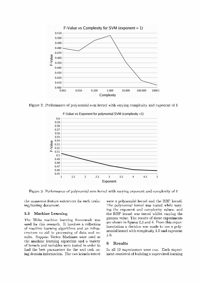
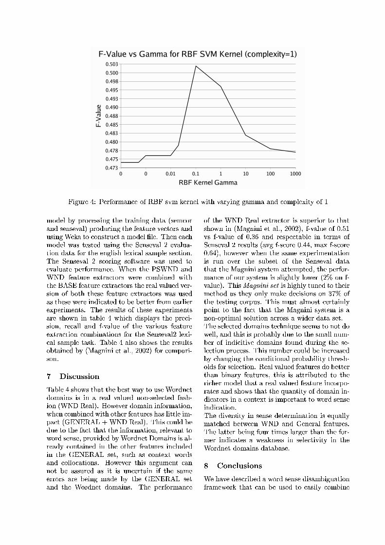
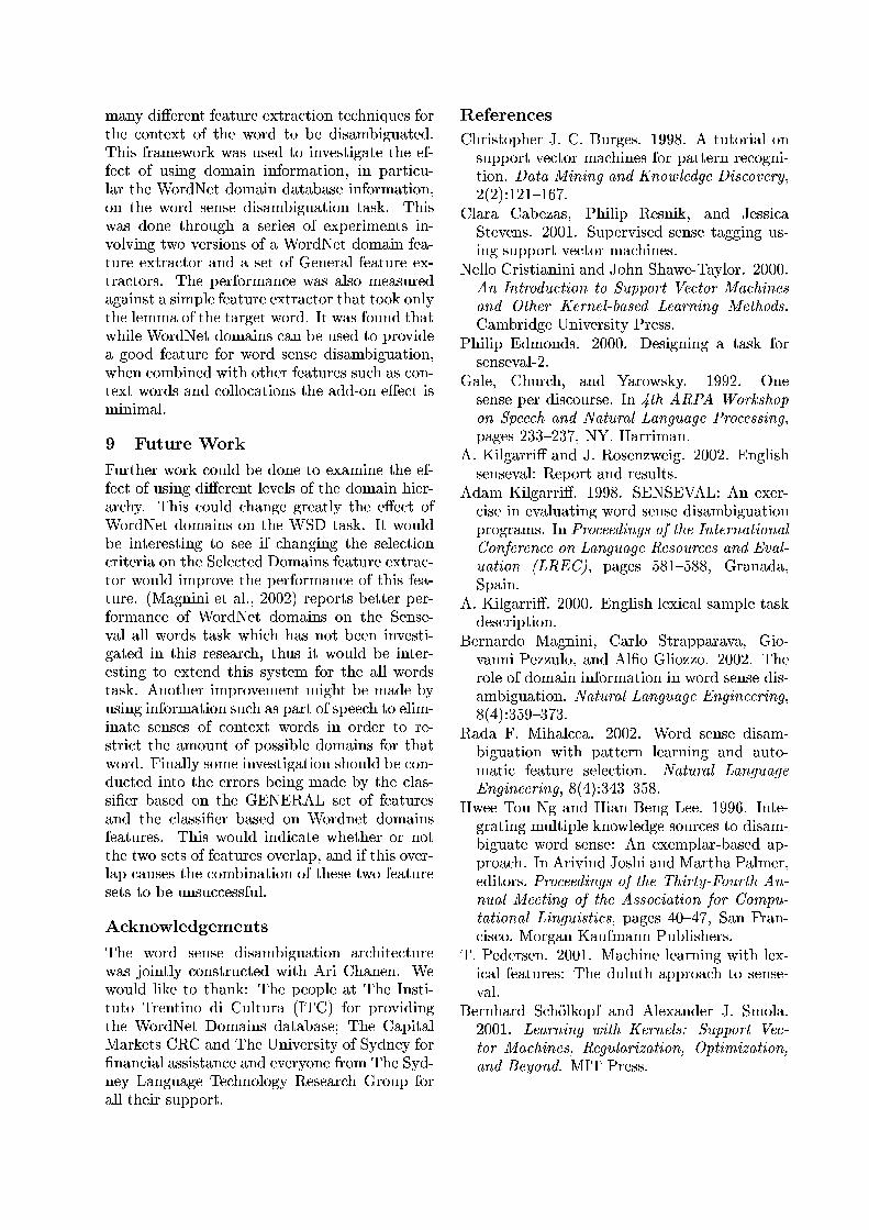
Embed Size (px)
Citation preview

!"#"$%"&'()*+',--.'
/0#120&3"'4536"&73)8'98:5"8+';27)&0<30'
'
=:3)>&7?'
;7*';72:"*+'@A#3<"'B0&37+'9)"C*"5'D05'
'
'
'
'
'
'
'
'
9C>57>&7?'


!
!
!
!
!
!
!
!
!
!
!
!
!
!
!
!
!
!
!
!
!
!
Complex, Corpus-Driven, Syntactic Features for Word SenseDisambiguation
Ari Chanen and Jon PatrickSydney Language Technology Research Group
School of Information TechnologiesUniversity of SydneySydney, Australia, 2006
ari,jonpat @it.usyd.edu.au
Abstract
Although syntactic features offer morespecific information about the contextsurrounding a target word in a WordSense Disambiguation (WSD) task, ingeneral, they have not distinguishedthemselves much above positional fea-tures such as bag-of-words. In this pa-per we offer two methods for increas-ing the recall rate when using syntac-tic features on the WSD task by: 1)using an algorithm for discovering inthe corpus every possible syntactic fea-ture involving a target word, and 2) us-ing wildcards in place of the lemmas inthe templates of the syntactic features.In the best experimental results on theSENSEVAL-2 data we achieved an F-measure of 53.1% which is well abovethe mean F-measure performance of of-ficial SENSEVAL-2 entries, of 44.2%.These results are encouraging consider-ing that only one kind of feature is usedand only a simple Support Vector Ma-chine (SVM) running with the defaultsis used for the machine learning.
1 Introduction: Syntactic Features
The best features for machine learning classifi-cation are the ones that have the most discrimi-natory power, for the task at hand. This paperwill be discussing the use of syntactic features(SF’s) in word sense disambiguation (WSD.) In
WSD, the task is to choose (or classify) the cor-rect sense of the target word (the word whosesense is to be disambiguated) given the surround-ing text. One type of feature that is commonlyused in WSD classification systems is called bag-of-words. Bag-of-words features are rather infor-mation poor, only specifying the presence or ab-sence of words in the target word’s context. SF’s,on the other hand, are much richer in information.Not only do syntactic features have information onthe presence of words in the context but they alsoinclude information about the syntactic relation-ships that hold between the target word and con-text words in the same sentence as the target.
In order to use SF’s, a syntactic parser is neededthat produces a parse tree for every training corpussentence. The parse tree gives the syntactic rela-tionships between words in each sentence. Con-nexor parser (Jarvinen and Tapanainen, 1997) wasused to annotate the data with syntactic relation-ships in the research presented here. In this re-search, a SF is defined as a connected group ofwords from a parse tree that must include the tar-get word. The SF includes information on eachof its words, the syntactic relationships betweenthem, and information on how each word relatesto the others in the tree hierarchy. The SF wordinformation includes the word, lemma, and part-of-speech (POS) for each word.The use of syntactic features in WSD might
seem to be a more effective discriminatory featurecompared to a information poor feature like bag-of-words because of the potential for SF’s to offermore specific information about how the sense of
root
check
spending no
a debtor
on
Subj:
Main:
Comp:
Det:
Cnt:
Phr:
Pcomp: Det:
10
20
to
Pm:
Qua:
Sense
Mod:
there
is
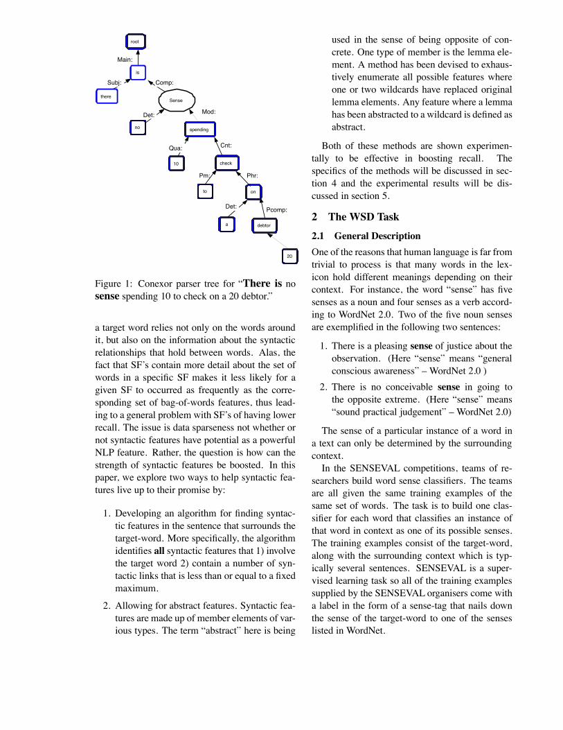
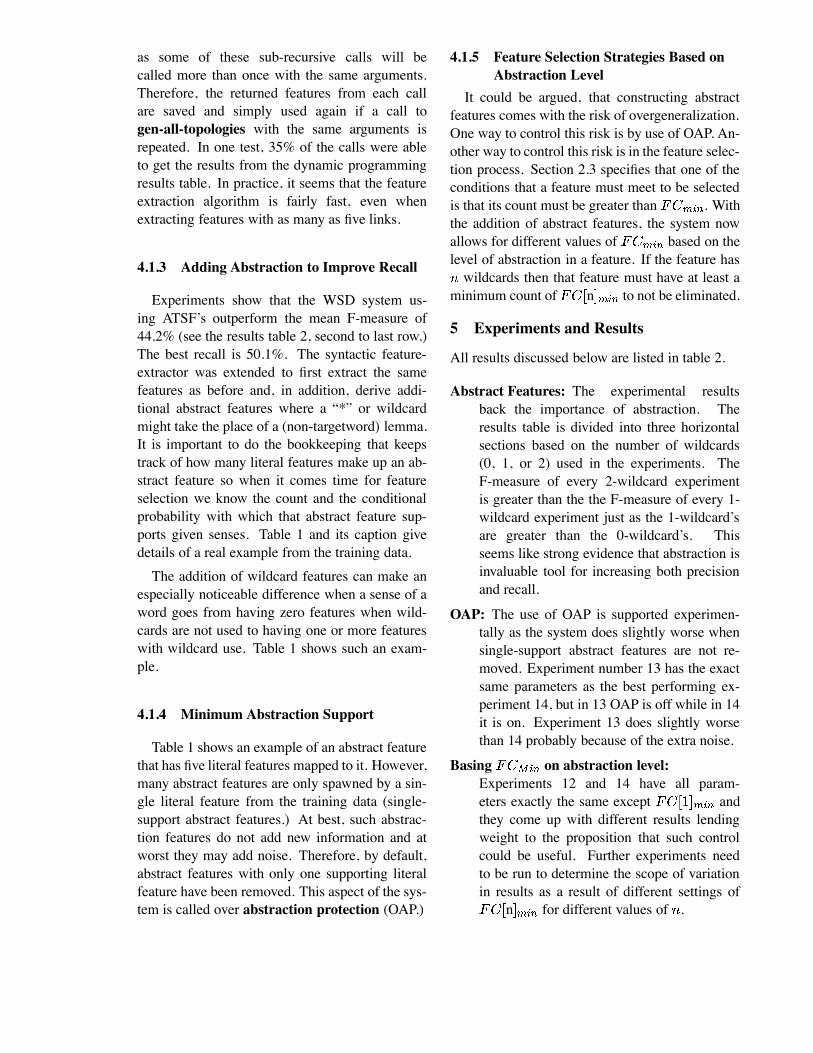
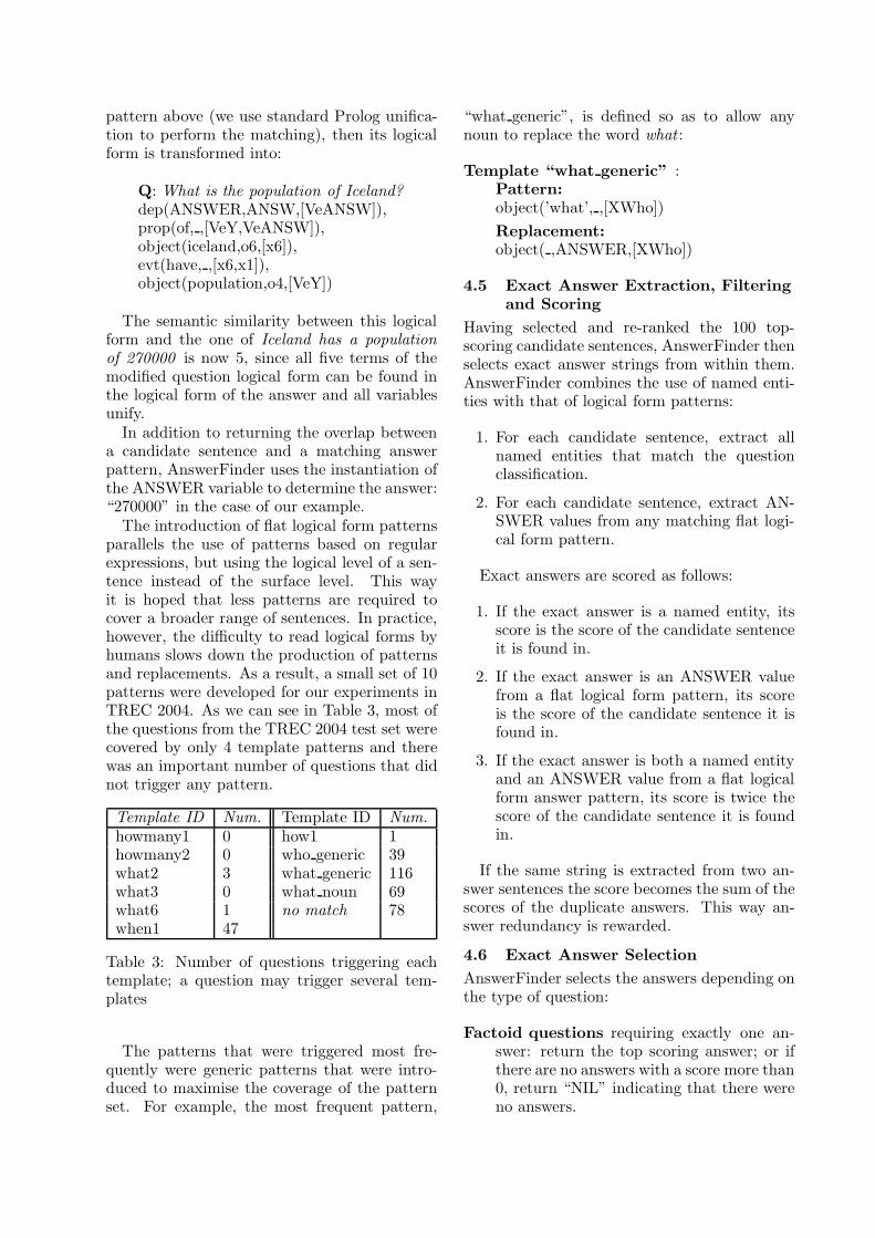
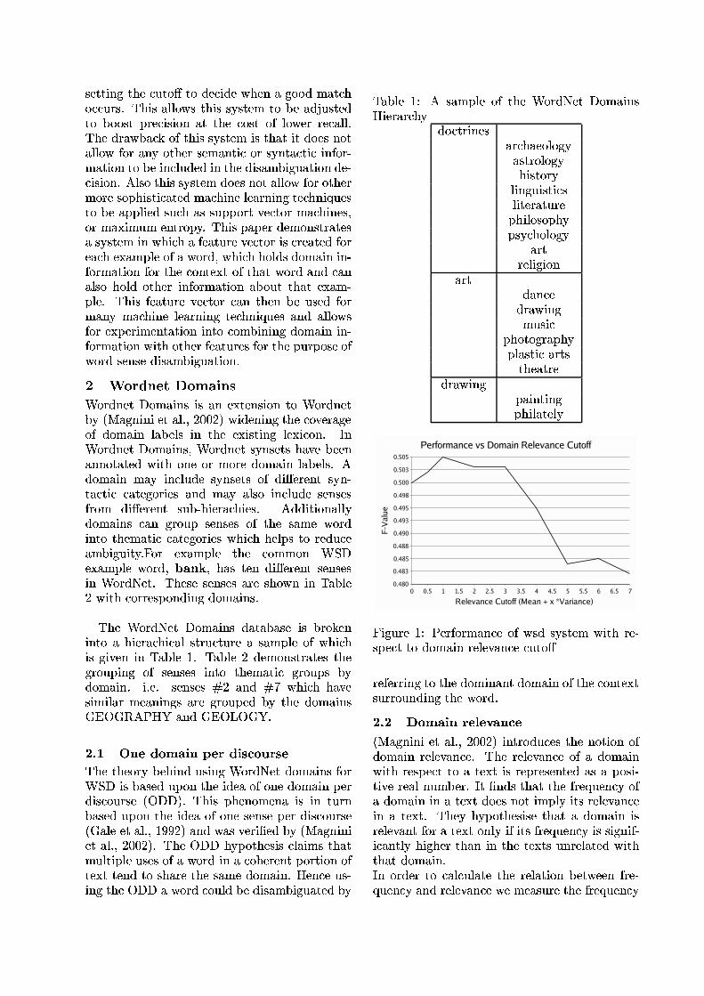
Figure 1: Conexor parser tree for “There is nosense spending 10 to check on a 20 debtor.”
a target word relies not only on the words aroundit, but also on the information about the syntacticrelationships that hold between words. Alas, thefact that SF’s contain more detail about the set ofwords in a specific SF makes it less likely for agiven SF to occurred as frequently as the corre-sponding set of bag-of-words features, thus lead-ing to a general problem with SF’s of having lowerrecall. The issue is data sparseness not whether ornot syntactic features have potential as a powerfulNLP feature. Rather, the question is how can thestrength of syntactic features be boosted. In thispaper, we explore two ways to help syntactic fea-tures live up to their promise by:
1. Developing an algorithm for finding syntac-tic features in the sentence that surrounds thetarget-word. More specifically, the algorithmidentifies all syntactic features that 1) involvethe target word 2) contain a number of syn-tactic links that is less than or equal to a fixedmaximum.
2. Allowing for abstract features. Syntactic fea-tures are made up of member elements of var-ious types. The term “abstract” here is being
used in the sense of being opposite of con-crete. One type of member is the lemma ele-ment. A method has been devised to exhaus-tively enumerate all possible features whereone or two wildcards have replaced originallemma elements. Any feature where a lemmahas been abstracted to a wildcard is defined asabstract.
Both of these methods are shown experimen-tally to be effective in boosting recall. Thespecifics of the methods will be discussed in sec-tion 4 and the experimental results will be dis-cussed in section 5.
2 The WSD Task2.1 General DescriptionOne of the reasons that human language is far fromtrivial to process is that many words in the lex-icon hold different meanings depending on theircontext. For instance, the word “sense” has fivesenses as a noun and four senses as a verb accord-ing to WordNet 2.0. Two of the five noun sensesare exemplified in the following two sentences:
1. There is a pleasing sense of justice about theobservation. (Here “sense” means “generalconscious awareness” – WordNet 2.0 )
2. There is no conceivable sense in going tothe opposite extreme. (Here “sense” means“sound practical judgement” – WordNet 2.0)
The sense of a particular instance of a word ina text can only be determined by the surroundingcontext.In the SENSEVAL competitions, teams of re-
searchers build word sense classifiers. The teamsare all given the same training examples of thesame set of words. The task is to build one clas-sifier for each word that classifies an instance ofthat word in context as one of its possible senses.The training examples consist of the target-word,along with the surrounding context which is typ-ically several sentences. SENSEVAL is a super-vised learning task so all of the training examplessupplied by the SENSEVAL organisers come witha label in the form of a sense-tag that nails downthe sense of the target-word to one of the senseslisted in WordNet.
Different research groups try to outperform theother groups by using different and hopefully su-perior methods. There are, at least, five basicareas in which the groups may differ 1) trainingdata used 2) enrichment of the training data, ifany 3) kinds of features extracted for the machine-learning process 4) method of selecting the bestfeatures 5) machine-learning algorithm or combi-nation of algorithms used.
2.2 Data Enhancements by ParsingThe SENSEVAL-2 and SEMCOR sense-taggedcorpora were used as the training data in this re-search. This data was enriched by extracting syn-tactic information using the Connexor parser. Itis difficult to extract reliable syntactic informa-tion without first processing the data with a goodparser. Connexor is a dependency parser, as op-posed to a constituency parser. Any type of syn-tactic parser that produces a hierarchical sentencetree could be used with the syntactic feature ex-traction methods used in this work.
2.3 Feature Selection MethodThe method used for feature selection follows (Ngand Lee, 1996). Three steps are used on all thefeatures found by a given feature-extractor to fil-ter them down to the selected, final set of featuresused in the machine learner. According to this pa-per, each feature must meet the following condi-tions to be selected:
1. The feature must have a feature count of atleast .
2. The conditional probability for some sensegiven the feature must be greater than a pre-determined probability. .
Condition one is enhanced by allowing the min-imum count to depend on the abstraction level ofthe feature where the abstraction level is definedas the number of wildcards in a syntactic feature.
2.4 MotivationThe SENSEVAL-2 papers indicate that no onecame up with a single “magic bullet” idea that putthem out in front of the crowd, rather the teamsthat did best were better able to combine knownideas and better able to make small adjustments in
the application of these ideas. This is one of rea-sons this study concentrates on understanding theproblems in-depth and improving a single type offeature rather than combining many features andusing many different machine learners.
2.5 WSD Learning InfrastructureOur WSD system is built on an extensible frame-work for feature extraction and feature vector con-struction. All of the experiments reported on herewere done using this in-house system. Due to lim-ited space, the system will not be described herebut in (Bell and Patrick 2004.)
3 Syntactic Features and WSD
3.1 Dekan Lin(Lin, 2000) describes the only other WSD systemwe are aware of that makes use of syntactic fea-tures alone. Lin’s system discovered all syntacticfeatures in the corpus which inspired the currentsystems principle of only using syntactic featuresdiscoved automatically in the corpus. Lin’s syn-tactic features are less inclusive, and less complexthen those described in this paper. See section forfurther comparisons. He used a nearest neighbour(NN) algorithm to choose the best sense of theword. Despite having simpler features, his systemshowed better performance on the same task. Inthe conclusion to this paper , we will speculate asto why.
3.2 David Yarowsky et al.(Yarowsky et al., 2001) describes the system thatdid best among all competing supervised-learningsystems at SENSEVAL-2. This system is not di-rectly comparable because they used five typesof features and a more complex, voting schememachine-learner. Nevertheless, it is instructive tocontrast the Yarowsky’s system syntactic featureswith those being described here. Their systemidentifies a closed set of syntactic feature typesfirst (e.g. verb/obj) and then can only extract thosetypes from the corpus.
3.3 David Fernandez-Amoros(Fernandez-Amoros, 2004) is also not directlycomparable because he uses unsupervised learn-ing. Again though, a comparison can be made be-
tween his syntactic features and those being de-scribed here. He first parsed all the WordNetglosses. He looked for parts of the parse trees thatcontained WSD target-words and used these sub-trees as patterns for that target-word. He also usedwildcards in place of pronouns and content words,like the current research. He uses transformationson these sub-tree patterns in a further attempts toincrease recall. In spirit, his research and that de-scribed here are similar however he was not ableto achieve the same amount of automation in bothidentifying syntactic tree topologies and in gener-ating wildcard features. Also, his base-syntacticpatterns were limited to those found in the Word-Net glosses for a given target-word.
4 Methods
The SF’s, described here, were originally inspiredby (Lin, 2000), however, a single one of Lin’s SF’sis not capable of capturing all the different topolo-gies of subtrees involving the target word. Linchose a limited yet easy to calculate set of syntac-tic features that involve the target word. Specifi-cally, he extracted features that always started withthe target word and included all the dependencylinks and words that would be touched on the wayto any word in the sentence. Because his featuresnever branch but rather are a string of words con-nected by dependency relationships we call themlinear syntactic features (LSF’s.) In his syntac-tic features he included the lemma and POS of thewords in the feature and the dependency relation-ships that are on the links in-between the words.We have followed his lead in including this infor-mation in the syntactic features.Figure 1 shows the Connexor dependency parse
of a random (and somewhat awkward) sentencefrom the SENSEVAL-2 data.An example of a two link feature in this sen-
tence would be one that started at the target word“sense” and then goes to the word “spending” byfollowing the “mod” link and then finally on to“check” by following the “cnt” link.From Lin’s description of his features, even
some linear features would not be extracted. Forinstance, features where the target word is in themiddle of a linear path from one word to anotherin this sentence would not be extracted because his
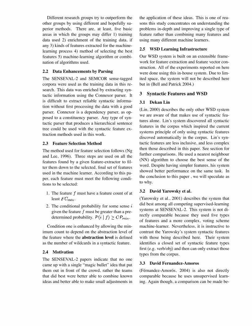
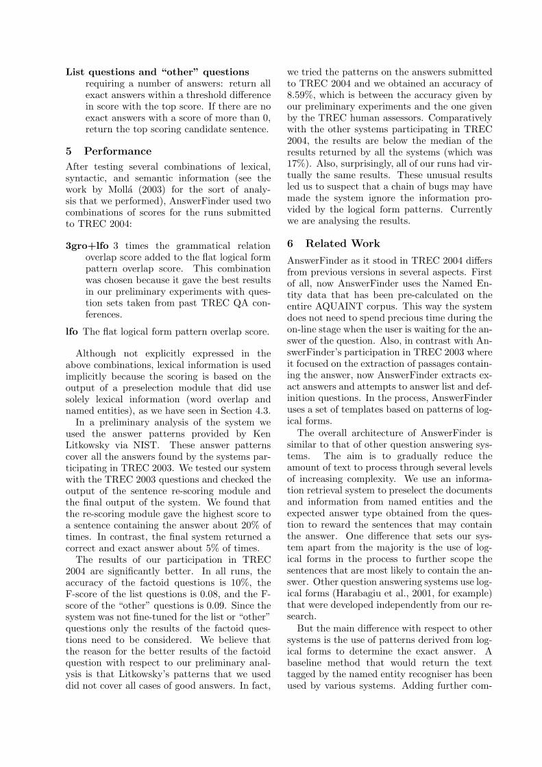
links ATSF running LSF runningtotal total
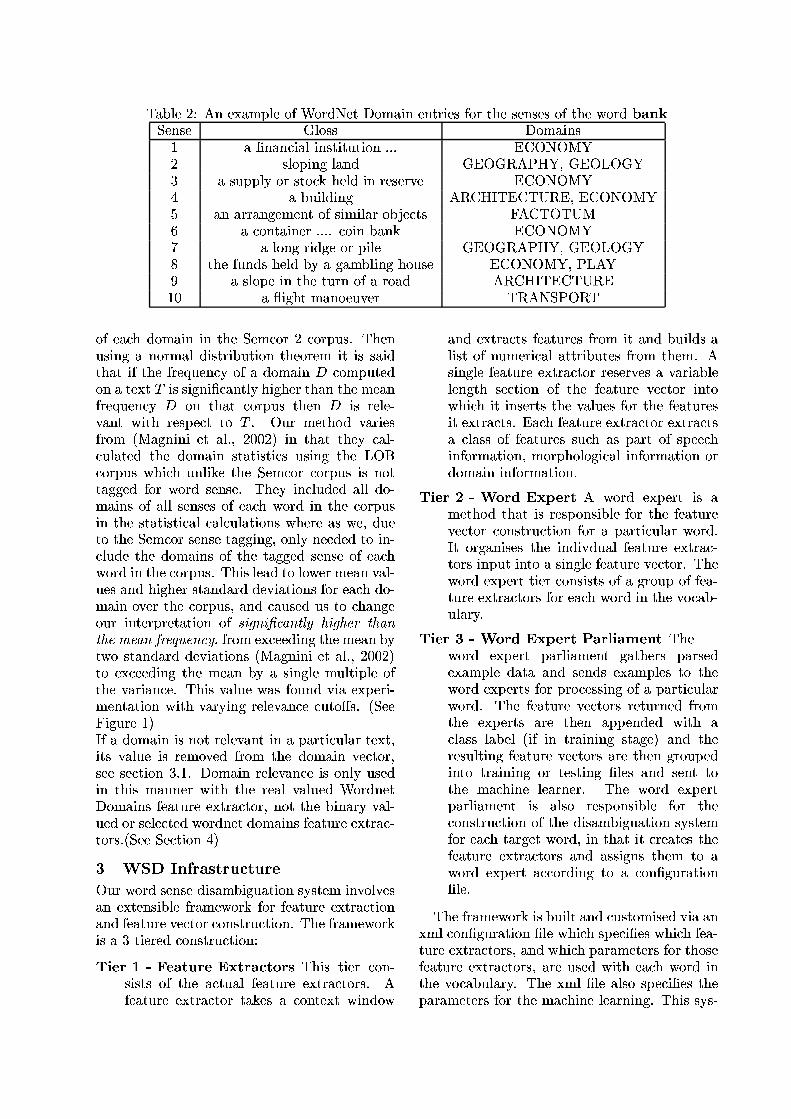
1 3 3 3 32 6 9 3 63 10 19 2 84 15 34 1 95 21 55 1 106 27 82 0 107 30 112 0 108 26 138 0 109 16 154 0 1010 6 160 0 1011 1 161 0 10
Table 3: Comparing the number of LSF’s vs.ATSF’s found in the sentence: “There is no sensespending 10 to check on a 20 debtor.” (from theSENSEVAL-2 corpus)
features must start with the target word.
4.1 All-topologies Syntactic Features(ATSF’s)
A version of Lin’s LSF’s was first implemented.Those types of SF’s were automatically extractedfrom the enhanced corpus documents. It was obvi-ous when looking at a dependency parse tree thatwhile many features were identified there weremany more potential features that the LSF feature-extractor was not able to catch. Thus, a more all-inclusive class of syntactic feature which we havenamed all-topology syntactic features (ATSF’s),was developed.The major motivating factor behind seeking to
extract ATSF’s was that it seemed they would bemore abundant than LSF’s. The basic idea isthat any subtree of a sentence parse tree with upto and including a maximum number of depen-dency links could be potentially useful as a fea-ture. Referring to figure 1, one example of a fea-ture that is not a LSF would be one that involvesthe words (is, no, sense, spending). The links in-volved in that feature could not be placed in a line.To give an idea of how many more ATSF’s theremight be compared to LSF’s, table 3 shows thefeature counts in the example parse tree. The fea-ture count is broken down into groups of features
that have the same number of dependency links inthem. In each of our experiments, a parameter setsthe maximum number of links that a feature canhave in that experiment. The best performance todate comes from a maximum of three links. Ta-ble 3 shows that there are five times as many threelink ATSF’s as three link LSF’s. In fact, in this ex-ample sentence, there are no LSF’s that have morethan five links and this sentence is typical.
4.1.1 Canonical Form and RepresentationThe same subtree could be represented in many
different ways so a canonical form needs to be de-fined. ATSF’s are defined as nested elements wereeach element has the basic form:
[DRWP]::lemma=POS [children]
Where DRWP stands for dependency relation-ship with parent. Out of the words in a feature, theword that is topmost in the parse tree being repre-sented is placed first in the feature set. The DRWPof that top-most word is deleted. The rest of thedependency relationships further down the tree arerepresented in the children element of the top treeitem. The children of a feature or sub-feature aresorted in alphabetical order by first the POS, thenDRWP and finally by lemma.For example, the feature involving the words
(is, no, sense, spending) is rendered as:
::be=v comp::sense=n det::no=det mod::spending=ing
4.1.2 Algorithm for Identifying ATSF’sIn (Fernandez-Amoros, 2004), the author called
the problem of systematically identifying all syn-tactic features “challenging” and said that for lackof time he was not able to come up with a solutionyet. We also found it challenging but were able tocome up with a divide-and-conquer/dynamic pro-gramming solution which is presented in outlineform here.The basic idea is to define a recursive func-
tion whose job it is to identify all possible parsetree topologies that can be formed with a constantnumber of links where all topologies must involvea target tree node and may involve any or all of agroup of neighbour nodes and their children. Letus call the function gen-all-topologies. It returns
a list of features of all topologies. Its argumentsare:
target-ID The unique identifier of the target node.This would usually be the ID of the tokennode for a word.
links The function returns only syntactic featureswith this many links.
neighbour-IDS The neighbours of the targetnode which can be used to form the features.Notice, this is usually not all of the neigh-bours of the target-ID
Inside gen-all-topologies there is a loop thatassigns a variable links-to-first-neighbour valuesfrom zero to the value of the argument links. Foreach iteration in this loop we try different splits ofthe links between the first neighbour in the list andthe target node1 Here are the two sub-recursivecalls:
feature-list-1 =gen-all-topologies(
first(neighbour-IDS),links-to-first-neighbour,neighbours*(first(neighbour-IDS))
feature-list-2 =gen-all-topologies(
target-ID,links - links-to-first-neighbour,rest(neighbour-IDS))
first and rest get the first element and the rest ofthe elements of a list, respectively. neighbours*gets all of the neighbours of a node except for thetarget node. Once these two sub-recursive callshave returned we do a cross product of the twolists meaning that each member of a list must becombined with each of the features on the otherlist yielding a number features equal to the productof the sizes of the two lists of features. Determinghow to combine two features into a bigger featurehas a straightforward solution.gen-all-topologies is called times, where the
links arguments ranges from 1 to which will ob-tain all features for a sentence with from 1 tolinks in the features.The implementation of gen-all-topologies
makes use of dynamic programming techniques,1Only on the top-level call is the target node actually the
target word for the WSD problem.
as some of these sub-recursive calls will becalled more than once with the same arguments.Therefore, the returned features from each callare saved and simply used again if a call togen-all-topologies with the same arguments isrepeated. In one test, 35% of the calls were ableto get the results from the dynamic programmingresults table. In practice, it seems that the featureextraction algorithm is fairly fast, even whenextracting features with as many as five links.
4.1.3 Adding Abstraction to Improve Recall
Experiments show that the WSD system us-ing ATSF’s outperform the mean F-measure of44.2% (see the results table 2, second to last row.)The best recall is 50.1%. The syntactic feature-extractor was extended to first extract the samefeatures as before and, in addition, derive addi-tional abstract features where a “*” or wildcardmight take the place of a (non-targetword) lemma.It is important to do the bookkeeping that keepstrack of how many literal features make up an ab-stract feature so when it comes time for featureselection we know the count and the conditionalprobability with which that abstract feature sup-ports given senses. Table 1 and its caption givedetails of a real example from the training data.The addition of wildcard features can make an
especially noticeable difference when a sense of aword goes from having zero features when wild-cards are not used to having one or more featureswith wildcard use. Table 1 shows such an exam-ple.
4.1.4 Minimum Abstraction Support
Table 1 shows an example of an abstract featurethat has five literal features mapped to it. However,many abstract features are only spawned by a sin-gle literal feature from the training data (single-support abstract features.) At best, such abstrac-tion features do not add new information and atworst they may add noise. Therefore, by default,abstract features with only one supporting literalfeature have been removed. This aspect of the sys-tem is called over abstraction protection (OAP.)
4.1.5 Feature Selection Strategies Based onAbstraction Level
It could be argued, that constructing abstractfeatures comes with the risk of overgeneralization.One way to control this risk is by use of OAP. An-other way to control this risk is in the feature selec-tion process. Section 2.3 specifies that one of theconditions that a feature must meet to be selectedis that its count must be greater than . Withthe addition of abstract features, the system nowallows for different values of based on thelevel of abstraction in a feature. If the feature haswildcards then that feature must have at least a
minimum count of n to not be eliminated.
5 Experiments and Results
All results discussed below are listed in table 2.
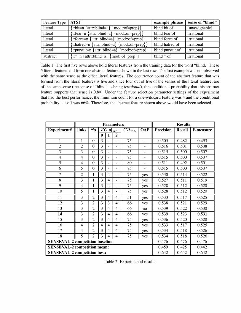
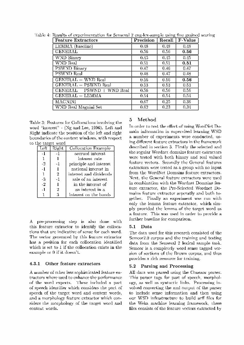
Abstract Features: The experimental resultsback the importance of abstraction. Theresults table is divided into three horizontalsections based on the number of wildcards(0, 1, or 2) used in the experiments. TheF-measure of every 2-wildcard experimentis greater than the the F-measure of every 1-wildcard experiment just as the 1-wildcard’sare greater than the 0-wildcard’s. Thisseems like strong evidence that abstraction isinvaluable tool for increasing both precisionand recall.
OAP: The use of OAP is supported experimen-tally as the system does slightly worse whensingle-support abstract features are not re-moved. Experiment number 13 has the exactsame parameters as the best performing ex-periment 14, but in 13 OAP is off while in 14it is on. Experiment 13 does slightly worsethan 14 probably because of the extra noise.
Basing on abstraction level:Experiments 12 and 14 have all param-eters exactly the same except andthey come up with different results lendingweight to the proposition that such controlcould be useful. Further experiments needto be run to determine the scope of variationin results as a result of different settings of
n for different values of .
Best performance: Experiment 14 performedbest.
Again, Lin’s system is one of the few SENSE-VAL systems that only uses syntactic features andthus should be quite comparable with our system.Lin only gave his results in the course-grainedscale. The scores in table 2 are all in terms of thefine-grained scale. Therefore, Lin’s results are notincluded in table 2. His most comparable exper-iment achieved a coarse-grained F-score of 67%.The best coarse-grained F-score, of the system de-scribed here, was 61.2%.
6 Conclusion
The Yarowsky et al. WSD system achieved thehighest official score with an F-measure of 64.2%.Their system used six types of features and avoting-scheme machine-learner that used five basemachine-learners. Given that the system describedhere is using only a single type of feature, syntac-tic, and a single type of machine-learner, SVM,coming within 11.1% of the top score is quite re-spectable.Lin’s system, that used LSF’s, performed bet-
ter then the ATSF’s despite our expectations to thecontrary. One reason that ATSF’s might not haveoutperformed Lin’s features could be because Linis using a nearest neighbor (NN) learner and Linmay be able to compose many simpler features tobuild up a similar picture to a fewer number of themore complex ATSF’s. If this is the case, thenATSF’s would not seem to offer any advantagesover LSF’s. The fact that Lin’s system did signifi-cantly better then this system might say somethingabout the use of nearest-neighbor , compared toSVM’s. Lin’s system built up a case library andthus did not forget any data quirks. This might beimportant in an area like WSD , where there is nota lot of supervised training data available, at thispoint.There are some advantages to the ATSF’s rep-
resentation of the data. If one thinks of a fea-ture as representing properties of the data thenATSF’s can represent such properties more com-pactly. Several of Lin’s features might be requiredto represent the same data property as one ATSF.Especially where it is important for humans to in-
terpret the features culled from the data, the ATSFrepresentation might be more efficient for humansto deal with.
Acknowledgements
The word sense disambiguation architecture wasjointly constructed with David Bell. We wouldlike to thank the Capital Markets CRC and theUniversity of Sydney for financial supported andeveryone in the Sydney Language Technology Re-search Group for their support.
ReferencesDavid F´ernandez-Amor´os. 2004. Wsd based on mu-tual information and syntactic patterns. In Rada Mi-halcea and Phil Edmonds, editors, Senseval-3: ThirdInternational Workshop on the Evaluation of Sys-tems for the Semantic Analysis of Text, pages 117–120, Barcelona, Spain, July. Association for Com-putational Linguistics.
Timo Jarvinen and Pasi Tapanainen. 1997. A de-pendency parser for english. Technical Report TR-1, Department of General Linguistics, University ofHelsinki, Finland.
David D. Lewis. 1992. An evaluation of phrasaland clustered representations on a text categoriza-tion task. In Proceedings of the 15th annual inter-national ACM SIGIR conference on Research anddevelopment in information retrieval, pages 37–50.ACM Press.
Dekang Lin. 2000. Word sense disambiguation with asimilarity-smoothed case library.
Hwee Tou Ng and Hian Beng Lee. 1996. Integratingmultiple knowledge sources to disambiguate wordsense: An exemplar-based approach. In ArivindJoshi andMartha Palmer, editors, Proceedings of theThirty-Fourth Annual Meeting of the Association forComputational Linguistics, pages 40–47, San Fran-cisco. Morgan Kaufmann Publishers.
Fabrizio Sebastiani. 2002. Machine learning in au-tomated text categorization. ACM Computing Sur-veys, 34(1):1–47.
David Yarowsky, Silviu Cucerzan, Radu Florian,Charles Schafer, and Richard Wicentowski. 2001.The johns hopkins SENSEVAL2 system descrip-tions.
D. Yarowsky. 2000. Hierarchical decision lists forword sense disambiguation.
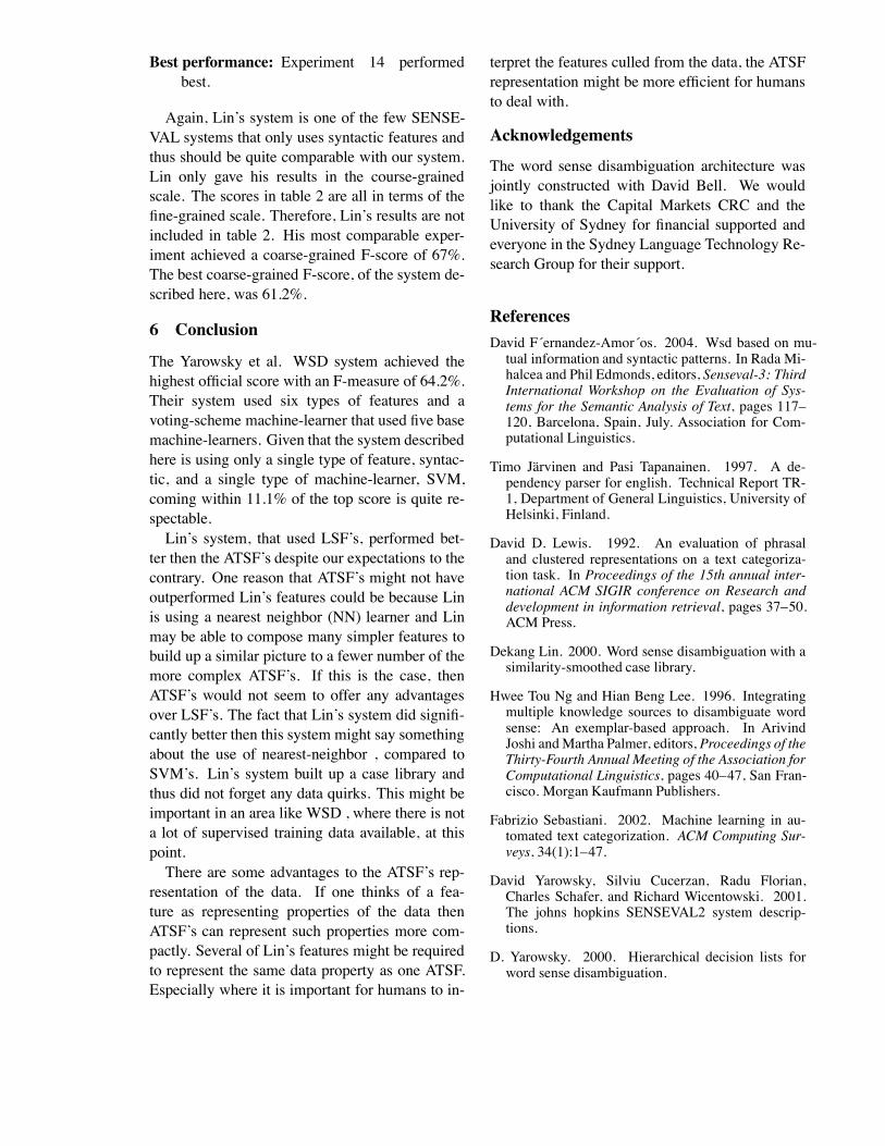
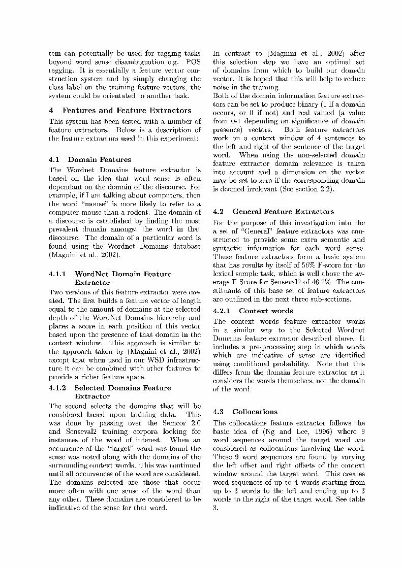
Feature Type ATSF example phrase sense of “blind”literal ::bit=n attr::blind=a mod::of=prep blind bit of [unassignable]literal ::fear=n attr::blind=a mod::of=prep blind fear of irrationalliteral ::force=n attr::blind=a mod::of=prep blind force of irrationalliteral ::hatred=n attr::blind=a mod::of=prep blind hatred of irrationalliteral ::pursuit=n attr::blind=a mod::of=prep blind pursuit of irrationalabstract ::*=n attr::blind=a mod::of=prep blind * of irrational
Table 1: The first five rows above hold literal features from the training data for the word “blind.” These5 literal features did form one abstract feature, shown in the last row. The first example was not observedwith the same sense as the other literal features. The occurrence count of the abstract feature that wasformed from the literal features is five and since four out of five of the senses of the literal feature, areof the same sense (the sense of “blind” as being irrational), the conditional probability that this abstractfeature supports that sense is 0.80. Under the feature selection parameter settings of the experimentthat had the best performance, the minimum count for a one-wildcard feature was 4 and the conditionalprobability cut-off was 66%. Therefore, the abstract feature shown above would have been selected.
Parameters ResultsExperiment# links *’s n OAP Precision Recall F-measure
0 1 21 1 0 3 - - 75 - 0.505 0.482 0.4932 2 0 3 - - 75 - 0.516 0.501 0.5083 3 0 3 - - 75 - 0.515 0.500 0.5074 4 0 3 - - 75 - 0.515 0.500 0.5075 4 0 3 - - 80 - 0.511 0.492 0.5016 5 0 3 - - 75 - 0.515 0.500 0.5077 2 1 3 4 - 75 yes 0.530 0.514 0.5228 3 1 3 4 - 75 yes 0.527 0.511 0.5199 4 1 3 4 - 75 yes 0.528 0.512 0.52010 5 1 3 4 - 75 yes 0.528 0.512 0.52011 3 2 3 4 4 51 yes 0.533 0.517 0.52512 3 2 3 3 4 66 yes 0.538 0.521 0.52913 3 2 3 4 4 66 no 0.539 0.522 0.53014 3 2 3 4 4 66 yes 0.539 0.523 0.53115 3 2 3 4 4 75 yes 0.536 0.520 0.52816 4 2 4 4 4 75 yes 0.533 0.517 0.52517 4 2 3 4 4 75 yes 0.534 0.518 0.52618 5 2 3 4 4 75 yes 0.534 0.518 0.526
SENSEVAL-2 competition baseline: 0.476 0.476 0.476SENSEVAL-2 competition mean: 0.459 0.425 0.442SENSEVAL-2 competition best: 0.642 0.642 0.642
Table 2: Experimental results
AnswerFinder — Question Answering by Combining Lexical,Syntactic and Semantic Information
Diego Molla and Mary GardinerCentre for Language Technology
Division of Information and Communication SciencesMacquarie University
Sydney, [email protected] and [email protected]
Abstract
We present a question answering system thatcombines information at the lexical, syntactic,and semantic levels, in the process to find andrank the candidate answer sentences. The can-didate exact answers are extracted from thecandidate answer sentences by means of a com-bination of information-extraction techniques(named entity recognition) and patterns basedon logical forms. The system participated in thequestion answering track of TREC 2004.
1 Introduction
Question answering is an area that is becom-ing increasingly active in research and is cur-rently being deployed into practical applica-tions. Research in question answering has re-cently been fostered by large-scale programslike AQUAINT1 and evaluation frameworks likeTREC2, NTCIR3, and CLEF4. Such researchand the current need to cope with large vol-umes of text has led various companies to pro-duce practical question answering systems. Forexample, research groups from Microsoft, IBM,NTT, Oracle, and Sun have participated in thequestion answering track of TREC. In addition,there are several attempts to provide question-answering extensions to the current Web searchengines, with demos available by MIT5, LCC6,and BrainBoost7, among others.
AnswerFinder is an open-domain question an-swering system that combines information atthe lexical, syntactic, and semantic levels invarious stages to find the exact answer to theuser question. This paper describes the An-swerFinder system as it stood at the time of the
1www.ic-arda.org/InfoExploit/aquaint/index.html2trec.nist.gov3research.nii.ac.jp/ntcir/index-en.html4clef.iei.pi.cnr.it5www.ai.mit.edu/projects/infolab/6www.languagecomputer.com/7www.brainboost.com/
TREC 2004 question answering track. Section 2introduces TREC and the question answeringtrack. Section 3 describes the architecture ofthe system. Section 4 details the function ofeach module within the AnswerFinder system.Section 5 gives the system performance on theTREC 2003 question set. Section 6 mentions re-lated work and Section 7 lists problems with theAnswerFinder system that should be addressedin the near future.
2 The TREC 2004 QuestionAnswering Track
The Text REtrieval Conference (TREC) startedin 1992 as part of the TIPSTER text program.A fundamental goal of the conference is to pro-vide an evaluation framework for the compar-ison of the results of independent informationretrieval systems. The concept of informationretrieval is to be understood in a broad sense,and this conference has developed various tracksthat focus on specific areas of information re-trieval, such as ad-hoc (the name given to docu-ment retrieval), routing, speech, cross-language,web, video, and very large corpora (Voorhees,2003).
The question answering track started in 1999and ever since its creation it has been the mostpopular track. Every year the complexity anddi!culty of the task increases. Thus, in 1999the competing systems were asked to retrievesmall snippets of text containing the answer.The questions were designed by the participantsand the answer was guaranteed to be in the textcorpus. In the 2004 competition, in contrast,the questions were extracted from logs of realquestions, the answer is not guaranteed to bein the corpus, and the systems were asked tofind the exact answers of factoid questions andlist questions. The questions were grouped intotargets, each target containing fact-based ques-tions and list questions (explicitly marked assuch), plus a question asking to find any other
information relevant to the target. The ques-tions were encoded in XML as shown in Fig-ure 1. In this example, the target is Fred Durst,so question with ID number 2.2 in the figureis asking What record company is Fred Durstwith?.<target id = "2" text = "Fred Durst">
<qa><q id = "2.1" type="FACTOID">What is the name of Durst’s group?</q>
</qa>
<qa><q id = "2.2" type="FACTOID">What record company is he with?</q>
</qa>
<qa><q id = "2.3" type="LIST">What are titles of the group’s releases?</q>
</qa>
<qa><q id = "2.4" type="FACTOID">Where was Durst born?</q>
</qa>
<qa><q id = "2.5" type="OTHER">Other</q>
</qa>
</target>
Figure 1: A hand-made example of a group ofquestions using the TREC 2004 format
The corpus of supporting text was theAQUAINT corpus, which comprises over 1 mil-lion news articles taken from the New YorkTimes, the Associated Press, and the Xin-hua News Agency newswires. This corpus isnot large in comparison with the terabites oftext available via the Internet, but it is stilllarge enough to require the need to resort toshallow-processing preselection methods beforeperforming a real attempt to find the answer.
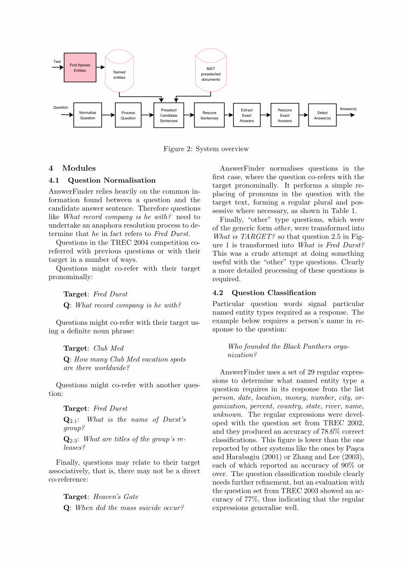
3 System Overview
The question answering procedure used by An-swerFinder follows a pipeline structure that is
typical of rule-based question answering sys-tems. The process is outlined in Figure 2 and isas follows:
1. All questions are normalised, so that Whatrecord company is he with? in Figure 1 be-comes What record company is Fred Durstwith?
2. The questions are classified into typesbased upon their expected answer. So thequestion How far is it from Mars to Earth?would be classified as a “Number” questionas it expects a numeric value in response.
3. 100 candidate answer sentences are ex-tracted from the corpus.
4. The 100 sentences are re-scored based upontheir word overlap, grammatical relationsoverlap, and flat logical form overlap withthe question text.
5. Exact answers —fragments like 416 millionmiles— are extracted from the candidateanswer sentences.
6. The exact answer list is sorted, re-scoredand filtered for duplicate exact answers.
7. A number of exact answers from the topof the list are selected, depending on thequestion type.
AnswerFinder uses the following knowledgesources to analyse the question and to selectfrom among possible answers:
Named entity data generated by the GATEsystem (Gaizauskas et al., 1996), markingpieces of text in the AQUAINT corpus asone of the types Date, Location, Money,Organization, and Person. These data aregenerated o"-line before any question isprocessed. GATE’s analysis was extendedwith a simple set of regular expressions thatdetect numbers as well.
The list of preselected documentsprovided by the US National Insti-tute of Standards and Technology (NIST),containing for each target entity, the 1,000top scoring documents for that entity.NIST co-sponsors the TREC conferencesand it obtained the list of preselecteddocuments by running the target querythrough the PRISE (Harman and Candela,1990) document retrieval system.
Find NamedEntities Named
entities
ProcessQuestion
NISTpreselecteddocuments
PreselectCandidateSentences
RescoreSentences
ExtractExact
Answers
RescoreExact
Answers
Question
Text
SelectAnswer(s)
Answer(s)NormaliseQuestion
Figure 2: System overview
4 Modules
4.1 Question NormalisationAnswerFinder relies heavily on the common in-formation found between a question and thecandidate answer sentence. Therefore questionslike What record company is he with? need toundertake an anaphora resolution process to de-termine that he in fact refers to Fred Durst.
Questions in the TREC 2004 competition co-referred with previous questions or with theirtarget in a number of ways.
Questions might co-refer with their targetpronominally:
Target: Fred DurstQ: What record company is he with?
Questions might co-refer with their target us-ing a definite noun phrase:
Target: Club MedQ: How many Club Med vacation spotsare there worldwide?
Questions might co-refer with another ques-tion:
Target: Fred DurstQ2.1: What is the name of Durst’sgroup?Q2.3: What are titles of the group’s re-leases?
Finally, questions may relate to their targetassociatively, that is, there may not be a directco-reference:
Target: Heaven’s GateQ: When did the mass suicide occur?
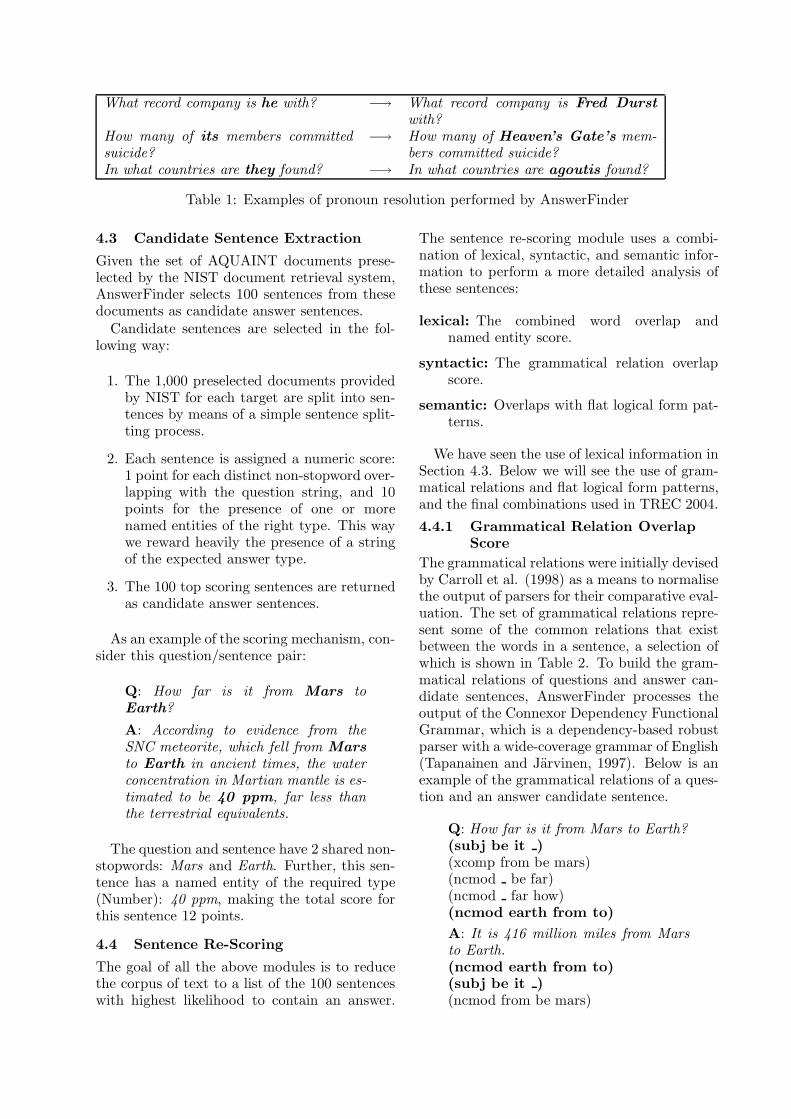
AnswerFinder normalises questions in thefirst case, where the question co-refers with thetarget pronominally. It performs a simple re-placing of pronouns in the question with thetarget text, forming a regular plural and pos-sessive where necessary, as shown in Table 1.
Finally, “other” type questions, which wereof the generic form other, were transformed intoWhat is TARGET? so that question 2.5 in Fig-ure 1 is transformed into What is Fred Durst?This was a crude attempt at doing somethinguseful with the “other” type questions. Clearlya more detailed processing of these questions isrequired.
4.2 Question ClassificationParticular question words signal particularnamed entity types required as a response. Theexample below requires a person’s name in re-sponse to the question:
Who founded the Black Panthers orga-nization?
AnswerFinder uses a set of 29 regular expres-sions to determine what named entity type aquestion requires in its response from the listperson, date, location, money, number, city, or-ganization, percent, country, state, river, name,unknown. The regular expressions were devel-oped with the question set from TREC 2002,and they produced an accuracy of 78.6% correctclassifications. This figure is lower than the onereported by other systems like the ones by Pascaand Harabagiu (2001) or Zhang and Lee (2003),each of which reported an accuracy of 90% orover. The question classification module clearlyneeds further refinement, but an evaluation withthe question set from TREC 2003 showed an ac-curacy of 77%, thus indicating that the regularexpressions generalise well.
What record company is he with? !" What record company is Fred Durstwith?
How many of its members committedsuicide?
!" How many of Heaven’s Gate’s mem-bers committed suicide?
In what countries are they found? !" In what countries are agoutis found?
Table 1: Examples of pronoun resolution performed by AnswerFinder
4.3 Candidate Sentence ExtractionGiven the set of AQUAINT documents prese-lected by the NIST document retrieval system,AnswerFinder selects 100 sentences from thesedocuments as candidate answer sentences.
Candidate sentences are selected in the fol-lowing way:
1. The 1,000 preselected documents providedby NIST for each target are split into sen-tences by means of a simple sentence split-ting process.
2. Each sentence is assigned a numeric score:1 point for each distinct non-stopword over-lapping with the question string, and 10points for the presence of one or morenamed entities of the right type. This waywe reward heavily the presence of a stringof the expected answer type.
3. The 100 top scoring sentences are returnedas candidate answer sentences.
As an example of the scoring mechanism, con-sider this question/sentence pair:
Q: How far is it from Mars toEarth?A: According to evidence from theSNC meteorite, which fell from Marsto Earth in ancient times, the waterconcentration in Martian mantle is es-timated to be 40 ppm, far less thanthe terrestrial equivalents.
The question and sentence have 2 shared non-stopwords: Mars and Earth. Further, this sen-tence has a named entity of the required type(Number): 40 ppm, making the total score forthis sentence 12 points.
4.4 Sentence Re-ScoringThe goal of all the above modules is to reducethe corpus of text to a list of the 100 sentenceswith highest likelihood to contain an answer.
The sentence re-scoring module uses a combi-nation of lexical, syntactic, and semantic infor-mation to perform a more detailed analysis ofthese sentences:
lexical: The combined word overlap andnamed entity score.
syntactic: The grammatical relation overlapscore.
semantic: Overlaps with flat logical form pat-terns.
We have seen the use of lexical information inSection 4.3. Below we will see the use of gram-matical relations and flat logical form patterns,and the final combinations used in TREC 2004.4.4.1 Grammatical Relation Overlap
ScoreThe grammatical relations were initially devisedby Carroll et al. (1998) as a means to normalisethe output of parsers for their comparative eval-uation. The set of grammatical relations repre-sent some of the common relations that existbetween the words in a sentence, a selection ofwhich is shown in Table 2. To build the gram-matical relations of questions and answer can-didate sentences, AnswerFinder processes theoutput of the Connexor Dependency FunctionalGrammar, which is a dependency-based robustparser with a wide-coverage grammar of English(Tapanainen and Jarvinen, 1997). Below is anexample of the grammatical relations of a ques-tion and an answer candidate sentence.
Q: How far is it from Mars to Earth?(subj be it )(xcomp from be mars)(ncmod be far)(ncmod far how)(ncmod earth from to)A: It is 416 million miles from Marsto Earth.(ncmod earth from to)(subj be it )(ncmod from be mars)
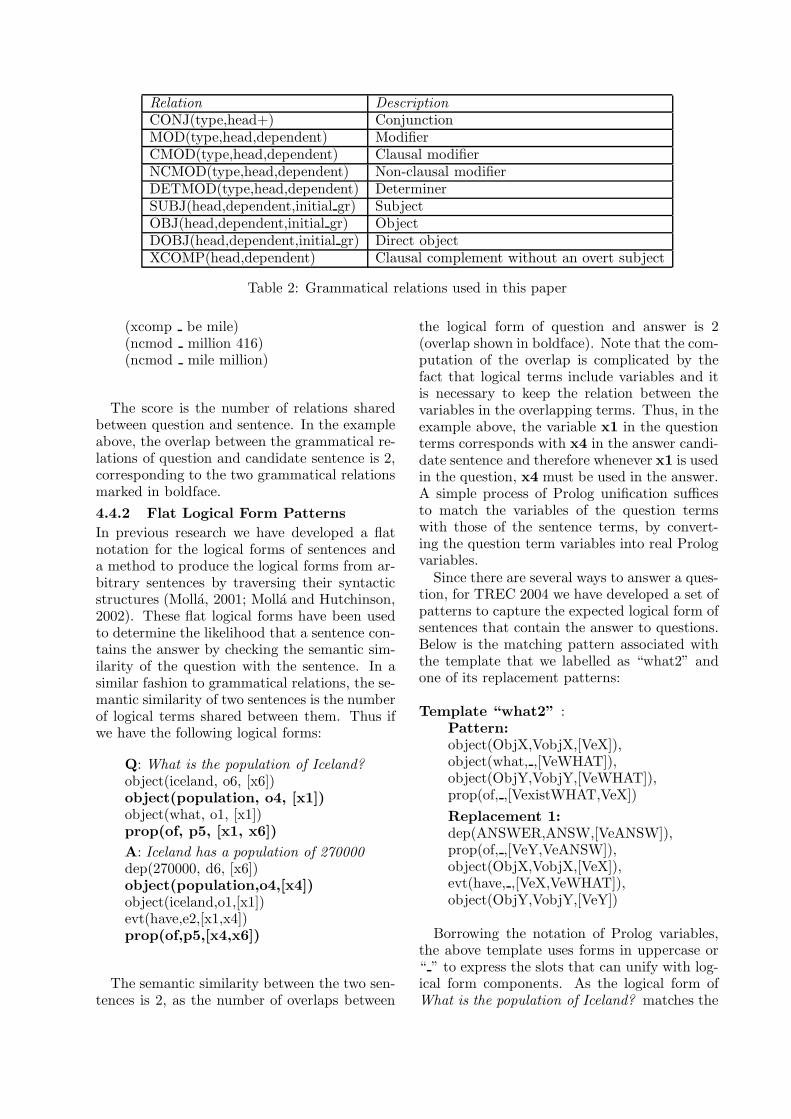
Relation DescriptionCONJ(type,head+) ConjunctionMOD(type,head,dependent) ModifierCMOD(type,head,dependent) Clausal modifierNCMOD(type,head,dependent) Non-clausal modifierDETMOD(type,head,dependent) DeterminerSUBJ(head,dependent,initial gr) SubjectOBJ(head,dependent,initial gr) ObjectDOBJ(head,dependent,initial gr) Direct objectXCOMP(head,dependent) Clausal complement without an overt subject
Table 2: Grammatical relations used in this paper
(xcomp be mile)(ncmod million 416)(ncmod mile million)
The score is the number of relations sharedbetween question and sentence. In the exampleabove, the overlap between the grammatical re-lations of question and candidate sentence is 2,corresponding to the two grammatical relationsmarked in boldface.4.4.2 Flat Logical Form PatternsIn previous research we have developed a flatnotation for the logical forms of sentences anda method to produce the logical forms from ar-bitrary sentences by traversing their syntacticstructures (Molla, 2001; Molla and Hutchinson,2002). These flat logical forms have been usedto determine the likelihood that a sentence con-tains the answer by checking the semantic sim-ilarity of the question with the sentence. In asimilar fashion to grammatical relations, the se-mantic similarity of two sentences is the numberof logical terms shared between them. Thus ifwe have the following logical forms:
Q: What is the population of Iceland?object(iceland, o6, [x6])object(population, o4, [x1])object(what, o1, [x1])prop(of, p5, [x1, x6])A: Iceland has a population of 270000dep(270000, d6, [x6])object(population,o4,[x4])object(iceland,o1,[x1])evt(have,e2,[x1,x4])prop(of,p5,[x4,x6])
The semantic similarity between the two sen-tences is 2, as the number of overlaps between
the logical form of question and answer is 2(overlap shown in boldface). Note that the com-putation of the overlap is complicated by thefact that logical terms include variables and itis necessary to keep the relation between thevariables in the overlapping terms. Thus, in theexample above, the variable x1 in the questionterms corresponds with x4 in the answer candi-date sentence and therefore whenever x1 is usedin the question, x4 must be used in the answer.A simple process of Prolog unification su!cesto match the variables of the question termswith those of the sentence terms, by convert-ing the question term variables into real Prologvariables.
Since there are several ways to answer a ques-tion, for TREC 2004 we have developed a set ofpatterns to capture the expected logical form ofsentences that contain the answer to questions.Below is the matching pattern associated withthe template that we labelled as “what2” andone of its replacement patterns:
Template “what2” :Pattern:object(ObjX,VobjX,[VeX]),object(what, ,[VeWHAT]),object(ObjY,VobjY,[VeWHAT]),prop(of, ,[VexistWHAT,VeX])Replacement 1:dep(ANSWER,ANSW,[VeANSW]),prop(of, ,[VeY,VeANSW]),object(ObjX,VobjX,[VeX]),evt(have, ,[VeX,VeWHAT]),object(ObjY,VobjY,[VeY])
Borrowing the notation of Prolog variables,the above template uses forms in uppercase or“ ” to express the slots that can unify with log-ical form components. As the logical form ofWhat is the population of Iceland? matches the
pattern above (we use standard Prolog unifica-tion to perform the matching), then its logicalform is transformed into:
Q: What is the population of Iceland?dep(ANSWER,ANSW,[VeANSW]),prop(of, ,[VeY,VeANSW]),object(iceland,o6,[x6]),evt(have, ,[x6,x1]),object(population,o4,[VeY])
The semantic similarity between this logicalform and the one of Iceland has a populationof 270000 is now 5, since all five terms of themodified question logical form can be found inthe logical form of the answer and all variablesunify.
In addition to returning the overlap betweena candidate sentence and a matching answerpattern, AnswerFinder uses the instantiation ofthe ANSWER variable to determine the answer:“270000” in the case of our example.
The introduction of flat logical form patternsparallels the use of patterns based on regularexpressions, but using the logical level of a sen-tence instead of the surface level. This wayit is hoped that less patterns are required tocover a broader range of sentences. In practice,however, the di!culty to read logical forms byhumans slows down the production of patternsand replacements. As a result, a small set of 10patterns were developed for our experiments inTREC 2004. As we can see in Table 3, most ofthe questions from the TREC 2004 test set werecovered by only 4 template patterns and therewas an important number of questions that didnot trigger any pattern.
Template ID Num. Template ID Num.howmany1 0 how1 1howmany2 0 who generic 39what2 3 what generic 116what3 0 what noun 69what6 1 no match 78when1 47
Table 3: Number of questions triggering eachtemplate; a question may trigger several tem-plates
The patterns that were triggered most fre-quently were generic patterns that were intro-duced to maximise the coverage of the patternset. For example, the most frequent pattern,
“what generic”, is defined so as to allow anynoun to replace the word what :
Template “what generic” :Pattern:object(’what’, ,[XWho])Replacement:object( ,ANSWER,[XWho])
4.5 Exact Answer Extraction, Filteringand Scoring
Having selected and re-ranked the 100 top-scoring candidate sentences, AnswerFinder thenselects exact answer strings from within them.AnswerFinder combines the use of named enti-ties with that of logical form patterns:
1. For each candidate sentence, extract allnamed entities that match the questionclassification.
2. For each candidate sentence, extract AN-SWER values from any matching flat logi-cal form pattern.
Exact answers are scored as follows:
1. If the exact answer is a named entity, itsscore is the score of the candidate sentenceit is found in.
2. If the exact answer is an ANSWER valuefrom a flat logical form pattern, its scoreis the score of the candidate sentence it isfound in.
3. If the exact answer is both a named entityand an ANSWER value from a flat logicalform answer pattern, its score is twice thescore of the candidate sentence it is foundin.
If the same string is extracted from two an-swer sentences the score becomes the sum of thescores of the duplicate answers. This way an-swer redundancy is rewarded.
4.6 Exact Answer SelectionAnswerFinder selects the answers depending onthe type of question:
Factoid questions requiring exactly one an-swer: return the top scoring answer; or ifthere are no answers with a score more than0, return “NIL” indicating that there wereno answers.
List questions and “other” questionsrequiring a number of answers: return allexact answers within a threshold di"erencein score with the top score. If there are noexact answers with a score of more than 0,return the top scoring candidate sentence.
5 Performance
After testing several combinations of lexical,syntactic, and semantic information (see thework by Molla (2003) for the sort of analy-sis that we performed), AnswerFinder used twocombinations of scores for the runs submittedto TREC 2004:
3gro+lfo 3 times the grammatical relationoverlap score added to the flat logical formpattern overlap score. This combinationwas chosen because it gave the best resultsin our preliminary experiments with ques-tion sets taken from past TREC QA con-ferences.
lfo The flat logical form pattern overlap score.
Although not explicitly expressed in theabove combinations, lexical information is usedimplicitly because the scoring is based on theoutput of a preselection module that did usesolely lexical information (word overlap andnamed entities), as we have seen in Section 4.3.
In a preliminary analysis of the system weused the answer patterns provided by KenLitkowsky via NIST. These answer patternscover all the answers found by the systems par-ticipating in TREC 2003. We tested our systemwith the TREC 2003 questions and checked theoutput of the sentence re-scoring module andthe final output of the system. We found thatthe re-scoring module gave the highest score toa sentence containing the answer about 20% oftimes. In contrast, the final system returned acorrect and exact answer about 5% of times.
The results of our participation in TREC2004 are significantly better. In all runs, theaccuracy of the factoid questions is 10%, theF-score of the list questions is 0.08, and the F-score of the “other” questions is 0.09. Since thesystem was not fine-tuned for the list or “other”questions only the results of the factoid ques-tions need to be considered. We believe thatthe reason for the better results of the factoidquestion with respect to our preliminary anal-ysis is that Litkowsky’s patterns that we useddid not cover all cases of good answers. In fact,
we tried the patterns on the answers submittedto TREC 2004 and we obtained an accuracy of8.59%, which is between the accuracy given byour preliminary experiments and the one givenby the TREC human assessors. Comparativelywith the other systems participating in TREC2004, the results are below the median of theresults returned by all the systems (which was17%). Also, surprisingly, all of our runs had vir-tually the same results. These unusual resultsled us to suspect that a chain of bugs may havemade the system ignore the information pro-vided by the logical form patterns. Currentlywe are analysing the results.
6 Related Work
AnswerFinder as it stood in TREC 2004 di"ersfrom previous versions in several aspects. Firstof all, now AnswerFinder uses the Named En-tity data that has been pre-calculated on theentire AQUAINT corpus. This way the systemdoes not need to spend precious time during theon-line stage when the user is waiting for the an-swer of the question. Also, in contrast with An-swerFinder’s participation in TREC 2003 whereit focused on the extraction of passages contain-ing the answer, now AnswerFinder extracts ex-act answers and attempts to answer list and def-inition questions. In the process, AnswerFinderuses a set of templates based on patterns of log-ical forms.
The overall architecture of AnswerFinder issimilar to that of other question answering sys-tems. The aim is to gradually reduce theamount of text to process through several levelsof increasing complexity. We use an informa-tion retrieval system to preselect the documentsand information from named entities and theexpected answer type obtained from the ques-tion to reward the sentences that may containthe answer. One di"erence that sets our sys-tem apart from the majority is the use of log-ical forms in the process to further scope thesentences that are most likely to contain the an-swer. Other question answering systems use log-ical forms (Harabagiu et al., 2001, for example)that were developed independently from our re-search.
But the main di"erence with respect to othersystems is the use of patterns derived from log-ical forms to determine the exact answer. Abaseline method that would return the texttagged by the named entity recogniser has beenused by various systems. Adding further com-
plexity, systems like the one developed by Echi-habi et al. (2004) use patterns based on namedentities and parts of speech. However, we arenot aware of any other system besides An-swerFinder that tries to use logical form pat-terns.
7 Conclusions and Further Work
AnswerFinder is a question answering systemthat uses a combination of lexical, syntactic,and semantic information to find the answer tothe user question. An early version of this sys-tem participated in the passages section of the2003 TREC question answering track. After theequivalent of only 55 person-hours work, thesystem ranked above the median of the sevenparticipating systems. For TREC 2004 we haveincluded a named entity recogniser and a pro-cess to find exact answers that uses a combi-nation of patterns based on logical forms andnamed entities.
Current and future work focuses on the re-fining of the candidate sentence scoring, exactanswer scoring, and pattern development. Wealso plan to work on a more detailed processingof list and definition questions.
For the refining of the sentence scoring, weare exploring the use of weighted measures fordi"erent types of terms in the flat logical forms.We are also exploring the integration of graph-based methods such as the ones developed by(Montes-y-Gomez et al., 2001).
For the exact answer scoring, we are de-veloping further logical form patterns to in-crease their coverage. We will also explore fuzzymatching methods so that every question willmatch at least one pattern.
To facilitate the discovery and developmentof logical form patterns, we are studying meth-ods to increase the readability of the flat logicalforms by converting them into graph structures.
References
John Carroll, Ted Briscoe, and Antonio Sanfil-ippo. 1998. Parser evaluation: a survey anda new proposal. In Proc. LREC98.
Abdessamad Echihabi, Ulf Hermjakob, EduardHovy, Daniel Marcu, Eric Melz, and DeepakRavichandran. 2004. How to select an an-swer string? In Tomek Strzalkowski andSanda Harabagiu, editors, Advances in Tex-tual Question Answering. Kluwer.
Robert Gaizauskas, Hamish Cunningham,Yorick Wilks, Peter Rodgers, and Kevin
Humphreys. 1996. GATE: an environment tosupport research and development in naturallanguage engineering. In Proceedings of the8th IEEE International Conference on Toolswith Artificial Intelligence, Toulouse, France.
Sanda Harabagiu, Dan Moldovan, MariusPasca, Mihai Surdeanu, Rada Mihalcea, Rox-ana Gırju, Vasile Rus, Finley Lacatusu,and Razvan Bunescu. 2001. Answeringcomplex, list and context questions withLCC’s question-answering server. In Ellen M.Voorhees and Donna K. Harman, editors,Proc. TREC 2001, number 500-250 in NISTSpecial Publication. NIST.
Donna K. Harman and Gerald Candela. 1990.Retrieving records from a gigabyte of texton a minicomputer using statistical ranking.Journal of the American Society for Informa-tion Science, 41(8):581–589.
Diego Molla and Ben Hutchinson. 2002.Dependency-based semantic interpretationfor answer extraction. In Proc. 2002 Aus-tralasian NLP Workshop.
Diego Molla. 2001. Ontologically promiscuousflat logical forms for NLP. In Harry Bunt,Ielka van der Sluis, and Elias Thijsse, edi-tors, Proceedings of IWCS-4, pages 249–265.Tilburg University.
Diego Molla. 2003. Towards semantic-basedoverlap measures for question answering. InProc. ALTW03, pages 130–137, Melbourne.
Manuel Montes-y-Gomez, Alexander Gelbukh,and Ricardo Baeza-Yates. 2001. Flexi-ble comparison of conceptual graphs. InProc. DEXA-2001, number 2113 in LectureNotes in Computer Science, pages 102–111.Springer-Verlag.
Marius A. Pasca and Sanda M. Harabagiu.2001. High performance question answering.In Proc. SIGIR’01, New Orleans, Luisiana,USA. ACM.
Pasi Tapanainen and Timo Jarvinen. 1997. Anon-projective dependency parser. In Proc.ANLP-97. ACL.
Ellen M. Voorhees and Lori P. Buckland, edi-tors. 2003. The Twelfth Text REtrieval Con-ference (TREC 2003), number 500-255 inNIST Special Publication. NIST.
Ellen M. Voorhees. 2003. Overview of TREC2003. In Voorhees and Buckland (Voorheesand Buckland, 2003).
Dell Zhang and See Sun Lee. 2003. Questionclassification using support vector machines.In Proc. SIGIR 03. ACM.
Using a Trie-based Structure for Question Analysis
Luiz Augusto Sangoi PizzatoCentre for Language Technology
Macquarie University2109 Sydney, [email protected]
http://www.clt.mq.edu.au
Abstract
This paper presents an approach for questionanalysis that defines the question subject andits required answer type by building a trie-based structure from a set of question patterns.The question analysis consists of comparing thequestion tokens with the path of nodes in thetrie. A look-ahead process solve the mismatchesof unknown words by assigning a entity-type orsemantically linking them with other questionwords. The developed approach is evaluatedusing di!erent datasets showing that its perfor-mance is comparable with state-of-the-art sys-tems.
1 Introduction
When a question is presented to a person, oreven to an automatic system, the first task, inorder to provide an answer, is to understand thequestion. The question analysis process maynot be very clear for people when answeringquestions, however for an automatic questionanswering (QA) system it plays a crucial role.
Acquiring the information embedded in aquestion is the primary task that allows thesystem to execute the right commands in orderto provide the correct answer to it. Accordingto Moldovan et al. (2003), when the questionanalysis fails, it is hard or almost impossible fora QA system to perform its task. The impor-tance of the question analysis is very clear inthe system of Moldovan et al. (2003) since thistask is performed by 5 of the 10 modules thatcompose their system.
The most common approach for analysingquestions is to divide the task into two parts:Finding the question expected answer type, andfinding the question focus.
Many systems (Molla-Aliod, 2003; Chen etal., 2001; Hovy et al., 2000) use a set of hand-crafted rules for finding the expected answertype (EAT). Normally the rules are written as
regular expressions (RE), while the task of find-ing the EAT consists of matching questions andREs. Every RE will have an associated EATthat will be assigned to a question if it matchesits pattern.
For the task of finding the question focus, thesimplest approach is to discard every stopwordon the question and to consider the remainingterms as the focus representation.
In the approach described in this paper, theEAT and the question focus are defined using atrie-based structure built from a manually anno-tated corpus of questions. The structure storesthe answer type in every trie node and uses thequestion words or entity types to link the nodes.
The question analysis method was evaluatedover an annotated set of question of an acad-emic domain, over the annotated TREC-2003questions and over the 6,000 questions of thetraining/testing set of question of Li and Roth(2002) showing promising results.
This paper addresses a technique used toanalyse natural language (NL) questions and itsevaluation. Section 2 describes the technique,while Section 3 presents its evaluation. In Sec-tion 4 some related work is described. Finally,in Section 5 we present the concluding remarksand some further work.
2 Question Analysis
The developed technique for finding the EATand the focus of the questions is based on atraining set of questions. The questions in thetraining corpus are marked with their EAT andwith their entities and entity types.
A training question is delimited by the tag Q.The Q tag must contain the attribute AT tellingthe EAT of a question. The question may con-tain entities, and these entities can be markedto help the learning process. For the purposesof presentation, the entity annotation is done ina way similar to the named entity task of pastMessage Understanding conferences (Grishman
and Sundheim, 1996) by using the ENAMEX tagand its type attribute.
(1) <Q AT=’NAME’> Who is the<ENAMEX type="POS">dean</ENAMEX> of<ENAMEX type="ORG">MacquarieUniversity</ENAMEX>?</Q>
Observe that Example 1 informs that ‘dean’is a POS (Position) and ‘Macquarie University’is an ORG (Organization).
Every question in the training file providesone question pattern. For instance, Example 1informs that a question matching the RE in Ex-ample 2 asks for a name.
(2) Who is the (.+) of (.+)?
Notice that the RE of Example 2 has twogroups of variable terms. If a question matchesthe RE, it is possible to assume that the wordsinside the groups match the same entity cate-gory as the one defined in the question RE. Ac-cording to Example 1, the Example 2 categoriesare POS and ORG.
In our technique we use the words matchingthe non-fixed part of the RE as the questionfocus, while we define the EAT using the answertype of the RE.
2.1 Trie-based StructureA trie T (S), according to Clement et al. (1998),is a data structure defined by a recursiverule T (S) = !T (S/a1), T (S/a2), . . . , T (S/ar)",where S is an set of strings of the alphabetA = {aj}r
j=1, and S/an is all string of S thatstarts with an stripped their initial letter.
In our question analysis we used a trie-basedstructure where our ‘strings’ are the questionpatterns and our ‘alphabet’ is the set of questionwords and entity types.
A question pattern is a representation of theRE where the beginning and the end of ques-tion is marked and its non-fixed parts are rep-resented by the entity type. For instance Ex-ample 1, would be transformed to:
(3) ˆWho is the !POS of !ORG $
The construction of our question trie is simi-lar to the construction of a dictionary trie. How-ever the information stored, the tokens used,and the structure utilisation are di!erent.
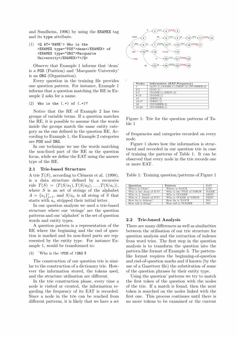
In the trie construction phase, every time anode is visited or created, the information re-garding the frequency of its EAT is recorded.Since a node in the trie can be reached fromdi!erent patterns, it is likely that we have a set
Nodes Information (EAT,Frequency)1 (LOC,1),(NAME,1),(DESC,2),(NUMBER,2)2-5 (LOC,1)6-7 (NAME,1),(DESC,2)8-12 (NAME,1)13 (DESC,2)14-17 (DESC,1)18 (NUMBER,2)19-26 (NUMBER,1)
Figure 1: Trie for the question patterns of Ta-ble 1
of frequencies and categories recorded on everynode.
Figure 1 shows how the information is struc-tured and recorded in our question trie in caseof training the patterns of Table 1. It can beobserved that every node in the trie records oneor more EAT.
Table 1: Training question/patterns of Figure 1
Question Pattern EATWhere is Chile? ˆWhere is !LOC$ LOCWho is the dean of ICS? ˆWho is the !POS of !ORG$ NAMEWho is J. Smith? ˆWho is !NAME$ DESCWho is J. Smith of ICS? ˆWho is !NAME of !ORG$ DESCHow far is Athens? ˆHow far is !LOC$ NOHow tall is Sting? ˆHow tall is !NAME$ NO
2.2 Trie-based AnalysisThere are many di!erences as well as similaritiesbetween the utilisation of our trie structure forquestion analysis and the extraction of indexesfrom word tries. The first step in the questionanalysis is to transform the question into thepattern-like format of Example 3. The pattern-like format requires the beginning-of-questionand end-of-question marks and if known (by theuse of a Gazetteer file) the substitution of someof the question phrases by their entity type.
Using the question’ patterns we try to matchthe first token of the question with the nodesof the trie. If a match is found, then the nexttoken is searched on the nodes linked with thefirst one. This process continues until there isno more tokens to be examined or the current
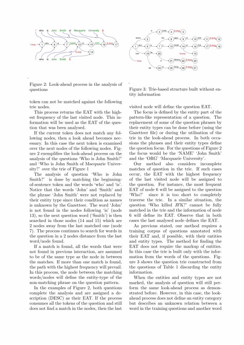
Figure 2: Look-ahead process in the analysis ofquestions
token can not be matched against the followingtrie nodes.
This process returns the EAT with the high-est frequency of the last visited node. This in-formation will be used as the EAT of the ques-tion that was been analysed.
If the current token does not match any fol-lowing nodes, then a look ahead becomes nec-essary. In this case the next token is examinedover the next nodes of the following nodes. Fig-ure 2 exemplifies the look-ahead process on theanalysis of the questions ‘Who is John Smith?’and ‘Who is John Smith of Macquarie Univer-sity?’ over the trie of Figure 1
The analysis of question ‘Who is JohnSmith?’ is done by matching the beginning-of-sentence token and the words ‘who’ and ‘is’.Notice that the words ‘John’ and ‘Smith’ andthe phrase ‘John Smith’ were not replaced bytheir entity type since their condition as namesis unknown by the Gazetteer. The word ‘John’is not found in the nodes following ‘is’ (node13), so the next question word (‘Smith’) is thensearched in those nodes (14 and 15) which are2 nodes away from the last matched one (node7). The process continues to search for words inthe question in a 2 nodes distance from the lastword/node found.
If a match is found, all the words that werenot found in previous interaction, are assumedto be of the same type as the node in betweenthe matches. If more than one match is found,the path with the highest frequency will prevail.In this process, the node between the matchingwords/nodes will define the entity-type of thenon-matching phrase on the question pattern.
In the examples of Figure 2, both questionscomplete the analysis and are assigned a de-scription (DESC) as their EAT. If the processconsumes all the tokens of the question and stilldoes not find a match in the nodes, then the last
Figure 3: Trie-based structure built without en-tity information
visited node will define the question EAT.The focus is defined by the entity part of the
pattern-like representation of a question. Thereplacement of some of the question phrases bytheir entity types can be done before (using theGazetteer file) or during the utilisation of thetrie in the look-ahead process. In both occa-sions the phrases and their entity types definethe question focus. For the questions of Figure 2the focus would be the ‘NAME’ ‘John Smith’and the ‘ORG’ ‘Macquarie University’.
Our method also considers incompletematches of question in the trie. If such casesoccur, the EAT with the highest frequencyof the last visited node will be assigned tothe question. For instance, the most frequentEAT of node 6 will be assigned to the question‘Who?’ since it is too short to completelytraverse the trie. In a similar situation, thequestion ‘Who killed JFK?’ cannot be fullymatched in the trie and the information of node6 will define its EAT. Observe that in bothcases the last analysed node defines the EAT.
As previous stated, our method requires atraining corpus of questions annotated withtheir EAT and, if possible, with their entitiesand entity types. The method for finding theEAT does not require the markup of entities.In this case the trie is built only with the infor-mation from the words of the questions. Fig-ure 3 shows the question trie constructed fromthe questions of Table 1 discarding the entityinformation.
When the entities and entity types are notmarked, the analysis of question will still per-form the same look-ahead process as demon-strated before. However, in this case, the look-ahead process does not define an entity categorybut describes an unknown relation between aword in the training questions and another word
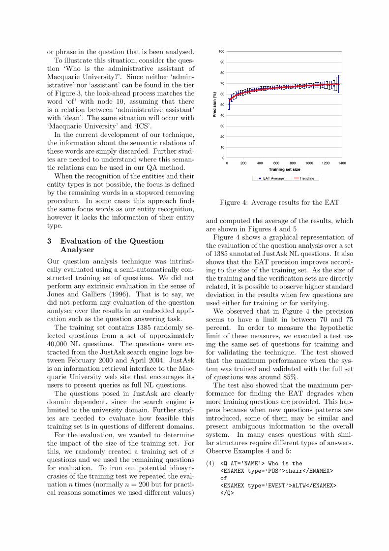
or phrase in the question that is been analysed.To illustrate this situation, consider the ques-
tion ‘Who is the administrative assistant ofMacquarie University?’. Since neither ‘admin-istrative’ nor ‘assistant’ can be found in the tierof Figure 3, the look-ahead process matches theword ‘of’ with node 10, assuming that thereis a relation between ‘administrative assistant’with ‘dean’. The same situation will occur with‘Macquarie University’ and ‘ICS’.
In the current development of our technique,the information about the semantic relations ofthese words are simply discarded. Further stud-ies are needed to understand where this seman-tic relations can be used in our QA method.
When the recognition of the entities and theirentity types is not possible, the focus is definedby the remaining words in a stopword removingprocedure. In some cases this approach findsthe same focus words as our entity recognition,however it lacks the information of their entitytype.
3 Evaluation of the QuestionAnalyser
Our question analysis technique was intrinsi-cally evaluated using a semi-automatically con-structed training set of questions. We did notperform any extrinsic evaluation in the sense ofJones and Galliers (1996). That is to say, wedid not perform any evaluation of the questionanalyser over the results in an embedded appli-cation such as the question answering task.
The training set contains 1385 randomly se-lected questions from a set of approximately40,000 NL questions. The questions were ex-tracted from the JustAsk search engine logs be-tween February 2000 and April 2004. JustAskis an information retrieval interface to the Mac-quarie University web site that encourages itsusers to present queries as full NL questions.
The questions posed in JustAsk are clearlydomain dependent, since the search engine islimited to the university domain. Further stud-ies are needed to evaluate how feasible thistraining set is in questions of di!erent domains.
For the evaluation, we wanted to determinethe impact of the size of the training set. Forthis, we randomly created a training set of xquestions and we used the remaining questionsfor evaluation. To iron out potential idiosyn-crasies of the training test we repeated the eval-uation n times (normally n = 200 but for practi-cal reasons sometimes we used di!erent values)
0
10
20
30
40
50
60
70
80
90
100
0 200 400 600 800 1000 1200 1400
Training set size
Prec
isio
n (%
)
EAT Average Trendline
Figure 4: Average results for the EAT
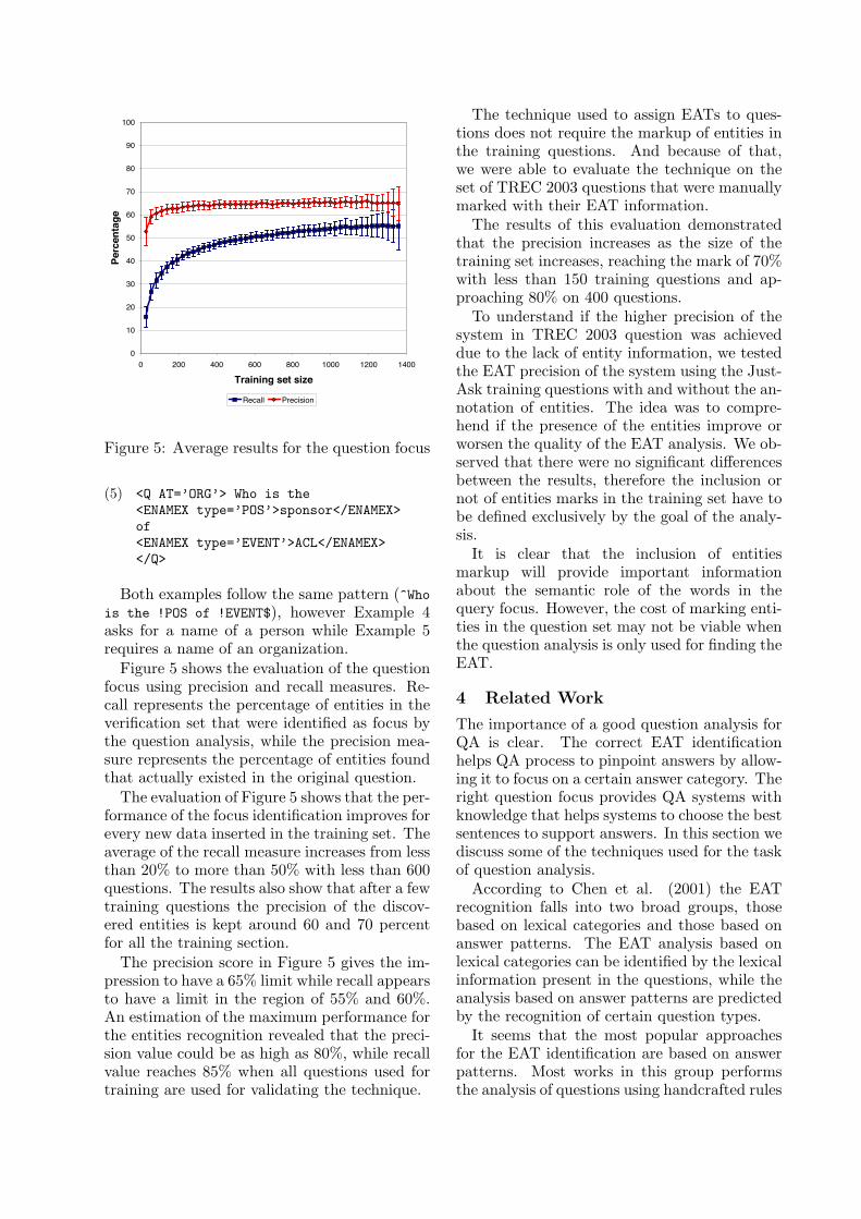
and computed the average of the results, whichare shown in Figures 4 and 5
Figure 4 shows a graphical representation ofthe evaluation of the question analysis over a setof 1385 annotated JustAsk NL questions. It alsoshows that the EAT precision improves accord-ing to the size of the training set. As the size ofthe training and the verification sets are directlyrelated, it is possible to observe higher standarddeviation in the results when few questions areused either for training or for verifying.
We observed that in Figure 4 the precisionseems to have a limit in between 70 and 75percent. In order to measure the hypotheticlimit of these measures, we executed a test us-ing the same set of questions for training andfor validating the technique. The test showedthat the maximum performance when the sys-tem was trained and validated with the full setof questions was around 85%.
The test also showed that the maximum per-formance for finding the EAT degrades whenmore training questions are provided. This hap-pens because when new questions patterns areintroduced, some of them may be similar andpresent ambiguous information to the overallsystem. In many cases questions with simi-lar structures require di!erent types of answers.Observe Examples 4 and 5:
(4) <Q AT=’NAME’> Who is the<ENAMEX type=’POS’>chair</ENAMEX>of<ENAMEX type=’EVENT’>ALTW</ENAMEX></Q>
0
10
20
30
40
50
60
70
80
90
100
0 200 400 600 800 1000 1200 1400
Training set size
Perc
enta
ge
Recall Precision
Figure 5: Average results for the question focus
(5) <Q AT=’ORG’> Who is the<ENAMEX type=’POS’>sponsor</ENAMEX>of<ENAMEX type=’EVENT’>ACL</ENAMEX></Q>
Both examples follow the same pattern (^Whois the !POS of !EVENT$), however Example 4asks for a name of a person while Example 5requires a name of an organization.
Figure 5 shows the evaluation of the questionfocus using precision and recall measures. Re-call represents the percentage of entities in theverification set that were identified as focus bythe question analysis, while the precision mea-sure represents the percentage of entities foundthat actually existed in the original question.
The evaluation of Figure 5 shows that the per-formance of the focus identification improves forevery new data inserted in the training set. Theaverage of the recall measure increases from lessthan 20% to more than 50% with less than 600questions. The results also show that after a fewtraining questions the precision of the discov-ered entities is kept around 60 and 70 percentfor all the training section.
The precision score in Figure 5 gives the im-pression to have a 65% limit while recall appearsto have a limit in the region of 55% and 60%.An estimation of the maximum performance forthe entities recognition revealed that the preci-sion value could be as high as 80%, while recallvalue reaches 85% when all questions used fortraining are used for validating the technique.
The technique used to assign EATs to ques-tions does not require the markup of entities inthe training questions. And because of that,we were able to evaluate the technique on theset of TREC 2003 questions that were manuallymarked with their EAT information.
The results of this evaluation demonstratedthat the precision increases as the size of thetraining set increases, reaching the mark of 70%with less than 150 training questions and ap-proaching 80% on 400 questions.
To understand if the higher precision of thesystem in TREC 2003 question was achieveddue to the lack of entity information, we testedthe EAT precision of the system using the Just-Ask training questions with and without the an-notation of entities. The idea was to compre-hend if the presence of the entities improve orworsen the quality of the EAT analysis. We ob-served that there were no significant di!erencesbetween the results, therefore the inclusion ornot of entities marks in the training set have tobe defined exclusively by the goal of the analy-sis.
It is clear that the inclusion of entitiesmarkup will provide important informationabout the semantic role of the words in thequery focus. However, the cost of marking enti-ties in the question set may not be viable whenthe question analysis is only used for finding theEAT.
4 Related Work
The importance of a good question analysis forQA is clear. The correct EAT identificationhelps QA process to pinpoint answers by allow-ing it to focus on a certain answer category. Theright question focus provides QA systems withknowledge that helps systems to choose the bestsentences to support answers. In this section wediscuss some of the techniques used for the taskof question analysis.
According to Chen et al. (2001) the EATrecognition falls into two broad groups, thosebased on lexical categories and those based onanswer patterns. The EAT analysis based onlexical categories can be identified by the lexicalinformation present in the questions, while theanalysis based on answer patterns are predictedby the recognition of certain question types.
It seems that the most popular approachesfor the EAT identification are based on answerpatterns. Most works in this group performsthe analysis of questions using handcrafted rules
60.00%
65.00%
70.00%
75.00%
80.00%
85.00%
90.00%
0 1000 2000 3000 4000 5000 6000
Size of the training set
Prec
isio
n (%
)
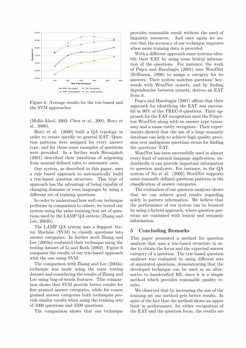
SVM - fine grained Trie - fine grainedSVM - coarse grained Trie - coarse grained
Figure 6: Average results for the trie-based andthe SVM approaches
(Molla-Aliod, 2003; Chen et al., 2001; Hovy etal., 2000).
Hovy et al. (2000) built a QA typology inorder to create specific to general EAT. Ques-tion patterns were assigned for every answertype, and for those some examples of questionswere provided. In a further work Hermjakob(2001) described their intentions of migratingfrom manual defined rules to automatic ones.
Our system, as described in this paper, usesa rule based approach to automatically builda trie-based question structure. This type ofapproach has the advantage of being capable ofchanging domains or even languages by using adi!erent set of training questions.
In order to understand how well our techniqueperforms in comparison to others, we tested oursystem using the same training/test set of ques-tions used by the LAMP QA system (Zhang andLee, 2003b).
The LAMP QA system uses a Support Vec-tor Machine (SVM) to classify questions intoanswer categories. In further work Zhang andLee (2003a) evaluated their technique using thetesting dataset of Li and Roth (2002). Figure 6compares the results of our trie-based approachwith the one using SVM.
The comparison with Zhang and Lee (2003a)technique was made using the same testingdataset and considering the results of Zhang andLee using bag-of-words features. This compar-ison shows that SVM provide better results forfine grained answer categories, while for coarsegrained answer categories both techniques pro-vide similar results when using the training setsof 1000 questions and 5500 questions.
The comparison shows that our technique
provides reasonable result without the need oflinguistic resources. And once again we no-tice that the accuracy of our technique improveswhen more training data is provided.
With a di!erent approach some systems iden-tify their EAT by using some lexical informa-tion of the questions. For instance, the workof Pasca and Harabagiu (2001) uses WordNet(Fellbaum, 1998) to assign a category for itsanswers. Their system matches questions’ key-words with WordNet synsets, and by findingdependencies between synsets, derives an EATfrom it.
Pasca and Harabagiu (2001) a"rm that theirapproach for identifying the EAT was success-ful in 90% of the TREC-9 questions. Their ap-proach for the EAT recognition used the Prince-ton WordNet along with an answer type taxon-omy and a name entity recogniser. Their exper-iments showed that the use of a large semanticdatabase can help to achieve high quality preci-sion over ambiguous questions stems for findingthe questions’ EAT.
WordNet has been successfully used in almostevery kind of natural language application; un-doubtedly it can provide important informationto question analysers. For instance, in the QAsystem of Na et al. (2002) WordNet supportssome manually defined questions patterns in theclassification of answer categories.
The evaluation of our question analyser showsthat we can achieve good results regardingsolely in pattern information. We believe thatthe performance of our system can be boostedby using a hybrid approach, where question pat-terns are combined with lexical and semanticinformation.
5 Concluding Remarks
This paper presented a method for questionanalysis that uses a trie-based structure in or-der to obtain the focus and the expected answercategory of a question. The trie-based questionanalyser was evaluated by using di!erent setsof annotated questions, demonstrating that thedeveloped technique can be used as an alter-native to handcrafted RE, since it is a simplemethod which provides reasonable quality re-sults.
We observed that by increasing the size of thetraining set our method gets better results. Inspite of the fact that the method shows an upperlimit in performance, for either recognition ofthe EAT and the question focus, the results are
not far from the hypothetic maximum value.It is observed that the hypothetic maximum
performance decreases when the training set in-creases in size. This, as already stated, is dueto implicit characteristics of question patterns;however this decrease in quality may be accen-tuated when poor or no guidelines are presentedon the stage of building the training corpus.
Sometimes the job of defining the questions’EAT and their entities is hard even for humanannotators. Some questions may have di!erentinterpretation on di!erent occasions making thequestion analysis a challenging task. It is essen-tial that the same decisions are made by thehuman annotator when dealing with ambiguousquestions. Since this problem was only identi-fied during the annotation of JustAsk trainingquestions, our training set may contain somenoisy markups. Some further work is needed todetermine how this noise degrades the results ofthe question analysis.
Manual question markup requires not onlywell defined guidelines but also a great amountof time. The complexity of manually building atraining corpus increases when the annotationof named-entities is required. In future workwe intend to use the training questions withoutthe markup of the named-entities. We are plan-ning on using the parts of speech (POS) of thequestions words and some semantic informationfrom WordNet to assign the question focus andto find out its semantic role.
The extraction of the question focus has notbeen totally explored yet. For the questionanalysis on the Macquarie domain, the resultsfor extracting the focus are promising. How-ever, we believe that the combination of POSand semantic information may increase the pre-cision and recall for either focus and the EAT.
To further ensure the e!ectiveness of thequestion analyser, we still need to perform anextrinsic analysis in a working question answer-ing environment. Still, the results shown inthis paper provide enough evidence that the ourquestion analysis is feasible to be applied in aQA system.
References
J. Chen, A.R. Diekema, M.D. Ta!et, N. Mc-Cracken, N. Ercan Ozgencil, O. Yilmazel,and E.D. Liddy. 2001. Question answering:CNLP at the TREC-10 question answeringtrack. In Proceedings of TREC-2001, pages485–494.
J. Clement, P. Flajolet, and B. Vallee. 1998.The analysis of hybrid trie structures. InProceedings of the Ninth Annual ACM-SIAMSymposium on Discrete Algorithms, pages531–539, Philadelphia, PA. SIAM Press.
C. Fellbaum. 1998. WordNet – An electroniclexical database. MIT Press, Cambridge,Massachusetts.
R. Grishman and B. Sundheim. 1996. Messageunderstanding conference-6: a brief history.In Proceedings of the Coling’96, pages 466–471.
U. Hermjakob. 2001. Parsing and questionclassification for question answering. In Pro-ceedings of the Workshop on Open-DomainQuestion Answering at ACL-2001, Toulouse,France, July.
E. Hovy, L. Gerber, U. Hermjakob, M. Junk,and C. Y. Lin. 2000. Question answeringin webclopedia. In Proceedings of TREC-9,pages 655–654.
K. Sparck Jones and J. R. Galliers. 1996.Evaluating Natural Language Processing Sys-tems: An Analysis and Review. Springer-Verlag New York, Inc.
X. Li and D. Roth. 2002. Learning questionclassifiers. In Proceedings of the COLING-02,pages 556–562.
D. Moldovan, M. Pasca, S. Harabagiu, andM. Surdeanu. 2003. Performance issues anderror analysis in an open-domain questionanswering system. ACM Trans. Inf. Syst.,21(2):133–154.
D. Molla-Aliod. 2003. Answerfinder in TREC2003. In Proceedings of TREC-2003.
S.H. Na, I.S. Kang, S.Y. Lee, and J.H. Lee.2002. Using grammatical relations, answerfrequencies and the world wide web for TRECquestion answering. In Proceedings of TREC-2002.
M. Pasca and S. Harabagiu. 2001. High per-formance question/answering. In Proceedingsof SIGIR’01, New Orleans, Louisiana, USA.ACM.
D. Zhang and W.S. Lee. 2003a. Question clas-sification using support vector machines. InProceedings of the SIGIR-03, pages 26–32.ACM Press.
D. Zhang and W.S. Lee. 2003b. A web-basedquestion answering system. In Proceedingsof the SMA Annual Symposium 2003, Singa-pore.
Evaluation of a Query-biased Document Summarisation Approach for the Question Ansnwering Task
Mingfang Wu1 Ross Wilkinson1 Cécile Paris2 CSIRO ICT Center,
1Gate 7, 71 Normanby Road, Private Bag 10, South Clayton 3169 2Locked Bag 17, North Ryde, NSW 1670, Australia
{Mingfang.Wu, Ross.Wilkinson, Cecile.Paris}@csiro.au
Abstract This paper presents an approach on a query-biased document summarisation and an evaluation of the use of such an approach for question answering tasks. We observed a significant difference in the user’s performance by presenting a list of documents customized to the task type, compared with a generic document summarization approach. This indicates that paying attention to the task and the searcher interaction may provide substantial improvement in task performance.
1 Introduction People are searching information to meet their
information needs from their tasks at hand. However, most search engines interact with user in a “one size fits all” fashion and ignore the user’s preferences, search context or the task context. The burden is then placed on the user to scan, navigate, and read the retrieved documents to identify what s/he wants. We believe that paying attention to the nature of the information task and the needs of the searcher may provide benefits beyond those available through more accurate matching. As Saracevic [9] pointed out, the key to the future of information systems and searching processes lies not only in increased sophistication of technology, but also in increased understanding of human involvement with information.
In the study presented in this paper, we examine searchers’ ability to carry out a question answering task [13]. Unlike the task of the non-interactive TREC question answer track [10], where the question answering focuses on fact-based, short answer questions such as “Who is the first prime minister of Australia”. We looked at the type of question answering task that is more complex than the task of finding a single fact. The answer to this type of questions would not generally be available in a single document, but would require facts to be
extracted from several documents. For example, an Australian cattle farmer would like an information access system that could tell s/he “which countries are the top ten importers of Australian beef?”. An ideal answer should consist of a list of country names together with corresponding beef import data. This answer could be synthesized from scattered information collected from various sources, such as a news article about Japanese meat imports and an analysis report on Australian beef in the European market.
The successful completion of such a task requires an answer to be obtained, citing the relevant source documents. If we assume that we do not have an advanced language engine that can understand such questions and then synthesize answers to them, a searcher will be involved in the process, beyond simply initiating a query and reading a list of answers. Some of the elements that might lead to successful answering might include: • support for query formulation (and re-
formulation) • effective matching and ordering of candidate
documents • delivery of a useful form of the list of the
candidate documents • support for extraction of answers from
documents • synthesis of the answer
There has been quite a bit of study on how to support query formulation, and the bulk of IR research has been devoted to better matching. Research into question answering technology (for automatic approaches) or text editing (for manual approaches) is needed for the last two activities. In this work, we have concentrated on the task of delivering a useful form of the list of the candidate documents. The research question we investigated is: given a same list of retrieved documents, will
the variation in document summary/surrogate improve searcher’s performance on question answering task?
Under the evaluation framework of the TREC (Text REtreieval Conference) interactive track [7], we conducted two experiments that compared two types of candidate lists in two experimental systems. One system (the control system) uses the document title and the first N words of a document as the document’s summary, while the other system (the testing system) uses the document title and the best three “answer chunks” extracted from the documents as the document’s summary. The second confirming experiment repeated the first experiment, but with different search engine, test collection and subjects. The purpose of the second experiment is to confirm the strong results from the first experiment and to test whether the methodology could be generalized to web data.
The rest of the paper is organized as follows: Section 2 discusses our motivation and approach. Section 3 describes the experimental setup, including experiment design and test collections. Section 4 presents the experiments’ results and provides detailed analysis. Section 5 provides the conclusions we have drawn.
2 Motivation and approach In our previous studies [12], we investigated the
use of clustering and classification methods to organize the retrieved documents, we found that while subjects could use the structured delivery format to locate groups of relevant documents, the subjects often either failed to identify a relevant document from the document summary or were unable to locate the answer component present within a relevant document.
We hypothesize that one of the reasons for potential gains from structured delivery not being realized is that in our previous test systems the tools that were provided to differentiate the answer containing documents from non-answer containing documents were inadequate for the task of question answering.
In our previous testing systems, a retrieved document is represented by its title. While a document’s title may tell what the document is about, very often an answer component exists within a small chunk of the document, and this small chunk may not be related to the main theme of the document. For example, for the question “Which was the last dynasty of China: Qing or Ming?”, the titles of the first two documents presented to a searcher are: “Claim Record Sale For Porcelain Ming Vase” and “Chinese Dish for Calligraphy Brushes Brings Record Price”. The themes of the two documents are Ming vases and
Chinese dishes respectively, but there are sentences in each document that mention the time span of the Ming Dynasty and of the Qing Dynasty. By reading only the titles, searchers miss a chance to easily and quickly determine the answer, even the answer components are in the top ranked documents.
In this work, we still use document retrieval, but focus on the surrogate or summary of the retrieved documents. Some experiments have evaluated the suitability of taking extracted paragraphs or sentences as a document summary [2], [6], [8]. The produced summary by these methods is purely based on individual document and basically a condensed version of a document - it requires the user less reading time to get to know the gist of the document. There are little studies that have shown whether the use of these summaries is suitable for the interactive question answering task.
In our approach, a document is summarized and represented by its title and the three best answer-indicative sentences (AIS). The three best AIS are dynamically generated after each query search, based on the following criteria: • An AIS should contain at least one query
word. • The AIS are first ranked according to the
number of unique query words contained in each AIS. If two AIS have the same number of unique query words, they will be ranked according to their order of appearance in the document.
• Only the top three AIS are selected. Our hypothesis is that the title and answer-
indicative sentences should provide a better indication of whether a document might help answer a given question. This is because documents can easily be completely off the topic of interest to the searcher, but still be relevant because they contain a part of the answer to the question. Therefore, our experiment focused on the comparison and evaluation of two systems using different summaries. The control system First20 uses the title and the first twenty words as the document summary, and the test system AIS3 uses the title and best three answer-indicative sentences as the document summary. Performance will be evaluated in terms of searchers’ abilities to locate answer components, searchers’ subjective perceptions of the systems, and the efforts required by searchers to determine answers.
3 Experimental setup Experimental design
The experimental design concerns three major factors: system, question, and searcher, with focus
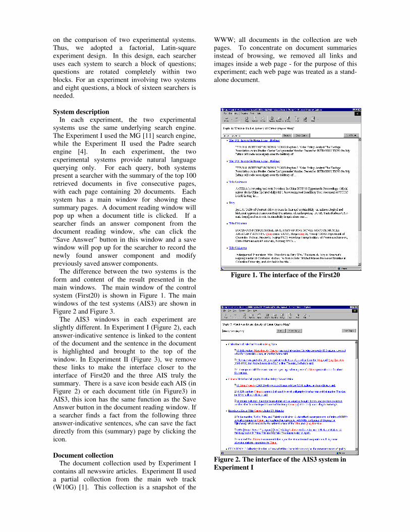
on the comparison of two experimental systems. Thus, we adopted a factorial, Latin-square experiment design. In this design, each searcher uses each system to search a block of questions; questions are rotated completely within two blocks. For an experiment involving two systems and eight questions, a block of sixteen searchers is needed.
System description
In each experiment, the two experimental systems use the same underlying search engine. The Experiment I used the MG [11] search engine, while the Experiment II used the Padre search engine [4]. In each experiment, the two experimental systems provide natural language querying only. For each query, both systems present a searcher with the summary of the top 100 retrieved documents in five consecutive pages, with each page containing 20 documents. Each system has a main window for showing these summary pages. A document reading window will pop up when a document title is clicked. If a searcher finds an answer component from the document reading window, s/he can click the “Save Answer” button in this window and a save window will pop up for the searcher to record the newly found answer component and modify previously saved answer components.
The difference between the two systems is the form and content of the result presented in the main windows. The main window of the control system (First20) is shown in Figure 1. The main windows of the test systems (AIS3) are shown in Figure 2 and Figure 3.
The AIS3 windows in each experiment are slightly different. In Experiment I (Figure 2), each answer-indicative sentence is linked to the content of the document and the sentence in the document is highlighted and brought to the top of the window. In Experiment II (Figure 3), we remove these links to make the interface closer to the interface of First20 and the three AIS truly the summary. There is a save icon beside each AIS (in Figure 2) or each document title (in Figure3) in AIS3, this icon has the same function as the Save Answer button in the document reading window. If a searcher finds a fact from the following three answer-indicative sentences, s/he can save the fact directly from this (summary) page by clicking the icon.
Document collection
The document collection used by Experiment I contains all newswire articles. Experiment II used a partial collection from the main web track (W10G) [1]. This collection is a snapshot of the
WWW; all documents in the collection are web pages. To concentrate on document summaries instead of browsing, we removed all links and images inside a web page - for the purpose of this experiment; each web page was treated as a stand-alone document.
Figure 1. The interface of the First20
Figure 2. The interface of the AIS3 system in Experiment I
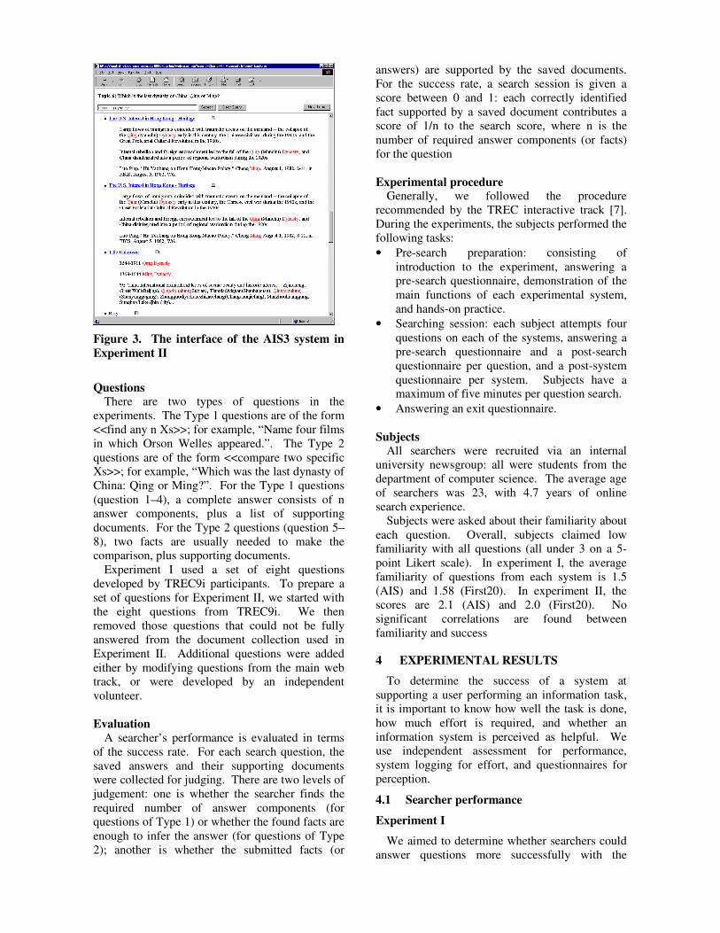
Figure 3. The interface of the AIS3 system in Experiment II Questions
There are two types of questions in the experiments. The Type 1 questions are of the form <<find any n Xs>>; for example, “Name four films in which Orson Welles appeared.”. The Type 2 questions are of the form <<compare two specific Xs>>; for example, “Which was the last dynasty of China: Qing or Ming?”. For the Type 1 questions (question 1–4), a complete answer consists of n answer components, plus a list of supporting documents. For the Type 2 questions (question 5–8), two facts are usually needed to make the comparison, plus supporting documents.
Experiment I used a set of eight questions developed by TREC9i participants. To prepare a set of questions for Experiment II, we started with the eight questions from TREC9i. We then removed those questions that could not be fully answered from the document collection used in Experiment II. Additional questions were added either by modifying questions from the main web track, or were developed by an independent volunteer.
Evaluation
A searcher’s performance is evaluated in terms of the success rate. For each search question, the saved answers and their supporting documents were collected for judging. There are two levels of judgement: one is whether the searcher finds the required number of answer components (for questions of Type 1) or whether the found facts are enough to infer the answer (for questions of Type 2); another is whether the submitted facts (or
answers) are supported by the saved documents. For the success rate, a search session is given a score between 0 and 1: each correctly identified fact supported by a saved document contributes a score of 1/n to the search score, where n is the number of required answer components (or facts) for the question
Experimental procedure
Generally, we followed the procedure recommended by the TREC interactive track [7]. During the experiments, the subjects performed the following tasks: • Pre-search preparation: consisting of
introduction to the experiment, answering a pre-search questionnaire, demonstration of the main functions of each experimental system, and hands-on practice.
• Searching session: each subject attempts four questions on each of the systems, answering a pre-search questionnaire and a post-search questionnaire per question, and a post-system questionnaire per system. Subjects have a maximum of five minutes per question search.
• Answering an exit questionnaire.
Subjects All searchers were recruited via an internal
university newsgroup: all were students from the department of computer science. The average age of searchers was 23, with 4.7 years of online search experience.
Subjects were asked about their familiarity about each question. Overall, subjects claimed low familiarity with all questions (all under 3 on a 5-point Likert scale). In experiment I, the average familiarity of questions from each system is 1.5 (AIS) and 1.58 (First20). In experiment II, the scores are 2.1 (AIS) and 2.0 (First20). No significant correlations are found between familiarity and success
4 EXPERIMENTAL RESULTS To determine the success of a system at
supporting a user performing an information task, it is important to know how well the task is done, how much effort is required, and whether an information system is perceived as helpful. We use independent assessment for performance, system logging for effort, and questionnaires for perception.
4.1 Searcher performance Experiment I
We aimed to determine whether searchers could answer questions more successfully with the
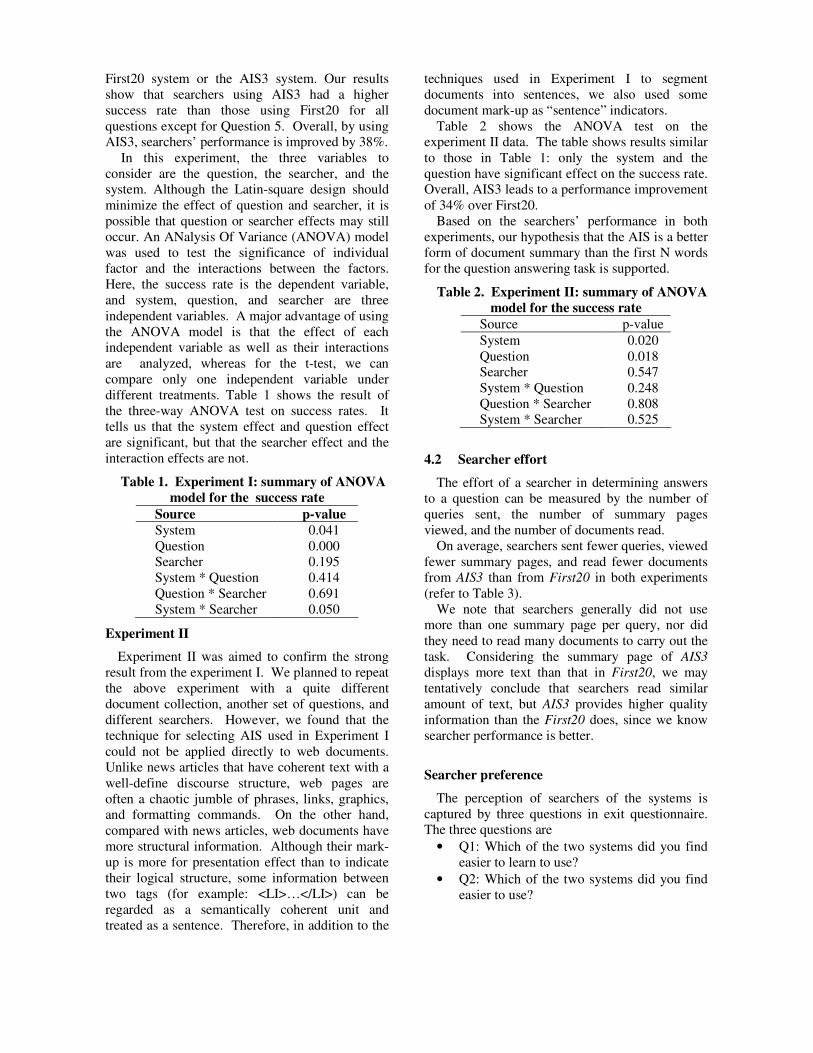
First20 system or the AIS3 system. Our results show that searchers using AIS3 had a higher success rate than those using First20 for all questions except for Question 5. Overall, by using AIS3, searchers’ performance is improved by 38%.
In this experiment, the three variables to consider are the question, the searcher, and the system. Although the Latin-square design should minimize the effect of question and searcher, it is possible that question or searcher effects may still occur. An ANalysis Of Variance (ANOVA) model was used to test the significance of individual factor and the interactions between the factors. Here, the success rate is the dependent variable, and system, question, and searcher are three independent variables. A major advantage of using the ANOVA model is that the effect of each independent variable as well as their interactions are analyzed, whereas for the t-test, we can compare only one independent variable under different treatments. Table 1 shows the result of the three-way ANOVA test on success rates. It tells us that the system effect and question effect are significant, but that the searcher effect and the interaction effects are not.
Table 1. Experiment I: summary of ANOVA model for the success rate
Source p-value System 0.041 Question 0.000 Searcher 0.195 System * Question 0.414 Question * Searcher 0.691 System * Searcher 0.050
Experiment II Experiment II was aimed to confirm the strong
result from the experiment I. We planned to repeat the above experiment with a quite different document collection, another set of questions, and different searchers. However, we found that the technique for selecting AIS used in Experiment I could not be applied directly to web documents. Unlike news articles that have coherent text with a well-define discourse structure, web pages are often a chaotic jumble of phrases, links, graphics, and formatting commands. On the other hand, compared with news articles, web documents have more structural information. Although their mark-up is more for presentation effect than to indicate their logical structure, some information between two tags (for example: <LI>…</LI>) can be regarded as a semantically coherent unit and treated as a sentence. Therefore, in addition to the
techniques used in Experiment I to segment documents into sentences, we also used some document mark-up as “sentence” indicators.
Table 2 shows the ANOVA test on the experiment II data. The table shows results similar to those in Table 1: only the system and the question have significant effect on the success rate. Overall, AIS3 leads to a performance improvement of 34% over First20.
Based on the searchers’ performance in both experiments, our hypothesis that the AIS is a better form of document summary than the first N words for the question answering task is supported.
Table 2. Experiment II: summary of ANOVA model for the success rate
Source p-value System 0.020 Question 0.018 Searcher 0.547 System * Question 0.248 Question * Searcher 0.808 System * Searcher 0.525
4.2 Searcher effort The effort of a searcher in determining answers
to a question can be measured by the number of queries sent, the number of summary pages viewed, and the number of documents read.
On average, searchers sent fewer queries, viewed fewer summary pages, and read fewer documents from AIS3 than from First20 in both experiments (refer to Table 3).
We note that searchers generally did not use more than one summary page per query, nor did they need to read many documents to carry out the task. Considering the summary page of AIS3 displays more text than that in First20, we may tentatively conclude that searchers read similar amount of text, but AIS3 provides higher quality information than the First20 does, since we know searcher performance is better.
Searcher preference The perception of searchers of the systems is
captured by three questions in exit questionnaire. The three questions are
• Q1: Which of the two systems did you find easier to learn to use?
• Q2: Which of the two systems did you find easier to use?
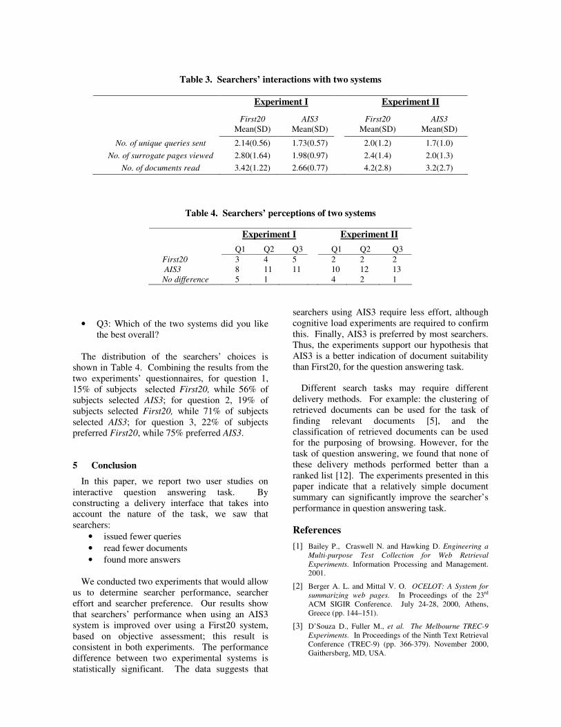
Table 3. Searchers’ interactions with two systems
Experiment I Experiment II
First20 Mean(SD)
AIS3 Mean(SD)
First20 Mean(SD)
AIS3 Mean(SD)
No. of unique queries sent 2.14(0.56) 1.73(0.57) 2.0(1.2) 1.7(1.0) No. of surrogate pages viewed 2.80(1.64) 1.98(0.97) 2.4(1.4) 2.0(1.3)
No. of documents read 3.42(1.22) 2.66(0.77) 4.2(2.8) 3.2(2.7)
Table 4. Searchers’ perceptions of two systems
Experiment I Experiment II Q1 Q2 Q3 Q1 Q2 Q3 First20 3 4 5 2 2 2 AIS3 8 11 11 10 12 13 No difference 5 1 4 2 1
• Q3: Which of the two systems did you like
the best overall? The distribution of the searchers’ choices is
shown in Table 4. Combining the results from the two experiments’ questionnaires, for question 1, 15% of subjects selected First20, while 56% of subjects selected AIS3; for question 2, 19% of subjects selected First20, while 71% of subjects selected AIS3; for question 3, 22% of subjects preferred First20, while 75% preferred AIS3.
5 Conclusion In this paper, we report two user studies on
interactive question answering task. By constructing a delivery interface that takes into account the nature of the task, we saw that searchers:
• issued fewer queries • read fewer documents • found more answers
We conducted two experiments that would allow
us to determine searcher performance, searcher effort and searcher preference. Our results show that searchers’ performance when using an AIS3 system is improved over using a First20 system, based on objective assessment; this result is consistent in both experiments. The performance difference between two experimental systems is statistically significant. The data suggests that
searchers using AIS3 require less effort, although cognitive load experiments are required to confirm this. Finally, AIS3 is preferred by most searchers. Thus, the experiments support our hypothesis that AIS3 is a better indication of document suitability than First20, for the question answering task.
Different search tasks may require different delivery methods. For example: the clustering of retrieved documents can be used for the task of finding relevant documents [5], and the classification of retrieved documents can be used for the purposing of browsing. However, for the task of question answering, we found that none of these delivery methods performed better than a ranked list [12]. The experiments presented in this paper indicate that a relatively simple document summary can significantly improve the searcher’s performance in question answering task.
References [1] Bailey P., Craswell N. and Hawking D. Engineering a
Multi-purpose Test Collection for Web Retrieval Experiments. Information Processing and Management. 2001.
[2] Berger A. L. and Mittal V. O. OCELOT: A System for summarizing web pages. In Proceedings of the 23rd ACM SIGIR Conference. July 24-28, 2000, Athens, Greece (pp. 144–151).
[3] D’Souza D., Fuller M., et al. The Melbourne TREC-9 Experiments. In Proceedings of the Ninth Text Retrieval Conference (TREC-9) (pp. 366-379). November 2000, Gaithersberg, MD, USA.
[4] Hawking D., Craswell N. and Thistlewaite P. ACSys TREC-8 Experiments. In Proceeding of Seventh Text Retrieval Conference (TREC-8), November 1999, Gaithersburg, MD, USA.
[5] Hearst M. A. and Pedersen J. O. Reexamining the cluster hypothesis: Scatter/gather on retrieval results. In Proceedings of the 19th ACM SIGIR conference, August 1996, Zurich, Switzerland (pp. 76-84).
[6] Kupiec J., Pedersen J. and Chen F. A Trainable Document Summarizer. In Proceedings of the ACM SIGIR conference, July 1995, New York, USA (pp. 68–73).
[7] Over P. TREC-9 Interactive Track – Basics. In Note papers of TREC-9. November 2000, Gaithersberg, MD, USA (pp 721-728).
[8] Salton G., Singhal A., Mitra M. and Buckley C. Automatic Text Structure and Summarization. Information Processing and Management. Vol. 33 (2) 193-207, 1997.
[9] Saracevic T. and Kentor P. A Study of Information Seeking and Retrieving: I. Background and Methodology. Journal of the American Society for Information Science. Vol. 39(3), 161-176. 1988.
[10] Voorhees E. M. The TREC-8 Question Answering Track Report. In proceedings of the Nipth Text Retrieval Conference (TREC-8). Novemeber 1999, Gaithersberg, MD, USA.
[11] Witten I., Moffat A. and Bell T. Managing Gigabytes: Compressing and indexing documents and images. Van Nostrand Reinhold. 1994.
[12] Wu M., Fuller M. and Wilkinson R. Using clustering and classification approaches in interactive retrieval. Information Processing & Management, 37 (2001) 459-484.
[13] Wu, M., Fuller, M. and Wilkinson, R. Searcher performance in question answering. In Proceedings of 24th Annual ACM SIGIR Conference on Research and Development in Information Retrieval, pp. 375-381, 2001.
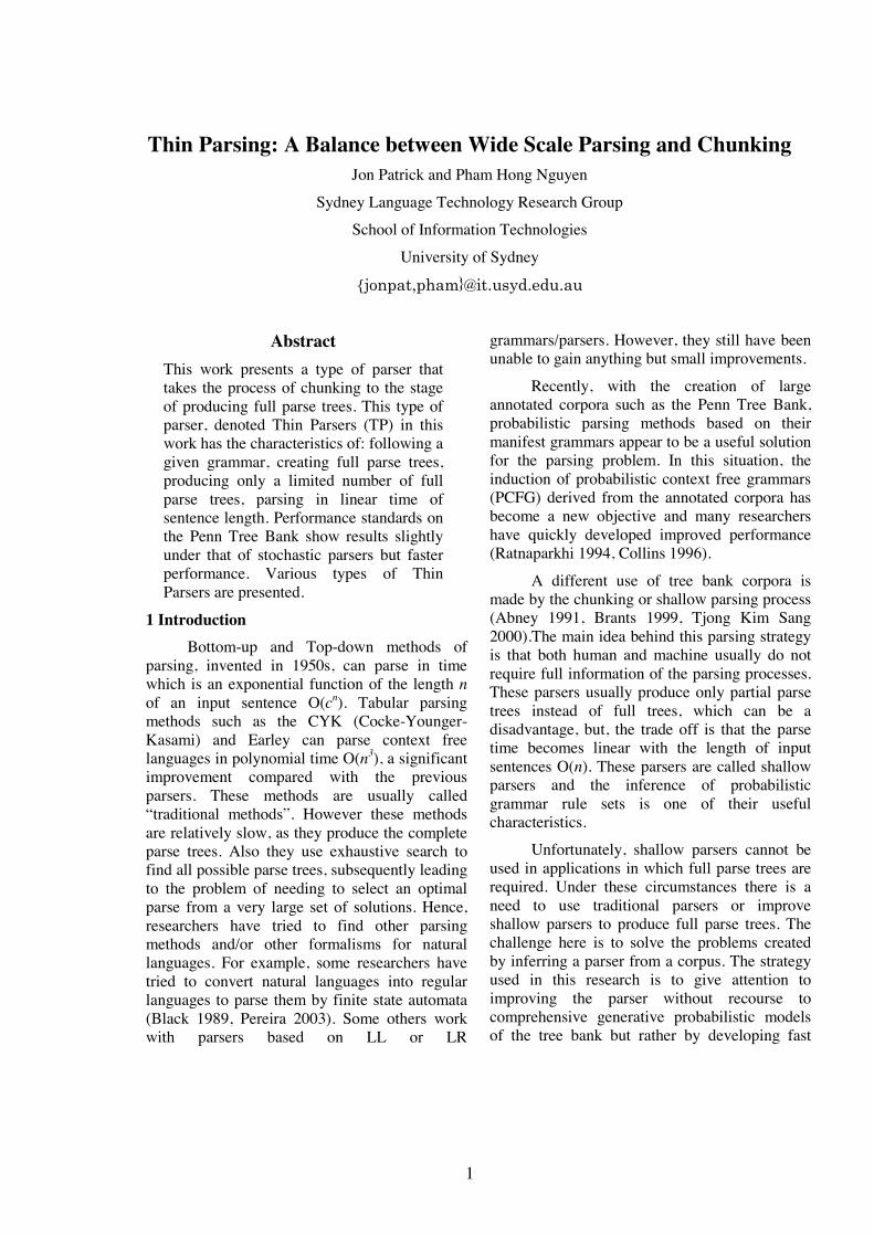
1
Thin Parsing: A Balance between Wide Scale Parsing and Chunking Jon Patrick and Pham Hong Nguyen
Sydney Language Technology Research Group
School of Information Technologies
University of Sydney
{
Abstract This work presents a type of parser that takes the process of chunking to the stage of producing full parse trees. This type of parser, denoted Thin Parsers (TP) in this work has the characteristics of: following a given grammar, creating full parse trees, producing only a limited number of full parse trees, parsing in linear time of sentence length. Performance standards on the Penn Tree Bank show results slightly under that of stochastic parsers but faster performance. Various types of Thin Parsers are presented.
1 Introduction Bottom-up and Top-down methods of
parsing, invented in 1950s, can parse in time which is an exponential function of the length n of an input sentence O(cn). Tabular parsing methods such as the CYK (Cocke-Younger-Kasami) and Earley can parse context free languages in polynomial time O(n3), a significant improvement compared with the previous parsers. These methods are usually called “traditional methods”. However these methods are relatively slow, as they produce the complete parse trees. Also they use exhaustive search to find all possible parse trees, subsequently leading to the problem of needing to select an optimal parse from a very large set of solutions. Hence, researchers have tried to find other parsing methods and/or other formalisms for natural languages. For example, some researchers have tried to convert natural languages into regular languages to parse them by finite state automata (Black 1989, Pereira 2003). Some others work with parsers based on LL or LR
grammars/parsers. However, they still have been unable to gain anything but small improvements.
Recently, with the creation of large annotated corpora such as the Penn Tree Bank, probabilistic parsing methods based on their manifest grammars appear to be a useful solution for the parsing problem. In this situation, the induction of probabilistic context free grammars (PCFG) derived from the annotated corpora has become a new objective and many researchers have quickly developed improved performance (Ratnaparkhi 1994, Collins 1996).
A different use of tree bank corpora is made by the chunking or shallow parsing process (Abney 1991, Brants 1999, Tjong Kim Sang 2000).The main idea behind this parsing strategy is that both human and machine usually do not require full information of the parsing processes. These parsers usually produce only partial parse trees instead of full trees, which can be a disadvantage, but, the trade off is that the parse time becomes linear with the length of input sentences O(n). These parsers are called shallow parsers and the inference of probabilistic grammar rule sets is one of their useful characteristics.
Unfortunately, shallow parsers cannot be used in applications in which full parse trees are required. Under these circumstances there is a need to use traditional parsers or improve shallow parsers to produce full parse trees. The challenge here is to solve the problems created by inferring a parser from a corpus. The strategy used in this research is to give attention to improving the parser without recourse to comprehensive generative probabilistic models of the tree bank but rather by developing fast
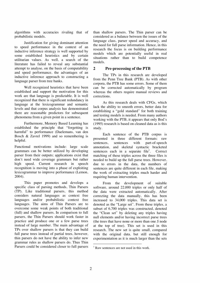
2
algorithms with accuracies rivaling that of probabilistic models.
Justification for giving dominant attention to speed performance in the context of an inductive inference strategy is well supported by some established heuristics and by certain utilitarian values. As well, a search of the literature has failed to reveal any substantial attempt to analyse, on the basis of computability and speed performance, the advantages of an inductive inference approach to constructing a language parser from tree banks.
Well recognized heuristics that have been established and support the motivation for this work are that language is predictable. It is well recognized that there is significant redundancy in language at the lexicogrammar and semantic levels and that corpus analysis has demonstrated there are reasonable predictors for subsequent phenomena from a given point in a sentence.
Furthermore, Memory Based Learning has established the principle that “forgetting is harmful” to performance (Daelemans, van den Bosch & Zavrel 1999) and so remembering is helpful.
Functional motivations include: large scale grammars can be better utilized by developing parser from their outputs; applications exist that don’t need wide coverage grammars but rather high speed. Current research in speech recognition is moving into a phase of exploiting lexicogrammar to improve performance (Lemon, 2004).
This paper promotes and develops a specific class of parsing methods, Thin Parsers (TP). Like traditional parsers, this method considers natural languages as context free languages and/or probabilistic context free languages. The aims of Thin Parsers are to overcome some weak points of both traditional (full) and shallow parsers. In comparison to full parsers, the Thin Parsers should work faster in practice and produce one or a few parse trees instead of large number. The main advantage of TPs over shallow parsers is that they can build full parse trees instead of partial trees, however, thin parsers do not have the ability to infer new grammar rules as shallow parsers do. Thus Thin Parsers could be considered closer to full parsers
than shallow parsers. The Thin parser can be considered as a balance between the issues of the language class, parser speed and accuracy, and the need for full parse information. Hence, in this research the focus is on building performance models which are potentially useful in real situations rather than to build competence models.
2 Pre-processing of the PTB The TPs in this research are developed
from the Penn Tree Bank (PTB). As with other corpora, the PTB has some errors. Some of them can be corrected automatically by program whereas the others require manual reviews and corrections.
As this research deals with CFGs, which lack the ability to smooth errors, better data for establishing a “gold standard” for both training and testing models is needed. From many authors working with the PTB, it appears that only Bod’s (1995) research is based on cleaned data as is this study.
Each sentence of the PTB corpus is presented in three different formats: raw sentences, sentences with part-of-speech annotation, and skeletal syntactic bracketed sentences each in a separate file1. Correct matching of these triples across the three files is needed to build up the full parse trees. However, due to errors in the data, the numbers of sentences are quite different in each file, making the work of extracting triples much harder and requiring human intervention.
From the development of suitable software, around 22,000 triples or only half of the data were extracted automatically. After correcting the data manually, this has been increased to 34,000 triples. This data set is denoted as the “Large set”. From these triples, a subset of 6,700 triples was constructed, denoted the “Clean set” by deleting any triples having null elements and/or having incorrect parse trees (the trees that have none or more than one S node at the top of tree). This set is used in this research. The new set is quite small, compared with the original data, but still enough for experimentation as it is much larger than the sets 1 Raw sentences are not used in this work.
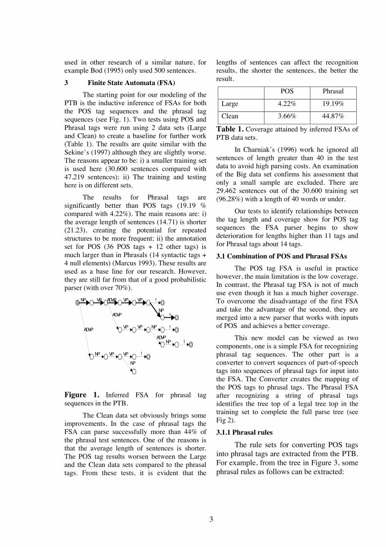
3
used in other research of a similar nature, for example Bod (1995) only used 500 sentences.
3 Finite State Automata (FSA) The starting point for our modeling of the
PTB is the inductive inference of FSAs for both the POS tag sequences and the phrasal tag sequences (see Fig. 1). Two tests using POS and Phrasal tags were run using 2 data sets (Large and Clean) to create a baseline for further work (Table 1). The results are quite similar with the Sekine’s (1997) although they are slightly worse. The reasons appear to be: i) a smaller training set is used here (30,600 sentences compared with 47,219 sentences); ii) The training and testing here is on different sets.
The results for Phrasal tags are significantly better than POS tags (19.19 % compared with 4.22%). The main reasons are: i) the average length of sentences (14.71) is shorter (21.23), creating the potential for repeated structures to be more frequent; ii) the annotation set for POS (36 POS tags + 12 other tags) is much larger than in Phrasals (14 syntactic tags + 4 null elements) (Marcus 1993). These results are used as a base line for our research. However, they are still far from that of a good probabilistic parser (with over 70%).
VPNP ADVP VP VP !
NP!ADVP
VP VP !
ADVP!
NP
NP
NP VP !
NP
VP
ADVP
Figure 1. Inferred FSA for phrasal tag sequences in the PTB.
The Clean data set obviously brings some improvements. In the case of phrasal tags the FSA can parse successfully more than 44% of the phrasal test sentences. One of the reasons is that the average length of sentences is shorter. The POS tag results worsen between the Large and the Clean data sets compared to the phrasal tags. From these tests, it is evident that the
lengths of sentences can affect the recognition results, the shorter the sentences, the better the result.
POS Phrasal
Large 4.22% 19.19%
Clean 3.66% 44.87%
Table 1. Coverage attained by inferred FSAs of PTB data sets.
In Charniak’s (1996) work he ignored all sentences of length greater than 40 in the test data to avoid high parsing costs. An examination of the Big data set confirms his assessment that only a small sample are excluded. There are 29,462 sentences out of the 30,600 training set (96.28%) with a length of 40 words or under.
Our tests to identify relationships between the tag length and coverage show for POS tag sequences the FSA parser begins to show deterioration for lengths higher than 11 tags and for Phrasal tags about 14 tags.
3.1 Combination of POS and Phrasal FSAs The POS tag FSA is useful in practice
however, the main limitation is the low coverage. In contrast, the Phrasal tag FSA is not of much use even though it has a much higher coverage. To overcome the disadvantage of the first FSA and take the advantage of the second, they are merged into a new parser that works with inputs of POS and achieves a better coverage.
This new model can be viewed as two components, one is a simple FSA for recognizing phrasal tag sequences. The other part is a converter to convert sequences of part-of-speech tags into sequences of phrasal tags for input into the FSA. The Converter creates the mapping of the POS tags to phrasal tags. The Phrasal FSA after recognizing a string of phrasal tags identifies the tree top of a legal tree top in the training set to complete the full parse tree (see Fig 2).
3.1.1 Phrasal rules
The rule sets for converting POS tags into phrasal tags are extracted from the PTB. For example, from the tree in Figure 3, some phrasal rules as follows can be extracted:
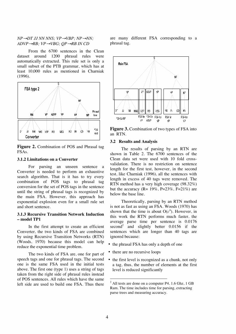
4
NP→DT JJ NN NNS; VP→VBP; NP→NN; ADVP→RB; VP→VBG; QP→RB IN CD
From the 6700 sentences in the Clean dataset around 1200 phrasal rules were automatically extracted. This rule set is only a small subset of the PTB grammar, which has at least 10,000 rules as mentioned in Charniak (1996).
Figure 2. Combination of POS and Phrasal tag FSAs.
3.1.2 Limitations on a Converter For parsing an unseen sentence a
Converter is needed to perform an exhaustive search algorithm. That is it has to try every combination of POS tags to phrasal tag conversion for the set of POS tags in the sentence until the string of phrasal tags is recognized by the main FSA. However, this approach has exponential explosion even for a small rule set and short sentence.
3.1.3 Recursive Transition Network Induction – model TP1
In the first attempt to create an efficient Converter, the two kinds of FSA are combined by using Recursive Transition Networks (RTN) (Woods, 1970) because this model can help reduce the exponential time problem.
The two kinds of FSA are, one for part of speech tags and one for phrasal tags. The second one is the same FSA used in the initial tests above. The first one (type 1) uses a string of tags taken from the right side of phrasal rules instead of POS sentences. All rules which have the same left side are used to build one FSA. Thus there
are many different FSA corresponding to a phrasal tag.
Figure 3. Combination of two types of FSA into an RTN.
3.2 Results and Analysis The results of parsing by an RTN are
shown in Table 2. The 6700 sentences of the Clean data set were used with 10 fold cross-validation. There is no restriction on sentence length for the first test, however, in the second test, like Charniak (1996), all the sentences with length in excess of 40 tags were removed. The RTN method has a very high coverage (98.32%) but the accuracy (R= 19%, P=23%, F=21%) are below the base line.
Theoretically, parsing by an RTN method is not as fast as using an FSA. Woods (1970) has shown that the time is about O(cn). However, in this work the RTN performs much faster, the average parse time per sentence is 0.0176 second2 and slightly better 0.0156 if the sentences which are longer than 40 tags are ignored because:
• the phrasal FSA has only a depth of one
• there are no recursive loops
• the first level is recognized as a chunk, not only a tag, thus, the number of elements at the first level is reduced significantly
2 All tests are done on a computer P4, 1.6 Ghz, 1 GB Ram. The time includes time for parsing, extracting parse trees and measuring accuracy.
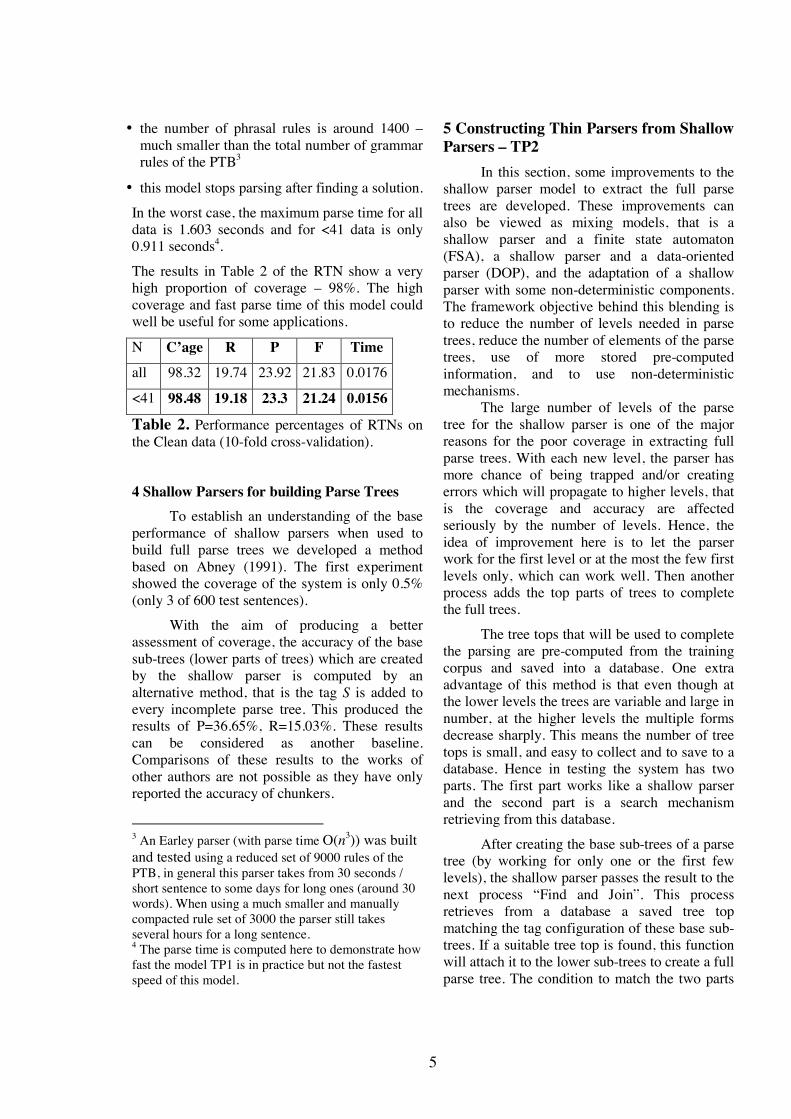
5
• the number of phrasal rules is around 1400 – much smaller than the total number of grammar rules of the PTB3
• this model stops parsing after finding a solution.
In the worst case, the maximum parse time for all data is 1.603 seconds and for <41 data is only 0.911 seconds4.
The results in Table 2 of the RTN show a very high proportion of coverage – 98%. The high coverage and fast parse time of this model could well be useful for some applications.
N C’age R P F Time
all 98.32 19.74 23.92 21.83 0.0176
<41 98.48 19.18 23.3 21.24 0.0156
Table 2. Performance percentages of RTNs on the Clean data (10-fold cross-validation).
4 Shallow Parsers for building Parse Trees
To establish an understanding of the base performance of shallow parsers when used to build full parse trees we developed a method based on Abney (1991). The first experiment showed the coverage of the system is only 0.5% (only 3 of 600 test sentences).
With the aim of producing a better assessment of coverage, the accuracy of the base sub-trees (lower parts of trees) which are created by the shallow parser is computed by an alternative method, that is the tag S is added to every incomplete parse tree. This produced the results of P=36.65%, R=15.03%. These results can be considered as another baseline. Comparisons of these results to the works of other authors are not possible as they have only reported the accuracy of chunkers.
3 An Earley parser (with parse time O(n3)) was built and tested using a reduced set of 9000 rules of the PTB, in general this parser takes from 30 seconds / short sentence to some days for long ones (around 30 words). When using a much smaller and manually compacted rule set of 3000 the parser still takes several hours for a long sentence. 4 The parse time is computed here to demonstrate how fast the model TP1 is in practice but not the fastest speed of this model.
5 Constructing Thin Parsers from Shallow Parsers – TP2
In this section, some improvements to the shallow parser model to extract the full parse trees are developed. These improvements can also be viewed as mixing models, that is a shallow parser and a finite state automaton (FSA), a shallow parser and a data-oriented parser (DOP), and the adaptation of a shallow parser with some non-deterministic components. The framework objective behind this blending is to reduce the number of levels needed in parse trees, reduce the number of elements of the parse trees, use of more stored pre-computed information, and to use non-deterministic mechanisms.
The large number of levels of the parse tree for the shallow parser is one of the major reasons for the poor coverage in extracting full parse trees. With each new level, the parser has more chance of being trapped and/or creating errors which will propagate to higher levels, that is the coverage and accuracy are affected seriously by the number of levels. Hence, the idea of improvement here is to let the parser work for the first level or at the most the few first levels only, which can work well. Then another process adds the top parts of trees to complete the full trees.
The tree tops that will be used to complete the parsing are pre-computed from the training corpus and saved into a database. One extra advantage of this method is that even though at the lower levels the trees are variable and large in number, at the higher levels the multiple forms decrease sharply. This means the number of tree tops is small, and easy to collect and to save to a database. Hence in testing the system has two parts. The first part works like a shallow parser and the second part is a search mechanism retrieving from this database.
After creating the base sub-trees of a parse tree (by working for only one or the first few levels), the shallow parser passes the result to the next process “Find and Join”. This process retrieves from a database a saved tree top matching the tag configuration of these base sub-trees. If a suitable tree top is found, this function will attach it to the lower sub-trees to create a full parse tree. The condition to match the two parts
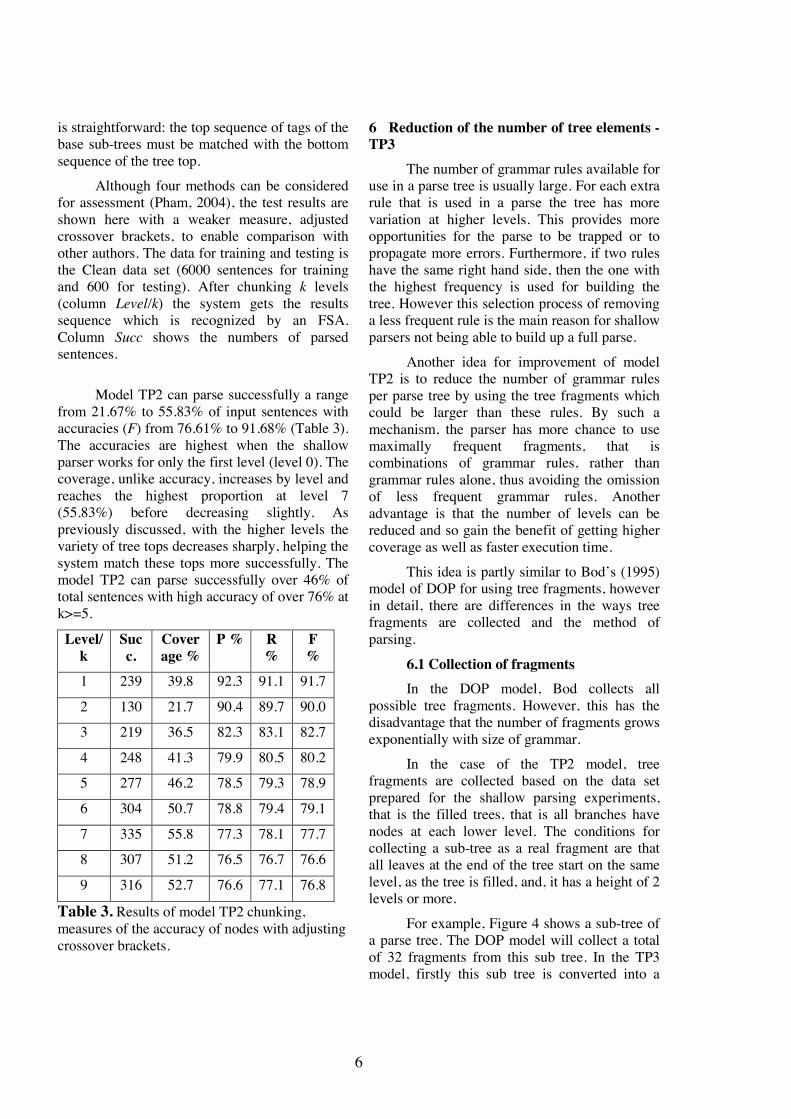
6
is straightforward: the top sequence of tags of the base sub-trees must be matched with the bottom sequence of the tree top.
Although four methods can be considered for assessment (Pham, 2004), the test results are shown here with a weaker measure, adjusted crossover brackets, to enable comparison with other authors. The data for training and testing is the Clean data set (6000 sentences for training and 600 for testing). After chunking k levels (column Level/k) the system gets the results sequence which is recognized by an FSA. Column Succ shows the numbers of parsed sentences.
Model TP2 can parse successfully a range from 21.67% to 55.83% of input sentences with accuracies (F) from 76.61% to 91.68% (Table 3). The accuracies are highest when the shallow parser works for only the first level (level 0). The coverage, unlike accuracy, increases by level and reaches the highest proportion at level 7 (55.83%) before decreasing slightly. As previously discussed, with the higher levels the variety of tree tops decreases sharply, helping the system match these tops more successfully. The model TP2 can parse successfully over 46% of total sentences with high accuracy of over 76% at k>=5.
Level/k
Succ.
Coverage %
P % R %
F %
1 239 39.8 92.3 91.1 91.7
2 130 21.7 90.4 89.7 90.0
3 219 36.5 82.3 83.1 82.7
4 248 41.3 79.9 80.5 80.2
5 277 46.2 78.5 79.3 78.9
6 304 50.7 78.8 79.4 79.1
7 335 55.8 77.3 78.1 77.7
8 307 51.2 76.5 76.7 76.6
9 316 52.7 76.6 77.1 76.8
Table 3. Results of model TP2 chunking, measures of the accuracy of nodes with adjusting crossover brackets.
6 Reduction of the number of tree elements - TP3
The number of grammar rules available for use in a parse tree is usually large. For each extra rule that is used in a parse the tree has more variation at higher levels. This provides more opportunities for the parse to be trapped or to propagate more errors. Furthermore, if two rules have the same right hand side, then the one with the highest frequency is used for building the tree. However this selection process of removing a less frequent rule is the main reason for shallow parsers not being able to build up a full parse.
Another idea for improvement of model TP2 is to reduce the number of grammar rules per parse tree by using the tree fragments which could be larger than these rules. By such a mechanism, the parser has more chance to use maximally frequent fragments, that is combinations of grammar rules, rather than grammar rules alone, thus avoiding the omission of less frequent grammar rules. Another advantage is that the number of levels can be reduced and so gain the benefit of getting higher coverage as well as faster execution time.
This idea is partly similar to Bod’s (1995) model of DOP for using tree fragments, however in detail, there are differences in the ways tree fragments are collected and the method of parsing.
6.1 Collection of fragments In the DOP model, Bod collects all
possible tree fragments. However, this has the disadvantage that the number of fragments grows exponentially with size of grammar.
In the case of the TP2 model, tree fragments are collected based on the data set prepared for the shallow parsing experiments, that is the filled trees, that is all branches have nodes at each lower level. The conditions for collecting a sub-tree as a real fragment are that all leaves at the end of the tree start on the same level, as the tree is filled, and, it has a height of 2 levels or more.
For example, Figure 4 shows a sub-tree of a parse tree. The DOP model will collect a total of 32 fragments from this sub tree. In the TP3 model, firstly this sub tree is converted into a
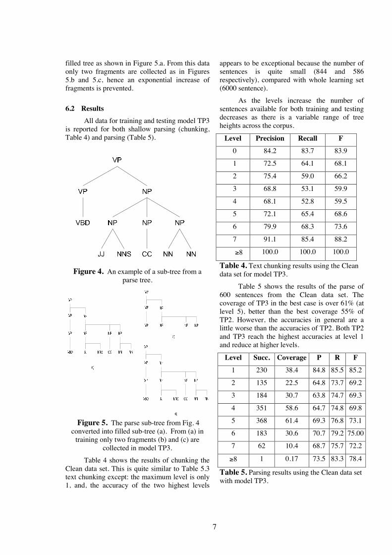
7
filled tree as shown in Figure 5.a. From this data only two fragments are collected as in Figures 5.b and 5.c, hence an exponential increase of fragments is prevented.
6.2 Results All data for training and testing model TP3
is reported for both shallow parsing (chunking, Table 4) and parsing (Table 5).
Figure 4. An example of a sub-tree from a
parse tree.
Figure 5. The parse sub-tree from Fig. 4 converted into filled sub-tree (a). From (a) in
training only two fragments (b) and (c) are collected in model TP3.
Table 4 shows the results of chunking the Clean data set. This is quite similar to Table 5.3 text chunking except: the maximum level is only 1, and, the accuracy of the two highest levels
appears to be exceptional because the number of sentences is quite small (844 and 586 respectively), compared with whole learning set (6000 sentence).
As the levels increase the number of sentences available for both training and testing decreases as there is a variable range of tree heights across the corpus.
Level Precision Recall F
0 84.2 83.7 83.9
1 72.5 64.1 68.1
2 75.4 59.0 66.2
3 68.8 53.1 59.9
4 68.1 52.8 59.5
5 72.1 65.4 68.6
6 79.9 68.3 73.6
7 91.1 85.4 88.2
≥8 100.0 100.0 100.0
Table 4. Text chunking results using the Clean data set for model TP3.
Table 5 shows the results of the parse of 600 sentences from the Clean data set. The coverage of TP3 in the best case is over 61% (at level 5), better than the best coverage 55% of TP2. However, the accuracies in general are a little worse than the accuracies of TP2. Both TP2 and TP3 reach the highest accuracies at level 1 and reduce at higher levels.
Level Succ. Coverage P R F
1 230 38.4 84.8 85.5 85.2
2 135 22.5 64.8 73.7 69.2
3 184 30.7 63.8 74.7 69.3
4 351 58.6 64.7 74.8 69.8
5 368 61.4 69.3 76.8 73.1
6 183 30.6 70.7 79.2 75.00
7 62 10.4 68.7 75.7 72.2
≥8 1 0.17 73.5 83.3 78.4
Table 5. Parsing results using the Clean data set with model TP3.
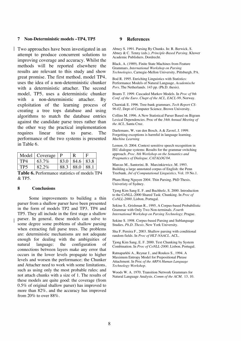
8
7 Non-Deterministic models –TP4, TP5
Two approaches have been investigated in an attempt to produce concurrent solutions to improving coverage and accuracy. Whilst the methods will be reported elsewhere the results are relevant to this study and show great promise. The first method, model TP4, uses the idea of a non-deterministic chunker with a deterministic attacher. The second model, TP5, uses a deterministic chunker with a non-deterministic attacher. By exploitation of the learning process of creating a tree tops database and using algorithms to match the database entries against the candidate parse trees rather than the other way the practical implementation requires linear time to parse. The performance of the two systems is presented in Table 6. Model Coverage P R F TP4 63.7% 83.0 84.6 83.8 TP5 82.2% 88.3 88.0 88.1
Table 6. Performance statistics of models TP4 & TP5.
8 Conclusions
Some improvements to building a thin parser from a shallow parser have been presented in the form of models TP2 and TP3, TP4 and TP5. They all include in the first stage a shallow parser. In general, these models can solve to some degree some problems of shallow parsing when extracting full parse trees. The problems are: deterministic mechanisms are not adequate enough for dealing with the ambiguities of natural language; the configuration of connections between layers make any error that occurs in the lower levels propagate to higher levels and worsen the performance; the Chunker and Attacher need to work with some limitations, such as using only the most probable rules; and not attach chunks with a size of 1. The results of these models are quite good: the coverage (from 0.5% of original shallow parser) has improved to more than 82%, and the accuracy has improved from 20% to over 88%.
9 References
Abney S. 1991. Parsing By Chunks. In: R. Berwick, S. Abney & C. Tenny (eds.), Principle-Based Parsing. Kluwer Academic Publishers, Dordrecht.
Black, A. (1989). Finite State Machines from Feature Grammars, International Workshop on Parsing Technologies, Carnegie-Mellon University, Pittsburgh, PA.
Bod R. 1995. Enriching Linguistics with Statistics: Performance Models of Natural Language, Academische Pers, The Netherlands. 143 pp. (Ph.D. thesis).
Brants T. 1999. Cascaded Markov Models. In Proc of 9th Conf. of the Euro. Chapt of the ACL, EACL-99, Norway.
Charniak E. 1996. Tree-bank grammars, Tech Report CS-96-02, Dept of Computer Science, Brown University.
Collins M. 1996. A New Statistical Parser Based on Bigram Lexical Dependencies. Proc of the 34th Annual Meeting of the ACL, Santa Cruz.
Daelemans, W, van den Bosch, A & Zavrel, J. 1999. Forgetting exceptions is harmful in language learning. Machine Learning
Lemon, O. 2004. Context sensitive speech recognition in ISU dialogue systems: Results for the grammar switching approach. Proc. 8th Workshop on the Semantics and Pragmatics of Dialogue, CATALOG'04.
Marcus M., Santorini, B. Marcinkiewicz, M. 1993. Building a large annotated corpus of English: the Penn Treebank, Jnl of Computational Linguistics, Vol. 19 No.1.
Pham Hong Nguyen 2004. Thin Parsing, PhD Thesis, Univeristy of Sydney.
Tjong Kim Sang E. F. and Buchholz, S. 2000. Introduction to the CoNLL-2000 Shared Task: Chunking. In Proc of CoNLL-2000, Lisbon, Portugal.
Sekine S., Grishman R., 1995, A Corpus-based Probabilistic Grammar with Only Two Non-terminals. Fourth International Workshop on Parsing Technology; Prague.
Sekine S. 1998. Corpus-based Parsing and Sublanguage Studies, Ph.D. Thesis, New York University.
Sha F. Pereira F., 2003. Shallow parsing with conditional random fields. In Proc of HLT-NAACL. ACL.
Tjong Kim Sang, E. F. 2000. Text Chunking by System Combination. In Proc of CoNLL-2000, Lisbon, Portugal.
Ratnaparkhi A., Reynar J., and Roukos S., 1994. A Maximum Entropy Model for Prepositional Phrase Attachment. In Proc of the ARPA Human Language Technology Workshop.
Woods W. A. 1970. Transition Network Grammars for Natural Language Analysis, Comm of the ACM, 13, 10.
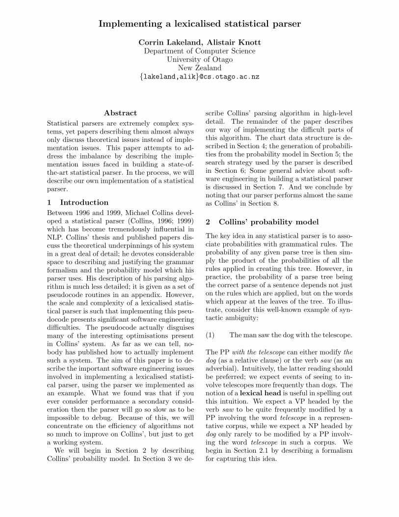
Implementing a lexicalised statistical parser
Corrin Lakeland, Alistair KnottDepartment of Computer Science
University of OtagoNew Zealand
{lakeland,alik}@cs.otago.ac.nz
Abstract
Statistical parsers are extremely complex sys-tems, yet papers describing them almost alwaysonly discuss theoretical issues instead of imple-mentation issues. This paper attempts to ad-dress the imbalance by describing the imple-mentation issues faced in building a state-of-the-art statistical parser. In the process, we willdescribe our own implementation of a statisticalparser.
1 Introduction
Between 1996 and 1999, Michael Collins devel-oped a statistical parser (Collins, 1996; 1999)which has become tremendously influential inNLP. Collins’ thesis and published papers dis-cuss the theoretical underpinnings of his systemin a great deal of detail; he devotes considerablespace to describing and justifying the grammarformalism and the probability model which hisparser uses. His description of his parsing algo-rithm is much less detailed; it is given as a set ofpseudocode routines in an appendix. However,the scale and complexity of a lexicalised statis-tical parser is such that implementing this pseu-docode presents significant software engineeringdi!culties. The pseudocode actually disguisesmany of the interesting optimisations presentin Collins’ system. As far as we can tell, no-body has published how to actually implementsuch a system. The aim of this paper is to de-scribe the important software engineering issuesinvolved in implementing a lexicalised statisti-cal parser, using the parser we implemented asan example. What we found was that if youever consider performance a secondary consid-eration then the parser will go so slow as to beimpossible to debug. Because of this, we willconcentrate on the e!ciency of algorithms notso much to improve on Collins’, but just to geta working system.
We will begin in Section 2 by describingCollins’ probability model. In Section 3 we de-
scribe Collins’ parsing algorithm in high-leveldetail. The remainder of the paper describesour way of implementing the di!cult parts ofthis algorithm. The chart data structure is de-scribed in Section 4; the generation of probabili-ties from the probability model in Section 5; thesearch strategy used by the parser is describedin Section 6; Some general advice about soft-ware engineering in building a statistical parseris discussed in Section 7. And we conclude bynoting that our parser performs almost the sameas Collins’ in Section 8.
2 Collins’ probability model
The key idea in any statistical parser is to asso-ciate probabilities with grammatical rules. Theprobability of any given parse tree is then sim-ply the product of the probabilities of all therules applied in creating this tree. However, inpractice, the probability of a parse tree beingthe correct parse of a sentence depends not juston the rules which are applied, but on the wordswhich appear at the leaves of the tree. To illus-trate, consider this well-known example of syn-tactic ambiguity:
(1) The man saw the dog with the telescope.
The PP with the telescope can either modify thedog (as a relative clause) or the verb saw (as anadverbial). Intuitively, the latter reading shouldbe preferred; we expect events of seeing to in-volve telescopes more frequently than dogs. Thenotion of a lexical head is useful in spelling outthis intuition. We expect a VP headed by theverb saw to be quite frequently modified by aPP involving the word telescope in a represen-tative corpus, while we expect a NP headed bydog only rarely to be modified by a PP involv-ing the word telescope in such a corpus. Webegin in Section 2.1 by describing a formalismfor capturing this idea.
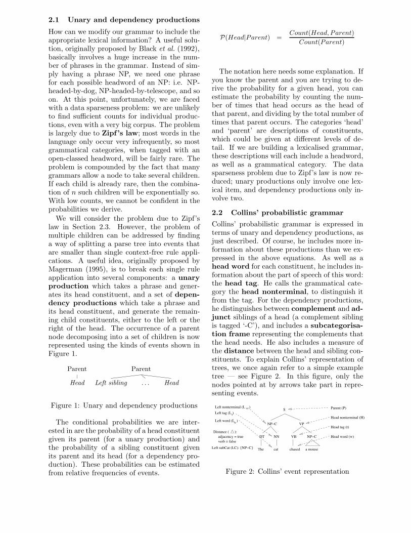
2.1 Unary and dependency productions
How can we modify our grammar to include theappropriate lexical information? A useful solu-tion, originally proposed by Black et al. (1992),basically involves a huge increase in the num-ber of phrases in the grammar. Instead of sim-ply having a phrase NP, we need one phrasefor each possible headword of an NP: i.e. NP-headed-by-dog, NP-headed-by-telescope, and soon. At this point, unfortunately, we are facedwith a data sparseness problem: we are unlikelyto find su!cient counts for individual produc-tions, even with a very big corpus. The problemis largely due to Zipf’s law; most words in thelanguage only occur very infrequently, so mostgrammatical categories, when tagged with anopen-classed headword, will be fairly rare. Theproblem is compounded by the fact that manygrammars allow a node to take several children.If each child is already rare, then the combina-tion of n such children will be exponentially so.With low counts, we cannot be confident in theprobabilities we derive.
We will consider the problem due to Zipf’slaw in Section 2.3. However, the problem ofmultiple children can be addressed by findinga way of splitting a parse tree into events thatare smaller than single context-free rule appli-cations. A useful idea, originally proposed byMagerman (1995), is to break each single ruleapplication into several components: a unaryproduction which takes a phrase and gener-ates its head constituent, and a set of depen-dency productions which take a phrase andits head constituent, and generate the remain-ing child constituents, either to the left or theright of the head. The occurrence of a parentnode decomposing into a set of children is nowrepresented using the kinds of events shown inFigure 1.
Parent
Head
Parent
Left sibling . . . Head
Figure 1: Unary and dependency productions
The conditional probabilities we are inter-ested in are the probability of a head constituentgiven its parent (for a unary production) andthe probability of a sibling constituent givenits parent and its head (for a dependency pro-duction). These probabilities can be estimatedfrom relative frequencies of events.
P(Head|Parent) =Count(Head, Parent)
Count(Parent)
The notation here needs some explanation. Ifyou know the parent and you are trying to de-rive the probability for a given head, you canestimate the probability by counting the num-ber of times that head occurs as the head ofthat parent, and dividing by the total number oftimes that parent occurs. The categories ‘head’and ‘parent’ are descriptions of constituents,which could be given at di"erent levels of de-tail. If we are building a lexicalised grammar,these descriptions will each include a headword,as well as a grammatical category. The datasparseness problem due to Zipf’s law is now re-duced; unary productions only involve one lex-ical item, and dependency productions only in-volve two.
2.2 Collins’ probabilistic grammar
Collins’ probabilistic grammar is expressed interms of unary and dependency productions, asjust described. Of course, he includes more in-formation about these productions than we ex-pressed in the above equations. As well as ahead word for each constituent, he includes in-formation about the part of speech of this word:the head tag. He calls the grammatical cate-gory the head nonterminal, to distinguish itfrom the tag. For the dependency productions,he distinguishes between complement and ad-junct siblings of a head (a complement siblingis tagged ‘-C’), and includes a subcategorisa-tion frame representing the complements thatthe head needs. He also includes a measure ofthe distance between the head and sibling con-stituents. To explain Collins’ representation oftrees, we once again refer to a simple exampletree — see Figure 2. In this figure, only thenodes pointed at by arrows take part in repre-senting events.
NP−C
DT NN VB NP−C
a mousechasedcatThe
VP
SLeft tag (L )t
Left nonterminal (L )NT Parent (P)
Head tag (t)
Head word (w)
Head nonterminal (H)
Distance ( ):adjacency = trueverb = false
Left subCat (LC): {NP−C}
wLeft word (L )
Figure 2: Collins’ event representation
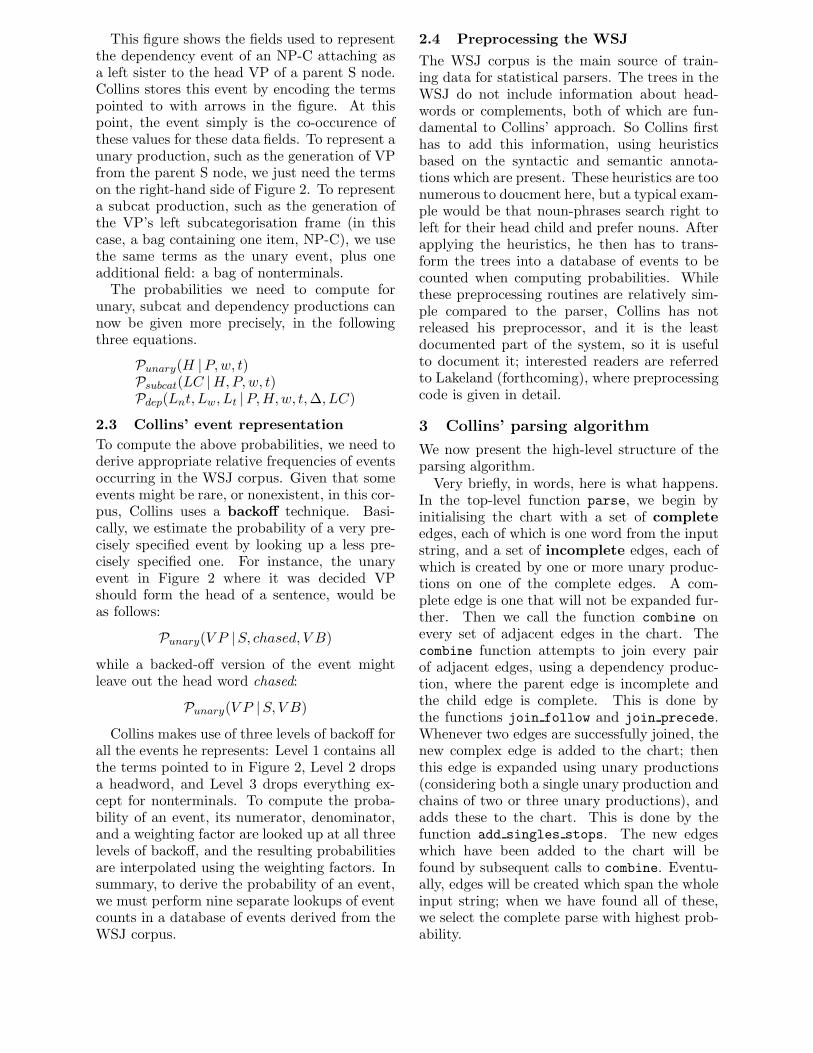
This figure shows the fields used to representthe dependency event of an NP-C attaching asa left sister to the head VP of a parent S node.Collins stores this event by encoding the termspointed to with arrows in the figure. At thispoint, the event simply is the co-occurence ofthese values for these data fields. To represent aunary production, such as the generation of VPfrom the parent S node, we just need the termson the right-hand side of Figure 2. To representa subcat production, such as the generation ofthe VP’s left subcategorisation frame (in thiscase, a bag containing one item, NP-C), we usethe same terms as the unary event, plus oneadditional field: a bag of nonterminals.
The probabilities we need to compute forunary, subcat and dependency productions cannow be given more precisely, in the followingthree equations.
Punary(H |P,w, t)Psubcat(LC |H,P,w, t)Pdep(Lnt, Lw, Lt |P,H,w, t,#, LC)
2.3 Collins’ event representation
To compute the above probabilities, we need toderive appropriate relative frequencies of eventsoccurring in the WSJ corpus. Given that someevents might be rare, or nonexistent, in this cor-pus, Collins uses a backo! technique. Basi-cally, we estimate the probability of a very pre-cisely specified event by looking up a less pre-cisely specified one. For instance, the unaryevent in Figure 2 where it was decided VPshould form the head of a sentence, would beas follows:
Punary(V P |S, chased, V B)
while a backed-o" version of the event mightleave out the head word chased:
Punary(V P |S, V B)
Collins makes use of three levels of backo" forall the events he represents: Level 1 contains allthe terms pointed to in Figure 2, Level 2 dropsa headword, and Level 3 drops everything ex-cept for nonterminals. To compute the proba-bility of an event, its numerator, denominator,and a weighting factor are looked up at all threelevels of backo", and the resulting probabilitiesare interpolated using the weighting factors. Insummary, to derive the probability of an event,we must perform nine separate lookups of eventcounts in a database of events derived from theWSJ corpus.
2.4 Preprocessing the WSJ
The WSJ corpus is the main source of train-ing data for statistical parsers. The trees in theWSJ do not include information about head-words or complements, both of which are fun-damental to Collins’ approach. So Collins firsthas to add this information, using heuristicsbased on the syntactic and semantic annota-tions which are present. These heuristics are toonumerous to doucment here, but a typical exam-ple would be that noun-phrases search right toleft for their head child and prefer nouns. Afterapplying the heuristics, he then has to trans-form the trees into a database of events to becounted when computing probabilities. Whilethese preprocessing routines are relatively sim-ple compared to the parser, Collins has notreleased his preprocessor, and it is the leastdocumented part of the system, so it is usefulto document it; interested readers are referredto Lakeland (forthcoming), where preprocessingcode is given in detail.
3 Collins’ parsing algorithm
We now present the high-level structure of theparsing algorithm.
Very briefly, in words, here is what happens.In the top-level function parse, we begin byinitialising the chart with a set of completeedges, each of which is one word from the inputstring, and a set of incomplete edges, each ofwhich is created by one or more unary produc-tions on one of the complete edges. A com-plete edge is one that will not be expanded fur-ther. Then we call the function combine onevery set of adjacent edges in the chart. Thecombine function attempts to join every pairof adjacent edges, using a dependency produc-tion, where the parent edge is incomplete andthe child edge is complete. This is done bythe functions join follow and join precede.Whenever two edges are successfully joined, thenew complex edge is added to the chart; thenthis edge is expanded using unary productions(considering both a single unary production andchains of two or three unary productions), andadds these to the chart. This is done by thefunction add singles stops. The new edgeswhich have been added to the chart will befound by subsequent calls to combine. Eventu-ally, edges will be created which span the wholeinput string; when we have found all of these,we select the complete parse with highest prob-ability.
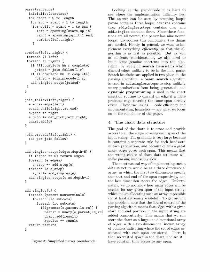
parse(sentence)initialise(sentence)for start = 0 to lengthfor end = start + 1 to lengthfor split = start + 1 to end {left = spanning(start,split)right = spanning(split+1,end)combine(left,right)
}
combine(left, right) {foreach (l left)foreach (r right) {if (!l.complete && r.complete)
joined = join_follow(l,r)if (l.complete && !r.complete)
joined = join_precede(l,r)add_singles_stops(joined)
}}
join_follow(left,right) {e = new edge(left)e.add_child(right,at_end)e.prob *= righte.prob *= dep_prob(left,right)chart.add(e)
}
join_precede(left,right) {(as per join follow)
}
add_singles_stops(edges,depth=5) {if (depth == 0) return edgesforeach (e edges)
e_stop += add_stop(e)foreach (e e_stop)
e_ns += add_singles(e)add_singles_stops(e_ns,depth-1)
}
add_singles(e) {foreach (parent nonterminals)
foreach (lc subcats)foreach (rc subcats)
if(grammar(e,parent,lc,rc)) {result = unary(e,parent,lc,rc)chart.add(result)results += result
return results}
Figure 3: Simplified parser pseudocode
Looking at the pseudocode it is hard tosee where the implementation di!culty lies.The answer can be seen by counting loops:parse contains three loops; combine containstwo; add singles stops contains one; andadd singles contains three. Since these func-tions are all nested, the parser has nine nestedloops. To address this complexity, two thingsare needed. Firstly, in general, we want to im-plement everything e!ciently, so that the al-gorithm is as fast as possible. But as wellas e!ciency considerations, we also need tobuild some genuine shortcuts into the algo-rithm, by applying search heuristics whichdiscard edges unlikely to be in the final parse.Search heuristics are applied in two places in theparsing algorithm: a beam search algorithmis used in add singles stops to stop unlikelyunary productions from being generated; anddynamic programming is used in the chartinsertion routine to discard an edge if a moreprobable edge covering the same span alreadyexists. These two issues — code e!ciency andimplementating heuristics — are what we focuson in the remainder of the paper.
4 The chart data structure
The goal of the chart is to store and provideaccess to all the edges covering each span of theinput string. The grammar is very large becauseit contains a separate rule for each headwordin each production, and because of this a greatmany edges cover each span. This means thatthe wrong choice of chart data structure willmake parsing impossibly slow.
The most natural way of implementing such adata structure would be as a three dimensionalarray, in which the first two dimensions specifythe start and end of the span respectively, andthe last dimension stores the edges. Unfortu-nately, we do not know how many edges will beneeded for any given span of the input string,which makes allocating such an array impossible(or at least extremely wasteful). To get aroundthis problem, note that the flow of control of theparsing algorithm means that edges with a givenstart and end position in the input string areadded consecutively. This means that we canstore the chart as a huge one dimensional arrayof edges, with a two dimensional index arrayof pointers indicating where the set of edges as-sociated with each span are stored. There isthen no wasted space in the chart, and we stillhave constant time access to any span.
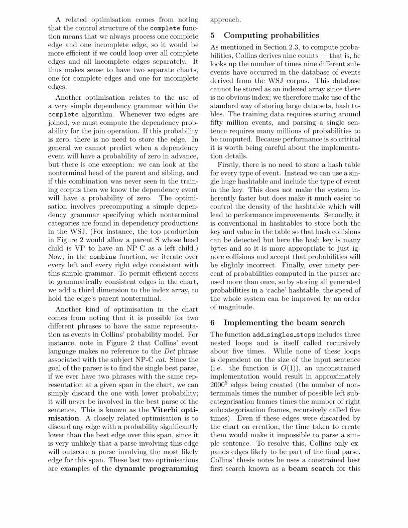
A related optimisation comes from notingthat the control structure of the complete func-tion means that we always process one completeedge and one incomplete edge, so it would bemore e!cient if we could loop over all completeedges and all incomplete edges separately. Itthus makes sense to have two separate charts,one for complete edges and one for incompleteedges.
Another optimisation relates to the use ofa very simple dependency grammar within thecomplete algorithm. Whenever two edges arejoined, we must compute the dependency prob-ability for the join operation. If this probabilityis zero, there is no need to store the edge. Ingeneral we cannot predict when a dependencyevent will have a probability of zero in advance,but there is one exception: we can look at thenonterminal head of the parent and sibling, andif this combination was never seen in the train-ing corpus then we know the dependency eventwill have a probability of zero. The optimi-sation involves precomputing a simple depen-dency grammar specifying which nonterminalcategories are found in dependency productionsin the WSJ. (For instance, the top productionin Figure 2 would allow a parent S whose headchild is VP to have an NP-C as a left child.)Now, in the combine function, we iterate overevery left and every right edge consistent withthis simple grammar. To permit e!cient accessto grammatically consistent edges in the chart,we add a third dimension to the index array, tohold the edge’s parent nonterminal.
Another kind of optimisation in the chartcomes from noting that it is possible for twodi"erent phrases to have the same representa-tion as events in Collins’ probability model. Forinstance, note in Figure 2 that Collins’ eventlanguage makes no reference to the Det phraseassociated with the subject NP-C cat. Since thegoal of the parser is to find the single best parse,if we ever have two phrases with the same rep-resentation at a given span in the chart, we cansimply discard the one with lower probability;it will never be involved in the best parse of thesentence. This is known as the Viterbi opti-misation. A closely related optimisation is todiscard any edge with a probability significantlylower than the best edge over this span, since itis very unlikely that a parse involving this edgewill outscore a parse involving the most likelyedge for this span. These last two optimisationsare examples of the dynamic programming
approach.
5 Computing probabilities
As mentioned in Section 2.3, to compute proba-bilities, Collins derives nine counts — that is, helooks up the number of times nine di"erent sub-events have occurred in the database of eventsderived from the WSJ corpus. This databasecannot be stored as an indexed array since thereis no obvious index; we therefore make use of thestandard way of storing large data sets, hash ta-bles. The training data requires storing aroundfifty million events, and parsing a single sen-tence requires many millions of probabilities tobe computed. Because performance is so criticalit is worth being careful about the implementa-tion details.
Firstly, there is no need to store a hash tablefor every type of event. Instead we can use a sin-gle huge hashtable and include the type of eventin the key. This does not make the system in-herently faster but does make it much easier tocontrol the density of the hashtable which willlead to performance improvements. Secondly, itis conventional in hashtables to store both thekey and value in the table so that hash collisionscan be detected but here the hash key is manybytes and so it is more appropriate to just ig-nore collisions and accept that probabilities willbe slightly incorrect. Finally, over ninety per-cent of probabilities computed in the parser areused more than once, so by storing all generatedprobabilities in a ‘cache’ hashtable, the speed ofthe whole system can be improved by an orderof magnitude.
6 Implementing the beam search
The function add singles stops includes threenested loops and is itself called recursivelyabout five times. While none of these loopsis dependent on the size of the input sentence(i.e. the function is O(1)), an unconstrainedimplementation would result in approximately20005 edges being created (the number of non-terminals times the number of possible left sub-categorisation frames times the number of rightsubcategorisation frames, recursively called fivetimes). Even if these edges were discarded bythe chart on creation, the time taken to createthem would make it impossible to parse a sim-ple sentence. To resolve this, Collins only ex-pands edges likely to be part of the final parse.Collins’ thesis notes he uses a constrained bestfirst search known as a beam search for this
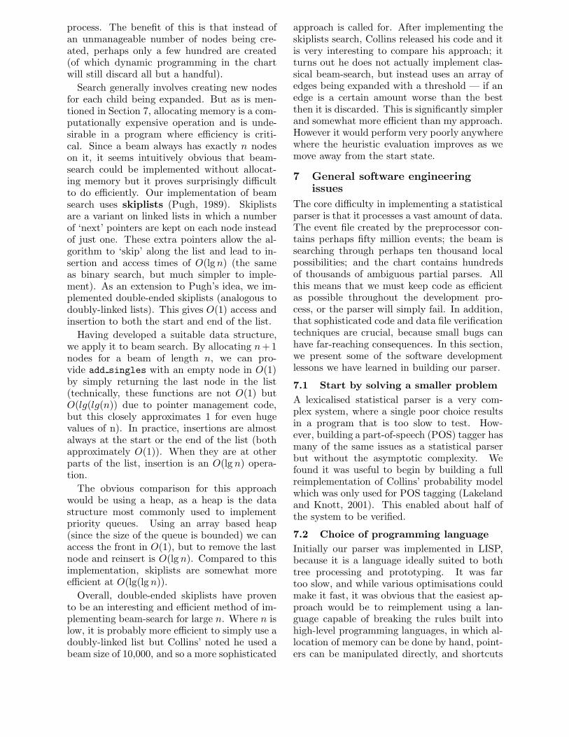
process. The benefit of this is that instead ofan unmanageable number of nodes being cre-ated, perhaps only a few hundred are created(of which dynamic programming in the chartwill still discard all but a handful).
Search generally involves creating new nodesfor each child being expanded. But as is men-tioned in Section 7, allocating memory is a com-putationally expensive operation and is unde-sirable in a program where e!ciency is criti-cal. Since a beam always has exactly n nodeson it, it seems intuitively obvious that beam-search could be implemented without allocat-ing memory but it proves surprisingly di!cultto do e!ciently. Our implementation of beamsearch uses skiplists (Pugh, 1989). Skiplistsare a variant on linked lists in which a numberof ‘next’ pointers are kept on each node insteadof just one. These extra pointers allow the al-gorithm to ‘skip’ along the list and lead to in-sertion and access times of O(lg n) (the sameas binary search, but much simpler to imple-ment). As an extension to Pugh’s idea, we im-plemented double-ended skiplists (analogous todoubly-linked lists). This gives O(1) access andinsertion to both the start and end of the list.
Having developed a suitable data structure,we apply it to beam search. By allocating n+1nodes for a beam of length n, we can pro-vide add singles with an empty node in O(1)by simply returning the last node in the list(technically, these functions are not O(1) butO(lg(lg(n)) due to pointer management code,but this closely approximates 1 for even hugevalues of n). In practice, insertions are almostalways at the start or the end of the list (bothapproximately O(1)). When they are at otherparts of the list, insertion is an O(lg n) opera-tion.
The obvious comparison for this approachwould be using a heap, as a heap is the datastructure most commonly used to implementpriority queues. Using an array based heap(since the size of the queue is bounded) we canaccess the front in O(1), but to remove the lastnode and reinsert is O(lg n). Compared to thisimplementation, skiplists are somewhat moree!cient at O(lg(lg n)).
Overall, double-ended skiplists have provento be an interesting and e!cient method of im-plementing beam-search for large n. Where n islow, it is probably more e!cient to simply use adoubly-linked list but Collins’ noted he used abeam size of 10,000, and so a more sophisticated
approach is called for. After implementing theskiplists search, Collins released his code and itis very interesting to compare his approach; itturns out he does not actually implement clas-sical beam-search, but instead uses an array ofedges being expanded with a threshold — if anedge is a certain amount worse than the bestthen it is discarded. This is significantly simplerand somewhat more e!cient than my approach.However it would perform very poorly anywherewhere the heuristic evaluation improves as wemove away from the start state.
7 General software engineeringissues
The core di!culty in implementing a statisticalparser is that it processes a vast amount of data.The event file created by the preprocessor con-tains perhaps fifty million events; the beam issearching through perhaps ten thousand localpossibilities; and the chart contains hundredsof thousands of ambiguous partial parses. Allthis means that we must keep code as e!cientas possible throughout the development pro-cess, or the parser will simply fail. In addition,that sophisticated code and data file verificationtechniques are crucial, because small bugs canhave far-reaching consequences. In this section,we present some of the software developmentlessons we have learned in building our parser.
7.1 Start by solving a smaller problem
A lexicalised statistical parser is a very com-plex system, where a single poor choice resultsin a program that is too slow to test. How-ever, building a part-of-speech (POS) tagger hasmany of the same issues as a statistical parserbut without the asymptotic complexity. Wefound it was useful to begin by building a fullreimplementation of Collins’ probability modelwhich was only used for POS tagging (Lakelandand Knott, 2001). This enabled about half ofthe system to be verified.
7.2 Choice of programming language
Initially our parser was implemented in LISP,because it is a language ideally suited to bothtree processing and prototyping. It was fartoo slow, and while various optimisations couldmake it fast, it was obvious that the easiest ap-proach would be to reimplement using a lan-guage capable of breaking the rules built intohigh-level programming languages, in which al-location of memory can be done by hand, point-ers can be manipulated directly, and shortcuts
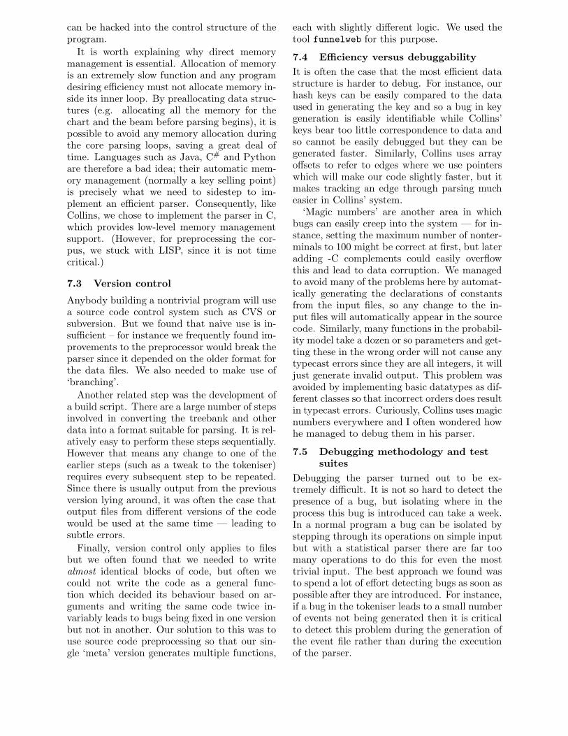
can be hacked into the control structure of theprogram.
It is worth explaining why direct memorymanagement is essential. Allocation of memoryis an extremely slow function and any programdesiring e!ciency must not allocate memory in-side its inner loop. By preallocating data struc-tures (e.g. allocating all the memory for thechart and the beam before parsing begins), it ispossible to avoid any memory allocation duringthe core parsing loops, saving a great deal oftime. Languages such as Java, C# and Pythonare therefore a bad idea; their automatic mem-ory management (normally a key selling point)is precisely what we need to sidestep to im-plement an e!cient parser. Consequently, likeCollins, we chose to implement the parser in C,which provides low-level memory managementsupport. (However, for preprocessing the cor-pus, we stuck with LISP, since it is not timecritical.)
7.3 Version control
Anybody building a nontrivial program will usea source code control system such as CVS orsubversion. But we found that naive use is in-su!cient – for instance we frequently found im-provements to the preprocessor would break theparser since it depended on the older format forthe data files. We also needed to make use of‘branching’.
Another related step was the development ofa build script. There are a large number of stepsinvolved in converting the treebank and otherdata into a format suitable for parsing. It is rel-atively easy to perform these steps sequentially.However that means any change to one of theearlier steps (such as a tweak to the tokeniser)requires every subsequent step to be repeated.Since there is usually output from the previousversion lying around, it was often the case thatoutput files from di"erent versions of the codewould be used at the same time — leading tosubtle errors.
Finally, version control only applies to filesbut we often found that we needed to writealmost identical blocks of code, but often wecould not write the code as a general func-tion which decided its behaviour based on ar-guments and writing the same code twice in-variably leads to bugs being fixed in one versionbut not in another. Our solution to this was touse source code preprocessing so that our sin-gle ‘meta’ version generates multiple functions,
each with slightly di"erent logic. We used thetool funnelweb for this purpose.
7.4 E"ciency versus debuggability
It is often the case that the most e!cient datastructure is harder to debug. For instance, ourhash keys can be easily compared to the dataused in generating the key and so a bug in keygeneration is easily identifiable while Collins’keys bear too little correspondence to data andso cannot be easily debugged but they can begenerated faster. Similarly, Collins uses arrayo"sets to refer to edges where we use pointerswhich will make our code slightly faster, but itmakes tracking an edge through parsing mucheasier in Collins’ system.
‘Magic numbers’ are another area in whichbugs can easily creep into the system — for in-stance, setting the maximum number of nonter-minals to 100 might be correct at first, but lateradding -C complements could easily overflowthis and lead to data corruption. We managedto avoid many of the problems here by automat-ically generating the declarations of constantsfrom the input files, so any change to the in-put files will automatically appear in the sourcecode. Similarly, many functions in the probabil-ity model take a dozen or so parameters and get-ting these in the wrong order will not cause anytypecast errors since they are all integers, it willjust generate invalid output. This problem wasavoided by implementing basic datatypes as dif-ferent classes so that incorrect orders does resultin typecast errors. Curiously, Collins uses magicnumbers everywhere and I often wondered howhe managed to debug them in his parser.
7.5 Debugging methodology and testsuites
Debugging the parser turned out to be ex-tremely di!cult. It is not so hard to detect thepresence of a bug, but isolating where in theprocess this bug is introduced can take a week.In a normal program a bug can be isolated bystepping through its operations on simple inputbut with a statistical parser there are far toomany operations to do this for even the mosttrivial input. The best approach we found wasto spend a lot of e"ort detecting bugs as soon aspossible after they are introduced. For instance,if a bug in the tokeniser leads to a small numberof events not being generated then it is criticalto detect this problem during the generation ofthe event file rather than during the executionof the parser.
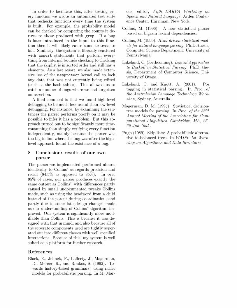
In order to facilitate this, after testing ev-ery function we wrote an automated test suitethat rechecks functions every time the systemis built. For example, the probability modelcan be checked by comparing the counts it de-rives to those produced with grep. If a bugis later introduced in the input to this func-tion then it will likely cause some testcase tofail. Similarly, the system is liberally scatteredwith assert statements that perform every-thing from internal bounds checking to checkingthat the skiplist is in sorted order and still has nelements. As a last resort, we also made exten-sive use of the memprotect kernel call to lockany data that was not currently being edited(such as the hash tables). This allowed us tocatch a number of bugs where we had forgottenan assertion.
A final comment is that we found high-leveldebugging to be much less useful than low-leveldebugging. For instance, by examining the sen-tences the parser performs poorly on it may bepossible to infer it has a problem. But this ap-proach turned out to be significantly more time-consuming than simply verifying every functionindependently, mainly because the parser wastoo big to find where the bug was after the high-level approach found the existence of a bug.
8 Conclusion: results of our ownparser
The parser we implemented performed almostidentically to Collins’ as regards precision andrecall (84.5% as opposed to 85%). In over95% of cases, our parser produces exactly thesame output as Collins’, with di"erences partlycaused by small undocumented tweaks Collinsmade, such as using the headword from a childinstead of the parent during coordination, andpartly due to some late design changes madeas our understanding of Collins’ algorithm im-proved. Our system is significantly more mod-ifiable than Collins. This is because it was de-signed with that in mind, and also because all ofthe seperate components used are tightly seper-ated out into di"erent classes with well specifiedinteractions. Because of this, my system is wellsuited as a platform for further research.
References
Black, E., Jelinek, F., La"erty, J., Magerman,D., Mercer, R., and Roukos, S. (1992). To-wards history-based grammars: using richermodels for probabilistic parsing. In M. Mar-
cus, editor, Fifth DARPA Workshop onSpeech and Natural Language, Arden Confer-ence Center, Harriman, New York.
Collins, M. (1996). A new statistical parserbased on bigram lexical dependencies.
Collins, M. (1999). Head-driven statistical mod-els for natural language parsing. Ph.D. thesis,Computer Science Department, University ofPennsylvania.
Lakeland, C. (forthcoming). Lexical Approachesto Backo" in Statistical Parsing. Ph.D. the-sis, Department of Computer Science, Uni-versity of Otago.
Lakeland, C. and Knott, A. (2001). Postagging in statistical parsing. In Proc. ofthe Australasian Language Technology Work-shop, Sydney, Australia.
Magerman, D. M. (1995). Statistical decision-tree models for parsing. In Proc. of the 33 rd
Annual Meeting of the Association for Com-putational Linguistics. Cambridge, MA, 26–30 Jun 1995 .
Pugh (1989). Skip lists: A probabilistic alterna-tive to balanced trees. In WADS: 1st Work-shop on Algorithms and Data Structures.
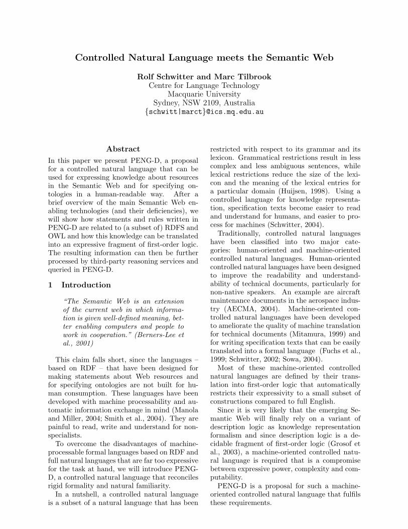
Controlled Natural Language meets the Semantic Web
Rolf Schwitter and Marc TilbrookCentre for Language Technology
Macquarie UniversitySydney, NSW 2109, Australia
{schwitt|marct}@ics.mq.edu.au
Abstract
In this paper we present PENG-D, a proposalfor a controlled natural language that can beused for expressing knowledge about resourcesin the Semantic Web and for specifying on-tologies in a human-readable way. After abrief overview of the main Semantic Web en-abling technologies (and their deficiencies), wewill show how statements and rules written inPENG-D are related to (a subset of) RDFS andOWL and how this knowledge can be translatedinto an expressive fragment of first-order logic.The resulting information can then be furtherprocessed by third-party reasoning services andqueried in PENG-D.
1 Introduction
“The Semantic Web is an extensionof the current web in which informa-tion is given well-defined meaning, bet-ter enabling computers and people towork in cooperation.” (Berners-Lee etal., 2001)
This claim falls short, since the languages –based on RDF – that have been designed formaking statements about Web resources andfor specifying ontologies are not built for hu-man consumption. These languages have beendeveloped with machine processability and au-tomatic information exchange in mind (Manolaand Miller, 2004; Smith et al., 2004). They arepainful to read, write and understand for non-specialists.
To overcome the disadvantages of machine-processable formal languages based on RDF andfull natural languages that are far too expressivefor the task at hand, we will introduce PENG-D, a controlled natural language that reconcilesrigid formality and natural familiarity.
In a nutshell, a controlled natural languageis a subset of a natural language that has been
restricted with respect to its grammar and itslexicon. Grammatical restrictions result in lesscomplex and less ambiguous sentences, whilelexical restrictions reduce the size of the lexi-con and the meaning of the lexical entries fora particular domain (Huijsen, 1998). Using acontrolled language for knowledge representa-tion, specification texts become easier to readand understand for humans, and easier to pro-cess for machines (Schwitter, 2004).
Traditionally, controlled natural languageshave been classified into two major cate-gories: human-oriented and machine-orientedcontrolled natural languages. Human-orientedcontrolled natural languages have been designedto improve the readability and understand-ability of technical documents, particularly fornon-native speakers. An example are aircraftmaintenance documents in the aerospace indus-try (AECMA, 2004). Machine-oriented con-trolled natural languages have been developedto ameliorate the quality of machine translationfor technical documents (Mitamura, 1999) andfor writing specification texts that can be easilytranslated into a formal language (Fuchs et al.,1999; Schwitter, 2002; Sowa, 2004).
Most of these machine-oriented controllednatural languages are defined by their trans-lation into first-order logic that automaticallyrestricts their expressivity to a small subset ofconstructions compared to full English.
Since it is very likely that the emerging Se-mantic Web will finally rely on a variant ofdescription logic as knowledge representationformalism and since description logic is a de-cidable fragment of first-order logic (Grosof etal., 2003), a machine-oriented controlled natu-ral language is required that is a compromisebetween expressive power, complexity and com-putability.
PENG-D is a proposal for such a machine-oriented controlled natural language that fulfilsthese requirements.
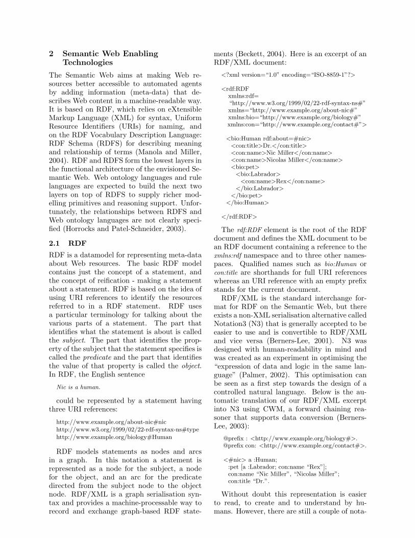
2 Semantic Web EnablingTechnologies
The Semantic Web aims at making Web re-sources better accessible to automated agentsby adding information (meta-data) that de-scribes Web content in a machine-readable way.It is based on RDF, which relies on eXtensibleMarkup Language (XML) for syntax, UniformResource Identifiers (URIs) for naming, andon the RDF Vocabulary Description Language:RDF Schema (RDFS) for describing meaningand relationship of terms (Manola and Miller,2004). RDF and RDFS form the lowest layers inthe functional architecture of the envisioned Se-mantic Web. Web ontology languages and rulelanguages are expected to build the next twolayers on top of RDFS to supply richer mod-elling primitives and reasoning support. Unfor-tunately, the relationships between RDFS andWeb ontology languages are not clearly speci-fied (Horrocks and Patel-Schneider, 2003).
2.1 RDFRDF is a datamodel for representing meta-dataabout Web resources. The basic RDF modelcontains just the concept of a statement, andthe concept of reification - making a statementabout a statement. RDF is based on the idea ofusing URI references to identify the resourcesreferred to in a RDF statement. RDF usesa particular terminology for talking about thevarious parts of a statement. The part thatidentifies what the statement is about is calledthe subject. The part that identifies the prop-erty of the subject that the statement specifies iscalled the predicate and the part that identifiesthe value of that property is called the object.In RDF, the English sentence
Nic is a human.
could be represented by a statement havingthree URI references:
http://www.example.org/about-nic#nichttp://www.w3.org/1999/02/22-rdf-syntax-ns#typehttp://www.example.org/biology#Human
RDF models statements as nodes and arcsin a graph. In this notation a statement isrepresented as a node for the subject, a nodefor the object, and an arc for the predicatedirected from the subject node to the objectnode. RDF/XML is a graph serialisation syn-tax and provides a machine-processable way torecord and exchange graph-based RDF state-
ments (Beckett, 2004). Here is an excerpt of anRDF/XML document:
<?xml version=“1.0” encoding=“ISO-8859-1”?>
<rdf:RDFxmlns:rdf=“http://www.w3.org/1999/02/22-rdf-syntax-ns#”xmlns=“http://www.example.org/about-nic#”xmlns:bio=“http://www.example.org/biology#”xmlns:con=“http://www.example.org/contact#”>
<bio:Human rdf:about=#nic><con:title>Dr.</con:title><con:name>Nic Miller</con:name><con:name>Nicolas Miller</con:name><bio:pet>
<bio:Labrador><con:name>Rex</con:name>
</bio:Labrador></bio:pet>
</bio:Human>
</rdf:RDF>
The rdf:RDF element is the root of the RDFdocument and defines the XML document to bean RDF document containing a reference to thexmlns:rdf namespace and to three other names-paces. Qualified names such as bio:Human orcon:title are shorthands for full URI referenceswhereas an URI reference with an empty prefixstands for the current document.
RDF/XML is the standard interchange for-mat for RDF on the Semantic Web, but thereexists a non-XML serialisation alternative calledNotation3 (N3) that is generally accepted to beeasier to use and is convertible to RDF/XMLand vice versa (Berners-Lee, 2001). N3 wasdesigned with human-readability in mind andwas created as an experiment in optimising the“expression of data and logic in the same lan-guage” (Palmer, 2002). This optimisation canbe seen as a first step towards the design of acontrolled natural language. Below is the au-tomatic translation of our RDF/XML excerptinto N3 using CWM, a forward chaining rea-soner that supports data conversion (Berners-Lee, 2003):
@prefix : <http://www.example.org/biology#>.@prefix con: <http://www.example.org/contact#>.
<#nic> a :Human;:pet [a :Labrador; con:name “Rex”];con:name “Nic Miller”, “Nicolas Miller”;con:title “Dr.”.
Without doubt this representation is easierto read, to create and to understand by hu-mans. However, there are still a couple of nota-
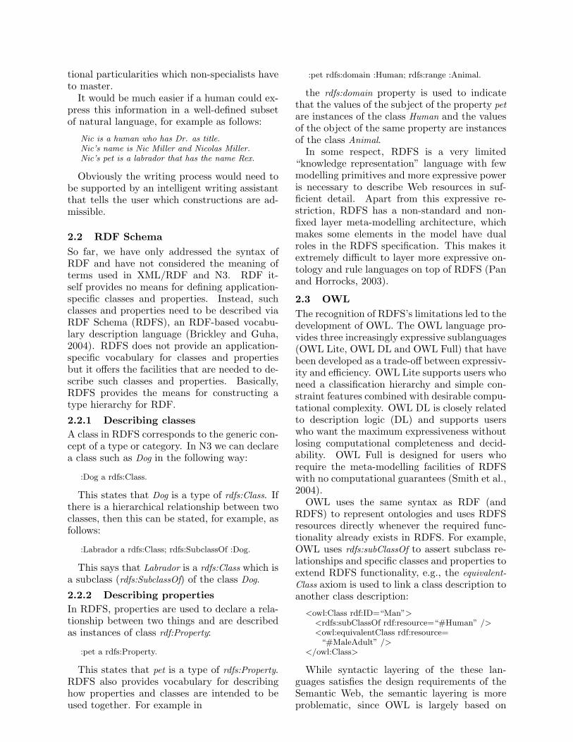
tional particularities which non-specialists haveto master.
It would be much easier if a human could ex-press this information in a well-defined subsetof natural language, for example as follows:
Nic is a human who has Dr. as title.Nic’s name is Nic Miller and Nicolas Miller.Nic’s pet is a labrador that has the name Rex.
Obviously the writing process would need tobe supported by an intelligent writing assistantthat tells the user which constructions are ad-missible.
2.2 RDF SchemaSo far, we have only addressed the syntax ofRDF and have not considered the meaning ofterms used in XML/RDF and N3. RDF it-self provides no means for defining application-specific classes and properties. Instead, suchclasses and properties need to be described viaRDF Schema (RDFS), an RDF-based vocabu-lary description language (Brickley and Guha,2004). RDFS does not provide an application-specific vocabulary for classes and propertiesbut it o!ers the facilities that are needed to de-scribe such classes and properties. Basically,RDFS provides the means for constructing atype hierarchy for RDF.2.2.1 Describing classesA class in RDFS corresponds to the generic con-cept of a type or category. In N3 we can declarea class such as Dog in the following way:
:Dog a rdfs:Class.
This states that Dog is a type of rdfs:Class. Ifthere is a hierarchical relationship between twoclasses, then this can be stated, for example, asfollows:
:Labrador a rdfs:Class; rdfs:SubclassOf :Dog.
This says that Labrador is a rdfs:Class which isa subclass (rdfs:SubclassOf) of the class Dog.2.2.2 Describing propertiesIn RDFS, properties are used to declare a rela-tionship between two things and are describedas instances of class rdf:Property:
:pet a rdfs:Property.
This states that pet is a type of rdfs:Property.RDFS also provides vocabulary for describinghow properties and classes are intended to beused together. For example in
:pet rdfs:domain :Human; rdfs:range :Animal.
the rdfs:domain property is used to indicatethat the values of the subject of the property petare instances of the class Human and the valuesof the object of the same property are instancesof the class Animal.
In some respect, RDFS is a very limited“knowledge representation” language with fewmodelling primitives and more expressive poweris necessary to describe Web resources in suf-ficient detail. Apart from this expressive re-striction, RDFS has a non-standard and non-fixed layer meta-modelling architecture, whichmakes some elements in the model have dualroles in the RDFS specification. This makes itextremely di"cult to layer more expressive on-tology and rule languages on top of RDFS (Panand Horrocks, 2003).
2.3 OWLThe recognition of RDFS’s limitations led to thedevelopment of OWL. The OWL language pro-vides three increasingly expressive sublanguages(OWL Lite, OWL DL and OWL Full) that havebeen developed as a trade-o! between expressiv-ity and e"ciency. OWL Lite supports users whoneed a classification hierarchy and simple con-straint features combined with desirable compu-tational complexity. OWL DL is closely relatedto description logic (DL) and supports userswho want the maximum expressiveness withoutlosing computational completeness and decid-ability. OWL Full is designed for users whorequire the meta-modelling facilities of RDFSwith no computational guarantees (Smith et al.,2004).
OWL uses the same syntax as RDF (andRDFS) to represent ontologies and uses RDFSresources directly whenever the required func-tionality already exists in RDFS. For example,OWL uses rdfs:subClassOf to assert subclass re-lationships and specific classes and properties toextend RDFS functionality, e.g., the equivalent-Class axiom is used to link a class description toanother class description:
<owl:Class rdf:ID=“Man”><rdfs:subClassOf rdf:resource=“#Human” /><owl:equivalentClass rdf:resource=
“#MaleAdult” /></owl:Class>
While syntactic layering of the these lan-guages satisfies the design requirements of theSemantic Web, the semantic layering is moreproblematic, since OWL is largely based on
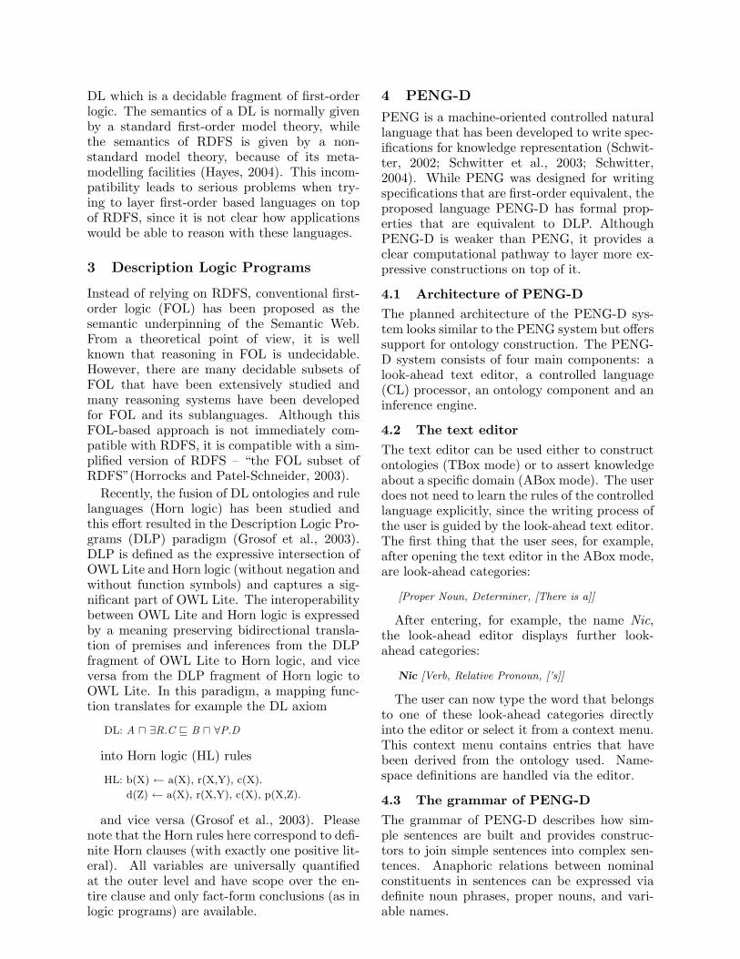
DL which is a decidable fragment of first-orderlogic. The semantics of a DL is normally givenby a standard first-order model theory, whilethe semantics of RDFS is given by a non-standard model theory, because of its meta-modelling facilities (Hayes, 2004). This incom-patibility leads to serious problems when try-ing to layer first-order based languages on topof RDFS, since it is not clear how applicationswould be able to reason with these languages.
3 Description Logic Programs
Instead of relying on RDFS, conventional first-order logic (FOL) has been proposed as thesemantic underpinning of the Semantic Web.From a theoretical point of view, it is wellknown that reasoning in FOL is undecidable.However, there are many decidable subsets ofFOL that have been extensively studied andmany reasoning systems have been developedfor FOL and its sublanguages. Although thisFOL-based approach is not immediately com-patible with RDFS, it is compatible with a sim-plified version of RDFS – “the FOL subset ofRDFS”(Horrocks and Patel-Schneider, 2003).
Recently, the fusion of DL ontologies and rulelanguages (Horn logic) has been studied andthis e!ort resulted in the Description Logic Pro-grams (DLP) paradigm (Grosof et al., 2003).DLP is defined as the expressive intersection ofOWL Lite and Horn logic (without negation andwithout function symbols) and captures a sig-nificant part of OWL Lite. The interoperabilitybetween OWL Lite and Horn logic is expressedby a meaning preserving bidirectional transla-tion of premises and inferences from the DLPfragment of OWL Lite to Horn logic, and viceversa from the DLP fragment of Horn logic toOWL Lite. In this paradigm, a mapping func-tion translates for example the DL axiom
DL: A ! "R.C # B ! $P.D
into Horn logic (HL) rules
HL: b(X) % a(X), r(X,Y), c(X).
d(Z) % a(X), r(X,Y), c(X), p(X,Z).
and vice versa (Grosof et al., 2003). Pleasenote that the Horn rules here correspond to defi-nite Horn clauses (with exactly one positive lit-eral). All variables are universally quantifiedat the outer level and have scope over the en-tire clause and only fact-form conclusions (as inlogic programs) are available.
4 PENG-D
PENG is a machine-oriented controlled naturallanguage that has been developed to write spec-ifications for knowledge representation (Schwit-ter, 2002; Schwitter et al., 2003; Schwitter,2004). While PENG was designed for writingspecifications that are first-order equivalent, theproposed language PENG-D has formal prop-erties that are equivalent to DLP. AlthoughPENG-D is weaker than PENG, it provides aclear computational pathway to layer more ex-pressive constructions on top of it.
4.1 Architecture of PENG-DThe planned architecture of the PENG-D sys-tem looks similar to the PENG system but o!erssupport for ontology construction. The PENG-D system consists of four main components: alook-ahead text editor, a controlled language(CL) processor, an ontology component and aninference engine.
4.2 The text editorThe text editor can be used either to constructontologies (TBox mode) or to assert knowledgeabout a specific domain (ABox mode). The userdoes not need to learn the rules of the controlledlanguage explicitly, since the writing process ofthe user is guided by the look-ahead text editor.The first thing that the user sees, for example,after opening the text editor in the ABox mode,are look-ahead categories:
[Proper Noun, Determiner, [There is a]]
After entering, for example, the name Nic,the look-ahead editor displays further look-ahead categories:
Nic [Verb, Relative Pronoun, [’s]]
The user can now type the word that belongsto one of these look-ahead categories directlyinto the editor or select it from a context menu.This context menu contains entries that havebeen derived from the ontology used. Name-space definitions are handled via the editor.
4.3 The grammar of PENG-DThe grammar of PENG-D describes how sim-ple sentences are built and provides construc-tors to join simple sentences into complex sen-tences. Anaphoric relations between nominalconstituents in sentences can be expressed viadefinite noun phrases, proper nouns, and vari-able names.
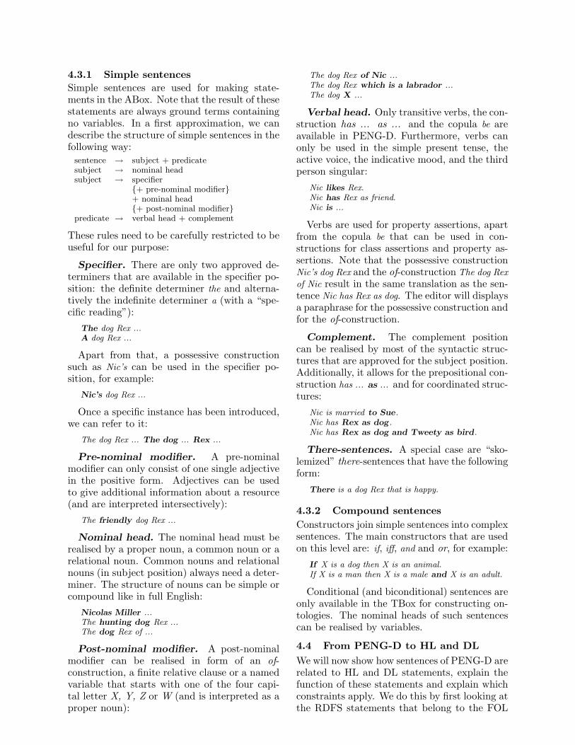
4.3.1 Simple sentencesSimple sentences are used for making state-ments in the ABox. Note that the result of thesestatements are always ground terms containingno variables. In a first approximation, we candescribe the structure of simple sentences in thefollowing way:
sentence & subject + predicatesubject & nominal headsubject & specifier
{+ pre-nominal modifier}+ nominal head{+ post-nominal modifier}
predicate & verbal head + complement
These rules need to be carefully restricted to beuseful for our purpose:
Specifier. There are only two approved de-terminers that are available in the specifier po-sition: the definite determiner the and alterna-tively the indefinite determiner a (with a “spe-cific reading”):
The dog Rex ...A dog Rex ...
Apart from that, a possessive constructionsuch as Nic’s can be used in the specifier po-sition, for example:
Nic’s dog Rex ...
Once a specific instance has been introduced,we can refer to it:
The dog Rex ... The dog ... Rex ...
Pre-nominal modifier. A pre-nominalmodifier can only consist of one single adjectivein the positive form. Adjectives can be usedto give additional information about a resource(and are interpreted intersectively):
The friendly dog Rex ...
Nominal head. The nominal head must berealised by a proper noun, a common noun or arelational noun. Common nouns and relationalnouns (in subject position) always need a deter-miner. The structure of nouns can be simple orcompound like in full English:
Nicolas Miller ...The hunting dog Rex ...The dog Rex of ...
Post-nominal modifier. A post-nominalmodifier can be realised in form of an of-construction, a finite relative clause or a namedvariable that starts with one of the four capi-tal letter X, Y, Z or W (and is interpreted as aproper noun):
The dog Rex of Nic ...The dog Rex which is a labrador ...The dog X ...
Verbal head. Only transitive verbs, the con-struction has ... as ... and the copula be areavailable in PENG-D. Furthermore, verbs canonly be used in the simple present tense, theactive voice, the indicative mood, and the thirdperson singular:
Nic likes Rex.Nic has Rex as friend.Nic is ...
Verbs are used for property assertions, apartfrom the copula be that can be used in con-structions for class assertions and property as-sertions. Note that the possessive constructionNic’s dog Rex and the of-construction The dog Rexof Nic result in the same translation as the sen-tence Nic has Rex as dog. The editor will displaysa paraphrase for the possessive construction andfor the of-construction.
Complement. The complement positioncan be realised by most of the syntactic struc-tures that are approved for the subject position.Additionally, it allows for the prepositional con-struction has ... as ... and for coordinated struc-tures:
Nic is married to Sue.Nic has Rex as dog.Nic has Rex as dog and Tweety as bird.
There-sentences. A special case are “sko-lemized” there-sentences that have the followingform:
There is a dog Rex that is happy.
4.3.2 Compound sentencesConstructors join simple sentences into complexsentences. The main constructors that are usedon this level are: if, i!, and and or, for example:
If X is a dog then X is an animal.If X is a man then X is a male and X is an adult.
Conditional (and biconditional) sentences areonly available in the TBox for constructing on-tologies. The nominal heads of such sentencescan be realised by variables.
4.4 From PENG-D to HL and DLWe will now show how sentences of PENG-D arerelated to HL and DL statements, explain thefunction of these statements and explain whichconstraints apply. We do this by first looking atthe RDFS statements that belong to the FOL
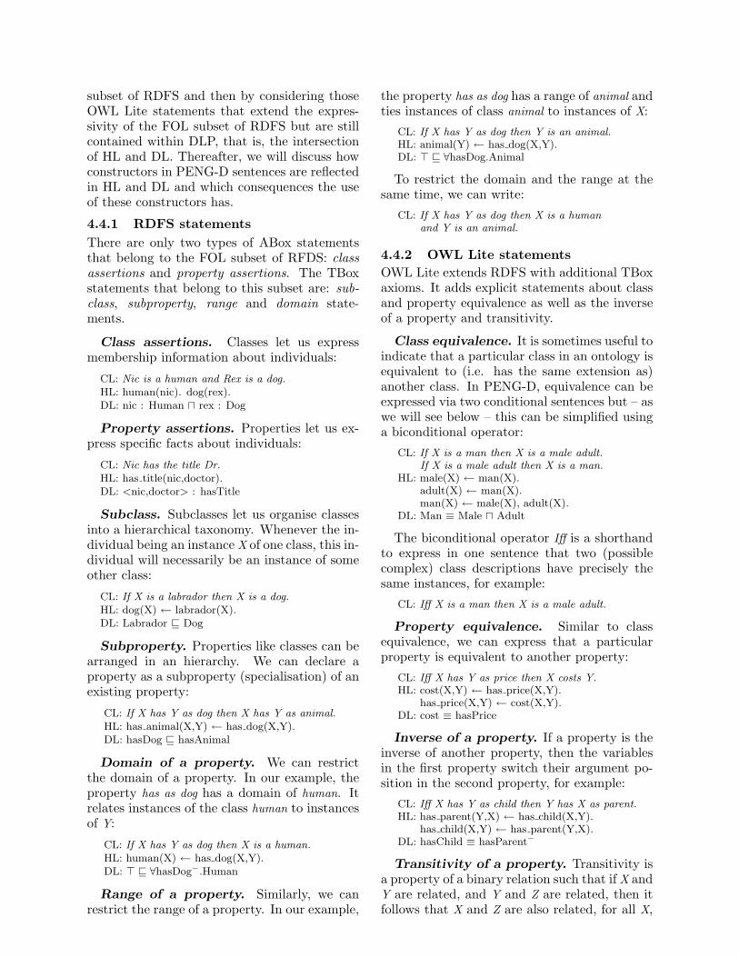
subset of RDFS and then by considering thoseOWL Lite statements that extend the expres-sivity of the FOL subset of RDFS but are stillcontained within DLP, that is, the intersectionof HL and DL. Thereafter, we will discuss howconstructors in PENG-D sentences are reflectedin HL and DL and which consequences the useof these constructors has.
4.4.1 RDFS statementsThere are only two types of ABox statementsthat belong to the FOL subset of RFDS: classassertions and property assertions. The TBoxstatements that belong to this subset are: sub-class, subproperty, range and domain state-ments.
Class assertions. Classes let us expressmembership information about individuals:
CL: Nic is a human and Rex is a dog.HL: human(nic). dog(rex).DL: nic : Human ! rex : Dog
Property assertions. Properties let us ex-press specific facts about individuals:
CL: Nic has the title Dr.HL: has title(nic,doctor).DL: <nic,doctor> : hasTitle
Subclass. Subclasses let us organise classesinto a hierarchical taxonomy. Whenever the in-dividual being an instance X of one class, this in-dividual will necessarily be an instance of someother class:
CL: If X is a labrador then X is a dog.HL: dog(X) % labrador(X).DL: Labrador # Dog
Subproperty. Properties like classes can bearranged in an hierarchy. We can declare aproperty as a subproperty (specialisation) of anexisting property:
CL: If X has Y as dog then X has Y as animal.HL: has animal(X,Y) % has dog(X,Y).DL: hasDog # hasAnimal
Domain of a property. We can restrictthe domain of a property. In our example, theproperty has as dog has a domain of human. Itrelates instances of the class human to instancesof Y:
CL: If X has Y as dog then X is a human.HL: human(X) % has dog(X,Y).DL: ' # $hasDog!.Human
Range of a property. Similarly, we canrestrict the range of a property. In our example,
the property has as dog has a range of animal andties instances of class animal to instances of X:
CL: If X has Y as dog then Y is an animal.HL: animal(Y) % has dog(X,Y).DL: ' # $hasDog.Animal
To restrict the domain and the range at thesame time, we can write:
CL: If X has Y as dog then X is a humanand Y is an animal.
4.4.2 OWL Lite statementsOWL Lite extends RDFS with additional TBoxaxioms. It adds explicit statements about classand property equivalence as well as the inverseof a property and transitivity.
Class equivalence. It is sometimes useful toindicate that a particular class in an ontology isequivalent to (i.e. has the same extension as)another class. In PENG-D, equivalence can beexpressed via two conditional sentences but – aswe will see below – this can be simplified usinga biconditional operator:
CL: If X is a man then X is a male adult.If X is a male adult then X is a man.
HL: male(X) % man(X).adult(X) % man(X).man(X) % male(X), adult(X).
DL: Man ( Male ! Adult
The biconditional operator I! is a shorthandto express in one sentence that two (possiblecomplex) class descriptions have precisely thesame instances, for example:
CL: I! X is a man then X is a male adult.
Property equivalence. Similar to classequivalence, we can express that a particularproperty is equivalent to another property:
CL: I! X has Y as price then X costs Y.HL: cost(X,Y) % has price(X,Y).
has price(X,Y) % cost(X,Y).DL: cost ( hasPrice
Inverse of a property. If a property is theinverse of another property, then the variablesin the first property switch their argument po-sition in the second property, for example:
CL: I! X has Y as child then Y has X as parent.HL: has parent(Y,X) % has child(X,Y).
has child(X,Y) % has parent(Y,X).DL: hasChild ( hasParent!
Transitivity of a property. Transitivity isa property of a binary relation such that if X andY are related, and Y and Z are related, then itfollows that X and Z are also related, for all X,
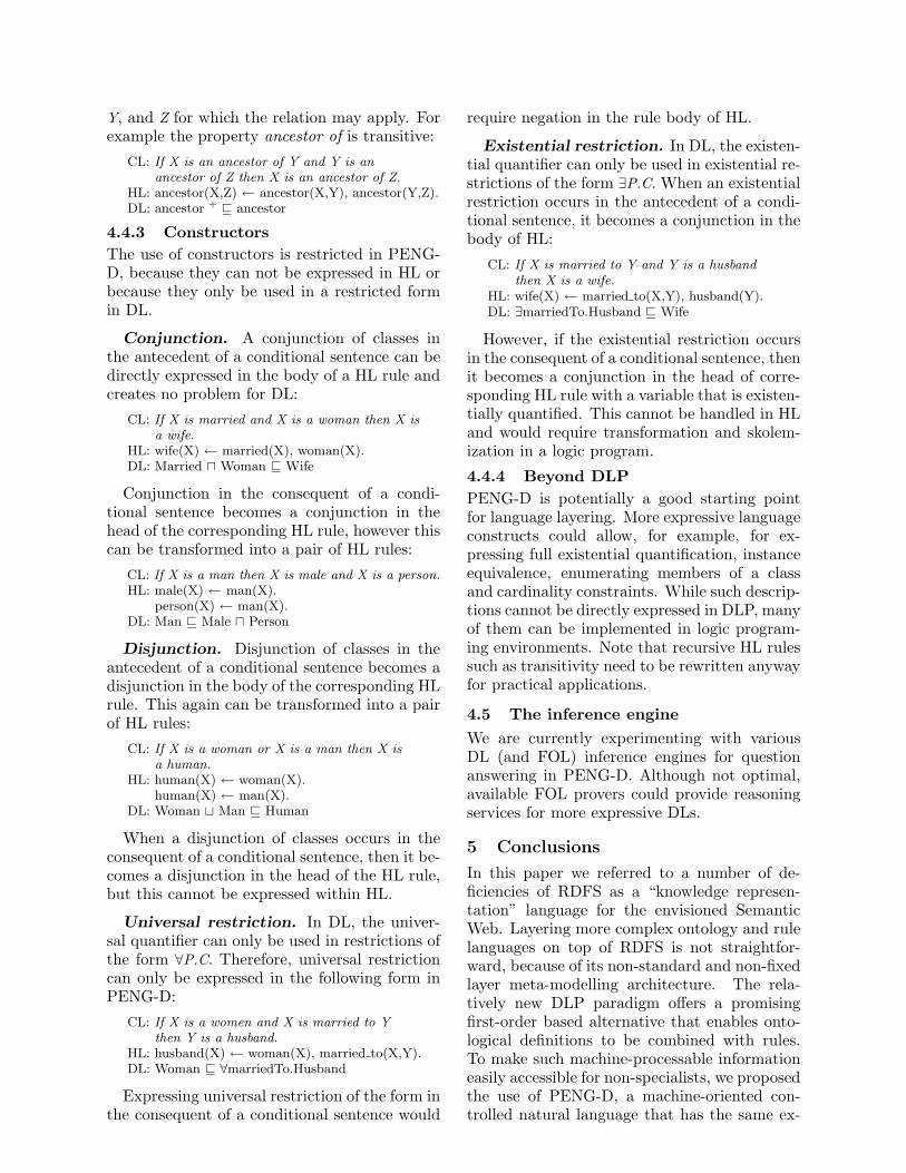
Y, and Z for which the relation may apply. Forexample the property ancestor of is transitive:
CL: If X is an ancestor of Y and Y is anancestor of Z then X is an ancestor of Z.
HL: ancestor(X,Z) % ancestor(X,Y), ancestor(Y,Z).DL: ancestor + # ancestor
4.4.3 ConstructorsThe use of constructors is restricted in PENG-D, because they can not be expressed in HL orbecause they only be used in a restricted formin DL.
Conjunction. A conjunction of classes inthe antecedent of a conditional sentence can bedirectly expressed in the body of a HL rule andcreates no problem for DL:
CL: If X is married and X is a woman then X isa wife.
HL: wife(X) % married(X), woman(X).DL: Married ! Woman # Wife
Conjunction in the consequent of a condi-tional sentence becomes a conjunction in thehead of the corresponding HL rule, however thiscan be transformed into a pair of HL rules:
CL: If X is a man then X is male and X is a person.HL: male(X) % man(X).
person(X) % man(X).DL: Man # Male ! Person
Disjunction. Disjunction of classes in theantecedent of a conditional sentence becomes adisjunction in the body of the corresponding HLrule. This again can be transformed into a pairof HL rules:
CL: If X is a woman or X is a man then X isa human.
HL: human(X) % woman(X).human(X) % man(X).
DL: Woman ) Man # Human
When a disjunction of classes occurs in theconsequent of a conditional sentence, then it be-comes a disjunction in the head of the HL rule,but this cannot be expressed within HL.
Universal restriction. In DL, the univer-sal quantifier can only be used in restrictions ofthe form !P.C. Therefore, universal restrictioncan only be expressed in the following form inPENG-D:
CL: If X is a women and X is married to Ythen Y is a husband.
HL: husband(X) % woman(X), married to(X,Y).DL: Woman # $marriedTo.Husband
Expressing universal restriction of the form inthe consequent of a conditional sentence would
require negation in the rule body of HL.
Existential restriction. In DL, the existen-tial quantifier can only be used in existential re-strictions of the form "P.C. When an existentialrestriction occurs in the antecedent of a condi-tional sentence, it becomes a conjunction in thebody of HL:
CL: If X is married to Y and Y is a husbandthen X is a wife.
HL: wife(X) % married to(X,Y), husband(Y).DL: "marriedTo.Husband # Wife
However, if the existential restriction occursin the consequent of a conditional sentence, thenit becomes a conjunction in the head of corre-sponding HL rule with a variable that is existen-tially quantified. This cannot be handled in HLand would require transformation and skolem-ization in a logic program.4.4.4 Beyond DLPPENG-D is potentially a good starting pointfor language layering. More expressive languageconstructs could allow, for example, for ex-pressing full existential quantification, instanceequivalence, enumerating members of a classand cardinality constraints. While such descrip-tions cannot be directly expressed in DLP, manyof them can be implemented in logic program-ing environments. Note that recursive HL rulessuch as transitivity need to be rewritten anywayfor practical applications.
4.5 The inference engineWe are currently experimenting with variousDL (and FOL) inference engines for questionanswering in PENG-D. Although not optimal,available FOL provers could provide reasoningservices for more expressive DLs.
5 Conclusions
In this paper we referred to a number of de-ficiencies of RDFS as a “knowledge represen-tation” language for the envisioned SemanticWeb. Layering more complex ontology and rulelanguages on top of RDFS is not straightfor-ward, because of its non-standard and non-fixedlayer meta-modelling architecture. The rela-tively new DLP paradigm o!ers a promisingfirst-order based alternative that enables onto-logical definitions to be combined with rules.To make such machine-processable informationeasily accessible for non-specialists, we proposedthe use of PENG-D, a machine-oriented con-trolled natural language that has the same ex-
pressivity as DLP. We expect that PENG-Dis easy to write for non-specialists with thehelp of a look-ahead text editor, easy to readin contrast to RDF-based notations, and easyto translated into a corresponding machine-processable format. In brief: PENG-D hasthe potential for complementing these moremachine-oriented notations.
Acknowledgments
The research reported here is supported by theAustralian Research Council (Discovery ProjectDP0449928). The authors would also like tothank two anonymous reviewers for the valuablecomments on a previous version of this paper.
References
AECMA. 2004. The European Associationof Aerospace Industries. AECMA SimplifiedEnglish, AECMA Document PSC-85-16598.A Guide for the Preparation of Aircraft Main-tenance Documentation in the InternationalAerospace Maintenance Language. Issue 2,January 15.
D. Beckett (ed). 2004. RDF/XML Syn-tax Specification (Revised). W3C Recom-mendation 10 February 2004. <http://www.w3.org/TR/rdf-syntax-grammar/>.
T. Berners-Lee, J. Hendler, Ora Lassila. 2001.The Semantic Web. In: Scientific American.May 17.
T. Berners-Lee. 2001. Notation 3. An RDFlanguage for the Semantic Web. <http://www.w3.org/DesignIssues/Notation3.html>.
T. Berners-Lee. 2003. Processing your datausing N3 and CWM. <http://www.w3.org/2000/10/swap/doc/Processing>.
D. Brickley, R. V. Guha. 2004. RDF Vocabu-lary Description Language 1.0: RDF Schema.W3C Recommendation 10 February 2004.<http://www.w3.org/TR/rdf-schema/>.
N. E. Fuchs, U. Schwertel, and R. Schwit-ter. 1999. Attempto Controlled English -Not Just Another Logic Specification Lan-guage. Lecture Notes in Computer Science1559, Springer, pp. 1-20.
B. N. Grosof, I. Horrocks, R. Volz, S. Decker.2003. Description logic programs: Combin-ing logic programs with description logic.In: Proceedings of the Twelfth InternationalWorld Wide Web Conference (WWW 2003),pp. 48-57.
P. Hayes. 2004. RDF Semantics. W3C Recom-
mendation 10 February 2004. <http://www.w3.org/TR/2004/REC-rdf-mt-20040210/>.
I. Horrocks, P. F. Patel-Schneider. 2003. Threetheses of representation in the semantic web.In: Proceedings of the Twelfth InternationalWorld Wide Web Conference (WWW 2003),pp. 39-47.
W. O. Huijsen. 1998. Controlled Language -An Introduction. In: Proceedings of CLAW1998. Pittsburgh, pp. 1-15.
F. Manola, E. Miller. 2004. RDF Primer.W3C Recommendation 10 February 2004.<http://www.w3.org/TR/rdf-primer/>.
T. Mitamura. 1999. Controlled Language forMultilingual Machine Translation. Invitedpaper. In: Proceedings of Machine Transla-tion Summit VII. Singapore, September 13-17. <http://www.lti.cs.cmu.edu/Research/Kant/>.
S. Palmer. 2002. A Rough Guide to Notation3.<http://infomesh.net/2002/notation3/>.
J. Z. Pan, I. Horrocks. 2003. RDFS(FA): A DL-ised Sub-language of RDFS. : In Proceedingsof the 2003 Description Logic Workshop (DL2003), volume 81 of CEUR, pp. 95-102.
R. Schwitter. 2002. English as a FormalSpecification Language. In: Proceedings ofthe Thirdteenth International Workshop onDatabase and Expert Systems Applications(DEXA 2002). Aix-en-Provence, pp. 228–232.
R. Schwitter, A. Ljungberg, and D. Hood. 2003.ECOLE: A Look-ahead Editor for a Con-trolled Language. In: Proceedings of EAMT-CLAW03, Controlled Language Translation.May 15-17, Dublin City University, pp. 141–150.
R. Schwitter. 2004. Representing Knowledge inControlled Natrual Language: A Case Study.In: M. G. Negoita, R. J. Howlett, L. C.Jain (eds.), Proceedings KES2004, Part I,Springer LNAI 3213, pp. 711-717.
M. K. Smith, C. Welty, D. L. Mc Guin-ness. 2004. OWL Web Ontology Language.Guide. W3C Recommendation 10 February2004. <http://www.w3.org/TR/2004/REC-owl-guide-20040210/>.
J. F. Sowa. 2004. Common Logic ControlledEnglish Draft, 24 February 2004. <http://www.jfsowa.com/clce/specs.htm>.
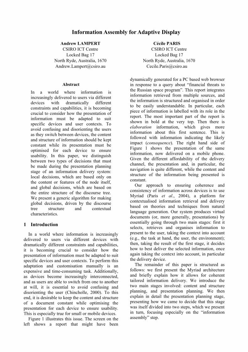
Information Assembly for Adaptive Display
Andrew LAMPERT CSIRO ICT Centre
Locked Bag 17 North Ryde, Australia, 1670 [email protected]
Cécile PARIS CSIRO ICT Centre
Locked Bag 17 North Ryde, Australia, 1670
Abstract
In a world where information is increasingly delivered to users via different devices with dramatically different constraints and capabilities, it is becoming crucial to consider how the presentation of information must be adapted to suit specific devices and user contexts. To avoid confusing and disorienting the users as they switch between devices, the content and structure of information should be kept constant while its presentation must be optimised for each device to ensure usability. In this paper, we distinguish between two types of decisions that must be made during the presentation planning stage of an information delivery system: local decisions, which are based only on the content or features of the node itself, and global decisions, which are based on the entire structure of the discourse tree. We present a generic algorithm for making global decisions, driven by the discourse tree structure and contextual characteristics.
1 Introduction
In a world where information is increasingly delivered to users via different devices with dramatically different constraints and capabilities, it is becoming crucial to consider how the presentation of information must be adapted to suit specific devices and user contexts. To perform this adaptation and customisation manually is an expensive and time-consuming task. Additionally, as devices become increasingly interconnected, and as users are able to switch from one to another at will, it is essential to avoid confusing and disorienting the user (Chincholle, 2000). To this end, it is desirable to keep the content and structure of a document constant while optimising the presentation for each device to ensure usability. This is especially true for small or mobile devices.
Figure 1 illustrates this issue. The screen on the left shows a report that might have been
dynamically generated for a PC based web browser in response to a query about “financial threats to the Russian space program”. This report integrates information retrieved from multiple sources, and the information is structured and organised in order to be easily understandable. In particular, each piece of information is labelled with its role in the report. The most important part of the report is shown in bold at the very top. Then there is elaboration information, which gives more information about this first sentence. This is followed with information indicating the likely impact (consequence). The right hand side of Figure 1 shows the presentation of the same information, now delivered on a mobile phone. Given the different affordability of the delivery channel, the presentation and, in particular, the navigation is quite different, while the content and structure of the information being presented is constant.
Our approach to ensuring coherence and consistency of information across devices is to use Myriad (Paris et al., 2004), a platform for contextualised information retrieval and delivery based on theories and techniques from natural language generation. Our system produces virtual documents (or, more generally, presentations) by essentially going through two main stages: first it selects, retrieves and organises information to present to the user, taking the context into account (e.g., the task at hand, the user, the environment); then, taking the result of the first stage, it decides how to best deliver the selected information, once again taking the context into account, in particular the delivery device.
The remainder of this paper is structured as follows: we first present the Myriad architecture and briefly explain how it allows for coherent tailored information delivery. We introduce the two main stages involved: content and structure planning, and presentation planning. We then explain in detail the presentation planning stage, presenting how we came to decide that this stage was itself divided into two steps, which we present in turn, focusing especially on the “information assembly” step.
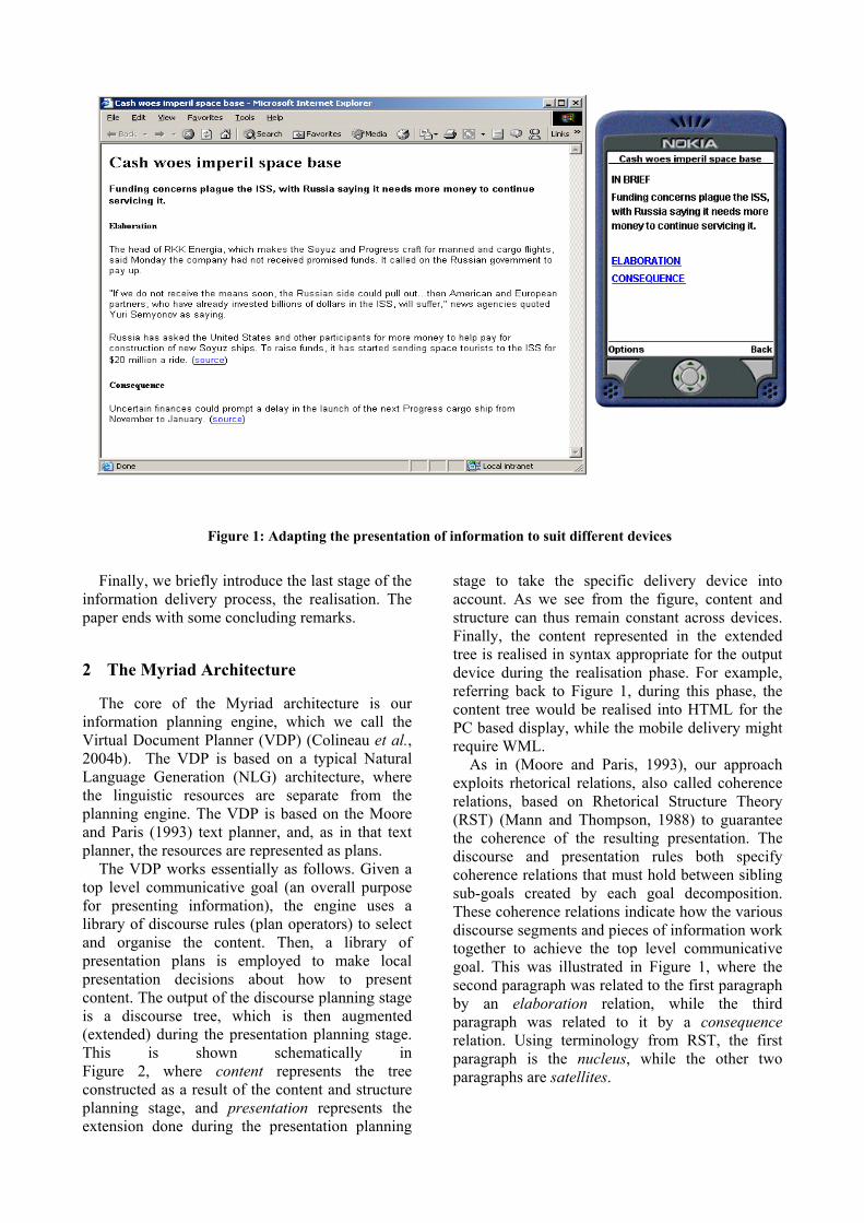
Figure 1: Adapting the presentation of information to suit different devices
Finally, we briefly introduce the last stage of the
information delivery process, the realisation. The paper ends with some concluding remarks.
2 The Myriad Architecture
The core of the Myriad architecture is our information planning engine, which we call the Virtual Document Planner (VDP) (Colineau et al., 2004b). The VDP is based on a typical Natural Language Generation (NLG) architecture, where the linguistic resources are separate from the planning engine. The VDP is based on the Moore and Paris (1993) text planner, and, as in that text planner, the resources are represented as plans.
The VDP works essentially as follows. Given a top level communicative goal (an overall purpose for presenting information), the engine uses a library of discourse rules (plan operators) to select and organise the content. Then, a library of presentation plans is employed to make local presentation decisions about how to present content. The output of the discourse planning stage is a discourse tree, which is then augmented (extended) during the presentation planning stage. This is shown schematically in Figure 2, where content represents the tree constructed as a result of the content and structure planning stage, and presentation represents the extension done during the presentation planning
stage to take the specific delivery device into account. As we see from the figure, content and structure can thus remain constant across devices. Finally, the content represented in the extended tree is realised in syntax appropriate for the output device during the realisation phase. For example, referring back to Figure 1, during this phase, the content tree would be realised into HTML for the PC based display, while the mobile delivery might require WML.
As in (Moore and Paris, 1993), our approach exploits rhetorical relations, also called coherence relations, based on Rhetorical Structure Theory (RST) (Mann and Thompson, 1988) to guarantee the coherence of the resulting presentation. The discourse and presentation rules both specify coherence relations that must hold between sibling sub-goals created by each goal decomposition. These coherence relations indicate how the various discourse segments and pieces of information work together to achieve the top level communicative goal. This was illustrated in Figure 1, where the second paragraph was related to the first paragraph by an elaboration relation, while the third paragraph was related to it by a consequence relation. Using terminology from RST, the first paragraph is the nucleus, while the other two paragraphs are satellites.
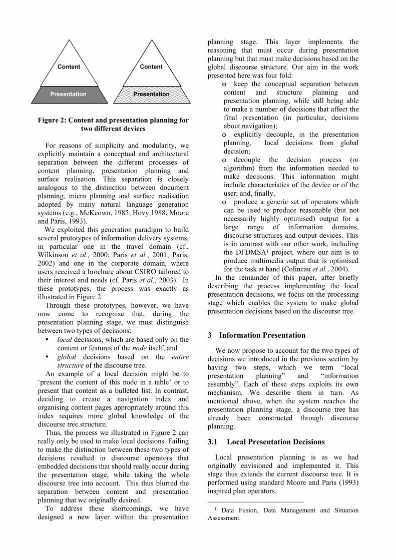
Figure 2: Content and presentation planning for two different devices
For reasons of simplicity and modularity, we
explicitly maintain a conceptual and architectural separation between the different processes of content planning, presentation planning and surface realisation. This separation is closely analogous to the distinction between document planning, micro planning and surface realisation adopted by many natural language generation systems (e.g., McKeown, 1985; Hovy 1988; Moore and Paris, 1993).
We exploited this generation paradigm to build several prototypes of information delivery systems, in particular one in the travel domain (cf., Wilkinson et al., 2000; Paris et al., 2001; Paris, 2002) and one in the corporate domain, where users received a brochure about CSIRO tailored to their interest and needs (cf. Paris et al., 2003). In these prototypes, the process was exactly as illustrated in Figure 2.
Through these prototypes, however, we have now come to recognise that, during the presentation planning stage, we must distinguish between two types of decisions:
• local decisions, which are based only on the content or features of the node itself, and
• global decisions based on the entire structure of the discourse tree.
An example of a local decision might be to ‘present the content of this node in a table’ or to present that content as a bulleted list. In contrast, deciding to create a navigation index and organising content pages appropriately around this index requires more global knowledge of the discourse tree structure.
Thus, the process we illustrated in Figure 2 can really only be used to make local decisions. Failing to make the distinction between these two types of decisions resulted in discourse operators that embedded decisions that should really occur during the presentation stage, while taking the whole discourse tree into account. This thus blurred the separation between content and presentation planning that we originally desired.
To address these shortcomings, we have designed a new layer within the presentation
planning stage. This layer implements the reasoning that must occur during presentation planning but that must make decisions based on the global discourse structure. Our aim in the work presented here was four fold:
o keep the conceptual separation between content and structure planning and presentation planning, while still being able to make a number of decisions that affect the final presentation (in particular, decisions about navigation); o explicitly decouple, in the presentation planning, local decisions from global decision; o decouple the decision process (or algorithm) from the information needed to make decisions. This information might include characteristics of the device or of the user; and, finally, o produce a generic set of operators which can be used to produce reasonable (but not necessarily highly optimised) output for a large range of information domains, discourse structures and output devices. This is in contrast with our other work, including the DFDMSA1 project, where our aim is to produce multimedia output that is optimised for the task at hand (Colineau et al., 2004).
In the remainder of this paper, after briefly describing the process implementing the local presentation decisions, we focus on the processing stage which enables the system to make global presentation decisions based on the discourse tree.
3 Information Presentation
We now propose to account for the two types of decisions we introduced in the previous section by having two steps, which we term “local presentation planning” and “information assembly”. Each of these steps exploits its own mechanism. We describe them in turn. As mentioned above, when the system reaches the presentation planning stage, a discourse tree has already been constructed through discourse planning.
3.1 Local Presentation Decisions
Local presentation planning is as we had originally envisioned and implemented it. This stage thus extends the current discourse tree. It is performed using standard Moore and Paris (1993) inspired plan operators.
1 Data Fusion, Data Management and Situation Assessment.
Content Content
Presentation Presentation
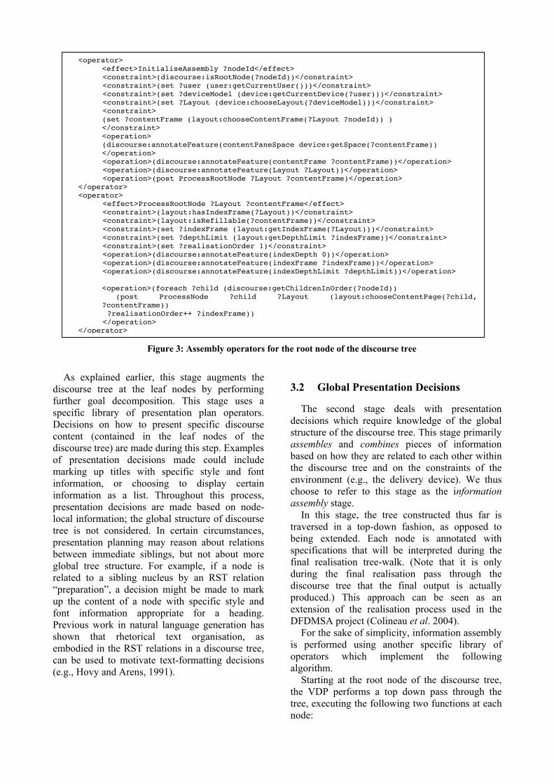
<operator> <effect>InitialiseAssembly ?nodeId</effect>
<constraint>(discourse:isRootNode(?nodeId))</constraint> <constraint>(set ?user (user:getCurrentUser()))</constraint> <constraint>(set ?deviceModel (device:getCurrentDevice(?user)))</constraint> <constraint>(set ?Layout (device:chooseLayout(?deviceModel)))</constraint> <constraint>
(set ?contentFrame (layout:chooseContentFrame(?Layout ?nodeId)) ) </constraint> <operation> (discourse:annotateFeature(contentPaneSpace device:getSpace(?contentFrame)) </operation>
<operation>(discourse:annotateFeature(contentFrame ?contentFrame))</operation> <operation>(discourse:annotateFeature(Layout ?Layout))</operation> <operation>(post ProcessRootNode ?Layout ?contentFrame)</operation> </operator> <operator> <effect>ProcessRootNode ?Layout ?contentFrame</effect> <constraint>(layout:hasIndexFrame(?Layout))</constraint> <constraint>(layout:isRefillable(?contentFrame))</constraint> <constraint>(set ?indexFrame (layout:getIndexFrame(?Layout)))</constraint> <constraint>(set ?depthLimit (layout:getDepthLimit ?indexFrame))</constraint> <constraint>(set ?realisationOrder 1)</constraint> <operation>(discourse:annotateFeature(indexDepth 0))</operation> <operation>(discourse:annotateFeature(indexFrame ?indexFrame))</operation> <operation>(discourse:annotateFeature(indexDepthLimit ?depthLimit))</operation>
<operation>(foreach ?child (discourse:getChildrenInOrder(?nodeId)) (post ProcessNode ?child ?Layout (layout:chooseContentPage(?child,
?contentFrame)) ?realisationOrder++ ?indexFrame)) </operation> </operator>
Figure 3: Assembly operators for the root node of the discourse tree
As explained earlier, this stage augments the
discourse tree at the leaf nodes by performing further goal decomposition. This stage uses a specific library of presentation plan operators. Decisions on how to present specific discourse content (contained in the leaf nodes of the discourse tree) are made during this step. Examples of presentation decisions made could include marking up titles with specific style and font information, or choosing to display certain information as a list. Throughout this process, presentation decisions are made based on node-local information; the global structure of discourse tree is not considered. In certain circumstances, presentation planning may reason about relations between immediate siblings, but not about more global tree structure. For example, if a node is related to a sibling nucleus by an RST relation “preparation”, a decision might be made to mark up the content of a node with specific style and font information appropriate for a heading. Previous work in natural language generation has shown that rhetorical text organisation, as embodied in the RST relations in a discourse tree, can be used to motivate text-formatting decisions (e.g., Hovy and Arens, 1991).
3.2 Global Presentation Decisions
The second stage deals with presentation decisions which require knowledge of the global structure of the discourse tree. This stage primarily assembles and combines pieces of information based on how they are related to each other within the discourse tree and on the constraints of the environment (e.g., the delivery device). We thus choose to refer to this stage as the information assembly stage.
In this stage, the tree constructed thus far is traversed in a top-down fashion, as opposed to being extended. Each node is annotated with specifications that will be interpreted during the final realisation tree-walk. (Note that it is only during the final realisation pass through the discourse tree that the final output is actually produced.) This approach can be seen as an extension of the realisation process used in the DFDMSA project (Colineau et al. 2004).
For the sake of simplicity, information assembly is performed using another specific library of operators which implement the following algorithm.
Starting at the root node of the discourse tree, the VDP performs a top down pass through the tree, executing the following two functions at each node:
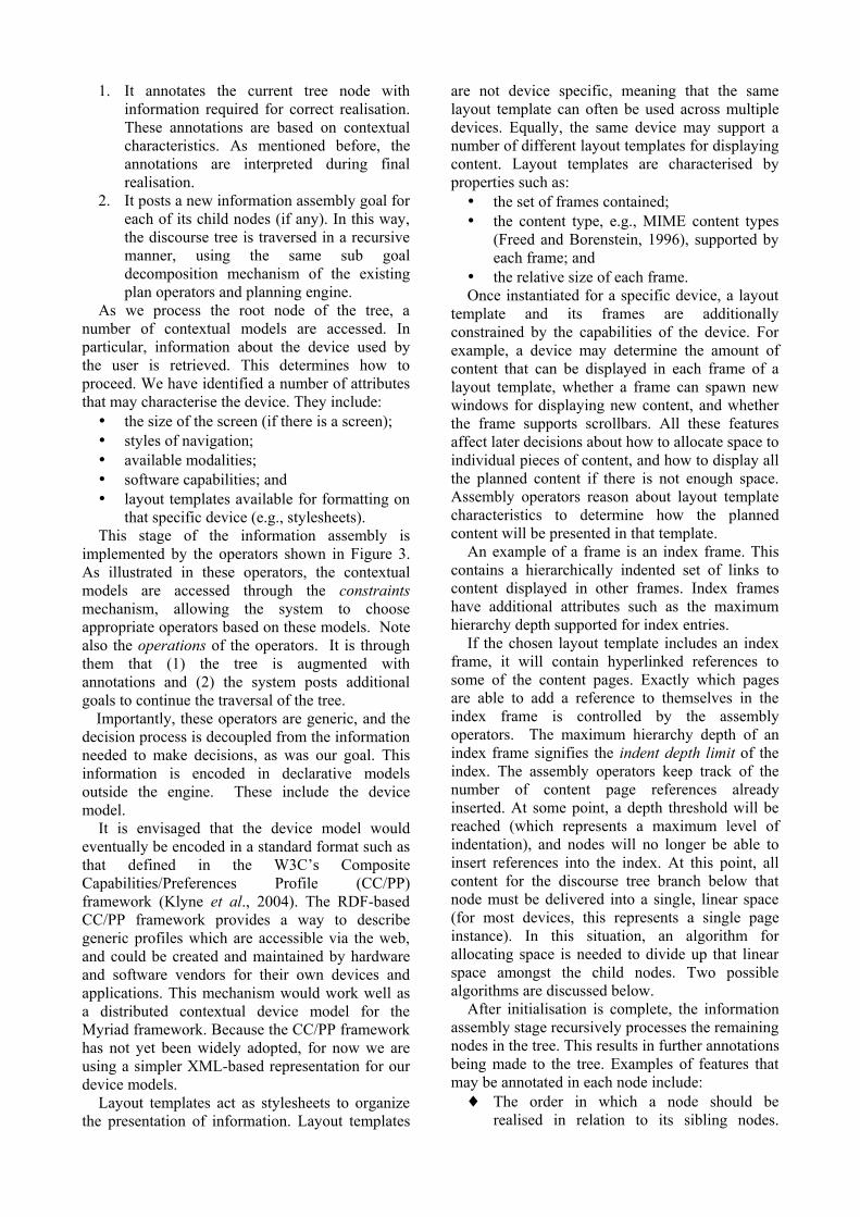
1. It annotates the current tree node with information required for correct realisation. These annotations are based on contextual characteristics. As mentioned before, the annotations are interpreted during final realisation.
2. It posts a new information assembly goal for each of its child nodes (if any). In this way, the discourse tree is traversed in a recursive manner, using the same sub goal decomposition mechanism of the existing plan operators and planning engine.
As we process the root node of the tree, a number of contextual models are accessed. In particular, information about the device used by the user is retrieved. This determines how to proceed. We have identified a number of attributes that may characterise the device. They include:
• the size of the screen (if there is a screen); • styles of navigation; • available modalities; • software capabilities; and • layout templates available for formatting on
that specific device (e.g., stylesheets). This stage of the information assembly is
implemented by the operators shown in Figure 3. As illustrated in these operators, the contextual models are accessed through the constraints mechanism, allowing the system to choose appropriate operators based on these models. Note also the operations of the operators. It is through them that (1) the tree is augmented with annotations and (2) the system posts additional goals to continue the traversal of the tree.
Importantly, these operators are generic, and the decision process is decoupled from the information needed to make decisions, as was our goal. This information is encoded in declarative models outside the engine. These include the device model.
It is envisaged that the device model would eventually be encoded in a standard format such as that defined in the W3C’s Composite Capabilities/Preferences Profile (CC/PP) framework (Klyne et al., 2004). The RDF-based CC/PP framework provides a way to describe generic profiles which are accessible via the web, and could be created and maintained by hardware and software vendors for their own devices and applications. This mechanism would work well as a distributed contextual device model for the Myriad framework. Because the CC/PP framework has not yet been widely adopted, for now we are using a simpler XML-based representation for our device models.
Layout templates act as stylesheets to organize the presentation of information. Layout templates
are not device specific, meaning that the same layout template can often be used across multiple devices. Equally, the same device may support a number of different layout templates for displaying content. Layout templates are characterised by properties such as:
• the set of frames contained; • the content type, e.g., MIME content types
(Freed and Borenstein, 1996), supported by each frame; and
• the relative size of each frame. Once instantiated for a specific device, a layout
template and its frames are additionally constrained by the capabilities of the device. For example, a device may determine the amount of content that can be displayed in each frame of a layout template, whether a frame can spawn new windows for displaying new content, and whether the frame supports scrollbars. All these features affect later decisions about how to allocate space to individual pieces of content, and how to display all the planned content if there is not enough space. Assembly operators reason about layout template characteristics to determine how the planned content will be presented in that template.
An example of a frame is an index frame. This contains a hierarchically indented set of links to content displayed in other frames. Index frames have additional attributes such as the maximum hierarchy depth supported for index entries.
If the chosen layout template includes an index frame, it will contain hyperlinked references to some of the content pages. Exactly which pages are able to add a reference to themselves in the index frame is controlled by the assembly operators. The maximum hierarchy depth of an index frame signifies the indent depth limit of the index. The assembly operators keep track of the number of content page references already inserted. At some point, a depth threshold will be reached (which represents a maximum level of indentation), and nodes will no longer be able to insert references into the index. At this point, all content for the discourse tree branch below that node must be delivered into a single, linear space (for most devices, this represents a single page instance). In this situation, an algorithm for allocating space is needed to divide up that linear space amongst the child nodes. Two possible algorithms are discussed below.
After initialisation is complete, the information assembly stage recursively processes the remaining nodes in the tree. This results in further annotations being made to the tree. Examples of features that may be annotated in each node include: ♦ The order in which a node should be
realised in relation to its sibling nodes.
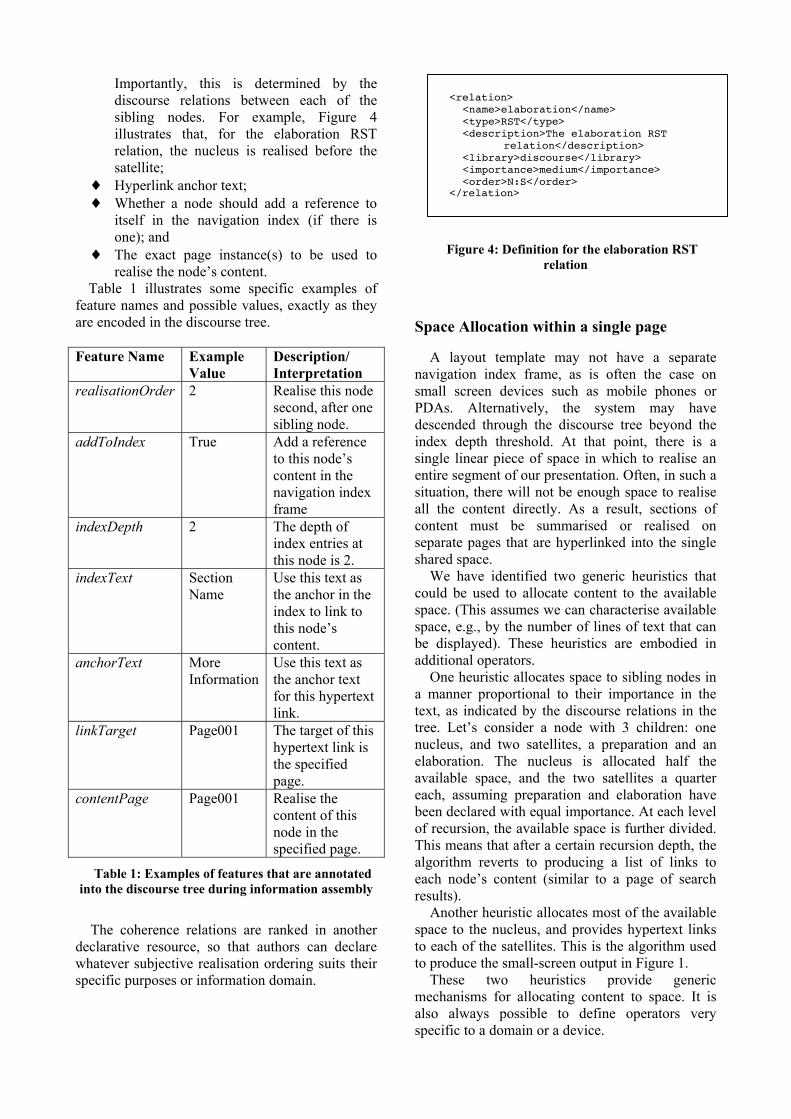
Importantly, this is determined by the discourse relations between each of the sibling nodes. For example, Figure 4 illustrates that, for the elaboration RST relation, the nucleus is realised before the satellite;
♦ Hyperlink anchor text; ♦ Whether a node should add a reference to
itself in the navigation index (if there is one); and
♦ The exact page instance(s) to be used to realise the node’s content.
Table 1 illustrates some specific examples of feature names and possible values, exactly as they are encoded in the discourse tree.
Feature Name Example
Value Description/ Interpretation
realisationOrder 2 Realise this node second, after one sibling node.
addToIndex True Add a reference to this node’s content in the navigation index frame
indexDepth 2 The depth of index entries at this node is 2.
indexText Section Name
Use this text as the anchor in the index to link to this node’s content.
anchorText More Information
Use this text as the anchor text for this hypertext link.
linkTarget Page001 The target of this hypertext link is the specified page.
contentPage Page001 Realise the content of this node in the specified page.
Table 1: Examples of features that are annotated into the discourse tree during information assembly
The coherence relations are ranked in another
declarative resource, so that authors can declare whatever subjective realisation ordering suits their specific purposes or information domain.
<relation> <name>elaboration</name> <type>RST</type> <description>The elaboration RST
relation</description> <library>discourse</library> <importance>medium</importance> <order>N:S</order>
</relation>
Figure 4: Definition for the elaboration RST relation
Space Allocation within a single page
A layout template may not have a separate navigation index frame, as is often the case on small screen devices such as mobile phones or PDAs. Alternatively, the system may have descended through the discourse tree beyond the index depth threshold. At that point, there is a single linear piece of space in which to realise an entire segment of our presentation. Often, in such a situation, there will not be enough space to realise all the content directly. As a result, sections of content must be summarised or realised on separate pages that are hyperlinked into the single shared space.
We have identified two generic heuristics that could be used to allocate content to the available space. (This assumes we can characterise available space, e.g., by the number of lines of text that can be displayed). These heuristics are embodied in additional operators.
One heuristic allocates space to sibling nodes in a manner proportional to their importance in the text, as indicated by the discourse relations in the tree. Let’s consider a node with 3 children: one nucleus, and two satellites, a preparation and an elaboration. The nucleus is allocated half the available space, and the two satellites a quarter each, assuming preparation and elaboration have been declared with equal importance. At each level of recursion, the available space is further divided. This means that after a certain recursion depth, the algorithm reverts to producing a list of links to each node’s content (similar to a page of search results).
Another heuristic allocates most of the available space to the nucleus, and provides hypertext links to each of the satellites. This is the algorithm used to produce the small-screen output in Figure 1.
These two heuristics provide generic mechanisms for allocating content to space. It is also always possible to define operators very specific to a domain or a device.
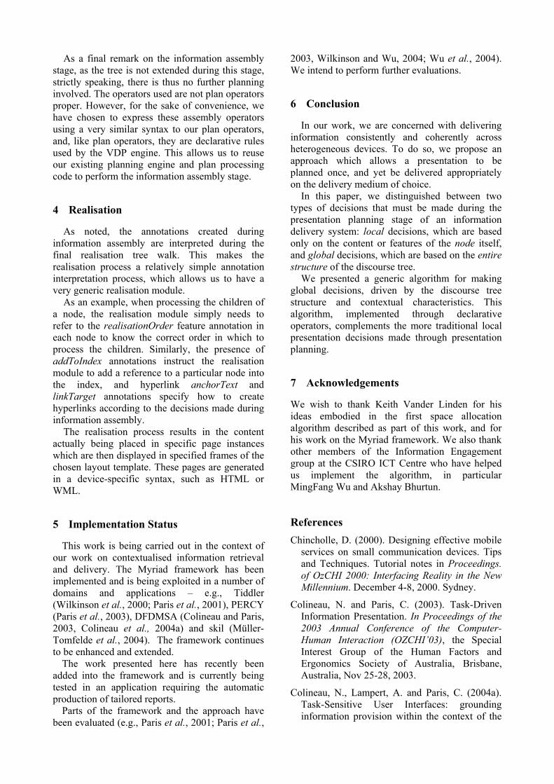
As a final remark on the information assembly stage, as the tree is not extended during this stage, strictly speaking, there is thus no further planning involved. The operators used are not plan operators proper. However, for the sake of convenience, we have chosen to express these assembly operators using a very similar syntax to our plan operators, and, like plan operators, they are declarative rules used by the VDP engine. This allows us to reuse our existing planning engine and plan processing code to perform the information assembly stage.
4 Realisation
As noted, the annotations created during information assembly are interpreted during the final realisation tree walk. This makes the realisation process a relatively simple annotation interpretation process, which allows us to have a very generic realisation module.
As an example, when processing the children of a node, the realisation module simply needs to refer to the realisationOrder feature annotation in each node to know the correct order in which to process the children. Similarly, the presence of addToIndex annotations instruct the realisation module to add a reference to a particular node into the index, and hyperlink anchorText and linkTarget annotations specify how to create hyperlinks according to the decisions made during information assembly.
The realisation process results in the content actually being placed in specific page instances which are then displayed in specified frames of the chosen layout template. These pages are generated in a device-specific syntax, such as HTML or WML.
5 Implementation Status
This work is being carried out in the context of our work on contextualised information retrieval and delivery. The Myriad framework has been implemented and is being exploited in a number of domains and applications – e.g., Tiddler (Wilkinson et al., 2000; Paris et al., 2001), PERCY (Paris et al., 2003), DFDMSA (Colineau and Paris, 2003, Colineau et al., 2004a) and skil (Müller-Tomfelde et al., 2004). The framework continues to be enhanced and extended.
The work presented here has recently been added into the framework and is currently being tested in an application requiring the automatic production of tailored reports.
Parts of the framework and the approach have been evaluated (e.g., Paris et al., 2001; Paris et al.,
2003, Wilkinson and Wu, 2004; Wu et al., 2004). We intend to perform further evaluations.
6 Conclusion
In our work, we are concerned with delivering information consistently and coherently across heterogeneous devices. To do so, we propose an approach which allows a presentation to be planned once, and yet be delivered appropriately on the delivery medium of choice.
In this paper, we distinguished between two types of decisions that must be made during the presentation planning stage of an information delivery system: local decisions, which are based only on the content or features of the node itself, and global decisions, which are based on the entire structure of the discourse tree.
We presented a generic algorithm for making global decisions, driven by the discourse tree structure and contextual characteristics. This algorithm, implemented through declarative operators, complements the more traditional local presentation decisions made through presentation planning.
7 Acknowledgements
We wish to thank Keith Vander Linden for his ideas embodied in the first space allocation algorithm described as part of this work, and for his work on the Myriad framework. We also thank other members of the Information Engagement group at the CSIRO ICT Centre who have helped us implement the algorithm, in particular MingFang Wu and Akshay Bhurtun.
References Chincholle, D. (2000). Designing effective mobile
services on small communication devices. Tips and Techniques. Tutorial notes in Proceedings. of OzCHI 2000: Interfacing Reality in the New Millennium. December 4-8, 2000. Sydney.
Colineau, N. and Paris, C. (2003). Task-Driven Information Presentation. In Proceedings of the 2003 Annual Conference of the Computer-Human Interaction (OZCHI’03), the Special Interest Group of the Human Factors and Ergonomics Society of Australia, Brisbane, Australia, Nov 25-28, 2003.
Colineau, N., Lampert, A. and Paris, C. (2004a). Task-Sensitive User Interfaces: grounding information provision within the context of the
user's activity. In Proceedings of the working conference on Advanced Visual Interfaces (AVI) Conference, Gallipoli, Italy, May 25-28 2004, 218-225.
Colineau, N., Paris, C. and Wu, M. (2004b). Actionable Information Delivery. In Revue d’Intelligence Artificielle (RSTI – RIA), Special Issue on Tailored Information Delivery, 18(4), 549-576. September 2004.
Freed, N and Borenstein, N. (1996). Multipurpose Internet Mail Extensions (MIME) Part Two: Media Types – Published as “Request For Comments: 2046”.
Hovy, E. (1988). Planning coherent multisentential text. In Proceedings. of the 26th Conference of the ACL, Buffalo, NY, 163-169.
Hovy, E., and Arens, Y., (1991). Automatic generation of formatted text. In Proceedings of the 8th Conference of the American Association for Artificial Intelligence. 92 – 96. Anaheim, CA: AAAI.
Klyne,G., Reynolds, F., Woodrow, C., Ohto, H., Hjelm, J., Butler, M. and Tran, L. (2004). Composite Capabilites/Preference Profiles (CC/PP): Structure and Vocabularies 1.0. W3C Recommendation 15 January 2004.
Mann, W. and Thompson S. (1988). Rhetorical Structure Theory: Towards a Functional Theory of Text Organization. In Text, 8(3), 243-281, 1988.
McKeown, K.R. (1985). Text Generation: Using Discourse Strategies and Focus Constraints to Generate Natural Language Text. Cambridge University Press, Cambridge, England.
Moore, J. and Paris, C. (1993). Planning text for advisory dialogues: Capturing intentional and rhetorical information. In Computational Linguistics, 19(4), 651-694.
Müller-Tomfelde, C, Paris, C. and Stevenson, D. (2004). Interactive Landmarks: Linking Virtual Environments with Knowledge-Based Systems. To appear in the Proceedings of the 2004 Annual Conference of the Computer-Human Interaction (OZCHI’04), the Special Interest Group of the Human Factors and Ergonomics Society of Australia, Wollongong , Australia, November 22-24, 2004.
Paris, C. (2002). Information Delivery for Tourism. In IEEE Intelligent Systems Intelligent Systems for Tourism: Trends and Controversies, Stephen Staab and Hannes Werthner (eds), November/December, 2002. pp 53 – 66, 2002.
Paris, C., Wan, S., Wilkinson, R. and Wu, M. (2001). Generating Personal Travel Guides – and who wants them? In Proceedings of the International Conference on User Modelling (UM2001); M. Bauer, P. Gmytrasiewicz and J. Vassileva (eds). Sonthofen, Germany, July 13-18, 2001. 251-253.
Paris C, Wu M, Vander Linden K, Post M, and Lu S. (2004). Myriad: An Architecture for Contextualized Information Retrieval and Delivery (2004). In AH2004: International Conference on Adaptive Hypermedia and Adaptive Web-based Systems. August 23-26 2004, The Netherlands. pp.205-214.
Paris, C., Wu, M., Vercoustre, A-M., Wan, S., Wilkins, P. and Wilkinson, R. (2003). An Empirical Study of the Effect of Coherent and Tailored Document Delivery as an Interface to Organizational Websites. In Proceedings of the Adaptive Hypermedia Workshop at the 2003 User Modelling Conference, Pittsburgh, USA, June 22, 2003. 133-144.
Wilkinson, R., Lu, S., Paradis, F., Paris, C., Wan, S. and Wu, M. (2000). Generating Personal Travel Guides from Discourse Plans. In Proceedings of International Conference on Adaptive Hypermedia and Adaptive Web-based Systems. Trento, Italy, August 2000.
Wilkinson, R and Wu, M. (2004). Evaluation Experiments and Experience from the Perspective of Interactive Information Retrieval, In the Proceedings of the Third Workshop on Empirical Evaluation of Adaptive Systems, in conjunction with AH2004. August 23-26, The Netherlands. pp.216-225.
Wu, M., Muresan, G., McLean, A. Tang, M., Wilkinson, R. ,Li, Y., Lee, H. and Belkin, N. (2004). Human versus Machine in the Topic Distillation Task, In the Proceedings of the 27th SIGIR Conference on Research and Development in Information Retrieval, July 25th-29th 2004, Sheffield, UK. pp. 385-392.
Referring Expression Generation as a Search Problem
Bernd [email protected] for Intelligent Systems
University of Stuttgart70569 Stuttgart
Germany
Robert [email protected]
Centre for Language TechnologyMacquarie UniversitySydney nsw 2109
Australia
Abstract
One of the most widely explored issues in natu-ral language generation is the generation of re-ferring expressions (gre): given an entity wewant to refer to, how do we work out the contentof a referring expression that uniquely identifiesthe intended referent? Over the last 15 years, anumber of authors have proposed a wide rangeof algorithms for addressing di!erent aspects ofthis problem, but the di!erent approaches takenhave made it very di"cult to compare and con-trast the algorithms provided in any meaningfulway. In this paper, we propose a characterisa-tion of the problem of referring expression gen-eration as a search problem; this allows us torecast existing algorithms in a way that makestheir similarities and di!erences clear.
1 Introduction
A major component task in natural languagegeneration (nlg) is the generation of referringexpressions: given an entity that we want torefer to, how do we determine the content of areferring expression that uniquely identifies thatintended referent? Since at least (Dale, 1989),the standard conception of this task in the lit-erature has been as follows:
1. We assume we have a knowledge base thatcharacterises the entities in the domain interms of a set of attributes and the valuesthat the entities have for these attributes;so, for example, our knowledge base mightrepresent the fact that entity e1 has thevalue cup for the attribute type, and thevalue red for the attribute colour.
2. In a typical context where we want to re-fer to some ei, which we call the intendedreferent, there will be other entities fromwhich the intended referent must be distin-guished; these are generally referred to as
distractors. So, for example, we may wantto distinguish a particular cup from all theother items present in the context of a din-ing table.
3. The goal of referring expression generationis therefore to find some collection of at-tributes and their values which distinguishthe intended referent from all the potentialdistractors in the context.
Over the last 15 years, a wide variety of algo-rithms have been proposed to deal with specificaspects of this problem. For example, while ear-lier algorithms focussed on the use of attributesthat correspond to simple one-place predicates,later work attempts to address the use of rela-tional predicates, and other work looks at theincorporation of boolean operators such as notand and. The consequence is that we now havea considerable body of research in this area, butit is di"cult to establish just how these di!erentalgorithms relate to each other.
This paper represents a first step to-wards consolidating the results in this area, withthe aim of developing a framework within whichdi!erent algorithms can be compared and as-sessed. The structure of the paper is as fol-lows. In Section 2, we provide a brief overviewof work on the generation of referring expres-sions to date. In Section 3, we borrow a stan-dard approach used in Artificial Intelligence (ai)to represent problems in an elegant and uni-form way (see, for example, (Simon and Newell,1963); (Russell and Norvig, 2003)), sketchinghow gre algorithms can be expressed in termsof problem-solving by search. In Section 4, weexplore how the most well-known algorithmscan be expressed in this framework. In Sec-tion 5, we discuss how this approach enables amore fruitful comparison of existing algorithms,and we point to ways of taking this work fur-ther.
2 A Brief Review of Work To Date
Although the task of referring expression gen-eration is discussed informally in earlier workon nlg (in particular, see (Winograd, 1972;McDonald, 1980; Appelt, 1981), the first for-mally explicit algorithm was introduced in Dale(1989). This algorithm, which we will referto as the Full Brevity (fb) algorithm, is stillfrequently used as a basis for other gre al-gorithms. The fb algorithm searches for thebest solution amongst all possible referring ex-pressions for an entity; the algorithm derivesthe smallest set of attributes for the referent inquestion, producing a referring expression thatis both adequate and e!cient.
This initial algorithm limited its ap-plication to one-place predicates. Dale andHaddock (1991) introduced a constraint-basedprocedure that could generate referring expres-sions involving relations (henceforth ir), usinga greedy heuristic to guide the search.
As a response to the computationalcomplexity of greedy algorithms, (Reiter andDale, 1992; Dale and Reiter, 1995) introducedthe psycholinguistically motivated IncrementalAlgorithm (ia). The most used and adaptedalgorithm, this is based on the observationthat people often produce referring expressionswhich are informationally redundant; the algo-rithm uses a preference ordering over the at-tributes to be used in a referring expression, ac-cumulating those attributes which rule out atleast one potential distractor.
In recent years there have been a num-ber of important extensions to the ia. TheContext-Sensitive extension (cs; (Krahmer andTheune, 2002)) is able to generate referring ex-pressions for the most salient entity in a con-text; the Boolean Expressions algorithm (be;(van Deemter, 2002)) is able to derive expres-sions containing boolean operators, as in the cupthat does not have a handle; and the Sets algo-rithm (set; (van Deemter, 2002)) extends thebasic approach to references to sets, as in thered cups.
Some approaches combine algorithmswhich reuse only parts of other algorithms:the Branch and Bound (bab; (Krahmer et al.,2003)) algorithm uses the Full Brevity algo-rithm, but is able to generate referring expres-sions with both attributes and relational de-scriptions using a graph-based technique.
We have identified here what we be-lieve to be the most cited strands of research inthis area, but of course there are many other al-gorithms described in the literature: see, for ex-ample, (Horacek, 1997; Bateman, 1999; Stone,2000). Space limitations prevent a completesummary of this other work here, but our in-tention is to extend the analysis presented inthis paper to as many of these other algorithmsas possible.
All these algorithms focus on the gen-eration of definite references; they are typicallyembedded in a higher-level algorithm that in-cludes cases for when the entity has not beenpreviously mentioned (thus leading to an ini-tial indefinite reference) or when the referentis in focus (thus leading to a pronominal refer-ence); see, for example, (Dale, 1989; Krahmerand Theune, 2002; Dale, 2003).
3 gre from the Perspective ofProblem Solving
With so many algorithms to choose from, itwould be useful to have a uniform framework inwhich to discuss and compare algorithms; unfor-tunately, this is rather di"cult given the varietyof di!erent approaches that have been taken tothe problem.
Within the wider context of ai, Russelland Norvig (2003) present an elegant definitionof a general algorithm for problem solving bysearch. The search graph consists of nodes withthe components state and path-cost; the prob-lem is represented by an initial-state, an expand-method which identifies new states in the searchspace, a queuing-method which determines theorder in which the states should be considered,and a path-cost-function which determines thecost of reaching a given state. In this frame-work, the search strategy is determined by thecombination of queuing-method and path-cost-function used.
In the following, we use this frameworkto provide a characterisation of existing gre al-gorithms in terms of problem solving by search.We conceptualise the search space as consist-ing of states that have three components: a de-scription that is true of the intended referent,the set of distractor entities that the descrip-tion also applies to besides the intended refer-ent, and the set of properties of the intendedreferent that have not yet been considered todescribe the referent.
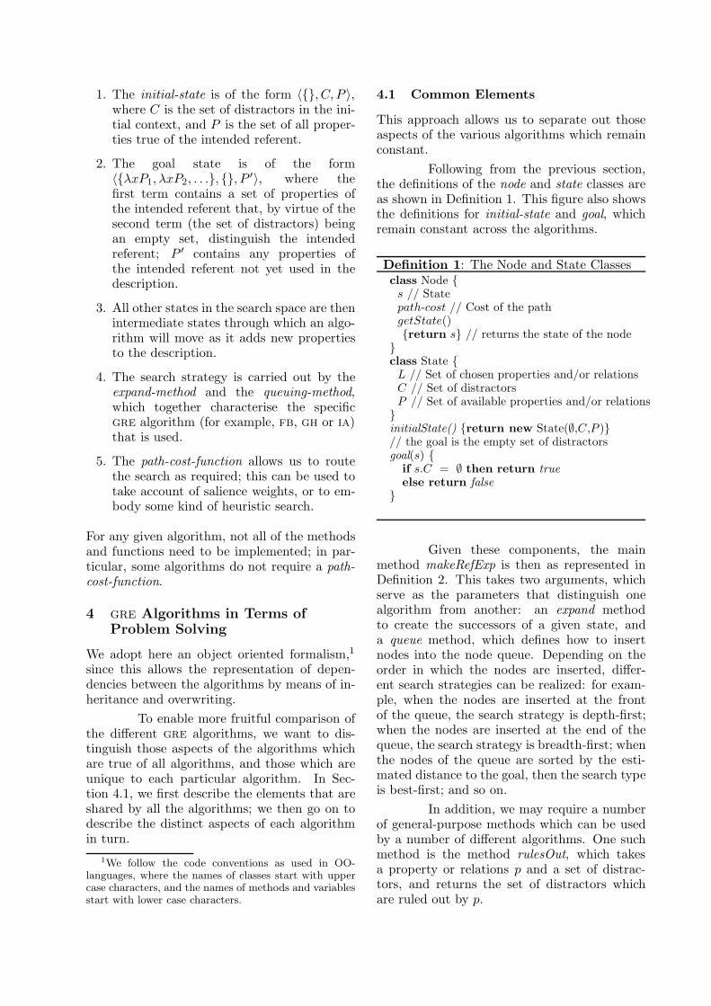
1. The initial-state is of the form !{}, C, P ",where C is the set of distractors in the ini-tial context, and P is the set of all proper-ties true of the intended referent.
2. The goal state is of the form!{!xP1,!xP2, . . .}, {}, P !", where thefirst term contains a set of properties ofthe intended referent that, by virtue of thesecond term (the set of distractors) beingan empty set, distinguish the intendedreferent; P ! contains any properties ofthe intended referent not yet used in thedescription.
3. All other states in the search space are thenintermediate states through which an algo-rithm will move as it adds new propertiesto the description.
4. The search strategy is carried out by theexpand-method and the queuing-method,which together characterise the specificgre algorithm (for example, fb, gh or ia)that is used.
5. The path-cost-function allows us to routethe search as required; this can be used totake account of salience weights, or to em-body some kind of heuristic search.
For any given algorithm, not all of the methodsand functions need to be implemented; in par-ticular, some algorithms do not require a path-cost-function.
4 gre Algorithms in Terms ofProblem Solving
We adopt here an object oriented formalism,1
since this allows the representation of depen-dencies between the algorithms by means of in-heritance and overwriting.
To enable more fruitful comparison ofthe di!erent gre algorithms, we want to dis-tinguish those aspects of the algorithms whichare true of all algorithms, and those which areunique to each particular algorithm. In Sec-tion 4.1, we first describe the elements that areshared by all the algorithms; we then go on todescribe the distinct aspects of each algorithmin turn.
1We follow the code conventions as used in OO-languages, where the names of classes start with uppercase characters, and the names of methods and variablesstart with lower case characters.
4.1 Common Elements
This approach allows us to separate out thoseaspects of the various algorithms which remainconstant.
Following from the previous section,the definitions of the node and state classes areas shown in Definition 1. This figure also showsthe definitions for initial-state and goal, whichremain constant across the algorithms.
Definition 1: The Node and State Classesclass Node {s // Statepath-cost // Cost of the pathgetState(){return s} // returns the state of the node
}class State {L // Set of chosen properties and/or relationsC // Set of distractorsP // Set of available properties and/or relations
}initialState() {return new State(#,C,P )}// the goal is the empty set of distractorsgoal(s) {
if s.C = # then return trueelse return false
}
Given these components, the mainmethod makeRefExp is then as represented inDefinition 2. This takes two arguments, whichserve as the parameters that distinguish onealgorithm from another: an expand methodto create the successors of a given state, anda queue method, which defines how to insertnodes into the node queue. Depending on theorder in which the nodes are inserted, di!er-ent search strategies can be realized: for exam-ple, when the nodes are inserted at the frontof the queue, the search strategy is depth-first;when the nodes are inserted at the end of thequeue, the search strategy is breadth-first; whenthe nodes of the queue are sorted by the esti-mated distance to the goal, then the search typeis best-first; and so on.
In addition, we may require a numberof general-purpose methods which can be usedby a number of di!erent algorithms. One suchmethod is the method rulesOut, which takesa property or relations p and a set of distrac-tors, and returns the set of distractors whichare ruled out by p.
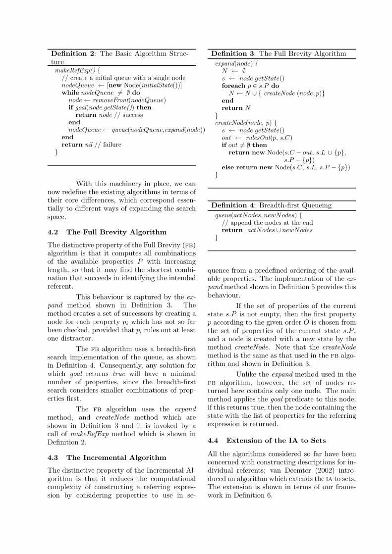
Definition 2: The Basic Algorithm Struc-turemakeRefExp() {
// create a initial queue with a single nodenodeQueue $ [new Node(initialState())]while nodeQueue %= # do
node $ removeFront(nodeQueue)if goal(node.getState()) then
return node // successendnodeQueue $ queue(nodeQueue,expand(node))
endreturn nil // failure
}
With this machinery in place, we cannow redefine the existing algorithms in terms oftheir core di!erences, which correspond essen-tially to di!erent ways of expanding the searchspace.
4.2 The Full Brevity Algorithm
The distinctive property of the Full Brevity (fb)algorithm is that it computes all combinationsof the available properties P with increasinglength, so that it may find the shortest combi-nation that succeeds in identifying the intendedreferent.
This behaviour is captured by the ex-pand method shown in Definition 3. Themethod creates a set of successors by creating anode for each property pi which has not so farbeen checked, provided that pi rules out at leastone distractor.
The fb algorithm uses a breadth-firstsearch implementation of the queue, as shownin Definition 4. Consequently, any solution forwhich goal returns true will have a minimalnumber of properties, since the breadth-firstsearch considers smaller combinations of prop-erties first.
The fb algorithm uses the expandmethod, and createNode method which areshown in Definition 3 and it is invoked by acall of makeRefExp method which is shown inDefinition 2.
4.3 The Incremental Algorithm
The distinctive property of the Incremental Al-gorithm is that it reduces the computationalcomplexity of constructing a referring expres-sion by considering properties to use in se-
Definition 3: The Full Brevity Algorithm
expand(node) {N $ #s $ node.getState()foreach p & s.P do
N $ N ' { createNode (node, p)}endreturn N
}createNode(node, p) {
s $ node.getState()out $ rulesOut(p, s.C)if out %= # then
return new Node(s.C ( out, s.L ' {p},s.P ( {p})
else return new Node(s.C, s.L, s.P ( {p})}
Definition 4: Breadth-first Queueing
queue(actNodes, newNodes) {// append the nodes at the endreturn actNodes ' newNodes
}
quence from a predefined ordering of the avail-able properties. The implementation of the ex-pand method shown in Definition 5 provides thisbehaviour.
If the set of properties of the currentstate s.P is not empty, then the first propertyp according to the given order O is chosen fromthe set of properties of the current state s.P ,and a node is created with a new state by themethod createNode. Note that the createNodemethod is the same as that used in the fb algo-rithm and shown in Definition 3.
Unlike the expand method used in thefb algorithm, however, the set of nodes re-turned here contains only one node. The mainmethod applies the goal predicate to this node;if this returns true, then the node containing thestate with the list of properties for the referringexpression is returned.
4.4 Extension of the IA to Sets
All the algorithms considered so far have beenconcerned with constructing descriptions for in-dividual referents; van Deemter (2002) intro-duced an algorithm which extends the ia to sets.The extension is shown in terms of our frame-work in Definition 6.
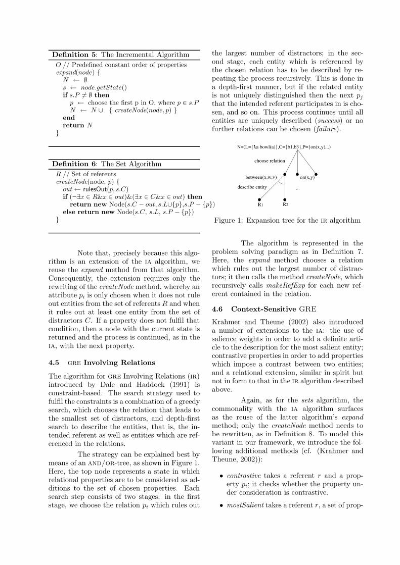
Definition 5: The Incremental Algorithm
O // Predefined constant order of propertiesexpand(node) {
N $ #s $ node.getState()if s.P %= # then
p $ choose the first p in O, where p & s.PN $ N ' { createNode(node, p) }
endreturn N
}
Definition 6: The Set Algorithm
R // Set of referentscreateNode(node, p) {
out $ rulesOut(p, s.C)if (¬)x & R&x & out)&()x & C&x & out) then
return new Node(s.C ( out, s.L'{p},s.P ( {p})else return new Node(s.C, s.L, s.P ( {p})
}
Note that, precisely because this algo-rithm is an extension of the ia algorithm, wereuse the expand method from that algorithm.Consequently, the extension requires only therewriting of the createNode method, whereby anattribute pi is only chosen when it does not ruleout entities from the set of referents R and whenit rules out at least one entity from the set ofdistractors C. If a property does not fulfil thatcondition, then a node with the current state isreturned and the process is continued, as in theia, with the next property.
4.5 gre Involving Relations
The algorithm for gre Involving Relations (ir)introduced by Dale and Haddock (1991) isconstraint-based. The search strategy used tofulfil the constraints is a combination of a greedysearch, which chooses the relation that leads tothe smallest set of distractors, and depth-firstsearch to describe the entities, that is, the in-tended referent as well as entities which are ref-erenced in the relations.
The strategy can be explained best bymeans of an and/or-tree, as shown in Figure 1.Here, the top node represents a state in whichrelational properties are to be considered as ad-ditions to the set of chosen properties. Eachsearch step consists of two stages: in the firststage, we choose the relation pi which rules out
the largest number of distractors; in the sec-ond stage, each entity which is referenced bythe chosen relation has to be described by re-peating the process recursively. This is done ina depth-first manner, but if the related entityis not uniquely distinguished then the next pj
that the intended referent participates in is cho-sen, and so on. This process continues until allentities are uniquely described (success) or nofurther relations can be chosen (failure).
describe entity ...
between(x,w,v) on(x,y)
N=(L={ a bowl(a)},C={b1,b3},P={on(x,y),..)
choose relation
R1 R2
Figure 1: Expansion tree for the ir algorithm
The algorithm is represented in theproblem solving paradigm as in Definition 7.Here, the expand method chooses a relationwhich rules out the largest number of distrac-tors; it then calls the method createNode, whichrecursively calls makeRefExp for each new ref-erent contained in the relation.
4.6 Context-Sensitive GRE
Krahmer and Theune (2002) also introduceda number of extensions to the ia: the use ofsalience weights in order to add a definite arti-cle to the description for the most salient entity;contrastive properties in order to add propertieswhich impose a contrast between two entities;and a relational extension, similar in spirit butnot in form to that in the ir algorithm describedabove.
Again, as for the sets algorithm, thecommonality with the ia algorithm surfacesas the reuse of the latter algorithm’s expandmethod; only the createNode method needs tobe rewritten, as in Definition 8. To model thisvariant in our framework, we introduce the fol-lowing additional methods (cf. (Krahmer andTheune, 2002)):
• contrastive takes a referent r and a prop-erty pi; it checks whether the property un-der consideration is contrastive.
• mostSalient takes a referent r, a set of prop-
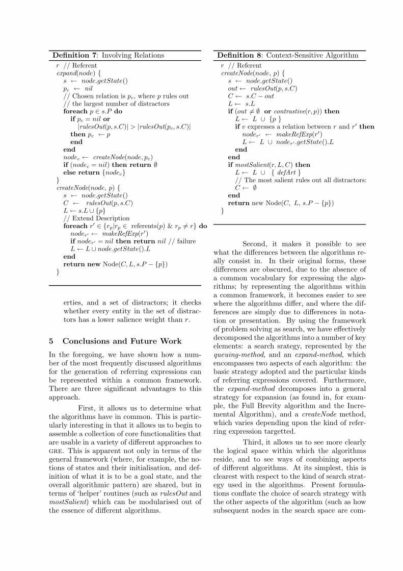
Definition 7: Involving Relations
r // Referentexpand(node) {
s $ node.getState()pc $ nil// Chosen relation is pc, where p rules out// the largest number of distractorsforeach p & s.P do
if pc = nil or|rulesOut(p, s.C)| > |rulesOut(pc, s.C)|
then pc $ pend
endnodec $ createNode(node, pc)if (nodec = nil) then return #else return {nodec}
}createNode(node, p) {
s $ node.getState()C $ rulesOut(p, s.C)L $ s.L ' {p}// Extend Descriptionforeach r! & {rp|rp & referents(p) & rp %= r} do
noder! $ makeRefExp(r!)if noder! = nil then return nil // failureL $ L ' node.getState().L
endreturn new Node(C, L, s.P ( {p})
}
erties, and a set of distractors; it checkswhether every entity in the set of distrac-tors has a lower salience weight than r.
5 Conclusions and Future Work
In the foregoing, we have shown how a num-ber of the most frequently discussed algorithmsfor the generation of referring expressions canbe represented within a common framework.There are three significant advantages to thisapproach.
First, it allows us to determine whatthe algorithms have in common. This is partic-ularly interesting in that it allows us to begin toassemble a collection of core functionalities thatare usable in a variety of di!erent approaches togre. This is apparent not only in terms of thegeneral framework (where, for example, the no-tions of states and their initialisation, and def-inition of what it is to be a goal state, and theoverall algorithmic pattern) are shared, but interms of ‘helper’ routines (such as rulesOut andmostSalient) which can be modularised out ofthe essence of di!erent algorithms.
Definition 8: Context-Sensitive Algorithm
r // ReferentcreateNode(node, p) {
s $ node.getState()out $ rulesOut(p, s.C)C $ s.C ( outL $ s.Lif (out %= # or contrastive(r, p)) then
L $ L ' {p }if v expresses a relation between r and r! then
noder! $ makeRefExp(r!)L $ L ' noder! .getState().L
endendif mostSalient(r, L, C) then
L $ L ' { defArt }// The most salient rules out all distractors:C $ #
endreturn new Node(C, L, s.P ( {p})
}
Second, it makes it possible to seewhat the di!erences between the algorithms re-ally consist in. In their original forms, thesedi!erences are obscured, due to the absence ofa common vocabulary for expressing the algo-rithms; by representing the algorithms withina common framework, it becomes easier to seewhere the algorithms di!er, and where the dif-ferences are simply due to di!erences in nota-tion or presentation. By using the frameworkof problem solving as search, we have e!ectivelydecomposed the algorithms into a number of keyelements: a search srategy, represented by thequeuing-method, and an expand-method, whichencompasses two aspects of each algorithm: thebasic strategy adopted and the particular kindsof referring expressions covered. Furthermore,the expand-method decomposes into a generalstrategy for expansion (as found in, for exam-ple, the Full Brevity algorithm and the Incre-mental Algorithm), and a createNode method,which varies depending upon the kind of refer-ring expression targetted.
Third, it allows us to see more clearlythe logical space within which the algorithmsreside, and to see ways of combining aspectsof di!erent algorithms. At its simplest, this isclearest with respect to the kind of search strat-egy used in the algorithms. Present formula-tions conflate the choice of search strategy withthe other aspects of the algorithm (such as howsubsequent nodes in the search space are com-
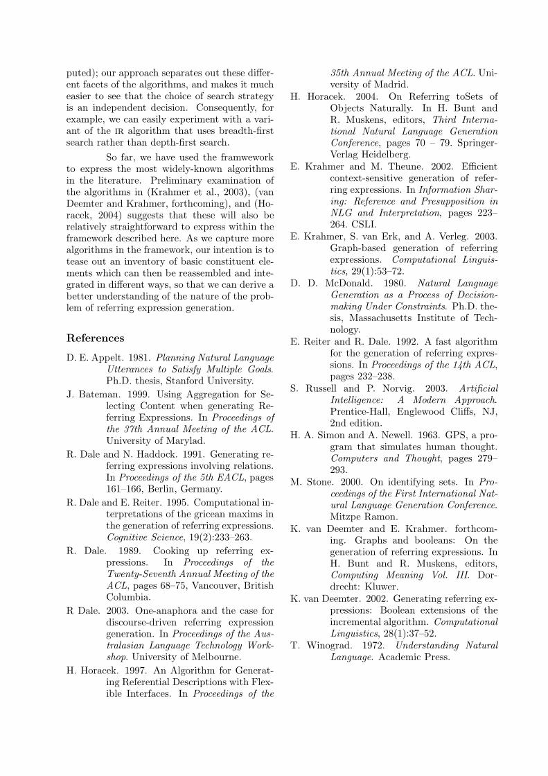
puted); our approach separates out these di!er-ent facets of the algorithms, and makes it mucheasier to see that the choice of search strategyis an independent decision. Consequently, forexample, we can easily experiment with a vari-ant of the ir algorithm that uses breadth-firstsearch rather than depth-first search.
So far, we have used the framweworkto express the most widely-known algorithmsin the literature. Preliminary examination ofthe algorithms in (Krahmer et al., 2003), (vanDeemter and Krahmer, forthcoming), and (Ho-racek, 2004) suggests that these will also berelatively straightforward to express within theframework described here. As we capture morealgorithms in the framework, our intention is totease out an inventory of basic constituent ele-ments which can then be reassembled and inte-grated in di!erent ways, so that we can derive abetter understanding of the nature of the prob-lem of referring expression generation.
References
D. E. Appelt. 1981. Planning Natural LanguageUtterances to Satisfy Multiple Goals.Ph.D. thesis, Stanford University.
J. Bateman. 1999. Using Aggregation for Se-lecting Content when generating Re-ferring Expressions. In Proceedings ofthe 37th Annual Meeting of the ACL.University of Marylad.
R. Dale and N. Haddock. 1991. Generating re-ferring expressions involving relations.In Proceedings of the 5th EACL, pages161–166, Berlin, Germany.
R. Dale and E. Reiter. 1995. Computational in-terpretations of the gricean maxims inthe generation of referring expressions.Cognitive Science, 19(2):233–263.
R. Dale. 1989. Cooking up referring ex-pressions. In Proceedings of theTwenty-Seventh Annual Meeting of theACL, pages 68–75, Vancouver, BritishColumbia.
R Dale. 2003. One-anaphora and the case fordiscourse-driven referring expressiongeneration. In Proceedings of the Aus-tralasian Language Technology Work-shop. University of Melbourne.
H. Horacek. 1997. An Algorithm for Generat-ing Referential Descriptions with Flex-ible Interfaces. In Proceedings of the
35th Annual Meeting of the ACL. Uni-versity of Madrid.
H. Horacek. 2004. On Referring toSets ofObjects Naturally. In H. Bunt andR. Muskens, editors, Third Interna-tional Natural Language GenerationConference, pages 70 – 79. Springer-Verlag Heidelberg.
E. Krahmer and M. Theune. 2002. E"cientcontext-sensitive generation of refer-ring expressions. In Information Shar-ing: Reference and Presupposition inNLG and Interpretation, pages 223–264. CSLI.
E. Krahmer, S. van Erk, and A. Verleg. 2003.Graph-based generation of referringexpressions. Computational Linguis-tics, 29(1):53–72.
D. D. McDonald. 1980. Natural LanguageGeneration as a Process of Decision-making Under Constraints. Ph.D. the-sis, Massachusetts Institute of Tech-nology.
E. Reiter and R. Dale. 1992. A fast algorithmfor the generation of referring expres-sions. In Proceedings of the 14th ACL,pages 232–238.
S. Russell and P. Norvig. 2003. ArtificialIntelligence: A Modern Approach.Prentice-Hall, Englewood Cli!s, NJ,2nd edition.
H. A. Simon and A. Newell. 1963. GPS, a pro-gram that simulates human thought.Computers and Thought, pages 279–293.
M. Stone. 2000. On identifying sets. In Pro-ceedings of the First International Nat-ural Language Generation Conference.Mitzpe Ramon.
K. van Deemter and E. Krahmer. forthcom-ing. Graphs and booleans: On thegeneration of referring expressions. InH. Bunt and R. Muskens, editors,Computing Meaning Vol. III. Dor-drecht: Kluwer.
K. van Deemter. 2002. Generating referring ex-pressions: Boolean extensions of theincremental algorithm. ComputationalLinguistics, 28(1):37–52.
T. Winograd. 1972. Understanding NaturalLanguage. Academic Press.
buys shares S\NP
buys (S\NP)/NP
John NP buys (S\NP)/NP shares NP
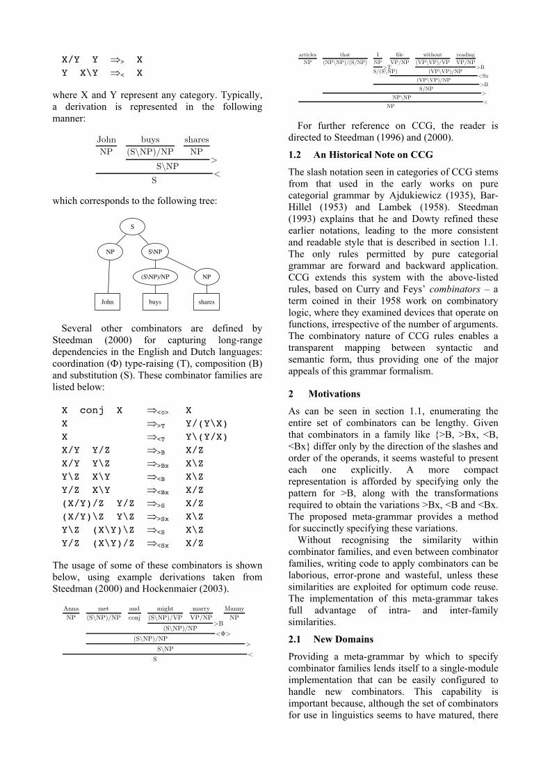
X/Y Y > X Y X\Y < X
John
NP
buys
(S\NP)/NP
shares
NP>
S\NP<
S
S
NP S\NP
John
(S\NP)/NP NP
buys shares
X conj X <> X X >T Y/(Y\X) X <T Y\(Y/X) X/Y Y/Z >B X/Z X/Y Y\Z >Bx X\Z Y\Z X\Y <B X\Z Y/Z X\Y <Bx X/Z (X/Y)/Z Y/Z >S X/Z (X/Y)\Z Y\Z >Sx X\Z Y\Z (X\Y)\Z <S X\Z Y/Z (X\Y)/Z <Sx X/Z
Anna
NP
met
(S\NP)/NP
and
conj
might
(S\NP)/VP
marry
VP/NP>B
(S\NP)/NP<!>
(S\NP)/NP
Manny
NP
>S\NP
<S
articles
NP
that
(NP\NP)/(S/NP)
I
NP>T
S/(S\NP)
file
VP/NP
without
(VP\VP)/VP
reading
VP/NP>B
(VP\VP)/NP<Sx
(VP\VP)/NP>B
S/NP>
NP\NP<
NP
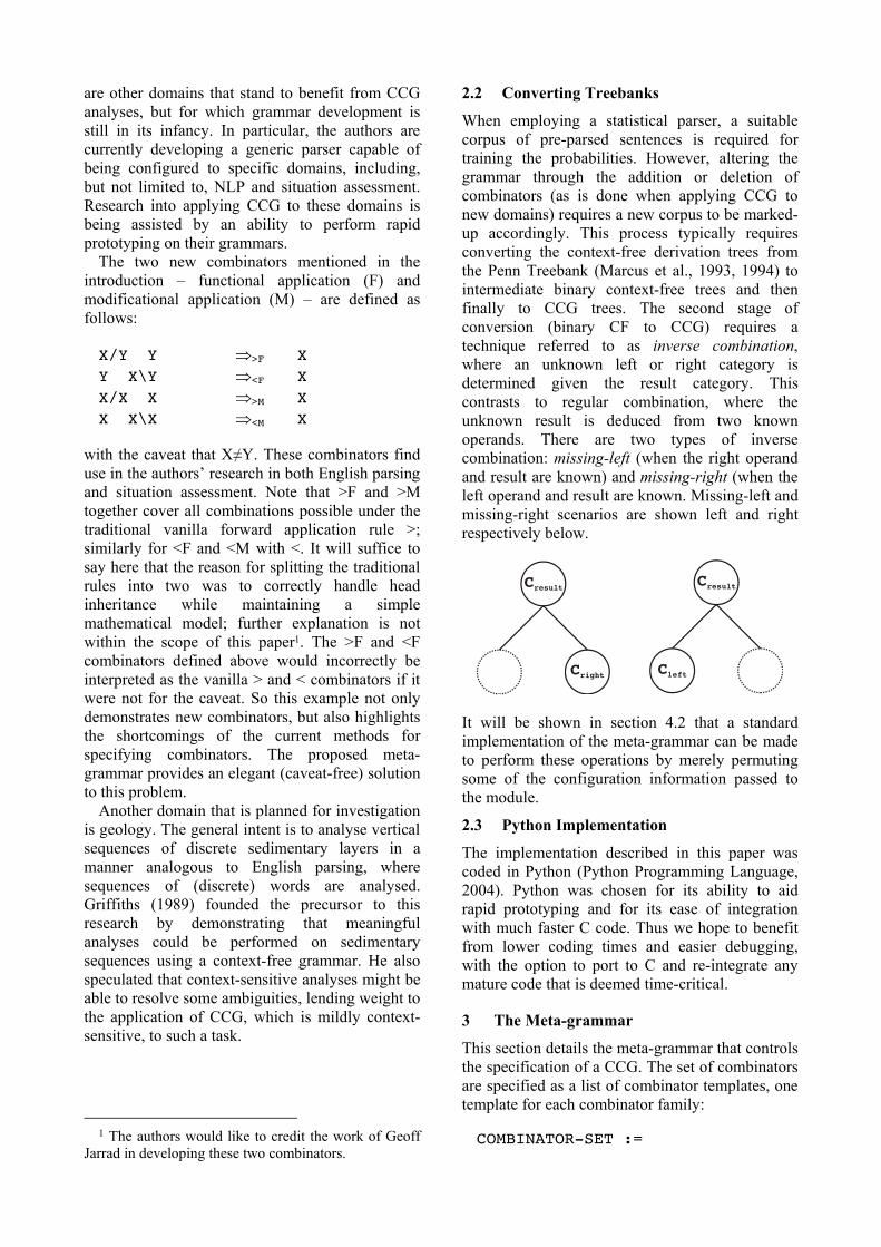
X/Y Y >F X Y X\Y <F X X/X X >M X X X\X <M X
Cresult
Cright Cleft
Cresult
COMBINATOR-SET :=
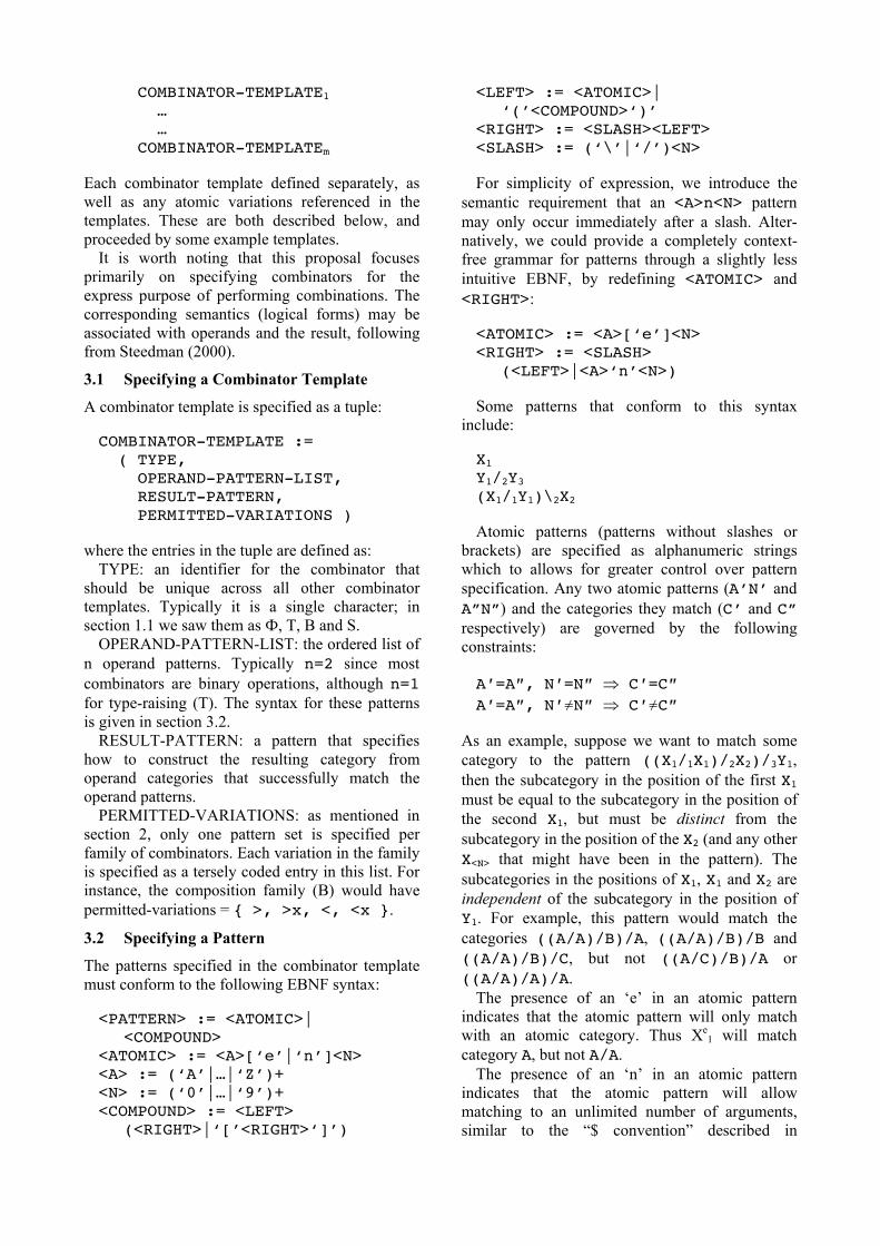
COMBINATOR-TEMPLATE1 … … COMBINATOR-TEMPLATEm
COMBINATOR-TEMPLATE := ( TYPE, OPERAND-PATTERN-LIST, RESULT-PATTERN, PERMITTED-VARIATIONS )
n=2 n=1
{ >, >x, <, <x }
<PATTERN> := <ATOMIC>| <COMPOUND>
<ATOMIC> := <A>[‘e’|‘n’]<N> <A> := (‘A’|…|‘Z’)+ <N> := (‘0’|…|‘9’)+ <COMPOUND> := <LEFT>
(<RIGHT>|‘[’<RIGHT>‘]’)
<LEFT> := <ATOMIC>| ‘(’<COMPOUND>‘)’
<RIGHT> := <SLASH><LEFT> <SLASH> := (‘\’|‘/’)<N>
<A>n<N> <ATOMIC> <RIGHT>
<ATOMIC> := <A>[‘e’]<N> <RIGHT> := <SLASH>
(<LEFT>|<A>‘n’<N>)
X1 Y1/2Y3 (X1/1Y1)\2X2
A’N’A”N” C’ C”
A=A, N=N C=C A=A, NN CC
((X1/1X1)/2X2)/3Y1X1 X1 X2X<N> X1X1X2 Y1 ((A/A)/B)/A ((A/A)/B)/B ((A/A)/B)/C ((A/C)/B)/A ((A/A)/A)/A
AA/A
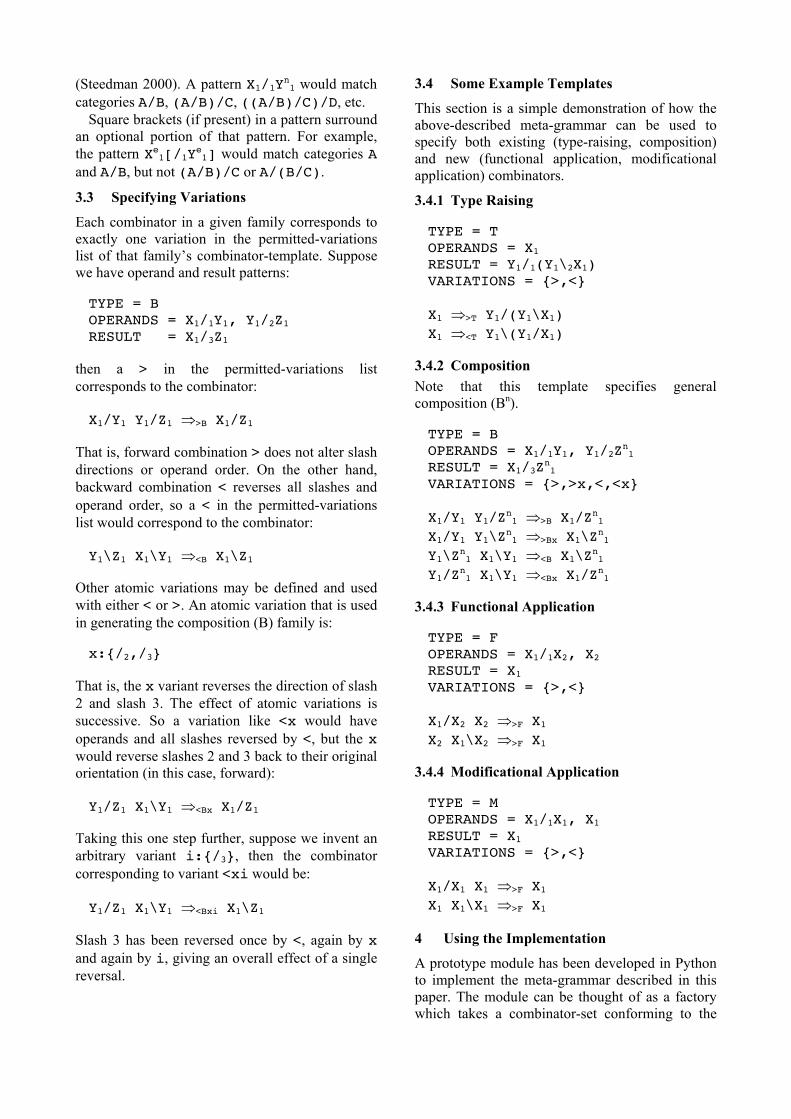
X1/1Yn1A/B(A/B)/C((A/B)/C)/D
Xe1[/1Ye1]AA/B(A/B)/CA/(B/C)
TYPE = B OPERANDS = X1/1Y1, Y1/2Z1 RESULT = X1/3Z1
>
X1/Y1 Y1/Z1 >B X1/Z1
> < <
Y1\Z1 X1\Y1 <B X1\Z1
<>
x:{/2,/3}
x <x < x
Y1/Z1 X1\Y1 <Bx X1/Z1
i:{/3} <xi
Y1/Z1 X1\Y1 <Bxi X1\Z1
< xi
TYPE = T OPERANDS = X1 RESULT = Y1/1(Y1\2X1) VARIATIONS = {>,<}
X1 >T Y1/(Y1\X1) X1 <T Y1\(Y1/X1)
TYPE = B OPERANDS = X1/1Y1, Y1/2Zn1 RESULT = X1/3Zn1 VARIATIONS = {>,>x,<,<x}
X1/Y1 Y1/Zn1 >B X1/Zn1 X1/Y1 Y1\Zn1 >Bx X1\Zn1 Y1\Zn1 X1\Y1 <B X1\Zn1 Y1/Zn1 X1\Y1 <Bx X1/Zn1
TYPE = F OPERANDS = X1/1X2, X2 RESULT = X1 VARIATIONS = {>,<}
X1/X2 X2 >F X1 X2 X1\X2 >F X1
TYPE = M OPERANDS = X1/1X1, X1 RESULT = X1 VARIATIONS = {>,<}
X1/X1 X1 >F X1 X1 X1\X1 >F X1
combine()
COMBINEFACTORY
combinatortemplates
combine()functionfn
combine()
combine() A/B
B\C A/B X1/1Y1 B\C Y1/2Zn1 {X1:A, Y1:B, Zn1:C} >x {s1:/, s2:\} {s1:/, s2:/} X1\Zn1:A\C A/BY1/2Zn1 B\C X1/1Y1 Y1=A Y1=C A/BB\C(A\C >Bx)A/BC
C
A {X1:A} {(*/(*\A) >T)(*\(*/A) <T)} * Y1
OPERANDS = A B RESULT = C VARIATIONS = {>*,<*}
ABC >*<* combine()
OPERANDS = A C RESULT = B VARIATIONS = {>*} [COMBINE FACTORY] combine1()
OPERANDS = C A RESULT = B VARIATIONS = {<*} [COMBINE FACTORY] combine2()
combine1(cA,cC) + combine2(cA,cC)
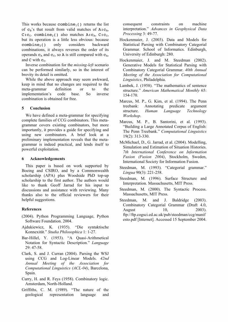
combine1() cB A:cAC:cC combine2() A:cA C:cC combine2() cAcCAcACcC
Intelligent Multi Media Presentation of information in a semi-immersive Command and Control environment
Cécile Paris, Nathalie Colineau Commonwealth Scientific and Industrial
Research Organisation (CSIRO) ICT Centre
Sydney, NSW, Australia [email protected]
Dominique Estival Defence Science & Technology
Organisation (DSTO) Human Systems Integration Group Command and Control Division
Edinburgh SA 5111, Australia [email protected]
Abstract We describe the framework for an
intelligent multimedia presentation system we designed to be part of the FOCAL laboratory, a semi-immersive environment for Command and Control Environment. FOCAL comprises a number of input devices and output media, animated virtual conversational characters, a spoken dialogue system, and sophisticated visual displays. These need to be coordinated to provide a useful and effective presentation to the user. In this paper, we describe the principles which underlie intelligent multimedia presentation (IMMP) systems and the design of such a system within the FOCAL multi-agent architecture.
1 Introduction 1.1 Description of FOCAL
FOCAL (Future Operations Centre Analysis Laboratory) was established at the Australian Defence Science and Technology Organisation (DSTO) to "pioneer a paradigm shift in command environments through a superior use of capability and greater situation awareness". The facility was designed to experiment with innovative technologies to support this goal, and it has now been running since 2000.
FOCAL contains a large-screen, semi-immersive virtual reality environment, where large quantities of information can be displayed. A number of modalities and media are available to display the information to the end-user. These include visual display mechanisms, such as 3-D virtual batttlespace, and spoken dialogue interaction with virtual conversational characters (VCCs) that allow presentation of information through speech as well as through textual
displays (Taplin et al. 2001; Broughton et al., 2002; Estival et al., 2003). While these have so far been studied and implemented somewhat independently of each other, ultimately all the different available means to present the information to the end-user must work together and be combined into a coherent whole; otherwise, the result would be very confusing to the user.
From the delivery perspective (as opposed to the input fusion aspect) with which we are concerned here, FOCAL can be considered as an instance of an intelligent multimedia presentation (IMMP) system (see Bordegoni et al., 1997 for a reference model).
1.2 An IMMP Architecture for FOCAL The framework for the design of an intelligent
multimedia presentation system (IMMP) within FOCAL was the result of a collaboration between DSTO and CSIRO. The aim was to design an architecture for the information delivery component, taking into account the existing architecture for the overall system, the available data sources and the type of desired presentations.
One of the main idea in FOCAL is that a VCC will serve as a Virtual Adviser (VA) to the team of commanding officers engaged in the planning or conduct of an operation. The aim of the VA is to engage in interactions with the officers, presenting information and offering advice. VAs are able to present the information and justify their advice through multimedia presentations (e.g., speech, video, text, map, etc.).
The remainder of this paper is structured as follows: in Section 2, we first briefly explain how research in multimedia presentation has grown from notions and systems developed in natural language generation. We then describe the process of generating multimedia
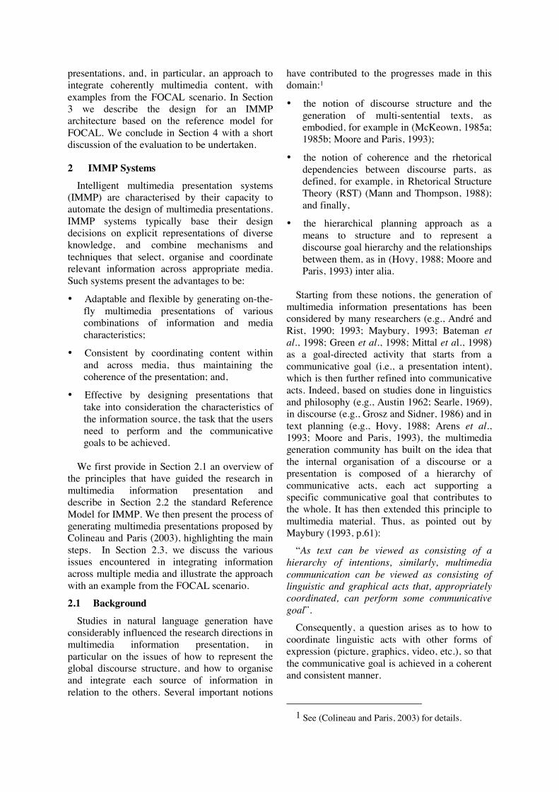
presentations, and, in particular, an approach to integrate coherently multimedia content, with examples from the FOCAL scenario. In Section 3 we describe the design for an IMMP architecture based on the reference model for FOCAL. We conclude in Section 4 with a short discussion of the evaluation to be undertaken.
2 IMMP Systems Intelligent multimedia presentation systems
(IMMP) are characterised by their capacity to automate the design of multimedia presentations. IMMP systems typically base their design decisions on explicit representations of diverse knowledge, and combine mechanisms and techniques that select, organise and coordinate relevant information across appropriate media. Such systems present the advantages to be:
• Adaptable and flexible by generating on-the-fly multimedia presentations of various combinations of information and media characteristics;
• Consistent by coordinating content within and across media, thus maintaining the coherence of the presentation; and,
• Effective by designing presentations that take into consideration the characteristics of the information source, the task that the users need to perform and the communicative goals to be achieved.
We first provide in Section 2.1 an overview of
the principles that have guided the research in multimedia information presentation and describe in Section 2.2 the standard Reference Model for IMMP. We then present the process of generating multimedia presentations proposed by Colineau and Paris (2003), highlighting the main steps. In Section 2.3, we discuss the various issues encountered in integrating information across multiple media and illustrate the approach with an example from the FOCAL scenario.
2.1 Background Studies in natural language generation have
considerably influenced the research directions in multimedia information presentation, in particular on the issues of how to represent the global discourse structure, and how to organise and integrate each source of information in relation to the others. Several important notions
have contributed to the progresses made in this domain:1
• the notion of discourse structure and the generation of multi-sentential texts, as embodied, for example in (McKeown, 1985a; 1985b; Moore and Paris, 1993);
• the notion of coherence and the rhetorical dependencies between discourse parts, as defined, for example, in Rhetorical Structure Theory (RST) (Mann and Thompson, 1988); and finally,
• the hierarchical planning approach as a means to structure and to represent a discourse goal hierarchy and the relationships between them, as in (Hovy, 1988; Moore and Paris, 1993) inter alia.
Starting from these notions, the generation of
multimedia information presentations has been considered by many researchers (e.g., André and Rist, 1990; 1993; Maybury, 1993; Bateman et al., 1998; Green et al., 1998; Mittal et al., 1998) as a goal-directed activity that starts from a communicative goal (i.e., a presentation intent), which is then further refined into communicative acts. Indeed, based on studies done in linguistics and philosophy (e.g., Austin 1962; Searle, 1969), in discourse (e.g., Grosz and Sidner, 1986) and in text planning (e.g., Hovy, 1988; Arens et al., 1993; Moore and Paris, 1993), the multimedia generation community has built on the idea that the internal organisation of a discourse or a presentation is composed of a hierarchy of communicative acts, each act supporting a specific communicative goal that contributes to the whole. It has then extended this principle to multimedia material. Thus, as pointed out by Maybury (1993, p.61):
“As text can be viewed as consisting of a hierarchy of intentions, similarly, multimedia communication can be viewed as consisting of linguistic and graphical acts that, appropriately coordinated, can perform some communicative goal”.
Consequently, a question arises as to how to coordinate linguistic acts with other forms of expression (picture, graphics, video, etc.), so that the communicative goal is achieved in a coherent and consistent manner.
1 See (Colineau and Paris, 2003) for details.
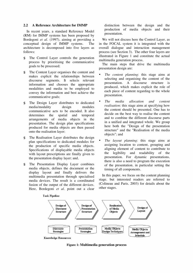
2.2 A Reference Architecture for IMMP In recent years, a standard Reference Model
(RM) for IMMP systems has been proposed by Bordegoni et al. (1997), aiming at providing a conceptual design of IMMP systems. The architecture is decomposed into five layers as follows:
§ The Control Layer controls the generation process by prioritising the communicative goals to be processed;
§ The Content Layer organises the content and makes explicit the relationships between discourse segments. It selects relevant information and chooses the appropriate modalities and media to be employed to convey the information and best achieve the communicative goals;
§ The Design Layer distributes to dedicated media/modality design modules communicative acts to be encoded. It also determines the spatial and temporal arrangements of media objects in the presentation. The design plan specifications produced for media objects are then passed onto the realisation layer;
§ The Realisation Layer distributes the design plan specifications to dedicated modules for the production of specific media objects. Specifications of displayable media objects with layout prescriptions are finally given to the presentation display layer; and,
§ The Presentation Display Layer combines media objects, defines the document or the display layout and finally delivers the multimedia presentation through specialised media devices. The result is a coordinated fusion of the output of the different devices. Here, Bordegoni et al. point out a clear
distinction between the design and the production of media objects and their presentation.
We will not discuss here the Control Layer, as in the FOCAL system it is integrated with the overall dialogue and interaction management process (see Section 3). The other four layers are illustrated in Figure 1 and constitute the actual multimedia generation process.
The main steps that drive the multimedia presentation design are:
• The content planning: this stage aims at selecting and organising the content of the presentation. A discourse structure is produced, which makes explicit the role of each piece of content regarding to the whole presentation.
• The media allocation and content realisation: this stage aims at specifying how the content should be presented. One has to decide on the best way to realise the content and to combine the different discourse parts in a unified and integrated whole. We group here both the "Design of the presentation structure" and the "Realisation of the media objects"; and
• The layout planning: this stage aims at assigning location to content, grouping and aligning element of content to contribute to the legibility and readability of the presentation. For dynamic presentations, there is also a need to program the execution of the presentation, in particular setting the timing of all components.
In this paper, we focus on the content planning stage, but interested readers are referred to (Colineau and Paris, 2003) for details about the other stages.
Figure 1: Multimedia generation process
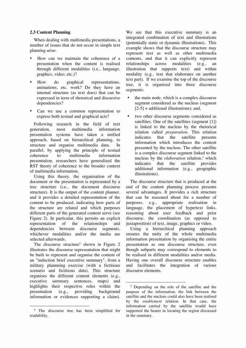
2.3 Content Planning When dealing with multimedia presentations, a
number of issues that do not occur in simple text planning arise:
• How can we maintain the coherence of a presentation when the content is realised through different modalities (i.e., language, graphics, video, etc.)?
• How do graphical representations, animations, etc. work? Do they have an internal structure (as text does) that can be expressed in term of rhetorical and discursive dependencies?
• Can we use a common representation to express both textual and graphical acts?
Following research in the field of text generation, most multimedia information presentation systems have taken a unified approach, based on hierarchical planning, to structure and organise multimedia data. In parallel, by applying the principle of textual coherence to multimedia information presentation, researchers have generalised the RST theory of coherence to the broader context of multimedia information.
Using this theory, the organisation of the document or the presentation is represented by a tree structure (i.e., the document discourse structure). It is the output of the content planner, and it provides a detailed representation of the content to be produced, indicating how parts of the structure are related and which purposes different parts of the generated content serve (see Figure 2). In particular, this permits an explicit representation of the relationships and dependencies between discourse segments, whichever modalities and/or the media are selected afterwards.
The discourse structure2 shown in Figure 2 illustrates the discourse representation that might be built to represent and organise the content of an "induction brief executive summary", from a military plannning exercise (with a fictitious scenario and fictitious data). This structure organises the different content elements (e.g., executive summary sentences, maps) and highlights their respective roles within the presentation (e.g., providing background information or evidences supporting a claim).
2 The discourse tree has been simplified for
readability.
We see that this executive summary is an integrated combination of text and illustrations (potentially static or dynamic illustrations). This example shows that the discourse structure may represent text as well as other multimedia contents, and that it can explicitly represent relationships across modalities (e.g., an illustration that supports text) and within modality (e.g., text that elaborates on another text part). If we examine the top of the discourse tree, it is organised into three discourse segments:
• the main node, which is a complex discourse segment considered as the nucleus (segment [2-5] + additional illustrations); and,
• two other discourse segments considered as satellites. One of the satellites (segment [1]) is linked to the nucleus by the rhetorical relation called preparation. This relation indicates that the satellite presents information which introduces the content presented by the nucleus. The other satellite is a complex discourse segment linked to the nucleus by the elaboration relation,3 which indicates that the satellite provides additional information (e.g., geographic illustrations).
The discourse structure that is produced at the end of the content planning process presents several advantages. It provides a rich structure that can be reasoned about for a number of purposes, e.g., appropriate realisation in language, the placement of hypertext links, reasoning about user feedback and prior discourse, the coordination (as opposed to juxtaposition) of text, image, graphics or video.
Using a hierarchical planning approach ensures the unity of the whole multimedia information presentation by organising the entire presentation as one discourse structure, even though subparts may correspond to elements to be realised in different modalities and/or media. Having one overall discourse structure enables and facilitates the integration of various discourse elements.
3 Depending on the role of the satellite and the
purpose of the information, the link between the satellite and the nucleus could also have been realised by the enablement relation. In that case, the information carried by the satellite would have supported the hearer in locating the region discussed in the summary.
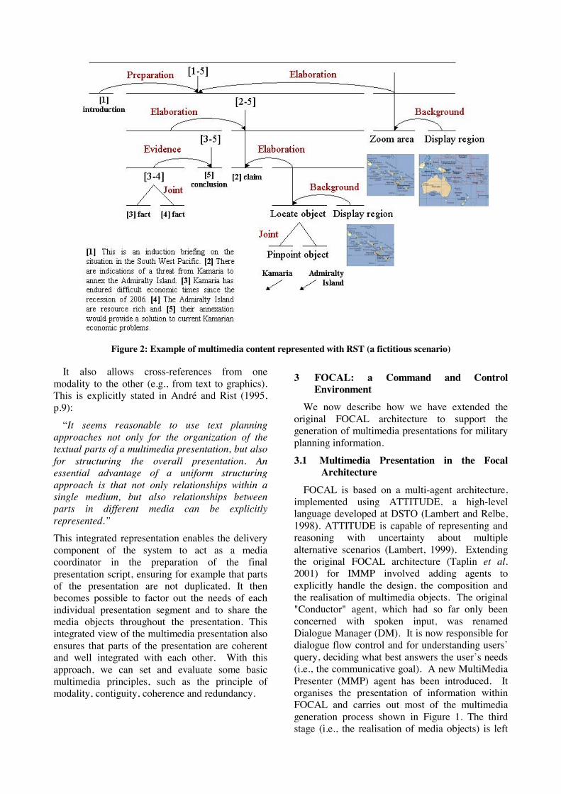
Figure 2: Example of multimedia content represented with RST (a fictitious scenario)
It also allows cross-references from one modality to the other (e.g., from text to graphics). This is explicitly stated in André and Rist (1995, p.9):
“It seems reasonable to use text planning approaches not only for the organization of the textual parts of a multimedia presentation, but also for structuring the overall presentation. An essential advantage of a uniform structuring approach is that not only relationships within a single medium, but also relationships between parts in different media can be explicitly represented.”
This integrated representation enables the delivery component of the system to act as a media coordinator in the preparation of the final presentation script, ensuring for example that parts of the presentation are not duplicated. It then becomes possible to factor out the needs of each individual presentation segment and to share the media objects throughout the presentation. This integrated view of the multimedia presentation also ensures that parts of the presentation are coherent and well integrated with each other. With this approach, we can set and evaluate some basic multimedia principles, such as the principle of modality, contiguity, coherence and redundancy.
3 FOCAL: a Command and Control Environment
We now describe how we have extended the original FOCAL architecture to support the generation of multimedia presentations for military planning information.
3.1 Multimedia Presentation in the Focal Architecture
FOCAL is based on a multi-agent architecture, implemented using ATTITUDE, a high-level language developed at DSTO (Lambert and Relbe, 1998). ATTITUDE is capable of representing and reasoning with uncertainty about multiple alternative scenarios (Lambert, 1999). Extending the original FOCAL architecture (Taplin et al. 2001) for IMMP involved adding agents to explicitly handle the design, the composition and the realisation of multimedia objects. The original "Conductor" agent, which had so far only been concerned with spoken input, was renamed Dialogue Manager (DM). It is now responsible for dialogue flow control and for understanding users’ query, deciding what best answers the user’s needs (i.e., the communicative goal). A new MultiMedia Presenter (MMP) agent has been introduced. It organises the presentation of information within FOCAL and carries out most of the multimedia generation process shown in Figure 1. The third stage (i.e., the realisation of media objects) is left
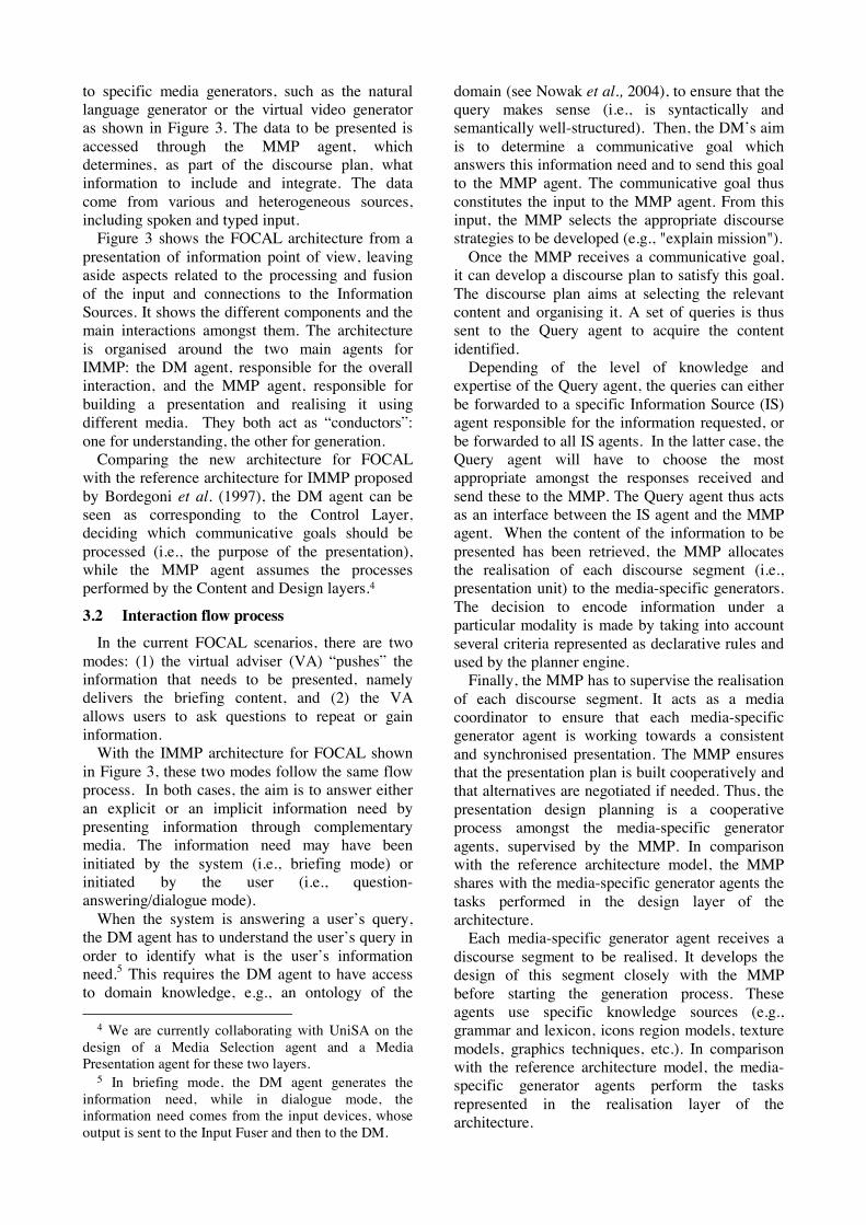
to specific media generators, such as the natural language generator or the virtual video generator as shown in Figure 3. The data to be presented is accessed through the MMP agent, which determines, as part of the discourse plan, what information to include and integrate. The data come from various and heterogeneous sources, including spoken and typed input.
Figure 3 shows the FOCAL architecture from a presentation of information point of view, leaving aside aspects related to the processing and fusion of the input and connections to the Information Sources. It shows the different components and the main interactions amongst them. The architecture is organised around the two main agents for IMMP: the DM agent, responsible for the overall interaction, and the MMP agent, responsible for building a presentation and realising it using different media. They both act as “conductors”: one for understanding, the other for generation.
Comparing the new architecture for FOCAL with the reference architecture for IMMP proposed by Bordegoni et al. (1997), the DM agent can be seen as corresponding to the Control Layer, deciding which communicative goals should be processed (i.e., the purpose of the presentation), while the MMP agent assumes the processes performed by the Content and Design layers.4
3.2 Interaction flow process In the current FOCAL scenarios, there are two
modes: (1) the virtual adviser (VA) “pushes” the information that needs to be presented, namely delivers the briefing content, and (2) the VA allows users to ask questions to repeat or gain information.
With the IMMP architecture for FOCAL shown in Figure 3, these two modes follow the same flow process. In both cases, the aim is to answer either an explicit or an implicit information need by presenting information through complementary media. The information need may have been initiated by the system (i.e., briefing mode) or initiated by the user (i.e., question-answering/dialogue mode).
When the system is answering a user’s query, the DM agent has to understand the user’s query in order to identify what is the user’s information need.5 This requires the DM agent to have access to domain knowledge, e.g., an ontology of the
4 We are currently collaborating with UniSA on the design of a Media Selection agent and a Media Presentation agent for these two layers.
5 In briefing mode, the DM agent generates the information need, while in dialogue mode, the information need comes from the input devices, whose output is sent to the Input Fuser and then to the DM.
domain (see Nowak et al., 2004), to ensure that the query makes sense (i.e., is syntactically and semantically well-structured). Then, the DM’s aim is to determine a communicative goal which answers this information need and to send this goal to the MMP agent. The communicative goal thus constitutes the input to the MMP agent. From this input, the MMP selects the appropriate discourse strategies to be developed (e.g., "explain mission").
Once the MMP receives a communicative goal, it can develop a discourse plan to satisfy this goal. The discourse plan aims at selecting the relevant content and organising it. A set of queries is thus sent to the Query agent to acquire the content identified.
Depending of the level of knowledge and expertise of the Query agent, the queries can either be forwarded to a specific Information Source (IS) agent responsible for the information requested, or be forwarded to all IS agents. In the latter case, the Query agent will have to choose the most appropriate amongst the responses received and send these to the MMP. The Query agent thus acts as an interface between the IS agent and the MMP agent. When the content of the information to be presented has been retrieved, the MMP allocates the realisation of each discourse segment (i.e., presentation unit) to the media-specific generators. The decision to encode information under a particular modality is made by taking into account several criteria represented as declarative rules and used by the planner engine.
Finally, the MMP has to supervise the realisation of each discourse segment. It acts as a media coordinator to ensure that each media-specific generator agent is working towards a consistent and synchronised presentation. The MMP ensures that the presentation plan is built cooperatively and that alternatives are negotiated if needed. Thus, the presentation design planning is a cooperative process amongst the media-specific generator agents, supervised by the MMP. In comparison with the reference architecture model, the MMP shares with the media-specific generator agents the tasks performed in the design layer of the architecture.
Each media-specific generator agent receives a discourse segment to be realised. It develops the design of this segment closely with the MMP before starting the generation process. These agents use specific knowledge sources (e.g., grammar and lexicon, icons region models, texture models, graphics techniques, etc.). In comparison with the reference architecture model, the media-specific generator agents perform the tasks represented in the realisation layer of the architecture.
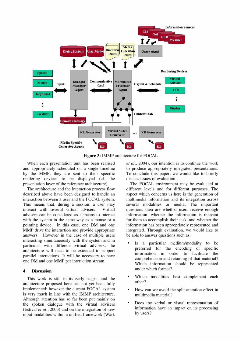
Figure 3: IMMP architecture for FOCAL
When each presentation unit has been realised and appropriately scheduled on a single timeline by the MMP, they are sent to their specific rendering devices to be displayed (cf. the presentation layer of the reference architecture).
The architecture and the interaction process flow described above have been designed to handle an interaction between a user and the FOCAL system. This means that, during a session, a user may interact with several virtual advisers. Virtual advisers can be considered as a means to interact with the system in the same way as a mouse or a pointing device. In this case, one DM and one MMP drive the interaction and provide appropriate answers. However in the case of multiple users interacting simultaneously with the system and in particular with different virtual advisers, the architecture will need to be extended to support parallel interactions. It will be necessary to have one DM and one MMP per interaction stream.
4 Discussion This work is still in its early stages, and the
architecture proposed here has not yet been fully implemented; however the current FOCAL system is very much in line with the IMMP architecture. Although attention has so far been put mainly on the spoken dialogue with the virtual advisers (Estival et al., 2003) and on the integration of new input modalities within a unified framework (Wark
et al., 2004), our intention is to continue the work to produce appropriately integrated presentations. To conclude this paper, we would like to briefly discuss issues of evaluation.
The FOCAL environment may be evaluated at different levels and for different purposes. The aspect which concerns us here is the generation of multimedia information and its integration across several modalities or media. The important questions then are whether users receive enough information, whether the information is relevant for them to accomplish their task, and whether the information has been appropriately represented and integrated. Through evaluation, we would like to be able to answer questions such as:
• Is a particular medium/modality to be preferred for the encoding of specific information in order to facilitate the comprehension and retaining of that material? Which information should be represented under which format?
• Which modalities best complement each other?
• How can we avoid the split-attention effect in multimedia material?
• Does the verbal or visual representation of information have an impact on its processing by users?
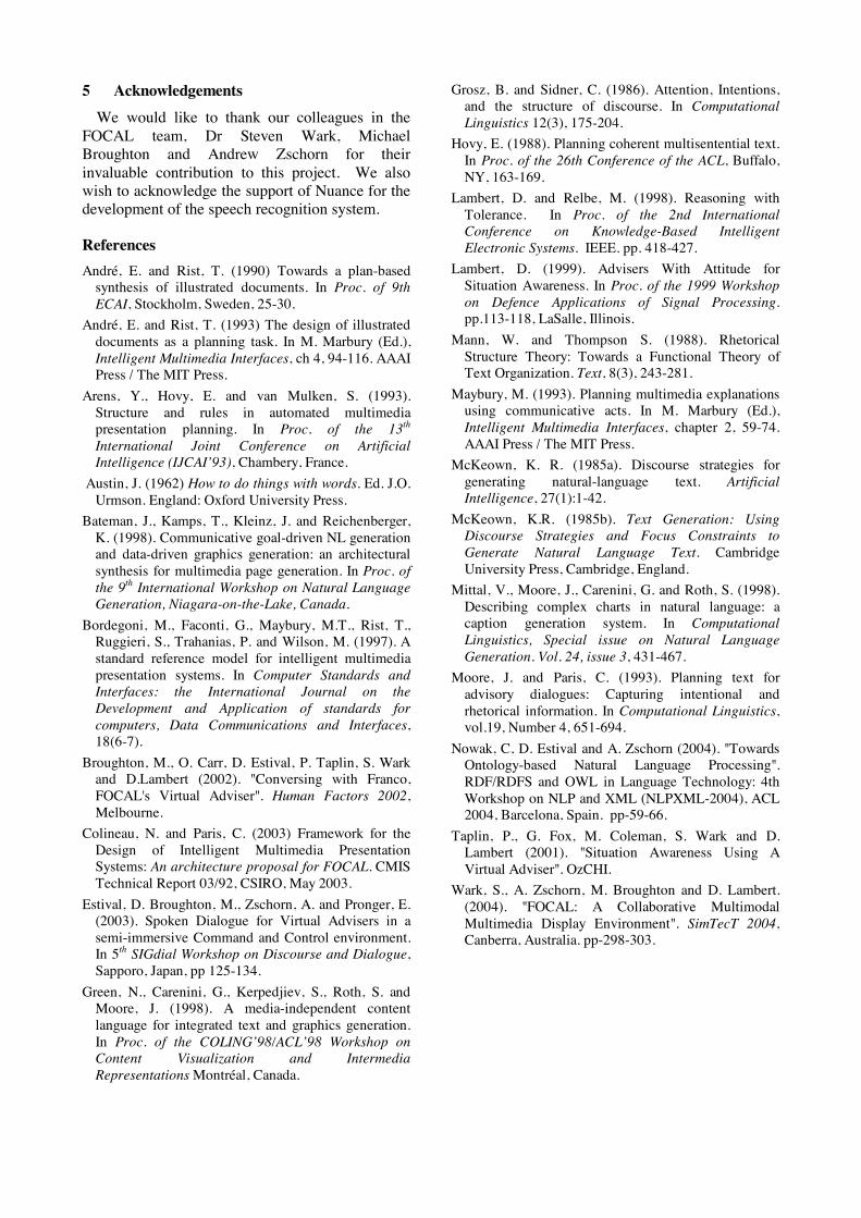
5 Acknowledgements We would like to thank our colleagues in the
FOCAL team, Dr Steven Wark, Michael Broughton and Andrew Zschorn for their invaluable contribution to this project. We also wish to acknowledge the support of Nuance for the development of the speech recognition system.
References André, E. and Rist, T. (1990) Towards a plan-based
synthesis of illustrated documents. In Proc. of 9th ECAI, Stockholm, Sweden, 25-30.
André, E. and Rist, T. (1993) The design of illustrated documents as a planning task. In M. Marbury (Ed.), Intelligent Multimedia Interfaces, ch 4, 94-116. AAAI Press / The MIT Press.
Arens, Y., Hovy, E. and van Mulken, S. (1993). Structure and rules in automated multimedia presentation planning. In Proc. of the 13th International Joint Conference on Artificial Intelligence (IJCAI’93), Chambery, France.
Austin, J. (1962) How to do things with words. Ed. J.O. Urmson. England: Oxford University Press.
Bateman, J., Kamps, T., Kleinz, J. and Reichenberger, K. (1998). Communicative goal-driven NL generation and data-driven graphics generation: an architectural synthesis for multimedia page generation. In Proc. of the 9th International Workshop on Natural Language Generation, Niagara-on-the-Lake, Canada.
Bordegoni, M., Faconti, G., Maybury, M.T., Rist, T., Ruggieri, S., Trahanias, P. and Wilson, M. (1997). A standard reference model for intelligent multimedia presentation systems. In Computer Standards and Interfaces: the International Journal on the Development and Application of standards for computers, Data Communications and Interfaces, 18(6-7).
Broughton, M., O. Carr, D. Estival, P. Taplin, S. Wark and D.Lambert (2002). "Conversing with Franco, FOCAL's Virtual Adviser". Human Factors 2002, Melbourne.
Colineau, N. and Paris, C. (2003) Framework for the Design of Intelligent Multimedia Presentation Systems: An architecture proposal for FOCAL. CMIS Technical Report 03/92, CSIRO, May 2003.
Estival, D. Broughton, M., Zschorn, A. and Pronger, E. (2003). Spoken Dialogue for Virtual Advisers in a semi-immersive Command and Control environment. In 5th SIGdial Workshop on Discourse and Dialogue, Sapporo, Japan, pp 125-134.
Green, N., Carenini, G., Kerpedjiev, S., Roth, S. and Moore, J. (1998). A media-independent content language for integrated text and graphics generation. In Proc. of the COLING’98/ACL’98 Workshop on Content Visualization and Intermedia Representations Montréal, Canada.
Grosz, B. and Sidner, C. (1986). Attention, Intentions, and the structure of discourse. In Computational Linguistics 12(3), 175-204.
Hovy, E. (1988). Planning coherent multisentential text. In Proc. of the 26th Conference of the ACL, Buffalo, NY, 163-169.
Lambert, D. and Relbe, M. (1998). Reasoning with Tolerance. In Proc. of the 2nd International Conference on Knowledge-Based Intelligent Electronic Systems. IEEE. pp. 418-427.
Lambert, D. (1999). Advisers With Attitude for Situation Awareness. In Proc. of the 1999 Workshop on Defence Applications of Signal Processing. pp.113-118, LaSalle, Illinois.
Mann, W. and Thompson S. (1988). Rhetorical Structure Theory: Towards a Functional Theory of Text Organization. Text, 8(3), 243-281.
Maybury, M. (1993). Planning multimedia explanations using communicative acts. In M. Marbury (Ed.), Intelligent Multimedia Interfaces, chapter 2, 59-74. AAAI Press / The MIT Press.
McKeown, K. R. (1985a). Discourse strategies for generating natural-language text. Artificial Intelligence, 27(1):1-42.
McKeown, K.R. (1985b). Text Generation: Using Discourse Strategies and Focus Constraints to Generate Natural Language Text. Cambridge University Press, Cambridge, England.
Mittal, V., Moore, J., Carenini, G. and Roth, S. (1998). Describing complex charts in natural language: a caption generation system. In Computational Linguistics, Special issue on Natural Language Generation. Vol. 24, issue 3, 431-467.
Moore, J. and Paris, C. (1993). Planning text for advisory dialogues: Capturing intentional and rhetorical information. In Computational Linguistics, vol.19, Number 4, 651-694.
Nowak, C, D. Estival and A. Zschorn (2004). "Towards Ontology-based Natural Language Processing". RDF/RDFS and OWL in Language Technology: 4th Workshop on NLP and XML (NLPXML-2004), ACL 2004, Barcelona, Spain. pp-59-66.
Taplin, P., G. Fox, M. Coleman, S. Wark and D. Lambert (2001). "Situation Awareness Using A Virtual Adviser". OzCHI.
Wark, S., A. Zschorn, M. Broughton and D. Lambert. (2004). "FOCAL: A Collaborative Multimodal Multimedia Display Environment". SimTecT 2004, Canberra, Australia. pp-298-303.
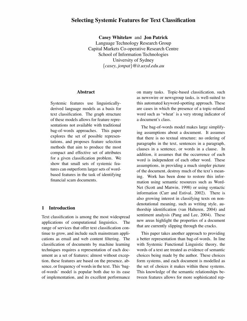
Selecting Systemic Features for Text Classification
Casey Whitelaw and Jon PatrickLanguage Technology Research Group
Capital Markets Co-operative Research CentreSchool of Information Technologies
University of Sydney{casey, jonpat}@it.usyd.edu.au
Abstract
Systemic features use linguistically-derived language models as a basis fortext classification. The graph structureof these models allows for feature repre-sentations not available with traditionalbag-of-words approaches. This paperexplores the set of possible represen-tations, and proposes feature selectionmethods that aim to produce the mostcompact and effective set of attributesfor a given classification problem. Weshow that small sets of systemic fea-tures can outperform larger sets of word-based features in the task of identifyingfinancial scam documents.
1 Introduction
Text classification is among the most widespreadapplications of computational linguistics. Therange of services that offer text classification con-tinue to grow, and include such mainstream appli-cations as email and web content filtering. Theclassification of documents by machine learningtechniques requires a representation of each doc-ument as a set of features; almost without excep-tion, these features are based on the presence, ab-sence, or frequency of words in the text. This ‘bag-of-words’ model is popular both due to its easeof implementation, and its excellent performance
on many tasks. Topic-based classification, suchas newswire or newsgroup tasks, is well-suited tothis automated keyword-spotting approach. Theseare cases in which the presence of a topic-relatedword such as ‘wheat’ is a very strong indicator ofa document’s class.
The bag-of-words model makes large simplify-ing assumptions about a document. It assumesthat there is no textual structure; no ordering ofparagraphs in the text, sentences in a paragraph,clauses in a sentence, or words in a clause. Inaddition, it assumes that the occurrence of eachword is independent of each other word. Theseassumptions, in providing a much simpler pictureof the document, destroy much of the text’s mean-ing. Work has been done to restore this infor-mation using semantic resources such as Word-Net (Scott and Matwin, 1998) or using syntacticinformation (Carr and Estival, 2002). There isalso growing interest in classifying texts on non-denotational meaning, such as writing style, au-thorship identification (van Halteren, 2004) andsentiment analysis (Pang and Lee, 2004). Thesenew areas highlight the properties of a documentthat are currently slipping through the cracks.
This paper takes another approach to providinga better representation than bag-of-words. In linewith Systemic Functional Linguistic theory, thewords of a text are treated as evidence of semanticchoices being made by the author. These choicesform systems, and each document is modelled asthe set of choices it makes within these systems.This knowledge of the semantic relationships be-tween features allows for more sophisticated rep-
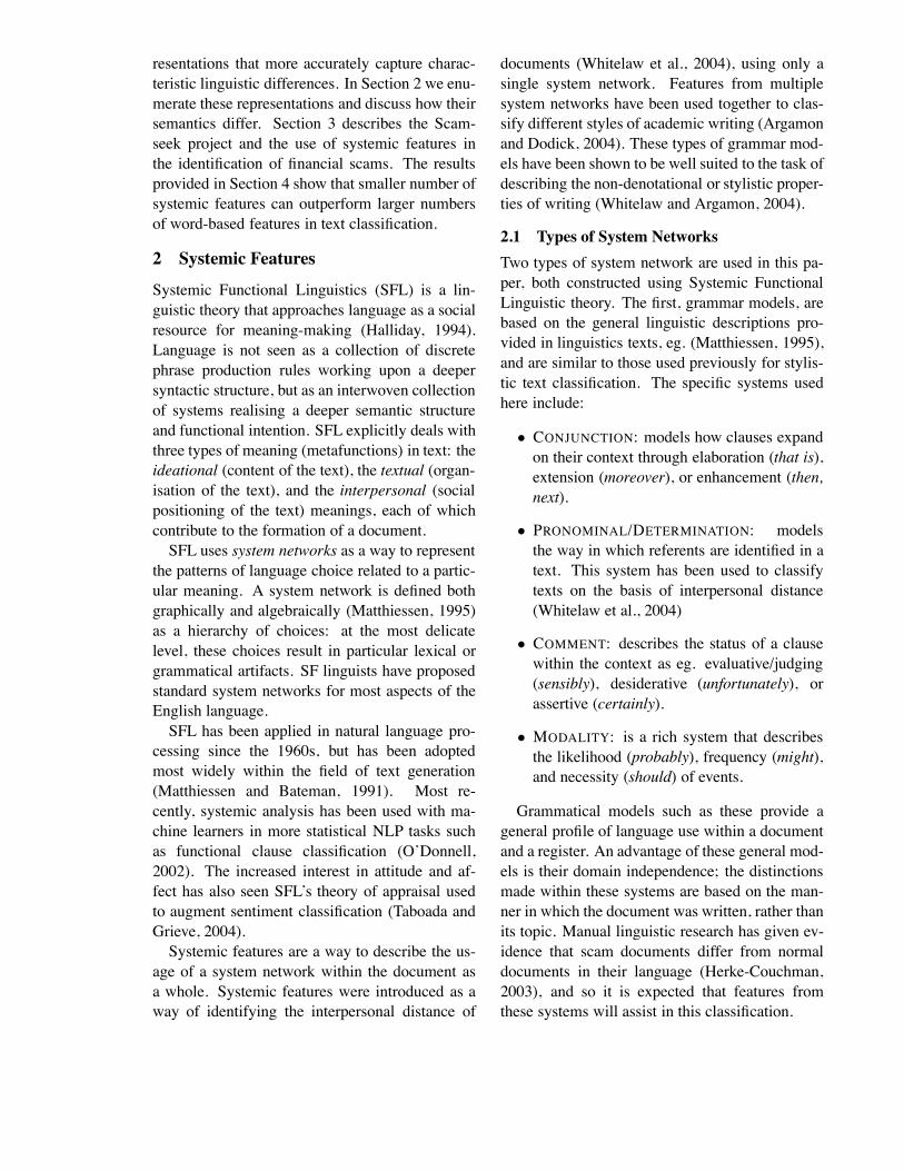
resentations that more accurately capture charac-teristic linguistic differences. In Section 2 we enu-merate these representations and discuss how theirsemantics differ. Section 3 describes the Scam-seek project and the use of systemic features inthe identification of financial scams. The resultsprovided in Section 4 show that smaller number ofsystemic features can outperform larger numbersof word-based features in text classification.
2 Systemic Features
Systemic Functional Linguistics (SFL) is a lin-guistic theory that approaches language as a socialresource for meaning-making (Halliday, 1994).Language is not seen as a collection of discretephrase production rules working upon a deepersyntactic structure, but as an interwoven collectionof systems realising a deeper semantic structureand functional intention. SFL explicitly deals withthree types of meaning (metafunctions) in text: theideational (content of the text), the textual (organ-isation of the text), and the interpersonal (socialpositioning of the text) meanings, each of whichcontribute to the formation of a document.SFL uses system networks as a way to represent
the patterns of language choice related to a partic-ular meaning. A system network is defined bothgraphically and algebraically (Matthiessen, 1995)as a hierarchy of choices: at the most delicatelevel, these choices result in particular lexical orgrammatical artifacts. SF linguists have proposedstandard system networks for most aspects of theEnglish language.SFL has been applied in natural language pro-
cessing since the 1960s, but has been adoptedmost widely within the field of text generation(Matthiessen and Bateman, 1991). Most re-cently, systemic analysis has been used with ma-chine learners in more statistical NLP tasks suchas functional clause classification (O’Donnell,2002). The increased interest in attitude and af-fect has also seen SFL’s theory of appraisal usedto augment sentiment classification (Taboada andGrieve, 2004).Systemic features are a way to describe the us-
age of a system network within the document asa whole. Systemic features were introduced as away of identifying the interpersonal distance of
documents (Whitelaw et al., 2004), using only asingle system network. Features from multiplesystem networks have been used together to clas-sify different styles of academic writing (Argamonand Dodick, 2004). These types of grammar mod-els have been shown to be well suited to the task ofdescribing the non-denotational or stylistic proper-ties of writing (Whitelaw and Argamon, 2004).
2.1 Types of System NetworksTwo types of system network are used in this pa-per, both constructed using Systemic FunctionalLinguistic theory. The first, grammar models, arebased on the general linguistic descriptions pro-vided in linguistics texts, eg. (Matthiessen, 1995),and are similar to those used previously for stylis-tic text classification. The specific systems usedhere include:
• CONJUNCTION: models how clauses expandon their context through elaboration (that is),extension (moreover), or enhancement (then,next).
• PRONOMINAL/DETERMINATION: modelsthe way in which referents are identified in atext. This system has been used to classifytexts on the basis of interpersonal distance(Whitelaw et al., 2004)
• COMMENT: describes the status of a clausewithin the context as eg. evaluative/judging(sensibly), desiderative (unfortunately), orassertive (certainly).
• MODALITY: is a rich system that describesthe likelihood (probably), frequency (might),and necessity (should) of events.
Grammatical models such as these provide ageneral profile of language use within a documentand a register. An advantage of these general mod-els is their domain independence; the distinctionsmade within these systems are based on the man-ner in which the document was written, rather thanits topic. Manual linguistic research has given ev-idence that scam documents differ from normaldocuments in their language (Herke-Couchman,2003), and so it is expected that features fromthese systems will assist in this classification.
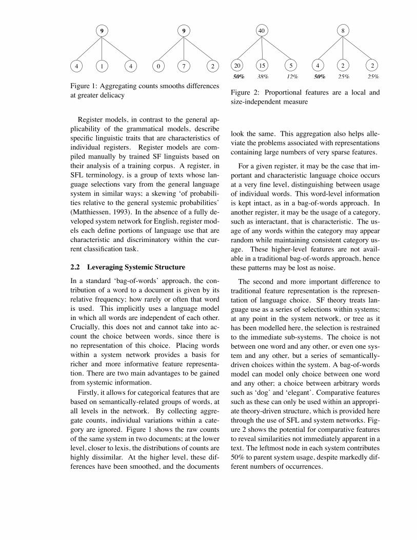
9
0 7 2414
9
Figure 1: Aggregating counts smooths differencesat greater delicacy
Register models, in contrast to the general ap-plicability of the grammatical models, describespecific linguistic traits that are characteristics ofindividual registers. Register models are com-piled manually by trained SF linguists based ontheir analysis of a training corpus. A register, inSFL terminology, is a group of texts whose lan-guage selections vary from the general languagesystem in similar ways; a skewing ‘of probabili-ties relative to the general systemic probabilities’(Matthiessen, 1993). In the absence of a fully de-veloped system network for English, register mod-els each define portions of language use that arecharacteristic and discriminatory within the cur-rent classification task.
2.2 Leveraging Systemic Structure
In a standard ‘bag-of-words’ approach, the con-tribution of a word to a document is given by itsrelative frequency; how rarely or often that wordis used. This implicitly uses a language modelin which all words are independent of each other.Crucially, this does not and cannot take into ac-count the choice between words, since there isno representation of this choice. Placing wordswithin a system network provides a basis forricher and more informative feature representa-tion. There are two main advantages to be gainedfrom systemic information.Firstly, it allows for categorical features that are
based on semantically-related groups of words, atall levels in the network. By collecting aggre-gate counts, individual variations within a cate-gory are ignored. Figure 1 shows the raw countsof the same system in two documents; at the lowerlevel, closer to lexis, the distributions of counts arehighly dissimilar. At the higher level, these dif-ferences have been smoothed, and the documents
20 15 5
38% 12% 25% 25%
40
4 2 2
8
50% 50%
Figure 2: Proportional features are a local andsize-independent measure
look the same. This aggregation also helps alle-viate the problems associated with representationscontaining large numbers of very sparse features.
For a given register, it may be the case that im-portant and characteristic language choice occursat a very fine level, distinguishing between usageof individual words. This word-level informationis kept intact, as in a bag-of-words approach. Inanother register, it may be the usage of a category,such as interactant, that is characteristic. The us-age of any words within the category may appearrandom while maintaining consistent category us-age. These higher-level features are not avail-able in a traditional bag-of-words approach, hencethese patterns may be lost as noise.
The second and more important difference totraditional feature representation is the represen-tation of language choice. SF theory treats lan-guage use as a series of selections within systems;at any point in the system network, or tree as ithas been modelled here, the selection is restrainedto the immediate sub-systems. The choice is notbetween one word and any other, or even one sys-tem and any other, but a series of semantically-driven choices within the system. A bag-of-wordsmodel can model only choice between one wordand any other; a choice between arbitrary wordssuch as ‘dog’ and ‘elegant’. Comparative featuressuch as these can only be used within an appropri-ate theory-driven structure, which is provided herethrough the use of SFL and system networks. Fig-ure 2 shows the potential for comparative featuresto reveal similarities not immediately apparent in atext. The leftmost node in each system contributes50% to parent system usage, despite markedly dif-ferent numbers of occurrences.
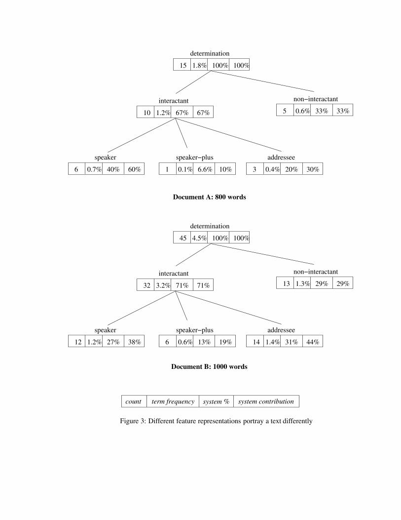
67%10 1.2% 67%
interactant
33%5 0.6% 33%
non!interactant
60%6 0.7% 40%
speaker
10%1 0.1% 6.6%
speaker!plus
30%3 0.4% 20%
addressee
100%15 1.8% 100%
determination
system contributionsystem %term frequencycount
19%6 0.6% 13%
speaker!plus
44%14 1.4% 31%
addressee
29%13 1.3% 29%
non!interactant
71%32 3.2% 71%
interactant
38%12 1.2% 27%
speaker
100%45 4.5% 100%
determination
Document A: 800 words
Document B: 1000 words
Figure 3: Different feature representations portray a text differently
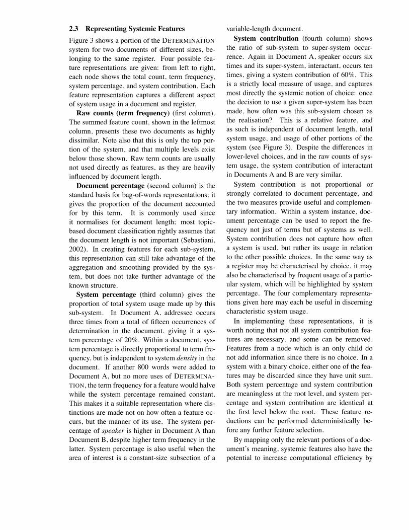
2.3 Representing Systemic FeaturesFigure 3 shows a portion of the DETERMINATIONsystem for two documents of different sizes, be-longing to the same register. Four possible fea-ture representations are given: from left to right,each node shows the total count, term frequency,system percentage, and system contribution. Eachfeature representation captures a different aspectof system usage in a document and register.Raw counts (term frequency) (first column).
The summed feature count, shown in the leftmostcolumn, presents these two documents as highlydissimilar. Note also that this is only the top por-tion of the system, and that multiple levels existbelow those shown. Raw term counts are usuallynot used directly as features, as they are heavilyinfluenced by document length.Document percentage (second column) is the
standard basis for bag-of-words representations; itgives the proportion of the document accountedfor by this term. It is commonly used sinceit normalises for document length; most topic-based document classification rightly assumes thatthe document length is not important (Sebastiani,2002). In creating features for each sub-system,this representation can still take advantage of theaggregation and smoothing provided by the sys-tem, but does not take further advantage of theknown structure.System percentage (third column) gives the
proportion of total system usage made up by thissub-system. In Document A, addressee occursthree times from a total of fifteen occurrences ofdetermination in the document, giving it a sys-tem percentage of 20%. Within a document, sys-tem percentage is directly proportional to term fre-quency, but is independent to system density in thedocument. If another 800 words were added toDocument A, but no more uses of DETERMINA-TION, the term frequency for a feature would halvewhile the system percentage remained constant.This makes it a suitable representation where dis-tinctions are made not on how often a feature oc-curs, but the manner of its use. The system per-centage of speaker is higher in Document A thanDocument B, despite higher term frequency in thelatter. System percentage is also useful when thearea of interest is a constant-size subsection of a
variable-length document.System contribution (fourth column) shows
the ratio of sub-system to super-system occur-rence. Again in Document A, speaker occurs sixtimes and its super-system, interactant, occurs tentimes, giving a system contribution of 60%. Thisis a strictly local measure of usage, and capturesmost directly the systemic notion of choice: oncethe decision to use a given super-system has beenmade, how often was this sub-system chosen asthe realisation? This is a relative feature, andas such is independent of document length, totalsystem usage, and usage of other portions of thesystem (see Figure 3). Despite the differences inlower-level choices, and in the raw counts of sys-tem usage, the system contribution of interactantin Documents A and B are very similar.System contribution is not proportional or
strongly correlated to document percentage, andthe two measures provide useful and complemen-tary information. Within a system instance, doc-ument percentage can be used to report the fre-quency not just of terms but of systems as well.System contribution does not capture how oftena system is used, but rather its usage in relationto the other possible choices. In the same way asa register may be characterised by choice, it mayalso be characterised by frequent usage of a partic-ular system, which will be highlighted by systempercentage. The four complementary representa-tions given here may each be useful in discerningcharacteristic system usage.In implementing these representations, it is
worth noting that not all system contribution fea-tures are necessary, and some can be removed.Features from a node which is an only child donot add information since there is no choice. In asystem with a binary choice, either one of the fea-tures may be discarded since they have unit sum.Both system percentage and system contributionare meaningless at the root level, and system per-centage and system contribution are identical atthe first level below the root. These feature re-ductions can be performed deterministically be-fore any further feature selection.By mapping only the relevant portions of a doc-
ument’s meaning, systemic features also have thepotential to increase computational efficiency by
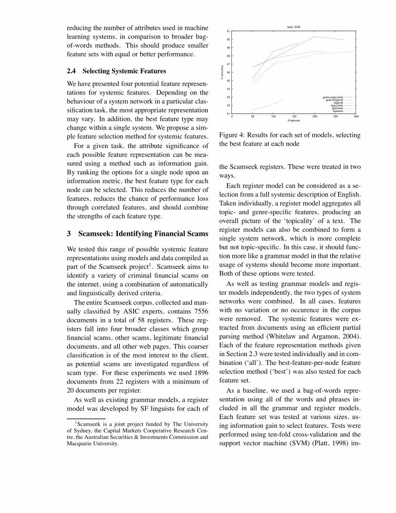
reducing the number of attributes used in machinelearning systems, in comparison to broader bag-of-words methods. This should produce smallerfeature sets with equal or better performance.
2.4 Selecting Systemic Features
We have presented four potential feature represen-tations for systemic features. Depending on thebehaviour of a system network in a particular clas-sification task, the most appropriate representationmay vary. In addition, the best feature type maychange within a single system. We propose a sim-ple feature selection method for systemic features.For a given task, the attribute significance of
each possible feature representation can be mea-sured using a method such as information gain.By ranking the options for a single node upon aninformation metric, the best feature type for eachnode can be selected. This reduces the number offeatures, reduces the chance of performance lossthrough correlated features, and should combinethe strengths of each feature type.
3 Scamseek: Identifying Financial Scams
We tested this range of possible systemic featurerepresentations using models and data compiled aspart of the Scamseek project1. Scamseek aims toidentify a variety of criminal financial scams onthe internet, using a combination of automaticallyand linguistically derived criteria.The entire Scamseek corpus, collected and man-
ually classified by ASIC experts, contains 7556documents in a total of 58 registers. These reg-isters fall into four broader classes which groupfinancial scams, other scams, legitimate financialdocuments, and all other web pages. This coarserclassification is of the most interest to the client,as potential scams are investigated regardless ofscam type. For these experiments we used 1896documents from 22 registers with a minimum of20 documents per register.As well as existing grammar models, a register
model was developed by SF linguists for each of
1Scamseek is a joint project funded by The Universityof Sydney, the Capital Markets Cooperative Research Cen-tre, the Australian Securities & Investments Commission andMacquarie University.
41
42
43
44
45
46
47
48
49
50
51
0 50 100 150 200 250 300
% a
ccur
acy
# features
best, SVM
gram+reg(comb)gram+reg(ind)
reg(ind)reg(comb)grammarbaseline
Figure 4: Results for each set of models, selectingthe best feature at each node
the Scamseek registers. These were treated in twoways.Each register model can be considered as a se-
lection from a full systemic description of English.Taken individually, a register model aggregates alltopic- and genre-specific features, producing anoverall picture of the ‘topicality’ of a text. Theregister models can also be combined to form asingle system network, which is more completebut not topic-specific. In this case, it should func-tion more like a grammar model in that the relativeusage of systems should become more important.Both of these options were tested.As well as testing grammar models and regis-
ter models independently, the two types of systemnetworks were combined. In all cases, featureswith no variation or no occurence in the corpuswere removed. The systemic features were ex-tracted from documents using an efficient partialparsing method (Whitelaw and Argamon, 2004).Each of the feature representation methods givenin Section 2.3 were tested individually and in com-bination (‘all’). The best-feature-per-node featureselection method (‘best’) was also tested for eachfeature set.As a baseline, we used a bag-of-words repre-
sentation using all of the words and phrases in-cluded in all the grammar and register models.Each feature set was tested at various sizes, us-ing information gain to select features. Tests wereperformed using ten-fold cross-validation and thesupport vector machine (SVM) (Platt, 1998) im-
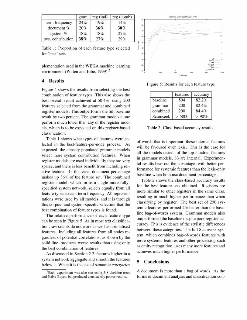
gram reg (ind) reg (comb)term frequency 24% 19% 14%document % 20% 36% 30%system % 18% 18% 27%
sys. contribution 38% 27% 29%
Table 1: Proportion of each feature type selectedfor ‘best’ sets
plementation used in the WEKAmachine learningenvironment (Witten and Eibe, 1999) 2
4 Results
Figure 4 shows the results from selecting the bestcombination of feature types. This also shows thebest overall result achieved at 50.4%, using 200features selected from the grammar and combinedregister models. This outperforms the full baselineresult by two percent. The grammar models aloneperform much lower than any of the register mod-els, which is to be expected on this register-basedclassification.Table 1 shows what types of features were se-
lected in the best-feature-per-node process. Asexpected, the densely populated grammar modelsselect more system contribution features. Whenregister models are used individually they are verysparse, and there is less benefit from including rel-ative features. In this case, document percentagemakes up 36% of the feature set. The combinedregister model, which forms a single more fully-specified system network, selects equally from allfeature types except term frequency. All represen-tations were used by all models, and it is throughthis corpus- and system-specific selection that thebest combination of feature types is found.The relative performance of each feature type
can be seen in Figure 5. As in most text classifica-tion, raw counts do not work as well as normalisedfeatures. Including all features from all nodes re-gardless of potential correlations, as shown by thesolid line, produces worse results than using onlythe best combination of features.As discussed in Section 2.2, features higher in a
system network aggregate and smooth the featuresbelow it. When it is the use of semantic categories
2Each experiment was also run using J48 decision treesand Naive Bayes, but produced consistently poorer results.
34
36
38
40
42
44
46
48
50
52
0 200 400 600 800 1000
% a
ccur
acy
# features
grammar and register features, SVM
alldoc %
rawsys.cont
sys %best
baseline
Figure 5: Results for each feature type
features accuracybaseline 594 82.2%grammar 200 82.4%combined 200 84.4%Scamseek > 5000 > 90%
Table 2: Class-based accuracy results.
of words that is important, these internal featureswill be favoured over lexis. This is the case forall the models tested: of the top hundred featuresin grammar models, 83 are internal. Experimen-tal results bear out the advantage, with better per-formance for systemic features than the lexis-onlybaseline when both use document percentage.Table 2 shows the class-based accuracy results
for the best feature sets obtained. Registers aremore similar to other registers in the same class,resulting in much higher performance than whenclassifying by register. The best set of 200 sys-temic features performed 2% better than the base-line bag-of-words system. Grammar models alsooutperformed the baseline despite poor register ac-curacy. This is evidence of the stylistic differencesbetween these categories. The full Scamseek sys-tem, which combines bag-of-words features withmore systemic features and other processing suchas entity recognition, uses many more features andachieves much higher performance.
5 Conclusions
A document is more than a bag of words. As theforms of document analysis and classification con-
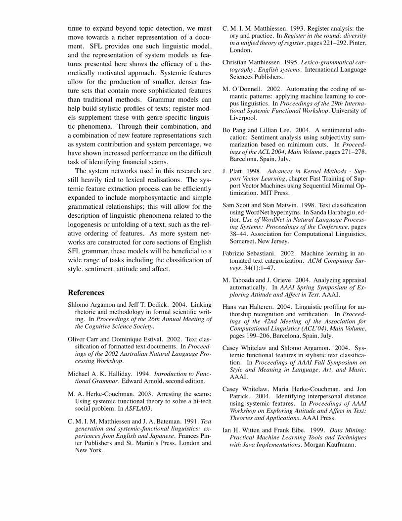
tinue to expand beyond topic detection, we mustmove towards a richer representation of a docu-ment. SFL provides one such linguistic model,and the representation of system models as fea-tures presented here shows the efficacy of a the-oretically motivated approach. Systemic featuresallow for the production of smaller, denser fea-ture sets that contain more sophisticated featuresthan traditional methods. Grammar models canhelp build stylistic profiles of texts; register mod-els supplement these with genre-specific linguis-tic phenomena. Through their combination, anda combination of new feature representations suchas system contribution and system percentage, wehave shown increased performance on the difficulttask of identifying financial scams.The system networks used in this research are
still heavily tied to lexical realisations. The sys-temic feature extraction process can be efficientlyexpanded to include morphosyntactic and simplegrammatical relationships; this will allow for thedescription of linguistic phenomena related to thelogogenesis or unfolding of a text, such as the rel-ative ordering of features. As more system net-works are constructed for core sections of EnglishSFL grammar, these models will be beneficial to awide range of tasks including the classification ofstyle, sentiment, attitude and affect.
ReferencesShlomo Argamon and Jeff T. Dodick. 2004. Linkingrhetoric and methodology in formal scientific writ-ing. In Proceedings of the 26th Annual Meeting ofthe Cognitive Science Society.
Oliver Carr and Dominique Estival. 2002. Text clas-sification of formatted text documents. In Proceed-ings of the 2002 Australian Natural Language Pro-cessing Workshop.
Michael A. K. Halliday. 1994. Introduction to Func-tional Grammar. Edward Arnold, second edition.
M. A. Herke-Couchman. 2003. Arresting the scams:Using systemic functional theory to solve a hi-techsocial problem. In ASFLA03.
C. M. I. M. Matthiessen and J. A. Bateman. 1991. Textgeneration and systemic-functional linguistics: ex-periences from English and Japanese. Frances Pin-ter Publishers and St. Martin’s Press, London andNew York.
C. M. I. M. Matthiessen. 1993. Register analysis: the-ory and practice. In Register in the round: diversityin a unified theory of register, pages 221–292. Pinter,London.
Christian Matthiessen. 1995. Lexico-grammatical car-tography: English systems. International LanguageSciences Publishers.
M. O’Donnell. 2002. Automating the coding of se-mantic patterns: applying machine learning to cor-pus linguistics. In Proceedings of the 29th Interna-tional Systemic Functional Workshop. University ofLiverpool.
Bo Pang and Lillian Lee. 2004. A sentimental edu-cation: Sentiment analysis using subjectivity sum-marization based on minimum cuts. In Proceed-ings of the ACL 2004, Main Volume, pages 271–278,Barcelona, Spain, July.
J. Platt, 1998. Advances in Kernel Methods - Sup-port Vector Learning, chapter Fast Training of Sup-port Vector Machines using Sequential Minimal Op-timization. MIT Press.
Sam Scott and Stan Matwin. 1998. Text classificationusingWordNet hypernyms. In Sanda Harabagiu, ed-itor, Use of WordNet in Natural Language Process-ing Systems: Proceedings of the Conference, pages38–44. Association for Computational Linguistics,Somerset, New Jersey.
Fabrizio Sebastiani. 2002. Machine learning in au-tomated text categorization. ACM Computing Sur-veys, 34(1):1–47.
M. Taboada and J. Grieve. 2004. Analyzing appraisalautomatically. In AAAI Spring Symposium of Ex-ploring Attitude and Affect in Text. AAAI.
Hans van Halteren. 2004. Linguistic profiling for au-thorship recognition and verification. In Proceed-ings of the 42nd Meeting of the Association forComputational Linguistics (ACL’04), Main Volume,pages 199–206, Barcelona, Spain, July.
Casey Whitelaw and Shlomo Argamon. 2004. Sys-temic functional features in stylistic text classifica-tion. In Proceedings of AAAI Fall Symposium onStyle and Meaning in Language, Art, and Music.AAAI.
Casey Whitelaw, Maria Herke-Couchman, and JonPatrick. 2004. Identifying interpersonal distanceusing systemic features. In Proceedings of AAAIWorkshop on Exploring Attitude and Affect in Text:Theories and Applications. AAAI Press.
Ian H. Witten and Frank Eibe. 1999. Data Mining:Practical Machine Learning Tools and Techniqueswith Java Implementations. Morgan Kaufmann.
A framework for utterance disambiguation in dialogue
Pont Lurcock, Peter Vlugter, Alistair KnottDepartment of Computer Science
University of OtagoNew Zealand
{pont,pvlugter,alik}@cs.otago.ac.nz
Abstract
We discuss the data sources available for ut-terance disambiguation in a bilingual dialoguesystem, distinguishing global, contextual, anduser-specific domains, and syntactic and seman-tic levels. We propose a framework for combin-ing the available information, and techniques forincreasing a stochastic grammar’s sensitivity tolocal context and a speaker’s idiolect.
1 Introduction
Resolving the ambiguities present in an incom-ing utterance is a key task in natural languageprocessing. Interpreting an utterance, whethersemantically, syntactically or phonologically, istypically construed as a two-stage process: thefirst stage involves deriving a set of all possi-ble analyses, using relatively well-defined prin-ciples, and the second stage involves selectingbetween these analyses, using principles that areharder to define and formalize.
This paper considers principles for disam-biguating utterances in a human-machine dia-logue system. Our main goal is to present aframework for integrating the di!erent sourcesof information relevant to this task, and theavailable techniques for making use of this in-formation. Working with a dialogue systemhighlights the need for such a framework; thereare additional types of ambiguity that need tobe considered (such as dialogue act ambiguity),and a particularly diverse set of informationalresources to consult (many of which relate to thecurrent dialogue context). At the same time,there are additional opportunities available—inparticular, the ability to ask the user clarifica-tion questions if a given ambiguity cannot beotherwise resolved.
We begin in Section 2 with an analysis of thekinds of disambiguation needed in our dialoguesystem, and of the information available to thesystem to perform the task. In Section 3, we
outline a general framework for performing dis-ambiguation in a dialogue system. In Sections 4and 5, we describe how our system implementsthis framework. We conclude in Section 6 withan account of our current work.
2 Sources of information availablefor utterance disambiguation
Utterance interpretation is typically modelledas a pipeline process, beginning with phono-logical interpretation, proceeding with syntacticanalysis and semantic analysis, and concludingwith discourse or dialogue attachment. We willillustrate by showing the pipeline used in ourown bilingual English/Maori dialogue system,Te Kaitito (see e.g. Knott and Wright (2003);Knott et al. (2004)). Our pipeline is shown inFigure 1. Since our input is a written sentence
Dialogue actidentification
Sentenceparsing
Presuppositionresolution
Figure 1: The utterance interpretation pipeline
we begin with sentence parsing, using the LKBsystem (Copestake and Flickinger, 2000). LKBworks with HPSG-like grammars; the gram-mar we use is bilingual, simultaneously encod-ing a fragment of English and Maori (Knott etal., 2002). LKB’s parser delivers ‘flat’ seman-tic representations in a format called MinimalRecursion Semantics (MRS) (Copestake et al.,1999), which are turned into Discourse Repre-sentation Structures (DRSs) distinguishing be-tween an assertion and a set of presuppositions(Kamp et al., in preparation). These DRSs arethen passed to a presupposition resolution mod-ule, which finds referents for anaphora, definiteNPs, and other presuppositional constructions.The resolved DRSs are passed to a dialogue actidentification module, which determines the di-alogue act made by the utterance.
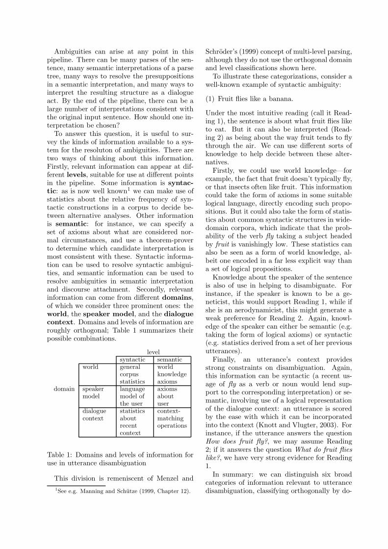
Ambiguities can arise at any point in thispipeline. There can be many parses of the sen-tence, many semantic interpretations of a parsetree, many ways to resolve the presuppositionsin a semantic interpretation, and many ways tointerpret the resulting structure as a dialogueact. By the end of the pipeline, there can be alarge number of interpretations consistent withthe original input sentence. How should one in-terpretation be chosen?
To answer this question, it is useful to sur-vey the kinds of information available to a sys-tem for the resoluton of ambiguities. There aretwo ways of thinking about this information.Firstly, relevant information can appear at dif-ferent levels, suitable for use at di!erent pointsin the pipeline. Some information is syntac-tic: as is now well known1 we can make use ofstatistics about the relative frequency of syn-tactic constructions in a corpus to decide be-tween alternative analyses. Other informationis semantic: for instance, we can specify aset of axioms about what are considered nor-mal circumstances, and use a theorem-proverto determine which candidate interpretation ismost consistent with these. Syntactic informa-tion can be used to resolve syntactic ambigui-ties, and semantic information can be used toresolve ambiguities in semantic interpretationand discourse attachment. Secondly, relevantinformation can come from di!erent domains,of which we consider three prominent ones: theworld, the speaker model, and the dialoguecontext. Domains and levels of information areroughly orthogonal; Table 1 summarizes theirpossible combinations.
levelsyntactic semantic
world generalcorpusstatistics
worldknowledgeaxioms
domain speakermodel
languagemodel ofthe user
axiomsaboutuser
dialoguecontext
statisticsaboutrecentcontext
context-matchingoperations
Table 1: Domains and levels of information foruse in utterance disambiguation
This division is remeniscent of Menzel and
1See e.g. Manning and Schutze (1999, Chapter 12).
Schroder’s (1999) concept of multi-level parsing,although they do not use the orthogonal domainand level classifications shown here.
To illustrate these categorizations, consider awell-known example of syntactic ambiguity:
(1) Fruit flies like a banana.
Under the most intuitive reading (call it Read-ing 1), the sentence is about what fruit flies liketo eat. But it can also be interpreted (Read-ing 2) as being about the way fruit tends to flythrough the air. We can use di!erent sorts ofknowledge to help decide between these alter-natives.
Firstly, we could use world knowledge—forexample, the fact that fruit doesn’t typically fly,or that insects often like fruit. This informationcould take the form of axioms in some suitablelogical language, directly encoding such propo-sitions. But it could also take the form of statis-tics about common syntactic structures in wide-domain corpora, which indicate that the prob-ability of the verb fly taking a subject headedby fruit is vanishingly low. These statistics canalso be seen as a form of world knowledge, al-beit one encoded in a far less explicit way thana set of logical propositions.
Knowledge about the speaker of the sentenceis also of use in helping to disambiguate. Forinstance, if the speaker is known to be a ge-neticist, this would support Reading 1, while ifshe is an aerodynamicist, this might generate aweak preference for Reading 2. Again, knowl-edge of the speaker can either be semantic (e.g.taking the form of logical axioms) or syntactic(e.g. statistics derived from a set of her previousutterances).
Finally, an utterance’s context providesstrong constraints on disambiguation. Again,this information can be syntactic (a recent us-age of fly as a verb or noun would lend sup-port to the corresponding interpretation) or se-mantic, involving use of a logical representationof the dialogue context: an utterance is scoredby the ease with which it can be incorporatedinto the context (Knott and Vlugter, 2003). Forinstance, if the utterance answers the questionHow does fruit fly?, we may assume Reading2; if it answers the question What do fruit flieslike?, we have very strong evidence for Reading1.
In summary: we can distinguish six broadcategories of information relevant to utterancedisambiguation, classifying orthogonally by do-
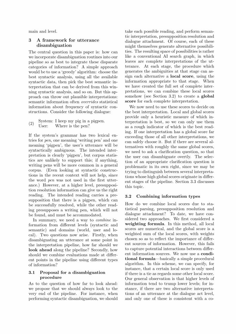
main and level.
3 A framework for utterancedisambiguation
The central question in this paper is: how canwe incorporate disambiguation routines into ourpipeline so as best to integrate these disparatecategories of information? A simple approachwould be to use a ‘greedy’ algorithm: choose thebest syntactic analysis, using all the availablesyntactic data, then pick the best semantic in-terpretation that can be derived from this win-ning syntactic analysis, and so on. But this ap-proach can throw out plausible interpretations:semantic information often overrides statisticalinformation about frequency of syntactic con-structions. Consider the following dialogue:
(2)System: I keep my pig in a pigpen.User: Where is the pen?
If the system’s grammar has two lexical en-tries for pen, one meaning ‘writing pen’ and onemeaning ‘pigpen’, the user’s utterance will besyntactically ambiguous. The intended inter-pretation is clearly ‘pigpen’, but corpus statis-tics are unlikely to support this; if anything,writing pens will be more common in a generalcorpus. (Even looking at syntactic construc-tions in the recent context will not help, sincethe word pen was not used in the first utter-ance.) However, at a higher level, presupposi-tion resolution information can give us the rightreading. The intended reading carries a pre-supposition that there is a pigpen, which canbe successfully resolved, while the other read-ing presupposes a writing pen, which will notbe found, and must be accommodated.
In summary, we need a way to combine in-formation from di!erent levels (syntactic andsemantic) and domains (world, user and lo-cal). Two questions now arise. Firstly, whendisambiguating an utterance at some point inthe interpretation pipeline, how far should welook ahead along the pipeline? Secondly, howshould we combine evaluations made at di!er-ent points in the pipeline using di!erent typesof information?
3.1 Proposal for a disambiguationprocedure
As to the question of how far to look ahead:we propose that we should always look to thevery end of the pipeline. For instance, whenperforming syntactic disambiguation, we should
take each possible reading, and perform seman-tic interpretation, presupposition resolution anddialogue attachment. Of course, each of thesemight themselves generate alternative possibili-ties. The resulting space of possibilities is ratherlike a conventional AI search graph, in whichleaves are complete interpretations of the ut-terance. At each stage, the procedure whichgenerates the ambiguities at that stage can as-sign each alternative a local score, using theinformation appropriate to that stage. Whenwe have created the full set of complete inter-pretations, we can combine these local scoressomehow (see Section 3.2) to create a globalscore for each complete interpretation.
We now need to use these scores to decide onthe best interpretation. Local and global scoresprovide only a heuristic measure of which in-terpretation is best, so we can only use themas a rough indicator of which is the best read-ing. If one interpretation has a global score farexceeding those of all other interpretations, wecan safely choose it. But if there are several al-ternatives with roughly the same global scores,we need to ask a clarification question, so thatthe user can disambiguate overtly. The selec-tion of an appropriate clarification question isproblematic in its own right, since we may betrying to distinguish between several interpreta-tions whose high global scores originate in di!er-ent stages of the pipeline. Section 3.3 discussesthis topic.
3.2 Combining information types
How do we combine local scores due to sta-tistical parsing, presupposition resolution anddialogue attachment? To date, we have con-sidered two approaches. We first considered aweighting formula. In this method, all localscores are numerical, and the global score is aweighted sum of the local scores, with weightschosen so as to reflect the importance of di!er-ent sources of information. However, this failsto capture potential interactions between di!er-ent information sources. We now use a condi-tional formula—basically a simple proceduralalgorithm. In this scheme, we can specify, forinstance, that a certain local score is only usedif there is a tie as regards some other local score.Our general observation is that higher levels ofinformation tend to trump lower levels; for in-stance, if there are two alternative interpreta-tions of an utterance at the dialogue act level,and only one of these is consistent with a co-
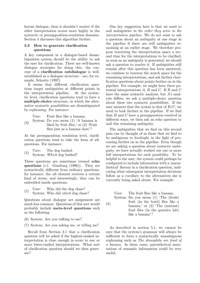
herent dialogue, then it shouldn’t matter if theother interpretation scores more highly in thesyntactic or presupposition-resolution domains.Section 4 discusses this algorithm further.
3.3 How to generate clarificationquestions
A key component in a dialogue-based disam-biguation system should be the ability to askthe user for clarification. There are well-knowndialogue strategies for doing this; the con-cept of a clarification subdialogue is well-established as a dialogue structure—see, for ex-ample, Schmitz (1997).
It seems that di!erent clarification ques-tions target ambiguities at di!erent points inthe interpretation pipeline. At the syntac-tic level, clarification questions tend to have amultiple-choice structure, in which the alter-native syntactic possibilities are disambiguatedby rephrasing. For instance:
(3)
User: Fruit flies like a banana.System: Do you mean (1) ‘A banana is
liked by fruit flies,’ or (2) ‘Fruitflies just as a banana does’?
At the presupposition resolution level, clarifi-cation questions tend to take the form of wh-questions. For instance:
(4)User: The dog barked.System: Which dog barked?
These questions are sometimes termed echoquestions (c.f. Ginzburg (1996)). They aresyntactically di!erent from ordinary questions:for instance, the wh element receives a certainkind of stress, and interestingly, they can beembedded inside questions:
(5)User: Who did the dog chase?System: Who did which dog chase?
Questions about dialogue act assignment aremuch less common. Questions of this sort wouldprobably include meta-level questions suchas the following:
(6) System: Are you talking to me?
(7) System: Are you asking me, or telling me?
Recall from Section 3.1 that a clarificationquestion will be asked if the highest-ranked in-terpretation is close enough in score to one ormore lower-ranked interpretations. What sortof clarification question should we then gener-ate?
Our key suggestion here is that we need tonail ambiguities in the order they arise in theinterpretation pipeline. We do not want to aska question about an ambiguity at one stage inthe pipeline if there are still ambiguities re-maining at an earlier stage. We therefore pro-pose traversing the interpretation space a sec-ond time for the interpretations to be clarified;as soon as an ambiguity is generated, we shouldask a question to resolve it. If ambiguities stillremain after this question has been answered,we continue to traverse the search space for theremaining interpretations, and ask further clari-fication questions about points further on in thepipeline. For example, we might have three po-tential interpretations A, B and C. If B and C
have the same syntactic analysis, but A’s anal-ysis di!ers, we ask a multiple-choice questionabout these two syntactic possibilities. If theuser answers that the syntax is that of B/C, weneed to look further in the pipeline. If we findthat B and C have a presupposition resolved indi!erent ways, we then ask an echo question tonail this remaining ambiguity.
The ambiguities that we find on this secondpass can be thought of as those that we find tobe ambiguous in hindsight, in the light of pro-cessing further on in the pipeline. Even thoughwe are asking a question about syntactic ambi-guity, we have actually worked out one or morefull interpretations for each possibility. To behelpful to the user, the system could perhaps beconfigured to include information with a ‘paren-thetical’ flavour in a clarification question, indi-cating what subsequent interpretation decisionsfollow as a corollary to the alternatives she iscurrently being asked about. For example:
(8)
User: The fruit flies like a banana.System: Do you mean (1) ‘The (fresh)
fruit (in the bowl) flies like abanana,’ or (2) ‘The (mutant)fruit flies (in the genetics lab)like a banana’?
As described in section 5.1, we cannot besure that the system’s grammar will always besu"cient to form a syntactically unambiguousrephrasing such as The drosophila are fond ofa banana. In these cases, parenthetical anno-tations of semantic information could be veryuseful.
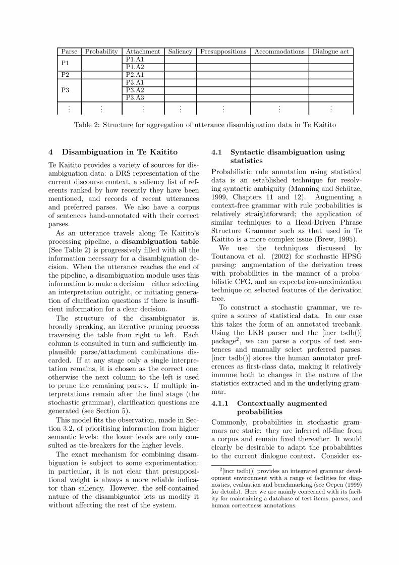
Parse Probability Attachment Saliency Presuppositions Accommodations Dialogue act
P1P1.A1P1.A2
P2 P2.A1
P3P3.A1P3.A2P3.A3
......
......
......
...
Table 2: Structure for aggregation of utterance disambiguation data in Te Kaitito
4 Disambiguation in Te Kaitito
Te Kaitito provides a variety of sources for dis-ambiguation data: a DRS representation of thecurrent discourse context, a saliency list of ref-erents ranked by how recently they have beenmentioned, and records of recent utterancesand preferred parses. We also have a corpusof sentences hand-annotated with their correctparses.
As an utterance travels along Te Kaitito’sprocessing pipeline, a disambiguation table(See Table 2) is progressively filled with all theinformation necessary for a disambiguation de-cision. When the utterance reaches the end ofthe pipeline, a disambiguation module uses thisinformation to make a decision—either selectingan interpretation outright, or initiating genera-tion of clarification questions if there is insu"-cient information for a clear decision.
The structure of the disambiguator is,broadly speaking, an iterative pruning processtraversing the table from right to left. Eachcolumn is consulted in turn and su"ciently im-plausible parse/attachment combinations dis-carded. If at any stage only a single interpre-tation remains, it is chosen as the correct one;otherwise the next column to the left is usedto prune the remaining parses. If multiple in-terpretations remain after the final stage (thestochastic grammar), clarification questions aregenerated (see Section 5).
This model fits the observation, made in Sec-tion 3.2, of prioritising information from highersemantic levels: the lower levels are only con-sulted as tie-breakers for the higher levels.
The exact mechanism for combining disam-biguation is subject to some experimentation:in particular, it is not clear that presupposi-tional weight is always a more reliable indica-tor than saliency. However, the self-containednature of the disambiguator lets us modify itwithout a!ecting the rest of the system.
4.1 Syntactic disambiguation usingstatistics
Probabilistic rule annotation using statisticaldata is an established technique for resolv-ing syntactic ambiguity (Manning and Schutze,1999, Chapters 11 and 12). Augmenting acontext-free grammar with rule probabilities isrelatively straightforward; the application ofsimilar techniques to a Head-Driven PhraseStructure Grammar such as that used in TeKaitito is a more complex issue (Brew, 1995).
We use the techniques discussed byToutanova et al. (2002) for stochastic HPSGparsing: augmentation of the derivation treeswith probabilities in the manner of a proba-bilistic CFG, and an expectation-maximizationtechnique on selected features of the derivationtree.
To construct a stochastic grammar, we re-quire a source of statistical data. In our casethis takes the form of an annotated treebank.Using the LKB parser and the [incr tsdb()]package2, we can parse a corpus of test sen-tences and manually select preferred parses.[incr tsdb()] stores the human annotator pref-erences as first-class data, making it relativelyimmune both to changes in the nature of thestatistics extracted and in the underlying gram-mar.
4.1.1 Contextually augmentedprobabilities
Commonly, probabilities in stochastic gram-mars are static: they are inferred o!-line froma corpus and remain fixed thereafter. It wouldclearly be desirable to adapt the probabilitiesto the current dialogue context. Consider ex-
2[incr tsdb()] provides an integrated grammar devel-opment environment with a range of facilities for diag-nostics, evaluation and benchmarking (see Oepen (1999)for details). Here we are mainly concerned with its facil-ity for maintaining a database of test items, parses, andhuman correctness annotations.
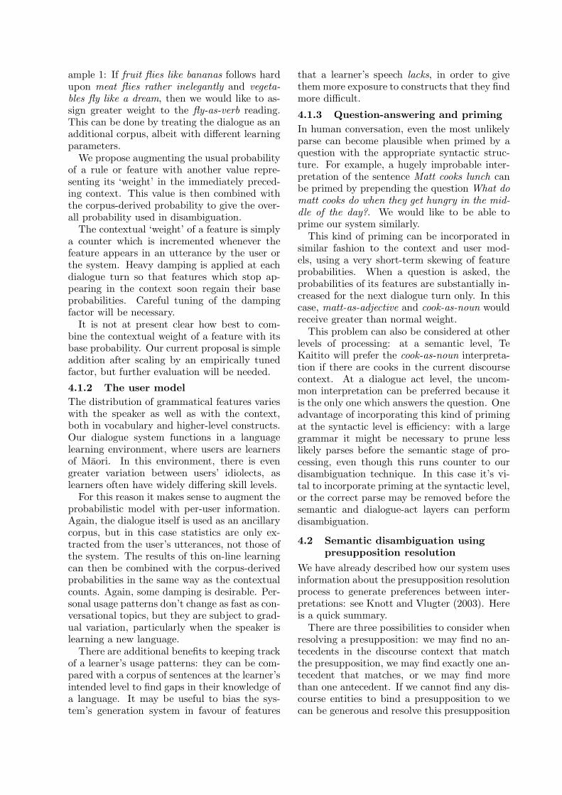
ample 1: If fruit flies like bananas follows hardupon meat flies rather inelegantly and vegeta-bles fly like a dream, then we would like to as-sign greater weight to the fly-as-verb reading.This can be done by treating the dialogue as anadditional corpus, albeit with di!erent learningparameters.
We propose augmenting the usual probabilityof a rule or feature with another value repre-senting its ‘weight’ in the immediately preced-ing context. This value is then combined withthe corpus-derived probability to give the over-all probability used in disambiguation.
The contextual ‘weight’ of a feature is simplya counter which is incremented whenever thefeature appears in an utterance by the user orthe system. Heavy damping is applied at eachdialogue turn so that features which stop ap-pearing in the context soon regain their baseprobabilities. Careful tuning of the dampingfactor will be necessary.
It is not at present clear how best to com-bine the contextual weight of a feature with itsbase probability. Our current proposal is simpleaddition after scaling by an empirically tunedfactor, but further evaluation will be needed.
4.1.2 The user model
The distribution of grammatical features varieswith the speaker as well as with the context,both in vocabulary and higher-level constructs.Our dialogue system functions in a languagelearning environment, where users are learnersof Maori. In this environment, there is evengreater variation between users’ idiolects, aslearners often have widely di!ering skill levels.
For this reason it makes sense to augment theprobabilistic model with per-user information.Again, the dialogue itself is used as an ancillarycorpus, but in this case statistics are only ex-tracted from the user’s utterances, not those ofthe system. The results of this on-line learningcan then be combined with the corpus-derivedprobabilities in the same way as the contextualcounts. Again, some damping is desirable. Per-sonal usage patterns don’t change as fast as con-versational topics, but they are subject to grad-ual variation, particularly when the speaker islearning a new language.
There are additional benefits to keeping trackof a learner’s usage patterns: they can be com-pared with a corpus of sentences at the learner’sintended level to find gaps in their knowledge ofa language. It may be useful to bias the sys-tem’s generation system in favour of features
that a learner’s speech lacks, in order to givethem more exposure to constructs that they findmore di"cult.
4.1.3 Question-answering and priming
In human conversation, even the most unlikelyparse can become plausible when primed by aquestion with the appropriate syntactic struc-ture. For example, a hugely improbable inter-pretation of the sentence Matt cooks lunch canbe primed by prepending the question What domatt cooks do when they get hungry in the mid-dle of the day?. We would like to be able toprime our system similarly.
This kind of priming can be incorporated insimilar fashion to the context and user mod-els, using a very short-term skewing of featureprobabilities. When a question is asked, theprobabilities of its features are substantially in-creased for the next dialogue turn only. In thiscase, matt-as-adjective and cook-as-noun wouldreceive greater than normal weight.
This problem can also be considered at otherlevels of processing: at a semantic level, TeKaitito will prefer the cook-as-noun interpreta-tion if there are cooks in the current discoursecontext. At a dialogue act level, the uncom-mon interpretation can be preferred because itis the only one which answers the question. Oneadvantage of incorporating this kind of primingat the syntactic level is e"ciency: with a largegrammar it might be necessary to prune lesslikely parses before the semantic stage of pro-cessing, even though this runs counter to ourdisambiguation technique. In this case it’s vi-tal to incorporate priming at the syntactic level,or the correct parse may be removed before thesemantic and dialogue-act layers can performdisambiguation.
4.2 Semantic disambiguation usingpresupposition resolution
We have already described how our system usesinformation about the presupposition resolutionprocess to generate preferences between inter-pretations: see Knott and Vlugter (2003). Hereis a quick summary.
There are three possibilities to consider whenresolving a presupposition: we may find no an-tecedents in the discourse context that matchthe presupposition, we may find exactly one an-tecedent that matches, or we may find morethan one antecedent. If we cannot find any dis-course entities to bind a presupposition to wecan be generous and resolve this presupposition
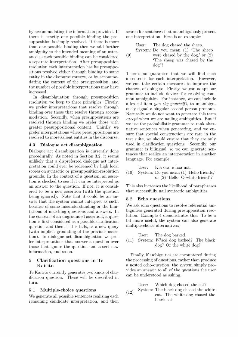
by accommodating the information provided. Ifthere is exactly one possible binding the pre-supposition is simply resolved. If there is morethan one possible binding then we add furtherambiguity to the intended meaning of an utter-ance as each possible binding can be considereda separate interpretation. After presuppositionresolution each interpretation has its presuppo-sitions resolved either through binding to someentity in the discourse context, or by accommo-dating the content of the presupposition, andthe number of possible interpretations may haveincreased.
In disambiguation through presuppositionresolution we keep to three principles. Firstly,we prefer interpretations that resolve throughbinding over those that resolve through accom-modation. Secondly, when presuppositions areresolved through binding we prefer those withgreater presuppositional content. Thirdly, weprefer interpretations where presuppositions areresolved to more salient entities in the discourse.
4.3 Dialogue act disambiguation
Dialogue act disambiguation is currently doneprocedurally. As noted in Section 3.2, it seemsunlikely that a dispreferred dialogue act inter-pretation could ever be redeemed by high localscores on syntactic or presupposition-resolutiongrounds. In the context of a question, an asser-tion is checked to see if it can be interpreted asan answer to the question. If not, it is consid-ered to be a new assertion (with the questionbeing ignored). Note that it could be an an-swer that the system cannot interpret as such,because of some misunderstanding or the limi-tations of matching questions and answers. Inthe context of an ungrounded assertion, a ques-tion is first considered as a possible clarificationquestion and then, if this fails, as a new query(with implicit grounding of the previous asser-tion). In dialogue act disambiguation we pre-fer interpretations that answer a question overthose that ignore the question and assert newinformation, and so on.
5 Clarification questions in TeKaitito
Te Kaitito currently generates two kinds of clar-ification question. These will be described inturn.
5.1 Multiple-choice questions
We generate all possible sentences realizing eachremaining candidate interpretation, and then
search for sentences that unambiguously presentone interpretation. Here is an example:
(9)
User: The dog chased the sheep.System: Do you mean (1) ‘The sheep
were chased by the dog,’ or (2)‘The sheep was chased by thedog’?
There’s no guarantee that we will find sucha sentence for each interpretation. However,we can take certain measures to improve thechances of doing so. Firstly, we can adapt ourgrammar to include devices for resolving com-mon ambiguities. For instance, we can includea lexical item you (by yourself), to unambigu-ously signal a singular second-person pronoun.Naturally we do not want to generate this termexcept when we are nailing ambiguities. But ifwe use the probabilistic grammar to rank alter-native sentences when generating, and we en-sure that special constructions are rare in thetest suite, we should ensure that they are onlyused in clarification questions. Secondly, ourgrammar is bilingual, so we can generate sen-tences that realize an interpretation in anotherlanguage. For example:
(10)User: Kia ora, e hoa ma.System: Do you mean (1) ‘Hello friends,’
or (2) ‘Hello, O white friend’?
This also increases the likelihood of paraphrasesthat successfully nail syntactic ambiguities.
5.2 Echo questions
We ask echo questions to resolve referential am-biguities generated during presupposition reso-lution. Example 4 demonstrates this. To be abit more useful, the system can also generatemultiple-choice alternatives:
(11)User: The dog barked.System: Which dog barked? The black
dog? Or the white dog?
Finally, if ambiguities are encountered duringthe processing of questions, rather than producea nested echo-question, the system simply pro-vides an answer to all of the questions the usercan be understood as asking.
(12)
User: Which dog chased the cat?System: The black dog chased the white
cat. The white dog chased theblack cat.
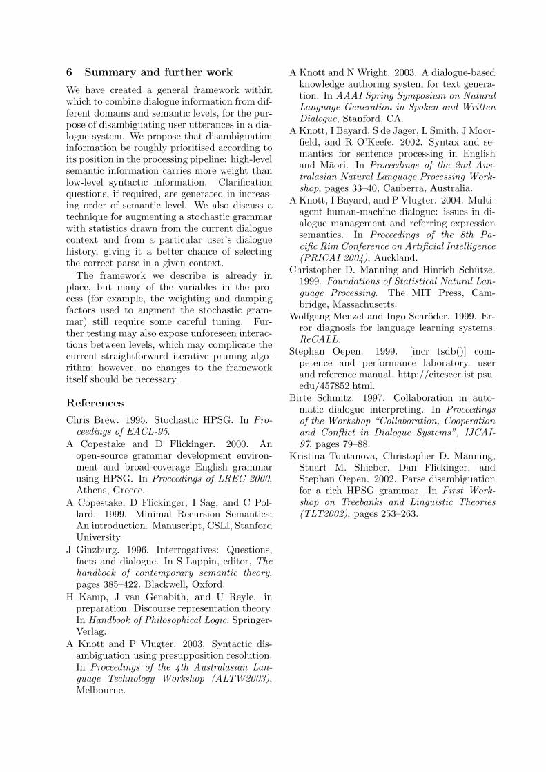
6 Summary and further work
We have created a general framework withinwhich to combine dialogue information from dif-ferent domains and semantic levels, for the pur-pose of disambiguating user utterances in a dia-logue system. We propose that disambiguationinformation be roughly prioritised according toits position in the processing pipeline: high-levelsemantic information carries more weight thanlow-level syntactic information. Clarificationquestions, if required, are generated in increas-ing order of semantic level. We also discuss atechnique for augmenting a stochastic grammarwith statistics drawn from the current dialoguecontext and from a particular user’s dialoguehistory, giving it a better chance of selectingthe correct parse in a given context.
The framework we describe is already inplace, but many of the variables in the pro-cess (for example, the weighting and dampingfactors used to augment the stochastic gram-mar) still require some careful tuning. Fur-ther testing may also expose unforeseen interac-tions between levels, which may complicate thecurrent straightforward iterative pruning algo-rithm; however, no changes to the frameworkitself should be necessary.
References
Chris Brew. 1995. Stochastic HPSG. In Pro-ceedings of EACL-95.
A Copestake and D Flickinger. 2000. Anopen-source grammar development environ-ment and broad-coverage English grammarusing HPSG. In Proceedings of LREC 2000,Athens, Greece.
A Copestake, D Flickinger, I Sag, and C Pol-lard. 1999. Minimal Recursion Semantics:An introduction. Manuscript, CSLI, StanfordUniversity.
J Ginzburg. 1996. Interrogatives: Questions,facts and dialogue. In S Lappin, editor, Thehandbook of contemporary semantic theory,pages 385–422. Blackwell, Oxford.
H Kamp, J van Genabith, and U Reyle. inpreparation. Discourse representation theory.In Handbook of Philosophical Logic. Springer-Verlag.
A Knott and P Vlugter. 2003. Syntactic dis-ambiguation using presupposition resolution.In Proceedings of the 4th Australasian Lan-guage Technology Workshop (ALTW2003),Melbourne.
A Knott and N Wright. 2003. A dialogue-basedknowledge authoring system for text genera-tion. In AAAI Spring Symposium on NaturalLanguage Generation in Spoken and WrittenDialogue, Stanford, CA.
A Knott, I Bayard, S de Jager, L Smith, J Moor-field, and R O’Keefe. 2002. Syntax and se-mantics for sentence processing in Englishand Maori. In Proceedings of the 2nd Aus-tralasian Natural Language Processing Work-shop, pages 33–40, Canberra, Australia.
A Knott, I Bayard, and P Vlugter. 2004. Multi-agent human-machine dialogue: issues in di-alogue management and referring expressionsemantics. In Proceedings of the 8th Pa-cific Rim Conference on Artificial Intelligence(PRICAI 2004), Auckland.
Christopher D. Manning and Hinrich Schutze.1999. Foundations of Statistical Natural Lan-guage Processing. The MIT Press, Cam-bridge, Massachusetts.
Wolfgang Menzel and Ingo Schroder. 1999. Er-ror diagnosis for language learning systems.ReCALL.
Stephan Oepen. 1999. [incr tsdb()] com-petence and performance laboratory. userand reference manual. http://citeseer.ist.psu.edu/457852.html.
Birte Schmitz. 1997. Collaboration in auto-matic dialogue interpreting. In Proceedingsof the Workshop “Collaboration, Cooperationand Conflict in Dialogue Systems”, IJCAI-97, pages 79–88.
Kristina Toutanova, Christopher D. Manning,Stuart M. Shieber, Dan Flickinger, andStephan Oepen. 2002. Parse disambiguationfor a rich HPSG grammar. In First Work-shop on Treebanks and Linguistic Theories(TLT2002), pages 253–263.
Maximum Entropy Markov Models for Semantic Role Labelling
Phil BlunsomDepartment of Computer Science and Software Engineering
University of Melbourne, Vic 3010, Australiaemail: [email protected]
AbstractThis paper investigates the application of Max-imum Entropy Markov Models to semantic rolelabelling. Syntactic chunks are labelled accordingto the semantic role they fill for sentence verb pred-icates. The model is trained on the subset of Prop-bank data provided for the Conference on Compu-tational Natural Language Learning 2004. Goodprecision is achieved, which is of key importancefor information extraction from large corpora con-taining redundant data, and for generalising systemsbeyond task specific, hand coded template meth-ods.
1 IntroductionIn recent years, much progress has been made inthe fields of information extraction and questionanswering. Research systems developed for confer-ence competitions have graduated into the commer-cial world in such applications as air travel infor-mation and booking, call handling, and banking.Although these systems perform well on their cho-sen tasks, they are generally based on a frame–and–slot approach. This approach uses application–dependent frames defined for propositions and thenattempts to fill slots from words surrounding theproposition that triggered the frame. For exam-ple, in a financial system we may be interested inextracting company mergers from newswires. Wecould define a frame for the verb stem merge, andslots in that frame for the companies involved inthe merger. Although this could be effective forthe chosen domain, each time we want to developa system for a new domain we need to start fromscratch. In order to build broad coverage systemscapable of generalising, we need a way of definingand labelling propositions and their arguments thatis not tied to a particular application.Systems have been developed to address the task
of semantic role labelling (SRL) using a variety ofmachine learning techniques and features rangingfrom simple lexical information to those derived
!"#$%&'()*"&+,-
! !""#$%$&#"'(#"($)*(+*""(,-**.%"/(0&$)(1*-.(%-234*"$('$-35$3-*
! 6-%4*(7#-(%,./'8
<!DOCTYPE frameset SYSTEM "frameset.dtd">
<frameset>
<predicate lemma="begin">
<roleset id="begin.01" name="start" vncls="55.1">
<roles>
<role descr="Agent" n="0">
<vnrole vncls="55.1" vntheta="Agent"/></role>
<role descr="Theme(-Creation)" n="1">
<vnrole vncls="55.1" vntheta="Theme"/></role>
<role descr="Instrument" n="2"/>
</roles>
Figure 1: Propbank XML frame for begin
from parse trees. These semantic roles identifyarguments of verb predicates and can be general,such as agent, theme, or verb specific, such as A0,A1.This paper presents a discriminative Markov
model for the semantic role labelling task proposedfor the Conference on Computational Natural Lan-guage Learning 2004 (CoNLL). Firstly, recent workon SRL is examined and the data available forthis task is presented. A discriminative maximumentropy framework is defined and a SRL modeldescribed. This model trains maximum entropyclassifiers for each state in the Markov model, rep-resenting the probability distribution for transitionsfrom that state for a given observation feature vec-tor. This approach combines the advantages of tran-sition sequence based models with the ability ofmaximum entropy classifiers to handle a diverserange of overlapping features. The results obtainedachieve precision comparable to the best performingsupport vector model, while requiring significantlyless time to train. However, recall is not as high asother approaches and provides an area for furtherimprovement.
2 BackgroundMany researchers have tackled semantic rolelabelling. Traditional parsing systems have per-formed tasks that incorporate a level of semanticlabelling and many information extraction systemsattempt to solve the labelling problem for a single,
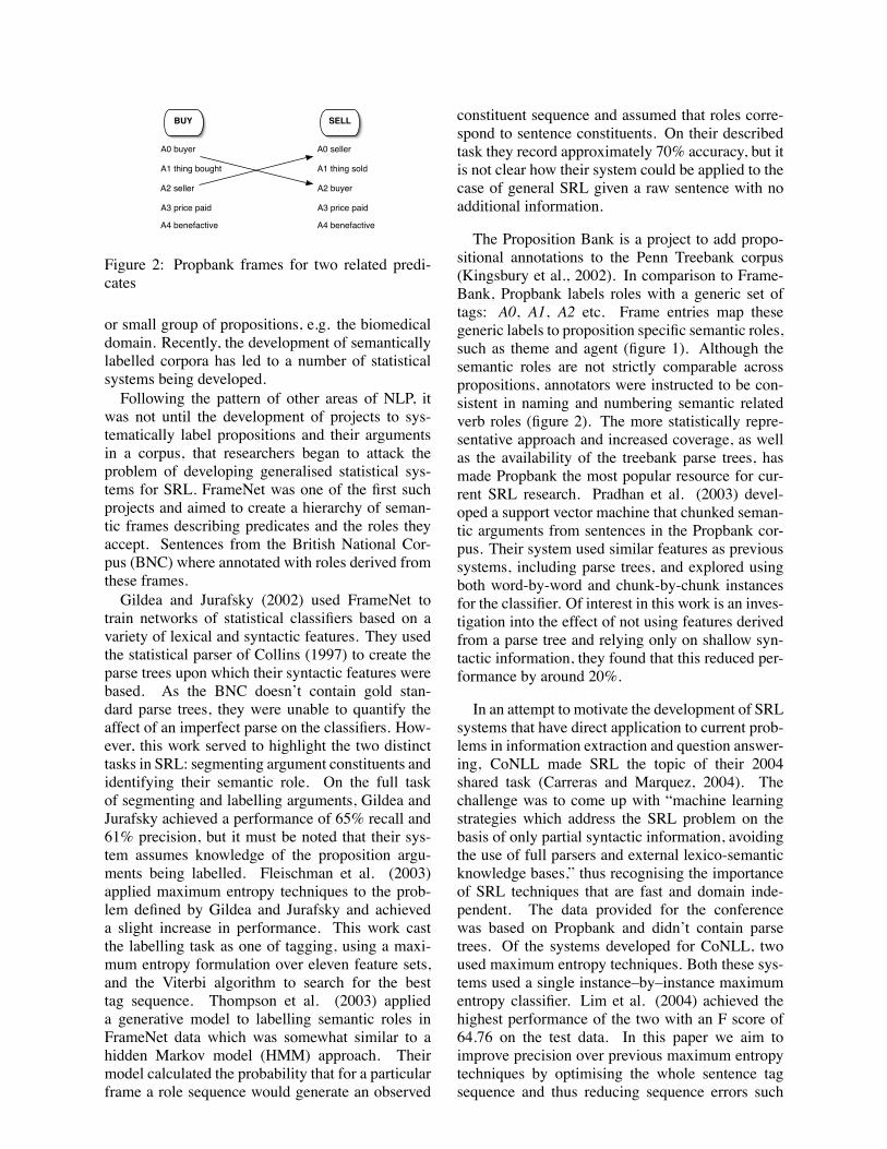
BUY SELL
A0 buyer
A2 seller
A1 thing bought
A3 price paid
A4 benefactive
A0 seller
A2 buyer
A1 thing sold
A3 price paid
A4 benefactive
Figure 2: Propbank frames for two related predi-cates
or small group of propositions, e.g. the biomedicaldomain. Recently, the development of semanticallylabelled corpora has led to a number of statisticalsystems being developed.Following the pattern of other areas of NLP, it
was not until the development of projects to sys-tematically label propositions and their argumentsin a corpus, that researchers began to attack theproblem of developing generalised statistical sys-tems for SRL. FrameNet was one of the first suchprojects and aimed to create a hierarchy of seman-tic frames describing predicates and the roles theyaccept. Sentences from the British National Cor-pus (BNC) where annotated with roles derived fromthese frames.Gildea and Jurafsky (2002) used FrameNet to
train networks of statistical classifiers based on avariety of lexical and syntactic features. They usedthe statistical parser of Collins (1997) to create theparse trees upon which their syntactic features werebased. As the BNC doesn’t contain gold stan-dard parse trees, they were unable to quantify theaffect of an imperfect parse on the classifiers. How-ever, this work served to highlight the two distincttasks in SRL: segmenting argument constituents andidentifying their semantic role. On the full taskof segmenting and labelling arguments, Gildea andJurafsky achieved a performance of 65% recall and61% precision, but it must be noted that their sys-tem assumes knowledge of the proposition argu-ments being labelled. Fleischman et al. (2003)applied maximum entropy techniques to the prob-lem defined by Gildea and Jurafsky and achieveda slight increase in performance. This work castthe labelling task as one of tagging, using a maxi-mum entropy formulation over eleven feature sets,and the Viterbi algorithm to search for the besttag sequence. Thompson et al. (2003) applieda generative model to labelling semantic roles inFrameNet data which was somewhat similar to ahidden Markov model (HMM) approach. Theirmodel calculated the probability that for a particularframe a role sequence would generate an observed
constituent sequence and assumed that roles corre-spond to sentence constituents. On their describedtask they record approximately 70% accuracy, but itis not clear how their system could be applied to thecase of general SRL given a raw sentence with noadditional information.
The Proposition Bank is a project to add propo-sitional annotations to the Penn Treebank corpus(Kingsbury et al., 2002). In comparison to Frame-Bank, Propbank labels roles with a generic set oftags: A0, A1, A2 etc. Frame entries map thesegeneric labels to proposition specific semantic roles,such as theme and agent (figure 1). Although thesemantic roles are not strictly comparable acrosspropositions, annotators were instructed to be con-sistent in naming and numbering semantic relatedverb roles (figure 2). The more statistically repre-sentative approach and increased coverage, as wellas the availability of the treebank parse trees, hasmade Propbank the most popular resource for cur-rent SRL research. Pradhan et al. (2003) devel-oped a support vector machine that chunked seman-tic arguments from sentences in the Propbank cor-pus. Their system used similar features as previoussystems, including parse trees, and explored usingboth word-by-word and chunk-by-chunk instancesfor the classifier. Of interest in this work is an inves-tigation into the effect of not using features derivedfrom a parse tree and relying only on shallow syn-tactic information, they found that this reduced per-formance by around 20%.
In an attempt to motivate the development of SRLsystems that have direct application to current prob-lems in information extraction and question answer-ing, CoNLL made SRL the topic of their 2004shared task (Carreras and Marquez, 2004). Thechallenge was to come up with “machine learningstrategies which address the SRL problem on thebasis of only partial syntactic information, avoidingthe use of full parsers and external lexico-semanticknowledge bases,” thus recognising the importanceof SRL techniques that are fast and domain inde-pendent. The data provided for the conferencewas based on Propbank and didn’t contain parsetrees. Of the systems developed for CoNLL, twoused maximum entropy techniques. Both these sys-tems used a single instance–by–instance maximumentropy classifier. Lim et al. (2004) achieved thehighest performance of the two with an F score of64.76 on the test data. In this paper we aim toimprove precision over previous maximum entropytechniques by optimising the whole sentence tagsequence and thus reducing sequence errors such
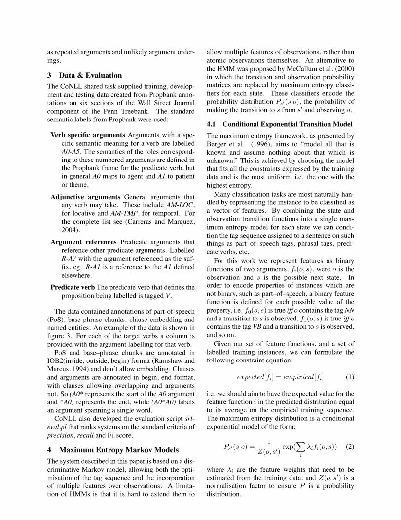
as repeated arguments and unlikely argument order-ings.
3 Data & EvaluationThe CoNLL shared task supplied training, develop-ment and testing data created from Propbank anno-tations on six sections of the Wall Street Journalcomponent of the Penn Treebank. The standardsemantic labels from Propbank were used:
Verb specific arguments Arguments with a spe-cific semantic meaning for a verb are labelledA0-A5. The semantics of the roles correspond-ing to these numbered arguments are defined inthe Propbank frame for the predicate verb, butin general A0 maps to agent and A1 to patientor theme.
Adjunctive arguments General arguments thatany verb may take. These include AM-LOC,for locative and AM-TMP, for temporal. Forthe complete list see (Carreras and Marquez,2004).
Argument references Predicate arguments thatreference other predicate arguments. LabelledR-A? with the argument referenced as the suf-fix, eg. R-A1 is a reference to the A1 definedelsewhere.
Predicate verb The predicate verb that defines theproposition being labelled is tagged V.
The data contained annotations of part-of-speech(PoS), base-phrase chunks, clause embedding andnamed entities. An example of the data is shown infigure 3. For each of the target verbs a column isprovided with the argument labelling for that verb.PoS and base–phrase chunks are annotated in
IOB2(inside, outside, begin) format (Ramshaw andMarcus, 1994) and don’t allow embedding. Clausesand arguments are annotated in begin, end format,with clauses allowing overlapping and argumentsnot. So (A0* represents the start of the A0 argumentand *A0) represents the end, while (A0*A0) labelsan argument spanning a single word.CoNLL also developed the evaluation script srl-
eval.pl that ranks systems on the standard criteria ofprecision, recall and F1 score.
4 Maximum Entropy Markov ModelsThe system described in this paper is based on a dis-criminative Markov model, allowing both the opti-misation of the tag sequence and the incorporationof multiple features over observations. A limita-tion of HMMs is that it is hard to extend them to
allow multiple features of observations, rather thanatomic observations themselves. An alternative tothe HMM was proposed by McCallum et al. (2000)in which the transition and observation probabilitymatrices are replaced by maximum entropy classi-fiers for each state. These classifiers encode theprobability distribution Ps!(s|o), the probability ofmaking the transition to s from s! and observing o.
4.1 Conditional Exponential Transition ModelThe maximum entropy framework, as presented byBerger et al. (1996), aims to “model all that isknown and assume nothing about that which isunknown.” This is achieved by choosing the modelthat fits all the constraints expressed by the trainingdata and is the most uniform, i.e. the one with thehighest entropy.Many classification tasks are most naturally han-
dled by representing the instance to be classified asa vector of features. By combining the state andobservation transition functions into a single max-imum entropy model for each state we can condi-tion the tag sequence assigned to a sentence on suchthings as part–of–speech tags, phrasal tags, predi-cate verbs, etc.For this work we represent features as binary
functions of two arguments, fi(o, s), were o is theobservation and s is the possible next state. Inorder to encode properties of instances which arenot binary, such as part–of–speech, a binary featurefunction is defined for each possible value of theproperty, i.e. f0(o, s) is true iff o contains the tagNNand a transition to s is observed, f1(o, s) is true iff ocontains the tag VB and a transition to s is observed,and so on.Given our set of feature functions, and a set of
labelled training instances, we can formulate thefollowing constraint equation:
expected[fi] = empirical[fi] (1)
i.e. we should aim to have the expected value for thefeature function i in the predicted distribution equalto its average on the empirical training sequence.The maximum entropy distribution is a conditionalexponential model of the form:
Ps!(s|o) =1
Z(o, s!)exp(
!
i
!ifi(o, s)) (2)
where !i are the feature weights that need to beestimated from the training data, and Z(o, s!) is anormalisation factor to ensure P is a probabilitydistribution.
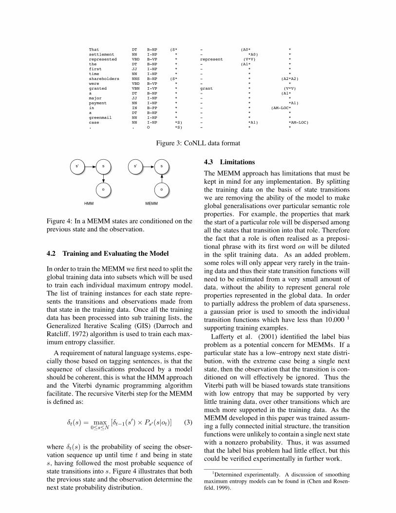
!"#"$%&'("#
!
That DT B-NP (S* - (A0* *
settlement NN I-NP * - *A0) *
represented VBD B-VP * represent (V*V) *
the DT B-NP * - (A1* *
first JJ I-NP * - * *
time NN I-NP * - * *
shareholders NNS B-NP (S* - * (A2*A2)
were VBD B-VP * - * *
granted VBN I-VP * grant * (V*V)
a DT B-NP * - * (A1*
major JJ I-NP * - * *
payment NN I-NP * - * *A1)
in IN B-PP * - * (AM-LOC*
a DT B-NP * - * *
greenmail NN I-NP * - * *
case NN I-NP *S) - *A1) *AM-LOC)
. . O *S) - * *
Figure 3: CoNLL data format
s' s
o
s' s
o
HMM MEMM
Figure 4: In a MEMM states are conditioned on theprevious state and the observation.
4.2 Training and Evaluating the Model
In order to train the MEMMwe first need to split theglobal training data into subsets which will be usedto train each individual maximum entropy model.The list of training instances for each state repre-sents the transitions and observations made fromthat state in the training data. Once all the trainingdata has been processed into sub training lists, theGeneralized Iterative Scaling (GIS) (Darroch andRatcliff, 1972) algorithm is used to train each max-imum entropy classifier.A requirement of natural language systems, espe-
cially those based on tagging sentences, is that thesequence of classifications produced by a modelshould be coherent, this is what the HMM approachand the Viterbi dynamic programming algorithmfacilitate. The recursive Viterbi step for the MEMMis defined as:
"t(s) = max0"s"N
["t#1(s!)! Ps!(s|ot)] (3)
where "t(s) is the probability of seeing the obser-vation sequence up until time t and being in states, having followed the most probable sequence ofstate transitions into s. Figure 4 illustrates that boththe previous state and the observation determine thenext state probability distribution.
4.3 LimitationsThe MEMM approach has limitations that must bekept in mind for any implementation. By splittingthe training data on the basis of state transitionswe are removing the ability of the model to makeglobal generalisations over particular semantic roleproperties. For example, the properties that markthe start of a particular role will be dispersed amongall the states that transition into that role. Thereforethe fact that a role is often realised as a preposi-tional phrase with its first word on will be dilutedin the split training data. As an added problem,some roles will only appear very rarely in the train-ing data and thus their state transition functions willneed to be estimated from a very small amount ofdata, without the ability to represent general roleproperties represented in the global data. In orderto partially address the problem of data sparseness,a gaussian prior is used to smooth the individualtransition functions which have less than 10,000 1
supporting training examples.Lafferty et al. (2001) identified the label bias
problem as a potential concern for MEMMs. If aparticular state has a low–entropy next state distri-bution, with the extreme case being a single nextstate, then the observation that the transition is con-ditioned on will effectively be ignored. Thus theViterbi path will be biased towards state transitionswith low entropy that may be supported by verylittle training data, over other transitions which aremuch more supported in the training data. As theMEMM developed in this paper was trained assum-ing a fully connected initial structure, the transitionfunctions were unlikely to contain a single next statewith a nonzero probability. Thus, it was assumedthat the label bias problem had little effect, but thiscould be verified experimentally in further work.
1Determined experimentally. A discussion of smoothingmaximum entropy models can be found in (Chen and Rosen-feld, 1999).
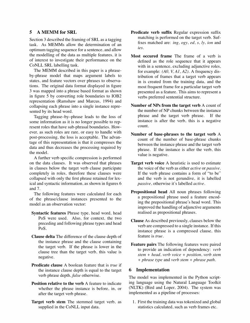
5 A MEMM for SRLSection 3 described the framing of SRL as a taggingtask. As MEMMs allow the determination of anoptimum tagging sequence for a sentence, and allowthe modelling of the data as multiple features, it isof interest to investigate their performance on theCoNLL SRL labelling task.The MEMM described in this paper is a phrase-
by-phrase model that maps argument labels tostates, and feature vectors over phrases to observa-tions. The original data format displayed in figure3 was mapped into a phrase based format as shownin figure 5 by converting role boundaries to IOB2representation (Ramshaw and Marcus, 1994) andcollapsing each phrase into a single instance repre-sented by its head word.Tagging phrase–by–phrase leads to the loss of
some information as it is no longer possible to rep-resent roles that have sub-phrasal boundaries. How-ever, as such roles are rare, or easy to handle withpost-processing, the loss is acceptable. The advan-tage of this representation is that it compresses thedata and thus decreases the processing required bythe model.A further verb specific compression is performed
on the data clauses. It was observed that phrasesin clauses below the target verb clause participatecompletely in roles, therefore these clauses werecollapsed with only the first phrase retained for lex-ical and syntactic information, as shown in figures 6and 7.The following features were calculated for each
of the phrase/clause instances presented to themodel as an observation vector:
Syntactic features Phrase type, head word, headPoS were used. Also, for context, the twopreceding and following phrase types and headPoS.
Clause delta The difference of the clause depth ofthe instance phrase and the clause containingthe target verb. If the phrase is lower in theclause tree than the target verb, this value isnegative.
Predicate clause A boolean feature that is true ifthe instance clause depth is equal to the targetverb phrase depth, false otherwise.
Position relative to the verb A feature to indicatewhether the phrase instance is before, in, orafter the target verb phrase.
Target verb stem The stemmed target verb, assupplied in the CoNLL input data.
Predicate verb suffix Regular expression suffixmatching is performed on the target verb. Suf-fixes matched are: ing, ogy, ed, s, ly, ion andies.
Most occured frame The frame of a verb isdefined as the role sequence that it appearswith in a sentence, excluding adjunctive roles,for example: (A0, V, A1, A2). A frequency dis-tribution of frames that a target verb appearsin is created from the training data, and themost frequent frame for a particular target verbpresented as a feature. This aims to represent averbs preferred sentential structure.
Number of NPs from the target verb A count ofthe number of NP chunks between the instancephrase and the target verb phrase. If theinstance is after the verb, this is a negativecount.
Number of base-phrases to the target verb Acount of the number of base-phrase chunksbetween the instance phrase and the target verbphrase. If the instance is after the verb, thisvalue is negative.
Target verb voice A heuristic is used to estimatethe voice of the verb as either active or passive.If the verb phrase contains a form of “to be”and the verb is not gerundive, it is labelledpassive, otherwise it’s labelled active.
Prepositional head All noun phrases followinga prepositional phrase used a feature encod-ing the prepositional phrase’s head word. Thisimproved the handling of adjunctive argumentsrealised as prepositional phrases.
Clause As described previously, clauses below theverb are compressed to a single instance. If thisinstance phrase is a compressed clause, thisfeature is true.
Feature pairs The following features were pairedto provide an indication of dependency: verbstem + head, verb voice + position, verb stem+ phrase type and verb stem + phrase path.
6 ImplementationThe model was implemented in the Python script-ing language using the Natural Language Toolkit(NLTK) (Bird and Loper, 2004). The system wasimplemented as a pipeline of processes:
1. First the training data was tokenized and globalstatistics calculated, such as verb frames etc.
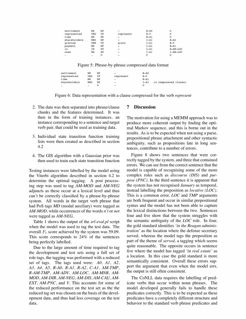
!"#"$%&'("#
!
settlement NN NP - B-A0 O
represented VBD VP represent B-V O
time NN NP - B-A1 O
shareholders NNS NP - I-A1 B-A2
granted VBN VP grant I-A1 B-V
payment NN NP - I-A1 B-A1
in IN PP - I-A1 B-AM-LOC
case NN NP - I-A1 I-AM-LOC
. . O - O O
Figure 5: Phrase-by-phrase compressed data format!"#"$%&'("#
!
settlement NN NP - B-A0
represented VBD VP represent B-V
time NN NP - B-A1
shareholders NNS NP - I-A1 (a compressed clause)
. . O - O
Figure 6: Data representation with a clause compressed for the verb represent
2. The data was then separated into phrase/clausechunks and the features determined. It wasthen in the form of training instances, aninstance corresponding to a sentence and targetverb pair, that could be used as training data.
3. Individual state transition function traininglists were then created as described in section4.2
4. The GIS algorithm with a Gaussian prior wasthen used to train each state transition function
Testing instances were labelled by the model usingthe Viterbi algorithm described in section 4.2 todetermine the optimal tagging. A post process-ing step was used to tag AM-MOD and AM-NEGadjuncts as these occur at a lexical level and thuscan’t be correctly classified by a phrase-by-phrasesystem. All words in the target verb phrase thathad PoS tags MD (modal auxiliary) were tagged asAM-MOD, while occurrences of the words n’t or notwere tagged as AM-NEG.Table 1 shows the output of the srl-eval.pl script
when the model was used to tag the test data. Theoverall F1 score achieved by the system was 59.09.This score corresponds to 24% of the sentencesbeing perfectly labelled.Due to the large amount of time required to tag
the development and test sets using a full set ofrole tags, the tagging was performed with a reducedset of tags. The tags used were: A0, A1, A2,A3, A4, A5, R-A0, R-A1, R-A2, C-A1, AM-TMP,R-AM-TMP, AM-ADV, AM-LOC, AM-MNR, AM-MOD, AM-DIR, AM-NEG, AM-DIS, AM-CAU, AM-EXT, AM-PNC, and V. This accounts for some ofthe reduced performance on the test set as the thereduced tag set was chosen on the basis of the devel-opment data, and thus had less coverage on the testdata.
7 Discussion
The motivation for using a MEMM approach was toproduce more coherent output by finding the opti-mal Markov sequence, and this is borne out in theresults. As is to be expected when not using a parse,prepositional phrase attachment and other syntacticambiguity, such as propositions late in long sen-tences, contribute to a number of errors.Figure 8 shows two sentences that were cor-
rectly tagged by the system, and three that containederrors. We can see from the correct sentence that themodel is capable of recognising some of the morecomplex roles such as discourse (DIS) and pur-pose (PNC). In the third sentence it is apparent thatthe system has not recognised January as temporal,instead labelling the preposition as locative (LOC).This is a common error, LOC and TMP argumentsare both frequent and occur in similar prepositionalsyntax and the model has not been able to capturethe lexical distinctions between the two. Sentencesfour and five show that the system struggles withthe semantic ambiguity of the LOC role. In four,the gold standard identifies ‘in the Reagan adminis-tration’ as the location where the defense secretaryserved, whereas the model tags the preposition aspart of the theme of served, a tagging which seemsquite reasonable. The opposite occurs in sentencefive where the model has tagged ‘in real estate’ asa location. In this case the gold standard is moresemantically consistent. Overall these errors sup-port the argument that even when the model errs,the output is still often consistent.The CoNLL data requires the labelling of pred-
icate verbs that occur within noun phrases. Themodel developed generally fails to handle thesepredicates correctly. This is to be expected as thesepredicates have a completely different structure andbehavior to the standard verb phrase predicates and
Mr. Johnson succeeds Harry W. Sherman,
who resigned to pursue other interests
,in both positions.
Figure 7: A clause tree showing a clause that would be collapsed to a single instance
1. [ Of course]DIS , [Mr. Wolf, 48 years old,]A0
[has]V [some savings]A1.
2. Mr Johnsom succeeds [Harry W. Sherman]A0,[who]R#A0 [resigned]V [to pursue otherinterests]PNC , in both positions.
3. ([In January]LOC)TMP , [he]A0 [accepted]V[the position ...]A1.
4. [Mr. Carlucci, 59 years old,]A0 [served]Vas [defense secretary (in the Reaganadministration)LOC ]A1.
5. [Balcor]A0, [which]R#A0 [has]V([interests]A1[in real estate]LOC)A1, saidthe position is newly created.
Figure 8: Example model output. Square bracketsindicate tags applied by the system, while roundbrackets and indicate the tagging from the gold stan-dard
are also in the minority in the training data. A sepa-rately trained model could solve this problem.There are a number of possible improvements to
the MEMMmodel. Prepositional phrase attachmentcould be handled explicitly in a subsystem. Eachstate transition function could induce the n mostinformative features and discard the rest, enablingthe model to be more able to avoid over–trainingproblems. Another obvious path to explore wouldbe the application of conditional random fields (Laf-ferty et al., 2001) to the SRL task. These modelshave the advantage of solving the label bias prob-lem, as well as allowing more flexibility in mod-elling, and by using an MEMM for initial weightsthey converge more quickly.The advantage of the approach described lies in
the increase in precision and the improved coher-ence of the sentence tag sequence. However, thenature of the SRL task as one that requires both localphrase level feature information and global sentenceinformation, would indicate that both need to be
Precision Recall F!=1
Overall 71.29% 50.45% 59.09A0 84.02% 66.11% 74.00A1 65.94% 51.81% 58.03A2 58.96% 42.92% 49.68A3 65.15% 28.86% 40.00A4 70.00% 42.00% 52.50A5 0.00% 0.00% 0.00AM-ADV 46.75% 11.76% 18.80AM-CAU 66.67% 4.08% 7.69AM-DIR 45.16% 28.00% 34.57AM-DIS 66.99% 32.39% 43.67AM-EXT 70.00% 50.00% 58.33AM-LOC 37.41% 22.81% 28.34AM-MNR 47.96% 18.43% 26.63AM-MOD 87.57% 92.26% 89.86AM-NEG 82.96% 88.19% 85.50AM-PNC 35.29% 7.06% 11.76AM-PRD 0.00% 0.00% 0.00AM-TMP 61.23% 26.64% 37.13R-A0 90.65% 61.01% 72.93R-A1 73.91% 48.57% 58.62R-A2 75.00% 33.33% 46.15R-A3 0.00% 0.00% 0.00R-AM-LOC 0.00% 0.00% 0.00R-AM-MNR 0.00% 0.00% 0.00R-AM-PNC 0.00% 0.00% 0.00R-AM-TMP 100.00% 7.14% 13.33V 96.63% 95.69% 96.16
Table 1: Model performance on the test set
modelled for maximal performance. Most currentapproaches, including the approach presented in thispaper, use word or phrase level classifiers and thentry to capture sentence level information throughfeatures such as phrase paths and counts.The evaluation metrics chosen for the CoNLL
shared task appear to be brittle, giving no recogni-tion to systems that come close to predicting argu-ments but fail to find exact matches. The main moti-vation for SRL techniques is to improve information
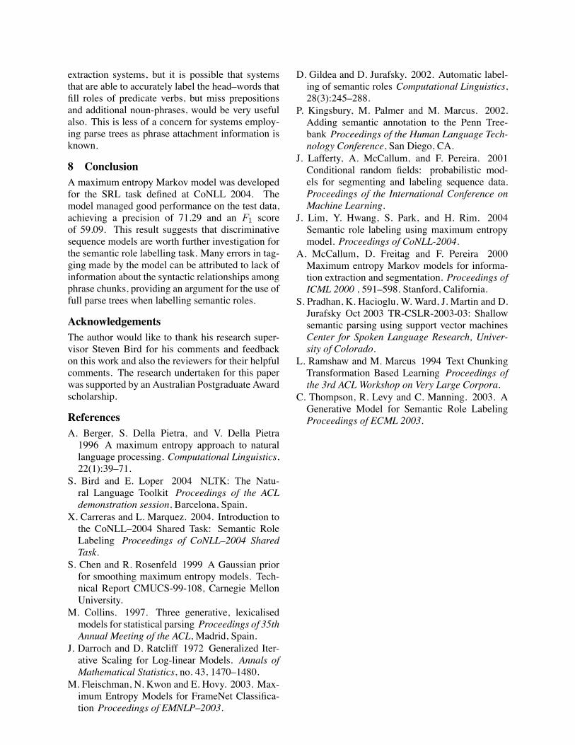
extraction systems, but it is possible that systemsthat are able to accurately label the head–words thatfill roles of predicate verbs, but miss prepositionsand additional noun-phrases, would be very usefulalso. This is less of a concern for systems employ-ing parse trees as phrase attachment information isknown.
8 ConclusionA maximum entropy Markov model was developedfor the SRL task defined at CoNLL 2004. Themodel managed good performance on the test data,achieving a precision of 71.29 and an F1 scoreof 59.09. This result suggests that discriminativesequence models are worth further investigation forthe semantic role labelling task. Many errors in tag-ging made by the model can be attributed to lack ofinformation about the syntactic relationships amongphrase chunks, providing an argument for the use offull parse trees when labelling semantic roles.
AcknowledgementsThe author would like to thank his research super-visor Steven Bird for his comments and feedbackon this work and also the reviewers for their helpfulcomments. The research undertaken for this paperwas supported by an Australian Postgraduate Awardscholarship.
ReferencesA. Berger, S. Della Pietra, and V. Della Pietra1996 A maximum entropy approach to naturallanguage processing. Computational Linguistics,22(1):39–71.
S. Bird and E. Loper 2004 NLTK: The Natu-ral Language Toolkit Proceedings of the ACLdemonstration session, Barcelona, Spain.
X. Carreras and L. Marquez. 2004. Introduction tothe CoNLL–2004 Shared Task: Semantic RoleLabeling Proceedings of CoNLL–2004 SharedTask.
S. Chen and R. Rosenfeld 1999 A Gaussian priorfor smoothing maximum entropy models. Tech-nical Report CMUCS-99-108, Carnegie MellonUniversity.
M. Collins. 1997. Three generative, lexicalisedmodels for statistical parsing Proceedings of 35thAnnual Meeting of the ACL, Madrid, Spain.
J. Darroch and D. Ratcliff 1972 Generalized Iter-ative Scaling for Log-linear Models. Annals ofMathematical Statistics, no. 43, 1470–1480.
M. Fleischman, N. Kwon and E. Hovy. 2003. Max-imum Entropy Models for FrameNet Classifica-tion Proceedings of EMNLP–2003.
D. Gildea and D. Jurafsky. 2002. Automatic label-ing of semantic roles Computational Linguistics,28(3):245–288.
P. Kingsbury, M. Palmer and M. Marcus. 2002.Adding semantic annotation to the Penn Tree-bank Proceedings of the Human Language Tech-nology Conference, San Diego, CA.
J. Lafferty, A. McCallum, and F. Pereira. 2001Conditional random fields: probabilistic mod-els for segmenting and labeling sequence data.Proceedings of the International Conference onMachine Learning.
J. Lim, Y. Hwang, S. Park, and H. Rim. 2004Semantic role labeling using maximum entropymodel. Proceedings of CoNLL-2004.
A. McCallum, D. Freitag and F. Pereira 2000Maximum entropy Markov models for informa-tion extraction and segmentation. Proceedings ofICML 2000 , 591–598. Stanford, California.
S. Pradhan, K. Hacioglu, W. Ward, J. Martin and D.Jurafsky Oct 2003 TR-CSLR-2003-03: Shallowsemantic parsing using support vector machinesCenter for Spoken Language Research, Univer-sity of Colorado.
L. Ramshaw and M. Marcus 1994 Text ChunkingTransformation Based Learning Proceedings ofthe 3rd ACL Workshop on Very Large Corpora.
C. Thompson, R. Levy and C. Manning. 2003. AGenerative Model for Semantic Role LabelingProceedings of ECML 2003.
A New Measure for Extracting Semantically Related Words
Yuanyong Wang and Achim [email protected]
[email protected] of Computer Science and Engineering
University of New South WalesSydney, 2052, NSW
Australia
AbstractThe identification of semantically related terms fora given word is an important problem. A numberof statistical approaches have been proposed to ad-dress this problem. Most approaches draw theirstatistics from a large general corpus. In this pa-per, we propose to use specialized corpora whichfocus strongly on the individual words of interest.We propose to collect such corpora through targetedqueries to Internet search engines. Furthermore, weintroduce a new statistical measure, Relative Fre-quency Ratio,tailored specifically for such special-ized corpora. We evaluated our approach by usingthe extracted related terms to attack the target wordselection problem in machine translation. This typeof indirect evaluation is conducted because a directevaluation on the set of related terms thus extractedrelies heavily on direct human involvement and isnot quantitatively comparable to others’ results. Ourexperimental results so far are very encouraging.
1 IntroductionThe identification of semantically related wordsfrom texts is an important problem in natural lan-guage processing. If successfully identified, theycould be used in query expansion, word sensedisambiguation, as well as document classifica-tion (Tomohiko Sugimachi and Matsuo, 2003).Another application concerns the identification ofnew word senses in specialized languages, whichare constantly evolving and, hence, no up-to-datedictionaries exist that could cover all those wordsenses. Many approaches, such as co-occurrencestatistics based on mutual information (Church andHanks, 1990), the Z-score (Tomohiko Sugimachiand Matsuo, 2003), have been used in the past totackle this problem. These approaches are limitedto be used only on general corpora in which largeamounts of texts are collected from sources as di-verse as possible. In this paper, we call this kindof corpus a General Corpus (GC). The nature ofthese measures (rate high co-occurrence high and
rate high frequency words low) requires generalityof the corpus. Generality is defined in our paper asfor a corpus not being biased toward any particulardomain or particular word. Mutual information isdefined as follows:
I(w1, w2) = logP (w1, w2)
P (w1)P (w2),
where P (wi) is the probability of word wi to occurin a document and P (wi, wj) is the probability ofboth words wi and wj to occur in a document.
If a good corpus with high generality could beobtained, the co-occurrence statistics collected fromthe corpus could be very good and reflect accuratelythe tendency of semantic association among words.But there are several innate drawbacks to these GCbased approaches. Firstly, generality is often verydifficult to define. Secondly, acquiring a GC withgood generality is a even more difficult problem.Thirdly, given that these above two problems areproperly addressed the set of related terms extractedfrom the corpora are still limited in number. Themain reason behind the third drawback is actuallythe generality required by these approaches. Sinceno words have a particularly high frequency in thecorpus. It is not difficult to prove that the num-ber of semantically related terms extracted for agiven word is usually very low, especailly if wetake away function words (which co-occur with anyword indiscriminately). These sets of extracted re-lated terms, if used to match the new context of theword in question, only provide very limited disam-biguating power.
Based on the above analysis, another type of cor-pus is needed to obtain a sufficiently large set of re-lated terms(so that they are practically useful) forany particular word. We call this type of corpus aWord Specific Corpus (WSC). It is constructed bycollecting only the texts where the particular wordof interest is present. We call this word the seedword and in formal contexts we refer to a WSCwith seed word s, by wsc(s). In such corporawords which occur with low frequency in a GC may
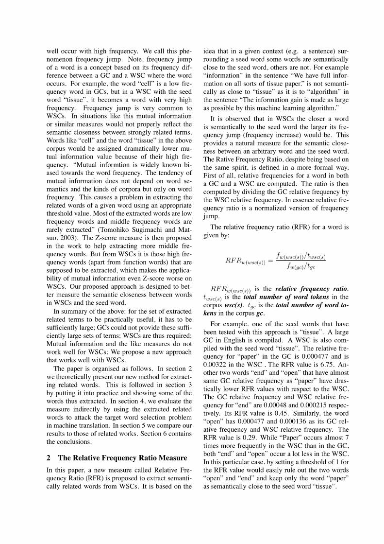
well occur with high frequency. We call this phe-nomenon frequency jump. Note, frequency jumpof a word is a concept based on its frequency dif-ference between a GC and a WSC where the wordoccurs. For example, the word “cell” is a low fre-quency word in GCs, but in a WSC with the seedword “tissue”, it becomes a word with very highfrequency. Frequency jump is very common toWSCs. In situations like this mutual informationor similar measures would not properly reflect thesemantic closeness between strongly related terms.Words like “cell” and the word “tissue” in the abovecorpus would be assigned dramatically lower mu-tual information value because of their high fre-quency. “Mutual informtion is widely known bi-ased towards the word frequency. The tendency ofmutual information does not depend on word se-mantics and the kinds of corpora but only on wordfrequency. This causes a problem in extracting therelated words of a given word using an appropriatethreshold value. Most of the extracted words are lowfrequency words and middle frequency words arerarely extracted” (Tomohiko Sugimachi and Mat-suo, 2003). The Z-score measure is then proposedin the work to help extracting more middle fre-quency words. But from WSCs it is those high fre-quency words (apart from function words) that aresupposed to be extracted, which makes the applica-bility of mutual information even Z-score worse onWSCs. Our proposed approach is designed to bet-ter measure the semantic closeness between wordsin WSCs and the seed word.
In summary of the above: for the set of extractedrelated terms to be practically useful, it has to besufficiently large; GCs could not provide these suffi-ciently large sets of terms; WSCs are thus required;Mutual information and the like measures do notwork well for WSCs; We propose a new approachthat works well with WSCs.
The paper is organised as follows. In section 2we theoretically present our new method for extract-ing related words. This is followed in section 3by putting it into practice and showing some of thewords thus extracted. In section 4, we evaluate themeasure indirectly by using the extracted relatedwords to attack the target word selection problemin machine translation. In section 5 we compare ourresults to those of related works. Section 6 containsthe conclusions.
2 The Relative Frequency Ratio MeasureIn this paper, a new measure called Relative Fre-quency Ratio (RFR) is proposed to extract semanti-cally related words from WSCs. It is based on the
idea that in a given context (e.g. a sentence) sur-rounding a seed word some words are semanticallyclose to the seed word, others are not. For example“information” in the sentence “We have full infor-mation on all sorts of tissue paper.” is not semanti-cally as close to “tissue” as it is to “algorithm” inthe sentence “The information gain is made as largeas possible by this machine learning algorithm.”
It is observed that in WSCs the closer a wordis semantically to the seed word the larger its fre-quency jump (frequency increase) would be. Thisprovides a natural measure for the semantic close-ness between an arbitrary word and the seed word.The Rative Frequency Ratio, despite being based onthe same spirit, is defined in a more formal way.First of all, relative frequencies for a word in botha GC and a WSC are computed. The ratio is thencomputed by dividing the GC relative frequency bythe WSC relative frequency. In essence relative fre-quency ratio is a normalized version of frequencyjump.
The relative frequency ratio (RFR) for a word isgiven by:
RFRw(wsc(s)) =fw(wsc(s))/twsc(s)
fw(gc)/tgc
RFRw(wsc(s)) is the relative frequency ratio.twsc(s) is the total number of word tokens in thecorpus wsc(s). tgc is the total number of word to-kens in the corpus gc.
For example, one of the seed words that havebeen tested with this approach is “tissue”. A largeGC in English is compiled. A WSC is also com-piled with the seed word “tissue”. The relative fre-quency for “paper” in the GC is 0.000477 and is0.00322 in the WSC . The RFR value is 6.75. An-other two words “end” and “open” that have almostsame GC relative frequency as “paper” have dras-tically lower RFR values with respect to the WSC.The GC relative frequency and WSC relative fre-quency for “end” are 0.00048 and 0.000215 respec-tively. Its RFR value is 0.45. Similarly, the word“open” has 0.000477 and 0.000136 as its GC rel-ative frequency and WSC relative frequency. TheRFR value is 0.29. While “Paper” occurs almost 7times more frequently in the WSC than in the GC,both “end” and “open” occur a lot less in the WSC.In this particular case, by setting a threshold of 1 forthe RFR value would easily rule out the two words“open” and “end” and keep only the word “paper”as semantically close to the seed word “tissue”.
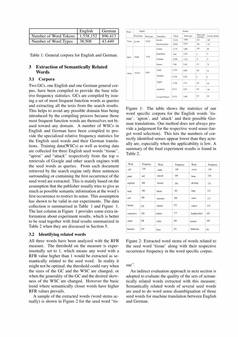
English GermanNumber of Word Tokens 1,538,152 896,413Number of Word Types 38,508 43,449
Table 1: General corpora for English and German.
3 Extraction of Semantically RelatedWords
3.1 CorporaTwo GCs, one English and one German general cor-pus, have been compiled to provide the base rela-tive frequency statistics. GCs are compiled by issu-ing a set of most frequent function words as queriesand extracting all the texts from the search results.This helps to avoid any possible domain bias beingintroduced by the compiling process because thosemost frequent function words are themselves not bi-ased toward any domain. A number of WSCs inEnglish and German have been compiled to pro-vide the specialized relative frequency statistics forthe English seed words and their German transla-tions. Training data(WSCs) as well as testing dataare collected for three English seed words “tissue”,“apron” and “attack” respectively from the top nretrievals of Google and other search engines withthe seed words as queries. From each documentretrieved by the search engine only three sentencessurrounding or containing the first occurrence of theseed word are extracted. This is mainly based on theassumption that the publisher usually tries to give asmuch as possible semantic information at the word’sfirst occurrence to restrict its sense. This assumptionhas shown to be valid in our experiments. The datacollection is summarised in Table 1 and Figure 1.The last column in Figure 1 provides some extra in-formation about experiment results, which is betterto be read together with final results summarized inTable 2 when they are discussed in Section 5.
3.2 Identifying related wordsAll three words have been analyzed with the RFRmeasure. The threshold on the measure is exper-imentally set to 1, which means any word with aRFR value higher than 1 would be extracted as se-mantically related to the seed word. In reality itmight not be optimal, the threshold could vary whenthe sizes of the GC and the WSC are changed, orwhen the generality of the GC and the desired skew-ness of the WSC are changed. However the basictrend where semantically closer words have higherRFR values prevails.
A sample of the extracted words (word stems ac-tually) is shown in Figure 2 for the seed word “tis-
Tissue
Apron
Attack
227,959
70,968
103,633
16,293
8,102
9,956
Translations
Gewebe
Papiertaschentuch
Vorfeld
Schutzblech
Vorbuhne
Schurze
Anfall
Ubefallen
Angriff
attackieren
In Angriff Nehmen
Word English
Word tokens Word types
German
Tokens Word types Sense cases(test data) Corretly identify
32,414
36,842
11,774
7,683
12,696
7,560
17,235
21,536
12,746
16,713
31,474
8,866
8,634
3,860
2,423
4,122
2,410
4,086
5,422
3,771
4,621
7,489
535
166
103
4
71
137
105
0
357
357
357
467
132
80
0
0
70
93
0
161
161
161
Figure 1: The table shows the statistics of ourword specific corpora for the English words ’tis-sue’, ’apron’, and ’attack’ and their possible Ger-man translations. Our method does not always pro-vide a judgement for the respective word sense (tar-get word selection). This lets the numbers of cor-rectly identified senses appear lower than they actu-ally are, especially when the applicability is low. Asummary of the final experiment results is found inTable 2.
Word Frequency Word Frequency Word Frequency
cell
paper
engineer
body
soft
human
connective
organ
function
study
muscle
disease
blood
structure
animal
culture
toilet
layer
cover
bone
develop
lung
cause
cancer
handkerchief
normal
bathroom
729
442
308
300
286
278
259
248
219
198
190
184
181
180
179
177
169
151
138
136
131
121
117
115
105
100
94
Figure 2: Extracted word stems of words related tothe seed word ‘tissue’ along with their respectiveoccurrence frequency in the word specific corpus.
sue”.An indirect evaluation approach in next section is
adopted to evaluate the quality of the sets of seman-tically related words extracted with this measure.Semantically related words of several seed wordsare used to do word sense disambiguation of thoseseed words for machine translation between Englishand German.
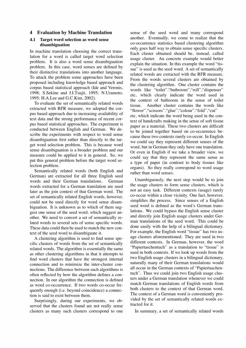
4 Evaluation by Machine Translation4.1 Target word selection as word sense
disambiguationIn machine translation choosing the correct trans-lation for a word is called target word selectionproblem. It is also a word sense disambiguationproblem. In this case, word senses are defined bytheir distinctive translations into another language.To attack the problem some approaches have beenproposed including knowledge based approach andcorpus based statistical approach (Ide and Veronis,1998; S.Sekine and J.I.Tsujii, 1995; N.Uramoto,1995; H.A.Lee and G.C.Kim, 2002).
To evaluate the set of semantically related wordsextracted with RFR measure, we adopted the cor-pus based approach due to increasing availability oftext data and the strong performance of recent cor-pus based statistical approaches. The experiment isconducted between English and German. We de-scribe the experiments with respect to word sensedisambiguation first rather than directly to the tar-get word selection problem. This is because wordsense disambiguation is a broader problem and ourmeasure could be applied to it in general. So, weput this general problem before the target word se-lection problem.
Semantically related words (both English andGerman) are extracted for all three English seedwords and their German translations. Germanwords extracted for a German translation are usedlater as the join context of that German word. Theset of semantically related English words, however,could not be used directly for word sense disam-biguation. It is unknown as to which of them sug-gest one sense of the seed word, which suggest an-other. We need to convert a set of semantically re-lated words to several sets of sense specific words.These data could then be used to match the new con-text of the seed word to disambiguate it.
A clustering algorithm is used to find sense spe-cific clusters of words from the set of semanticallyrelated words. The algorithm is essentially the sameas other clustering algorithms in that it attempts tofind word clusters that have the strongest internalconnection and to minimize the inter-cluster con-nections. The difference between such algorithms isoften reflected by how the algorithm defines a con-nection. In our algorithm the connection is definedas word co-occurrence. If two words co-occur fre-quently enough (i.e. beyond coincidence) a connec-tion is said to exist between them.
Surprisingly, during our experiments, we ob-served that the clusters found are not really senseclusters as many such clusters correspond to one
sense of the seed word and many correspondanother. Eventually, we come to realize that theco-occurrence statistics based clustering algorithmonly goes half way to obtain sense specific clusters.Each cluster obtained should be, instead, calledusage cluster. An concrete example would betterexplain the situation. In this example the word “tis-sue” is used as the seed word. A set of semanticallyrelated words are extracted with the RFR measure.From the words several clusters are obtained bythe clustering algorithm. One cluster contains thewords like “toilet”,“bathroom”,“roll”,“dispenser”etc, which clearly indicate the word used inthe context of bathroom in the sense of toilettissue. Another cluster contains the words like“flower”,“scissors”,“glue”,“colour”,“fold”,“cut”etc, which indicate the word being used in the con-text of handcrafts making in the sense of soft tissuepaper as a material. These two clusters are difficultto be joined together based on co-occurrence be-cause these two contexts rarely co-occur. In Englishwe could say they represent different senses of theword, but in German they only have one translation.Or even in English if we take a broader view, wecould say that they represent the same sense asa type of paper (in contrast to body tissues likeorgans). So they really correspond to word usagerather than word senses.
Unambiguously, the next step would be to jointhe usage clusters to form sense clusters, which isnot an easy task. Different contexts (usage) rarelyco-occur within a close vicinity. One fact, however,simplifies the process. Since senses of a Englishseed word is defined as the word’s German trans-lations. We could bypass the English sense clusterand directly join English usage clusters under Ger-man translations of the seed word. This could bedone easily with the help of a bilingual dictionary.For example, the English word “tissue” has two us-age clusters aforementioned. They are used in twodifferent contexts. In German, however, the word“Papiertaschentuch” as a translation to “tissue” isused in both contexts. If we look up words from thetwo English usage clusters in a bilingual dictionary,naturally many of their German translations wouldall occur in the German contexts of “Papiertaschen-tuch”. Thus we could join two English usage clus-ters under a German translation whenever we couldmatch German translations of English words fromboth clusters to the context of that German word.The context of a German word is conveniently pro-vided by the set of semantically related words ex-tracted for it.
In summary, a set of semantically related words
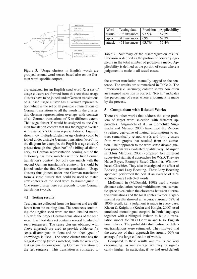
...
tartget, war
BilingualDictionary
Medical sense
Attack
(Anfall)
Military, offensive sense (Attackieren)
Sense cluster!1
Usage cluster!1
plan, alqaeda, say
Usage cluster!2israely, kill, palestinian, soldier
Usage cluster!311, 9, september, terrorist, unit
Usage cluster!4
against, air, defend, enemy, force, military,
Sense cluster!2
artery, block, blood , cause, coronary, death
usage cluster!5
diabetis, disease, factor, flow, heart, increa
Figure 3: Usage clusters in English words aregrouped around word senses based also on the Ger-man word-specific corpora.
are extracted for an English seed word X; a set ofusage clusters are formed from this set; these usageclusters have to be joined under German translationsof X; each usage cluster has a German representa-tion which is the set of all possible enumerations ofGerman translations to all the words in the cluster;this German representation overlaps with contextsof all German translations of X to different extent.The usage cluster Y would be assigned to one Ger-man translation context that has the biggest overlapwith one of Y’s German representations. Figure 3shows how multiple English usage clusters could bejoined under a single German translation (word). Inthe diagram for example, the English usage cluster2passes through the “glass bar” of a bilingual dictio-nary, its German representation coming out of thedictionary has three matches with the first Germantranslation’s context, but only one match with thesecond German translation’s context. It should bejoined under the first German translation. Usageclusters thus joined under one German translationform a sense cluster that could be used to matchnew contexts of the seed word to disambiguate it.One sense cluster here corresponds to one Germantranslation (word).
4.2 Testing resultsTest data are collected from the Internet and are dif-ferent from the training data. The sentences contain-ing the English seed word are then labelled manu-ally with the proper German translations of the seedword. Each test data set contains several hundred ofsuch sentences. The sense clusters obtained withabove approach are used to provide evidence forsense disambiguation alone and no other types ofknowledge is used. The sense cluster that has thebiggest overlap (words matched) with the new con-text assigns its corresponding German translation tothe test sentence. This translation is compared to
Word Testing data Precision Applicabilitytissue 703 instances 97.5% 87.2%apron 315 instances 69% 67.3%attack 471 instances 93.7% 57.4%
Table 2: Summary of the disambiguation results.Precision is defined as the portion of correct judge-ments in the total number of judgments made. Ap-plicability is defined as the portion of cases where ajudgement is made in all tested cases.
the correct translation manually tagged to the sen-tence. The results are summarized in Table 2. The‘Precision’(i.e. accuracy) column shows how oftenan assigned selection is correct. “Recall” indicatesthe percentage of cases where a judgment is madeby the process.
5 Comparison with Related WorksThere are other works that address the same prob-lem of target word selection with different ap-proaches. Sugimachi et al. in (Tomohiko Sugi-machi and Matsuo, 2003) have used the Z-score(a refined derivative of mutual information) to ex-tract semantically related words and form clustersfrom word graphs that resulted from the extrac-tion. Their approach to the word sense disambigua-tion problem was evaluated qualitatively. Marquezin (Lluıs Marquez, 2000) compared five differentsupervised statistical approaches for WSD. They areNaive Bayes, Example Based Classifier, Winnow-based Classifier. They also investigated the effect ofBoosting and Lazy Boosting. Their Lazy Boostingapproach performed the best at an average of 71%accuracy on 21 selected words.
McDonald in (McDonald, 1998) used a vectordistance calculation based multidimensional seman-tic space to calculate the closeness between alterna-tive translations and the local context vector. Exper-imental results showed an accuracy around 58% at100% recall, i.e. a judgment is made in every case.Khoen & Knight in (Koehn and Knight, 2000) usedunrelated monolingual corpora in both languagestogether with a bilingual lexicon to build a trans-lation model for 3830 German and 6147 Englishnoun tokens. The probability distribution of differ-ent translations were estimated. They showed thatthe accuracy of their approach lies around 70% onaverage for a large collection of words.
Compared to these results our results are veryencouraging, as our average accuracy is signifi-cantly higher. In particular, if we had used default
decisions provided in (Koehn and Knight, 2000),the recall would be much higher without substan-tially reducing the precision. What’s important isthat this machine translation application uses as itsmain knowledge only the set of semantically re-lated words extracted with RFR. This (although in-directly) is sufficient as a proof to the effectivenessof the RFR measure we propose in this paper. Thelast thing worth mentioning is that mutual informa-tion has been used in place of RFR at early stages ofthe experiment but the precision rate stays at around75 to 80% on average. Simply replacing mutual in-formation with RFR under the exactly same frame-work pushes the rate up to 87% on average withoutcompromising the applicability. One major differ-ence made by RFR in comparison to mutual infor-mation is extraction of semantically related wordswith very high frequency. These high frequencywords from WSCs all play vital roles in constrain-ing the sense usage of the seed words.
6 Discussion and ConclusionIn this paper we introduced a new statistical mea-sure RFR to extract semantically related words fora given word. The method can be applied to wordsense disambiguation in general although we onlyshowed how it could be applied to target word se-lection. Our experiments showed encouraging re-sults, but because of time and resource limits it isonly conducted for a small number of words so far.
The RFR measure could be used to obtain lists ofdomain specific words, topic specific words and ba-sically, as long as a biased corpus could be obtainedthe list of words that are related to the biase couldbe extracted by the RFR measure. In our paper theWSCs are such corpora biased toward single words.
Some of the challenges that this measure facesare the same to those of current co-occurence basedstatistical approaches. One is to obtain a GC thatis large enough and with good generality to providegood base statistics. But the seriousness of the prob-lem is reduced by the fact that RFR measure is notoverall sensitive to the bias unlike mutual informa-tion. If the GC is biased toward one domain, it willonly affect the extraction of semantically relatedwords for seed words in this domain. How could webetter utilize the set of semantically related wordsis also an challenging problem. A general impres-sion developed during the experiment of using theextracted words for WSD is that the measure oftenperforms strongly in extracting domain or topic spe-cific words. But word sense division does not of-ten coincide with domain differences of the dividedsenses. Quite many sense divisions are based on lo-
cal syntactic interaction of the word with surround-ing words. This type of sense division is typical toverbs, nouns that originate from verbs and some-times nouns with fine sense divisions. The extractedand clustered words usually do not perform well inthis case. The core of the difficulty could just be thesimple use of only word form co-occurrence infor-mation during the extraction and clustering. Futuredevelopment of the work would be likely to focus onintegrating other types of knowledge beyond wordforms into the measure as well as finding of less de-manding applications compared to WSD.
ReferencesKenneth Ward Church and Patrick Hanks. 1990.
Word association norms, mutual information,and lexicography. Computational Linguistics,16(1):22–29.
H.A.Lee and G.C.Kim. 2002. Translation selectionthrough source word sense disambiguation andtarget word selection. In In COLONG-2002.
Nancy Ide and Jean Veronis. 1998. Introduction tothe special issue on word sense disambiguation:The state of the art. In Computational Linguis-tics. Special Issue on Word Sense Disambigua-tion.
Philipp Koehn and Kevin Knight. 2000. Estimat-ing word translation probabilities from unrelatedmonolingual corpora using the em algorithm.In Proceddings of the AAAI/IAAI 2000. AAAI,Austin, Texas, USA.
Lluıs Marquez. 2000. Machine learning and natu-ral language processing. Technical Report LSI-00-45-R, Departament de Llenguatges i Sis-temes Informatics (LSI), Universitat Politecnicade Catalunya (UPC), Barcelona, Spain.
Scott McDonald. 1998. Target word selection asproximity in semantic space. In COLING-ACL,pages 1496–1498.
N.Uramoto. 1995. Automatic learning of knowl-edge for example-based disambiguation of at-tachment. In In Sixth International Conferenceon Theoretical and Methodological Issues in Ma-chine Translation, pages 295–302, KU Leuven,Belgium.
S.Sekine and J.I.Tsujii. 1995. Automatic acquisi-tion of semantic collocation from corpora. Ma-chine Translation, 10(3):218–258.
Masayuki Takeda Tomohiko Sugimachi,Akira Ishino and Fumihiro Matsuo. 2003.A method of extracting related words usingstandardized mutual information. In Proceedingsof 6th Discovery Science Conference, Sapporo,Japan, October. Springer-Verlag.
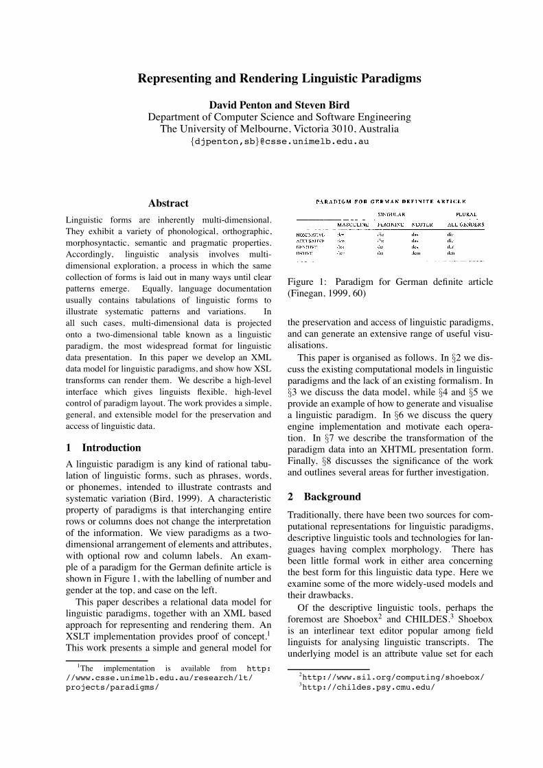
Representing and Rendering Linguistic Paradigms
David Penton and Steven BirdDepartment of Computer Science and Software EngineeringThe University of Melbourne, Victoria 3010, Australia
{djpenton,sb}@csse.unimelb.edu.au
AbstractLinguistic forms are inherently multi-dimensional.They exhibit a variety of phonological, orthographic,morphosyntactic, semantic and pragmatic properties.Accordingly, linguistic analysis involves multi-dimensional exploration, a process in which the samecollection of forms is laid out in many ways until clearpatterns emerge. Equally, language documentationusually contains tabulations of linguistic forms toillustrate systematic patterns and variations. Inall such cases, multi-dimensional data is projectedonto a two-dimensional table known as a linguisticparadigm, the most widespread format for linguisticdata presentation. In this paper we develop an XMLdata model for linguistic paradigms, and show how XSLtransforms can render them. We describe a high-levelinterface which gives linguists flexible, high-levelcontrol of paradigm layout. The work provides a simple,general, and extensible model for the preservation andaccess of linguistic data.
1 IntroductionA linguistic paradigm is any kind of rational tabu-lation of linguistic forms, such as phrases, words,or phonemes, intended to illustrate contrasts andsystematic variation (Bird, 1999). A characteristicproperty of paradigms is that interchanging entirerows or columns does not change the interpretationof the information. We view paradigms as a two-dimensional arrangement of elements and attributes,with optional row and column labels. An exam-ple of a paradigm for the German definite article isshown in Figure 1, with the labelling of number andgender at the top, and case on the left.This paper describes a relational data model for
linguistic paradigms, together with an XML basedapproach for representing and rendering them. AnXSLT implementation provides proof of concept.1This work presents a simple and general model for
1The implementation is available from http://www.csse.unimelb.edu.au/research/lt/projects/paradigms/
Figure 1: Paradigm for German definite article(Finegan, 1999, 60)
the preservation and access of linguistic paradigms,and can generate an extensive range of useful visu-alisations.This paper is organised as follows. In §2 we dis-
cuss the existing computational models in linguisticparadigms and the lack of an existing formalism. In§3 we discuss the data model, while §4 and §5 weprovide an example of how to generate and visualisea linguistic paradigm. In §6 we discuss the queryengine implementation and motivate each opera-tion. In §7 we describe the transformation of theparadigm data into an XHTML presentation form.Finally, §8 discusses the significance of the workand outlines several areas for further investigation.
2 BackgroundTraditionally, there have been two sources for com-putational representations for linguistic paradigms,descriptive linguistic tools and technologies for lan-guages having complex morphology. There hasbeen little formal work in either area concerningthe best form for this linguistic data type. Here weexamine some of the more widely-used models andtheir drawbacks.Of the descriptive linguistic tools, perhaps the
foremost are Shoebox2 and CHILDES.3 Shoeboxis an interlinear text editor popular among fieldlinguists for analysing linguistic transcripts. Theunderlying model is an attribute value set for each
2http://www.sil.org/computing/shoebox/3http://childes.psy.cmu.edu/
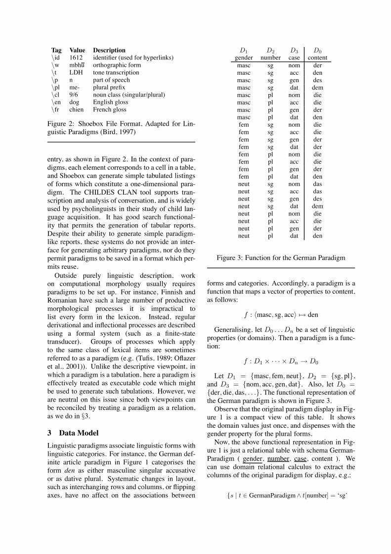
Tag Value Description\id 1612 identifier (used for hyperlinks)\w mbhu orthographic form\t LDH tone transcription\p n part of speech\pl me- plural prefix\cl 9/6 noun class (singular/plural)\en dog English gloss\fr chien French gloss
Figure 2: Shoebox File Format, Adapted for Lin-guistic Paradigms (Bird, 1997)
entry, as shown in Figure 2. In the context of para-digms, each element corresponds to a cell in a table,and Shoebox can generate simple tabulated listingsof forms which constitute a one-dimensional para-digm. The CHILDES CLAN tool supports tran-scription and analysis of conversation, and is widelyused by psycholinguists in their study of child lan-guage acquisition. It has good search functional-ity that permits the generation of tabular reports.Despite their ability to generate simple paradigm-like reports, these systems do not provide an inter-face for generating arbitrary paradigms, nor do theypermit paradigms to be saved in a format which per-mits reuse.Outside purely linguistic description, work
on computational morphology usually requiresparadigms to be set up. For instance, Finnish andRomanian have such a large number of productivemorphological processes it is impractical tolist every form in the lexicon. Instead, regularderivational and inflectional processes are describedusing a formal system (such as a finite-statetransducer). Groups of processes which applyto the same class of lexical items are sometimesreferred to as a paradigm (e.g. (Tufis, 1989; Oflazeret al., 2001)). Unlike the descriptive viewpoint, inwhich a paradigm is a tabulation, here a paradigm iseffectively treated as executable code which mightbe used to generate such tabulations. However, weare neutral on this issue since both viewpoints canbe reconciled by treating a paradigm as a relation,as we do in §3.
3 Data ModelLinguistic paradigms associate linguistic forms withlinguistic categories. For instance, the German def-inite article paradigm in Figure 1 categorises theform den as either masculine singular accusativeor as dative plural. Systematic changes in layout,such as interchanging rows and columns, or flippingaxes, have no affect on the associations between
D1 D2 D3 D0
gender number case contentmasc sg nom dermasc sg acc denmasc sg gen desmasc sg dat demmasc pl nom diemasc pl acc diemasc pl gen dermasc pl dat denfem sg nom diefem sg acc diefem sg gen derfem sg dat derfem pl nom diefem pl acc diefem pl gen derfem pl dat denneut sg nom dasneut sg acc dasneut sg gen desneut sg dat demneut pl nom dieneut pl acc dieneut pl gen derneut pl dat den
Figure 3: Function for the German Paradigm
forms and categories. Accordingly, a paradigm is afunction that maps a vector of properties to content,as follows:
f : !masc, sg, acc" #$ den
Generalising, let D0 . . . Dn be a set of linguisticproperties (or domains). Then a paradigm is a func-tion:
f : D1 % · · ·% Dn $ D0
Let D1 = {masc, fem, neut}, D2 = {sg, pl},and D3 = {nom, acc, gen, dat}. Also, let D0 ={der, die, das, . . .}. The functional representation ofthe German paradigm is shown in Figure 3.Observe that the original paradigm display in Fig-
ure 1 is a compact view of this table. It showsthe domain values just once, and dispenses with thegender property for the plural forms.Now, the above functional representation in Fig-
ure 1 is just a relational table with schema German-Paradigm ( gender, number, case, content ). Wecan use domain relational calculus to extract thecolumns of the original paradigm for display, e.g.:
{s | t & GermanParadigm' t[number] = ‘sg’
' t[gender] = ‘masc’ ' t[case] = s[case]' t[content] = s[content]}
= {!nom, der" , !acc, den" , !gen, des" , !dat, dem"}
The same query is expressed in SQL as follows:
SELECT case, contentFROM GermanParadigmWHERE number = "sg"AND gender = "masc".
nom, deracc, dengen, desdat, dem
Standard XML technologies provide a more con-venient way to map from this abstract representationto a range of visualisations. The relational tablerepresentation of a paradigm in XML is as follows:
<paradigm><form><attribute name="gender" value="masc"/><attribute name="number" value="sg"/><attribute name="case" value="nom"/><attribute name="content" value="der"/>
</form>...
</paradigm>
XSL transforms provide a method to render thismaterial into XHTML or into some other presenta-tional markup language for delivery to users. Usingthis approach we will accomplish a round-trip, fromexisting visualisations to the abstract model dis-cussed here, then back to visualisations. The nexttwo sections describe this process in more detail.
4 Generating ParadigmsThis section provides an overview of the stepsrequired to produce a paradigm of possessivepronouns in Anejom, an Austronesian language ofVanuatu. The source data is from (Lynch, 1998).The process of generating paradigms is the samefor paradigms that are more complicated, so thesimplified Anejom paradigm provides a helpfulintroduction. First there is a simple examination ofthe paradigm structure which motivates the choiceof model for the paradigm. Then, by investigatingan example query and looking at how it is processedand presented, the intricacies and obstacles to aneffective model are evident. This leads onto thediscussion in §6 and §7 which provides the finerdetails of the implementation and presents moreelaborate examples in order to reveal the strengthsand weaknesses of the model.Figure 4 shows the architecture of the system.
The processing pipeline has three components: an
Figure 4: Architecture of System
Figure 5: Anejom Possessive Pronouns (Lynch1998:106) - Scanned Version
XML model, a query engine, and a presentationengine.Figure 5 shows a visualisation of a paradigm for
Anejom. It displays suffix morphemes for posses-sive pronouns for different combinations of numberand person. Each cell is characterised by its contentand its attributes. For instance, the top right cellhas content -n, a ‘number’ attribute whose value is‘singular’, and a ‘person’ attribute whose value is‘3’. Each attribute has a domain of possible values.For example, the domain of ‘number’ is ‘singular’,‘dual’, ‘trial’ and ‘plural’. The content is likewisea domain, having values such as ‘-jau’ and ‘-mrau’.Figure 6 shows the XML model for Anejom. Theattributes and their domains make up the first sec-tion, while the cells – the correspondences betweencontent and attribute values, make up the secondsection.The XMLmodel provides a representation for the
paradigm; the remainder of this section describesa plain text query language for generating differentpresentations from that model. The plain text querymaps to an XML based representation. Then a XSLtransform performs the underlying operations on the
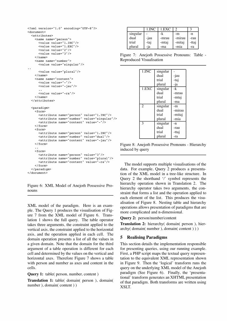
<?xml version="1.0" encoding="UTF-8"?><document>
<attributes><name name="person">
<value value="1.INC"/><value value="1.EXC"/><value value="2"/><value value="3"/>
</name><name name="number">
<value value="singular"/>..
<value value="plural"/></name><name name="content">
<value value="-"/><value value="-jau"/>..<value value="-ra"/>
</name></attributes>
<paradigm><form>
<attribute name="person" value="1.INC"/><attribute name="number" value="singular"/><attribute name="content" value="-"/>
</form><form>
<attribute name="person" value="1.INC"/><attribute name="number" value="dual"/><attribute name="content" value="-jau"/>
</form>..<form>
<attribute name="person" value="3"/><attribute name="number" value="plural"/><attribute name="content" value="-ra"/>
</form></paradigm>
</document>
Figure 6: XML Model of Anejom Possessive Pro-nouns
XML model of the paradigm. Here is an exam-ple. The Query 1 produces the visualisation of Fig-ure 7 from the XML model of Figure 6. Trans-lation 1 shows the full query. The table operatortakes three arguments, the constraint applied to thevertical axis, the constraint applied to the horizontalaxis, and the operation applied in each cell. Thedomain operation presents a list of all the values ina given domain. Note that the domain for the thirdargument of a table operation is different for eachcell and determined by the values on the vertical andhorizontal axes. Therefore Figure 7 shows a tablewith person and number as axes and content in thecells.Query 1: table( person, number, content )Translation 1: table( domain( person ), domain(number ), domain( content ) )
1.INC 1.EXC 2 3singular - -k -m -ndual -jau -mrau -mirau -rautrial -taj -mtaj -mitaj -ttajplural -ja -ma -mia -ra
Figure 7: Anejom Possessive Pronouns: Table -Reproduced Visualisation
1.INC singular -dual -jautrial -tajplural -ja
1.EXC singular -kdual -mrautrial -mtajplural -ma
2 singular -mdual -mirautrial -mitajplural -mia
3 singular -ndual -rautrial -ttajplural -ra
Figure 8: Anejom Possessive Pronouns - Hierarchyinduced by query
The model supports multiple visualisations of thedata. For example, Query 2 produces a presenta-tion of the XML model in a tree-like structure. InQuery 2 the shorthand ‘/’ symbol represents thehierarchy operation shown in Translation 2. Thehierarchy operator takes two arguments, the con-straint that forms a list and the operation applied toeach element of the list. This produces the visu-alisation of Figure 8. Nesting table and hierarchyoperations allows presentation of paradigms that aremore complicated and n-dimensional.Query 2: person/number/contentTranslation 2: hierarchy( domain( person ), hier-archy( domain( number ), domain( content ) ) )
5 Realising ParadigmsThis section details the implementation responsiblefor presenting queries, using our running example.First, a PHP script maps the textual query represen-tation to the equivalent XML representation shownin Figure 9. Then the ‘logical’ transform runs thequery on the underlying XML model of the Anejomparadigm (See Figure 6). Finally, the ‘presenta-tional’ transform generates an XHTML presentationof that paradigm. Both transforms are written usingXSLT.
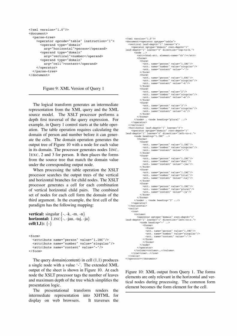
<?xml version="1.0"?><document>
<parse-tree><operator opcode="table" instruction="1">
<operand type="domain"arg="horizontal">person</operand>
<operand type="domain"arg="vertical">number</operand>
<operand type="domain"arg="cell">content</operand>
</operator></parse-tree>
</document>
Figure 9: XML Version of Query 1
The logical transform generates an intermediaterepresentation from the XML query and the XMLsource model. The XSLT processor performs adepth first traversal of the query expression. Forexample, in Query 1 control starts at the table oper-ation. The table operation requires calculating thedomain of person and number before it can gener-ate the cells. The domain operation generates theoutput tree of Figure 10 with a node for each valuein its domain. The processor generates nodes 1INC,1EXC, 2 and 3 for person. It then places the formsfrom the source tree that match the domain valueunder the corresponding output node.When processing the table operation the XSLT
processor searches the output trees of the verticaland horizontal branches for child nodes. The XSLTprocessor generates a cell for each combinationof vertical horizontal child pairs. The combinedset of nodes for each cell form the domain of thethird argument. In the example, the first cell of theparadigm has the following mapping:
vertical: singular {-, -k, -m. -n}horizontal: 1.INC{-, -jau, -taj, -ja}cell(1,1): {-}
<form><attribute name="person" value="1.INC"/><attribute name="number" value="singular"/><attribute name="content" value="-"/>
</form>
The query domain(content) in cell (1,1) producesa single node with a value ‘-’. The extended XMLoutput of the sheet is shown in Figure 10. At eachnode the XSLT processor tags the number of leavesand maximum depth of the tree which simplifies thepresentation logic.The presentational transform renders the
intermediate representation into XHTML fordisplay on web browsers. It traverses the
<?xml version="1.0"?><document><operator optype="table">
<vertical leaf-depth="1" leaves="4"><operator optype="domain" root-depth="1"
leaf-depth="1" leaves="4" direction="top-to-b."><node ..>
<att><html-att. element-name="th"/></att><forms>
<form><att. name="person" value="1.INC"/><att. name="number" value="singular"/><att. name="content" value="-"/>
</form><form>
<att. name="person" value="1.EXC"/><att. name="number" value="singular"/><att. name="content" value="-k"/>
</form><form>
<att. name="person" value="2"/><att. name="number" value="singular"/><att. name="content" value="-m"/>
</form><form>
<att. name="person" value="3"/><att. name="number" value="singular"/><att. name="content" value="-n"/>
</form></forms>
</node> . <node heading="plural" ../></operator>
</vertical><horizontal leaf-depth="1" leaves="4">
<operator optype="domain" root-depth="1"leaf-depth="1" leaves="4" direction="left-to-r.">
<node heading="1.INC" ..><forms>
<form><att. name="person" value="1.INC"/><att. name="number" value="singular"/><att. name="content" value="-"/>
</form><form>
<att. name="person" value="1.INC"/><att. name="number" value="dual"/><att. name="content" value="-jau"/>
</form><form>
<att. name="person" value="1.INC"/><att. name="number" value="trial"/><att. name="content" value="-taj"/>
</form><form>
<att. name="person" value="1.INC"/><att. name="number" value="plural"/><att. name="content" value="-ja"/>
</form></forms>
</node> . <node heading="3" ../></operator>
</horizontal><cells>
<row><column>
<operator optype="domain" root-depth="1"leaf-depth="1" leaves="1" direction="left-to-r.">
<node heading="-" ..><forms><form><att. name="person" value="1.INC"/><att. name="number" value="singular"/><att. name="content" value="-"/>
</form></forms>
</node></operator>
</column><column>..</column></row><row>..</row>
</cells></operator></document>
Figure 10: XML output from Query 1. The formselements are only relevant in the horizontal and ver-tical nodes during processing. The common formelement becomes the form element for the cell.
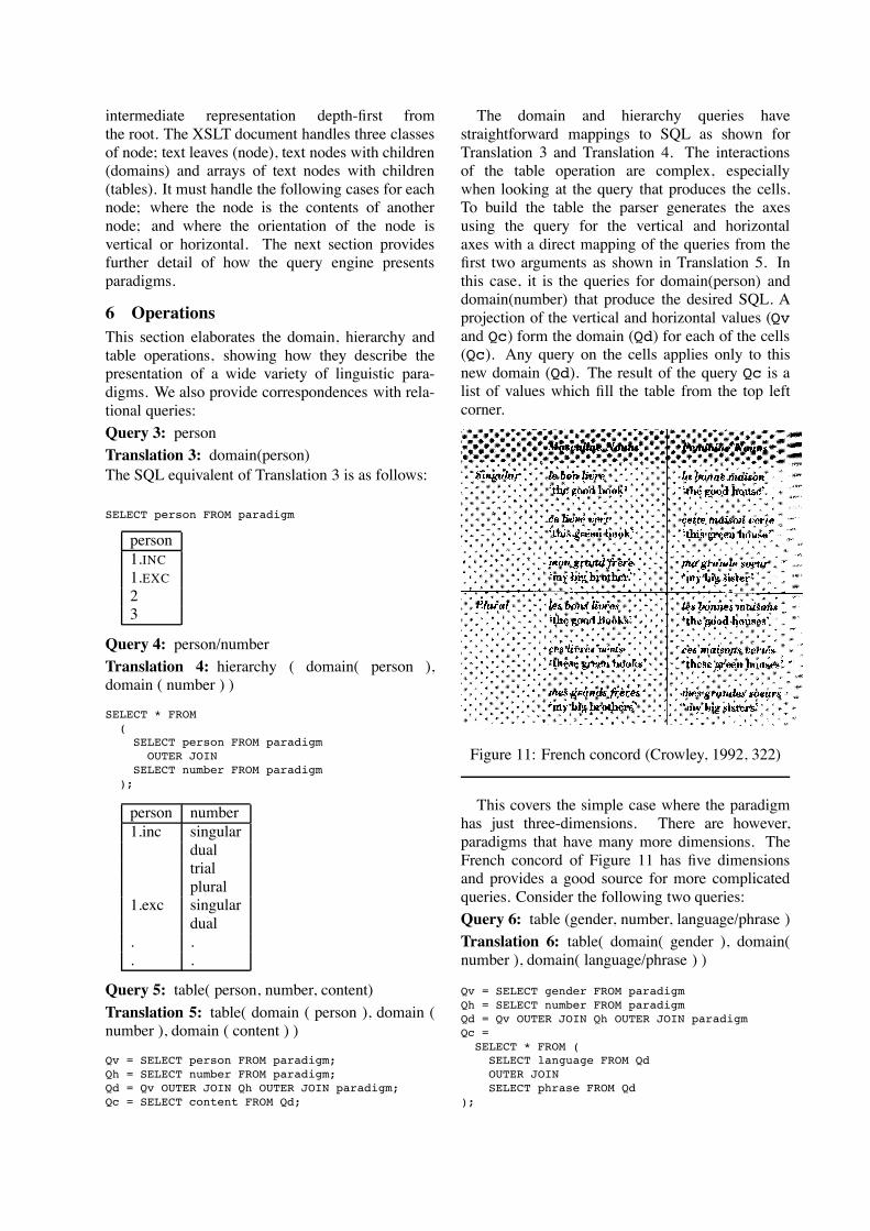
intermediate representation depth-first fromthe root. The XSLT document handles three classesof node; text leaves (node), text nodes with children(domains) and arrays of text nodes with children(tables). It must handle the following cases for eachnode; where the node is the contents of anothernode; and where the orientation of the node isvertical or horizontal. The next section providesfurther detail of how the query engine presentsparadigms.
6 OperationsThis section elaborates the domain, hierarchy andtable operations, showing how they describe thepresentation of a wide variety of linguistic para-digms. We also provide correspondences with rela-tional queries:Query 3: personTranslation 3: domain(person)The SQL equivalent of Translation 3 is as follows:
SELECT person FROM paradigm
person1.INC1.EXC23
Query 4: person/numberTranslation 4: hierarchy ( domain( person ),domain ( number ) )
SELECT * FROM(SELECT person FROM paradigm
OUTER JOINSELECT number FROM paradigm
);
person number1.inc singular
dualtrialplural
1.exc singulardual
. .
. .
Query 5: table( person, number, content)Translation 5: table( domain ( person ), domain (number ), domain ( content ) )
Qv = SELECT person FROM paradigm;Qh = SELECT number FROM paradigm;Qd = Qv OUTER JOIN Qh OUTER JOIN paradigm;Qc = SELECT content FROM Qd;
The domain and hierarchy queries havestraightforward mappings to SQL as shown forTranslation 3 and Translation 4. The interactionsof the table operation are complex, especiallywhen looking at the query that produces the cells.To build the table the parser generates the axesusing the query for the vertical and horizontalaxes with a direct mapping of the queries from thefirst two arguments as shown in Translation 5. Inthis case, it is the queries for domain(person) anddomain(number) that produce the desired SQL. Aprojection of the vertical and horizontal values (Qvand Qc) form the domain (Qd) for each of the cells(Qc). Any query on the cells applies only to thisnew domain (Qd). The result of the query Qc is alist of values which fill the table from the top leftcorner.
Figure 11: French concord (Crowley, 1992, 322)
This covers the simple case where the paradigmhas just three-dimensions. There are however,paradigms that have many more dimensions. TheFrench concord of Figure 11 has five dimensionsand provides a good source for more complicatedqueries. Consider the following two queries:Query 6: table (gender, number, language/phrase )Translation 6: table( domain( gender ), domain(number ), domain( language/phrase ) )
Qv = SELECT gender FROM paradigmQh = SELECT number FROM paradigmQd = Qv OUTER JOIN Qh OUTER JOIN paradigmQc =
SELECT * FROM (SELECT language FROM QdOUTER JOINSELECT phrase FROM Qd
);
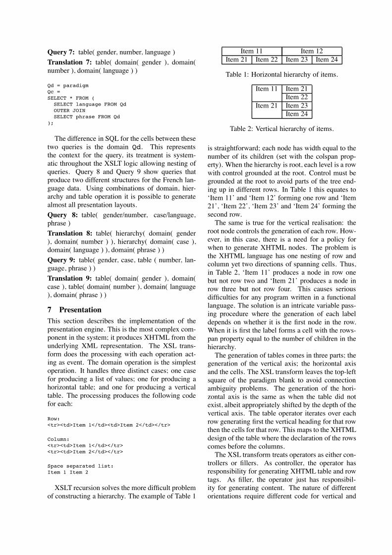
Query 7: table( gender, number, language )Translation 7: table( domain( gender ), domain(number ), domain( language ) )
Qd = paradigmQc =SELECT * FROM (
SELECT language FROM QdOUTER JOINSELECT phrase FROM Qd
);
The difference in SQL for the cells between thesetwo queries is the domain Qd. This representsthe context for the query, its treatment is system-atic throughout the XSLT logic allowing nesting ofqueries. Query 8 and Query 9 show queries thatproduce two different structures for the French lan-guage data. Using combinations of domain, hier-archy and table operation it is possible to generatealmost all presentation layouts.Query 8: table( gender/number, case/language,phrase )Translation 8: table( hierarchy( domain( gender), domain( number ) ), hierarchy( domain( case ),domain( language ) ), domain( phrase ) )Query 9: table( gender, case, table ( number, lan-guage, phrase ) )Translation 9: table( domain( gender ), domain(case ), table( domain( number ), domain( language), domain( phrase ) )
7 PresentationThis section describes the implementation of thepresentation engine. This is the most complex com-ponent in the system; it produces XHTML from theunderlying XML representation. The XSL trans-form does the processing with each operation act-ing as event. The domain operation is the simplestoperation. It handles three distinct cases; one casefor producing a list of values; one for producing ahorizontal table; and one for producing a verticaltable. The processing produces the following codefor each:
Row:<tr><td>Item 1</td><td>Item 2</td></tr>
Column:<tr><td>Item 1</td></tr><tr><td>Item 2</td></tr>
Space separated list:Item 1 Item 2
XSLT recursion solves the more difficult problemof constructing a hierarchy. The example of Table 1
Item 11 Item 12Item 21 Item 22 Item 23 Item 24
Table 1: Horizontal hierarchy of items.
Item 11 Item 21Item 22
Item 21 Item 23Item 24
Table 2: Vertical hierarchy of items.
is straightforward; each node has width equal to thenumber of its children (set with the colspan prop-erty). When the hierarchy is root, each level is a rowwith control grounded at the root. Control must begrounded at the root to avoid parts of the tree end-ing up in different rows. In Table 1 this equates to‘Item 11’ and ‘Item 12’ forming one row and ‘Item21’, ‘Item 22’, ‘Item 23’ and ‘Item 24’ forming thesecond row.The same is true for the vertical realisation: the
root node controls the generation of each row. How-ever, in this case, there is a need for a policy forwhen to generate XHTML nodes. The problem isthe XHTML language has one nesting of row andcolumn yet two directions of spanning cells. Thus,in Table 2, ‘Item 11’ produces a node in row onebut not row two and ‘Item 21’ produces a node inrow three but not row four. This causes seriousdifficulties for any program written in a functionallanguage. The solution is an intricate variable pass-ing procedure where the generation of each labeldepends on whether it is the first node in the row.When it is first the label forms a cell with the rows-pan property equal to the number of children in thehierarchy.The generation of tables comes in three parts; the
generation of the vertical axis; the horizontal axisand the cells. The XSL transform leaves the top-leftsquare of the paradigm blank to avoid connectionambiguity problems. The generation of the hori-zontal axis is the same as when the table did notexist, albeit appropriately shifted by the depth of thevertical axis. The table operator iterates over eachrow generating first the vertical heading for that rowthen the cells for that row. This maps to the XHTMLdesign of the table where the declaration of the rowscomes before the columns.The XSL transform treats operators as either con-
trollers or fillers. As controller, the operator hasresponsibility for generating XHTML table and rowtags. As filler, the operator just has responsibil-ity for generating content. The nature of differentorientations require different code for vertical and
horizontal orientations. When supported this allowsintegration and presentation of arbitrary commands.In fact this XSLT framework can display any querythat used operations from §6.
8 ConclusionThis paper describes an XML model for linguisticparadigms, including a query language andimplementation, along with a model for generatingpresentations and an implementation. This workprovides a flexible and extensible representationfor storing multidimensional linguistic paradigms;and a simple yet powerful method for accessingand analysing stored data. This model allows theeasy manipulation of paradigm structure, and easypresentation of systematic patterns and variations.We believe that the XML representation will beuseful for archiving linguistic paradigms and forthe interchange of paradigms between programs.We also believe the presentation system supportsmultidimensional exploration of complex linguisticdatasets, a linguistic version of what is known inthe database world as online analytical processing(OLAP).In the future, we plan to investigate the following:
ordering paradigm content; generating paradigmsfrom interlinear text; and investigating a multi-tablemodel. Ordering the cells of a paradigm is anissue because it complicates the axes, which thenrequire the repetition of headings. The secondline of enquiry is the generation and integrationof paradigm presentation into interlinear textsystems, which requires a level of machine learningcombined with an understanding of how to integratedifferent levels of linguistic description. The otherissue is how to represent some of the relationshipswithin paradigms such as the phonetic charactersfor a vowel and its height (eg. ! is a high vowel).We believe that the optimum solution for some ofthese problems is a multi-table model.
AcknowledgementsThis paper extends earlier work by (Penton etal., 2004). This research has been supported bythe National Science Foundation grant number0317826 Querying Linguistic Databases.
ReferencesSteven Bird. 1997. A lexical database tool forquantitative phonological research. In Proceed-ings of the Third Meeting of the ACL Spe-cial Interest Group in Computational Phonology,pages 33–39.
Steven Bird. 1999. Multidimensional explorationof online linguistic field data. In Pius Tamanji,Masako Hirotani, and Nancy Hall, editors,Proceedings of the 29th Annual Meeting ofthe Northeast Linguistics Society, pages 33–47.GLSA, University of Massachusetts at Amherst.
Terry Crowley. 1992. An Introduction to Histori-cal Linguistics, second edition. Auckland, NZ:Oxford University Press.
Edward Finegan. 1999. Language: its structureand use. Fort Worth: Harcourt Brace.
John Lynch. 1998. Pacific Languages: an Introduc-tion. Honolulu: University of Hawai’i Press.
Kemal Oflazer, Sergei Nirenburg, and MarjorieMcShane. 2001. Bootstrapping morphologicalanalyzers by combining human elicitation andmachine learning. Computational Linguistics,27(1):59–85.
David Penton, Catherine Bow, Steven Bird, andBaden Hughes. 2004. Towards a general modelfor linguistic paradigms.
Dan Tufis. 1989. It would be much easier if wentwere goed. In Proceedings of the 4th EuropeanConference of the Association for ComputationalLinguistics U.K. Manchester, 1989.
Tauira: A tool for acquiring unknown words in a dialogue context
Maarten van SchagenHuman Media Interaction Group
University of Twente7500AE Enschedethe Netherlands
Alistair KnottDepartment of Computer Science
University of OtagoDunedin 9015New Zealand
Abstract
This paper describes a tool for acquiring un-known words, which operates in a bilingualhuman-machine dialogue system. When theuser’s utterance includes a word which is notin the system’s lexicon, the system initiates asubdialogue to find out about the new word, byquerying the user about the syntactic validityof a number of example sentences generated au-tomatically from the grammar’s test suite. Thetool can handle multiple unknown words, reg-ular morphology and translation of new wordswithin a very complex unification feature struc-ture type hierarchy.
1 Introduction
A major problem for current wide-coveragesymbolic parsing systems is the existence of un-known words: words which appear in the in-put strings to be parsed, but which are not inthe system’s lexicon. To give a representativeexample: when the English Resource Grammar(ERG: Copestake and Flickinger (2000)) wastested over a portion of the British NationalCorpus, unknown words accounted for 40% ofall unparsed sentences (Baldwin et al., 2004).There are several ways of tackling this prob-lem. Some of these are o!ine, and simply in-volve making the lexicon bigger, adding new en-tries by hand or by some semiautomatic process.Other methods are on-line, and are designed tocope with unknown words which are encoun-tered during the parsing process itself.
This paper is concerned with on-line meth-ods for dealing with unknown words. We fo-cus on methods which are appropriate for im-plementation in a human-machine dialoguesystem. In this application, a human user en-ters a sentence; the system then parses the sen-tence, derives a semantic interpretation, andgenerates a suitable response. If the user’s sen-tence contains an unknown word, then the sys-tem must somehow compute information about
this word’s syntactic characteristics (so that thesentence can be parsed), and about its seman-tics (so that the sentence can receive an inter-pretation). Some of this information can typi-cally be inferred from the context in which thenew word appears—but it is unusual if it canall be provided this way. Typically, some othersource of knowledge needs to be actively con-sulted before the dialogue can resume.
A dialogue application opens up some newpossibilities for unknown word processing, be-cause when the system encounters an unknownword, it can initiate a subdialogue to findout more about this word. We will begin inSection 2 by outlining current approaches tounknown words in parsing, both in dialogueand non-dialogue applications. In Section 3 wewill propose a new approach, which combinesand extends existing approaches. In Section 4we will present a new tool for unknown wordprocessing which implements the proposed ap-proach. Section 5 gives some examples of word-authoring dialogues produced by the tool webuilt, and Section 6 describes some avenues forfurther work.
2 Current approaches to handlingunknown words in parsing
2.1 Knight: word-authoring dialogues
The suggestion that lexical items can be au-thored in a human-computer dialogue systemis not new. The idea is first proposed byKnight (1996) as the learning by instructionparadigm. Knight proposes two dialogue basedmethods whereby a naive user could add newwords to a system’s lexicon. The first approachis to ask a set of multiple choice questions inwhich the new word is placed in di"erent gram-matical contexts and the user is asked abouttheir syntactic correctness or where the user isasked various conceptual questions about thenature of the new word, as illustrated in thedialogue in Figure 1. The second approach is
H: John is hungry.C: I don’t know the meaning of ”hungry”. Is
”very hungry” a reasonable phrase?H: Yes.C: Is ”hungry” a visually detectable property ?H: No. (. . . )
Figure 1: A multi-choice word-authoring dia-logue
to let the user paraphrase the sentence con-taining the unknown word using concepts thesystem is already familiar with, as illustratedin Figure 2. Knight observes that although the
H: ”John is hungry.”C: I don’t know the meaning of ”hungry”H: I mean: ”John wants to eat”. (. . . )
Figure 2: An authoring dialogue using para-phrases
multiple choice method might work well for syn-tax, for semantics, the appropriate set of ques-tions is rather ill-defined, and giving good an-swers requires a fair amount of semantic sophis-tication on the part of the user. He thereforedid not try implementing this method. Evenat the syntactic level, it is quite a challenge todecide what syntactic contexts to present theunknown word in when querying the user. Wesomehow need to choose the most informativecontexts, so that the user is not queried moreoften than necessary, and so that we eventuallyend up identifying the actual syntax of the newword. If we assume a wide-coverage grammarsuch as the ERG, with over five hundred lexicaltypes, this is a complex task.
2.2 Erbach, Barg & Walther, Fouvry:making use of sentence context
Even without asking the user about how a newword can be used in other contexts, it is stillpossible to extract a lot of information aboutthe word’s syntactic characteristics from theoriginal sentence in which it appears. If we as-sume (a) that the word is of a syntactic typewhich the grammar already knows about, and(b) that the sentence would be parseable if theword were correctly identified as this type, thereare only certain possibilities as to what type itcan be. For example, a human reader ignorantof the word zapf could deduce from the sentencethe zapf chased his mother that zapf is a noun,
that zapf is singular (otherwise it would be thezapf chase their mother) and this particular in-stance of zapf is male.
A number of researchers have considered howbest to make use of syntactic context to pro-duce a set of hypotheses about an unknownword. Most such proposals are tied to a spe-cific grammar formalism—typically, some formof typed unification grammar. An influentialapproach was that of Erbach (1990). In his sys-tem (as in many others), a set of open-classword types is defined (a subset of the full setof lexical types), and it is assumed that the un-known word is one of these types. Erbach de-fines a formalism for representing disjunctionsof word types, and assigns the unknown word alexical type using this formalism.
Much of the complexity of this formalism de-rives from the fact that lexical types can be de-fined for various features which can take dif-ferent values; for instance, the type noun takesa feature number which can be singular orplural. When an unknown word is encoun-tered it must be filtered before it can actuallybe added as a new word. This filtering processconsists of selecting which features may be in-cluded in the final lexical entry. For the typenoun the feature number of an unknown wordderived from the sentence context will be in-cluded in the new lexical entry. The featuretense, however, which can also be derived fromthe sentence context for the unknown word, willnot be included in new lexical entries for thetype noun.
Barg and Walther (1998) refine Erbach’streatment of unknown words. A word accord-ing to Barg and Walther is not just known orunknown, but is an entry open to constant re-vision. Every time a word appears within thesentence context a revision takes place. A wordnot available in the lexicon is represented bythe conjunction of all open class word types.For the revision process, features are marked aseither generalizable or specializable. General-izable features are features such as gender fornouns, which can have di"erent values in dif-ferent contexts (e.g. the word zapf in the sen-tences the zapf chased his mother and the zapfchased her mother). Specializable features arefeatures such as number, which once they oc-cur once with a value in a context cannot occurwith another value in a di"erent context. (Notethat when number for a noun is specializable,morphologically irregular words such as sheep
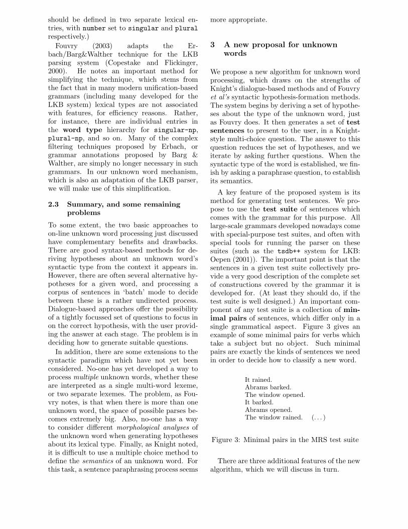
should be defined in two separate lexical en-tries, with number set to singular and plural
respectively.)Fouvry (2003) adapts the Er-
bach/Barg&Walther technique for the LKBparsing system (Copestake and Flickinger,2000). He notes an important method forsimplifying the technique, which stems fromthe fact that in many modern unification-basedgrammars (including many developed for theLKB system) lexical types are not associatedwith features, for e#ciency reasons. Rather,for instance, there are individual entries inthe word type hierarchy for singular-np,plural-np, and so on. Many of the complexfiltering techniques proposed by Erbach, orgrammar annotations proposed by Barg &Walther, are simply no longer necessary in suchgrammars. In our unknown word mechanism,which is also an adaptation of the LKB parser,we will make use of this simplification.
2.3 Summary, and some remainingproblems
To some extent, the two basic approaches toon-line unknown word processing just discussedhave complementary benefits and drawbacks.There are good syntax-based methods for de-riving hypotheses about an unknown word’ssyntactic type from the context it appears in.However, there are often several alternative hy-potheses for a given word, and processing acorpus of sentences in ‘batch’ mode to decidebetween these is a rather undirected process.Dialogue-based approaches o"er the possibilityof a tightly focussed set of questions to focus inon the correct hypothesis, with the user provid-ing the answer at each stage. The problem is indeciding how to generate suitable questions.
In addition, there are some extensions to thesyntactic paradigm which have not yet beenconsidered. No-one has yet developed a way toprocess multiple unknown words, whether theseare interpreted as a single multi-word lexeme,or two separate lexemes. The problem, as Fou-vry notes, is that when there is more than oneunknown word, the space of possible parses be-comes extremely big. Also, no-one has a wayto consider di"erent morphological analyses ofthe unknown word when generating hypothesesabout its lexical type. Finally, as Knight noted,it is di#cult to use a multiple choice method todefine the semantics of an unknown word. Forthis task, a sentence paraphrasing process seems
more appropriate.
3 A new proposal for unknownwords
We propose a new algorithm for unknown wordprocessing, which draws on the strengths ofKnight’s dialogue-based methods and of Fouvryet al’s syntactic hypothesis-formation methods.The system begins by deriving a set of hypothe-ses about the type of the unknown word, justas Fouvry does. It then generates a set of testsentences to present to the user, in a Knight-style multi-choice question. The answer to thisquestion reduces the set of hypotheses, and weiterate by asking further questions. When thesyntactic type of the word is established, we fin-ish by asking a paraphrase question, to establishits semantics.
A key feature of the proposed system is itsmethod for generating test sentences. We pro-pose to use the test suite of sentences whichcomes with the grammar for this purpose. Alllarge-scale grammars developed nowadays comewith special-purpose test suites, and often withspecial tools for running the parser on thesesuites (such as the tsdb++ system for LKB:Oepen (2001)). The important point is that thesentences in a given test suite collectively pro-vide a very good description of the complete setof constructions covered by the grammar it isdeveloped for. (At least they should do, if thetest suite is well designed.) An important com-ponent of any test suite is a collection of min-imal pairs of sentences, which di"er only in asingle grammatical aspect. Figure 3 gives anexample of some minimal pairs for verbs whichtake a subject but no object. Such minimalpairs are exactly the kinds of sentences we needin order to decide how to classify a new word.
It rained.Abrams barked.The window opened.It barked.Abrams opened.The window rained. (. . . )
Figure 3: Minimal pairs in the MRS test suite
There are three additional features of the newalgorithm, which we will discuss in turn.
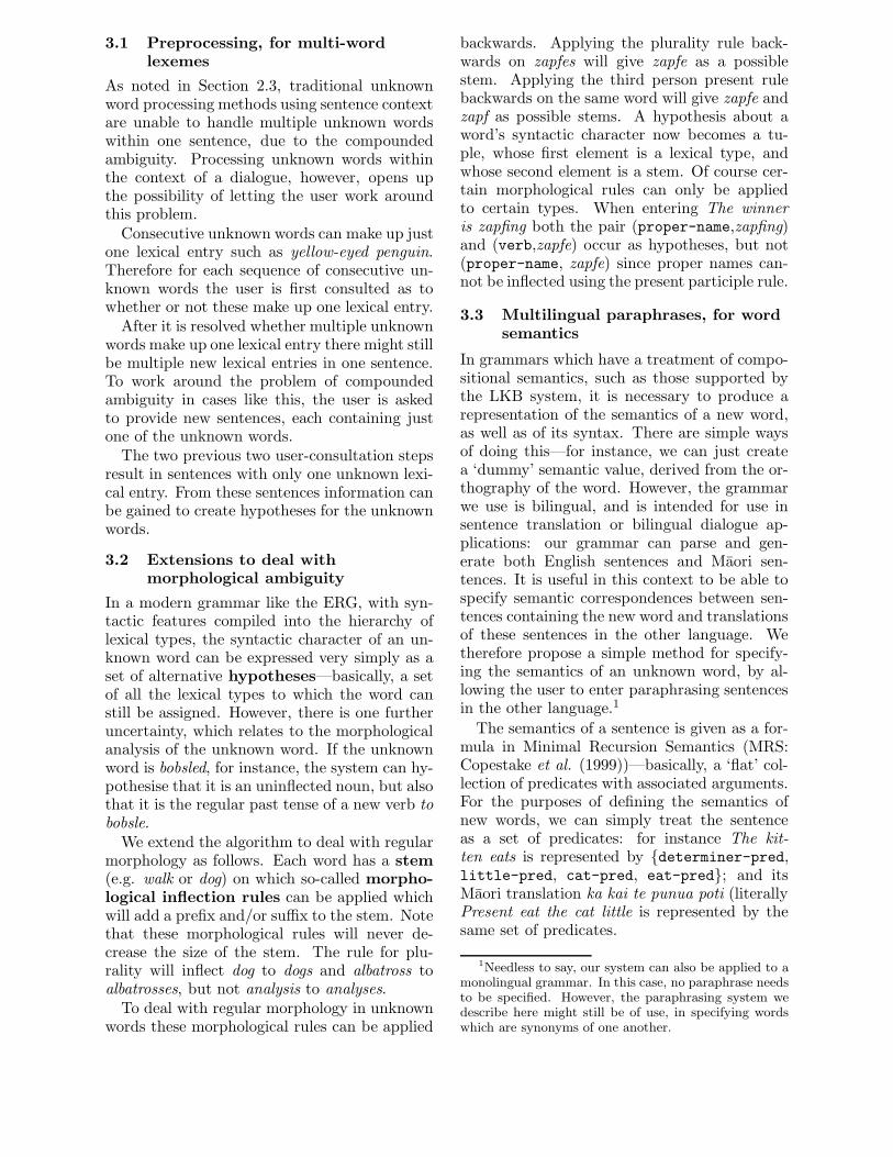
3.1 Preprocessing, for multi-wordlexemes
As noted in Section 2.3, traditional unknownword processing methods using sentence contextare unable to handle multiple unknown wordswithin one sentence, due to the compoundedambiguity. Processing unknown words withinthe context of a dialogue, however, opens upthe possibility of letting the user work aroundthis problem.
Consecutive unknown words can make up justone lexical entry such as yellow-eyed penguin.Therefore for each sequence of consecutive un-known words the user is first consulted as towhether or not these make up one lexical entry.
After it is resolved whether multiple unknownwords make up one lexical entry there might stillbe multiple new lexical entries in one sentence.To work around the problem of compoundedambiguity in cases like this, the user is askedto provide new sentences, each containing justone of the unknown words.
The two previous two user-consultation stepsresult in sentences with only one unknown lexi-cal entry. From these sentences information canbe gained to create hypotheses for the unknownwords.
3.2 Extensions to deal withmorphological ambiguity
In a modern grammar like the ERG, with syn-tactic features compiled into the hierarchy oflexical types, the syntactic character of an un-known word can be expressed very simply as aset of alternative hypotheses—basically, a setof all the lexical types to which the word canstill be assigned. However, there is one furtheruncertainty, which relates to the morphologicalanalysis of the unknown word. If the unknownword is bobsled, for instance, the system can hy-pothesise that it is an uninflected noun, but alsothat it is the regular past tense of a new verb tobobsle.
We extend the algorithm to deal with regularmorphology as follows. Each word has a stem(e.g. walk or dog) on which so-called morpho-logical inflection rules can be applied whichwill add a prefix and/or su#x to the stem. Notethat these morphological rules will never de-crease the size of the stem. The rule for plu-rality will inflect dog to dogs and albatross toalbatrosses, but not analysis to analyses.
To deal with regular morphology in unknownwords these morphological rules can be applied
backwards. Applying the plurality rule back-wards on zapfes will give zapfe as a possiblestem. Applying the third person present rulebackwards on the same word will give zapfe andzapf as possible stems. A hypothesis about aword’s syntactic character now becomes a tu-ple, whose first element is a lexical type, andwhose second element is a stem. Of course cer-tain morphological rules can only be appliedto certain types. When entering The winneris zapfing both the pair (proper-name,zapfing)and (verb,zapfe) occur as hypotheses, but not(proper-name, zapfe) since proper names can-not be inflected using the present participle rule.
3.3 Multilingual paraphrases, for wordsemantics
In grammars which have a treatment of compo-sitional semantics, such as those supported bythe LKB system, it is necessary to produce arepresentation of the semantics of a new word,as well as of its syntax. There are simple waysof doing this—for instance, we can just createa ‘dummy’ semantic value, derived from the or-thography of the word. However, the grammarwe use is bilingual, and is intended for use insentence translation or bilingual dialogue ap-plications: our grammar can parse and gen-erate both English sentences and Maori sen-tences. It is useful in this context to be able tospecify semantic correspondences between sen-tences containing the new word and translationsof these sentences in the other language. Wetherefore propose a simple method for specify-ing the semantics of an unknown word, by al-lowing the user to enter paraphrasing sentencesin the other language.1
The semantics of a sentence is given as a for-mula in Minimal Recursion Semantics (MRS:Copestake et al. (1999))—basically, a ‘flat’ col-lection of predicates with associated arguments.For the purposes of defining the semantics ofnew words, we can simply treat the sentenceas a set of predicates: for instance The kit-ten eats is represented by {determiner-pred,little-pred, cat-pred, eat-pred}; and itsMaori translation ka kai te punua poti (literallyPresent eat the cat little is represented by thesame set of predicates.
1Needless to say, our system can also be applied to amonolingual grammar. In this case, no paraphrase needsto be specified. However, the paraphrasing system wedescribe here might still be of use, in specifying wordswhich are synonyms of one another.
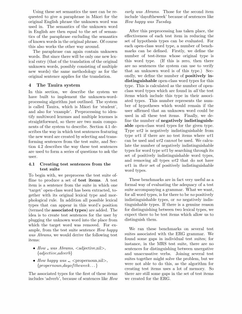
Using these set semantics the user can be re-quested to give a paraphrase in Maori for theoriginal English phrase the unknown word wasused in. The semantics of the unknown wordin English are then equal to the set of seman-tics of the paraphrase excluding the semanticsof known words in the original phrase. Of coursethis also works the other way around.
The paraphrase can again contain unknownwords. But since there will be only one new lex-ical entry (that of the translation of the originalunknown words, possibly consisting of multiplenew words) the same methodology as for theoriginal sentence applies for the translation.
4 The Tauira system
In this section, we describe the system wehave built to implement the unknown-word-processing algorithm just outlined. The systemis called Tauira, which is Maori for ‘student’,and also for ‘example’. Preprocessing to iden-tify multiword lexemes and multiple lexemes isstraightforward, so there are two main compo-nents of the system to describe. Section 4.1 de-scribes the way in which test sentences featuringthe new word are created by selecting and trans-forming sentences from the test suite, and Sec-tion 4.2 describes the way these test sentencesare used to form a series of questions to ask theuser.
4.1 Creating test sentences from thetest suite
To begin with, we preprocess the test suite of-fline to produce a set of test items. A testitem is a sentence from the suite in which one‘target’ open-class word has been extracted, to-gether with its original lexical type and mor-phological rule. In addition all possible lexicaltypes that can appear in this word’s position(termed the associated types) are added. Theidea is to create test sentences for the user byplugging the unknown word into the place fromwhich the target word was removed. For ex-ample, from the test suite sentence How happywas Abrams, we would derive the following testitems:
• How was Abrams, <adjective,nil>,{adjective,adverb}
• How happy was , <propernoun,nil>,{propernoun,dayoftheweek. . . }
The associated types for the first of these itemsincludes ‘adverb’, because of sentences like How
early was Abrams. Those for the second iteminclude ‘dayoftheweek’ because of sentences likeHow happy was Tuesday.
After this preprocessing has taken place, thee"ectiveness of each test item in reducing theset of hypothesis types can be evaluated. Foreach open-class word type, a number of bench-marks can be defined. Firstly, we define thenumber of test-items whose original type isthis word type. (If this is zero, then thereare no sentences the system can use to verifythat an unknown word is of this type.) Sec-ondly, we define the number of positively in-distinguishable open-class word types for thistype. This is calculated as the number of open-class word types which are found in all the testitems which include this type in their associ-ated types. This number represents the num-ber of hypotheses which would remain if theuser a#rmed that an unknown word could beused in all these test items. Finally, we de-fine the number of negatively indistinguish-able open-class word types for the given type.Type wt2 is negatively indistinguishable fromtype wt1 if there are no test items where wt1can be used and wt2 cannot be used. We calcu-late the number of negatively indistinguishabletypes for word type wt1 by searching through itsset of positively indistinguishable word types,and removing all types wt2 that do not havewt1 in their set of positively indistinguishableword types.
These benchmarks are in fact very useful as aformal way of evaluating the adequacy of a testsuite accompanying a grammar. What we want,for all word types, is for there to be no positivelyindistinguishable types, or no negatively indis-tinguishable types. If there is a genuine reasonfor distinguishing between two lexical types, weexpect there to be test items which allow us todistinguish them.
We ran these benchmarks on several testsuites associated with the ERG grammar. Wefound some gaps in individual test suites; forinstance, in the MRS test suite, there are nosentences for distinguishing between unergativeand unaccusative verbs. Joining several testsuites together might solve the problem, but wewere not able to do this, as the algorithm forcreating test items uses a lot of memory. Sothere are still some gaps in the set of test itemswe created for the ERG.
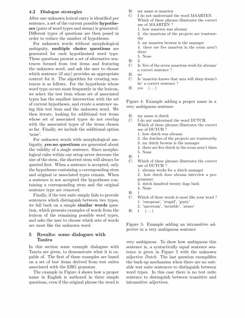
4.2 Dialogue strategies
After one unknown lexical entry is identified persentence, a set of the current possible hypothe-ses (pairs of word types and stems) is generated.Di"erent types of questions are then posed inorder to reduce the number of hypotheses.
For unknown words without morphologicalambiguity, multiple choice questions aregenerated for each hypothesised word type.These questions present a set of alternative sen-tences formed from test items and featuringthe unknown word, and ask the user to choosewhich sentence (if any) provides an appropriatecontext for it. The algorithm for creating sen-tences is as follows. For the hypothesis whoseword type occurs most frequently in the lexicon,we select the test item whose set of associatedtypes has the smallest intersection with the setof current hypotheses, and create a sentence us-ing this test item and the unknown word. Wethen iterate, looking for additional test itemswhose set of associated types do not overlapwith the associated types of the items chosenso far. Finally, we include the additional option‘none’.
For unknown words with morphological am-biguity, yes-no questions are generated aboutthe validity of a single sentence. Since morpho-logical rules within our setup never decrease thesize of the stem, the shortest stem will always bequeried first. When a sentence is accepted, onlythe hypotheses containing a corresponding stemand original or associated types remain. Whena sentence is not accepted the hypotheses con-taining a corresponding stem and the originalsentence type are removed.
Finally, if the test suite simply fails to providesentences which distinguish between two types,we fall back on a simple similar words ques-tion, which presents examples of words from thelexicon of the remaining possible word types,and asks the user to choose which sets of wordsare most like the unknown word.
5 Results: some dialogues withTauira
In this section some example dialogues withTauria are given, to demonstrate what it is ca-pable of. The first of these examples are basedon a set of test items derived from test suitesassociated with the ERG grammar.
The example in Figure 4 shows how a propername in English is authored in three simplequestions, even if the original phrase the word is
H: my name is maartenC: I do not understand the word MAARTEN.
Which of these phrases illustrates the correctuse of MAARTEN ?1. how maarten was abrams2. the maartens of the projects are trustwor-thy3. mr maarten browne is the manager4. there are five maarten in the room aren’tthere5. None
H: 3C: Is ’five of the seven maartens work for abrams’
a correct sentence ?H: noC: Is ’maarten knows that sara will sleep doesn’t
he’ a correct sentence ?H: yes (. . . )
Figure 4: Example adding a proper name in avery ambiguous sentence
H: my name is dutchC: I do not understand the word DUTCH.
Which of these phrases illustrates the correctuse of DUTCH ?1. how dutch was abrams2. the dutches of the projects are trustworthy3. mr dutch browne is the manager4. there are five dutch in the room aren’t there5. None
H: 1C: Which of these phrases illustrates the correct
use of DUTCH ?1. abrams works for a dutch manager2. how dutch does abrams interview a pro-grammer3. dutch hundred twenty dogs bark4. None
H: 1C: Which of these words is most like your word ?
1. ’european’, ’stupid’, ’gusty’2. ’uncertain’, ’invisible’, ’aware’
H: 1 (. . . )
Figure 5: Example adding an intransitive ad-jective in a very ambiguous sentence
very ambiguous. To show how ambiguous thissentence is, a syntactically equal sentence sen-tence is given in Figure 5 with the unknownadjective Dutch. The last question exemplifiesthe back-up mechanism when there are no suit-able test suite sentences to distinguish betweenword types. In this case there is no test suitesentence to distinguish between transitive andintransitive adjectives.
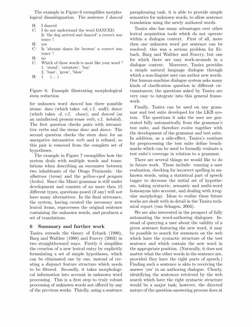
The example in Figure 6 exemplifies morpho-logical disambiguation. The sentence I danced
H: I dancedC: I do not understand the word DANCED.
Is ’the dog arrived and danced’ a correct sen-tence ?
H: yesC: Is ’abrams dancs for browne’ a correct sen-
tence ?H: noC: Which of these words is most like your word ?
1. ’stand’, ’orientate’, ’bay’2. ’bust’, ’grow’, ’blow’
H: 1 (. . . )
Figure 6: Example illustrating morphologicalstem reduction
for unknown word danced has three possiblestems: danc (which takes -ed, c.f. walk); dance(which takes -d, c.f. chase); and danced (asan uninflected present-tense verb, c.f. bobsled).The first question checks pairs with intransi-tive verbs and the stems danc and dance. Thesecond question checks the stem danc for anunergative intransitive verb and is refused, sothis pair is removed from the complete set ofhypotheses.
The example in Figure 7 exemplifies how thesystem deals with multiple words and trans-lations when describing an encounter betweentwo inhabitants of the Otago Peninsula: thealbatross (toroa) and the yellow-eyed penguin(hoiho). Since the Maori grammar is still underdevelopment and consists of no more then 15di"erent types, questions posed (if any) will nothave many alternatives. In the final utterance,the system, having created the necessary newlexical items, reprocesses the original sentencecontaining the unknown words, and produces aset of translations.
6 Summary and further work
Tauira extends the theory of Erbach (1990),Barg and Walther (1998) and Fouvry (2003) intwo straightforward ways. Firstly it simplifiesthe creation of a new lexical entry by explicitlyformulating a set of simple hypotheses, whichcan be eliminated one by one, instead of cre-ating a disjunct feature structure which needsto be filtered. Secondly, it takes morphologi-cal information into account in unknown wordprocessing. This is a first step to truly robustprocessing of unknown words not o"ered by anyof the previous works. Thirdly, using a sentence
paraphrasing task, it is able to provide simplesemantics for unknown words, to allow sentencetranslation using the newly authored words.
Tauira also has many advantages over otherlexical acquisition tools which do not operatewithin a dialogue context. First of all, morethen one unknown word per sentence can beresolved; this was a serious problem for Er-bach, Barg and Walther and Fouvry, but onefor which there are easy work-arounds in adialogue context. Moreover, Tauira providesa simple natural language dialogue throughwhich a non-linguist user can author new words.Our human-machine dialogue system asks manykinds of clarification question in di"erent cir-cumstances; the questions asked by Tauira arevery easy to integrate into this general frame-work.
Finally, Tauira can be used on any gram-mar and test suite developed for the LKB sys-tem. The questions it asks the user are gen-erated fully automatically from the grammar’stest suite, and therefore evolve together withthe development of the grammar and test suite.In addition, as a side-e"ect, Tauira’s routinesfor preprocessing the test suite define bench-marks which can be used to formally evaluate atest suite’s coverage in relation to a grammar.
There are several things we would like to doin future work. These include: running a userevaluation, checking for incorrect spelling in un-known words, using a statistical part of speechtagger to decrease the initial set of hypothe-ses, taking syntactic, semantic and multi-wordhomonyms into account, and dealing with irreg-ular morphology. Ideas to realize these futureworks are dealt with in detail in the Tauira tech-nical report (van Schagen, 2004).
We are also interested in the prospect of fullyautomating the word-authoring dialogues. In-stead of querying a user about the validity of agiven sentence featuring the new word, it maybe possible to search for sentences on the webwhich have the syntactic structure of the testsentence and which contain the new word inthe appropriate position. (Naturally, it does notmatter what the other words in the sentence are,provided they have the right parts of speech.)Finding such a sentence is akin to receiving theanswer ‘yes’ in an authoring dialogue. Clearly,identifying the sentences retrieved by the websearch which have the right syntactic structurewould be a major task; however, the directednature of the question-answering process does at
least strongly minimize the number of searcheswhich would be needed. This is a topic we planto address in future work.
References
T Baldwin, E Bender, D Flickinger, A Kim, andS Oepen. 2004. Road-testing the english resourcegrammar over the british national corpus. In Pro-ceedings of LREC 2004, Lisbon, Portugal.
P Barg and M Walther. 1998. Processing unknownwords in HPSG. In Proceedings of the 36th An-nual Meeting of the Association for Computa-tional Linguistics and 17th International Con-ference on Computational Linguistics, Montreal,Canada.
A Copestake and D Flickinger. 2000. An open-source grammar development environment andbroad-coverage English grammar using hpsg. InProceedings of LREC 2000, Athens, Greece.
A Copestake, D Flickinger, I Sag, and C Pollard.1999. Minimal Recursion Semantics: An intro-duction. Manuscript, CSLI, Stanford University.
C Erbach. 1990. Syntactic processing of unknownwords. In P Jorand and V Sgurev, editors, Artifi-cial Intelligence IV: methodology, systems, appli-cations, pages 371–382. North-Holland, Amster-dam.
F Fouvry. 2003. Lexicon acquisition with a large-coverage unification-based grammar. In 10thConference of the European Chapter of the Asso-ciation for Computational Linguistics, Researchnotes and demos, Budapest, Hungary.
K Knight. 1996. Learning word meanings by in-struction. In Proceedings of the 13th NationalConference on Artificial Intelligence, Portland,Oregon.
Stephan Oepen. 2001. [incr tsdb()] — competenceand performance laboratory. User manual. Tech-nical report, Computational Linguistics, SaarlandUniversity, Saarbrucken, Germany.
Maarten van Schagen. 2004. Tauira: A bilingualdialogue-based lexical acquisition system. Techni-cal Report OUCS-2004-06, Department of Com-puter Science, University of Otago, Dunedin, NewZealand.
H: the albatross chases the yelloweyed penguinC: I do not understand the words ALBATROSS,
YELLOWEYED, PENGUIN.Is YELLOWEYED PENGUIN one word ?
H: yesC: Could you provide me an example sentence
with the unknown word ’ALBATROSS’ usingwords I know ?
H: the albatross eatsC: Which of these phrases illustrates the correct
use of ALBATROSS ?1. the albatrosses of the projects are trustwor-thy2. mr albatross browne is the manager3. browne was hired on january albatross 19844. None
H: 4C: Is ’he showed her an albatross’ a correct sen-
tence ?H: yesC: Which of these words is most like your word ?
1. ’sec’, ’counter narcotics’, ’paycheck’2. ’school’, ’black’, ’distance’3. ’delivery’, ’record’, ’treatment’4. ’specification’, ’subscriber’, ’deviation’
H: 1C: What is the translation of ’the albatross eats’
in Maori.H: ka kai te toroaC: Is ’kua pai te toroa’ a correct sentence ?H: yesC: Which of these phrases illustrates the correct
use of YELLOWEYED PENGUIN ?1. the yelloweyed penguins of the projects aretrustworthy2. mr yelloweyed penguin browne is the man-ager3. browne was hired on january yelloweyedpenguin 19844. there are five yelloweyed penguin in theroom aren’t there5. None
H: 5C: Is ’list yelloweyed penguins who have book-
cases’ a correct sentence ?H: yesC: Which of these words is most like your word ?
1. ’sec’, ’counter narcotics’, ’paycheck’2. ’school’, ’black’, ’distance’3. ’delivery’, ’record’, ’treatment’4. ’specification’, ’subscriber’, ’deviation’
H: 1C: What is the translation of ’the albatross chases
the yelloweyed penguin’ in Maori.H: ka whai te toroa i te hoihoC: ’the albatross chases the yelloweyed penguin’
translates to:ka whaia te hoiho e te toroaka whai te toroa i te hoiho
Figure 7: Example illustrating multiple wordsand translation
Querying and Updating Treebanks:A Critical Survey and Requirements Analysis
Catherine Lai and Steven BirdDepartment of Computer Science and Software Engineering
University of Melbourne, Victoria 3010, Australia{clai,sb}@csse.unimelb.edu.au
AbstractLanguage technology makes extensive use of hierarchi-cally annotated text and speech data. These databases arestored in flat files and manipulated using corpus-specificquery tools or special-purpose scripts. While the size ofthese databases and the range of applications has grownrapidly in recent years, neither method for managing thedata has led to reusable, scalable software. The formalproperties of the query languages are not well under-stood. Hence established methods for indexing tree dataand optimizing tree queries cannot be employed. Weanalyze a range of existing linguistic query languages,and adduce a set of requirements for a reusable, scalablelinguistic query language.
1 IntroductionCorpora form the backbone of language technol-ogy. However corpora usually need to be annotatedwith structural information describing, for example,syntax or phonology. Query languages are neces-sary to extract useful information from these mas-sive data sets. Moreover, annotated corpora requirethousands of hours of manual annotation to create,revise and maintain. Query languages are also use-ful during this process. For example, queries can beused to find parse errors or to transform annotationsinto different schemes.However, the query languages currently available
for annotated corpora suffer from several problems.Firstly, updates are not supported as querylanguages focus on the needs of linguists searchingfor syntactic constructions. Secondly, theirrelationship to existing database query languagesis poorly understood, making it difficult to applystandard database indexing and query optimizationtechniques. As a consequence they do not scalewell. Finally, linguistic annotations have both asequential and a hierarchical organization. Querylanguages must support queries that refer to both
of these types of structure simultaneously. Suchhybrid queries should have a concise syntax. Theinterplay between these factors has resulted in avariety of mutually-inconsistent approaches.This paper aims to describe the query language
requirements for navigating and modifying struc-turally annotated corpora. We focus on tree struc-tured annotation. This entails sequential structure.This paper is organized as follows. Section 2
surveys six linguistic tree querying languages andwhere appropriate the data models they are basedon. The survey is the basis of the linguistic treequery requirements presented in Section 3. We con-clude in Section 4 with suggested areas for furtherwork.
2 Tree Models and Query LanguagesThe prototypical hierarchical linguistic annotationis the syntax tree, an ordered tree where termi-nals (leaves) contain the text of a sentence beinganalyzed. Non-terminals represent syntactic cate-gories, and the hierarchical organization representsconstituency. The leaf level is usually consideredimmutable. The queries in Figure 1 have been cho-sen to highlight the expressive capabilities of cur-rent tree query languages.A query language must be able to accurately
specify which subtrees to match in a corpus. Thismeans quantifying the existence of nodes andsuccintly stating the relationships between them.Q1 is a simple query based on the dominancerelation inherent in trees. As mentioned earlier,however, the sequential ordering of nodes is alsoan important factor. Q3 and Q4 demonstrate theprecision that is available for describing subtreesconstrained by both dominance and precedencerelations.It is also desirable to specify subtrees by what
they do not contain. This requires some form ofnegation. Q2 is a simple example of this type of
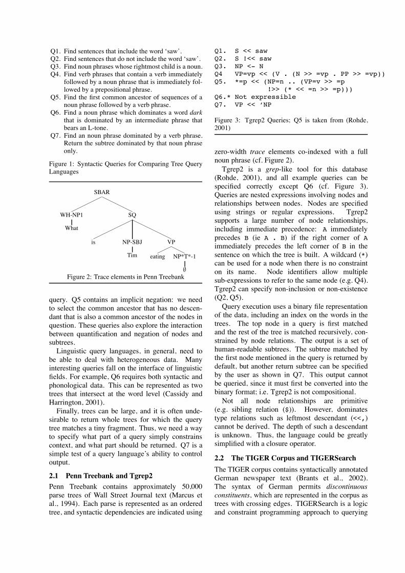
Q1. Find sentences that include the word ‘saw’.Q2. Find sentences that do not include the word ‘saw’.Q3. Find noun phrases whose rightmost child is a noun.Q4. Find verb phrases that contain a verb immediately
followed by a noun phrase that is immediately fol-lowed by a prepositional phrase.
Q5. Find the first common ancestor of sequences of anoun phrase followed by a verb phrase.
Q6. Find a noun phrase which dominates a word darkthat is dominated by an intermediate phrase thatbears an L-tone.
Q7. Find an noun phrase dominated by a verb phrase.Return the subtree dominated by that noun phraseonly.
Figure 1: Syntactic Queries for Comparing Tree QueryLanguages
SBAR
WH-NP1
What
SQ
is NP-SBJ
Tim
VP
eating NP*T*-1
!
Figure 2: Trace elements in Penn Treebank
query. Q5 contains an implicit negation: we needto select the common ancestor that has no descen-dant that is also a common ancestor of the nodes inquestion. These queries also explore the interactionbetween quantification and negation of nodes andsubtrees.Linguistic query languages, in general, need to
be able to deal with heterogeneous data. Manyinteresting queries fall on the interface of linguisticfields. For example, Q6 requires both syntactic andphonological data. This can be represented as twotrees that intersect at the word level (Cassidy andHarrington, 2001).Finally, trees can be large, and it is often unde-
sirable to return whole trees for which the querytree matches a tiny fragment. Thus, we need a wayto specify what part of a query simply constrainscontext, and what part should be returned. Q7 is asimple test of a query language’s ability to controloutput.
2.1 Penn Treebank and Tgrep2Penn Treebank contains approximately 50,000parse trees of Wall Street Journal text (Marcus etal., 1994). Each parse is represented as an orderedtree, and syntactic dependencies are indicated using
Q1. S << sawQ2. S !<< sawQ3. NP <- NQ4 VP=vp << (V . (N >> =vp . PP >> =vp))Q5. *=p << (NP=n .. (VP=v >> =p
!>> (* << =n >> =p)))Q6.* Not expressibleQ7. VP << ‘NP
Figure 3: Tgrep2 Queries; Q5 is taken from (Rohde,2001)
zero-width trace elements co-indexed with a fullnoun phrase (cf. Figure 2).Tgrep2 is a grep-like tool for this database
(Rohde, 2001), and all example queries can bespecified correctly except Q6 (cf. Figure 3).Queries are nested expressions involving nodes andrelationships between nodes. Nodes are specifiedusing strings or regular expressions. Tgrep2supports a large number of node relationships,including immediate precedence: A immediatelyprecedes B (ie A . B) if the right corner of Aimmediately precedes the left corner of B in thesentence on which the tree is built. A wildcard (*)can be used for a node when there is no constrainton its name. Node identifiers allow multiplesub-expressions to refer to the same node (e.g. Q4).Tgrep2 can specify non-inclusion or non-existence(Q2, Q5).Query execution uses a binary file representation
of the data, including an index on the words in thetrees. The top node in a query is first matchedand the rest of the tree is matched recursively, con-strained by node relations. The output is a set ofhuman-readable subtrees. The subtree matched bythe first node mentioned in the query is returned bydefault, but another return subtree can be specifiedby the user as shown in Q7. This output cannotbe queried, since it must first be converted into thebinary format; i.e. Tgrep2 is not compositional.Not all node relationships are primitive
(e.g. sibling relation ($)). However, dominatestype relations such as leftmost descendant (<<,)cannot be derived. The depth of such a descendantis unknown. Thus, the language could be greatlysimplified with a closure operator.
2.2 The TIGER Corpus and TIGERSearchThe TIGER corpus contains syntactically annotatedGerman newspaper text (Brants et al., 2002).The syntax of German permits discontinuousconstituents, which are represented in the corpus astrees with crossing edges. TIGERSearch is a logicand constraint programming approach to querying
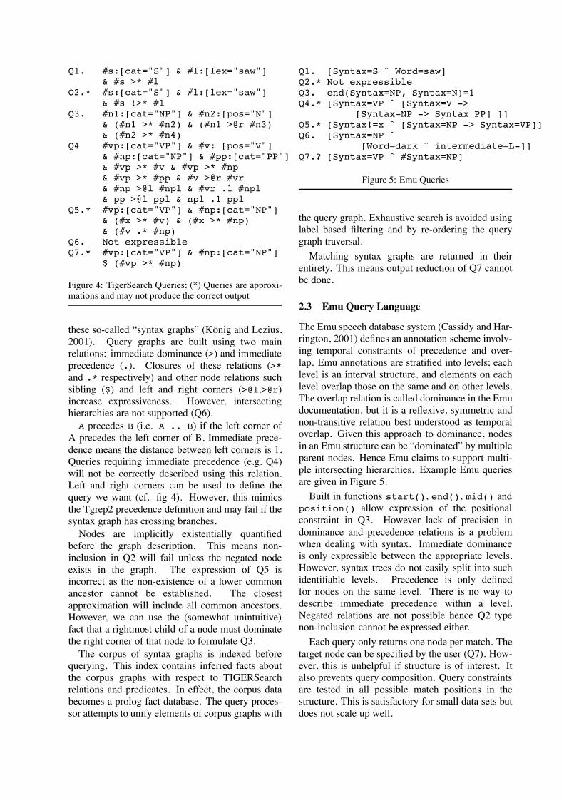
Q1. #s:[cat="S"] & #l:[lex="saw"]& #s >* #l
Q2.* #s:[cat="S"] & #l:[lex="saw"]& #s !>* #l
Q3. #n1:[cat="NP"] & #n2:[pos="N"]& (#n1 >* #n2) & (#n1 >@r #n3)& (#n2 >* #n4)
Q4 #vp:[cat="VP"] & #v: [pos="V"]& #np:[cat="NP"] & #pp:[cat="PP"]& #vp >* #v & #vp >* #np& #vp >* #pp & #v >@r #vr& #np >@l #npl & #vr .1 #npl& pp >@l ppl & npl .1 ppl
Q5.* #vp:[cat="VP"] & #np:[cat="NP"]& (#x >* #v) & (#x >* #np)& (#v .* #np)
Q6. Not expressibleQ7.* #vp:[cat="VP"] & #np:[cat="NP"]
$ (#vp >* #np)
Figure 4: TigerSearch Queries; (*) Queries are approxi-mations and may not produce the correct output
these so-called “syntax graphs” (Konig and Lezius,2001). Query graphs are built using two mainrelations: immediate dominance (>) and immediateprecedence (.). Closures of these relations (>*and .* respectively) and other node relations suchsibling ($) and left and right corners (>@l,>@r)increase expressiveness. However, intersectinghierarchies are not supported (Q6).A precedes B (i.e. A .. B) if the left corner of
A precedes the left corner of B. Immediate prece-dence means the distance between left corners is 1.Queries requiring immediate precedence (e.g. Q4)will not be correctly described using this relation.Left and right corners can be used to define thequery we want (cf. fig 4). However, this mimicsthe Tgrep2 precedence definition and may fail if thesyntax graph has crossing branches.Nodes are implicitly existentially quantified
before the graph description. This means non-inclusion in Q2 will fail unless the negated nodeexists in the graph. The expression of Q5 isincorrect as the non-existence of a lower commonancestor cannot be established. The closestapproximation will include all common ancestors.However, we can use the (somewhat unintuitive)fact that a rightmost child of a node must dominatethe right corner of that node to formulate Q3.The corpus of syntax graphs is indexed before
querying. This index contains inferred facts aboutthe corpus graphs with respect to TIGERSearchrelations and predicates. In effect, the corpus databecomes a prolog fact database. The query proces-sor attempts to unify elements of corpus graphs with
Q1. [Syntax=S ˆ Word=saw]Q2.* Not expressibleQ3. end(Syntax=NP, Syntax=N)=1Q4.* [Syntax=VP ˆ [Syntax=V ->
[Syntax=NP -> Syntax PP] ]]Q5.* [Syntax!=x ˆ [Syntax=NP -> Syntax=VP]]Q6. [Syntax=NP ˆ
[Word=dark ˆ intermediate=L-]]Q7.? [Syntax=VP ˆ #Syntax=NP]
Figure 5: Emu Queries
the query graph. Exhaustive search is avoided usinglabel based filtering and by re-ordering the querygraph traversal.Matching syntax graphs are returned in their
entirety. This means output reduction of Q7 cannotbe done.
2.3 Emu Query Language
The Emu speech database system (Cassidy and Har-rington, 2001) defines an annotation scheme involv-ing temporal constraints of precedence and over-lap. Emu annotations are stratified into levels; eachlevel is an interval structure, and elements on eachlevel overlap those on the same and on other levels.The overlap relation is called dominance in the Emudocumentation, but it is a reflexive, symmetric andnon-transitive relation best understood as temporaloverlap. Given this approach to dominance, nodesin an Emu structure can be “dominated” by multipleparent nodes. Hence Emu claims to support multi-ple intersecting hierarchies. Example Emu queriesare given in Figure 5.Built in functions start(), end(), mid() and
position() allow expression of the positionalconstraint in Q3. However lack of precision indominance and precedence relations is a problemwhen dealing with syntax. Immediate dominanceis only expressible between the appropriate levels.However, syntax trees do not easily split into suchidentifiable levels. Precedence is only definedfor nodes on the same level. There is no way todescribe immediate precedence within a level.Negated relations are not possible hence Q2 typenon-inclusion cannot be expressed either.Each query only returns one node per match. The
target node can be specified by the user (Q7). How-ever, this is unhelpful if structure is of interest. Italso prevents query composition. Query constraintsare tested in all possible match positions in thestructure. This is satisfactory for small data sets butdoes not scale up well.
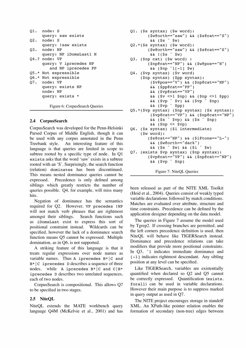
Q1. node: Squery: saw exists
Q2. node: Squery: !saw exists
Q3. node: NPquery: NP iDomsLast1 N
Q4.? node: VPquery: V iprecedes NP
and NP iprecedes PPQ5.* Not expressibleQ6.* Not expressibleQ7. node: VP
query: exists NPnode: NPquery: exists *
Figure 6: CorpusSearch Queries
2.4 CorpusSearchCorpusSearch was developed for the Penn-HelsinkiParsed Corpus of Middle English, though it canbe used with any corpus annotated in the PennTreebank style. An interesting feature of thislanguage is that queries are limited in scope tosubtree rooted by a specific type of node. In Q1exists asks that the word ‘saw’ exists in a subtreerooted with an ‘S’. Surprisingly, the search function(relation) dominates has been discontinued.This means nested dominance queries cannot beexpressed. Precedence is only defined amongsiblings which greatly restricts the number ofqueries possible. Q4, for example, will miss manyhits.Negation of dominance has the semantics
required for Q2. However, VP precedes !NPwill not match verb phrases that are rightmostamongst their siblings. Search functions suchas iDomsLast exist to express this sort ofpositional constraint instead. Wildcards can bespecified, however the lack of a dominance searchfunction means Q5 cannot be expressed. Multipledomination, as in Q6, is not supported.A striking feature of this language is that it
treats regular expressions over node names asvariable names. Thus A iprecedes B*|C andB*|C iprecedes D describes a sequence of threenodes, while A iprecedes B*|C and C|B*iprecedes D describes two unrelated sequences,each of two nodes.CorpusSearch is compositional. This allows Q7
to be specified in two stages.
2.5 NiteQLNiteQL extends the MATE workbench querylanguage Q4M (McKelvie et al., 2001) and has
Q1. ($s syntax) ($w word):($w@orth=="saw") && ($s@cat=="S")&& ($s ˆ $w)
Q2.*($s syntax) ($w word):($w@orth=="saw") && ($s@cat=="S")&& !($s ˆ $w)
Q3. ($np cat) ($w word) :($np@cat=="NP") && ($w@pos=="N")&& ($np ˆ1[-1] $w)
Q4. ($vp syntax) ($v word)($np syntax) ($pp syntax):
($v@pos=="V") && ($np@cat=="NP")&& ($pp@cat=="PP")&& ($vp@cat=="VP")&& ($v <>1 $np) && ($np <>1 $pp)&& ($vp ˆ $v) && ($vp ˆ $np)&& ($vp ˆ $pp)
Q5.*($vp syntax) ($np syntax) ($x syntax):($vp@cat=="VP") && ($np@cat=="NP")&& ($x ˆ $vp) && ($x ˆ $np)&& ($np <> $vp)
Q6. ($s syntax) ($i intermediate)($w word):
($s@cat=="NP") && ($i@tone=="L-")&& ($w@orth=="dark")&& ($s ˆ $w) && ($i ˆ $w)
Q7. (exists $vp syntax) ($np syntax):($vp@cat=="VP") && ($np@cat=="NP")&& ($vp ˆ $np)
Figure 7: NiteQL Queries
been released as part of the NITE XML Toolkit(Heid et al., 2004). Queries consist of weakly typedvariable declarations followed by match conditions.Matches are evaluated over attribute, structure andtime constraints. Precedence can be defined by theapplication designer depending on the data model.The queries in Figure 7 assume the model used
by Tgrep2. If crossing branches are permitted, andthe left corners precedence definition is used, thenNiteQL will behave like TIGERSearch instead.Dominance and precedence relations can takemodifiers that provide more positional constraints.In Q3, ˆ1 indicates immediate dominance and[-1] indicates rightmost descendant. Any siblingposition at any level can be specified.Like TIGERSearch, variables are existentially
quantified when declared so Q2 and Q5 cannotbe correctly expressed. Quantification (exists,forall) can be used in variable declarations.However their main purpose is to suppress markedin query output as used in Q7.The NITE project encourages storage in standoff
XML. An XPath-like pointer relation enables theformation of secondary (non-tree) edges between
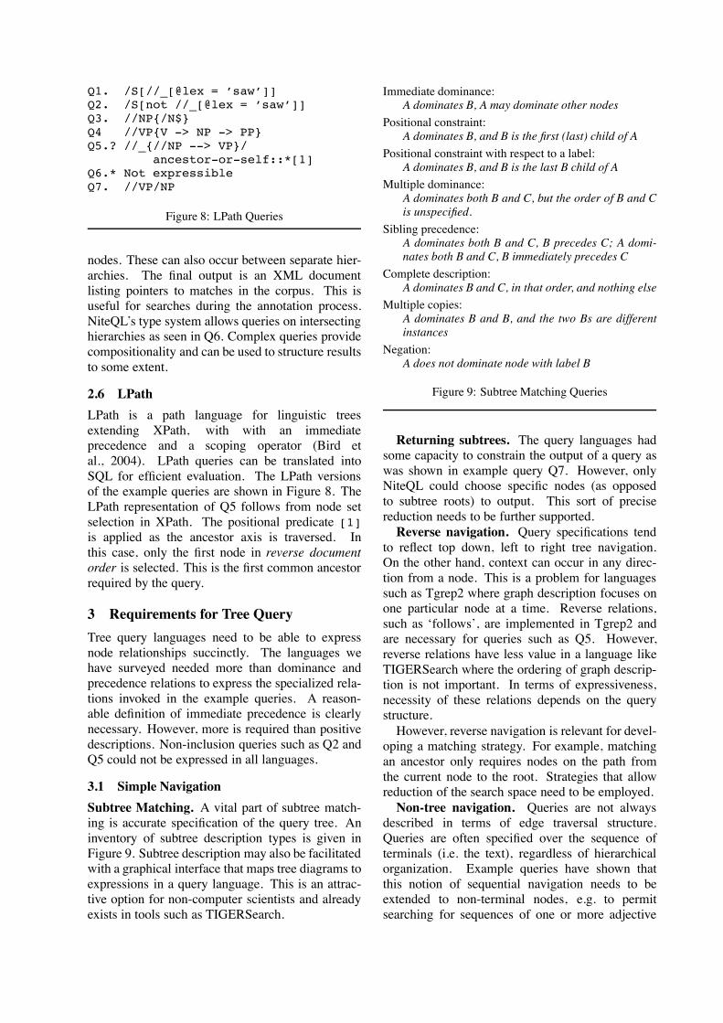
Q1. /S[//_[@lex = ’saw’]]Q2. /S[not //_[@lex = ’saw’]]Q3. //NP{/N$}Q4 //VP{V -> NP -> PP}Q5.? //_{//NP --> VP}/
ancestor-or-self::*[1]Q6.* Not expressibleQ7. //VP/NP
Figure 8: LPath Queries
nodes. These can also occur between separate hier-archies. The final output is an XML documentlisting pointers to matches in the corpus. This isuseful for searches during the annotation process.NiteQL’s type system allows queries on intersectinghierarchies as seen in Q6. Complex queries providecompositionality and can be used to structure resultsto some extent.
2.6 LPathLPath is a path language for linguistic treesextending XPath, with with an immediateprecedence and a scoping operator (Bird etal., 2004). LPath queries can be translated intoSQL for efficient evaluation. The LPath versionsof the example queries are shown in Figure 8. TheLPath representation of Q5 follows from node setselection in XPath. The positional predicate [1]is applied as the ancestor axis is traversed. Inthis case, only the first node in reverse documentorder is selected. This is the first common ancestorrequired by the query.
3 Requirements for Tree QueryTree query languages need to be able to expressnode relationships succinctly. The languages wehave surveyed needed more than dominance andprecedence relations to express the specialized rela-tions invoked in the example queries. A reason-able definition of immediate precedence is clearlynecessary. However, more is required than positivedescriptions. Non-inclusion queries such as Q2 andQ5 could not be expressed in all languages.
3.1 Simple NavigationSubtree Matching. A vital part of subtree match-ing is accurate specification of the query tree. Aninventory of subtree description types is given inFigure 9. Subtree description may also be facilitatedwith a graphical interface that maps tree diagrams toexpressions in a query language. This is an attrac-tive option for non-computer scientists and alreadyexists in tools such as TIGERSearch.
Immediate dominance:A dominates B, A may dominate other nodes
Positional constraint:A dominates B, and B is the first (last) child of A
Positional constraint with respect to a label:A dominates B, and B is the last B child of A
Multiple dominance:A dominates both B and C, but the order of B and Cis unspecified.
Sibling precedence:A dominates both B and C, B precedes C; A domi-nates both B and C, B immediately precedes C
Complete description:A dominates B and C, in that order, and nothing else
Multiple copies:A dominates B and B, and the two Bs are differentinstances
Negation:A does not dominate node with label B
Figure 9: Subtree Matching Queries
Returning subtrees. The query languages hadsome capacity to constrain the output of a query aswas shown in example query Q7. However, onlyNiteQL could choose specific nodes (as opposedto subtree roots) to output. This sort of precisereduction needs to be further supported.Reverse navigation. Query specifications tend
to reflect top down, left to right tree navigation.On the other hand, context can occur in any direc-tion from a node. This is a problem for languagessuch as Tgrep2 where graph description focuses onone particular node at a time. Reverse relations,such as ‘follows’, are implemented in Tgrep2 andare necessary for queries such as Q5. However,reverse relations have less value in a language likeTIGERSearch where the ordering of graph descrip-tion is not important. In terms of expressiveness,necessity of these relations depends on the querystructure.However, reverse navigation is relevant for devel-
oping a matching strategy. For example, matchingan ancestor only requires nodes on the path fromthe current node to the root. Strategies that allowreduction of the search space need to be employed.Non-tree navigation. Queries are not always
described in terms of edge traversal structure.Queries are often specified over the sequence ofterminals (i.e. the text), regardless of hierarchicalorganization. Example queries have shown thatthis notion of sequential navigation needs to beextended to non-terminal nodes, e.g. to permitsearching for sequences of one or more adjective
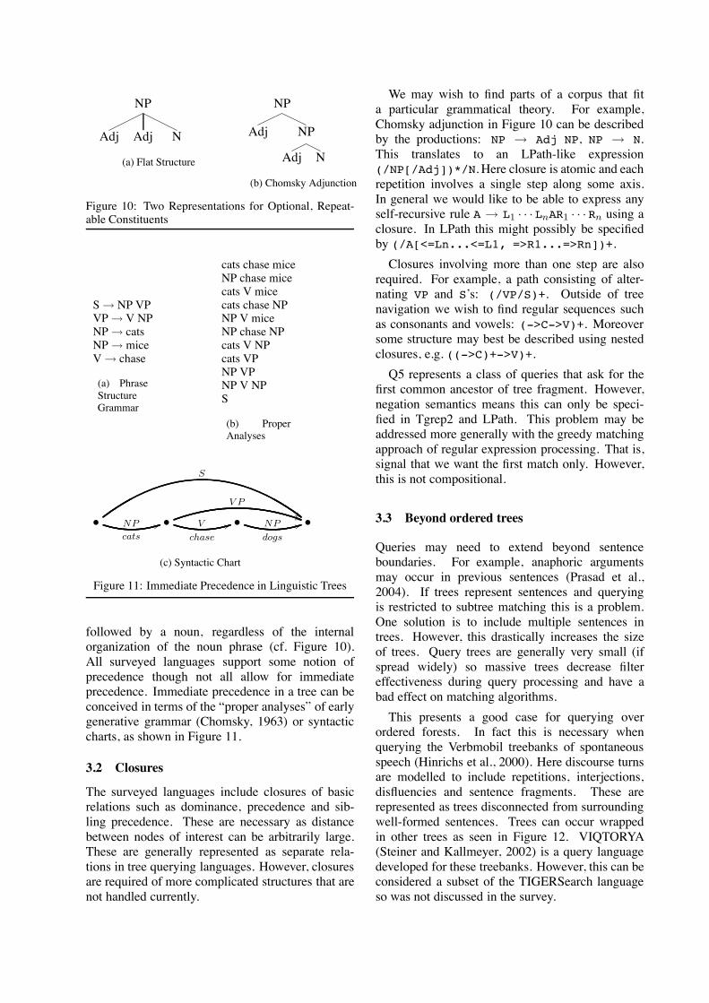
NP
Adj Adj N
(a) Flat Structure
NP
Adj NP
Adj N
(b) Chomsky Adjunction
Figure 10: Two Representations for Optional, Repeat-able Constituents
S! NP VPVP! V NPNP! catsNP! miceV! chase
(a) PhraseStructureGrammar
cats chase miceNP chase micecats V micecats chase NPNP V miceNP chase NPcats V NPcats VPNP VPNP V NPS
(b) ProperAnalyses
•cats
NP !!
S
""
•chase
V !!
V P
##•dogs
NP !! •
(c) Syntactic Chart
Figure 11: Immediate Precedence in Linguistic Trees
followed by a noun, regardless of the internalorganization of the noun phrase (cf. Figure 10).All surveyed languages support some notion ofprecedence though not all allow for immediateprecedence. Immediate precedence in a tree can beconceived in terms of the “proper analyses” of earlygenerative grammar (Chomsky, 1963) or syntacticcharts, as shown in Figure 11.
3.2 Closures
The surveyed languages include closures of basicrelations such as dominance, precedence and sib-ling precedence. These are necessary as distancebetween nodes of interest can be arbitrarily large.These are generally represented as separate rela-tions in tree querying languages. However, closuresare required of more complicated structures that arenot handled currently.
We may wish to find parts of a corpus that fita particular grammatical theory. For example,Chomsky adjunction in Figure 10 can be describedby the productions: NP ! Adj NP, NP ! N.This translates to an LPath-like expression(/NP[/Adj])*/N. Here closure is atomic and eachrepetition involves a single step along some axis.In general we would like to be able to express anyself-recursive rule A ! L1 · · · LnAR1 · · · Rn using aclosure. In LPath this might possibly be specifiedby (/A[<=Ln...<=L1, =>R1...=>Rn])+.Closures involving more than one step are also
required. For example, a path consisting of alter-nating VP and S’s: (/VP/S)+. Outside of treenavigation we wish to find regular sequences suchas consonants and vowels: (->C->V)+. Moreoversome structure may best be described using nestedclosures, e.g. ((->C)+->V)+.Q5 represents a class of queries that ask for the
first common ancestor of tree fragment. However,negation semantics means this can only be speci-fied in Tgrep2 and LPath. This problem may beaddressed more generally with the greedy matchingapproach of regular expression processing. That is,signal that we want the first match only. However,this is not compositional.
3.3 Beyond ordered trees
Queries may need to extend beyond sentenceboundaries. For example, anaphoric argumentsmay occur in previous sentences (Prasad et al.,2004). If trees represent sentences and queryingis restricted to subtree matching this is a problem.One solution is to include multiple sentences intrees. However, this drastically increases the sizeof trees. Query trees are generally very small (ifspread widely) so massive trees decrease filtereffectiveness during query processing and have abad effect on matching algorithms.This presents a good case for querying over
ordered forests. In fact this is necessary whenquerying the Verbmobil treebanks of spontaneousspeech (Hinrichs et al., 2000). Here discourse turnsare modelled to include repetitions, interjections,disfluencies and sentence fragments. These arerepresented as trees disconnected from surroundingwell-formed sentences. Trees can occur wrappedin other trees as seen in Figure 12. VIQTORYA(Steiner and Kallmeyer, 2002) is a query languagedeveloped for these treebanks. However, this can beconsidered a subset of the TIGERSearch languageso was not discussed in the survey.
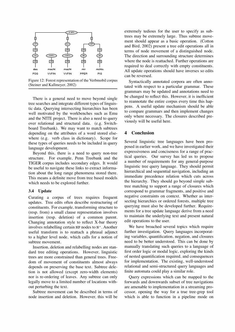
Figure 12: Forest representation of the Verbmobil corpus(Steiner and Kallmeyer, 2002)
There is a general need to move beyond singletree searches and integrate different types of linguis-tic data. Querying intersecting hierarchies has beenwell motivated by the workbenches such as Emuand the NITE project. There is also a need to queryover relational and structural data. (e.g. Switch-board Treebank). We may want to match subtreesdepending on the attributes of a word stored else-where (e.g. verb class in dictionary). Scope forthese types of queries needs to be included in querylanguage development.Beyond this, there is a need to query non-tree
structure. For example, Penn Treebank and theTIGER corpus includes secondary edges. It wouldbe useful to navigate these links to extract informa-tion about the long range phenomena stored there.This means a definite move from tree based modelswhich needs to be explored further.
3.4 UpdateCurating a corpus of trees requires frequentupdates. Tree edits often describe restructuring ofconstituents. For example, transforming structure to(resp. from) a small clause representation involvesinsertion (resp. deletion) of a common parent.Changing annotation style to reflect X-bar theoryinvolves relabelling certain NP nodes to N’. Anotheruseful transform is to reattach a phrasal adjunctto a higher level node, which calls for a notion ofsubtree movement.Insertion, deletion and relabelling nodes are stan-
dard tree editing operations. However, linguistictrees are more constrained than general trees. Free-dom of movement of constituents almost alwaysdepends on preserving the base text. Subtree dele-tion is not allowed (except zero-width elements)nor is re-ordering of leaves. Any subtree can onlylegally move to a limited number of locations with-out perturbing the text.Subtree movement can be described in terms of
node insertion and deletion. However, this will be
extremely tedious for the user to specify as sub-trees may be extremely large. Thus subtree move-ment should appear as a basic operation. (Cottonand Bird, 2002) present a tree edit operations all interms of node movement of a distinguished node.The direction and surrounding structure determineswhere the node is reattached. Further operations arerequired to deal correctly with empty constituents.All update operations should have inverses so editscan be reversed.Syntactically annotated corpora are often anno-
tated with respect to a particular grammar. Thesegrammars may be updated and annotations need tobe changed to reflect this. However, it is inefficientto reannotate the entire corpus every time this hap-pens. A useful update mechanism should be ableto compare grammars and then implement changesonly where necessary. The closures described pre-viously will be useful here.
4 Conclusion
Several linguistic tree languages have been pro-posed in earlier work, and we have investigated theirexpressiveness and conciseness for a range of prac-tical queries. Our survey has led us to proposea number of requirements for any general-purposelinguistic tree query language. They should permithierarchical and sequential navigation, including animmediate precedence relation which cuts acrossthe hierarchy. They should go beyond simple sub-tree matching to support a range of closures whichcorrespond to grammar fragments, and positive andnegative constraints on context. Whether as inter-secting hierarchies or ordered forests, multiple treequerying must also be developed further. Require-ments for a tree update language derive from a needto maintain the underlying text and present naturaledit operations to the user.We have broached several topics which require
further investigation. Query languages incorporat-ing variables, quantification, negation, and closuresneed to be better understood. This can be done bymanually translating such queries to a language offirst order logic or modal logic, exploring the kindsof nested quantification required, and consequencesfor implementation. The existing, well-understoodrelational and semi-structured query languages andfinite automata could play a similar role.Query expressions which can be mapped to the
forwards and downwards subset of tree navigationsare amenable to implementation in a streaming pro-cessor, opening the way for a true tree-grep toolwhich is able to function in a pipeline mode on
unpreprocessed treebank files. Other areas of fur-ther work include an exploration of an appropriatetyping system as used to navigate intersecting hier-archies; investigation of boundaries for contextualsearch; and the interaction of indexing and updates.
AcknowledgementsThis research has been supported by an AustralianPostgraduate Award (Lai), and a US National Sci-ence Foundation grant number 0317826 QueryingLinguistic Databases, to the University of Pennsyl-vania (Bird).
ReferencesS. Bird, Y. Chen, S. Davidson, H. Lee, andY. Zheng. 2004. LPath: A path language for lin-guistic trees. Unpublished manuscript.
S. Brants, S. Dipper, S. Hansen, W. Lezius, andG. Smith. 2002. The TIGER Treebank. In Pro-ceedings of the Workshop on Treebanks and Lin-guistic Theories Sozopol.
S. Cassidy and J. Harrington. 2001. Multi-levelannotation in the Emu speech database man-agement system. Speech Communication, 33(1-2):61–77.
N. Chomsky. 1963. Formal properties of gram-mars. In D. Luce, R. Bush, and E. Galanter,editors, Handbook of Mathematical Psychology,volume 2, pages 323–418. New York: Wiley andSons.
S. Cotton and S. Bird. 2002. An Integrated Frame-work for Treebanks and Multilayer Annotations.In Proceedings of the Third International Con-ference on Language Resources and Evaluation,pages 1670–1677. ELRA.
U. Heid, H. Voormann, J-T Milde, U. Gut, K. Erk,and S. Pado. 2004. Querying both time-alignedand hierarchical corpora with nxt search. InFourth Language Resources and Evaluation Con-ference, Lisbon, Portugal.
E. W. Hinrichs, J. Bartels, Y. Kawata, and V. Kor-doni. 2000. The VERBMOBIL Treebanks. InKONVENS 2000 Sprachkommunikation, ITG-Fachbericht 161, pages 107–112. VDE Verlag.
E. Konig and W. Lezius. 2001. The TIGER lan-guage - a description language for syntax graphs.Part 1: User’s guidelines. Technical report, Uni-versity of Stuttgart, Stuttgart, Germany.
M. Marcus, G. Kim, M. Marcinkiewicz, R. Mac-Intyre, A. Bies, M. Ferguson, K. Katz, andB. Schasberger. 1994. The Penn treebank:Annotating predicate argument structure. InARPA Human Language Technology Workshop.
D. McKelvie, A. Isard, A. Mengel, M. B. Moller,M. Gross, and M. Klein. 2001. The MATEworkbench — an annotation tool for XML codedspeech corpora. Speech Communication, 33(1-2):97–112.
R. Prasad, E. Miltsakaki, A. Joshi, and B. Webber.2004. Annotation and Data Mining of the PennDiscourse TreeBank. In Proceedings of the ACLWorkshop on Discourse Annotation Barcelona,Spain.
D. Rohde. 2001. Tgrep2 user manual.I. Steiner and L. Kallmeyer. 2002. VIQTORYA– A Visual Query Tool for Syntactically Anno-tated Corpora. In Proceedings of the Third Inter-national Conference on Language Resourcesand Evaluation (LREC 2002), pages 1704–1711.ELRA.
Converting the Penn Treebank to Systemic Functional Grammar
Matthew HonnibalDepartment of Linguistics, Macquarie University
Macquarie University2109 SydneyAustralia
AbstractSystemic functional linguistics offers a grammarthat is semantically organised, so that salient gram-matical choices are made explicit. This paper de-scribes the explication of these choices through theconversion of the Penn Treebank into a systemicfunctional grammar corpus. Developing such a re-source can help connect work in natural languageprocessing to a significant body of research dealingexplicitly with the issue of how lexical and gram-matical selections create meaning.
1 IntroductionThe Penn Treebank was designed to maximise con-sistency and annotator efficiency, rather than con-formity with any particular linguistic theory (Mar-cus et al., 1994). This results in trees that stronglysuggest the use of synthetic features to explicatesemantically significant grammatical choices likemood, tense, voice or negation. These distinctionslie latent in the configuration of the tree in the Tree-bank II annotation scheme, making it difficult for amachine learner to make use of them.Rather than the ad hoc addition of this informa-
tion at the feature extraction stage, the corpus can bere-presented in a way that makes feature extractionmore principled. This involves increasing the sizeand complexity of the representation of a sentenceby organising the tree semantically. Organising agrammar semantically is by no means a trivial task,and has been an active area of linguistic research forthe last forty years. This paper describes the con-version of the Penn Treebank into a prominent out-put of such research, systemic functional grammar(SFG).Systemic functional grammar does not confine its
description to syntactic structure, but includes a rep-resentation of the choices grammatical configura-tions represent — or ‘realise’, to use the term pre-ferred in the linguistics literature (Halliday, 1976).There is growing evidence that systemic func-
tional grammar can be usefully applied to natural
language processing (Munro, 2003; Couchman andWhitelaw, 2003), and there is a strong history ofinteraction between systemic functional linguisticsand natural language generation (Matthiessen andBateman, 1991). However, there is currently a lackof computational SFG resources. There is no stan-dard format for machine readable annotation, no an-notated corpora, and no useable parsers. Convertingthe Penn Treebank will make a large body of SFGannotated data available to computational linguistsfor the first time, an important step towards address-ing this situation.We first discuss some preliminaries relating to
the nature of systemic functional grammar, and thescope of the converted corpus’s annotation. Wethen discuss the conversion of the treebank’s phrase-structure representation to SFG constituency struc-ture, and finally we discuss the addition of interper-sonal and textual function structures.
2 Some preliminaries2.1 Structure of the SFG analysisSystemic functional grammar divides the task ofgrammatical analysis — the process of stating thegrammatical properties of a text — into two parts:analysis of syntactic structures, and analysis offunction structures.SFG syntactic analysis is constituency based,
and is predicated on Halliday’s notion of the rankscale (Halliday, 1966): clauses are composed ofgroups/phrases, which are composed of words,which are composed of morphemes. The mainconcerns of SFG syntactic analysis are the chunk-ing of words into groups/phrases, and the chunk-ing of groups/phrases into clauses. Levels of con-stituency between groups/phrases and their wordsare recognised in the literature (Matthiessen, 1995),but rarely brought into focus in research unlessthe group/phrase contains, or is, an embedded con-stituent from another rank (e.g., a nominal grouplike ‘the man’ with an embedded relative clause like‘who knew too much’).
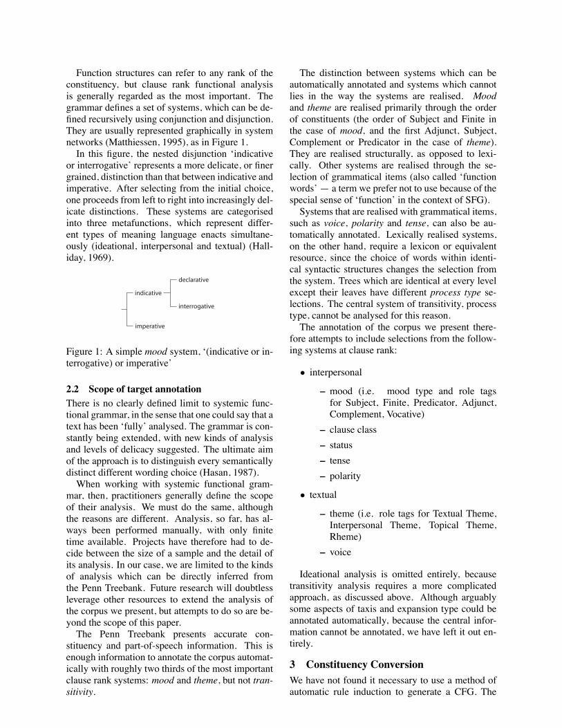
Function structures can refer to any rank of theconstituency, but clause rank functional analysisis generally regarded as the most important. Thegrammar defines a set of systems, which can be de-fined recursively using conjunction and disjunction.They are usually represented graphically in systemnetworks (Matthiessen, 1995), as in Figure 1.In this figure, the nested disjunction ‘indicative
or interrogative’ represents a more delicate, or finergrained, distinction than that between indicative andimperative. After selecting from the initial choice,one proceeds from left to right into increasingly del-icate distinctions. These systems are categorisedinto three metafunctions, which represent differ-ent types of meaning language enacts simultane-ously (ideational, interpersonal and textual) (Hall-iday, 1969).
Figure 1: A simple mood system, ‘(indicative or in-terrogative) or imperative’
2.2 Scope of target annotationThere is no clearly defined limit to systemic func-tional grammar, in the sense that one could say that atext has been ‘fully’ analysed. The grammar is con-stantly being extended, with new kinds of analysisand levels of delicacy suggested. The ultimate aimof the approach is to distinguish every semanticallydistinct different wording choice (Hasan, 1987).When working with systemic functional gram-
mar, then, practitioners generally define the scopeof their analysis. We must do the same, althoughthe reasons are different. Analysis, so far, has al-ways been performed manually, with only finitetime available. Projects have therefore had to de-cide between the size of a sample and the detail ofits analysis. In our case, we are limited to the kindsof analysis which can be directly inferred fromthe Penn Treebank. Future research will doubtlessleverage other resources to extend the analysis ofthe corpus we present, but attempts to do so are be-yond the scope of this paper.The Penn Treebank presents accurate con-
stituency and part-of-speech information. This isenough information to annotate the corpus automat-ically with roughly two thirds of the most importantclause rank systems: mood and theme, but not tran-sitivity.
The distinction between systems which can beautomatically annotated and systems which cannotlies in the way the systems are realised. Moodand theme are realised primarily through the orderof constituents (the order of Subject and Finite inthe case of mood, and the first Adjunct, Subject,Complement or Predicator in the case of theme).They are realised structurally, as opposed to lexi-cally. Other systems are realised through the se-lection of grammatical items (also called ‘functionwords’ — a term we prefer not to use because of thespecial sense of ‘function’ in the context of SFG).Systems that are realised with grammatical items,
such as voice, polarity and tense, can also be au-tomatically annotated. Lexically realised systems,on the other hand, require a lexicon or equivalentresource, since the choice of words within identi-cal syntactic structures changes the selection fromthe system. Trees which are identical at every levelexcept their leaves have different process type se-lections. The central system of transitivity, processtype, cannot be analysed for this reason.The annotation of the corpus we present there-
fore attempts to include selections from the follow-ing systems at clause rank:
• interpersonal
– mood (i.e. mood type and role tagsfor Subject, Finite, Predicator, Adjunct,Complement, Vocative)
– clause class– status– tense– polarity
• textual
– theme (i.e. role tags for Textual Theme,Interpersonal Theme, Topical Theme,Rheme)
– voice
Ideational analysis is omitted entirely, becausetransitivity analysis requires a more complicatedapproach, as discussed above. Although arguablysome aspects of taxis and expansion type could beannotated automatically, because the central infor-mation cannot be annotated, we have left it out en-tirely.
3 Constituency ConversionWe have not found it necessary to use a method ofautomatic rule induction to generate a CFG. The
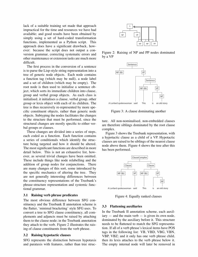
lack of a suitable training set made that approachimpractical for the time and resources we have hadavailable; and good results have been obtained bysimply using a set of hard-coded transformationfunctions, implemented as a Python script. Thisapproach does have a significant drawback, how-ever: because the script does not output a con-version grammar, correcting systematic errors andother maintenance or extension tasks are much moredifficult.The first process in the conversion of a sentence
is to parse the Lisp-style string representation into atree of generic node objects. Each node containsa function tag (which may be null), a node labeland a set of children (which may be empty). Theroot node is then used to initialise a sentence ob-ject, which sorts its immediate children into clause,group and verbal group objects. As each class isinitialised, it initialises a clause, verbal group, othergroup or lexis object with each of its children. Thetree is thus recursively re-represented by more spe-cific constituent objects, rather than generic nodeobjects. Subtyping the nodes facilitates the changesto the structure that must be performed, since thestructural changes are mostly specific to either ver-bal groups or clauses.These changes are divided into a series of steps,
each coded as a function. Each function containsa series of conditionals which identify the struc-ture being targeted and how it should be altered.The most significant functions are described in moredetail below. This is not an exhaustive list, how-ever, as several trivial changes have been omitted.These include things like node relabelling and theaddition of group nodes for conjunctions. Thereare many changes of this sort, some introduced bythe specific mechanics of altering the tree. Theyare not generally interesting differences betweenthe constituency representations of the Treebank’sphrase-structure representation and systemic func-tional grammar.
3.1 Raising verb phrase predicatesThe most obvious difference between SFG con-stituency and the Treebank II annotation scheme isthe flatter, ‘minimal bracketing’ style SFG uses. Toconvert a tree to SFG clause constituency, all com-plements and adjuncts must be raised by attachingthem to the clause node; in the Treebank annotationthey attach to the verb. Figure 2 illustrates the rais-ing of clause constituents from the verb phrase.
3.2 Raising hypotactic clausesSFG represents the distinction between hypotaxisand parataxis with features, rather than tree struc-
Figure 2: Raising of NP and PP nodes dominatedby a VP
Figure 3: A clause dominating another
ture. All non-nominalised, non-embedded clausesare therefore siblings dominated by the root clausecomplex.Figure 3 shows the Treebank representation, with
a hypotactic clause as a child of a VP. Hypotacticclauses are raised to be siblings of the nearest clausenode above them. Figure 4 shows the tree after thishas been performed.
Figure 4: Equally ranked clauses
3.3 Flattening auxiliariesIn the Treebank II annotation scheme, each auxil-iary — and the main verb — is given its own node,dominated by the auxiliary before it. This structureneeds to be flattened to match the SFG representa-tion. If all of a verb phrase’s lexical items have POStags in the following list: VB, VBD, VBG, VBN,VBP, VBZ; and it only has one verb phrase child,then its lexis attaches to the verb phrase below it.The empty internal node will later be removed in
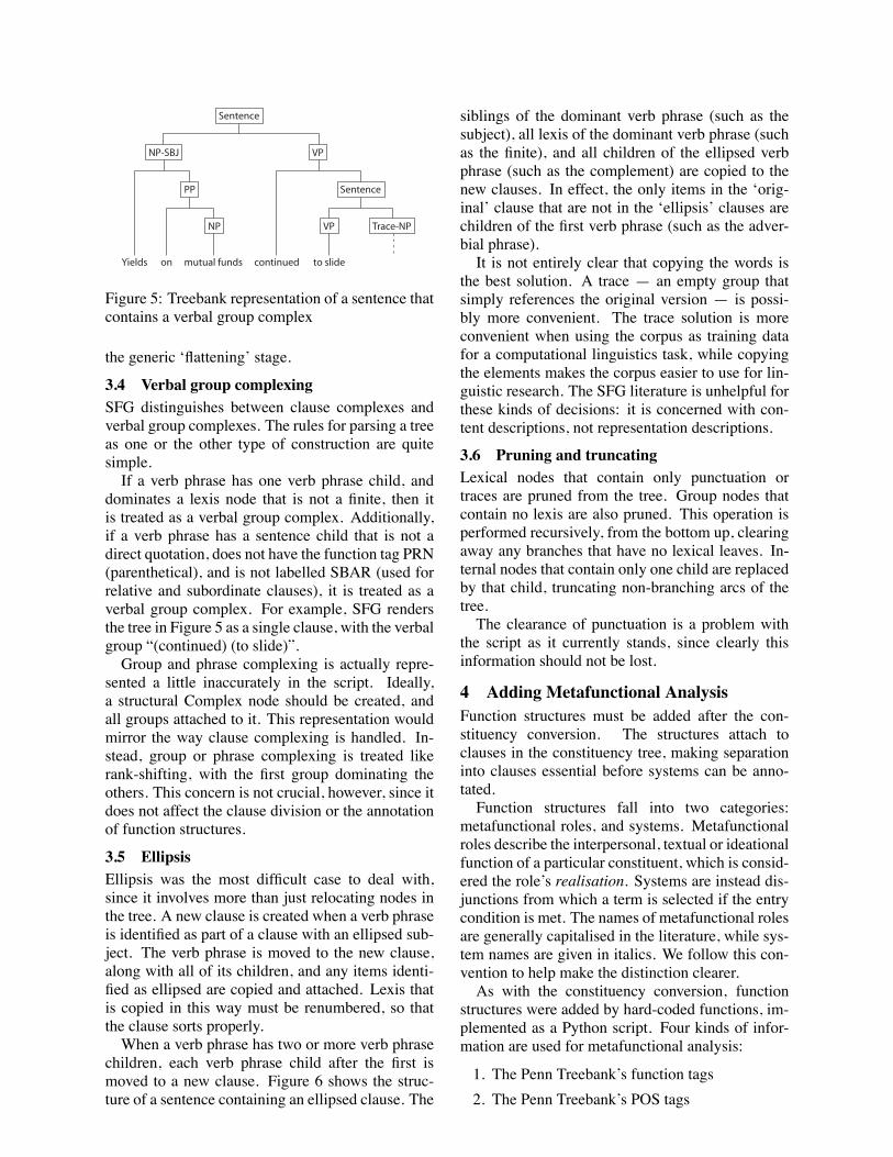
Figure 5: Treebank representation of a sentence thatcontains a verbal group complex
the generic ‘flattening’ stage.
3.4 Verbal group complexingSFG distinguishes between clause complexes andverbal group complexes. The rules for parsing a treeas one or the other type of construction are quitesimple.If a verb phrase has one verb phrase child, and
dominates a lexis node that is not a finite, then itis treated as a verbal group complex. Additionally,if a verb phrase has a sentence child that is not adirect quotation, does not have the function tag PRN(parenthetical), and is not labelled SBAR (used forrelative and subordinate clauses), it is treated as averbal group complex. For example, SFG rendersthe tree in Figure 5 as a single clause, with the verbalgroup “(continued) (to slide)”.Group and phrase complexing is actually repre-
sented a little inaccurately in the script. Ideally,a structural Complex node should be created, andall groups attached to it. This representation wouldmirror the way clause complexing is handled. In-stead, group or phrase complexing is treated likerank-shifting, with the first group dominating theothers. This concern is not crucial, however, since itdoes not affect the clause division or the annotationof function structures.
3.5 EllipsisEllipsis was the most difficult case to deal with,since it involves more than just relocating nodes inthe tree. A new clause is created when a verb phraseis identified as part of a clause with an ellipsed sub-ject. The verb phrase is moved to the new clause,along with all of its children, and any items identi-fied as ellipsed are copied and attached. Lexis thatis copied in this way must be renumbered, so thatthe clause sorts properly.When a verb phrase has two or more verb phrase
children, each verb phrase child after the first ismoved to a new clause. Figure 6 shows the struc-ture of a sentence containing an ellipsed clause. The
siblings of the dominant verb phrase (such as thesubject), all lexis of the dominant verb phrase (suchas the finite), and all children of the ellipsed verbphrase (such as the complement) are copied to thenew clauses. In effect, the only items in the ‘orig-inal’ clause that are not in the ‘ellipsis’ clauses arechildren of the first verb phrase (such as the adver-bial phrase).It is not entirely clear that copying the words is
the best solution. A trace — an empty group thatsimply references the original version — is possi-bly more convenient. The trace solution is moreconvenient when using the corpus as training datafor a computational linguistics task, while copyingthe elements makes the corpus easier to use for lin-guistic research. The SFG literature is unhelpful forthese kinds of decisions: it is concerned with con-tent descriptions, not representation descriptions.
3.6 Pruning and truncatingLexical nodes that contain only punctuation ortraces are pruned from the tree. Group nodes thatcontain no lexis are also pruned. This operation isperformed recursively, from the bottom up, clearingaway any branches that have no lexical leaves. In-ternal nodes that contain only one child are replacedby that child, truncating non-branching arcs of thetree.The clearance of punctuation is a problem with
the script as it currently stands, since clearly thisinformation should not be lost.
4 Adding Metafunctional AnalysisFunction structures must be added after the con-stituency conversion. The structures attach toclauses in the constituency tree, making separationinto clauses essential before systems can be anno-tated.Function structures fall into two categories:
metafunctional roles, and systems. Metafunctionalroles describe the interpersonal, textual or ideationalfunction of a particular constituent, which is consid-ered the role’s realisation. Systems are instead dis-junctions from which a term is selected if the entrycondition is met. The names of metafunctional rolesare generally capitalised in the literature, while sys-tem names are given in italics. We follow this con-vention to help make the distinction clearer.As with the constituency conversion, function
structures were added by hard-coded functions, im-plemented as a Python script. Four kinds of infor-mation are used for metafunctional analysis:
1. The Penn Treebank’s function tags2. The Penn Treebank’s POS tags
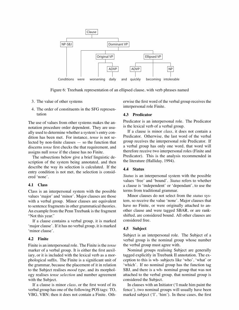
Figure 6: Treebank representation of an ellipsed clause, with verb phrases named
3. The value of other systems
4. The order of constituents in the SFG represen-tation
The use of values from other systems makes the an-notation procedure order dependent. They are usu-ally used to determine whether a system’s entry con-dition has been met. For instance, tense is not se-lected by non-finite clauses — so the function thatdiscerns tense first checks the that requirement, andassigns null tense if the clause has no Finite.The subsections below give a brief linguistic de-
scription of the system being annotated, and thendescribe the way its selection is calculated. If theentry condition is not met, the selection is consid-ered ‘none’.
4.1 ClassClass is an interpersonal system with the possiblevalues ‘major’ and ‘minor’. Major clauses are thosewith a verbal group. Minor clauses are equivalentto sentence fragments in other grammatical theories.An example from the Penn Treebank is the fragment“Not this year.”If a clause contains a verbal group, it is marked
‘major clause’. If it has no verbal group, it is marked‘minor clause’.
4.2 FiniteFinite is an interpersonal role. The Finite is the tensemarker of a verbal group. It is either the first auxil-iary, or it is included with the lexical verb as a mor-phological suffix. The Finite is a significant unit ofthe grammar, because the placement of it in relationto the Subject realises mood type, and its morphol-ogy realises tense selection and number agreementwith the Subject.If a clause is minor class, or the first word of its
verbal group has one of the following POS tags: TO,VBG, VBN; then it does not contain a Finite. Oth-
erwise the first word of the verbal group receives theinterpersonal role Finite.
4.3 PredicatorPredicator is an interpersonal role. The Predicatoris the lexical verb of a verbal group.If a clause is minor class, it does not contain a
Predicator. Otherwise, the last word of the verbalgroup receives the interpersonal role Predicator. Ifa verbal group has only one word, that word willtherefore receive two interpersonal roles (Finite andPredicator). This is the analysis recommended inthe literature (Halliday, 1994).
4.4 StatusStatus is an interpersonal system with the possiblevalues ‘free’ and ‘bound’. Status refers to whethera clause is ‘independent’ or ‘dependant’, to use theterms from traditional grammar.Minor clauses do not select from the status sys-
tem, so receive the value ‘none’. Major clauses thathave no Finite, or were originally attached to an-other clause and were tagged SBAR, or are rank-shifted, are considered bound. All other clauses areconsidered free.
4.5 SubjectSubject is an interpersonal role. The Subject of averbal group is the nominal group whose numberthe verbal group must agree with.Nominal groups realising Subject are generally
tagged explicitly in Treebank II annotation. The ex-ception to this is wh- subjects like ‘who’, ‘what’ or‘which’. If no nominal group has the function tagSBJ, and there is a wh- nominal group that was notattached to the verbal group, that nominal group isconsidered the Subject.In clauses with an Initiator (‘I made him paint the
fence’), two nominal groups will usually have beenmarked subject (‘I’, ‘him’). In these cases, the first
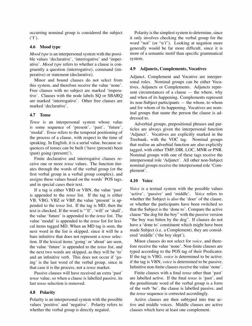
occurring nominal group is considered the subject(‘I’).
4.6 Mood typeMood type is an interpersonal system with the possi-ble values ‘declarative’, ‘interrogative’ and ‘imper-ative’. Mood type refers to whether a clause is con-gruently a question (interrogative), command (im-perative) or statement (declarative).Minor and bound clauses do not select from
this system, and therefore receive the value ‘none’.Free clauses with no subject are marked ‘impera-tive’. Clauses with the node labels SQ or SBARQare marked ‘interrogative’. Other free clauses aremarked ‘declarative’.
4.7 TenseTense is an interpersonal system whose valueis some sequence of ‘present’, ‘past’, ‘future’,‘modal’. Tense refers to the temporal positioning ofthe process of a clause, with respect to the time ofspeaking. In English, it is a serial value, because se-quences of tenses can be built (‘have (present) been(past) going (present)’).Finite declarative and interrogative clauses re-
ceive one or more tense values. The function iter-ates through the words of the verbal group (or thefirst verbal group in a verbal group complex), andassigns these values based on the words’ POS tags,and in special cases their text.If a tag is either VBD or VBN, the value ‘past’
is appended to the tense list. If the tag is eitherVB, VBG, VBZ or VBP, the value ‘present’ is ap-pended to the tense list. If the tag is MD, then thetext is checked. If the word is “’ll”, ‘will’ or ‘shall’,the value ‘future’ is appended to the tense list. Thevalue ‘modal’ is appended to the tense list for lexi-cal items tagged MD. When an MD tag is seen, thenext word in the list is skipped, since it will be abare infinitive that does not represent a tense selec-tion. If the lexical items ‘going’ or ‘about’ are seen,the value ‘future’ is appended to the tense list, andthe next two words are skipped, as they will be ‘to’and an infinitive verb. This does not occur if ‘go-ing’ is the last word of the verbal group, since inthat case it is the process, not a tense marker.Passive clauses will have received an extra ‘past’
tense value, so when a clause is labelled passive, itslast tense selection is removed.
4.8 PolarityPolarity is an interpersonal system with the possiblevalues ‘positive’ and ‘negative’. Polarity refers towhether the verbal group is directly negated.
Polarity is the simplest system to determine, sinceit only involves checking the verbal group for theword “not” (or “n’t”). Looking at negation moregenerally would be far more difficult, since it ismore of a semantic motif than specific grammaticalsystem.
4.9 Adjuncts, Complements, Vocatives
Adjunct, Complement and Vocative are interper-sonal roles. Nominal groups can be either Voca-tives, Adjuncts or Complements. Adjuncts repre-sent circumstances of a clause — the where, whyand when of its happening. Complements representits non-Subject participants — the whom, to whomand for whom of its happening. Vocatives are nom-inal groups that name the person the clause is ad-dressed to.Adverbial groups, prepositional phrases and par-
ticles are always given the interpersonal function‘Adjunct’. Vocatives are explicitly marked in theTreebank, with the VOC tag. Nominal groupsthat realise an adverbial function are also explicitlytagged, with either TMP, DIR, LOC, MNR or PNR.Nominal groups with one of these tags receive theinterpersonal role ‘Adjunct’. All other non-Subjectnominal groups receive the interpersonal role ‘Com-plement’.
4.10 Voice
Voice is a textual system with the possible values‘active’, ‘passive’ and ‘middle’. Voice refers towhether the Subject is also the ‘doer’ of the clause,or whether the participants have been switched sothat the Subject is the ‘done to’. Compare the activeclause “the dog bit the boy” with the passive version“the boy was bitten by the dog”. If clauses do nothave a ‘done to’ constituent which might have beenmade Subject (i.e. a Complement), they are consid-ered ‘middle’ (‘the boy slept’).Minor clauses do not select for voice, and there-
fore receive the value ‘none’. Non-finite clauses aretyped according to the POS tag of their Predicator.If the tag is VBG, voice is determined to be active;if the tag is VBN, voice is determined to be passive.Infinitive non-finite clauses receive the value ‘none’.Finite clauses with a final tense other than ‘past’
are labelled active. If the final tense is ‘past’, andthe penultimate word of the verbal group is a formof the verb ‘be’, the clause is labelled passive, andthe tense sequence is corrected accordingly.Active clauses are then subtyped into true ac-
tive and middle voices. Middle clauses are activeclauses which have at least one complement.
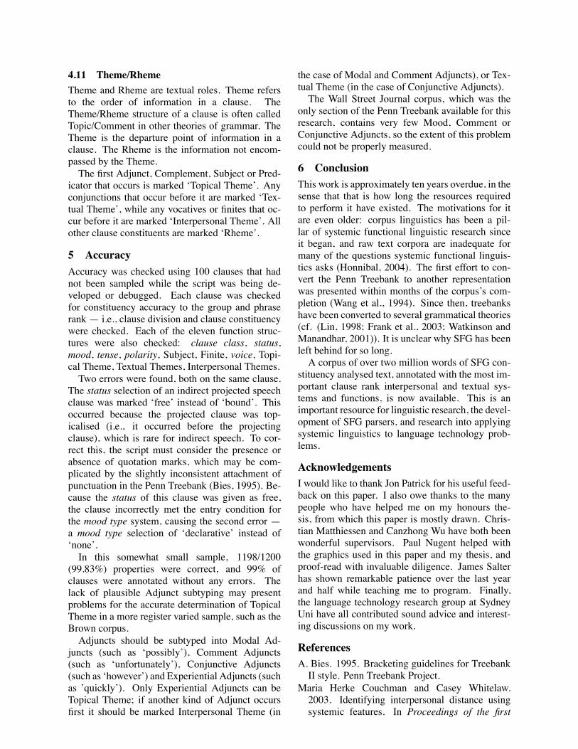
4.11 Theme/RhemeTheme and Rheme are textual roles. Theme refersto the order of information in a clause. TheTheme/Rheme structure of a clause is often calledTopic/Comment in other theories of grammar. TheTheme is the departure point of information in aclause. The Rheme is the information not encom-passed by the Theme.The first Adjunct, Complement, Subject or Pred-
icator that occurs is marked ‘Topical Theme’. Anyconjunctions that occur before it are marked ‘Tex-tual Theme’, while any vocatives or finites that oc-cur before it are marked ‘Interpersonal Theme’. Allother clause constituents are marked ‘Rheme’.
5 AccuracyAccuracy was checked using 100 clauses that hadnot been sampled while the script was being de-veloped or debugged. Each clause was checkedfor constituency accuracy to the group and phraserank — i.e., clause division and clause constituencywere checked. Each of the eleven function struc-tures were also checked: clause class, status,mood, tense, polarity, Subject, Finite, voice, Topi-cal Theme, Textual Themes, Interpersonal Themes.Two errors were found, both on the same clause.
The status selection of an indirect projected speechclause was marked ‘free’ instead of ‘bound’. Thisoccurred because the projected clause was top-icalised (i.e., it occurred before the projectingclause), which is rare for indirect speech. To cor-rect this, the script must consider the presence orabsence of quotation marks, which may be com-plicated by the slightly inconsistent attachment ofpunctuation in the Penn Treebank (Bies, 1995). Be-cause the status of this clause was given as free,the clause incorrectly met the entry condition forthe mood type system, causing the second error —a mood type selection of ‘declarative’ instead of‘none’.In this somewhat small sample, 1198/1200
(99.83%) properties were correct, and 99% ofclauses were annotated without any errors. Thelack of plausible Adjunct subtyping may presentproblems for the accurate determination of TopicalTheme in a more register varied sample, such as theBrown corpus.Adjuncts should be subtyped into Modal Ad-
juncts (such as ‘possibly’), Comment Adjuncts(such as ‘unfortunately’), Conjunctive Adjuncts(such as ‘however’) and Experiential Adjuncts (suchas ’quickly’). Only Experiential Adjuncts can beTopical Theme; if another kind of Adjunct occursfirst it should be marked Interpersonal Theme (in
the case of Modal and Comment Adjuncts), or Tex-tual Theme (in the case of Conjunctive Adjuncts).The Wall Street Journal corpus, which was the
only section of the Penn Treebank available for thisresearch, contains very few Mood, Comment orConjunctive Adjuncts, so the extent of this problemcould not be properly measured.
6 ConclusionThis work is approximately ten years overdue, in thesense that that is how long the resources requiredto perform it have existed. The motivations for itare even older: corpus linguistics has been a pil-lar of systemic functional linguistic research sinceit began, and raw text corpora are inadequate formany of the questions systemic functional linguis-tics asks (Honnibal, 2004). The first effort to con-vert the Penn Treebank to another representationwas presented within months of the corpus’s com-pletion (Wang et al., 1994). Since then, treebankshave been converted to several grammatical theories(cf. (Lin, 1998; Frank et al., 2003; Watkinson andManandhar, 2001)). It is unclear why SFG has beenleft behind for so long.A corpus of over two million words of SFG con-
stituency analysed text, annotated with the most im-portant clause rank interpersonal and textual sys-tems and functions, is now available. This is animportant resource for linguistic research, the devel-opment of SFG parsers, and research into applyingsystemic linguistics to language technology prob-lems.
AcknowledgementsI would like to thank Jon Patrick for his useful feed-back on this paper. I also owe thanks to the manypeople who have helped me on my honours the-sis, from which this paper is mostly drawn. Chris-tian Matthiessen and Canzhong Wu have both beenwonderful supervisors. Paul Nugent helped withthe graphics used in this paper and my thesis, andproof-read with invaluable diligence. James Salterhas shown remarkable patience over the last yearand half while teaching me to program. Finally,the language technology research group at SydneyUni have all contributed sound advice and interest-ing discussions on my work.
ReferencesA. Bies. 1995. Bracketing guidelines for TreebankII style. Penn Treebank Project.
Maria Herke Couchman and Casey Whitelaw.2003. Identifying interpersonal distance usingsystemic features. In Proceedings of the first
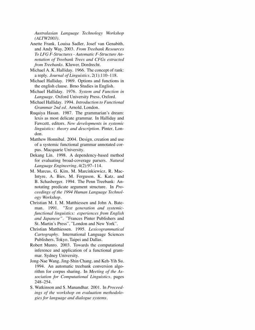
Australasian Language Technology Workshop(ALTW2003).
Anette Frank, Louisa Sadler, Josef van Genabith,and Andy Way, 2003. From Treebank ResourcesTo LFG F-Structures - Automatic F-Structure An-notation of Treebank Trees and CFGs extractedfrom Treebanks. Kluwer, Dordrecht.
Michael A. K. Halliday. 1966. The concept of rank:a reply. Journal of Linguistics, 2(1):110–118.
Michael Halliday. 1969. Options and functions inthe english clause. Brno Studies in English.
Michael Halliday. 1976. System and Function inLanguage. Oxford University Press, Oxford.
Michael Halliday. 1994. Introduction to FunctionalGrammar 2nd ed. Arnold, London.
Ruqaiya Hasan. 1987. The grammarian’s dream:lexis as most delicate grammar. In Halliday andFawcett, editors, New developments in systemiclinguistics: theory and description. Pinter, Lon-don.
Matthew Honnibal. 2004. Design, creation and useof a systemic functional grammar annotated cor-pus. Macquarie University.
Dekang Lin. 1998. A dependency-based methodfor evaluating broad-coverage parsers. NaturalLanguage Engineering, 4(2):97–114.
M. Marcus, G. Kim, M. Marcinkiewicz, R. Mac-Intyre, A. Bies, M. Ferguson, K. Katz, andB. Schasberger. 1994. The Penn Treebank: An-notating predicate argument structure. In Pro-ceedings of the 1994 Human Language Technol-ogy Workshop.
Christian M. I. M. Matthiessen and John A. Bate-man. 1991. ”Text generation and systemic-functional linguistics: experiences from Englishand Japanese”. ”Frances Pinter Publishers andSt. Martin’s Press”, ”London and New York”.
Christian Matthiessen. 1995. LexicogrammaticalCartography. International Language SciencesPublishers, Tokyo, Taipei and Dallas.
Robert Munro. 2003. Towards the computationalinference and application of a functional gram-mar. Sydney University.
Jong-Nae Wang, Jing-Shin Chang, and Keh-Yih Su.1994. An automatic treebank conversion algo-rithm for corpus sharing. In Meeting of the As-sociation for Computational Linguistics, pages248–254.
S. Watkinson and S. Manandhar. 2001. In Proceed-ings of the workshop on evaluation methodolo-gies for language and dialogue systems.
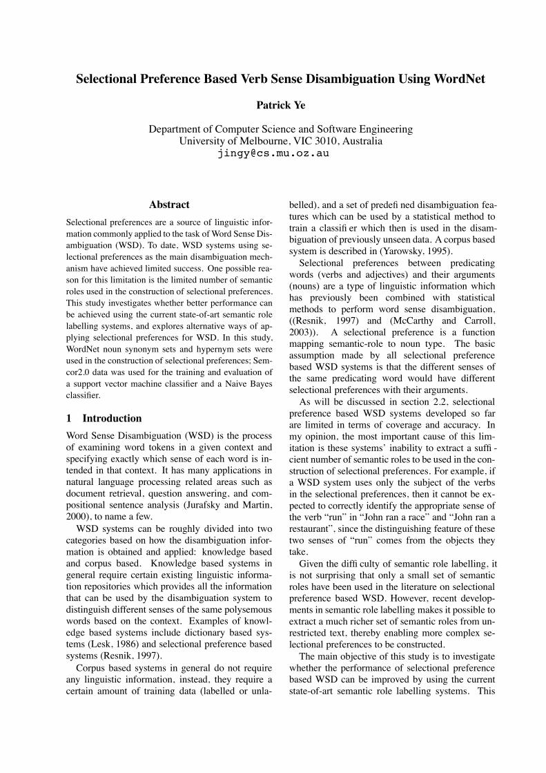
Selectional Preference Based Verb Sense Disambiguation Using WordNet
Patrick Ye
Department of Computer Science and Software EngineeringUniversity of Melbourne, VIC 3010, Australia
AbstractSelectional preferences are a source of linguistic infor-mation commonly applied to the task ofWord Sense Dis-ambiguation (WSD). To date, WSD systems using se-lectional preferences as the main disambiguation mech-anism have achieved limited success. One possible rea-son for this limitation is the limited number of semanticroles used in the construction of selectional preferences.This study investigates whether better performance canbe achieved using the current state-of-art semantic rolelabelling systems, and explores alternative ways of ap-plying selectional preferences for WSD. In this study,WordNet noun synonym sets and hypernym sets wereused in the construction of selectional preferences; Sem-cor2.0 data was used for the training and evaluation ofa support vector machine classifier and a Naive Bayesclassifier.
1 IntroductionWord Sense Disambiguation (WSD) is the processof examining word tokens in a given context andspecifying exactly which sense of each word is in-tended in that context. It has many applications innatural language processing related areas such asdocument retrieval, question answering, and com-positional sentence analysis (Jurafsky and Martin,2000), to name a few.WSD systems can be roughly divided into two
categories based on how the disambiguation infor-mation is obtained and applied: knowledge basedand corpus based. Knowledge based systems ingeneral require certain existing linguistic informa-tion repositories which provides all the informationthat can be used by the disambiguation system todistinguish different senses of the same polysemouswords based on the context. Examples of knowl-edge based systems include dictionary based sys-tems (Lesk, 1986) and selectional preference basedsystems (Resnik, 1997).Corpus based systems in general do not require
any linguistic information, instead, they require acertain amount of training data (labelled or unla-
belled), and a set of predefi ned disambiguation fea-tures which can be used by a statistical method totrain a classifi er which then is used in the disam-biguation of previously unseen data. A corpus basedsystem is described in (Yarowsky, 1995).Selectional preferences between predicating
words (verbs and adjectives) and their arguments(nouns) are a type of linguistic information whichhas previously been combined with statisticalmethods to perform word sense disambiguation,((Resnik, 1997) and (McCarthy and Carroll,2003)). A selectional preference is a functionmapping semantic-role to noun type. The basicassumption made by all selectional preferencebased WSD systems is that the different senses ofthe same predicating word would have differentselectional preferences with their arguments.As will be discussed in section 2.2, selectional
preference based WSD systems developed so farare limited in terms of coverage and accuracy. Inmy opinion, the most important cause of this lim-itation is these systems’ inability to extract a suffi -cient number of semantic roles to be used in the con-struction of selectional preferences. For example, ifa WSD system uses only the subject of the verbsin the selectional preferences, then it cannot be ex-pected to correctly identify the appropriate sense ofthe verb “run” in “John ran a race” and “John ran arestaurant”, since the distinguishing feature of thesetwo senses of “run” comes from the objects theytake.Given the diffi culty of semantic role labelling, it
is not surprising that only a small set of semanticroles have been used in the literature on selectionalpreference based WSD. However, recent develop-ments in semantic role labelling makes it possible toextract a much richer set of semantic roles from un-restricted text, thereby enabling more complex se-lectional preferences to be constructed.The main objective of this study is to investigate
whether the performance of selectional preferencebased WSD can be improved by using the currentstate-of-art semantic role labelling systems. This
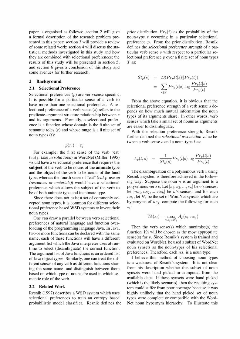
paper is organised as follows: section 2 will givea formal description of the research problem pre-sented in this paper; section 3 will provide a reviewof some related work; section 4 will discuss the sta-tistical methods investigated in this study and howthey are combined with selectional preferences; theresults of this study will be presented in section 5;and section 6 gives a conclusion of this study andsome avenues for further research.
2 Background2.1 Selectional PreferenceSelectional preferences (p) are verb-sense specifi c.It is possible for a particular sense of a verb tohave more than one selectional preference. A se-lectional preference of a verb-sense (s) refers to thepredicate-argument structure relationship between sand its arguments. Formally, a selectional prefer-ence is a function whose domain is the fi nite set ofsemantic roles (r) and whose range is a fi nite set ofnoun types (t):
p(ri) = tj
For example, the fi rst sense of the verb “eat”(eat1: take in solid food) in WordNet (Miller, 1995)would have a selectional preference that requires thesubject of the verb to be nouns of the animate typeand the object of the verb to be nouns of the foodtype; whereas the fourth sense of “eat” (eat4: use up(resources or materials)) would have a selectionalpreference which allows the subject of the verb tobe of both animate type and inanimate type.Since there does not exist a set of commonly ac-
cepted noun types, it is common for different selec-tional preference basedWSD systems to invent theirnoun types.One can draw a parallel between verb selectional
preferences of natural language and function over-loading of the programming language Java. In Java,two or more functions can be declared with the samename, each of these functions will have a differentargument list which the Java interpreter uses at run-time to select (disambiguate) the correct function.The argument list of Java functions is an ordered listof Java object types. Similarly, one can treat the dif-ferent senses of any verb as different functions shar-ing the same name, and distinguish between thembased on which type of nouns are used in which se-mantic role of the verb.
2.2 Related WorkResnik (1997) describes a WSD system which usesselectional preferences to train an entropy basedprobabilistic model classifi er. Resnik defi nes the
prior distribution Prp(t) as the probability of thenoun-type t occurring in a particular selectionalpreference p. From the prior distribution, Resnikdefi nes the selectional preference strength of a par-ticular verb sense s with respect to a particular se-lectional preference p over a fi nite set of noun typesT as:
Stp(s) = D(Prp(t|s)!Prp(t))
=!
t!T
Prp(t|s) logPrp(t|s)
Prp(t)
From the above equation, it is obvious that theselectional preference strength of a verb sense s de-pends on how much mutual information the nountypes of its arguments share. In other words, verbsenses which take a small set of nouns as argumentsare easier to disambiguate.With the selection preference strength, Resnik
further defi ned the selectional association value be-tween a verb sense s and a noun-type t as:
Ap(t, s) =1
Stp(s)Prp(t|s) log
Prp(t|s)
Prp(t)
The disambiguation of a polysemous verb v usingResnik’s system is therefore achieved in the follow-ing way: Suppose the noun n is an argument to apolysemous verb v; Let [s1, s2, ..., sn] be v’s senses;let [ns1, ns2, ..., nsk] be n’s senses; and for eachnsj , letHj be the set of WordNet synsets which arehypernyms of nsj; compute the following for eachsi:
VA(si) = maxnsj!Hj
Ap(si, nsj)
Then the verb sense(s) which maximise(s) thefunction VA will be chosen as the most appropriatesense(s) for v. Since Resnik’s system is trained andevaluated on WordNet, he used a subset of WordNetnoun synsets as the noun-types of his selectionalpreferences. Therefore, each nsi is a noun type.I believe this method of choosing noun types
is a weakness of Resnik’s system. It is not clearfrom his description whether this subset of nounsynsets were hand picked or computed from theavailable data. If these synsets were hand picked(which is the likely scenario), then the resulting sys-tem could suffer from poor coverage because it washighly unlikely that the hand picked set of nountypes were complete or compatible with the Word-Net noun hypernym hierarchy. To illustrate this
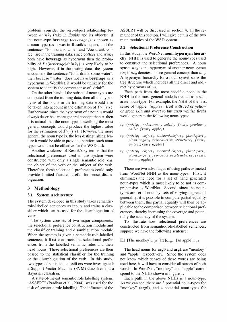
problem, consider the verb-object relationship be-tween drink1 (take in liquids and its objects: ifthe noun-type beverage (beverage1) is chosen asa noun type (as it was in Resnik’s paper), and thesentences “John drank wine” and “Joe drank cof-fee” are in the training data, since coffee1 and wine1both have beverage as hypernym then the proba-bility of Pr(beverage|drink1) is very likely to behigh. However, if in the testing data, the systemencounters the sentence “John drank some water”,then because “water” does not have beverage as ahypernym in WordNet, it would be unlikely for thesystem to identify the correct sense of “drink”.On the other hand, if the subset of noun types are
computed from the training data, then all the hyper-nyms of the nouns in the training data would alsobe taken into account in the estimation of Prp(t|s).Furthermore, since the hypernym of a noun nwouldalways describe a more general concept than n, thenit is natural that the noun types describing the mostgeneral concepts would produce the highest valuefor the estimation of Prp(t|s). However, the moregeneral the noun type is, the less distinguishing fea-ture it would be able to provide, therefore such nountypes would not be effective for the WSD task.Another weakness of Resnik’s system is that the
selectional preferences used in this system wereconstructed with only a single semantic role, e.g.the object of the verb or the subject of the verb.Therefore, these selectional preferences could onlyprovide limited features useful for sense disam-biguation.
3 Methodology3.1 System ArchitectureThe system developed in this study takes semantic-role-labelled sentences as inputs and trains a clas-sifi er which can be used for the disambiguation ofverbs.The system consists of two major components:
the selectional preference construction module andthe classifi er training and disambiguation module.When the system is given a semantic-role-labelledsentence, it fi rst constructs the selectional prefer-ences from the labelled semantic roles and theirhead nouns. These selectional preferences are thenpassed to the statistical classifi er for the trainingor the disambiguation of the verb. In this study,two types of statistical classifi ers were investigated:a Support Vector Machine (SVM) classifi er and aBayesian classifi er.A state-of-the-art semantic role labelling system,
“ASSERT” (Pradhan et al., 2004), was used for thetask of semantic role labelling. The influence of the
ASSERT will be discussed in section 4. In the re-mainder of this section, I will give details of the twomain modules of the WSD system.
3.2 Selectional Preference ConstructionIn this study, the WordNet noun hypernym hierar-chy (NHH) is used to generate the noun-types usedto construct the selectional preferences. A nounsynset nsa is the hypernym of another noun synsetnsb if nsa denotes a more general concept than nsb.A hypernym hierarchy for a noun synset ns is thetree structure which includes all the direct and indi-rect hypernyms of ns.Each path from the most specifi c node in the
NHH to the most general node is treated as a sep-arate noun-type. For example, the NHH of the fi rstsense of “apple” (apple1: fruit with red or yellowor green skin and sweet to tart crisp whitish flesh)would generate the following noun-types:
t1: (entity1, substance1, solid1, food2, produce1,edible fruit1, apple1)
t2: (entity1, object1, natural object1, plant part1,plant organ1, reproductive structure1, fruit1,edible fruit1, apple1)
t3: (entity1, object1, natural object1, plant part1,plant organ1, reproductive structure1, fruit1,pome1, apple1)
There are two advantages of using paths extractedfrom WordNet NHH as the noun-types. First, iteliminates the need for a set of hand generatednoun-types which is most likely to be not as com-prehensive as WordNet. Second, since the noun-types are set of noun synsets of varying degrees ofgenerality, it is possible to compute partial equalitybetween them, this partial equality will then be ap-plicable to the comparison between selectional pref-erences, thereby increasing the coverage and poten-tially the accuracy of the system.To illustrate how selectional preferences are
constructed from semantic-role-labelled sentences,suppose we have the following sentence:
E1 [The monkey]arg0 [ate]target [an apple]arg1
The head nouns for arg0 and arg1 are “monkey”and “apple” respectively. Since the system doesnot know which senses of these words are beingused here, it will have to consider all senses of bothwords. In WordNet, “monkey” and “apple” corre-spond to the NHHs shown in fi gure 1.Each path in the above NHHs is a noun-type.
As we can see, there are 3 potential noun-types for“monkey” (arg0), and 4 potential noun-types for
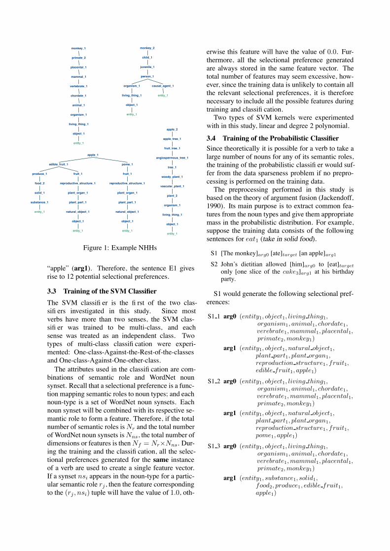
monkey_1
primate_2
placental_1
mammal_1
vertebrate_1
chordate_1
animal_1
organism_1
living_thing_1
object_1
entity_1
monkey_2
child_1
juvenile_1
person_1
organism_1
living_thing_1
object_1
entity_1
causal_agent_1
entity_1
apple_1
edible_fruit_1
produce_1
food_2
solid_1
substance_1
entity_1
fruit_1
reproductive_structure_1
plant_organ_1
plant_part_1
natural_object_1
object_1
entity_1
pome_1
fruit_1
reproductive_structure_1
plant_organ_1
plant_part_1
natural_object_1
object_1
entity_1
apple_2
apple_tree_1
fruit_tree_1
angiospermous_tree_1
tree_1
woody_plant_1
vascular_plant_1
plant_2
organism_1
living_thing_1
object_1
entity_1
Figure 1: Example NHHs
“apple” (arg1). Therefore, the sentence E1 givesrise to 12 potential selectional preferences.
3.3 Training of the SVM ClassifierThe SVM classifi er is the fi rst of the two clas-sifi ers investigated in this study. Since mostverbs have more than two senses, the SVM clas-sifi er was trained to be multi-class, and eachsense was treated as an independent class. Twotypes of multi-class classifi cation were experi-mented: One-class-Against-the-Rest-of-the-classesand One-class-Against-One-other-class.The attributes used in the classifi cation are com-
binations of semantic role and WordNet nounsynset. Recall that a selectional preference is a func-tion mapping semantic roles to noun types; and eachnoun-type is a set of WordNet noun synsets. Eachnoun synset will be combined with its respective se-mantic role to form a feature. Therefore, if the totalnumber of semantic roles isNr and the total numberof WordNet noun synsets isNns, the total number ofdimensions or features is thenNf = Nr"Nns. Dur-ing the training and the classifi cation, all the selec-tional preferences generated for the same instanceof a verb are used to create a single feature vector.If a synset nsi appears in the noun-type for a partic-ular semantic role rj , then the feature correspondingto the (rj , nsi) tuple will have the value of 1.0, oth-
erwise this feature will have the value of 0.0. Fur-thermore, all the selectional preference generatedare always stored in the same feature vector. Thetotal number of features may seem excessive, how-ever, since the training data is unlikely to contain allthe relevant selectional preferences, it is thereforenecessary to include all the possible features duringtraining and classifi cation.Two types of SVM kernels were experimented
with in this study, linear and degree 2 polynomial.
3.4 Training of the Probabilistic ClassifierSince theoretically it is possible for a verb to take alarge number of nouns for any of its semantic roles,the training of the probabilistic classifi er would suf-fer from the data sparseness problem if no prepro-cessing is performed on the training data.The preprocessing performed in this study is
based on the theory of argument fusion (Jackendoff,1990). Its main purpose is to extract common fea-tures from the noun types and give them appropriatemass in the probabilistic distribution. For example,suppose the training data consists of the followingsentences for eat1 (take in solid food).
S1 [The monkey]arg0 [ate]target [an apple]arg1
S2 John’s dietitian allowed [him]arg0 to [eat]target
only [one slice of the cake3]arg1 at his birthdayparty.
S1 would generate the following selectional pref-erences:
S1 1 arg0 (entity1, object1, living thing1,organism1, animal1, chordate1,verebrate1, mammal1, placental1,primate2, monkey1)
arg1 (entity1, object1, natural object1,plant part1, plant organ1,reproduction structure1, fruit1,edible fruit1, apple1)
S1 2 arg0 (entity1, object1, living thing1,organism1, animal1, chordate1,verebrate1, mammal1, placental1,primate2, monkey1)
arg1 (entity1, object1, natural object1,plant part1, plant organ1,reproduction structure1, fruit1,pome1, apple1)
S1 3 arg0 (entity1, object1, living thing1,organism1, animal1, chordate1,verebrate1, mammal1, placental1,primate2, monkey1)
arg1 (entity1, substance1, solid1,food2, produce1, edible fruit1,apple1)
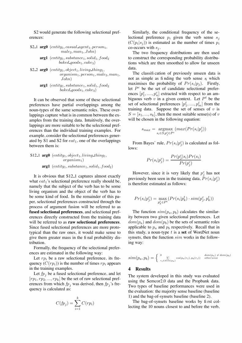
S2 would generate the following selectional pref-erences:
S2 1 arg0 (entity1, casual agent1, person1,male2, man1, John)
arg1 (entity1, substance1, solid1, food2
baked goods1, cake3)
S2 2 arg0 (entity1, object1, living thing1,organism1, person1, male2, man1,John)
arg1 (entity1, substance1, solid1, food2
baked goods1, cake3)
It can be observed that some of these selectionalpreferences have partial overlappings among thenoun-types of the same semantic roles. These over-lappings capture what is in common between the ex-amples from the training data. Intuitively, the over-lappings are more suitable to be the selectional pref-erences than the individual training examples. Forexample, consider the selectional preferences gener-ated by S1 and S2 for eat1, one of the overlappingsbetween them is:
S12 1 arg0 (entity1, object1, living thing1,organism1)
arg1 (entity1, substance1, solid1, food2)
It is obvious that S12 1 captures almost exactlywhat eat1’s selectional preference really should be,namely that the subject of the verb has to be someliving organism and the object of the verb has tobe some kind of food. In the remainder of this pa-per, selectional preferences constructed through theprocess of argument fusion will be referred to asfused selectional preferences, and selectional pref-erences directly constructed from the training datawill be referred to as raw selectional preferences.Since fused selectional preferences are more proto-typical than the raw ones, it would make sense togive them greater mass in the fi nal probability dis-tribution.Formally, the frequency of the selectional prefer-
ences are estimated in the following way:Let rpi be a raw selectional preference, its fre-
quency (C(rpi)) is the number of times rpi appearsin the training examples.Let fpj be a fused selectional preference, and let
[rp1, rp2, ..., rpk] be the set of raw selectional pref-erences from which fpj was derived, then fpj’s fre-quency is calculated as:
C(fpj) =k
!
i=1
C(rpi)
Similarly, the conditional frequency of the se-lectional preference pi given the verb sense sj
(C(pi|sj)) is estimated as the number of times pi
co-occurs with sj .The two frequency distributions are then used
to construct the corresponding probability distribu-tions which are then smoothed to allow far unseendata.The classifi cation of previously unseen data is
not as simple as fi nding the verb sense si whichmaximises the probability of Pr(si|pj). Firstly,let P c be the set of candidate selectional prefer-ences [pc
1, ...., pcn] extracted with respect to an am-
biguous verb v in a given context. Let P t be theset of selectional preferences [pt
1, ...., ptm] from the
training data. Suppose the set of senses of v isS = [s1, ..., sk], then the most suitable sense(s) of vwill be chosen in the following equation:
smax = argmaxsi!S,pc
j!P c(max(Pr(si|p
cj))
From Bayes’ rule, Pr(si|pcj) is calculated as fol-
lows:
Pr(si|pcj) =
Pr(pcj|si)Pr(si)
Pr(pcj)
However, since it is very likely that pcj has not
previously been seen in the training data, Pr(si|pcj)
is therefore estimated as follows:
Pr(si|pcj) = max
ptk!P t
(Pr(si|ptk) · sim(pc
j , ptk))
The function sim(pa, pb) calculates the similar-ity between two given selectional preferences. Letdom(pa) and dom(pb) be the sets of semantic rolesapplicable to pa and pb respectively. Recall that inthis study, a noun-type t is a set of WordNet nounsynsets, then the function sim works in the follow-ing way:
sim(pa, pb) ="
0 dom(pa) != dom(pb)P
ri!dom(pa)cos(pa(ri), pb(ri)) otherwise
4 ResultsThe system developed in this study was evaluatedusing the Semcor2.0 data and the Propbank data.Two types of baseline performances were used inthe evaluation: the majority sense baseline (baseline1) and the bag-of-synsets baseline (baseline 2).The bag-of-synsets baseline works by fi rst col-
lecting the 10 nouns closest to and before the verb,
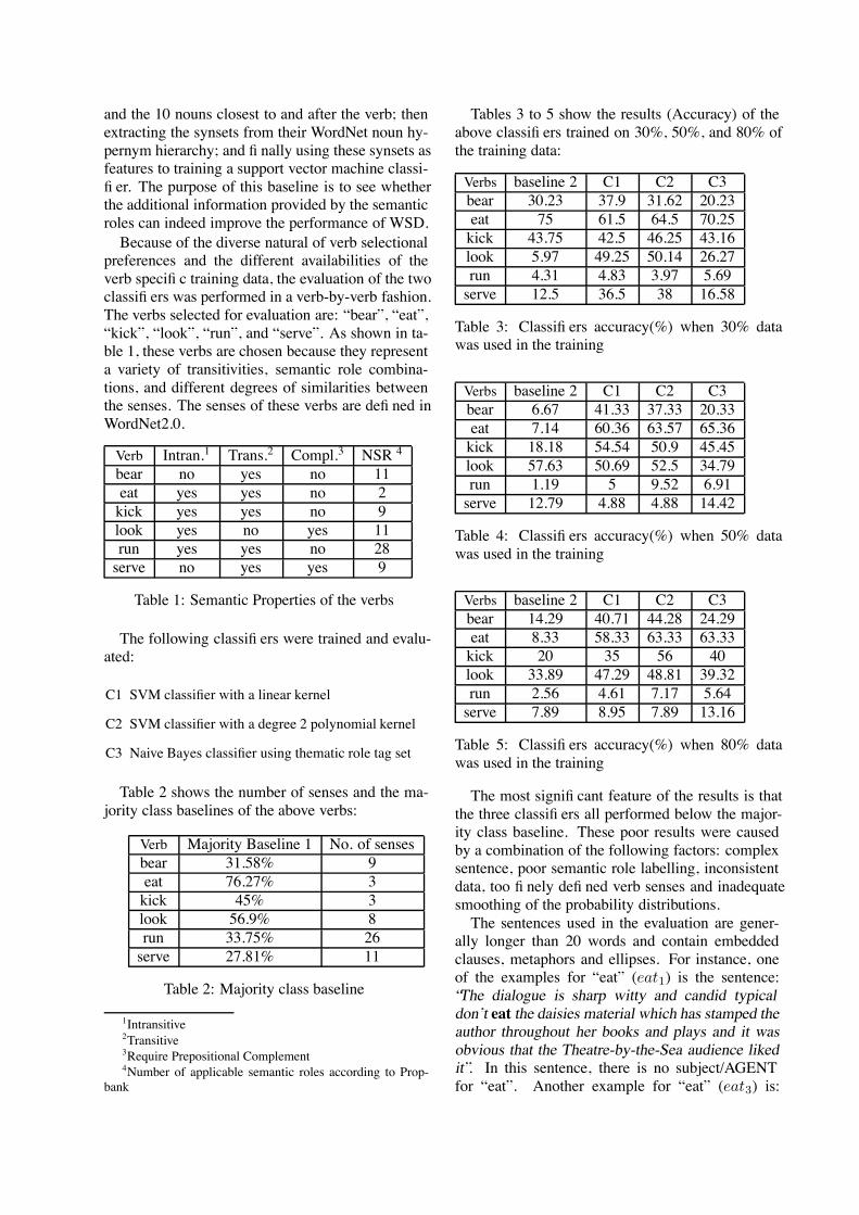
and the 10 nouns closest to and after the verb; thenextracting the synsets from their WordNet noun hy-pernym hierarchy; and fi nally using these synsets asfeatures to training a support vector machine classi-fi er. The purpose of this baseline is to see whetherthe additional information provided by the semanticroles can indeed improve the performance of WSD.Because of the diverse natural of verb selectional
preferences and the different availabilities of theverb specifi c training data, the evaluation of the twoclassifi ers was performed in a verb-by-verb fashion.The verbs selected for evaluation are: “bear”, “eat”,“kick”, “look”, “run”, and “serve”. As shown in ta-ble 1, these verbs are chosen because they representa variety of transitivities, semantic role combina-tions, and different degrees of similarities betweenthe senses. The senses of these verbs are defi ned inWordNet2.0.
Verb Intran.1 Trans.2 Compl.3 NSR 4
bear no yes no 11eat yes yes no 2kick yes yes no 9look yes no yes 11run yes yes no 28serve no yes yes 9
Table 1: Semantic Properties of the verbs
The following classifi ers were trained and evalu-ated:
C1 SVM classifier with a linear kernel
C2 SVM classifier with a degree 2 polynomial kernel
C3 Naive Bayes classifier using thematic role tag set
Table 2 shows the number of senses and the ma-jority class baselines of the above verbs:
Verb Majority Baseline 1 No. of sensesbear 31.58% 9eat 76.27% 3kick 45% 3look 56.9% 8run 33.75% 26serve 27.81% 11
Table 2: Majority class baseline
1Intransitive2Transitive3Require Prepositional Complement4Number of applicable semantic roles according to Prop-
bank
Tables 3 to 5 show the results (Accuracy) of theabove classifi ers trained on 30%, 50%, and 80% ofthe training data:
Verbs baseline 2 C1 C2 C3bear 30.23 37.9 31.62 20.23eat 75 61.5 64.5 70.25kick 43.75 42.5 46.25 43.16look 5.97 49.25 50.14 26.27run 4.31 4.83 3.97 5.69serve 12.5 36.5 38 16.58
Table 3: Classifi ers accuracy(%) when 30% datawas used in the training
Verbs baseline 2 C1 C2 C3bear 6.67 41.33 37.33 20.33eat 7.14 60.36 63.57 65.36kick 18.18 54.54 50.9 45.45look 57.63 50.69 52.5 34.79run 1.19 5 9.52 6.91serve 12.79 4.88 4.88 14.42
Table 4: Classifi ers accuracy(%) when 50% datawas used in the training
Verbs baseline 2 C1 C2 C3bear 14.29 40.71 44.28 24.29eat 8.33 58.33 63.33 63.33kick 20 35 56 40look 33.89 47.29 48.81 39.32run 2.56 4.61 7.17 5.64serve 7.89 8.95 7.89 13.16
Table 5: Classifi ers accuracy(%) when 80% datawas used in the training
The most signifi cant feature of the results is thatthe three classifi ers all performed below the major-ity class baseline. These poor results were causedby a combination of the following factors: complexsentence, poor semantic role labelling, inconsistentdata, too fi nely defi ned verb senses and inadequatesmoothing of the probability distributions.The sentences used in the evaluation are gener-
ally longer than 20 words and contain embeddedclauses, metaphors and ellipses. For instance, oneof the examples for “eat” (eat1) is the sentence:“The dialogue is sharp witty and candid typicaldon’t eat the daisies material which has stamped theauthor throughout her books and plays and it wasobvious that the Theatre-by-the-Sea audience likedit”. In this sentence, there is no subject/AGENTfor “eat”. Another example for “eat” (eat3) is:
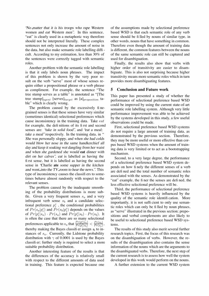
“No matter that it is his troops who rape Westernwomen and eat Western men”. In this sentence,“eat” is clearly used in a metaphoric way thereforeshould not be interpreted literally. These complexsentences not only increase the amount of noise inthe data, but also make semantic role labelling diffi -cult. According to my estimation, less than 30% ofthe sentences were correctly tagged with semanticroles.Another problem with the semantic role labelling
is that it only labels noun phrases. The impactof this problem is shown by the very poor re-sult on the verb “serve” most of whose senses re-quire either a propositional phrase or a verb phraseas compliment. For example, the sentence “Thetree stump serves as a table” is annotated as “[Thetree stump]agent [serves]target as [a]proposition ta-ble” which is clearly wrong.The problem caused by the excessively fi ne-
grained senses is that these senses have very similar(sometimes identical) selectional preferences whichcause inconsistency in the training data. Take eatfor example, the defi nitions of its fi rst and secondsenses are: “take in solid food”, and “eat a meal;take a meal” respectively. In the training data, in “She was personally sloppy, and when she had coldswould blow her nose in the same handkerchief allday and keep it soaking wet dangling from her waistand when she gardened she would eat dinner withdirt on her calves”, eat is labelled as having thefi rst sense, but it is labelled as having the secondsense in “Charlie ate some supper in the kitchenand went into the TV room to hear the news.”. Thistype of inconsistency causes the classifi ers to some-times behave almost randomly with respect to therelevant senses.The problem caused by the inadequate smooth-
ing of the probability distributions is more sub-tle. Given a very frequent senses sa and a veryinfrequent verb sense sb and a candidate selec-tional preference pc
i , the conditional probabilitiesof Pr(sa|pc
i) and Pr(sb|pci) depends on the values
of Pr(pci |sa) · Pr(sa) and Pr(pc
i |sb) · Pr(sb). Itis often the case that there are so many selectionalpreferences applicable to sa that
Pr(pci |sa)
Pr(pci |sb)
< Pr(sb)Pr(sa) ,
thereby making the Bayes classifi er assign sb to in-stances of sa. Currently, the Lidstone probabilitydistribution with ! of 0.0001 is used by the Bayesclassifi er; further study is required to select a moresuitable probability distribution.Another interesting feature of the results is that
the differences of the accuracy is relatively smallwith respect to the different amounts of data usedin training. This feature is expected because one
of the assumptions made by selectional preferencebased WSD is that each semantic role of any verbsense should be fi lled by nouns of similar type, inother words, nouns that have something in common.Therefore even though the amount of training datais different, the common features between the nounsof the same semantic role can still be captured andused for disambiguation.Finally, the results also show that verbs with
higher order of transitivity are easier to disam-biguate. This is also not surprising because highertransitivity means more semantic roles which in turnprovides more disambiguating features.
5 Conclusion and Future workThis paper has presented a study of whether theperformance of selectional preference based WSDcould be improved by using the current state-of-artsemantic role labelling system. Although very littleperformance improvement was able to be achievedby the systems developed in this study, a few usefulobservations could be made.First, selectional preference based WSD systems
do not require a large amount of training data, asdemonstrated by the previous section. Therefore,they may be more useful or more effective than cor-pus based WSD systems when the amount of train-ing data is very limited or to act as a bootstrappingmechanism.Second, to a very large degree, the performance
of a selectional preference based WSD system de-pends on how fi nely the different senses of a verbare defi ned and the total number of semantic rolesassociated with the senses. As demonstrated by the“eat” example, the fi ner the senses are defi ned, theless effective selectional preference will be.Third, the performance of selectional preference
based WSD systems is heavily influenced by thequality of the semantic role identifi cation. Moreimportantly, it is not suffi cient to only use seman-tic roles which can only be fi lled by noun phrases,as “serve” illustrated in the previous section; prepo-sitions and verbal complements are also likely tobe useful to selectional preference based WSD sys-tems.The results of this study also merit several further
research topics. First, the focus of this research wason the disambiguation of verbs. However, the re-sults of the disambiguation also contains the senseinformation of the nouns which are the arguments tothe disambiguated verbs. Therefore, the next step ofthe current research is to assess how well the systemdeveloped in this work would perform on the nouns.A further extension to the current WSD system
would be to incorporate extra information such asthe prepositions and other open class words in thedisambiguation. This extension may require a hy-brid WSD system incorporating selectional prefer-ence based mechanisms and corpus based mecha-nisms.Finally, as it was observed that the performance
of a selectional preference based WSD system washeavily influenced by the quality of semantic rolelabelling; it might also be possible to use selec-tional preference as a crude measure of the perfor-mances of semantic role labelling systems on unla-belled data. This is because it is likely for a par-ticular semantic role to be fi lled by nouns of simi-lar types, therefore nouns correctly labelled for thesame semantic role should exhibit a greater similar-ity than if incorrectly labelled.
AcknowledgementsI would like thank my supervisors, Professor StevenBird and Dr. Adrian Pearce, for reviewing the paper.This research was sponsored by Australian Post-graduate Awards (APA) from the Australian Re-search Council (ARC).
ReferencesRay Jackendoff, 1990. Semantic Structures, chap-ter 2. The MIT Press.
Daniel Jurafsky and James H. Martin, 2000. Speechand Language Processing, chapter 17. PrenticeHall, 1 edition.
Michael Lesk. 1986. Automatic sense disambigua-tion using machine readable dictionaries: howto tell a pine cone from an ice cream cone. InProceedings of the 5th annual international con-ference on Systems documentation, pages 24–26.ACM Press.
Diana McCarthy and John Carroll. 2003. Disam-biguating nouns, verbs, and adjectives using auto-matically acquired selectional preferences. Com-putational Linguistics, 29(4):639–654, Decem-ber.
George A. Miller. 1995. Wordnet: a lexicaldatabase for english. Communications of theACM, 38(11):39–41.
S. Pradhan, W. Ward, K. Hacioglu, J. Martin,and D. Jurafsky. 2004. Shallow semantic pars-ing using support vector machines. In Proceed-ings of the Human Language Technology Con-ference/North American chapter of the Associa-tion for Computational Linguistics annual meet-ing (HLT/NAACL-2004), Boston, MA, May 2–7.
Philip Resnik. 1997. Selectional preference andsense disambiguation. In Proceedings of ACLSiglex Workshop on Tagging Text with Lexical
Semantics, Why, What and How?, Washington,April 4-5, 1997.
David Yarowsky. 1995. Unsupervised word sensedisambiguation rivaling supervised methods. InMeeting of the Association for ComputationalLinguistics, pages 189–196.
1
Differentiating Types of Verb Particle Constructions
Jon Patrick and Jeremy Fletcher Sydney Language Technology Research Group
School of Information Technologies University of Sydney
Sydney, Australia, 2006 [email protected], [email protected]
Abstract A verb particle construction (VPC) classification scheme gleaned from linguistic sources has been used to assess its usefulness for identifying issues in decomposability. Linguistic sources have also been used to inform the features suitable for use in building an automatic classifier for the scheme with a series of good performance results. The notions of how to define the task of computing phrasal verbs are discussed and new proposals are presented.
1 Introduction
Our area of research focuses on verb-particle constructions (VPCs), a sub-section of multi-word expressions (MWEs). MWEs are a generic term for the group of expressions that include idioms (e.g. over the moon), lexically fixed expressions (e.g. ad hoc), light verb constructions (e.g. make a mistake), institutionalised phrases (e.g. kindle excitement), and verb-particle constructions (e.g. run away). All these expressions have in common the occurrence of words adjacent to each other that would be more frequent than if they were simply random words put together. Hence the words which constitute them have some particular meaning together that they would not have apart. VPCs consist of a simplex (single-word) verb, and a particle, whether preposition or adverb. A particular subset of interest are “phrasal” verbs which are considered to be non-decomposable structures where the meaning is in the whole and not the parts of the phrase (Dixon, 1978). Previous research into the area of MWEs, shows a number of places in which there has been a lack of research. The area which is of interest to us is the approach of bringing reliable resources and specific encodeable linguistic knowledge for use in feature selection in supervised learning tasks of categorisation and WSD.
2 Previous Research There has been only limited research done in the field of MWEs in computational linguistics, mostly focusing on VPCs; although much research (Abeillé, 1988, 1995; Barkema, 1994; Wehrli, 1998) has been done on such MWEs as idioms (Abeillé, 1995; Barkema, 1994; Wehrli, 1998) and light verbs (Abeillé, 1988) within the traditional linguistics field. MWEs are very idiosyncratic constructs making progress in their computation difficult. They have been called “a serious problem for many areas of language technology” (Copestake, Lambeau, Villavicencio, Bond, Baldwin, Sag, Flickinger, 2002) “unpredictable” (Baldwin & Villavicencio, 2002) and “a pain in the neck” (Sag, Baldwin, Bond, Copestake and Flickinger. 2002), and thus many applications of computational linguistics such as machine translation put multiword expressions in the “too-hard” basket. However, the use of MWEs in natural language is widespread, and thus comes about the need for what has been called “a robust, structured handling [of MWEs]” (Baldwin & Villavicencio, 2002, Calzolari, Fillmore, Grishman, Ide, Lencu, MacLeod, and Zampolli. 2002). Much of the previous work on VPCs has revolved around tasks besides WSD, focused on the extraction of multiple word constructs from corpora (Abeillé,1988, Baldwin & Villavicencio, 2002, Maynard & Ananiadou, 1999.) which we will discuss in some detail below, or what is termed the “decomposability” or “compositionality” of VPCs.
2.1 Extraction of MWEs from Corpora One of the important components of research in MWEs is their automatic extraction from some corpora. The best results for precision and recall on this task is clearly the work of Baldwin and Villavicencio (2002), who used a combination of part-of-speech (POS)-based extraction (using Brill’s POS tagger (Brill, 1995)), chunk-based
2
extraction, and chunk-grammar-based extraction, to extract VPCs from the Wall Street Journal section of the Penn Treebank. They report precision of 0.889 and recall of 0.903 (F 1 = 0.896) for this task. Although they cite some other research into a similar area, there had been very little research in this specific area of extracting VPCs automatically from corpora, although some studies without quantitative analysis had been done previously (Kaalep & Muischnek, 2002, Krenn & Evert, 2001), along with work on the extraction of other collocations other than MWEs (Abeillé, 1988, Basili, Pazienza and Velardi, 1993, Maynard and Ananiadou, 1999).
Table 1. Summativity of VPCs; whether individual elements determine the meaning of the construction.
2.2 Determining the Decomposability of
MWEs
As the semantics of most MWEs are more difficult to ascertain than the semantics of simplex words (even taking into account the problem of disambiguating between different senses of a simplex word), there has been some research done into what is termed the “compositionality” or “decomposability” of VPCs. In Bannard, Baldwin & Lascarides (2003) some examples are given of VPCs which illustrate one way of describing “summativity” (See table 1). In these examples, 1) “put up”, is entirely composed of its constituent parts, as at the end of the action, the painting is both “put” somewhere, and is now “up”. In 2) “finished up”, the paper is “finished”, but nothing is “up”, in 3) “made away”, the thief is “away”, but nothing is “made”, and in 4) nothing is either “made” or “out”. Lin (1999) discusses the principle of decomposability with regards to constructs other than VPCs, (e.g. “red tape”), and conducted an experiment whereby individual words in the collocation are replaced by words with similar meanings taken from a thesaurus.
This word-substitution technique is transferred to VPCs in Bannard (2002) where he suggests that a similar approach could be used to determine the “decomposability” of VPCs. He obtains disappointing results ranging from precision of 0.516 and recall of 0.739 (for the largest class) to precision of 0.286 and recall of 0.083 (for the smallest class). Bannard et al (2003) describe a statistical distribution modelling framework for determining whether specific VPCs are “decomposable”, and hence automatically infer their meaning. They conducted an internet-based experiment whereby non-expert native English speakers were asked whether certain VPCs, in sets of 5 sentences for each exemplar VPC, entailed the meaning of the simplex verb and/or the meaning of the preposition. They used this as their gold standard test data to evaluate their results. This contrasts with the approach taken by Lin (1999), in that their evaluation is based on a more intuitive level, although this could in fact lead to their results becoming affected by subjective judgments. They then encapsulated the problem as a classification task, to classify VPCs into classes depending on whether or not they were composed of their individual elements. They achieved results that improved on a baseline of classifying everything as the most common class, with results ranging from 0.735 for precision and 0.892 for recall (F 1= 0.810) to 0.303 for precision and 0.769 for recall (F 1=0.435) by using their distribution modelling approach. 2.3 Word Sense Disambiguation (WSD) There has been much general research done in the field of WSD (Krovetz & Croft, 1989, Maynard & Ananiadou, 1998, Yarowsky, 1992, 1995, for example), although very little relating specifically to disambiguating MWEs. O’Hara and Wiebe, 2003 do perhaps what is the most relevant research, on the task of disambiguating prepositions as having a locative, temporal or other meaning. They report average accuracy of 0.703, although they don’t provide precision and recall scores, so it is difficult to ascertain the particular shortcomings of the system, and where improvements could be made. However, we can make the conjecture that had they determined the compositionality of the VPC to which the prepositional particle belongs, their reported accuracy would be higher.
VPC Example Verb
Contributes to Meaning
Particle Contributes to Meaning
1. Peter put the picture up Yes Yes 2. Susan finished up her paper Yes No
3. The thief made away with the cash No Yes
4. Barbara and Simon made out No No
3
3 Method
Our research goal is to create a system that can accurately disambiguate between the different semantics of different instances of VPCs. It is interesting to note that the task of disambiguating VPCs has not been undertaken by other researchers working on MWEs possibly for a number of reasons. Firstly, there is no readily available corpus that has VPCs tagged for semantic differences. Hence, a major part of the work described is to collect a suitable subset of a given corpus – in this case, we use the British National Corpus (BNC) – and manually tag target VPCs as having certain semantic features. Another reason why semantic disambiguation has not been undertaken to such a fine degree for VPCs is that there is, in fact, no comprehensive electronic resource which contains different senses of a given verb-particle construction, although there are large, readily available resources for different simplex verbs (the most obvious being WordNet (G. Miller, Beckwith, Fellcaum, Gross, and K. Miller. 1990). Hence, the main difference between the research being undertaken in this project and that which has been done previously is the exploitation of a lexical database of phrasal verbs (constructed from Meyer, 1975). This will be used to increase the accuracy of our task on VPCs, and provide us with a compendium of “valid” verb-particle constructions. Also, whilst most semantic identification tasks relate to simplex words, there has been little research on disambiguation of MWEs. Disambiguation in this sense is most applicable to VPCs, as most other idiomatic MWEs have a single, fixed (if still metaphorical) meaning. For example, the idiom “kick the bucket”, once it has been identified as a MWE has only the sense of “dying”. Although the phrase itself could also have a literal sense of kicking, once it has been extracted and identified as an idiom, only this idiomatic, metaphoric sense applies. It is a similar situation with other idioms. However, with VPCs, there are many examples that have different senses. For example the phrasal verb “to check out” has the sense of leaving a hotel, and the sense of checking something to make sure it is correct. Other examples of VPCs with multiple senses are “pick up” (understand/comprehend, retrieve from the ground, hook up with someone of the opposite sex), “look out” (look out of a window, watch out for) and “set up” (put into position, furnish with money/resources, establish, etc…).
4 Motivation Unlike the current trend in other works that focus on recognition of VPCs from thesaural expansion of context whether automatically (Lin, 1999, Bannard et al, 2003, McCarthy et al, 2003) or using WordNet (Bannard et al 2003) and the establishment of gold standards by survey (Bannard et al, 2003, McCarthy et al, 2003) we prefer a principled method using the understandings developed by linguistic studies. The identification of (virtually) all candidate VPCs have been captured in 3 Phrasal Verb dictionaries (Collins, Oxford, and Meyer) so as a resource to determine the definitions of VPCs we use the dictionary of Meyer (1975). As well as the dictionaries, a variety of linguistic studies provide an extensive analysis of the features of VPCs. Our procedure is to use the dictionaries to guide the compilation of our gold standard and the studies to guide feature selection for automated classification to both establish the parameterisation of a generative model for recognising VPCs and to identify the strengths of the various features established by linguists. The most comprehensive analysis of this problem has been completed by Dixon, (1982) and we use his classification scheme to guide the development of our own classification scheme and much feature selection has been gleaned from his work. For the definition of verbs we use the new Shorter Oxford English Dictionary (1993) and for particle description Lindstromberg, (1998). Dixon produced a 5 class classification scheme:
A. Literal usage of all VPC components, e.g.
John walked on the grass, B. Like A but with missing arguments that are
reasonably inferable e.g. He ran down (the bank) to the railway line,
C. Obvious metaphorical extensions form literal phrases e.g. the firm went under,
D. non-literal constructions that cannot obviously be related to the literal form e.g. They are going to have it out;
E. Full idioms, e.g. turn over a new leaf.
This scheme is more extensive than that used in any computational study we have found, most of which attempt to resolve the compositional/non-compositional dichotomy of a VPC or at best provide a graded scale. Whilst the Dixon scheme is more detailed than other schemes we are not entirely satisfied with it. In our own studies we have come to recognise that there is a dimension of diversity in VPCs not captured by it. Some VPCs have become so established that they
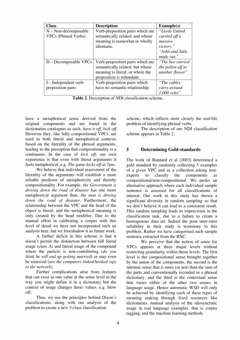
4
have a metaphorical sense derived from the original components and are found in the dictionaries catalogues as such, have it off, kick off. However they, like fully compositional VPCs, are used in both literal and metaphorical contexts based on the literality of the phrasal arguments, leading to the perception that compositionality is a continuum. In the case of kick off, our own experience is that even with literal arguments it feels metaphorical, e.g. The game kicks off at 7pm. We believe that individual assessment of the literality of the arguments will establish a more reliable predictor of metaphoricity and thereby compositionality. For example, the Government is driving down the road of disaster has one more metaphorical argument than, the man is driving down the road of disaster. Furthermore, the relationship between the VPC and the head of the object is literal, and the metaphorical meaning is only created by the head modifier. Due to the manual effort in calibrating a corpus with this level of detail we have not incorporated such an analysis here, but we foreshadow it as future work. A further deficit in this scheme is that it doesn’t permit the distinction between full literal usage (class A) and literal usage of the compound where the particle is non-contributing (do you think he will end up getting married) or may even be removed (are the computers linked/hooked (up) to the network). Further complications arise from features that can exist as one value at the sense level in the way you might define it in a dictionary but the context of usage changes those values, e.g. blow off. Thus, we use the principles behind Dixon’s classifications, along with our analysis of the problem to create a new 3-class classification
scheme, which reflects more closely the real-life problem of identifying phrasal verbs. The description of our NDI classification scheme appears in Table 2. 5 Determining Gold-standards The work of Bannard et al (2003) determined a gold standard by randomly collecting 5 examples of a given VPC and as a collection asking non-experts to classify the components as compositional/non-compositional. We prefer an alternative approach where each individual sample sentence is assessed for all classifications of interest. Our work in this study has shown a significant diversity in random sampling so that we don’t believe it can lead to a consistent result. This random sampling leads to imprecision in the classification task, due to a failure to create a homogenous data set. Indeed the poor inter-rater reliability in their study is testimony to this problem. Rather we have categorised each sample sentence extracted from the BNC. We perceive that the notion of sense for VPCs appears at three major levels without restricting granularity within those levels. The first level is the compositional sense brought together by the union of the components, the second is the intrinsic sense that is more (or not) than the sum of the parts and conventionally recorded in a phrasal dictionary, and the third is the contextual sense that varies either of the other two senses in language usage. Hence automatic WSD will only be achieved by identifying each of these types of meaning making through fixed resources like dictionaries, manual analysis of the idiosyncratic usage in real language examples, that is corpus tagging, and the machine learning methods
Class Description Example(s) N – Non-decomposable VPCs (Phrasal Verbs)
Verb-preposition pairs which are semantically related, and whose meaning is somewhat or wholly idiomatic.
“Leeds United carried off a massive victory.” “John and Julie made out.”
D – Decomposable VPCs Verb-preposition pairs which are semantically related, but whose meaning is literal, or where the preposition is redundant.
“The bee carried the pollen off to another flower”
I – Independent verb-preposition pairs
Verb-preposition pairs which have no semantic relationship.
“The cables carry around 1,000 volts”
Table 2. Description of NDI classification scheme.
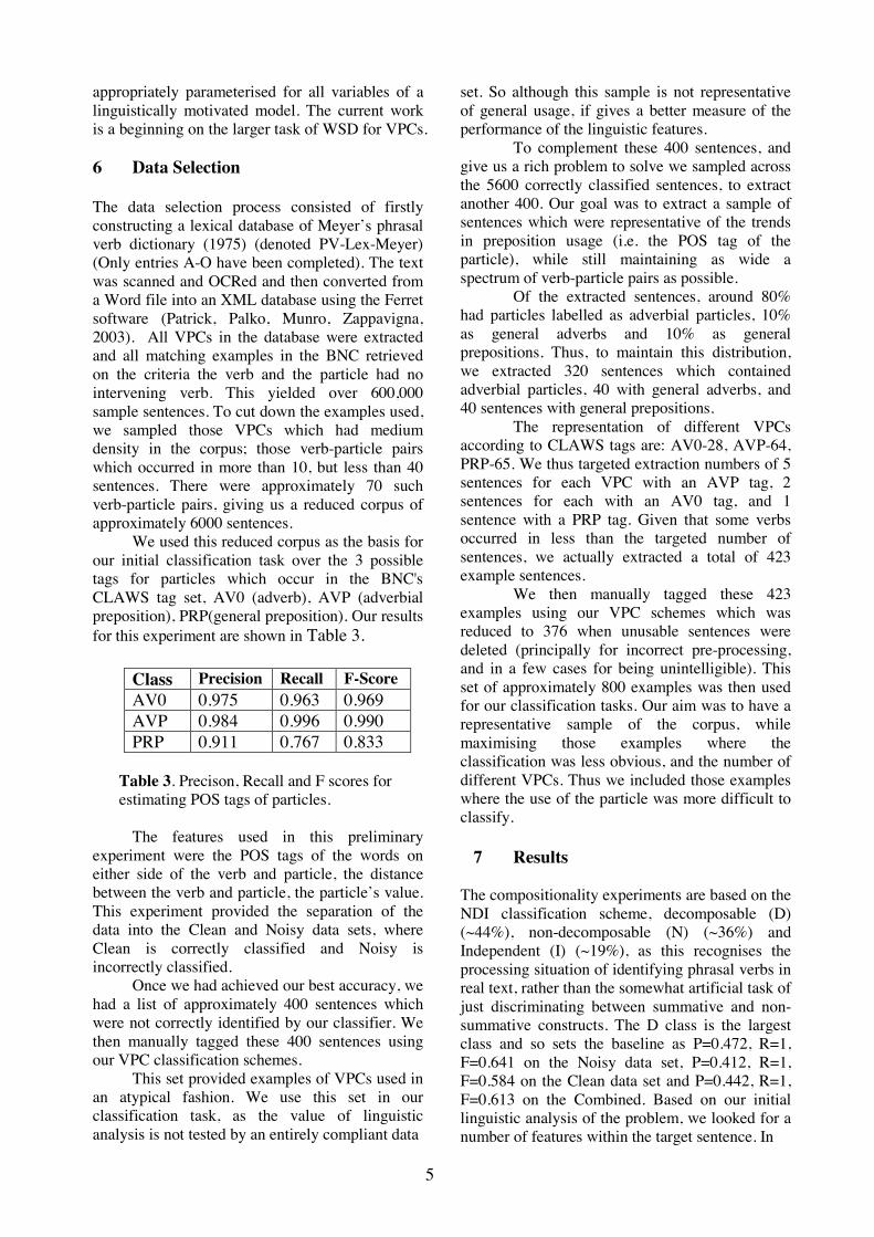
5
appropriately parameterised for all variables of a linguistically motivated model. The current work is a beginning on the larger task of WSD for VPCs.
6 Data Selection
The data selection process consisted of firstly constructing a lexical database of Meyer’s phrasal verb dictionary (1975) (denoted PV-Lex-Meyer) (Only entries A-O have been completed). The text was scanned and OCRed and then converted from a Word file into an XML database using the Ferret software (Patrick, Palko, Munro, Zappavigna, 2003). All VPCs in the database were extracted and all matching examples in the BNC retrieved on the criteria the verb and the particle had no intervening verb. This yielded over 600,000 sample sentences. To cut down the examples used, we sampled those VPCs which had medium density in the corpus; those verb-particle pairs which occurred in more than 10, but less than 40 sentences. There were approximately 70 such verb-particle pairs, giving us a reduced corpus of approximately 6000 sentences. We used this reduced corpus as the basis for our initial classification task over the 3 possible tags for particles which occur in the BNC's CLAWS tag set, AV0 (adverb), AVP (adverbial preposition), PRP(general preposition). Our results for this experiment are shown in Table 3.
Table 3. Precison, Recall and F scores for estimating POS tags of particles.
The features used in this preliminary experiment were the POS tags of the words on either side of the verb and particle, the distance between the verb and particle, the particle’s value. This experiment provided the separation of the data into the Clean and Noisy data sets, where Clean is correctly classified and Noisy is incorrectly classified. Once we had achieved our best accuracy, we had a list of approximately 400 sentences which were not correctly identified by our classifier. We then manually tagged these 400 sentences using our VPC classification schemes. This set provided examples of VPCs used in an atypical fashion. We use this set in our classification task, as the value of linguistic analysis is not tested by an entirely compliant data
set. So although this sample is not representative of general usage, if gives a better measure of the performance of the linguistic features. To complement these 400 sentences, and give us a rich problem to solve we sampled across the 5600 correctly classified sentences, to extract another 400. Our goal was to extract a sample of sentences which were representative of the trends in preposition usage (i.e. the POS tag of the particle), while still maintaining as wide a spectrum of verb-particle pairs as possible. Of the extracted sentences, around 80% had particles labelled as adverbial particles, 10% as general adverbs and 10% as general prepositions. Thus, to maintain this distribution, we extracted 320 sentences which contained adverbial particles, 40 with general adverbs, and 40 sentences with general prepositions. The representation of different VPCs according to CLAWS tags are: AV0-28, AVP-64, PRP-65. We thus targeted extraction numbers of 5 sentences for each VPC with an AVP tag, 2 sentences for each with an AV0 tag, and 1 sentence with a PRP tag. Given that some verbs occurred in less than the targeted number of sentences, we actually extracted a total of 423 example sentences. We then manually tagged these 423 examples using our VPC schemes which was reduced to 376 when unusable sentences were deleted (principally for incorrect pre-processing, and in a few cases for being unintelligible). This set of approximately 800 examples was then used for our classification tasks. Our aim was to have a representative sample of the corpus, while maximising those examples where the classification was less obvious, and the number of different VPCs. Thus we included those examples where the use of the particle was more difficult to classify.
7 Results The compositionality experiments are based on the NDI classification scheme, decomposable (D) (~44%), non-decomposable (N) (~36%) and Independent (I) (~19%), as this recognises the processing situation of identifying phrasal verbs in real text, rather than the somewhat artificial task of just discriminating between summative and non-summative constructs. The D class is the largest class and so sets the baseline as P=0.472, R=1, F=0.641 on the Noisy data set, P=0.412, R=1, F=0.584 on the Clean data set and P=0.442, R=1, F=0.613 on the Combined. Based on our initial linguistic analysis of the problem, we looked for a number of features within the target sentence. In
Class Precision Recall F-Score AV0 0.975 0.963 0.969 AVP 0.984 0.996 0.990 PRP 0.911 0.767 0.833
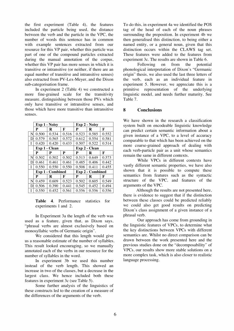
6
the first experiment (Table 4), the features included the particle being used, the distance between the verb and the particle in the VPC, the number of words this sentence has in common with example sentences extracted from our resource for this VP pair, whether this particle was part of one of the compound particles extracted during the manual annotation of the corpus, whether this VP pair has more senses in which it is transitive or intransitive (or neither, if there are an equal number of transitive and intransitive senses) also extracted from PV-Lex-Meyer, and the Dixon sub-categorisation frame. In experiment 2 (Table 4) we constructed a more fine-grained scale for the transitivity measure, distinguishing between those PVs which only have transitive or intransitive senses, and those which have more transitive than intransitive senses.
Exp 1 - Noisy Exp 2 - Noisy P R F P R F
N 0.500 0.534 0.516 0.523 0.585 0.552 D 0.579 0.565 0.572 0.612 0.554 0.581 I 0.420 0.420 0.433 0.507 0.522 0.514
Exp 1 - Clean Exp 2 - Clean P P P P R F
N 0.502 0.502 0.502 0.513 0.649 0.573 D 0.461 0.461 0.461 0.485 0.406 0.442 I 0.550 0.550 0.550 0.508 0.411 0.455
Exp 1 - Combined Exp 2 - Combined P R F P R F
N 0.459 0.609 0.523 0.502 0.605 0.549 D 0.506 0.390 0.441 0.545 0.452 0.494 I 0.550 0.452 0.561 0.556 0.556 0.556
Table 4. Performance statistics for experiments 1 and 2.
In Experiment 3a the length of the verb was used as a feature, given that, as Dixon says, “phrasal verbs are almost exclusively based on monosyllabic verbs of Germanic origin”. We considered that this length would give us a reasonable estimate of the number of syllables. This result looked encouraging, so we manually annotated each of the verbs in our resource for the number of syllables in the word. In experiment 3b we used this number instead of the verb length. This showed an increase in two of the classes, but a decrease in the largest class. We hence included both these features in experiment 3c (see Table 5). Some further analysis of the linguistics of these constructs led to the creation of a measure of the differences of the arguments of the verb.
To do this, in experiment 4a we identified the POS tag of the head of each of the noun phrases surrounding the preposition. In experiment 4b we then generalised this distinction, to being either a named entity, or a general noun, given that this distinction occurs within the CLAWS tag set. These features were added to the features from experiment 3c. The results are shown in Table 6. Following on from the potential phonological interpretation of Dixon’s “Germanic origin” thesis, we also used the last three letters of the verb, each as an individual feature in experiment 5. However, we appreciate this is a primitive representation of the underlying linguistic model, and needs further maturity. See Table 7. 8 Conclusions We have shown in the research a classification system built on encodeable linguistic knowledge can predict certain semantic information about a given instance of a VPC, to a level of accuracy comparable to that which has been achieved on the more coarse-grained approach of dealing with each verb-particle pair as a unit whose semantics remain the same in different contexts. While VPCs in different contexts have vastly different semantic properties, we have also shown that it is possible to compute these semantics from features such as the syntactic structure of the VPC, and features of the arguments of the VPC. Although the results are not presented here, there is evidence to suggest that if the distinction between these classes could be predicted reliably we could also get good results on predicting Dixon’s class assignment of a given instance of a phrasal verb. Our approach has come from grounding in the linguistic features of VPCs, to determine what the key distinctions between VPCs with different semantics are. Whilst no direct comparison can be drawn between the work presented here and the previous studies done on the “decomposability” of VPCs, our results show more stable solutions on a more complex task, which is also closer to realistic language processing.
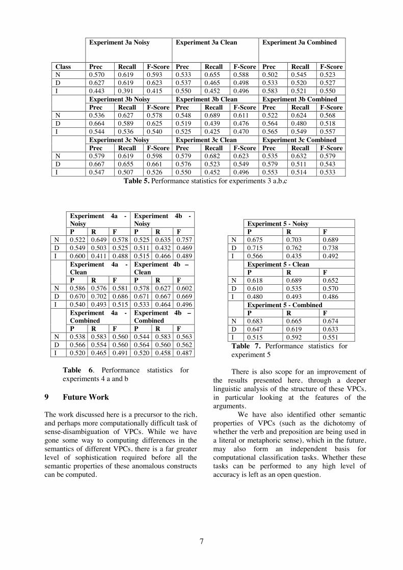
7
Experiment 4a - Noisy
Experiment 4b - Noisy
P R F P R F N 0.522 0.649 0.578 0.525 0.635 0.757 D 0.549 0.503 0.525 0.511 0.432 0.469 I 0.600 0.411 0.488 0.515 0.466 0.489
Experiment 4a - Clean
Experiment 4b – Clean
P R F P R F N 0.586 0.576 0.581 0.578 0.627 0.602 D 0.670 0.702 0.686 0.671 0.667 0.669 I 0.540 0.493 0.515 0.533 0.464 0.496
Experiment 4a - Combined
Experiment 4b – Combined
P R F P R F N 0.538 0.583 0.560 0.544 0.583 0.563 D 0.566 0.554 0.560 0.564 0.560 0.562 I 0.520 0.465 0.491 0.520 0.458 0.487
Table 6. Performance statistics for experiments 4 a and b
9 Future Work
The work discussed here is a precursor to the rich, and perhaps more computationally difficult task of sense-disambiguation of VPCs. While we have gone some way to computing differences in the semantics of different VPCs, there is a far greater level of sophistication required before all the semantic properties of these anomalous constructs can be computed.
Experiment 5 - Noisy P R F
N 0.675 0.703 0.689 D 0.715 0.762 0.738 I 0.566 0.435 0.492
Experiment 5 - Clean P R F
N 0.618 0.689 0.652 D 0.610 0.535 0.570 I 0.480 0.493 0.486
Experiment 5 - Combined P R F
N 0.683 0.665 0.674 D 0.647 0.619 0.633 I 0.515 0.592 0.551 Table 7. Performance statistics for experiment 5
There is also scope for an improvement of
the results presented here, through a deeper linguistic analysis of the structure of these VPCs, in particular looking at the features of the arguments.
We have also identified other semantic properties of VPCs (such as the dichotomy of whether the verb and preposition are being used in a literal or metaphoric sense), which in the future, may also form an independent basis for computational classification tasks. Whether these tasks can be performed to any high level of accuracy is left as an open question.
Experiment 3a Noisy Experiment 3a Clean Experiment 3a Combined
Class Prec Recall F-Score Prec Recall F-Score Prec Recall F-Score N 0.570 0.619 0.593 0.533 0.655 0.588 0.502 0.545 0.523 D 0.627 0.619 0.623 0.537 0.465 0.498 0.533 0.520 0.527 I 0.443 0.391 0.415 0.550 0.452 0.496 0.583 0.521 0.550
Experiment 3b Noisy Experiment 3b Clean Experiment 3b Combined Prec Recall F-Score Prec Recall F-Score Prec Recall F-Score
N 0.536 0.627 0.578 0.548 0.689 0.611 0.522 0.624 0.568 D 0.664 0.589 0.625 0.519 0.439 0.476 0.564 0.480 0.518 I 0.544 0.536 0.540 0.525 0.425 0.470 0.565 0.549 0.557
Experiment 3c Noisy Experiment 3c Clean Experiment 3c Combined Prec Recall F-Score Prec Recall F-Score Prec Recall F-Score
N 0.579 0.619 0.598 0.579 0.682 0.623 0.535 0.632 0.579 D 0.667 0.655 0.661 0.576 0.523 0.549 0.579 0.511 0.543 I 0.547 0.507 0.526 0.550 0.452 0.496 0.553 0.514 0.533
Table 5. Performance statistics for experiments 3 a,b,c
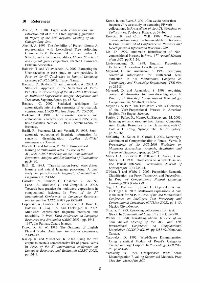
8
10 References
Abeillé, A. 1988. Light verb constructions and extraction out of NP in a tree adjoining grammar. In Papers of the 24th Regional Meeting of the Chicago Ling. Soc.
Abeillé, A. 1995. The flexibility of French idioms: A representation with Lexicalised Tree Adjoining Grammar. In M. Everaert, E-J. van der Linden, A. Schenk, and R. Schreuder, editors, Idioms: Structural and Psychological Perspectives, chapter 1. Lawrence Erlbaum Associates.
Baldwin, T. and Villavicencio, A. 2002. Extracting the Unextractable: A case study on verb-particles. In Proc. of the 6th Conference on Natural Language Learning (CoNLL-2002), Taipei, Taiwan
Bannard, C., Baldwin, T. and Lascarides, A.. 2003. A Statistical Approach to the Semantics of Verb-Particles. In Proceedings of the ACL-2003 Workshop on Multiword Expressions: Analysis, Acquisition and Treatment, Sapporo, Japan, pp. 65-72.
Bannard, C. 2002. Statistical techniques for automatically inferring the semantics of verb-particle constructions. LinGO Working Paper No. 2002-06.
Barkema, H. 1994. The idiomatic, syntactic and collocational characteristics of received NPs: some basic statistics. Hermes 13: 19-40. Aarhus School of Business.
Basili, R., Pazienza, M. and Velardi, P. 1993. Semi-automatic extraction of linguistic information for syntactic disambiguation. Applied Artificial Intelligence, 7:339-64.
Blaheta, D. and Johnson, M. 2001. Unsupervised learning of multi-word verbs. In Proc. of the ACL/EACL 2001 Workshop on the Computational Extraction, Analysis and Exploitation of Collocations, pp 54-60.
Brill, E. 1995. “Transformation-based error-driven learning and natural language processing: A case study in part-of-speech tagging”, Computational Linguistics. 21:543-65.
Calzolari, N., Fillmore, C., Grishman, R., Ide, N., Lencu, A., MacLeod, C. and Zampolli, A. 2002. Towards best practice for multiword expressions in computational lexicons. In Proc. of the 3rd International Conference on Language Resources and Evaluation (LREC 2002), pp 1934-40
Copestake, A., Lambeau, F., Villavicencio, A., Bond, F., Baldwin, T., Sag, I.A. and Flickinger, D. 2002. Multiword expressions: linguistic precision and reusability. In Proc. Third conference on Language Resources and Evaluation (LREC-2002), pp. 1941—1947. Las Palmas, Canary Islands.
Dixon, R. M. W. 1982. The Grammar of English Phrasal Verbs. Australian Journal of Linguistics, 2:149-247.
Kaalep, K. and Muischnek, K. 2002. Using the text corpus to create a comprehensive list of phrasal verbs. In Proc. of the 3rd International conference on Language Resources and Evaluation (LREC 2002), pp 101-5.
Krenn, B. and Evert, S. 2001. Can we do better than frequency? A case study on extracting PP-verb collocations. In Proceedings of the ACL Workshop on Collocations, Toulouse, France, pp 39-46.
Krovetz, R. and Croft, W.B. 1989. Word sense disambiguation using machine-readable dictionaries. In Proc. Annual ACM Conference on Research and Development in Information Retrieval 1989.
Lin, D. 1999. Automatic Identification of Non-compositional Phrases. In Proc. 37th Annual Meeting of the ACL, pp 317-24.
Lindstromberg, S. 1998. English Prepositions Explained. Amsterdam: John Benjamins.
Maynard, D. and Ananiadou, S. 1999. Identifying contextual information for multi-word term extraction. In 5th International Congress on Terminology and Knowledge Engineering (TKE 99), pp 212-21.
Maynard, D. and Ananiadou, S. 1998. Acquiring contextual information for term disambiguation. In Proc. of 1st Workshop Computational Terminology, Computerm ’98, Montreal, Canada.
Meyer, G. A. 1975. The Two-Word Verb, A Dictionary of the Verb-Prepositional Phrases in American English. The Hague: Mouton.
Patrick, J., Palko, D., Munro, R., Zappavigna, M. 2003. Inferring semantic structure from format, Computing Arts: Digital Resources in the Humanities, (ed) C. Cole & H. Craig, Sydney: The Uni of Sydney, pp150-168.
McCarthy, D., Keller, B., Carroll, J. 2003, Detecting a Continuum of Compositionality in Phrasal Verbs. In Proceedings of the ACL-2003 Workshop on Multiword Expressions: Analysis, Acquisition and Treatment, Sapporo, Japan, pp. 65-72.
Miller, G.A., Beckwith, R., Fellcaum, C., Gross, D. and Miller, K.J. 1990. Introduction to WordNet: an on-line lexical database. International Journal of Lexicography, 3(4):235-44.
O’Hara, T and Wiebe J. 2003. Preposition Semantic Classification via PENN TREEBANK and FRAMENET. In Proc. of Computational Natural Language Learning-2003 (CoNLL-03).
Sag, I.A., Baldwin, T., Bond, F., Copestake, A. and Flickinger, D. 2002. Multiword expressions: A pain in the neck for NLP. In Proc. of the 3rd International Conference on Intelligent Text Processing and Computational Linguistics (CICLing-2002), pp 1-15, Mexico City, Mexico.
Smadja, F. 1993. Retrieving collocations from text: Xtract. In Computational Linguistics, 19(1):143-78.
Wehrli, E. 1998. Translating idioms. In Proc. of the 36th Annual Meeting of the ACL and 17th International Conference on Computational Linguistics: COLING/ACL-98, pp 1388-92, Montreal, Canada.
Yarowsky, D. 1992. Word-Sense Disambiguation Using Statistical Models of Roget’s Categories Trained on Large Corpora. In Proceedings, COLING-92. pp 454-460.
Yarowsky, D. 1995. Unsupervised Word Sense Disambiguation Rivalling Supervised Methods. Proc 33rd Ann. Meet.of the ACL.


