arX

iv:1

404.

7733

v1 [

nlin

.SI]

30

Apr

201

4

Darboux Transformation and Exact Solutions of the

Myrzakulov-Lakshmanan-II Equation

M. Zhassybayeva, G. Mamyrbekova, G. Nugmanova, R. Myrzakulov∗

Eurasian International Center for Theoretical Physics and Department of General

& Theoretical Physics, Eurasian National University, Astana 010008, Kazakhstan

Abstract

The Myrzakulov-Lakshmanan-II (ML-II) equation is one of a (2+1)-dimensional general-izations of the Heisenberg ferromagnetic equation. It is integrable and has a non-isospectralLax representation. In this paper, the Darboux transformation (DT) for the ML-II equationis constructed. Using the DT, the 1-soliton and 2-soliton solutions of the ML-II equation arepresented.

1 Introduction

During the past decades, there has been an increasing interest in the investigation of integrable clas-sical and quantum systems. The theory of integrable systems is an important branch of nonlinearscience. Integrable systems describe various kinds of nonlinear phenomena, such as soliton signals,soliton waves and etc. At the same time, the soliton theory gives many methods of finding exactsolutions of nonlinear ordinary and partial differential equations of modern mathematical physics.Constructing exact solutions of such nonlinear differential equations is a hard job. However, dur-ing the past decades, some methods to find exact solutions are proposed, such as Hirota method,Backlund transformations, Darboux transformations and etc. In this paper, we will construct theDarboux transformation (DT) for the Myrzakulov-Lakshmanan-II equation (ML-II equation) andusing the DT, some exact soliton solutions of this equation are found. Note that the DT for someother Heisenberg ferromagnetic equations (HFE) were constructed in [1]-[4] (see also Refs. [5]-[35]).

The paper is organized as follows. In section 2, the ML-II equation and its Lax representationare introduced. In section 3, we derived the DT of the ML-II equation. Using the one-fold DT,some exact soliton solutions are derived in section 4. Section 5 is devoted to conclusion.

2 The Myrzakulov-Lakshmanan-II equation

Let us we consider the Myrzakulov-Lakshmanan-II equation or shortly ML-II equation. It lookslike [6]

iSt +1

2[S, Sxy] + iuSx +

1

ω[S,W ] = 0, (2.1)

ux −i

4tr(S[Sx, Sy]) = 0, (2.2)

iWx + ω[S,W ] = 0, (2.3)

∗Email: rmyrzakulov@gmail.com

1

where

S =

(

S3 S−

S+ −S3

)

, W =

(

W3 W−

W+ −W3

)

. (2.4)

The ML-II equation is integrable by the IST. Its Lax representation reads as [6]

Φx = UΦ, (2.5)

Φt = 2λΦy + V Φ, (2.6)

where

U = −iλS, (2.7)

V = λV1 +i

λ+ ωW −

i

ωW (2.8)

with

V1 = 2Z =1

2([S, Sy] + 2iuS). (2.9)

3 Darboux transformation

In this section, our aim is to construct the DT for the ML-II equation. We first consider theone-fold DT in detail. Then we consider briefly the two-fold and n-fold DT.

3.1 One-fold DT

We start from the following transformation for the any two solutions of the equations (2.4)-(2.5):

Φ′ = LΦ, (3.1)

where we assume that

L = λN −K. (3.2)

Here

N =

(

n11 n12

n21 n22

)

. (3.3)

Of course that the matrix function Φ′ satisfies the same Lax representation as (2.4)-(2.5) so that

Φ′x = U ′Φ′, (3.4)

Φ′t = 2λΦ′

y + V ′Φ′. (3.5)

The matrix function L obeys the following equations

Lx + LU = U ′L, (3.6)

Lt + LV = 2λLy + V ′L. (3.7)

From the first equation of this system we obtain

N : λx = 0 (3.8)

λ0 : Kx = 0 (3.9)

λ1 : Nx = iS′

K − iKS, (3.10)

λ2 : 0 = −iS′

N + iNS. (3.11)

Hence we have the following DT for the matrix S:

S′

= NSN−1. (3.12)

2

At the same time, the second equation of the system (3.6)-(3.7) gives us

N : λt = 2λλy, (3.13)

λ0 : −Kt = iW ′N +i

ωW ′K − iNW −

i

ωKW, (3.14)

λ1 : Nt = −2Ky −i

ωW ′K − 2Z

′

K +i

ωNW + 2KZ, (3.15)

λ2 : 0 = 2Ny + 2Z′

N − 2NZ, (3.16)

(λ+ ω)−1 : 0 = −iωW′

N − iW ′K + iωNW + iKW. (3.17)

These equations tell us that

Kt = 0 (3.18)

so that we can put

K = I. (3.19)

Also they give the following DT for the W :

W ′ = (I + ωN)W (I + ωN)−1. (3.20)

For the unknown matrix function N we get the equations

Nx = i(S′

− S), (3.21)

Ny = −Z′

N +NZ, (3.22)

Nt = −i

ωW ′N − 2Z

′

+i

ωNW + 2Z. (3.23)

Hence we get the second form of the DT for S as:

S′

= S − iNx, (3.24)

Also let us calculate Z ′. We have

Z ′ =1

2(S′S′

y + iu′S′). (3.25)

After some algebra this equation takes the form

Z ′ =1

2(NSN−1NySN

−1 +NSSyN−1 −NyN

−1 + iu′NSN−1), (3.26)

so that we obtain

NyN−1 =

1

2[(NSSyN

−1 + iuNSN−1)− (NSN−1NySN−1 +NSSyN

−1 −NyN−1 + iu′NSN−1)](3.27)

or

2NyN−1 = NSSyN

−1 + iuNSN−1 −NSN−1NySN−1 −NSSyN

−1 +NyN−1 − iu′NSN−1.(3.28)

So finally we get

NyN−1 = iuNSN−1 −NSN−1NySN

−1 − iu′NSN−1. (3.29)

This equation simplies as

i(u′ − u)NSN−1 = −(NSN−1NySN−1 +NyN

−1) (3.30)

or

u′ − u = i(NSN−1NyN−1 +NySN

−1) = iN(SN−1Ny +N−1NyS)N−1. (3.31)

Hence we get the DT for the potential u:

u′ = u+ itr(SN−1Ny). (3.32)

3

3.1.1 DT in terms of the N matrix

We now ready to write the DT for the ML-II equation in the more explicit form. First we collectall DT for the ML-II equation. We have

S′

= NSN−1, (3.33)

u′

= u+ itr(SN−1Ny), (3.34)

W ′ = (I + ωN)W (I + ωN)−1. (3.35)

It is not difficult to verify that the matrix N has the form

N =

(

n11 n12

−n∗12 n∗

11

)

, (3.36)

so that we have

N−1 =1

n

(

n∗11 −n12

n∗12 n11

)

, (3.37)

I + ωN =

(

n11ω + 1 ωn12

−ωn∗12 ωn∗

11 + 1

)

, (I + ωN)−1 =1

�

(

ωn∗11 + 1 −ωn12

ωn∗12 ωn11 + 1

)

. (3.38)

Here

n = detN = |n11|2 + |n12|

2, � = det(M + ωI) = ω2(|n11|2 + |n12|

2) + ω(n11 + n∗11) + 1. (3.39)

Finally we have the DT in terms of the elements of N as:

S′

=1

n

(

S3(|n11|2 − |n12|

2) + S−n11n∗12 + S+n∗

11n12 S−n211 − S+n2

12 − 2S3n11n12

S+n∗211 − S−n∗2

12 − 2S3n∗11n

∗12 S3(|n12|

2 − |n11|2)− S−n11n

∗12 − S+n∗

11n12

)

,

(3.40)

u′

= u+i

n[(n11yn

∗11 + n∗

12yn12 − n12yn∗12 − n∗

11yn11)S3 + (n11yn∗12 − n∗

12yn11)S− + (n12yn

∗11 − n∗

11yn12)S+],

(3.41)and

W ′ =1

�

(

1 +A11 A12

A21 −1 +A22

)

, (3.42)

where

A11 = (ω2(|n11|2 − |n12|

2) + ω(n11 + n∗11))W3 + (ωn∗

11 + 1)ωn12W+ + (ωn11 + 1)ωn∗

12W−, (3.43)

A12 = −2ω2n11n12W3 − 2ωn12W3 + ω2n211W

− + 2ωn11W− +W− − ω2n2

12W+, (3.44)

A21 = −2ω2n∗11n

∗12W3 − 2ωn∗

12W3 + ω2(n∗11)

2W+ + 2ωn∗11W

+ +W+ − ω2(n∗12)

2W−, (3.45)

A22 = −((ω2(|n11|2−|n12|

2)+ω(n11+n∗11))W3+(ωn∗

11+1)ωn12W++(ωn11+1)ωn∗

12W−). (3.46)

At last, we give the another form of the DT of S as:

S′

= S − iNx = S − i

(

n11x n12x

−n∗12x n∗

11x

)

. (3.47)

3.1.2 DT in terms of eigenfunctions

To construct exact solutions of the ML-II equation, we must find the explicit expressions of nij .To do that, we assume that

N = HΛ−1H−1, (3.48)

where

H =

(

ψ1(λ1; t, x, y) ψ1(λ2; t, x, y)ψ2(λ1; t, x, y) ψ2(λ2; t, x, y)

)

. (3.49)

4

Here

Λ =

(

λ1 00 λ2

)

(3.50)

and det H 6= 0, where λ1 and λ2 are complex constants. It is easy to show that H satisfies thefollowing equations

Hx = −iSHΛ, (3.51)

Ht = 2HyΛ + 2ZHΛ−i

ωWH +WHΣ, (3.52)

where

Z = 0.25([S, Sy] + 2iuS), Σ =

(

iλ1+ω

0

0 iλ2+ω

)

. (3.53)

From these equations follow that N obeys the equations

Nx = iNSN−1 − iS, (3.54)

Ny = [HyH−1, N ], (3.55)

Nt = 2Z − 2Z′

−i

ω(WN −NW ) +WHΣΛ−1H−1 −NWHΣH−1, (3.56)

These equations are in fact equivalent to the equations (3.21)-(3.23), respectively as we think. Forexample, from the equations for Nt (3.23) and (3.56) we get

−i

ωW ′ − 2Z

′

+i

ωNW + 2Z = 2Z − 2Z

′

−i

ω(WN −NW ) +WHΣΛ−1H−1 −NWHΣH−1,(3.57)

or

−i

ωW ′N = −

i

ωWN +WHΣΛ−1H−1 −NWHΣH−1. (3.58)

Let us one more rewrite this formula as

−i

ωW ′ = −

i

ωW +WHΣH−1 −NWHΣΛH−1. (3.59)

Now we using the formula for W′

, we have

−i

ω(I + ωN)W (I + ωN)−1 = −

i

ωW +WHΣH−1 −NWHΣΛH−1. (3.60)

Hence we get

− iWN + ωWHΣΛ−1H−1 +WHΣH−1 = 0. (3.61)

This equation satisfies identically if we use the following formulas

ΣΛ−1 =i

ωΛ−1 −

1

ωΣ, ΣΛ = i− ωΣ. (3.62)

In order to satisfy the constraints of S and W , the S and the matrix solution of the Lax equationsobey the condition

Φ† = Φ−1, S† = S, (3.63)

which follow from the equations

Φ†x = iλΦ†S†, (Φ−1)x = iλΦ−1S−1, (3.64)

5

where † denote an Hermitian conjugate. After some calculations we come to the formulas

λ2 = λ∗1, H =

(

ψ1(λ1; t, x, y) −ψ∗2(λ1; t, x, y)

ψ2(λ1; t, x, y) ψ∗1(λ1; t, x, y)

)

, (3.65)

H−1 =1

∆

(

ψ∗1(λ1; t, x, y) ψ∗

2(λ1; t, x, y)−ψ2(λ1; t, x, y) ψ1(λ1; t, x, y)

)

, (3.66)

where

∆ = |ψ1|2 + |ψ2|

2. (3.67)

So for the matrix N we have

N =1

∆

(

λ−11 |ψ1|

2 + λ−12 |ψ2|

2 (λ−11 − λ−1

2 )ψ1ψ∗2

(λ−11 − λ−1

2 )ψ∗1ψ2 λ−1

1 |ψ2|2 + λ−1

2 |ψ1|2)

)

. (3.68)

Now let us rewrite the 1-fold DT in the more unified form:

Φ[1] = L1Φ, (3.69)

whereL1 = λl11 + l01 = λl11 − I. (3.70)

Then the 1-fold DT can be written as

S[1] = l11S(l11)

−1, (3.71)

u[1] = u+ itr[S(l11)−1l11y], (3.72)

W [1] = L1|λ=−ωWL−11 |λ=−ω . (3.73)

3.2 n-fold DT

As the 1-fold DT, now we can construct the n-fold DT. In this case we have the following trans-formation for eigenfunctions:

Φ[n] = LnΦ[n−1] = (λN [n] − I)Φ[n−1] = (λNn − I) . . . (λN2 − I)(λN1 − I)Φ (3.74)

so thatΦ[n] = [λnlnn + λn−1ln−1

n + ...+ λl1n + l0n]Φ. (3.75)

For the n-fold DT of the ML-II equation the matrix function Ln satisfies the equations

Lnx = U [n]Ln − LnU, (3.76)

Lnt = 2λLny + V [n]Ln − TnV. (3.77)

As result, we obtain

U [n] = LnxL−1n + LnUL

−1n , (3.78)

V [n] = LntL−1n − 2λLnyL

−1n + LnV L

−1n . (3.79)

4 Soliton solutions

In this section, we apply the above constructed DT to find the 1-soliton and 2-soliton solutions ofthe ML-II equation.

6

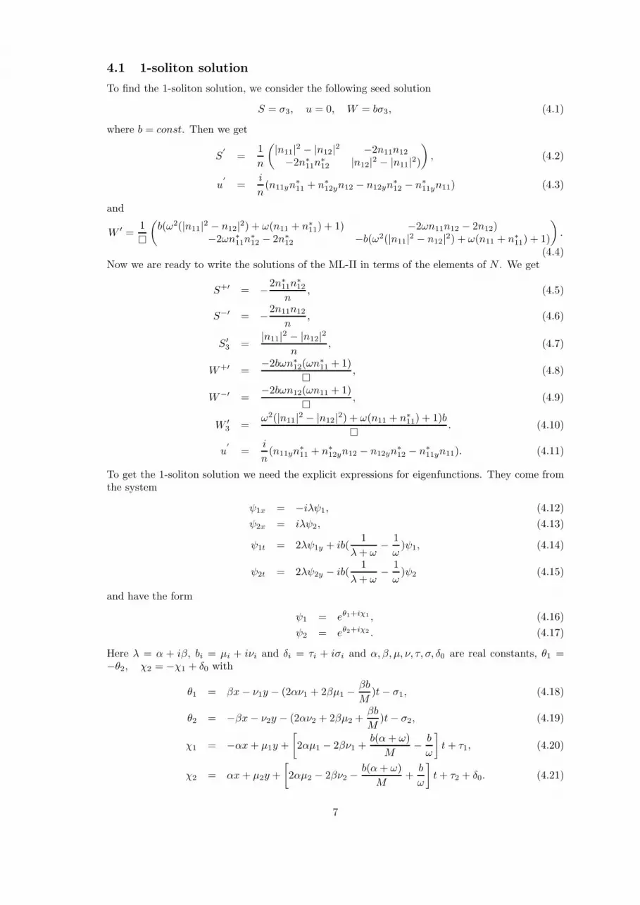
4.1 1-soliton solution

To find the 1-soliton solution, we consider the following seed solution

S = σ3, u = 0, W = bσ3, (4.1)

where b = const. Then we get

S′

=1

n

(

|n11|2 − |n12|

2 −2n11n12

−2n∗11n

∗12 |n12|

2 − |n11|2)

)

, (4.2)

u′

=i

n(n11yn

∗11 + n∗

12yn12 − n12yn∗12 − n∗

11yn11) (4.3)

and

W ′ =1

�

(

b(ω2(|n11|2 − n12|

2) + ω(n11 + n∗11) + 1) −2ωn11n12 − 2n12)

−2ωn∗11n

∗12 − 2n∗

12 −b(ω2(|n11|2 − n12|

2) + ω(n11 + n∗11) + 1)

)

.

(4.4)Now we are ready to write the solutions of the ML-II in terms of the elements of N . We get

S+′ = −2n∗

11n∗12

n, (4.5)

S−′ = −2n11n12

n, (4.6)

S′3 =

|n11|2 − |n12|

2

n, (4.7)

W+′ =−2bωn∗

12(ωn∗11 + 1)

�, (4.8)

W−′ =−2bωn12(ωn11 + 1)

�, (4.9)

W ′3 =

ω2(|n11|2 − |n12|

2) + ω(n11 + n∗11) + 1)b

�. (4.10)

u′

=i

n(n11yn

∗11 + n∗

12yn12 − n12yn∗12 − n∗

11yn11). (4.11)

To get the 1-soliton solution we need the explicit expressions for eigenfunctions. They come fromthe system

ψ1x = −iλψ1, (4.12)

ψ2x = iλψ2, (4.13)

ψ1t = 2λψ1y + ib(1

λ+ ω−

1

ω)ψ1, (4.14)

ψ2t = 2λψ2y − ib(1

λ+ ω−

1

ω)ψ2 (4.15)

and have the form

ψ1 = eθ1+iχ1 , (4.16)

ψ2 = eθ2+iχ2 . (4.17)

Here λ = α + iβ, bi = µi + iνi and δi = τi + iσi and α, β, µ, ν, τ, σ, δ0 are real constants, θ1 =−θ2, χ2 = −χ1 + δ0 with

θ1 = βx − ν1y − (2αν1 + 2βµ1 −βb

M)t− σ1, (4.18)

θ2 = −βx− ν2y − (2αν2 + 2βµ2 +βb

M)t− σ2, (4.19)

χ1 = −αx+ µ1y +

[

2αµ1 − 2βν1 +b(α+ ω)

M−b

ω

]

t+ τ1, (4.20)

χ2 = αx + µ2y +

[

2αµ2 − 2βν2 −b(α+ ω)

M+b

ω

]

t+ τ2 + δ0. (4.21)

7

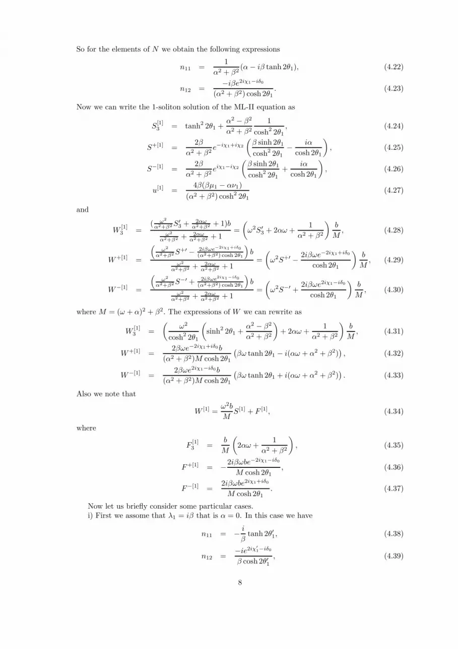
So for the elements of N we obtain the following expressions

n11 =1

α2 + β2(α− iβ tanh 2θ1), (4.22)

n12 =−iβe2iχ1−iδ0

(α2 + β2) cosh 2θ1. (4.23)

Now we can write the 1-soliton solution of the ML-II equation as

S[1]3 = tanh2 2θ1 +

α2 − β2

α2 + β2

1

cosh2 2θ1, (4.24)

S+[1] =2β

α2 + β2e−iχ1+iχ2

(

β sinh 2θ1

cosh2 2θ1−

iα

cosh 2θ1

)

, (4.25)

S−[1] =2β

α2 + β2eiχ1−iχ2

(

β sinh 2θ1

cosh2 2θ1+

iα

cosh 2θ1

)

, (4.26)

u[1] =4β(βµ1 − αν1)

(α2 + β2) cosh2 2θ1(4.27)

and

W[1]3 =

( ω2

α2+β2S′3 +

2αωα2+β2 + 1)b

ω2

α2+β2 + 2αωα2+β2 + 1

=

(

ω2S′3 + 2αω +

1

α2 + β2

)

b

M, (4.28)

W+[1] =

(

ω2

α2+β2S+′ − 2iβωe−2iχ1+iδ0

(α2+β2) cosh 2θ1

)

b

ω2

α2+β2 + 2αωα2+β2 + 1

=

(

ω2S+′ −2iβωe−2iχ1+iδ0

cosh 2θ1

)

b

M, (4.29)

W−[1] =

(

ω2

α2+β2S−′ + 2iβωe2iχ1−iδ0

(α2+β2) cosh 2θ1

)

b

ω2

α2+β2 + 2αωα2+β2 + 1

=

(

ω2S−′ +2iβωe2iχ1−iδ0

cosh 2θ1

)

b

M, (4.30)

where M = (ω + α)2 + β2. The expressions of W we can rewrite as

W[1]3 =

(

ω2

cosh2 2θ1

(

sinh2 2θ1 +α2 − β2

α2 + β2

)

+ 2αω +1

α2 + β2

)

b

M, (4.31)

W+[1] =2βωe−2iχ1+iδ0b

(α2 + β2)M cosh 2θ1

(

βω tanh 2θ1 − i(αω + α2 + β2))

, (4.32)

W−[1] =2βωe2iχ1−iδ0b

(α2 + β2)M cosh 2θ1

(

βω tanh 2θ1 + i(αω + α2 + β2))

. (4.33)

Also we note that

W [1] =ω2b

MS[1] + F [1], (4.34)

where

F[1]3 =

b

M

(

2αω +1

α2 + β2

)

, (4.35)

F+[1] = −2iβωbe−2iχ1−iδ0

M cosh 2θ1, (4.36)

F−[1] =2iβωbe2iχ1+iδ0

M cosh 2θ1. (4.37)

Now let us briefly consider some particular cases.i) First we assome that λ1 = iβ that is α = 0. In this case we have

n11 = −i

βtanh 2θ′1, (4.38)

n12 =−ie2iχ

′1−iδ0

β cosh 2θ′1, (4.39)

8

where θ′1 = θ1|α=0 and χ′1 = χ1|α=0. The corresponding 1-soliton solution takes the form

S[1]3 = tanh2 2θ′1 −

1

cosh2 2θ′1, (4.40)

S+[1] =2e−iχ′

1+iχ′2 sinh 2θ′1

cosh2 2θ′1, (4.41)

S−[1] =2eiχ

′1−iχ′

2 sinh 2θ′1cosh2 2θ′1

, (4.42)

u[1] =4µ1

cosh2 2θ′1, (4.43)

and

W[1]3 =

[

ω2

cosh2 2θ′1

(

sinh2 2θ′1 − 1)

+1

β2

]

b

M ′, (4.44)

W+[1] =2ωe−2iχ′

1+iδ0b

M ′ cosh 2θ′1(ω tanh 2θ′1 − iβ) , (4.45)

W−[1] =2ωe2iχ

′1−iδ0b

M ′ cosh 2θ′1(ω tanh 2θ′1 + iβ) . (4.46)

where M ′ = ω2 + β2.

ii) Now we consider the case λ1 = α that β = 0. Then we have

n11 =1

α, (4.47)

n12 = 0. (4.48)

Now we can write the 1-soliton solution of the ML-II equation as

S[1]3 = 1, (4.49)

S+[1] = 0, (4.50)

S−[1] = 0, (4.51)

u[1] = 0 (4.52)

and

W[1]3 =

(

ω2 + 2αω +1

α2

)

b

(ω + α)2, (4.53)

W+[1] = 0, (4.54)

W−[1] = 0. (4.55)

4.2 2-soliton solution

Now we are going to construct the 2-soliton solution of the ML-II equation. For this purpose, letus consider the following transformation

Φ[2] = L2Φ[1], (4.56)

where we assume that

L2 = λN [2] − I (4.57)

with

N [2] =

(

n[1]11 n

[1]12

−n[1]∗12 n

[1]∗11

)

. (4.58)

9

Here Φ[j] satisfy the systems

Φ[2]x = U [2]Φ[2], (4.59)

Φ[2]t = 2λΦ[2]

y + V [2]Φ[2] (4.60)

and

Φ[1]x = U [1]Φ[1], (4.61)

Φ[1]t = 2λΦ[1]

y + V [1]Φ[1]. (4.62)

The matrix L[2] obeys the following equations

L2x + L2U[1] = U [2]L2, (4.63)

L2t + L2V[1] = 2λL2y + V [2]L2. (4.64)

In terms of eigenfunctions, the matrix N [2] takes the form

N [2] =1

∆[1]

(

λ−13 |ψ

[1]1 |2 + λ−1

4 |ψ[1]2 |2 (λ−1

3 − λ−14 )ψ

[1]1 ψ

[1]∗2

(λ−13 − λ−1

4 )ψ[1]∗1 ψ

[1]2 λ−1

3 |ψ[1]2 |2 + λ−1

4 |ψ[1]1 |2)

)

, (4.65)

where λ4 = λ∗3. To find elements of Φ[1] we use the one-fold DT saying the formula

Φ[1] = L1Φ[0]. (4.66)

Here

Φ[0] =

(

ψ1(λ1) −ψ∗2(λ1)

ψ2(λ1) ψ∗1(λ1)

)

(4.67)

and

L1 =

(

λn11(λ1)− 1 λn12(λ1)−λn∗

12(λ1) λn∗11(λ1)− 1

)

. (4.68)

So we finally have

Φ[1] =

(

(λn11 − 1)ψ1 + λn12ψ2 −(λn11 − 1)ψ∗2 + λn12ψ

∗1

−λn∗12ψ1 + (λn∗

11 − 1)ψ2 λn∗12ψ

∗2 + (λn∗

11 − 1)ψ∗1

)

=

(

ψ[1]1 −ψ

[1]∗2

ψ[1]2 ψ

[1]∗1

)

. (4.69)

Here

ψ[1]1 =

(α3 + iβ3)eiχ1

α21 + β2

1

[(

α1 − iβ1 tanh 2θ1 −α21 + β2

1

α3 + iβ3

)

eθ1 −iβ1e

−θ1

cosh 2θ1

]

, (4.70)

ψ[1]2 =

(α3 + iβ3)e−iχ1+iδ0

α21 + β2

1

[(

α1 + iβ1 tanh 2θ1 −α21 + β2

1

α3 + iβ3

)

e−θ1 −iβ1e

θ1

cosh 2θ1

]

, (4.71)

∆[1] =2(α3 + iβ3)

2 cosh 2θ1(α2

1 + β21)

2

(

A+β21

cosh2 2θ1

)

. (4.72)

10

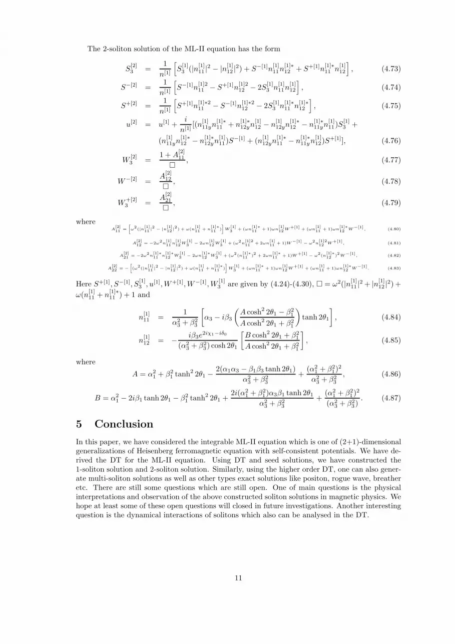
The 2-soliton solution of the ML-II equation has the form

S[2]3 =

1

n[1]

[

S[1]3 (|n

[1]11 |

2 − |n[1]12 |

2) + S−[1]n[1]11n

[1]∗12 + S+[1]n

[1]∗11 n

[1]12

]

, (4.73)

S−[2] =1

n[1]

[

S−[1]n[1]211 − S+[1]n

[1]212 − 2S

[1]3 n

[1]11n

[1]12

]

, (4.74)

S+[2] =1

n[1]

[

S+[1]n[1]∗211 − S−[1]n

[1]∗212 − 2S

[1]3 n

[1]∗11 n

[1]∗12

]

, (4.75)

u[2] = u[1] +i

n[1][(n

[1]11yn

[1]∗11 + n

[1]∗12yn

[1]12 − n

[1]12yn

[1]∗12 − n

[1]∗11yn

[1]11)S

[1]3 +

(n[1]11yn

[1]∗12 − n

[1]∗12yn

[1]11)S

−[1] + (n[1]12yn

[1]∗11 − n

[1]∗11yn

[1]12)S

+[1]], (4.76)

W[2]3 =

1 +A[2]11

�, (4.77)

W−[2] =A

[2]12

�, (4.78)

W+[2]3 =

A[2]21

�, (4.79)

whereA

[2]11

=

[

ω2(|n

[1]11

|2

− |n[1]12

|2) + ω(n

[1]11

+ n[1]∗11

)

]

W[1]3

+ (ωn[1]∗11

+ 1)ωn[1]12

W+[1]

+ (ωn[1]11

+ 1)ωn[1]∗12

W−[1]

, (4.80)

A[2]12

= −2ω2n[1]11

n[1]12

W[1]3

− 2ωn[1]12

W[1]3

+ (ω2n[1]211

+ 2ωn[1]11

+ 1)W−[1] − ω2n[1]212

W+[1]

, (4.81)

A[2]21 = −2ω

2n[1]∗11 n

[1]∗12 W

[1]3 − 2ωn

[1]∗12 W

[1]3 + (ω

2(n

[1]∗11 )

2+ 2ωn

[1]∗11 + 1)W

+[1]− ω

2(n

[1]∗12 )

2W

−[1], (4.82)

A[2]22 = −

[

(ω2(|n

[1]11 |

2− |n

[1]12 |

2) + ω(n

[1]11 + n

[1]∗11 )

]

W[1]3 + (ωn

[1]∗11 + 1)ωn

[1]12W

+[1]+ (ωn

[1]11 + 1)ωn

[1]∗12 W

−[1]. (4.83)

Here S+[1], S−[1], S[1]3 , u[1],W+[1],W−[1],W

[1]3 are given by (4.24)-(4.30), � = ω2(|n

[1]11 |

2 + |n[1]12 |

2) +

ω(n[1]11 + n

[1]∗11 ) + 1 and

n[1]11 =

1

α23 + β2

3

[

α3 − iβ3

(

A cosh2 2θ1 − β21

A cosh2 2θ1 + β21

)

tanh 2θ1

]

, (4.84)

n[1]12 = −

iβ3e2iχ1−iδ0

(α23 + β2

3) cosh 2θ1

[

B cosh2 2θ1 + β21

A cosh2 2θ1 + β21

]

, (4.85)

where

A = α21 + β2

1 tanh2 2θ1 −

2(α1α3 − β1β3 tanh 2θ1)

α23 + β2

3

+(α2

1 + β21)

2

α23 + β2

3

, (4.86)

B = α21 − 2iβ1 tanh 2θ1 − β2

1 tanh2 2θ1 +

2i(α21 + β2

1)α3β1 tanh 2θ1α23 + β2

3

+(α2

1 + β21)

2

(α23 + β2

3). (4.87)

5 Conclusion

In this paper, we have considered the integrable ML-II equation which is one of (2+1)-dimensionalgeneralizations of Heisenberg ferromagnetic equation with self-consistent potentials. We have de-rived the DT for the ML-II equation. Using DT and seed solutions, we have constructed the1-soliton solution and 2-soliton solution. Similarly, using the higher order DT, one can also gener-ate multi-soliton solutions as well as other types exact solutions like positon, rogue wave, breatheretc. There are still some questions which are still open. One of main questions is the physicalinterpretations and observation of the above constructed soliton solutions in magnetic physics. Wehope at least some of these open questions will closed in future investigations. Another interestingquestion is the dynamical interactions of solitons which also can be analysed in the DT.

11

References

[1] Gutshabash E. Sh. On some set of models of magnets and chiral fields: integrability, Darbouxtransformation and exact solutions. Zapiski nauqnyh seminarov POMI, 269, 164-179 (2000)

[2] Nian-Ning Huang, Bing Xu. Darboux Tranformation Method for Finding Soliton Solutions ofthe Landau-Lifshitz Equation of a Classical Heisenberg Spin Chain, Commun. Theor. Phys.,12, 121-126 (1989).

[3] U. Saleem, M. Hasan. Quasideterminant solutions of the generalized Heisenberg magnet modelJ. Phys. A: Math. Theor., 43, 045204 (2010). [arXiv:0912.5030]

[4] Chen Chi, Zhou Zi-Xiang. Darboux Tranformation and Exact Solutions of the Myrzakulov-IEquations. Chin. Phys. Lett., 26, N8, 080504 (2009)

[5] Zh. Kh. Zhunussova, K. R. Yesmakhanova, D. I. Tungushbaeva, G. K. Mamyrbekova, G. N.Nugmanova, R. Myrzakulov. Integrable Heisenberg Ferromagnet Equations with self-consistentpotentials. [arXiv:1301.1649]

[6] R.Myrzakulov, G. K. Mamyrbekova, G. N. Nugmanova, M. Lakshmanan. Integrable (2+1)-dimensional spin models with self-consistent potentials. [arXiv:1305.0098]

[7] G. Shaikhova, K. Yesmakhanova, G. Mamyrbekova, R. Myrzakulov. Darboux tran-formation and solutions of the (2+1)-dimensional Schrodinger-Maxwell-Bloch equation,[arXiv:1402.4669]

[8] R. Myrzakulov, G. K. Mamyrbekova, G.N. Nugmanova, K.R.Yesmakhanova, M. Lakshmanan.Integrable Motion of Curves in Self-Consistent Potentials : Relation to Spin Systems andSoliton Equations, [arXiv:1404.2088]

[9] Z.S. Yersultanova, M. Zhassybayeva, G. Mamyrbekova, G. Nugmanova, R. Myrzakulov. Dar-boux Transformation and Exact Solutions of the integrable Heisenberg ferromagnetic equationwith self-consistent potentials, [arXiv:1404.2270]

[10] K. Yesmakhanova, G. Shaikhova, K. Zhussupbekov, R. Myrzakulov. The (2+1)-dimensional Hirota-Maxwell-Bloch equation: Darboux transformation and soliton solutions,[arXiv:1404.5613]

[11] J.-S. He, Y. Cheng, Y.-S. Li. Commun. Theor. Phys., 38, 493-496 (2002).

[12] M. Lakshmanan, Phil. Trans. R. Soc. A, 369 1280-1300 (2011).

[13] M. Lakshmanan, Phys. Lett. A A 53-54 (1977).

[14] L.A. Takhtajan, Phys. Lett. A 64 235-238 (1977).

[15] C. Senthilkumar, M. Lakshmanan, B. Grammaticos, A. Ramani, Phys. Lett. A 356 339-345(2006).

[16] Y. Ishimori, Prog. Theor. Phys. 72 33 (1984).

[17] R. Myrzakulov, S. Vijayalakshmi, G. Nugmanova , M. Lakshmanan Physics Letters A, 233 ,14-6, 391-396 (1997).

[18] R. Myrzakulov, S. Vijayalakshmi, R. Syzdykova, M. Lakshmanan, J. Math. Phys., 39, 2122-2139 (1998).

[19] R. Myrzakulov, M. Lakshmanan, S. Vijayalakshmi, A. Danlybaeva , J. Math. Phys., 39,3765-3771 (1998).

[20] Myrzakulov R, Danlybaeva A.K, Nugmanova G.N. Theoretical and Mathematical Physics,V.118, 13, P. 441-451 (1999).

12

[21] Myrzakulov R., Nugmanova G., Syzdykova R. Journal of Physics A: Mathematical & Theo-retical, V.31, 147, P.9535-9545 (1998).

[22] Myrzakulov R., Daniel M., Amuda R. Physica A., V.234, 13-4, P.715-724 (1997).

[23] Myrzakulov R., Makhankov V.G., Pashaev O.. Letters in Mathematical Physics, V.16, N1,P.83-92 (1989)

[24] Myrzakulov R., Makhankov V.G., Makhankov A. Physica Scripta, V.35, N3, P. 233-237 (1987)

[25] Myrzakulov R., Pashaev O.., Kholmurodov Kh. Physica Scripta, V.33, N4, P. 378-384 (1986)

[26] Anco S.C., Myrzakulov R. Journal of Geometry and Physics, v.60, 1576-1603 (2010)

[27] Myrzakulov R., Rahimov F.K., Myrzakul K., Serikbaev N.S. On the geometry of stationaryHeisenberg ferromagnets. In: ”Non-linear waves: Classical and Quantum Aspects”, KluwerAcademic Publishers, Dordrecht, Netherlands, P. 543-549 (2004)

[28] Myrzakulov R., Serikbaev N.S., Myrzakul Kur., Rahimov F.K. On continuous limits of somegeneralized compressible Heisenberg spin chains. Journal of NATO Science Series II. Mathe-matics, Physics and Chemistry, V 153, P. 535-542 (2004)

[29] Myrzakulov R., Martina L., Kozhamkulov T.A., Myrzakul Kur. Integrable Heisenberg ferro-magnets and soliton geometry of curves and surfaces. In book: ”Nonlinear Physics: Theoryand Experiment. II”. World Scientific, London, P. 248-253 (2003)

[30] Myrzakulov R. Integrability of the Gauss-Codazzi-Mainardi equation in 2+1 dimensions. In”Mathematical Problems of Nonlinear Dynamics”, Proc. of the Int. Conf. ”Progress in Non-linear sciences”, Nizhny Novgorod, Russia, July 2-6, 2001, V.1, P.314-319 (2001)

[31] Zhao-Wen Yan, Min-Ru Chen, Ke Wu, Wei-Zhong Zhao. J. Phys. Soc. Jpn., 81, 094006 (2012)

[32] Yan Zhao-Wen, Chen Min-Ru, Wu Ke, Zhao Wei-Zhong. Commun. Theor. Phys., 58, 463-468(2012)

[33] K.R. Esmakhanova, G.N. Nugmanova, Wei-Zhong Zhao, Ke Wu. Integrable inhomogeneousLakshmanan-Myrzakulov equation, [nlin/0604034]

[34] Zhen-Huan Zhang, Ming Deng, Wei-Zhong Zhao, Ke Wu. On the integrable inhomogeneousMyrzakulov-I equation, [nlin/0603069]

[35] Martina L, Myrzakul Kur., Myrzakulov R, Soliani G. Journal of Mathematical Physics, V.42,13, P.1397-1417 (2001).

13