Embed Size (px)
Citation preview
Published in Optical Review, vol. 3, no. 4 (1996) - this is a draft version
Cross Absolute Filter for removing speckle noisefrom interference patterns
Jacek Mandziuk1, Christophe Gorecki2 and Bohdan Macukow1
1Faculty of Mathematics and Information Science,
Warsaw University of Technology,
Plac Politechniki 1, 00-661 Warsaw, Poland.2Laboratoire d’Optique P.M. Duffieux, (URA CNRS 214)
Universite de Franche-Comte, Route de Gray,
25030 Besancon cedex, France.
Abstract
A new algorithm for speckle noise removal from interference patterns is proposed.
The method, called Cross Absolute Filter (CAF), is especially well suited to the case
of noisy interferograms with phase error pixels. Extensive computer simulations per-
formed on both digitally generated fringes and experimental data show that CAF
performs better than classical median-type filters, preserving more subtle details.
Keywords - interferometry, speckle smoothing, non-linear filter, neural network,
median filter.
1 Introduction
In interferometry, the period and phase of fringe pattern are the parameters of in-
terest, since they allow direct relationship between optical path lengths with the
wavelength of the illuminating light. A linear change in phase of one wavefront of
an interferometer introduces a variation of sinusoidal form in intensity at locations
of interference fringes. The change in intensity at any pixel location can be used to
compute the interferometric value at that pixel with high resolution. However, in
many applications the efficiency of this technique is limited because the original in-
terference data have often poor contrast and in the case of laser illumination they are
noisy due to speckle effects. This random granular structure is formed when coher-
ent light is scattered or transmitted through an optically rough surface or a medium
with random refractive index fluctuations. The structure of speckle patterns is highly
complex. It depends on the coherence properties of the illuminating incident beam
and also on the surface characteristics of the illuminated rough object.
The speckle phenomenon can be considered as resulting from a sum of contribu-
tions from elementary scattering areas on the rough surface called scatterers. The
following experimental assumptions about the contributions from elementary scatter-
ers are made 7):
- the scatterers are independent of each other and introduce phase fluctuations
larger than 2π,
- a large number of scatterers contribute to the speckle pattern at any point on
the observation plane. It can be shown that the intensity at a given point, has a
negative exponential probability density function, and
- the scattering medium does not depolarize the coherent light.
In order to measure the phase of a static wavefront using standard phase-shifting
techniques, phase extraction from an interferogram must be interpolated between
fringe minima and maxima with a resolution better than 1100
of the fringe separation.
The speckle noise is a main source of random errors in phase-shifting interferometry
(PSI), and one of goals that should be taken is to suppress it. PSI is currently
used to nondestructively determine the shape of specular objects or wavefronts by
calculating a phase map from the measured intensities 3). The phase of one arm
of the interferometer is shifted with respect to the other. The phase of the test
wavefront relative to the reference wavefront is computed from the interference data
measured for multiple phase shifts. The phase-shifting algorithms firstly calculate the
phase modulo π. The 2π ambiguities are removed by adding or subtracting 2π from
individual pixels until the phase difference between adjacent pixels is < π. When
this technique is applied, the randomness of the speckles causes noisy data points. If
there are bad pixels, the phase errors can transform that from one pixel to the next
pixel, and the phase may jump by 2π and then jump back.
Several digital image processing techniques using computer facilities were devel-
oped to reduce speckle noise. So far the most popular filter is Gaussian smoothing 2).
Many specific linear methods are used for removing speckle noise: gray scale modifi-
cation, low-pass filtering, short space spectral subtraction technique, frame averaging,
etc... 9). In general the linear filters have good noise attenuation capability, but can
attenuate and disturb thin lines present in the original interference pattern because
of the linear averaging operation that they perform. Such filters are simple and fast,
but they will fail in critical applications because of image blurring. On the other
hand, non-linear filtering is a well-known noise filtering and edge-preserving method.
These techniques often perform a local filtering in which each pixel is replaced by a
value obtained through a ”non-linear” operation performed within a window which
refers to a neighborhood of the pixel 6). One technique which has been particularly
successful in reducing speckle noise is median filter, widely used in association with
phase-shifting methods 4). The median filter is very efficient in bad data points, but
does not change the pixel value where the phase error is present.
In order to smooth data point where the phase is slightly off and to preserve edges
as well, we have developed another new processing routine called CAF. Discussion on
the theoretical basis of the proposed filter is given and its performance is illustrated
and compared with these of two different conventional median-type filters.
It will be demonstrated that the CAF routine is essentially a parallel algorithm,
which can operate very well on details of a certain size without affecting, for example,
fringe edges that share some of the same spatial frequency. Almost all optoelectronic
processors applied to morphological and filtering operations present a similar ap-
proach 10,12). Consequently, the future opportunity of optical implementation of the
CAF algorithm will be discussed in the last Section.
2 CAF - algorithm description
CAF algorithm works iteratively and synchronously (all pixels are updated simulta-
neously) and after each iteration the interference pattern has less noise and the noise
is, in average, of less strength. At each iteration the new value for every pixel is
calculated based on the values of pixels in four directions in the pixel’s neighborhood
(lattice points). The size of the neighborhood as well as the number of iterations are
adjustable and have to be defined a priori. The general idea of the algorithm is based
on the two following principles:
α) if the absolute difference between the pixel’s value and the mean values of
the pixels in at least three of directions in the pixel’s neighborhood is less than a
predefined threshold value, then the pixel is treated as the appropriate one and its
value remains unchanged,
β) if the absolute difference between the pixel’s value and the mean values of the
pixels in at least two of directions in the pixel’s neighborhood is greater or equal
than a threshold value, then the pixel is treated as the wrong one and its value is
changed.
The new value of the pixel is equal to the mean value among those pixels that
belong to these and only these directions which mean values were different (in absolute
difference) from the pixel’s value by at least the threshold value. Since the massive
parallelism of the proposed algorithm permits an analogy with optical approach of the
filtering operation as well as to neural networks processing techniques, we will here
use the general term - ”processing element (pe.)” - instead of ”convolution element”
or ”neuron”.
Condition α means that the pixel is surrounded in at least three specified direc-
tions by pixels with similar intensity of gray, whereas β denotes the cases in which
ether the pixel ”stands out” in exactly one direction or is significantly different from
all its neighbors (in the specified directions).
Input parameters for the algorithm are established a priori and are not being
changed through the whole simulation test. These parameters should be chosen based
on some amount of preliminary tests or by using any additional information concern-
ing the nature of patterns to be processed - mainly their shape, size of speckles, fringe
contrast as well as the signal-to-noise ratio. The input for a simulation test is defined
by:
- size of a neighborhood (common for all pe.’s) - denoted by N . This parameter defines
the smoothing window and is strongly dependent on the average size of speckles;
- number of iterations - denoted by n;
- threshold value (common for all pe.’s) - denoted by T .
The last two parameters are close to the signal-to-noise ratio of interference pat-
terns and the presence on nonlinearities which can appear due to the bad data points.
Let us consider a single pe. corresponding to pixel (x, y) on a square interferogram
of size S × S, and let V be a square matrix S × S representing present pixel’s values
(levels of gray), i.e. integers from interval < 0, 255 >. Value of pixel (x, y) for x, y < S
will be denoted by Vx,y.
Note 1
A square matrix (pattern) is used only to simplify the notation. The generaliza-
tion to rectangle shape is obvious.
At the beginning matrix V represents a real interference pattern and changes
gradually during the iteration test. Since V depends on the iteration number, it
should - to be more precise - be denoted by V (t) where t denotes time (the iteration
number). Dependence on time is omitted for simplification - instead the number of
iteration is clearly indicated by a context.
Moreover, henceforth indices R, L, U and D will always denote directions: Right,
Left, Up and Down, respectively. In particular the term
∀ i ∈ {R, L, U,D} Θi
will denote the fact that function or value Θ is counted separately in four directions.
In other words, the above term is equivalent to
ΘR and ΘL and ΘU and ΘD

In each iteration of a simulation test, there are calculated the following auxiliary
mean values:
MR(x, y)def=
1
LMR
i=N∑i=1
x+i≤S
Vx+i,y ML(x, y)def=
1
LML
i=N∑i=1x>i
Vx−i,y
MU(x, y)def=
1
LMU
i=N∑i=1y>i
Vx,y−i MD(x, y)def=
1
LMD
i=N∑i=1
y+i≤S
Vx,y+i
where LMR, LML
, LMUand LMD
denote numbers of items that fulfil index requirements
under sum signs in respective equations.
Then, for each above defined mean value it is checked whether it differs or not
from the pe.’s value by more than a threshold value, i.e. the following four auxiliary
Boolean variables are set:
∀ i ∈ {R, L, U,D} Bi(x, y) =
{1 if ABS(Mi(x, y)− Vx,y) > T
0 in the opposite case
Denoting by Z(x, y) the set of indices (directions) for which Boolean variables Bi
are set to 1 and by | Z(x, y) | the cardinality of Z(x, y), i.e.
Z(x, y)def= {i ∈ {R, L, U,D} : Bi(x, y) = 1}
a new value V ′x,y for pe. (x, y) is defined as below
V ′x,y =
Vx,y if | Z(x, y) |= 0, 1
1|Z(x,y)|
∑
i∈Z(x,y)
Mi(x, y) if | Z(x, y) |= 2, 3, 4
3 Computer simulation results
Quality of the algorithm has been checked by comparing the results of extensive
computer simulations of CAF with the results obtained for the two versions of a well
known method called the Median Filter 11).
Let us very briefly recall a general idea of the parallel Median Filter method:
Cross Median Filter (CMF): at each iteration, for each pixel (x, y) the middle (not
arithmetic mean) value is found among the following values: pixel (x, y), NC pixels
to the left, right, up and down of pixel (x, y) (totally 4NC + 1 values are taken into
account).
Square Median Filter (SMF): at each iteration, for each pixel (x, y) the middle value
among values in all lattice points belonging to the square of a center in (x, y) and
edges of length 2NS + 1 (totally (2NS + 1)2 pixels) is found.

(a) input pattern (b) CAF output
(c) CMF output (d) SMF output
Figure 1: Case 1)
Computer software was written with Visual C++ compiler and run on a se-
quential PC 386/33 (parallelism of the methods was implemented in software, not in
hardware).
The input data, i.e. interference patterns, were obtained either from interferomet-
ric device by interferometric fringe projection technique, or from computer program
which simulated interference fringes with speckle noise.
In both cases fringes were of various periods and inclinations, and the noise was
of various average sizes.
In the experimental case, fringes were either linear or linear with parabolic incli-
nation due to the deformations of the thin-film silicon membrane, measured by the
projection fringe method 13). The bulging membrane, initially flat and unstressed

(a) input pattern (b) CAF output
(c) CMF output (d) SMF output
Figure 2: Case 1) binarized
(linear fringes), involves the fringe deformations (parabolic shape). In fact the last,
mixed case was of our main interest. Since the membrane is under coherent illu-
mination (Argon laser) a speckle phenomenon appears due to the Silicon roughness
properties. In the case of computer simulated interference data, we assumed that the
speckle is produced by adding independent gaussian random variables computed in
the same manner as in 8). First, a random phase of a light scattering object is sim-
ulated. Then, a speckle pattern is generated by a 256x256 point 2-D FFT algorithm
with the possibility of choice of the speckle average size. Finally, the speckle pattern
is added to the interference fringes. Computer simulated fringes were linear, however
the inclination angle varied from horizontal, through diagonal up to vertical.
The performance of CAF will be presented on three 256x256x8 bits range images

(a) input pattern (b) CAF output
(c) CMF output (d) SMF output
Figure 3: Case 2)
of interference patterns, henceforth referred as 1), 2) and 3). In case 1), fringes were
taken experimentally from interferometric device in absence of membrane deformation
- their shape was linear in vertical direction. In case 2), fringes simulated on computer
were of linear shape at the inclination of 45 degrees. At last, in case 3), fringes were
originated like in 1), but since the membrane was under stress - their shape presented
a parabolic deformation in the center of the image.
The set of data chosen for presentation of results represents various cases of the
shape and orientation of fringes and sizes of speckle. Algorithm parameters were
established based on some amount of preliminary tests performed for that reason.
Finally, the parameters (common for all three cases) were set as below:

N = 2, n = 10, T = 5, NC = NS = 4
The above choice of parameters allowed efficient performance of the methods on
one side, and guaranteed that simulations be finished in a reasonable time (this espe-
cially concerns the SMF method). More precisely, for NC and NS greater than 4 the
time evaluation of one test becomes significantly longer without visible improvement
of results. In fact, the neighborhood in CMF and SMF (and also in CAF) cannot be
extended beyond a ”reasonable” value depending mostly on the nature and parame-
ters of speckles. On the other hand, choosing the neighborhood too small, lessens the
effectiveness of any of the three methods.
Before the detailed analysis of results, let us state two general, introductory
remarks.
(i) Binarized versions of full grayscale patterns (see descriptions of figs. 2, 4, 6)
were calculated by thresholding patterns at level 128 of grey, i.e. by applying the
following function:
f(x) =
{0 for 0 ≤ x ≤ 127
1 for 128 ≤ x ≤ 255
(ii) On the output patterns, due to the nature of filters, picks are smoothed, i.e.
values near zero and 1 are replaced by more ”middle” values. This situation can be
observed especially for CAF. In fact, application of CAF requires some postprocessing
techniques allowing extension of the output pattern to the full grayscale. However,
for checking the quality of the algorithm more important is the shape of a plot across
the pattern (which should resemble the sin function), rather than exact pixels’ values.
Case 1)
In case of linear input fringes (Fig. 1a), CAF performs very well (Fig. 1b). The
results are slightly better than that for SMF (Fig. 1d) and visibly better than that
for CMF (Fig. 1c). On binarized versions of output patterns the improvement made
by CAF (Fig. 2b) is certainly better than that of SMF (Fig. 2d). However, in the
top of the patterns both algorithms ”lost” fringes because of low contrast of fringes
on the input pattern. The worst is the result of applying CMF (Fig. 2c).
Case 2)
In case of input pattern simulated on the computer (Fig. 3a), the CAF algorithm
is very efficient - nearly all noise is cut out (Fig. 3b). The result is much better
than the result obtained with the CMF (Fig. 3c), and comparably good as the one
obtained with SMF (Fig. 3d). The same observation can be made when comparing
binary versions of grayscale results (Figs. 4b− d, resp.).
Case 3)

(a) input pattern (b) CAF output
(c) CMF output (d) SMF output
Figure 4: Case 2) binarized
The performance of the CAF algorithm is also very good in this case, and most
of the noise is smoothed (Fig. 5b). The result is significantly better than the one
obtained for CMF (Fig. 5c) and better than the result of applying SMF (Fig. 5d).
The differences of quality among the algorithms are enhanced on binarized images.
On the input image processed by CAF (Fig. 6b) there is almost no speckles, whereas
there are some of them on the SMF (Fig. 6d) pattern, and many more on the pattern
processed with CMF (Fig. 6c).
The main difference can be seen in the parts of fringe pattern that present par-
abolic deformations, especially in the parts where curvature and linear zones are
connected to each other. In these zones the phase distribution presents significant
slopes and the probability of presence of bad pixels (phase error) is strong. By use of

(a) input pattern (b) CAF output
(c) CMF output (d) SMF output
Figure 5: Case 3)
CAF routine, the jumps and creases have been preserved while the curvature zone has
been smoothed, and the irregularities present in the original image have disappeared.
In that places CMF works poor, SMF is much better but still worst than CAF.
The results indicate that the CAF filter is more effective than median filter in
reducing both the effects of discrete impulse noise (Fig. 3a) and smoothly generated
noise (Figs. 1a and 5a).
Generally speaking, input patterns were full of noise and such unexpectedly good
improvement after applying CAF is worth further research. Very noisy patterns were
transformed to patterns with very little noise (in binarized patterns speckles are
smoothed).
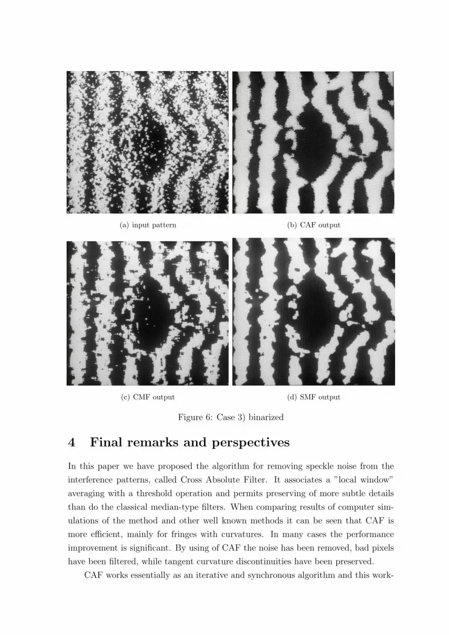
(a) input pattern (b) CAF output
(c) CMF output (d) SMF output
Figure 6: Case 3) binarized
4 Final remarks and perspectives
In this paper we have proposed the algorithm for removing speckle noise from the
interference patterns, called Cross Absolute Filter. It associates a ”local window”
averaging with a threshold operation and permits preserving of more subtle details
than do the classical median-type filters. When comparing results of computer sim-
ulations of the method and other well known methods it can be seen that CAF is
more efficient, mainly for fringes with curvatures. In many cases the performance
improvement is significant. By using of CAF the noise has been removed, bad pixels
have been filtered, while tangent curvature discontinuities have been preserved.
CAF works essentially as an iterative and synchronous algorithm and this work-
ing mode is well suited to optoelectronic implementations because of the inherent
parallelism of optical processors. Filtering of fringe patterns, performed in real-time,
is very easy to implement optically if the filtering operation performed optically is
only linear (without the threshold). The association of this linear operation with a
threshold operation leads to nonlinear operations. The thresholding can be imple-
mented electronically by use of spatial light modulators (SLMs). Almost all available
optoelectronic processors are based on correlator architecture. They perform a con-
volution between an input element and a structuring element 5,1). The output of this
convolution is often thresholded by the use of SLMs. Due of the limited resolution
and contrast of commercially available SLMs, this approach is not presently compet-
itive with fully digital implementation, especially in the case of grey level images.
However, this situation may be expected to change with continuing advances in SLM
development.
Acknowledgement
Jacek Mandziuk was supported in this work by Robert Schuman Foundation, Paris.
Results were obtained on leave at Laboratoire d’Optique P.M. Duffieux, Besancon,
France.
References
1) D. Casasent, R. Schaefer and R. Sturgil: ”Optical hit-miss morphological trans-
form”, Appl. Optics, 31 ,No. 29, (1992), p. 6255-6263.
2) J.C. Chen and G. Medioni: ”Adaptive smoothing: principles and applications”,
Advances in Image Analysis, eds. Y. Mahdavieh and R.C. Gonzalez (SPIE Publica-
tion, Bellingham, 1992), p. 13-54.
3) K. Creath: ”Phase-measuring interferometry techniques”, Progress in Optics, ed.
E.Wolf, (Elsevier Publishers, Amsterdam, 1988) Vol. XXVI, p. 349-393.
4) K. Creath: ”Phase-shifting speckle interferometry”, Appl. Optics, 24, No. 18,
(1985), p. 3053-3058.
5) A. Fedor and O. Freeman: ”Optical multiscale morphological processor using a
complex-valued kernel”, Appl. Optics 31, No. 20, (1992), p. 4042-4050.
6) Y.S. Fong, C.A. Pomalaza-Raez and X.-H. Wang: ”Comparison study of nonlinear
filters in image processing applications”, Opt. Engineering 28, No. 7, (1988), p.

749-760.
7) J.W. Goodman: ”Statistical properties of laser speckle patterns”, Laser Speckle
and Related Phenomena, ed. J.C. Dainty, (Topics in Applied Physics 9, Springer-
Verlag, 1975), p. 9-75.
8) J. M. Huntley: ”Speckle photography fringe analysis: assessment of current algo-
rithms”, Appl. Optics 28 (1989), p. 4316-4322.
9) J.S. Lim and H. Nawab: ”Techniques for speckle noise removal”, Opt. Engineering
20, No. 3, (1981), p. 472-480.
10) E. Ochoa, J.P. Allebach and D.W. Sweeney, ”Optical median filtering using
threshold decomposition”, Appl. Optics 26, No. 2, (1987), p. 252-260.
11) W.K. Pratt: Digital Image Processing, (J. Wiley & Sons, New York, 1978).
12) T. Szoplik, J. Garcia and C. Ferreira: ”Rank-order and morphological enhance-
ment of image details with an optoelectronic processor”, Appl. Optics 34, No. 2,
(1995), p. 267-275.
13) G. Tribillon, B. Trolard, P. Delobelle, E. Bonnotte and L. Bornier: ”Optical
methods for the characterization of mechanical properties of thin films”, Proc. SPIE,
2248, (1995), p.198-209.


