Cronin 2010 Hierarch Bayes Markov Chain Analysis

103:591-602, 2010. First published Nov 4, 2009; doi:10.1152/jn.00379.2009 J NeurophysiolBeau Cronin, Ian H. Stevenson, Mriganka Sur and Konrad P. Körding

You might find this additional information useful...

for this article can be found at: Supplemental material http://jn.physiology.org/cgi/content/full/00379.2009/DC1

44 articles, 14 of which you can access free at: This article cites http://jn.physiology.org/cgi/content/full/103/1/591#BIBL

including high-resolution figures, can be found at: Updated information and services http://jn.physiology.org/cgi/content/full/103/1/591

can be found at: Journal of Neurophysiologyabout Additional material and information http://www.the-aps.org/publications/jn

This information is current as of January 11, 2010 .

http://www.the-aps.org/.American Physiological Society. ISSN: 0022-3077, ESSN: 1522-1598. Visit our website at (monthly) by the American Physiological Society, 9650 Rockville Pike, Bethesda MD 20814-3991. Copyright © 2005 by the

publishes original articles on the function of the nervous system. It is published 12 times a yearJournal of Neurophysiology

on January 11, 2010 jn.physiology.org

Dow

nloaded from

http://jn.physiology.org/cgi/content/full/00379.2009/DC1

http://jn.physiology.org/cgi/content/full/103/1/591#BIBL

http://jn.physiology.org/cgi/content/full/103/1/591

http://www.the-aps.org/publications/jn

http://www.the-aps.org/

http://jn.physiology.org

Innovative Methodology

Hierarchical Bayesian Modeling and Markov Chain Monte Carlo Samplingfor Tuning-Curve Analysis

Beau Cronin,1,* Ian H. Stevenson,2,* Mriganka Sur,1 and Konrad P. Kording2

1Department of Brain and Cognitive Sciences, Picower Institute for Learning and Memory, Massachusetts Institute of Technology,Cambridge, Massachusetts; and 2Department of Physiology, Rehabilitation Institute of Chicago, Northwestern University, Chicago, Illinois

Submitted 29 April 2009; accepted in final form 31 October 2009

Cronin B, Stevenson IH, Sur M, Kording KP. Hierarchical Bayes-ian modeling and Markov chain Monte Carlo sampling for tuning-curve analysis. J Neurophysiol 103: 591–602, 2010. First publishedNovember 4, 2009; doi:10.1152/jn.00379.2009. A central theme ofsystems neuroscience is to characterize the tuning of neural responsesto sensory stimuli or the production of movement. Statistically, weoften want to estimate the parameters of the tuning curve, such aspreferred direction, as well as the associated degree of uncertainty,characterized by error bars. Here we present a new sampling-based,Bayesian method that allows the estimation of tuning-curve parame-ters, the estimation of error bars, and hypothesis testing. This methodalso provides a useful way of visualizing which tuning curves arecompatible with the recorded data. We demonstrate the utility of thisapproach using recordings of orientation and direction tuning inprimary visual cortex, direction of motion tuning in primary motorcortex, and simulated data.

I N T R O D U C T I O N

A primary goal of many neuroscience experiments is tounderstand the relationship between the firing properties of aneuron and a single external variable. For sensory neurons, thisexternal variable is typically a property of the stimulus, such asthe orientation of a bar or a grating (cf. Hubel and Wiesel 1959,1962). For motor neurons, this external variable typically refersto a property of the executed movement, for example thedirection of hand movement (e.g., Georgopoulos et al. 1986).The relationship between the external variable and the firingrate, the tuning curve (see Fig. 1A), is one of the mostfrequently used tools to describe the response properties ofneurons.

In these experiments, researchers often wish to answerquestions such as the following. (1) Is the recorded neuronselective for the stimulus property in question? For example, anumber of studies have asked what percentage of neurons invisual cortex are tuned to orientation (e.g., Maldonado et al.1997; Ohki et al. 2005). 2) If the neuron is selective, how canits selectivity be described quantitatively? For example, manystudies describe how well a neuron is tuned to the orientationof a stimulus (Carandini and Ferster 2000; Ringach et al.2002). 3) How much uncertainty remains in this quantificationafter all of the evidence from the data has been taken intoaccount? Often studies aim at giving error bounds on estimatedneuronal properties. For example, it has long been a debate ifneurons have sharper orientation tuning late in response thanearlier in the response (Gillespie et al. 2001; Ringach et al.

1997a). Answering such questions demands reliable margins ofcertainty (Schummers et al. 2007). 4) Given two or morehypotheses concerning the functional or qualitative form of theneuron’s selectivity, for which of these hypotheses does thedata provide the most evidence (Amirikian and Georgopulos2000; Swindale 1998)? For example, it has been asked iforientation-selective cells in monkey striate cortex are tuned inthe shape of a so-called Mexican hat (Ringach et al. 1997a).5) Do the neuron’s selectivity properties change after anexperimental manipulation, either qualitatively or quantita-tively? For example, several studies have asked whether adap-tation, pharmacological intervention, or attention affect thetuning of neural responses to visual stimuli (Dragoi et al. 2001;McAdams and Maunsell 1999; Nelson et al. 1994; Sharmaet al. 2003; Somers et al. 2001), while others have posedsimilar questions in the motor domain (Gandolfo et al. 2000; Liet al. 2001).

In addition to well controlled experiments, answering thequestions in the preceding text requires statistical tools. Gen-erally, there are two classes of methods for statistical analysisof tuning curves: parametric methods, which assume an ex-plicit tuning function with several parameters, and nonpara-metric methods, which allow for essentially complete freedomin the form the tuning curve can take. Here we focus onparametric methods, such as circular Gaussian models for theorientation selectivity of simple cells in primary visual cortex(Hubel and Wiesel 1959, 1962) or cosine tuning models fordirection of movement in primary motor cortex. These para-metric models are particularly powerful when we know theform of tuning curves from past research—until the form isknown nonparametric analysis such as spike-triggered averag-ing may be more appropriate. From a statistical point of view,we wish to estimate the parameter values given the data,estimate confidence intervals for the parameters, and select thebest model from a set of possible models.

There are a number of well-established techniques in thestatistical literature for solving these problems such as maxi-mum likelihood estimation (MLE) (e.g., Swindale 1998), re-verse-correlation (Simoncelli et al. 2004), boot-strapping (Stark andAbeles 2005), model comparison methods, and many others(Kass et al. 2005). These approaches have provided principledanswers to scientific questions across a wide range of species,brain areas, and experimental manipulations. In this paper, weintroduce a set of methods based on Bayesian statistics, whichcomplement and extend these previous approaches for tuning-curve analysis.

Bayesian models start by formalizing how the variables weare interested in depend on one another and how uncertainty

* B. Cronin and I. H. Stevenson contributed equally to this work.Address for reprint requests and other correspondence: I. Stevenson, 345 E Superior

St Attn: ONT-931, Chicago, IL 60611 (E-mail: [email protected]).

J Neurophysiol 103: 591–602, 2010.First published November 4, 2009; doi:10.1152/jn.00379.2009.

5910022-3077/10 $8.00 Copyright © 2010 The American Physiological Societywww.jn.org


Dow

nloaded from


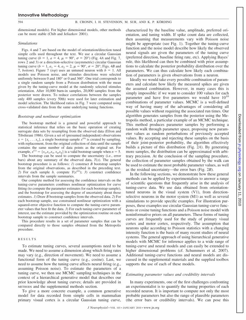
arises. In neuroscience, this implies specifying the assumptionswe have about how neural responses are generated from stimulior movements. We first describe the framework for makingthese assumptions (a Bayesian hierarchical modeling frame-work). Second, we present a Markov chain Monte Carlo(MCMC) sampling process for performing the statistical infer-ence procedures necessary for estimation of parameters andtheir credibility intervals, as well as, hypothesis testing. Thecentral difference between the Bayesian approach presentedhere and more commonly used methods is that we attempt todescribe the entire distribution over tuning curves (the poste-rior probability distribution) rather than a single tuning-curveestimate (such as the maximum likelihood estimate). Eachpoint in this posterior probability distribution describes howcompatible a given tuning curve is with the measured data.Samples from this distribution allow for straightforward esti-mation of parameters and error bars, as well as, hypothesistesting and model selection.

For many analyses, Bayesian methods yield the same resultsone would obtain when using more traditional ones. However,there are two cases where Bayesian methods can be particu-larly helpful: when there is limited data and when there aremany parameters. Both cases are typical of problems in neu-roscience where recording times are limited and neurons ex-hibit complicated tuning properties. Moreover, in both cases,estimating the parameter of tuning curves is difficult. Withoutconsidering distributions over parameters or using priors mostmodels may over-fit the data. In the descriptions that follow,we focus on illustrating the utility of Bayesian methods forlimited data and assume noninformative (flat) priors over theparameters. When there are many parameters, informativepriors are often useful, but the application of these priors mayrequire specific knowledge about the problem. However, evenwithout using informative priors, many problems may benefitfrom Bayesian approaches, given the fact that electrophysio-logical experiments obtain datasets of limited size.

The statistical methods described here have been success-fully applied in a range of scientific fields (Gelman et al. 2004;Liu 2002; MacKay 2003; Metropolis et al. 1953; Robert and

Casella 2004). In electrophysiology, MCMC sampling hasbeen used for fitting peristimulus time histograms (Dimatteoet al. 2001), fitting nonparametric tuning curves (Kaufmanet al. 2005), spike sorting (Nguyen et al. 2003; Wood et al.2006), and neural decoding. However, these methods, andBayesian methods in general, have not yet been adopted byneurophsyiologists on a large scale. One major barrier to theiradoption has been the difficulty in implementing MCMCsampling routines that are both appropriate and computation-ally efficient. To alleviate this obstacle, we make available asoftware toolbox that will allow researchers to easily androutinely apply all of the methods discussed here in theanalysis of their own data.

M E T H O D S

The spiking patterns of neurons will depend both on the propertiesof a stimulus and on the tuning properties of the neuron. In a typicalexperiment, we observe signals from neurons (e.g., spikes), and wewant to ask which tuning properties are exhibited by the recordedneuron. In Bayesian terms, we want to ask which tuning properties aremost consistent with the measured data given assumptions about theirfunctional form (e.g., Gaussian or sigmoid). These Bayesian modelsassume an explicit generative process that defines how the observedfiring patterns are (statistically) related to both the stimuli and theunderlying tuning properties of the recorded neurons. We then usenumerical methods to optimally estimate the values of the tuningproperties as well as the uncertainty which remains (i.e., the errorbars).

Hierarchical model

The key feature of our analysis method is that it describes a(hypothesized) probabilistic relationship between the parameters of achosen tuning-curve (TC) function, any external variables (e.g., stim-uli), and the neuronal responses collected in an experiment (see Fig.1, B and C).

Given experimental data, such as spike counts, knowledge of thestimuli presented over the course of the experiment, and an assump-tion about the functional form of the TC, we want to know how likelyeach set of tuning-curve parameters is. Example tuning-curve func-

FIG. 1. Introduction. A: a schematic illustrating the setupof the sensory neuroscience experiments for which theanalyses discussed here are applicable. An animal, eitheranesthetized or awake, is presented with stimuli that varyalong a single feature dimension. Neuronal responses tothese stimuli are recorded and then described using tuning-curve functions. B: an example tuning-curve model, thecircular Gaussian function. The function can be describedby the values of 4 parameters: the baseline (B), amplitude(A), preferred orientation (PO), and tuning width (TW).C: a schematic of the generative process assumed by thehierarchical statistical model. A neuron exhibits tuningdescribed by a particular tuning-curve function. Thefiring rate in response to a stimulus of a particular valueis determined by the value of this tuning-curve functionwhen evaluated at this location. The response for aparticular trial is then generated according to the assumedprobability model, here a Poisson process.


592 B. CRONIN, I. H. STEVENSON, M. SUR, AND K. P. KORDING

J Neurophysiol • VOL 103 • JANUARY 2010 • www.jn.org


Dow

nloaded from


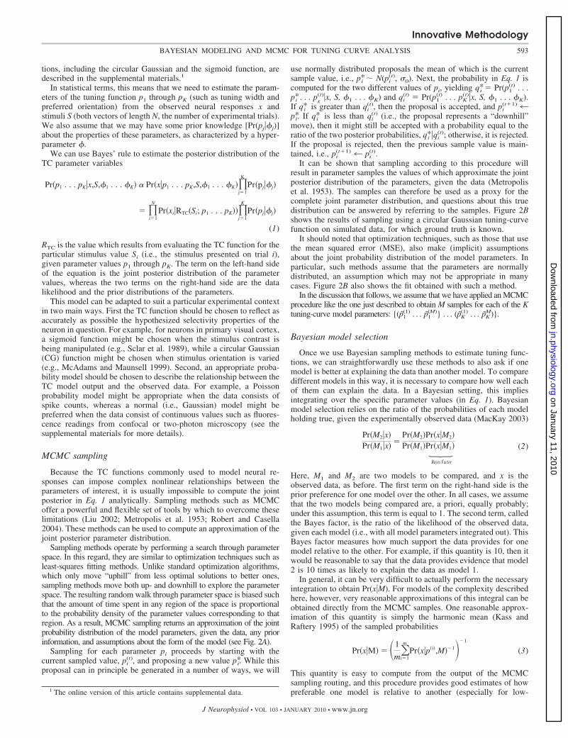
tions, including the circular Gaussian and the sigmoid function, aredescribed in the supplemental materials.1

In statistical terms, this means that we need to estimate the param-eters of the tuning function p1 through pK (such as tuning width andpreferred orientation) from the observed neural responses x andstimuli S (both vectors of length N, the number of experimental trials).We also assume that we may have some prior knowledge [Pr(pj��j)]about the properties of these parameters, as characterized by a hyper-parameter �.

We can use Bayes’ rule to estimate the posterior distribution of theTC parameter variables

Pr�p1 . . . pK�x,S,�1 . . . �K� � Pr�x�p1 . . . pK,S,�1 . . . �K��j�1

K

Pr�pj��j�

� �i�1

N

Pr�xi�RTC�Si; p1 . . . pK��j�1

K

Pr�pj��j�

(1)

RTC is the value which results from evaluating the TC function for theparticular stimulus value Si (i.e., the stimulus presented on trial i),given parameter values p1 through pK. The term on the left-hand sideof the equation is the joint posterior distribution of the parametervalues, whereas the two terms on the right-hand side are the datalikelihood and the prior distributions of the parameters.

This model can be adapted to suit a particular experimental contextin two main ways. First the TC function should be chosen to reflect asaccurately as possible the hypothesized selectivity properties of theneuron in question. For example, for neurons in primary visual cortex,a sigmoid function might be chosen when the stimulus contrast isbeing manipulated (e.g., Sclar et al. 1989), while a circular Gaussian(CG) function might be chosen when stimulus orientation is varied(e.g., McAdams and Maunsell 1999). Second, an appropriate proba-bility model should be chosen to describe the relationship between theTC model output and the observed data. For example, a Poissonprobability model might be appropriate when the data consists ofspike counts, whereas a normal (i.e., Gaussian) model might bepreferred when the data consist of continuous values such as fluores-cence readings from confocal or two-photon microscopy (see thesupplemental materials for more details).

MCMC sampling

Because the TC functions commonly used to model neural re-sponses can impose complex nonlinear relationships between theparameters of interest, it is usually impossible to compute the jointposterior in Eq. 1 analytically. Sampling methods such as MCMCoffer a powerful and flexible set of tools by which to overcome theselimitations (Liu 2002; Metropolis et al. 1953; Robert and Casella2004). These methods can be used to compute an approximation of thejoint posterior parameter distribution.

Sampling methods operate by performing a search through parameterspace. In this regard, they are similar to optimization techniques such asleast-squares fitting methods. Unlike standard optimization algorithms,which only move “uphill” from less optimal solutions to better ones,sampling methods move both up- and downhill to explore the parameterspace. The resulting random walk through parameter space is biased suchthat the amount of time spent in any region of the space is proportionalto the probability density of the parameter values corresponding to thatregion. As a result, MCMC sampling returns an approximation of the jointprobability distribution of the model parameters, given the data, any priorinformation, and assumptions about the form of the model (see Fig. 2A).

Sampling for each parameter pi proceeds by starting with thecurrent sampled value, pi

(t), and proposing a new value p*i. While thisproposal can in principle be generated in a number of ways, we will

use normally distributed proposals the mean of which is the currentsample value, i.e., p*i � N(pi

(t), �0). Next, the probability in Eq. 1 iscomputed for the two different values of pi, yielding q*i � Pr(p1

(t) . . .p*i . . . p

K

(t)�x, S, �1 . . . �K) and qi(t) � Pr(p1

(t) . . . pK(t)�x, S, �1 . . . �K).

If q*i is greater than qi(t), then the proposal is accepted, and pi

(t�1) 4p*i. If q*i is less than qi

(t) (i.e., the proposal represents a “downhill”move), then it might still be accepted with a probability equal to theratio of the two posterior probabilities, q*i �qi

(t); otherwise, it is rejected.If the proposal is rejected, then the previous sample value is main-tained, i.e., pi

(t�1) 4 pi(t).

It can be shown that sampling according to this procedure willresult in parameter samples the values of which approximate the jointposterior distribution of the parameters, given the data (Metropoliset al. 1953). The samples can therefore be used as a proxy for thecomplete joint parameter distribution, and questions about this truedistribution can be answered by referring to the samples. Figure 2Bshows the results of sampling using a circular Gaussian tuning-curvefunction on simulated data, for which ground truth is known.

It should noted that optimization techniques, such as those that usethe mean squared error (MSE), also make (implicit) assumptionsabout the joint probability distribution of the model parameters. Inparticular, such methods assume that the parameters are normallydistributed, an assumption which may not be appropriate in manycases. Figure 2B also shows the fit obtained with such a method.

In the discussion that follows, we assume that we have applied an MCMCprocedure like the one just described to obtain M samples for each of the Ktuning-curve model parameters: {(p1

(1) . . . p1(M)} . . . (pK

(1) . . . pKM)}.

Bayesian model selection

Once we use Bayesian sampling methods to estimate tuning func-tions, we can straightforwardly use these methods to also ask if onemodel is better at explaining the data than another model. To comparedifferent models in this way, it is necessary to compare how well eachof them can explain the data. In a Bayesian setting, this impliesintegrating over the specific parameter values (in Eq. 1). Bayesianmodel selection relies on the ratio of the probabilities of each modelholding true, given the experimentally observed data (MacKay 2003)

Pr�M2�x�Pr�M1�x�

�Pr�M2�Pr�M1�

Pr�x�M2�Pr�x�M1�Ç

Bayes Factor

(2)

Here, M1 and M2 are two models to be compared, and x is theobserved data, as before. The first term on the right-hand side is theprior preference for one model over the other. In all cases, we assumethat the two models being compared are, a priori, equally probably;under this assumption, this term is equal to 1. The second term, calledthe Bayes factor, is the ratio of the likelihood of the observed data,given each model (i.e., with all model parameters integrated out). ThisBayes factor measures how much support the data provides for onemodel relative to the other. For example, if this quantity is 10, then itwould be reasonable to say that the data provides evidence that model2 is 10 times as likely to explain the data as model 1.

In general, it can be very difficult to actually perform the necessaryintegration to obtain Pr(x�M). For models of the complexity describedhere, however, very reasonable approximations of this integral can beobtained directly from the MCMC samples. One reasonable approx-imation of this quantity is simply the harmonic mean (Kass andRaftery 1995) of the sampled probabilities

Pr�x�M� � �1

m�i�1

m

Pr�x�p�i�,M��1��1

(3)

This quantity is easy to compute from the output of the MCMCsampling routing, and this procedure provides good estimates of howpreferable one model is relative to another (especially for low-1 The online version of this article contains supplemental data.


593BAYESIAN MODELING AND MCMC FOR TUNING CURVE ANALYSIS



Dow

nloaded from


dimensional models). For higher dimensional models, other methodscan be more stable (Chib and Jeliazkov 2001).

Simulations

Figs. 4 and 7 are based on the model of orientation/direction tunedsimple cells used throughout the text. We use a circular Gaussiantuning curve (b � 1, a � 4, � � 90°, � � 20°) (Fig. 4A and Fig. 7,rows 2 and 3) or a direction-selective (asymmetric) circular Gaussiantuning curve (b � 1, a1 � 4, a2 � 2, � � 90°, � � 20°; Figs. 4B and7, bottom). Figure 7 (top) uses an untuned neuron with b � 1. Allmodels use Poisson noise, and stimulus directions were selecteduniformly between 0 and 180° or 0 and 360°. One trial corresponds toa single random sample from a Poisson distribution with the meangiven by the tuning-curve model at the randomly selected stimulusorientation. After 10,000 burn-in samples, 20,000 samples from theposterior were drawn. To reduce correlations between the samplesonly 400 samples (every 50th) were used for later estimation andmodel selection. The likelihood ratios in Fig. 7 were computed usingcross-validated data from the same underlying tuning functions.

Bootstrap and nonlinear optimization

The bootstrap method is a general and powerful approach tostatistical inference that relies on the basic operation of creatingsurrogate data sets by resampling from the observed data (Efron andTibshirani 1986). Given a set of (presumed independent) observationsx � {xi . . . xn}, a single bootstrap sample x(b) is created by sampling,with replacement, from the original collection of data until the samplecontains the same number of data points as the original set. Forexample, x(1) � {x1,x1,x3, x4,x4} is a valid bootstrap sample when n � 5.

The bootstrap can be used to compute the uncertainty (i.e., errorbars) about any summary of the observed data, T(x). The generalbootstrap procedure is as follows: 1) construct B bootstrap samplesfrom the original observations, as described in the preceding text.2) For each sample b, compute T(x(b)); 3) construct confidenceintervals from the sample summaries.

Our complete method for assessing the confidence intervals on thetuning-curve parameters combines nonlinear optimization for curvefitting (to compute the parameter estimates for each bootstrap sample),and the bootstrap for assessing the degree of uncertainty about thoseestimates. 1) Draw B bootstrap samples from the observed data. 2) Foreach bootstrap sample, use constrained nonlinear optimization with asquared-error objective function to compute the tuning-curve param-eter values that best fit the data. 3) For each tuning-curve parameter ofinterest, use the estimate provided by the optimization routine on eachbootstrap sample to construct confidence intervals.

This procedure results in a set of parameter samples that can becompared directly to those samples obtained from the Metropolisprocedure.

R E S U L T S

To estimate tuning curves, several assumptions need to bemade. We need to assume a dimension along which firing ratesmay vary (e.g., direction of movement). We need to assume afunctional form of the tuning curve (e.g., cosine). Last, weneed to assume how the tuning curve affects neural firing (e.g.,assuming Poisson noise). To estimate the parameters of atuning curve, we then use MCMC sampling techniques in thecontext of a hierarchical generative model that describes ourprior knowledge about tuning curves; details are provided inMETHODS and the supplemental methods section.

To give a more concrete example, a common generativemodel for data recorded from simple cells in mammalianprimary visual cortex is a circular Gaussian tuning curve,

characterized by the baseline value, amplitude, preferred ori-entation, and tuning width. If spike count data are collected,then assuming that measurements vary with Poisson noisemight be appropriate (see Fig. 1). Together the tuning-curvefunction and the noise model describe how likely the observedneural signals are given the parameters of the tuning curve(preferred direction, baseline firing rate, etc). Applying Bayes’rule, this likelihood can then be combined with prior assump-tions to calculate the posterior probability distribution over theparameters. We can thus calculate how likely each combina-tion of parameters is given observations from a neuron.

Ideally we would take every possible combination of param-eters and calculate how likely the measured spikes are giventhe assumed combination. However, in many cases this issimply impossible: if we want to consider 100 values for eachparameter and have five parameters we would have 1010

combinations of parameter values. MCMC is a well-definedway of having many of the advantages of considering allpossible values without requiring the associated run times. Ouralgorithm generates samples from the posterior using the Me-tropolis method, a particular example of an MCMC technique.This method produces parameter samples by performing arandom walk through parameter space, proposing new param-eter values as random perturbations of previously acceptedvalues. By accepting and rejecting these samples on the basisof their joint-posterior probability, the algorithm effectivelybuilds a picture of this distribution (Fig. 2A). By generatingmore samples, the distribution can be approximated with arbi-trary precision. At the conclusion of the sampling procedure,the collection of parameter samples obtained by the walk canbe used to estimate the most probable parameter values, as wellas the residual uncertainty—the error bars (Fig. 2B).

In the following sections, we demonstrate how these generalmethods can be applied by experimentalists to answer a rangeof scientific questions that frequently arise in the analysis oftuning-curve data. We use data obtained from orientation-tuned neurons in the visual system (V1), from direction-selective neurons in the motor system (M1) as well as severalsimulations to provide specific examples. For illustration pur-poses, these examples use circular Gaussian tuning-curve func-tions or cosine tuning functions and a Poisson noise model withnoninformative priors on all parameters. These forms of tuningcurves are frequently used for the study of primary visualcortex and motor cortex, respectively. The assumption thatneurons spike according to Poisson statistics with a changingintensity function is the basis of many recent studies of neuralsystems. The general approach of using hierarchical generativemodels with MCMC for inference applies to a wide range oftuning-curve and neural models and can easily be extended tohigher dimensional problems (cf. Schummers et al. 2007).Additional tuning-curve functions and neural models are dis-cussed in the supplemental materials and the supplied toolboxsupports the use of each of these models.

Estimating parameter values and credibility intervals

In many experiments, one of the first challenges confrontingan experimentalist is to quantify the tuning properties of eachrecorded neuron. It is important to compute not only the mostprobable parameters but also the range of plausible parameters(the error bars or credibility intervals). We can pose this





Dow

nloaded from


question more precisely by asking, for each parameter of thechosen tuning-curve function, what range of parameter valuesis consistent with the set of observed neuronal responses? Forexample, what is the plausible range of preferred orientationsfor an orientation selective neuron in V1?

Questions of this type can be answered directly from a set ofMCMC samples because they approximate the joint posteriordistribution over the parameter values. Parameter values thatare sampled more often correspond to those that are morelikely to account for the data. To obtain, say, a 95% credibilityinterval for parameter pi, the samples {pi

(1) . . . pi(M)} are first

sorted from lowest to highest to obtain the rank order �pi[1] . . .

pi[M]�. Next, the lowest and highest 2.5% of the samples are

discarded. For example, if 1,000 samples were collected, thenthe lowest and highest 25 would be discarded. The remainingextreme values define the desired error margin (see Fig. 3, Aand B). In the 1,000-sample example, these would be the 26thand 975th sample from the ranked list. Importantly, thismethod does not need to make the assumption that the posterioris Gaussian. Depending on the model, the distribution mayeven been asymmetric or multimodal. As such, this method candeal with many of the potentially non-Gaussian distributionsoccurring in neuroscience.

In addition to credibility intervals, several other statisticalestimates can be calculated from the samples. We can find amaximum a posteriori (MAP) estimate as well as the median ormean values of each parameter (Fig. 2B). When the prior overparameters is noninformative, the MAP estimate is equivalentto a MLE. However, in many cases, the mean or medianposterior is a more robust estimate of the parameters. Theseestimators are optimal in that the posterior mean minimizes thesquared error between the estimated parameter and its truevalue while the posterior median minimizes linear loss (Berger1985). Like the maximum likelihood estimate, these estimatorsare asymptotically unbiased and efficient in most cases. Thedifference between MLE and Bayes estimators is generallyapparent only for small sample sizes and disappears as moredata are collected. In simulations of orientation-tuned neurons,for instance, the MLE and Bayes tuning-curve estimates are thesame after �40 trials (Fig. 4). For small sample sizes, usingBayes estimators, which take the distribution over parametersinto account, can improve estimation.

Visualization of potential tuning curves

The presented approach also allows for simple visualizationof the set of potential tuning curves that are compatible withthe observed data. This visualization can be a useful tool forunderstanding the quantitative power that is provided by thedata from a single cell (as used in Figs. 3 and 5). Because theposterior distribution over potential tuning curves may not beGaussian and the parameters may not always be linearlyindependent, error bars on each parameter provide only part ofthe picture. For instance, the distribution of potential tuningcurves may be skewed or multimodal (Fig. 5, B and E). This isone advantage of representing an entire distribution over thetuning curves described by a certain model.

Assaying quantitative changes in response properties

Quantifying tuning properties using the methods in thepreceding text is often merely the first step in answeringscientific questions about physiological data. Frequently, wewish to know whether a particular manipulation has resulted ina significant change in tuning properties. For example, it mightbe asked whether visual neurons change their orientation se-lectivity properties in response to attentional influences, sen-sory pattern adaptation, or perceptual learning (Dragoi et al.2000, 2001; McAdams and Maunsell 1999) or if the preferreddirections of neurons in motor cortex change in a force field(Rokni et al. 2007). In these kinds of experiments, neuronalresponses would be measured in both the control and test

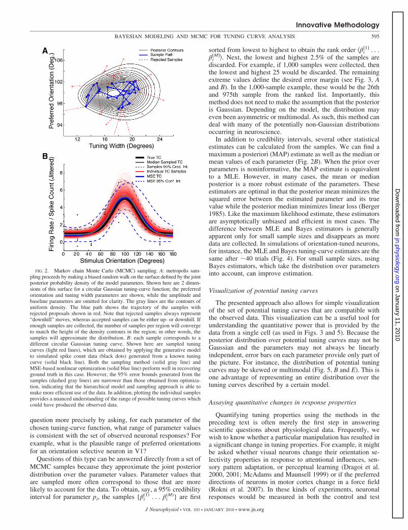
FIG. 2. Markov chain Monte Carlo (MCMC) sampling. A: metropolis sam-pling proceeds by making a biased random walk on the surface defined by the jointposterior probability density of the model parameters. Shown here are 2 dimen-sions of this surface for a circular Gaussian tuning-curve function; the preferredorientation and tuning width parameters are shown, while the amplitude andbaseline parameters are omitted for clarity. The gray lines are the contours ofuniform density. The blue path shows the trajectory of the samples withrejected proposals shown in red. Note that rejected samples always represent“downhill” moves, whereas accepted samples can be either up- or downhill. Ifenough samples are collected, the number of samples per region will convergeto match the height of the density contours in the region; in other words, thesamples will approximate the distribution. B: each sample corresponds to adifferent circular Gaussian tuning curve. Shown here are sampled tuningcurves (light red lines), which are obtained by applying the generative modelto simulated spike count data (black dots) generated from a known tuningcurve (solid black line). Both the sampling method (solid gray line) andMSE-based nonlinear optimization (solid blue line) perform well in recoveringground truth in this case. However, the 95% error bounds generated from thesamples (dashed gray lines) are narrower than those obtained from optimiza-tion, indicating that the hierarchical model and sampling approach is able tomake more efficient use of the data. In addition, plotting the individual samplesprovides a nuanced understanding of the range of possible tuning curves whichcould have produced the observed data.





Dow

nloaded from


conditions, and MCMC samples would be generated separatelyfor these two sets of data. To determine whether the datasupports a conclusion of significant changes in tuning, credi-bility intervals are computed for each of the two conditions asin the preceding text. To ascertain whether a significant shifthas occurred, it is sufficient to observe whether these twointervals overlap. If there is no overlap (i.e., the intervals aredisjoint), then the data support the conclusion that the corre-sponding response property has changed between the two

conditions (see Fig. 3, C and D). If the two intervals dooverlap, then this conclusion is not supported. This negativeresult is consistent with two possibilities. First, the underlyingresponse property might really be unaffected by the experi-mental manipulation, which is a true negative result. Second,the tuning property has indeed changed but not enough data hasbeen collected to reduce uncertainty to the point where thischange can be reliably detected. In neither of the cases will thismethod wrongly report a change.

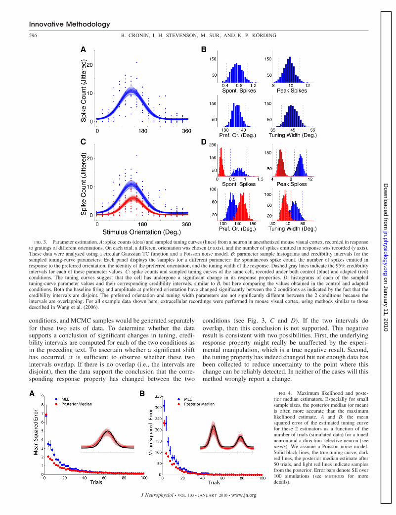
FIG. 3. Parameter estimation. A: spike counts (dots) and sampled tuning curves (lines) from a neuron in anesthetized mouse visual cortex, recorded in responseto gratings of different orientations. On each trial, a different orientation was chosen (x axis), and the number of spikes emitted in response was recorded (y axis).These data were analyzed using a circular Gaussian TC function and a Poisson noise model. B: parameter sample histograms and credibility intervals for thesampled tuning-curve parameters. Each panel displays the samples for a different parameter: the spontaneous spike count, the number of spikes emitted inresponse to the preferred orientation, the identity of the preferred orientation, and the tuning width of the response. Dashed gray lines indicate the 95% credibilityintervals for each of these parameter values. C: spike counts and sampled tuning curves of the same cell, recorded under both control (blue) and adapted (red)conditions. The tuning curves suggest that the cell has undergone a significant change in its response properties. D: histograms of each of the sampledtuning-curve parameter values and their corresponding credibility intervals, similar to B, but here comparing the values obtained in the control and adaptedconditions. Both the baseline firing and amplitude at preferred orientation have changed significantly between the 2 conditions as indicated by the fact that thecredibility intervals are disjoint. The preferred orientation and tuning width parameters are not significantly different between the 2 conditions because theintervals are overlapping. For all example data shown here, extracellular recordings were performed in mouse visual cortex, using methods similar to thosedescribed in Wang et al. (2006).

FIG. 4. Maximum likelihood and poste-rior median estimators. Especially for smallsample sizes, the posterior median (or mean)is often more accurate than the maximumlikelihood estimate. A and B: the meansquared error of the estimated tuning curvefor these 2 estimators as a function of thenumber of trials (simulated data) for a tunedneuron and a direction-selective neuron (seeinsets). We assume a Poisson noise model.Solid black lines, the true tuning curve; darkred lines, the posterior median estimate after50 trials, and light red lines indicate samplesfrom the posterior. Error bars denote SE over100 simulations (see METHODS for moredetails).





Dow

nloaded from


Assessing selectivity to the stimulus feature usingmodel selection

In many cases, it is of primary scientific interest to determinewhether a neuron is actually selective for the stimulus propertythat is being varied in the experiment. For example, many butnot all neurons in striate cortex are selective for particularstimulus orientations (Maldonado et al. 1997), and �20% ofneurons in primary motor cortex are not cosine tuned (e.g.,Georgopoulos et al. 1986). Before drawing conclusions aboutthe quantitative details of each neuron’s orientation-dependentresponse, it is necessary to assess whether the cell is selectivein the first place.

Bayesian model selection (BMS) can be used to determinehow much evidence is provided by the data for one responsemodel over another (Kass and Raftery 1995; MacKay 2003).To determine whether a cell is indeed selective for a stimulusproperty, BMS can be employed to compare models with twodifferent tuning-curve functions: one in which the responsevaries with the stimulus value, and another in which theresponse is assumed to be insensitive to the particular stimulus(see Fig. 5, A–C).

BMS is similar to traditional hypothesis testing methodssuch as the likelihood ratio test in that we compare theprobability of observing the data under each model. However,unlike the likelihood ratio test, BMS uses Bayes factors—theratio of probability assigned to the data by each model, inte-grating over all possible parameter values. In general, it isdifficult to compute Bayes factors because this integration canbe nonlinear and high dimensional. For models with relativelysmall numbers of parameters, however, such as those usedhere, approximate Bayes factors can be computed directly fromthe MCMC samples (see Eq. 2). Furthermore, the quality ofthese estimates can be improved by increasing the number ofsamples computed. We have found that excellent results can beobtained for the models discussed here with very reasonablecomputational resources (1 min/cell on a desktop machine).

A key property of BMS is that it appropriately penalizesmodels with more degrees of freedom. This “regularization”ensures that models with extra parameters are not favoredmerely because they are more expressive, which is a well-known complication in model comparison procedures (Buck-land et al. 1997; MacKay 2003; Pitt and Myung 2002). Thispenalty is in some ways similar to the Akaike informationcriterion (AIC) or Bayesian information criterion (BIC). How-ever, unlike these two methods, the Bayes factor applies to anypriors over parameters or model types.

Comparing different selectivity models

A number of scientific questions can be posed in terms ofBMS. For example, some neurons in primary visual cortex ofthe cat are direction selective, meaning that their responses toa grating of a particular orientation depend on the direction ofmotion of the grating. Other cells are not direction selective,and their responses are not modulated by the direction ofmotion of the grating. BMS can be used to distinguish betweenthese two types of cells. In this case, two different tuning-curvefunctions would be used, each of which corresponds to one ofthe two hypotheses. The first is a circular Gaussian functionwith a periodicity of 180°; this function represents a nondirec-tion-selective response because its values are the same forstimuli of opposite direction. The second TC function is acircular Gaussian with a periodicity of 360°, which representsresponses for only one direction of motion (see Fig. 5, D andE). In the case of neurons in motor cortex, one might comparea cosine tuning function and a constant tuning function (Fig. 6).When BMS is applied in this setting, using the methodsdescribed above, its output indicates the strength of evidenceprovided by the data that a particular cell is tuned for directionof motion.

In real data, the “true” tuning curve is generally unknown.However, we can illustrate some of the features of BMS usingsimulated data. To this end, we performed four simulations where

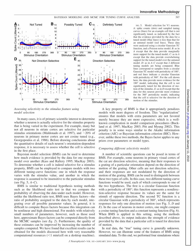
FIG. 5. Model selection for V1 neurons.A: spike counts (dots) and sampled tuningcurves (lines) for an example cell that is notsignificantly tuned, as indicated by the factthat the evidence provided by the data for atuned model (blue lines) is less than that foran untuned model (red lines). These datawere analyzed using a circular Gaussian TCfunction, and a Poisson noise model. B: as inA except that the data provide marginallymore support for the tuned model. C: as in Aexcept that the data provide overwhelmingsupport for the tuned model over the untunedmodel. D: as in A–C except that 2 differenttuning models are being compared. Bluelines correspond to samples from a circularGaussian TC model with periodicity of 180°,and red lines indicate a circular Gaussianwith periodicity of 360°. For the cell shownhere, the data provide more evidence for the180° model, indicating that the cell is notsignificantly tuned for the direction of mo-tion of the stimulus. E: as in D except that thedata for this neuron provide more evidencefor the 360° periodicity model, indicatingthat the cell is selective for the direction ofmotion of the stimulus.





Dow

nloaded from


the true tuning-curve and noise model are known (Fig. 7). Wesimulated spikes from an untuned neuron (Fig. 7, top), anorientation-tuned neuron (Fig. 7, 2nd row), a nondirection-selective neuron (Fig. 7, 3rd row), and a direction-selectiveneuron (Fig. 7, bottom). For each of these sets of simulateddata, we then generated MCMC samples from two models:untuned and tuned models for the first two cases (Fig. 7A) andnondirection-selective and direction-selective models for thesecond two cases (B). A Bayes factor 1 (or a log-ratio 0)suggests that model 1 is preferred, while a Bayes factor 1(log-ratio 0) suggests that model 2 is preferred. Similar tocross-validated likelihood ratio tests, the Bayes factor selectsthe correct underlying tuning-curve model after a relativelysmall number of trials (Fig. 7, right).

Comparison with the bootstrap

One established alternative to the methods presented here isbootstrapping. Bootstrap methods are a very general set oftechniques by which to estimate the residual uncertainty ofarbitrary statistical summaries, including credibility intervals

for model parameters (Efron and Tibshirani 1997). Thesetechniques have reached fairly wide use in neuroscience andsolve some of the same problems that the techniques presentedhere address, particularly the estimation of error-bars (Brownet al. 2004; Kass et al. 2005; Paninski et al. 2003; Ringach et al.2003; Schwartz et al. 2006; Stark and Abeles 2005; Venturaet al. 2005). Briefly, the bootstrap involves generating a seriesof surrogate data sets (“bootstrap samples”) by sampling withreplacement from the observed data; estimates of the uncer-tainty—error bars—are then computed by computing separateestimates from each of these samples. As such, bootstrapmethods are a natural point of comparison for the hierarchicalmodeling and sampling methods described here. We haveperformed a series of comparisons between the two methods,using simulated orientation data for which the “true” tuningcurve was known. A complete description of the bootstrapprocedure used for these comparisons is provided in METHODS.

Figure 8 shows the results of several comparisons betweenthe two methods. While the bootstrap performs similarly toposterior sampling when a large amount of data are available(Fig. 8A), the advantage of sampling becomes clear when lessdata are available. In this situation, the fully Bayesian approachis better able to recover the underlying tuning curve. Thiseffect has been noted previously (Kass et al. 2005) and cangenerally by avoided by collecting more data, but it points to amore fundamental difference in the way these methods testtuning-curve models.

In addition to robustness to small sample sizes, the Bayesianmethod has several advantages over the bootstrap. Bootstrap-ping generally requires a nonlinear optimization, which can besubject to local minima in the error function. Manual interven-tion or more complicated methods, such as double bootstrap,may be necessary to correct for biases and dependencies inbootstrap estimates (Davison and Hinkley 1997). The Bayesianapproach, on the other hand, does not include any optimization.Assuming appropriate mixing, the MCMC samples approxi-mate the full posterior distribution over the parameters. More-over, these techniques can easily be adapted to a wide range oftuning-curve functions, noise models, and priors.

D I S C U S S I O N

Here we have shown how methods based on MCMC canhelp answer frequently occurring questions in the realm ofelectrophysiology. We have shown that the same method canbe used to estimate properties of neural tuning for several kindsof neurons, obtain bounds on their values, examine if theychange from one condition to the next and ask which modelbest explains the data. With the provided toolbox these meth-ods are easy to implement and have the potential to signifi-cantly improve practical data analysis.

Comparison with other methods

The primary difference between the Bayesian samplingapproach and more traditional approaches such as reverse-correlation, maximum likelihood estimation, and bootstrappingis that we attempt to consider all the tuning curves that wouldbe compatible with the data. This analysis can reproduce theresults from MLE by searching for the parameter values thatare associated with the highest sample density and a noninfor-

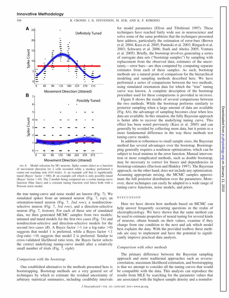
FIG. 6. Model selection for M1 neurons. Spike counts (dots) as a functionof movement direction for 2 cells recorded while a monkey performed acenter-out reaching task (414 trials). A: an example cell that is significantlytuned (Bayes’ factor 100); B: an example cell which is only possibly tuned(Bayes’ factor 10). The 2 models being compared are a cosine tuning-curvefunction (blue lines) and a constant tuning function (red lines) both with aPoisson noise model.





Dow

nloaded from


mative prior. It obtains the same results as bootstrapping whenthere is enough data. However, for small sample sizes, Bayesestimators, such as the posterior median, and Bayesian credi-bility intervals are often more robust than these alternatives.

In hypothesis testing, Bayesian sampling methods convergeto the results from likelihood ratio tests as well as AIC/BIC,under certain assumptions. For nonlinear or hierarchical mod-els, the Bayes factor offers a more principled approach tomodel comparison. As experimental methods advance andstimulus-response models become more sophisticated, accuratemodel selection will become more and more important. By

looking at the distribution over potential tuning curves and notjust the most likely tuning curve, physiologists may be able togain insight into scientific questions as well as the statisticalproperties of tuning-curve models.

Another key feature of the sampling approach is its flexi-bility. Most analyses are based on an implicit assumption ofGaussian noise (Amirikian and Georgopulos 2000; Swindale1998), an assumption that is inappropriate for some commonforms of neuronal data (e.g., spike counts). The hierarchicalmodel described here can incorporate a range of probabilitymodels, such as the Poisson and negative binomial distribu-

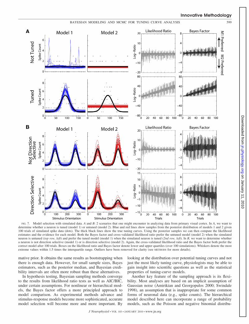
FIG. 7. Model selection with simulated data. A and B: 2 scenarios that one might encounter in analyzing data from primary visual cortex. In A, we want todetermine whether a neuron is tuned (model 1) or untuned (model 2). Blue and red lines show samples from the posterior distribution of models 1 and 2 given100 trials of simulated spike data (dots). The thick black lines show the true tuning curves. Using the posterior samples we can then compute the likelihoodestimates and the evidence for each model. Both the Bayes factor and cross-validated likelihood ratio prefer the untuned model (model 2) when the simulatedneuron is untuned (top row, left) and prefer the tuned model (model 1) when the simulated neuron is tuned (2nd row, left). In B, we want to determine whethera neuron is not direction selective (model 1) or is direction selective (model 2). Again, the cross-validated likelihood ratio and the Bayes factor both prefer thecorrect model after 100 trials. Boxes on the likelihood ratio and Bayes factor denote lower and upper quartiles (over 100 simulations). Whiskers denote the mostextreme values within 1.5 times the interquartile range. Outliers have been removed for clarity (see METHODS for more details).





Dow

nloaded from


tions in addition to Gaussian. This modeling flexibility alsomeans that the framework described here can be directlyapplied to data other than spike counts, including fluores-cence measurements from confocal and two-photon micros-copy. There are a wide range of easily applicable tuningfunctions, including sigmoids, bilinear, von Mises func-tions, rectified cosines, and so on (see the supplementalmethods for a full description of the tuning functions andlikelihood models).

Although the methods we present here are flexible in thechoice of tuning functions and noise models, they are generallymuch more constrained than nonparametric methods. In addi-tion to MCMC for nonparametric tuning-curve estimation(Dimatteo et al. 2001; Kaufman et al. 2005), a large body ofwork exists on reverse-correlation approaches. These ap-proaches aim to directly map stimulus properties to neuralresponses (Dayan and Abbott 2001; Eggermont et al. 1983;Marmarelis and Marmarelis 1978; Ringach et al. 1997b; Si-moncelli et al. 2004). A wide range of toolboxes support theanalysis of neural data using such nonsampling based methods(for useful software packages, see: http://chronux.org/ http://pillowlab.cps.utexas.edu/code.html, http://find.bccn.uni-freiburg.de/).More recently, techniques have been developed that constrainreverse-correlation estimates using specific noise models andpriors (Paninski 2004; Sahani and Linden 2003; Smith andLewicki 2006). In many ways, these two strategies, nonpara-metric estimation of response functions with priors and fullyBayesian parametric estimation of response functions, repre-sent a continuum of modeling frameworks that extends fromminimally constrained modeling to very constrained mod-eling. This continuum allows experimentalists to decidehow to model their data depending how much is knownabout the neural system or experimental manipulation inquestion. For instance, in a system where the exact para-metric form of a tuning curve is unknown, experimentalistsmay want to use nonparametric or semi-parametric modelsrather than assuming a poorly fitting fully parameterizedtuning function.

Inference assumptions and prior knowledge

All statistical inference methods, including nonparametricmethods and bootstrapping, require assumptions. For example,to compute bootstrap estimates that were comparable to the

results of the Bayesian methods, it was necessary to performnonlinear least-squares optimization to estimate the parametervalues for each bootstrap sample (Swindale 1998). All optimi-zation methods make use of an error function; the squared-error function that is used by this method is equivalent to anassumption of Gaussian noise in the data. In short, there is noway to estimate parameter values, or their residual uncertainty,or to compare different models with respect to their ability toexplain the data without making assumptions. Bayesian meth-ods generally make all such assumptions explicit.

One specific kind of inferential assumption that bears specialattention is the prior distribution placed on the tuning-curveparameters. In most cases (including all of those used in theexamples), a noninformative prior such as a uniform distribu-tion over an appropriate range is sufficient. In this case, theposterior is equivalent to the likelihood, and one can easily findthe maximum likelihood sample or compute a likelihood ratiobetween two models. However, in some cases, such as whenthere is very limited data or tuning functions are complicated,it may be necessary to include a more informative prior on oneor more of the parameters. In these cases, it is incumbent on theexperimenter to justify the use of a prior, such as by appealingto past measurements, literature, or to biophysical properties ofthe neurons under study. While such prior information may becontroversial, we note that Bayesian methods provide theopportunity—though not the requirement—to introduce suchinformation in a coherent and statistically principled way.

Extensions to more complex models

The general approach of using MCMC sampling to drawfrom the posterior distribution of model parameters can beapplied to models that are more complex than those describedhere. These methods have been used previously to infer theparameter distribution of a model that described the orientationtuning dynamics of neurons in cat primary visual cortex inresponse to oriented reverse-correlation stimuli (Schummerset al. 2007). Nonparametric approaches to tuning-curve fittingusing MCMC and splines have also been developed (Kaufmanet al. 2005). These analyses use the same principles as thosedescribed here, illustrating that these techniques are applicableto a wide range of neurophysiological data analysis problems.We note, however, that more complex models (i.e., modelscontaining more parameters than those described here) do

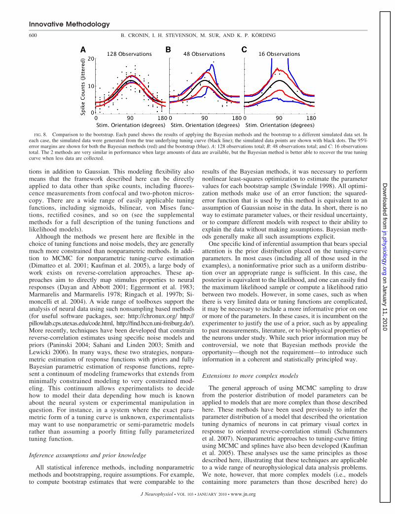
FIG. 8. Comparison to the bootstrap. Each panel shows the results of applying the Bayesian methods and the bootstrap to a different simulated data set. Ineach case, the simulated data were generated from the true underlying tuning curve (black line); the simulated data points are shown with black dots. The 95%error margins are shown for both the Bayesian methods (red) and the bootstrap (blue). A: 128 observations total; B: 48 observations total; and C: 16 observationstotal. The 2 methods are very similar in performance when large amounts of data are available, but the Bayesian method is better able to recover the true tuningcurve when less data are collected.





Dow

nloaded from


require more care in the selection of inference methods. Inparticular, special attention must be paid to the proposaldistribution that is used to generate candidate parameter sam-ples; additional detail can be found in Schummers et al. (2007).This study demonstrates that, once an appropriate proposaldistribution has been identified, sampling methods scale quitewell, and can be successfully applied to models with �100parameters or more.

Many if not most statistical estimation techniques are cur-rently viewed as approximations to optimal Bayesian infer-ence. The approach we used here has the benefit that even forsmall amounts of data, in the limit of sufficient computerpower (large number of samples), it will provably converge tothe correct answers. These tools should thus be useful for thegeneral analysis of tuning curves, which is a central statisticalobjective in neuroscience.

A C K N O W L E D G M E N T S

The authors thank C. Runyan, J. Schummers, and R. Mao for supplying thedata used in the V1 examples and A. Cherian and L. Miller for the data usedin the M1 examples.

G R A N T S

B. Cronin and M. Sur were supported by National Eye Institute GrantEY-07023.

R E F E R E N C E S

Amirikian B, Georgopulos AP. Directional tuning profiles of motor corticalcells. Neurosci Res 36: 73–79, 2000.

Berger JO. Statistical Decision Theory and Bayesian Analysis. New York:Springer, 1985.

Brown EN, Kass RE, Mitra PP. Multiple neural spike train data analysis:state-of-the-art and future challenges. Nat Neurosci 7: 456–461, 2004.

Buckland ST, Burnham KP, Augustin NH. Model selection: an integral partof inference. Biometrics 53: 603–618, 1997.

Carandini M, Ferster D. Membrane potential and firing rate in cat primaryvisual cortex. J Neurosci 20: 470–484, 2000.

Chib S, Jeliazkov I. Marginal likelihood from the Metropolis-Hastings output.J Am Stat Assoc 96: 270–281, 2001.

Davison AC, Hinkley DV. Bootstrap Methods and Their Application. Cam-bridge, UK: Cambridge Univ. Press, 1997.

Dayan P, Abbott LF. Theoretical Neuroscience: Computational and Mathe-matical Modeling of Neural Systems. Cambridge, MA: MIT Press, 2001.

Dimatteo I, Genovese CR, Kass RE. Bayesian curve-fitting with free-knotsplines. Biometrika 88: 1055–1071, 2001.

Dragoi V, Rivadulla C, Sur M. Foci of orientation plasticity in visual cortex.Nature 411: 80–86, 2001.

Dragoi V, Sharma J, Sur M. Adaptation-induced plasticity of orientationtuning in adult visual cortex. Neuron 28: 287–298, 2000.

Efron B, Tibshirani R. Bootstrap methods for standard errors, confidenceintervals, and other measures of statistical accuracy. Stat Sci 1: 54–75, 1986.

Efron B, Tibshirani RJ. An Introduction to the Bootstrap. New York:Chapman and Hall, 1997.

Eggermont JJ, Johannesma PM, Aertsen AM. Reverse-correlation methodsin auditory research. Q Rev Biophys 16: 341, 1983.

Gandolfo F, Li C, Benda BJ, Schioppa CP, Bizzi E. Cortical correlates oflearning in monkeys adapting to a new dynamical environment. Proc NatlAcad Sci USA 97: 2259–2263, 2000.

Gelman A, Carlin JB, Stern HS, Rubin DB. Bayesian Data Analysis. BocaRaton, FL: Chapman and Hall, 2004.

Georgopoulos AP, Schwartz AB, Kettner RE. Neuronal population codingof movement direction. Science 233: 1416–1419, 1986.

Gillespie DC, Lampl I, Anderson JS, Ferster D. Dynamics of the orienta-tion-tuned membrane potential response in cat primary visual cortex. NatNeurosci 4: 1014–1019, 2001.

Hubel DH, Wiesel TN. Receptive fields of single neurons in the cat’s striatecortex. J Physiol 148: 574–591, 1959.

Hubel DH, Wiesel TN. Receptive fields, binocular interaction and functionalarchitecture in the cat’s visual cortex. J Physiol 160: 106–154, 1962.

Kass R, Raftery A. Bayes factors. J Am Stat Assoc 90: 773–795, 1995.Kass RE, Ventura V, Brown EN. Statistical issues in the analysis of neuronal

data. J Neurophysiol 94: 8–25, 2005.Kaufman CG, Ventura V, Kass RE. Spline-based non-parametric regression

for periodic functions and its application to directional tuning of neurons.Stat Med 24: 2255–2265, 2005.

Li CS, Padoa-Schioppa C, Bizzi E. Neuronal correlates of motor performanceand motor learning in the primary motor cortex of monkeys adapting to anexternal force field. Neuron 30: 593–607, 2001.

Liu J. Monte Carlo Strategies in Scientific Computing. New York: Springer,2002.

MacKay DJC. Information Theory, Inference, and Learning Algorithms.Cambridge, MA: Cambridge, 2003.

Maldonado PE, Godecke I, Gray CM, Bonhoeffer T. Orientation selectivityin pinwheel centers in cat striate cortex. Science 276: 1551–1555, 1997.

Marmarelis PZ, Marmarelis VZ. Analysis of Physiological Systems: TheWhite-Noise Approach. New York: Plenum, 1978.

McAdams CJ, Maunsell JH. Effects of attention on orientation-tuningfunctions of single neurons in macaque cortical area V4. J Neurosci 19:431–441, 1999.

Metropolis N, Rosenbluth A, Rosenbluth M, Teller A, Teller E. Equationsof state calculations by fast computing machines. J Chem Phys 21: 1087–1092, 1953.

Nelson S, Toth L, Sheth B, Sur M. Orientation selectivity of cortical neuronsduring intracellular blockade of inhibition. Science 265: 774–777, 1994.

Nguyen DP, Frank LM, Brown EN. An application of reversible-jumpMarkov chaine Monte Carlo to spike classification of multi-unit extracellu-lar recordings. Network Comput Neural Syst 14: 61–82, 2003.

Ohki K, Chung S, Ch’ng YH, Kara P, Reid RC. Functional imaging withcellular resolution reveals precise micro-architecture in visual cortex. Nature433: 597–603, 2005.

Paninski L. Maximum likelihood estimation of cascade point-process neuralencoding models. Network Comput Neural Syst 15: 243–262, 2004.

Paninski L, Fellows MR, Hatsopoulos NG, Donoghue JP. Spatiotemporaltuning of motor cortical neurons for hand position and velocity. J Neuro-physiol 91: 515–532, 2003.

Pitt MA, Myung IJ. When a good fit can be bad. Trends Cogn Sci 6: 421–425,2002.

Ringach DL, Hawken MJ, Shapley R. Dynamics of orientation tuning inmacaque primary visual cortex. Nature 387: 281–284, 1997a.

Ringach DL, Hawken MJ, Shapley R. Dynamics of orientation tuning inmacaque V1: the role of global and tuned suppression. J Neurophysiol 90:342–352, 2003.

Ringach DL, Sapiro G, Shapley R. A subspace reverse-correlation techniquefor the study of visual neurons. Vision Res 37: 2455–2464, 1997b.

Ringach DL, Shapley RM, Hawken MJ. Orientation selectivity in macaqueV1: diversity and laminar dependence. J Neurosci 22: 5639–5651, 2002.

Robert CP, Casella G. Monte Carlo Statistical Methods (2nd ed.). New York:Springer, 2004.

Rokni U, Richardson AG, Bizzi E, Seung HS. Motor learning with unstableneural representations. Neuron 54: 653–666, 2007.

Sahani M, Linden JF. Evidence optimization techniques for estimatingstimulus-response functions. Adv Neural Inform Process Syst 15: 317–324,2003.

Schummers J, Cronin B, Wimmer K, Stimberg M, Martin R, ObermayerK, Koerding K, Sur M. Dynamics of orientation tuning in cat V1 neuronsdepend on location within layers and orientation maps. Front Neurosci 1:145–159, 2007.

Schwartz O, Pillow JW, Rust NC, Simoncelli EP. Spike-triggered neuralcharacterization. J Vision 6: 484–507, 2006.

Sclar G, Lennie P, DePriest DD. Contrast adaptation in striate cortex ofmacaque. Vision Res 29: 747–755, 1989.

Sharma J, Dragoi V, Tenenbaum JB, Miller EK, Sur M. V1 neurons signalacquisition of an internal representation of stimulus location. Science 300:1758–1763, 2003.

Simoncelli EP, Paninski L, Pillow J, Schwartz O. Characterization of neuralresponses with stochastic stimuli. In: The New Cognitive Neurosciences (3rded.), edited by Gazzaniga M. Cambridge, MA: MIT Press 2004, p. 327–338.

Smith EC, Lewicki MS. Efficient auditory coding. Nature 439: 978–982,2006.





Dow

nloaded from


Somers DC, Dragoi V, Sur M. Orientation selectivity and its modulation by localand long-range connections in visual cortex. In: Cat Primary Visual Cortex,edited by Payne B, Peters A. New York: Academic, 2001, p. 471–520.

Stark E, Abeles M. Applying resampling methods to neurophysiological data.J Neurosci Methods 145: 133–144, 2005.

Swindale NV. Orientation tuning curves: empirical description and estimationof parameters. Biol Cybern 78: 45–56, 1998.

Ventura V, Cai C, Kass RE. Statistical assessment of time-varying depen-dency between two neurons. J Neurophysiol 94: 2940–2947, 2005.

Wang KH, Majewska A, Schummers J, Farley B, Hu C, Sur M, TonegawaS. In vivo two-photon imaging reveals a role of arc in enhancing orientationspecificity in visual cortex. Cell 126: 389–402, 2006.

Wood F, Goldwater S, Black MJ. A non-parametric Bayesian approach tospike sorting. IEEE Eng Med Biol Syst 1: 1165, 2006.





Dow

nloaded from


Documents

Cronin 2010 Hierarch Bayes Markov Chain Analysis