Embed Size (px)
Citation preview

Bayes Estimates of Markov Trends in Possibly
Cointegrated Series: An Application to
US Consumption and Income
Richard Paap∗
Econometric Institute
Erasmus University Rotterdam
and
Herman K. van DijkEconometric Institute
Erasmus University Rotterdam
Econometric Institute Report EI 2002-42
Abstract
Stylized facts show that average growth rates of US per capita consumptionand income differ in recession and expansion periods. Since a linear combinationof such series does not have to be a constant mean process, standard cointegrationanalysis between the variables to examine the permanent income hypothesis maynot be valid. To model the changing growth rates in both series, we introduce amultivariate Markov trend model, which accounts for different growth rates in con-sumption and income during expansions and recessions and across variables withinboth regimes. The deviations from the multivariate Markov trend are modeled bya vector autoregressive model. Bayes estimates of this model are obtained usingMarkov chain Monte Carlo methods. The empirical results suggest the existence ofa cointegration relation between US per capita disposable income and consumption,after correction for a multivariate Markov trend. This results is also obtained whenper capita investment is added to the vector autoregression.
Key words: multivariate Markov trend, cointegration, MCMC, permanent incomehypothesis
∗The first author thanks the Netherlands Organization for Scientific Research (N.W.O.) for its financialsupport. We thank three anonymous referees for very helpful comments, which substantially improvedthe paper. We also thank Peter Boswijk, Philip Hans Franses, Niels Haldrup, Frank Kleibergen and Kat-suhiro Sugita. Correspondence to: Richard Paap, Econometric Institute (H11-25), Erasmus UniversityRotterdam, P.O. Box 1738, NL-3000 DR Rotterdam, The Netherlands, e-mail: [email protected]
1

1 Introduction
The permanent income hypothesis implies that there exists a long-run relation between
consumption and disposable income; see for example Flavin (1981). One may translate
this theoretical result to time series properties. Most studies on the univariate properties
of consumption and income series suggest that they are integrated processes; see the
applications following Dickey and Fuller (1979). Hence, both series have to be cointegrated
for the permanent income hypothesis to hold. As a result, recent empirical research on
the permanent income hypothesis focuses on cointegration analysis between consumption
and income; see Campbell (1987) and Jin (1995) among others.
In these studies it is usually assumed that the logarithm of real income is a linear
process. However, Goodwin (1993), Potter (1995) and Peel and Speight (1998) among
others argue that the logarithm of many real income series contain a nonlinear cycle.
This nonlinear cycle is often interpreted as the business cycle in real income. A popular
model used to describe the business cycle in time series is the Markov switching model of
Hamilton (1989). This model allows for different average growth rates in income during
expansion and recession periods, where the transitions between expansions and recessions
are modeled by an unobserved first-order Markov process. We refer to the trend that
models this specific behavior as a Markov trend. Hall et al. (1997) consider the permanent
income hypothesis under the assumption that real income contains a Markov trend. They
show that in that case the difference between log consumption and log income is affected by
changes in the mean, caused by changes in the growth rate of the real income series. The
difference between log consumption and income series is not a constant mean process such
that standard cointegration analysis in linear vector autoregressive models may wrongly
indicate the absence of cointegration; see Nelson et al. (2001) and Psaradakis (2001, 2002)
for some results in univariate time series.
Several studies already consider the effects of deterministic shifts on cointegration re-
lations; see, for example, Gregory and Hansen (1996), Hansen and Johansen (1999) and
Martin (2000). In this paper, we analyze the long-run relationship between quarterly sea-
sonally adjusted aggregate consumption and disposable income for the United States [US],
where we allow for the possibility of a Markov trend in both the income and consumption
2

series. Our paper differs from previous studies in several ways. We consider a full system
cointegration analysis in a nonlinear model. Cointegration is tested in a vector autore-
gression, which models the deviation of log per capita consumption and income from a
multivariate Markov trend. This differs from the approach of Hall et al. (1997), who
consider a single equation analysis and use an ad hoc procedure for cointegration analy-
sis. Our model is a multivariate generalization of Hamilton’s (1989) model and nests the
theoretical results in Hall et al. (1997). Furthermore, the model allows the growth rate of
consumption to be different from the growth rate in income in each stage of the business
cycle as suggested by a simple stylized facts analysis. Hence, we analyze the presence of a
cointegration relation between consumption and income series while allowing for different
growth rates in expansion and recession periods via the multivariate Markov trend. We
investigate the robustness of our results by including an investment variable in the model.
To perform econometric inference on the presence of a stable long-run relation between
per capita consumption and income we follow a Bayesian approach. We apply Markov
chain Monte Carlo methods to evaluate posterior distributions and construct Bayes factors
to determine the cointegration rank. Our Bayesian cointegration analysis is an extension
of the techniques of Kleibergen and van Dijk (1998) and Kleibergen and Paap (2002) to
the case of a nonlinear vector autoregressive model containing a Markov trend.
The outline of this paper is as follows. In Section 2 we give a short review on the
current state of the literature on the permanent income hypothesis in case income is
assumed to contain a Markov trend. In Section 3 we discuss some stylized facts of US
per capita income and consumption series. In Section 4 we propose the multivariate
Markov trend model and discuss its interpretation. Given the main application of this
paper, we limit the discussion to a bivariate model, but it can easily be extended to
more dimensions as shown in Section 9. Section 5 deals with prior specification and in
Section 6 we propose a Markov chain Monte Carlo algorithm to sample from the posterior
distribution. Section 7 deals with Bayes factors used to determine the cointegration rank.
In Section 8 we apply our multivariate Markov model to the US series and relate the
posterior results to suggestions made by economic theory and the stylized facts analysis.
To analyze the robustness of our results, we consider in Section 9 a Markov trend model
for US per capita income, consumption and investment series. We conclude in Section 10.
3

2 The Permanent Income Hypothesis and a Markov
Trend
The permanent income hypothesis states that current aggregate consumption is equal to
a weighted average of expected future real disposable incomes. More precisely, aggregate
consumption ct can be written as
ct =r
1 + r
∞∑
j=0
1
(1 + r)jE[yt+j|Ωt], (1)
where yt is real disposable income1 at time t, r is the interest rate and Ωt denotes the
information set that is available to economic agents at time t. Straightforward algebra
shows that (1) is the forward solution of the following expectational difference equation
ct =r
1 + rE[yt|Ωt] +
1
1 + rE[ct+1|Ωt]. (2)
If one subtracts yt from both sides of (1) one obtains
ct − yt =r
1 + r
∞∑
j=0
1
(1 + r)jE[yt+j − yt|Ωt], (3)
which shows that there exists a stationary relation between current consumption and
income if the first difference of yt is stationary; see for example Campbell (1987)2. In
many studies it is therefore assumed that real income follows a random walk process; see
for example Jin (1995). Several other studies, however, suggest that the log income series
contains a nonlinear cycle, which corresponds to the business cycle; see Goodwin (1993),
Potter (1995), Peel and Speight (1998) among others. To capture this business cycle, one
often assumes that log real income is the sum of a random walk process and a Markov
trend as suggested by Hamilton (1989). To explain the role of the Markov trend on the
permanent income hypothesis, we now discuss briefly the approach of Hall et al. (1997).
The logarithm of real income is written as
ln yt = nt + zt, (4)
1In Flavin’s (1981) formulation yt denotes labor income solely in which case one has to add real wealthto (1). We follow Sargent’s (1978) assumption that the annuity value of future capital income is equal tothe value of real financial wealth, see Flavin (1981) for a critique on this assumption.
2Note that yt+j − yt =∑j
i=1 ∆yt+i.
4

where zt is a standard random walk process
zt = zt−1 + εt, (5)
with εt ∼ NID(0, σ2), and where nt is a so-called univariate Markov trend. This Markov
trend is defined as
nt = nt−1 + γ0 + γ1st, (6)
where γ0 and γ1 are parameters and st is an unobserved binary random variable, which
models the business cycle. In the remainder of this paper we will assume that st = 0
corresponds to an expansion observation, while st = 1 corresponds to a recession. This
implies that during an expansion the slope of the Markov trend equals γ0, while during
a recession the slope is given by γ0 + γ1. The random variable st is assumed to follow a
first-order two-state Markov process with transition probabilities
Pr[st = 0|st−1 = 0] = p, Pr[st = 1|st−1 = 0] = 1− p,Pr[st = 1|st−1 = 1] = q, Pr[st = 0|st−1 = 1] = 1− q;
(7)
see Hamilton (1989) for details.
As Hall et al. (1997) show, equations (2) and (4)–(6) with Ωt = yt, yt−1, . . . , st, st−1, . . . imply that ct = eκ0yt for st = 0 and ct = eκ0+κ1yt for st = 1 with
κ0 = ln
(
r + peκ0E0 + (1− p)eκ0+κ1E11 + r
)
κ0 + κ1 = ln
(
r + (1− q)eκ0E0 + qeκ0+κ1E11 + r
)
,
(8)
where E0 = eγ0+12σ and E1 = eγ0+γ1+
12σ. As st is an unobserved random process, one
obtains the following relation between log consumption and log income
ln ct = κ0 + κ1st + ln yt, (9)
where κ0 and κ1 result from (8), that is,
κ0 = ln
(
r(1 + (1− p− q)(1 + r)−1E1)
(1 + r − pE0 − qE1)− (1 + r)−1(1− p− q)E0E1
)
κ1 = ln
(
(1 + r) + (1− p− q)E0(1 + r) + (1− p− q)E1
)
.
(10)
5

If one substitutes (4) in the consumption-income relation (9), one notices that the log of
consumption can be written as
ln ct = nt + κ0 + κ1st + zt, (11)
where zt and nt are defined in (5) and (6), respectively. It follows that log consumption
is build up of the same Markov trend as log income and hence it corresponds to the
idea that growth rates of consumption and income are the same during expansions and
recessions. Note that (4) and (11) with (5) and (6) imply a stochastically singular system
for yt and ct. To describe consumption and income series with this model one has to add
extra noise to (11). Equation (9) implies that the difference between log consumption
and log income is different across the phases of the business cycle and is described by the
process wt = κ0 + κ1st. This process can be written as wt = µ + ρwt−1 + κ1vt, where
µ = (1−ρ)κ0+κ1(1−p), ρ = (−1+p+q) and where vt is a martingale difference sequence;
see Hamilton (1989). This implies that (9) can be seen as a cointegration relation between
log consumption and income with non-Gaussian innovations. If the transition probabilities
p and q are near 1, that is, if both regimes are persistent, it may be difficult to distinguish
the process wt from a random walk process; see also Nelson et al. (2001) and Psaradakis
(2001, 2002). In turn, this may complicate the detection of a stationary relation between
log consumption and income using a standard cointegration analysis approach.
To test the presence of a stationary relation between US log consumption and income,
when the log of real income contains a Markov trend, we propose in Section 4 a multivari-
ate Markov trend model. As the economic theory in this section may be too simplistic in
describing reality, we allow for a more flexible structure than the theory suggests. This
flexible structure will be based on a simple stylized facts analysis of the US per capita
income and consumption series given in the next section.
3 Stylized Facts
Figure 1 shows a plot of the logarithm of quarterly observed seasonally adjusted per capita
real disposable income and private consumption of the United States, 1959.1–1999.4. The
series are obtained from the Federal Reserve Bank of St. Louis. Both series are increasing
over the sample period with short periods of decline, for example in the middle and the
6

-5.0
-4.8
-4.6
-4.4
-4.2
-4.0
-3.8
-3.6
-3.4
60 65 70 75 80 85 90 95
consumption income
Figure 1: The logarithm of US per capita consumptionand income, 1959.1–1999.4.
end of the 1970s. These periods of decline are more pronounced in the income series
than in the consumption series but seem to occur roughly simultaneously. The average
quarterly growth rate of the income series is 0.67% per quarter. For the consumption
series the average quarterly growth rates equals 0.62%. The growth rates in both series
seem to be roughly the same.
To analyze the effect of the business cycle on real per capita income and consumption
we split the sample in two subsamples. The first subsample corresponds to quarters
which are labeled as a recession according to the NBER peaks and troughs3. The average
quarterly growth rates of per capita income during recessions equals −1.03%, while for
consumption the average growth rate equals −0.24%. The second subsample contains
quarters, which corresponds to expansion observations. During expansions, the average
quarterly growth rate in per capita income is 0.93%, while the average quarterly growth
rate in per capita consumption is 0.75%. Although the average quarterly growth rates
based on the whole sample are roughly the same across the two series, the average growth
rates in both subsamples seem to be different.
The differences in the average growth rates in the consumption and income series in
3The NBER peaks and troughs can be found at http://www.nber.org/cycles.html.
7

-0.22
-0.20
-0.18
-0.16
-0.14
-0.12
-0.10
60 65 70 75 80 85 90 95
Figure 2: Difference between log per capita consumptionand log per capita income, 1959.1–1999.4.
recessions and expansions may have consequences for analyzing the permanent income
hypothesis. A simple cointegration analysis in a linear (vector) autoregressive model as
for example in Jin (1995) may lead to the wrong conclusion. If the growth rates in
both series are different in both stages of the business cycle it is unlikely that a linear
combination of the two series has a constant mean. To make this more clear we depict
in Figure 2 the difference between log per capita consumption and log per capita income.
The graph shows that the mean of this possible cointegration relation is not constant over
time but displays a more or less changing regime pattern. This switching patterns seems
to coincide with the NBER-defined business cycle.
If we relate the stylized facts to the simple model in Section 2, we notice that the
possible changes in the mean of the difference between log consumption and income are
captured by the switching constant κ0 + κ1st in (9). The differences in growth rates of
both series in each stage of the business cycle are however not captured by the model, as
relation (11) implies that the growth rates in both series during recessions and expansions
have to be the same. A consumption-income relation which allows for the former behavior
is given by
ln ct = κ0 + κ1st + β2 ln yt. (12)
8

The trend in consumption now equals β2nt, where nt is the Markov trend in log income
defined in (6). If β2 < 1, κ0 > 0 and κ0 + κ1 < 0, the growth rate in consumption
during expansions is smaller than in income, while during recessions it is larger, which
corresponds to our earlier findings. We note that relation (12) corresponds to a nonlinear
relation between consumption and income, that is, ct = eκ0+κ1styβ2
t .
To analyze the permanent income hypothesis for the US consumption and income se-
ries, we propose in the next section a multivariate Markov trend model. This multivariate
model is an extension of Hamilton’s univariate model. The models contains a multivari-
ate Markov trend, which allows for different growth rates in the consumption and income
series during recessions and expansions. The deviations from the Markov trend are mod-
eled by a vector autoregressive model. To analyze the presence of a consumption-income
relation, we perform a cointegration analysis on these deviations from the multivariate
Markov trend. Additionally, we check whether the mean of the possible cointegration
relation is affected by changes in the business cycle as suggested by the economic theory
in Section 2.
4 The Multivariate Markov Trend Model
In this section we propose the multivariate Markov trend model on which we base our
analysis of the consumption-income relation. This model is a multivariate generalization of
the model proposed by Hamilton (1989), where the slope of the multivariate Markov trend
is different across series and across the regimes. The regime changes occur simultaneous in
all series. The deviations from the Markov trend are modeled by a vector autoregressive
model, which may contain unit roots. A similar representation was suggested by Dwyer
and Potter (1996).
In Section 4.1 we discuss representation, while in Section 4.2 we deal with model
interpretation. In Section 4.3 we derive the likelihood function of the model. Although
we explain the model for bivariate time series, the discussion can easily be extended to
more than two time series as shown in Section 9.
9

4.1 Representation
Let YtTt=1 denote a 2-dimensional time series containing the log of per capita consump-
tion and income series. Assume that Yt = (ln ct ln yt)′ can be decomposed as
Yt = Nt +Rt + Zt, (13)
whereNt represents a trend component, Rt allows for possible level shifts and Zt represents
the deviations from Nt and Rt. The 2-dimensional trend component Nt is a multivariate
generalization of the univariate Markov trend (6), that is,
Nt = Nt−1 + Γ0 + Γ1st, (14)
where Γ0 and Γ1 are (2 × 1) parameter vectors, st is an unobserved first-order Markov
process with transition probabilities given in (7). Kim and Yoo (1995) add an extra
normally distributed error term to (14) but this is not pursued here as it a priori imposes
a unit root in the series Yt; see also Luginbuhl and de Vos (1999). We only allow unit
roots to enter Yt through Zt; see also Section 4.2. The value of the unobserved state
variable st models the stages of the business cycle. If st = 0 (expansion) the slope of
the Markov trend is Γ0, while for st = 1 (recession) the slope equals Γ0 + Γ1; see also
Hamilton (1989). The values of the slopes of the trends in the individual series in Yt do
not have to be the same although the changes in the value of the slope occur at the same
time. The latter assumption can be relaxed; see for example Phillips (1991), but this
extension is not necessary for the application in this paper. The expected slope value of
the Markov trend equals Γ0+Γ1(1−p)/(2−p− q); see Hamilton (1989). Hence, one may
have different slopes values in each regime but the same expected slope. The backward
solution of (14) equals
Nt = Γ0 (t− 1) + Γ1
t∑
i=2
si +N1, (15)
where N1 denotes the initial value of the Markov trend, which is independent of t. Hence,
the Markov trend consists of a deterministic trend with slope Γ0 and a stochastic trend∑t
i=2 si with impact vector Γ1.
The component Rt models possible level shifts in the first series of Yt during recessions
Rt =
(
δ10
)
st = δst, (16)
10
such that δ = (δ1 0)′. This term takes care of level shifts in the consumption series during
recessions as suggested by the theory in Section 2. We refer to Krolzig (1997, Chapter 13)
for a similar discussion about the role of this term. The parameter δ1 turns out to be
related to the κ1 parameter in (9), as will be shown at the end of Section 4.2.
The deviations from the Markov trend and Rt, that is, Zt are assumed to be a vector
autoregressive process of order k [VAR(k)]
Zt =k∑
i=1
ΦiZt−i + εt, (17)
or using the lag polynomial notation
Φ(L)Zt = (I− Φ1L− · · · − ΦkLk)Zt = εt, (18)
where εt is a 2-dimensional vector normally distributed process with mean zero and a
(2× 2) positive definite symmetric covariance matrix Σ, and where Φi, i = 1, . . . , k, are
(2× 2) parameter matrices.
4.2 Model Interpretation
For our analysis of a potentially stationary relation between log consumption and income
it is convenient to write (17) in error correction form
∆Zt = ΠZt−1 +k−1∑
j=1
Φj∆Zt−j + εt, (19)
where Π =∑k
j=1Φj − I and Φi = −∑k
j=i+1Φj, i = 1, . . . , k − 1. The characteristic
equation of the Zt process is given by
|I− Φ1z − · · · − Φkzk| = 0. (20)
We can now distinguish three cases depending on the number of unit root solutions
of the characteristic equation (20). The first case corresponds to the situation where the
solutions of (20) are outside the unit circle. The process Zt is stationary and hence Yt is
a stationary process around a multivariate Markov trend. This is in fact the multivariate
11

extension of the model proposed by Lam (1990). We can write
(∆Yt − Γ0 − Γ1st − δ∆st) = Π(Yt−1 − Γ0(t− 2)− Γ1
t−1∑
i=2
si −N1 − δst−1)+
k−1∑
i=1
Φi(∆Yt−i − Γ0 − Γ1st−i − δ∆st−i) + εt, (21)
where Π a full rank matrix. The vectors Γ0 and Γ0 + Γ1 contain the slopes of the trend
in Yt during expansions and recessions respectively. The initial value of the Markov trend
N1 is unknown and plays the role of an intercept parameter vector. The δ1 parameter
models a level shift in the intercept of the Markov trend during recessions for the log
consumption series. If st = 0 the initial value of the Markov trend equals N1, while for
st = 1 this value equals N1 + δst.
The second case concerns the situation of two unit root solutions of (20) with the
remaining roots outside the unit circle. In that case Π = 0 and (21) becomes
(∆Yt − Γ0 − Γ1st − δ∆st) =k−1∑
i=1
Φi(∆Yt−i − Γ0 − Γ1st−i − δ∆st−i) + εt. (22)
The first difference of Yt is a stationary VAR process with a stochastically changing mean
(= Γ0 + Γ1st). Note that the initial value of the Markov trend N1 drops out of the
model. If st = st−1, ∆Yt is not affected by Rt. If however st 6= st−1 the growth rate in
consumption is δ1 larger or smaller than the growth rate in income. A change in the stage
of the business cycle leads to a one time extra adjustment in the growth rate of per capita
consumption. This adjustment is absent if δ1 = 0, in which case the model simplifies to
the one considered by Kim and Nelson (1999a), who a priori impose that Π = 0; see also
Hamilton and Perez-Quiros (1996).
The third case corresponds to the situation where only one of the roots equals unity,
while the other roots are outside the unit circle. The series in Zt are said to be cointe-
grated; see Johansen (1995) for a discussion on cointegration. Under cointegration the
rank of Π equals one and we can write Π as αβ ′, where α and β are (2×1) vectors. The β
vector describes the cointegration relation between the elements of Zt and hence β ′Zt is a
stationary process. The α vector contains the adjustment parameters. Since the number
of free parameters in α and β is larger than in Π under rank reduction, the parameters
12

in α or β have to be restricted to become estimable. We choose to impose the following
restriction: β = (1 − β2)′. Under cointegration model (21) becomes
(∆Yt − Γ0 − Γ1st − δ∆st) = αβ ′(Yt−1 − Γ0(t− 2)− Γ1
t−1∑
i=2
si −N1 − δst)+
k−1∑
i=1
Φi(∆Yt−i − Γ0 − Γ1st−i − δ∆st−i) + εt. (23)
The cointegration relation is given by β ′Yt = β′(Nt + Rt + Zt). For β ′Γ0 = β′Γ1 = 0,
κ0 = β′N1 and κ1 = β′δ we obtain the consumption-income relation (12). The extra
condition β2 = 1 leads to relation (9). Finally note that the restriction β ′Γ1 = 0 removes
the Markov trend from the cointegration relation. Dwyer and Potter (1996) refer to
this phenomenon as reduced rank Markov trend cointegration. Note that in their model
δ1 = 0.
4.3 The Likelihood Function
To analyze the multivariate Markov trend model we derive the likelihood function. First,
we consider the likelihood function of the least restricted Markov trend stationary model
(21) conditional on the states st. The conditional density of Yt for this model given the past
and current states st = s1, . . . , st and given the past observations Y t−1 = Y1, . . . , Yt−1is given by
f(Yt|Y t−1, st,Γ0,Γ1, N1, δ1,Σ,Π, Φ) =1
(√2π)2
|Σ|− 12 exp(−1
2ε′tΣ
−1εt), (24)
where εt is given in (21) and Φ = Φ1, . . . , Φk−1. Hence the likelihood function for model
(21) conditional on the states sT and the first k initial observations Y k equals
L2(Y T |Y k, sT ,Θ2) = pN0,0 (1− p)N0,1 qN1,1 (1− q)N1,0
T∏
t=k+1
f(Yt|Y t−1, st,Γ0,Γ1, N1,Σ,Π, Φ), (25)
where Θ2 = Γ0,Γ1, N1, δ1,Σ,Π, Φ, p, q and where Ni,j denotes the number of transitions
from state i to state j. The unconditional likelihood function L2(Y T |Y k,Θ2) can be
obtained by summing over all possible realizations of sT
L2(Y T |Y k,Θ2) =∑
s1
∑
s2
· · ·∑
sT
L2(Y T |Y k, sT ,Θ2). (26)
13

The unconditional likelihood function for the Markov trend model with one cointegration
relation (23) follows directly from (26)
L1(Y T |Y k,Θ1) = L2(Y T |Y k,Θ2)|Π=αβ′ , (27)
with Θ1 = Γ0,Γ1, N1, δ1,Σ, α, β2, Φ, p, q. In case of no cointegration (22) the uncondi-
tional likelihood function is given by
L0(Y T |Y k,Θ0) = L2(Y T |Y k,Θ2)|Π=0, (28)
with Θ0 = Γ0,Γ1, N1, δ1,Σ, Φ, p, q. Note that the subscript r of Θr and Lr refers to the
number of cointegration relations in Zt.
In the next section we discuss the prior distributions for the model parameters of the
multivariate Markov trend model presented in this section.
5 Prior Specification
In order to perform inference on the parameters of the multivariate Markov trend model
and on the presence of a stationary relation between consumption and income, we opt
for a Bayesian approach. We have chosen to impose prior information, which is relatively
uninformative compared to the information in the likelihood. The Markov trend model
is nonlinear in certain parameters, which leads to local non-identification for certain pa-
rameters in the model. In sum, we have to deal with three types of identification issues,
namely, the initial value identification (N1), the regime identification (Γ0 and Γ1) and
the identification of β2 in the reduced rank model (23). To tackle these identification
problems, we proceed as follows.
It follows from (21) that the parameter N1 drops out of the model in case Π = 0.
Even in the case of rank reduction in Π it follows from (23) that we can only identify
βN1. Specifying a diffuse prior onN1 implies that the conditional posterior ofN1 given Π is
constant and non-zero at the point of rank reduction. The integral over this conditional
posterior at the point of rank reduction is therefore infinity, favoring rank reduction;
see Schotman and van Dijk (1991a,b) for a related discussion of identification problems
associated with the intercept term in univariate autoregressions. To circumvent this
identification problem we follow the prior specification of Zivot (1994); see also Hoek
14

(1997, Chapter 2). The prior distribution for N1 conditional on both Σ and the first
observation Y1 is normal with mean Y1 and covariance Σ
N1|Y1,Σ ∼ N(Y1,Σ). (29)
For Σ we take a standard inverted Wishart prior with scale parameter S and degrees of
freedom ν
p(Σ) ∝ |S| 12ν |Σ|− 12(ν+3) exp(−1
2Σ− 1
2S). (30)
If we do not want to impose an informative prior for Σ we opt for p(Σ) ∝ |Σ|−1, whichresults from (30) by letting the degrees of freedom approaching zero; see Geisser (1965).
The prior distributions for the transition probabilities p and q are independent and
uniform on the unit interval (0, 1)
p(p) = I(0,1)
p(q) = I(0,1),(31)
where I(0,1) represents an indicator function which is one on the interval (0,1) and zero
elsewhere. Under flat priors for p and q special attention must be payed to the priors for
Γ0 and Γ1. It is easy to show that under Π = 0 the likelihood has the same value if we
switch the role of the states and change the values of Γ0, Γ1, δ, p and q into Γ0 + Γ1,
−Γ1, −δ, q and p respectively. This complicates proper posterior analysis if we specify
uninformative priors on Γ0 and Γ1. There are several ways to identify the parameters.
One could for example impose specify appropriate matrix normal prior distributions for
Γ0 and Γ1. We however define priors for Γ0 and Γ1 on subspaces which identify the
regimes for all specifications of the model. Several specifications for these subspaces are
possible. With our application in mind we restrict the growth rates in the income series
to be positive during expansions and negative in recessions. This results in the following
prior specification
p(Γ0) ∝
1 if Γ0 ∈ Γ0 ∈ R2|Γ0,2 > 00 elsewhere,
p(Γ1|Γ0) ∝
1 if Γ1 ∈ Γ1 ∈ R2|Γ0,2 + Γ1,2 ≤ 00 elsewhere.
(32)
We note that since we have identified the two regimes by the prior on Γ0 and Γ1 we may
use an improper prior for δ1
p(δ1) ∝ 1. (33)
15

For the autoregressive parameters apart from Π we also use flat priors
p(Φi) ∝ 1, i = 1, . . . , k − 1. (34)
The three model specifications are different with respect to the rank of Π. Under
cointegration the rank of Π equals 1 and we can write Π = αβ ′. It is easy to see that
if α = 0, β2 is not identified; compare Kleibergen and van Dijk (1994) for a general
discussion. To solve this identification problem we follow the approach of Kleibergen
and Paap (2002); see also Kleibergen and van Dijk (1998) for a similar approach in
simultaneous equation models. A convenient by-product of this approach is a Bayesian
posterior odds analysis for the rank of Π; see also Section 7. The analysis is based on the
following decomposition of the matrix Π
Π = αβ ′ + α⊥λβ′⊥, (35)
where α⊥ and β⊥ are specified such that α′⊥α = 0 with α′
⊥α⊥ = 1 and β ′⊥β = 0 with
β′⊥β⊥ = 1. It is easy to see that cointegration (rank reduction in Π) occurs if λ = 0
and hence the parameter λ can be used to test for cointegration. The matrix (α⊥λβ′⊥)
models the deviation from cointegration. The row- and column-space of this matrix are
spanned by the orthogonal complements of the vector of adjustment parameters α and the
cointegrating vector β, respectively. The decomposition in (35) is however not unique. To
identify α and β we impose that β = (1 − β2)′, as is often done in cointegration analysis.
To identify λ α⊥ and β⊥ in α⊥λβ′⊥, we relate λ to the smallest singular value of Π. Note
that singular values determine the rank of Π in an unambiguous way.
The singular value decomposition of Π is given by,
Π = USV ′, (36)
where U and V are (2×2) orthonormal matrices, S is an (2×2) diagonal matrix containing
the positive singular values of Π (in decreasing order); see Golub and van Loan (1989,
p. 70). If we write
U =
(
u11 u12u21 u22
)
, S =
(
s11 00 s22
)
and V =
(
v11 v12v21 v22
)
, (37)
with uij, sij, vij, i = 1, 2, j = 1, 2 scalars and use that
(α α⊥)
(
1 00 λ
)
(β′ β′⊥) = USV ′, (38)
16

we obtain the following expressions for α and β2
α =
(
u11s11v11u21s11v11
)
β2 = −v21/v11.(39)
The identification of λ follows from the fact that we have to express α⊥ and β⊥ in terms
of u11, u21, v11, v11 and v21 to obtain a 1-1 relation with the singular value decomposition.
Kleibergen and Paap (2002) show that if we take
α⊥ =√
u222
(
u12u−122
1
)
and β⊥ =√
v222
(
v−122 v121
)
(40)
λ is identified by
λ =u22s22v22√
u222√
v222= sign(u22v22)s22, (41)
where sign(·) denotes the sign of the argument. Hence, the absolute value of λ is equal
to the smallest singular value of Π which corresponds to s22. Note that λ can be positive
and negative in contrast to the singular value s22 which is always positive. Golub and
van Loan (1989) show that the number of non-zero eigenvalues of a matrix completely
determine the rank of a matrix. Restricting the scalar λ to equal zero is therefore an
unambiguous way of restricting the rank of Π and imposing cointegration.
To construct priors for the α and β2 parameters, which take into account the identifi-
cation problem, we take as starting point the prior for Π given Σ denoted by p(Π|Σ). Asthe matrix Π can be decomposed using (35), p(Π|Σ) implies the following joint prior for
α, λ and β2 given Σ
p(α, λ, β2|Σ) ∝ p(Π|Σ)|Π=αβ′+α⊥λβ′⊥|J(α, λ, β2)|, (42)
where |J(α, λ, β2)| is the Jacobian of the transformation from Π to (α, λ, β2). The deriva-
tion and expression of this Jacobian are given in Appendix A. As restricting λ to equal
zero is an unambiguous way of restricting the rank of Π and imposing cointegration, we
construct the joint prior for α and β2 by restricting (42) in λ = 0
p(α, β2|Σ) ∝ p(α, λ, β2|Σ)|λ=0∝ p(Π|Σ)|Π=αβ′ |J(α, λ, β2)|λ=0.
(43)
The posterior resulting from this prior leads to proper posterior distributions for α and β2;
see Kleibergen and Paap (2002). Additionally, the posteriors are unique in the sense that
17

they do not depend on the ordering of the variables in the system and the normalization to
identify α and β (in our case β = (1 −β2)′). The proposed strategy for prior construction
for α and β2 can be carried out for a proper or an improper prior specification on Π given
Σ. In this paper we opt for a normal prior on Π given Σ with mean P and covariance
matrix (Σ⊗ A−1)
p(Π|Σ) ∝ |Σ|−1|A| exp(−1
2tr(Σ−1(Π− P )′A(Π− P ))). (44)
Hence the prior for α and β2 is given by
p(α, β2|Σ) ∝ |Σ|−1|A| exp(−1
2tr(Σ−1(αβ ′ − P )′A(αβ ′ − P )))|J(α, λ, β2)|λ=0. (45)
If one prefers a noninformative prior one may consider p(Π|Σ) ∝ 1 in combination with
p(Σ) ∝ |Σ|−1. The resulting prior for α and β2 given Σ is in that case p(α, β2|Σ) ∝|J(α, λ, β2)|λ=0.
The joint priors for the Markov trend models with different numbers of unit roots
follow from the marginal priors in this section. The joint prior for the Markov trend
stationary model (21), p2(Θ2), is given by the product of (29)–(34) and (44). The prior
for the Markov trend model with one cointegration relation (23), p1(Θ1), is the product
of (29)–(34) and (45), while the prior for the model without cointegration (22), p0(Θ0), is
simply the product of (29)–(34).
6 Posterior Distributions
The posterior distributions for the model parameters of the multivariate Markov trend
models is proportional to the product of the priors, pr(Θr), and the unconditional likeli-
hood functions, Lr(Y T |Y k,Θr), r = 0, 1, 2. These posterior distributions are too compli-
cated to enable the analytical derivation of posterior results. As Albert and Chib (1993),
McCulloch and Tsay (1994), Chib (1996) and Kim and Nelson (1999b) demonstrate, the
Gibbs sampling algorithm of Geman and Geman (1984) is a very useful tool for the compu-
tation of posterior results for models with unobserved states. The state variables stTt=1can be treated as unknown parameters and simulated alongside the model parameters.
This technique is known as data augmentation; see Tanner and Wong (1987).
18

The Gibbs sampler is an iterative algorithm, where one consecutively samples from the
full conditional posterior distributions of the model parameters. This produces a Markov
chain, which converges under mild conditions. The resulting draws can be considered as
a sample from the posterior distribution. For details on the Gibbs sampling algorithm we
refer to Smith and Roberts (1993) and Tierney (1994). In Appendix B we derive the full
conditional posterior distributions associated with the most general Markov trend sta-
tionary model (21). The full conditional posterior distributions associated with the other
models can be derived in a similar way. Unfortunately, the full conditional distributions
of the α and the β2 parameters are not of a known type. To sample these parameters we
need to build in a Metropolis-Hastings step in the Gibbs sampler; see Chib and Greenberg
(1995) for a discussion.
7 Determining the Cointegration Rank
To determine the cointegration rank we begin by assigning prior probabilities to every
possible rank of Π
Pr[rank = r], r = 0, 1, 2. (46)
This is equivalent to assigning prior probabilities to the different possible number of
cointegration relations, r. The prior probabilities imply the following prior odds ratios
[PROR]
PROR(r|2) = Pr[rank = r]
Pr[rank = 2], r = 0, 1, 2. (47)
The Bayes factor to compare rank r with rank 2 equals
BF(r|2) =∫
Lr(Y T |Y k,Θr) pr(Θr) dΘr∫
L2(Y T |Y k,Θ2) p2(Θ2) dΘ2, r = 0, 1, (48)
where Lr(Y T |Y k,Θr) and pr(Θr) denote respectively the unconditional likelihood function
and the joint prior of the model with rank r. The posterior odds ratio to compare rank
r with rank 2 equals prior odds ratio times the Bayes factor, POR(r|2) = PROR(r|2) ×BF(r|2), and the posterior probabilities for each rank are simply
Pr[rank = r|Y T ] =POR(r|n)
∑2i=0 POR(i|2)
, r = 0, 1, 2. (49)
19

The Bayes factors in (48) are in fact Bayes factors for Π = 0 and λ = 0 respectively.
They can be computed using the Savage-Dickey density ratio of Dickey (1971), which
states that the Bayes factor for Π = 0 (or λ = 0) equals the ratio of the marginal posterior
density and the marginal prior density of Π (λ), both evaluated in Π = 0 (λ = 0)
BF(0|2) = p(Π|Y T )|Π=0
p(Π)|Π=0
BF(1|2) = p(λ|Y T )|λ=0p(λ)|λ=0
.
(50)
This means that we need the marginal posterior densities of Π and λ to compute these
Savage-Dickey density ratios. The marginal posterior density of Π can be computed
directly from the Gibbs output by averaging the full conditional posterior distribution
of Π in the point 0 over the sampled model parameters; see Gelfand and Smith (1990).
This approach cannot be used for λ, since the full conditional distribution of λ is of an
unknown type. To compute the height of the marginal posterior of λ we may use a kernel
estimator on simulated λ values; see for example Silverman (1986). Another possibility
is to use an approximation of the full conditional posterior of λ in combination with
importance weights; see Chen (1994). Kleibergen and Paap (2002) argue that the density
function g(λ|Θ1, Y T ) defined in (74) is a good approximation. This results in the following
expression to compute the marginal posterior height at λ = 0
p(λ|Y T )|λ=0 ≈1
N
N∑
i=1
|J(αi, λ, βi2)|λ=0||J(αi, λi, βi2)|
g(λ|Θi1, Y
T )|λ=0, (51)
where N denotes the number of simulations. Note that one can avoid the importance
weights if one uses numerical integration to determine the integrating constant of the full
posterior conditional distribution of λ in every Gibbs step.
As we have a closed form for the prior density of Π, the prior height of Π at Π = 0
can be computed directly. To compute the prior height of λ we follow a similar procedure
as for the posterior height. First, sample from the prior of Σ and Π given Σ. Next,
perform a singular value decomposition on the sampled Πi (37) resulting in λi αi and βi2.
To compute the marginal prior height of λ at λ = 0 one may use a kernel estimator on
the sampled λi. It is again also possible to use an approximation of the full conditional
prior of λ in combination with importance weights. The prior height can be computed as
20

follows
p(λ)|λ=0 ≈1
N
N∑
i=1
|J(αi, λ, βi2)|λ=0||J(αi, λi, βi2)|
h(λ|Θi1)|λ=0, (52)
where h(λ|Θ1) is an approximation of the full conditional prior distribution of λ. An
appropriate candidate for h turns out to be
h(λ|Θ1) = (2π)−12 |α⊥Σ
−1α′⊥|
12 |β′
⊥Aβ⊥|12
exp(−1
2tr(β ′
⊥Aβ⊥(λ− l)α⊥Σ−1α′
⊥(λ− l)′)), (53)
with l = (β ′⊥Aβ⊥)
−1β′⊥A(P − βα)Σ−1α′
⊥(α⊥Σ−1α′
⊥)−1.
Finally, if one specifies an improper prior for Π and λ, the height of the marginal prior
at Π = 0 and λ = 0 is not defined. The Bayes factors in (50) are therefore not properly
defined in case of diffuse priors. Kleibergen and Paap (2002) argue that a Bayesian
cointegration analysis under a diffuse prior specification on Π is possible if one replaces
the prior height by the factor (2π)−12(2−r)2 . This leads to a Bayes factor that corresponds
to the posterior information criterion [PIC] of Phillips and Ploberger (1994). We opt for
the same solution in this paper.
8 US Consumption and Income
In this section we analyze the presence of a long-run relation between the US per capita
consumption and income series considered in Section 3. We first start in Section 8.1 with
a simple analysis of cointegration between the two series in a vector autoregression with a
linear deterministic trend to illustrate the effects of neglecting the presence of a possible
Markov trend in the series. In Section 8.2 we analyze the presence of a long-run relation
between consumption and income using the multivariate Markov trend model proposed
in Section 4.
8.1 A VAR model without Markov Trend
If we restrict Γ1 and δ1 in the Markov trend model (21) to zero, we end up with a vector
autoregression for Yt with only a linear deterministic trend. In this subsection we analyze
the presence of a cointegration relation between US per capita consumption and income
21

in this vector autoregression for Yt = 100 × (ln ct, ln yt)′. The priors for N1 and Σ are
given by (29) and (30), with S = I and ν = 3. For Π given Σ we opt for a g-type prior;
see Zellner (1986). This prior is given in (44) with P = 0 and A = τ/T∑T
t=1 Y′t Yt for
different values of τ , where Yt denotes the demeaned and detrended value of Yt. As we
are dealing with non-stationary time series, we divide by the number of observations T ;
see Kleibergen and Paap (2002) for a similar approach. A smaller value of τ implies less
precision in the prior information on Π|Σ. For Γ0 and Φi we take flat priors p(Γ0) ∝ 1
and p(Φi) ∝ 1.
Before we start our analysis we have to choose the lag order k of the VAR model. To
determine the lag order we sequentially test for the significance of an extra lag using PIC
based Bayes factors starting with k = 1. Given this strategy we find that k = 2. We
note that the same lag order is found if one uses the BIC of Schwarz (1978) to determine
k. For the cointegration analysis, we assign equal prior probabilities to the possible
cointegration ranks (46), i.e. Pr[rank = r] = 13for r = 0, 1, 2. The prior for α and β2 for
the cointegration specification (rank=1) is given by (45).
Columns 2 to 7 in the first panel of Table 1 shows log Bayes factors and posterior
probabilities for the cointegration rank r for different values of τ . The results show that a
model where the rank of Π is 0 or 1 is preferred to a model with full rank for Π. The log
Bayes factors computed for the model with rank 0 versus the model with rank 1, are 4.20
(6.69–2.49), 7.64 and 11.09 for τ equal to 1, 0.1 and 0.01, respectively. Hence, the model
with no cointegration relation is preferred to the model with 1 cointegration relation. The
Bayes factors lead to the assignment of 98% posterior probability to the model with no
cointegration relation if τ = 1 and 100% for the other values of τ . In sum, there is no
evidence for a long-run equilibrium between US per capita consumption and income in
a VAR model with only a linear deterministic trend4. Unreported results show that this
results is robust with respect to the chosen lag order. The log Bayes factors for models
with order 2 < k ≤ 5 are very similar to the ones reported in Table 1.
The results in Table 1 show that if we increase the prior variance of Π by decreasing
τ , the evidence for rank reduction and hence the presence of unit roots increases. This is
4The standard Johansen (1995) trace tests for rank reduction also do not indicate the presence of acointegration relation between the two series.
22

Table 1: Log Bayes factors, posterior probabilities for the cointegration rank in a linearVAR model (k = 2) and the multivariate Markov trend model (k = 1).
τ = 1 τ = 0.1 τ = 0.01 PICr lnBF(r|2) Pr[r|Y T ] lnBF(r|2) Pr[r|Y T ] lnBF(r|2) Pr[r|Y T ] lnBF(r|2) Pr[r|Y T ]
Linear VAR model
0 6.69 0.98 11.28 1.00 15.88 1.00 11.66 1.001 2.49 0.02 3.64 0.00 4.79 0.00 4.55 0.002 0.00 0.00 0.00 0.00 0.00 0.00 0.00 0.00
Multivariate Markov trend model
0 < −5 0.00 < −5 0.00 < −5 1.00 < −5 0.001 1.82 0.86 2.98 0.95 4.27 0.99 3.96 0.982 0.00 0.14 0.00 0.05 0.00 0.01 0.00 0.02
1 A log Bayes factor lnBF(r|2) > 0 denotes that a cointegration model with r cointegration relationsis more likely than a model with 2 cointegration relations.
2 The posterior probability of the cointegration rank Pr[r|Y T ] is defined in (49) and based on equalprior probabilities (46) for every rank r.
3 Posterior results are based on 400,000 iterations with the Gibbs sampler neglecting the first 100,000draws.
due to the fact that our prior is centered at Π = 0. When we increase the prior variance,
the prior height at Π = 0 decreases. The posterior height at Π = 0 remains almost the
same since the value of τ is so small that the prior has only a minimal effects on the
posterior. From Section 7 we have seen that the Bayes factor for Π = 0 equals the ratio
of the posterior and prior heights at Π = 0 and hence too small a value of τ leads to
rank reduction being favored, no matter what the nature of the sample evidence. This
phenomenon is known as the Lindley Paradox; see Zellner (1971). In the second last
column of the first panel of Table 1 we report the log Bayes factors for improper priors
on Π and Σ, that is, p(Π,Σ) ∝ |Σ|−1. Under this prior specification Bayes factors are not
properly defined. Instead, we report a PIC based Bayes factor, where we replace the prior
heights in (50) by the penalty function (2π)−12(2−r)2 . These Bayes factors again indicate
23

that rank reduction is preferred to the full rank case and lead to the assignment of 100%
posterior probability to the model with no cointegration relation.
With no cointegration imposed, the estimated VAR model is
Yt = Nt + Zt,
Nt = −
481.70(0.69)
469.61(1.03)
+
0.63(0.06)
0.68(0.07)
(t− 1),
Zt =
1.11 0.08(0.10) (0.06)
0.59 0.94(0.16) (0.10)
Zt−1 +
−0.09 −0.11(0.10) (0.06)
−0.47 −0.07(0.16) (0.10)
Zt−2 + εt, with
Σ =
0.48 0.45(0.06) (0.07)
0.45 1.14(0.07) (0.13)
,
(54)
where the point estimates are posterior means based on the improper prior specification
discussed above, and where posterior standard deviations appear in parentheses. Note
that this model is equal to (13)-(17) with Γ1 = 0, δ1 = 0 and k = 1. The posterior means
of the slopes of the deterministic trends in the consumption and income series are 0.63%
and 0.68% respectively. They differ by about 0.01% from the average quarterly growth
rates reported in Section 3. Note that this difference is small compared to the posterior
standard deviations of the slopes.
8.2 A Bivariate Markov Trend Model
The VAR model with a deterministic trend assumes that the quarterly growth rates of
consumption and income are constant over time. However, the stylized facts suggest that
the long-run average quarterly growth rates are roughly the same, but that there may
be different growth rates in both series during expansions and recessions. To allow for
the possibility of different growth rates in consumption and income during recessions and
expansions, we consider the Markov trend model (21). The prior for the model parameters
is given by (29)–(34) with S = I and ν = 3. For Π given Σ we again use the same g-
type prior as for the non-Markov model. The prior is given in (44) with P = 0 and
A = τ/T∑T
t=1 Y′t Yt, where Yt denotes the demeaned and detrended value of Yt.
24

Again, we perform a cointegration analysis but now we analyze the presence of a
cointegration relation in the deviations from a Markov trend instead of a deterministic
trend. To determine the lag order of the VAR part of the model we use the same strategy
as for the non-Markov model. It turns out to be that one lag is sufficient and hence
we impose k = 1. We assign equal probabilities to the possible cointegration ranks,
i.e. Pr[rank = r] = 13for r = 0, 1, 2. The prior for α and β2 for the cointegration
specification (r = 1) is given by (45). Columns 2 to 7 of the second panel of Table 1
report the log Bayes factors and posterior probabilities for the rank of Π for different
values of τ . If we compare the corresponding results in the first panel, where we show
the results for the model without Markov trend, we see that all log Bayes factors are
smaller. Not surprisingly, there is more posterior evidence for rank reduction if we allow
for a Markov trend instead of a deterministic trend. For all values of τ , the model with
2 unit roots (r = 0) is clearly rejected against both the cointegration (r = 1) and the
Markov trend stationary (r = 2) specifications. The posterior probabilities assign more
than 86% posterior probability to the cointegration specification. For τ = 0.01 we find the
least evidence for cointegration although the evidence is certainly not weak. As discussed
before, under this prior specification we a priori favor the presence of two unit roots
and no cointegration as the prior height at Π = 0 in the second Bayes factor in (50) is
relatively small. The final two columns of the second panel of Table 1 refers to the case
where we impose an improper prior on Π and Σ. We report again a PIC based log Bayes
factor, where replace the prior heights in (50) by the penalty function (2π)−12(2−r)2 . The
log Bayes factors imply an assignment of 98% posterior probability to the cointegration
specification.
Overall, the Bayes factor analysis suggests that the multivariate Markov trend model
with one cointegration relation (23) is suitable to model the logarithm of US per capita
25

consumption and income. The estimated model is given by
Yt = Nt + Rt + Zt,
Nt = −
481.89(0.63)
469.85(0.81)
+
0.83(0.13)
1.16(0.17)
(t− 1)−
0.60(0.21)
1.33(0.20)
t∑
i=2
si,
Rt =
0.15(0.22)
0
st,
∆Zt =
0.24(0.08)
0.55(0.19)
(
1 −0.81)
Zt−1 + εt, with Σ =
0.40 0.26(0.06) (0.07)
0.26 0.66(0.07) (0.11)
,
(55)
where the point estimates are posterior means5 and posterior standard deviations appear
in parentheses. The posterior means of the transition probabilities equal
p = 0.86 (0.05) and q = 0.76 (0.10).
The posterior results are based on the prior specification (29), (31)–(34), p(Σ) ∝ |Σ|−1
and p(α, β2|Σ) ∝ |J(α, λ, β2)|λ=0 and are obtained by including a Metropolis-Hastings
step in the Gibbs sampler to sample α and β2; see Appendix B. The candidate draw for
α and β2 was accepted in about 70% of the iterations. Note that a noninformative prior
does not lead to problems if one just wants to estimate the model parameters without
testing the rank.
Figure 3 shows the posterior density of β2. The posterior mode of the cointegration
relation parameter is −0.81. The 95% highest posterior density region [HPD] region for
β2 is (−1.05,−0.65) and hence −1 is just included in this region. There is only weak
evidence for the consumption-income relation (9). The adjustment parameters 0.24 and
0.55 are both positive, which indicates that there is no adjustment towards equilibrium
for the consumption equation. Note that this does not imply that the series move away
from the equilibrium, since the adjustment of income towards equilibrium is larger than
the non-adjustment in consumption; see also Johansen (1995, p. 39–42).
5As the posterior distribution of β2 may have Cauchy-type tails, we report the posterior mode. Thisis also done for other posterior quantities which involve β2.
26

0.0
0.5
1.0
1.5
2.0
2.5
3.0
-1.6 -1.4 -1.2 -1.0 -0.8 -0.6 -0.4 -0.2 0.0
Figure 3: Posterior density of β2
The posterior mean of the δ1 parameter equals 0.15. The 95% HPD region for this
parameter is (−0.31, 0.59) and hence it is very likely that δ1 equals 0. The posterior means
of the quarterly growth rates of the income series are 1.16% during an expansion regime
and −0.17% (= 1.16− 1.33) during a contraction regime. For the consumption series we
get 0.83% and 0.23% (= 0.83 − 0.60), respectively. Hence, during recessions the growth
rate in consumption is larger than the negative growth rate in income. To correct for this
difference in the growth rates, the growth rate in income has to be larger than the growth
rate in consumption during expansions.
Reduced rank Markov trend cointegration (β ′Γ1 = 0) is not likely as the posterior
mode of β ′Γ1 equals 0.44 and its 95% HPD region is (0.20, 0.89). The 95% HPD re-
gion of β ′Γ0 is (−0.39, 0.37) with a posterior mode of −0.08. Hence, the existence of a
consumption-income relation (9) which requires that both β ′Γ1 and β′Γ0 equal 0 is not
likely. On the other hand the results suggest that during recession periods the growth
rate in consumption is larger than in income, which is compensated for in the expansion
periods where income grows faster than consumption.
27
The posterior means of the expected slope of the Markov trend are 0.65%6 for the
income series and 0.60% for the consumption series. These values only differ 0.02 from
the average quarterly growth rates reported in Section 3. The 95% HPD region of the
expected slope of the Markov trend in the cointegration relation is (−0.10, 0.46) and the
posterior mode equals 0.08. During recessions the posterior mode of the growth of the
cointegration relation β ′(Γ0 + Γ1) is 0.34 (0.21, 0.62), while during expansions it equals
−0.08 (−0.39, 0.37) as reported before.
Finally, we analyze how the estimated Markov trend relates to the NBER business
cycle. The posterior mean of the probability of staying in the expansion regime is 0.86,
which is larger than the posterior mean of the probability of staying in a recession 0.76.
The posterior probability that p is larger than q is 0.88, which indicates the existence
of an asymmetric cycle. The posterior expectations of the states variables E[st|Y T ] are
shown in Figure 4. Values of these expectation which are close to one correspond to
recessionary periods. Figure 5 shows the difference between the logarithm of US income
and consumption. The shaded areas correspond to the recessionary periods, where the
growth rate in consumption is larger than the growth rate in income.
Table 2 shows the estimated peaks and troughs based on the posterior expectation
of the states variables together with the official NBER peaks and troughs. We define a
recession by 2 consecutive quarters for which E[st|Y T ] > 0.5. A peak is defined by the last
expansion observation before a recession. A trough is defined by the last observation in a
recession. We see that the estimated turning points correspond very well with the official
NBER peaks and troughs. However, we detect two extra recessionary periods, which do
not correspond to official reported recessions. Note that the consumption income analysis
in this paper is based on per capita disposable income. If we look at the government
purchases on goods and services, which are used to create the disposable income series,
we see that government expenses increase during recessions resulting in an extra decrease
in disposable income. However, there was also a large increase in government expenses
during the two periods which are incorrectly reported as recession. This resulted in a
small decline or a smaller growth in disposable income during these two periods, which
explains the detection of the two extra recessions in our data.
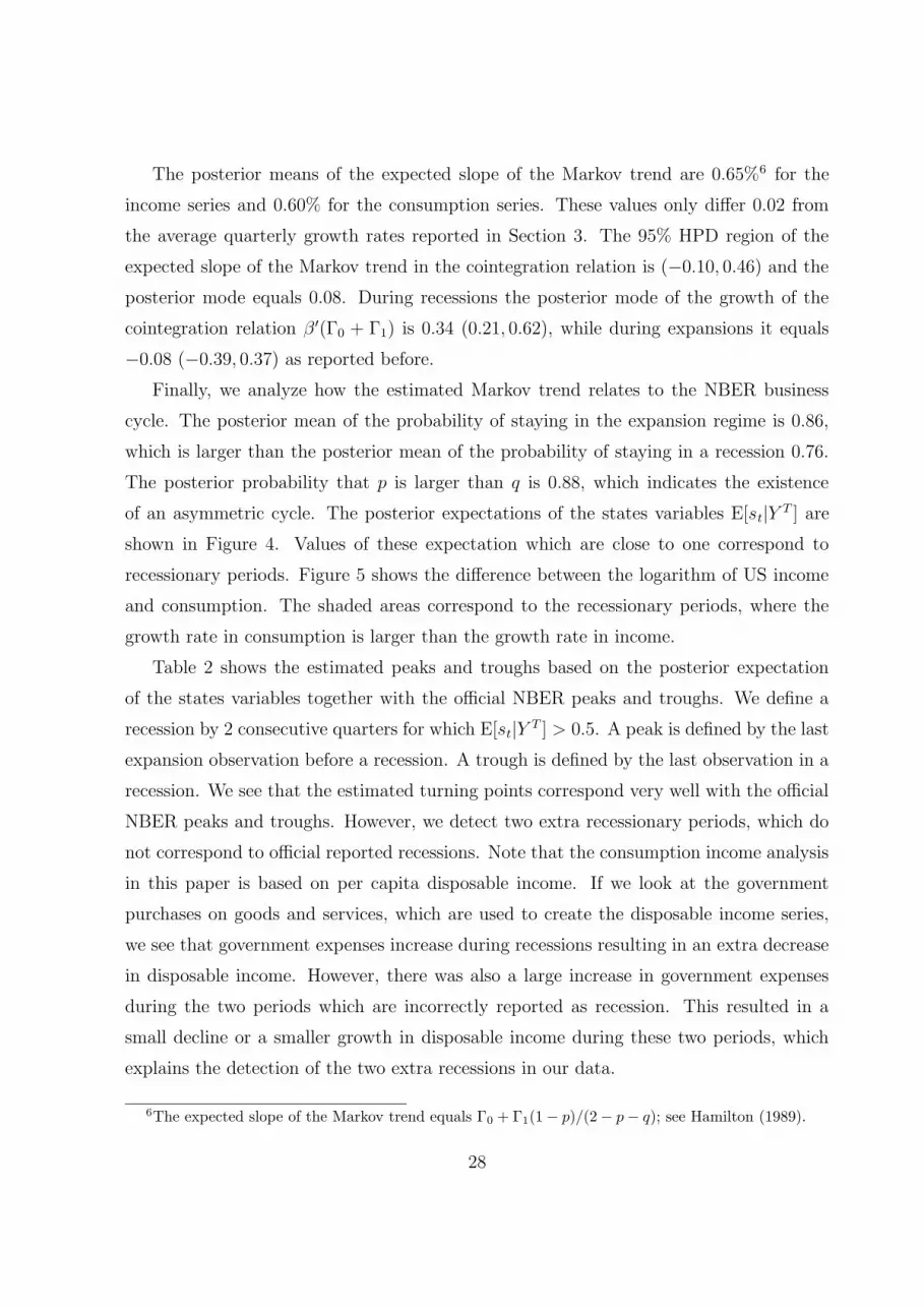
6The expected slope of the Markov trend equals Γ0 + Γ1(1− p)/(2− p− q); see Hamilton (1989).
28

0.0
0.2
0.4
0.6
0.8
1.0
60 65 70 75 80 85 90 95
Figure 4: Posterior expectations of the state variablesE[st|Y T ].
-.22
-.20
-.18
-.16
-.14
-.12
-.10
60 65 70 75 80 85 90 95
Figure 5: Difference between log US per capita con-sumption and income. The shaded areas correspond torecessionary periods.
29

Table 2: Peaks and troughs based on theposterior expectations of the unobserved statevariables1.
US NBERpeak trough peak trough
1960.1 1960.4 1960.2 1961.11966.1 1967.41968.2 1970.4 1969.4 1970.41973.2 1975.1 1973.4 1975.11979.3 1980.2 1980.1 1980.31981.3 1982.4 1981.3 1982.41984.4 1987.31989.2 1991.1 1990.3 1991.1
1 A recession is defined by 2 consecutive quarters forwhich E[st|Y T ] > 0.5. A peak corresponds with thelast expansion observation before a recession and atrough with the last observation in a recession.
In summary, the multivariate Markov trend model provides a good description for the
US per capita income and consumption series. The multivariate Markov trend captures
the different growth rates in both series during recession and expansion periods. After
detrending with the Markov trend we detect a stationary linear combination between log
per capita income and consumption. This cointegration relation is not found if we use a
regular deterministic trend instead of a Markov trend for detrending.
9 US Consumption, Income and Investment
In the previous section we have seen that there exist a cointegration relation between
log per capita income and consumption only if we allow for a Markov trend. One may
investigate whether the inclusion of a third variable with a more pronounced cyclical pat-
tern may help to improve the model. Therefore we consider in this section a multivariate
Markov trend model for per capita real disposable income, private consumption and pri-
vate investment of the United States, 1959.1–1999.4. The consumption and income series
are the same as in the previous section. The investment series is also obtained from the
30

-7.0
-6.5
-6.0
-5.5
-5.0
-4.5
-4.0
-3.5
60 65 70 75 80 85 90 95
incomeinvestment
consumption
Figure 6: The logarithm of US per capita consumption,income and investment, 1959.1–1999.4.
Federal Reserve Bank of St. Louis. Figure 6 shows a plot of the log of the three series.
It is clear that the investment series shows a more pronounced cyclical pattern than the
other two series.
To describe the three series we consider in Section 9.1 a VAR model without a Markov
trend. In Section 9.2 we introduce the multivariate Markov trend in the model, where we
allow the growth rates in the three series to be different across the series and across the
stages of the business cycle.
9.1 A VAR model without Markov Trend
In this subsection we analyze the presence of a cointegration relations in a VAR model
without Markov trend (Γ1 = 0 and δ1 = 0 in (21)) for Yt = 100×(ln ct, ln yt, ln it)′, where it
denotes per capita investment series. The priors for model parameters are the same as in
the previous example. The priors for N1 and Σ are given by (29) and (30), with S = I and
ν = 4. The g-type prior for Π given Σ is given in (44) with P = 0 and A = τ/T∑T
t=1 Y′t Yt
for different values of τ , where Yt denotes the demeaned and detrended value of Yt. For
Γ0 and Φi we take flat priors p(Γ0) ∝ 1 and p(Φi) ∝ 1.
The lag order determination is done in the same way as in Section 8. The resulting
31

Table 3: Log Bayes factors, posterior probabilities for the cointegration rank in a linearVAR model (k = 2) and the multivariate Markov trend model (k = 1).
τ = 1 τ = 0.1 τ = 0.01 PICr lnBF(r|3) Pr[r|Y T ] lnBF(r|3) Pr[r|Y T ] lnBF(r|3) Pr[r|Y T ] lnBF(r|3) Pr[r|Y T ]
Linear VAR model
0 < −5 0.00 < −5 0.00 < −5 0.00 < −5 0.001 14.75 1.00 10.15 1.00 5.58 1.00 15.23 1.002 2.30 0.00 1.15 0.00 0.01 0.00 3.06 0.003 0.00 0.00 0.00 0.00 0.00 0.00 0.00 0.00
Multivariate Markov trend model
0 < −5 0.00 < −5 0.00 < −5 1.00 < −5 0.001 15.54 1.00 9.58 1.00 5.28 0.99 14.93 1.002 2.47 0.00 1.39 0.00 0.27 0.01 3.33 0.003 0.00 0.00 0.00 0.00 0.00 0.00 0.00 0.00
1 A log Bayes factor lnBF(r|3) > 0 denotes that a cointegration model with r cointegration relationsis more likely than a model with 3 cointegration relations.
2 Posterior results are based on 400,000 iterations with the Gibbs sampler neglecting the first 100,000draws.
order is 2, which is also obtained if one uses the BIC to determine k. The Bayesian
cointegration analysis is a multivariate extension of the analysis in Section 7. The prior for
α and β2 for the cointegration specifications (rank 1 and 2) are similar to (45). We assign
equal prior probabilities to the possible cointegration ranks (46), i.e. Pr[rank = r] = 14
for r = 0, 1, 2, 3.
The first panel of Table 3 displays the log Bayes factors together with the posterior
probabilities for different values of τ . For all values of τ the Bayes factors lead to 100%
probability of a VAR model with rank 1 cointegration relation7. This is also true if one
chooses to consider the PIC based Bayes factors.
7The standard Johansen (1995) trace tests do not indicate the presence of a cointegration relationbetween the three series if one restricts the deterministic trend within the cointegration space.
32
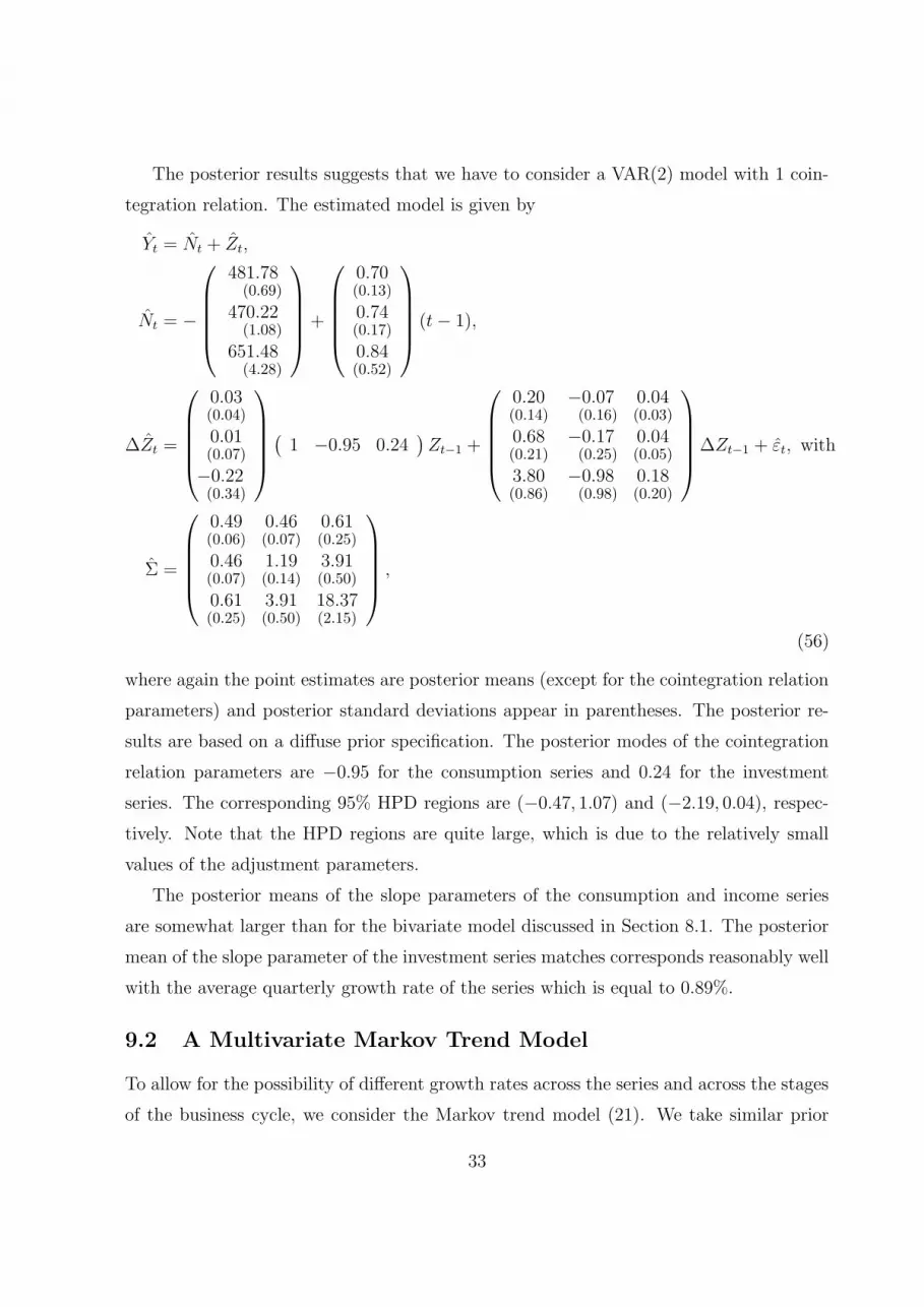
The posterior results suggests that we have to consider a VAR(2) model with 1 coin-
tegration relation. The estimated model is given by
Yt = Nt + Zt,
Nt = −
481.78(0.69)
470.22(1.08)
651.48(4.28)
+
0.70(0.13)
0.74(0.17)
0.84(0.52)
(t− 1),
∆Zt =
0.03(0.04)
0.01(0.07)
−0.22(0.34)
(
1 −0.95 0.24)
Zt−1 +
0.20 −0.07 0.04(0.14) (0.16) (0.03)
0.68 −0.17 0.04(0.21) (0.25) (0.05)
3.80 −0.98 0.18(0.86) (0.98) (0.20)
∆Zt−1 + εt, with
Σ =
0.49 0.46 0.61(0.06) (0.07) (0.25)
0.46 1.19 3.91(0.07) (0.14) (0.50)
0.61 3.91 18.37(0.25) (0.50) (2.15)
,
(56)
where again the point estimates are posterior means (except for the cointegration relation
parameters) and posterior standard deviations appear in parentheses. The posterior re-
sults are based on a diffuse prior specification. The posterior modes of the cointegration
relation parameters are −0.95 for the consumption series and 0.24 for the investment
series. The corresponding 95% HPD regions are (−0.47, 1.07) and (−2.19, 0.04), respec-tively. Note that the HPD regions are quite large, which is due to the relatively small
values of the adjustment parameters.
The posterior means of the slope parameters of the consumption and income series
are somewhat larger than for the bivariate model discussed in Section 8.1. The posterior
mean of the slope parameter of the investment series matches corresponds reasonably well
with the average quarterly growth rate of the series which is equal to 0.89%.
9.2 A Multivariate Markov Trend Model
To allow for the possibility of different growth rates across the series and across the stages
of the business cycle, we consider the Markov trend model (21). We take similar prior
33

distributions as for the bivariate model in Section 8.2. Hence, the prior distributions
for the model parameters are given by (29)–(44) with S = I, ν = 4, P = 0 and A =
τ/T∑T
t=1 Y′t Yt, where Yt denotes the demeaned and detrended value of Yt.
The lag order selection procedure for the VAR part of the model results in k = 1.
The prior for α and β2 for the cointegration specifications are similar to (45). We assign
again equal probabilities to the possible cointegration ranks, i.e. Pr[rank = r] = 14for
r = 0, 1, 2, 3. The second panel of Table 3 report the log Bayes factors and posterior
probabilities for the rank of Π for different values of τ . The values of the log Bayes
factors are similar to the values in the first panel of the table. Hence, adding a Markov
trend to the model does not change the posterior probabilities concerning the number of
cointegration relations.
The selected model by the Bayes factor is a VAR(1) model with 1 cointegration rela-
tion. The estimated model is given by
Yt = Nt + Rt + Zt,
Nt = −
481.95(0.61)
469.78(0.79)
648.54(3.03)
+
0.86(0.11)
1.15(0.15)
2.80(0.49)
(t− 1)−
0.66(0.16)
1.32(0.16)
5.12(0.62)
t∑
i=2
si,
Rt =
0.34(0.14)
00
st,
∆Zt =
0.22(0.07)
0.50(0.14)
2.02(0.64)
(
1 −0.71 −0.06)
Zt−1 + εt, with Σ =
0.40 0.27 −0.15(0.05) (0.06) (0.22)
0.27 0.72 2.21(0.06) (0.11) (0.41)
−0.15 2.21 12.72(0.11) (0.41) (1.93)
,
(57)
where again the point estimates are posterior means and posterior standard deviations
appear in parentheses. The posterior results are based on a diffuse prior specification.
The posterior means of the transition probabilities equal
p = 0.86 (0.05) and q = 0.76 (0.10),
which are equal to the bivariate Markov trend model in Section 8.2.
34

The posterior modes of the cointegration relation parameters are −0.71 and −0.06for consumption and investment series, respectively. The corresponding HPD regions
are (−1.00,−0.35) and (−0.18, 0.06), which are clearly smaller than for the linear VAR
specification. The adjustment parameters are more than two posterior standard deviations
away from zero and hence the cointegration relation seems to be more relevant than in
the model without the Markov trend. The HPD region of the cointegration relation
parameter for investment contains zero, which suggests that contribution of investment
to the cointegration relation is of minor importance.
The posterior means of the Markov trend parameters of the consumption and income
series are almost the same as for the bivariate model in Section 8.1. For the investment
series the posterior mean of the quarterly growth rate during expansions is 2.80%, while
during recessions we have a growth rate of −2.32% (2.80− 5.12). Reduced rank Markov
trend cointegration (β ′Γ1 = 0) is again not very likely as the posterior mode of β ′Γ1 equals
0.45 and its 95% HPD region is (0.19, 0.99).
In sum, we have seen that Bayes factors suggest 1 out of 3 possible cointegration
relations in a VAR model with deterministic trend for per capita consumption, income
and investment. This implies that there are still two unit roots remaining in the system
as was also the case in our bivariate specification in Section 8. Although Bayes factors
suggest the presence of one cointegration relation, the relevance of the error correction
term is small. If we turn to a multivariate Markov trend model, the error correction term
becomes more relevant and the contribution of investment to the cointegration relation
is negligible. The inclusion of a Markov trend now does not lead to a decrease in the
number of unit roots in the system as in the bivariate case. Although investments seems
to partly replace the role of the Markov trend in the linear VAR, the posterior results of
the Markov trend model role suggest that the Markov trend remains important.
10 Conclusion
In this paper we have proposed a multivariate Markov trend model to analyze the possible
existence of a long-run relation between per capita consumption and income of the United
States. The model specification has been based on suggestions by simple economic theory
35

and a simple stylized facts analysis on both series. The model contains a multivariate
Markov trend specification, which allows for different growth rates in the series and differ-
ent growth rates during recessions and expansions. The deviations from the multivariate
Markov trend are modeled by a vector autoregressive model. To analyze US series with
the multivariate Markov trend model, we have chosen a Bayesian approach. Bayes factors
are proposed to analyze the presence of a cointegration relation in the deviations of the
series from the multivariate Markov trend.
The posterior results suggest that there exists a stationary linear relation between log
per capita consumption and income after correcting for a Markov trend. The Markov
trend models the different growth rates in both series during recessions and expansions.
The growth rate in consumption is larger than the negative growth rate in income during
recessions. To compensate for this difference the growth rate in income is larger than the
growth rate in consumption during expansion periods. If we replace the Markov trend by
a deterministic linear trend posterior results do not indicate the presence of a stationary
linear relation between both series.
To analyze the robustness of our approach we included per capita investment to the
model as this series has a more pronounced cyclical pattern. Hence, we consider a multi-
variate Markov trend model for log per capita consumption, income and investment series.
Posterior results suggest the presence of only one cointegration relation between the three
series. This result is found for both the Markov trend and the linear deterministic trend
specification. Hence, adding a possible non-stationary variable to the Markov trend model
therefore does not increase the number of cointegration relations in the system. Although
Bayes factors suggest cointegration in the linear VAR model with deterministic trend, the
posterior standard deviations of the adjustment parameters show that the cointegration
relation is of minor importance. In the multivariate Markov trend model, the error cor-
rection term is more relevant and investment does not have a significant contribution to
the cointegration relation.
We end this conclusion with some suggestion for further research. The multivariate
Markov trend model we proposed in this paper is linear in deviation from the Markov
trend. Possible cointegrating vectors and adjustment parameters are not affected by
regime changes. We may however also allow that the adjustment parameters or the
36

cointegrating vector have different values over the business cycle. This implies a nonlinear
error correction mechanism in consumption and income; see also Peel (1992). It is then
even possible that the series are only cointegrated in expansions and not in recessions.
Testing for the presence of cointegration in the different regimes may however be difficult
as the number of observations for recessionary periods is usually very small. Furthermore,
the dynamic properties of such models are not easy to derive; see Holst et al. (1994) and
Warne (1996). Finally, we may also consider alternative multivariate nonlinear models
to analyze the consumption and income series, like threshold models; see for example
Granger and Terasvirta (1993) and Balke and Fomby (1997).
37

A Jacobian Transformation
In this appendix we derive the Jacobian of the transformation from Π to (α, λ, β2) for
a 2-dimensional vector autoregressive model. For larger dimensions; see Kleibergen and
Paap (2002). Define α = (α1, α2), where α1 and α2 are scalars and θ2 = −α2/α1 such
that α = α1θ with θ = (1 − θ2)′. The derivation of the Jacobian of the complete
transformation from Π to (α1, α2, λ, β2) is for notional convenience split up in the Jacobian
of the transformation of Π to (α1, θ2, λ, β2) and then the transformation of θ2 to α2. As
θ⊥ ∈ α⊥ we can write
Π = αβ ′ + α⊥λβ′⊥
= (α α⊥)
(
1 00 λ
)(
β′
β′⊥
)
=
(
1 θ2/√
1 + θ22−θ2 1/
√
1 + θ22
)(
α1 00 λ
)(
1 −β2−β2/
√
1 + β22 1/√
1 + β22
)
= α1
(
1 −β2−θ2 θ2β2
)
+λ
√
(1 + θ22)(1 + β22)
(
−θ2β2 θ2−β2 1
)
.
(58)
The derivatives of Π with respect to α1, θ2, λ and β2 read
J1 =∂ vec(Π)
∂α1=
1−θ2−β2θ2β2
J2 =∂ vec(Π)
∂θ2=
0−α10
α1β2
+λ
√
(1 + θ22)(1 + β22)
−β2 + θ22β2/(1 + θ22)θ2β2/(1 + θ22)1− θ22/(1 + θ22)−θ2/(1 + θ22)
J3 =∂ vec(Π)
∂λ=
1√
(1 + θ22)(1 + β22)
−θ2β2−β2θ21
J4 =∂ vec(Π)
∂β2=
00−α1α1θ2
+λ
√
(1 + θ22)(1 + β22)
−θ2 + θ2β22/(1 + β22)]
−1 + β22/(1 + β22)−θ2β2/(1 + β22)−β2/(1 + β22)
.
(59)
The Jacobian from θ2 to α2 is simply
G =
∣
∣
∣
∣
∂θ2∂α2
∣
∣
∣
∣
= − 1
α1. (60)
38

Hence, the Jacobian for the total transformation equals
J(α, λ, β2) = |J1 J2 J3 J4| |G|. (61)
B Full Conditional Posterior Distributions
Full Conditional Posterior of the States
To sample the states, we need the full conditional posterior density of st, denoted by
p(st|s−t,Θ2, Y T ), t = 1, . . . , T , where s−t = sT\st. Since st follows a first-order Markov
process, it is easily seen that
p(st|s−t) ∝ p(st|st−1) p(st+1|st), (62)
due to the Markov property. Following Albert and Chib (1993), we can write
p(st|s−t,Θ2, Y T ) =p(st|s−t,Θ2, Y t) f(Yt+1, . . . , YT |Y t, s−t, st,Θ2)
f(Yt+1, . . . , YT |Y t, s−t,Θ2)
∝ p(st|s−t,Θ2, Y t) f(Yt+1, . . . , YT |Y t, s−t, st,Θ2). (63)
Using the rules of conditional probability, the first term of (63) can be simplified as
p(st|s−t,Θ2, Y t) ∝ p(st|s−t,Θ2, Y t−1) f(Yt, st+1, . . . , sT |Y t−1, st,Θ2)
∝ p(st|st−1,Θ2) f(Yt|Y t−1, st,Θ2)
p(st+1|st,Θ2, Y t) p(st+2, . . . , sT |st+1,Θ2, Y t)
∝ p(st|st−1,Θ2) f(Yt|Y t−1, st,Θ2) p(st+1|st,Θ2), (64)
where we use the fact that st+2, . . . , sT is independent of st given st+1. The second term
of (63) is proportional to
f(Yt+1, . . . , YT |Y t, st,Θ2) ∝T∏
i=t+1
f(Yi|Y i−1, si,Θ2). (65)
Next, using (64) and (65) the full conditional distribution of st for t = k + 1, . . . , T is
given by
p(st|s−t,Θ2, Y T ) ∝ p(st|st−1,Θ2) p(st+1|st,Θ2)T∏
i=t
f(Yi|Y i−1, si,Θ2), (66)
39

where f(Yt|Y t−1, st,Θ2) is defined in (24) and the constant of proportionality can be
obtained by summing over the two possible values of st. At time t = T the term
p(sT+1|sT ,Θ2) drops out. The first k states can be sampled from the full conditional
distribution
p(st|s−t,Θ2, Y T ) ∝ p(st|st−1,Θ2) p(st+1|st,Θ2)T∏
i=k+1
f(Yi|Y i−1, si,Θ2), (67)
for t = 1, . . . , k, where at time t = 1 the term p(st|st−1,Θ2) is replaced by the uncondi-
tional density p(s1|Θ2), which is a binomial density with probability (1− p)/(2− p− q).
As Albert and Chib (1993) show, sampling of the state variables is easier if Π = 0.
Under this restriction only the first (k − 1) future conditional densities of Yt depend on
st instead of all future conditional densities. However, sampling is possible in the same
way: take the most recent value of sT and sample the states backward in time, one after
another, starting with sT . After each step, the t-th element of sT is replaced by its most
recent draw.
Full Conditional Posterior of p and q
From the conditional likelihood function (25) if follows that the full conditional posterior
densities of the transition parameters are given by
p(p|sT ,Θ2\p, Y T ) ∝ pN0,0(1− p)N0,1
p(q|sT ,Θ2\q, Y T ) ∝ qN1,1(1− q)N1,0 ,(68)
where Ni,j again denotes the number of transitions from state i to state j. This implies
that the transition probabilities can be sampled from beta distributions.
Full Conditional Posterior of Σ
It is easy to see from the conditional likelihood (25) that the full conditional posterior of
Σ is proportional to
p(Σ|sT ,Θ2\Σ, Y T ) ∝ |Σ|− 12(T−k+2+λ) exp(−1
2tr(Σ−1(S + (Y1−N1)(Y1−N1)
′ +T∑
t=k+1
εtε′t)),
(69)
and hence the covariance matrix Σ can be sampled from an inverted Wishart distribution;
see Zellner (1971, p. 395).
40

Full Conditional Posterior of N1, Γ0 and Γ1
To derive the full conditional posterior distribution of N1, Γ0 and Γ1 we write (21) as
Σ− 12Φ(L)Yt = Σ− 1
2Φ(L)(Γ0(t− 1) + Γ1
t∑
i=2
si +N1) + Σ− 12 εt
= −Σ− 12
k∑
j=1
Φj(Γ0 Γ1 N1)
Lj(t− 1)
Lj∑t
i=2 si1
+ Σ− 12 εt,
(70)
where Φ0 = −I. Without the Φj matrices, we have a multivariate regression model in the
parameters N1, Γ0 and Γ1 and the full conditional distribution would be matrix normal.
To reverse the order of Φ(L) and the parameters (Γ0 Γ0 N1), we apply the vec operator to
both sides of (70). Using the vec notation and the fact that vec(ABC) = (C ′⊗A)vec(B),
we can write (70) as a linear regression model and hence the full conditional distributions
of vec(N1), vec(Γ0) and vec(Γ1) are normal.
Full Conditional Posterior of δ1
We write (21) as
Σ− 12Φ(L)(Yt −Nt) = Σ− 1
2φ(L)δRt + Σ− 12 εt, (71)
with Φ0 = −I. Applying the vec operator to both sides leads to a standard regression
model with regression parameter δ1. The full conditional posterior of δ1 is therefore
normal.
Full Conditional Posterior of Π and Φ
To sample from the full conditional posterior of the autoregressive parameters we use that
conditional on Γ0, Γ1, N1 and the states stTt=1, equation (21) can be seen as a multi-
variate regression model in the parameters Π and Φ. From Zellner (1971, chapter VIII)
if follows that the full conditional posterior distribution of the parameter matrices are
matrix normal. A draw from the full conditional distribution of λ can be obtained by
performing a singular value decomposition on the sampled Π and solving for λ using (39).
41

Sampling of α and β2
To derive the full conditional posterior distributions for α and β2 we rewrite (23) such
that conditional on Φ, N1, Γ0, Γ1 and the states stTt=1 it resembles a simple VAR(1)
model. Using Zt = Yt −Nt −Rt−1 we can write
∆Zt −k−1∑
i=1
Φi∆Zt−i = αβ ′Zt−1,+εt
∆Z∗t = αβ ′Z∗
t−1 + εt,
(72)
where ∆Z∗t = ∆Zt −
∑k−1i=1 Φi∆Zt−i and Z∗
t−1 = Yt−1 − Nt−1 − Rt−1. It is easy to see
that the full conditional posterior distributions of α and β2 are non-standard. Therefore
Kleibergen and Paap (2002) propose a Metropolis-Hastings algorithm to sample α and
β2 in this simple VAR model. Chib and Greenberg (1994, 1995) show that it is possible
to build such a Metropolis-Hastings algorithm into the Gibbs sampling procedure. The
Metropolis-Hastings algorithm step works as follows. First, draw in iteration i of the
Gibbs sampler Πi from its full conditional posterior distribution; see above. Perform a
singular value decomposition on Π and solve for αi, λi and βi2 using (39). Now accept this
draw of αi and βi2 with probability min(
w(αi,λi,βi
2)
w(αi−1,λi−1,βi−1
2), 1)
, where i denotes the current
draw, i− 1 the previous draw and
w(α, λ, β2) =|J(α, λ, β2)|λ=0||J(α, λ, β2)|
g(λ|Θ1, Y T )|λ=0, (73)
where
g(λ|Θ1, Y T ) = (2π)−12 |α′
⊥Σ−1α⊥|
12 |β′
⊥(A+ Z∗′−1Z
∗−1)β⊥|
12
exp(−1
2tr((β ′
⊥(A+ Z∗′−1Z
∗−1)β⊥)(λ− λ)(α′
⊥Σ−1α⊥)(λ− λ))), (74)
with
λ = (β ′⊥(A+ Z∗′
−1Z∗−1)β⊥)
−1β′⊥(A(P − βα′) + Z∗′
−1(∆Z∗ − Z∗
−1βα′))Σ−1α⊥(α
′⊥Σ
−1α⊥)−1,
(75)
and Z∗−1 = (Z∗
k . . . Z∗T−1)
′, ∆Z∗ = (∆Z∗k+1 . . .∆Z
∗T )
′. If the draw of αi and βi2 is rejected,
one has to take the previous draw i.e. αi = αi−1 and βi2 = βi−12 .
42

References
Albert, J. H. and S. Chib (1993), Bayes Inference via Gibbs Sampling of Autoregres-
sive Time Series subject to Markov Mean and Variance Shifts, Journal of Business &
Economic Statistics , 11, 1–15.
Balke, N. S. and T. B. Fomby (1997), Threshold Cointegration, International Economic
Review , 38, 627–646.
Campbell, J. Y. (1987), Does Saving Anticipate Declining Labor Income? An Alternative
Test of the Permanent Income Hypothesis, Econometrica, 55, 1249–1273.
Chen, M.-H. (1994), Importance-Weighted Marginal Bayesian Posterior Density Estima-
tion, Journal of the American Statistical Association, 89, 818–824.
Chib, S. (1996), Calculating Posterior Distributions and Model Estimates in Markov
Mixture Models, Journal of Econometrics , 75, 79–97.
Chib, S. and E. Greenberg (1994), Bayes Inference in Regression Models with ARMA(p,q)
Errors, Journal of Econometrics , 64, 183–206.
Chib, S. and E. Greenberg (1995), Understanding the Metropolis-Hastings Algorithm,
American Statistician, 49, 327–335.
Dickey, D. A. and W. A. Fuller (1979), Distribution of Estimators for Autoregressive Time
Series with a Unit Root, Journal of the American Statistical Association, 74, 427–431.
Dickey, J. (1971), The Weighted Likelihood Ratio, Linear Hypothesis on Normal Location
Parameters, The Annals of Mathematical Statistics , 42, 240–223.
Dwyer, M. J. and S. M. Potter (1996), Markov Trend Cointegration, unpublished working
paper, University of California.
Flavin, M. A. (1981), The Adjustment of Consumption to Changing Expectations about
Future Income, Journal of Political Economy , 89, 974–1009.
Geisser, S. (1965), A Bayes Approach for Combining Correlated Estimates, Journal of
the American Statistical Association, 60, 602–607.
43

Gelfand, A. E. and A. F. M. Smith (1990), Sampling-Based Approaches to Calculating
Marginal Densities, Journal of the American Statistical Association, 85, 398–409.
Geman, S. and D. Geman (1984), Stochastic Relaxations, Gibbs Distributions, and the
Bayesian Restoration of Images, IEEE Transaction on Pattern Analysis and Machine
Intelligence, 6, 721–741.
Golub, G. H. and C. F. van Loan (1989), Matrix Computations , The John Hopkins Uni-
versity, Baltimore.
Goodwin, T. H. (1993), Business-Cycle Analysis with a Markov-Switching Model, Journal
of Business & Economic Statistics , 11, 331–339.
Granger, C. W. J. and T. Terasvirta (1993), Modelling Nonlinear Economic Relations ,
Oxford University Press, Oxford.
Gregory, A. G. and B. E. Hansen (1996), Residual-based Tests for Cointegration in Models
with Regime Shifts’, Journal of Econometrics , 70, 99–126.
Hall, S. G., Z. Psaradakis, and M. Sola (1997), Cointegration and Changes in Regime:
The Japanese Consumption Function, Journal of Applied Econometrics , 12, 151–168.
Hamilton, J. D. (1989), A New Approach to the Econometric Analysis of Nonstationary
Time Series and Business Cycles, Econometrica, 57, 357–384.
Hamilton, J. D. and G. Perez-Quiros (1996), What Do the Leading Indicators Lead,
Journal of Business , 69, 27–49.
Hansen, H. and S. Johansen (1999), Some Tests for Parmater Constancy in Cointegrated
VAR models, Econometrics Journal , 2, 306–333.
Hoek, H. (1997), Variable Trends: A Bayesian Perspective, Ph.D. thesis, Tinbergen In-
stitute, Thesis Publishers, Amsterdam.
Holst, U., G. Lindgren, J. Holst, and M. Thuvesholmen (1994), Recursive Estimation in
Switching Autoregressions with a Markov Regime, Journal of Time Series Analysis ,
15, 489–506.
44

Jin, F. (1995), Cointegration of Consumption and Disposable Income: Evidence from
Twelve OECD Countries, Southern Economic Journal , 62, 77–88.
Johansen, S. (1995), Likelihood-Based Inference in Cointegrated Vector Autoregressive
Models , Oxford University Press, Oxford.
Kim, C.-J. and C. R. Nelson (1999a), Has the U.S. Economy Become More Stable:
A Bayesian Approach Based on a Markov-Switching Model of the Business Cycle, Re-
view of Economics and Statistics , 81, 608–616.
Kim, C.-J. and C. R. Nelson (1999b), State-Space Models with Regime Switching: Classical
and Gibbs-Sampling Approaches with Applications , MIT Press, Cambridge, MA.
Kim, M.-J. and J.-S. Yoo (1995), New Index of Coincident Indicators: A Multivariate
Markov Switching Factor Model Approach, Journal of Monetary Economics , 36, 607–
630.
Kleibergen, F. and R. Paap (2002), Priors, Posterior and Bayes Factors for a Bayesian
Analysis of Cointegration, Journal of Econometrics , 111, 223–249.
Kleibergen, F. and H. K. van Dijk (1994), On the Shape of the Likelihood/Posterior in
Cointegration Models, Econometric Theory , 10, 514–551.
Kleibergen, F. and H. K. van Dijk (1998), Bayesian Simultaneous Equation Analysis using
Reduced Rank Regression, Econometric Theory , 14, 701 – 743.
Krolzig, H.-M. (1997), Markov Switching Vector Autoregressions: Modelling, Statistical
Inference, and an Application to Business Cycle Inference, Springer, Berlin.
Lam, P.-S. (1990), The Hamilton Model with a General Autoregressive Component, Jour-
nal of Monetary Economics , 26, 409–432.
Luginbuhl, R. and A. de Vos (1999), Bayesian Analysis of an Unobserved-Component
Time Series Model of GDP with Markov-Switching and Time-Varyings Growths, Jour-
nal of Business & Economic Statistics , 17, 456–465.
45

Martin, G. M. (2000), US Deficit Sustainability: A new Approach based on Multiple
Endogeneous Breaks, Journal of Applied Econometrics , 15, 83–105.
McCulloch, R. E. and R. S. Tsay (1994), Statistical Analysis of Economic Time Series
via Markov Switching Models, Journal of Time Series Analysis , 15, 523–540.
Nelson, C. R., J. Piger, and E. Zivot (2001), Markov Regime Switching and Unit-Root
Tests, Journal of Business & Economic Statistics , 19, 404–415.
Peel, D. A. (1992), Some Analysis of the Long-run Time Series Properties of Consumption
and Income in the U.K., Economics Letters , 39, 173–178.
Peel, D. A. and A. E. H. Speight (1998), Threshold Nonlinearities in Output: Some
International Evidence, Applied Economics , 30, 323–334.
Phillips, K. L. (1991), A Two-Country Model for Stochastic Output with Changes in
Regime, Journal of International Economics , 31, 121–142.
Phillips, P. C. B. and W. Ploberger (1994), Posterior Odds Testing for a Unit Root with
Data-based Model Selection, Econometric Theory , 10, 774–808.
Potter, S. M. (1995), A Nonlinear Approach to US GNP, Journal of Applied Econometrics ,
10, 109–125.
Psaradakis, Z. (2001), Markov Level Shifts and the Unit-Root Hypothesis, Econometrics
Journal , 4, 225–241.
Psaradakis, Z. (2002), On the Asymptotic Behaviour of Unit-Root Tests in the Presence
of a Markov Trend, Statistiscs & Probability Letters , 57, 101–109.
Sargent, T. J. (1978), Rational Expectations, Econometric Exogeneity, and Consumption,
Journal of Political Economy , 86, 673–700.
Schotman, P. C. and H. K. van Dijk (1991a), A Bayesian Analysis of the Unit Root in
Real Exchange Rates, Journal of Econometrics , 49, 195–238.
Schotman, P. C. and H. K. van Dijk (1991b), On Bayesian Routes to Unit Roots, Journal
of Applied Econometrics , 6, 387–401.
46

Schwarz, G. (1978), Estimating the Dimension of a Model, The Annals of Statistics , 6,
461–464.
Silverman, B. W. (1986), Density Estimation for Statistics and Data Analysis , Chapman
and Hall, London.
Smith, A. F. M. and G. O. Roberts (1993), Bayesian Computation via the Gibbs Sampler
and Related Markov Chain Monte Carlo Methods, Journal of the Royal Statistical
Society B , 55, 3–23.
Tanner, M. A. and W. H. Wong (1987), The Calculation of Posterior Distributions by
Data Augmentation, Journal of the American Statistical Association, 82, 528–550.
Tierney, L. (1994), Markov Chains for Exploring Posterior Distributions, The Annals of
Statistics , 22, 1701–1762.
Warne, A. (1996), Autocovariance Functions and Maximum Likelihood in a VAR Model
under Markov Switching, unpublished working paper, Stockholm University.
Zellner, A. (1971), An Introduction to Bayesian Inference in Econometrics , Wiley, New
York.
Zellner, A. (1986), On Assesing Prior Distributions and Bayesian Regression Analysis with
g-prior Distributions, in P. Goel and A. Zellner (eds.), Bayesian Inference and Decesion
Techniques: Essays in Honor of Bruno de Finetti , North-Holland, Amsterdam, pp.
233–243.
Zivot, E. (1994), A Bayesian Analysis of the Unit Root Hypothesis within an Unobserved
Components Model, Econometric Theory , 10, 552–578.
47


