Credit cycles and macro fundamentals

No. 2006/33

Credit Cycles and Macro Fundamentals

Siem Jan Koopman, Roman Kräussl, André Lucas, and André Monteiro

Center for Financial Studies

The Center for Financial Studies is a nonprofit research organization, supported by an association of more than 120 banks, insurance companies, industrial corporations and public institutions. Established in 1968 and closely affiliated with the University of Frankfurt, it provides a strong link between the financial community and academia.

The CFS Working Paper Series presents the result of scientific research on selected topics in the field of money, banking and finance. The authors were either participants in the Center´s Research Fellow Program or members of one of the Center´s Research Projects.

If you would like to know more about the Center for Financial Studies, please let us know of your interest.

Prof. Dr. Jan Pieter Krahnen Prof. Volker Wieland, Ph.D.

* The authors would like to thank seminar participants at Vrije Universiteit Amsterdam for valuable comments. Financial support from Funda¸c˜ao para a Ciˆencia e a Tecnologia (Portuguese Foundation for Science and Technology), the Vrije Universiteit Amsterdam, and the VU Institute for Asset Management is gratefully acknowledged. The rating transition data for this research was generously supplied by Standard and Poor’s.

1 Vrije Universiteit Amsterdam, Department of Econometrics, and Tinbergen Institute Amsterdam 2 Vrije Universiteit Amsterdam, Department of Finance 3 Corresponding author: Vrije Universiteit Amsterdam and Tinbergen Institute Amsterdam

Contact Details: Vrije Universiteit Amsterdam, FEWEB, De Boelelaan 1105,081HV Amsterdam, Netherlands, phone: +31 20 598 6039, fax: +31 20 598 6020, email: [email protected]

4 Vrije Universiteit Amsterdam, Department of Finance, VU Institute for Asset Management Training, and Tinbergen Institute Amsterdam

CFS Working Paper No. 2006/33

Credit Cycles and Macro Fundamentals*

Siem Jan Koopman1, Roman Kräussl2 André Lucas3, and André Monteiro4

December 6, 2006

Abstract: We study the relation between the credit cycle and macro economic fundamentals in an intensity based framework. Using rating transition and default data of U.S. corporates from Standard and Poor’s over the period 1980–2005 we directly estimate the credit cycle from the micro rating data. We relate this cycle to the business cycle, bank lending conditions, and financial market variables. In line with earlier studies, these variables appear to explain part of the credit cycle. As our main contribution, we test for the correct dynamic specification of these models. In all cases, the hypothesis of correct dynamic specification is strongly rejected. Moreover, accounting for dynamic mis-specification, many of the variables thought to explain the credit cycle, turn out to be insignificant. The main exceptions are GDP growth, and to some extent stock returns and stock return volatilities. Their economic significance appears low, however. This raises the puzzle of what macro-economic fundamentals explain default and rating dynamics JEL Classification: G11, G21 Keywords: Credit Cycles, Business Cycles, Bank Lending Conditions, Unobserved

Component Models, Intensity Models, Monte Carlo Likelihood.

1 Introduction

Systematic credit risk factors play a dominant role in current credit risk management. Tra-

ditionally, credit scoring methodologies focus on assessing the credit risk of individual coun-

terparties (see i.a. Altman (1983), Altman (2000)). Though important, at the portfolio level

most of the idiosyncratic risks can be diversified and only the systematic credit risk components

remain, see, e.g., Lucas et al. (2002), Schonbucher (2001), Frey and McNeil (2003). This also

holds if bond or loan portfolios are repackaged into new products like CDOs. In order to assess

the credit risk at the portfolio level, it is important to model the correct dynamics of systematic

credit risk components.

In this paper, we use the methodology of Koopman et al. (2005) to estimate the credit

cycle directly from rating and default data at the micro level using intensity models with

unobserved common risk factors. The data used are rating and default transitions for U.S.

corporates rated by Standard and Poor’s and observed over December 1980 to June 2005. We

condition the credit cycle on a number of macro economic fundamentals, reflecting the state

of the business cycle, bank lending conditions, and financial market conditions. In line with

results by for example Couderc and Renault (2005), these variables appear to capture part of

the credit cycle dynamics. The models, however, turn out to be dynamically mis-specified as

there is strong remaining autocorrelation in the intensities. If we account for this, many of the

familiar macro variables become insignificant, giving way to a significant unobserved common

risk factor. The results are robust to a variety of specifications of the model. The main puzzle

that emerges is what macro fundamentals drive systematic default and (re-)rating behavior.

The formal testing procedure for dynamic mis-specification introduced in this paper consti-

tutes a powerful tool in the empirical modeling of intensities. For example, in the current paper

we model intensities of rating and default transitions on both observed macro fundamentals

and on an unobserved credit cycle component. If the fundamentals explain the credit cycle

completely, the unobserved component should drop from the analysis. This can be tested using

standard likelihood ratio tests. The computation of the likelihood ratio test, however, is not

trivial because the latent component must be integrated out of the likelihood. We describe the

importance sampling methodology that makes these types of tests possible.

Empirically, the relation between default rates and growth has been addressed in a number

of studies. Fama (1986) and Wilson (1997), regress default rates on observed macro variables

and find cyclicality in probabilities of default (PDs), particularly in the case of economic down-

turns when PDs increase significantly. Koopman and Lucas (2005) concentrate on the time

series dimension of PDs and present evidence of co-cyclicality between GDP and default rates.

2

Kavvathas (2001) shows the influence of the term structure of interest rates over the rating mi-

gration (including default) intensities using parametric and semi-parametric duration models.

Carling et al. (2002) employ the semi-parametric duration model of Cox (1972) conditioning on

both firm specific and macroeconomic variables to analyze a dataset on business loans. Duffie,

Saita and Wang (2006a) also incorporate firm specific information in their duration models.

Their results indicate that both the level of real economic activity and the term structure of

interest rates are important determinants of default risk. A commonality between the papers

based on the intensity framework for credit risk is that hardly any attention is paid to the cor-

rect specification of the model. This is particularly relevant given the demonstrated stickiness

of aggregate rating migrations and defaults.

Our results in this paper show that out of a number of possible macro fundamentals, many

appear to describe rating and default behavior. If we account for a single unobserved common

risk factor, however, most of the variables become statistically insignificant. At first sight, it

appears that downgrades, up-grades, and defaults are all driven by different sets of macros.

If we further refine the model to allow for three unobserved risk factors, however, the only

relevant macros turn out to be GDP growth, and to some extent stock market returns and return

volatilities. GDP has the significant and expected impact on both upgrade intensities (positive),

and downgrade and default intensities (negative). The stock market variables only appear

relevant for the upgrade intensities. In line with the basic structural model of Merton (1974),

returns have a positive impact on upgrade intensities, whereas volatilities have a negative effect.

More importantly, however, is that in all cases there is a significant unobserved component

present in the model. This component is not captured by the macro variables included.

In terms of the related literature, our analysis is most closely related to the work by Coud-

erc and Renault (2005) and Duffie, Eckner, Horel, and Saita (2006b). There are a number

of important differences. First, our modeling framework is significantly different from that of

Couderc and Renault (2005). We use a parameter driven dynamic intensity model that condi-

tions on observable macro variables. Couderc and Renault focus more on the macros only or on

an observation driven autoregressive conditional duration (ACD) model for defaults. Second,

Couderc and Renault condition intensities on the value of fundamentals at the start of the

company’s rating. In contrast, we allow the intensities to change over time due to both changes

in observables and unobservables. This is an explicit advantage of the intensity framework

over an approach starting directly from durations. Duffie et al. (2006b) have a similar inten-

sity framework as ours. They employ a different estimation methodology than the Simulated

Maximum Likelihood (SML) approach presented in this paper. Also, their specification search

over explanatory macro variables is different. Third, we do not only consider information from

3

defaults to estimate the credit cycle, but also information from downgrades and upgrades. In

this way we can test to what extent rating changes co-vary with the business cycle. This allows

us to address some of the concerns in the pro-cyclicality debate as well. Bangia, Diebold and

Schuermann (2000) and Nickel, Perraudin and Varotto (2000) show that changes in the macro-

economic environment have significant effects on firms’ credit rating transitions. Ferri, Liu and

Majnoni (2000) and Kraussl (2003) provide empirical evidence that credit rating agencies be-

have cyclically, especially when assessing credit risk of sovereign borrowers. The proliferation of

credit risk models may accentuate the pro-cyclical tendencies of banking with potential sharp

macroeconomic consequences. For instance, if credit risk models are overly pessimistic during

economic downturns, then even the most expansionary monetary policy many not sufficiently

encourage commercial banks to lend to borrowers that are perceived to be of high default risk.

If, as this paper shows, the relation between systematic credit risk and business cycles is only

limited, pro-cyclicality concerns might be put into a more moderated perspective.

The paper is set up as follows. In Section 2, we explain the modeling and estimation

framework. In Section 3, we present the data. The empirical results can be found in Section 4.

Finally, Section 5 concludes.

2 The model and likelihood function

2.1 The model

Our modeling framework builds on standard (marked) point process methodology, see Andersen

et al. (1993) for a textbook exposition on this topic. Consider a set of counting processes Njk(t)

for firm k = 1, . . . , K. The type j = 1, . . . , J of each counting process indicates the type of

transition that is counted. For example, j = 1 may correspond to a transition from investment

grade to sub-investment grade, j = 2 from investment grade into default, j = 3 from sub-

investment grade to investment grade, and j = 4 from sub-investment grade into default.

When a rating event of type j occurs for firm k at time t, the counting process Njk(t) jumps

by U . It is assumed that we can model the count processes through their intensities. Let λjk(t)

be the intensity at time t of the counting process Njk(t). The intensities are modeled through

the latent factor intensity model of Koopman et al. (2005). In particular, we have

λjk(t) = Rjk(t) · exp(ηj + β′

jx(t) + αjψ(t)). (1)

where Rjk(t) is a dummy variable indicating whether firm k is at risk for transition type j at

time t. The model explicitly accounts for the fact that if, for example, the firm is currently

investment grade, it is not at risk for transitions from sub-investment grade to default. The

4

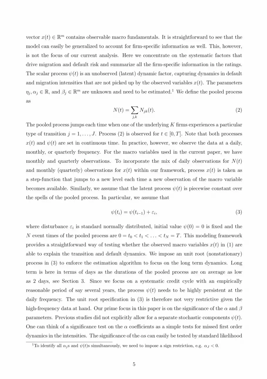
vector x(t) ∈ Rm contains observable macro fundamentals. It is straightforward to see that the

model can easily be generalized to account for firm-specific information as well. This, however,

is not the focus of our current analysis. Here we concentrate on the systematic factors that

drive migration and default risk and summarize all the firm-specific information in the ratings.

The scalar process ψ(t) is an unobserved (latent) dynamic factor, capturing dynamics in default

and migration intensities that are not picked up by the observed variables x(t). The parameters

ηj, αj ∈ R, and βj ∈ Rm are unknown and need to be estimated.1 We define the pooled process

as

N(t) =∑

j,k

Njk(t). (2)

The pooled process jumps each time when one of the underlyingK firms experiences a particular

type of transition j = 1, . . . , J . Process (2) is observed for t ∈ [0, T ]. Note that both processes

x(t) and ψ(t) are set in continuous time. In practice, however, we observe the data at a daily,

monthly, or quarterly frequency. For the macro variables used in the current paper, we have

monthly and quarterly observations. To incorporate the mix of daily observations for N(t)

and monthly (quarterly) observations for x(t) within our framework, process x(t) is taken as

a step-function that jumps to a new level each time a new observation of the macro variable

becomes available. Similarly, we assume that the latent process ψ(t) is piecewise constant over

the spells of the pooled process. In particular, we assume that

ψ(ti) = ψ(ti−1) + εi, (3)

where disturbance εi is standard normally distributed, initial value ψ(0) = 0 is fixed and the

N event times of the pooled process are 0 = t0 < t1 < . . . < tN = T . This modeling framework

provides a straightforward way of testing whether the observed macro variables x(t) in (1) are

able to explain the transition and default dynamics. We impose an unit root (nonstationary)

process in (3) to enforce the estimation algorithm to focus on the long term dynamics. Long

term is here in terms of days as the durations of the pooled process are on average as low

as 2 days, see Section 3. Since we focus on a systematic credit cycle with an empirically

reasonable period of say several years, the process ψ(t) needs to be highly persistent at the

daily frequency. The unit root specification in (3) is therefore not very restrictive given the

high-frequency data at hand. Our prime focus in this paper is on the significance of the α and β

parameters. Previous studies did not explicitly allow for a separate stochastic components ψ(t).

One can think of a significance test on the α coefficients as a simple tests for missed first order

dynamics in the intensities. The significance of the αs can easily be tested by standard likelihood

1To identify all αjs and ψ(t)s simultaneously, we need to impose a sign restriction, e.g. αJ < 0.

5

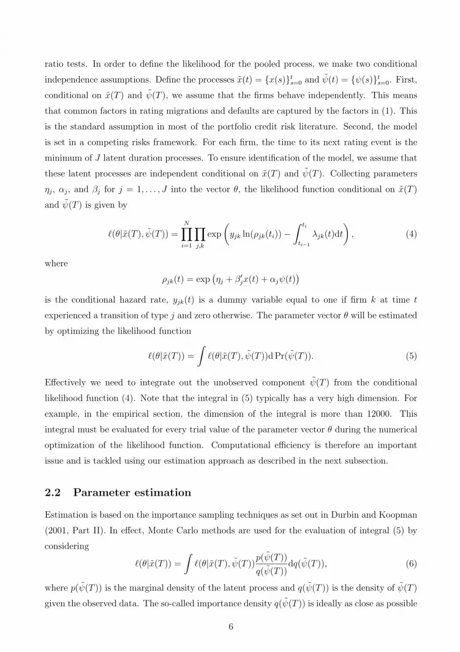
ratio tests. In order to define the likelihood for the pooled process, we make two conditional

independence assumptions. Define the processes x(t) = {x(s)}ts=0 and ψ(t) = {ψ(s)}t

s=0. First,

conditional on x(T ) and ψ(T ), we assume that the firms behave independently. This means

that common factors in rating migrations and defaults are captured by the factors in (1). This

is the standard assumption in most of the portfolio credit risk literature. Second, the model

is set in a competing risks framework. For each firm, the time to its next rating event is the

minimum of J latent duration processes. To ensure identification of the model, we assume that

these latent processes are independent conditional on x(T ) and ψ(T ). Collecting parameters

ηj, αj, and βj for j = 1, . . . , J into the vector θ, the likelihood function conditional on x(T )

and ψ(T ) is given by

ℓ(θ|x(T ), ψ(T )) =N∏

i=1

∏

j,k

exp

(yjk ln(ρjk(ti)) −

∫ ti

ti−1

λjk(t)dt

), (4)

where

ρjk(t) = exp(ηj + β′

jx(t) + αjψ(t))

is the conditional hazard rate, yjk(t) is a dummy variable equal to one if firm k at time t

experienced a transition of type j and zero otherwise. The parameter vector θ will be estimated

by optimizing the likelihood function

ℓ(θ|x(T )) =

∫ℓ(θ|x(T ), ψ(T ))d Pr(ψ(T )). (5)

Effectively we need to integrate out the unobserved component ψ(T ) from the conditional

likelihood function (4). Note that the integral in (5) typically has a very high dimension. For

example, in the empirical section, the dimension of the integral is more than 12000. This

integral must be evaluated for every trial value of the parameter vector θ during the numerical

optimization of the likelihood function. Computational efficiency is therefore an important

issue and is tackled using our estimation approach as described in the next subsection.

2.2 Parameter estimation

Estimation is based on the importance sampling techniques as set out in Durbin and Koopman

(2001, Part II). In effect, Monte Carlo methods are used for the evaluation of integral (5) by

considering

ℓ(θ|x(T )) =

∫ℓ(θ|x(T ), ψ(T ))

p(ψ(T ))

q(ψ(T ))dq(ψ(T )), (6)

where p(ψ(T )) is the marginal density of the latent process and q(ψ(T )) is the density of ψ(T )

given the observed data. The so-called importance density q(ψ(T )) is ideally as close as possible

6

to the conditional density corresponding to ℓ(θ|x(T )), but at the same time should be more

convenient for the generation of samples of ψ(T ) conditional on the observed data. Samples

from q(ψ(T )) are used to evaluate the integral (6), also known as Monte Carlo integration.

The main advantage is that the simulations through q(ψ(T )) contribute significantly to the

likelihood. The alternative route of using (5) directly for generating samples and evaluating

the likelihood is much less efficient and not feasible as the majority of draws from p(ψ(T )) have

little resemblance to the observed data and make negligible contributions to the likelihood. The

construction of q(ψ(T )) is based on linear approximations to non-Gaussian state space models.

The current model falls in this general class of time series models, see Durbin and Koopman

(2001). The stochastic log intensity function log λjk(t) can be generally presented as a linear

function of fixed coefficients and linear dynamic stochastic processes. In particular, we have

log λjk(ti) = Zijkνi, νiU = Tiνi +Riξi, i = 1, . . . , N, (7)

where the state vector νi = ν(ti) and ν(t) consists of the unobserved process ψ(t) and the

unknown coefficients ηj and βj for j = 1, . . . , J . The row vector Zijk is a selection loaded with

zeros and ones or exogenous regressors. The unobserved process for ψ(ti) in (3) is a special

case of the second equation in (7). The fixed coefficients are transformed to functions of time

but are made subject to the identities ηj ≡ ηj(t) = ηj(s) and βj ≡ βj(t) = βj(s) for any t 6= s.

Therefore ηj(ti) and βj(ti) can also be represented by the second equation in (7). As a result

the dimension of the parameter vector θ is reduced considerably since the regression parameters

ηj and βj have become part of the state vector that will be integrated out using importance

sampling. Although the Monte Carlo integration applies to a larger state vector ν(ti) rather

than to ψ(ti) only, we save on the estimation of a large vector θ by the numerical maximization

of the likelihood function (5). Also note that by including ηj ≡ ηij and βj ≡ βij in the state

vector νi, the parameter vector θ is reduced to the coefficients αj only, for j = 1 . . . , J .

Numerical efficiency and computational speed is primarily obtained through the reduction of

the dimension of θ and the efficient importance sampling algorithm of Durbin and Koopman

(2001). The likelihood function (6) can be reformulated as

ℓ(θ|x(T )) = ℓ(α|x(T )) =

∫ℓ(α|x(T ), ν(T ))

p(ν(T ))

q(ν(T ))dq(ν(T )), (8)

where α = (α1, . . . , αJ)′ and ν(t) = {ν(s)}ts=0. Samples from the Gaussian importance density

function q(ν(T )) are based on the linear Gaussian model

yjk(ti) = cijk + log λjk(ti) + uijk, uijk ∼ NID(0, Cijk), (9)

where NID refers to the assumption of a normal distribution for mutually and serially inde-

pendent random variables. The variables cijk and Cijk are known functions of the unobservable

7

λjk(ti). The functions are implied by the density (4). Appropriate values for cijk and Cijk

are found by repeatedly applying the Kalman filter and smoothing equations to obtain new

estimates of λjk(ti) (based on all data-points yjk(ti)) and to compute new values for cijk and

Cijk. This process converges quickly to an unique solution. Given model (9) with the solu-

tions for cijk and Cijk, simulations for log λjk(ti) (based on all data-points yjk(ti)) are obtained

by the simulation smoothing algorithm of Durbin and Koopman (2002). More details on this

method of likelihood evaluation by importance sampling for the model of Section 2 are given

by Koopman, Lucas and Monteiro (2005).

The likelihood function evaluated by importance sampling methods is subject to the value of α.

Numerical optimization methods can be used to obtain the maximum likelihood estimate of α.

Given an estimate of α, the state vector can be estimated as part of the numerical integration

process of the likelihood function since

ν(T ) =

∫ν(T )

p(ν(T ))

q(ν(T ))dq(ν(T )),

where ν(T ) = {ν(ti)}Ni=1. The same importance sampling techniques are therefore applied to

the evaluation of ν(T ). This estimator includes the estimator of the unobservable variable ψ(t)

and the regression coefficient estimators for ηj and βj with j = 1, . . . , J . The estimates are

reported for the empirical study in the sections below.

3 Data

The data come from several sources. For rating transition and default data, we use the Cred-

itPro 7.0 data set of Standard and Poor’s over the period December 1980 to June 2005. The

data set contains the rating histories of all firms rated by Standard and Poor’s. We select all

U.S. firms and use a broad rating category classification of investment grade (BBB- and above)

and subinvestment grade (BB+ and below). We also experimented with a broader seven letter

grade rating system (AAA – CCC), but did not alter the qualitative conclusions regarding the

impact of macro variables on systematic credit risk. We therefore stick to the simpler two-

grade rating system, as this makes the presentation of the estimation results in Section 4 more

compact.

We consider all days on which there was an event. Events are defined as (i) one of the firms

in the database experiencing a rating transition (given the two rating classes) or default, (ii) a

firm becoming non-rated, (iii) a firm entering the sample. All three types of events result in a

change in the intensity of the pooled process. We obtain 4437 event days over the period.

We make three further modifications to the data. First, we remove weekends from the data

8

and measure durations in terms of working days. Some of the rating events are recorded in the

data base during the weekends. We transferred all these rating events to the Friday preceding

the weekend.2 Second, if firms enter the data base or if their rating is withdrawn, this is treated

as a non-informative event. For example, if the rating is withdrawn, we only use the fact that

the company has survived up to the point of the rating withdrawal. The main exception is

when the company defaults at some later stage after the rating withdrawal. These defaults

are recorded in the database. If there is a default following a rating withdrawal, we discard

the withdrawal event and treat the default as a default from its last recorded rating category.

Third, we try to eliminate rating clustering as much as possible. If companies merge or are

taken over, ratings of the merged companies move in lock-step for the remainder of their history

in the data base. Eliminating this type of dependence is important, because it may result in

an over-estimation of the systematic component in the credit and default risk. To reduce this

potential bias, we subsequently look for firms that have (the maximum of) 11 down to 3 rating

events precisely on the same day. If two such firms are found, the most recent rating events of

one of these are discarded and substituted by a rating withdrawal.

The 9 macroeconomic variables in our study are taken from the data base of the Federal

Reserve Bank of St. Louis (FRED). Our dataset of explanatory variables includes both current

information and forward looking indicators such as interest rate-based measures and stock

market variables.

We distinguish three blocks of variables: business cycle, bank lending conditions, and finan-

cial market variables. The business cycle block contains the Gross Domestic Product (GDP).

We convert the data to annual growth rates, observed quarterly.

Bangia, Diebold and Schuermann (2000) and Nickell, Perraudin and Varotto (2000) find

evidence of macroeconomic effects on corporate rating transitions. They show that corporate

defaults are more likely during downturns in economic activity. As a signal of current macro-

economic conditions, we expect that the variable real GDP growth and its four ingredients are

negatively correlated with short-term default probabilities. We are not considering industrial

production, manufacturer’s orders, and capacity utilization, as explanatory variables since they

are already captured in GDP developments. We are also not considering employment series

and personal income growth since they are lagging the business cycle.

Besides general economic variables we expect that indicators of current bank lending con-

ditions prove valuable in explaining default intensities. We consider in our empirical analysis

four different bank lending conditions variables: commercial and industrial loans outstanding,

2The fact that rating decisions taken on a Friday are recorded during weekends is a technical administration

issue in the S&P data base.

9

money supply / M2 growth rate, discount rate, and the quality spread.

The series commercial and industrial loans outstanding measures the volume of business

loans held by banks, and commercial paper issued by non-financial companies. The series tend

to peak during recessions, when many firms need additional outside funding to replace declining

or even negative cash flow. We expect this series to positively correlate with default intensities

as higher borrowing is an indicator of economic difficulties.

The series M2 growth rate measures the aggregate money supply in the economy. It is

either directly or indirectly affected by both Federal Reserve policy (usually showing an inverse

relationship with interest rates) and private demand for credit and liquidity. We expect that a

lower M2 growth rate and, thus, less credit supply by commercial banks, lower market liquidity

should be associated with higher default intensities.

Short-term interest rates have a long history of use as predictors of output changes. We

expect the higher the discount rate, the more expensive it is for companies to take a fresh

credit, the more defaults we observe.

Stock and Watson (1989) show that the quality spread is a potent predictor of output

growth. We measure the quality spread as the difference between interest rates on BBB and

AAA corporate bonds. We expect that the higher this quality spread, the harder the bank

lending conditions, the higher the default intensities.

The financial market variables we consider are the returns on the S&P500, the volatility of

the S&P500 returns, and the interest rate spread.

A simple model of stock price valuation is that stock prices equal the discounted expected

value of future earnings. This implies that short- and mid-term economic performance should be

positively correlated with the returns on the S&P500. In addition, an increase in equity prices

tends to decrease firm leverage. We expect that the lower the stock market index S&P500, the

higher the default intensities.

In a traditional Merton (1974)-type model, the two drivers of default probability are leverage

and the volatility of firms’ assets. (We use the volatility of equity returns as a proxy for the

volatility of firms’ assets.) We expect that the (daily) realized annual volatility of the S&P500

returns computed over the last 260 trading days to be positively correlated with the default

intensities.

Various studies have shown that the interest rate spread has significant predictive power for

output growth, in particular at horizons of one or two years. This term spread series measures

the difference between the 10-year Treasury bond rate and the Federal funds rate. It is felt to be

a reliable indicator of the stance of monetary policy and general financial conditions, because it

rises (falls) when short rates are relatively low (high). When the term spread becomes negative,

10

i.e. short rates are higher than long rates, and the yield curve inverts, its record as an indicator

of recessions is particularly strong. We expect a positive impact on default intensities since

higher interest rate levels imply higher cost of borrowing.

4 Empirical results

4.1 No macro fundamentals

We first implement our model without any macro fundamentals to obtain a preliminary estimate

of the credit cycle present in our data set. The results are presented in Table 1 and Figure 1. We

estimate five different models. In model 0a, no systematic credit risk component is present. All

defaults and rating migrations are idiosyncratically driven. We then proceed to introduce the

common factor ψ(t). First, in model 0b we restrict the loading to be the same for all transition

types. The increase in likelihood from model 0a to model 0b clearly signals that there is common

risk in default and rating migrations. We proceed by relaxing the assumption of a common

loading across transition types. Model 0c allows for a different sensitivity to the common risk

factor between investment grade and sub-investment grade companies. The likelihood increases

by 3.8 points upon adding one parameter. This is statistically significant at the 1% level. If we

allow a different sensitivity to ψ(t) for every transition type, the results for model 0e show that

the increase in likelihood is again significant: 17.3 points for 2 additional parameters. The values

of the parameter estimates are also interesting. In particular, default intensities appear much

more sensitive to systematic risk factors than upgrades and downgrades, whereas downgrades

are slightly more sensitive than upgrades. This is in line with earlier empirical results, see for

example Kavvathas (2001) and Das et al. (2002) and Lucas and Klaassen (2006). The estimated

component ψ(t) visualized in Figure 1 shows the clear troughs in the mid 1980s, early 1990s,

and early 2000s. As the number of investment grade defaults is very small, the precision

of αj for this transition type is low. To limit the number of parameters, we test whether

we can pool the investment grade and sub-investment grade defaults. Model 0d restricts the

loadings for investment grade and sub-investment grade transitions to default to be the same,

αI→D = αSI→D. The reduction in likelihood compared to model 0e is insignificant. Therefore,

from now on we pool the sensitivity parameters to systemic risk factors (i.e., αj and βj) for

investment grade and sub-investment grade defaults.3

As a preliminary analysis, we took the estimated credit cycle from Figure 1 and ran a simple

3Also note that it is empirically very difficult, if not impossible to calibrate the sensitivity to (up to) 10

systematic risk factors separately for investment grade to default transitions, as these transitions are very rare.

11

Table 1: Benchmark model estimates

The table presents the estimated parameters for the benchmark model in

(1) with βj ≡ 0, i.e., without explanatory macro fundamentals for the mi-

gration intensities. Transition types j are from investment grade to sub-

investment grade (I → S), from investment grade to default (I → D), from

sub-investment grade to investment grade (S → I), and from sub-investment

grade to default (S → D). The models 0a-0e have a univariate common

risk factor ψ(t). Model 0f has three separate common risk factors ψj(t) for

j = I → S, S → I, (I, S) → D.

Transition type j Transition type j

I → S I → D S → I S → D I → S I → D S → I S → D

Model 0a Model 0b

ηj -3.43 -6.54 -3.13 -2.56 -3.91 -7.05 -2.80 -3.10

αj -0.030 -0.030 0.030 -0.030

Log-lik = -10384.6 Log-lik = -10168.6

Model 0c Model 0d

ηj -3.82 -6.96 -2.69 -3.26 -3.84 -7.44 -2.85 -3.50

αj -0.022 -0.022 0.034 -0.034 -0.023 -0.043 0.019 -0.043

Log-lik = -10162.8 Log-lik = -10145.7

Model 0e Model 0f

ηj -3.85 -7.71 -2.84 -3.49 -3.51 -7.55 -2.82 -3.63

αj -0.023 -0.053 0.019 -0.043 -0.029 -0.042 0.014 -0.042

Log-lik = -10145.5 Log-lik = -10096.3

regression on the explanatory macro factors presented in Section 3. The regression explains

up to 60%-70% of the credit cycle using our macro fundamentals. This percentage is in line

with results obtained by Couderc and Renault (2005). The regression is, however, dynamically

misspecified as the Durbin Watson is very close to zero. Including an autoregressive error term

in the regression reduces this problem substantially, but at the same time renders many of the

regressors statistically insignificant. It is not straightforward, however, that such a procedure is

econometrically sound. The credit cycle from Figure 1 is a smoothed estimate. The smoothing

procedure by itself may introduce correlations between observations and thus influence the

regression results. We therefore proceed by directly incorporating the macro fundamentals in

the specification of the intensities. This allows us to test formally for their significance before

and after the inclusion of a latent component ψ(t). The model estimates are presented in

Tables 2 and 3.

12

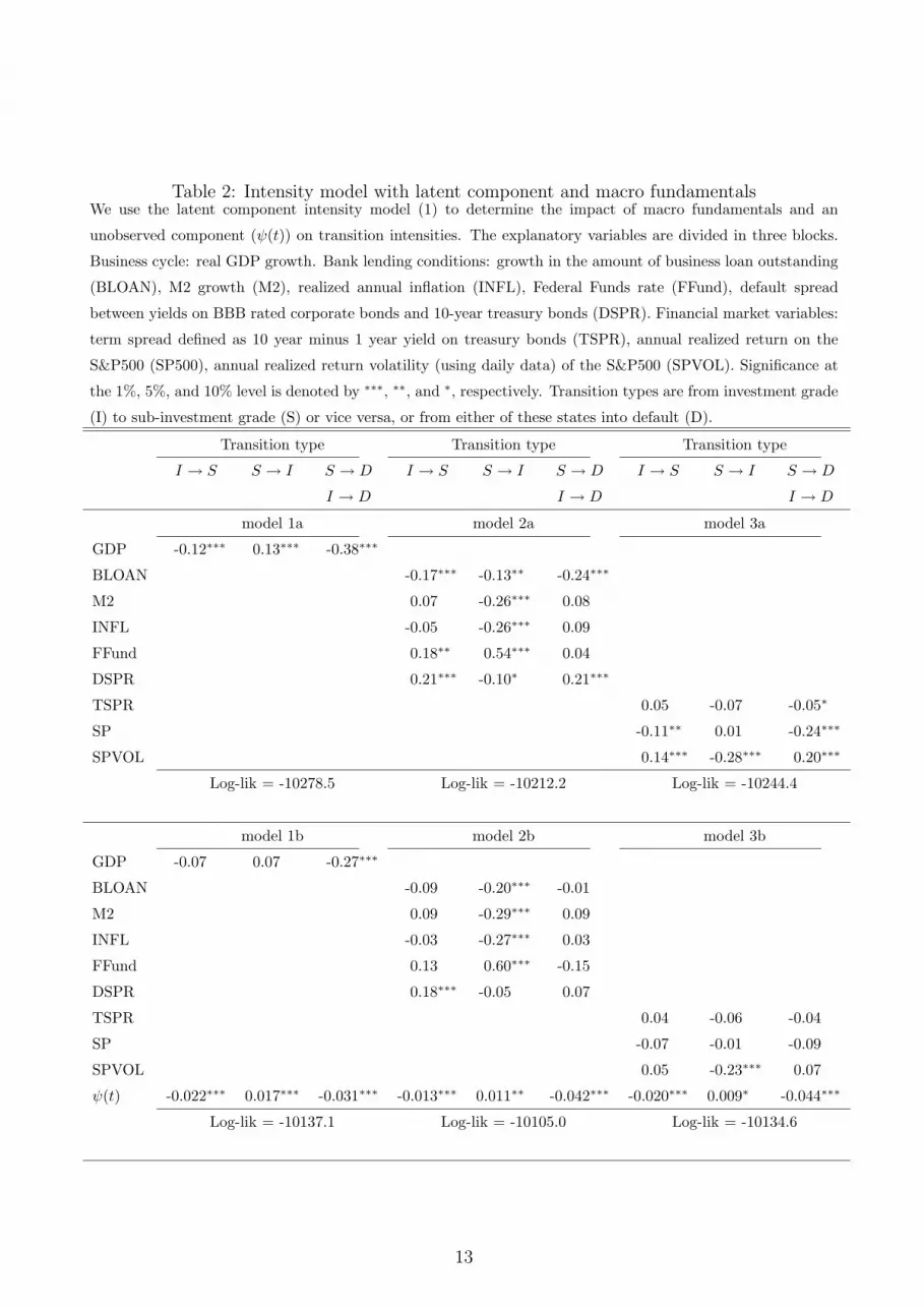
Table 2: Intensity model with latent component and macro fundamentalsWe use the latent component intensity model (1) to determine the impact of macro fundamentals and an

unobserved component (ψ(t)) on transition intensities. The explanatory variables are divided in three blocks.

Business cycle: real GDP growth. Bank lending conditions: growth in the amount of business loan outstanding

(BLOAN), M2 growth (M2), realized annual inflation (INFL), Federal Funds rate (FFund), default spread

between yields on BBB rated corporate bonds and 10-year treasury bonds (DSPR). Financial market variables:

term spread defined as 10 year minus 1 year yield on treasury bonds (TSPR), annual realized return on the

S&P500 (SP500), annual realized return volatility (using daily data) of the S&P500 (SPVOL). Significance at

the 1%, 5%, and 10% level is denoted by ∗∗∗, ∗∗, and ∗, respectively. Transition types are from investment grade

(I) to sub-investment grade (S) or vice versa, or from either of these states into default (D).

Transition type Transition type Transition type

I → S S → I S → D I → S S → I S → D I → S S → I S → D

I → D I → D I → D

model 1a model 2a model 3a

GDP -0.12∗∗∗ 0.13∗∗∗ -0.38∗∗∗

BLOAN -0.17∗∗∗ -0.13∗∗ -0.24∗∗∗

M2 0.07 -0.26∗∗∗ 0.08

INFL -0.05 -0.26∗∗∗ 0.09

FFund 0.18∗∗ 0.54∗∗∗ 0.04

DSPR 0.21∗∗∗ -0.10∗ 0.21∗∗∗

TSPR 0.05 -0.07 -0.05∗

SP -0.11∗∗ 0.01 -0.24∗∗∗

SPVOL 0.14∗∗∗ -0.28∗∗∗ 0.20∗∗∗

Log-lik = -10278.5 Log-lik = -10212.2 Log-lik = -10244.4

model 1b model 2b model 3b

GDP -0.07 0.07 -0.27∗∗∗

BLOAN -0.09 -0.20∗∗∗ -0.01

M2 0.09 -0.29∗∗∗ 0.09

INFL -0.03 -0.27∗∗∗ 0.03

FFund 0.13 0.60∗∗∗ -0.15

DSPR 0.18∗∗∗ -0.05 0.07

TSPR 0.04 -0.06 -0.04

SP -0.07 -0.01 -0.09

SPVOL 0.05 -0.23∗∗∗ 0.07

ψ(t) -0.022∗∗∗ 0.017∗∗∗ -0.031∗∗∗ -0.013∗∗∗ 0.011∗∗ -0.042∗∗∗ -0.020∗∗∗ 0.009∗ -0.044∗∗∗


13

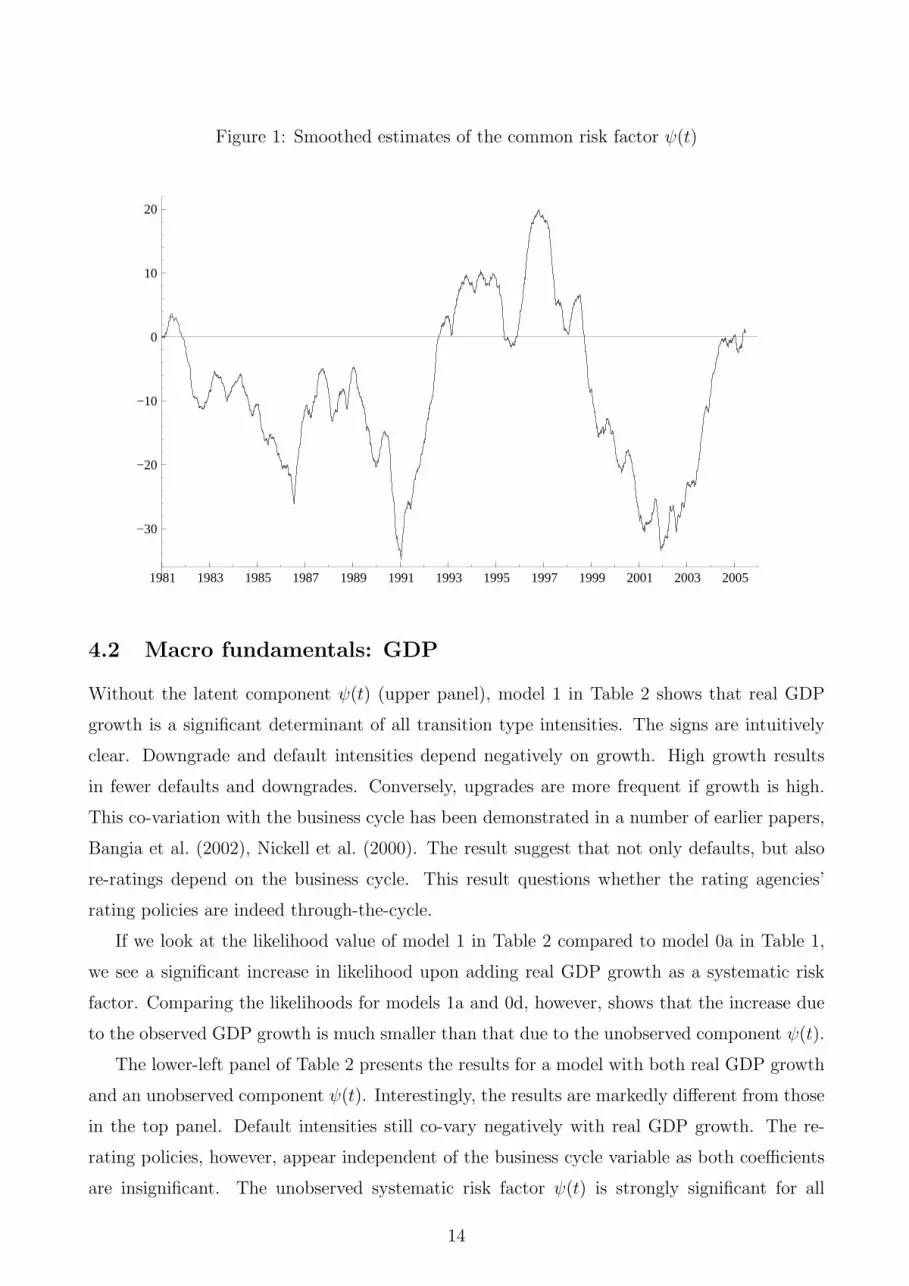
Figure 1: Smoothed estimates of the common risk factor ψ(t)

1981 1983 1985 1987 1989 1991 1993 1995 1997 1999 2001 2003 2005

−30

−20

−10

0

10

20

4.2 Macro fundamentals: GDP

Without the latent component ψ(t) (upper panel), model 1 in Table 2 shows that real GDP

growth is a significant determinant of all transition type intensities. The signs are intuitively

clear. Downgrade and default intensities depend negatively on growth. High growth results

in fewer defaults and downgrades. Conversely, upgrades are more frequent if growth is high.

This co-variation with the business cycle has been demonstrated in a number of earlier papers,

Bangia et al. (2002), Nickell et al. (2000). The result suggest that not only defaults, but also

re-ratings depend on the business cycle. This result questions whether the rating agencies’

rating policies are indeed through-the-cycle.

If we look at the likelihood value of model 1 in Table 2 compared to model 0a in Table 1,

we see a significant increase in likelihood upon adding real GDP growth as a systematic risk

factor. Comparing the likelihoods for models 1a and 0d, however, shows that the increase due

to the observed GDP growth is much smaller than that due to the unobserved component ψ(t).

The lower-left panel of Table 2 presents the results for a model with both real GDP growth

and an unobserved component ψ(t). Interestingly, the results are markedly different from those

in the top panel. Default intensities still co-vary negatively with real GDP growth. The re-

rating policies, however, appear independent of the business cycle variable as both coefficients

are insignificant. The unobserved systematic risk factor ψ(t) is strongly significant for all

14

transition types. Also note that the magnitude of both the GDP and ψ(t) coefficients (model

1b) has decreased compared to a model with only one source of systematic risk (models 0d and

1a). The real GDP thus explains some, but not all variation in default intensities.

To illustrate how the model operates in more detail, we present Figures 2 and 3. In Figure 2, we

first plot the estimate of the credit cycle from model 0d, which is the model without exogenous

variables and with a univariate ψ(t) factor. In the same graph, we present the result of model

1b, which is the model with the exogenous factor (in this case GDP growth) only. The factors

are multiplied by their loadings presented in Tables 1 and 2, respectively. It is clear that GDP

has some of the peaks and troughs roughly in common with the latent component ψ(t), but

there are also a number of significant differences. For example, during the early eighties, the

GDP swings do not at all resemble the movements in the unobserved credit cycle. Also in later

years, there are periods that the dynamics of GDP do not match those of ψ(t). In the late

1990s, GDP growth shows hardly any variation, whereas the ψ(t) clearly experiences a trough

and a sharp increase.4 Figure 3 continues this pattern. The first curve is the univariate credit

cycle ψ(t) estimated from model 0d. The second curve is the cycle ψ(t) from model 1b, so where

we condition on GDP growth as an explanatory variable. The third curve combines the latter

estimate of ψ(t) for model 1b with its loading on GDP growth. Clearly and as expected, the

first and third curve are very similar. Using the differences between the first and second curve,

we can get an idea of what part of the credit cycle is captured by GDP growth. First, we note

that the proportion of credit cycle variance explained by GDP growth is quite modest. The

latent component in models 0d and 1b are very similar. Second, GDP growth appears to explain

some of the peak default intensities near 1991 and 2000-2001. Generally speaking, however,

given the unconditional variation of ψ(t), the additional contribution of GDP is limited. So

even though the statistical significance is clear, the economic significance of GDP growth for

default dynamics is questionable.

4.3 Macro fundamentals: multivariate analysis

In the middle panels (model 2a,2b) we can see the impact of the variables measuring bank

lending conditions. Again, the increase in likelihood compared to the model without systematic

risk (model 0a) is significant. The increase, however, is much less than that of including a single

unobserved component (model 0d). The bank lending conditions are particularly important for

the upgrade intensity. If we include both the bank lending variables and ψ(t) (model 2b),

4At first sight, there may appear a closer resemblance between GDP growth and the credit cycle in the

Greenspan period, so after September 1987. We re-estimated the model on this sub-sample, but the results

remained robust.

15

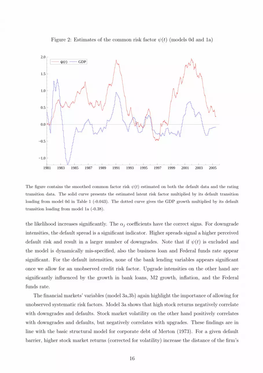
Figure 2: Estimates of the common risk factor ψ(t) (models 0d and 1a)

1981 1983 1985 1987 1989 1991 1993 1995 1997 1999 2001 2003 2005

−1.0

−0.5

0.0

0.5

1.0

1.5

2.0ψ(t) GDP

The figure contains the smoothed common factor risk ψ(t) estimated on both the default data and the rating

transition data. The solid curve presents the estimated latent risk factor multiplied by its default transition

loading from model 0d in Table 1 (-0.043). The dotted curve gives the GDP growth multiplied by its default

transition loading from model 1a (-0.38).

the likelihood increases significantly. The αj coefficients have the correct signs. For downgrade

intensities, the default spread is a significant indicator. Higher spreads signal a higher perceived

default risk and result in a larger number of downgrades. Note that if ψ(t) is excluded and

the model is dynamically mis-specified, also the business loan and Federal funds rate appear

significant. For the default intensities, none of the bank lending variables appears significant

once we allow for an unobserved credit risk factor. Upgrade intensities on the other hand are

significantly influenced by the growth in bank loans, M2 growth, inflation, and the Federal

funds rate.

The financial markets’ variables (model 3a,3b) again highlight the importance of allowing for

unobserved systematic risk factors. Model 3a shows that high stock returns negatively correlate

with downgrades and defaults. Stock market volatility on the other hand positively correlates

with downgrades and defaults, but negatively correlates with upgrades. These findings are in

line with the basic structural model for corporate debt of Merton (1973). For a given default

barrier, higher stock market returns (corrected for volatility) increase the distance of the firm’s

16

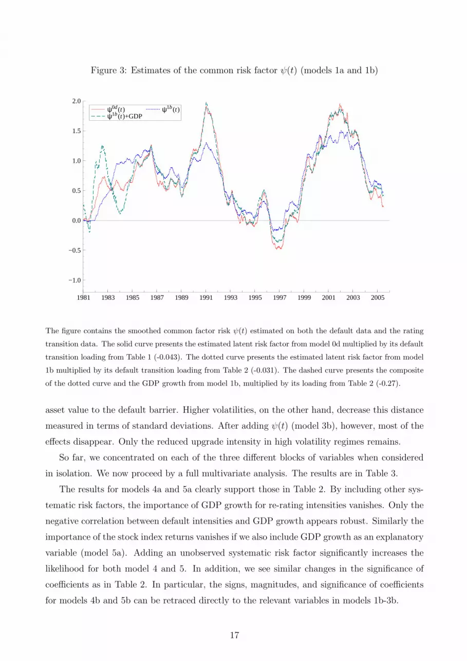
Figure 3: Estimates of the common risk factor ψ(t) (models 1a and 1b)

1981 1983 1985 1987 1989 1991 1993 1995 1997 1999 2001 2003 2005

−1.0

−0.5

0.0

0.5

1.0

1.5

2.0ψ0d(t) ψ1b(t)+GDP

ψ1b(t)

The figure contains the smoothed common factor risk ψ(t) estimated on both the default data and the rating

transition data. The solid curve presents the estimated latent risk factor from model 0d multiplied by its default

transition loading from Table 1 (-0.043). The dotted curve presents the estimated latent risk factor from model

1b multiplied by its default transition loading from Table 2 (-0.031). The dashed curve presents the composite

of the dotted curve and the GDP growth from model 1b, multiplied by its loading from Table 2 (-0.27).

asset value to the default barrier. Higher volatilities, on the other hand, decrease this distance

measured in terms of standard deviations. After adding ψ(t) (model 3b), however, most of the

effects disappear. Only the reduced upgrade intensity in high volatility regimes remains.

So far, we concentrated on each of the three different blocks of variables when considered

in isolation. We now proceed by a full multivariate analysis. The results are in Table 3.

The results for models 4a and 5a clearly support those in Table 2. By including other sys-

tematic risk factors, the importance of GDP growth for re-rating intensities vanishes. Only the

negative correlation between default intensities and GDP growth appears robust. Similarly the

importance of the stock index returns vanishes if we also include GDP growth as an explanatory

variable (model 5a). Adding an unobserved systematic risk factor significantly increases the

likelihood for both model 4 and 5. In addition, we see similar changes in the significance of

coefficients as in Table 2. In particular, the signs, magnitudes, and significance of coefficients

for models 4b and 5b can be retraced directly to the relevant variables in models 1b-3b.

17

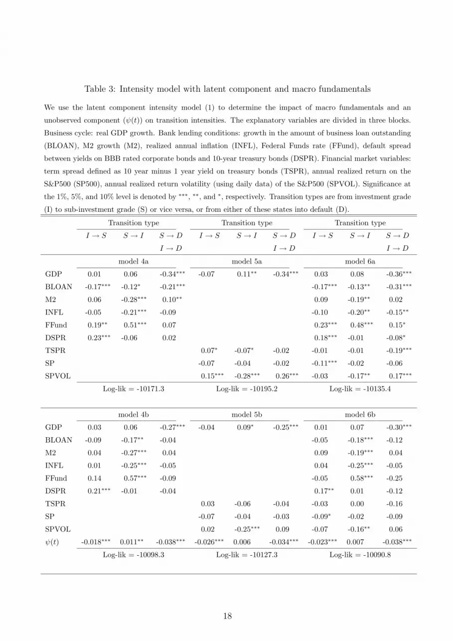
Table 3: Intensity model with latent component and macro fundamentals

We use the latent component intensity model (1) to determine the impact of macro fundamentals and an

unobserved component (ψ(t)) on transition intensities. The explanatory variables are divided in three blocks.

Business cycle: real GDP growth. Bank lending conditions: growth in the amount of business loan outstanding

(BLOAN), M2 growth (M2), realized annual inflation (INFL), Federal Funds rate (FFund), default spread

between yields on BBB rated corporate bonds and 10-year treasury bonds (DSPR). Financial market variables:

term spread defined as 10 year minus 1 year yield on treasury bonds (TSPR), annual realized return on the

S&P500 (SP500), annual realized return volatility (using daily data) of the S&P500 (SPVOL). Significance at

the 1%, 5%, and 10% level is denoted by ∗∗∗, ∗∗, and ∗, respectively. Transition types are from investment grade

(I) to sub-investment grade (S) or vice versa, or from either of these states into default (D).



I → D I → D I → D

model 4a model 5a model 6a

GDP 0.01 0.06 -0.34∗∗∗ -0.07 0.11∗∗ -0.34∗∗∗ 0.03 0.08 -0.36∗∗∗

BLOAN -0.17∗∗∗ -0.12∗ -0.21∗∗∗ -0.17∗∗∗ -0.13∗∗ -0.31∗∗∗

M2 0.06 -0.28∗∗∗ 0.10∗∗ 0.09 -0.19∗∗ 0.02

INFL -0.05 -0.21∗∗∗ -0.09 -0.10 -0.20∗∗ -0.15∗∗

FFund 0.19∗∗ 0.51∗∗∗ 0.07 0.23∗∗∗ 0.48∗∗∗ 0.15∗

DSPR 0.23∗∗∗ -0.06 0.02 0.18∗∗∗ -0.01 -0.08∗

TSPR 0.07∗ -0.07∗ -0.02 -0.01 -0.01 -0.19∗∗∗

SP -0.07 -0.04 -0.02 -0.11∗∗∗ -0.02 -0.06

SPVOL 0.15∗∗∗ -0.28∗∗∗ 0.26∗∗∗ -0.03 -0.17∗∗ 0.17∗∗∗


model 4b model 5b model 6b

GDP 0.03 0.06 -0.27∗∗∗ -0.04 0.09∗ -0.25∗∗∗ 0.01 0.07 -0.30∗∗∗

BLOAN -0.09 -0.17∗∗ -0.04 -0.05 -0.18∗∗∗ -0.12

M2 0.04 -0.27∗∗∗ 0.04 0.09 -0.19∗∗∗ 0.04

INFL 0.01 -0.25∗∗∗ -0.05 0.04 -0.25∗∗∗ -0.05

FFund 0.14 0.57∗∗∗ -0.09 -0.05 0.58∗∗∗ -0.25

DSPR 0.21∗∗∗ -0.01 -0.04 0.17∗∗ 0.01 -0.12

TSPR 0.03 -0.06 -0.04 -0.03 0.00 -0.16

SP -0.07 -0.04 -0.03 -0.09∗ -0.02 -0.09

SPVOL 0.02 -0.25∗∗∗ 0.09 -0.07 -0.16∗∗ 0.06

ψ(t) -0.018∗∗∗ 0.011∗∗ -0.038∗∗∗ -0.026∗∗∗ 0.006 -0.034∗∗∗ -0.023∗∗∗ 0.007 -0.038∗∗∗


18

Finally, model 6 contains the full set of results. When including all variables of the 3 blocks

as explanatory regressors for the intensities, the results are unaffected. Macro fundamentals

significantly explain transition and default intensities. A number of these relations, however,

is spurious and caused by dynamic mis-specification of the model. Including an unobserved

dynamic factor ψ(t) significantly increases the likelihood. This is mainly due to the fact that

default and downgrade intensities are not fully captured by the observed macro variables.

Upgrade intensities appear to be captured sufficiently by bank lending conditions and the

volatility regime, in line with our earlier discussion. Interestingly, real GDP only explains

default intensities and not re-rating intensities. This is in line with the claimed through-

the-cycle rating methodology adopted by rating agencies. For downward rating movements,

however, agencies also appear to draw information from financial markets in the form of default

spreads and (marginally) stock returns.

4.4 Robustness analyses

To test for the robustness of these results, we performed a number of sensitivity checks. First

included all explanatory variables in lagged rather than contemporaneous form. Both at lags

of one and two years, the results remain unaltered in the sense that models with only observed

macro variables appear dynamically mis-specified. Including a latent component ψ(t) in all

cases significantly increases the likelihood. If ψ(t) is included, some of the macros loose their

significance for specific transition types, similar to Tables 2 and 3. The effect of lagging on the

likelihood values does not reveal a clear-cut pattern and is overall limited. Moreover, including

lagged business cycle variables in several cases produces non-intuitive signs for the coefficients,

e.g., a positive relation between past growth and current defaults or downgrades. We also

considered including leads of the observed macro variables. Again, however, the results are

highly similar. Macro variables capture some of the default and re-rating activity, but certainly

not all.

As a further check we also incorporated a non-constant baseline hazard rate. We replace

the constant ηj in (1) by ηj + γjδk(t), with δk(t) an indicator variable that equals 1 if firm k is

less than one year in its current rating category. This non-constant base-line hazard rate allows

us to capture non-Markovian behavior of rating transitions, see Lando and Fledelius (2004).5

The results show that our findings remain robust. Though adding the non-constant baseline

hazard increases the likelihood, it does not affect the sign, size, or significance of the macro

variables and the unobserved ψ(t).

5The estimates of the macro variables for this variant of the model are available upon request.

19

The most puzzling fact in Table 3, model 6b, is the apparent block structure of the macro

variables across the transition types. This result may be caused by a similar phenomenon as

the significance of the macro variables in model 6a versus 6b. Because of the broad rating

buckets, it is likely that the ψ(t) factor is mainly capturing the default cycle of subinvestment

grade companies. The macro variables can then be used to account for systematic effects in the

upgrade and downgrade intensities. To allow for upgrade and downgrade intensities to have

their own systematic component, we enlarge model (1) to

λjk(t) = Rjk(t) · exp(ηj + β′

jx(t) + αjψj(t)), (10)

where we know have three different ψj(t) factors. The estimation results are in Table 4.

Model (10) is not nested in (1), so the likelihoods between the models in Tables 2 and 3

cannot be compared directly to those in Table 4. Generally speaking, however, the likelihood

values increase by having more ψj(t) factors. Interestingly, the phenomenon witnessed earlier

when going from the 1a-6a models to the 1b-6b models, repeats itself when considering the 1c-6c

models. In particular, the importance of the economic variables is further reduced. Effectively,

there only appear three important variables. GDP growth explains a part of all four types

of transitions. The signs are as expected. The intensities of downgrades and defaults react

negatively to growth, whereas upgrades react positively. Furthermore, there is a marginally

significant effect of stock market returns and stock market return volatilities on upgrade inten-

sities. The signs are in line with the standard structural model of Merton. High stock returns

increase the distance to default and therefore increase upgrade intensities. High volatilities, on

the other hand, decrease the distance to default and therefore decrease upgrade intensities.

Two other things worth noting in Table 4 concern the sizes of the αj coefficients. Again, the

upgrade intensities appear much less driven by unobserved systematic risk than the downgrade

and default intensities. In contrast to some of the results in Tables 2 and 3, however, the effect

always remains significantly different from zero. The other important difference with the earlier

results is the magnitude of the αj corresponding to investment grade downgrades. Though this

coefficient is still lower than its default intensity counterpart, they are now much closer. We

conclude that both downgrade and default intensities are driven to a similar extent by common

components. The commonality in all results, however, remains that the macro variables only

explain part of the credit cycle. The unobserved credit risk components appear to be at least

as important to describe the dynamics of rating intensities.

We again illustrate the model by looking at the estimated latent risk components ψj(t). We

concentrate on model 1c. The results are presented in Figure 4. In the top line of graphs

in Figure 4, we compare the estimation results for models with a univariate latent risk factor

20

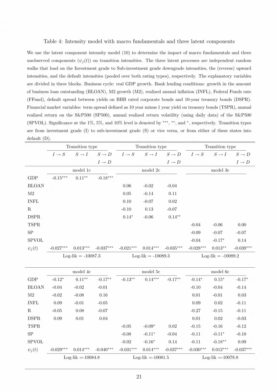
Table 4: Intensity model with macro fundamentals and three latent components

We use the latent component intensity model (10) to determine the impact of macro fundamentals and three

unobserved components (ψj(t)) on transition intensities. The three latent processes are independent random

walks that load on the Investment grade to Sub-investment grade downgrade intensities, the (reverse) upward

intensities, and the default intensities (pooled over both rating types), respectively. The explanatory variables

are divided in three blocks. Business cycle: real GDP growth. Bank lending conditions: growth in the amount

of business loan outstanding (BLOAN), M2 growth (M2), realized annual inflation (INFL), Federal Funds rate

(FFund), default spread between yields on BBB rated corporate bonds and 10-year treasury bonds (DSPR).

Financial market variables: term spread defined as 10 year minus 1 year yield on treasury bonds (TSPR), annual

realized return on the S&P500 (SP500), annual realized return volatility (using daily data) of the S&P500

(SPVOL). Significance at the 1%, 5%, and 10% level is denoted by ∗∗∗, ∗∗, and ∗, respectively. Transition types

are from investment grade (I) to sub-investment grade (S) or vice versa, or from either of these states into

default (D).



I → D I → D I → D

model 1c model 2c model 3c

GDP -0.15∗∗∗ 0.11∗∗ -0.18∗∗∗

BLOAN 0.06 -0.02 -0.04

M2 0.05 -0.14 0.11

INFL 0.10 -0.07 0.02

R -0.10 0.13 -0.07

DSPR 0.14∗ -0.06 0.14∗∗

TSPR -0.04 -0.06 0.00

SP -0.09 -0.07 -0.07

SPVOL -0.04 -0.17∗ 0.14

ψj(t) -0.027∗∗∗ 0.013∗∗∗ -0.037∗∗∗ -0.021∗∗∗ 0.014∗∗∗ -0.035∗∗∗ -0.028∗∗∗ 0.013∗∗ -0.039∗∗∗


model 4c model 5c model 6c

GDP -0.12∗ 0.11∗∗ -0.17∗∗ -0.13∗∗ 0.14∗∗∗ -0.17∗∗ -0.14∗ 0.15∗ -0.17∗

BLOAN -0.04 -0.02 -0.01 -0.10 -0.04 -0.14

M2 -0.02 -0.08 0.16 0.01 -0.01 0.03

INFL 0.09 -0.01 -0.05 0.09 0.02 -0.11

R -0.05 0.08 -0.07 -0.27 -0.15 -0.11

DSPR 0.09 0.01 0.04 0.01 0.02 -0.03

TSPR -0.05 -0.09∗ 0.02 -0.15 -0.16 -0.12

SP -0.08 -0.11∗ -0.04 -0.11 -0.11∗ -0.10

SPVOL -0.02 -0.16∗ 0.14 -0.11 -0.18∗∗ 0.09

ψj(t) -0.029∗∗∗ 0.014∗∗∗ -0.040∗∗∗ -0.031∗∗∗ 0.014∗∗∗ -0.037∗∗∗ -0.030∗∗∗ 0.012∗∗∗ -0.037∗∗∗

Log-lik =-10084.8 Log-lik =-10081.5 Log-lik =-10078.8

21

(model 1b) with those for three risk factors. It is easily seen that the univariate common risk

factor mainly captures the dynamics of the default intensity. The estimated ψj(t) component

is for this type of transition very similar between models 0d and 1c. Again, there are many

discrepancies with the dynamics of GDP growth. It is very interesting to see the large differ-

ences between the univariate estimate of ψ(t) and the multivariate ψj(t) for downgrades and

upgrades. Although some of the peaks are shared between downgrade and default activity, the

overall difference in dynamics between the two series is significant. For example, the decline in

downgrade intensities during the stock market boom is much more pronounced than the decline

in default intensities. The difference is even more striking for the upgrade intensity. We do

not only obtain the result that upgrade activity is much less driven by systematic factors, as

witnessed by the smaller loading coefficients αj. In addition, the estimated risk factor ψS→I(t)

shows a markedly different behavior. In the early 2000s, whereas macroeconomic activity was

already picking up and default intensities decreased, the systematic effect in upgrade intensities

remained at a very low level. This might be linked with a possible prudential re-rating policy

of the major rating agencies after the bad credit years around the turn of the century.

In Figure 4 we can assess the economic significance of the results. The figure shows the

individual latent components ψj(t) with and without conditioning on the GDP growth. Though

there are some differences between the two estimates, the main feature of the graphs is that

the estimates are quite similar. Again, this underlines the fact that even though some macro

fundamentals may be statistically significant, their economic significance for default and rating

transition dynamics is much less clear-cut.

5 Conclusions

In this paper we conducted a systematic search on the determinants of corporate credit rating

migrations and defaults. We used a novel econometric methodology introduced Koopman et

al. (2005). The framework is set in a continuous time duration model where we focus on the

dynamics of migration intensities. We conditioned on three sets of variables: GDP growth

(for business cycle effects), bank lending conditions, and financial markets variables. In line

with previous studies we found that the level of economic activity, bank lending conditions,

and financial markets variables are all important determinants of default and rating migration

intensities. The models, however, appear significantly dynamically mis-specified. Once we

account for this mis-specification, many of the macro fundamentals fall out of the model. The

prime remaining candidate is GDP growth, and to some extent financial markets’ variables like

stock returns and stock return volatilities. The results appear robust over a variety of model

22

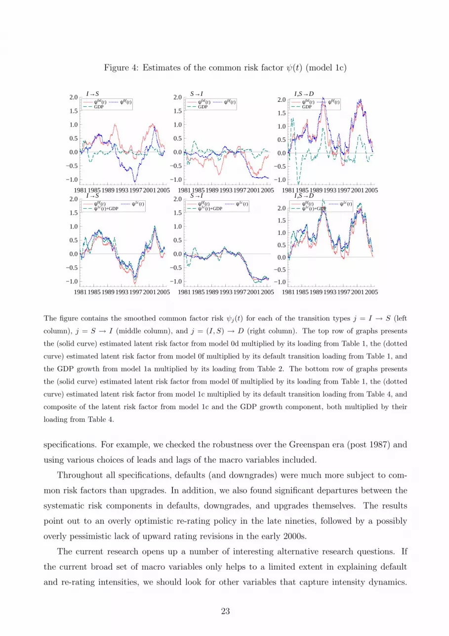
Figure 4: Estimates of the common risk factor ψ(t) (model 1c)

1981198519891993199720012005

−1.0

−0.5

0.0

0.5

1.0

1.5

2.0 I→Sψ0d(t) GDP

ψ0f(t)

1981198519891993199720012005

−1.0

−0.5

0.0

0.5

1.0

1.5

2.0 S→Iψ0d(t) GDP

ψ0f(t)

1981198519891993199720012005

−1.0

−0.5

0.0

0.5

1.0

1.5

2.0I,S→D

ψ0d(t) GDP

ψ0f(t)

1981198519891993199720012005

−1.0

−0.5

0.0

0.5

1.0

1.5

2.0 I→Sψ0f(t) ψ1c(t)+GDP

ψ1c(t)

1981198519891993199720012005

−1.0

−0.5

0.0

0.5

1.0

1.5

2.0 S→Iψ0f(t) ψ1c(t)+GDP

ψ1c(t)

1981198519891993199720012005

−1.0

−0.5

0.0

0.5

1.0

1.5

2.0

I,S→Dψ0f(t) ψ1c(t)+GDP

ψ1c(t)

The figure contains the smoothed common factor risk ψj(t) for each of the transition types j = I → S (left

column), j = S → I (middle column), and j = (I, S) → D (right column). The top row of graphs presents

the (solid curve) estimated latent risk factor from model 0d multiplied by its loading from Table 1, the (dotted

curve) estimated latent risk factor from model 0f multiplied by its default transition loading from Table 1, and

the GDP growth from model 1a multiplied by its loading from Table 2. The bottom row of graphs presents

the (solid curve) estimated latent risk factor from model 0f multiplied by its loading from Table 1, the (dotted

curve) estimated latent risk factor from model 1c multiplied by its default transition loading from Table 4, and

composite of the latent risk factor from model 1c and the GDP growth component, both multiplied by their

loading from Table 4.

specifications. For example, we checked the robustness over the Greenspan era (post 1987) and

using various choices of leads and lags of the macro variables included.

Throughout all specifications, defaults (and downgrades) were much more subject to com-

mon risk factors than upgrades. In addition, we also found significant departures between the

systematic risk components in defaults, downgrades, and upgrades themselves. The results

point out to an overly optimistic re-rating policy in the late nineties, followed by a possibly

overly pessimistic lack of upward rating revisions in the early 2000s.

The current research opens up a number of interesting alternative research questions. If

the current broad set of macro variables only helps to a limited extent in explaining default

and re-rating intensities, we should look for other variables that capture intensity dynamics.

23

Some obvious ways forward appear to be variables capturing industry and contagion effects.

Alternatively, we could enlarge the model by the inclusion of firm-specific variables. The latter,

however, would only help if they are correlated with any missing systematic effect in the credit

risk dynamics. Finally, we can enlarge the class of dynamic models for the latent common risk

component from the current random walk to a more richly specified autoregressive structure.

References

Altman, E. (1983): Corporate Financial Distress, John Wiley.

Altman, E. (2000): Predicting Financial Distress of Companies: Revisiting the Z-Score

and Zeta, Working paper - Stern School of Business, New York University.

Andersen, P.K., Borgan, Ø., Gill, R.D. and Keiding, N. (1993): Statistical Models Based

on Counting Processes, Springer-Verlag.

Bangia, A., F. X. Diebold, A. Kronimus, C. Schagen, and T. Schuermann, 2002, Ratings

migration and the business cycle, with applications to credit portfolio stress testing.

Journal of Banking & Finance 26, 445-474.

Carling, K., Jacobson, T., Linde, J., and K. Roszbach, 2002, Capital charges under Basel

II: Corporate credit risk modeling and the macro economy, Working paper - Sveriges

Riksbank.

Couderc, F. and O. Renault (2005): “Times-to-Default: Life Cycles, Global and Industry

Cycle Impacts,” FAME Research series, No. 142.

Cox, D.R. (1972): “Regression Models and Life Tables,” Journal of the Royal Statistical

Society, B Vol 34, pp 187-200.

Das, S.R., Freed, L., Geng, G. and N. Kapadia, 2002, Correlated default risk, Working

paper - Santa Clara University.

Doornik, J.A. (2002): Object-oriented matrix programming using Ox. 3rd ed. Timberlake

Consultants Press, London and Oxford: www.nuff.ox.ac.uk/Users/Doornik.

Duffie, D., L. Saita, and K. Wang (2006a): “Multi-Period Corporate Default Prediction

with Stochastic Covariates,” Journal of Financial Economics, forthcoming.

Duffie, D., A. Eckner, G. Horel, and L. Saita (2006b): “Frailty correlated default,” Working

paper Stanford.

Fama, E., 2002, Term Premiums and Default Premiums in Money Markets. Journal of

Financial Economics 17(1), 175-196.

24

Fledelius, P., D. Lando and J. P. Nielsen (2004): “Non-parametric Analysis of Rating

Transition and Default Data,” Journal of Investment Management, Vol. 2, No.2.

Frey, R. and A.J. McNeil (2003): “Dependent Defaults in Models of Portfolio Credit Risk,”

Journal of Risk, Vol. 6, pp 59-92.

Kavvathas, D. 2001, Estimating credit rating transition probabilities for corporate bonds,

Working paper - University of Chicago.

Koopman, S.J. and A. Lucas (2005): “Business and Default Cycles for Credit Risk,”

Journal of Applied Econometrics, Vol 20, pp 311-323.

Koopman, S.J., A. Lucas and A. Monteiro (2005): “The Multi-State Latent Factor Model

for Credit Rating Transitions,” Tinbergen Institute Discussion Paper, No. 05-071/4.

Kraussl, R. (2003): Sovereign Risk, Credit Ratings and the Recent Financial Crises in

Emerging Markets, Fritz-Knapp Verlag.

Lancaster, T. (1990): The Econometric Analysis of Transition Data, Cambridge University

Press.

Lando, D. and T.M. Skødeberg (2002): “Analyzing rating transitions and rating drift with

continuous observations,” Journal of Banking and Finance, Vol 26, pp 423-444.

Lucas, A., P. Klaassen, P. Spreij and S. Straetmans (2002): “An Analytic Approach to

Credit Risk of Large Corporate Bond and Loan Portfolios,” Journal of Banking and

Finance, Vol 25(9), pp 1635-1664.

Lucas, A. and P. Klaassen (2006): “Discrete versus continuous state switching models for

portfolio credit risk,” Journal of Banking and Finance, Vol. 30(1), 23-35.

Merton, R. (1974): “On the Pricing of Corporate Debt: the Risk Structure of Interest

Rates,” Journal of Finance, Vol 29, pp 449-470.

Nickell, P., W. Perraudin, and S. Varotto, 2000, Stability of rating transitions, Journal of

Banking & Finance 24, 203-227.

Schonbucher, P.J. (2001): “Factor Models: Portfolio Credit Risk when Defaults are Cor-

related,” The Journal of Risk Finance, Vol 3(1), pp. 45-56.

Stock, J.H., and M.W. Watson 1989, New Indexes of Coincident and Leading Indicators,

in Blanchard, O., and S. Fischer, eds. NBER Macroeconomics Manual, 351-394, MIT

Press.

Wilson, T., 1997, Portfolio Credit Risk - Part I and II. Risk Magazine, September and

October.

25

CFS Working Paper Series:

No. Author(s) Title

2006/32 Rachel A. Campbell Roman Kräussl

Does Patience Pay? Empirical Testing of the Option to Delay Accepting a Tender Offer in the U.S. Banking Sector

2006/31 Rachel A. Campbell Roman Kräussl

Revisiting the Home Bias Puzzle. Downside Equity Risk

2006/30 Joao Miguel Sousa Andrea Zaghini

Global Monetary Policy Shocks in the G5: A SVAR Approach

2006/29 Julia Hirsch Public Policy and Venture Capital Financed Innovation: A Contract Design Approach

2006/28 Christian Gollier Alexander Muermann

Optimal Choice and Beliefs with Ex Ante Savoringand Ex Post Disappointment

2006/27 Christian Laux Uwe Walz

Tying Lending and Underwriting: Scope Economies, Incentives, and Reputation

2006/26 Christian Laux Alexander Muermann

Mutual versus Stock Insurers: Fair Premium, Capital, and Solvency

2006/25 Bea Canto Roman Kräussl

Stock Market Interactions and the Impact of Macroeconomic News – Evidence from High Frequency Data of European Futures Markets

2006/24 Toker Doganoglu Christoph Hartz Stefan Mittnik

Portfolio Optimization when Risk Factors are Conditionally Varying and Heavy Tailed

2006/23 Christoph Hartz Stefan Mittnik Marc S. Paolella

Accurate Value-at-Risk Forecasting Based on the (good old) Normal-GARCH Model

2006/22 Dirk Krueger Hanno Lustig Fabrizio Perri

Evaluating Asset Pricing Models with Limited Commitment using Household Consumption Data

Copies of working papers can be downloaded at http://www.ifk-cfs.de

Documents

Credit cycles and macro fundamentals