Embed Size (px)
Citation preview
Electronic copy available at: http://ssrn.com/abstract=1641305
Counterfactual Analysis of Bank Mergers∗
Pedro P. Barros† Diana Bonfim‡ Moshe Kim§ Nuno C. Martins¶
July 2010
Abstract
Estimating the impact of bank mergers requires a framework distinguishing endoge-
nous changes in market structure and conduct from exogenous changes. Conventionally,
the literature relies on differential analysis, considering market structure as exogenous by
using concentration indexes such as the HHI. We introduce an econometric methodology
relying on a structural model of the credit market from which we derive a counterfactual
scenario of what would have happened if mergers had not occurred. We find that merg-
ers increased firms’ access to credit, but had an opposite effect on households. Moreover,
we find that mergers led to a widespread decrease in interest rates.
JEL codes: G21; G34; L10.
Keywords: banks, mergers, competition.
∗We would like to thank Daniel Ackerberg, Filipa Lima, Mark Roberts, João Santos, Giancarlo Spagnolo,Nuno Ribeiro and António Antunes for insightful comments and suggestions. The analysis, opinions and
findings of this paper represent the views of the authors, they are not necessarily those of the Banco de
Portugal or the Eurosystem.†Universidade Nova de Lisboa, Travessa Estevão Pinto, Campolide, 1070, Lisboa, Portugal. E-
mail:[email protected].‡Banco de Portugal and ISEG-UTL, Av. Almirante Reis, 71, 1150-012 Lisboa, Portugal. E-mail: dbon-
[email protected]§Universitat Pompeu Fabra, Ramon Trias Fargas, 25-27, 08005 Barcelona, Spain. E-mail:
[email protected].¶E-mail: [email protected]. This work was initiated when Nuno was working at the Banco
de Portugal and Universidade Nova de Lisboa.
Electronic copy available at: http://ssrn.com/abstract=1641305
1 Introduction
We analyze the effects bank mergers exert on market structure and credit conditions. The
conventional approach employed in the literature relies on the comparison of market charac-
teristics before and after the mergers, overlooking endogenous changes in market structure in
the post-merger industry equilibrium. For example, in order to evaluate the ex-ante potential
impact of mergers, competition authorities usually conduct merger simulation analysis1. In
this paper, we present a methodology that allows overcoming this gap in the evaluation of
merger impact in banking. By deriving a structural model of the credit market, we are able
to perform a counterfactual analysis of mergers, combining the pre-merger equilibrium setting
with characteristics of the post-merger environment, while accounting for endogenously prop-
agated changes in market structure. Using this procedure we are able to estimate loan flows
and interest rates that would be observed if the pre-merger equilibrium was not altered, i.e.,
if mergers had not occurred. We obtain more accurate estimates of the impact of mergers,
given that we are able to take into account the effects associated with endogenous changes
in conduct and market structure after mergers have taken place. These effects are usually
ignored in the assessment of merger impact and can lead to a significant bias in the results
obtained. Moreover, we disentangle the effect of changes in the macroeconomic and financial
environment from endogenous changes in market structure resulting from the mergers. Hence,
this methodology can be an important additional tool for bank regulators and competition
authorities when assessing possible impacts of mergers, allowing for the estimation of what
would have happened if a merger had not taken place - a counterfactual scenario.
We apply the proposed methodology to a detailed dataset with unique characteristics. This
dataset covers a banking system which went through a wave of mergers, thus constituting an
ideal laboratory for estimating a counterfactual scenario. Our dataset allows for the investi-
gation of the merger impact on firm and household bank loans separately2. Furthermore, we
1See, for instance, Epstein and Rubinfeld (2000) or, for a more recent approach, Goppelsroeder et al (2008).2Beck et al (2009) provide evidence regarding the importance of analyzing household and firm loans sepa-
rately.
2
are able to analyze the effects of mergers on the merged banks as well as on those banks out-
side the merging circles, taking into account endogenous changes in the post-merger market
structure. Furthermore, we analyze the resulting changes in local competition by modeling
the effects of changes in local market structure on the aggregate industry configuration.
There is a large literature on the gains banks obtain from merging. For instance, Focarelli
et al (2002) find that mergers increase return on equity, but they also lead to a rise in staff
costs. In turn, they find that acquisitions generate a long-term reduction in lending, mainly
for small firms, and a permanent decrease in bad quality loans, which positively affects long-
run profitability. Focusing on European mergers, Altunbas and Marqués (2008) find that
improvements in banks’ performance subsequent to mergers are more significant if there are
strategic similarities between the merging banks. Mergers and acquisitions also generate im-
portant changes in market structure and financial stability, as discussed in Berger et al (2004),
Cerasi et al (2010), Craig and Santos (1997) or in Gowrisankaran and Holmes (2004). Some
authors also find that mergers may enhance cost reduction and improve resource allocation3.
Moreover, mergers may generate informational gains, which improve banks’ screening abilities
and customer discrimination (see, for instance, Hauswald and Marquez (2006) or Panetta et
al (2009)). In turn, Beck et al (2006) show that bank mergers may have implications for
financial stability.
It is also important to assess the impact of bank mergers on customers with varying
characteristics. Several authors conclude that bank mergers may negatively affect borrowers,
most notably if they are small and medium size firms, dependent on bank funding and with a
limited number of bank relationships. For instance, Bonaccorsi di Patti and Gobbi (2007) find
that, for a sample of Italian firms, bank mergers have a negative effect on credit, particularly if
the lending relationship comes to an end after the merger, even though this effect should persist
only during the three years after the merger. However, this negative effect is not sufficient
3For instance, Carbó Valverde and Humphrey (2004) argue that mergers should reduce costs faced by
banks, raise their return on assets and improve general resource utilization. They also find that a merger
is more likely to be successful if it is large (scale effect) and also if it is initiated by a bank that has been
previously involved in a merger (learning effect).
3
to generate a negative impact on firms’ investment or cash-flow sensitivity. Other authors
find mixed evidence regarding the impact of bank mergers. Also using a sample of Italian
firms, Sapienza (2002) concludes that in-market mergers benefit borrowers if these mergers
involve banks with limited market power. However, as the market share of the acquired bank
increases, the efficiency gains are offset by an increase in market power, which may imply a
decrease in loan supply, especially to small borrowers. In another study, Scott and Dunkelberg
(2003) analyze the results of a survey on US firms and find that bank mergers do not affect
loan supply or interest rates, even though there is some deterioration in non-price loan terms,
such as fees for specific services. Degryse et al (2010) find that the impact of a bank merger
is more negative for smaller borrowers and for single relationship borrowers. Moreover, target
bank borrowers should be more harmed by the merger than borrowers of the acquiring bank.
Finally, Karceski, Ongena and Smith (2005) show that mergers may have impacts on borrowers
beyond credit availability and interest rates. These authors show that mergers may in fact
have important consequences on firm value, observing that borrowers of the acquiring banks
usually benefit from the mergers, whereas firms that borrow from the target bank suffer an
opposite impact4 5.
In the present paper, we use a structural model of equilibrium in credit markets to analyze
the impact of changes in market factors due to the merger wave. One of the most common
approaches in the literature is to estimate the differential impact of mergers. Using the
structural model, we are able to go further and estimate a counterfactual scenario for the
post-merger period, thus going beyond the simple (and insufficient) comparison of variables
before and after mergers occur, which is usually performed for the assessment of merger
impact. Using this methodology, we compare the interest rate and credit flows in the post-
4There is less work done on the impact of bank mergers on depositors. There is some empirical evidence for
Italian firms which suggests that bank mergers may have positive consequences for depositors in the long-run,
even though there may be some negative effects in the short run (Focarelli and Panetta, 2003). However,
Craig and Dinger (2009), using US data, obtain a different result, given that they do not observe any positive
long-term effect of mergers on deposit interest rates. Their results are consistent with previous work done by
Prager and Hannan (1998).5For a more detailed review of the recent literature on the impact of bank mergers, please see DeYoung et
al (2009).
4
merger equilibrium setup with the value of these variables under a counterfactual equilibrium.
This counterfactual equilibrium is estimated using the after-merger exogenous environment
under the pre-merger market structure.
The estimation of counterfactuals to assess the impacts of a merger may be considered an
important policy tool. For instance, Ivaldi and Verboven (2005) emphasize that the evaluation
of a merger from a policy perspective should not be based solely on a static comparative
analysis, but should also consider dynamic effects and alternative merger scenarios. Berry
and Pakes (1993) also argue that static models of equilibrium do not take into account the
long-run reactions of merging and non-merging firms, thus generating misleading results. In an
application to the airline industry, Peters (2006) demonstrates the importance of designing a
counterfactual analysis to evaluate the impact of mergers, but is silent regarding the possibility
of collusion or strategic interactions between firms. Berger et al (1998) find empirical evidence
which supports the view that the dynamic effects of mergers may generate results different
from those obtained using static analysis. The authors identify a decrease in lending to small
business after a merger, even though this static effect is largely offset by dynamic effects
associated with changes in the focus of the merging banks or with the reaction of other banks.
Nevertheless, these authors do not consider local changes induced by mergers, neither do they
compare the impact on different institutional sectors.
Our paper contributes to the literature on merger impact in banking markets by presenting
a counterfactual analysis, based on a structural model of equilibrium that clearly disentangles
the effects of bank mergers on loan flows and interest rates and takes into account changes in
market structure and conduct that may occur after the merger takes place. Our analysis is
based on loan flows, as opposed to outstanding amounts, thus allowing us to better capture
changes in credit markets over time. Moreover, the data used allow us to discriminate effects
among corporate and household borrowers, and to simulate the counterfactual equilibrium to
the mergers that occurred. This approach lends itself to the reporting of intuitive measures
of merger impact upon the degree of competition in the market. The use of a counterfactual
scenario becomes necessary, as mergers change the market structure underlying bank compe-
5
tition. In particular, as borrowers’ choices among alternative banks often take place in small
local markets (even though banks’ policies can be national), the changes in competition in
local markets resulting from a merger may be larger than an estimate based on aggregate,
country-wide, figures. This issue is important to stress, as virtually all banking merger studies
rely on some exogenously treated market structure measure (such as the Herfindahl index)
for the post merger configuration, even though the merger itself endogenously propagates the
new equilibrium configuration.
We are able to make use of a significant change in market structure in the Portuguese
banking market. Portugal is a small economy participating in the European Union, and
joined the euro area at its inception. Like other European Union countries, it experienced a
wave of mergers in the banking sector. The most significant changes occurred in 2000, with
the merger of several financial institutions. The almost simultaneous nature of these mergers
provides a natural break point in time, allowing us to define a pre- and a post-merger period.
Hence, we divide the 1995-2002 period in two: the pre-merger 1995-1999 period and the post-
merger 2000-2002 period6. Four out of the seven major financial groups were directly involved
in those changes, either by selling or by acquiring at least one financial institution. In this
paper, we analyze two different products (credit to households and to firms), two different
groups of institutions (those that are directly involved in the mergers and those that are not)
and consider two different periods (pre- and post-mergers).
Several interesting findings emerge from our analysis. We find that the 2000 merger wave
globally increased total credit granted and decreased interest rates. However, the analysis
of aggregate credit flows hides important differences between institutional sectors. In fact,
we find that the amount of credit flow granted to the household sector decreased, while the
amount of credit granted to the corporate sector increased during the same period. The
changes in credit flows affected both the banking groups involved in the mergers and the
6Even though Portugal joined the euro area at its inception in January 1st 1999, the effects of the con-
vergence process in credit markets were felt mainly during the 90s. As discussed in Antão et al. (2009),
interest rates decreased gradually during the 90s due to this convergence process and, simultaneously, credit
accelerated during this period. Hence, the effects of joining the euro area were gradual and not concentrated
specifically around 1999.
6
groups not involved. In fact, all financial institutions experienced an increase in the corporate
credit sold following the mergers and a decrease in the interest rate charged. However, the
banks directly involved in the merger recorded a larger increase in corporate credit than the
banks that were not directly involved in the merger. The decline in credit granted to the
household sector after the merger period, which was concentrated in banks not involved in
the merger wave, suggests that households may be more sensitive to changes in local market
competition. These results show that mergers may actually affect the degree of competition
in the market, through the changes in the local market structure, to a larger extent than
predicted by aggregate market analysis.
In sum, we observe that potential efficiency gains generated by the mergers seem to have
been transmitted to customers through lower lending rates7. Moreover, access to credit im-
proved significantly for firms after the mergers, though the same was not observed for house-
holds. When compared to the differential analysis usually implemented in the literature,
the counterfactual estimation allows for a more precise and correct quantification of these
impacts, while isolating changes in the exogenous environment from changes in endogenous
market structure. The results obtained suggest that changes in banks’ exogenous environment
were behind most of the changes in interest rates and loan flows after the merger, particularly
so for loans to households.
The paper proceeds as follows. Section 2 develops the model of the equilibrium in the
credit market. Section 3 describes the data and the major corporate changes in the banking
system in 2000. Section 4 estimates the structural model of equilibrium in the credit market
and Section 5 analyzes the impact of the merger wave. Section 6 presents some concluding
remarks.
7For a discussion on efficiency gains arising from bank mergers, see Sapienza (2002).
7

2 The Analytical Framework
2.1 Demand Equation
Given our purpose of assessing the market equilibrium effects of bank mergers, our approach
to estimation has to rely on a minimum structure, such that alternative market equilibria can
be computed. At the same time, the model needs to be parsimonious and flexible. More-
over, changes in competition should be analyzed at the most disaggregated level possible.
Even though there is no information on the local market operations of each bank, we do have
information on the location of branches and on characteristics of local markets (such as pop-
ulation), thus allowing us to consider differences in local bank competition. In fact, as local
market competition certainly depends on the number and location of branches, the relative
position of the branch network of each bank does affect the demand faced by the bank, and
thus own and rival banks branch densities are considered in our model. The branch density is
commonly used in the empirical literature on local banking competition (see, for instance, De-
gryse and Ongena, 2005). We consider that rivalry between banks is relevant on the choice of
interest rates. Finally, economy-wide variables should influence demand and must be included
as demand-side controls.
Since our unit of observation is the bank, we consider the total market demand function
directed at each bank (), during a quarter (), as a function of both economy-wide variables
() and bank-level determinants ()8:
=
As mentioned above, loan demand, , is measured by loan flows, rather than outstanding
loans, thus capturing loan demand in each quarter. The set of variables includes the
aggregate average interest rate on new loans granted in the country in quarter , , and
which refers to other relevant economy-wide variables. The vector is given by:
8See Kim and Vale (2001) for further details.
8
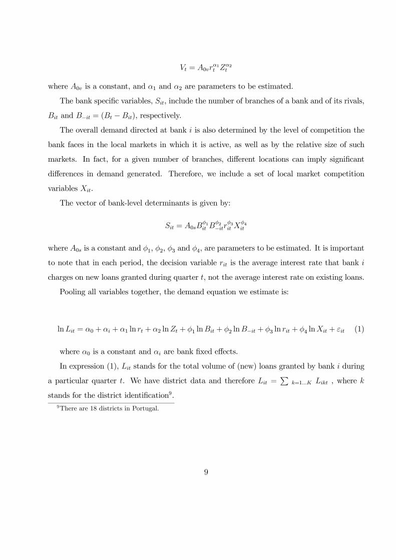
= 01 2
where 0 is a constant, and 1 and 2 are parameters to be estimated.
The bank specific variables, , include the number of branches of a bank and of its rivals,
and − = ( −), respectively.
The overall demand directed at bank is also determined by the level of competition the
bank faces in the local markets in which it is active, as well as by the relative size of such
markets. In fact, for a given number of branches, different locations can imply significant
differences in demand generated. Therefore, we include a set of local market competition
variables .
The vector of bank-level determinants is given by:
= 01
2−
3
4
where 0 is a constant and 1, 2, 3 and 4, are parameters to be estimated. It is important
to note that in each period, the decision variable is the average interest rate that bank
charges on new loans granted during quarter , not the average interest rate on existing loans.
Pooling all variables together, the demand equation we estimate is:
ln = 0 + + 1 ln + 2 ln + 1 ln + 2 ln− + 3 ln + 4 ln + (1)
where 0 is a constant and are bank fixed effects.
In expression (1), stands for the total volume of (new) loans granted by bank during
a particular quarter . We have district data and therefore =P
=1 , where
stands for the district identification9.
9There are 18 districts in Portugal.
9
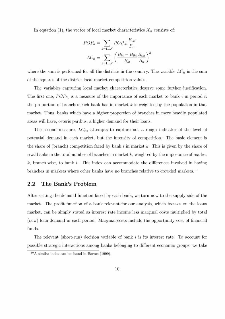
In equation (1), the vector of local market characteristics consists of:
=X
=1
=X
=1
µ −
¶2where the sum is performed for all the districts in the country. The variable is the sum
of the squares of the district local market competition values.
The variables capturing local market characteristics deserve some further justification.
The first one, , is a measure of the importance of each market to bank in period :
the proportion of branches each bank has in market is weighted by the population in that
market. Thus, banks which have a higher proportion of branches in more heavily populated
areas will have, ceteris paribus, a higher demand for their loans.
The second measure, , attempts to capture not a rough indicator of the level of
potential demand in each market, but the intensity of competition. The basic element is
the share of (branch) competition faced by bank in market . This is given by the share of
rival banks in the total number of branches in market , weighted by the importance of market
, branch-wise, to bank . This index can accommodate the differences involved in having
branches in markets where other banks have no branches relative to crowded markets.10
2.2 The Bank’s Problem
After setting the demand function faced by each bank, we turn now to the supply side of the
market. The profit function of a bank relevant for our analysis, which focuses on the loans
market, can be simply stated as interest rate income less marginal costs multiplied by total
(new) loan demand in each period. Marginal costs include the opportunity cost of financial
funds.
The relevant (short-run) decision variable of bank is its interest rate. To account for
possible strategic interactions among banks belonging to different economic groups, we take
10A similar index can be found in Barros (1999).
10
a simple approach, assuming that they take into consideration the impact they have on the
profits of other banks. Under perfect collusion (or joint management) banks would maximize
joint profits, while under perfectly independent behavior each would maximize own profits.
Thus, this approach accommodates intermediate situations by the introduction of a single
parameter, which measures to what extent a bank considers the impact of its decisions on the
profits of other banks11.
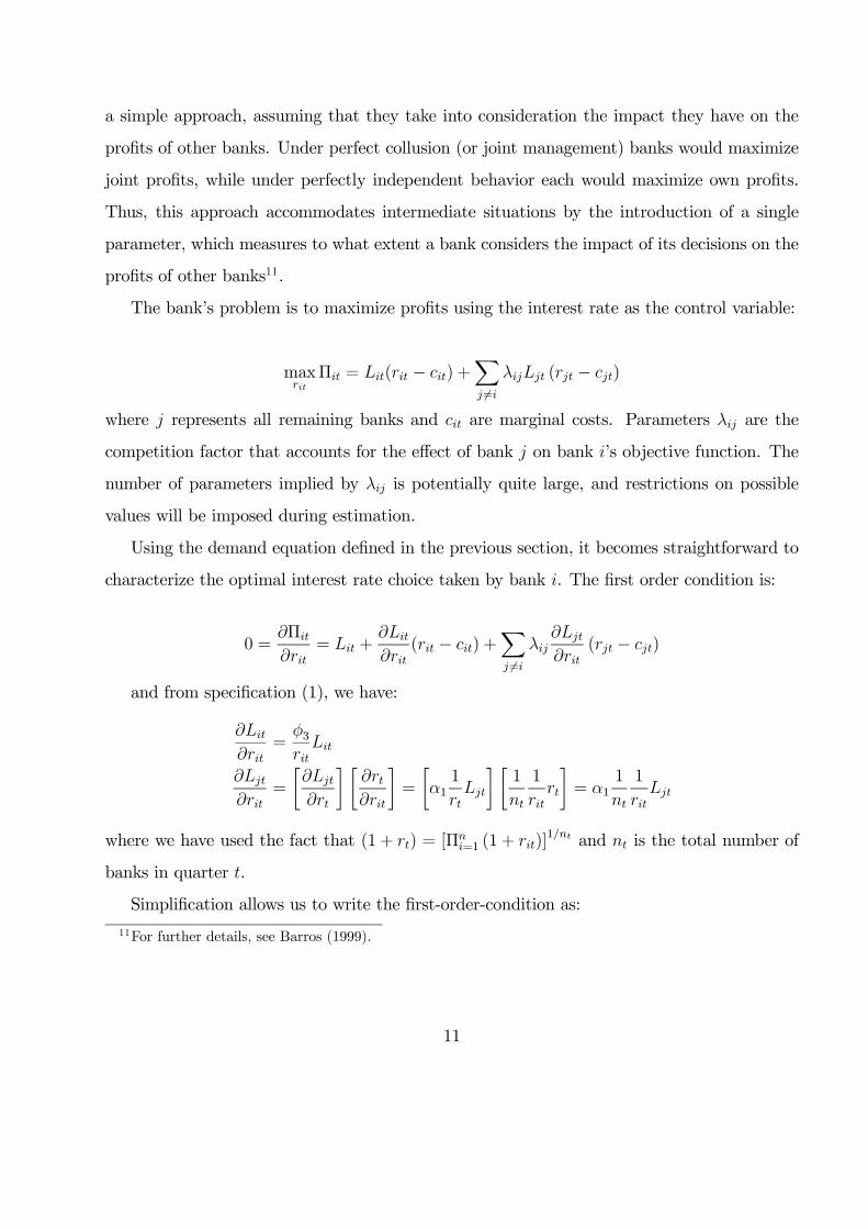
The bank’s problem is to maximize profits using the interest rate as the control variable:
max
Π = ( − ) +X 6=
( − )
where represents all remaining banks and are marginal costs. Parameters are the
competition factor that accounts for the effect of bank on bank ’s objective function. The
number of parameters implied by is potentially quite large, and restrictions on possible
values will be imposed during estimation.
Using the demand equation defined in the previous section, it becomes straightforward to
characterize the optimal interest rate choice taken by bank . The first order condition is:
0 =Π
= +
( − ) +
X 6=
( − )
and from specification (1), we have:
=
3
=
∙
¸ ∙
¸=
∙11
¸ ∙1
1
¸= 1
1
1
where we have used the fact that (1 + ) = [Π=1 (1 + )]
1 and is the total number of
banks in quarter .
Simplification allows us to write the first-order-condition as:
11For further details, see Barros (1999).
11
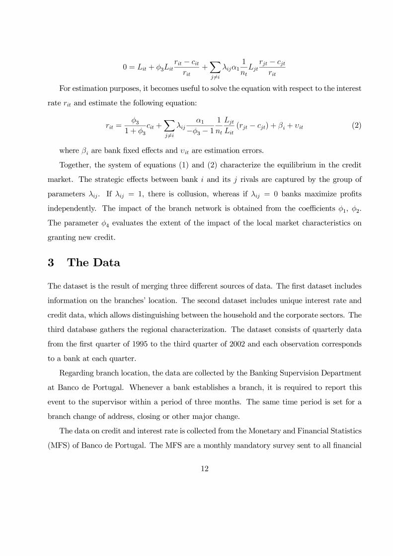
0 = + 3
−
+X 6=
11
−
For estimation purposes, it becomes useful to solve the equation with respect to the interest
rate and estimate the following equation:
=3
1 + 3 +
X 6=
1
−3 − 11
( − ) + + (2)
where are bank fixed effects and are estimation errors.
Together, the system of equations (1) and (2) characterize the equilibrium in the credit
market. The strategic effects between bank and its rivals are captured by the group of
parameters . If = 1, there is collusion, whereas if = 0 banks maximize profits
independently. The impact of the branch network is obtained from the coefficients 1, 2.
The parameter 4 evaluates the extent of the impact of the local market characteristics on
granting new credit.
3 The Data
The dataset is the result of merging three different sources of data. The first dataset includes
information on the branches’ location. The second dataset includes unique interest rate and
credit data, which allows distinguishing between the household and the corporate sectors. The
third database gathers the regional characterization. The dataset consists of quarterly data
from the first quarter of 1995 to the third quarter of 2002 and each observation corresponds
to a bank at each quarter.
Regarding branch location, the data are collected by the Banking Supervision Department
at Banco de Portugal. Whenever a bank establishes a branch, it is required to report this
event to the supervisor within a period of three months. The same time period is set for a
branch change of address, closing or other major change.
The data on credit and interest rate is collected from the Monetary and Financial Statistics
(MFS) of Banco de Portugal. The MFS are a monthly mandatory survey sent to all financial
12
institutions operating in the country and includes information on end-of-period stocks and
flows of credit granted to households and to non-financial corporations. Data on interest
rates are based on the flows of new credit granted. There was a major revision in interest
rate statistics at the end of 2002, with the purpose of harmonizing methodologies within the
Eurosystem, which prevents the use of more recent data. In fact, from 2003 onwards, interest
rate statistics began to be estimated using a sample of representative banks, instead of using
the whole universe of banking institutions, as before. Hence, there are several banks (including
small banks belonging to the seven largest banking groups) for which there is no interest rate
data after end-2002. Nevertheless, a longer estimation period would probably not be adequate,
given that the effects of mergers should be more strongly and clearly captured in the years
immediately after these mergers12. Moreover, it would be a very strong assumption to require
that the pre-merger equilibrium holds for many years after the merger wave, as changes in
economic and financial variables should also shape this equilibrium.
Finally, we further collected data on the demographic characteristics of the districts from
Statistics Portugal, including total population by municipality.
3.1 Description of the 2000 Merger Wave
During the 1995 to 2002 sample period, the Portuguese financial system experienced several
restructuring processes. Among the main corporate changes, we highlight the five most signif-
icant ones: (i) in January 1996, Banco Português de Investimento (BPI) buys Banco Borges &
Irmão (BBI) and Banco Fonsecas e Burnay (BFB); (ii) in December 1997, Banco Comercial
de Macau (BCM) changes to Expresso Atlantico; (iii) in September 1998, there was a merger
between BBI, Banco Fomento e Exterior (BFE) and BFB and the new institution is named
as BBPI; (iv) in March 2000, the group Banco Pinto e Sotto Mayor (BPSM), which included
the banks BPSM, Banco Totta e Sotto Mayor Inv (BTSM Inv), Banco Totta e Açores (BTA)
and Credito Predial Português (CPP) is extinguished. The bank BPSM is bought by Banco
12For instance, Berger et al (1998) consider that the dynamic effects of bank mergers should be analyzed in
the three years following the merger.
13
Comercial Português (BCP). At the same time, BTSM Inv is acquired by Caixa Geral de
Depósitos (CGD); BTA is created and CPP is acquired by BTA and finally (v) in September
2000, Santander buys BTA.
Among the main events, the ones occurred in 2000 are by far the most important, as they
involved major banks as well as major financial groups. Among the seven major financial
groups, four were directly involved either by selling a financial institution or by acquiring one,
thus generating profound changes in the structure of the Portuguese banking market. Due to
the significant changes occurring in 2000, we may distinguish between specific characteristics
of the pre-2000 period, which we designate as the pre-merger period, comprehending the
1995-1999 period, and specific characteristics of an after-2000 period, which we denominate
the post-merger period (including the 2000-2002 period).
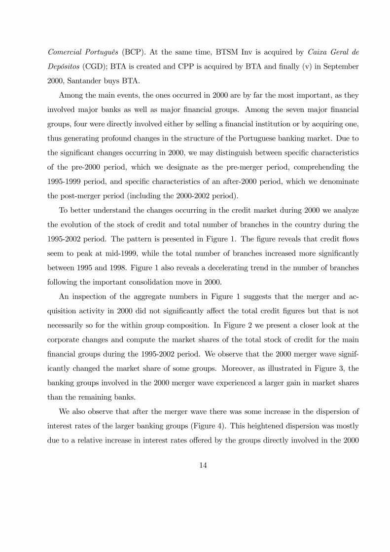
To better understand the changes occurring in the credit market during 2000 we analyze
the evolution of the stock of credit and total number of branches in the country during the
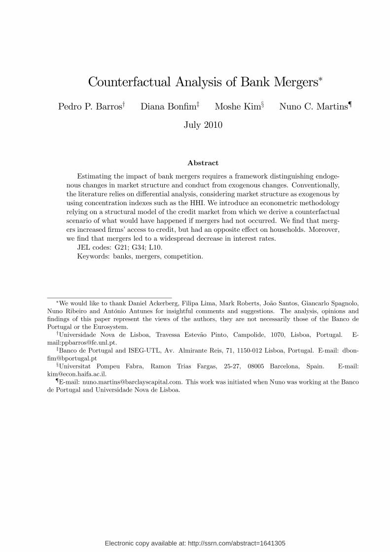
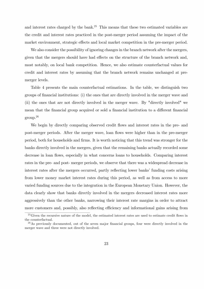
1995-2002 period. The pattern is presented in Figure 1. The figure reveals that credit flows
seem to peak at mid-1999, while the total number of branches increased more significantly
between 1995 and 1998. Figure 1 also reveals a decelerating trend in the number of branches
following the important consolidation move in 2000.
An inspection of the aggregate numbers in Figure 1 suggests that the merger and ac-
quisition activity in 2000 did not significantly affect the total credit figures but that is not
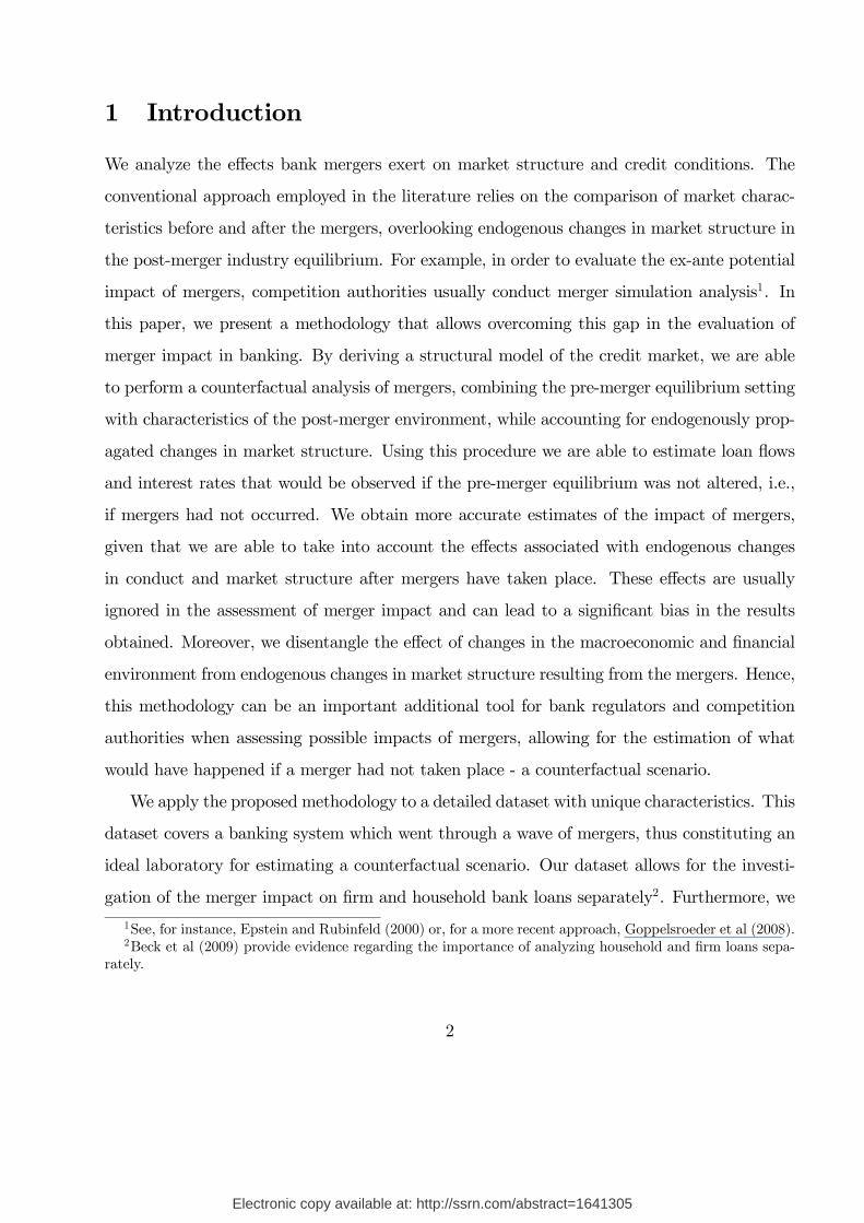
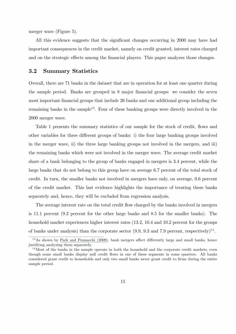
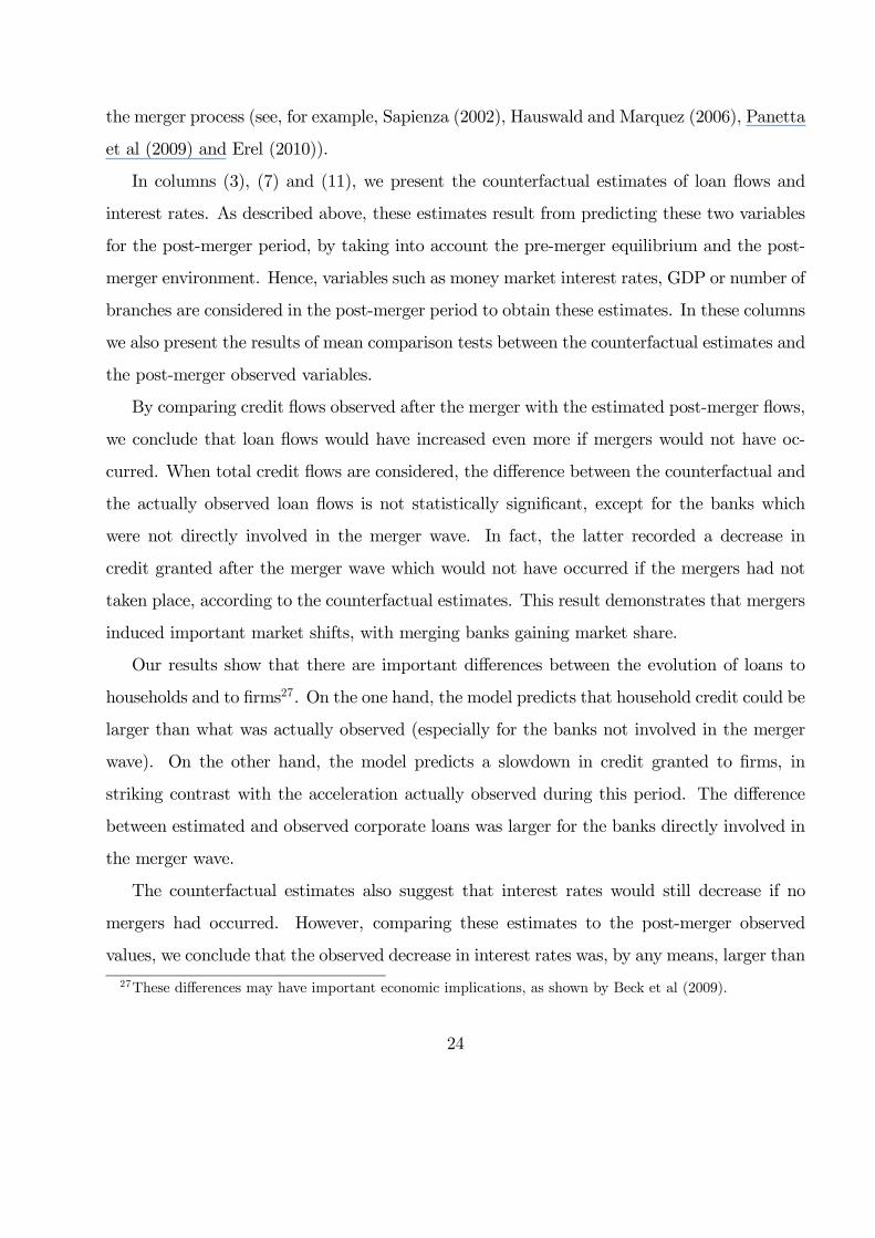
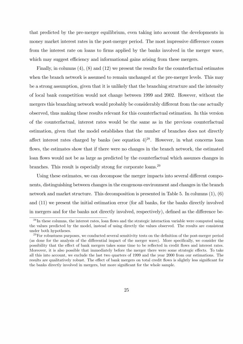
necessarily so for the within group composition. In Figure 2 we present a closer look at the
corporate changes and compute the market shares of the total stock of credit for the main
financial groups during the 1995-2002 period. We observe that the 2000 merger wave signif-
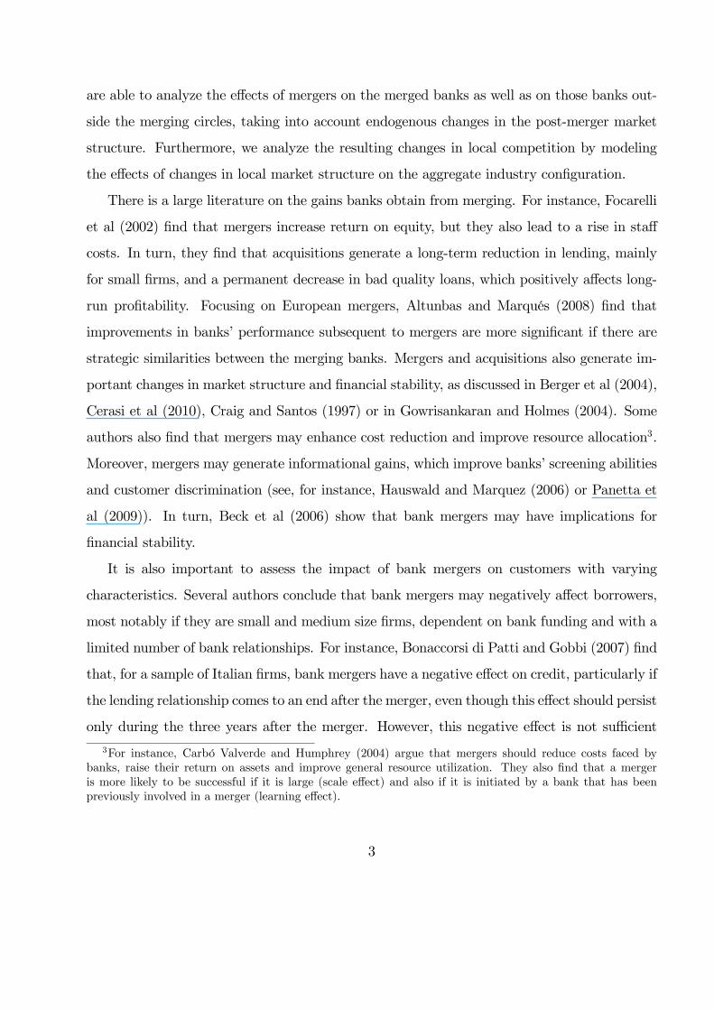
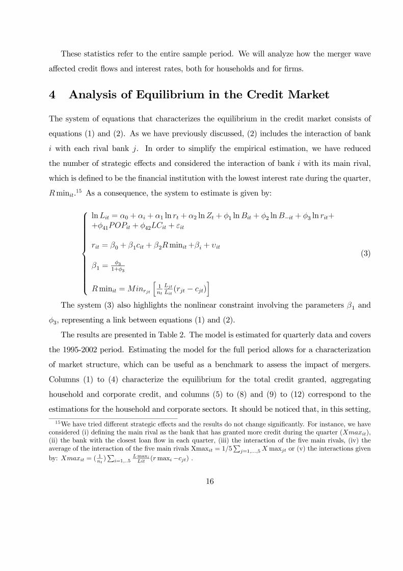
icantly changed the market share of some groups. Moreover, as illustrated in Figure 3, the
banking groups involved in the 2000 merger wave experienced a larger gain in market shares
than the remaining banks.
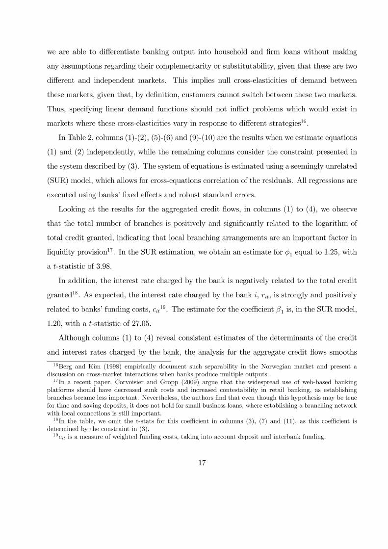
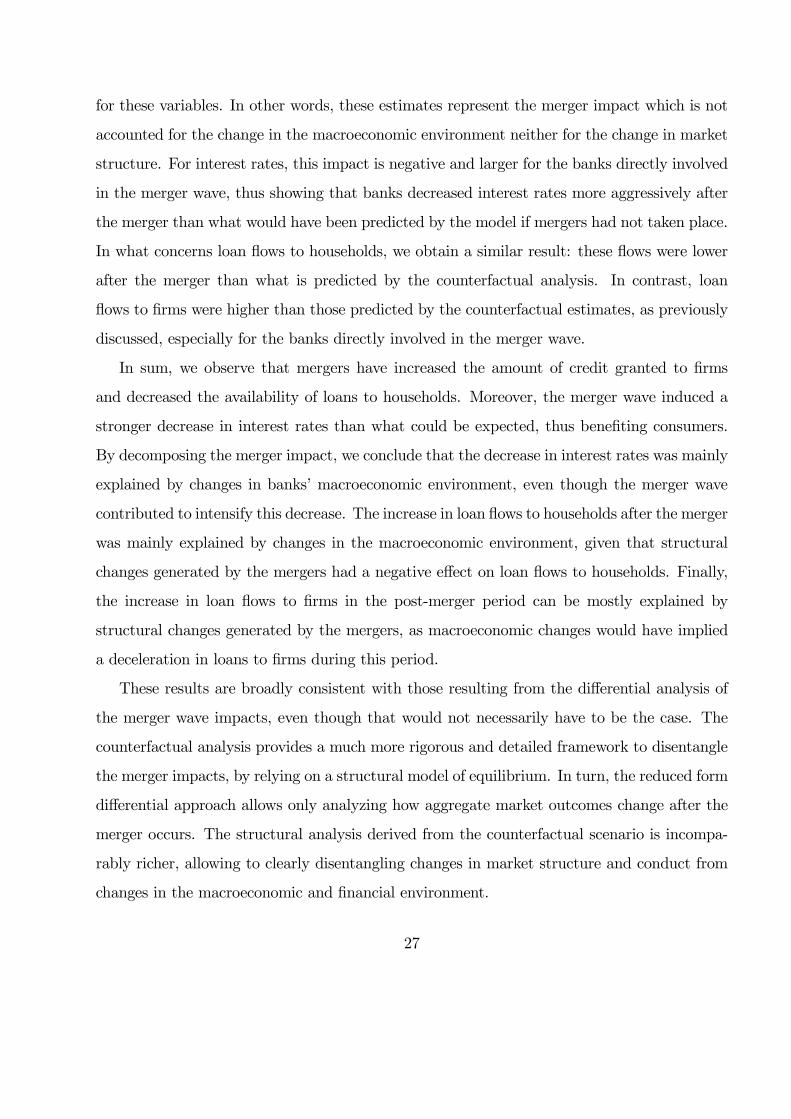
We also observe that after the merger wave there was some increase in the dispersion of
interest rates of the larger banking groups (Figure 4). This heightened dispersion was mostly
due to a relative increase in interest rates offered by the groups directly involved in the 2000
14
merger wave (Figure 5).
All this evidence suggests that the significant changes occurring in 2000 may have had
important consequences in the credit market, namely on credit granted, interest rates charged
and on the strategic effects among the financial players. This paper analyzes those changes.
3.2 Summary Statistics
Overall, there are 71 banks in the dataset that are in operation for at least one quarter during
the sample period. Banks are grouped in 8 major financial groups: we consider the seven
most important financial groups that include 26 banks and one additional group including the
remaining banks in the sample13. Four of these banking groups were directly involved in the
2000 merger wave.
Table 1 presents the summary statistics of our sample for the stock of credit, flows and
other variables for three different groups of banks: i) the four large banking groups involved
in the merger wave, ii) the three large banking groups not involved in the mergers, and iii)
the remaining banks which were not involved in the merger wave. The average credit market
share of a bank belonging to the group of banks engaged in mergers is 3.4 percent, while the
large banks that do not belong to this group have on average 6.7 percent of the total stock of
credit. In turn, the smaller banks not involved in mergers have only, on average, 0.6 percent
of the credit market. This last evidence highlights the importance of treating these banks
separately and, hence, they will be excluded from regression analysis.
The average interest rate on the total credit flow charged by the banks involved in mergers
is 11.1 percent (9.2 percent for the other large banks and 8.5 for the smaller banks). The
household market experiences higher interest rates (13.2, 10.4 and 10.2 percent for the groups
of banks under analysis) than the corporate sector (9.9, 9.3 and 7.9 percent, respectively)14.
13As shown by Park and Pennacchi (2009), bank mergers affect differently large and small banks, hence
justifying analyzing them separately.14Most of the banks in the sample operate in both the household and the corporate credit markets, even
though some small banks display null credit flows in one of these segments in some quarters. All banks
considered grant credit to households and only two small banks never grant credit to firms during the entire
sample period.
15
These statistics refer to the entire sample period. We will analyze how the merger wave
affected credit flows and interest rates, both for households and for firms.
4 Analysis of Equilibrium in the Credit Market
The system of equations that characterizes the equilibrium in the credit market consists of
equations (1) and (2). As we have previously discussed, (2) includes the interaction of bank
with each rival bank . In order to simplify the empirical estimation, we have reduced
the number of strategic effects and considered the interaction of bank with its main rival,
which is defined to be the financial institution with the lowest interest rate during the quarter,
min.15 As a consequence, the system to estimate is given by:
⎧⎪⎪⎪⎪⎪⎪⎪⎪⎪⎪⎪⎨⎪⎪⎪⎪⎪⎪⎪⎪⎪⎪⎪⎩
ln = 0 + + 1 ln + 2 ln + 1 ln + 2 ln− + 3 ln +
+41 + 42 +
= 0 + 1 + 2min+ +
1 =31+3
min =
h1
( − )
i(3)
The system (3) also highlights the nonlinear constraint involving the parameters 1 and
3, representing a link between equations (1) and (2).
The results are presented in Table 2. The model is estimated for quarterly data and covers
the 1995-2002 period. Estimating the model for the full period allows for a characterization
of market structure, which can be useful as a benchmark to assess the impact of mergers.
Columns (1) to (4) characterize the equilibrium for the total credit granted, aggregating
household and corporate credit, and columns (5) to (8) and (9) to (12) correspond to the
estimations for the household and corporate sectors. It should be noticed that, in this setting,
15We have tried different strategic effects and the results do not change significantly. For instance, we have
considered (i) defining the main rival as the bank that has granted more credit during the quarter (),
(ii) the bank with the closest loan flow in each quarter, (iii) the interaction of the five main rivals, (iv) the
average of the interaction of the five main rivals Xmax = 15P
=15max or (v) the interactions given
by: = (1)P
=15max
(max−) .
16
we are able to differentiate banking output into household and firm loans without making
any assumptions regarding their complementarity or substitutability, given that these are two
different and independent markets. This implies null cross-elasticities of demand between
these markets, given that, by definition, customers cannot switch between these two markets.
Thus, specifying linear demand functions should not inflict problems which would exist in
markets where these cross-elasticities vary in response to different strategies16.
In Table 2, columns (1)-(2), (5)-(6) and (9)-(10) are the results when we estimate equations
(1) and (2) independently, while the remaining columns consider the constraint presented in
the system described by (3). The system of equations is estimated using a seemingly unrelated
(SUR) model, which allows for cross-equations correlation of the residuals. All regressions are
executed using banks’ fixed effects and robust standard errors.
Looking at the results for the aggregated credit flows, in columns (1) to (4), we observe
that the total number of branches is positively and significantly related to the logarithm of
total credit granted, indicating that local branching arrangements are an important factor in
liquidity provision17. In the SUR estimation, we obtain an estimate for 1 equal to 1.25, with
a -statistic of 3.98.
In addition, the interest rate charged by the bank is negatively related to the total credit
granted18. As expected, the interest rate charged by the bank , , is strongly and positively
related to banks’ funding costs, 19. The estimate for the coefficient 1 is, in the SUR model,
1.20, with a -statistic of 27.05.
Although columns (1) to (4) reveal consistent estimates of the determinants of the credit
and interest rates charged by the bank, the analysis for the aggregate credit flows smooths
16Berg and Kim (1998) empirically document such separability in the Norwegian market and present a
discussion on cross-market interactions when banks produce multiple outputs.17In a recent paper, Corvoisier and Gropp (2009) argue that the widespread use of web-based banking
platforms should have decreased sunk costs and increased contestability in retail banking, as establishing
branches became less important. Nevertheless, the authors find that even though this hypothesis may be true
for time and saving deposits, it does not hold for small business loans, where establishing a branching network
with local connections is still important.18In the table, we omit the t-stats for this coefficient in columns (3), (7) and (11), as this coefficient is
determined by the constraint in (3).19 is a measure of weighted funding costs, taking into account deposit and interbank funding.
17
important idiosyncratic characteristics of the determinants of the household and corporate
sectors credit markets. Columns (5) to (8) present the results for equations (1) and (2) and
system (3) for the household sector and columns (9) to (12) present a similar analysis for
the corporate sector. The distinction across these institutional sectors highlights important
differences in these markets, thus justifying a disaggregate specification rather than treating
the credit market as a homogeneous market20.
We observe that the banks’ own number of branches positively influences credit granted,
both to households and to firms (the estimated coefficients are 0.88 and 1.66, respectively).
In turn, the number of branches of the remaining banks is not significantly correlated with
credit granted to households, as illustrated in columns (5) and (7), while it has a negative and
significant impact on credit supplied to the corporate sector.
Looking at the macro determinants, Table 2 reveals that the impact of the GDP level
on credit granted is positive for both credit markets. Given that GDP reflects changes in
global macroeconomic conditions and also changing industry risk, this result confirms the
usually observed pro-cyclicality of liquidity provision21. However, this impact is statistically
significant only for credit to households. Moreover, local branch competition has a positive
impact on the credit flow. This impact is fourfold larger in the corporate than in the household
sector22.
The evidence on strategic behavior, measured by the coordination parameter , suggests
that there is no collusion between banks, as is always less than one. The statistical tests
on these parameters show that we can reject the hypothesis of perfect collusion ( = 1) in
the corporate credit market, thus suggesting that banks behave competitively in this market.
However, for households we cannot rule out either the hypothesis of perfect collusion ( = 1)
20The lower number of observations in the regressions for households and firms is due to the fact that some
small banks show null credit flows in one of these market segments in some quarters, as discussed in Section
3.2. Moreover, two small banks never grant credit to firms during the entire sample period.21Controlling for GDP should capture the most relevant time fixed effects. To mitigate concerns about
potential cointegration issues, we also considered the GDP growth rate, having obtained broadly similar
results.22The estimated coefficient 42 is 5.36 for households (with a -statistic of 1.94) and 20.13 for firms (with a
-statistic of 6.23).
18
or perfect competition ( = 0). These results are consistent with previous evidence obtained
by Berg and Kim (1998), who argue that the mobility of customers in the corporate market is
stronger than in other markets, thus generating more competitive behaviors by banks. More
recently, Degryse et al (2010) show that firms may benefit from switching banks after mergers
occur, which is related to banks’ competitive strategies.
Having analyzed the determinants of credit flow and interest rates for the household and
corporate markets, we can now determine how these parameters change following bank merg-
ers.
5 The Impact of the Merger Wave
This section analyzes the impact of the 2000 merger wave on the determinants of credit flows
and interest rates. On the one hand, we are interested on the impact of the merger wave
on the credit flow and interest rates charged and, on the other hand, we aim at determining
how the merger has affected local branch competition and coordination moves in the banking
industry.
For illustration purposes, we begin by estimating the differential impact of the merger
wave, given that this is one of the most common approaches in the literature (see for example
Erel (2010), Focarelli and Panetta (2003) or Sapienza (2002)). However, this reduced form
differential analysis suffers from several drawbacks. In fact, this analysis does not take into
account changes in market structure and conduct. In our opinion using a Herfindahl Hirschman
Index should not be sufficient to adequately capture changes in market power resulting from
mergers, as this measure is exogenous and may reflect other market dynamics. In fact, the
magnitude of the merger wave should generate changes in the interaction between banks and
possibly also in consumer preferences. Given these changes, the differential analysis, usually
conducted in the literature, may lead to biased and incorrect estimates of the merger impact.
Hence, we propose a new methodology for the comparison between the pre- and post-merger
periods, through the estimation of a counterfactual. We explicitly consider that the merger
wave might have generated a new setup in credit markets in the post-merger period. In
19

this estimation we combine the pre-merger equilibrium setup with the post-merger observed
environment to answer the "what if" question.
5.1 The Differential Impact of the Merger Wave
Taking into account one of the most common approaches used to assess the impact of mergers,
we compute the differential impact of the merger wave on the equilibrium in the credit market.
In particular, we analyze how variables such as the strategic behavior and local competition
change after the merger. In order to pursue this objective, we consider a dummy variable
that has value one if the quarter is in year 2000 or after, and zero otherwise, and
run a modified empirical model of (3)23:
⎧⎪⎪⎪⎪⎪⎪⎪⎪⎪⎪⎪⎨⎪⎪⎪⎪⎪⎪⎪⎪⎪⎪⎪⎩
ln = 0 + + 01+ 1 ln + 2 ln + 1 ln + 2 ln− + 3 ln +
+41 + 42 + 43 ∗+
= 0 + 1 + 2min+3min ∗+ +
1 =31+3
min =
h1
( − )
i(4)
In this model, the coefficient 01 captures eventual changes in the level of credit flow
after the merger wave and 43 considers the difference in the impact of the local branch
competition on the quarterly credit flow following the 2000 merger with respect to the impact
during the pre-merger period. Using the coefficient 3 and equation (2) we can compute a
similar differential effect for the strategic interaction, , which we name .
The results for the differential impact are presented in Table 3. Columns (1) to (4) present
the analysis for the total credit flow (household plus corporate credit) and columns (5) to (8)
and (9) to (12) present the results for the household and corporate sectors, respectively. As
23The choice of the year 2000 is motivated by the large number of mergers observed, some of which involving
some of the largest banks. As illustrated in section 3.1, these mergers had a substantial impact on market
structure.
20
before, columns (1)-(2), (5)-(6) and (9)-(10) represent the first two equations of the model (4)
without considering the non-linear constraint.
The first row of the estimated coefficients in Table 3 shows the results for the variable
. The negative coefficients in columns (5) and (7) reveal that the quarterly credit
flow decreased after the mergers for the household sector, despite the decrease in interest
rates (columns (6) and (8)). This suggests that there were important changes in market
equilibrium after the mergers, given that a pure shift along the demand curve would imply a
positive effect on credit due to the decrease in interest rates. For the corporate sector, the sale
of credit increased after the merger, as observed in columns (9) and (11), and the interest rate
charged decreased, as shown in columns (10) and (12). Post-merger equilibrium loan rates
decrease when the merger induces large cost advantages relative to the increase in banks’
market power, as shown by Carletti et al (2007). Our results are consistent with Fonseca and
Normann (2008), who argue that even though a merger involving the largest firm in a market
creates a more asymmetric market structure, asymmetric markets exhibit lower prices than
symmetric markets with the same number of firms.24
For robustness purposes, we considered the possibility that the effect of bank mergers
takes some time to be reflected in credit flows and interest rates. To test this possibility,
we estimated the same regressions, but considering that the dummy variable would
take the value of unity only from 2001 onwards. The results for households remain broadly
unchanged. For firms, we continue to observe the negative impact on interest rates, but the
positive impact on credit ceases to be significant. Nevertheless, the impact of the mergers
should have been felt almost immediately, as suggested by the rapid change in banks’ names
and identities. To test the hypothesis that the merger impact could have had immediate
impacts, we also estimated these regressions with the dummy variable taking the
value of unity from 1999 onwards. We observe that, in this situation, the differential impact
of the merger wave on credit flows looses significance, thus confirming 2000 as a sensible break
24In order to confirm the validity and strength of these differential impacts, we tested for the existence of
a structural break after the merger wave, using a Chow test. In all the tests performed we reject the null
hypothesis of structural stability of the parameters.
21
point.
Looking at the effect of local branch competition, we find that the impact was most
significant for the corporate sector. In this credit market, we find that the merger leads to
a decrease in the impact of local competition on the credit flow. Hence, the positive impact
of local bank competition on credit granted to firms becomes slightly smaller (though still
positive and large) after the merger wave.
The strategic effect of the main rival following the merger is presented in the last two
groups of rows in Table 3. In what concerns the market for household loans, we clearly reject
the hypothesis of collusion, though that conclusion does not hold for the post-merger period.
In turn, in the corporate loan market we always reject the existence of full coordination moves
between banks, even though increased somewhat after the merger wave.
5.2 Counterfactual Analysis of the Merger Wave
The previous analysis computes a differential effect of specific variables and assumes that
all remaining interactions remain constant. However, this analysis does not fully take into
account the structural changes which should have occurred in credit markets after the merger
wave. Given the magnitude and extension of the mergers, the way banks (and their costumers)
interact should have changed substantially after the merger. In this section, we assume that a
new scenario is created that influences all variables in the credit market. Under this scenario,
the evaluation of the differences in strategic effects requires the comparison between the results
for the post-merger period and the ones obtained from the estimation of the pre-merger
equilibrium using the post-merger data (counterfactual). The main advantage is that we can
analyze the merger impact using the post-merger environment which is obviously a much more
realistic assumption.
The way we construct the counterfactual for the empirical estimation is the following. We
first estimate the model (3) for the 1995-1999 period and obtain estimates for the pre-merger
period. We then use the pre-merger coefficient estimates of this model for the 2000-2002
data on exogenous variables to obtain the value of the estimated post-merger credit flows
22
and interest rates charged by the bank.25 This means that these two estimated variables are
the credit and interest rates practiced in the post-merger period assuming the impact of the
market environment, strategic effects and local market competition in the pre-merger period.
We also consider the possibility of ignoring changes in the branch network after the mergers,
given that the mergers should have had effects on the structure of the branch network and,
most notably, on local bank competition. Hence, we also estimate counterfactual values for
credit and interest rates by assuming that the branch network remains unchanged at pre-
merger levels.
Table 4 presents the main counterfactual estimations. In the table, we distinguish two
groups of financial institutions: (i) the ones that are directly involved in the merger wave and
(ii) the ones that are not directly involved in the merger wave. By "directly involved" we
mean that the financial group acquired or sold a financial institution to a different financial
group.26
We begin by directly comparing observed credit flows and interest rates in the pre- and
post-merger periods. After the merger wave, loan flows were higher than in the pre-merger
period, both for households and firms. It is worth noticing that this trend was stronger for the
banks directly involved in the mergers, given that the remaining banks actually recorded some
decrease in loan flows, especially in what concerns loans to households. Comparing interest
rates in the pre- and post- merger periods, we observe that there was a widespread decrease in
interest rates after the mergers occurred, partly reflecting lower banks’ funding costs arising
from lower money market interest rates during this period, as well as from access to more
varied funding sources due to the integration in the European Monetary Union. However, the
data clearly show that banks directly involved in the mergers decreased interest rates more
aggressively than the other banks, narrowing their interest rate margins in order to attract
more customers and, possibly, also reflecting efficiency and informational gains arising from
25Given the recursive nature of the model, the estimated interest rates are used to estimate credit flows in
the counterfactual.26As previously documented, out of the seven major financial groups, four were directly involved in the
merger wave and three were not directly involved.
23
the merger process (see, for example, Sapienza (2002), Hauswald and Marquez (2006), Panetta
et al (2009) and Erel (2010)).
In columns (3), (7) and (11), we present the counterfactual estimates of loan flows and
interest rates. As described above, these estimates result from predicting these two variables
for the post-merger period, by taking into account the pre-merger equilibrium and the post-
merger environment. Hence, variables such as money market interest rates, GDP or number of
branches are considered in the post-merger period to obtain these estimates. In these columns
we also present the results of mean comparison tests between the counterfactual estimates and
the post-merger observed variables.
By comparing credit flows observed after the merger with the estimated post-merger flows,
we conclude that loan flows would have increased even more if mergers would not have oc-
curred. When total credit flows are considered, the difference between the counterfactual and
the actually observed loan flows is not statistically significant, except for the banks which
were not directly involved in the merger wave. In fact, the latter recorded a decrease in
credit granted after the merger wave which would not have occurred if the mergers had not
taken place, according to the counterfactual estimates. This result demonstrates that mergers
induced important market shifts, with merging banks gaining market share.
Our results show that there are important differences between the evolution of loans to
households and to firms27. On the one hand, the model predicts that household credit could be
larger than what was actually observed (especially for the banks not involved in the merger
wave). On the other hand, the model predicts a slowdown in credit granted to firms, in
striking contrast with the acceleration actually observed during this period. The difference
between estimated and observed corporate loans was larger for the banks directly involved in
the merger wave.
The counterfactual estimates also suggest that interest rates would still decrease if no
mergers had occurred. However, comparing these estimates to the post-merger observed
values, we conclude that the observed decrease in interest rates was, by any means, larger than
27These differences may have important economic implications, as shown by Beck et al (2009).
24
that predicted by the pre-merger equilibrium, even taking into account the developments in
money market interest rates in the post-merger period. The most impressive difference comes
from the interest rate on loans to firms applied by the banks involved in the merger wave,
which may suggest efficiency and informational gains arising from these mergers.
Finally, in columns (4), (8) and (12) we present the results for the counterfactual estimates
when the branch network is assumed to remain unchanged at the pre-merger levels. This may
be a strong assumption, given that it is unlikely that the branching structure and the intensity
of local bank competition would not change between 1999 and 2002. However, without the
mergers this branching network would probably be considerably different from the one actually
observed, thus making these results relevant for this counterfactual estimation. In this version
of the counterfactual, interest rates would be the same as in the previous counterfactual
estimation, given that the model establishes that the number of branches does not directly
affect interest rates charged by banks (see equation 4)28. However, in what concerns loan
flows, the estimates show that if there were no changes in the branch network, the estimated
loan flows would not be as large as predicted by the counterfactual which assumes changes in
branches. This result is especially strong for corporate loans.29
Using these estimates, we can decompose the merger impacts into several different compo-
nents, distinguishing between changes in the exogenous environment and changes in the branch
network and market structure. This decomposition is presented in Table 5. In columns (1), (6)
and (11) we present the initial estimation error (for all banks, for the banks directly involved
in mergers and for the banks not directly involved, respectively), defined as the difference be-
28In these columns, the interest rates, loan flows and the strategic interaction variable were computed using
the values predicted by the model, instead of using directly the values observed. The results are consistent
under both hypotheses.29For robustness purposes, we conducted several sensitivity tests on the definition of the post-merger period
(as done for the analysis of the differential impact of the merger wave). More specifically, we consider the
possibility that the effect of bank mergers takes some time to be reflected in credit flows and interest rates.
Moreover, it is also possible that immediately before the merger there were some strategic effects. To take
all this into account, we exclude the last two quarters of 1999 and the year 2000 from our estimations. The
results are qualitatively robust. The effect of bank mergers on total credit flows is slightly less significant for
the banks directly involved in mergers, but more significant for the whole sample.
25

tween the predicted values for the pre-merger period and the observed loan flows and interest
rates in this period. On average, this estimation error is virtually negligible.
In columns (2), (7) and (12) we present the effect of changes in the exogenous environment
on loan flows and interest rates, for the three groups of banks under analysis. This effect is
computed as the difference between the counterfactual estimates for the post-merger period
when holding the branch network and market structure at pre-merger levels, but taking into
account changes in macroeconomic and financial conditions after the merger wave (columns
(4), (8) and (12) in Table 4). In what concerns interest rates, the effect was clearly negative
and close to 2 p.p. Hence, a considerable part of the decrease in interest rates in the post-
merger period was due to changes in macroeconomic conditions. Regarding loan flows, changes
in banks’ economic and financial environment led to an increase in loan flows to households
and to a decrease in loan flows to firms. As discussed above, this result means that the
counterfactual estimates without changes in branches suggest that loans to households should
have been higher if the mergers had not occurred (the opposite being true concerning loans to
firms). The impact of the changes in the macroeconomic and financial environment on loan
flows was stronger for the banks directly involved in the merger wave.
When changes in the branch network and in local market competition are considered
(columns (3), (8) and (13)), we observe a positive impact in loan flows, when compared to the
impact of considering only changes in the exogenous environment. These estimates correspond
to the difference between columns (3) and (4) in Table 4, i.e., the difference between the
counterfactuals with and without changes in branches. Hence, when changes in the branching
network observed after the merger wave are considered, we conclude that loan flows should
have been even higher if mergers had not occurred. This difference assumes a larger magnitude
in loans to firms. As previously discussed, interest rates estimates remain unchanged, given
that they are not directly influenced by the number of branches in our structural model.
Finally, we present the estimates for the impact of other structural changes (which includes
a prediction error), defined as the difference between interest rates and loan flows observed
after the merger wave and the counterfactual estimates (with changes in the branch network),
26
for these variables. In other words, these estimates represent the merger impact which is not
accounted for the change in the macroeconomic environment neither for the change in market
structure. For interest rates, this impact is negative and larger for the banks directly involved
in the merger wave, thus showing that banks decreased interest rates more aggressively after
the merger than what would have been predicted by the model if mergers had not taken place.
In what concerns loan flows to households, we obtain a similar result: these flows were lower
after the merger than what is predicted by the counterfactual analysis. In contrast, loan
flows to firms were higher than those predicted by the counterfactual estimates, as previously
discussed, especially for the banks directly involved in the merger wave.
In sum, we observe that mergers have increased the amount of credit granted to firms
and decreased the availability of loans to households. Moreover, the merger wave induced a
stronger decrease in interest rates than what could be expected, thus benefiting consumers.
By decomposing the merger impact, we conclude that the decrease in interest rates was mainly
explained by changes in banks’ macroeconomic environment, even though the merger wave
contributed to intensify this decrease. The increase in loan flows to households after the merger
was mainly explained by changes in the macroeconomic environment, given that structural
changes generated by the mergers had a negative effect on loan flows to households. Finally,
the increase in loan flows to firms in the post-merger period can be mostly explained by
structural changes generated by the mergers, as macroeconomic changes would have implied
a deceleration in loans to firms during this period.
These results are broadly consistent with those resulting from the differential analysis of
the merger wave impacts, even though that would not necessarily have to be the case. The
counterfactual analysis provides a much more rigorous and detailed framework to disentangle
the merger impacts, by relying on a structural model of equilibrium. In turn, the reduced form
differential approach allows only analyzing how aggregate market outcomes change after the
merger occurs. The structural analysis derived from the counterfactual scenario is incompa-
rably richer, allowing to clearly disentangling changes in market structure and conduct from
changes in the macroeconomic and financial environment.
27
6 Concluding remarks
Bank mergers usually have important consequences in terms of bank competition, access to
credit or loan pricing. However, the effects of bank mergers on these variables are hard to
disentangle from other market and macroeconomic dynamic effects that occur simultaneously,
affecting loan demand and supply, as well as its pricing. In this paper, we present a struc-
tural analysis of the impact of mergers in the Portuguese banking market. In the late 90s,
several large banks were involved in a strong and fast consolidation process, thus providing
an empirical setup to assess changes in market structure after the mergers.
Using a structural model, we derive the equilibrium in the pre-merger setting. Combining
this estimated equilibrium with the post-merger environment, we are able to construct a
counterfactual estimate of loans and interest rates. This allows us to compare the observed loan
flows and interest rates with those resulting from the pre-merger equilibrium, thus assessing
the impacts of the bank merger wave. Moreover, the counterfactual estimation allows for
taking into account changes in conduct and market structure after the mergers take place.
These effects are usually ignored in the assessment of merger impacts and may lead to a
significant bias in the results obtained.
We obtain several interesting results. The interest rates observed after the mergers were
lower than those predicted by the model, in the pre-merger equilibrium. This may reflect
efficiency and informational gains resulting from the mergers and translated into more com-
petitive pricing. In turn, there are important differences between loans granted to households
and to firms: whereas loans granted to households were in fact lower than what would be sug-
gested using the pre-merger equilibrium, loans granted to firms actually recorded a stronger
growth than what could have occurred if no mergers had taken place. All in all, households
may have faced some constraints in access to credit after the merger, even though loans to
households recorded robust growth rates during this period. On the contrary, loans granted
to firms seem to have surpassed by a large extent the counterfactual estimates.
The counterfactual estimates also highlight important differences between the banks di-
28
rectly involved in the merger wave and the remaining large banking groups. The banks directly
involved in this process decreased their interest rates on corporate loans much more aggres-
sively than other banks. Simultaneously, credit granted to firms by these banks was also much
larger than what could have been expected if no mergers had occurred. In turn, the estimated
decrease of loans granted to households assumed a larger magnitude for the banks which did
not directly participate in the merger wave.
By decomposing the merger impacts through the use of the counterfactual estimates, we
conclude that changes in banks’ macroeconomic and financial environment were the main
driving force when explaining the differences in interest rates and loan flows before and af-
ter the merger wave. Structural changes generated by the mergers contributed to intensify
these changes in interest rates and loans to firms, but had the opposite impact on loans to
households.
The structural model used to perform these counterfactual estimates allows for clear iden-
tification of the effects of bank mergers on credit and interest rates, isolating changes in the
exogenous environment and in market structure. Changes in market equilibrium resulting
from the mergers affect significantly banks’ decisions, as well as their strategic interactions,
thus demonstrating the importance of relying on a structural estimation method. All in all,
we observe that potential efficiency and informational gains seem to haven been transmitted
to customers through lower lending rates and firms have faced less bank financing constraints
than they otherwise would.
References
[1] Altunbas, Y. and D. Marqués (2008), Mergers and acquisitions and bank performance
in Europe: The role of strategic similarities, Journal of Economics and Business, 60,
204-222.
[2] Antão, P., M. Boucinha, L. Farinha, A. Lacerda, A.C. Leal and N. Ribeiro (2009), Fi-
nancial integration, financial structures and the decisions of households and firms in
29
Economics and Research Department of Banco de Portugal, The Portuguese Economy in
the Context of Economic, Financial and Monetary Integration.
[3] Barros, P. P. (1999), Multimarket Competition in Banking with an Example from the
Portuguese Market, International Journal of Industrial Organization, 17, Iss. 3, pp. 335-
352.
[4] Beck, T., B. Buyukkarabacak, F. Rioja and N. Valev (2009), Who gets the credit? And
does it matter? Household vs. firm lending across countries, CEPR Discussion Paper No.
7400.
[5] Berg, S. A. andM. Kim (1998), Banks as multioutput oligopolies: An empirical evaluation
of the retail and corporate banking markets, Journal of Money, Credit and Banking, 30
(2), 135-153.
[6] Berger, A., S. D. Bonime, L. G. Goldberg and L. J. White (2004), The dynamics of
market entry: the effects of mergers and acquisitions on entry in the banking industry,
Journal of Business, 77 (4), 797-834.
[7] Berger, A., A. Saunders, J. M. Scalise, G. F. Udell (1998), The effects of bank mergers
and acquisitions on small business lending, Journal of Financial Economics, 50, 187-229.
[8] Berry, S. and A. Pakes (1993), Some applications and limitations of recent advances in
empirical industrial organization: merger analysis, American Economic Review, 83 (2),
247-252.
[9] Bonaccorsi di Patti, E. and G. Gobbi (2007), Winners or Losers? The effects of banking
consolidation on corporate borrowers, The Journal of Finance, 62, 669-695.
[10] Carbó Valverde, S. and D. B. Humphrey (2004), Predicted and actual costs from indi-
vidual bank mergers, Journal of Economics and Business, 56, 137-157.
[11] Carletti, E., P. Hartmann and G. Spagnolo (2007), Bank mergers, competition, and
liquidity, Journal of Money, Credit and Banking, 39 (5), 1067-1105.
30
[12] Cerasi, V., B. Chizzolini and M. Ivaldi (2010), The impact of mergers on the degree of
competition in the banking industry, CEPR Discussion Paper No. DP 7618.
[13] Corvoisier, S. and R. Gropp (2009), Contestability, technology and banking, ZEW Dis-
cussion Paper No. 09-007..
[14] Craig, B. and V. Dinger (2009), Bank mergers and the dynamics of deposit interest rates,
Journal of Financial Services Research, 36, 111-133.
[15] Craig. B. and J. A. C. Santos (1997), The Risk Effects of Bank Acquisitions, Federal
Reserve Bank of Cleveland Economic Review, 33(2), 25-35.
[16] Degryse, H., N. Masschelein and J. Mitchell (2010), Staying, dropping or switching: the
impacts of bank mergers on small firms, Review of Financial Studies, forthcoming.
[17] Degryse, H. and S. Ongena (2005), Distance, lending relationships, and competition,
Journal of Finance, 60 (1), 231-266.
[18] DeYoung, R., D. Evanoff and P. Molyneux (2009), Mergers and acquisitions of financial
institutions: a review of the post-2000 literature, Journal of Financial Services Research,
36, 87-110.
[19] Epstein, R. J. and D. Rubinfeld (2001), Merger simulation: A simplified approach with
new applications, Antitrust Law Journal, 69, 883-919.
[20] Erel, I. (2010), The effect of bank mergers on loan prices: Evidence from the United
States, Review of Financial Studies, forthcoming.
[21] Focarelli, D. and F. Panetta (2003), Are mergers beneficial to consumers? Evidence from
the market for bank deposits, American Economic Review, 93 (4), 1152-1172.
[22] Focarelli, D., F. Panetta and C. Salleo (2002), Why do banks merge?, Journal of Money,
Credit and Banking, 34, 1047-1066.
31
[23] Fonseca, M. A. and H. T. Normann (2008), Mergers, asymmetries and collusion: experi-
mental evidence, The Economic Journal, 118, 387-400.
[24] Goppelsroeder, M., M. P. Schinkel, J, Tuinstra (2008), Quantifying the scope for efficiency
defense in merger control: theWerden-Froeb-Index, The Journal of Industrial Economics,
56, (4), 778-808.
[25] Gowrisankaran, G. and T. J. Holmes (2004), Mergers and the evolution of industry con-
centration: results from the dominant-firm model, RAND Journal of Economics, 35 (3),
1-22
[26] Hauswald, R. and R. Marquez (2006), Competition and strategic information acquisition
in credit markets, Review of Financial Studies, 19 (3), 967-1000.
[27] Ivaldi, M. and F. Verboven (2005), Quantifying the effects from horizontal mergers in
European competition policy, International Journal of Industrial Organization, 23, 669-
691.
[28] Karceski, J., S. Ongena, and D. C. Smith (2005), The impact of bank consolidation on
commercial borrower welfare, Journal of Finance, 60 (4), 2043-2082.
[29] Kim, M. and B. Vale (2001), Non-price Strategic Behavior: The Case of Bank Branches,
International Journal of Industrial Organization, 19 (19), 1583-1602.
[30] Panetta, F., F. Schivardi and M. Shum (2009), Do mergers improve information? Evi-
dence from the loan market, Journal of Money, Credit and Banking, 41 (4), 673-709.
[31] Park, K. and G. Pennacchi (2009), Harming depositors and helping borrowers: the dis-
parate impact of bank consolidation, Review of Financial Studies, 22 (1), 1-40.
[32] Peters, C. (2006), Evaluating the performance of merger simulation: Evidence from the
US airline industry, Journal of Law and Economics, 49, 627-649.
32

[33] Prager, R. and T. Hannan (1998), Do substantial horizontal mergers generate significant
price effects? Evidence from the banking industry, Journal of Industrial Economics, 46
(4), 433-452.
[34] Sapienza, P. (2002), The effects of banking mergers on loan contracts, The Journal of
Finance, 57 (1), 329-367.
[35] Scott, J. A. andW. C. Dunkelberg (2003), Bank mergers and small firm financing, Journal
of Money Credit and Banking, 35 (6), 999-1017.
33
Figures and tables
Figure 1
Credit and total number of branches
0
1000
2000
3000
4000
5000
6000
7000
8000
1995Q1 1996Q1 1997Q1 1998Q1 1999Q1 2000Q1 2001Q1 2002Q1
0
20000
40000
60000
80000
100000
120000
140000
160000
180000
Number of branches
Credit flow
(EUR million)
Stock of credit
(rhs; EUR million)
Notes: The stock of credit and the credit flow reported are aggregate values from the Monetary and Financial Statistics, Banco de Portugal.
0%
5%
10%
15%
20%
25%
30%
1995Q1 1996Q1 1997Q1 1998Q1 1999Q1 2000Q1 2001Q1 2002Q1
Perc
enta
ge
Figure 2
Market shares of the major financial groups
Notes: Market shares are computed by taking into account the total outstanding amount of credit. Banks were grouped into 8 major groups: the 7 largest banking
groups in the banking system, plus one additional group including all other small banks.
30%
35%
40%
45%
50%
55%
60%
65%
70%
1995Q1 1996Q1 1997Q1 1998Q1 1999Q1 2000Q1 2001Q1 2002Q1
Perc
enta
ge
Figure 3
Market shares of the groups involved in mergers and of the remaining banks
Not involved in mergers
Involved in mergers
Notes: Market shares are computed by taking into account the total outstanding amount of credit. The group of financial institutions directly involved in the
merger includes institutions belonging to financial groups that have acquired or sold a financial institution to a different financial group in 2000. The small
banks not belonging to any large banking group are considered in the set of banks not directly involved in the mergers.
Figure 4
Relative interest rates of the major financial groups
0.00
0.20
0.40
0.60
0.80
1.00
1.20
1.40
1.60
1.80
2.00
1995Q1 1996Q1 1997Q1 1998Q1 1999Q1 2000Q1 2001Q1 2002Q1
Notes: Only the 7 largest banking groups are considered in this figure. The relative interest rates are computed as the average rate on new loans granted by each
banking group relative to the average rate on all new loans granted in each quarter.
Figure 5
Relative interest rates of the groups involved in mergers and of the remaining banks
0.80
0.85
0.90
0.95
1.00
1.05
1.10
1.15
1.20
1.25
1.30
1995Q1 1996Q1 1997Q1 1998Q1 1999Q1 2000Q1 2001Q1 2002Q1
Not involved in mergers
Involved in mergers
Notes: The relative interest rates are computed as the average rate on new loans granted by each banking group relative to the average rate on all new loans
granted in each quarter. The group of financial institutions directly involved in the merger includes institutions belonging to financial groups that have acquired
or sold a financial institution to a different financial group in 2000. The small banks not belonging to any large banking group are considered in the set of banks
not directly involved in the mergers.

Obs Mean Std. Dev. Min Max Obs Mean Std. Dev. Min Max Obs Mean Std. Dev. Min Max
Stock of credit
Total stock of credit 323 2751 5134 1.5 31866 232 5422 7270 0.04 37014 791 419 580 0.24 3268
Number of branches 323 175 249 1 1312 232 242 229 1 786 791 26 44 1 217
Market share (total credit) 323 3.4 4 0.0 26.1 232 6.7 8 0.0 27.4 791 0.6 1 0.0 3.9
Flow of credit
Total credit flow 323 2268 6064 0.2 39776 232 1903 2866 0 16420 791 314 555 0 3514
Credit flow (households) 323 318 761 0 5769 232 401 567 0 2750 791 41 78 0 437
Credit flow (corporate sector) 323 1950 5335 0 35655 232 1502 2341 0 13812 791 273 496 0 3116
Interest rates
Interest rate 323 11.1 5 3.2 25.7 232 9.2 4 3.8 20.0 791 8.5 4 2.6 23.6
Interest rate (household credit) 287 13.2 5 3.2 25.7 213 10.4 4 3.2 20.0 622 10.2 5 1.5 28.0
Interest rate (corporate sector credit) 264 9.9 4 3.1 23.5 226 9.3 4 3.8 18.8 736 7.9 3 2.6 22.3
Interbank market rate 323 5.2 2 2.4 9.1 232 5.0 2 2.4 9.1 791 4.9 2 2.4 9.1
Bank specific and demographic variables
ROA 323 0.003 0.0 -0.1 0.03 232 0.003 0.0 -0.1 0.02 791 0.001 0.0 -0.3 0.04
LC 323 0.3 0.3 0.1 1.0 232 0.3 0.3 0.1 1.0 791 0.5 0.3 0.1 1.0
POP 323 14.0 3.8 9.4 21.4 232 13.0 3.7 2.4 21.4 791 15.0 5.1 2.5 21.4
Table 1 - Summary statistics
Notes: The group of financial institutions directly involved in the merger includes institutions belonging to financial groups that have acquired or sold a financial institution to a different
financial group in 2000. All credit values are in Eur million. Market shares are computed by taking into account the total outstanding amount of credit and are displayed as percentages.
Interest rates are annualized and refer to new loans granted in each quarter. ROA is the return on assets of each bank, LC is a measure of local competition and POP is a measure of the
importance of each market to bank i in period t. LC and POP are defined in Section 2.1.
Banks involved in mergers Large banks not involved in mergers Other banks not involved in mergers
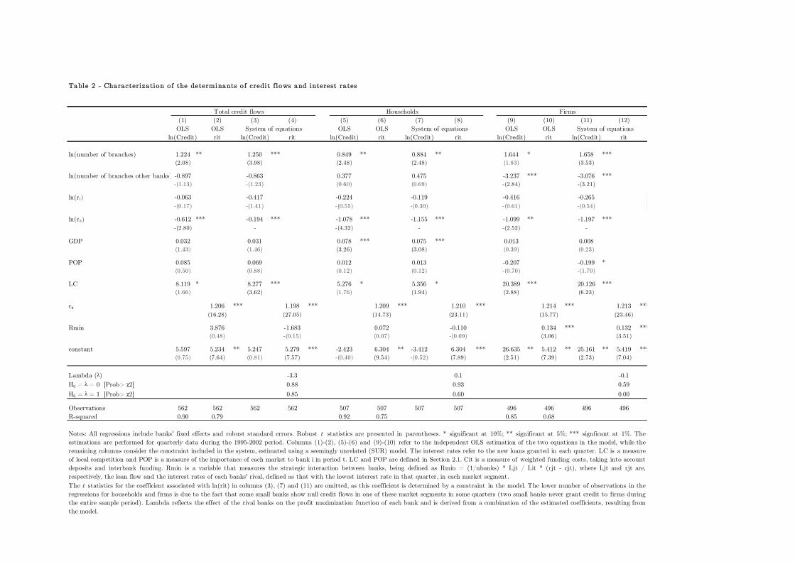
Table 2 - Characterization o f the determinants o f credit flows and interest rates
(1) (2) (3) (4) (5) (6) (7) (8) (9) (10) (11) (12)
OLS OLS OLS OLS OLS OLS
ln(Credit) rit ln(Credit) rit ln(Credit) rit ln(Credit) rit ln(Credit) rit ln(Credit) rit
ln(number of branches) 1.224 ** 1.250 *** 0.849 ** 0.884 ** 1.644 * 1.658 ***
(2.08) (3.98) (2.48) (2.48) (1.83) (3.53)0.038 0.000 0.014 0.013 0.068 0.000
ln(number of branches other banks) -0.897 -0.863 0.377 0.475 -3.237 *** -3.076 ***
-(1.13) -(1.23) (0.60) (0.69) -(2.84) -(3.21)0.261 0.219 0.551 0.490 0.005 0.001
ln(rt) -0.063 -0.417 -0.224 -0.119 -0.416 -0.265
-(0.17) -(1.41) -(0.55) -(0.30) -(0.61) -(0.54)0.861 0.158 0.585 0.761 0.541 0.589
ln(rit) -0.612 *** -0.194 *** -1.078 *** -1.155 *** -1.099 ** -1.197 ***
-(2.80) - -(4.32) - -(2.52) -0.005 0.000 0.000 0.000 0.012 0.000
GDP 0.032 0.031 0.078 *** 0.075 *** 0.013 0.008
(1.43) (1.46) (3.26) (3.08) (0.39) (0.23)0.152 0.144 0.001 0.002 0.697 0.820
POP 0.085 0.069 0.012 0.013 -0.207 -0.199 *
(0.50) (0.88) (0.12) (0.12) -(0.70) -(1.70)0.618 0.381 0.906 0.906 0.485 0.090
LC 8.119 * 8.277 *** 5.276 * 5.356 * 20.389 *** 20.126 ***
(1.66) (3.62) (1.76) (1.94) (2.88) (6.23)0.097 0.000 0.079 0.053 0.004 0.000
cit 1.206 *** 1.198 *** 1.209 *** 1.210 *** 1.214 *** 1.213 ***
(16.28) (27.05) (14.73) (23.11) (15.77) (23.46)0.000 0.000 0.000 0.000 0.000 0.000
Rmin 3.876 -1.683 0.072 -0.110 0.134 *** 0.132 ***
(0.48) -(0.15) (0.07) -(0.09) (3.06) (3.51)0.633 0.884 0.946 0.927 0.002 0.000
constant 5.597 5.234 *** 5.247 5.279 *** -2.423 6.304 *** -3.412 6.304 *** 26.635 ** 5.412 *** 25.161 *** 5.419 ***
(0.75) (7.64) (0.81) (7.57) -(0.40) (9.54) -(0.52) (7.89) (2.51) (7.39) (2.73) (7.04)0.451 0.000 0.417 0.000 0.692 0.000 0.606 0.000 0.012 0.000 0.006 0.000
Lambda (λ) -3.3 0.1 -0.1
H0 = λ = 0 [Prob> χ2] 0.88 0.93 0.59
H0 = λ = 1 [Prob> χ2] 0.85 0.60 0.00
Observations 562 562 562 562 507 507 507 507 496 496 496 496
R-squared 0.90 0.79 0.92 0.75 0.85 0.68
The t statistics for the coefficient associated with ln(rit) in columns (3), (7) and (11) are omitted, as this coefficient is determined by a constraint in the model. The lower number of observations in the
regressions for households and firms is due to the fact that some small banks show null credit flows in one of these market segments in some quarters (two small banks never grant credit to firms during
the entire sample period). Lambda reflects the effect of the rival banks on the profit maximization function of each bank and is derived from a combination of the estimated coefficients, resulting from
the model.
Notes: All regressions include banks' fixed effects and robust standard errors. Robust t statistics are presented in parentheses. * significant at 10%; ** significant at 5%; *** signficant at 1%. The
estimations are performed for quarterly data during the 1995-2002 period. Columns (1)-(2), (5)-(6) and (9)-(10) refer to the independent OLS estimation of the two equations in the model, while the
remaining columns consider the constraint included in the system, estimated using a seemingly unrelated (SUR) model. The interest rates refer to the new loans granted in each quarter. LC is a measure
of local competition and POP is a measure of the importance of each market to bank i in period t. LC and POP are defined in Section 2.1. Cit is a measure of weighted funding costs, taking into account
deposits and interbank funding. Rmin is a variable that measures the strategic interaction between banks, being defined as Rmin = (1/nbanks) * Ljt / Lit * (rjt - cjt), where Ljt and rjt are,
respectively, the loan flow and the interest rates of each banks' rival, defined as that with the lowest interest rate in that quarter, in each market segment.
Total credit flows Households Firms
System of equations System of equations System of equations
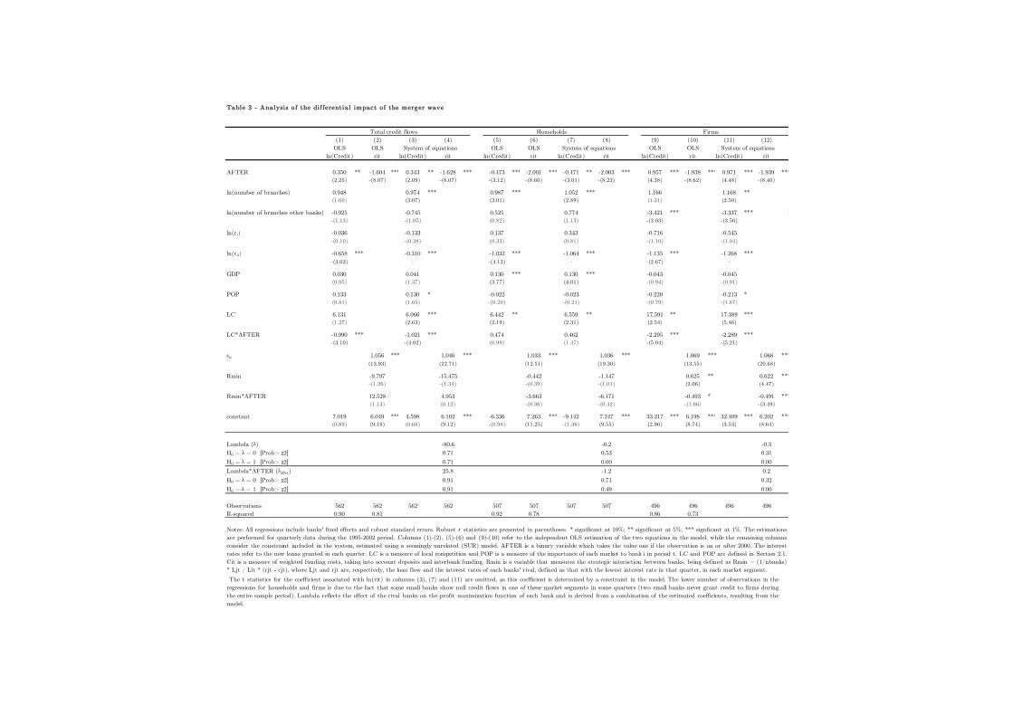
Table 3 - Analysis o f the differentia l impact o f the merger wave
(1) (2) (3) (4) (5) (6) (7) (8) (9) (10) (11) (12)
OLS OLS OLS OLS OLS OLS
ln(Credit) rit ln(Credit) rit ln(Credit) rit ln(Credit) rit ln(Credit) rit ln(Credit) rit
AFTER 0.350 ** -1.604 *** 0.343 ** -1.628 *** -0.473 *** -2.001 *** -0.471 *** -2.003 *** 0.957 *** -1.938 *** 0.971 *** -1.939 ***
(2.25) -(8.07) (2.09) -(8.07) -(3.12) -(8.60) -(3.01) -(8.22) (4.38) -(8.62) (4.48) -(8.40)0.025 0.000 0.037 0.000 0.002 0.000 0.003 0.000 0.000 0.000 0.000 0.000
ln(number of branches) 0.948 0.974 *** 0.987 *** 1.052 *** 1.166 1.168 **
(1.60) (3.07) (3.01) (2.89) (1.31) (2.50)0.110 0.002 0.003 0.004 0.192 0.012
ln(number of branches other banks) -0.925 -0.745 0.525 0.774 -3.421 *** -3.337 ***
-(1.13) -(1.05) (0.82) (1.13) -(3.03) -(3.56)0.257 0.295 0.415 0.258 0.003 0.000
ln(rt) -0.036 -0.133 0.137 0.343 -0.716 -0.545
-(0.10) -(0.38) (0.33) (0.81) -(1.10) -(1.04)0.924 0.704 0.742 0.416 0.273 0.298
ln(rit) -0.658 *** -0.310 *** -1.032 *** -1.064 *** -1.135 *** -1.268 ***
-(3.03) - -(4.13) - -(2.67) -0.003 0.000 0.000 0.000 0.008 0.000
GDP 0.030 0.041 0.130 *** 0.130 *** -0.043 -0.045
(0.95) (1.37) (3.77) (4.01) -(0.94) -(0.91)0.344 0.171 0.000 0.000 0.349 0.364
POP 0.133 0.130 * -0.022 -0.023 -0.220 -0.213 *
(0.81) (1.65) -(0.20) -(0.21) -(0.79) -(1.87)0.417 0.098 0.842 0.830 0.427 0.062
LC 6.131 6.066 *** 6.442 ** 6.559 ** 17.591 ** 17.389 ***
(1.27) (2.63) (2.19) (2.31) (2.54) (5.46)0.206 0.009 0.029 0.021 0.011 0.000
LC*AFTER -0.990 *** -1.021 *** 0.474 0.462 -2.295 *** -2.289 ***
-(3.10) -(4.02) (0.99) (1.47) -(5.04) -(5.21)0.002 0.000 0.321 0.142 0.000 0.000
cit 1.056 *** 1.046 *** 1.033 *** 1.036 *** 1.069 *** 1.068 ***
(13.93) (22.71) (12.51) (19.30) (13.55) (20.68)0.000 0.000 0.000 0.000 0.000 0.000
Rmin -9.797 -15.475 -0.442 -1.147 0.625 ** 0.622 ***
-(1.26) -(1.34) -(0.39) -(1.01) (2.06) (4.47)0.208 0.179 0.695 0.312 0.040 0.000
Rmin*AFTER 12.528 4.953 -3.663 -6.171 -0.493 * -0.491 ***
(1.13) (0.12) -(0.36) -(0.42) -(1.66) -(3.49)0.259 0.901 0.717 0.675 0.097 0.000
constant 7.019 6.049 *** 4.598 6.102 *** -6.336 7.263 *** -9.142 7.247 *** 33.217 *** 6.198 *** 32.409 *** 6.202 ***
(0.89) (9.18) (0.68) (9.12) -(0.98) (11.25) -(1.36) (9.55) (2.96) (8.74) (3.53) (8.64)0.375 0.000 0.499 0.000 0.325 0.000 0.175 0.000 0.003 0.000 0.000 0.000
Lambda (λ) -80.6 -0.2 -0.3
H0 = λ = 0 [Prob> χ2] 0.71 0.53 0.31
H0 = λ = 1 [Prob> χ2] 0.71 0.00 0.00
Lambda*AFTER (λafter) 25.8 -1.2 0.2
H0 = λ = 0 [Prob> χ2] 0.91 0.71 0.32
H0 = λ = 1 [Prob> χ2] 0.91 0.49 0.00
Observations 562 562 562 562 507 507 507 507 496 496 496 496
R-squared 0.90 0.81 0.92 0.78 0.86 0.73
Notes: All regressions include banks' fixed effects and robust standard errors. Robust t statistics are presented in parentheses. * significant at 10%; ** significant at 5%; *** signficant at 1%. The estimations
are performed for quarterly data during the 1995-2002 period. Columns (1)-(2), (5)-(6) and (9)-(10) refer to the independent OLS estimation of the two equations in the model, while the remaining columns
consider the constraint included in the system, estimated using a seemingly unrelated (SUR) model. AFTER is a binary variable which takes the value one if the observation is on or after 2000. The interest
rates refer to the new loans granted in each quarter. LC is a measure of local competition and POP is a measure of the importance of each market to bank i in period t. LC and POP are defined in Section 2.1.
Cit is a measure of weighted funding costs, taking into account deposits and interbank funding. Rmin is a variable that measures the strategic interaction between banks, being defined as Rmin = (1/nbanks)
* Ljt / Lit * (rjt - cjt), where Ljt and rjt are, respectively, the loan flow and the interest rates of each banks' rival, defined as that with the lowest interest rate in that quarter, in each market segment.
The t statistics for the coefficient associated with ln(rit) in columns (3), (7) and (11) are omitted, as this coefficient is determined by a constraint in the model. The lower number of observations in the
regressions for households and firms is due to the fact that some small banks show null credit flows in one of these market segments in some quarters (two small banks never grant credit to firms during
the entire sample period). Lambda reflects the effect of the rival banks on the profit maximization function of each bank and is derived from a combination of the estimated coefficients, resulting from the
model.
Total credit flows Households Firms
System of equations System of equations System of equations
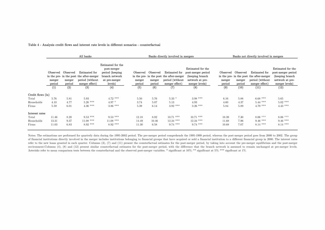
Table 4 - Analysis credit flows and interest rate levels in different scenarios - counterfactual
Observed
in the pre-
merger
period
Observed
in the post-
merger
period
Observed
in the pre-
merger
period
Observed
in the post-
merger
period
Observed
in the pre-
merger
period
Observed
in the post-
merger
period
(1) (2) (3) (4) (5) (6) (7) (8) (9) (10) (11) (12)
Credit flows (ln)
Total 5.76 5.81 5.93 4.72 *** 5.50 5.76 5.33 * 3.98 *** 6.16 5.88 6.68 *** 5.65
Households 4.10 4.77 5.26 *** 4.97 * 3.74 5.07 5.13 4.93 4.60 4.37 5.44 *** 5.02 ***
Firms 5.59 6.01 4.36 *** 3.86 *** 5.39 6.14 3.92 *** 3.26 *** 5.84 5.89 4.79 *** 4.43 ***
Interest rates
Total 11.46 8.20 9.53 *** 9.53 *** 12.18 8.92 10.71 *** 10.71 *** 10.39 7.30 8.06 *** 8.06 ***
Households 13.31 9.37 11.08 *** 11.08 *** 14.49 10.46 12.34 *** 12.34 *** 11.68 7.96 9.46 *** 9.46 ***
Firms 11.03 6.83 8.92 *** 8.92 *** 11.30 6.58 9.74 *** 9.74 *** 10.68 7.07 8.14 *** 8.14 ***
Banks not directly involved in mergers
Estimated for the
post-merger period
(keeping branch
network at pre-
merger levels)
Estimated for
the after-merger
period (without
merger effect)
Notes: The estimations are performed for quarterly data during the 1995-2002 period. The pre-merger period comprehends the 1995-1999 period, whereas the post-merger period goes from 2000 to 2002. The group
of financial institutions directly involved in the merger includes institutions belonging to financial groups that have acquired or sold a financial institution to a different financial group in 2000. The interest rates
refer to the new loans granted in each quarter. Columns (3), (7) and (11) present the counterfactual estimates for the post-merger period, by taking into account the pre-merger equilibrium and the post-merger
environment.Columns (4), (8) and (12) present similar counterfactual estimates for the post-merger period, with the difference that the branch network is assumed to remain unchanged at pre-merger levels.
Asterisks refer to mean comparison tests between the counterfactual and the observed post-merger variables. * significant at 10%; ** significant at 5%; *** signficant at 1%.
All banks Banks directly involved in mergers
Estimated for
the after-merger
period (without
merger effect)
Estimated for the
post-merger
period (keeping
branch network
at pre-merger
levels)
Estimated for
the after-merger
period (without
merger effect)
Estimated for the
post-merger period
(keeping branch
network at pre-
merger levels)
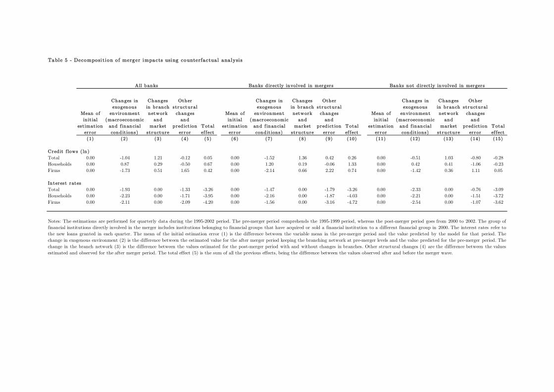
Table 5 - Decomposition of merger impacts using counterfactual analysis
Mean of
in it ial
est imation
error
Changes in
exogenous
environment
(macroeconomic
and f inancial
condit ions)
Changes
in branch
network
and
market
structure
Other
structural
changes
and
predict ion
error
Total
ef fect
Mean of
in it ial
est imation
error
Changes in
exogenous
environment
(macroeconomic
and f inancial
condit ions)
Changes
in branch
network
and
market
structure
Other
structural
changes
and
predict ion
error
Total
ef fect
Mean of
in it ial
est imation
error
Changes in
exogenous
environment
(macroeconomic
and f inancial
condit ions)
Changes
in branch
network
and
market
structure
Other
structural
changes
and
predict ion
error
Total
ef fect
(1) (2) (3) (4) (5) (6) (7) (8) (9) (10) (11) (12) (13) (14) (15)
Credit f lows ( ln)
Total 0.00 -1.04 1.21 -0.12 0.05 0.00 -1.52 1.36 0.42 0.26 0.00 -0.51 1.03 -0.80 -0.28
Households 0.00 0.87 0.29 -0.50 0.67 0.00 1.20 0.19 -0.06 1.33 0.00 0.42 0.41 -1.06 -0.23
Firms 0.00 -1.73 0.51 1.65 0.42 0.00 -2.14 0.66 2.22 0.74 0.00 -1.42 0.36 1.11 0.05
Interest rates
Total 0.00 -1.93 0.00 -1.33 -3.26 0.00 -1.47 0.00 -1.79 -3.26 0.00 -2.33 0.00 -0.76 -3.09
Households 0.00 -2.23 0.00 -1.71 -3.95 0.00 -2.16 0.00 -1.87 -4.03 0.00 -2.21 0.00 -1.51 -3.72
Firms 0.00 -2.11 0.00 -2.09 -4.20 0.00 -1.56 0.00 -3.16 -4.72 0.00 -2.54 0.00 -1.07 -3.62
Banks not direct ly involved in mergers
Notes: The estimations are performed for quarterly data during the 1995-2002 period. The pre-merger period comprehends the 1995-1999 period, whereas the post-merger period goes from 2000 to 2002. The group of
financial institutions directly involved in the merger includes institutions belonging to financial groups that have acquired or sold a financial institution to a different financial group in 2000. The interest rates refer to
the new loans granted in each quarter. The mean of the initial estimation error (1) is the difference between the variable mean in the pre-merger period and the value predicted by the model for that period. The
change in exogenous environment (2) is the difference between the estimated value for the after merger period keeping the branching network at pre-merger levels and the value predicted for the pre-merger period. The
change in the branch network (3) is the difference between the values estimated for the post-merger period with and without changes in branches. Other structural changes (4) are the difference between the values
estimated and observed for the after merger period. The total effect (5) is the sum of all the previous effects, being the difference between the values observed after and before the merger wave.
Banks d irect ly involved in mergersAll banks


