Embed Size (px)
Citation preview

arX
iv:0
710.
3319
v3 [
cond
-mat
.sta
t-m
ech]
8 M
ay 2
010
Correlations in connected random graphs
Piotr Bialas1, 2, ∗ and Andrzej K. Oleś1, †
1Marian Smoluchowski Institute of Physics, Jagellonian University, Reymonta 4, 30–059 Krakow, Poland2Mark Kac Complex Systems Research Centre, Faculty of Physics, Astronomy and Applied Computer Science,
Jagellonian University, Reymonta 4, 30–059 Krakow, Poland
We study the properties of the giant connected component in random graphs with arbitrary degreedistribution. We concentrate on the degree-degree correlations. We show that the adjoining nodesin the giant connected component are correlated and derive analytic formulas for the joint nearest-neighbor degree probability distribution. Using those results we describe correlations in maximalentropy connected random graphs. We show that connected graphs are disassortative and thatcorrelations are strongly related to the presence of one-degree nodes (leaves). We propose an efficientalgorithm for generating connected random graphs. We illustrate our results with several examples.
Published in: Phys. Rev. E 77, 036124 (2008). PACS numbers: 89.75.Hc, 05.10.–a, 05.90.+m
I. INTRODUCTION
In the last decade or so, there has been a great in-crease of interest in the theory of random graphs andnetworks (in the following we will use those two termsinterchangeably). While in principle this is a branch ofmathematics, much of this effort was fueled by the avail-ability of “experimental” data on real graphs (see [1] forreview). These data are compared to the predictions ofvarious random graphs models. Probably the best knownand simplest example of such reference models is the en-semble of all labeled graphs with V vertices and L links(without multiple- and self-links), chosen with uniformprobability. We will call this model Erdös-Rényi (ER)graphs after the authors, who were the first to introduceand study them [2].
The ER ensemble is the simplest example of the so-called “maximally random” graphs. Intuitively those arethe ensembles where the distributions of vertices andlinks joining them are “as random as possible” for a givenset of constraints. In the case of ER graphs the only con-straints are the fixed number of links and vertices. The“maximal randomness” can be formalized using the no-tion of entropy (see next section). The maximally randomensembles serve as null hypothesis. For example, it wasthe deviation of data collected on the World Wide Web(WWW) graph from the predictions of the ER modelthat triggered the interest in random networks [3], be-cause it implied that those graphs were not created justby joining vertices at random, but required the existenceof another mechanism [4].
A popular generalization of the ER ensemble aregraphs with a given degree distribution (degree of a nodeis the number of links attached to it) [5–10]. One featureof those ensembles is the absence of correlations betweenneighboring nodes’ degrees, at least for degree distribu-
∗email: [email protected]†email: [email protected]
tions without heavy tails (see the discussion in Sec. IVC).The object of our study was to find what happens whenwe constrain to connected graphs only. A simple argu-ment indicated that correlations would appear: a neigh-bor of a node with degree one (leaf) must have its degreegreater than 1; otherwise, they would form a separateconnected component. Similarly, all neighbors of a nodecannot have their degree equal to 1, as such a “hedge-hog” would also form a separate connected component[11, 12]. This obviously leads to correlations. It is notclear, however, how strong they are and if they survivethe large-V limit. We have already studied those corre-lations numerically in Ref. [12] and found that they alsoappear in large graphs. In this paper we derive the an-alytic formulas describing them. We also found a strongindication that the described mechanism is the only oneresponsible for the correlation in maximally random con-nected graphs: when we forbid vertices with degree 1correlations disappear.
Connectivity is a nonlocal constraint hard to dealwith. To study the properties of connected graphs weuse another feature of maximally random graphs witha given degree distribution: the appearance of a con-nected component that includes a finite fraction of allthe vertices (and links). From the properties of this gi-ant connected component we can infer the properties ofconnected graphs.
The paper is organized as follows: Section II intro-duces some basic definitions concerning random graphs.In Sec. III we present the method of generating functionsused to study the properties of the giant connected com-ponent in random graphs with arbitrary degree distribu-tion [6]. Then we calculate degree-degree correlations inthe giant component. Section IV contains some exam-ples where we compare our predictions with the resultsof Monte Carlo (MC) simulations. Finally, we show inSec. V how to relate connected random graphs to giantconnected components in other ensembles. In Sec. VI weaddress the situation when correlations in random graphsare suppressed by the absence of vertices with degree one(leaves). The paper is summarized in Sec. VII.

2
II. RANDOM GRAPHS
A. Average degree
Formally we consider random graphs as an ensemble ofgraphs G with probability P (G) assigned to every graphG ∈ G. Using this definition we introduce the entropy ofthe ensemble:
S = −∑
G∈G
P (G) lnP (G). (1)
The maximally random ensembles described in the pre-vious section are those which for given constraints havemaximal entropy.
Denoting by O(G) some property of graph G we cancalculate its average over the whole ensemble:
〈O〉G =∑
G∈G
O(G)P (G). (2)
The most widely studied example is the probability dis-tribution of node degrees:
pk =
⟨nk(G)
V (G)
⟩
G
, (3)
where nk(G) is the number of vertices with degree k andV (G) is the total number of vertices in graph G (in thefollowing we will often omit the argument G). The meanof this distribution is the “link density,”
〈k〉 =∑
k
kpk =
⟨2L(G)
V (G)
⟩
G
≡ z, (4)
because∑
k knk = 2L(G); by L(G), we denote the num-ber of links in graph G.
However, what is frequently observed is not an average(2), but the properties of a single graph (e.g., WWW).That is why we are actually interested in the probabilitythat our model will produce a graph with those proper-ties. It is described by the distribution
P (O) =∑
G∈G
δ(O −O(G))P (G). (5)
In many cases this distribution is sufficiently well char-acterized by its mean (2) with relative fluctuations dis-appearing in the large-V limit. In this situation we willsay the O is self-averaging. In such a case one can inferthe properties of the whole ensemble from the propertiesof just one large graph. We want to emphasize, however,that this is only an assumption that has to be checkedfor each particular model (see [13] for a discussion of self-averaging in real graphs).
In Appendix A we show for illustration a definitionof a non-self-averaging ensemble. Although this is anartificial example, let it serve as a warning. In this paperwe assume that our models are self-averaging without anyfurther formal proofs.
We end with the following comment: as in the self-averaging ensemble fluctuations do not matter, in thelarge-volume limit we have
pk =
⟨nk(G)
V (G)
⟩
G
∼〈nk(G)〉G〈V (G)〉G
. (6)
We will use this kind of approximations in the followingsections.
B. Correlations
The distribution pk does not give any informationabout the correlations between vertices. An obvious gen-eralization is the joint distribution pq,r which describesthe probability that a pair of nearest neighbors (NNs)has degrees q and r (we assume that we pick a pair ofNNs with uniform probability):
pq,r =⟨nq,r
2L
⟩, (7)
where nq,r is the number of links with their start pointhaving degree q and endpoint having degree r. Note thatwe treat each undirected link as two directed links. Onan undirected graph,
nq,r = nr,q,∑
q,r
nq,r = 2L and∑
r
nq,r = qnq. (8)
If vertex degrees are independent, the probability (7)should factorize:
pq,r = p̃qp̃r, p̃q =∑
r
pq,r, (9)
leading to the relation
⟨nq,r
2L
⟩= qr
⟨ nq
2L
⟩⟨ nr
2L
⟩. (10)
One should, however, keep in mind that this defines theabsence of correlations in the ensemble of graphs. A moreappropriate question could be, are the vertices on indi-vidual graphs uncorrelated (see previous section)? Thecondition for absence of correlations between vertices ineach individual graph G is
nq,r(G)
2L(G)= qr
nq(G)
2L(G)
nr(G)
2L(G)(11)
or, after averaging,
⟨nq,r
2L
⟩= qr
⟨ nq
2L
nr
2L
⟩. (12)
As already pointed out, for a large class of ensembles con-ditions (10) and (12) are equivalent in the large-volumelimit. However, it is easy to check that for the non-self-averaging ensemble in Appendix A vertices on each indi-vidual graph are uncorrelated according to the condition

3
(12), but correlated according to (10). Again, we leavethis as a warning and proceed further with the assump-tion that our models are self-averaging and that thosetwo conditions are equivalent.
In practice, checking the condition (9) is difficult asit entails measuring a two dimensional distribution withgood accuracy. Therefore we introduce another quantity[14]
k(k) =∑
q
⟨qnk,q
knk
⟩. (13)
It describes the average degree of nearest neighbors ofa vertex with degree k. Obviously k(k) is defined for agiven k only if nk>0. k(k) can be interpreted as the firstmoment of the conditional probability:
p(q|k) =pq,kp̃k
. (14)
Assuming self-averaging,
k(k) ≈∑
q
qp(q|k). (15)
If the degrees are independent, k(k) should not dependon k and (12) implies
k(k) =∑
q
q2⟨ nq
2L
⟩≈
⟨k2⟩
〈k〉. (16)
When k(k) grows with k the graph is called assortative
and when it shrinks disassortative.
III. CONNECTED COMPONENTS
In general, maximally random graphs with a given de-gree distribution do not need to be connected. However,if
∑
k
k(k − 2)pk > 0 (17)
(which translates into z>1 in the case of ER graphs), oneof the connected components (called the giant connectedcomponent) will gather a finite fraction of all links andvertices [6]. This is a phenomenon akin to percolation.In Ref. [6] the size of the giant component and the sizedistribution of finite components were calculated. The
degree distribution in the giant component p(g)k was cal-
culated in Ref. [8]. Here we generalize those results and
calculate the two-point distributions p(g)q,r and k
(g)(k) for
the giant component.We will use the method of generating functions intro-
duced in [6]. The crucial observation is that the finiteconnected components are essentially trees. That is be-cause a link emerging from one of the vertices in the com-ponent has the probability ∝ s/V of connecting back to
a node from this component, where s is the size of thecomponent. So for finite s this becomes negligible in thelarge-V limit.
Now let us pick a link from the graph at random. Itbelongs to some connected component. We will call P1(s)the probability that cutting this link will split the com-ponent into two parts, one of them finite and having sizes. Stated differently, P1(s) is the probability that a ran-domly chosen link will lead into a finite part of size s.By the argument above this finite “half” will be a tree.Because of that, one can write down the equation for thegenerating function H1(x) =
∑s P1(s)x
s [6]:
H1(x) = xG1(H1(x)), (18)
where
G1(x) =G′
0(x)
G′0(1)
=1
zG′
0(x), G0(x) =
∞∑
k=0
pkxk. (19)
We denote by u the value of H1(1):
u ≡ H1(1) =∑
s
P1(s). (20)
When there is no giant component in the graph, all con-nected components are finite and are trees. This meansthat cutting each link will result in two finite parts; thus,u=1 However, when the giant component appears, thenthere is a nonzero probability that the chosen link willbelong to this component and either cutting it will splitthe component into two infinite parts, or will not split itat all. As this probability is missing from P1(s) the sum(20) will be smaller the one. u is to be interpreted as theprobability that a randomly chosen link is connected to afinite part on at least one side of the graph [10]. It followsthat u2 is the probability that a random link belongs toa finite component of arbitrary size.
That can be derived in a more explicit way. Let usdenote by P1,1(s) the probability that a randomly chosenlink belongs to a component of size s. Then,
P1,1(s) =s∑
t=0
P1(t)P1(s− t). (21)
It is a convolution of the probability distribution P1(s)with itself, so its generating function is just H2
1 (x). Thenu2 = H2
1 (1) =∑
s P1,1(s) is the probability that a linkbelongs to a finite connected component of arbitrary sizeand 1−u2 is the probability that it is inside the giantcomponent.
Finally, if we denote by P0(s) the probability that arandomly chosen vertex belongs to a finite component ofsize s, we can obtain its generating function H0(x) fromH1(x) [6]:
H0(x) ≡∑
s
P0(s)xs = xG0(H1(x)). (22)
4
By the same arguments as above,
h ≡ H0(1) = G0(u) (23)
is the probability that a randomly chosen vertex belongsto a finite connected component and 1−h is the proba-bility that it belongs to the giant component.
It follows from (18) and (20) that u is the solution ofthe equation
u = G1(u). (24)
From the definition (19) it is easy to note that u = 1is always a solution, but when condition (17) is fulfilledthe above equation has a solution smaller than 1 as well[6]. As argued, this signals the appearance of a giantcomponent.
A. Average degree
Using the results of the previous section it is easy toderive formulas for the average degree in the giant com-ponent z(g) and in the rest of the graph z(f):
z(g) =
⟨2L(g)
V (g)
⟩= z
1− u2
1− h, (25a)
z(f) =
⟨2L(f)
V (f)
⟩= z
u2
h. (25b)
As we have already pointed out, the giant connectedcomponent is not a tree. The number of independentloops that it contains equals
L(g) − V (g) + 1 ≈ V(z2(1− u2)− 1 + h
), (26)
and as all the remaining connected components are trees,this is also the number of loops in the whole graph.
We can also easily calculate the number of finite con-nected components ncn knowing that they form a forest.The number of links in the forest is L(f) = V (f) − ncn
which gives
〈ncn〉 =(h− u2 z
2
)V. (27)
From that we can derive the formula for the averagesize of the finite connected component:
〈s〉(f) =
⟨V (f)
ncn
⟩=
2h
2h− u2z. (28)
B. Degree distribution
In this section we will calculate the degree distribution
p(f)k in the nongiant component part of the graph. From
the relation
pk = (1 − h)p(g)k + hp
(f)k , (29)
we automatically get the distribution p(g)k in the giant
component. This has been already done in [8], but wefind it instructive to use the same method of generatingfunctions as described in Sec. III. The idea is to apply itonly to the graph with the giant component excluded—i.e., to the finite connected components. We will use atilde to denote the generating functions of the soughtprobability:
G̃0(x) =
∞∑
k=0
p(f)k xk, G̃1(x) =
G̃′0(x)
G̃′0(1)
. (30)
Using the argument from Ref. [6] we obtain the sameequations
H̃1(x) = xG̃1(H̃1(x)), (31a)
H̃0(x) = xG̃0(H̃1(x)), (31b)
for the generating functions of the probabilities P̃1(s) and
P̃0(s). Here P̃0(s) is the probability that a vertex belongsto a finite component of size s provided that it belongs
to a finite component and P̃1(s) is the probability that alink leads into a finite component of size s provided thatit leads into a finite component. From this we can writethe relations
P0(s) = hP̃0(s), P1(s) = uP̃1(s), (32)
which leads to
H0(x) = hH̃0(x), (33a)
H1(x) = uH̃1(x). (33b)
To solve Eqs. (30), (31), and (33) for p(f)k we make an
ansatz
p(f)k =
pkak
G(a). (34)
Then,
G̃0(x) =G0(xa)
G0(a), G̃1(x) =
G1(xa)
G1(a), (35)
so that Eq. (31a) can be rewritten as
aH̃1(x) =a
G1(a)xG1(H̃1(x)a). (36)
Comparing with (18) we see that it will be fulfilled if
aH̃1(x) = H1
(a
G1(a)x
). (37)
Inserting this into (33b) we get
aH1(x) = uH1
(a
G1(a)x
), (38)
because of Eq. (24), which can be solved by putting a=u.

5
1 2 3 4 50
1
2
3
4
5
PSfrag repla ements
z
z
,
zg
,
zf
FIG. 1: Average degree z (dashed line), average degree zgof the connected component (upper solid line), and averagedegree of the rest zf (lower solid line) as a function of z forER graphs. Circles mark the results of MC simulations.
Now we must check Eq. (33a). Using Eqs. (22), (31b),and (33b) we get
hH̃0(x) = hxG̃0(H̃1(x)) = hxG0(uH̃1(x))
G0(u)
= xhG0(H1(x))
h= H0(x).
(39)
So finally,
p(f)k =
pkuk
h. (40)
From that and relation (29) we get the formula for thedegree distribution in the giant component:
p(g)k = pk
(1 − uk)
1− h. (41)
In the limit u → 1 and h → 1 this reduces to
p(g)k =
k
zpk. (42)
In this limit the connected giant cluster is a tree. Indeed,one can check that
∑
k
kp(g)k =
∑
k
k2
zpk = 2. (43)
To see this we must first note that Eq. (24) has always thesolution u=1. It becomes the only one when G′
1(1) = 1,which is equivalent to the condition (43).
C. Correlations
To calculate p(g)q,r we use the relation
nq,r(G) = n(g)q,r(G) + n(f)
q,r (G). (44)
0 2 4 6 8 100
0.1
0.2
0.3
0.4
giantfull
PSfrag repla ements
k
pk
,
p(g
)k
FIG. 2: Degree distribution for ER graphs with z=2. Circlesmark the results of MC simulations for the giant componentand diamonds for the full graph. Solid lines denote analyticalsolutions.
We have already assumed that vertex degrees are un-correlated; we further assume that this is also true forthe finite connected components (nongiant) part of thegraph. Assuming self-averaging and using Eq. (10) for
nq,r and n(f)q,r we obtain
p(g)q,r =qpqrprz2
1
1− u2
(1−
uqur
u2
)(45)
and
k(g)
(k) =
⟨k2⟩
z
1
1− uk
(1−
⟨k2⟩(f)
z(f)z
〈k2〉uk
). (46)
In the derivation we have used the relation⟨AB
⟩= 〈A〉
〈B〉 ,
which should be valid for self-averaging quantities in thelarge-V limit. Comparing this with formulas (10) and(16) we note that the correlations disappear in the limitu→ 0. In the tree limit u→ 1 the formulas above takethe form
limu,h→1
p(g)q,r = (q + r − 2)1
2
qpqrprz2
(47)
and
limu,h→1
k(g)
(k) =1
zk
((k − 2)
⟨k2⟩+⟨k3⟩)
. (48)
IV. EXAMPLES
While deriving our formulas we have made several as-sumptions: (i) the vertex orders are uncorrelated, (ii)the measured quantities are self-averaging, and of course(iii) all the derivations are only valid in the large-V limit.To check to what extent those assumptions are satisfied
6
0 2 4 6 8 102.9
3.0
3.1
3.2
3.3
3.4
3.5
giantfull
PSfrag repla ements
k
k(k
),
k(k
)(g)
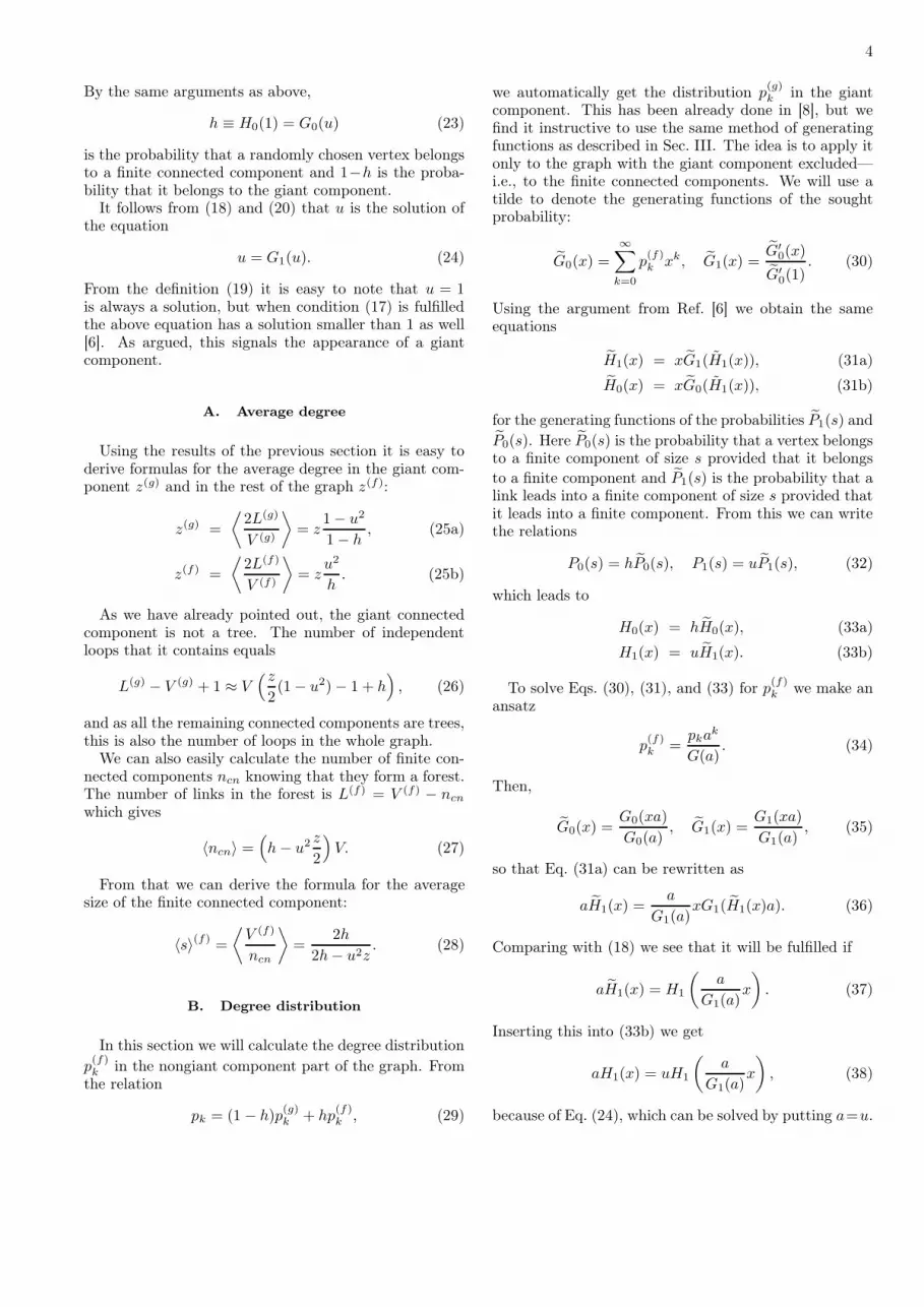
FIG. 3: k(k) for ER graphs with z = 2. Circles mark theresults of MC simulations for the giant component and dia-monds for the full graph; solid lines stand for analytical solu-tions.
and, more importantly, to check the magnitude of the fi-nite size effects, we have compared our predictions to theresults of MC simulations of moderate-sized graphs (5000vertices). To simulate ER graphs we used a straightfor-ward algorithm which connects vertices at random. Togenerate maximally random graphs with a given distri-bution we used the method described in Refs. [9, 15] andimplemented in Ref. [16]. This method consists of gener-ating graphs with suitably chosen one-point weights usinga Metropolis-type algorithm.
A. Erdös-Rényi graphs
For ER graphs the distribution pk is Poissonian,
pk = e−z zk
k! and
G0(x) = G1(x) = ez(x−1). (49)
It follows that H1(x) = H0(x) ≡ H(x), so h= u with hbeing the closest to one (from below) positive solution ofthe equation
h = ez(h−1). (50)
The results for z(f) and z(g) are shown in Fig. 1. Theyare compared with the results of the MC simulations ofER graphs. The agreement is perfect, and there are novisible finite-size effects (error bars are smaller than thesize of the points). The degree distribution can be noweasily obtained from (41). The results are presented inFig. 2. Again, the agreement is very good without anynoticeable finite-size effects.
In this case it may be instructive to derive those resultsin a simpler way: when we omit the giant componentfrom our considerations we are left with a graph withhN vertices and h2L links on average. As there are no
1 2 3 4 50
1
2
3
4
5
6
PSfrag repla ements
κ
z
,
zg
,
zf
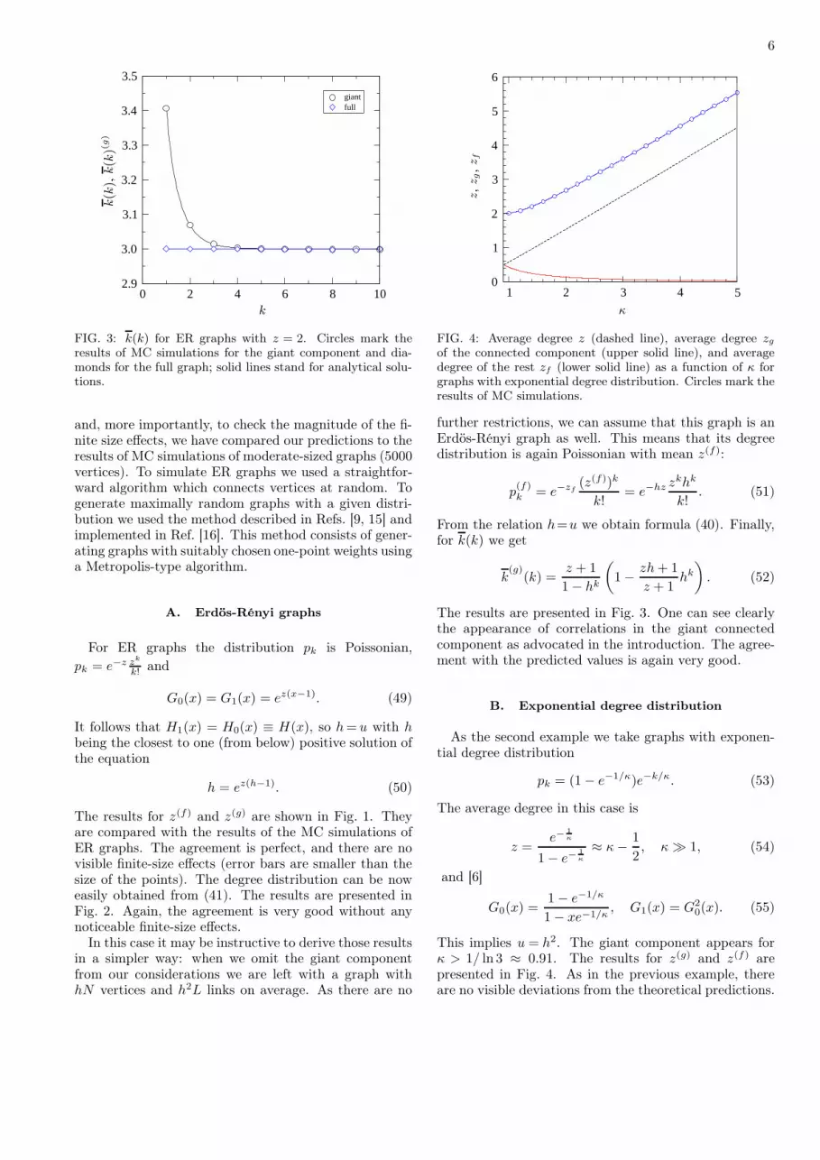
FIG. 4: Average degree z (dashed line), average degree zgof the connected component (upper solid line), and averagedegree of the rest zf (lower solid line) as a function of κ forgraphs with exponential degree distribution. Circles mark theresults of MC simulations.
further restrictions, we can assume that this graph is anErdös-Rényi graph as well. This means that its degreedistribution is again Poissonian with mean z(f):
p(f)k = e−zf
(z(f))k
k!= e−hz z
khk
k!. (51)
From the relation h=u we obtain formula (40). Finally,for k(k) we get
k(g)
(k) =z + 1
1− hk
(1−
zh+ 1
z + 1hk
). (52)
The results are presented in Fig. 3. One can see clearlythe appearance of correlations in the giant connectedcomponent as advocated in the introduction. The agree-ment with the predicted values is again very good.
B. Exponential degree distribution
As the second example we take graphs with exponen-tial degree distribution
pk = (1− e−1/κ)e−k/κ. (53)
The average degree in this case is
z =e−
1κ
1− e−1κ
≈ κ−1
2, κ ≫ 1, (54)
and [6]
G0(x) =1− e−1/κ
1− xe−1/κ, G1(x) = G2
0(x). (55)
This implies u = h2. The giant component appears forκ > 1/ ln 3 ≈ 0.91. The results for z(g) and z(f) arepresented in Fig. 4. As in the previous example, thereare no visible deviations from the theoretical predictions.

7
0 2 4 6 8 100
0.1
0.2
0.3
0.4
0.5
giantfullp
1 = 0
PSfrag repla ements
k
pk
,
p(g
)k
FIG. 5: Degree distribution for graphs with exponential de-gree distribution with κ = 1.5. Circles mark the results ofMC simulations for the giant component and diamonds forthe full graph; squares stand for the special case of connectedgraphs without leaves described in Sec. VI. Solid lines denoteanalytical solutions.
0 5 10 153
3.25
3.5
3.75
4 giantfullp
1 = 0
PSfrag repla ements
k
k(k
),k(k
)(g)
FIG. 6: k(k) for graphs with exponential degree distributionwith κ=1.5. Circles mark the results of MC simulations forthe giant component and diamonds for the full graph; squaresstand for the special case of connected graphs without leavesdescribed in Sec. VI. Solid lines denote analytical solutions.
In Figs. 5 and 6 results for p(g)k and k
(g)(k) are pre-
sented for κ = 1.5. We observe the same kind of cor-relations in the giant component as in the case of ERgraphs.
C. Scale-free graphs
Probably the most interesting case are scale-freegraphs with distribution pk ∼ k−β. While studying themwe have to consider two scenarios 2< β ≤ 3 and β > 3.In the first case we expect correlations between node de-
1 10 10010
-8
10-7
10-6
10-5
10-4
10-3
10-2
10-1
100
giantfullp
1=0
PSfrag repla ements
k
pk
,
p(g
)k
FIG. 7: Degree distribution for scale-free graphs with β =3.25. Circles mark the results for the giant component anddiamonds for the full graph; squares stand for the special caseof connected graphs without leaves described in Sec. VI. Solidlines denote analytical solutions.
grees, as pointed out in Refs. [9, 17–19]. This invalidatesboth the derivation of Eqs. (18) and (45). Additionallythe quantity
⟨k2⟩
diverges and so k(k) is not defined.Because our aim was to investigate the correlations ap-pearing solely as an effect of the connectedness of graphs,we have decided not to study the β≤3 case in this paper.This is, however, an interesting issue and merits furtherinvestigation. One line of pursuit is to use the algorithmproposed in [19] to generate uncorrelated graphs withheavy tails. Then one should obtain predictions at leastfor the joint probability pq,r which does not contain anydivergences. One could also use the V -dependent “cut-off” distribution as proposed in [19] instead of the “full”distribution pk ∼ k−β . This would yield the V depend-ing results, but may not be feasible analytically. In thecase of β<2 already the first moment of the distributionpk is not defined and the generating function approachfails completely.
When β>3 the⟨k2⟩
is finite and there are no correla-tions, at least in the infinite-size limit [18, 19]. However,for finite V we expect strong finite-size effects for β closeto 3. To see this let us estimate the asymptotic behaviorof⟨k2⟩:
⟨k2⟩≈∑
k
k2pk−
∫ ∞
kc(V )
k2pk ≈⟨k2⟩∞− cV − β−3
β−1 . (56)
In the above we have assumed the natural cutoff kc(V ) ∼
V1
β−1 [9, 17–19]. For β close to 3, this converges veryslowly. To observe those effects we have simulated oursystem at β=13/4, when
⟨k2⟩
approaches its asymptotic
value as V −1/9. The results of our simulations of graphswith 5000 vertices are presented in Figs. 7 and 8. As ex-
pected the data for pk and p(g)k distributions show strong
cutoff effects around k = 40, but for smaller values of k

8
0 20 40 60 80 1000
5
10
15
giantfullp
1 = 0
PSfrag repla ements
k
k(k
),k(k
)(g)
FIG. 8: k(k) for scale-free graphs with β = 3.25. Circlesmark the results for the giant component and diamonds forthe full graph; squares stand for the special case of connectedgraphs without leaves described in Sec. VI. Solid lines denoteanalytical solutions.
the agreement with theoretical predictions is rather good.Looking at the results for k(k) we notice two things: (i)Data for the full graph show a deviation from a straightline, indicating the presence of some correlations due toheavy tails. (ii) Data for the giant connected componentshow a very strong effect of correlations. The agreementwith theoretical values is very poor, so we have not in-cluded them in the picture. This is due to the describedcutoff effect on
⟨k2⟩. We can obtain a better agreement
if we use in Eq. (46) the actual value of⟨k2⟩
measuredin simulations instead of its infinite-volume limit.
V. CONNECTED GRAPHS
Finally, we would like to calculate the properties of themaximally random connected graphs. To this end we as-sume that the ensemble of giant connected componentsof the maximal entropy graphs with distribution pk is amaximal entropy ensemble of connected graphs with dis-
tribution p(g)k (we neglect the fluctuations in the number
of vertices and links of the giant component). This is aplausible assumption as we do not put any additional con-straints except connectivity. In Appendix B we providea more detailed argumentation. With this assumptionthe properties of the maximal entropy connected ran-
dom graphs with distribution p(g)k and/or average degree
z(g) are the same as that of the maximal entropy ran-dom graphs with distribution pk and/or average degreez given by Eqs. (41) and (25a).
0 5 10 150
0.1
0.2
0.3
0.4
z = 2.2z = 2.4z = 3.0z = 4.0
PSfrag repla ements
k
pk
FIG. 9: Degree distribution pk(k) in connected ER graphswith various average degrees. Points mark the results of MCsimulations, while solid lines denote analytical solutions. Thesize of each graph is 5000 vertices.
0 5 10 152.5
3
3.5
4
4.5
5
z = 2.2z = 2.4z = 3.0z = 4.0
PSfrag repla ements
k
k(k
)
FIG. 10: k(k) for connected ER graphs with various averagedegrees. Points mark the results of MC simulations, whilesolid lines denote analytical solutions. The size of each graphis 5000 vertices.
A. Connected ER graphs
By connected ER graphs we mean maximal entropyconnected graphs with a given average degree z(g). Ac-cording to the arguments from the previous section thisensemble corresponds to the ensemble of giant compo-nents in ER graphs with average degree z related byEq. (25a). For a given z(g) we solve this equation for z(numerically) and use formulas (41) and (52) for degreedistribution and for k(k) respectively. The results arepresented in Figs. 9 and 10 and compared with the MCdata for connected graphs taken from [12]. The agree-ment is very good which confirms the validity of the as-sumption made in the previous section.
9
B. Connected random graphs with arbitrary
degree distribution
To calculate the properties of connected randomgraphs with arbitrary degree distribution we need to in-vert Eq. (41). This can be done by rewriting it as
pk = (1 − h)p(g)k
1− uk, p0 > 0, (57)
where u satisfies Eq. (24):
u =
∑∞k=1 p
(g)k
kuk−1
1−uk
∑∞k=1 p
(g)k
k1−uk
. (58)
The above equation can be solved by the simple iterationprocedure. To prove that it has a solution we rewrite it as
∞∑
k=1
p(g)k ku
1− uk−2
1− uk≡ g(u) = 0. (59)
It is easy to check that
g(0) = −p(g)1 , lim
u→1g(u) =
∞∑
k=1
p(g)k k − 2. (60)
So for connected graphs g(1) is positive (z(g) ≥ 2) and
g(0) negative (p(g)1 ≥0).
Once we know u we can calculate h and p0 from thenormalization of the distribution pk and Eq. (23):
1 = p0 + (1−h)
∞∑
k=1
p(g)k
1−uk, h = p0 + (1−h)
∞∑
k=1
ukp(g)k
1−uk.
(61)
Because∑∞
k=1pgk1−uk −
∑∞k=1
ukpgk1−uk = 1, those two equa-
tions are not independent and we can set p0=0. Then,
h = 1−
(∞∑
k=1
p(g)k
1− uk
)−1
. (62)
C. Simulating connected graphs
This procedure may be actually used to generate con-nected random graphs in an efficient way. Instead of
generating connected graphs with degree distribution p(g)k
and checking the connectivity after every move, we cangenerate graphs with distribution pk given by (57) anduse the giant connected component. This still requirescalculating the connected parts, but it need to be doneonly once before each measurement.
As an example, we have generated connected maxi-mally random graphs with Poissonian degree distribution
p(g)k = e−z z
k
k!, k > 0, p0 = 0, (63)
0 5 10 152.5
3
3.5
4
4.5
5
z = 2.2z = 2.4z = 3.0z = 4.0
PSfrag repla ements
k
k(k
)
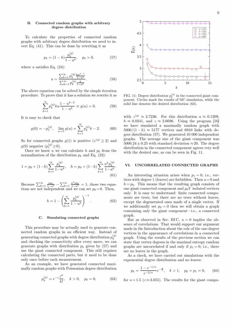
FIG. 11: Degree distribution p(g)k in the connected giant com-
ponent. Circles mark the results of MC simulation, while thesolid line denotes the desired distribution (63).
with z(g) ≈ 2.7236. For this distribution u ≈ 0.1209,h ≈ 0.0341, and z ≈ 2.6696. Using the program [16]we have simulated a maximally random graph with5000/(1− h) ≈ 5177 vertices and 6910 links with de-gree distribution (57). We generated 10 000 independentgraphs. The average size of the giant component was5000.24± 0.25 with standard deviation ≈20. The degreedistribution in the connected component agrees very wellwith the desired one, as can be seen in Fig. 11.
VI. UNCORRELATED CONNECTED GRAPHS
An interesting situation arises when p1 = 0; i.e., ver-tices with degree 1 (leaves) are forbidden. Then u=0 andh= p0. This means that the resulting graph consists ofone giant connected component and p0V isolated verticesonly. It is easy to understand: finite connected compo-nents are trees, but there are no trees without leaves,except the degenerated ones made of a single vertex. Ifwe additionally set p0 = 0 then we will obtain a graphcontaining only the giant component—i.e., a connectedgraph.
But as observed in Sec. III C, u = 0 implies the ab-sence of correlations. That would support our argumentmade in the Introduction about the role of the one-degreevertices in the appearance of correlations in a connectedgraph. Using the results of the previous section we canstate that vertex degrees in the maximal entropy randomgraphs are uncorrelated if and only if p1 = 0; i.e., thereare no leaves in the graph.
As a check, we have carried out simulations with theexponential degree distribution and no leaves:
pk =1− e−1/κ
e−2/κe−
kκ , k > 1, p0 = p1 = 0, (64)
for κ=1.5 (z≈ 3.055). The results for the giant compo-

10
nent which consisted on average of more the 99.9% of thewhole graph are presented in Figs. 5 and 6 (squares). Aspredicted, vertices are uncorrelated in the stark contrastto the p1>0 case plotted in the same figures.
We have also performed simulations for the scale-freedistribution 1/k13/4 and no leaves. The results are pre-sented in Figs. 7 and 8 (squares). We see that correlationsare very much suppressed compared to the case when weadmit leaves (presented in the same figures). The slightremaining correlation is due to long tails as explained inSec. IVC.
VII. SUMMARY
In this paper we have studied the correlations in con-nected random graphs. We have extended the results ofRefs. [6, 8, 10] and calculated correlations in the giantconnected components of random graphs. We argue thatthose correlations are related to the presence of nodeswith degree 1, suggesting that the only cause of corre-lations is the absence of “hedgehogs.” This has been al-ready stated in [11] where it has been shown that in thegrand-canonical ensemble of arbitrary-sized trees, where“hedgehogs” appear, correlations vanish. We find this tobe a very interesting issue that merits further studies.
The correlations observed in connected random graphsare an example of the so-called “structural” or “kine-matic” correlations, as they appear in consequence ofsome global constraint. This should be contrasted with“dynamic” correlations which are the result of local two-point interactions between vertices. Such correlationsmay be generated by two-point weights [20]. This dis-tinction can be important in simplicial quantum grav-ity where degree-degree correlations are interpreted ascurvature-curvature correlations (see, for example, [21]).However, as the simplicial manifolds are connected bydefinition those correlations are due to the above de-scribed mechanism rather than to some kind of gravi-tational interaction [11, 22]. We believe that our resultsmay help in clarifying such issues and in the interpreta-tion of data obtained from MC simulations.
Finally, we have shown how to relate the giant con-nected components to the maximal entropy connectedgraphs ensemble. This allowed us to propose an efficientmethod for generating connected random graphs basedon the Metropolis algorithm.
Acknowledgments
We would like to thank Zdzislaw Burda, Jerzy Ju-rkiewicz, Andrzej Krzywicki, and Bartłomiej Wacław forvaluable discussions. This work was supported by KBNGrant No. 1P03B-04029 and EU Grants Nos. MTKD-CT-2004-517186 (COCOS) and MRNT-CT-2004-005616(ENRAGE).
Appendix A: Non-self-averaging ensemble
Denoting by G(V ; k) the ensemble of all simple regulargraphs with V vertices and degree k (in a regular graphall vertices have the same degree), we define
G(V ) =⋃
k
G(V ; k), P (G) =wk
#G(V ; k), (A1)
where #G(V ; k) denotes the number of graphs in the en-semble G(V ; k) and wk is an arbitrary probability distri-bution. With this definition we find
pq =∑
G∈G
nq
VP (G) =
∑
k
∑
G∈G(V ;k)
wkδk,q#G(V ; k)
=∑
k
wkδk,q = wq.
(A2)
It is easy to note that this poorly describes the distribu-tions of single graphs which are just δ’s. The variance ofpk is
δ2pq =∑
G∈G
(nq
V−wq)
2P (G) =∑
k
∑
G∈G(V ;k)
wk(δk,q−wq)2
#G(V ; k)
=∑
k
wk(δk,q−wq)2 = wq − 2w2
q + w2q
∑
k
wk.
(A3)
and indeed does not disappear in the large-V limit.For correlations we obtain⟨nq,r
2L
⟩= qr
⟨ nq
2L
nr
2L
⟩=∑
k
wkδq,kδr,k = wqδq,r (A4)
and
qr⟨ nq
2L
⟩⟨ nr
2L
⟩=∑
k
wkδk,q∑
k′
wk′δk′,r = wqwr. (A5)
So the condition (10) is not satisfied. It means thatvertices on each particular graph are uncorrelated, butcorrelated if the whole ensemble is considered. This iseasy to explain: if we pick a link from a graph with agiven k, then the information about the first vertex doesnot provide any additional information; however, if wedo not know k, then the degree of the first vertex willgive us immediately the value of its neighbor.
Appendix B: Entropy of the giant connected
components
Let G and P (G) define a maximal entropy ensemblewith V vertices, L links, and vertex degree distributionpk. We assume that the probability P (G) factorizes:
P (G) =∏
C∈G
Pc(C), (B1)

11
where C are the connected components of the graph G.Let Gc denote the ensemble of all giant connected com-
ponents. We assume that we can neglect the fluctuations,so all the graphs in this ensemble have V (g) vertices andL(g) links. The degree distribution in this ensemble is
p(g)k . Because of the property (B1), the entropy (1) of
the whole ensemble (G, P ) is the sum of the entropy ofthe giant connected component ensemble and the rest:
S = S(g) + S(f). (B2)
Now we assume that there exists a probability P ′c defined
on the ensemble Gc such that the entropy
−∑
G∈Gc
P ′c(G) lnP ′
c(G) (B3)
is greater than S(g), but the vertex degree probabilitydistribution remains unchanged. Then we can define anew probability on the ensemble G:
P ′(G) = P ′c(C
(g))∏
C 6=C(g)
Pc(C), (B4)
where C(g) is the giant connected component of graph G.The degree distribution of the ensemble (G, P ′) would bethe same as that of (G, P ) ensemble, but according to(B2), its entropy would be greater. This contradicts theassumption that (G, P ) is the maximal entropy ensembleand proves that the ensemble of giant connected compo-nents is a maximal entropy ensemble.
[1] R. Albert and A.-L. Barabasi, Rev. Mod. Phys. 74, 47(2002).
[2] P. Erdös and A. Rényi, Publ. Math. 6, 290 (1959); Publ.Math. Inst. Hung. Acad. Sci. 5, 17 (1961).
[3] R. Albert, H. Yeong, and A.-L. Barabasi, Nature (Lon-don) 401, 130 (1999).
[4] R. Albert and A.-L. Barabasi, Science 286, 509 (1999).[5] M. Molloy and B. Reed, Random Struc. Algorithms 6,
161 (1995); Combinatorics, Probab. Comput. 7, 295(1998).
[6] M. E. J. Newman, S. H. Strogatz, and D. J. Watts, Phys.Rev. E 64, 026118 (2001).
[7] Z. Burda, J. D. Correia, and A. Krzywicki, Phys. Rev. E64, 46118 (2001).
[8] M. Bauer and D. Bernard, e-print arXiv:cond-mat/0206150.
[9] Z. Burda and A. Krzywicki, Phys. Rev. E 67, 046118(2003).
[10] A. Fronczak, P. Fronczak, and J. Hołyst, in Science of
Complex Networks: From Biology to the Internet and
WWW; CNET 2004, edited by J. F. F. Mendes et. al.,AIP Conf. Proc. No. 776 (AIP, Melville, NY, 2005), p. 52.In this reference u is denoted by 1−R.
[11] P. Bialas, Phys. Lett. B 373, 289 (1996).[12] A. K. Oleś, Master’s thesis (in Polish), Jagellonian Uni-
versity, 2006.[13] M. Serrano, A. Maguitman, M. Boguñá, S. Fortunato,
and A. Vespignani, ACM Trans. Web 1, 10 (2007).[14] R. Pastor-Satorras, A. Vazquez, and A. Vespignani,
Phys. Rev. Lett. 87, 258701 (2001).[15] L. Bogacz, Z. Burda, and B. Wacław, Physica A 366,
587 (2006).[16] L. Bogacz, Z. Burda, W. Janke, and B. Wacław, Comput.
Phys. Commun. 173, 162 (2005).[17] S. N. Dogorovtsev. J. F. F. Mendes, and A. N. Samukhin,
Phys. Rev. E 63, 062101 (2001).[18] M. Boguñá, R. Pastor-Satorras, A. Vespignani, Eur.
Phys. J. B 38, 205 (2004).[19] M. Catanzaro, M. Boguñá, R. Pastor-Satorras, Phys.
Rev. E 71, 027103 (2005).[20] P. Bialas, Nucl. Phys. B 575, 645 (2000).[21] B. V. de Bakker and J. Smit, Nucl. Phys. B 454, 343
(1995).[22] P. Bialas, Z. Burda, B. Petersson, and J. Tabaczek, Nucl.
Phys. B 495, 463 (1997).


