Preprint typeset in JHEP style - HYPER VERSION

Convergence of Derivative Expansion in

Supersymmetric Functional RG Flows

Marianne Heilmann, Tobias Hellwig, Benjamin Knorr, Marcus Ansorg and Andreas

Wipf

Theoretisch-Physikalisches Institut, Friedrich-Schiller-Universitat Jena, Max-Wien-Platz

1, D-07743 Jena, Germany

E-mail: marianne.heilmann@uni-jena.de, tobias.hellwig@uni-jena.de,

benjamin.knorr@uni-jena.de, marcus.ansorg@uni-jena.de, wipf@tpi.uni-jena.de

Abstract: We confirm the convergence of the derivative expansion in two supersymmetric

models via the functional renormalization group method. Using pseudo-spectral methods,

high-accuracy results for the lowest energies in supersymmetric quantum mechanics and a

detailed description of the supersymmetric analogue of the Wilson-Fisher fixed point of the

three-dimensional Wess-Zumino model are obtained. The superscaling relation proposed

earlier, relating the relevant critical exponent to the anomalous dimension, is shown to be

valid to all orders in the supercovariant derivative expansion and for all d ≥ 2.

Keywords: Renormalization Group, Effective Action, Superspace, Supersymmetric

Effective Theories, Nonperturbative Effects, Quantum Mechanical Tunneling,

Pseudo-spectral methods.

arX

iv:1

409.

5650

v1 [

hep-

th]

19

Sep

2014

Contents

1. Introduction 1

2. Supersymmetric quantum mechanics 4

2.1 Flow equation in superspace 5

2.1.1 Supercovariant derivative expansion in NNLO 6

2.1.2 Introducing the regulator functional 6

2.1.3 Flow equation 7

2.2 Effective potential and first excited energy 8

2.2.1 On-shell effective potential 8

2.2.2 Numerical results 9

2.3 Supersymmetry breaking 12

2.3.1 Problems with the expansion in powers of F 12

2.3.2 Numerical results 14

3. N = 1 Wess-Zumino model in 3 dimensions 16

3.1 Preliminaries 16

3.2 Derivation of flow equation 16

3.3 Superscaling relation & Wilson-Fisher fixed point 18

4. Summary 22

A. Greens function in d = 1 23

B. Flow equation of Y ′1 + Y2 23

C. Greens function in d = 3 25

D. (Pseudo-)spectral methods 25

1. Introduction

Supersymmetry (SUSY) is an essential ingredient in most theories beyond the Standard

Model of particle physics. Under certain natural conditions it is the unique extension of

the Poincare symmetry. Although many predictions of supersymmetry can be explored

by perturbative calculations there remain interesting phenomena which fall into the non-

perturbative regime. Examples are collective condensation phenomena, topological effects

and supersymmetry breaking. Thus, powerful methods are needed to investigate and cal-

culate such non-perturbative effects in order to understand the underlying physics and to

obtain quantitative predictions in the strong-coupling regime.

– 1 –

A well-established method to study non-perturbative effects in supersymmetric theo-

ries is based on a discretization of spacetime and the corresponding supersymmetric lattice

models, see e.g. [1, 2, 3, 4, 5, 6, 7, 8]. Yet, as supersymmetry involves spacetime transla-

tions and rotations, lattice approaches usually go along with a complete (for models with

extended supersymmetry partial) loss of supersymmetry.

In this work, we choose an alternative approach based on the functional renormalization

group (FRG). The FRG is a powerful non-perturbative tool to study continuum physics

and was successfully applied to a plethora of physical systems which include fermionic

systems, gauge theories or gravity, see e.g. [9, 10, 11, 12, 13, 14]. Only lately, the FRG

has been applied to SUSY models - mainly due to the difficulty of constructing a sensible

regularization that preserves SUSY. Here, we will extend previous results [15, 16, 17] by

examining whether the derivative expansions for supersymmetric quantum mechanics or

supersymmetric Yukawa theories are convergent, and further investigate SUSY breaking in

these models. To that aim we admit higher order supercovariant derivative terms in the

effective actions of supersymmetric Wess-Zumino-models in various dimensions.

In the early days of the FRG, ordinary quantum mechanics was already utilized as toy

model to test the power of the techniques beyond perturbation theory. In (supersymmet-

ric) quantum mechanics, flow equations are easily obtained and solutions to truncated flow

equations can be compared with exact results. The focus in these studies were the energies

of the low lying states [18, 19, 20, 21, 22]. It turned out that systems with single-well

potentials can be successfully described all the way from weak to strong couplings, whereas

double-wells are more challenging, partially due to exponentially suppressed instanton ef-

fects.

The cited works satisfactorily calculated the energy spectrum of non-supersymmetric

systems. In non-supersymmetric systems there is no need to relate the regulators of bosons

and fermions. However, in a supersymmetric systems they must be related by supersymme-

try in order to disentangle the effects of spontaneous and explicit supersymmetry breaking.

Thus in the present work we use manifestly supersymmetric regulators such that for su-

persymmetric initial conditions the scale dependent effective action is supersymmetric at

all scales. This way we considerably improve upon previous results obtained in [15]. Other

works using a supersymmetric regularization include [23, 24, 25].

Regarding the models investigated in the present work, we shall see that the superco-

variant derivative expansion converges nicely. To calculate the flow of the superpotential

and wave functions renormalizations to fourth order in this expansion with high precision

we employ the powerful spectral method [26]. This method has been very successfully ap-

plied to problems in hydrodynamics, quantum chemistry and in particular gravity [27]. To

solve the system of coupled nonlinear partial differential equations with spectral methods

we use the Chebyshev polynomials as basis in the domain where the effective potential

is flat or concave and rational Chebyshev functions in the domains where the effective

potential is convex. For the RG-evolution, another Chebyshev spectralization was used.

This way we are able to construct global solutions to the truncated flow equations with

unmatched numerical accuracy.

The paper is organized as follows: In section 2 we review the relevant features of SUSY

– 2 –

quantum mechanics. Sections 2.1 and 2.2 contain the derivation of the flow equations in

next-to-next-to-leading order (NNLO) as well as numerical results for the first excited

energies in systems with unbroken supersymmetry. Spontaneous supersymmetry breaking

is analyzed in next-to-leading order (NLO) in section 2.3. In section 3 we proceed with

the derivative expansion of the three-dimensional Wess-Zumino models. The truncated

flow equations are analysed in section 3, which contains an analysis of the physics of

the Wilson-Fisher fixed point and the superscaling relation previously discovered in [28].

The appendices contain further details on the derivation of the flow equations and on the

spectral method used in the present work.

– 3 –

2. Supersymmetric quantum mechanics

In order to derive the flow equations for supersymmetric quantum mechanics, we employ

the superfield formalism [29]. For more details we refer the reader to [15]. The Euclidean

superfield, expanded in terms of the anticommuting Grassmann variables θ and θ, reads

Φ(τ, θ, θ) = φ(τ) + θψ(τ) + ψθ(τ) + θθF (τ). (2.1)

Both the superfield and the Grassmann variables θ, θ have mass dimension −1/2. Next,

we introduce the superpotential and expand it in powers of the Grassmann variables,

W (Φ) = W (φ) +(θψ + ψθ

)W ′(φ) + θθ

(FW ′(φ)−W ′′(φ)ψψ

). (2.2)

The one-dimensional equivalent of the Super-Poincare algebra contains only translations of

Euclidean time and is generated by one pair of conserved nilpotent fermionic supercharges

Q = i∂θ + θ∂τ and Q = i∂θ + θ∂τ . The anticommutator of them is the super-Hamiltonian,

Q, Q = 2H, [H,Q] = [H, Q] = 0. (2.3)

Supersymmetry variations are generated by δε = εQ − εQ. We may easily read off the

following transformation rules of the component fields

δφ = iεψ − iψε , δψ = (φ− iF )ε , δψ = ε(φ+ iF ), δF = −εψ − ˙ψε , (2.4)

by acting with the supersymmetry variations on the superfield:

δεΦ = ε(iψ + iθF + θφ− θθψ

)−(iψ + iθF − θφ+ θθ ˙ψ

)ε. (2.5)

Here and in the following, a dot denotes differentiation w.r.t. τ . In order to obtain a

supersymmetric action, we further need the supercovariant derivatives D = i∂θ − θ∂τ and

D = i∂θ− θ∂τ . They fulfill almost identical anticommutation relations as the supercharges,

D,D = D, D = 0 and D, D = −2H, (2.6)

and anticommute with the supercharges. With these definitions, one can write down the

supersymmetric Euclidean off-shell action within the superfield formalism:

S[φ, F, ψ, ψ] =

∫dτdθdθ

[−1

2ΦKΦ + iW (Φ)

]=

∫dτ

[1

2φ2 − iψψ + iFW ′(φ)− iψW ′′(φ)ψ +

1

2F 2

], (2.7)

where we introduced the kinetic operator

K =1

2(DD −DD). (2.8)

A prime always denotes the derivative with respect to the scalar field φ. Eliminating the

auxiliary field F by its equation of motion, F = −iW ′, we obtain the on-shell action

Son[φ, ψ, ψ] =

∫dτ

[1

2φ2 − iψψ +

1

2W ′2(φ)−W ′′(φ)ψψ

]. (2.9)

– 4 –

From (2.9) we read off the bosonic potential V (φ) = 12W

′2(φ) and the Yukawa term W ′′ψψ.

If supersymmetry is unbroken, the ground state energy vanishes.

Let us assume the superpotential W (φ) to be a polynomial in the scalar field. Then,

the global properties of the superpotential W (φ) ∼ φn for large φ determine whether

spontaneous breaking of supersymmetry occurs or not. If n is even, supersymmetry will

be intact on all scales. This is realized e.g. for quartic classical superpotentials

W (φ) = eφ+m

2φ2 +

g

3φ3 +

a

4φ4 , (2.10)

which we will consider in section 2.2.2. W (φ) represents the microscopic superpotential, i.e.

the initial potential of our quantum system before fluctuations are taken into account. If n is

odd, the effective potential exhibits a ground state with positive energy and supersymmetry

is spontaneously broken, even if we may start with a microscopic potential with vanishing

ground state energy. This applies e.g. to cubic classical superpotentials of the form

W (φ) = eφ+g

3φ3, e < 0, g > 0, (2.11)

which will be discussed in detail in section 2.3.

2.1 Flow equation in superspace

In order to analyze supersymmetric quantum mechanical systems, we resort to Wilsonian

renormalization group techniques. Specifically, we adopt the framework of the FRG, for-

mulated in terms of a flow equation for the effective average action Γk. It is based on the

infinitesimal integrating-out of degrees of freedom with momenta larger than some infrared

momentum scale k2. Thus, at a certain scale k all quantum fluctuations with momenta

|p| > k are taken into account. Hence, Γk interpolates between the microscopic action S

in the ultraviolet and the full quantum effective action Γk→0 = Γ in the infrared (IR). It

obeys the exact functional differential equation [9]

∂kΓk =1

2STr

[Γ

(2)k +Rk

]−1∂kRk

. (2.12)

This flow equation reads in superspace

∂kΓk =1

2

∫dz dz′∂kRk(z, z

′)Gk(z′, z), Gk = (Γ

(2)k +Rk)

−1, (2.13)

where z = (τ, θ, θ) denotes the coordinates in superspace. Therein the second functional

derivative with respect to the superfield Γ(2)k is given by

(Γ(2)k )(z, z′) =

−→δ

δΦ(z)Γk

←−δ

δΦ(z′). (2.14)

Note that the supertrace in (2.12) as well as the right- and left-derivatives in (2.14) take

care of the minus signs for anticommuting variables.

– 5 –

2.1.1 Supercovariant derivative expansion in NNLO

In this work, we employ the expansion of Γk in powers of the supercovariant derivatives

D and D with mass-dimension 1/2. Unfortunately, a systematic and consistent expansion

scheme of Γk does not guarantee convergence. One goal of the present work is to demon-

strate the convergence of the supercovariant derivative expansion at NNLO to numerically

known values of observables. We will derive the flow equation in the off-shell formulation

with a manifestly supersymmetric regulator such that in each order of the supercovariant

derivative expansion the flow preserves supersymmetry.

To this order, the most general ansatz for the scale-dependent effective action reads

Γk[Φ] =

∫dz

[iWk(Φ)− 1

2Zk(Φ)KZk(Φ) +

i

4Y1,k(Φ)K2Φ +

i

4Y2,k(Φ)(KΦ)(KΦ)

],

(2.15)

with the scale and field dependent functions Wk, Zk, Y1,k and Y2,k and the kinetic operator

K introduced in (2.8). A contribution to Γk where the derivatives act on three superfields,

Y3,k(DΦ)(DΦ)(KΦ), is already included in our truncation, since∫dz A(Φ)K2Φ =

∫dz[A′(Φ)(KΦ)(KΦ) +A′′(Φ)(DΦ)(DΦ)(KΦ)

]. (2.16)

Terms with D, D acting on four superfields do not exist since (DΦDΦ)2 = 0. In component

fields the action (2.15) takes the form1

Γk[Φ] =

∫dτ

[1

2Z ′2φ2 − iZ ′2ψψ − i

2

(Y ′1 + Y2

) ˙ψψ − i(W ′′ + Z ′Z ′′φ− 1

2Y ′′1 φ−

1

4Y ′′′1 φ2

)ψψ

+

(iW ′ − Z ′Z ′′ψψ − i

2

(Y ′1 + Y2

)φ− i

4Y ′′1 φ

2 +1

2Y ′2(ψψ − ˙ψψ

))F

+

(1

2Z ′2 − i

4Y ′′2 ψψ

)F 2 +

i

4Y ′2F

3

], (2.17)

where the terms are ordered according to increasing powers of the auxiliary field F .

2.1.2 Introducing the regulator functional

The flow of Γk is regularized by adding a suitable regulator functional ∆Sk to the action, in

such a way that Rk = ∆S(2)k . Given a supersymmetric truncation Γk and a supersymmetric

initial condition, we only need a supersymmetric regulator in order to construct a manifestly

supersymmetric flow. Following [15, 16, 17], the most general off-shell supersymmetric

cutoff action quadratic in the superfields can be written as

∆Sk =1

2

∫dzΦRk(D, D)Φ . (2.18)

As D and D satisfy the anticommutation relation (2.6), it can be written as

∆Sk =1

2

∫dzΦ

[ir1(−∂2

τ , k)− Z ′2(Φ) r2(−∂2τ , k)K

]Φ, (2.19)

1For convenience, we often omit the index k and the explicit dependence on the superfield Φ of the scalar

functions Wk, Zk, Y1,k and Y2,k from now on.

– 6 –

where Z ′ is evaluated at the background field Φ = φ. Thus, in momentum space Rk is

given by2

Rk(q, q′, θ, θ′) =

[ir1(q2, k)− Z ′2(φ) r2(q2, k)K(q, θ)

]δ(q, q′)δ(θ, θ′) . (2.20)

The regulator function r1 with mass dimension 1 acts like an additional momentum-

dependent mass and ensures a gap ∼ k for the IR modes. Note that we do not spectrally

adjust this regulator function by multiplying it with the wave function renormalization

as has been done in [15]. The latter approach would actually slow down the flow of the

higher order operators Z, Y1, Y2. The dimensionless regulator function r2 can be viewed

as a deformation of the momentum dependence of the kinetic term. The term q2r2(q2/k2)

represents the supersymmetric analogue of the corresponding regulator function rk(q2/k2)

in scalar field theory [10]. Here, a spectral adjustment via the inclusion of the wave func-

tion renormalization Z ′(Φ) is helpful in order to provide a simple form for the flow of Γk[30]. We did check the influence of the spectral adjustment on the flow of Γk carefully.

2.1.3 Flow equation

We begin with the calculation of the second functional derivative of Γk as defined in (2.14)

in order to derive its flow according to (2.13). We find3(Γ

(2)k +Rk

)(z, z′) =

[i(W ′′ + r1)− Z ′′(KZ)− Z ′KZ ′ − Z ′(Φ)2r2K +

i

4

Y ′′1 (K2Φ)

+Y ′1K2 +K2Y ′1 + Y ′′2 (KΦ)2 + 2Y ′2(KΦ)K + 2KY ′2(KΦ) + 2KY2K

]δ(z, z′). (2.21)

The scale dependent functions W,Z, Y1, Y2 are functions of the superfield Φ(z) whereas the

scale dependent Z ′(Φ) has the background field as argument. Here, a bracket implies that

the kinetic operator K only acts within the bracket. If there is no bracket, then it acts on

everything on its right hand side.

We may derive the flow of the scalar functions W ′(φ), Z ′(φ) and Y ′2(φ) via a projection

onto the coefficients of F, F 2 and F 3 in (2.17) with fermionic fields and time derivatives set

to zero. Thus, it suffices to consider constant component fields in (2.21) and set ψ = ψ = 0

afterwards. Switching to momentum space, the inverse propagator (2.21) takes the form(Γ

(2)k +Rk

)(q, q′, θ, θ′) =

[(i(W ′′ + r1

)+ Z ′Z ′′F +

i

2

(Y ′1 + Y2

)q2 +

i

4Y ′′2 F

2)δ(θ, θ′)

+(iW ′′′F +

(Z ′Z ′′′ + Z ′′2

)F 2 +Bq2 +

i

4Y ′′′2 F 3 + i

(1

2Y ′′1 + Y ′2

)Fq2

)θθθ′θ′ (2.22)

+(B +

3

2iFY ′2

)+(Bq + iFY ′2q

)(θ′θ − θθ′) +

(Z ′Z ′′F +

i

2Y ′′2 F

2)(θθ + θ′θ′)

]δ(q, q′),

where the background field enters via B = Z ′2 + r2Z′2(φ). The Greens function in super-

space, Gk = (Γ(2)k +Rk)

−1, is determined by∫dq′

2πdθ′ dθ′G−1

k (q, q′, θ, θ′)Gk(q′, q′′, θ′, θ′′) = δ(q, q′′) δ(θ, θ′′). (2.23)

2We abbreviate δ(θ, θ′) := δ(θ − θ′)δ(θ − θ′).3The functional derivative w.r.t. the superfields is defined such that

∫dz δΦ(z)

δΦ(z′) =∫dzδ(z, z′) = 1, where

δ(z, z′) := δ(τ, τ ′)δ(θ, θ′).

– 7 –

To continue, we make the general ansatz

Gk(q, q′, θ, θ′) =

(a+ b θθ + c θ′θ′ + d θθ′ + e θ′θ + f θθθ′θ′

)δ(q, q′) , (2.24)

with arbitrary coefficients depending on the scalar functions in (2.22) and the momentum

q. By solving (2.23) for the coefficients in Gk, the projected flow equation reads:

∂kΓk|φ=F=ψ=ψ=0 =

∫dτ

(i∂kW

′F +1

2∂kZ

′2F 2 +i

4∂kY

′2F

3

)=

1

2

∫dq

2π

dq′

2πdθ dθ dθ′ dθ′(∂kRk)(q

′, q, θ′, θ)Gk(q, q′, θ, θ′)

=1

2

∫dτ

dq

2π

[i(∂kr1)(b+ c+ d+ e) + ∂k

(r2Z

′2(φ))(f + aq2 − eq + dq)

]. (2.25)

The solutions for the coefficients are presented in appendix A. By extracting the coefficients

of F, F 2 and F 3 on the right hand side we obtain the flow equations for W ′, Z ′ and Y ′2 .

Since the flow of Y1 is missing, we further project the flow equation onto the coefficient

of F φ. This way, one obtains the flow of Y ′1(φ) + Y2(φ) and thus a closed system of four

coupled PDE’s. Appendix B contains the detailed derivation of this flow which requires

the inverse propagator for momentum-dependent fields φ, F . To simplify the obtained flow

equations, we define the new functions

Y := Y ′2 and X := Y ′1 + Y2. (2.26)

It remains to solve the flow equations for the scale dependent functions W ′, Z ′, X and Y .

2.2 Effective potential and first excited energy

The low lying energies can be extracted from the bosonic on-shell effective potential Veff =

Vk=0. In order to compute Vk, we set the fermionic fields to zero in the truncated effective

average action (2.17).

2.2.1 On-shell effective potential

At a given scale, the auxiliary field F fulfills the equation of motion

F = − 2i

3Y

(√Z ′4 +

3

4

(4W ′ − 2Xφ− (X ′ − Y )φ2

)Y − Z ′2

), (2.27)

and hence becomes dynamical, in contrast to the situation in the NLO approximation.

Next, we eliminate the auxiliary field in the bosonic action by its equation of motion. To

calculate the effective potential Veff , it is sufficient to consider Γk[φ] for constant φ in which

case

Vk(φ) =2

27Y 2

(√3W ′Y + Z ′4 − Z ′2

)(6W ′Y + Z ′4 − Z ′2

√3W ′Y + Z ′4

). (2.28)

We determine the energy of the first excited state E1 from the propagator Gk at vanishing

k, where the regulator Rk vanishes. Supersymmetry is unbroken if the potential Vk in

– 8 –

(2.28) vanishes at its minimum φmin, which is the case if W ′k(φmin) = 0. Actually, in the

strong coupling regime there exists a second solution for which [4W ′(Y + Z ′4)](φmin) = 0.

However, we believe this solution to be unphysical, see section 2.2.2.

For a constant φmin, the auxiliary field F in (2.27) vanishes if W ′k(φmin) = 0. Thus, we

determine the excited energies E1 by considering the propagator (2.24) for constant fields

φ and W ′ = F = 0. After an integration over the Grassmann variables, we obtain

Gk(q, q′, θ, θ′)

∣∣θθ θ′θ′

=Z ′2q2

Z ′4q2 + (W ′′ + 1/2Xq2)2δ(q − q′). (2.29)

The square of the excited energy E21 is then given by the pole of the propagator at the

minimum of the effective potential:

limk→0

(Z ′4q2

0 + (W ′′ +1

2Xq2

0)2

) ∣∣∣φmin

= 0 with q20 = (iE1)2. (2.30)

This equation possesses the two solutions

E21 = lim

k→0

2

X2

(Z ′4 +XW ′′ ± Z ′2

√Z ′4 + 2XW ′′

) ∣∣∣φmin

, (2.31)

where the solution with the negative sign is the correct one, since it reduces to the known

limiting value E1 = |W ′′(φmin)| in the LPA approximation with Z ′ = 1 and X = 0. The

other solution with positive sign diverges in this limit.

Note that if supersymmetry is spontaneously broken, W ′k(φmin) 6= 0 and the corresponding

auxiliary field F does not vanish. Then the first excited energy E1 is extracted from the

pole of the general propagator (2.24), i.e. of

limk→0

Gk(q, q′, θ, θ′)

∣∣θθ θ′θ′

(2.32)

at the (constant) minimum φmin of the potential, where F has to be replaced by its equation

of motion (2.27).

2.2.2 Numerical results

The flow equation of the superpotential in NNLO in the derivative expansion is given in

its full form by

∂kW′k(φ)=

1

2

∞∫−∞

dq

2π

[∂kr1

2(Z ′Z ′′

(A2 −B2q2

)−BAA′

)(B2q2 +A2)2

+ ∂k(r2Z

′2(φ))(A′ (A2 −B2q2

)+ 4Bq2AZ ′Z ′′

)(B2q2 +A2)2

], (2.33)

where A = W ′′+r1 + q2

2 X and as earlier B = Z ′2 +r2Z′2(φ). Now, we specify the regulator

functions and choose r2(q2, k) = 0 and the Callan-Symanzik regulator r1(q2, k) = k. Then

there is no dependence on the background field and the flow equation of W ′(φ) simplifies

to

∂kW′(φ) =

Z ′

4W ′′2W ′′2 (X ′Z ′ + 4XZ ′′)−W ′′′Z ′

(3W ′′X + Z ′4

)(2W ′′X + Z ′4)3/2

, W ′′ = W ′′ + k, (2.34)

– 9 –

where the momentum integration has been performed. Note that the right hand side of the

flow equations only depends via W ′′ and W ′′′ on the superpotential. The corresponding

microscopic action in the UV is given by (2.9) and we focus on quartic superpotentials of

the form (2.10). Thus, the initial conditions for the flow at k = Λ read

W ′Λ(φ) = e+mφ+ gφ2 + aφ3, Z ′Λ(φ) = 1, YΛ(φ) = XΛ(φ) = 0. (2.35)

In supersymmetric quantum mechanics the fluctuations in the UV are suppressed and

the flow freezes out for k → Λ → ∞. Hence the initial conditions are stable for large

UV-cutoffs. Indeed, plugging (2.35) into the flow equations yields

∂kW′∣∣

Λ= O

(Λ−2

), ∂kZ

′∣∣Λ

= O(Λ−4

), ∂kX

∣∣Λ

= O(Λ−5

), ∂kY

∣∣Λ

= O(Λ−6

). (2.36)

For W ′Λ in (2.35) supersymmetry remains unbroken at all scales. Note that the initial

superpotentialWΛ is non-convex if g2 > 3ma. Besides, we may shift the field φ→ φ−g/(3a)

such that the quadratic term of W ′Λ vanishes.

We solved the set of the four coupled partial differential equations for W ′, Z ′, X, Y

numerically with spectral methods (see Appendix D). Besides, we repeated the calculations

with the implicit Runge-Kutta method of NDSolve of MATHEMATICA 9. Here, we have

chosen φ ∈ (−100, 100) and kept the four functions at their classical values at the boundary

for all scales as the flows vanish for |φ| → ∞. With both methods we obtained the same

results to three or four significant digits.

Table 1 displays the energy gap E1(g) for e = a = m = 1 and various values of the coupling

g. We also listed the resulting energies obtained by solving the PDE’s in LPA (includes

Wk(φ)) as well as NLO (includes Wk(φ) and Zk(φ)).

**

**

*

*

*

*

*

*

*

*

*

*

*

*

*

*

**

* **

*

*

*

*

*

++

+

+

+

+

+

+

+

+

+

+

+

+

+

+

+

++ + +

+

+

+

+

+

+

æ

æ

æ

æ

æ

æ

æ

æ

æ

æ

æ

æ

æ

æ

æ

ææ æ

æ

æ

æ

æ

æ

æ

æ

LPANLONNLOexact

+ + + +

* * * *

0.0 0.5 1.0 1.5 2.0 2.5

1.5

2.0

2.5

3.0

g

E1

æ æ æ æ æ æ æ æ æ ææ

ææ

æ

æ

æ

æ

æ

æ

æ

æ

æ

æ

æ

* * * * * * * * * * * * * * * * * * * * **

*

*

*

*

*

+ + + + + + + + + + + + + + + ++

++

+

+

+

+

+

+

+

+

ææ

ææ æ æ æ

ææ

æ

æ

æ

æ

* * * * * * * * * * * * * * * * * * **

*

*

*

*

+ + + + + + + + + + ++

++

+

+

+

+

+

+

0.0 0.2 0.4 0.6 0.8 1.0 1.2 1.40.00

0.02

0.04

0.06

0.08

0.10LPANLONNLO

+ + + +

* * * *

0.0 0.5 1.0 1.5 2.0 2.50.0

0.2

0.4

0.6

0.8

1.0

g

etrunc

Figure 1: Energy gap E1(g) and relative error etrunc for classical superpotentials of the form

W ′Λ(φ) = 1 + φ+ gφ2 + φ3 and various g. For convex initial potentials (g <√

3) we achieve a nice

convergence as well as a relative error of 1% in NNLO. For couplings larger than g ≈ 2, where the

classical potential becomes non-convex, we observe significant deviations from the exact results.

Fig.1 shows the first excited energies E1 (left figure) and the relative deviation from

the exact values etrunc = (E1 − Eex1 )/Eex

1 (right figure) as a function of the coupling g.

Obviously, an inclusion of terms of fourth-order in the derivative expansion improves the

results for the energy gap considerably. We obtain a relative error of < 1% for couplings

– 10 –

g <√

3. For couplings√

3 < g < 2.3 the relative deviations from the exact results lie

within a 10% error.

g ELPA1 ENLO

1 ENNLO1 Eex

1

0.0 2.202 2.086 2.038 2.022

0.2 2.136 2.028 1.986 1.970

0.4 2.061 1.957 1.920 1.905

0.6 1.978 1.876 1.842 1.827

0.8 1.889 1.784 1.752 1.738

1.0 1.797 1.687 1.653 1.639

1.2 1.709 1.584 1.547 1.534

1.4 1.632 1.486 1.440 1.426

1.6 1.583 1.398 1.337 1.323

1.8 1.590 1.339 1.250 1.235

2.0 1.702 1.337 1.199 1.173

2.2 2.005 1.442 1.216 1.153

2.4 2.627 1.764 1.378 1.183

2.6 3.661 2.525 1.895 1.254

2.8 4.988 3.961 3.195 1.343

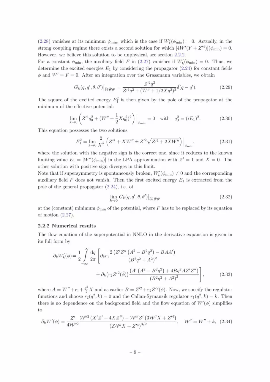
Table 1: Energy ENNLO1 of the first excited state, calculated according to (2.31) for r1 = k,

e = m = a = 1 and various g. For comparison, also the results ELPA1 obtained in LPA, ENLO

1

derived in NLO as well as the exact values Eex1 from numerically diagonalizing the Hamiltonian

are given. Here, ELPA1 , ENLO

1 and ENNLO1 were derived by solving the respective partial differential

equations numerically.

Note that for couplings larger than g ≈ 2 the error increases exponentially and the

supercovariant derivative approximation breaks down. The breakdown of the NNLO ap-

proximation for couplings g & 2 is also indicated by the structure of the effective average

potential. In this regime, Vk(φ) becomes complex for all scales smaller than a k0 > 0 for

field values close to the local minimum of W ′Λ. This is due to the expression√

3W ′Y + Z ′4

appearing in (2.28) which becomes complex near the local minimum of W ′Λ for non-convex

initial potentials, owing to an increasingly negative Y ; see also figures 3, 4. Another sign

of the breakdown is given by the appearance of a further mass at g ≈ 1.7, splitting in

two masses for even larger couplings g. This is due to the formation of one/two further

minima of the effective potential, where 4W ′Y + Z ′4∣∣φmin

= 0 holds. Here, the fourth order

correction Y is of the same order as the leading and next-to leading order terms W ′ and

Z ′ indicating the invalidity of the truncation. The corresponding masses become paramet-

rically large. These large masses in the strong coupling regime are probably an artifact of

the regularization and have no physical significance. Similar artifacts have already been

encountered in O(N) symmetric Wess-Zumino models [24].

We thus observe a very good convergence of the derivative expansion in case the local

barrier of the classical potential is small. However, as the non-convexity of VΛ increases,

tunneling events are exponentially suppressed and are no longer captured by the flow equa-

– 11 –

tions in the derivative expansion. Here, the inclusion of non-local operators should lead to

a better convergence behaviour in the strong coupling regime.

-1 - 0.8 - 0.6 - 0.4 - 0.2 0 0.20

0.4

0.8k = L

k = 1k = 0

-1.5 -1.0 - 0.5 0.0 0.5 1.00

2

4

6

8

10

Φ

Vk H Φ L

g =0

-1.8 -1.6 -1.4 -1.2 -1 - 0.8 - 0.60

0.4

0.8

1.2k = L

k = 1k = 0

- 2.0 -1.5 -1.0 - 0.5 0.0 0.50

2

4

6

8

Φ

Vk H Φ L

g =1.8

Figure 2: Flow of the effective average potential Vk(φ) as obtained by solving the system of PDE’s

numerically in NNLO in the derivative expansion with initial conditions (2.35), where e = m = a = 1

and g = 0 (left panel) and g = 1.8 (right panel).

The flow of the bosonic potential Vk(φ) for g = 0 and g = 1.8 is depicted in figure 2.

Apparently, non-convexities appearing in the classical potential diminish as more and more

long-range quantum fluctuations are taken into account such that the effective potentials

in figure 2 become convex.4 Furthermore, figures 3 and 4 show the flow of W ′, Z ′, X and

Y for g = 1.8. From (2.36) we infer the following deviation of the solutions at k = 0 from

their classical values for large values of |φ|:

W ′0 −W ′Λ ∼1

2φ, Z ′0 − Z ′Λ ∼

1

12φ4, X0 −XΛ ∼

1

18φ6, Y0 − YΛ ∼ −

1

9φ7. (2.37)

As expected, the higher-order operators show a faster decay for large field values, see Fig.

3 and 4.

2.3 Supersymmetry breaking

If we choose the classical superpotential to be a polynomial of the form W ′Λ(φ) ∼ O (φn)

with leading power n even, we expect spontaneous supersymmetry breaking to occur during

the flow towards the IR [6, 17, 31]. It is known that spontaneous supersymmetry breaking

is an IR effect, where the ground state is lifted to E0 > 0 [32].

2.3.1 Problems with the expansion in powers of F

In order to study SUSY breaking within the FRG framework we focus on the Z2 symmetric

even function

W ′Λ(φ) = e+ gφ2, e < 0, g > 0. (2.38)

Then the RG flow preserves the symmetry and W ′k(φ) will remain Z2 symmetric for all

scales.4However, note that the structure of the flow equation (2.12) forces rather the superpotential than the

scalar potential to become convex in the IR. Since the scalar potential is a complicated function of W ′, Z, Y ,

i.e. of the form (2.28), the flow equation does not immediately imply Vk→0 to be convex.

– 12 –

-1.5 -1.0 - 0.5 0.0 0.5- 0.5

0.0

0.5

1.0

1.5

2.0

Wk 'H Φ L

- 3 - 2 -1 0 1 21.00

1.02

1.04

1.06

1.08

1.10

Zk H Φ L

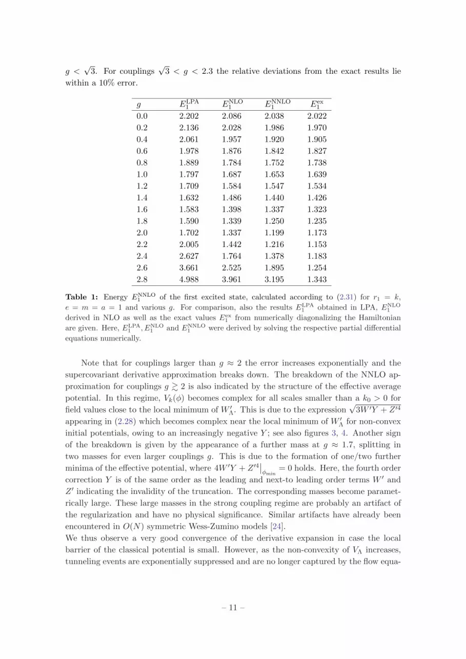
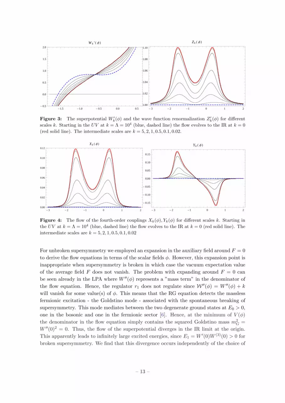
Figure 3: The superpotential W ′k(φ) and the wave function renormalization Z ′k(φ) for different

scales k. Starting in the UV at k = Λ = 104 (blue, dashed line) the flow evolves to the IR at k = 0

(red solid line). The intermediate scales are k = 5, 2, 1, 0.5, 0.1, 0.02.

- 3 - 2 -1 0 1 20.00

0.02

0.04

0.06

0.08

0.10

0.12

Xk H Φ L

- 3 - 2 -1 0 1 2

- 0.15

- 0.10

- 0.05

0.00

0.05

0.10

0.15

Yk H Φ L

Figure 4: The flow of the fourth-order couplings Xk(φ), Yk(φ) for different scales k. Starting in

the UV at k = Λ = 104 (blue, dashed line) the flow evolves to the IR at k = 0 (red solid line). The

intermediate scales are k = 5, 2, 1, 0.5, 0.1, 0.02

For unbroken supersymmetry we employed an expansion in the auxiliary field around F = 0

to derive the flow equations in terms of the scalar fields φ. However, this expansion point is

inappropriate when supersymmetry is broken in which case the vacuum expectation value

of the average field F does not vanish. The problem with expanding around F = 0 can

be seen already in the LPA where W ′′(φ) represents a ”mass term” in the denominator of

the flow equation. Hence, the regulator r1 does not regulate since W ′′(φ) = W ′′(φ) + k

will vanish for some value(s) of φ. This means that the RG equation detects the massless

fermionic excitation - the Goldstino mode - associated with the spontaneous breaking of

supersymmetry. This mode mediates between the two degenerate ground states at E0 > 0,

one in the bosonic and one in the fermionic sector [6]. Hence, at the minimum of V (φ)

the denominator in the flow equation simply contains the squared Goldstino mass m2G =

W ′′(0)2 = 0. Thus, the flow of the superpotential diverges in the IR limit at the origin.

This apparently leads to infinitely large excited energies, since E1 = W ′(0)W (3)(0) > 0 for

broken supersymmetry. We find that this divergence occurs independently of the choice of

– 13 –

the regulator r2 and of the order of truncation.5

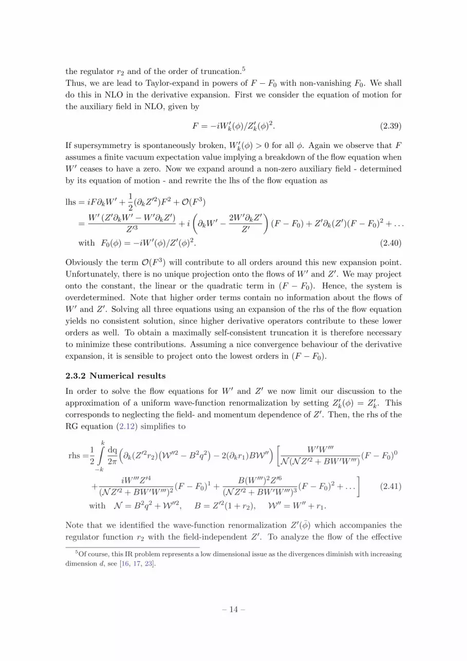
Thus, we are lead to Taylor-expand in powers of F − F0 with non-vanishing F0. We shall

do this in NLO in the derivative expansion. First we consider the equation of motion for

the auxiliary field in NLO, given by

F = −iW ′k(φ)/Z ′k(φ)2. (2.39)

If supersymmetry is spontaneously broken, W ′k(φ) > 0 for all φ. Again we observe that F

assumes a finite vacuum expectation value implying a breakdown of the flow equation when

W ′ ceases to have a zero. Now we expand around a non-zero auxiliary field - determined

by its equation of motion - and rewrite the lhs of the flow equation as

lhs = iF∂kW′ +

1

2(∂kZ

′2)F 2 +O(F 3)

=W ′ (Z ′∂kW

′ −W ′∂kZ ′)Z ′3

+ i

(∂kW

′ − 2W ′∂kZ′

Z ′

)(F − F0) + Z ′∂k(Z

′)(F − F0)2 + . . .

with F0(φ) = −iW ′(φ)/Z ′(φ)2. (2.40)

Obviously the term O(F 3) will contribute to all orders around this new expansion point.

Unfortunately, there is no unique projection onto the flows of W ′ and Z ′. We may project

onto the constant, the linear or the quadratic term in (F − F0). Hence, the system is

overdetermined. Note that higher order terms contain no information about the flows of

W ′ and Z ′. Solving all three equations using an expansion of the rhs of the flow equation

yields no consistent solution, since higher derivative operators contribute to these lower

orders as well. To obtain a maximally self-consistent truncation it is therefore necessary

to minimize these contributions. Assuming a nice convergence behaviour of the derivative

expansion, it is sensible to project onto the lowest orders in (F − F0).

2.3.2 Numerical results

In order to solve the flow equations for W ′ and Z ′ we now limit our discussion to the

approximation of a uniform wave-function renormalization by setting Z ′k(φ) = Z ′k. This

corresponds to neglecting the field- and momentum dependence of Z ′. Then, the rhs of the

RG equation (2.12) simplifies to

rhs =1

2

k∫−k

dq

2π

(∂k(Z

′2r2)(W ′′2 −B2q2

)− 2(∂kr1)BW ′′

)[ W ′W ′′′

N (NZ ′2 +BW ′W ′′′)(F − F0)0

+iW ′′′Z ′4

(NZ ′2 +BW ′W ′′′)2(F − F0)1 +

B(W ′′′)2Z ′6

(NZ ′2 +BW ′W ′′′)3(F − F0)2 + . . .

](2.41)

with N = B2q2 +W ′′2, B = Z ′2(1 + r2), W ′′ = W ′′ + r1.

Note that we identified the wave-function renormalization Z ′(φ) which accompanies the

regulator function r2 with the field-independent Z ′. To analyze the flow of the effective

5Of course, this IR problem represents a low dimensional issue as the divergences diminish with increasing

dimension d, see [16, 17, 23].

– 14 –

average potential we proceed in two steps. First we start with a classical potential of the

form (2.11) in the UV at k = Λ. Down to some scale k0 > 0, W ′ will have a zero. In this

regime k ∈ (k0,Λ) we employ the flow equations obtained by an expansion around F = 0.

Starting with k0 down to the IR limit k = 0 the scale-dependence of W ′, Z ′ is determined

by the flow equations derived via an expansion around F0 6= 0. As regulator functions

we choose r1 = 0 and r2 =(k2/p2 − 1

)θ(k2 − p2). To calculate the ground state energies

E0 we Taylor-expand W ′ about φ = 0 up to some order and solve the system of coupled

ordinary differential equations numerically. This is a sensible approach when W ′ becomes

flat in the IR, because due to supersymmetry the physics happens at vanishing field, in

contrast to e.g. usual O(N)-models [24, 25], where the situation is exactly opposite: in the

unbroken regime, the derivative of the potential is positive, whereas in the broken phase,

one has a zero. As in the case of unbroken supersymmetry, we compare our results for E0

with the ones obtained by numerically diagonalizing the Hamiltonian of the system.

Fig. 5 displays the ground state energies as well as the relative error etrunc in LPA and NLO

as obtained via two different projection methods. Here, (i, j) corresponds to a projection

onto (F−F0)i and (F−F0)j . Apparently, the results are significantly improved by including

**

**

**

**

**

**

**

**

**

**

ô

ô

ô

ô

ô

ô

ô

ôô

ôô

ôô

ôô

ôô

ôô

ô

ì

ì

ì

ì

ì

ì

ì

ì

ìì

ìì

ìì

ìì

ìì

ìì

* Φ12 ,LPA,H 0Lô Φ12 ,NLO,H 0,1Lì Φ12 ,NLO,H 0,2L

Exact

0 1 2 3 4

0.0

0.2

0.4

0.6

0.8

g

E0

** * * * * * * * * * * * * * * * * * *

ô

ô

ô

ô

ô

ôô

ôô

ôô ô ô ô ô ô ô ô ô ô

ì

ì

ì

ìì ì

ì ì ì ì ì ì ì ì ì ì ì ì ì ì

* Φ12 ,LPA,H 0Lô Φ12 ,NLO,H 0,1Lì Φ12 ,NLO,H 0,2L

0 1 2 3 40.0

0.1

0.2

0.3

0.4

g

etrunc

Figure 5: Ground state energy E0 and its relative error etrunc for initial potentials of the form

WΛ = −0.1 + g3φ

3 as a function of g obtained via a polynomial expansion of W ′k(φ) up to φ12. The

brackets encode the projection scheme, i.e. (i, j) corresponds to a projection onto (F − F0)i and

(F − F0)j .

a constant wave-function renormalization. In particular, this applies to large couplings g,

where the relative error is approximately 4%. Contrary to unbroken supersymmetry, the

relative error increases with decreasing g. This originates from the fact that for decreasing

g the minima of the potential drift apart and tunneling effects become effective, see [20].

In NLO, a (0, 2)-projection shows a smaller relative error than the (0, 1)-projection up to

some gmax ≈ 3.6, since the flow of Z ′ slows down when including the higher order term

(F − F0)2 resulting in a higher ground state energy E0 = V (0) = W ′(0)/Z ′(0)2. However,

for large g > gmax the (0, 1)-projection leads to superior results. This may be due to a

larger truncation error in (F − F0)2 compared to (F − F0)1 with increasing coupling g,

originating from the missing higher order terms X,Y which are of importance there.

– 15 –

3. N = 1 Wess-Zumino model in 3 dimensions

As a second testing ground for the convergence properties of the supercovariant derivative

expansion we choose the three-dimensional N = 1 Wess-Zumino model. This model has

been examined in next-to-leading order in the derivative expansion with a momentum- and

field-independent wave-function renormalization Zk in [17]. It was shown that at zero tem-

perature, this model possesses an analogue of the Wilson-Fisher fixed point, separating the

supersymmetric (spontaneously broken Z2) from the nonsupersymmetric (Z2-symmetric)

phase.

3.1 Preliminaries

Here, we shortly recall the main properties of the three-dimensional model. For more details

in the context of flow equations we refer to [17]. The real scalar field φ, real auxiliary field

F and real fermion field ψ are components of a real superfield

Φ(x, θ) = φ(x) + θψ(x) +1

2θθF (x). (3.1)

The supersymmetry variations δεΦ are generated by fermionic supercharges Q, Q, where

Q = −i∂θ − /∂θ and Q = −i∂θ − θ /∂ with anticommutation relations Qk, Ql = 2i/∂kl. The

supercovariant derivatives - fulfilling the corresponding relation Dk, Dl = −2i/∂kl - read

D = ∂θ + i/∂θ, and D = −∂θ − iθ /∂. (3.2)

Since there are no Majorana fermions in 3 Euclidean dimensions we switch to Minkowski-

space with metric tensor ηµν = diag(1,−1,−1) and γ-matrices γµ = (σ2, iσ3, iσ1), where

µ = 0, 1, 2. After setting up the flow equation we return to Euclidean space, see [17]. With

the above definitions we are able to construct the off-shell supersymmetric action in R1,2

superspace:

S[Φ] =

∫dz

[−1

2ΦKΦ + 2W (Φ)

], K =

1

2(DD −DD), (3.3)

where z = (x, θ, θ) denotes the coordinates in superspace. After integration over the

Majorana Grassmann variables θ, θ and elimination of the auxiliary field F via its equation

of motion F = −W ′(φ), we arrive at the following on-shell action in components,

Son[φ, F, ψ, ψ] =

∫d3x

[1

2∂µφ∂

µφ− i

2ψ /∂ψ − 1

2W ′2(φ)− 1

2W ′′(φ)ψψ

]. (3.4)

The last term in ( 3.4) describes a Yukawa interaction between the scalars and fermions

and V (φ) = W ′2(φ)/2 the potential self-energy of the scalars.

3.2 Derivation of flow equation

Now we use the flow equation in Minkowski spacetime

∂kΓk =i

2STr

∂kRk

[Γ

(2)k +Rk

]−1

(3.5)

– 16 –

and perform a Wick rotation of the zeroth momentum component afterwards to obtain the

corresponding flow in Euclidean space.

Analogously to eq. (2.15), the general ansatz for the scale-dependent effective average action

reads

Γk[Φ] =

∫dz

[2Wk(Φ)− 1

2Zk(Φ)KZk(Φ)− 1

8Y1,k(Φ)K2Φ− 1

8Y2,k(Φ)(KΦ)(KΦ)

](3.6)

with the scale- and field-dependent functions Wk, Zk, Y1,k, Y2,k. We chose the prefactors

of each term such that the resulting flow equations in Euclidean space exactly match the

corresponding flow equations derived in supersymmetric quantum mechanics with∫ dq

2π →∫ d3q(2π)3 . By integrating over the anticommuting Grassmann variables in (3.6) we get

Γk[Φ] =

∫d3x

[1

2(∂µZ)(∂µZ)− i

2(Z ′ψ)/∂(Z ′ψ)− 1

4Y ′1ψ∂

2ψ −(

1

2W ′′ +

1

8Y ′′1 (∂2φ)

)ψψ

+1

4Y2(∂µψ)(∂µψ) +

(W ′ − 1

2Z ′Z ′′ψψ +

1

2(Y ′1 + Y2)(∂2φ) +

1

4Y ′′1 (∂µφ)(∂µφ) +

i

2Y ′2ψ /∂ψ

)F

+

(1

2Z ′2 +

1

8Y ′′2 ψψ

)F 2 − 1

4Y ′2F

3

], (3.7)

where again we ordered the terms in powers of the auxiliary field F . In analogy to (2.19),

we assume the supersymmetric cutoff action to be of the form

∆Sk[Φ] =1

2

∫dzΦ

[2r1(−∂µ∂µ, k)− Z ′k2(Φ) r2(−∂µ∂µ, k)K

]Φ, (3.8)

with Z ′k evaluated at the background field Φ = φ. As in quantum mechanics, we extract

the scale dependence of W ′, Z ′ and Y ′2 by projecting the rhs of (3.5) onto F, F 2 and F 3 for

constant bosonic fields and a vanishing fermion field. This way we obtain (cf. eq. (2.25))

∂kΓk|∂µφ=∂µF=ψ=ψ=0 =

∫d3x

(∂kW

′F +1

2∂kZ

′2F 2 − 1

4∂kY

′2F

3

)=i

2

∫d3q

(2π)3

d3q′

(2π)3dθ dθ dθ′ dθ′(∂kRk)(q

′, q, θ′, θ)Gk(q, q′, θ, θ′)

=i

2

∫d3x

d3q

(2π)3

[(2∂kr1)(b+ c+ d) + ∂k(r2Z

′2k (φ))(−2fq2 + aq2 + 4e)

], (3.9)

where (a, b, c, d, e, f) again represent the coefficients of the Greens function Gk, see ap-

pendix C. Finally, we obtain the flow equations in Euclidean space with metric −δµν via

a Wick rotation of the zeroth momentum component, i.e. q0 → iq0. As mentioned above,

these equations are by construction identically to the ones derived in SUSY quantum me-

chanics up to an integration over a three dimensional momentum space.

The missing flow of Y ′1 +Y2 is derived in an exactly similar manner to d = 1 as presented in

appendix B by considering momentum-dependent fields φ, F and projecting onto the con-

tribution in Q2δφ(Q)δF (−Q) with an additional Wick rotation of q0 afterwards. Finally,

we define and substitute Y := Y ′2 and X := Y ′1 + Y2 in order to simplify the equations.

– 17 –

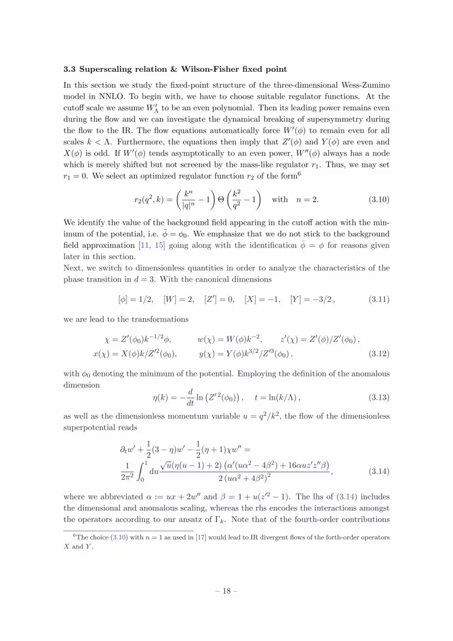
3.3 Superscaling relation & Wilson-Fisher fixed point

In this section we study the fixed-point structure of the three-dimensional Wess-Zumino

model in NNLO. To begin with, we have to choose suitable regulator functions. At the

cutoff scale we assume W ′Λ to be an even polynomial. Then its leading power remains even

during the flow and we can investigate the dynamical breaking of supersymmetry during

the flow to the IR. The flow equations automatically force W ′(φ) to remain even for all

scales k < Λ. Furthermore, the equations then imply that Z ′(φ) and Y (φ) are even and

X(φ) is odd. If W ′(φ) tends asymptotically to an even power, W ′′(φ) always has a node

which is merely shifted but not screened by the mass-like regulator r1. Thus, we may set

r1 = 0. We select an optimized regulator function r2 of the form6

r2(q2, k) =

(kn

|q|n− 1

)Θ

(k2

q2− 1

)with n = 2. (3.10)

We identify the value of the background field appearing in the cutoff action with the min-

imum of the potential, i.e. φ = φ0. We emphasize that we do not stick to the background

field approximation [11, 15] going along with the identification φ = φ for reasons given

later in this section.

Next, we switch to dimensionless quantities in order to analyze the characteristics of the

phase transition in d = 3. With the canonical dimensions

[φ] = 1/2, [W ] = 2, [Z ′] = 0, [X] = −1, [Y ] = −3/2 , (3.11)

we are lead to the transformations

χ = Z ′(φ0)k−1/2φ, w(χ) = W (φ)k−2, z′(χ) = Z ′(φ)/Z ′(φ0) ,

x(χ) = X(φ)k/Z ′2(φ0), y(χ) = Y (φ)k3/2/Z ′3(φ0) , (3.12)

with φ0 denoting the minimum of the potential. Employing the definition of the anomalous

dimension

η(k) = − d

dtln(Z ′ 2(φ0)

), t = ln(k/Λ) , (3.13)

as well as the dimensionless momentum variable u = q2/k2, the flow of the dimensionless

superpotential reads

∂tw′ +

1

2(3− η)w′ − 1

2(η + 1)χw′′ =

1

2π2

∫ 1

0du

√u(η(u− 1) + 2)

(α′(uα2 − 4β2) + 16αuz′z′′β

)2 (uα2 + 4β2)2 , (3.14)

where we abbreviated α := ux + 2w′′ and β = 1 + u(z′2 − 1). The lhs of (3.14) includes

the dimensional and anomalous scaling, whereas the rhs encodes the interactions amongst

the operators according to our ansatz of Γk. Note that of the fourth-order contributions

6The choice (3.10) with n = 1 as used in [17] would lead to IR divergent flows of the forth-order operators

X and Y .

– 18 –

only x and not y directly couples to the flow of the superpotential. The expressions of the

remaining flows are rather long and therefore not written down explicitly.

Now we analyze the physics at the Wilson-Fisher fixed point, corresponding to

∂tO∗ = 0, with O = (w′, z′, x, y). (3.15)

For large fields |χ| 1 the rhs of eq. (3.14), i.e. the nontrivial flow, vanishes as we generally

expect |w′′∗ | to be large for a Z2-symmetric system. This holds for the remaining flows as

well. Thus, the fixed-point solution for large χ is fixed by the anomalous and canonical

scaling, leading to the asymptotic behaviour

w′∗(χ) ∼ χ(

3−ηη+1

), z′∗(χ) ∼ χ−

(ηη+1

), x∗(χ) ∼ χ−2, y∗(χ) ∼ χ−3. (3.16)

Thus, for positive η, the higher order functions vanish for large fields. In [17], one non-

Gaussian IR-stable fixed point as the supersymmetric analogue of the Wilson-Fisher fixed

point has been spotted. It possesses one IR unstable direction defined by w′∗(0) with critical

exponent θ0 = 1/νw which can be related to the anomalous dimension η via the superscaling

relation 1/νw = (3− η)/2 [17].

To begin with, we show that this interesting superscaling relation holds true to all orders

in the supercovariant derivative expansion of Γk and derive its form for arbitrary d ≥ 2.

To show this, let us note that the only fixed point equation which depends explicitly on w′ is

the one for w′ itself. Thus, we consider small fluctuations around the fixed-point solution in

w′-direction, i.e. w′(t, χ) = w′∗(χ)+δw′(t, χ) and possible higher order operators evaluated

at the fixed point. By linearizing the flow (3.14) - generalized to d dimensions7 - in δw′ we

arrive at the fluctuation equation

∂tδw′ =

(η − d

2+ F(χ)∂χ + G(χ)∂2

χ

)δw′ . (3.17)

Here, F and G are functionals obtained from the linearization. The critical exponents then

correspond to the negative eigenvalues of the operator on the rhs. Apparently, a constant

variation is an eigenfunction to this operator with eigenvalue (η − d)/2. Since the flow of

all higher operators of Γk remain independent of w′ this is true to all orders. Hence, we

have verified the superscaling relation

1

νw=

1

2(d− η), d ≥ 2. (3.18)

Next we present the numerical results to the fixed point equations. We solved the fixed point

equation globally via a combination of Chebyshev and rational Chebyshev polynomials.

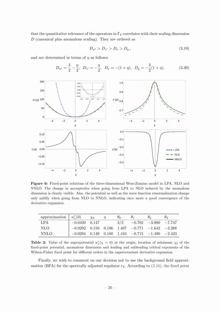
The fixed-point solutions of the four operators considered are illustrated in Fig. 6. The

IR relevant coupling w′(0), the location of the minimum of the potential as well as the

anomalous dimension and leading critical exponents are displayed in Table 2. We observe a

nice convergence behaviour with increasing order in the derivative expansion. This confirms

7The rhs of (3.14) holds for arbitrary d up to a different dimensional prefactor of 1/(2d−1πd/2Γ(d/2)).

– 19 –

that the quantitative relevance of the operators in Γk correlates with their scaling dimension

D (canonical plus anomalous scaling). They are ordered as

Dw′ > Dz′ > Dx > Dy , (3.19)

and are determined in terms of η as follows:

Dw′ =3

2− η

2, Dz′ = −η

2, Dx = −(1 + η), Dy = −3

2(1 + η). (3.20)

-4 -2 0 2 4

0

50

100

150

200

χ

w'*[χ]-0.2 -0.1 0.0 0.1 0.2

-0.04

-0.02

0.00

0.02

0.04

-4 -2 0 2 4

0.7

0.8

0.9

1.0

χ

z'*[χ]

-4 -2 0 2 4

-0.10

-0.05

0.00

0.05

0.10

χ

x*[χ]

-4 -2 0 2 4

-0.4

-0.3

-0.2

-0.1

0.0

χ

y*[χ] LPA

NLO

NNLO

Figure 6: Fixed-point solutions of the three-dimensional Wess-Zumino model in LPA, NLO and

NNLO. The change in asymptotics when going from LPA to NLO induced by the anomalous

dimension is clearly visible. Also, the potential as well as the wave function renormalization change

only mildly when going from NLO to NNLO, indicating once more a good convergence of the

derivative expansion.

approximation w′∗(0) χ0 η θ0 θ1 θ2 θ3

LPA −0.0420 0.147 3/2 −0.702 −3.800 −7.747

NLO −0.0292 0.150 0.186 1.407 −0.771 −1.642 −3.268

NNLO −0.0294 0.149 0.180 1.410 −0.715 −1.490 −2.423

Table 2: Value of the superpotential w′∗(χ = 0) at the origin, location of minimum χ0 of the

fixed-point potential, anomalous dimension and leading and subleading critical exponents of the

Wilson-Fisher fixed point for different orders in the supercovariant derivative expansion.

Finally, we wish to comment on our decision not to use the background field approxi-

mation (BFA) for the spectrally adjusted regulator r2. According to (3.16), the fixed point

– 20 –

solution z′∗ vanishes for large fields |χ| → ∞. Implementing the BFA goes along with the

replacement z′(χ0) = 1 → z′(χ) in the dimensionless regulator. Thus, the regulator is

suppressed artificially for large fields. This in turn can lead to instabilities. Indeed, during

our numerical investigation of the fixed point equations we could not find a global solution

in NNLO when employing the background field approximation, even though a solution via

a Taylor expansion seems to exist. The difference between the physical quantities (critical

exponents etc.) obtained by a Taylor expansion with BFA and the spectral method without

BFA are almost identical. Thus one might argue that the error made in this approxima-

tion is irrelevant. However, one should bear in mind that a fixed point potential better

be globally defined, and that there might be systems that are unstable against such types

of approximations. Note also that when integrating the dimensionful flow equations, the

difference should be even smaller as Z ′(φ) does not fall off asymptotically.

– 21 –

4. Summary

In this paper we studied the convergence of the derivative expansion in two supersymmetric

theories via the functional renormalization group. Our approach includes a manifestly

supersymmetric regulator and thus is suited to study systems with broken and unbroken

supersymmetry.

In the first part, we investigated supersymmetric quantum mechanical systems. Start-

ing with symmetry-preserving flows, we obtained very good results for the energy gap

within a truncation containing forth-order derivative terms. The relative error to the ex-

act results is below one percent for a wide range of couplings 0 < g <√

3 including the

non-perturbative regime. For larger couplings, we observe a breakdown of the derivative

expansion, which is expected since in this regime non-local instanton contributions play

a crucial role. In the SUSY-breaking case, we studied the flow of the superpotential to-

gether with a constant wave-function renormalization. This required a suitable choice of

projection to obtain the flow equations, because in the broken regime, the auxiliary field

acquaints a finite expectation value which has to be accounted for. The results are again

in agreement to exact results within a few percent.

The second part of this work deals with the Wess-Zumino model in 3 dimensions. In

particular, we were interested in the analogue of the Wilson-Fisher fixed point of standard

O(N)-theories. We were able to calculate all functionals at the fixed point up to forth

order in supercovariant derivatives. Again, a very good convergence has been observed,

and this convergence is further substantiated by two facts: On the one hand, the change

of the fixed functionals is tiny when including forth-order terms in the effective average

action. On the other hand, the critical exponents converge. Additionally, we could prove

the superscaling relation to all orders in the derivative expansion.

In both studies, globally defined spectral methods were used to obtain the results. This

ensures the numerical validity of our results, which are naturally free from any boundary

effects usually present when applying a domain truncation.

Acknowledgments

The authors want to thank J. Borchardt, J.M. Pawlowski, R. Sondenheimer, F. Synatschke-

Czerwonka and L. Zambelli for useful discussions. The research was supported by the

Deutsche Forschungsgemeinschaft (DFG) graduate school GRK 1523/2. B. Knorr and A.

Wipf thank the DFG for supporting this work under grant no. Wi777/11-1.

– 22 –

A. Greens function in d = 1

An analysis of the flow equation (2.12) requires the determination of the connected two-

point function Gk as the inverse of (Γ(2)k +Rk). In superspace, the relation 1 = Gk(Γ

(2)+Rk)

is given by (2.23) with Gk according to (2.24). The latter simply represents an expansion of

Gk in the Grassmann variables (θ, θ′) with arbitrary “bosonic” coefficients (a, b, c, d, e, f).

By solving (2.23), we finally obtain

a =

(B + 3

2 iFY′

2

)116 (4A+ F (3FY ′′2 − 8iZ ′Z ′′)) 2 +

(B + 3

2 iFY′

2

)C

b = c =−(iA+ 3

4 iF2Y ′′2 + 2FZ ′Z ′′

)(116 (4A+ F (3FY ′′2 − 8iZ ′Z ′′)) 2 +

(B + 3

2 iFY′

2

)C)

d =4i

4A− 4iBq + F (FY ′′2 + 4qY ′2 − 4iZ ′Z ′′)

e =4i

4A+ 4iBq + F (FY ′′2 − 4qY ′2 − 4iZ ′Z ′′)(A.1)

f =1(

B + 32 iFY

′2

) +

(iA+ 3

4 iF2Y ′′2 + 2FZ ′Z ′′

)2(

B + 32 iFY

′2

) (116 (4A+ 3F 2Y ′′2 − 8iFZ ′Z ′′) 2 +

(B + 3

2 iFY′

2

)C) ,

where we introduced the abbreviations

A = W ′′ + r1 +1

2(Y ′1 + Y2)q2

B = Z ′2 + r2Z′2k (φ)

C = Bq2 +i

4F 3Y2

′′′ + F 2(Z ′′2 + Z ′′′Z ′

)+i

2F(q2(2Y ′2 + Y ′′1

)+ 2W ′′′

). (A.2)

B. Flow equation of Y ′1 + Y2

This section explains the derivation of the flow of Y ′1 + Y2. To derive the corresponding

flow equation, we project the rhs of (2.12) onto the time dependent term F φ. This requires

an expansion of the inverse propagator around field configurations of F and φ exhibiting

a small momentum dependence. Again, we therefore only consider the bosonic part of the

superfield in the inverse propagator, i.e. we set ψ and ψ equal to zero. The background

field configurations in momentum space are then given by

φ(p) = φδ(p) + δφ(p) (δ(p−Q) + δ(p+Q)) and

F (p) = Fδ(p) + δF (p) (δ(p−Q) + δ(p+Q)) (B.1)

with δφ(p) φ, δF (p) F . Note that φ(p) = φ∗(−p) is real and F (p) = −F ∗(−p) purely

imaginary. Next, we perform an expansion of the inverse Green’s function Γ(2)k +Rk up to

O (δφ(Q)δF (−Q)) quadratic in the fluctuations. In the following, z denotes the superspace

coordinates (q, θ, θ). Thus, the inverse propagator may be written in the form(Γ

(2)k +Rk

)(z, z′) =

[Γ0(q, q′) + Γφ(q, q′) + ΓF (q, q′) + ΓφF (q, q′)

]δ(θ, θ′), (B.2)

– 23 –

corresponding to an expansion in powers of δφ and δF with

Γ0(q, q′) = Γ0(q)δ(q − q′) with

Γ0(q) =

(i(W ′′ + r1)−BK(q) +

i

2(Y ′1 + Y2)q2

),

Γ−10 (q) =

−i(W ′′ + r1 + 12(Y ′1 + Y2)q2)−BK(q)

B2q2 + (W ′′ + r1 + 12(Y ′1 + Y2)q2)2

Γφ(q, q′) = Γφ(q,Q)δ(q − q′ −Q) + Γφ(q,−Q)δ(q − q′ +Q) with

Γφ(q,Q) =

(iW ′′′ + Z ′Z ′′Q2θθ − Z ′Z ′′(K(q) +K(q −Q))− i

2Y ′2Q

2θθK(q −Q)

− i2Y ′2Q

2K(q)θθ +i

2Y ′2K(q)K(q −Q) +

i

4Y ′′1 (q2 +Q2 + (q −Q)2)

)δφ(Q),

ΓF (q, q′) = ΓF (q,Q)δ(q − q′ −Q) + ΓF (q,−Q)δ(q − q′ +Q) with

ΓF (q,Q) =

(iW ′′′θθ + Z ′Z ′′ − Z ′Z ′′K(q)θθ − Z ′Z ′′θθK(q −Q)− i

2Y ′2K(q)

− i2Y ′2K(q −Q) +

i

2Y ′2K(q)θθK(q −Q) +

i

4Y ′′1 (q2 +Q2 + (q −Q)2)θθ

)δF (Q),

ΓφF (q, q′) = ΓφF (q)δ(q − q′) with

ΓφF (q)∣∣∣O(Q2)

=i

2(Y ′′2 + Y ′′′1 )Q2θθ(δφ(Q)δF (−Q) + δF (Q)δφ(−Q)). (B.3)

Thereby, we considered only terms quadratic in Q in ΓφF (q, q′) as other terms do not

contribute to the flow. Note that the operator K occurring in eq. (B.3) is a function of the

momentum as well as the Grassmann variables θ, θ. Inserting the configuration (B.1) into

(2.17) we obtain

i

2(Y ′1 + Y2) =

1

ΩlimQ2→0

∂

∂Q2

δ2Γkδ(δφ(Q))δ(δF (−Q))

∣∣∣∣φ, F=ψ=ψ=δF=δφ=0

, (B.4)

where Ω denotes the total volume of “space” and should be taken to infinity at the end.

Now, the Green’s function follows from (B.2) via an expansion in powers of δφ and δF .

Keeping only contributions quadratic in the fluctuations ∼ (δF )(δφ) we find

(Gk) (z, z′)(δφδF ) =−Γ−1

0 (q)ΓφF (q, q′)Γ−10 (q)

+

∫q

Γ−10 (q)Γφ(q, q)Γ−1

0 (q)ΓF (q, q′)Γ−10 (q)

+

∫q

Γ−10 (q)ΓF (q, q)Γ−1

0 (q)Γφ(q, q′)Γ−10 (q)

δ(θ, θ′) (B.5)

Inserting the above propagator (B.5) into the flow equation and keeping only terms in

– 24 –

δφ(Q)δF (−Q) we have

i

2∂k(Y

′1 + Y2) Q2 δφ(Q)δF (−Q) =

1

2

∫dq

2πdθdθdθ′dθ′∂k

[ir1 − Z ′2k (φ)r2K(q, θ′)

]δ(θ′, θ)×[

−Γ−10 (q)ΓφF (q)Γ−1

0 (q) + Γ−10 (q)Γφ(q,Q)Γ−1

0 (q −Q)ΓF (q −Q,−Q)Γ−10 (q)

+ Γ−10 (q)ΓF (q,−Q)Γ−1

0 (q +Q)Γφ(q +Q,Q)Γ−10 (q)

]δ(θ, θ′). (B.6)

By integrating over the Grassmann variables and projecting the rhs onto the contribution

∼ Q2 we thus get the flow of Y ′1 + Y2.

C. Greens function in d = 3

Similarly to the analysis in d = 1, we determine the Greens function Gk of the general form

Gk(q, q′, θ, θ′) =

(a+ b θθ + c θ′θ′ + d θθ′ + e θθθ′θ′ + fθ′/pθ

)δ(q, q′) (C.1)

by solving ∫d3q′

(2π)3dθ′ dθ′G−1

k (q, q′, θ, θ′)Gk(q′, q′′, θ′, θ′′) = δ(q, q′′)δ(θ, θ′′), (C.2)

for the coefficients (a, b, c, d, e, f). This yields

a =8 (2B − 3FY ′2)

8C (2B − 3FY ′2)− (4A− 3F 2Y ′′2 + 8FZ ′Z ′′)2

b = c =8A− 6F 2Y ′′2 + 16FZ ′Z ′′

(4A− 3F 2Y ′′2 + 8FZ ′Z ′′) 2 + 8C (3FY ′2 − 2B)

d = −4(A− 1

4F2Y ′′2 + FZ ′Z ′′

)4(A− 1

4F2Y ′′2 + FZ ′Z ′′

)2 − 4q2 (B − FY ′2) 2

e =4C

8C (2B − 3FY ′2)− (4A− 3F 2Y ′′2 + 8FZ ′Z ′′) 2

f = − 16 (B − FY ′2)

(4A− 4Bq + F (−FY ′′2 + 4qY ′2 + 4Z ′Z ′′)) (4A+ 4Bq − F (FY ′′2 + 4qY ′2 − 4Z ′Z ′′)),

(C.3)

where we have used the abbreviations

A = W ′′ + r1 −1

2(Y ′1 + Y2)q2

B = Z ′2 + r2Z′2k (φ)

C = Bq2 − 1

4F 3Y ′′′2 + F 2

(Z ′′2 + Z ′′′Z ′

)+

1

2F(2W ′′′ − q2

(2Y ′2 + Y ′′1

)). (C.4)

D. (Pseudo-)spectral methods

We obtained the numerical results in this work in part with so-called (pseudo-)spectral

methods. Spectral methods were studied from a mathematical point of view already some

– 25 –

decades ago, however, they were only applied in certain fields of physics up to now, e.g.

in numerical relativity, meteorology or fluid mechanics. The basic idea behind spectral

methods is to expand the solution into orthogonal polynomials which should be chosen to

fit the problem. A well-known example is the Fourier series of a periodic function. In our

case, we chose a combination of Chebyshev and rational Chebyshev polynomials in order

to resolve the operators globally. On the other hand, in RG-time-direction, we chose to

map the (infinite) time axis onto a finite interval, then slicing it into smaller pieces and

apply a Chebyshev spectralization in this direction. With a stabilized Newton-Raphson

iteration scheme, we demanded that the flow equations are satisfied on collocation points

up to a certain tolerance. This twofold application of spectral methods was considered too

expensive in former times, but thanks to the progress in computing power, it is feasible

now. This point is also undermined by the recent application of this method to gain

exact solutions to the Einstein field equations for axisymmetric and stationary space times

[27, 33].

The reason to use spectral methods is their extraordinary speed of convergence. For

well-behaved functions, a spectral method may convergence exponentially, i.e. faster than

any power law. Another advantage is that the expansion coefficients give a rough estimate

of the maximal error in the interpolation of the solution. A general rule of thumb is that

the error is bounded by roughly the absolute value of the last coefficient retained. For an

extensive review of spectral methods, see e.g. [26].

References

[1] Alessandra Feo. Predictions and recent results in SUSY on the lattice. Mod.Phys.Lett.,

A19:2387–2402, 2004.

[2] Joel Giedt. Deconstruction and other approaches to supersymmetric lattice field theories.

Int.J.Mod.Phys., A21:3039–3094, 2006.

[3] Simon Catterall. From Twisted Supersymmetry to Orbifold Lattices. JHEP, 0801:048, 2008.

[4] Georg Bergner, Tobias Kaestner, Sebastian Uhlmann, and Andreas Wipf. Low-dimensional

Supersymmetric Lattice Models. Annals Phys., 323:946–988, 2008.

[5] Tomohisa Takimi. Relationship between various supersymmetric lattice models. JHEP,

0707:010, 2007.

[6] Christian Wozar and Andreas Wipf. Supersymmetry Breaking in Low Dimensional Models.

Annals Phys., 327:774–807, 2012.

[7] David Baumgartner and Urs Wenger. Exact results for supersymmetric quantum mechanics

on the lattice. PoS, LATTICE2011:239, 2011.

[8] Georg Bergner, Istvan Montvay, Gernot Munster, Dirk Sandbrink, and Umut D. Ozugurel.

N=1 supersymmetric Yang-Mills theory on the lattice. PoS, LATTICE2013:483, 2013.

[9] Christof Wetterich. Exact evolution equation for the effective potential. Phys. Lett.,

B301:90–94, 1993.

[10] N. Tetradis and C. Wetterich. Critical exponents from effective average action. Nucl.Phys.,

B422:541–592, 1994.

– 26 –

[11] M. Reuter and C. Wetterich. Effective average action for gauge theories and exact evolution

equations. Nucl.Phys., B417:181–214, 1994.

[12] Holger Gies and Lukas Janssen. UV fixed-point structure of the three-dimensional Thirring

model. Phys.Rev., D82:085018, 2010.

[13] Tina K. Herbst, Mario Mitter, Jan M. Pawlowski, Bernd-Jochen Schaefer, and Rainer Stiele.

Exploring the Phase Structure and Thermodynamics of QCD. PoS, QCD-TNT-III:030, 2013.

[14] Nicolai Christiansen, Benjamin Knorr, Jan M. Pawlowski, and Andreas Rodigast. Global

Flows in Quantum Gravity. 2014.

[15] Franziska Synatschke, Georg Bergner, Holger Gies, and Andreas Wipf. Flow Equation for

Supersymmetric Quantum Mechanics. JHEP, 0903:028, 2009.

[16] Franziska Synatschke, Holger Gies, and Andreas Wipf. Phase Diagram and Fixed-Point

Structure of two dimensional N=1 Wess-Zumino Models. Phys. Rev., D80:085007, 2009.

[17] Franziska Synatschke, Jens Braun, and Andreas Wipf. N=1 Wess Zumino Model in d=3 at

zero and finite temperature. Phys. Rev., D81:125001, 2010.

[18] Atsushi Horikoshi, Ken-Ichi Aoki, Masa-aki Taniguchi, and Haruhiko Terao. Nonperturbative

renormalization group and quantum tunneling. pages 194–203, 1998.

[19] A.S. Kapoyannis and N. Tetradis. Quantum mechanical tunneling and the renormalization

group. Phys.Lett., A276:225–232, 2000.

[20] D. Zappala. Improving the renormalization group approach to the quantum mechanical

double well potential. Phys.Lett., A290:35–40, 2001.

[21] Holger Gies. Introduction to the functional RG and applications to gauge theories.

Lect.Notes Phys., 852:287–348, 2012.

[22] Andreas Wipf. Statistical approach to quantum field theory. Lect.Notes Phys., 864:1, 2013.

[23] Franziska Synatschke, Holger Gies, and Andreas Wipf. The Phase Diagram for Wess-Zumino

Models. AIP Conf. Proc., 1200:1097–1100, 2010.

[24] Marianne Heilmann, Daniel F. Litim, Franziska Synatschke-Czerwonka, and Andreas Wipf.

Phases of supersymmetric O(N) theories. Phys.Rev., D86:105006, 2012.

[25] Daniel F. Litim, Marianne C. Mastaler, Franziska Synatschke-Czerwonka, and Andreas Wipf.

Critical behavior of supersymmetric O(N) models in the large-N limit. Phys.Rev.,

D84:125009, 2011.

[26] John P. Boyd. Chebyshev and Fourier Spectral Methods. Dover Publications, 2nd edition,

2000.

[27] Marcus Ansorg, A. Kleinwachter, and R. Meinel. Highly accurate calculation of rotating

neutron stars: detailed description of the numerical methods. Astron.Astrophys., 405:711,

2003.

[28] Holger Gies, Franziska Synatschke, and Andreas Wipf. Supersymmetry breaking as a

quantum phase transition. Phys.Rev., D80:101701, 2009.

[29] Abdus Salam and J.A. Strathdee. Supergauge Transformations. Nucl.Phys., B76:477–482,

1974.

[30] Daniel F. Litim. Optimized renormalization group flows. Phys.Rev., D64:105007, 2001.

– 27 –

[31] Edward Witten. Dynamical Breaking of Supersymmetry. Nucl.Phys., B188:513, 1981.

[32] Michael Dine and John D. Mason. Supersymmetry and Its Dynamical Breaking.

Rept.Prog.Phys., 74:056201, 2011.

[33] Rodrigo P. Macedo and Marcus Ansorg. Axisymmetric fully spectral code for hyperbolic

equations. 2014.

– 28 –