Embed Size (px)
Citation preview
Università degli Studi di PadovaDipartimento di Fisica e Astronomia “Galileo Galilei”
Scuola di Dottorato di Ricerca in FisicaCiclo XXVIII
Confined event samples usingCompton coincidence measurementsfor signal and background studies in
the Gerda experiment
Doctoral Dissertation ofKatharina Cäcilie
von Sturm zu Vehlingen
Head of doctoral schoolProf. Andrea Vitturi
SupervisorProf. Alberto Garfagnini


for my family


Summary
In rare event searches, such as the search for Neutrinoless Double-Beta Decay(0νββ), the experimental sensitivity critically depends on the remaining backgroundafter all data cuts in the region of interest, where signal events are expected. Back-ground reduction is essential to obtain the necessary experimental sensitivity. TheGermanium Detector Array (Gerda) experiment is searching for 0νββ decay in76Ge. Recently, 30 newly produced germanium detectors of Broad Energy Ger-manium (BEGe) type have been implemented in Gerda. Analyzing the shape ofdetector pulses, background can be distinguished from signal events and discarded.The major advantage of the new BEGe detectors are their excellent properties forthis kind of analysis.
The main focus of this thesis is the preparation of pure 0νββ-like event samplesfrom confined interaction regions in a BEGe in order to study the response of thedetector with respect to the interaction position. This is useful to validate and im-prove pulse shape simulations of germanium detectors and can help creating newalgorithms which effectively reduce the background in Gerda. An experimentalsetup was assembled and used to collect events due to single Compton interactionsof photons with a BEGe detector. Because of their localized energy deposition singleCompton events can be used as prototypes for 0νββ event pulse shapes. The assem-bly is capable of a full three-dimensional scan of the BEGe detector. An extensivecharacterization of all detectors used was realized to assure stable conditions of theexperimental setup. Furthermore, detailed fine grain surface scans were performedwhich can give valuable input for simulation. A comprehensive Monte Carlo (MC)description of the assembly was implemented in a Geant4 based framework. Thesimulations provided means to conduct detailed studies of the spatial and energydistribution of single and multiple Compton events. Based on these studies the se-lection of pure samples of single Compton events from localized regions in the BEGewas optimized. In a data taking campaign event samples were collected for differ-ent experimental configurations. Differences in the pulse shape are observed whenchanging the scanned detector location or the High Voltage (HV) on the BEGe. Inparticular it was found that the first part of the average pulse is most sensitive.
Another aspect of rare event searches is the detailed analysis and decomposition ofbackground events. A major background component in Gerda Phase I is intro-duced by the isotope 42Ar. In this work, the specific activity of 42Ar in the Gerdaliquid Argon (LAr) was analyzed using a Bayesian approach. The detection efficien-cies were calculated by means of MC simulations of part of the Gerda experimental
i
Summary
setup. This permitted to study systematic effects introduced by inhomogeneities ofthe distribution of the studied background component in the LAr. The final valueof the specific activity was obtained with a binned maximum likelihood fit of twofit models. Correcting the result for the time the LAr was kept under ground thespecific activity can be compared to other experimental results, and furthermore, totheoretical calculations regarding production mechanisms of 42Ar in the atmosphere.A corrected specific activity of A0(42Ar) = 101.0+2.5
−3.0(stat)± 7.4(syst)µBq/kg wasfound in this analysis; it is compatible with a theoretical calculation based on a ma-jor production mechanisms of 42Ar in the atmosphere. However, it results incompat-ible with the upper limit, 43 Bq/kg at 90 % CL, reported in a previous measurement.
ii
Riassunto
Nelle ricerche di eventi rari, come, per esempio, il decadimento doppio beta senzaneutrini (0νββ), la sensibilità sperimentale dipende dal numero di eventi di fondoche rimangono nella regione di interesse dopo tutti i tagli di analisi. Per raggiun-gere una elevata sensibilità sperimentale è pertanto essenziale ridurre gli eventi difondo. L’esperimento Gerda sta cercando il decadimento 0νββ mediante l’impiegodell’isotopo 76Ge. Recentemente l’esperimento si è dotato di 30 nuovi rivelatori algermanio del tipo BEGe. Il maggiore vantaggio di tali rivelatori è di permettereuna efficace separazione degli eventi di segnale da quelli di fondo mediante lo studiodella forma del segnale elettrico.
Lo scopo primario di questa tesi è la ricerca di un metodo di raccolta di eventiche possano simulare quelli del decadimento 0νββ. Si vuole inoltre che tali eventisiano distribuiti su tutto il volume del rivelatore. Questo risulta molto utile percreare algoritmi che permettano di ridurre gli eventi di fondo in Gerda. Inoltre,lo studio della risposta del rivelatore a seconda del punto di interazione del fotoneincidente permette di controllare e migliorare la descrizione della forma d’impulsoottenuta dalle simulazioni. È stato allestito un apparato sperimentale che permettedi selezionare eventi caratterizzati da una singola interazione Compton provenientida regioni ben definite del rivelatore sotto esame (nel nostro caso un rivelatore ditipo BEGe). Gli eventi provenienti da una singola interazione Compton giacchérilasciano l’energia in una regione ben circoscritta del rivelatore simulano gli even-ti doppio beta. L’apparato ha la capacità di analizzare l’intero volume del BEGenelle sue tre dimensioni. Come passo propedeutico è stato eseguito uno studio dellecaratteristiche fondamentali dei rivelatori usati. Questo è servito per assicurare unfunzionamento stabile e affidabile all’apparato sperimentale. Lo studio ha compor-tato anche l’esecuzione di dettagliate scansioni superficiali dei rivelatori utili questecome informazioni in ingresso ai programmi di simulazione. Le simulazioni hannopermesso un’analisi della distribuzione spaziale ed energetica degli eventi caratte-rizzati da una singola interazione Compton come di quelli da molteplici interazioniCompton. Basandosi su tale studio e’ stata ottimizzata la selezione degli eventiprovenienti da un solo scattering Compton e da una posizione nota del rivelatore.Durante la campagna di raccolta dati sono stati acquisiti dei campioni di dati sottodiverse configurazioni dell’apparato sperimentale. Sono stati osservati delle differen-ze nella forma degli impulsi cambiando sia la posizione da cui proviene l’interazioneche il valore di alta tensione applicata sul BEGe. In particolare, si è notato che laregione più sensibile è la parte iniziale dell’impulso.
iii
Riassunto
Per poter rigettare gli eventi di fondo è importante anche conoscerli e classificarli.L’analisi dei dati di Gerda nella sua prima fase sperimentale ha mostrato che unadelle componenti principali degli eventi di fondo è dovuta all’isotopo 42Ar presentenel LAr. L’attività dell’42Ar è stata studiata con un approccio bayesiano usandodati di Gerda fase I. Il risultato finale è stato ottenuto tramite un ottimizzazionedi una binned likelihood. Una cura particolare è stata rivolta all’analisi di possi-bili effetti sistematici dovuti ad una possibile distribuzione spaziale non omogeneadell’42Ar nel criostato di Gerda. Il risultato finale dell’attività specifica dell’42Ar èA0(42Ar) = 101.0+2.5
−3.0(stat)± 7.4(syst)µBq/kg. Tale valore risulta compatibile conuna stima derivata da un particolare modello di produzione di tale isotopo raro nel-l’atmosfera. Risulta invece incompatibile con il limite superiore, 43 Bq/kg al 90 %CL, riportato in una precedente misura sperimentale.
iv
Contents
Summary i
Riassunto iii
Introduction ix
1 Neutrinoless Double-Beta Decay 1
2 Experimental view on Neutrinoless Double-Beta Decay 72.1 Experimental sensitivity . . . . . . . . . . . . . . . . . . . . . . . . . 72.2 Germanium as a 0νββ candidate . . . . . . . . . . . . . . . . . . . . 82.3 The Gerda experiment . . . . . . . . . . . . . . . . . . . . . . . . . 9
2.3.1 The Gerda detectors . . . . . . . . . . . . . . . . . . . . . . 92.3.2 Phase I result . . . . . . . . . . . . . . . . . . . . . . . . . . . 92.3.3 Phase II upgrade . . . . . . . . . . . . . . . . . . . . . . . . . 11
3 High Purity Germanium detectors 133.1 Interaction of photons with matter . . . . . . . . . . . . . . . . . . . 13
3.1.1 Elastic scattering . . . . . . . . . . . . . . . . . . . . . . . . . 133.1.2 Photoelectric effect . . . . . . . . . . . . . . . . . . . . . . . . 143.1.3 Compton scattering . . . . . . . . . . . . . . . . . . . . . . . . 143.1.4 Pair production . . . . . . . . . . . . . . . . . . . . . . . . . . 143.1.5 Gamma ray attenuation . . . . . . . . . . . . . . . . . . . . . 17
3.2 Semiconductors . . . . . . . . . . . . . . . . . . . . . . . . . . . . . . 173.2.1 Doping of semiconductors . . . . . . . . . . . . . . . . . . . . 193.2.2 P-n junctions as diode detectors . . . . . . . . . . . . . . . . . 19
3.3 High Purity Germanium detectors . . . . . . . . . . . . . . . . . . . . 213.3.1 Signal formation . . . . . . . . . . . . . . . . . . . . . . . . . 213.3.2 Charge carrier mobilities . . . . . . . . . . . . . . . . . . . . . 223.3.3 Energy resolution and the Fano factor . . . . . . . . . . . . . 223.3.4 Spatial resolution limit . . . . . . . . . . . . . . . . . . . . . . 233.3.5 Operational voltage and temperature . . . . . . . . . . . . . . 23
4 Detector characterization 254.1 Detectors and voltage supply . . . . . . . . . . . . . . . . . . . . . . . 254.2 Data acquisition . . . . . . . . . . . . . . . . . . . . . . . . . . . . . . 26
4.2.1 Signal amplification . . . . . . . . . . . . . . . . . . . . . . . . 27
v
Contents
4.2.2 Genius Shaper . . . . . . . . . . . . . . . . . . . . . . . . . . . 274.3 Data processing . . . . . . . . . . . . . . . . . . . . . . . . . . . . . . 304.4 Energy reconstruction and optimization . . . . . . . . . . . . . . . . . 304.5 Energy calibration and resolution . . . . . . . . . . . . . . . . . . . . 334.6 High voltage scan . . . . . . . . . . . . . . . . . . . . . . . . . . . . . 354.7 Baseline stability . . . . . . . . . . . . . . . . . . . . . . . . . . . . . 384.8 Fine grain surface scans . . . . . . . . . . . . . . . . . . . . . . . . . 39
4.8.1 Scanning table setup . . . . . . . . . . . . . . . . . . . . . . . 394.8.2 Analysis of surface scans . . . . . . . . . . . . . . . . . . . . . 404.8.3 Alignment . . . . . . . . . . . . . . . . . . . . . . . . . . . . . 404.8.4 Collimation . . . . . . . . . . . . . . . . . . . . . . . . . . . . 404.8.5 Linear surface scans . . . . . . . . . . . . . . . . . . . . . . . 414.8.6 PPC detector top and lateral linear surface scan . . . . . . . . 424.8.7 BEGe detector top and lateral surface scan . . . . . . . . . . . 444.8.8 Circular surface scans . . . . . . . . . . . . . . . . . . . . . . . 464.8.9 PPC detector top circular surface scan . . . . . . . . . . . . . 464.8.10 PPC detector lateral circular surface scan . . . . . . . . . . . 484.8.11 BEGe detector top and lateral surface scan . . . . . . . . . . . 48
5 Compton coincidences: Setup 535.1 Motivation for single site event studies . . . . . . . . . . . . . . . . . 535.2 Single Compton events . . . . . . . . . . . . . . . . . . . . . . . . . . 55
5.2.1 Topology . . . . . . . . . . . . . . . . . . . . . . . . . . . . . . 555.2.2 Selection . . . . . . . . . . . . . . . . . . . . . . . . . . . . . . 57
5.3 Experimental setup . . . . . . . . . . . . . . . . . . . . . . . . . . . . 575.3.1 Source collimation . . . . . . . . . . . . . . . . . . . . . . . . 615.3.2 Automatic filling system . . . . . . . . . . . . . . . . . . . . . 625.3.3 Low and high voltage supply and safety shutdown . . . . . . . 625.3.4 Three dimensional accessibility . . . . . . . . . . . . . . . . . 635.3.5 Position calibration of source and table . . . . . . . . . . . . . 63
5.4 DAQ and trigger . . . . . . . . . . . . . . . . . . . . . . . . . . . . . 665.4.1 External trigger logic . . . . . . . . . . . . . . . . . . . . . . . 665.4.2 Trigger gate calibration . . . . . . . . . . . . . . . . . . . . . . 69
5.5 Data taking campaign . . . . . . . . . . . . . . . . . . . . . . . . . . 695.6 Data processing and selection . . . . . . . . . . . . . . . . . . . . . . 715.7 Compton coincidences . . . . . . . . . . . . . . . . . . . . . . . . . . 73
6 Compton coincidences: Simulation 756.1 Setup implementation . . . . . . . . . . . . . . . . . . . . . . . . . . 75
6.1.1 137Cs source implementation . . . . . . . . . . . . . . . . . . . 756.1.2 Setup optimization . . . . . . . . . . . . . . . . . . . . . . . . 77
6.2 Energy distribution of single Compton events . . . . . . . . . . . . . 786.3 Interaction region and confinement . . . . . . . . . . . . . . . . . . . 826.4 Energy cuts . . . . . . . . . . . . . . . . . . . . . . . . . . . . . . . . 866.5 Comparing Monte Carlo simulations with measurements . . . . . . . 86
6.5.1 Solid angle calculation . . . . . . . . . . . . . . . . . . . . . . 866.5.2 Rate calculation . . . . . . . . . . . . . . . . . . . . . . . . . . 88
vi
Contents
6.5.3 Expected number of events . . . . . . . . . . . . . . . . . . . . 896.5.4 Exemplary comparison of measurement and simulation . . . . 89
7 Compton coincidences: Analysis 917.1 Analysis flow . . . . . . . . . . . . . . . . . . . . . . . . . . . . . . . 917.2 Improvement of single site event selection with A/E - cut . . . . . . . 93
7.2.1 Single site event to background ratio . . . . . . . . . . . . . . 937.2.2 Systematic behavior . . . . . . . . . . . . . . . . . . . . . . . 95
7.3 Selection confinement . . . . . . . . . . . . . . . . . . . . . . . . . . . 987.4 Pulse shape discrimination parameters . . . . . . . . . . . . . . . . . 987.5 Average pulse construction . . . . . . . . . . . . . . . . . . . . . . . . 987.6 Reproducibility . . . . . . . . . . . . . . . . . . . . . . . . . . . . . . 1017.7 Pulse shape comparison . . . . . . . . . . . . . . . . . . . . . . . . . 1017.8 Signal to background ratio in 228Th measurement . . . . . . . . . . . 105
8 Analysis of the background component 42Ar in Gerda 1078.1 Production mechanism of 42Ar . . . . . . . . . . . . . . . . . . . . . . 1078.2 Previous measurements . . . . . . . . . . . . . . . . . . . . . . . . . . 1088.3 Methodology . . . . . . . . . . . . . . . . . . . . . . . . . . . . . . . 1088.4 Distribution of 42K . . . . . . . . . . . . . . . . . . . . . . . . . . . . 1098.5 Efficiencies . . . . . . . . . . . . . . . . . . . . . . . . . . . . . . . . . 109
8.5.1 Simulation . . . . . . . . . . . . . . . . . . . . . . . . . . . . . 1098.5.2 Efficiency calculation . . . . . . . . . . . . . . . . . . . . . . . 1118.5.3 Systematic uncertainty of efficiencies . . . . . . . . . . . . . . 115
8.6 Energy resolution . . . . . . . . . . . . . . . . . . . . . . . . . . . . . 1158.7 Bayesian analysis . . . . . . . . . . . . . . . . . . . . . . . . . . . . . 116
8.7.1 Choice of prior distributions . . . . . . . . . . . . . . . . . . . 1178.7.2 Building the likelihood . . . . . . . . . . . . . . . . . . . . . . 1178.7.3 Building the refined likelihood . . . . . . . . . . . . . . . . . . 1178.7.4 The Bayesian Toolkit - BAT . . . . . . . . . . . . . . . . . . . 1208.7.5 P-value estimation . . . . . . . . . . . . . . . . . . . . . . . . 1208.7.6 Global and marginalized mode . . . . . . . . . . . . . . . . . . 121
8.8 Data selection and run configurations . . . . . . . . . . . . . . . . . . 1218.8.1 Data cuts . . . . . . . . . . . . . . . . . . . . . . . . . . . . . 121
8.9 Final fit result . . . . . . . . . . . . . . . . . . . . . . . . . . . . . . . 1228.10 Crosschecks . . . . . . . . . . . . . . . . . . . . . . . . . . . . . . . . 124
8.10.1 Comparison of fit precisions . . . . . . . . . . . . . . . . . . . 1248.10.2 Comparison of flat and erfc background model . . . . . . . . . 1248.10.3 Consistency checks . . . . . . . . . . . . . . . . . . . . . . . . 125
8.11 Systematic uncertainties . . . . . . . . . . . . . . . . . . . . . . . . . 1278.12 Correction for 42Ar lifetime . . . . . . . . . . . . . . . . . . . . . . . . 128
8.12.1 Equilibrium specific activity of 42Ar above ground . . . . . . . 1298.13 LArGe measurement . . . . . . . . . . . . . . . . . . . . . . . . . . . 1298.14 Discussion . . . . . . . . . . . . . . . . . . . . . . . . . . . . . . . . . 129
9 Conclusions and Outlook 131
vii
Contents
A Multi-tier data structure and decoder implementation 135
B Decay schemes of calibration sources 137
C Full Width at fw Maximum 141
D Dual Timer Unit gate calibration 143
E Coincidence Monte Carlo simulation options 145
F Specific activity of 42Ar from relative abundance 149
G Gerda run setup 151
H Energy resolution plots 155
List of Figures 159
List of Tables 163
List of Acronyms 165
Bibliography 169
Acknowledgements 177
viii
Introduction
I have done a terrible thing, I have postu-lated a particle that cannot be detected.
— W. Pauli
Pauli could not have been more wrong with this statement after postulating theexistence of the neutrino in 1930, which ever since has been challenging the physicsworld. It has been 60 years since its first experimental confirmation. Although alot has been learned about neutrinos, the picture unrevealed still has obvious andprofound flaws: the absolute neutrino masses are unmeasured and their smallness isunexplained, it is unknown which of the three generations of neutrinos is the lightestand experimental data is not sufficient to decide whether the neutrino is of Dirac orMajorana nature.
To complete the picture, neutrinos are and will be a main focus of fundamentalresearch for many years to come. They offer an exciting field of study as Neutri-nos are very different from other constituents of the Standard Model of ParticlePhysics (SM) [1], and findings in the neutrino sector have far reaching implicationsalso in other fields, for instance in cosmology [2]. Neutrinos have opened a windowto new physics beyond the SM when solar neutrino oscillation experiments foundcompelling evidence for a nonzero neutrino mass [3–5]. Moreover, neutrino mix-ing could be a source of Charge Parity (CP) violation in the leptonic sector of theSM [6,7]. The utmost importance is given to determining whether the neutrino is ofDirac or Majorana nature [8]. It is fundamental for the understanding of the originof neutrino masses, mixing and symmetries in the leptonic sector.
The only realistic probe of the existence of a Majorana neutrino mass term in thenext 20−30 years is the search for Neutrinoless Double-Beta Decay (0νββ) [9]. Thisdecay would be Lepton number violating by two units and require physics beyondthe SM. A very brief introduction to 0νββ decay will be given in Chapter 1; a fullycomprehensive review is beyond the scope of this work and excellent, recent reviewsabout neutrinos in general and 0νββ decay in particular can be found in [9–11].
Several experiments are looking for 0νββ decay in different isotopes and with verydifferent detection techniques [12–17]. They have one thing in common: they arelooking for a very rare — if existing — decay, which makes them low background
ix
Introduction
experiments. Reduction of background which can mimic signal events and under-standing of the background components present is vital for all of them, and becomesmore important with higher active mass. This is explained in a little more detail inChapter 2.
Background can be reduced in three ways: 1) passively, by building experimentsdeeper underground, selecting radiopure construction materials and shielding withlead, water or similar; 2) actively vetoing background which enters from the outsideleaving traces inside a veto system; 3) discriminating background from signal eventsby studying the shape of pulses from the detector(s). This work focuses on the latter.
This thesis has been conducted in the framework of the Gerda experiment, which issearching for 0νββ decay in 76Ge [14]. In Gerda, High Purity Germanium (HPGe)detectors enriched in 76Ge are used as source and detector simultaneously. An in-troduction to germanium detectors and interaction of photons with the detectormaterial can be found in Chapter 3. A comprehensive characterization of the detec-tors used in this work is described in the following Chapter 4.
The properties of signal-like events are studied in order to improve background rejec-tion by Pulse Shape Discrimination (PSD) in germanium detectors for applicationin 0νββ experiments. An existing experimental setup for the purpose of collect-ing single site event (SSE) (interactions with localized energy deposition) samplesof confined regions inside a Broad Energy Germanium (BEGe) detector [18] hasbeen rebuilt and significantly improved. It is based on measurement of energy de-posited inside a BEGe detector by photon interacting via Compton scattering andcoincident tagging of the scattered photons. The setup has the potential of a fullthree-dimensional scan of any HPGe detector. The collected event samples canbe used to improve background rejection, for Pulse Shape Analysis (PSA) and forcomparison with pulse shape simulations. Chapter 5ff contain a description of theexperimental purpose and functionality, a full Monte Carlo (MC) description of thesetup, and finally, results of Compton coincidence measurements taken with the ap-paratus.
Another aspect of low background experiments is the study of different backgroundcomponents present in the experimental setup, which can mimic signal events. Theunique setup of the Gerda experiment, operating bare HPGe detectors in liquidArgon (LAr), gives the possibility to study the content of 42Ar in LAr which is amajor background source for Gerda. The last Chapter 8 contains a study of thespecific activity of 42Ar in the Gerda LAr with a Bayesian approach using Phase Idata .
x
Chapter 1
Neutrinoless Double-Beta Decay
Double-Beta Decay (ββ) is a second order weak decay transforming two neutronsbound in a nucleus simultaneously into two protons via virtual levels. In additionto the ordinary decay mode (2νββ) with two neutrinos in the final state, a secondmode (0νββ) without neutrinos is theoretically possible:
2νββ : A(Z,N) → A(Z + 2, N − 2) + 2 e− + 2 νe (1.1)0νββ : A(Z,N) → A(Z + 2, N − 2) + 2 e− (1.2)
Two Neutrino Double-Beta Decay (2νββ) can be observed in even-even nuclei forwhich ordinary beta decay is energetically forbidden but an energetically prefer-able energy level exists. It has been measured in a handful of isotopes with lifetimesof (1018 − 1024) yr [19,20]. The latest value for 76Ge is T 2ν
1/2 =(1.84+0.14
−0.10
)·1021 yr [21].
Neutrinoless Double-Beta Decay (0νββ) is a by two units Lepton Number Violat-ing (LNV) decay; thus forbidden in the Standard Model of Particle Physics (SM).Lepton number conservation however is just an accidental symmetry in the SM asno operator can be found which violates Lepton number. LNV is introduced takinghigher dimension operators into account giving rise to physics beyond the SM.
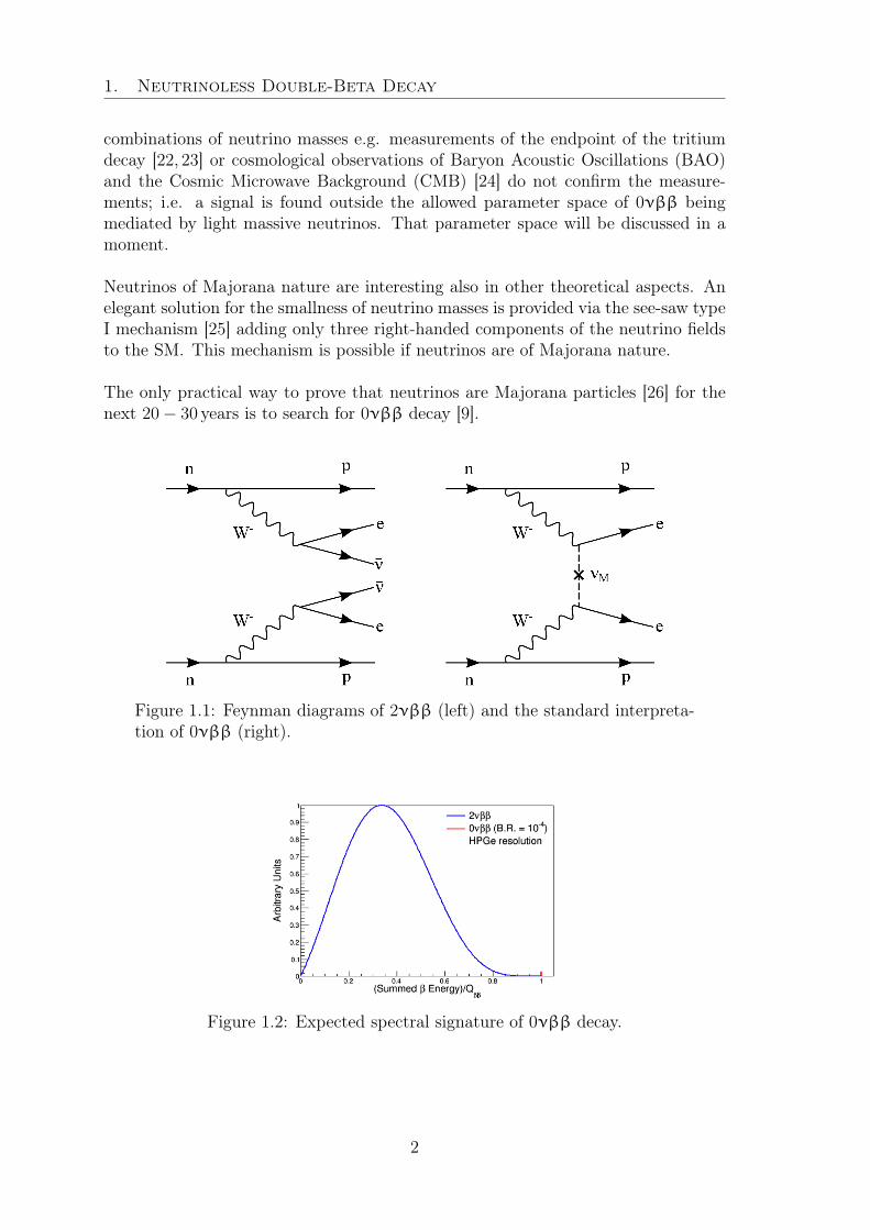
The possible Majorana nature of neutral spin-1/2 particles was pointed out alreadyin 1937 by Ettore Majorana [8]. Being the only neutral fermion, the neutrino is thesole candidates for a Majorana particle in the SM. Moreover, compelling evidencefor a nonzero neutrino mass was found by neutrino oscillation experiments [3–5].The standard interpretation of 0νββ decay is the mediation by light massive neu-trinos which fulfill the Majorana condition ν = ν as dominant process. 0νββ decay— mediated by light Majorana neutrinos — is visualized in contrast to the knowndecay mode, 2νββ, in Figure 1.1, by the corresponding Feynman diagrams.
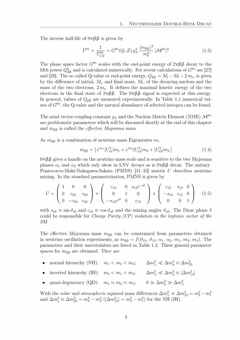
The expected signature of such a decay — in the standard interpretation — wouldbe a peak at the end-point of the continuous 2νββ spectrum (see Figure 1.2).
It shall be noted that quite some non-standard interpretations of 0νββ decay existbut are not considered in the following. See e.g. [9] for a compilation of non-standardinterpretations and further reference. They become interesting if experiments look-ing for 0νββ decay see a signal, while experiments which are sensitive to other
1
1. Neutrinoless Double-Beta Decay
combinations of neutrino masses e.g. measurements of the endpoint of the tritiumdecay [22, 23] or cosmological observations of Baryon Acoustic Oscillations (BAO)and the Cosmic Microwave Background (CMB) [24] do not confirm the measure-ments; i.e. a signal is found outside the allowed parameter space of 0νββ beingmediated by light massive neutrinos. That parameter space will be discussed in amoment.
Neutrinos of Majorana nature are interesting also in other theoretical aspects. Anelegant solution for the smallness of neutrino masses is provided via the see-saw typeI mechanism [25] adding only three right-handed components of the neutrino fieldsto the SM. This mechanism is possible if neutrinos are of Majorana nature.
The only practical way to prove that neutrinos are Majorana particles [26] for thenext 20− 30 years is to search for 0νββ decay [9].
Figure 1.1: Feynman diagrams of 2νββ (left) and the standard interpreta-tion of 0νββ (right).
Figure 1.2: Expected spectral signature of 0νββ decay.
2
1. Neutrinoless Double-Beta Decay
The inverse half-life of 0νββ is given by
Γ0ν =1
T 0ν1/2
= G0ν(Q,Z) g4A
〈mββ〉2
m2e
|M0ν|2 (1.3)
The phase space factor G0ν scales with the end-point energy of 2νββ decay to thefifth power Q5
ββ and is calculated numerically. For recent calculations of G0ν see [27]and [28]. The so called Q-value or end-point energy, Qββ = Mi−Mf −2me, is givenby the difference of initial, Mi, and final mass, Mf , of the decaying nucleus and themass of the two electrons, 2me. It defines the maximal kinetic energy of the twoelectrons in the final state of 2νββ. The 0νββ signal is expected at this energy.In general, values of Qββ are measured experimentally. In Table 1.1 numerical val-ues of G0ν, the Q-value and the natural abundance of selected isotopes can be found.
The axial vector coupling constant gA and the Nuclear Matrix Element (NME)M0ν
are problematic parameters which will be discussed shortly at the end of this chapterand mββ is called the effective Majorana mass.
As mββ is a combination of neutrino mass Eigenstates mi
mββ =∣∣ eiα1|U2
e1|m1 + eiα2|U2e2|m2 + |U2
e3|m3
∣∣ (1.4)
0νββ gives a handle on the neutrino mass scale and is sensitive to the two Majoranaphases α1 and α2 which only show in LNV decays as is 0νββ decay. The unitaryPontecorvo-Maki-Nakagawa-Sakata (PMNS) [31–33] matrix U describes neutrinomixing. In the standard parametrization, PMNS is given by
U =
1 0 0
0 c23 s23
0 −s23 c23
× c13 0 s13e
−iδ
0 1 0
−s13eiδ 0 c13
× c12 s12 0
−s12 c12 0
0 0 1
(1.5)
with sab ≡ sinϑab and cab ≡ cosϑab and the mixing angles ϑab. The Dirac phase δcould be responsible for Charge Parity (CP) violation in the leptonic sector of theSM.
The effective Majorana mass mββ can be constrained from parameters obtainedin neutrino oscillation experiments, as mββ = f(ϑ12, ϑ13, α1, α2, m1, m2, m3). Theparameters and their uncertainties are listed in Table 1.2. Three general parameterspaces for mββ are obtained. They are
• normal hierarchy (NH): m1 < m2 < m3; ∆m2 ∆m2
a ≡ ∆m223
• inverted hierarchy (IH): m3 < m1 < m2; ∆m2 ∆m2
a ≡ |∆m213|
• quasi-degeneracy (QD): m1 ' m2 ' m3; 0 ∆m2a ∆m2
With the solar and atmospheric squared mass differences ∆m2 ≡ ∆m2
12 = m22−m2
1
and ∆m2a ≡ ∆m2
23 = m23 −m2
2 (|∆m213| = m2
3 −m21) for the NH (IH).
3
1. Neutrinoless Double-Beta Decay
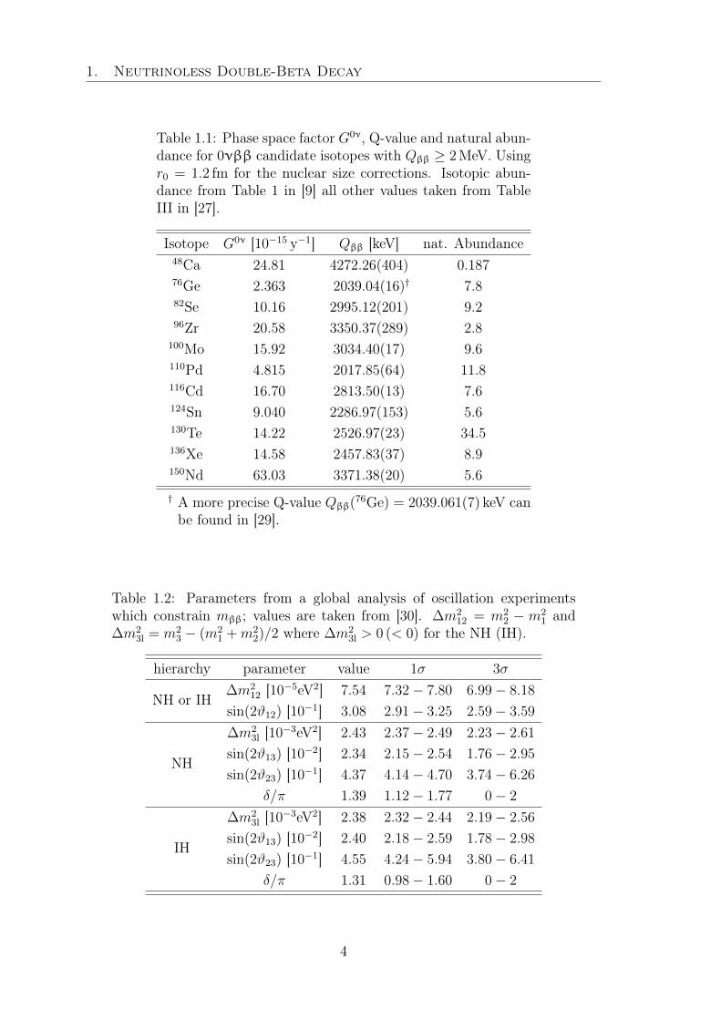
Table 1.1: Phase space factor G0ν, Q-value and natural abun-dance for 0νββ candidate isotopes with Qββ ≥ 2MeV. Usingr0 = 1.2 fm for the nuclear size corrections. Isotopic abun-dance from Table 1 in [9] all other values taken from TableIII in [27].
Isotope G0ν [10−15 y−1] Qββ [keV] nat. Abundance48Ca 24.81 4272.26(404) 0.18776Ge 2.363 2039.04(16)† 7.882Se 10.16 2995.12(201) 9.296Zr 20.58 3350.37(289) 2.8
100Mo 15.92 3034.40(17) 9.6110Pd 4.815 2017.85(64) 11.8116Cd 16.70 2813.50(13) 7.6124Sn 9.040 2286.97(153) 5.6130Te 14.22 2526.97(23) 34.5136Xe 14.58 2457.83(37) 8.9150Nd 63.03 3371.38(20) 5.6† A more precise Q-value Qββ(76Ge) = 2039.061(7) keV canbe found in [29].
Table 1.2: Parameters from a global analysis of oscillation experimentswhich constrain mββ; values are taken from [30]. ∆m2
12 = m22 − m2
1 and∆m2
3l = m23 − (m2
1 +m22)/2 where ∆m2
3l > 0 (< 0) for the NH (IH).
hierarchy parameter value 1σ 3σ
NH or IH∆m2
12 [10−5eV2] 7.54 7.32− 7.80 6.99− 8.18
sin(2ϑ12) [10−1] 3.08 2.91− 3.25 2.59− 3.59
NH
∆m23l [10−3eV2] 2.43 2.37− 2.49 2.23− 2.61
sin(2ϑ13) [10−2] 2.34 2.15− 2.54 1.76− 2.95
sin(2ϑ23) [10−1] 4.37 4.14− 4.70 3.74− 6.26
δ/π 1.39 1.12− 1.77 0− 2
IH
∆m23l [10−3eV2] 2.38 2.32− 2.44 2.19− 2.56
sin(2ϑ13) [10−2] 2.40 2.18− 2.59 1.78− 2.98
sin(2ϑ23) [10−1] 4.55 4.24− 5.94 3.80− 6.41
δ/π 1.31 0.98− 1.60 0− 2
4
1. Neutrinoless Double-Beta Decay
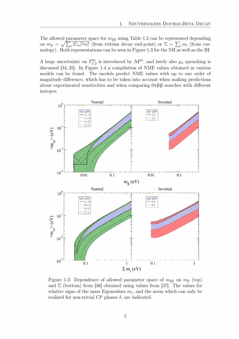
The allowed parameter space for mββ using Table 1.2 can be represented dependingon mβ =
√∑i |Uei|2m2
i (from tritium decay end-point) or Σ =∑
imi (from cos-mology). Both representations can be seen in Figure 1.3 for the NH as well as the IH.
A large uncertainty on T 0ν1/2 is introduced by M0ν, and lately also gA quenching is
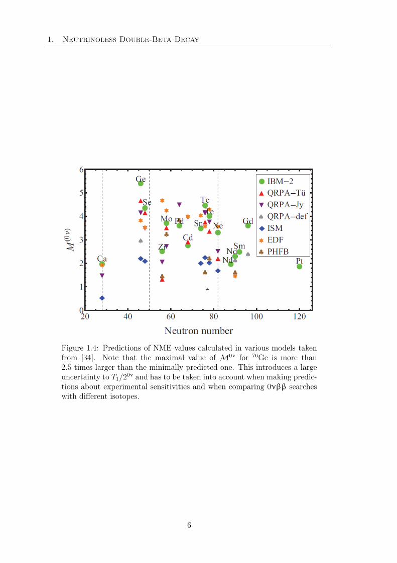
discussed [34, 35]. In Figure 1.4 a compilation of NME values obtained in variousmodels can be found. The models predict NME values with up to one order ofmagnitude difference, which has to be taken into account when making predictionsabout experimental sensitivities and when comparing 0νββ searches with differentisotopes.
Figure 1.3: Dependence of allowed parameter space of mββ on mβ (top)and Σ (bottom) from [36] obtained using values from [37]. The values forrelative signs of the mass Eigenvalues mi, and the areas which can only berealized for non-trivial CP phases δ, are indicated.
5
1. Neutrinoless Double-Beta Decay
Figure 1.4: Predictions of NME values calculated in various models takenfrom [34]. Note that the maximal value of M0ν for 76Ge is more than2.5 times larger than the minimally predicted one. This introduces a largeuncertainty to T1/2
0ν and has to be taken into account when making predic-tions about experimental sensitivities and when comparing 0νββ searcheswith different isotopes.
6
Chapter 2
Experimental view on NeutrinolessDouble-Beta Decay
Background reduction is one of the main issues low background experiments have toface. In this chapter we derive an expression for the sensitivity of 0νββ experiments[38] which shows how important it is to keep the background as low as possible.Finally, the Gerda experiment is introduced.
2.1 Experimental sensitivityThe sensitivity of a 0νββ experiment depends strongly on the experimental con-ditions. Every experiment conducted with presently known techniques will havebackground. If assumed flat, the number of background events can be written as
NB = Bi M ∆t∆E (2.1)
with the source mass M1 and the measurement time ∆t in the energy window ∆Ewhich depends on the energy resolution. The background index (BI) Bi is usuallygiven in counts kg−1 keV−1 yr−1.
A criterion for the discovery potential of a 0νββ decay experiment can be expressedas Nββ = C1
√Nββ +NB with the confidence level C1 in units of the σ of a Poisson
distribution and the number of signal counts from 0νββ decay Nββ. If we requirea certain signal to background ratio Nββ/NB ≡ rSB the number of signal events isgiven as
Nββ = C1
√(1 + rSB)NB = C1γ
√NB (2.2)
We can further express the number of signal events using the decay rate λββ
Nββ = λββNA
WaεM ∆t (2.3)
where Avogadro’s number NA and the atomic weight W are physical constants andthe isotopic abundance 0 < a ≤ 1 is defined by the natural abundance or the en-richment fraction.
1In the Gerda experiment, as detector and source are equivalent, M is the total detector mass.
7
2.2. Germanium as a 0νββ candidate
Combining equations 2.1-2.3 and writing the decay rate in terms of the half-lifeT 0ν
1/2 = ln(2)/λββ we get an expression for the sensitivity
T 0ν1/2 = α1 a ε
√M∆t
Bi ∆E(2.4)
whereα1 =
ln(2)NA
W
(C1
√1 + rSB
)−1 (2.5)
When comparing different experiments rSB is chosen and is then fixed.
If we assume that the isotopic abundance, the detection efficiency and the energyresolution are naturally given, a higher sensitivity can be reached increasing thesource mass M , the measurement time ∆t and reducing the background Bi as muchas possible. In general, the source material is expensive and sometimes hard to get,and each experimental setup has a limit on how much material can be hosted. Also,the measurement time has to stay in reasonable boundaries, let’s say < 10 yr. Inconclusion, the only real handle to get a better sensitivity is to reduce the back-ground.
For a certain time no background counts are expected in the Region of Interest(ROI)2. Optimal experimental conditions are reached if this limit of zero-backgroundis maintained for the major part of the experimental runtime. Without backgroundthe sensitivity takes the form
T 0ν1/2 = α2 a εM ∆t (2.6)
with α2 = α1
√1 + rSB.
Note that the dependence on source mass and measurement time in Equation 2.6is linear, in contrast to Equation 2.4 where T 0ν
1/2 ∝√M∆t. Thus, in the limit of
zero-background the experimental resources of source mass and time are used in themost efficient way. In general, the design goal for the background index of every lowbackground experiment is based on the objective to reach this limit. From Equa-tion 2.1 it is evident that the higher the source mass and measurement time thelower Bi has to be, in order to stay in the limit of zero-background.
2.2 Germanium as a 0νββ candidateExperiments in 0νββ decay searches make use of very different 0νββ candidateisotopes. In some sense germanium is not a preferable 0νββ candidate isotope:the decay rate (Equation 1.3) depends upon the phase space factor (see Table 1.1),hence, the expected half-life is lower for many other 0νββ candidates as can be seenin Figure 2.1.
2The region around Qββ
8
2.3. The Gerda experiment
In the case of nonzero-background the sensitivity of a 0νββ experiment dependsupon the energy resolution (see Equation 2.4). Hence, the relatively long expectedhalf-life is partly compensated by the exceptional energy resolution achievable withgermanium detectors (see Section 3.3). Moreover, 2νββ decay is an irreduciblebackground source for 0νββ decay searches. Thus, for longer half-lives a good en-ergy resolution is necessary to distinguish the peak expected from 0νββ decay fromthe tail of the distribution of 2νββ decay.
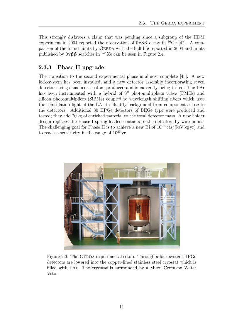
2.3 The Gerda experimentThe Germanium Detector Array (Gerda) experiment is located at LaboratoriNazionali del Gran Sasso (LNGS) of Istituto Nazionale di Fisica Nucleare (INFN)in Italy with an overburden of about 3600m.w.e.. Gerda is operating High PurityGermanium (HPGe) detectors bare in liquid Argon (LAr) [14], which are enrichedin the 0νββ candidate isotope 76Ge. The setup, which is shown in Figure 2.3, in-corporates a copper lined stainless steel cryostat, 4m in diameter, containing 63 m3
of LAr. It is surrounded by a 3-m-thick active Muon Cerenkov Water Veto, whichserves also as a passive γ and neutron shield. The Muon Veto is instrumented with66 photomultipliers in order to identify muon induced events. The detectors aresubmerged into the cryostat through a lock-system from a glove box in the cleanroom above the neck of the cryostat. An additional muon veto made of plastic scin-tillator panels is installed on the roof of the clean room. It is meant to cover theweak spot of the water veto: the neck of the cryostat. Special care was devoted tothe selection of radiopure materials for construction, and to a sparse design of allcomponents near the detectors (holders, electronics, cables, etc.) to reduce therebyintroduced background.
2.3.1 The Gerda detectors
The Gerda detectors are p -type HPGe detectors (for details see the next Chapter 3)enriched in the isotope 76Ge. In the experimental Phase I mainly semi-coaxial (Coax)detectors were used while new detectors were produced for the second experimentalstage. The Phase II detectors are of Broad Energy Germanium (BEGe) type. InFigure 2.2 the Coax and BEGe detector geometry can be seen alongside the P-typePoint Contact (PPC) detector geometry which is similar to the BEGe but has aneven smaller read-out contact.
2.3.2 Phase I result
Gerda has concluded the first experimental phase publishing a lower limit on thehalf-life of 0νββ of T 0ν
1/2 > 2.1 · 1025 yr (90%C.L.), with a median sensitivity ofT 0ν
1/2 > 2.4 ·1025 yr [39]. The achieved background index of 10−2 cts/(keV−1kg−1yr−1)at Qββ was unpreceded. By combining results with prior 0νββ searches by theHeidelberg-Moscow experiment (HDM) [40] and the International Germanium Ex-periment (IGEX) [41] the limit was strengthened to T 0ν
1/2 > 3.0 · 1025 yr (90%C.L.).
9
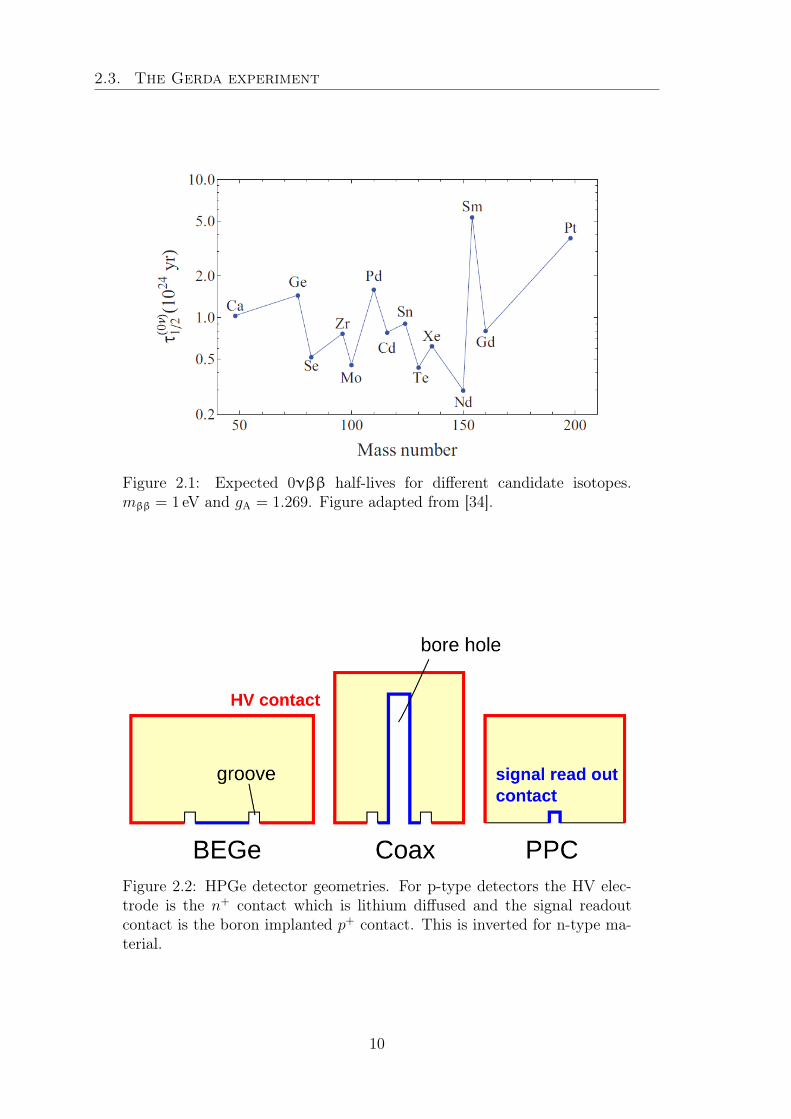
2.3. The Gerda experiment
Figure 2.1: Expected 0νββ half-lives for different candidate isotopes.mββ = 1 eV and gA = 1.269. Figure adapted from [34].
Figure 2.2: HPGe detector geometries. For p-type detectors the HV elec-trode is the n+ contact which is lithium diffused and the signal readoutcontact is the boron implanted p+ contact. This is inverted for n-type ma-terial.
10
2.3. The Gerda experiment
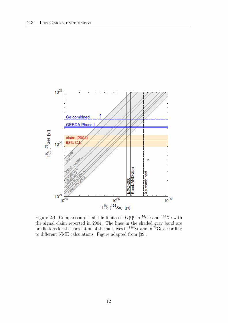
This strongly disfavors a claim that was pending since a subgroup of the HDMexperiment in 2004 reported the observation of 0νββ decay in 76Ge [42]. A com-parison of the found limits by Gerda with the half-life reported in 2004 and limitspublished by 0νββ searches in 136Xe can be seen in Figure 2.4.
2.3.3 Phase II upgrade
The transition to the second experimental phase is almost complete [43]. A newlock-system has been installed, and a new detector assembly incorporating sevendetector strings has been custom produced and is currently being tested. The LArhas been instrumented with a hybrid of 8" photomultipliers tubes (PMTs) andsilicon photomultipliers (SiPMs) coupled to wavelength shifting fibers which usesthe scintillation light of the LAr to identify background from components close tothe detectors. Additional 30 HPGe detectors of BEGe type were produced andtested; they add 20 kg of enriched material to the total detector mass. A new holderdesign replaces the Phase I spring-loaded contacts to the detectors by wire bonds.The challenging goal for Phase II is to achieve a new BI of 10−3 cts/(keV kg yr) andto reach a sensitivity in the range of 1026 yr.
Figure 2.3: The Gerda experimental setup. Through a lock system HPGedetectors are lowered into the copper-lined stainless steel cryostat which isfilled with LAr. The cryostat is surrounded by a Muon Cerenkov WaterVeto.
11
2.3. The Gerda experiment
Figure 2.4: Comparison of half-life limits of 0νββ in 76Ge and 136Xe withthe signal claim reported in 2004. The lines in the shaded gray band arepredictions for the correlation of the half-lives in 136Xe and in 76Ge accordingto different NME calculations. Figure adapted from [39].
12
Chapter 3
High Purity Germanium detectors
In the next section a short overview of interactions of photons with matter is given.Hereafter, germanium is introduced as a semiconductor material and the propertiesof semiconductor diode detector are discussed. The following information can easilybe found in every text book about radiation and detection measurements and semi-conductor devices. Still one of the best and easiest to understand introductions isgiven in [44].
3.1 Interaction of photons with matter
Photons are neutral and massless, thus being able to travel deeper in material thancharged particles. In their interactions with matter the incident photon can beabsorbed and disappear, or be scattered and change energy and/or direction. Whendetecting γ radiation, i.e. high-energetic photon radiation originating from nucleardecays, only inelastic processes play a role where energy is absorbed in the detectormaterial or transferred to it. Nevertheless, a very brief description of elastic processesis given.
3.1.1 Elastic scattering
An interactions in which the photon energy in the initial and final state of the re-action is conserved is called elastic scattering.
Thomson scattering is the low energy limit (visible part of the electromagnetic spec-trum) of Compton scattering, where a photon gets elastically scattered on free un-polarizable charged particles e.g. free electrons. The electromagnetic componentof the photon field accelerates a free electron which in turn radiates at the samefrequency. Depending on the observation angle the observed radiation is more orless polarized.
Rayleigh scattering is the elastic scattering of photons on harmonically bound elec-trons e.g. shell electrons in an atom. The differential cross section of Rayleighscattering depends on the wavelength of the photon to the fourth power, in contrastto Thomson scattering, which does not depend on the photon wavelength.
13
3.1. Interaction of photons with matter
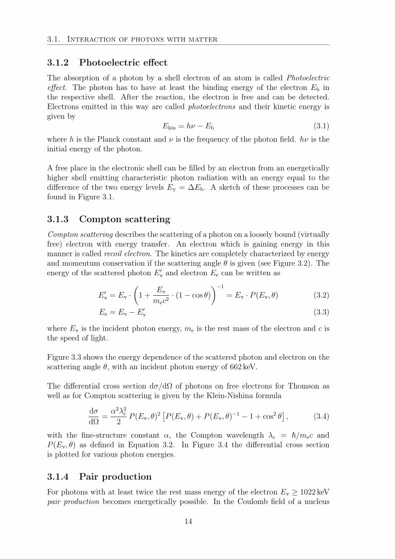
3.1.2 Photoelectric effect
The absorption of a photon by a shell electron of an atom is called Photoelectriceffect. The photon has to have at least the binding energy of the electron Eb inthe respective shell. After the reaction, the electron is free and can be detected.Electrons emitted in this way are called photoelectrons and their kinetic energy isgiven by
Ekin = hν − Eb (3.1)
where h is the Planck constant and ν is the frequency of the photon field. hν is theinitial energy of the photon.
A free place in the electronic shell can be filled by an electron from an energeticallyhigher shell emitting characteristic photon radiation with an energy equal to thedifference of the two energy levels Eγ = ∆Eb. A sketch of these processes can befound in Figure 3.1.
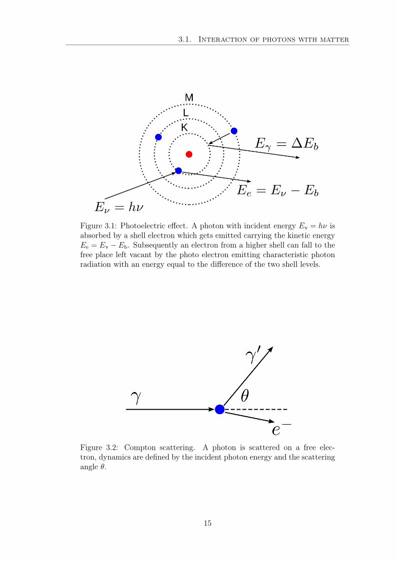
3.1.3 Compton scattering
Compton scattering describes the scattering of a photon on a loosely bound (virtuallyfree) electron with energy transfer. An electron which is gaining energy in thismanner is called recoil electron. The kinetics are completely characterized by energyand momentum conservation if the scattering angle θ is given (see Figure 3.2). Theenergy of the scattered photon E ′ν and electron Ee can be written as
E ′ν = Eν ·(
1 +Eν
mec2· (1− cos θ)
)−1
= Eν · P (Eν, θ) (3.2)
Ee = Eν − E ′ν (3.3)
where Eν is the incident photon energy, me is the rest mass of the electron and c isthe speed of light.
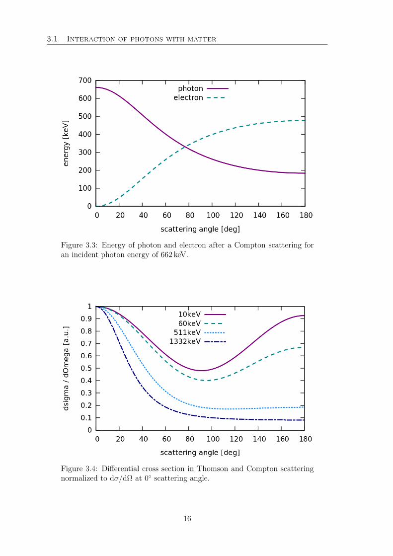
Figure 3.3 shows the energy dependence of the scattered photon and electron on thescattering angle θ, with an incident photon energy of 662 keV.
The differential cross section dσ/dΩ of photons on free electrons for Thomson aswell as for Compton scattering is given by the Klein-Nishina formula
dσ
dΩ=α2λ2
c
2P (Eν, θ)
2[P (Eν, θ) + P (Eν, θ)
−1 − 1 + cos2 θ], (3.4)
with the fine-structure constant α, the Compton wavelength λc = ~/mec andP (Eν, θ) as defined in Equation 3.2. In Figure 3.4 the differential cross sectionis plotted for various photon energies.
3.1.4 Pair production
For photons with at least twice the rest mass energy of the electron Eν ≥ 1022 keVpair production becomes energetically possible. In the Coulomb field of a nucleus
14
3.1. Interaction of photons with matter
Figure 3.1: Photoelectric effect. A photon with incident energy Eν = hν isabsorbed by a shell electron which gets emitted carrying the kinetic energyEe = Eν − Eb. Subsequently an electron from a higher shell can fall to thefree place left vacant by the photo electron emitting characteristic photonradiation with an energy equal to the difference of the two shell levels.
Figure 3.2: Compton scattering. A photon is scattered on a free elec-tron, dynamics are defined by the incident photon energy and the scatteringangle θ.
15
3.1. Interaction of photons with matter
Figure 3.3: Energy of photon and electron after a Compton scattering foran incident photon energy of 662 keV.
Figure 3.4: Differential cross section in Thomson and Compton scatteringnormalized to dσ/dΩ at 0 scattering angle.
16
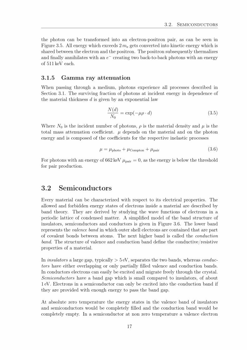
3.2. Semiconductors
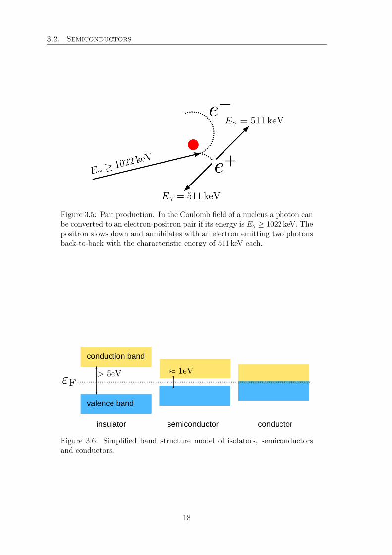
the photon can be transformed into an electron-positron pair, as can be seen inFigure 3.5. All energy which exceeds 2me gets converted into kinetic energy which isshared between the electron and the positron. The positron subsequently thermalizesand finally annihilates with an e− creating two back-to-back photons with an energyof 511 keV each.
3.1.5 Gamma ray attenuation
When passing through a medium, photons experience all processes described inSection 3.1. The surviving fraction of photons at incident energy in dependence ofthe material thickness d is given by an exponential law
N(d)
N0
= exp(−µρ · d) (3.5)
Where N0 is the incident number of photons, ρ is the material density and µ is thetotal mass attenuation coefficient. µ depends on the material and on the photonenergy and is composed of the coefficients for the respective inelastic processes
µ = µphoto + µCompton + µpair (3.6)
For photons with an energy of 662 keV µpair = 0, as the energy is below the thresholdfor pair production.
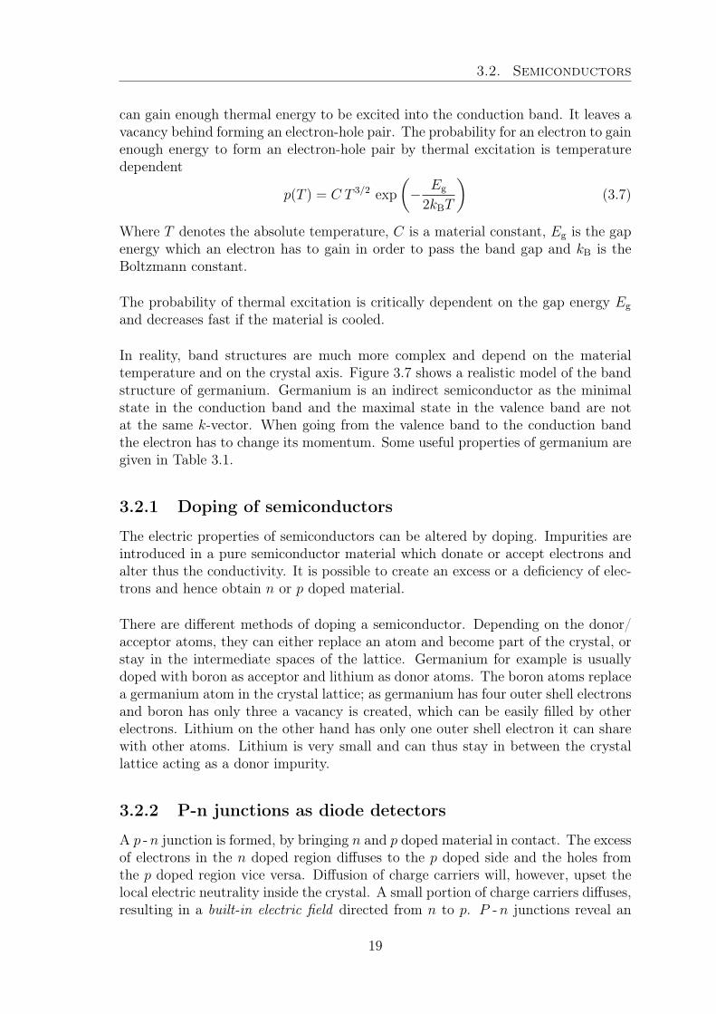
3.2 SemiconductorsEvery material can be characterized with respect to its electrical properties. Theallowed and forbidden energy states of electrons inside a material are described byband theory. They are derived by studying the wave functions of electrons in aperiodic lattice of condensed matter. A simplified model of the band structure ofinsulators, semiconductors and conductors is given in Figure 3.6. The lower bandrepresents the valence band in which outer shell electrons are contained that are partof covalent bonds between atoms. The next higher band is called the conductionband. The structure of valence and conduction band define the conductive/resistiveproperties of a material.
In insulators a large gap, typically > 5 eV, separates the two bands, whereas conduc-tors have either overlapping or only partially filled valence and conduction bands.In conductors electrons can easily be excited and migrate freely through the crystal.Semiconductors have a band gap which is small compared to insulators, of about1 eV. Electrons in a semiconductor can only be excited into the conduction band ifthey are provided with enough energy to pass the band gap.
At absolute zero temperature the energy states in the valence band of insulatorsand semiconductors would be completely filled and the conduction band would becompletely empty. In a semiconductor at non zero temperature a valence electron
17
3.2. Semiconductors
Figure 3.5: Pair production. In the Coulomb field of a nucleus a photon canbe converted to an electron-positron pair if its energy is Eγ ≥ 1022 keV. Thepositron slows down and annihilates with an electron emitting two photonsback-to-back with the characteristic energy of 511 keV each.
Figure 3.6: Simplified band structure model of isolators, semiconductorsand conductors.
18
3.2. Semiconductors
can gain enough thermal energy to be excited into the conduction band. It leaves avacancy behind forming an electron-hole pair. The probability for an electron to gainenough energy to form an electron-hole pair by thermal excitation is temperaturedependent
p(T ) = C T 3/2 exp
(− Eg
2kBT
)(3.7)
Where T denotes the absolute temperature, C is a material constant, Eg is the gapenergy which an electron has to gain in order to pass the band gap and kB is theBoltzmann constant.
The probability of thermal excitation is critically dependent on the gap energy Eg
and decreases fast if the material is cooled.
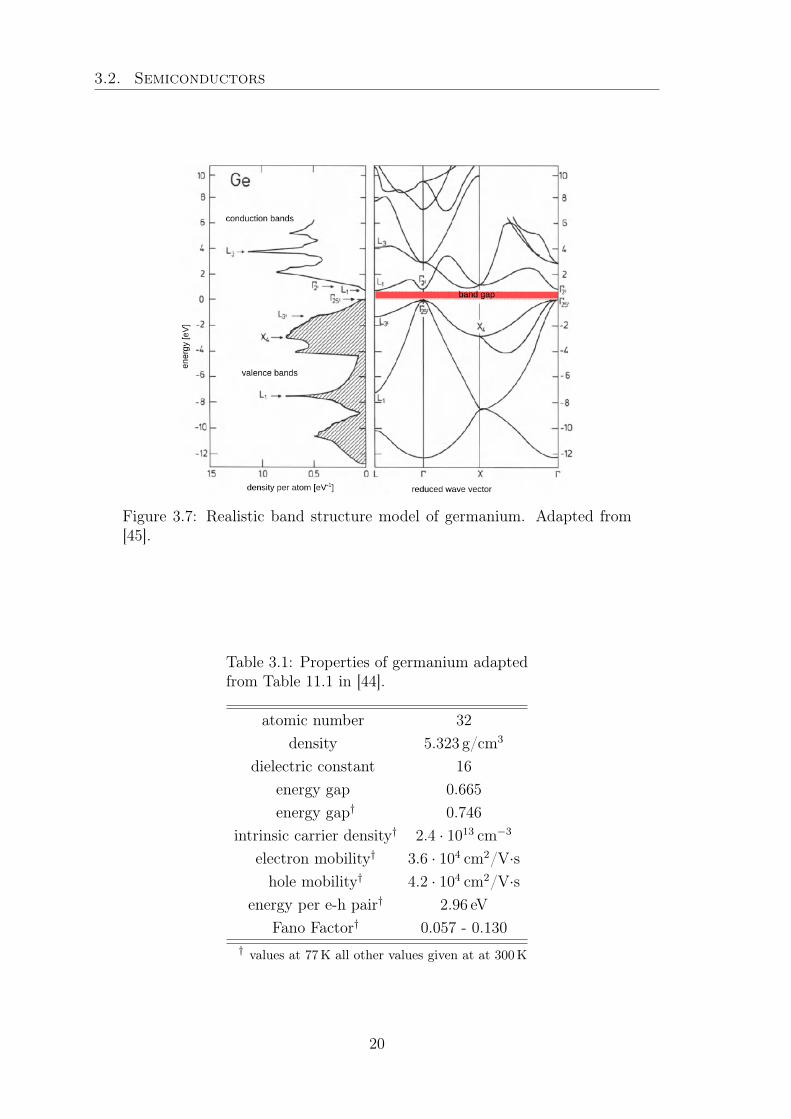
In reality, band structures are much more complex and depend on the materialtemperature and on the crystal axis. Figure 3.7 shows a realistic model of the bandstructure of germanium. Germanium is an indirect semiconductor as the minimalstate in the conduction band and the maximal state in the valence band are notat the same k-vector. When going from the valence band to the conduction bandthe electron has to change its momentum. Some useful properties of germanium aregiven in Table 3.1.
3.2.1 Doping of semiconductors
The electric properties of semiconductors can be altered by doping. Impurities areintroduced in a pure semiconductor material which donate or accept electrons andalter thus the conductivity. It is possible to create an excess or a deficiency of elec-trons and hence obtain n or p doped material.
There are different methods of doping a semiconductor. Depending on the donor/acceptor atoms, they can either replace an atom and become part of the crystal, orstay in the intermediate spaces of the lattice. Germanium for example is usuallydoped with boron as acceptor and lithium as donor atoms. The boron atoms replacea germanium atom in the crystal lattice; as germanium has four outer shell electronsand boron has only three a vacancy is created, which can be easily filled by otherelectrons. Lithium on the other hand has only one outer shell electron it can sharewith other atoms. Lithium is very small and can thus stay in between the crystallattice acting as a donor impurity.
3.2.2 P-n junctions as diode detectors
A p -n junction is formed, by bringing n and p doped material in contact. The excessof electrons in the n doped region diffuses to the p doped side and the holes fromthe p doped region vice versa. Diffusion of charge carriers will, however, upset thelocal electric neutrality inside the crystal. A small portion of charge carriers diffuses,resulting in a built-in electric field directed from n to p. P -n junctions reveal an
19
3.2. Semiconductors
Figure 3.7: Realistic band structure model of germanium. Adapted from[45].
Table 3.1: Properties of germanium adaptedfrom Table 11.1 in [44].
atomic number 32density 5.323 g/cm3
dielectric constant 16energy gap 0.665energy gap† 0.746
intrinsic carrier density† 2.4 · 1013 cm−3
electron mobility† 3.6 · 104 cm2/V·shole mobility† 4.2 · 104 cm2/V·s
energy per e-h pair† 2.96 eVFano Factor† 0.057 - 0.130
† values at 77K all other values given at at 300K
20
3.3. High Purity Germanium detectors
asymmetric conductance transmitting current only in one direction; they are diodes.
The contact zone in a p -n junction is depleted of free charge carriers. We call thisthe depletion region. It can be enlarged applying an inverse bias voltage. If energy isdeposited inside the depletion region, e.g. by ionizing radiation, electron-hole pairsare created. They drift along the internal electric field lines and can be collectedand read. Thus, semiconductor diodes can be used as detectors for ionizing radiation.
3.3 High Purity Germanium detectorsTo further enlarge the depletion zone, diode detectors are built as p - I -n junctionsinstead of simple p -n junctions. I stands for intrinsic semiconductor material as itis undoped and has intrinsic impurities only. The outer surface is doped to form ann+1 and a p+ contact and the interior region can be fully depleted.
Germanium detectors are produced with depletion layers of several centimeters inheight and areas of many square centimeters. They are operated at a reverse bias of afew thousand volts. To achieve such thick depletion layers and collect all the chargesgenerated in the depletion region it is essential that the net-impurity concentrationdoes not exceed 2.5 · 10−13 impurities / Ge-atom [46]. Because of the ultra-purityof the detector material these detectors are called High Purity Germanium (HPGe)detectors.
All properties of HPGe detectors are defined by the intrinsic impurity concentration:a surplus of negative (positive) intrinsic charges will create an n-type (p-type) germa-nium detector. In the production process the intrinsic impurities can be influencedwithin certain limits and the type of detector can be chosen.
3.3.1 Signal formation
If energy is deposited in a diode detector a charge cloud is formed. The chargesdrift along the field lines of the interior electric field. An induced charge Q on theread out electrode is formed by their movement along the trajectory2 rq(t). Asdemonstrated independently by Shockley and Ramo [47] the charge signal on theelectrode is given by
Q(t) = −q φw(rq(t)) (3.8)
The current signal, which is given by the time derivative of Q(t), is then
I(t) =dQ
dt= q vd(rq(t)) · Ew(rq(t)) (3.9)
with the total charge q, the weighting potential φw(rq(t)) and the weighting fieldEw(rq(t)) = −∇φw(rq(t)); and the charge carrier drift velocity vd(rq(t)) = drq(t)/dt.
1Here: + stands for highly doped material2position rq at time t
21
3.3. High Purity Germanium detectors
The weighting potential is defined as the potential that can be calculated solvingthe Laplace equation ∇2φw = 0 for the boundary conditions φw(b∗) = 1 on the readout electrode b∗ and φw(b∗) = 0 on all other boundaries when removing all internalcharges.
3.3.2 Charge carrier mobilities
The determination of the charge carrier mobilities and thereby the drift velocitiesvd inside the detector crystal is a rather non-trivial problem: e.g. it depends on thefield orientation with respect to the crystal lattice. Therefore, we will not discussthis in detail. It shall be noted that both for electrons and for holes the mobility isstrongly anisotropic. Large differences for the longitudinal and tangential velocityanisotropy of electrons and holes are observed [48]. They cause specific rise times andpulse shapes as a function of the location of energy deposition inside the crystal [49].Along the three crystallographic axis 〈100〉, 〈110〉 and 〈111〉 direct information onthe longitudinal anisotropy can be obtained experimentally; when simulating pulseshapes of germanium detectors the anisotropy of the charge carrier mobilities hasto be taken into account.
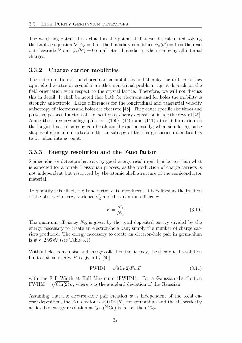
3.3.3 Energy resolution and the Fano factor
Semiconductor detectors have a very good energy resolution. It is better than whatis expected for a purely Poissonian process, as the production of charge carriers isnot independent but restricted by the atomic shell structure of the semiconductormaterial.
To quantify this effect, the Fano factor F is introduced. It is defined as the fractionof the observed energy variance σ2
E and the quantum efficiency
F =σ2
E
NQ
(3.10)
The quantum efficiency NQ is given by the total deposited energy divided by theenergy necessary to create an electron-hole pair; simply the number of charge car-riers produced. The energy necessary to create an electron-hole pair in germaniumis w ≈ 2.96 eV (see Table 3.1).
Without electronic noise and charge collection inefficiency, the theoretical resolutionlimit at some energy E is given by [50]
FWHM =√
8 ln(2)FwE (3.11)
with the Full Width at Half Maximum (FWHM). For a Gaussian distributionFWHM =
√8 ln(2)σ, where σ is the standard deviation of the Gaussian.
Assuming that the electron-hole pair creation w is independent of the total en-ergy deposition, the Fano factor is < 0.06 [51] for germanium and the theoreticallyachievable energy resolution at Qββ(76Ge) is better than 1%.
22
3.3. High Purity Germanium detectors
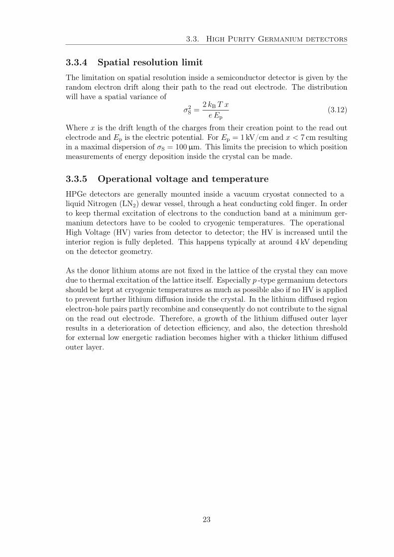
3.3.4 Spatial resolution limit
The limitation on spatial resolution inside a semiconductor detector is given by therandom electron drift along their path to the read out electrode. The distributionwill have a spatial variance of
σ2S =
2 kB T x
eEp
(3.12)
Where x is the drift length of the charges from their creation point to the read outelectrode and Ep is the electric potential. For Ep = 1 kV/cm and x < 7 cm resultingin a maximal dispersion of σS = 100µm. This limits the precision to which positionmeasurements of energy deposition inside the crystal can be made.
3.3.5 Operational voltage and temperature
HPGe detectors are generally mounted inside a vacuum cryostat connected to aliquid Nitrogen (LN2) dewar vessel, through a heat conducting cold finger. In orderto keep thermal excitation of electrons to the conduction band at a minimum ger-manium detectors have to be cooled to cryogenic temperatures. The operationalHigh Voltage (HV) varies from detector to detector; the HV is increased until theinterior region is fully depleted. This happens typically at around 4 kV dependingon the detector geometry.
As the donor lithium atoms are not fixed in the lattice of the crystal they can movedue to thermal excitation of the lattice itself. Especially p -type germanium detectorsshould be kept at cryogenic temperatures as much as possible also if no HV is appliedto prevent further lithium diffusion inside the crystal. In the lithium diffused regionelectron-hole pairs partly recombine and consequently do not contribute to the signalon the read out electrode. Therefore, a growth of the lithium diffused outer layerresults in a deterioration of detection efficiency, and also, the detection thresholdfor external low energetic radiation becomes higher with a thicker lithium diffusedouter layer.
23

3.3. High Purity Germanium detectors
24
Chapter 4
Detector characterization
In order to perform the measurement campaign described in the following chaptersin a reliable manner, it was necessary to conduct an extensive characterization of thevarious detectors used. This is the argument of the following chapter. First of all,the data acquisition system (DAQ) including signal amplification is described; next,the energy reconstruction and calibration are explained and the determination of theoperational voltage with an HV scan is illustrated. Finally, an automatized systemis presented which serves to perform fine grain surface scans of HPGe detectors.Surface scans of two detectors taken with this system are compared.
4.1 Detectors and voltage supply
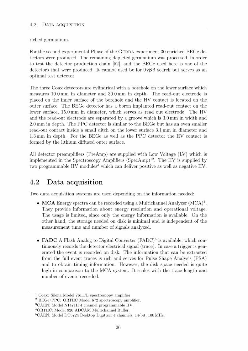
The HPGe detectors at hand are three Coax n -type detectors, one BEGe detectorand one detector of PPC geometry. The last two are made of p -type material. Allof them, except for the BEGe, contain a natural mixture of germanium isotopes. Asketch of the detector geometries can be found in Figure 2.2 and a summary of theirbasic properties is listed in Table 4.1.
The germanium of the Gerda detectors is enriched in the 0νββ candidate isotope76Ge. The residual material remaining after the enrichment process is commonlyreferred to as depleted material. It behaves chemically identical to natural and en-
Table 4.1: Available detectors. The BEGe and the PPC detector are ofp -type material with holes as dominant charge carriers, the Coax detectorsare n -type detectors with electrons as main charge carrier type.
operational dewardetector material voltage [kV] volume [l] height [mm] diameter [mm]BEGe depleted +4.0 7 40.7 74.1PPC natural +4.4 7 50.5 66.7
Coax1-3 natural −4.0 3 74.0 72.0
25
4.2. Data acquisition
riched germanium.
For the second experimental Phase of the Gerda experiment 30 enriched BEGe de-tectors were produced. The remaining depleted germanium was processed, in orderto test the detector production chain [52], and the BEGe used here is one of thedetectors that were produced. It cannot used be for 0νββ search but serves as anoptimal test detector.
The three Coax detectors are cylindrical with a borehole on the lower surface whichmeasures 10.0mm in diameter and 30.0mm in depth. The read-out electrode isplaced on the inner surface of the borehole and the HV contact is located on theouter surface. The BEGe detector has a boron implanted read-out contact on thelower surface, 15.0mm in diameter, which serves as read out electrode. The HVand the read-out electrode are separated by a groove which is 3.0mm in width and2.0mm in depth. The PPC detector is similar to the BEGe but has an even smallerread-out contact inside a small ditch on the lower surface 3.1mm in diameter and1.3mm in depth. For the BEGe as well as the PPC detector the HV contact isformed by the lithium diffused outer surface.
All detector preamplifiers (PreAmp) are supplied with Low Voltage (LV) which isimplemented in the Spectroscopy Amplifiers (SpecAmp)12. The HV is supplied bytwo programmable HV modules3 which can deliver positive as well as negative HV.
4.2 Data acquisitionTwo data acquisition systems are used depending on the information needed:
• MCA Energy spectra can be recorded using a Multichannel Analyzer (MCA)4.They provide information about energy resolution and operational voltage.The usage is limited, since only the energy information is available. On theother hand, the storage needed on disk is minimal and is independent of themeasurement time and number of signals analyzed.
• FADC A Flash Analog to Digital Converter (FADC)5 is available, which con-tinuously records the detector electrical signal (trace). In case a trigger is gen-erated the event is recorded on disk. The information that can be extractedfrom the full event traces is rich and serves for Pulse Shape Analysis (PSA)and to obtain timing information. However, the disk space needed is quitehigh in comparison to the MCA system. It scales with the trace length andnumber of events recorded.
1 Coax: Silena Model 7611/L spectroscopy amplifier2 BEGe/PPC: ORTEC Model 672 spectroscopy amplifier.3CAEN: Model N1471H 4 channel programmable HV.4ORTEC: Model 926 ADCAM Multichannel Buffer.5CAEN: Model DT5724 Desktop Digitizer 4 channels, 14-bit, 100MHz.
26
4.2. Data acquisition
4.2.1 Signal amplification
Each system is implemented with its proper amplification method.
The MCA system is used in combination with a SpecAmp12 which amplifies thesignal and applies a semi-Gaussian shaping to the pulses. The SpecAmps featurepole-zero adjustment, and the shaping constant and amplification gain can be cho-sen manually. The gain is set such as to utilize the full range of the MCA if possible.
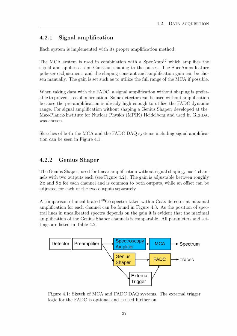
When taking data with the FADC, a signal amplification without shaping is prefer-able to prevent loss of information. Some detectors can be used without amplificationbecause the pre-amplification is already high enough to utilize the FADC dynamicrange. For signal amplification without shaping a Genius Shaper, developed at theMax-Planck-Institute for Nuclear Physics (MPIK) Heidelberg and used in Gerda,was chosen.
Sketches of both the MCA and the FADC DAQ systems including signal amplifica-tion can be seen in Figure 4.1.
4.2.2 Genius Shaper
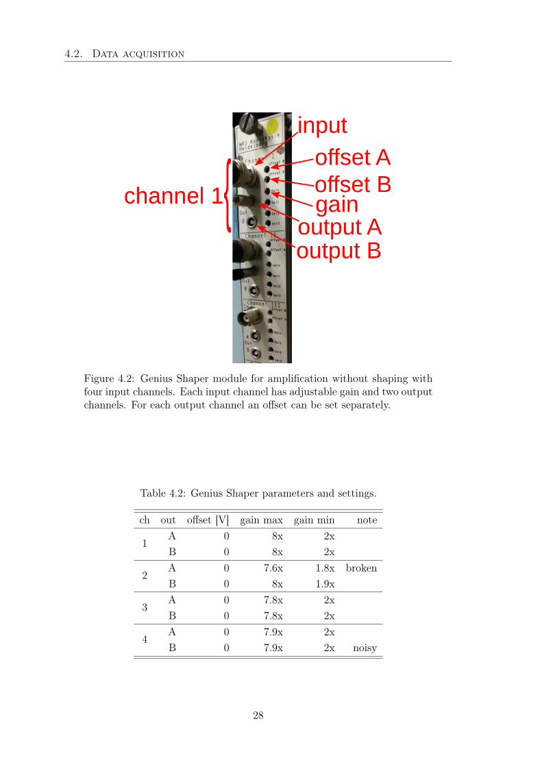
The Genius Shaper, used for linear amplification without signal shaping, has 4 chan-nels with two outputs each (see Figure 4.2). The gain is adjustable between roughly2 x and 8 x for each channel and is common to both outputs, while an offset can beadjusted for each of the two outputs separately.
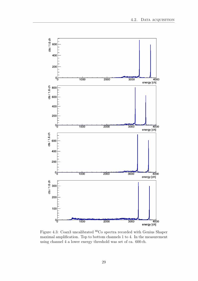
A comparison of uncalibrated 60Co spectra taken with a Coax detector at maximalamplification for each channel can be found in Figure 4.3. As the position of spec-tral lines in uncalibrated spectra depends on the gain it is evident that the maximalamplification of the Genius Shaper channels is comparable. All parameters and set-tings are listed in Table 4.2.
Figure 4.1: Sketch of MCA and FADC DAQ systems. The external triggerlogic for the FADC is optional and is used further on.
27
4.2. Data acquisition
Figure 4.2: Genius Shaper module for amplification without shaping withfour input channels. Each input channel has adjustable gain and two outputchannels. For each output channel an offset can be set separately.
Table 4.2: Genius Shaper parameters and settings.
ch out offset [V] gain max gain min note
1A 0 8x 2xB 0 8x 2x
2A 0 7.6x 1.8x brokenB 0 8x 1.9x
3A 0 7.8x 2xB 0 7.8x 2x
4A 0 7.9x 2xB 0 7.9x 2x noisy
28
4.2. Data acquisition
Figure 4.3: Coax3 uncalibrated 60Co spectra recorded with Genius Shapermaximal amplification. Top to bottom channels 1 to 4. In the measurementusing channel 4 a lower energy threshold was set of ca. 600 ch.
29
4.3. Data processing
4.3 Data processingPulses recorded with the FADC system can be fully analyzed off-line and containall information that can be extracted from the traces.
The data is processed as is usually done with Gerda data, using a multi-tierapproach. The raw data is transformed into a format based on Cern ROOTclasses [53] which is compressed by a factor of about two. We call the raw dataformat tier0 and the rootified format tier1. Both formats contain the same infor-mation but the tier1 format can be read by the Gerda analysis software [54, 55].A new decoder for this conversion was written and integrated into the Gerda soft-ware. It reads the tier0 data recorded with the FADC DAQ (see Section 4.2) andtransforms it into the tier1 format. For details about the multi-tier structure andthe implemented decoder see Appendix A.
4.4 Energy reconstruction and optimizationTo extract the energy of an FADC trace we use a pseudo-Gaussian filter whichcorresponds to a high-pass filter followed by n low-pass filters. First step is a de-convolution of the original trace x0[t] by the transform
x′[t] = x0[t]− x0[t− δ]
x1[t] = x′[t] + f ·t−1∑t′=0
x′[t′],(4.1)
where δ is called delay and f = 1 − exp(−1/τ). The decay parameter τ ∼ 50µsis supposed to compensate the exponential decay of the trace which by design iscaused by a feedback circuit in the PreAmp [56]. As can be seen in the first stepof Figure 4.4, this parameter is chosen such that the tail of the traces becomes flatafter applying Equation 4.1.
Thereafter, n moving window averages (MWA) are applied:
xi+1[t] =1
δ
t∑t′=t−δ
xi[t′] i = 2, ..., n (4.2)
The signal is transformed into a pseudo-Gaussian and its height is proportional tothe energy deposition in the detector. After each MWA, its maximum moves furtherto the right side of the trace (see Figure 4.4) which has a limited size. The maximumof the pseudo-Gaussian has to stay inside the trace: this is the limiting factor for n,the number of MWAs applicable.
The standard energy reconstruction in Gerda is done with f = 0, δ = 5µs andn = 25 [56] and a trace length of 160µs. Here, shorter FADC traces were chosen inorder to save disk space, and therefore the combination of δ and n was optimized
30
4.4. Energy reconstruction and optimization
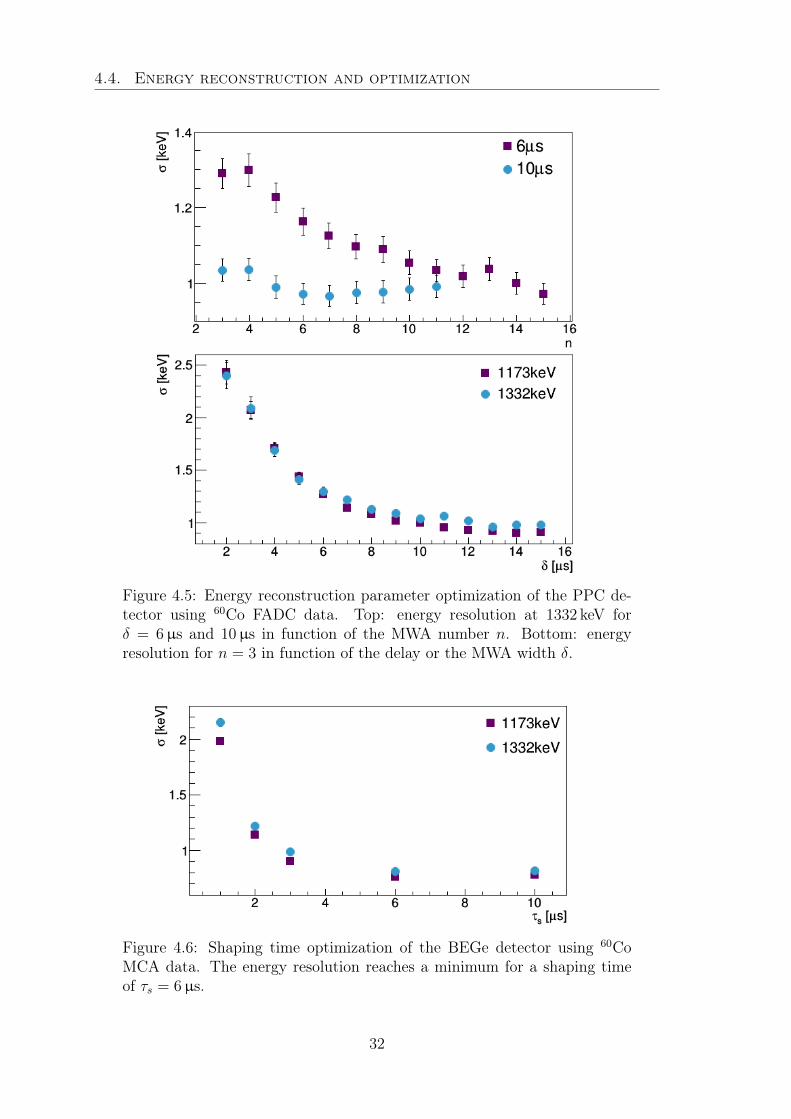
to minimize the energy resolution σ (see Section 4.5). As can be seen in Figure 4.5for the PPC detector a better energy resolution is achieved with larger n and δ.With δ = 10µs a slightly better energy resolution is achieved with n = 0 than withδ = 6µs and n = 15. For the PPC detector we chose δ = 10µs and n = 7 or lowerif the trace length is too short for seven iterations. In general, the higher δ and n,the better the energy resolution. Also if the resolution worsens after some iterationsthe effect is small with respect to the gain in resolution achieved beforehand. If anoptimization is too time consuming the parameters δ and n can be chosen in a quickmanner shifting the pseudo-Gaussian to the end of the trace.
Also the MCA shaping time τs, which can be set on the SpecAmp, has to be op-timized in order to minimize the energy resolution (see Section 4.5). In Figure 4.6the resolution of the BEGe detector at 60Co energies is plotted as a function of theMCA shaping time. The best resolution is achieved for a shaping time of τs = 6µs.
The chosen shaping parameters for all detectors and for FADC as well as MCAsystems is summarized in Table 4.3.
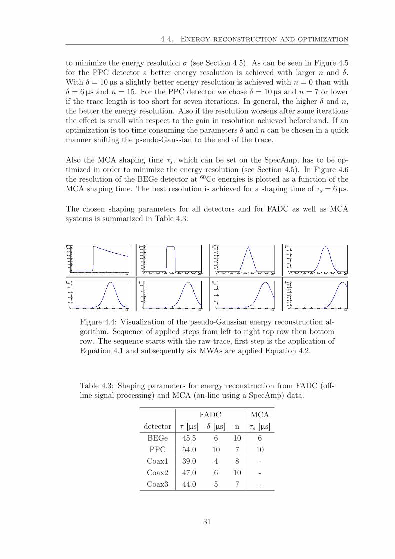
Figure 4.4: Visualization of the pseudo-Gaussian energy reconstruction al-gorithm. Sequence of applied steps from left to right top row then bottomrow. The sequence starts with the raw trace, first step is the application ofEquation 4.1 and subsequently six MWAs are applied Equation 4.2.
Table 4.3: Shaping parameters for energy reconstruction from FADC (off-line signal processing) and MCA (on-line using a SpecAmp) data.
FADC MCAdetector τ [µs] δ [µs] n τs [µs]BEGe 45.5 6 10 6PPC 54.0 10 7 10Coax1 39.0 4 8 -Coax2 47.0 6 10 -Coax3 44.0 5 7 -
31
4.4. Energy reconstruction and optimization
Figure 4.5: Energy reconstruction parameter optimization of the PPC de-tector using 60Co FADC data. Top: energy resolution at 1332 keV forδ = 6µs and 10µs in function of the MWA number n. Bottom: energyresolution for n = 3 in function of the delay or the MWA width δ.
Figure 4.6: Shaping time optimization of the BEGe detector using 60CoMCA data. The energy resolution reaches a minimum for a shaping timeof τs = 6µs.
32
4.5. Energy calibration and resolution
4.5 Energy calibration and resolutionVarious γ sources were used for energy calibrations and dedicated measurements,precisely:
• 22Na: energy calibration, external trigger gate calibration (Section 5.4.2)• 60Co: energy calibration• 137Cs: coincidence measurement (Chapter 5-7)• 228Th: energy calibration, PSA calibration (Section 7.8)• 241Am: fine grain surface scan (Section 4.8)
The decay schemes of these sources with their individual γ energies and branchingratios can be found in Appendix B.
Energy calibration and resolution measurements are performed regularly using mostly60Co with γ-lines at 1173 keV and 1332 keV. To calibrate the recorded spectra theROOT [53] TSpectrum class is used to find the γ-lines, and the spectrum is cali-brated assuming a linear calibration function. The calibration curves obtained canbe used to calibrate other data; e.g. 137Cs spectra in which usually only one γ-lineis observed.
Finally all γ-lines are fitted using two different fit functions in order to determinethe energy resolution and Gaussianity of the lines.
The first fit is done using a Gaussian peak on a background modeled with an inverseerror function (erfc)
f(x) = bl +bl − br
2· erfc
(µ− x√
2σ
)+
a√2π σ
· exp
(−(x− µ)2
2σ2
)(4.3)
With the background on the left bl and on the right br side of the peak, the centroidµ and the standard deviation σ. The amplitude a is also the integral of the Gaussianitself.
The second fit models the background with the same inverse error function but thepeak is allowed to have a low energy tail
g(x) = bl +bl − br
2· erfc
(µ− x√
2σ
)
+a√2π σ
·
exp(− (x−µ)2
2σ2
), if x < (µ− C)
exp(C (2 (x−µ)+C)
2σ2
), if x ≥ (µ− C)
(4.4)
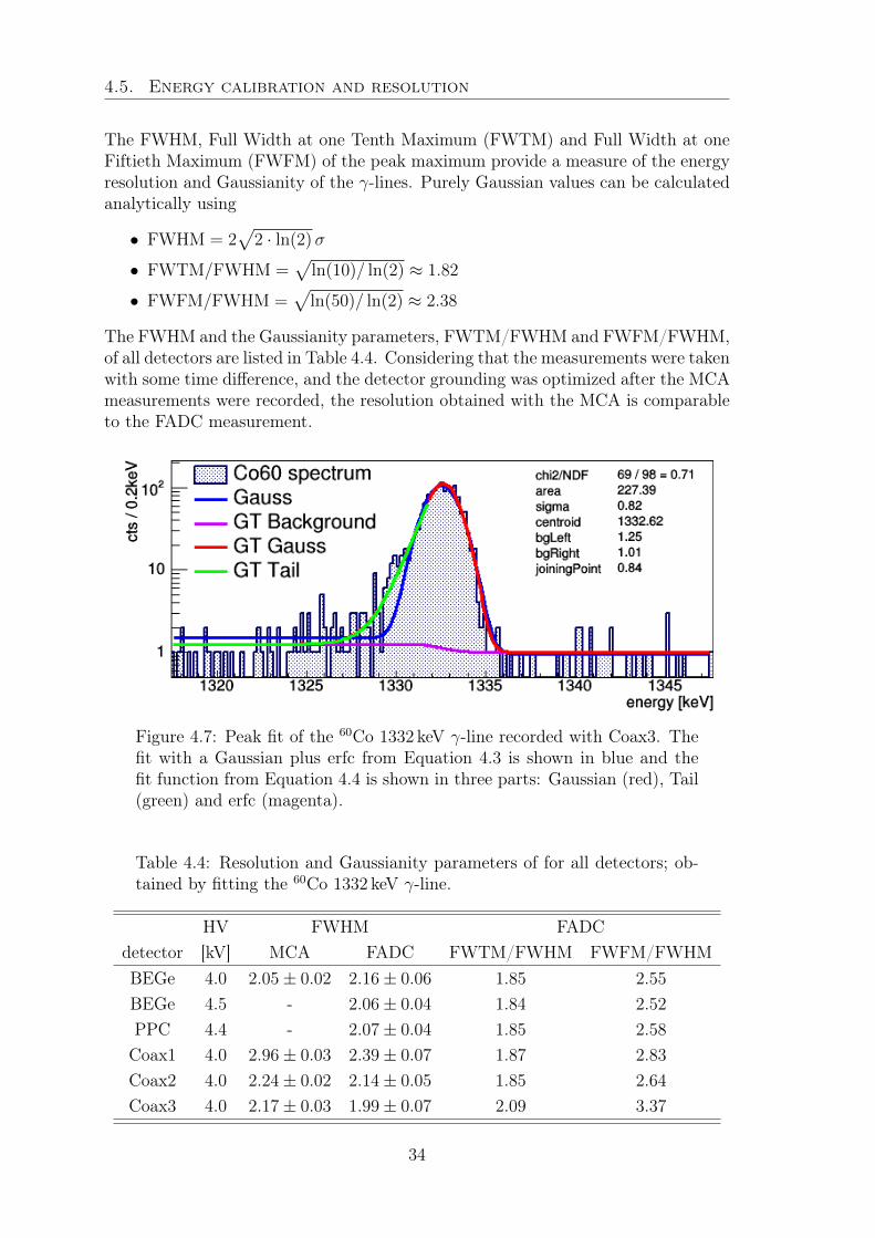
At the joining point C, to the left of the centroid µ, the fit function starts to deviatefrom the Gaussian form and fits a low energy tail. An example of a γ-line fit ofthe 60Co 1332 keV line recorded with Coax3 can be found in Figure 4.7; showing allcomponents of the two fit functions 4.3 and 4.4.
33
4.5. Energy calibration and resolution
The FWHM, Full Width at one Tenth Maximum (FWTM) and Full Width at oneFiftieth Maximum (FWFM) of the peak maximum provide a measure of the energyresolution and Gaussianity of the γ-lines. Purely Gaussian values can be calculatedanalytically using
• FWHM = 2√
2 · ln(2)σ
• FWTM/FWHM =√
ln(10)/ ln(2) ≈ 1.82
• FWFM/FWHM =√
ln(50)/ ln(2) ≈ 2.38
The FWHM and the Gaussianity parameters, FWTM/FWHM and FWFM/FWHM,of all detectors are listed in Table 4.4. Considering that the measurements were takenwith some time difference, and the detector grounding was optimized after the MCAmeasurements were recorded, the resolution obtained with the MCA is comparableto the FADC measurement.
Figure 4.7: Peak fit of the 60Co 1332 keV γ-line recorded with Coax3. Thefit with a Gaussian plus erfc from Equation 4.3 is shown in blue and thefit function from Equation 4.4 is shown in three parts: Gaussian (red), Tail(green) and erfc (magenta).
Table 4.4: Resolution and Gaussianity parameters of for all detectors; ob-tained by fitting the 60Co 1332 keV γ-line.
HV FWHM FADCdetector [kV] MCA FADC FWTM/FWHM FWFM/FWHMBEGe 4.0 2.05± 0.02 2.16± 0.06 1.85 2.55
BEGe 4.5 - 2.06± 0.04 1.84 2.52
PPC 4.4 - 2.07± 0.04 1.85 2.58
Coax1 4.0 2.96± 0.03 2.39± 0.07 1.87 2.83
Coax2 4.0 2.24± 0.02 2.14± 0.05 1.85 2.64
Coax3 4.0 2.17± 0.03 1.99± 0.07 2.09 3.37
34
4.6. High voltage scan
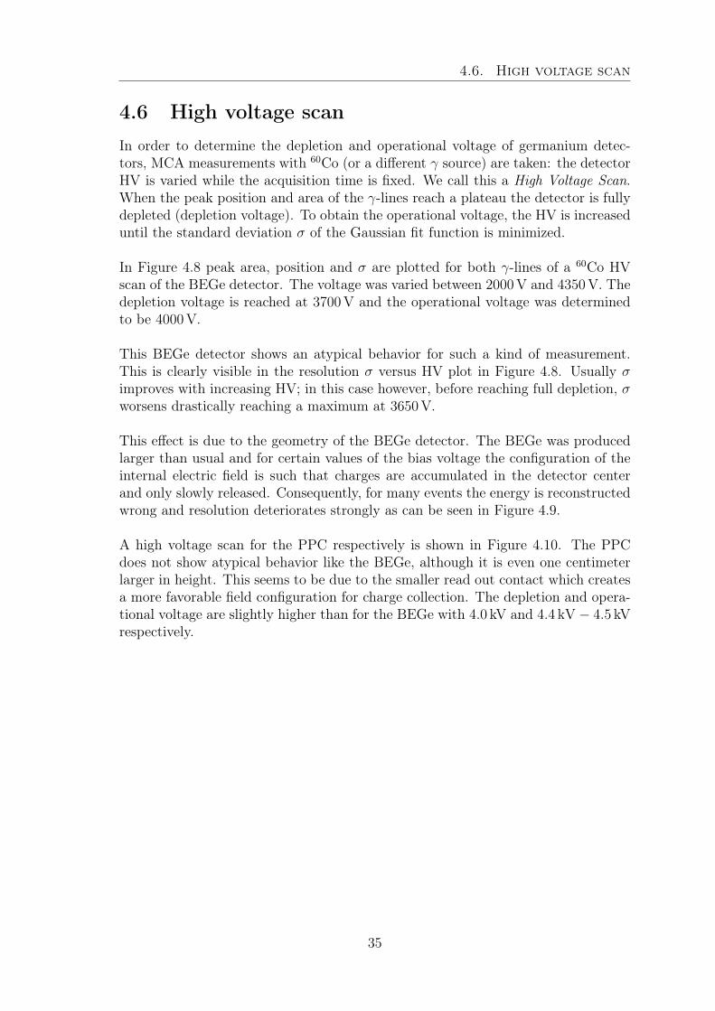
4.6 High voltage scanIn order to determine the depletion and operational voltage of germanium detec-tors, MCA measurements with 60Co (or a different γ source) are taken: the detectorHV is varied while the acquisition time is fixed. We call this a High Voltage Scan.When the peak position and area of the γ-lines reach a plateau the detector is fullydepleted (depletion voltage). To obtain the operational voltage, the HV is increaseduntil the standard deviation σ of the Gaussian fit function is minimized.
In Figure 4.8 peak area, position and σ are plotted for both γ-lines of a 60Co HVscan of the BEGe detector. The voltage was varied between 2000V and 4350V. Thedepletion voltage is reached at 3700V and the operational voltage was determinedto be 4000V.
This BEGe detector shows an atypical behavior for such a kind of measurement.This is clearly visible in the resolution σ versus HV plot in Figure 4.8. Usually σimproves with increasing HV; in this case however, before reaching full depletion, σworsens drastically reaching a maximum at 3650V.
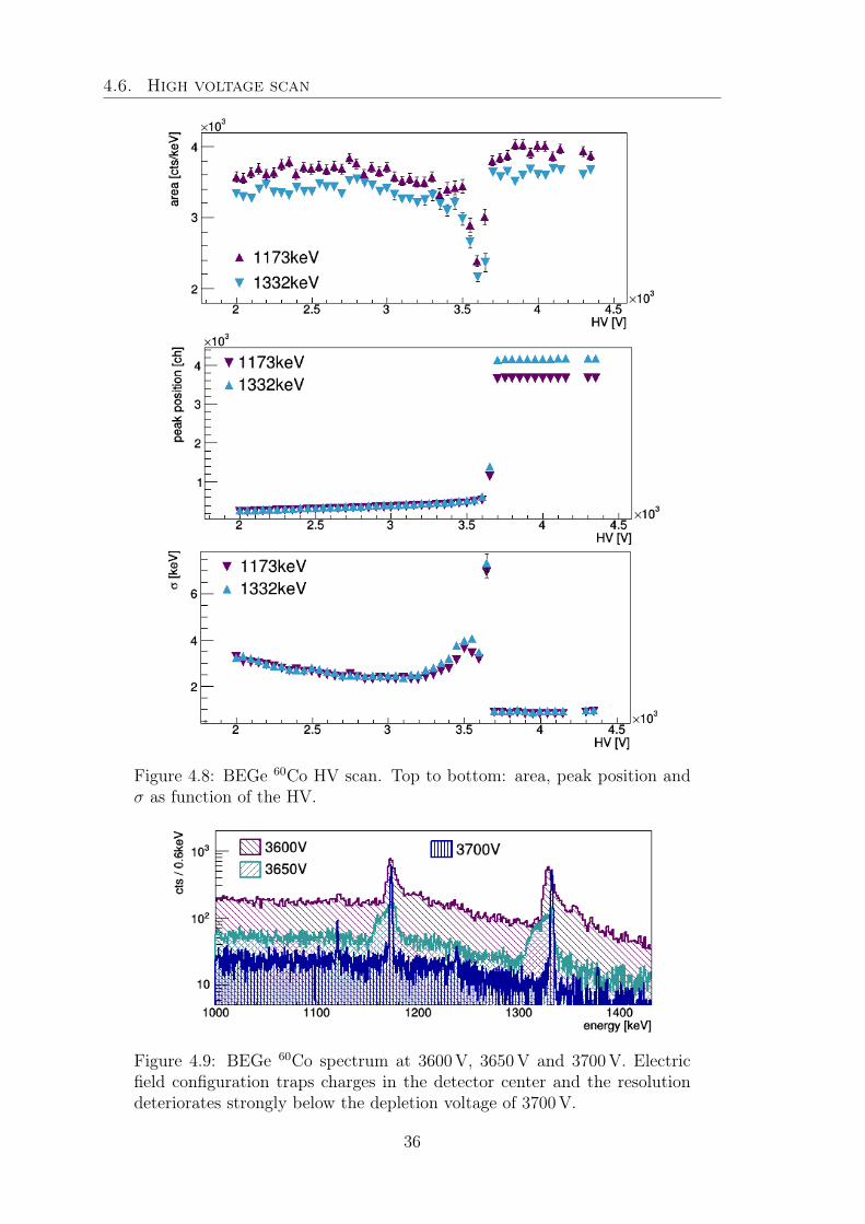
This effect is due to the geometry of the BEGe detector. The BEGe was producedlarger than usual and for certain values of the bias voltage the configuration of theinternal electric field is such that charges are accumulated in the detector centerand only slowly released. Consequently, for many events the energy is reconstructedwrong and resolution deteriorates strongly as can be seen in Figure 4.9.
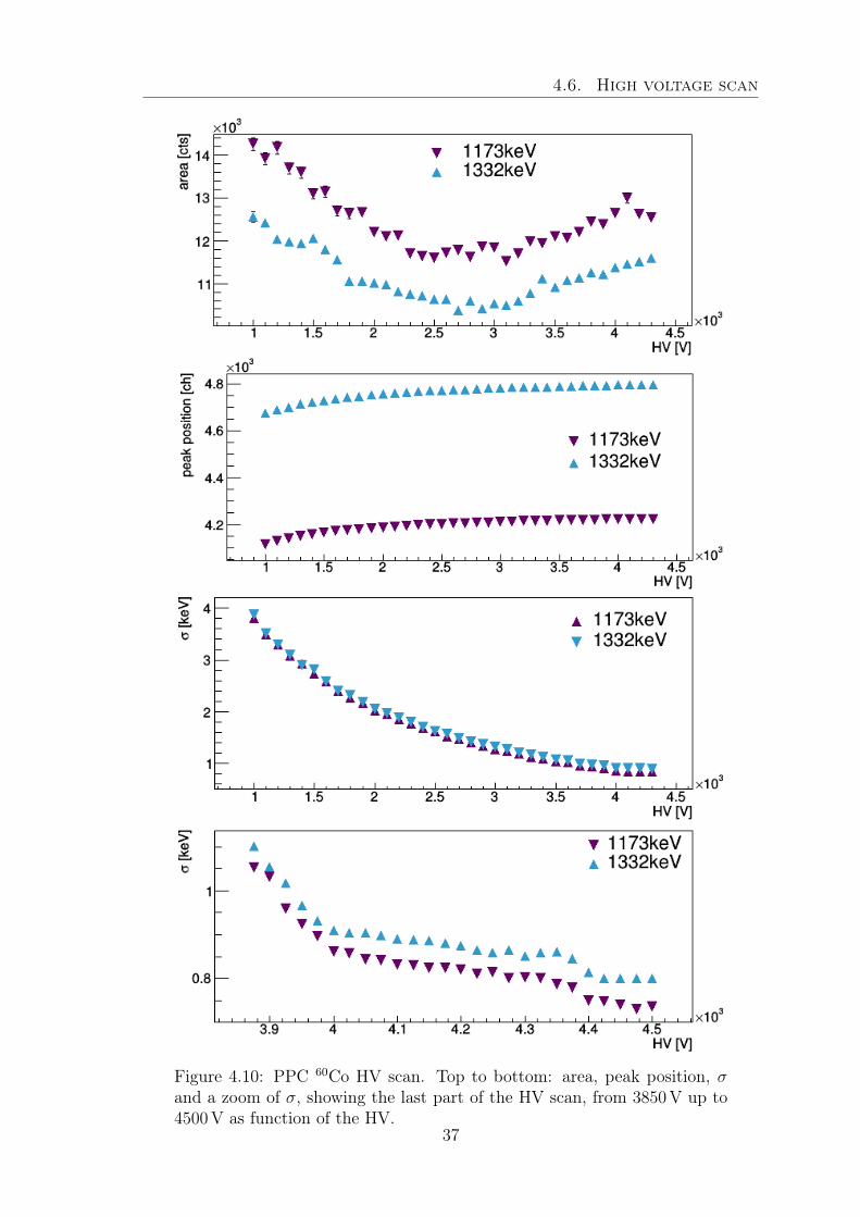
A high voltage scan for the PPC respectively is shown in Figure 4.10. The PPCdoes not show atypical behavior like the BEGe, although it is even one centimeterlarger in height. This seems to be due to the smaller read out contact which createsa more favorable field configuration for charge collection. The depletion and opera-tional voltage are slightly higher than for the BEGe with 4.0 kV and 4.4 kV − 4.5 kVrespectively.
35
4.6. High voltage scan
Figure 4.8: BEGe 60Co HV scan. Top to bottom: area, peak position andσ as function of the HV.
Figure 4.9: BEGe 60Co spectrum at 3600V, 3650V and 3700V. Electricfield configuration traps charges in the detector center and the resolutiondeteriorates strongly below the depletion voltage of 3700V.
36
4.6. High voltage scan
Figure 4.10: PPC 60Co HV scan. Top to bottom: area, peak position, σand a zoom of σ, showing the last part of the HV scan, from 3850V up to4500V as function of the HV.
37
4.7. Baseline stability
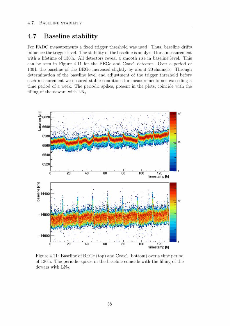
4.7 Baseline stabilityFor FADC measurements a fixed trigger threshold was used. Thus, baseline driftsinfluence the trigger level. The stability of the baseline is analyzed for a measurementwith a lifetime of 130 h. All detectors reveal a smooth rise in baseline level. Thiscan be seen in Figure 4.11 for the BEGe and Coax1 detector. Over a period of130 h the baseline of the BEGe increased slightly by about 20 channels. Throughdetermination of the baseline level and adjustment of the trigger threshold beforeeach measurement we ensured stable conditions for measurements not exceeding atime period of a week. The periodic spikes, present in the plots, coincide with thefilling of the dewars with LN2.
Figure 4.11: Baseline of BEGe (top) and Coax1 (bottom) over a time periodof 130 h. The periodic spikes in the baseline coincide with the filling of thedewars with LN2.
38
4.8. Fine grain surface scans
4.8 Fine grain surface scansPositioning of detectors inside their vacuum cryostats as well as the homogeneity oftheir outer contacts can only be measured from the outside. A dedicated setup isused which is able to perform automatized, fine grain, full surface scans [52].
4.8.1 Scanning table setup
The setup incorporates a collimated 241Am γ source with an activity of 5MBq.241Am has a prominent γ-line at 60 keV. These photons penetrate only the outerlayer of the detector interacting almost exclusively through photoelectric effect andare sensitive to changes of the outer contact of the order of a few tens of µm. Allnumbers derived in the following are valid for 60 keV photons.
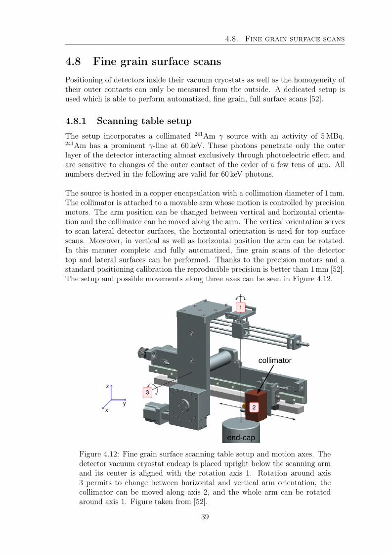
The source is hosted in a copper encapsulation with a collimation diameter of 1mm.The collimator is attached to a movable arm whose motion is controlled by precisionmotors. The arm position can be changed between vertical and horizontal orienta-tion and the collimator can be moved along the arm. The vertical orientation servesto scan lateral detector surfaces, the horizontal orientation is used for top surfacescans. Moreover, in vertical as well as horizontal position the arm can be rotated.In this manner complete and fully automatized, fine grain scans of the detectortop and lateral surfaces can be performed. Thanks to the precision motors and astandard positioning calibration the reproducible precision is better than 1mm [52].The setup and possible movements along three axes can be seen in Figure 4.12.
Figure 4.12: Fine grain surface scanning table setup and motion axes. Thedetector vacuum cryostat endcap is placed upright below the scanning armand its center is aligned with the rotation axis 1. Rotation around axis3 permits to change between horizontal and vertical arm orientation, thecollimator can be moved along axis 2, and the whole arm can be rotatedaround axis 1. Figure taken from [52].
39
4.8. Fine grain surface scans
4.8.2 Analysis of surface scans
For each position an 241Am spectrum is taken and the count rate C of the 60 keVγ-line is calculated by subtracting the background at the left Bleft and the rightBright from the peak region P
C = P −Bleft −Bright
=E+w∑i=E−w
bi −E−w∑
j=E−2w
bj −E+2w∑k=E+w
bk(4.5)
Where E is the centroid of the γ-line and b denotes the respective bin content. Thewindow size w is large enough to contain all the peak and small enough so that thebackground is flat on the left and on the right side of the γ-line.
4.8.3 Alignment
The detector has to be carefully aligned with the robotic arm; laser optics help tocenter the detector and adjust inclination.
Slight inclination of the detector with respect to the scanning arm is almost un-avoidable. When scanning the lateral detector surface structures which should beon a fixed height are seen at different heights depending on the inclination. This isvisualized in Figure 4.13; a sketch of a sharp edge scan is shown for small and largeinclination. The count rate pattern observed depends on the inclination value.
4.8.4 Collimation
The initial source collimation is 1mm but the further the collimator is placed fromthe scanned surface the more the photon beam diverges. The divergence of thesource beam can be measured by the change of rate on sharp edges. The sketchshown in Figure 4.14 shows the movement of the source beam over the edge.
A count rate simulation of a sharp edge scan with a step size of 1mm can be seenin Figure 4.15. Ten different start positions were simulated at random. The most
Figure 4.13: Sketch of the count rate pattern observed in a sharp edge scanfor a large (left) and for a small inclination value (right).
40
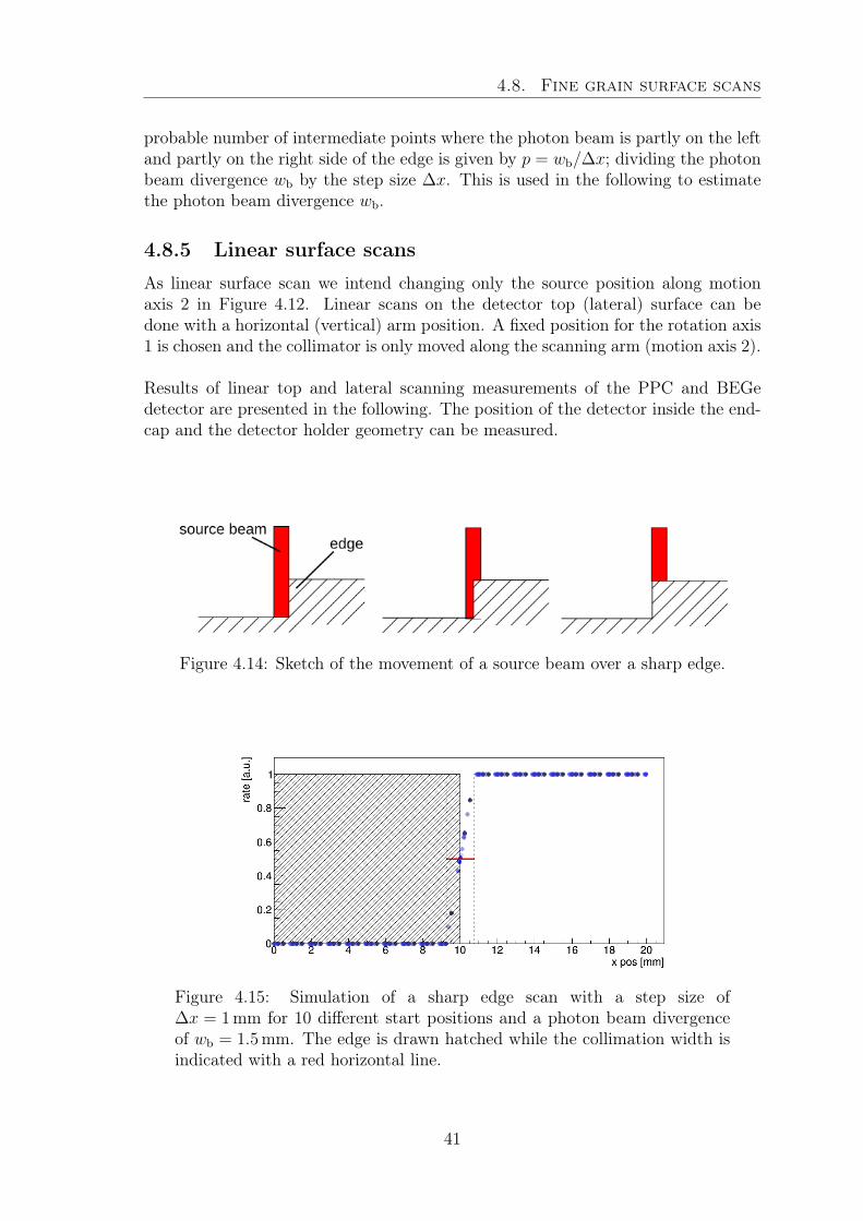
4.8. Fine grain surface scans
probable number of intermediate points where the photon beam is partly on the leftand partly on the right side of the edge is given by p = wb/∆x; dividing the photonbeam divergence wb by the step size ∆x. This is used in the following to estimatethe photon beam divergence wb.
4.8.5 Linear surface scans
As linear surface scan we intend changing only the source position along motionaxis 2 in Figure 4.12. Linear scans on the detector top (lateral) surface can bedone with a horizontal (vertical) arm position. A fixed position for the rotation axis1 is chosen and the collimator is only moved along the scanning arm (motion axis 2).
Results of linear top and lateral scanning measurements of the PPC and BEGedetector are presented in the following. The position of the detector inside the end-cap and the detector holder geometry can be measured.
Figure 4.14: Sketch of the movement of a source beam over a sharp edge.
Figure 4.15: Simulation of a sharp edge scan with a step size of∆x = 1mm for 10 different start positions and a photon beam divergenceof wb = 1.5mm. The edge is drawn hatched while the collimation width isindicated with a red horizontal line.
41

4.8. Fine grain surface scans
4.8.6 PPC detector top and lateral linear surface scan
The PPC detector top and lateral surface were scanned with a step size of ∆x = 1mm;each point with a measurement lifetime6 of TL = 120 s. The source position alongthe scanning arm will be denoted by x in the following. In Figure 4.16 the countrate of the 60 keV 241Am γ-line is plotted versus the scanning position for both mea-surements.
In the lateral scan we see that from x = 266mm to x = 271mm the count ratedrops significantly; we infer that in this region the holder material is substantiallythicker than the rest of the holder cup and exhibits a sort of ring structure; this iscommon for germanium detector holders.
With the difference in count rate and the knowledge that the holder cup is made ofcopper we can estimate the thickness of the ring structure rearranging Equation 3.5.Fitting the flat parts of the graph with a constant we can extract the different countrates
dring = ln
(N1
N2
)· 1
µCuρCu
= ln
(819± 7
284± 9
)· 1
1.485 cm2/g · 8.9 g/cm3
= (0.80± 0.03) mm
The ring structure has a sharp edge hence we can analyze the divergence of thesource beam wb. It is at least 1mm from collimation and maximal 2mm consid-ering that at x = 264mm the source beam is on the left side of the edge and atx = 266mm it has already passed it; therefore we make the conservative estimateof wb = (1.5± 0.5)mm.
The height of the ring is estimated making use of the photon beam divergence wb
ashring = 271 mm− 266 mm + wb = (6.5± 1.5) mm
considering a position uncertainty of ∆x = ±1mm.
The edges of the PPC are rounded as can be seen in both the top and the lateralscan possibly to ensure a good charge collection as the internal electric field is weakin corners.
We estimate the active length of the PPC from the lateral scan as La = 48.5± 1.5mmand the active diameter from the top scan as Da = 62.5± 1.5mm.
6 The lifetime of a measurement is given by the real measurement time minus the dead time.
42
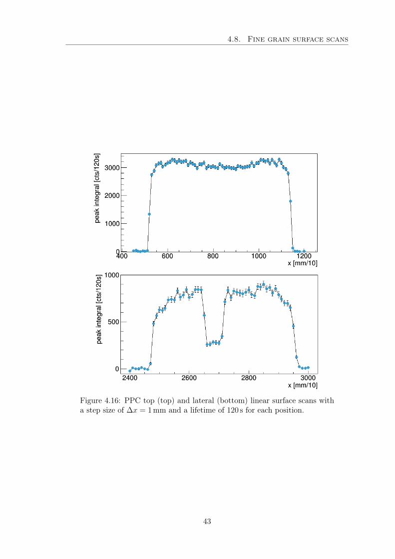
4.8. Fine grain surface scans
Figure 4.16: PPC top (top) and lateral (bottom) linear surface scans witha step size of ∆x = 1mm and a lifetime of 120 s for each position.
43
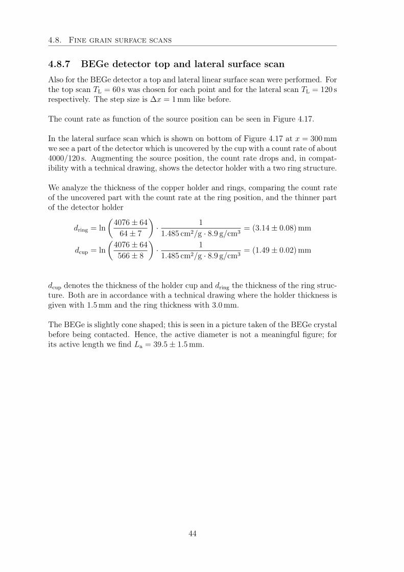
4.8. Fine grain surface scans
4.8.7 BEGe detector top and lateral surface scan
Also for the BEGe detector a top and lateral linear surface scan were performed. Forthe top scan TL = 60 s was chosen for each point and for the lateral scan TL = 120 srespectively. The step size is ∆x = 1mm like before.
The count rate as function of the source position can be seen in Figure 4.17.
In the lateral surface scan which is shown on bottom of Figure 4.17 at x = 300mmwe see a part of the detector which is uncovered by the cup with a count rate of about4000/120 s. Augmenting the source position, the count rate drops and, in compat-ibility with a technical drawing, shows the detector holder with a two ring structure.
We analyze the thickness of the copper holder and rings, comparing the count rateof the uncovered part with the count rate at the ring position, and the thinner partof the detector holder
dring = ln
(4076± 64
64± 7
)· 1
1.485 cm2/g · 8.9 g/cm3= (3.14± 0.08) mm
dcup = ln
(4076± 64
566± 8
)· 1
1.485 cm2/g · 8.9 g/cm3= (1.49± 0.02) mm
dcup denotes the thickness of the holder cup and dring the thickness of the ring struc-ture. Both are in accordance with a technical drawing where the holder thickness isgiven with 1.5mm and the ring thickness with 3.0mm.
The BEGe is slightly cone shaped; this is seen in a picture taken of the BEGe crystalbefore being contacted. Hence, the active diameter is not a meaningful figure; forits active length we find La = 39.5± 1.5mm.
44
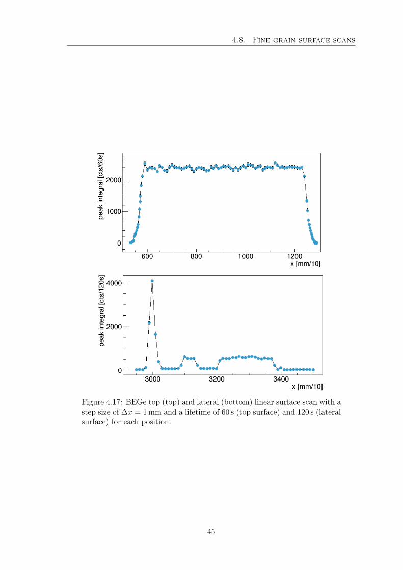
4.8. Fine grain surface scans
Figure 4.17: BEGe top (top) and lateral (bottom) linear surface scan with astep size of ∆x = 1mm and a lifetime of 60 s (top surface) and 120 s (lateralsurface) for each position.
45
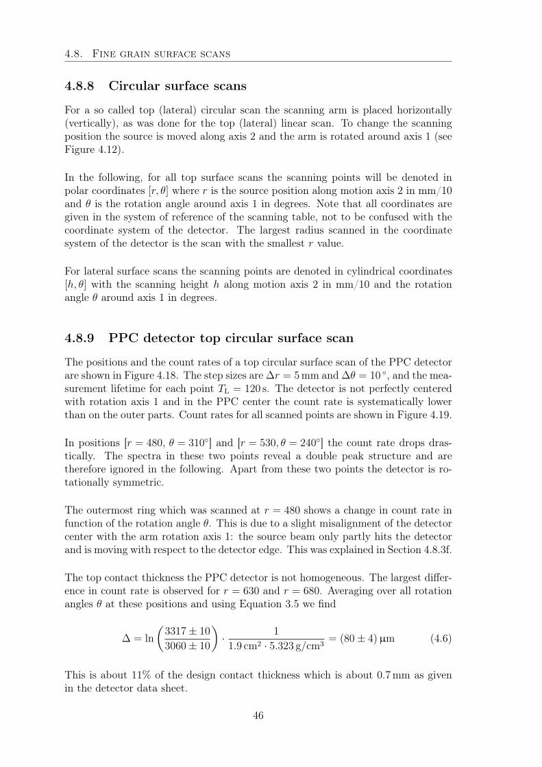
4.8. Fine grain surface scans
4.8.8 Circular surface scans
For a so called top (lateral) circular scan the scanning arm is placed horizontally(vertically), as was done for the top (lateral) linear scan. To change the scanningposition the source is moved along axis 2 and the arm is rotated around axis 1 (seeFigure 4.12).
In the following, for all top surface scans the scanning points will be denoted inpolar coordinates [r, θ] where r is the source position along motion axis 2 in mm/10and θ is the rotation angle around axis 1 in degrees. Note that all coordinates aregiven in the system of reference of the scanning table, not to be confused with thecoordinate system of the detector. The largest radius scanned in the coordinatesystem of the detector is the scan with the smallest r value.
For lateral surface scans the scanning points are denoted in cylindrical coordinates[h, θ] with the scanning height h along motion axis 2 in mm/10 and the rotationangle θ around axis 1 in degrees.
4.8.9 PPC detector top circular surface scan
The positions and the count rates of a top circular surface scan of the PPC detectorare shown in Figure 4.18. The step sizes are ∆r = 5mm and ∆θ = 10 , and the mea-surement lifetime for each point TL = 120 s. The detector is not perfectly centeredwith rotation axis 1 and in the PPC center the count rate is systematically lowerthan on the outer parts. Count rates for all scanned points are shown in Figure 4.19.
In positions [r = 480, θ = 310] and [r = 530, θ = 240] the count rate drops dras-tically. The spectra in these two points reveal a double peak structure and aretherefore ignored in the following. Apart from these two points the detector is ro-tationally symmetric.
The outermost ring which was scanned at r = 480 shows a change in count rate infunction of the rotation angle θ. This is due to a slight misalignment of the detectorcenter with the arm rotation axis 1: the source beam only partly hits the detectorand is moving with respect to the detector edge. This was explained in Section 4.8.3f.
The top contact thickness the PPC detector is not homogeneous. The largest differ-ence in count rate is observed for r = 630 and r = 680. Averaging over all rotationangles θ at these positions and using Equation 3.5 we find
∆ = ln
(3317± 10
3060± 10
)· 1
1.9 cm2 · 5.323 g/cm3= (80± 4)µm (4.6)
This is about 11% of the design contact thickness which is about 0.7mm as givenin the detector data sheet.
46
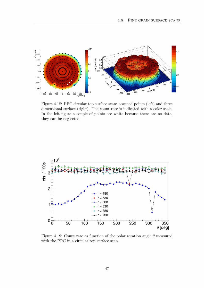
4.8. Fine grain surface scans
Figure 4.18: PPC circular top surface scan: scanned points (left) and threedimensional surface (right). The count rate is indicated with a color scale.In the left figure a couple of points are white because there are no data;they can be neglected.
Figure 4.19: Count rate as function of the polar rotation angle θ measuredwith the PPC in a circular top surface scan.
47
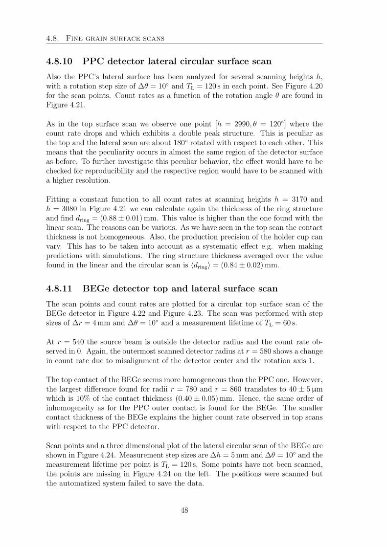
4.8. Fine grain surface scans
4.8.10 PPC detector lateral circular surface scan
Also the PPC’s lateral surface has been analyzed for several scanning heights h,with a rotation step size of ∆θ = 10 and TL = 120 s in each point. See Figure 4.20for the scan points. Count rates as a function of the rotation angle θ are found inFigure 4.21.
As in the top surface scan we observe one point [h = 2990, θ = 120] where thecount rate drops and which exhibits a double peak structure. This is peculiar asthe top and the lateral scan are about 180 rotated with respect to each other. Thismeans that the peculiarity occurs in almost the same region of the detector surfaceas before. To further investigate this peculiar behavior, the effect would have to bechecked for reproducibility and the respective region would have to be scanned witha higher resolution.
Fitting a constant function to all count rates at scanning heights h = 3170 andh = 3080 in Figure 4.21 we can calculate again the thickness of the ring structureand find dring = (0.88± 0.01)mm. This value is higher than the one found with thelinear scan. The reasons can be various. As we have seen in the top scan the contactthickness is not homogeneous. Also, the production precision of the holder cup canvary. This has to be taken into account as a systematic effect e.g. when makingpredictions with simulations. The ring structure thickness averaged over the valuefound in the linear and the circular scan is 〈dring〉 = (0.84± 0.02) mm.
4.8.11 BEGe detector top and lateral surface scan
The scan points and count rates are plotted for a circular top surface scan of theBEGe detector in Figure 4.22 and Figure 4.23. The scan was performed with stepsizes of ∆r = 4 mm and ∆θ = 10 and a measurement lifetime of TL = 60 s.
At r = 540 the source beam is outside the detector radius and the count rate ob-served in 0. Again, the outermost scanned detector radius at r = 580 shows a changein count rate due to misalignment of the detector center and the rotation axis 1.
The top contact of the BEGe seems more homogeneous than the PPC one. However,the largest difference found for radii r = 780 and r = 860 translates to 40 ± 5µmwhich is 10% of the contact thickness (0.40 ± 0.05)mm. Hence, the same order ofinhomogeneity as for the PPC outer contact is found for the BEGe. The smallercontact thickness of the BEGe explains the higher count rate observed in top scanswith respect to the PPC detector.
Scan points and a three dimensional plot of the lateral circular scan of the BEGe areshown in Figure 4.24. Measurement step sizes are ∆h = 5 mm and ∆θ = 10 and themeasurement lifetime per point is TL = 120 s. Some points have not been scanned,the points are missing in Figure 4.24 on the left. The positions were scanned butthe automatized system failed to save the data.
48
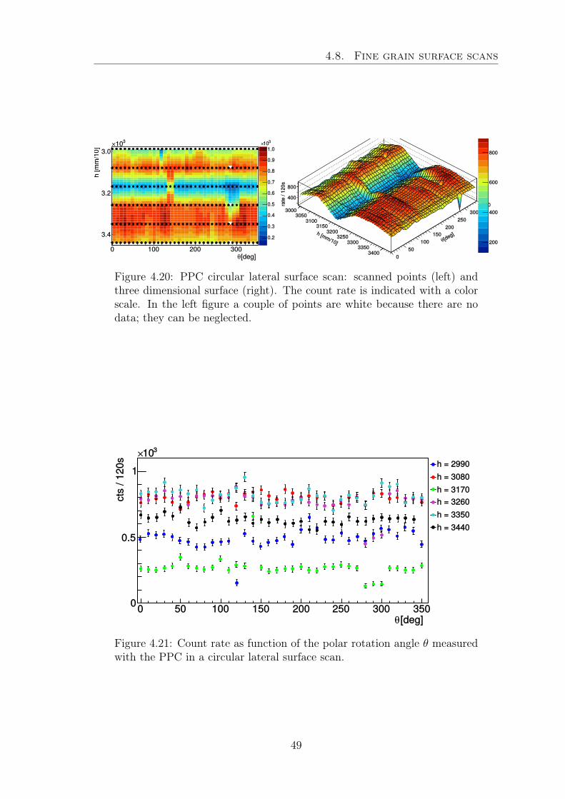
4.8. Fine grain surface scans
Figure 4.20: PPC circular lateral surface scan: scanned points (left) andthree dimensional surface (right). The count rate is indicated with a colorscale. In the left figure a couple of points are white because there are nodata; they can be neglected.
Figure 4.21: Count rate as function of the polar rotation angle θ measuredwith the PPC in a circular lateral surface scan.
49
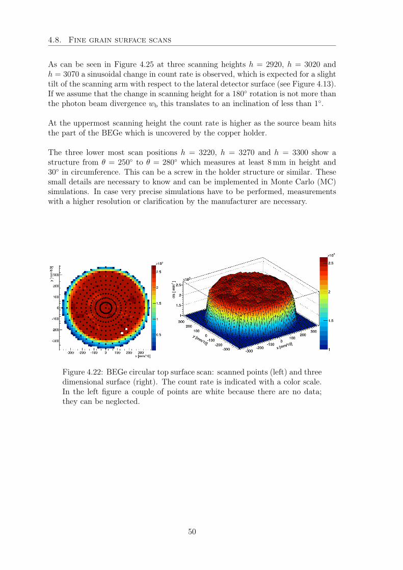
4.8. Fine grain surface scans
As can be seen in Figure 4.25 at three scanning heights h = 2920, h = 3020 andh = 3070 a sinusoidal change in count rate is observed, which is expected for a slighttilt of the scanning arm with respect to the lateral detector surface (see Figure 4.13).If we assume that the change in scanning height for a 180 rotation is not more thanthe photon beam divergence wb this translates to an inclination of less than 1.
At the uppermost scanning height the count rate is higher as the source beam hitsthe part of the BEGe which is uncovered by the copper holder.
The three lower most scan positions h = 3220, h = 3270 and h = 3300 show astructure from θ = 250 to θ = 280 which measures at least 8mm in height and30 in circumference. This can be a screw in the holder structure or similar. Thesesmall details are necessary to know and can be implemented in Monte Carlo (MC)simulations. In case very precise simulations have to be performed, measurementswith a higher resolution or clarification by the manufacturer are necessary.
Figure 4.22: BEGe circular top surface scan: scanned points (left) and threedimensional surface (right). The count rate is indicated with a color scale.In the left figure a couple of points are white because there are no data;they can be neglected.
50
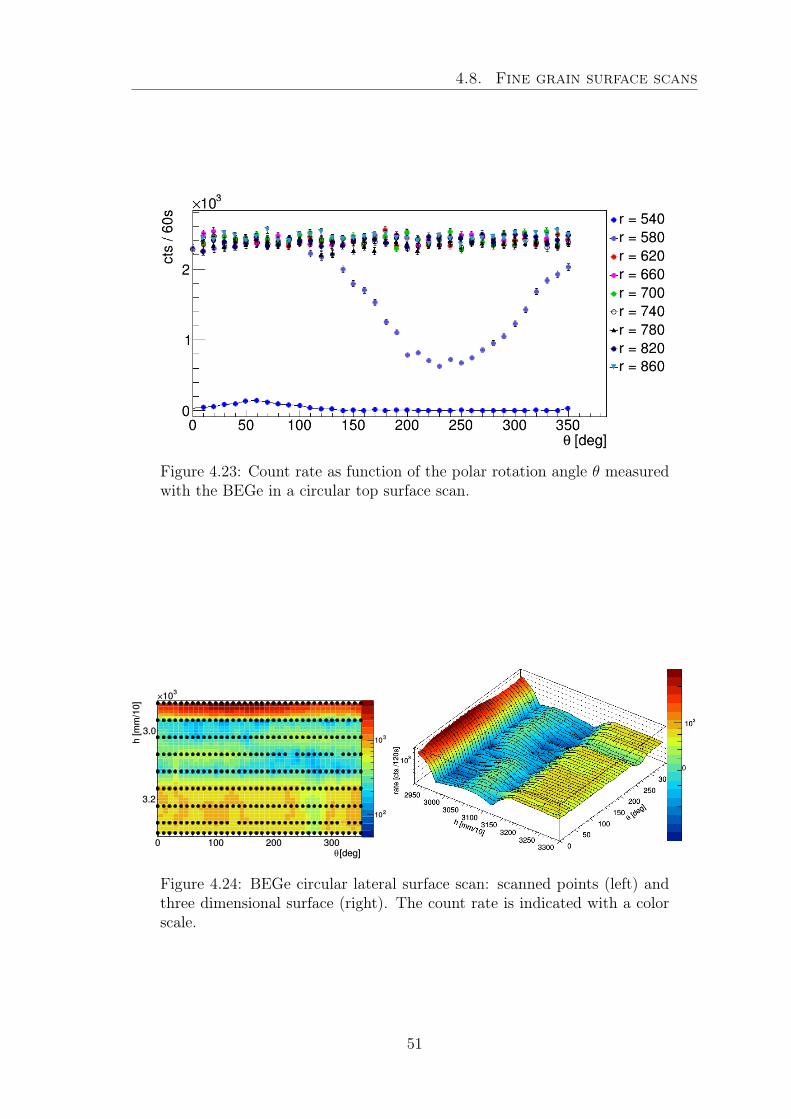
4.8. Fine grain surface scans
Figure 4.23: Count rate as function of the polar rotation angle θ measuredwith the BEGe in a circular top surface scan.
Figure 4.24: BEGe circular lateral surface scan: scanned points (left) andthree dimensional surface (right). The count rate is indicated with a colorscale.
51
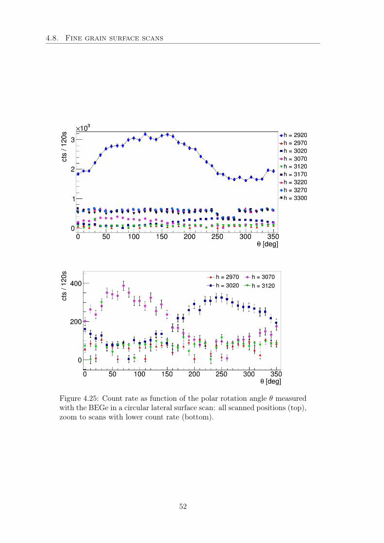
4.8. Fine grain surface scans
Figure 4.25: Count rate as function of the polar rotation angle θ measuredwith the BEGe in a circular lateral surface scan: all scanned positions (top),zoom to scans with lower count rate (bottom).
52
Chapter 5
Compton coincidences: Setup
In order to develop new algorithms for background rejection in Gerda Phase II,detailed knowledge of signal-like event structure in BEGe detectors is of great im-portance.
In this chapter an experimental setup is described which has been designed and con-structed with the purpose of performing three-dimensional scans of BEGe detectorsin order to study signal-like pulse shapes in confined detector regions. We base theselection of such events on single Compton interactions in coincidence measurements.
The method has been used with non-segmented and segmented HPGe detectors[57, 58] and for detector characterization in the Greta and Agata experiment[59–61]. It is adapted in this work for a BEGe detector in the context of the Gerdaexperiment. The Compton coincidence measurements described in the followinghave never been successfully performed before with a BEGe detector.
After an introduction in which we explain the principle of operation, the experimen-tal setup is described in detail. Finally, the measurement campaign is displayed.
5.1 Motivation for single site event studies
In Figure 5.1 measured charge and respective current pulses for three different eventclasses are plotted. The current pulse x′[t] was calculated based on the charge pulsex[t] by a moving window differentiation with a width of wd = 80 ns
x′[t] = x[t]− x[t− wd] (5.1)
The three event types shown are a single site event (SSE) depositing energy in onesmall region, a multiple site event (MSE) depositing energy in two well separatedregions and a slow pulse event which deposits energy in the outer n+ contact of thedetector. The latter type is called slow pulse because charge carriers have to diffusefrom the outer contact layer into the active volume of the detector, before driftingalong the electric field lines and being collected on the read-out electrode. The dif-fusion process is rather slow, resulting in a distinct pulse shape. MSE events reveal
53
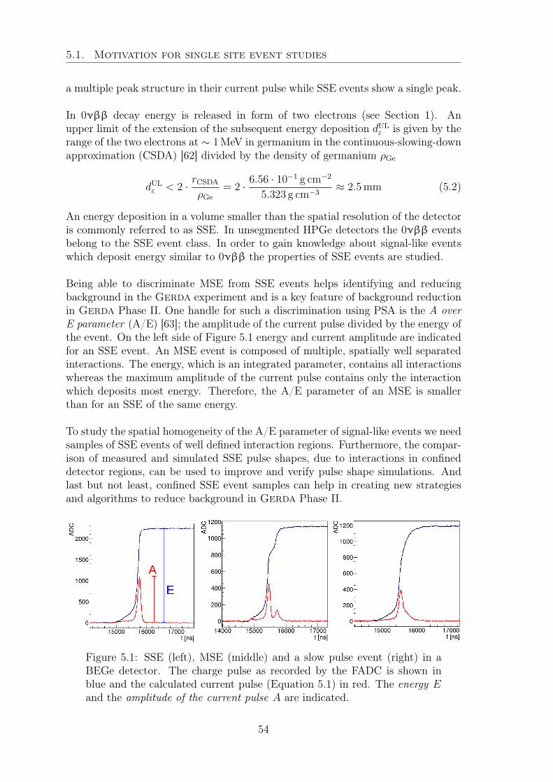
5.1. Motivation for single site event studies
a multiple peak structure in their current pulse while SSE events show a single peak.
In 0νββ decay energy is released in form of two electrons (see Section 1). Anupper limit of the extension of the subsequent energy deposition dUL
ε is given by therange of the two electrons at ∼ 1MeV in germanium in the continuous-slowing-downapproximation (CSDA) [62] divided by the density of germanium ρGe
dULε < 2 · rCSDA
ρGe
= 2 · 6.56 · 10−1 g cm−2
5.323 g cm−3≈ 2.5 mm (5.2)
An energy deposition in a volume smaller than the spatial resolution of the detectoris commonly referred to as SSE. In unsegmented HPGe detectors the 0νββ eventsbelong to the SSE event class. In order to gain knowledge about signal-like eventswhich deposit energy similar to 0νββ the properties of SSE events are studied.
Being able to discriminate MSE from SSE events helps identifying and reducingbackground in the Gerda experiment and is a key feature of background reductionin Gerda Phase II. One handle for such a discrimination using PSA is the A overE parameter (A/E) [63]; the amplitude of the current pulse divided by the energy ofthe event. On the left side of Figure 5.1 energy and current amplitude are indicatedfor an SSE event. An MSE event is composed of multiple, spatially well separatedinteractions. The energy, which is an integrated parameter, contains all interactionswhereas the maximum amplitude of the current pulse contains only the interactionwhich deposits most energy. Therefore, the A/E parameter of an MSE is smallerthan for an SSE of the same energy.
To study the spatial homogeneity of the A/E parameter of signal-like events we needsamples of SSE events of well defined interaction regions. Furthermore, the compar-ison of measured and simulated SSE pulse shapes, due to interactions in confineddetector regions, can be used to improve and verify pulse shape simulations. Andlast but not least, confined SSE event samples can help in creating new strategiesand algorithms to reduce background in Gerda Phase II.
Figure 5.1: SSE (left), MSE (middle) and a slow pulse event (right) in aBEGe detector. The charge pulse as recorded by the FADC is shown inblue and the calculated current pulse (Equation 5.1) in red. The energy Eand the amplitude of the current pulse A are indicated.
54
5.2. Single Compton events
In the next section the physical prerequisites of Compton coincidence measurementsare describe, which make it possible to select SSE event samples from confined re-gions in a HPGe detector. The experiment presented in the following is based onsingle Compton interactions of 137Cs photons with a scattering angle of 90.
5.2 Single Compton events137Cs has only one prominent γ-line, with an energy of 661.657 keV (≈ 662 keV inthe following) and a branching ratio of RB = (84.99 ± 0.20) % (see Figure B.3).The interaction cross section of photons in germanium, as a function of energy anddepending on the interaction mechanism, is shown in Figure 5.2. The 137Cs γ energyis indicated with a black vertical line. At this energy, Compton scattering is thedominant interaction process of photons with germanium.
5.2.1 Topology
In Compton scattering energy is transfered from a γ-photon to a shell electron ofan atom (see Section 3.1.3). The energy of the scattered photon and the energytransferred to the electron, for an incident photon energy of 662 keV, are listed inTable 5.1. Different scattering angles are tabulated. For a scattering angle of 90
an energy of 373 keV is transfered to the shell electron.
The stopping power of germanium for electrons at 373 keV is about 31MeVcm2/g[62]. Thus, the scattered electron has a maximal range of about
rCSDA/ρGe = 0.2 g cm−2/5.323 g cm−3 ≈ 0.4 mm (5.3)
This limit is smaller region than was derived for 0νββ events (see Equation 5.2).Thus, a single Compton event has SSE event topology and can be studied as a pro-totype for 0νββ events.
Table 5.1: Energies of single Compton scattered photon E ′γ and transferredenergies to electron Ee for different scattering angles and an incident photonenergy of 662 keV.
scattering angle [deg] E ′γ [keV] Ee [keV]90 288 37360 402 26045 480 182
55
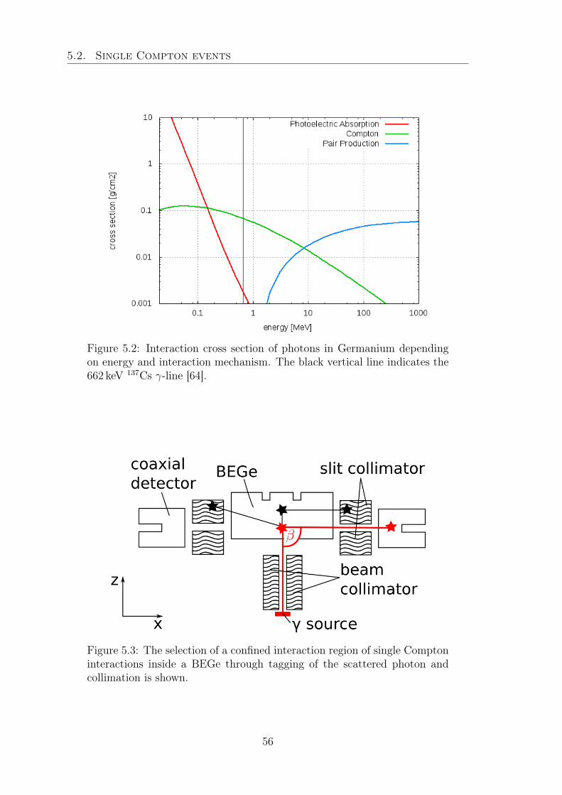
5.2. Single Compton events
Figure 5.2: Interaction cross section of photons in Germanium dependingon energy and interaction mechanism. The black vertical line indicates the662 keV 137Cs γ-line [64].
Figure 5.3: The selection of a confined interaction region of single Comptoninteractions inside a BEGe through tagging of the scattered photon andcollimation is shown.
56
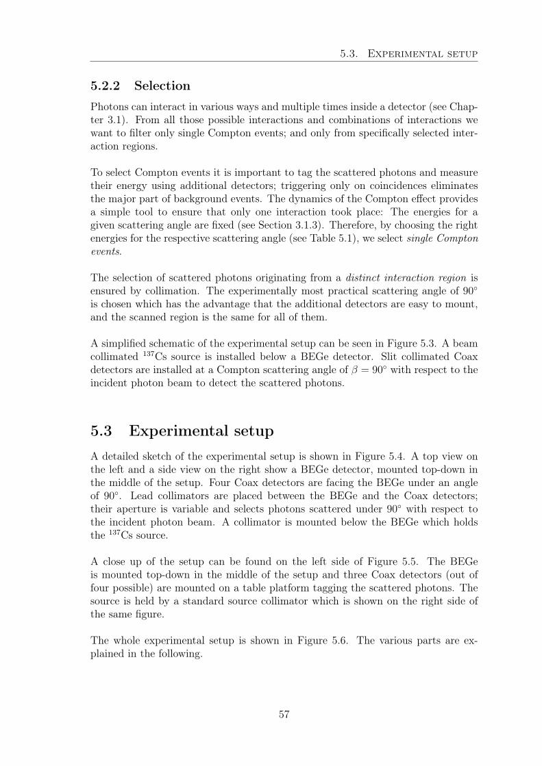
5.3. Experimental setup
5.2.2 Selection
Photons can interact in various ways and multiple times inside a detector (see Chap-ter 3.1). From all those possible interactions and combinations of interactions wewant to filter only single Compton events; and only from specifically selected inter-action regions.
To select Compton events it is important to tag the scattered photons and measuretheir energy using additional detectors; triggering only on coincidences eliminatesthe major part of background events. The dynamics of the Compton effect providesa simple tool to ensure that only one interaction took place: The energies for agiven scattering angle are fixed (see Section 3.1.3). Therefore, by choosing the rightenergies for the respective scattering angle (see Table 5.1), we select single Comptonevents.
The selection of scattered photons originating from a distinct interaction region isensured by collimation. The experimentally most practical scattering angle of 90
is chosen which has the advantage that the additional detectors are easy to mount,and the scanned region is the same for all of them.
A simplified schematic of the experimental setup can be seen in Figure 5.3. A beamcollimated 137Cs source is installed below a BEGe detector. Slit collimated Coaxdetectors are installed at a Compton scattering angle of β = 90 with respect to theincident photon beam to detect the scattered photons.
5.3 Experimental setupA detailed sketch of the experimental setup is shown in Figure 5.4. A top view onthe left and a side view on the right show a BEGe detector, mounted top-down inthe middle of the setup. Four Coax detectors are facing the BEGe under an angleof 90. Lead collimators are placed between the BEGe and the Coax detectors;their aperture is variable and selects photons scattered under 90 with respect tothe incident photon beam. A collimator is mounted below the BEGe which holdsthe 137Cs source.
A close up of the setup can be found on the left side of Figure 5.5. The BEGeis mounted top-down in the middle of the setup and three Coax detectors (out offour possible) are mounted on a table platform tagging the scattered photons. Thesource is held by a standard source collimator which is shown on the right side ofthe same figure.
The whole experimental setup is shown in Figure 5.6. The various parts are ex-plained in the following.
57

5.3. Experimental setup
Figure 5.4: Sketch of top view (left) and side view (right) of the Comptoncoincidence experimental setup. Germanium detectors are shown in blue,vacuum cryostats as dotted volumes, lead collimators as wavy blocks andthe 137Cs source is drawn in red.
Figure 5.5: Close up of the coincidence measurement setup (left) with theBEGe detector in the middle and three Coax detectors measuring the scat-tered photons and the standard source collimator (right).
58
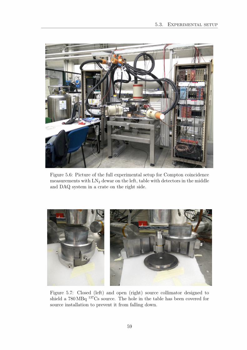
5.3. Experimental setup
Figure 5.6: Picture of the full experimental setup for Compton coincidencemeasurements with LN2 dewar on the left, table with detectors in the middleand DAQ system in a crate on the right side.
Figure 5.7: Closed (left) and open (right) source collimator designed toshield a 780MBq 137Cs source. The hole in the table has been covered forsource installation to prevent it from falling down.
59
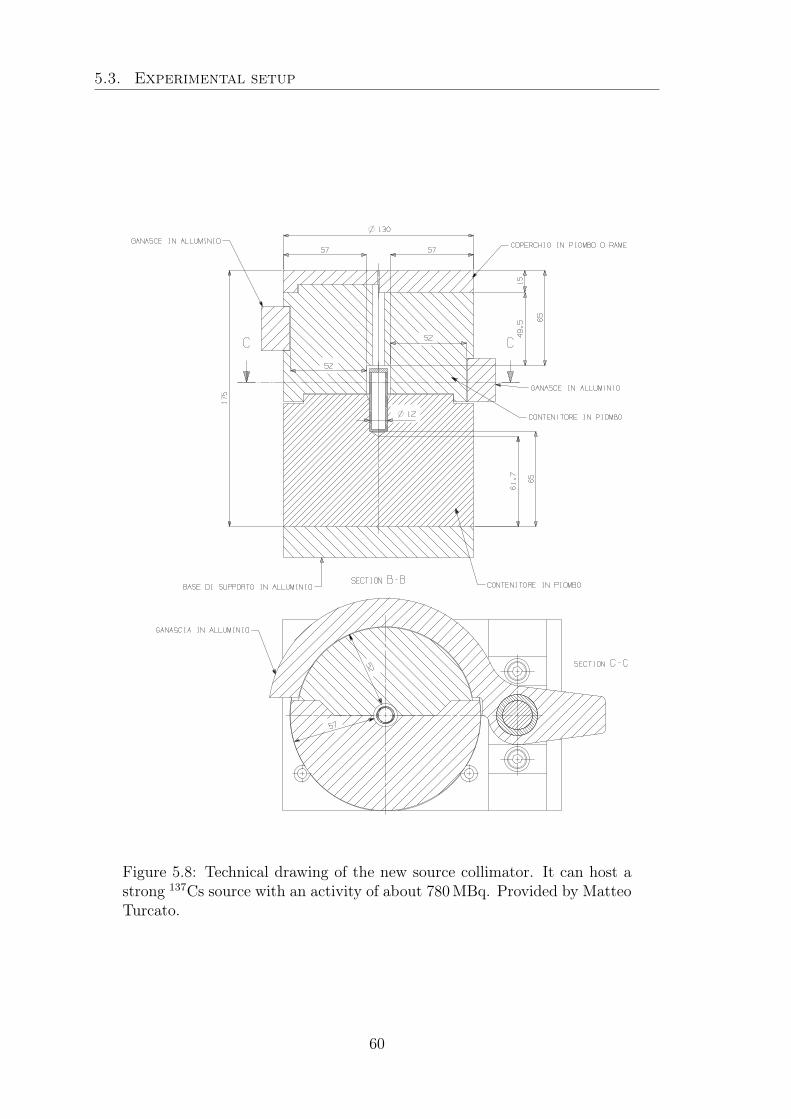
5.3. Experimental setup
Figure 5.8: Technical drawing of the new source collimator. It can host astrong 137Cs source with an activity of about 780MBq. Provided by MatteoTurcato.
60
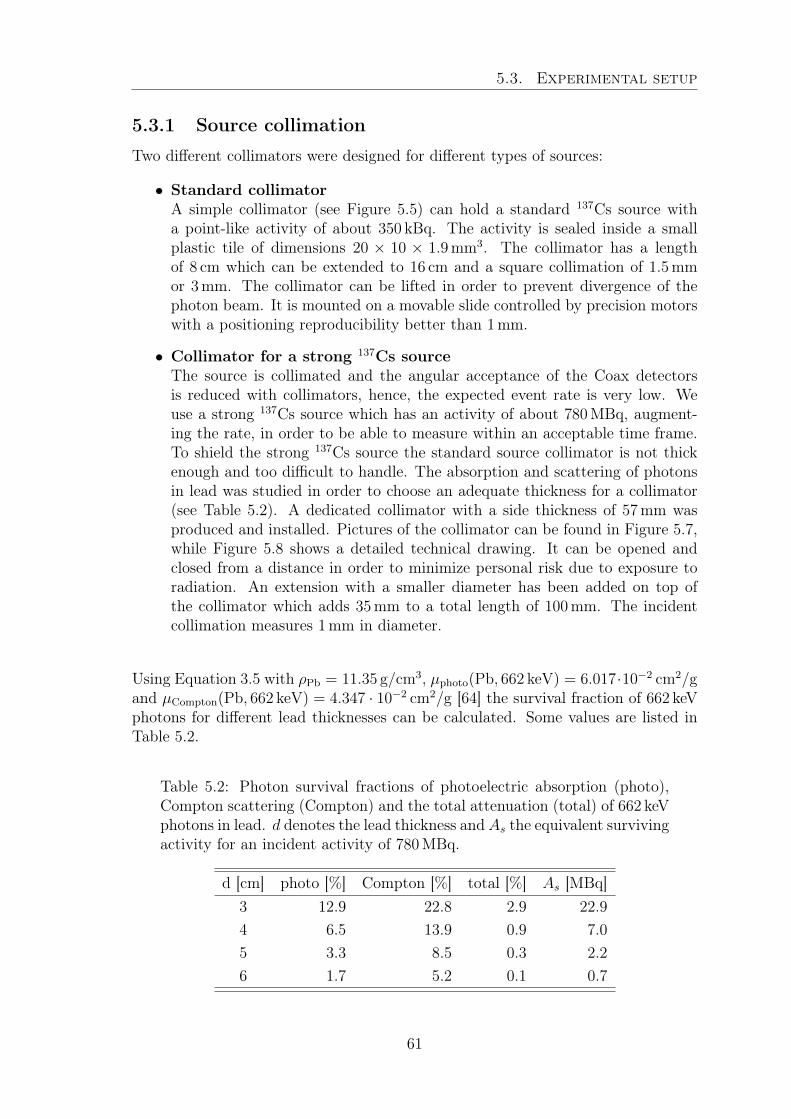
5.3. Experimental setup
5.3.1 Source collimation
Two different collimators were designed for different types of sources:
• Standard collimatorA simple collimator (see Figure 5.5) can hold a standard 137Cs source witha point-like activity of about 350 kBq. The activity is sealed inside a smallplastic tile of dimensions 20 × 10 × 1.9mm3. The collimator has a lengthof 8 cm which can be extended to 16 cm and a square collimation of 1.5mmor 3mm. The collimator can be lifted in order to prevent divergence of thephoton beam. It is mounted on a movable slide controlled by precision motorswith a positioning reproducibility better than 1mm.
• Collimator for a strong 137Cs sourceThe source is collimated and the angular acceptance of the Coax detectorsis reduced with collimators, hence, the expected event rate is very low. Weuse a strong 137Cs source which has an activity of about 780MBq, augment-ing the rate, in order to be able to measure within an acceptable time frame.To shield the strong 137Cs source the standard source collimator is not thickenough and too difficult to handle. The absorption and scattering of photonsin lead was studied in order to choose an adequate thickness for a collimator(see Table 5.2). A dedicated collimator with a side thickness of 57mm wasproduced and installed. Pictures of the collimator can be found in Figure 5.7,while Figure 5.8 shows a detailed technical drawing. It can be opened andclosed from a distance in order to minimize personal risk due to exposure toradiation. An extension with a smaller diameter has been added on top ofthe collimator which adds 35mm to a total length of 100mm. The incidentcollimation measures 1mm in diameter.
Using Equation 3.5 with ρPb = 11.35 g/cm3, µphoto(Pb, 662 keV) = 6.017·10−2 cm2/gand µCompton(Pb, 662 keV) = 4.347 · 10−2 cm2/g [64] the survival fraction of 662 keVphotons for different lead thicknesses can be calculated. Some values are listed inTable 5.2.
Table 5.2: Photon survival fractions of photoelectric absorption (photo),Compton scattering (Compton) and the total attenuation (total) of 662 keVphotons in lead. d denotes the lead thickness and As the equivalent survivingactivity for an incident activity of 780MBq.
d [cm] photo [%] Compton [%] total [%] As [MBq]3 12.9 22.8 2.9 22.94 6.5 13.9 0.9 7.05 3.3 8.5 0.3 2.26 1.7 5.2 0.1 0.7
61

5.3. Experimental setup
5.3.2 Automatic filling system
Germanium detectors have to be operated at cryogenic temperatures. All detectorsare mounted in vacuum cryostats connected to dewar vessels, which contain LN2, bya cold finger. The Coax detectors, mounted on the table platform, have very smalldewars with a volume of 3 l only. They have to be filled within a time interval of∼ 16 h, which makes manual filling unfeasible.
Therefore, all dewar vessels have been connected to an automatic filling system con-trolled by a Keysight1 Data Acquisition Unit2. The unit has been programmed toread the values of temperature sensors inside the vacuum cryostats of each detector.Moreover, it reads the temperature of all valves in the automatic filling system andmanages an opening and closing sequence in order to fill all dewars in a predefinedtime interval.
Originally, the filling interval was set to 14 h; after a couple of months of stable op-eration the interval was changed to 16 h. The system can also be managed remotelyvia a Graphical User Interface (GUI) and detectors can be manually excluded fromrefilling via the GUI.
The LN2 is provided by a storage tank with a total volume of about 180 l. Thisvessel has to be filled manually in a five day interval if all detectors are connected.
5.3.3 Low and high voltage supply and safety shutdown
The PreAmps of all detectors are powered by SpecAmps34, with a LV of 6V.
The Coax detectors use negative HV and the BEGe positive HV (see Table 4.1).This is provided by two programmable HV modules5.
Each detector has an HV inhibit signal output which changes its voltage level ifthe crystal becomes too warm; this happens typically above 110K. All HV inhibitsignals are collected in a dedicated unit which further connects to the HV modules.If one detector is sending the HV inhibit signal the unit sends a shut down signal tothe HV modules in order to ramp down all detector HVs; it is assumed that noneof the detectors has been refilled.
The Keysight unit can provide a shutdown trigger with a programmable temperaturetrigger level. In this manner the shutdown can be triggered at a lower temperaturethan with the HV inhibit signals.
1Former Agilent234970A Data Acquisition / Data Logger Switch Unit3Coax: Silena 7611/L Spectroscopy Amplifier4BEGe: Ortec 762 Spectroscopy Amplifier5CAEN N1471H: NIM HV Power Supply High Accuracy Module
62
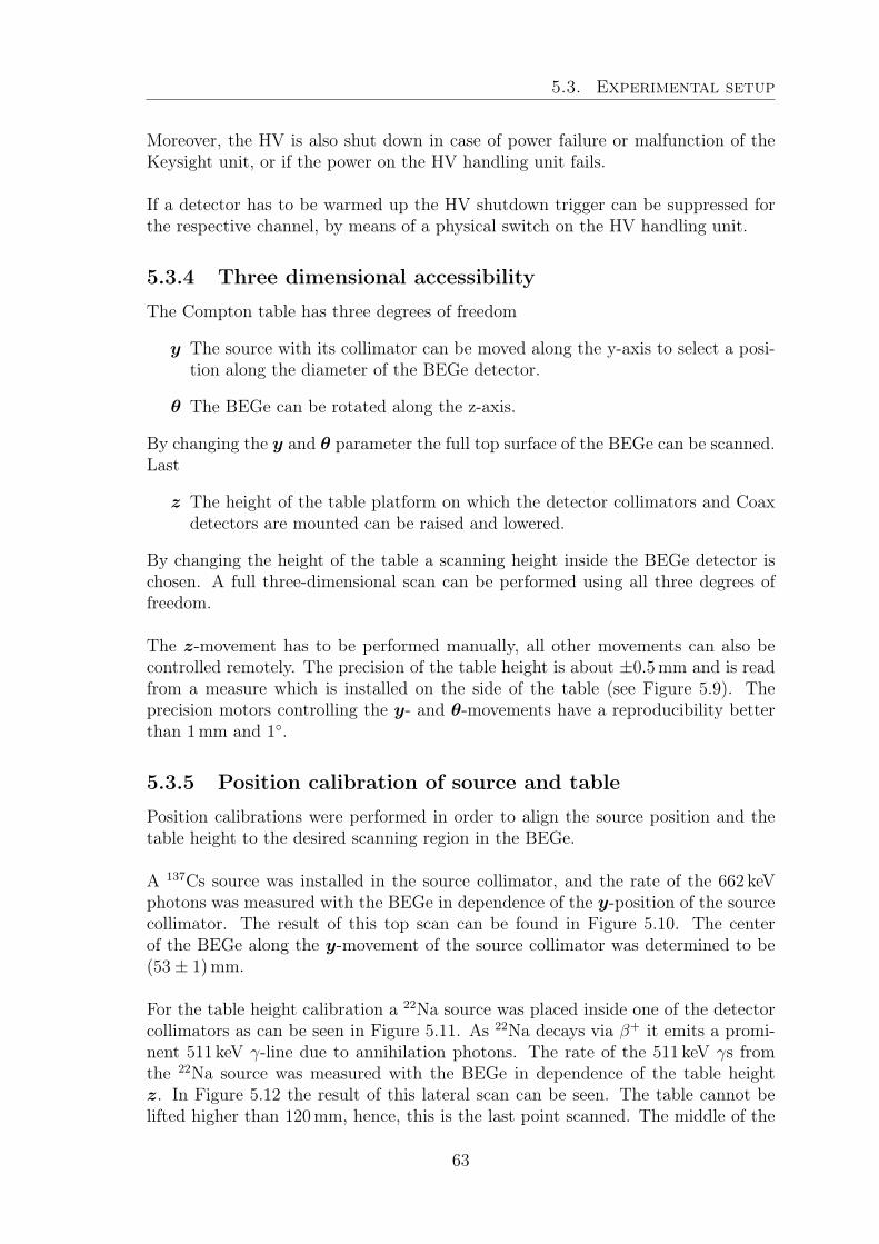
5.3. Experimental setup
Moreover, the HV is also shut down in case of power failure or malfunction of theKeysight unit, or if the power on the HV handling unit fails.
If a detector has to be warmed up the HV shutdown trigger can be suppressed forthe respective channel, by means of a physical switch on the HV handling unit.
5.3.4 Three dimensional accessibility
The Compton table has three degrees of freedom
y The source with its collimator can be moved along the y-axis to select a posi-tion along the diameter of the BEGe detector.
θ The BEGe can be rotated along the z-axis.
By changing the y and θ parameter the full top surface of the BEGe can be scanned.Last
z The height of the table platform on which the detector collimators and Coaxdetectors are mounted can be raised and lowered.
By changing the height of the table a scanning height inside the BEGe detector ischosen. A full three-dimensional scan can be performed using all three degrees offreedom.
The z-movement has to be performed manually, all other movements can also becontrolled remotely. The precision of the table height is about ±0.5mm and is readfrom a measure which is installed on the side of the table (see Figure 5.9). Theprecision motors controlling the y- and θ-movements have a reproducibility betterthan 1mm and 1.
5.3.5 Position calibration of source and table
Position calibrations were performed in order to align the source position and thetable height to the desired scanning region in the BEGe.
A 137Cs source was installed in the source collimator, and the rate of the 662 keVphotons was measured with the BEGe in dependence of the y-position of the sourcecollimator. The result of this top scan can be found in Figure 5.10. The centerof the BEGe along the y-movement of the source collimator was determined to be(53± 1)mm.
For the table height calibration a 22Na source was placed inside one of the detectorcollimators as can be seen in Figure 5.11. As 22Na decays via β+ it emits a promi-nent 511 keV γ-line due to annihilation photons. The rate of the 511 keV γs fromthe 22Na source was measured with the BEGe in dependence of the table heightz. In Figure 5.12 the result of this lateral scan can be seen. The table cannot belifted higher than 120mm, hence, this is the last point scanned. The middle of the
63
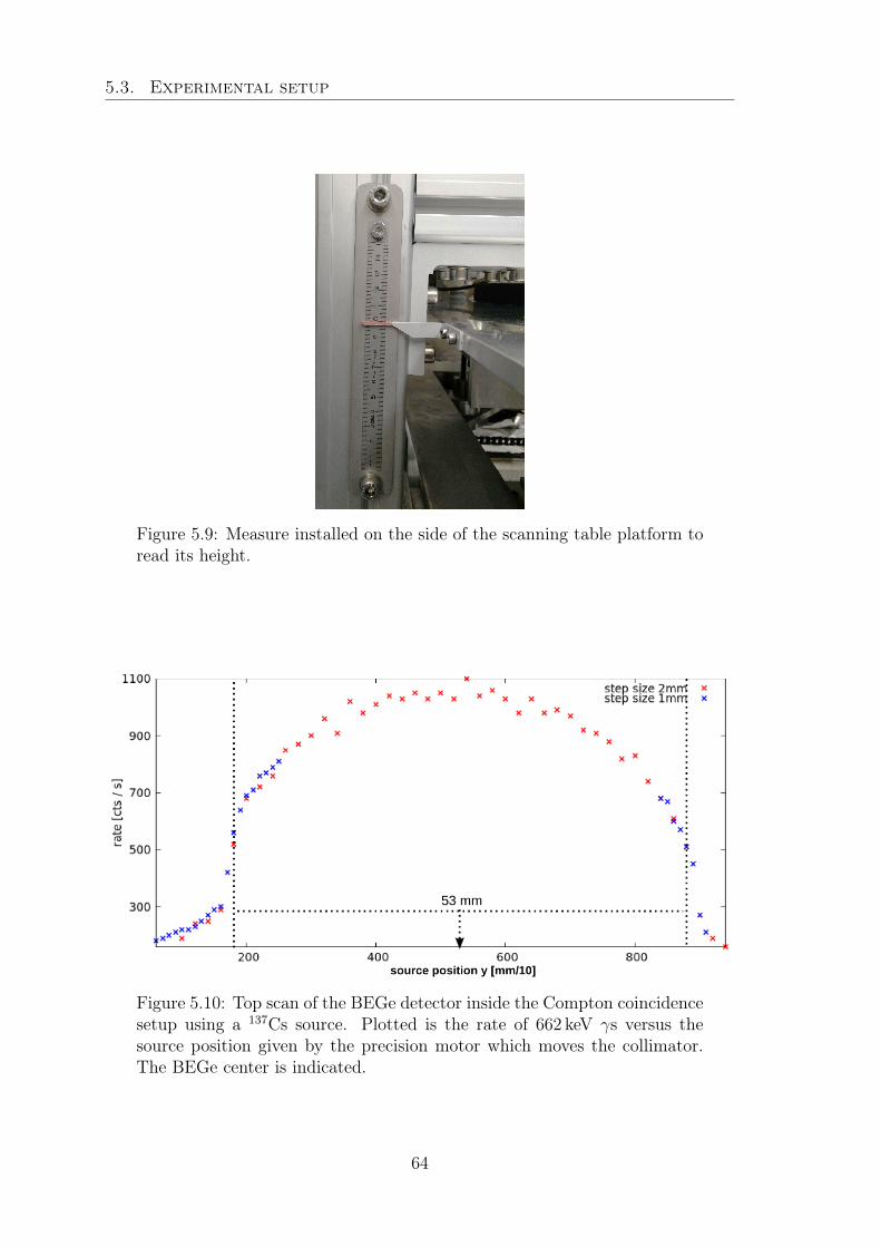
5.3. Experimental setup
Figure 5.9: Measure installed on the side of the scanning table platform toread its height.
Figure 5.10: Top scan of the BEGe detector inside the Compton coincidencesetup using a 137Cs source. Plotted is the rate of 662 keV γs versus thesource position given by the precision motor which moves the collimator.The BEGe center is indicated.
64
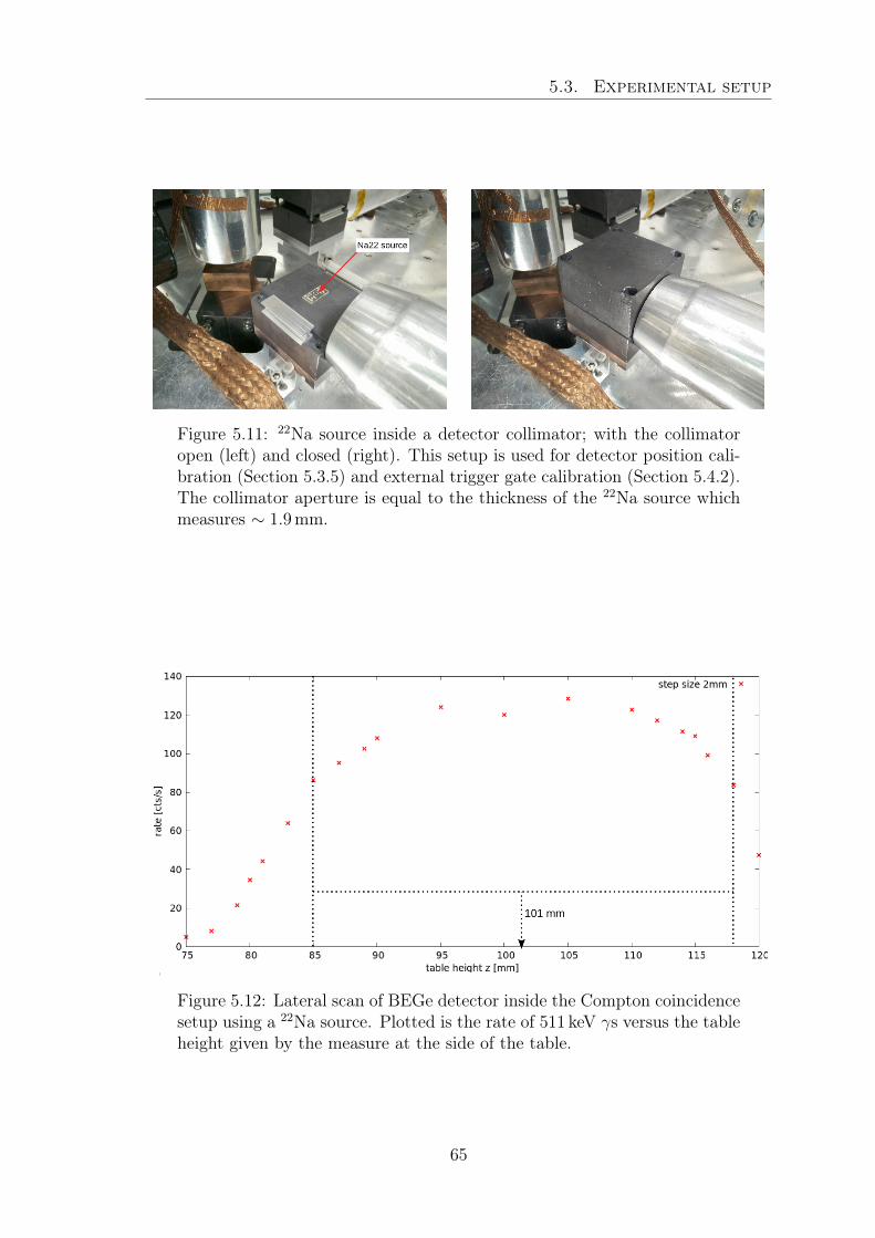
5.3. Experimental setup
Figure 5.11: 22Na source inside a detector collimator; with the collimatoropen (left) and closed (right). This setup is used for detector position cali-bration (Section 5.3.5) and external trigger gate calibration (Section 5.4.2).The collimator aperture is equal to the thickness of the 22Na source whichmeasures ∼ 1.9mm.
Figure 5.12: Lateral scan of BEGe detector inside the Compton coincidencesetup using a 22Na source. Plotted is the rate of 511 keV γs versus the tableheight given by the measure at the side of the table.
65
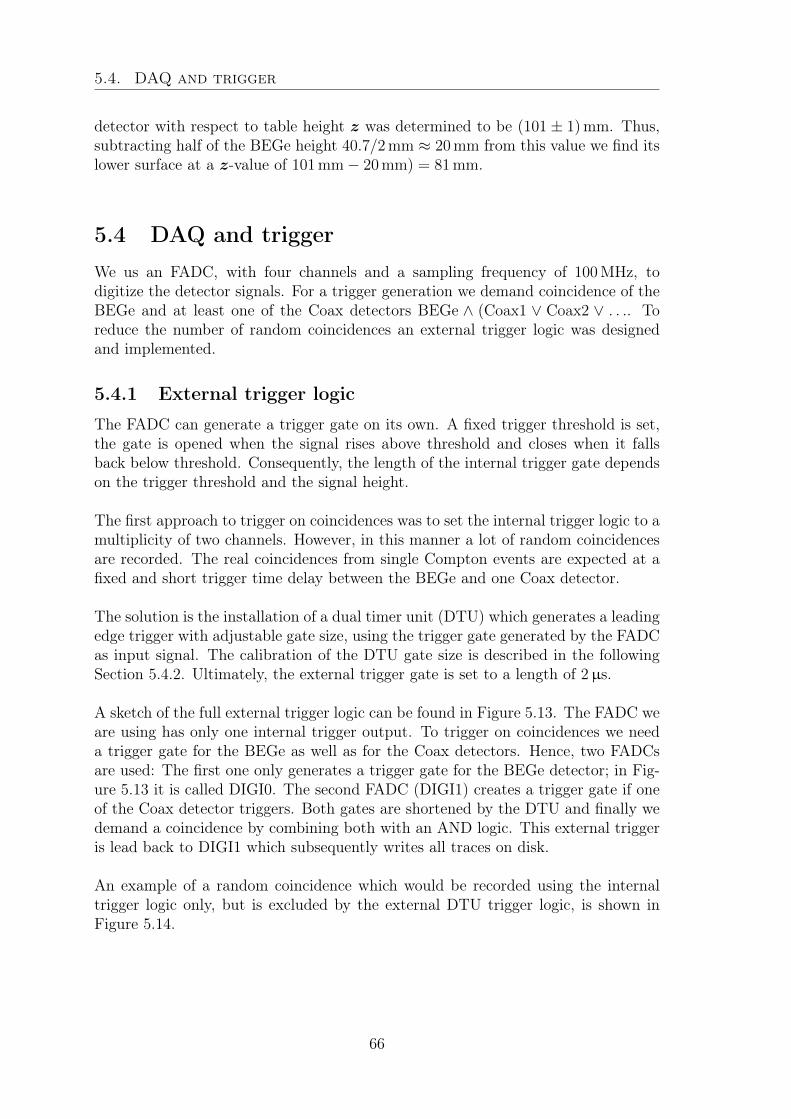
5.4. DAQ and trigger
detector with respect to table height z was determined to be (101± 1)mm. Thus,subtracting half of the BEGe height 40.7/2 mm ≈ 20 mm from this value we find itslower surface at a z-value of 101 mm− 20 mm) = 81 mm.
5.4 DAQ and triggerWe us an FADC, with four channels and a sampling frequency of 100MHz, todigitize the detector signals. For a trigger generation we demand coincidence of theBEGe and at least one of the Coax detectors BEGe ∧ (Coax1 ∨ Coax2 ∨ . . .. Toreduce the number of random coincidences an external trigger logic was designedand implemented.
5.4.1 External trigger logic
The FADC can generate a trigger gate on its own. A fixed trigger threshold is set,the gate is opened when the signal rises above threshold and closes when it fallsback below threshold. Consequently, the length of the internal trigger gate dependson the trigger threshold and the signal height.
The first approach to trigger on coincidences was to set the internal trigger logic to amultiplicity of two channels. However, in this manner a lot of random coincidencesare recorded. The real coincidences from single Compton events are expected at afixed and short trigger time delay between the BEGe and one Coax detector.
The solution is the installation of a dual timer unit (DTU) which generates a leadingedge trigger with adjustable gate size, using the trigger gate generated by the FADCas input signal. The calibration of the DTU gate size is described in the followingSection 5.4.2. Ultimately, the external trigger gate is set to a length of 2µs.
A sketch of the full external trigger logic can be found in Figure 5.13. The FADC weare using has only one internal trigger output. To trigger on coincidences we needa trigger gate for the BEGe as well as for the Coax detectors. Hence, two FADCsare used: The first one only generates a trigger gate for the BEGe detector; in Fig-ure 5.13 it is called DIGI0. The second FADC (DIGI1) creates a trigger gate if oneof the Coax detector triggers. Both gates are shortened by the DTU and finally wedemand a coincidence by combining both with an AND logic. This external triggeris lead back to DIGI1 which subsequently writes all traces on disk.
An example of a random coincidence which would be recorded using the internaltrigger logic only, but is excluded by the external DTU trigger logic, is shown inFigure 5.14.
66
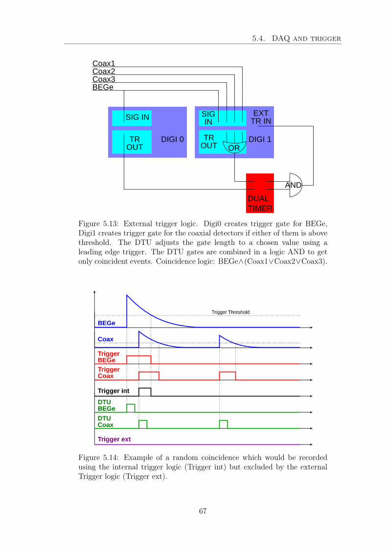
5.4. DAQ and trigger
Figure 5.13: External trigger logic. Digi0 creates trigger gate for BEGe,Digi1 creates trigger gate for the coaxial detectors if either of them is abovethreshold. The DTU adjusts the gate length to a chosen value using aleading edge trigger. The DTU gates are combined in a logic AND to getonly coincident events. Coincidence logic: BEGe∧(Coax1∨Coax2∨Coax3).
Figure 5.14: Example of a random coincidence which would be recordedusing the internal trigger logic (Trigger int) but excluded by the externalTrigger logic (Trigger ext).
67
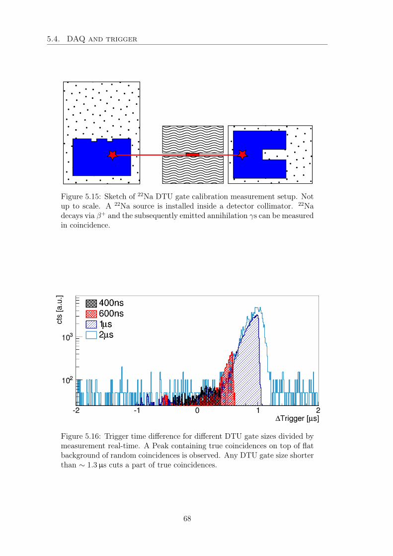
5.4. DAQ and trigger
Figure 5.15: Sketch of 22Na DTU gate calibration measurement setup. Notup to scale. A 22Na source is installed inside a detector collimator. 22Nadecays via β+ and the subsequently emitted annihilation γs can be measuredin coincidence.
Figure 5.16: Trigger time difference for different DTU gate sizes divided bymeasurement real-time. A Peak containing true coincidences on top of flatbackground of random coincidences is observed. Any DTU gate size shorterthan ∼ 1.3µs cuts a part of true coincidences.
68
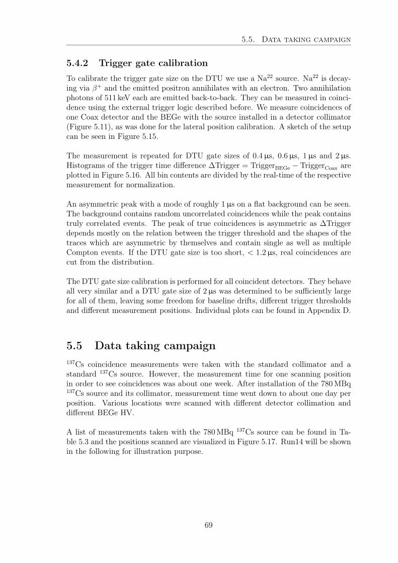
5.5. Data taking campaign
5.4.2 Trigger gate calibration
To calibrate the trigger gate size on the DTU we use a Na22 source. Na22 is decay-ing via β+ and the emitted positron annihilates with an electron. Two annihilationphotons of 511 keV each are emitted back-to-back. They can be measured in coinci-dence using the external trigger logic described before. We measure coincidences ofone Coax detector and the BEGe with the source installed in a detector collimator(Figure 5.11), as was done for the lateral position calibration. A sketch of the setupcan be seen in Figure 5.15.
The measurement is repeated for DTU gate sizes of 0.4µs, 0.6µs, 1µs and 2µs.Histograms of the trigger time difference ∆Trigger = TriggerBEGe − TriggerCoax areplotted in Figure 5.16. All bin contents are divided by the real-time of the respectivemeasurement for normalization.
An asymmetric peak with a mode of roughly 1µs on a flat background can be seen.The background contains random uncorrelated coincidences while the peak containstruly correlated events. The peak of true coincidences is asymmetric as ∆Triggerdepends mostly on the relation between the trigger threshold and the shapes of thetraces which are asymmetric by themselves and contain single as well as multipleCompton events. If the DTU gate size is too short, < 1.2µs, real coincidences arecut from the distribution.
The DTU gate size calibration is performed for all coincident detectors. They behaveall very similar and a DTU gate size of 2µs was determined to be sufficiently largefor all of them, leaving some freedom for baseline drifts, different trigger thresholdsand different measurement positions. Individual plots can be found in Appendix D.
5.5 Data taking campaign137Cs coincidence measurements were taken with the standard collimator and astandard 137Cs source. However, the measurement time for one scanning positionin order to see coincidences was about one week. After installation of the 780MBq137Cs source and its collimator, measurement time went down to about one day perposition. Various locations were scanned with different detector collimation anddifferent BEGe HV.
A list of measurements taken with the 780MBq 137Cs source can be found in Ta-ble 5.3 and the positions scanned are visualized in Figure 5.17. Run14 will be shownin the following for illustration purpose.
69
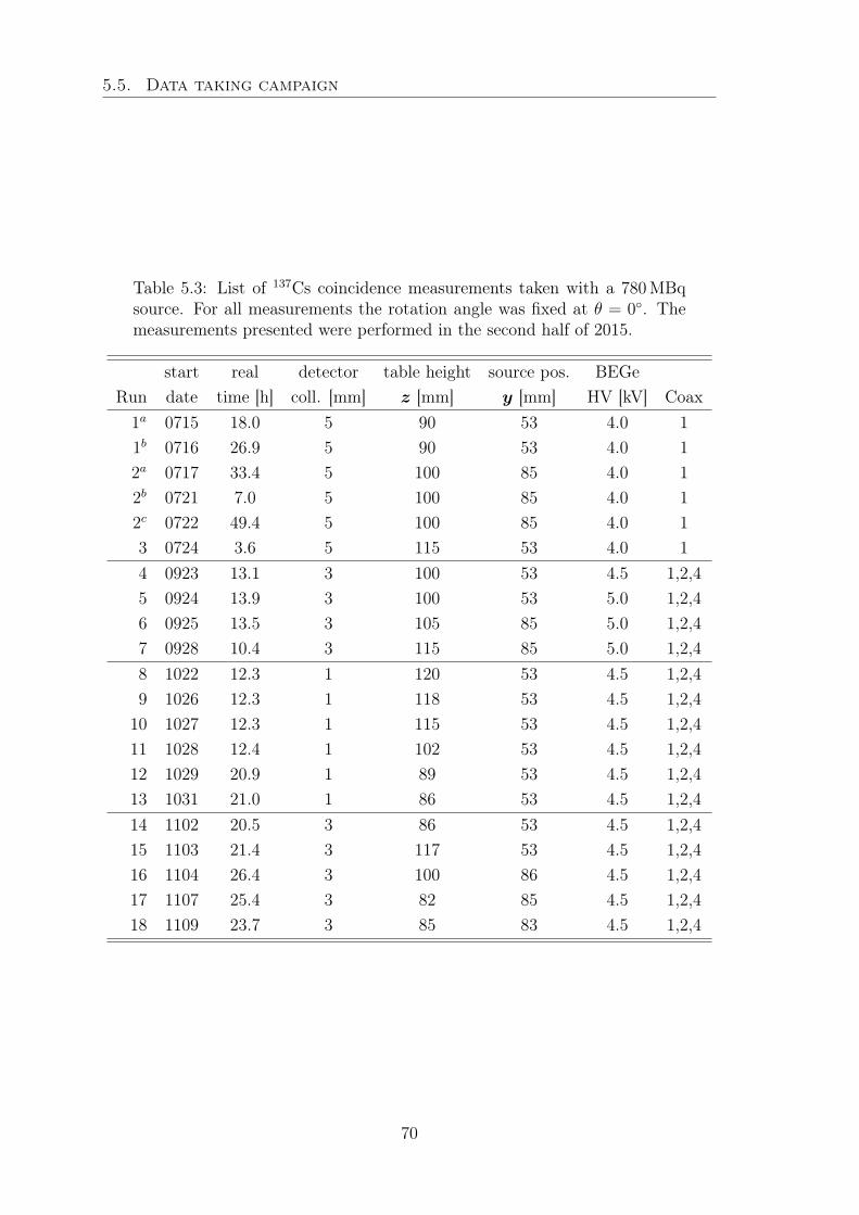
5.5. Data taking campaign
Table 5.3: List of 137Cs coincidence measurements taken with a 780MBqsource. For all measurements the rotation angle was fixed at θ = 0. Themeasurements presented were performed in the second half of 2015.
start real detector table height source pos. BEGeRun date time [h] coll. [mm] z [mm] y [mm] HV [kV] Coax
1a 0715 18.0 5 90 53 4.0 11b 0716 26.9 5 90 53 4.0 12a 0717 33.4 5 100 85 4.0 12b 0721 7.0 5 100 85 4.0 12c 0722 49.4 5 100 85 4.0 13 0724 3.6 5 115 53 4.0 14 0923 13.1 3 100 53 4.5 1,2,45 0924 13.9 3 100 53 5.0 1,2,46 0925 13.5 3 105 85 5.0 1,2,47 0928 10.4 3 115 85 5.0 1,2,48 1022 12.3 1 120 53 4.5 1,2,49 1026 12.3 1 118 53 4.5 1,2,410 1027 12.3 1 115 53 4.5 1,2,411 1028 12.4 1 102 53 4.5 1,2,412 1029 20.9 1 89 53 4.5 1,2,413 1031 21.0 1 86 53 4.5 1,2,414 1102 20.5 3 86 53 4.5 1,2,415 1103 21.4 3 117 53 4.5 1,2,416 1104 26.4 3 100 86 4.5 1,2,417 1107 25.4 3 82 85 4.5 1,2,418 1109 23.7 3 85 83 4.5 1,2,4
70
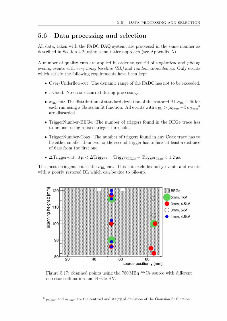
5.6. Data processing and selection
5.6 Data processing and selectionAll data, taken with the FADC DAQ system, are processed in the same manner asdescribed in Section 4.2, using a multi-tier approach (see Appendix A).
A number of quality cuts are applied in order to get rid of unphysical and pile-upevents, events with very noisy baseline (BL) and random coincidences. Only eventswhich satisfy the following requirements have been kept
• Over/Underflow-cut: The dynamic range of the FADC has not to be exceeded.
• IsGood: No error occurred during processing.
• σBL-cut: The distribution of standard deviation of the restored BL σBL is fit foreach run using a Gaussian fit function. All events with σBL > µGauss +3σGauss
6
are discarded.
• TriggerNumber-BEGe: The number of triggers found in the BEGe trace hasto be one, using a fixed trigger threshold.
• TriggerNumber-Coax: The number of triggers found in any Coax trace has tobe either smaller than two, or the second trigger has to have at least a distanceof 6µs from the first one.
• ∆Trigger-cut: 0µ < ∆Trigger = TriggerBEGe − TriggerCoax < 1.2µs.
The most stringent cut is the σBL-cut. This cut excludes noisy events and eventswith a poorly restored BL which can be due to pile-up.
Figure 5.17: Scanned points using the 780MBq 137Cs source with differentdetector collimation and BEGe HV.
6 µGauss and σGauss are the centroid and standard deviation of the Gaussian fit function.71
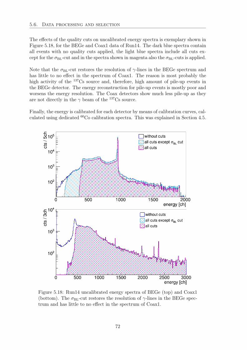
5.6. Data processing and selection
The effects of the quality cuts on uncalibrated energy spectra is exemplary shown inFigure 5.18, for the BEGe and Coax1 data of Run14. The dark blue spectra containall events with no quality cuts applied, the light blue spectra include all cuts ex-cept for the σBL-cut and in the spectra shown in magenta also the σBL-cuts is applied.
Note that the σBL-cut restores the resolution of γ-lines in the BEGe spectrum andhas little to no effect in the spectrum of Coax1. The reason is most probably thehigh activity of the 137Cs source and, therefore, high amount of pile-up events inthe BEGe detector. The energy reconstruction for pile-up events is mostly poor andworsens the energy resolution. The Coax detectors show much less pile-up as theyare not directly in the γ beam of the 137Cs source.
Finally, the energy is calibrated for each detector by means of calibration curves, cal-culated using dedicated 60Co calibration spectra. This was explained in Section 4.5.
Figure 5.18: Run14 uncalibrated energy spectra of BEGe (top) and Coax1(bottom). The σBL-cut restores the resolution of γ-lines in the BEGe spec-trum and has little to no effect in the spectrum of Coax1.
72
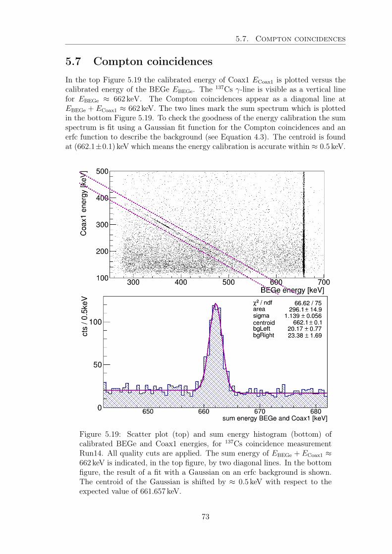
5.7. Compton coincidences
5.7 Compton coincidencesIn the top Figure 5.19 the calibrated energy of Coax1 ECoax1 is plotted versus thecalibrated energy of the BEGe EBEGe. The 137Cs γ-line is visible as a vertical linefor EBEGe ≈ 662 keV. The Compton coincidences appear as a diagonal line atEBEGe + ECoax1 ≈ 662 keV. The two lines mark the sum spectrum which is plottedin the bottom Figure 5.19. To check the goodness of the energy calibration the sumspectrum is fit using a Gaussian fit function for the Compton coincidences and anerfc function to describe the background (see Equation 4.3). The centroid is foundat (662.1±0.1) keV which means the energy calibration is accurate within ≈ 0.5 keV.
Figure 5.19: Scatter plot (top) and sum energy histogram (bottom) ofcalibrated BEGe and Coax1 energies, for 137Cs coincidence measurementRun14. All quality cuts are applied. The sum energy of EBEGe + ECoax1 ≈662 keV is indicated, in the top figure, by two diagonal lines. In the bottomfigure, the result of a fit with a Gaussian on an erfc background is shown.The centroid of the Gaussian is shifted by ≈ 0.5 keV with respect to theexpected value of 661.657 keV.
73

5.7. Compton coincidences
74
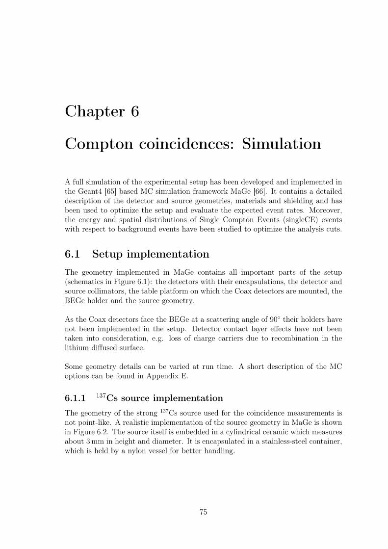
Chapter 6
Compton coincidences: Simulation
A full simulation of the experimental setup has been developed and implemented inthe Geant4 [65] based MC simulation framework MaGe [66]. It contains a detaileddescription of the detector and source geometries, materials and shielding and hasbeen used to optimize the setup and evaluate the expected event rates. Moreover,the energy and spatial distributions of Single Compton Events (singleCE) eventswith respect to background events have been studied to optimize the analysis cuts.
6.1 Setup implementationThe geometry implemented in MaGe contains all important parts of the setup(schematics in Figure 6.1): the detectors with their encapsulations, the detector andsource collimators, the table platform on which the Coax detectors are mounted, theBEGe holder and the source geometry.
As the Coax detectors face the BEGe at a scattering angle of 90 their holders havenot been implemented in the setup. Detector contact layer effects have not beentaken into consideration, e.g. loss of charge carriers due to recombination in thelithium diffused surface.
Some geometry details can be varied at run time. A short description of the MCoptions can be found in Appendix E.
6.1.1 137Cs source implementation
The geometry of the strong 137Cs source used for the coincidence measurements isnot point-like. A realistic implementation of the source geometry in MaGe is shownin Figure 6.2. The source itself is embedded in a cylindrical ceramic which measuresabout 3mm in height and diameter. It is encapsulated in a stainless-steel container,which is held by a nylon vessel for better handling.
75
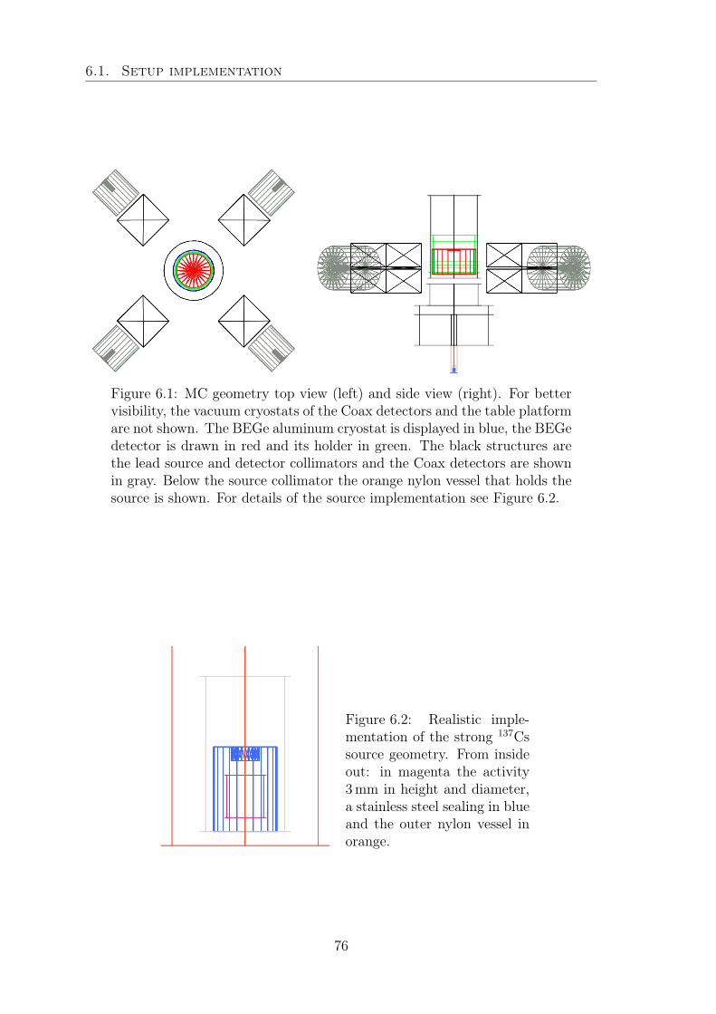
6.1. Setup implementation
Figure 6.1: MC geometry top view (left) and side view (right). For bettervisibility, the vacuum cryostats of the Coax detectors and the table platformare not shown. The BEGe aluminum cryostat is displayed in blue, the BEGedetector is drawn in red and its holder in green. The black structures arethe lead source and detector collimators and the Coax detectors are shownin gray. Below the source collimator the orange nylon vessel that holds thesource is shown. For details of the source implementation see Figure 6.2.
Figure 6.2: Realistic imple-mentation of the strong 137Cssource geometry. From insideout: in magenta the activity3mm in height and diameter,a stainless steel sealing in blueand the outer nylon vessel inorange.
76
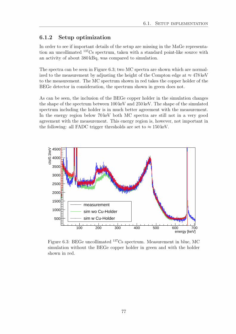
6.1. Setup implementation
6.1.2 Setup optimization
In order to see if important details of the setup are missing in the MaGe representa-tion an uncollimated 137Cs spectrum, taken with a standard point-like source withan activity of about 380 kBq, was compared to simulation.
The spectra can be seen in Figure 6.3; two MC spectra are shown which are normal-ized to the measurement by adjusting the height of the Compton edge at ≈ 478 keVto the measurement. The MC spectrum shown in red takes the copper holder of theBEGe detector in consideration, the spectrum shown in green does not.
As can be seen, the inclusion of the BEGe copper holder in the simulation changesthe shape of the spectrum between 100 keV and 250 keV. The shape of the simulatedspectrum including the holder is in much better agreement with the measurement.In the energy region below 70 keV both MC spectra are still not in a very goodagreement with the measurement. This energy region is, however, not important inthe following: all FADC trigger thresholds are set to ≈ 150 keV.
energy [keV]100 200 300 400 500 600 700
cts/
0.1k
eV
500
1000
1500
2000
2500
3000
3500
4000
4500
measurement
sim wo Cu-Holder
sim w Cu-Holder
Figure 6.3: BEGe uncollimated 137Cs spectrum. Measurement in blue, MCsimulation without the BEGe copper holder in green and with the holdershown in red.
77
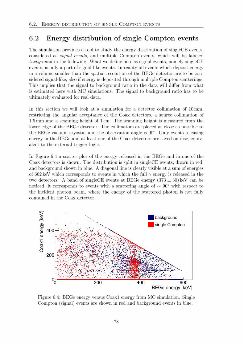
6.2. Energy distribution of single Compton events
6.2 Energy distribution of single Compton eventsThe simulation provides a tool to study the energy distribution of singleCE events,considered as signal events, and multiple Compton events, which will be labeledbackground in the following. What we define here as signal events, namely singleCEevents, is only a part of signal-like events. In reality all events which deposit energyin a volume smaller than the spatial resolution of the BEGe detector are to be con-sidered signal-like, also if energy is deposited through multiple Compton scatterings.This implies that the signal to background ratio in the data will differ from whatis estimated here with MC simulations. The signal to background ratio has to beultimately evaluated for real data.
In this section we will look at a simulation for a detector collimation of 10mm,restricting the angular acceptance of the Coax detectors, a source collimation of1.5mm and a scanning height of 1 cm. The scanning height is measured from thelower edge of the BEGe detector. The collimators are placed as close as possible tothe BEGe vacuum cryostat and the observation angle is 90. Only events releasingenergy in the BEGe and at least one of the Coax detectors are saved on disc, equiv-alent to the external trigger logic.
In Figure 6.4 a scatter plot of the energy released in the BEGe and in one of theCoax detectors is shown. The distribution is split in singleCE events, drawn in red,and background shown in blue. A diagonal line is clearly visible at a sum of energiesof 662 keV which corresponds to events in which the full γ energy is released in thetwo detectors. A band of singleCE events at BEGe energy (373 ± 30) keV can benoticed; it corresponds to events with a scattering angle of ∼ 90 with respect tothe incident photon beam, where the energy of the scattered photon is not fullycontained in the Coax detector.
Figure 6.4: BEGe energy versus Coax1 energy from MC simulation. SingleCompton (signal) events are shown in red and background events in blue.
78
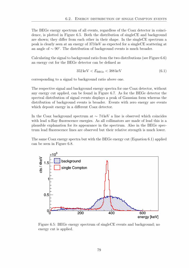
6.2. Energy distribution of single Compton events
The BEGe energy spectrum of all events, regardless of the Coax detector in coinci-dence, is plotted in Figure 6.5. Both the distribution of singleCE and backgroundare shown; they differ from each other in their shape. In the singleCE spectrum apeak is clearly seen at an energy of 373 keV as expected for a singleCE scattering atan angle of ∼ 90. The distribution of background events is much broader.
Calculating the signal to background ratio from the two distributions (see Figure 6.6)an energy cut for the BEGe detector can be defined as
352 keV < EBEGe < 388 keV (6.1)
corresponding to a signal to background ratio above one.
The respective signal and background energy spectra for one Coax detector, withoutany energy cut applied, can be found in Figure 6.7. As for the BEGe detector thespectral distribution of signal events displays a peak of Gaussian form whereas thedistribution of background events is broader. Events with zero energy are eventswhich deposit energy in a different Coax detector.
In the Coax background spectrum at ∼ 74 keV a line is observed which coincideswith lead x-Ray fluorescence energies. As all collimators are made of lead this is aplausible explanation for its appearance in the spectrum. Also in the BEGe spec-trum lead fluorescence lines are observed but their relative strength is much lower.
The same Coax energy spectra but with the BEGe energy cut (Equation 6.1) appliedcan be seen in Figure 6.8.
Figure 6.5: BEGe energy spectrum of singleCE events and background; noenergy cut is applied.
79
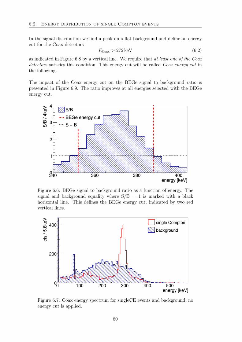
6.2. Energy distribution of single Compton events
In the signal distribution we find a peak on a flat background and define an energycut for the Coax detectors
ECoax > 272 keV (6.2)
as indicated in Figure 6.8 by a vertical line. We require that at least one of the Coaxdetectors satisfies this condition. This energy cut will be called Coax energy cut inthe following.
The impact of the Coax energy cut on the BEGe signal to background ratio ispresented in Figure 6.9. The ratio improves at all energies selected with the BEGeenergy cut.
Figure 6.6: BEGe signal to background ratio as a function of energy. Thesignal and background equality where S/B = 1 is marked with a blackhorizontal line. This defines the BEGe energy cut, indicated by two redvertical lines.
Figure 6.7: Coax energy spectrum for singleCE events and background; noenergy cut is applied.
80
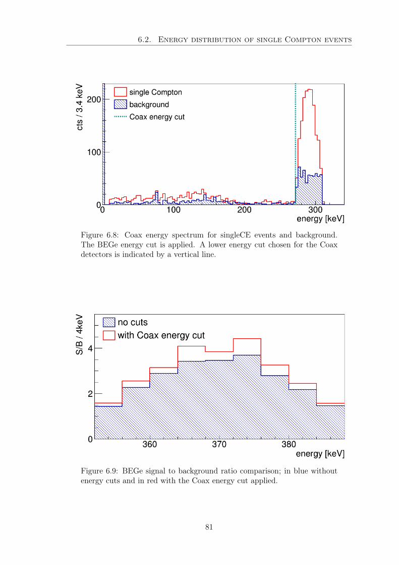
6.2. Energy distribution of single Compton events
Figure 6.8: Coax energy spectrum for singleCE events and background.The BEGe energy cut is applied. A lower energy cut chosen for the Coaxdetectors is indicated by a vertical line.
Figure 6.9: BEGe signal to background ratio comparison; in blue withoutenergy cuts and in red with the Coax energy cut applied.
81
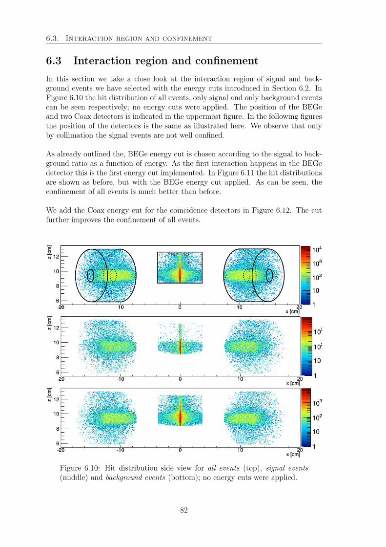
6.3. Interaction region and confinement
6.3 Interaction region and confinementIn this section we take a close look at the interaction region of signal and back-ground events we have selected with the energy cuts introduced in Section 6.2. InFigure 6.10 the hit distribution of all events, only signal and only background eventscan be seen respectively; no energy cuts were applied. The position of the BEGeand two Coax detectors is indicated in the uppermost figure. In the following figuresthe position of the detectors is the same as illustrated here. We observe that onlyby collimation the signal events are not well confined.
As already outlined the, BEGe energy cut is chosen according to the signal to back-ground ratio as a function of energy. As the first interaction happens in the BEGedetector this is the first energy cut implemented. In Figure 6.11 the hit distributionsare shown as before, but with the BEGe energy cut applied. As can be seen, theconfinement of all events is much better than before.
We add the Coax energy cut for the coincidence detectors in Figure 6.12. The cutfurther improves the confinement of all events.
Figure 6.10: Hit distribution side view for all events (top), signal events(middle) and background events (bottom); no energy cuts were applied.
82
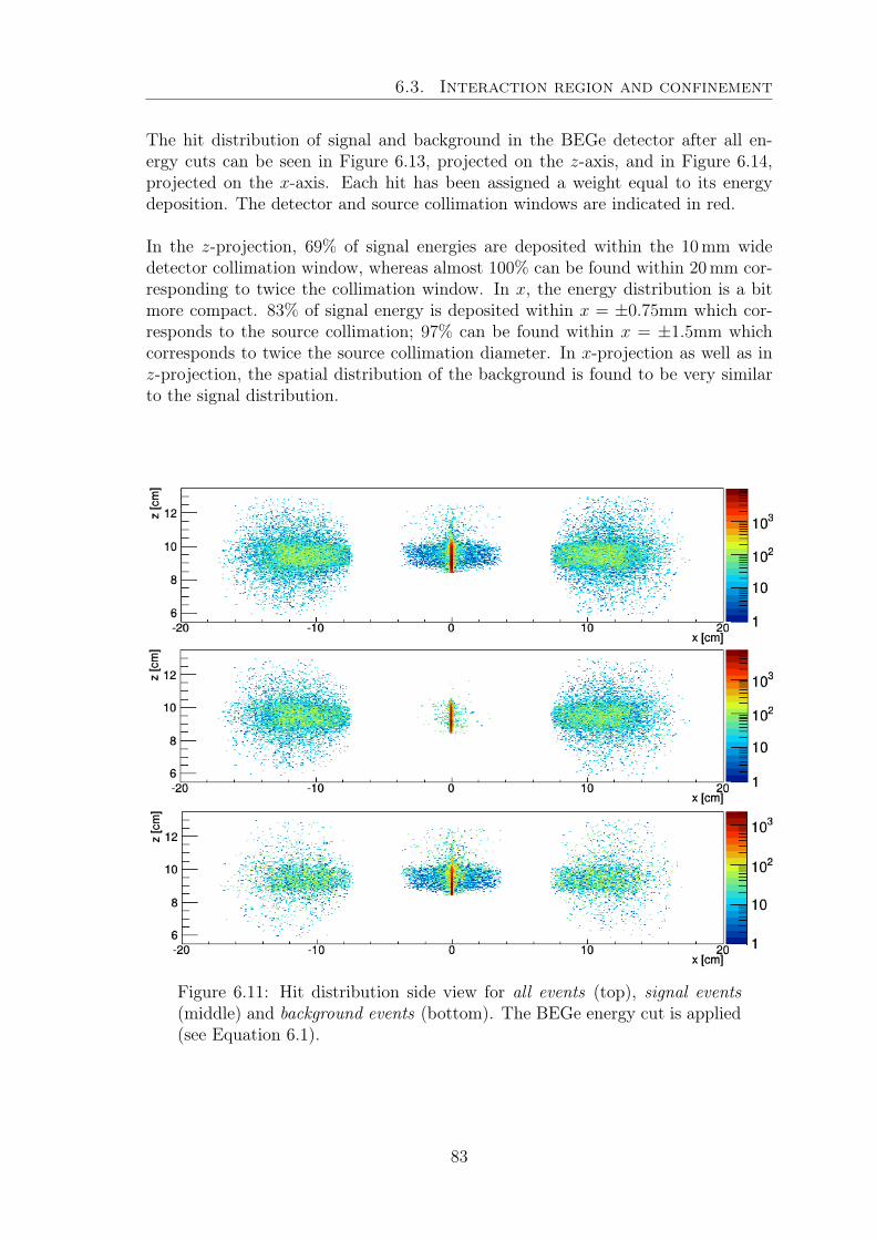
6.3. Interaction region and confinement
The hit distribution of signal and background in the BEGe detector after all en-ergy cuts can be seen in Figure 6.13, projected on the z-axis, and in Figure 6.14,projected on the x-axis. Each hit has been assigned a weight equal to its energydeposition. The detector and source collimation windows are indicated in red.
In the z-projection, 69% of signal energies are deposited within the 10mm widedetector collimation window, whereas almost 100% can be found within 20mm cor-responding to twice the collimation window. In x, the energy distribution is a bitmore compact. 83% of signal energy is deposited within x = ±0.75mm which cor-responds to the source collimation; 97% can be found within x = ±1.5mm whichcorresponds to twice the source collimation diameter. In x-projection as well as inz-projection, the spatial distribution of the background is found to be very similarto the signal distribution.
Figure 6.11: Hit distribution side view for all events (top), signal events(middle) and background events (bottom). The BEGe energy cut is applied(see Equation 6.1).
83
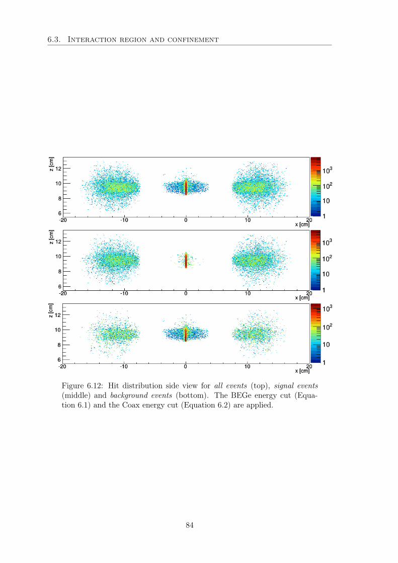
6.3. Interaction region and confinement
Figure 6.12: Hit distribution side view for all events (top), signal events(middle) and background events (bottom). The BEGe energy cut (Equa-tion 6.1) and the Coax energy cut (Equation 6.2) are applied.
84
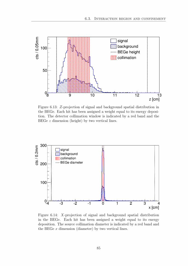
6.3. Interaction region and confinement
Figure 6.13: Z-projection of signal and background spatial distribution inthe BEGe. Each hit has been assigned a weight equal to its energy deposi-tion. The detector collimation window is indicated by a red band and theBEGe z dimension (height) by two vertical lines.
Figure 6.14: X-projection of signal and background spatial distributionin the BEGe. Each hit has been assigned a weight equal to its energydeposition. The source collimation diameter is indicated by a red band andthe BEGe x dimension (diameter) by two vertical lines.
85
6.4. Energy cuts
6.4 Energy cutsSummarizing Section 6.2 and Section 6.3, we have defined energy cuts for the BEGedetector and the Coax detectors in order to select signal events from a confinedinteraction region.
In the MC simulation pile-up events and random coincidences are not considered.Thus, above the sum energy of 662 keV no events are found in the MC spectra. Aswas shown before (see Figure 5.19), this is different for real data. Therefore, weintroduce an additional cut on the BEGe and Coax sum energy for data analysis.The sum energy spectra are fit with a Gaussian fit function modeling the backgroundby an erfc and the cut is defined as
662 keV − 3σ < EBEGe + ECoax ≡ ESum < 662 keV + 3σ (6.3)
where σ is the standard deviation of the Gaussian. An example of the fit was alreadyshown in Figure 5.19.
Summarizing, all energy cuts we apply are the following
• BEGe energy cut 352 keV < EBEGe < 388 keV
• Coax energy cut ECoax > 272 keV
• Sum energy cut 662 keV − 3σ < ESum < 662 keV + 3σ
Figure 6.15 shows a scatter plot of the BEGe and Coax1 energies for Run14; energycuts are indicated in red.
Applying all energy cuts to simulation, we expect a reduction in the BEGe energyspectrum as is shown in Figure 6.16. The demonstrated energy spectra were ob-tained applying all energy cuts to the usual simulation with detector collimation of10mm, source collimation of 1.5mm etc..
6.5 Comparing Monte Carlo simulations with mea-surements
To be able to compare MC simulations with measurements some general consider-ations have to be made. The MC simulations do not contain pile-up or randomcoincidences, and in order to save simulation time we do not simulate the full solidangle of incident photons from the 137Cs source. In the next subsections we explainhow the number of expected events is calculated from MC simulation.
6.5.1 Solid angle calculation
In order to save simulation time, only a part of the solid angle of incident pho-tons from the 137Cs source is simulated. The respective solid angle fraction can be
86
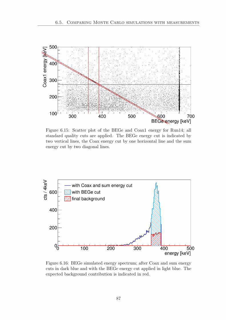
6.5. Comparing Monte Carlo simulations with measurements
Figure 6.15: Scatter plot of the BEGe and Coax1 energy for Run14; allstandard quality cuts are applied. The BEGe energy cut is indicated bytwo vertical lines, the Coax energy cut by one horizontal line and the sumenergy cut by two diagonal lines.
Figure 6.16: BEGe simulated energy spectrum; after Coax and sum energycuts in dark blue and with the BEGe energy cut applied in light blue. Theexpected background contribution is indicated in red.
87
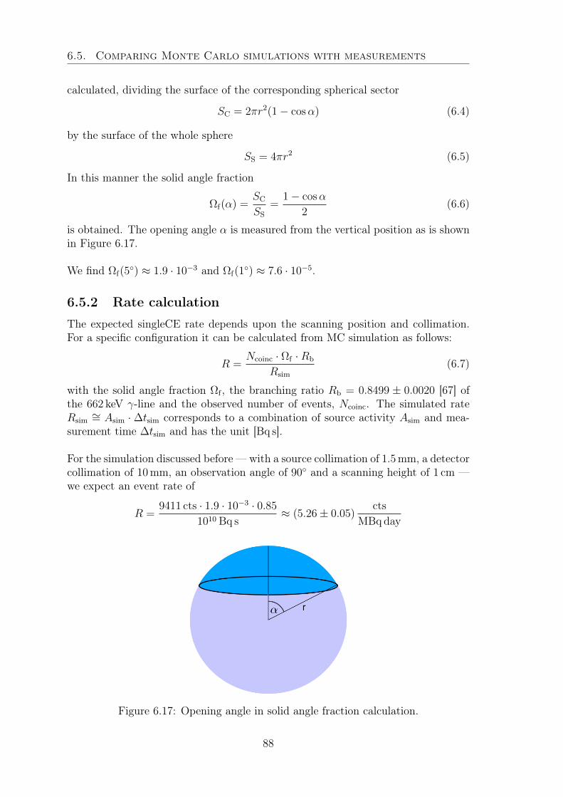
6.5. Comparing Monte Carlo simulations with measurements
calculated, dividing the surface of the corresponding spherical sector
SC = 2πr2(1− cosα) (6.4)
by the surface of the whole sphere
SS = 4πr2 (6.5)
In this manner the solid angle fraction
Ωf(α) =SC
SS
=1− cosα
2(6.6)
is obtained. The opening angle α is measured from the vertical position as is shownin Figure 6.17.
We find Ωf(5) ≈ 1.9 · 10−3 and Ωf(1
) ≈ 7.6 · 10−5.
6.5.2 Rate calculation
The expected singleCE rate depends upon the scanning position and collimation.For a specific configuration it can be calculated from MC simulation as follows:
R =Ncoinc · Ωf ·Rb
Rsim
(6.7)
with the solid angle fraction Ωf , the branching ratio Rb = 0.8499 ± 0.0020 [67] ofthe 662 keV γ-line and the observed number of events, Ncoinc. The simulated rateRsim
∼= Asim ·∆tsim corresponds to a combination of source activity Asim and mea-surement time ∆tsim and has the unit [Bq s].
For the simulation discussed before — with a source collimation of 1.5mm, a detectorcollimation of 10mm, an observation angle of 90 and a scanning height of 1 cm —we expect an event rate of
R =9411 cts · 1.9 · 10−3 · 0.85
1010 Bq s≈ (5.26± 0.05)
cts
MBq day
Figure 6.17: Opening angle in solid angle fraction calculation.
88
6.5. Comparing Monte Carlo simulations with measurements
using four coincident detectors and a simulation opening angle of 5. The expectedsignal to background ratio is S/B = 7052/2359 ≈ 3.0± 0.1. See also Figure 6.16 forthe expected background contribution.
6.5.3 Expected number of events
The number of expected coincidences Nexp is given by
Nexp = R · A · TR · fD ·ND
4(6.8)
where R is the expected rate calculated using Equation 6.7, A is the source activity,TR is the real time of the measurement and ND is the number of Coax detectors incoincidence. fD denotes the fraction of data which is discarded by quality cuts andis not accounted for in the simulation.
It shall be noted here that the cumulative fraction fD ·ND/4 only holds if the sourceposition is central; for all detectors the fraction of events discarded by the qualitycuts is different. In the case of a non central source position the expected numberof events should be calculated using
Nexp = A · TR ·ND∑i=1
RifD,i, (6.9)
where Ri = Ncoinc,i ·Ωf ·Rb/Nsim and fD,i is the part of events, Ncoinc,i, in coincidencewith detector i and discarded by the quality cuts listed above.
In general, fD,i is difficult to obtain and is not constant in energy. Therefore, wetake fD,i = 1 in the following and keep in mind that the obtained expected numberof events Nexp is only qualitative. The important information obtained from simu-lation is the energy and spatial distribution of events.
A comparison of the measured and expected rate, R, and number of coincidences,Nexp, for all central measurements of the data taking campaign presented in Sec-tion 5.5 can be found in the next chapter in Table 7.1. In the next Section 6.5.4 acomparison of simulation and measurement is demonstrated, using data of Run14.
6.5.4 Exemplary comparison of measurement and simulation
For each measurement of the data taking campaign a proper MC simulation was run.Combining Equation 6.7 and Equation 6.8 a normalization factor can be calculatedin order to scale the MC spectra to match respective measured ones
Nexp
Ncoinc
=Ωf ·Rb
Rsim
· A · TR ·ND
4(6.10)
For Run14 a simulation with an opening angle α = 1 and Rsim = 1010 Bq s —primary γ particles with an energy of 662 keV — was performed. The measurement
89
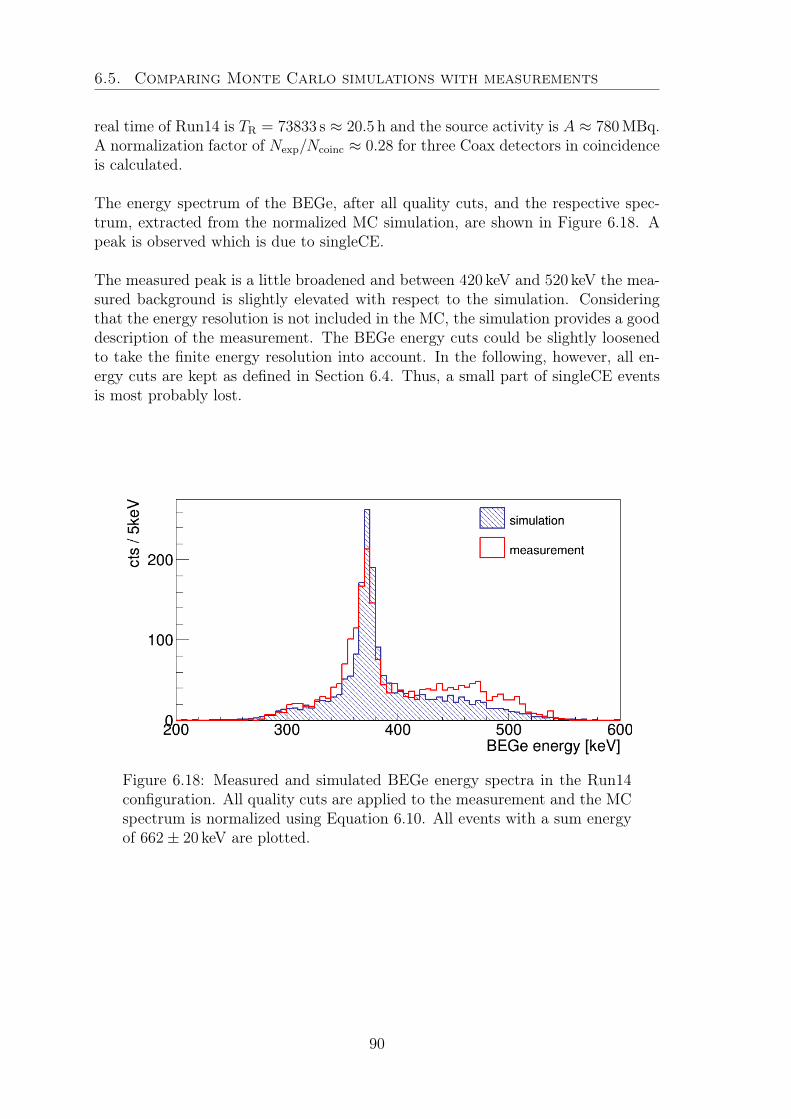
6.5. Comparing Monte Carlo simulations with measurements
real time of Run14 is TR = 73833 s ≈ 20.5 h and the source activity is A ≈ 780MBq.A normalization factor of Nexp/Ncoinc ≈ 0.28 for three Coax detectors in coincidenceis calculated.
The energy spectrum of the BEGe, after all quality cuts, and the respective spec-trum, extracted from the normalized MC simulation, are shown in Figure 6.18. Apeak is observed which is due to singleCE.
The measured peak is a little broadened and between 420 keV and 520 keV the mea-sured background is slightly elevated with respect to the simulation. Consideringthat the energy resolution is not included in the MC, the simulation provides a gooddescription of the measurement. The BEGe energy cuts could be slightly loosenedto take the finite energy resolution into account. In the following, however, all en-ergy cuts are kept as defined in Section 6.4. Thus, a small part of singleCE eventsis most probably lost.
Figure 6.18: Measured and simulated BEGe energy spectra in the Run14configuration. All quality cuts are applied to the measurement and the MCspectrum is normalized using Equation 6.10. All events with a sum energyof 662± 20 keV are plotted.
90
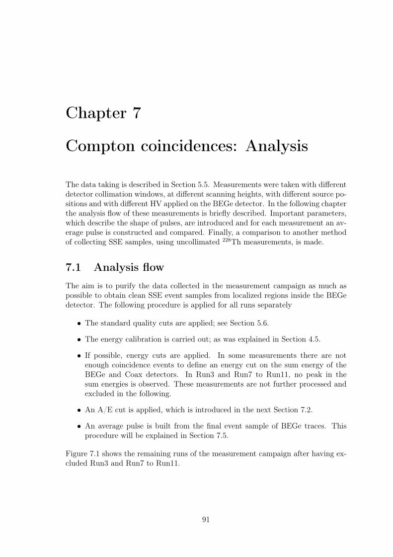
Chapter 7
Compton coincidences: Analysis
The data taking is described in Section 5.5. Measurements were taken with differentdetector collimation windows, at different scanning heights, with different source po-sitions and with different HV applied on the BEGe detector. In the following chapterthe analysis flow of these measurements is briefly described. Important parameters,which describe the shape of pulses, are introduced and for each measurement an av-erage pulse is constructed and compared. Finally, a comparison to another methodof collecting SSE samples, using uncollimated 228Th measurements, is made.
7.1 Analysis flowThe aim is to purify the data collected in the measurement campaign as much aspossible to obtain clean SSE event samples from localized regions inside the BEGedetector. The following procedure is applied for all runs separately
• The standard quality cuts are applied; see Section 5.6.
• The energy calibration is carried out; as was explained in Section 4.5.
• If possible, energy cuts are applied. In some measurements there are notenough coincidence events to define an energy cut on the sum energy of theBEGe and Coax detectors. In Run3 and Run7 to Run11, no peak in thesum energies is observed. These measurements are not further processed andexcluded in the following.
• An A/E cut is applied, which is introduced in the next Section 7.2.
• An average pulse is built from the final event sample of BEGe traces. Thisprocedure will be explained in Section 7.5.
Figure 7.1 shows the remaining runs of the measurement campaign after having ex-cluded Run3 and Run7 to Run11.
91
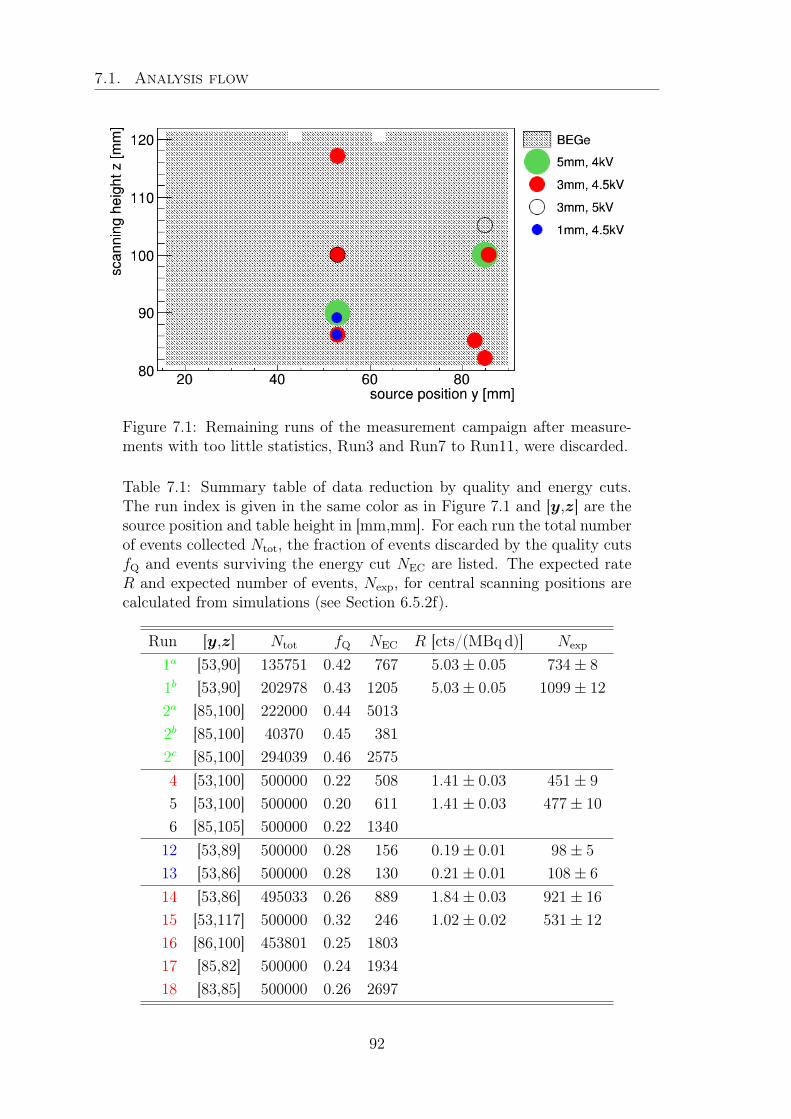
7.1. Analysis flow
Figure 7.1: Remaining runs of the measurement campaign after measure-ments with too little statistics, Run3 and Run7 to Run11, were discarded.
Table 7.1: Summary table of data reduction by quality and energy cuts.The run index is given in the same color as in Figure 7.1 and [y,z] are thesource position and table height in [mm,mm]. For each run the total numberof events collected Ntot, the fraction of events discarded by the quality cutsfQ and events surviving the energy cut NEC are listed. The expected rateR and expected number of events, Nexp, for central scanning positions arecalculated from simulations (see Section 6.5.2f).
Run [y,z] Ntot fQ NEC R [cts/(MBqd)] Nexp
1a [53,90] 135751 0.42 767 5.03± 0.05 734± 8
1b [53,90] 202978 0.43 1205 5.03± 0.05 1099± 12
2a [85,100] 222000 0.44 50132b [85,100] 40370 0.45 3812c [85,100] 294039 0.46 25754 [53,100] 500000 0.22 508 1.41± 0.03 451± 9
5 [53,100] 500000 0.20 611 1.41± 0.03 477± 10
6 [85,105] 500000 0.22 134012 [53,89] 500000 0.28 156 0.19± 0.01 98± 5
13 [53,86] 500000 0.28 130 0.21± 0.01 108± 6
14 [53,86] 495033 0.26 889 1.84± 0.03 921± 16
15 [53,117] 500000 0.32 246 1.02± 0.02 531± 12
16 [86,100] 453801 0.25 180317 [85,82] 500000 0.24 193418 [83,85] 500000 0.26 2697
92
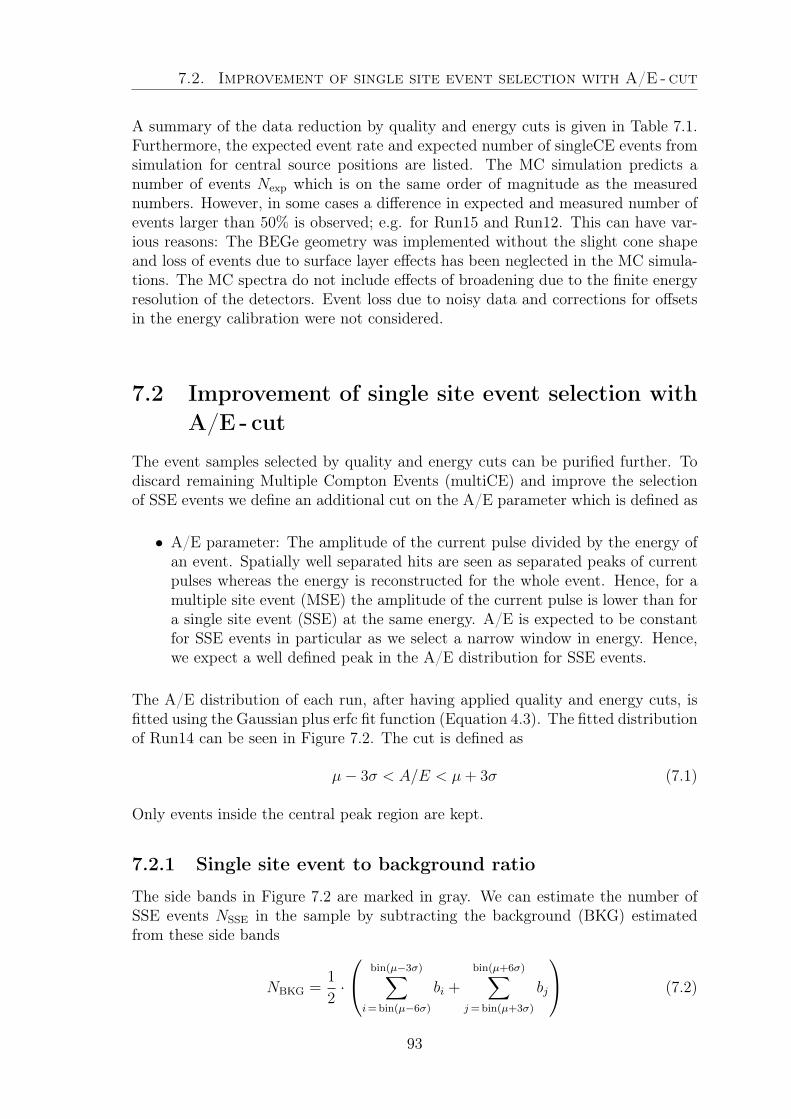
7.2. Improvement of single site event selection with A/E - cut
A summary of the data reduction by quality and energy cuts is given in Table 7.1.Furthermore, the expected event rate and expected number of singleCE events fromsimulation for central source positions are listed. The MC simulation predicts anumber of events Nexp which is on the same order of magnitude as the measurednumbers. However, in some cases a difference in expected and measured number ofevents larger than 50% is observed; e.g. for Run15 and Run12. This can have var-ious reasons: The BEGe geometry was implemented without the slight cone shapeand loss of events due to surface layer effects has been neglected in the MC simula-tions. The MC spectra do not include effects of broadening due to the finite energyresolution of the detectors. Event loss due to noisy data and corrections for offsetsin the energy calibration were not considered.
7.2 Improvement of single site event selection withA/E - cut
The event samples selected by quality and energy cuts can be purified further. Todiscard remaining Multiple Compton Events (multiCE) and improve the selectionof SSE events we define an additional cut on the A/E parameter which is defined as
• A/E parameter: The amplitude of the current pulse divided by the energy ofan event. Spatially well separated hits are seen as separated peaks of currentpulses whereas the energy is reconstructed for the whole event. Hence, for amultiple site event (MSE) the amplitude of the current pulse is lower than fora single site event (SSE) at the same energy. A/E is expected to be constantfor SSE events in particular as we select a narrow window in energy. Hence,we expect a well defined peak in the A/E distribution for SSE events.
The A/E distribution of each run, after having applied quality and energy cuts, isfitted using the Gaussian plus erfc fit function (Equation 4.3). The fitted distributionof Run14 can be seen in Figure 7.2. The cut is defined as
µ− 3σ < A/E < µ+ 3σ (7.1)
Only events inside the central peak region are kept.
7.2.1 Single site event to background ratio
The side bands in Figure 7.2 are marked in gray. We can estimate the number ofSSE events NSSE in the sample by subtracting the background (BKG) estimatedfrom these side bands
NBKG =1
2·
bin(µ−3σ)∑i= bin(µ−6σ)
bi +
bin(µ+6σ)∑j= bin(µ+3σ)
bj
(7.2)
93
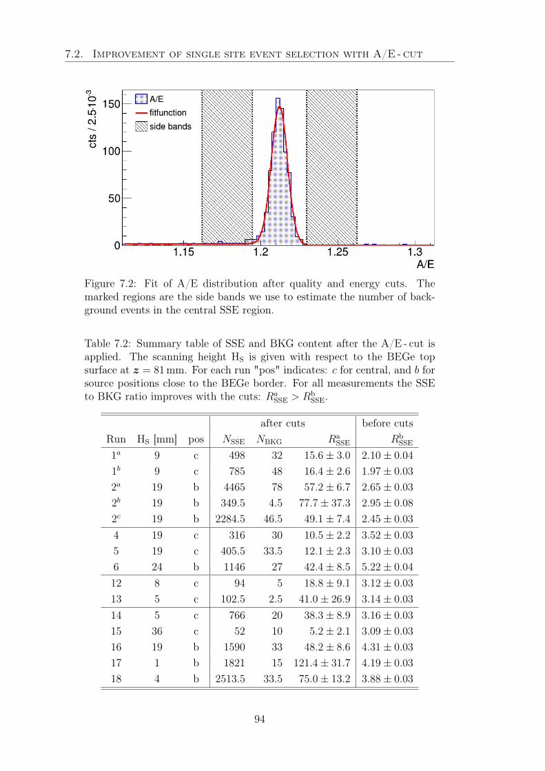
7.2. Improvement of single site event selection with A/E - cut
Figure 7.2: Fit of A/E distribution after quality and energy cuts. Themarked regions are the side bands we use to estimate the number of back-ground events in the central SSE region.
Table 7.2: Summary table of SSE and BKG content after the A/E - cut isapplied. The scanning height HS is given with respect to the BEGe topsurface at z = 81mm. For each run "pos" indicates: c for central, and b forsource positions close to the BEGe border. For all measurements the SSEto BKG ratio improves with the cuts: Ra
SSE > RbSSE.
after cuts before cutsRun HS [mm] pos NSSE NBKG Ra
SSE RbSSE
1a 9 c 498 32 15.6± 3.0 2.10± 0.04
1b 9 c 785 48 16.4± 2.6 1.97± 0.03
2a 19 b 4465 78 57.2± 6.7 2.65± 0.03
2b 19 b 349.5 4.5 77.7± 37.3 2.95± 0.08
2c 19 b 2284.5 46.5 49.1± 7.4 2.45± 0.03
4 19 c 316 30 10.5± 2.2 3.52± 0.03
5 19 c 405.5 33.5 12.1± 2.3 3.10± 0.03
6 24 b 1146 27 42.4± 8.5 5.22± 0.04
12 8 c 94 5 18.8± 9.1 3.12± 0.03
13 5 c 102.5 2.5 41.0± 26.9 3.14± 0.03
14 5 c 766 20 38.3± 8.9 3.16± 0.03
15 36 c 52 10 5.2± 2.1 3.09± 0.03
16 19 b 1590 33 48.2± 8.6 4.31± 0.03
17 1 b 1821 15 121.4± 31.7 4.19± 0.03
18 4 b 2513.5 33.5 75.0± 13.2 3.88± 0.03
94
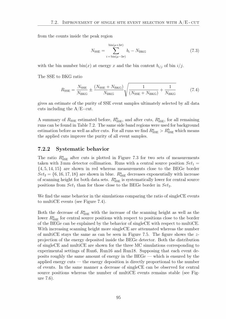
7.2. Improvement of single site event selection with A/E - cut
from the counts inside the peak region
NSSE =
bin(µ+3σ)∑i= bin(µ−3σ)
bi −NBKG (7.3)
with the bin number bin(x) at energy x and the bin content bi/j of bin i/j.
The SSE to BKG ratio
RSSE =NSSE
NBKG
± (NSSE +NBKG)
NBKG
√1
(NSSE +NBKG)+
1
NBKG
(7.4)
gives an estimate of the purity of SSE event samples ultimately selected by all datacuts including the A/E - cut.
A summary of RSSE estimated before, RbSSE, and after cuts, Ra
SSE, for all remainingruns can be found in Table 7.2. The same side band regions were used for backgroundestimation before as well as after cuts. For all runs we find Ra
SSE > RbSSE which means
the applied cuts improve the purity of all event samples.
7.2.2 Systematic behavior
The ratio RaSSE after cuts is plotted in Figure 7.3 for two sets of measurements
taken with 3mm detector collimation. Runs with a central source position Set1 =4, 5, 14, 15 are shown in red whereas measurements close to the BEGe borderSet2 = 6, 16, 17, 18 are shown in blue. Ra
SSE decreases exponentially with increaseof scanning height for both data sets. Ra
SSE is systematically lower for central sourcepositions from Set1 than for those close to the BEGe border in Set2.
We find the same behavior in the simulations comparing the ratio of singleCE eventsto multiCE events (see Figure 7.4).
Both the decrease of RaSSE with the increase of the scanning height as well as the
lower RaSSE for central source positions with respect to positions close to the border
of the BEGe can be explained by the behavior of singleCE with respect to multiCE.With increasing scanning height more singleCE are attenuated whereas the numberof multiCE stays the same as can be seen in Figure 7.5. The figure shows the z-projection of the energy deposited inside the BEGe detector. Both the distributionof singleCE and multiCE are shown for the three MC simulations corresponding toexperimental settings of Run6, Run16 and Run18. Supposing that each event de-posits roughly the same amount of energy in the BEGe — which is ensured by theapplied energy cuts — the energy deposition is directly proportional to the numberof events. In the same manner a decrease of singleCE can be observed for centralsource positions whereas the number of multiCE events remains stable (see Fig-ure 7.6).
95
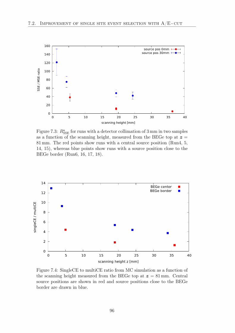
7.2. Improvement of single site event selection with A/E - cut
Figure 7.3: RaSSE for runs with a detector collimation of 3mm in two samples
as a function of the scanning height, measured from the BEGe top at z =81mm. The red points show runs with a central source position (Run4, 5,14, 15), whereas blue points show runs with a source position close to theBEGe border (Run6, 16, 17, 18).
Figure 7.4: SingleCE to multiCE ratio from MC simulation as a function ofthe scanning height measured from the BEGe top at z = 81mm. Centralsource positions are shown in red and source positions close to the BEGeborder are drawn in blue.
96
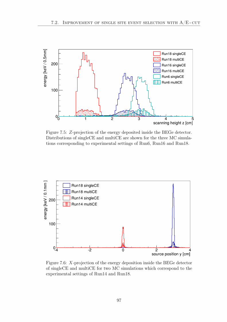
7.2. Improvement of single site event selection with A/E - cut
Figure 7.5: Z-projection of the energy deposited inside the BEGe detector.Distributions of singleCE and multiCE are shown for the three MC simula-tions corresponding to experimental settings of Run6, Run16 and Run18.
Figure 7.6: X-projection of the energy deposition inside the BEGe detectorof singleCE and multiCE for two MC simulations which correspond to theexperimental settings of Run14 and Run18.
97
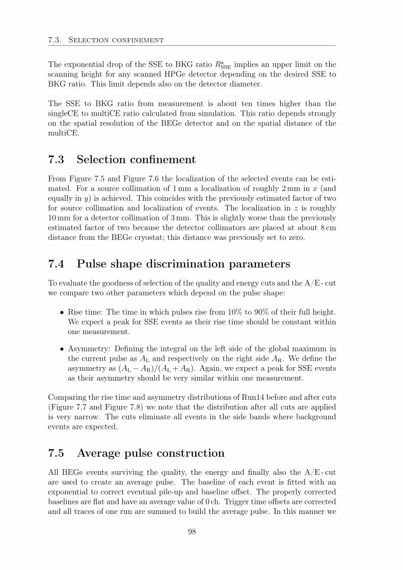
7.3. Selection confinement
The exponential drop of the SSE to BKG ratio RaSSE implies an upper limit on the
scanning height for any scanned HPGe detector depending on the desired SSE toBKG ratio. This limit depends also on the detector diameter.
The SSE to BKG ratio from measurement is about ten times higher than thesingleCE to multiCE ratio calculated from simulation. This ratio depends stronglyon the spatial resolution of the BEGe detector and on the spatial distance of themultiCE.
7.3 Selection confinement
From Figure 7.5 and Figure 7.6 the localization of the selected events can be esti-mated. For a source collimation of 1mm a localization of roughly 2mm in x (andequally in y) is achieved. This coincides with the previously estimated factor of twofor source collimation and localization of events. The localization in z is roughly10mm for a detector collimation of 3mm. This is slightly worse than the previouslyestimated factor of two because the detector collimators are placed at about 8 cmdistance from the BEGe cryostat; this distance was previously set to zero.
7.4 Pulse shape discrimination parameters
To evaluate the goodness of selection of the quality and energy cuts and the A/E - cutwe compare two other parameters which depend on the pulse shape:
• Rise time: The time in which pulses rise from 10% to 90% of their full height.We expect a peak for SSE events as their rise time should be constant withinone measurement.
• Asymmetry: Defining the integral on the left side of the global maximum inthe current pulse as AL and respectively on the right side AR. We define theasymmetry as (AL−AR)/(AL +AR). Again, we expect a peak for SSE eventsas their asymmetry should be very similar within one measurement.
Comparing the rise time and asymmetry distributions of Run14 before and after cuts(Figure 7.7 and Figure 7.8) we note that the distribution after all cuts are appliedis very narrow. The cuts eliminate all events in the side bands where backgroundevents are expected.
7.5 Average pulse construction
All BEGe events surviving the quality, the energy and finally also the A/E - cutare used to create an average pulse. The baseline of each event is fitted with anexponential to correct eventual pile-up and baseline offset. The properly correctedbaselines are flat and have an average value of 0 ch. Trigger time offsets are correctedand all traces of one run are summed to build the average pulse. In this manner we
98
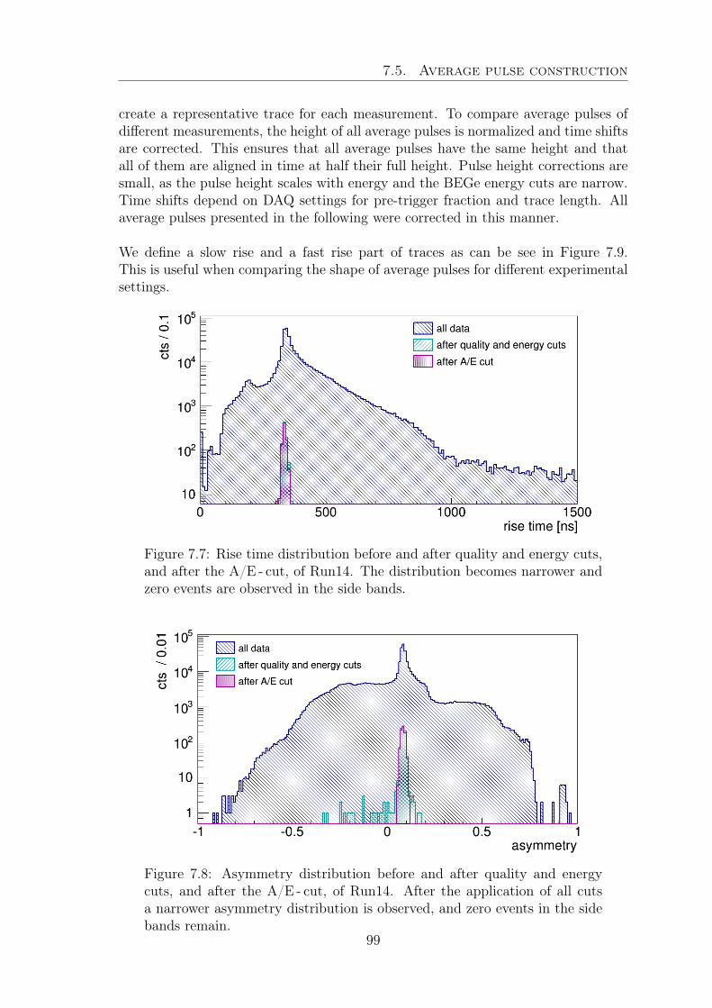
7.5. Average pulse construction
create a representative trace for each measurement. To compare average pulses ofdifferent measurements, the height of all average pulses is normalized and time shiftsare corrected. This ensures that all average pulses have the same height and thatall of them are aligned in time at half their full height. Pulse height corrections aresmall, as the pulse height scales with energy and the BEGe energy cuts are narrow.Time shifts depend on DAQ settings for pre-trigger fraction and trace length. Allaverage pulses presented in the following were corrected in this manner.
We define a slow rise and a fast rise part of traces as can be see in Figure 7.9.This is useful when comparing the shape of average pulses for different experimentalsettings.
Figure 7.7: Rise time distribution before and after quality and energy cuts,and after the A/E - cut, of Run14. The distribution becomes narrower andzero events are observed in the side bands.
Figure 7.8: Asymmetry distribution before and after quality and energycuts, and after the A/E - cut, of Run14. After the application of all cutsa narrower asymmetry distribution is observed, and zero events in the sidebands remain.
99
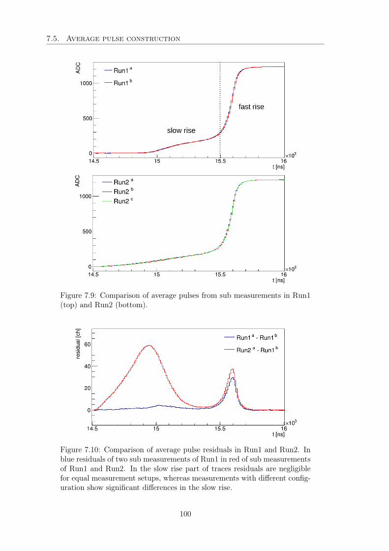
7.5. Average pulse construction
Figure 7.9: Comparison of average pulses from sub measurements in Run1(top) and Run2 (bottom).
Figure 7.10: Comparison of average pulse residuals in Run1 and Run2. Inblue residuals of two sub measurements of Run1 in red of sub measurementsof Run1 and Run2. In the slow rise part of traces residuals are negligiblefor equal measurement setups, whereas measurements with different config-uration show significant differences in the slow rise.
100
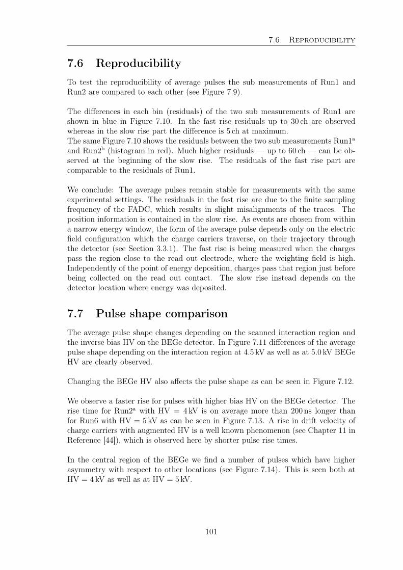
7.6. Reproducibility
7.6 ReproducibilityTo test the reproducibility of average pulses the sub measurements of Run1 andRun2 are compared to each other (see Figure 7.9).
The differences in each bin (residuals) of the two sub measurements of Run1 areshown in blue in Figure 7.10. In the fast rise residuals up to 30 ch are observedwhereas in the slow rise part the difference is 5 ch at maximum.The same Figure 7.10 shows the residuals between the two sub measurements Run1a
and Run2b (histogram in red). Much higher residuals — up to 60 ch — can be ob-served at the beginning of the slow rise. The residuals of the fast rise part arecomparable to the residuals of Run1.
We conclude: The average pulses remain stable for measurements with the sameexperimental settings. The residuals in the fast rise are due to the finite samplingfrequency of the FADC, which results in slight misalignments of the traces. Theposition information is contained in the slow rise. As events are chosen from withina narrow energy window, the form of the average pulse depends only on the electricfield configuration which the charge carriers traverse, on their trajectory throughthe detector (see Section 3.3.1). The fast rise is being measured when the chargespass the region close to the read out electrode, where the weighting field is high.Independently of the point of energy deposition, charges pass that region just beforebeing collected on the read out contact. The slow rise instead depends on thedetector location where energy was deposited.
7.7 Pulse shape comparisonThe average pulse shape changes depending on the scanned interaction region andthe inverse bias HV on the BEGe detector. In Figure 7.11 differences of the averagepulse shape depending on the interaction region at 4.5 kV as well as at 5.0 kV BEGeHV are clearly observed.
Changing the BEGe HV also affects the pulse shape as can be seen in Figure 7.12.
We observe a faster rise for pulses with higher bias HV on the BEGe detector. Therise time for Run2a with HV = 4 kV is on average more than 200 ns longer thanfor Run6 with HV = 5 kV as can be seen in Figure 7.13. A rise in drift velocity ofcharge carriers with augmented HV is a well known phenomenon (see Chapter 11 inReference [44]), which is observed here by shorter pulse rise times.
In the central region of the BEGe we find a number of pulses which have higherasymmetry with respect to other locations (see Figure 7.14). This is seen both atHV = 4 kV as well as at HV = 5 kV.
101
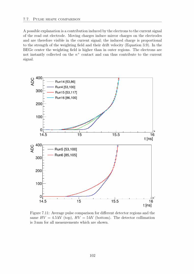
7.7. Pulse shape comparison
A possible explanation is a contribution induced by the electrons to the current signalof the read out electrode. Moving charges induce mirror charges on the electrodesand are therefore visible in the current signal; the induced charge is proportionalto the strength of the weighting field and their drift velocity (Equation 3.9). In theBEGe center the weighting field is higher than in outer regions. The electrons arenot instantly collected on the n+ contact and can thus contribute to the currentsignal.
Figure 7.11: Average pulse comparison for different detector regions and thesame HV = 4.5 kV (top), HV = 5 kV (bottom). The detector collimationis 3mm for all measurements which are shown.
102
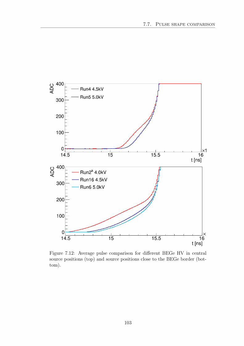
7.7. Pulse shape comparison
Figure 7.12: Average pulse comparison for different BEGe HV in centralsource positions (top) and source positions close to the BEGe border (bot-tom).
103
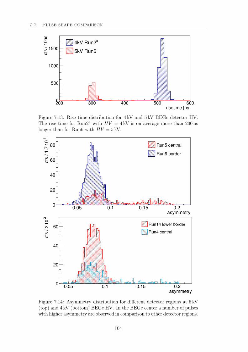
7.7. Pulse shape comparison
Figure 7.13: Rise time distribution for 4 kV and 5 kV BEGe detector HV.The rise time for Run2a with HV = 4 kV is on average more than 200 nslonger than for Run6 with HV = 5 kV.
Figure 7.14: Asymmetry distribution for different detector regions at 5 kV(top) and 4 kV (bottom) BEGe HV. In the BEGe center a number of pulseswith higher asymmetry are observed in comparison to other detector regions.
104
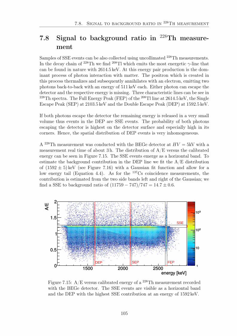
7.8. Signal to background ratio in 228Th measurement
7.8 Signal to background ratio in 228Th measure-ment
Samples of SSE events can be also collected using uncollimated 228Th measurements.In the decay chain of 228Th we find 208Tl which emits the most energetic γ-line thatcan be found in nature with 2614.5 keV. At this energy pair production is the dom-inant process of photon interaction with matter. The positron which is created inthis process thermalizes and subsequently annihilates with an electron, emitting twophotons back-to-back with an energy of 511 keV each. Either photon can escape thedetector and the respective energy is missing. Three characteristic lines can be see in228Th spectra. The Full Energy Peak (FEP) of the 208Tl line at 2614.5 keV, the SingleEscape Peak (SEP) at 2103.5 keV and the Double Escape Peak (DEP) at 1592.5 keV.
If both photons escape the detector the remaining energy is released in a very smallvolume thus events in the DEP are SSE events. The probability of both photonsescaping the detector is highest on the detector surface and especially high in itscorners. Hence, the spatial distribution of DEP events is very inhomogeneous.
A 228Th measurement was conducted with the BEGe detector at HV = 5kV with ameasurement real time of about 3 h. The distribution of A/E versus the calibratedenergy can be seen in Figure 7.15. The SSE events emerge as a horizontal band. Toestimate the background contribution in the DEP line we fit the A/E distributionof (1592 ± 5) keV (see Figure 7.16) with a Gaussian fit function and allow for alow energy tail (Equation 4.4). As for the 137Cs coincidence measurements, thecontribution is estimated from the two side bands left and right of the Gaussian; wefind a SSE to background ratio of (11759− 747)/747 = 14.7± 0.6.
Figure 7.15: A/E versus calibrated energy of a 228Th measurement recordedwith the BEGe detector. The SSE events are visible as a horizontal bandand the DEP with the highest SSE contribution at an energy of 1592 keV.
105
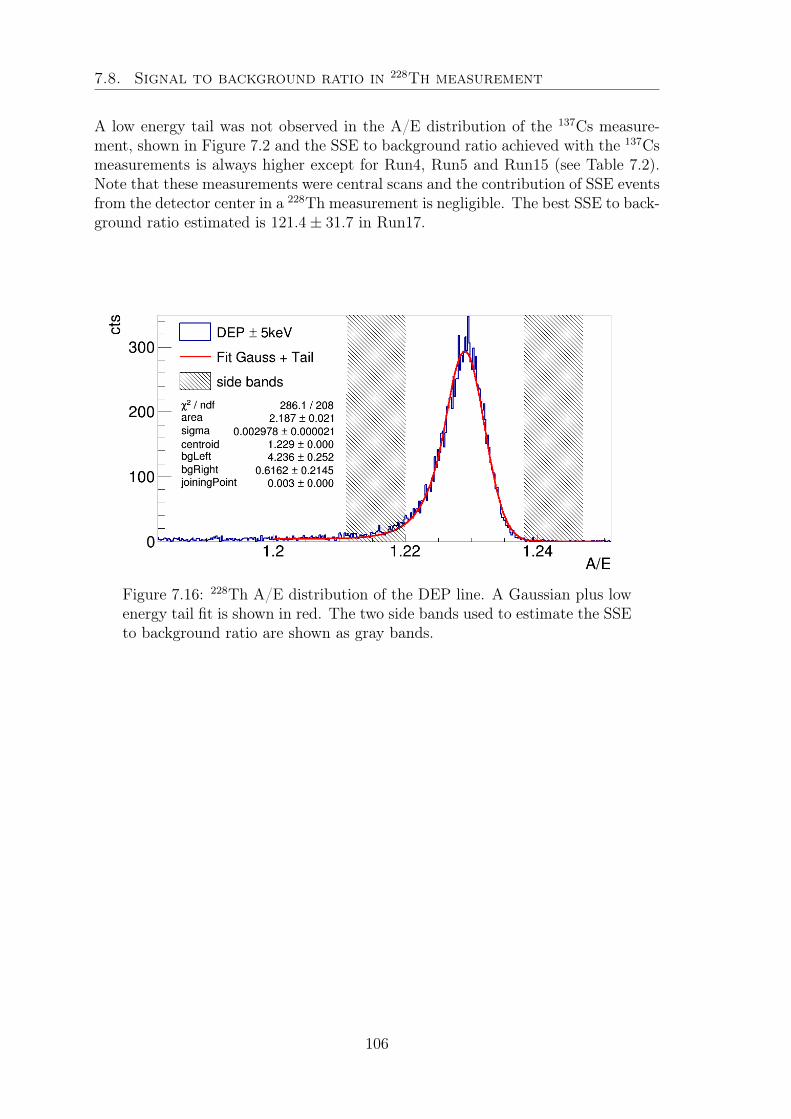
7.8. Signal to background ratio in 228Th measurement
A low energy tail was not observed in the A/E distribution of the 137Cs measure-ment, shown in Figure 7.2 and the SSE to background ratio achieved with the 137Csmeasurements is always higher except for Run4, Run5 and Run15 (see Table 7.2).Note that these measurements were central scans and the contribution of SSE eventsfrom the detector center in a 228Th measurement is negligible. The best SSE to back-ground ratio estimated is 121.4± 31.7 in Run17.
Figure 7.16: 228Th A/E distribution of the DEP line. A Gaussian plus lowenergy tail fit is shown in red. The two side bands used to estimate the SSEto background ratio are shown as gray bands.
106
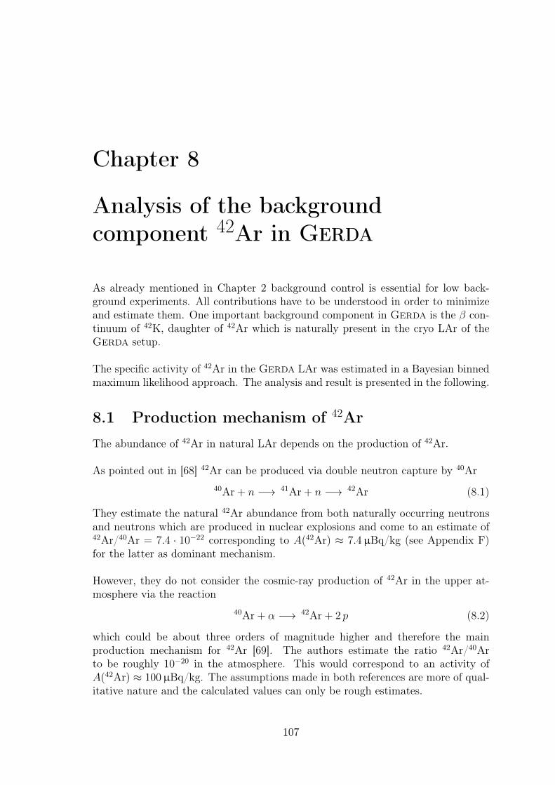
Chapter 8
Analysis of the backgroundcomponent 42Ar in Gerda
As already mentioned in Chapter 2 background control is essential for low back-ground experiments. All contributions have to be understood in order to minimizeand estimate them. One important background component in Gerda is the β con-tinuum of 42K, daughter of 42Ar which is naturally present in the cryo LAr of theGerda setup.
The specific activity of 42Ar in the Gerda LAr was estimated in a Bayesian binnedmaximum likelihood approach. The analysis and result is presented in the following.
8.1 Production mechanism of 42ArThe abundance of 42Ar in natural LAr depends on the production of 42Ar.
As pointed out in [68] 42Ar can be produced via double neutron capture by 40Ar40Ar + n −→ 41Ar + n −→ 42Ar (8.1)
They estimate the natural 42Ar abundance from both naturally occurring neutronsand neutrons which are produced in nuclear explosions and come to an estimate of42Ar/40Ar = 7.4 · 10−22 corresponding to A(42Ar) ≈ 7.4µBq/kg (see Appendix F)for the latter as dominant mechanism.
However, they do not consider the cosmic-ray production of 42Ar in the upper at-mosphere via the reaction
40Ar + α −→ 42Ar + 2 p (8.2)
which could be about three orders of magnitude higher and therefore the mainproduction mechanism for 42Ar [69]. The authors estimate the ratio 42Ar/40Arto be roughly 10−20 in the atmosphere. This would correspond to an activity ofA(42Ar) ≈ 100µBq/kg. The assumptions made in both references are more of qual-itative nature and the calculated values can only be rough estimates.
107
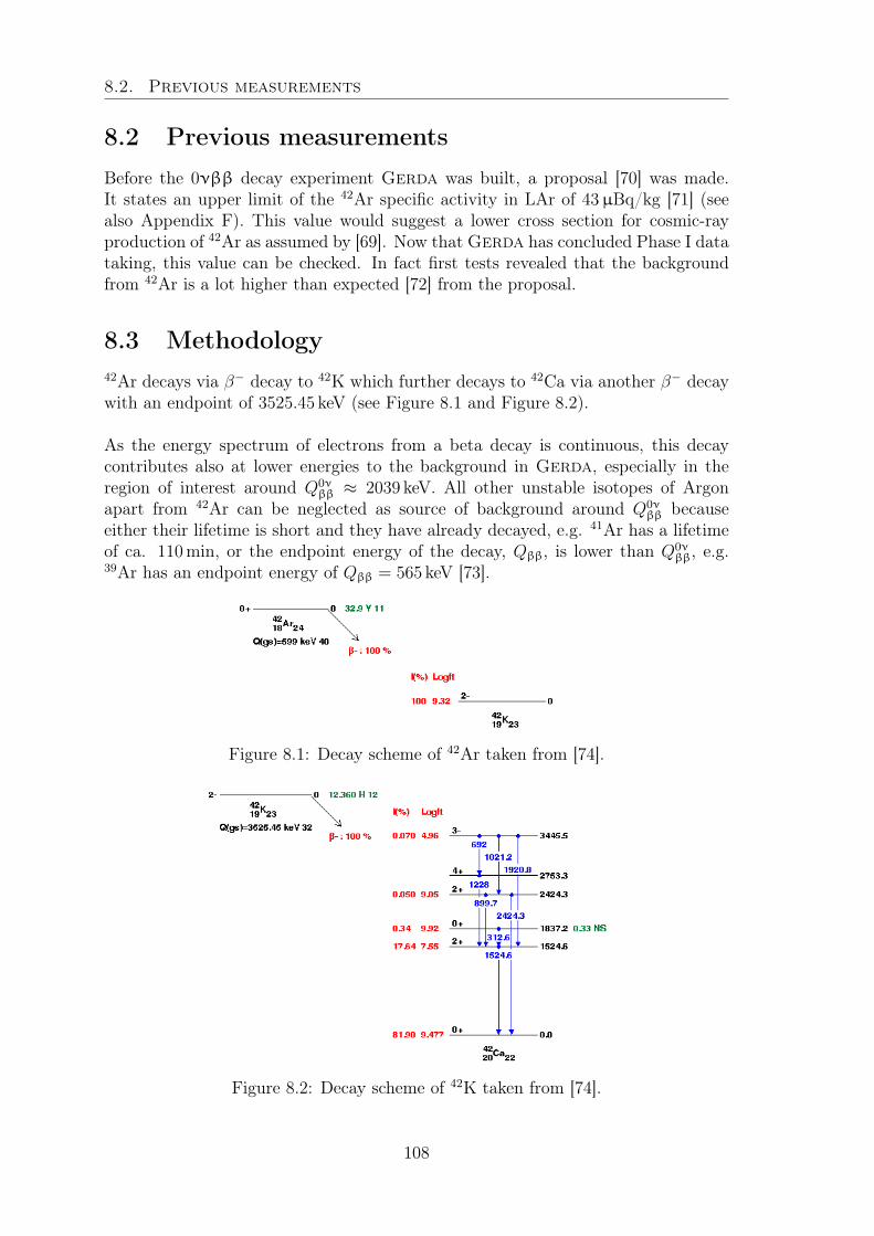
8.2. Previous measurements
8.2 Previous measurementsBefore the 0νββ decay experiment Gerda was built, a proposal [70] was made.It states an upper limit of the 42Ar specific activity in LAr of 43µBq/kg [71] (seealso Appendix F). This value would suggest a lower cross section for cosmic-rayproduction of 42Ar as assumed by [69]. Now that Gerda has concluded Phase I datataking, this value can be checked. In fact first tests revealed that the backgroundfrom 42Ar is a lot higher than expected [72] from the proposal.
8.3 Methodology42Ar decays via β− decay to 42K which further decays to 42Ca via another β− decaywith an endpoint of 3525.45 keV (see Figure 8.1 and Figure 8.2).
As the energy spectrum of electrons from a beta decay is continuous, this decaycontributes also at lower energies to the background in Gerda, especially in theregion of interest around Q0ν
ββ ≈ 2039 keV. All other unstable isotopes of Argonapart from 42Ar can be neglected as source of background around Q0ν
ββ becauseeither their lifetime is short and they have already decayed, e.g. 41Ar has a lifetimeof ca. 110min, or the endpoint energy of the decay, Qββ, is lower than Q0ν
ββ, e.g.39Ar has an endpoint energy of Qββ = 565 keV [73].
Figure 8.1: Decay scheme of 42Ar taken from [74].
Figure 8.2: Decay scheme of 42K taken from [74].
108
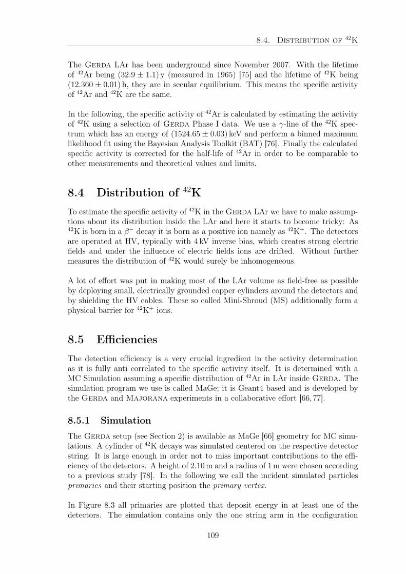
8.4. Distribution of 42K
The Gerda LAr has been underground since November 2007. With the lifetimeof 42Ar being (32.9 ± 1.1) y (measured in 1965) [75] and the lifetime of 42K being(12.360 ± 0.01) h, they are in secular equilibrium. This means the specific activityof 42Ar and 42K are the same.
In the following, the specific activity of 42Ar is calculated by estimating the activityof 42K using a selection of Gerda Phase I data. We use a γ-line of the 42K spec-trum which has an energy of (1524.65± 0.03) keV and perform a binned maximumlikelihood fit using the Bayesian Analysis Toolkit (BAT) [76]. Finally the calculatedspecific activity is corrected for the half-life of 42Ar in order to be comparable toother measurements and theoretical values and limits.
8.4 Distribution of 42KTo estimate the specific activity of 42K in the Gerda LAr we have to make assump-tions about its distribution inside the LAr and here it starts to become tricky: As42K is born in a β− decay it is born as a positive ion namely as 42K+. The detectorsare operated at HV, typically with 4 kV inverse bias, which creates strong electricfields and under the influence of electric fields ions are drifted. Without furthermeasures the distribution of 42K would surely be inhomogeneous.
A lot of effort was put in making most of the LAr volume as field-free as possibleby deploying small, electrically grounded copper cylinders around the detectors andby shielding the HV cables. These so called Mini-Shroud (MS) additionally form aphysical barrier for 42K+ ions.
8.5 EfficienciesThe detection efficiency is a very crucial ingredient in the activity determinationas it is fully anti correlated to the specific activity itself. It is determined with aMC Simulation assuming a specific distribution of 42Ar in LAr inside Gerda. Thesimulation program we use is called MaGe; it is Geant4 based and is developed bythe Gerda and Majorana experiments in a collaborative effort [66, 77].
8.5.1 Simulation
The Gerda setup (see Section 2) is available as MaGe [66] geometry for MC simu-lations. A cylinder of 42K decays was simulated centered on the respective detectorstring. It is large enough in order not to miss important contributions to the effi-ciency of the detectors. A height of 2.10m and a radius of 1m were chosen accordingto a previous study [78]. In the following we call the incident simulated particlesprimaries and their starting position the primary vertex.
In Figure 8.3 all primaries are plotted that deposit energy in at least one of thedetectors. The simulation contains only the one string arm in the configuration
109
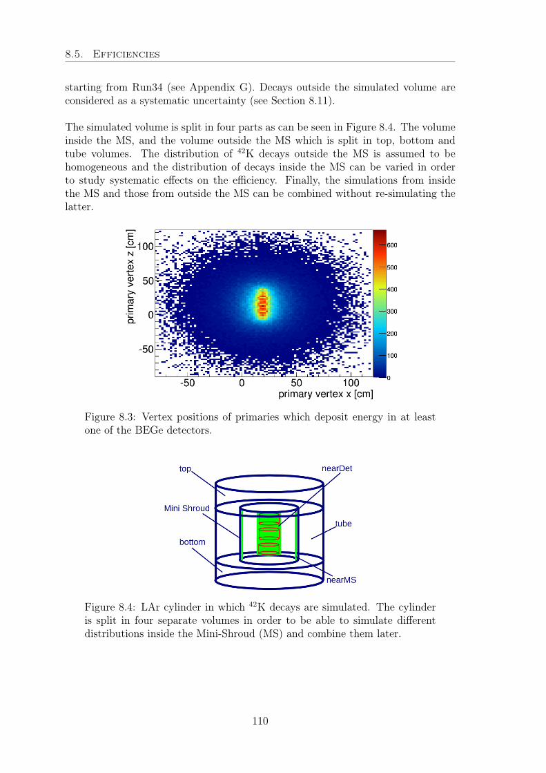
8.5. Efficiencies
starting from Run34 (see Appendix G). Decays outside the simulated volume areconsidered as a systematic uncertainty (see Section 8.11).
The simulated volume is split in four parts as can be seen in Figure 8.4. The volumeinside the MS, and the volume outside the MS which is split in top, bottom andtube volumes. The distribution of 42K decays outside the MS is assumed to behomogeneous and the distribution of decays inside the MS can be varied in orderto study systematic effects on the efficiency. Finally, the simulations from insidethe MS and those from outside the MS can be combined without re-simulating thelatter.
Figure 8.3: Vertex positions of primaries which deposit energy in at leastone of the BEGe detectors.
Figure 8.4: LAr cylinder in which 42K decays are simulated. The cylinderis split in four separate volumes in order to be able to simulate differentdistributions inside the Mini-Shroud (MS) and combine them later.
110
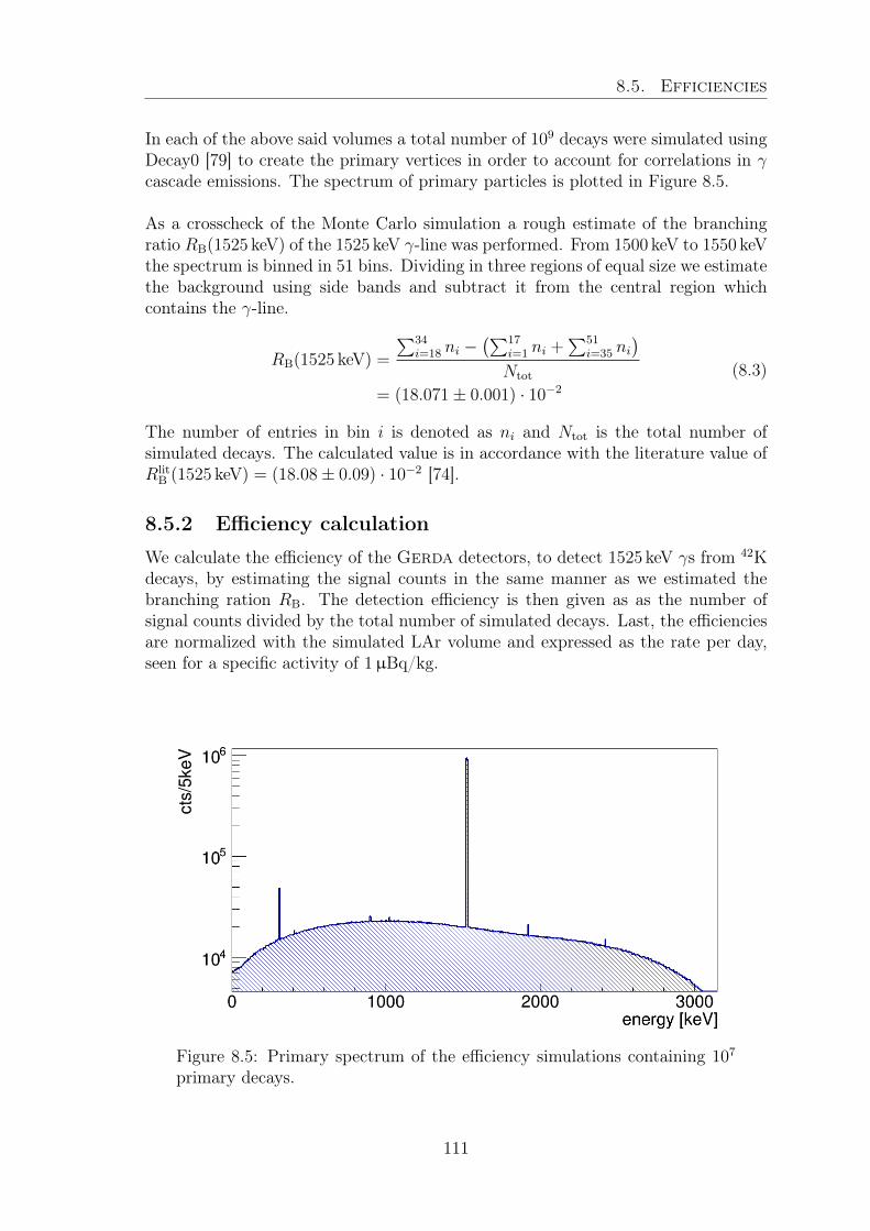
8.5. Efficiencies
In each of the above said volumes a total number of 109 decays were simulated usingDecay0 [79] to create the primary vertices in order to account for correlations in γcascade emissions. The spectrum of primary particles is plotted in Figure 8.5.
As a crosscheck of the Monte Carlo simulation a rough estimate of the branchingratio RB(1525 keV) of the 1525 keV γ-line was performed. From 1500 keV to 1550 keVthe spectrum is binned in 51 bins. Dividing in three regions of equal size we estimatethe background using side bands and subtract it from the central region whichcontains the γ-line.
RB(1525 keV) =
∑34i=18 ni −
(∑17i=1 ni +
∑51i=35 ni
)Ntot
= (18.071± 0.001) · 10−2
(8.3)
The number of entries in bin i is denoted as ni and Ntot is the total number ofsimulated decays. The calculated value is in accordance with the literature value ofRlit
B (1525 keV) = (18.08± 0.09) · 10−2 [74].
8.5.2 Efficiency calculation
We calculate the efficiency of the Gerda detectors, to detect 1525 keV γs from 42Kdecays, by estimating the signal counts in the same manner as we estimated thebranching ration RB. The detection efficiency is then given as as the number ofsignal counts divided by the total number of simulated decays. Last, the efficienciesare normalized with the simulated LAr volume and expressed as the rate per day,seen for a specific activity of 1µBq/kg.
Figure 8.5: Primary spectrum of the efficiency simulations containing 107
primary decays.
111
8.5. Efficiencies
To extract the signal counts, the energy window [1499 keV,1550 keV] of the simu-lation output spectra is subdivided in three regions of same size. B1 and B2 arethe sidebands and M denotes the middle region which contains the 42K γ-line at≈ 1525 keV which we use to estimate the specific activity of 42Ar. Using the twoside bands we estimate the background contribution in region M and calculate thesignal counts S as follows
S = M − B1 +B2
2(8.4)
We calculate the efficiency ε by dividing S by the number of simulated decays Nsim
ε =S
Nsim
(8.5)
Effectively we are not calculating the efficiency on the full decay but on the 1525 keVline which we will denote as ε15
ε15 =S
Nsim ·RB
(8.6)
To estimate the uncertainty on the efficiency we have to take the branching ratioRB of the 1525 keV line into account. The uncertainty, which is calculated usingbinomial statistics, is then
∆ε15 =
√ε15 (1− ε15)
Nsim ·RB
(8.7)
The uncertainty on the total efficiency ε is therefore
∆ε =
√(∂ε
∂ε15
·∆ε15
)2
+
(∂ε
∂RB
·∆RB
)2
(8.8)
∆ε
ε=
√(∆ε15
ε15
)2
+
(∆RB
RB
)2
(8.9)
If we neglect the uncertainty on the branching ratio ∆RB for Nsim →∞ this tendsto
∆ε
ε≈ ∆ε15
ε15
=
√ε15 (1− ε15)
Nsim ·RB · ε215
=
√(1− ε15)
S
Nsim→∞−→ 1√S
(8.10)
With RB = 0.1808 ± 0.009 [74] and ∆ε/ε ≈ 10−2 though, the uncertainty on thebranching ratio can not simply be neglected but contributes with approximately10 % to the total uncertainty. In the following ∆ε contains this contribution. In thefinal analysis the efficiency enters as the rate per day which is seen by the respectivedetector for an 42Ar activity of 1µBq/kg. Therefore, we define the normalizedefficiency εn as
εn = ε ·mLAr · fn (8.11)
With the LAr mass mLAr, which is given by the density of LAr ρLAr = 1.39 g/cm3
multiplied by its volume VLAr
mLAr = ρLAr · VLAr (8.12)
112
8.5. Efficiencies
and the normalization factor
fn = 1µBq
kg· 8.64 · 104 s
d= 8.64 · 10−2 decays
kg d(8.13)
efficiencies of complementary simulations i can be combined by simply summingthem up
En = Σiεn,i (8.14)provided there is no overlap of the simulated LAr volume and if the single valuesare normalized. Supposing that complementary simulations are uncorrelated we addup the uncertainties on the single efficiencies in quadrature to obtain the combineduncertainty
Ξn =√
Σi∆ε2n,i (8.15)
All simulations with their normalization factors are listed in Table 8.1. In orderto ensure that the volume splitting, which was described in Section 8.5.1, leadsto a reasonable result for the efficiencies, for detector string 3 (S3) a simulationwithout volume splitting as well as with volume splitting was done. S3 contains threedetectors; their efficiencies for the split simulation and the full volume simulationare compared in Table 8.2.
Table 8.1: List of simulations and normalization factors. The normalizationfactor for inhomogeneous distributions inside the MS is the same as forthe homogeneous distribution because a priori we do not know the realdistribution and assume a homogeneous one.
# string position V [cm3] m [kg] mfn
1 S1 top 2543330 3535 305.4442 S1 bottom 2544630 3537 305.6003 S1 tube 1500070 2085 180.1524 S1 hom 3285.45 4.57 0.3955 S1 near BEGe - - hom6 S1 near MS - - hom7 S2 all 6591250 9162 791.5838 S3 all 6591360 9162 791.5969 S3 top 2543320 3535 305.44310 S3 bottom 2544630 3537 305.60011 S3 tube 1500600 2086 180.21612 S3 hom 2746.51 3.82 0.33013 S3 near BEGe - - hom14 S3 near MS - - hom15 S4 all 6591280 9162 791.58616 S1 AC 6591070 9162 791.561
113
8.5. Efficiencies
Table 8.2: Comparison of complete (all) and split efficiency simulations(hom). The split simulation has four different volume parts which areadded like described in Equation 8.14. The difference ∆ = (εn(hom) −εn(all))/εn(hom) is well within the uncertainty bounds.
hom allname εn [10−3/d] εn [10−3/d] ∆[%]
RGI 3.75± 0.03 3.75± 0.06 -0.08ANG4 4.27± 0.03 4.20± 0.06 1.64RGII 3.90± 0.03 3.86± 0.06 1.01
Table 8.3: Efficiencies of all Phase I detectors with the list of simulationswhich were combined to calculate them. The values indicated with homare used as central value and the nearDet and nearMS values are used toestimate a systematic uncertainty due to the inhomogeneity of 42K decays(see Section 8.11).
hom nearDet nearMSname εn [10−3/d] εn [10−3/d] εn [10−3/d] sim listGD32B 1.03± 0.01 1.01± 0.01 0.94± 0.01 1-6GD32C 1.10± 0.01 1.22± 0.01 1.02± 0.01 1-6GD32D 1.07± 0.01 1.19± 0.01 0.98± 0.01 1-6GD35B 1.20± 0.01 1.32± 0.01 1.12± 0.01 1-6GD35C 0.87± 0.01 0.87± 0.01 0.80± 0.01 1-6ANG3 4.23± 0.06 - - 15ANG5 5.24± 0.07 - - 15RGIII 4.08± 0.06 - - 15RGI 3.75± 0.03 3.57± 0.03 3.59± 0.03 9-14ANG4 4.27± 0.03 4.81± 0.03 4.10± 0.03 9-14RGII 3.90± 0.03 3.97± 0.03 3.77± 0.03 9-14
GTF112 6.15± 0.08 - - 7ANG2 5.43± 0.07 - - 7ANG1 1.44± 0.03 - - 7GTF45 5.02± 0.07 - - 16GTF32 4.83± 0.07 - - 16
114
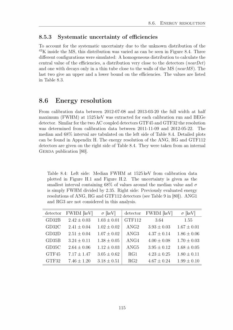
8.6. Energy resolution
8.5.3 Systematic uncertainty of efficiencies
To account for the systematic uncertainty due to the unknown distribution of the42K inside the MS, this distribution was varied as can be seen in Figure 8.4. Threedifferent configurations were simulated: A homogeneous distribution to calculate thecentral value of the efficiencies, a distribution very close to the detectors (nearDet)and one with decays only in a thin tube close to the walls of the MS (nearMS ). Thelast two give an upper and a lower bound on the efficiencies. The values are listedin Table 8.3.
8.6 Energy resolutionFrom calibration data between 2012-07-08 and 2013-03-20 the full width at halfmaximum (FWHM) at 1525 keV was extracted for each calibration run and BEGedetector. Similar for the two AC coupled detectors GTF45 and GTF32 the resolutionwas determined from calibration data between 2011-11-09 and 2012-05-22. Themedian and 68% interval are tabulated on the left side of Table 8.4. Detailed plotscan be found in Appendix H. The energy resolution of the ANG, RG and GTF112detectors are given on the right side of Table 8.4. They were taken from an internalGerda publication [80].
Table 8.4: Left side: Median FWHM at 1525 keV from calibration dataplotted in Figure H.1 and Figure H.2. The uncertainty is given as thesmallest interval containing 68% of values around the median value and σis simply FWHM divided by 2.35. Right side: Previously evaluated energyresolutions of ANG, RG and GTF112 detectors (see Table 9 in [80]). ANG1and RG3 are not considered in this analysis.
detector FWHM [keV] σ [keV] detector FWHM [keV] σ [keV]GD32B 2.42± 0.03 1.03± 0.01 GTF112 3.64 1.55GD32C 2.41± 0.04 1.02± 0.02 ANG2 3.93± 0.03 1.67± 0.01
GD32D 2.51± 0.04 1.07± 0.02 ANG3 4.37± 0.14 1.86± 0.06
GD35B 3.24± 0.11 1.38± 0.05 ANG4 4.00± 0.08 1.70± 0.03
GD35C 2.64± 0.06 1.12± 0.03 ANG5 3.95± 0.12 1.68± 0.05
GTF45 7.17± 1.47 3.05± 0.62 RG1 4.23± 0.25 1.80± 0.11
GTF32 7.46± 1.20 3.18± 0.51 RG2 4.67± 0.24 1.99± 0.10
115
8.7. Bayesian analysis
8.7 Bayesian analysis
We use Bayes’ theory to perform a binned maximum likelihood fit to the spectralshape of the 42K γ-line and to estimate the 42Ar specific activity in the Gerda LAr.
Poisson statistics expresses the probability of a discrete random variable k with anaverage rate λ
P (k|λ) =λke−λ
k!(8.16)
The likelihood to observe ni events in the ith bin of a histogram for λi events expectedis given by
P (→n |λ) =
∏i
λnii e−λi
ni!(8.17)
In the case of multiple detectors with index j the combined likelihood has the fol-lowing form
P (→n |λ) =
∏j
∏i
λnij
ij e−λij
nij!(8.18)
The global posterior probability density function (pdf)
P (λ| →n) =P (→n |λ) · P (λ)
P (→n)
(8.19)
has to be marginalized over all nuisance parameters pm in order to obtain the pos-terior pdf for the parameter of interest A
P (λ(A)| →n) =
∫P (λ(A, pm)| →n) dpm (8.20)
where m = 1, 2 . . .M and M is the total number of nuisance parameters. Note thathere λ depends on the nuisance parameters pm and the parameter of interest A soλ = λ(A, pm).
Using the law of total probability we can express
P (→n) =
∫P (→n |λ)P (λ) dλ (8.21)
And as all parameters are assumed to be independent we can rewrite the priorprobability
P (λ) = P (λ(A, pm)) = P (A)∏m
P (pm) (8.22)
The prior probability P (λ) contains all our knowledge about the parameters. Asit factorizes completely we can choose the prior conditions of each parameter sepa-rately. The last thing we have to do is define the model λ.
116
8.7. Bayesian analysis
8.7.1 Choice of prior distributions
The prior distribution should reflect our degree of belief in a free fit parameter. Ifa fit tells us that we have a negative number of background counts we would notbelieve this result because it is not physical. Thus, in the prior distribution of thebackground index we exclude values below zero. A prior distribution should benormalizable otherwise it is called an improper prior. A common distribution wechose is a gaussian distribution of a parameter giving preference to the central valuewith some uncertainty. Having no value of preference is reflected in a so called noninformative prior. A flat prior in a large enough closed range is quasi non informativeand is also normalizable. The range should be large enough to cover all the posteriordistribution without cutting it.
8.7.2 Building the likelihood
We want to approximate the 42K γ-line with a Gaussian on a flat background. Inthis model the number of expected events in the ith bin are expressed by
λij = Aεj Tj
∫∆Ei
1√2π σj
exp
(−(E − (µ+ ∆µj))
2
2σ2j
)dE ′ + Tj
∫∆Ei
Bj dE ′ (8.23)
The specific activity A is common to all detectors and is the parameter of inter-est. The fit parameters for each detector j are the efficiency εj, the resolution σjat 1525 keV, the γ-line shift ∆µj and the background index Bj. They are all nui-sance parameters, which means they are free parameters of the fit but we are notinterested in their posterior pdf. The lifetimes Tj and the common γ-line energyµ = 1524.65 keV are fixed. All parameters and their type of prior pdf are listed inTable 8.6. In the following we refer to this model as flat background model.
As each detector has four free fit parameters in this model, fitting the spectra of 13detectors the number of nuisance parameters is M = 13 · 4 = 52. All input valuesof Gaussian and fixed parameters are listed in Table 8.5. For the γ-line shift ∆µjwe use a Gaussian prior pdf with the same parameters for all detectors: As mostprobable value we choose no shift ∆µj = 0 and a reasonable assumption for thewidth of the prior pdf is the energy resolution of the detectors ∆∆µj = σj.
8.7.3 Building the refined likelihood
The statistics of the Phase I data is good enough to see a difference between thebackground level at the right and the left side of the γ-line. A refined model accountsfor this difference modeling the background with an inverse error function. This addsanother parameter to the model and we have now a flat background and the stepsize as additional parameter for the fit. In order to be more controllable we expressthe step size by the difference between the left and the right background level. Likethis, it is easier to prohibit for example a negative background level.
117
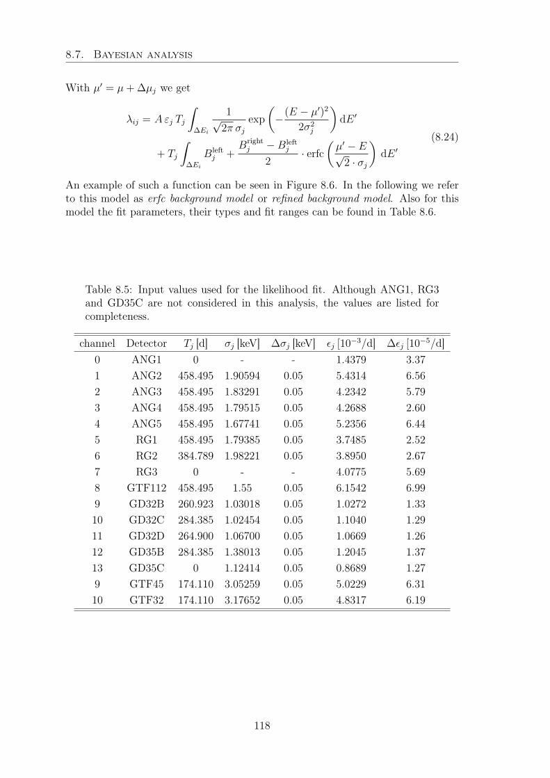
8.7. Bayesian analysis
With µ′ = µ+ ∆µj we get
λij = Aεj Tj
∫∆Ei
1√2π σj
exp
(−(E − µ′)2
2σ2j
)dE ′
+ Tj
∫∆Ei
Bleftj +
Brightj −Bleft
j
2· erfc
(µ′ − E√
2 · σj
)dE ′
(8.24)
An example of such a function can be seen in Figure 8.6. In the following we referto this model as erfc background model or refined background model. Also for thismodel the fit parameters, their types and fit ranges can be found in Table 8.6.
Table 8.5: Input values used for the likelihood fit. Although ANG1, RG3and GD35C are not considered in this analysis, the values are listed forcompleteness.
channel Detector Tj [d] σj [keV] ∆σj [keV] εj [10−3/d] ∆εj [10−5/d]0 ANG1 0 - - 1.4379 3.371 ANG2 458.495 1.90594 0.05 5.4314 6.562 ANG3 458.495 1.83291 0.05 4.2342 5.793 ANG4 458.495 1.79515 0.05 4.2688 2.604 ANG5 458.495 1.67741 0.05 5.2356 6.445 RG1 458.495 1.79385 0.05 3.7485 2.526 RG2 384.789 1.98221 0.05 3.8950 2.677 RG3 0 - - 4.0775 5.698 GTF112 458.495 1.55 0.05 6.1542 6.999 GD32B 260.923 1.03018 0.05 1.0272 1.3310 GD32C 284.385 1.02454 0.05 1.1040 1.2911 GD32D 264.900 1.06700 0.05 1.0669 1.2612 GD35B 284.385 1.38013 0.05 1.2045 1.3713 GD35C 0 1.12414 0.05 0.8689 1.279 GTF45 174.110 3.05259 0.05 5.0229 6.3110 GTF32 174.110 3.17652 0.05 4.8317 6.19
118
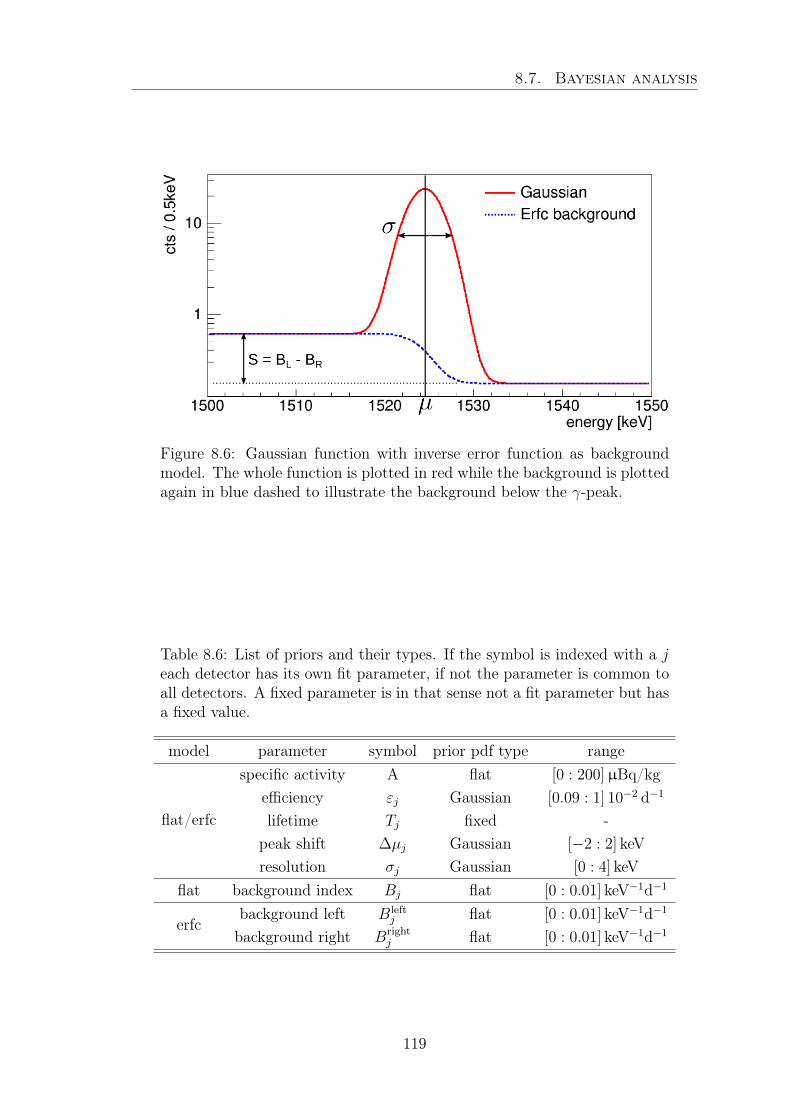
8.7. Bayesian analysis
Figure 8.6: Gaussian function with inverse error function as backgroundmodel. The whole function is plotted in red while the background is plottedagain in blue dashed to illustrate the background below the γ-peak.
Table 8.6: List of priors and their types. If the symbol is indexed with a jeach detector has its own fit parameter, if not the parameter is common toall detectors. A fixed parameter is in that sense not a fit parameter but hasa fixed value.
model parameter symbol prior pdf type range
flat/erfc
specific activity A flat [0 : 200]µBq/kgefficiency εj Gaussian [0.09 : 1] 10−2 d−1
lifetime Tj fixed -peak shift ∆µj Gaussian [−2 : 2] keVresolution σj Gaussian [0 : 4] keV
flat background index Bj flat [0 : 0.01] keV−1d−1
erfcbackground left Bleft
j flat [0 : 0.01] keV−1d−1
background right Brightj flat [0 : 0.01] keV−1d−1
119
8.7. Bayesian analysis
8.7.4 The Bayesian Toolkit - BAT
The likelihood fits are done using the Bayesian Analysis Toolkit (BAT) version0.9.4.1 [76]. It is based on a marginalization using the Metropolis Markov ChainMonte Carlo (MCMC) algorithm. Four predefined levels of fit precision can bechosen kLow (1 chain with 104 iterations), kMedium (5 chains with 105 iterationseach), kHigh (10 chains with 106 iterations each) and kVeryHigh (10 chains with 107
iterations each). The number of chains and iterations per chain can also be chosenmanually using MCMCSetNChains and MCMCSetNIterationsRun which are meth-ods of the BCEngineMCMC class of BAT.
Both models, the flat and the erfc background model, are implemented inside oneC++ class which inherits from the BCModel class of BAT. Two methods have tobe implemented in a BCModel: LogAPrioriProbability which serves to calculate thenatural logarithm (ln) of the prior probability P (λ) and LogLikelihood to calculatedthe ln of P (
→n |λ). To estimate P (
→n |λ) the respective model is integrated over each
bin. The integral of the Gaussian part can be done using the error function whichis defined as
erf(y) =2√π
∫ y
0
e−t2
dt (8.25)
Here y = (E − µ)/(√
2 · σ).
Integrating the flat background model is trivial but the integration of the erfc back-ground model has to be done numerically. We use the following approach∫ E2
E1
erfc(z)dz ≈ E2 − E1
n
[erfc(E1) + erfc(E2)
2+
n−1∑k=1
erfc
[E1 +
k · (E2 − E1)
n
]](8.26)
Where z = (µ − E)/(√
2 · σ) and n which reflects the precision of the numericalintegration was chosen as 1000.
8.7.5 P-value estimation
To calculated the p-value usually P (→n) =
∫P (→n |λ)P (λ) dλ has to be calculated for
normalization. Apparently no algorithm is able to do this integration in our casebut there is an elegant and fast method to estimate p-values which is described inthe appendix of [81]. Here, the p-value is estimated using the Metropolis-Hastingsalgorithm. This algorithm is based on MCMC and is a method to obtain randomsamples of probability distributions for which direct sampling is difficult. As thecounts in the fitted histograms are ∈ N0, a proposal distribution is chosen by theinteger values just below λbest fit which is denoted by bλbest fitc. In each samplingiteration each bin in each histogram is attempted to be randomly increased or de-creased. The new value is randomly accepted or rejected and the probability isupdated; values closer to λbest fit are more probable to be accepted. The likelihoodof the new distribution, obtained with this methods, is compared to the likelihood ofλbest fit. Dividing the number of sampled distributions with a lower likelihood thanλbest fit by the number of iterations gives the approximate p-value.
120
8.8. Data selection and run configurations
8.7.6 Global and marginalized mode
The global mode is the most probable fit parameter that is found by the MCMCalgorithm while marginalizing over the nuisance parameters. BAT is not optimizedto find the global mode and is "neither effective nor accurate" in doing so [76].Nevertheless we mostly give that value to have a reference as it turns out to bequite stable. The marginalized mode is the most probable value for a parameterafter marginalizing over all nuisance parameters. We use the root version of MinuitTMinuit to find all modes and call the most probable of them themarginalized mode.If the fit precision is high enough we obtain only one local mode in all posterior pdfsin this analysis. Hence, this local mode and the marginalized mode coincide. Theuncertainty given is the smallest interval containing at least 68% of the posteriorpdf and the marginalized mode.
8.8 Data selection and run configurationsA sketch and a table of the Gerda Phase I runs and their setup can be found inAppendix G. The Phase I Gerda setup consists of two so called arms. The firstarm contains one string of detectors and the second arm consists of three detectorstrings. The configuration of the three string arm stays the same in all the PhaseI run period. Run33, Run34 and Run35 were not included in the fits. Run33 isvery unstable and in Run33 and Run34 the detector configuration was changedwhich leads to a higher background index for about 20 days. Run34 plus Run35 areabout 32 days long which should be sufficient for the background index to decay toa normal level. Some of the detectors were unstable and had to be switched off aftera while, which is why they were excluded in some later runs. The HV configurationsof each run can be found in detail in Table G.4. All exclusions from this analysisare indicated.
8.8.1 Data cuts
Test pulser events and cosmic muon induced events are cut from the data; eventswith a detector multiplicity larger than 1 on the other hand are kept. The cutefficiency and therefore the detection efficiency would depend on which detectorwas included in the analysis. As the configuration of detectors suitable for analysischanges within the data sample, efficiencies would change for every run period. Byincluding events with a detector multiplicity lager than 1 we keep one efficiency perdetector. The respective data flags are listed in Table 8.7.
Table 8.7: Event flags which can be used for data cuts.
flag description kept/cutisVetoed muon induced event cutisTP test pulser event cut
multiplicity number of det fired kept
121
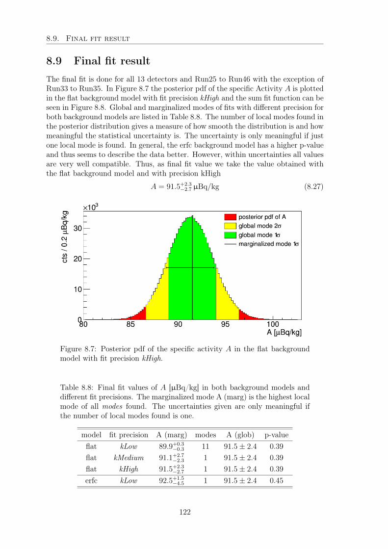
8.9. Final fit result
8.9 Final fit resultThe final fit is done for all 13 detectors and Run25 to Run46 with the exception ofRun33 to Run35. In Figure 8.7 the posterior pdf of the specific Activity A is plottedin the flat background model with fit precision kHigh and the sum fit function can beseen in Figure 8.8. Global and marginalized modes of fits with different precision forboth background models are listed in Table 8.8. The number of local modes found inthe posterior distribution gives a measure of how smooth the distribution is and howmeaningful the statistical uncertainty is. The uncertainty is only meaningful if justone local mode is found. In general, the erfc background model has a higher p-valueand thus seems to describe the data better. However, within uncertainties all valuesare very well compatible. Thus, as final fit value we take the value obtained withthe flat background model and with precision kHigh
A = 91.5+2.3−2.7 µBq/kg (8.27)
Figure 8.7: Posterior pdf of the specific activity A in the flat backgroundmodel with fit precision kHigh.
Table 8.8: Final fit values of A [µBq/kg] in both background models anddifferent fit precisions. The marginalized mode A (marg) is the highest localmode of all modes found. The uncertainties given are only meaningful ifthe number of local modes found is one.
model fit precision A (marg) modes A (glob) p-valueflat kLow 89.9+0.3
−0.3 11 91.5± 2.4 0.39flat kMedium 91.1+2.7
−2.3 1 91.5± 2.4 0.39flat kHigh 91.5+2.3
−2.7 1 91.5± 2.4 0.39erfc kLow 92.5+1.5
−4.5 1 91.5± 2.4 0.45
122
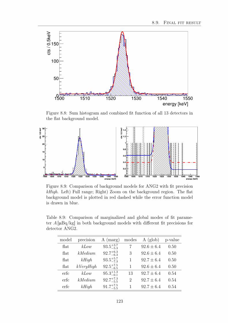
8.9. Final fit result
Figure 8.8: Sum histogram and combined fit function of all 13 detectors inthe flat background model.
Figure 8.9: Comparison of background models for ANG2 with fit precisionkHigh. Left) Full range; Right) Zoom on the background region. The flatbackground model is plotted in red dashed while the error function modelis drawn in blue.
Table 8.9: Comparison of marginalized and global modes of fit parame-ter A [µBq/kg] in both background models with different fit precisions fordetector ANG2.
model precision A (marg) modes A (glob) p-valueflat kLow 93.5+3.7
−5.3 7 92.6± 6.4 0.50flat kMedium 92.7+6.3
−6.3 3 92.6± 6.4 0.50flat kHigh 93.5+5.7
−7.3 1 92.7± 6.4 0.50flat kVeryHigh 92.5+7.5
−6.5 1 92.6± 6.4 0.50erfc kLow 95.3+1.3
−0.1 13 92.7± 6.4 0.54erfc kMedium 92.7+7.3
−5.5 2 92.7± 6.4 0.54erfc kHigh 91.7+7.5
−5.5 1 92.7± 6.4 0.54
123
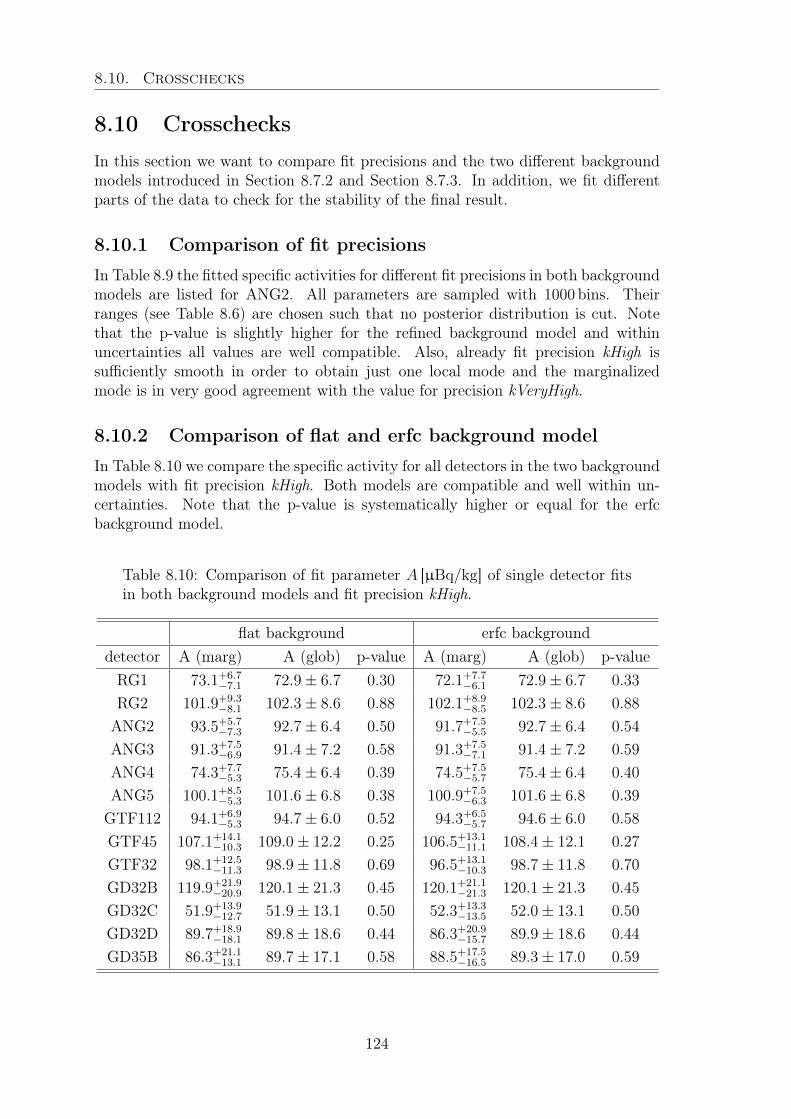
8.10. Crosschecks
8.10 CrosschecksIn this section we want to compare fit precisions and the two different backgroundmodels introduced in Section 8.7.2 and Section 8.7.3. In addition, we fit differentparts of the data to check for the stability of the final result.
8.10.1 Comparison of fit precisions
In Table 8.9 the fitted specific activities for different fit precisions in both backgroundmodels are listed for ANG2. All parameters are sampled with 1000 bins. Theirranges (see Table 8.6) are chosen such that no posterior distribution is cut. Notethat the p-value is slightly higher for the refined background model and withinuncertainties all values are well compatible. Also, already fit precision kHigh issufficiently smooth in order to obtain just one local mode and the marginalizedmode is in very good agreement with the value for precision kVeryHigh.
8.10.2 Comparison of flat and erfc background model
In Table 8.10 we compare the specific activity for all detectors in the two backgroundmodels with fit precision kHigh. Both models are compatible and well within un-certainties. Note that the p-value is systematically higher or equal for the erfcbackground model.
Table 8.10: Comparison of fit parameter A [µBq/kg] of single detector fitsin both background models and fit precision kHigh.
flat background erfc backgrounddetector A (marg) A (glob) p-value A (marg) A (glob) p-valueRG1 73.1+6.7
−7.1 72.9± 6.7 0.30 72.1+7.7−6.1 72.9± 6.7 0.33
RG2 101.9+9.3−8.1 102.3± 8.6 0.88 102.1+8.9
−8.5 102.3± 8.6 0.88ANG2 93.5+5.7
−7.3 92.7± 6.4 0.50 91.7+7.5−5.5 92.7± 6.4 0.54
ANG3 91.3+7.5−6.9 91.4± 7.2 0.58 91.3+7.5
−7.1 91.4± 7.2 0.59ANG4 74.3+7.7
−5.3 75.4± 6.4 0.39 74.5+7.5−5.7 75.4± 6.4 0.40
ANG5 100.1+8.5−5.3 101.6± 6.8 0.38 100.9+7.5
−6.3 101.6± 6.8 0.39GTF112 94.1+6.9
−5.3 94.7± 6.0 0.52 94.3+6.5−5.7 94.6± 6.0 0.58
GTF45 107.1+14.1−10.3 109.0± 12.2 0.25 106.5+13.1
−11.1 108.4± 12.1 0.27GTF32 98.1+12.5
−11.3 98.9± 11.8 0.69 96.5+13.1−10.3 98.7± 11.8 0.70
GD32B 119.9+21.9−20.9 120.1± 21.3 0.45 120.1+21.1
−21.3 120.1± 21.3 0.45GD32C 51.9+13.9
−12.7 51.9± 13.1 0.50 52.3+13.3−13.5 52.0± 13.1 0.50
GD32D 89.7+18.9−18.1 89.8± 18.6 0.44 86.3+20.9
−15.7 89.9± 18.6 0.44GD35B 86.3+21.1
−13.1 89.7± 17.1 0.58 88.5+17.5−16.5 89.3± 17.0 0.59
124
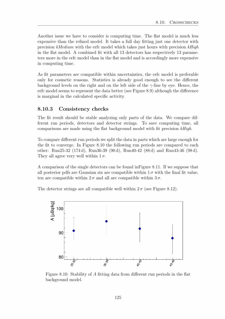
8.10. Crosschecks
Another issue we have to consider is computing time. The flat model is much lessexpensive than the refined model. It takes a full day fitting just one detector withprecision kMedium with the erfc model which takes just hours with precision kHighin the flat model. A combined fit with all 13 detectors has respectively 13 parame-ters more in the erfc model than in the flat model and is accordingly more expensivein computing time.
As fit parameters are compatible within uncertainties, the erfc model is preferableonly for cosmetic reasons. Statistics is already good enough to see the differentbackground levels on the right and on the left side of the γ-line by eye. Hence, theerfc model seems to represent the data better (see Figure 8.9) although the differenceis marginal in the calculated specific activity.
8.10.3 Consistency checks
The fit result should be stable analyzing only parts of the data. We compare dif-ferent run periods, detectors and detector strings. To save computing time, allcomparisons are made using the flat background model with fit precision kHigh.
To compare different run periods we split the data in parts which are large enough forthe fit to converge. In Figure 8.10 the following run periods are compared to eachother: Run25-32 (174 d), Run36-39 (90 d), Run40-42 (88 d) and Run43-46 (98 d).They all agree very well within 1σ.
A comparison of the single detectors can be found inFigure 8.11. If we suppose thatall posterior pdfs are Gaussian six are compatible within 1σ with the final fit value,ten are compatible within 2σ and all are compatible within 3σ.
The detector strings are all compatible well within 2σ (see Figure 8.12).
Figure 8.10: Stability of A fitting data from different run periods in the flatbackground model.
125
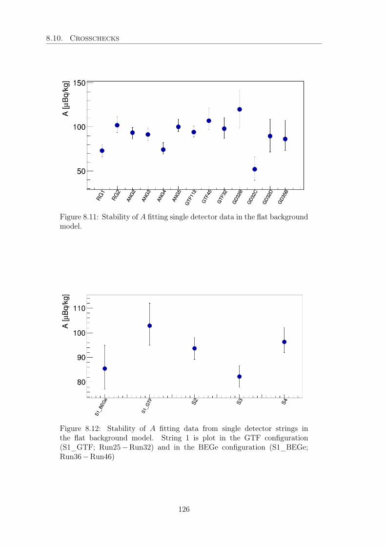
8.10. Crosschecks
Figure 8.11: Stability of A fitting single detector data in the flat backgroundmodel.
Figure 8.12: Stability of A fitting data from single detector strings inthe flat background model. String 1 is plot in the GTF configuration(S1_GTF; Run25−Run32) and in the BEGe configuration (S1_BEGe;Run36−Run46)
126
8.11. Systematic uncertainties
8.11 Systematic uncertaintiesThe systematic uncertainties considered are
• Active mass As all Germanium detectors in the Gerda experiment are p-type they suffer non negligible efficiency loss due to the fact that the outerlayer, which is Lithium diffused, is partly in-active. The thickness of this layeris only known with limited accuracy [82].
• Dimensions in MaGe Size of geometry details can influence the detectionefficiency.
• LAr density Also an uncertainty on the LAr density affects the detectionefficiency calculated using Monte Carlo simulation
• Geometry details Some details are only approximated and not implementedin full detail e.g. rounded corners of the detectors.
• Decays outside sampling volume As only a part of the LAr volume issimulated we consider a systematic error for decays out side the simulatedvolume
• Non-uniformity Inside the Mini-Shroud the distribution of 42K decays isunknown. We consider two extreme cases to get a lower and an upper boundon the detection efficiency.
• Geant4 physics Deviations of cross-sections in the Monte Carlo simulationlead to an overall systematic uncertainty [83] which has to be taken into con-sideration for the detection efficiency.
The uncertainty on the non uniformity of 42K decays inside the Mini-Shrouds isestimated by simulation of two extreme cases of the distribution. A sketch of thesecases can be found in Figure 8.4. Outside the MS we assume the decays to bedistributed homogeneously, inside the MS decays are simulated
1) Homogeneous to obtain a central value (hom)
2) Very close to the MS for a lower bound (nearMS )
3) Very close to the detectors for an upper bound (nearDet)
The detection efficiencies of all considered cases were evaluated and can be found inTable 8.3.
An average variation of efficiencies was calculated and the BAT fit was repeatedusing the lower and the upper bound of values assuming the uncertainty to be cor-related. The variation in A from those fits was ±4.4 %. This value and all othersystematic uncertainties considered can be found in Table 8.11. To obtain the finalsystematic uncertainty all values are summed in quadrature and the total uncer-tainty is multiplied by the final fit value.
127
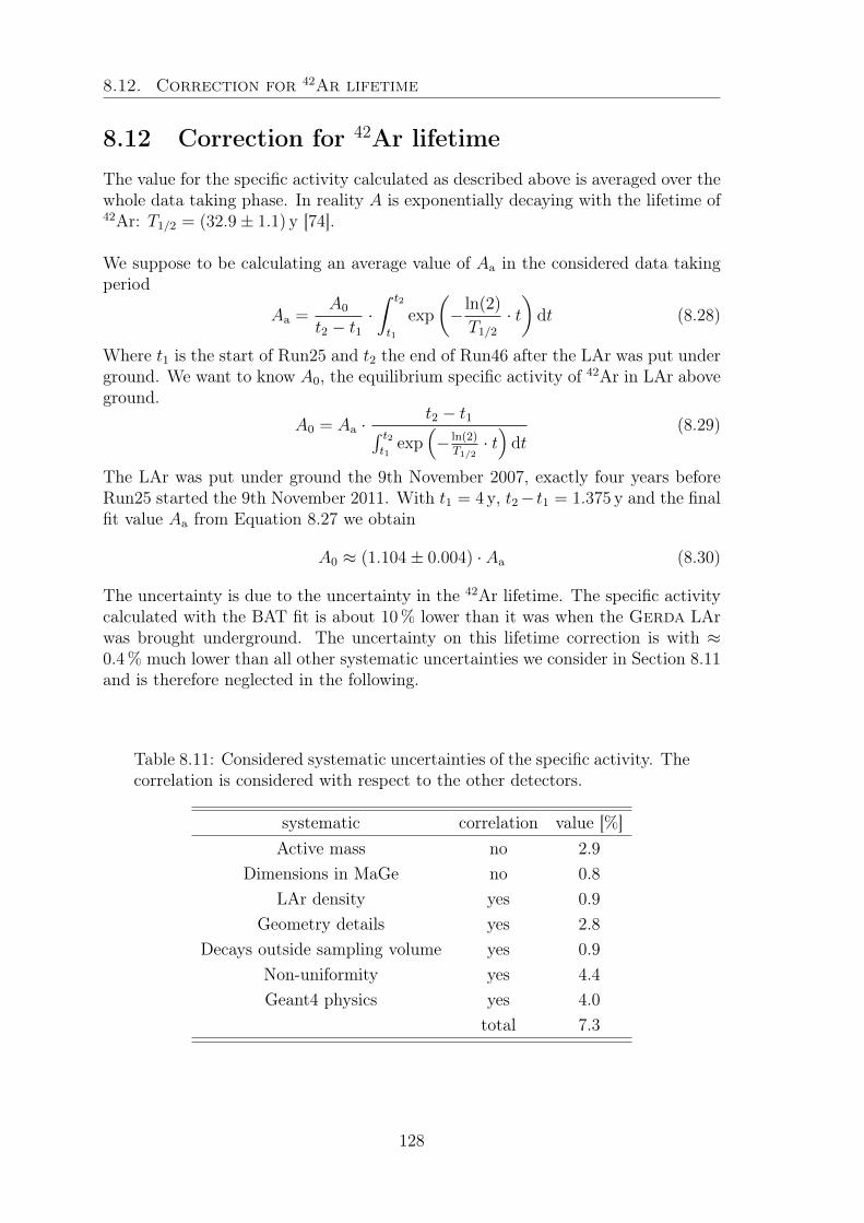
8.12. Correction for 42Ar lifetime
8.12 Correction for 42Ar lifetimeThe value for the specific activity calculated as described above is averaged over thewhole data taking phase. In reality A is exponentially decaying with the lifetime of42Ar: T1/2 = (32.9± 1.1) y [74].
We suppose to be calculating an average value of Aa in the considered data takingperiod
Aa =A0
t2 − t1·∫ t2
t1
exp
(− ln(2)
T1/2
· t)
dt (8.28)
Where t1 is the start of Run25 and t2 the end of Run46 after the LAr was put underground. We want to know A0, the equilibrium specific activity of 42Ar in LAr aboveground.
A0 = Aa ·t2 − t1∫ t2
t1exp
(− ln(2)
T1/2· t)
dt(8.29)
The LAr was put under ground the 9th November 2007, exactly four years beforeRun25 started the 9th November 2011. With t1 = 4 y, t2− t1 = 1.375 y and the finalfit value Aa from Equation 8.27 we obtain
A0 ≈ (1.104± 0.004) · Aa (8.30)
The uncertainty is due to the uncertainty in the 42Ar lifetime. The specific activitycalculated with the BAT fit is about 10 % lower than it was when the Gerda LArwas brought underground. The uncertainty on this lifetime correction is with ≈0.4 % much lower than all other systematic uncertainties we consider in Section 8.11and is therefore neglected in the following.
Table 8.11: Considered systematic uncertainties of the specific activity. Thecorrelation is considered with respect to the other detectors.
systematic correlation value [%]Active mass no 2.9
Dimensions in MaGe no 0.8LAr density yes 0.9
Geometry details yes 2.8Decays outside sampling volume yes 0.9
Non-uniformity yes 4.4Geant4 physics yes 4.0
total 7.3
128
8.13. LArGe measurement
8.12.1 Equilibrium specific activity of 42Ar above ground
The final fit value (see Equation 8.27) for the decay of 42Ar is corrected usingEquation 8.30. Finally, the systematic error is calculated with the values fromTable 8.11. The final result for the equilibrium specific activity of 42Ar in LAr is
A0(42Ar) = 101.0+2.5−3.0(stat)± 7.4(syst)µBq/kg (8.31)
8.13 LArGe measurementData from the Gerda test facility Liquid Argon Germanium Experiment (LArGe)has also been used to determine the 42Ar specific activity. A sample of LAr enrichedin the isotope 42Ar with known concentration was flushed into the LArGe cryostat.One Germanium detector (GTF44) was used for the analysis, encapsulated in acopper shroud. The count rates in the 1525 keV 42K line were compared beforeand after flushing with the enriched LAr for different HV applied on the copperencapsulation. The final result was obtained by combining all values with a weightedaverage. The final result, uncorrected for the 42Ar decay time, is
ALArGe(42Ar) = 65.6± 3.7(stat)± 13.5(syst)µBq/kg (8.32)
If we suppose that the LAr inside LArGe has been underground for about 3 yearsand 8 months, which is roughly the middle of their data taking period, we have tocorrect this value by about 8% to be comparable with the final result of this analysisfrom Section 8.12.1. As corrected value we obtain
AcorrLArGe(
42Ar) = 70.8± 4.0(stat)± 14.6(syst)µBq/kg (8.33)
8.14 DiscussionThe 42Ar specific activity obtained in this analysis is in very good agreement withthe theoretical value quoted in [69]. However, the theoretical value is a qualitativeguess. It results incompatible with the result of a previous measurement introducedin Section 8.2, which found an upper limit of 43µBq/kg.
The final result is only compatible within 1.8σ with the value obtained using LArGedata. There is some tension between the two analysis. It could well be that theHV cables which are connected to the detectors in the Gerda setup are not as wellshielded as is assumed and residual electrical fields attract 42K to the surface of theMini-Shroud. But, no evidence has been found for a higher count rate of detectorscloser to the top of the Mini-Shroud where the cables are located. By convection42K could be transported to the vicinity of the Mini-Shrouds and stay there due toan unknown mechanism.
Evaluating the count rate of the 42K line right after applying HV on the detectorscould give evidence for attraction of 42K ions. Run33 and Run34 are taken witha new detector configuration and are the sole candidates for such a study in the
129
8.14. Discussion
Gerda Phase I configuration. However, the count rate is so low that this studyremains inconclusive. In the LArGe setup with augmented 42Ar concentration ameasurement like that would be possible but has never been performed. A Gerdalike detector string should be deployed into LArGe and after a stabilization periodthe detectors switched on. The number of counts in the 1525 keV line of 42K overtime should give information about whether 42K gets attracted towards the detec-tors and about how well the MS actually works as barrier and in closing the fieldlines of the electric field around the detectors in the Phase I setup.
In Gerda Phase II the analysis, presented in this chapter, can be refined withmore statistics. It will substantially differ from this work as the MS in Phase II istransparent and a new veto system is installed using LAr scintillation light.
130
Chapter 9
Conclusions and Outlook
Finding Neutrinoless Double-Beta Decay (0νββ) decay is one of the holy grails ofexperimental neutrino physics. Its existence would clarify some of the problemsregarding neutrino particles that are still unsolved. All experiments searching for0νββ decay are low background experiments looking for an extremely rare — ifexisting — phenomenon. Their sensitivity depends strongly on the expected back-ground: events which can mimic 0νββ decay. Hence, the reduction of background isessential to all of them. Background can be suppressed in various ways: by selectingradio-pure construction material, passive shielding against external γ and neutronradiation, by tagging cosmic muons using instrumented veto systems and by ana-lyzing the form of pulses generated by signal events with respect to the background.
In the Gerda experiment 0νββ decay is searched for in the 0νββ candidate isotope76Ge. High Purity Germanium (HPGe) detectors, enriched in this isotope, serve assource and detector simultaneously. Recently, new detectors, of Broad Energy Ger-manium (BEGe) type, were produced to be hosted in the second experimental phase.They have excellent properties for pulse shape analysis, which will be one of the keyfeatures of the Gerda Phase II background reduction.
To create algorithms which effectively reduce background, based on the pulse shapes,signal-like events are extensively studied. The main property of 0νββ events is givenby their localized energy deposition inside the detector crystals. An energy depo-sition in a volume smaller than the spatial resolution of the detector is commonlyreferred to as single site event (SSE). Hence, for studies of signal-like events puresamples of SSEs are prepared and analyzed. Furthermore, the study of SSEs permitsto draw conclusions about the internal electric field properties of HPGe detectors.Pulse shape simulations rely on a precise description of these electric fields and com-parison to real data is necessary in order to validate and improve them.
The standard procedure in Gerda to obtain SSE samples is the selection of eventsfrom a Double Escape Peak (DEP). They are observed in pair production processesif both created annihilation photons escape the detector volume. In that case theenergy deposition is localized and in fact DEPs are dominated by SSEs. However,a part of hereby collected events is still due to background and the distribution of
131
9. Conclusions and Outlook
the selected events in the detector volume is extremely inhomogeneous. The proba-bility for both annihilation photons to escape is largest on the detector surface andespecially high in its corners.
For this work an experimental setup was built and optimized which is able to se-lect pure samples of SSEs from distinct locations inside a HPGe detector: A testdetector of BEGe type was implemented in the setup. The event selection of thissystem is based on Single Compton Events (singleCE) interactions, which meet thesignal-like event condition, depositing energy in localized positions in the detector.In Compton scattering interactions, kinematics are defined by the scattering angleand the incident photon energy. singleCE interactions can, thus, be selected by tag-ging of the scattered photons and selection of the energies matching the scatteringangle. A collimated photon beam, emitted by a 137Cs source, is used to irradiate theBEGe detector. Additional HPGe detectors, with a semi-coaxial (Coax) geometry,are used to tag the photons which are Compton scattered inside the BEGe with ascattering angle of 90 with respect to the incident photon beam. Their angularacceptance is restricted by collimation in order to select a specific region inside theBEGe detector. The source can be moved, the BEGe can be rotated and the heightat which the Coax detectors are placed with respect to the BEGe can be varied. Inthis manner, three-dimensional scans of the full volume of the BEGe detector canbe made.
The dewar vessels of all detectors are connected to an automatized filling systemand a safety High Voltage (HV) shut down prevents detector damage, in case adetector starts to warm up with its HV supply switched on. A data acquisitionsystem (DAQ) system was assembled and tested which records the full event traceson disk. In order to record only true coincidences of the BEGe and one of theCoax detectors, a dedicated external trigger logic was designed and implemented.A calibration and optimization method for the external trigger was established andwas successfully carried out. In order to augment the event rate a new collimatorwas designed and installed which can hold a 137Cs source with an activity of about780MBq. The collimator is very easy to handle and effectively shields radiation inorder to reduce personal risk.
This work contains a detailed description of the experimental setup, its way of op-eration and the results of the testing campaign undertaken.
An extensive characterization of the detectors used in the setup was carried out.This was necessary in order to optimize the energy reconstruction algorithm, de-termine the detector depletion and operational voltages and the energy resolutions.Furthermore, it was important to test the stability of the detector baselines in orderto operate the system under stable conditions over a long time period. The inter-nal geometry of the BEGe detector was studied in detail using a dedicated setup.Automatized fine grain surface scans give insight on the detector crystal geometry,the holder positioning and dimension, and on inhomogeneities of the outer contactlayer. A comparison to a similar HPGe detector of P-type Point Contact (PPC)
132
9. Conclusions and Outlook
type was carried out. The fine grain surface scan can give valuable input to studythe Compton coincidences in simulations.
A detailed description of the Compton coincidence setup was implemented in aMonte Carlo (MC) simulation framework. The simulations conducted allowed foran intense study of the energetic and spatial distribution of singleCE events withrespect to Multiple Compton Events (multiCE) interactions. The energy selectionof the BEGe as well as the Coax detectors were optimized in order to select confinedsingleCE events.
In a measurement campaign several locations of the BEGe detector were scannedat different HV values. The signal to background of the event samples was furtherimproved using a descriptive parameter of the pulse shape. The selection of SSEsamples with high purity was accomplished and the sample size of each location waslarge enough to compute average pulses for each scanned location. These averagetraces were found to be of high reproducibility. This enables a comparison of averagepulses of BEGe detector regions and different HV values. Differences in the shapeof the average pulse are observed when changing the scanned detector location orthe HV on the BEGe detector. In particular it was found that the first part of theaverage pulse is most sensitive. The purity of the collected samples in function of thescanned location was analyzed and compared to the MC simulations. Conclusionscan be drawn on the limitations of Compton coincidence measurements conductedwith this experimental setup.
Finally, the purity of SSE samples was compared to the standard method used inthe Gerda experiment. An uncollimated 228Th spectrum was recorded and the SSEto background ratio of the DEP from the 2.6MeV 208Tl γ-line was analyzed. Thepurity of SSE samples from the Compton coincidence measurements proved to besuperior in the surface regions of the BEGe detector where events from the DEP arelocated. Moreover, the Compton setup permits to collect SSEs from interior regionsof the BEGe to which the DEP shows negligible sensitivity.
Future improvements of the Compton setup can be made by measuring at differentscanning angles. The differential cross section for Compton scattering is larger forsmaller scattering angles. This could augment the event rate and further improvethe SSE to background ratio of the collected event samples.
The results from a first comparison of average pulse shapes is promising. A prospec-tive key point is a more detailed scanning measurement of a BEGe detector andsubsequent comparison to pulse shape simulations. The profile of the impurity con-centration in a BEGe could be fine-tuned based on such measurements and improvethe reliability of pulse shape simulations. Other detector geometries can be studiedwith the setup in order to compare their Pulse Shape Discrimination (PSD) powerto the Gerda Phase II BEGe detectors and possibly more adapt geometries couldbe found.
133
9. Conclusions and Outlook
Returning to 0νββ experiments in general and the Gerda experiment in particu-lar, another important aspect in rare event searches is the full decomposition andanalysis of background contributions. One major background component in GerdaPhase I is the isotope 42Ar, which decays via β− decay in 42K. 42K further decaysvia a β− decay with an endpoint energy above the endpoint of the Two NeutrinoDouble-Beta Decay (2νββ) spectrum of 76Ge. Thus, the continuous energy spec-trum of the electrons can deposit energy in the region of Qββ contributing to theexpected background of the Gerda experiment.
The specific activity of 42Ar in the Gerda liquid Argon (LAr) was analyzed usinga Bayesian approach. The unique, highly radiopure environment of Gerda per-mits this type of study. Two fit models were implemented in a Bayesian AnalysisFramework to fit a γ-line of 42K which is in secular equilibrium with 42Ar. A binnedmaximum likelihood fit with four (five for the second fit model) nuisance parametersper detector and a common parameter for the activity was performed and the resultwas analyzed for its stability. The detection efficiencies, which introduce a majorsystematic uncertainty to the result, were calculated by means of MC simulations ofpart of the Gerda experimental setup. This permitted to study systematic effectsintroduced by inhomogeneities of the 42K distribution in the LAr and provided aconservative estimate of the uncertainty on the efficiencies, which were then propa-gated to the activity.
This analysis is not only providing an estimate of the specific activity of 42Ar inthe Gerda LAr. Correcting the found value for the time the LAr was kept underground it can be compared to other experimental results, and furthermore, to the-oretical calculations regarding production mechanisms of 42Ar in the atmosphere.This has been done as a last step of the analysis conducted in this work and thevalue is found compatible within 1.8σ with result found by the Gerda test facilityLArGe and in very good agreement with a theoretical calculation based on a majorproduction mechanisms of 42Ar. However, the theoretical value is only an educatedguess. More precise calculations are needed to fully comprehend the implications ofthe experimental value calculated in this thesis.
134
Appendix A
Multi-tier data structure anddecoder implementation
The Gerda analysis program transforms data in a multi-tier structure approach.Raw data is called the tier0 level data. A decoder step transforms tier0 level datain a compressed and rootified structure containing exactly the same informationcontained on tier0 level but compatible with all other Gerda analysis software. Wecall this the tier1 level. In the next step transforms are applied to the traces andparameters like energy, current pulse amplitude and rise time are extracted. Thisinformation is contained on the tier2 level of data analysis. Every higher analysisstep is a higher level in the tier structure. E.g. the calibrated energy can be con-tained on a tier3 level.
In order to transform tier0 data into the tier1 rootified format an FADC specificdecoder has to be implemented which reads the data from tier0 files and stores theevent traces in a root tree. Also for data taken with the FADCs in this setup adedicated decoder was implemented. The program Raw2MGDO has to be calledwith the option -c LEGO for the 100MHz 4 channel FADC. A version for a 500MHz8 channel FADC has also been implemented and can be called via -c LEGO_DIGI8.The filename is handed with the option -f. FADC channels can be excluded fromthe transform with the -e option and the pre-trigger fraction fpre of the trace can behanded calling the -P option. Per default all channels are processed with fpre = 0.5.
100MHz digitizer $ Raw2MGDO -c LEGO -f filename
500MHz digitizer $ Raw2MGDO -c LEGO_DIGI8 -f filename
Optional -e FADC channel
-P fpre
Detectors with positive and negative voltage have to be analyzed separately as alldata analysis works on positive pulses and negative traces get simply inverted. Thepolarity is expected to be the same in all channels for a tier0 → tier1 and tier1 →tier2 transformation.
135

Appendix
136
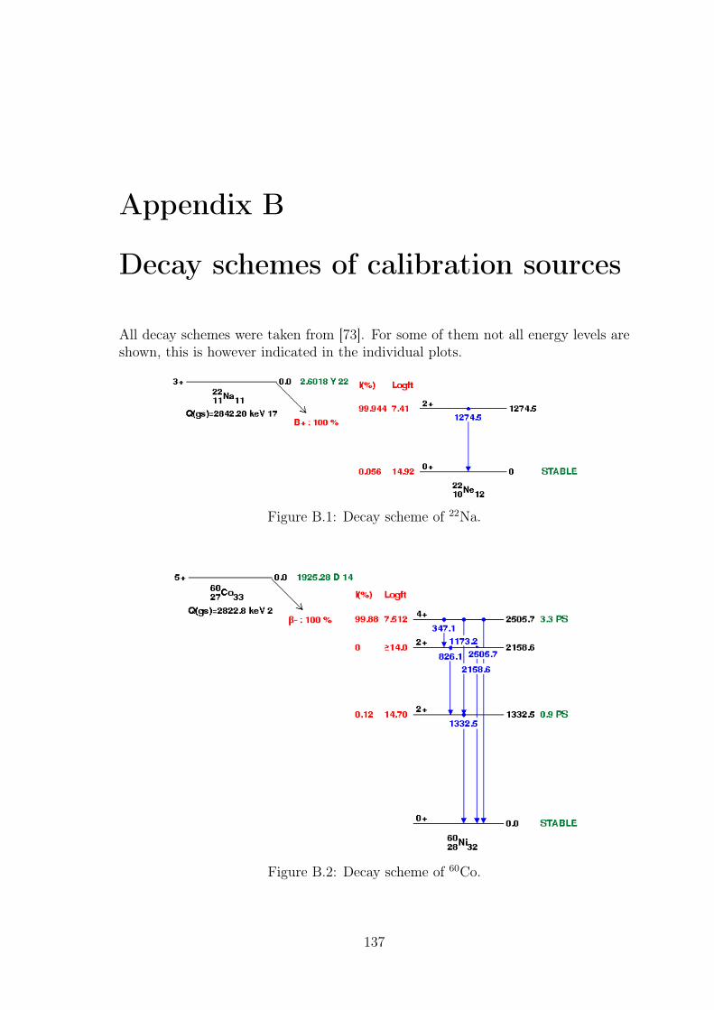
Appendix B
Decay schemes of calibration sources
All decay schemes were taken from [73]. For some of them not all energy levels areshown, this is however indicated in the individual plots.
Figure B.1: Decay scheme of 22Na.
Figure B.2: Decay scheme of 60Co.
137
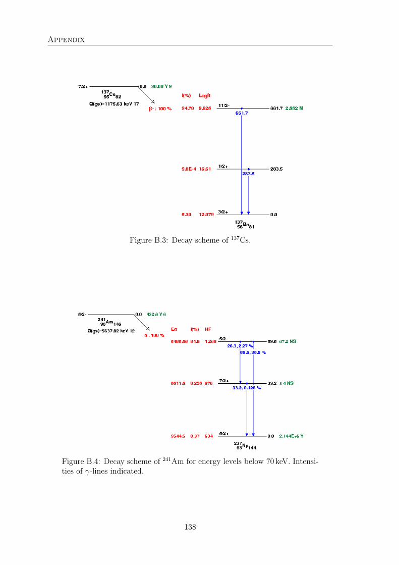
Appendix
Figure B.3: Decay scheme of 137Cs.
Figure B.4: Decay scheme of 241Am for energy levels below 70 keV. Intensi-ties of γ-lines indicated.
138
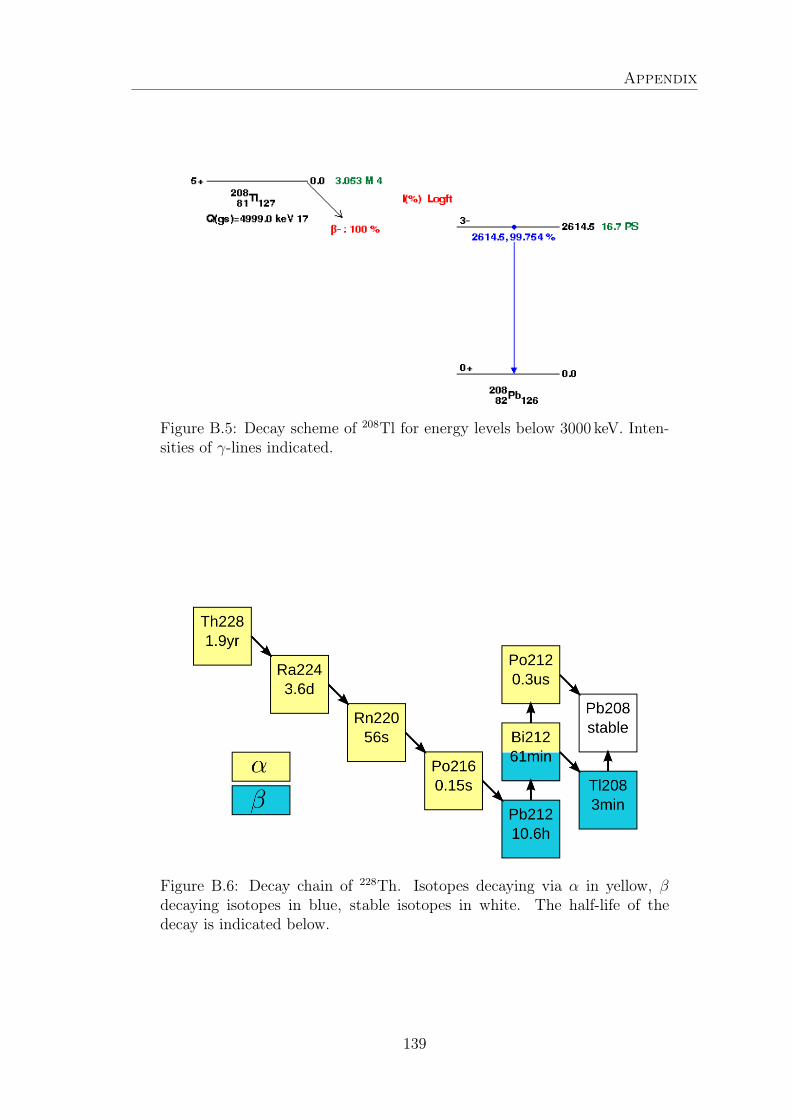
Appendix
Figure B.5: Decay scheme of 208Tl for energy levels below 3000 keV. Inten-sities of γ-lines indicated.
Figure B.6: Decay chain of 228Th. Isotopes decaying via α in yellow, βdecaying isotopes in blue, stable isotopes in white. The half-life of thedecay is indicated below.
139

Appendix
140
Appendix C
Full Width at fw Maximum
To get the full width of a γ-line at some fraction fw of the peak maximum (FWfwM)the γ-line is fit using a Gaussian plus tail fit function (Equation 4.4). The corre-sponding x-value of the fit function is evaluated left and right of the peak centroidto satisfy g(x) = fw ·mµ and the difference is taken as the respective FWfwM. mµ
is the maximum height of the Gaussian peak. The error is estimated as follows
∆FWfwM
FWfwM=
∆σ
σ(C.1)
Where σ and ∆σ are the standard deviation and its uncertainty from the Gaussianplus tail fit function. When calculating a fraction FWfwM/FWHM the errors areassumed to be fully correlated and therefore
∆(FWfwM/FWHM)
(FWfwM/FWHM)=
√∆FWfwM
FWfwM
2
+∆FWHM
FWHM
2
− 2∆FWfwM
FWfwM
∆FWHM
FWHM
= 0
(C.2)
141

Appendix
142
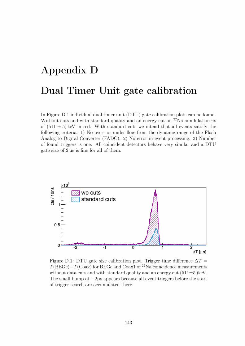
Appendix D
Dual Timer Unit gate calibration
In Figure D.1 individual dual timer unit (DTU) gate calibration plots can be found.Without cuts and with standard quality and an energy cut on 22Na annihilation γsof (511 ± 5) keV in red. With standard cuts we intend that all events satisfy thefollowing criteria: 1) No over- or under-flow from the dynamic range of the FlashAnalog to Digital Converter (FADC). 2) No error in event processing. 3) Numberof found triggers is one. All coincident detectors behave very similar and a DTUgate size of 2µs is fine for all of them.
Figure D.1: DTU gate size calibration plot. Trigger time difference ∆T =T (BEGe)−T (Coax) for BEGe and Coax1 of 22Na coincidence measurementswithout data cuts and with standard quality and an energy cut (511±5 )keV.The small bump at −2µs appears because all event triggers before the startof trigger search are accumulated there.
143
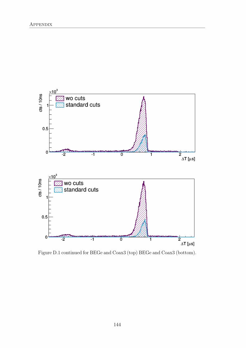
Appendix
Figure D.1 continued for BEGe and Coax3 (top) BEGe and Coax3 (bottom).
144
Appendix E
Coincidence Monte Carlo simulationoptions
Some geometry details are implemented variable in size. The options that can bechosen and a short description can be found here
BEGe cryostat dimensions
/MG/geometry/LEGOTable/CryostatWindowThicknessSets cryostat window thickness, which is the front part [mm]
/MG/geometry/LEGOTable/CryostatWallThicknessSets cryostat wall thickness, which is the side part [mm]
/MG/geometry/LEGOTable/CryostatDiameterSets cryostat diameter [mm]
/MG/geometry/LEGOTable/CryostatHeightSets cryostat height [mm]
BEGe Xtal dimensions
/MG/geometry/LEGOTable/XtalDiameterSets crystal diameter (incl. DL) [mm]
/MG/geometry/LEGOTable/XtalHeightSets crystal height (incl. DL) [mm]
/MG/geometry/LEGOTable/XtalDistanceToWindowSets distance of crystal top to cryostat window [mm]
/MG/geometry/LEGOTable/XtalDitchInnerRadiusSets inner radius of groove [mm]
145
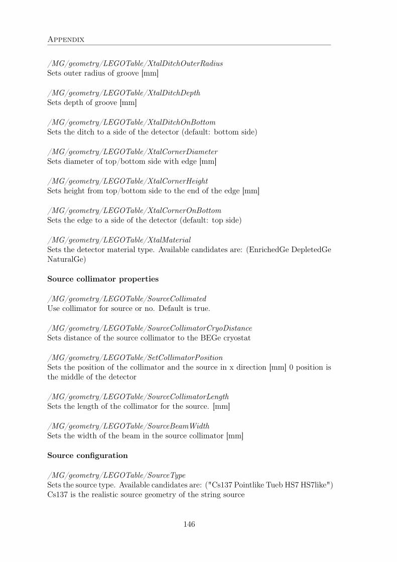
Appendix
/MG/geometry/LEGOTable/XtalDitchOuterRadiusSets outer radius of groove [mm]
/MG/geometry/LEGOTable/XtalDitchDepthSets depth of groove [mm]
/MG/geometry/LEGOTable/XtalDitchOnBottomSets the ditch to a side of the detector (default: bottom side)
/MG/geometry/LEGOTable/XtalCornerDiameterSets diameter of top/bottom side with edge [mm]
/MG/geometry/LEGOTable/XtalCornerHeightSets height from top/bottom side to the end of the edge [mm]
/MG/geometry/LEGOTable/XtalCornerOnBottomSets the edge to a side of the detector (default: top side)
/MG/geometry/LEGOTable/XtalMaterialSets the detector material type. Available candidates are: (EnrichedGe DepletedGeNaturalGe)
Source collimator properties
/MG/geometry/LEGOTable/SourceCollimatedUse collimator for source or no. Default is true.
/MG/geometry/LEGOTable/SourceCollimatorCryoDistanceSets distance of the source collimator to the BEGe cryostat
/MG/geometry/LEGOTable/SetCollimatorPositionSets the position of the collimator and the source in x direction [mm] 0 position isthe middle of the detector
/MG/geometry/LEGOTable/SourceCollimatorLengthSets the length of the collimator for the source. [mm]
/MG/geometry/LEGOTable/SourceBeamWidthSets the width of the beam in the source collimator [mm]
Source configuration
/MG/geometry/LEGOTable/SourceTypeSets the source type. Available candidates are: ("Cs137 Pointlike Tueb HS7 HS7like")Cs137 is the realistic source geometry of the string source
146
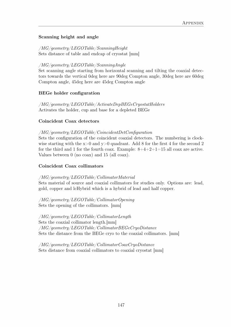
Appendix
Scanning height and angle
/MG/geometry/LEGOTable/ScanningHeightSets distance of table and endcap of cryostat [mm]
/MG/geometry/LEGOTable/ScanningAngleSet scanning angle starting from horizontal scanning and tilting the coaxial detec-tors towards the vertical 0deg here are 90deg Compton angle, 30deg here are 60degCompton angle, 45deg here are 45deg Compton angle
BEGe holder configuration
/MG/geometry/LEGOTable/ActivateDepBEGeCryostatHoldersActivates the holder, cup and base for a depleted BEGe
Coincident Coax detectors
/MG/geometry/LEGOTable/CoincidentDetConfigurationSets the configuration of the coincident coaxial detectors. The numbering is clock-wise starting with the x>0 and y>0 quadrant. Add 8 for the first 4 for the second 2for the third and 1 for the fourth coax. Example: 8+4+2+1=15 all coax are active.Values between 0 (no coax) and 15 (all coax).
Coincident Coax collimators
/MG/geometry/LEGOTable/CollimatorMaterialSets material of source and coaxial collimators for studies only. Options are: lead,gold, copper and lcHybrid which is a hybrid of lead and half copper.
/MG/geometry/LEGOTable/CollimatorOpeningSets the opening of the collimators. [mm]
/MG/geometry/LEGOTable/CollimatorLengthSets the coaxial collimator length.[mm]/MG/geometry/LEGOTable/CollimatorBEGeCryoDistanceSets the distance from the BEGe cryo to the coaxial collimators. [mm]
/MG/geometry/LEGOTable/CollimatorCoaxCryoDistanceSets distance from coaxial collimators to coaxial cryostat [mm]
147

Appendix
148
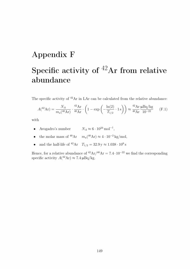
Appendix F
Specific activity of 42Ar from relativeabundance
The specific activity of 42Ar in LAr can be calculated from the relative abundance:
A(42Ar) =NA
ma(40Ar)·
42Ar40Ar
·(
1− exp
(− ln(2)
T1/2
· 1 s
))≈
42Ar40Ar
µBq/kg
10−22(F.1)
with
• Avogadro’s number NA ≈ 6 · 1023 mol−1,
• the molar mass of 40Ar ma(40Ar) ≈ 4 · 10−2 kg/mol,
• and the half-life of 42Ar T1/2 = 32.9 y ≈ 1.038 · 109 s
Hence, for a relative abundance of 42Ar/40Ar = 7.4 ·10−22 we find the correspondingspecific activity A(42Ar) ≈ 7.4µBq/kg.
149

Appendix
150
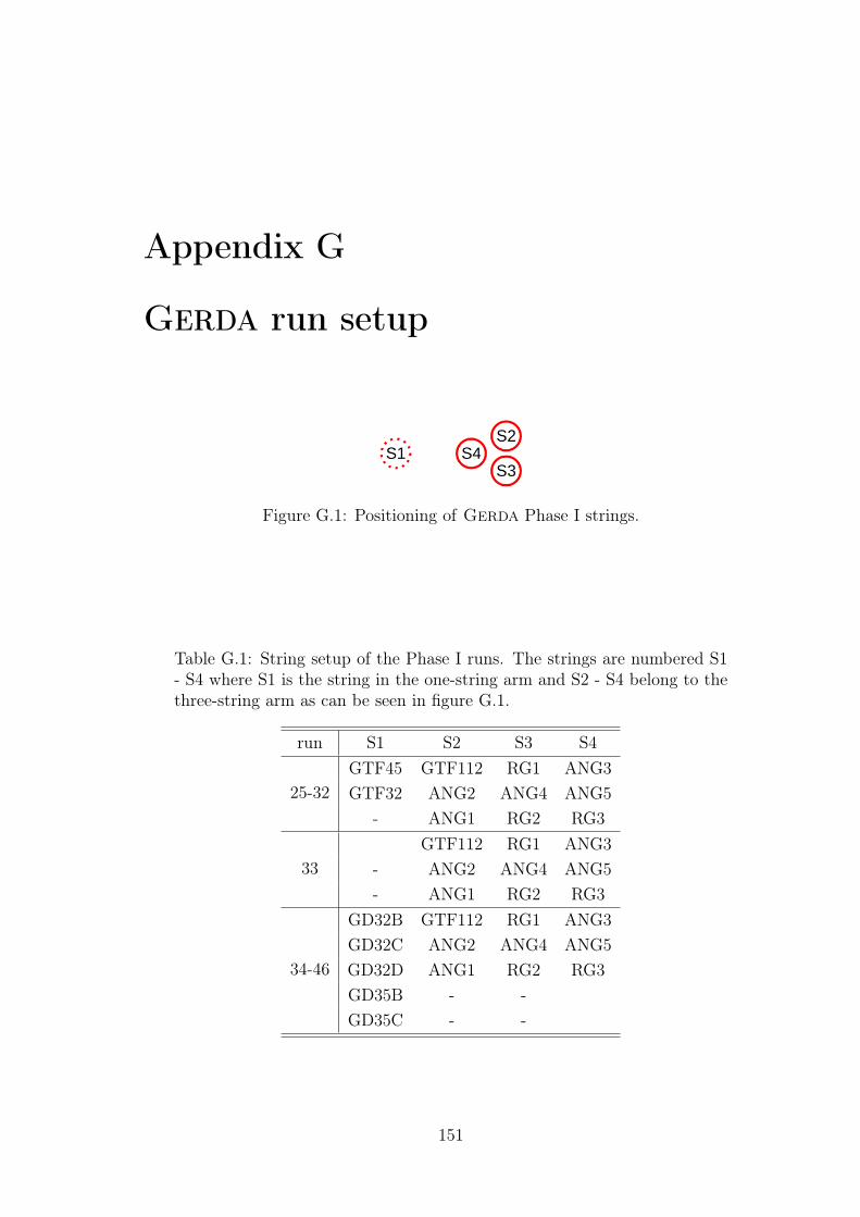
Appendix G
Gerda run setup
Figure G.1: Positioning of Gerda Phase I strings.
Table G.1: String setup of the Phase I runs. The strings are numbered S1- S4 where S1 is the string in the one-string arm and S2 - S4 belong to thethree-string arm as can be seen in figure G.1.
run S1 S2 S3 S4
25-32GTF45 GTF112 RG1 ANG3GTF32 ANG2 ANG4 ANG5
- ANG1 RG2 RG3
33GTF112 RG1 ANG3
- ANG2 ANG4 ANG5- ANG1 RG2 RG3
34-46
GD32B GTF112 RG1 ANG3GD32C ANG2 ANG4 ANG5GD32D ANG1 RG2 RG3GD35B - -GD35C - -
151
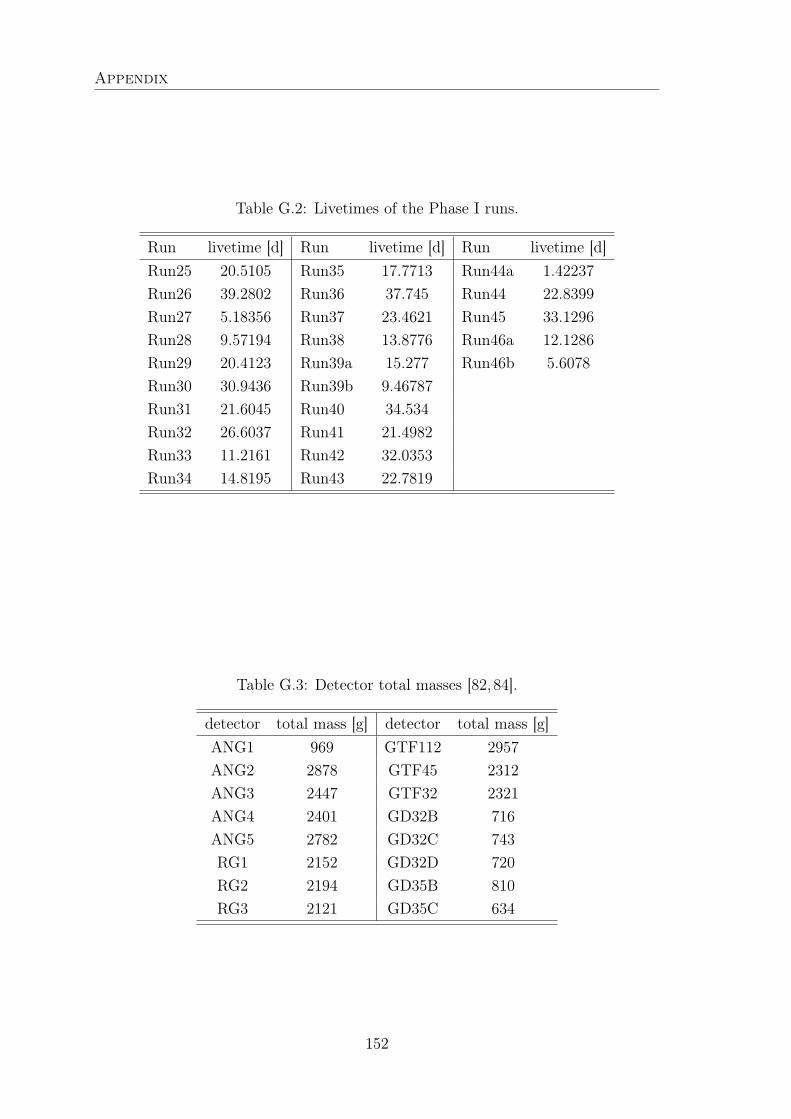
Appendix
Table G.2: Livetimes of the Phase I runs.
Run livetime [d] Run livetime [d] Run livetime [d]Run25 20.5105 Run35 17.7713 Run44a 1.42237Run26 39.2802 Run36 37.745 Run44 22.8399Run27 5.18356 Run37 23.4621 Run45 33.1296Run28 9.57194 Run38 13.8776 Run46a 12.1286Run29 20.4123 Run39a 15.277 Run46b 5.6078Run30 30.9436 Run39b 9.46787Run31 21.6045 Run40 34.534Run32 26.6037 Run41 21.4982Run33 11.2161 Run42 32.0353Run34 14.8195 Run43 22.7819
Table G.3: Detector total masses [82,84].
detector total mass [g] detector total mass [g]ANG1 969 GTF112 2957ANG2 2878 GTF45 2312ANG3 2447 GTF32 2321ANG4 2401 GD32B 716ANG5 2782 GD32C 743RG1 2152 GD32D 720RG2 2194 GD35B 810RG3 2121 GD35C 634
152
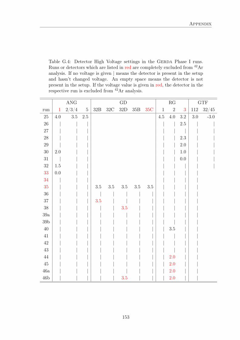
Appendix
Table G.4: Detector High Voltage settings in the Gerda Phase I runs.Runs or detectors which are listed in red are completely excluded from 42Aranalysis. If no voltage is given | means the detector is present in the setupand hasn’t changed voltage. An empty space means the detector is notpresent in the setup. If the voltage value is given in red, the detector in therespective run is excluded from 42Ar analysis.
ANG GD RG GTFrun 1 2/3/4 5 32B 32C 32D 35B 35C 1 2 3 112 32/4525 4.0 3.5 2.5 4.5 4.0 3.2 3.0 -3.026 | | | | | 2.5 | |27 | | | | | | | |28 | | | | | 2.3 | |29 | | | | | 2.0 | |30 2.0 | | | | 1.0 | |31 | | | | | 0.0 | |32 1.5 | | | | | | |33 0.0 | | | | | |34 | | | | | | |35 | | | 3.5 3.5 3.5 3.5 3.5 | | | |36 | | | | | | | | | | | |37 | | | 3.5 | | | | | | | |38 | | | | | 3.5 | | | | | |39a | | | | | | | | | | | |39b | | | | | | | | | | | |40 | | | | | | | | | 3.5 | |41 | | | | | | | | | | | |42 | | | | | | | | | | | |43 | | | | | | | | | | | |44 | | | | | | | | | 2.0 | |45 | | | | | | | | | 2.0 | |46a | | | | | | | | | 2.0 | |46b | | | | | 3.5 | | | 2.0 | |
153

Appendix
154
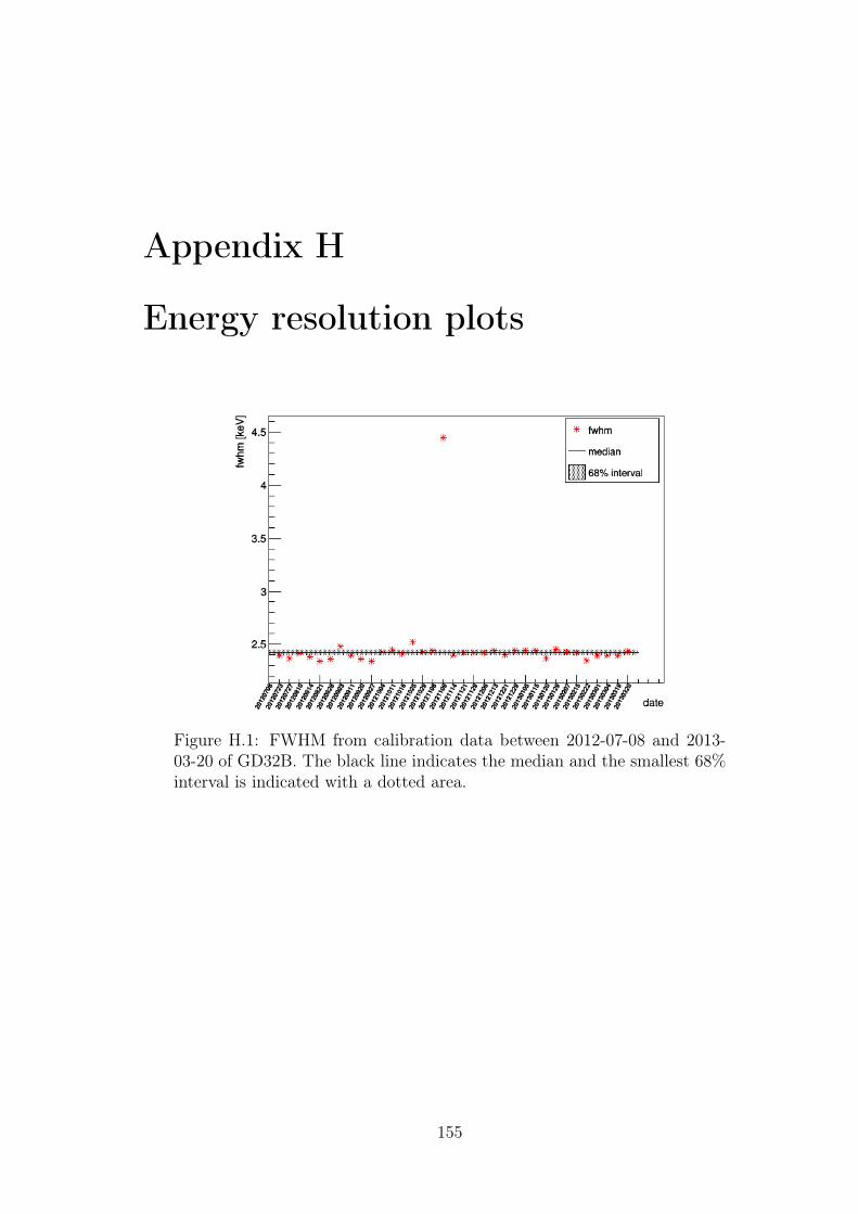
Appendix H
Energy resolution plots
Figure H.1: FWHM from calibration data between 2012-07-08 and 2013-03-20 of GD32B. The black line indicates the median and the smallest 68%interval is indicated with a dotted area.
155
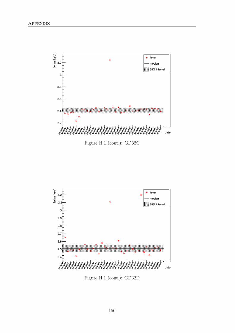
Appendix
Figure H.1 (cont.): GD32C
Figure H.1 (cont.): GD32D
156
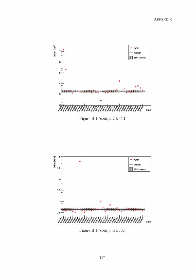
Appendix
Figure H.1 (cont.): GD35B
Figure H.1 (cont.): GD35C
157
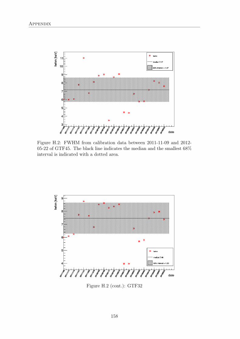
Appendix
Figure H.2: FWHM from calibration data between 2011-11-09 and 2012-05-22 of GTF45. The black line indicates the median and the smallest 68%interval is indicated with a dotted area.
Figure H.2 (cont.): GTF32
158
List of Figures
1.1 Feynman diagrams of 2νββ and 0νββ . . . . . . . . . . . . . . . . . 21.2 Expected spectral signature of 0νββ decay . . . . . . . . . . . . . . . 21.3 Dependence of allowed parameter space of mββ on mβ and Σ . . . . 51.4 Predictions of Nuclear Matrix Element (NME) values calculated in
various models . . . . . . . . . . . . . . . . . . . . . . . . . . . . . . 6
2.1 Expected 0νββ half-lives for different candidate isotopes . . . . . . . 102.2 HPGe detector geometries . . . . . . . . . . . . . . . . . . . . . . . . 102.3 The Gerda setup . . . . . . . . . . . . . . . . . . . . . . . . . . . . 112.4 Comparison of half-life limits of 0νββ in 76Ge and 136Xe . . . . . . . 12
3.1 Photoelectric effect and characteristic photon radiation . . . . . . . . 153.2 Compton scattering . . . . . . . . . . . . . . . . . . . . . . . . . . . 153.3 Photon and electron energy in Compton scattering . . . . . . . . . . 163.4 Differential cross section in Thomson and Compton scattering . . . . 163.5 Pair production . . . . . . . . . . . . . . . . . . . . . . . . . . . . . . 183.6 Band structure model of isolators, semiconductors and conductors . . 183.7 Realistic band structure model of germanium . . . . . . . . . . . . . 20
4.1 Sketch of Multichannel Analyzer (MCA) and FADC DAQ systems . . 274.2 Genius Shaper module for amplification without shaping . . . . . . . 284.3 Coax3 60Co spectra with Genius Shaper maximal amplification . . . . 294.4 Visualization of the pseudo-Gaussian energy reconstruction algorithm 314.5 FADC Energy reconstruction parameter optimization: PPC . . . . . 324.6 MCA Shaping time optimization: BEGe . . . . . . . . . . . . . . . . 324.7 Peak fit of the 60Co 1332 keV γ-line recorded with Coax3 . . . . . . . 344.8 BEGe 60Co HV scan . . . . . . . . . . . . . . . . . . . . . . . . . . . 364.9 BEGe 60Co spectrum at 3600V, 3650V, 3700V and 4000V . . . . . 364.10 PPC 60Co HV scan . . . . . . . . . . . . . . . . . . . . . . . . . . . . 374.11 Baseline of BEGe and Coax1 over a time period of 130 h . . . . . . . 384.12 Fine grain surface scanning table setup and its motion axes . . . . . 394.13 Sketch of the count rate pattern observed in a sharp edge scan . . . 404.14 Sketch of the movement of a source beam over a sharp edge . . . . . 414.15 Simulation of a sharp edge scan . . . . . . . . . . . . . . . . . . . . . 414.16 PPC top and lateral linear surface scans . . . . . . . . . . . . . . . . 434.17 BEGe top and lateral linear surface scan . . . . . . . . . . . . . . . . 454.18 Scan points of PPC circular top surface scan . . . . . . . . . . . . . 47
159
List of Figures
4.19 Count rates of PPC circular top surface scan . . . . . . . . . . . . . 474.20 Scan points of PPC circular lateral surface scan . . . . . . . . . . . . 494.21 Count rates of PPC circular lateral surface scan . . . . . . . . . . . . 494.22 Scan points of BEGe circular top surface scan . . . . . . . . . . . . . 504.23 Count rates of BEGe circular top surface scan . . . . . . . . . . . . . 514.24 Scan points of BEGe circular lateral surface scan . . . . . . . . . . . 514.25 Count rates of BEGe circular lateral surface scan . . . . . . . . . . . 52
5.1 Pulse shapes due to a SSE, multiple site event (MSE) and a slowpulse event . . . . . . . . . . . . . . . . . . . . . . . . . . . . . . . . 54
5.2 Interaction cross sections of photons in Germanium . . . . . . . . . . 565.3 Selection of confined Compton interactions . . . . . . . . . . . . . . 565.4 Sketch of Compton coincidence setup top and side view . . . . . . . . 585.5 Close up of experimental setup for Compton coincidence measurements 585.6 Full experimental setup for Compton coincidence measurements . . . 595.7 Collimator for 780MBq 137Cs source . . . . . . . . . . . . . . . . . . 595.8 Technical drawing of the new source collimator . . . . . . . . . . . . . 605.9 Measure of scanning table height . . . . . . . . . . . . . . . . . . . . 645.10 BEGe top scan in Compton coincidence setup . . . . . . . . . . . . . 645.11 22Na source installed inside a detector collimator for position calibration 655.12 BEGe lateral scan in Compton coincidence setup . . . . . . . . . . . 655.13 Sketch of external trigger logic . . . . . . . . . . . . . . . . . . . . . . 675.14 External trigger generation . . . . . . . . . . . . . . . . . . . . . . . 675.15 Sketch of 22Na DTU gate calibration measurement setup . . . . . . . 685.16 Trigger time difference for different DTU gate sizes . . . . . . . . . . 685.17 Scanned points using the 780MBq 137Cs source . . . . . . . . . . . . 715.18 Impact of standard quality cuts on uncalibrated energy spectra . . . 725.19 Calibrated scatter plot and sum energy spectrum of Run14 data . . . 73
6.1 Compton coincidence setup MC implementation in MaGe . . . . . . . 766.2 Realistic MC implementation of strong 137Cs source geometry . . . . 766.3 Uncollimated 137Cs spectrum comparison of measurement and MC . . 776.4 BEGe energy versus Coax1 energy from MC simulation . . . . . . . . 786.5 BEGe signal and background spectrum without energy cuts . . . . . 796.6 BEGe signal to background ratio as a function of energy . . . . . . . 806.7 Coax signal and background spectrum without energy cuts . . . . . . 806.8 Coax signal and background spectrum with BEGe energy cut applied 816.9 BEGe signal to background ratio comparison . . . . . . . . . . . . . . 816.10 Hit distributions without energy cut . . . . . . . . . . . . . . . . . . . 826.11 Hit distributions with BEGe energy cut . . . . . . . . . . . . . . . . . 836.12 Hit distributions with BEGe and Coax energy cuts . . . . . . . . . . 846.13 Z-projection of signal and background energy distribution in the BEGe 856.14 X-projection of signal and background energy distribution in the BEGe 856.15 Scatter plot of the BEGe and Coax1 energy in Run14 . . . . . . . . . 876.16 BEGe simulated energy spectrum after all energy cuts . . . . . . . . . 876.17 Opening angle α in the solid angle fraction calculation . . . . . . . . 88
160

List of Figures
6.18 Measured and simulated BEGe energy spectra in the Run14 configu-ration . . . . . . . . . . . . . . . . . . . . . . . . . . . . . . . . . . . 90
7.1 Remaining scan points of the measurement campaign . . . . . . . . . 927.2 Fit of A/E distribution after quality and energy cuts . . . . . . . . . 947.3 SSE event to background (BKG) ratio as a function of the scanning
height . . . . . . . . . . . . . . . . . . . . . . . . . . . . . . . . . . . 967.4 MC singleCE to multiCE ratio in dependence of the scanning height 967.5 Z-projection of the energy deposited inside the BEGe detector . . . 977.6 X-projection of the energy deposition inside the BEGe detector . . . 977.7 Rise time distribution before and after quality and energy cuts . . . . 997.8 Asymmetry distribution before and after quality and energy cuts . . . 997.9 Comparison of Run1 and Run2 sub measurement average pulses . . . 1007.10 Comparison of average pulse residuals in Run1 and Run2 . . . . . . . 1007.11 Average pulse comparison of different detector regions . . . . . . . . 1027.12 Average pulse comparison for different BEGe HV . . . . . . . . . . . 1037.13 Rise time distributions for 4 kV and 5 kV BEGe HV . . . . . . . . . . 1047.14 Asymmetry distributions for 4 kV and 5 kV BEGe HV . . . . . . . . . 1047.15 A/E versus calibrated energy of a 228Th measurement . . . . . . . . 1057.16 228Th A/E distribution fit of the DEP line . . . . . . . . . . . . . . . 106
8.1 Decay scheme of 42Ar . . . . . . . . . . . . . . . . . . . . . . . . . . 1088.2 Decay scheme of 42K . . . . . . . . . . . . . . . . . . . . . . . . . . . 1088.3 Primary vertex positions with energy deposition in the BEGes . . . . 1108.4 LAr cylinder in which 42K decays are simulated . . . . . . . . . . . . 1108.5 Primary spectrum of efficiency simulations . . . . . . . . . . . . . . . 1118.6 Gaussian function with inverse error function as background model . 1198.7 Posterior pdf of specific activity A . . . . . . . . . . . . . . . . . . . . 1228.8 Sum histogram and combined fit function in the flat background model1238.9 Comparison of background models for ANG2 with fit precision kHigh 1238.10 Stability of A fitting data from different run periods . . . . . . . . . . 1258.11 Stability of A fitting single detector data . . . . . . . . . . . . . . . . 1268.12 Stability of A fitting data from single detector strings . . . . . . . . . 126
B.1 Decay scheme of 22Na . . . . . . . . . . . . . . . . . . . . . . . . . . . 137B.2 Decay scheme of 60Co . . . . . . . . . . . . . . . . . . . . . . . . . . . 137B.3 Decay scheme of 137Cs . . . . . . . . . . . . . . . . . . . . . . . . . . 138B.4 Decay scheme of 241Am . . . . . . . . . . . . . . . . . . . . . . . . . . 138B.5 Decay scheme of 208Tl . . . . . . . . . . . . . . . . . . . . . . . . . . 139B.6 Decay chain of 228Th . . . . . . . . . . . . . . . . . . . . . . . . . . . 139
D.1 DTU gate size calibration . . . . . . . . . . . . . . . . . . . . . . . . 143
G.1 Positioning of Gerda Phase I strings. . . . . . . . . . . . . . . . . . 151
H.1 Variation in time of the FWHM of the Phase I BEGe detectors . . . . 155H.2 Variation in time of the FWHM of GTF45 and GTF32 . . . . . . . . 158
161

List of Figures
162
List of Tables
1.1 Phase space factor, Q-value and natural abundance . . . . . . . . . . 41.2 Parameters from global analysis of oscillation experiments . . . . . . 4
3.1 Properties of germanium . . . . . . . . . . . . . . . . . . . . . . . . . 20
4.1 Available detectors . . . . . . . . . . . . . . . . . . . . . . . . . . . . 254.2 Genius Shaper parameters and settings . . . . . . . . . . . . . . . . . 284.3 Shaping parameters for energy reconstruction of FADC and MCA data 314.4 Resolution and Gaussianity parameters of all detectors . . . . . . . . 34
5.1 Photon and electron energies in single Compton scattering . . . . . . 555.2 Photon survival fraction in lead . . . . . . . . . . . . . . . . . . . . . 615.3 List of 137Cs coincidence measurements . . . . . . . . . . . . . . . . . 70
7.1 Summary table of data reduction by quality and energy cuts. . . . . 927.2 Summary table of SSE and BKG content after A/E - cut . . . . . . . 94
8.1 List of simulations and normalization factors . . . . . . . . . . . . . . 1138.2 Comparison of complete and split efficiency simulations . . . . . . . . 1148.3 Efficiencies of all Phase I detectors . . . . . . . . . . . . . . . . . . . 1148.4 Median FWHM at 1525 keV from calibration data . . . . . . . . . . 1158.5 Input values used for the likelihood fit . . . . . . . . . . . . . . . . . 1188.6 List of priors and their types . . . . . . . . . . . . . . . . . . . . . . . 1198.7 Event flags which can be used for data cuts . . . . . . . . . . . . . . 1218.8 Final fit values of A in both background models . . . . . . . . . . . . 1228.9 Comparison of fit parameter A for different fit precisions . . . . . . . 1238.10 Comparison of fit parameter A of single detector fits . . . . . . . . . . 1248.11 Considered systematic uncertainties . . . . . . . . . . . . . . . . . . . 128
G.1 String setup of the Phase I runs . . . . . . . . . . . . . . . . . . . . . 151G.2 Livetimes of the Phase I runs . . . . . . . . . . . . . . . . . . . . . . 152G.3 Detector total masses . . . . . . . . . . . . . . . . . . . . . . . . . . . 152G.4 Detector High Voltage settings in the Gerda Phase I runs . . . . . . 153
163

List of Tables
164

List of Acronyms
ββ Double-Beta Decay
0νββ Neutrinoless Double-Beta Decay
2νββ Ordinary Double-Beta Decay
BAO Baryon Acoustic Oscillations
BAT Bayesian Analysis Toolkit
BEGe Broad Energy Germanium
BI background index
BKG background
BL baseline
CMB Cosmic Microwave Background
Coax semi-coaxial detector
CP Charge Parity
CSDA continuous-slowing-down approximation
DAQ data acquisition system
DEP Double Escape Peak
DTU dual timer unit
erfc inverse error function
165

List of Acronyms
FADC Flash ADC
FEP Full Energy Peak
FWHM Full Width at Half Maximum
FWTM Full Width at one Tenth Maximum
FWFM Full Width at one Fiftieth Maximum
GUI Graphical User Interface
Gerda Germanium Detector Array experiment
HDM Heidelberg-Moscow experiment
HPGe High Purity Germanium
HV High Voltage
IGEX International Germanium Experiment
IH inverted hierarchy
INFN Istituto Nazionale di Fisica Nucleare
LAr liquid Argon
LArGe Liquid Argon Germanium Experiment
LN2 liquid Nitrogen
LNGS Laboratori Nazionali del Gran Sasso
LNV Lepton Number Violating
LV Low Voltage
MC Monte Carlo
MCA multichannel analyzer
MCMC Markov Chain Monte Carlo
multiCE Multiple Compton Events
MPIK Max-Planck-Institute for Nuclear Physics
MS Mini-Shroud
MSE multiple site event
MWA moving window average
166
List of Acronyms
NH normal hierarchy
NME Nuclear Matrix Element
pdf probability density function
PMNS Pontecorvo-Maki-Nakagawa-Sakata
PPC P-type Point Contact
PSA Pulse Shape Analysis
PSD Pulse Shape Discrimination
PreAmp Preamplifier
QD quasi-degeneracy
ROI Region of Interest
singleCE Single Compton Events
SEP Single Escape Peak
SM Standard Model
SpecAmp Spectroscopy Amplifier
SSE single site event
167

List of Acronyms
168
Bibliography
[1] Bettini, A. Introduction to elementary particle physics. Cambridge UniversityPress, 2014.
[2] Lesgourgues, J. and Pastor, S. Massive neutrinos and cosmology. PhysicsReports, volume 429(6):pp. 307, 2006. doi:10.1016/j.physrep.2006.04.001.
[3] Cleveland, B. T., et al. Measurement of the Solar Electron Neutrino Flux withthe Homestake Chlorine Detector. The Astrophysical Journal, volume 496(1):p.505, 1998. doi:10.1086/305343.
[4] Fukuda, S. et al. Tau Neutrinos Favored over Sterile Neutrinos in AtmosphericMuon Neutrino Oscillations. Phys.Rev.Lett., volume 85(19):pp. 3999, Nov2000. doi:10.1103/PhysRevLett.85.3999.
[5] Ahmad, Q. R. et al. Measurement of the Rate of νe + d → p + p + e− Inter-actions Produced by 8B Solar Neutrinos at the Sudbury Neutrino Observatory.Phys.Rev.Lett., volume 87(7):p. 071301, Jul 2001. doi:10.1103/PhysRevLett.87.071301.
[6] Wolfenstein, L. CP properties of Majorana neutrinos and double beta decay.Physics Letters B, volume 107(1):pp. 77, 1981. doi:10.1016/0370-2693(81)91151-5.
[7] Kayser, B. CPT, CP, and C phases, and their effects, in Majorana-particle pro-cesses. Physical Review D, volume 30(5):p. 1023, 1984. doi:10.1103/PhysRevD.30.1023.
[8] Majorana, E. Teoria simmetrica dell’elettrone e del positrone. Il Nuovo Cimento(1924-1942), volume 14(4):pp. 171, 1937. doi:10.1007/BF02961314.
[9] Rodejohann, W. Neutrino-less double beta decay and particle physics. Inter-national Journal of Modern Physics E, volume 20(09):pp. 1833, 2011. doi:10.1142/S0218301311020186.
[10] Nakamura, K. and Petcov, S. T. Neutrino mass, mixing, and oscillations.RPP2014, 2014.
[11] Cremonesi, O. and Pavan, M. Challenges in Double Beta Decay. Advances inHigh Energy Physics, volume 2014, 2014. doi:10.1155/2014/951432.
169
Bibliography
[12] Auger, M., et al. Search for Neutrinoless Double-Beta Decay in 136Xe withEXO-200. Phys.Rev.Lett., volume 109(3):p. 032505, Jul 2012. doi:10.1103/PhysRevLett.109.032505.
[13] The KamLAND-Zen Collaboration. Limit on Neutrinoless Decay of Xe-136from the First Phase of KamLAND-Zen and Comparison with the PositiveClaim in Ge-76. Physical Review Letters, 2014. doi:10.1103/PhysRevLett.110.062502.
[14] Ackermann, K.-H., et al. The Gerda experiment for the search of 0νββ decayin 76Ge. The European Physical Journal C, volume 73(3), 2013. doi:10.1140/epjc/s10052-013-2330-0.
[15] Artusa, D. R., et al. Searching for neutrinoless double-beta decay of 130Tewith CUORE. Advances in High Energy Physics, volume 2015, 2015. doi:10.1155/2015/879871.
[16] Abgrall, N., et al. The Majorana Demonstrator Neutrinoless Double-Beta Decay Experiment. Advances in High Energy Physics, volume 2014, 2014.doi:10.1155/2014/365432.
[17] Ebert, J., et al. Current status and future perspectives of the COBRAexperiment. Advances in High Energy Physics, volume 2013, 2013. doi:10.1155/2013/703572.
[18] Agostini, M., et al. Characterization of a broad energy germanium detectorand application to neutrinoless double beta decay search in 76Ge. Journal ofInstrumentation, volume 6(04):p. P04005, 2011. doi:10.1088/1748-0221/6/04/P04005.
[19] Barabash, A. S. Precise half-life values for two-neutrino double-β decay.Phys.Rev.C, volume 81(3):p. 035501, Mar 2010. doi:10.1103/PhysRevC.81.035501.
[20] Tetyak, V. I. and Zdesenko, Y. G. Tables of Double Beta Decay data — anupdate. Atomic Data and Nuclear Data Tables, volume 80(1):pp. 83, 1 2002.doi:10.1006/adnd.2001.0873.
[21] The Gerda Collaboration. Measurement of the half-life of the two-neutrinodouble beta decay of 76Ge with the Gerda experiment. Journal of PhysicsG: Nuclear and Particle Physics, volume 40(3):p. 035110, 2013. doi:10.1088/0954-3899/40/3/035110.
[22] The KATRIN Collaboration. KATRIN: A next generation tritium beta de-cay experiment with sub-eV sensitivity for the electron neutrino mass. 2001.arXiv:hep-ex/0109033.
[23] The KATRIN Collaboration. KATRIN - direct measurement of a sub-eV neu-trino mass. Nuclear Physics B - Proceedings Supplements, volume 145:pp. 263,8 2005. doi:10.1016/j.nuclphysbps.2005.04.019.
170
Bibliography
[24] The Planck Collaboration. Planck 2013 results. XVI. Cosmological parameters.A&A, volume 571:p. A16, 2014. doi:10.1051/0004-6361/201321591.
[25] Mohapatra, R. N. and Goran, S. Neutrino Mass and Spontaneous ParityNonconservation. Phys.Rev.Lett., volume 44(14):pp. 912, Apr 1980. doi:10.1103/PhysRevLett.44.912.
[26] Schechter, J. and Valle, J. W. F. Neutrinoless double β decay in SU(2)×U(1)theories. Phys.Rev.D, volume 25(11):pp. 2951, Jun 1982. doi:10.1103/PhysRevD.25.2951.
[27] Kotila, J. and Iachello, F. Phase-space factors for double-β decay. Phys.Rev.C,volume 85(3):p. 034316, Mar 2012. doi:10.1103/PhysRevC.85.034316.
[28] Mirea, M., et al. Phase Space Factors for Double Beta Decay: an up-date. 2014.ArXiv:1411.5506.
[29] Mount, B. J., et al. Double-β-decay Q values of 74Se and 76Ge. Phys.Rev.C,volume 81(3):p. 032501, Mar 2010. doi:10.1103/PhysRevC.81.032501.
[30] Capozzi, F., et al. Status of three-neutrino oscillation parameters, circa 2013.Phys.Rev.D, volume 89(9):p. 093018, May 2014. doi:10.1103/PhysRevD.89.093018.
[31] Pontecorvo, B. Mesonium and antimesonium. Zhur.Eksptl’.i Teoret.Fiz., vol-ume 33, 1957.
[32] Pontecorvo, B. Inverse β processes and non-conservation of lepton charge.Zhur.Eksptl’.i Teoret.Fiz., volume 34, 1958.
[33] Maki, Z., et al. Remarks on the unified model of elementary particles. Progressof Theoretical Physics, volume 28(5):pp. 870, 1962. doi:10.1143/PTP.28.870.
[34] Barea, J., et al. Nuclear matrix elements for double-β decay. Phys.Rev.C,volume 87(1):p. 014315, Jan 2013. doi:10.1103/PhysRevC.87.014315.
[35] Dell’Oro, S., et al. New expectations and uncertainties on neutrinoless doublebeta decay. Physical Review D, volume 90(3):p. 033005, 2014. doi:10.1103/PhysRevD.90.033005.
[36] Päs, H. and Rodejohann, W. Neutrinoless double beta decay. New Journal ofPhysics, volume 17(11):p. 115010, 2015. doi:10.1088/1367-2630/17/11/115010.
[37] Forero, D. V., et al. Neutrino oscillations refitted. Physical Review D, vol-ume 90(9):p. 093006, 2014. doi:10.1103/PhysRevD.90.093006.
[38] Avignone, F. T., et al. Next generation double-beta decay experiments: metricsfor their evaluation. New Journal of Physics, volume 7(1):p. 6, 2005. doi:10.1088/1367-2630/7/1/006.
171
Bibliography
[39] Agostini, M., et al. Results on Neutrinoless Double-β Decay of 76Ge from PhaseI of the Gerda Experiment. Phys.Rev.Lett., volume 111(12):p. 122503, Sep2013. doi:10.1103/PhysRevLett.111.122503.
[40] Klapdor-Kleingrothaus, H. V., et al. Latest results from the HEIDELBERG-MOSCOW double beta decay experiment. The European Physical Journal A-Hadrons and Nuclei, volume 12(2):pp. 147, 2001. doi:10.1007/s100500170022.
[41] Aalseth, C. E., et al. IGEX 76Ge neutrinoless double-beta decay experiment:prospects for next generation experiments. Physical Review D, volume 65(9):p.092007, 2002. doi:10.1103/PhysRevD.65.092007.
[42] Klapdor-Kleingrothaus, H. V., et al. Search for neutrinoless double beta de-cay with enriched 76Ge in Gran Sasso 1990–2003. Physics Letters B, volume586(3–4):pp. 198, 4/29 2004. doi:10.1016/j.physletb.2004.02.025.
[43] The Gerda Collaboration. Upgrade of the Gerda Experiment. Proceedingsof Science, p. Pos(TIPP2014)109, 2014.
[44] Knoll, G. F. Radiation detection and measurement, 4th Edition. John Wiley &sons, Hoboken, 2010.
[45] Ibach, H. and Lüth, H. Festkörperphysik: Einführung in die Grundlagen.Springer-Verlag, 2009.
[46] Haller, E. E., et al. Physics of ultra-pure germanium. Advances in Physics,volume 30(1):pp. 93, 02/01 1981. doi:10.1080/00018738100101357.
[47] He, Z. Review of the Shockley–Ramo theorem and its application in semicon-ductor gamma-ray detectors. Nuclear Instruments and Methods in Physics Re-search Section A: Accelerators, Spectrometers, Detectors and Associated Equip-ment, volume 463(1):pp. 250, 2001. doi:10.1016/S0168-9002(01)00223-6.
[48] Bruyneel, B., et al. Characterization of large volume HPGe detectors. Part I:Electron and hole mobility parameterization. Nuclear Instruments and Meth-ods in Physics Research Section A: Accelerators, Spectrometers, Detectors andAssociated Equipment, volume 569(3):pp. 764, 2006. doi:10.1016/j.nima.2006.08.130.
[49] Bruyneel, B., et al. Characterization of large volume HPGe detectors. Part II:Experimental results. Nuclear Instruments and Methods in Physics ResearchSection A: Accelerators, Spectrometers, Detectors and Associated Equipment,volume 569(3):pp. 774, 2006. doi:10.1016/j.nima.2006.08.129.
[50] Leo, W. R. Techniques for nuclear and particle physics experiments: a how-toapproach. Springer Science & Business Media, 2012.
[51] Papp, T., et al. A new approach to the determination of the Fano factor forsemiconductor detectors. X-Ray Spectrometry, volume 34(2):pp. 106, 2005.doi:10.1002/xrs.754.
172
Bibliography
[52] Andreotti, E., et al. HEROICA: an underground facility for the fast screeningof germanium detectors. Journal of Instrumentation, volume 8(06):p. P06012,2013. doi:10.1088/1748-0221/8/06/P06012.
[53] Brun, R. and Rademakers, F. ROOT — An object oriented data analysisframework. Nuclear Instruments and Methods in Physics Research SectionA: Accelerators, Spectrometers, Detectors and Associated Equipment, volume389(1–2):pp. 81, 4/11 1997. doi:10.1016/S0168-9002(97)00048-X.
[54] Agostini, M., et al. GELATIO: a general framework for modular digital analysisof high-purity Ge detector signals. Journal of Instrumentation, volume 6(08):p.P08013, 2011. doi:10.1088/1748-0221/6/08/P08013.
[55] Agostini, M., et al. Off-line data processing and analysis for the Gerda exper-iment. Journal of Physics: Conference Series, volume 368(1):p. 012047, 2012.doi:10.1088/1742-6596/368/1/012047.
[56] Agostini, M., et al. Improvement of the energy resolution via an optimizeddigital signal processing in Gerda Phase I. The European Physical Journal C,volume 75(6), 2015. doi:10.1140/epjc/s10052-015-3409-6.
[57] Petry, F., et al. Background recognition in Ge detectors by pulse shape analysis.Nuclear Instruments and Methods in Physics Research Section A: Accelerators,Spectrometers, Detectors and Associated Equipment, volume 332(1):pp. 107,15 July 1993 1993. doi:10.1016/0168-9002(93)90746-5. ID: 271580271580.
[58] Abt, I., et al. Test of pulse shape analysis using single Compton scatteringevents. The European Physical Journal C, volume 54(3):pp. 425, 2008. doi:10.1140/epjc/s10052-008-0555-0.
[59] Vetter, K., et al. Three-dimensional position sensitivity in two-dimensionallysegmented HP-Ge detectors. Nuclear Instruments and Methods in Physics Re-search Section A: Accelerators, Spectrometers, Detectors and Associated Equip-ment, volume 452(1–2):pp. 223, 9/21 2000. doi:10.1016/S0168-9002(00)00430-7.
[60] Nelson, L., et al. Characterisation of an AGATA symmetric prototype detector.Nuclear Instruments and Methods in Physics Research Section A: Accelerators,Spectrometers, Detectors and Associated Equipment, volume 573(1–2):pp. 153,4/1 2007. doi:10.1016/j.nima.2006.11.042.
[61] Boston, A. J., et al. Gamma-ray tracking: Characterisation of the AGATAsymmetric prototype detectors. Nuclear Instruments and Methods in PhysicsResearch Section B: Beam Interactions with Materials and Atoms, volume261(1–2):pp. 1098, 8 2007. doi:10.1016/j.nimb.2007.04.305.
[62] Berger, M. J., et al. ESTAR, PSTAR, and ASTAR: Computer Pro-grams for Calculating Stopping-Power and Range Tables for Elec-trons, Protons, and Helium Ions (version 1.23). National In-stitute of Standards and Technology, Gaithersburg, MD., 2005.http://physics.nist.gov/Star [Wednesday, 09-Dec-2015].
173
Bibliography
[63] Budjáš, D., et al. Pulse shape discrimination studies with a Broad-EnergyGermanium detector for signal identification and background suppression inthe Gerda double beta decay experiment. Journal of Instrumentation, vol-ume 4(10):p. P10007, 2009. doi:10.1088/1748-0221/4/10/P10007.
[64] Berger, M. J., et al. XCOM: Photon Cross Section Database (version 1.5).National Institute of Standards and Technology, Gaithersburg, MD., 2010.http://www.nist.gov/pml/data/xcom/ [Wednesday, 09-Dec-2015].
[65] Agostinelli, S., et al. Geant4 — a simulation toolkit. Nuclear Instruments andMethods in Physics Research Section A: Accelerators, Spectrometers, Detectorsand Associated Equipment, volume 506(3):pp. 250, 7/1 2003. doi:10.1016/S0168-9002(03)01368-8.
[66] Boswell, M., et al. MaGe - a Geant4-Based Monte Carlo Application Frameworkfor Low-Background Germanium Experiments. Nuclear Science, IEEE Trans-actions on, volume 58(3):pp. 1212, June 2011. doi:10.1109/TNS.2011.2144619.
[67] Bé, M. M., et al. Table of Radionuclides (Vol. 3 — A = 3 to 244). BureauInternational des Poids et Mesures, Sèvres, France, 2006.
[68] Cennini, P., et al. On atmospheric 39Ar and 42Ar abundance. Nuclear Instru-ments and Methods in Physics Research Section A: Accelerators, Spectrome-ters, Detectors and Associated Equipment, volume 356(2–3):pp. 526, 3/15 1995.doi:10.1016/0168-9002(94)01234-2.
[69] Peurrung, A. J., et al. Expected atmospheric concentration of 42Ar. NuclearInstruments and Methods in Physics Research Section A: Accelerators, Spec-trometers, Detectors and Associated Equipment, volume 396(3):pp. 425, 9/111997. doi:10.1016/S0168-9002(97)00819-X.
[70] Simgen, H. Gerda: A new 76Ge Double Beta Decay Experiment at Gran Sasso.Nuclear Physics B - Proceedings Supplements, volume 143:p. 567, 6 2005. doi:10.1016/j.nuclphysbps.2005.01.232.
[71] Ashitkov, V. D., et al. Liquid argon ionization detector for double beta decaystudies. 2003. ArXiv:nucl-ex/0309001.
[72] Agostini, M., et al. The background in the 0νββ experiment Gerda. TheEuropean Physical Journal C, volume 74(4):pp. 1, 2014. doi:10.1140/epjc/s10052-014-2764-z.
[73] Kinsey, R. R., et al. The NUDAT/PCNUDAT pro-gram for nuclear data. Springer, Hungary, 1997.http://www.nndc.bnl.gov/nudat2/ [Wednesday, 09-Dec-2015].
[74] Singh, B. and Cameron, J. A. Nuclear Data Sheets for A = 42. Nuclear DataSheets, volume 92(1):pp. 1, 2001. doi:10.1006/ndsh.2001.0001.
174
Bibliography
[75] G. Audi, F.G. Kondev, M. Wang. The Nubase2012 evaluation of nuclearproperties. Chinese Physics C, volume 36(12), 2012. doi:10.1088/1674-1137/36/12/001.
[76] Caldwell, A., et al. BAT – The Bayesian analysis toolkit. Computer PhysicsCommunications, volume 180(11):pp. 2197, 11 2009. doi:10.1016/j.cpc.2009.06.026.
[77] Bauer, M., et al. MaGe: a Monte Carlo framework for the Gerda and Ma-jorana double beta decay experiments. Journal of Physics: Conference Series,volume 39(1):p. 362, 2006. doi:10.1088/1742-6596/39/1/097.
[78] Lehnert, B. Analysis of Double Beta Decays in Germanium, Palladium and Ar-gon. Master’s thesis, Technische Universität Dresden, Germany, Fakultät Math-ematik und Naturwissenschaften Fachrichtung Physik 01062 Dresden, Germany,2011. Diploma Thesis.
[79] Ponkratenko, O. A., et al. Event generator DECAY4 for simulating double-beta processes and decays of radioactive nuclei. Physics of Atomic Nuclei, vol-ume 63(7):pp. 1282, 2000. doi:10.1134/1.855784.
[80] Benato, G. FWHM at Qββ and Energy Reconstruction Uncertainty for the 3Gerda Phase I Data. Gerda Scientific Technical Report, 03 2013.
[81] Beaujean, F., et al. p-values for model evaluation. Phys.Rev.D, volume 83(1):p.012004, Jan 2011. doi:10.1103/PhysRevD.83.012004.
[82] Agostini, M., et al. Production, characterization and operation of 76Ge enrichedBEGe detectors in Gerda. The European Physical Journal C, volume 75(2),2015. doi:10.1140/epjc/s10052-014-3253-0.
[83] Cirrone, G. A. P., et al. Validation of the Geant4 electromagnetic pho-ton cross-sections for elements and compounds. Nuclear Instruments andMethods in Physics Research Section A: Accelerators, Spectrometers, Detec-tors and Associated Equipment, volume 618(1–3):pp. 315, 6/1–21 2010. doi:10.1016/j.nima.2010.02.112.
[84] Heider, M. B. Performance and stability tests of bare high purity germaniumdetectors in liquid argon for the Gerda experiment. Ph.D. thesis, Ruperto-Carola University Heidelberg, Germany. PhD Thesis.
[85] Watterson, B. Calvin and Hobbes. http://www.gocomics.com/calvinandhobbes/.
175

Bibliography
176
The End...
Having reached the end of this thesis I look back at three years of ups and downs,of frustration and success, and many precious experiences I wouldn’t want to havemissed for gold. Coming to Padova and leaving everything behind in Tübingen wasone of the best choices I have ever made and has been a small personal adventure.The support I found, here in Padova, has been tremendous and at this point I wantto thank some important people, for whose advice, backing, encouragement and ex-istence I am endlessly grateful:
Thank you, Alberto Garfagnini, my supervisor, for your trust in my work and for thefreedom to tackle problems on my own. Your advice and critics helped me a greatdeal to become a better physicist and to be proud of the things I have accomplished.Thank you for the involvement and stimulation in working with students, in schoolsand conferences, in letting me share and increase my knowledge and by getting toknow a lot of other fascinating people. I am equally thankful to Riccardo Brugnera,your kind support and commitment were a fundamental basis in the creation of thisthesis. You always gave importance to my work and made the impossible possible.
I want to thank Ivano Lippi, Luciano Modenese, Davide Rosso and Matteo Turcatoand the guys from the mechanical workshop; your work and availability have beena vital ingredient in the creation of the experimental setup built in the "cage" atLegnaro. Ivano, you are a formidable physicist, a miracle worker in programing andone of the most tranquil, forward and humorous people I know. Thank you, Lu-ciano, for your kindness and availability, without your skill in electronics this workwould have not been possible. Davide, your knowledge, encouragement and supplywith the semi-coaxial detectors of the former GASP experiment were a necessaryingredient in the creation of this thesis, thank you so much. Matteo and the guysfrom the mechanical workshop, thank for your time and sweat; without you therewould be no Compton table, no source collimator and no thesis.
My thanks go to all the people in the Gerda collaboration for valuable input anddiscussions; especially to you, Luciano Pandola and Sabine Hemmer, for the basisof the 42Ar analysis. I had so much fun with all of you at the legendary Gerdacollaboration meetings, thank you for a little craziness and a great time. Gettingstuck in the snow at three o’clock in the night (on purpose) is only fun with theright Panda and people.
I thank you, Marco Roda and Eduardo Medinaceli, for noisy office hours, openears and hearts whenever necessary, and fruitful discussions and your support whichmeant a great deal to me. Marco, you are a kind and loud (but never off-key) soul,
177

The End...
thanks for all the laughter and your legendary Risotto alla pilota and the Tigelle.Thank you, Edu, although you had a rough time in the last years, you did your verybest to be there, help me understand what I was doing, and taking some workloadoff my shoulders when I needed it the most.
Max and the Torelle Sudate, you are one of the best things that happened to me inthe last three years. Thank you for a great time, making me discover a passion inRugby and the possibility to affront and surpass my fears and anxieties. Withoutyou I wouldn’t be the person I am today, I wouldn’t know the "arts of the bestem-mia" and I would have missed that happiness of mud and sweat and exhaustion.The team spirit I experience with you is an incredible gift to my life.
Mauro, Sandra, Davide, Rino and Dik, thank you for a second home and open armsand paws. Mauro, your friendship means a lot to me and your kind heart is a lightthat shines at every hour of the day.
Thank you, Ivonne, I always look forward to your visits in Padova, you are a splen-did person and a very precious and very German friend.
I thank you all, my friends and colleagues in Padova and Tübingen and in all theworld, for the PhD seminars, "Romolo il grande", Cena Cinema, Dark Heresy, LiveEgea and the Isole senza Mare, the great times at the Mythodea Conquest and theSummer Breeze, and a lot of other things. Three years seem to have passed withinthe blink of an eye with all the enjoyable moments you gave me.
Finally, a very special thanks goes to Peter, Michaela, Max und Moritz, Theresa,Ferdinand and Ursula, Helga, and the rest of my family. You all have a special placein my heart, your support is my very essence and I feel blessed for heaving each andevery one of you in my life. Peter, your fatherly love knows no boundaries and youare the backbone to this family, thank you. Michaela, thank you for being there, forbeing an incredible mother with a great heart and for always putting your childrenfirst. And, Elisabeth, thank you for supporting the "woman power" in our family,your encouragement endures the boundaries of time.
Ignacio Miguel, you are the one person that makes me shine, thank you for liftingme up and never letting me down, for enduring my moods, for being with me andthe gift of your love ♥
178