arX

iv:1

206.

4110

v1 [

cs.L

G]

19

Jun

2012

ConeRANK: Ranking as Learning Generalized

Inequalities

Truyen T. Tran† and Duc-Son Pham‡† Center for Pattern Recognition and Data Analytics (PRaDA),

Deakin University, Geelong, VIC, Australia

‡ Department of Computing, Curtin University, Western AustraliaEmail: truyen@vietlabs.com dspham@ieee.org

June 20, 2012

Abstract

We propose a new data mining approach in ranking documents based on the concept ofcone-based generalized inequalities between vectors. A partial ordering between two vec-tors is made with respect to a proper cone and thus learning the preferences is formulatedas learning proper cones. A pairwise learning-to-rank algorithm (ConeRank) is proposedto learn a non-negative subspace, formulated as a polyhedral cone, over document-pairdifferences. The algorithm is regularized by controlling the ‘volume’ of the cone. Theexperimental studies on the latest and largest ranking dataset LETOR 4.0 shows thatConeRank is competitive against other recent ranking approaches.

1 Introduction

Learning to rank in information retrieval (IR) is an emerging subject [7, 11, 9, 4, 5] with greatpromise to improve the retrieval results by applying machine learning techniques to learn thedocument relevance with respect to a query. Typically, the user submits a query and the systemreturns a list of related documents. We would like to learn a ranking function that outputs theposition of each returned document in the decreasing order of relevance.

Generally, the problem can be studied in the supervised learning setting, in that for eachquery-document pair, there is an extracted feature vector and a position label in the ranking.The feature can be either query-specific (e.g. the number of matched keywords in the documenttitle) or query-independent (e.g. the PageRank score of the document, number of in-links andout-links, document length, or the URL domain). In training data, we have a groundtruthranking per query, which can be in the form of a relevance score assigned to each document, oran ordered list in decreasing level of relevance.

The learning-to-rank problem has been approached from different angles, either treatingthe ranking problem as ordinal regression [10, 6], in which an ordinal label is assigned to adocument, as pairwise preference classification [11, 9, 4] or as a listwise permutation problem[14, 5].

We focus on the pairwise approach, in that ordered pairs of document per query will betreated as training instances, and in testing, predicted pairwise orders within a query willbe combined to make a final ranking. The advantage of this approach is that many existingpowerful binary classifiers that can be adapted with minimal changes - SVM [11], boosting [9],or logistic regression [4] are some choices.

1

We introduce an entirely new perspective based on the concept of cone-based generalizedinequality. More specifically, the inequality between two multidimensional vectors is definedwith respect to a cone. Recall that a cone is a geometrical object in that if two vectors belongto the cone, then any non-negative linear combination of the two vectors also belongs to thecone. Translated into the framework of our problem, this means that given a cone K, whendocument l is ranked higher than document m, the feature vector xl is ‘greater’ than the featurevector xm with respect to K if xl − xm ∈ K. Thus, given a cone, we can find the correct orderof preference for any given document pair. However, since the cone K is not known in advance,it needs to be estimated from the data. Thus, in our paper, we consider polyhedral conesconstructed from basis vectors and propose a method for learning the cones via the estimationof this set of basis vectors.

This paper makes the following contributions:

• A novel formulation of the learning to rank problem, termed as ConeRank, from the angleof cone learning and generalized inequalities;

• A study on the generalization bounds of the proposed method;

• Efficient online cone learning algorithms, scalable with large datasets; and,

• An evaluation of the algorithms on the latest LETOR 4.0 benchmark dataset 1.

2 Previous Work

Learning-to-rank is an active topic in machine learning, although ranking and permutationshave been studied widely in statistics. One of the earliest paper in machine learning is perhaps[7]. The seminal paper [11] stimulates much subsequent research. Machine learning methodsextended to ranking can be divided into:

Pointwise approaches, that include methods such as ordinal regression [10, 6]. Each query-document pair is assigned a ordinal label, e.g. from the set {0, 1, 2, ..., L}. This simplifiesthe problem as we do not need to worry about the exponential number of permutations. Thecomplexity is therfore linear in the number of query-document pairs. The drawback is that theordering relation between documents is not explicitly modelled.

Pairwise approaches, that span preference to binary classification [11, 9, 4] methods, wherethe goal is to learn a classifier that can separate two documents (per query). This casts theranking problem into a standard classification framework, wherein many algorithms are readilyavailable. The complexity is quadratic in number of documents per query and linear in numberof queries.

Listwise approaches, modelling the distribution of permutations [5]. The ultimate goal isto model a full distribution of all permutations, and the prediction phase outputs the mostprobable permutation. In the statistics community, this problem has been long addressed [14],from a different angle. The main difficulty is that the number of permutations is exponentialand thus approximate inference is often used.

However, in IR, often the evaluation criteria is different from those employed in learning. Sothere is a trend to optimize the (approximate or bound) IR metrics [8].

1Available at: http://research.microsoft.com/en-us/um/beijing/projects/letor/letor4dataset.aspx

2

−1

−0.5

0

0.5

1

−1

−0.5

0

0.5

1

−1

−0.8

−0.6

−0.4

−0.2

0

0.2

0.4

0.6

0.8

1

Figure 1: Illustration of ConeRank. Here the pairwise differences are distributed in 3-dimensional space, most of which however lie only on a surface and can be captured mosteffectively by a ‘minimum’ cone plotted in green. Red stars denotes noisy samples.

3

3 Proposed Method

3.1 Problem Settings

We consider a training set of P queries q1, q2, . . . , qP randomly sampled from a query spaceQ according to some distribution PQ. Associated with each query q is a set of documentsrepresented as pre-processed feature vectors {xq

1,xq2 . . .},xq

l ∈ RN with relevance scores rq1, r

q2, . . .

from which ranking over documents can be based. We note that the values of the feature vectorsmay be query-specific and thus the same document can have different feature vectors accordingto different queries. Document xq

l is said to be more preferred than document xqm for a given

query q if rql > rqm and vice versa. In the pairwise approach, pursued in this paper, equivalentlywe learn a ranking function f that takes input as a pair of different documents x

ql ,x

qm for a

given query q and returns a value y ∈ {+1,−1} where +1 corresponds to the case where xql

is ranked above xqm and vice versa. For notational simplicity, we may drop the superscript q

where there is no confusion.

3.2 Ranking as Learning Generalized Inequalities

In this work, we consider the ranking problem from the viewpoint of generalized inequalities.In convex optimization theory [3, p.34], a generalized inequality ≻K denotes a partial orderinginduced by a proper cone K, which is convex, closed, solid, and pointed:

xl ≻K xm ⇐⇒ xl − xm ∈ K.

Generalized inequalities satisfy many properties such as preservation under addition, transitiv-ity, preservation under non-negative scaling, reflexivity, anti-symmetry, and preservation underlimit.

We propose to learn a generalized inequality or, equivalently, a proper cone K that best de-scribes the training data (see Fig. 1 for an illustration). Our important assumption is that thisproper cone, which induces the generalized inequality, is not query-specific and thus predictioncan be used for unseen queries and document pairs coming from the same distributions.

From a fundamental property of convex cones, if z ∈ K then wz ∈ K for all w > 0, and anynon-negative combination of the cone elements also belongs to the cone, i.e. if uk ∈ K then∑

k wkuk ∈ K, ∀wk > 0.In this work, we restrict our attention to polyhedral cones for the learning of generalized

inequalities. A polyhedral cone is a polyhedron and a cone. A polyhedral cone can be definedas sum of rays or intersection of halfspaces. We construct the polyhedral cone K from ‘basis’vectors U = [u1,u2, . . . ,uK ]. They are the extreme vectors lying on the intersection of hyper-planes that define the halfspaces. Thus, the cone K is a conic hull of the basis vectors and iscompletely specified if the basis vectors are known. A polyhedral cone with K basis vectors issaid to have an order K if one basis vector cannot be expressed as a conic combination of theothers. It can be verified that under these regular conditions, a polyhedral cone is a propercone and thus can induce a generalized inequality. We thus propose to learn the basis vectorsuk, k = 1, . . . , K for the characterization of K.

A projection of z onto the cone K, denoted by PK(z), is generally defined as some z′ ∈ Ksuch that a certain criterion on the distance between z and z′ is met. As z′ ∈ K, it followsthat it admits a conic representation z′ =

∑K

k=1wkuk = Uw, wk ≥ 0. By restricting the orderK ≤ N , it can be shown that when U is full-rank then the conic representation is unique.

Define an ordered document-pair (l, m) difference as z = xl − xm where, without loss ofgenerality, we assume that rl ≥ rm. The linear representation of z′ ∈ K can be found from

minw

‖z−Uw‖22, w ≥ 0 (1)

4

where the inequality constraint is element-wise. It can be seen that PK(z) = z, ∀z ∈ K.Otherwise, if z 6∈ K then it can be easily proved by contradiction that the solution w is suchthat Uw lies on a facet of K. Let K− be the cone with the basis −U then it can be easilyshown that if z ∈ K− then PK(z) = 0.

Returning to the ranking problem, we need to find a K-degree polyhedral cone K thatcaptures most of the training data. Define the ℓ2 distance from z to K as dK(z) = ‖z−PK(z)‖2then we define the document-pair-level loss as

l(K; z, y) = dK(z)2. (2)

Suppose that for a query q, a set of document pair differences Sq = {zq1, . . . , zqnq} with relevance

differences φq1, . . . , φ

qnq, φq

j > 0 can be obtained. Following [13], we define the empirical query-level loss as

L(K; q, Sq) =1

nq

nq∑

j=1

l(K; zq, yq). (3)

For a full training set of P queries and S = {Sq1, . . . , SqP } samples, we define the query-levelempirical risk as

R(K;S) = 1

P

P∑

i=1

L(K; qi, Sqi). (4)

Thus, the polyhedral cone K can be found from minimizing this query-level empirical risk.Note that even though other performance measures such as mean average precision (MAP)or normalized discounted cumulative gain (NDCG) is the ultimate assessment, it is observedthat good empirical risk often leads to good MAP/NDCG and simplifies the learning. We nextdiscuss some additional constraints for the algorithm to achieve good generalization ability.

3.3 Modification

Normalization. Using the proposed approach, the direction of the vector z is more importantthan its magnitude. However, at the same time, if the magnitude of z is small it is desirableto suppress its contribution to the objective function. We thus propose the normalization ofinput document-pair differences as follows

z← ρz/(α+ ‖z‖2), α, ρ > 0. (5)

The constant ρ is simply the scaling factor whilst α is to suppress the noise when ‖z‖2 is toosmall. With this normalization, we note that

‖z‖2 ≤ ρ. (6)

Relevance weighting. In the current setting, we consider all ordered document-pairs equallyimportant. This is however a disadvantage because the cost of the mismatch between the twovectors which are close in rank is less than the cost between those distant in rank. To addressthis issue, we propose an extension of (2)

l(K; z, y) = φdK(z)2. (7)

where φ > 0 is the corresponding ordered relevance difference.Conic regularization. From statistical learning theory [15, ch.4], it is known that in order to

obtain good generalization bounds, it is important to restrict the hypothesis space from which

5

the learned function is to be found. Otherwise, the direct solution from an unconstrained em-pirical risk minimization problem is likely to overfit and introduces large variance (uncertainty).In many cases, this translates to controlling the complexity of the learning function. In thecase of support vector machines (SVMs), this has the intuitive interpretation of maximizingthe margin, which is the inverse of the norm of the learning function in the Hilbert space.

In our problem, we seek a cone which captures most of the training examples, i.e. thecone that encloses the conic hull of most training samples. In the SVM case, there are manypossible hyperplanes that separates the samples without a controlled margin. Similarly, there isalso a large number of polyhedral cones that can capture the training samples without furtherconstraints. In fact, minimizing the empirical risk will tend to select the cone with largersolid angle so that the training examples will have small loss (see Fig. 2). In our case, thecomplexity is translated roughly to the size (volume) of the cone. The bigger cone will likelyoverfit (enclose) the noisy training samples and thus reduces generalization. Thus, we proposethe following constraint to indirectly regularize the size of the cone

0 ≤ λl ≤ ‖w‖1 ≤ λu, w ≥ 0 (8)

where w is the coefficients defined as in (1) and for simplicity we set λl = 1. To see how thiseffectively controls K, consider a 2D toy example in Fig. 2. If λu = 1, the solution is the coneK1.In this case, the loss of the positive training examples (within the cone) is the distance from themto the simplex define over the basis vectors u1,u2 (i.e. {z : z = λu1 + (1 − λ)u2, 0 ≤ λ ≤ 1})and the loss of the negative training example is the distance to the cone. With the sametraining examples, if we let λu > 1 then there exists a cone solution K2 such that all thelosses are effectively zero. In particular, for each training example, there exists a corresponding‖w‖1 = λ such that the corresponding simplex {z : z = w1u1 + w2u2, w1 + w2 = λ}, passes allpositive training examples.

Finally, we note that as the product Uwqij appears in the objective function and that both

U and wqij are variables then there is a scaling ambiguity in the formulation. We suggest to

address this scale ambiguity by considering the norm constraint ‖uk‖2 = c > 0 on the basisvectors.

In summary, the proposed formulation can be explicitly written as

minU

{

1

P

P∑

i=1

1

nqi

( nqi∑

j=1

minw

qij

φqij ‖zqij −Uw

qij ‖22

)}

(9)

s.t. ‖uk‖2 = c,wqij ≥ 0, 0 < λl ≤ ‖wqi

j ‖1 ≤ λu.

3.4 Generalization bound

We restrict our study on generalization bound from an algorithmic stability viewpoint, which isinitially introduced in [2] and based on the concentration property of random variables. In theranking context, generalization bounds for point-wise ranking / ordinal regression have beenobtained [1, 8]. Recently, [13] show that the generalization bound result in [2] still holds inthe ranking context. More specifically, we would like to study the variation of the expectedquery-level risk, defined as

R(K) =∫

Q×Y

L(K; q)PQ(dq). (10)

where L(K; q) denotes the expected query-level loss defined as

L(K; q) =∫

Z

l(K; zq, yq)PZ(dzq) (11)

6

K1

K2

u1

u1

u2

u2

z1

z1

z2

z2

z3

z3

z4

z4

‖w‖1 = 1

‖w‖1 = λ1

‖w‖1 = λ3

‖w‖1 = λ2

Figure 2: Illustration of different cone solutions. For simplicity, we plot for the case c = 1 and‖z‖2 ≈ 1.

and PZ denotes the probability distribution of the (ordered) document differences.Following [2] and [13] we define the uniform leave-one-query-out document-pair-level stability

as

β = supq∈Q,i∈[1,...,P ]

|l(KS; zq, yq)− l(KS−i; zq, yq)| (12)

where KS and KS−i are respectively the polyhedral cones learned from the full training set andthat without the ith query. As stated in [13], it can be easily shown the following query-levelstability bounds by integration or average sum of the term on the left hand side in the abovedefinition

|L(KS ; q)− L(KS−i ; q)| ≤ β, ∀i (13)

|L(KS ; q)− L(KS−i; q)| ≤ β, ∀i. (14)

Using the above query-level stability results and by considering Sqi as query-level samples, onecan directly apply the result in [2] (see also [13]) to obtain the following generalization bound

Theorem 1 For the proposed ConeRank algorithm with uniform leave-one-query-out document-pair-level stability β, with probability of at least 1− ε it holds

R(KS) ≤ R(KS) + 2β + (4Pβ + γ)

√

ln(1/ε)

2P, (15)

where γ = supq∈Q l(KS; zq, yq) and ε ∈ [0, 1].

7

As can be seen, the bound on the expected query-level risk depends on the stability. It isof practical interest to study the stability β for the proposed algorithm. The following resultshows that the change in the cone due to leaving one query out can provide an effective upperbound on the uniform stability β. For notational simplicity, we only consider the non-weightedversion of the loss, as the weighted version is simply a scale of the bound by the maximumweight.

Theorem 2 Denote as U and U−i the ‘basis’ vectors of the polyhedral cones KS and KS−i

respectively. For a ConeRank algorithm with non-weighted loss, we have

β ≤ 2smaxλu(ρ+√Kcλu) + s2maxλ

2u, (16)

where smax = maxi ‖U−U−i‖, ‖ • ‖ denotes the spectral norm, and ρ is the normalizing factorof z (c.f. (6)).

Proof. Following the proposed algorithm, we equivalently study the bound of

β = supq∈Q

‖zq‖2≤ρ

∣

∣

∣

∣

minw∈C‖zq −Uw‖22 −min

w∈C‖zq −U−iw‖22

∣

∣

∣

∣

where the constraint set C = {w : w ≥ 0, λl ≤ ‖w‖1 ≤ λu}. Without loss of generality, we canassume that

minw∈C‖zq −Uw‖22 > min

w∈C‖zq −U−iw‖22

and the minima are attained at w and w−i respectively. Due to the definition, it follows that

β ≤ supq∈Q

‖zq‖2≤ρ

(

‖zq −Uw−i‖22 − ‖zq −U−iw−i‖22)

.

Expanding the term on the left, and using matrix norm inequalities, one obtains

β ≤ supq∈Q

(

2‖U‖‖∆‖+ ‖∆‖2)‖w−i‖22

+2‖zq‖2‖∆‖‖w−i‖2)

(17)

where ∆ = U−U−i. The proof follows by the following facts

• ‖U‖ ≤√Kc due to each ‖uk‖2 ≤ c and that ‖U‖ ≤ ‖U‖F where ‖ • ‖F denotes the

Frobenius norm.

• ‖w‖22 ≤ ‖w‖21 for w ≥ 0

• ‖zq‖2 ≤ ρ due to the normalization

and that ‖∆‖ ≤ smax by definition.It is more interesting to study the bound on smax. We conjecture that this will depend on

the sample size as well as the nature of the proposed conic regularization. However, this is stillan open question and such an analysis is beyond the scope of the current work.

We note importantly that as the stability bound can be made small by lowering λu. Doingso definitely improves stability at the cost of making the empirical risk large and hence the biasbecomes significantly undesirable. In practice, it is important to select proper values of theparameters to provide optimal bias-variance trade-off. Next, we turn the discussion on practicalimplementation of the ideas, taking into account the large-scale nature of the problem.

8

4 Implementation

In the original formulation (9), the scaling ambiguity is resolved by placing a norm constrainton uk. However, a direct implementation seems difficult. In what follows, we propose analternative implementation by resolving the ambiguity on w instead. We fix ‖w‖1 = 1 andconsider the norm inequality constraint on uk as ‖uk‖2 ≤ c (i.e. convex relaxation on equalityconstraint) where c is a constant of O(‖zq‖2). This leads to an approximate formulation

minU,w

qij

{

1

P

P∑

i=1

1

nqi

( nqi∑

j=1

φqij ‖zqij −Uw

qij ‖22

)}

(18)

s.t. ‖uk‖2 ≤ c,wqij ≥ 0, ‖wqi

j ‖1 = 1.

The advantage of this approximation is that the optimization problem is now convex withrespect to each uk and still convex with respect to each w

qij . This suggests an alternating

and iterative algorithm, where we only vary a subset of variables and fix the rest. The objec-tive function should then always decrease. As the problem is not strictly convex, there is noguarantee of a global solution. Nevertheless, a locally optimal solution can be obtained. Theadditional advantage of the formulation is that gradient-based methods can be used for eachsub-problem and this is very important in large-scale problems.

Algorithm 1 Stochastic Gradient Descent

Input: queries qi and pair differences zqij .Randomly initialize uk, ∀k ≤ K; set µ > 0repeat

1. The folding-in step (fixed U):Randomly initialize w

qij : wqi

j ≥ 0; ‖wqij ‖1 = 1;

repeat

1a. Compute wqij ← w

qij − µ∂R(wqi

j )/∂wqij

1b. Set wqij ← max{wqi

j , 0} (element-wise)1c. Normalize w

qij ← w

qij /‖wqi

j ‖1until converged2. The basis-update step (fixed w):for k = 1 to K do

2a. Update uk ← uk − µ∂R(uk)/∂uk

2b. Normalize uk to norm c if violated.end for

until converged

4.1 Stochastic Gradient

Since the number of pairs may be large for typically real datasets, we do not want to storeevery w

qj . Instead, for each iteration, we perform a folding-in operation, in that we fix the basis

U, and estimate the coefficients wqj . Since this is a convex problem, it is possible to apply the

stochastic gradient (SG) method as shown in Algorithm 1. Note that we express the empiricalrisk as the function of only variable of interest when other variables are fixed for notationalsimplicity. In practice, we also need to check if the cone is proper and we find this is alwayssatisfied.

9

4.2 Exponentiated Gradient

Exponentiated Gradient (EG) [12] is an algorithm for estimating distribution-like parameters.Thus, Step 1a can be replaced by

wqij ← w

qij exp

{

−µ∂R(wqij )/∂w

qij

}

(element-wise).

For faster numerical computation (by avoiding the exponential), as shown in [12], this step canbe approximated by

(wqij )k ← (wqi

j )k

(

1− µ(

∂R(zqij )/∂zqij

)⊤

(uk − zqij )

)

where the empirical risk R is parameterized in terms of zqij = Uwqij . When the learning rate µ

is sufficiently small, this update readily ensures the normalization of wqij . The main difference

between SG and EG is that, update in SG is additive, while it is multiplicative in EG.

Algorithm 2 Query-level Prediction

Input: New query q with pair differences {zqj}nq

j=1

Maintain a scoring array A of all pre-computed feature vectors, initialize Al = 0 for all l.Set φq

j = 1, ∀j ≤ nq.for j = 1 to nq do

Perform folding-in to estimate the coefficients without the non-negativity constraints.Check if the sum of the coefficients is positive, then Al ← Al +1 ; otherwise Am ← Am+1

end for

Output the ranking based on the scoring array A.

4.3 Prediction

Assume that the basis U = (u1,u2, ...,uK) has been learned during training. In testing, foreach query, we are also given a set of feature vectors, and we need to compute a ranking functionthat outputs the appropriate positions of the vectors in the list.

Unlike the training data where the order of the pair (l, m) is given, now this order informationis missing. This breaks down the conic assumption, in that the difference of the two vectorsis the non-negative combination of the basis vectors. Since the either preference orders canpotentially be incorrect, we relax the constraint of the non-negative coefficients. The idea isthat, if the order is correct, then the coefficients are mostly positive. On the other hand, if theorder is incorrect, we should expect that the coefficients are mostly negative. The query-levelprediction is proposed as shown in Algorithm 2. As this query-level prediction is performedover a query, it can address the shortcoming of logical discrepancy of document-level predictionin the pairwise approach.

5 Discussion

RankSVM [11] defines the following loss function over ordered pair differences

L(u) =1

P

∑

j

max(0, 1− u⊤zj) +C

2‖u‖22

where u ∈ RN is the parameter vector, C > 0 is the penalty constant and P is the number of

data pairs.

10

Being a pairwise approach, RankNet instead uses

L(u) =1

P

∑

j

log(1 + exp{−u⊤zj}) +C

2‖u‖22.

This is essentially the 1-class SVM applied over the ordered pair differences. The quadraticregularization term tends to push the separating hyperplane away from the origin, i.e. maxi-mizing the 1-class margin.

It can be seen that the RankSVM solution is the special case when the cone approaches ahalfspace. In the original RankSVM algorithm, there is no intention to learn a non-negativesubspace where ordinal information is to be found like in the case of ConeRank. This couldpotentially give ConeRank more analytical power to trace the origin of preferences.

6 Experiments

6.1 Data and Settings

We run the proposed algorithm on the latest and largest benchmark data LETOR 4.0. Thishas two data sets for supervised learning, namely MQ2007 (1700 queries) and MQ2008 (800queries). Each returned document is assigned a integer-valued relevance score of {0, 1, 2} where0 means that the document is irrelevant with respect to the query. For each query-documentpair, a vector of 46 features is pre-extracted, and available in the datasets. Example featuresinclude the term-frequency and the inverse document frequency in the body text, the title or theanchor text, as well as link-specific like the PageRank and the number of in-links. The data issplit into a training set, a validation set and a test set. We normalize these features so that theyare roughly distributed as Gaussian with zero means and unit standard deviations. During thefolding-in step, the parameters wq

j corresponding to pair jth of query q are randomly initializedfrom the non-negative uniform distribution and then normalized so that ‖wq

j‖1 = 1. The basisvectors uk are randomly initialized to satisfy the relaxed norm constraint. The learning rateis µ = 0.001 for the SG and µ = 0.005 for the EG. For normalization, we select α = 1 andρ =√N where N is the number of features, and we set c = 2ρ.

6.2 Results

The two widely-used evaluation metrics employed are the Mean Average Precision (MAP) andthe Normalized Discounted Cumulative Gain (NDCG).We use the evaluation scripts distributedwith LETOR 4.0.

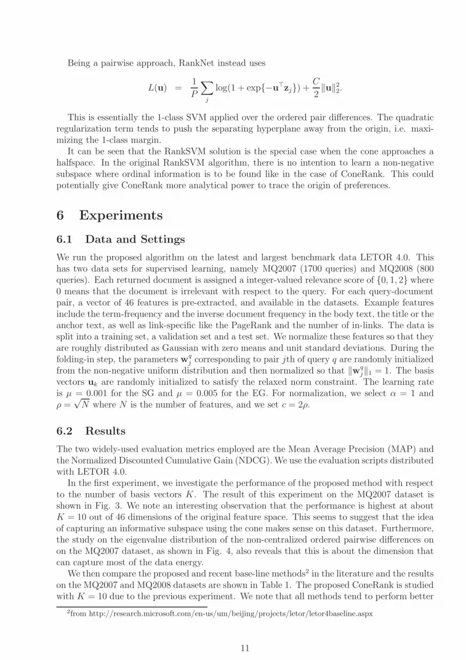
In the first experiment, we investigate the performance of the proposed method with respectto the number of basis vectors K. The result of this experiment on the MQ2007 dataset isshown in Fig. 3. We note an interesting observation that the performance is highest at aboutK = 10 out of 46 dimensions of the original feature space. This seems to suggest that the ideaof capturing an informative subspace using the cone makes sense on this dataset. Furthermore,the study on the eigenvalue distribution of the non-centralized ordered pairwise differences onon the MQ2007 dataset, as shown in Fig. 4, also reveals that this is about the dimension thatcan capture most of the data energy.

We then compare the proposed and recent base-line methods2 in the literature and the resultson the MQ2007 and MQ2008 datasets are shown in Table 1. The proposed ConeRank is studiedwith K = 10 due to the previous experiment. We note that all methods tend to perform better

2from http://research.microsoft.com/en-us/um/beijing/projects/letor/letor4baseline.aspx

11

0 10 20 30 40 500.44

0.45

0.46

0.47

0.48

0.49

0.5

0.51

0.52

0.53

number of basis vectors

perf

orm

ance

EG−MAP

EG−NDCG

SG−MAP

SG−NDCG

Figure 3: Performance versus basis number

on MQ2007 than MQ2008, which can be explained by the fact that the MQ2007 dataset ismuch larger than the other, and hence provides better training.

On the MQ2007 dataset, ConeRank compares favourably with other methods. For example,ConeRank-SG achieves the highest MAP score, whilst its NDCG score differs only less than2% when compared with the best (RankSVM-struct). On the MQ2008 dataset, ConeRank stillmaintains within the 3% margin of the best methods on both MAP and NDCG metrics.

Table 1: Results on LETOR 4.0.

MQ2007 MQ2008

Algorithms MAP NDCGMAP NDCG

AdaRank-MAP 0.482 0.518 0.463 0.480

AdaRank-NDCG 0.486 0.517 0.464 0.477

ListNet 0.488 0.524 0.450 0.469

RankBoost 0.489 0.527 0.467 0.480

RankSVM-struct 0.489 0.528 0.450 0.458

ConeRank-EG 0.488 0.514 0.444 0.456

ConeRank-SG 0.492 0.517 0.454 0.464

12

5 10 15 20 25 30 35 40 450

0.05

0.1

0.15

0.2

Figure 4: Eigenvalue distribution on the MQ2007 dataset.

7 Conclusion

We have presented a new view on the learning to rank problem from a generalized inequali-ties perspective. We formulate the problem as learning a polyhedral cone that uncovers thenon-negative subspace where ordinal information is found. A practical implementation of themethod is suggested which is then observed to achieve comparable performance to state-of-the-art methods on the LETOR 4.0 benchmark data.

There are some directions that require further research, including a more rigorous studyon the bound of the spectral norm of the leave-one-query-out basis vector difference matrix, abetter optimization scheme that solves the original formulation without relaxation, and a studyon the informative dimensionality of the ranking problem.

References

[1] S. Agarwal, Lecture notes in artificial intelligence. Springer-Verlag, 2008, ch. Generaliza-tion bounds for some ordinal regression algorithms, pp. 7–21.

[2] O. Bousquet and A. Elisseff, “Stability and generalization,” Journal of Machine LearningResearch, pp. 499–526, 2002.

[3] S. Boyd and L. Vandenberghe, Convex Optimization. Cambridge University Press, 2004.

[4] C. Burges, T. Shaked, E. Renshaw, A. Lazier, M. Deeds, N. Hamilton, and G. Hullender,“Learning to rank using gradient descent,” in Proc. ICML, 2005.

[5] Z. Cao, T. Qin, T. Liu, M. Tsai, and H. Li, “Learning to rank: from pairwise approach tolistwise approach,” in Proc. ICML, 2007.

[6] W. Chu and Z. Ghahramani, “Gaussian processes for ordinal regression,” Journal of Ma-chine Learning Research, vol. 6, no. 1, p. 1019, 2006.

[7] W. Cohen, R. Schapire, and Y. Singer, “Learning to order things,” J Artif Intell Res,vol. 10, pp. 243–270, 1999.

13

[8] D. Cossock and T. Zhang, “Statistical analysis of Bayes optimal subset ranking,” IEEETransactions on Information Theory, vol. 54, pp. 5140–5154, 2008.

[9] Y. Freund, R. Iyer, R. Schapire, and Y. Singer, “An efficient boosting algorithm for com-bining preferences,” Journal of Machine Learning Research, vol. 4, no. 6, pp. 933–969,2004.

[10] R. Herbrich, T. Graepel, and K. Obermayer, “Large margin rank boundaries for ordinalregression,” in Proc. KDD, 2000.

[11] T. Joachims, “Optimizing search engines using clickthrough data,” in Proc. KDD, 2002.

[12] J. Kivinen and M. Warmuth, “Exponentiated gradient versus gradient descent for linearpredictors,” Information and Computation, 1997.

[13] Y. Lan, T.-Y. Liu, T. Quin, Z. Ma, and H. Li, “Query-level stability and generalization inlearning to rank,” in Proc. ICML, 2008.

[14] R. Plackett, “The analysis of permutations,” Applied Statistics, pp. 193–202, 1975.

[15] B. Scholkopf and Smola, Learning with kernels. MIT Press, 2002.

14