Computing the Well-Founded Semantics FasterKenneth A. Berman, John S. Schlipf, and John V. FrancoUniversity of Cincinnati, Department of ECE&CS, USAAbstract. We address methods of speeding up the calculation of thewell-founded semantics for normal propositional logic programs. We �rstconsider two algorithms already reported in the literature and show thatthese, plus a variation upon them, have much improved worst-case be-havior for special cases of input. Then we propose a general algorithmto speed up the calculation for logic programs with at most two positivesubgoals per clause, intended to improve the worst case performance ofthe computation. For a logic program P in atomsA, the speed up over thestraight Van Gelder alternating �xed point algorithm (assuming worst-case behavior for both algorithms) is approximately (jPj=jAj)(1=3). ForjPj � jAj4, the algorithm runs in time linear in jPj.1 IntroductionLogic programming researchers have, over the last several years, proposed manylogic-based declarative semantics for various sorts of logic programming. Thehope is that, if they can be e�ciently implemented, these semantics can restorethe separation between logic and implementation that motivated the developersof Prolog but that Prolog did not achieve. In the last few years, several projectshave begun to produce working implementations of some of these semantics.A major di�culty with all such approaches is the complexity of the calcu-lations, and various approaches have been tried to speed the calculations up.We feel that serious investigation of new algorithms to compute these semanticsmay have signi�cant practical importance at this time.Two quite popular semantics for the class of normal logic program are thestable [4] and the well-founded [14]. For propositional logic programs, computinginferences under the stable semantics is known to be co-NP-complete [7]; com-puting inferences under the well-founded is known to be quadratic time (folk-lore), and no faster algorithm is known. Work in [8] (on questions of updatingaccessibility relations in graphs) suggests that it may be quite di�cult, usingstandard techniques, to break the quadratic-time bound on the well-foundedsemantics. We are concerned here with speeding up the computation of thewell-founded semantics; in particular, we �nd a large class of propositional logicprograms for which we can break the quadratic time bound. As an additionalapplication, we also note that, if the calculation of the well-founded semanticscan be made su�ciently fast, that calculation may also prove a highly usefulsubroutine in computing under the stable semantics.The standard calculation methods for the well-founded semantics are basedupon the alternating �xed-point algorithmof Van Gelder [13]. Several researchers

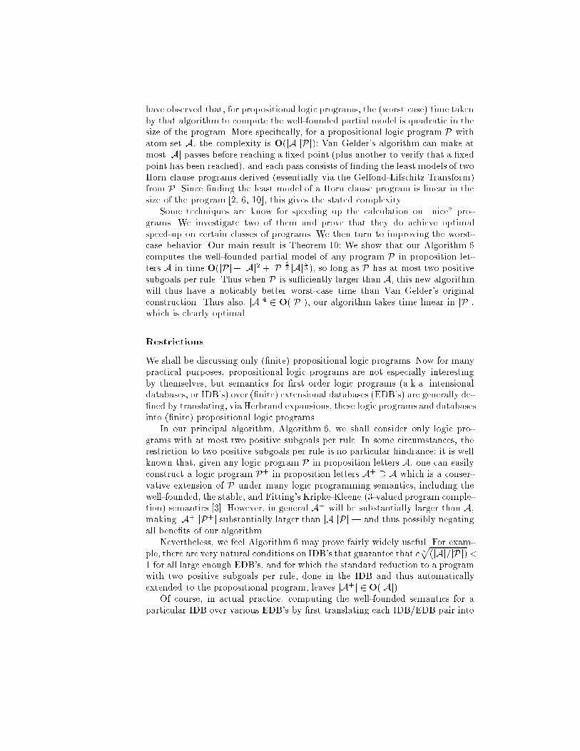
have observed that, for propositional logic programs, the (worst case) time takenby that algorithm to compute the well-founded partial model is quadratic in thesize of the program. More speci�cally, for a propositional logic program P withatom set A, the complexity is O(jAjjPj): Van Gelder's algorithm can make atmost jAj passes before reaching a �xed point (plus another to verify that a �xedpoint has been reached), and each pass consists of �nding the least models of twoHorn clause programs derived (essentially via the Gelfond-Lifschitz Transform)from P. Since �nding the least model of a Horn clause program is linear in thesize of the program [2, 6, 10], this gives the stated complexity.Some techniques are know for speeding up the calculation on \nice" pro-grams. We investigate two of them and prove that they do achieve optimalspeed-up on certain classes of programs. We then turn to improving the worst-case behavior. Our main result is Theorem 10: We show that our Algorithm 6computes the well-founded partial model of any program P in proposition let-ters A in time O(jPj+ jAj2 + jPj 23 jAj 43 ), so long as P has at most two positivesubgoals per rule. Thus when P is su�ciently larger than A, this new algorithmwill thus have a noticably better worst-case time than Van Gelder's originalconstruction. Thus also, jAj4 2 O(jPj), our algorithm takes time linear in jPj,which is clearly optimal.RestrictionsWe shall be discussing only (�nite) propositional logic programs. Now for manypractical purposes, propositional logic programs are not especially interestingby themselves, but semantics for �rst order logic programs (a.k.a. intensionaldatabases, or IDB's) over (�nite) extensional databases (EDB's) are generally de-�ned by translating, via Herbrand expansions, these logic programs and databasesinto (�nite) propositional logic programs.In our principal algorithm, Algorithm 6, we shall consider only logic pro-grams with at most two positive subgoals per rule. In some circumstances, therestriction to two positive subgoals per rule is no particular hindrance; it is wellknown that, given any logic program P in proposition letters A, one can easilyconstruct a logic program P+ in proposition letters A+ � A which is a conser-vative extension of P under many logic programming semantics, including thewell-founded, the stable, and Fitting's Kripke-Kleene (3-valued program comple-tion) semantics [3]. However, in general A+ will be substantially larger than A,making jA+jjP+j substantially larger than jAjjPj| and thus possibly negatingall bene�ts of our algorithm.Nevertheless, we feel Algorithm 6 may prove fairly widely useful. For exam-ple, there are very natural conditions on IDB's that guarantee that c 3p(jAj=jPj) <1 for all large enough EDB's, and for which the standard reduction to a programwith two positive subgoals per rule, done in the IDB and thus automaticallyextended to the propositional program, leaves jA+j 2 O(jAj).Of course, in actual practice, computing the well-founded semantics for aparticular IDB over various EDB's by �rst translating each IDB/EDB pair into

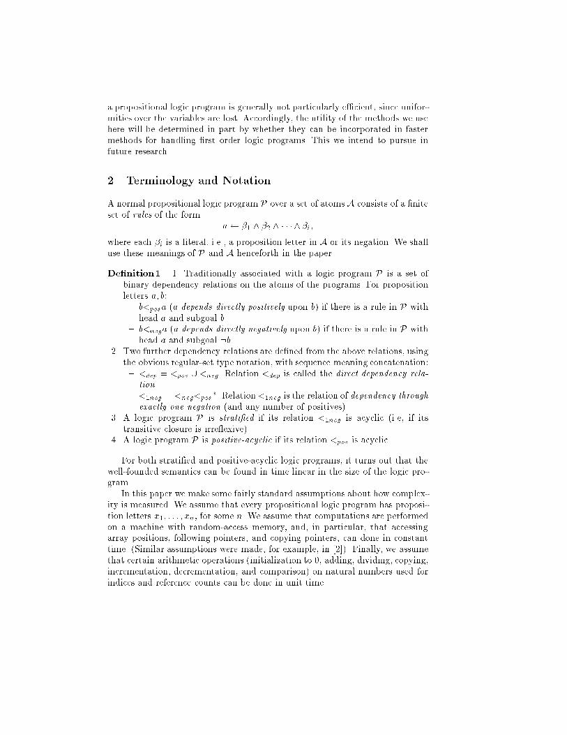
a propositional logic program is generally not particularly e�cient, since unifor-mities over the variables are lost. Accordingly, the utility of the methods we usehere will be determined in part by whether they can be incorporated in fastermethods for handling �rst order logic programs. This we intend to pursue infuture research.2 Terminology and NotationA normal propositional logic program P over a set of atoms A consists of a �niteset of rules of the form a �1 ^ �2 ^ � � � ^ �i;where each �i is a literal, i.e., a proposition letter in A or its negation. We shalluse these meanings of P and A henceforth in the paper.De�nition1. 1. Traditionally associated with a logic program P is a set ofbinary dependency relations on the atoms of the programs. For propositionletters a; b:{ b<posa (a depends directly positively upon b) if there is a rule in P withhead a and subgoal b.{ b<nega (a depends directly negatively upon b) if there is a rule in P withhead a and subgoal :b.2. Two further dependency relations are de�ned from the above relations, usingthe obvious regular-set type notation, with sequence meaning concatenation:{ <dep = <pos [ <neg. Relation <dep is called the direct dependency rela-tion.{ <1neg = <neg<pos�. Relation<1neg is the relation of dependency throughexactly one negation (and any number of positives).3. A logic program P is strati�ed if its relation <1neg is acyclic (i.e, if itstransitive closure is irre exive).4. A logic program P is positive-acyclic if its relation <pos is acyclic.For both strati�ed and positive-acyclic logic programs, it turns out that thewell-founded semantics can be found in time linear in the size of the logic pro-gram.In this paper we make some fairly standard assumptions about how complex-ity is measured. We assume that every propositional logic program has proposi-tion letters x1; : : : ; xn, for some n. We assume that computations are performedon a machine with random-access memory, and, in particular, that accessingarray positions, following pointers, and copying pointers, can done in constanttime. (Similar assumptions were made, for example, in [2]). Finally, we assumethat certain arithmetic operations (initialization to 0, adding, dividing, copying,incrementation, decrementation, and comparison) on natural numbers used forindices and reference counts can be done in unit time.

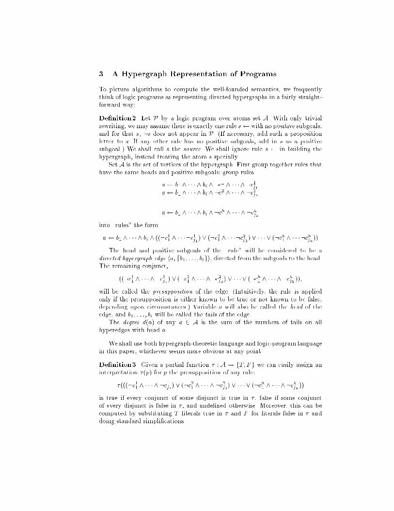
3 A Hypergraph Representation of ProgramsTo picture algorithms to compute the well-founded semantics, we frequentlythink of logic programs as representing directed hypergraphs in a fairly straight-forward way:De�nition2. Let P by a logic program over atoms set A. With only trivialrewriting, we may assume there is exactly one rule s with no positive subgoals,and for that s, :s does not appear in P. (If necessary, add such a propositionletter to a. If any other rule has no positive subgoals, add in s as a positivesubgoal.) We shall call s the source. We shall ignore rule s in building thehypergraph, instead treating the atom s specially.Set A is the set of vertices of the hypergraph. First group together rules thathave the same heads and positive subgoals: group rulesa b1 ^ � � � ^ bi ^ :c11 ^ � � � ^ :c1j1a b1 ^ � � � ^ bi ^ :c21 ^ � � � ^ :c2j2...a b1 ^ � � � ^ bi ^ :ch1 ^ � � � ^ :chjhinto \rules" the forma b1 ^ � � � ^ bi ^ ((:c11 ^ � � �:c1j1) _ (:c21 ^ � � �:c2j2) _ � � � _ (:ch1 ^ � � �:chjh))The head and positive subgoals of the \rule" will be considered to be adirected hypergraph edge ha; fb1; : : : ; bigi, directed from the subgoals to the head.The remaining conjunct,((:c11 ^ � � � ^ :c1j1) _ (:c21 ^ � � � ^ :c2j2) _ � � � _ (:ch1 ^ � � � ^ :chjh));will be called the presupposition of the edge. (Intuitively, the rule is appliedonly if the presupposition is either known to be true or not known to be false,depending upon circumstances.) Variable a will also be called the head of theedge, and b1; : : : ; bi will be called the tails of the edge.The degree d(a) of any a 2 A is the sum of the numbers of tails on allhyperedges with head a.We shall use both hypergraph-theoretic language and logic-program languagein this paper, whichever seems more obvious at any point.De�nition3. Given a partial function � : A ! fT; Fg we can easily assign aninterpretation � (p) for p the presupposition of any rule:� (((:c11 ^ � � � ^ :c1j1) _ (:c21 ^ � � � ^ :c2j2) _ � � � _ (:ch1 ^ � � � ^ :chjh))is true if every conjunct of some disjunct is true in � , false if some conjunctof every disjunct is false in � , and unde�ned otherwise. Moreover, this can becomputed by substituting T literals true in � and F for literals false in � anddoing standard simpli�cations.

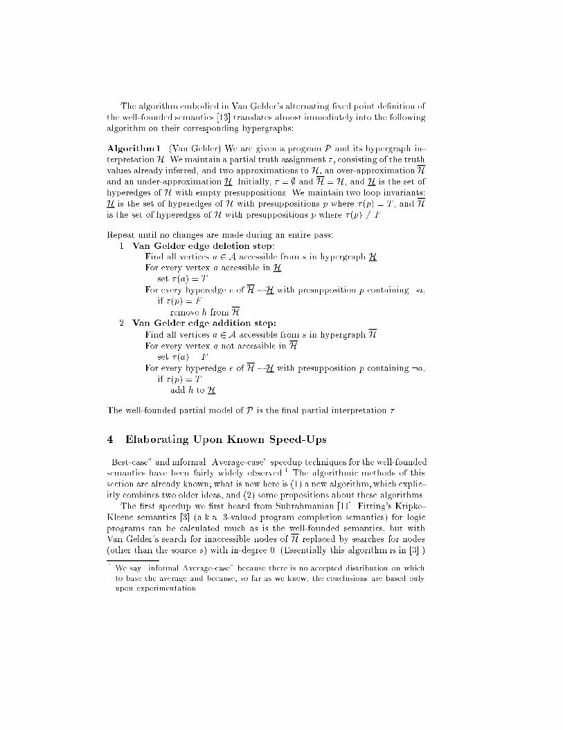
The algorithm embodied in Van Gelder's alternating �xed point de�nition ofthe well-founded semantics [13] translates almost immediately into the followingalgorithm on their corresponding hypergraphs:Algorithm1. (Van Gelder) We are given a program P and its hypergraph in-terpretation H. We maintain a partial truth assignment � , consisting of the truthvalues already inferred, and two approximations to H, an over-approximationHand an under-approximation H. Initially, � = ; and H = H, and H is the set ofhyperedges of H with empty presuppositions. We maintain two loop invariants:H is the set of hyperedges of H with presuppositions p where � (p) = T , and His the set of hyperedges of H with presuppositions p where � (p) 6= F .Repeat until no changes are made during an entire pass:1. Van Gelder edge deletion step:Find all vertices a 2 A accessible from s in hypergraph H.For every vertex a accessible in Hset � (a) = T .For every hyperedge e of H�H with presupposition p containing :a,if � (p) = Fremove h from H.2. Van Gelder edge addition step:Find all vertices a 2 A accessible from s in hypergraph H.For every vertex a not accessible in Hset � (a) = F .For every hyperedge e of H�H with presupposition p containing :a,if � (p) = Tadd h to H.The well-founded partial model of P is the �nal partial interpretation � .4 Elaborating Upon Known Speed-Ups\Best-case" and informal \Average-case" speedup techniques for the well-foundedsemantics have been fairly widely observed.1 The algorithmic methods of thissection are already known; what is new here is (1) a new algorithm,which explic-itly combines two older ideas, and (2) some propositions about these algorithms.The �rst speedup we �rst heard from Subrahmanian [11]. Fitting's Kripke-Kleene semantics [3] (a.k.a. 3-valued program completion semantics) for logicprograms can be calculated much as is the well-founded semantics, but withVan Gelder's search for inaccessible nodes of H replaced by searches for nodes(other than the source s) with in-degree 0. (Essentially this algorithm is in [3].)1 We say \informal Average-case" because there is no accepted distribution on whichto base the average and because, so far as we know, the conclusions are based onlyupon experimentation.

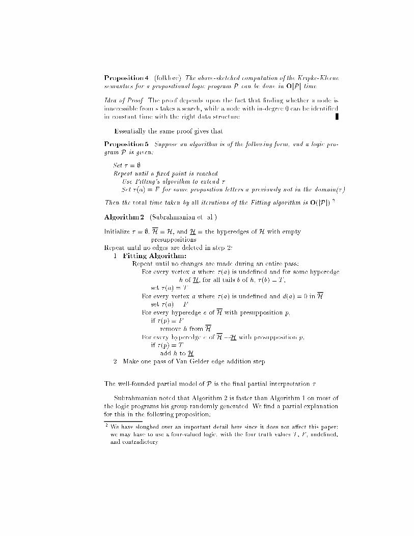
Proposition4. (folklore) The above-sketched computation of the Kripke-Kleenesemantics for a propositional logic program P can be done in OjPj time.Idea of Proof. The proof depends upon the fact that �nding whether a node isinaccessible from s takes a search, while a node with in-degree 0 can be identi�edin constant time with the right data structure.Essentially the same proof gives thatProposition5. Suppose an algorithm is of the following form, and a logic pro-gram P is given:Set � = ;Repeat until a �xed point is reachedUse Fitting's algorithm to extend �Set � (a) = F for some proposition letters a previously not in the domain(�).Then the total time taken by all iterations of the Fitting algorithm is O(jPj).2Algorithm2. (Subrahmanian et. al.)Initialize � = ;, H = H, and H = the hyperedges of H with emptypresuppositions.Repeat until no edges are deleted in step 2:1. Fitting Algorithm:Repeat until no changes are made during an entire pass:For every vertex a where � (a) is unde�ned and for some hyperedgeh of H, for all tails b of h, � (b) = T ,set � (a) = T .For every vertex a where � (a) is unde�ned and d(a) = 0 in Hset � (a) = F .For every hyperedge e of H with presupposition p,if � (p) = Fremove h from H.For every hyperedge e of H�H with presupposition p,if � (p) = Tadd h to H.2. Make one pass of Van Gelder edge addition stepThe well-founded partial model of P is the �nal partial interpretation � .Subrahmanian noted that Algorithm 2 is faster than Algorithm 1 on most ofthe logic programs his group randomly generated. We �nd a partial explanationfor this in the following proposition:2 We have sloughed over an important detail here since it does not a�ect this paper:we may have to use a four-valued logic, with the four truth values T , F , unde�ned,and contradictory.

Proposition6. Let P be a logic program.1. If P is positive-acyclic, then the Kripke-Kleene semantics for P agrees withthe well-founded semantics, and hence Algorithm 2 �nds the well-foundedsemantics in time O(jPj).2. If P consists of a positive-acyclic program plus some additional rules givingonly k hyperedges (possibly with very long presuppositions), then Algorithm 2�nds the well-founded semantics in time O(kjPj).Proof. 1. In [9] we showed that, for a logic program with no positive subgoals,the Kripke-Kleene and well-founded semantics agree. It is routine to extendthat proof to all positive-acyclic logic programs.2. The di�erence between the Kripke-Kleene semantics and the well-foundedsemantics is that the well-founded semantics identi�es positive dependencycycles. Since the �rst part of each pass through the outside loop of the algo-rithm is Fitting's algorithm, and since A is �nite, each atom found by step 2must be in a positive cycle, all of whose atoms are inaccessible. Thus one ofthe k special edges (the \back-edges") must be in this cycle. Accordingly, atleast one back-edge will be added to H in each pass. Thus, after k passes, noadditional cycles in H remain to be discovered, and all additional inferencesmay be made by the Fitting semantics.A second speed-up is motivated by the fact that calculating the perfect modelof a strati�ed logic program (which is also the well-founded partial model and theunique stable model) can be done in linear time. Consider hA;<depi as a directedgraph. In linear time, form the strongly connected components of the graph as in[12], and topologically sort the components. Let P1 be the set of rules of P whoseheads occur in the �rst component of the graph. P1 turns out to be pure Horn,so its perfect model is its minimal model M1, which can be computed in timelinear in jP1j [2, 6, 10]. Let P2 be the set of rules of P whose heads occur in thesecond component. Substitute into P2 the truth values computed for variables inthe �rst component and simplify. The result is a pure Horn program, so computeits minimal model, in time linear in jP2j, and the perfect model of P1 [ P2 isM1 [M2. Continue this way through all the strongly connected components.The result is the perfect model, which has been constructed in time linear injPj.Now for the well-founded and Kripke-Kleene semantics, the same partition-ing into strongly-connected components, decomposition of the program by thecomponents and construction of the semantics for each piece separately cor-rectly constructs the semantics. We shall call the levels P1;P2; : : : strata, ormodules. (These were investigated in the current context in [9] and [1].) Un-like with strati�ed programs, there is no guarantee that the strata are Horn.However, for programs with more than one strongly connected component, thisgives a divide-and-conquer approach which can sometimes, as with strati�edprograms, reduce the complexity of �nding the well-founded model. (The sametechnique has been used [5] to speed up the search for individual stable models,

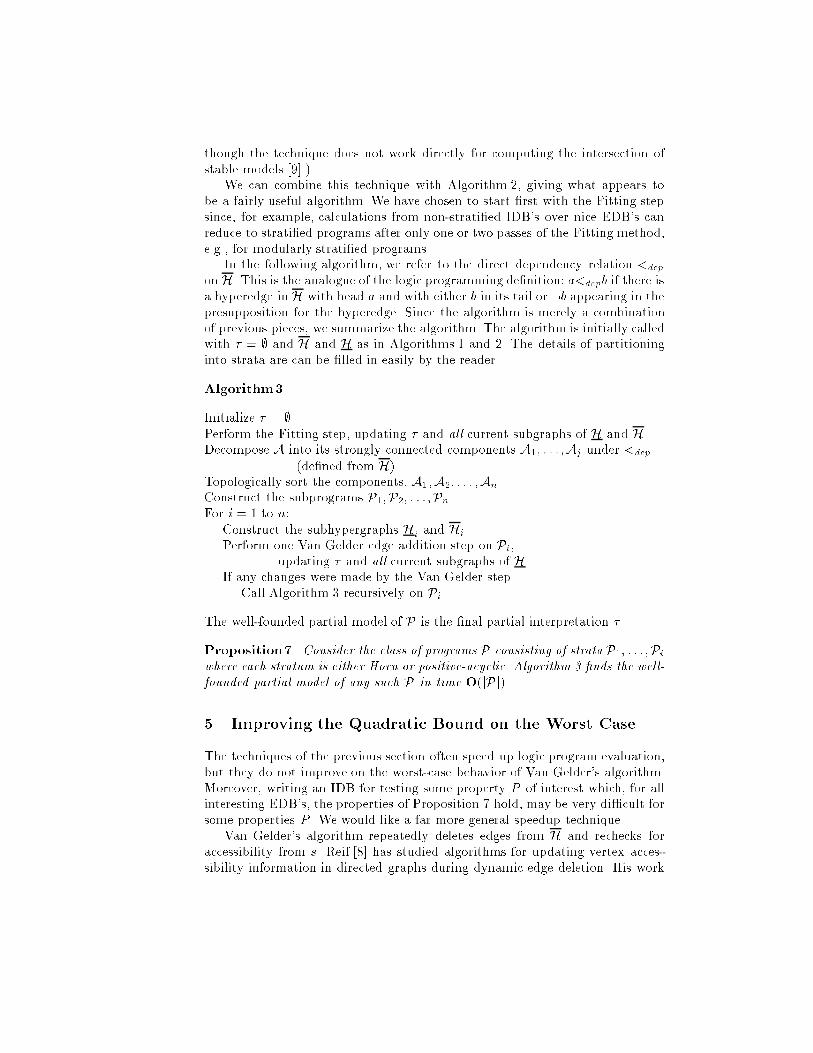
though the technique does not work directly for computing the intersection ofstable models [9].)We can combine this technique with Algorithm 2, giving what appears tobe a fairly useful algorithm. We have chosen to start �rst with the Fitting stepsince, for example, calculations from non-strati�ed IDB's over nice EDB's canreduce to strati�ed programs after only one or two passes of the Fitting method,e.g., for modularly strati�ed programs.In the following algorithm, we refer to the direct dependency relation <depon H. This is the analogue of the logic programming de�nition: a<depb if there isa hyperedge in H with head a and with either b in its tail or :b appearing in thepresupposition for the hyperedge. Since the algorithm is merely a combinationof previous pieces, we summarize the algorithm. The algorithm is initially calledwith � = ; and H and H as in Algorithms 1 and 2. The details of partitioninginto strata are can be �lled in easily by the reader.Algorithm3.Initialize � = ;.Perform the Fitting step, updating � and all current subgraphs of H and H.Decompose A into its strongly connected components A1; : : : ;Aj under <dep(de�ned from H).Topologically sort the components, A1;A2; : : : ;An.Construct the subprograms P1;P2; : : : ;Pn.For i = 1 to n:Construct the subhypergraphs Hi and Hi.Perform one Van Gelder edge addition step on Pi,updating � and all current subgraphs of H.If any changes were made by the Van Gelder stepCall Algorithm 3 recursively on Pi.The well-founded partial model of P is the �nal partial interpretation � .Proposition7. Consider the class of programs P consisting of strata P1; : : : ;Piwhere each stratum is either Horn or positive-acyclic. Algorithm 3 �nds the well-founded partial model of any such P in time O(jPj).5 Improving the Quadratic Bound on the Worst CaseThe techniques of the previous section often speed up logic program evaluation,but they do not improve on the worst-case behavior of Van Gelder's algorithm.Moreover, writing an IDB for testing some property P of interest which, for allinteresting EDB's, the properties of Proposition 7 hold, may be very di�cult forsome properties P . We would like a far more general speedup technique.Van Gelder's algorithm repeatedly deletes edges from H and rechecks foraccessibility from s. Reif [8] has studied algorithms for updating vertex acces-sibility information in directed graphs during dynamic edge deletion. His work

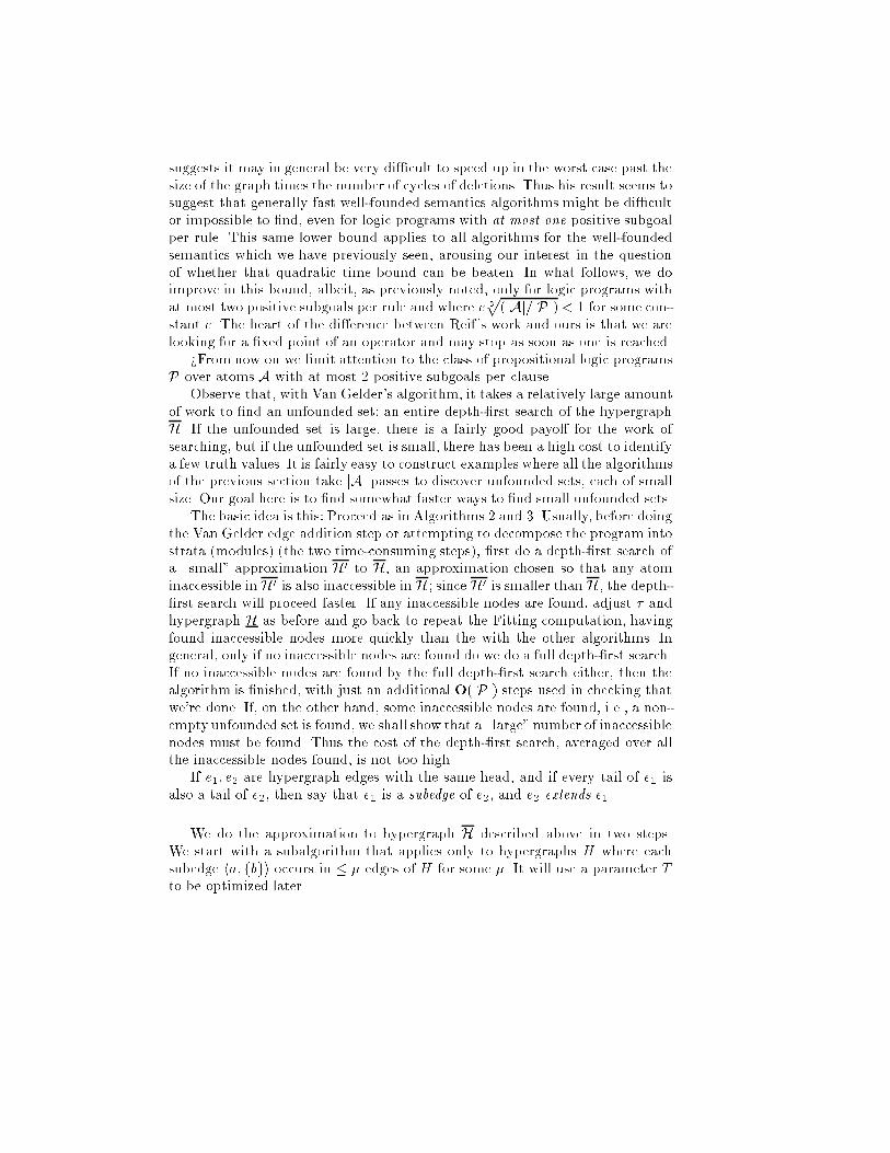
suggests it may in general be very di�cult to speed up in the worst case past thesize of the graph times the number of cycles of deletions. Thus his result seems tosuggest that generally fast well-founded semantics algorithms might be di�cultor impossible to �nd, even for logic programs with at most one positive subgoalper rule. This same lower bound applies to all algorithms for the well-foundedsemantics which we have previously seen, arousing our interest in the questionof whether that quadratic time bound can be beaten. In what follows, we doimprove in this bound, albeit, as previously noted, only for logic programs withat most two positive subgoals per rule and where c 3p(jAj=jPj) < 1 for some con-stant c. The heart of the di�erence between Reif's work and ours is that we arelooking for a �xed point of an operator and may stop as soon as one is reached.>From now on we limit attention to the class of propositional logic programsP over atoms A with at most 2 positive subgoals per clause.Observe that, with Van Gelder's algorithm, it takes a relatively large amountof work to �nd an unfounded set: an entire depth-�rst search of the hypergraphH. If the unfounded set is large, there is a fairly good payo� for the work ofsearching, but if the unfounded set is small, there has been a high cost to identifya few truth values. It is fairly easy to construct examples where all the algorithmsof the previous section take jAj passes to discover unfounded sets, each of smallsize. Our goal here is to �nd somewhat faster ways to �nd small unfounded sets.The basic idea is this: Proceed as in Algorithms 2 and 3. Usually, before doingthe Van Gelder edge addition step or attempting to decompose the program intostrata (modules) (the two time-consuming steps), �rst do a depth-�rst search ofa \small" approximation H0 to H, an approximation chosen so that any atominaccessible inH0 is also inaccessible in H; since H0 is smaller than H, the depth-�rst search will proceed faster. If any inaccessible nodes are found, adjust � andhypergraph H as before and go back to repeat the Fitting computation, havingfound inaccessible nodes more quickly than the with the other algorithms. Ingeneral, only if no inaccessible nodes are found do we do a full depth-�rst search.If no inaccessible nodes are found by the full depth-�rst search either, then thealgorithm is �nished, with just an additional O(jPj) steps used in checking thatwe're done. If, on the other hand, some inaccessible nodes are found, i.e., a non-empty unfounded set is found, we shall show that a \large" number of inaccessiblenodes must be found. Thus the cost of the depth-�rst search, averaged over allthe inaccessible nodes found, is not too high.If e1; e2 are hypergraph edges with the same head, and if every tail of e1 isalso a tail of e2, then say that e1 is a subedge of e2, and e2 extends e1.We do the approximation to hypergraph H described above in two steps.We start with a subalgorithm that applies only to hypergraphs H where eachsubedge ha; fbgi occurs in � � edges of H for some �. It will use a parameter Tto be optimized later.

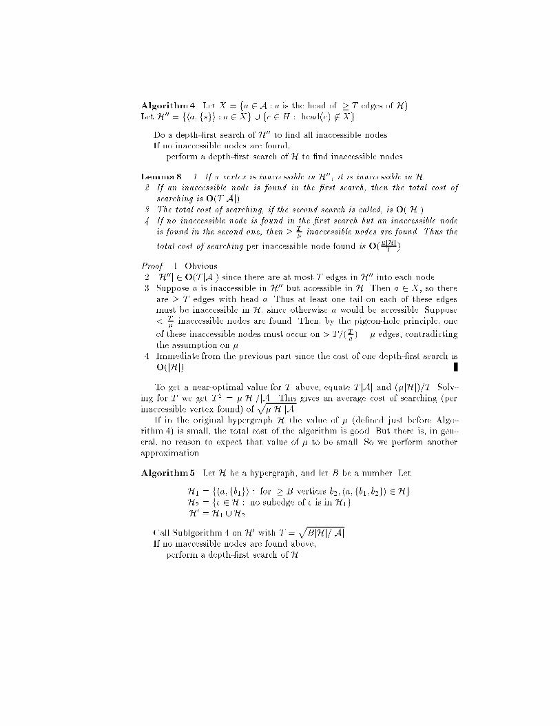
Algorithm4. Let X = fa 2 A : a is the head of � T edges of Hg.Let H00 = fha; fsgi : a 2 Xg [ fe 2 H : head(e) 62 Xg.Do a depth-�rst search of H00 to �nd all inaccessible nodes.If no inaccessible nodes are found,perform a depth-�rst search of H to �nd inaccessible nodes.Lemma8. 1. If a vertex is inaccessible in H00, it is inaccessible in H.2. If an inaccessible node is found in the �rst search, then the total cost ofsearching is O(T jAj).3. The total cost of searching, if the second search is called, is O(jHj).4. If no inaccessible node is found in the �rst search but an inaccessible nodeis found in the second one, then � T� inaccessible nodes are found. Thus thetotal cost of searching per inaccessible node found is O(�jHjT ).Proof. 1. Obvious.2. jH00j 2 O(T jAj) since there are at most T edges in H00 into each node.3. Suppose a is inaccessible in H00 but accessible in H. Then a 2 X, so thereare � T edges with head a. Thus at least one tail on each of these edgesmust be inaccessible in H, since otherwise a would be accessible. Suppose< T� inaccessible nodes are found. Then, by the pigeon-hole principle, oneof these inaccessible nodes must occur on > T=(T� ) = � edges, contradictingthe assumption on �.4. Immediate from the previous part since the cost of one depth-�rst search isO(jHj).To get a near-optimal value for T above, equate T jAj and (�jHj)=T . Solv-ing for T we get T 2 = �jHj=jAj. This gives an average cost of searching (perinaccessible vertex found) of p�jHjjAj.If in the original hypergraph H the value of � (de�ned just before Algo-rithm 4) is small, the total cost of the algorithm is good. But there is, in gen-eral, no reason to expect that value of � to be small. So we perform anotherapproximation.Algorithm5. Let H be a hypergraph, and let B be a number. LetH1 = fha; fb1gi : for � B vertices b2; ha; fb1; b2gi 2 HgH2 = fe 2 H : no subedge of e is in H1gH0 = H1 [H2Call Sublgorithm 4 on H0 with T =pBjHj=jAj.If no inaccessible nodes are found above,perform a depth-�rst search of H.

Lemma9. Let H, B, and H0 be as in Sublgorithm 5.1. If some vertex a 2 A is inaccessible from s in H0, it is inaccessible from sin H.2. No edge ha; fbgi is a subedge of � B edges of H0 (i.e, the property of Algo-rithm 4 holds with � = B).3. If every vertex a 2 A is accessible from s in H0, but some vertex a 2 A isinaccessible from s in H, then � B vertices of A are inaccessible in H.4. jH0j � jHj. Thus: (i) The cost to perform the search in this algorithm isin O(T jAj) if inaccessible nodes are found by the �rst step of Algorithm 4.(ii) If no inaccessible nodes are found by the �rst step of Algorithm 4 butsome inaccessible nodes are found by the second step, the cost to perform thesearch is in O(jH0j) � O(jHj). (iii) If no inaccessible nodes are found byAlgorithm 4, the total cost to perform the search is O(jHj).5. If this subalgorithm performs the search of H and inaccessible nodes arefound, then the average cost of searching for each inaccessible node found isO(jHj=B).Proof.1. Obvious.2. The subedges inH1 have no tails in common, and no edge in H1 is a subedgeof any edge in H2. If any B edges in H2 had a subedge in common, thatsubedge would have been put into H1.3. Suppose a is accessible in H0 but not in H. Then there must be an edgeha; fbgi 2 H0 � H where b is accessible in H but a is not. By de�nition ofH0, there must be � B edges ha; fb; b2gi 2 H. Since a is inaccessible in H,none of these � B b2's can be accessible in H either.4. That jH0j � jHj is obvious. Statements (i) and (ii) then follow fromLemma 8.Statement (iii) follows from the fact that the searching cost is dominated bythe cost of the search of H0 followed by the search of H.5. Follows from the two previous steps.A near-optimal value for B can be computed by equating the two previousaverage costs, pBjHjjAj and jHjB . This gives B = 3pjHj=jAj, yielding a �nalaverage cost of O(jAj(1=3)jPj(2=3)). The total search cost must be at most jAjtimes this | thus O(jAj(4=3)jPj(2=3)). The speedup is on the order of 3pjPj=jAj,as stated earlier.

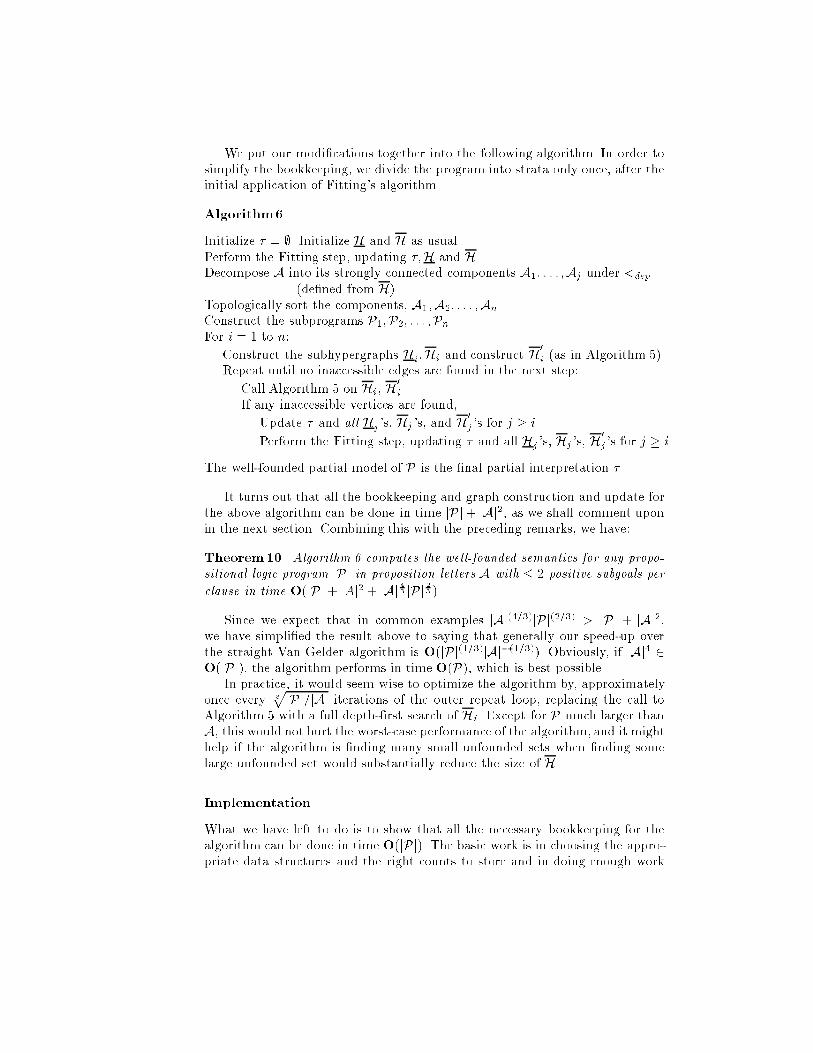
We put our modi�cations together into the following algorithm. In order tosimplify the bookkeeping, we divide the program into strata only once, after theinitial application of Fitting's algorithm.Algorithm6.Initialize � = ;. Initialize H and H as usual.Perform the Fitting step, updating �;H and H.Decompose A into its strongly connected components A1; : : : ;Aj under <dep(de�ned from H).Topologically sort the components, A1;A2; : : : ;An.Construct the subprograms P1;P2; : : : ;Pn.For i = 1 to n:Construct the subhypergraphs Hi;Hi and construct H0i (as in Algorithm 5).Repeat until no inaccessible edges are found in the next step:Call Algorithm 5 on Hi, H0iIf any inaccessible vertices are found,Update � and all Hj 's, Hj 's, and H0j 's for j � i.Perform the Fitting step, updating � and all Hj 's, Hj 's, H0j's for j � i.The well-founded partial model of P is the �nal partial interpretation � .It turns out that all the bookkeeping and graph construction and update forthe above algorithm can be done in time jPj+ jAj2, as we shall comment uponin the next section. Combining this with the preceding remarks, we have:Theorem10. Algorithm 6 computes the well-founded semantics for any propo-sitional logic program jPj in proposition letters A with � 2 positive subgoals perclause in time O(jPj+ jAj2 + jAj 43 jPj 23 ).Since we expect that in common examples jAj(4=3)jPj(2=3) > jPj + jAj2,we have simpli�ed the result above to saying that generally our speed-up overthe straight Van Gelder algorithm is O(jPj(1=3)jAj�(1=3)). Obviously, if jAj4 2O(jPj), the algorithm performs in time O(P), which is best possible.In practice, it would seem wise to optimize the algorithm by, approximatelyonce every 3pjPj=jAj iterations of the outer repeat loop, replacing the call toAlgorithm 5 with a full depth-�rst search of Hi. Except for P much larger thanA, this would not hurt the worst-case performance of the algorithm, and it mighthelp if the algorithm is �nding many small unfounded sets when �nding somelarge unfounded set would substantially reduce the size of H.ImplementationWhat we have left to do is to show that all the necessary bookkeeping for thealgorithm can be done in time O(jPj). The basic work is in choosing the appro-priate data structures and the right counts to store and in doing enough work

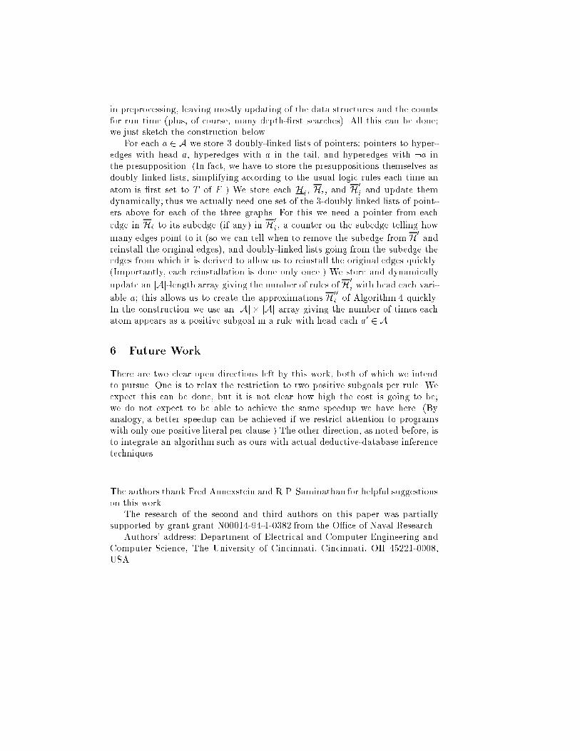
in preprocessing, leaving mostly updating of the data structures and the countsfor run time (plus, of course, many depth-�rst searches). All this can be done;we just sketch the construction below.For each a 2 A we store 3 doubly-linked lists of pointers: pointers to hyper-edges with head a, hyperedges with a in the tail, and hyperedges with :a inthe presupposition. (In fact, we have to store the presuppositions themselves asdoubly linked lists, simplifying according to the usual logic rules each time anatom is �rst set to T of F .) We store each Hi, Hi, and H0i and update themdynamically; thus we actually need one set of the 3-doubly linked lists of point-ers above for each of the three graphs. For this we need a pointer from eachedge in Hi to its subedge (if any) in H0i, a counter on the subedge telling howmany edges point to it (so we can tell when to remove the subedge from H0 andreinstall the original edges), and doubly-linked lists going from the subedge theedges from which it is derived to allow us to reinstall the original edges quickly.(Importantly, each reinstallation is done only once.) We store and dynamicallyupdate an jAj-length array giving the number of rules of H0i with head each vari-able a; this allows us to create the approximations H00i of Algorithm 4 quickly.In the construction we use an jAj � jAj array giving the number of times eachatom appears as a positive subgoal in a rule with head each a0 2 A.6 Future WorkThere are two clear open directions left by this work, both of which we intendto pursue. One is to relax the restriction to two positive subgoals per rule. Weexpect this can be done, but it is not clear how high the cost is going to be;we do not expect to be able to achieve the same speedup we have here. (Byanalogy, a better speedup can be achieved if we restrict attention to programswith only one positive literal per clause.) The other direction, as noted before, isto integrate an algorithm such as ours with actual deductive-database inferencetechniques.The authors thank Fred Annexstein and R.P. Saminathan for helpful suggestionson this work.The research of the second and third authors on this paper was partiallysupported by grant grant N00014-94-1-0382 from the O�ce of Naval Research.Authors' address: Department of Electrical and Computer Engineering andComputer Science, The University of Cincinnati, Cincinnati, OH 45221-0008,USA.

References1. J. Dix. A classi�cation theory of semantics of normal logic programs: II. Weakproperties. To appear in JCSS.2. W. F. Dowling and J. H. Gallier. Linear time algorithms for testing the satis�-ability of propositional Horn formulae. Journal of Logic Programming 1 (1984),267{284.3. M. Fitting. A Kripke-Kleene semantics for logic programs. Journal of Logic Pro-gramming, 2(4):295{312, 1985.4. M. Gelfond and V. Lifschitz. The stable model semantics for logic programming.In Proc. 5th Int'l Conf. Symp. on Logic Programming, 1988.5. V. Lifschitz and H. Turner. Splitting a logic program. Preprint.6. A. Itai and J. Makowsky, On the complexity of Herbrand's theorem. TechnicalReport No. 243, Department of Computer Science, Israel Institute of Technology,Haifa (1982).7. W. Marek and M. Truszczy�nski. Autoepistemic logic. Journal of the ACM 38(3),pages 588-619, 1991.8. J. Reif. A topological approach to dynamic graph connectivity. Information Pro-cessing Letters 25(1), pages 65-70.9. J. S. Schlipf. The expressive powers of the logic programming semantics. Toappear in JCSS. A preliminary version appeared in Ninth ACM Symposium onPrinciples of Database Systems, pages 196-204, 1990. Expanded version availableas University of Cincinnati Computer Science Technical Report CIS-TR-90-3.10. M. G. Scutell�a. A note on Dowling and Gallier's top-down algorithm for proposi-tional Horn satis�ability. Journal of Logic Programming 8, pages 265-273, 1990.11. V. S. Subrahmanian, personal communication.12. R. Tarjan, \Depth �rst search and linear graph algorithms," SIAM Journal onComputing 1 (1972), 146{160.13. A. Van Gelder. The alternating �xpoint of logic programs with negation. In EighthACM Symposium on Principles of Database Systems, pages 1{10, 1989. Availablefrom UC Santa Cruz as UCSC-CRL-88-17.14. A. Van Gelder, K. A. Ross, and J. S. Schlipf. The well-founded semantics forgeneral logic programs. Journal of the ACM 38(3), pages 620-650, 1991.This article was processed using the LaTEX macro package with LLNCS style