DOTTORATO DI RICERCA IN INFORMATICA(Ciclo XIX)

PhD thesis

Dependency Tree Semantics

Livio Robaldo

Universita degli Studi di Torino

Dipartimento di InformaticaC.so Svizzera, 185 - 10149 Torino, Italia

SUPERVISORProf. Leonardo Lesmo

PhD Coordinator:Prof. Piero Torasso

2

Contents

Acknowledgements 7

Introduction 9

1 Underspecification: goals and techniques 131.1 Building semantic representations in NLP . . . . . . . . . . . 131.2 Underspecification as an alternative to

strict compositionality . . . . . . . . . . . . . . . . . . . . . . 161.2.1 Enumerative approach . . . . . . . . . . . . . . . . . . 171.2.2 Constraint-based Approach . . . . . . . . . . . . . . . 201.2.3 A comparison between different approaches . . . . . . . 22

1.3 Summary . . . . . . . . . . . . . . . . . . . . . . . . . . . . . 27

2 Intuitions behind Dependency Tree Semantics 292.1 An alternative way to specify orderings on quantifiers . . . . . 30

2.1.1 Skolem Normal Form Theorem (SNFT) . . . . . . . . . 302.1.2 Generalizing SNFT to handle NL semantics . . . . . . 31

2.2 Branching Quantifier (BQ) readings . . . . . . . . . . . . . . . 352.3 Partial orderings on quantifiers . . . . . . . . . . . . . . . . . 382.4 DTS Formalisation . . . . . . . . . . . . . . . . . . . . . . . . 412.5 Summary . . . . . . . . . . . . . . . . . . . . . . . . . . . . . 43

3 DTS Syntax-Semantic Interface 453.1 Dependency Grammar . . . . . . . . . . . . . . . . . . . . . . 453.2 Extensible Dependency Grammar - XDG . . . . . . . . . . . . 483.3 DTS syntax-semantic interface . . . . . . . . . . . . . . . . . . 54

3.3.1 A simple Dependency Grammar . . . . . . . . . . . . . 563.3.2 Sem and SV ar function . . . . . . . . . . . . . . . . . 583.3.3 Extracting predicate-argument relations from a Depen-

dency Tree . . . . . . . . . . . . . . . . . . . . . . . . . 603.3.4 Restriction . . . . . . . . . . . . . . . . . . . . . . . . . 66

3.3.5 The G⇒ DTS interface . . . . . . . . . . . . . . . . . 693.4 Comparison with other approaches . . . . . . . . . . . . . . . 693.5 Summary . . . . . . . . . . . . . . . . . . . . . . . . . . . . . 80

4 Scope disambiguation in DTS 814.1 Monotonic Disambiguation . . . . . . . . . . . . . . . . . . . . 81

4.1.1 Partially and fully disambiguated readings in DTS . . . 844.2 World knowledge exploitation . . . . . . . . . . . . . . . . . . 86

4.2.1 Formalisation . . . . . . . . . . . . . . . . . . . . . . . 904.3 Constraints on SemDep arcs . . . . . . . . . . . . . . . . . . . 92

4.3.1 Nested Quantification . . . . . . . . . . . . . . . . . . 924.3.2 Redundant Readings . . . . . . . . . . . . . . . . . . . 964.3.3 Additional constraints . . . . . . . . . . . . . . . . . . 98

4.4 Comparison with current constraint-based approaches . . . . . 1004.5 Summary . . . . . . . . . . . . . . . . . . . . . . . . . . . . . 102

5 Models and Branching Quantification 1035.1 Are BQ readings really available in NL? . . . . . . . . . . . . 1035.2 (Mostowskian) Generalized Quantifiers . . . . . . . . . . . . . 1075.3 Barwise . . . . . . . . . . . . . . . . . . . . . . . . . . . . . . 1105.4 Sher . . . . . . . . . . . . . . . . . . . . . . . . . . . . . . . . 113

5.4.1 Classifying BQ quantifications . . . . . . . . . . . . . . 1225.4.2 Formalization . . . . . . . . . . . . . . . . . . . . . . . 127

5.5 Summary . . . . . . . . . . . . . . . . . . . . . . . . . . . . . 132

6 Sher’s theory extensions 1356.1 The ⊆

maxoperator . . . . . . . . . . . . . . . . . . . . . . . . . 135

6.2 Nested Quantification . . . . . . . . . . . . . . . . . . . . . . . 1396.3 The logics L . . . . . . . . . . . . . . . . . . . . . . . . . . . . 1486.4 Future extension: cumulative readings . . . . . . . . . . . . . 1536.5 Summary . . . . . . . . . . . . . . . . . . . . . . . . . . . . . 156

7 Model theoretic interpretation of DTS 1577.1 Translating DTS into L . . . . . . . . . . . . . . . . . . . . . 158

7.1.1 Extracting quantifier prefix from SemDep arc . . . . . 1587.1.2 Extracting maximality conditions from a Scoped De-

pendency Graph . . . . . . . . . . . . . . . . . . . . . 1617.2 An algorithm for translating Scoped Dependency Graphs into

L formulae . . . . . . . . . . . . . . . . . . . . . . . . . . . . . 1767.3 Examples . . . . . . . . . . . . . . . . . . . . . . . . . . . . . 1817.4 Summary . . . . . . . . . . . . . . . . . . . . . . . . . . . . . 200

4

Conclusions 201

References 204

5

6

Acknowledgements

I would like to thank my supervisor Leonardo Lesmo, for his great help in thewriting of this thesis. This has clearly to be extended to all members of theNatural Language Processing research group at the Computer Science depart-ment of the University of Turin: Vincenzo Lombardo, Guido Boella, RossanaDamiano, Cristina Bosco, Alessandro Mazzei, Jelle Gerbrandy, Daniele Radi-cioni and Serena Villata for three years of help, suggestions, and encourage-ment.I would like to thank Maria Isabel Romero and Johan Bos for their carefulreviews of this thesis, the precious comments and suggestions and the wordsof appreciation.I would like to thank all colleagues of the Computer Science Departments, inparticular the PhD students of the XIX cycle, for the great vibe, the parties,the jokes, and so on.I would like to thank all my friends for...well, the same reasons, I think...:Stefano Sicco, Alberto Perrone, Simone Donetti (‘The fellowship of the Okto-berfest Fest’), Luca Taliano, Gianluca Toffanello, Gheorghe Suhani, LetiziaMarvaldi, and again Luca, Elisa, Valentina, Enrica, Raffaella, Pauline, andso on.I would like to thank my parents for their support.Last (but not least!) I would like to thank my “sister” Claudia Biancotti, forthe huge help (for English, in particular...), the discussions, the hospitalityin Rome and the fine drinking :-)

7

8

Introduction

This thesis concerns the automatic translation of Natural Language (NL)sentences into a logical representation that enables reasoning.This translation is of paramount importance for all those tasks that requirethe extraction of knowledge from human sentences. Practical applicationsare information retrieval systems, automatic translators, or human-machineinterfaces.In the past years, many formal languages have been defined in order to rep-resent knowledge; archetypal examples are classical logics, such as standardFirst Order or Second Order Logic, or more sophisticated logical frameworks,explicitly designed to handle the semantic of Natural Language, such as Dis-course Representation Theory [Kamp and Reyle, 1993].All these logical languages are intrinsically designed to express semanticallyunambiguous meaning; this amounts to saying that their formulae can re-ceive a single interpretation.Unfortunately, this characteristic makes the aforementioned translation ratherdifficult; NL sentences can have several different interpretations, dependingon syntax and context.In order to facilitate the translation, research on computational linguisticsled to the identification of two sequential steps. In the first one, a syntacticrepresentation of the sentence is built and several language-dependent ambi-guities are removed. The syntactic representation collects information aboutthe words occurring in the sentence and how they are organized with respectto the rules of the specific natural language they belong to (English, Italian,etc.). Finally, a semantic analysis starts from this representation to build thefinal non-ambiguous logical formula.Nevertheless, recent literature highlighted that another intermediate step isneeded in order to computationally obtain the logical formula starting fromthe syntactic representation.Natural Language shows pure semantic ambiguities that have to be solvedby semantic analysis; in particular, this thesis is focused on Quantifier Scopeambiguities. These ambiguities arise when the quantifiers contained in the

9

sentence can interact in several possible ways. For example, the followingsentence

Every man heard a mysterious sound

can be associated to a single syntactic representation, although it could meaneither that all involved men heard the same sound, or that each of them hearda different one.As said above, the choice of one of these two different interpretations dependson the context in which the sentence is uttered. For instance, if the sentence isabout a particular group of men occupying the same room, perhaps the firstinterpretation has to be chosen (a single sound heard by everyone), whileif the sentence is talking about men in general, it is reasonable to choosethe second one (everyone heard a potentially different sound). This may behighlighted by adding additional specifications in the sentence as the onesshown in parentheses in the following examples

Every man (in the room) heard a mysterious sound.Every man heard a mysterious sound (at least once in his life).

In most real-life scenarios, the context might not be completely accessibleduring the processing of the sentence; should that be the case, it is not pos-sible to immediately retrieve the information needed to identify the correctinteraction between quantifiers, so this choice has to be delayed. The part ofunambiguous knowledge carried by the sentence, however, still needs to bemade available, even if a formula in the logical language cannot be instanti-ated yet.To achieve this, the use of the so-called underspecified semantic formalismshas been proposed.These are formalisms that allow to devise, in a compact way, ambiguous for-mulae referring to more than one interpretation. Afterwards, as contextualknowledge becomes available, they can be specified into one of these inter-pretations, or into a subset of them.Moreover, it is possible to enable reasoning already in the underspecifiedrepresentation; in such a case, only a limited form reasoning can be licensed,since the semantic knowledge described by an underspecified formula is par-tial.Several approaches to underspecification have been proposed in the litera-ture; the main existing formalisms will be discussed in the first part of thethesis.These formalisms differ from each other for expressive power, computationalcomplexity, and several other features. As it is very often the case in com-puter science, there is a trade-off between features: an improvement of one

10

of these features will entail the worsening of another one.In this thesis, particular attention will be paid to analyze one of these trade-offs: simplicity in obtaining the underspecified formula from a syntactic struc-ture versus possibility of achieving incremental disambiguation1.Moreover, it will be shown that it is actually possible to devise an under-specified formalism that is immune from this trade-off.The thesis also investigates the existence, in Natural Language, of the so-called Branching Quantifier readings. A Branching Quantifier reading ariseswhen at least two quantifications occurring in a sentence have to be inter-preted “in parallel”, rather than identifying one of the two as included inthe scope of another one, and repeating the former quantification for eachindividual quantified by the latter. For example, the following sentence

Three teachers marked six exams.

can yield three different interpretations: in the first one, the sentence is aboutthree teachers, each of whom marked six (potentially different) exams; in thesecond one, the sentence is about six exams, each of which has been markedby three (potentially different) teachers; in the third one, the sentence isabout three teachers and six exams, and states that each of the three teach-ers marked each of the six exams. The third interpretation is the BranchingQuantifier reading of the sentence.It is well known that standard logic is not able to express Branching Quan-tifier readings, since it is linear in the architecture. All quantifiers occurringin a formula can be related, with respect to the relation of scope inclusion,just in terms of a strictly sequential order. On the contrary, in order to en-able Branching Quantifier readings, the syntax of the logic must also enablepartial orderings on quantifiers; in other words, this orderings has to containa branch on the scope inclusion relation.The actual existence of Branching Quantifier readings in Natural Languagehas not been completely accepted by the linguistic community: many re-searchers argue that there is no need to enable them in the logical formalism,because they can be pragmatically inferred from other readings. Conse-quently, many logical and underspecified semantic formalisms, including theones that will be illustrated in the following, do not license Branching Quan-tifier readings.Instead, this thesis shows evidence in favour of Branching Quantification andargues that it has to be seriously taken into account in Natural Languagesemantics. To handle Branching Quantification in a logical language, it is

1For a broader comparison among existing underspecified formalisms, see [Bunt, 2003]and [Ebert, 2005].

11

necessary to import the same concepts and constructs of the theory proposedby Thoralf Skolem, defined in the context of standard logics, by means ofwhich quantifiers are replaced by suitable functions, called Skolem functions,denoting the scopal dependencies among these quantifiers.This will lead to a new semantic underspecified formalism called DependencyTree Semantics. As the name suggests, Dependency Tree Semantics is builton a Dependency Tree, i.e. its well-formed structures can be computation-ally obtained starting from a Dependency Tree [Tesniere, 1959], a particularsyntactic representation that links the words in the sentence via grammaticalfunctions named dependency relations.

12

Chapter 1

Underspecification: goals andtechniques

This chapter concerns the representation of Natural Language (NL) meaningand discusses the need for underspecified formalisms both from a theoreticaland an applied point of view.Section 1.1 outlines the context of the thesis: the semantic representation ofNL sentences. In particular, I introduce the Principle of Compositionalityand discuss the main problems concerning its applicability, i.e. pure semanticambiguities. A brief summary of these ambiguities is then presented, with aspecial focus on quantifier scope ambiguities.Section 1.2 presents Underspecification as a way of dealing with semanticambiguities without compromising the Principle of Compositionality. Fur-thermore, some recent underspecified formalisms are presented. In particular,they are classified as either Enumerative or Constraint-based. A comparisonbetween the two types concludes the section.

1.1 Building semantic representations in NLP

The goal of translating NL sentences into a logical representation that en-ables reasoning is difficult to achieve because it is possible to reason onlyon unambiguous knowledge; Natural Language sentences, on the other hand,generally contain many ambiguities, some of which require a lot of effort tobe solved.The translation is basically carried out through three sequential tasks: mor-phologic, syntactic and semantic processing. In the morphologic phase, wordsare analysed individually, and associated with some relevant features, e.g.part of speech and lexical semantics. The syntactic module then parses the

13

whole sentence and produces a representation depicting its structure, i.e.how the words are organized.Finally, semantic processing – the task on which this thesis is focused – buildsa logical representation of the global meaning, based on word semantics andorganization.As far as I know, every approach in the literature states that this constructionhas to conform as much as possible to Frege’s Principle of Compositionality.

Definition 1.1 (The principle of Compositionality).The meaning of a complex expression is determined by the meanings of itsconstituent expressions and the rules used to combine them.

This principle, which concerns logical representations in general, was adaptedto NL Semantics especially by Montague (see, for example, [Dowty et al.,1981]). In the standard Montagovian approach, NL sentences are not trans-lated into formulae pertaining to some logic; NL is considered a compositionallogic of its own.Hence, in this view, once we know the syntactic structure of a sentence andthe meaning of its lexical units, we can deterministically compute the mean-ing of the whole sentence.In order to realize this functional syntax-semantics mapping, all NL ambi-guities must be treated as structural ambiguities; in other words, if a NLlanguage sentence is ambiguous between n different interpretations, it mustbe associated to n different syntactic representations1.Unfortunately, this view is at odds with the fact that NL features pure se-mantic ambiguities; this is discussed in the next subsection.

Semantic Ambiguities

In NL, some elements can interact semantically in different ways, giving riseto a semantic ambiguity.One of the most studied semantic ambiguity is the Quantifier Scope Ambi-guity, which leads to different interpretations of an NL sentence dependingon how we choose to order the scope of the quantifiers occurring therein. Forinstance, consider the following sentence

(1) Every man has heard a mysterious sound.

This sentence is ambiguous between two readings, which can be representedin First Order Logics via the formulae in (2); in (2.1), ∀ is in the scope of ∃:

1The principle of compositionality was largely studied in the literature on formal se-mantics (see, for example, [Partee, 2004]). This thesis will make use of a very narrow viewof compositionality, focusing on the aforementioned functional syntax-semantics mapping.

14

the formula is true iff a particular sound was heard by every man. On thecontrary, in (2.2), the quantifier ∃ is in the scope of ∀: the formula is true iffeach man has heard a (potentially different) sound.

(2) 1. ∃y[mSound(y) ∧ ∀x[man(x) → heard(x, y)]]

2. ∀x[man(x) → ∃y[mSound(y) ∧ heard(x, y)]]

The choice of the correct scope is notoriously hard from a computationalpoint of view, since it strongly depends on the context. Let us look atsentences (3.1) and (3.1), where contextual information has been added (inparentheses) to (1). The preferred reading of sentence (3.1) seems to be theone in (2.1); in real-life contexts, when a man hears a sound, the same soundis generally heard by everyone who is physically close to him. Conversely, in(3.1) it is not reasonable to infer that the same sound was heard by everyone,so (2.1) has to be preferred.

(3) 1. Every man (in the room) has heard a mysterious sound.

2. Every man has heard a mysterious sound (at least once in his life).

The number of different readings produces a combinatorial explosion if thesentence contains more than two quantifiers or other interacting semanticambiguities; more examples are shown in the following.Before I take the argument further, it is worth noting that, although thisthesis is focused on Quantifiers, there are other scope-bearers occurring inNL. For example, consider the sentences in (4)

(4) 1. I will eat mozzarella and tomatoes or potatoes.

2. John is looking for a friend.

Sentence (4.1) could mean either that I will definitely eat mozzarella but Ihave not decided if I will also eat tomatoes or potatoes, or that I am unsurebetween eating mozzarella together with tomatoes or eating only potatoes.In the former reading, the boolean connective or is in the scope of (the secondargument) of the boolean connective and, while in the latter and is in thescope of (the first argument) of or.The same considerations apply to (4.2): the indefinite a friend can haveeither wide or narrow scope with respect to the intensional verb look for; inthe first case (the so-called de-re reading), John is looking for a particularfriend (for instance, his friend Bob); in the second case (the so-called de dictoreading), John wants to have a friend and he is looking for someone, but hedoes not have any particular person in mind.Furthermore, quantifiers can interact with the predicates occurring in the

15

sentence in three different ways: distributive, collective and cumulative.Sentence (1) is an example of distributive interpretation of its main predicatehear(x, y), in that this predicate is true for each pair (x, y) of individualsquantified by ∀ and ∃.The sentences in (5.1) and (5.2) are examples of collective and cumulativereadings respectively.

(5) 1. The boys lift the table.

2. Three monkeys ate all our bananas.

In sentence (5.1), the entities involved are three boys (b1, b2 and b3) and atable (t1). However, contrary to all previous cases, this sentence could alsobe true in a situation in which the three boys lift the table together, i.e. bymeans of a collective lifting action. In this case, the predicate lift(bi, t1) hasnot to be asserted for each bi ∈ b1, b2, b3 since this would mean that eachboy lifts the table on his own at different times. We need a way to refer tothe group of the three boys (let me denote this group by a constant g1) andassert the predicate lift only on the pair (g1, t1).Finally, sentence (5.2) has neither a distributive nor a collective interpreta-tion; it does not refer to a situation in which each monkey ate each banana (abanana can be eaten only by a single monkey) nor that the group of monkeyscollectively ate them (the eating action cannot be performed with a conjoinedeffort of a group of individuals: it is strictly personal). The sentence describesa situation in which each of the three monkeys ate a (different) set of ba-nanas, and the ‘cumulation’ of these sets is the set of all bananas.In this thesis, I focus on distributive readings, and devote a few words tocumulative readings. Collective readings are not discussed.

1.2 Underspecification as an alternative to

strict compositionality

As pointed out above, Quantifier Scope Ambiguities are troublesome for Mon-tague’s assumption since they establish an 1:n correspondence between NLsyntax and NL meaning, i.e. each syntactic representation may correspondto several interpretations.[Montague, 1988] tried to restore Compositionality by associating a differentsyntactic structure to each available scope order on quantifiers. Montague’sapproach does preserve functionality, but this is compensated by artfullycasting semantic ambiguities as syntactic ones.An alternative solution is to make use of an Underspecified representation.

16

An underspecified semantic representation is a logical representation thatencapsulates semantic ambiguities. Such a representation preserves compo-sitionality in that it can be deterministically computed from the syntacticstructure, but, contrary to standard logical formulae, it is not totally unam-biguous and must therefore be specified afterwards.Nevertheless, this turns out to be an advantage in most cases because, asexample (1) shows, in order to determine the correct disambiguation, it isoften necessary to inspect the context, which may not be completely acces-sible during the phase of semantic interpretation.In such cases, by making use of standard unambiguous logics, we shouldstore all possible fully specified interpretations and, whenever more informa-tion about the context will be available, check their respective consistencyin parallel. Clearly, this is a complex solution from a computational point ofview, both in terms of space and time.On the other hand, the use of an underspecified representation allows us toovercome this problem in that it is possible to store and work on a singlerepresentation rather than several ones.Finally, another advantage is that, for some tasks, a fully specified represen-tation is not required. For instance, in Machine Translation, it is not alwaysnecessary to specify a scope order on quantifiers, since the translated sen-tence could contain the same scope ambiguities.Again, an underspecified representation allows us to improve the computa-tional performances accruing to this task: once we obtain the underspecifiedrepresentation of a sentence in the source language, we immediately computeits deterministic translation in the object grammar without performing anyuseless disambiguation.In the next two sections, I will outline two main approaches to underspeci-fication proposed in the literature; they will be referred to as Enumerativeand Constraint-based.I remark that I will discuss their behaviour only with respect to QuantifierScope Ambiguity, even if most of them deal with a broader range of semanticambiguities. A full overview of goals and techniques recently proposed inUnderspecification may be found in [Bunt, 2003].

1.2.1 Enumerative approach

One of the first important attempts to underspecify scoping relations onquantifiers was the proposal made by Hobbs and Shieber ([Hobbs and Shieber,1987]).In their algorithm, the underspecified representation is a partial formula,containing unsolved terms named complex terms. A complex term is an or-

17

dered triple <q v r> where q is a Mostowskian Generalized Quantifier (see[Mostowski, 1957] or [Sher, 1990]), v is its associated variable and r, the so-called restriction of q, is another partial formula2. An example formula inHobbs and Shieber’s underspecified logics is reported in (6).

(6) Every representative of a company saw most samples.

saw(<∀ x rep(x) ∧ of(x,<∃ y comp(y)>)>,<Most z samp(z)>)

The algorithm triggers the enumeration of all readings associated to a par-tial formula by recursively “pulling out” and “unstoring” complex terms thatobey to certain constraints, until none of them appears in the formula. De-pending on the order chosen to solve them, different readings are obtained.In particular, at each recursive step on a partial formula Φ, the algorithmchooses a complex terms c =<q v r> in Φ such that c does not occur inthe restriction of any other complex term; then, it builds the new formulaΨ = qv(r,Φ

′), where Φ

′is obtained by substituting c with v in Φ, while qv is

the a FOL term obtained by associating the quantifier q with the variable v.Finally, the algorithm makes a recursive call on Ψ.For example, the partial formula in (6) contains two complex terms not in-cluded in any other complex term: <∀ x rep(x) ∧ of(x,<∃ y comp(y)>)>and <Most z samp(z)>. Suppose the algorithm chooses the former; then itbuilds the following new partial formula

(7) ∀x(rep(x) ∧ of(x,<∃ y comp(y)>), saw(x,<Most z samp(z)>))

In the next step, any of the other two complex terms can be selected; if stillthe left one is chosen, the formula turns into

(8) ∃y(comp(y), ∀x(rep(x) ∧ of(x, y), saw(x,<Most z samp(z)>)))

Finally, the last complex term is solved and the following fully specifiedformula, corresponding to one reading of the sentence, is returned

(9) Mostz(samp(z), ∃y(comp(y), ∀x(rep(x) ∧ of(x, y), saw(x, z)))

Then, the algorithm performs a backtracking until the last choice point, i.e.(7). Obviously, this time it chooses and solves <Most z samp(z)> before<∃ y comp(y)>, obtaining a further available reading of the sentence, i.e.

(10) ∃y(comp(y),Mostz(samp(z), ∀x(rep(x) ∧ of(x, y), saw(x, z))))

2As it will be made clear afterwards, the semantic restriction is the subformula neededto identify the set of individuals for which the assertion made by the sentence holds.

18

Then, as the reader can easily check, the execution of the algorithm in allother recursive branches leads to three further disambiguated formulae; thefive readings are listed below

(11) 1. Mostz(samp(z), ∃y(comp(y), ∀x(rep(x) ∧ of(x, y), saw(x, z)))

2. ∃y(comp(y),Mostz(samp(z), ∀x(rep(x) ∧ of(x, y), saw(x, z))))

3. ∀x(∃y(comp(y), rep(x) ∧ of(x, y)),Mostz(samp(z), saw(x, z)))

4. Mostz(samp(z), ∀x(∃y(comp(y), rep(x) ∧ of(x, y)), saw(x, z)))

5. ∃y(comp(y), ∀x(rep(x) ∧ of(x, y)),Mostz(samp(z), saw(x, z)))

With respect to the possible interpretations, (11.1) is true in those mod-els which feature a set of most samples S and, for each of them, there isa (potentially different) company such that all its representatives saw thisset. The interpretation in (11.2) differs because the company is the same foreach sample in S; (11.3) means that all persons representing any companysaw a (potentially different) set of most samples, and in (11.4) this set is thesame for all of them. Finally, (11.5) is true in those models in which thereis a particular company c such that all its representatives saw a (potentiallydifferent) set of samples.The ideas lying behind the Hobbs and Shieber’s algorithm have been im-ported and extended in several underspecified frameworks such as QuasiLogical Form (QLF, henceforth) [Alshawi, 1992].The QLF scoping mechanism (described in [Moran, 1988]) is basically thesame one that is implemented in Hobbs and Shieber’s algorithm; the maindifference is that QLF is able to list the available readings in order of pref-erence. Furthermore, QLF features a wider linguistic coverage: it allows formanagement of the interaction between quantifiers, modals, opaque opera-tors and other scope bearers; it also permits underspecification of anaphoraeand implicit relations like ellipsis.Both Hobbs and Shieber’s algorithm and QLF feature a scoping mechanismwhich could be named ‘Enumerative’; it defines a set of rules for enumerat-ing procedurally the different scope orders corresponding to an underspecifiedrepresentation.This strategy clearly reflects the first attempts to solve the problem of quan-tifier scope, as [Montague, 1988] or the Cooper Storage [Cooper, 1983].Other Enumerative underspecified techniques proposed in the literature areNested Cooper Storage ([Keller, 1988]) and LFG\GlueSemantics ([Dalrym-ple, 2001] and related papers, in particular [Dalrymple et al., 1996] for quan-tifier scoping).

19

1.2.2 Constraint-based Approach

Most recent underspecified formalisms build ambiguous representations thatdiffer greatly from Quasi Logical Form. Instead of partial formulae containingterms that have to be solved, such formalisms instantiate sets of unambigu-ous pieces of formula to be put together, much like a puzzle.In case of scope ambiguity, these pieces can be linked in several ways, lead-ing to different interpretations. Also, it is possible to reduce the number ofavailable readings by adding constraints on allowed links in a monotonic way.Such constraints are initially asserted on syntactic grounds, and can after-wards be specified by an external source, e.g. the context.One of the first relevant proposals along this line is [Reyle, 1993]. Thiswork describes UDRT, an underspecified version of Discourse Representa-tion Theory (DRT, henceforth) [Kamp and Reyle, 1993]; DRT is one of themost widespread frameworks for representing (unambiguous) NL meaning.In particular, a UDRT representation is made up of two sets: a set of labeledDRT-atoms (i.e. constants and higher level terms, as predicates or quanti-fiers, instantiated on constants or on other labels; in DRT, they are called,respectively, discourse referents and DRS-conditions) and a set of constraintson labels in the form l ≤ l′, where l and l′ are labels, to reduce the availablereadings to the ones where l is in the scope of l′.For instance, consider sentence (12)

(12) Every man loves a woman.

the fully underspecified UDRT representation of (12) is:

(13) lt, l1: ⇒(l11, l12), l2: x, l2: man(x), l3: y, l3: woman(y), l4: loves(x, y)

l4 ≤ l12, l4 ≤ l3, l2 ≤ l11, l1 ≤ lt, l3 ≤ lt

This representation consists of two sets; the former is the set of labelledDRT-atoms

lt, l1: ⇒(l11, l12), l2: x, l2: man(x), l3: y, l3: woman(y), l4: loves(x, y)

where lt, l1, l11, etc. are labels referring to a certain scope level3; each of themcan label either a discourse referent as x and y, or a predicate instantiated onthem, as man(x), woman(y) and loves(x, y), or a quantifier as ⇒(l11, l12) (⇒denotes a universal quantifier, while l11 and l12 are two labels that respectivelyrefer to the restriction and the body of the universal quantifier)On the contrary, the second set is the set of constraints on labels

3lt is a particular label referring to the wider scope; it does not label any DRT-atomsin that its role is simply the one of being the root starting from which we build the finalrepresentation.

20

l4 ≤ l12, l4 ≤ l3, l2 ≤ l11, l1 ≤ lt, l3 ≤ lt

specifying which DRT-atoms must have narrow scope with respect to otherones in the final representation.Note that these constraints do not specify any order between labels l2 andl3, i.e. they underspecify the scope order between the generalized quantifierevery man and the indefinite a woman.The UDRT formula is then disambiguated by inserting a set of equalityassertions in the form l = l′ satisfying the set of constraints. In (13), onlytwo disambiguations are possible: lt = l1, l11 = l2, l12 = l3, l3 = l4 whichleads to the DRT representation in fig.1.1 on the left, and lt = l3, l3 = l1,l11 = l2, l12 = l4 which leads to the DRT representation in fig.1.1 on theright. In the former, every man loves a (potentially different) woman, while,in the latter, they all love a particular one.

y

woman(y)

love(x, y)man(x) ⇒

x

y

woman(y)

love(x, y)man(x) ⇒

x

Figure 1.1: DRT formulae for Every man loves a woman

The ideas lying behind UDRT have been generalized in Hole Semantics (HS,henceforth) [Bos, 1995].HS is a metalanguage that can be wrapped around an object language in orderto create an underspecified version of it. In [Bos, 1995] this is shown for stan-dard predicate logics, dynamic predicate logics [Groenendijk and Stokhof,1991] and DRT but, in principle, the object language may be any unambigu-ous logics.Like UDRT, HS is made up of a set of labelled fragments of a formula inthe object language and a set of constraints on labels, but it differs fromUDRT in that the fragments of formulae in the object language also containparticular meta-variables named holes, and disambiguation is performed byinserting labels into holes rather than by equality statements between labels.For example, taking standard predicate logics as the object language, theunderspecified representation of (12) is

(14) h0, l1: ∀x[h11 → h12], l2: ∃y[h21 ∧ h22], l3: man(x), l4: woman(y),

l5: loves(x, y)

l1 ≤ h0, l2 ≤ h0, l3 ≤ h11, l4 ≤ h21, l5 ≤ h12, l5 ≤ h22

21

Then, two possible “pluggings”, i.e. total bijective functions from holes tolabels, are possible; clearly, they correspond to the two available disam-biguations of the sentence. The first one, which leads to the Predicate Logicsformula in which every man loves a (potentially different) woman is

(15) P (h0) = l1, P (h11) = l3, P (h21) = l4, P (h12) = l2, P (h22) = l5

∀x[man(x) → ∃y[woman(y) ∧ loves(x, y)]]

the second one, , which builds the Predicate Logics formula stating that thereis a particular woman loved by all men, is

(16) P (h0) = l2, P (h21) = l4, P (h11) = l3, P (h22) = l1, P (h12) = l5

∃y[woman(y) ∧ ∀x[man(x) → loves(x, y)]]

In the next section I will show an example of Hole Semantics wrapped aroundDRT. The reader can easily see the equivalence with UDRT.Other underspecified constraint-based formalisms are Minimal Recursion Se-mantics (MRS) [Copestake et al., 1999], Dominance Graphs [Koller et al.,2000] and its extension CLLS [Egg et al., 2001], which deal with quantifierambiguity by means of dominance relations between subformulae. Their ex-pressive power is equivalent to MRS and HS (see, for example, [Koller et al.,2003] and [Fuchss et al., 2004]) but they have the advantage that it is eas-ier to build efficient algorithms for finding solutions in CLLS rather than inMinimal Recursion Semantics.

1.2.3 A comparison between different approaches

In the last two sections, I presented the two main approaches to underspeci-fication proposed in the literature.The first one basically entails the setting up of a partial formula containingambiguous elements; then, a resolution algorithm removes such elements andtriggers the enumeration of all available interpretations.The second approach collects all the unambiguous “pieces” of meaning fromthe sentence and specifies a set of constraints on how they can be recon-nected. Each possible composition meeting these constraints corresponds toan available reading of the sentence.Despite the fact that QLF was formulated several years ago, it is nowadaysone of the most cited underspecified formalisms. Its popularity is mostlyowed to its strict correspondence to the syntactic structure of the sentence,which allows for a straightforward syntax-semantics interface.Strong evidence of this closeness is particularly notable between QLF and aDependency Grammar, a formal tool that allow to syntactically analyze a

22

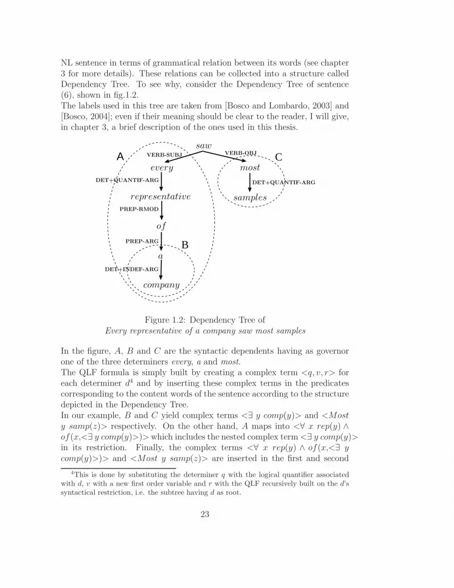
NL sentence in terms of grammatical relation between its words (see chapter3 for more details). These relations can be collected into a structure calledDependency Tree. To see why, consider the Dependency Tree of sentence(6), shown in fig.1.2.The labels used in this tree are taken from [Bosco and Lombardo, 2003] and[Bosco, 2004]; even if their meaning should be clear to the reader, I will give,in chapter 3, a brief description of the ones used in this thesis.

saw

every most

samplesrepresentative

of

a

company

VERB-SUBJ VERB-OBJ

DET+QUANTIF-ARG

DET+INDEF-ARG

PREP-RMOD

PREP-ARG B

Α C

DET+QUANTIF-ARG

Figure 1.2: Dependency Tree ofEvery representative of a company saw most samples

In the figure, A, B and C are the syntactic dependents having as governorone of the three determiners every, a and most.The QLF formula is simply built by creating a complex term <q, v, r> foreach determiner d4 and by inserting these complex terms in the predicatescorresponding to the content words of the sentence according to the structuredepicted in the Dependency Tree.In our example, B and C yield complex terms <∃ y comp(y)> and <Mosty samp(z)> respectively. On the other hand, A maps into <∀ x rep(y) ∧of(x,<∃ y comp(y)>)>which includes the nested complex term<∃ y comp(y)>in its restriction. Finally, the complex terms <∀ x rep(y) ∧ of(x,<∃ ycomp(y)>)> and <Most y samp(z)> are inserted in the first and second

4This is done by substituting the determiner q with the logical quantifier associatedwith d, v with a new first order variable and r with the QLF recursively built on the d’ssyntactical restriction, i.e. the subtree having d as root.

23

argument of the predicate associated to the main verb, i.e. saw.The main problem of enumerative approaches is that the disambiguation pro-cess is basically considered as a non-separable whole, i.e. all interpretationsare listed in a single run of the algorithm, therefore it is difficult to introduceadditional rules for incremental reduction in the number of possible readings.However, it is often the case that this is precisely what is needed. In suchcases, it is possible to perform only partial disambiguations, rather than com-plete ones, since the knowledge about the context is incomplete.Constraint-based approaches, instead, easily allow one to reduce the numberof available readings by adding constraints in a monotonic way.For example, consider Hole Semantics representation of (6) (the object lan-guage is DRT) shown below

(17) h0, l1: h11⇒h12, l11: x, rep(x), of(x, y), l4: saw(x, z),

l2: h21 ∧ h22, l3: h31 most h32, l21: y, comp(y), l31: z, samp(z),

l11 ≤ h11, l4 ≤ h12, l21 ≤ h21, l11 ≤ h22, l31 ≤ h31, l4 ≤ h32,

l1 ≤ h0, l2 ≤ h0, l3 ≤ h0

which can be represented as in fig.1.4, where the arrows represents dominancerelations (i.e. l ≤ h):

h0

l1 : h11 ⇒ h12l2 : h21 ∧ h22

l1 : saw(x, z)

l3 : h21 most h32

l21 : y, comp(y) l11 : x, rep(x), of(x, y) l31 : z, sam(z)

Figure 1.3: Graphical representation of (17)

Now, suppose that an external module, after inspecting the context, detectsthat the sentence refers to a particular set of samples.In this case, the quantifier most has to receive wide scope. However, the scopeorder between the two other quantifiers still has to remain underspecified.

24

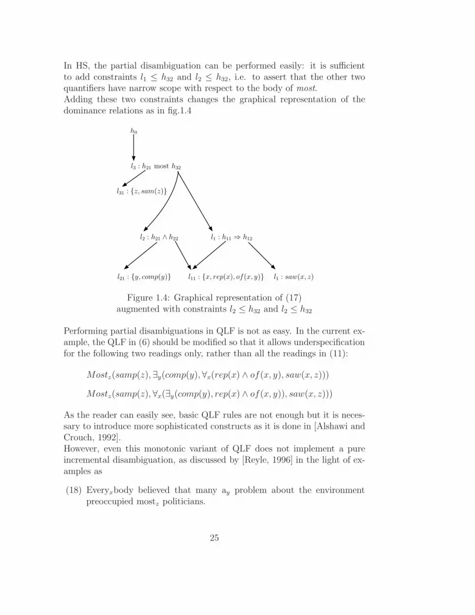
In HS, the partial disambiguation can be performed easily: it is sufficientto add constraints l1 ≤ h32 and l2 ≤ h32, i.e. to assert that the other twoquantifiers have narrow scope with respect to the body of most.Adding these two constraints changes the graphical representation of thedominance relations as in fig.1.4

h0

l1 : h11 ⇒ h12l2 : h21 ∧ h22

l1 : saw(x, z)

l3 : h21 most h32

l21 : y, comp(y) l11 : x, rep(x), of(x, y)

l31 : z, sam(z)

Figure 1.4: Graphical representation of (17)augmented with constraints l2 ≤ h32 and l2 ≤ h32

Performing partial disambiguations in QLF is not as easy. In the current ex-ample, the QLF in (6) should be modified so that it allows underspecificationfor the following two readings only, rather than all the readings in (11):

Mostz(samp(z), ∃y(comp(y), ∀x(rep(x) ∧ of(x, y), saw(x, z)))

Mostz(samp(z), ∀x(∃y(comp(y), rep(x) ∧ of(x, y)), saw(x, z)))

As the reader can easily see, basic QLF rules are not enough but it is neces-sary to introduce more sophisticated constructs as it is done in [Alshawi andCrouch, 1992].However, even this monotonic variant of QLF does not implement a pureincremental disambiguation, as discussed by [Reyle, 1996] in the light of ex-amples as

(18) Everyxbody believed that many ay problem about the environmentpreoccupied mostz politicians.

25

As is well known, quantifiers are clause bounded; this means that bothManyay and Mostz must have narrow scope wrt Everyx (in symbols: Manyay ≤ Everyx and Mostz ≤ Everyx). However, the sentence does not pro-vide enough information to establish the relative scope between Many ay

and Mostz . In other words, we cannot yet to specify whether everybodybelieves that most politicians are worried about a (potentially different) setof many problems about the environment (i.e. Many ay ≤ Mostz), or thatfor many a problem about the environment, there is (potentially different)set of politicians worried about it (i.e. Mostz ≤Many ay).In QLF it is impossible to describe this partial scoping. In fact, once we fixthe relative scope between two quantifiers, for example Many ay ≤ Everyx,it is only possible to specify the scope of Mostz wrt both of them, i.e. toestablish one of the two final orders

- Mostz ≤Many ay ≤ Everyx

- Many ay ≤Mostz ≤ Everyx

Whereas we cannot independently assert the weaker constraint Mostz ≤Everyx only.On the contrary, this may be easily handled in HS, since each dominance con-straint indicates that a certain piece of formula must be inserted into anotherone, but it still leaves underspecified whether this insertion is achieved di-rectly or transitively, via other pieces. For example, in the HS representationof (18), reported below

(19)

l1:Everyx(h11, h12), l2:Many ay(h21, h22),

l3:Mostz(h31, h32), l4:person(x), l6:politician(z),

l5:env−problem(y), l7:believe(x, h7), l8:preocc(y, z)

l4 ≤ h11, l5 ≤ h21, l12 ≤ h31, l7 ≤ h12

constraints can be added independently of each other and in an incrementalway; e.g., in order to handle the partial scoping relations described above,the following two constraints simply have to be added to (19)

- l2 ≤ h7

- l3 ≤ h7

In this way, only the two scope orders Many ay ≤ Everyx and Mostz ≤Everyx are established while the one between Many ay and Mostz still re-mains ambiguous.

26

Nevertheless, enumerative approaches feature a simpler syntax-semantic in-terface in that they basically separate predicate-argument relations fromscoping relations; hence, it is possible to leave the syntax-semantic inter-face to manage the former, and the resolution algorithm to handle the latter.On the other hand, constraint-based approaches spread sentence meaningacross several atomic pieces and constrain their recomposition. This amountsto taking dominance relations into account together with predicate-argumentrelations, i.e. to managing and establishing initial scope constraints alreadyin the syntax-semantic interface, that, consequently, turns out to be morecomplex (see [Frank and Reyle, 1995], [Joshi and Kallmeyer, 2003] and [Bos,2004])5.

1.3 Summary

In this chapter, I presented a synopsis of the current literature about Under-specification, with a particular focus on quantifier scope ambiguities.The comparison between the two main underspecified approaches highlightsa trade-off between flexibility with respect to the syntactic side and flexibil-ity with respect to the pragmatic side. Enumerative approaches feature asyntax-semantics interface that is more direct compared to constraint-basedapproaches, since the former tend to leave material in place with respect tothe syntactic structure, whereas the latter split it up in atomic pieces and con-strain their recomposition. However, constraint-based approaches suitablyallow for incremental disambiguations by keeping the unambiguous parts ofmeanings separate from scope constraints; in enumerative approaches, theseare mixed together.In the next chapter, I will present a new underspecified formalism namedDependency Tree Semantics (DTS).DTS minimizes the trade-off discussed above: it features both a close syntax-semantic interface with respect to a Dependency Tree (as the name Depen-dency Tree Semantics suggests) and a flexible management of partial dis-ambiguations. In particular, this twofold advantage is obtained in DTS byleaving material in place (as enumerative approaches do) and by maintain-ing scope constraints separate from predicate-argument relations occurringin the sentence (as constraint-based approaches do). However, DTS scope

5It must be pointed out that some translation processes from enumerative representa-tions to constraint-based ones have been proposed; the aim is to combine the advantagesof both by obtaining an enumerative underspecified formula from the syntactic tree, thentranslating it into a constraint based one. See [van Genabith and Crouch, 1996] (fromLFG to QLF and UDRT) and [Lev, 2005] (from QLF to HS).

27

constraints, unlike their Hole Semantic counterparts, do not consist in dom-inance relations between special metavariables and subformulae; they ratherconsist in semantic dependencies between involved (groups of) entities, i.e.Skolem functions.

28

Chapter 2

Intuitions behind DependencyTree Semantics

In the previous section, I presented some of the current approaches to se-mantic underspecification, and classified them according to their approach,which is either enumerative and constraint-based.The Enumerative approach aims to build a compact ambiguous formula de-scribing the predicate-argument relations occurring in the sentence, with-out any quantification; quantifiers are instead referred to by some kind ofplace-holder, such as qterms in QLF. A resolution algorithm removes allplace-holders one by one in a certain order, and embeds subformulae in theircorresponding quantifiers; depending on the order chosen, different readingsare obtained. This strategy renders enumerative formalisms suitable to in-terface an NL syntactic representation, especially a Dependency Tree, sinceit already provides a rough description of the predicate-argument relations.Nevertheless, since the algorithm reshuffles the partial formula, in that itdeletes a place-holder and creates a new embedding, incremental disambigua-tions cannot be achieved in a formalism based on the enumerative approach.Conversely, this can be easily done in the constraint-based approach, in whichno representation is reshuffled, but the pieces constituting it are simply gluedtogether. The fully ambiguous representation is, however, still radically dif-ferent from the syntactic structure, so that the interface between the twoturns out to be more complex.In this chapter, I present an alternative way to underspecify quantifier scop-ings, which makes use of semantic dependencies to relate quantifiers. In par-ticular, this is done by applying the concepts lying behind the well-knownSkolem theory in standard logics to underspecification.It is shown that the main advantage of this solution is the possibility of rep-resenting Branching Quantifier (BQ) readings in semantic formalisms.

29

BQ readings, examined in further detail in the second part of the thesis,may be found very often in NL, but they received very little attention in therecent literature.The use of semantic dependencies to specify scope orderings between quan-tifiers leads to an approach that features both an easy interface to a Depen-dency Grammar and an incremental constraint-based mechanism on semanticdependency insertion.This twofold advantage can be easily achieved, because the approach does notmake use of the standard quantifier embedding operation. In other words,semantic dependencies can be kept separated from predicate-argument rela-tions, without breaking the latter into “pieces” to enable the reconstructionof all admitted embeddings of quantifiers.

2.1 An alternative way to specify orderings

on quantifiers

The key idea of DTS is to devise a NL semantic formalism aiming at exploit-ing the well-known Skolem Normal Form Theorem (SNFT), defined by thelogician Thoralf Skolem in the context of First Order Logics (FOL).However, SNFT deals with FOL quantifiers only; in order to representing NLmeaning, Second Order Logics (SOL) quantifiers are useful too (see section5.2). We must therefore define a new Skolem-like mechanism, suitable tohandle dependencies from individuals to sets of individuals rather than fromindividuals to individuals.Chapter 5 shows how this may be done in terms of quantifications on rela-tional variables.

2.1.1 Skolem Normal Form Theorem (SNFT)

As is well known, in standard logics it is possible to transform a quantifiedformula into an equi-satisfiable one by applying the Skolem Normal FormTheorem1.

Definition 2.1 (Skolem Normal Form Theorem).Every standard FOL formula Ψ is logically equivalent to the second orderlogics (SOL) well formed formula

∃f1 . . . fn∀x1 . . . xmΦ

1This procedure is often called “Skolemization”.

30

Where f1 . . . fn are functional variables, x1 . . . xn are individual variables,n,m ≥ 0 and Φ is a quantifier-free formula.

A simple example can be helpful in illustrating the intuitions underlyingSkolemization and how it works in practice. Consider the sentence

(20) a. Every man loves a woman.

b. ∀x[man(x) → ∃y[woman(y) ∧ love(x, y)]]

c. ∃y[woman(y) ∧ ∀x[man(x) → love(x, y)]]

As I discussed in chapter 1, the FOL formulae in (20.b) and (20.c) depictthe two possible readings of sentence (20.a). The former is true only in thosemodels where, for each man, there is a (potentially different) loved woman,while the latter is true only in those models in which there is a single womanloved by every man. Intuitively, this means that (20.b) is true in a certainmodel only if given a man m, we can identify the woman (or one of thewomen) he loves.Analogous considerations hold for (20.c): the formula is true in a model onlyif it contains a particular woman loved by every man. Therefore, we candirectly refer to this particular woman with a constant term2.These tacit dependencies can be made explicit by applying Skolemization,which leads to the two following formulae

(21) a ∃f1∀x[man(x) → [woman(f1(x)) ∧ love(x, f1(x))]]

b ∃f0∀x[woman(f0) ∧ (man(x) → love(x, f0))]

In (21.a), f1 establishes a dependency between the group of women and thegroup of men: given a man x, f1(x) is the woman he loves; on the otherhand, in (21.b), f0 is a constant denoting the woman loved by every man.

2.1.2 Generalizing SNFT to handle NL semantics

This section presents a new strategy for the specification of orderings betweenquantifiers. Starting from an underspecified representation, which describesonly the involved groups of entities and the predications in which they takepart, a particular ordering can be specified by inserting additional functionaldependencies between these groups of entities.In other words, this thesis proposes a new mechanism to perform disambigua-tion, based on the same concepts lying behind Skolem’s theory: dependencies

2I remark that, from a formal point of view, a constant can be substituted by a functionhaving no arguments.

31

are rendered explicit in the formula rather than handled implicitly via ap-propriate subformula embeddings.Consider again the formulae in (20). The underspecified representation hasto include all information common to both interpretations, i.e. that thereare two groups of individuals involved (the former is composed only by menand the second only by women), and there is a “love” relation between menand women. The chosen disambiguation will add additional constraints thatmust be satisfied by this relation: it will specify that either the group ofwomen includes a single woman loved by every man, or that the group ofwomen can include several women, each of whom is loved by at least one man.This common knowledge can be represented via appropriate predicate-argumentrelations between two terms, respectively referring to the set of men and theset of women.In this thesis, these terms are called discourse referents, following DRTnomenclature [Kamp and Reyle, 1993], and will be referred to by symbolssuch as x, y, z, etc.Therefore, assuming that x and y denote two groups of individuals, thepredicate-argument relations can be roughly represented by this simple flatformula3:

(22) man(x) ∧ woman(y) ∧ love(x, y)

However, in order to increase readability, especially when more complex ex-amples are considered, I introduce the equivalent graphical notation in fig.2.1

love’

man’

x y

woman’

1 2

1 1

Figure 2.1: Graphical representation for (22)

Fig.2.1 is simply a notational variant of (22): the nodes in the graph are thesame predicates and discourse referents occurring in (22), while the edges arelabelled with the predicate-argument positions. The conjunction is implicit.Fig.2.1 can then be augmented with additional dependencies; they are shownin the graph by means of dotted arcs between discourse referents named

3This expression could be read as “there is a love relation defined over the set of manand the set of woman”.

32

SemDep arcs. For instance, the interpretation triggered by the SOL formula(21.a), in which there is a potentially different woman for each man, is rep-resented by fig.2.2.a; in this graph, the dotted arc from y to x represents theDTS counterpart of the Skolem function f1.On the contrary, in order to represent (21.b), where there is a single womanloved by every man, a new node is introduced in the representation (Ctx4)and a SemDep arc links y to it (see fig.2.2.b). The dotted arc linked to Ctx

is the DTS counterpart of the function f0.

x y

1 2

1 1x y

1 2

1 1

Ctxa) b)love’

love’

man’

man’

woman’

woman’

Figure 2.2: DTS formulae (first approximation) forEvery man loves a woman

For the sake of representational homogeneity, fig.2.2.a and fig.2.2.b can bemodified as in fig.2.3. The only difference between these variants and theprevious ones is that all discourse referents are the source of one SemDep arc;the discourse referents that are not linked to any other discourse referents,are linked to Ctx.

Ctx Ctxa) b)

x y

1 2

1 1

love’

man’ woman’

x y

1 2

1 1

love’

man’ woman’

Figure 2.3: DTS fully specified formulae (second version) forEvery man loves a woman

4As it will be clear afterwards, Ctx simply refers to the context, i.e. the domain ofindividuals with respect to which the representation will be evaluated.

33

However, the underspecified representations shown above are incomplete inthat they do not specify the quantifier associated with each discourse referent,nor the distinction between the predicates that identify the set of individualson which the formula makes a certain assertion (the so-called restriction) andthe predicates that constitute this assertion (the so-called body).This distinction is necessary to discriminate, for example, between the rep-resentation of sentence (23.a) and the representation of (23.b): these twosentences have very different meaning, but they can both be associated withthe graph in (23) on the right.

(23) a All men run.

b All runners are men.

Ctx

x

1

man’

1

run’

To include these two missing pieces of information, I introduce two functionson discourse referents: quant and restr.The former associates a quantifier to each discourse referent; therefore, forexample, in fig.2.3, it holds that

quant(x) = ∀quant(y) = ∃

On the other hand, restr associates, to each of them, the set of all predicatesneeded to identify the restriction, i.e. a subgraph of the main graph.The graphical representations associated with (23.a) and (23.b) are shownin fig.2.4.a and fig.2.4.b respectively. In fig.2.5, the complete underspecified

Ctx

x

1

man’

1

run’

quant(x)=∀

restr(x)

x

1

man’

a) b) Ctx

x

1

man’

1

run’

quant(x)=∀

restr(x)

x

1

run’

Figure 2.4: DRT formulae for All man run and All runners are man.

representation for sentence (20.a) is reported. It must be remarked that,

34

although the values of restr are shown separately, they are subgraphs of themain graph (i.e. there is a single instance of the discourse referents x and yand the predicates man′ and woman′).

love’

man’

x y

woman’

1 2

1 1

quant(x)=∀

restr(x)

x

1 quant(y)=∃

restr(y)

1

man’ woman’

y

Figure 2.5: DTS fully underspecified formula forEvery man loves a woman

This representation can then be disambiguated in two ways, by inserting dot-ted arcs as in fig.2.3; however, it must be remarked that the chosen disam-biguation does not change the values of functions quant and restr. In otherwords, in DTS, dependencies between quantifiers are maintained stronglyseparated from the predicates needed for identifying restrictions. This willbe very important in defining a monotonic disambiguation in DTS (see chap-ter 4).

2.2 Branching Quantifier (BQ) readings

As discussed in the previous section, rather than embedding quantified sub-formulae into the scope of other quantifiers, it is possible to specify scopingrelations by rendering explicit the dependencies between quantifiers via aSkolem-like mechanism.This alternative strategy allows for the representation of the so-called branch-ing quantifier (BQ) readings. In fact, consider the following sentence, whichcan be interpreted, in QLF, through one of the two formulae below:

(24) a. Two students study three theorems.

b. Twox(stud′(x), Threey(theor

′(y), study′(x, y)))

c. Threey(theor′(y), Twox(stud

′(x), study′(x, y)))

(24.b) requires the existence of two particular students studying three (po-tentially different) theorems each, and it corresponds to the DTS formula infig.2.6, where such dependencies are explicitly shown via SemDep arcs.Much in the same way, (24.c), which requires the existence of three particulartheorems studied each by two (potentially different) students, corresponds to

35

study’

stud’

x y

theor’

1 2

1 1

Ctx

stud’

x y

theor’

1 1

Restr(x)

Quant(x)= two

Quant(y)= three

Restr(y)

students theorems

Figure 2.6: DRT formula corresponding to (24.b).

study’

stud’

x y

theor’

1 2

1 1

Ctx

stud’

x y

theor’

1 1

Restr(x)

Quant(x)= two

Quant(y)= three

Restr(y)

students theorems

Figure 2.7: DTS formula corresponding to (24.c).

the DTS in fig.2.7.However, DTS allows for a very natural representation of a third reading ofsentence (24.a): the Branching Quantifier reading in fig.2.8.As shown in fig.2.8 on the right, this reading is true only for those modelswhere we can find a set of two particular students who study the same setof three particular theorems (or, equivalently, where there is a set of threeparticular theorems studied by the same pair of students).Branching quantifier readings are not enabled in current underspecified for-malisms, such as the ones analyzed in chapter 1. One of the reasons for this,perhaps, consists in the idea that an explicit representation of BQ readings isnot strictly necessary; they always imply some linearly-ordered ones anyway.For instance, it is easy to see that in all models satisfying the BQ readingin fig.2.8, the two linearly-ordered readings (figg. 2.6 and 2.7) are also true.BQ readings might therefore appear to concern a pragmatic ambiguity only:during the model-theoretic interpretation of (2.6), we can simply take aninterpretation function which assigns the same three theorems to both stu-dents, thus obtaining the same truth-conditions of the reading in fig.2.8.

36

Ctx

students theorems

study’

stud’

x y

theor’

1 2

1 1

stud’

x y

theor’

1 1

Restr(x)

Quant(x)= two

Quant(y)= three

Restr(y)

Figure 2.8: DTS formula corresponding to (24.c).

On the other hand, it may be argued that what is really important for asemantic formalism is the ability to restrict as much as possible the set ofpossible models in which the sentence is true. Therefore, there does not seemto be any reason for disregarding BQ readings in the semantic representation.The actual availability of BQ readings in NL will be discussed in depth insection 5.1; this section only provides some linguistic examples so as to justifythe need of a BQ reading for sentences as (24); these examples are reportedin (25).It is easy to add some syntactic element in order to force the two involvedsets to be constant:

(25) a. Two students, John and Jack, study three theorems: the first threeof the book.

b. Two friends of mine went to three concerts with my sister.

c. Two students of mine have seen three drug dealers in front of theschool.

In (25.a), the students and theorems involved are explicitly mentioned in twoappositions, while in (25.b) the prepositional modifier with my sister favoursan interpretation in which three persons, two friends of mine and my sister,went together to the same three concerts.However, aside from a few explicit syntactic constructions such as these two,world knowledge seems to be the main factor inducing a BQ reading. Forinstance, in (25.c), world knowledge seems to render the reading in which twostudents have seen the same three drug dealers the most salient; in fact, thepresence of drug dealers in front of a school is (fortunately) a rare event,andthis induces to prefer the reading minimizing the number of involved drugdealers.

37

Since DTS enables BQ readings, it is clear that the model-theoretic interpre-tation of its well formed structures cannot be defined in a standard way. Infact, standard logics are strictly linear, and we can easily define an interpre-tation that assigns a truth-value to the formula by applying its main term,e.g. a quantifier, on the truth values recursively calculated on the embeddedsubformulae. On the contrary, a BQ formula may have, as main term, a clus-ter of quantifiers, rather than a single one; the quantifiers in this cluster haveto be applied in parallel with respect to the truth values of their (private orcommon) subformulae.Since the definition of such a model-theoretic interpretation is rather difficultand needs a careful analysis of the main works in Branching Quantification,the second half of the thesis is entirely devoted to it.In the next two chapters, I assume that this model-theoretic interpretationhas already been defined, and it correctly handles the sets of entities de-scribed by the dependencies.

2.3 Partial orderings on quantifiers

Let me move on to more complicated examples, in order to understand pre-cisely the relation between SemDep arcs and dependencies between groupsof involved entities they denote. Consider

(26) a. Each boy broke two boxes with a hammer.

b. Each boy broke two windows with a stone.

c. Each boy leave a book on each table.

These sentences have the same syntactic structure; they also have an isomor-phic predicate-argument relations graph. Their main verbs denote a ternarypredicate, whose arguments are denoted by the subject, the object and theprepositional modifier.However, despite these similarities in the syntactic and semantic structures,their preferred readings are triggered by different dependencies between theirthree quantifiers, as shown in figg.2.9, 2.10 and 2.11. World knowledge sug-gests us to imagine, for sentence (26.a), a scenario in which each boy helda (different) hammer and broke two different boxes by means of it, i.e. aninterpretation in which both the hammer and the pair of boxes depend onthe specific boy. On the contrary, it is rather strange to think, in sentence(26.b), that each boy picked up and reused the same stone for breaking dif-ferent windows.Therefore, at first glance, it seems that the stone depends on the windows

38

Restr(z)

Quant(y)= TwoQuant(x)= ∀

11

broke’

boy’ Quant(z)= ∃

x y

2

z

1

box’

1

hammer’

1

3

Restr(x) Restr(y)

z

1

y

1

x

1

Ctx

boy’ box’ hammer’

Figure 2.9: DTS formula corresponding to (26.a).

Restr(z)

Quant(y)= TwoQuant(x)= ∀

11

broke’

boy’ Quant(z)= ∃

x y

2

z

1

window’

1

stone’

1

3

Restr(x) Restr(y)

z

1

y

1

x

1

Ctx

boy’ window’ stone’

Figure 2.10: DTS formula corresponding to (26.b).

rather than on the boys. Finally, it is clear that sentence (26.c) talks abouta different book for each pair 〈boy, table〉; therefore, discourse referent y, inthis case, has to be linked to both of the other two, via two distinct SemDeparcs.Nevertheless, a proviso on what these structure actually denote is in order.In fig.2.10, the stone does not depend only on the window, as the representa-tion may suggest, but also on the boy. In other words, similarly to fig.2.11,fig.2.10 denotes an interpretation in which there is a different stone for eachpair 〈boy, window〉.Picture a situation in which two boys, e.g. John and Jack, broke the samepair of windows5; if, in the formula, z depends only on y, then it would betrue only if the two boys broke the windows by means of the same stones,whereas, obviously, the sentence may be true also if they used different ones.Therefore, z has to depend on both x and y, as in fig.2.11.

5Of course, in a real situation, this can be done only at different times; e.g. John brokethe windows, then someone repaired them, and then Jack re-broke them again.

39

Restr(z)

Quant(y)= ∃Quant(x)= ∀

11

leave’

boy’ Quant(z)= ∀

x y

2

z

1

book’

1

table’

1

3

Restr(x) Restr(y)

z

1

y

1

x

1

Ctx

boy’ book’ table’

Figure 2.11: DTS formula corresponding to (26.c).

In a non-graphical representation this double dependency may be handledby Skolemization-like mechanisms able to substitutes z with a function fwith two parameters: x and y. On the contrary, in the chosen graphicalrepresentation this may be made by inserting the dotted arcs correspondingto all the necessary dependencies, as shown by the following figure6

x y z

Ctx

Figure 2.12: Alternative SemDep configurationto handle dependencies in (26.b).

From a formal point of view, this is precisely what will be done below; inparticular, as it will be shown in section 2.4, dependencies between discoursereferents will be implemented as a function SemDep from discourse referentsto sets of discourse referents, and Ctx. SemDep(d) will be the set of all dis-course referents on which d (directly or indirectly) depends.For example, SemDep will have the following values for the example infig.2.10:

• SemDep(x) = Ctx

6Clearly, for homogeneity of representation, also the indirect dependencies betweeneach discourse referent and Ctx have to be inserted; in other words, all quantifiers dependon the context.

40

• SemDep(y) = x, z,Ctx

• SemDep(z) = Ctx

while, referring to example in fig.2.11, SemDep’s values will be

• SemDep(x) = Ctx

• SemDep(y) = x,Ctx

• SemDep(z) = x, y,Ctx

However, to decrease verbosity, I will not show all SemDep values in thegraphical representation, but only the non-transitive ones. In other words,the set of SemDep arcs will be the minimum set such that its transitiveclosure is equal to the function SemDep.In order to avoid confusion, the reader should consider the set of SemDeparcs as a whole, as describing a partial order on discourse referents, and keepin mind that a discourse referent actually depends on all discourse referentsoccurring before it in this order.Chapter 4 shows that not all partial orders have to be allowed, in particularwhen an NL nested quantification occurs in the sentence; consequently, it isnecessary to assert a set of constraints on SemDep arc insertion.However, in the next section I propose an initial formalization of DTS well-formed structures, that allows for any partial order on SemDep arcs.This formalization will be refined in chapter 4, after discussing which config-urations of SemDep arcs have to be blocked.

2.4 DTS Formalisation

A wf structure in DTS is a Scoped Dependency Graph (SDG), as definedbelow. As in standard semantics, the definitions below are stated in termsof three sets:

- A set of predicates pred.

- A set of constants name.

- A set of variables D named discourse referents.

Moreover, I write P 1⊆pred for the unary predicates, P 2⊆pred for the binaryones and ιname⊆P

1 for those obtained by applying the ι-operator to a con-stant in name7.

7The ι-operator has the standard semantics: if α is a constant, ια is a unary predicatewhich is true only for α

41

The definition of Scoped Dependency Graph is based upon the definition ofFlat Dependency Graph, which simply collects all predicate-argument rela-tions occurring in the sentence.

Definition 2.2. [Flat Dependency Graphs (FDG)]A Flat Dependency Graph is a tuple 〈N,L,A,Dom, f〉 s.t.:

- N is a set of nodes n1, n2, . . . , nk.

- L is a set of labels l1, l2, . . ., lm; in all figures of the thesis,L≡1, 2.

- Dom ≡ pred∪D is a set of domain objects: predicates and discoursereferents

- f is a function f : N 7→ Dom, specifying the node referent, i.e. thedomain object with which the node is associated. In the following,whenever f(n) ∈ X, I will informally say that node n is of type X.

- A is a set of arcs. An arc is a triple (ns, nd, l), where ns, nd ∈ N , ns

is of type pred, nd is of type D and l ∈ L.

Without going into further detail, I stipulate that Gf is a connected acyclicgraph such that each node of type pred has one node of type D for each of itsplaces. Note that there can be two different nodes u and v s.t. f(u)=f(v),i.e. the nodes in N can be seen as occurrences of symbols from Dom.However, to increase readability, I never show the node names n1, n2, etc.,in the boxes of the graphical representations, opting instead for their corre-sponding values in f , e.g. the predicates study′, theor′, etc. or the discoursereferents x, y, etc.

Definition 2.3.[Scoped Dependency Graph (SDG)]A Scoped Dependency Graph is a tuple 〈Gf ,Ctx,Q, quant, restr, SemDep〉 s.t.:

- Gf = 〈N,L,A,Dom, f〉 is an FDG.

- Ctx is a special element called ”the context”.

- Q is a set of 2-place Mostowskian quantifiers (Mostowski [1957], seesection 5.2) as every, most, two, . . ..

- quant is a total function ND 7→ Q, where ND ⊆ N are the nodes oftype D.

- restr is a function assigning to each d ∈ ND its restriction, which isa subgraph of Gf .

- SemDep is a total function ND 7→ ℘(ND) ∪ Ctx, where ℘(ND) isthe power set of ND (the set of all its subsets).

42

When d′ ∈ SemDep(d), we say that d depends on d′. Note that, as it waspointed out above, SemDep implements all dependencies between discoursereferents.Therefore, a Scoped Dependency GraphGs = 〈Gf ,Ctx,Q, quant, restr, SemDep〉is fully underspecified iff SemDep(x)=Ctx for each discourse referent x ∈ D.Finally, it must be observed that SemDep has been only partially defined inthis section; its complete formalization requires a set of constraints on valuesit may assume that will be presented in chapter 4.

2.5 Summary

In this chapter, the key idea of DTS was presented. In particular, I proposedto import the mechanisms underlying the Skolem Normal Form Theorem,defined in the context of First Order Logics, into NL semantics. By usinga Skolemization-like mechanism, it is possible to make explicit the depen-dencies between involved entities that would make true the correspondingnon-Skolemized formula.DTS well-formed structures are based on a simple graph G representing thepredicate-arguments relations, without any quantification. The nodes of Gare either predicates or discourse referents; each arc connects a predicate witha discourse referent, and is labeled with the predicate argument position. Toeach discourse referent, we associate a quantifier (given by a function quant

from discourse referents to quantifiers) and its restriction, which is given bya function restr that associates a subgraph of G to each discourse referent.Dependencies between involved groups of entities can be asserted by introduc-ing additional dotted arcs, called SemDep arcs, between discourse referents.Any partial order defined by SemDep arcs on discourse referents potentiallyrefers to a possible reading of sentence, even if I pointed out that this doesnot always hold and, therefore, that a set of constraints on SemDep arcinsertion is needed. These constraints will be discussed in chapter 4.

43

44

Chapter 3

DTS Syntax-Semantic Interface

This chapter presents the syntax-semantics interface of DTS. As the name“Dependency Tree Semantics” suggests, this interface relates DTS with aDependency Grammar. The Dependency approach is briefly discussed insection 3.1; this section also defines a Dependency Grammar G for a smallfragment of English. Section 3.2 presents Extensible Dependency Grammar(XDG), one of the most recent formalisms that interface an UnderspecifiedSemantic representation with a Dependency Grammar.The DTS syntax-semantic interface between G and DTS will then be shownin section 3.3. This interface basically consists in two principles, importedfrom XDG: the Linking Principle, which extracts the predicate-argumentrelations from the Dependency Tree and builds the corresponding Flat De-pendency Graph, and the Restriction Principle, which sets up the values ofthe function restr in order to preserve the structural information stored inthe Dependency Tree, i.e. the subtrees of dependencies.Finally, a comparison between this interface and the one of other approaches,first at all XDG, concludes the chapter. This comparison highlights the mainadvantage of DTS the syntax-semantic interface with respect to other pro-posals in the literature: the DTS syntax-semantic interface is simpler in thatit just deals with predicate-argument relations, while the management ofscope constraints is completely devolved upon a subsequent disambiguationprocess.

3.1 Dependency Grammar

A Dependency Grammar (DG) is a formalisms that allows to describe NLsyntax in terms of oriented relations between words, called dependency rela-tions or grammatical functions.

45

In particular, a DG analysis represents a NL sentence by hierarchically ar-ranging its words and linking pairs of them via dependency relations.Dependency Grammar represents an alternative with respect to the standardConstituency Approach [Chomsky, 1957], which aims to recursively group thewords occurring in the sentence into constituents called phrases.As pointed out above, dependency relations are oriented; therefore, for eachpair of linked words, we can identify a head (the source of the link) and adependent (the destination of the link). The link states that the latter syn-tactically depends on the former.The dependent plays a role of “completion” of the head, i.e. it provides a sortof “parameter” to the latter, instantiating, in this way, the head meaning onthe dependent meaning. For this reason, Dependency Grammars are tradi-tionally expressed in terms of valency. The word “valency” is taken fromchemistry: the valency number of an atom is the number of electrons thatit is able to take from (or give to) another atom in order to form a chemicalcompound. By metaphor, then, a DG grammar specifies, for each lexicalentry of the NL vocabulary, the incoming dependency relations (in valency)and the outgoing ones (out valency). Basically, there are two kinds of in\outvalency: mandatory and optional. In the first case, the dependent is saidto be a complement of the head, while in the second case it is said to be anadjunct. Dependency relations are usually labeled in order to make explicitthe function played by a dependent with respect to the head. Although theprecise inventory of labels varies from theory to theory, many grammaticalfunctions, such as subject, object, etc., are commonly accepted in the litera-ture and may be found in all DGs.For example, the lexical entry “study”, belonging to a vocabulary for english,could hold the following valencies

word=study

inval=verb-rmod?

outval=verb-subj!, verb-obj!, prep-rmod*

where ‘!’ marks a mandatory dependency (complement), ‘?’ a single optionalone (adjunct), and ‘*’ one or more optional ones. Therefore, the lexical en-try specifies that the word “study” can be the destination of a grammaticalfunction labeled as “verb-rmod” (verbal modifier, in relative clauses), whichmust be the source of two dependencies respectively labeled as “verb-subj”and “verb-obj” (verbal subject and object). It can also be the source of oneor more dependencies labeled with “prep-rmod” (prepositional adjunct).In this thesis, the inventory of the labels on the dependency links is taken

46

from [Bosco, 2004].We can represent a DG analysis of a sentence by means of a tree (graph),named Dependency Tree (Dependency Graph), which collects all grammat-ical functions between pairs of words in the sentence. For example, thesentence in (27) can be associated with the Dependency Tree below it1.

(27)

All students study a theorem of the book

study

all

students

a

theorem

of

the

book

VERB-SUBJ VERB-OBJ

DET-ARG DET-ARG

DET-ARG

PREP-RMOD

PREP-ARG

It is important to note that, in a dependency relation, not only the depen-dent, but the whole subtree having the dependent as root can contribute tothe “completion” of the head. For example, in (27), the mandatory valencyof the verb study marked as Verb-Subj is filled by the whole subtree a theoremof the book rather than by the single determiner a.The last observation is very important for defining the values of restr in thesyntax-semantic interface and the constraints on SemDep arcs (see section4.3.1).The first work defining the main principles of modern Dependency Grammarsis [Tesniere, 1959]. Tesniere’s Structural Syntax (SS) analyzes sentences interms of functions held by the words, which trigger subordinative relationscalled connections. In particular, there are two kinds of functions: nodalfunctions, triggering structural (syntactic) connections, and semantic func-tions, triggering semantic connections. Structural Syntax has been formal-ized in a computational model in Functional Dependency Grammar (FDG)

1All Dependency Trees presented in this chapter are built via the Dependency Grammardefined in section 3.3.1.

47

[Tapanainen, 1999].One of the central differences between SS and FDG is that the former repre-sents both syntactic and semantic dependencies in the same graph, whereasthe latter separates them among different levels of representations.Other important works belonging to the DG approach are Hudson’s WordGrammar ([Hudson, 1990]), a Dependency Grammar structured in an “is-a” taxonomy that allows for linguistic generalizations and enables one todeal with default cases\exceptions, and Meaning⇔Text Theory ([Mel’cuk,1988]), a formal framework structured along seven sequential levels of de-scription, which allows for the parallel representation of various kinds oflinguistic knowledge carried by the sentence.One of the most recent proposals in the research on Dependency Grammaris Extensible Dependency Grammar (XDG) ([Debusmann, 2006]).XDG, to which I will devote the next section, is a modular framework able tohandle different aspects of Natural Language, such as Meaning⇔Text The-ory. However, contrary to the latter, in XDG the several levels of description,called dimensions, are more integrated (besides being more fine-grained).In particular, while in Meaning⇔Text Theory the levels of description arestrictly sequential, i.e. the rules to interface a level to another one are definedonly for adjacent levels, in XDG such rules can be in principle defined foreach pair of dimensions.

3.2 Extensible Dependency Grammar - XDG

Extensible Dependency Grammar (XDG) (see [Debusmann, 2006]) is a for-malism that represents linguistic knowledge along several levels of descrip-tion, called dimensions.Each dimension refers to a particular phonologic\syntactic\semantic infor-mation and enables the construction of a graph. Each graph that can bebuilt in a dimension is called a model for that dimension.The graphs licensed in the different dimensions share the same set of nodes,but have different sets of (labeled) edges.The nodes are records called lexical entries that specify attributes for eachdimension; each lexical entry is indexed by a word named anchor. Finally, aset of principles, acting on these attributes, constrains the graphs that canbe built in the various dimensions, and relate them to each other.The XDG definition includes the following main six dimensions:

- Prosodic (PS) dimension, describing phonologic information.

48

- Immediate Dominance (ID) dimension and Linear Precedence (LP )dimension, describing syntactic information.

- Predicate Argument (PA) dimension, Scope (SC) dimension, and In-formation Structure (IS) dimension, describing semantic information.

Furthermore, there are additional dimensions defining the interfaces betweenthe main six ones. For example, a dimension called ID\PA characterizesthe relation between the ID dimension (grammatical functions) and the PAdimension (thematic roles) by constraining how semantic arguments must beimplemented syntactically.The models in the “interface” dimensions are graphs without edges.Finally, XDG includes about twenty principles to manage the dimensionsand to enforce the consistency of the models appearing in them.Even if the reader interested in XDG is addressed to [Debusmann, 2006], inthis thesis I will present just the preliminary and simpler version shown in[Debusmann et al., 2004]. The level of detail and the linguistic coverage ofthe latter, in fact, is more suited for a comparison with the syntax-semanticinterface of DTS, which is also at a very preliminary stage.This version of XDG only includes three dimensions (PA, ID and SC)and the relations between dimensions are specified via particular attributes(“features”) rather than via additional dimensions. For example, a featurelinkPA,ID belonging to the PA dimension, specifies how thematic roles aresyntactically realized.Principles are divided into classes: dimensional, acting on a single dimension,and multi-dimensional, acting on (and relating) two dimensions.The ID dimension specifies grammatical functions between words in a De-pendency Tree. Conversely, the PA dimension represents predicate-argumentrelations by means of a Direct Acyclic Graph (DAG) whose edges are labeledby thematic roles. Finally, the SC dimension relates the nodes by means ofa DAG of scopal dominance relations.As in standard constraint-based approaches (see chapter 1), these scopaldominance relations may be consistent with several interpretations of thesentence, i.e. the DAG in the SC dimension actually is an underspecifiedrepresentation2.The particular topology of each dimension (a tree rather than a DAG) isobtained by applying the correct dimensional principle, named Tree or Dagprinciple. Furthermore, a third dimensional principle, i.e. the Valency prin-ciple, constrains the labels on the Tree\Dag arcs

2[Debusmann, 2006] also defines an interface between XDG and CLLS ([Egg et al.,2001]) by introducing a CLLS dimension and ad-hoc attributes to integrate it.

49

(28)

- Tree Principle. The ID structure must be a tree.

- Dag Principle. The PA and SC structures must be direct acyclicgraphs.

- Valency Principle. The dimension d ∈ ID, PA, SC must obey tothe ind, outd features, that specify the constraints on the incoming andoutgoing arcs of each node. The possible value for each feature ind,outd are subsets of Lab(d)×!, ?, ∗, where Lab(d) is the set of availablelabels in d.

The ind and outd features belong to the lexical entry of the words. In fig. 3.1,the values of the in and out features in the three dimensions for an examplegrammar are reported.

inID

outID

inPA

DET

CN

TV

PN

PREP

(subj? obj? pcomp?)!

det?

subj? obj? pcomp?

prep?

det!

prep*

subj! obj! prep*

pcomp!

prep*

ag? pat? arg?

quant?

mod? instr?

ag? pat? arg?

outSC

DET

CN

TV

PN

PREP

outPA

quant!

mod*

ag! pat! instr?

arg!

mod?

r!, s!

a!

r!, s!

inSC

r?, s?, a?

r?, s?, a?

r?, s?, a?

r?, s?, a?

r?, s?, a?

Figure 3.1: In and out feature values for an XDG grammaron three dimensions: ID, PA, and SC

This XDG grammar includes just five POS: determiner (DET), common noun(CN), proper name (PN), transitive verb (TV), and preposition (PREP); thegrammatical functions are subject (subj), object (obj), prepositional com-plement (pcomp), prepositional argument (prep), and determiner argument(det); the thematic roles are agent (agt), patient (pat), argument of a modi-fier (arg), modifier (mod), common noun pertaining to a quantifier (quant),

50

and instrument (instr); finally, dominance relations are restriction and nu-clear scope (body) of a quantifier (r and s, respectively) and argument (a).Therefore, for example, a determiner (DET) must have an incoming arc inthe dimension ID that may be labeled by either subj or obj or pcomp andmust have an outgoing arc labeled by det; on the contrary, in the dimensionPA, it could have an incoming arc labeled by either ag or pat or arg andmust have an outgoing arc labelled by quant.The interfaces between these levels are specified by other features and threemulti-dimensional principles acting on them. One of these principles (theLinking Principle) relates the graph in PA with the tree in ID, while theother two (the Co-dominance and the Contra-dominance Principles) relatesthe graph in PA with the one in SC. The XDG Linking Principle acts on afeature linkPA,ID, belonging to the PA dimension, whose values are shown infig.3.2; these values are functions from labels in PA to labels in ID specifyinghow thematic roles have to be realized in terms of grammatical functions

DET

CN

TV

PN

PREP

quant 7→ det

linkPA,ID

mod 7→ prep

mod 7→ prep

ag 7→ subj, pat 7→ obj, instr 7→ prep

arg 7→ pcomp

Figure 3.2: linkPA,ID feature values

The Linking principle is formally asserted in (29)

(29)Linking Principle. Dependencies in d1 are related to dependenciesin d2 according with the following formula

v →l

d1 v′ ⇒ ∃l

′∈ linkd1,d2(v)(l): v →l′

d2 v′

This principle requires that for each connection from v to v′ with label l inthe dimension d1, there must be a corresponding connection in the dimensiond2 with label l′, where l′ must belong to the set of labels linkd1,d2(v)(l), i.e.the set obtained by the functional application of the node v and the label lto the linkd1,d2 feature.In fig.3.3 a first simple example of XDG derivation is reported. The linking

51

principle constrains the two structures by requiring, for example, that theagent (ag) of reads be realized as the subject (subj), i.e.

reads −→ag

PA every ⇒ reads −→subj

ID every

Every student reads a book

subj

det det

obj

ID dimension PA dimension

Every student reads a book

ag

arg arg

pat

Figure 3.3: Graphs in PA and ID for the sentenceEvery students read a book

Another example is reported in fig.3.4.On the contrary, the Co-dominance and the Contra-dominance principles(shown in (30)) relate dimensions PA and SC by asserting initial domi-nance constraints on the latter on the basis of the predicate-argument re-lations described in PA. These two principles act on the codomPA,SC andcontradomPA,SC features belonging to the PA dimension. For our examplegrammar, the values of these features are reported in fig.3.2.

(30)Co-Dominance Principle. Dominance relations in d1 are related todominance relations, with the same direction, in d2 according with thefollowing formula

v →l

d1 v′ ⇒ ∃l

′∈ codomd1,d2(v)(l): v →l′

d2→∗ v′

Contra-Dominance Principle. Dominance relations in d1 are re-lated to dominance relations, with opposite direction, in d2 accordingwith the following formula

v →ld1 v

′ ⇒ ∃l′∈ contradomd1,d2(v)(l): v

′ →l′

d2→∗ v

These two principles behave exactly as the Linking principle shown above;the only difference is that these two principles require a path of connectionsrather than a single one. This is graphically shown by means of the notation“ → d2→

∗” in place of “→d2”.

52

Mary saw studenta

subj obj

ID dimension

with

det

prep

pcomp

det

a book

Mary saw studenta

ag pat

PA dimension

with

arg

mod

arg

quant

a book

Figure 3.4: Graphs in PA and ID for the sentenceMary saw a student with a book

It is clear that the purpose of the Co-dominance principle is to insert therestriction of a quantifier in its scope. As pointed out in the previous section,in a Dependency Tree this is already represented, in that a quantifier has anoutgoing valency that has to be filled by a restriction: as a consequence, wejust need to project in the SC dimension a dominance relation in the samedirection of the grammatical function between a quantifier and its restriction.For example, with respect to the graph in fig.3.3, we obtain

every −→quant

PA student ⇒ every →r → SC* student

The dominance relation between a quantifier and its body (e.g. the mainverb) has opposite direction with respect to the dependency relation betweenthem, in that the former acts as syntactic argument of the latter. In thiscase, then, the dual version of the Co-dominance principle, i.e. the Contra-dominance principle, is required.

53

DET

CN

TV

PN

PREP

quant 7→ r

codomPA,SC

contradomPA,SC

mod 7→ a

mod 7→ a

ag 7→ s, pat 7→ s, instr 7→ a

arg 7→ s

Figure 3.5: codomPA,SC and contradomPA,SC features values

reads −→ag

PA every ⇒ every →s → SC* reads

reads −→ag

PA a ⇒ a →s → SC* reads

The two principles allow to associate the graphs in fig.3.3 to the one in fig.3.6,where the dotted arrows indicate that the dominance relations need not beimmediate. In other words, the graph is an underspecified representationthat may be specified, through a translation of XDG into CLLS, into one ofthe two graphs reported in fig.3.7

Every student reads a book

r

SC dimension

sr

s

Figure 3.6: The (underspecified) graph in SC for the sentenceEvery students read a book

3.3 DTS syntax-semantic interface

In this section, an interface between a generic Dependency Grammar G(shown subsection 3.3.1) and Dependency Tree Semantics is presented. Iwill refer to this interface by the term “the G⇒ DTS interface”.In particular, the G⇒ DTS interface allows to associate a Dependency Tree

54

Every student reads a book

r

s

rs

Every student reads a book

s

rs

r

Figure 3.7: The two fully specified graphs in SC for the sentenceEvery students read a book

in G to a Scoped Dependency Graph (SDG) in DTS (see subsection 2.4). It isimportant to remind that this interface is compositional, i.e. a DependencyTree is related to only one Scoped Dependency Graph.The G⇒ DTS is a generalization of Extensible Dependency Grammar. Themain difference between the two is that the former relates structures withdifferent sets of nodes. In fact, the nodes of a Dependency Tree in G arewords study, every, of, etc., while the nodes in a Scoped Dependency Graphsare predicates like study’, of’, ιJohn, etc. or discourse referents like x, y, z,etc.Therefore, first at all it is necessary to define a mapping between these twosets of nodes. This mapping is implemented by means of two functions Semand SV ar (Lex and LV ar implements the inverse mapping) that will beshown in details in the next subsection.In subsection 3.3.3, it will be shown how the predicate-argument relations,that in an SDG are collected into the Flat Dependency Graph (FDG), canbe extracted from a Dependency Tree by means of a set of if-then rules.A principle similar to the XDG’s Linking Principle will act on these rulesand perform the extraction.Finally, in subsection 3.3.4 we will see how the values of the restr function,belonging to an SDG, can be set by a simple principle, called the RestrictionPrinciple, acting on the Dependency Tree and the predicate-argument rela-tions stored in the FDG. Clearly, this principle corresponds to the XDG’sCo-dominance principles and the feature codomPA,SC.On the contrary, in the G ⇒ DTS interface there is nothing that corre-sponds to the XDG’s Contra-dominance Principle. In fact, as it will be clearin next chapters, DTS scope constraints are maintained strongly separatedfrom predicate-argument relations; therefore, there is no need to set up initial

55

scope constraints between the quantifiers and their body; in DTS terms, thismeans that the G ⇒ DTS will set up the value of the function SemDep(x),for each discourse referent x in the SemDep’s domain, to the constant valueCtx.

3.3.1 A simple Dependency Grammar

This subsection formally defines a simple Dependency GrammarG for a smallfragment of english. Afterwards, the syntax-semantic interface of DTS willbe defined with respect to this grammar.Well formed structures of G are Dependency Trees. They are syntacticallydefined as the Flat Dependency Graphs in def.4.1, with the following differ-ences

- The structures are Trees rather than Graphs.

- The set of domain objects Dom is different: it contains syntactic wordsrather than predicates and discourse referents.

- The set of labels L is different: it contains labels denoting grammaticalfunctions rather than predicate-argument positions

- Labels in L have to obey to valency requirements, defined for eachsyntactic category.

Formal definitions are reported in def.3.1 and def.3.2; note, however, thatthis is only a small fragment of the full dependency grammar described in[Bosco, 2004] and used in the TUT treebank project [Lesmo et al., 2003]. Forinstance, the full grammar includes sixteen syntactic categories with varioussubcategories (e.g. ordinal adjective) and over two hundred dependency arclabels.

Definition 3.1. [Dependency Tree (DT)]A Dependency Tree in G is a tuple 〈N,L,A,Dom, f〉 where:

- N is a set of nodes n1, n2, . . . , nk.

- L is a set of labels verb-subj, verb-obj, det-arg, prep-arg, prep-rmod,verb-rmod.

- Dom ≡ IV ∪ TV ∪ PN ∪ CN ∪ PREP ∪ DET ∪ RP is a set of do-main objects: intransivite verbs, transitive verbs, proper names, com-mon names, prepositions, determiners3, and relative pronouns.

3Determiners are quantifiers and definite articles.

56

- f is a function f : N 7→ Dom, specifying the node referent, i.e. thedomain object with which the node is associated.

- A is a set of labelled and oriented arcs. In particular, an arc is a triple(ns, nd, l), where ns ∈ N is the source node, nd ∈ N the destinationnode, and l ∈ L the label on the arc. The set A defines a Tree betweenall nodes in N and obeys to the valencies defined in def.3.2

Definition 3.2. [Valency in G]A Dependency Tree in G must obey to the following valencies

in out

DET

CN

TV

PN

PREP

(verb-subj? verb-obj? prep-arg?)!

det-arg!

prep-rmod!

verb-rmod?

det-arg!

prep-rmod*

verb-subj! verb-obj! prep-rmod*

prep-arg!

IV verb-rmod?

verb-subj? verb-obj? prep-arg?

RP verb-subj!

verb-subj! prep-rmod*

An example of Dependency Tree in G has already been shown in (27); otherexamples are reported in (31) and (32)

(31)

Few men inserted a coin in every coffee machine.

inserted

few

VERB-SUBJVERB-OBJ

coffee-machine

DET-ARG

a

PREP-RMOD

men

DET-ARG

coin

DET-ARG

in

PREP-ARG

every

57

(32)

The students who passed the test arrive

arrive

the

VERB-SUBJ

students

DET-ARG

passed

VERB-RMOD

who

VERB-SUBJ VERB-OBJ

the

test

DET-ARG

3.3.2 Sem and SV ar function

As pointed out above, the mapping from the nodes of a Dependency Tree inG to the nodes of a Scoped Dependency Graph in DTS is realized by meansof two functions: Sem and SV ar.The domain objects of the two structures, i.e. the possible types of theirnodes, are repeated below

• The domain objects of a Dependency Tree in G, indicated by the termDomG, is a set of words belonging to a standard english vocabulary, andclassified into seven Part Of Speech (POS), indicated by the terms IV ,TV , PN , CN , PREP , DET , and RP (intransivite verbs, transitiveverbs, proper names, common names, prepositions, determiners, andrelative pronouns).

• The domain objects of a Scoped Dependency Graph in DTS, indicatedby the term DomDTS, is a set of semantic objects classified in two mainclasses: predicates and discourse referents, indicated by the terms pred

and D respectively.

As it is done in standard semantics, a proper name corresponds to a constant(the set of all constants is indicated with the term name). Nevertheless, name

does not belong to DomDTS. In DTS, a proper name is associated to a pred-icate ια, where α ∈ name is the constant denoted by the proper name and ι

58

is a standard operator that, when applied to a constant, builds a predicatethat is true for that constant and false otherwise. ια is a predicate, it alsobelongs to pred. In particular, pred is divided into two subgroups: P2 and P1,the set of all binary and unary predicates respectively. P1 has a subset, calledιname, containing the unary predicates obtained by applying the ι operatorto the constants in name.Sem relates verbs, common nouns, and other content words in G to a predi-cate in pred. On the contrary, SV ar relates determiners, proper names, andrelative pronouns in G to a discourse referent in D.In this thesis, the two functions are bijective, since linguistic phenomena suchas polysemy and lexical ambiguity are not considered. Therefore, it is imme-diate to define two inverse functions, named Lex and LV ar respectively.Sem and SV ar are formally defined as follows

Definition 3.3. [Sem and SV ar functions]Sem is defined for each node n of type IV ∪TV ∪PN∪CN∪PREP and SV arfor each node n of type PN∪DET∪RP according to the following constraints

- for all [n]TV ∪PREP , Sem(n) is of type P 2.

- for all [n]IV ∪CN , Sem(n) is of type P 1.

- for all [n]PN , Sem(n) is of type ιname.

- for all [n]PN∪DET∪RP , SV ar(n) is of type D.

Note also that these functions have been defined between the nodes of thetwo structures rather than between their domain objects; in other words,Sem and SV ar ar do not relate English words with predicates and discoursereferents, but occurrences of English words with occurrences of predicatesand discourse referents.In fact, two occurrences of a determiner such as most may correspond totwo different discourse referents, as well as two instances of a proper namecould correspond to two different predicates ια and ιβ, i.e. they can denotetwo different individuals having the same name, and a preposition such asof could refer to different predicates. Note also that nodes of type PNbelong to the domain of both Sem and SV ar. This is done for the sake ofrepresentional homogeneity, like in DRT, in which a proper name such asJohn produces both a discourse referent x and a DRS-condition John(x).

59

3.3.3 Extracting predicate-argument relations from a

Dependency Tree

Having defined Sem and SV ar, it is possible to describe how a Flat Depen-dency Graph in DTS can be obtained from a Dependency Tree of G. We needa formal device similar to the XDG Linking Principle, and the LinkPA,ID at-tribute on which it operates.In this section, I will define a set of if-then rules, called LinkG,FDG, and aPrinciple, called G⇒ DTS Linking Principle, acting on it.Contrary to XDG, in which LinkPA,ID expresses a kind of if-then rules be-tween the labels of the two dimensions, LinkG,FDG is a set of if-then rulesbetween “pieces” of structures. The reason for this is that the G⇒ DTS in-terface relates structures with different sets of nodes. The graphical patternof these if-then rules is reported in fig.3.8; Sc1 and Sc2 are set of connectionsbetween nodes in a Dependency Tree and in a Flat Dependency Graph re-spectively. The pattern of each connection is reported in fig.3.9. In fig.3.9,u1 and u2 indicate a node in the structure. Their types are T1 and T2 respec-tively. Finally, lab indicates the label of the arc from u1 to u2.

G FDG

Sc1 Sc2

Figure 3.8: G⇒ DTS interface: rule pattern

u1

T1

u2

T2

lab

Figure 3.9: G⇒ DTS interface: connection pattern

The first simple example of the rules in LinkG,FDG is reported in fig.3.10;these two rules specify how the subject of a verb is interpreted. In partic-ular, they assert that the subject of an intransitive (transitive) verb has tocorrespond to the first argument of the unary (binary) predicate associatedto it by the function Sem. Clearly, the argument of those predicates will

60

just be the discourse referent associated to the dependent of the verb by thefunction SV ar. Similar rules constrain the semantic realization of the directobject and of the argument of a preposition.

uIV ∪ TV

v

P1

D

G FDG

DET ∪ PN ∪ RP

Subj

Sem(u)

SVar(v)

1

Figure 3.10: G⇒ DTS interface: Subject

A different kind of rule (shown in fig.3.11) deals with the argument of adeterminer. In fact, in G, the dependency relation labeled as det-arg leadsfrom a determiner to a common noun, whereas the corresponding predicate-argument relation has opposite direction: it leads from the predicate asso-ciated with the common noun to the discourse referent associated with thedeterminer (note that, in fig.3.11, the nodes in the FDG are Sem(u) andSV ar(v) rather than Sem(v) and SV ar(u) as in the rules in fig.3.10).

u

v

P1

D

G FDG

CN

Det-arg

Sem(v)

SVar(u)

1

DET

Figure 3.11: G⇒ DTS interface: argument of a determiner

By means of the rules introduced so far, we are able to intepreter simple sen-tences such as (33) (the values of the functions Sem and SV ar are obviouslydefined).

(33)

All students study a theorem

study

all

students

a

theorem

VERB-SUBJ VERB-OBJ

DET-ARG DET-ARG

study’

student’

y

theorem’

1 2

1 1

x

61

In order to deal with adjuncts, i.e. optional dependents, it is necessary tointroduce rules featuring an additional level of complexity; the two optionalgrammatical functions allowed in G, i.e. prepositional and verbal modifier,link a common noun (associated with a predicate) to a preposition\verb (as-sociated with a predicate too); clearly, the latter predicate has to be instan-tiated on the same discourse referent already instantiated on the former4. Tothis end, we introduce in the rules a new variable d, referring to this commondiscourse referent; however, contrary to what happens for the variables v andu, in the rules there is no requirement on d’s counterpart (i.e. on LV ar(d)).These rules are shown in fig.3.12.

u

v

P1

D

G FDG

PREP

Prep-rmod

Sem(u)

d

1

CN P2Sem(v)

1

u

v

P1

D

G FDG

IV ∪ TV

Verb-rmod

Sem(u)

d

1

CN P2

Sem(v)

1

Figure 3.12: G⇒ DTS interface: adjunct

Finally, the G ⇒ DTS interface also includes two additional rules for map-ping with proper names and relative pronouns. In fact, as stated above, aproper name p has to be mapped in two different nodes, e.g. ια and x, whereα ∈ name is the constant associated with p and x is the discourse referentcorresponding to the (singleton of the) individual p denotes. Furthermore, xhas to be the argument of the unary predicate ια.Conversely, a relative pronoun has to correspond to a discourse referent al-ready introduced by a determiner. To handle this case, I define a functionRef on the fly, without going into formal details. Ref simply associates arelative pronoun with the determiner it refers to5.Fig.3.13 shows these two additional rules. In fig.3.14, the set of all if-then

4In G, this discourse referent is the one associated with the determiner governing thecommon noun. In fact, G does not license sentences having a common noun not governedby a determiner, as Dogs bark.

5Note that Ref is not a mapping function, as Sem or SV ar, in that both its domainand its codomain are subsets of DomG.

62

rules defined in this section are listed. As it will be clear in the next section,these rules are actually implemented into a function named LinkG,FDG.

u

ιname

D

G FDG

Sem(u)

SVar(u)

1PN

uD

G FDG

SVar(Ref(u))RP

Figure 3.13: G⇒ DTS interface: proper names and relative pronouns

The G⇒ DTS Linking Principle

The last ingredient needed to extract the predicate-argument relations is aprinciple relating a Dependency Tree in G with a Flat Dependency Graphin DTS on the basis of the if-then rules in LinkG,FDG. This principle iscalled “the G⇒ DTS Linking Principle”. The G⇒ DTS Linking Principleformalization needs the following preliminary definitions

Definition 3.4. [Set of connections]Sc = C1, C2, . . . , Cn is a set of connections where each connection Ci ∈ Scis a quintuple 〈us, Ts, ud, Td, lab〉 where us is the source node with type Ts, u2

is the destination node with type T2, and lab is the label on the arc from us

to ud. Each connection is graphically shown as in fig.3.9.

Definition 3.5. [linkG,FDG]linkG,FDG is formally defined as a function from set of connections to set ofconnections. It is graphically shown as a set of if-then rules as in fig.3.14.

Definition 3.6. [Structural Unification Un(Str, Sc)]Un(Str, Sc), where Str is a structure Str = 〈N,L,A,Dom, f〉 (e.g. a De-pendency Tree as defined in def.3.1 or a Flat Dependency Graph as definedin def.4.1) and Sc a set of connections, is a binary predicate such that

Un(Str, Sc) = true⇔

( Str = 〈N,L,A,Dom, f〉 ∧ Sc = C1, C2, . . . , Cn∧

∀Ci∈Sc[ Ci = 〈us, Ts, ud, Td, lab〉 →

∃a∈A[ a = 〈us, ud, lab〉 ∧ f(us) = Ts ∧ f(ud) = Td ] ] )

Note that if Sc is empty, Un(Str, Sc) is true for any structure Str.Now it is possible to formally express the linking principle,that must holdbetween a Dependency Tree Dt and its (unique) corresponding Flat Depen-dency Graph Fdg.

63

u

v

P1

D

G FDG

PREP

Prep-rmod

Sem(u)

d

1

CN P2

Sem(v)

1

u

v

P1

D

G FDG

IV ∪ TV

Verb-rmod

Sem(u)

d

1

CN P2

Sem(v)

1

uIV ∪ TV

v

P1

D

G FDG

DET ∪ PN ∪ RP

Subj

Sem(u)

SVar(v)

1

uPREP

v

FDG

DET ∪ PN ∪ RP

Prep-arg

G

uTV

v

P2

D

FDG

DET ∪ PN ∪ RP

Obj

Sem(u)

SVar(v)

2

G

P2

D

Sem(u)

SVar(v)

2

u

v

P1

D

G FDG

CN

Det-arg

Sem(v)

SVar(u)

1

DET

u

ιname

D

G FDG

Sem(u)

SVar(u)

1PN

uD

G FDG

SVar(Ref(u))RP

Figure 3.14: G⇒ DTS interface: LinkG,FDG values

Definition 3.7. [The G⇒ DTS Linking Principle]Let Dt be a Dependency Tree allowed by the Dependency Grammar G; Fdgis the Flat Dependency Graph describing all the predicate-argument relationscarried by Dt iff it holds that

∀S[ Un(Dt, S) ⇒ Un(Fdg, linkG,FDG(S)) ]

64

Three examples of structures related by the G⇒ DTS interface are reportedin fig.3.15, fig.3.16, and fig.3.17

study

all

students

a

theorem

of

the

book

VERB-OBJ

DET-ARG DET-ARG

DET-ARG

PREP-RMOD

PREP-ARG

students theorem

VERB-SUBJ

study’

student’

y

theorem’

1 2

1 1

x

of’

z

book’

2

1

1

Figure 3.15: Dependency Tree and related Flat Dependency Graph forAll students study a theorem of the book

arrive

the

VERB-SUBJ

students

DET-ARG

passed

VERB-RMOD

who

VERB-SUBJ VERB-OBJ

the

test

DET-ARG

arrive’

x

1

students’

passed’

test’

1

2

1

y

1

Figure 3.16: Dependency Tree and related Flat Dependency Graph forThe students who passed the test arrive.

65

arrive

students

two

of

the

DET-ARG

DET-ARG

PREP-RMOD

PREP-ARG

students

representatives

VERB-SUBJ

of

the

DET-ARG

PREP-RMOD

PREP-ARG

universities

of

PREP-RMOD

PREP-ARG

Massachusetts

arrive’

x

1

1

1representative’

of’

1

student’

y

2

1

2

z

enrolled−in’

1

1university’

in’

2

w 1 ιMassachusetts’

Figure 3.17: Dependency Tree and related Flat Dependency Graph forTwo representatives of the students of the universities of Massachusetts

arrive.

3.3.4 Restriction

As argued in section 3.1, in a dependency relation between a word headand a word dependent, the latter plays a role of “completion” of the former,in the sense that it circumscribes\restricts the head meaning by acting asits parameter. However, it has been pointed out that it is not just thedependent that is involved in this completion, but the whole subtree havingthe dependent as root. The if-then rules presented in the previous section donot preserve this structural information; hence, for example, we are not able

66

to distinguish between the two sentences in (34), which have very differentmeaning, in that their common Flat Dependency Graph (on the right) doesnot specify whether “all men” is an argument of “run” (34.a) or “all runners”is an argument of “man”.

(34) a All men run.

b All runners are men.x

1

man’

1

run’

Therefore, in order to correctly handle the semantic of a Dependency Treeit is necessary to represent the subtrees of dependencies also in the semanticrepresentation.In DTS, as shown in chapter 2, this is carried out by the function restr that,together with other two functions (i.e. quant and SemDep), extends the FlatDependency Graph into a Scoped Dependency Graph. The function restr isdefined for each discourse referent x in the Flat Dependency Graph; it is clearthat, in order to mirror the structural knowledge depicted in the DependencyTree, restr(x) should be set up to the subgraph of all the predicate-argumentrelations corresponding to the subtree having LV ar(x) as root, i.e. all pred-icates P such that Lex(P ) is placed under LV ar(x) in the Dependency Tree(reminder: LV ar and Lex are the inverse functions of SV ar and Sem re-spectively).The only exception concerns proper names; in this case, restr(x) is the sub-graph including ια and its single argument x, where α is the constant denotedby the proper name.However, actually restr(x) will be set up to the subgraph of all predicate-argument relations corresponding to the subtree of LV ar(x) in which x oc-curs as argument. Therefore, for example, concerning fig.3.18, the G⇒ DTSinterface will set up restr(y) to the subgraph containing just the predicatestheorem′ and of ′ and their arguments (fig.3.19.a), not to the one containingalso the predicate book′ (fig.3.19.b)The chosen solution allows to decrease verbosity without loss of information;in fact, in order to obtain the subgraphs corresponding to the whole subtrees,it is sufficient to operate a transitive closure with respect to the function restr.The restr’s values are triggered by a new principle introduced in the G ⇒DTS: the Restriction principle, whose definition is reported in def.3.8; com-plex formal details of the definition are omitted

67

study

all

students

a

theorem

of

the

book

VERB-OBJ

DET-ARG DET-ARG

DET-ARG

PREP-RMOD

PREP-ARG

students theorem

VERB-SUBJ

study’

student’

y

theorem’

1 2

1 1

x

of’

z

book’

1

1 2

student’

y

theorem’

1

1

x z

book’

1

restr(x) restr(z)of’

z

1 2

restr(y)

Figure 3.18: Dependency Tree and related Scoped Dependency Graph forAll students study a theorem of the book

a)

y

theorem’

1

of’

z

1 2

y

theorem’

1

of’

z

1 2

book’

1

b)

Figure 3.19: Possible choices for restr(y); (a) is the oneadopted in the G⇒ DTS interface

Definition 3.8.[Restriction Principle]If Dt is a Dependency Tree allowed in G, Fdg is the Flat Dependency Graphdescribing all predicate-argument relations of Dt and Sdg = 〈Fdg, Ctx, Q,quant, restr, SemDep〉 is a Scoped Dependency Graph describing a (possiblyunderspecified) interpretation of Dt, then:

For each node d of type D, restr(d) is the subgraph of Fdg composed by thenodes p of type pred linked to d, the nodes d1 of type D linked to p and allthe connections among those nodes.

68

3.3.5 The G⇒ DTS interface

This subsection concludes the formalization of the DTS syntax-semanticsinterface. It introduces a final definition stating the 1:1 correspondence be-tween a Dependency Tree in G and a fully underspecified Scoped DependencyGraph. This definition makes use of the Linking and the Restriction princi-ples introduced in the previous sections.

Definition 3.9.[The G⇒ DTS interface]If Dt is a Dependency Tree allowed in G and Sdg = 〈Fdg, Ctx, Q, quant,restr, SemDep〉 is a Scoped Dependency Graph, then Sdg represents the fullyunderspecified semantics of Dt iff

- Dt and Fdg satisfy the Linking principle.

- Dt and restr satisfy the Restriction principle.

- For each node d of type D, quant(d) is a Mostowskian GeneralizedQuantifier in Q. Clearly, the specific quantifier depends on the lexicalsemantics of the word denoting d6.

- For each node d of type D, SemDep(d)= Ctx.

In fig.3.20 and fig.3.21 two final examples are reported (SemDep values areomitted for the sake of readability).

3.4 Comparison with other approaches

In this section, a brief comparison between the DTS syntax-semantic interfaceand the one of other approaches is presented. The first formalism with respectto which this comparison should be made is clearly Extensible DependencyGrammar, in that it is one of the most recent works that subsume the mainresults of past research on Dependency Grammars.As pointed out above, XDG and DTS feature close similarities where theextraction of predicate-argument relations is concerned. In both theories,this extraction is implemented in accordance with a principle named LinkingPrinciple; the XDG Linking Principle differs from the DTS one only in tworespects

6It must be pointed out that, since proper names and definite articles are mapped intoa discourse referent, they also have to be associated to a quantifier. Their quantifiers arerespectively called Pn and The and semantically behave as a universal quantifier, i.e. theyrange over all the individuals satisfying the restriction.

69

arrive

the

VERB-SUBJ

students

DET-ARG

passed

VERB-RMOD

who

VERB-SUBJ VERB-OBJ

the

test

DET-ARG

arrive’

x

1

students’

passed’

test’

1

21

y

1

1

restr(x)

z

1 2

test’

y

restr(y)

student’

1

x

passed’

quant(x)=The quant(y)=The

Figure 3.20: Dependency Tree and related Scoped Dependency Graph forThe students who passed the test arrive

- The XDG Linking Principle relates only the labels of two dimensions,in that it assumes they share the same nodes. In contrast, the DTSLinking Principle relates pieces of structures, having differents nodes,edges, and labels. The latter is inevitably more complex than theformer, but it is also more flexible and more scalable.

- XDG provides a suitable treatment of thematic roles, while in DTS thisstill needs further study. At the moment, DTS represents predicate-argument relations in First Order Logics fashion, by indicating thepredicate-argument positions only.

Another correspondence between the two theories may be found in the XDGCo-dominance Principles and the DTS Restriction Principle. In fact, bothprinciples have been asserted in order to preserve the dependency subtreestructures; in the former, this is achieved by asserting that between a quan-tifier and its argument both the semantic relation marking the restriction(with label “r”) and the syntactic dependency marking the argument of thequantifier (with label “quant”) must have the same direction. On the con-trary, the DTS Restriction Principle sets the values of a function named restr,defined for each discourse referent d, to the subgraph of predicate-argument

70

representative’

x

1

2

1

arrive’

y

1

1

of’

Restr(x)

Restr(z)

x

2

1

y

of’

1

student’

2

z

1

Restr(y)

1

2

11 1

y

z

Quant(y)= The

Quant(x)= Two

Quant(z)= The

enrolled−in’

arrive

students

two

of

the

DET-ARG

DET-ARG

PREP-RMOD

PREP-ARG

students

representatives

VERB-SUBJ

of

the

DET-ARG

PREP-RMOD

PREP-ARG

universities

of

PREP-RMOD

PREP-ARG

university’ 1

1

2

w

in’

1

representative’

1

student’ enrolled−in’

1

2

11 1

y

university’ in’

w

w

ιMassachusetts’

1

Restr(w)

Quant(w)= Pn

ιMassachusetts’

Massachusetts

Figure 3.21: Dependency Tree and related Scoped Dependency Graph forTwo representatives of the students of the universities of Massachusetts

arrive

relations arising from the subtree having the d’s syntactic counterpart asroot.Instead, the great advantage of DTS with respect to XDG is that the for-mer does not contain any principle that corresponds or replaces the XDG’sContra-dominance principle, resulting in a simpler syntax-semantic interface.The contra-dominance principle asserts initial scope constraints in terms ofdominance relations between quantifiers and predicates in their body, and,

71

together with the Co-dominance principle, provides an underspecified repre-sentation of the sentence in the SC dimension. In order to disambiguate thisunderspecified representation, the dominance relations are then translatedin CLLS terms [Egg et al., 2001], a well-known constraint-based formalism;in particular, as recalled above, in [Debusmann, 2006] this is done by intro-ducing a CLLS dimension and ad-hoc attributes and principles to integrateit with the rest of the framework. In other words, XDG provides a syntax-semantic interface between CLLS and a Dependency Grammar.A syntax-semantics interface between a constraint based approach and MC-LTAG is presented in [Joshi and Kallmeyer, 2003]. MC-LTAG, i.e. multi-component LTAG, is a version of LTAG ([Joshi and Schabes, 1997]) in whichthe elementary objects can be set of trees rather than single trees. As dis-cussed in [Weir, 1988], MC-LTAG is weakly equivalent to LTAG, but notstrongly equivalent (i.e. MC-LTAG can give rise to structural descriptionsnot obtainable in LTAG).[Joshi and Kallmeyer, 2003] define a compositional semantics of MC-LTAGin Montagovian fashion: the elementary objects in the grammar G are asso-ciated with elementary semantic descriptions (that are flat sets of MRS-likeatomic formulae) and each syntactic derivation in G univocally correspondsto a semantic derivation of the semantic descriptions associated with the el-ementary objects of G involved in the derivation.This syntax-semantic interface is defined with respect to MC-LTAG ratherthan LTAG in that some scope bearers, such as the quantifiers, are associ-ated to two elementary trees rather than a single one. These two elementarytrees are called predicate-argument component and scope component respec-tively. The former is the LTAG tree of a lexical anchor, and it is associatedwith a semantic description that indicates how the elementary predicate-argument structure is related to its syntactic counterpart. Conversely, thescope component is a degenerate tree, i.e. a tree consisting of single node(S, i.e. a syntactical component referring to a whole sentence), which canbe added in a derivation just through an operation of adjoining (for thisreason, it is marked with a ∗). The elementary semantic description of thescope component consists in a set of atomic formulae, among which we findthe logical quantifier associated with the lexical anchor instantiated on threearguments: the variable on which it ranges on and two holes bearing thescope of its restriction and its body respectively. Furthermore, the semanticdescriptions of the two components of a quantifier contain initial dominancerelations between the holes and the labels occurring in the atomic formulae.For instance, in fig.3.22, the elementary descriptions of the quantifiers Someand Every are reported.

72

S*

l2: some(x, h2, h3)

s1 ≤ h3

arg: s1

,

l3: p1(x)

l3 ≤ h2

arg: 〈p1, 01〉

NP

N↓Det

Some

S*

l4: every(y, h4, h5)

s2 ≤ h5

arg: s2

,

l5: p2(y)

l5 ≤ h4

arg: 〈p2, 01〉

NP

N↓Det

Every

Figure 3.22: MC-LTAG elementary descriptions forthe quantifiers Some and Every.

Concerning the one of Some, note that the predicate-argument componentcontains a dominance relations between the holes h2 (belonging to the seman-tic description of the scope component) and the label of p1(x), where p1 isthe predicate denoted by the syntactic argument of the tree in the predicateargument component7. Note also that the semantic description of the scopecomponent contains a dominance relation between the hole h3, associatedwith the body of some (the logical quantifier denoted by the lexical anchorSome), and s1, the only argument of the semantic description. Clearly, thelabel of s1 is left, up to this point, underspecified, in that it depends on thedisambiguation that will be chosen.As stated above, only the elementary objects of some scope bearers havemore than one component; on the contrary, the ones of content words likeverbs and nouns have a single component. For example, fig.3.23 shows theelementary objects associated with the lexical anchors student, course, andloves. Now, consider the following sentence

(35) Some students loves every course.

The syntactic derivation proceeds as follows. The two components of a quan-tifier are added simultaneously to the same elementary tree; for example,fig.3.24 shows how the tree α2 in the predicate-argument component of Someand the degenerate tree β2 in its scope component are attached to the treeα1 of loves. Note that α2 is added via substitution, while β2 is added viaadjoining on the root of α1; clearly, this adjoining does not affect the derivedtree, but only, as it will be shown below, the derivation tree.

7“01” refers to the second child of the root, i.e. to the node N↓.

73

Analogously, as shown in fig.3.25, α3 and β3 associated with Every are addedto the partial derived tree obtained so far.

q2: course

arg:−

N

course

l1: loves(x1, x2)

l3 ≤ h1

arg: 〈x1, 00〉, 〈x2, 011〉

VP

NP↓V

loves

q1: student

arg:−

N

student

S

NP↓

Figure 3.23: MC-LTAG elementary descriptions forthe quantifiers student, course, and loves.

VP

NP↓V

loves

S

NP↓

NP

N↓Det

Some

S*α1

α2

β2

Figure 3.24: MC-LTAG derivation step adding the two elementarytrees of Some to the elementary tree of loves.

Finally, the two trees α4 and α5, associated with student and course, areadded to the partial derived tree via two operations of substitution, as shownin fig.3.26.Besides a derived tree, an MC-LTAG analysis produces a derivation tree.This structure records the history of composition of the elementary trees andis rather close to a dependency tree. The nodes of the derivation tree are thelabels of the elementary trees (α1, α2, etc.). Two nodes are connected withan arc iff; during the derivation, they have been attached via substitution oradjoining. If a tree α is linked to another tree β via substitution, then theconnection among them leads from α to β; if a is linked to β via adjoining,the connection in the derivation tree leads from β to α. The derivation tree

74

VP

NP↓V

loves

S

NP

N↓Det

Every

S*α1

α3

β3

NP

N↓Det

Some

Figure 3.25: MC-LTAG derivation step adding the two elementarytrees of Every to the partial derived tree in fig.3.24.

VP

V

loves

S

NP

N↓Det

Every

α1

NP

N↓Det

Some

N

course

N

student

α4

α5

Figure 3.26: MC-LTAG derivation for the sentenceSome student loves every course.

corresponding to the derived tree in fig.3.26 is reported in fig.3.27 (note thatalso β2 and β3, i.e. the two degenerate trees, appear in the derivation tree).The semantic rules that allow to compositionally build an underspecifiedrepresentation of the sentence, starting from the semantic description of theinvolved elementary objects, are defined with respect to the derivation treerather than the derived tree. Without going into formal details, the rule ofcomposition between two elementary semantic descriptions sem1 and sem2,associated with two elementary trees tr1 and tr2 such that an arc leading fromtr1 to tr2 occurs in the derivation tree, simply states that all occurrences ofa particular argument of sem1 must be substituted with a particular term

75

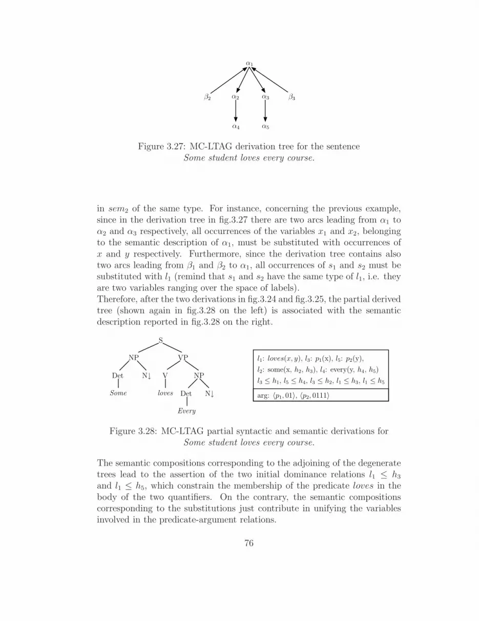
α1

β2 β3α2 α3

α4 α5

Figure 3.27: MC-LTAG derivation tree for the sentenceSome student loves every course.

in sem2 of the same type. For instance, concerning the previous example,since in the derivation tree in fig.3.27 there are two arcs leading from α1 toα2 and α3 respectively, all occurrences of the variables x1 and x2, belongingto the semantic description of α1, must be substituted with occurrences ofx and y respectively. Furthermore, since the derivation tree contains alsotwo arcs leading from β1 and β2 to α1, all occurrences of s1 and s2 must besubstituted with l1 (remind that s1 and s2 have the same type of l1, i.e. theyare two variables ranging over the space of labels).Therefore, after the two derivations in fig.3.24 and fig.3.25, the partial derivedtree (shown again in fig.3.28 on the left) is associated with the semanticdescription reported in fig.3.28 on the right.

VP

V

loves

S

NP

N↓Det

Every

NP

N↓Det

Some

l2: some(x, h2, h3), l4: every(y, h4, h5)

arg: 〈p1, 01〉, 〈p2, 0111〉

l1: loves(x, y), l3: p1(x), l5: p2(y),

l3 ≤ h1, l5 ≤ h4, l3 ≤ h2, l1 ≤ h3, l1 ≤ h5

Figure 3.28: MC-LTAG partial syntactic and semantic derivations forSome student loves every course.

The semantic compositions corresponding to the adjoining of the degeneratetrees lead to the assertion of the two initial dominance relations l1 ≤ h3

and l1 ≤ h5, which constrain the membership of the predicate loves in thebody of the two quantifiers. On the contrary, the semantic compositionscorresponding to the substitutions just contribute in unifying the variablesinvolved in the predicate-argument relations.

76

Finally, the fully underspecified representation obtained by adding the ele-mentary semantic descriptions of student and course to the one shown infig.3.28, is reported in fig.3.29 on the right. The two final derivation stepscause the substitution of p1 and p2 with the predicates student and course.

VP

V

loves

S

NP

Det

Every

NP

NDet

Some

l2: some(x, h2, h3), l4: every(y, h4, h5)

l1: loves(x, y), l3: student(x), l5: course(y),

l3 ≤ h1, l5 ≤ h4, l3 ≤ h2, l1 ≤ h3, l1 ≤ h5

student N

course

Figure 3.29: MC-LTAG syntactic and semantic derivations forSome student loves every course.

To summarize, the approach of [Joshi and Kallmeyer, 2003] defines a typeof compositional semantics, with respect to a constraint based approach, interms of the LTAG derivation tree which, as said above, is a kind of Depen-dency Tree. Therefore, this syntax-semantics interface gets the same resultsof the XDG one, but it preserves all other linguistic and mathematical ben-efits of LTAG. However, in order to manage both the predicate-argumentrelations and the initial scope constraints, it is necessary to use MC-LTAGrather than LTAG, in order to associate with a quantifier two elementary ob-jects, one devoted to the predicate-argument structure and one to the scopeone.Returning to the underspecified formalisms based on dominance constraints,the construction of an interface with a strictly generative grammar tendsto result in a more rigid framework. For example, in [Bos, 2004] an inter-face is proposed between UDRT and a generic phrase structure grammar,each entry in the lexicon is paired up with a λ-abstractions on a UDRTstructure, which specifies both predicate-argument relations and initial scopeconstraints. Similarly to what happens in the Montagovian tradition, therewriting rules of the grammar are associated with λ-functional applicationsmerging a pair of UDRTs into a more complex structure. For example,fig.3.30 shows the lexical entries for the words a, woman and smokes, whilethree rules of the grammar are reported in (36)8.In the lexical entries, the operator “;”, called “the merge operator”, is im-

8Actually, the grammar presented in [Bos, 2004] enables the representation of the tenseinformation via particular UDRT, labels and holes. Nevertheless, for simplicity, in figg.3.30and 3.31 they are omitted.

77

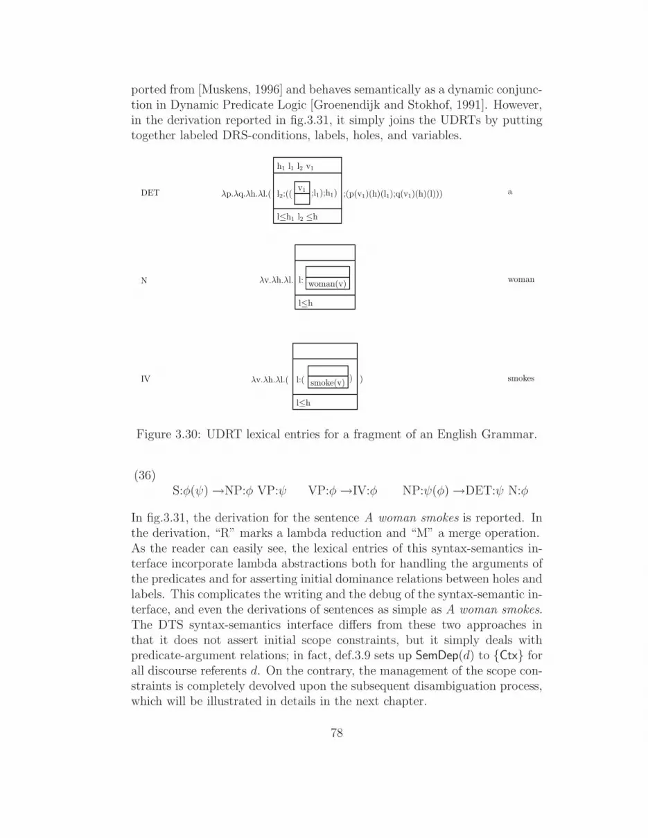
ported from [Muskens, 1996] and behaves semantically as a dynamic conjunc-tion in Dynamic Predicate Logic [Groenendijk and Stokhof, 1991]. However,in the derivation reported in fig.3.31, it simply joins the UDRTs by puttingtogether labeled DRS-conditions, labels, holes, and variables.

λp.λq.λh.λl.(

h1 l1 l2 v1

v1l2:(( ;l1);h1) ;(p(v1)(h)(l1);q(v1)(h)(l)))DET a

λv.λh.λl. woman(v)l:

l≤h

N woman

λv.λh.λl.( l:( )IV smokessmoke(v)

l≤h

)

l≤h1 l2 ≤h

Figure 3.30: UDRT lexical entries for a fragment of an English Grammar.

(36)S:φ(ψ) →NP:φ VP:ψ VP:φ→IV:φ NP:ψ(φ) →DET:ψ N:φ

In fig.3.31, the derivation for the sentence A woman smokes is reported. Inthe derivation, “R” marks a lambda reduction and “M” a merge operation.As the reader can easily see, the lexical entries of this syntax-semantics in-terface incorporate lambda abstractions both for handling the arguments ofthe predicates and for asserting initial dominance relations between holes andlabels. This complicates the writing and the debug of the syntax-semantic in-terface, and even the derivations of sentences as simple as A woman smokes.The DTS syntax-semantics interface differs from these two approaches inthat it does not assert initial scope constraints, but it simply deals withpredicate-argument relations; in fact, def.3.9 sets up SemDep(d) to Ctx forall discourse referents d. On the contrary, the management of the scope con-straints is completely devolved upon the subsequent disambiguation process,which will be illustrated in details in the next chapter.

78

λp.λq.λh.λl.(

h1 l1 l2 v1

v1l2:(( ;l1);h1) ;(p(v1)(h)(l1);q(v1)(h)(l)))a(woman)≡ λv.λh.λl. woman(v)l:

l≤h

( )

=R

λq.λh.λl.( ;( λv.λh.λl.woman(v)l:

l≤h

(v1)(h)(l1);q(v1)(h)(l)))

=R

λq.λh.λl.( ;( woman(v1)l1:

l1 ≤h

;q(v1)(h)(l)))

a woman (smokes)≡ λq.λh.λl.(

h1 l1 l2 v1

v1l2:(( ;l1);h1) ;( woman(v1)

l1:

l1 ≤h

;q(v1)(h)(l))) λv.λh.λl.(( )

=R

λh.λl.( ;( woman(v1)l1:

l1 ≤h

; λv.λh.λl.( ) (v1)(h)(l)))

=R

λh.λl.( ;( woman(v1)l1:

l1 ≤h

; )l:( smoke(v1)

l≤h

=M

λh.λl.(

h1 l1 l2 v1

v1l2:(( ;l1);h1) woman(v1)

l1:

l≤h1 l2 ≤h l1 ≤h l≤h

l:( )smoke(v)

l≤h

)

l:( )smoke(v)

l≤h

)

l:(smoke(v1)

)

l≤h1 l2 ≤h

l≤h1 l2 ≤h

h1 l1 l2 v1

v1l2:(( ;l1);h1)

l≤h1 l2 ≤h

h1 l1 l2 v1

v1l2:(( ;l1);h1)

l≤h1 l2 ≤h

h1 l1 l2 v1

v1l2:(( ;l1);h1)

l≤h1 l2 ≤h

h1 l1 l2 v1

v1l2:(( ;l1);h1)

l≤h1 l2 ≤h

Figure 3.31: UDRT derivation for the sentence.A woman smokes.

79

In this respect, the DTS syntax-semantics interface is closer to the onesobtained from enumerative approaches, such as QLF. As I discussed inchapter 1, these are basically simpler than the syntax-semantic interfacesof constraint-based formalisms.

3.5 Summary

In this chapter, the relationship between Dependency Tree Semantics and aDependency Grammar has been shown. In particular, I defined formally howit is possible to obtain a fully underspecified Scoped Dependency Graph bymeans of two principles: a Linking Principle acting on a set of if-then rules inorder to extract the Predicate-argument relations stored in the DependencyTree, and a Restriction Principle setting the values of the function restr onthe basis of the subtrees of dependencies, , i.e. discriminating between thepredicate-argument relations and identifying a set of involved entities (re-strictions) out of those constituting the main assertion (body).This interface is basically simpler than the syntax-semantics interfaces pro-posed in the literature for those approaches referred to in this thesis bythe term “constraint-based approaches”. In particular, DTS performs lesswork in that it does not assert initial scope constraints, but only deals withpredicate-argument relations.

80

Chapter 4

Scope disambiguation in DTS

In the previous chapter it has been shown how an initial Scoped DependencyGraph can be obtained from a Dependency Tree by means of a simple if-thenrules system. Such a system does not assert initial scope constraints as itis done in other constraint-based approaches; therefore, the obtained ScopedDependency Graph is fully underspecified, i.e. all its discourse referents arelinked to Ctx via a SemDep arc.This chapter shows how the next step, i.e. the Scope Disambiguation process,is carried out. Scope disambiguation will be realized in a monotonic, incre-mental fashion. Section 4.1 sums up the reasons why such a kind of scopedisambiguation is needed, already discussed in chapter 1, and distinguishesbetween partial and full disambiguations. This will lead to some changesin the formalization shown in section 2.4; a new formalization will be thenpresented in subsection 4.2.1.The rest of the chapter will be devoted to illustrate constraints on SemDeparcs for reducing the number of available readings to those admitted in Natu-ral Language. In particular, section 4.3 presents the constraints arising fromNested Quantification, section 4.3.2 focuses on logical redundancy, while sec-tion 4.3.3 briefly discusses, without going into details, which other furtherconstraints could be needed.A comparison with a recent approach ([Joshi et al., 2003]), implementing asimilar set of constraints, concludes the chapter.

4.1 Monotonic Disambiguation

In chapter 1, the two main approaches to underspecification, that I calledenumerative and constraint-based approaches, have been presented. Further-more, it has been pointed out that the main advantage featured by the latter

81

with respect to the former is the possibility of realizing monotonic disam-biguation, i.e. to specify partial scope constraints one by one, rather than allfinal ones in a whole.The claim that a formalism as QLF, which aims to (totally or partially)instantiate the final scoping relations on quantifiers, intrinsically preventspartial disambiguations has been discussed by [Reyle, 1996] in the light ofexamples as

(37) Everyxbody believed that many ay problem about the environmentpreoccupied mostz politicians.

Since quantifiers are clause bounded, Many ay and Mostz must have bothnarrow scope with respect to Everyx (in symbols, it must hold that Manyay ≤ Everyx and Mostz ≤ Everyx). However, the sentence does not provideenough information to establish also the relative scope between Many ay andMostz: this relative scope has to remain underspecified.In QLF it is impossible to describe this partial scoping; in fact, in QLF,disambiguation is performed by incrementally instantiating the final linearsequence of scope relations on involved quantifiers. For example, concerningsentence (37), we could start the disambiguation process by instantiating thepartial sequence

- 〈Many ay, Everyx〉

asserting that Many ay ≤ Everyx; at this point, we can add Mostz to thispartial sequence and obtain one of the two following

- 〈Many ay,Mostz, Everyx〉

- 〈Mostz,Many ay, Everyx〉

but this amounts to establishing already one of the two final scopings

- Everyx ≤ Many ay ≤Mostz

- Everyx ≤ Mostz ≤Many ay

whereas we cannot specify a weaker constraint Mostz ≤ Everyx, and leaveunderspecified the relative scope between Mostz and Many ay.On the contrary, this may be easily handled in constraint-based approachesas Hole Semantics or UDRT, since they perform the disambiguation by (in-crementally) asserting dominance relations between involved quantifier. Eachof these dominance relations expresses a weak scope constraint. Then, oncethat the disambiguation is completely achieved, i.e. it is not possible to add

82

further dominance relations, partial scope constraints can be “frozen” intofinal ones via some formal device.For example, in the Hole Semantics representation of (37), reported below

(38)

l1:Everyx(h11, h12), l2:Many ay(h21, h22),

l3:Mostz(h31, h32), l4:person(x), l6:politician(z),

l5:env−problem(y), l7:believe(x, h7), l8:preocc(y, z)

l4 ≤ h11, l5 ≤ h21, l6 ≤ h31, l7 ≤ h12

in order to specify the two partial constrains discussed above, we can add thetwo following dominance relations between h7 (the hole as argument of theintensional predicate believe) and the labels of quantifiers Mostz and Manyay.

- l2 ≤ h7

- l3 ≤ h7

Afterwards, when more contextual information will be available, we can as-sert an additional dominance relation specifying the scope between Mostzand Many ay; for example, if we find in the context that the sentence talksabout a different set of many a problem about the environment for each in-volved politician, the following dominance relation is simply added to theones above

- l2 ≤ h32

Now, it is not possible to add further dominance relations without obtain-ing an ill-formed representation; therefore, the partial scope constraints are“freeze” into final ones. In Hole Semantics, this is carried out by a pluggingfunction named P . P assigns a label to each hole in order to link the severalpieces and build a formula in the object language. Clearly, P has to satisfythe previously asserted dominance relations.Therefore, in the example under exam, the plugging function P assumes thefollowing values:

(39)

P (h0) = l1, P (h11) = l4, P (h12) = l7, P (h7) = l3, P (h21) = l5,

P (h22) = l8, P (h31) = l6, P (h32) = l2

leading to the formula

83

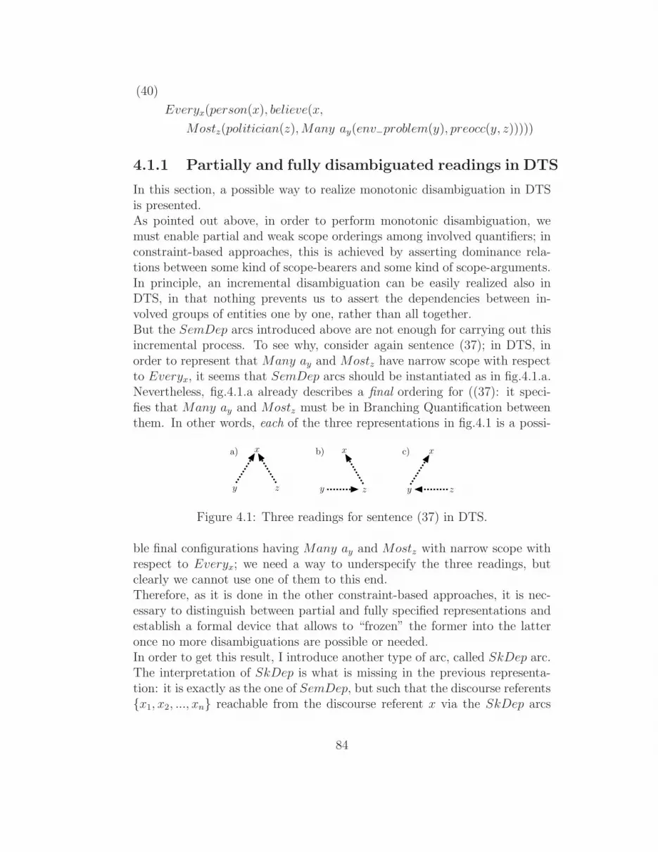
(40)

Everyx(person(x), believe(x,

Mostz(politician(z),Many ay(env−problem(y), preocc(y, z)))))

4.1.1 Partially and fully disambiguated readings in DTS

In this section, a possible way to realize monotonic disambiguation in DTSis presented.As pointed out above, in order to perform monotonic disambiguation, wemust enable partial and weak scope orderings among involved quantifiers; inconstraint-based approaches, this is achieved by asserting dominance rela-tions between some kind of scope-bearers and some kind of scope-arguments.In principle, an incremental disambiguation can be easily realized also inDTS, in that nothing prevents us to assert the dependencies between in-volved groups of entities one by one, rather than all together.But the SemDep arcs introduced above are not enough for carrying out thisincremental process. To see why, consider again sentence (37); in DTS, inorder to represent that Many ay and Mostz have narrow scope with respectto Everyx, it seems that SemDep arcs should be instantiated as in fig.4.1.a.Nevertheless, fig.4.1.a already describes a final ordering for ((37): it speci-fies that Many ay and Mostz must be in Branching Quantification betweenthem. In other words, each of the three representations in fig.4.1 is a possi-

x

zy

x

zy

x

zy

a) b) c)

Figure 4.1: Three readings for sentence (37) in DTS.

ble final configurations having Many ay and Mostz with narrow scope withrespect to Everyx; we need a way to underspecify the three readings, butclearly we cannot use one of them to this end.Therefore, as it is done in the other constraint-based approaches, it is nec-essary to distinguish between partial and fully specified representations andestablish a formal device that allows to “frozen” the former into the latteronce no more disambiguations are possible or needed.In order to get this result, I introduce another type of arc, called SkDep arc.The interpretation of SkDep is what is missing in the previous representa-tion: it is exactly as the one of SemDep, but such that the discourse referentsx1, x2, ..., xn reachable from the discourse referent x via the SkDep arcs

84

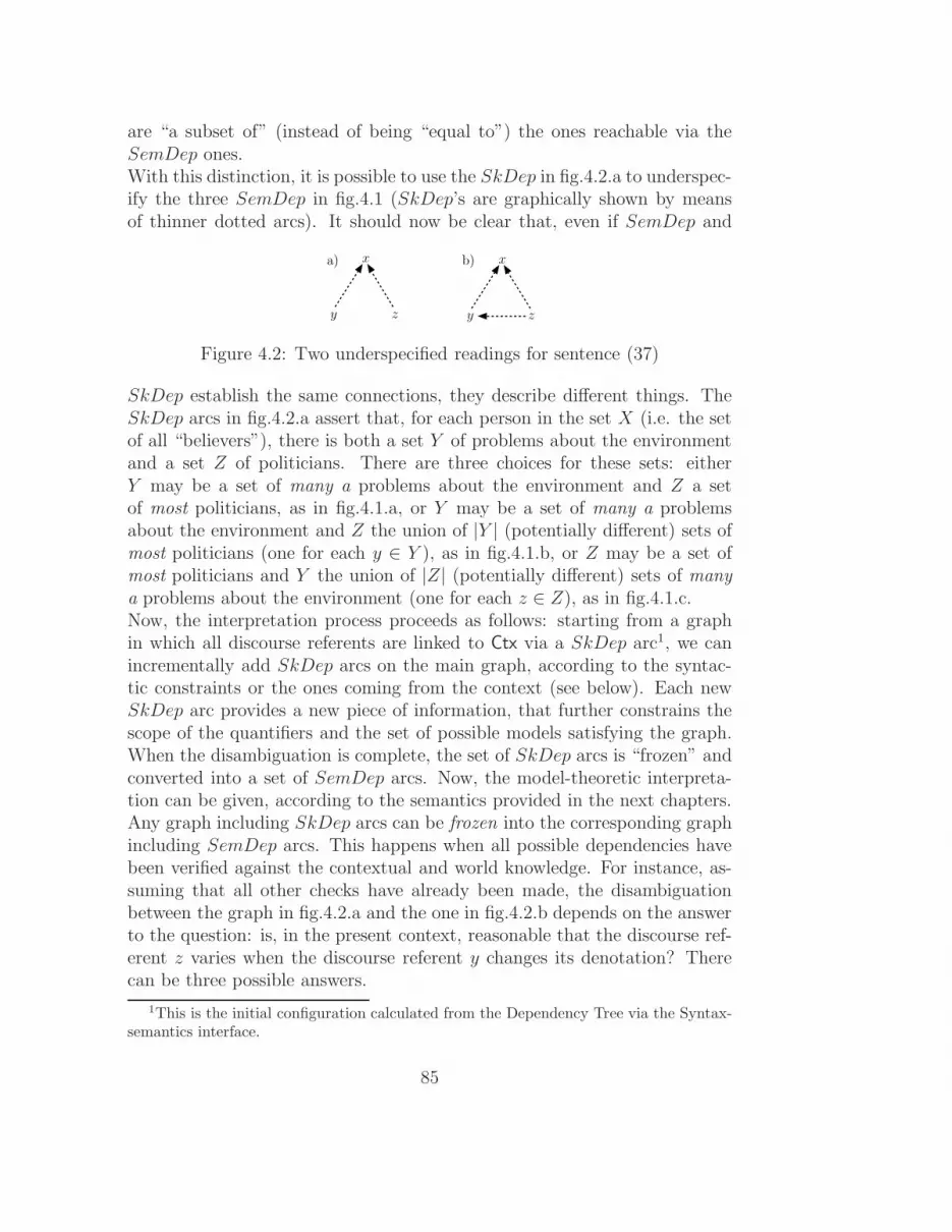
are “a subset of” (instead of being “equal to”) the ones reachable via theSemDep ones.With this distinction, it is possible to use the SkDep in fig.4.2.a to underspec-ify the three SemDep in fig.4.1 (SkDep’s are graphically shown by meansof thinner dotted arcs). It should now be clear that, even if SemDep and

x

zy

x

zy

a) b)

Figure 4.2: Two underspecified readings for sentence (37)

SkDep establish the same connections, they describe different things. TheSkDep arcs in fig.4.2.a assert that, for each person in the set X (i.e. the setof all “believers”), there is both a set Y of problems about the environmentand a set Z of politicians. There are three choices for these sets: eitherY may be a set of many a problems about the environment and Z a setof most politicians, as in fig.4.1.a, or Y may be a set of many a problemsabout the environment and Z the union of |Y | (potentially different) sets ofmost politicians (one for each y ∈ Y ), as in fig.4.1.b, or Z may be a set ofmost politicians and Y the union of |Z| (potentially different) sets of manya problems about the environment (one for each z ∈ Z), as in fig.4.1.c.Now, the interpretation process proceeds as follows: starting from a graphin which all discourse referents are linked to Ctx via a SkDep arc1, we canincrementally add SkDep arcs on the main graph, according to the syntac-tic constraints or the ones coming from the context (see below). Each newSkDep arc provides a new piece of information, that further constrains thescope of the quantifiers and the set of possible models satisfying the graph.When the disambiguation is complete, the set of SkDep arcs is “frozen” andconverted into a set of SemDep arcs. Now, the model-theoretic interpreta-tion can be given, according to the semantics provided in the next chapters.Any graph including SkDep arcs can be frozen into the corresponding graphincluding SemDep arcs. This happens when all possible dependencies havebeen verified against the contextual and world knowledge. For instance, as-suming that all other checks have already been made, the disambiguationbetween the graph in fig.4.2.a and the one in fig.4.2.b depends on the answerto the question: is, in the present context, reasonable that the discourse ref-erent z varies when the discourse referent y changes its denotation? Therecan be three possible answers.

1This is the initial configuration calculated from the Dependency Tree via the Syntax-semantics interface.

85

• Yes. In this case, the graph in fig.4.2.a is modified into the one fig.4.2.b.Then, this is frozen into the SemDep configuration in fig.4.1.c (as usual,the transitive arc from z to x is not shown).

• No. In this case, the graph in fig.4.2.a is frozen into the SemDepconfiguration in fig.4.1.a.

• Don’t know. In this case, the graph in fig.4.2.a is left unchanged, butno freezing is possible.

In the light of this, it is clear that the semantics of DTS has to be definedonly in terms of SemDep values, while a set of inference rules to performpartial reasoning in the underspecified representation (see [Reyle, 1993] and[Reyle, 1996] for a proposal of such a set in UDRT) has to be defined onlyin terms of SkDep’s values.

In the light of this, it is clear that the semantics of DTS has to be definedonly in terms of SemDep values, while a set of inference rules to performpartial reasoning in the underspecified representation (see [Reyle, 1993] and[Reyle, 1996] for a proposal of such a set in UDRT) has to be defined onlyin terms of SkDep’s values.

4.2 World knowledge exploitation

This section briefly discusses how the disambiguation process may be carriedout in a semantic underspecified framework based on dependencies betweenquantifiers.The choice of the correct scope between quantifiers is notoriously hard, sinceit depends on the preferences grounded on the syntactic structure, on thecontextual world-knowledge, and on the topic\focus distinction. Althoughit is generally agreed that, among these factors, contextual knowledge is themost relevant in the choice of the correct scope (see [Kurtzman and MacDon-ald, 1993] and [Villalta, 2003] for a brief overview), in the literature thereare mainly proposals based on syntactic grounds only (see [Moran, 1988] forsuch a proposal in QLF).As it should be clear at this point, DTS disambiguation machinery is sub-stantially different from the MRS\UDRT\CLLS dominance relations, thatsimply assert the plugging of a subformula into another one, i.e. that act onthe syntax of a (basically independent) object logical language.SkDep arcs denote semantic dependencies between involved groups of enti-ties, that can be directly related to the semantic dependencies arising from

86

a knowledge repository, such as a formal ontology.For instance, consider the representation of the following sentence, reportedin fig.4.3.

(41)

There were always twox students of mine in oney of the first tenz placesof thew classification of eachv exam held in thisk school.

x

2be−in’ y

Restr(x)

Quant(y)= ∃

Quant(x)= Two

2

w

classification−of’ place−of’

1

vmyStud’

1

exam’

1

1

x

1

Quant(z)= TheF10

1 2 z

1

held−in’

k2

school’myStud’

Restr(y)

11 2

∈

zy

Restr(z)

wz

place−of’

v

classification−of’

Restr(v)

1 21

exam’ held−in’

v

Restr(k)

1

k

school’

Quant(v)= ∀

Quant(w)= The Quant(k)= The

1

2

1

k

Flat Dependency Graph

11 2

Restr(w)

1 2

w

∈

Figure 4.3: USDG of sentence (41).

In order to disambiguate this representation, the correct dependencies be-tween discourse referents and Ctx have to be inserted.Each discourse referent marks a group of entities involved in the situationexpressed by the sentence. The function restr provides a partial “description”of these groups in that, as pointed out above, restr(x) collects all predicate-argument relations, carried by the sentence, that act to restrict the set ofentities referred by x. For example, concerning the USDG in fig.4.3, it iseasy to see that

- x refers to a set of students.

- y refers to a subset of the set referred by z.

- z refers to a set of places belonging to some elements in the set referredby w.

- w refers to a set of classifications of some elements in the set referredby v.

87

- v refers to a set of exams held in some elements in the set referred byk.

- k refers to a set of schools.

Clearly, these descriptions are “partial” in that they do not specify whichand how many elements of a certain group of entities participate, with anelement of another group, in a binary predication relating the two groups;for example, we just know that, in any interpretation, each classificationin w is the classification of at least one exam in v, but we do not knowwhich and how many are these exams, i.e. the precise pairs constituting theclassification−of

′’s extension.Clearly, this missing information cannot be found in the UnderspecifiedScoped Dependency Graph in that it depends on pragmatics; the goal of thesemantic disambiguation process is precisely the one of adding constraintson possible models in order to reduce the set of available ones and help thepragmatic analyzer to identify, as much as possible, the entities involved inthe predications.The disambiguation process, starting from these partial descriptions, can in-teract with an ontology in order to derive that the semantics of the wordsstudent and school is hightly related, despite the fact that, both in the ScopedDependency Graph, and in the Dependency Tree and in the words order,there is an high “distance” between these words. In other words, it canderive that there is a high probability that, in the preferred reading of thesentence, a semantic dependency occurs between x and k.Nevertheless, it must be stressed that the world-knowledge, in most cases,can indicate just the preferred paths of dependencies, but not their directions;for example, it can suggest the existence of a SkDep arc between x and k,butnot if this arc leads from x to k rather than from k to x.Instead, the direction of the arcs are suggested by other factors as, for ex-ample, preferences induced by the use of particular quantifiers or linguisticexpressions, topic\focus distinction, prosody, and so on.To summarize, the insertion of certain SkDep arcs in the representation de-pend on the following question

Which involved groups of entities, i.e. which discourse referents, candepend on each other?

It is apparent that restr(v) makes explicit the fact that the connection be-tween exams and school concerns the fact that the exams are held in theschool, so that any known functional constraint existing between exams andschools can immediately be checked to set up the semantic dependencies.

88

In this case, the actual choice (the exams depend on the school) is due tothe fact that the school is introduced by the demonstrative “this” (so it is aconstant and must depend only on Ctx); consequently, the exams (v) dependon the school (k). On the contrary, for the predicate classification−of ’ thisis not the case: the decision criterion is that given a classification, the set ofplaces are determined: w depends on v. Analogously, we could easily findout that

• Each school has its own set of students [x depends on k].

• Each exam has its own classification [w depends on v].

• A given individual cannot appear in two places in a classification [ydepends on x].

Clearly, these dependencies produce the SkDep arcs shown in fig.4.4.a.

x

Ctx

y

w

z

k

v

a) b) c)

x

Ctx

y

w

z

k

v

x

Ctx

y

w

z

k

v

Figure 4.4: Possible configuration of dependencies for the USDG in (4.3).

In fig.4.4.b, the SemDep arcs corresponding to the freezing of fig.4.4.a areshown. This SDG is true in those models in which “this school” is suchthat two particular students of mine enrolled in it (e.g. John and Jack)and the set S of exams held in it are such that for each e ∈ S, the set offirst ten places of the e’s classification contains both a place occupied byJohn and a place occupied by Jack. Clearly, this interpretation representsone of the available readings for (41). Another reading can be obtained bylinking x to w via SkDep2. The new SkDep obtained by this addition canthen be “frozen”. The resulting SDG, shown in fig.4.4.c, corresponds to aninterpretation analogous to the previous one, but where the two students ofmine may be different from classification to classification. Of course, otherpossible readings can be obtained by extending fig.4.4.a, but they are not

2A further link from x to v would lead to an equivalent reading, since it is assumedthat each exam has a single classification.

89

compatible with world knowledge, as the dependency of y from z, whichwould mean that a place in the classification (e.g. the third one) depends oneach of the ten places (there is a different “third” for each place).However, to summarize, I repeat that what matters is not the fact that inthis example one choice is better than the other, but that, given the DTS,it is immediately clear what checks must be performed in order to make achoice (though a check could return a “don’t know” answer).For most other underspecification formalisms it is a bit harder to find outthe relations to verify. This is due to the fact that predicates and variablesare scattered around in the representation. For instance, in Hole Semantics,the interaction between labels and holes makes difficult to determine thelocal effects (and, consequently, the decision criteria) of a given choice. Inparticular, while in DTS the predicate-argument relations constituting thequantifier restrictions, i.e. the subgraphs as values of the restr function,that are needed to determine which discourse referents depend on whichother ones, are fixed regardless the chosen interpretation, in Hole Semanticsdifferent choices on the dominance relations lead to different restrictions;moreover, each quantifier is associated to two holes, one for the body andone for the restriction. Therefore, the exploitation of world knowledge is inprinciple harder in Hole Semantics, in that it requires additional reasoningsteps to identify the predicate argument relations involved in the checks orto determine if a label has to be dominated by the hole associated with therestriction rather than the body of a certain quantifier.

4.2.1 Formalisation

This subsection formalizes the concept previously introduced. In particu-lar, the definitions presented in section 2.4 (and reported below to increasereadability) will be revised in order to distinguish two kinds of DTS wellformed structures: a partially disambiguated representation named Under-specified Scoped Dependency Graph (USDG), and a fully specified represen-tation named Scoped Dependency Graph (SDG); the only difference betweenthe two structures is the function used to specify (partial rather than final)scope constrains: SkDep rather than SemDep. An USDG can be convertedinto one of the SDGs it refers to3 by means of a “freezing” operation.Both structures are defined in terms of a third one, the Flat DependencyGraph (FDG), whose formal definition is the same presented in section 2.4

Definition 4.1. [Flat Dependency Graphs (FDG)]A Flat Dependency Graph is a tuple 〈N,L,A,Dom, f〉 s.t.:

3The one having the same semantic dependencies.

90

- N is a set of nodes n1, n2, . . . , nk.

- L is a set of labels l1, l2, . . ., lm; in all figures of the thesis,L≡1, 2.

- Dom ≡ pred ∪ D is a set domain objects: predicates and discoursereferents

- f is a function f : N 7→ Dom, specifying the node referent, i.e. thedomain object with which the node is associated. In the following,whenever f(n) ∈ X, I will informally say that node n is of type X,so that we can have nodes of type pred and nodes of type D.

- A is a set of arcs. An arc is a triple (ns, nd, l), where ns, nd ∈ N , ns

is of type pred, nd is of type D and l ∈ L.

Definition 4.2.[Underspecified Scoped DependencyGraph (USDG)]An Underspecified Scoped Dependency Graph is a tuple 〈Gf , Ctx, Q, quant,restr, SkDep〉 s.t.:

- Gf = 〈N,L,A,Dom, f〉 is an FDG.

- Ctx is a special element called “the context”.

- Q is a set of 2-place Mostowskian quantifiers (Mostowski [1957]) asevery, most, two, . . ..

- quant is a total function ND 7→ Q, where ND ⊆ N are the nodes oftype D.

- restr is a total function assigning to each d ∈ ND its restriction, whichis a subgraph of Gf .

- SkDep is a total function ND 7→ ℘(ND) ∪ Ctx

Definition 4.3.[Scoped Dependency Graph (SDG)]A SDG Gs is a tuple 〈Gf ,Ctx,Q, quant, restr, SemDep〉 s.t.

- Gf , Ctx, Q, quant and restr are defined as in def.4.2

- SemDep is a total function ND 7→ ℘(ND) ∪ Ctx

The next definitions concern the monotonic semantic disambiguation as de-scribed above; the former defines the way this disambiguation has to proceed,while the latter allows to “transform” an USDG into a corresponding SDG.

91

Definition 4.4.[Specification Relation]A USDG G1 〈Gf1,Ctx1,Q1, quant1, restr1, SkDep1〉 is a specification of theUSDG G2 〈Gf2,Ctx2,Q2, quant2, restr2, SkDep2〉 iff:

- Gf1 = Gf2, Ctx1 = Ctx2, Q1 = Q2, quant1 = quant2, restr1 = restr2

- ∀(n ∈ D)SkDep2(n) ⊆ SkDep1(n).

Definition 4.5.[Freezing]A SDG SG 〈SGf ,Ctx1,Q1, quant1, restr1, SemDep〉 is a freezing of the USDGUSG 〈USGf ,Ctx2,Q2, quant2, restr2, SkDep〉 iff:

- SGf = USGf , Ctx1 = Ctx2, Q1 = Q2, quant1 = quant2, restr1 = restr2

- ∀(n ∈ D)SemDep(n) = SkDep(n).

When d′ ∈ SkDep(d) or d′ ∈ SemDep(d), we say that d depends on d′. Iremind that the SemDep\SkDep arc introduced above is just a compactgraphical representation of the SemDep\SkDep function. If we take intoaccount the transitive closure of SemDep, i.e. SemDep∗, we have that n1

SemDep∗ n2 iff n2 ∈ SemDep(n1) (analogously for SkDep).

4.3 Constraints on SemDep arcs

The syntactic formalization of DTS still lacks an important ingredient.In the previous section, I pointed out that SkDep\SemDep arcs have todefine a partial order between discourse referents and Ctx, with Ctx as itsmaximal element; however, not all partial orders are allowed; therefore, it isnecessary to define a set of constraints that have to be satisfied by the twofunctions.There are several kinds of these constraints; this section does not present anexhaustive list of them but focuses on the ones triggered by Nested Quantifi-cation and Redundancy and briefly discusses which other factors are involvedin establishing further constraints.

4.3.1 Nested Quantification

As it is well known in the literature, in sentences featuring Nested Quantifi-cation, i.e. sentences in which a quantifier occurs in the syntactic restrictionof another quantifier, not all possible scopings between quantifiers are logi-cally available.For example, consider sentence (42), in which the quantifier ay is embed-ded into the syntactic restriction of the quantifier Everyx. The dependencies

92

depicted in the USDG below this sentence describe an unreasonable interpre-tation. In fact, it is awkward to take this sentence as describing a situationin which there is a fixed set of most representatives each of which saw everysample and such that there is a different company to which s\he belongs foreach sample s\he saw.These readings have been avoided in current approaches to underspecifica-tion by introducing constraints on the syntax of the formalism. For example,[Joshi et al., 2003] extends the LTAG semantics previously defined in [Joshiand Kallmeyer, 2003] by introducing a mechanism acting on quantifier setsto prevent them.

(42)

Everyx [representative of [ay company]] saw mostz samples.

Restr(x)

Quant(y)= ∃Quant(x)= ∀

Restr(z)Restr(y)

saw’

rep’

Quant(z)= Most

x

1 2

z

1

samp’

1

11 2

of’Ctx

rep’

x

1

y

y

comp’

1

z

samp’

1

11 2

of’

ycomp’ 1

In this section, similar constraints for DTS are introduced. Afterwards, theireffects will be compared with the ones obtained by [Joshi et al., 2003]. Theconstraints are given in terms of SkDep arcs, since SemDep are just a “freez-ing” of SkDep, in the sense explained above, so that all constraints on SkDeptransfer directly to their SemDep counterparts. The set of constraints is thefollowing:

93

Definition 4.6.[Constraints on SkDep function]

1. SkDep implements a partial order on discourse referents and Ctx, withCtx as its maximal element.

2. Let d be a discourse referent, and let R(d) be the closure of restr, i.e.the smallest set that contains d, and for which it holds that if d′ is inR(d) and d′′ occurs in the restriction of d′, then also d′′ ∈ R(d). Itmust hold that:

• If d1 ∈ R(d), d2 6∈ R(d), and d1 depends on d2, then also d dependson d2.

• If d1 ∈ R(d), d2 6∈ R(d), and d2 depends on d1, then also d dependson d1.

The set R(d) is the set of all discourse referents that contribute to the iden-tification of the set of individuals on which the assertion holds. Formally, itcan be calculated by starting from d and recursively applying the functionrestr. It must be recalled that restr (and its transitive closure R(d)) stronglydepends on the syntactic structure of the sentence and, in particular, on thepredicate-argument relations extracted from it. For instance, with respect tothe graph in (43), we have that R(x) = x, y, z.

(43) Two representatives of the students of the Piedmontese universitiesarrive.

rep’

x

1 21

arrive’

1

of’

Restr(x) Restr(z)

rep’

x

1

2

1

y

of’

1 1 1

Restr(y)

1

2

11 1

y

stud’

z

piem−univ’

z

Quant(y)= The

Quant(x)= Two

Quant(z)= The

in’y

21

in’

1

stud’

z

1

piem−univ’

Flat Dependency Graph

The first part of the second constraint above specifies that if a discoursereferent d1, which contributes (on the basis of syntactic information) to theidentification of d, semantically depends on another discourse referent d2,then also d depends (syntax notwithstanding) on d2. d may depend on d2

in two ways: directly (as in fig.4.5.a) or indirectly via d1 (as in fig.4.5.b).In the first case we obtain a Branching Quantifier reading, whereas in thesecond case, we obtain the so-called Inverse Linking reading (see [May and

94

Bale, 2002]).Analogously, the second part of the second constraint specifies that if d2

semantically depends on d1, then also d depends on d1. Again, this can beachieved in two ways (triggering a Branching Quantification or an InverseLinking respectively): directly (fig.4.6.a) or indirectly via d2 (fig.4.6.b).

d

d1

d2

R(d)

a) d

d1

d2

R(d)

b)

Figure 4.5: Allowed dependencies in DTS - 1

d

d1

d2

R(d)

a) d

d1

d2

R(d)

b)

Figure 4.6: Allowed dependencies in DTS - 2

An example of Inverse Linking (corresponding to fig.4.5.b) is reported in(fig.4.7.a). This structure describes a reading of the associated sentence inwhich there are two particular boys, e.g. John and Jack, each of which ate aportion of most courses of the menu (clearly, we have a different portion foreach course), but the set of most courses whose portion has been eaten byJohn may be different from the ones of Jack.Note that this is different from the readings triggered by the dependenciesin fig.4.7.b, in which the set of most courses is the same for both boys4.

(44) Twox boys ate [Ay portion of [Mostz courses]].

Restr(x)

Quant(y)= ∃

Quant(x)= Two

x

1

Restr(z)

111

ate’

boy’

Quant(z)= Most

x y

2 11 2

z

of’

1

portion’

1

course’

1

z

boy’ course’

11 2

z

of’

portion’

1

y

Restr(y)

4On the contrary, the set of eaten portions still remain different, i.e. again a portiondepends on a pair 〈boy, course〉.

95

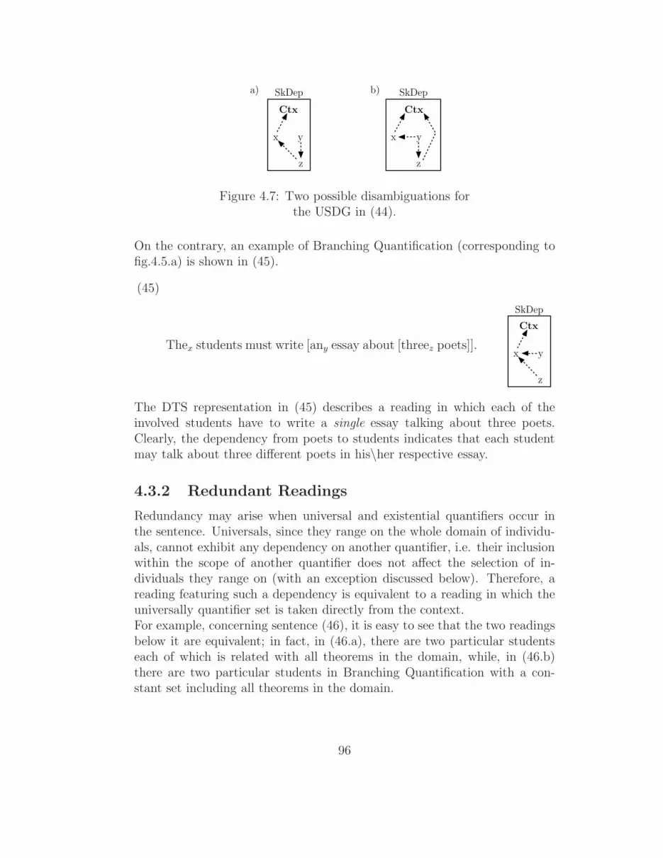
x y

Ctx

z

SkDepa)

x y

Ctx

z

b) SkDep

Figure 4.7: Two possible disambiguations forthe USDG in (44).

On the contrary, an example of Branching Quantification (corresponding tofig.4.5.a) is shown in (45).

(45)

Thex students must write [any essay about [threez poets]].x y

Ctx

z

SkDep

The DTS representation in (45) describes a reading in which each of theinvolved students have to write a single essay talking about three poets.Clearly, the dependency from poets to students indicates that each studentmay talk about three different poets in his\her respective essay.

4.3.2 Redundant Readings

Redundancy may arise when universal and existential quantifiers occur inthe sentence. Universals, since they range on the whole domain of individu-als, cannot exhibit any dependency on another quantifier, i.e. their inclusionwithin the scope of another quantifier does not affect the selection of in-dividuals they range on (with an exception discussed below). Therefore, areading featuring such a dependency is equivalent to a reading in which theuniversally quantifier set is taken directly from the context.For example, concerning sentence (46), it is easy to see that the two readingsbelow it are equivalent; in fact, in (46.a), there are two particular studentseach of which is related with all theorems in the domain, while, in (46.b)there are two particular students in Branching Quantification with a con-stant set including all theorems in the domain.

96

(46) Twox students study everyy theorem.

x y

Ctx

SkDepa)

x y

Ctx

SkDepb)

For analogous reasons, a dependency on an existential quantifier implies asingle selection for the internally quantified set of individuals; as in the pre-vious case, a reading containing such a dependency is equivalent to a readingin which the two quantifiers are in Branching Quantification between them.Concerning sentence (47), in the reading (47.a) there is a single student andthree theorems depending on him\her and this is clearly equivalent to (47.b),in which the three theorems do not depend on the involved student but aretaken from the context.

(47) Ax student studies threey theorem.

x y

Ctx

SkDepa)

x y

Ctx

SkDepb)

Anyway, there is an exception to the rule about universals. It concerns anuniversal acting as a modifier for another quantifier in its restriction. Forexample, in the case of (48), there are two possibilities, according to theintention of referring to ‘all friends of any participant’ or to ‘all friends of allparticipants’. In the first case, we enable the upper universal to be linkedvia a SemDep arc to its modifier as in (48.a). Clearly, the standard link toCtx is possible, so also the second case is accounted for (48.b).

(48) Every friend of every participant arrives.

x

y

Ctx

SemDepa)

x

y

Ctx

b)SemDep

97

Clearly, the exception arises also when the quantifier in the syntactic restric-tion of the universal one is not another universal quantifier, as in

(49) Every friend of two participants arrives.

x

y

Ctx

SemDepa)

x

y

Ctx

b)SemDep

x

y

Ctx

c)SemDep

x

However, contrary to the previous case, for (49) three readings are available:a reading (49.a) in which there are two particular participants and all personsthat are friends of at least one of them arrive, a reading (49.b) in which allcommon friends of two particular participants arrive, and a reading (49.c) inwhich there are two particular participants and all persons that are friendsof at least one of them arrive.Note that there is not a similar exception for existential quantifiers.The problem of the logical redundancy is not new in Underspecification; forexample, [Chaves, 2003] and [Koller and Thater, 2006] present two differentapproaches to solve it in Hole Semantics and CLLS respectively. In partic-ular, the former devises a strategy that allows to prevent, when a certainreading is produced, the generation of its equivalent ones. On the contrary,the method presented in the latter generates all the readings, but allows togroup them into classes of equivalence.In this thesis, I follow the first approach; this is done, in particular, by addingthe following constraints to the ones in def.4.6

Definition 4.7.[Constraints on SkDep to avoid redundancy]

1. If quant(d) = ∃, then for no discourse referent d′ holds that d ∈SkDep(d′).

2. If quant(d) = ∀ and d′ /∈ R(d), then d′ /∈ SkDep(d).

4.3.3 Additional constraints

The constraints introduced in the two previous sections are logical constraintsin the sense that they enable all logically possible readings, for which amodel-theoretic interpretation is provided (see next chapters). However, notall such readings are available also in Natural Language; hence, several other

98

constraints are needed in order to identify the subset of NL readings.In this subsection, I briefly indicate some of the main sources that set upsuch additional constraints.For example, there are linguistic island constraints as the one discussed aboveabout the sentence

(50)

Everyxbody believed that many ay problem about the environmentpreoccupied mostz politicians.

The island constraint under exam states that quantifiers Many a and Mostcannot take scope over Every; in DTS terms, this has to be realized byinserting suitable constraints that prevent dependencies from x to y or z.Another linguistic constraint concerns proper names, which are associated,as in DRT, to a discourse referent5. Since proper names are associated toconstant individuals, it is clear that their discourse referent cannot dependon other quantifiers but must always have wide scope, i.e. their SkDep’s valuehas to be set to the singleton Ctx.Analogous considerations hold for the discourse referents associated withdefinites, that can refer to individuals already introduced in the previoussentences, even if their behaviour is much more complicated in that they canbe also interpreted anaphorically, as in

(51)

Thex toy of everyy child is red.

In (51), discourse referent x can depend on y, i.e. the sentence can describea situation in which each child has his own toy.Then, as observed in [Hobbs and Shieber, 1987], §1.2., there are also severalextra-linguistic factors acting as “barriers” on the available NL interpreta-tions. For instance, it is impossible to interpreter the sentence

(52)

I’ve met ax child of everyy man in this room. [Hobbs and Shieber, 1987]

5If x is the discourse referent associated with a proper name N that denotes an indi-vidual α, restr(x) is the subgraph containing just the two nodes ια and x, linked by anarc with label 1 (i.e. x is the only argument of the unary predicate ια). Furthermore,quant(x) =Pn, where Pn is a dummy Mostowskian Generalized Quantifier that behaves asa universal quantifier, i.e. it ranges over all individuals satisfiying its restriction. However,since its restriction includes only the predicate ια, it just ranges over α.

99

with A having wide scope over Every, since this would describe a reading inwhich there is a child having several fathers, which in our society is absurd.Therefore, in this case, we need constraints to prevent a dependency from yto x.Finally, it must be pointed out that, besides constraints that prevent impos-sible readings, also criteria to choose the correct scope of quantifiers amongthose available are needed. This choice is notoriously hard, in that it de-pends on several factors among which the context, the preferences groundedin the syntactic structure, the topic\focus structure, etc. The analysis ofthese criteria goes beyond the scope of the thesis; the reader is addressed to,for example, [Moran, 1988], [Kurtzman and MacDonald, 1993] and [Villalta,2003].

4.4 Comparison with current constraint-based

approaches

We can now test the predictions of DTS on a well known example, i.e.

(53) Two politicians spy on someone from every city.[Larson, 1985]

In which it is assumed that the syntactic structure of (53) is the one wherethe PP “from every city” is included on the NP “on someone from everycity”. The USDG of (53) is reported in fig.4.8.

Restr(x)

Quant(y)= ∃

Quant(x)= Two

x

1

Restr(z)

111

spy−on’

politician’

Quant(z)= Most

x y

2 11 2

z

from’

1

person’

1

city’

1

z

11 2

z

1

y

Restr(y)

politician’

Flat Dependency Graph

city’

from’

person’

Figure 4.8: USDG for sentence (53)

Just two SemDep arcs can vary: the one exiting two, and the one exitingsome. The rules presented above (both the ones in def.4.6 and the ones con-cerning redundancy) allow for 6 interpretations, reported in fig.4.9.On the contrary, [Joshi et al., 2003], accepts just 4 readings for (53), ex-pressed as 2∀∃, 2∃∀, ∀∃2 and ∃∀2, while ∀2∃ and ∃2∀ are unacceptable.Their conclusions are based upon the results presented in [May, 1985] and

100

∃

Ctx

∀

2 ∃

Ctx

∀

2 ∃

Ctx

∀

2 ∃

Ctx

∀

2 ∃

Ctx

∀

2 ∃

Ctx

∀

2∃

Ctx

∀

2 ∃

Ctx

∀

2

Figure 4.9: The six disambiguated readings forTwo politicians spy on someone from every city.

[Larson, 1985], asserting that an NP behaves as a scope island, i.e. that anNP1 syntactically nested within another NP2 may take scope over (or be into scope of) other NPs only if this is done also NP2.Nevertheless, consider the following sentences; because of semantic prefer-ences, their preferred reading may correspond to the dependencies (in thesame order from left to right) described in fig.4.9.

(54) 1. Two boys, John and Jack, went (together) to a show about allrockstars.

2. Two boys, John and Jack, visited (together) a museum in everyregion of Italy.

3. Two boys, John and Jack, (each) bought an atlas with all countriesof the world.

4. Two soldiers guard a door of every building.

5. Two women were sitting in a central seat of each table.

6. Two boys, John and Jack, ate a portion of every course of themenu.

In [Joshi et al., 2003], the left one in fig.4.9 is not a valid interpretation be-cause “it may be banned due to general architectural reasons” (p.3). Thelogical representation they propose for this reading is ([Joshi et al., 2003],footnote 2):

∃y[ person′(y) ∧ 2x[politicians

′(x)∧

∀z[(city′(z) ∧ from′(y, z)) → spy′(x, y)]]]

And the comment is that “∃2∀ involves having ∃y separated from its restric-tor from(y, z), a configuration that should perhaps be banned ...”.However, as it will be shown afterwards in the thesis, it is possible to build a

101

Second Order Logics formula in which this separation does not arise6. Read-ing (54.5) is more complex, but it seems possible to express that situation,although [Joshi et al., 2003] sees it as unacceptable.

4.5 Summary

In this chapter, the disambiguation mechanism of Dependency Tree Seman-tics has been presented. In particular, in order to achieve disambiguationin an incremental fashion, two kinds of dependency arcs have been distin-guished: SkDep arcs, that denote partial dependencies, and SemDep arcs,that denote final dependencies. The disambiguation task starts from an Un-derspecified Scoped Dependency Graph, i.e. a fully ambiguous structureobtained from the Dependency Tree of the sentence via the syntax-semanticinterface presented in chapter 3. Then, SkDep arcs are added monotoni-cally, according to the constraints coming from the context; finally, when thedisambiguation task is finished, the set of SkDep arcs is frozen into a cor-responding set of SemDep arcs and the Underspecified Scoped DependencyGraph converted into a Scoped Dependency Graph, a fully unambiguousstructure that can be model-theoretically interpreted.The chapter presented also a set of constraints on SkDep insertion; theseconstraints reduce the set of available readings that can be produced by thedisambiguation task. In particular, it has been shown that some of themhave been asserted in order to prevent logically impossible readings whenthe sentence contains a syntactic Nested Quantification, while the other oneshave been asserted to prevent logical redundancy. Finally, it has been brieflyargued which other further constraints could be needed for reducing the num-ber of available readings to those admitted in Natural Language.

6Actually, it is possible to set up even a First Order Logic formula without such aseparation under exam; see [Lesmo and Robaldo, 2005].

102

Chapter 5

Models and BranchingQuantification

In this chapter, some of the most relevant theories of Branching Quantifi-cation (BQ) are presented. Their analysis provides a starting point fromwhich we can define the model-theoretic interpretation of Dependency TreeSemantics.However, it must be pointed out that Branching quantification has lost at-tention from the linguistic community in recent years and, to my knowledge,no relevant proposal to include them into a semantic underspecified formal-ism has ever been made; section 5.1 tries to outline the possible reasons ofthis, and to argue that, on the contrary, a formalism for representing NLmeaning should take BQ readings into account. Then, sections 5.3 and 5.4present two of the most relevant works on BQ: the one carried out by Bar-wise in [Barwise, 1979] and the one carried out by Sher in [Sher, 1990] and[Sher, 1997]. The work of Sher will then be modified and extended in orderto handle the truth conditions of DTS well formed structures.

5.1 Are BQ readings really available in NL?

As pointed out in the introduction, Branching Quantifier readings are notaccounted for in most recent semantic underspecified formalisms. One ofthe reasons of this, perhaps, is the idea that an explicit representation ofBQ readings is not strictly necessary, since they always imply some linearly-ordered ones1.

1The contents of this chapter are based on my personal communications with people ofthe community; however, to my knowledge, they have not been explicitly asserted in anyarticle, apart some hints in [Barwise, 1979].

103

In fact, consider again example (55)

(55) Two students study three theorems.

and its three possible disambiguations in DTS, shown in fig.5.1.

study’

stud’

x y

theor’

1 2

1 1

Ctx

study’

stud’

x y

theor’

1 2

1 1

Ctx

study’

stud’

x y

theor’

1 2

1 1

Ctxa) b) c)

Figure 5.1: The three disambiguations available in DTS for sentence (55)

It is easy to check that the set of models accepted by the BQ reading (fig.5.1on the right) is the intersection of the sets of models accepted by the othertwo.In fact, a reading where there are two specific students that study three giventheorems implies both that each of the students studies “some” three theo-rems and that each of the theorems is studied by “some” two students: thefact that the three theorems\two students are the same could be seen justas a pragmatic specification concerning the dynamics of the dialogue.Therefore, during the model-theoretic interpretation of fig.5.1.a, we can sim-ply take an interpretation function which assigns the same three theoremsto both students obtaining, in this way, the same truth-conditions of thereading in fig.5.1.c.I disagree with this general supposition and I believe it is logically, linguisti-cally and methodologically non motivated.Concerning its logical inadequacy, I will show in section 5.4 that in the logicsdeveloped by Sher, that I will take as starting point for defining the model-theoretic interpretation of Dependency Tree Semantics, a BQ reading doesnot always entail its linear counterparts.Nevertheless, even if Sher’s results may be considered acceptable from a logi-cal point of view, the debate about the actual availability of the BQ readingsin NL still remains open; in fact, the logical adequacy of Sher’s logics doesnot prove the actual existence of BQ interpretations in natural language.In other words, Sher’s theory could be too expressive for representing NLmeaning.However, not only BQ interpretations do actually occur in NL, but theyare rather widespread in human everyday life, as is shown by the linguisticexamples as the ones shown in section 2.2, reported below

104

(56) a. Two students, John and Jack, study three theorems: the first threeof the book.

b. Two friends of mine went to three concerts with my sister.

c. Two students of mine have seen three drug dealers in front of theschool.

As previously noted, in (56.a), the involved students and theorems are explic-itly mentioned in two appositions, while in (56.b) the prepositional modifierwith my sister favors an interpretation in which three persons, two friends ofmine and my sister, went together to three same concerts.However, it may be argued that world knowledge is the main factor that cansuggest a BQ reading; in fact, in (56.c), world knowledge seems to renderthe reading in which two students have seen the same three drug dealers themost salient.As final complex example concerning world knowledge, consider a class ofstudents on the last day of the school-year. Imagine the students try to getsome information about their success\failure from one of their teacher viasome strategical questions. Then, suppose the teacher answers as follow

(57) I can only give you bad news:

The director suggested the failure of two students (of this class) to mostof the teachers.

Clearly, in this situation, the teacher is saying that the director has two spe-cific persons in mind and suggested their respective failure to any teacherhe contacted in some way (such that the sum of these teachers are “mostteachers”). Again, a branching quantification between the quantifiers twoand most is preferred.So, it is possible to conclude that BQ readings acquire linguistic valency whensentences are evaluated with respect to a broader context. In other words,even if it may seem difficult to interpreter a sentence taken in isolation viaa BQ reading, in real cases it is quite common that the speaker intends torefer to fixed sets of involved entities.Finally, it seems the rejection of BQ as autonomous readings is also method-ologically incoherent. In fact, BQ readings are not the only interpretationswhich are special cases of other ones. This is rather common also in sentencesincluding universal or existential quantifiers. For instance, it is well knownthat, in (58), the linear reading in which Two has wide scope with respectto Every is a special case of the one in which it has narrow scope.

(58) Every man loves two women.

105

Nevertheless, these two readings are commonly considered as two distinct in-terpretations of the sentence. This consideration leads to conclude that it ishard to tell which is the correct level of specificity; in principle, it is not clearwhy we should keep apart two non-BQ readings, even if none of them im-plies the other! Since a BQ reading can be used to convey both of them, andonly the context can tell them apart, the same line of reasoning could leadto the conclusion that the unique reading of a sentence is its underspecifiedlogical counterpart, leaving to pragmatics the task to choose the “intended”model. Hence, it seems that the reason why current semantic underspecifiedformalisms do not take BQ readings into account is simply mirroring whatis done in standard logics, not avoiding readings which are special cases ofother ones.In the light of this, I find methodologically more coherent a view as the one of[Kempson and Cormak, 1981], in which both the linear and the BQ readingsare accepted, but it is argued that they are not cases of semantic ambiguity:they all concern vagueness.Finally, in the criticisms about methodological coherence, an account on cu-mulativity should also be included.In fact, as argued in [Sher, 1990], cumulative readings simply arise from an-other type of branching quantification. In particular, Sher talks about Com-plex Dependence for referring to what it is commonly assumed for branchingquantification and Independence for referring to what it is commonly assumedfor Cumulativity (see section 5.4.1). Complex dependence and Independenceare the two extremes of the whole range of possible NL non-linear quantifi-cations.Contrary to “standard” branching quantification, i.e. Sher’s Complex de-pendence, the actual existence of cumulative readings in NL has been widelyaccepted by the linguistic community. However, they received little attentionin Underspecification: to my knowledge, the only two attempts for takinginto account cumulative readings in an underspecified formalism (UDRT) are[Reyle, 1996] and, recently, [Chaves, 2005].In fact, for handling cumulative readings, as well as other types of branch-ing quantification, in a strictly linear framework, it is necessary to introducesome complex and unnatural mechanisms2. On the contrary, as it will beshown, DTS enables cumulative readings in a straightforward fashion, sinceit considers partial orderings on quantifiers as natural as linear ones.To conclude, what is really important for a semantic formalism is the abilityto restrict as much as possible the set of possible models in which the sen-tence is true while it does not matter if this set is also included in the set

2For instance, [Reyle, 1996] uses of polyadic quantifications.

106

of models satisfying another reading. Therefore, since NL provides ways toidentify a BQ reading, it seems that there is no reason for disregarding themin an NL semantic representation.

5.2 (Mostowskian) Generalized Quantifiers

This section briefly introduces the concept of Generalized Quantifier, used inthe logical theories on Branching Quantification illustrated below.As already said, FOL does not suffice to represent NL meaning. In par-ticular, it is necessary to introduce, in the logics, Mostowskian GeneralizedQuantifiers ([Mostowski, 1957]).Contrary to the two standard quantifiers, i.e. ∃ and ∀, which only allow tomake assertions for at least one or all individuals in a domain A, by means ofMostowskian Generalized Quantifiers it is possible to make these assertionsfor any subset of individuals in A.In other words, in standard First Order Logics, we can assert, for example,that at least one individual in A is red (59.a) or that all individuals in A arered (59.b).

(59) a. ∃x[Red(x)]

b. ∀x[Red(x)]

On the contrary, by using Mostowskian Generalized Quantifiers it is pos-sible to assert the “red” property for More than half, Almost all, No, etc.,individuals in A (see (60.a-c))

(60) a. MTHx[Red(x)]

b. ∼∀x[Red(x)]

c. Nox[Red(x)]

In (60), MTH , ∼∀ and No are Mostowskian Generalized Quantifiers. A(1-place) Mostowskian Generalized Quantifier Q is formally defined as follow

Definition 5.1. [Syntax of 1-place Mostowskian Quantifiers]A 1-place Mostowskian Quantifier is a symbol Q such that, if x is an indi-vidual variable, and Φ is a formula, then Qx(Φ) is also a formula.

Definition 5.2. [Semantics of 1-place Mostowskian Quantifiers]A 1-place Mostowskian Quantifier Q denotes, in every modelM with universeA, a function q from ℘(A) to T, F3. Furthermore, if there are two models

3℘(A) is the power set of A, that is, the set of all subsets of A; T, F is the set oftruth-values: T = true and F = false.

107

M1, M2 with universe A1, A2 respectively and two sets B1, B2 such that B1 ⊆A1 and B2 ⊆ A2 and the two structures (B1, A1), (B2, A2) are isomorphic,then q(B1) = q(B2).

MGQs are cardinality quantifiers since q(B) only depends on the cardinalitiesof B and A \ B (the complement of B in the domain A). The 1-placeMostowskian Generalized Quantifiers used in (60) are defined as4

- ‖MTHx(P (x))‖M = true iff | ‖P‖M | > 1

2∗ |A|

- ‖ ∼∀x(P (x))‖M = true iff α ∗ |A| < | ‖P‖M |

- ‖Nox(P (x))‖M = true iff | ‖P‖M | = 0

Of course, we can express in this form the two standard quantifiers too

- ‖∃x(P (x))‖M = true iff | ‖P‖M | ≥ 1

- ‖∀x(P (x))‖M = true iff | ‖P‖M | = |A|

The use of 1-place Generalized Quantifiers increases the expressive power ofstandard First Order Logics, but not enough to represent the meaning of anyNatural Language quantifier.A further step can be made by introducing 2-place Mostowskian GeneralizedQuantifiers. These quantifiers have two sets as argument and denote a truth-value depending on the ratio between the cardinalities of these sets. Formally:

Definition 5.3. [Syntax of 2-place Mostowskian Quantifiers]A 2-place Mostowskian Quantifier is a symbol Q such that, if x is an indi-vidual variable, and Ψ, Φ are formulae, then Qx(Ψ,Φ) is also a formula.

Definition 5.4. [Semantics of 2-place Mostowskian Quantifiers]A 2-place Mostowskian Quantifier Q denotes, in every model M with universeA, a function q taking in input two subsets B and C of A and returning atruth-value. Furthermore, if there are two models M1, M2 with universe A1,A2 respectively and four sets B1, B2, C1, C2 such that B1 ⊆ A1, C1 ⊆ A1,B2 ⊆ A2 and C2 ⊆ A2 and the two structures (A1, (B1, C1)), (A2, (B2, C2))are isomorphic, then q(B1, C1) = q(B2, C2).

q(B,C) only depends, apart from the order of the pair (B, C), on the car-dinalities of the sets (B ∩ C), (B \ C), (C \ B) and (A \ (B ∪ C)). Someexamples of 2-place Mostowskian Quantifier are

4α is a (contextually dependent) positive real number slightly smaller than 1.

108

- ‖MTHx(P1(x), P2(x))‖M = true iff

|(‖P1(x) ∧ P2(x)‖M)| > |(‖P1(x)‖

M)|/2

- ‖ ∼∀x(P1(x), P2(x))‖M = true iff

|(‖P1(x) ∧ P2(x)‖M)| = α ∗ |(‖P1(x)‖

M)|

- ‖Nox(P1(x), P2(x))‖M = true iff

|(‖P1(x) ∧ P2(x)‖M)| = 0

- ‖∀x(P1(x), P2(x))‖M = true iff

|(‖P1(x) ∧ ¬P2(x)‖M)| = 0

- ‖∃x(P1(x), P2(x))‖M = true iff

|(‖P1(x) ∧ P2(x)‖M)| ≥ 1

- ‖Exactly-nx(P1(x), P2(x))‖M = true iff

|(‖P1(x) ∧ P2(x)‖M)| = n

- ‖Mostx(P1(x), P2(x))‖M = true iff

|(‖P1(x) ∧ P2(x)‖M)| > |(‖P1(x) ∧ ¬P2(x)‖

M)|

- ‖Fewx(P1(x), P2(x))‖M = true iff

|(‖P1(x) ∧ P2(x)‖M)| < η

As stressed above, 2-place Mostowskian Generalized Quantifiers provide usenough expressivity to represent the meaning of sentences containing, in prin-ciple, any NL quantifier, whereas, as it will be shown in section 5.4.2 by using1-place Mostowskian Generalized Quantifiers, it is possible to represent themeaning of sentences containing only NL numerals.For example, consider the following sentence

(61) Most men walk.

The truth-conditions of (61) can be handled by the following formula, whichmakes use of the 2-place Generalized Quantifier Most, defined above

(62) Mostx(man′(x), walk′(x)).

109

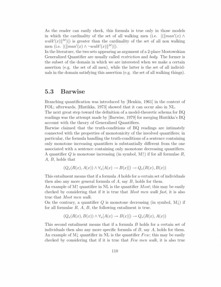
As the reader can easily check, this formula is true only in those modelsin which the cardinality of the set of all walking men (i.e. |(‖man′(x) ∧walk′(x)‖M)|) is greater than the cardinality of the set of all non walkingmen (i.e. |(‖man′(x) ∧ ¬walk′(x)‖M)|).In the literature, the two sets appearing as argument of a 2-place MostowskianGeneralized Quantifier are usually called restriction and body. The former isthe subset of the domain in which we are interested when we make a certainassertion (e.g. the set of all men), while the latter is the set of all individ-uals in the domain satisfying this assertion (e.g. the set of all walking things).

5.3 Barwise

Branching quantification was introduced by [Henkin, 1961] in the context ofFOL; afterwards, [Hintikka, 1973] showed that it can occur also in NL.The next great step toward the definition of a model-theoretic schema for BQreadings was the attempt made by [Barwise, 1979] for merging Hintikka’s BQaccount with the theory of Generalized Quantifiers.Barwise claimed that the truth-conditions of BQ readings are intimatelyconnected with the properties of monotonicity of the involved quantifiers; inparticular, the formula handling the truth-conditions of a sentence containingonly monotone increasing quantifiers is substantially different from the oneassociated with a sentence containing only monotone decreasing quantifiers.A quantifier Q is monotone increasing (in symbol, M↑) if for all formulae R,A, B, holds that

(Qx(R(x), A(x)) ∧ ∀x[A(x) → B(x)]) → Qx(R(x), B(x))

This entailment means that if a formula A holds for a certain set of individualsthen also any more general formula of A, say B, holds for them.An example of M↑ quantifier in NL is the quantifier Most; this may be easilychecked by considering that if it is true that Most men walk fast, it is alsotrue that Most men walk.On the contrary, a quantifier Q is monotone decreasing (in symbol, M↓) iffor all formulae R, A, B, the following entailment is true.

(Qx(R(x), B(x)) ∧ ∀x[A(x) → B(x)]) → Qx(R(x), A(x))

This second entailment means that if a formula B holds for a certain set ofindividuals then also any more specific formula of B, say A, holds for them.An example of M↓ quantifier in NL is the quantifier Few; this may be easilychecked by considering that if it is true that Few men walk, it is also true

110

that Few men walk fast.As pointed out above, Barwise proposes a model-theoretic schema of BQreading based on the monotonicity of the quantifiers occurring in the sen-tence. For example, for sentence (63) which contains only M↑ quantifiers

(63) Most of the dots and most of the stars are all connected by lines.

Barwise provides an analysis which produces the following interpretation

(64) ∃P1P2[ Mostx(dot(x), P1(x)) ∧Mosty(star(y), P2(y)) ∧

∀xy[(P1(x) ∧ P2(y)) → connected(x, y)] ]

Viceversa, when both quantifiers are M↓, as in the following sentence

(65) Few of the dots and few of the stars are all connected by lines.

We get

(66) ∃P1P2[ Fewx(dot(x), P1(x)) ∧ Fewy(star(y), P2(y)) ∧

∀xy[connected(x, y) → (P1(x) ∧ P2(y))] ]

Barwise proposes these formulae by analogy with respect to the behavior ofsingle quantifications, as the two sentences in (67)

(67) a. Most men walk.

b. Few men walk.

As observed by [Aczel, 1975], the formulae associated with these two sen-tences, namely Most(man(x), walk(x)) and Few(man(x), walk(x)), are re-spectively equivalent to the 2-order formulae in (68).

(68) a. ∃P [Mostx(man(x), P (x)) ∧ ∀x[P (x) → walk(x)]]

b. ∃P [Fewx(man(x), P (x)) ∧ ∀x[walk(x) → P (x)]]

Intuitively, in (68.a) we need to find at least one set P (the extension of P )5

that is large enough to be “most men”, but small enough to be containedin the extension of “walk” (see fig. 5.2). On the contrary, in (68.b) we needa set that is small enough to include only “few men”, but large enough toinclude all walking things (see fig. 5.3)6.As pointed out above, Barwise’s intuition was that the model-theoretic in-terpretation of a BQ reading is simply obtained by “merging” the ones ofeach single quantification. Therefore, the truth conditions of sentences (63)and (65) are respectively expressed by (64) and (66), reported in again (69)for simplicity.

5In the following, if A is a predicate, I will denote with A its extension.6In these figures, “P?” indicate the impossibility to find a set P satisfying the require-

ments imposed by the formula.

111

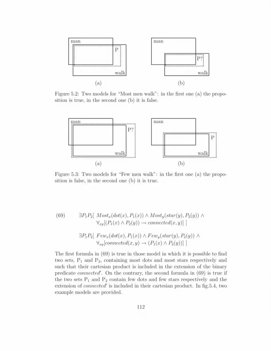
man

walk

P

(a)

man

walk

P?

(b)

Figure 5.2: Two models for “Most men walk”: in the first one (a) the propo-sition is true, in the second one (b) it is false.

man

walk

P?

(a)

man

walk

P

(b)

Figure 5.3: Two models for “Few men walk”: in the first one (a) the propo-sition is false, in the second one (b) it is true.

(69) ∃P1P2[ Mostx(dot(x), P1(x)) ∧Mosty(star(y), P2(y)) ∧

∀xy[(P1(x) ∧ P2(y)) → connected(x, y)] ]

∃P1P2[ Fewx(dot(x), P1(x)) ∧ Fewy(star(y), P2(y)) ∧

∀xy[connected(x, y) → (P1(x) ∧ P2(y))] ]

The first formula in (69) is true in those model in which it is possible to findtwo sets, P1 and P2, containing most dots and most stars respectively andsuch that their cartesian product is included in the extension of the binarypredicate connected′. On the contrary, the second formula in (69) is true ifthe two sets P1 and P2 contain few dots and few stars respectively and theextension of connected′ is included in their cartesian product. In fig.5.4, twoexample models are provided.

112

(a)

P1

*****

P2

(b)*****

P1 P2

Figure 5.4: Models for formulae in (69); the former is true in (a) and false in(b), while the opposite holds for the latter.

To conclude about Barwise proposal, it must be pointed out that rules aregiven only for BQ containing only M↑ quantifiers or only M↓. Instead, itis not specified how the truth-conditions should be handled for sentencesinvolving non-monotone quantifiers (as quantifiers Exactly two, which is nei-ther M↑ nor M↓).Finally, Barwise claimed that a Branching Quantification on quantifiers withmixed monotonicity makes no sense from a linguistic point of view and there-fore there is no need to identify a method to handle such cases.The claim that the mixing of increasing and decreasing quantifiers yieldssentences having no sense is supported by examples such as:

(70) Few of the boys in my class and most of the girls in your class have alldated each other.

5.4 Sher

The second relevant theory on Branching Quantification presented in thisthesis, and starting from which the model-theoretic interpretation of Depen-dency Tree Semantics will be defined, is the one of Sher (see [Sher, 1990] and[Sher, 1997]).Sher criticizes Barwise by asserting that his proposal is methodologically in-adequate; in fact, since the semantics of linearly ordered quantification isprovided independently of the monotonicity properties of the involved quan-tifiers or the actual availability of the sentence in NL, there seems to be

113

no methodological reason for imposing such further constraints in case ofpartially ordered (as in BQ) quantification. In other words, the assumedunavailability of NL sentences should not exclude that suitable formulae canbe built, for which a model-theoretic interpretation is provided.Moreover, a closer look at Barwise’s theory reveals that the schema he pro-poses for M↓ quantifiers indeed triggers a cumulative reading of the sentence(which, as it is well-know, could also occur with M↑ quantifiers).Let me analyze Barwise’s formulae in (69) in the light of Sher’s criticisms.While the formula proposed for M↑ quantifiers seems to work properly, theone for M↓ quantifiers presents some problems, as it is shown in the twomodels in fig.5.5. Taking sets P1 and P2 as indicated in fig.5.5.a, the formula

(a)

P1

*****

P2

(b)*****

P1

P2

Figure 5.5: Models for the second formula in (69); in (a), the formula is true,while, in (b), it is false.

turns out to be true: these sets contain few dots and few stars respectivelyand the extension of the predicate connected′ is included in their Cartesianproduct. Nevertheless, it has to be noted that the existence of these twoparticular sets should not be relevant for asserting the truth-conditions ofsentence (65) since the stars in P1 are not connected to all dots in P2.With respect to the model in fig.5.5.b, the formula evaluates to false since,in order to include all dots in the range of the predicate connected′, P2 hasto include at least three of the five dots, hence, the requirement that P2 justcontains few dots cannot be satisfied at the same time. Nevertheless, linguis-tic intuitions seems to predict the opposite result since the model actuallycontains a set of few stars (the two in P1) and a set of few dots (the twolower ones in P2) all connected each other.These counterintuitive results arise from an implicit condition imposed bythe formula on the two sets: it is required that P1 and P2 respectively con-tain the domain and the range of the predicate connected′.

114

In other words, the formula proposed by Barwise for M↓ quantifiers is equiv-alent to the following

(71) ∃P1P2[ Fewx(dot(x), P1(x)) ∧ Fewy(star(y), P2(y)) ∧

∀x[P1(x) → ∃y[connected(x, y)] ] ∧

∀y[P2(y) → ∃x[connected(x, y)] ] ]

As it is well-known, this is the formula usually associated to a cumulativereading. However, cumulative readings may occur also with M↑ quantifiers;for instance, consider

(72) The Japanese kamikaze hit more than 300 Usa battleships.

This formula is true iff there are two sets P1 and P2 including, respectively,all japanese kamikazes and more than 300 Usa battleships such that for eachkamikaze in P1 there is a battleship in P2 that has been hit by him and foreach battleship in P2 there is at least a kamikaze in P1 who hit it.To summarize, Sher concluded that the schema proposed by Barwise for M↓quantifiers does not represent a BQ reading, but a cumulative one, and maybe used also with M↑ quantifiers.Sher proposed to use in all cases the Barwise’s schema for M↑ quantifiersaugmented with a maximality condition on the involved sets.In particular, Sher expresses (67.1) as follows:

(73) ∃P [Mostx(man(x), P (x)) ∧ ∀x[P (x) → walk(x)]]∧

∀P ′[∀x[(P (x) → P ′(x)) ∧ (P ′(x) → walk(x))] →

∀x[P′(x) → P (x)] ]

The added part, i.e. the inner universal quantification, simply says that ifthere is a set P’ including P, such that all its members walk, then it mustbe included in P. In other words, P is “maximal” with respect to its definingconditions (i.e. walk′).The maximality condition allows the formula to work with any quantifier.Hence, for sentence (67.b) we get the formula (note that the only changewith respect to the previous one concerns the quantifier: Few in place ofMost):

(74) ∃P [Fewx(man(x), P (x)) ∧ ∀x[P (x) → walk(x)]]∧

∀P ′[∀x[(P (x) → P ′(x)) ∧ (P ′(x) → walk(x))] →

∀x[P′(x) → P (x)] ]

It is easy to realize that, in case of unary predicates, as walk′, there is onlyone choice for the set P: it must coincide with the extension of the unary

115

man

walk

P

(a)

man

walk

P

(b)

Figure 5.6: Models for sentences in (67): “Most men walk” is true in (a) andfalse in (b), while the opposite holds for “Few men walk”.

predicate in the body of the quantifier (see fig. 5.6).

However, the role of the maximality conditions takes center stage when n-ary predicates (as connected) are involved; for instance, consider the Sher’srepresentations of sentences (63) and (65).

(75) a. ∃P1P2[Mostx(dot(x), P1(x)) ∧Mosty(star(y), P2(y))∧

∀xy[(P1(x) ∧ P2(y)) → connected(x, y)]∧

∀P ′

1P ′

2[ ∀xy[ (P1(x) ∧ P2(y)) → (P ′

1(x) ∧ P ′

2(y))∧

((P1(x) ∧ P2(y)) → connected(x, y))] →

∀xy[(P′

1(x) ∧ P ′

2(y)) → (P1(x) ∧ P2(y))] ] ]

b. ∃P1P2[Fewx(dot(x), P1(x)) ∧ Fewy(star(y), P2(y))∧

∀xy[(P1(x) ∧ P2(y)) → connected(x, y)]∧

∀P ′

1P ′

2[ ∀xy[ (P1(x) ∧ P2(y)) → (P ′

1(x) ∧ P ′

2(y))∧

((P1(x) ∧ P2(y)) → connected(x, y))] →

∀xy[(P′

1(x) ∧ P ′

2(y)) → (P1(x) ∧ P2(y))] ] ]

The reader can verify that these expressions fulfil our expectations aboutthe model in fig.5.6, reported below for simplicity, both when the involvedquantifiers are two instances of Most and when they are two instances ofFew. Concerning the latter, notice that connected(x,y) does not imply P1(x)or P2(y), so P1 and P2 are not required to cover the full range and domainof “connected”. In particular, the formula is true if the sets indicated inthe figure are chosen as extensions of P1 and P2; with respect to fig.5.6.b,

116

(a)

P1

*****

P2

(b)*****

P1 P2

Figure 5.7: Models for formulae in (75) (75.a) is false in bothwhereas (75.b) is always true.

note that the second dot from the top has not to belong to P2, otherwise thecondition concerning the inclusion of the cartesian product in the extensionof connected would not to be respected. This seems to be correct since thisdot is not connected to all stars in P1, so its membership to P2 should beirrelevant for establishing the truth or falsity of the sentence.Another important point that has to be highlighted is that, contrary to whathappens with unary predicates, in case of n-ary ones there are often morepossibilities for choosing the sets that make true the formula. For instance,it is easy to check that also the P1 and P2 chosen in fig.5.8 make true (75.b).

P1

*****

P2

Figure 5.8: Different, but equally correct, choice of P1 and P2

for formula (75.b).

Before moving on to more complex examples, a notational variant is pre-

117

sented. This notation has been introduced by Sher in order to make theformulae more readable. In particular, Sher rewrites (75.a) as

(76) ∃P1, P2[ Cx : Mostx(dot′(x), P1(x)) &

Cy : Mosty(star′(y), P2(y)) &

IN : ∀xy[(P1(x) ∧ P2(y)) → connected′(x, y)] &

Max(〈P1, P2〉, 〈IN〉) ]

Where Cx, Cy and IN are simply “labels” to refer to subformulae, whileMax(〈P1, P2〉, 〈IN〉) states the maximality condition of P1, P2 with respectto the subformula with label IN ; that is, it requires that P1× P2 is a maximalcartesian product7 included in the extension of connected′.Furthermore, Sher often matches her formulae with a graphical description ofthe dependencies between quantifiers; I adopt this additional representationtoo; hence, the final complete representation for sentence (63) is

(77) Mostx(dot′(x))

Mosty(star′(y))

connected′(x, y)

=df ∃P1, P2[ Cx: Mostx(dot′(x), P1(x)) &

Cy: Mosty(star′(y), P2(y)) &

IN: ∀xy[(P1(x) ∧ P2(y)) → connected′(x, y)] &

Max(〈P1, P2〉, 〈IN〉) ]

Another example is8

(78) My friends promised to come with me to at most four concerts of mychoice.

7In the thesis, the term Massive nucleus will be used to refer to a maximal cartesianproduct; this term was introduced by [Fauconnier, 1975].

8In (78) the two existentially quantified predicates are called Px and Py rather thanP1, P2. Clearly, this has been done in order to make clearer the correspondence betweeninvolved sets and variables ranging over them.

118

Thex(myFriend’(x))

AtMost4y(myConcert’(y))

promiseToGo’(x, y)

=df ∃Px, Py[ Cx: Thex(friendOfMine’(x), Px(x)) &

Cy: AtMost4y(myConcert’(y), Py(y)) &

IN: ∀xy[(Px(x)∧Px(x))→ promiseToGo’(x, y)] &

Max(〈Px, Py〉, IN)]

Which shows a Branching Quantification between an M↑ quantifier (The)and an M↓ one (At most four); in other words, while in Barwise’s theorythe truth conditions of this sentence cannot be represented, in Sher’s onethey can, since, as stressed above, the involved quantifiers may feature anymonotonicity.Besides being independent of the monotonicities of the involved quantifiers,Sher’s theory is also independent of the number of such quantifiers and thepartial order between them. For instance, (79) shows a sentence containingthree quantifiers and its corresponding representation in Sher. Note thatquantifiers Every and Few are in Branching Quantification while A dependson both of them, since the sentence depicts a scenario in which each involvedman inserted a different coin in each involved coffee machine.

(79) Few men inserted a coin in every coffee machine.

Fewx(man’(x))

Everyy(CoffeeMach’(y))

Az(Coin’(z)) Inserted’(x, z, y)

=df ∃Px, Py, Pz[ Cx: Fewx(man’(x), Px(x)) &

Cy: Everyy(CoffeeMach’(y), Py(y)) &

Cz: ∀xy[(Px(x)∧Py(y))→ Az(coin’(z), Pz(x, y, z))] &

IN : ∀xyz[Pz(x, y, z)→ inserted′(x, y, z)] &

Max(〈Px, Py〉, Cz) & Max(〈Pz〉, IN) ]

The example in (79) needs some additional explanations. First at all, whilePx and Py are sets of individuals, Pz is a set of triples of individuals. To beprecise, Pz is a ternary predicate implementing a dependency from pair of in-dividuals (x, y) to a set of individuals Z such that ∀z[Pz(x, y, z) → z ∈ Z](seenext section for formal details).

119

Second, the formula contains two maximality conditions, i.e. Max(〈Pz〉, IN)and Max(〈Px, Py〉, Cz). The former states that Pz has to coincide with theextension of the predicate inserted′, while the latter requires that Px×Py isa massive nucleus satisfying Cz, i.e. it requires that Px×Py is a maximal setof pairs (x, y) such that the extension of λz.Pz(x,y,z) contains at least onecoin.In fig.5.9, a final complex example of Sher’s logics is reported (without pro-viding also a NL sentence having the corresponding interpretation). In thefigure, dashed boxes indicate the different kind of imposed conditions.Before proceeding, a proviso is in order. In section 5.1, I claimed that, inSher’s logics, it is not assured that a BQ reading entails its linear counter-parts, as generally assumed by the linguistic community. Now, having intro-duced Sher’s logics, some more details about this point can be provided. Forexample, consider the following sentence

(80) Exactly three students study exactly two (same) theorems.

In Sher’s theory, the BQ reading of (80) corresponds to the following formula

(81) ∃PxPy[Cx :!2x(stud′(x), Px(x)) ∧

Cy :!3y(theor′(y), Py(y)) ∧

IN : ∀xy[(Px(x) ∧ Py(y)) → study′(x, y)] ∧

Max(〈Px, Py〉, 〈IN〉) ]

while the two linear counterparts are

(82) ∃PxPy[Cx :!2x(stud′(x), Px(x)) ∧

Cy : ∀x[Px(x) →!3y(theor′(y), Py(x, y))] ∧

IN : ∀y[Py(x, y) → study′(x, y)] ∧

Max(〈Px〉, 〈Cy〉) ∧Max(〈Py〉, 〈IN〉) ]

∃PxPy[Cy :!3y(theor′(y), Py(y)) ∧

Cx : ∀y[Py(y) →!2x(stud′(x), Px(y, x))] ∧

IN : ∀y[Px(y, x) → study′(x, y)] ∧

Max(〈Py〉, 〈Cx〉) ∧Max(〈Px〉, 〈IN〉) ]

It is easy to check that, in the model shown below (in which si are studentsand ti theorems), the BQ reading evaluates to true while the two linear onesevaluate to false.In fact, the number of students studying exactly two (potentially different)theorems is zero, not exactly three, hence the first linear reading in (82) is

120

q1x(Ψx(x))

q2y(Ψy(y))

q3z(Ψz(z))

q4v(Ψv(v))

q5w(Ψw(w))

q6u(Ψu(u))

q7t(Ψt(t))

Φ

=df

∃Px, Py, Pz, Pv, Pw, Pu, Pt Quantified Predicates

[Cx : q1x(Ψx(x), Px(x)) ∧ Quantifier Conditions

Cy : q2y(Ψy(y), Py(y)) ∧

Cz : ∀x(Px(x) → q3z(Ψz(z), Pz(x, z)) ∧

Cv : ∀x(Px(x) → q4v(Ψv(v), Pv(x, v)) ∧

Cw : ∀x,y((Px(x) ∧ Py(y)) → q5w(Ψw(w), Pw(x, y, w)) ∧

Cu : ∀x,z,v((Pz(x, z) ∧ Pv(x, v)) →

q6u(Ψu(u), Pu(x, z, v, u))) ∧

Ct : ∀x,y,v,w((Pv(x, v) ∧ Pw(x, y, w)) →

q7t(Ψt(t), Pt(x, y, v, w, t))) ∧

Inclusion conditionIN : ∀x,y,z,v,u,w,t

((Pu(x, z, v, u) ∧ Pt(x, y, v, w, t)) → Φ(x, y, z, v, w, u, t) ∧

Maximality conditionsMax(〈Px, Py〉, 〈Cz, Cv, Cw〉) ∧

Max(〈Pz, Pv, Pw〉, 〈Cu, Ct〉) ∧

Max(〈Pu, Pt〉, 〈IN〉)]

Figure 5.9: A complex example in Sher’s logics.

121

t1, t2, t3

s1

t1, t2, t4

s2

t1, t2, t5

s3

t2

s4

false. Analogously, there is a single theorem (t1), not exactly two, studied byexactly three students, hence also the second linear reading in (82) is false.On the contrary, the BQ reading in (81) is true: the extension of study′

contains a cartesian product, i.e. s1, s2, s3×t1, t2, such that the involvedstudents and theorems are exactly three and exactly two respectively andsuch that the cartesian product is maximal: it is impossible to add a studentor a theorem so that the study′’s extension still includes this new cartesianproduct. Clearly, the reason of the missed logical implicature is that, in aBQ reading, only the theorems commonly studied by the involved studentshave to be taken into account; it does not matter, instead, if some of thestudents also study other theorems.

5.4.1 Classifying BQ quantifications

Before proceeding to the formalization details, the classification of all existingnon linear quantification proposed by Sher in [Sher, 1990] will be presented.This classification is very important in order to understand how DTS canbe extended in order to capture the truth conditions of cumulative readings(see section 6.4).Sher argued that what is generally intended for “branching quantification”is just a special case of non linear quantification. She decided to name it asComplex dependence non linear quantification.In contrast, it is possible to consider a broader range of interpretations,among which there are cumulative readings (called, by Sher, Independentnon linear quantification), by simply generalizing the meta-quantificationsoccurring in the formulae. Let’s consider the following example

(83) Two students study three theorems.

∃PxPy[Cx :!2x(stud′(x), Px(x)) ∧

Cy :!3y(theor′(y), Py(y)) ∧

IN : ∀xy[(Px(x) ∧ Py(y)) → study′(x, y)] ∧

Max(〈Px, Py〉, 〈IN〉) ]

122

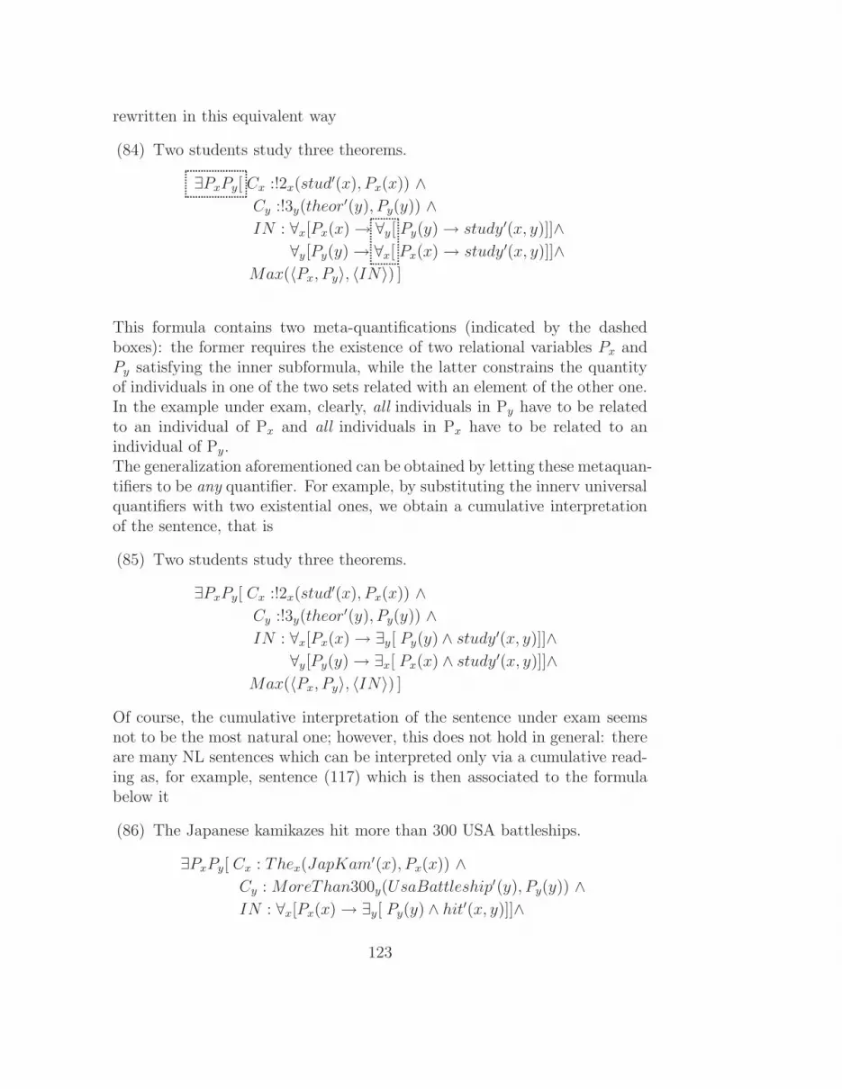
rewritten in this equivalent way

(84) Two students study three theorems.

∃PxPy[ Cx :!2x(stud′(x), Px(x)) ∧

Cy :!3y(theor′(y), Py(y)) ∧

IN : ∀x[Px(x) → ∀y[ Py(y) → study′(x, y)]]∧

∀y[Py(y) → ∀x[ Px(x) → study′(x, y)]]∧

Max(〈Px, Py〉, 〈IN〉) ]

This formula contains two meta-quantifications (indicated by the dashedboxes): the former requires the existence of two relational variables Px andPy satisfying the inner subformula, while the latter constrains the quantityof individuals in one of the two sets related with an element of the other one.In the example under exam, clearly, all individuals in Py have to be relatedto an individual of Px and all individuals in Px have to be related to anindividual of Py.The generalization aforementioned can be obtained by letting these metaquan-tifiers to be any quantifier. For example, by substituting the innerv universalquantifiers with two existential ones, we obtain a cumulative interpretationof the sentence, that is

(85) Two students study three theorems.

∃PxPy[ Cx :!2x(stud′(x), Px(x)) ∧

Cy :!3y(theor′(y), Py(y)) ∧

IN : ∀x[Px(x) → ∃y[ Py(y) ∧ study′(x, y)]]∧

∀y[Py(y) → ∃x[ Px(x) ∧ study′(x, y)]]∧

Max(〈Px, Py〉, 〈IN〉) ]

Of course, the cumulative interpretation of the sentence under exam seemsnot to be the most natural one; however, this does not hold in general: thereare many NL sentences which can be interpreted only via a cumulative read-ing as, for example, sentence (117) which is then associated to the formulabelow it

(86) The Japanese kamikazes hit more than 300 USA battleships.

∃PxPy[ Cx : Thex(JapKam′(x), Px(x)) ∧

Cy : MoreThan300y(UsaBattleship′(y), Py(y)) ∧

IN : ∀x[Px(x) → ∃y[ Py(y) ∧ hit′(x, y)]]∧

123

∀y[Py(y) → ∃x[ Px(x) ∧ hit′(x, y)]]∧

Max(〈Px, Py〉, 〈IN〉) ]

Therefore, in order to trigger a cumulative interpretation, it is necessary toassert a BQ reading in which each individual of Px is related with at leastone individual of Py and vice versa.Other examples of “generalized” BQ readings provided by Sher9 are (87.a),in which each individual of Px is related with exactly one individual of Py

and viceversa, (87.b), in which each individual of Px is related with two ormore individuals of Py and each individual of Py is related with at least oneindividual of Px, and (87.c) in which each individual of Px is related with atleast half individuals of Py and each individual of Py is related with at leasthalf individuals of Px.

(87) a. Most of my right gloves and most of my left hand gloves matchone to one.

∃PxPy[ Cx : Mostx(MyRHGlove′(x), Px(x)) ∧

Cy : Mosty(MyLHGlove′(y), Py(y)) ∧

IN : ∀x[Px(x) → ∃Py[ !1y(Py(y), Py(y))∧

∀y[Py(y) → match′(x, y)]]]∧

∀y[Py(y) → ∃Px[ !1x(Px(x), Px(x))∧

∀y[Py(y) → match′(x, y)]]]∧

Max(〈Px, Py〉, 〈IN〉) ]

b. Most of my friends saw at least two of the same few Truffautmovies.

∃PxPy[ Cx : Mostx(MyFriend′(x), Px(x)) ∧

Cy : Fewy(TrMovie′(y), Py(y)) ∧

IN : ∀x[Px(x) → ∃Py[ 2orMorey(Py(y), Py(y))∧

∀y[Py(y) → saw′(x, y)]]]∧

∀y[Py(y) → ∃x[ Px(x) ∧ saw′(x, y)]]∧

Max(〈Px, Py〉, 〈IN〉) ]

c. Most of the boys and most of the girls in this party are such thateach boy has chased at least half the girls and each girl has been

9In (87), it is necessary to represent inner meta-quantifiers different from ∀, and ∃;to this end, two new predicates, i.e. Px and Py , are introduced and two corresponding2-place Mostowskian Generalized Quantifier are applied on them.

124

chased by at least half the boy.

∃PxPy[ Cx : Mostx(boy′(x), Px(x)) ∧

Cy : Mosty(girl′(y), Py(y)) ∧

IN : ∀x[Px(x) → ∃Py[ AtLeastHalfy(Py(y), Py(y))∧

∀y[Py(y) → chased′(x, y)]]]∧

∀y[Py(y) → ∃Px[ AtLeastHalfx(Px(x), Px(x))∧

∀y[Py(y) → chased′(x, y)]]]∧

Max(〈Px, Py〉, 〈IN〉) ]

Now, recalling the schema in (84), the second generalization proposed bySher is presented. It amounts to letting the existential quantifications on Px

and Py to be any quantification.In other words, rather than requiring that at least one pair of relationalvariables Px and Py satisfies the inner subformula, we require that all, most,more than two, etc. of such pairs satisfy it.Sher supports this second generalization by providing examples as10:

(88) a. By and large, no more than a few boys and a few girls all dateone another.

b. There are at most few cases of more than one couple of Easterndelegates and more than one couple of Western delegates who areall on speaking terms with one another.

Sentence (88.a) is true only in those worlds in which in in general no morethan few boys and a few girls all date one another, i.e. in those models inwhich most of the pairs 〈Px, Py〉 in the model are such that Px contains nomore than a few boys, Py contains a few girls, and the individuals in the twosets all date one another. Analogous considerations hold for (88.b); the maindifference is that the inner branching quantifiers formula has to hold for atmost few pairs 〈Px, Py〉.To summarize, Sher proposed to generalize the meta-quantifications occur-ring in her formulae to be any quantification; the need of these generalizationsis justified by linguistic examples.However, it could be argued that Sher is right in saying that there are sev-eral kinds of non linear quantifications besides Complex dependence, andthat the semantic formalism must be enable all of them, but the set of such

10For this second generalization, I present only the NL sentences shown by Sher, withoutproviding also an associated formula handling the expected truth conditions. In fact, sucha formula would require a meta-quantification in the space of all pairs of unary predicatesin the domain A, i.e. it should be expressed in a third order logics.

125

interpretations actually available in NL has to be restricted.In particular, concerning the generalization of the inner meta-quantifications,only the (pair of) universal quantifications, triggering a Complex dependencenon linear reading, and the (pair of) existential quantifications, triggering anIndependent (cumulative) non linear reading, should be allowed.In fact, while there is clear evidence to justify the existence in NL of thesetwo “extremes”, the examples provided by Sher for the other interpretations,i.e. (87).a-c, are not convincing.Furthermore, even if we can accept them as real instances of NL sentences, itis not clear if they have to receive the interpretation depicted by the formulaeshown above.For example, (87.a) could be better represented by means of a formula in-volving a binary collective predicate, say match1to1′(X, Y ), which is true ifthe sets used as arguments, i.e. X and Y , are such that all their elements canbe paired up. Therefore, in this view, sentences as (87.a) have to be analysedin a different way with respect to the one proposed by Sher, in which a puredistributive binary predicate match′ is involved.Also about the generalization of the outer meta-quantifications my opinion isthat Sher is partially right (even if I am again skeptical about the possibilityof generalizing to any quantifier).In fact, besides the sentences she proposes in (87), her analysis can be sup-ported also by sentences as

(89) Only two men love three (same) women.

John

Jack

Ann

Sue

Mary

Paul

Mark

Sophie

Kate

Maggie

Figure 5.10: An example highlighting the need of a generalization of theouter meta-quantification: it seems that the BQ reading of the

sentence has to be false in the model shown.

As the intuition suggests, the BQ reading of (89) has to be false in the modelreported below it; nevertheless, the non generalized formula proposed by Sherfor this reading, reported in (90), evaluates to true.

126

(90) ∃PxPy[ Cx :!2x(men′(x), Px(x)) ∧

Cy :!3y(woman′(y), Py(y)) ∧

IN : ∀xy[(Px(x) ∧ Py(y)) → loves′(x, y)]]∧

Max(〈Px, Py〉, 〈IN〉) ]

In fact, this formula requires the existence of at least one massive nucleusin the model, while the sentence should be true only if there is exactly onemassive nucleus.The Sher generalization proposal allows to handle this case, in that it allowsthe outer quantifications on the relational variables to be stated in terms ofthe quantifier 1! rather than ∃.To conclude, the generalization of all possible logical non-linear quantifica-tions proposed by Sher has to be taken into account, but still deserves furtherstudy, in order to investigate how many of such non linear quantification yieldreadings actually available in Natural Language.

5.4.2 Formalization

This section presents the formal details of the logics developed by Sher, thatI will call L0. In next chapter, L0 will be extended in order to handle moregeneral cases of quantification; from a formal point of view, this will be doneby modifying some points in the formalization presented here.The first point that has to be stressed is that the author formalizes L0 interms of 1-place Mostowskian quantifiers (see §5.2).As pointed out, these quantifiers do not distinguish between body and re-striction and provide expressivity to represent NL sentences containing onlynumerals. In other words, L0 just allows to represent sentences as the fol-lowing one ([Sher, 1997], pp.38)11

(91) Two boys have two toys and two friends who don’t like their toys.

Which can be represented by the formula

11In this example, Two has to be intended as Exactly two.

127

(92)

2!x

!2y

!2z

boy′(x) ∧ toy−of(y, x) ∧ friend−of(z, x) ∧ ¬likes(z, y)

=df ∃Px, Py, Pz[ Cx: 2!x(Px(x)) &

Cy: ∀x[Px(x)→2!y(Py(x, y))] &

Cz: ∀x[Px(x)→2!z(Pz(x, z))] &

IN : ∀xyz[(Py(x, y) ∧ Pz(x, z))→ (boy′(x)∧ toy−of(y, x) ∧

friend−of(z, x) ∧ ¬ likes(z, y))] &

Max(〈Px〉, 〈Cy, Cz〉) & Max(〈Py , Pz〉, 〈IN〉) ]

In which the 2! is a 1-place Mostowskian quantifier (hence, its three occur-rences have a single argument, i.e. the predicates Px, Py and Pz respectively)and all the predicates are inserted in the IN condition.As the reader can easily check, (92) correctly captures the truth-conditionsof (91); however, if we change (91) by substituting the occurrences of the NLnumeral Two, with other quantifiers as Most, Few, etc., the correspondingformula cannot be obtained simply by substituting the occurrences of the 1-place quantifiers 2! in (92) with the Mostowskian Quantifiers correspondingto Most, Few, etc.To this end, it is necessary to introduce 2-place Mostowskian quantifiers, asin all examples of the previous paragraph.

The language L0

Before presenting the syntax of L0, some preliminary definitions is intro-duced; the first two are taken from section 5.2 and are reported here only forthe sake of simplicity.

Definition 5.5. [Syntax of 1-place Mostowskian Quantifiers]A 1-place Mostowskian Quantifier is a symbol Q, belonging to the vocabularyof L0, such that, if x is an individual variable of L0, and Φ is a formula ofL0, then Qx(Φ) is also a formula of L0.

Definition 5.6. [Semantics of 1-place Mostowskian Quantifiers]A 1-place Mostowskian Quantifier Q denotes, in every model M with universeA, a function q from ℘(A) to T, F12. Furthermore, if there are two models

12℘(A) is the power set of A, that is, the set of all subsets of A; T, F is, clearly, theset of truth-values: T = true and F = false.

128

M1, M2 with universe A1, A2 respectively and two sets B1, B2 such that B1 ⊆A1 and B2 ⊆ A2 and the two structures (B1, A1), (B2, A2) are isomorphic,then q(B1) = q(B2). This amounts to say that the value assigned by q to aset B, only depends on the cardinalities of B and A \B (the complement ofB in A).

Definition 5.7. [Quantifier Prefix]A quantifier prefix QP = (q1, q2, . . . , qn, <) is a structure such that:

• Each qi (1 ≤ i ≤ n) has the form Qixi where Qi is a MostowskianGeneralized Quantifier and xi is an individual variable ranging on auniverse A.

• < is a partial order relation on q1, q2, . . . , qn. If qi < qj, we saythat qi is a dependent of qj and that qj is a governor of qi. qi is animmediate dependent of qj if qi < qj and does not exist any qk such thatqi < qk < qj. Analogously for immediate governors.

• The rank ri of a quantifier qi is the number of quantifiers qm in theprefix such that qm is a governor of qi.

Definition 5.8. [Relational variable]If QP = (q1, q2, . . . , qn, <) is a quantifier prefix, then each qi (1 ≤ i ≤ n)is associated with

• a relational variable Pi, whose arity is ri (the rank of qi).

• a term Ti = Pi(xi1 , xi2 , . . . , xiri, xi), where each xik is the variable as-

sociated with one of the governors of qi. Such governors are orderedaccording to a total order whose sole function is to determine the orderof the variables xik .

Definition 5.9. [Cluster of quantifiers]If QP = (q1, q2, . . . , qn, <) is a quantifier prefix, then q1, q2, . . . , qn ispartitioned into a set of clusters CL = Cl1, Cl2, . . . , Clm; each Cli, i =1 . . . (m − 1) is a minimal set of quantifiers such that if qr ∈ Cli, qr is animmediate dependent of qu and qs an immediate dependent of qu (i.e. qu is acommon immediate ancestor of qr and qs) then qs ∈ Cli. Finally, Clm, calledthe final cluster (or the smallest cluster, according to Sher’s terminology),contains all quantifiers on which no other quantifier depends.

The third and the fourth definition respectively formalize the partial orderon quantifiers and introduce some useful terms. Finally, the last definitionconstitutes the core of the L0’s syntax. In particular, it introduces the notion

129

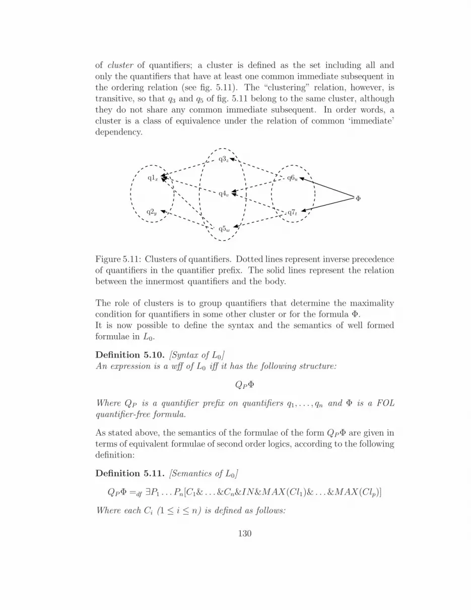
of cluster of quantifiers; a cluster is defined as the set including all andonly the quantifiers that have at least one common immediate subsequent inthe ordering relation (see fig. 5.11). The “clustering” relation, however, istransitive, so that q3 and q5 of fig. 5.11 belong to the same cluster, althoughthey do not share any common immediate subsequent. In order words, acluster is a class of equivalence under the relation of common ‘immediate’dependency.

q1x

q2y

q3z

q4v

q5w

q6u

q7t

Φ

Figure 5.11: Clusters of quantifiers. Dotted lines represent inverse precedenceof quantifiers in the quantifier prefix. The solid lines represent the relationbetween the innermost quantifiers and the body.

The role of clusters is to group quantifiers that determine the maximalitycondition for quantifiers in some other cluster or for the formula Φ.It is now possible to define the syntax and the semantics of well formedformulae in L0.

Definition 5.10. [Syntax of L0]An expression is a wff of L0 iff it has the following structure:

QP Φ

Where QP is a quantifier prefix on quantifiers q1, . . . , qn and Φ is a FOLquantifier-free formula.

As stated above, the semantics of the formulae of the form QP Φ are given interms of equivalent formulae of second order logics, according to the followingdefinition:

Definition 5.11. [Semantics of L0]

QP Φ =df ∃P1 . . . Pn[C1& . . .&Cn&IN&MAX(Cl1)& . . .&MAX(Clp)]

Where each Ci (1 ≤ i ≤ n) is defined as follows:

130

Ci =

Qixi(Ti) if ri = 0

∀xj1 . . . xjz[(T1& . . .&Tm) → Qixi(Ti)] otherwise

Where the xjw(1 ≤ w ≤ z) are the individual variables occurring in some Tk

(1 ≤ k ≤ m). According to def.5.8, each Tk has the form Pk(xk1, . . . , xkrk, xk),

where Pk is one of the P1 . . . Pn and the variables xkv (1 ≤ v ≤ rk) are indi-vidual variables such that qkv is a governor of qk in the quantifier prefix, andrk is the rank of Qk. Moreover, qk is an immediate governor of qi

IN is defined as follows:

IN =df ∀xj1 . . . xjz[(T1 ∧ . . . ∧ Tm) → Φ]

where qk (1 ≤ k ≤ m) are all quantifiers having no dependent in QP , whileTk (1 ≤ k ≤ m) and the variables xjw

(1 ≤ w ≤ z) are defined as above.Finally, the maximality conditions MAX(Cli), (1 ≤ i ≤ p), where Cli =qi1 , . . . , qij is a cluster of quantifiers, are defined as follow:

MAX(Cli) = ∀P ′

i1, . . . , P ′

ij

[ ∀x1,...,xz[ (Ti1 ∧ . . . ∧ Tij ) → (T ′

i1∧ . . . ∧ T ′

ij)∧

Ω[P ′

i1\Pi1, . . . , P

′

ij\Pij ] ] →

[ ∀x1,...,xz[(T ′

i1∧ . . . ∧ T ′

ij) → (Ti1 ∧ . . . ∧ Tij ) ]

Where

• P ′

i1, . . . , P ′

ijare new relational variables having, respectively, the same

arity of Pi1 , . . ., Pij .

• T ′

i1, . . . , T ′

ijare obtained from Ti1 , . . . , Tij by replacing the relational

variables Pi1 , . . . , Pij with P ′

i1, . . . , P ′

ijrespectively.

• x1, . . . , xz are all individuals variables occurring in some Tiv (1 ≤ v ≤ j)

• Ω = IN if the elements in the cluster Cli have no dependents; other-wise, if the immediate dependents of these elements are qh1 , . . . , qhr

,then Ω = Ch1& . . .&Chr

.

• Ω[P ′

i1\Pi1 , . . . , P

′

ij\Pij ] is the formula obtained by replacing, in Ω, the

relational variables Pi1, . . . , Pij with P ′

i1, . . . , P ′

ijrespectively.

131

An example of formula in L0 is the one in (92), that captures the righttruth-conditions of sentence (91). However, as pointed out above, L0 has notenough expressivity to represent sentences containing any quantifier as theones analyzed in the previous section, e.g.

(93) a. My friends promised to come with me to at most four concerts ofmy choice.

b. Few men inserted a coin in every coffee machine.

In order to capture the correct true-conditions for these sentences, it is nec-essary to modify the formula by substituting the condition of terms Ci withthe following

. . .

Ci =

Qixi(Ψi(xi), Ri) if ri = 0

∀xi1 . . . xim [(Ri1& . . .&Rim) → Qixi(Ψi(xi), Ri)] otherwise

. . .

In which Qi are now 2-place Mostowskian Generalized quantifiers and Ψi, i.e.the restrictions, are first-order formulae in which xi is the only variable thatmay occur free.By means of this simple modification, we can represent sentences in (93) withthe formulae showed in the previous section (for example, (94) reports theone corresponding to (93.a)).

(94) My friends promised to come with me to at most four concerts of mychoice.

Thex(myFriend’(x))

AtMost4y(myConcert’(y))

promiseToGo’(x, y)

=df ∃Px, Py[ Cx: Thex(friendOfMine’(x), Px(x)) &

Cy: AtMost4y(myConcert’(y), Py(y)) &

IN: ∀xy[(Px(x)∧Px(x))→ promiseToGo’(x, y)] &

Max(〈Px, Py〉, IN)]

Nevertheless, as it will be cleared in next section, L0 needs a more radicalgeneralization in order to allow the representation of a broader relevant setof NL sentences.

132

5.5 Summary

In this chapter, two of the main relevant works on Branching Quantificationhave been presented. Particular attention has been paid to the work of Sher,which defines a logics L0 able to represent BQ readings involving any kind of(first order) quantifiers and any partial order between them. Moreover, L0

can be easily generalized to handle any kind of logical non linear readings;first at all cumulative readings.Nevertheless, L0 presents also some relevant limitations. First, it does notprovide rules to represent sentences featuring Nested Quantifications, i.e. sen-tences containing quantifiers nested into the syntactical restriction of otherquantifiers13, as the following

(95) [A representative of [every african country]] arrives.

Second, Sher defined L0 and showed that it may be used for the represen-tation of NL meaning, but she does not provide rules to map NL sentencesinto L0 formulae, i.e. she does not define any interface with a NL grammar.

13The reader should note that the syntactical restriction of an NL quantifier, i.e. thesubtree of syntactic dependents governed by the NL quantifier, and the semantic restrictionof the logical quantifier, i.e. sets of individuals as first argument of the logical quantifier,are not the same thing.

133

134

Chapter 6

Sher’s theory extensions

In the previous chapter, the work of Sher ([Sher, 1990] and [Sher, 1997]),implemented into a new logics referred, in this thesis, by the term L0, hasbeen presented. This work defines an ingenious mechanism to handle thetruth values of Branching Quantifier structures via maximality conditionsexpressed by particular Second Order Logics formulae.However, it has been argued that L0 still features two important limits:

• It does not cover Nested Quantifications, i.e. sentences containingquantifiers nested into the syntactical restriction of other quantifiers;in fact L0 has been defined only in terms of 1-place Mostowskian Gen-eralized Quantifiers, that do not distinguish between restriction andbody.

• Although, in principle, L0 allows for the representation of NL BranchingQuantifier readings, no rules to computationally obtain its formulaestarting from an NL grammar are provided.

This chapter focuses on the first limit. Section 6.2 gives some more detailsabout the linguistic phenomena of Nested Quantification and the difficult toextend L0 in order to enable its representation. Then, section 6.3 intuitivelyproposes a solution to this problem and section 6.3 formalizes it into a newlogics L. Finally, section 6.4 briefly discusses how it is in principle possibleto extend L in order to enable cumulative readings.

6.1 The operator⊆max

Before presenting a possible solution to handle Nested Quantification in L0,

135

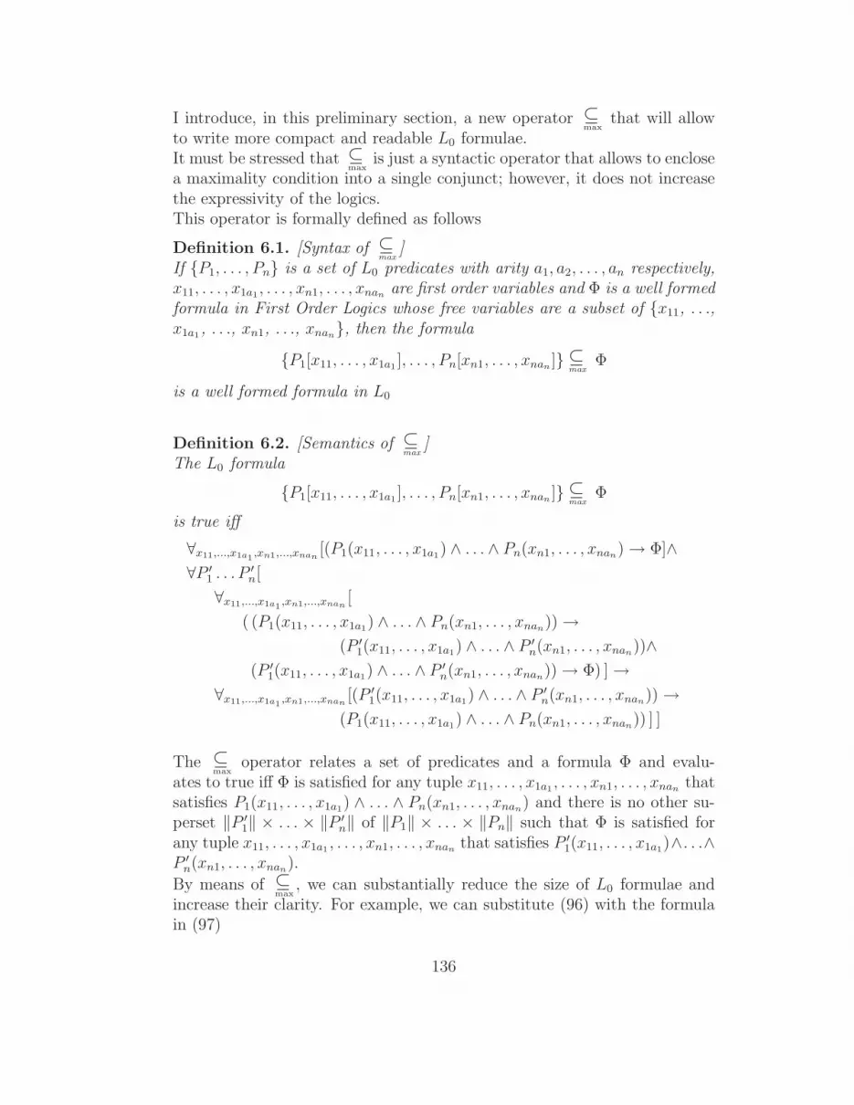
I introduce, in this preliminary section, a new operator ⊆max

that will allowto write more compact and readable L0 formulae.It must be stressed that ⊆

maxis just a syntactic operator that allows to enclose

a maximality condition into a single conjunct; however, it does not increasethe expressivity of the logics.This operator is formally defined as follows

Definition 6.1. [Syntax of ⊆max

]If P1, . . . , Pn is a set of L0 predicates with arity a1, a2, . . . , an respectively,x11, . . . , x1a1 , . . . , xn1, . . . , xnan

are first order variables and Φ is a well formedformula in First Order Logics whose free variables are a subset of x11, . . .,x1a1 , . . ., xn1, . . ., xnan

, then the formula

P1[x11, . . . , x1a1 ], . . . , Pn[xn1, . . . , xnan]⊆

max

Φ

is a well formed formula in L0

Definition 6.2. [Semantics of ⊆max

]The L0 formula

P1[x11, . . . , x1a1 ], . . . , Pn[xn1, . . . , xnan]⊆

max

Φ

is true iff

∀x11,...,x1a1 ,xn1,...,xnan[(P1(x11, . . . , x1a1) ∧ . . . ∧ Pn(xn1, . . . , xnan

) → Φ]∧

∀P ′

1. . . P ′

n[

∀x11,...,x1a1 ,xn1,...,xnan[

( (P1(x11, . . . , x1a1) ∧ . . . ∧ Pn(xn1, . . . , xnan)) →

(P ′

1(x11, . . . , x1a1) ∧ . . . ∧ P

′

n(xn1, . . . , xnan))∧

(P ′

1(x11, . . . , x1a1) ∧ . . . ∧ P

′

n(xn1, . . . , xnan)) → Φ) ] →

∀x11,...,x1a1 ,xn1,...,xnan[(P ′

1(x11, . . . , x1a1) ∧ . . . ∧ P′

n(xn1, . . . , xnan)) →

(P1(x11, . . . , x1a1) ∧ . . . ∧ Pn(xn1, . . . , xnan)) ] ]

The ⊆max

operator relates a set of predicates and a formula Φ and evalu-ates to true iff Φ is satisfied for any tuple x11, . . . , x1a1 , . . . , xn1, . . . , xnan

thatsatisfies P1(x11, . . . , x1a1) ∧ . . . ∧ Pn(xn1, . . . , xnan

) and there is no other su-perset ‖P ′

1‖ × . . . × ‖P ′

n‖ of ‖P1‖ × . . . × ‖Pn‖ such that Φ is satisfied forany tuple x11, . . . , x1a1 , . . . , xn1, . . . , xnan

that satisfies P ′

1(x11, . . . , x1a1)∧. . .∧P ′

n(xn1, . . . , xnan).

By means of ⊆max

, we can substantially reduce the size of L0 formulae andincrease their clarity. For example, we can substitute (96) with the formulain (97)

136

(96) Fewx men inserted ay coin in everyz coffee machine.

Fewx(man’(x))

Everyy(CoffeeMach’(y))

Az(Coin’(z)) Inserted’(x, z, y)

=df ∃Px, Py, Pz[ Cx: Fewx(man’(x), Px(x)) &

Cy: Everyy(CoffeeMach’(y), Py(y)) &

Cz: ∀xy[(Px(x)∧Py(y))→ Az(coin’(z), Pz(x, y, z))] &

IN : ∀xyz[Pz(x, y, z)→ inserted′(x, y, z)] &

Max(〈Px, Py〉, Cz) & Max(〈Pz〉, IN) ]

(97) Fewx men inserted az coin in everyy coffee machine.

∃Px, Py, Pz[ Fewx(man’(x), Px(x)) &

Everyy(CoffeeMach’(y), Py(y)) &

Px[x], Py[y]⊆max

( Az(coin’(z), Pz(x, y, z)) ) &

Pz[x, y, z]⊆max

(insert′(x, y, z)) ]

In (97), the conjunct

Pz[x, y, z]⊆max

(insert′(x, y, z))

has simply to be read “‖Pz‖ is a maximal set of triples included in the exten-sion of the formula on the right hand side”; in this case, in order to satisfythis requirement, ‖Pz‖ has to coincide with the extension of the predicateinsert′ in that they are related to each other with respect to the same vari-ables (x, y, and z).In order to make clear the correspondence with L0 syntax, sometimes I willindicate in the formulae also the labels IN , Cx, Cy, etc. For example, in (98)the equivalent notation of (97) that makes use of such labels is reported

(98) Fewx men inserted az coin in everyy coffee machine.

∃Px, Py, Pz[ Cx: Fewx(man’(x), Px(x)) &

Cy: Everyy(CoffeeMach’(y), Py(y)) &

Cz: Px[x], Py[y]⊆max

( Az(coin’(z), Pz(x, y, z)) ) &

IN : Pz[x, y, z]⊆max

(insert′(x, y, z)) ]

137

However, in some cases, the labels will be merged into a single one in that⊆max

operator collects, in its right hand side, all the conditions that have tobe maximized with respect to the same relational variables in its left handside. I remind that, in L0, the information about which conditions have tobe maximized with respect to which relational variables is specified in the“Max” predicate, whose second argument is the set of all labels referringto the clauses to be maximized together. On the contrary, the second ar-gument of ⊆

max, that replaces “Max”, is directly the conjunction of these

clauses rather than the set of their labels. Therefore, in order to maintainthe correspondence with L0, the maximality condition triggered by ⊆

maxhas

to be labeled with a label referring to all the labels of such clauses.For example, the L0 formula in (99), that requires

• The maximization of the conditions with label Cz, Cv, and Cw withrespect to Px and Py.

• The maximization of the conditions with label Cu and Ct with respectto Pz, Pv and Pw.

• The maximization of IN with respect to Pu and Pt.

corresponds to (100) in which “Cz\Cv\Cw” and “Cu\Ct” are labels thatrespectively refers to the groups of labels Cz, Cv, Cw and Cu, Ct in (99)

(99)

q1x

q2y

q3z

q4v

q5w

q6u

q7t

Φ

=df ∃Px, Py, Pz, Pw, Pv, Pu, Pt[ Cx: q1x(Px(x)) & Cy: q2y(Py(y)) &

Cz: ∀xy[Px(x) → q3z(Pz(x, z))] &

Cv: ∀xy[Px(x) → q4v(Pv(x, v))] &

Cw: ∀xy[(Px(x) ∧ Py(y)) → q5w(Pw(x, y, w))] &

Cu: ∀xzv[(Pz(x, z) ∧ Pv(x, v)) → q6u(Pu(x, z, v, u))] &

Ct: ∀xyvw[(Pv(x, v) ∧ Pw(x, y, w)) → q7t(Pt(x, y, v, w, t))] &

IN : ∀xyzvwut[(Pu(x, z, v, u) ∧ Pt(x, y, v, w, t)) → Φ] &

138

Max(〈Px, Py〉, 〈Cz, Cv, Cw〉) &

Max(〈Pz , Pv, Pw〉, 〈Cu, Ct〉) &

Max(〈Pu, Pt〉, 〈IN〉) ]

(100)∃Px, Py, Pz, Pw, Pv, Pu, Pt[ Cx: q1x(Px(x)) & Cy: q2y(Py(y)) &

Cz\Cv\Cw: Px[x], Py[y]⊆max

(q3z(Pz(x, z)) ∧ q4v(Pv(x, v)) ∧ q5w(Pw(x, y, w))) &

Cu\Ct: Pz[x, z], Pv[x, v], Pw[x, y, w]⊆max

(q6u(Pu(x, z, v, u)) ∧ q7t(Pt(x, y, v, w, t))) &

IN : Pu[x, z, v, u], Pt[x, y, v, w, t]⊆max

(Φ(x, y, z, w, u, t)) ]

6.2 Nested Quantification

The previous chapter describes the work of [Sher, 1990] and [Sher, 1997].These articles provide a way to interpreter Branching Quantifier readings bymeans of formulae in SOL augmented with standard Mostowskian General-ized Quantifiers (see section 5.2). The proposal is particularly relevant inthat it allows to set up formulae with any set of quantifiers and any partialorder on them.However, Sher defines her logics, called L0 in this thesis, just in terms of1-place Mostowskian Generalized Quantifiers. Since these quantifiers have asingle argument, they do not distinguish between restriction and a body, andprovide expressivity only for representing NL numerals as Two, Three, etc.;for example, in L0 we are able to represents sentences as (101)

(101) Twox boys have twoy toys and twoz friends who don’t like their toys.

∃Px, Py, Pz[ 2!x(Px(x)) &

Px[x]⊆max

(2!y(Py(x, y)) ∧ 2!z(Pz(x, z))) &

Py[x, y], Pz[x, z]⊆max

(boy′(x) ∧ toy−of(y, x)∧

friend−of(z, x) ∧ ¬ likes(z, y)) ]

where 2! are 1-place Mostowskian Generalized Quantifiers that are true iffonly two individuals in the domain satisfy the predicate.

139

On the contrary, in order to represent the semantics of sentences contain-ing any NL quantifier besides numerals, it is necessary to introduce 2-placeMostowskian Generalized Quantifiers. In this way, we enable L0 to representsentences as (102)

(102) Fewx men inserted az coin in everyy coffee machine.

∃Px, Py, Pz[ Fewx(man’(x), Px(x)) &

Everyy(CoffeeMach’(y), Py(y)) &

Px[x], Py[y]⊆max

( Az(coin’(z), Pz(x, y, z)) ) &

Pz[x, y, z]⊆max

(insert′(x, y, z)) ]

where Every, Few, and A are 2-place Mostoskian Generalized Quantifiersthat are true iff the extension of their second arguments contains respectivelyall, few or at least one elements of the extension of their first argument.However, while this move does not pose any problem when the first argu-ment, i.e. the restriction, is made up by a unary predicate as man′, coin′,and CoffeeMach′, it is not immediatly clear how to deal with quantifiersoccurring in the syntactic restriction of other quantifiers, i.e. in NL sentencesfeaturing a Nested Quantification, e.g.

(103)

[Twox representatives of [threey African countries]] arrive.

According to the constraints on SkDep function presented in section 4.3.1,three interpretations of (103) respect the syntactic constraints: the two linearreadings in which one of the two quantifier depends on the other one, andthe Branching Quantifier reading, that is true in those models including twoarriving persons that represents each the same three african countries.In (103), the quantifier Three occurs in the syntactic restriction of Two.Therefore, it is not clear how to build the L0 formula corresponding to theBranching Quantifier reading; in particular, it is not clear what has to beinserted in place of “???” in the following

∃PxPy[ Twox(???, Px(x)) & . . . ]

At first glance, it could seem that the Nested Quantification in the NL sen-tence must be mirrored by a Nested Quantification in the logical formula,i.e. that it has to trigger a formula similar to the following one

140

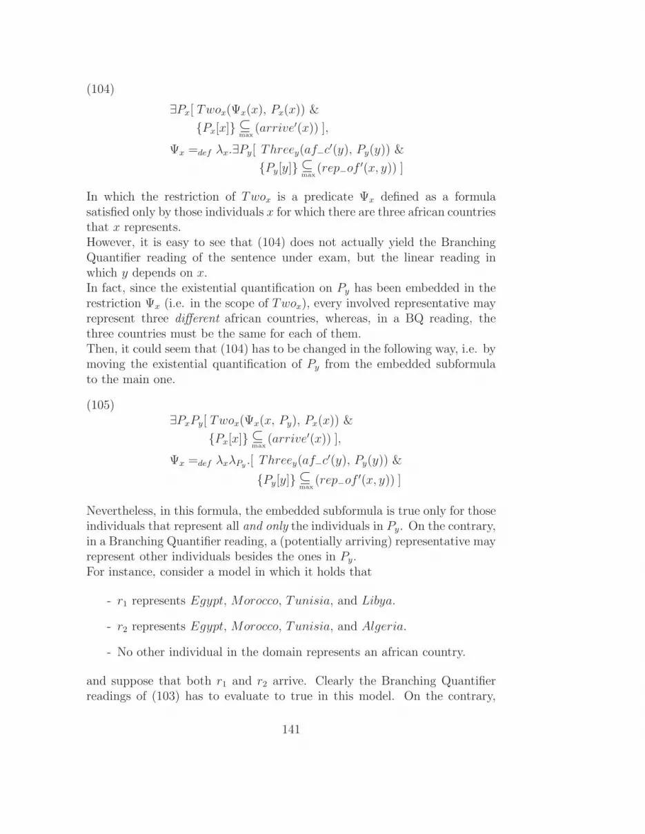
(104)

∃Px[ Twox(Ψx(x), Px(x)) &

Px[x]⊆max

(arrive′(x)) ],

Ψx =def λx.∃Py[ Threey(af−c′(y), Py(y)) &

Py[y]⊆max

(rep−of′(x, y)) ]

In which the restriction of Twox is a predicate Ψx defined as a formulasatisfied only by those individuals x for which there are three african countriesthat x represents.However, it is easy to see that (104) does not actually yield the BranchingQuantifier reading of the sentence under exam, but the linear reading inwhich y depends on x.In fact, since the existential quantification on Py has been embedded in therestriction Ψx (i.e. in the scope of Twox), every involved representative mayrepresent three different african countries, whereas, in a BQ reading, thethree countries must be the same for each of them.Then, it could seem that (104) has to be changed in the following way, i.e. bymoving the existential quantification of Py from the embedded subformulato the main one.

(105)∃PxPy[ Twox(Ψx(x, Py), Px(x)) &

Px[x]⊆max

(arrive′(x)) ],

Ψx =def λxλPy.[ Threey(af−c

′(y), Py(y)) &

Py[y]⊆max

(rep−of′(x, y)) ]

Nevertheless, in this formula, the embedded subformula is true only for thoseindividuals that represent all and only the individuals in Py. On the contrary,in a Branching Quantifier reading, a (potentially arriving) representative mayrepresent other individuals besides the ones in Py.For instance, consider a model in which it holds that

- r1 represents Egypt, Morocco, Tunisia, and Libya.

- r2 represents Egypt, Morocco, Tunisia, and Algeria.

- No other individual in the domain represents an african country.

and suppose that both r1 and r2 arrive. Clearly the Branching Quantifierreadings of (103) has to evaluate to true in this model. On the contrary,

141

(104) evaluates to false.In fact, taking ‖Py‖ ≡ Egypt,Morocco, Tunisia, the conjunct in the sub-formula

Py[y]⊆max

(rep−of′(x, y))

is false both when x = r1 and x = r2; in fact, the chosen Py does not concidewith the set of individuals represented by x in any of these cases. On thecontrary, when ‖Py‖ ≡ Egypt,Morocco, Tunisia, Libya, ‖Ψx‖ will containjust r1 and when ‖Py‖ ≡ Egypt,Morocco, Tunisia, Algeria, just r2. Inother words, there is no choice of Py that makes the subformula true for boththe arriving representatives.The solution is to introduce, for each quantifier Qx, two relational variablesrather than a single one. The former will be true for all and only the indi-viduals that satisfy Qx’s body, as in L0, while the latter will be true just forall and only the individuals that satisfy Qx’s restriction.These relational variables will be called PR

x and PBx where the apexes “R”

and “B” mark the relational variable associated with the restriction of Qx

and the one associated with its body.PR

x and PBx behave exactly as the relational variables in L0: they are inserted

in the left hand side of a ⊆max

operator (perhaps with other relational vari-ables, in Branching Quantification) and have to be maximized with respectto a formula in the right hand side. This formula can be either a formulain First Order Logics or a conjunction of a set of quantifiers Qy1, . . . , Qyn

depending on Qx, instantiated on their arguments.In L0, in which each (1-place) Generalized Quantifier is associated with asingle relational variable, it is rather simple to understand which predicatesor quantifiers conjunctions have to be inserted in the ⊆

max’s right hand sides:

all predicates have to be inserted in the final maximality condition, withoutdistinguishing between restriction and body, and the quantifiers conjunctionsare directly made up on the basis of the clustering on quantifiers.On the contrary, in this new logics, that will be called “The logics L”, thepredicates or the quantifiers in the conjunctions, to be inserted in the righthand sides, depend on the NL syntactic structures: if they arise from a wordoccurring in the syntactical restriction of a quantifier Qx, then they will beinserted into a maximality condition associated to PR

x , otherwise into a max-imality condition associated to PB

x .In other words, while L0 formulae feature a single inclusion condition withlabel IN , that imposes a maximality condition on the conjunction of allpredicates carried by the sentence, L formulae distinguish between predi-cates belonging to the body of the sentence and predicates belonging to the

142

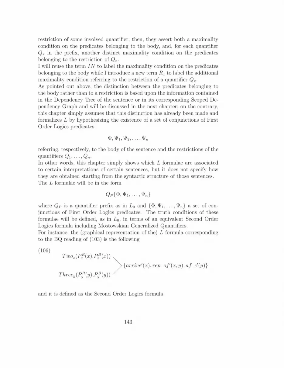
restriction of some involved quantifier; then, they assert both a maximalitycondition on the predicates belonging to the body, and, for each quantifierQx in the prefix, another distinct maximality condition on the predicatesbelonging to the restriction of Qx.I will reuse the term IN to label the maximality condition on the predicatesbelonging to the body while I introduce a new term Rx to label the additionalmaximality condition referring to the restriction of a quantifier Qx.As pointed out above, the distinction between the predicates belonging tothe body rather than to a restriction is based upon the information containedin the Dependency Tree of the sentence or in its corresponding Scoped De-pendency Graph and will be discussed in the next chapter; on the contrary,this chapter simply assumes that this distinction has already been made andformalizes L by hypothesizing the existence of a set of conjunctions of FirstOrder Logics predicates

Φ,Ψ1,Ψ2, . . . ,Ψn

referring, respectively, to the body of the sentence and the restrictions of thequantifiers Q1, . . . , Qn.In other words, this chapter simply shows which L formulae are associatedto certain interpretations of certain sentences, but it does not specify howthey are obtained starting from the syntactic structure of those sentences.The L formulae will be in the form

QPΦ,Ψ1, . . . ,Ψn

where QP is a quantifier prefix as in L0 and Φ,Ψ1, . . . ,Ψn a set of con-junctions of First Order Logics predicates. The truth conditions of theseformulae will be defined, as in L0, in terms of an equivalent Second OrderLogics formula including Mostowskian Generalized Quantifiers.For instance, the (graphical representation of the) L formula correspondingto the BQ reading of (103) is the following

(106)Twox(P

Rx (x),PB

x (x))

Threey(PRy (y),PB

y (y))

arrive′(x), rep−of′(x, y), af−c

′(y)

and it is defined as the Second Order Logics formula

143

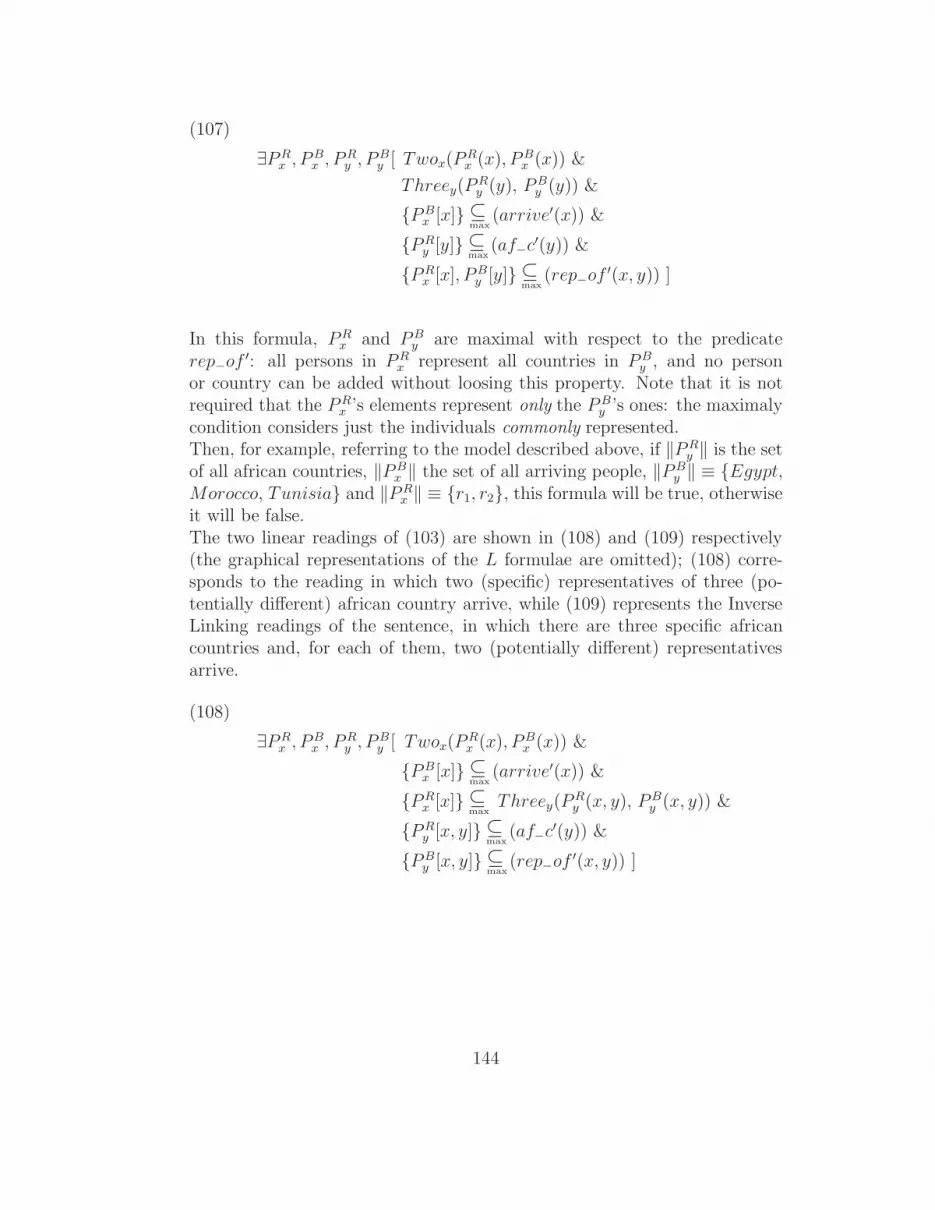
(107)

∃PRx , P

Bx , P

Ry , P

By [ Twox(P

Rx (x), PB

x (x)) &

Threey(PRy (y), PB

y (y)) &

PBx [x]⊆

max(arrive′(x)) &

PRy [y]⊆

max(af−c

′(y)) &

PRx [x], PB

y [y]⊆max

(rep−of′(x, y)) ]

In this formula, PRx and PB

y are maximal with respect to the predicaterep−of

′: all persons in PRx represent all countries in PB

y , and no personor country can be added without loosing this property. Note that it is notrequired that the PR

x ’s elements represent only the PBy ’s ones: the maximaly

condition considers just the individuals commonly represented.Then, for example, referring to the model described above, if ‖PR

y ‖ is the setof all african countries, ‖PB

x ‖ the set of all arriving people, ‖PBy ‖ ≡ Egypt,

Morocco, Tunisia and ‖PRx ‖ ≡ r1, r2, this formula will be true, otherwise

it will be false.The two linear readings of (103) are shown in (108) and (109) respectively(the graphical representations of the L formulae are omitted); (108) corre-sponds to the reading in which two (specific) representatives of three (po-tentially different) african country arrive, while (109) represents the InverseLinking readings of the sentence, in which there are three specific africancountries and, for each of them, two (potentially different) representativesarrive.

(108)

∃PRx , P

Bx , P

Ry , P

By [ Twox(P

Rx (x), PB

x (x)) &

PBx [x]⊆

max(arrive′(x)) &

PRx [x]⊆

maxThreey(P

Ry (x, y), PB

y (x, y)) &

PRy [x, y]⊆

max(af−c

′(y)) &

PBy [x, y]⊆

max(rep−of

′(x, y)) ]

144

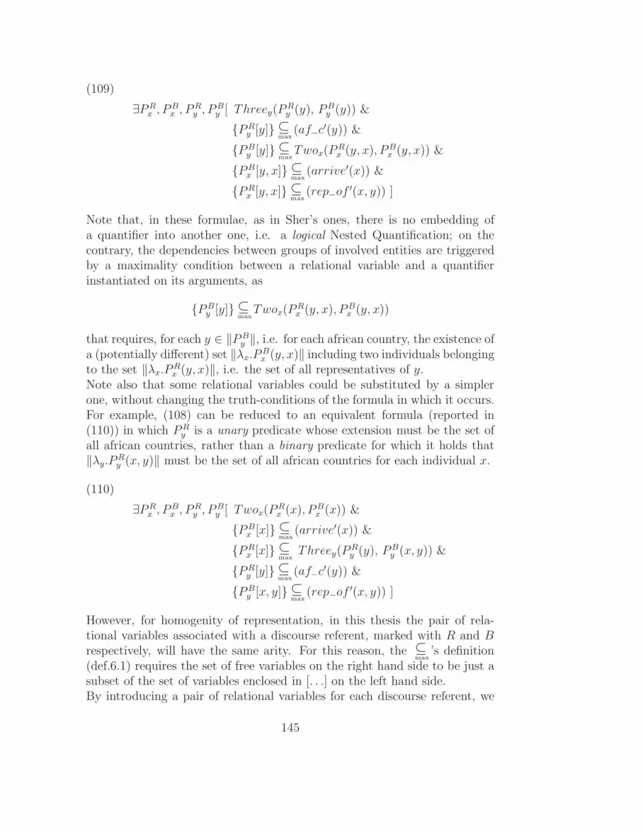
(109)

∃PRx , P

Bx , P

Ry , P

By [ Threey(P

Ry (y), PB

y (y)) &

PRy [y]⊆

max(af−c

′(y)) &

PBy [y]⊆

maxTwox(P

Rx (y, x), PB

x (y, x)) &

PBx [y, x]⊆

max(arrive′(x)) &

PRx [y, x]⊆

max(rep−of

′(x, y)) ]

Note that, in these formulae, as in Sher’s ones, there is no embedding ofa quantifier into another one, i.e. a logical Nested Quantification; on thecontrary, the dependencies between groups of involved entities are triggeredby a maximality condition between a relational variable and a quantifierinstantiated on its arguments, as

PBy [y]⊆

maxTwox(P

Rx (y, x), PB

x (y, x))

that requires, for each y ∈ ‖PBy ‖, i.e. for each african country, the existence of

a (potentially different) set ‖λx.PBx (y, x)‖ including two individuals belonging

to the set ‖λx.PRx (y, x)‖, i.e. the set of all representatives of y.

Note also that some relational variables could be substituted by a simplerone, without changing the truth-conditions of the formula in which it occurs.For example, (108) can be reduced to an equivalent formula (reported in(110)) in which PR

y is a unary predicate whose extension must be the set ofall african countries, rather than a binary predicate for which it holds that‖λy.P

Ry (x, y)‖ must be the set of all african countries for each individual x.

(110)

∃PRx , P

Bx , P

Ry , P

By [ Twox(P

Rx (x), PB

x (x)) &

PBx [x]⊆

max(arrive′(x)) &

PRx [x]⊆

maxThreey(P

Ry (y), PB

y (x, y)) &

PRy [y]⊆

max(af−c

′(y)) &

PBy [x, y]⊆

max(rep−of

′(x, y)) ]

However, for homogenity of representation, in this thesis the pair of rela-tional variables associated with a discourse referent, marked with R and Brespectively, will have the same arity. For this reason, the ⊆

max’s definition

(def.6.1) requires the set of free variables on the right hand side to be just asubset of the set of variables enclosed in [. . .] on the left hand side.By introducing a pair of relational variables for each discourse referent, we

145

can easily represent the semantics of the SemDep configurations enabled bythe constraints in def.4.6 (see section 4.3.1), i.e. configurations featuring ei-ther an Inverse Linking or a Branching Quantification between a discoursereferent x and another discourse referent y in x’s syntactical restriction (as(111) and (112) respectively).

(111) Twox boys ate ay portion of mostz courses.

∃PRx , P

Bx , P

Ry , P

By , P

Rz , P

Bz [

Twox(PRx (x), PB

x (x)) &

PRx [x]⊆

max(boy′(x)) &

PBx [x]⊆

max(Mostz(P

Rz (x, z), PB

z (x, z))) &

PRz [x, z]⊆

max(course′(z)) &

PBz [x, z]⊆

max(∃y(P

Ry (x, z, y), PB

y (x, z, y))) &

PRy [x, z, y]⊆

max(portion′(y) ∧ of ′(y, z)) &

PBy [x, z, y]⊆

max(ate′(x, y)) ]

x y

Ctx

z

SemDep

(112) Thex students must write any essay about threez poets.

∃PRx , P

Bx , P

Ry , P

By , P

Rz , P

Bz [

Thex(PRx (x), PB

x (x)) &

PRx [x]⊆

max(student′(x)) &

PBx [x]⊆

max( ∃y(P

Ry (x, y), PB

y (x, y))) ∧

Threez(PRz (x, z), PB

z (x, z)) ) &

PRz [x, z]⊆

max(poet′(z)) &

PRy [x, y], PB

z [x, z]⊆max

(essay′(y) ∧ about′(y, z)) &

PBy [x, y]⊆

max(write′(x, y)) ]

x y

Ctx

z

SemDep

The formula in (111) meets the truth conditions of the corresponding NLsentence. In fact, ‖PB

y ‖ must be a maximal set of triples (x, z, y) that as-sociates, to each individual z in the domain, the extension of the predicateate′. On the contrary, ‖PR

y ‖ must be a maximal set of triples (x, z, y) thatassociates, to each individual x in the domain, the extension of the formulaλyλz.(portion

′(y) ∧ of ′(y, z))1.

1Clearly, as in (108), ‖PBy ‖ and ‖PR

y ‖ may be reduced to two binary predicates whoseextension coincide with the ones of ate′ and λyλz .(portion′(y) ∧ of ′(y, z)) respectively.

146

With these requirements on PBy and PR

y , ‖PBz ‖ must be the maximal set

of pairs (x, z) for which it holds that ‖λy.PBy (x, z, y)‖ contains at least one

element of ‖λy.PRy (x, z, y)‖, i.e. for which it holds that all that has been

eaten by x contains at least a portion of z. Therefore, PBx is the maximal set

of individuals x for which it holds that ‖λz.PBz (x, z)‖ contains most courses.

Finally, if at least two individuals of PBx are boys, the formula will be true,

otherwise it will be false.Understanding the truth conditions of the formula in (112) is more complex,in that the two relational variables PR

y and PBz are maximized together in

the same maximality condition, i.e.

PRy [x, y], PB

z [x, z]⊆max

(essay′(y) ∧ about′(y, z))

In order to understand which requirements the maximality condition imposeson their extensions, it is better to “expand” the ⊆

maxand express the conjunct

in Sher’s style, i.e.

Rx : ∀xyz[(PRy (x, y) ∧ PB

z (x, z)) → (essay′(y) ∧ about′(y, z))]∧

Max(〈PRy , P

Bz 〉, Rx)

Now it may be seen that, in order to satisfy the formula, for each individualx in the domain, the set ‖λy.P

Ry (x, y)‖ has to be a set of essays each of which

talks about all individuals in the set ‖λz.PBz (x, z)‖. Furthermore, these two

sets have to be maximal; this implies that PRy and PB

z are such that for eachindividual x in the domain, there is a massive nucleus Y × Z, where Y isthe set of all and only the essays talking about all and only the elements ofZ. It is important to note that this massive nucleus may be different fromindividual to individual.Then, the maximality condition

PBx [x]⊆

max( Ay(P

Ry (x, y), PB

y (x, y)) ∧ Threez(PRz (x, z), PB

z (x, z)) )

is satisfied only if the extension of PBx is the maximal set of individuals

x for which the massive nucleus Y × Z, associated to x by the previouslydiscussed maximality condition, is such that all that x must write (i.e. theset ‖λy.P

By (x, y)‖ contains at least one element of Y and Z contains three

poets, i.e. three elements of ‖λz.PRz (x, z)‖. Finally, if ‖PB

x ‖ contains at leastthe (contextually relevant) students, the formula will be true, otherwise itwill be false.

147

6.3 The logics L

This section formalizes the concepts introduced above into a new logics called“The logics L”. Since L expands the logics L0 presented in the previous chap-ter, its formalization extends\modifies the one shown in section 5.4.2.The main difference between L0 and L is that the latter makes use of 2-placeMostowskian Generalized Quantifiers rather than 1-place Mostowskian Gen-eralized Quantifiers, and, consequently, its formulae include two relationalvariables for each involved quantifier rather than a single one.Therefore, before presenting the syntax of L, we need to modify three of thefive preliminary definitions given for L0 in section 5.4.2. Instead, a prelimi-nary definitions imported from L0 without any modification is the definitionof Quantifier Prefix; it is reported below for the sake of convenience. Notethat L does not make use of the definition of cluster of quantifiers; the reasonof this is that, in L it is not always the case that each maximality conditionhas to be asserted on all discourse referents belonging to a same cluster.Therefore, the well formed L formulae, contrary to the L0 ones, are notdefined upon the notion of cluster. I will return on this point in the nextsection.

Definition 6.3. [Quantifier Prefix]A quantifier prefix QP = (q1, q2, . . . , qn, <) is a structure such that:

• Each qi (1 ≤ i ≤ n) has the form Qixi where Qi is a MostowskianGeneralized Quantifier and xi is an individual variable ranging on auniverse A.

• < is a partial order relation on q1, q2, . . . , qn. If qi < qj, we saythat qi is a dependent of qj and that qj is a governor of qi. qi is animmediate dependent of qj if qi < qj and does not exist any qk such thatqi < qk < qj. Analogously for immediate governors.

• The rank ri of a quantifier qi is the number of quantifiers qm in theprefix such that qm is a governor of qi.

The definitions of quantifiers used in the logics, and their associated re-lational variables, are changed into the following ones (concerning 2-placeMostowskian Generalized Quantifiers, see also section 5.2). Clearly, the useof the 2-place Mostowskian Generalized Quantifiers extends the expressivepower of the logics, so that L is able to represent all that is possible torepresent in L0.

148

Definition 6.4. [Syntax of 2-place Mostowskian Quantifiers]A 2-place Mostowskian Quantifier is a symbol Q such that, if x is an indi-vidual variable, and Ψ, Φ are formulae, then Qx(Ψ,Φ) is also a formula.

Definition 6.5. [Semantics of 2-place Mostowskian Quantifiers]A 2-place Mostowskian Quantifier Q denotes, in every modelM with universeA, a function q taking in input two subsets B and C of A and returning atruth-value. Furthermore, if there are two models M1, M2 with universe A1,A2 respectively and four sets B1, B2, C1, C2 such that B1 ⊆ A1, C1 ⊆ A1,B2 ⊆ A2 and C2 ⊆ A2 and the two structures (A1, (B1, C1)), (A2, (B2, C2))are isomorphic, then q(B1, C1) = q(B2, C2).

Definition 6.6. [Relational variable]If QP = (q1, q2, . . . , qn, <) is a quantifier prefix, then each qi (1 ≤ i ≤ n)is associated with

• Two relational variables PRi and PB

i , whose arity is ri (the rank of qi).

• two terms TRi = PR

i (xi1 , . . . , xiri, xi) and TB

i = PBi (xi1 , . . . , xiri

, xi),where each xik is a variable associated with one of the governors ofqi. Such governors are ordered according to a total order whose solefunction is to determine the order of the variables xik .

As argued above, contrary to what is done in L0, L formulae assert botha maximality condition with label IN on the conjunction Φ of predicatesbelonging to the body, and, for each quantifier Qx in the prefix, a maximalitycondition with label Rx on the conjunction Ψx of predicates belonging to therestriction of Qx.The distinction between the predicates belonging to the body and the onesbelonging to the restriction is based upon the information contained in theScoped Dependency Graph of the sentence and will be presented, from acomputational point of view, in the next chapter.Moreover, L features a further level of complexity with respect to L0 in thatthe relational variables that have to be maximized on the formulae Φ, Ψ1,Ψ2, . . ., Ψn are not always the ones associated to the discourse referents onwhich no other discourse referent depends.For example, in the following L0 formula (in which the three clusters areindicated by dotted circles), the “IN” condition is asserted just in terms ofPu and Pt, i.e. the relational variables belonging to the final cluster, while Px,Py, Pz, Pv, and Pw are involved just in the maximality conditions triggeringthe dependencies between the quantifiers.

149

q1x

q2y

q3z

q4v

q5w

q6u

q7t

Φ

=df ∃Px, Py, Pz, Pw, Pv, Pu[ Cx: q1x(Px(x)) & Cy: q2y(Py(y)) &

Cz\Cv\Cw: Px[x], Py[y]⊆max

(q3z(Pz(x, z)) ∧ q4v(Pv(x, v)) ∧ q5w(Pw(x, y, w))) &

Cu\Ct: Pz[x, z], Pv[x, v], Pw[x, y, w]⊆max

(q6u(Pu(x, z, v, u)) ∧ q7t(Pt(x, y, v, w, t))) &

IN : Pu[x, z, v, u], Pt[x, y, v, w, t]⊆max

(Φ(x, y, z, w, u, t)) ]

On the contrary, in a L formula, the conditions with labels IN,R1, . . . , Rn

can be asserted in terms of relational variables not necessarily associatedwith a discourse referent belonging to the final cluster.For example, in the following reading of sentence (103)

(113) [Twox representatives of [threey African countries]] arrive.

Twox Threey arrive′(x), rep−of′(x, y), af−c

′(y)

=df ∃PRx , P

Bx , P

Ry , P

By [ Cx: Twox(P

Rx (x), PB

x (x)) &

IN : PBx [x]⊆

max(arrive′(x)) &

Cy: PRx [x]⊆

maxThreey(P

Ry (x, y), PB

y (x, y)) &

Ry: PRy [x, y]⊆

max(af−c

′(y)) &

Rx: PBy [x, y]⊆

max(rep−of

′(x, y)) ]

the IN condition is asserted in terms of PBx , i.e. one of the relational variables

associated with Twox. On the contrary, the other relational variable actingas argument of Twox, i.e. PR

x , is involved in the clause with label Cy in orderto trigger the quantifier dependency on Threey. Then, the other inclusioncondition, with label Rx, is asserted with respect to PB

y .

150

Analogous considerations hold for the Inverse Linking reading of the sentence,i.e.

(114) [Twox representatives of [threey African countries]] arrive.

Threey Twox arrive′(x), rep−of′(x, y), af−c

′(y)

=df ∃PRx , P

Bx , P

Ry , P

By [ Cy: Threey(P

Ry (y), PB

y (y)) &

IN : PBx [y, x]⊆

max(arrive′(x)) &

Cx: PBy [y]⊆

maxTwox(P

Rx (y, x), PB

x (y, x)) &

Ry: PRy [y]⊆

max(af−c

′(y)) &

Rx: PRx [y, x]⊆

max(rep−of

′(x, y)) ]

Also in this case, in fact, there is an inclusion condition, with label Rx, in-volving a relational variable associated to a quantifier not belonging to thefinal cluster.To summarize, in L it is not always the case that the conditions with labelIN,R1, . . . , Rn are asserted only in terms of relational variables associatedwith the discourse referents on which no other discourse referent depends.In other terms, the relational variables associated with the discourse refer-ents on which some other discourse referent depends, do not always occurin the clauses with label C1, . . . , Cn: a dependency from a discourse referentx to another discourse referent y has to be triggered by at least one of therelational variables associated to y, i.e. by either PB

y or PRy , while the other

one can either trigger another dependency or belong to a clause with labelIN,R1, . . . , Rn.Of course, also the decision about which relational variables are involved inthe C1, . . . , Cn conditions rather than in the IN,R1, . . . , Rn ones depends onthe NL syntactic structure and will be then discussed in the next chapter.However, the L formalization that will be presented in this chapter just dealswith the syntax of the logics, without taking care of this distinction; in par-ticular, it assures that the maximality conditions belonging to an L formulado not contain free variables. This is achieved by making use of the ⊆

max

operator that requires the set of variables occurring in its right hand side tobe a subset of the ones enclosed in [. . .] in its left hand side.Of course, this requirement does not prevent the construction of formulaethat, though well-formed, make no sense if taken as NL semantic interpre-tations of a sentence, e.g. a formula in which a relational variable occurs in

151

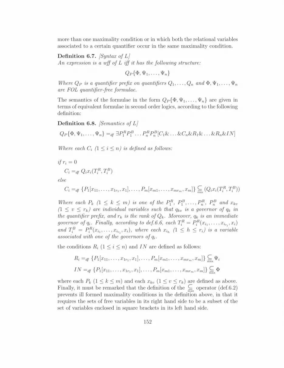
more than one maximality condition or in which both the relational variablesassociated to a certain quantifier occur in the same maximality condition.

Definition 6.7. [Syntax of L]An expression is a wff of L iff it has the following structure:

QPΦ,Ψ1, . . . ,Ψn

Where QP is a quantifier prefix on quantifiers Q1, . . . , Qn and Φ,Ψ1, . . . ,Ψn

are FOL quantifier-free formulae.

The semantics of the formulae in the form QPΦ,Ψ1, . . . ,Ψn are given interms of equivalent formulae in second order logics, according to the followingdefinition:

Definition 6.8. [Semantics of L]

QPΦ,Ψ1, . . . ,Ψn =df ∃PR1 P

B1 . . . PR

n PBn [C1& . . .&Cn&R1& . . .&Rn&IN ]

Where each Ci (1 ≤ i ≤ n) is defined as follows:

if ri = 0

Ci =df Qixi(TRi , T

Bi )

else

Ci =df P1[x11, . . . , x1r1 , x1], . . . , Pm[xm1, . . . , xmrm, xm]⊆

max

(Qixi(TRi , T

Bi ))

Where each Pk (1 ≤ k ≤ m) is one of the PR1

, PB1, . . . , PR

n , PBn and xkv

(1 ≤ v ≤ rk) are individual variables such that qkv is a governor of qk inthe quantifier prefix, and rk is the rank of Qk. Moreover, qk is an immediategovernor of qi. Finally, according to def.6.6, each TR

i = PRi (xi1 , . . . , xiri

, xi)

and TBi = PR

i (xi1 , . . . , xiri, xi), where each xih (1 ≤ h ≤ ri) is a variable

associated with one of the governors of qi.

the conditions Ri (1 ≤ i ≤ n) and IN are defined as follows:

Ri =df P1[x11, . . . , x1r1 , x1], . . . , Pm[xm1, . . . , xmrm, xm]⊆

maxΨi

IN =df P1[x11, . . . , x1r1 , x1], . . . , Pm[xm1, . . . , xmrm, xm]⊆

maxΦ

where each Pk (1 ≤ k ≤ m) and each xkv (1 ≤ v ≤ rk) are defined as above.Finally, it must be remarked that the definition of the ⊆

maxoperator (def.6.2)

prevents ill formed maximality conditions in the definition above, in that itrequires the sets of free variables in its right hand side to be a subset of theset of variables enclosed in square brackets in its left hand side.

152

6.4 Future extension: cumulative readings

This section briefly discusses how it may be possible to handle cumulativereadings in L and DTS.In section 5.4.1, I presented the classification of all non-linear quantifica-tions proposed by Sher in [Sher, 1990]. This classification simply arises bygeneralizing the meta-quantifications occurring in the formulae to be anyquantification.Among all non-linear quantifications, Sher identified two “extremes”: Com-plex Dependence non-linear quantification and Independence non-linear quan-tification.The former is what is generally taken as Branching Quantification, i.e. anon-linear quantification on two or more sets of individuals that requires theexistence of a maximal each-all inclusion (i.e. a massive nucleus) in the ex-tension of the quantified formula. All examples shown above in this chapterare examples of Complex Dependence non-linear quantification.On the contrary, Independence is what is generally called cumulative quan-tification, i.e. a non-linear quantification on two or more sets of individuals inwhich each individual in each set makes true the quantified formula togetherwith at least one individual for each other involved set.Many NL sentences, as those reported in (115), can be interpreted only viaa formula containing a cumulative quantification

(115) a. Three monkeys ate all our bananas.

b. The Japanese kamikaze hit more than 300 Usa battleships.

c. Many politicians have taken a bribe from the five companies.[Beckand Sauerland, 2000]

For example, (115.a) describes a situation in which there are three monkeysand the sum of the sets of bananas they respectively ate is equal to the setof all our bananas. Analogous considerations hold for (115.b): each involvedkamikaze hit one single involved battleship and each battleship was hit by atleast one kamikaze. Sentence (115.c) is a bit more complex in that it containsthree quantifiers: it describes a situation in which each of the five companiescorrupted a group of politicians by giving a bribe to each of them; the setof politicians may be different from company to company, provided that the“cumulation” of all politicians corrupted by at least one of the five companiesconstitutes a set of many politicians.However, despite the evident existence of cumulative readings in NaturalLanguage, they received very little attention in Underspecification; to my

153

knowledge, the only two attempts for taking cumulative readings into ac-count in an underspecified formalism (UDRT) are [Reyle, 1996] and, recently,[Chaves, 2005].In fact, for handling cumulative readings, as well as other types of branch-ing quantification, in a strictly linear framework, it is necessary to introducesome complex and unnatural mechanisms; for instance, [Reyle, 1996] makesuse of polyadic quantifications.On the contrary, the logics L may handle cumulative readings in a straight-forward fashion, since it considers partial orderings on quantifiers as naturalas linear ones. In fact, on the basis of the classification proposed by Sher,it seems that it is sufficient to introduce in L a new operator, called, forinstance, ⊆

cum, and defined as follows

Definition 6.9. [Syntax of ⊆cum

]If P1, . . . , Pn is a set of L predicates with arity a1, a2, . . . , an respectively,x11, . . . , x1a1 , . . . , xn1, . . . , xnan

are first order variables and Φ is a well formedformula in First Order Logics whose free variables are a subset of x11, . . .,x1a1 , . . ., xn1, . . ., xnan

, then the formula

P1[x11, . . . , x1a1 ], . . . , Pn[xn1, . . . , xnan]⊆

cum

Φ

is a well formed formula in L

Definition 6.10. [Semantics of ⊆cum

]The L formula

P1[x11, . . . , x1a1 ], . . . , Pn[xn1, . . . , xnan]⊆

cum

Φ

is true iff

∀x11,...,x1a1[(P1(x11, . . . , x1a1) →

∃x21,...,x2a2 ,xn1,...,xnan[(P2(x21, . . . , x2a2) ∧ . . . ∧ Pn(xn1, . . . , xnan

) ∧ Φ]∧

∀x21,...,x2a2[(P2(x21, . . . , x2a2) →

∃x11,...,x1a1 ,xn1,...,xnan[(P1(x11, . . . , x1a1) ∧ . . . ∧ Pn(xn1, . . . , xnan

) ∧ Φ]∧

. . .

∀P ′

1. . . P ′

n[

∀x11,...,x1a1 ,xn1,...,xnan[

( (P1(x11, . . . , x1a1) ∧ . . . ∧ Pn(xn1, . . . , xnan)) →

(P ′

1(x11, . . . , x1a1) ∧ . . . ∧ P

′

n(xn1, . . . , xnan))∧

(P ′

1(x11, . . . , x1a1) ∧ . . . ∧ P

′

n(xn1, . . . , xnan)) → Φ) ) →

154

(P ′

1(x11, . . . , x1a1) ∧ . . . ∧ P

′

n(xn1, . . . , xnan)) →

(P1(x11, . . . , x1a1) ∧ . . . ∧ Pn(xn1, . . . , xnan)) ] ]

By means of the ⊆cum

operator, then, we can associate to (115.b) the followingL formula

(116)

Thex japanese kamikazes hit more than 300y USA battleships.

∃PRx , P

Bx , P

Ry , P

By [ Thex(P

Rx (x), PB

x (x)) &

MT300y(PRy (y), PB

y (y)) &

PRx [x]⊆

max(jap−kam

′(x)) &

PRy [y]⊆

max(usa−batShip

′(y)) &

PBx [x], PB

y [y]⊆cum

(hit′(x, y)) ]

It is easier to see that the formula captures the right truth-conditions if we“expand” the ⊆

cumoperator and rewrite the formula in Sher terms, i.e.

(117)

Thex japanese kamikazes hit more than 300y USA battleships.

∃PxPy[ Cx : Thex(JapKam′(x), Px(x)) ∧

Cy : MoreThan300y(UsaBattleship′(y), Py(y)) ∧

IN : ∀x[Px(x) → ∃y[ Py(y) ∧ hit′(x, y)]]∧

∀y[Py(y) → ∃x[ Px(x) ∧ hit′(x, y)]]∧

Max(〈Px, Py〉, 〈IN〉) ]

In fact, this formula makes evident that for each involved kamikaze theremust be at least one battleship that has been hit by him and that for eachinvolved battleship there must be at least one kamikaze who hit it.However, although this solution seems to work for basic cases of cumulativereadings, it is not clear how to represents a NL sentence containing both acumulative interaction between two or more sets of entities and a standardsemantic dependency among others. For example, how to express the truth-conditions of a sentence as (115.c), in which the set of politicians and the setof companies are in cumulative branching quantification but each involvedbribe depends on the pair 〈politician, company〉?To summarize, in a logical framework that enables branching quantifications,

155

as L or DTS, cumulative readings can be in principle handled; however, sincethe groups of entities involved in a cumulative quantification may be involvedin other semantic dependencies, it is not immediate to understand how theseveral kinds of quantifications may interact to each other. Therefore, devis-ing such a framework deserves further study.

6.5 Summary

In this chapter, an extension of the logics shown in [Sher, 1997] has beenpresented. In particular, the proposed extension, formalized in a new logicscalled L, allows to handle the truth-conditions of partially ordered sets of 2-place Mostowskian Generalized Quantifiers. Therefore, L is able to representsthe semantics of NL sentences containing, in principle, any quantifier, whileSher’s logics covers just the ones containing numerals as Two, Three, etc.,in that it only deals with 1-place Mostowskian Generalized Quantifiers.The main problem faced in achieving the presented extension was representedby Nested Quantification, in which a quantifier occurs in the syntacticalrestriction of another quantifier.This problems was solved by introducing, in the formulae, two relationalvariables for each quantifier, i.e. one for each of its two arguments, and byasserting maximality conditions on them both.However, it must be stressed that L simply allows for the representation ofNL sentences containing nested quantifications, but it does not specify howto computationally obtain them starting from the syntactic structure of thosesentences. The methods to obtain this are presented in the next chapter.A section discussing the possibility to handle cumulative readings in L and,therefore, in DTS concludes the chapter.

156

Chapter 7

Model theoretic interpretationof DTS

This final chapter presents a model theoretic interpretation of DependencyTree Semantics. This model theoretic interpretation is achieved by definingan algorithm, called DTStoL, that translates well formed Scoped Depen-dency Graphs into equivalent L formulae, whose semantics is already welldefined. This has been done both to increase readability, and to allow forthe exploitation of Second Order theorem provers to perform reasoning1.Furthermore, it must be pointed out that DTStoL, together with the DTSsyntax-semantic interface presented in chapter 3, also provides a further ex-tension of Sher’s theory; in fact, as discussed in the previous chapter, a biglimit of the latter is that it does not specify how to obtain L formulae start-ing from the syntactic representation of the sentence. DTStoL and the DTSsyntax-semantic interface fill this gap in that they act as a bridge between aDependency Grammar and L.However, DTStoL is rather complex, in that it builds maximality conditionsby taking into account both the dependencies between involved entities (i.e.the SemDep arcs) and the subformulae embedding arising from the valuesof the function restr.For this reason, DTStoL will be presented via incremental steps.Subsection 7.1.1 discusses the relationships between the SemDep function be-longing to an SDG and the clusters in the quantifier prefix of a correspondingL formula; moreover, it defines an algorithm to determine the several clusterson the basis of the SemDep values.

1This is not new in real systems; see, for example, [Bos, 2004], that describes a system inwhich DRT well formed structures are translated into First Order Logics (FOL) formulae,rather than directly interpreted, in order to perform reasoning via standard FOL theoremprovers.

157

However, as it will be cleared in subsection 7.1.2, contrary to L0, in whicheach maximality condition has to be asserted on the relational variables cor-responding to all discourse referents belonging to the same cluster, in L themaximality conditions may be asserted also on a subset of such relationalvariables. Consequently, although the partition on clusters is taken intoaccount in DTStoL, it may be not found also in the resulting L formula,contrary to what happen in L0. This is the reason why the definition of Lwell formed formulae (def.6.7, in the previous chapter) does not rely on thenotion of cluster.Subsection 7.1.2 distinguishes between two kinds of maximality conditions,one concerning the predicate-argument relations occurring in the Flat De-pendency Graph (inclusion conditions) and one the dependencies among dis-course referents (quantifier conditions); these two kinds of maximality con-ditions are then analyzed separately.Section 7.1 reports the final version ofDTStoL and formally defines the truthconditions of a Scoped Dependency Graph in its terms. Finally, section 7.3concludes the chapter by reporting examples of DTStoL applications.

7.1 Translating DTS into L

In the previous chapter, an extension of the logics L0, proposed by Sher tointerpreter logical structures featuring partial orders on quantifiers, has beenpresented. This extension, implemented into a new logics called L, evolves L0

in that it allows for the representation of NL sentences in which a quantifieroccurs in the restriction of another quantifier, i.e. of NL sentences featuringNested Quantifications.Therefore, we are able now to translate any well-formed Scoped DependencyGraph, satisfying the constraints presented in chapter 4, into an equivalentL formula.The next subsections analyze and present possible solutions to achieve thesethree subtasks (in the listed order); this will lead to an algorithm, calledDTStoL, able to perform the translation from DTS into L.

7.1.1 Extracting quantifier prefix from SemDep arc

In L0, as discussed in [Sher, 1997], each maximality condition has to be as-serted on all relational variables belonging to a same cluster. A cluster is aclass of equivalence under the relation of common ‘immediate’ dependence.Therefore, having a partial order between discourse referents, that can bedescribed, in L0 or L, by a quantifier prefix or, in DTS, by the values of

158

the SemDep function, we can univocally determinate the several clusters ofdiscourse referents.This section presents a procedure, called buildClusters, to computational ob-tain the partition on clusters on the basis of a SemDep function. buildClustersmakes use of another function, called immGov(d, SemDep), that, taken a dis-course referent d in the SemDep’s domain, returns all immediate governorsof d; immGov(d, SemDep) is simply defined as follows:

Definition 7.1 (immGov).immGov(d, SemDep), where d is a discourse referents in SemDep’s domain,returns a subset of SemDep(d):

immGov(d, SemDep) =

if SemDep(d) = Ctx then

return Ctx

else

return SemDep(d)\ ∪d′∈SemDep(d)

SemDep(d′)

Clearly, the set of immediate governors of d, except in case d is directly linkedto Ctx, is the set of all discourse referents on which d depends (both directlyand transitively), i.e. SemDep(d), minus the discourse referents on whichat least one element of SemDep(d) also depends, i.e. minus those discoursereferents on which d transitively depends.Now we are able to define buildClusters; this function takes as input SemDep

and its domain D and returns a set of pairs. Each pair is in the form 〈cl, id〉,where cl is a cluster, i.e. a class of equivalence under the relation of commonimmediate dependence, and id the set of all immediate dependents of someelements in cl; id is another cluster except in case cl is the smallest cluster;in this case, id is the empty set.

159

Definition 7.2 (buildClusters).buildClusters(D, SemDep), where D is the set of all discourse referents inSemDep’s domain, returns a set of pairs 〈cl, id〉, where cl is a cluster of Dand id is the set of all immediate dependents of some element in cl; id isanother cluster except in case cl is the smallest cluster; in this case, id is theempty set. The clusters form a partition of D. The returned set of pairs isbuilt according to the following instructions:

buildClusters(D, SemDep) =

- set Clusters = Ø

- for each d ∈ D do

- set newGov = immGov(d, SemDep)

- if newGov 6= Ctx then

- if ∃ 〈cl, id〉 ∈ Clusters such that (cl ∩ newGov 6= Ø) then

- remove 〈cl, id〉 from Clusters

- set cl = cl ∪ newGov

- set id = id ∪ d

- add 〈cl, id〉 to Clusters

else

- add 〈newGov, d〉 to Clusters

- set smallestCluster = D \ ∪〈cl, id〉 ∈ Clusters

cl

- add 〈smallestCluster,Ø〉 to Clusters

- return Clusters

In order to identify the correct clusters, buildClusters, for each discoursereferent in D, computes the set of its immediate governors. For example, asexemplified in the figure below, let d1, . . . , dm be the set of all discourse ref-erents D and let di1, . . . , dini

, for each i = 1..m, be the set of all immediategovernors of di.

160

d11, d12, . . . d1n1 d21, d22, . . . d1n2 dm1, dm2, . . . dmnm

d1 d2 dm. . .

. . .

The discourse referents di1, . . . , dinihave to belong to the same clusters, in

that they share a common dependent, i.e. di. However, it could also hap-pen that a discourse referent d′ belongs to two differents sets of immediategovernors di1, . . . , dini

and dj1, . . . , djnj, with i 6= j; for example, in the

figure below, w belongs both to the set of immediate governors of x and theset of immediate governors of y

z h w

x

w v k

y

In such a case, the discourse referents in the two sets of immediate governorsmust belong to a same cluster; concerning the example under exam, thediscourse referents z, h, w, v, k have to belong to a same cluster.Therefore, each set of immediate governors found by buildClusters is addedto the family of sets that will be returned (i.e. the content of the variableClusters) unless there is already a set cl, in a pair 〈cl, id〉 previously addedto Clusters, that shares some elements with it. In this case, the set ofimmediate governors do not constitute a new cluster, but its elements aresimply added to cl.Nevertheless, this criterion finds all clusters but one; the last missing clusteris the smallest one, i.e. the cluster composed by all discourse referents thathave no dependents at all. These discourse referents are never consideredduring the for cycle iterations in that they are not immediate governors ofanyone. However, the smallest clusters can be easily found after the for cycleby taking all discourse referents in D that do not belong to any cluster inClusters. Examples of buildClusters applications are provided below.

7.1.2 Extracting maximality conditions from a ScopedDependency Graph

Having identified the clusters, we can now set up the maximality condi-tions that constitute the L formula equivalent to a given Scoped Dependency

161

Graph.In L0, as discussed in [Sher, 1997], the relational variables corresponding tothe discourse referents belonging to a same cluster have to be maximizedtogether on a same clause. One of these clauses is a conjunction of predicatesand is inserted into a maximality condition called inclusion condition (withlabel IN), while all other clauses are conjunctions of quantifiers instantiatedon their corresponding relational variables and are inserted into maximal-ity conditions called quantifier conditions (with label Cd1\Cd2 . . . \Cdn

whered1, d2, . . . , dn are all discourse referents whose relational variables are involvedin the conjunction).For example, the following L0 formula (in which clusters are marked by meansof dotted circles), that includes a quantifier prefix involving discourse refer-ents x, y, z, v, w, u, and t and a conjunction of predicates Φ,

q1x

q2y

q3z

q4v

q5w

q6u

q7t

Φ

is equivalent to the second order formula

∃Px, Py, Pz, Pv, Pw, Pu, Pt[

Cx: q1x(Px(x)) & Cy: q2y(Py(y)) &

Cz\Cv\Cw: Px[x], Py[y]⊆max

(q3z(Pz(x, z)) ∧ q4v(Pv(x, v)) ∧ q5w(Pw(x, y, w))) &

Cu\Ct: Pz[x, z], Pv[x, v], Pw[x, y, w]⊆max

(q6u(Pu(x, z, v, u)) ∧ q7t(Pt(x, y, z, v, w, t))) &

IN : Pu[x, z, v, u], Pt[x, y, z, v, w, t]⊆max

Φ ]

In the latter, the IN condition, i.e. the only clause involving predicatesrelations, is asserted on the relational variable associated with the discoursereferents in the smallest cluster, i.e. u and t. On the contrary, the othermaximality conditions are quantifier conditions asserted on the relational

162

variables associated with all discourse referents in a same cluster C and theconjunction of quantifier corresponding to all discourse referents immediatlydepending on some elements of C, i.e. all discourse referents belonging tothe “subsequent” cluster.Setting up an L formula on the basis of the cluster partition is much morecomplex in that L introduces two further problems

- There are several conjunctions of predicates, rather than a single one,each of which has to be included into a different inclusion condition;with respect to a Scoped Dependency Graph, all but one of these con-junctions are obtained by conjoining all predicats belonging to a restr

value, while the last one by conjoining all predicats not belonging toany of these values.

- Each discourse referent d is associated with two relational variables, PRd

and PBd ; the former refers to the restriction of d while the latter refers

to its body.

Consequently, in L it is not true that the relational variables associated toall discourse referents in a same cluster have to be maximized together; infact, taken a discourse referent d, its two associated relational variables, i.e.PR

d and PBd , may be inserted into two different maximality conditions2.

Therefore, it is clear that, contrary to L0, in L each cluster of quantifier canbe associated with two or more maximality conditions.Moreover, will become clear below, the set of maximality conditions associ-ated with a cluster may include both inclusion and quantifier conditions.

Inclusion conditions

The inclusion conditions are maximality conditions in the form

P1, . . . , Pn⊆max

Φ

where P1, . . . , Pn is a set of (instantiated) relational variables and Φ is aconjunction of predicates.As said above, in L0 there is just one of such conditions: the “IN” condition,in which P1, . . . , Pn is the set of all relational variables associated with thediscourse referents in the smallest cluster and Φ is the conjunction of allpredicates occurring in the formula.On the contrary, in L, there are |D| + 1 inclusion conditions, where D is

2Actually, this is precisely what has to be done, because, as pointed out above, an L

formula including a maximality condition asserted on both PRd and PB

d makes no sense iftaken as an interpretation of a NL sentence.

163

the set of all discourse referents. As pointed out above, with respect to aScoped Dependency Graph, the first |D| conjunctions, to be inserted in |D|corresponding inclusion conditions, are obtained by conjoining all predicatesoccurring in restr(d), for each d ∈ D, while the last one is obtained byconjoining all predicates not belonging to any restr value.In order to obtain these conjunctions starting from a Scoped DependencyGraphs, two useful functional operators are introduced: ∗ and body. Theformer applies to a Flat Dependency Graph and returns the conjunction ofall predicate-argument relations in it, while the latter indicates the subgraphof all predicate-argument relations in the Flat Dependency Graph that donot belong to any restr’s value. These two terms are formally defined asfollows:

- IfGf is a Flat Dependency Graph, G∗

f is the SOL formula correspondingto the conjunction of all terms Ti, such that Ti=P (d1, . . . dk) iff Gf

contains the nodes np, nd1 , . . ., ndk, where nd1 , . . ., ndk

are all nodeslinked to np in A and f(np) = P ∈ pred, f(nd1) = d1 ∈ D . . . ,f(ndk

) = dk ∈ D.

- IfGs = 〈Gf ,Ctx,Q, quant, restr, SemDep〉 is a Scoped Dependency Graph,body(Gs) is the subgraph of Gf that contains all and only the predicate-argument relations that do not belong to restr(d) for any d ∈ D. In allexamples presented in this paper, this subgraph is made up just by thepredicate denoted by the main verb of the sentence instantiated on thediscourse referents corresponding to the verbal dependents.

Example of applications of the two functional operators just introduced areprovided below.Once we have identified the conjunctions to be inserted in the ⊆

max’s right

hand sides, we need a criterion to identify also the discourse referents whoserelational variables have to be inserted in the ⊆

max’s left hand sides.

In L0, we already know which are the discourse referents involved in itssingle inclusion condition: all those belonging to the smallest cluster. Onthe contrary, in L, not all inclusion conditions involve discourse referentsbelonging to the smallest cluster only. For example, consider the followingScoped Dependency Graph Gs

164

(118)

Twox [representatives of [Threey african countries]] arrive.

rep’

x

1 21

arrive’

1

of’

Restr(x)

2

y

Restr(y)

y

Quant(y)= Three

Quant(x)= Two

y

1

af−c’

Flat Dependency Graph

1

af−c’rep’

x

1 1

of’

And the two disambiguations reported below

(119)

x

y

Ctx

x

y

Ctxa) b)

As discussed in chapter 6, the truth conditions of the inverse linking readingof the sentence under exam, i.e. (119.a), are handled by the following Lformula:

(120)

∃PRx , P

Bx , P

Ry , P

By [ Threey(P

Ry (y), PB

y (y)) &

PRy [y]⊆

max(af−c

′(y)) &

PBy [y]⊆

max(Twox(P

Rx (y, x), PB

x (y, x))) &

PRx [y, x]⊆

max(rep′(x) ∧ of ′(x, y)) &

PBx [y, x]⊆

max(arrive′(x)) ]

This formula contains three inclusion conditions, i.e.

- PRy [y]⊆

max(af−c

′(y))

- PRx [y, x]⊆

max(rep′(x) ∧ of ′(x, y))

- PBx [y, x]⊆

max(arrive′(x))

165

Nevertheless, note that the first of these three conditions involves a relationalvariables associated with the discourse referents y, that does not belong tothe smallest cluster. In other words, as highlighted by the following schema,in which, as usual, the clusters of quantifiers are marked by dotted circles

(121)

xy body*(Gs)

restr*(x)restr*(y)

body*(Gs) = arrive’(x)

restr*(x) = rep’(x) ∧ of’(x, y)

restr*(y) = af−c’(y)

PRy PR

x

PBy PB

x

the conjunction of predicates restr*(y) is maximized with respect to PRy , i.e.

one of the relational variables associated with y. The other relational vari-able associated with y, i.e. PB

y , is used then to trigger the dependency fromx to y, as it is done in L0.Analogous considerations hold for the other linear reading of (118), i.e.(119.b), whose L formula is

(122)

∃PRx , P

Bx , P

Ry , P

By [ Twox(P

Rx (x), PB

x (x)) &

PBx [x]⊆

max(arrive′(x)) &

PRx [x]⊆

max(Threey(P

Ry (x, y), PB

y (x, y))) &

PRy [x, y]⊆

max(af−c

′(y)) &

PBy [x, y]⊆

max(rep′(x) ∧ of ′(x, y)) ]

This formula contains the following inclusion conditions

- PBx [x]⊆

max(arrive′(x))

- PRy [x, y]⊆

max(af−c

′(y))

- PBy [x, y]⊆

max(rep′(x) ∧ of ′(x, y))

But only the last two are asserted in terms of the discourse referent constitut-ing the smallest cluster, i.e. y, as depicted by the following representation3

3The analysis of the third interpretation of the sentence, i.e. the Branching Quantifierreading, is not shown in that it is not interesting for the current discussion; in fact, ifboth discourse referents are linked to Ctx, they both belong to the smallest cluster and,obviously, all inclusion conditions are asserted just in their terms.

166

(123)

yx restr*(x)

restr*(y)body*(Gs)

body*(Gs) = arrive’(x)

restr*(y) = af−c’(y)

PBx PR

y

PRx PB

x

restr*(x) = rep’(x) ∧ of’(x, y)

As final complex example, consider the following Scoped Dependency Graph,whose SemDep function establishes three clusters.

Restr(x)

Quant(y)= Two

Quant(x)= ∀

x

1

Restr(z)

11

failed’

teacher’

Quant(z)= < 1

2

x y

2

1

stud’

1

study’

1

11 2

Flat Dependency Graph

topic’

2

z

1

of’1w 2

program’

1

teacher’

z

topic’ of’

2

Restr(w)

1

Restr(y)

11 2

2

z

stud’

program’

w

study’

w

y

Quant(w)= The

x

y

Ctx

SemDep

w

z

However, three of the five conjunctions of predicates do not involve z, i.e.the only discourse referent in the smallest cluster, and therefore have to bemaximized with respect to the relational variables associated with discoursereferents belonging to other clusters.In particular, it is clear that the maximality conditions constituting the finalL formula have to be set up according to the following representation

167

y

x

restr*(x)

restr*(w)

body*(Gs)

body*(Gs) = failed’(x, y)

restr*(x) = teacher’(x)

restr*(y) = stud’(y) ∧ study’(y, z)

w

z

restr*(z)

restr*(y)

restr*(z) = topic’(z) ∧ of’(z, w)

restr*(w) = program’(w)

from which we can derive the following partial inclusion conditions (they arepartial in that the apex on the relational variables, i.e. R rather than B, isleft, up to this point, underspecified)

- P ?

x [x]⊆max

(teacher′(x))

- P ?

w[x, w]⊆max

(program′(w))

- P ?

y [x, y]⊆max

(failed′(x, y))

- P ?

z [x, y, w, z]⊆max

(topic′(z) ∧ of(z, w))

- P ?

z [x, y, w, z]⊆max

(stud′(y) ∧ study(y, z))

In order to build an inclusion condition involving a certain conjunction ofpredicates Φ, it is necessary to instantiate Φ in the minimum quantifier scopein which all variables occurring in Φ are bound. Of course, this is reasonable,since no variable can occur outside the scope of its quantifier and, intuitively,there is no reason to move a basic formula inside the scope of a quantifiernot involving its variables. With respect to a partial order, this amounts toset up a maximality condition in the form

P ?

d1[~d1, d1], . . . , P

?

dn[ ~dn, dn]⊆

maxΦ

where d1, . . . , dn is the minimun set of discourse referents such that theunion of d1, . . . , dn and the set of discourse referents on which some di ∈d1, . . . , dn depends covers the set of all discourse referents occurring in Φ.

Furthermore, ~d denotes the sequence of all discourse referents on which ddepends on. It is formally defined as follows:

168

If d ∈ D, ~d is a sequence d1, . . . , dn, where d1, . . . , dn ≡ SemDep(d) \

Ctx. Each occurrence of ~d always gives us a sequence in the same

order. If SemDep(d) = Ctx, ~d is clearly an empty sequence.

Therefore, concerning the previous example, we get P ?

z [~z, z] = P ?

z [x, y, w, z]and P ?

y [~y, y] = P ?

y [x, y].In order to identify, for each conjunction of predicates, the correspondingminimun set of discourse referents that satisfies the constraint just discussed,it is sufficient to take the set DΦ of all discourse referents occurring in theconjunction and remove all the ones that precede some element of DΦ in thepartial order. Concerning the previous example, body*(Gs) contains the dis-course referent x and y; however, since y depends on x, just the former has tobe involved in the inclusion condition associated with body(Gs). Analogously,restr*(z) contains y and z, but only z has to be involved in its inclusion con-dition.In the light of this, we are able now to define a procedure, called build-InclusionConditions, that takes in input a Scoped Dependency Graph andreturns the conjunction of all inclusion conditions of the equivalent L for-mula. buildInclusionConditions makes use of a function D(Φ) that takes ininput a conjunction of predicates Φ and returns the set of all discourse ref-erents occurring in Φ; for istance, concerning the previous example, we getD(body*(Gs)) = x, y and D(restr*(y)) = y, z

Definition 7.3 (buildInclusionConditions).buildInclusionConditions(Gs), where Gs = 〈Gf ,Ctx,Q, quant, restr, SemDep〉)is a Scoped Dependency Graph, returns an conjunction of inclusion condi-tions

buildInclusionConditions(Gs) =

- set InclConds=true

- set Conjs = 〈Ctx, body*(Gs)〉, 〈d1, restr*(d1)〉, . . . , 〈dn, restr*(dn)〉,where d1, . . . , dn ≡ D.

- for each 〈dc, conj〉 ∈ Conjs do

- set DrToMaximize = D(conj) \ ( ∪d ∈ D(conj)

SemDep(d) )

- set InclConds = InclConds∧

buildLHS(DRToBeMax ∩ dc, DRToBeMax \ dc) ⊆max

conj*

- return InclConds

169

This function makes use of the following two variables:

- Conjs, that contains the set of all pairs 〈d, restr∗(d)〉, for each d ∈ D,and the pair 〈Ctx, body*(Gs)〉. Conjs keeps track of all conjunctionsof predicates that have to be maximized into an inclusion condition.

- DrToMaximize, that contains, for each inclusion condition, the set ofall discourse referent whose relational variables have to be maximizedin the ⊆

max’s left hand side. As said above, for each conjunction conj,

DrToMaximize must be equal to the set of all discourse referentsoccurring in conj, i.e. D(conj), minus the ones on which some discoursereferent in D(conj) depend.

buildInclusionConditions invokes a subprocedure (buildLHS) that buildsthe ⊆

max’s left hand side. This procedure takes two parameters in order to dis-

criminate whether the relational variables associated with a discourse referentin DrToMaximize, and that has to be asserted in the inclusion condition,must be the one with apex R or the one with apex B: the first parameterof buildLHS contains all discourse referents whose relational variables withapex R must be included in the ⊆

max’s left hand side, while the second one

all the ones whose relational variables with apex B must be included in it.buildLHS is formally defined below.Note that if dc, i.e. the discourse referent in 〈dc, conj〉 is in DRToMaximize,then conj is restr*(dc) and PR

dcis the only relational variable with apex R

that must be included in the ⊆max

’s left hand side.

Definition 7.4 (buildLHS).buildLHS(Dr, Db), where Dr and Db are sets of discourse referents, returnsa set of instantiated relational variables according:

buildLHS(Dr, Db)

- set RelV ars=Ø

- for each d ∈ Dr do

- set RelV ars = RelV ars ∪ PRd [~d, d]

- for each d ∈ Db do

- set RelV ars = RelV ars ∪ PBd [~d, d]

- return RelV ars

170

Finally, note that, in order to assert the inclusion conditions, it is notactually required to know which are the clusters of quantifiers; therefore,buildInclusionConditions does not need to invoke the function buildClusterspreviously introduced.

Quantifier conditions

Quantifier conditions are in the form:

P ?

d1[~d1, d1], . . . , P

?

dn[ ~dn, dn]⊆

max

( quant(d11)(PRd11

( ~d11, d11), PBd11

( ~d11, d11))∧

. . .

quant(d1m)(PRd1m

( ~d1m, d1m), PBd1m

( ~d1m, d1m)) )

Where d1, . . . , dn, d11, . . . , d1m is a set of discourse referents such that eachd′ ∈ d11, . . . , d1m immediatly depends on some d ∈ d1, . . . , dn.In L0, once we know the partition into cluster, we already know also thequantifier conditions to be asserted; in fact, taken two clusters C1 and C2,such that C2 contains all discourse referents immediatly depending on somediscourse referent in C1, the quantifier condition is immediatly found byinstantiating ⊆

maxbetween the relational variable associated with all discourse

referents in C1 and the quantifiers associated with all discourse referents inC2. For example, taking C1 and C2 as indicated in the following figure

v

w

k

x

y

z

C1 C2

we can immediatly assert the following quantifier condition

Px[~x, x], Py[~y, y], Pz[~z, z]⊆max

( quant(v)(Pv(~v, v)) ∧ quant(w)(Pw(~w,w)) ∧ quant(k)(Pk(~k, k)) )

On the contrary, in L, since each discourse referent is associated to tworelational variables rather than a single one, identifying the cluster partitionis no longer sufficient to identify also the correct quantifier conditions. Infact it may be the case that the two relational variables associated with a

171

discourse referent in C1 are maximized with respect two differents subsets ofC2; in other words, it may be the case that two or more quantifier conditions,rather than a single one, can arise from the interaction between C1 and C2.An example of such a case is the L formula corresponding to the ScopedDependency Graph in fig.7.1; this Scoped Dependency Graph denotes aninterpretation of the sentence in which every representative that belongs toa potentially different company saw a potentially different set of samples.

Restr(x)

Quant(y)= ∃

Quant(x)= ∀

Restr(z)

Restr(y)

saw’

rep’

Quant(z)= Most

x

1 2

z

1

samp’

1

11 2

of’

rep’

x

1

y

y

comp’

1

z

samp’

1

11 2

of’

ycomp’ 1

x

y

Ctx

z

SemDepFlat Dependency Graph

Figure 7.1: Available Scoped Dependency Graph for the sentenceEvery representative of a company saw most samples

The SemDep’s values in fig.7.1 describes two clusters: x and, the small-est cluster, y, z. The L formula that has to correspond to this ScopedDependency Graph is reported in (124)

(124)

∃PRx , P

Bx , P

Ry , P

By , P

Rz , P

Bz [ ∀x(P

Rx (x), PB

x (x)) &

PRx [x]⊆

max(∃y(P

Ry (x, y), PB

y (x, y))) &

PBx [x]⊆

max(Mostz(P

Rz (x, z), PB

z (x, z))) &

PRy [x, y]⊆

max(comp′(y)) &

PBy [x, y]⊆

max(rep′(y) ∧ of ′(x, y)) &

PRz [x, z]⊆

max(samp′(z)) &

PBz [x, z]⊆

max(saw′(x, z)) ]

in this formula, there is not a single quantifier condition in the form

P ?x [x]⊆

max(∃y(P

Ry (x, y), PB

y (x, y)) & Mostz(PRz (x, z), PB

z (x, z)))

172

as an attempt to follow what is done in L0 would suggest, but the two dif-ferent quantifier conditions

PRx [x]⊆

max(∃y(P

Ry (x, y), PB

y (x, y))) &

PBx [x]⊆

max(Mostz(P

Rz (x, z), PB

z (x, z)))

In fact, PRx has to be the maximal set of individuals xr such that there is

some company represented by xr (independently by the fact that xr saw aset of most samples), while PB

x has to be the maximal set of individuals xb

such that there is a set of most samples he saw (independently by the factthat xb belongs to some company).In other words, in this example, y just affects the restriction of x, while zjust its body; therefore, the former has to affect just the maximization ofPR

y , while the latter just the maximization of PBy .

In the light of this, once we obtain, via an invokation of buildClusters, the setCl1, . . . , Clm of of clusters described by SemDep, together with the set ofall immediate dependents of their elements, i.e. Id1, . . . , Idm respectively,we have still to understand which immediate dominance relations existingbetween the elements of Cli and those of Idi, i = 1..m, contribute to therestriction of the governor rather than to its body.As depicted by the following figure,

v

w

k

x

y

z

C1 C2

t

D(restr*(y))

If a discourse referent t, depending on w, belongs to D(restr*(y)), or perhapsw itself belongs to D(restr*(y))), it is clear that the immediate dependencyrelation from w to y has to be handled into a quantifier condition includingPR

y [~y, y] in the ⊆max

’s left hand side, and quant(w)(PRw (~w,w), PB

w (~w,w)) in the⊆max

’s right hand side.In fact, in such a case, the immediate dependency relation contributes toidentify the set ‖PR

y ‖, i.e. the restriction of y, rather than ‖PBy ‖, i.e. the

body of y.Of course, since w also depends on z, besides PR

y it is necessary to include,

in the ⊆max

’s left hand side, also a relational variable of z: PBz or PR

z .Including one of these two variables or them both leads to a syntacticallywell-formed L formula; nevertheless, it is easy to see that the restriction of

173

a discourse referent must be maximized into a maximality condition withoutany other restriction. In other words, the ⊆

max’s left hand side of a maximality

condition cannot contain more than one variable referring to the restrictionof a discourse referent (with apex R). With respect to the previous example,this amounts to say that PR

y and PRz cannot be inserted in the same maxi-

mality condition, so the only right choice is PBz .

More in general, in order to build L formulae denoting proper NL readings,once we understand that a certain maximality condition Mc involves a re-lational variable PR

d , we can deduct that all other relational variables to bealso involved in Mc must have apex B, i.e. they must refer to the body oftheir associated discourse referents.In the light of these consideration, we can get all quantifier conditions in theL formula equivalent to a Scoped Dependency Graph by setting up a func-tion, say buildQuantifierConditions, that, for each pair of clusters 〈cl, id〉,such that id is the set of all immediate dependents of the elements in cl,checks if there is a subset of id d′

1, . . . , d′m contributing to the restriction

of some discourse referent d ∈ cl. In such a case, it identifies the set of allimmediate governors of d′1, . . . , d

′

m (clearly, this will be a set d, d1, . . . , dnincluded in cl) and builds a quantifier condition in the form

PRd [~d, d], PB

d1[~d1, d1] . . . , P

Bdn

[ ~dn, dn]⊆max

( quant(d′1)(PR

d′1(~d′1, d

′

1), PB

d′1(~d′1, d

′

1))∧

. . .

quant(d′m)(PRd′m

( ~d′m, d′

m), PBd′m

( ~d′m, d′

m)) )

finally, we need to assert a final quantifier condition triggering the immediatedependencies from all discourse referents in id that do not contribute to anyrestriction of the ones in cl to their immediate governors. Clearly, all therelational variables associated with the latter, to be included in the ⊆

max’s left

hand side, will have apex B.The only exception to this rule is when cl is the smallest cluster; in this case,id is the empty set and no quantifier condition arises.The function buildQuantifierConditions is formally defined as follows

174

Definition 7.5 (buildQuantifierConditions).buildQuantifierConditions(Gs), where Gs = 〈Gf ,Ctx,Q, quant, restr, SemDep〉)is a Scoped Dependency Graph, returns an conjunction of quantifier condi-tions:

buildQuantifierConditions(Gs) =

- set QuantConds = ∧d ∈ NG

quant(d)(PRd (d), PB

d (d)), where NG = d such

that SemDep(d) = Ctx

- set Clusters = buildClusters(D, SemDep)

- set Temp = Ø

- for each 〈cl, id〉 ∈ Clusters do

- if id 6= Ø then

- for each d ∈ cl do

- set DRHS = id ∩ (D(restr(d)) ∪ ∪d′ ∈ D(restr(d))

SemDep(d′))

- set Temp = Temp ∪DRHS

- if DRHS 6= Ø then

- set RelV arB = ( ∪d′ ∈ DRHS

immGov(d′, SemDep)) \ d

- set QuantConds = QuantConds∧

buildLHS(d, RelV arB) ⊆max

∧d′ ∈ DRHS

quant(d′)(PRd′ (~d′, d′), PB

d′ (~d′, d′))

- set DRHS = id \ Temp

- if DRHS 6= Ø then

- set RelV arB = ( ∪d′ ∈ DRHS

immGov(d′, SemDep))

- set QuantConds = QuantConds∧

buildLHS(, RelV arB) ⊆max

∧d′ ∈ DRHS

quant(d′)(PRd′ (~d′, d′), PB

d′ (~d′, d′))

- return QuantConds

175

This function makes use of the following three variables:

- QuantConds, that (incrementally) contains the conjunction of all quan-tifier conditions; this variable is initialized to the conjunction of allinstantiated quantifiers associated with the discourse referents directlylinked to Ctx; in fact, this condition does not belong to any quantifiercondition.

- DRHS contains all discourse referents such that the conjunction of alltheir istantiated quantifiers constitues the ⊆

max’s right hand side of a

quantifier condition. As said above, DRHS may correspond to the setof all discourse referents in id that contributes to the restriction ofsome discourse referent in cl, or to all discourse referents that do notcontribute to any of these restrictions.

- RelV arB, that contains all discourse referents whose variables withapex B have to be inserted in the ⊆

max’s right hand side. As said above,

these discourse referents are the immediate governors of those in DRHS

(less the discourse referent d, if the ones inDRHS contributes to restr(d))

Finally, note that the algorithm can be improved a little by removing theinstruction

if id 6= Ø then

checking that cl is not the smallest cluster, on condition that buildClustersdoes not insert in its return values the pair 〈smallestCluster,Ø〉. This isprecisely what will be done in the last version of the algorithm presented inthe next section.

7.2 An algorithm for translating Scoped De-

pendency Graphs into L formulae

In this section, the truth-conditions of a well-formed Scoped DependencyGraph are formally defined in terms of an algorith, called DTStoL, thatbuilds the conjunctions of all maximality conditions corresponding to theScoped Dependency Graph. DTStoL simply invokes the functions presentedabove; for the sake of readability, the formal definitions of these functionsand of any term they make use of are also reported here

176

Definition 7.6 (DTS model theoretic interpretation).A Scoped Dependency Graph Gs = 〈Gf ,Ctx,Q, quant, restr, SemDep〉) is logi-cally equivalent to the L formula

∃PRd1, PB

d1. . . PR

dn, PB

dn[DTStoL(Gs)]

where d1 . . . dn ≡ D and DTStoL satisfies the definition below.

Definition 7.7 (DTStoL).DTStoL(Gs), where Gs = 〈Gf ,Ctx,Q, quant, restr, SemDep〉) is a Scoped De-pendency Graph, returns a conjunction of maximality conditions:

DTStoL(Gs) =

return buildInclusionConditions(Gs) ∧ buildQuantifierConditions(Gs)

where buildInclusionConditions and buildQuantifierConditions satisfy thedefinitions below

Definition 7.8 (buildInclusionConditions).buildInclusionConditions(Gs), where Gs = 〈Gf ,Ctx,Q, quant, restr, SemDep〉)is a Scoped Dependency Graph, returns an conjunction of inclusion condi-tions:

buildInclusionConditions(Gs) =

- set InclConds=true

- set Conjs = 〈Ctx, body*(Gs)〉, 〈d1, restr*(d1)〉, . . . , 〈dn, restr*(dn)〉,where d1, . . . , dn ≡ D.

- for each 〈dc, conj〉 ∈ Conjs do

- set DrToMaximize = D(conj) \ ( ∪d ∈ D(conj)

SemDep(d) )

- set InclConds = InclConds∧

buildLHS(DRToBeMax ∩ dc, DRToBeMax \ dc) ⊆max

conj*

- return InclConds

177

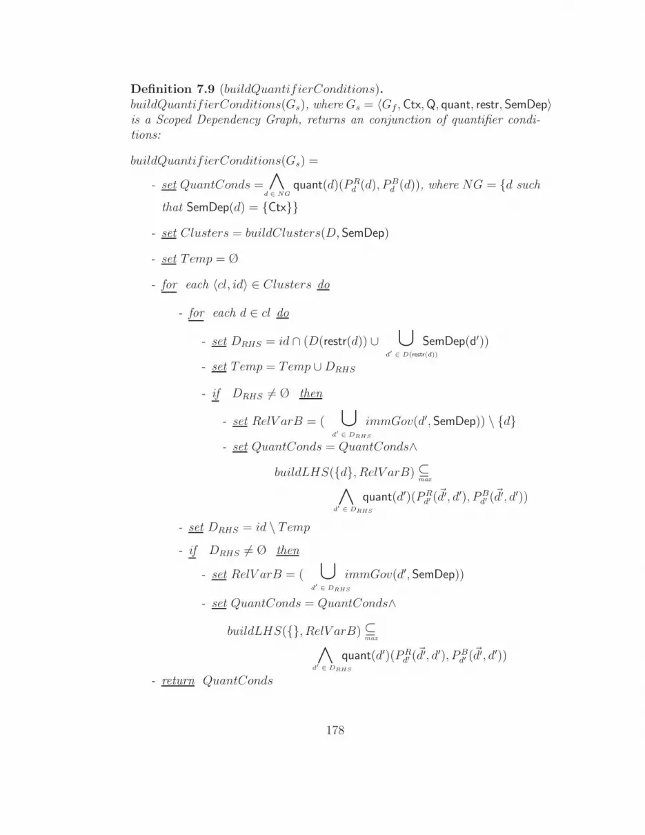
Definition 7.9 (buildQuantifierConditions).buildQuantifierConditions(Gs), where Gs = 〈Gf ,Ctx,Q, quant, restr, SemDep〉is a Scoped Dependency Graph, returns an conjunction of quantifier condi-tions:

buildQuantifierConditions(Gs) =

- set QuantConds = ∧d ∈ NG

quant(d)(PRd (d), PB

d (d)), where NG = d such

that SemDep(d) = Ctx

- set Clusters = buildClusters(D, SemDep)

- set Temp = Ø

- for each 〈cl, id〉 ∈ Clusters do

- for each d ∈ cl do

- set DRHS = id ∩ (D(restr(d)) ∪ ∪d′ ∈ D(restr(d))

SemDep(d′))

- set Temp = Temp ∪DRHS

- if DRHS 6= Ø then

- set RelV arB = ( ∪d′ ∈ DRHS

immGov(d′, SemDep)) \ d

- set QuantConds = QuantConds∧

buildLHS(d, RelV arB) ⊆max

∧d′ ∈ DRHS

quant(d′)(PRd′ (~d′, d′), PB

d′ (~d′, d′))

- set DRHS = id \ Temp

- if DRHS 6= Ø then

- set RelV arB = ( ∪d′ ∈ DRHS

immGov(d′, SemDep))

- set QuantConds = QuantConds∧

buildLHS(, RelV arB) ⊆max

∧d′ ∈ DRHS

quant(d′)(PRd′ (~d′, d′), PB

d′ (~d′, d′))

- return QuantConds

178

buildInclusionConditions and buildQuantifierConditions invoke the func-tions buildClusters, immGov, and buildLHS defined as follows:

Definition 7.10 (buildClusters).buildClusters(D, SemDep), where D is the set of all discourse referents inSemDep’s domain, returns a set of pairs 〈cl, id〉, where cl is a cluster ofD and id is the set of all immediate dependents of some element in cl; idis another cluster except in case cl is the smallest cluster; in this case, idis the empty set. All clusters form a partition of D, i.e. a family of setsCl1, . . . Clm such that Cli ∩ Clj = Ø for each i, j = 1 . . .m, i 6= j. Thereturned set of pairs is built according to the following instructions:

buildClusters(D, SemDep) =

- set Clusters = Ø

- for each d ∈ D do

- set newGov = immGov(d, SemDep)

- if newGov 6= Ctx then

- if ∃ 〈cl, id〉 ∈ Clusters such that (cl ∩ newGov 6= Ø) then

- remove 〈cl, id〉 from Clusters

- set cl = cl ∪ newGov

- set id = id ∪ d

- add 〈cl, id〉 to Clusters

else

- add 〈newGov, d〉 to Clusters

- return Clusters

179

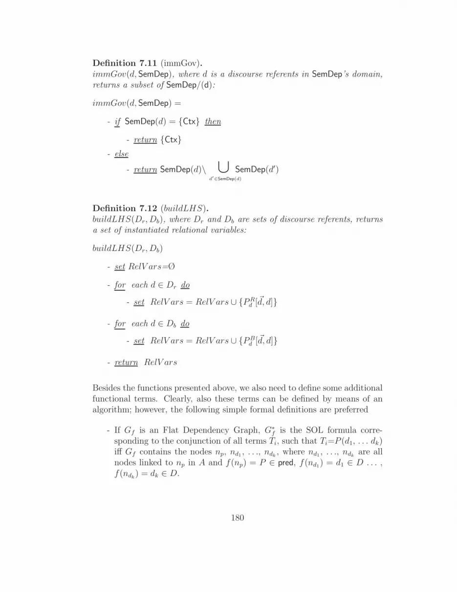
Definition 7.11 (immGov).immGov(d, SemDep), where d is a discourse referents in SemDep’s domain,returns a subset of SemDep/(d):

immGov(d, SemDep) =

- if SemDep(d) = Ctx then

- return Ctx

- else

- return SemDep(d)\ ∪d′∈SemDep(d)

SemDep(d′)

Definition 7.12 (buildLHS).buildLHS(Dr, Db), where Dr and Db are sets of discourse referents, returnsa set of instantiated relational variables:

buildLHS(Dr, Db)

- set RelV ars=Ø

- for each d ∈ Dr do

- set RelV ars = RelV ars ∪ PRd [~d, d]

- for each d ∈ Db do

- set RelV ars = RelV ars ∪ PBd [~d, d]

- return RelV ars

Besides the functions presented above, we also need to define some additionalfunctional terms. Clearly, also these terms can be defined by means of analgorithm; however, the following simple formal definitions are preferred

- If Gf is an Flat Dependency Graph, G∗

f is the SOL formula corre-sponding to the conjunction of all terms Ti, such that Ti=P (d1, . . . dk)iff Gf contains the nodes np, nd1 , . . ., ndk

, where nd1 , . . ., ndkare all

nodes linked to np in A and f(np) = P ∈ pred, f(nd1) = d1 ∈ D . . . ,f(ndk

) = dk ∈ D.

180

- IfGs = 〈Gf ,Ctx,Q, quant, restr, SemDep〉 is a Scoped Dependency Graph,body(Gs) is the subgraph of Gf that contains all and only the predicate-argument relations that do not belong to restr(d) for any d ∈ D. In allexamples presented in this paper, this subgraph is made up just by thepredicate denoted by the main verb of the sentence instantiated on thediscourse referents corresponding to the verbal dependents.

- If Φ is a SOL formula, D(Φ) denotes the set of all discourse referentsoccurring in Φ.

7.3 Examples

In this final section, ten examples of DTStoL applications are reported. Eachexample below consists of three parts:

- A NL sentence and the fully Underspecified Scoped Dependency GraphGu representing its ambiguous meaning (the graphical representationof the SkDep function is omitted).

- One or more istantiations of SemDep, i.e. one or more possible disam-biguations of Gu.

- An L formula equivalent to the Scoped Dependency Graph obtained bysubstituting one of the SemDep instantiations under exam to the func-tion SkDep in Gu; this L formula is clearly calculated by applying theDTS model theoretic interpretation as defined in the previous section.

- A description of the requirements that the maximality conditions inthe L formula impose to the relational variables involved.

Example 1

Twox students study threey theorems.

x

Quant(y)= ThreeQuant(x)= Two

study’

stud’

1

1 2

y

theor’

1

Restr(x)

x

1

Restr(y)

stud’ theor’

1

y

181

x y

Ctx

SemDepa)

x y

Ctx

SemDepb)

The L formula equivalent to the Scoped Dependency Graph having theSemDep in (a) is:

∃PRx , P

Bx , P

Ry , P

By [

Twox(PRx (x), PB

x (x)) & Threey(PRy (y), PB

y (y)) &

PRx [x]⊆

max(stud′(x)) & PR

y [y]⊆max

(teor′(y)) &

PBx [x], PB

y [y]⊆max

(study′(x, y)) ]

This formula, that handles the Branching Quantifier reading of the sentence,imposes the following constraints on the involved relational variables:

• ‖PRx ‖ and ‖PR

y ‖ must be, respectively, the set of all students and alltheorems in the domain.

• ‖PBx ×PB

y ‖ must be a maximal cartesian product such that ‖PBy ‖ is the

set of all individuals commonly studied by those in ‖PBx ‖ and ‖PB

x ‖ isthe set of all individuals studying each element of ‖PB

y ‖.

Therefore, if ‖PBx ‖ contains at least two elements of ‖PR

x ‖ and ‖PBy ‖ at least

three elements of ‖PRy ‖, the formula will be true, otherwise it will be false.

On the contrary, the L formula equivalent to the Scoped Dependency Graphhaving the SemDep in (b) is:

∃PRx , P

Bx , P

Ry , P

By [

Twox(PRx (x), PB

x (x)) &

PRx [x]⊆

max(stud′(x)) &

PBx [x]⊆

max(Threey(P

Ry (x, y), PB

y (x, y))) &

PRy [x, y]⊆

max(teor′(y)) &

PBy [x, y]⊆

max(study′(x, y)) ]

This formula, that handles one of the two linear readings of the sentence,imposes the following constraints on the involved relational variables:

182

• ‖PRx ‖ must be the set of all students in the domain.

• ‖PRy ‖ must be the set of pairs such that, for each x in the domain,

‖λy.PRy (x, y)‖ is the set of all theorems in the domain.

• ‖PBy ‖ must be the extension of the predicate study′.

• ‖PBx ‖ must be the set of all individuals x such that all that x studies

(i.e. ‖λy.PBy (x, y)‖) contains at least three elements of ‖λy.P

Ry (x, y)‖,

i.e. at least three theorems.

Therefore, if ‖PBx ‖ contains at least two elements of ‖PR

x ‖, i.e. if at leasttwo individuals, that study three potentially different theorems each, arestudents, the formula is true, otherwise it is false.

Example 2

Fewx men inserted ay coin in everyz coffee machine.

Restr(x)

Quant(y)= ∃Quant(x)= Few

x

1

Restr(y)

111

inserted’

man’Quant(z)= ∀

x y

32

z

1

coin’

1

coffeeMac’

1

Flat Dependency Graph

man’ coin’

y

Restr(z)

1

coffeeMac’

z

x y

Ctx

SemDep

z

The L formula equivalent to the Scoped Dependency Graph having the re-ported SemDep is:

∃PRx , P

Bx , P

Ry , P

By , P

Rz , P

Bz [

Fewx(PRx (x), PB

x (x)) & ∀z(PRz (z), PB

z (z)) &

PRx [x]⊆

max(man′(x)) & PR

z [z]⊆max

(coffeeMac′(z)) &

PBx [x], PB

z [z]⊆max

(∃y(PRy (x, z, y), PB

y (x, z, y)) &

PRy [x, z, y]⊆

max(coin′(y)) & PB

y [x, z, y]⊆max

(inserted′(x, y, z)) ]

183

This formula imposes the following constraints on the involved relationalvariables:

• ‖PRx ‖ and ‖PR

z ‖ must be, respectively, the set of all men and all coffeemachines in the domain.

• ‖PRy ‖ must be the set of triples such that, for each x, z in the domain,

‖λy.PRy (x, z, y)‖ is the set of all coins in the domain.

• ‖PBy ‖ must be the extension of the predicate inserted′.

• ‖PBx × PB

z ‖ must be a maximal cartesian product such that all andonly the individuals in ‖PB

x ‖ inserted a (potentially different) coin inall and only the individuals in ‖PB

z ‖.

Therefore, if ‖PBx ‖ contains few elements of ‖PR

x ‖, i.e. few men, and ‖PBz ‖

all elements of ‖PRz ‖, i.e. all coffee machines, the formula is true, otherwise

it is false.

Example 3

Twox representatives of threey african countries arrive.

rep’

x

1 21

arrive’

1

of’

Restr(x)

2

y

Restr(y)

y

Quant(y)= Three

Quant(x)= Two

y

1

af−c’

Flat Dependency Graph

1

af−c’rep’

x

1 1

of’

x

y

Ctx

x

y

Ctxa) b)

x

y

Ctxc)

y

Ctx

The L formula equivalent to the Scoped Dependency Graph having theSemDep in (a) is:

184

∃PRx , P

Bx , P

Ry , P

By [

Twox(PRx (x), PB

x (x)) & Threey(PRy (y), PB

y (y)) &

PBx [x]⊆

max(arrive′(x)) & PR

y [y]⊆max

(af−c′(y)) &

PRx [x], PB

y [y]⊆max

(rep′(x) ∧ of ′(x, y)) ]

This formula, that handles the Branching Quantifier reading of the sentence,imposes the following constraints on the involved relational variables:

• ‖PBx ‖ and ‖PR

y ‖ must be, respectively, the set of all arriving individualsand all african countries in the domain.

• ‖PRx × PB

y ‖ must be a maximal cartesian product such that all andonly the individuals in ‖PR

x ‖ represent all and only the individuals in‖PB

y ‖.

Therefore, if at least two elements in ‖PRx ‖ belong also to ‖PB

x ‖, i.e. theyarrive, and at least three elements in ‖PB

y ‖ are african countries, i.e. theybelong also to ‖PR

y ‖, the formula is true, otherwise it is false.

On the contrary, the L formula equivalent to the Scoped Dependency Graphhaving the SemDep in (b) is:

∃PRx , P

Bx , P

Ry , P

By [

Twox(PRx (x), PB

x (x)) &

PBx [x]⊆

max(arrive′(x)) &

PRy [x, y]⊆

max(af−c

′(y)) &

PRy [x, y]⊆

max(rep′(x) ∧ of ′(x, y)) &

PRx [x]⊆

max(Threey(P

Ry (x, y), PB

y (x, y))) ]

This formula imposes the following constraints on the involved relationalvariables:

• ‖PBx ‖ must be the set of all arriving individuals.

• ‖PRy ‖ must be the set of pairs such that, for each x in the domain,

‖λy.PRy (x, y)‖ is the set of all african countries.

• ‖PBy ‖ must be the set of pairs such that, for each x in the domain,

‖λy.PRy (x, y)‖ is the set of all individuals represented by x.

185

• ‖PRx ‖ must be the set of all individuals x for which the set of all that

is represented by x contains at least three potentially different africancountries.

Therefore, if at least two elements in ‖PRx ‖ belong also to ‖PB

x ‖, i.e. theyarrive, the formula is true, otherwise it is false.

Finally, the L formula equivalent to the Scoped Dependency Graph havingthe SemDep in (c) is:

∃PRx , P

Bx , P

Ry , P

By [

Threey(PRy (y), PB

y (y)) &

PRy [y]⊆

max(af−c

′(y)) &

PBy [y]⊆

max(Twox(P

Rx (y, x), PB

x (y, x))) &

PRx [y, x]⊆

max(rep′(x) ∧ of ′(x, y)) &

PBx [y, x]⊆

max(arrive′(x)) ]

This formula, that handles the Inverse Linking reading of the sentence, im-poses the following constraints on the involved relational variables:

• ‖PRy ‖ must be the set of all african countries in the domain.

• ‖PRx ‖ must be the set of pairs such that, for each y in the domain,

‖λx.PRx (y, x)‖ is the set of all representatives of y.

• ‖PBx ‖ must be the set of pairs such that, for each y in the domain,

‖λx.PBx (y, x)‖ is the set of all arriving individuals.

• ‖PBy ‖ must be the set of all individuals y such that there are at least

two representatives of y that arrive.

Therefore, if at least three elements in ‖PBy ‖ belong also to ‖PR

y ‖, i.e. theyare african countries, the formula is true, otherwise it is false.

Example 4

Twox boys ate ay portion of mostz courses.

186

Restr(x)

Quant(y)= ∃

Quant(x)= Two

x

1

Restr(z)

111

ate’

boy’

Quant(z)= Most

x y

2 11 2

z

of’

1

portion’

1

course’

1

z

boy’ course’

11 2

z

of’

portion’

1

y

Restr(y)Flat Dependency Graph

x y

Ctx

z

SemDepa)

x y

Ctx

z

b) SemDep

The L formula equivalent to the Scoped Dependency Graph having theSemDep in (a) is:

∃PRx , P

Bx , P

Ry , P

By , P

Rz , P

Bz [

Twox(PRx (x), PB

x (x)) &

PRx [x]⊆

max(boy′(x)) &

PBx [x]⊆

max(Mostz(P

Rz (x, z), PB

z (x, z))) &

PRz [x, z]⊆

max(course′(z)) &

PBz [x, z]⊆

max(∃y(P

Ry (x, z, y), PB

y (x, z, y))) &

PRy [x, z, y]⊆

max(portion′(y) ∧ of ′(y, z)) &

PBy [x, z, y]⊆

max(ate′(x, y)) ]

This formula imposes the following constraints on the involved relationalvariables:

• ‖PRx ‖ must be the set of all boys in the domain.

• ‖PRy ‖ must be the set of triples such that, for each x, z in the domain,

‖λy.PRy (x, z, y)‖ is the set of all portions of z.

• ‖PBy ‖ must be the set of triples such that, for each x, z in the domain,

‖λy.PBy (x, z, y)‖ is the extension of the predicate ate′.

187

• ‖PRz ‖ must be the set of pairs such that, for each x in the domain,

‖λz.PRz (x, z)‖ is the set of all courses (of the menu) in the domain.

• ‖PBz ‖ must be the set of pairs 〈x, z〉 such that all that has been eaten

by x (i.e. ‖λy.PBy (x, z, y)‖) contains at least a portion of z (i.e. an

element of ‖λy.PRy (x, z, y)‖).

• ‖PBx ‖ must be the set of all individuals x such that most individuals of

which x ate at least a portion (i.e. ‖λz.PBx (x, z)‖) also belong to the

set of courses (i.e. to ‖λz.PRz (x, z)‖).

Therefore, if ‖PBx ‖ contains at least two elements of ‖PR

x ‖, i.e. two boys, theformula is true, otherwise it is false.

On the contrary, the L formula equivalent to the Scoped Dependency Graphhaving the SemDep in (b) is:

∃PRx , P

Bx , P

Ry , P

By , P

Rz , P

Bz [

Twox(PRx (x), PB

x (x)) & Mostz(PRz (z), PB

z (z)) &

PRx [x]⊆

max(boy′(x)) &

PRz [z]⊆

max(course′(z)) &

PBx [x], PB

z [z]⊆max

(∃y(PRy (x, z, y), PB

y (x, z, y))) &

PRy [x, z, y]⊆

max(portion′(y) ∧ of ′(y, z)) &

PBy [x, z, y]⊆

max(ate′(x, y)) ]

This formula imposes the following constraints on the involved relationalvariables:

• ‖PRx ‖ must be the set of all boys in the domain.

• ‖PRz ‖ must be the set of all courses (of the menu) in the domain.

• ‖PRy ‖ must be the set of triples such that, for each x, z in the domain,

‖λy.PRy (x, z, y)‖ is the set of all portions of z.

• ‖PBy ‖ must be the set of triples such that, for each x, z in the domain,

‖λy.PBy (x, z, y)‖ is the set of all that has been eaten by x.

• ‖PBx × PB

z ‖ must be a maximal cartesian product such that all andonly the individuals in ‖PB

x ‖ ate a (potentially different) portion of alland only the individuals in ‖PB

z ‖.

188

Therefore, if ‖PBx ‖ contains at least two elements of ‖PR

x ‖, i.e. two boys, and‖PB

z ‖ all elements of ‖PRz ‖, i.e. all courses, the formula is true, otherwise it

is false.

Example 5

Twox boys visited ay museum in everyz region of Italyw.

Restr(x)

Quant(y)= ∃

Quant(x)= Two

x

1

Restr(w)

1

11

visited’

boy’

Quant(z)= ∀

x y

2 11 2

z

of’

1

museum’

1

region’

1 boy’

11 2

z

of’

1

y

Restr(y)

museum’

1 2

w

ιItaly’

1

in’

Flat Dependency Graph

1

Restr(z)

z

2

w

1

in’

w

ιItaly’

Quant(w)= Pnregion’

x y

Ctx

z

SemDep

w

The L formula equivalent to the Scoped Dependency Graph having the re-ported SemDep is:

189

∃PRx , P

Bx , P

Ry , P

By , P

Rz , P

Bz , P

Rw , P

Bw [

Twox(PRx (x), PB

x (x)) & ∀z(PRz (z), PB

z (z)) & Pnw(PRw (w), PB

w (w)) &

PRx [x]⊆

max(boy′(x)) & PR

w [w]⊆max

(ιItaly′(w)) &

PRz [z], PB

w [w]⊆max

(region′(z) ∧ in′(z, w)) &

PBz [z]⊆

max(∃y(P

Ry (z, y), PB

y (z, y))) &

PRy [z, y]⊆

max(museum′(y) ∧ of ′(y, z)) &

PBx [x], PB

y [z, y]⊆max

(visited′(x, y)) ]

This formula imposes the following constraints on the involved relationalvariables:

• ‖PRx ‖, ‖PR

w ‖ must be, respectively, the set of all boys in the domainand the singleton containing the individual referring to Italy, i.e. theonly individual satisfying the predicate ιItaly.

• ‖PRz ‖ must be the set of all common regions of the elements in ‖PB

w ‖;since this set contains just the individual referring to Italy, ‖PR

z ‖ mustbe the set of all italian regions.

• ‖PRy ‖ must be the set of pairs such that, for each z in the domain,

‖λy.PRy (z, y)‖ is the set of all museums in z.

• ‖PBx × PB

y ‖ must be a maximal cartesian product such that, for eachz in the domain, all and only the individuals in ‖PB

x ‖ visited all andonly the individuals in ‖λy.P

By (z, y)‖; in other words, let Y be the set

of all that has been commonly visited by all and only the individual in‖PB

x ‖; then it holds that ∀z∀y[Y (y) ↔ PBy (z, y)].

• ‖PBz ‖ must be the set of all individuals z such that the set of all that

has been commonly visited by the elements in ‖PBx ‖, i.e. Y as defined

above, contains at least a museum in z, i.e. ‖λy.PBy (z, y)‖.

Therefore, if ‖PBz ‖ contains all italian regions, i.e. all elements in ‖PR

z ‖,and ‖PB

x ‖ contains two boys, i.e. two elements in ‖PRx ‖, the formula is true,

otherwise it is false.

Example 6

There are twox soldiers in front of they main door of eachz building.

190

Restr(x)

Quant(y)= The

Quant(x)= Two

x

111

be−infront’

soldier’

Quant(z)= ∀

x y

2 1 2

z

of’

1

door’

1

building’

1

11 2

z

of’

1

y

Restr(y)Flat Dependency Graph Restr(z)

z

building’

1

soldier’

door’

x y

Ctx

z

SemDep

The L formula equivalent to the Scoped Dependency Graph having the re-ported SemDep is:

∃PRx , P

Bx , P

Ry , P

By , P

Rz , P

Bz [

∀z(PRz (z), PB

z (z)) &

PRz [z]⊆

max(building′(z)) &

PBx [z, x]⊆

max∃y(P

Ry (z, y), PB

y (z, y)) ∧ Twox(PRx (z, x), PB

x (z, x))) &

PRx [z, x]⊆

max(soldier′(x)) &

PRy [z, y]⊆

max(door′(y) ∧ of ′(y, z)) &

PBx [z, x], PB

y [z, y]⊆max

(be−infront′(x, y)) ]

This formula imposes the following constraints on the involved relationalvariables:

• ‖PRz ‖ must be the set of all buildings in the domain.

• ‖PRy ‖ must be the set of pairs such that, for each z in the domain,

‖λy.PRy (z, y)‖ is the set of all main doors of z.

• ‖PRx ‖ must be the set of pairs such that, for each z in the domain,

‖λx.PRx (z, x)‖ is the set of all soldiers in the domain.

191

• ‖PBx ×PB

y ‖ must be a set of tuples such that for each z in the domain,‖λx.P

Bx (z, x)×λy .P

By (z, y)‖ is a maximal cartesian product such that all

and only the individuals in ‖λx.PBx (z, x)‖ are in front of all and only the

individuals in ‖λy.PBy (z, y)‖. Note that this maximal cartesian product

can be different for each z.

• ‖PBz ‖ must be the set of all individuals z such that the maximal carte-

sian product ‖λx.PBx (z, x)×λy.P

By (z, y)‖ associated to it, by the inclu-

sion condition discussed above, is such that ‖λy.PBy (z, y)‖ contains the

main door of z, i.e. an element of ‖λy.PRy (z, y)‖ and ‖λx.P

Bx (z, x)‖ at

least two soldiers, i.e. two elements of ‖λx.PRx (z, x)‖.

Therefore, if ‖PBz ‖ contains all buildings, i.e. all elements of ‖PR

z ‖, the for-mula is true, otherwise it is false.

Example 7

Everyx representative of ay company saw mostz samples

Restr(x)

Quant(y)= ∃

Quant(x)= ∀

Restr(z)

Restr(y)

saw’

rep’

Quant(z)= Most

x

1 2

z

1

samp’

1

11 2

of’

rep’

x

1

y

y

comp’

1

z

samp’

1

11 2

of’

ycomp’ 1

Flat Dependency Graph

x

y

Ctx

z

SemDep

The L formula equivalent to the Scoped Dependency Graph having the re-ported SemDep is:

192

∃PRx , P

Bx , P

Ry , P

By , P

Rz , P

Bz [

∀x(PRx (x), PB

x (x)) &

PRx [x]⊆

max(∃y(P

Ry (x, y), PB

y (x, y))) &

PBx [x]⊆

max(Mostz(P

Rz (x, z), PB

z (x, z))) &

PRy [x, y]⊆

max(comp′(y)) &

PBy [x, y]⊆

max(rep′(y) ∧ of ′(x, y)) &

PRz [x, z]⊆

max(samp′(z)) &

PBz [x, z]⊆

max(saw′(x, z)) ]

This formula imposes the following constraints on the involved relationalvariables:

• ‖PRz ‖ must be the set of pairs such that, for each x in the domain,

‖λz.PRz (x, z)‖ is the set of all samples in the domain.

• ‖PBz ‖ must be the set of pairs such that, for each x in the domain,

‖λz.PBz (x, z)‖ is the set of all that has been seen by x.

• ‖PRy ‖ must be the set of pairs such that, for each x in the domain,

‖λy.PBy (x, y)‖ is the set of all companies.

• ‖PBy ‖ must be the set of pairs such that, for each x in the domain,

‖λy.PRy (x, y)‖ is the set of all that x represents.

• ‖PRx ‖ must be the set of all individuals x such that all that x represents,

i.e. ‖λy.PBy (x, y)‖ contains at least a company, i.e. an element of

‖λy.PRy (x, y)‖.

• ‖PBx ‖ must be the set of all individuals x such that all that has been

seen by x, i.e. ‖λz.PBz (x, z)‖ contains most samples, i.e. most elements

of ‖λz.PRz (x, z)‖.

Therefore, if ‖PBx ‖ contains all elements of ‖PR

x ‖, i.e. all representative of a(potentially different) company, the formula will be true, otherwise it will befalse.

193

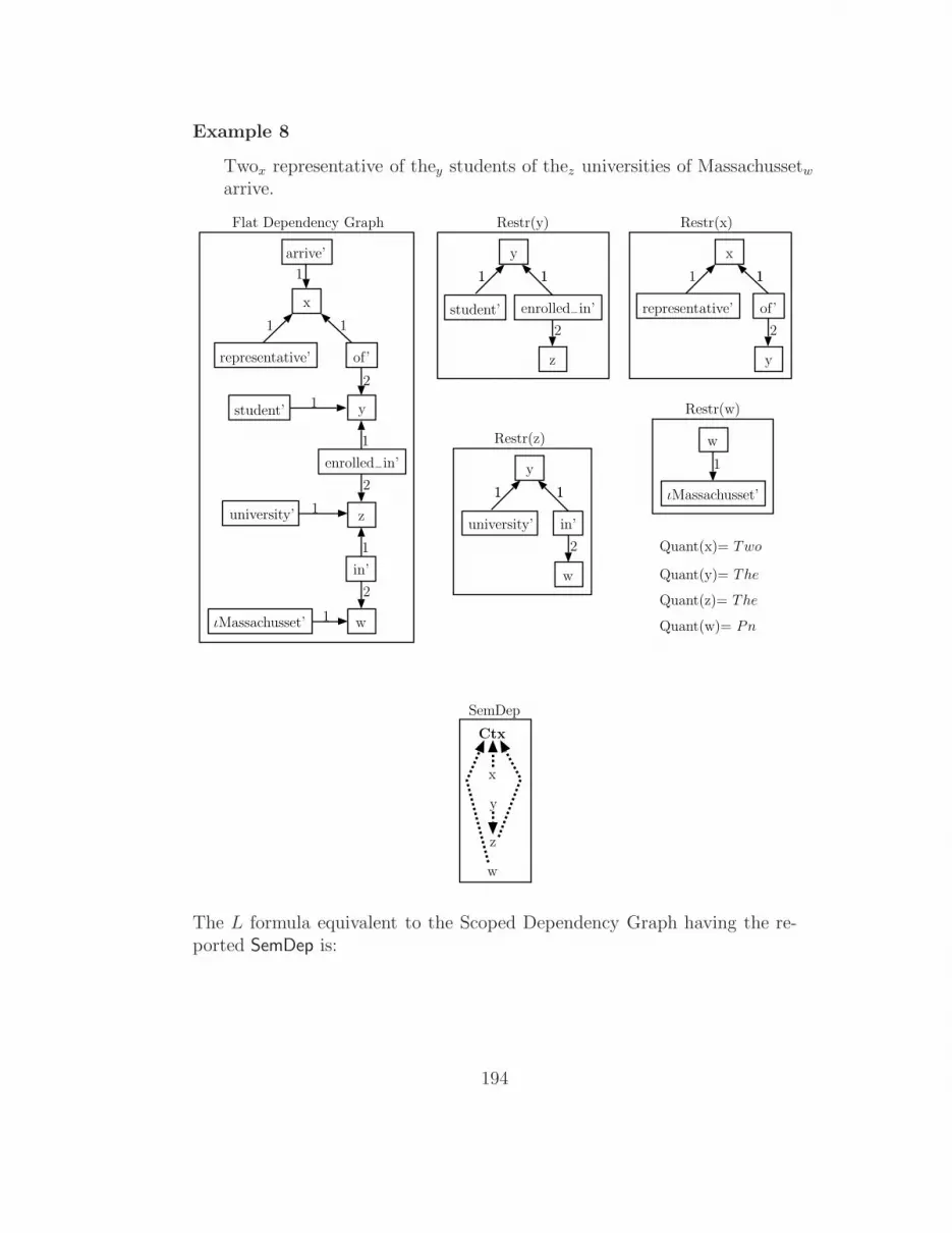
Example 8

Twox representative of they students of thez universities of Massachussetw

arrive.

representative’

x

1

2

1

arrive’

y

1

1

of’

Restr(x)

Restr(z)

x

2

1

y

of’

1

student’

2

z

1

Restr(y)

1

2

11 1

y

z

Quant(y)= The

Quant(x)= Two

Quant(z)= The

enrolled−in’

university’ 1

1

2

w

in’

ιMassachusset’ 1

representative’

1

student’ enrolled−in’

1

2

11 1

y

university’ in’

w

w

ιMassachusset’

1

Restr(w)

Quant(w)= Pn

Flat Dependency Graph

x

y

Ctx

z

SemDep

w

The L formula equivalent to the Scoped Dependency Graph having the re-ported SemDep is:

194

∃PRx , P

Bx , P

Ry , P

By , P

Rz , P

Bz , P

Rw , P

Bw [

Twox(PRx (x), PB

x (x)) & Thez(PRz (z), PB

z (z)) & Pnw(PRw (w), PB

w (w)) &

PRw [w]⊆

max(ιMassachusset′(w)) &

PRz [z], PB

w [w]⊆max

(university′(z) ∧ in′(z, w)) &

PBz [z]⊆

max(They(P

Ry (z, y), PB

y (z, y))) &

PRy [z, y]⊆

max(student′(y) ∧ enrolled−in

′(y, z)) &

PRx [x], PB

y [z, y]⊆max

(representative′(y) ∧ of ′(x, y)) &

PBx [x]⊆

max(arrive′(x)) ]

This formula imposes the following constraints on the involved relationalvariables:

• ‖PBx ‖, ‖PR

w ‖ must be, respectively, the set of all arriving people inthe domain and the singleton containing the individual referring toMassachusset.

• ‖PRz ‖ must be the set of all common universities of the elements in

‖PBw ‖; since this set contains just the individual referring to Massachus-

set, ‖PRz ‖ must be the set of all universities of Massachusset.

• ‖PRy ‖ must be the set of pairs such that, for each z in the domain,

‖λy.PRy (z, y)‖ is the set of all students enrolled in z.

• ‖PRx ×PB

y ‖ must be a maximal cartesian product such that, for each zin the domain, all and only the individuals in ‖PB

x ‖ represents all andonly the individuals in ‖λy.P

By (z, y)‖; in other words, let Y be the set

of all that is commonly represented by all and only the individual in‖PB

x ‖; then it holds that ∀z∀y[Y (y) ↔ PBy (z, y)].

• ‖PBz ‖ must be the set of all individuals z such that the set of all that

has been commonly represented by the elements in ‖PBx ‖, i.e. Y as

defined above, contains the students enrolled in z, i.e. ‖λy.PRy (z, y)‖.

Therefore, if ‖PBz ‖ contains all universities of Massachusset, i.e. all elements

in ‖PRz ‖, and at least two elements of ‖PR

x ‖ arrive, i.e. they belong also to‖PB

x ‖, the formula is true, otherwise it is false.

195

Example 9

Everyx teacher failed twoy students that study less than halfz ofthe topics in thew program.

Restr(x)

Quant(y)= Two

Quant(x)= ∀

x

1

Restr(z)

11

failed’

teacher’

Quant(z)= < 1

2

x y

2

1

stud’

1

study’

1

11 2

Flat Dependency Graph

topic’

2

z

1

of’1w 2

program’

1

teacher’

z

topic’ of’

2

Restr(w)

1

Restr(y)

11 2

2

z

stud’

program’

w

study’

w

y

Quant(w)= The

x

y

Ctx

SemDep

w

z

The L formula equivalent to the Scoped Dependency Graph having the re-ported SemDep is:

∃PRx , P

Bx , P

Ry , P

By , P

Rz , P

Bz , P

Rw , P

Bw [

∀x(PRx (x), PB

x (x)) &

PRx [x]⊆

max(teacher′(x)) &

PBx [x]⊆

max(Thew(PR

w (x, w), PBw (x, w))∧ Twoy(P

Ry (x, y), PB

y (x, y))) &

PRw [x, w]⊆

max(program′(w)) &

PBy [x, y]⊆

max(failed′(x, y)) &

PRy [x, y], PB

w [x, w]⊆max

(< 1

2 z(PR

z (x, w, y, z), PBz (x, w, y, z))) &

PRz [x, w, y, z]⊆

max(topic′(z) ∧ of ′(w, z)) &

PBz [x, w, y, z]⊆

max(stud′(y) ∧ study′(y, z)) ]

196

This formula imposes the following constraints on the involved relationalvariables:

• ‖PRx ‖ must be the set of all teachers in the domain.

• ‖PRz ‖ must be the set of all tuples 〈x, w, y, z〉 such that for each x, w, y

in the domain, ‖λz.PRz (x, w, y, z)‖ must be the set of all topics of w.

• ‖PBy ‖ must be the set of pairs such that, for each x in the domain,

‖λy.PBy (x, y)‖ is the set of all individuals failed by x.

• ‖PRw ‖ must be the set of pairs such that, for each x in the domain,

‖λw.PRw (x, w)‖ is the set of all programs of x.

• ‖PBz ‖ must be the set of all tuples 〈x, w, y, z〉 such that for each x, w

in the domain, ‖λyλz.PBz (x, w, y, z)‖ must be the set of all pairs 〈y, z〉

such that y is a student and z an individual studied by y.

• ‖PRy × PB

w ‖ must be a set of tuples 〈x, y, x, w〉 such that for each x, win the domain, ‖λy.P

Ry (x, y)‖ is the set of all and only the students

y such that all that they study (i.e. ‖λz.PBz (x, w, y, z)‖) contains less

than half of the topics of w (i.e. less than half of the elements in‖λz.P

Rz (x, w, y, z)‖).

• ‖PBx ‖ must be the set of all individuals x such that the set ‖λw.P

Bw (x, w)‖

contains the contextually relevant program of x (i.e. an element of‖λw.P

Rw (x, w)‖) and all individuals failed by x (i.e. ‖λy.P

By (x, y)‖)

contains at least two students that study less than half of the topics inthe program of x (i.e. at least two elements of ‖λy.P

Ry (x, y)‖).

Therefore, if ‖PBx ‖ contains all teachers, i.e. all elements in ‖PR

x ‖, the for-mula is true, otherwise it is false.

Example 10

There were always twox students of mine in oney of the first tenz placesof thew classification of eachv exam held in thisk school.

197

x

2be−in’ y

Restr(x)

Quant(y)= ∃Quant(x)= Two

2

w

classification−of’ place−of’

1

vmyStud’

1

exam’

1

1

x

1

Quant(z)= TheF10

1 2 z

1

held−in’

k2

school’

myStud’

Restr(y)

11 2

∈

zy

Restr(z)

wz

place−of’

v

classification−of’

Restr(v)

1 21

exam’ held−in’

v

Restr(k)

1

k

school’

Quant(v)= ∀Quant(w)= The

Quant(k)= The

1

2

1

k

Flat Dependency Graph

11 2

Restr(w)

1 2

w

SemDep

x

Ctx

y

w

z

k

v

∈

The L formula equivalent to the Scoped Dependency Graph having the re-ported SemDep is:

∃PRx , P

Bx , P

Ry , P

By , P

Rz , P

Bz , P

Rw , P

Bw , P

Rv , P

Bv , P

Rk , P

Bk [

Thisk(PRk (k), PB

k (k)) &

PRk [k]⊆

max(school′(k)) &

PBk [k]⊆

max(∀v(P

Rv (k, v), PB

v (k, v))) &

PRv [k, v]⊆

max(exam′(v) ∧ held′(v, k)) &

PBv [k, v]⊆

max(Thew(PR

w (k, v, w), PBw (k, v, w))) &

PRw [k, v, w]⊆

max(classification−of

′(w, v)) &

PBw [k, v, w]⊆

max(TheF10z(P

Rz (k, v, w, z), PB

z (k, v, w, z))∧

Twox(PRx (k, v, w, x), PB

x (k, v, w, x)) ) &

PRz [k, v, w, z]⊆

max(place−of

′(z, w)) &

PRx [k, v, w, x]⊆

max(myStud′(x)) &

PBx [k, v, w, x]⊆

max(∃y(P

Ry (k, v, w, x, y), PB

y (k, v, w, x, y))) &

PRy [k, v, w, x, y], PB

z [k, v, w, z]⊆max

(∈(y, z)) &

PBy [k, v, w, x, y]⊆

max(be−in

′(x, y)) ]

198

This formula imposes the following constraints on the involved relationalvariables:

• ‖PRk ‖ must be the set of all schools in the domain.

• ‖PBy ‖ must be the set of all tuples 〈k, v, w, x, y〉 such that for each

k, v, w in the domain ‖λx.λy.PBy (k, v, w, x, y)‖ is the extention of the

predicate be−in′.

• ‖PRy ×PB

z ‖ must be a set of tuples 〈k, v, w, x, y, k, v, w, z〉 such that foreach k, v, w, x in the domain, ‖λy.P

Ry (k, v, w, x, y)‖ is the set of all and

only the individuals belonging to the set ‖λz.PBz (k, v, w, z)‖; in other

words, the set two sets have to be coincide, i.e. they both must be aset of individuals A(k, v, w). This means that the inclusion conditionunder exam associates, to each tuple 〈k, v, w, x〉 of individuals in thedomain, a set A(k, v, w). Note that A(k, v, w) may be any set; in fact,just the elements of A(k, v, w) are all and only the elements includedin itself.

• ‖PRx ‖ must be the set of all tuples 〈k, v, w, x〉 such that for each k, v, w

in the domain ‖λx.PRx (k, v, w, x)‖ is the set of all the students of mine.

• ‖PBx ‖ must be the set of all tuples 〈k, v, w, x〉 such that for each k, v, w

in the domain ‖λx.PBx (k, v, w, x)‖ is the set of all individuals x that

“be−in” one of the individuals of the set A(k, v, w), as defined above, i.e.all individuals x that are in one of the individuals in ‖λy.P

By (k, v, w, x, y)‖.

• ‖PRz ‖ must be the set of all tuples 〈k, v, w, z〉 such that for each k, v, w

in the domain, ‖λz.PRz (k, v, w, z)‖ is the set of all places of w.

• ‖PRw ‖ must be the set of all tuples 〈k, v, w〉 such that, for each k, w in

the domain, ‖λw.PRw (k, v, w)‖ is the set of all classifications of v.

• ‖PBw ‖ must be the set of all tuples 〈k, v, w〉 such that the set A(k, v, w),

as defined above, is the set of the first ten places of w, and the set ofall individuals that are in some of them contains at least two studentsof mine.

• ‖PRv ‖ must be the set of all pairs 〈k, v〉 such that for each k in the

domain, ‖λv.PRv (k, v)‖ is the set of all exams held in k.

• ‖PBv ‖ must be the set of all pairs 〈k, v〉 such that for each k in the

domain, ‖λv.PBv (k, v)‖ is the set of all individuals v such that the set

199

of all individuals such that at least two (potentially different) studentsof mine are (each) in one of its ten places, i.e. ‖λw.P

Bw (k, v, w)‖, is the

classification of v.

• ‖PBk ‖ must be the set of all individuals k such that the set of individuals

‖λv.PBv (k, v)‖, i.e. the set of all individuals v such that at least two

(potentially different) students of mine are (each) in one of the tenplaces of the classification of v, contains all exams held in k.

Therefore, if ‖PBk ‖ is the set containing “this” contextually relevant school,

the formula is true, otherwise it is false.

7.4 Summary

In this chapter, a model theoretic interpretation of Dependency Tree Seman-tics has been presented. In particular, the chapter presents an algorithm,called DTStoL, translating well-formed Scoped Dependency Graphs intoequivalent L formulae, where L is the extension of the Sher’s logics pre-sented in the previous chapter.This algorithm completes the definition of Dependency Tree Semantics asa semantic formalism able to represent semantic knowledge starting from adependency tree, through a management of underspecification on quantifierscope, until the thruth conditions of the chosen disambiguation.DTStoL invokes two subfunctions: buildInclusionConditions and buildQuan-tifierConditions that, on the basis of the information contained in the ScopedDependency Graph, respectively set up all the inclusion and the quantifierconditions of the equivalent L formula. This formula is basically the con-junction of all these conditions.The construction of these two kinds of maximality conditions has been main-tained separated in that they are based upon different criteria. Several ex-amples of DTStoL applications conclude the chapter.

200

Conclusions

This thesis analyzed the current literature on semantic underspecificationand proposed a new approach.The definition of an underspecified semantic formalism as an intermediatestep between the syntactic representation of a sentence in Natural Languageand the final (non-ambiguous) logical formula expressing its meaning is ofparamount importance for Natural Language Processing, because it allowsfor exploitation of partial knowledge without requiring a complete disam-biguation of pure semantic ambiguities.In this thesis, the focus was restricted to the ambiguities arising from dif-ferent possible interactions between quantifiers carried by the sentence, theso-called Quantifier Scope ambiguities.Concerning these ambiguities, two important issues were addressed:

• Current semantic underspecified formalisms do not take BranchingQuantifier readings into account. These are logical readings in whichtwo or more quantifications have to be evaluated “in parallel”; in otherwords, in these readings, the ordering of quantifiers along the relationof scope inclusion must feature a branch.

• Current semantic underspecified formalisms differ in several properties,which are often in a trade-off. In this thesis, one of these trade-offs wasanalyzed in depth: simplicity in obtaining the underspecified formulafrom a syntactic structure versus possibility of achieving incrementaldisambiguation. In the light of this trade-off, current semantic un-derspecified formalisms have been classified as either enumerative orconstraint-based. The former feature a simple syntax-semantic inter-face but do not license incremental disambiguation, while the oppositeholds for the latter.

Branching Quantifiers have been, by and large, neglected in the literatureon natural language semantics; in fact, many authors argue that there is noneed to provide an explicit representation for such interpretations, since theyare simply subcases of other available ones. This thesis showed evidence in

201

favour of the actual existence of Branching Quantifier readings in NaturalLanguage and, consequently, argued that they have to be enabled in the (un-derspecified) semantic language chosen to express its meaning.In order to achieve this goal, it is necessary to introduce in the logical lan-guage some formal constructs able to explicitly assert whether an involvedgroup of entities depends on another one or not. This variation adds theexpressivity needed to represent Branching Quantification: by asserting thata quantifier Q1 depends on Q2, we require a different quantification of Q2for each entity quantified by Q1, as per usual; conversely, if we do not assertany dependence among Q1 and Q2, their evaluation will then be triggered inparallel. In standard logic, this is implemented by means of the well-knownSkolem Normal Form Theorem.This theorem states that each formula in First Order Logics can be convertedinto a logically equivalent formula in Second Order Logics by replacing thequantifiers with appropriate functions describing the dependencies amongthem.Some attempts to adapt the Skolem Normal Form Theorem to the handlingof Natural Language semantics have been proposed in the literature, suchas the proposal made by Sher, who presents an extension of Second OrderLogics merging Skolem theory and Generalized Quantifiers.This thesis represents an attempt to import the concepts lying behind theSkolem Normal Form Theorem in semantic underspecification. It defines anew underspecified semantic formalism, called Dependency Tree Semantics(DTS), that allows us to underspecify dependencies between quantifiers.DTS well-formed structures are based on a simple graph G, called Flat De-pendency Graph, which describes the predicate-argument relations carriedby the sentence, without any quantification. The nodes of G are either pred-icates or discourse referents; each arc connects a predicate with a discoursereferent and is labelled with the number of the argument position. Eachdiscourse referent is also associated, by means of suitable functions, witha quantifier and a restriction, which is a subgraph of the Flat DependencyGraph. Intuitively, the restriction of a discourse referent x is the subgraphthat includes all the nodes that contribute to the identification of the indi-viduals referred by x.Furthermore, it is possible to insert additional dependencies between involvedentities, which are represented by particular arcs between discourse referents.There are two types of arcs: SkDep arcs, denoting partial dependencies, andSemDep arcs, denoting final dependencies.By means of these constructs, DTS is able to incrementally specify an un-derspecified reading into one of its possible interpretations. SkDep arcs aremonotonically added against the constraints coming from the context; then,

202

they can be frozen into a corresponding set of SemDep arcs in order to get afully specified reading.In principle, it is possible to define a model-theoretic interpretation of DTSin terms of nodes and arcs of its graphs. However, in this thesis the DTSmodel-theoretic interpretation was provided via a translation from the fullyspecified DTS structures into formulae derived from an extension of Sher log-ics. Sher’s framework was extended in order to cover Nested Quantifications,which are not licensed in its initial definition.Besides being able to represent Branching Quantifier readings, DTS also hasanother advantage with respect to current approaches to underspecification:it is immune from the aforementioned trade-off.The assertion of dependencies between quantified groups of entities does notdepend on the structural syntactic properties of the sentence. Thus, contraryto what is done in other constraint-based approaches, the syntax-semanticinterface does not have to assert initial scope constraints, but only to dealwith predicate-argument relations. Consequently, the DTS syntax-semanticinterface turns out to be computationally simpler than the ones of the otherconstraint-based approaches: it has to perform less work.To summarize, Dependency Tree Semantics defines a new approach to un-derspecification that achieves the following two advantages with respect toother current proposals in the literature:

• From a linguistic point of view, it covers Branching Quantifier readings.

• From a computational point of view, it has an easy syntax-semanticsinterface and it licenses partial disambiguations.

Finally, the thesis further contributes to the literature by extending Sherlogics so as to enable the representation of NL sentences featuring NestedQuantification.

203

204

Bibliography

Aczel, P.: 1975, ‘Quantifiers, games and inductive definitions.’. In: Proc. ofthe 3rd Scandinavian Logic Symposium. North-Holland.

Alshawi, H. (ed.): 1992, The Core Language Engine. Cambridge, MA: MitPress.

Alshawi, H. and R. Crouch: 1992, ‘Monotonic Semantic Interpretation’. In:Proc. of the 30th Annual Meeting of the ACL. pp. 32–39, MIT Press.

Barwise, J.: 1979, ‘On branching quantifiers in english’. The Journal ofPhilosophical Logic (8), 47–80.

Beck, S. and U. Sauerland: 2000, ‘Cumulativity is needed: a reply to Winter’.Natural Language Semantics 8, 349–371.

Bos, J.: 1995, ‘Predicate Logic Unplugged’. In: Proc. Of the 10th AmsterdamColloquium. Amsterdam, pp. 133–142.

Bos, J.: 2004, ‘Computational Semantics in Discourse: Underspecification,Resolution, and Inference’. J. of Logic, Lang. and Inf. 13(2), 139–157.

Bosco, C.: 2004, ‘A grammatical relation system for treebank annotation’.Ph.D. thesis.

Bosco, C. and V. Lombardo: 2003, ‘A relation schema for treebank annota-tion’. In: In Proc. of ’Ottavo congresso Nazionale dell’Associazione Ital-iana per l’Intelligenza Artificiale’ (AI*IA 2003), Pisa, 2003. Lecture Notesin Computer Science (LNCS), vol. 2829, Springer, Berlin. pp. 462–473.

Bunt, H.: 2003, ‘Underspecification in Semantic Representations: WhichTechnique for What Purpose?’. In: Proc. 5th Workshop on ComputationalSemantics (IWCS-5). Tilburg, pp. 37–54.

205

Chaves, R.: 2003, ‘Non-Redundant Scope Disambiguation in UnderspecifiedSemantics.’. In: In Balder ten Cate (Ed.) Proceedings of the 8th ESSLLIStudent Session. Vienna, pp. 47–58.

Chaves, R.: 2005, ‘DRT and Underspecification of Plural ambiguities.’. In:In Proc. 6th Workshop on Computational Semantics (IWCS-6). Tilburg,pp. 139–150.

Chomsky, N.: 1957, Syntactic Structures. The Hague: Mouton and Co.

Cooper, R.: 1983, Quantification and Syntactic Theory. Dordrecht: D.Reidel.

Copestake, A., D. Flickinger, and I. Sag: 1999, ‘Minimal Recursion Seman-tics. An introduction’. Technical report, Manuscript, Stanford University.

Dalrymple, M.: 2001, Lexical Functional Grammar, Vol. 34 of Syntax andSemantics. New York: Academic Press.

Dalrymple, M., J. Lamping, F. Pereira, and V. Saraswat: 1996, ‘A Deduc-tive Account of Quantification in LFG’. In: Quantifiers, Deduction, andContext, No. 57 in CSLI Lecture Notes. Stanford, California: Center forthe Study of Language and Information, pp. 33–57.

Debusmann, R.: 2006, ‘Extensible Dependency Grammar: A Modular Gram-mar Formalism Based On Multigraph Description’. Ph.D. thesis, SaarlandUniversity.

Debusmann, R., D. Duchier, A. Koller, M. Kuhlmann, G. Smolka, and S.Thater: 2004, ‘A Relational Syntax-Semantics Interface Based on Depen-dency Grammar’. In: Proceedings of the 20th COLING. Geneva.

Dowty, D. R., R. E. Wall, and S. Peters: 1981, Introduction to MontagueSemantics. Dordrecht: Reidel.

Ebert, C.: 2005, ‘Formal Investigations of Underspecified Representations’.Ph.D. thesis, Department of Computer Science, King’s College London.

Egg, M., A. Koller, and J. Niehren: 2001, ‘The Constraint Language forLambda Structures.’. Journal of Logic, Language and Information 10(4),457–485.

Fauconnier, G.: 1975, ‘Do quantifiers branch?’. Linguistic inquiry (6), 555–567.

206

Frank, A. and U. Reyle: 1995, ‘Principle Based Semantics for HPSG’. In:Proc. of 6th Meeting of the ACL, European Chapter. Dublin.

Fuchss, R., A. Koller, J. Niehren, and S. Thater: 2004, ‘Minimal RecursionSemantics as Dominance Constraints: Translation, Evaluation, and Anal-ysis.’. In: In Proceedings of the 42th Annual Meeting of the Association ofComputational Linguistics. pp. 247–254.

Groenendijk, J. and M. Stokhof: 1991, ‘Dynamic Predicate Logic’. Linguis-tics and Philosophy (14), 39–100.

Henkin, L.: 1961, ‘Some remarks on infinitely long formulas’. In: Finitisticmethods, Proc. Symphosium of Foundations Math. Warsaw, pp. 167–183.

Hintikka, J.: 1973, ‘Quantifiers vs Quantification Theory’. Dialectica (27),329–358.

Hobbs, J. and S. Shieber: 1987, ‘An Algorithm for Generating QuantifierScoping’. Computational Linguistics (13), 47–63.

Hudson, R. (ed.): 1990, English word grammar. Basil Blackwell, Oxford andCambridge, MA.

Joshi, A. and Y. Schabes: 1997, ‘Tree-Adjoining Grammars’. In: S. Ver-lag (ed.): Handbook of Formal Languages. Berlin: In G. Rozenberg, A.Salomaa (eds.), pp. 69–123.

Joshi, A. K. and L. Kallmeyer: 2003, ‘Factoring Predicate Argument andScope Semantics: Underspecified Semantics with LTAG’. Research onLanguage and Computation (1), 3–58.

Joshi, A. K., L. Kallmeyer, and M. Romero: 2003, ‘Flexible Composition inLTAG: Quantifier Scope and Inverse Linking’. In: Kluwer (ed.): Comput-ing Meaning, Vol. 3. R. Musken and H. Bunt (eds).

Kamp, H. and U. Reyle: 1993, From Discourse to Logic: an introductionto modeltheoretic semantics, formal logic and Discourse RepresentationTheory. Dordrecht: Kluwer Academic Publishers.

Keller, W.: 1988, ‘Nested Cooper Storage: The Proper Treatment of Quan-tification in Ordinary Noun Phrases’. In: U. Reyle and C. Rohrer (eds.):Natural Language Parsing and Linguistic Theories. Dordrecht: Reidel, pp.432–447.

207

Kempson, R. M. and A. Cormak: 1981, ‘Ambiguity and Quantification’.Linguistics and Philosophy 4(2), 259–309.

Koller, A., K. Mehlhorn, and J. Niehren: 2000, ‘A polynomial-time fragmentof dominance constraints’. In: In Proceedings of the 38th Annual Meetingof the Association of Computational Linguistics. Hong Kong, pp. 368–375.

Koller, A., J. Niehren, and S. Thater: 2003, ‘Bridging the Gap Between Un-derspecification Formalisms: Hole Semantics as Dominance Constraints’.In: Meeting of the European Chapter of the Association of ComputationalLinguistics. pp. 195–202.

Koller, A. and S. Thater: 2006, ‘Towards a redundancy elimination algorithmfor underspecified descriptions’. In: Proceedings of the 5th Intl. Workshopon Inference in Computational Semantics (ICoS-5). Buxton, England.

Kurtzman, H. and M. MacDonald: 1993, ‘Resolution of quantifier scopeambiguities’. Cognition (48), 243–279.

Larson, R.: 1985, ‘Quantifying into NP’. Ms. MIT.

Lesmo, L., V. Lombardo, and C. Bosco: 2003, ‘Treebank Development: theTUT Approach’. In: V. P. House (ed.): Recent Advances in Natural Lan-guage Processing. New Delhi: R.Sangal and S.M. Bendre (eds.), pp. 61–70.

Lesmo, L. and L. Robaldo: 2005, ‘Underspecification of Quantifier Scope inMTT’. In: In Proc. of 2th International Conference on the Meaning TextTheory (MTT-2005). Moscow.

Lev, I.: 2005, ‘Decoupling Scope Resolution from Semantic Composition’. In:In Proc. 6th Workshop on Computational Semantics (IWCS-6). Tilburg,pp. 139–150.

May, R.: 1985, Logical Form: Its Structure and Derivation. Cambridge: MITPress.

May, R. and A. Bale: 2002, ‘Inverse Linking’. In: Encyclopedia Entry inSyncom. http://kleene.sss.uci.edu/ rmay.

Mel’cuk, I.: 1988, Dependency syntax: theory and practice. SUNY UniversityPress.

Montague, R.: 1988, ‘The Proper Treatment of Quantification in OrdinaryEnglish’. In: J. Kulas, J. H. Fetzer, and T. L. Rankin (eds.): Philosophy,Language, and Artificial Intelligence: Resources for Processing NaturalLanguage. Boston: Kluwer, pp. 141–162.

208

Moran, D. B.: 1988, ‘Quantifier scoping in the SRI core language engine’. In:Proceedings of the 26th annual meeting on Association for ComputationalLinguistics. pp. 33–40, Association for Computational Linguistics.

Mostowski, A.: 1957, ‘On a generalization of quantifiers.’. Fundamenta Math-ematicae 44, 12–36.

Muskens, R.: 1996, ‘Combining Montague Semantics and Discourse Repre-sentation’. Linguistics and Philosophy 19, 143–186.

Partee, B. H.: 2004, Compositionality in Formal Semantics: Selected Pa-pers of Barbara H. Partee, Vol. 1 of Explorations in Semantics. Oxford:Blackwell Publishing.

Reyle, U.: 1993, ‘Dealing with ambiguities by Underspecification: Construc-tion, Representation and Deduction’. Journal of Semantics (13), 123–179.

Reyle, U.: 1996, ‘Co-Indexing Labelled DRSs to Represent and Reason withAmbiguities’. In: C. L. Notes (ed.): Semantic Ambiguity and Underspeci-fication. Stanford: In S. Peters and K. van Deemter (Eds.), pp. 239–268.

Sher, G.: 1990, ‘Ways of branching quantifiers’. Linguistics and Philosophy(13), 393–422.

Sher, G.: 1997, ‘Partially-ordered (branching) generalized quantifiers: a gen-eral definition’. The Journal of Philosophical Logic (26), 1–43.

Tapanainen, P.: 1999, ‘Parsing in two frameworks: finite-state and functionaldependency grammar’. Ph.D. thesis.

Tesniere, L.: 1959, Elements de Syntaxe Structurale. Paris: Librairie C.Klincksieck.

van Genabith, J. and R. Crouch: 1996, ‘F-Structures, QLFs and UDRSs’.In: M. Butt and T. King (eds.): in Proc. of the 1st Intl Conference onLFG. p. 190205, CSLI Publications.

Villalta, E.: 2003, ‘The Role of Context in the Resolution of Quantifier ScopeAmbiguities’. Journal of Semantics 2(20), 115–162.

Weir, D. J.: 1988, ‘Characterizing mildly context-sensitive grammar for-malisms’. Ph.D. thesis.

209