Foundations of Computational

Mathematics

This page is intentionally left blank

Foundations of

Computational Mathemati

Proceedings of the SMALEFEST 2000 Hong Kong, 13 - 17 2000

editors

Felipe Cucker City University of Hong Kong

J. Maurice Rojas Texas A&M University

V^b World Scientific W B New Jersey London 'Sinqapore* Singapore • Hong Kong

Published by

World Scientific Publishing Co. Pte. Ltd.

P O Box 128, Farrer Road, Singapore 912805

USA office: Suite IB, 1060 Main Street, River Edge, NJ 07661

UK office: 57 Shelton Street, Covent Garden, London WC2H 9HE

British Library Cataloguing-in-Publication Data A catalogue record for this book is available from the British Library.

FOUNDATIONS OF COMPUTATIONAL MATHEMATICS Proceedings of Smalefest 2000

Copyright © 2002 by World Scientific Publishing Co. Pte. Ltd.

All rights reserved. This book, or parts thereof, may not be reproduced in any form or by any means, electronic or mechanical, including photocopying, recording or any information storage and retrieval system now known or to be invented, without written permission from the Publisher.

For photocopying of material in this volume, please pay a copying fee through the Copyright Clearance Center, Inc., 222 Rosewood Drive, Danvers, MA 01923, USA. In this case permission to photocopy is not required from the publisher.

ISBN 981-02-4845-8

Printed in Singapore by World Scientific Printers

V

FOREWORD

In August 1990 a conference celebrating the 60th birthday of Steve Smale was held at the University of California at Berkeley. The goal of that conference, in the words of its organizers, was "to gather in a single meeting mathematicians working in the many fields to which Smale has made lasting contributions." Thus, the contributed and invited lectures covered a broad scope of subjects including Differential Topology, Dynamical Systems, and Mathematical Eco­nomics, among many others. A volume containing most of those lectures was subsequently published by Springer-Verlag (From Topology to Computation, Proceedings of the Smalefest, M. W. Hirsch, J. E. Marsden, M. Shub (Eds.), Springer-Verlag, 1993).

Steve moved to City University of Hong Kong in 1995 and on July 15th 2000 he turned 70. It was a pleasure for his friends and colleagues to orga­nize a conference to celebrate this event. On July 13-17, 2000, the second Smalefest was held in Hong Kong. Unlike the first one, however, the goal was to focus on the subject Steve had been working on since the early 80's: Theory of Computation. It was a simple matter to gather people who had been influenced by Steve's work on the Theory of Computation, and a glance at this volume shows that other subjects were quite well represented as well.

In the the first Smalefest volume, articles were grouped according to sub­jects and each group of articles was preceded by an article commenting on Steve's work on that subject. In this volume we have included one such arti­cle — "The Work of Steve Smale on the Theory of Computation: 1990-1999" — doing so for the period between the two conferences. We thank Singapore University Press and World Scientific which granted us permission to reprint this article. For the remaining articles, we thank the contributors for their valuable work.

Special thanks go to the referees, who helped us select and polish the papers in this volume; to the Liu Bie Ju Centre for Mathematical Sciences for its generous sponsorship; and to Ms. Robin Campbell for her lightning-fast LaTeX formatting.

Steve Smale has positively influenced not only our mathematics but — through his friendship, sincerity, and generosity — our lives. It is with great pleasure that we (the editors and the contributors) dedicate this volume to Steve Smale as a belated gift on his 70th birthday. Happy 70 Steve!

Felipe Cucker J. Maurice Rojas December 2001

This page is intentionally left blank

VII

CONTENTS

Foreword v

Extending Triangulations and Semistable Reduction 1 DAN ABRAMOVICH AND J. MAURICE ROJAS

The Work of Steve Smale on the Theory of Computation: 1990-1999 15 LENORE BLUM AND FELIPE CUCKER

Data Compression and Adaptive Histograms 35 OLIVIER CATONI

Bifurcations of Limit Cycles in Zq-Equivariant Planar Vector Fields 61 of Degree 5

HENRY S. Y. CHAN, K. W. CHUNG, AND JIBIN LI

Systems of Inequalities and the Stability of Decision Machines 85 JEAN-PIERRE DEDIEU

Reconciliation of Various Complexity and Condition Measures for 93 Linear Programming Problems and a Generalization of Tardos' Theorem

JACKIE C. K. H O AND LEVENT TUN$EL

On the Expected Number of Real Roots of a System of Random 149 Polynomial Equations

ERIC KOSTLAN

Almost Periodicity and Distributional Chaos 189 GONGFU LIAO AND LIDONG WANG

Polynomials of Bounded Tree-Width 211 JANOS A. MAKOWSKY AND KLAUS M E E R

Polynomial Systems and the Momentum Map 251 GREGORIO MALAJOVICH AND J. MAURICE ROJAS

VIII

Asymptotic Acceleration of the Solution of Multivariate Polynomial 267 Systems of Equations

BERNARD MOURRAIN, VICTOR Y. PAN, AND OLIVIER RUATTA

IBC-Problems Related to Steve Smale 295 ERICH NOVAK AND HENRYK WOZNIAKOWSKI

On Sampling Integer Points in Polyhedra 319 IGOR PAK

Nearly Optimal Polynomial Factorization and Rootfinding I: 325 Splitting a Univariate Polynomial into Factors over an Annulus

VICTOR Y. PAN

Complexity Issues in Dynamic Geometry 355 JURGEN RICHTER-GEBERT AND ULRICH H. KORTENKAMP

Grace-Like Polynomials 405 DAVID RUELLE

From Dynamics to Computation and Back? 423 MIKE SHUB

Simultaneous Computation of All the Zero-Clusters of a Univariate 433 Polynomial

JEAN-CLAUDE YAKOUBSOHN

Cross-Constrained Variational Problem and Nonlinear Schrodinger 457 Equation

JIAN ZHANG

1

E X T E N D I N G T R I A N G U L A T I O N S A N D S E M I S T A B L E R E D U C T I O N

D. ABRAMOVICH*

Department of Mathematics, Boston University 111 Cummington, Boston, MA 02215, USA

abrmovicQmath.bu.edu http://math.bu.edu/INDIVIDUAL/abrmovic

J. M. ROJAS*

Department of Mathematics, Texas A&M University College Station, TX 77843-3368, USA

ro j asQmath.tamu.edu http://www.math.tamu.edu/~roj as

1 I N T R O D U C T I O N

In the past three decades, a strong relationship has been established between convex geometry, represented by convex polyhedra and polyhedral complexes, and algebraic geometry, represented by toric varieties and toroidal embed-dings. In this note we exploit this relationship in the following manner . We ad­dress a basic problem in algebraic geometry: a certain version of s e m i s t a b l e r e d u c t i o n .

Semistable reduction, for non-algebraic geometers, can be thought of as a far-reaching extension of Hironaka's famous r e so lu t ion of s ingular i t i e s 8 . a

Technically, Hironaka's result is semistable reduction over a O-dimensional base (see problem 1.3 below). Semistable reduction over a 1-dimensional base was proved in 1 3 , and was later applied in the classification of algebraic threefolds 14 and the enumerative geometry of curves 4 '5 to name but a few examples. Semistable reduction for families of surfaces and threefolds (i.e., par t of the case of a 2-dimensional base), in characteristic 0, was proved in n

but remains an open problem for a higher-dimensional base. This has moti­vated alternative constructions, e.g, weak semistable reduction (see theorem

'PARTIALLY SUPPORTED BY NSF GRANT DMS-9503276 AND AN ALFRED P. SLOAN RESEARCH FELLOWSHIP.

tPARTIALLY SUPPORTED BY AN NSF MATHEMATICAL SCIENCES POSTDOC­TORAL FELLOWSHIP AND HONG KONG UGC GRANT #9040402-730. "Roughly, his result is that any algebraic variety over an algebraically closed field of char­acteristic 0 is birationally equivalent to one without singularities.

2

1.6 below and the paragraph after the theorem), which could be proved in full generality in characteristic 0 2, and has also yielded important applications 10,17

Here, we will translate the local case of semistable reduction, over a base variety of dimension > 1, into a basic problem about polyhedral complexes: extending triangulations. Once we solve the second problem, the first follows. We have taken the opportunity with this note to try to extend some bridges between the terminologies of these two theories.

1.1 Semistable Reduction

We work over the field of complex numbers C. Let / : X —> B be a proper morphism of algebraic varieties, whose generic fiber is reduced and absolutely irreducible. Thus there exists a Zariski dense open set U C B such that the fiber / _ 1 (6 ) over any point in b € U is a compact complex algebraic variety.

Loosely speaking, semistable reduction for a morphism like / is a meta-problem of "desingularization of morphisms," where the goal is to "change / slightly" so that it becomes "as nice as possible". Of course, we need to specify more precisely what we mean by the clauses in quotation marks.

1.1.1 What do we mean by a morphism being "as nice as possible?"

First of all, X and B should be as nice as possible, namely nonsingular. Moreover, we want / to have a nice, explicit local description, so that the fibers of / have the simplest possible singularities.

Such a morphism will be called semistable. Here is the definition:

Definition 1.1 Let f : X —>• B be a flat projective morphism, with con­nected fibers, of nonsingular varieties. We say that f is semistable if for each point x G X with f(x) = b there is a choice of formal coordinates Bf, = Spec C[[t i , . . . ,tm}] and Xx = Spec <C[[a;i,... ,£„]], such that f is given by:

h

ti = Y\_ xj: j = J i _ i + i

where 0 = IQ < h • • • < lm < n, n = dimX, and m = dimB.

We must state right up front that in this note we will not end up with a semistable morphism, but we will get very close. In particular, our results form an additional step in work on semistable reduction x, continuing the work of 2 for the case of a higher-dimensional base.

3

1.1.2 What do we mean by "changing f slightly?"

First we define two types of operations necessary for semistable reduction:

Definition 1.2 An alteration B\ —> B is a proper, generically finite, sur-jective morphism. A modification Y —> X is a birational proper morphism (equivalently, a birational alteration).

Given a morphism X —> B as before, and an alteration B\ —> B, we call the component oiX XgB\ dominating Bi the main component and denote it by XxBBi.

We are now ready to state the semistable reduction problem in its ultimate form:

Problem 1.3 LetX —> B be a flat projective morphism, with connected fibers and B nonsingular. Find an alteration B\ —> B, and a modification Y —>• X x g B i , such that Y —> B\ is semistable.

Note that thanks to resolution of singularities 8 , we may assume in the char­acteristic 0 case that X is nonsingular.

1.1.3 Nearly Semistable Morphisms

We will need some terminology in order to state the weaker version of semistable reduction we actually address here. We will follow 13 for the basic definitions.6

Definition 1.4

1. A toric variety is a norma? variety X with an open embedded copy T of (C*)n, such that the natural (C*)n-action on T extends to all of X. We sometimes call the pair (X, T) a torus embedding.

2. More generally, suppose Y is a normal variety with a smooth open sub-variety Uy satisfying the following condition: locally analytically at every point, (Y, Uy) is isomorphic to a local analytic neighborhood of some torus embedding (X, T). We then call Y a toroidal variety and (Y, UY) a toroidal embedding.d

''Also, mimicking standard notation from algebraic topology, / : (X, A) — • (Y, B) will be understood to mean that A and B are subvarieties of X and Y respectively; and that / is a morphism from X to Y satisfying f(A) C B. cAlthough normality is not assumed in some contexts, all toric varieties will be normal in this paper. dWe will sometimes follow 1 3 and also refer to the inclusion Uy C Y as a toroidal embedding.

4

3. A dominant morphism f : (X,Ux) —> (B,UB) of toroidal embeddings is called a toroidal morphism, if locally analytically near every point on X it is isomorphic to a torus equivariant morphism of toric varieties.

Roughly speaking, a toric variety is "monomial:" an affine toric variety is always defined by binomial equations, and any toric variety can always be covered by affine charts in such a way that every overlap isomorphism is a monomial map. Similarly, a toroidal variety is "locally monomial" and a toroidal morphism is a "locally monomial morphism."

If UB C B i s a toroidal embedding, then we may write B \ UB as a union of divisors D\U- • -L)Dk- More precisely, recall that B \ UB can be decomposed into strata of varying dimensions (see 13 or 7 ) . In particular, let us define UB

to be the union of UB and the codimension 0 strata of B \ UB- This notation makes sense since we've actually only removed pieces of codimension > 2 from B to construct UB .

We now detail the type of morphisms we will treat: Definition 1.5 A proper toroidal morphism f : (X,Ux) —>• {B,UB) is said to be nearly semistable if the following conditions hold:

1. There are no horizontal divisors in X, namely: Ux = /~1(UB)-

2. The base B is nonsingular.

3. The morphism f is equidimensional.

4. All the fibers of f are reduced.

5. The restriction of f to UB is semistable, i.e., "f is semistable in codi­mension < 1."

6. The singularities of variety X are at worst finite quotient singularities.

One may ask how far a nearly semistable morphism is from a semistable one. The answer is simple: every toroidal semistable morphism is nearly semistable; and a nearly semistable morphism X —> B is semistable if and only if X is nonsingular (see 2 ) .

1.1.4 The Result

The problem addressed in this paper is a special (local) case of nearly semistable reduction:

5

Theorem 1.6 Set B = A£ and let UB be the natural open subscheme of B whose underlying complex variety is (C*)n. Note that the inclusion UB C B is a toroidal embedding, and let f : X —>• B be a proper morphism satisfying:

1. Ux := J~1(UB) C X is a toroidal embedding, and f : (X,Ux) -> {B,UB)

is a toroidal morphism;

2. f is equidimensional, with smooth and absolutely irreducible generic fiber;

3. every fiber of f is reduced.

Then there exists a finite toric morphism (B\, UB^) —> {B, UB) and a toroidal modification Y —> X x B B± , such that Y —> Bi is nearly semistable.

One may ask what right we have to make all these assumptions on the morphism / we start with. In 2 it is shown that given any morphism / , as in Problem 1.3, we can reduce it to a toroidal morphism / as in Theorem 1.6. Such morphisms are called weakly semistable in 2.

The methods of 2 are quite different from what we do here. In short, they involve:

1. Making X —> B toroidal. This follows easily from the methods of 1.

2. Making a toroidal X —> B satisfy the conditions in the theorem. Lo­cally this can be done easily using toroidal modifications and finite base changes. To do it globally one uses a covering trick of Kawamata (see 12

)•

Moreover, once the local results here are established, we can go back to 2

and, using Kawamata's covering trick, extend it to prove nearly semistable reduction in general.

1.2 Extending Triangulations

We now wear our polyhedral glasses. For the concepts of a compact polyhedral complex A and a conical

polyhedral complex £ see 13 . An integral structure on a compact or conical polyhedral complex is denned in 13 . We will always assume that our complexes come equipped with an integral structure. From here on, we will simply say polyhedral complex, when we mean a compact polyhedral complex with integral structure. Remark 1.7 A useful example of a polyhedral complex to consider is a finite collection V of integral polyhedra in Mn. (Recall that a polyhedron in W1 is integral iff all its vertices lie in %n.) If V is closed under intersection and

6

taking faces, then V is a polyhedral complex. Note, however, that not all polyhedral complexes arise this way. This accounts for some of the geometric richness of toroidal varieties, o

Again, in 13 , it is shown that for any compact polyhedral complex A, one can construct a conical polyhedral complex, which we denote E(A) — namely the cone over A. To reverse the process, define a slicing function h : S —> E to be a nonnegative continuous function, whose restriction to every cone a S £ is linear, which vanishes only at the origin O s E . Then the slice / i _ 1( l ) of S defines a compact polyhedral complex A(£,/i) .

We denote by Sk*(A) the fc-skeleton of A. We will also use # 5 for the cardinality of a set S, and Cone(V) for the set of all nonnegative linear combinations of a set of vectors V C E™.

By a subdivision A' of A (resp. £ ' of S) we will mean a finite partial polyhedral decomposition of A (resp. £ ) , as in 13 , with the completeness property: |A'| = |A|. (Recall that the notation |A| simply means the topo­logical space consisting of the union of all the cells of A.) A subdivision A' is called a triangulation or a simplicial subdivision if every cell of A' is a simplex.

A lifting function (or order function) / : A —» K on a polyhedral complex is a continuous function, convex and piecewise linear on each cell of A, respecting the integral structure. (Briefly, the last appelation means that every maximal connected subdomain S on which / is in fact a linear function must satisfy the following conditions: (a) S is contained in some cell a of A, (b) the underlying homeomorphism from a to a polytope RN with vertices in Z " restricts to a homemorphism of 5 to a polytope r C o defined by linear inequalities with rational coefficients.) In the conical case (/ : X —> E) we add the requirement that / be homogeneous: f(Xx) = Xf(x), for all A> 0 and all xe\A\ 13 .

Remark 1.8 We follow the convention in 13, where one requires a lifting function to be "convex down" on each cell, namely f(Xx + fiy) > Xf(x) + Hf{y). Also, all our lifting functions take rational values on the lattices in the cells. This is in contrast with the polyhedral convention, as in 18, where lifting functions are "convex up" and real values are allowed, o

Given a lifting function / : A -» E, (resp. / : £ -> E) we define the subdivision A/ (resp. £ / ) induced by / , to be the coarsest subdivision such that / is linear on each cell.

Remark 1.9 The subdivision induced by f is clearly determined by the val­ues of f on its vertices Sk°(A/) (resp. its edges Sk1(E/)J. In fact, one can construct f from its values on Sk (A/) (resp. Sk1 (£/),) as the minimal func-

7

tion which is convex on each cell, having the given values on Sk°(A/) (resp. Sk1(E/)J. However, note that A/ (resp. £ / j may have strictly more vertices (resp. edges) than A (resp. £J / Nevertheless, with some care, we can control this behavior, o

We will prove the following result: T h e o r e m 1.10 Let A be a polyhedral complex andA0 C A a subcomplex. Let AQ be a triangulation of AQ induced by a lifting function. Then there exists a triangulation A' of A, also induced by a lifting function, which extends A'Q

and introduces no new vertices. That is, Sk°(A') = Sk°(A) U Sk°(A{,). Applying this to a slice of a conical polyhedral complex we obtain:

Corollary 1.11 Let E be a conical polyhedral complex admitting a slicing function h : £ -f R, and let E0 C E be a subcomplex. Let EQ fee a triangulation of En induced by a lifting function. Then there exists a triangulation £ ' of E, also induced by a lifting function, which extends Eg and introduces no new edges. That is, Sk^E') = Sk^E) U Sk1 (£{,).

One may ask, "Do we really need to assume that A'0 is induced by a lifting function?" The simplest example showing that this is indeed the case was communicated to us independently by R. Adin and B. Sturmfels:

(0 1,0) (1,1,0)

(0,1,1

(0,0,1)

Figure 1. There is no subdivision of the solid prism which preserves the number of vertices and restricts to the subdivision depicted on the boundary.

8

Let A C I 3 be the triangular prism S = Conv{uo,o, • • • ^1,2}, where:

v0,o = (0,0,0); v0,i = (1,0,0); v0,2 = (0,0,1) vh0 = (0,1,0); V l i l = (1,1,0); vlt2 = (0,1,1)

Let Ao = dA be the boundary of our prism. Let A0 be the subdivision of Ao obtained by inserting the following new

edges:

WfivTJ, voJvTji, vofiVifi

(So we've "cut" a new edge into each square 2-face of Ao-) It is an easy exercise to see that there is no extension of AQ (to a triangulation of A) without new vertices: in particular, any 3-cell of such an extension must have an edge intersecting the midpoint of some edge of A0 — a contradiction. It is also not hard to see that A0 can not be induced by any lifting function 6 .

2 Reduction of Theorem 1.6 to 1.10

Let / : X —> B be as in Theorem 1.6 and / s : Ex —• Ejg the associated mor-phism of rational conical polyhedral complexes. (Recall that X is toroidal and / is a toroidal morphism, so these associated combinatorial structures indeed exist and are well-defined.) Note that E# is a nonsingular cone (a simplicial cone of index 1): it is simply the nonnegative orthant in R™, generated by the standard basis vectors {£{}. Let T{ be the edges of E#, namely T* = Cone(ej). We identify the lattice of Ti with Ze^.

Let Y}B = {Jn be the 1-skeleton of E B and E x = / ^ ( E ^ ) - Also let Sx,j = f^in)- For an integer fcj let Ni(ki) be the integral structure on Sx,i obtained by intersecting the lattices in Ex,; with /£"1(Zfcj • ii).

By 13 , as interpreted in 13 , there exists an integer k, and a simplicial subdivision E x { of Sx,i> which is induced by a lifting function, having index 1 with respect to the integral structure Ni(ki).

Let B\ — A^ be complex affine space with coordinates s\,... , sn. The substitution s^ = U gives a homomorphism C[ti,... ,tn] —> C[s j , . . . ,sn], giving rise to a finite morphism B\ -> B. Then Y.B1 is the same as E# but taken instead with the lattice NBX = WLkii-i. Let X\ = X x# B\. Since the fibers of X are reduced, it follows that Xi is normal and Xi —> B\ is again toroidal. Likewise, Ex : is just Ex with integral structure given by intersecting the lattices in Ex with /^ 1(NB1)-

Putting the triangulations E x t of Ex,i together, there exists a triangu­lation E x of E x (induced by a lifting function) of index 1 with respect to the integral structure on Exi!

9

Let us verify that Ex admits a slicing function: let hs '• E# —»• R be the function defined by h(,(^2cae-i) — Ylai- Then the pullback /if, o / s is a slicing function on Ex-

By Corollary 1.11 of Theorem 1.10, there is an extension of E x to a triangulation E x of E (induced by a lifting function) without added edges.

Let Y —> Xi be the corresponding toroidal modification and let f\ : Y —> B\ the resulting morphism.

Note that since all the edges in the triangulation E'x map to the edges n of E B 1 ( we have that f\ is equidimensional 2. Since the integral generator of every edge in E x maps to the generator of the image edge in EBJ , and since B is nonsingular, all the fibers of f\ are reduced 2 . By the construction of 13, / i is semistable in codimension 1. Since A'x is simplicial, Y has at worst quotient singularities. Thus f\ is nearly semistable. • Remark 2.1 The variety Y may be singular, as the following example shows: let Ey C R4 be the nonnegative orthant, generated by the standard basis vec­tors e i , . . . £4. Let w = (1/2,1/2,1/2,1/2) 6 R4 and Ny the lattice generated by w,£i,.. .£4. Also let Y be the corresponding toric variety — the quotient of A4; by the diagonal Z/2 action given by p i-+ — p — which happens to be singular. Finally, let E^ C K2 be the first quadrant, generated by the standard basis vectors e.\,e*2, with the standard lattice NB = ({0}UN)2 . We have a canonical morphism Ey —>• E B via

(a,b,c,d) i-> (a + b,c + d)

which maps Ny into NB- The resulting morphism Y —> A2- is nearly semistable, but not semistable. o

3 Proof of Theorem 1.10

It is a simple fact, made precise in Lemma 3.1 below, that any generic lifting function on a polyhedral complex induces a simplicial subdivision. This fact is used frequently in applications of subdivisions to the computation of mixed volumes, polyhedral homotopies, and toric (or sparse) resultants 16>9.3>15. The last two constructions give effective recent techniques, sometimes more efficient than Grobner bases, for solving systems of polynomial equations.

However, it should be emphasized that the lifting functions considered here and in 13 are more general than those in 16>9,3: the lifting functions in the latter references are completely determined by the values assigned to the vertices of A. We will call these more restricted lifting functions verticial. The verticial lifting functions are a bit more "economical" in the sense that their corresponding subdivisions never introduce any new vertices.

10

There is a simple way to resolve this difference by passing to the verticial case from the start. In fact, we will reduce the proof of Theorem 1.10 to finding any triangulation (given by a verticial lifting function) in a new, specially constructed, polyhedral complex. The latter problem is then almost trivial to solve.

First recall (see 13, Corollary 1.12) that induced subdivisions are transi­tive: if A' is a subdivision of A induced by a lifting function / on A, and A" is a subdivision of A' induced by a lifting function / ' on A', then A" is a subdivision of A as well. In fact, A" is induced by / + ef for sufficiently small e > 0.

Thus let /o : A0 -» R be a lifting function which induces the given subdivision A0 in our theorem. By adding a constant if necessary, we may assume /o is positive. Following Remark 1.9, we can take the values of /o on Sk°(A0), extend them by zero to the other vertices Sk°(A) \ Sk°(A0), and take the minimal lifting function / : A —»• E which has these values on the vertices Sk°(A) U Sk°(A0). Clearly / | A o = /o- Let Aj be the induced subdivision. Then clearly the restriction of Ai to Ao coincides with A0 . If A' is any subdivision of Aj without new vertices, then its restriction to Ao must be AQ, since A0 is already simplicial: any subdivision of a simplicial complex without new vertices is trivial. Thus all we need to do to prove Theorem 1.10 is find a verticial lifting function on Ax giving a triangulation. In summary, by replacing A with Ai, we can assume that Ao = A0 and then conclude by finding any triangulation of Ai (given by a verticial lifting function) — a simpler problem than finding a triangulation of one complex extending some other triangulation.

To complete the proof of Theorem 1.10, recall the following lemma: Lemma 3.1 Supppose A is a polyhedral complex. Then

1. The set L A of all verticial lifting functions on A is a finite-dimensional rational vector space.

2. The set of all lifting functions which do not induce simplicial subdivisions is a finite union of proper subspaces of LA •

Proof: Note that any verticial lifting function on A is uniquely determined by its values on Sk (A), which are assumed to be rational, so part (1) follows immediately.

To prove (2), let C := (c„ | v G Sk (A)) be a vector of rational constants. Let Ac denote the subdivision of A induced by the verticial lifting function sending v H-»- CV for all u£Sk°(A).

Now suppose that there is a nonsimplicial cell C, with vertex set V(C), in Ac- Recall that the coordinates of d+ 2 points lying on a d-R&t in Rn must

11

make a certain n x n determinant vanish.e (In particular, this determinant is a nonconstant multilinear function in the coordinates of the points.) Then, by the definition of a cell in a subdivision induced by lifting, there must be a (nontrivial) linear relation satsified by (c„ | v € V(C)). Furthermore, this linear relation depends only on A and the set of vertices V(C). Since there are only finitely many possible nonsimplicial cells (since, by definition, our poly­hedral complexes have only finitely many vertices), (2) follows immediately. •

The following is an immediate corollary of our lemma. Corollary 3.2 Recall the notation of the proof of Lemma 3.1, and endow Q#Sk°(A) with the standard Euclidean metric || • ||. Let C £ dJ#Sk°(A). Then for sufficiently small e > 0,

1. Ac is a simplicial subdivision for some C € Q* s k (A) satisfying \\C — C\\<£.

2. If Ac is already a simplicial subdivision, then so is Ac, for all C € Q#Sk°<A) satisfying \\C -C\\<e. •

Remark 3.3 Put another way, simplicial subdivisions are a dense (via (1)) and open (via (2)) subset of the space of all subdivisions arising from verticial lifting functions. In fact, we really have the stronger statement that the set of all lifting values giving a particular simplicial subdivision forms an open cell within the space of all subdivisions.

Note also two "nearby" subdivisions Si and S2 need not have the same extensions, even if Si = S2 '• for example, consider the unit square S with vec­tor of vertices (ordered clockwise) (a, b, c, d), and the subcomplex E consisting of the edges {a,b} and {c,d}. Then C = (0,0,0,0) and C = ( - 1 , 1 , - 1 , 1 ) both generate the same (trivial) subdivision of E. However, these two liftings generate different subdivisions of S, the first being trivial, o

Returning to the proof of Theorem 1.10, it follows by Corollary 3.2 that there exists a simplicial subdivision of Ai without new vertices, which is what we needed to prove. •

3.1 Acknowledgements

We would like to thank B. Sturmfels for inciting this collaboration, and R. Adin for a discussion of ideas relevant to this note.

12 - H I / 2 - 2/1 13 - x\ 2/3 - j/i

Note also that this determinant is linear in the "last" coordinates {yi, j/2,3/3}-

6For example, (x\,y\), (12,4/2), and (13,2/3) lie on a line iff Det

2

1. Abramovich, Dan and de Jong, Aise Johan, "Smoothness, Semistability, and Toroidal Geometry,", J. Algebraic Geom. 6 (1997), no. 4, pp. 789-801. (Formerly available as Math ArXiV preprint alg-geom/9603018.)

2. Abramovich, Dan and Karu, Kalle, "Weak Semistable Reduction in Char­acteristic 0," Invent. Math. 139 (2000), no. 2, pp. 241-273.

3. Canny, John F. and Emiris, Ioannis Z., "A Subdivision-Based Algorithm for the Sparse Mixed Resultant," J. ACM 47 (2000), no. 3, pp. 417-451.

4. Caporaso, Lucia and Harris, Joe, "Parameter Spaces for Curves on Surfaces and Enumeration of Rational Curves," Compositio Math. 113 (1998), no. 2, pp. 155-208.

5. , "Enumerating Rational Curves: the Ratio­nal Fibration Method," Compositio Math. 113 (1998), no. 2, pp. 209-236.

6. Fulton, William, Introduction to Toric Varieties, Annals of Mathematics Studies, no. 131, Princeton University Press, Princeton, New Jersey, 1993.

7. Goresky, Mark and MacPherson, Robert, Stratified Morse Theory, Ergeb-nisse der Mathematik und ihrer Grenzgebiete, Springer-Verlag, 1988.

8. Hironaka, Heisuke, "Resolution of Singularities of an Algebraic Variety over a Field of Characteristic Zero: I and II," Ann. of Math. (2) 79 (1964), pp. 109-203, 205-326.

9. Huber, Birkett and Sturmfels, Bernd, "A Polyhedral Method for Solving Sparse Polynomial Systems," Mathematics of Computation, 64, pp. 1541— 1555, 1995.

10. Karu, Kalle, "Minimal Models and Boundedness of Stable Varieties," J. Algebraic Geom. 9 (2000), no. 1, pp. 93-109.

11. , "Semistable Reduction in Characteristic Zero for Families of Surfaces and Threefolds," Discrete Comput. Geom. 23 (2000), no. 1, pp. 111-120.

12. Kawamata, Y., "Characterization of Abelian Varieties," Comp. Math. 43, 1981 p 253-276.

13. Kempf, G.; Knudsen, F.; Mumford, D.; and Saint-Donat, B., Toroidal Embeddings I, Springer, LNM 339, 1973.

14. Kollar, Janos and Mori, Shigefumi, "Birational Geometry of Algebraic Varieties," with the collaboration of C. H. Clemens and A. Corti, trans­lated from the 1998 Japanese original, Cambridge Tracts in Mathematics, 134, Cambridge University Press, Cambridge, 1998.

15. Rojas, J. Maurice, "Algebraic Geometry Over Four Rings and the Fron­tier to Tractability," Contemporary Mathematics, vol. 270, Proceedings of a Conference on Hilbert's Tenth Problem and Related Subjects (Uni-

13

versity of Gent, November 1999, edited by Jan Denef, Leonard Lipschitz, Thanases Pheidas, and Jan Van Geel), pgs. 270-321, AMS Press (2000).

16. Sturmfels, Bernd, "Sparse Elimination Theory," In D. Eisenbud and L. Robbiano, editors, Proc. Computat. Algebraic Geom. and Commut. Algebra 1991, pp. 377-396, Cortona, Italy, 1993, Cambridge Univ. Press,

17. Viehweg, Eckart and Zuo, Kang, "On the Brody Hyperbolicity of Mod­uli Spaces for Canonically Polarized Manifolds," math arXiv preprint math.AG/0101004 (h t tp : / /math .a rXiv .org /abs /math . AG/0101004).

18. Ziegler, Gunter M., Lectures on Polytopes, Graduate Texts in Mathemat­ics, Springer Verlag, 1995.

15

THE WORK OF STEVE SMALE ON THE THEORY OF COMPUTATION: 1990-1999

FELIPE CUCKER

Dept. of Mathematics, City Univ. of Hong Kong, 83, Tat Chee Avenue, HONG KONG

E-mail: macuckerQmath. cityu. edu. hk

LENORE BLUM

Dept. of Computer Science, Carnegie Mellon University, 5000 Forbes Avenue, Pittsburgh, PA 15213-3890, USA

E-mail: lblum@cs.cmu.edu

Steve Smale's work on the theory of computation during the 1980's has been carefully reviewed by Mike Shub in 21. At the end of this period, two key aspects of Smale's work stand out. Firstly, there is the understanding he achieved of certain fundamental numerical algorithms. Quoting Shub's paper,

He has firmly grounded himself in the mathematics of practical al­gorithms, Newton's method, and the simplex method of linear pro­gramming, inventing the tools and methodology for their analysis.

Secondly, there is the awareness of the need for a theory laying out the foun­dations for scientific computation. This need is a motivating goal behind 29

where a comparison between theoretical computer science and scientific com­putation constitutes the opening theme of the article. The following is taken from his paper.

Algorithms in numerical analysis are primarily a means to solve prac­tical problems, while in computer science, algorithms are studied systematically in their own right. [... ] note that algorithms are the main object of study in scientific computation, yet there is not a for­mal definition of algorithm. I am reminded of how the development of the definition of differentiable manifold was so important in the history of differential topology.

Thus, Smale wants to construct foundations for scientific computation just as those for discrete computation are constructed in theoretical computer science. A good part of Smale's work during the 1980's points in this direction. For instance, in 28, complexity lower bounds are proved by what Smale called

16

"tame machines", and notably in 6 , a very general machine model is defined and a theory of computability and complexity is developed.

Two main results of 6 are the existence of universal machines and the NP-completeness of several feasibility problems. The latter reaffirmed the importance of equation solving as a computational problem and suggested two lines of research. On the one hand, there is the P / NP conjecture which implies that, even deciding feasibility for systems of equations cannot be done efficiently. On the other hand, while accepting the difficulty of equation solving, one might try to find algorithms which behave well "in general" or with respect to some particular viewpoint. These two problems appear in a list of problems for the next century proposed in 32 in response to a request from V. I. Arnold (on behalf of the International Mathematical Union). Smale selected 18 problems from which the 3rd exactly asks whether P = NP and the 17th ("Solving polynomial equations") reads,

Can a zero of n complex polynomial equations in n unknowns be found approximately, on the average, in polynomial time with a uni­form algorithm?

In the next section we will review some of Smale's work in relation to the first problem. Then we will focus on the second.

1 The P vs. NP problem

1.1 By the end of the 1980's a complexity theory over the reals had been established 6. This theory of complexity, although primarily devised to de­scribe computations with real numbers, is actually much more general. It describes computations over arbitrary rings and can be "parameterized" by the following five features: 1) a base ring, 2) allowable operations, 3) allowable branching tests, 4) a cost measure, and 5) input size.

For instance, for the ring of integers 2Z with operations {+, - , x } , branch­ing on <, logarithmic (or bit) cost and bit input size, we recover, up to polyno­mial equivalence, the usual Turing machine model and the classical complexity theory of computer science. The same is true for the ring ZZ2 = {0,1} with operations {+, —, x, / } , branching on =, unit cost and vector length as input size. If we replace 2Z2 by the complex numbers C, we get a corresponding theory of computation and complexity over C. For a theory over the reals R, we allow branching on <.

For each combination of these parameters (let's call this a setting) one has a natural P=NP problem. Here P is the class of (Yes-No decision) problems

17

solvable in polynomial time in the setting; NP is the class of problems whose Yes instances are checkable in polynomial time in the setting.

For some settings, one can prove that P ^ NP simply because NP contains undecidable problems. For a few, a proof that P 7 NP can be obtained together with the standard inclusion NP C EXP. But for the majority, the question remains wide open.

An issue raised by the variety of settings just mentioned is how the P=NP question relates between one setting and another. Thus in the foreword of 4

Richard Karp writes,

It is interesting to speculate as to whether the questions of whether P R = NPIR and whether P<c = NP<n are related to each other and to the classical P versus NP question [...].

A good part of the research in complexity theory over arbitrary rings during the last ten years has been dominated by this issue.

1.2 An example of a relation between different settings is found in 26. Here an NP-complete problem over C is considered and its intractability is deduced from a hardness assumption concerning computations over TL. This reduces a complexity question over TL to a complexity question over <D, thus considerably enhancing a classical tool in computer science (the idea of reduction between discrete problems) to apply now to a broader class of problems (reductions between problems in different settings).

The Hilbert Nullstellensatz as a decision problem can be stated as follows. Given polynomials fx,..., fs with complex coefficients, in n variables, decide whether or not there exists z € <D™ such that fi(z) ~ 0 for i = l , . . . , s . Even restricted to the case when all the ft have degree 2, the problem is NP<c-complete (cf. 6 ) .

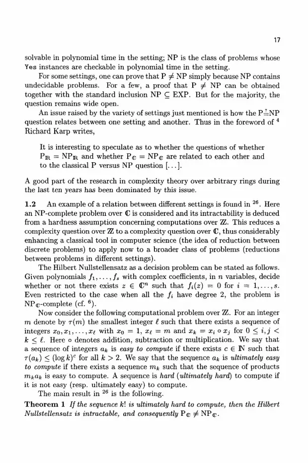
Now consider the following computational problem over TL. For an integer m denote by -r(m) the smallest integer I such that there exists a sequence of integers xo,x\,... ,xe with x0 = 1, xi — m and 11 = D; o Xj for 0 < i, j < k < t. Here o denotes addition, subtraction or multiplication. We say that a sequence of integers o^ is easy to compute if there exists c € IN such that r(afc) < (logfc)c for all k > 2. We say that the sequence afc is ultimately easy to compute if there exists a sequence m^ such that the sequence of products rrikCik is easy to compute. A sequence is hard (ultimately hard) to compute if it is not easy (resp. ultimately easy) to compute.

The main result in 26 is the following. Theo rem 1 / / the sequence k\ is ultimately hard to compute, then the Hilbert Nullstellensatz is intractable, and consequently P<c 7 NP(p.

18

We remark here that the assumption of hardness of the sequence k\ in the sense above is related to the hardness of integer factorization classically (cf. 4 ) .

1.3 Although there is a general belief that P ^ NP for every "reasonable" setting, it would appear wishful thinking to believe the resolution of the P=NP question over C, say, would resolve the question over 7L2, i-e. classically. Indeed, continuing the remarks quoted above, Karp adds,

I am inclined to think that the three questions [over H, C and TL2\ are very different and need to be attacked independently.

However, inroads are being made. For example, we now know that if P = NP over <D then BPP 3 NP classically. Here BPP is the class of decision problems solvable in probabilistic polynomial time, the modern version of the concept of "feasible."

It is not difficult to prove that the answer to the P=NP question is the same for all finite fields. This is the case since, for any two finite fields K\ and K2, one can simulate computations over K\ with a machine over K2 with only a constant slowdown. In the same vein, one may ask whether the P=NP question has the same answer for all algebraically closed fields of characteristic zero. The main result of 2, which we now state, gives a positive answer to this question.

Theorem 2 Let Q be the algebraic closure of Q and K be any algebraically closed field of characteristic zero. Then P = NP over K if and only if P = NP over Q.

The "if" part of Theorem 2 was first proved by Michaux 20 using model-theoretic arguments. The "only if" part required the use of properties of heights of algebraic numbers and establishing an Elimination of Constants theorem.

So far, there is no transfer result corresponding to Theorem 2 for real closed fields. Michaux 20 proves the "if" part, the "only if" part remains open. Partial results in this direction can be found in 7.

1.4 Another form of comparison arises naturally when considering {0,1} (i.e. 7L2) as a subset of a larger ring, most importantly as a subset of ]R or C. One may wonder about the computational power of machines over H, for instance, when input instances are assumed to be strings of zeros and ones.

Such questions are first considered by Koiran in 17. Here he introduced a measure of cost for computations over IR intended to be closer to the bit cost of the Turing model. More precisely, in Koiran's weak cost model, additions and comparisons are performed with unit cost but multiplications are penalized so

19

that iterated multiplications becomes expensive (just as in the Turing model where one can compute 2™ with log n multiplications but with bit cost at least n).

Now, let C be a complexity class of subsets of M°°. Denote by

BP(C) = { S n { 0 , l } ° ° | 5 e C } ,

i.e., BP(C) is the complexity class over K2 consisting of all those sets (of bit strings) decidable by a machine0 in class C. The main result of 17 is the following.

Theorem 3 Let Pw and NPw be the classes of subsets of IR00 decidable in weak deterministic and nondeterministic polynomial time respectively. Then

BP(PW) = P/poly and BP(NPW) 2 NP/po/y.

The "/poly" in the statement above introduces non-uniform complexity classes. These classes contain some undecidable sets but also they are known not to contain some decidable sets with high complexity. Also, P/poly is generally assumed to be strictly included in NP/poly since, by 15, if this is not the case then the polynomial hierarchy collapses at its second level6. Thus, Koiran's theorem yields a twofold insight. Firstly, it exactly describes the gain of using real constants and weak polynomial time for binary inputs (this gain is given by the "/poly"). Secondly, it gives evidence that Pw ^ NPw since the contrary would imply the collapse of the polynomial hierarchy.

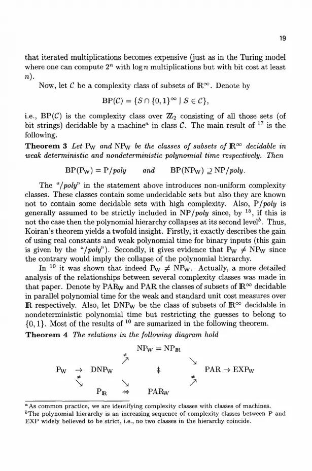
In 10 it was shown that indeed Pw 7 NPw- Actually, a more detailed analysis of the relationships between several complexity classes was made in that paper. Denote by PARw and PAR the classes of subsets of M°° decidable in parallel polynomial time for the weak and standard unit cost measures over B, respectively. Also, let DNPw be the class of subsets of M°° decidable in nondeterministic polynomial time but restricting the guesses to belong to {0,1}. Most of the results of 10 are sumarized in the following theorem. Theorem 4 The relations in the following diagram hold

NPW = NPm

> \ P w -> DNPW % PAR -> EXPW

PIR -* PARw

"As common practice, we are identifying complexity classes with classes of machines. ' T h e polynomial hierarchy is an increasing sequence of complexity classes between P and EXP widely believed to be strict, i.e., no two classes in the hierarchy coincide.

20

where an arrow -> means inclusion, an arrow —> means strict inclusion and a crossed arrow *» means that the inclusion does not hold.

Other results in 10 include a proof of the equality BP(PARyv) = PSPACE/poly. Here PSPACE denotes the class of subsets of {0,1}°° de-cidable in polynomial space.

2 Solving equations

2.1 Algorithms for deciding the feasibility (and finding solutions, if appro­priate) of complex systems of polynomial equations, or real systems of poly­nomial equations and inequalities, have a long history. For the most part, at least concerning feasibility, they rely on algebra or, more precisely, on elimi­nation theory. These algorithms have several virtues (for instance, they show that NP is included in EXP, the class of problems decidable in exponential time). But they are slow and they do not appear to be stable when imple­mented with floating point numbers. A possible reason for these drawbacks is that these algorithms solve in exponential time all input systems. Therefore, they have to deal, on equal footing, with a collection of ill-posed systems (e.g. feasible overdetermined systems, systems with multiple roots, etc.).

The tradition in numerical analysis suggests a different strategy for the design and analysis of algorithms. A condition number is associated to an input. Several features of the algorithm and of the output corresponding to the input will depend on this number. In particular, ill-posed inputs, those having infinite condition number, may produce exceptional behavior of the algorithm.

Condition numbers were originally introduced to measure the sensitivity of a given input (for a specific computational problem) to perturbations. If tp is the function we are computing, the condition number of x measures how large \\<p(x + Ax) — ip(x)\\ may be compared to ||Aa;|| for small perturbations Ax.

x

i • , <p{x)

ip(x + Ax)

Inputs with small condition number are well-conditioned and those with large condition number are ill-conditioned. This idea of conditioning is already present in a paper of Turing 33 from the early days of computers.

21

We should describe the equations (8.2) as an ill-conditioned set, or, at any rate, as ill-conditioned when compared with (8.1). It is char­acteristic of ill-conditioned sets of equations that small percentage errors in the coefficients given may lead to large percentage errors in the solution.

In this paper Turing introduced the term condition number for linear equation solving. In this case, the condition number K(A) of a square matrix A is given by K(A) — | |A||| |A_1 | | where the norm denotes the operator norm with respect to the Euclidean norm in both domain and target spaces.

Note that a matrix has infinite condition number if and only if it is not invertible. Thus, the set E of all ill-posed problems has measure zero in the space I t " oinxn matrices. The distance of a matrix A to E is closely related to K(A).

Theorem 5 (Condition Number Theorem) For any nxn real matrix A one has

A (A ^ - HA|I MA^-^Ay

Here dp means distance in H™ with respect to the Frobenius norm, \\A\\p =

4 E4-This theorem was first proved in 13 under the equivalent form || L 1 j) =

For non-linear systems, the consideration of a condition number poses some difficulties. Suppose we want to compute some solution to a system of non-linear equations / . Since the system may have several solutions and we do not require any one in particular, <p(/) is not well-defined.

A possible resolution is to consider the condition number ^i(f, £) for a pair (/, £) with £ G R m a solution of / = 0. Then, one may define the condition number /i(/) in terms of the worst conditioned solution £, i.e.,

M/) ^i^fvLo^1 '^"

This is the tack taken by Smale and Mike Shub in the Bezout series of pa­pers [Shub and Smale 22,23,24,27,25j j j e r e a n jmp ressive development of homo-topy methods for systems of complex polynomial equations provides a non­uniform solution to Problem 17 in Smale's list. We shall now attempt to summarize some of the main results in the series.

2.2 Let d = (d i , . . . ,d„ ) G IN" and H^) denote the set of polynomial systems / = ( /1 , . . . , /« ) where fi is a complex homogeneous polynomial of

22

degree dj in Xo, • • • ,xn. The problem at hand is: given / € 'H(d), find £ S C™+1, £ 7 0, such that /(£) = 0. Notice that replacing / by any nonzero multiple A/ will not affect the problem. Also, since the / , are homogeneous, if /(£) = 0 then /(A£) = 0 for all A € € , A 0. It is thus natural to consider a "scale invariant" version of the above problem. This is done by replacing the spaces 'H(d) a n d C n + 1 by their induced projective spaces. Let TP(7i(d)) denote the complex projective space associated to 7i(d) • The problem now can be restated: given / € P (71(d)), find £ € P ( C n + 1 ) such that /(£) = 0. For each sytem / and each root £ 6 P ( C n + 1 ) Shub and Smale define a condition number fi(f, £) extending classical work in numerical analysis going back to Wilkinson 34 and Wozniakowski 35 . They then prove the following equality

M/,0 = ll/IIIP/(Olr(!1A(||^||*-1)||.

Here, | | / | | denotes the norm induced by the Weyl Hermitian product on %(d)c- Also, A(| |£| |d i _ 1) denotes the diagonal matrix with diagonal (M\^-1,...M\\d"'1)^dTi = {v&€n+1\(v,O^0}.

From this characterization, a closed form of the set X' of ill-posed pairs (/, £) follows. More precisely,

£ ' = { ( / , 0 I f(0 = 0 and ker(Z?/(£)h) ^ 0},

i.e., £ ' is the set of pairs (/, £) such that £ is a degenerate zero of / . Shub and Smale then prove a result akin to a Condition Number Theorem.

The standard Hermitian product in C n + 1 naturally induces a Riemannian metric on P ( C n + 1 ) . In a similar way, the Weyl Hermitian product naturally induces a Riemannian metric on P(71(d))- This allows us to consider distances in P(f t ( d )) x P ( C n + 1 ) . Let

Vt = {/ € W(7i(d)) | /(£) = 0}

and dz((f,£),£') denote the fiber distance, i.e. the distance in V^ x {£}, between (/, £) and £ ' . Define the normalized condition number by

AWm(/,0 = \\f\\\\Df(0\T^(m\dl~1y/dl)l Then

/ i n o r m ( / ^ ) = d£((/,£),S')' cAlthough this is not relevant for what follows, we mention here that the Weyl Hermitian product is, essentially, the only such product in H(d) invariant under unitary substitution of the variables. This means that if a : C n + 1 -> C n + 1 is unitary (i.e. ||<T(Z)|| = ||z|| for every z £ C n + 1 ) then, for f,g £ %(<*)> (af,ag} = (f,g)- Here af denotes the polynomial in ti^d) satisfying (<r/)(z) = f(tr(z)) for all z € <Cn+1 and ( , ) denotes the Weyl Hermitian product.

23

To obtain a condition number for / only, Shub and Smale define

Mnorm(/) = max p n o r m ( / , 0 -CI/(€)=0

The condition number of a polynomial system is thus that of its worst condi­tioned zero. The set S of ill-posed systems is then the image of £ ' under the projection

7 r : P ( K ( d ) ) x P ( ( C " + 1 ) ^ P ( K ( ( i ) ) ,

i.e., the set of all systems having a degenerate zero. Defining

p ( / ) = ? m i n = o d s ( ( / , C ) , S ' )

one gets /inorm(/) = p{f)~l. This is not, strictly speaking, a Condition Num­ber Theorem for Mnorm(/) since p(f) is not the distance from / to E, but it is akin to one. A simplified account of this is presented in Chapter 12 of 4.

2.3 Let us consider again the problem: given / € P(%(d)), find £ £ C"+ 1 , C 0, such that /(£) = 0.

Consider an initial pair (g,£) with g G P(%(d)) and £ G P ( C n + 1 ) satisfy­ing g(£) = 0. Define, for t £ [0,1], the function ft = tf + (1 — i)#. In general, as t varies from 0 to 1, a curve C of pairs (ft,^t) with /t(£t) = 0 is generated in the product space P(%(d)) x P((C"+1). Since / i = / , £i is the point C we are looking for. The homotopy algorithm in 22 produces a sequence

0 = t0 < *i < • • • < ** = 1

and a sequence of pairs (/t^,^*) which "closely follows" this curve provided k is large enough. By "closely follows" we mean that £* is a good approximation of the root £t; of ftt (in the sense that Newton's method for fti with initial point £* converges quadratically to &; from the first iteration). Notice that this property implies, in particular, that £jj! is a good approximation of the desired root C = £i •

The expression "fc is large enough" in the paragraph above has a precise meaning, namely,

k>cD2n(C)2Lf. (1)

Here c is a universal constant and D = max{di,... ,dn}. In addition Lf is the length of the curve {ft | 0 < t < 1} in P('H(d)) and /j,(C) is a condition number for C (thus depending on / , g and £o) defined by

fi(C) = max «(/(,(()• t€[0,l]

24

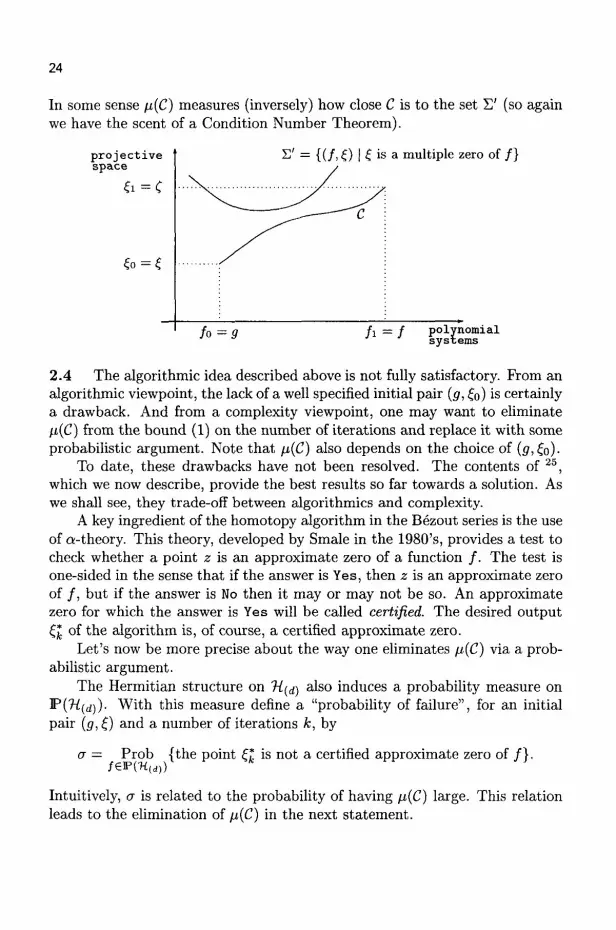
In some sense JJ,{C) measures (inversely) how close C is to the set £ ' (so again we have the scent of a Condition Number Theorem).

pro jec t ive space

£' = {(/, £) | £ is a multiple zero of /}

polynomial systems

2.4 The algorithmic idea described above is not fully satisfactory. Prom an algorithmic viewpoint, the lack of a well specified initial pair (g, £0) is certainly a drawback. And from a complexity viewpoint, one may want to eliminate fi(C) from the bound (1) on the number of iterations and replace it with some probabilistic argument. Note that n(C) also depends on the choice of (<7,£o).

To date, these drawbacks have not been resolved. The contents of 25, which we now describe, provide the best results so far towards a solution. As we shall see, they trade-off between algorithmics and complexity.

A key ingredient of the homotopy algorithm in the Bezout series is the use of a-theory. This theory, developed by Smale in the 1980's, provides a test to check whether a point z is an approximate zero of a function / . The test is one-sided in the sense that if the answer is Yes, then z is an approximate zero of / , but if the answer is No then it may or may not be so. An approximate zero for which the answer is Yes will be called certified. The desired output ££ of the algorithm is, of course, a certified approximate zero.

Let's now be more precise about the way one eliminates fi(C) via a prob­abilistic argument.

The Hermitian structure on 11(d) a l s o induces a probability measure on P(%(d))- With this measure define a "probability of failure", for an initial pair (g, £) and a number of iterations k, by

a = Prob {the point £j* is not a certified approximate zero of / } . /eP('H((J))

Intuitively, a is related to the probability of having /z(C) large. This relation leads to the elimination of /z(C) in the next statement.

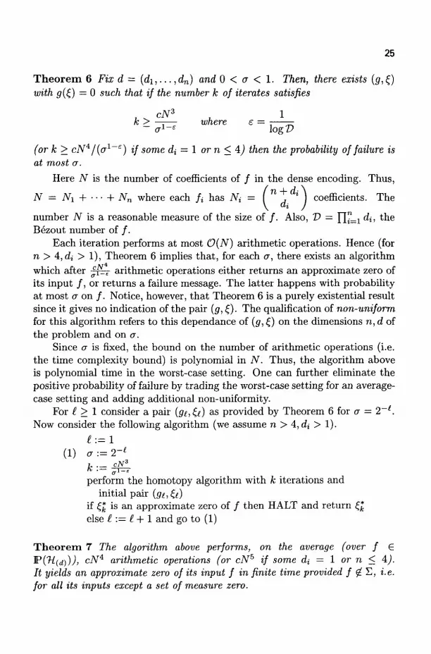
25

Theorem 6 Fix d = (di,...,dn) and 0 < a < 1. Then, there exists ((?,£) with g(£) = 0 such that if the number k of iterates satisfies

k > ^ where e = ' logP

(or k > cN4/(a1 6) if some d, = 1 or n < A) then the probability of failure is at most a.

Here JV is the number of coefficients of / in the dense encoding. Thus,

N = N\ + • • • + Nn where each /$ has Ni = I , ' J coefficients. The

number N is a reasonable measure of the size of / . Also, V = JJ"=1 di, the Bezout number of / .

Each iteration performs at most O(N) arithmetic operations. Hence (for n > 4, di > 1), Theorem 6 implies that, for each a, there exists an algorithm which after -^i^r arithmetic operations either returns an approximate zero of its input / , or returns a failure message. The latter happens with probability at most a on / . Notice, however, that Theorem 6 is a purely existential result since it gives no indication of the pair (g, £). The qualification of non-uniform for this algorithm refers to this dependance of (g, £) on the dimensions n, d of the problem and on a.

Since a is fixed, the bound on the number of arithmetic operations (i.e. the time complexity bound) is polynomial in N. Thus, the algorithm above is polynomial time in the worst-case setting. One can further eliminate the positive probability of failure by trading the worst-case setting for an average-case setting and adding additional non-uniformity.

For t > 1 consider a pair (<?<,&) as provided by Theorem 6 for a = 2~l. Now consider the following algorithm (we assume n > 4, di > 1).

£ : = 1 (1) a:=2-l

h — cN* perform the homotopy algorithm with k iterations and

initial pair (gi,£t) if ££ is an approximate zero of / then HALT and return ££ else I := I + 1 and go to (1)

Theorem 7 The algorithm above performs, on the average (over f £ P(7^(d))/), cN* arithmetic operations (or cN5 if some di = 1 or n < A). It yields an approximate zero of its input f in finite time provided f £ E, i.e. for all its inputs except a set of measure zero.

26

The algorithm in Theorem 7 has no failure return. One may consider the infinite running time for inputs / € £ as a failure, but this event has measure zero in P("K(d)). On the other hand, the polynomial time bound is only on the average and the non-uniform character has increased since we now need an infinite sequence of pairs (ge,^e) at hand.

The non-uniform character of these algorithms is certainly unsatisfactory. Shub and Smale conjecture, however, that making them uniform is easy. More concretely, let

gi=ZQi~1zi for i = l , . . . , n

andf = (1 ,0 , . . . , 0).

Conjecture The pair (<?,£)> with g = (gi, • • • ,gn), satisfies the hypothesis of Theorem 6. Consequently, one may take the constant sequence (g,£) for the algorithm in Theorem 7.

2.5 The main focus of 29 was on complexity theory. Smale explained the path that led him (together with L. Blum and M. Shub) to the machine model in 6 and the complexity theory built upon this model. In an appendix, called "Round-off error, approximate solutions, and complexity theory," he proposed to integrate conditioning and round-off with complexity theory. (Other dis­cussions along these lines appear in S'1'30*3.)

In 31, by invitation of Acta Numerica, Smale wrote a paper with his views on complexity theory and numerical analysis. Here one can see advances towards the integration of complexity theory and conditioning, of which the Bezout series is a landmark. The consideration of round-off in a general complexity theory remained an open issue although Smale proposed some suggestions in the last part of the paper which he qualified as "tentative".

By the end of 1996, when the Acta Numerica paper was already in the printing process, Smale proposed to Cucker to study the feasibility problem for semi-algebraic systems from a round-off perspective. The goal was to provide an algorithm whose analysis would involve both complexity and round-off and in which conditioning would play a central role.

The turf for this goal was unclear. Traditional round-off analysis has dealt mainly with linear algebra problems. The field of semi-algebraic geometry had not been a major concern of numerical analysts. Thus, condition numbers for our problem had to be defined. But, since the feasibility problem is a decision problem, the definition of condition number using perturbations as in 2.1 is of no use. The condition number would be infinity for systems on the boundary between feasible and infeasible and zero otherwise.

The definition of condition number Cucker and Smale proposed, /J*(<p),

27

has two different expressions according to whether ip is feasible or not (cf. n ) . In the feasible case, if x € R™ is a point satisfying ip, then the condition n((p,x) of the pair (<p,x) is defined in a way which extends the condition number of the Bezout series. But unlike the latter, the condition number of <p is now taken to be the condition of its best conditioned solution. That is,

fi*(ip) = inf n(ip,x). z€Sol(v?)

Here Sol(y) denotes the set of solutions of <p. Thus, for <p to be ill-posed, all its solutions need be. One can see fj.*(p) as a far-reaching generalization of the condition numbers used by Turing and Wilkinson.

Having defined (i*{<p), there still remains the problem of what kind of result one may prove for a decision problem since the output of the problem does not allow for "perturbations", it is either Yes or No. The main result of n can be stated as follows.

Theorem 8 Let ip denote a semi-algebraic system as follows

( fi(x) = 0 i = l,...,m gj(x) > 0 j = l,...,r hk(x) >0k = l,...,q

where fi,gj,hk are polynomials in x\,... ,xn with real coefficients. There is a machine M over M which decides, on input ip, whether there

is a point x € H™ satisfying (p. The halting time of the machine is bounded by

H*(<p)2nsize{<p)cn

with c a universal constant (and thus, in particular, M may not halt on inputs ip such that H*(<p) = oo).

Moreover, on each arithmetic operation, a round-off error is permitted with precision polynomialy bounded in log fi*(<p) and in size((p).

Here size(<p) is the size of the dense encoding of ip and is independent of the coefficients of the f 's, g 's and h 's.

The round-off model considered in Theorem 8 is the absolute error model. An absolute round-off unit S < 1 is considered such that, the result of each arithmetic operation performed with round-off unit 6 satisfies

xoy = (x o y) + p

with \p\ < 5. The precision of the computation is | log <5|. This roughly corresponds to the number of bits necessary to write down a number with round-off unit 6. It is also in agreement with the expression "infinite precision"

28

(for <5 = 0) and with the idea that the higher the precision, the more accurate the final result. A similar result (polynomial precision) can also be obtained for the (more usual nowadays) model of relative error.

An additional feature, not present in the statement of Theorem 8, is that if no round-off is allowed and M halts on a feasible input then, in addition, M returns an approximate solution of (p. (By approximate solution we mean a point such that Newton's method, for a specific function associated to ip, will immediately converge quadratically to a solution of ip). The reason this additional bonus is not present in general here is made clear in Remark 24 of n . Rougly speaking, in the feasible case, fi*{<p) is given by the best conditioned solution of ip. But there may be points which are not approximate solutions of tp but which can be erroneously tested as such if the machine precision is low. To avoid the return of such a point as an approximate solution, a more restrictive condition number is required to control the machine precision, one depending on all points in E " and not just on the solutions of ip. In 8 another condition number, Q*(<p), is defined along these lines for which the following is true. Theo rem 9 If the precision of the machine M in Theorem 8 satisfies a cer­tain bound polynomial in log a* (<p) and size(ip) then the following holds: for feasible inputs ip, if M halts it also returns an approximate solution of ip.

2.6 Two more papers dealing with algorithms for equation solving are 12 '9. In the first one, lower bounds for the kind of algorithms used in the Bezout series are given. Firstly, the class of algorithms is formally defined. A Newton Continuation Method sequence (NCM sequence) is a sequence

(fu d) € F(riid)) x P ( C n + 1 ) 0 < i < k

satisfying fi((i) = 0 and Q is a certified approximate zero of / i + 1 for 0 < i < k. The main result of 12 is the following.

Theo rem 10 For any NCM sequence {fi,(i)> 0 < i < k,

(i) k > ci max ( 1, —-— J dR((0, (k), and

( i i ) k>C2 dR&M .

Here C\ and C2 are universal constants, dn is the Riemannian distance in P ( C " + 1 ) and S/. = {z € P(<D"+1) | rankD/ < n} .

29

Actually, the version of Theorem 10 appearing in 12 is more general in the sense that it holds also for underdetermined systems. That is, the functions fi above may satisfy

fi : C n + 1 -)• <Dro

with m < n. To apply Newton's method in the underdetermined case, i.e., when m < n, one replaces the inverse Df(z)]^1 by the Moore-Penrose inverse Df(z)\^.

In the second paper, 9, a totally diferent context is considered, that of diophantine equations. The general problem of deciding whether a polynomial equation has integer roots is known to be undecidable. For the special case of only one variable, algorithms exist which compute all the integer roots. If

d

f = Y^

with o; £ ffi, ad / 0, these algorithms return the integer roots of / in time polynomial in d and L = max{height(oj)}. Here, for an integer a, height(a) = log(l + \a\). This is roughly the number of bits necessary to write down the binary expansion of a. We conclude that these algorithms are polynomial time in the dense encoding of / , i.e. in the encoding of / consisting of the list of all its coefficients,

dense(/) = {a0,ai,... ,ad}.

For polynomials with few non-zero coefficients this way of representing / can be artificially expensive. For such polynomials possibly a more sensible en­coding is the sparse encoding in which only non-zero coefficients are specified, together with their indices,

sparse(/) = {(di,i) | 0 < i < d, en ^ 0}.

This encoding uses at least L bits to write down the largest coefficient plus logd bits to write down the exponent d. But it may be exponentially more succint than the dense encoding since the latter specifies all d+ 1 coefficients. In particular, the algorithms mentioned above for computing the integer roots of / may take exponential time in the sparse encoding. The main result of 9

is the following. Theorem 11 There is a polynomial time algorithm which, given input f G 7L[t] in the sparse encoding, decides whether f has an integer root and, if this is the case, outputs the set of integer roots of f.

30

3 Additional remarks

Many of the themes outlined in this article, and more, are developed in the book Complexity and Real Computation published toward the end of the 1990's 4 . An approach that initially was met with a certain degree of skepti­cism ("machines are finite so how can you have a theory of computation over the reals?" and "what use is a foundational theory for numerical analysis, anyway?") has led to fertile areas of research producing new insights, new algorithms, new methodologies for their analysis, and certainly a deeper un­derstanding of computation. Connections are being made between the newer theories and the classical theory of computational complexity (e.g. tantaliz­ing transfer results for the fundamental P=NP problem), paving the way to employ techniques of mainstream (continuous) mathematics to grapple with hard (discrete) problems of computer science.

Steve Smale, indeed, has been the driving force behind the creation of an overarching community of researchers interested in the foundations of com­putational mathematics. One need only look at the titles of the workshops'* offered at the Foundations of Computational Mathematics conference at Ox­ford University during the summer of 1999 to gleam an appreciation of the scope of this community. Smale's vision, drive, and personality —at once unassuming and compelling— has inspired many young (and some old) re­searchers to chart new territory. The wonderful work of Koiran 18>19, Kim 16, and Gradel and Meer 14, amongst others, testimony enough to Smale's influ­ence, promises even more to come.

Acknowledgments

Partially supported by SRG grant 7001290. Thanks to the Computer Science Department, Carnegie Mellon University.

References

1. L. Blum, Lectures on a theory of computation and complexity over the reals (or an arbitrary ring), in Lectures in the Sciences of Complexity II, ed. E. Jen (Addison-Wesley, pp. 1-47, 1990).

d Approximation theory; Complexity theory, real machines and homotopy; Computational dynamics; Relations to computer science; Computational geometry and topology; Mul-tiresolution, computer vision and PDEs; Optimization; Stochastic computation; Symbolic algebra and analysis; Computational number theory; Geometric integration and computa­tion on manifolds; Information-based complexity; Numerical linear algebra.

31

2. L. Blum, F. Cucker, M. Shub, and S. Smale, Algebraic settings for the problem "P ^ NP". in The Mathematics of Numerical Analysis, eds. J. Renegar, M. Shub, and S. Smale (Volume 32 of Lectures in Applied Mathematics, American Mathematical Society, pp. 125-144, 1996a).

3. L. Blum, F. Cucker, M. Shub, and S. Smale, Complexity and real com­putation: a manifest, Int. J. of Bifurcation and Chaos 6, 3-26 (1996b).

4. L. Blum, F. Cucker, M. Shub, and S. Smale, Complexity and Real Com­putation, (Springer-Verlag, 1998).

5. L. Blum and M. Shub, Evaluating rational functions: infinite precision is finite cost and tractable on average, SIAM Journal on Computing 15, 384-398 (1986).

6. L. Blum, M. Shub, and S. Smale, On a theory of computation and com­plexity over the real numbers: NP-completeness, recursive functions and universal machines, Bulletin of the Amer. Math. Soc. 21, 1-46 (1989).

7. O. Chapuis and P. Koiran, (1997), Saturation and stability in the theory of computation over the reals, to appear in Annals of Pure and Applied Logic.

8. F. Cucker, Approximate zeros and condition numbers, Journal of Com­plexity 15, 214-226 (1999).

9. F. Cucker, P. Koiran, and S. Smale, A polynomial time algorithm for diophantine equations in one variable, Journal of Symbolic Computation 27, 21-29 (1999).

10. F. Cucker, M. Shub, and S. Smale, Complexity separations in Koiran's weak model, Theoretical Computer Science 133, 3-14 (1994).

11. F. Cucker and S. Smale, Complexity estimates depending on condition and round-off error, Journal of the ACM 46, 113-184 (1999).

12. J.-P. Dedieu and S. Smale, Some lower bounds in the complexity of con­tinuation methods, Journal of Complexity 14, 454-465 (1998).

13. C. Eckart and G. Young, The approximation of one matrix by another of lower rank, Psychometrika 1, 211-218 (1936).

14. E. Gradel and K. Meer, Descriptive complexity theory over the real numbers, in The Mathematics of Numerical Analysis, eds. J. Renegar, M. Shub, and S. Smale (Volume 32 of Lectures in Applied Mathematics, American Mathematical Society, pp. 381-404, 1996).

15. R. Karp and R. Lipton, Turing machines that take advice, L'Enseigne-ment Mathematique 28, 191-209 (1982).

16. M.-H. Kim, An average complexity estimate of a path-following method for a polynomial root, preprint, (1999).

17. P. Koiran, A weak version of the Blum, Shub k, Smale model, J. Comput. System Sci. 54, 177-189 (1997). A preliminary version appeared in 34th

32

annual IEEE Symp. on Foundations of Computer Science, pp. 486-495, 1993.

18. P. Koiran, The real dimension problem is NPiR-complete, Journal of Com­plexity 15, 227-238 (1999).

19. P. Koiran, Circuits versus trees in algebraic complexity, to appear in Proceedings of ST ACS, (2000).

20. C. Michaux, P ^ NP over the nonstandard reals implies P / NP over H, Theoretical Computer Science 133, 95-104 (1994).

21. M. Shub, On the work of Steve Smale on the theory of computation, in From Topology to Computation: Proceedings of the Smalefest, eds. M. Hirsch, J. Marsden, and M. Shub (Springer-Verlag, pp. 281-301, 1993).

22. M. Shub and S. Smale, Complexity of Bezout's theorem I: geometric aspects, Journal of the Amer. Math. Soc. 6, 459-501 (1993a).

23. M. Shub and S. Smale, Complexity of Bezout's theorem II: volumes and probabilities, in Computational Algebraic Geometry, eds. F. Eyssette and A. Galligo, (Volume 109 of Progress in Mathematics, Birkhauser, pp. 267-285, 1993b).

24. M. Shub and S. Smale, Complexity of Bezout's theorem III: condition number and packing, Journal of Complexity 9, 4-14 (1993c).

25. M. Shub and S. Smale, Complexity of Bezout's theorem V: polynomial time, Theoretical Computer Science 133, 141-164 (1994).

26. M. Shub and S. Smale, On the intractability of Hilbert's Nullstellensatz and an algebraic version of "P = NP", Duke Math. J. 81, 47-54 (1995).

27. M. Shub and S. Smale, Complexity of Bezout's theorem IV: probability of success; extensions, SIAM J. of Numer. Anal. 33, 128-148 (1996).

28. S. Smale, On the topology of algorithms I, Journal of Complexity 3, 81-89 (1987).

29. S. Smale, Some remarks on the foundations of numerical analysis, SIAM Review 32, 211-220 (1990).

30. S. Smale, Theory of computation, in Symp. on the Current State and Prospects of Mathematics, ed. M. Castellet, (Lect. Notes in Math., Springer-Verlag, pp. 59-69, 1991).

31. S. Smale, Complexity theory and numerical analysis, in Acta Numerica, ed. A. Iserles (Cambridge University Press, pp. 523-551, 1997).

32. S. Smale, Mathematical problems for the next century, Mathematical Intelligencer 20, 7-15 (1998).

33. A. Turing, Rounding-off errors in matrix processes, Quart. J. Mech. Appl. Math. 1, 287-308 (1948).

34. J. Wilkinson, Rounding Errors in Algebraic Processes, (Prentice Hall,

33

1963). 35. H. Wozniakowski, Numerical stability for solving non-linear equations,

Numer. Math 27, 373-390 (1977).

35

DATA COMPRESSION A N D ADAPTIVE HISTOGRAMS

0 . CATONI Laboratoire de Probability et Modeles Aleatoires U.M.R. 7599 du C.N.R.S., Case 188, Universite Paris 6, bureau 4 E 19 bat Chevaleret, 4, place Jussieu, F-75 252

Paris Cedex 05 catoni@ccr.jussieu.fr

We describe and study in this paper a two step estimation scheme for density esti­mation from i.i.d. observations. Each step is based on the Gibbs aggregation rule and computes an adaptive histogram for which a non asymptotic oracle inequality is satisfied. The estimator computed in the first step is used to code the data in the unit interval in a way that is inspired by arithmetic coding. The second es­timator analyzes the coded sample and refines the first one. Numerical evidences are provided of the efficiency of the method.

1 Introduction

We will present an approach to adaptive inference that mixes ideas coming from data compression, statistical mechanics and model selection (or rather model aggregation, as we will see).

We will concentrate on the problem of density estimation by histograms. Numerical experiments will consist in estimating densities with respect to the Lebesgue measure on the unit interval. The observation will be an i.i.d. sam­ple {Xi)f=1 with joint distribution P®N, where P 6 M^([0,1],S) is a Borel probability measure on the unit interval (throughout this paper, M+(X, 3") will be the set of probability measures on the measurable space (X, 3"), more­over we will forget to mention the sigma algebra 2f when its choice is obvious from the context).

This problem is interesting in itself, but also has some connection with the analysis of "symbolic sequences", such as DNA sequences or typed texts. Let us comment on this to start with, since it was the main motivation for writing this paper. More precisely, the observation (Xi)^L1 which we were talking about can be constructed from an experiment on words: Let A be a finite alphabet, and assume that we observe an i.i.d. sample (Si)^ of infinite (or if you prefer very long when compared with the number of samples N) sequences of letters :

Si = (S!)?=1, SfeA. (1)

These sequences may for example be built by choosing at random a starting point in a DNA sequence or a digitized ASCII text.

36

We may be interested in coding a new-coming sequence SN+I to achieve the best possible compression rate (i.e. the best possible average number of bits in the coded representation of SN+I, supposed to be of variable length). If we knew the distribution of SN+I , then we could code the prefix of length M of this sequence, namely (SN+1,..., S^+l), or with shorter notations S]j+1, using arithmetic coding (sometimes called the Shannon-Fano-Elias algorithm, see 16 ). Let us remind that an arithmetic code based on P(<iS^+1) (our notation for the distribution of the random variable SN+1 € AM) is a mapping from AM to the set of finite binary sequences {0,1}*, c : AM -> {0,1}*, which is built from F{dSN

I^l) in such a way that the length of the code for word s e AM is approximately equal to — log2[P(5Jy+1 = s)]. The average code length is the expectation E\l[c (S^^KL)] of the length I of coded words. When arithmetic coding is used, the average code length is upper bounded by

n[v(dS1£1j\+2,

where H is the Shannon entropy (expressed in bits : the Shannon en­tropy of a probability distribution P on a finite set E is equal to — YlseE P(s) 1°S2 [P(s)] > l°g2 being the logarithm with base two).

If we do not know this distribution, then we can replace it with an estimate P, computed from the observation of (Si)^.1. An arithmetic code based on P will have an average length not greater than

I f [ F ( d S ] & ) ] + j ^ 2 ) 3 c [ p ( d S ^ ) , p ] + 2, (2)

where 3C is the Kullback Leibler divergence function : if /i and v are two probability distributions, then

log I — 1 d\i when /i <C v,

-oo otherwise.

Thus it is advisable in this situation to minimize what is usually called the ideal redundancy

^ [ F ^ S J . P ] (3)

of the "ideal code" corresponding to the coding distribution P, with respect to F(dSN+1). Equation (3) defines a natural risk function to guide the choice of the estimator P.

37

We get back to the setting of density estimation on the unit interval by labeling the alphabet A with integers, taking A = {0,1,.. .,\A\ - 1}, and by defining Xt as

oo

^ = £#14--*. (4) fc=i

When this identification is made, the Lebesgue measure appears as the iden­tity code in the binary case A = {0,1} and in the general case as a code of approximately constant length. If we replace the Lebesgue measure with an histogram, whose cells are defined from the first digits of X only (in the rep­resentation of X defined by (4)), then, apart from some rounding effects due to the discrete nature of coding, we essentially compress the representation of the first digits of X and let the remaining digits uncompressed. Thus, to an histogram model on [0,1], corresponds some kind of generalized n-gram model on the symbolic sequence S.

Another, maybe more familiar, interpretation of all this, is that we are looking for an estimator of the distribution of SN+I which maximizes the mean log-likelihood of SN+I. In this interpretation, the Lebesgue measure gives the same likelihood to all sequences of length M, and histograms based on the first digits give uniform weights to the following digits, not implied in the cell definition.

Note here that we neither assume that the distribution of the sequence SN+I is time-homogeneous, nor that it satisfies the Markov property.

2 The model

Let A be some finite alphabet. Let A* = U ^ i A% be the set of all finite sequences of letters (i.e. of finite words). Let 0 be the empty word (of null length). For any word s £ A*U{0}, let £(s) be the length of s, i.e. its number of letters. (We put l{0) = 0.)

Let us say that T> C A* is a complete prefix dictionary if no word in D is the beginning (or as it is usual to say in these matters, the prefix) of another word in T>, and if the addition of any new word to D would break this rule. For any complete prefix dictionary, let n(T>) be the set {(s i , . . . , s*) : s € D, 1 < k < £(s)} U {0} of all the (possibly empty) prefixes of all the words of V. We will call 7r(D) the prefix set of D.

Consider some i.i.d. random variables ( X ^ ) ^ with values in some mea­surable space (X,<B). Let n £ 3Vt+(DC,!B) be some reference probability mea­sure on DC.

38

Let S be a set of words that is either the set of all finite words A* U {0} or the prefix set 7r(Doo) of some large complete prefix dictionary "D^,. Assume that for each word s G § a measurable cell Is G 05 has been chosen, and that these cells satisfy the three following properties :

• i0 — X,

• {Is,a •" a G 4} is a partition of Is, for any s G 7r(Doo) \ T>oo,

• fJ,(Is) > 0 for any s G S.

This cell structure {Is : s € §} induces a mapping of complete prefix dictionaries to measurable partitions of X, as is stated in the following lemma

Lemma 2 .1 . For any complete prefix dictionary ! D c § , {Is : s G D} is a measurable partition ofX.

The proof is left to the reader. Let D c S b e some complete prefix dictionary. Let us consider the family

2) of all complete prefix dictionaries D such that D C TT(I ' ) . Let us consider the family of histogram probability distributions qxi,e(x)p,(dx) G M:"j_(X, !B), where T> G £> and where 6 6 M+(D). We define the histogram density q^tg with respect to fi to be

*D,*(*) = £ ^ r l ( s G / . ) • (5) S £ B W J s J

Our aim will be to estimate the distribution P®N of (Xi)^ by an his­togram 9Dte (x)fi(dx), trying to minimize the Kullback divergence

X(P,qvAx)Kdx))

with respect to T> and 6. Let us recall here that the Kullback divergence between two probability measures v and p is defined to be

[+00 otherwise.

To make sure that we approximately minimize this risk function, we will pro­duce an oracle inequality. This inequality provides an upper bound for the risk that implies no prior knowledge of the properties of the true marginal distribution P, and therefore shows that the estimator is in some sense adap­tive.

39

3 Estimation scheme

Our strategy to compute an estimator will be the following : • First aggregate the histogram models qi>t0(x)ij,(dx) using the Gibbs

estimator 15, to compute a first estimator Q(dx) = q(x)n(dx). Base this first estimator on some part (Xi,... ,XK) of the observations only (where 0<K <N).

• Using Q as a coding distribution, map X to the unit interval, in the spirit of arithmetic coding. More precisely, A* U {0} may be totally ordered by the lexicographic rule, which stipulates that sas' < sbs" and s < ss', whenever s, s', s" £ A* U {0} , and a < b £ A. We define a map F from X to [0,1] in two different ways, depending on whether 8 is finite or infinite.

1. When 8 = ^(Doo) is finite, we define a map a : X —»• Doo by the non ambiguous rule x £ I(T(X)- Then we define F : X —• [0,1] by

F(x) = Q[a{X) < a(x)] + \Q[O{X) = a{x)}. (7)

Note that the arithmetic code for a(X) based on the estimation Q of P would be obtained by truncating F(x) to the (approximately) shortest binary representation which allows to recover a{x) from F(x) in a non ambiguous way (see 16 ).

2. When § = A* U {0} is infinite, we define a : X ->• AN by the rule x £ Is for all the prefixes s of a(x) (i.e. all finite words s of the form (a(x)i,...,a(x)k), with k ranging in M). Then we define again F : X —> [0,1] by

F(x) = Q [a(X) < e[x)] + \Q [a(X) = a(x)]. (8)

Lemma 3.1. In both cases for any x £ X

\ {Q[F(X) < F(x)} +Q[F(X) < F(x)]} = F(x). (9)

Consequently, when 8 = A* U {0} , the following statements are equivalent :

1. The image Q o F _ 1 of Q by F has no atom.

2. The image measure Q o F _ 1 is the Lebesgue measure on [0,1].

3. For any x £ X

Q[a(X) = a(x)} = 0 .

40

Remark 3.2. The proof can be found in the appendix. To summarize things, what we wanted to express by this lemma is that F(X) is almost uniformly distributed on [0,1] under P, up to the estimation error between P and Q, and discretization phenomena.

• Code the remaining part of the observations {XK+\ , Xx+2, • • • j -Xjv)> to create

Yi=F(Xi), K<i<N.

The distribution of (Yi)^LK+1 is i.i.d., and its marginal distribution should be close to the Lebesgue measure. Therefore, it is natural to consider the Lebesgue measure A as the reference measure on [0,1]. A second estimator Q is built for the distribution of Y*. It is computed along the same principles as the first estimator. The unit interval is equipped with the cell structure of the dyadic intervals : for any s G {0,1}* U {0} we put

+ [0,2"'W[. (10)

The second estimator Q is built by aggregating histogram distributions based on the cell structure {J s : s £ {0,1}* U {0}} , using the Lebesgue measure as our reference measure on the unit interval.

• Eventually we compute an estimator Q in the following way. We put for every Is, s £ B

Q(IS) = Q(Q({J /. ') + [O,Q(I.)[)- (II) «'<s, s'es

This characterizes a probability measure on the sigma algebra 3 generated by {Is : s e §}. Indeed, in the case when § = 7r(Doo) is finite, 3 is finite, and it is elementary to check that Q is additive on 3. Indeed, if we put

JS = Q ( \ J is>) + [o,Q{i.)[, ses, (12) «'<s, s'es

we see immediately that Js = \JaeA Jsa, and that this is a disjoint union. In the infinite case, when S = AM, 3 is isomorphic to the sigma algebra of A® generated by the coordinate maps. The same reasoning as in the finite case shows that Q is additive on any sigma algebra generated by a finite number of coordinates. Therefore, by a well known extension theorem (see e.g. 30 ),

41

it can be uniquely extended to a probability measure on 3. Then we complete the definition of Q by taking

Q ( . | 3 ) = M ( - | 3 ) . (13)

The reason for using this two step estimation scheme is that we can save some computing and memory resources by using in the first and second esti­mates two maximal dictionaries (i.e. two values for D) which are both smaller than what would have been required in a one step estimation algorithm to achieve the same accuracy. This allows to use a static implementation of the tree structure 7r(D), resulting in faster computations. We are planning to use this approach in application fields where it is crucial to optimize memory requirements, due to the necessity to use complex models. Performing succes­sive zooming on high probability regions by successive recoding of the data is a way to "factorize" the choice of a model adapted to the data.

4 Details of estimator definition

We build the first estimator in the following way. This variant of what we proposed in 15 was influenced by Alain Trouve, who suggested to estimate the conditional distributions 6(sk | s j _ 1 ) instead of estimating directly 6(s). We are glad to thank him for this contribution. We cut ( X i , . . . ,XK) into (X\,..., XM) and (XM+I > • • • > XK). We use (Xi,..., XM) first to estimate the parameter 6 e M\CD). We write

l(s)

9(s) = Y[e(sk\skl-

1). (14) k=i

Each conditional distribution d(sk \ s^1) takes its range in the set 0 of all possible distributions on the alphabet A, which is nothing but the \A\ — 1 dimensional simplex. We estimate these conditional distributions using the Laplace estimator. An oracle inequality for this estimator applied to any exchangeable sample is derived in 14. The estimator itself was introduced by Laplace a long time ago (as mentioned in Rissanen's lecture notes 3 2 ) , and is for instance used by J. Rissanen in his papers about the context algorithm 33>36. Let us introduce the counters

M

6(s) = 5 3 l ( X i e / a ) . s€7r(D). (15)

Let Si S S be the random variable Si = cr(Xi) (this coincides with the defini­tion given in the introduction in the case of the unit interval). The Laplace

42

estimator is

a (Ck _ Q | C j fc - i sdef &(gl) + l 'M^JW+1 — sifc P t f + 1 — Sx J — fc_1

Hi*-1) + w

Theorem 4.1. Wi'£/j tte previous notations and hypotheses,

(16)

* ^(a,,E"(«-){-tog[^(^+i)]} + § ^ f d7)

Proof. For any X € X, let D(x) € T> be defined by the relation x e /u( x) . Let d\V(x)l

us notice that g© e (x) = —j y , and therefore that it is enough to prove

the theorem with ? B , « ( J M + I ) replaced with # [ D ( X M + I ) ] -

Let us change within this proof the definition of the counters b(s) and put

Af+l

b(s)= £ 1 (*<€/.) •

With this modified definition

8M [SM+1 I SM+i ) =

(18)

HsT. Kst1) + \A\-i

(19)

Let us also introduce the notation 6M,I to indicate the estimator based on the modified sample (Xi,... ,Xi-\,Xi+i,... ,XM,XM+I)- We can use the fact that p®(M + 1) is exchangeable to write

-E|log[0M[:D(*M+i)]j j = -E j ^- j- j 53 log[0M,;[W)] (20)

= ^E^T l0S s € D

M + l &(**)

(21)

43

. . . To get this second expression, we have grouped the indices according to the values taken by T>(Xi) and used the definition of 9M- Moreover we have used the convention 6(si) = M + 1 . . .

= * -£ Hs) , _ / Hs) log

seB M + l °\M + 1

(22)

^m><-m (23)

We ftove used the identity —L , ' = — tH ( 1 y 6(af-1)+|>l|-i ( ^ T 1 ) \

I l>tj-i

\jL M + 1 H M + I (24)

^ b{s) , / | A | - 1

se7r(D)\© M + l

(25)

We have exchanged the order of summations in the second term ..

< E £-#^0/ 6(S)

.sen

+

M + l °VM + 1

|7 r (P) \ I> l (M-l ) M + l

(26)

(27)

and used the inequality log(l + r) < r

= E { inf \eeM\_iV)

b(s E^h^m S g D

+ M + l

(28)

44

. . . We have rewritten both terms. The transformation of the first one is justified by the fact that the Kullback divergence function is non-negative and zero on the diagonal, the second term has been rewritten from the identity \TT(T)) \ T>\ = I4 _i

: E I inf \eeM\CD)

+

M+l

M

-. M+l

i = l

M + l

... where we have just switched back to a summation with respect to time indices

< inf(x)EJ-log[.[l)(XM+1)]]} + ^ (31)

. . . where we have pulled back inf from the expectation and used the fact that the sample is exchangeable once more. •

Once we have built the estimators q^ •§ , we can aggregate them, using the Gibbs aggregation rule based on the independent subsample (XM+\, • • • ,XK)- Let p 6 M+(£>) be the probability distribution

PCD) = a(m-D/(\A\-i)(1 _ a)\v\v\_ ( 3 2 )

(We remind the reader tha t T) is the set of all prefix dictionaries D C 7r(CD)-) It is obtained by considering a branching process s tar t ing a t the empty word, where generation d is made of a set of words of length d. The transition between generation d and d + 1 is the following : each word s £ 7r(D) — D of the population independently gives bir th to {sa : a S ^4} with probability a, and dies without heirs with probability (1 - a), whereas the words of T> die with probability 1.

We define the Gibbs estimator

<7W = - 3 , (33)

(Xi))

where /? is a parameter in the range 0 < /3 < 1/2. The following theorem holds :

45

Theorem 4.2. Let

X = max max log — . , , (34) D.D-es.ex *\qv,jjx))'

and let

Wiift t/ie previous notations and hypotheses

E { - l 0 g [ g ( X K + 1 ) ] } < m^ge m f ( 2 ) ) E { - l o g [ ^ , , ( X K + 1 ) ] }

, P l - l log(p(P)) E f 9 - u rtfi, + M T T ~ ( i f - M + l ) E W }- (36)

Remark 4-3. Note that x < log(M + 1), and that consequently in any case, taking a = logW we obtain that

EOT 1 ) log(M + 1) - 1

^ + ' t s y (2 - 1tff£t)1))) N M +1) - 0 -1 log(M + 1)

(37) M-><X> y21og(log(M+T))

Remark 4-4- Note also that the theorem implies that

E[X{P,W)] < inf inf X{P,qv el*) + T^T ~ T F i ^ T E ( 0 - 1 ) •

(38)

Remark 4-5. For a large dictionary D, the maximum of p(T>) is reached when the branching process is critical, that is when a = o j . Therefore it is advis­able to set a to this particular value.

For a proof of theorem 4.2, we refer the reader to 15. Hopefully, there are fast algorithms to compute q(x). We propose one

which is inspired by the data compression algorithm described in 37, although we have slightly modified the induction step, because it is more efficient here to work with conditional probabilities. Define the counters

K

c(s)= ] T 1 ( ^ 6 / , ) , s G T r p ) . (39) i=M+l

46

Attach to each node of the tree ir(T>) a weight Ts(a;) defined in a recursive way by

- | ^ c ( s a ) + l ( a ; 6 / , o ) '

T.(ar) = < when SGTT(V)\V,

1 when s £ T>.

6M{a\s)

Viha I Is) (40)

The Gibbs estimator q is given by the formula

q(x) = Y0(x)

fxT0(y)n(dy)' (41)

It is constant on each cell 7S, s £ T> of the partition defined by the maximal dictionary T>. Therefore there are |D| numbers to compute. The computation of q{x) for a; 6 7S and s 6 B requires an update of T(s*) (x), for k = 1 , . . . ,i(s), starting from a tree of weights Y s (0) , where "l(a; € 7S) has been set to 0 everywhere", namely T s (0 ) is defined by

T.(0) = I ( i - « ) + « n T » ( 0 )

ae.4 [ when s 6 7r(l>) \ T>,

1 when s £ D.

0Af(a|s) - i / 3 c ( s a ) '

A*(^Sa | /») (42)

Therefore the number of operations involved to compute q is of order at most P l^ iD) , where l(TJ) = m a x s e ^ ( s ) . Note also that

Jx r0(y)fi(dy) = r0(0). (43)

The second estimator Q £ M+([0,1]) is built from (YK+I,---,YN) and the cell structure {J s : s £ {0,1}* U {0}} using the Lebesgue measure as

the reference measure, in the same way as Q is built from (X\,... ,XK), {ls : s £ S} and /i. The last appendix contains the source code of the function WeightMix computing equation (40), with some comments about numerical stability issues.

5 Simulat ions

All the simulations presented here are made in the case when X = [0,1] and fj, — A (the Lebesgue measure). To perform them we wrote some piece of

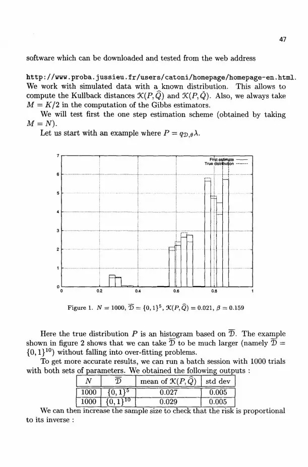
47

software which can be downloaded and tested from the web address

h t tp : / /www.proba. j ussieu.fr /users/catoni/homepage/homepage-en.html. We work with simulated data with a known distribution. This allows to compute the KuUback distances X(P,Q) and X(P,Q). Also, we always take M = K/2 in the computation of the Gibbs estimators.

We will test first the one step estimation scheme (obtained by taking M = N).

Let us start with an example where P — qvfi^-

First estimate • True distribution -

ftu 0.4 0.6

\ 5 Figure 1. N = 1000, D = {0 ,1} 5 , X(P, Q) =0 .021 , P = 0.159

Here the true distribution P is an histogram based on T>. The example shown in figure 2 shows that we can take D to be much larger (namely D = {0, l}10) without falling into over-fitting problems.

To get more accurate results, we can run a batch session with 1000 trials with both sets of parameters. We obtained the following outputs :

N T> mean of X{P, Q)

1000 1 {0,1}5 0.027 1000 {0,1}1U 0.029

std dev

0.005 0.005

We can then increase the sample size to check that the risk is proportional to its inverse :

1 1 First estimate

True distribution

Hi

A 0 0.2 0.4 0.6 0.8 1

Figure 2. N = 1000, V = {0, l } 1 0 , %{P,Q) = 0.026, 0 = 0.155

N 100 1000 10 000 100 000

mean of X(P,Q)

0.24 0.029 0.002 4 0.000 23

std dev

0.02 0.005

0.000 46 5 x 10~5

Let us notice that the proportionality is remarkably well maintained through a large scale of sample sizes. Considering that the probability to be estimated depends on ten parameters (counting for one parameter the def­inition of the support, which is clearly an underestimation), we see that the risk observed in the simulations is less than 3d/N, where d is the dimension of the problem. This is better than what is proved by the theory, which gives an upper bound larger than 2d[l + 21og(2)E(/?-1)]/iV with /? < 1/2 (note that 2[l+41og(2)] > 7.5).

Let us present now an example where the true distribution is not con­tained in the models used by the first estimator. In this second example, the true distribution is a mixture of four Gaussian distributions. Figures 3, 4, 5 and 6 show the evolution of the quality of estimation with the sample size. As expected, the decrease is slower than what is observed when the true dis­tribution belongs to one of the models used by the estimator, because of the influence of the bias term. Of course, the speed of approximation of such a

48

7

6

5

4

3

2

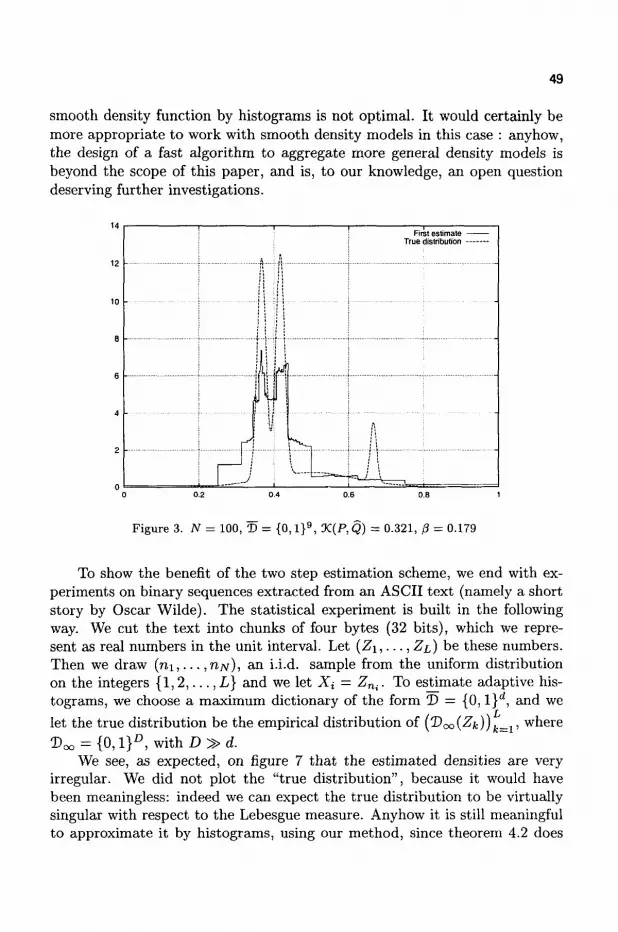
49

smooth density function by histograms is not optimal. It would certainly be more appropriate to work with smooth density models in this case : anyhow, the design of a fast algorithm to aggregate more general density models is beyond the scope of this paper, and is, to our knowledge, an open question deserving further investigations.

Figure 3. N = 100, V = {0, l } 9 , X(P, Q) = 0.321, /3 = 0.179

To show the benefit of the two step estimation scheme, we end with ex­periments on binary sequences extracted from an ASCII text (namely a short story by Oscar Wilde). The statistical experiment is built in the following way. We cut the text into chunks of four bytes (32 bits), which we repre­sent as real numbers in the unit interval. Let (Z\,...,ZL) be these numbers. Then we draw ( m , . . . ,njv), an i.i.d. sample from the uniform distribution on the integers {1,2,...,L} and we let A* = Zni. To estimate adaptive his­tograms, we choose a maximum dictionary of the form T> = {0, l}d, and we let the true distribution be the empirical distribution of (D00(Zfc))Jfe_1, where T)^ = {0,1}£), w i t h D » d .

We see, as expected, on figure 7 that the estimated densities are very irregular. We did not plot the "true distribution", because it would have been meaningless: indeed we can expect the true distribution to be virtually singular with respect to the Lebesgue measure. Anyhow it is still meaningful to approximate it by histograms, using our method, since theorem 4.2 does

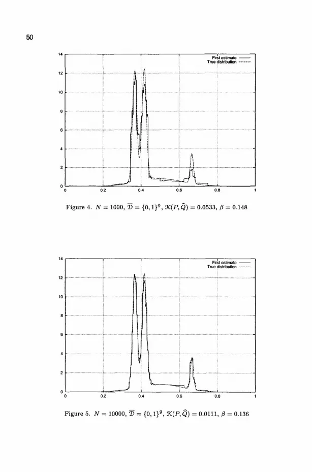
50

Figure 4. N = 1000, T> = {0, l } 9 , %(P, Q) = 0.0533, 0 = 0.148

Figure 5. N - 10000, D = {0, l } 9 , X(P, Q) = 0.0111, 0 = 0.136

not require that P <C \i.

51

L 7072

N 1000

K 100

T) {0,1}«

Doc

{0,!}1* mean X(P,Q)± std dev mean X(P,Q)± std dev

5.12 ±0.08 1 3.70 ±0.07

Table 1.

Table 1 gathers the results of a batch session illustrating the use of a two step estimation scheme. It contains 50 trials: As can be seen, the parameters are the same as in figure 7. Profile data reproduced in appendix indicate the time spent in the different functions of the program (when it is run on a Pentium II processor at 266 MHz with 144 Mb of RAM). They show that (discarding ancillary functions added to compute the risk) most computing time is spent in the critical function WeightMix, where densities are aggregated according to equation (40), and that the time spent in this function jumps from 0.38 to 1.69 seconds when one goes from a two step scheme to a one step scheme of comparable accuracy.

I jj

:...: 1

if

1 J.1—

First estimate True distribution - -

-

Figure 6. N = 100000, D = {0, l } 9 , X(P, Q) = 0.00232, 0 = 0.121

52

Example from ascii text analysis

First estimate Second estimate

i_ i lil : 1 Figure 7. N = 1000, K = 100, T> = {0 ,1} 8 , Hoc = {0 ,1} 1 8 , %(P,Q) - 5.0088, X(P,Q) 3.6160, 0 = 0.162 (second estimate)

Conclusion

We have shown in this paper that the Gibbs estimator for adaptive histogram aggregation is not only a theoretical object with a nice oracle inequality, but also an efficient practical way of performing density estimation. Nice features are that no fine hand tuning of parameters is needed to make the algorithm work (considering that it is reasonable to take M = K/2, a = 1/\A\ and K = 0.17V), and that overfitting is avoided even when the finer cell size is very small with respect to the sample size. The results shown here are obtained with the algorithm corresponding to theorem 4.2. The implementation is strictly faithful to the theory. To make a better use of the sample, we could however think about using some cross validation scheme, instead of cutting the sample into two independent chunks, (X\,..., XM) and (XM+I, - • •, -X"K)-

The second point discussed in the paper is a two step estimation scheme, where a first coarse estimate is used to code the data into the unit interval, in a close to uniform way. We showed that it is a way to cut down computation and memory requirements when the distribution to be estimated is close to be singular with respect to the reference measure used to define the histograms. This idea could be generalized to multiple step schemes.

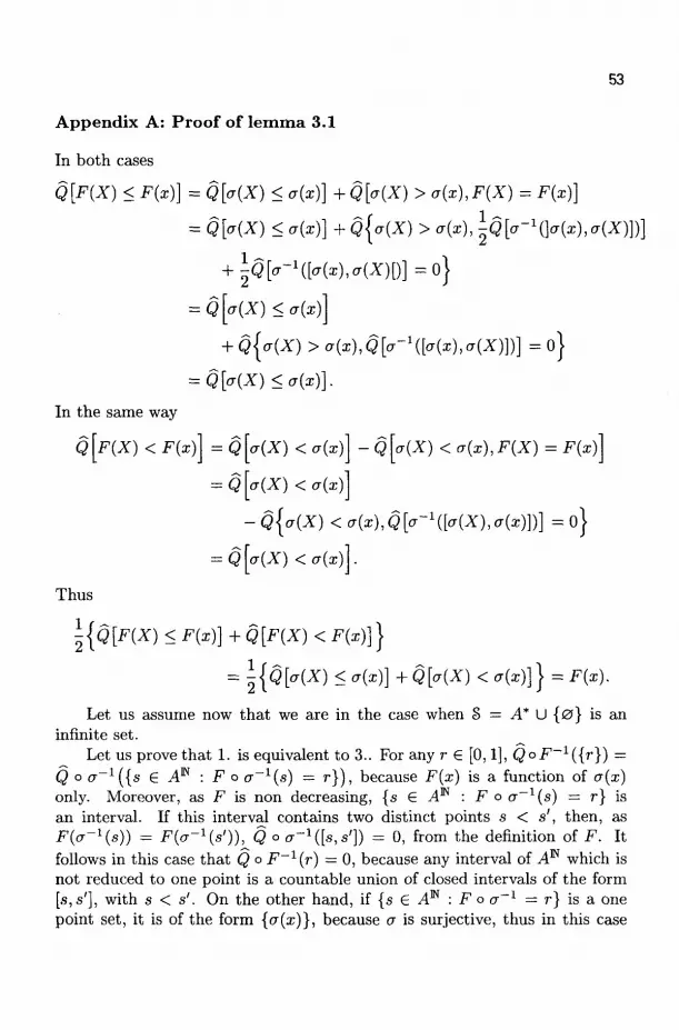
53

Appendix A: Proof of lemma 3.1

In both cases

Q[F{X) < F(x)] = Q[a(X) < a(x)] +Q[a{X) > a{x),F(X) = F(x)]

= Q[a(X)<a(x)]+Q{a(X)>a(x),^Q[a-1{}a{X),a(X)])}

+ \Q[cr-1([<T(x),a(X)[)]=0}

= Q[<T(X) <<T(X)]

+ Q{CJ(X) > a(x),Q[^1([<j(x),(r(X)])} = 0 }

= Q[a(X)<a(x)].

In the same way

Q[F(X) < F(xj\ =Q[*(X) < a(xj\ -Q[o{X) < a(x),F(X) = F(x)]

= Q[a(X) <a(x)\

- Q{J{X) < a(x),Q[a~1([a(X),c7(x)])] = o}

= Q[a(X) <a{x) .

Thus

1{Q[F(X) < F(x)] + Q[F(X) < F(x)}}

= \{QW < *(*)] +G[°(X) < a(x)}} = F(x).

Let us assume now that we are in the case when S = A* U {0} is an infinite set.

Let us prove that 1. is equivalent to 3.. For any r € [0,1], QoF^dr}) = Q o <7-1({s £ Am : F o er -1(s) = r}), because F{x) is a function of a(x) only. Moreover, as F is non decreasing, {s S ^4^ : F o cr_1(s) = r} is an interval. If this interval contains two distinct points s < s', then, as F(o--1(s)) = Fia-1^')), Q o o--1 ([«,«']) = 0, from the definition of F. It follows in this case that Q o F~l(r) = 0, because any interval of AN which is not reduced to one point is a countable union of closed intervals of the form [s,s'], with s < s'. On the other hand, if {s £ Aw : F o a"1 = r] is a one point set, it is of the form {a(x)}, because a is surjective, thus in this case

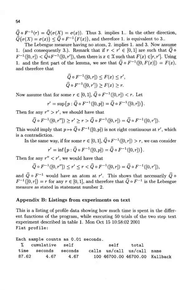
54

Q o F _ 1 ( r ) = Q(a(X) = a(x)). Thus 3. implies 1.. In the other direction, Q(a(X) = cr(x)) < Q o F~x(F(x)), and therefore 1. is equivalent to 3..

The Lebesgue measure having no atom, 2. implies 1. and 3. Now assume 1. (and consequently 3.). Remark that if r < r' G [0,1] are such that Q o F_ 1([0,r]) < QoF_ 1([0,r ' ]) , then there is x G X such that F(x) £]r,r']. Using 1. and the first part of the lemma, we see that Q o F~1([0,F(x)]) — F(x), and therefore that

QoF _ 1 ( [0 , r ] ) <F{x) <r',

Q o F - 1 ( [ 0 , r ' ] ) >F(x) >r.

Now assume that for some r G [0,1], Q o F~1([07r]) < r. Let

r'=sup{p:QoF-1([0,p]) = QoF-l(lO,r})}.

Then for any r" > r', we should have that

Q o F - ^ l C r " ] ) > r ' > r > Q o ^ ( [ O . r ] ) = Q ° F-^fO.r ' ]) .

This would imply that p i-> QoF~l(]f),p\) is not right continuous at r', which is a contradiction.

In the same way, if for some r G [0,1], QoF_ 1([0,r]) > r, we can consider

r'=mi{p:QoF-1({0,p]) = QoF-1([0,r})}.

Then for any r" < r', we would have that

Q o -^ [O.r"] ) < r' < r < Q o F ' ^ l C r ] ) = Q o ^-^[O. r ' ] ) ,

and Q ° F~l would have an atom at r'. This shows that necessarily Q o F _ 1 ([0, r)) = r for any r G [0,1], and therefore that Q o F~l is the Lebesgue measure as stated in statement number 2.

Appendix B: Listings from experiments on t ex t

This is a listing of profile data showing how much time is spent in the differ­ent functions of the program, while executing 50 trials of the two step text experiment described in table 1. Mon Oct 15 10:58:02 2001 F la t p r o f i l e :

Each sample counts as 0.01 seconds.

7, cumulative self self total

time seconds seconds calls us/call us/call name

87.62 4.67 4.67 100 46700.00 46700.00 Kullback

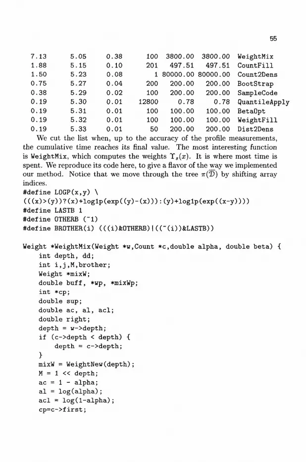
55

7.13 1.88 1.50 0.75 0.38 0.19 0.19 0.19 0.19

5.05 5.15 5.23 5.27 5.29 5.30 5.31 5.32 5.33

0.38 0.10 0.08 0.04 0.02 0.01 0.01 0.01 0.01

3800.00 497.51

80000.00 200.00 200.00 0.78

100.00 100.00 200.00

3800.00 497.51

80000.00 200.00 200.00 0.78

100.00 100.00 200.00

WeightMix CountFill Count2Dens Bootstrap SampleCode QuantileApply BetaOpt WeightFill Dist2Dens

100 201

1 200 100

12800 100 100 50

We cut the list when, up to the accuracy of the profile measurements, the cumulative time reaches its final value. The most interesting function is WeightMix, which computes the weights Ts(a;). It is where most time is spent. We reproduce its code here, to give a flavor of the way we implemented our method. Notice that we move through the tree 7r(D) by shifting array indices. #define L0GP(x,y) \ (((x)>(y))?(x)+loglp(exp((y)-(x))):(y)+loglp(exp((x-y)))) #define LASTB 1 #define 0THERB (~1) #define BROTHER(i) (((i)feOTHERB)|((~(i))&LASTB))

Weight *WeightMix(Weight *w,Count *c,double alpha, double beta) { int depth, dd; int i,j,M.brother; Weight *mixW; double buff, *wp, *mixWp; int *cp; double sup; double ac, al, acl; double right; depth = w->depth; if (c->depth < depth) {

depth = c->depth; } mixW = WeightNew(depth); M = 1 « depth; ac = 1 - alpha; al = log(alpha); acl = log(l-alpha); cp=c->first;

56

wp=w->first; mixWp=mixW->first; for (i=(M»l);i<M;i++) {

right = al+(beta*cp[i«l])*wp[i«l] + ( b e t a * c p [ ( i « l ) + l ] ) * w p [ ( i « l ) + l ] ;

mixWpEi] = LOGP(acl ,r ight) ; > f o r ( i = ( M » l ) - l ; i ; i — ) {

r i g h t = a l+mixWp[i«l]+mixWp[( i«l )+l] + ( b e t a * c p [ i « l ] ) * w p [ i « l ] + ( b e t a * c p [ ( i « l ) + l ] ) * w p [ ( i « l ) + l ] ;

mixWp[i] = LOGP(acl ,r ight) ; } M = 1 « (depth+1); sup = 0; for(i=(l«depth);i<M;i++) {

brother = BROTHER(i); right = al+((beta*cp[i])+l)*wp[i]

+ (beta*cp[brother])*wp[brother]; buff = LOGP(acl,right); for(j = (i»l),dd=depth-l;j>l;j»=l,dd—) {

brother = BROTHER(j); right = al+buff+mixWp[brother]

+ ((beta*cp[j])+l)*wp[j] + (beta* cp[brother]) *wp[brother];

buff = LOGP(acl,right); } mixWp[i] = buff; if (buff > sup) {

sup = buff; >

/* normalizing the weights in two steps to make things numerically more stable */

for (i=(l«depth);i<M;i++) { mixWp[i] -= sup;

> for (i=(l«depth)-l;i;i~) {

mixWp[i] = LOGP(mixW->f irst [i«l] ,mixW->f irst [(i«l) + l]) ; } for (i=M-l;i;i—) { /* back from the log

57

r e p r e s e n t a t i o n of weights */ mixWp[i] = exp(mixWp[i]-mixWp[l]);

} r e t u r n mixW;

} Note that we preferred not to use equation (43) to compute the nor­

malizing factor of the estimated distribution, in order to increase numerical stabibility and be sure that round off errors do not prevent the estimated distribution from summing up to one within a good accuracy. Numerical sta­bility was checked for samples up to size N = 107 (which is the maximum size we tried).

The following reports of batch sessions show that it is necessary to increase the depth d of the maximal dictionary by two units, going from 8 to 10, to reach the same accuracy with a one step estimation scheme :

L 7072

7072 7072 7072

N 1000 1000 1000 1000

K 100

1000 1000 1000

D

{0,1}» {0,1}«

{o,i}9

{o,i}10

©oo { 0 , l } l g

{o,ir { 0 , 1 } 1 8

{ 0 , 1 } 1 S

E|0C(P,Q)1 5.12 ± 0 . 0 8 4.56 ± 0 . 0 1

4.017 ± 0 . 0 0 9 3.788 ± 0 . 0 1 4

E\X(P,Q)] 3.70 ± 0.07

4.561 ± 0 . 0 1 4.017 ± 0.009 3.788 ± 0.014

Table 2.

These are the profile data for the last batch session : F l a t p r o f i l e :

Each sample counts as 0.01 seconds. '/. c u m u l a t i v e

t i m e 6 9 . 7 2 2 4 . 9 6

1.62 1.18 1.03 0 . 5 9 0 .30 0 .30 0 . 1 5 0 . 1 5

s econds 4 . 7 2 6 . 4 1 6 .52 6 . 6 0 6 .67 6 . 7 1 6 . 7 3 6 . 7 5 6 .76 6 .77

s e l f s econds

4 . 7 2 1.69 0 . 1 1 0 . 0 8 0 .07 0 .04 0 .02 0 .02 0 . 0 1 0 . 0 1

c a l l s 100 100 201

1 100

51200 200 100 100

50

s e l f t o t a l u s / c a l l u s / c a l l

47200 .00 47200 .00 16900.00 16900.00

547 .26 547 .26 80000 .00 80000 .00

700 .00 700 .00 0 .78 0 .78

100.00 100.00 200 .00 200 .00 100.00 100.00 200 .00 1000.00

name K u l l b a c k WeightMix C o u n t F i l l Count2Dens WeightLog Q u a n t i l e A p p l y B o o t s t r a p Weigh t2Dis t B e t a S e t Est2Dens

The Ku l lback function is used only to compute the Kullback divergence between estimated and t rue distributions therefore it is not pa rt of the esti-

mation algorithm itself, but is just a tool used to test its performance. The important thing is the time spent in WeightMix, which jumps to 1.69

seconds, whereas it was only 0.38 seconds for the two step scheme.

N.B.: We included in the following bibliography some references about adaptive regression estimation, because of its numerous links with density estimation.

References

1. Y. Baraud (1998) Selection de modeles et estimation adaptative dans differents cadres de regression, PHD, Universite Paris 11.

2. Y. Baraud, F. Comte and G. Viennet (1998) Adaptive estimation in an autoregressive and a geometrical beta-mixing framework, preprint 98-07 CREST-INSEE.

3. Y. Baraud, F. Comte and G. Viennet (1999) Model selection for (auto-) regression with dependent data, preprint.

4. A. Barron (1987) Are Bayes Rules Consistent in Information? Open Prob­lems in Communication and Computation, T. M. Cover and B. Gopinath Ed., Springer Verlag 1987.

5. A. Barron and Y. Yang (1999) Information Theoretic Determination of Minimax Rates of Convergence, Ann. Statist. 27, no. 5, 1564-1599.

6. A. Barron, L. Birge and P. Massart, (1999) Risk bounds for model selec­tion via penalisation, Probab. Theory Related Fields 113, no 3, 301-413.

7. L. Birge and P. Massart (1997) From model selection to adaptive estima­tion, Festschrift for Lucien Le Cam, 55-87, Springer, New York.

8. L. Birge and P. Massart (1998) Minimum contrast estimators on sieves : exponential bounds and rates of convergence, Bernoulli, 4 (1998), no. 3, 329-375.

9. L. Birge and P. Massart (1996) An adaptive compression algorithm in Besov spaces, Prepublication d'Orsay numero 39, http:/ /www.math.u-psud.fr/~biblio/pub/1996/ppo_1996.html

10. L. Birge and Y. Rozenholc (1999) How many bins should be put in a regular histogram?, preprint.

11. G. Castellan (1999) Modified Akaike's criterion for histogram density estimation, preprint http:/ /www.math.u-psud.fr/~biblio/pub/1999/ppo_1999.html

12. Castellan, G. (2000) Selection d'histogrammes a I'aide d'un critere de type Akaike. [Histogram selection with an Akaike-type criterion] C. R. Acad. Sci. Paris Sr. I Math. 330, no. 8, 729-732.

13. O. Catoni (1997) The mixture approach to universal model selection,

59

preprint LMENS-97-22 http://www.dmi.ens.fr/EDITION/preprints/1997/resu9722.html

14. Olivier Catoni. Universal aggregation rules with sharp oracle inequalities. Annals of Statistics, to appear, pages 1-37, 1999. Revised and augmented from A mixture approach to universal model selection.

15. Olivier Catoni. Gibbs estimators. Probab. Theory Relat. Fields, to appear, pages 1-23, 2000. see h t tp : / /www.dmi .ens . f r /p repr in t s .

16. T. M. Cover and J. A. Thomas (1991) Elements of information theory, John Wiley, New York, 542 pages.

17. Csiszar I. and Korner J. (1981) Information theory : coding theorems for discrete memoryless systems, Academic Press, New York.

18. Hardle, Wolfgang; Kerkyacharian, Gerard; Picard, Dominique; Tsy-bakov, Alexander (1998) Wavelets, approximation, and statistical ap­plications. Lecture Notes in Statistics, 129. Springer-Verlag, New York. xviii-|-265 pp.

19. Donoho, David L.; Johnstone, Iain M. (1995) Adapting to unknown smoothness via wavelet shrinkage. J. Amer. Statist. Assoc. 90, no. 432,1200-1224.

20. Donoho, David L.; Johnstone, Iain M. (1994) Ideal spatial adaptation by wavelet shrinkage. Biometrika 81, no. 3, 425-455.

21. Donoho, David L.; Johnstone, Iain M. (1999) Asymptotic minimaxity of wavelet estimators with sampled data. Statist. Sinica 9, no. 1, 1-32.

22. Donoho, David L.; Johnstone, Iain M.; Kerkyacharian, Gerard; Picard, Dominique (1996) Density estimation by wavelet thresholding. Ann. Statist. 24, no. 2,508-539.

23. Donoho, D. L.; Johnstone, I. M.; Kerkyacharian, G.; Picard, D. (1997) Universal near minimaxity of wavelet shrinkage. Festschrift for Lucien Le Cam, 183-218, Springer, New York.

24. M. Feder and N. Merhav, (1996) Hierarchical Universal Coding, IEEE Trans. Inform. Theory, vol 42, no 5, Sept.

25. Goldenshluger, A.; Nemirovski, A. (1997) On spatially adaptive estima­tion of nonparametric regression. Math. Methods Statist. 6, no. 2, 135-170.

26. I. Johnstone (1998) Function estimation and wavelets, Lecture Notes, ENS Paris.

27. A. Juditsky, A. Nemirovski (1996) Functional aggregation for nonpara­metric regression in 4th World Congress of the Bernouilli Society, Vienna, Austria, August 26-31.

28. Lugosi, Gabor; Nobel, Andrew (1996) Consistency of data-driven his­togram methods for density estimation and classification. Ann. Statist.

60

24, no. 2, 687-706. 29. A. Nemirovski (1998) Topics in Non-Parametric Statistics Saint-Flour

Summer School on Probability Theory. 30. Neveu, Jacques, (1965) Mathematical foundations of the calculus of prob­

ability, Holden-Day, San-Francisco. 31. Nobel, Andrew (1996) Histogram regression estimation using data-

dependent partitions. Ann. Statist. 24, no. 3, 1084-1105. 32. J. Rissanen (2001) Lectures on statistical modeling theory, Lecture notes,

avaible at the author's site h t t p : / / w w w . c s . t u t . f i / ~ r i s s a n e n / 33. J. Rissanen (1983) A universal data compression system, IEEE Trans.

Inform. Theory, Vol. IT-29, no 5, 656-664. 34. B. Y. Ryabko, (1984) Twice-universal coding, Probl. Inform. Transm.,

vol 20, no 3, pp. 24-28, July-Sept. 35. Vapnik V. (1998) Statistical Learning Theory, Wiley. 36. M. J. Weinberger, J. Rissanen and M. Feder (1995) A universal finite

memory source, IEEE Trans. Inform. Theory, Vol. IT-41, no 3, pp 643-652.

37. F. M. J. Willems, Y. M. Shtarkov and T. J. Tjalkens (1995) The Context-Tree Weighting Method: Basic Properties, IEEE Trans. Inform. Theory, vol 41, no 3, May, 1995.

38. F. M. J. Willems, Y. M. Shtarkov and T. J. Tjalkens (1996) Context Weighting for General Finite-Context Sources, IEEE Trans. Inform. Theory, vol 42, no 5, Sept, 1996.

39. Yang, Y. (2000) Mixing strategies for density estimation. Ann. Statist. 28, no. 1, 75-87.

40. Yang Yuhong (1998) Combining Different Procedures for Adaptive Re­gression, preprint h t tp : / /www.pub l i c . i a s t a t e . edu /~s t a t / upda t e / r epo r t s . h tml

61

BIFURCATIONS OF LIMIT CYCLES IN Z Q - E Q U I V A R I A N T P L A N A R VECTOR FIELDS OF DEGREE 5

H.S .Y.CHAN A N D K . W . C H U N G

Department of Mathematics, City University of Hong Kong, Hong Kong, China

J IBIN LI

School of Science, Kunming University of Science and Technology, Kunming,

China

Consider the weakened Hilbert's 16th problem for symmetric planar perturbed polynomial Hamiltonian systems. In particular, for perturbed Hamiltonian poly­nomial vector fields of degree 5, numerical examples of Z9-equivariant planar per­turbed Hamiltonian systems are constructed, having maximal number of centers. They give rise to different configurations of limit cycles forming compound eyes. These are studied by the bifurcation theory of planar dynamical systems and the method of detection functions. With the help of numerical analysis, it is shown that there exist parameter groups such that a polynomial vector field of degree 5 has at least 20 limit cycles with Zs symmetry and at least 24 limit cycles with Z$ symme­try. There is reason to conjecture that the Hilbert number H(2fc + l ) > (2fc + l ) 2 —1 for the perturbed Hamiltonian systems.

1 Introduction

One of the problem posed by Smale[26] in his "Mathematical Problems for the Next Century" is Hilbert's 16th problem. It is well known that Hilbert's 16th problem consists of two parts. The first part studies the mutual disposi­tion of maximal number ( in the sense of Harnack) of separate branches of an algebraic curve, and also the "corresponding investigation" for non-singular real algebraic varieties; and the second part poses the questions of the maxi­mal number and relative dispositions of limit cycles of the planar polynomial vector field:

^ = Pn(x,y), ft=Qn(x,y), (En)

where Pn and Qn are polynomials of degree n(See Hilbert[ll], Farkas[8], Ye[29], Zhang et al [31]). As professor Smale said: "Except for the Riemann hypothesis, it seems to be the most elusive of Hilbert's problems." In fact, for the first part, the specialists of the real algebraic geometry usually study the topology of non-singular real planar projective algebraic curves of degree m. Up to now, we know the schemes of mutual arrangement of ovals realized by M-curves only for m < 7(see Gudkov[10], Viro[27] and Wilson[28] etc).

62

For the second part, the answer still seems to be far away. Let H(n) be the maximal number of limit cycles of (En). Up to now, we only know that the system (En) always has a finite number of limit cycles(see Ilyashenko[12]) and that H(2) > 4,H(3) > 11 (see recent discussions in Chan et al[4], Li[14,15], ,Lloyd[20], Luo[21], Perko[23], Ye[29] and etc). Also by considering a small neighbourhood of a singular point, H(ri) > (n2 + 5n - 20 — 6(-l)™)/2 for n > 6(see Otrokov[22]). Recently, Christopher and Lloyd[6] showed that H{2k - 1) > 4k-1(2k - ^ ) + 3.2fc - § (for example H(7) > 25) by perturbing some families of closed orbits of a Hamiltonian system. However, in global phase plane, when n > 3, how many cycles can be created by (En), and what global limit cycle configurations can appear? These are still interesting open problems. In order to obtain more limit cycles and various configu­ration patterns of their relative dispositions, one of us indicated in [13]-[17] that an efficient method is to perturb the symmetric Hamiltonian systems having maximal number of centers, i.e., to study the weakened Hilbert's 16th problem posed by V.I.Arnold[2] in 1977 for the symmetric planar polynomial Hamiltonian systems, since bifurcation and symmetry are closely connected and symmetric systems play pivotal roles as a bifurcation point in all planar Hamiltonian system class. To investigate perturbed Hamiltonian systems, we should first know the global behaviour of unperturbed polynomial systems, namely, determine the global property for the families of real planar algebraic curves defined by the Hamiltonian functions. Then by using proper pertur­bation techniques, we shall obtain the global information of bifurcations for the perturbed non-integrable systems. In this sense, we say that our study method will utilize both parts of Hilbert's 16th problem.

On the basis of the method of detection functions posed by Li[13], we give in this paper a method of control parameters in order to obtain more limit cycles for some Zg-equivariant perturbed polynomial Hamiltonian system of degree n = 5 (q = 2 — 6). With the help of numerical analysis ( using Maple[l] or Mathematica) we show that there exist parameter groups such that there exists at least 15 to 24 limit cycles having the configurations of compound eyes in these systems. The cases for q = 2,3 and 4 are being reported separately in [5] and [19] where at least 15 and 23 limit cycles are respectively obtained. The case for q = 6 is discussed in [18]. Here we will give an overall view of the process and fill in more details using q = 5 and 6 as examples.

The paper is divided into five sections. Section 2 gives a general Zg-equivariant fifth degree planar polynomial vector fields and their Hamiltonian forms. As examples, for q = 5,6 we discuss the behaviour of sextic algebraic curves defined by the Hamiltonian vector fields. In Section 3 we introduce the detection function and its properties for the perturbed planar Hamiltonian

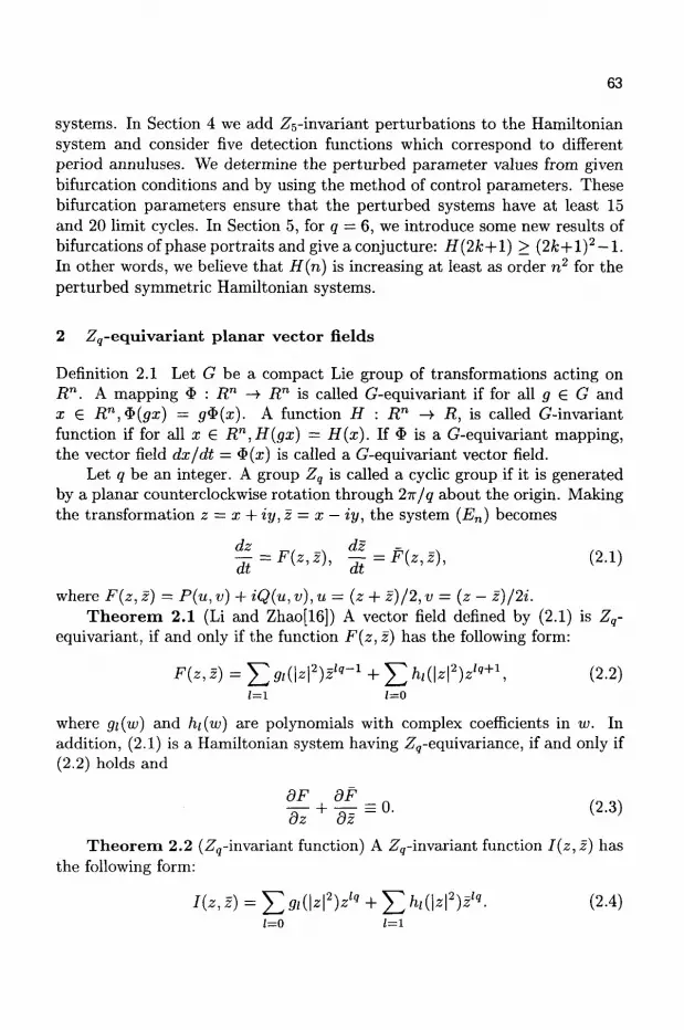
63

systems. In Section 4 we add ^-invariant perturbations to the Hamiltonian system and consider five detection functions which correspond to different period annuluses. We determine the perturbed parameter values from given bifurcation conditions and by using the method of control parameters. These bifurcation parameters ensure that the perturbed systems have at least 15 and 20 limit cycles. In Section 5, for q — 6, we introduce some new results of bifurcations of phase portraits and give a conjucture: H(2k+1) > (2fc+l) 2 - l . In other words, we believe that H(n) is increasing at least as order n2 for the perturbed symmetric Hamiltonian systems.

2 .Zg-equivariant planar vector fields

Definition 2.1 Let G be a compact Lie group of transformations acting on Rn. A mapping $ : Rn -¥ Rn is called G-equivariant if for all g £ G and x 6 Rn,$(gx) = g$(x). A function H : Rn -¥ R, is called G-invariant function if for all x € Rn,H(gx) = H(x). If $ is a G-equivariant mapping, the vector field dx/dt = $(x) is called a G-equivariant vector field.

Let q be an integer. A group Zq is called a cyclic group if it is generated by a planar counterclockwise rotation through 27r/g about the origin. Making the transformation z = x + iy, z = x — iy, the system (En) becomes

%=F(z,z), ft=F(z,z), (2.1)

where F(z,z) = P(u,v) + iQ(u,v),u = (z + z)/2,v = (z — z)/2i. Theorem 2.1 (Li and Zhao[16]) A vector field defined by (2.1) is Zq-

equivariant, if and only if the function F(z, z) has the following form:

F(Z,J) = £ J 1 ( | Z | V ' - 1 + E A I ( N V ' + 1 > (2-2) (=1 1=0

where gi{w) and hi(w) are polynomials with complex coefficients in w. In addition, (2.1) is a Hamiltonian system having Zg-equivariance, if and only if (2.2) holds and

9F OF n

fl- + 7 F = °- 2 - 3

az oz T h e o r e m 2.2 (Z9-invariant function) A .^-invariant function I(z,z) has

the following form:

/(z,!) = £ f f ;(|2|V? + EMM2)^- (2-4) ;=o i= i

64

Corollary 2.3 For the planar polynomial systems of degree 5, all non-trivial Zg-equivariant vector fields have the following forms:

(1) q = 6,F{z,z) = (A0 + Ax\z\2 + A2\z\4)z + A3z5;

(2) q = 5,F(z,z) = (A0 + Ax\z\2 + A2\z\4)z + A3z4;

(3) q = 4,F(z,z) = {AQ + Ax\z\2 + A2\z\4)z + (A3 + A» |* | 2 )* 3 + A5z5;

(4) q = 3,F(z,z) = (A0+Al\z\2+A2\z\4)z+(A3+Ai\z\2)z2+A5zi+A6z

5; (5) q = 2,F(z,z) = (A0 + A!\z\2 + A2\z\i)z + (A3 + A^\z\2 + A5\z\4)z +(A(s+A7\z\2)z3+(A8+A9\z\2)z3+Aioz5+Anz5, where Aj = aj+ibj(j -

0 — 11) are complex. The above F{z,z) define -Z^-equivariant Hamiltonian vector fields if and only if a0 = ai = a2 = 0 and for q = 4, Ai = — 5J4S; for q = 3, Ai = -4A5; for q = 2, A4 = -3A6, A5 = -2AT, A9 = -5A~10.

The orbits of these Hamiltonian polynomial systems define different fam­ilies of sextic (m = 6) algebraic curves having Z,-equivariance. One of the main questions in real algebraic geometry is to describe what schemes of the mutual arrangement (schemes or configurations) of ovals can be realized by curves of given degree. By using some Z,-equivariant Hamiltonian systems, we can realize a lot of configurations of ovals for planar algebraic curves of degree m. Rokhlin[25] listed all real schemes of ovals with m < 5. Leaving aside the simple case m = 1,2,3, we know that for m — 4, there are six real schemes: a nest of depth 2 and five unnested schemes with I = 0,1,2,3,4; for m = 5, there are eight real schemes: a scheme with a nest of depth 2, and seven unnested schemes with Z = 0,1,2,3,4,5,6.

Theorem 2.4 For m = 4 and 5, all real schemes of projective algebraic curves in RP2 can be realized by the orbits of Z,-equivariant Hamiltonian vector fields.

For m = 6, the system (E$) is Zg-equivariant Hamiltonian system if and only if it can be reduced to the following 3-parameter family:

dv — =£r5sin60,

— = l - 2 J r 2 + (a + /3cos6(9)r4, (2.5)

which has the Hamiltonian

H(r,0) = -\r2 + hr4 - ha + /?cos60)r6 (2.6)

2 2 6 Suppose that a > /3 > 0,6 = (a + ft + l ) /2 . Then, there exist 25 finite

singular points of (2.5) at (0,0),(zi,0), (z2,0), (z3,ir/6), (z4,7r/6) and their

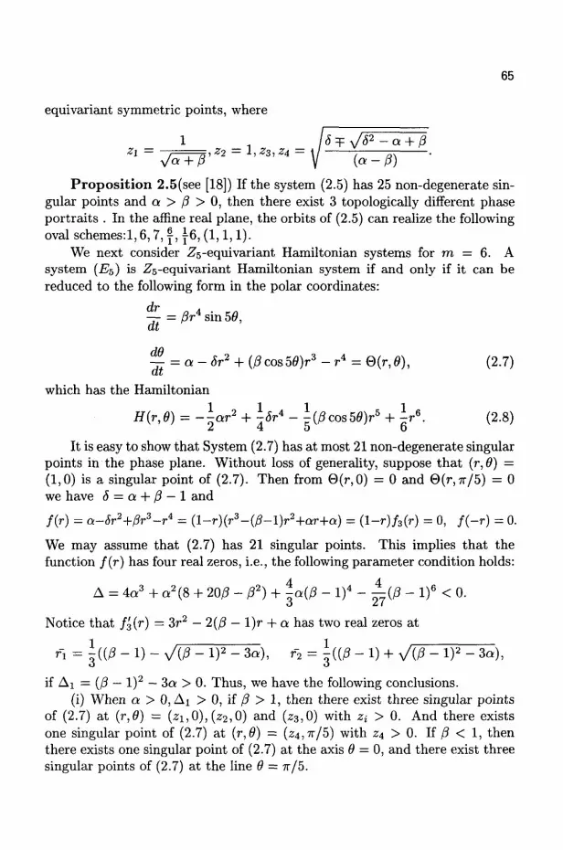
65

equivariant symmetric points, where

Z\ = , -=,Z2 = l,ZZ,Z4= >>

Proposition 2.5(see [18]) If the system (2.5) has 25 non-degenerate sin­gular points and a > /3 > 0, then there exist 3 topologically different phase portraits . In the afnne real plane, the orbits of (2.5) can realize the following oval schemes:l,6,7, | , j 6 , (1,1,1).

We next consider Zs-equivariant Hamiltonian systems for m = 6. A system (E5) is Zs-equivariant Hamiltonian system if and only if it can be reduced to the following form in the polar coordinates:

J=£r4sin50,

dQ

^=a-Sr2 + (/?cos50)r3 - r4 = Q(r,6), (2.7)

which has the Hamiltonian

H(r,0) = -lar2 + hr4-hpcos59)r5 + lr6. (2.8) 2 4 5 6

It is easy to show that System (2.7) has at most 21 non-degenerate singular points in the phase plane. Without loss of generality, suppose that (r, 6) = (1,0) is a singular point of (2.7). Then from 0(r,O) = 0 and 9(r,7r/5) = 0 we have S = a + /? — 1 and f(r) = Q-Jr 2 +^r 3 - r 4 = {l-r)(r3-(fi-l)r2+ar+a) = ( l - r ) / 3 ( r ) = 0, / ( - r ) = 0. We may assume that (2.7) has 21 singular points. This implies that the function f(r) has four real zeros, i.e., the following parameter condition holds:

A = 4a3 + a2(8 + 20/? - /32) + ^a(p - l ) 4 - ^(fi - if < 0.

Notice that f'3{r) = 3r2 - 2(/3 — \)r + a has two real zeros at

1 ry-r — —N 1 fi = -W-\)-y/{p-\)*-$a), r2 = - ( ( / 3 - l ) + v ' ^ - l ) 2 - 3 a ) ,

if Ai = (f3 — l ) 2 — 3a > 0. Thus, we have the following conclusions. (i) When a > 0,Ai > 0, if/? > 1, then there exist three singular points

of (2.7) at (r,8) = (zi,0), (z2,0) a n d (^3,0) with zt > 0. And there exists one singular point of (2.7) at (r, 9) = (z4,ir/5) with 2:4 > 0. If /? < 1, then there exists one singular point of (2.7) at the axis 6 = 0, and there exist three singular points of (2.7) at the line 6 = TT/5.

66

(ii) When a < 0, there exist two singular points (zi,0) and (zj,rr/5),i — 1,2, j — i + 2 of (2.7) at the axes 0 = 0 and 9 = JT/5, respectively.

To determine the type (center or saddle point) of singular poinits (z»,0) and (zj,n/5) of (2.7). We only need to use the signs of the Jacobians of the linearized system of (2.7):

J(zt,0) = -50z?f'(zi), J(zj,Tf/5) = 5/?zf/'(-*;)•

a) Hi*, »/** < w*& w ax**.*/*) "••• &*>a). ® mutt-j® > ^u»m Figure 1: Zs-equivariant polynomial Hamiltonian vector fields of degree 5

Obviously, for a > 0, the singular points [zi, 0), (ZA, T / 5 ) are saddle points and (zi,0), (z3,0) are centers; for a < 0, the singular points (zi,0),(.Z4,7r/5) are saddle points and (^2,0), (zs,ir/5) are centers. Since the Hamiltonian defined by (2.8) is of definite sign near the origin (0,0) and at infinity, hence the origin ia a center and there exists a global periodic family of (2.7) surrounding all 21 singular points. By the above qualitative analysis and Z5-equivariance of (2.7), we have the following result.

Propos i t ion 2.6 For the i^-equivariant polynomial Hamiltonian system (2.7) having 21 non-degenerate singular points, there exist 6 topologically different phase portraits as shown in Figure 1.

67

As h varies, the level curves H(r, 9) = h of the Hamiltonian defined by (2.8) give rise to a family of sextic algebraic curves in the affine real plane. As an example, we

*~'r~-w¥j~v~T*"^s "<#

>4 -? K* - 1

i Si

C?) h\ < h < k§. <$j fe&*j & < %- P)A^.V

M| h. < A < 0- {&} & < /> < &*- Wl?* ** >V

Figure 2:Different schemes of ovals defined by (2.3) under the parameter condition Gi.

consider Figure 1 (3). Let Gt = (o,/J) = (0.1551515151,2.7575757575) and * = 1.91272727. We have zx = 0.4, z2 =• 1, z3 = l.Q, z4 = 0.2424242424 and

tn = H(z3,0) = -0.05163442391, /i2 = ff(*i,0) - -0.005135515151,

h3 = H{zt,w/5) = -.002411905557, h4 = H(z2,0) = 0.0157575757.

As h increases from hi to oo, the schemes of ovals of the sextic algebraic curves will be varied. This change process is shown in Figure 2. Similarly, we can discuss other portraits in Figure 1. Therefore, by using Gudkov's oval notation (see [10]), we have the conclusion as follows.

Propos i t ion 2.7 In the affine real plane, the integral curves of the Hamiltonian system (2.7) can realize the following oval schemes:!, 5,6,10, f, \5, (1,1,1).

68

3 The method of detection functions

Consider the following perturbed planar Hamiltonian system

ex(p(x,y) - A ) , dx ~di ~ dy_ _ dt ~

dH

dy dH dx

-ey(p(x,y)-X), (3.1)

where H(x, y) is the Hamiltonian, p(0,0) = 0,0 < e <C 1, A € -R. Suppose that the origin in the phase plane is a singular point of (3.1) and

the following conditions hold: (Al) The unperturbed system (3.1)e=0 is a Zg-equivariant Hamiltonian

vector field. For h € (/ii,/j2) one branch family of the curves {Th} defined by the Hamiltonian function H(x,y) = h lies in a period annulus enclosing at least one singular point. As h increases, Th expands outwards. When h —¥ / i i ,^approaches a singular point or an inner boundary of the period annulus consisting of a heteroclinic (or homoclinic) loop.

(A2) Surrounding the period annulus, there exists a heteroclinic (or ho­moclinic) loop T7*2 at h = h2 connecting some hyperbolic saddle points (ai,/?j),l <i <q.

(A3) The divergence 2(A - F(x,y)) = 2 ( A - f § 2 - f g - p(x,y)) of the perturbed vector field is a Zq -invariant function.

We define the function

A = X(h) = (J J h F(x, y)dxdy)/(J J ^ dxdy) = iP(h)/<t>(h), (3.2)

which is called a detection function corresponding to the periodic family {Th}. The graph of A = A(/i) in the plane (h, A) is called a detection curve, where Dh is the area inside Th.

Clearly, if H(x,y) — h is a polynomial, then X(h) is a ratio between two Abelian integrals (see Carr, Chow and Hale[3]). In this case, X(h) is a differentiate function with respect to h. Of course, when the degree of H(x,y) is more than 4, classical mathematical analysis cannot provide the calculating method for X(h) in general. We must use a numerical technique to compute these Abelian integrals.

On the basis of the Poincare-Pontrjagin-Andronov theorem on the global center bifurcation and Melnikov method (see Perko[23], Guckenheimer and Holmes [9]), we have the following two conclusions (as in Li Jibin etc.[13][15]):

Theorem 3.1 (Bifurcation of limit cycles) Suppose that the conditions (Al) and (A3) hold. For a given A = AQ, considering the set S of the in-

69

tersection points of the straight line A = A0 and the curve A = X(h) in the (h, A)-plane, we have

(i) if S consists of exactly one point (/io,Ao) and \'(h) > 0(< 0), then there exists a stable(unstable) limit cycle of (3.1) near Tho;

(ii) if S consists of two points (h0, A0) and (h0,X0) having ho > h0 and X'(h0) > 0,X'(h0) < 0, then there exist two limit cycles near T^0 and Th° respectively, the former is stable and the latter is unstable;

(hi) if S contains a point (h0,Xo) and X'(h0) = X"(h0) = ••• = A(*-1)(/io) = 0, but A(fc)(/i0) ^ 0, then (3.1) has at most k limit cycles near Th0.

(iv) if S is empty, then (3.1) has no limit cycle. Theorem 3.2 (Bifurcation parameter created by a heterochnic or ho-

moclinic loop) Suppose that the conditions (A1),(A2) and (A3) hold. Then for 0 < e <C 1, when A = A(/i2) + O(e), System (3.1) has a heterochnic (or homoclinic) loop having Z^-equivariance.

The following two propositions describe the properties of the detection function at the boundary values of h.

Proposition 3.3 (The parameter value of Hopf bifurcation) Suppose that as h -> hi, the periodic orbit Fh of (3.1) approaches a singular point (£,77), then at this point the Hopf bifurcation parameter value is given by

bH = A(/n) + O(e) = lim X(h) + O(e) = F(£,»i) + O(e). (3.3)

Proposition 3.4 (Bifurcation direction of heterochnic or homoclinic loop) Suppose that as h —> /12, the periodic orbit Th of (3.1) approaches a heterochnic (or homoclinic) loop connecting a hyperbolic saddle point (a, /?), where the saddle point value satisfies

SQ(a, p) = 2ea(a, /3) = 2e(X(h2) - F(a, /?)) > 0(< 0),

then we have

A'(/i2) = lim X'(h) = -oo(+oo). (3.4)

Remark 3.5 (1) If r f t contracts inwards as h increases, then the stability of limit cycles

mentioned in Theorem 3.1 and the sign of A'(/i2) in (3.4) have the opposite conclusion.

(2) If the curve Th defined by H{x,y) — h (h £ (hi,h2)) consists of m components of oval families having ^9-equivariance, then Theorem 3.1 gives rise to simultaneous global bifurcations of limit cycles from all these m oval families.

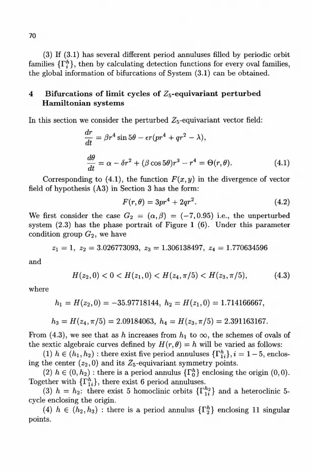
70

(3) If (3.1) has several different period annuluses filled by periodic orbit families {T^1}, then by calculating detection functions for every oval families, the global information of bifurcations of System (3.1) can be obtained.

4 Bifurcations of limit cycles of Z5-equivariant perturbed Hamiltonian systems

In this section we consider the perturbed Zs-equi variant vector field:

— = fir4 sin 58 — er(pri + qr1 — A), at

^-=a-Sr2 + (l3 cos 50)r3 - r4 = 0(r , 6). (4.1)

Corresponding to (4.1), the function F(x,y) in the divergence of vector field of hypothesis (A3) in Section 3 has the form:

F(r,0) = 3pr4 + 2qr2. (4.2)

We first consider the case G2 — (a,/3) = (—7,0.95) i.e., the unperturbed system (2.3) has the phase portrait of Figure 1 (6). Under this parameter condition group G2, we have

Zl = 1, z2 = 3.026773093, z3 = 1.306138497, z4 = 1.770634596

and

H(z2,0) < 0 < H(Zl,0) < H(zi,ir/5) < H(z3,ir/5), (4.3)

where

hi = H(z2,0) = -35.97718144, h2 = H(zu0) = 1.714166667,

h3 = H(z4,ir/5) = 2.09184063, h4 = H{z3,n/5) = 2.391163167.

From (4.3), we see that as h increases from hi to 00, the schemes of ovals of the sextic algebraic curves defined by H(r, 9) = h will be varied as follows:

(1) h € {h\, h2) : there exist five period annuluses { r ^ } , i = 1 — 5, enclos­ing the center (22,0) and its Z5-equivariant symmetry points.

(2) h 6 (0, h2) : there is a period annulus {TQ} enclosing the origin (0,0). Together with { r ^ } , there exist 6 period annuluses.

(3) h = h2: there exist 5 homoclinic orbits {ri8?} and a heteroclinic 5-cycle enclosing the origin.

(4) h 6 (h2,h3) : there is a period annulus {r^} enclosing 11 singular points.

71

(5) h = /13: there exist 5 homoclinic orbits {Tj?} enclosing the singu­lar point (z3,7r/5) and its Zs-equivariant symmetry points, and there is a heteroclinic 5-cycles enclosing 11 singular points.

(6) h G (/i3,/i4): there exist 5 period annuluses { r ^ i = 1 - 5 , enclosing the singular point (2:3,7r/5) and its Z5-equivariant symmetry points, and there is a global period annulus {r j} enclosing all 21 singular points.

(7) h € (/i4,oo) : there is a global period annulus {r j} enclosing all 21 singular points.

Notice that as h increases, the periodic orbits T^ constract inwards while all other periodic orbits expand outwards.

We compute five detection functions defined by (3.2) which correspond to the above five types of period annuluses {TJ} — { r j} .

/ JV,/, F(r, 9)rdrd9 ^.(u\ 1

«*> - //„.-*•"* = s w = sW 3" '"""+^'^ = 3pJil(h) + 2qJi2(h), t = 0 , - - - ,4 , (4.4)

where Jij(h) = Iij(h)/(j)i(h), j = 1,2, and

<t>i(h) = rdrdO, D^ is the area inside T1}, J JD?

Inih) = [ f r5drd6, Ii2(h) = f f r3drd6.

For the given parameter group G2 the functions Jij(h) can be numerically calculated to a given degree of accuracy. We will give these results in the Appendix.

By using the theory given in Section 3, we immediately obtain the follow­ing values of bifurcation parameters and bifurcation direction detections.

(i) Hopf bifurcation parameters: (1) Bifurcation from the origin (0,0):

b» = A0(0) + 0(e) =0 + 0(e);

(2) Simultaneous bifurcations from the center (z2,0) and its Z5- equivari-ant symmetry points:

6f = Ai(fti) + 0(e) = F(z2,0) + 0(e) = 3pz\ + 2qz22 + 0(e)

= 251.7912959p+18.32271071g + O(e);

72

(3) Simultaneous bifurcations from the center (z3,ir/5) and its Z5- equiv-ariant symmetry points:

6f = A3(/i4) + 0(e) = F(z3, TT/5) + 0(e) = 2,pz\ + 2qz% + O(e)

= 8.731285209p+ 3.411995546? + 0(e);

(ii) Bifurcations from heteroclinic or homoclinic loops:

(1) The heteroclinic bifurcation value from TQ2:

\0(h2) = SpJ01(h2) + 2qJQ2(h2) = 0.6447758181p+ 0.7977862274?;

(2) The homoclinic bifurcation value from I \ ? :

Ai(/i2) = 3pJ u( / i 2) + 2qJ12(h2) = 132.5289769p+ 11.90914478?;

(3) The homoclinic and heteroclinic loop bifurcation value from T22:

\2(h2) = 3pJ2i(h2) + 2qJ22(h2) = 117.8557157p+ 10.67290976?;

(4) The heteroclinic 5-cycle bifurcation value from r 23 :

\2(h3) = 3pJ2i(h3)+2qJ22(h3) = 107.7755921p+9.989393194?;

(5) The homoclinic bifurcation value from Tg?:

A3(/i3) = A3(/i3) = 3pJ3i(/i3) + 2?J32(/i3) = 9.777634251p+ 3.48267226?;

(6) The heteroclinic 5-cycle bifurcation value from T43:

A4(/i3) = 3pJa(h3) + 2?J42(/i3) = 102.7553682p+ 9.656067918?.

(iii) The values of bifurcation direction detections of heteroclinic and homoclinic loops:

(1) (70(^,0) = A0(/i2) -F{Zl,Q) = -2.355224182p- 1.202213773?; (2) CTI (zi, 0) = Ai (h2) - F(zi, 0) = 129.5289769p + 9.90914478?; (3) a2(zi,0) = A2(/i2) -F{zi,0) = I14.8557157p +8.67290976?; (4) CT2(z4,7r/5) = A2(/i3) - F(z4,7r/5) = 78.28815436p+ 3.719099448?; (5) a3(zi7Tr/5) = X3(h3)I- F ( Z 4 , T T / 5 ) = -19.70980349p-2.787621486?; (6) CT4(z4,7r/5) = A4(/i3) - F ( Z 4 , T T / 5 ) = 73.26793046p+ 3.385774172?; To control the perturbed parameters (p, q) such that System (4.1) has

more limit cycles, we suppose that the following two conditions hold: (CI) Ai(/i2) = A3(/i3)-0.00M.e.,122.7513426p+8.42647252?+0.001 = 0; (C2) <7i(.zi,0) > 0,i.e., 129.5289769p+ 9.90914478? > 0; These conditions imply that

? = - 14.56734622p - 0.0001186736203, p < -0.00007934395757.

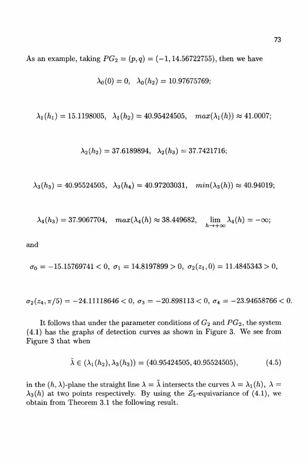
73

As an example, taking PG2 = {p,q) = (—1,14.56722755), then we have

Ao(0) = 0, X0(h2) = 10.97675769;

Ai(/n) = 15.1198005, Ai(/i2) = 40.95424505, maz(Ai(/i)) « 41.0007;

\2{h2) = 37.6189894, A2(/i3) = 37.7421716;

A3(/i3) = 40.95524505, A3(/i4) = 40.97203031, mm(A3(/i)) « 40.94019;

A4(/i3) = 37.9067704, max(X4(h) « 38.449682, lim A4(/i) - - co ;

and

(T0 = -15.15769741 < 0, ax = 14.8197899 > 0, cr2(zi,0) = 11.4845343 > 0,

a2(z4,n/5) = -24.11118646 < 0, CT3 = -20.898113 < 0, a4 = -23.94658766 < 0.

It follows that under the parameter conditions of G2 and PG2, the system (4.1) has the graphs of detection curves as shown in Figure 3. We see from Figure 3 that when

A e (A1(/z2),A3(/i3)) = (40.95424505,40.95524505), (4.5)

in the (h, A)-plane the straight line A = A intersects the curves A = Ai (h), A = A3(/i) at two points respectively. By using the Z5-equivariance of (4.1), we obtain from Theorem 3.1 the following result.

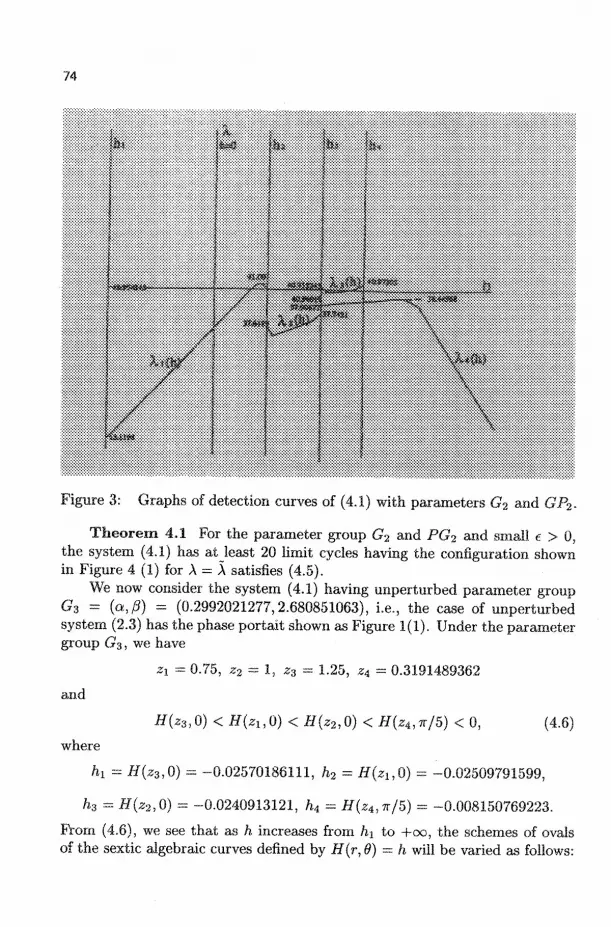
74

Figure 3: Graphs of detection curves of (4.1) with parameters G2 and GP2.

T h e o r e m 4.1 For the parameter group G2 and PG2 and small e > 0, the system (4.1) has atjeast 20 limit cycles having the configuration shown in Figure 4 (1) for A = A satisfies (4.5).

We now consider the system (4.1) having unperturbed parameter group G3 = (a,/3) = (0.2992021277,2.680851063), i.e., the case of unperturbed system (2.3) has the phase portait shown as Figure 1(1). Under the parameter group G-i, we have

zx = 0.75, z2 = 1, z3 = 1.25, z4 = 0.3191489362

and

H(z3,0) < H(zi,0) < H(z2,0) < H{zA,Tx/b) < 0, (4.6)

where

fti = H(z3,0) = -0.02570186111, h2 = H(zu0) = -0.02509791599,

ha = H(z2,0) = -0.0240913121, h4 = H(Z4,TT/5) - -0.008150769223.

From (4.6), we see that as h increases from hi to +oo, the schemes of ovals of the sextic algebraic curves defined by H(r, 8) = h will be varied as follows:

75

(1) h 6 (hi,h3) : there exist five period annuluses { I ^ } , * = 1 — 5, enclos­ing the center (23,0) and its Z5-equivariant symmetry points.

(2) h € (h2, ^3) : there is a period annulus { r^} , i = 1 — 5 enclosing the center (zi,0) and its Zs-equivariant symmetry points. Together with { r ^ } , there exist 10 period annuluses.

(3) h = h3: there exist 5 homoclinic loops {I^3} in 'figure of eight' fashion connecting the saddle (z2,0) and its Zs-equivariant symmetry points.

(4) h € (/i3,/i4) : there exist 5 period annuluses { r ^ } ^ = 1 — 5 enclos­ing 3 singular points (zi, 0), (z2,0), (z3,0) and their Z5-equivariant symmetry points.

(5) h — hiiiheve exist 10 heteroclinic orbits { r ^ } and {TQ?} connecting the singular point (23,IT/5) and its Z5-equivariant symmetry points.

(6) h € (/t4,0): there exist two period annuluses {FQ} enclosing the origin and { r j} enclosing all 21 finite singular points of (2.7).

(7) h £ (0,oo) : there is a global period annulus {T%} enclosing all 21 singular points.

Notice that as h increases, the periodic orbits TQ constract inwards, all other periodic orbits expand outwards. Corresponding to the above 5 different classes {TQ} — {Tj} of the period annuluses, we also calculate 5 detection functions defined by (4.4) and obtain the bifurcation parameter values. To control the perturbed parameters (p, q) such that the system (4.1) has also more limit cycles, we suppose that

(C3) \x\h3) - \2(h3) = 0, (C4) £Ti(zi,0) > 0. This condition group implies that p > 0, q = —3.092791861p. As an example, taking PG3 = {p,q) = (1, -3.092791861), then we have

Ao(0) = 0, A0(/i4) = -0.2325782105;

\1(h2) = -2.530172094, Ax(/i3) = -2.578978734;

A2(/n) = -2.340755816, X2(h3) = -2.578978734;

A3(/j3) = -2.578978734, \3(h4) = -1.725044127;

A4(/i4) = -1.427510837, lim \4{h) = +00; h—>+oo

and

aa = 0.3663369133 > 0, ax = 0.606604988 > 0, a2 = 0.606604989 > 0,

CT3(*4,ff/5) = -1-126129003 < 0, CT4 = -0.8285957134 < 0.

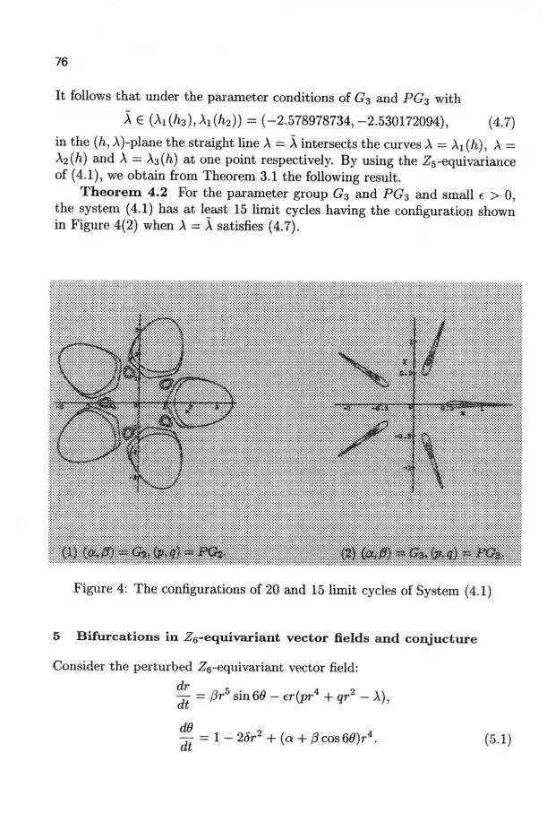
76

It follows that under the parameter conditions of G3 and PG3 with

A € (Xi(h3), Ai(/»2)) = (-2.578978734, -2.530172094), (4.7)

in the (h, A)-plane the straight line A = A intersects the curves A = Ai(ft), A = X2(h) and A = X3(h) at one point respectively. By using the Z5-equivariance of (4.1), we obtain from Theorem 3.1 the following result.

T h e o r e m 4.2 For the parameter group G3 and PG3 and small e > 0, the system (4.1) has at least 15 limit cycles having the configuration shown in Figure 4(2) when A = A satisfies (4.7).

Figure 4: The configurations of 20 and 15 limit cycles of System (4.1)

5 Bifurcations in Z6-equivariant vector fields and conjucture

Consider the perturbed Z6-equivariant vector field:

dr

n d0 dt

= /3r5 sin 68 - er(pr4 + qr2 - A),

= 1 - 28r2 + (a + @cos6d)r4. (5.1)

77

Corresponding to (5.1), the function F(x,y) in the divergence of vector field of the hypothesis (A3) in Section 3 has the same form as (4.2). We discuss the case d = {a, ft) = (1.4,0.25). Under this parameter condition group, we have

H{zi,0) < H(z2,0) < H{z3,n/6) < 0 < H{z4,n/6), i.e, h1<h2<h3<0< h4, (5-2)

where H(x,y) is defined by (2.6). Prom (5.2) we see that as h increases from —oo to h4 the schemes of ovals of the sextic algebraic curves defined by H(r,9) = h will be varied and there exist five types of period annuluses {TQ} - { r j } of (2.5). We define 5 detection functions A,(/i),i = 0 - 4 similar to (4.4). By taking PG4 = (p,q) = (1, -3.376113233), we have the following values of bifurcation parameters and bifurcation direction detections (in detail, see[18]):

Ao(0) = 0, Ao(/i3) = -1.207972277;

Ai(hi) = -2.990330089, Ax(/i2) = -2.96704993, maa;(Ai(/i)) « -2.97;

\2(h2) = -2.51962967, X2(h3) = -2.4842287;

\3(h3) = -2.96604993, A3(/i4) = -2.31457964, min{\3{h)) « -2.967;

\Ah2) = -2.564531384, max(Xi(h) « -2.5779, lim A4(/i) = +00; h—> — 00

And

cr0 > 0 , o-i > 0 , a2(z2,0) > 0 ,

0-2(2:3,77/6) > 0, 0-3 < 0, cr4 > 0.

78

Figure 5: Graphs of detection curves of (5.1) with parameters G4 and GP4

The above information follows that under the parameter conditions of G4

and PG4, the system (5.1) has the graphs of detection curves shown as Figure 5. We see from Figure 5 that when

A € (Ai(ft2), A3(ft3)) = (-2.96704993, -2.96604993), (5.3)

in the (ft, A)-plane the straight line A = A intersects the curves A = Ai(ft), A = A3(ft) at two points respectively. By using the Z6-equivariance of (5.1), we obtain from Theorem 3.1 the following result.

Theorem 5.1 For the parameter group G4 and PG4 and small e > 0, when A = A satisfies (5.3), the system (5.1) has at least 24 limit cycles having the configuration shown in Figure 6. Thus, we have H(5) > 24 = 52 - 1.

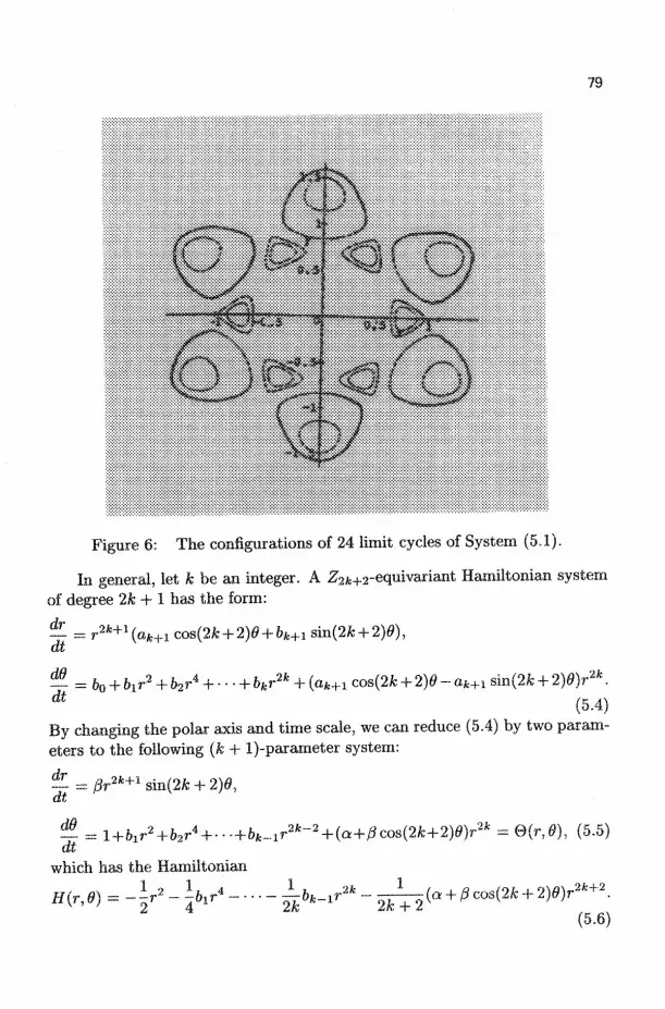
79

Figure 6: The configurations of 24 limit cycles of System (5.1).

In general, let k be an integer. A Z2fc+2-equivariant Hamiltonian system of degree 2k + 1 has the form:

— = r2k+1(ak+1 cos(2k + 2)0 + bk+1 sin(2fc + 2)6>), dt

m di

: 6() + 5 i r2 + 52r4 + . . . + bkr2k + (o*+i cos(2fc + 2)6 - ak+1 sin(2& + 2)0)r2*.

(5.4) By changing the polar axis and time scale, we can reduce (5.4) by two param­eters to the following (k + l)-parameter system:

* = @r2k+lsm(2k + 2)0,

dt

— = l + 61r2+62r4 + ---+6^.ir2 f c"2 + (a+/3co8(2fc+2)^)r2* = 0(r ,0) , (5.5) dt

which has the Hamiltonian 1

ffM) = ^ i r 2- i 6 l r4 _ 6 f c _ i r « _ _ _ ^ (a + /3cos(2fc + 2)0)r2*+2.

(5.6)

80

Suppose that a > ft > 0 and the algebraic equation

(a + p)r2k + bk^r2k-2 + ••• + b2rA + bxr

2 + 1 = 0 (5.7)

and

(a - p)r2k + bk-.ir2k-2 + ••• + b2r

i + hr2 + 1 = 0 (5.8)

have respectively k different positive roots, i.e., in the polar axis 6 = 0 and 6 = ir/(2k + 2), the system (5.5) has repectively k singular points at

(Z!,0), ( z 2 ) 0 ) , • • • , (zk,0), (zk+1,7r/(2k+2)), (zk+2,7r/(2k+2)), ••• , (z2k,7v/(2k+2)).

By the Z2fc+2-equivariance, there exist (2fc + l ) 2 singular points of (5.5). Thus, we can choose a parameter group, such that the system (5.5) has k different period annuluses with Z2Jt+2-equivariant symmetry. In other words, there are k(2k + 2) + 1 centers of (5.5). We next consider the perturbed system

%- = pr2k+1 sin(2fc + 2)9 - r(Plr2k + p2r

2k~2 + ••• +pkr2 - A),

at

^ = 1 + bxr2 + 62r4 + • • • + bk-ir

2k-2 + (a + /3cos(2k + 2)6)r2k. (5.9) at

It is similar to the discussion for the system (5.1). By controlling the perturbed parameters pi,i = 1 — k, such that enclosing every centers (except the origin), there exist two limit cycles created by homoclinic or heteroclinic bifurcations. Therefore, we may obtain 2A;(2fc + 2) = (2k +1)2 — 1 limit cycles of the system (5.9). It means that the conjecture: H(2k + 1) > (2k + l ) 2 - 1 holds.

Acknowledgement The research work is supported by the strategic re­search grant No. 7000934 from the City University of Hong Kong.

Appendix: Ratio Between Double Integrals and Areas: the val­ues of Jij(hs).

For the fixed unperturbed parameter group G2 = (a, /?) = (—7,-0.95), we obtain the values of Jij (hs) by numerical integration to four digits accuracy after the decimal point as follows:

J01(h2) = 0.2149252727, J02(h2) = 0.3988931137;

Jn(/ i2) = 44.17632564, Jl2(h2) = 5.954572388;

J21(h2) = 39.28523855, J22(h2) = 5.33645488;

J21(h3) = 35.92519738, J22(h3) = 4.994696597;

Jsiih) = 3.259211417, J32(h3) = 1.74133613;

81

Ju(h3) = 34.2517894, Ji2(h3) = 4.828033959.

For the fixed unperturbed parameter group G3 = (a,/?) = (0.2992021277,2.680851063), we have the values of Jij(hs) by numerical inte­gration to four digits accuracy after the decimal point as follows:

Joi{hi) = 0.002025353778, J02(/i4) = 0.03858233638;

Jn(h3) = 0.3790647646, Ju(h3) = 0.6007796831;

J2i(h3) = 2.109516141, J22(h3) = 1.440046333;

J31{h4) = 0.5477732675, J32(/i4) = 0.5445506974;

J 4 i ( M = 0.4389746838, Ji2{K) = 0.4436824416.

References

1. M.L. Abell and J.P. Braselton, Maple V: by Example, AP Professional, Boston, 1994.

2. V.I. Arnold, Geometric Methods in Theory of Ordinary Differential Equa­tions, Springer-Verlag, New York, 1983.

3. J. Carr, S.N. Chow and J.K. Hale, Abelian integrals and bifurcation theory, Journal of Differential Equations 59, 413-417 (1985).

4. H.S.Y. Chan, K.W. Chung and Dongwen Qi, Some bifurcation diagrams for limit cycles of quadratic differential systems, Int. J. Bifurcation and Chaos 11, 197-206 (2001).

5. H.S.Y. Chan, K.W. Chung and Jibin Li, Bifurcations of limit cycles in a Z3-equivariant planar vector field of degree 5, Int. J. Bifurcation and Chaos 11, 2287-2298 (2001).

6. C.J.Christopher and N.G. Lloyd, Polynomial systems: lower bound for the Hilbert numbers, Proc. Royal Soc. London Ser. A 450, 219-224 (1995).

7. G.B. Dantzig, Linear Programming and Extensions, Princeton University Press, Princeton, N.J., 1963.

8. M. Farkas, Periodic Motion, Springer-Verlag, New York, 1994. 9. J. Guckenheimer and P. Holmes, Nonlinear Oscillations, Dynamical Sys­

tems, and Bifurcations of Vector Fields, Springer-Verlag, New York, 1983. 10. D.A. Gudkov, The topology of real projective algebraic varieties, Russian

Math. Surveys 29, 4:1-79 (1974).

82

11. D. Hilbert, Mathematical problems, In Proceeding of Symposia in Pure Mathematics 28, 1-34 (1976).

12. Yu. Ilyashenko, Finiteness Theorem for Limit Cycles, American Mathe­matical Society, Providence, RI, 1991.

13. Li Jibin and Li Cunfu, Planar cubic Hamiltonian systems and distribution of limit cycles of (E3), Acta. Math.Sinica 28, 4:509-521 (1985).

14. Li Jibin and Huang Qimin, Bifurcations of limit cycles forming compound eyes in the cubic system, Chinese Ann. of Math. 8B, 391-403 (1987).

15. J. Li and Liu Zhengrong, Bifurcation set and compound eyes in a per­turbed cubic Hamiltonian system, in Ordinary and Delay Differential Equations,ir (Pitman Research Notes in Math. Series 272, Longman, England, 116-128, 1992).

16. J. Li and Zhao Xiaohua, Rotation symmetry groups of planar Hamilto­nian systems, Ann. of Diff. Eqs. 5, 25-33 (1989).

17. J. Li and Liu Zhenrong, Bifurcation set and limit cycles forming com­pound eyes in a perturbed Hamiltonian system, Publications Mathma-tiques 35, 487-506 (1991, Spain).

18. J. Li, H.S.Y. Chan and K.W. Chung, Bifurcations of limit cycles in a Z6-equivariant planar vector field of degree 5, to appear.

19. J. Li, H.S.Y.Chan and K.W.Chung, Investigations of bifurcations of limit cycles in a Z2-equivariant planar vector field of degree 5, Int. J. Bifur­cation and Chaos, to appear.

20. N.G. Lloyd, Limit cycles of polynomial systems, in New Directions in Dynamical Systems, T. Bedford and J. Swift, eds. 40, (London Mathe­matical Society Lecture Notes, 192-234, 1988).

21. Luo Dingjun, Wang Xian, Zhu Deming and Han Mouan, Bifurcation Theory and Methods of Dynamical Systems, (World Scientific, Singapore, 1997).

22. N.T. Otrokov, On the number of limit cycles of a differential equation in a neighbourhood of a singular point (in Russian), Mat. Sb. 34, 127-144 (1955).

23. L.M. Perko, Differential Equations and Dynamical Systems, Springer-Verlag, New York, 1991.

24. L.M. Perko, Limit cycles of quadratic systems in the plane, Rocky Moun­tain Journal of Math. 14, 619-645 (1984).

25. V.A. Rokhlin, Complex topological characteristics of real algebraic curves, Russian Math. Surveys 33, 85-98 (1978).

26. S. Smale, Mathematical problems for the next century, The Mathematical Intelligencer 20, 2:7-15 (1998).

27. O.Ya. Viro, Progress in topology of real algebraic varieties over the last

83

six years, Usp. Mat. Nauk. 41, 3:45-67 (1986). 28. G. Wilson, Hilbert's sixteenth problem, Topology 17, 53-73 (1978). 29. Ye Yanqian, Theory of Limit Cycles, Transl. Math. Monographs 66

(Amer. Math.Soc, Providence, RI, 1986). 30. Ye Yanqian, Qualitative Theory of Polynomial Differential Systems,

(Modern Mathematics Series, Shanghai Scientific and Technical Publish­ers, Shanghai, 1995) (in Chinese).

31. Zhang Zhifeng, Ding Tongren, Huang Wenzao and Dong Zhenxi, Quali­tative Theory of Differential Equations, Transl. Math. Monographs 101. (Amer. Math.Soc, Providence, RI, 1992).

85

SYSTEMS OF INEQUALITIES A N D THE STABILITY OF DECISION MACHINES

JEAN-PIERRE DEDIEU MIP, Departement de Mathematique, Universite Paul Sabatier, 31077 Toulouse

Cedex 4- France E-mail: dedieu6@mip.ups-tlse.fr

1 Introduction

In their 1989 paper, Lenore Blum, Mike Shub and Steve Smale introduced a model of computation over the real numbers in order to "[give] a foundation to the theory of modern scientific computation, where most of the algorithms ... are real number algorithms." Real number computations are described by machines over the real numbers. A finite dimensional machine over the real numbers consists of a finite directed connected graph with four types of nodes: an input node, the input is a vector x £ R™, computation nodes where real polynomials or rational fractions f(x) are computed, branching nodes defined by polynomial inequalities f{x) > 0, and an output node. This model of computation is called the BSS model. It is described in 5 or in 4 .

In real life computations we do not use real numbers but floating point numbers and a finite precision arithmetic. For this reason we do not com­pute exactly the quantities appearing in our theoretical machine but only approximations. In other words we have two machines: a theoretical ma­chine designed over the real numbers and an approximate machine, designed similarly, which uses floating point numbers and a finite precision arithmetic.

On a certain input x € R™, due to the presence of branching nodes, these two machines may have a different behaviour: to the question "is f(x) > 0" the answer may be "yes" in the exact machine and "no" in the approximate machine. In such a case the computation paths and the outputs may be completely different. This is a typical example of instability introduced by floating point numbers and a finite precision arithmetic.

In this paper we consider decision machines i.e. machines where the output is yes or no. To analyse the stability of such machines we adopt a backward analysis viewpoint. We show that, under a certain hypothesis, the decision taken on a; £ Rra by the approximate machine is identical to the decision taken by the exact machine on a nearby input y € R n .

Since the computation path on input x is described by the answers at the

86

branching nodes, our starting point is a system of inequalities

fi(x) > 0, 1 < i < m,

where fi : R™ -» R is a polynomial or, more generally, an analytic function. To a vector a £ R m we associate its positive part a+ and its negative part

a~. The i-th coordinate of a+ (resp. a~) is a (resp. 0) when a; is nonnegative and 0 (resp. — a*) otherwise so that, as for real numbers, a = a+ — a". In our context we use | | / (z)~ | | to measure the deviation of the vector f{x) from positivity.

To begin we show that when ||/(a:)~|| is small enough, there exists a certain y £ R™ close to x such that the system of inequalities is satisfied exactly at y:

fi(y) > 0, 1 < i < m

and we give an estimate for the distance of y from x in terms of | |/(x) us denote by a the sum of the following series:

I. Let

k=0 v '

1

= 1.63284

To an analytic map / : R" —> RTO and to a; 6 following numbers:

T(/, x) = sup k>2

Dkf(x) k\

1

and

6(f, x) = (Df(x)Df(x)* + 4 Diag (/(*)+)) - l

We also let 6(f,x) = oo when the matrix Df(x)Df(x)* + 4Diag(/(a;)+) is singular. Here A* denotes the adjoint of the matrix A, \\ \\ is the operator norm associated with the usual Euclidean norms in Rn and Rm and Diag (d) is the diagonal matrix with diagonal entries di,d2,... Notice that T(f,x) is always finite because / is analytic. Theorem 1. Let x G R™ be such that

\\f(x)~\\ < -" n ' " - 8(1+ T(/, *))*(/, a;) max(l, <*(/,*))'

Then the set f-° = {x € R n : f(x) > 0} is nonempty and

DiSt(xJ^°)<a6(f,x)\\f(x)-\\.

87

When f is a polynomial system with Degree ft < 2 this result holds when

U{X) ll-4(2 + \\D*f(x)\\)5(f,x)i-

In the following we consider the case of inequalities and strict inequalities. Like in Theorem 1 we assume | | / ( x ) - | | small enough so that f(y) > 0 for a certain y close to x. Let us assume that fi(x) > 0 for each i in a certain set J C { 1 , . . - , m}. If the quantities fi(x), i € J , are far enough from 0 we show that these strict inequalities are also valid at y. Theorem 2. Let x G R n be such that

l l / ( a ° " - 8 (1+ r(/,a:))<J(/,x)maX(l ) « ( / , ! ) ) •

Let us also suppose that

fi(x)>(aS(f,x)\\f(x)-\\)2

for each i in a certain set J C { 1 , - . . ,m}. Then there exists y G / - ° such that

fi(y) > 0 for each i G J

and

\\x-y\\<ad(f,x)\\f(x)-\\.

The following corollary is another formulation of these theorems. We introduce here a computation error e. In an exact machine we branch on the inequality fi(x) > 0 while in the approximate machine we have to take into account computation errors: we branch on fi(x) + e» > 0. Corollary 3. Let x G R" and e G R m be given. Let us denote e< 0 the vector in R m with i—th component equal to €i when fi(x) < 0 and 0 otherwise. When the three following conditions are satisfied

• fi(x) + ei > 0 for each i = 1 . . .p,

• fi(x) > (<r5(f,2:)||e<0||)2 for each i=p+l...m,

. ||e<°|| < 1/(8(1 + r(f,x))6(f,x)max(l,8(f,x))),

then, there exists y G R" such that

• fi(y) ^ 0 for each i = 1 . . .p,

• fi(y) > 0 for each i = p + 1 . . . m,

• lk-y||<aJ(/>a:)||C<0 | | .

88

2 A word about the proofs

To prove these theorems we use a powerful argument based on Smale's alpha-theory. We associate to the system of inequalities f(y) > 0 the underdeter-mined system

Fi{y,t) = fi{y)-t1, \<%<m,

which is a system of m equations i n r a + n unknowns: (y,t) € R™ x RTO. We see easily that F(y,t) = 0 implies f(y) > 0. To prove the existence of a zero (y,t) for F with y close to x we show that Newton's sequence (xk+i,tk+i) = NF(xk,tk) starting at (xQ,t0) - (x,^/f{x)+) is converging. Its limit is a zero for F. This process is interesting because it provides a very efficient way to compute y.

Such a method has already been used by F. Cucker and S. Smale in 9 where the authors study the complexity of the feasibility of a system of polynomial equalities and inequalities in n variables.

Newton's method for underdetermined systems of equations was intro­duced for the first time in 1966 by Ben-Israel 3 . This iteration is defined by

NF(z) = z - DF{zj*F{z), zk+1 = NF(zk),

where ZQ is given. We denote here by DF(z)^ the Moore-Penrose inverse of the derivative DF(z). When DF{z) is onto and more generally for a surjective linear operator L between two Euclidean spaces, its Moore-Penrose inverse ie given by Lt = L*{LL*)~l with L* the adjoint of L.

To prove the convergence of the sequence (xk+i,tk+i) = NF(xk,tk) we use a theorem due to M. Shub and S. Smale 1996 19 .

Let F : E —>• F be an analytic function between two Euclidean spaces. We suppose here that dim E > dim F . To F and a given z £ E we associate the three following numbers:

a(F,z) = /3(F,z)7(F,z),

P(F,z) = \\DF(z)^F(z)l

7(F, z) = sup fc>2

Theorem 4. There is a universal constant ao, approximately 1/7, with the following property. For any z0 e ~E with a(F, z0) < a0, all the Newton iterates

Zk+l — Zk - DF(zk?F(zk), k > 0,

Dm<?$*

89

are defined, converge to £ £ E with F(Q = 0 and for all k > 0

lkfc+i -.Zfcll < ( 2 ) ^Zl ~ • 2 ° " '

/n particular

\\<-zo\\<<rP(F,zo).

3 Comments and similar results

The material contained in this paper is taken from Cucker-Dedieu 1998 8 and from Dedieu 2000 10. In the first paper the authors study the behaviour of round-off decision machines. This talk is inspirated by these ideas. Decision problems and round-off computations are also considered by Cucker and Smale 1999 9 where the authors design robust algorithms to solve decision problems.

The main ingredient to study such problems is given by the relation be­tween the number | | /(a;)_ | | and the distance to the feasible set f-°. Classical results relate these two quantities.

First of all, Hoffman's Theorem, published in 1952 13, and reconsidered by Giiler, Hoffman and Rothblum in 1995 n . Hoffman considers linear in­equalities: Theorem 5. (Hoffman) Let A £ R r n X n . Then there exists a scalar K{A), such that for each b £ R m for which the set A-b = {x' £ R™ : Ax' < b} is not empty and for each x € R"

Dist (x, A^b) < K(A)\\(Ax - 6)+||.

There have been a number of generalizations of Hoffman's Theorem to nonlinear cases. A first class of results uses a convexity assumption and is proved via convex analysis: Robinson 1975 18, Mangasarian 1985 17, Auslender and Crouzeix 1988 1 . A recent paper in these directions is "Error Bounds for Convex Inequality Systems" by Lewis and Pang 1998 15.

Let / : R n —> R U {oo} be an extended-valued closed proper convex function and S the closed convex set defined by f(x) < 0. We denote by f'(x, d) the directional derivative of / at x along a direction d and by N{x, S) the normal cone of S at a vector x £ >S. With these notations Lewis and Pang prove the following: Theorem 6. (Lewis-Pang) The following statements are equivalent:

• Dist (x,S) < jf(x)+ for any x € R n ,

90

• For any x 6 / 1(0) and d £ Af(x,S)

/ ' ( x , d ) > 7 - 1 | | d | | .

Another generalization of Hoffman's Theorem to a nonlinear and noncon-vex case may be obtained via Lojasiewiecz's Inequality. This result was proved for the first time by Lojasiewiecz 1964 16 for semianalytic or semialgebraic sets and functions and then extended to the subanalytic case by Hironaka 1973 12. A good expose of such questions is contained in Bierstone-Milman 1988 6. Theo rem 7. (Lojasiewiecz) Let K be a compact and subanalytic set contained in R n . Let f : K -> R™ be a continuous subanalytic function. There exist a > 0 and an integer N > 0 such that for all x € K,

a D i s t O c / ^ T ^ I I / ^ r i l -

Hoffman's Theorem has also been extended by Ioffe (1979) 14 to locally Lipschitz functions using Clarke's subgradient, and more recently by Aze, Corvellec and Lucchetti (1999) 2 who consider the case of lower semicontin-uous functions defined over Banach spaces. Let us recall the definition of Clarke's subgradient 7 . Prom Rademacher's Theorem, a function which is Lipschitz on an open subset of R™ is differentiable almost everywhere on that subset. Based on this result, the generalized gradient at x, denoted dg(x) has the following characterization: for any set S of measure zero

dg(x) = co{ lim \7g(xi) | g is differentiable at X%, X} ^t <^, Xi 7 Xj i—>oo

where co denotes the convex hull. Theo rem 8. (Ioffe) Let given f : R™ —> R m locally Lipschitz, x e R n with f(x) > 0 and e > 0. Let us define c = min \\y*\\ where the minimum is taken for \\y - x\\ < e with y £ f^° and y* € <9||/"||(y). Then

c D i 8 t ( y , / ^ ° ) < | | / ( y ) - | |

for any y with Dist (y, f-°) < e/2.

References

1. AUSLENDER A. AND J . -P. CROUZEIX, Global Regularity Theorems, Math. Oper. Res., 13 (1988) 243-253.

2. AZE D., J.-N. CORVELLEC AND R. F. LUCCHETTI, Variational Pairs and Applications to Stability in Nonsmooth Analysis, (1999) Preprint.

91

3. BEN-ISRAEL A., A Newton-Raphson Method for the Solution of Systems of Equations, J. Math. Anal. Appl. 15 (1966) 243-252.

4. BLUM, L., F . CUCKER, M. SHUB, S. SMALE , Complexity and Real Computation, (1998) Springer Verlag.

5. BLUM, L., M. SHUB, S. SMALE , On a Theory of Computation and Complexity over the Real Numbers; NP Completeness, Recursive Func­tions and Universal Machines, Bull. Amer. Math. Soc. (New Series) Vol. 21 (1989) 1-46.

6. BiERSTONE E. AND P . MILMAN, Semianalytic and Subanalytic sets, IHES Pub. Math. 67 (1988) 5-42.

7. CLARKE F . Optimization and nonsmooth analysis, J. Wiley and Sons. New York. 1983.

8. CUCKER, F . AND J . -P. DEDIEU, Decision Problems and Round-Off Ma­chines, to appear in: Theory of Computing Systems, 2001.

9. CUCKER, F . AND S. SMALE, Complexity Estimates Depending on Con­dition and Round-off Error, Journal of the ACM, 46 (1999) 113-184.

10. DEDIEU, J . -P. , Approximate Solutions of Analytic Inequality Systems, SIAM Opt., to appear.

11. GULER, O., A. HOFFMAN, U. ROTHBLUM, On Approximations to So­lutions to Systems of Linear Inequalities, SIAM J. Matrix Anal. Appl., 16 (1995) 688-696.

12. HiRONAKA H., Introduction to Real-Analytic Sets and Real-Analytic Maps, Preprint, Pisa (1973).

13. HOFFMAN, A., On Approximate Solutions of Systems of Linear Inequal­ities, J. Res. Nat. Bur. Stand., 49 (1952) 263-265.

14. IOFFE A., Regular points of Lipschitz functions, Trans, of the Amer. Math. Soc. 251 (1979) 61-69.

15. LEWIS, A. AND J.-S. PANG, Error Bounds for Convex Inequality Sys­tems, in: J.-P. Crouzeix, J.-E. Martinez-Legaz and M. Voile (eds), Gen­eralized Convexity, Generalized Monotonicity, Kluwer (1998) 75-110.

16. LOJASIEWICZ S., Ensembles Semi-Analytiques., IHES Mimeographed Notes (1964).

17. MANGASARIAN O., A Condition Number for Differentiable Convex In­equalities, Math. Oper. Res., 10 (1985) 175-179.

18. ROBINSON S., An Application of Error Bounds for Convex Programming in Linear Spaces, SIAM Journal of Control and Opt. 13 (1975) 271-273.

19. SHUB, M. AND S. SMALE, Complexity of Bezout's Theorem IV: Proba­bility of Success, Extensions, SIAM J. Numer. Anal., 33 (1996) 128-148.

93

RECONCILIATION OF VARIOUS COMPLEXITY A N D CONDITION MEASURES FOR LINEAR PROGRAMMING

PROBLEMS A N D A GENERALIZATION OF TARDOS' THEOREM

JACKIE C. K. HO Ph.D. student, Department of Combinatorics and Optimization, Faculty of

Mathematics, University of Waterloo, Waterloo, Ontario N2L 3G1, Canada.

L E V E N T T U N Q E L

Department of Combinatorics and Optimization, Faculty of Mathematics, University of Waterloo, Waterloo, Ontario N2L 3G1, Canada

First, we review and clarify the relationships amongst various complexity and con­dition measures for linear programming problems. Then, we generalize Tardos' Theorem for linear programming problems with integer data to linear program­ming problems with real number data. Our generalization, in contrast to the only previous such generalization due to Vavasis and Ye, shows that many conventional, polynomial-time (in the sense of the Turing Machine Model, with integer data) primal-dual interior-point algorithms can be adapted in a Tardos' like scheme, to solve linear programming problems with real number data in time polynomial in the dimensions of the coefficient matrix and the logarithms of certain measures of the coefficient matrix (independent of the objective function and the right-hand-side vectors).

Keywords: linear programming, computational complexity, complexity mea­sures, interior-point methods AMS Subject Classification: 90C05, 90C60, 49K40, 90C31, 90C51

1 Introduction

Let A e Emx™, b e E m , and c e W1. In this paper, one of our main concerns is the computational complexity of solving linear programming (LP) prob­lems with data (A, b, c) in a way that the number of arithmetic operations is bounded by polynomial functions determined only by A.

For t £ M_|_, poly(i) denotes a polynomial function of t. For a £ Z, we define

size(a) := [log (|a| + 1)] + 1;

94

for A G Z m x n ,

size(A) := yjsize(af/).

When A G Z m x n , b G Z m , c £ Z", Tardos 22 proved that the existence of an algorithm for LP which performs only polynomially many elementary arithmetic operations in size(A, b, c) implies the existence of an algorithm for LP which performs only poly(size(A)) elementary arithmetic operations. (Her results also apply in the more general case A £ Qmx™; b G Q™, c G <QP, also see 23 for network flow problems.)

Tardos' proof is constructive in the sense that it shows how to use any polynomial time algorithm for LP as a subroutine to achieve the goal of solving LP problems in poly(size(A)) time complexity. However, the proof requires calling the subroutine (the LP solver with poly(size(A,b,c)) time complexity), polynomially many times using modi­fied data so that the sizes of the modified LP instances can be bounded by poly(size(A)).

Later Vavasis and Ye 29, in another seminal paper (with many new in­sights), proposed a new kind of interior-point algorithm and proved that their algorithm can solve LP problems with data A € E m x n , b € E m , c € E n , in O (n 3 5 (logx(A) + log(n)) loglogx(^l)) interior-point iterations. Also, see Adler and Beling's 1 paper which is more specialized than the Vavasis-Ye pa­per since it is concerned with the polynomial-time LP algorithms over the algebraic numbers. When specialized to integer (or rational) data, Vavasis-Ye result gives another proof of Tardos' theorem (using xG4) = 20(-slze(-A^—see Section 2). So, in this sense, Vavasis-Ye result generalizes Tardos' theorem to LP problems with data A £ E m x n , b G l m , c G Kn. Vavasis-Ye proof is even "more constructive" in the sense that their algorithm is a specialized algorithm designed for such a purpose, and need not be called many times (except to guess an upper bound for x(^)—accounted for in the above quoted iteration bound by the loglogx(^4) term; also see 1 5 ) .

One advantage of Vavasis-Ye algorithm is that it has the potential of becoming a practical algorithm. However, theoretically speaking, Vavasis and Ye left open the question of whether conventional polynomial time interior-point algorithms (or perhaps some others) can be adapted in a scheme more directly related to Tardos' to solve the LP problems with data A G E m x " , b G E m , c £ 1 " in polynomially many elementary arithmetic operations where the polynomial bound depends only on the (properly defined) "size" of A e l m x " . In fact, Vavasis and Ye 29 state that "Tardos uses the assumption of integer data in a fairly central way: an

95

important tool in 22 is the operation of rounding down to the nearest integer. It is not clear how to generalize the rounding operation to noninteger data."

For example, let A £ Z m x n , c € Z". Then if d is an extreme ray of { i e Rn : Ax — 0,a; > 0} such that cTd < 0, then we know that there exists an integral extreme ray d in the above cone such that cTd < (—1). Of course, such arguments do not directly apply in general when the entries of A and c are real numbers. When A and c have only rational entries, the data can be multiplied by a large enough (but not too large) integer such that the new scaled data contain only integers. This again ensures a notion of a "unit" to round to, even after a normalization of the integral d such that J]?=i dj = 1, so that the arguments similar to the above still work (e.g., after such a normalization, cTd < — 1/A(A), where A(A) denotes the largest absolute value of a subdeterminant of A). In addition to this, a few other obstacles arise in an attempt to obtain such a generalization of Tardos' theorem and proof to the real number model.

In this paper, we overcome these obstacles, and generalize Tardos' theo­rem and a significant part of her proof to the case when A e E m x " , b € Rm, c £ W1. Our results also generalize Vavasis and Ye's result in the sense that in our scheme almost any polynomial time LP algorithm can be adapted, whereas their result uses a new, specialized algorithm.

Before we describe the generalization of Tardos' theorem, we review and clarify (with many new results) relationships amongst various complexity and condition measures such as x(^)> x(-^)i the condition number of (AAT) de­noted by K(AAT), Hoffman's bound (or the Lipschitz bound) for systems of linear inequalities, Ye's complexity measure for LP (also known as the small­est large variable bound), A (A) and the smallest nonzero absolute value of a subdeterminant of A, denoted 6(A). Special emphasis is put on establish­ing various fundamental properties of x> which becomes one of the central tools in the last section when we deal with generalization of Tardos' result. While our proof of the generalization of her theorem is very similar to hers, a key part of the proof which makes it work in the real number case, is the generalization of the rounding operation to noninteger data (in the sense of choosing an appropriate "unit" for the data at hand). For this, we rely heav­ily on those fundamental properties of \ mentioned above. We first perform our analysis on deciding the feasibility of a system of inequalities, and then use the resulting algorithm as a subroutine to solve the whole primal-dual LP problem. In both cases, we solve the original problem by solving a sequence of polynomially many "nicer" or smaller LP problems, each of which has in­tegral right hand side vector (and cost vector, in the latter case) whose size is bounded by a polynomial function of our complexity measures. This is one of

96

the fundamental tools for eliminating the dependence on b and c in the overall complexity bound of the algorithms. Solving these "nicer" LP problems gives us important information about the structure of the optimal solutions of the main LP problem in terms of the linear algebraic structures of the input data. For example, "there exists an optimal solution at which the jth inequality is tight" or "at all optimal solutions, the jth inequality is strictly satisfied." Such information helps us reduce the dimensions of the problem at hand; but, it also requires us to analyze the complexity measures for the subproblems.

The sizes of all the integers making up the right hand side and objective vectors of these "nicer" LP problems are bounded above by a polynomial function of n and the logarithm of ( S>A1 1. Many are also bounded by a

polynomial function of n and logx(A). As mentioned, we need to use an LP solver as a subroutine in our proof

of Tardos' theorem. While any polynomial time LP solver can be used, we describe a very useful formulation - the homogeneous self-dual form - in Section 5. The complexity of running an interior-point algorithm (with a certain termination rule) on such a form can be expressed in terms of Ye's complexity measure, which becomes convenient in our complexity analysis.

This paper is organized as follows. In Section 2, we review definitions and characterizations of some complexity measures which are relevant to our stated interest in this paper. We also present some new results in this sec­tion. Section 3 includes the Cauchy-Binet formula and an application of it to obtain a bound on the condition number of (AAT). In Section 4, we discuss Hoffman's Theorem and relate the Hoffman constant to x(^4)- In Section 5, we discuss Ye's complexity measure for LP problems and relate it to the Hoff­man constant. Also in Section 5, we show that the number of iterations of many primal-dual interior-point algorithms to solve LP problems with data (A, b, c), with arbitrary A and special b and c, can be bounded by a polyno­mial function of n and logarithms of certain complexity measures. We review a sensitivity bound result of Cook, Gerards, Schrijver, Tardos 3 in Section 6 and establish various variants of it based on the complexity measures x(A) and x(^4). Section 7 contains our main result - a generalization of Tardos' Theorem - based on the results obtained in the preceding sections. We con­clude with a very brief discussion of the special cases when A is integral and totally unimodular.

97

2 Complexity and Condition Measures: x a n d X

We denote by Af(A), the null-space of A; K(A) denotes the range (or column-space) of A. We assume A ^ 0, n > m > 3. Recall the definitions:

\\A\\P := max ||-Aar||p, for 1 < p < oo, llz||»=i

F •= \ 4=1 j=l

It is not hard to show that m

11 11!= max £>«l> (1) i<i<n"

2 = 1

ll^lloo = max £ 1 ^ 1 . (2)

We have the following well-known matrix norm inequalities:

I H h < \\A\\F < Vn||A||2, (3)

4 = P l l o o < P | | 2 < V ^ M H o o , (4)

4=Pl l i < Plb < v^Plli, (5)

We also have the submultiplicative property for p-norms, 1 < p < 00. For all A e E m x " , C G M"x?, we have

| |^C| | P < ||A||P||C7||P. (6)

For the rest of the paper, the 2-norm is assumed when norms are mentioned, unless stated otherwise.

We assume throughout this section that A has full row rank. Define

X(A) := sap{\\AT(ADAT)-1AD\\ -.DeV},

where V is the set of all positive definite n x n diagonal matrices. Note that X.(RA) = x(A) for all nonsingular R € E m x m . In fact, x(A) depends only on the pair of orthogonal subspaces, M(A) and 1Z(AT). So, it can be defined on subspaces instead. Note that for all D € T>,

\\AT\\ = \\AT(ADAT)-1ADAT\\ < \\AT(ADATylAD\\ • \\AT\\.

98

Hence \\AT{ADAT)-lAD\\ > 1, and thus \{A) > 1. Similarly we define

X(A) := sup{||(AD.4T)-1.4D|| : D g D}.

Note that both x(A) and x (^ ) a r e finite. Also,

mT(A JDAT)-1A£)| | < \\AT\\ • \\{ADAT)-1AD\\,

\\{ADAT)-XAD\\ < \\{AAT)'lA\\ • \\AT(ADAT)-lAD\\.

Therefore, we have

P j j X ^ ) < X(A) < \\(AAT)-iA\\x(A) = A / , 8 ( ^ |) ^ ( A ) , (7)

where K(R) := \\R\\ • | | i?_ 1 | | , the condition number of R, for any nonsingular matrix R. Note that if m = n, then K{AAT) = \\A\\2 • WA^W2 = (\\A\\x(A))2.

An equivalent way to define these parameters is in terms of weighted least squares:

f II ATy || x(A) = sup < —r—r— : y minimizes || D1'2(ATy — c) ||

I l | c | |

for some c € Rn,D €T>\,

x(A) = sup -J |LO- : y minimizes || D1^2(ATy - c) \\ U l c l l

for some cG W,D &v\.

Let us define, for 1 < a,/? < oo,

pa,p(A) : = i n f { | | z - y\\$ : x G X,y eYa},

where X := {D£ : £ e Af(A),D G c\(V)},Ya := {7 : 7 G ft(,4T), | |7 | |« = 1}, and cl(D) denotes the closure of the set £>, that is, the set of nonnegative diagonal matrices. Note that pa,p(-) > 0. If we have || • \\p < c\\ • \\a, then Pa,s{') < c, as 0 G X. In particular, pa,a{-) < 1- Also note that the definition of pa<p(A) depends only on K{AT) and its orthogonal complement Af(A). Gonzaga and Lara 8 prove that when a = /? = 2, the subspaces M{A) and 1l(AT) can be interchanged in the definition of pa^(A). In the following, we denote /9QjQ simply by pa. We are mostly interested in p2, which we denote simply by p.

All vector p-norms are equivalent, that is, given a,ji such that 1 < a,/3 < oo, there exist positive ci,C2 such that ci|| • ||Q < || • \\p < C2II • | |a . This property also applies to pas'-

99

Proposition 2.1 Suppose 1 < a,/3,7,<5 < oo, and ci,c2 ,di,(i2 > 0 such that di\\ • \\a < II • ||<5 < d2\\ • ||a and ci| | • ||7 < || • ||/3 < c2|| • ||7. Then

Clrfl/9<5,7(-) < Pa,/3(-) < C 2 d 2 ^ , 7 ( - ) -

Proof Note that pgtp(A) = inf {||a; — y\\p : x € X, y € Y^} is attained, by say, a; and y. Let y* := j / / | | j / | | Q . Then y* £ Ya, and we have

Ps,p(A) = llx-2/11/3 V > ^-pa,M) = ±PaAA). a2 d2

By considering the infimum in pa^(A), similarly we have pa^(A) > dip$tp{A). Combining the above, we have dips,/3(A) < pa^{A) < d2Ps,p(A). By using cl|l • Ik < II " 11/3 < c2|| • H7. w e h a v e Cldi/9,5)7(-) < Pa,p(-) < C2d2p6n{-)- D

In particular, we have

~P(-) < Poc(-) < v M O - (8) y n

The following is a well-known fact.

Proposition 2.2 (Stewart 21)

X(A) = l/p(A).

A basis of A is a set of indices B C { 1 , . . . , n} such that \B\= m and the columns of As are linearly independent. We denote the set of all bases of A by B(A). Proposition 2.3 (Vavasis and Ye 29, Todd, Tuncel and Ye 2i)

x{A)=max{\\A-BlA\\:BeB{A)}.

Here, ">" is proven in 29 and "<" is proven in 24. It is known and not hard to show that an analogous characterization for x(A) also exists:

X(A)=max{\\Ag1\\:B€B(A)}. (9)

Using the above proposition, we prove that x cannot increase if any column is removed. Proposition 2.4 Suppose A is obtained by removing a column a 6 Em from Aemmxn. We have the following:

• //rank(A) = m, then x{A) < x(A).

100

• If iank(A) < m — 1, then let A be obtained by removing any dependent row from A. We have rank(^4) = m — 1 and x(A) = x(A).

Proof If rank(^4) = m, we have

x{A) = WAg1 A\\, for some basis B of A

< H^Ali^aHI = \\A^A\\ < X(A).

We used the fact that B is also a basis of A. Now, consider the case where rank(Ji) < m — 1. Without loss of generality, assume a is the last column of A. Then by row reduction, there exists a nonsingular G € R m x m such that

/ A' (1 GA = G[A\a]=\Jr\

for some A' £ K^"1-1'**"-1) having full row rank (hence, rank(A) = m — 1). Then

n{AT) = Tl(AT) = K((GA)T) = TZ{A,T),

and hence N(A) = M{A'). So, x(A) = x(A'). Now, since every basis of GA must include the last column,

'(A'z)-1 0\ ( A'0'

(A'zV'A'O' QT 1

X(GA) = , for some basis B of A'

= m a x { | | ( ^ ) - 1 ^ | | , l } < x ( ^ ) -

The proof of x{A') < x(GA) is similar. Therefore, we have

X(A) = x(A') = X(GA) = X(A).

•

Consider A € Q m x r a . Let L denote the total number of bits required to store A. We have the following. Proposition 2.5 (Vavasis and Ye 29) If Ae <QPxn, X{A) and x(A) are both bounded by 2°(L\

Khachiyan 14 proved that approximating x(A) within a factor of 2P0ly(™' is NP-hard. Similarly, approximating x(A) within a factor of 2 ? ° ^ ' " ' is also NP-hard2 5 .

The following observation is due to O'Leary 17. Naturally, for a £ E, sign(a) is either +,0, or — depending on the sign of a.

101

Proposition 2.6 (O'Leary 17) Considering J, 7, £ as the variables, we have

pa,0(A) = min \\-yj\\0

subject to sign(7j) = sign(^), j & J

IMU = 1, 7 € n(AT),

Consider the matrix:

Ac:=

i € M(A), J C { l , 2 , . . . , n } , J # 0 .

A 0

where C is an n x n invertible matrix. Obviously Ac also has full row rank. We have the following result.

Proposition 2.7 (Ho n)

X(AC) = y/2x(A).

Proof It is easy to see that

JV(^c) = { ( _ y : £ e J V ( A ) } and

We will prove that p(A) = y/2p(Ac) using the characterization of p in Propo­sition 2.6 with 7£(AT) and M(A) interchanged (which we can do since we are working with the 2-norms). Let us denote this minimization problem as Q{A).

1. p(A) > V2p(Ac) Let (£*,7*, J*) be an optimal solution of Q(A). We now define a y* that satisfies certain sign conditions. If j £ J*, let yj be such that sign(—£j) = sign(j/|). Therefore sign(^) ^ sign(7J' + y])- Now if j # J*, we can let y* be such that sign(-£*) = sign(j/}), and sign(£*) = sign(7* +y*), by ensuring |2/*| is small enough. Thus, the 3-tuple

is feasible for Q(i4c). Therefore, V2p(Ac) < ||f}*ll = P(A)-

102

2. p(A) < V2p(Ac) Let

•VJ'K y* ' '

be an optimal solution of Q(Ac)- Let

J := {j G { 1 , . . . ,n} : sign(£) 7 sign(7 ;)}.

Since £* is orthogonal to 7*, and £* ^ 0, there must exist j such that sign(^) ^ sign(7;). Hence J jt 0. The 3-tuple ( 7 2 ^ , 7 * , ^ ) is fea­sible for Q(A), and therefore p(A) < \/2||£}||- Now take any j € J . Since s ignup 7 s i g n ^ ) , there does not exist a yj which satisfies both sign(£?) = sign(7J' + yj) and s ign(-£p = sign(j/.,) at the same time. Hence, at least one of j or n 4- j is in J*. Therefore we have

-J=P(A) < \\Cj\\ < -c = P(AC).

D

Using a proof similar to the above or using Proposition 2.3, we easily prove the following fact. Proposition 2.8 (Ho n )

x([A\-A)) = V2x(A).

Recall that the singular values of A are the square roots of the eigen­values of the matrix ATA. The largest singular value of A is simply ||^4||2-Let Cmin(^l) denote the smallest nonzero singular value of A. We have the following connection to p(A). Proposition 2.9 (Stewart 21 and O'Leary 17) Let the columns ofUG R n x m form an orthonormal basis for 1Z(AT). Then

p(A) = min trmin (£//), 0#/C{l,...,n}

where Uj denotes the submatrix formed from a set I of rows of U.

First, Stewart proved "<", next O'Leary proved ">". A nonzero x € M(A) (with nonzero entries in positions {i\,... ,ip} C { 1 , . . . , n}) is said to define a minimal linear dependence amongst the columns of A if for every subset / of size at most (p - 1) of {i%,..., ip}, the columns of A indexed by J are linearly independent. We have the following proposition due to Vavasis.

103

Proposition 2.10 (Vavasis 2S) Let x G A/"(A) be a nonzero vector defining a minimal linear dependence amongst the columns of A. We have

Jrdn{\Xj\:Xj^0} >

m&x{\xj\ : Xj 7 0} —

We now give a new proof that is different from Vavasis'. Proof Let k and I be such that min{|:rj| : Xj ^ 0} = \xk\ = I. Let us denote the j th column of A as Aj, for all j e { 1 , . . . ,n}. Then there exists J C { 1 , . . . ,n}\{fc} such that AJXJ = ±lAk, where xj contains precisely the nonzero entries of x other than Xk- Since x defines a minimal linear dependence, the columns of Aj must be linearly independent. So we can extend J to a basis B of A to get ABXB = ±/Afc. Now,

IWloo = I M U < HZBII = i P i 1 Afc|| < IWA^AW < lx(A).

In other words,

or equivalently,

P(A)<

X(A) > ^

I mm{\xj\ : Xj ^ 0}

max{|a;j| : Xj ^ 0}

D

Using these arguments, it is not hard to show that the same result holds for any extreme ray x of the cone {x : Ax = 0, x > 0}.

Corollary 2.11 Suppose { d e l " : Ad = 0,eTd = \,d > 0} is not empty. Then, it is compact and every extreme point d of it has the property

wm{dj : dj ^ 0} > — • J n

Proof Compactness of the set is clear. Every extreme point corresponds to an ex­treme ray (and hence a basic feasible direction) of {x : Ax = 0,x > 0}. For every basic feasible direction x, we identify the smallest nonzero component Xk first, and then B € B{A) such that all other nonzero components of x are determined by the system of equations

ABxB = -xkAk.

104

Then, as in the proof of Proposition 2.10, we get ||x||oo < XkX(A)- Letting d :— x/(eTx), we see that

mm{dj : dj ? 0} > . ** , . > —±— = ^ - . w J r - xk [mX(A) + 1] - nX(A) n

We used the facts that n> (m + 1) and x(A) > 1. •

Recall that A(A) and 6(A) denote the maximum and minimum (re­spectively) of the absolute values of the determinants of all the nonsingular square submatrices of A. We have the following relationship among p00,A(A) and S(A), proven via exploitation of the sign pattern characterization and Cramer's Rule. Proposition 2.12 (Tungel 27)

6(A) Poo(A)> y '

mA(A)'

Proof Recall the definition

Poa(A) := va£{\\Dx - </||oo : D € c\(V), x € Af(A),y € K(AT), ||2/||oo = 1}-

Clearly here we can restrict x to be in {x G N(A) : ||x|| < 1}. Let {(Dk,xk,yk)} be a sequence of feasible solutions such that \\Dkxk — yk\\oo converges to poo(A). Since {xk} and {yk} are in compact feasible sets, we may assume {(xk,yk)} converges to, say, (x*,y*). Let J* be the set of indices such that the signs of x* and y* disagree. Note that J* ^ 0 because otherwise we can choose D € cl(Z>) such that Dx* —y* = 0, contradicting the fact that Poo(A) > 0. Note that for the pair (x*,y*), a best D* is such that

Dl = < 0, i E J*, 1, i$J*,xl=0,

So Poo(A) = ||j/}.||oo) a n d therefore

Poo(A) = min{||yj. ||TO : y £ TZ(AT), WyW^ = 1, sign(«/) = sign(y*)}.

Then it is easy to see that

j-r = maxflMloo : y € TZ(AT),sign(y) = sign(y*), \\yj.\U < 1} Poo(-tt-)

= max{||A rw||00 : sign(Arw) = sign(i/*), ||(ATt«)j.||oo < ! } •

105

Let w* be a maximizer of this expression,

e:=mm{\(ATwnJ\:(ATw*)j^0},

(ATw)j>e, ifsign(j/p = l, ^ . (Arw)j=0, if s ignup = 0

(ATw)j < - e , if s ignup F(sign(2/*),J*):=

Then

w

(ATw)j < 1, if je J*

> .

P°o{A) = max{||ATw||00 : w 6 F(sign(y*), J*)}

= max{a ru) : w G F(sign(j/*), J*)},

where a is a column of A (or its negation) such that aTw* = \\ATw\\00. Equivalently this is the optimal value of the LP:

(P) max Tj subject to weF(sign(y*),J*),

aTw — T) > 0.

Suppose the feasible region of (P) contains a line. So there exist (w,r)) and (d, t) ^ 0 such that w + kd € F(sign(y*), J*) and aT(w + kd) >rj + kt, for all fc6t So ATd = 0. If d ^ 0, then it contradicts that fact that A has full row rank. So d = 0 and t / 0. But then aTiu = a r (w + fcd) >rj + ht for all A; 6 E also gives a contradiction. So the feasible region of (F) is pointed, and hence contains an optimal basic feasible solution. Let /(e) be the vector representing the right-hand-side values in the definition of F(sign(y*), J*) (entries of /(e) are 0,1,e, —e). Then using Cramer's Rule, we have

M)

subdet T

a1

/(e)

0

subdet AT

ATJ. 0

< mA{A)

6(A) •

Here, we used that fact that e < 1; because 0 ^ \\(ATw*)j» otherwise, it would contradict Poo(A) > 0).

< 1 (as •

In fact, the above was originally stated for A € we have Poo(A) > l /(mA(A)).

j m X " in 27, in which case

106

Proposition 2.5 is a consequence of Proposition 2.12 and (8). Indeed,

P(A) PooiA) 5(A)

Therefore, for A £ Q"1 *",

log(x(^)) < log (jtff) + loS(m) + \ log(n) = O(L).

Directly utilizing equation (9) and Proposition 2.3, we also bound x a n d X in terms of A/5 in the following two propositions. Proposition 2.13

Proof Suppose B £ B(A) maximizes (9). Let y be such that ||y|| = 1 and H-A^H = H-A^yU. Let x £ Rm such that ABX — y. Then by Cramer's rule, for each i 6 { l , . . . , m } ,

So,

Therefore,

|det(AB) | -W,,1S(A) ~ v 5(A)

x(,4) = |lVll<™-5(A) D

Proposition 2.14

X(A) < y/m(n-m) + l ^ .

Proof Suppose B £ B(A) maximizes the expression in Proposition 2.3. Let {y1,.. .,yn~m} be the columns of A that are not in AB- Let xl £ Rm such that ABX1 = yl, for all / £ { 1 , . . . , n — m}. Then by Cramer's rule, for each i £ { l , . . . , m } ,

, jdet(C)| A(A) 1 il \det(AB)\ ~ 5(A)'

107

for some mxm submatrix C of A. So, denoting the maximum eigenvalue of a matrix by Amax(-), we have

HAWAII2 = \\[I\x\ • • \xn~m]\\2 = Amax[7 + z V ) T + •" • + xn~m(xn-m)T]

< 1 + {x1)Tx1 + ••• + {xn-mfxn-m

A(A)2 A(A)2

<l + m(n~m)^T<[m(n~m) + l } ^ T .

Therefore,

X(A) = \\A-BlA\\ < V

/ m ( n - m ) + l ^ . n

Facts similar to those given in last three propositions can also be obtained by employing the Cauchy-Binet Formula. This goes back at least to Dikin 4. (For a historical account and related results, see Forsgren 7 and the references therein.)

3 Cauchy-Binet Formula and the Condition Number of AAT

Recall that B(A) denotes the set of all bases of A. We represent each basis B of A as a m-subset of the set of numbers from the natural numbering of the columns of A. Proposition 3.1 (Cauchy-Binet Formula) Let A,Ae R m x n with full row rank. Then

d e t ( A i T ) = J2 d e t ( ^ B ) d e t ( i B ) . BeB(A)nB{A)

Using this, we can prove the following relationship among K, A and <5. Proposition 3.2 Suppose A G ]Rmxn ^ a s jun row ran]t Then

K{AAT)<m3/2nm+1^l.

Proof

We have \Aij\ < A (A) for all i,j, and hence by (3),

\\AAT\\ = \\A\\2 < \\A\\2F < mnA(A)2.

On the other hand,

• r w , , ^ / - n ^ ^ - i , , ^m^2A(AAT) | | ( A A T ) - 1 | | < % M | | ( A ^ ) - 1 | | o o <

det{AAT)

108

Now, by Proposition 3.1,

A(AAT) = d e t ( ^ / , t J 4 j j (for some sets I,J C{1,... ,m} , |J| = |J|)

Y^ det(AIt,B)det(Aj,tB)

nmA(A)2

< ( A ( ^ <

and det(;L4T) = EB&B(A) det(AB)2 > 5{A)2. Therefore,

r r M / . . T W | I m3/2nm+1A(A)4

K(AA1) = \\AA1\\-\\(AA1)-1\\< 5{AY

D

4 Hoffman's Bound and x

For a vector u 6 Mn, let pos(u) € K™ be such that (pos(u))j := max{ttj,0} for each j £ { l , . . . , n } . The following result gives an upper bound on the distance of a point to a polyhedron, in terms of its violation of the constraints defining the polyhedron. Theo rem 4.1 (Hoffman 12) Let A E ]Rmxn (not necessarily full row rank) and let \\ • \\a and \\ • \\p be norms on Rm and on K.", respectively. Then there exists a scalar Ka^(A), such that for every c € i " for which the set {y € W1 : ATy < c} ^ 0, and for every j / ' e l ™ ,

min \\y-y' \\a< KaS{A) || pos(ATy' - c) \\0 . y.ATy<c

The coefficient Ka^(A) is sometimes called a Lipschitz bound of A. For a norm || • || on K™, let || • ||* be the dual norm defined by

|| v ||*:= max{uTx : x G Rn , || x ||< 1},

for each v £ Kn. Note that for p-norms (1 < p < oo), we have || • ||* = || • ||9, where q is such that p~1 + q~x = 1. In particular, || • ||£ = || • Ife- Let ext(5) denote the set of extreme points of a set S. We have the following geometric representation of the Lipschitz bound.

Propos i t ion 4.2 (Giiler, Hoffman and Rothblum 9) Theorem 4-1 holds with Ka^{A) := max{|| v ||£: v € ext(Va(A))}, where Va(A) : = K 1 " : » > 0 , || Av \\*a< 1}.

109

We write K2(A) := K2t2(A) for all A. There is also a representation of the Lipschitz bound via singular values. For any E £ Rnxm. Let U(E) be the set of subsets of { 1 , . . . , n} for which the corresponding rows of E are linearly independent. Let U*(E) be the maximal elements in U(E). Proposition 4.3 (Giiler, Hoffman and Rothblum 9)

K2{A) < max TTrT-Jzu*(An am-m(Aj)

Note that minJ€U.(AT) amin(A^) = min0^jc{i,...,„} o-min(Aj). To prove this, first note that ">" is clear. Take A € R m x n with rank, say, r. Take any nonempty J C { 1 , . . . , n } . Let ai(E) denote the ith largest singular value of any matrix E, and k := rank(Aj). Then C7min(^j) = Vk(A'j). Let / C J be such that rank(Af) = k = \I\. Then by the interlacing property of singular values, (Tk(Aj) < ak(A^). Let M € U*(AT) be such that I CM. Then

CTmin(AM) = Pr(Alf) < Ok{A]) < ami„(A^),

where we used the interlacing property again in the first inequality above. Therefore,

1 1 max „ —, = max

The next proposition gives a connection between K2 and x V i a singular values. Proposition 4.4 Suppose A € ]Rmxn has full row rank. Then

\\A\\K2(A) < X(A).

Proof Consider the singular value decomposition of A. Let A = UDVT, where U € E m X m is orthogonal, D € ffimxn is diagonal (with singular values ai,...,am

of A on the diagonal, in that order), and V £ R n x n is orthogonal as well. Suppose V = [v\ | • • • |i>„], i.e., {i>i,..., vn} are the columns of V. Let V := [vi\ • • • \vm] and S := Diag(cri,..., am). Then A = UT,VT. Since A has full row rank, <j\,..., <xm > 0, and hence S is invertible. We have AT = VHUT, and V = ATUH~1. So K{AT) = Tl{V), and V has orthonormal columns. By Propositions 2.9 and 4.3,

K2(VT) < max - = - = max - = - = x(A).

ICU'{V) (Tmin(Vf) 0^IC{l,...,n} CTmin(V/)

Now it remains to show ||A||K2(A) < K2{VT). Note that

\\ATv\\2 = yTUXVTV2UTy = \\ZUTy\\*.

110

Therefore,

P | | = \\AT\\ = max \\ATy\\ = | |S[ /T | | = ||[/E||. Ily||=i

Now we consider the relationship between K2(A) and K2(VT). Suppose

K2(A) = \\v\\, where v is an extreme point of V2(A). Let v := \\A\\v. We will prove that v is an extreme point of V2(V

T). Suppose v — Xw + (1 — X)z, where A G (0,1), and w,z € V2(V

T). Then

w = APiT(1~A)PT Since io G V2(V

T), w > 0 and therefore t«/||i4|| > 0. Also,

w = ^ H ^ E E - ^ ^ t u l l < ^ | | L / £ | | | | V T U ; | | < 1-

So w / m i | € V2(A), and similarly so does .z/||A||. Therefore, w = z, implying that v is an extreme point of V2(V

T). Now,

\\A\\K2(A) = \\A\\\\v\\ = \\v\\ < K2(VT) < x(A).

a

As a corollary, since x(A) < \\A\\x(A), we have K2(A) < x(A). During the review of our paper, we became aware of 33. Note that the relation K2(A) < x(A) implies Theorem 3.6 from 33 which states that Theorem 4.1 holds with Katp{A) replaced by x(A), when a = ft = 2 and A has full row rank. Also Lemmas 3.3, 3.4 and 3.5 of 33 follow from equation (9) and the fact that whenever {x : Ax = b, x > 0} is nonempty, it contains a basic feasible solution.

We also note that, by Proposition 2.12, we have

K (A\ < m A ( ^ K^A) * umAY

Let Q be the set of diagonal matrices in E " x n with diagonal entries from { 1 , - 1 } . Take G G Q. Then \\AG\\ = \\A\\. Also for any diagonal matrix D G Rnxn, IKAG^iAGDiAGf^AGDW = {^(ADA^^ADW, and hence X(AG) = x(A). (Similarly, x(AG) = x(A).) Therefore, we have

maKK2(AG)<^<X(A). (11)

Also, A(AG) = A(A) and 5{AG) = 6(A). So we also have

T . . _,, mA(A) max K2(AG) < „ . , , . . ' • Gee v 7 _ L4 J(A)

111

We now characterize the extreme points of Vi(A). Recall that

V1(A) = {v€Rn v <

which is a polyhedron, and the constraint matrix in the above description has full column rank. Let J C { 1 , . . . ,n} such that \J\ < m. Then we pick h,h Q {1, • • - , ' "} such that Ix n h = % and \IX\ + \I2\ = \J\. Assume that the matrix

Ah,J

is nonsingular. Here Ajltj denotes the submatrix of A with rows indexed by h and columns indexed by J . Let x 6 E™ be such that Xj = 0 if j 0 J and

Ah,J -AI2,J

xj

If x £ Vi(A), then x is an extreme point of Vi(A). Vice versa, any given x € ext(Vi (A)) must satisfy the above for some J, I\ and I%. So using Cramer's rule, for each j £ J,

subdet Ah,J e

-AI2,J e

det Ailtj -AI2,J

< lJlA(^) < ™A(^) 8(A) 6(A)

So,

KX(A) = Halloo <

Therefore, we have

maxKi(AG) < GeS -

mA(A)

&(A) '

mA(A) 6(A) '

and Kit00(A) = | | i | | i < m2A(A)

6(A) •

and m&xKxj00(AG) < GtQ

m2A(A)

8(A) •

In fact, the extreme points of V\(AG) can be characterized in a similar way. The only difference is that we require x to satisfy the sign pattern given by G, instead of x > 0. Now, we give another proof of the implication K2(AG) < x(A), VG € Q of (11). We use the following characterization of K-z(A) for this purpose. L e m m a 4.5

K2(A) = maxiWA^AyW : 7 € K(AT),B e B(A), ||A7|| = 1,7B < - A ^ A ^ i v }

112

Proof

Note that

K2(A) = max {|M| : v € ext(V2(A))

n{£ - 7 : £ > 7,£ e W(^ ) ,T e (^T),ll^-yll = i }}-Let 7 G 7£(,4T) such that \\Aj\\ - 1; also let B € S(.4) such that -yB < —A^Awypt and ||A^1A7|| is equal to the maximum value in the statement of the lemma. Define f € K™ as follows. £/v := "/N, £B '•— —A^ApfyN. Thus, we have £ £ JVC-A), £ > 7- Next, we claim v := (£ - 7) € ext(V204))- Suppose not. Then, there exist v(1\v^ € V2(A) such that | (u*1' + t/2>) = £ - 7,

uf1) ^ i;(2). We immediately have i/jy = wj = 0. Thus,

1 - \\ABVB\\ < \\\ABv$\\ + \\\ABv^\\ < 1

which implies

\\ABvB\\ = \\ABv%)\\ = \\ABv{g\\ = \.

Therefore (since vB = \vB + \vB ), by the characterization of the equality

case in the Cauchy-Schwarz inequality, we must have ABvB = ABvB =

ABvB'. Since vB ^ vB', AB must be singular, we arrived at a contradiction.

In addition to (£ — 7) being an extreme point of V2(A), we have

U - 7II = WAjAfryn + 7B|| = l l ^ ^ l l -

Therefore,

K2(A) > m a x { | | A ^ ^ 7 | | : 1&TI(AT),B € B(A), \\Aj\\ = 1,

7s < -ABlAN~/N},

as desired. To prove the reversed inequality, we let £ € JV(A), 7 G 7£(AT) such that P7II = 1. £ > 7, a - 7) € ext(V2(,4)) and U - l\\ = K2{A). Let J C {1,2, . . . , n } be such that £7 = 7 J and £j > 7 j . Then since (f - 7) is in ext (14(A)), we must have rank(Aj) = \J\ < m (otherwise, we can find £ G Af(Aj)\{0} such that

~ _ J 0 iijeJ

now £ G A/"( 4) and for small enough e > 0, (£ + e£ - 7) and (f - e£ - 7) G V2{A), a contradiction). Complete J to a basis B of A Then £N = 7^ and

113

AB£B = -AJV7AT- The latter implies £B = -A^ANIN- Thus,

K2{A) = U ~ 7ll = MB - 7 B | | = l l ^ 1 ^ * + 7fl|| = P i ^ l l -

Hence yielding the desired inequality

K2{A) < max{11^^711 : 7 e K(AT),B € B(A),\\A7\\ = 1,

7 B < -^s1AAr7Ar}.

D

Theorem 4.6

maxK2(AG)<X(A). Get*

Proof By Lemma 4.5,

K2(A) = m a x d l A ^ ^ I I : 7 G ^ ( A T ) , B e B(A),| |A7 | | = 1 , 7 B < ~A^ANlN}.

So,

max JT(AG) < maxiWAg1 AGi\\ : 7 6 K{GAT),B e B(AG), \\AG-y\\ = l,GeG} GEQ

= max{||A51 AGj\\ : G7 G K{AT), B e B{A), \\AG-y\\ = 1, G £ Q}

= m a x { | | V ^ 7 l l : 7 G 1l(AT),B £ S(A), | |A7 | | = 1}

= maxf l l i^Acl l : x G Rn,B € 5 (4 ) , ||Ar|| = 1}

= maxdlA^i/H : B G B(>1), ||i/|| = 1}

= max{\\A-B1\\:B£B(A)} = X(A).

n We note that the inequality above may be strict. Otherwise, using (11) we would have had x(A) = ||i4||x(-4) which is clearly false in general —take for

A ^ 1 0 1 \ instance A := I 1.

5 Ye's Complexi ty Measure for L P and Hoffman's Bound

We are going to look at two more complexity measures, 77 and symm. These complexity measures relate closely to the symmetry of certain geometric ob­jects of the LP problem. Let us consider the LP problem in the following primal form:

(P) min cTx subject to Ax — b

x e Rl,

114

and the corresponding dual form:

(D) max bTy subject to ATy + s = c

y G f s G «l

where c € Rn, b e E m , A €

Under the assumption that both (P) and (D) have feasible solutions, Ye 31

first defines a complexity measure for each of the problems (P) and (D):

•qp := min max Xj, j£B xeopt(P)

T]D := min max Sj. jeN s£opt(£>)

Then, Ye 31 defines the complexity measure of the primal dual pair as the minimum of the two:

r)(P,D) :=mm{riP,r)D},

where opt(P) and opt(£>) denote the sets of optimal solutions of (P) and (D) respectively, and (B,N) denotes the strict complementarity partition.

Let us study these measures for feasibility problems over polyhedra ex­pressed in Karmarkar's (13) standard form:

V := {x : Ax = 0,eTx = l,x > 0}.

(This form is relevant in Subsection 5.1 as well.) We assume A to have full row rank and no zero columns because, without loss of generality, we can always eliminate the variables that correspond to zero columns in A. Let S := M{A) and (hence) S1- = 1Z(AT). (P) and its dual can now be written as a primal-dual pair of feasibility problems. See Vavasis and Ye 30 and 26.

{FP) x € S, (FD) se S x ,

IMIi = i> INIi = i) x > 0. s > 0.

(FD) is the dual of (FP) in the sense that every feasible solution to the dual problem of maximizing 0 over the constraints denned by (FP), corresponds to a feasible solution of (FD), except for s = 0 which does not correspond to a feasible solution in (FD). In this setting, even though (FP) is always bounded, (FD) can still be infeasible (for example, A := [1, -1]) .

When (FP) is feasible, there exists a pair (x, s) such that x £ S, XN = 0,XB > 0, S G S-1-^^ > 0,SB = 0, where [B,N] is the corresponding strict

115

complementarity partition with B nonempty. Furthermore, all feasible solu­tions of (FP) and (FD) must satisfy XN = 0 and SB = 0. We allow B or N to be empty. The condition B ^ 0 is equivalent to (FP) being feasible. Similarly, N ^ 0 is equivalent to (FD) being feasible.

Since the problems (FP) and (FD) are written in terms of the subspaces 5 and S^, let us redefine Ye's measures accordingly. For any subspace C, define C(l) := {x G C : ||x||i = 1}. Let

T)(S) := min max a;,-, j £ B i e S ( l ) , ! > 0

77(5 ) := min max s,-, jeArses-L(i),s>o

i,(A) := m i n ^ S ) ^ ^ ) } .

We define »7(5) to be 1, when (FP) is infeasible (similarly, ^(S-1) is 1 if (F£>) is infeasible). Notice that all of T](S),r](S±) and r](A) are positive for all A. r)(S) measures some kind of symmetry of the columns vectors of AB about the origin. The set {ABXB • | |ZB| | I = 1,XB > 0} is the set of all convex combinations of the columns of AB- Therefore {x G 5(1) : x > 0} corresponds to the coefficients when 0 is written as convex combinations of the columns of AB, and hence r) measures their sizes. If the columns of AB are perfectly symmetric about the origin, TJ(S) would be 1/2. And if the columns are highly asymmetric, T](S) would be much smaller than 1/2.

The following results give dual descriptions for r/(5) and ^(S-1). For v G E", J G { l , 2 , . . . , n } , let

vj:= —00 if vj < 0, maxv-j otherwise,

{ +00 if vj > 0, minu, otherwise.

Proposition 5.1 (Tuncel 26) Suppose {ej : j G {1 ,2 , . . . , n}} n 5 = 0 and B 7 0. Then

n(S) = min{7+ : 7 G 5 ± , 0 < 7 + < 1,7+ - ^ = 1}-

Proposition 5.2 (Tuned 26 j Suppose {e, : j G {1, 2 , . . . , n}} n S1- - 0 and iV ^ 0. Then

77(5X) = min{£+ : £ G 5,0 < £+ < 1,£+ - ^ = 1}.

116

Note that under our assumptions, we always have {ej : j € {1 ,2 , . . . , n}}n 5 = 0 because A has no zero columns. Also, the condition B ^ 0 is equivalent to (FP) being feasible. Similarly, N ^ 0 is equivalent to (FD) being feasible.

Recently, Epelman 5 , Epelman and Freund 6 presented another complex­ity measure based on A. Let V.(AB) '•= {ABXB • XB > 0, | |XB| |I = 1}. That is, V.{AB) is the convex hull of the column vectors of AB- Let

symm(A) := max{t: -tv 6 H{AB) for all v 6 U(AB)}-

Note that a generalized version of this measure has been used before by Rene-gar 18 to estimate complexity for convex optimization problems.

It is clear that symm(J4) measures precisely the degree of symmetry of H(AB) about the origin in Mm ( i £ r x n ) . When H(AB) is centrally sym­metric (about the origin), symm(A) = 1. Proposition 5.3 (Epelman 5 , Epelman and Freund 6)

symm(A) ^ l + symm(A) m >'

The above proposition gives an explicit relation between the two com­plexity measures, T](S) and symm(A). Since the function x/(l + x) is strictly increasing on (0,1], rj(S) also measures the degree of symmetry of H(AB) about the origin. In fact, by combining Proposition 5.1 and Proposition 5.3, we get the following.

Corollary 5.4 (Ho11)

symm(A) = min Bz.

7 6 S - L , | W B | | = 1 7 B

We can state similar results for ^(S1-). Let us define H G 8 '""™'x" to be a full row rank matrix obtained by deleting linearly dependent rows from PA-=I- AT{AAT)-1A.

Corollary 5.5 (Ho n) Suppose (FD) is feasible and {ej : j £ {1 ,2 , . . . , n}}fl 5-1 = 0. Then

symm(ff) u l + symm(#) A >'

Similarly, we can combine Proposition 5.2 and Corollary 5.5. Corollary 5.6 (Ho n ) Suppose (FD) is feasible and {ej : j £ {1 ,2 , . . . , n}}n S-1 = 0. Then

symm(.ff') = min ——. C€S,||«W|| = 1 £N

117

We now look at a relationship between the complexity measures n(A) and p(A). We call AG a signing of A, where G € G and Q is the set of diagonal matrices in E n x " with diagonal entries from { 1 , - 1 } . Note that X(AG) = x(A).

Define rj(A) := min i](AG). We have the following fact.

Proposition 5.7 (Todd, Tungel and Ye 2i)

~v(A)<p(A)<r1(A). \/n- -

The second inequality above can be obtained easily from the results of Vavasis and Ye 30 and Gonzaga and Lara 8 . The first inequality can be proved using Propositions 2.6 and 5.1. The second author 26 showed that in general, r] may carry no information about p. Indeed, suppose the columns of A define an almost centrally symmetric polytope. Then there is a signing of A such that the new polytope is highly asymmetric and therefore has a very small r\ value, which in turn implies a very small p value. This suggests that x may not be a good complexity measure as it tends to grossly overestimate the complexity of interior-point algorithms. Even though x(A) grossly overestimates the amount of computational work to solve LP problems with data ( 4, b, c), it has been useful in estimating the work for LP problems having A as the coefficient matrix, with arbitrary b and c and arbitrary orientation of inequalities. Also, A(A)/S(A) has a similar role.

Proposition 5.7 shows that -^r behaves like rj[A) or like r)(AG), where G is "the worst signing of A" in this context. Notice that Theorem 4.6 relates Hoffman's bound to x(A) m a similar way. It shows that x(A) is at least K2(AG), where G is "the worst signing of A" in this latter context. Since n(S) is essentially symm(A) and we have noticed the above parallel, we give below a brief geometric interpretation of Kij00, in a special but illustrative case. Note that the essential difference between n and K is that of formulation. They both measure similar quantities; considering the problem (D), K works in the y-space and n in the s-space. See the next section for similar situations between x and X-

Let us now look at Ka^(A) more closely. For this brief discussion, we assume that Va(A) is bounded. This is true if and only if {v : Av = 0,v > 0, v ^ 0} = 0, if and only if there exists y € E™ such that ATy > 0, by LP duality theory. Under this assumption,

Ka,0(A) = max{||t;||£ : v > 0, \\Av\\*a < 1}

= maxflMfc : t; > 0, \\Av\\*a = 1}

118

= max r His 1

Also v = 0 if and only if Av = 0. Hence,

--•--•- =mmi$£§s-:v>0,v *0 Ka,M) \ M\% )

= min{j|A«||* : « > 0, ||w||J = 1}.

For the case a = l,/3 = oo, we have

— -—r = mindlAulloo : v > 0,eTv = 1}. -"•l,ool.A)

This is precisely the oo-norm distance of the origin of Rm to the convex hull of the column vectors of A. Since we assume that Vj is bounded, 0 is not in this convex hull. On the other hand,

TJT = min{t: \\AvWn < t,v > 0,eTv = 1}

It: ( _ A j v + te > 0, eTv = 1, v > 0 1 .

This is an LP problem. So by LP duality theory,

— T^T = maxJT? : [AT\ - AT]y + 7?e < 0, eTy = 1, y > 0}

= max{smallest entry of [—^4T|ylT]2/ : eTy = l,y > 0}.

In other words, it is the maximum of the smallest entry of any vector in the convex hull of the rows of A and their negations.

5.1 Linear Programming Solver Subroutine

In Section 7, we generalize Tardos' scheme. To do so, we need to solve LP problems with the following data. Define

= min

q := max { ' [ * (»"}• ' - ' • p : = 2n°g(2(2m+n) 3 ' ' 2 (2mn+l) ) l2? a n d p . _ 2 r i°g(2(2m+n) 3 / 2 (2mn+l)) l 2«_ Q 2 )

Let p be a positive integer power of two and p < p. We will not have any restriction on the entries of A, except that we want A to have full row rank (easily ensured). The rest of the data, b and c, for the LP solver subroutine will be restricted to the following two cases.

119

(i) We set I := [{p+ 1), (p + l ) 2 , . . . , (p + l)n]T, and b := Al. We have c e Z " such that ||c||oo < p-

<P-(ii) We have b G Z m , c G Z " such that H&Hoo < p and ||c||

In this subsection, we assume that b and c satisfy at least one of (i) and (ii). We also need the following function of A in our estimations. Definition 5.8 Let A := [A\I]. For every B G B(A) (N is the complement of B) consider the smallest absolute value of nonzero entries of

Al^u, Vu G Z m such that llulloo <P,

A^Aw, Vw G Z", with entries from (p + 1), (p + l ) 2 , . . . , (p + 1)",

where p is a positive integer power of two and p < p,

[-AJ!AsT\l] v, Vv e Zn+m, such that I H U < p.

Also consider the entries of the vectors for the same construction in which A is replaced by

A := [AT\ - AT\ - 1} .

These generate a finite collection of positive real numbers depending only on A. We call the minimum of all these numbers Ss(A).

Note that 0 < SS(A) < 1 for all A G Rmxn. If A £ Z m x " then ^(,4) > 1/A(A).

The LP problems with b and c described as above (in (i) and (ii)) depend only on A. As we show in this subsection, many algorithms can be adapted

to solve such LP problems in poly (n, | log(<5<j(J4))|, log ( 7 /4 ) ) ) elementary arithmetic operations. In particular, we show that such polynomial bounds can be satisfied by employing almost any primal-dual interior-point algorithm with (mild centrality properties and) polynomial-time complexity in the Tur­ing Machine Model. Consider the homogeneous self-dual linear programming problem (HSDLP):

min (n + 1)0 / 0 A -b b-Ae\ /y\ = (

—AT 0 c e — c la ; bT -cT 0 eTc+l T

\(Ae - b)T (c - e)T - ( e T c + l ) 0 ) \9 J

subject to > >

\

= \-(n+l)J y free, x > 0, T > 0, 9 free.

120

Note that (HSDLP) is self-dual, and that 6 = 0 at every optimal solution of (HSDLP). Let us define the surplus variables for the inequalities above:

s :- -ATy + TC + 0(e - c),

ij} := bTy - cTx + 6(eTc + 1).

Then y := 0, x := e, s := e, f := 1,ijj := 1,6 := 1 is feasible in (HSDLP). For various facts on such formulations, see the book by Roos, Terlaky and Vial 19. Theorem 5.9 (Ye, Todd and Mizuno32) Let (y*,x*,T*,6* — 0,s*,ijj*) be a strictly self-complementary solution for (HSDLP). Then,

1. (P) has a solution if and only T* > 0. In this case, x*/r* is an optimal solution for (P) and (y*/r*, s*/r*) is an optimal solution for (D),

2. if T* = 0, then i\>* > 0, which implies that cTx* — bTy* < 0, that is, at least one of cTx* and —bTy* is strictly less than zero. If cTx* < 0, then (D) is infeasible; if —bTy* < 0, then (P) is infeasible; if both cTx* < 0 and —bTy* < 0, then both (P) and (D) are infeasible.

Consider the setting at the very beginning of Section 5. Assume both (P) and (D) have feasible solutions. Let {(x^k\ s^)}, k G Z + denote the iterates of a primal-dual interior-point algorithm (with feasible iterates). Giiler and Ye 10 proved that the mild, wide neighborhood condition (or centrality condition)

mmj{xf)sf] ^ / !

(xWf s(V ~ U

guarantees that every limit point of {(x^k\s^)} is a strictly complementary pair. Mehrotra and Ye 16 and Ye 31 showed how to make such polynomial-time primal-dual interior-point algorithms terminate in O(y/n\\og(n(P,D)\) iterations.

Results of Ye-Todd-Mizuno 32 and Ye 31 also show how to terminate primal-dual interior-point algorithms (those converging to a strictly com­plementary pair) after 0(yfn\ log(n(HSDLP))\) iterations. We denoted by n(HSDLP), Ye's complexity measure applied to the problem (HSDLP). Since the problem is self-dual, the notation is consistent.

Next, we will estimate n(HSDLP). The optimal value of (HSDLP) is 0. Therefore, we can represent the set of optimal solutions of (HSDLP) as (FHSDLP):

(13)

Ax = rb,

121

ATy + s = TC,

bTy — cTx = ij),

eTx + eTs + T + if> = n + l,

x,s,r,ip > 0.

By the last equation and the nonnegativity constraints, we have

Q<r]{HSDLP) <n+l.

It remains to bound rj(HSDLP) from below and away from zero. We want to maximize each restricted variable (say Xj for some j) subject to (FHSDLP). We will split the analysis into three exhaustive cases:

1. (P) and (D) both have feasible solutions, 2.(a) (D) is infeasible, 2.(b) (P) is infeasible.

As mentioned before, we will assume that b and c satisfy (i) or (ii), and we will differentiate the analysis of these two cases, whenever necessary.

Case 1.: (P) and (D) both have feasible solutions Every solution of (FHSDLP) satisfies ip = bTy — cTx = 0, by LP weak

duality and the constraint tp > 0. Also, there exists a solution of (FHSDLP) with T > 0. Let (x,y, s) be a basic primal-dual pair of optimal solutions for (P) and (D). So for some B G B(A), we have

XB = A^b, §N = cN - Aj,Ag CB-,

where N := { 1 , . . . , n} \ B. For case (i), we have

eTx = \\xB\\i < V^\\xB\\ = V^WA^AIW < v ^ P i ^ l l • ll'll

<y/nmx(A)(p+l)n.

For case (ii), we have

eTx < V^WA^bW < yMU^W • ||b|| < mX(A)p

- m 2 p ^ ~p3~ ^ / ?S"X(^)(P + 1)",

where the fourth inequality uses Proposition 2.13. Similarly,

eTs < Itcyvlli + \\AJ,A-TCB\\I < v^x(^)Hc||i < n*'2x(A)p.

Let TI+ 1

T := . eTx + eTs + 1

122

Then (ry, fx, TS, T, xp ~ 0) is a solution of (FHSDLP). Hence,

n + 1 max r > f >

>

(y,x,s,T,i/>)e(FfiSDLP) ~ ~ y/nmx(A)(p + 1)™ + n3/2\(A)p + 1 n + 1

3n3/2x(A)(p+l)n'

Let [B1, TV'] be the (unique) strict complementarity partition (restricted to just the indices x, or s) for (HSDLP). Let j E B'. Then there exists a basic primal-dual pair of optimal solutions for (P) and (D), (x,y, s), corresponding to some new basis B, such that xj > 0. Then all the above arguments apply with this new B. Since Xj — (Ag b)j > 5s(A), we have

m a x Xj > TXJ > • „ , - -, t.._———.

(y,x,s,T,ii>)e(FHSDLP) J ~ J ~ 3n3/2x(A)(p + 1)"

Similarly, for each j € N', there exists s corresponding to some basis B such that Sj > 0. Then j & N and

sj=([-A]fABT\I][l»]y>68(A).

Hence, we have

^ - ^ (n + l)Ss(A) JJJ.PLX S ' s* TS ' --> 1 . —

(y,x,s,r,4,)&(FHSDLP) 3 ~ 3 ~ 3n3/2x(A)(p + l)n '

Therefore, since 5s{A) < 1,

(n + l)Ss(A) r}(HSDLP) > 3n3/2x(A)(p + l)n

in this case. Case 2.(a): (D) is infeasible Every solution of (FHSDLP) satisfies r = 0, because if (y, x, s, r, ip) is a

solution such that r > 0, then (y/r, S/T) is a feasible solution of (D). On the other hand, by Farkas' lemma,

min{cTa; : Ax — 0, eTx = 1, x > 0} < 0.

Let i b e a basic optimal solution of this problem. So for some B e 13(A) and k € {l,...,n}\B such that Xk 0, we have AB&B = -AkXk and Xj = 0 for all j £ B U {k}. It is easy to see that

123

Note that 1 = eTx = Xk — xkeTAB

1Ak, which implies

%k = ™ 5 — > 0. 1 - eTA^A,

Now, 1 - eTAg1Ak < 1 + HAB^fcHi < 1 + V M I ^ B 1 ^ * ! ! < 1 + y/mx(A). So,

0 < -cTx = \cTx\ = \ckxk + c^i-A^AkX^l

= \ck-cT

BA-BxAk\ 56{A)

l - e % ' 4 - l + y/^x(AY [ '

Also, —cTx < p (since x > 0 and eTx = 1). So,

( n + l ) c 7 \ = (n+l ) fc (X) max tp > — ^n— > (y,x,s,T,^)€(FHSDLP) 1 - CTX ~ (1 + y/mx(A))(j> + 1) '

Let j 6 5 ' where [B',N'] is, as before, the (unique) strict complementar­ity partition (restricted to just the subvectors x and s) for (HSDLP). Let x be a maximizer of

maxjxj : Ac = 0,eTx = l,x > 0}.

Note that £j > T;(JV(A)) > r](A). Also |cTz| < p. Let

x := (1 + v ^ x ( ^ ) ) 5 + ^ 4 ^ z .

Now, by (14), cTx < 0. So,

0 , - f e ^ r , 0 t 0 , - ( " + 1 ) ^ > l € (FF5Z5LP).

Note that - c T £ < (1 + v ^ x ( ^ ) ) P + ^ ( ^ ) < (1 + %A"X(^))P + 1 and eTx < 2 + v^nx(^)- Therefore,

(n + 1)% (n + l)5g(A)r)(A) max a;,- > -=r =4r > (y,x,s,T,ip)e(FHSDLP) 3 ~ eTx — cTx ~ p [(1 + y/mx{A))(p + 1) + 2]'

Now let j & N'. Consider the problem

maxjsj : s 6 7^(AT) ,e rs = l , s > 0}.

First note that if this problem is infeasible, then every solution of (FHSDLP) satisfies s = 0 and hence N' is empty; and we are done. So we assume the problem has a feasible solution and because the feasible set is compact, the maximum is attained by some basic solution, say s, corresponding to some basis B € B(A). Note that Sj > 7](Jl(AT)) > r](A). We (again) let

124

N := { 1 , . . . , n} \ B. Let y be the unique vector in Rm such that ATy — —s. For case (i), we let I € Rn be as in the assumption given before. For case (ii), we let I £ 1 " be such that IB := AB

xb and IN := 0. In both cases, we have Al = b and

bTy = lTATy = -lTs.

For case (i), it is clear that \lTs\ < (p + 1)". This is also true for case (ii) because

|FS-| = \ll~SB\ = \{AB'b)T~sB\ < WAjbW • \\SB\\ < X(A)V^-\\b\U\sB\\i

< V^PX(A) < m*l*p ( ^ ) < f < (p + 1)",

where we use Proposition 2.13 and the fact that n > 3. If lTs < 0, then

We then have

Sj > (" + > £±JMd). (y,x,s,r,it>)e(FHSDLP) 1 - I1 S ~ (p + l ) n + 1

If ZTs > 0, then we can easily show that

' - ( n + l ) ( ^ ) y (n + l ) ( ^ - ) x "<» + l ) ( ^ 0 > 0 W f f S D L P ) . ZTs — cTx

Now, using the fact that —cTx < p, we have

^ - ( n + i)(cTx)Sj ^ (n + \)6s{A)ri{A) max So > " _ ' > (y,x,s,r^)e{FHSDLP) 3 ~ lT§-CTX ~ (1 + y/mx(A)) [{p + l)n + p] '

Case 2.(b): (P) is infeasible Note that this case does not apply to case (i), since by construction,

Al — b, I > 0, and therefore (P) must have a feasible solution. So we only need to consider case (ii).

Every solution of (FHSDLP) satisfies r = 0, because if (y, x, s, r, ip) is a solution such that r > 0, then X/T is a feasible solution of (P). On the other hand, by Farkas' lemma,

max{bTy : ATy < 0, eTATy = 1} > 0.

Let s = — ATy. Then as before, we have bTy = —lTs. So the above problem can be rewritten as

max{- / T s : s G Tl(AT),eTs = l,s> 0}.

125

Now let D € ]R("-m)xn be such that the rows are precisely a basis of M{A). We know K{DT) = M(A) and M{D) = Tl(AT). In particular, x{D) = x{A), which we will use later on. Therefore, the above problem can be further rewritten as

max{-! T s : Ds - 0, eTs = 1, s > 0}.

Let s be a basic optimal solution of this problem. So for some N e B(D) and k € { 1 , . . . , n} \ N such that sk ^ 0, we have DJ^SN = —Dksk and Sj = 0 for all j £ N U {k}. Let y be the unique vector in Km such that ATy = -s. It is easy to see that

(» + l ) | i 0 > (n + l g ^ (n + l)bT_y\ e {FHSDLn

1 + bTy ' ' 1 + bTy ' ' 1 + bTy

Note that 1 = eTs = s^ — skeTD^lDk, which implies

Si. = ; > 0. \-eTD-N

lDk

Now,

1 - eTD^Dk < 1 + | | £ # D * | | i < 1 + y/K=^\\D-£Dk\\

< 1 + \/n - mx(D) = 1 + y/n^mx(A).

Since the choice of B in the definition of I (for case (ii) in case 2(a)) does not affect the previous arguments, we can redefine / using B := { 1 , . . . , n} \ N. It is not hard to see that B £ B(A). So we have

0 < bTy = \lTs\ = \lTBsB\ = \{A-BH)TsB\ = \{A-BH)k\sk > 1 + J^-^y

^ ( 1 5 ) Also, bTy = — lTs < (p+ 1)", as we have shown before. So,

*>(" + 1>f*> {n + 1)6s{A) {y,x,s,T,i,)£(FHSDLP) ~ 1 + bTy ~ (1 + \ /n - mx(A)) [(p + 1)™ + 1]'

Recall that [B',N'] denotes, as in the previous cases, the (unique) strict complementarity partition (restricted to the subvectors x and s) for (HSDLP). Now let j € N'. Let s be a maximizer of

max{sj : s £ Tl{AT),eTs = l,s > 0}.

Note that Sj > f](A), and \lTs\ < (p+ 1)™. Let

s := (p + 1)"(1 + \ /n - mx(A))s + <^«(^)s-

126

Let y be the unique vector in Km such that ATy = —s. Now, by (15), lTs < 0. So we have bTy = — lTs > 0. Therefore,

\ e J s + oJy e's + b11!) eJ s + b1 y J

Now,

- Z r s <(p + l ) 2 n ( l + v / ^ 3 ^ x ( ^ ) ) + (P + 1)".

Therefore,

(n + l)gj (y,x,s,r,ip)e(FHSDLP) e1 S + O1 y

> (n + 1 ) ^ ( ^ ) 1 ? ^ ) - [(p + l ) 2 " + (p+ l)n] (1 + y/n - mx{A)) + (p + 1)" + 1'

If B' is empty, then we are done. Otherwise, let j S B'. Consider the problem

max{xj : Ax = 0,eTx = l,x > 0}.

Let x be a basic optimal solution of this problem such that AB&B = —XjAj, where we called the corresponding basis B. First, we have Xj > rf(S) > rj(A) by definitions. Also, | c T i | < p. If cTx < 0, then

1 — c1 x 1 — c1 x 0 , ^ 1 3 ^ , 0 , 0 , - ^ ^ ^ . - ) e (FHSDLP).

If cTx > 0, then

'(n + l)(cTx)j/ (n + l)(6Ty)i (n + l)(cTx)s ,0,0 € (FHSDLP).

bTy + cTx ' bTy + cTx ' bTy + cTx

Using i+y/n-m-(A) — bTy — (P + 1)" an(^ cT% < Pi w e conclude

max (E^M (y,x,s,T,ip)€(FHSDLP) b1 y + C1 X

> (n + l)55(A)V(A)

[(p + 1)" +p](l + \/n - mx(A))'

The above lower bound on Xj also applies in the case that cTx < 0. We proved the following fact.

127

Theorem 5.10 Consider feasible-start primal-dual interior-point algorithms satisfying condition (13) above and have been proven to run in polynomial time, with 0(y/n\log(ri(P,D)\) iteration complexity. Every such algorithm when applied to (HSDLP) with the staring point y := 0,x := e,s := e,f := l,i/> := 1,6 := 1, terminates correctly in

o(yz(\ log(65(A))\ + nlog ( - L j M +nlog(n)

iterations.

Here we used Propositions 5.7 and 2.14 to see that

n{A) > p(A) = —— > ^ ' X(A) ~ ^m(n - m) + 1 A(A)'

and so conclude that

I log(^(A))| < O (log(n) + log ( f ^ y ) ) •

The last inequality above can also be obtained directly from the definition of 77( 4) by utilizing the techniques in Section 2. Note that the above theorem stays valid if we replace A by any submatrix of it. This is one of the reasons why in Definition 5.8, we chose A as [A\I], rather than just A. Each iteration can be performed in 0(n3) elementary arithmetic operations.

6 Sensitivity Analysis, Hoffman's Bound, x>X>A; and 6

Given an LP max{bTy : ATy < c}, we are interested in the change in the set of optimal solutions as the vector c is varied. Let A(^4) denote the maximum of the absolute values of the entries of C _ 1 over all nonsingular submatrices Cof A. Proposition 6.1 (Cook, Gerards, Schrijver, Tardos 3 , 20) Suppose A £ Wnxn (not necessarily full row rank), c,c' £ W1, and b £ Rm, such that both LP problems max{6Tt/ : ATy < c} and max{6Ty : ATy < c'} have optimal solutions. Then for every optimal solution y ofmax{bTy : Ay < c}, there exists an optimal solution y' ofmax{bTy : ATy < c'} with

| | y - y ' | | 0 0 < m A ( A ) | | c - C ' | | 0 0 .

Note that A(A) < A(A)/6(A) for all A, by Cramer's Rule. In particular, if A e Zmxn, then A(A) < A(A). In fact, Cook et al. state the above proposition in 3 for integral A, and A(A) above is replaced by A(A).

128

We define, for A with full row rank,

Xi(A):=max{\\AB%:BeB(A)},

and

Xi(A):=max{\\AB1A\\1:BeB(A)}.

Using almost exactly the same arguments as in the above proof, together with Proposition 2.3, we can give an alternative sensitivity bound in terms of X(A). Corollary 6.2 / / the A in Proposition 6.1 has full row rank, then

\\y-y'\\°°<xi(A)\\c-c'\U

Following the proof of Cook et al. we also have the following useful theorem in terms of x(A). T h e o r e m 6.3 Let A € l m x n , iank(A) = m, c,c' € Rn, and b € Rm, such that both LP problems max{bTy : ATy + s = c, s > 0} and ma,x{bTy : ATy + s = c',s > 0} have optimal solutions. Then for every optimal solution (y,s) of the former problem, there exists an optimal solution (y',s') of the latter problem with

lis - s ' lU < (xi(A) + l)||c - c'lU.

Proof We first show the inequality for the special case 6 = 0. Then we use the special case to establish the theorem. Assume for now that 6 = 0. Suppose for a contradiction that there exists (y, s) feasible for the first problem such that no feasible solution (y1, s') of the latter problem satisfies

ll« - ^lloo < ( X i ( A ) + l ) | | c - c ' | | 0 0 .

Then the system

ATy + s = c', s < s + pe, -s < -s + pe,s > 0,

where p := (xi(A) + l)||c — c'||oo, has no solution. By Farkas' lemma, there exist x eRn,u,v eWl such that

Ax = 0, x + u - v > 0, (c')Tx + sT{u-v)+ p(eTu + eTv) < 0.

Note that if u = v = 0, then the above x proves that the system {ATy + s = c', s > 0} is infeasible, a contradiction. Therefore, u + v^0. Let

u _ v u : = 71 ^~>v '•= T, T7-)

U + W 1 U + U 1

129

so that ||u + z)||i = 1. Let x be a basic optimal solution of

min{(c')Ta; : Ax = 0,x > —(u - v)}.

Note that this problem has a feasible solution (for example, a;/||u + u||i). Also it is bounded, because otherwise there exists d £ R£ such that d ^ 0, Ad = 0, {c')Td < 0 which implies that {ATy + s = c', s > 0} is infeasible, a contradiction. Note that x = x — (u — v), where, for some B € B(A),

±B = A~^A{u — v) > 0, XN = 0.

Thus,

Pl l i < | |i | | i + | |u-«| | i < II^M^-fJjIlx+Hii+Clli < H ^ ^ l l i + l < Xi(^)+1-

This gives a contradiction since

0 > ( C ' ) T ( F T ^ T ) + S " T ( " " ' ) + P

> (c')Tx + sT(u-v) + p

> (c')T2 - (c - ATy)Tx + p

— (c' — c)Tx + p

> - | | c - c ' | | 0 0 | | « | | 1 + p

> - ( X i ( A ) + l ) | | c - c ' | | o o + p = 0.

So there exists (y1', s') feasible in the second system of the theorem such that

i|s - s ' lU < (xi(-4) + l)lk - c'Hoo-

This completes the proof for the special case 6 = 0.

Now, consider the general case. Let (y, s, x) be an optimal solution of

max{bTy : ATy + s = c, s > 0}

and its dual. Let J := {j : Sj = 0}. Let (y*,s*) be an optimal solution of

max{bTy : ATy + s = c',s> 0}.

We have, by complementary slackness, Xj = 0 for all j $ J, and so

Ajxj = b,xj > 0.

Also,

A'jy = cj > c'j - \\cj - c'jW^e > ATjy* - \\c - c'H^e.

We proved that

ATy < c, -ATjy < \\c - c'W^e - ATjV*.

130

Also the system

ATy<c',-ATJy<-AT

Jy*

has a feasible solution (for example, y*). Therefore, by applying the first part of the proof (with b = 0) to these two systems of inequalities, we conclude that there exists (y',s') such that

ATy' + s' = c', -ATjy' < -ATjV*,s' > 0,

and

lis - s-'||oc < {Xi{[A\ - Aj]) + l)| |c - c ' lU.

Note that

bTy' = xTjATjy' > xTjATjy* = bTy*.

Therefore, {y',s') is an optimal solution of max.{bTy : ATy + s — c',s > 0}. We have (trivially, from (1))

Xi([A\-Aj])=xi(A).

We conclude

l|5 - S'lloo < ( X l ( ^ ) + 1)I|C - c'Hoo

and this completes the proof. •

Using (5), we easily have the following facts.

Corollary 6.4 Under the same assumptions as in Theorem 6.3, we have

IIS-y'lloo<v^xMltc-c'lU

and

||s - s'Hoo < (Vm~X~(A) + l)||c - c'lU-

Note that converting norms inside the proof of Theorem 6.3 would also give the same constant for the bound in terms of x; however, for x, we would have to resort to Proposition 2.8, leading to an unnecessary factor of \/2 in the upper bound.

For the LP problems in the primal form, we define

Xoo04) := rnaxiH^1 AIU : B e B(A)}

and prove by the above techniques the following fact.

131

Theorem 6.5 Suppose A € E m x n has full row rank, e e l " and 1,1' 6 Rn

such that both LP problems min{cra; : Ax = 0,x > - / } and min{cTx : Ax — 0,x > —I'} have optimal solution(s). Then for every optimal solution x of the former problem, there exists an optimal solution x' of the latter problem with

P - Z ' I | O O < ( X O O 0 4 ) + 2 ) - | | / - Z ' | | O O .

7 Tardos' Theorem

Tardos 22 shows that any LP problem max{6Tj/ : ATy < c} (with integer or rational data) can be solved in at most poly(size(A)) elementary arithmetic operations on numbers of size polynomially bounded by size(^4, b, c). Here we extend her ideas to the case of real number data. The following proofs are very similar to Tardos', and Schrijver's presentation in 20.

7.1 Assumptions

Tardos 22 works with integer (can also easily handle rational numbers) data and the Turing Machine Model. So, not only the number of arithmetic opera­tions but also the sizes of the numbers in intermediate steps are to be bounded by polynomial functions of the input size. In this section, we work with real numbers and utilize Blum-Shub-Smale (BSS) Model (see the book by Blum, Cucker, Shub and Smale 2) . Our final complexity bounds involve complexity measures of the input other than the dimension n. Therefore, to unify the approaches of Vavasis-Ye and Tardos, we introduce below some integers to the complexity model. The sizes of the integers are polynomially bounded in terms of the sizes of the integers closest to our complexity measures. We allow comparison of real numbers to such integers in 0(1) time. As a result, determining the "ceiling" of a real number arising from the input data in polynomially many steps of BSS model becomes a polynomial operation for our purposes in this paper. For simplicity, we assume that we can compute the ceiling of such real numbers in 0(1) time and consider this operation an elementary operation.

Here are some other assumptions that we will make:

1. A € Kmx™ has full row rank.

2. We can solve the LP problems of the form (D) : max{&Ty : ATy < c}, where c € {-1,0,1}", b € {-1,0, l } m , in at most poly(n,log(x(A))) elementary arithmetic operations.

132

As we noted before in various settings, Assumption 1 can be made without loss of generality, and is assumed throughout Section 7. Also note that As­sumption 2 holds for the Vavasis-Ye algorithm. It is possible that there exists simpler algorithms than Vavasis-Ye's (and with better complexity bounds) for LP problems with the above-mentioned special data.

In this section, we first do our analysis under Assumption 2. This will lay down most of the main ideas and main technical tools needed. Using these, we then show that removing Assumption 2 is possible by utilizing the results of Subsection 5.1. Proposition 7.1 Suppose Assumption 2 holds. Then we can solve (D), where c e E" \ {0},b € Rm \ {0}, in at most

Hell poly (n,log(x(A)),log ' ,minc.^o|Cj|

elementary arithmetic operations.

Proof The feasible set {ATy < c} can be rewritten as {CATy < Cc}, where C € Enx™, diagonal, such that for all j € { 1 , . . . ,n},

. _ / l / M , • " l l / I H l o o ,

C33 — 1 1 l\\A\ if Cj = 0.

Now the problem max{bTy : CATy < Cc} is equivalent to max{{Bb)Tw : CATBw < Cc}, where w := B~ly and B € Mm X m , diagonal, such that for all i € { 1 , . . . ,m} ,

f i / M , lih^Q, U • " I l/IHloo, if bi = 0.

Now Cc € {-1 ,0 ,1}" and Bb e {—1,0, l } m . So by Assumption 2, we can solve m&x{bTy : ATy < c} in at most poly(n,log(x(-B^4C))) elementary arith­metic operations. Now x(BAC) = x (^C) since B is nonsingular. Also,

\\{AC)T{ACD{AC)T)-lACD\\ = \\CAT{A(CDC)AT)~1A(CDC)C-1\\

< \\C\\ • WC^W • \\AT(A{CDC)AT)-1A(CDC)\\,

for all positive definite diagonal n x n matrices D. Therefore,

X(AC) < \\C\\ • \\C-i\\.x(A) = 1^X(A) = J | c | l o o , „ tx(A).

So we get the bound

poly ln,log(x(A)),log

m i n i Cjj

minCi^0 |Cj|yy n

133

7.2 Deciding the Feasibility of ATy < c

In this subsection, we describe an iterative algorithm to determine whether ATy < c has a solution and if not, find a certificate of its infeasibility.

We first use Gaussian elimination to remove any redundant rows of A, to get A. (Clearly, the given data A has no redundant rows since it has full row rank; but, this procedure is necessary beyond the first iteration as our A changes.) As before, we can replace A by A without changing our problem. Now A has full row rank.

Let c' := (I - AT(AAT)-1A)c. Then for all d G M(A),

c'Td = cTd - dTAT(AAT)-1Ac = cTd.

Since c' is the orthogonal projection of c onto M{A),

{y : ATy < c] = 0 <S> {y : ATy < c'} = 0.

Therefore, we can replace c by c' without changing our problem. Now we have c e AT (A).

If c = 0, then y = 0 is a feasible solution, and we are done. So, we replace c by c/||c||oo. This does not change our problem since the feasibility of the system is invariant under positive scalar multiplication of c (or independently A). Now we have \\c\loo = 1.

Suppose we are given an integer p such that p > 2n3/2(x(A))2. We first solve ATy < \pc]. If it has no solution, then we have a d > 0 such that Ad = 0 and [pc]T<i < 0. This d is also a certificate of the infeasibility of ATy < c, since (pc)Td < \pc]Td < 0, which implies cTd < 0. So we stop.

Therefore, we assume we get (y, s) such that

ATy + s= \pc],s > 0 . (16)

Lemma 7.2 Let c € ^(^4), c / 0. Suppose (y, s) is given such that ATy+s — c. Then \\s\\ > ||c||/x(A). Proof We use Proposition 2.6. Note that since the 2-norms are used here, we can interchange TZ(AT) and Af(A) in Proposition 2.6, as we noted earlier. Let 7 —c/ | | c | | ,£ := ATy, and

J := {j € { 1 , . . . ,n} : sign(7j) ^ sign(^)}.

Note that J ^ 0 because otherwise sign(c) = sign(ATy) together with c € N(A) would imply c = 0, a contradiction. So (7, £, J ) is a feasible solution

134

to the minimization problem in Proposition 2.6, and hence \\cj\\ > \\c\\/x{A). Now, for each j € J ,

\SJ\ = \cj + (-(ATy)j)\ = \Cj\ + \(ATy)j\ > \Cj\,

where the second equality above uses the fact that c,- and —(Ay)j either have the same sign or at least one of them is 0. So, ||s|| > \\sj\\ > \\cj\\ > ||c||/x(-4)-D

From (16), we have

ATy + s + pc — \pc\ = pc,

and hence by Lemma 7.2,

I- , r in ^ lbcll ^ P\\c\\oo P \s+pc- \pc\\\ > _ > —

So,

and hence,

X(A) - x(A) x(A)

M I ^ H I P C - M I I ^ - ^ ,

Tn>vm)-li2nm-^nXlA)- <I7)

Let J := {j £ {1,... ,n} : Sj < ||s||oo}- (We could have defined J := {j 6 { l , . . . , n } : Sj < nx(A)} and the following arguments would work as well. But the difficulty is we cannot compute n\{A) efficiently.) Lemma 7.3 The system ATy < c has a feasible solution if and only if AT

3y < cj has a feasible solution. Proof Clearly, if ATy < c has a feasible solution, so does AT

3y < cj since the latter has possibly fewer constraints. If ATy < c has no solution, then by Farkas' lemma, there exists d > 0 such that Ad = 0,cTd < 0, and (without loss of generality) eTd = 1. We can assume that d is an extreme point of the compact set

{d : Ad = 0, eTd = l,d>0}.

So, by Corollary 2.11, we have

1 min{|dj| : dj ^ 0} >

nX{A)'

135

Now,

dTs = dT{\pc\ - pc) + pcTd - dTATy < 1.

For each j £ J, Sj > nx(A), and so if dj > 0, then djSj > 1, which contradicts dTs < 1. Therefore, dj = 0 for all j g J. So dj satisfies dj > 0,Ajdj = 0 and Cjdj < 0. Hence by Farkas' lemma, AT

3y < cj has no solution. •

If A J y < cj has no solution, then we have a dj > 0 such that Ajdj = 0 and Cjdj < 0. By inserting zero(es) to dj, we have a d > 0 such that Ad = 0 and cTd < 0. This is a certificate of the infeasibility of ATy < c.

Therefore, we can repeat this algorithm with the data (AJ,CJ). Since we remove at least one column from A to get Aj in each iteration, the algorithm will terminate in at most n iterations.

We now look at the complexity of running the above algorithm. In each iteration, we solve ATy < \pc\. Note that

HMHoo = nwiooi =p, and

min ITDC,-!! > 1.

Therefore, by using the proof of Proposition 7.1 for the case b = 0, we have proven that if Assumption 2 holds, we can solve ATy < \pc] in at most poly(n,log(x(^4)),log(p)) elementary arithmetic operations. Here we use Proposition 2.4 repeatedly to conclude that x(Aj) < x(A) in every itera­tion.

Proposition 7.4 Suppose Assumption 2 holds and that we are given an inte­ger p > 2nz/2{x{A))2. Then in at most poly(n,log(x(A)),log(p)) elementary arithmetic operations, we can determine whether ATy < c has a solution, and if not, find a certificate of its infeasibility.

Similarly we have the following result, in which we use the algorithm and the analysis in Subsection 5.1 and the relation (10). Proposition 7.5 Suppose we are given p, an integer power of 2, that is at least as large as 2n3^2(x(A))2. Then in at most poly(n, \log(8s(A))\,\og(/\(A)/6(A))Aog(p)) elementary arithmetic opera­tions, we can determine whether ATy < c has a solution, and if not, find a certificate of its infeasibility.

7.3 Main Results

From now on, we assume that c € 1™ \ {0}, and b € l m \ {0}.

136

Propos i t ion 7.6 Suppose Assumption 2 holds, (D) is feasible and we are given an integer p > 2n3/2(x(-4))2. Then in at most poly(n,\og(x(A)), \og(p)) elementary arithmetic operations, we can either:

(i) find z such that ATz = c, or (ii) detect that (D) is unbounded, or (Hi) find an inequality ay < 7 in Ay < c such that ay* < 7 for some optimal solution y* of {D).

Proof Let z be the (unique) minimizer of \\ATz — c\\. z can be computed by solving AATz = Ac using a good implementation of Gaussian elimination, in poly(n) elementary arithmetic operations. Let c' := c — ATz. Ii c' = 0, then we have found z that satisfies condition (i) above. So we assume c' 7 0. Let

," p -' c : = II / I I c • IFIIOO

Note that ATy < c" arises from ATy < c by a translation and a scaling. Hence maximizing bTy over ATy < c is equivalent to maximizing bTy over ATy < c" in the sense that y* is an optimal solution of max{bTy : ATy < c} if and only if (p/||c'||oo)(2/* — z) is an optimal solution of ma,x{bTy : ATy < c"}. Also note that c" € N{A), since c' is. Now we solve the problem (£>') : max{6Ty : ATy < \c"~\}. Note that (£>') is feasible since (D) is and {y : ATy < c"} C {y : ATy < [c"]}. Also, (D1) is unbounded if and only if (D) is unbounded because each of these is true if and only if there exists d ^ 0 such that ATd < 0 and bTd > 0. Hence condition (ii) is satisfied. We can now assume both (D) and (D1) are bounded. Let (y,s) be an optimal solution of (D1). We have by (17) that PHoo > n\{A). Corollary 6.4 implies that there exists an optimal solution (y', s') of max{bTy : ATy < c"} such that

II* - s-'IU < [V^X(A) + 1] ||c" - IV'llloo < ^x(A) + 1.

Therefore, we pick the inequality with the largest Sj among the inequalities ATy < \c"~\, and condition (hi) is satisfied. We now look at the complexity of solving (£>') using Proposition 7.1. We have

iirc"ni0O = nic"iu=p. Also, \c"] ^ 0 and min fc»i^0 | T<="11 > 1- So,

l°gf • " ^ " " ^ n i l ^ l o g ^ + l ) ; ymm [ cy 1 #oirc" | |y

137

therefore, the required time bound is satisfied. •

Proposition 7.7 Suppose Assumption 2 holds and that we are given an inte­

ger p > 2n5/2m ( S?AJ J . Then we can find a solution of the system ATy < c

or a certificate of its infeasibility in at most

poly ( n,log (jr^r) , log(p)

elementary arithmetic operations.

Proof Let b := A (p + 1, (p + l ) 2 , • • •, (p + l ) n ) T . We apply Proposition 7.4 to test whether (D) : max{bTy : ATy < c} has a feasible solution, and if not, we obtain a certificate of its infeasibility. Therefore, we assume that (D) is fea­sible. Since (D) is not unbounded (by construction of b), (D) has optimal solution(s). Suppose b is a linear combination of fewer than m columns of A. Then there exists an m x (m — 1) submatrix C of A of rank m — 1, so that the matrix [C\b] is singular. Hence,

0 = det[C|S]

= (p + 1) det[C|4i] + (P+ l ) 2 det[C|A2] + • • • + (p + l ) n det[C|j4„],

where Aj denotes the j th column of A. Suppose det[C|A,] ^ 0 for some j . Let k be the largest j such that det[C|Aj] ^ 0. Then

k-l

0 = E [(P+ l ) ' ' (±det [C|^]) ] + (p + l)k\det[C\Ak]\ i= i

fc-i

> - A ( A ) E ( P + l)J + ( P + l ) f c ^ )

= -A(A)(p + i ) ^ ± i ^ l l + (p + l)k5(A)

= {p+1r(s{A)-^-) + ^^±^>o, V P ) P

. A(A)

138

This gives a contradiction. So det[C|Aj] = 0 for all j 6 { l , . . . , n } , contra­dicting the fact that A has rank m. So b is not a linear combination of fewer than m columns of A. Therefore, (D) is attained at a unique minimal face. We now apply Proposition 7.6 to (£>). If it returns a z such that ATz = c, we stop. Otherwise, we have an inequality aTy < 7 in ATy < c such that aTy* < 7 for some optimal solution y* of (D). Let A € Km x(""1) be A with the column a removed, and c € E'™-1' be c with the corresponding entry 7 removed. We then solve the more relaxed problem max{(iTy : ATy < c} and repeat the above. Note that A must have full row rank in order to apply Proposition 7.6 to the new relaxed problem. So we perform the following procedures to reformulate this problem. We do Gaussian elimination to eliminate any redundant row of [ 4|&] to get [A\b]. Now,

max{6 y : Ay < c] = min{c x : Ax = b, x > 0}

= min{c x : Ax = b, x > 0}

= max{6Tj7 : ATy < c}.

It is not hard to see that the first problem (and hence all of them) has an optimal solution (so the equations above are justified). Since the system Ax — b is consistent, A must have full row rank. So we apply Proposition 7.6 to the last problem above. If it returns a z such that ATz = c, then ATz — c, where z is obtained from z by adding a zero entry in the place that corresponds to the redundant row of A being eliminated earlier. Otherwise, it returns an inequality aTy < 7 in ATy < c such that aTy* < 7 for some optimal solution y*. Let y* be obtained from y* by adding a zero entry as before. Then y* is an optimal solution of max{bTy : ATy < c} because ATy* — ATy* < c and bTy* = bTy*. Also, aTy* = aTy* < 7. Note that for each submatrix C of A, we have (using Proposition 2.14),

Hence p satisfies the supposition of Proposition 7.6 every time it is being called. By repeatedly applying Proposition 7.6, we obtain an ordering of the inequal­ities in ATy < c, say, a[y < 71, a^y < 72, • • •, a^y < 7„, such that for some r,l <r < n - 1, and some z G Mm:

• ajz = 7j , for all r + 1 < j < n,

• for each 1 < j < r, ajyi < 7^ for some optimal solution yi of max.{bTy :

139

That is, we run Proposition 7.6 r times, by removing one inequality each time from ATy < c until we find a z that satisfies the remaining inequalities as equalities. Since the maximum is attained at a unique minimal face, the optimal solution set can be written as

{y : ALy = c=} = {y : Aly = c=,AT<y < c<},

where ([J4^|c<],[A^|c=]) is a row-partition of [AT|c]. It is easy to see that the rows of A^ are precisely {aj : 1 < j < r}, whereas the rows of AE are precisely {aj : r + 1 < j < n}. So ALz = c = , which implies A^z < c<. Therefore, z is a feasible solution of (D). We now look at the complexity of the above algorithm. We apply Proposi­tion 7.4 once to (£>), which takes time

poly(n,log(x(A)),log(p)) < poly (n,log I jr^r) ,log(p)

by (10). Afterwards, we apply Proposition 7.6 at most n times. At the fcth time (1 < k < r + 1), Proposition 7.6 takes at most poly(n,log(x(^4^')),log(p)) elementary arithmetic operations, where A^ := A and for k > 2, A^ is obtained by first removing some column of A^k~y\ and then removing any redundant row. By Proposition 2.4, we have x(Ak)) < x(^ ( f c _ 1 )) < x(A), for all fc > 2, and we can again use (10). •

Theorem 7.8 / / Assumption 2 holds, then we can solve the primal-dual LP problems

(P) : min{cTa; : Ax = b, x > 0} and (D) : max{bTy : ATy < c}

in at most poly In,log ( S>J J j elementary arithmetic operations.

Proof Suppose we are given an integer p > p, where p is defined in (12). We first describe an algorithm for solving the given LPs, and later explain how to obtain such a p. We apply Proposition 7.7 to test if {ATy < c] and {Ax = b, x > 0} are feasible, where the latter is the same as

x <

(To use Proposition 7.7 for the above displayed data, we apply Proposi­tions 2.14 and 2.4 to the matrix [^4T| — AT\ — I] and note that p is large

140

enough for the application of Proposition 7.7—and the results it uses—to this matrix too.) If one of them is infeasible, then we stop (having determined the status of each problem). Therefore, we may assume that both (P) and (D) are feasible. By repeated application of Proposition 7.6 (as in the proof of Proposition 7.7, and we again have 2n3/2 (x(C)) < p, for all submatrices C of ^4), we can split {ATy < c} into {Aj^y < c^,AT2-,y < C(2)} and find a vector z, such that Aj2yZ = C(2) and Aj^y* < C(i) for some optimal solution y* oimax{bTy : ATy < c}. Let (xT1\,xJ2^)T be a partition of any primal solution x such that xT^ corresponds to AT^ and xT2^ corresponds to Aj2y Hence every primal optimal solution x satisfies x^ = 0. So,

min{c x : Ax = b,x > 0} = mm{c72\X(2) : ^4(2) (2) = b,X(2) > 0}

= max{bTy : Aj2)y < c(2)}.

Using Proposition 7.7, we can find a feasible solution x?2) of

x <

Then cT2*.x?2s = zT A^x*,2^ = bTz, and by LP duality, x%-, is an optimal solution of min{cj^a:(2) : ^4(2)a;(2) = b,X(2) > 0}. Let xJ^ := 0. Then x* is an optimal solution of min{cTa; : Ax — b, x > 0}. Let Aj^y < C(3) be the subsystem of AT2-,y < C(2) corresponding to the positive

components of x*,2y By complementary slackness, it follows that {y : ATy < c,AT3yy = C(3)} is the set of optimal solutions of max{bTy : ATy < c}. We can use Proposition 7.7 to find such a solution. As in the proof of Proposition 7.7, identifying the partition [J4(1j|^4(2)] of A

takes at most poly in,log (-ghr) ,log(p)) elementary arithmetic operations.

Also, note that A/6 values for [AT|-AT|-I], [Aj2)\-Aj2)\-1], [^4j^4(3)| — 4(3)]

are all bounded by 5>J. Therefore, the algorithm terminates in at most

poly in, log ( -ghtJ ,log(p) J elementary arithmetic operations.

The correctness of the above algorithm is guaranteed by the assumption that

p > p. Without a prior knowledge of ( j^J- J, we will use the following "log-

squaring trick". (Similar tricks have been used before for similar purposes;

see 29.) Initially, we can guess n for the value of log I S>J I and run the

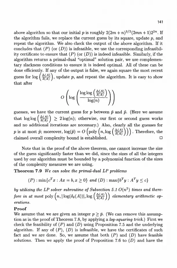
141

above algorithm so that our initial p is roughly 2(2m + n)3/2(2mn + l )2 2 n . If the algorithm fails, we replace the current guess by its square, update p, and repeat the algorithm. We also check the output of the above algorithm. If it concludes that (P) (or (D)) is infeasible, we use the corresponding infeasibil-ity certificate to ensure that (P) (or (D)) is indeed infeasible. Similarly, if the algorithm returns a primal-dual "optimal" solution pair, we use complemen­tary slackness conditions to ensure it is indeed optimal. All of these can be done efficiently. If any of the output is false, we again square the most recent

guess for log ( j^J- J, update p, and repeat the algorithm. It is easy to show

that after

H log(n)

guesses, we have the current guess for p between p and p. (Here we assume

that log log I - jW J > 21og(n); otherwise, our first or second guess works

and no additional iterations are necessary.) Also, clearly all the guesses for

p is at most p; moreover, log(p) = O (poly f n,log ( - jW-) ) ) • Therefore, the

claimed overall complexity bound is established. •

Note that in the proof of the above theorem, one cannot increase the size of the guess significantly faster than we did, since the sizes of all the integers used by our algorithm must be bounded by a polynomial function of the sizes of the complexity measures we are using. Theorem 7.9 We can solve the primal-dual LP problems

(P) : min{cTa; : Ax — b, x > 0} and (D) : m&x{bTy : ATy < c}

by utilizing the LP solver subroutine of Subsection 5.1 0(n2) times and there­

fore in at most poly In, | log(<5a(^4))|, log ( s(A) )) elementary arithmetic op­

erations.

Proof We assume that we are given an integer p>p. (We can remove this assump­tion as in the proof of Theorem 7.8, by applying a log-squaring trick.) First we check the feasibility of (P) and (D) using Proposition 7.5 and the underlying algorithm. If any of (P), (D) is infeasible, we have the certificates of such fact and we are done. So, we assume that both (P) and (D) have feasible solutions. Then we apply the proof of Proposition 7.6 to (D) and have the

142

problem

(D'):max{bTy:ATy< \c"]}.

Our theorem in Subsection 5.1 cannot deal with this LP problem (since the objective function of (£>') is arbitrary). We form the dual (call it (P')) of (D1) and apply the proof of Proposition 7.6 to (P1). Now, the LP problems arising from the applications of Proposition 7.6 to (P') all satisfy the conditions needed in Subsection 5.1 (namely, condition (ii) of the subsection for b and c). So, calling this subroutine 0(n) times, as in the proof of Theorem 7.8, we can compute optimal solutions of (P1) and (£>'). (At some point, during this process, inside the proof of Theorem 7.8, the method in the proof of Proposition 7.7 is used. This requires the LP solver subroutine to be called with data satisfying condition (i)—potentially not satisfying condition (ii)—of Subsection 5.1.) Now, we have an optimal solution of (D1) and we can keep applying this technique in using the proof of Theorem 7.8 to solve (P) and (£>). This clearly requires no more than 0(n) problems of the type (£>') to be solved. Since each such problem can be solved with 0(n) calls to the LP solver subroutine, the 0(n2) bound follows. •

7-4 Overall Complexity Bounds

Suppose we have an interior-point algorithm satisfying Assumption 2, with

an O (na (logixiA)))13) iteration bound, for some a > 0, /? > 0. Then

Theorem 7.8 implies an iteration bound of

o(.~K^)+H'(*(**^))).

On the other hand, using the methods of Subsection 5.1 and Theorem 7.9, we obtain the iteration bound

O ( V 5 (\log(Ss(A))\ + nlog (j^j + nlog(n))

The above bound is not better than Vavasis-Ye's and can be much worse in general. However, in the case that A is totally unimodular, it becomes the same. In this very special case, we can omit the factor of (\oglog(x(A)))

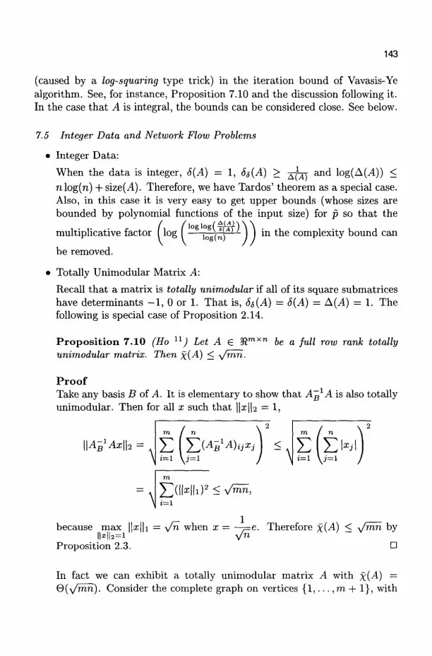
143

(caused by a log-squaring type trick) in the iteration bound of Vavasis-Ye algorithm. See, for instance, Proposition 7.10 and the discussion following it. In the case that 4 is integral, the bounds can be considered close. See below.

7.5 Integer Data and Network Flow Problems

• Integer Data:

When the data is integer, 8(A) = 1, 8S(A) > ^fjy and log(A(A)) <

nlog(n) + size(A). Therefore, we have Tardos' theorem as a special case.

Also, in this case it is very easy to get upper bounds (whose sizes are

bounded by polynomial functions of the input size) for p so that the

multiplicative factor (log

be removed.

'°g'°8($ff) log(n)

in the complexity bound can

Totally Unimodular Matrix A:

Recall that a matrix is totally unimodular if all of its square submatrices have determinants - 1 , 0 or 1. That is, S5(A) = 5(A) = A(A) = 1. The following is special case of Proposition 2.14.

Proposition 7.10 (Ho n ) Let A € SRmxn be a full row rank totally unimodular matrix. Then x(A) < y/mn.

Proof Take any basis B of A. It is elementary to show that A^1 A is also totally unimodular. Then for all x such that ||i||2 = 1,

\\A~BlAx\h =

\

m, I n

»=1 \ j = l \

m I n

£ E N »=i y = i

because max ||a;||i = y/n when x — —y=e. Therefore x(A) < Jmn by IWI2=I Vn

Proposition 2.3. •

In fact we can exhibit a totally unimodular matrix A with x(A) = Q(y/mn). Consider the complete graph on vertices { l , . . . , m + 1}, with

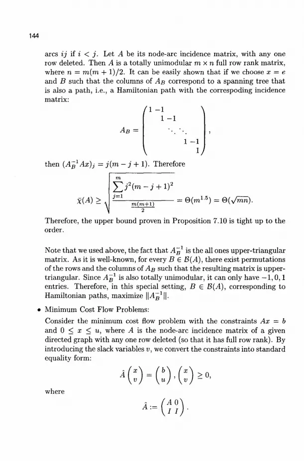
144

arcs ij Hi < j . Let A be its node-arc incidence matrix, with any one row deleted. Then A is a totally unimodular mxn full row rank matrix, where n = m(m + l ) /2 . It can be easily shown that if we choose x = e and B such that the columns of AB correspond to a spanning tree that is also a path, i.e., a Hamiltonian path with the correspoding incidence matrix:

/ l - l \ 1 - 1

AB =

1 - 1

V 1 /

then (AB1Ax)j = j(m - j + 1). Therefore

X(A)>

N j = i

m(m+l) 2

= 0 ( m 1 5 ) = e(y/mri).

Therefore, the upper bound proven in Proposition 7.10 is tight up to the order.

Note that we used above, the fact that Ag1 is the all ones upper-triangular matrix. As it is well-known, for every B £ B(A), there exist permutations of the rows and the columns of AB such that the resulting matrix is upper-triangular. Since A^1 is also totally unimodular, it can only have — 1,0,1 entries. Therefore, in this special setting, B e B(A), corresponding to Hamiltonian paths, maximize H^s1!!-

Minimum Cost Flow Problems:

Consider the minimum cost flow problem with the constraints Ax = b and 0 < x < u, where A is the node-arc incidence matrix of a given directed graph with any one row deleted (so that it has full row rank). By introducing the slack variables v, we convert the constraints into standard equality form:

b' > 0 ,

where

A:= A0 I I

145

This structure arises whenever we convert an upper bounded LP problem to the standard equality form. Vavasis and Ye 29 prove that x{A) =

0(mn). Using Propositions 2.7 and 7.10 (and the arguments following that), we have x(A) = Q{y/mri) when A is totally unimodular.

Acknowledgment

Part of this work was done while both authors were visiting The Fields In­stitute, Toronto, Ontario, Canada (Fall, 1999). Research of the first author was supported in part by an OGSST, an NSERC PGSB, and by an NSERC research grant and a PREA of the second author. Research of the second author was supported in part by a Faculty Research Grant from University of Waterloo, research grants from NSERC, and a PREA from Ontario, Canada.

Part of this work was done while the second author was visiting the Department of Mathematical and Computing Sciences of Tokyo Institute of Technology on a sabbatical leave from the University of Waterloo (October 1997-March 1998). Support and hospitality of Masakazu Kojima and T.I.T. are gratefully acknowledged.

References

1. I. Adler and P.A. Beling, Polynomial algorithms for linear programming over the algebraic numbers, Algorithmica 12, 436-457 (1994).

2. L. Blum, F. Cucker, M. Shub and S. Smale, Complexity and Real Com­putation, Springer-Verlag, New York, NY, U.S.A., 1998.

3. W. Cook, A.M.H. Gerards, A. Schrijver and E. Tardos, Sensitivity theo­rems in integer programming, Mathematical Programming A 34, 251-264 (1986).

4. I.I. Dikin, On the speed of an iterative process, Upravlaemye Sistemy 12, 54-60 (1974).

5. M. Epelman, Complexity, Conditions Numbers, and Conic Linear Sys­tems, Ph. D. Thesis, Massachusetts Institute of Technology, 1999.

6. M. Epelman and R.M. Freund, Pre-conditioners and relations between different measures of conditioning for conic linear systems, Working Paper OR-344-001, Operations Research Center, M.I.T., 2000.

7. A. Forsgren, On linear least-squares problems with diagonally dominant weight matrices, SIAM J. Matrix Anal. Appl. 17, 763-788 (1996).

8. C.C. Gonzaga and H. Lara, A note on properties of condition numbers, Linear Algebra And Its Applications 261, 269-273 (1997).

9. O. Giiler, A.J. Hoffman and U.G. Rothblum, Approximations to solutions

to systems of linear inequalities, SI AM J. Matrix Anal. Appl. 16, 688-696 (1995).

10. 0 . Giiler ad Y. Ye, Convergence behavior of interior-point algorithms, Mathematical Programming A 60, 215-228 (1993).

11. J.C.K. Ho, Structure of the Central Path and Related Complexity Issues for ILnear Programming, M. Math. Thesis, University of Waterloo, De­cember 1998.

12. A.J. Hoffman, On approximate solutions of systems of linear inequalities, J. Res. Nat. Bur. Stand. 49, 263-265 (1952).

13. N. Karmarkar, A new polynomial time algorithm for linear programming, Combinatorica 4, 373-395 (1984).

14. L. Khachiyan, On the complexity of approximating extremal determi­nants in matrices, Journal of Complexity 11, 138-153 (1995).

15. N. Megiddo, S. Mizuno and T. Tsuchiya, A modified layered-step interior point algorithm for linear programming, Mathematical Programming A 82, 339-355 (1998).

16. S. Mehrotra and Y. Ye, Finding an interior point in the optimal face of linear programs, Mathematical Programming A 62, 497-515 (1993).

17. D.P. O'Leary, On bounds for scaled projections and pseudoinverses, Lin­ear Algebra And Its Applications 132, 115-117 (1990).

18. J. Renegar, Linear programming, complexity theory and elementary func­tional analysis, Mathematical Programming A 70, 279-351 (1995).

19. C. Roos, T. Terlaky and J.-Ph. Vial, Theory and algorithms for linear optimization. An interior point approach, Wiley-Interscience Series in Discrete Mathematics and Optimization. John Wiley and Sons, Ltd., Chichester, 1997.

20. A. Schrijver, Theory of Linear and Integer Programming, John Wiley and Sons, 1986.

21. G.W. Stewart, On scaled projections and pseudoinverses, Linear Algebra And Its Applications 112, 189-193 (1989).

22. E. Tardos, A strongly polynomial algorithm to solve combinatorial linear programs, Operations Research 34, 250-256 (1986).

23. E. Tardos, A strongly polynomial mimimum cost circulation algorithm, Combinatorica 5, 247-255 (1985).

24. M.J. Todd, L. Tuncel and Y. Ye, Probabilistic analysis of two complexity measures for linear programming problems, Mathematical Programming A 90, 59-69 (2001).

25. L. Tuncel, Approximating the complexity measure of Vavasis-Ye algo­rithm is NP-hard, Mathematical Programming A 86, 219-223 (1999).

26. L. Tuncel, On the condition numbers for polyhedra in Karmarkar's form,

147

Operations Research Letters 24, 149-155 (1999). 27. L. Tuncel, A pseudo-polynomial complexity analysis for interior-point

algorithms, Dept. of Comb, and Opt. Research Report 93-16 (June 1993, Revised November 1993).

28. S.A. Vavasis, Stable numerical algorithms for equilibrium systems, SIAM J. Matrix Anal. Appl. 15, 1108-1131 (1994).

29. S.A. Vavasis and Y. Ye, A primal-dual interior point method whose run­ning time depends only on the constraint matrix, Mathematical Program­ming A 74, 79-120 (1996).

30. S.A. Vavasis and Y. Ye, Condition numbers for polyhedra with real num­ber data, Operations Research Letters 17, 209-214 (1995).

31. Y. Ye, Toward probabilistic analysis of interior-point algorithms for linear programming, Mathematics of Operations Research 19, 38-52 (1994).

32. Y. Ye, M.J. Todd and S. Mizuno, An 0(V"X)-iteration homogeneous and self-dual linear programming algorithm, Mathematics of Operations Research 19, 53-67 (1994).

33. S. Zhang, Global error bounds for convex conic problems, SIAM J. Op­timization 10, 836-851 (2000).

149

ON THE EXPECTED N U M B E R OF REAL ROOTS OF A SYSTEM OF R A N D O M POLYNOMIAL EQUATIONS

ERIC KOSTLAN

eric ©developments erver. com

We unify and generalize several known results about systems of random polyno­mials. We first classify all orthogonally invariant normal measures for spaces of polynomial mappings. For each such measure we calculate the expected number of real zeros. The results for invariant measures extend to underdetermined systems, giving the expected volume for orthogonally invariant random real projective va­rieties. We then consider noninvariant measures, and show how the real zeros of random polynomials behave under direct sum, tensor product and composition.

Part I - Introduction

1 Overview

To motivate our investigation, we begin this chapter with some known results about systems of random polynomials. In particular, we discuss results of Mark Kac 12, Edelman and Kostlan 7, Shub and Smale 23, and Rojas 21. We conclude Part I with a detailed discussion of the level of generality adopted in this chapter. The titles for Part II and Part III were chosen to indicate something about the level of generality of the results in each respective section.

Part II is devoted to random polynomials whose coefficient vectors form orthogonally invariant normal measures. We classify all such measures. We then consider a systems of such polynomials. The system may be mixed - that is, the polynomials making up the system do not have to be identical - and the system may be underdetermined. In all cases we calculate the expected volume of the corresponding random real projective variety. For a completely determined system, this is simply the expected number of real zeros.

In Part III of this chapter we consider the direct sum, tensor product and composition of random polynomials. This is a familiar theme in mathematics. We have systems of random polynomials, and we wish to use them to construct new systems of random polynomials. Our focus will be on how the expected number of real zeros behaves under sum, product and composition.

This chapter is not self-contained. It is written with 7, Sections 1-4 and Section 7, as a necessary prerequisite. Although this chapter does discuss volumes of random varieties, the focus is on the expected number of real zeros of systems. A more detailed discussion of random real varieties is in preparation 15. An open-ended web-based project, 15 completes a series of

150

five papers: 13, 14, 7, this paper, and 15. All these papers are available at http://www.developmentserver.com/randompolynomials. One result appear­ing in 13 and 14 that might be of particular interest to readers of this chapter is the calculation (over the complexes) of the joint distribution of zeros for pairs of plane conies. For most readers interested in random polynomials, 7

is sufficient.

2 Summary of previous results

2.1 Polynomials with independent standard normal coefficients

Consider a system of m polynomials in m variables with independent standard normal coefficients. Assume that each variable has degree at most d. There­fore, the Newton polytope, that is, the convex hull of the support of each polynomial, is an m-dimensional hypercube. If E^ represents the expected number of zeros for the system,

As d —> oo,

i ^ ~ ^ r ( ^ ) ( 2 i o g d r .

The univariate case was established by Kac 12, and generalized to systems of equations in 7. In Section 10.1 we show that this result may be viewed as a special case of the tensor product of random polynomials.

We conjecture that the same asymptotic formula holds for a large class of monomial term structures, as long as all the coefficients are i.i.d. central normal random variables. This is because for any fixed C, as d -> oo,

We may choose C « 1 and C » 1, to inscribe and circumscribe any given polytope with cubes. Conjecture Let K be any bounded set in {x £ R|a; > 0 } m with nonzero interior. Assume that either K or {x € R|ar > 0}m — K is the finite union of convex sets. Consider a sequence {Pd} of completely determined systems of polynomials with independent standard normal coefficients. Assume that the support of Pd is the set of integer lattice points contained in dK. If Ed

151

represents the expected number of zeros for the system, then as d —>• oo,

i W - ^ r ( ^ ) ( 2 i Q g 4 T .

The assumption about K is to avoid pathologies and make a precise conjec­ture. I doubt the correct hypothesis would have anything to do with convexity. I suspect the same asymptotic formula holds for mixed systems as well.

The study of random polynomials began with the assumption that the coefficients were identically distributed. These early works include the 1932 paper by Block and Polya 2 , and the seminal work of Mark Kac 12, published in 1943. The extensive literature that has grown out of this work (and this assumption) has been documented by Bharucha-Reid and Sambandham l .

I feel that the subject of random polynomials is blessed by the fact that these obvious random polynomials (polynomials with independent standard normal coefficients) are not the natural random polynomials. The attempt to replace these measures with more natural measures was, in part, the mo­tivation for 7, 13, 14, 21, and Part II of this chapter. Furthermore, when we study random polynomials, we can use this case as a convenient non-invariant random polynomial. For example, comparing Section 7.1 of 7 and 21, we see that orthogonal invariance is not required to make the tensor product theorem work.

2.2 The most natural random polynomial

Consider a random polynomials

/ , ai\--im"-k=lxk >

where YA!=I h < d and where the a^...^ are independent normals with mean zero and variances equal to multinomial coefficients:

d\

~ (d-E)T=i'*)!n*Li*fc! ' Consider m independent equations of degrees di,...,dm, each defined this way. Then the expected number of real zeros of the system is

m

x IK The general case was established by Shub and Smale 23. For the case where all the degrees are equal, the result was established in 14. Furthermore, 14

H,

152

stated the result for underdetermined systems as well, thus giving the expected volume of a real projective variety of dimension k and degree d:

d{m-k)/2^(k+l)/2

r p + i)/2] •

In Part II of this chapter we will unify these results. Following 14, we will consider arbitrary codimension, but like 23, we will avoid the assumption that the polynomials are of equal degree. In this chapter we will refer to any of these results as the square root result.

We can characterize these random polynomials using a combination of invariance and independence. See 7, 13 and 14 for detailed discussions. We define the action of the orthogonal group on random polynomials in Section 3.1. The following result, that appears in 14, is true for both real and complex random polynomials. A central probability measure on a vector space of real polynomial mappings has the following two properties, (1) orthogonal invariance of the measure and (2) statistical independence of the coefficients, iff it is, up to a scalar multiple, the polynomial discussed above. That is, the coefficients must be independent, and the variances of the coefficients are some constant multiplied by the multinomial coefficients. Notice we are not assuming normality of the coefficients. This is one of many theorems in statistics of the form

independence + invariance -» normallydistributed

In 7 we referred to these polynomials as "a random polynomial with a nice answer" and discussed the geometry of these polynomials in detail. A homo­geneous real quadratic system may be written as a real symmetric matrix. For this case, the above result reduces to the characterization of Gaussian orthogonal ensemble given by 19.

Over the complex numbers, we may replace the assumption of indepen­dence with the assumption of normality of coefficients. This is equivalent to saying that there is (up to a constant) a unique unitarily invariant multivari­ate normal. In Section 5.1 of this chapter, we give a simple proof of this classical result. The significance of these complex random polynomials has also been noted by physicists 3. Therefore, it should come as no surprise that the real versions of these random polynomials have nice properties as well.

However, there are other orthogonally invariant normal random polyno­mials. One goal of this chapter is to give a unified treatment of them. We will produce a complete list of all random polynomials with orthogonally in­variant normal coefficients - we say exactly what we mean by orthogonally

153

invariant in Section 3.1. For each we will calculate the expected volume of the real hypersurface determined by the polynomials. We will also establish a product formula that will give us the expected volume of a variety of any codimension generated by a set of (possibly distinct) random polynomials of this type.

2.3 Random harmonic polynomials

Consider the vector space of homogeneous polynomials of degree d in m + 1 variables that are harmonic, that is, the Laplacians of the polynomials are equal to zero. There is, up to a constant, a unique normal measure on harmonic polynomials that is invariant under the orthogonal action defined in Section 3.1. The expected number of real zeros for a system of m such random harmonic polynomial is

(d(d + m-l)\m/2

This result appears in 7. Here are random polynomials with natural measures. It seems that the random polynomials described in Section 2.2 have rivals for the status of most natural random polynomial. We shall address this issue by considering, in Part II of this chapter, all orthogonally invariant normal random polynomials.

2.4 Rojas polynomials

Assume that the support for a random polynomial is a product of simplices

p

{lizik;0<\Ik\<6k,l<k<p} , k=i

where h are multi-indices, \h\ is the sum of the indices of IK, and zk S Rmfc. Assume that the coefficients of the polynomials are independent central normals with variances

<n(£)>-The expected number of real zeros of a system of such polynomials is equal to

154

where m is the sum of the m^. These polynomials were introduced by Rojas in 1996 21. In Section 10.1 we see that the product formula used by Rojas can be applied to the tensor product of any central multivariate normal random polynomials.

3 Level of generali ty

The emphasis of 7 is on generality. For the most part, however, we proved re­sults for polynomial systems with any central multivariate normal coefficients. However, we did call attention to the existence of preferred orthogonally in­variant random polynomials with particularly nice properties. This paper expands on both of these subjects. Part II is dedicated to orthogonally in­variant random polynomials, with coefficients that are multivariate normal random variables, not necessarily central. Both underdetermined and mixed systems are considered. In Part III we drop invariance and add centrality. In fact, like 7 many of of the results of Part III may be generalized to finite-dimensional space of rectifiable functions. However, in Part III we add the assumption that the system is central. Furthermore, we will not allow mixed or underdetermined systems in Part III.

Throughout this chapter we will allow measures to be restricted to proper subsets of our function space. The domain of our functions may be any measurable subset U of R m + 1 . Therefore, is some sense, all of our results are local in nature. For simplicity, we will not specify the domain U in each theorem and corollary, as we did in 7. However, when explicit formulas are given for the expected number of real zeros, we are assuming that the domain i s a l l o f R m + 1 .

Let P be a finite dimensional function space, and consider a (random) p e P, p : R m + 1 -» R. The evaluation mapping to the dual of P:

ev : Rm+1 -> P\

is denned by ev(x)(f) = f(x). The function p thus corresponds to a hyper-plane in P*. The intersection of this (random) hyperplane with ev pulls back to the zero set for p. In P* integral geometry provides a simple intersection theory to handle (unmixed) systems of equations. This simple theory pulls back to a simple intersection theory in R m + 1 .

Ideally, we would like to prove every result for systems that are possibly mixed and possibly underdetermined. If the system in underdetermined, we have the problem that the random variety is distorted by the pullback. Thus our intersection theory gives us answers about expected projective volumes in (ev) ( R m + 1 ) instead of in R m + 1 . For varieties of dimension zero this distortion

155

is not an issue. For mixed systems the picture is complicated by the presence of several different evaluation mapping, and therefore no intersections can be pulled back. We must work with intersections of different random hypersur­faces in R m + 1 . For mixed invariant systems, these random hypersurfaces are orthogonally invariant and therefore classical integral geometry provides simple answers.

3.1 Homogeneous and inhomogeneous systems

Given an inhomogeneous polynomial with m variables z\,...,zm, we can al­ways consider, instead, the corresponding homogeneous polynomial i n m + 1 homogeneous variables zo,. -. ,zm. For completely determined systems, this should cause no confusion, because all of our results about expected number of real zeros apply to both homogeneous and inhomogeneous systems. When considering underdetermined systems, we must make sure that the domain is projective space.

When we speak of unitary or orthogonal invariance, we will always be considering the homogeneous version of the random polynomial. We assume the unitary and orthogonal groups act on the right,

U{p)(z)=p{U(z)).

Actions of products of orthogonal groups have also been considered 17'?>?, but we will not consider them here. We will be studying both inner products and multivariate normal measures on vector spaces of polynomials. Our focus will be on the real case, so we will usually just consider orthogonal invariance. For the complex case we replace orthogonal invariance with unitary invariance.

By convention, we will make no effort to distinguish between an inhomoge­neous system and its homogeneous counterpart. For example, by a univariate polynomial we will mean a random polynomial that may be written as

d d

pi*) = 5Z "-Ji <* P(X' y)^^2 aixiyd~i • i=0 i=0

Elements of the orthogonal group reflect or rotate p to give d

rd Y^ «i cos*(0 + Sy and-i(e + S) , i=0

where x — rcos(6), y — rsin(0). The random polynomial will be said to be orthogonally invariant if the probability measure is invariant under this action. Using this convention, the random polynomial

p(t) = a{t2 + 1) ,

156

where a is a standard normal random variable, is considered to be orthogonally invariant.

3.2 Under determined and overdetermined systems

For invariant random polynomials we will prove results for underdetermined systems thus giving results about the expected volume of random projective varieties. Several interesting problems suggest themselves when considering random real varieties, and little is known. In this chapter, underdetermined and overdetermined systems, and the corresponding random varieties, are strictly tools to study the expected number of zeros of (possible mixed) sys­tems. We consider only the expected volumes of such varieties, ignoring their more interesting invariants. The key motivation for 15 is to focus on the ge­ometric properties of random real varieties that are ignored in this chapter. For this chapter, we will only need one result about overdetermined systems. Lemma 3.1 Let U be a measurable subset o / R m , and consider a real-valued random function

a0fo(t) + o i / i ( t ) + . . . + anfn{t), t e U,

where the ai are independent standard normals, n > m. Generate a random variety of dimension m in R fc+1, k > m, by choosing an independent sample of k + 1 such functions. The expected volume of the projection of this variety onto the unit sphere in R*+ 1 is equal to the expected number of zeros in U of a system of m independent random functions of this form, multiplied the volume of m-dimensional real projective space

m + l

r(2*±i) '

Proof Let N be the random variety generated in the lemma, and let M to be the subspace of R f t + 1 , defined by XQ = ... = xm-\ = 0. The proof is then a straightforward generalization of the proof of Lemma 6.1 in 7. •

3.3 Mixed systems

I recall having two contrary emotions when Steve Smale told me that he and Mike Shub 23 had generalized the square root result of14 to mixed completely determined systems. The first was a pleasant lack of surprise. The answer derived by Shub and Smale was the only reasonable result. Furthermore, my research had received an unusually strong endorsement. On the other hand, I was discouraged. I felt that 14 had presented the correct picture of random

157

systems. But in 14, a system of equation was a plane in the space of real-valued polynomial mapping, or a point in the Grassmann manifold. Unfortunately, this viewpoint precludes the consideration of mixed systems. Nonetheless, the generalization to mixed systems is clearly desirable. In Part II of this chapter, we will consider invariant mixed systems. We will use the viewpoint of 14 to get results about random hypersurfaces, and then develop an intersection theory similar to 23 to deal with mixed systems. The Grassmann manifold will never be used. We will also allow mixed systems in Section 11, where we discuss the composition of random polynomials.

The generalization of the square root result to mixed systems by Shub and Smale has motivated at least three resent papers. The first of these papers was by Rojas 21. Rojas attempts to define, for any given support structure, distinguished measures for the corresponding random polynomials. I do not believe this issue has been completely resolved. Rojas also considers mixed systems, and conjectures a relationship between the square root of the mixed volume and the expected number of real zeros. McLennan 18 considers (the multihomogeneous version of) the Rojas polynomials, and shows that the square root of the (normalized) mixed volume provides a lower bound for the expected number of real zeros. In the words of McLennan, "The mean exceeds the square root of the maximum." The third paper, by Malajovich and Rojas 1T, produce an explicit, albeit coarse, upper bound for the expected number of real zeros in terms of the square root of the mixed volume for arbitrary central normal random polynomial systems. Reading these three papers, one sees a wealth of new ideas emerging.

Part II — Orthogonally Invariant Normal Coefficients

4 Classification of invariant inner products

We will now classify invariant inner products on vector spaces of homogeneous polynomials. These are the classical results we will need for the rest of the chapter. We include proofs because they are surprisingly easy. Before we try to understand the real case, we discuss the complex case, which is considerably easier.

4-1 The complex analogue

Over the complexes, there is, up to a constant, a unique unitarily invariant Hermitian inner product. This is a well known classical result. The general­ization to multihomogenous polynomials may be found in 18.

158

Theorem 4.1 Assume a Hermitian inner product is defined on a vector space of complex homogeneous polynomials of degree d, and assume it is invariant under the right action of the unitary group. Then monomials are perpendicular to each other, and the lengths of the monomials {x1} are, up to a constant, square roots of multinomial coefficients

/ where I is a multi-index. Proof This is the corollary following Theorem 3.2 of 13, and is Theorem 4.1 in 14. We now outline a simplified version of the proof given in 13. Fix y and think of v(x)TCv(y) as a function of x on y±. Assume that for any unitary matrix U, v(Ux)TCv(Uy) — v(x)TCv(y). Then for any U that fixes y, we must have v(Ux)TCv(y) = v(x)TCv(y). Thus v(Ux)TCv(y) must be constant for x on the unit sphere in y±, and therefore it's gradient has rank one. But for an analytic function this implies that v(x)TCv(y) is constant on y±, and therefore, by symmetry, zero. Thus

x ±y ^ v(x)TCv{y) = 0 .

Therefore xTy divides v(x)TCv(y). We then apply the same argument to the v(x)TCv(y) I xTy, and so on. We ultimately deduce that v(x)T Cv(y) — a(xTy)d, which completes the proof. • We have just established that the space of homogeneous complex valued poly­nomials of a fixed degree i n m + 1 complex variables is an irreducible repre­sentation of the unitary group U(m + 1). As stated in 14, this may also be shown using classical invariant theory.

4-2 Classification of indefinite inner products

Assume that for any orthogonal matrix Q, v(Qx)TCv(Qy) = v(x)TCv(y). This implies that v{x)TCv{y) must be a polynomial in x • x, x • y, and y • y. This is classical invariant theory. For proofs and discussion of such results, see 24 . We thus deduce that there must exist /3, such that

[d/2]

v(x)TCv(y) = J2^(x-x)k(yy)k(x-y)d-2k. (1)

Thus we have a [d/2] parameter family of orthogonally invariant inner prod­ucts. For example, if we set /?0 = 1 and /?* = 0 for k > 1, we produce a inner product for which the monomials are orthogonal.

159

This completely classified all orthogonally invariant inner products on spaces of homogeneous polynomials of degree d. But this classification is unsatisfactory. We wish to use these inner products as covariance matrices, so we must identify the positive definite inner products - actually positive semidefinite, since we allow normal measures restricted to proper subspaces of polynomials. Unfortunately, if we use the parameters (5k it is difficult to see which inner products are positive definite. We therefore will construct a different parameterization of these inner products. First we review some basic facts about Gegenbauer polynomials.

4-3 Gegenbauer polynomials

The reference for all the results in this section is 10 and 25. This section includes formulas we use in this chapter, along with other well-known and useful formulas. The Gegenbauer polynomials may be defined in terms of their generating function

( l -2 te + z2)-" = ^ Q ( t ) z n . ra=0

25 In 25 these functions are called "ultraspherical functions" and are denoted as Pn (t). The Gegenbauer polynomials are Gaussian hypergeometric functions,

T(2v + n) „ / 1 1 — t

T{n + l)T(2u) V ' 2 ' 2

If n is a non-negative integer,

nW(v) V 2 ' 2 ' '*2

The polynomials

2T(i/) (n 4- v)n\ 1 '

2-KT(2V + n) cm, n = 0 , . . . , d, form an orthonormal bases for polynomials of degree d, with do­main t e [—1,1] and weight (1— t2)""^. The first few Gegenbauer polynomials are

C%{t) = 1 , Cr(t) = 2ut , C%(t) = 2v{v + \)t2 - v ,

C£(t) = \v{v + l)(i/ + 2)t3 - 2v(y + l)t .

160

Subsequent Gegenbauer polynomials may be calculated using either of the following formulas.

{n + 2)Cvn+2{t) = 2{v+n+l)tCv

n+l{t)-(2v+n)Cvn{t) ; ±Cv

n(t) = 2vC»n+_\{t) .

We also have

T(2u + n) C»(l) = r(n + i)r(2i/) '

Associated Legendre functions may be written in terms of Gegenbauer polynomials:

{-l)m{2m)\{l-t2)m'2rim+l m!2m

If m and / are non-negative integers,

(_-\\l+m rfl+m P™(t) = I l> (l-f)™/2^— (1-t2)1 .

i v ' 2ll\ K ' dtl+m K ' The spherical harmonics that arise in the solution of the Schrodinger equation for the hydrogen atom are

*T(M) = /(2f + l ) ( i - m ) ! im,

y 47r(/ + m)! ' v ;

where I is the azimuthal quantum number, and m = —/,..., / is the magnetic quantum number. Here I — 0 ,1 ,2 ,3 ,4 ,5 , . . . for the s,p, d, f,g,h,... orbitals. Unfortunately, the definitions of associated Legendre functions and spherical harmonics are not entirely uniform through the literature. Compare 8 , 10, 20

and 25. The Gegenbauer polynomials are Jacobi polynomials, but with different

normalization constants,

C n W _r(2i0r(n+ «, + §)** Special cases of the Gegenbauer polynomials include the Legendre polynomi­als,

Pn(t)=ClJ2(t),

and the Chebyshev polynomials of the second kind,

= = sintnarccosffl] _ sin[arccos(t)]

161

We will need to define Gegenbauer polynomials for which v — 0. Unfor­tunately, C°(£) = 0, unless n = 0. However, we can renormalize, because

Um &1 = 2cos["arccosW] = 2 v^o v n n

where Tn are the Chebyshev polynomials of the first kind. We choose a normalization that is suited to our needs, and that is continuous as v -» 0. We use that fact that

lim ™ _ 2 i/-»0 V

Notation. We define

when v ^ 0, and we define

n{) ~ Q(l) '

C°n(t) = Tn(t) .

The first few renormalized Gegenbauer polynomials are

3 w 2v + 1 2i/ + 1

If we rewrite the results in this chapter in terms of Jacobi polynomials, the problem at v — 0 does not arise. Nonetheless, we will use Gegenbauer poly­nomials, because the Jacobi polynomials are too general for the problems we will consider.

We will make use of the following explicit formula:

- 2 " - 1 n! r (2 i /+ l ) ' ^ ] (-iyr(v + n-j) 2 , n W r (2^ + n ) I > + 1) ^ 22jjl{n-2j)l ' W

where n is a non-negative integer. Here we define

Tjv + n- j) ——— — = z , not 1 ,

Y(2v + n)

162

when n = j = v = 0. This is because we set n = j = 0 before we set v — 0. This formula may be inverted, to give

_ n ! i y + 1) [ ^ ] (,/ + n - 2j)T{2u + n - 2j) ^

" 2»-ir(2i/ + 1) ^ j ! (n - 2j)!r(i/ + n - j + 1) " ~ 2 ^ ' ' [ '

where we define

(v + n- 2j)T(2i> + n - 2j) = - , not 1 ,

when n = 2j and v = 0. Using functional properties of the Gamma function, these formulas may be rewritten in many ways.

4-4 The eigenspaces ofr2V2

A straightforward calculation using multivariate calculus yields the following Lemma 4.1 / / / is a homogeneous polynomial of degree d — 2i in m + 1 variables, then

V 2 / = 0 -* r2V2(r2if) = 2i(m + 2d-2i-l)(r2if) .

Let Pd be the space of homogeneous real-valued polynomials of degree d in m + 1 real variables. The operator r 2 V 2 maps this space to itself. Let Ha be the subspace of this space for which V2 is equal to zero. By the lemma, {r2lHd-2i}, i = 0 , . . . , [d/2], are eigenspaces of r2 V2 with distinct eigenvalues {2i(m + 2d— 2i — 1)}. Furthermore, since H^ is the kernel of V2 : Pd -> Pd-2,

dim Hd > dim Pd — dimPd_2 .

Therefore the sum of the dimensions of these eigenspaces is at least the di­mension of Pd- We conclude that

[d/2]

Pd = 2~] r2lHd-2i (direct sum). i=0

As a consequence of this argument, we see that this sum is exactly the de­composition of Pd into the eigenspaces of r 2 V 2 . Furthermore,

dim Hd = dim Pd - dim P^-2 ,

and V2 : Pd —> Pd-2 is onto. This result may be stated as

Pd=Hd® r2Pd-2 •

We will now show that for each eigenspace, there is a unique orthogonally invariant inner product, up to a constant. Thus each of these subspaces form

163

irreducible representations of the orthogonal group 0{m + 1). We fix y, and consider v(x)TCv(y) to be a function of x — r alone. We then consider the following equation:

r2V2v(x)TCv(y) = \v(x)TCv{y) .

By substituting (1) into this equation, and applying elementary calculus, we obtain a first order difference equation, [2k{m + 2d — 2k — 1) — \]0k + (d — 2k + 2){d-2k + l)/3k-i = 0. But A = 2i(m + 2d-2i-l), where 0 < i < [d/2]. Therefore, {3k = 0, for 0 < k < i. We therefore replace k with k — i, and conclude that for 0 < i < [d/2] and 1 < k < [d - 2i],

2k[m+2(d-2i)-2k-l]/3k+i+[(d-2i)-2k+2][(d-2i)-2k+l]l3k+i-1 = 0 . (4)

We see that v(x)TCv(y) is uniquely determined, up to a constant. We may now use (2) to see that the coefficients of certain Gegenbauer polynomials satisfy (4). Therefore, we can write

v(x)TCv(y) = P{x-x)d'2(yy)dl2C^i{c0&B),

where 8 is the angle between the vectors x and y in the Euclidean norm. Notice that these inner products are positive definite iff /3 > 0. We set /? = 1 to make the definition of inner product unambiguous.

4-5 Classification of positive definite inner products

Any invariant inner product on Pj can be written as a weighted sum of the invariant inner products on the eigenspaces of r 2 V 2 derived above. The inner product on F j is positive definite iff all these weights are positive. We therefore use Gegenbauer polynomials to write any inner product as

[d/2]

v(x)TCv(y) = (x • x)d'2{y • y)d'2 £ O ^ J M (COS 6) . (5) i=0

If all the (Xi are greater than zero, then the inner product is positive definite. To indicate this, we write

fd/2]

v(x)TCv(y) = (x • x)dl2(y • y)d'2 £ r2C^ (cos 0) . (6) i=0

The {Vj} have a clear geometric interpretation. They are the lengths of the projections of v(x) onto the subspaces {r2tHd-2i}, where x is any unit vector

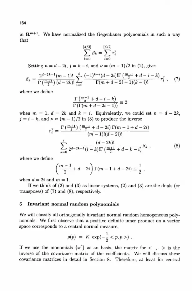
164

in R m + 1 . We have normalized the Gegenbauer polynomials in such a way that

[d/2] [d/2]

S > = £»-? k=0 i=0

Setting n = d — 2i, j = k — i, and v = (m — l ) /2 in (2), gives

_ 2rf-2fc-1(m-l)! * ( - l )* -<(d-2») ! r (V+d- i -A: ) 2

Pfc r ( m ± i ) ( d _ 2 f c ) ! Z . r ( m + d - 2 t - l ) ( A - i ) ! ^ ' U

where we define

r ( g f ^ + d - i - f c ) r (r(m + d - 2» -1))

when m = 1, d = 2A; and k = i. Equivalently, we could set n = d — 2A;, j = i — k, and v — (m — l ) /2 in (3) to produce the inverse

? _ r (a**) ( ^ + d - 2i) r(m - 1 + d - 2t) r i ~ ( m - l ) ! ( d - 2 t ) !

V ( r f~2 f c ) ! a ,«* Z . 2 d - 2 * - i ( i _ f c ) ! r ( 2 2 ± i + d - f c - i ) P / : ' W

where we define

m ~ + d - 2 z ) r ( m - l + d - 2 i ) = - ,

when d = 2i and m = 1. If we think of (2) and (3) as linear systems, (2) and (3) are the duals (or

transposes) of (7) and (8), respectively.

5 Invariant normal random polynomials

We will classify all orthogonally invariant normal random homogeneous poly­nomials. We first observe that a positive definite inner product on a vector space corresponds to a central normal measure,

pip) = K e x p ( - - <p,p>) .

If we use the monomials {x1} as an basis, the matrix for < .,. > is the inverse of the covariance matrix of the coefficients. We will discuss these covariance matrices in detail in Section 8. Therefore, at least for central

165

random polynomials, we reduce the problem of invariant normal measures to the problem that we considered in the previous section.

We first resolve the easier problem of unitarily invariant random polyno­mials. We then turn our attention to real invariant random polynomials. We produce a product formula that reduces our problem to the study of random hypersurfaces, and allows use to treat mixed invariant systems. We then re­duce the problem to the study of a single central invariant polynomial. For each such random polynomial, we calculate the expected volume of the cor­responding random projective hypersurface. This completes the calculation of the expected volume for all invariant normal random polynomials, and concludes this section. We conclude Part II with detailed discussions of two special cases: random symmetric matrices, and univariate polynomials.

5.1 The complex analogue

Over the complexes, there is, up to a constant, a unique unitarily invariant normal measure.

Theorem 5.1 Assume a measure on a vector space of complex polynomial mappings has the following two properties: (1) the measure is unitarily in­variant and (2) the coefficients of the polynomial are a multivariate normal random variable. Then the coefficients must be independent, the real and imaginary part of each coefficient must be independent, and the variances of the coefficients are some constant times the binomial coefficients.

Proof This follows from the classification of unitarily invariant inner prod­ucts. See Section 7.1. •

This theorem resembles the characterization of these random polynomials given in Section 2.2, but it is quite different. In Section 2.2, independence was part of the assumption, and normality was part of the conclusion. But in 5.1, normality is assumed, and independence is deduced. For unitarily invariant complex random polynomials, independence of the coefficients is equivalent to normality of the coefficients.

This characterization has an obvious, but interesting, consequence ob­served in 13. It is a central limit theorem for unitarily invariant random polynomials.

Theorem 5.2 13 Assume we are given any unitarily invariant probability measure on the space of complex-valued polynomials of a fixed degree. Let {pi} be an independent sample from this space. Then the measures of the

166

random polynomial

1 "

converge weakly to a measure that is, up to a constant, the independent in­variant measure we are considering in this section.

In 13 this result is stated for systems, using the two sided action of the unitary group, but the proof is similar.

This is the central limit theorem for unitarily invariant random polyno­mials. It is precisely the central limit theorem that is the explanation of why normal distributions are observed in practice. Therefore, this theorem would suggest that the polynomials we discuss in this section would be observed, in nature, if some complicated unitarily invariant process was generating com­plex valued polynomials. Indeed, some physicists have began to show interest in these random polynomials 3.

5.2 The expected volume of a real projective variety

Definition 5.1 Consider any orthogonally invariant normal measure on a vector space of real valued, real polynomials of degree d, in the variables to,...,tm. Let /J, and a be the mean and standard deviation of the t$ coef­ficient, and let a' be the standard deviation of the t0~ t\ coefficient. Then we define

as the expected geometric degree for that random polynomial.

For the random polynomials in Section 2.2, , a = 1 and a' — \[d. For the random harmonic polynomials of Section 2.3,

&__ ld(d + m - \)

er V m

Theorem 5.3 For any orthogonally invariant normal homogeneous random polynomial of degree d in m + 1 homogeneous variable,

l - ( - l ) d &_ ld(d + m-lj 2 - a ~ V m

The right hand inequality becomes equality for harmonic polynomials. The left hand inequality is attained by concentrating the measure on {ard} if d is even, and on {linear polynomials x r^1^2} when d is odd.

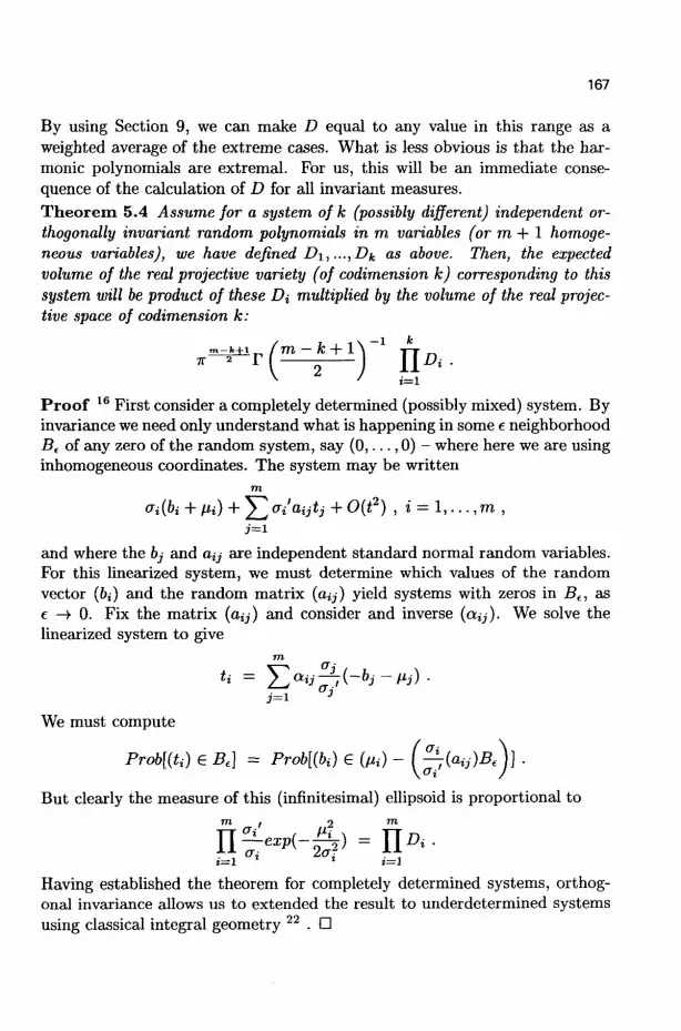
167

By using Section 9, we can make D equal to any value in this range as a weighted average of the extreme cases. What is less obvious is that the har­monic polynomials are extremal. For us, this will be an immediate conse­quence of the calculation of D for all invariant measures. Theorem 5.4 Assume for a system of k (possibly different) independent or­thogonally invariant random polynomials in m variables (or m + 1 homoge­neous variables), we have defined D\,...,Dk as above. Then, the expected volume of the real projective variety (of codimension k) corresponding to this system will be product of these D{ multiplied by the volume of the real projec­tive space of codimension k:

Proof 16 First consider a completely determined (possibly mixed) system. By invariance we need only understand what is happening in some e neighborhood Be of any zero of the random system, say ( 0 , . . . , 0) - where here we are using inhomogeneous coordinates. The system may be written

m

&i(bi + Hi) + ] P o-i'aijtj + 0(t2) , i = 1 , . . . , m , i= i

and where the bj and Oy are independent standard normal random variables. For this linearized system, we must determine which values of the random vector (bi) and the random matrix (a^) yield systems with zeros in Be, as e -^ 0. Fix the matrix (aij) and consider and inverse (aij). We solve the linearized system to give

m

U = y " a i j ^ 7 ( - 6 j - fij) .

We must compute

Prob[(U) e Bt] = Prob[(bi) £ (m) - (^(a^B^j] .

But clearly the measure of this (infinitesimal) ellipsoid is proportional to

Having established the theorem for completely determined systems, orthog­onal invariance allows us to extended the result to underdetermined systems using classical integral geometry 22 . •

168

5.3 Non-central invariant normal random polynomials

Fortunately, we will dispense with the non-central case quickly, and then focus on the central case. Theorem 5.5 The mean of any invariant random polynomial must be of the form [i(Y,x2)d/2 where fi is the mean of the t$ coefficient (as defined in the previous section). If d is odd, any invariant measure is central. Proof This is classical invariant theory. For proofs and discussion of such results, see 24 . • Thus any non central invariant random polynomial can be studied in terms of the central case. We need only adjust D by the factor

e*p(-£j) in the calculations of expected volume and expected number of real zeros.

5-4 Central invariant normal random polynomials

We now calculate D for every central invariant normal random polynomial system. Theorem 5.6 For any invariant normal random polynomial, we may write

[d/2]

v(x)TCv(y) = J2Mx-x)k(yy)k(x-y)d'2k . (9)

k=0

Then a2 = E L = O ' Pk and a'2 = Y}k=o(d ~ 2k)0k, and therefore

D Z[dll](d-2k)Pk

\ Eifflfc Proof By orthogonal invariance of the random polynomial, we know that any orthogonal matrix Q, v(Qx)TCv(Qy) = v(x)TCv(y). Then v(x)TCv(y) must be a polynomial in x • x, x • y, and y • y. This is classical invariant theory. For proofs and discussion of such results, see 24 . But v(x)TCv(y) is homogeneous in x and y separately, so it must be of the form (1). Since the matrix C is the covariance matrix of the coefficients of the polynomial, the value of a and a' may be deduced from (1). The value of D then follows from Definition 5.1 and Theorem 5.3. •

Thus we have a [d/2] parameter family of central invariant normal mea­sures. For example, if we set /3Q = 1 and /?* = 0 for k > 1, we recover the random polynomials in Section 2.2. Another example was given in Section 7.3 of7.

169

5.5 Classification of invariant normal measures

It would seem that we are done. We have a list of all central invariant normal measures and have calculated D for each of them. But we are really miss­ing something. We do not know which values of /?j are admissible. If we let them be arbitrary, we can generate non positive definite metrics, which do not correspond to any measures at all. In some sense, the Pi are the wrong param­eters to use. That is why we will express vT(x)Cv(y) in terms of Gegenbauer polynomials. In Section 7.3 of T, we saw that for invariant normal random harmonic polynomials

_ /d{d + m-l)

m

Theorem 5.7 For any central invariant measure, we may write

[d/2]

v(x)TCv(y) = ( z - z ) d / V 2 / ) d / 2 £ ^ ( & ( « > s 0 ) . i=0

Then

D = Y}^\d-2i){d-2i + m-l)rf

Proof For Hd_2i we have, by Section 7.3 of 7,

_ ' ( d - 2 i ) ( d - 2 t + m - l ) m

We may now calculate the fik using (7), and then apply Theorem 5.6 to complete the proof. • We will give an alternate proof of this theorem in Section 9.

From this theorem we can calculate the expected number of real zeros of any set of m independent orthogonally invariant normal random polynomials.

6 Quadratic forms

It will be instructive to reproduce all of the work in this section for the special case d = 2. Our problem reduces to a discussion of random real symmetric (m + 1) x (m + 1) matrices. The orthogonal group acts by conjugation

Q{M) = Q-XMQ .

170

There is a three parameter family of orthogonally invariant random symmetric (m + 1) x (m + 1) matrices. The joint probability density for the elements of the matrix may be written in the form by

p(M) = Cexp j - i [b0tr((M - ^I)2) + fc^M - /.J))2] 1 ,

where bo > 0 and bi > —bo/(m + l). Harmonic quadratic forms correspond to traceless matrices {bo/b\ —y 0). The other extremal case is when the measure is concentrated on scalar multiples of the identity matrix (&0/&1 - • —(m+1)). The case 61 = 0 has been studied extensively (see 4 5 and 1 9 ) . This is the only case for which the elements of the random matrix are independent.

Formula (1) reduces to

v{x)TCv{y) = /?„(*• 2/)2 + Pi{x-x){yy) . (10)

Since C is the (m + l)(m + 2)/2 x (m + l)(m + 2)/2 covariance matrix of the coefficients of the quadratic form, it must be inverted, to express {&o,&i} in terms of {/?0, Pi}- If we define e = ( 1 , . . . , 1) € R m + 1 ,

(fhl + faTe)-1 = 1 / + - — - I ^ _ — e T e . A> m(m + i)A + A)]

We deduce that

h 1 - h ~h

For d = 2 and v = (m — l) /2 , the renormalized Gegenbauer polynomials are For d = 2 and v = (m - l ) /2 ,

m m

and the triangular systems (7) and (8) reduce to

Therefore, we conclude that

, m rn - mr? "0 = 7 , -.x 9 ; ° i = (m + l)r2 ' l ( m + l ) 2 r 2 r 2 '

where r2 —» 0 for traceless random matrices, where r2, -> 0 for measures concentrated on scalar multiples of the identity. A straightforward calculation shows that

Var{Mii) = fa + ft = r2 + r? ,

171

and

t / I-Kir \ ^0 m + 1 2

when i ^ j . An easy way to generate these random matrices is to start with a random

nonsymmetric (m + 1) x (m + 1) matrix with independent standard normal coefficients, and then compute

w m rT 2*r(M) M + M1 y—<-I

m + 1 + (nz + fx)! , (11)

m + 1

where z is a standard normal random variable independent of M.

6.1 The expected volume of random conies

For random conies

a2 = Var(Mu) = 0O + ft = r2 + r\ ,

and

a'2 = Var(2A^-) = 2ft = ^ l) r2 ,

when i ^ j . Furthermore, we know that the mean of Mu = fi. We combine Theorem 3.6 with Theorem 3.7 to get

2/?o D = \ n s - exP

V A> + A V 2(00+0!))

Vm{r^+r2) F \ 2(r2 + r 2 ) , / ~ V m

If the coefficients are independent this reduces to D = y/2 and for the traceless case this reduces to D = y/2(m + l ) /m . We then can apply Theorem 2.2 to calculate expected volumes of projective varieties. Example 6.1 If the coefficients are independent D = v 2 . For a random harmonic conic D = ^ /2 (m+ l ) /m. We then can apply Theorem 2.2 to calculate expected volumes of projective varieties. We thus recover the results of Section 2.2 and Section 2.3, for the case d — 2.

Example 6.2 Consider an invariant normal random plane projective conic (m=2). The expected length of such a curve is TTD which is always less than

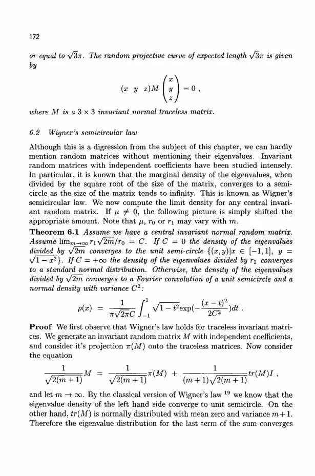
172

or equal to \ / 3 T - The random projective curve of expected length ^/3TT is given by

where M is a 3 x 3 invariant normal traceless matrix.

6.2 Wigner's semicircular law

Although this is a digression from the subject of this chapter, we can hardly mention random matrices without mentioning their eigenvalues. Invariant random matrices with independent coefficients have been studied intensely. In particular, it is known that the marginal density of the eigenvalues, when divided by the square root of the size of the matrix, converges to a semi­circle as the size of the matrix tends to infinity. This is known as Wigner's semicircular law. We now compute the limit density for any central invari­ant random matrix. If /j ^ 0, the following picture is simply shifted the appropriate amount. Note that fi, r0 or n may vary with m. Theorem 6.1 Assume we have a central invariant normal random matrix. Assume limm-i<X1rl^/2rn/ro = C. If C = 0 the density of the eigenvalues divided by V2m converges to the unit semi-circle {(x,y)\x £ [—1,1], y = y/1 — x2}. If C = +oo the density of the eigenvalues divided by r\ converges to a standard normal distribution. Otherwise, the density of the eigenvalues divided by y2rn converges to a Fourier convolution of a unit semicircle and a normal density with variance C2:

Proof We first observe that Wigner's law holds for traceless invariant matri­ces. We generate an invariant random matrix M with independent coefficients, and consider it's projection ir(M) onto the traceless matrices. Now consider the equation

. 1 M = . 1 TT(M) + \ tr(M)I , y/2(m +1) V 2 ( m +1 ) (m+l)y/2(m + l)

and let m -> oo. By the classical version of Wigner's law 19 we know that the eigenvalue density of the left hand side converge to unit semicircle. On the other hand, tr(M) is normally distributed with mean zero and variance m + 1 . Therefore the eigenvalue distribution for the last term of the sum converges

173

to a measure concentrated at zero. Therefore the first term of the sum must converge to a semicircle.

We then decompose any invariant random matrix using (11). The eigen­values of the first term of (11), when divided by ro\/2(m + 1), converge to a unit semicircle. The eigenvalues of the second term of (11) when divided by r i , are (dependent) standard normals. The eigenvalues of the sum are con­volutions of the eigenvalues of each summand. Therefore, as m -4 oo, we are convolving a semicircle with a normal density. We need only pay attention to the ratio of ro ^/2{m + 1) to r i .

Finally we observe that to make the statement of the proof shorter, we have replaced m + 1 with m. For large m this difference can be ignored. •

Although there is no difference in the asymptotic density for the inde­pendent and traceless cases, for finite size the distributions are qualitatively different. See15 for examples. All of these eigenvalue densities can be obtained by convolving a normal density with the eigenvalue density for the traceless matrices. This convolution blurres the eigenvalue distribution. Therefore the traceless matrices yield the sharpest pictures.

7 Univariate polynomials

As a final special case, we reproduce the work in this section for univariate polynomials, that is we will assume m = 1.

Using the substitution t = tan(0), we see that these random polynomials are actually special case of the random trigonometric sums studied in Section 3.2.4., and Section 5.3 Case I Example 2, of 7 . However, for the random trigonometric sums we are concerned with, that is, we can say more.

The renormalized Gegenbauer polynomials have reduced to the Cheby-shev polynomials of the first kind,

C°d_2i{t) = Td-2i(t) = cos[(d - 2i) arccos(t)] ,

and the eigenspaces of r2 V2 are given by

r2iHd_2i = {rd sin(d - 2i)0, rd cos{d - 2i)d) ,

i = 0 , . . . , [d/2\. These are all two dimensional eigenspaces, unless d is even and i — d/2. Note that the number of real zeros is exactly d — 2i for any polynomial in Ha-2i-

Formula (7) reduces to

0fc=2d-2fe-l£ i=0

d — i — k k — i

174

where we define

d-2i = 2

d — i — k

when d—2i and k = i. Similarly, (8) reduces to

U - 2k rf=2 -5

k=0

2k

i — k Pk ,

where we define 5 = d if d = 2i, and <5 = d — 1 otherwise. We see that Theorem 5.6 remains unchanged,

D =

and Theorem 5.7 reduces to

N Eil/o1(^-2fc)^

exp /*

2 E ! ^ ] A

£> = \

,[d/2] 2-2 TZoiid-2i^r exp -o V ^ / 2 ! r-2

Note that £ i ^ ] A = E&aI»?-The simplest non-trivial example is d = 2. This is just the case m = 1 of

the previous subsection, but we will instead approach it as a generalization of Section 5.3 Case I Example 2 of 7 . Example 7.1 Let ao, a\, and 02 be independent standard normal random variables. Any orthogonally invariant normal random quadratic polynomial may be written

a0rQ(t2 - 1) + ai2r0t + (a2rx + fi)(t2 + 1) .

The conversion formulas (7) and (8) reduce to

Po = 2r20 ; /J1 = -r2+r2

and

I00 '0 - 0^0 , rt = -fa + /?! .

We see that the expected number of real zeros is

' ,2 2/?o exp(-

/* 2r0 exp(- A*

P0+P1 ^ 2(p0 + Pi)' y/if+rl V 2(r2+r2)

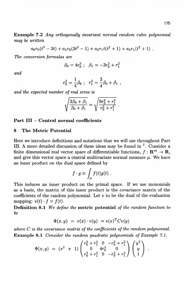
175

Example 7.2 Any orthogonally invariant normal random cubic polynomial may be written

a0r0{t3 - 3t) + airo{3t2 - 1) + a2r1t{t2 + 1) + a3n{t2 + 1) .

The conversion formulas are

Po = 4r2 ; fa = -3r02 + r\

and

and the expected number of real zeros is

/3fl) + ft kr2Q + r\

V ft + ft V r o + ^ '

Part III — Central normal coefficients

8 The Metric Potential

Here we introduce definitions and notations that we will use throughout Part III. A more detailed discussion of these ideas may be found in 7. Consider a finite dimensional real vector space of differentiable functions, / : R m —• R, and give this vector space a central multivariate normal measure \i. We have an inner product on the dual space defined by

/ • g = f f(t)g(t) . Jfi

This induces an inner product on the primal space. If we use monomials as a basis, the matrix of this inner product is the covariance matrix of the coefficients of the random polynomial. Let v to be the dual of the evaluation mapping: v(t) • f = f(t). Definition 8.1 We define the metric potential of the random function to be

$(x,y) - v(x)-v(y) =v(x)TCv(y)

where C is the covariance matrix of the coefficients of the random polynomial. Example 8.1 Consider the random quadratic polynomials of Example 7.1.

/ r g + r ? 0 -r*+rl\ (y*\ ${x,y) = (x2 x 1) 0 Ar2 0 \ \ y .

\r2+r2 0 -r2+rlj \ l j

176

This 3 x 3 matrix is the covariance matrix for the coefficients of the random ,2 quadratic. From, this we see immediately that a = r% + r\ and a' = 4r$, and

therefore the expected number of real zeros is

2r0 D =

Example 8.2 Consider the random cubic polynomials of Example 7.2.

( r2+r 0 -H+rl $(x,y) = (x3 x2 x 1)

V

0 9rg + r\ 0 3rg + r\ 0 9r% + r\

0 -3rg + r\ 0

0 \ -3r2 + r\

0 r2

0+rj J

h3\ y

v iy This 4 x 4 matrix is the covariance matrix for the coefficients of the random cubic. From this we see immediately that a2 = rg + r2 and a' — 9rg + r\, and therefore the expected number of real zeros is

D = !9r2 + r\

rZ+r2 'o ^ ' i

Example 8.3 . Consider a random polynomial with normal independent co­efficients. Assume the variance of the I — th coefficient is a2. Then

®(x,y) = ^ajx'y1 .

Definition 8.2 We define the metric of the random polynomial G(P) to be the pullback of the projective metric to the space of zeros, using v:

^ ^ ( x , y ) \ y = x = t ] G(P) =

Definition 8.3 For any random polynomial P, we define p{P) to be the den­sity of real zeros for a completely determined system of such random polyno­mials, and we define E{P) to be the expected number of real zeros of such a system. Therefore

'm + V p(P) = 7T- y/det(G(P))

Definition 8.4 For any system of random homogeneous polynomials P, we define Vol(P) to be the expected volume of the real projective variety deter­mined by P. For a completely determined system, Vol(P) = E{P).

177

9 Direct Sums

Let P be the direct sum of central normal random polynomials Pi : R m -¥ R. Let Ti be the lengths of the evaluation mappings Vi, and r be the length of the evaluation mapping v.

n(t) = ^Vi(t)TCiVi(t) , r(t) = ^Jv(t)TCv(t) ,

for all t G R m . Our results regarding direct sums follow from simple geomet­ric considerations. In particular, we compare the projections of the tangent spaces of Vi onto the unit sphere in Pi and the unit sphere in P. For brevity we will omit proofs.

Theorem 9.1 For any such random polynomials,

Theorem 9.2 Let Pi{t) be m independent central normal random polynomi­als in m variables with proportional metrics ctiG(t). We may therefore write the zero densities as a™ p(t), and expected number of real roots as a™1' E. Then the direct sum has metric

curl G(t)

Example 9.1 Consider the eigenspaces r2lHd-2i ofr2V2 introduced in Sec­tion 4-4- As pointed out in Section 4-5, we defined ri so that \\v(t)\\ = ri\\t\\. Also, by Section 7.3 of7, the expected number of real zeros for a system of m such random polynomials is

{d-2i)(d-2i + m-l)^m/2

m

178

Therefore we may apply Theorem 9.2 with

(d~2i)(d-2i + m- 1) cti = ,

m and E = 1, to see that Theorem 5.7 may be considered as a special case of direct sums of random polynomials.

If we restrict our attention to univariate polynomials, we can get sharper estimates. Theorem 9.3 Let P be the direct sum of univariate central normal random polynomials Pi. Then

V i i

Since £ ^ r2 = r2, Yl>i{r'i)2 ( r ' )2- IfVi ^ie r* are constant, then

p(p) = w t ^ w ) and £(p) ^ E jEi(Pi)-V i i

10 Tensor products

We now consider the tensor product of random polynomials. Much of this section is motivate by the proof of Main Theorem 2 in 21. Be aware that we must distinguish beween the tensor product of a space with itself, and the tensor product of copies of the same space. For example, the tensor product of a random univariate polynomial of degree d with itself is a univariate poly­nomial of degree 2d. But the tensor product of two univariate polynomials denned on different domains (this is, with distinct variables) is a bivariate polynomials. We will consider both constructions in this section. Our def­inition of tensor product of random polynomials is essentially the standard definition of the tensor product of Hilbert spaces.

Definition 10.1 Let us consider central normal random polynomials Pi de­fined on (possibly distinct) sets of mi variables. We define the tensor product P of the Pi to be a central normal random polynomial defined on the tensor product of the domains for the Pi, We define the covariance of the coefficients of the tensor product to be equal to the tensor product of the corresponding covariance matrices. If there are overlaps in the variables of any of the Pi, these tensor products must by symmetrized over the common variables. Actually, there is no need to symmetrize. We can as easily work with non-commutative polynomials, defining zeros in the usual way. This is, however, a

179

bit unorthodox, so we have chosen to symmetrize, so that the tensor product of spaces of (commutative) polynomials are (commutative) polynomials. If the variables of Pi and Pj are distinct for all i ^ j , this issue does not arise, and the support of P is simply the Cartesian product of the support of Pj. Theorem 10.1 For each i let pi be the density of the real zeros of a system ofrrii independent central normal random polynomials Pi, with corresponding metrics Gi- Consider the tensor product P of the random polynomials Pi, with corresponding metric potential $(x,y) and metric G. Then

$(x,y) = J J $«(£«, 2/j) and G = ^ G j . i i

Proof Consider the matrix defined in Theorem 7.1 of 7:

d2

G(t) = to^0°s*(*.»)>U=« (12)

where $(x,y) = v(x)TCv(y). Here G{t) is the pullback of the metric from the space of polynomials to the space of zeros, and ${x,y) could be called the metric potential. Let Pi be random polynomials, and for each we have potentials $i(xi,yi) and corresponding metrics Gi. Then the potential of the tensor product is given by

i

and therefore

G(t) = £ G i ( t i ) . D i

We would like to replace this theorem with one about the density of real zeros. Unfortunately, the determinant of a sum of matrices is not, in general, well behaved. In the following two subsections, we consider two special cases. First we assume the factors are defined on different domains, that is, we assume each random polynomial has distinct variables. Later we assume the factors are defined on the same domain, that is, we assume the variables are identical.

10.1 Distinct variables

Theorem 10.2 For each i let Ei be the expected number of real zeros of a system of mi independent identically distributed central normal random poly­nomials Pi. Assume that that sets of variables for Pi and Pj are disjoint for

180

i ^ j . Then the density of the real zeros of the tensor product is

and the expected number of the real zeros is given by

where m is the sum of the rrii

Proof Because the variables are distinct, the sum G — Yli Gi is direct, that is, the Gi form a block decomposition of G. So det(G) = J^de^Gi ) , and therefore p(t) = YliPi(t)- Since each Pi has distinct variable, the integral of p(t), decomposes into a product of separate integrals. Each integral repre­sents the expected number of zeros of Pi, at least up to some constant. The correct normalization constant is calculated by comparing the normalization constants found in Theorem 7.1 of 7 when the number of variables is nii and m. • Example 10.1 Let each Pi be univariate random polynomials with indepen­dent standard normal coefficients. The above theorem then gives the results stated in Section 2.1. Example 10.2 Let Pi be the random polynomials defined in Section 2.2. Then the above theorem yields the Rojas polynomials discussed in Section 2-4-

10.2 Identical variables

Theorem 10.3 For each i let pi and Ei be the density and expected number of real zeros of a system of m independent identically distributed central nor­mal random polynomials from Pi, with metrics Gi, densities pi, and expected number of real zeros Ei. Assume that for all i the sets of m variables of Pi are the same. Then the density p of a system of m independent polynomials from the tensor product of the Pi satisfies

Pit) > /x>?w.

Proof The proof follows from the fact that, for any symmetric positive definite matrices Gi,

det(J]Gi)>5]det(Gi) . D i i

181

Notice that we cannot deduce from this theorem that E > y/^~Ef , even if we assume that the pi(t) are all proportional. However, if we make a much stronger assumption, that the G, are proportional, everything becomes trivial.

Theorem 10.4 Let Pi(t) be m independent central normal random polyno­mials in m variables with metrics cti(t)G(t) and densities a™ {t)p(t). Then the density of the real zeros of a system of m independent polynomials from the tensor product of the Pi is

( \ m/2

If furthermore the ai do not depend on t, then if we write expected number of real zeros for Pi as a™ E, and the expected number of real zeros is equal to

( s m/2

?"') E

Corollary 10.1 Consider the (symmetric) tensor product of n independent identically distributed central normal random polynomials Pi, each in m + 1 homogeneous variables. Assume that the density and expected number of real zeros for a system of m such Pi is given by p and E respectively. Then the density and expected number of zeros for a system of m independent elements of the tensor product is equal to nm'2p(t) and nm>2E respectively. Example 10.3 Consider the symmetric product of n linear polynomials in m + 1 homogeneous variables. Assume the coefficients of the linear polynomial are independent standard normal coefficients. According to the theorem, the expected number of zeros for a system ofn such polynomials is n m / 2 . But these tensor products are exactly the random polynomials considered in Section 2.2. We therefore recover the square root result of14.

For random polynomials with independent coefficients, we have the fol­lowing immediate consequence of Theorem 10.1, and Example 8.3. Theorem 10.5 Let Pi be random polynomial with normal independent coef­ficients, and assume the variance of the I — th coefficient of Pi is c*jj. Let P be the symmetric tensor product of the Pi, and assume the variance of the I — th coefficient of P is aj. Then

z^7 = nz^7-/ i I

Example 10.4 Consider a univariate random polynomials of even degree d with independent coefficients. Assume that the variance of the i-th coefficient

182

is either i or d — i, whichever is less. Let Ed be the expected number of real zeros. This random polynomial is the two-fold tensor product of the random polynomial of degree d/2 with independent standard normal coefficients. By the asymptotic result in Section 2.1, we see that as d —> oo,

Ed ~ log d .

Example 10.5 Consider univariate random polynomials of even degrees d = 0,2 ,4 ,6 ,8 , . . . , with independent coefficients. Assume that the variances of the coefficients of these random polynomials form the trinomial triangle 25 :

1 1 1 1

1 2 3 2 1 1 3 6 7 6 3 1

1 4 10 16 19 16 10 4 1

Each number in this triangle is the sum of the three closest numbers in the previous row. Let Ed be the expected number of real zeros. Than

Ed = yJlE2. Note that

n Jo - Vt^TW+l.

E* = - ' * + e + i dt

or approximately 1.297023574-Corollary 10.2 Consider the (symmetric) tensor product of m independent orthogonally central invariant normal random polynomials Pi, each in m + 1 homogeneous variables. Assume that the density and expected number of real zeros for a system of m such Pi is given by p and Ei respectively. Then the density and expected number of zeros for a system of m independent elements of the tensor product is equal to

and

respectively.

183

Notice that the symmetric tensor product of orthogonally central invariant random polynomials is orthogonally invariant. This is not true if the variables are distinct. For example, the Rojas polynomials discussed in Section 2.4, and in the previous subsection, are not orthogonally invariant. However, Rojas polynomials are indeed invariant with respect to a similarly defined action of a product of orthogonal groups. Example 10.6 Consider a simple nontrivial case of Corollary 10.2, the prod­uct of a linear and a (central) quadratic. Following Example 7.1, we may write this tensor product as

a0r0t{t2 - 1) + ai2r0 i2 + a^ntif + \) + a3r0(t2 - 1) + a42r0t + ahn(t2 + 1) ,

where the di are independent standard normal random variables. This may be rewritten as

(aoro+a2r1)t3+(ai2r0+a3ro+a5ri)t2+(-aoro+a2ri+ai2r0)t+(-a3r0+a5ri) .

Let

F = d(a0r0 + o 2 r i ,a i2r 0 + a3r0 + a 5r i , - a 0 r 0 + a2n + a42r0, -a3r0 + 05^1)

Since

F =

d(a0,ai,a2,a3,a4,a5)

/ rQ 0 ^ 0 0 0 \ 0 2r0 0 r0 0 n

-7-0 0 n 0 2r0 0 \ 0 0 0 -r0 0 nj

we see that

FF1 =

( rl+r\ 0 0 5rl + r\

-r\ + r\

-rl + r? 0 5rR + r? -rl + r?

V 0 -rl + r\ rl+r2

and therefore

$(x,i/) = (x3 x2 x 1)

( r2+r2 0 - r § + r\ 0 hr% +r\ 0

-rl + r\ 0 hr\ + r\ \ 0 -rfi + ri

0 ~r2o + r\

0 rl+r2 J

fy3\ y2

y \ 1 y

From this we see immediately that 0 — rl + r\ and a' = 5r0 + rf, and therefore the expected number of real zeros is

D = !5r2+r2

rl+r2

184

Combining this with Example 7.1, we confirm Corollary 10.2 for this particular case:

!5r%+r2

rl 1 2 + / *«

If we replace {r^,r2) with (2rg, — r$ + r2), we recover Example 8.2, with the added restriction that r\ > r2,. Theorem 10.6 Let pi and Ei be densities of zeros for central univariate nor­mal random polynomials, and let p be the density of zeros of their tensor product. Then

pit) = Jj2pm •

If the pi are proportional, we may integrate to give

s-fi*. Proof This is just the univariate version of Theorem 10.4, along with the observation that all 1 x 1 matrices are proportional. • Example 10.7 Let Pd be the random polynomial a + bxd, where a and b are independent standard normal random variables. It may be seen in a number of ways that the density of real zeros is

Pd{t) = *(1 + t " ) "

Note that the expected number of real zeros is one for all d. Since

k - l 2 f c - l

na+z2i) = E * \ i=0 i=0

we see that the univariate random polynomial discussed in Section 2.1 is, when the degree n = 2* — 1, a tensor product of k — 1 random polynomials with different zero densities. Applying Theorem 10.6, we recover the density of zeros originally derived by Kac 1 2 :

(fn+2 _ 1 ) 2 _ ( n + 1)2 i2n ( i2 _ 1 ) 2

p\t) = 1T2(t2 - l)(t2n+2 - 1)

= 2^.7 r2n . *2*+iy2 = 2^P2'(*) -fc-1 2 2 i i 2 i + 1 - 2 — l

^ TT2(I + t2i+y t=0 V ; i=0

185

11 Compositions

Given random univariate polynomials f(t) and g{t), we could try to determine the expected number of real zeros of f°g{t). Unfortunately, we cannot express this in terms of the expected number of real zeros of f(t) and g(t). Consider, for example, g(t) = a(t2 + c2), where a is a standard normal random variable, and c is a constant. Instead, we will consider polynomial compositions that are homogeneous in nature. In Example 11.1 we replace f(t) with a multivariate homogeneous function, and in Theorem 11.2 we replace g(t) with a rational function.

Theorem 11.1 Let Pij : R m -»• R, i = 0 , . . . , A:, j = 1 , . . . , m, be(k + l)xm i.i.d. central normal random polynomials, and let Q : Rk+1 —> R m be any homogeneous random system, k > m. Let E(P) be the expected number of real roots of any one of the k + 1 systems Pn = ... = Pim = 0. Let E(Q o P) be the expected number of real roots of the system Q(Poi,... ,Pki) = 0. Let Vol(Q) be the expected volume of {t : Q(t) = 0} D {t : | | i | | = 1}. Then

E{QoP) = ^ - ^ r ( * ^ ± ± ) E(P)Vol(Q).

Proof Fix j and consider the random variety p : R™ -> Rfc+1, defined to be the image of any one of the random vectors (Pij), i = 0 , . . . , k. Note that this random variety is invariant under the left action of the orthogonal group on Rfc+1. By Lemma 3.1, the expected volume of the projection of this variety onto the unit sphere in Rfc+1 is

i + i r(^)E(P,.

We then apply formula (11) from Section 4.5 of 7, with M = {t : Q(t) = 0} PI {t : \\t\\ = 1}, and where ./V is the projection of p onto the unit sphere inR*+1. • Note that Q need not be normal. In fact Q can be a measure concentrated on a single polynomial. In otherwords, we may assume, as a special case, that Q is a fixed (non-random) polynomial.

Example 11.1 (Theorem 6.1 of7) Let A be a p x p random matrix polyno­mial. Assume the p2 elements of A are i.i.d. central normal random polyno­mials. Let ap denote the expected number of real solutions, in some interval [a,b] o /R , of the equation det(^4) = 0. Then

Q p / Q l = ^ r(p/2) •

186

To prove this let Q : R p —> R be the determinant. The volume of {t : Q{i) = 0} n {t : \\t\\ = 1} is known 6 to be

27rP2/2r((p + l) /2) r(p/2)r((p2 - 1 ) / 2 ) •

We then apply Theorem 11.1 with k — p2 — 1, and observe that a\ = .E(P) a n d a p = E(Q o P). D

We now apply Theorem 11.1 to calculate the expected number of real zeros of a composition of univariate random rational functions. Theorem 11.2 Let R(t) = P\{t)/P2{t) be a random rational function, where Pi(t) and P2(i) are i.i.d. central normal random polynomials of the same degree. Let S(t) be any random rational function, independent of R(t). Let ER, ES and EsoR be the expected number of real zeros for R(t), S(t) and S(R(t)), respectively. Then

EsoR = ESER .

Proof Define Q(x,y) = S(x/y). Clearly Q(P1(t),P2{t)) = Q(-Pi(t), -P 2 ( t ) ) = S(R(t)). We then apply Theorem 11.1 with m = k = 1, and P = Pi . Note that Vol(Q) = 2E{S). D Note that since Q{i) may be any random rational function. For example, we could take Q(t) to be fixed (concentrated at a point), or we could assume Q(t) is a univariate random polynomial. Example 11.2 Let Pi(t), i = 0, . . .2k + 1 be independent univariate central normal random polynomials from Section 2.2, and assume that the degree of P2i andP<zi+\ isdi. Define random rational functions Ri(t) = P2i(t)/P2i+i(t), i — 0,...,k. Then the expected number of real zeros of RQ ° . . . o R). is equal to

= 0 d{. In Section 3.1.2 of7 we used the equation p2i(i) — *P2i+i(i) — 0 to show that the expected number of fixed points of the rational mapping Ri (t) : R n oo -» R f~l oo is exactly \/di + 1.

Acknowledgments

I thank Maurice Rojas and Gregorio Malajovich for their input while produc­ing the paper, and the City University of Hong Kong for its support during Smalefest 2000. Of particular value were conversations with Maurice Rojas and Andrei Zelevinsky while at the Foundations of Computational Mathe­matics Conference, IMPA, Rio de Janeiro, January 5-12, 1997. I thank Alan Edelman for allowing me to present part of this paper during his random matrix seminar at the University of California at Berkeley, on April 1, 1999.

187

I thank the referee for providing many useful suggestions. This chapter is dedicated to Steve Smale on the occasion of his seventieth birthday.

References

1. A.T. Bharucha-Reid and M. Sambandham, Random Polynomials, Aca­demic Press, New York, 1986.

2. A. Bloch and G. Polya, On the roots of a certain algebraic equations, Proc. London Math. Soc. 33 (1932), 102-114.

3. E. Bogomolny, O. Bohias, and P. Lebceuf, Distribution of roots of random polynomials, Phys. Rev. Lett. 68 (1992), 2726-2729.

4. A. Edelman, Eigenvalues and condition numbers of random matrices, SIAM J. Matrix Anal. Appl. 9 (1988), 543-560.

5. A. Edelman, Bibliography of random eigenvalue literature, available by anonymous ftp from math.berkeley.edu in the directory /pub/edelman. PhD thesis, Department of Mathematics, MIT, 1989.

6. A. Edelman, E. Kostlan, and M. Shub, How many eigenvalues of a random matrix are real?, J. Amer. Math. Soc. 7 (1994), 247-267.

7. A. Edelman and E. Kostlan, How many roots of a random polynomial are real?, Bull. Amer. Math. Soc. 32 (1995), 1-37.

8. R.P. Feynman, R.B. Leighton and M. Sands, The Feynman Lectures on Physics, Addison-Wesley, Reading, 1965.

9. J. Ginibre, Statistical ensembles of complex, quaternion, and real matri­ces, Ann. Probab. 14 (1986), 1318-1328.

10. I. Gradshteyn and I. Ryzhik, Table of Integrals, Series, and Products, Academic Press, New York, 1980.

11. J. Hammersley, The zeros of a random polynomial, Proc. Third Berkeley Symp. Math. Statist. Prob. 2 (1956), 89-111.

12. M. Kac, On the average number of roots of a random algebraic equation, Bull. Amer. Math. Soc. 49 (1943), 314-320.

13. E. Kostlan, Random polynomials and the statistical fundamental theorem of algebra, (1987). Available at http://developmentserver.com/randompolynomials

14. E. Kostlan, On the distribution of roots of random polynomials, Chapter 38 (pp. 419-431) of From Topology to Computation: Proceedings of the Smalefest edited by M.W. Hirsch, J.E. Marsden and M. Shub, Springer-Verlag, New York, 1993.

15. E. Kostlan, On the expected volume of a real algebraic variety. An open-ended web-based project. http://developmentserver.com/randompolynomials

16. E. Kostlan and A. Zelevinsky, Conversation, Foundations of Computa­tional Mathematics Conference, IMPA, Rio de Janeiro, January 5-12, 1997.

188

17. G. Malajovich and J.M. Rojas, Random sparse polynomial systems, preprint, July 2000. This paper is included as a chapter of these con­ference proceedings.

18. A. McLennan, The expected number of real roots of a multihomogeneous system of polynomial equations, preprint, February 2000. Available at http://www.econ.umn.edu/~mclennan/Papers/papers.html

19. M.L. Mehta, Random Matrices, Academic Press, New York, 1991. 20. A. Messiah, Quantum Mechanics, translated from French by G.M. Tem-

mer, Wiley, New York, 1958. 21. J.M. Rojas, On the average number of real roots of certain random sparse

polynomial system, Lectures in Applied Mathematics, American Mathe­matical Society 32 (1996), 689-699.

22. L.A. Santalo, Integral Geometry and Geometric Probability, Volume 1 of Encyclopedia of Mathematics and Its Applications, Addison-Wesley, Reading, 1976.

23. M. Shub and S. Smale, Complexity of Bezout's Theorem II: Volumes and Probabilities, in Computational Algebraic Geometry, F. Eyssette and A. Galligo, eds, Progress in Mathematics, v 109, Birkhauser, 1993, 267-285.

24. M. Spivak, A Comprehensive Introduction to Differential Geometry(2nd Ed.) Publish or Perish, Berkeley, 1979.

25. E. Weisstein, CRC Concise Encyclopedia of Mathematics Chapman & Hall/CRC, Boca Raton, 1999.

189

ALMOST PERIODICITY A N D DISTRIBUTIONAL CHAOS

GONGFU LIAO

Department of Mathematics, Jilin University, Changchun, Jilin, People's Republic of China

E-mail: UaogfQpublic.cc.jl.cn

LIDONG WANG

Department of Calculator, Siping Normal College, Siping, Jilin, People's Republic of China

In this paper, we discuss for some compact systems the existence of distributionally scrambled set. It is proved that (1) There exists a distributionally chaotic subshift of the one-sided full two shift which is strictly ergodic; (2) If a continuous self-map of a compact metric space has a regular shift invariant set, then it has an uncountable distributionally scrambled set in which each point is almost periodic; (3) If a continuous self-map of an interval has positive topological entropy, then it has an uncountable distributionally scrambled set in which each point is almost periodic.

1 Introduction

Throughout this paper, X will denote a compact metric space with metric d; I is the closed interval [0, 1].

Let / : X —> X be a continuous map. For any integer n > 0, we use / " to denote the nth iterate.

The notion of distributional chaos first occurred in ref. [9] (where, how­ever, "distributional chaos" is called "strong chaos"), which is characterized by distribution function of distances between trajectories of two points, The concrete version is as follows.

For any x,y 6 X, any real t and any positive integer n, let

Mf,x,y,t) = #{i ; d(f(x)Ji(y)) <t,0<i<n},

where #{•} denotes the cardinality. Let

F(f,x,V,t) = liminf - £ „ ( / , x, y,t) n—»cx> n

and let

F*(f,x,y,t) = l im s u p - £ „ ( / , £ , y, t).

190

Call D C X a distributionally scrambled set of / or, simply, a DS scrambled set, if for any distinct points x,y £ D,

(i) F(f,x,y,t) = 0 for some t > 0, and (ii) F*(/,aM/,t) = l f o r a l l f > 0 .

/ is said to be distributionally chaotic or, simply, DS chaotic, if it has a DS scrambled set which is uncountable.

For a continuous map / : / — > / , Schweizer and Smitalt9' have proven: (CI) If / has zero topological entropy, then any pair of points can not

form a DS scrambled set and therefore / is not DS chaotic; (C2) If / has positive topological entropy, then there exists an uncountable

DS scrambled set contained in an w-limit set of some point and therefore / is DS chaotic.

One may pose the following questions: (Ql) Is (CI) still true for a continuous map of any compact metric space

XI (Q2) Is there an uncountable DS scrambled set in which each member is

an almost periodic point of / under the hypothesis of (C2) ?

A negative answer for (Ql) has been given in [5], where a minimal DS chaotic subshift having zero topological entropy was formed.

In the present paper, we first derive in Theorem A a stronger formulation of a result in [5]. And then we discuss in Theorem B the existence of DS scrambled set and prove in Theorem C that / is DS chaotic iff so is / " . Finally, a positive answer to (Q2) is given in Theorem D.

The main results are stated as follows.

Theorem A. There exists a DS chaotic subshift of the one-sided full two shift which is strictly ergodic and has zero topological entropy.

Theorem B. Let / : X —• X be continuous. If / has a regular shift invariant set (see §4 for the definition), then it has an uncountable DS scrambled set in which each point is almost periodic and therefore / is DS chaotic.

Theorem C. Let / : X -4 X be a continuous map and n > 0 an integer. Then / is DS chaotic iff so is / " .

191

Theorem D. Let / : I —> I be continuous. If / has positive topological entropy, then it has an uncountable DS scrambled set in which each point is almost periodic.

The proof of Theorem A will be given in §3, the proof of Theorem B in §4, and the proofs of Theorem C and D in §5. Here we use an immediate consequence of Theorem D and some results in [9] to end this section.

Corollary E. Let / : J —> I be continuous. Then the following are equivalent. (1) / has positive topological entropy. (2) / has an uncountable DS scrambled set in which each point is almost

periodic. (3) / has an uncountable DS scrambled set in which each member is an

w-limit point of / . (4) / has a DS scrambled set containing two points.

Remark. In Corollary E, (1)=>(3) and (4)=*(1) are the results in [9]; (2)=>(3) holds because each almost periodic point is an w-limit one (see (2.1)); (3)=>(4) is obvious; However, (1)=>(2) is new. Many authors are interested in the scrambled set in the sense of Li and Yorke (see [7] or [2] for the definition). Since any DS scrambled set must be scrambled, some results in [2], [6], [8] and [11] may be also deduced directly from our Theorem D.

2 Basic definitions and preparations

Let / : X —¥ X be a continuous map. Let x £ X. y £ X is said to be an w-limit point of x, if the sequence

f(x),f2(x),---, has a subsequence converging to y. The set of w-limit points of x is denoted by u(x,f). Each point in the set lixexoj(x,f) is called an w-limit point of / .

x £ X is called almost periodic for / , if for any e > 0, one can find K > 0 such that for any integer q > 0, there is an integer r with q <r < q + K satisfying d(fr(x),x) < e. Denote by A(f) the set of all almost periodic points of / . Obviously,

A(f)C (J <"(*>/)• (2-1) x£X

Y C X is said to be a minimal set of / , if for any x eY, w(x, / ) = Y.

Lemma 2.1. For any x £ X and any N > 0, the following are equivalent. (l)xeA(f).

192

(2) x € A(fN). (3) x € ui(x, / ) and w(a;, / ) is a minimal set of / .

For a proof see [3] and [4].

Let B denote the cr-algebra of Borel sets of X. Call a probability measure H on (X, B) invariant under / , if p.(f~1(B)) = n(B) for any B £ B. The set of all the invariant measure of / will be denoted by M(X,f). fi G M(X,f) is said to be ergodic if for B £ B, f_1(B) = B implies n{B) = 0 or 1. If ^ is the only member of M(X,f), then it must be ergodic([10]). In this case, we call / uniquely ergodic. A minimal and uniquely ergodic map is simply said to be strictly ergodic.

Lemma 2.2. Let X,B, M(X,f) be defined as above. The following are equivalent.

n - l (1) There exists \i € M(X,f) such that for all x € X, ^ £) ^f'(x) ~~> Mi

where Sy(B) is 1 if y £ B and 0 otherwise for any B £ B. (2) There exists p, € M(X, f) such that for all complex-valued continuous

function g on X and all x € X,

nH J

(3) / is uniquely ergodic.

For a proof see [10].

Let S = {0,1}, S = {x — X\X2---\ Xi € S, i = 1,2, • • • } . Define p S x S -> i? as follows: for any x, y £ E, if a; = a;ia;2 ••• ,y = 2/12/2 • • •, then

/ x f 0, if x = y "(*>*) = { l / 2 * , i f a r ^ j y and k = min {n > 1; x n ^ j/n} — 1-

It is not difficult to check that p is a metric on £.(£, p) is compact and called the one-sided symbolic space(with two symbols).

Define a : S -> E by

£T(:E) = ^2^3 • • • for any x — X\X2 • • • € E.

a is continuous and called the one-sided full two shift or, simply, the shift on E. If Y C E is closed and a(Y) C Y, then a\y : Y -> Y is called a subshift of cr.

193

Call A a tuple, if it is a finite arrangement of the elements in S. If A — a\ • • • am, where a; G S, 1 < i < m, then the length of A is said to be m, denoted by \A\ = m. Let B = b\ • • • bn be another tuple. Denote

AB = ai • • -ambi • • -bn.

Then AB is also a tuple. We say B occurs in A, denoted by B -< A, if there is an i > 0 such that

bj = a,i+j for each j = 1,2, • • •, n. (2.2)

The number of i satisfying (2.2) is called the occurrence number of B in A, denoted by LB {A).

For any tuple B = b\ • • • bn, denote

[B] — {x = Xix2 • - • £ E; Xi = bi,l <i < n}, (2.3)

which will be called a cylinder generated by B. The following Lemmas 2.3 and 2.4 may be simply deduced from the defi­

nition.

Lemma 2.3. For any two tuples A and B,LB(A) < \A\.

Lemma 2.4. If B, P\ • • • Pn are all tuples, then n n

J2LB(Pi) < LB(Pi ...Pn)< ^2LB(Pi) + (n- 1)\B\.

3 Proof of theorem A

In this section we shall use the subshift formed in [5] to prove Theorem A. For this we first restate, for completeness, the construction of the subshift as follows:

For any tuple A = a\ •• • an , we denote A = 5i • • • a„, and call it the inverse of A, where

0, aj = 1, , . .. ' _ ' for 1 = 1,2,...,n.

J-, tij — u,

Take a tuple, denoted by Ai. Let A2 be an arrangement of Ai and A\, say Ai — A\A\ (or A\A{). Define inductively the tuples Ai,Az,---, such that for any n > 2, An is exactly a finite arrangement of all the tuples of the set

a-i = <

Vn-i = {J1J2 • • • Jn-i\ J i e { ^ , A i } , l < t < n - l } . (3.1)

194

Denote a = A\Ai • • • and let Y — w(a, a). Then a\y : Y —> Y is the subshift.

Theorem A will be completed by proving the following three propositions:

Proposition 3.1. a\y is minimal and DS chaotic.

Proposition 3.2. a\y has zero topological entropy.

Proposition 3.3. a\y is uniquely ergodic. A proof of the first proposition will be given in the Appendix. For a

proof of the second proposition see [5]. And here we only prove the third proposition. To do this we first give several lemmas.

Lemma 3 .1 . For any n > 2,\An\ = \~An\ = 2n-1\A1A2 • • • A„_i|.

L e m m a 3.2. For any n > 1, a = A\Ai • • • is an infinite arrangement of tuples in Vn, where Vn is defined as in (3.1).

These two lemmas may be simply deduced from the definitions, here the proofs are omitted.

Lemma 3.3. If B is any given tuple, then when n —> oo, the sequence LB(Jn)/\Jn\ converges to a real number uniformly for J„ € {An,An}.

Proof: For a given tuple B, we put

In = Yl LB(P), rn = -J-r. P € P „ _ , ' n |

It is easy to check from the definition that 0 < rn < 1 for any n > 1. Note that Q G Vn iff there exists P € Vn-i such that Q — PAn or PAn. By using Lemma 2.4 repeatedly, we get

qn+i = Yl LB{Q) Qevn

= Y LB(PAn)+ J2 LB{PAU)

>2 J2 (LB(P)+q„) PEVn-l

= 2(2n~1 qn + qn)

= (2n + 2)qn.

195

On the other hand, by Lemma 3.1,

\An+1\ = 2n\AxA2...An\

= 2" |A 1--- .4 n_ 1 | + 2"|A„|

= 2 - 2 " - V 1 - - - A „ _ 1 | + 2 " K |

= 2\An\ + 2n\An\

= {2n + 2)\An\.

Thus for each n > 1,

qn+i (2" + 2)g„ gn Tn+l | A „ + 1 | - ( 2 " + 2 ) K | \An\

Tn-

So when n —>• oo, the sequence {rn} admits a limit, denoted by ds- We will prove

lim ^ - = dB

uniformly for Jn € {An, An}. For given e > 0, there is an N > 0 such that for any n > N,

e ( 2 " - x - l ) l i ? | e | r " _ d B | < 2 ' | X | K2-

The later can hold because \Jn\ = 2n~1\Ai - - - ^4„_i | and |-B|/|Ai • • -.A„_i| -4 0 as n —>• oo. By Lemma 2.4,

< i s ( 4 ) < £ L B (P ) + ( 2 " - 1 - l ) | S |

-Pe-p„-i

So

Moreover,

= g„ + ( 2 " - 1 - l ) | 5 | .

0 < L B ( J „ ) - g „ < ( 2 " - 1 - l ) | 5 | .

LB(JTI)

\Jn\ <

(2"~i - l ) !^ !

196

It follows tha t for n > N,

LB{JTI)

\Jn\ d,B <

<

LB(Jn) -rr,

| " 7 1

( 2 " - 1 - 1)[5] e

\Jn\ 2

+ \rn -dB\

+

e e < 2 + 2

= e.

The lemma is shown.

L e m m a 3 .4 . When n -> o o , L s ( J i J2 • • • J n ) / " i n ->• d,B uniformly for Jj € {Aj ,Aj}, i = 1,2, •••, where ds = lim„^.oo LB(Jn)/\Jn\ as shown in Lemma 3.3, and mn =• \A\ A2 ... An\.

Proof: Since, by Lemma 2.4,

LB{J\ • • • Jn-l) + LB{JTI)

< Ls{Jl • • • Jn)

< LB(Jl • • • Jn-l) + LB(Jn) + \B\,

we have

Ls(Jl • • • Jn-l) + LB(JTI) < LB(JI •• • Jn)

rrir. mr,

< LB(Jl • • • Jn-l) + LB(Jn) + \B\

mn

By Lemma 2.3,

(3.2)

LB(JI • • -Jn-i) < mn-i _

~ mn-i ~ m n _ i

and for n —> 00, mn —> 00 and mn-i/mn —> 0, we have

LB(JI • • • Jn-i) + LB(JU)

mn

LB{JI • • • J n - i } LB{JU)

mr, TTlr, (3.3)

197

LB(Ji • • • Jn-i) mn-i LB{Jn) , = 1——— > aB

m „ _ i m „ m „

uniformly for J; £ {Ai, Ai},i = 1,2, • • •. Moreover,

LB{J\ • • • Jn-l) + LB(JTI) + \B\

mri

= LB(Jx---Jn-i) + LB(Jn) + \3.^dB (3.4) mn mn

uniformly for J, € {Ai, Ai}, i = 1,2, • • •. From (3.2)-(3.4), we see immediately that the conclusion follows.

Proof of proposition 3.3. For any tuple B = bi • • • bn, denote [B] = [J5]nY, where [B] is as in (2.3). Then all such [B] form a subalgebra of subsets of Y, which generates the cr-algebra B(Y). Write a — A\A2 • • - as a = a\a2 • • -, ai € {0,1}. Define p : B(Y) -¥ R by

fj,([B])= lim #{i < m„; a* •••a i + iB i_i = B}, n->oo m n

where m„ = |^4iA2 • • • An\ is as in Lemma 3.4. By Lemma 3.4, /t([B]) — dB. In other words,

.. mn—l

lim V 8irHa)=neM(Y,<r\Y) «->oo rnn *—' i=0

(see [10]). To show the proposition, by Lemma 2.2, we have to prove that for any tuple B,

lim X g ( Q ; V ? I + J v ) = „([*]) (3-5) N->oo JV + 1

uniformly in i. Let N 3> n. By Lemma 3.2, we may decompose

di---ai+N - KPniPn2---PniQ, (3.6)

where K, Q are tuples with length < mn and Pnj £ Vn for each j" = 1,2, • • •, /. It follows that iV + 1 = |if | + \Q\ + I • mn. By Lemma 2.4, we get

i

^ L B ( P „ J . ) <LB(ai---ai+N) (3.7)

198

El <£ rnn 6

LB{Pn) *[*]) < 3 -

< LB{K) + LB{Q) + 2LB(Pn.) + (l + 1)\B\.

For any given e > 0, we first take an n large enough, such that

and for all Pn £ Vn,

We then take N0 » n, such that for N > N0,

2(p([B]) + 1) e l(N) + 1 Z(JV) 3 ' I(JV) '

where l(N) = Hs as in (3.6) (Note that for given n, Z(iV) -> oo as N -> oo). Since, by Lemma 2.3, LB(K) < \K\ < mn,LB(Q) < \Q\ < mn, it follows

from (3.7) that for any N > N0 and all i > 1,

(l/(iV + l))LB(ai • • • ai+N) - //([#])

+ (l/(iV + l))(2m„ + (Z + l ) |5 | < {mN + l))ZLB{Pnj)-n([B])

ZLB(Pnj)-(N + lM[B}) = (1/(JV + 1))

+(l/(iV + l))(2mn + (l + l)|JB|)

= (1/(N+1)) ZLB(Pni)-(lmn + \P\ + \Q\M[B])

+ (l/(JV + l))(2ron + (/ + l)|B|)

E i i j (P n j ) -Zm n M[B]) <(1/(JV + 1))

+ (1/(JV + l))(|tf| + \Q\M[B}) + (1/(JV + l))(2mn + (i + 1)|B|)

199

< ( l / /m„) £ LB(Pnj) -lmnn([B])

+ (2mn/lmn)(n([B}) + 1) + {l/lmn){l + 1)\B\

< ( 1 / / ) E (l/mn)LB(Pnj) - »({B})

+ (2/l)(^[B}) + l) + ((l + l)/l)(\B\/mn)

< (l/l) • I • (e/3) + e/3 + 2 • (e/6) = e.

Thus (3.5) is true and so the result follows.

Proof of theorem A. This follows clearly from Propositions 3.1, 3.2 and 3.3.

4. Proof of theorem B

For any tuple B — b\ • • • bn, let [B] = [bi • • • bn] be a cylinder generated by B as defined in (2.3). For any n > 1, let

Bn = {[h • • • bn}; bi = 0 or 1,1 < i < n}.

Then the collection U™=lBn is a subalgebra which generates the cr-algebra of Borel sets of S.

Definition 4.1. Let / : X -» X be continuous. A compact set A C X is said to be regular shift invariant, if:

( 1 ) / ( A ) C A ; (2) there exists a continuous surjection h : A —> E satisfying (a) ho / | A = a o h, (b) there exists M > 0 such that for any n > 1,

Y^ diamh^dB]) < M, [B}eBn

where diam denotes the diameter.

Example 4.2. Let / : X —> X be continuous. If there exists an isometric homeomorphism h : X -> S such that ho f = a oh, then X is regular shift

200

invariant under / . This is because, in this case,

Y^ diamh-1{[B])= ^ diam[B}<\ [B}eBn [B]£Bn

and therefore (2) — (6) in Definition 4.1 is satisfied. As a special case, E is regular shift invariant under a, since the identity mapping of E into itself is an isometric homeomorphism satisfying the requirement.

Example 4.3. Let / : I - » I be continuous. Call / strictly turbulent, if there exist disjoint compact subintervals J,K C I such that J U K C / ( J ) n f(K). One can see from the proof of Prop. 15 of Chap. II in [1] that if / is strictly turbulent, then it has a regular shift invariant set.

Lemma 4.4. Let X be infinite and let / : X —> X be minimal. If fi is the only invariant probability measure of / , then it has no atoms (i.e., each point of X has zero /i-measure).

Proof: Let x € X. We first claim that {x},f~1(x),f~2(x), • • • are pairwise disjoint. Assume the claim to be false, then f~m(x)f)f~n(x) ^ 0 for some m, n with m > n > 0. Take any y € f~m(x) nf~n(x), we have fm(y) = fn(y) = x. Furthermore,

fm-n{x) = fm-n{r{y)) = fm{y) = ^

which contradicts the minimality of / , and so the claim follows. Thus by the property of n, we get ^{{x}) = 0.

Lemma 4.5. Let Y C E be an infinite minimal set of a and let /i be the only invariant probability measure of a\y. Then when n —> oo, the sequence of real numbers /J([&I&2 • • • bn]) converges to zero uniformly for 6, € {0,1}, 1 < i < n.

Proof: Fix e > 0. For any x £ Y, by Lemma 4.4, there exists an open neighborhood Vx of x such that fi{Vx) < e. Since Y is compact, the open cover {Vx ; x € Y} of Y has a Lebesgue number, say S > 0. There is an N > 0 such that for all n > N, diam[bi • • • bn] < S uniformly for bi G {0,1}, 1 < i < n. Thus if n > N, then any member of the form [&i • • • bn] D Y is contained in some Vx and so ju([6i • • • bn]) — /J,([bi • • • bn] C\Y) < e, which proves the lemma.

Lemma 4.6. Let f : X -t X, g : Y -> Y be continuous, where X, Y are compact metric space. If there exists a continuous surjection h : X —> Y such that goh = hof, then h(A(f)) = A(g).

201

Proof: By the definition of almost periodic points, we have obviously

h(A(f)) C A(g).

To prove the lemma, it suffices to show h(A(f)) D A(g). For any y G A(g), h~1(ui(y,g)) is an invariant subset, so it contains a minimal set M of / . Clearly, h(M) C u(y,g) is invariant under g. By minimality of Lo(y,g),h(M) = uj(y,g). Thus there exists an almost periodic point x £ M such that h(x) — y, which proves

h(A(f))DA(g).

Proof of theorem B. By the hypothesis, / has a regular shift invariant set A, thus there is a continuous surjection h : A -» S such that for any i £ A ,

h o f(x) — a o h(x).

By Theorem A, there is a minimal set 7 ' c S such that a\y has a uniquely ergodic measure fi and Y' contains an uncountable DS scrambled set D1 of a. Again by Lemma 2.1, each point of Y' is almost periodic. Denote, for simplicity, g = / | A . By Lemma 4.6, for each y G D', we can take an a; € A(g) such that h(x) = y. All of these points form an uncountable set of A, which we will denote by D. To complete the theorem, it suffices to show that D is an DS scrambled set of g.

For any distinct xi,X2 G D, there exist distinct 2/1,1/2 € D' such that h(Xi) = yi,i = 1,2. Since 2/1,2/2 are in an DS scrambled set of a, there exist s > 0 and a sequence {n^} of positive integers such that for n^ ->• 00,

—&u(ff,Wi,l/2,«)->0. (4.1)

Choose an iV > 0 such that diam[B] < s for all [B] G Bjv- Denote, for simplicity,

J t B ] = / . - 1 ( [ 5 ] )

for any [2?] G BAT, and let

t = mm{d(I[B],I[c]); [B], [C] G BN with [B] ^ [C]},

where d(I[B],I[c]) — inf{d(p,g);p G I[B]>Q G ^[C]}- Since all members in BJV

are pairwise disjoint and closed, it follows that if [B], [C] G BN with [B] / [C], then I[B] and J[cj are disjoint compact subsets in A and so d(I[B]>I[c\) > 0-Therefore, by the definition, t > 0. It is easily seen that for any i > 0,

202

P ( < T % l ) , < 7 % 2 ) ) > S

=> ol(yi) £ [B],at(y2) £ [C] for some distinct [B], [C] £ BN

=> 9%{xi) £ I[B},9 fa) € I[C] and d(7[B], J[C]) > t =>• d(3*(a;i),9*(a;2)) > t, therefore, we have for each k

Znk(9,Xl,X2,t) <tnk{(7,yi,y2,s).

It follows from (4.1) that for n^ -» oo,

£nk{9,Xl,X2,t) ->0,

and hence

F( f l,a;i,i2,«) = 0. (4.2)

We now prove F*(g, xi,x2,t) = 1 for all t > 0. Choose M > 0 such that for any fixed n > 0

[J3]6Bn

Such an N exists by the hypothesis of the theorem. Fix t > 0, e > 0. Choose an integer A; > 0, such that tk > M. And by Lemma 4.5, we may also choose an Ni large enough, such that for any [B] € 2?JVJ,//([.£?]) < ^ , i.e., for any yeY,

lim - #{i ; flr'(y) € [B],0 < i<n}<^-. (4.3) n->oo n Ik

Put

1

Since F*{cr,yi,y2,s) = 1, there exists a sequence {n,} of positive integers such that for n,j —> oo,

— ^ ( C T , 2 / I , 2 / 2 , S ) -> 1. (4.4)

Denote, for simplicity,

9ni = Yl —*{^ 9i{xi),gi{x2) £ I[B],0 < i < rij}. [B]eBNl

3

Noting that

203

p(<Ti(y1),ai(y2))<s

o'faWiv*) € [B] for some [B] € BNl

fl^xi),^^) e /[B] for some [J3] £ B ^ ,

by (4.4), we have for n, -> oo

<?„,. -> 1. (4.5)

Thus we can from (4.3) and (4.5) choose N large enough, such that for any rij > N and any [B] € BNX ,

^7#{»; 9i(xi),gi(x2) € 7[B],0 < i < nj} < ~ (4.6)

and

! - * » , < § • (4.7)

On one hand, by the definition of 6n.,

[B]^BNx,diamJ[B]>t J

E ^-#{«;ff i(^i) , ff i(^)e/ tB],o<i<n j} (4.8)

On the other hand, because of the choice of k, there exist in BN1 at most k different [B]'s with diamI[B] > <, it follows from (4.6) and (4.8) that

6nj - ^ = #«i - k • 2h - - T ^ - C S ' 1 ! ' ^ , * ) -

Combining this with (4.7), we see that for rij > N,

0 < 1 £nj(9,xi,X2,i) < £ nj

which gives

F*(g,Xl,x2,t) = l. (4.9)

By (4.2), (4.9) and the arbitrariness of xx and x2, we know that D is a DS scrambled set of g.

204

5. Proofs of theorems C and D

Lemma 5.1. Let / : X ->• X be continuous, x,y £ X, N > 0 and t > 0. Then the following follow.

(i) If F(f, x, y, t) = 0, then F(fN, x, y, t) = 0; (ii) IiF*(f,x,y,t) = 1, then F*(fN,x,y,t) = 1.

Proof: (i) If F(f,x,y,t) = 0, then there is an increasing sequence {n&} of positive integers such that for k —• oo,

— W / , a M / , * ) - » 0 . (5.1)

Put

where [^-] denotes the integral part of ~^-. Then for each k,

( / ,x,y,t) <£nk(f,x,y,t).

It follows from (5.1) that for k -> 00,

and further,

This gives for A; —>• 00,

Hence F(.fN, x, y, t) = 0.

—Uk(fN,x,y,t)^0

—tmk(fN,x,y,t)^o.

nk

—Uk(fN,x,y,t)^o.

mk

(ii) If F*(f,x,y,t) = 1, then there exists an increasing sequence {nk} of positive integers such that for k —> 00,

—W/.s .y . *)->!• (5-2) nk

Set Snk(f,x,y,t) = #{i ; d{f{x),f{y)) >t,0<i< nk}. (5.3)

205

Then by (5.2), for k ->• oo,

1 $nk{f,x,y,t) -> 0,

which is because for each nk,

— in k (/, x, y, t) + —Snk (/, x,y,t) = l. (5.4) nu nk

Put

By a similar argument given above, we get that for A; ->• oo,

— S m k ( f N , x , y , t ) ->0

and further

— U k ( f N , x , y , t ) = 1 6mk{fN,x,y,t) -> 1.

This proves

F*(/A r ,a ; ,2 / , i) = l.

Lemma 5.2 Let / : X -> X be continuous, x,y € X and TV > 0. Then the following follow.

(i) If for s > 0,F(fN,x,y,s) = 0, then there exists t > 0 such that F ( / , i , y , t ) = 0.

(ii) HF*(fN,x,y,s) = 1 for all s > 0, then F*(f,x,y,t) = 1 for all t > 0.

Proof: (i) If F(fN,x,y,s) = 0 for s > 0, then there exists an increasing sequence {n*} of positive integers such that for k —> oo

—UVN,z,y,s)^o. (5.5)

Since X is compact, / ' is uniformly continuous for each i = 1,2,. . . , TV. Con­sequently, for fixed s > 0, there exists t > 0 such that for all p,q S X and each i = 1,2, • • •, AT, <*(/*(?), / % ) ) > t provided d(fN(p), fN(q)) > s. So we have

N(5nk(fN,x,y,s) - I) < 6nkN(f,x,y,t), (5.6)

where Snk(-) and <5nfcN(-) are as in (5.3). Put

mk = nkN.

206

By a simple calculation, we may derive from (5.4) and (5.6) that

—Zm k ( / ,x ,y , t) < —fnt {fN,x,y,s) + —. (5.7) mk nk nk

Noting that ^—> 0 for k —> oo, by (5.7) and (5.5) we have for A; —>• oo,

—£m k( f ,x ,y , t ) -> 0. mk

This shows

F(f,x,y,t)=0.

(ii) Suppose F*(fN,x,y,s) = 1 for all s > 0. Fix t > 0- Since for each i = 0,1, • • •, N — 1, / ' is uniformly continuous as indicated above, there exists s > 0 such that for allp,q E X and each i = 0,1, • • •, jV-1 ,d ( /* (p ) , /%) ) < i provided d(p,q) < s. For such an s,F*(fN,x,y,s) = 1 by the hypothesis. So there exists an increasing sequence {nk} of positive integers, such that for k —> oo

—U(fN,x,V,s)-*l- (5-8) nk

Put

mk = nkN.

We easily see that

NU* (fN,x, V, s) < Zmk (/, x, y, t).

Dividing both sides by mk gives for each k,

—£nk(fN,x,y,s) < —£m k ( f N , x , y , t ) .

nk mk

Therefore by (5.8),for k -» oo

— U k ( f N , x , y , t ) ^ l , mk

and further

— tm k { f ,x ,y , t ) - • 1, mk

which shows

F*(f,x,y,t) = l.

207

Proof of theorem C. The necessity holds by Lemma 5.1 and the sufficiency by Lemma 5.2.

Proof of theorem D. If / has positive topological entropy, then by [1] fN is strictly turbulent for some N > 0 (cf. Prop. 34 of Chapt.VIII in [1]). Hence fN has a regular shift invariant set as indicated in Example 4.3. It follows from Theorem B that fN has an uncountable DS scrambled set, say D, in which each point is almost periodic under fN. By Lemma 5.2, D is also an DS scrambled set for / . And by Lemma 2.1, D C A(f). Hence the result follows.

Appendix

The aim of this appendix is to prove Proposition 3.1. The argument is pat­terned on that given in [5].

We will continue to use the notations Vn and m„, whose definitions are as in (3.1) and Lemma 3.4 respectively. And we will use the following lemmas in which Lemmas A.l and A.2 may be simply deduced from the definitions.

Lemma A . l . For any n > l,mn — mn-\ = 2n~1mn-x-

Lemma A.2. Let x = xix2 • • • £ £ . If for any n > 1 there is a K > 0 such that for each i > 1,

then x e A(a).

Lemma A.3. a = A\A2 • • • € A(a).

Proof of lemma A.3. Write a as a = aia2 • • •, a, € {0,1}, i — 1,2, • • •. Fixing an n > 1, we have obviously

aia2 ---an -< A%A2 •• • An. (A-l)

By the definition of An+i,

AiA2---An<An+1, (A.2)

A~1A~2---A~n~(An+1. (A3)

Taking inverses on both sides of (A.3), we also have

AiA2---An*A~n+i. (A A)

208

Combining (A.4) with (A.2), we know that

AiA2 ---An^ Jn+i -< J1J2 • • • Jn+i, (A.5)

provided J\ J2 • • • Jn+i € Vn+i- Thus for given n, we may take K = 3mn+i. For any i > 1, by Lemma 3.2, there is a tuple J\ J2 • • • Jn+i € Vn+i occurring in didi+i • • -ai+K, i .e .

J \ J i - - - J n + i -< a-io-i+i • • • o-i+K • 04-6)

This is because the length of any J i J2 • • • Jn+i € Vn+i is m n + 1 . Summing up (A.l), (A.5) and (A.6) gives 0,10,2 •••an -< atOi+i • • -ai+K- Thus by Lemma A.2, a e A{a).

L e m m a A.4. There is an uncountable subset E in E such that for any different points x = X\X2 • • •, y = 2/1J/2 • • 6 S, xn = yn for infinitely many n and xm ^ ym for infinitely many m.

Proof: For any x = X1X2 • • •, y = J/1J/2 • • • G S, denote x ~ y, if xn = j/„ holds only for finitely many n or i r a / ym holds only for finitely many m. We easily check that ~ is an equivalence relation on E. Let x 6 E. It is easy to see that the set {y € E; y ~ a;} is countable and so the quotient set E/ ~ is uncountable. Taking a representative in each equivalent class of E / ~ , we get an uncountable set E which satisfies the requirement.

Proof of proposition 3.1. By Lemmas 2.1 and A.3, we easily see that <T\Y is minimal. So to complete the proof of the proposition, it suffices to show that G\Y is DS chaotic.

Take an uncountable subset E in E such that for any different points x = x\X2---,y = t/ij/2 - • • S E,xn = yn holds for infinitely many n and Xm 7 2/m holds for infinitely many m. By Lemma A.4, such a subset is existent. Define <p : E —> E by <p(x) = J\ J2 • • •, where

T I Ai, 11 Xi = 1, . .

Set Z) = <p(E). Since for fixed i, J\ • • • Ji -< 4i+i -< a, no matter what J , ( l < j < i) is taken, there is a k > 0 such that the first m, symbols of ak(a) is exactly the tuple Ji • • • Ji{ note that | Ji • • • Ji\ = rrii). This shows ip(x) € w(a,cr) = Y" for all x £ E. And therefore D C Y. Since JB is uncountable and ip is injective, D is uncountable.

Let b — B\B2 • • •, c = C1C2 • • • be different points in D, where Bi, C» G {Aj, i4j}, z = 1,2, • • •. By the definition we know that there exist sequences of

209

positive integers Pi -> oo and qi -» oo such t ha t BPi = CPi and Bqi = Cqi for all i. Pu t , for simplicity,

5bc(j) = p(<Tj(b),<Tj(c)), j = l , 2 , - . - .

First, it is easily seen tha t for given pi > 1, if m P i _ ! < j < mpv — m P j _ 1 ;

then the first m P i _ i symbols of aj(b) and ^ ( c ) coincide correspondingly. So for such j Sbc(j) < l / 2 m ' , i - 1 . Thus for given t > 0,Sbc(j) < t provided pi is large enough. Furthermore,

£mp. - rap;-! (^, &, C, t)

= # 0 ' ; $bc{j) < t,0 < j < mPi - m P i _ i } Tll/p- Tl^n;—1

> #{«; Sbc(j) < t, m P i _ ! < j < mPi - m P i _ i } mPi — mPi-i

_ mPi - mPi-i - m P i _ i _ mPi-i

mPi — mPi-\ mPi — m P i _ i

= 1 - 2 ^ P m P i _ 1 ' ' 1 ( P i " > 0 0 ) '

where the last equality is by Lemma A. l . This proves

F*((T,b,c,t) = l. {A.7)

Secondly, it is easy to see tha t for given qi > 1, if m g ; _ i < j < mQi — m 9 i _ i , then the first m 9 i _ i symbols of a* {b) and aj (c) are all distinct correspondingly. So for such j,Sbc(j) — 1. Then for any t 6 (0,1] , we have

W , : —m,a:~\ \Pl ®1 C1 t)

mqi -mqi-i 9'

1 mqi - mqi-i

1

mqi - m 3 i _ i

# 0 ' ; focti) < *> ° < i < m9.- _ m ? , - i }

# { i ; M i ) <t, 0 < j < m 9 i _ i }

< — = ^ — r — > 0 (% -» oo). mqi-mqi-i 2«>-1m,._i

210

This shows

F(a,b,c,t) = 0. (A8)

(A.7) and (A.8) prove that b and c are a pair of DS scrambled points. By the arbitrariness of b and c, a\y is DS chaotic.

Acknowledgements

Supported by the National Natural Science Foundation of China

References

1. L. S. Block and W. A. Coppel, Dynamics in one dimension, Lecture Notes in Math., 1513, Springer-Verlag, New York, Berlin Heidelberg, 1992.

2. B. S. Du, Every chaotic interval map has a scrambled set in the recurrent set, Bull. Aust. Math. Soc. 39(1989), 259 - 264.

3. P. Erdos and A. H. Stone, Some remarks on almost transformation, Bull. Amer. Math. Soc. 51(1945), 126- 130.

4. W. H. Gottschalk, Orbit-closure decompositions and almost periodic properties, Bull. Amer. Math. Soc. 50(1944), 915 - 919.

5. G. F. Liao and Q. J. Fan, Minimal subshifts which display Schweizer-Smital chaos and have zero topological entropy, Science in China, Series A 41(1988), 3 3 - 3 8 .

6. G. F. Liao and L. Y. Wang, Almost periodicity, chain recurrence and chaos, Israel J. Math. 93(1996), 145 - 156.

7. T. Y. Li and J. A. Yorke, Period three implies chaos, Amer. Math. Monthly 82(1975), 985 - 992.

8. Ft. S. Yang, Pseudo shift invariant sets and chaos (Chinese), Chinese Ann. Math. Series A 13(1992), 22 - 25.

9. B. Schweizer and J. Smital, Measures of chaos and a spetral decompo­sition of dynamical systems on the interval, Tran. Amer. Math. Soc. 344(1994), 737- 754.

10. P. Walters, An introduction to ergodic theory, Springer-Verlag, New York, Berlin Heidelberg, 1982.

11. Z. L. Zhou, Chaos and topological entropy (Chinese), Acta Math. Sintica 31(1988), 8 3 - 8 7 .

211

P O L Y N O M I A L S O F B O U N D E D T R E E - W I D T H

J A N O S A. M A K O W S K Y

Department of Computer Science, Technion - Israel Institute of Technology, Haifa,

Israel

E-mail: janos@cs.technion.ac.is

K L A U S M E E R

SDU Odense, Department of Mathematics and Computer Science, Campusvej 55, DK-5230 Odense M, Denmark

E-mail: meer@imada.sdu.dk

We introduce a new sparsity conditions, the tree-width, on multivariate polynomi­als in n variables (over some ring ft) and show that under this condition many otherwise intractable computational problems involving these polynomials become solvable in polynomial (in some cases even linear) time in n in the Blum-Shub-Smale-model over ft. To define our sparsity condition we associate with these polynomials a hypergraph and study classes of polynomials where this hypergraph has tree-width at most k for some fixed fcgR We are interested in three cases: (1) The evaluation of multivariate polynomials where the number of monomials is 0 ( 2 n ) . Examples are the permanent or the hamiltonian polynomials. (2) For finite fields F the question whether a system of n polynomials p,(x) £ F[x] of fixed degree d in n variables has a root in F " . (3) For infinite ordered rings (or fields) Rord, a polynomial of fixed degree d in n variables p(x) € Rord[x] and a finite subset A C Rord w e want to know whether p(a) > 0 for all a G R%rd. Our method uses graph theoretic and model theoretic tools developed in the last 15 years and applies them to the algebraic setting. This work is an extension of work by B. Courcelle, J.A. Makowsky, and U. Rotics and by Arneborg, Lagergren, and Seese.

Key words: Blum-Shub-Smale model, meta-finite structures, bounded tree-width, monadic second order logic

1 Introduction and results

It is well known that deciding the solvability of polynomial systems and ap­proximating solutions, if they exist, are in general difficult computational tasks. In a complexity theoretic framework for real or algebraically closed fields Blum, Shub, and Smale 10 substantiated this experience by introducing a computational model over R, C and more general ring structures and show­ing NP-completeness results for the above mentioned decision problem. The

212

same is true over finite fields. For an introduction into the Blum-Shub-Smale (shortly BSS) model of computation see 5 .

Another interesting problem is the computation of families of polynomials having exponentially many monomials. Prominent examples are the perma­nent and the hamiltonian polynomials. Their computational complexity has been studied by Valiant 42.

A lot of work has been done in analyzing subclasses of such hard problems hoping for better algorithms when problem instances are restricted to these classes. For example, in relation with polynomial systems sparsity conditions were previously used in order to analyze location of zeros of multivariate polynomials. One of the most spectacular stems from the Newton polytope associated with a system of multivariate polynomials over the complex num­bers. Bernstein's theorem then relates the number of isolated zeros of this system to the mixed volume of the Newton polytope; for more on this subject see 12>26'30.

In our approach we are more interested in deciding the existence of zeros than in counting. For this purpose we introduce a new sparsity condition, the tree-width, on systems of multivariate polynomials in n variables (over some ring R) and show that under this condition many otherwise intractable computational problems involving these polynomials become solvable in poly­nomial or even linear time in n (in the BSS-model over R).

We associate with these polynomials a hypergraph and study classes of polynomials where this hypergraph has tree-width at most k for some fixed k £ N. Tree-width of graphs is a useful concept with a long history and a plethora of results, cf. 20. A definition for hypergraphs is given in section 2 below.

We are interested in three cases:

(i) The evaluation of multivariate polynomials where the number of mono­mials is 0(2") , such as the permanent of a matrix, the permanent of the Hadamard powers of a matrix, the hamiltonian or many other generating functions of graph properties, see n . In general most of these polynomials are not known to allow evaluation in polynomial time. Here, the sparsity condition we impose is the bound k on the tree-width of the underlying graph. We show that all these generating functions can be evaluated in time 0(n) where the constant depends (super-exponentially) on k.

(ii) The feasibility problem over a finite field F. Here, the question is whether a system of n polynomials Pi{x) € ¥[x] of fixed degree d in n variables has a root in F™.

213

This problem is NP$ hard for large enough degree d. The sparsity con­dition we impose is the bound k on the tree-width of the d-hypergraph of non-vanishing monomials. We show that for finite fields the problem is solvable in time 0(n) where the constant depends super-exponentially on k and the size of the field F. The same is true for finite rings.

(iii) We analyze an extension of (ii) to infinite fields or rings. It turns out that we have to impose further conditions on the decision problem being considered. For infinite ordered rings Rord, a polynomial of fixed degree d in n variables p(x) 6 i?ord[x] and a finite subset A C Rord we want to know both whether there exists an a £ An such that p(a) = 0 or whether p(a) > 0 for all a € An. Though not known to be NPR complete any more, these problems are important members of the subclass DNPR of NPR where the search space for verification is restricted to be finite. Feasibility and positivity turn out to be decidable in polynomial time in n for polynomials of tree-width at most k if we impose some further restriction on the coefficients of p and A.

For positivity we finally show how this additional coefficient condition can be avoided.

Our approach applies to a general setting where properties being express­ible in a specific logical manner are considered. It uses methods from graph theory and model theoretic tools developed in the last 15 years and applies them to the algebraic setting. This work is an extension of work by B. Cour-celle, J.A. Makowsky and U. Rotics 15, which extends 13 and 1 . The main new aspect with respect to those works is the ability to deal with a much larger class of algebraic properties captured by the logical framework we are going to define. This allows treatment of problems like the existence of zeros for polynomials, linear programming and many more.

The paper is organized as follows. In section 2 we introduce tree-width of matrices, polynomials and systems of polynomials. In section 3 we state a result from 15 to illustrate the definition. Section 4 collects problems in relation with polynomial systems our approach applies to. The main results are then stated. The mathematical development begins in section 5. We define the logical framework in which we express our problems. This mainly refers to developing so-called existential monadic second-order logic for meta-finite structures. The latter is crucial in order to combine algebraic issues with the concept of bounded tree-width. Proofs of the theorems are given in section 6 and further discussions follow in section 7. Since the arguments in sections 5 and 6 use a lot of previous work which we could not find presented in a compact fashion in literature, a detailed appendix is added. With the appendix the

214

paper is self-contained. It explains the construction of parse-trees starting from tree-decompositions of hypergraphs; full proofs of the crucial theorems by Fraisse-Hintikka and Feferman-Vaught are given together with its algorithmic use.

2 Tree-width of polynomials and matrices

Let V = {0 ,1 ,2 , . . . , n} be the index set of the variables of

p{X) = P(XQ, X\, . . . , Xn) = } d Cjj ^...jjXij • Xi2 • . . . • Xid

(iu...id)€B

with E C Vd and XQ = \. E is the set of d-tuples of indices (i\,.. .id) such that the coefficient c$j ,...,*,, 7 0. Definition 1. With p(x) we associate the (/-hypergraph G — (V,E) and de­fine the tree-width of p(x) as the tree-width of G.

For systems of polynomials pj of degree d we look at the hypergraph of the non-vanishing coefficients c J i a , i.e. the induced d + 1-hypergraph. Definition 2 (Tree-width of a d-hypergraph). A &-tree decomposition of G is defined as follows:

(i) T = (T, <T) is a tree with t <T s expressing that t is a child of s.

(ii) For each t € T we have a subset Vt C V of size at most k + 1.

(iii) For each hyperedge (i\,..., id) € E there is a t € T such that {ii,.. .id} C Vt.

(iv) For each i € V the set V(i) — {t e T \ i € Vt} forms a (connected) subtree of T.

G has tree-width at most k if there exists a fc-tree decomposition of G. The tree width of G is the smallest such k. Examples 3. (i) The polynomial p\{x) = £]™=i x i n a s tree-width 0.

Note that the Newton polytope of pi is maximal with respect to polyno­mials of degree 4 in n variables.

(ii) Consider the polynomial p(xi,..., x7) := Xi • x2 • x3 + x\\ • x\ + x\ +x\-XQ + X2 • X3 • X5 + X\ • x\ • Xi + Xi • Xz • X7 + if + £3 • X7 - X\ • X3 - x \ . It

has tree-width 2 according to the following tree decomposition:

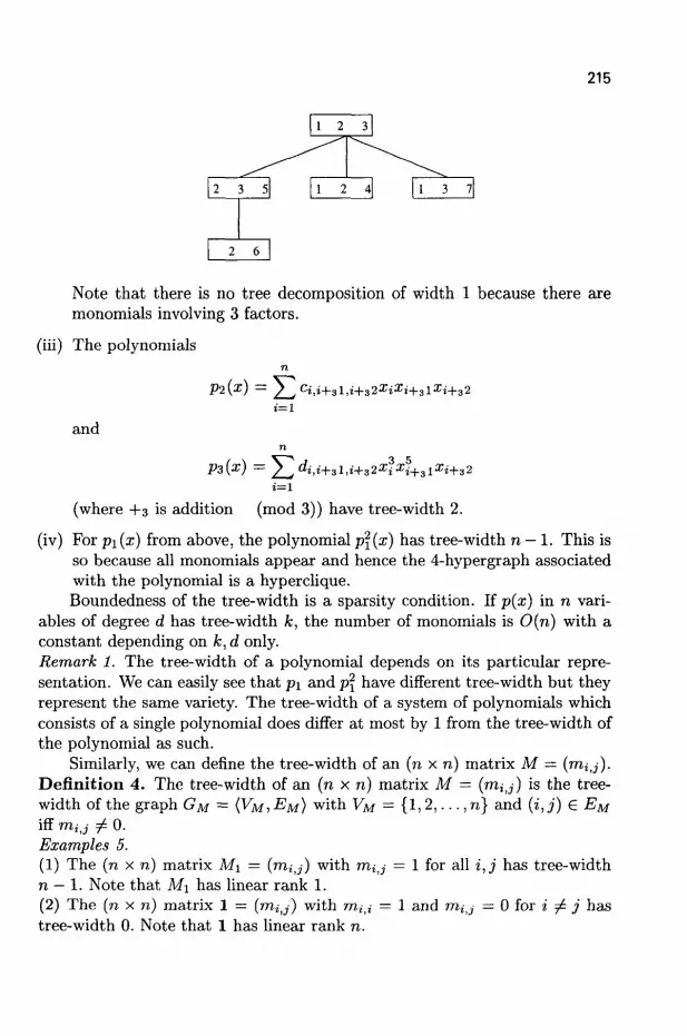
215

1 2 3

2 3 5 1 2 4 1 3 7

2 6

Note that there is no tree decomposition of width 1 because there are monomials involving 3 factors.

(iii) The polynomials n

P2^) - ^ c M + 3 l , i + 3 2 3 ^ i + 3 l x » + 3 2 i = l

and

n

i=l

(where +3 is addition (mod 3)) have tree-width 2. (iv) For pi(x) from above, the polynomial p\{x) has tree-width n — 1. This is

so because all monomials appear and hence the 4-hypergraph associated with the polynomial is a hyperclique. Boundedness of the tree-width is a sparsity condition. If p(x) in n vari­

ables of degree d has tree-width k, the number of monomials is 0(n) with a constant depending on k, d only. Remark 1. The tree-width of a polynomial depends on its particular repre­sentation. We can easily see that p\ and p\ have different tree-width but they represent the same variety. The tree-width of a system of polynomials which consists of a single polynomial does differ at most by 1 from the tree-width of the polynomial as such.

Similarly, we can define the tree-width of an (n x n) matrix M = (rriij). Definition 4. The tree-width of an (n x n) matrix M = {rriij) is the tree-width of the graph GM = (^M, EM) with VM = {1 ,2 , . . . , n} and (i,j) £ EM iff TTlij / 0. Examples 5. (1) The (n x n) matrix Mi = (rriij) with rriij = 1 for all i,j has tree-width n — 1. Note that M\ has linear rank 1. (2) The (n x n) matrix 1 = (rriij) with m ^ = 1 and rriij = 0 for i ^ j has tree-width 0. Note that 1 has linear rank n.

216

Theorem 6 (Bodlaender) . a) There is a linear time algorithm (with bad constants) which decides, given a hypergraph G whether it has a k-tree decomposition, and if yes, constructs one.

b) If a hypergraph G over n vertices has a k-tree decomposition, then one can construct in linear time a balanced 0{k)-tree decomposition of depth 0(logn). Though originally formulated for graphs, the extension of the above re­

sults to hypergraphs is straightforward. A survey of such results may be found in 8 '7.

3 Generating functions of graph properties

The first use of tree-width of a matrix was presented in 15. There the com­putational complexity of computing the permanent and hamiltonian of a matrix was studied.

Let M = {rriij} be an (n x n) matrix over a field K. The permanent per(M) of M is defined as

ir£Sn i

The hamiltonian ham(M) of M is defined as

TrGKn i

where Hn is the set of hamiltonian permutations of { 1 , . . . ,n}. Recall that a permutation •K G Sn is hamiltonian if the relation {(i,ir(i)) : i < n} is connected and forms a cycle.

In general, both the permanent and the hamiltonian are hard to compute and the best algorithms known so far are exponential in n, 4 ' n . This applies also for the computational model due to Blum, Shub and Smale (BSS model), cf. 5 . Barvinok in 2 has shown that if the (linear) rank of the matrix is bounded by r both the permanent and the hamiltonian can be computed in polynomial (not linear) time. Hence these problems are parametrically tractable in the sense of 19. Linear rank and tree-width are independent notions: The (n x n) matrix consisting of l's only has rank 1 but tree-width n — 1 (it is a clique). The corresponding unit matrix has rank n but tree-width 1, as the graph consists of isolated points. Tree-width of a matrix also makes the permanent and the hamiltonian parametrically tractable.

217

Theorem 7 (Courcelle, Makowsky, Rotics, 1998). Let M be a real(nx n) matrix of tree-width k. Then per(M) and ham(M) can be computed in time 0(n).

The same technique can also be applied to other families of multivariate polynomials such as cycle format polynomials, and, more generally, generating functions of graph properties, cf. 2 9>n .

Let G = (V, E, w) be an edge weighted graph with weights in a field K and £ be a class of (unweighted) graphs closed under isomorphisms. We extend w to subsets of E by defining w(E') = Y[e<EE' w(e)- The generating function corresponding to G and £ is defined by

GF{G,£) =def ]T{w(£ ' ) : (V,E') e £ and E' C E)

Strictly speaking GF(G,£) is a function with argument w and value in K. Furthermore, t o i s a function

w : { l , . . . , n } 2 -> K

which can be interpreted as an (n x n) matrix over K. If we view w(i, j) = Uij as indeterminates, GF(G,£) is a multivariate polynomial in K[u^j : i,j < n].

The permanent is the generating function for G = Kn, the clique on n vertices, and £per the perfect matchings. The hamiltonian, similarly, is the generating function for Sham, the class of n-cycles.

Similarly, Km>n is the complete bipartite graph on m and n vertices, Rn is the two-dimensional (n x n) grid and Cn is the corresponding three-dimensional grid.

In n the complexity of many generating functions is discussed. Among his examples we have also:

Cliques: Let £cuque be the class of cliques, which is an MS\ property. By 11, GF{Kn,£Cuque) is ttP hard (or VNP^-complete).

Maximal Clique: Let £MaxCUque be the class of maximal cliques, which is an MSX property. By 42, GF(Kn,£MaxCuque) is fP hard (or V N P X -complete).

Perfect Matchings: Let £perjM be the class of perfect matchings, which is an MS2 property. By 42, GF{Cn,£PerfM) is W hard (or V N P K -complete).

Partial permanent: Let £partM be the class of partial matchings, which is an MS2 property. By 29, both GF(Kn,£pm) and GF(Rn,£pm) are ()P hard (or VNP/f-complete).

218

The proof of theorem 7 relies on the observation that in these two (and many more) cases £ is definable in Monadic Second Order Logic. This allows us to apply techniques first used in a more restrictive framework in * and extended in 15. For more details, cf. section 5.

In 25 (n x n)-matrices M over {0,1} are considered where one knows in advance that the permanent is bounded by a polynomial, i.e. per(M) < k-nq

for some constants k, q £ N. Grigoriev and Karpinski prove that under this assumption per{M) can be computed in N C 3 , and hence in P . To the best of our knowledge no similar result is known for ham(M).

More about the complexity of generating functions of graph properties in the BSS framework can be found in 35-34.

4 Feasibility and positivity of polynomial systems

We now want to explore how far these techniques can be pushed further. We will state our main results; proofs then follow in the next sections.

Is the tree-width of a system of polynomials an appropriate tool to decide the existence of zeros?

We look at the following problems: Definition 8. Let F be a field (finite or infinite). Let i C F b e finite of car­dinality a. Let p(x) be a polynomial in F[ar] in the variables x = (xi,..., xn) of degree d and tree-width k, and E be a system of such polynomials, whose d + 1-hypergraph is of tree-width at most k.

(d, k) - FEAS¥: Does p have a zero in F"?

(d, k) - FEAS(A)F: Does p have a zero in An?

(d, k) — HNw'- Does E have a common zero in F1?

(d, k) — HN(A)F: Does E have a common zero in Anl

For F an ordered field we can also ask

(d, k) - POS¥: Is p(r) > 0 for all r € F"?

(d, k) - POS(A)¥: Is p(r) > 0 for all r e An?

If the tree-width is not bounded we write (d, oo) - FEAS(A)¥, etc. If R is an (finite, infinite, ordered) ring rather than a field, we use the analogous notation (d,k) - FEAS(A)R, etc.

219

Remark 2. The finite set A C F can be viewed as condition of zero-dimensionality. A can be encoded by an additional polynomial which has exactly the elements of A as its zeros. Such problems are considered in 39. Remark 3. The way we have set up the definitions there is a minor discrep­ancy between (d, k) - FEASF and (d, k) — HNF for systems consisting of one polynomial. We have (d, k) - FEASF C (d, k + 1) - HNF, but not necessarily (d, k) - FEASp C (d, A;) - HNF. This does not affect the results.

[d, oo) - FEASw, (d, oo) - HNF and, for ordered fields (d, oo) - POSF

are discussed in 5 '37. In general they are NPp resp. CO-NPF hard, and no subexponential algorithms are known for their solution. If we relativize the problems to (d, oo) - FEAS(A)¥ and (d, oo) - POS(A)F they are in D N P F

resp. co-DNPjr, the classes digital N P resp. digital co-NP over F. It is known that Pp C DNPp C NPp for any field F but it is not known

whether the inclusions are proper, cf. 38 '37. P r o b l e m 1. Are the problems (d, oo) - FEAS(A)u and (d, oo) - POS(A)R D N P R resp. C O - D N P F complete over the reals? Is (d, oo) - HNc{A) is D N P c complete over the complex numbers?

The problem with proving one of these questions is the following: If we mimic the original proof of N P R completeness of (4, oo) — FEASR in 10 it does not apply to (4,oo) - FEASu({0,1}) if we restrict to problems in D N P R . The reason is that intermediate results of a computation are also used as guesses. They might be reals even though the initial guesses are zeros and ones. However, some seemingly hard problems can be reduced to (4, oo) — FEASR(A) for \A\ > 2. This includes for example the real Knapsack problem and, of course, also the classical SAT problem. It is therefore reasonable considering (4, oo) — FEASR(A) to be a difficult problem in the BSS setting. Complete problems for DNPfc do exist (18).

Our first main theorem is Theo rem 9. For finite fields F of size f the problems (d,k) — FEASw and (d, k) — HNF can be solved in time 0(n) where the constant depends on k, d, / . The same holds for finite rings.

The proof exploits the finiteness of the field (ring) by making all elements of it part of the underlying logic. In this way the problem becomes a prob­lem of the weighted hypergraph of the non-vanishing monomials (with the coefficients as weights). The proof has no particular algebraic content, but shows that the notion of tree-width of systems of polynomials has surprising algebraic applications. Vardi pointed out that, using the methods of 22, the result can be sharpened a little by making it independent of the size of the finite field. Unfortunately, this does not help in the case of infinite structures,

220

cf. the conclusion section. The same technique as for the proof of Theorem 9 can also be used for infi­

nite fields like E when dealing with so called 3 - M S O R decision and evaluation problems (to be defined later on). This includes the evaluation of polyno­mials with exponentially many monomials like the permanent of a matrix of bounded tree-width and many other. We obtain Theorem 10. For R-structures of tree-width at most k, 3-MSOR-decision and evaluation problems can be solved in linear time (in the size of the struc­ture).

We next generalize the discussion of the feasibility and positivity prob­lems to infinite fields. Here it turns out that the tree-width condition alone seems not to be strong enough to allow similar results. We can afford infinite fields (or rings), but restrict the set of tuples for which we want to evalu­ate the polynomial. This results in decision problems belonging to the class D N P R . Without bounded tree-width no polynomial algorithm is know for these problems.

We then prove Theorem 11. a) For arbitrary fields F the problem (d, k) — FEAS(A)$ can

be solved in polynomial time in n where the constants of the polynomial bound depend on k, d and a condition concerning the number of different values the monomials take over A.

b) For ordered fields F the problem (d,k) — POS(A)p can be solved in poly­nomial time in n where the constants of the polynomial bound depend on k,d and a condition concerning the number of different values the mono­mials take over A. The same holds for any ordered ring R.

The condition concerning the coefficients and A basically requests that the set of partial sums of the monomials evaluated in A be bounded by a polynomial function in n.

A similar theorem can be proved also for (d, k) — PIS(A)R, systems of polynomial inequalities of polynomials of bounded degree d > 2 over an or­dered ring R.

The most general result on infinite fields in this paper is on 3 - M S O R

extended decision problems (to be defined): Theorem 12. For structures of tree-width at most k 3-MSOu-extended deci­sion problems can be solved in time 0(n-t(n)) provided the number of possible values of the subterms appearing in the formalization of the problem is bounded by 0(t(n)) where n is the size of the structure.

Finally, we discuss how the coefficient condition mentioned in Theorems

221

11 and 12 in some cases can be avoided. A kind of linearization of the positivity problem in fact allows us to strengthen Theorem 11, b). Here, by linearization we mean that the weight terms are linear in the variables. We obtain Theorem 13. For ordered fields F the problem (d, k)—POS(A)Y can be solved in linear time in n where the constants of the linear bound depend on k,d. The same holds for any ordered ring R.

5 Meta-finite Monadic Second Order Logic

In this and the next section the main mathematical ideas behind the results stated above are developed. Complete proofs are given.

Before going into details let us first outline the overall foregoing: the major point of our approach is to extend the (previously known) handling of MS2 properties over finite structures to algebraic issues, i.e. decision and evaluation problems as they naturally appear in the Blum-Shub-Smale frame­work. To this aim we consider problem instances as specific finite, relational structures together with real-valued weight functions. The latter are called R-structures in 24>27. Problems are then given as conjunction of two formulas; one is expressed in monadic second order logic MS2 over the underlying finite structure and the other is given in existential monadic second order logic over the corresponding K-structure (a logic to be defined). This generalizes the framework of Extended Monadic Second order Logic EM SOL proposed in x

and unifies it with the framework of Meta-finite Model Theory of 24. On the underlying finite structure we evaluate MS2 properties using the

Feferman-Vaught theorem. The latter is rigorously proved in the Appendix together with its use for algorithmic purposes. Those readers being not famil­iar with it are strongly encouraged to study the Appendix before continuing.

The results of this paper rely on a careful definition of the meta-finite monadic second order logic for expressing algebraic issues. It has to be strong enough to capture interesting problems; on the other hand, it must be defined in such a way that we can perform a decomposition on the meta-finite struc­ture in parallel to the one given by the bounded tree-width decomposition and the Feferman-Vaught theorem on the underlying finite structure. This will be done now.

5.1 Hypergraphs and parse trees

Let us formalize the kind of meta-finite structures and decompositions of them we are interested in. Some missing proofs are in the Appendix.

We consider problem instances as logical structures representing particu-

222

lar hypergraphs. To capture the combinatorial aspects of a problem we start with a finite relational structure (V, E, Ri,..., Re) of signature r . Here, (V, E) is a hypergraph, i.e. V := { 1 , . . . , n} for some n G N and any element of E is a (non-void) subset of V (of arbitrary but fixed arity). Every relation Ri is a subset of Vni, where rn £ N denotes its corresponding arity.

We consider (V,E,Ri,... ,Ri) as a two-sorted structure with universe V U E; by convention, there is a relation Rinc CVxE among the symbols in r which gives the incidence relation between vertices and edges. If more comfortable, we can also choose VU V2 as the two-sorted universe and include a relation RE C V2 representing the edge set, see below.

The monadic second order logic MS2(T) over hypergraphs is defined as sublogic of second order logic, where we allow quantified and free second order variables of arity 1 only. In addition, set variables range over subsets of V or E. Example 1. (cf. 1 5) . In order to give an idea about the expressiveness of the logics we are using two examples related to graph properties are studied. As we will see both can be captured by MS2 logic.

We will be very precise here concerning the logical representation of graphs as structures. Later on, we will just keep in mind how to represent (weighted) hypergraphs as logical structures without going through all the details every time. Firstly, a graph G — (V, E) is represented as a two-sorted finite structure. The universe U of this structure consists of the union of two sorts, namely the vertex set V and the set V2 of possible edges (sometimes, we also directly take E as second sort). Several relations are included in the structure whose interpretation will give the graph G. More precisely, a unary relation Ry C U is interpreted as Ry(x) •& x e V, a unary relation RE C U is interpreted as i?fi(e) O e £ £ , and a binary incidence relation Rinc is inter­preted as Rinc(v, e) -» Rv{v) A i?#(e) A v is incident with e. Thus, the graph G is represented as the finite structure (VUV2, Ry, RE,Rinc)- We can as well add unary predicates either on V or on V2 (the two sorts); for example, such unary relations might indicate labels of either the vertices or the edges.

Note that for a subset X C U we can easily express in MS2 logic that XCV (resp. X C E) by

Vx € U X(x) => Rv(x) resp. Vx e U X{x) =• RE(x) .

This will be used implicitly throughout the paper.

a) 3-Colorability: given a graph G as (V U V2, Ry, RE, Rinc) we define a MS2 formula $ as follows:

223

$ = 3 Xi C V,X2 C V,X3 C V such that P A R r ( X ! , X2 , X3) A NO-EDGEiXi) A NO-EDGE{X2)

ANO-EDGE(X3).

Here, -PART(Xi,X2,X3) is true if and only if the sets X1,X2,XZ build a partition of V, i.e.

PA JRT(X1 ,X2 ,X3) E V ^ e V (Xxiv) V X2(«) V X3(«)) A

- 3 u e V ({*i(«) A X2(u)} V {Xi(u) A X3(u)} V

{X2(u)AX3(«)})

and NO-EDGE(X) is true if and only if no two vertices in X are incident with the same edge of G :

NO-EDGE{X) = Vu,v £ V (X(u) A X(v) =» -.£;(«,w))

Clearly, G is 3-colorable iff G )= $ . In the above example we do not really need the full power of MS2(T) logic; the quantification is just extending to subsets of the first sort V of the universe. Therefore we could represent G as well as a one-sorted structure only and still express colorability. This will be different with the next example.

b) Another M52-definable property is that of being a perfect matching. This time we need set quantifiers over both sorts of the universe. Again, let a graph G being given as (V U V2, RE, Rv,Rinc)- For a subset X C V2 we want to find a MS2 formula $(X) such that {G,X) |= $(X) iff X is a perfect matching of G. Using Rinc we can either deal with an edge e G E or with the two incident vertices; just consider the MS2 formula

<p(u, v, e) = Rindu, e) A Rinc(y, e) A u ^ v

which gives the incident vertices of an edge. Having this in mind we define the formula

$(X) = Vu,v,€V{(u,v) £X=>E(u,v)} A Vw e v 3u e v {(«, v) e X v (v, u) e V] A Wu,v,w eV {((u,v) E X A (u,w) € X) => v = w}

A v«,t),tiiey{((i),u)ei A (W,U) e X)=>V = W}

which satisfies the properties we are looking for.

224

Besides the combinatorial part of our structures the use of weights in some algebraic structure (ring, field, ordered ring, etc.) has to be incorporated. To simplify our notation we assume here that weights are in the ordered field of real numbers EL Structures of this kind are particular M-structures in the sense of24'27.

Towards this aim a weight function C : E H-> R is added to the structure, thereby turning it into a meta-finite one. The ordered structure

(K, +, *, < , 1,0, — 1, r\,..., rs) is included as well. Here, the rj are fixed real constants.

We could also think about more than one weight function or weights on the vertices, but the above is sufficient for our purposes.

The properties which will be checked on such M-structures are twofold. One is combinatorial and expressed by a MS2(T) formula. The other involves the weight functions and the real number part. It is given as well as a specific monadic second order property, this time defined for the real number part of the structure.

For structures of bounded tree-width one major ingredient of our algo­rithm is a decomposition. This is first done on the underlying finite structure (the hypergraph without weights). Definition 14 (cf. 1 9 ) . A hypergraph G is fc-boundaried if exactly fc of its vertices are labelled by { 1 , . . . ,fc} (i.e. every label appears with one vertex). The labelled vertices are called the boundary 6(G) of G.

We next define the gluing operations we are interested in:

a) create : this operation creates a fc + 1 boundaried hypergraph with no edges (i.e. fc + 1 vertices all of which are labelled);

b) join : the join © operates on two fc + 1 boundaried hypergraphs G\ = (Vi,Ei) with boundary 6(Gi) and G<i = ( T ^ , ^ ) with boundary S(G2)-The graph G\ ® G2 is obtained by joining V\ and V2 in such a way that those vertices in 6(d) and <S(C?2) having the same label are identified. The vertices in V\ :— V\ \ S(G\) and those in V2 := V2 \ ^(G^) obtain an own copy. After this identification the hyperedges E\ and E2 are unified;

c) c h a n g e ^ (G) : in the fc + 1 boundaried hypergraph G labels i and j are interchanged;

d) addilij2i...ija(G') : adds an hyperedge between vertices with labels z i , i 2 , . . . , i s ;

e) ne\Vj(G) : adds a new vertex, labels it i and removes label i from the previously labelled vertex.

225

Remark 4- Later on we decompose a given structure into substructures using the above operations in an inverse manner. Note that in that situation a decomposition is not always unique. Most important for our purposes is the case where a structure G is divided into substructures A and B such that G = A® B. We fix by convention that hyperedges being made of vertices in the common boundary 6(A) = 6(B) then are only transferred to substructure A, not to B. Definition 15. Let G be a, k+1 boundaried hypergraph. A parse-tree for G is a tree whose vertices are labelled by one of the above operators such that the following holds:

- the leafs are labelled by create;

- the branch nodes are labelled by ffi;

- the other nodes are labelled by one of the other operations;

- G is the hypergraph obtained at the root after performing all the opera­tions along the tree bottom-up.

The main relation between parse-trees and hypergraphs of bounded tree-width is the following: Theorem 16 (cf. 1 9 ) . Let G be a hypergraph of tree-width at most k. Start­ing from a tree-decomposition of G we can compute in linear time w.r.t. \G\ a parse-tree of G.

A tree-decomposition itself can also be obtained in linear time according to theorem 6.

The Feferman-Vaught theorem gives information about the way MS2(T)

properties on a finite structure can be evaluated on substructures if the rela­tion between these structures are given by one of the above operations. We state it here for the join operation ffi. The proof can be found in the Appendix.

Let 21 and 03 be k +1 boundaried hypergraphs over r with universes A and B resp., and boundaries 6(A) C A, 6(B) C B,A := A \ 6(A), B := B \ 6(B). Let € := 21 © 03 be the join of 21 and 03.

Let z be an assignment of the variables in a MS2(T) formula $(x,y_,w_,X_) into the universe C of £ such that the following is true:

- z maps the variables Xi of block x_ to the set A

- z maps the variables y, of block y to the set B

- z maps the variables Wi of block w_ to the boundary 6(A) — 6(B) (recall that the two boundaries were identified). In particular, z(wi) is member of both the universes A and B.

226

Denote by ZA, ZB the assignments with ZA(X) = X D A, ZA{S) = z(s) for s e A and zB(X) - X nB,zB(s) = z{s) for s € B. Theorem 17 (Feferman-Vaught). For every MS2{T) formula V'fejM'Zi^O there are finitely many so called Hintikka formulas fci n{x,w,X) and /i2,a(y,M>,2Q such that for every T-structure £ given as join 21 © 23 and every assignment z as above we have

(£,z)\=ip(x,y_,w,X_) & 3a(%zA)\=hlta(x,w,2QA{%,zB)\=h2,a{y,w,2L)-

If if) itself is a Hintikka formula then there exist uniquely determined Hin­tikka formulas h\ and h-2 such that

(C,z)\=rP(x,y,w,X) «• (%zA) |= hi(x,w,X) A (<B,zB) \= h2{y,w,X).

5.2 MSO logic over R-structures

In order to extend the Feferman-Vaught approach to meta-finite structures we have to look for an appropriate definition of monadic second order logic M S O R for these structures. The major task is to define it in such a way that the decomposition operations of section 5.1 extend in a natural manner also to weighted structures and the M S O R formulas.

Let us inductively define terms and formulas for obtaining this monadic second order logic over weighted hypergraphs (V,E,C). In each step we first define the class of terms or formulas which will be used. Then, it is shown how the corresponding terms and formulas can be decomposed to the substructures involved. We restrict the presentation again to the © operation. For the other parse operations similar statements hold true.

Simple terms are of the following form:

- for any edge e 6 E the expression C(e) is a simple term;

- the constants r i , . . . , r s 6 l are simple terms;

- if t\ and £2 are simple terms so are t\ + £2 and t\ -ti-

Thus, simple terms are of the form pol(C(e\),... ,C(em)) for a polyno­mial pol and edges e\,..., em .

Decomposition: For a decomposition £ = 21 © 03 a term C(e) is taken over to that substructure e belongs to. Note that for e £ ?P(5(A)) by convention e appears in the second sort of the substructure 21 only. The constants can be used in both substructures. A polynomial pol(C(ei),..., C(eTO)) is evaluated on £ by first evaluating C(e;), 1 < i <

227

m (and further parts as far as possible) on the corresponding substructure and then putting together the results on C. Note that the complexity of the latter step only depends on the size of the polynomial pol, not on €.

Summation and product terms are expressions of the following form:

- for a subset U C E a summation term has the form T(U) := J3 C(e) and a product term has the form T(U) := n C( e); for

eeU e€U the empty set we can define T(0) to be any fixed real value.

- if T\(Ui) and T2(U2) are summation and product terms so are Tx(U{) + T2(U2) and Ti(tfi) • T2(U2).

Decomposition: For £ = 21 © 03 and T(U) = £ C(e) denote UA := e€U

UHEA and UB := U n EB. Then TX{UA) :== ^ C(e) and T2{UB) :=

53 C(e) can be evaluated on 21 and 03 resp. Their sum gives the result e£UB

of T on €. The same holds true for T(U) := n C(e)- Polynomials in summation or product terms are evaluated as it was explained for simple terms.

Remark 5. Note that according to our convention EA n EB = 0. Thus, there will be no hyperedge taken into account twice. We could have modeled the decomposition by including all hyperedges relating vertices from the boundary in both substructures and giving them the weight 0 in one of it. But this would raise some technical problems; for example, in a product term we would obtain the value 0 above.

M i n / m a x terms are defined as summation and product terms but using

T(U) := maxC(e) and T(U) := minC(e)

instead of Yl a n d II-

Monadic second order M S O R terms are all terms above together with terms of the following form:

- for a summation or product term of the form T(U) (not a polyno­mial in such terms!) and a MS2 formula g on the underlying finite structure the term £3 ^ (^0 is a

M S O R term;

228

- for a summation or product term of the form T(U) and a univariate polynomial pol the term £ pol(T(U)) is a M S O R term;

U,Q(U)

- for 1 < i < m let Ti(Ui) := FJ C(e) be product terms and eeUi

g(Xi,..., Xm) be a MS2 formula on the underlying finite structure. Then £ T^Ui) • ... • Tm(Um) is a MSOR term;

(uu...,Um),e(U)

- sums and products of M S O R terms are M S O R terms.

Decomposition: Let € = 21 © 05 and consider as example a M S O R term of the form £ T i ( t / i ) - . . . - T m ( [ / m ) , where all Tj are product

(U1,...,Um),e(U)

terms. The evaluation on £ uses the Feferman-Vaught theorem for g as well as evaluations on 21 and 05 as follows. W.l.o.g. suppose g to be a Hintikka formula and hi as well as /12 to be the corresponding unique formulas for 21 and 55 given by theorem 17. Let {/• := (Uij,..., Umj),j € J be those assignments with (<£,IZj) \= Q{JLJ)- Furthermore, let U_j and U_f be its corresponding decompositions for the substructures 21 and 05, see the definition of © and remark 4.

Now

£ T^C/x) • . . . • Tm(Um) = £ Tx(£/!,-) • . . . • Tm(£7mj-)

= E T x ( ^ . ) • ^(17*) • . . . • Tm(U^) • Tm(U%) jeJ

= E TW*) •... • rm(^,) • Tdu%) •... • rm(t/£.)

= ( E ^ ( [ / ^ . . . . - T ^ l M ) ) .

( E r1(£/1B)-...-rm(Oj

\C/B>2(C/B) /

where the latter equality holds because of the Feferman-Vaught theorem.

For the other types of M S O R terms the decomposition can be done in the same manner.

Remark 6. The above definition of M S O R terms probably is not the most general one. However, the reader might check the difficulties arising when

229

performing a decomposition for a term like f] ^2 C(e) or one like ILeGZ) e€u

J2 Ti(Ui)+T2{U2) where Xi and T2 are product terms. The above (UUU2),Q(UI,U2)

setting nevertheless is strong enough to capture important problems. For the other operations op £ {add^ ...j3,changeij, neun] the evaluation

of a M S O R term on a structure op(€) can be done similarly by first evaluating a corresponding term on £ and then extending the result to op(<£).

After having introduced monadic second order terms we turn to monadic second order formulas built from these terms.

Basic M S O R formulas are expressions of the form T(vi...,Vk,Ui,...,Ut)AO with A e { = , > , > } ; here, T is a monadic second order term, the Vi are elements of the universe and the Ui are subsets of E.

M S O R formulas are all basic M S O R formulas together with

- if ip(vi,..., Vk, W i , . . . , Wt) is a M S O R formula and U\,...,Uk are subsets of E, then g(Wl7... ,Wt) = A ^fa,.. .,Vk,Wi,... ,Wt)

Vi£Ui

is a M S O R formula;

- i f ip(vi,...,Vk,Ui,...,Us,Wi,...,Wt) is a M S O R formula and g(yi,...,Vk,Ui,...,Us) is a MSOL(T) formula then <KW!,...,Wt) = A ^(v,U,Wu...,Wt) is a M S O R for-

V,U_,Q(V,U)

mula (for Wi C E);

- the closure of the above construction scheme under logical conjunc­tion, disjunction and negation gives the set of M S O R formulas.

3 - M S O R (Existential monadic second order logic) over E-structures is ob­tained from M S O R logic by defining

- all formulas in M S O R to belong to 3 - M S O R

- if 4>{Wu...,Wt) € 3 - M S O R then 3Wu...,Wt il>(W!,...,Wt) € 3-MSOR.

The problems considered in this paper are of the following type:

Decision problems: For a fixed MS2 formula ifj, decide whether Q (= ip.

Evaluation problem: For a fixed M S O R term T, compute its value over Q.

230

Extended decision problem: Given a MS<2(T) formula if) as well as a 3 - M S O R formula $ we want to decide whether Q |= ip A $.

Optimization problems: These are like the extended decision problems, but with $ quantifier free, but possibly involving the functions max and min.

For other fields F the definition of 3-MSOp is done on a similar way.

6 Proofs

After clarifying the above way to define 3 - M S O R logic by dealing with some examples we will turn to rigorous proofs of the theorems stated in section 4.

6.1 Guiding examples

Let us consider some examples and the way they fit into the formal setting of the previous section. Example 2. The generating functions of section 3

GF{G,S) =def ^{w(E') : (V,E') € £ and E' C E}

with £ MSOL-definable by ip{E') can be written as a Monadic Second Order Term

E n i>{E')/\E'CEeeE'

Hence they are 3-MSOR-evaluation problems. Example 3 (#4-FEAS(A)). In order to formalize the #4rFEAS(A) problem as an 3 - M S O R extended decision problem we use the representation of degree 4 polynomials as given in 27: let V = { 0 , 1 , . . . , n}, E := V4 and C : E -> E be a weight function giving the coefficients of / in the following sense: for (i,j,k,l) € E the value C(i,j,k,l) is the coefficient of the monomial Xi • Xj • Xk • xi in / . Note that here we assume / to be homogeneous of degree 4. Later on / is dehomogenized by adding the condition xo '•= 1.

Let A~ {si,..., sTO}; for every 1 < i < m define a function Wi : V —> A such that V x g V Wi(x) := s,. We are looking for disjunct subsets Ui,..., Um

m of V such that the following holds: \J Ui =V and if we assign to every x £Ui

i=l the value Wi(x) = s* then this assignment of variables gives a zero of / .

231

For any quadruple A = ( E I , £ 2 , £ 3 , £ 4 ) where e, 6 { 1 , . . . , m} define the set Ex := En (UEl x US2 x US3 x UeJ (i.e. a point a = (ai,a2,a3,ai) e V4

belongs to i?,\ iff every component <*» lies in USi). For a € £ A the corresponding monomial C(a) • xa gives the value C(a) •

sEl • s£2 • s<r3 • sE4 under the above assignment. The MS2{T) formula for #4-FEAS{A) simply is

if) = 3Ui, ...,UmCV such that Vi,j £ { 1 , . . . , m ^ n t / , = 0A[/1U.. .UUm = V

(note that m is independent of the structure). The real number part of the logical description is $ = J2 T(E\) —

A€{l,...,m}4

0 , where T(E\) := ^ C(a) -se i -s£2 -s£3 -s£4 is a summation/product term.

Again note that m is independent of the structure; hence, the same is true for the size of the first sum above. For dehomogenization one can introduce a further subset Uo CV which only consists of the element 0 and put SQ :— 1. It follows that / has a zero in A if and only if (V, E,C) (= ip A $.

Note that over a finite field F this logical description works as well taking A :— F, but could of course be simplified. We used the above description in order to cover already the infinite field case we are interested in later on.

In a completely similar fashion the feasibility of polynomial inequality systems 2-PIS(A)u fits into the framework of 3 - M S O R extended decision problems and (d, oo) — POS(A)f can be coded as an optimization problem. If the ring (field) is finite the coding yields an 3 - M S O R decision problem. Example 4- Another example fitting into the framework is the computation of the determinant of a square matrix A € Rnxn (whose computation is not that interesting in its own but in relation with more complicated problems like, for example, the linear programming problem). It can be expressed as a M S O R term as follows.

Since A is not necessarily symmetric we represent it as a directed weighted graph (G,c) with vertices V := { l , . . . , n } . The weight function c : V2 -» M. for (i,j) € V2 gives the value c(i, j) := aij. This implies that in the model theoretic representation of A we use a vocabulary r with two incidence rela­tions i?i,i?2 instead of Rinc (and the obvious meaning: R\{i,e) & i is the start node for edge e). Moreover, we include a linear order < o n V (with the same interpretation as the natural order 1 < 2 < . . . < n). The interested reader might try to define such an order in MS2 logic.

In the first step we now define a formula PERM(U) such that (G,II) (= PERM(U) iff IT C V2 is a permutation of V (where (i,j) € II stands for U(i) = j). This formula can easily be written down in MS2 logic.

232

Secondly, for a permutation II we define the set INV(IV) C V of its inversions by

i e INV(IL) <s> 3j e y : (i,j) e n A i > j .

Here, we use the linear order on V. Thirdly, we need two product terms T\ and T2; the first is defined on subsets U of V :

Ti(U) := H(-l) (andT1(0):=l); i€U

the second is defined on subsets II of V2 (the second sort of the universe)

r 2 ( n ) : = J ] C(*.J')-(»,j)en

If now £>([/, II) is the MS 2 formula expressing

g(U,U) = U CV A UCV2 A U = INV(U.) A PERM(U)

we obtain the determinant of A as

DET(A) = J2 ri(^)-r2(n) c/,n,e(t/,n)

which is a MS OR term according to the definition of section 5.2. Although the determinant of a matrix can be computed quickly, the ex­

ample can be modified, such as to include the permament and other matrix functions, which are # P hard to compute, cf. 15.

We will now turn to the proof of Theorem 9.

Proof of Theorem 9: We restrict ourselves to the case (4, A:) - FEASr. The other cases can

be treated in the same way. Let the input polynomial be represented as in example 3 by a structure 2) = (V, E, C) of tree-width at most k and size n; let V and $ be the corresponding MS2 and 3 - M S 0 F formulas.

Perform the Feferman-Vaught decomposition of 2) and i/> according to theorem 17. Suppose ip to be a disjunction V /i7 of Hintikka formulas h7. We

7 check for each of it whether 2) |= /i7 A $ holds. With respect to the MS2 formulas /i7 we do this as shown in the Appendix: We precompute all triples of Hintikka formulas of a given quantifier rank and number of variables which are linked by the Feferman-Vaught theorem according to the gluing operation ©. The corresponding tables are precomputed as well for the other operations. Climbing up the parse tree for D by looking into these precomputed tables we check in linear time whether D |= /i7 .

233

For the 3-MSOp formula $ we proceed as follows: first, we decompose the MS2 formulas involved in $ in the same way using Theorem 17. Next, we begin the evaluation at the leave structures of the parse tree for 2). Since all of them have a universe of size at most k we can use a brute algorithm which evaluates the corresponding M S O R terms for the leave structures by consider­ing all possible choices for second order variables. This takes exponential time only in the fixed parameter k. We store the computed results in order to use them again on the further structures appearing when we glue substructures and climb up the parse tree.

Note that there are at most |F| many different subresults, i.e. a constant number.

We continue along the parse tree until the root, representing 2), is reached. We check the possible results of the evaluation (which are at most |F| many) and decide whether 2) f= /i7 A $ for all 7. Climbing up the tree according to the decomposition has running time 0(n).

A technical problem appears during the evaluation of MSOp terms. Here, joining two substructures 21 and 03 and identifying their boundaries makes it necessary to consider only assignments treating the boundary elements the same in 21 and 53. If we decompose a structure top down that's of course no problem. But in the above algorithm we compute bottom up. Suppose we want to evaluate a term ^Z ^(10 o v e r 2t © 05 using the Feferman-Vaught

theorem. Suppose furthermore w.l.o.g. Q to be a Hintikka formula and

(2l©03,t/) |= Q{X) & (%UA) \= h(X) A (05,UB) \= h2(X) .

If we evaluate bottom up then only assignments ^ , t / B can be combined which give the same pattern for elements in the boundary of the two struc­tures. That is, only if Vx e 5{A) = 8{B) and Vi e { 1 , . . . , m} x £ Uf- <=> x € Uf. This control can be organized either by enlarging the vocabulary or by keeping track of the possible patterns arising when checking which boundary elements belong to which of the {/*. Because at every step there are only k +1 boundary values this bookkeeping does not effect the overall linear running time. •

For decision and evaluation problems even over infinite fields the above proof can be adapted as well:

Proof of Theorem 10: Let £> = (V, E, C) be a E-structure of bounded tree-width. If we are

dealing with decision problems we just have to check the validity of 2) |= tp for a M52-formula ip. We do that in the same manner as explained in the proof of Theorem 9. If a M S O R term T has to be computed over 2), on every

234

substructure of the tree decomposition we evaluate that term corresponding to the decomposition of T; climbing up the tree we combine the two values computed at the two substructures to obtain the value on the joined structure. This needs constant time for every substructure in the decomposition. •

6.2 Extended decision problems over infinite fields

If we consider extended decision problems like the feasibility problem over infinite fields there arise some problems with the tree decomposition approach.

The first observation is that in 3 - M S O R logic we cannot quantify over the real numbers. Thus, at first sight it is not clear whether the existence of a real zero of a polynomial can be expressed in this logic. We therefore restrict ourselves to ask for zeros the components of which belong to a fixed finite subset A C K (cf. Remark 2). Nevertheless, there are still many interesting and potentially hard problems captured in this situation, recall the discussion in section 4. Furthermore it turns out that for some problems we have to require an additional condition on the values of the weight function. The necessity of such a condition will become evident in the proof of Theorem 11. A precise definition is then provided after it.

Proof of Theorem 11: We again restrict to the case (4, k) — FEAS(A) and the representation of

an input polynomial by 2) = (V, E, C) as in Example 3. Let rp and $ be the corresponding formulas in MS2 and 3 - M S O R . The decomposition of 33, ip and $ is done as in the proof of Theorem 10. The same is true for checking 2) |= hy

for at least one of the Hintikka formulas ip decomposes into. The validity of an additional condition has to be required when climbing up the parse tree in order to evaluate M S O R terms in $. The number of different intermediate values which are taken by the MSOp terms during the evaluation process has to be bounded by a polynomial in the size of the input-structure.

Note that in the current situation this condition is satisfied if the set of partial sums of the monomials evaluated on the finite set A is bounded by a function in 0(p(n)) for p a polynomial. This is true because the decomposition of $ according to the definition of M S O R logic in the previous section implies that the M S O R terms evaluated on substructures of the input polynomial precisely are such partial sums.

At the root of the parse tree we check all possible results of the evaluation, which are now polynomially many. The rest of the proof again works as the one of Theorem 9.

The proof of part b) works precisely the same. Instead of checking whether at least one result is zero we only have to check the positivity of all results

235

(which are at most polynomially many). D

The above proof substantiates the interest in the following condition on a meta-finite structure 2) together with a MS2 formula ip and a 3 - M S O R

formula $ : Definition 18. Let p be a polynomial and ID,I / '>$ as above. The triple (?D,ip, $) satisfies the "coefficient condition" w.r.t. polynomial p if the num­ber of intermediate results of M S O R terms which have to be evaluated when applying the above algorithm is bounded by p(size('D)).

In some situations we will restrict ourselves to structures 2) of bounded tree-width which in addition satisfy the coefficient condition with respect to a given polynomial and the decision problem D (= ip A $ we are interested in.

Let us comment on the coefficient condition. Since it depends on V and $ as well as on the used algorithmic implementation of the Feferman-Vaught theorem it might be possible to strengthen the results by carefully considering the formulation of a problem and the evaluation process. However, this might result in quite complicated conditions. For example, consider the proof of theorem 11. Instead of dealing with all partial sums of monomials it would actually be sufficient to take into account only those appearing along the de­composition. Nevertheless, it seems to be more practical to look for sufficient conditions like the one mentioned in the proof.

It is not always obvious whether the additional coefficient condition on the partial sums of a polynomial implies a real restriction. For an example like the real Knapsack problem (given n real numbers xi,...,xn, is there a subset S C { 1 , . . . ,71} s.t. ^2 Xi = 1) it implies a serious restriction because

i€S under the additional hypothesis that all sums ^ Xi only take polynomially

ies many different values the problem lies in PR. On the other hand, if we re­duce a problem like 3-SAT to an instance of 4 - FEAS({0,1}) the coefficient condition is automatically fulfilled because of the lemma below. Thus, in re­lated situations our approach gives linear algorithms on structures of bounded tree-width without any additional assumption on the weights. Lemma 1. Let q be a polynomial, i c l " finite and d 6 N. Then for all poly­nomial functions / : I " -> I 0/ degree d which only have integer coefficients in {—q(n), —q(n) + 1 , . . . , q(n)} the number of different values for the partial sums of the monomials of f if evaluated on A is bounded by 0(N • q(n)). Here, N is the number of non-zero monomials in f.

Proof. For fixed degree d the normalized monomials £;, • . . . • Xid, i\,..., id €

236

{ 1 , . . . , n} of / only take polynomially in \A\ many different values if evaluated in elements of A. Let S be the set of these results. Each value in S is multiplied by the sum of the coefficients of those monomials actually giving the value (or by 0). Since the number of monomials is bounded by a N (which itself is bounded by 0(nd)) every such sum gives an integer in {—q(n)-N,..., q(n)-N}. Thus, there are only polynomially many different possibilities to multiply one of the finitely many elements in 5 by a particular sums of the coefficients. The assertion follows. •

Recall that in particular for polynomials of bounded tree-width the num­ber of non-zero monomials is linear in the variable number.

From the previous proofs it should be clear that Theorem 12 summarizes the general way for obtaining polynomial time algorithms by exploiting the above methods. We therefore omit its proof.

6.3 Getting around the coefficient condition

For some of the problems studied above it is possible to avoid the coefficient condition over infinite fields. The ideas are already present in 1 (in an au­tomata theoretic framework) and 14 (in a logical framework). Therefore we just outline how some of these problems can be putted into their framework.

The problems we can handle that way have to be optimization problems where the objective function has a linear structure. In the framework of weighted hypergraphs 2) = (V, E, C) linear structure means that we want to compute

s

min y~]at • \Xt\ , where X_ = (Xi,X2,. • •,Xs).

Here, <j> is a MS2 formula and |Xt| is an abbreviation for Yl C(e).Insuch e€Xi

a situation analyzing the Feferman-Vaught theorem for all of the parse opera­tions shows that the special linear structure of the evaluation term (which is a MS OR term according to our definition) allows to compute the minimum (or maximum) of a E-structure obtained after applying a parse operation in con­stant time from the corresponding extremal values on the substructure (see 1 , x 4 ) . In particular, we do not have to store too many intermediate results. This ideas can be applied to the POS(A) problem: Theorem 10. For ordered fields ¥ the problem (d, k)—POS(A)-p can be solved in linear time in n where the constants of the linear bound depend on k, d.

237

Proof. We restrict ourselves to proving how (d, k) — POS(A) can be expressed as a linear optimization problem in the above sense. The linear algorithm can then be obtained by the algorithm given in the proofs of Theorems 9 and 11 and the above remarks.

Let A := {s%,..., sm} C K and 2) = (V, E, C) be a M-structure represent­ing a polynomial f in n variables of degree d. Obviously, f(x) > 0 Va; £ A" iff min{/(a;)|x £ A71} > 0. We enlarge 2) by d incidence relations Ri,... ,Rd C V x E having the interpretation Ri(j,e) •& the i-th factor in monomial e £ E is Xj. Note that for this enlarged structure the tree-width concept and the Feferman-Vaught approach work similarly as before.

In order to make the problem linear we consider all (at most md many) values a i , . . -amd which can be obtained from A by multiplying d elements. The at thus give possible values of a monomial (with coefficient 1) if an as­signment from An is chosen.

For any at there is a set tyt of finitely many patterns in { 1 , . . . , m}d such that for every (ki,..., kd) £ tyt we have s^ • • • • • Sfcd —at- Now consider md

subsets Xf C E. The intended meaning of the MS2 formula <f>(Xi,..., Xmd) we want to be fulfilled on 2? is a decomposition of all monomials in E into sets Xt such that there is a minimizing assignment which for every monomial e £ Xt gives the value at, 1 < t < md. Thus

</>(*!,..., Xma) = 3U1,...,UmCV,\)Ui = V, all disjoint

A VI < t <md V i i , . . . , i d € V :

if e £ Xt and Ri(ii,e) A . . - A Rd(ia,e) then (ii,...,id) £ Vt

If (2), X) |= 0(20 then there is an assignment ( f / i , . . . , Um) for a^, . . . , a;n

from A™ which is compatible with 2£ in the sense that for every monomial e € Xt the assignment given by the U, yields the corresponding value at.

Finally, the linear objective function to be minimized is Yl at • 2 C(e)- n

t = l eeXt

7 Conclusions and further research

We have shown how the concept of tree-width of multivariate polynomial systems can be used in finding polynomial time algorithms for some other­wise difficult computational problems provided the tree-width is bounded by a constant. The method has further extensions to linear and quadratic pro­gramming, previously analyzed in 36. This will be worked out in a future paper.

238

Our proofs use a detour through logic. An alternative route would be through automata theory, as in 1. But automata theory and Monadic Sec­ond Order Logic are just two faces of the same definability phenomenon, cf. 17,16,41

Using the methods developed in 21-22-31 theorem 9 can be improved to Theorem 19. For finite rings R of size r, (d, k) — FEASR and (d, k) — HNR

can be solved in time 0(n • r) where the constant depends on k,d. The point is to view feasibility of systems of polynomials over finite struc­

tures as constraint satisfaction problems. However, this method does not give improvements for infinite structures.

Another direction of further research is the restriction of our feasibility problems to finite subsets A for the components of possible zeros.

Using very effective versions of quantifier elimination over the reals R one might ask: Problem 2. Can K (d,k) - POSR and (d,k) - FEASR be solved in time 0(n) over the reals, where the constant in 0(n) depends on k,d only?

For the best known algorithms to solve (d, oo) — FEASR and for quantifier elimination the reader should consult the surveys 9>40'3.

It remains a challenging problem to find direct algebraic proofs and to overcome the limitations imposed by our coding technique.

8 Appendix

In this Appendix we want to give a rigorous presentation of the results used in the previous sections. This will make the paper self-contained; though well-known to logicians people in complexity theory of algebraic problems might not be that familiar with the Feferman-Vaught theorem. However, a lot of different results and concepts have to be put together which to our knowledge are hard to find at a single place in literature. So even for readers familiar with the background we believe it might be useful having all this available in an Appendix.

Moreover, we adapted the proofs to the framework in which we need the corresponding statements.

8.1 MSO logic over finite structures

We suppose the reader to be familiar with the notions of a finite structure and second order logic SOL over a given signature (see 2 3) . the finite structures we are interested in are hypergraphs. These are two-sorted structures the

239

universe of which consists V and E, the vertices and hyperedges respectively. In addition, there is one binary relation symbol Rinc for the incidence relation between edges and vertices. (This relation is not always needed, for example when dealing with the zero-existence problem for a polynomial). In case E is the set of edges of a directed graph we might also include 'another binary relation in order to distinguish the direction of an edge. Furthermore, we allow an arbitrary but finite number of constant symbols and unary predicate symbols. In MSO logic the set variables range over subsets of V or E only. We denote the vocabulary by r and the MSO logic over r by M52(r) (the index "2" indicates the two sorts), see also 15.

8.2 Hintikka formulas; the Fraisse-Hintikka theorem

Fix a relational, finite vocabulary r as above and consider the monadic sec­ond order logic M52(r) over r . In MS2(T) we are interested in formulas with first-order variables among x\,..., xni and second-order variables among X\,..., Xn2. Later on it will be convenient to split the block x\,..., xni into further blocks.

Proviso: In order to avoid confusion by mixing too many things we reduce our description of theorem 20 and 17 to MS2(T) formulas with free first order variables for vertices only and free second order variables for subsets of vertices.

However, it should be clear from the presentation that a generalization including the edges as second sort of our structures is straightforward from that.

Let n := ni + ni- We denote by F£r the set of MS^ir) formula with n variables and quantifier rank at r (the quantifier rank is the maximal number of nested quantifiers in a formula). Theorem 20. Let r be a signature. For each r, n € N we can effectively find a finite set Hn,r °f unnested formulas in F^r such that the following is true:

a) for every r-structure 21 and for every tuple {a,M_) := ( a i , . . . , a n i , M i , . . . , M„2) ; where the a,i are elements of the finite universe A of 21 and the Mj are subsets of A there exists exactly one formula 6 € Hn<r such that (21,a, M) \= 8(a,M).

b) For every r £ N and every un-nested formula <j> € F„ r there is a disjunc­tion hi V . . . V hm of formulas hi £ Hn<r which is equivalent to 4> for any T-structure. The hi can be computed effectively.

240

Proof. We follow closely 2 8 , where this theorem is established for first-order logic.

Ad a) We define the sets Hn,r recursively with respect to the parameter r. First, consider all unnested atomic formula in n variables. There are only finitely many such atomic formulas, say tpi,..., ips. Define Hn£ to be the set of all formulas

v r A ... A i>f-, where a* £ {0,1} and ip° := _ |V'>^1 : = ip- Obviously, 21 together with a tuple (o, M ) satisfies either ipi or ->ipi (of course, we regard only those formulas with the same shape of variables as (a,M_)). Thus, (21, a, M ) satisfies exactly one of the formulas in Hnfl-

Now let the set H^r be defined for a l H e N according to the assertion of par t a) . In particular, suppose the set Hn+i,r to consist of formulas # i , . . . , 8m. Define the set Hn<T+i as follows:

First, divide Hn+i>r into a par t H^+1 r where the n + 1-st free variable is first-order and a pa r t H^+lr where the n + 1-st free variable is second-order. T h a t way one obtains two disjunct index sets Ii,l2 such tha t I\ U h = {1, • • •, m } . We consider two ways to define formulas in MS2(T) with n variables and quantifier rank r + 1 from those in H^+1 r and in H^+1 r :

for any nonempty subset X C Ii build the formula

/ \ 3 a n + 1 e A 9i(a,M_,an+i) A \Jan+1 € A 3i € X 9i(a,M_,an+i) . (1) iex

Accordingly, for any nonempty subset X C I2 build the formula

f\ 3Mn+1 C A 0 i ( o , M , M „ + i ) A y M „ + 1 C A 3i e X 9i(a,M,Mn+1) .

iex (2)

Now, combine any formula of type (1) with a formula of type (2) by conjunction. This gives for any pair (X, X) the formula

f\ 3a„+i G A 0i(a,M_,an+1) A \/an+1 € A 3i e X 9i(a,M_,an+1) f\ iex

<

f\ 3Mn+1 C A 0i(a,M.,Mn+i) A y Mn+1 CA3ieX ^ ( o , M , M „ + 1 )

' iex

(3)

241

where X CIX and X C J2 and not both of them are empty.

Consider a structure 21 over r and assignments ai,...,ani € A , M i , . . . , M n 2 a .

For every o n + i € A the induction hypothesis yields the existence of a formula 9io € H\+lr such that (2 l , a ,M,a n + i ) (= 0 j o (a ,M,a n + i ) . Define X C 7X as the set of all indices i £ 7i such that there is a a„+ i € A with (21, a, M j^n+i) f= Si{a,M_,an+i). Similarly, for every Mn+i C A the in­duction hypothesis yields the existence of a formula 9j0 E H%+1 r such that (21,a, M_,Mn+i) (= ^ 0 ( a , M , M „ + i ) . Define l c / 2 a s the set of all indices i 6 h such that there is a M n + i C A with (21, o, M, M„+i) |= 9i(a,M_, Mn+i). Now it is easy to see that (21, a, M) satisfies exactly that formula built accord­ing to rule (3) in which the sets X and X are chosen as explained above. This gives claim a).

Ad b) Again via induction over r : For r = 0 let tp be a quantifier free formula in MS2{T) with n variables; tp is a disjunction of conjunctions of atomic formulas. Let Qi A . . . A Qt be such a conjunction; consider all elements 6 £ Hnfi containing the Qi in exactly the same form. Now, Qi A . . . A gt is equivalent to the disjunction of all the 0's chosen above. The formula ip itself then is equivalent to all the corresponding disjunctions.

For the induction step from r to r + 1 we assume the set H„+lr to be {#! , . . . , 8m}. Without loss of generality let (j> = 8\ V . . . V 6S (i.e. we assume the n + 1-st variable to be a set-variable). Consider the formula

<P(x,Y) :=3Yn+1 cf>(x,Y,Yn+1) .

In order to express tp as a disjunction of formulas in Hn^r+1, among the for­mulas in (3) take all those where X is the empty set and X C I2 contains at least one index in { 1 , . . . , s}. This gives a new set of formulas

9i,...,9g € Hn,r+i. (4)

Claim: V = ^ " i V . . . v 4

To prove the claim suppose (21,x,Y_) (= 9i(x_,Y_) V . . . V 9s(x_,Y_) holds. Then there exists a formula, say 8\, such that (21, x, Y_) (= 9\ (x, Y_). According to rule (3) we find a set X containing an element IQ £ { 1 , . . . , s} and

( a , T , y ) N A 3 Y"+! Si(x,y,yn+i)-

242

In particular, we obtain (%i,x_,Y_) \= 3 Yn+i Oi0(x_,Y_,Yn+i) which implies (*,£,£) N V'feZ)-

To show the opposite, assume (2l,z,H) |= V'felQj s a y

(a, &10 N 3 M „ + 1 ^ ( X , F , M „ + 1 ) .

We define X as set of all those indices i £ { 1 , . . . , m} for which #j 6 H^+1 r

as well as (%L,x,Y_) (= 3 M n + i #i(£,H, Mn+i). According to the definition we get ii 6 X; thus, the formula obtained by choosing our particular X together with X = 0 in (3) belongs to the formulas under (4), which immediately gives the reverse direction.

If ip has the shape VMn+i <f>(x,Y_, Mn+i), for building the corresponding set of formulas in (4) consider all choices X C { 1 , . . . , s}.

If ip is obtained by quantification of a first-order variable xn+\ the proof works similarly after replacing X by X and the formulas in H%+1 r by those in Hi+l iP . ' n

Remark 7. In the above proof there are several ways to obtain a conjunction of atomic formulas which is false over any structure with an equality relation, for example by including x ^ x for one or several variables. By convention, we include only one such formula into each of the sets Hnfi. This will be needed later on in order to avoid ambiguities.

8.3 Parse-trees for hypergraphs of bounded tree-width

Let G be a hypergraph of bounded tree-width k. Our goal is to create G from some elementary hypergraphs by applying finitely many operations to the latter. The initial hypergraphs will be structures of size at most k. The operations have to be chosen carefully in order to guarantee validity of the theorem by Feferman-Vaught.

The hypergraphs in-between the building procedure of G all are (k + 1)-boundaried hypergraphs in the in the sense defined in section 5. The following example shows how the decomposition of a hypergraph of tree-width k into (k — 1) boundaried hypergraphs works. Example 5. We consider once again the polynomial p from Example 3, ii). Starting with a tree decomposition of p the latter is first turned into a binary tree. To this aim branch nodes are simply duplicated sufficiently many times. By adding further nodes to those subsets Vt with cardinality less than k + 1 (without destroying the tree decomposition requirements) we can assume all sets Vt to be of cardinality k + 1. Furthermore, by duplication once again branch nodes every branch has identical children. Finally, including additional

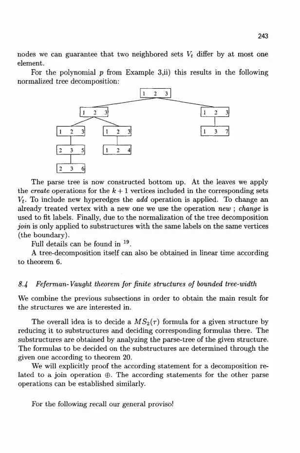
243

nodes we can guarantee that two neighbored sets Vt differ by at most one element.

For the polynomial p from Example 3,ii) this results in the following normalized tree decomposition:

The parse tree is now constructed bottom up. At the leaves we apply the create operations for the k + 1 vertices included in the corresponding sets Vt. To include new hyperedges the add operation is applied. To change an already treated vertex with a new one we use the operation new ; change is used to fit labels. Finally, due to the normalization of the tree decomposition join is only applied to substructures with the same labels on the same vertices (the boundary).

Full details can be found in 19. A tree-decomposition itself can also be obtained in linear time according

to theorem 6.

8.4 Feferman- Vaught theorem for finite structures of bounded tree-width

We combine the previous subsections in order to obtain the main result for the structures we are interested in.

The overall idea is to decide a MS 2 (T) formula for a given structure by reducing it to substructures and deciding corresponding formulas there. The substructures are obtained by analyzing the parse-tree of the given structure. The formulas to be decided on the substructures are determined through the given one according to theorem 20.

We will explicitly proof the according statement for a decomposition re­lated to a join operation ©. The according statements for the other parse operations can be established similarly.

For the following recall our general proviso!

244

Let 21 and 03 be k + l boundaried hypergraphs over r with universes A and B resp., and boundaries 6(A) C A, 6(B) C B,A : +A \ 6(A), B := B \ 6(B). Let <t = 21 © 03 be the join of 21 and 03 as explained in subsection 8.4.

Let z be an assignment of the variables in a MS2 (T) formula $(«, y_, ui, X_) into the universe C of £ such that the following holds:

- z maps the variables xi of block x to the set A

- z maps the variables yi of block y to the set B

- z maps the variables Wi of block w; to the boundary 6(A) = 6(B) (recall that the two boundaries were identified). In particular, z(wi) is member of both the universes A and B.

Denote by ZA, ZB the assignments with ZA(X) = X f) A, ZA(S) = z(s) for s £ A and zB(X) = I f l B,zB(s) = z(s) for s £ B.

Then the following is true Theorem 21. Let € be the join of 21 and 03 : € = 21 ©05 and let h(x,i,w_,X_) be a MS2(T) formula which is a Hintikka formula in some HHtr(x^,y,ui,2C). Then there are unique Hintikka formulas hi(x_,w_,X) G Hn,r(x.,Ul,]Q and h2(y,Ul,X_) £ Hn,T(y,ui,X) such that for every assignment z as above we have (€,z)\=h(x,y,w,T) ^ (%zA) \= hx(x,w,X_) A (03,zB) \= h2(y,w,X_).

Proof. Induction on the quantifier rank r of h:

r = 0 : According to the proof of theorem 20 the quantifier free Hintikka formula h

is a conjunction of all atomic formulas (where the latter appear either negated or not). We indicate with some examples how hi and h2 are being built given these parts in h:

i) suppose an atomic formula xi = yj appears unnegated in h. Then (£, z) \£ h because z assigns different values to Xi and yj. This holds independently of € . We are therefore done by including in hi (or in h2) an atomic formula x ^ x which is always false as well (according to the uniqueness condition mentioned in remark 7).

ii) Suppose an atomic formula Wi ^ Wj appears in h. Then we include it both in h\ and in h2. A formula like Xi ^ Xj is only included in hi, similarly for variables from the block y and h2.

iii) For a unary relation flinra formula R(xi) is maintained in hi, whereas R(yj) is transferred to h2- An atomic formula R(u)i) will again be both present in hi and in h2.

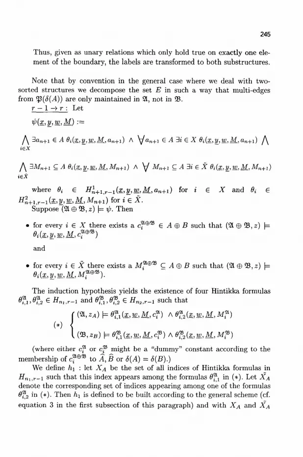
245

Thus, given as unary relations which only hold true on exactly one ele­ment of the boundary, the labels are transformed to both substructures.

Note that by convention in the general case where we deal with two-sorted structures we decompose the set E in such a way that multi-edges from ty(5(A)) are only maintained in 21, not in 05.

r - 1 -> r : Let

f\ 3an+i G A 6i{x,y_,w_,M.,an+1) A \/an+1 G A 3i € X 0i(z,|/, w, M,a n + i ) f\ tex

f\ 3Mn + i C A 6i{x,yJ,w_,M_,Mn+1) A \J Mn+1 CABieX 9i(x,y,w,M.,Mn+1) tex

where 9t £ H^+lr_1(gc_,y^,w_,A£,an+i) for i € X and 0» € Hl+i,r-i(x,y,w,M,Mn+1) for i e X.

Suppose (21 © 03, z) |= V- Then

• for every i £ X there exists a cf®® £ A® B such that (21 © 03, z) |=

and

• for every i € X there exists a Mf®* C A@B such that (21 © 03,z) j= ei{x,y_,w,M,Mf®*).

The induction hypothesis yields the existence of four Hintikka formulas C i ' ^ 2 e ffm.r-i and 0£,0j?2 G ffna,r-i such that

|- (21, ) \= 6?tl (x, w, M, cf) A 6*2(x, w, M, M?)

(*) < I (58,zB) |= e^(x,w,M,cf) A 6\» (£,«;, M , M f )

(where either cf or c® might be a "dummy" constant according to the membership of cf®® to A,B or 6(A) = 5{B).)

We define /ii : let XA be the set of all indices of Hintikka formulas in i f n i j r - i such that this index appears among the formulas 6fx in (*). Let XA denote the corresponding set of indices appearing among one of the formulas 6f2 in (*). Then hi is defined to be built according to the general scheme (cf. equation 3 in the first subsection of this paragraph) and with XA and XA

246

as the chosen index sets. Formula /12 is given in the same manner. It's now straightforward to check that hi and /J2 satisfy the requirements. D

The theorem together with finiteness of Hn,r implies that there are only finitely many triples € = 21 © 05 with respect to the uniquely determined Hintikka formulas. The same is true if we allow parameters.

The Feferman-Vaught theorem generalizes the previous theorem by get­ting independent of the particular structures involved. It can be proved now as follows:

Proof of theorem 17: According to theorem 20 I/J is equivalent to a disjunction #1 V . . . V 9S

of finitely many Hintikka formulas. For each 0j there exist finitely many triples (6i,h{,hJ

2),j £ Ji,\Ji\ finite such that for given structures € = 21 © 53 theorem 21 is true for exactly one .;' G Jj . If C, 21,23 are varied then (£ |= 6i iff V 21 |= hi A 53 (= h2- The formula ijj itself is equivalent to the disjunction

j€Ji s V V 21 |= hi A 53 |= h2. This gives the formulas h\,a and h2,a-

n

i=ijeJi

8.5 The algorithm

The Feferman-Vaught theorem holds also true in a corresponding way for the other parsing operations introduced above. It is true as well for other classes of parameters like the clique-width of a graph and its corresponding graph operations, see 15.

It is then used for computational purposes as follows. Given a MS2(T)

formula xp € F„i7. we precompute a table of all Hintikka formulas in i7„?r and how three of them fit together with respect to the Feferman-Vaught theorem for all the parsing operations. The formula ip is written in its equivalent form as disjunction of Hintikka formulas, say ip = 6\ V . . . V 6S.

Now, given a structure of bounded tree-width we first construct its tree decomposition and the corresponding parse tree according to theorems 6 and 16. From the precomputed table of Hintikka formulas we obtain a correspond­ing decomposition of the 6i 's. Then we evaluate bottom-up from the leaves of the parse tree to its root the Hintikka formulas in the decomposition (using again the precomputed table) and check whether if) is true on the input. Since the parse tree has linear size in the size of the structure the running time is linear (though with large constants).

Some technicalities have to be taken care of. We demonstrate them again for the join operator ©.

247

Theorem 17 depends on the shape (x_,y) an assignment z induces on the free first-order variables. Therefore, if the above algorithm is performed bottom up, we have to take into account all possible assignments for z, that is all possible patterns z induces on the free first-order variables. Suppose there are s many of them (where s only depends on the given formula). If we consider all decomposition patterns of these s many variables along the parse tree of a given structure of bounded tree-width we see that their number only depends on a function f(s) in s. For every fixed pattern we perform the above algorithm in linear time, giving an 0(n) algorithm in total.

The interested reader might try to perform a proof of Feferman-Vaught theorem and the subsequent algorithm for the operator newj.

The main contribution of the present paper is to combine the theory over finite structures presented in the Appendix with algebraic issues. To this aim a meta-finite monadic second order logic is defined carefully. It is constructed in such a way that on the one hand side a lot of important problems can be expressed by it. On the other hand side it is not too general in the sense that we can decompose a given meta-finite structure together with a 3 - M S O R

property in parallel to the decomposition of the underlying finite structure described in this Appendix.

Acknowledgments

The first author would like to thank D. Grigoriev, I. Shparlinski, M. Vardi and V. Weisspfenning for their interest and comments. The first author was partially supported by a Grant of the Fund for Promotion of Research of the Technion-Israeli Institute of Technology and the second author was supported in part by the 1ST Programme of the EU under contract number IST-1999-14186 ALCOM-FT. Both authors were partially supported by EU ESPRIT project NeuroCOLT 2.

References

1. S. Arnborg, J. Lagergren, and D. Seese, Easy problems for tree decom­posable graphs, Journal of Algorithms 12, 308-340 (1991).

2. A.I. Barvinok, Two algorithmic results for the traveling salesman prob­lem, Mathematics of Operations Research 21, 65-84 (1996).

3. S. Basu, New results on Quantifier Elimination Over Real Closed Fields and Applications to Constraint Databases, Journal of the ACM 46, No. 4, 537-555 (1999).

248

4. P. Biirgisser, M. Clausen, and M.A. Shokrollahi, Algebraic Complexity Theory, (Volume 315 of Grundlehren, Springer Verlag, 1997).

5. L. Blum, F. Cucker, M. Shub, and S. Smale, Complexity and Real Com­putation, (Springer Verlag, 1998).

6. B. Bank, M. Giusti, J. Heintz, and G.M. Mbakop, Polar varieties, real equation solving, and data structures: The hypersurface case, Journal of Complexity 13, 5-27 (1997).

7. H. Bodlaender, Treewidth: Algorithmic techniques and results, in Proc. of the 22nd Symposium Mathematical Foundation of Computer Science, I. Privara, P. Ruzicka, eds. (Volume 1295 of Lecture Notes in Computer Science, 19-36, Springer, 1997).

8. H. Bodlaender, A partial k-arboretum of graphs with bounded tree-width (tutorial), Theoretical Computer Science 208, 1-45 (1998).

9. S. Basu, R. Pollack, and M.-F. Roy, On the combinatorial and algebraic complexity of quantifier elimination, Journal of the ACM 43(6), 1002-1045 (1996).

10. L. Blum, M. Shub, and S. Smale, On a theory of computation and com­plexity over the real numbers: NP-completeness, recursive functions and universal machines, Bull. Amer. Math. Soc. 21, 1-46 (1989).

11. P. Biirgisser, Completeness and Reduction in Algebraic Complexity The­ory, (Algorithms and Computation in Mathematics, vol. 7 Springer Ver­lag, 2000).

12. D. Cox, J. Little, and D. O'Shea, Using Algebraic Geometry, (Graduate Texts in Mathematics. Springer Verlag, 1997).

13. B. Courcelle and M. Mosbah, Monadic second-order evaluations on tree-decomposable graphs, Theoretical Computer Science 109, 49-82 (1993).

14. B. Courcelle, J.A. Makowsky, and U. Rotics, Linear Time Solvable Op­timization Problems on Graphs of Bounded Clique Width, Theory of Computing Systems 33, No.2, 125-150 (2000).

15. B. Courcelle, J.A. Makowsky, and U. Rotics. On the fixed parameter complexity of graph enumeration problems definable in monadic second order logic, Discrete and Applied Mathematics xx, xx-yy (2000).

16. B. Courcelle, Graph rewriting: An algebraic approach, in Handbook of Theoretical Computer Science, J. van Leeuwen, ed. (Volume 2, Chapter 5. Elsevier Science Publishers, 1990).

17. Bruno Courcelle, The expression of graph properties and graph transfor­mations in monadic second-order logic, in Handbook of graph grammars and computing by graph transformations, Vol. 1: Foundations, G. Rosen­berg, ed. (pp. 313-400, World Scientific, 1997).

18. F. Cucker and M. Matamala, On digital nondeterminism, Mathematical

249

Systems Theory 29, 635-647 (1996). 19. R.G. Downey and M.F Fellows, Parametrized Complexity, (Springer,

1999). 20. R. Diestel, Graph Theory, (Graduate Texts in Mathematics. Springer,

1996). 21. T. Feder and M. Vardi, The computational structure of monotone

monadic SNP and constraint satisfaction, in STOC'93, (pp. 612-622, ACM, 1993).

22. T. Feder and M. Vardi, The computational structure of monotone monadic SNP and constraint satisfaction: A study through Datalog and group theory, SIAM Journal on Computing 28, 57-104 (1999).

23. H.D. Ebbinhaus and J. Flum, Finite Model Theory (Perspectives in Math­ematical Logic, Springer, 1995).

24. E. Gradel and Y. Gurevich, Metafinite model theory, Information and Computation 140, 26-81 (1998). See also: Logic and Computational Complexity, D. Leivant ed. (Selected Papers, Springer, 1995, 313-366).

25. D.Y. Grigoriev and M. Karpinski, The matching problem for bipartite graphs with polynomial bounded permanents is in NC, in 28th Annual Symposium on Foundations of Computer Science, pages 166-172, 1987.

26. I. Gelfand, M. Kapranov, and A. Zelevinsky, Discriminants, Resultants and Multidimensional Determinants, (Birkhauser Verlag, 1994).

27. E. Gradel and K. Meer, Descriptive complexity theory over the real num­bers, Lectures in Applied Mathematics 32, 381-403 (1996). A prelimi­nary version has been presented at the 27th ACM-Symposium on Theory of Computing, Las Vegas, 1995.

28. W. Hodges, Model theory, Encyclopedia of Mathematics and its Applica­tions, (Vol. 42, Cambridge University Press, 1993).

29. M. Jerrum, Two-dimensional monomer-dimer systems are computation­ally intractable, Journal Stat. Phys. 48, 121-134 (1987). Erratum in vol. 59, 1087-1088, 1990.

30. A.G. Khovanskii Fewnomials, Translations of Mathematical Monographs, (Vol. 88. American Mathematical Society, 1991).

31. P. Kolaitis and M. Vardi, Conjunctive query containement and constraint satisfaction, in PODS'98, (425-435, ACM, 1998).

32. Y.N. Lakshman and D. Lazard, On the complexity of zero-dimensional algebraic systems, in Effective methods in Algebraic Geometry, T. Mora and C. Traverso, eds. (Volume 94 of Progress in Mathematics, pp. 217-225, Birkhauser, Basel, 1991).

33. J.A. Makowsky, Logical methods in graph algorithms, Lecture Notes of a course given at ESSLLF99 in Utrecht, August, 1999.

250

34. J.A. Makowsky, Colored Tutte Polynomials and Kauffman Brackets for Graphs of Bounded Tree Width, Extended Abstract , submitted MFCS'OO; revised further, March 31, 2000, submitted to Combinatorics, Probability and Computation.

35. J.A. Makowsky and K. Meer, On the Complexity of Combinatorial and Metafinite Generating Functions of Graph Properties in the Computa­tional Model of Blum, Shub and Smale. Extended abstract, to appear in: Proc. CSL 2000, (LNCS, Springer).

36. K. Meer, On the complexity of quadratic programming in real number models of computation, Theoretical Computer Science 133, 85-94 (1994).

37. K. Meer and C. Michaux, A survey on real structural complexity theory, Bulletin of the Belgian Math. Soc. 4, 113-148 (1997).

38. B. Poizat, Les Petits Cailloux: Une approche modele-theorique de I'algorithmie, Aleas, Paris, 1995.

39. P. Pedersen, M.-F. Roy, and A. Szpirglas, Counting real zeros in the multivariate case, in Computational Algebraic Geometry, F. Eysette and A. Galligo, eds. (Volume 109 of Progress in Mathematics, pp. 203-224, Birkhauser, Basel, 1993).

40. M.-F. Roy, Basic algorithms in real algebraic geometry and their complex­ity: from Sturm's theorem to the existential theory of reals, in Lectures in Real Geometry, F. Broglia, ed. (Walter de Gruyter, 1996).

41. W. Thomas, Automata on infinite objects, in Handbook of Theoretical Computer Science, J. van Leeuwen, ed. (Volume 2, Chapter 4, Elsevier Science Publishers, 1990).

42. L.G. Valiant, The complexity of computing the permanent, Theoretical Computer Science 8, 189-201 (1979).

251

POLYNOMIAL SYSTEMS AND THE MOMENTUM MAP

GREGORIO MALAJOVICH*

Departamento de Matemdtica Aplicada, Universida.de Federal do Rio de Janeiro, Caixa Postal 68530, CEP 21945-970, Rio de Janeiro, RJ, Brasil

http://www.labma.ufr j . b r / ~ g r e g o r i o e-mail: gregorioSlabma.ufrj .br

On leave at the Department of Mathematics, City University of Hong Kong.

J. MAURICE ROJAS*

Department of Mathematics, City University of Hong Kong and

Department of Mathematics Texas A&M University

College Station, Texas 77843-3368, USA ht tp : / /math . tamu.edu/~rojas e-mail: rojas@math.tamu.edu

K e y w o r d s : mixed volume, condition number, polynomial systems, sparse, random. 2000 M a t h S u b j e c t Class i f icat ion: 65H10, 52A39.

1 I n t r o d u c t i o n

This paper outlines a Kahler-geometric approach to the study of random sparse polynomial systems, with a view toward understanding the distribution of solutions and their numerical conditioning. Section 2 develops the necessary mathemat ical framework while section 3 contains our main results for random sparse polynomial systems, including:

1. a new formula, in terms of a particular differential form, for the average number of complex roots in any measurable region

2. new bounds relating numerical conditioning of any given sparse polyno­mial system to the nearest ill-posed problem.

*G.M.'S VISIT TO CITY UNIVERSITY OF HONG KONG WAS SUPPORTED BY CERG GRANTS 9040393, 9040402, AND 9040188.

tPARTIALLY SUPPORTED BY HONG KONG UGC GRANT #9040402 AND A US NATIONAL SCIENCE FOUNDATION MATHEMATICAL SCIENCES POSTDOC­TORAL FELLOWSHIP.

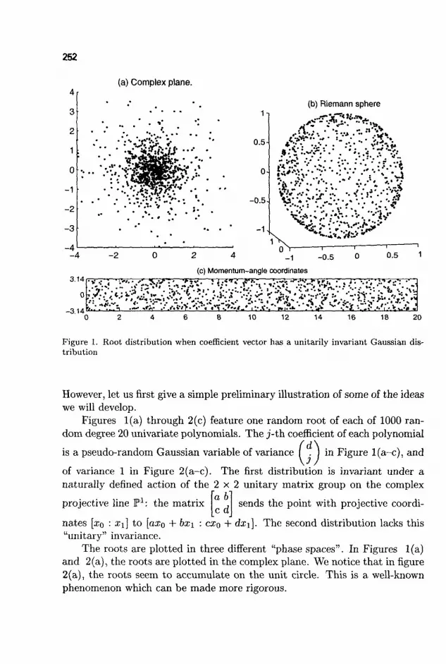
252

4

3

2

1 f c

0

-1

-2

-3

-4

(a) Complex plane.

£*• *

0.5-

(b) Riemann sphere

, $ , . ,

-0.54 VS.

-1 (c) Momentum-angle coordinates

-0.5 0.5

0 2 4 6 8 10 12 14 16 18 20

Figure 1. Root distribution when coefficient vector has a unitarily invariant Gaussian dis­tribution

However, let us first give a simple preliminary illustration of some of the ideas we will develop.

Figures 1(a) through 2(c) feature one random root of each of 1000 ran­dom degree 20 univariate polynomials. The j-th coefficient of each polynomial

is a pseudo-random Gaussian variable of variance ( . J in Figure l(a-c), and

of variance 1 in Figure 2(a-c). The first distribution is invariant under a naturally defined action of the 2 x 2 unitary matrix group on the complex

projective line F1: the matrix , sends the point with projective coordi­

nates [xo : x{\ to [axo + bx\ : CXQ + dx\]. The second distribution lacks this

"unitary" invariance. The roots are plotted in three different "phase spaces". In Figures 1(a)

and 2(a), the roots are plotted in the complex plane. We notice that in figure 2(a), the roots seem to accumulate on the unit circle. This is a well-known phenomenon which can be made more rigorous.

253

4

3

2r

1

0

-1

-2

-3

(a) Complex plane.

-2

3.14

-3.14

1 l

0.5-

-0.5

- 1 ,

(b) Riemann sphere

• • • . . • • * . : v *

1

*•*

2 4 _! _o.5

(c) Momentum-angle coordinates

0.5

10 12 14 16

Figure 2. Root distribution when the coefficients are identically and independently dis­tributed Gaussians

In Figures 1(b) and 2(b), we show the same roots as points in the Rie­mann Sphere. We can see that the selected roots of the unitarily invariant distributed polynomials are uniformly distributed on the Riemann Sphere, while those of the variance-one polynomials are not (this shows graphically that the distribution of the roots is not unitarily invariant).

There is strong evidence in 9 and 3 suggesting that unitarily invariant dis­tribution would be the natural distribution for Gaussian random polynomials. While the unitarily invariant paradigm was fundamental to the development m 17,18,19,20,21 ^ w e W JU s e e n e r e f.nat a m o r e general approach is viable and fruitful.

In figures 1(c) and 2(c), the same roots are plotted in a different "phase space", that we will construct below. The distribution seems uniform, it is indeed uniform. This suggests that there is another approach to random poly­nomials, that allows arbitrary variances through different coordinate systems.

This approach extends to systems of polynomial equations. While the unitary-invariant paradigma precluded the treatment of sparse polynomial

254

systems, the approach we suggest extends naturally to systems of equations. For instance, it is possible to bound the probability that the condition

number of a random sparse polynomial system (arbitrary variances) is large. The roots of a sparse polynomial system are known to belong to a certain

toric variety. However, in order to obtain the theorems below, we needed to endow the toric variety with a certain geometrical structure, as explained below. The main insight comes from mechanics, and from symplectic and Kahler geometry. The main tool is the Momentum map.

The proofs of the results mentioned herein may be found in 10 and its references.

2 General setting

Let A be an M x n matrix, with non-negative integer entries. To the matrix A we associate the convex polytope Conv(il) given by the convex hull of all the rows, {^4a}ae{i,...,M}> of A:

{ M M \

J2 t<*Aa : 0<ta<l, 5 3 ta = 1 l C (K")V . a=l a=l J

Here, we use the notation Xy to denote the dual of a vector space X. Assume that dim(Conv(>l)) = n. Then we can associate to the matrix A

the space TA OI polynomials with support contained in {Aa : 1 < a < M}. This is a linear space, and there are many reasonable choices of an inner product in TA-

Let C be a diagonal positive definite M x M matrix. Its inverse C _ 1 is also a diagonal positive definite M x M matrix. This inverse matrix defines the inner product:

(z ,Z ) c - i = {C~l)afi .

The matrix C will be called the variance matrix. This terminology arises when we consider random normal polynomials in !FA with variance Caa for the a-th coefficient. We will refer to these randomly generated functions as random normal polynomials, for short.

We may also produce several objects associated to the matrix A (and to the variance matrix C). The most important one for this paper will be a Kahler manifold (Tn,0JA, J)- This manifold is a natural "phase space" for the roots of polynomial systems with support in A. It is the natural phase space for the roots of systems of random normal polynomials in (J7A, (•, - ) C - I ) .

255

A3 = (2,6)

Figure 3. Geometric interpretation of the Momentum map V34. The momentum is related to the derivative of the Veronese embedding v_& by the formula: Dv\ = v\{Ax — Vg^)

256

More explicitly, let Tn = C" (mod 27r\/—TZn) (which, as a real mani­fold, happens to be an n-fold product of cylinders). Let exp : Tn -> (C*)n

denote coordinatewise exponentiation. Then we will look at the preimages of the roots of a polynomial system by exp. We leave out roots that have one coordinate equal to zero and roots at infinity.

The Kahler manifold may be constructed as follows. The Complex Struc­ture J is defined locally by

J(P,q)(p,<i)'= (-q,p)

The form OJA is the pull-back of the Fubini-Study 2-form in C M by the em­bedding

vA:Tn -»• C M

(p,q)^C1/2-eMMP + qVl:l)) If VA '• Tn —> P M _ 1 is the composition of VA with the canonical map C ^ —> P M _ 1 , then UJA is also the pull-back by VA of the canonical symplectic form of P M _ 1 .

Another important invariant is the real function:

gA : Tn ->• R p,q^ log | |^ (p) | |

This function is independent of p and we may treat gA as a function of p alone. In that setting, the gradient V ^ : W1 —> (E n ) v maps Rn diffeomor-phically onto the interior of the convex hull of the rows of A (See Figure 3 and 10 ). The mapping

V<M : T " -> (E") v

is called the Momentum map. It was introduced in its modern formulation by Smale 22 and Souriau 23. The reader may consult one of the many textbooks in the subject (such as Abraham and Marsden 1 or McDuff and Salamon 13) for a general exposition.

We can say now what the "phase space" of Figures 1(c) and 2(c) was. It was the image of the toric manifold (TH,COA,J) by the "volume-preserving" (up to a constant) map:

(p,q) •-> ((VgA)\P,q)

The potential gA and the Kahler form LUA are related as follows:

u>A = -^dJ*dgA

257

where d stands for exterior differentiation. The Hermitian metric associated to A has also the expressions:

(a, b) d= uA(a, Jb) = aHDvAIDvAb = ±D2gA(a,b)

3 Mixed and Unmixed systems

Systems where all the polynomials have the same support are called unmixed. The general situation (mixed polynomial systems), where the polynomials may have different supports, is of greater practical interest. It is also a much more challenging situation. We shall consider systems of n polynomials in n vari­ables, each polynomial in some inner product space of the form (JFA; , (•, - ) c r i ) (where i — 1, • • • , n and each Ai and each d are as above).

In this realm, a mathematical object (that we may call a mixed man­ifold) seems to arise naturally. A mixed manifold is an (n + 2)-tuple (Tn,u>Ai,' " ,uAn,J) where for each i, (Tn,LJAi,J) is a Kahler manifold. Mixed manifolds do not have a natural canonical Hermitian structure. They have n equally important Hermitian structures. However, they have one nat­ural volume element, the mixed volume form, given by

(_l)n(n-l)/2 dTn = V 1 A . . . A _

n!

As explained in 7, the volume of Tn relative to the mixed volume form is (up to a constant) the mixed volume of the n-tuple of polytopes (Conv(Ai),--- ,Conv(A„)).

We extend the famous result by Bernshtein 4 on the number of roots of mixed systems of polynomials as follows: Theorem 1. Let A\,--- ,An and C\,--- ,Cn be as above. For each i = l,--- ,n, let fi be an (independently distributed) normal random polynomial in (TAH (•, ^cr1)- Let U be a measurable region of Tn• Then, the expected number of roots of the polynomial system f(z) = 0 in expC/ C (C*)n is

^ [ dTn

7T" Ju IV

Example 1. When each /j is dense with a variance matrix Ci of the form:

d — Diag / 1 ! / 2 ! . - - , / „ ! ( d e g / i - E " = 1 / i ) !

258

the volume element dTn becomes the Bezout number \[ deg / ; times the pull-back to Tn of the Fubini-Study metric. We thus recover Shub and Smale's stochastic real version of Bezout's Theorem 18. •

The general unmixed case (Ai = • • • = An, C\ = • • • = Cn) is a particular case of Theorem 8.1 in 6. This is the only overlap, since neither theorem generalizes the other.

On the other hand, when one sets U = T", one recovers Bernshtein's first theorem. The quantity -n~n L-n dTn is precisely the mixed volume of polytopes A\,- • • ,An (see 16 for the classical definition of Mixed Volume and main properties).

A version of Theorem 1 was known to Kazarnovskii 8 and Khovanskii. In 8, the supports Ai are allowed to have complex exponents. However, uni­form variance (Ci = I) is assumed. His method may imply this special case of Theorem 1, but the indications given in 8 were insufficient for us to reconstruct a proof.

The idea of working with roots of polynomial systems in logarithmic co­ordinates seems to be extremely classical, yet it gives rise to interesting and surprising connections (see the discussions in 1:L>12>24).

4 The Condition Number

Let T — TAX x • • • x TA„ , and let / € T. A root of / will be represented by some p + qy/^1 G T n . (Properly speaking, the root of / is exp(p + qy/^1)).

In this discussion, we assume that the "root" p+qy/^1 is non-degenerate. This means that the derivative of the evaluation map

ev : fxT"->e (f,P + Qy/1^) •-> ( / ° exp)(p + qyf^)

with respect to the variable in Tn at the pomt p + q^/^T has rank 2n. We are then in the situation of the implicit function theorem, and there is (locally) a smooth function G : T -> T " such that for / in a neighborhood of / , we have ev(f,G(/)) = 0 and G(f) =p + qy/^l.

The condition number of / at (p + qyf-l) is usually defined as

ti(f;p + qV=l) = \\DGf\\ .

This definition is sensitive to the norm used in the space of linear maps between tangent spaces L(TfT, T(Pig)Tra). In general, one would like to use an operator norm, related to some natural Hermitian or Riemannian structure on T and 7~n.

259

In the previous section, we already defined an inner product in each co­ordinate subspace J-A{, given by the variance matrix d. Since the evalua­tion function is homogeneous in each coordinate, it makes sense to projec-tivize each of the coordinate spaces TAI (with respect to the inner product (-,-)c-i). Alternatively, we can use the Fubini-Study metric in each of the pAi's- By doing so, we are endowing T with a Fubini-like metric that is scaling-invariant. We will treat J7 as a multiprojective space, and write P(.F) f o r P p ^ J x - . - x P O F ^ J .

Another useful metric in f(!F) is given by

, . . ,2def A / . | | r - A f f ' | | V

Mf,g) = E (jg§?-ji?ii~J '

Each of the terms in the sum above corresponds to the square of the sine of the Fubini (or angular) distance between p and g%. Therefore, dp is never larger than the Hermitian distance between points in !F, but is a correct first-order aproximation of the distance when g —> f in P(J r). (Compare with 3 ).

While T admits a natural Hermitian structure, the solution-space Tn

admits n possibly different Hermitian structures, corresponding to each of the Kahler forms UJA{ •

In order to elucidate what the natural definition of a condition number for mixed systems of polynomials is, we will interpret the condition number as the inverse of the distance to the discriminant locus. Given p + q\f—\ £ T™, we set:

Jr{p,q) = {f£3r:ev(f;(p,q)) = 0}

and we set S(Pj9) as the space of degenerate polynomial systems in ^(p^)-Since the fiber J-(Ptq) inherits the metric structure of T, we can speak of the distance to the discriminant locus along a fiber. In this setting, Theorem 3 in 3 becomes: Theorem 2 (Condition number theorem). Under the notations above, if (p, q) is a non-degenerate root of f,

max mm\\DGff\\Ai < 7 7 7 ^ r < max m a x | | D G / / m ; . ||/||<i i dp( / ,L ( P i g ) ) ||/||<i i

There are two interesting particular cases. First of all, if A\ = • • • = An

and C\ = • • • = Cn, we obtain an equality:

260

Corollary 2.1 (Condition number theorem for unmixed systems). Let A\ = • • • = An and C\ = • • • = Cn, then under the hypotheses of Theo­rem 2,

def ' - 1 fJ-if; (P,q)) = max min \\DGff\\Ai = max max \\DGff\\Ai = . r .

We can also obtain a version of Shub and Smale's condition number the­orem (Theorem 3 in 3 ) for dense systems as a particular case, once we choose the correct variance matrices: Corollary 2.2 (Condition number theorem for dense systems). Let di, • • • ,dn be positive integers, and let Ai be the n-columns matrix having all possible rows with non-negative entries adding up to at most di. Let

Then,

def • - 1 M(/; (P><?)) = max min \\DGff\\Ai = max max \\DGff\\Ai = , , , v r -

The factor j : in the definition of the variance matrix d corresponds to the factor y/d~i in the definition of the normalized condition number in 3 .

In the general mixed case, we would like to interpret the two "minmax" bounds as condition numbers related to some natural Hermitian or Finslerian structures on T". See 10 for a discussion

Theorem 2 is very similar to Theorem D in 5, but the philosophy here is radically different. Instead of changing the metric in the fiber ^F(p^), we consider the inner product in T as the starting point of our investigation. Theorem 2 gives us some insight about reasonable metric structures in T n .

As in Theorem 1, let U be a measurable set of T™. In view of Theorem 2, we define a restricted condition number (with respect to U) by:

M(/;t/)=f l m m (p ,9 )6C/ dp(f, S( P ) g))

where the distance dp is taken along the fiber J-(p,q) = {/ : ( / ° exp)(p + qy/^l) = 0}.

Although we do not know in general how to bound the expected value of M / ; Tn), we can give a convenient bound for n(f; U) whenever U is compact and in some cases where U is not compact.

261

The group GL{n) acts on T(p^Tn by sending (p, q) into (Lp, Lq), for any L € GL(n). In more intrinsic terms, J and the GL(n)-action commute. With this convention, we can define an intrinsic invariant of the mixed structure (Tn,uAl,--- ,uAn,J): Definition 1. The mixed dilation of the tuple (CJAI >''" > UA„) is :

, , „ def . ^^\\u\\ = l{^Ai)(p,q)(Lu,JLu) K(UAI,--- ,UAn;(p,q)) = nun max . " " ^ — ' — — — .

LEGL(n) t m m | | u | | = 1 (LOAi)(pq){Lu,JLu)

Given a set U, we define:

def , KV = SUP K[(JJAI , •

{p,q)eu ,uAn;{p,q))

provided the supremum exists, and KJJ = oo otherwise. We will bound the expected number of roots with condition number fj. >

e _ 1 on U in terms of the mixed volume form, the mixed dilation KU and the expected number of ill-conditioned roots in the linear case. The linear case corresponds to polytopes and variances below:

A Lin = c L , n =

1

Theorem 3 (Expected value of the condition number). Let i/Lin(n,e) be the probability that a random n-variate linear complex polynomial has con­dition number larger than e _ 1 . Let vA{U,e) be the probability that fJ.{f, U) > e _ 1 for a normal random polynomial system f with supports A\, • • • ,An and variance C\, • • • ,Cn-

Then,

vA(U,e)< lu A ^AV'"

z / L i n ( n , ^ e )

There are a few situations where we can assert that KU = 1- For instance, Corollary 3.1. Under the hypotheses of Theorem 3, if A = Ai = • • • = An

and C = Ci = • • • = Cn, then

vA{U,e)<Vo\{U) vLin{n,e

The dense case (Theorem 1 p. 237 in 3) is also a consequence of Theorem 3.

262

Remark 1. We interpret uhin(n,e) as the probability that a random linear polynomial / is at multiprojective distance less than e from the discriminant variety S(P)9)- Let g £ £(P,g) be such that the following minimum is attained:

n Up — Ao*ll2

*( / .S ( , . „ ) a = - 6 j n f f ) E y / i | |2 • A€(C*)" ' - 1

Without loss of generality, we may scale g such that Ai = • • • = An = 0. In that case,

*(/ . so.,,)) - i . n^ip > E » = l u / T • The right hand term is the projective distance to the discriminant variety along the fiber, in the sense of 3. Since we are in the linear case, this may be interpreted as the inverse of the condition number of / in the sense of 3 .

Recall that each / ' is an independent random normal linear polynomial of degree 1, and that Ci is the identity. Therefore, each f%

a is an i.i.d. Gaussian variable. If we look at the system / as a random variable in p«(«+1)-1

) then we obtain the same probability distribution as in 3. Then, using Theorem 6 p. 254 ibid, we deduce that

Li n*(n + l)T(n*+n) v (n,e)S r ( n 2 + n _ 2 )

£ • •

5 Real Polynomials

Shub and Smale showed in 18 that the expected number of real roots, in the dense case (with unitarily invariant probability measure) is exactly the square root of the expected number of roots.

Unfortunately, this result seems to be very hard to generalize to the un­mixed case. Under certain conditions, explicit formula? for the unmixed case are available 15. Also, less explicit bounds for the multi-homogeneous case were given by 14.

Here, we will give a very coarse estimate in terms of the square root of the mixed volume: Theorem 4. Let U be a measurable set in Rn, with total Lebesgue volume \(U). Let Ai, • • • ,An and Ci, • • • , Cn be as above. Let f be a normal random real polynomial system. Then the average number of real roots of f in exp[7 C

263

(Rt)n is bounded above by

V peu

This is of interest when n and U are fixed. In that case, the expected number of positive real roots (hence of real roots) grows as the square root of the mixed volume.

It is somewhat easier to investigate real random polynomials in the un­mixed case.

Let VR(n,e) be the probability that a linear random real polynomial has condition number larger than e _ 1 . Theorem 5. Let A = A\ = • • • - An and C = Cx = • • • = Cn. Let U C E" be measurable. Let f be a normal random real polynomial system. Then,

Prob \p(f,U) > e'1] < E{U) i*(n,e)

where E(U) is the expected number of real roots on U. Notice that E(U) depends on C. Even if we make [/ = E", we may still

obtain a bound depending on C.

6 Mechanical Interpretation

The momentum map defined above is also the the momentum map (in the sense of 22) associated to a certain Lie group action, namely the natural action of the n-torus on the toric manifold T n :

The n-torus T" = Rn (mod 2TT Zn) acts on T " by

p • [p, q) *+(p,q + p) ,

where p € Tn . This action preserves the symplectic structure, since it fixes the p-variables

and translates the q-variables. Also, the Lie algebra of T™ is Rn. An element £ of E™ induces an infinitesimal action (i.e. a vector field) X^ in T" .

This vector field is the derivation that to any smooth function / associates:

(xi)(P,q)(f) = Ld2WA)(P,q)(df) d= {-^jA)(p,q){i,d}) .

If we write df = dpfdp + dqfdq, then this formula translates to:

{Xi)(p,q)U) = -(r{D2gA)PdP!

264

This vector field is Hamiltonian: if (p(t),q(t)) is a solution of the equation

(?(*),?(*)) = (xt)P(t)Mt)

then we can write

where H^ = § V S A ( P ) • £• This construction associates to every $ £ l n , the Hamiltonian function

H± = VgA(p) £• The term V ^ ( p ) is a function of p, with values in (M")v (the dual of K"). In more general Lie group actions, the momentum map takes values in the dual of the Lie algebra, so that the pairing WgA (p) • £ always makes sense. A Lie group action with such an expression for the Hamiltonian is called Hamiltonian or Strongly Hamiltonian.

7 Acknowledgements

Steve Smale provided valuable inspiration for us to develop a theory similar to i?,.i8.19,20,2i for S p a r s e polynomial systems. He also provided examples on how to eliminate the dependency upon unitary invariance in the dense case.

The paper by Gromov 7 was of foremost importance to this research. To the best of our knowledge, 7 is the only clear exposition available of mixed volume in terms of a wedge of differential forms. We thank Mike Shub for pointing out that reference, and for many suggestions.

We would like to thank Jean-Pierre Dedieu for sharing his thoughts with us on Newton iteration in Riemannian and quotient manifolds.

Also, we would like to thank Felipe Cucker, Alicia Dickenstein, Ioannis Emiris, Askold Khovanskii, Eric Kostlan, T.Y. Li, Martin Sombra, and Jorge P. Zubelli for their suggestions and support.

This paper was written while G.M. was visiting the Liu Bie Ju Center for Mathematics at the City University of Hong Kong. He wishes to thank CityU for their generous support.

References

1. Abraham, Ralph and Marsden, Jerrold E., Foundations of mechanics, Second edition, revised and enlarged, With the assistance of Tudor Ratiu and Richard Cushman, Benjamin/Cummings Publishing Co. Inc. Ad­vanced Book Program, Reading, Mass., 1978.

265

2. Abreu, Miguel, "Kahler geometry of toric manifolds in symplectic co­ordinates", April, 2000, Preprint, Mathematics ArXiv DG/0004122, h t t p : / / f ron t .ma th .ucdav i s . edu .

3. Blum, Lenore; Cucker, Felipe; Shub, Michael; and Smale, Steve, Com­plexity and real computation, With a foreword by Richard M. Karp, Springer-Verlag, New York, 1998.

4. Bernstein, D. N., "The number of roots of a system of equations", Func­tional Anal. Appl., Vol. 9, No. 2, (1975), pp. 183-185.

5. Dedieu, Jean-Pierre, "Approximate solutions of numerical problems, con­dition number analysis and condition number theorem", The mathematics of numerical analysis (Park City, UT, 1995), pp. 263-283, Amer. Math. Soc, Providence, RI, 1996.

6. Edelman, Alan and Kostlan, Eric, "How many zeros of a random polyno­mial are real?", Bull. Amer. Math. Soc. (N.S.), American Mathematical Society. Bulletin. New Series, vol. 32, 1995, no. 1, pp. 1-37.

7. Gromov, M., "Convex sets and Kahler manifolds", Advances in differen­tial geometry and topology, pp. 1-38, World Sci. Publishing, Teaneck, NJ, 1990.

8. Kazarnovskii, B. Ja., "On zeros of exponential sums", Soviet Math. Dok-lady, vol. 23, 1981, no. 2, pp. 347-351.

9. Eric Kostlan, "Random Polynomials and the Statistical Fundamental Theorem of Algebra", Preprint, MSRI, 1987.

10. Gregorio Malajovich and J. Maurice Rojas, "Random Sparse Polynomial Systems", Preprint, City University of Hong Kong and Math Archive, 2000.

11. Gregorio Malajovich and Jorge Zubelli, "On the Geometry of Graeffe Iteration", Journal of Complexity (To appear).

12. Gregorio Malajovich and Jorge Zubelli, "Tangent Graeffe Iteration", Nu-merische Mathematik (To appear).

13. McDuff, Dusa and Salamon, Dietmar, Introduction to symplectic topology, second edition, The Clarendon Press Oxford University Press, New York, 1998.

14. Andrew McLennan, "The expected number of real roots of a multihomo-geneous system of polynomial equations", American Journal of Mathe­matics, to appear.

15. J. Maurice Rojas, "On the Average number of Real Roots of Certain Random Sparse Polynomial Systems", Lectures in Applied Mathematics, vol. 32, 1996, pp. 689-699.

16. Sangwine-Yager, J. R., "Mixed volumes", Handbook of convex geometry, Vol. A, B, pp. 43-71, North-Holland, Amsterdam, 1993.

266

17. Shub, Michael and Smale, Steve, "Complexity of Bezout's theorem I — Geometric aspects", Journal of the American Mathematical Society, vol. 6, 1993, no. 2, pp. 459-501.

18. Shub, Mike and Smale, Steve, "Complexity of Bezout's theorem II— Vol­umes and probabilities", Computational algebraic geometry (Nice, 1992), pp. 267-285, Birkhauser Boston, Boston, MA, 1993.

19. Shub, Michael and Smale, Steve, "Complexity of Bezout's theorem III — Condition number and packing", Festschrift for Joseph F. Traub, Part I, Journal of Complexity, vol. 9, 1993, no. 1, pp. 4-14.

20. Shub, Michael and Smale, Steve, "Complexity of Bezout's theorem IV — Probability of success; extensions", SIAM Journal on Numerical Analysis, vol. 33, 1996, no. 1, pp. 128-148.

21. Shub, Mike and Smale, Steve, "Complexity of Bezout's theorem V — Polynomial time, Selected papers of the Workshop on Continuous Algo­rithms and Complexity (Barcelona, 1993), Theoretical Computer Science, vol. 133, 1994, no. 1, pp. 141-164.

22. Smale, Steve, "Topology and mechanics I", Invent. Math., vol. 10, 1970, pp. 305-331.

23. Souriau, J.-M., "Structure des systemes dynamiques", Maitrises de mathematiques, Dunod, Paris, 1970.

24. Oleg Viro, "Dequantization of real algebraic geometry on logarith­mic paper", June, 2000, Preprint, Mathematics ArXiv AG/0005163, h t t p : / / f r on t .ma th .ucdav i s . edu

267

ASYMPTOTIC ACCELERATION OF THE SOLUTION OF MULTIVARIATE POLYNOMIAL SYSTEMS OF EQUATIONS

B. MOURRAIN INRIA, GALAAD, BP 93, 06902 Sophia-Antipolis, France

E-mail: mourrain@sophia.inria.fr

V.Y. PAN Dept. of Mathematics and Computer Science, Lehman College, City University of

New York, Bronx, NY 10468 E-mail: vpan@lehman.cuny.edu

O. R U A T T A

INRIA, GALAAD, BP 93, 06902 Sophia-Antipolis, France E-mail: oruatta@sophia.inria.fr

We propose new Las Vegas randomized algorithms for the solution of a square non-degenerate system of equations. The algorithms use 0(<53™£>2 log(D) log(6)) arithmetic operations to approximate all real roots of the system as well as all roots lying in a fixed n-dimensional box or disc. Here D is an upper bound on the number of all complex roots of the system, 8 is the number of real roots or the roots lying in the box or disc, e ~ 2~b is the required upper bound on the output errors. We also yield the bound 0(3™ D 2 log(D)) on the complexity of counting the numbers of all roots in a fixed box (disc) and all real roots. For a large class of inputs and typically in practical computations, the factor 8 is much smaller than D, 8 = o(D). This improves by order of magnitude the known complexity estimates of order at least 3™£)3log(6) or 3"£>3, which so far are the record ones even for the approximation of a single root of a system and for each of the cited counting problems, respectively. Our progress relies on proposing several novel techniques. In particular, we exploit the structure of matrices associated to a given polynomial system and relate it to the associated linear operators, dual space of linear forms, and normal forms of polynomials in the quotient algebra; furthermore, our techniques support the new nontrivial extension of the matrix sign and quadratic inverse power iterations to the case of multivariate polynomial systems, where we emulate the recursive splitting of a univariate polynomial into factors of smaller degree.

1 Introduction.

The classical problem of solving a multivariate polynomial system of equations is presently the subject of intensive research and one of the central practical and theoretical problems in the area of algebraic computation (see some bib­liography in 18, 4 , 28, 13.) It has major applications, for instance, to robotics, computer modelling and graphics, molecular biology, and computational al-

268

gebraic geometry. The oldest approach to the solution is the elimination method, reduc­

ing the problem to the computation of the associated resultant or its multi­ples. This classical method evolved in the old works by Bezout, Dixon, and Macaulay (see e.g. 18, 4 1 ) , then remained largely ignored by the researchers and algorithm designers but it was resurrected by Canny in the 80s to become a very popular approach since then. One of the major further steps was the reduction of the solution of a multivariate polynomial system to matrix oper­ations, in particular, by rational transformation of the original problem into a matrix eigenproblem (cf. 1, 14, 23, 21, 8 ) .

The approach has been explored and extended by many researchers, has been exploited in practice of algebraic computing, and also supported the record asymptotic upper bound O* (D3) on the arithmetic computational com­plexity of the solution of a polynomial system having a finite number of roots. Here and hereafter, 0*(s) stands for C(slog cs) , c denoting a constant in­dependent of s, and D is an upper bound on the number of roots of the given polynomial system. (For D, one may choose either the Bezout bound, Y\t di, di denoting the maximum degree in the i-th variable in all monomials of the system, or the Bernstein bound, which is much smaller for sparse sys­tems and equals the mixed volume of the associated Newton polytope, defined by the exponents of the monomials.) The cited record bound 0*(D3) is due to 35 but also has several other derivations and has been staying as a stable landmark for the multivariate polynomial system solving, much like the com­plexity bound 0{N3) for solving nonsingular linear system of N equations, which was supported by Gaussian elimination and stayed as a landmark and a record until Strassen's celebrated result of 1969. In fact, even in the case of solving non-degenerate polynomial system as well as for many subproblems and related problems, no known algorithms support any better bound than 0(D3). This includes approximation of all real roots of a polynomial sys­tem (which is highly important due to applications to robotic and computer graphics), all its roots lying in a fixed n-dimensional box or disc, counting all roots in such a box or disc or all real roots, and even approximation of a single root. Some progress was achieved in 26, where a single root was approximated in 0*(3nD2) time, but under a strong restriction on the input polynomials.

Our new algorithms support the computational cost estimate of 0*(3nD2), for all the listed above subproblems, that is, for both of the count­ing problems, the computation of a single root, all real roots, and all roots in a fixed box or disc. More precisely, our bound is 0*(S3nD2) in the latter two cases, where S is the number of real roots or roots in the selected box or disc, respectively. In practical applications, such a number is typically much

269

less than D. The number of real roots grows as \D for a large class of input systems 37. See also for the sparse case 36. Thus, for all listed problems, we improve the known complexity estimates by an order of magnitude.

We have a reservation from a theoretical point of view, that is, our main algorithm relies on the known effective algorithms for the computation of the normal form of monomials on the boundary of the monomial basis (see section 4). These algorithms exploit structured matrices and in practice, apper to run faster than our subsequent computations (see 15, 2 9 ) , but their known theoretical cost bound are greater than the order of D3 (see 1 9) .

Our paper addresses the problem of the asymptotic acceleration of the res­olution stage where the structure of the quotient algebra A (associated with the polynomial system) is already described by using the minimal number of parameters, that is, via the normal form of the monomials on the boundary of the basis. From a purely theoretical point of view, we have an alternative approach that avoids the normal form algorithms at the price of using the order of 0(12" D2) additional arithmetic operations 27 . This should be tech­nically interesting because no other known approach yields such a bound, but in this paper, we prefer to stay with our present, practically superior version, referring the reader to 27 on the cited theoretical approach.

Our algorithms approximate the roots numerically, and in terms of the required upper bound 2~b (b is the bit precsion) on the output errors of the computed solution, we obtain the estimate C(log b). Within a constant factor, such an estimate matches the lower bound of 34 and enables us to yield a high output precision at relatively low cost; this gives us a substantial practical advantage versus the algorithms that only reach 0(b), because the solution of a polynomial system is usually needed with a high precision. We achieve this by using the matrix sign and inverse quadratic iterations, which converge with quadratic rate right from the start. All techniques and results can be extended to the case of sparse input polynomials (see remark 3.16, section 3). In this case, the computation cost bounds become 0(DCp0iMuit) where CpoiMuit is the cost of polynomial multiplication, which is small when the polynomials are sparse (this cost depends on the degree of the polynomials, not only on an upper bound D on the number of roots).

The factor 3" is a substantial deficiency, of course, but it is still much less than D for the large and important class of input polynomials of degree higher than 3.

Our results require some other restrictions. First, we consider systems with simple roots or well separated roots. In the presence of a cluster, a specific analysis is needed 39 and deserves additional work, which is not in the scope of this paper. Secondly, we need the existence of a non-degenerate

270

linear form, which implies that the quotient algebra A is a Gorenstein algebra 10,12. This is the case where the solution set is 0-dimensional and is denned by n equations. If we have more than n equations denning a 0-dimensional variety, we may take their n-random linear combination (see, e.g. n ) , which yields the required Gorenstein property, but this may introduce extra solutions that we will have to remove at the end. Finally, for approximation, our algorithms converge quadratically (using £>(log(b)) steps) but require certain nondegeneracy assumptions (such as uniqueness of the minimum of the value of |ft(C)|, where £ is a root and ft(x) a polynomial). The latter assumptions can be ensured with a high probability by a random linear transformation of the variables. Even if these assumptions are barely satisfied, the slowdown of the converge is not dramatic, because the convergence is quadratic right from the start.

Similarly, we apply randomization to regularize the computations at the counting stages, and for the auxiliary computation of the non-degenerate lin­ear form in the dual space A. Then again, non-degeneracy is ensured proba­bilistically, and verified in the subsequent computation (that is, we stay under the Las Vegas probabilistic model where failure may occur, with a small prob­ability, but otherwise correctness of the output is ensured).

Some of our techniques should be of independent interest. In particular, we extend the theory of structured matrices to the ones associated to mul­tivariate polynomials and show correlation among computations with such matrices and dual spaces of linear forms. We show some new non-trivial applications of the normal forms of polynomials of the quotient algebra. Fur­thermore, we establish new reduction from multivariate polynomial compu­tations to some fundamental operations of linear algebra (such as the matrix sign iteration, the quadratic inverse power iteration, and the computation of Schur's complements).

Our progress has some technical similarity to the acceleration of the solu­tion of linear systems of equations via fast matrix multiplication (in particular, we also rely on faster multiplication in the quotient algebra defined by the in­put polynomials), but even more so, with the recent progress in the univariate polynomial rootfinding via recursive splitting of the input polynomial into fac­tors (cf. 5 , 30, 31, 3 2 ) . Although recursive splitting into factors may be hard even to comprehend in the case of multivariate polynomial systems, this is exactly the basic step of our novel recursive process, which finally reduces our original problem to ones of small sizes. Of course, we could not achieve splitting in the original space of the variables, but we yield it in terms of idem-potent elements of the associated quotient algebra (such elements represent the roots), and for this purpose we had to apply all our advanced techniques.

271

This approach generalizes the methods of 5 and 31 to the multivariate case. The only missing technical point of our extension of the univariate splitting construction of 31 is the balancing of the splitting, which was the most recent and elusive step in the univariate case (cf. 31, 3 2 ) . It is a major challenge to ad­vance our approach to achieve balancing in our recursive splitting process even in the worst case (possibly by using the geometry of discriminant varieties) and, consequently, to approximate all the roots of any specific polynomial system in 0*(3"D2log6) arithmetic time. Another goal is the computations in the dual space, as well as with structured matrices. The latter subject is of independent interest too 40>28.

Let us conclude this section with a high level description of our approach. Our solution of polynomial systems consists of the following stages:

1. Compute a basic non-degenerate linear form on the quotient algebra A associated to a given system of polynomial equations.

2. Compute non-trivial idempotent elements of A. 3. Recover the roots of the given polynomial system from the associated

idempotents. The quotient algebra A and the dual space of linear forms on it are defined

and initially studied in section 2. Stage 1 is elaborated in section 4. Idempo­tents are computed by iterative algorithms of section 6. Section 7 shows how to recover or to count the roots efficiently when the idempotents are avail­able. The computations are performed in the quotient algebra, and they are reduced to operations in the dual space by using the associated structured (quasi-Toeplitz and quasi-Hankel) matrices. In section 3 we define the classes of such matrices, show their correlation to polynomial computations, and ex­ploit it to operate with such matrices faster. In section 5 we show how the combined power of the latter techniques and the ones developed for working in the dual space enables us to perform rapidly the basic operations in the quotient algebra and, consequently, the computations of sections 6 and 7.

Stage 1 contributes 0 (3 n D 2 logD) ops to the overall complexity bound, assuming that the normal form of the monomials on the boundary of a basis is known. The computation of a nontrivial idempotent at stage 2 has cost 0(3"-D2 log D log b), which dominates the cost of the subsequent root counting or their recovery from the idempotents. The overall complexity depends on the number of idempotents that one has to compute, which in turn depends on the number S of roots of interest. So far, we cannot utilize here the effective tools of balanced splitting, available in the similar situation for the univariate polynomial rootfinding. Thus, in the worst case, in each step we split out only a single root from the set of all roots, and then we need 5 idempotents.

272

2 Definitions and preliminaries

Hereafter, R — C[a;i,. . . , xn] is the ring of multivariate polynomials in the variables x i , . . . ,xn, with coefficients in the complex field C. Z is the set of integers, N is its subset of nonnegative integers, L = C[xf,... ,x„] is the set of Laurent polynomials with monomial exponents in Z". For any a = ( a i , . . . , a„) £ Z n , x a is the monomial x a = a;"1 •••x%n. [E~\ is the cardinality (that is, the number of elements) of a finite subset E of Z™. "ops" will stand for "arithmetic operations" in the underlying coefficient ring or field.

2.1 Quotient algebra

To motivate and to demonstrate our study, we will next consider the univariate case, where we have a fixed polynomial / £ C[x] of degree d with d simple roots: f(x) = fa Yli=i(x ~ d)- The quotient algebra of residue polynomials modulo / , denoted by A = C[x]/(f), is a vector space of dimension d. Its basis is (1, x,... , a;d_1). Consider the Lagrange polynomials

One immediately sees that Yli e« = 1 and e^e^ = ej(ej — 1) = 0 (for these two polynomials vanish at the roots of / ) . In other words, the Lagrange polynomials e* are orthogonal idempotents in A, and we have A = S i^ - e «-Moreover, for any polynomial a £ A, we also have (a — a{Q))ei = 0, so that e* is an eigenvector for the operator of multiplication by a in A, for the eigenvalue a(Q). These multiplication operators have a diagonal form in the basis (ej) of A. According to a basic property of Lagrange polynomials, we have a = J2ia(d)^i(^), for any a £ A. Therefore, the dual basis of (e*) (formed by the coefficients of the e; in this decomposition) consists of the linear forms associating to a its values at the points Q. We will extend this approach to the case of multivariate polynomial systems, which, of course, will require substantial further elaboration and algebraic formalism. We refer the reader to 22, 23, 28, 38 for further details.

Let / i , . . . , fm be m polynomials of R, defining the polynomial system / i (x) = 0 , . . . , fm(x) = 0. Let / be the ideal generated by these polynomials, that is, the set of polynomial combinations ^2, hit of these elements. A = R/I denotes the quotient ring (algebra) defined in R by 7, and = denotes the equality in A. We consider the case, where the quotient algebra A — R/I is of finite dimension D over C. This implies that the set of roots or solutions

273

Z(I) = { ( e C ; / i ( C ) = . . . = fm(0 = 0} is finite: Z(I) = {&,... ,(d} with d < D. Then we have a decomposition of the form

A = Ai®---®Ad, (1)

where Ai is a local algebra, for the maximal ideal m ^ defining the root Q. From decomposition (1), we deduce that there exist orthogonal idempotents e i , . . . , ed satisfying

ei + • • • + e,j = 1, and e e,- = f 0 if i? j , \ et if i = j .

It I = Qi fl • • • (~l Qd is the minimal primary decomposition of / , we have e-iA ~ R/Qi, where Ai — ei A is a, local algebra, for the maximal ideal m ^ defining the root Q. Thus, to any root £ € Z, we associate an idempotent e c .

2.2 Dual space

Let R denote the dual of the C-vector space R, that is, the space of linear forms

A: # - ) • C

P >-»• A(p).

(R will be the primal space for R.) Let us recall two celebrated examples, that is, the evaluation at a fixed point £,

l c : R -*• C

p^p(0,

and the map

(d» = ( d 1 r - - - ( d n ) ° - ) : i ? - * C

P^fJ—T(dx1)Ol"-(d«»)a"(p)(0), (2)

where a = ( a i , . . . , an) is any vector from M1, and dXi is the partial derivative with respect to the variable Xj. For any b = {b\,... , bn) 6 N", we have

(ja/xb^ _ f 1 if Vi',aj = 6j, 10 otherwise.

274

Therefore, (da)a eNn is the dual basis of the primal monomial basis. Thus, we decompose any linear form A € R as

A = ^ A ( x a ) d a . (3) aGN"

Hereafter, we will identify R with C[[di , . . . ,d„]]. The map A - • SaeNn A( x a ) d a defines a one-to-one correspondence between the set of lin­ear forms A and the set C[[di , . . . d„]] = C[[d]] = { £ a g N „ Aad?] • • • d£" } of polynomials in the variables d i , . . . , d„.

The evaluation at 0 corresponds to the constant 1, under this definition. It will be also denoted by So = d°.

We will denote by A and also by I1- the subspace of R made of those linear forms that vanish on the ideal / .

We now define multiplication of a linear form by a polynomial (R is an .R-module) as follows. For any p € R and A 6 R, we write

p*A: R^C

q H-> A(pq).

For any pair of elements p £ R and a € N, a > 1, we have

(dXi)a(xip){0) = a(dXi)

a-1p(0).

Consequently, for any pair (p,a), p 6 R, a = ( a i , . . . ,on) € N™ (where ai 7 0 for a fixed i), we obtain

Xi*d*{p) =da{xip)

i • • • d i _ 1 d ; d i + + • • • d „ " ( p ) ,

that is, Xi acts as the inverse of di in C[[d]]. For this reason such a represen­tation is referred to as the inverse systems (see, for instance, 2 0 ) . If a; = 0, then Xi *d a (p) = 0 , which allows us to redefine the product p * A as follows: Proposition 2.1 For any pair p,q 6 R and any A(d) € C[[d]], we have

p*A(q)=A(pq)=ir+(p(d-1)A(d))(q),

where ix+ is the projection mapping Laurent series onto the space generated by the monomials in d with positive exponents. This yields the following algorithm: Algorithm 2.2 F O R ANY POLYNOMIAL p € (•xa)aeE AND A VECTOR

[ A ( x / 3 ) ] / 3 6 £ ; + i r , COMPUTE THE VECTOR [ p * A ( x / 3 ) ] / 3 e F as follows:

. Write A(d) = £ / 3 e £ ; + FA(xV / 3-

275

• Compute the product p(d) = p(d 1)A(d) in C[d, d 1], and

• keep the coefficients pa of da for a £ F.

3 Quasi-Toeplitz and quasi-Hankel matrices

In this section we describe the structure of the matrices and some tools that we will use for our algorithm design.

Let us recall first the known arithmetic complexity bounds for polynomial multiplication (see 2, pp. 56-64), which is the basic step of our subsequent algorithms. Let Cp0iMuit{E,F) denote the number of ops (that is, of arith­metic operations) required for the multiplication of a polynomial with support in £ by a polynomial with support in F.

Theorem 3.1 LetE+F = {a1 = (a^\... ,0$), i = l,... ,N} with\a^\ = ^ • or*' = di for i = 1 , . . . ,N and d = maXi(di). Let CfC;Evai(G) ops suffice to evaluate a polynomial with a support G on a set of K points. Then we have

CPolMut(E,F) = O {CN.iEvai(E) + CN,Eval{F) + N(\og2(N) + log(d))) .

Proof. Apply the evaluation-interpolation techniques to multiply the two polynomials (cf. 2 ) . That is, first evaluate the input polynomials on a fixed set of N points, then multiply pairwise the computed values to obtain the val­ues of the product on the same set, and finally interpolate from these values and compute the coefficients of the product by applying the (sparse) polyno­mial interpolation algorithm (cf. 2 ) . By summarizing the computational cost estimates, we obtain the theorem. • For special sets E and F, we have better bounds. Theorem 3.2 Let Ed = [0, . . . , d - 1] C N. Then

CPoiMuit(Ed,Ed) = 0(dlog(d)).

Theorem 3.3 Let Ec = { ( a i , . . . ,an) ; 0 < at < Ci - 1}, Ed = {(/3i,... ,/?„) ; 0 < Pi < di - 1}, c = max{ci,... ,cn}, and d = max{di,... ,dn}. Then we have

Cp0iMuit(Ec,Ed) = 0(Mlog(M)),

where M — fn, and f - c + d + 1. Theorem 3.4 Let EfiTl be the set of exponents having total degree at most f in n variables. Then

Cp0lMult(Ec ) = 0{T log2(T)),

where T = ( n + c + ) is the number of monomials of degree at most c + d in n variables.

276

Remark 3.5 Theorems 3.1 and 3.3 correspondly respectively to lattice points in a product of intervals or in the scaled standard simplex, can be extended to the computations over any ring of constants (rather than over the complex field) at the expense of increasing their complexity bounds by at most the fac­tors of loglog(./V) or log log(M), respectively2. Theorem 3.4 can be extended similarly to any field of constants having characteristic 0.

Next, by following 28-27, we will extend the definitions of Toeplitz and Hankel matrices to the multivariate case. As we will see, these structures are omnipresent, when we solve polynomial systems. Definition 3.6 Let E and F be two finite subsets of N" and let M = (ma^aeE^eF be a matrix whose rows are indexed by the elements of E and columns by the elements of F. Let i denote the Ith basis coordinate vector of W.

• M = [ma!J3]asE,/3eF is an (E, F) quasi-Toeplitz matrix if and only if, for all a E E,(3 £ F, the entries ma^ = ta-p depend only on a — /3, that is, if and only if, for i — 1 , . . . , n, we have ma+ifi+i = ma^, provided that a, a + i E E;(3,/3 + i 6 F; such a matrix M is associated with the polynomial TM(x) = E u e E + F ^ " -

• M is an (E, F) quasi-Hankel matrix if and only if, for all a £ E,/3 £ F, the entries ma^ = ha+p depend only on a + 0, that is, if and only if, for i = 1 , . . . ,n, we have ma-i^+i = ma^ provided that a,a — i € E; /?, (3 + i £ F; such a matrix M is associated with the Laurent polynomial HM(d) = E U S B - F M U -

For E = [0, . . . , m -1] and F = [0 , . . . , n - 1] (resp. F = [-n +1,... , 0]), definition 3.6 turns into the usual definition of Toeplitz (resp. Hankel) matri­ces (see 2 ) . Quasi-Toeplitz matrices have also been studied under the name of Multilevel Toeplitz matrices (see, e.g., 4 0 ) , in the restricted special case where the sets E and F are rectangular (ie. a product of intervals). For our study of polynomial systems of equations, using the latter restricted case is not sufficient, and our more general definitions are required.

The definitions can be immediately extended to all subsets E, F of Z n , if we work with the Laurent polynomials.

The classes of quasi-Toeplitz and quasi-Hankel matrices can be trans­formed into each other by means of multiplication by the reflection matrix, having ones on its antidiagonal and zeros elsewhere.

Definition 3.7 Let TTE '• L —> L be the projection map such that 7T£:(xQ) = x a if a £ E and nE(*a) = 0 otherwise. Also let TTE : C[[d]] -> C[[d]]

277

denote the projection map such that 7r£(da) = d a if a G E and 7T£(cP) = 0 otherwise.

We can describe the quasi-Toeplitz and quasi-Hankel operators in terms of polynomial multiplication (see 26, 2 5 ) , and the next proposition reduces multiplication of an (E, F) quasi-Toeplitz (resp. quasi-Hankel) matrix by a vector v = [vp] E CF to (Laurent) polynomial multiplication. Proposition 3.8 The matrix M is an (E,F) quasi-Toeplitz (resp. an {E,F) quasi-Hankel) matrix, if and only if it is the matrix of the operator TTE o HTM O •Kp (resp. •KE ° MHM ° nF), where for any p € L, /zp : q i-> pq is the operator of multiplication by p in L.

Proof. (See 25.) We will give a proof only for an (E, F) quasi-Toeplitz matrix M — {Ma^)aeE,peF- (The proof is similar for a quasi-Hankel matrix.) The associated polynomial is TM{X) = Eues+F*"-*" - ^or a n ^ v e c t ° r v = [v&\ ^ C F , let v(x) denote the polynomial E s e F VPK^- Then

TM(x)V(x)= Y, X U + / 3 * U ^ ueE+F,0€F

a=u+/3€F+2F \0£F J

where we assume that tu — 0 if u £ E + F. Therefore, for a e E, the coefficient of xQ equals

5 3 ta-0 V0 = 5 3 M<*,P V0> /3€F /3€F

which is precisely the coefficient a of Mv. D

A l g o r i t h m 3.9 MULTIPLICATION OF THE (E,F) QUASI-TOEPLITZ (RESP.

QUASI-HANKEL) MATRIX M = (Ma,p)aeE,/3eF BY A VECTOR V = [vp] e CF:

• multiply the polynomials TM = E u e £ + f *u x " (resp. HM{&) = E u e . E - F ^ud" ; by v(x) = T^peF v ^ 0 (resP- v ( d _ 1 ) = E/3eF vpd~0)

• and output the projection of the product on xB (resp. dE).

Definition 3.10 Cp0iMuit{E,F) denotes the number of ops required to mul­tiply a polynomial with a support in E by a polynomial with a support in F. Clearly, algorithm 3.9 uses CPoiMuu{E + F,F), resp. CPoiMuit(E - F, -F), ops. Propos i t ion 3.11

278

a) An (E,F) quasi-Hankel (resp. an (E,F) quasi-Toeplitz) matrix M can be multiplied by a vector by using 0(N log2(iV) + Nlog(d) + CM,N) ops, where d = degHM (resp. degTM) , N = [E-2F] (resp. [E '+ 2F]), and CM,N denotes the cost of the evaluation of all monomials of the polynomial HM (resp. TM) on a fixed set of N points.

b) In particular, the ops bound becomes 0{M log(M)) where E + F = EC,F = Ed and Ec,Ed and M = (c + d + 1)" are defined as in theo­rem 3.3, whereas

c) the bound turns into 0(Tlog2:(T)) where E + F — Ec>n,F = E^n and Ec<n,Edtn, and T = (n+c+ ) are defined as in theorem 3-4-

Proof. Reduce the problem to computing the product of the two polynomials HM(X) (resp. TM(X)) and V(x) and then apply theorems 3.1-3.4. • Applying these results, we can bound the number of ops in algorithm 2.2 as follows Propos i t ion 3.12 For any polynomial p £ R with support in E, for any vector [A(x.a)]aeE+F (with A € R), the vector \p*A(x.P)]peF can be computed in 0([E + F | log 2 ( |£ + F])) ops.

Once we have a fast matrix-by-vector multiplication, a nonsingular linear system of equations can be also solved fast by means of the conjugate gradient algorithm, which is based on the following theorem (16, sect. 10.2).

Theo rem 3.13 Let W v = w be a nonsingular linear system of N equations. Then N multiplications of each of the matrices W and WT by vectors and 0(N2) additional ops suffice to compute the solution v to this linear system.

Note that WT is a quasi-Toeplitz (resp. quasi-Hankel) matrix if so is W, and then both matrices can be multiplied by a vector quickly (see proposition 3.11). Therefore, in the cases of quasi-Toeplitz and quasi-Hankel matrices W, theorem 3.13, yields a fast algorithm for solving the linear system Wv = w. We will also need the following related result. Theo rem 3.14 28 . Let W be an N-by-N real symmetric or Hermitian ma­trix. Let S be a fixed finite set of complex numbers. Then there is a randomized algorithm that selects N random parameters from the set S independently of each other (under uniform probability distribution on S) and either fails with a probability at most 2TSI— or Performs 0(N) multiplications of the ma­trix W by vectors and 0{N2 log(iV)) other ops to compute the rank and the signature of W.

Hereafter, random selection of elements of a set S as in theorem 3.14, will be called sampling.

279

Proof. To support the claimed estimate, we first tridiagonalize the matrix W by the Lanczos randomized algorithm (2, pp.118-119), which involves an initial vector of dimension N and fails with a probability at ' 2,gj if the N coordinates of the vector have been sampled at random from the set S. The above bound on the failure probability and the cost bound of O(N) multiplications of the matrix W by vectors and 0(N2 log(JV)) other ops of this stage have been proved in 33. Then, in 0{N) ops, we compute the Sturm sequence of the JV values of the determinants of all the k x k northwestern (leading principal) submatrices of W for k = 1,...,N and obtain the numbers N+ and iV_ of positive and negative eigenvalues of W from the Sturm sequence (cf., e.g., 3 ) . These two numbers immediately define the rank and the signature of W. •

Combining proposition 3.11 with theorems 3.13 and 3.14 gives us the next corollary.

Corollary 3.15 For an N x N quasi-Toeplitz or quasi-Hankel matrix W, the estimates of Theorems 3.13 and 3.14 turn into 0{N2 log(iV)) ops if the matrix has a maximal (c, d) support where c + d — N. They turn into 0(N2 log2(N)) ops if the matrix has a total degree (c, d) support where c + d = 0(N) and into 0((log2(N) + \og(d))N2 + CW,N) otherwise where d and CW,N are defined as in proposition 3.11 (a) for M = W.

Remark 3.16 Hereafter, we will refer to the matrices of case (b) in proposi­tion 3.11 as the matrices with support of the maximal degree (c,d) and to the matrices of case (c) as the ones with support of the total degree (c, d). Fur­thermore, stating our estimates for the arithmetic complexity of computations, we will assume that the input polynomials have the maximal degree (c, d) sup­port. That is, we will rely on theorem 3.3 and proposition 3.11 (b) and we will express the estimates in terms of the cardinality of the supports E and/or F or in terms of an upper bound D of the number of common roots of the input polynomials. The estimates can be easily extended to the other cases based on theorems 3.1 or 3.4 and proposition 3.11 (a) or (c) instead of theorem 3.3 and proposition 3.11 (b). In the latter case (theorem 3.4 and proposition 3.11 (c)), the cost estimates increase by the factors log(D), log(|_-E"|) or log(L-F~|), respectively. In case of using theorems 3.1 and proposition 3.11 (a), the es­timates are expressed in terms of the bounds Cp0iMuit(G,H) or CM,N for appropriate sets G and H, matrix M and integer N. The latter case covers sparse input polynomials for which the respective bounds Cp0iMuit{G,H) and CM,N are smaller than for the general (or dense) input, though they are not expressed solely in terms of the cardinality D (they also depend on the degree

280

of the monomials or the cardinality of the supports of the input polynomial system).

4 Computation of a non-degenerate linear form

In this section, we will compute a non-degenerate linear form on A provided that we are given a basis (xa)aeE of A and the normal form of the elements on the boundary of this basis. This is the case, for instance, when we have computed a Grobner basis of our ideal I for any monomial ordering 7 or when we apply any other normal form algorithm 24>29. Definition 4.1

• Let Vi = (<$i,i,... ,Si<n) € N™, where 6ij is the Kronecker symbol.

• For all A C N1, SI (A) = {a € N1 : a € A or 3i € {1,... ,n} ,a - vt E A}.

• Na, for a E il(E) is the normal form of the monomial xamodI, i.e. the canonical representative of its class modulo the ideal I. Na = x a if a E E and

peE

ifaen(E)-E.

Our goal is to obtain the coefficients r ( x a ) for a € E+E+E where r € A = I1-is a generic linear form. We will compute them, by induction, under the following hypotheses:

Hypothesis 4.2

aeE is stable under derivation, that is, a = a' + V{ £ E implies that a' eE.

• Na, the normal form of x a is available for every a £ Q, (E).

• The values ra = r (xa) are available for all a S E, where r is not degen­erate € A = 7X .

For the third part, we can remark that a random choice of r (x a ) will imply with a high probability that r does not degenerate. Our procedure is based on the following property:

281

Propos i t ion 4.3 For each a E ft (E), we have Ta— r (Na) = Y^B^E na,&T&-This value can be computed by applying O (D) ops, where D = [ £ ] . More generally, V7 6 E we have the following inductive relation :

0€E

Now assume that we have computed all the values T$ , for j3 E ft (E), and let a = a0 + vt G ft (ft (£)) with a0 € ft (£) . Then

r (x a) = T (xiNao) = ^2 naOi0T (xiX0) . 0eE

We know all the na0tp and all the r (ZJX^) , because /?+f» € ft (-E). Therefore, we obtain rQ = X /3e£ nao,/3T/3+«; by computing a scalar product. Recursively, this leads us to the following inductive definition of the "levels" ft,. Definition 4.4 Write ft0 = E, ftx = ft (E) and ft* = ft ( f t ^ ) n (E + E + .E), i — 2 , 3 , . . . , and wn'fe /i = max{|a | : a E E} so that E + E + E = ft2/j.

P ropos i t ion 4.5 For every a 6 ftj, there is a' EN1 and a.\ E fti — fto such that a = a.\ + a' with \a'\ < i — 1 and for all 0 E E we have /3 + a' E fti_i.

Proof. Assume that i > 0. Let aE^liCE + E + E. Then a can be decomposed as follows: a = 70+71+72 with 70,71,72 E E and I71 +72I = i-As i > 1 there exists a ' = 71 + 72 — Vj E N", and because ( x a ) a e £ is stable by hypothesis 4.2, we have a' E E + E. It follows that a = a\ + a1 where Q l = 70 + Vj E fti and \a'\ <i-l. Therefore, V/3 E E, /3 + a' E fti_i, which completes the proof. D

Assume now that we have already computed all the values Tp for /? E ftj-i. Then, according to proposition 4.5, for any a € fti, we have a = a.\ +a', with ai E fti and \a'\ <i — l. Thus, if a-i E fti — fto, we have

r ( x a ) = r ( x a i x a ' ) = Y, n°iM*f,+a') P&E

with 0 + a' E fti-i; otherwise if Qi E fto, we have a = a i + a' € ftj_i. In other words, we can compute by induction the values of r on fti from its values on ftj_i. This yields the following recursive algorithm for the computation of T ( X " ) with aE E + E + E. Algor i thm 4.6 COMPUTE THE FIRST COEFFICIENTS OF THE SERIES ASSO­

CIATED WITH A LINEAR FORM T OF Ix as follows:

1. For i from 1 to 2/i do

282

for each a = ao + a.\ £ fli with ao and ax as in proposition 4-5 compute

End for

2. Compute and output the polynomial S = YlaeE+E+E Ta<^a •

Propos i t ion 4.7 The arithmetic complexity of algorithm 4-6 is O (3nD2). Proof. For each element a£E + E + E,we compute ra in O (D) arithmetic operations, and there are at most O {3nD) elements in E + E + E, which gives us the claimed arithmetic complexity estimate. •

5 Arithmetic in the algebra A

Our algorithms of the next sections perform computations in A efficiently based on the knowledge of a certain linear form on A (such as the one com­puted in the previous section), which induces a non-degenerate inner product. More precisely, we assume the following items available:

Basic Set of Items.

• a linear form r 6 A = I1-, such that the bilinear form r(a b) from Ax A to C is non-degenerate,

• a monomial basis {x.a)a^E of A,

• the coefficients (r(xQ))QgF where F = E + E + E.

The number of elements in E is the dimension D of A over C We describe basic operations in the quotient ring A, in terms of the following quasi-Hankel matrix: Definition 5.1 For any A in A and for any subset F of W1, let H^ denote the quasi-Hankel matrix, Hj[ = (A(x a + / 3)) a i06f.

By default we will assume dealing with the maximal degree support when­ever we state our arithmetic complexity estimates (see remark 3.16). Propos i t ion 5.2 The matrix H^ can be multiplied by a vector by using 0(3"L.Fllog(3n |Fl)) ops. Proof. Apply proposition 3.11 (b) to the (F,F) quasi-Hankel matrix H^ and observe that [F + F + F] = 3" [F]. D Combining corollary 3.15 and proposition 5.2 implies the following result: Propos i t ion 5.3 Checking if the linear system H^u = v has a unique so­lution and if so computing the solution requires 0(3n|_.F'|2log(3n[.Fl)) ops. The same cost estimate applies to the computation of the rank of the matrix

283

H^, which involves randomization with \F~\ random parameters and has fail­ure probability of at most ([F] + 1) [F\/ (2[S]) provided that the parameters have been sampled from a fixed finite set S.

5.1 Dual basis

As r defines a non-degenerate bilinear form, there exists a family of polyno­mials ( w 0 ) o 6 # such that r (x aw /3) = datg, 5a>f} being Kronecker's symbol, <>a,a — 1, &a,@ — 0 if ct 7 /? . The family (wa)aeB is called the dual basis of (x a )ae£ for T. Proposition 5.4 (Projection formula). For any p € R, we have

p=Y, r(P™a)xa = J2 r(Pxa)wa. (4)

Proof. See 6 , 9 . •

Definition 5.5 For any p S A, denote by \p]x and [p]w the coordinate vectors of p in the bases ( x a ) Q e # and {vfa)a^B, respectively.

Let wQ = ]C,3e£:u;/3,ax'3) ^et WT = (wa,0)a,peE be the coefficient matrix. By the definition of the dual basis,

r ( w a x ^ ) = ^ ^ Q , ^ T ( x ' 3 ^ ) (5) 0eE

is 1 if a = 7 and 0 elsewhere. In terms of matrices, equation (5) implies that

HT WT = lD (6)

where Hr = H^ = (r(x /?+7)) /g)Te£;. From the definition of WT and equation (6), we deduce that

[p]x=Wr[p]w, b ] w = H r [ p ] x . (7)

The next result follows from proposition 5.3. Proposition 5.6 For any p £ A, the coordinates [p]x of p in the monomial basis can be computed from its coordinates [p]w in the dual basis by using 0(3nD2 log(3n£>)) ops.

5-2 Product in A

We apply projection formula (4) and for any / e R deduce that / = 52a£ET(fxC")w<x - £ Q £ E / * T ( x Q ) w a in A Furthermore, by expressing the linear form / * r as a formal power series, we obtain f*r = J2aeNn Z*1"^") d a ,

284

so that the coefficients of (da)a£E in the expansion of / * r are the coefficients [/]w of / in the dual basis (w Q ) a e g .

Similarly, for any f,g € A, the coefficients of (da)a^E in fg*r are the coefficients [fg]w of / g in the dual basis (w Q ) a € £ ; . This leads to the following algorithm for computing the product in A as follow:

Algor i thm 5.7 F O R ANY PAIR f,g € (x.a)aeE, COMPUTE THE PRODUCT fg IN THE BASIS (xa)a€E OF A as follows:

1. Compute the coefficients of (da)aeE in the product f g*T.

2. Obtain the coefficients [f g]w from the first coefficients of fg-kr.

3. Solve in u the linear system [f g]w = ET u.

Output the vector u, which is the coordinate vector [f g]x of f g in the mono­mial basis of A.

Proposition 5.8 The product f g can be computed in 0(3nD2 log(3nD)) ops. Proof. / g -k T is the product of polynomials with supports in — E or E + E + E. Such a product can be computed in 0(3"Dlog2(3".D)) ops (see proposition 3.11 and remark 3.16 and observe that [E + E + E] = O (3 n [# l ) ) . The complexity of the third step is bounded according to proposition 5.3 (with F = E). a

5.3 Inversion in A

The projection formula of proposition 5.4 implies that fxa = J2BSE f * r (xQ +^)w /3, which means that [ / x a ] w is the coordinate vector [/ * T(xa+P)]peE: that is, the column of the matrix H/*T indexed by a. In other words, [ /x Q ] w = H/*r [x a ] x . By linearity, for any g 6 A, we have

[/3]w = H/*r[5]x = HT [fg]x,

according to (7). Thus, if fg = 1, that is, if g — / _ 1 , we have H/*r[g]x = Hr [l]x . This leads to the following algorithm for computing the inverses (re­ciprocals) in A: A l g o r i t h m 5 . 9 F O R ANY / £ (xa)aeE, VERIFY WHETHER THERE EXISTS

THE INVERSE (RECIPROCAL) OF / G A AND IF SO COMPUTE IT.

1. Compute v = Hr [ l]x .

2. Solve in u the linear system H/*ru = v or output FAILURE if the matrix HT is not invertible.

285

Output the vector u, which is the coordinate vector [ / - 1 ] x of f~l in the mono­mial basis of A. By combining propositions 5.2, 5.3, and remark 3.16, we obtain Proposition 5.10 The inverse (reciprocal) f~l of an element f of A can be computed by using 0(ZnD2 log(3"D)) ops.

6 Iterative methods

Our algorithms for the root approximation will essentially amount to comput­ing non-trivial idempotents in the quotient algebra A by iterative processes with the subsequent simple recovery of the roots from the idempotents. The algorithms work in CD, and we write will i = y/^-T. More rudimentary uni­variate versions of such algorithms were studied in 5. We will use the basic operations in the quotient algebra A in order to devise two iterative methods, which will converge to non-trivial idempotents. We will first consider iteration associated to a slight modification of the so-called Joukovski map (see 1 7 , 5 ) : z >->• \(z + 1) and its variant z !-• \{Z~\)- The two attractive fixed points of this map are 1 and —1; for its variant, they turn into i and —i. Algorithm 6.1 SIGN ITERATION. Choose UQ = h e ( x a ) a £ £ and recursively compute uk+i = \{uk - ±) e A, k - 0 , 1 , . . . . By applying proposition 5.10 and remark 3.16, we obtain the following result. Proposition 6.2 Each iteration of algorithm 6.1 requires 0(3nD2log(3nD)) ops. Proof. Apply proposition 5.3 and remark 3.16 to estimate the arithmetic cost of the computation of the inverse (reciprocal) of an element of A. To yield the claimed cost bound of proposition 6.2, it remains to compute a linear combi­nation of un and u~l in O(D) ops, by direct operations on vectors of size D. •

Hereafter, 5R(/i) and ^t(h) denote the real and the imaginary parts of a complex number h, respectively. Recall that we write ( to denote the common roots ( £ Z (I) of given polynomials / i , . . . ,fm.

Remark 6.3 In proposition 6.4 we will assume that J(h(Q) ^ 0 for all £ € Z (I) and in proposition 6.6 that \h(Q \ is minimized for a unique root C £ Z (J). These assumptions are satisfied for a generic system of polynomials or a generic polynomial h.

Proposition 6.4 The sequence (uo,Ui,...) of algorithm 6.1 converges quadratically to a = 5^3(h(<-))>o eC ~ Es(),(())<oeC' and we have

| K - a\\ < K x p2"

286

(for some constant K), where

p — maa;cJ(/j(C))>0)CeZ(/)

p = maa;cj(h(£))<o)c6.z(/)

i = y/—\, and p — max{p+ ,p }. Proof. Apply the classical convergence analysis of the Joukovski map (see 17) to the matrices of multiplication by un in A, whose eigenvalues are {un((),( 6 2(1)}. • Let

E eC HHC))>o

= | (1 + *), = E 3(MO)<o

eC = | ( l - ^ )

denote the two sums of the idempotents associated to the roots ( £ Z such that 3(/i(C)) > ° a n d S(/i(0) < 0, respectively.

If h(x) is a linear function in x, then each of the idempotents e + and e~ is associated with all the roots lying in a fixed half-space of C" defined by the inequalities 3(/i(C)) > 0 or S(ft(£)) < 0. Conversely, an appropri­ate linear function h(x) defines the idempotents e + and e~ associated with any fixed half-space of C". Furthermore, for any fixed polytope in C™ de­fined as the intersection of half-spaces, we may compute the family of the associated idempotents whose product will be associated with the polytope. In particular, any bounded box is the intersection of 4n half-spaces, and the associated idempotent can be computed in 4n applications of algorithm 6.1. Let us specify the case where the polytope is the almost flat unbounded box approximating the real manifold Rn = {x : 5$(xi) = 0, i = 1 , . . . , n} . In this case, the choices of h = x% — e and h = Xi + e allow us to approximate the two idempotents,

e.-« = E S(Ci)<e

eC> e r = E ec .

Their product can be computed in 0(3nD2 log(3n£>)) ops to yield rjiC = 5Z|9(C0I<«e^' anc* *^e P r 0 ( m c t r« — ri,f'" rn,<f c a n De computed in 0(3nD2 log(3n.D)) ops, to yield the sum of the fundamental idempotents whose associated roots of the polynomial system are nearly real. Algorithm 6.5 COMPUTING THE SUM OF THE FUNDAMENTAL (NEARLY REAL) IDEMPOTENTS.

287

• for i from 1 to n do

UQ - Xi± e; ui := | ( u 0 - ^ ) in A; k := 1;

while \\uk - itfc—1|| < 2~b do { uk+1 := \{uk - ±); k := k + 1 }

Compute efe and r ^ .

• Compute and output the product re = ri iC • • -Tn>e in A.

According to propositions 6.2 and 6.4 and remark 3.16, we have

Proposition 6.6 An approximation of re (within the error bound e - 2~b) can be computed in 0(p3nD2 log(3n.D)) ops, where

U = fi(b:P) =log\b/log (p)\ (8)

and

p = maxi{ maa;cj(C.)>ojC62(/)|^pf |,

maxcj (C j )<o,ceZ(/) |^rrl } (9)

The second iterative method is the quadratic power method: Algor i thm 6.7 QUADRATIC POWER ITERATION. Choose u0 — h e (xa)aeE and recursively compute u„_|_i = u\ 6 A, n = 0 , 1 , . . . . Each step of this iteration requires at most O (3nZ?2 log (3n-D)) ops, and we have the following property: Proposition 6.8 An approximation (within the error bound e = 2~b) of the idempotent e^ such that a unique simple root £ minimizes \h\ on Z(I) can be computed in O (i/3"D2 log (3nD)) ops, where

!/ = !/(&, 7) = log (&/| log (7) | ) , (10)

7 = 1 ^ 1 (11)

and |/i(C')l is the second smallest value of \h\ over Z(I). Proof. We rely on the convergence analysis of the quadratic power method applied to the matrices of multiplication by un in A, whose eigenvalues are {u„(0,Ce.Z(/)}. n

288

7 Counting and approximating the roots and the real roots

In this section we will apply the techniques and algorithms of the previous sections to the problems of counting and approximation of the roots of the system p = 0.

In the algorithms for counting roots, we will use the randomization re­quired to apply theorem 3.13. The resulting randomized algorithms and the computational complexity estimates for counting (excluding preprocessing stage of subsection 7.5) will apply to any zero-dimensional polynomial system.

In the approximation algorithms we do not need randomization except for the ensurance of the assumption of propositions 6.4 (cf. remark 6.3), but the estimates for the computational cost depend on the parameters p and 7 of the two latter propositions (cf. equations 8, 11) and remain meaningful unless these parameters are extremely close to 1.

7.1 Counting the roots and the real roots

Theorem 7.1 25. The number of the roots (resp. real roots) of the system p = 0 is given by the rank (resp. the signature) of the quasi-Hankel matrix H*.

Theorem 7.1, corollary 3.15, and remark 3.16 together imply the following result. Corollary 7.2 The numbers of the roots and of the real roots of the polyno­mial system p = 0 can be computed by a randomized algorithm that generates D random parameters and in addition performs 0(3nD2 log(3".D)) ops. If the random parameters are sampled from a fixed finite set S, then the algorithm may fail with a probability at most (3"Z> + 1) 3"£>/ (2[S]).

7.2 Approximation of a root

Application of algorithm 6.7 in A yields the following theorem. Theorem 7.3 The idempotent corresponding to a root £ that maximizes the absolute values |/i(C)| of a fixed polynomial h(x) can be approximated (within an error bound e = 2~b) by using 0(3nD2v\og(3nD)) ops where 1/ is defined in equations (10) and (11) of Proposition 6.8.

The latter cost bound dominates the cost of the subsequent transition from the idempotent to a root.

Theorem 7.4 The n coordinates of a simple root £ can be determined from the idempotent e^ in (D(3nD2 log(3"Z?)) ops. This bound increases by the factor of n if the root is multiple.

289

Proof. We compute Je^ in A (where J is the Jacobian of the n equations) by algorithm 5.7. According to 25, 28, in the case of a simple root, we have

H f [ J e c ] x = A [ C ° W , A € G

This vector is computed at the arithmetic cost within the complexity bound of the proposition 5.2 (cf. 2 8 ) , and this immediately gives us the coordinates of the root ( if xE contains 1, x\,... ,xn, which is generically the case. If the root is not simple, then, according to the relation

Xi J eQ = Q J e<j

(see 25, 28, 9 ) , we recover the coordinates of (, by computing n + 1 products in A (by algorithm 5.7). •

7.3 Approximation of a selected root

In view of theorem 7.4, it is sufficient to approximate the idempotents asso­ciated to the roots.

Suppose that we seek a root of the system p = 0 whose coordinate Xi is the closest to a given value u € C Let us assume that u is not a projection of any root of the system p = 0, so that xi — u has the inverse (reciprocal) in A. Let /i(x) denote such an inverse (reciprocal). We have h(x)(xi - u) = 1 and h{C,) = , 1 . Therefore, a root whose coordinate X\ is the closest to u\ is a root for which |/i(C)l 1S t n e largest. Consequently, iterative squaring of h = /i(x) shall converge to this root.

The polynomial h can be computed by using 0(3nD2i>\og(3nD)) ops for v of equations (10) and (11) (see 28, section 3.3.4).

One may compute several roots of the polynomial system by applying the latter computation (successively or concurrently) to several initial values u.

7-4 Counting nearly real roots and the roots in a polytope

As long as we have (a close approximation to) the idempotent r associated with a fixed polytope, we may restrict our counting and approximation al­gorithms to such a polytope simply by moving from the basic nondegenerate linear form r to the form r * r (by using 0(3nD2 log(3"D)) ops). Let us spec­ify this in the case where the polytope is the nearly flat box approximating the real space Rn (cf. algorithm 6.5 and proposition 6.6).

Let Af — rtA denote the subalgebra of A corresponding to the (nearly) real idempotents for a fixed e = 2~~b.

290

We may restrict our computation on Af by computing the linear form r ' = r£ * T (in 0(3nD2 log(D)) ops, according to proposition 3.12), and we have the following properties: Proposition 7.5

• The linear form T' = re * r defines a non-degenerate inner product on

• The number of nearly real roots (counted with their multiplicities) is the rank of the matrix H^^ = (r£ • r (x ' 3 + 7 ) ) / 3 i 7 £ F.

• Let E' be a subset of E such that the submatrix Hf, is of the maximal rank. Then E' is a basis of At.

Proof. See 28. D This leads to an algorithm for computing the rank of H^,. Assuming (8) and (9), we deduce the following result from theorem 3.14. Proposition 7.6 The number of all nearly real roots can be computed by using (9(/i3nI>2log(3"L>)) ops (for n of (8) and (9)).

7.5 Approximation of nearly real roots and the roots in a box.

To compute a nearly real root as well as a root lying in a fixed box in C™ maximizing a given function \h\, we may apply algorithm 6.7 in A (or Af) and proposition 6.8 and obtain the following theorem:

Theorem 7.7 A nearly real root (as well as a root lying in a fixed box) that maximizes a function \h\ can be computed (up to an error e = 2~b) by using 0((n + v) 3"£>2 log(3n£>)) ops for n and v of equations (8)-(ll).

This process can be extended to compute the other roots via deflation. That is, we replace re by r'e — r£ — e^, compute r " = r'e * r and apply the same iteration to compute the next (real) root, where \h\ takes on its second smallest value over Z(I). We can also restrict our computation to a fixed box by using the algorithm of subsection 7.4 to compute the sum of the idempotents corresponding to the roots lying inside the box. The complexity of each step being bounded in theorem 7.7, this leads to the following result for S (real) roots in a given box:

Theorem 7.8 The S (real) roots £ lying in a given box can be computed (up to an error e = 2~b) by using 0((/u + v) n3n5 D2 \og(D) log(6)) ops for \i and v of equations (8)-(ll).

291

Acknowledgments

Some results of this paper were presented at the 30th Annual ACM Sympo­sium on Theory of Computing, in May 1998. The second author was supported by NSF Grant CCR 9732206 and PSC CUNY Award 62435-0031.

References

1. W. Auzinger and H. J. Stetter, An elimination algorithm for the compu­tation of all zeros of a system of multivariate polynomial equations, in Proc. Intern. Con}, on Numerical Math., (Volume 86 of Int. Series of Numerical Math, pp. 12-30, Birkhauser, 1988).

2. D. Bini and V. Y. Pan, Polynomial and matrix computations, Vol 1 : Fundamental Algorithms, Birkhauser, Boston, 1994.

3. D. Bini and V. Y. Pan, Computing matrix eigenvalues and polynomial zeros where the output is real, SIAM J. on Computing 27(4), 1099-1115 (1998).

4. J. Canny and I. Emiris, An efficient algorithm for the sparse mixed resultant, in Proc. Intern. Symp. on Applied Algebra, Algebraic Algo­rithms and Error-Corr. Codes (Puerto Rico), G. Cohen, T. Mora, and O. Moreno, eds. (Volume 673 of Led. Notes in Comp. Science, pp. 89-104. Springer, 1993).

5. J. P. Cardinal, On two iterative methods for approximating the roots of a polynomial, in Proc. AMS-SIAM Summer Seminar on Math, of Numerical Analysis, (Park City, Utah, 1995), J. Renegar, M. Shub, and S. Smale, eds. (Volume 32 of Lectures in Applied Math., pp. 165-188, American Mathematical Society Press, Providence, 1996).

6. J. P. Cardinal and B. Mourrain, Algebraic approach of residues and appli­cations, in Proc. AMS-SIAM Summer Seminar on Math, of Numerical Analysis, (Park City, Utah, 1995), J. Renegar, M. Shub, and S. Smale, eds. (Volume 32 of Lectures in Applied Math., pp. 189-210, American Mathematical Society Press, Providence, 1996).

7. D. Cox, J. Little, and D. O'Shea, Ideals, Varieties, and Algorithms: An Introduction to Computational Algebraic Geometry and Commutative Al­gebra, (Undergraduate Texts in Mathematics. Springer, New York, 1992).

8. D. Cox, J. Little, and D. O'Shea, Using Algebraic Geometry, Undergrad­uate Texts in Mathematics. Springer-Verlag, New York, 1998.

9. M. Elkadi and B. Mourrain, Approche effective des residus algebriques, Rapport de Recherche 2884, INRIA, Sophia Antipolis, 1996.

10. M. Elkadi and B. Mourrain, Some applications of bezoutians in effective

292

algebraic geometry, Rapport de Recherche 3572, INRIA, Sophia Antipo-lis, 1998.

11. M. Elkadi and B. Mourrain, A new algorithm for the geometric decom­position of a variety, in Proc. Intern. Symp. on Symbolic and Algebraic Computation, S. Dooley, ed. (ACM Press, pp. 9-16, New York, 1999).

12. M. Elkadi and B. Mourrain, Algorithms for residues and Lojasiewicz ex­ponents, J. of Pure and Applied Algebra 153, 27-44 (2000).

13. I. Z. Emiris and V. Y. Pan, The structure of sparse resultant matrices, in Proc. Intern. Symp. on Symbolic and Algebraic Computation, (ACM Press, pp. 189-196, New York, 1997).

14. I. Z. Emiris and A. Rege, Monomial bases and polynomial system solving, in Proc. Intern. Symp. on Symbolic and Algebraic Computation, (ACM Press, pp. 114-122, New York, 1994).

15. J. C. Faugere, A new efficient algorithm for computing Grobner Basis (F4), J. of Pure and Applied Algebra 139, 61-88 (1999).

16. G. H. Golub and C. F. Van Loan, Matrix Computations, John Hopkins University Press, Baltimore, Maryland, 3 r d edition, 1996.

17. P. Henrici, Applied and Computational Complex Analysis, Volume I. Wi­ley, 1988.

18. D. Kapur and Y. N. Lakshman, Elimination methods: an introduction, in Symbolic and Numerical Computation for Artifxtial Intellingence, B. Don­ald, D. Kapur, and J. Mundy, eds. (Academic Press, pp. 45-89, New York, 1992).

19. Y. N. Lakshman and D. Lazard, On the complexity of zero-dimensional algebraic systems, in Effective Methods in Algebraic Ge­ometry (MEGA'90), (Volume 94 of Progress in Math., pages 217-225, Castiglioncello Italy, Birkhauser, 1991).

20. F. S. Macaulay, The Algebraic Theory of Modular Systems, Cambridge Univ. Press, 1916.

21. D. Manocha, Systems Using Matrix Computations, (Advances in Compu­tational Mathematics (New Delhi), pp. 99-129, Ser. Approx. Decompos., 4, World Sci. Publishing, River Edge, NJ, 1994).

22. B. Mourrain, Isolated points, duality and residues, J. of Pure and Applied Algebra 117 &: 118, 469-493 (1996). Special issue for the Proc. of the 4th Int. Symp. on Effective Methods in Algebraic Geometry (MEGA).

23. B. Mourrain, Computing isolated polynomial roots by matrix methods, J. of Symbolic Computation, Special Issue on Symbolic-Numeric Algebra for Polynomials 26(6), 715-738 (Dec. 1998).

24. B. Mourrain, A new criterion for normal form algorithms, in Proc. Intern. Symp. on Applied Algebra, Algebraic Algorithms and Error-Corr. Codes

293

(Puerto Rico), M. Fossorier, H. Imai, Shu Lin, and A. Poli, eds. (Volume 1719 of LNCS, pp. 430-443, Springer, Berlin, 1999).

25. B. Mourrain and V. Y. Pan, Multidimensional structured matrices and polynomial systems, Calcolo, Special Issue for the workshop: Structure, Algorithms and Applications 33, 389-401 (1997).

26. B. Mourrain and V. Y. Pan, Solving special polynomial systems by using structured matrices and algebraic residues, in Foundations of Computa­tional Mathematics (Rio de Janeiro), F. Cucker and M. Shub, eds. (pp. 87-304, Springer, 1997).

27. B. Mourrain and V. Y. Pan, Asymptotic acceleration of solving multi­variate polynomial systems of equations, in Proc. 30th Annual Symp. on Theory of Computing (STOC'98), (ACM Press, pp. 488-496, New York, 1998).

28. B. Mourrain and V. Y. Pan, Multivariate polynomials, duality and struc­tured matrices, J. of Complexity 16(1), 110-180 (2000).

29. B. Mourrain and Ph. Trebuchet, Solving projective complete intersec­tion faster, Proc. Intern. Symp. on Symbolic and Algebraic Computation, (ACM Press, pp. 231-238, New York, 2000).

30. V. Y. Pan, Optimal (up to polylog factors) sequential and parallel algo­rithms for approximating complex polynomial zeros, in Proceedings, 27th Annual Symp. on Theory of Computing (STOC'95), (ACM Press, pp. 741-750, New York, 1995).

31. V. Y. Pan, Optimal and nearly optimal algorithms for approximat­ing complex polynomial zeros, Computers and Math, with Applications 31(12), 97-138 (1996).

32. V. Y. Pan, Solving a polynomial equation: some history and recent progress, SIAM Review 39(2), 187-220 (1997).

33. V. Y. Pan and Z. Chen, The complexity of matrix eigenproblem, in Proc. 31st Annual Symposium on Theory of Computing (STOC'99), (ACM Press, pp. 507-516, New York, 1999).

34. J. Renegar, On the worst-case complexity of approximating zeros of poly­nomials, J. of Complexity 3(2), 90-113 (1987).

35. J. Renegar, On the worst-case arithmetic complexity of approximating ze­ros of system of polynomials, SIAM J. of Computing 18, 350-370 (1989).

36. J. M. Rojas, On the Average Number of Real Roots of Certain Ran­dom Sparse Polynomial Systems, in Proc. AMS-SIAM Summer Seminar on Math, of Numerical Analysis, (Park City, Utah, 1995), J. Renegar, M. Shub, and S. Smale, eds. (Volume 32 of Lectures in Applied Math., American Mathematical Society Press, pp. 689-699, Providence, 1996).

37. M. Shub and S. Smale, On the complexity of Bezout's theorem I - geo-

294

metric aspects, J. AMS 6(2), 459-501 (1993). 38. H. J. Stetter, Eigenproblems are at the heart of polynomial system solv­

ing, SIGSAM Bulletin 30(4), 22-25 (1996). 39. H. J. Stetter, Analysis of zero clusters in multivariate polynomial systems,

in Proc. Intern. Symp. on Symbolic and Algebraic Computation, (ACM Press, pp. 127-135, New York, 1996).

40. E. E. Tyrtyshnikov, A unifying approach to some old and new theorems on distribution and clustering, Linear Alg. and Its Applications 232, 1-43 (1996).

41. B. L. Van der Waerden, Modern algebra, Vol. II, Frederick Ungar Pub­lishing Co. New-York, 1948.

IBC-PROBLEMS RELATED TO STEVE SMALE

E R I C H NOVAK

Mathematisches Institut, Universitat Jena, Ernst-Abbe-Platz 4, D-07740 Jena,

Germany

E-mail: novak@mathematik.uni-jena.de

H E N R Y K W O Z N I A K O W S K I

Department of Computer Science, Columbia University, New York, NY 10027,

USA, and Institute of Applied Mathematics, University of Warsaw, ul. Banacha

02-097 Warsaw, Poland E-mail: henryk@cs.columbia.edu

The first problem deals with topological complexity; that is, with the minimal num­ber of comparisons which have to be performed to solve certain numerical prob­lems. We present recent results on solving scalar nonlinear equations to within e for different classes F of continuous functions. Depending on F and the set of per­missible arithmetic operations, the topological complexity may be zero or roughly log l o g e - 1 or even l o g s - 1 . The second problem concerns uniform versus nonuniform algorithms. In particular, we discuss the role of the error threshold e. If e is regarded as a fixed parameter we permit built-in constants of algorithms depending on e, and this is the case of nonuniform algorithms. On the other hand, if e is treated as a varying parameter and as one of the inputs, the built-in constants of algorithms are independent of e, and this is the case of uniform algorithms. For some problems, the minimal costs of nonuniform and uniform algorithms may be quite different. We present conditions under which they are roughly the same. We started these two projects during the Park City conference organized by Steve Smale and the discussions with Steve in Park City and later in Hong Kong, Dagstuhl and by e-mail were very helpful for us. We end this paper by discussing tractability which is a central theme of discrete and continuous computational complexity. This problem has been also studied by Steve Smale. We want to know for which problems there exists an algorithm which computes an ^approximation with cost bounded by a polynomial in e - 1 and in the input size. In contrast to many areas of complexity, we prove intractability or tractability of some problems using information-based arguments. We illustrate this in the worst case setting for numerical integration and discrepancy. We re­port on recent results that numerical integration is intractable in the L2 norm and tractable in the h\ norm. The latter is done jointly with S. Heinrich and G. W. Wasilkowski and follows from the fact that the inverse of the star-discrepancy depends linearly on the dimension.

296

1 Introduction

Information-based complexity, IBC, is part of continuous computational com­plexity. IBC is usually developed over abstract infinite-dimensional linear spaces such as Hilbert or Banach spaces. The applications are typically mul­tivariate problems sometimes in hundreds or thousands of variables. Examples of such problems include multivariate integration or approximation, ordinary or partial differential equations, integral equations, optimization, and non­linear equations. For instance, consider a partial differential equation whose boundary conditions and coefficients are specified by multivariate functions. Since functions cannot be entered into a digital computer, we may only com­pute a finite number of functionals, such as function values. These functionals are sometimes called oracles or subroutines. Thus only partial information about the problem is available in the computer and the original problem can be only approximately solved. Furthermore, this partial information is often contaminated with noise. Contaminated information is studied by Plaskota (1996); for simplicity we assume here that the partial information is not con­taminated.

The goal of IBC is to compute an approximation of the original problem at minimal cost. The error and the cost of approximation can be denned in different settings. In this paper we concentrate on the worst case setting. The e-complexity is defined as the minimal cost of computing an approximation with error at most e.

We use the real number model with an oracle. Roughly speaking, we add an oracle (or subroutine) for the computation of function values to the BSS-model over the reals, see Blum, Shub, Smale (1989), Blum, Cucker, Shub, Smale (1998), Meer, Michaux (1997), Novak (1995), as well as Traub, Wozniakowski (1980), and Traub, Wasilkowski, Wozniakowski (1988). In this model we assume that we can exactly compute arithmetic operations over reals, comparisons of real numbers and function values by an oracle. This model is typically used for numerical and scientific computations since it is an abstraction of floating point arithmetic in fixed precision. More about this model of computation can be found in Novak, Wozniakowski (1996, 1999a, 2000a), and in Wozniakowski (1998).

Usually we are interested in the total cost of an algorithm which is given by a weighted sum of all operations and often it turns out that sharp complexity bounds are obtained by studying only the information cost. But sometimes it is interesting to count only one kind of admissible operations. Section 2 deals with topological complexity or the question of how many comparisons have to be performed to solve certain numerical problems. We present recent results

297

on solving scalar nonlinear equations to within e for different classes F of continuous functions. Depending on F and the set of permissible arithmetic operations, the topological complexity may be zero or roughly log loge ' 1 or even loge - 1 .

In Section 3 we discuss the problem of uniform versus nonuniform algo­rithms. In particular, we discuss the role of the error threshold e. If e is regarded as a fixed parameter we may have built-in constants of algorithms depending on e, and this is the case of nonuniform algorithms. On the other hand, if e is treated as a varying parameter and as one of the inputs, the built-in constants of algorithms are independent of e, and this is the case of uniform algorithms. For some problems, the minimal costs of nonuniform and uniform algorithms may be quite different. We present conditions under which they are roughly the same.

We started our research concerning topological complexity and uniform algorithms during the Park City conference organized by Steve Smale. The discussions with Steve in Park City and later in Hong Kong, Dagstuhl and by e-mail were very helpful for us.

We end this paper by discussing tractability which is a central theme of discrete and continuous computational complexity. This problem has been also studied by Steve Smale. We want to know for which problems there exists an algorithm which computes an e-approximation with cost bounded by a polynomial in e~x and in the input size. In contrast to many areas of complexity, we prove intractability or tractability of some problems using information-based arguments. We illustrate this in the worst case setting for numerical integration and discrepancy. We report on recent results that numerical integration is intractable in the L? norm and tractable in the Li norm. The latter is done jointly with S. Heinrich and G. W. Wasilkowski and follows from the fact that the inverse of the star-discrepancy depends linearly on the dimension.

2 Topological Complexity

Our interest in the topological complexity is motivated by the work of Smale (1987) and Vassiliev (1992, 1996). In particular, they consider zero-finding for monic univariate polynomials of degree d with complex coefficients whose absolute values are at most one. They prove that the minimal total number of comparison nodes in the computational graph is roughly d for small e.

We deal with zero-finding for univariate functions defined on the inter­val [0,1], and by the topological complexity we mean the minimal depth of the computational graph. We present some results from our paper Novak,

298

Wozniakowski (1996) where the proofs and more details can be found. We analyze different classes F of functions that are subsets of the class

F* = {/ € C[0,1] | /(0) < 0 and / ( l ) > 0}. (1)

We consider the root error criterion", which was used in Smale and Vas-siliev's papers. For this criterion, x is an e-approximation of a zero of the function / if

\x — x*\ < e for some x* such that f(x*) — 0.

We now comment on arithmetic operations. Usually the standard opera­tions of addition, subtraction, multiplication and division are called arithmetic operations. As in many papers in this area, we understand arithmetic oper­ations in a more general sense. Namely, by an arithmetic operation we mean an operation from a given set ARI. We consider various sets ARI. We always assume that

ARImin = { + , - , * } ,

i.e., addition, subtraction and multiplication, is a subset of the set ARI. As we shall see, division plays a special role and the results depend on whether division belongs to the set ARI.

Since we are primarily interested in the topological complexity, we assume that the cost of each comparison is taken as unity, whereas information and arithmetic operations are free of charge. By

compT O P(F,ARI,e)

we denote the topological complexity, which is defined as the minimal num­ber of comparisons necessary to compute an e-approximation for any function from the class F by using finitely many information operations (function val­ues), and finitely many arithmetic operations from the set ARI.

Observe that we define the topological complexity here as the depth of the computation graph which corresponds to the maximal number of comparisons used in one particular computation. The total number of comparison nodes in the computation graph can be much bigger. This latter quantity is also called topological complexity, see Smale (1987).

We will see that the topological complexity depends crucially on the class F of functions and on the choice of arithmetic operations ARI. Sometimes ap­parently innocent changes of F or ARI lead to completely different topological complexities. a I n our paper Novak, Wozniakowski (1996) we also consider the residual error criterion, where x is an ^-approximation of a zero of the function / if | / ( i ) | < e. The results for these two error criteria can be very different.

299

For all F and AM studied in this paper we have

0 < compT O P(F,ARI,e) < [-log2 e - 1~|. (2)

The lower bound is trivial, and the upper bound follows from the bisection algorithm which is well defined for any / £ F* and only uses operations from ARImjn. For e > 1/2, bisection gives x — 1/2 with 0 = r_ l°g2 £ ~ 1] comparisons. For a positive e < 1/2, bisection uses k — [-log2 e - 1] function values and comparisons. The number of additions and multiplications is 2k.

It is known, see Kung (1976), that at least k function values must be used by any algorithm which computes an e-approximation for all functions from F*. Hence, bisection is optimal with respect to the number of function val­ues. Optimality of bisection is preserved also for subsets of F* which consist of smooth functions, see Sikorski (1985). On the other hand, bisection is not op­timal in an average case setting (with a Brownian bridge on smooth functions as the probability measure), see Novak, Ritter, Wozniakowski (1995).

We stress that for most classes F of functions and sets ARI studied in this paper, the total complexity, i.e., when all information, arithmetic and comparison operations cost unity, is insensitive to these changes and is always of order — log2 e. Hence, the sensitivity of the topological complexity usually does not correspond to the sensitivity of the total complexity.

We ask whether the upper bound of (2) is sharp, or equivalently, is bi­section also optimal with respect to the number of comparisons? The answer depends on F and ARI. The bound is sharp even for small subsets F of F* if we only allow arithmetic operations that are Holder on bounded domains. More precisely, let

F l i n = {/ € F* : f(x) = ax + b, Vx € [0,1], for some a,b }.

That is, Fiin is a subclass of the class of linear functions. Observe that / e F* implies that /(0) = b < 0 and / ( l ) = a + b > 0. This implies a > 0, however, \a\ can be arbitrarily small. The only zero of / is

If the set ARI contains division then the exact solution may be computed without comparisons, and therefore the topological complexity for Fun is zero.

On the other hand, if division is not in ARI then, as we shall see, com­parisons are needed and the upper bound (2) is sharp. This holds for the set ARIhoi which is defined as the set of all operations that are Holder on bounded domains. That is, the operation op belongs to ARInoi iff op : Dop -4 E, where

300

the domain Dop C W for some j , and for any bounded set M C Dop there are constants ft, 7 > 0 such that

\op(x) - ov(y)\ < 1 • \\x - y\f Var.i/G Af. (3)

The set ARIhoi is very large. It obviously contains ARImjn as well as many of the standard functions. Note that the operation op(x, y) — x/y with the domain Dop C M2 belongs to ARIhoi if there exists a positive S such that the domain Dop satisfies the condition

(x,y) e Dop implies \y\ > 5.

Of course, the division op(x,y) = x/y with the domain Dop = {(x,y) : y ^ 0} does not belong to ARIhoi- Similarly, the natural logarithm op(2:) = log(a;) with the domain Dop = {x : x > 6} belongs to ARIhoi if $ > 0, but not for 6 = 0.

Theorem 1.

compTOP(Fi i n ,ARIho l ,e) = |"-log2 e - 11-

Observe that, contrary to the case of Smale and Vassiliev, the topological complexity depends on e and goes to infinity as e approaches zero.

Assume that we want to approximate — b/a for pairs a, b G K such that b < 0 and a + b > 0. If we allow Holder operations, i.e., no division, then comparisons are necessary and bisection is optimal. Hence, one division can be avoided at the expense of [— log2 e — 1] comparisons to compute an e-approximation of — b/a. This result can be compared with other results in complexity theory, see e.g., Strassen (1973).

We now show that the assumptions of Theorem 1 are essential. First we replace the set ARIhoi by ARIsgn = ARImin U {sgn}, where sgn(t/) = 1 for y > 0, sgn(0) = 0, and sgn(y) = — 1 for y < 0. That is, we can now compute signs of the function values, sgn(/(:r)) for x 6 [0,1]. How many comparisons do we now need? It turns out that no comparisons are needed. Indeed, this follows from a modification of the bisection algorithm presented in Novak and Wozniakowski (1996).

Hence, the signum function makes the topological complexity zero. Ob­viously, the signum function is discontinuous. The use of this particular dis­continuous operation allows us to eliminate comparisons.

How about continuous operations which are not Holder? Once more, Theorem 1 is not true for the class Fan and the set ARI of continuous oper­ations since division is continuous. But what will happen if we enlarge the

301

class Fiin? Again, Theorem 1 does not hold for the class of polynomials of bounded degree. This follows from the result of Renegar (1987) who proved that bisection is far from being optimal for polynomials of bounded degree assuming that the four standard arithmetic operations are used, i.e., ARIm;n

and division. We now show that Theorem 1 does not hold and, in fact, the topological

complexity is zero for the class of strictly increasing functions,

Fine = {/ € F*| / is strictly increasing }

and for the set ARIext of the four standard arithmetic operations, the expo­nential function exp(rr), V i £ t , and the natural logarithm log(a;), Va; > 0,

ARIext = ARImin U { / , exp, log }.

Observe that all operations in ARIext are continuous.

T h e o r e m 2. For every e > 0,

compT O P (F i nc , ARIext, e) = 0.

We present an algorithm (machine) Pe which computes an e-approximation and which does not use comparisons. At the computation nodes, the algorithm Pe uses function values and operations from ARIext- Let

n = | l + 9/(4e)"|.

The idea of the algorithm is to compute a suitable weighted mean of the equally spaced Xi = (i — l ) / (n — 1), i = l , 2 , . . . , n . The weights depend on the function values /(xi) and are chosen such that the weighted mean approximates the zero of the function / . Hence, the weights are now used instead of comparisons to localize the position of the zero. It is convenient to assume that

/ (0) 2 + / ( l ) 2 = 1. (4)

This can be done without loss of generality since, in what follows, we can replace the f(xi) by Vi = f(xi)/{f{xi)2 + f(xn)

2). The algorithm Ps(f) is defined as follows:

Step 1: Compute f(xi),..., f{xn)

Step 2: Compute the numbers

djk •= (f{xj) - f{xk))2 > 0

for all j , k = 1 , . . . , n with j ^ k.

302

It is important that each djk is strictly positive. This holds since / £ F;nc. We will see later that Theorem 2 does not hold for the slightly larger class of nondecreasing functions.

Step 3: Compute

for j ^ k, and

and finally,

1 Wijk ' •=

2n4/d,- fc

f(Xi)2+ djk

m := ^ Wjjk,

Pe(/) := 2?=i "«** E n

i=iwi

All quantities are well defined since djk > 0 and division by 0 does not occur in the definition of tOyi. Since we use ARIext, the computation of powers is possible using log and exp, i.e., by using xv = exp(y \og(x)). We stress that no comparison is used during the computation of Ps{f). One can show that Ps(f) is an e-approximation of the zero x* = x*(f) for / from Fjn c , see Novak, Wozniakowski (1996) for details.

Comparing Theorem 1 and 2 we see that Theorem 1 holds for all subsets of F* that contain the class Fhn of linear functions, while Theorem 2 is only proved for the class F;nc of strictly increasing functions. Actually, Theorem 2 is not true for the slightly larger class Fnd of nondecreasing functions,

F n d = {/ e F* | / i s nondecreasing, /(0) = - 1 , / ( l ) = 1} .

We close this section with some results of Peter Hertling. In his paper Hertling (1996) proved results about the power of the set of arithmetic oper­ations

ARIabs = { + , - , * , / , | - | } -

That is, he permits the four standard arithmetic operations and the absolute value. First of all, Hertling (1996) modified Theorem 2 and proved that

compT O P(F i n c ,ARI a b s ,e) = 0.

Hertling also proved that the arithmetic operations ARIabs are exponentially better than ARIhoi for all classes F between F n d and F*.

303

Theorem 3 (Hertling 1996). Assume that F n d C F C F*. Then

compT O P(F,ARI a b s ,e) = [log2 ([ log^e"1 + 2)] - 1)] .

Hence, the topological complexity is roughly log2 log2 e_ 1 which is expo­

nentially smaller than log2 e_ 1 . This also shows that bisection is not optimal

for the set ARIabs. Hertling (1996) also proved that adding more continuous operations to the set ARIabs does not help. Namely, if ARIcon denotes the set of all continuous operations then

compT O P (F n d , ARIcon, e) = compT O P (Fn d , ARIabs, e).

One may argue that the most interesting set of arithmetic operations is the standard set

ARIs td = { + , - , * , / } .

Until recently, not much was known about this set. The following results are from Hertling (2000).

Theorem 4 (Hertling 2000).

• Bisection is optimal for F* and ARIstd-

• For the class F n d , the topological complexity for the sets ARIabS and ARIstd differs at most by 1.

• For the class Finc and ARIstd, the topological complexity is 1 for all 0 < e < l / 2 .

It is interesting to note that the addition of the operation x \-t \x\ to the set ARIstd does not change much the topological complexity for the class F n d

but gives an exponential improvement for the class F*.

3 Uniform versus Nonuniform Algorithms

Different notions of computation over the reals were considered before 1989 in algebraic complexity theory and in IBC. These approaches were nonuni­form, however, and only problems with a fixed input dimension or a fixed error threshold could be studied. The BSS-model, introduced in Blum, Shub, Smale (1989), is a uniform model which permits varying input dimension or error threshold and generalizes many ideas of discrete complexity theory to computation over more general rings.

304

Similar as in algebraic complexity theory, most work in IBC assumes the nonuniform model. A typical question is the following: given a class Fd of functions / : [0, l]d -» E and given a positive e, what is the complexity (minimal cost) of computing values Sd(f) of a given functional Sd : Fd —> K up to some error e? We will illustrate such a problem by the integration problem for which Sd(f) = J,0 ^d f(x)dx, see also Section 4. Observe that usually the dimension d, the class Fd, as well as Sd and e are given and fixed. Any algorithm to solve this problem may use this a priori information and the only input of such an algorithm is / from Fd-

In this section we study the "uniform versus nonuniform" alternatives for the BSS-model with an oracle, i.e., for the IBC-model of computation. An example of an uniform algorithm for the integration problem is an algorithm that works for different classes Fd and for different positive e. Input for such an algorithm might consist of (d,e,f), where / € Fd- As in Section 2 we assume that / € Fd is given by an oracle (black box, subroutine) for function values.

In particular, we discuss the role of the error threshold e. If e is regarded as a fixed parameter we may have built-in constants of algorithms depending on £, and this is the case of nonuniform algorithms. On the other hand, if e is treated as a varying parameter and as one of the inputs, the built-in constants of algorithms are independent of e, and this is the case of uniform algorithms. We compare the costs of uniform and nonuniform algorithms for approximate solutions of continuous problems assuming the real number model. By the complexity we mean the minimal cost of nonuniform algorithms for computing an e-approximation. In our paper Novak, Wozniakowski (1999a) we show that, in general, anything can happen:

1. For some problems, the class of uniform algorithms that compute an e-approximation is empty even though the class of nonuniform algorithms is non-empty and the complexity is relatively small.

2. For some problems, the cost of any uniform algorithm is arbitrarily larger than the complexity.

3. For some problems, there exist uniform algorithms with essentially the same cost as the complexity.

Our examples for problems for which the negative results (1) and (2) hold are rather artificial. Therefore we concentrate here on problems for which the positive result (3) hold. Our first result guarantees the existence of uniform algorithms if we assume the existence of continuous or weakly continuous

305

nonuniform algorithms. To define the concept of continuity we proceed as follows.

Let S : F -»• G be a operator, possibly nonlinear. Here F is a given set and G is assumed to be a metric space with the metric g. We assume that G is a subset of

oo

1* = (J W

consisting of finite sequences of real numbers. We want to approximate S(f) for all / from F by means of oracles L(f) for some functionals L, i.e., L : F —>• R. Assume that for all positive e, there exists a nonuniform algorithm Pe which computes an ^-approximation. That is,

supe (S ( / ) ,P e ( / ) ) < e . f€F

We assume that the built-in constants of the nonuniform algorithm Pe

9l,e,- •• ,9k(s),e

are real numbers. By continuity, we mean that a small change of the numbers gitE does not

cause much change in the computed result P6{f)- More precisely, for S > 0 we define a nonuniform algorithm Pej in the following way. The algorithms PE and Pe,8 are identical except that the built-in real numbers c ^ of Pe are replaced by built-in rational numbers gfE for Pej such that

\9i,e ~ 9te\ < 5, Vi = l,2,. . . ,fc(£). (5)

We say that the nonuniform algorithm P£ is continuous if for any positive e there exists a positive S such that for all rationals gfe satisfying (5) we have

s u P e ( S ( / ) , P e , * ( / ) ) < 2 e . (6) f£F

We say that the nonuniform algorithm Pe is weakly continuous if for any pos­itive £ there exists a positive <5 such that for some rationals gf e satisfying (5) we have (6). We now illustrate continuous and weakly continuous algorithms by an example. Example 1. We discuss these concepts for integration and quadrature for­mulas. We show that continuity and weak continuity depend on how the quadrature formulas are implemented. Consider the class

F = {/eC1([o,i]) | ||/'lloo < i>

306

with S(f) = J0 f(t) dt, g(a, b) = \a — b\, and the quadrature formulas

It is well known that for n = |"l/(4e)], the error of Pe is at most e. Observe that any linear algorithm Ae with a finite worst case error must

exactly integrate the constant functions /c(-) = c. This means, A£(fc) = S(fc) = c , V c £ l . This condition, obviously, holds for Qn.

Assume for a moment that e = 1/8 so that n = 2. An obvious way to compute Q2(f) is by the formula

Q2(f)=gif(92)+93f(9i)

with the four constants gi = 33 = \ and g2 — \ and 34 = | . If programmed this way then Q2 is not continuous. Indeed, if we use gf such that g( + g% ^ 1 then we do not integrate fc exactly and the error is infinity. Hence (6) does not hold.

Let us now return to an arbitrary e. We have to guarantee that the sum of the weights is 1. Clearly, for some rational approximations gf we have 9i + 9z + " ' + 92n-i = 1- I n fact w e c a n n o w e v e n take 3*1-1 = V n - So -^ is weakly continuous.

To obtain continuity we can eliminate one of the constants gt. For in­stance, we take 921-1 = V n for i = 2,3, ...,n and g2% = (2i — l)/(2n) for i = 1,2,. . . , n. Then we compute 31 = 1 — 33 — 35 32«-i • A small error in the constants 32,33, . . . , 92n now leads to a small error in the result, which yields continuity of PE.

To illustrate further this point, let us consider integration for the class

F = Fk = {/GC f c[0,l] I | | /<*>||oo<l}.

Then n

Qn(f) = $ > / & ) i= l

has finite worst case error iff Qn is exact for all polynomials of degree less than k. Furthermore, for n = Q(e~1^k) there exist g^ = 3 ^ and ti = ti<£ for which Pe — Qn has error at most e.

Hence, for distinct sample points ti, the constants gi must satisfy the linear equations

Qn(tj) = f > 4 = S(f') = -J-r, i = 0,l, . . . ,*-l. i= l 1

307

To obtain continuity of Pe, we have to guarantee that the perturbed knots ts

ie and weights gf£ satisfy the same system of linear equations, i.e.,

E <4 (C)j = ~~r 3 = 0,1, • • •, k - 1. (7)

Hence, if all gi<e and ti<e are regarded as built-in constants of Pe then PE is not continuous since not all small rational perturbations g\ £ and t\ e satisfy (7). On the other hand, P£ is weakly continuous since some small rational perturbations gf and t\ satisfy (7). As before, we can obtain continuity of Pe by eliminating, say, the first k constants gi, g2, - . . , gu and compute them as the solution of the linear equations

EaMJ = -^- - E 4etf,ey, j = o,i,...,k-i. i= l 3 i=k+l

We stress that such elimination of built-in constants is not always needed. For instance, if Fk is replaced by the smaller class

Fk = {f E Ck[0,l] | ||/<r>||oo < l f o r r = 0 fc}

then we can implement quadrature formulas in the obvious way and still get continuous algorithms.

We are ready to prove that weak continuity implies the existence of uni­form algorithms. This will be shown by coding and a magic constant.

Theorem 5. Assume that for each positive e we can approximate S to within e by weakly continuous nonuniform algorithms Pe. Then there exists a uni­form algorithm which computes an £-approximation of S.

To obtain a uniform algorithm, we consider the sequence of weakly con­tinuous nonuniform algorithms Pi-* with error 2-2~*\ Since each P2-

k needs only finitely many rational built-in numbers, we can code these numbers as well as the whole program P2-*

; i n t ° a single (natural or rational) number Gk- As in the classical theory of computable functions, this number Gk can be called a Godel number. All these Godel numbers can be coded into one (magic) real number G and a universal BSS-machine can run (simulate) a computation P2-k(f) o n a n input G, f and e with k = [log2 2/e] . See Blum, Shub, Smale (1989) for the construction of a universal machine over the reals.

Theorem 5 does not address the cost of uniform algorithms. We now ana­lyze the cost of uniform algorithms in terms of the minimal cost of nonuniform algorithms. This will be done for linear functionals. That is, S : F\ -> E is a

308

linear functional and F\ is a linear normed space of real functions. We want to approximate S(f) for all / from a given subset F of F\. We assume that F is convex and balanced. By oracles, we now mean function values.

Let the (nonuniform) complexity be

comp(e) = O (e-1,q • ( - loge) a) , 0 < e < 1/2 (8)

for some positive q and nonnegative a. It is known that the complexity in the nonuniform case is obtained by

linear algorithms using nonadaptive function values, see Traub, Wasilkowski, Wozniakowski (1988). That is, there exists an integer n = n(e) = 0 ( £ - 1 / 9 ( - l o g e ) Q ) and a linear PE such that

n

P e ( / ) = X > * - i , e / ( 0 K , e ) (9)

has worst case error s u p j e F |<S(/) — Pe(f)\ < £• We assume that the built-in constants gi>e of PE are uniformly bounded,

\9iA<M, Vi = l ,2 , . . . ,2n(e ) , Ve > 0, (10)

for some M > 2. We assume that Pe is weakly continuous. That is, for a positive e there

exists a positive 5 such that the linear algorithm

n

PeAf) = T,92i-l,ef(9ke) i=l

with some rational gfe satisfying \gi<e — gfE\ < 6 has error at most 2e,

s u p | 5 ( / ) - P e , 4 ( / ) | < 2 e . (11) feF

Without loss of generality we may assume that the perturbed constants gfe

are bounded by M, i.e., \gfe\ < M. We additionally assume that

0( logM + logn) (12)

bits are sufficient to represent each gf e exactly. We add in passing that for the classes F^ discussed above it is relatively

easy to check that (12) holds.

309

Theorem 6. Under the above assumptions (8-12) there exists a uniform al­gorithm P which computes an e-approximation to S with cost

cost(e) = O (e-1/q • ( - l o g e ) a + 1 ) .

That is, the cost of P is at most logl /e larger than the (nonuniform) com­plexity.

We do not claim that the positive results of Theorem 5 and Theorem 6 (both are from Novak, Wozniakowski (1999a)) are always practical. All these results are based on some kind of coding and to use such uniform algorithms one has, in general, to find out and store at least one magic real number. This magic number is needed with arbitrary precision, i.e., exactly. Such an assumption is not realistic in practical computation where usually floating point arithmetic is used, and all numbers are rounded and only their ap­proximations are used. This suggests that one should also study algorithms where only integer or rational numbers are allowed as built-in constants, see Hemmerling (1998).

To address the practical side, we note that the difference between uniform and nonuniform algorithms basically disappears if we do not let e go to zero, and instead consider e in the interval [eiowj upp] with, say, £iow = 10~8 and £upp = 10~2. Then no magic numbers are needed to construct a uniform algorithm which works well for all e G [eiow>£upp], see Novak, Wozniakowski (1999a) for more details.

4 When are Integration and Discrepancy Tractable?

One of the most important problems in computer science and mathematics concerns the tractability of problems. Usually this problem, and the famous P = NP problem, is posed for discrete decision problems and the Turing machine. The same problem was generalized to the real number model in Blum, Shub, Smale (1989).

One can also study the class of tractable problems in the case of partial information, i.e., in the IBC model, see Wozniakowski (1994a, 1994b). The basic question is the following:

For which problems does there exist an algorithm which computes an E-approximation with cost bounded by a polynomial in e~l and the input

size?

By "input size" we mean here the number d of variables of a function. Tractability means that there is an algorithm that approximates the solution

310

with error e using n = n(e,d) samples of the function, where n(e,d) is poly­nomially bounded in e _ 1 and d. The number n(e,d) of samples is usually directly related to the cost of an algorithm, and therefore tractability means that we can solve the problem to within e in cost polynomially dependent on e _ 1 and d.

In this section we present some recent results for numerical integration in the worst case setting, see Novak, Wozniakowski (2000b) for more details and a survey of recent results. For some classes of functions integration is related to various notions of discrepancy, such as the Z/2-discrepancy and the ^-discrepancy. Discrepancy is widely used and studied in many areas of mathematics.

Let Fd be a normed space of integrable functions / : Dd -> K where Dd = [0, l]d. For / G Fd we want to approximate the multivariate integral

W) = f f(t)dt. (13) JDd

We approximate Id{f) by algorithms that use finitely many function values. We consider a number of classes of algorithms:

• The class QMC of quasi-Monte Carlo algorithms, which is widely used for financial problems for which d is often very large, say in the hundreds or thousands. QMC algorithms are of the form

QnAf) = - £ / ( * < ) • (14)

The sample points ti are deterministic, belong to Dd, and may depend on n and d as well as on the space Fd- The sample points ti are nonadaptive. That is, they are given a priori and do not depend on the integrand / .

• The class POS of algorithms for which the weights \/n of QMC algo­rithms are replaced by positive or non-negative weights a . The POS algorithms are of the form

n

QnAf) = E ° ' ^ ) > ai^0- (15)

The coefficients a,j and the sample points ti are deterministic and may depend on n, d and Fd.

• The class LIN is the class of linear algorithms of the form (15) with arbitrary real weights a;. In this case, some a^'s may be negative. The

311

sample points U for this class satisfy the same conditions as for the classes QMC and LIN, i.e., they are nonadaptive.

As long as the class Fd is convex and symmetric, it is not necessary to study more general algorithms, see Traub, Wasilkowski, Wozniakowski (1988). That is, the worst case error is minimized by linear algorithms using non-adaptive sample points. This important result is due to Bakhvalov and Smolyak.

We are ready to define the error of an algorithm Qn,d for any of these classes. In this paper we restrict ourselves to the worst case error, which is defined by the worst case performance of Qn,d over the unit ball of Fd,

e(Qn,d) = sup \ld(f) - Qn,d(f)\- (16) / e ^ , | | / | | < i < i

For n — 0 we do not sample the function and we6 set Qo,d = 0. Then

e{Qo,d) = sup | / „ ( / ) | = ||/d | | f£Fd,\\f\U<l

is the initial error. This is the a priori error in multivariate integration with­out sampling the function. We call e{Qn4) the (absolute) error of Qn,d and e(Qn,d)/e(Qo,d) its normalized error.

For each class of algorithms we want to find Qn,d having minimal error. Let A be one of the class QMC, POS or LIN, and let

e{n,Fd,A) = inf {e{Qn4) : Qn,d € A } (17)

be the minimal error of algorithms from the class A when we use n function values. Clearly,

e(Q,Fd,A) = e(Q0>d) = \\Id\\, A e {QMC, POS, LIN}.

Since QMC C POS C LIN we also have

e(n,Fd ) LIN) < e(n,Fd ,POS) < e{n,Fd, QMC).

We now formally define tractability for the class Ae {QMC, POS, LIN}. We would like to reduce the initial error by a factor e, where e € (0,1). We are looking for the smallest n = n{e,Fd,A) for which there exists an algorithm from the class A such that e{Qn4) < ee(Q0,d). That is,

n(e,Fd,A) = min { n : e(n,Fd,A) < ee(Q0,d) } . (18)

'For n = 0 we could take Qo,d = c for some number c. It is easy to see that c = 0 minimizes the error of Qo,d-

312

We say that integration for a sequence {Fd} of spaces is tractable (with respect to the normalized error) in the class A iff there exist nonnegative C, q and p such that

n(e,Fd,A) < Cdqe~p V d = 1,2,... , Ve € (0,1). (19)

Tractability means that we can reduce the initial error by a factor e by using a number of function values which is polynomial in d and e _ 1 . If q — 0 in the bound above we say that the problem is strongly tractable, and the infimum of p satisfying the bound above is called the strong exponent.

We stress that the minimal number n(e,Fd,LIN) of function samples is directly related to the complexity, which is the minimal cost of computing an approximation with error e.

Discrepancy is a quantitative measure of the lack of uniformity of the points in the <i-dimensional unit cube. Today we have various notions of discrepancy, and there are literally thousands of papers studying different aspects of discrepancy. Research on discrepancy is very intensive, and the reader is referred to the recent books Drmota, Tichy (1997), Matousek (1999), Niederreiter (1992), and Tezuka (1995).

We study the classical L2-discrepancy, which is sometimes also called £2-star discrepancy or L2-star discrepancy with boundary condition. We first recall the definition of the ^-discrepancy and then present some bounds. Then we discuss the _Lp-star discrepancy for finite p and the *-discrepancy, where p = 00.

Let x = [xi,... ,Xd] G [0, l]d. By the box [0,a;) we mean the set [0, xi) x • • • x [0, Xd) whose (Lebesgue) volume is clearly x\ • • • Xd- For given points *! , . . . ,£„ 6 [0, l ] d , we approximate the volume of [0, x) by the fraction of the points ti which are in the box [0,a;). The error of such an approximation is

1 ™ xi---xd y^ho,x){U),

where l[0iX)(£i) is the indicator (characteristic) function, which is equal to 1 if U 6 [0, x), and to 0 otherwise.

Observe that we use equal coefficients n~l in the previous approximation scheme. As we shall see, this corresponds to QMC algorithms for integration. We generalize this approach by allowing arbitrary coefficients a, instead of n - 1 . That is, we approximate the volume of [0,2;) by the weighted sum

n

disc(x) := xi---xd - ^ Oil [0iX)(^). (20)

313

The /^-discrepancy of points t\,..., tn and coefficients a\,..., an is just the Z/2-norm of the error function (20),

disc2({ti},{ai}) = / [xi---xd - y2ad[o,x)(ti)\ dx . (21) \Jl^]d V i=i / /

By direct integration, we have the explicit formula

disc!({fc},{ai})= (22) - - n d n d

^d~ ^lY^aiIl^1~tlk')+ 5Z aiaj]l(1-laax(ti,k,ti,k)), i = l k=l i,j=l k—1

for the L2-discrepancy, where ti — [ t ^ , . . . , tij]-The major problem of /^-discrepancy is to find points t\,..., tn and co­

efficients a i , . . . , an for which disc2({£i}, {at}) is minimized. Let

and

disc2(n,d) = inf disc2({*i},{n x}) t\ ,...,tn

disc2(n,d)= inf disc2({£i},{a;}) t\ ,...,tn, ax , . . . ,a„

denote the minimal /^-discrepancy when we use n points in dimension d. For the minimal L2-discrepancy disc2(n,d) we choose optimal i, for coefficients a; = n~l whereas for disc2(n,d) we also choose optimal en.

Observe that for n = 0 we do not use the points tt or the coefficients ai, and obtain the initial L2-discrepancy

dlic"2(0,d) = disc2(0,d) = ( / x\---x2ddx\ = 3~d/2. (23)

\J[o,i]* J

Hence, the initial I/2-discrepancy is exponentially small in d. We now discuss bounds on the normalized Z/2-discrepancy. By the nor­

malized 1,2-discrepancy we mean disc2({<i}, {o2})/disc2(0,d). That is, we normalize by the initial value of the /^-discrepancy, which is 3 _ d / / 2 . As we shall see, this case is directly related to tractability of integration for some spaces Fa when we reduce the initial error by a factor of e. Similarly to (18), we define

n(e,d) = min{n : disc2(n,d) < e disc2(0, d) }, (24)

n(e,d) = min{n : disc2(n,d) < edisc2(0,d)} (25)

314

and ask whether n(e,d) and n(e,d) are polynomial in e 1 and d. Recent results show that the normalized /^-discrepancy is intractable.

Theo rem 7.

n(e,d) > ( 9 / 8 ) d ( l - £ 2 ) . (26)

The bound (26) is also valid if a,i > 0, which corresponds to the assumption defining the class POS. For arbitrary a,i,

n(e,d) > 1.0628d (l + o(l)) as d -> oo, (27)

the lower bound holding for any fixed e < 1.

The bound (26) was proven in Wozniakowski (1999), see also Sloan, Wozniakowski (1998). The bound (27) is from Novak, Wozniakowski (1999b).

The Z/2-discrepancy is related to uniform integration for Sobolev spaces and the Wiener sheet measure. Consider the classical Sobolev space W^CIPJ 1]) of absolutely continuous univariate functions / : [0,1] -> K for which / ' e 1*2([0,1]) and /(0) = 0. The space T-^QO, 1]) is equipped with the inner product

</,<?) = / f'(x)g'(x)dx. Jo

The Sobolev space ^^([0,1]) is a reproducing kernel Hilbert space with the reproducing kernel

K\(x,t) = min(x,t).

Take now Fd as the tensor product of W^dP,1]),

Fd = W j 1 ' - ' 1 ^ , l]d) := W}([0,1]) ® • • • ® ^ ( [ 0 , 1 ] ) , (dtimes),

i.e., the completion of the algebraic tensor product. Then Fd is the Sobolev space of multivariate functions / : [0, l]d —» K that are differentiable once with respect to each variable, and for which f{x) = 0 if at least one component of x is zero. It is a reproducing kernel Hilbert space with the reproducing kernel

d

Kd{x,t) = Y[mm(x j,tj). (28)

Let Qn,d(f) — S r = i aif(ti) be an algorithm for approximating Id(f)-Consider now the worst case error e(Qn^) of Qn,d- It is known that

-j n d n d

e2{Qn,d) = —[ ~ 2 ^ a i Y[{ti>k - t\k/2) + ] P a^ - J J mm(U,k,tj,k). i = l fc=l i,j=l k=l

315

Since for any numbers a, b we have

min(a, 6) = 1 - max(l - a, 1 - b) and a - a2/2 = (l - (1 - a)2) /2,

comparing the last formula with the Z/2-discrepancy formula (20), we imme­diately obtain

e{Qn,d,Fd) = d isc 2 ({l - t i} ,{aj}) ,

where 1 - U = [1 - titi,..., 1 - tiid]. From the normalized bounds on the I/2-discrepancy we conclude that

integration for Fd = W2'"' ([0, l]d) is intractable for the normalized error, i.e., for reduction of the initial error.

Recall that the Lp-star discrepancy of points t\,...,tn S [0, l]d is defined by

disc*(i i , . . . , t n) = I / xi---xd y ^ l r o . i ) ^ ) dx)\ , (29) V7[o,i]d n ^ f /

for 1 < p < oo, and

d i s c ^ o ( * l , - - - , * n ) sup xg[0,l]' i

1 " a^i • • • X d y]1[o,x)(^)

»=i

(30)

for p — oo. It is customary to denote the Loo-star discrepancy as the *-discrepancy. Let

disc*(n, d) = inf disc*(ti,. ..,tn) £l , . . . , t n

denote the minimal Lp-discrepancy for n points. Note that for n = 0 we get the initial discrepancy disc*(0,<i) = ( l / ( p + l ) ) d / p . This shows that for p < oo, the initial discrepancy in the Lp-norm goes exponentially fast to zero as d approaches infinity. For p = oo, we have discoo(0,d) = 1 and the initial discrepancy is properly normalized. Finally, let

rip(e,d) = min{n : disc*(n,d) < e } .

The usual bounds on the Lp-star discrepancy are for fixed dimension d and large n. The asymptotic behavior of disc* (n, d) with respect to n is known, see once more Drmota, Tichy (1997), Matousek (1999), and Niederreiter (1992). This yields to

n*p(e,d) = 0 (e - 1 ( log l / e ) ( ' ' - 1 ) / 2 ) f o r p € ( l , o o ) ,

n;(e,d) = o ( e - 1 ( l o g l / e ) ( d - 1 ^ ) f o r p e { l , o o } ,

316

where a\ = 1/2 and a^ = 1, as e tends to zero. Here 0- and ©-factors depend on d.

The question of dependence on d for p = oo was raised by Larcher who asked whether there exists an a > 1 such that disc^, (fad], d) tends to 1 as d goes to infinity, and also asked whether, in particular, disc^,(2d, d) goes to 1 as d goes to infinity. Based on the results for p = 2 one might have been inclined to believe that the answer to at least one of these questions is affirmative.

It was surprising for us that this is not the case and that a positive result holds. In Heinrich, Novak, Wasilkowski, Wozniakowski (1999), it is shown that n^0(e, d) depends only polynomially on d and n _ 1 .

Theorem 8. There exists a positive number C such that

< , ( e , d ) <Cde~2 V n , d = 1,2,... . (31)

Hence, the inverse of the ^-discrepancy depends at most linearly on d. This dependence on d cannot be improved. The proof of (31) follows from deep results from the theory of empirical processes. The proof is non-constructive, and we do not know for which points the bound (31) holds.

Acknowledgment

We wish to thank Joseph Traub for valuable comments.

References

1. L. Blum, M. Shub, and S. Smale, On a theory of computation and com­plexity over the real numbers: NP-completeness, recursive functions and universal machines.=, Bull, of the AMS 21 , 1-46 (1989).

2. L. Blum, F. Cucker, M. Shub, and S. Smale, Complexity and Real Com­putation, (Springer, New York, 1998).

3. M. Drmota and R.F. Tichy, Sequences, Discrepancies and Applications, (Lecture Notes in Mathematics, 1651 Springer, 1997).

4. S. Heinrich, E. Novak, G.W. Wasilkowski, and H. Wozniakowski, The inverse of the star-discrepancy depends linearly on the dimension, ACTA Arithmetica (2000), to appear.

5. A. Hemmerling, Computability of string functions over algebraic struc­tures, Math. Logic Quarterly 44, 1-44 (1998).

6. P. Hertling, Topological complexity with continuous operations, J. Com­plexity 12, 315-338 (1996).

317

7. P. Hertling, Topological complexity of zero finding with algebraic opera­tions, (2000), submitted.

8. H.T. Kung, The complexity of obtaining starting points for solving oper­ator equations by Newton's method, in Analytical Computational Com­plexity J.F. Traub, ed. (Academic Press, New York, pp. 35-75, 1976).

9. J. Matousek, Geometric Discrepancy, (Springer-Verlag, Berlin, 1999). 10. K. Meer and C. Michaux, A survey on real structural complexity theory,

Bull. Belg. Math. Soc. 4, 113-148 (1997). 11. H. Niederreiter, Random Number Generation and Quasi-Monte Carlo

Methods, (SIAM, Philadelphia, 1992). 12. E. Novak, The real number model in numerical analysis, J. Complexity

11, 57-73 (1995). 13. E. Novak, K. Ritter, and H. Wozniakowski, Average case optimality of

a hybrid secant-bisection method, Math. Computation 64, 1517-1539 (1995).

14. E. Novak and H. Wozniakowski, Topological complexity of zero finding, J. Complexity 12, 380-400 (1996).

15. E. Novak and H. Wozniakowski, On the cost of uniform and nonuniform algorithms, Theoretical Computer Science 219, 301-318 (1999a).

16. E. Novak and H. Wozniakowski, Intractability results for integration and discrepancy, J. Complexity, (1999b), to appear.

17. E. Novak and H. Wozniakowski, Complexity of linear problems with a fixed output basis, J. Complexity 16, 333-362 (2000a).

18. E. Novak and H. Wozniakowski, When are integration and discrepancy tractable? To appear in the FOCM Proceedings, (Oxford, 1999) (2000b).

19. L. Plaskota, Noisy Information and Computational Complexity, (Cam­bridge Univ. Press, Cambrigde, 1996).

20. J. Renegar, On the worst-case arithmetic complexity of approximating zeros of polynomials, J. Complexity 3, 90-113 (1987).

21. K. Sikorski, Optimal solution of nonlinear equations, J. Complexity 1, 197-209 (1985).

22. I.H. Sloan and H. Wozniakowski, When are quasi-Monte Carlo algorithms efficient for high dimensional integrals? J. Complexity 14, 1-33 (1998).

23. S. Smale, On the topology of algorithms, J. Complexity 3, 81-89 (1987). 24. V. Strassen, Vermeidung von divisionen, J. Reine Angew. Math. 264,

184-202 (1973). 25. S. Tezuka, Uniform Random Numbers: Theory and Practice, (Kluwer,

Boston, 1995). 26. J.F. Traub, G.W. Wasilkowski, and H. Wozniakowski, Information-Based

Complexity, (Academic Press, New York, 1988).

318

27. J.F. Traub and H. Wozniakowski, A general theory of optimal algorithms, (Academic Press, New York, 1980).

28. V.A. Vassiliev, Complements of discriminants of smooth maps: topology and applications, Transl. of Math. Monographs 98, 1992, revised 1994, (Amer. Math. Soc, Providence, R.I., 1992).

29. V.A. Vassiliev, Topological complexity of root-finding algorithms, in The Mathematics of Numerical Analysis, J. Renegar, M. Shub, and S. Smale, eds., (Lectures in Applied Mathematics, 32 AMS, pp. 831-856, 1996).

30. H. Wozniakowski, Tractability and strong tractability of linear multivari­ate problems, J. Complexity 10, 96-128 (1994).

31. H. Wozniakowski, Tractability and strong tractability of multivariate ten­sor product problems, J. of Computing and Information 4, 1-19 (1994b).

32. H. Wozniakowski, Why does information-based complexity use the real number model? Theoretical Computer Science 219, 451-466 (1998).

33. H. Wozniakowski, Efficiency of quasi-Monte Carlo algorithms for high dimensional integrals, in Monte Carlo and Quasi-Monte Carlo Meth­ods 1998, H. Niederreiter and J. Spanier, eds. (Springer Verlag, Berlin, pp. 114-136, 1999).

319

ON SAMPLING INTEGER POINTS IN POLYHEDRA

IGOR PAK

Department of Mathematics, Yale University, New Haven, CT 06520 E-mail: paki@math.yale.edu

We investigate the problem of sampling integer points in rational polyhedra pro­vided an oracle for counting these integer points. When dimension is bounded, this assumption is justified in view of a recent algorithm due to Barvinok 1<2'3. We show that the exactly uniform sampling is possible in full generality, when the oracle is called polynomial number of times. Further, when Barvinok's algorithm is used, poly-log number of calls suffices.

Introduction

Let P C Ed be a rational polyhedron of dimension d, where d is a fixed constant. Let B — P D Z d be the set of integer points in P. In a pioneering paper 2, Barvinok presented an algorithm for computing |B | in time polyno­mial in the size of the input. In sharp contrast with various approximation algorithms (see 7 ' 1 0 ) , Barvinok's algorithm is algebraic, and by itself insuffi­cient for sampling from B, i.e. picking a uniformly random integer point in P. In this paper we show how one can efficiently utilize advantages of this algorithm for uniform sampling from B.

The problem of uniform sampling of integer points in polyhedra is of interest in computational geometry as well as in enumerative combinatorics, algebraic geometry, and Applied Statistics (see 4>6.9.13.14). There are numerous algorithms for uniform sampling of combinatorial objects (see e.g. 1 1 , 1 5 ) , which often can be viewed as integer points in very special rational polyhedra. In statistics, one often need to obtain many independent uniform samples of the integer points in certain polyhedra (e. g. the set of contingency tables) to approximate a certain distribution on them (e. g. x2 distribution). We refer to 5 '6 for references and details.

Let us note that Monte Carlo algorithms for nearly uniform sampling, based on a Markov chain approach, have been of interest for some time. Re­markable polynomial time algorithms (polynomial in even the dimension!) have been discovered (see 7 ' 1 0 ) . These algorithms, however, work under cer­tain "roundness" assumptions on polytopes and miss some "hard to reach" points. Theoretical results (see 9) show hardness of uniform sampling in time polynomial in dimension. While the dimension of polytopes often grows quickly in cases of practical interest, it still remains to be seen what can be

320

done when the dimension is bounded.

By L everywhere below we denote the bit size of the input, and d will denote the dimension (cf. 1 2) .

Theorem 1. Let P C Md be a rational poly tope, and let B = P n Z d . Assume an oracle can compute \B\ for any P as above. Then there exists a polynomial time algorithm for sampling uniformly from B which calls this oracle 0{d2 L2) times.

Theorem 2. In conditions of Theorem 1, there exists a polynomial time algorithm for sampling uniformly from B which calls Barvinok's algorithm 0(d2 log L) times.

1 Uniform sampling

First we shall prove Theorem 1. Here is a general strategy. We will find a hyperplane H such that a = \B D H+\/\B\ and 0 = \B D H-\/\B\ < | , where i7_, H+ are the two halfspaces of Rd \ H. Note that we can have 7 = \B n H\/\B\ > \, a + /9 + 7 = 1. Then sample a random variable with three outcomes,with respective probabilities a, /3,7. Depending on the outcome, reduce the overall problem to the smaller subproblem. Observe that either dimension drops, or the the number of integer points is reduced by a factor > 2. On the other hand, the dimension can be decreased at most d times. Since the number of integer points is exp(0(dL)), we need O(dL) times to halve it.

To find the hyperplane as above, consider all level hyperplanes x\ — C, where coordinates in V = M.d. Clearly, for some integer C this defines H as above. Now determine the constant C by binary search. Recall that C is bounded by Ci < C < C2, where c\, c-i are polynomial in exp(dL). Checking whether conditions a, 0 < | are satisfied requires two calls of an oracle for each constant to be tested, the total number of calls to half the polytope is 0(dL). Combining with the previous observation, this completes the proof of Theorem 1. D

2 Using Barvinok's algorithm

The strategy is similar, but we will choose a desired constant C in a "smarter way", by utilizing the full power of Barvinok's algorithm.

Recall the idea of the algorithm in 2 (see also 1>3). Given a presentation of P by equations and inequalities, Barvinok computed F(x) = F{x\,.. .,£</; P)

321

defined as

F(Xl,...,xd)= Yl xm' m=(miy...,md)(zB

where xm — x™1 x™d. The solution is given in the form

w F{x) = E e* (i-^,)X.a.3..(i-x^)'

where tj G {±1}, J = { 1 , . . . , r } , and aj,bitj 6 Zd , are of size L°(d\ polyno­mial in the size of the input. Now |B| = F ( l , . . . , 1), where the substitution is taken with care (cf. 8 ) .

The real meaning of (*) is that F is presented as a short alternating sum of the integer points of unimodular cones (with det = ±1). These cones originate in the vertices a,j of the polytope P. It is crucial that the number of cones r = \ J\ = L°^d\ and was shown in 2 that this bound can be achieved.

Now we can present our algorithm which proves Theorem 2. For simplicity assume that P € R+, and has no facets parallel to H = {xi = 0} (otherwise, one can always find a unimodular transformation of V which places P in general position).

Let us orient all unimodular cones "upward", i.e. to not intersect H. Simply, for each bij 6 H- make a substitution b'tj = —b\p e'j = —tj, a'j = ai ~ bi,j • Geometrically, this corresponds to flipping a cone in an appropriate cone with the same defining hyperplanes but different orientation. This is possible since the function F(x) = 0 for sets containing lines (see part 4) of Theorem 3.1 in 3 ) . Algebraically, this corresponds to substitution

1 _ -z 1-z-1 ~ 1 - z

for every z = xbi'j, b{j € H~. Now observe that the volume vol(P n {xi < C}) is piecewise polynomial

in C, with the polynomial changing at first coordinate of vertices. Use binary search as in the previous section to determine between which of these the desired C lies (such that a,/3 < | as in section 1.) The number of vertices is at most Ld, so O(logL) calls of an oracle suffices. One can simply pick random vertices, use oracle to determine the probabilities of restricting the polytope to either half, etc. With probability > 1/2 at most 3/4 fraction of the points will remain in the half, so it will take O(dlogL) iterations. At the end we obtain that the desired "random" point has been sampled uniformly from a polytope Q = P n {ci < x± < C2}.

322

Consider the structure of the polytope Q. Let Qc = Q D {xi < C}. From above, the volume vol(Qc) is polynomial in C degree C. Recall that we have presented all integer points in Q as an alternating sum of the integer points in the unimodular cones Rj, j E J, since each cone Rj is chosen to have a compact intersection with a plane {xi = C}.

Fix one cone R = {a + nibi + ••• + Hdbd I A*t £ J&+-}, where a, bi E Zd . For simplicity, assume a = 0. Denote by M the sum of the first coordinates of bi (all positive, from above). Observe that every integer point in Rc-M corresponds to a block of volume 1 in Qc, which implies that

| R C - M n Z d | <vol (R c ) < | R c + M n Z d | .

By linearity, the above inequality holds for Qc as well. Now, the volume vol(Rc) as a polynomial of degree d in C can be ex­

plicitly computed from a, bi and c\. Thus we obtain an explicit polynomial f(C) for the volume of Qc- Let N — |Q D TL\ and pick a random number n E { 1 , . . . , N}. Estimate the unique solution Co of the equation / (C) = n (up to the nearest integer). Then use binary search to determine the desired C E {Co - M, . . . , C 0 + M] (i.e. such that a,/3 < | ) . This will require 0(log.L) oracle calls. Then proceed as in section 1.

Adding up the number of calls for Barvinok's algorithm, we conclude that for each of the d directions we need to call it 0(dlog L) times. This completes the proof of Theorem 2. •

3 Concluding remarks

It remains to be seen if Barvinok's algorithm is efficient in practice. In theory, it has L°(d) cost, which is perhaps excessive unless general assumptions are made. In particular, recall that one needs to calculate all vertices of the polyhedron when running Barvinok's algorithm. The main point of this note is to show that at a small additional cost one can use the algorithm for sampling of integer points in the convex hull as well.

Let us give a few simple observations to show that the performance of our algorithm is somewhat better than we showed. First, recall that in section 2 all polytopes Qc have the same combinatorial structure and thus covered by the second part of Theorem 4.4 in 3. Also, the estimate 0(d2 logL) is too conservative. One can make an argument that 0(dlog L) is enough when the hyperplane H is chosen appropriately. Roughly, one can choose hyperplanes in general position and avoid paying the "dimension price". Additional analysis of our simple algorithm is unnecessary since the dominating term - cost of Barvinok's algorithm - grows exponentially with the dimension.

323

Note that when faster approximation algorithms are available, one can use them in place of a counting oracle everywhere when determining which hyperplane to use. But the probabilities must be determined by the precise counting oracle since the errors will blow up otherwise.

Finally, when the function to be approximated on integer points is poly­nomial or exponential, one can use Barvinok's algorithm to obtain the exact result. In general, however, our approach can be effective.

Acknowledgments

We would like to thank A. Barvinok for explaining his algorithm and for help­ful conversations. The author was partially supported by an NSF Postdoctoral Research Fellowship.

References

1. A. Barvinok, Computing the volume, counting integer points, and expo­nential sums, Discrete and Computational Geometry, 10 (1993), 123-141.

2. A. Barvinok, A polynomial time algorithm for counting integral points in polyhedra when the dimension is fixed, Mathematics of Operations Research, 19 (1994), 769-779.

3. A. Barvinok, J. Pommersheim, An algorithmic theory of lattice points in polyhedra, in New perspectives in algebraic combinatorics, Math. Sci. Res. Inst. Publ., 38 Cambridge Univ. Press, Cambridge, 1999, 91-147.

4. M. Brion, Points entiers dans les polytopes convexes, (Seminaire Bour-baki, Vol. 1993/94) Asterisque No. 227, (1995), Exp. No. 780, 4, 145-169.

5. P. Diaconis, B. Efron, Testing for independence in a two-way table: new interpretations of the chi-square statistic. With discussions and with a reply by the authors, Ann. Statist. 13 (1985), 845-913.

6. P. Diaconis, A. Gangolli, Rectangular arrays with fixed margins, IMA series, Springer 72 (1995), 15-41.

7. M. Dyer, A. Frieze, R. Kannan, A random polynomial-time algorithm for approximating the volume of convex bodies, J. ACM, 38 (1991), 1-17.

8. M. Dyer, R. Kannan, On Barvinok's algorithm for counting lattice points in fixed dimension, Math. Oper. Res., 22 (1997), 545-549.

9. M. Dyer, R. Kannan, J. Mount, Sampling contingency tables, Random Structures and Algorithms, 10 (1997), 487-506.

10. R. Kannan, L. Lovsz, M. Simonovits, Random walks and an 0*(n5) vol­ume algorithm for convex bodies, Random Structures Algorithms, 11

324

(1997), 1-50. 11. J. Propp, D. B. Wilson, How to get a perfectly random sample from a

generic Markov chain and generate a random spanning tree of a directed graph, J. Algorithms, 27 (1998), 170-217.

12. A. Schrijer, Theory of Integer and Linear Programming, John Wiley, New York, NY, 1988.

13. R. Stanley, Combinatorics and Commutative Algebra, Birkhouser, Boston, 1996.

14. B. Sturmfels, Equations denning toric varieties, A.M.S. Proceeding of Symposia in Pure Mathematics, 62 Providence, RI, (1998), 447-449.

15. H. Wilf, Combinatorial algorithms: an update, CBMS-NSF Regional Conference Series in Applied Mathematics, 55. Society for Industrial and Applied Mathematics, Philadelphia, PA, 1989.

16. G. Ziegler, Lectures on Polytopes, Graduate Texts in Mathematics 152, Springer, New York, 1995.

325

NEARLY OPTIMAL POLYNOMIAL FACTORIZATION A N D ROOTFINDING I: SPLITTING A UNIVARIATE

POLYNOMIAL INTO FACTORS OVER A N A N N U L U S

VICTOR Y. PAN Mathematics and Computer Science Department, Lehman College, CUNY, Bronx,

NY 10468 E-mail: vpan@alpha.lehman.cuny.edu

S u m m a r y

We improve substantially our lifting/descending algorithms that enable nu­merical splitting of a univariate polynomial of degree n into the product of two nonlinear factors over a fixed thin zero-free annulus on the complex plane. In combination with our improved computation of some basic annuli for split­ting, this improves the known algorithms for complete numerical factorizaton of a polynomial into the product of linear factors, so the estimated compu­tational precision and the Boolean (bit-operation) cost bound decrease by roughly the factor of n. The computational complexity estimates supported by the resulting algorithms are optimal (up to polylogarithmic factors) under both arithmetic and Boolean models of computing. The algorithms are imme­diately extended to yield nearly optimal polynomial rootfinders for the input polynomial with both well conditioned (pairwise isolated) and ill conditioned (clustered or multiple) zeros. The resulting upper estimates for the compu­tational precision and the Boolean (bit-operation) complexity are also nearly optimal and also improve by roughly the factor of n the known estimates for polynomial rootfinding in the case where all the zeros are well conditioned (well isolated). The same algorithm remains nearly optimal (under both Boolean and arithmetic models of computing) where the roots are allowed to be ill conditioned, that is, for the worst case input. All our algorithms can be implemented in polylogarithmic parallel time still using arithmetic and Boolean work which is optimal up to polylog factors. For some classes of input polynomials the presented algorithms are practically promising. The auxiliary analysis of the perturbation of Pade approximation and the converse of the Graeffe lifting may be of independent interest.

Keywords: univariate polynomials, rootfinding, numerical factorization, Pade approximation, Graeffe's lifting, computational complexity

326

2000 AMS Math. Subject Classification

68Q40, 68Q25, 65D99, 12Y05

1 Introduction

1.1 The subject, some background, and new progress

Univariate polynomial rootnnding is a classical subject, both four millennia old (see 2, 3 on its study since the time of Babylonia and ancient Egypt) and still fundamental for algebraic and numerical computing. The study of this subject is related to various areas of pure and applied mathematics as well as the theory and practice of computing and has huge bibliography 18, 19, 29, 7. We focus on one important aspect of this study, that is, the computational complexity of the solution under the arithmetic and Boolean bit-operation) models. The modern interest to this aspect of the study is due to 39, 40, and 37, and major progress was obtained quite recently. Nearly optimal solution algorithms were devised in 26, 28. They rely on the recursive balanced splitting of an input polynomial p = p(x) into the product of two factors of balanced degrees (that is, neither the ratio of the degrees nor its resiprocal can exeed a fixed constant).

More precisely, the recursive balanced splitting finally ends with complete numerical factorization of an input polynomial p = p(x) of degree n into the product of n linear factors, each of which defines a root (zero) of the polyno­mial. For both complete factorization and rootnnding, the cited algorithms of 26, 28 support the optimal arithmetic time bound 0(n) (up to a polylogarith-mic factor). Estimating the Boolean time-cost and computational precision, we assume that p = SiLoP*^8 ' Pi a r e r e a l j with the order of bn bits querried for each coefficient pi, b being the required output precision.

In the case of complex coefficients pi, one may routinely shift to the real coefficient polynomial

PP = [y^Pi^j [y^PiX] '

pi denoting the complex conjugates of pi. Arithmetic time and precision bounds combined immediately imply Boolean cost bounds under the custom­ary model of Boolean circuits n .

We recall that the [n/2] leading coefficients of p must be represented with the precision of the order of bn to ensure the output precision of b bits (see Fact 1.1 in both 26 and 2 8 ) . This implies the Boolean time bound of the order

327

of at least bn2. That is, the entire input representation of n + 1 coefficients requires at least the order of nb2 bits to ensure the output precision of b bits. The algorithms in 26, 28 yield (up to polylog factors) these nearly optimal precision and Boolean cost bounds for the worst case polynomial rootfinding.

The argument of Fact 1.1 in 26, 28 leading to the cited lower bounds on the precision and Boolean cost, however, extends neither to the polynomial factorization problem nor to the special but important case of the problem of rootfinding where all the zeros of a polynomial are well conditioned, that is, simple and well isolated from each other. The lower bounds on the computa­tional complexity of these problems are smaller by the factor of n. That is, the factor of n gap between the lower and upper bounds was left here by the algorithms in 26 and 28 .

In the present paper and in 32, we fill this gap. We revisit the construction in 26, 28, modify and rearrange its techniques, and improve the algorithms to yield near optimality for both complete factorization and well conditioned rootfinding.

In the present paper, we revisit the splitting stage provided that the zero sets of the two factors are isolated from each other by a fixed and not extremely thin zero-free annulus on the complex plane 26, 28, 29. This enables a decisive improvement. In 31, we describe an algorithm that computes the desired basic annuli for splitting by extending the earlier techniques of 23, 26, and 28. Thus, our work is naturally partitioned into two parts.

Presently we cover splitting stage. We focus on the computation of a suf­ficiently close initial approximation to the splitting, which is rapidly improved by Newton's iteration elaborated upon in 3T and 16. Note, however, that the perfection at the improvement stage alone is not sufficient for our final goal. Indeed, the overall arithmetic and Boolean cost bound of the algorithms in 37 and 16 for rootfinding are inferior by roughly factor n to the ones in 26, 28

except that 16 reaches the same Boolean cost bounds as 26, 28 in the patho­logical case where the output precision has the order of (1 + 1(* )n2 bits, 7 being the minimum distance between the distinct roots. We refer the reader to 31, 7, and our Appendix D on some further comparison with related works, to 17, 4, 29, 21, 30, 34, 22, 7, and 32 on the applications to solving polynomial systems of equations, the algebraic eigenproblem, and the computation of ap­proximate polynomial gcd, and to 29, 31 and 7 on further study of polynomial rootfinding and some related subjects. It is important that our algorithm handles the splitting of a polynomial over narrow (zero free basic) annuli. If the annuli are wide, various known techniques can handle splitting as well 37, 31 16

More rudimentary version of splitting (based on 37 and not including

328

our lifting/descending process) was implemented by X. Gourdon in 1993 and 1996. This implementation is now a part of the PARI and MAGMA packages. Splitting itself is a major part of Gourdon's implementation, whose power should be substantially extended when our block of lifting/descending process is added because with this block we may utilize more narrow basic annuli for splitting. The implementation of our more advanced algorithms requires further effort, and our ability to utilize narrow basic annuli as well as our improvement of the estimated computational cost should motivate this effort.

Our analysis of the auxiliary stages of reversing Graeffe's lifting and com­puting Pade approximation may be of independent technical interest—we bound the perturbation of Pade approximants caused by the input pertur­bation where the zeros of the approximants are weakly isolated from its poles and apply these results to support our descending process, which reverses Graeffe's lifting process.

1.2 The problem and some known results

Let us write n n

p = p(x) = Y^PiX% =pn Y[(x-Zj), Pny^O, (1.1)

A = A{X,r-,r+) = {x : r_ < \x - X\ < r+ } , (1.2)

|u| = ||u(a;)|| = \ J \ui\ for u = u(x) = 2~)uixt, (1-3) i i

^b) = 0((blogb)\oglogb), (1.4)

p,(b) denoting the number of bit-operations required to multiply two integers modulo 2b + 1. The norm in (1.3) is the 1-norm of the coefficient vector of the polynomial u = u(x). We use both definitions |u| and ||u(x)||. Assume by default that a polynomial is given with its coefficients and assume w.l.o.g. (cf. 26, 28, 29, 16) that all its (unknown) zeros satisfy the bounds

1 1 < 1 , j = l,...,n. (1.5)

We call by "op" each arithmetic operation as well as a comparison of two real numbers and the computation of the values \z\ and |^r|a/fc for a complex number z and a positive integer k. We say that the ratio tp = r+ / r_ is the

329

relative width of the annulus A of (1.2). We also call ip the isolation ratio of the internal disc

D = D(-X>_) = { x : | i | < r_ } , (1.6)

of the annulus A, and we call this disc rp -isolated 25, 29. Technically, the nearly optimal rootfinders of 26, 28 rely on some prepro­

cessing algorithms, which compute the basic annulus A for balanced splitting with relative width

r c i> = — > 1 + —d (1-7)

r_ nd

for two real constants c > 0 and d independent of n and have their latest version in 31, and splitting algorithms, which consist of two stages: computing a crude initial splitting and its refinementhy nearly optimal Newton's iterative process. The latter process has been elaborated upon in several papers (see 18, 19, 9, 13, 37, 1 6) . Hereafter, log stands for log2. Theorem 1.1. 3T, 16. Given a polynomialp of (1.1), (1.5), a positive integer k, k <n, real c > 0, d,

\n for d < 0, .„ „. N = N(n,d) = { J - ' (1.8)

I n logn for a > 0,

and b> N, an annulus A — A(X,r^,r+) of (1.2), (1-7) such that

\ZJ\ < r- for j < k, \ZJ\ > r+ for j > k, (1.9)

and two polynomials F (monic, of degree k, with all zeros lying in the disc D = D(X,r^)) and G (of degree n — k, with all zeros lying outside the disc D(X,r+)), satisfying

\p-FG\<2-SN\p\ (1.10)

for a fixed and sufficiently large constant c independent of n, it is sufficient to perform O((nlogn) logb) ops with 0(b)-bit precision, that is, 0(p(b)n) bit-operations for p(b) of (1.4)7 to compute the coefficients of two polynomials F* = F*(x) (monic, of degree k, and having all its zeros lying in the disc D — D(X, r_)J and G* — G*(x) (of degree n — k and having all its zeros lying outside the disc D) such that

\p-F*G*\<2-b\p\. (1.11)

330

Theorems 1.1 above and 1.2 below are implicit in 3 7 , 1 6 although the stated assumptions are slightly different and ops count is not stated in these two papers (see 7 on details). We use an equivalent version of the theorem where we relax assumption (1.5) and make linear transformation of the variable x (shifting X into the origin) to ensure that

X = 0, q r _ = l , q = r+, $ = q2 (1.12)

for some q > 1. In this case, we say that all concentric annuli A{0,r\,r2) for r_ < r± < r2 < r + as well as the unit circle (7(0,1) = { x, \x\ = 1 } are basic for splitting the polynomial p into factors, and we call the computation of the factors F* and G* of Theorem 1.1 satisfying (1.11) splitting the polynomial p over the unit circle. Under these assumptions, an algorithm in 37 (which uti­lizes the construction in 9) supports the following result on the initial splitting computation (cf. our Appendix C): Theorem 1.2. 37 (cf. 9 , 18, 19, and27 ) . Given a polynomialp of (1.1), a real N and an annulus A = A(0,r-,r+) such that (1.2), (1.7)-(1.9), (1.12) hold, it is sufficient to perform 0{MlogM) ops with 0{N)-bit precision, that is, 0((M log M)fj,(N)) bit-operations, to compute the initial splitting polynomials F (monic, of degree k, and with all zeros lying in the disc D = D(0,1)) and G (of degree n — k and with all zeros lying outside the disc D(0, \)) satisfying (1.10). Here, we have (cf. (1.7)):

*TH , ^ \0{n) ford<0, M = n + N (ib - 1) = I K {, J

J - ' ' \0(n1+d log n) ford>0.

Based on this theorem the initial splitting can be computed in nearly optimal time (up to a polylog factor) if d < 0 but not so if d > 0.

The bit-operation cost bounds of Theorems 1.1, 1.2, and apparently also 1.3 (below) can be improved by roughly logarithmic factor if one applies fast integer arithmetic based on the binary segmentation techniques (cf. 36, 37, 16, and 6 ). Indeed, these techniques are slightly superior to the FFT-based arithmetic, on which we rely to extend the ops and precision bounds of these theorems to the bounds on the bit-operation cost.

1.3 Our results

As in 26, 28, we rely on a lifting/descending process to reduce the case of bound (1.7) for a positive d to the case of d = 0 but now yield a substantially stronger result, that is, we obtain the factor of n improvement of the resulting bounds on the computational precision and the Boolean cost versus the bounds in 26, 28. The next theorem states the complexity estimates, under the same

331

assumption that b > N required in the splitting algorithms of 37 and 16, which we use as the basis. Theorem 1.3. Under the assumptions of Theorem 1.2, it is sufficient to per­form 0((nlogn)(log n + log6)) ops with 0(b) precision, that is, to perform 0((jx(6)nlogn)(log n + log&)) bit-operations, to compute the coefficients of the two polynomials F* and G* of Theorem 1.1 satisfying (1-11).

Combined with the algorithms in 32 for the computation of the zero-free annuli of relative width xp (for xp of (1.7)) that support the balanced splitting of a polynomial p, we yield a similar improvement of the known estimates for the computational precision and the Boolean cost of complete numerical factorization of a polynomial into the product of its linear factors and, consequently, of rootfinding for polynomials with well conditioned zeros. As well as the algorithms of [P95a], [P96a], our algorithm supports the nearly optimal arithmetic and Boolean complexity estimates for the rootfinding for the worst case input and allows processor efficient parallel implementation that uses polylogarithmic arithmetic and Boolean parallel time. Note that the upper bound 8 on ||p* — p\\ implies an upper bound 6/J.J on the perturbation of the zero Zj of p in the transition to p* where [ij is the condition number of the zero z-j under the same norm 11 • 111.

Technically, we focus on the refined analysis of the lifting/descending process, which, in spite of its crucial role in the design of nearly optimal polynomial rootfinders, remains essentially unknown to the computer algebra community. For instance, even the most serious and comprehensive treatise of the splitting of a polynomial in 16 apparently overlooks the glaring flaw in the variation of this process presented in 24, even though this process is a centerpiece of the paper 24 , whose main result was invalidated by the flaw (see Appendix D).

Our analysis of this process is technically involved but finally reveals surprising numerical stability (in terms of the asymptotic relative errors of the order 2~c") of Pade approximation (provided that the zeros of the input analytic function are isolated from its poles) and of Graeffe's lifting process, and this is a springboard for our current progress in polynomial factorization and rootfinding.

1.4 Organization of the paper

In the next section we define our lifting/descending process, which splits a polynomial into two factors over a fixed zero-free annulus. We also estimate the arithmetic cost of the performance of this process and state the bound on the precision of its computation. The correctness of the algorithm under

332

this precision bound is shown in Sections 3 — 5. The analysis includes the error estimates for the perturbation of the Pade approximation involved. In the appendix, we cover the extensions of our splitting over the unit circle to any basic circle (in part A) and to complete numerical factorization of a polynomial (in part B) as well as the computation of an initial splitting (in part C) and comparison with some related works (in part D). The computation of the basic annuli for splitting is covered in 31.

2 Initial Splitting via a Lifting / Descending Process

Here is our algorithm supporting Theorem 1.3: Algorithm 2.1. Recursive lifting, splitting, and descending.

INPUT: positive c,r-,r+, realc andd, and the coefficients of a polynomial p satisfying (1.1), (1.7), (1.9), and (1.12).

OUTPUT: polynomials F* (monic and of degree k) and G* (of degree n — k), split by the unit circle C(0,1) and satisfying bound (1.10) for e = 2~cN

andN of (1.8). COMPUTATION:

Stage 1 ('recursive lifting,). Write qo = p/pn, compute the integer

u = r d l o g n + log(2/c)l, (2.1)

and apply root-squaring Graeffe's steps:

ql+1(x) = (-l)nqi(-^)qi(V^), Z = 0 , l , . . . , u - 1 . (2.2)

n

(Note that qi = Y\(x — zf ),l = 0,1,... ,u, so D(0,1) is a tj)2 -isolated disc i=l

for qi, for all I.) Stage 2 (splitting qu). Deduce from (2.1) that ip2" > 4 and apply the

algorithms supporting Theorem 1.2 to split numerically the polynomial pu_ — Qu/\Qu\ over the unit circle. Denote the two computed factors by F* andGu. Obtain numerical factorization of the polynomial qu into the product F*G^, where G*u = \qu\Gu,

\qu - F:G*U\ = eu\qu\, eu<2~CN (2.3)

for a sufficiently large constant C — C(c,d). Stage 3 (recursive descending^. Based on the latter splitting of qu, proceed

recursively to recover some approximations to the factors Fu-j and Gu~j that split the polynomials qu~j of (2.2) over the unit circle, for j — 1 , . . . ,u. Output the computed approximations F* = F£ and G* = PUGQ to the two

333

factors of the polynomial p = pn% = FG. (The approximation error bounds are specified later on.) Remark 2.1. The presented algorithm applies Theorem 1.2 only at Stage 2, where its supporting computations are not costly because we have sufficient isolation of the zeros of the input polynomial pu from the unit circle, that is, we satisfy relations (1.7), (1.9), and (1.12) with l/(ip — 1) = 0(1), for p replaced by pu.

Let us specify Stage 3 of the recursive descending. Stage 3 {recursive descending). Step j , j = 1,2,... , u. Stop where j = u;

for j < u, go to the (j + l)-st step. INPUT: the polynomial qu-j (computed at Stage 1) and the computed

approximations F*_j+l and G* -+1 to the factors -Fu_j+i and Gu-j+i of the polynomial <7„_j+i, which is split over the unit circle. (The approximations are computed at Stage 2 for j — 1 and at the preceding, (j — l)-st, descending step of Stage 3 for j > 1.)

COMPUTATION: approximate the pair of polynomials Fu-j(x) and Gu-j{—x) as the pair filling the (k,n — fc)-entry of the Pade approximation table for the meromorphic function

Mu-j(x) = qn-j(x)/Gu-j+i(x2)

= (~ir-kFu^(x)/Gu-j(-x).

That is, given polynomials qu-j and G*_,-+1 (the latter one approximating the factor Gu_j+ i of qu-j+i), first approximate the polynomial Mu-j{x) mod xn+1. Then solve the Pade approximation problem (cf. Problem 5.2b (PADE) in Chapter 1, or Problem 2.9.2 in 33) where the computed approximation to the polynomial Mu~j(x) mod xn+1 is used as the input and approximations F*_j(x) and G*u_j{-x) to the polynomials Fu-j(x) and G„_,-(—i) are output.

O U T P U T OF STEP j : polynomials F*_j = F*_j(x) (approximating Fu-j) and G* • = G*u_j{x) (approximating Gu-j) such that

K % G ; _ , . - Qu-j\ = eu-fa-jl £„_,- < 2~'cN, (2.5)

for c of (1.10), where qu-j = Fu-jGu-j, degF*_j = k, the polynomial F*_j is monic, and degG*_^ <n — k.

Bound (2.5) enables us to improve the approximations of Fu-j by F*_j and of Gu-j by Gu_j, by applying the algorithm supporting Theorem 1.1 where p is replaced by qu-j, F* by F*_j, and G* by G*_^. In the refinement, eu-j remains the value of the order of i/2°(" l o s"> for j < u, whereas the bound eo < 2~b is ensured at the last (u-th) step.

334

Of the two computed factors, F*_- and G*_ -, only the latter one is used at the subsequent descending step, although at the last step, both F* and G* are output.

The polynomial equations gcd(Fu_j(x),Gu-j(—x)) = 1 and Gu-j+i(x2) — (-l)n~kGu-j(x)Gu-j(-x) together with the ones of (2.4) im­mediately imply the correctness of Algorithm 2.1 under the assumptions that it is performed with infinite precision and with no rounding errors and that bound (2.5) holds true for eu_j = 0 (that is, that F*_j = Fu_j,G*u_j = Gu-j) for all j .

Let us next estimate the arithmetic complexity of Algorithm 2.1. Stage 1. 0(un log n) — 0 (n log 2 n) ops are used at the u = O(logn)

lifting steps, each amounts to a polynomial multiplication (we use the FFT based algorithms).

Stage 2 (for eu = i /2°(n l°g")). a total of 0(n log 2 n) ops are sufficient, by Theorems 1.1 and 1.2.

Stage 3 0(n log2 n) ops are used for the computation of the polynomi­als M U _ J + I ( I ) mod xn+1 for all j,j — 1 , . . . ,u (this is polynomial division modulo xn+1 for each j) and 0(n log n) ops for the computation of the (k, n — fc)-th entries of the Pade approximation tables for the polynomials Mu-j+i (x) mod xn+1 for j — 1 , . . . , u.

Let us specify the latter computation. For every j , this computation is reduced to solving the associated nonsingular Toeplitz or Hankel linear sys­tem of n — k equations (see, e.g., 6 , equation (5.6) for z0 = 1 or Proposition 9.4 where s(x) = 1); this entry is filled with the nondegenerating pair of poly­nomials (Fu-j(x),Gu-j(—x)). (Nonsingularity and nondegeneration follow because the polynomials Fu-j(x) and Gu-j{—x) have no common zeros and, therefore, have only constant common divisors; we extend this property to their approximations in the next section.) Moreover, the input coefficients of the auxiliary nonsingular Toeplitz linear systems (each of n — k equations) are exactly the coefficients of the input polynomial Mu_j (x) mod xn+1 of the Pade approximation problem.

To solve the u nonsingular Toeplitz linear systems (where u = O(logn)), we first symmetrize these systems and then apply the fast MBA algorithm, by Morf and by Bitmead and Anderson (cf. 6 or 33 ). The symmetrization ensures positive definiteness of the resulting linear system of equations, and this implies numerical stability of the algorithm (cf. 8 ) . This approach to the solution of Pade problems enables us to perform the u steps of Stage 3 in (9(nlog3n) ops. Summarizing, we arrive at the aritmetic cost estimates of Theorem 1.3.

We perform all computations by Algorithm 2.1 with the precision of

335

0(n log n) bits, except for the refinement of the approximate initial split­ting of the polynomial qo(x). At the latter stage, we require (1.11) for a fixed e = 2~b, b> N, and use computations with the 6-bit precision. Now to prove Theorem 1.3, it remains to show that under the cited precision bounds, Algo­rithm 2.1 remains correct, that is, bound (2.5) holds for a fixed and sufficiently large c. We show this in the next section.

3 Pade Approximation and Polynomial Splitting: Precision and Complexity Estimates

Our goal to prove that the computational precision of O(N) bits and the bounds of order 2~cN on the values e„_j of (2.5) for j = 0 , 1 , . . . ,u are sufficient to support Algorithm 2.1. We first recall Theorem 3 .1 . 38 . Let

n n

P = Pn^\{x-Zj), P* =P*n Y[{X-Z*), j = l j=l

| p * - p | < " | p | . ^ < 2 - 7 n , \ZJ\ < 1, j = 1 , . . . ,fc; \ZJ\ > 1, j = fc+1,... ,n.

Then after appropriate reordering of z*-, we have

\zj-Zj\<9tfu, j = l,...,k;

\l/zj-l/zj\<9tf/, j =fc + l , . . . ,n.

We easily deduce from the latter theorem that even where €u_ j is as large

as 2~cN, we have the desired equation gcd(Fu*_ j(x),G;_ J(-a;)) = 1 for all j : Corollary 3 .1 . Let relations (1.1), (1.9), (1.12), (2.1), and (2.5) hold and let eu_j < min{2-7",((^ - 1)0/9)"} for all j and a fixed 9, 0 < 6 < 1. Then for all j , j — 0 , 1 , . . . ,u, all zeros of the polynomials F*_j(x) and the reciprocals of all zeros of the polynomials G*_, (x) lie inside the disc D(0,0 + (1 - Q)/ip). For tp - 1 > c/nd, c > 0, the latter properties of the zeros are ensured already where eu_j < l / n 0 ^ ' for all j .

We next estimate the error of splitting the polynomial qu-j(x) in terms of the approximation error bound for splitting the polynomial qu-j+i(x). Propos i t ion 3 .1 . Suppose that a polynomial G^-j+i approximates the factor Gu-j+i ofqu_j+i such that

\F*_j+1G1-j+i - Qu-j+i\ < eu-j+iWj-j+i\

336

for some real eu_j+i and a monic polynomial F^_,+1 of degree k. Let Fu-j' ^u-j denote the solution to the Pade approximation problem solved ex­actly (with infinite precision) for the input polynomial

M:-j(x) = (qu-j(x)/Gl_j+1{x2)) mod xn+\

and let eu-j be defined by the equation of (2.5). Then

f • — e . L 1 2 ° ( r a l o g T l '

Due to this proposition applied for the value eu-j of (2.5) of the order of eu-j+i2~cN for a large positive c, we ensure the splitting of the polyno­mial qu_j within an error bound (1.10), that is, small enough to allow the subsequent refinement of the splitting based on Theorem 1.1.

The next theorem of independent interest is used in the proof of Propo­sition 3.1; it shows upper estimates for the perturbation error of the Pade approximation problem. Generally, the input perturbation for this problem causes unbounded output errors but not so in our special case where the zeros of the output pair of polynomials are separated by a fixed annulus containing the unit circle. T h e o r e m 3.2. Let us be given two integers, k and n, n > k > 0, three positive constants Co (to be specified by relations (5.6) and (5.7) of Section 5), 7, and tp,

i> > 1, (3.1)

and six polynomials F, f, G,g, M and m. Let the following relations hold:

k

F = Y[(x-Zi), | i i |<lM i = l,...,k, (3.2)

n

G= I J (l-x/zi), \zi\>r/>, i = k + l,...,n (3.3)

(compare (1.9), (1.12)),

F = MG mod xn+\ (3.4)

F + f = (M + m) (G + g) mod xn+1, (3.5)

deg/<A; , (3.6)

degg <n- k, (3.7)

M < 7 n ( 2 + l / ( t f - l ) ) " C o n , (3.8)

7 < min{l/128, (1 - 1/V0/9}-

337

Then there exist two positive constants C and C* independent of n and such that if \m\ < (2 + l/(ip - l))~Cn, then

| / | + | 3 | < | m | ( 2 + 1 / ( ^ - 1 ) ) ° * " . (3.9)

The proof of Theorem 3.2 is elementary but quite long and is covered in the next two sections.

P R O O F OF PROPOSITION 3.1. The relative error norms eu-j and e„_j+i are invariant in the scaling of the considered polynomials. For convenience, we will use the scaling that makes the polynomials F, F*, Grev = xn~kG(l/x),

k k

and G*ev = xn~kG*(l/x) monic, that is, F = Y[(x - Zj), F* = J ] > - z*),

n n

G = Y[ (! - X/ZJ)> G* = I I ^ - x / 4 ) ' 9 = FG> q* = F*G*' where

j=k+l j=k+l

for simplicity we drop all the subscripts of F, F*,G,q and q*. (Note that the polynomials q and q* are not assumed monic anymore and compare Remark 3.1 at the end of this section.) Furthermore, by (3.1)-(3.3) and Corollary 3.1, we may assume that \ZJ\ < 1, \ZJ\ < 1, for j < k, whereas \zj\ > 1, \ZJ\ > 1, for j > k. Therefore, 1 < |F | < 2k, 1 < \F*\ < 2k, 1 < |G| < 2n~fc, 1 < \G*\ < 2"- fc, 1 < | 9 | < 2", 1 < |<f| < 2".

Let us deduce that

-p—* , , mod xr+1

8=0

< | | ( l - x ) f c - " m o d a ; r + 1 |

(n — k

r =E(B:_ t::7 iWB-;+o <*--*•'. ^ for any positive r. Indeed, write (—x)n k/Gn-k{x) = / J p i / z i - Observe

i=0

for each i that |<7J| reaches its maximum where Zi = 1, that is, where {-x)n-k/G„-k{x) = x n ~*/( l - x)n~k, and (3.10) follows.

Likewise, we have

| | ( l /G;_ j + 1 ( a ; ) )modx ' - | |<2" - f c + r .

We also apply a bound of Section 10 of 37 to obtain that

|G*_j-+1 -Gu-j+i\ < eu-j+i2

Now, we write

A _ ( 1 1 \ _ G n - j + l - G u - j + l

l±u-j+l - \Gl_j + 1 Gu_j + J ~ G„_j+1G*_. + 1 >

338

summarize the above estimates, and obtain that

\\Au.j+1(x) mod xr\\ < eu_,+ 12°(" l 08")

for r = 0(n). Next, let us write mu_j = mu-j(x) = {M*_j(x) - Mu-j(x)) mod xn+1

and combine our latter bound with (2.4) and with the bound \qu-j\ < 2n to obtain that |m u _ j | < eu-j+i2°^. By combining this estimate with the ones of Theorem 3.2, we obtain that

AF,G = |Ftt*_j - Fu.j\ + \Gl_j - Gu-j\ < eu.j+l2°(Nl

Now, we deduce that

f-u-j = \Fu-jG*u. - Fu-jGu-j\

< IF^jiG^j - Gu-j) + (F*_j - Fu-j)Gu-j\

< \K-j\ • \G*u-j - Gu-j\ + \F*-j ~ Fu-j\ • \Gu-j\

< max {IF^- I , \Gu-j\} AF ,G < cu_i+12°<JV>.

D Similarly to Proposition 3.1, we may prove that any perturbation of the

coefficients of the polynomial qu-j within the relative norm bound of the order 1 /2°W causes a perturbation of the factors of qu-j within the relative error norm of the order of 1 / 2 ° ^ as well.

Proposition 3.1 and Theorem 3.2 together show that the relative errors of the order of O(N) bits do not propagate in the descending process of Stage 3 of Algorithm 2.1. To complete the proof of Theorem 1.3, it remains to prove Theorem 3.2 (see the next sections) and to show that the relative precision of O(N) bits for the output of the descending process of Algorithm 2.1 can be supported by the computations with rounding to the precision of O(N) bits. To yield this goal one may apply the elaborate but tedious techniques of 36 (cf. also 37 and 1 6) . Alternatively, one may apply the backward error analysis to all the polynomial multiplications and divisions involved, to simulate the effect of rounding errors of such operations by the input perturbation errors. This will lead us to the desired estimates simply via the invocation of Theorem 3.2 and Proposition 3.1, except that we need some distinct techniques at the stages of the solution of Toeplitz or Hankel linear systems of equations associated with the Pade problem.

To extend our analysis to these linear systems, we recall that they are non-singular because the Pade problem does not degenerate in our case. Moreover, Theorem 3.2 bounds the condition number of the problem. Furthermore, we

339

solve the Pede problem by applying the cited MBA algorithm to the sym­metrized linear systems. (The symmetrization squares the condition number, which may require doubling the precision of the computation, but this is not substantial for proving our estimate of O(N) bits.) We then recall that the algorithm only operates with some displacement generators denned by the en­tries of the Pade input, M* -(a;) mod xn+1, and is proved to be numerically stable 8. It follows that 0(iV)-bit precision of the computation is sufficient at the stages of solving Pade problems too, and we finally arrive at Theorem 1.3. D

Remark 3.1. One could have expected even a greater increase of the preci­sion required at the lifting steps of (2.2). Indeed, such steps generally cause rapid growth of the ratio of the absolutely largest and the absolutely smallest coefficients of the input polynomial. Such a growth, however, does not affect the precision of computing because all our error norm bounds are relative to the norms of the polynomials. Technically, to control the output errors, we apply scaling, to make the polynomials F, F*, Grev and G*ev monic, and then proceed as in the proof of Proposition 3.1, where the properties (1.9) of the zeros of the input polynomials are extended to the approximations to the zeros, due to Corollary 3.1.

4 Perturbation Error Bounds for Pade Approximation

Corollary 4.1, which we will prove in this section, implies Theorem 3.2 in the case where assumption (3.6) is replaced by the following inequality:

d e g / < f c . (4.1)

We need some auxiliary estimates.

Proposition 4.1. 20 . If p = p(x) — TT/i, degp < n, and all /, _ , are

i=l I

polynomials, then TT | / j | < 2" max \p(x)\ < 2n\p\2-

The next two results extend ones of 37. Proposition 4.2. For a fixed pair of scalars, ip > 1 and /3, let

k n

p=0Y[(x-zi) n (l-x/zi), j= l i=k+l

where \zi\ < l/ip for i < k; \z{\ >ip for i > k (cf. (1.9), (1.12)). Then

| 0 | > | p | / ( l + l /V) n .

340

Proof. The assumed factorization of the polynomial p yields the inequality

k n

\P\m<([[\x-Zi\) n wi-x/zii i=l i=k+l

where neither of the n factors on the right-hand side exceeds 1 + 1/^- •

Proposition 4.3. Let (1.9) hold for some ip > 1. Then

\p\($=±)n<rnm\p(X)\<\p\.

Proof. The upper bound on min \p(x)\ is obvious. To prove the lower bound, |x | = l

recall the equation of Proposition 4.2 and deduce that k n

\p{x)\ > \P\J]_\x-Zi\ Y[ |1 - x/zi | for all x. i= l i=k+l

Substitute the bounds |x| = 1, (1.9) and (1.12) and obtain that

\P(x)\ > (i - i/i>rm. Now substitute the bound on |/3| of Proposition 4.2 and arrive at Proposition 4.3. D

Proposition 4.4. Let f(x) and F(x) be two polynomials having degrees at most k — 1 and k, respectively. Let R(x) be a rational function having no poles in the disc D(0,1) = {a;, \x\ < 1}. Then, for any complex x, we have

J\x\ / | x | = l

and if F(x) ^ 0 for \x\ = 1, then

R(t)F^-F^dt = 0,

1-K\fI\ J\x\=i

/ W F{x) - F(t)

|a|=i F(t) x - t f{x) = _ L = / ^ l . l _ ^ _ L w d 4 .

Proof, (compare 35, III, Ch.4, No. 163; 15, proof of Lemma 4.6). The first equation of Proposition 4.4 immediately follows from the Cauchy theorem on complex contour integrals of analytic functions 1. Cauchy's integral formula 1 implies the second equation of Proposition 4.4 for every x equal to a zero of F(x). If F(x) has k distinct zeros, then the second equation is extended identically in x, since f(x) has a degree less than k. The confluence argu­ment enables us to extend the result to the case of a polynomial F(x) having multiple zeros. •

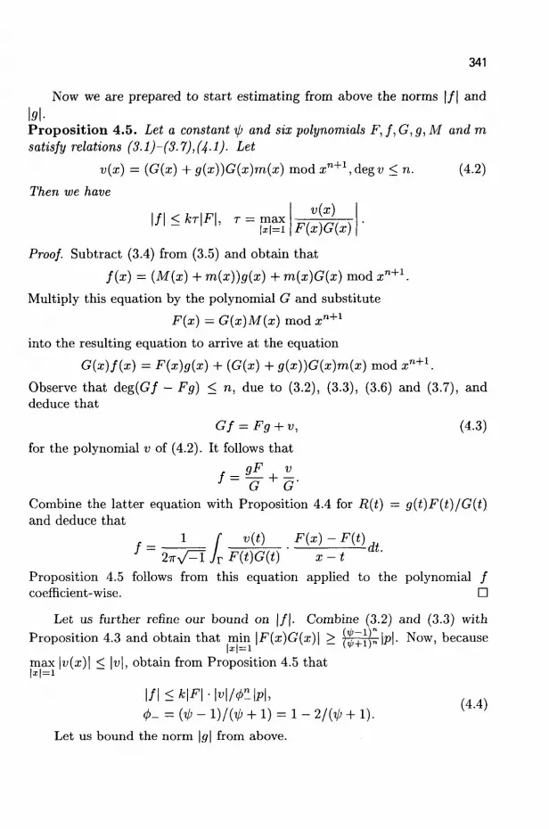
341

\f\<kr\F\, r = max 1x1=1

Now we are prepared to start estimating from above the norms | / | and

l9l-Proposition 4.5. Let a constant i/j and six polynomials F, f, G, g, M and m satisfy relations (3.1)-(3.7),(4-l)- Let

v(x) = (G(x) + g(x))G(x)m(x) mod xn+1, deg v < n. (4.2)

Then we have v(x)

F{x)G{x)

Proof. Subtract (3.4) from (3.5) and obtain that

f(x) = (M(x) + m(x))g(x) + m(x)G{x) mod xn+1.

Multiply this equation by the polynomial G and substitute

F(x) = G{x)M(x) mod xn+1

into the resulting equation to arrive at the equation

G(x)f(x) = F(x)g{x) + (G(x) + g{x))G(x)m(x) mod xn+1.

Observe that deg(G/ - Fg) < n, due to (3.2), (3.3), (3.6) and (3.7), and deduce that

Gf = Fg + v, (4.3)

for the polynomial v of (4.2). It follows that

gF v f = 1 • 1 G G

Combine the latter equation with Proposition 4.4 for R(t) = g(t)F(t)/G(t)_ and deduce that

f = 1 f v{t) F{x)~F{t)dt 1 27rv/^T i r F(t)G{t) x-t

Proposition 4.5 follows from this equation applied to the polynomial / coefficient-wise. •

Let us further refine our bound on | / | . Combine (3.2) and (3.3) with Proposition 4.3 and obtain that min \F(x)G(x)\ > [^^L \p\- Now, because

max \v(x)\ < \v\, obtain from Proposition 4.5 that

\f\<k\F\-\v\/r-\Pi <t>- = (il>-l)/W + l) = l-2/W>+l).

Let us bound the norm |^| from above.

342

Proposition 4.6. Assume relations (3.1)-(3.7) and (4-l)-(4-3). Then

\g\ < 2nr+-k(\f\ + #r*M)/( i - 2nr+-k\™\),

where 4>+ = 1 + 1/tp < 2.

Proof. Combine the relations degg < n — k and degF = k (cf. (3.2) and (3.7)) with Proposition 4.1 for / = 2 and obtain the bound \F\ • \g\ < 2n\Fg\. Therefore, \g\ < 2n\Fg\ because | F | > 1 (see (3.2)). On the other hand, (4.3) implies that \Fg\ < \G\ • \f\ + \v\. Combine the two latter bounds to obtain that \g\ < 2n(\G\ • \f\ + \v\). Deduce from (4.2) that \v\ < \G + g\ • \G\ • \m\. Substitute the bound |G| < <£"~fc, </>+ = 1 + 1/tp, implied by (3.3), and deduce that

M < i<n~k + \g\m~kH, (4-5)

\g\ < 2n^-k(\f\ + (<f>l~k + \g\)\m\).

Therefore, we have

(1 - 2n4>n+-h\m\)\g\ < 2nd>n

+-h(\f\ + # T * M ) ,

and Proposition 4.6 follows. •

Corollary 4.1. Assume relations (3.1)-(3.7), (4-1) and let

2"<^-*|m| < 1/2, (4.6)

k2n{4>+l<t>-r<f>n+-k\m\ < |p|/4. (4.7)

Then we have

| / | < 4 f c ( 0 + / 0 _ ) " # f r f c M M (4.8)

\g\ < 2"+ 1( l + 4A;(0+ /^_)"/W)^"-2 f c |m| , (4.9)

1 < |p| < K (4.10)

for <j>- = l - 2/{ip + 1) of (44) and for

</>+= 1 + l/</>< 2, 0 + / 0 _ = (^ + l ) 2 / ( ( ^ - l ) ^ ) - (4-11)

Proof. Combine Proposition 4.6 with inequality and obtain that

M < 2 n + 1 ( l / l + # T * M ) # T * - (4.12)

Combine (4.4), (4.5), and the bound |F | < </>*., implied by (3.2), and obtain that

|/| < fc(0+/<A_)"(^-A + M)M/|p|.

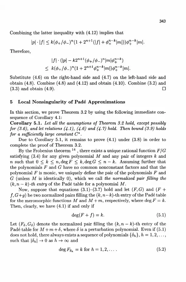
343

Combining the latter inequality with (4.12) implies that

N • i/i < *(0+/0-ni+2"+ io/i+0r f chi))^r f cH-Therefore,

| / | - ( | p | - f c 2 " + 1 ^ + / 0 _ ) " | m | ^ - f c )

< A(0+/0_)n(i+2n+vrfci"»i)0r*imi-Substitute (4.6) on the right-hand side and (4.7) on the left-hand side and obtain (4.8). Combine (4.8) and (4.12) and obtain (4.10). Combine (3.2) and (3.3) and obtain (4.9). •

5 Local Nonsingularity of Pade Approximations

In this section, we prove Theorem 3.2 by using the following immediate con­sequence of Corollary 4.1: Corollary 5.1. Let all the assumptions of Theorem 3.2 hold, except possibly for (3.6), and let relations (4-1), (4-6) and (4-7) hold. Then bound (3.9) holds for a sufficiently large constant C*.

Due to Corollary 5.1, it remains to prove (4.1) under (3.8) in order to complete the proof of Theorem 3.2.

By the Frobenius theorem 14 , there exists a unique rational function F/G satisfying (3.4) for any given polynomial M and any pair of integers k and n such that 0 < k < n,degF < k,degG < n - k. Assuming further that the polynomials F and G have no common nonconstant factors and that the polynomial F is monic, we uniquely define the pair of the polynomials F and G (unless M is identically 0), which we call the normalized pair filling the (k,n — k)-th entry of the Pade table for a polynomial M.

Now, suppose that equations (3.1)-(3.7) hold and let (F,G) and (F + f, G+g) be two normalized pairs filling the (k, n — k)-ih entry of the Pade table for the meromorphic functions M and M + m, respectively, where degF = k. Then, clearly, we have (4.1) if and only if

deg(F + f) = k. (5.1)

Let (Fs,Gs) denote the normalized pair filling the (k,n — fc)-th entry of the Pade table for M + m + S, where S is a perturbation polynomial. Even if (5.1) does not hold, there always exists a sequence of polynomials {5h},h = 1,2,..., such that \Sh\ —• 0 as h —> oo and

deg Fsh = k for h = 1,2,... . (5.2)

344

(Indeed, the coefficient vectors of polynomials 6 for which deg F$ < k form an algebraic variety of dimension k in the space of the (k + l)-st dimensional coefficient vectors of all polynomials of degree at most k.)

Due to (5.2), we have degfsh < k, and therefore, we may apply Corollary 5.1 to the polynomials M + m + 5h and obtain that the coefficient vectors of all polynomials F$n and Gsh are uniformly bounded as follows:

\FSh -F\ + \GSh -G\<(2+ ^ f n m + 5h\ (5.3)

provided that \m + Sh\ < (2 + l/(ip - l ) )~ c °" . Because of this bound, there exists a subsequence {h(i), i = 1,2,.. .} of the sequence h = 1,2,. . . , for which the coefficient vectors (FT , Gj h ) T of the polynomials Fsh(i), G,5Mi)

converge to some (n + 2)-nd dimensional vector (F* T ,G* T ) T . Let F*, G* denote the associated polynomials and let us write

F + f = F*, G + g = G*. (5.4)

Because 6^ —t 0, we immediately extend (5.3) and obtain that

F*(x) = (M(x) + m{x))G*{x) mod xn+1

and

| / | + \g\ - |F* -F\ + |G* - G\ < (2 + ^ f ^ H (5.5)

provided that

H<(2+^rrCon-To complete the proofs of Theorems 3.2 and 1.3, it remains to show that d e g / < k, that is, that degF* = k and that the polynomials F* and G* of (5.4) have only constant common factors. We do this by applying Theorem 3.1. First combine the bounds (4.8) and (3.8) (where Co satisfies the bound

(2 + ^)Con > 4fc(<A+)""fc ( | i ) n | p | / |F | (5.6)

for <f>- and cf>+ of (4.4) and (4.11)) with Theorem 3.1, for p and p* replaced by F and F*, respectively, and deduce that the zeros of the polynomial F + f deviate from the respective zeros of the polynomial F by less than 1 — l/tp, so the polynomial F + f has exactly k zeros all lying strictly inside the unit disc -D(0,1). Similarly, obtain that deg(G + g) — n — k and all the zeros of the polynomial G + g lie outside this disc (provided that the constant Co of (3.8) satisfies the inequality

(2 + jsfo* > 2"+Vr-" (l + § (£)" /) gf (5.7)

345

(cf. (4.9))), so the polynomial G + g has only constant common factors with F + f. This completes the proof of (4.1) and, therefore, also the proofs of Theorems 3.2 and 1.3. •

Acknowledgment

Thanks go to a referee for helpful comments. Supported by NSF Grant CCR 9732206 and PSC-CUNY Awards 669363 and 62435-0031

References

1. L. Ahlfors, Complex analysis, McGraw-Hill, New York, 1979. 2. E. T. Bell, The Development of Mathematics, McGraw-Hill, New York,

1940. 3. C. A. Boyer, A History of Mathematics, Wiley, New York, 1968. 4. L. Blum, F. Cucker, M. Shub, S. Smale, Complexity and Real Computa­

tions, Springer, New York, 1997. 5. R. P. Brent, F. G. Gustavson, D. Y. Y. Yun, Fast solution of Toeplitz

systems of equations and computation of Pade approximations, J. Algo-rithms, 1, 259-295, 1980.

6. D. Bini and V. Y. Pan, Polynomial and Matrix Computations, Vol.1: Fundamental Algorithms, Birkhauser, Boston, 1994.

7. D. Bini and V. Y. Pan, Polynomial and Matrix Computations, Vol.2: Fundamental and Practical Algorithms, Birkhauser, Boston, to appear.

8. J. R. Bunch, Stability of Methods for Solving Toeplitz Systems of Equa­tions, SIAM J. Sci. Stat. Comput, 6, 2, 349-364, 1985.

9. L. M. Delves, J. N. Lyness, A numerical method for locating zeros of an analytic functions, Math. Comp., 21, 543-560, 1967.

10. I. Z. Emiris, A. Galligo, H. Lombardi, Numerical Univeriate Polynomial GCD, Proc. of AMS-SIAM Summer Seminar: Mathematics of Numerical Analysis: Real Number Algorithms, (Park City, Utah, 1995), Lectures in Applied Math., 32, 323-343, Amer. Math. Society, Providence, Rhode Island, 1996.

11. J. von zur Gathen, Parallel Arithmetic Computations: A Survey, Proc. Math. Foundation of Computer Science, Lecture Notes in Computer Sci­ence, 233, 93-112, Springer, Berlin, 1986.

12. I. Z. Emiris, A. Galligo, H. Lombardi, Certified approximate polynomial gcds, J. Pure and Applied Algebra, 117/118, 229-251, 1997.

13. A. A. Grau, The simultaneous improvement of a complete set of approx­imate factors of a polynomial, SIAM J. of Numer. Analysis, 8, 425-438,

346

1971. 14. W. B. Gragg, The Pade table and its relation to certain algorithms of

numerical analysis, SIAM Review, 14, 1, 1-62, 1972. 15. P. Kirrinnis, Fast computation of numerical partial fraction decompo­

sitions and contour integrals of rational functions, Proc. Inter. Symp. on Symb. and Algebraic Comput. (ISSAC 92), (Paul S. Wang editor), 16-26, ACM Press, New York, 1992.

16. P. Kirrinnis, Polynomial factorization and partial fraction decomposition by simultaneous Newton's iteration, J. of Complexity, 14, 3, 378-444, 1998.

17. D. Kapur and Y. N. Lakshman, Elimination methods: An introduction, in Symbolic and Numerical Computation for Artificial Intelligence (B. Donald, D. Kapur, and J. Mundy, editors), pp. 45-89, Academic Press, New York, 1992.

18. J. M. McNamee, bibliography on roots of polynomials, J. Comp. Appl. Math., 47, 391-394, 1993.

19. J. M. McNamee, A supplementary bibliography on roots of poly­nomials, J. Computational Applied Mathematics, 78, 1, 1997, also http://www.elsevier. nl/homepage/sac/cam/mcnamee/index.html.

20. M. Mignotte, An inequality about factors of polynomials, Math. Comp., 28, 1153-1157, 1974.

21. B. Mourrain, V. Y. Pan, Asymptotic acceleration of solving polynomial systems, Proc. 27th Ann. ACM Symp. on Theory of Computing, 488-496, ACM Press, New York, May 1998.

22. B. Mourrain, V. Y. Pan, Multivariate Polynomials, Duality, and Struc­tured Matrices, J. of Complexity, 16, 1, 110-180, 2000.

23. C. A. Neff, J. H. Reif, An 0(nl+t) algorithm for the complex root prob­lem, in Proc. 35th Ann. IEEE Symp. on Foundations of Computer Sci­ence, 540-547, IEEE Computer Society Press, Los Alamitos, California, 1994.

24. C. A. Neff, J. H. Reif, An efficient algorithm for the complex roots prob­lem, J. of Complexity, 12, 81-115, 1996.

25. V. Y. Pan, Sequential and parallel complexity of approximate evaluation of polynomial zeros, Computers & Math, (with Applications), 14, 8, 591-622, 1987.

26. V. Y. Pan, Optimal (up to polylog factors) sequential and parallel al­gorithms for approximating complex polynomial zeros, Proc. 27th Ann. ACM Symp. on Theory of Computing, 741-750, ACM Press, New York, May, 1995.

27. V. Y. Pan, Deterministic improvement of complex polynomial factoriza-

347

tion based on the properties of the associated resultant, Computers & Math, (with Applications), 30, 2, 71-94, 1995.

28. V. Y. Pan, Optimal and nearly optimal algorithms for approximating polynomial zeros, Computers & Math, (with Applications), 3 1 , 12, 97-138, 1996.

29. V. Y. Pan, Solving a polynomial equation: Some history and recent progress, SIAM Review, 39, 2, 187-220, 1997.

30. V. Y. Pan, Approximate polynomial gcds, Pade approximation, polyno­mial zeros, and bipartite graphs, Proc. 9th Ann. ACM-SIAM Symp. on Discrete Algorithms, 68-77, ACM Press, New York, and SIAM Publica­tions, Philadelphia, 1998.

31. V. Y. Pan, Univariate polynomials: nearly optimal algorithms for fac­torization and rootfinding, ACM-SIGSAM International Symposium on Symbolic and Algebraic Computation (ISSAC 2001), ACM Press, New York, 2001.

32. V. Y. Pan, Approximate polynomial gcd, Information and Computation, in press.

33. V. Y. Pan, Structured matrices and polynomials: Unified superfast Algo­rithms, Birkhauser/Springer, Boston, 2001.

34. V. Y. Pan, Z. Q. Chen, The complexity of the matrix eigenproblem, Proc. 31st Annual ACM Symposium on Theory of Computing, 507-516, ACM Press, New York, 1999.

35. G. Polya, G. Szego, Aufgaben und Lehrsdtze aus der Analysis, Verlag Von Julius Springer, Berlin, 1925.

36. A. Schonhage, Asymptotically fast algorithms for the numerical multi­plication and division of polynomials with complex coefficients, Proc. EUROCAM, Marseille, Lecture Notes in Computer Science, 144, 3-15, Springer, Berlin, 1982.

37. A. Schonhage, The fundamental theorem of algebra in terms of compu­tational complexity, Math. Dept., University of Tubingen, Tubingen, Germany, 1982.

38. A. Schonhage, Quasi-gcd computation, J. of Complexity, 1, 118-137, 1985.

39. S. Smale, The fundamental theorem of algebra and complexity theory, Bull. Amer. Math. Soc., 4, 1, 1-36, 1981.

40. S. Smale, On the efficiency of algorithms of analysis, Bulletin of the Amer­ican Mathematical Society, 13, 2, 87-121, 1985.

348

Appendix A: Extension to Splitting over Any Circle

By the initial scaling of the variable, we may move the zeros of a given polyno­mial into the unit disc D(0,1). Therefore, it is sufficient to consider splitting of a polynomial p of (1.1) (within a fixed error tolerance e) over any disc D(X,r), with X and r satisfying the bounds r > 0 and

r + | X | < l . (A.l)

To reduce such a splitting to the normalized case of splitting over the unit circle C(0,1), we will shift and scale the variable x and estimate the new relative error norm bound e as a function in e, X and r. To relate e and e, we will prove the following result: Proposition A . l . Let relations (1.11) and (A.l) hold. Write

y = rx + X, (A.2)

P(y) = 2PiVl = p(rx + x) = q(x), i=0 (A.3)

p{x)=q(x)/\\q(x)\\,

F*(y) = F*(rx + X) = F*{x)rk,

G*{y) = G*{rx + X) = G* {x) / {\\q{x)\\rk),

A(x)=p(x)-F*(x)G*(x),

My)=p(y)-F*(y)G*(y).

Then (A.2) maps the disc D(0,1) = {x : |a;| < 1} onto the disc D(X,r) = {y : \y — X\ < r}; moreover,

\\A(y)\\ < \\A(x)\\ • ((1 + \X\)/r)» • \\P(y)\\ „ 4 )

<| |A(x) | | - ((2 -r)lr)n • ||p(y)||.

Proof. Clearly, (A.2) maps the disc D(X,r) as we stated. To prove (A.4), first observe that A(x) = A ( 2 ^ ) = A(y)/\\q(x)\\. Therefore,

||A(y)|| = | | A ( ^ ) | | • 11,(1)11. (A.5)

349

By combining the relations 1 < Wiy-XY/r^] = (l + | X | ) 7 r \ for i = 0 , 1 , . . with the one of (A.l), we deduce that

| A ( ^ ) | | < | | A ( x ) | | . m a x ( M i ^ )

= | | A ( , ) | | ( i i ^ i ) n

< | | A ( x ) | | ( 2 = r ) n .

(A.6)

On the other hand, having q(x) = p(rx + X) and IKrx + X)*!! = ( r + | X | ) J

for i = 0 , 1 , . . . , we deduce that

^ptirx + Xy i=0

<X>i | (r + |X|)' i = 0

\\q(x)\\ = \\p(rx + X)\\ =

Due to (A.l), it follows that

Il9(*)ll < ElPil = i=0

Combine the latter bound with (A.5) and (A.6) to obtain (A.4).

Appendix B: Error Estimates for Recursive Splitting Suppose that we recursively split each approximate factor of p over the bound­ary circle of some well isolated disc and continue this process until we arrive at the factors of the form (ux + v)d. This gives us a desired approximate factorization

•

P* =P*(x) = J I ^ - z + Vj),

and we next estimate the norm of the residual polynomial

A* = p* - p.

(B.l)

(B.2)

Note that the perturbation of the coefficients of p such that \p* — p\ < 5 implies that a zero Zj oip is perturbed by at most Sfij where fij is the condition number of this zero 7. We are going to estimate the perturbation of the zeros without involving the condition numbers fij. We begin with an auxiliary result from 37 .

350

Proposition B . l . Let

&k = \p-fi---fk\<ke\p\/n, (B.3)

A = | / i - / f f | < e * | / i | , (B.4)

for some nonconstant polynomials fi, •. • , fk, f and g and for

k

e*<e|p|/("IIW)- (BJ5)

Then

|A fc+i | = \p - fgh • • • fk\ < (k + l)e\P\/n. (B.6)

Proof. Ak+1 = \p-h ... fk + (fi ~fg)f2 ...fk\< A f c+A|/ 2 ...fk\. Substitute (B.3)-(B.5) and deduce (B.6). D

If we write / i = / , fk+i = g, then (B.6) will turn into (B.3) for k replaced by k + 1. If we now split one of the factors fi, as in (B.4), we may apply Proposition B.l and then recursively continue splitting p into factors of smaller degrees until we arrive at factorization (B.l), with

|A* |<e |p | (B.7)

for A* of (B.2). Let us call this computation Recursive Splitting Process provided that it starts with k = 1 and fi=p and ends with k — n. Proposition B.2. 37 . Performing Recursive Splitting Process for a positive e < 1, it is sufficient to choose £jt in (B.4) satisfying

ek < e/(n2"+1) (B.8)

for all k in order to support (B.3) for all k = 1,2,... ,n.

Proof. We will prove the bound (B.3) for all k by induction on k. Clearly, the bound holds for k = 1. Therefore, it remains to deduce bound (B.6) from bounds (B.3) and (B.8) for any k. By first applying Proposition 4.1 and then the bound of (B.3), we obtain that

< 2n{l+ keIn)\p\,

which cannot exceed 2 n + 1 |p | for k < n,e < 1. Consequently, (B.8) ensures (B.5), and then (B.6) follows by Proposition B.l. D

k

l[\fi\<ln k

»=i

351

Appendix C: Initial Approximate Splitting via FFT

In this section, we follow 9 and 37 (compare also Appendix A of 27) to describe an algorithm that supports Theorem 1.2, that is, given a polynomial p sat­isfying (1.1), (1.9) and (1.12) computes its initial approximate splitting over the unit circle C(0,1) into the product of two factors F and G . Furthermore, the algorithm performs within the cost bounds of Theorem 1.2.

The algorithm first computes sufficiently close approximations

1 g _ 1 Q - i ,(m+l)qP'(uq)

Q U *(«") '

m = 1 , . . . , <2; ui = exp(27T\A-T/Q), to the power sums,

k

sm = J2z7> m = l,... ,2k-l,

and then approximates (within the error bounds 2~cn for two fixed constants c = cp and c = CQ) the coefficients of the two factors F and G.

Let us estimate the errors of tha computed approximations and the com­putational cost. By 37, we have

\s*m - am\ < (kz<3+m + (n - fc)^-m)/(l - zQ), (C.2)

z — max min(|z,-|, l/|z,-|). (C3) l<j<n

The computation of the values s j , . . . , s | f c _ 1 costs 0(QlogQ) ops for Q > n because it is reduced to performing three discrete Fourier transforms (DFT's) on the set of the Q-th roots of 1. Due to (C.2) and (C.3), it is sufficient to choose Q of the order of N(n)/(i/j — 1) to ensure the error bound

\s*m - S m | < 2"cJV<") (C.4)

for any function N(n) > n, for all m < 2k, and for any fixed constant c. Under such a choice, the bound 0{Q log Q) turns into 0(-J^f log -J^-), and it is sufficient to perform the computations with the precision of 0(N(n)) bits (cf. Corollary 4.1 of 6 , Chapter 3). Then, the algorithm from Sec­tion 4 of Chapter 1 of 6 for Problem 4.8 {I • POWER • SUMS) which uses 0(nlogn)ops(performed with 0(iV(n))-bit precision) computes an approxi-

mation F* to the factor F = T\(x — Zj) of the polynomial p, within the error

352

norm bound

eF\F\ = \F* - F\, eir < 2" C F i V ( " \ (C.5)

for some fixed constant cp (provided that the exponent c in (C.4) is chosen sufficiently large). Then again, it is sufficient to perform the computations by this algorithm with 0(iV(n))-bit precision (cf. 37 .

Similarly we compute an approximation G*ev to the factor Grev of the reverse polynomial prev = FrevGrev, where we write wrev(x) = xmw(l/x) = m m

^S2,WiXm~l for a polynomial w{x) — Y^u^a;2 of a degree m. Observe that, j=0 i=0

the sets of the coefficients as well as the norms of any pair of polynomials w and wrev coincide with each other. On the other hand, all zeros of the reverse polynomial Grev lie in the disc D(0,1//). Therefore, the same techniques that we applied previously enable us to approximate the polynomial Grev, which gives us a polynomial G* of degree n — k satisfying

ea\G\ = \G* - G\, eG < 2~CGN^ (C.6)

for some fixed constant cG. (See 37 for the alternative ways of the computation of the approximate factor G* via polynomial division.)

Let us now deduce the bound 1.10. With no loss of generality, we may assume that |p| = 1. Write p* = F*G* and recall that \F\ < 2" (by (1.9)), |F*| > 1 (because F* is a monic polynomial), |G*| < 2n\p*\/\F*\ (by Propo­sition 4.1), and therefore, |G*| < 2n|p*| < 2 n( l + \p* - p\). Observe that p* - p = F*G* - FG = (F* - F)G* + F(G* - G), write ep = \p* - p\, and deduce that

eP < eF\G*\ + eG\F\ < 2"(eF(l + ep) + eG) < 2^N^ (C.7)

for cp < min(cp, CQ) — n — 2, provided that cp > 1. It is sufficient to perform the entire algorithm for the above computa­

tion of F* and G* with the precision of 0(N(n)) bits to arrive at the error norm bounds of (C.5)-(C7) (apply the estimates of 36, equation (12.6) of 37, and Corollary 4.1 of 6 , Chapter 3). By summarizing our analysis, we obtain Theorem 1.2. • R e m a r k C . l . By choosing sufficiently large constants cp (or cp and cG), one may ensure that the unit circle C(0,1) splits the polynomials F* and G* (see Theorem 3.1).

353

Appendix D: Modifications of the Descending Process

Consider modifications of the descending stage of Algorithm 2.1 based on either or both of the two following equations applied for all j :

Fu-.j(x) = gcd(qu-j{x),Fu-j+1{x2)),

Gu-j(x) = gcd(qu-j(x),Gu-j+i(x2)), j = 1 , . . . ,u.

Here and hereafter, gcd(u(x),v(x)) denotes the monk greatest common divisor (gcd) of the two polynomials u(x) and v(x).

In this modification of Algorithm 2.1, Pade computation is replaced by the polynomial gcd computation. This produces the same output as in Al­gorithm 2.1 if we assume infinite precision of computing. The approach was originally introduced in the proceedings paper 26 but in its journal version 28 was replaced by the one based on Pade computation. This enabled more direct control over the propagation of the perturbation errors (cf. Theorem 3.2), although both approaches can be made computationally equivalent be­cause both Pade and gcd computations can be reduced to the same Toeplitz linear system of equations (cf. 5, 6 ) .

The gcd approach, however, may lead into a trap if one tries to solve the gcd problems based on the fast Euclidean algorithm (cf. Algorithm 5.1a of 6 or 33 ). In this case, each descending step (2.4) is replaced by a recursive Euclidean process, known to be prone to the severe problems of numerical stability involved in it (cf. 38, 10, and 12) and to possible blow up of the precision of the computations and their Boolean cost as a result. In partic­ular, this is the case with the paper 24 where the fast Euclidean algorithm in the gcd version of the descending process is applied reproduced from 26, but unfortunately their analysis of its Boolean cost has been invalidated by a technical flaw. Namely, the analysis hinges on the invalid assumption that the value 5 = ip — 1 exceeds a fixed positive constant (tp2 being the relative width of the basic annulus for splitting a polynomial qu-j)- This assumption is satisfied only for the polynomials qu-j computed at a few last lifting steps, that is, for j = u — 0(1) but not for j = 0 , 1 , . . . ,u/2 (say). Thus, the analysis presented in 24 applies only to a few first descending steps, and the Boolean cost of performing all other steps remains unbounded. Furthermore, this flaw is not easy to fix; clearly it cannot be fixed based on the techniques of the paper 24. Fortunately, the distinct construction of 28 achieves the same result, and now we have its extension to the complete factorization problem as well.

355

COMPLEXITY ISSUES IN D Y N A M I C GEOMETRY

J U R G E N R I C H T E R - G E B E R T

TV Miichen, Zentrum Mathematik, SB4, D-80290 Miinchen, Germany

E-mail: richter@ma.tum.de

U L R I C H H. K O R T E N K A M P

FU Berlin, Institut fr Informatik, Takustrae 9, D-14195 Berlin, Germany

E-mail: kortenkamp@inf.fu-berlin.de

This article deals with the intrinsic complexity of tracing and reachability questions in the context of elementary geometric constructions. We consider constructions from elementary geometry as dynamic entities: while the free points of a construc­tion perform a continuous motion the dependent points should move consistently and continuously. We focus on constructions that are entirely built up from join, meet and angular bisector operations. In particular the last operation introduces an intrinsic ambiguity: Two intersecting lines have two different angular bisectors. Under the requirement of continuity it is a fundamental algorithmic problem to resolve this ambiguity properly during motions of the free elements. After formalizing this intuitive setup we prove the following main results of this article:

• It is NP-hard to trace the dependent elements in such a construction.

• It is NP-hard to decide whether two instances of the same construction lie in the same component of the configuration space.

• The last problem becomes PSPACE-hard if we allow one additional sidedness test which has to be satisfied during the entire motion.

On the one hand the results have practical relevance for the implementations of Dynamic Geometry Systems. On the other hand the results can be interpreted as statements concerning the intrinsic complexity of analytic continuation.

1 Introduction

1.1 What is Dynamic Geometry

Imagine any construction of elementary geometry - for instance, a ruler and compass construction of the midpoint of two points A and B. It consists of certain free elements (the points A and B) and certain dependent elements whose positions are determined by the positions of the free elements. Each specific drawing of such a construction is a snapshot that belongs to the whole continuum of all possible drawings for all possible locations of the free

Keywords: Dynamic Geometry, analytic continuations, NP, PSPACE, complexity, reachability, ruler and compass, linkages, warehouseman's problem

356

elements. If we move the free elements we can walk continuously from one instance (i.e. snapshot) of the construction to another one. During such a walk a continuous motion of the free elements should result in a continuous movement of the dependent elements.

This article deals with those effects and problems that genuinely arise from such a dynamic and continuous setup of geometry. The research that led to the results presented in this article was motivated by the desire (and the actual work) of implementing a software package for doing Dynamic Ge­ometry on a computer 22>23. With such a program one should be able to do constructions of elementary geometry with a few mouse clicks, and after this pick the free elements with the mouse - drag them around - while the whole construction follows accordingly. The unsuspicious looking requirement of continuity of dependent elements turned out to be fundamentally hard to fulfill. In fact, one has to rely on notions of complex function theory and Rie-mann surfaces to get a mathematically sound treatment of these effects 11>12. While this is no problem in theory, we prove here that from a complexity theoretic point of view most algorithmic questions related to that context are provably intractable (unless P=NP, of course). The complexity classes that arise here range from NP-hard problems via PSPACE-hard problems up to even undecidable problems. In particular we prove that . . .

. . . it is NP-hard to calculate the positions of the dependent elements after a specific move of a free element (Sec. 5),

. . . in general, it is PSPACE-hard to decide whether two instances of the same construction can be continuously deformed into each other if all free and dependent elements must have real coordinates (Sec. 6),

. . . this reachability problem is still NP-hard if only join, meet, and angular bisector operations occur (Sec. 4),

. . . it is undecidable whether two instances of a construction involving "wheels" - devices that transfer angles to distances - can be continu­ously deformed into each other by moving the base elements (Sec. 7).

Although the results of this article arose from the study of configuration spaces of elementary geometric constructions they are naturally related to many other setups in the area of geometry. Among those are the study of configuration spaces of mechanical linkages 6<g<10

t realization spaces of ori­ented matroids 16>4>20,25 and polytopes 21, and the warehouseman's problem 7,24. The results of this article are partially generalizations and strengthenings of known complexity results in these areas. Besides the context of Dynamic

357

1: A=FreePoint; 2: B=FreePoint; 3: C=FreePoint; 4: a=Join(B,C); 5: b=Join(A,C); 6: c=Join(A,B); 7: d=AngularBisector(b,c) 8: e=AngularBiseetor(a,e) 9: f=AngularBisector(a,b) 10: D=Heet(d,e);

Construction sequence static picture idea of the dynamic picture

Fig. 1: Dynamic behavior of the angular bisector theorem.

Geometry our results are relevant for all areas where geometric objects are moved around under certain geometric constraints, like robotics, paramet­ric CAD 5 , virtual reality, or computational kinematics. Our results imply that many problems of these areas are computationally difficult (like the per­sistent naming problem of parametric CAD 5 or the navigation problem of computational kinematics). Also one can interpret the results of this paper as statements on the complexity of analytic continuation (all coordinate func­tions in our setup turn out to be analytic). In particular this gives intrinsic complexity bounds on homotopy methods for solving polynomial equations as they were discussed in 26,27,28,29,30 This article is complemented by n ' 1 2

were we give conceptual approaches to handle a dynamic setup of geometry at all.

1.2 Constructions, Forbidden Situations and Ambiguities

In a typical setup for this article we will study construction sequences in which each single construction step is of very elementary nature like taking the join of two points, the meet of two lines, the angular bisector of two lines, or the intersection of a line and a circle, etc. A construction sequence starts with some free points and generates new elements by performing elementary operations on already existing elements one at a time. It may happen that an operation cannot be carried out (for instance, if one wants to construct the join of two identical points, the meet of two identical or parallel lines, or the intersection of a line and a circle that do not meet). In order to avoid such situations let us assume that the input points are in suitable positions such that each step of the construction sequence can be done. In that case we will call the input point position admissible, otherwise we call it forbidden.

The join and meet operations are deterministic construction steps in the

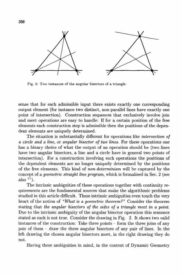
358

A A Fig. 2: Two instances of the angular bisectors of a triangle.

sense that for each admissible input there exists exactly one corresponding output element (for instance two distinct, non-parallel lines have exactly one point of intersection). Construction sequences that exclusively involve join and meet operations are easy to handle: If for a certain position of the free elements each construction step is admissible then the positions of the depen­dent elements are uniquely determined.

The situation is substantially different for operations like intersection of a circle and a line, or angular bisector of two lines. For these operations one has a binary choice of what the output of an operation should be (two lines have two angular bisectors, a line and a circle have in general two points of intersection). For a construction involving such operations the positions of the dependent elements are no longer uniquely determined by the positions of the free elements. This kind of non-determinism will be captured by the concept of a geometric straight line program, which is formalized in Sec. 2 (see also n ) .

The intrinsic ambiguities of these operations together with continuity re­quirements are the fundamental sources that make the algorithmic problems studied in this article difficult. These intrinsic ambiguities even touch the very heart of the notion of "What is a geometric theorem?" Consider the theorem stating that the angular bisectors of the sides of a triangle meet in a point. Due to the intrinsic ambiguity of the angular bisector operation this sentence stated as such is not true. Consider the drawing in Fig. 2. It shows two valid instances of the construction: Take three points - form the three joins of any pair of them - draw the three angular bisectors of any pair of lines. In the left drawing the chosen angular bisectors meet, in the right drawing they do not.

Having these ambiguities in mind, in the context of Dynamic Geometry

359

two natural questions arise:

• Reachability problem: Is it possible to move the free points such that a first instance is smoothly deformed into a specific second one?

• Tracing problem: How can a Dynamic Geometry program decide after a motion of the free elements what instance to draw for the new position?

After a suitable formalization, we will show that the reachability problem is in general PSPACE-hard. It is still NP-hard if one restricts oneself to constructions that only use join, meet, and angular bisector operations. The tracing problem turns out to be (at least) NP-hard.

1.3 Restricting the Operations

We try to formulate our statements as strongly as possible and restrict the allowed elementary operations to a minimum. The only operations we will use are join, meet, angular bisectors and intersection of circle and line. Further­more, we assume that initially four fixed constant base points (0,0), (1,0), (0,1) and (1,1) are given. In fact, we try to use the intersection of circle with line operation as sparsely as possible. The reason for this is that the possible non-existence of such an intersection includes the possibility to en­code sidedness conditions and "cutting holes" in the admissible range of input parameters. By explicitly excluding operations like intersection of circle and line we substantially strengthen our results. In fact the NP-hardness results for the tracing and reachability problems can be exclusively stated in terms of angular bisectors, join and meet. The PSPACE-hardness results need just one single intersection-of-circle-and-line operation. We also try to introduce as few free points as possible into or constructions. This complements many other related complexity results since there usually many free variables are needed. The following table summarizes the complexity results covered in this article:

Problem

Tracing Reachability Reachability Reachability Reachability Reachability

Complexity

NP-hard NP-hard NP-hard

PSPACE-hard PSPACE-hard Undecidable

#free points

1 many

1 1

many 1

^angular bisectors

many

3 many many

— 2

# int. circle/lines

— — — 1 1

—

# wheels

— — — — — 11

360

In order to exclude unnecessary technicalities arising from special cases we also assume that the plane is extended by elements at infinity to the usual projective plane.

The results that use exclusively angular bisectors (and join and meet) are in a sense generalizations of corresponding results in other setups in the following sense. While with mechanical linkages or with ruler and compass constructions it is easily possible to construct angular bisectors, the converse is impossible. A complexity theoretic lower bound for a setup that uses only angular bisectors is therefore a stronger result than a corresponding one for linkages or ruler and compass constructions.

1.4 Related Results

There are other related areas of geometry where similar complexity results arise. In this section we want to briefly discuss the relations - similarities and differences - to these results.

I.4.I Oriented Matroids and Polytopes

Research over the last few decades showed that for oriented matroids and poly­topes so called universality theorems can be proved. These theorems show that the corresponding realization spaces can essentially be (stably equivalent to) any solution space of a system of (finitely many) polynomial equations and in­equalities 16.4,20,2i,25_ These results are usually derived by a direct translation procedure, which starts from a system of polynomials and ends up with a con­figuration of the desired category (an oriented matroid or a polytope). In the realization space of the oriented matroid (or polytope) the original variables of the algebraic equations can be rediscovered from the coordinates of certain points. The constructions of universality theorems deeply rely on the genera­tion of large loops that feedback the result of an evaluation of a polynomial to a initially chosen constant (for instance a point whose coordinates represent the "1".) Deciding whether the realization space of an oriented matroid or polytope is empty or not turns out to be NP-hard. Deciding whether two realizations of an oriented matroid (or polytope) are in the same connected component of the realization space turns out to be PSPACE-hard.

In Sec. 4 although we derive a similar result for elementary geometric constructions where we rely on very different effects. The complex behavior is generated by a strictly forward oriented construction without any feedback of information. Orientation information cannot and is not included in any way

IFor the PSPACE-hardness result in Sec. 6. the significant difference to the constructions for oriented matroids or polytopes is that we use only one

361

free point instead of many free points.

1.4-2 Mechanical Linkages

A similar comparison holds for mechanical linkages, for which universality theorems are known 6>9>10 that prove that arbitrary primary semialgebraic sets can show up as components of configuration spaces. The corresponding reachability problem ("Do two instances of a linkage lie in the same component of the configuration space?") is also PSPACE-hard.

The results there are obtained by making use of construction loops and inequality relations. The inequality relations arise naturally in that context, since the bars of a linkage are only of finite length. In our setup only weaker construction primitives are allowed. Furthermore also the linkage results rely on the introduction of many free elements, in contrast to our results.

1-4-3 Warehouseman's Problem

Moving an object with a non-restricted number of degrees of freedom through a world of geometric obstacles leads to another PSPACE-hard reachability problem 7 '24. Again, the use of inequality relations is already inherent in the statement of the problem, and many free elements are needed.

1.5 Acknowledgements

We want to thank Alexander Below, Vanessa Krummeck and Jesus de Loera for careful proofreading and many valuable discussions. We want to thank Maurice Rojas for drawing our attention to Plaisted's Theorem that served as a paradigm for the proof in Sec. 5 and simplified our original construction. We also thank Yuri Matiyasevich who supplied us with the proper reference for the best known bound for the number of variables that is needed to prove the undecidability of Hiberts 10th problem over the integers (see Sec. 7).

2 Geometric Constructions

2.1 Geometric Straight Line Programs

We now start to formalize the concept of a geometric construction. We take special care to have a setup that allows the results of an operation to be non-existent or ambiguous. For this we first define the notion of a relational instruction set. Here, instead of giving an algorithm or formula for the op­eration, only a relation is specified that enables us to check the validity of a

362

certain input and output pair. A slightly more general approach can be found in 1 1 . Definition 2 .1 . A relational instruction set (RIS) is a pair (0,fi) of objects O and primitive operations fi with the following properties: O = ( C i , . . . , Ok) is a family of sets d. These sets partition the objects into classes of the same type. The primitive operations $7 = (uii,... ,ui{) are relations

with input size (arity) ar(wj) = Si and type type(wi) := Oxi . An element (o i , . . . , oar(w)) € Oxt x • • • x 0 X J is called an input and an element o € 0 ^ +1

is called an output of w;. Remark 2.2. For the relation (o\,... ,oaT^,o) £ to, we will also use the more intuitive notation

o <- Ui(oi,... , o a r ( w ) ) .

This notion may be considered as a non-deterministic assignment operation. It assigns to an input (o\,... ,oar(w)) one of the potential outputs o of ui. However, one should have in mind that this notion still represents a relation that can be true or false. It is true if the input is admissible for the operation and if the output is one of the proper evaluations of ui on this input.

In our geometric setup the different classes of objects will correspond to points, lines, circles, etc. Each primitive operation will represent a certain type of geometric primitive construction like join, meet, angular bisectors, etc. In addition, we will allow special operations to create free points which will play the role of the "input" of our constructions. Observe that relational instruction sets are general enough to describe not only geometric, but also arithmetic operations (see u ) .

We now describe the specific objects and operations used in this article. Although we will make use of Euclidean operations, we will describe the purely incidence geometric part for points and lines in terms of projective geometry. This will exclude unnecessary special cases and helps in defining the right concept of continuity later on. We embed everything in the real projective plane MP2. In the usual way we can represent points and lines (in homoge­neous coordinates) by vectors in K3 \ {(0,0,0)}. Vectors that only differ by a scalar multiple are identified and represent the same point (or line). A point (x, y, z) is on a line (a, 6, c) if and only if ax + by + cz = 0. Meet and join can then be simply expressed as cross-products of such vectors (see for instance

" ) •

Since we also want to deal with objects and operations of Euclidean geom­etry like circles and angular bisectors, we have to embed the usual Euclidean

363

plane (equipped with a Euclidean metric) in RP2. A finite point (x,y) € R2

will be represented by the point (x,j/,l) of UP2. With this standard em­bedding a line ax + by + c = 0 of R2 is represented by (a, b, c), i^ — (0,0,1) represents the line at infinity, and two lines l\ = (a\, b\, c\) and I2 = (02, 2, C2) are orthogonal if 0162 — b2a2 — 0. In order to simplify the notation later on we will also identify a finite point (a;, y, 1) with a complex number x + iy. By this we identify the finite part of the projective plane with C

We restrict the use of angular bisectors to those lines that pass through the origin (0,0) of E2 . An angular bisector of two lines l\ and l2 through the origin is a line t through the origin such that Z(/i,£) = /(•£, k)- For a pair of lines there are two angular bisectors, which are orthogonal to each other. Restricting the use of angular bisectors to lines through the origin reduces the occurrence of non-admissible situations to a minimum. Formally, we will make use of the following primitive operations. For the sets P of points and L of lines, we define:

JOIN := {(pi,P2,0 I I is the line through p\ and p% and p\ ^ p2}

C{PxP)xL

MEET := {{h,l2,p) I P is the intersection of l\ and Z2 and /1 ^ l2}

C{LxL)xP

BISECT := {(/i,/2,0 I Hs an angular bisector of l\ and I2 and

h,h,l pass through the origin}

C (L x L) x L

Furthermore, we define the following four constants (i.e. primitives with input size zero):

p(a,b) . = {(a j 6) !)}<- p. for a b £ | 0 ; J}

These constants will be used to fix a coordinate system. For the generation of free points we define a special instruction that has no input elements and allows the output to be any point of P:

FREE := P.

We will deal with the following relational instruction set:

JMB := ((P, L), (JOIN, MEET, BISECT, FREE, p(0,0)) p(l,0) ( p(0,l)) p(Ll))).

364

Remark 2.3. Here are three comments on the choice of the primitive oper­ations:

(i) The only cases where the two operations JOIN and MEET are not admissi­ble is when the two input elements are identical. For all other cases they are well-behaved.

(ii) The only operation that introduces an ambiguity is BISECT. The primi­tives JOIN and MEET are "deterministic" in the sense that each admissible input has exactly one possible output.

(iii) The operation BISECT has been chosen for our investigations since it iso­lates the effect of generating an ambiguity. Unlike the intersection circle with line operation it has no open region of the input parameters where it is not admissible. Such effects (which we want to exclude here) would allow the possibility to construct some kind of "sidedness test", which are at the core of of complexity results for oriented matroids, polytopes, mechanical linkages or the warehouseman's problem. In Sec. 6 when we prove the PSPACE-hardness result we will make a very selected use of one such additional operation.

A construction sequence is formalized by the concept of a geometric straight line program (GSP). Definition 2.4. A geometric straight-line program on a relational instruction set (0,0.) is defined by a sequence of statements F = (Ti,..., Fm). Each Tj has the form P,- = (oJ,ii, • • • ,«ar(o;)) where

(i) UJ is an operation from the instruction set fl,

(ii) the type of Fj is defined to be the type of w,

(iii) for each k 6 { 1 , . . . , ar(w)} we have iu < j ,

(iv) for each k G { 1 , . . . , ar(w)} the type of F;fc matches the type of the A;-th input of u.

After a suitable set of primitive operations is given it is straightfor­ward to describe construction sequences by a GSP. Each statement Fj — (w, i\,... , iar(tj)) °f a GSP describes the generation of a new element by means of a primitive operation ui whose input is given by the output of the statements r ^ , . . . ,Fi^(ui). Item (iii) of the above definition ensures that only elements are used as input that have been already constructed. Item (iv) ensures a cor­rect typing. The concept of a GSP emphasizes the constructive step-by-step

365

nature, however it allows for a certain "non-determinism" during a construc­tion, since it does not specify which output of an (ambiguous) operation to take. To make GSPs more readable we also use the " <— " notation of Remark 2.2 to encode each statement. A statement Tj = (ui,ii, • •. , *ar(w)) will then be written as j <— u>(ii,. • • ,iar(u,))- Furthermore, we allow to exchange the references j,i\,... ,iar(w) by meaningful variable names.

We may consider a certain set of primitive operations as a kind of pro­gramming language. Each GSP is a certain program. In what follows we are mainly interested in the constructions/programs that can be described by the operations in JMB. Example 2.5. The following sequence of instructions is a simple GSP over the JMB instruction set. It takes two free points p and q, joins them to the origin o, and constructs the angular bisector of the two resulting lines.

p 4 - FREE

q « - FREE

o « - P(°>°)

lx < - JOIN(a ,o )

l2 <r- JOIN(6,o)

b < - BISECT( / i , / 2 )

We will still simplify the notions by assuming that points that do not occur explicitly on the left of any assignment are automatically initialized by a FREE operation. Furthermore, if the output of an operation is unique and used only once we allow that it is used directly (without intermediate variable) as an input of another operation. In particular this convention applies to the constants in JMB. With these conventions the above GSP can simply be written as

b <- B I S E C T ( j O I N ( p , P ( 0 ' 0 ) ) , J O I N ( g , P ( 0 ' ° ) ) ) .

Closely related to the concept of a GSP ( r \ , . . . , Tm) is the notion of an instance of the GSP. Roughly speaking an instance of a GSP is an assignment of a concrete object to each of the statements r» such that all corresponding relations are satisfied. Definition 2.6. An instance of a geometric straight-line program (ITi,... , r m ) is an assignment of objects X — Xi,...,Xm such that all primitives are satisfied, that is, for every statement Fj = (uij,i\,... ,*ar(wj)) the relation (Xtl,... ,-Xi„(„.>,Xj) & LOJ holds. Example 2.7. For the GSP given in Example 2-5. we have in particular the

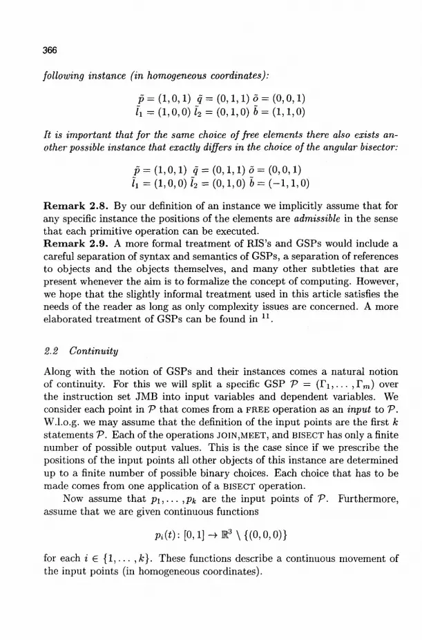
366

following instance (in homogeneous coordinates):

p= (1,0,1) gf= (0,1,1)5 = (0,0,1) J~i = (1,0,0) J2 = (0,1,0)6 = (1,1,0)

It is important that for the same choice of free elements there also exists an­other possible instance that exactly differs in the choice of the angular bisector:

p = (1,0,1) q= (0,1,1) 5= (0,0,1) fi = (l,0,0)f2 = (0,1,0)6 = ( - 1 , 1 , 0 )

R e m a r k 2.8. By our definition of an instance we implicitly assume that for any specific instance the positions of the elements are admissible in the sense that each primitive operation can be executed. R e m a r k 2.9. A more formal treatment of RIS's and GSPs would include a careful separation of syntax and semantics of GSPs, a separation of references to objects and the objects themselves, and many other subtleties that are present whenever the aim is to formalize the concept of computing. However, we hope that the slightly informal treatment used in this article satisfies the needs of the reader as long as only complexity issues are concerned. A more elaborated treatment of GSPs can be found in n .

2.2 Continuity

Along with the notion of GSPs and their instances comes a natural notion of continuity. For this we will split a specific GSP V = (I"i , . . . , r m ) over the instruction set JMB into input variables and dependent variables. We consider each point in V that comes from a FREE operation as an input to V. W.l.o.g. we may assume that the definition of the input points are the first k statements V. Each of the operations JOIN,MEET, and BISECT has only a finite number of possible output values. This is the case since if we prescribe the positions of the input points all other objects of this instance are determined up to a finite number of possible binary choices. Each choice that has to be made comes from one application of a BISECT operation.

Now assume that p\,... ,Pk are the input points of V- Furthermore, assume that we are given continuous functions

Pi{t): [0,1] - > M 3 \ {(0,0,0)}

for each i g {1, - • • ,k}. These functions describe a continuous movement of the input points (in homogeneous coordinates).

367

Definition 2.10. A continuous evaluation of the GSP V over the JMB in­struction set under the movement pi(t) is an assignment of continuous func­tions

0i(t): [0,1]-> E 3 \ { (0 ,0 ,0 )}

for each i € {k + 1 , . . . , m} such that for all t £ [0,1] the objects

(Pi(*),--- ,Pk{t),ok+i(t),... ,om(t))

form an (admissible) instance of V'. This concept formalizes the intuitive requirement that under a continuous

movement of free elements the dependent elements should move continuously as well. For instance, if we have the simple GSP of Example 2.5 and move from one instance to another by changing the positions of the free elements a and b, a continuous evaluation makes sure that we do not jump spontaneously from one choice of the angular bisector to the other one.

Observe that the way we define continuity leaves room for the necessary indeterminism: Usually one would require that the output elements are given by continuous functions in the input, but here both the path of the input and the path of the output are given by continuous functions on the interval [0,1].

The following property of continuous evaluations is crucial: Lemma 2.11. If there exists a continuous evaluation of the GSP V over the JMB for a continuous movement Pi(t) then it is unique.

Proof. We can prove this lemma by induction on the length of P. Assuming that the statement holds for all programs of length m — 1 we prove that it also holds for programs of length m. Assume that for such a program V the functions pi (t) describe a continuous movement for which a continuous evalu­ation exists. If the last operation of V is one of the constant points then the statement holds trivially. If the last operation of V is one of the determinis­tic operations JOIN or MEET, then the statement holds by the continuity of these operations. If the last operation is BISECT then we can argue as follows: The two possible outputs of BISECT are two lines that are orthogonal to each other. If there was a way to continuously get from one branch to the other there must be a position in which these two lines coincide. This is impossible since the two angular bisectors are orthogonal. •

R e m a r k 2.12. This Lemma shows the importance of non-admissible posi­tions: At these singularities the different branches coincide, both angular bisectors degenerate to the zero vector. It is not possible to extend the pro­jective setting by this additional line (0,0,0) (and a corresponding point)

368

without destroying the uniqueness of continuous evaluations, even though it is possible to extend the JMB instruction set to include them.

2.3 Fundamental Problems in Dynamic Geometry

After formalizing the concept of GSPs and continuity we are finally in the position of formalizing the main questions of this work. The first problem formalizes the most fundamental operation of a Dynamic Geometry program: After you pick a free point of a construction and move it to another position, how did the rest of the construction change? Definition 2.13. (Tracing problem): Let V be a GSP and let Pi(t) describe a continuous movement for which a continuous eval­uation (pi(t),... ,Pk(t), Of.+i (t),... , om(t)) exists. Furthermore, let (p i , . . . ,pk,Ok+i, • • • ,om) be an instance of V with free points pi — Pi{l) for alH 6 { 1 , . . . , k}. Decide whether Oj = 0^(1) for alH 6 {k + 1 , . . . , m}.

The second problem asks for the mere existence of a path from one in­stance to another. Definition 2.14. (Reachability problem): Let P° = (/>?,••• ,P°k,o0

k+i,--- ,o°m) and P 1 = (p{,... ,pl,ol+1,. •. ,oJ„). Decide whether there exists a continuous evaluation that starts at P° and ends at P1.

We will see that both problems turn out to be (at least) NP-hard. If we allow one single use of a sidedness test to constrain admissible regions the reachability problem even turns out to be PSPACE-hard.

3 Useful Gadgets

This section will describe small constructions that are helpful to compose the more complicated constructions that we need later.

3.1 More Primitives

Since our set of primitive operations is very restricted we first show that other useful primitive operations can be easily composed from these primitives.

369

3.1.1 The Line at Infinity

By a simple sequence of join and meet operations we can construct the line at infinity:

a <- MEET(JOIN(P(°'0),P(0'1)),JOIN(P(1'°),P(1'1)))

b «- MEET(JOIN(P(0'0»,P(1'°)),JOIN(P(0'1),P(1'1)))

too «- JOIN(O,6)

By construction, a and b are two distinct points on the line at infinity and hence l^ is the line at infinity with homogeneous coordinates (0,0,1).

3.1.2 Parallel Lines

For a line / and a point p we can calculate the parallel to / through p by

JOIN(MEET(Z,4O) ,P) .

If p lies on / this formula produces I itself. If / = 1^ this formula is not admissible. We will refer to this "macro" by PARALLEL , p).

3.1.3 Perpendicular

A bit less trivial is the construction of a perpendicular to I trough p. We can only do such a construction since the choice of our constant points pro­vides us with a sample of two perpendicular lines. This right angle can then be transferred to another line. Since we already have a parallel operation w.l.o.g. we may assume that I passes through p(°>°) and that p = p(°'°). The construction is given in Fig. 3. We have

a <- MEET(JOIN(P( 1 ' 0 \P( 1 ' 1 ) ) , / ) ,

b <- MEET(jOIN(p(0 '0),P(0 '1)),PARALLEL(a,JOIN(p(1 '°),p(0 '1)))),

C «- MEET(JOIN(P(° '1 ) ,P(1 '1 ' ) ,PARALLEL(6,JOIN(P ( 0 '0 ) ,P ( 1 '1 )))) ,

perp <- JOIN(C, P ( 0 ' 0 )) .

This construction is admissible for all situations where I passes through p(°.°). We will refer to the general construction for perpendiculars by PERPENDICULAR^, p) .

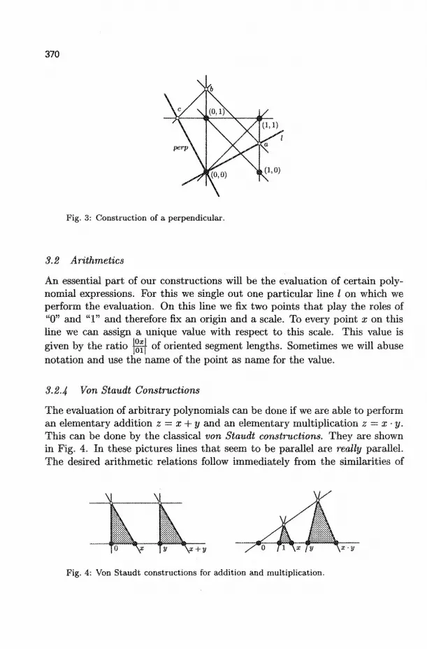
370

Fig. 3: Construction of a perpendicular.

3.2 Arithmetics

An essential part of our constructions will be the evaluation of certain poly­nomial expressions. For this we single out one particular line / on which we perform the evaluation. On this line we fix two points that play the roles of "0" and " 1 " and therefore fix an origin and a scale. To every point x on this line we can assign a unique value with respect to this scale. This value is given by the ratio |~f of oriented segment lengths. Sometimes we will abuse notation and use the name of the point as name for the value.

3.2.4 Von Staudt Constructions

The evaluation of arbitrary polynomials can be done if we are able to perform an elementary addition z = x + y and an elementary multiplication z = x • y. This can be done by the classical von Staudt constructions. They are shown in Fig. 4. In these pictures lines that seem to be parallel are really parallel. The desired arithmetic relations follow immediately from the similarities of

\ 1

___

[ M

k ir"1'A* * y \ i + V

Fig. 4: Von Staudt constructions for addition and multiplication.

371

jo 1 U TR TO

Fig. 5: Coordinate extraction for "complex" points.

the darkened triangles. Both constructions can be easily decomposed into a sequence of JOIN, MEET and PARALLEL operations, that start from the points 0, 1, x, y and one auxiliary point p not on! . In particular we get

MEET(JOIN(0 ,X) ,

PARALLEL(JOIN(:E,P),

MEET(PARALLEL( JOIN(0, p), y),

PARALLEL(JOIN(0, x),p)))), MEET(JOIN(0 ,X) ,

PARALLEL(JOIN(:E,P),

MEET(PARALLEL(JOIN(1,P), y), J O I N ( 0 , P ) ) ) ) .

These construction sequences are chosen with care such that as long as the auxiliary point p is not on Z the only non-admissible situations arise when in the addition both points x and y are at infinity or in the multiplication one of the points is at 0 and the other is at infinity.

x + y «-

x-y «-

3.2.5 Complex Arithmetics

As well as calculations over the real numbers we can also do calculations over complex numbers. For this we fix points "0", " 1 " and "i" in the plane, such that the lines ZR «— JOIN(0,1) and Z$R <- JOIN(0 , I ) are perpendicular and such that the distance from 0 to 1 is the same as the distance from 0 to i. For convenience we take 0 «- p(°-°), 1 «- pC1-0), i <- p(°,i). The lines lR

and ZJR play the roles of the real and imaginary axes of the complex plane. The points 0 and 1 define a scale on ZR. The points 0 and i define a scale on ZJR. For each point p in the plane we can (after orthogonal projection to these two axes) assign two coordinates, the real and the imaginary part of a complex number a + ib. If no confusion can arise we simply denote the points

372

with homogeneous coordinates (a, b, 1) by the corresponding complex number a+ib. By a parallel projection along the direction of JOIN(1, i) we can transfer any number in ZJR to the corresponding number on ZR, and vice versa. Let z\ = a,\ + ib\ and z2 = a2 + ib2 be two complex numbers. With respect to our coordinate system we can model complex addition and complex multiplication of the points z\ and Z2 by first transferring the real and imaginary parts to the line ZR, then modeling the formulas

z\ + z2 — (ax + o2) + i(h + b2), z\ • z2 = (aia2 - hb2) + i(aib2 + b\a2),

by a sequence of von Staudt constructions and finally construct a new point from the resulting real and imaginary part. The complex addition can be used for addition of vectors as well. Remark 3.1. One might think that using von Staudt constructions for vector addition is more than necessary. The simple construction sequence

Zi+Z2 4- M E E T ( P A R A L L E L ( 0 , ; ? I ) , P A R A L L E L ( 0 , 2 : 2 ) )

seems to work as well. However, this construction has the disadvantage that it is non-admissible whenever 0, z\ and z2 are collinear. For the complexity issues that we consider later the actual length of these elementary operations is irrelevant as long as it is constant.

3.2.6 Integer and Rational Points

By being able to add and multiply via von Staudt constructions we are also able to construct points a + ib for arbitrary integers a and b with respect to our coordinate system. We simply have to find a sequence of additions and multiplications that computes the numbers a and b starting from 0 and 1. In particular, using the binary representation any integer n > 0 can be constructed in 0(log(n)) construction steps.

It is also easy to construct numbers of the form ^ . The construction in Fig. 6 shows that this can be done in 0(n) steps.

3.3 Points on Circles and Intervals

In our relational instruction set JMB we do not have direct access to circles. However, by Thales' theorem we can freely generate points on circles that are given by two diameter points (see Fig. 7 left). Let a and b be the two endpoints of a diameter of the desired circle. We take a free point p and construct

q 4- MEET(jOIN(a,p),PERPENDICULAR(jOIN(a,p),6)).

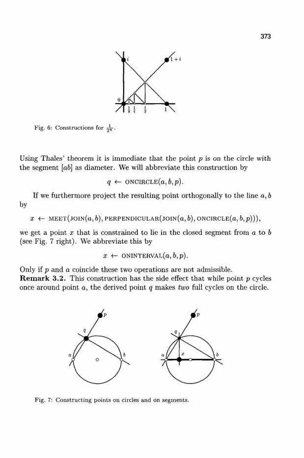
373

Fig. 6: Constructions for ^ - .

Using Thales' theorem it is immediate that the point p is on the circle with the segment [ab] as diameter. We will abbreviate this construction by

q <- ONCIRCLE(a, b,p).

If we furthermore project the resulting point orthogonally to the line a, b by

X « - M E E T ( J O I N ( O , 6) ,PERPENDICULAR(jOIN(a,6) ,ONCIRCLE(a, b,p))),

we get a point x that is constrained to lie in the closed segment from a to b (see Fig. 7 right). We abbreviate this by

X <- ONINTERVAL(a, b,p).

Only if p and a coincide these two operations are not admissible. Remark 3.2. This construction has the side effect that while point p cycles once around point o, the derived point q makes two full cycles on the circle.

Fig. 7: Constructing points on circles and on segments.

374

Fig. 8: Detection of a winding number.

Remark 3.3. Although by this construction we can generate a point freely on the boundary of a circle, this circle is not available for further constructions like intersecting it with a line.

3.4 Detecting a Winding Number

So far the constructions used in our gadgets did not contain any BISECT op­erations and therefore no non-determinism occurred. The basic functionality for which we will use BISECT operations is the generation of monodromy ef­fects: "One can start with an instance A of a GSP and continuously make a round-trip with the free elements and end up in a different instance B." The smallest device for which such an effect occurs is given by the following GSP:

£0 «- JOlN(a,0) £l < - B I S E C T ( / R , ^ 0 )

£2 < - BISECT(ZR, ^ i )

It takes a free point a, joins it with the origin and constructs an angular "quad-sector" of this line and /R. Assume that a is in a certain position (^ 0) and from there makes a round-trip with continuous speed around the origin. While £0 moves with an angular velocity w the line £\ moves with angular velocity w/2 and the line £2 moves with angular velocity u/4. Thus after a has performed a full cycle around the origin the line £2 has made a quarter turn. If a moves along an arbitrary path (that avoids point 0) and returns to its original position then the resulting situation reflects the parity of the winding number of a around the origin. If £2 returned to its original position,

375

the winding number was even, if £2 moved to the orthogonal of its original position the winding number was odd.

We can furthermore iterate this construction by adding more statements of the form

li « - B I S E C T ( / R , ^ _ i )

for i £ { 3 , . . . ,k}. The resulting line l^ moves with angular velocity uj/2k. By this construction we can determine the winding number of a round-trip of a modulo the exponential number 2k~1. If the line Ik made a total turn of i • n/2k~1 the winding number w satisfies

w = i mod2* _ 1 .

The situation for the first two iterations is shown in Fig. 8.

4 Reachability Problems

This chapter is dedicated to our first theorem. We will prove: Theorem 4.1. The following decision problem is NP-hard: Given a GSP V over the JMB instruction set that uses at most three BISECT operations. Furthermore, given two instances A and B of V• Decide whether there is an admissible real path from A to B.

We will prove this theorem by giving a reduction from the well known 3-SAT decision problem.

4.1 From 3-SAT to Algebra

The following problem is one of the standard NP-complete decision problems 2

Decision Problem 4.2 (3-SAT). Let B = (b\,... ,bn) be boolean vari­ables, and let the literals over B be B = (61 , . . . ,bn, ->&i,... , ->6n)- Further­more, let C\,... , Ck be clauses formed by disjunction of three literals from B. Decide whether there is a truth assignment for B that satisfies all clauses Ci,... ,Ck simultaneously.

W.l.o.g. we may assume that each variable occurs at most once in each clause. We first give a (polynomial time) procedure that transfers each in­stance of 3-SAT into a corresponding problem concerning the roots of a multi­variate polynomial. Let b\,... , bn be the boolean variables and let C\,... ,Ck be the clauses of a given 3-SAT S. To each bi we assign a formal variable £;.

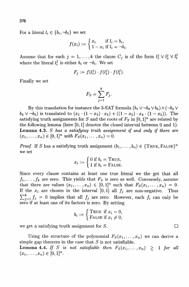
376

For a literal /, € {&;,-•&;} we set

r/ \ J %i U ii = Oj,

J ^ ^ - \ l _ a ; i i f / i = - , 6 i .

Assume that for each j = 1 , . . . , k the clause Cj is of the form Z£ V / V l\ where the literal l\ is either bi or -hi. We set

Finally we set

By this translation for instance the 3-SAT formula (&! V-163 V65) A (~^b2 V 64 V -165) is translated to (x\ • (1 — X3) • x5) + ((1 — X2) • X4 • (1 — £5)). The satisfying truth assignments for S and the roots of Fs in [0,1]" are related by the following lemma (here [0,1] denotes the closed interval between 0 and 1). Lemma 4.3. S has a satisfying truth assignment if and only if there are (xi,... , xn) e [0,1]™ with Fs(xi,... , xn) - 0.

Proof. If S has a satisfying truth assignment (b\,... , bn) £ {TRUE, FALSE}"

we set

- { 0 if bi = TRUE,

1 if bi = FALSE.

Since every clause contains at least one true literal we the get that all / 1 , . . . , fk are zero. This yields that Fs is zero as well. Conversely, assume that there are values ( x i , . . . ,xn) e [0,1]" such that Fs(xi,... ,xn) = 0. If the X j 3/1TG chosen in the interval [0,1] all fj are non-negative. Thus

Ylj=i fj = 0 implies that all fj are zero. However, each fa can only be zero if at least one of its factors is zero. By setting

, _ J TRUE if Xi = 0, { :~ { FALSE if x{ ^ 0,

we get a satisfying truth assignment for S. •

Using the structure of the polynomial Fs(a; i , . . . ,xn) we can derive a simple gap theorem in the case that 5 is not satisfiable. Lemma 4.4. / / S is not satisfiable then Fs(xi,... ,xn) > 1 for all (Xl,...,xn)€[0,i\n.

377

Proof. This is true since F$ is a multilinear form and Fs(x\,... ,xn) is an integer that is greater or equal to zero for all vertices (x\,... ,xn) 6 {0,1}™ of the unit cube. •

4-2 From Algebra to Geometry

Our next step is to transfer the algebraic situation in Fs to a geometric construction using exclusively JOIN and MEET operations and the constant points 0, 1, i, and 1 + i. This construction has the following properties: It contains freely movable points p\,... ,pn (one for each boolean variable in S), and a dependent point q that is constrained to lie on ZR. There will be admissible positions for p\,. . . ,pn such that 0 and q coincide if and only if 5 is satisfiable.

Using the gadgets from Sec. 3 the construction is straightforward. We construct n points x\,... ,xn according to

Xi « - ONINTERVAL(0, I,Pi).

The construction constrains each of the points Xi to the segment [0,1] (see Sec. 3.3). Except for this there is no restriction to the positions of the points xi,... ,xn. These points model the input variables x\,... , xn of the equation Fs whose values should be chosen in the interval [0,1].

Using von Staudt constructions we now encode the polynomial Fs(xi,... ,xn) geometrically. All calculations are carried out on the line /R. The point that finally represents the result of the calculation is called q. This point q lies on /R by its construction and Lemma 4.3. It can coincide with 0 if and only if S was satisfiable. We call the whole construction Cs-Altogether we obtain: L e m m a 4.5. (i) In Cs the point q lies on ZR.

(ii) There is an admissible position for pi,.. • ,p„ in Cs such that q and 0 coincide if and only if S has a satisfying truth assignment.

(iii) If S is not satisfiable then q > 1 for all admissible positions ofpi,... ,pn.

Proof, (i) The point q lies on /R by construction, (ii) is a consequence of the construction and Lemma 4.3. (iii) is a consequence of the construction and Lemma 4.4. •

4-3 A Geometric Combination Lock

Our final task for proving Thm. 4.1 is to transfer the construction Cs into a construction that can be used for proving NP-hardness of a reachability prob-

378

Fig. 9: Schematic view of the construction of a "geometric combination lock".

lem. The construction of Cs so far included only JOIN and MEET operations without non-determinism. The idea now is to conclude the construction by linking it to the "winding number gadget" presented in Sec. 3.4. We will do this in such a way such that a certain angular bisector can be rotated by 7r/2 if and only if the original 3-SAT problem was satisfiable.

For this we add a new free point p from which we construct a derived point v on the circle with diameter [—| + Oi, | + Oi]. The construction is standard using the point on circle gadget from Sec. 3.3:

V 4- ONCIRCLE(--, ~,p).

Then we take the construction for Cs and use our gadget for complex addition to construct w = q + v and the line £Q 4— JOIN(0, W). Finally, we add three non-deterministic statements

(.1 <r- BISECT(/R,£ 0 ) , £2 <~ BISECT(/R,^I) , £3 <r- BISECT(/K,£2)-

The line £3 is a three times iterated angular bisector of /R and £$. By con­struction the lines £0, £1, and £2 pass through the origin. Hence the bisector operations are admissible. If the positions of p, pi,... ,pn are fixed then the construction is completely determined up to the actual position of £\, £2, and £3. The final construction is called TZs-

For the positions p — p{ = ...=p^=l the line £0 coincides with ZR and the choice

£i=£2 = £3 = IK

379

is a proper instance A of Us- For these positions of p,pi,... ,pn also the choice

(l = (-2 = IR, @3 = liR

is a proper instance B. The only distinction between the instances A and B is the position of £3. Lemma 4.6. There is a continuous admissible path from A to B (induced by a movement of the free points p,p±,... ,pn) if and only if S is satisfiable.

Proof. The only way to get from A to B is that the point w = q + v turns an odd number of cycles around the origin. Assume for a moment that pi,... ,pn

are fixed. Then the point q has a certain position on the line IR. The point w is then constrained to lie on a circle of radius \ around q. By moving p we can freely influence the position of w on this circle. The only way to let w cycle around the origin is to move p to a position that has less than distance I to the origin, and then move p to achieve a full cycle of w around the origin. However, Lemma 4.5 shows that q can only come so close to the origin if and only if S was satisfiable. This proves the claim. •

We may think of the whole construction as a "geometric combination lock:" The points pi, • • • ,pn play the role of the code dials. The point p plays the role of an opening wheel. The angular bisector is the bolt of the combi­nation lock. The reachability problem translates to the question whether one can open the lock. Initially the dials and the wheel are in some position. If we want to open the combination lock we first have to move the dials into the correct position (this can only be done if we know the solution to the 3-SAT problem 5). If the dials are in the correct position we can turn the opening wheel and open the lock. After opening the lock we move all dials and the opening wheel again to the initial position. Nothing has changed except for the fact that the lock is now open.

A schematic picture of the whole situation is shown in Fig. 9. Points on an interval are used for von Staudt constructions. The result of this computation is used for the opening wheel.

Finally, observing that the whole translation from the original 3-SAT to the construction TZs can be carried out in polynomial (even linear) time in the length of the 3-SAT problem proves Thm. 4.1.

5 Computing a Specific Trace

The goal of this section is to prove our next main theorem. It describes the complexity of the basic situation in a Dynamic Geometry system: You pick

380

a point and move it from one position to another. It will turn out to be NP-hard to decide whether a continuous evaluation of the situation ends up in a specific situation. Theo rem 5.1. Given a GSP V over the JMB instruction set that contains exactly one free point p. Furthermore, given two instances A and B such that p is at position a in A and p is at position b in B. Let p{t) : [0,1] —> [a, b] be a (straight) movement of p with p(0) = a and p(l) = b. It is NP-hard to decide whether a continuous evaluation of V under this movement that starts at instance A ends up at the instance B.

Here is an overview over the ingredients of our proof: First, we map the moving point p to the unit circle. Then we construct a set of polynomials Bj(z) that correspond to the variables of a given 3-SAT problem in a way that all possible 0-1 combinations are represented by the values of the Bj on the unit circle. Finally, another polynomial Fs(z) encodes the boolean formula of the 3-SAT problem and controls a point q, that will cycle around the origin. The winding number of this point can be used to read off the satisfiability of the 3-SAT.

A similar polynomial construction has been used by Plaisted in 17>18'19. He used it to prove that it is NP-hard to decide for a sparse univariate polynomial whether it has a complex root of modulus 1. Our constructions differ from Plaisted's work by being more focused on evaluations of polynomials over the real numbers. One of the direct consequences of our construction is that it is NP-hard to decide whether a real polynomial encoded by a straight line program has a root over the real numbers (see Sec. 5.7). This fact can also be derived as a consequence of Plaisted's Theorem by a Moebius transformation argument. The alert reader will find out that we could have used the binary counter construction of Sec. 6 to prove Thm. 5.1, but the additional results for real polynomial roots (and some additional insight) would not have been possible then. We are convinced that the additional effort pays off very well.

5.1 A Point on the Unit Circle

We will start our construction with a little gadget that maps a certain line segment to a point on the unit-circle. For this we first use the point-on-circle gadget of Sec. 3.3. and set

W <- ONCIRCLE(- l , l ,p) .

If p is located at 2 the point w is located at 1. While p moves on a straight vertical path to the point 2 + 3i point w makes a quarter turn on the unit

381

circle. We set

This point is constructible by the gadgets for complex arithmetics from Sec. 3.2. While p moves along the segment from 2 to 2 + 3i the point z =: z(p) makes exactly one full cycle on the unit circle.

5.2 Complex Polynomials for Variables

From now on we fix a specific instance 5 of a 3-SAT problem with variables b\,... ,bn and clauses C\,... ,Ck- We will encode S into an instance of the decision problem of Thm. 5.1.

Let Pj be the j-th prime number, and let M = n?=i Pj ^ e t n e product of the first n primes. The size of the j - th prime is less than jlog(j). Hence the size of M is less than n " l o g n . The polynomial zM — 1 has altogether M single roots, the M-th roots of unity, equally spaced on the unit circle at z = e

2i^rlM\ for r G {1,2 , . . . , M } . We abbreviate eM(r) = e2i<r'M\ We

consider two classes of polynomials for which the sets of roots are subsets of the roots of zM - 1:

Bj(z) = \-zMlpi, Bj{z) = 1 + ZMlPi + Z2MlPi + Z3M'Pi +••• + zlPi-»M/Pi.

For each j e { l , . . . , n } we set Aj = {PJ,2PJ,3PJ, ... , M} and Aj = {1,2 , . . . , M] — Aj. The following relations are immediate. Lemma 5.2. With the notation as set above we have:

(i) For each j S { 1 , . . . ,n} we have Bj(z) • Bj(z) = zM — 1.

(ii) The roots of Bj(z) are at z = EM(r), for r G Aj.

(iii) The roots of Bj(z) are at z — eM{f), for r S Aj.

Proof. Claim (i) can be directly proved by expansion of the product. Claim (ii) is trivial. Claim (iii) is a consequence of (i) and (ii) and the fact that there are no multiple roots in zM — 1. •

Later on we will associate to each number r £ {1 ,2 , . . . ,M} a certain evaluation of the boolean variables b\,... ,bn. For a number r the boolean variable bj will be considered T R U E if ej^(r) is a root of Bj and FALSE oth­erwise. The above lemma proves that under this correspondence bj is FALSE

(at r) if and only if CM (r) is a root of Bj. We set

i , M . _ / T R U E ifBj(eM(r))=0, j{ ' — \ FALSE if Bj(eM(r)) ± 0.

382

Lemma 5.3. For each truth assignment (&i,... ,bn) € {TRUE, FALSE}"

there is at least one number r € { 1 , . . . ,M} such that bj(r) = bj for all j e { 1 , . . . ,n}.

Proof. For a given assignment (&i,... , bn) e {TRUE, FALSE}" we are looking for an integer r < M that has Pj as a prime factor if and only if bj(r) = TRUE.

For this we can simply take the number

n ^ {j |6i(r)=TRUB}

which has this property. •

We will explicitly calculate the above polynomials Bj(z), Bj{z) and zM — 1 by suitable geometric constructions. We will have to take care that the effort of doing this is no more than polynomial in the coding length of the original 3-SAT 5. For this we need: Lemma 5.4. For each n the polynomial zn can be evaluated by a straight line program using at most 0(log2(n)) multiplications. Similarly for each n and each divisor m of n the polynomial 1 + zm + z2m -\— • + zn can be evaluated by a straight line program using at most 0(log(n)2) additions or multiplications.

Proof. Let n = CT02° + ax2l + a22

2 + • • -+ah2k with k < log2(n) and a{ € {0,1}

be the binary expansion of n. We can write zn = Y[u i a=i\ z2' • This product has at most log2(n) terms. The polynomial z2' — z2' • z2' uses only one additional multiplication if we already have z2' . This proves the first claim.

For the second claim we first set fk{z) = 1 + z1 + z2 + • • • + zk. We have 1 + zm + z2m + • • • + zn = fn/m(zm). Thus after having used 21og2(m) multiplications for computing zm we just have to care about fk(z) for k — n/m. If k is even we get fk{z) = fk/2{z){l + zkl2), if k is odd we get fk(z) = fk/2-i(z)(l + zhl2) + zk/2, and a simple recursion on k proves the claim. •

The last lemma together with the observation that M is less than n™log n

shows that all polynomials Bj(z), Bj(z) and zM — 1 can be encoded by straight line programs whose length is polynomial in n.

5.3 Evaluating a 3-SAT

We now proceed by encoding the original 3-SAT instance 5 into our con­struction. For a complex number z = o + ib we set ||z|| — a2 + b2. For all i e { l , . . . , n } we consider Lj(z) = ||i?j(,z)|| and Lj(z) = ||Bj(,z)||. These two

383

functions are real-valued and even non-negative. The only way for these func­tions to be zero is that the corresponding functions Bj (z) and Bj (z) become zero. For a literal lj 6 {bj, -*bj} we set

1 (Z)- \Lj(z)iili = -,bi.

Assume that for each j = 1 , . . . , k the clause Cj is of the form Pr V l{ V l\ where the literal l\ is either b^ or —>6fe. We set

Fj(z) := flHz) • fli(z) • fHz)-

Finally we set

k

Fs(z) = Y,Fj(z).

If z = a + ib the function Fs(z) is a real polynomial in a and b that can be realized by a straight line program with length polynomial in the size of the 3-SAT instance S. It is important that Fs{z) is not an element of the polynomial ring C[Z], because otherwise the following lemma could not be true. Lemma 5.5. It is NP-hard to decide whether there is a z e C with Fs(z) = 0.

Proof. The only way for Fs(z) to become zero is that all its summands are zero. This however can only be the case if z is of the form cu (r) for an r that corresponds to a satisfying truth assignment of 5. •

Example 5.6. Let us consider a specific satisfiability problem S and the associated function Fs • In order for the example to have a reasonable size we consider a 2-SAT instead of an actual 3-SAT instance:

S = (&! V 63) A (62 V 61) A (-.&2 V 63).

The satisfying truth assignments are (1,0,0), (1,0,1) and (1,1,1). We asso­ciate 61 with the prime number 2, 62 with 3, and 63 with 5. The resulting graph of Fs(cos(27ri/30) + i sin(2-7ri/30)) together with the corresponding bit patterns is shown in Fig. 10. The ticks mark the corresponding 30 th roots of unity. Whenever we have a bit pattern corresponding to a satisfying assign­ment the function is zero, else it is greater than zero.

384

IAIUAAAMIA 1 0 1 0 1 0 1 0 1 0 1 0 1 0 1 0 1 0 1 0 1 0 1 0 1 0 1 0 1 0 1 1 0 0 1 0 0 1 0 0 1 0 0 1 0 0 1 0 0 1 0 0 1 0 0 1 0 0 1 0 0 1 1 0 0 0 0 1 0 0 0 0 1 0 0 0 0 1 0 0 0 0 1 0 0 0 0 1 0 0 0 0 1

Fig. 10: The graph of the function Fs(cos(27rt/30) + isin(27ri/30)).

5.4 Another Gap-Theorem

Again we need an estimate how small the function Fs(z) can become if S is not satisfiable. In fact we will need this minimum only for points tM{r) with r € {1 ,2 , . . . , M } . We can get a lower bound for this value by calculating the smallest possible non-zero summand of FS{€-M{T))- This value in turn can be bounded by the cube of the smallest non-zero value a that one of the functions Lj(eM(r)), Lj(cM(r)) can take for r £ {1 ,2 , . . . , M } . For this it is useful to observe that Lj{eM{r)) = 2 — 2cos(27T • r/Pj). This desired value a is taken at £ „ ( £ M ( 1 ) ) - Thus we have a = 2 — 2cos(27r/Pn). We obtain the following lemma. L e m m a 5.7. / / Fs(eM(r)) *s non-zero for some r 6 { 1 , . . . ,M}, then we have

FS{tM{r)) > (2 - 2cos(27r/P„))3 > (2 - 2cos(27r2-los<n>2)3.

Proof. The first inequality follows from our considerations above. The second inequality is a very rough estimate following from the monotonicity of cos(i) in [0, TT/2] and the fact that Pn < 2los(")2. •

We set /3S = (2 - 2cos(2?r • 2- los(")2))3 . This number can be constructed geometrically using an iterative sequence of log(n)2

BISECT operations start­ing with the right angle followed by a constant number of JOIN and MEET

operations.

5.5 Tracing the Flight of a Bumble Bee

Now we are done with the algebraic part of our construction. We come back to the geometric part that started with the construction of a point z that moves once around the unit circle while the free point p moves from a to b (Sec. 5.1).

385

Fig. 11: The path of the dependent point <?s(z)-

We take z as the input of Fs(z) and model the evaluation of Fs(z) by von Staudt constructions as described in Sec. 3.2. The result is a non-negative point q on the real axis JR. This point can coincide with the origin whenever z corresponds to a satisfying truth assignment of 5. In particular, this can only happen if z = E M W for a suitable r. We now consider the function

gs(Z)~ZM-l-FS(z)+PS.

Lemma 5.8. Let G be the path of gs{z) while z makes one full cycle around the unit circle. The winding number of G with respect to the origin is zero if and only if S has no satisfying truth assignment.

Proof. Let z = e2l7rt for t € [0,1] move with constant speed on the unit circle. We can get the corresponding winding number around the origin in the following way: We take the ray of all positive real numbers. We calculate two numbers: w+ counts how often the point gs(z) crosses this ray moving from the lower to the upper half plane, and w~ counts how often the point gs(z) crosses this ray moving from the upper to the lower half plane. The number w+ — w~ gives the winding number.

The real part of gs{z) is by construction and by Lemma 5.7 at most j3s-For gs(z) being real and positive the numbers zM — 1 and Fs(z) must both vanish. Thus we obtain

w+ = \{r e { 1 , . . . ,M} \Fs{eM{r)) = 0}| and w~ = 0.

The winding number counts exactly the number of possible r € {0 , . . . , M} for which bj(r) is a satisfying truth assignment of S. •

Fig. 11 shows the trace of gs(z) for the 2-SAT formula of Example 5.6. The origin lies on the symmetry axis of the figure very close to the right boundary. The winding number will be exactly 12 corresponding to the 12 zeros of Fs(z) shown in Fig. 10.

386

5.6 NP-hardness of Tracing

Now we are in principle done. We do a geometric construction that calculates gs(z(p)) using the free point p as input parameter. This can be done by a number of JOIN, MEET, and BISECT operations that is polynomial in the parameter n and k of S (by Lemma 5.4 and the considerations in Sec. 5.4). We construct the line £0 = JOIN(0, gs(z(p))). Finally, we add n3 non-deterministic statements:

ti <- B I S E C T ( / R , 4 ) l2 *r- B I S E C T ( / R , 4 )

£„3 <- BISECTOR, £„3_!)

The winding number w of Lemma 5.8 satisfies

w < M < nnl0«<n> < n"2 < (2n)"2 = 2"3.

Thus we obtain the following lemma. L e m m a 5.9. Let A be an initial position of our entire construction for p = 2 and let B be the corresponding position with identical choice of the angular bisectors for p = 2 + 3i. B is the result of a continuous evaluation under the straight movement of p if and only if S was not satisfiable.

Proof. If 5 is not satisfiable, then the winding number of gs(z(p)) around the origin is zero and the position of the angular bisectors remains unchanged. If S is satisfiable, then the winding number lies between 1 and 2™ . Thus a movement of p causes a change of the positions of the angular bisectors. •

This concludes our proof of Thm. 5.1, which is a direct consequence of the above Lemma and the fact that the construction was polynomial in the size of n and k.

5.7 Roots of Univariate Polynomials

We will close this chapter with a little side remark. Assume that the free point p of our construction is parameterized by (2, x, 1) (in homogeneous coordinates with i 6 E ) . The construction of the function Fs(z(p)) could be exclusively done with JOIN and MEET operations. The coordinates of the resulting point Fs(z(p)) = (a(x),0(x),'y(x)) are then polynomials in the single variable x. These polynomials can be calculated by straight line programs whose length is polynomial in the size of 5 , by translating the GSP into an equivalent SLP (see n ) . The 3-SAT 5 is satisfiable if and only if there is an x with a(x) = 0. Thus we obtain

387

Theorem 5.10. It is NP-hard to decide whether a univariate polynomial en­coded by a straight line program has a real root.

6 PSPACE-Hard Problems

This section focuses on proving that certain reachability problems are PSPACE-hard do decide. Compared to the previous sections there is one important difference. Every construction done so far only needed constant points, meet, join, and bisect operations. For the proof of the following PSPACE-hardness results for real reachability we need one additional ingre­dient, a semialgebraic constraint on the configuration space of the geometric configuration. We will demonstrate several variants of the result with different such constraints:

• the condition that a certain point is always on the left of a certain line,

• the condition that a certain point is always inside a certain circle,

• the condition that the intersection of a line and a circle is always real,

• the condition that the total length of the path of a freely movable point stays below a certain threshold.

Note that the first three variants can be transformed into each other. In fact there are many other variants of the result since the necessary restrictions that come from the additional inequality can be formalized in a very weak way. Nevertheless we have not been able to derive a comparable result without the additional condition. Our proof will be entirely constructive and self contained. It just relies on the well known PSPACE hardness of quantified boolean formulas. Moreover we will be very restrictive in the use of free points: the final construction has only one free point.

Let us first formulate one of the natural version of the main result of this section which is very similar to Thm. 4.1, except for the additional inequality constraint (for which we choose an incircle test here). Theorem 6 .1. The following decision problem is PSPACE-hard: Given a GSP V over the JMB instruction set that has exactly one free point and a certain dependent point d. Furthermore, given two instances A and B of V. Decide whether there is an admissible real path from A to B, such that along the path we always have \d\ < 2.

The proof of this result will be done by a reduction to the PSPACE-hardness of Quantified Boolean Formulas (QBF). Formally the PSPACE-hardness of QBF can be stated as "it is PSPACE-hard to decide whether

388

the formula

Vxi3y1Vx23y2 • ••Vxn3ynf(xi,y1,x2,y2,... ,x„,yn)

is true, where / is a boolean expression." In a sense this formula resembles a two player game with players X and Y. It asks for a winning strategy for player Y. The formula / encodes the winning positions of Y: "For each move xi of X there is a move j/i for Y such that for each move x2 of X there is a move 2/2 for Y such that . . . such that there is a final move yn for Y such that Y wins the game.

For the proof we will geometrically construct a binary counter that counts through all possibilities for the x\,... ,x„. The entire construction is such that in order to get from position A to B in the reachability problem one has (at certain positions) to set the values of the j / i , . . . ,yn properly which can only be done if one knows the complete strategy for player Y. Remark 6.2. Before we start with the proof let us contemplate for a mo­ment the value of the following constructions. It is a remarkable fact that a similar result can be obtained even without using the BISECT operation at all - however for the price of an unbounded number of free points. The idea for this is to use one of the well known PSPACE-hard semialgebraic reachability problems (like the warehouseman's problem 7 '24) as the starting point of the reduction. All involved equations and inequalities can be condensed into one big inequality (this new inequality describes an e-approximation of the orig­inal problem). This translation can only be done with the help of additional slack-variables (one variable per original inequality). The information of a certain state of the construction is "stored" in the actual values of the slack variables. Particular technical difficulties arise from the right choice of the involved e-sizes.

Compared to this approach the construction presented on the following pages is much more direct. Its "computational power" is more or less dis­tributed among the monodromy behavior of several BISECT operations. Each of these angular bisectors contributes one bit of information to the "storage" of the device.

Our construction allows for variants and extensions that are not possible in the other approach. In particular, the results can be strengthened further to have only one free complex input variable. A streamlined variant of this result for the case of analytic continuation will be presented in 14.

389

Fig. 12: Two instances of an INT-UNITCIRCLE(Z) gadget.

6.1 Another Gadget

Before starting the crucial construction of a binary counter we will introduce another gadget that simplifies this construction. We show that over the JMB construction set, we can intersect a line through the origin with the unit circle (note that there are no circles available in JMB). Let I be a line through the origin and ZR be the real axis. We consider the following GSP:

g<- BISECT(Z,/R) q <- MEET(Z, P A R A L L E L ^ , - 1 ) )

The output point q is one of the intersections of I and the unit circle. Which of the two intersections we get, depends on the choice of angular bisector. If the line I makes a half turn (and by this comes back to its original position), the intersection moves continuously from one possibility to the other, see Fig. 12. We will encapsulate this construction within a (non-deterministic) macro INT_TJNITCIRCLE(Z) that produces one of the two intersections.

6.2 A Binary Counter

Our first sub-goal is to construct a binary counter, that drives the construction through an exponential number of different stages. For this we again start with a point z, which is given by

w <- O N C I R C L E ( - 1 , 1 , P ) ,

Z 4- W4.

As described in Sec. 5.1, while p moves on a straight vertical path from o = 2 to the point b = 2 + 3i, the point z makes one full counterclockwise cycle on the unit circle, starting and ending at 1. W.l.o.g. for our considerations we may assume that p is bound to lie on the line that connects a and b.

390

We will consider the point z directly as a driving input point that is bound to lie on the unit circle. We now have a look at the following functions:

zi <- Re(z2) + z2" - 2 z2 *- Re(z4) + z2" - 2 z3 <- Re(z8) + z2" - 2

zn <r- Re(z2") + z2" - 2

The Re( . . . ) operation (that extracts the real part of complex number) can be carried out geometrically by a projection to the real axis. All the z\,... ,zn

can be constructed by a GSP whose total number of construction steps is linear in n. No angular bisectors are needed.

All the real parts of the functions z\,... ,zn are in the interval [—2,0], since the numbers zk all lie on the unit circle. While z moves along the unit circle the function Zk is zero exactly if z is a 2fc-th root of unity. Each of the functions z/. is real iff z is a 2"+1-st root of unity. For j = 0 , . . . , 2n we set

a. =e2«r072») a n d 6 j = e 2«r ( i / 2 " + l/2" + 1).

We will refer to regions on the unit circle by the term circular interval. For two points a, b on the unit circle the open circular interval (a, b) is the (open) arc on the unit circle that arises by traveling counterclockwise from a to b.

The imaginary parts of the functions Zk only depend on the function z2". lm(zk) is positive in the circular intervals (a,j,bj) and negative in the circular intervals (bj,a,j+i) for j = 0 , . . . ,2n. The largest purely real value that occurs for the function Zk is 0, the second largest real value is cos(27r/2fc) - 1. We set e — — cos(27r/2n+1) + 1, a number that can be constructed geometrically by n successive BISECT operations of a right angle, followed by a projection.

Now let ZR be the real axis and we add for each A; = 1 , . . . , n the following instructions to our GSP:

lk <- BISECT(]OlN(0,zk+e),lu) qk <~ INT_UNITCIRCLE(Zjfc)

First observe that the operation JOIN(0, Zk+e) is always admissible, since Zk +e is never 0. The line JOIN(0,Zk+e) is identical to ZR whenever z is either Oj or bj for some i £ {0 , . . . ,2™}. Thus at these places the line lk can either be the real or the imaginary axis. Note that the only freely movable point in the whole construction so far is z (indirectly controlled by p). As a starting instance of the GSP we set z = 1. All lines JOIN(0, Zk + e) are then identical to ZK. We get an admissible instance of the above operations by setting all lk = ZR and setting all qk = 1.

391

From this admissible starting instance A the behavior of the entire con­struction is determined (by analytic continuation) while z travels along the unit circle. Lemma 6.3. With all settings as above (starting at A) the values of the qk are uniquely determined for all z (with \z\ = 1). In particular, we have that for all j € {0 , . . . , 2™ — 1} the value z = bj implies that

_[ i for an-k = 0, \-i for <r„_fc ^ 0.

Here j = a02° + ax2Y + a22

2 H h an-^71'1 with ak 6 {0,1} is the binary expansion.

Proof. For the proof let us investigate what happens during a full counter­clockwise cycle of the driving point z. At the beginning (z = 1 = a0) all the Ik are by definition of A identical to the real axis and all qk are by definition equal to 1. Furthermore, all Zk are positive (namely equal to e). While z travels from oo to bo all Zk move through the upper halfplane to a negative value. Thus all lines JOIN(0, Zk + e) make a counterclockwise half turn. Con­sequently all 1^ make a counterclockwise quarter turn and all qk move to the value i as stated in the theorem.

Now let us investigate what happens when z moves from position bj on the shortest possible path via aj+i to position bj+\. During such a move the position of qk will make a half turn if and only if Zk makes a cycle around the origin. This in turn exactly happens if for z = o,-+i the value of Zk is positive. However, this is only the case if a ,+ i is a 2*-th root of unity. This gives exactly the desired counting behavior. Finally after z has completed one full cycle, all elements are back to their initial positions. Hence no global monodromy occurs and the behavior is globally determined. •

The whole construction behaves like a binary counter. For each position z = bj all qk are either i or — i. The positions exactly resemble the behavior of the binary expansion of j with i playing the role of the 0 and —i playing the role of the 1.

6.3 A Register

The output of the counter we constructed so far will later on play the role of the Xk that occur in the quantified boolean formula

Vxi3yiV:E23y2---V:cn3yn/(xi,2/1,12,J/2,--- ,xn,yn).

392

We now explain how to model the yk. For this we construct a register with dependent points r\,... ,rn. Whenever the driving point z is at a position bj the rk will either be i or —i. However, which of the two values will be taken depends on the position of certain free points P i , . . . , p„ during z being at a position a,j. We will call the points bj evaluation points and call the points aj setting points. For each k £ { 1 , . . . , n} we add the following four lines to our GSP constructed so far:

p'k <- ONINTERVAL(0, l,pk)

4 <- p'k-l + zk+e l'k <r- B I S E C T ( J O I N ( 0 , 2 ^ ) , Z R )

rk < - INT_UNITCIRCLE(/fc)

We extend our initial position A (remember there we had z = 1) first by setting pi = p2 = ... = pn = 2. This forces the lines JOIN(0, z'k) to be ZR. AS we did for the counter we set all l'k — ZR and all rk = 1. The following Lemma summarizes the properties of the register. Lemma 6.4. For any admissible move of the free input points p,pi , • • • ,pn

starting from instance A we have the following properties:

(i) Whenever z is at an evaluation point each of the rk is either i or —i.

(ii) For each k £ { 1 , . . . , n} and each j € {0 , . . . , 2k — 1} we have: Whenever z stays in the circular interval Ikj = (aj.2"-k,aij+1\.2

n-k)> aH values of rk when z is at an evaluation point in Ikj are identical.

(iii) Except conditions (i) and (ii) there are no other restrictions to the values of rk when z is at an evaluation point.

Proof. The proof is very similar to the proof of Lemma 6.3. The initial situa­tion of A ensures that condition (i) is satisfied. For each j e {0 , . . . , 2k — 1} the function z'k is always negative within the entire circular interval Ikj. Hence, as long as z does not leave this interval for all evaluation points the values of the rk must be identical (since z'k cannot cycle around the origin.) This proves (ii). The function z'k can be positive whenever z takes one of the values aj.2^-k with j £ {0, . . . , 2k — 1} (these are the 2^-th roots of unity). Whether it actually is positive depends on the position of the free point pk. Thus whenever z makes a transition between the intervals Ikj and Ikj+i (in either direction) we can (by moving pk accordingly) control whether the rk at z be­ing at an evaluation point in Ikj and Ikj+i are identical for both intervals or not. This proves (iii). •

393

Vxi3j/;

Vx23i/:

Vi33i/3

• 1 1 I i

ao &o a i &l 02 &2 a3 &3 04 64 05 65 <IQ &6 07 67

Fig. 13: The timing of the counter and the register

6.4 Encoding the QBF

Let us now step back and see what we have achieved so far. We have con­structed a GSP together with an initial position A. The free points of the GSP are p,p\,,... ,pn. We have output points qi,- • • , qn for the counter and r i , . . . ,rn for the register. Whenever z is at an evaluation point all these output points are either i or —i. For n = 3 the "timing" of the whole con­struction is shown in Fig. 13. The horizontal axis shows the positions for z on the unit circle. Each of the oscillating curves roughly represents the values of the counting points qi,q2,qz- The dots mark those positions that are relevant for possibly changing the values of the register points r\,r2,rz. The bottom row represents the point pair (g3, r3) . The middle row represents (92, r2) , and the top row represents (qi,ri). Between two of the positions marked with a dot the corresponding r-point always has the same value at the evaluation points. If for instance z passes ao in clockwise direction the position of p\ de­termines which values n can take at the evaluation points 60, &i, b2,63. These values can only be changed if z passes once more one of the setting points ao or 04.

We are now going to link a given QBF formula to our construction. For this consider the QBF

Va;i32/iVa;23j/2 • • • ^xn3ynf{xi,yx,x2,2/2, • • • ,xn,yn)

where we assume that / is given in conjunctive normal form. As in Sec. 4.1 we first translate the boolean formula / into a polynomial Ff by replacing each positive literal Xk by a real variable Xk and each negative literal -ixk

394

by (1 — Xk)- We do so similarly for the y%. Then each and-operation is replaced by a multiplication and each or-operation is replaced by an addition. The resulting polynomial is called Ff(xi,yi,x2,y2, • • • ,xn,yn)- Similar to Lemma 4.4 we obtain Lemma 6.5. We have Ff(xi,yi,x2,y2,-• • ,xn,yn) = 0 for some (xi, 2/i, • • • , xn,yn) € [0, l ] 2 n if and only if all variables are either 0 or 1, and f(b(xi), b(yi),... , b{xn), b{yn)) = TRUE with b(0) - TRUE and 6(1) = FALSE. For all other choices of the variables in [0, l ] 2 " the value of Ff is strictly positive. Furthermore, at each corner of the cube [0, l]2™ the polynomial Ff evaluates to an integer number.

Proof. The proof is straightforward. It follows exactly the considerations in Sec. 4.1. •

We now (constructively) identify the values —i and i (of the Qk and r^) with the boolean values T R U E and FALSE, respectively by adding the state­ments

Xk <- \{iqk + 1),

Vk <- §(""* + 1)

for k — 1 , . . . , n to our GSP. Furthermore, we set with these newly constructed points

F'«- Ff(xi,yi,x2,y2,... ,xn,yn).

The next lemma brings us close to the complexity result we are aiming for. Recall that the point p was w.l.o.g bound to the line connecting 2 and 2 + 3t, and that while p moves straight from 2 to 2 + 3i the path of the point z is a full clockwise cycle on the unit circle, by Lemma 6.6. The QBF \fxi3y1^x2By2---^xn3ynf(xi,y1,x2,y2,--- ,xn,yn) is true if and only if the following holds: In our GSP starting with instance A there is an admissible path that moves point p from 2 to 2 + 3i such that the value of F is 0 whenever z is at an evaluation point.

Proof. First assume that ^Xi3yi\/x23y2 • • -Vxn3ynf(xi,yi,x2,y2,... ,xn,yn) is true. We can skolemize the variables yk of the B-quantors by introducing Skolem functions

si{xi),S2{xi,x2),... ,sn(xi,... ,xn)

such that

f(xi,si(x1),x2,s2(xi,x2),... ,xn,sn(xi,... , i n ) )

395

is a tautology. These Skolem functions are exactly the "strategy" of the two player game associated to the QBF, which tell player Y how to move. We can derive a path as desired in the theorem as follows. We first choose S to be a sufficiently small positive number such that for p — 2 — Si the point z lies in the circular interval (fc2n_i, eto) and move point p straight from 2 to 2 — 6i while leaving the pk unchanged.

After that we move point p straight from 2 — 5i to 2 + 3i. Whenever z passes one of the setting points we make sure that the positions of the points P\,... , pn were adjusted such that for the forthcoming evaluation point the j/t take the values of the corresponding Skolem functions (this is possible by Lemma 6.4). The construction allows exactly enough freedom to possibly change the value of Sk whenever the variable Xk changes its value. By this choice and by Lemma 6.5 the derived point F is 0 at each evaluation point.

Conversely assume that we know how to move the points Pk such that point p can move from 2 to 2 + 2>i in a way that whenever z is at an evaluation point the dependent point F is 0. We call such a path correct. We show how to reconstruct the Skolem functions from the situations at the evaluation points. One technical difficulty arises from the fact that it may happen that p changes its moving direction while traveling from 2 to 2 + 2>i arbitrarily often. If this is the case the point z possibly meets several of the points a,j or bj more than once.

Assume that the movement of p — 2 + 4>(t)i is given by the function <f>{t) : [0,1] -> E with <p(0) = 0 and 0(1) = 3. The induced movement of z will be denoted by z(t). Furthermore, we set b(i) = FALSE and b(—i) = TRUE. Let us abbreviate T R U E by T and FALSE by F. We describe step by step how to derive the functions s(xi), s{x\,x2), • • • •

Since z(t) (continuously) describes one full cycle there is an (open) interval If C (0,1) such that z(lf) equals the (open) circular interval (ao,a2n-i). Lemma 6.5(h) tells us, that within this interval the value of point ri must be the same for all evaluation points. Lemma 6.5(i) shows that this value rf must be either i or —i. We set Si(F) = b(rf). Similarly there is an open interval if C (0,1) such that z{lf) = (a2n~i,a2n). Also there the value rj at the evaluation points is uniquely either i or —i. We set Si(T) = b(rj).

We now proceed inductively. Within the interval If there are subintervals I2 ' a n d / 2 ' such that z (I2' ) = (ao,o2n-2) andz( / 2 ' ) = (fl2.-2,a2n-i). We let s 2 (F,F) = 6(r2 'F) and s 2(F,T) = b(rl'T). Similarly we define the values s 2(T,F) and s 2 (T,T) by considering suitable subintervals of if. The values of the Skolem functions S3, . . . ,sn are defined similarly each one by looking at a suitable subintervals of the intervals considered for the previous function. Now, by our initial assumption the value of F was 0 at each evaluation point.

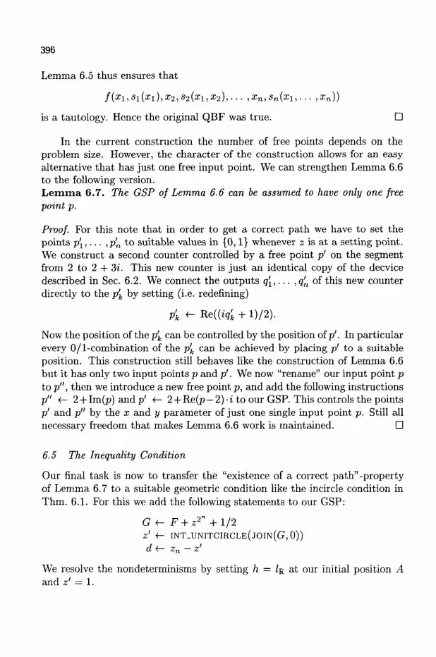
396

Lemma 6.5 thus ensures that

/(zi,si(a;i),a;2,S2(xi,a;2),... ,xn,sn(xi,... ,xn))

is a tautology. Hence the original QBF was true. •

In the current construction the number of free points depends on the problem size. However, the character of the construction allows for an easy alternative that has just one free input point. We can strengthen Lemma 6.6 to the following version. Lemma 6.7. The GSP of Lemma 6.6 can be assumed to have only one free point p.

Proof. For this note that in order to get a correct path we have to set the points p[,... ,p'n to suitable values in {0,1} whenever z is at a setting point. We construct a second counter controlled by a free point p' on the segment from 2 to 2 + 3i. This new counter is just an identical copy of the decvice described in Sec. 6.2. We connect the outputs q[,... , q'n of this new counter directly to the p'k by setting (i.e. redefining)

p'k «- Re((tg£ + l) /2) .

Now the position of thep'k can be controlled by the position ofp'. In particular every 0/1-combination of the p'k can be achieved by placing p' to a suitable position. This construction still behaves like the construction of Lemma 6.6 but it has only two input points p and p'. We now "rename" our input point p to p", then we introduce a new free point p, and add the following instructions p" <r- 2 + Im(p)andp' <- 2 + Re(p- 2) -i to our GSP. This controls the points p' and p" by the x and y parameter of just one single input point p. Still all necessary freedom that makes Lemma 6.6 work is maintained. •

6.5 The Inequality Condition

Our final task is now to transfer the "existence of a correct path"-property of Lemma 6.7 to a suitable geometric condition like the incircle condition in Thm. 6.1. For this we add the following statements to our GSP:

G « - F + z2" + 1/2 z' «- INT_UNITCIRCLE(JOlN(C?,0)) d <— zn — z'

We resolve the nondeterminisms by setting h = /R at our initial position A and z' = 1.

397

Lemma 6.8. In our GSP starting with instance A consider an admissible path that moves point p from 2 to 2 + 3i. For such a path the following conditions are equivalent:

(i) If z is at an evaluation point the value of F is 0.

(ii) We have \d\ < 2 throughout the path.

Proof. Since F is positive and stays on the real axis the value of G is real if and only if z2" is real. This is exactly the case if z is either at a setting point aj (then z2 — 1) or at an evaluation point bj (then z2 = — 1). This implies that G is positive at all setting points. Remember that F assumes only integer values at the evaluation points. Hence G is negative at an evaluation point if and only if F = 0 at this evaluation point. Point z' is the image of this point G mapped by a central projection to the unit circle.

Now assume that the path has the property as claimed in (i). We prove that this path automatically satisfies (ii). In this path z' = 1 at each set­ting point, z' — — 1 at each evaluation point. Furthermore, sign(Im(z')) = sign(Im(z2")). Hence there is always a line through the origin that has z' and z2 on the same side and therefore we have |d| < 2 throughout the path.

Conversely, assume that there is no path that satisfies condition (i). This means that for every possible path along which p is moved from 2 to 2 + 3i the total winding number of z' with respect to the origin is less than 2". This is the case since z' can cross the negative half line only for all the evaluation points. On the other hand the total winding number of z2 with respect to the origin is 2". This implies that there is at least one position along the path where z and z2" are antipodals on the circle. At this position we have d = 2. •

Now we obtain Thm. 6.1 as a direct consequence of the PSPACE-hardness of QBF, Lemma 6.5 and Lemma 6.6. This finishes the proof of Thm. 6.1. Remark 6.9. Without formal proof we mention a few possible alterations of Thm. 6.1.

• Non-Strict inequalities: The construction we gave really needed a strict inequality as additional obstruction (two points on the unit circle cannot be further apart than 2 units). It is easy to obtain the same result also with a non strict inequality. For instance one could introduce an additional BISECT operation of J O I N ( G , 0 ) and ZK intersect the result with the unit circle and compare the resulting point with z2

• Sidedness vs. incircle test: One can turn an incircle condition \d\ < 1 as used in Thm. 6.1 into a sidedness test of a point w.r.t. a line. One

398

possibility for this is to construct the point

d! <- (MEET(PERPENDICULAR(jOIN(0,rf),d),/K))2.

The incircle condition then translates to d! < 1.

• Admissibility of circle-line intersections: We may also introduce the operation of intersecting the unit circle with a line. We may restrict the range of admissible situations to those where such an intersection properly exists. By this we can also express the inequality conditions that are needed in Thm. 6.1.

• Restriction on total length of the path of p: One can also perturb Thm. 6.1 in a way such that the inequality becomes a restriction on the total length of the path of p in a reachability problem. For this we first replace our assignment p' <— 2+Re(p— 2)i hyp' <- 2 + N-Re(p—2)i for a very large number N. This operation rescales the imaginary part of p such that the control of the p\ does not really contribute significantly to the overall length of the path p takes. Then we take the (n + l)-times iterated angular bisector hn+\ of JOIN(G, 0) and /R and ask the following reachability problem. "Is it possibly to move p from 2 to 2 + 3i such that / J„+I make a 90°-turn into its other alternative such that the total length of the path described by p does not exceed 3 + S (for sufficiently small S > 0)?" The only way to do this is to move straight from 2 to 2 -I- 3i by passing every setting point at most once. At each evaluation point the function F must be 0 in order to end up with a rotation of the desired amount. This is by Lemma 6.5 equivalent to knowing the Skolem functions for the QBF. This variant is particularly important, since then no additional sidedness or incircle test is needed.

• Games against external forces: The last statement can reformulated also in another way. Redefine p' and p" as free points again. Assume that an exterior force moves p" from 2 — 6i to 2+3i. Can you simultaneously move the points p' such that hn+1 makes a 90°-turn? This is PSPACE-hard to decide.

7 Undecidable Problems

In this section we enlarge the set of our possible primitive operations. We add one non-deterministic operation that models the mechanical behavior of a wheel that rolls along a road. In principle wheels have the ability to transfer angles to distances. If the wheel was rotated for a certain angle it has traveled

399

along the road for a certain distance. If we (as usual) denote angles modulo 2ir this introduces a new kind of monodromy behavior to our context. For the same angle as input there is an infinity of possible output values. All these output lengths are integer multiples of the length that is generated by rotating the wheel once by 2n.

This new type of monodromy introduces a drastic change in the complex­ity behavior of the reachability problem. We will see that we can translate the solvability of Diophantine equations into a reachability problem for a con­struction involving several wheels. By the undecidability of Hibert's 10th problem this induces the undecidability for this reachability problem.

1.1 Wheels

Let us first formalize the concept of a wheel to fit into our setup of geo­metric straight line programs. The right algebraic function that models the behavior of wheels is the logarithm function applied to points on the unit circle. Our WHEEL-primitive will take a point p = r • elv / 0 and map it non-deterministically to a point on the real axis that represents the possible angles. We define the relation

WHEEL := {(p, q) \q = f/2ir; q = r • e ^ j c P x P.

As usual we allow ourselves to write q 4- WHEEL(P) if (p, q) e WHEEL. The operation is not admissible for p = 0. If (p, q) € WHEEL then we have also (p, q + k) e WHEEL for all k 6 Z. In particular we have (1, k) e WHEEL for all k € Z. If we start with an admissible instance p = l;q = 0 oi q «- WHEEL(P)

then we can continuously reach the situation p = l;q = k by letting p spin around the origin k times. In our picture of an actual mechanical wheel the operation WHEEL is designed to model the properties of a wheel of circum­ference 1 (and thus of irrational (!) radius ^ ) . The resulting MS is called JMBW.

1.2 Diophantine Equations

The following theorem states one version of the famous undecidability of Dio­phantine equations. Theo rem 7.1 . Let N = 11 and f € l*[xi,... ,x;v] be a polynomial. It is algorithmically undecidable whether f has a zero in X .

The number N depends on the actual state of research in the area around Hilbert's 10th problem 31-32. We keep it fixed for the following considerations.

We will prove the following theorem by reduction to the above statement:

400

Theorem 7.2. Let V be a GSP over the JMBW instruction set with at least N WHEEL -operations and two BISECT -operations. Let A and B be two admis­sible instances ofV. It is undecidable whether there is an admissible real path from A to B.

Proof. Step by step we will construct the translation from the polynomial in Thm. 7.1 to the GSP in Thm 7.2. We start with a free point p and a point z given by

z 4- O N C I R C L E ( - 1 , 1 , P ) .

Then we add for i = 1,... ,N the instructions:

qi 4- ONINTERVAL(0, 2, p^ Xi 4- WBEEh(qi + z)

Assume that in the instances A and B we have p = p\ = ... = p^ = (3,0) and thus z — 1, and q\ = . . . = qn — 2. Any admissible instance with z = 1 that is reachable from A by an admissible path satisfies i j £ Z for all i = 1 , . . . ,N, since whenever z = 1 the qi + z are positive. Additionally, for every (y; , . . . , IJN) £ 1>N there is an admissible path starting at A and ending at a position with z — 1 and X{ = yi for all i — 1 , . . . , N. For this claim we only have to prove that each variable Xi can be changed by ±1 independently from the others. In order to obtain such an elementary change simply set qi = 0 and qj = 2 for i ^ j , and do a full clockwise or counterclockwise turn with point z.

Now let f(xi,... ,XN) be an instance of the polynomial used in Thm. 7.1. We finish our construction by adding the following statements to our GSP:

F QN+I

lo

h h

•f-•f-

<-4-4-

-(f(xu... ,xN))2-3/: ONINTERVAL(0, 1,PN+I)

30lN(qN+1 +F + z,0)

B I S E C T ( / R , / 0 )

B I S E C T ( Z R , / I )

For the starting instance A we assume that we have PN+I = — 1 and hence <7JV+I = 0. This implies that QTV+I + F is real. Thus in A we have /0 = /K. For A we resolve the ambiguities of the BiSECT-operations by setting h = h = IR-The only point in which instance B differs from A is that in B we set l<i = ZJR-

We now claim that it is undecidable whether instance B is reachable from instance A: Observe that the only way in which A can be transformed into B is that the point qN+i + F + z makes an odd number of cycles around the origin.

401

If there are (?/;,... ,DN) € Z N with f(y\,... , T/AT) = 0 we can achieve such a movement as follows. We set C[N+I = 0. By the procedure described above we follow a path that puts the Xi to the values of the yi. Then we set all Qi = ...qpf = 0 and QN+I = 1> do another full cycle with z, set qN+i = 0 again, and reset to Xi — 0 again by a suitable movement. The resulting situation is exactly instance B.

Conversely assume that there is an admissible path from A to B. During this path we must have at least one position where qN+i + F + z is real and positive. This can only happen if z — 1, since <7JV+I + F is always real and by definition at most —1/2. However, if z = 1 the f(x\,... , XN) must have an integer value. The only way to get <7JV+I + F + z > 0 is to have / ( x i , . . . ,XN) — 0. Since all Xi were integral this means that a solution of the Diophantine equation exists. •

8 Open Problems

We end our considerations by stating at least some of the open problems in decision complexity of tracing and reachability. Problem 8.1. Determine upper bounds for the decision complexity in the various setups described in this paper. Problem 8.2. Extend the JMB instruction set by a new non-deterministic operation that intersects a circle and a line. Furthermore, enlarge the setup such that also complex coordinates for points lines and circles are allowed. By this a circle and a line always have two or one intersections. What is the decision complexity of the reachability problem in this context?

This problem is of fundamental importance, since if the intrinsic com­plexity would turn out not to be too big this might yield good algorithms for randomized theorem proving for ruler and compass theorems. The structure of this problem seems to be fundamentally different from the problems dis­cussed in this paper. It is not unlikely that for this problem there are effective randomized methods. However, we are pessimistic about fast deterministic methods, since we can prove that it is at least as hard as zero testing for polynomials 13.

Closely related to the above problem is the following: Problem 8.3. Extend the JMB instruction set by a new non-deterministic operation that intersects a circle and a line. Furthermore, enlarge the setup such that also complex coordinates for points, lines, and circles are allowed. Let A be an instance of a construction and let B' be a partial instance that just defines the positions of the free elements. How difficult is it to complete B' to an instance B that is reachable from A ?

Our last problem forms another approach that may single out certain tracing problems to be more easy than others. Since it asks for a new concept, the formulation is kept a little vague on purpose. Problem 8.4. Define the "right" concept of output sensitivity for the tracing problem that allows statements like "if the elements move not too wildly we can trace them easily".

Finally we ask for a slightly stronger version of Thm. 7.2 that gets rid of the constant n hidden in the WHEEL-operation. Problem 8.5. Redefine the relation WHEEL by

WHEEL := {{p, q)\q = f,q = r • eiv}C P x P.

Is Thm. 7.2 still valid in this setup?

References

1. J. Culberson, Sokoban is PSPACE-complete, Proceedings in Informatics 4, Fun With Algorithms, E. Lodi, L. Pagli and N. Santoro, eds. (Carleton Scientific, Waterloo, pp. 65-76, 1999).

2. M.J. Garey amd D. S. Johnson, Computers and Intractability, (W.H. Freeman and Company, New York, 1979).

3. J.R. Gilbert, T. Lengauer and R.E. Tarjan, The pebbling problem is complete in polynomial space, SIAM J. Comput. 9, 513-524 (1980).

4. H. Giinzel, The universal partition theorem for oriented matroids, Dis­crete Comput. Geom. 19, 521-551 (1998).

5. Ch.M. Hoffmann, Solid modeling, in Handbook of Discrete and Compu­tational Geometry, J.E. Goodman & J. O'Rourke eds. (Lecture Notes in Mathematics 1346, CRC Press, Boca Raton, New York, pp. 863-880, 1997).

6. J. Hopcroft, D. Joseph and S. Whitesides, Movement problems for 2-dimensional Linkages, SIAM J. Comput. 13, 610-629 (1984).

7. J. Hopcroft, J.T. Schwarz and M. Sharir, On the complexity of mo­tion planning for multiple independent objects; PSPACE-Hardness of the "Warehouseman's Problem", Intern. J. Robotics Research 3, 76-87 (1984).

8. N. Jackiw, The Geometer's Sketchpad, (Key Curriculum Press, Berkeley, 1991-1995).

9. D. Jordan and M. Steiner, Configuration Spaces of Mechanical Linkages, Discrete Comput. Geom. 22, 297-315 (1999).

403

10. M. Kapovich and J. Millson, On the moduli spaces of polygons in the Euclidean plane, J. of Differential Geometry 42, 133-164 (1995).

11. U. Kortenkamp, Foundations of Dynamic Geometry, (PhD-thesis, ETH Zurich, 1999) h t t p : //www. inf . f u - b e r l i n . de /~kor tenka /Papers /d i s s .pdf.

12. U. Kortenkamp and J. Richter-Gebert, Grundlagen dynamischer geome-trie, in Zeichnung - Figur - Zugfigur, H.-J. Elschenbroich, Th. Gawlick and H.-W. Henn, eds. (Franzbecker, 2001).

13. U. Kortenkamp and J. Richter-Gebert, Decision complexity in dynamic geometry, in Automated Deduction in Geometry (ADG 2000), J. Richter-Gebert, D. Wang, eds. (LNAI 2061, Springer, Heidelberg, pp. 193-198, 2001).

14. U. Kortenkamp and J. Richter-Gebert, The intrinsic complexity of ana­lytic continuation, in preparation.

15. Jean-Marie Laborde and Franck Bellemain, Cabri-Geometry II, (Texas Instruments, 1993-1998).

16. N.E. Mnev, The universality theorems on the classification problem of configuration varieties and convex polytopes varieties, in Topology and Geometry - Rohlin Seminar, O.Ya. Viro, ed. (Lecture Notes in Mathe­matics, 1346 Springer, Heidelberg, pp. 527-544, 1988).

17. D.A. Plaisted, Sparse complex polynomials and polynomial reducibility, Journal of Computers and System Sciences 14, 210-221 (1977).

18. D.A. Plaisted, Some polynomial and integer divisibility problems are NP-hard, SIAM J. Comput. 7, 458-464 (1978).

19. D.A. Plaisted, New NP-Hard and NP-Complete Polynomial and Integer Divisibility Problems, Theoretical Computer Science 31, 125-138 (1984).

20. J. Richter-Gebert, The Universality theorems for oriented matroids and polytopes, Contemporary Mathematics 223, 269-292 (1999).

21. J. Richter-Gebert, Realization Spaces of Polytopes, (Lecture Notes in Mathematics, 1643 Springer, Heidelberg, 1996).

22. J. Richter-Gebert and U. Kortenkamp, Cinderella - The Interactive Ge­ometry Software, (Springer 1999); see also h t tp : / /www.c indere l la .de .

23. J. Richter-Gebert and U. Kortenkamp, Cinderella - Die Interaktive Ge-ometriesoftware, (HEUREKA Klett, 2000).

24. J. Reif, Complexity of the Movers' Problem and Generalizations, (Proc. 20th IEEE Conf. on Foundations of Comp. Sci., Long Beach, Calif.: IEEE Computer Society, pp. 421-427, 1979).

25. P. Shor, Stretchability of pseudolines is A^P-hard, in: Applied Geometry and Discrete Mathematics - The Victor Klee Festschrift, P. Gritzmann and B. Sturmfels, eds. (DIMACS Series in Discrete Mathematics and

404

Theoretical Computer Science, Amer. Math. Soc, Providence, RI, 4 pp. 531-554, 1991).

26. M. Shub and S. Smale, Complexity of Bezout's theorem I: Geometric aspects, J. Amer. Math. Soc. 6, 459-501 (1993).

27. M. Shub and S. Smale, Complexity of Bezout's theorem II: Volumes and probabilities, in: Computational Algebraic Geometry, F. Eyssette and A. Galligo, eds. (Progress in Mathematics, Birkhauser, 109 pp. 267-285, 1993).

28. M. Shub and S. Smale, Complexity of Bezout's theorem III: Condition number and packing, J. Complexity 9, 4-14 (1993).

29. M. Shub and S. Smale, Complexity of Bezout's theorem IV: Probability of success, SIAM Jour, of Numerical Analysis 33, 128-148 (1996).

30. M. Shub and S. Smale, Complexity of Bezout's theorem V: Polynomial time, Theoretical Computer Science 133, 141-164 (1994).

31. Z.W. Sun, Reduction of unknowns in Diophantine representations (En­glish Summary), Sci. Schina Ser A 35, 257-269 (1992).

32. Z.W. Sun, J.P. Jones' work on Hilbert's tenth problem and related topics, Adv. in Math. (China) 22, 312-331 (1993).

405

GRACE-LIKE POLYNOMIALS

DAVID R U E L L E

IHES, 91440 Bures sur Yvette, France E-mail: ruelle@ihes.fr

Results of somewhat mysterious nature are known on the location of zeros of certain polynomials associated with statistical mechanics (Lee-Yang circle theorem) and also with graph counting. In an attempt at clarifying the situation we. introduce and discuss here a natural class of polynomials. Let P(z\,... , zm, w\, • • • , % ) be separately of degree 1 in each of its m + n arguments. We say that P is a Grace­like polynomial if P(z\, • . • ,wn) ^ 0 whenever there is a circle in C separating z\,... , zm from wi, • •. , wn. A number of properties and characterizations of these polynomials are obtained. I had the luck to meet Steve Smale early in my scientific career, and I have read his 1967 article in the Bulletin of the AMS more times than any other scientific paper. It took me a while to realize that Steve had worked successively on a variety of subjects, of which "differentiable dynamical systems" was only one. Progressively also I came to appreciate his independence of mind, expressed in such revolutionary notions as that the beaches of Copacabana are a good place to do mathematics. Turning away from scientific nostalgy, I shall now discuss a problem which is not very close to Steve's work, but has relations to his interests in recent years: finding where zeros of polynomials are located in the complex plane.

1 Introduction

One form of the Lee-Yang circle theorem 3 states that if |a; j | < 1 for i, j = 1 , . . . ,n, and ay = a* , the polynomial

xc{i,••-,"} iex jgx

has all its zeros on the unit circle {z : \z\ = 1}. Let now T be a finite graph. We denote by r" the set of dimer subgraphs 7

(at most one edge of 7 meets any vertex of T), and by T" the set of unbranched subgraphs 7 (no more than two edges of 7 meet any vertex of T). Writing I7I for the number of edges in 7, on proves that

x>w i

7er"

has all its zeros on the negative real axis (Heilmann-Lieb 2) and

406

has all its zeros in the left-hand half plane {z : Imz < 0} (Ruelle 6 ) . The above results can all be obtained in a uniform manner by studying

the zeros of polynomials

P(zi,... ,zn)

which are multiaffine (separately of degree 1 in their n variables), and then taking z\ = ... = zn = z. The multiaffine polynomials corresponding to the three examples above are obtained by multiplying factors for which the location of zeros is known and performing Asano contractions:

Auv + Bu + Cv + D ->• Az + D

The key lemma (see 5) is that if K, L are closed subsets of C\{0} and if

u$ K,v <£ L => Auv + Bu + Cv + D ^ 0

then

z<£-K*L => Az + D^0

where we have written K * L = {uv : u € K,v S L}. To get started, let P{z\,... ,2n) be a multiaffine symmetric polynomial.

If W\,... , Wn are the roots of P(z,... , z) = 0, we have

n

P(z i , . • • , zn) = const. ^ Y[{ZJ - Wn(j)) n j=l

where the sum is over all permutations •K of n objects. Grace's theorem asserts that if Z\,... ,Zn are separated from W\,... , Wn by a circle of the Riemann sphere, then P{Z\... , Zn) ^ 0. For example, if a is real and - 1 < a < 1, the roots of z2 + 2az + 1 are on the unit circle, and therefore

uv + au + av + 1

cannot vanish when \u\ < 1, \v\ < 1; from this one can get the Lee-Yang theorem.

In view of the above, it is natural to consider multiaffine polynomials

P(zi,... ,zm,wi,... ,wn)

which cannot vanish when z\,... , zm are separated from w\,... ,wn by a circle. We call these polynomials Grace-like, and the purpose of this note is to study and characterize them.

407

2 General theory

We say that a complex polynomial P(zi,z2,. •.) in the variables z\, z2,. •. is a Multi-AfRne Polynomial {MA-nomial for short) if it is separately of degree l'vnzi,Zi, We say that a circle T C C separates the sets A', A" C C if C \ r = C U C", where C, C" are open, C" n C" = 0 and A' cC, A" C C". We say that the MA-nomial P ( z i , . . . , zm, w\,... , wn) is Grace-like (or a G-nomial for short) if it satisfies the following condition

(G) Whenever there is a circle T separating {Zi,... , Zm}, {Wi,... , Wn}, then

P(Zu...,Wn)?0

[Note that we call circle either a straight line F C R or a proper circle T = {z e C : \z - a\ = R} with a e C, 0 < R < oo]. Lemma 1 (homogeneity) . The G-nomial P is homogeneous of degree k < min(m,n).

If there is a circle Y separating {z\,... ,zm}, {wi,... ,uin}, then the polynomial A H> P(\zi,... ,Xwn) does not vanish when A ^ 0, hence it is of the form C\k, where C = P{z\,... , wn). Thus

P{Xz1,... , \wn) = XkP(z!,... ,wn)

on an open set of C m + n , hence identically, i.e., P is homogeneous of degree k.

Assuming k > n, each monomial in P would have a factor zt, hence

P ( 0 , . . . , 0 , 1 , . . . , 1 ) = 0

in contradiction with the fact that {0 , . . . ,0}, { 1 , . . . ,1} are separated by a circle. Thus k <n, and similarly k < m. [] Lemma 2 (degree). If all the variables z\,... ,wn effectively occur in the G-nomial P, then m = n and P has degree k = n.

By assumption m n

(n^xn^wr1.---,^1) t=i i = i

is a homogeneous MA-nomial P{z\,... ,wn) of degreem+n — k. \iZ\,... ,W„ are all ^ 0 and {Zx,... ,Zm}, {W\,... ,W»} are separated by a circle T, we may assume that T does not pass through 0. Then {Z^1,... ,Z^}, {Wf 1 , . . . ,W~1} are separated by r _ 1 , hence P(Zi,... ,Wn) jt 0. Let V be the variety of zeros of P and

Zi = {{zi,... , wn) : Zi = 0} , Wj = {(zi,... ,wn) : Wj = 0}

408

Then

V C (V\ Uitj {Zi U W,)) U Ui,j(Zi U W,-)

Since all the variables z%,... ,wn effectively occur in P(zi,... ,wn), none of the hyperplanes Zi, Wj is contained in V, and therefore

V C closure(V\ Uitj (Zi U VV,))

We have seen that the points (Z\,... , Wn) in V\ Ujj (Zi U VV,) are such that {Zi,... , Zm}, {W\,... , Wm} cannot be separated by a circle F, and the same applies to their limits. Therefore P again satisfies (G). Applying Lemma 1 to P and P we see that k < min(m,n), m + n — k < min(m,n). Therefore m + n <2min(m,n), thus m = n, and also k — n. [] Proposition 3 (reduced G-nomials). / / P(zi,... , zm, u>\,... , wn) is a G-nomial, then P depends effectively on a subset of variables which may be relabelled Z\,... ,Zk,W\,... ,Wk so that

P(zi,... ,zm,wi,... ,w„) =aR(z1,... ,zk,wi,... ,wk)

where a ^ 0, the G-nomial R is homogeneous of degree k, and the coefficient of zi • • • Zk in R is 1.

This follows directly from Lemma 2. [] We call a G-nomial R as above a reduced G-nomial.

Lemma 4 (translation invariance). IfP(z\,... ,wn) is a G-nomial, then

P(Z! +S, . . . ,Wn +S) = P(Z1,... ,Wn)

i.e., P is translation invariant. If there is a circle T separating {z\,... ,zm}, {u>i,... ,wn}, then the

polynomial

p(s) = P(zi +s,... ,wn + s)

satisfies p(s) ^ 0 for all s G C. This implies that p(s) is constant, or dp/ds = 0, for (z\,... ,w n ) in a nonempty open subset of C 2" . Therefore dp/ds = 0 identically, and p depends only on (z\,... , wn). From this the lemma follows.

D

Proposition 5 (properties of reduced G-nomials). If P(zi,... ,wn) is

a reduced G-nomial, the following properties hold: (reduced form) there are

constants Cn such that P has the reduced form n

pfa,..., wn)=^2c* n (ZJ ~ w*u)) 7T j=\

409

where the sum is over all permutations IT of ( 1 , . . . , n) (conformal invariance)

if ad— bc^ 0, then

'azi+b awn+b\ -r-r ad — be fazi+b awn+b\ -pr ^ (CZJ + d)(cu)j + d)

in particular we have the identity

[flZi) lfl^\li(h1,...,^1) = (-l)kIi(zi,-..,wk)

(roots) the polynomial

P(z) = P(z,... ,z,wx,... ,wn)

is equal to Y\k=1{z — Wk), so that its roots are the wk (repeated according to multiplicity).

Using Proposition 3 and Lemma 4, the above properties follow from Proposition A2 and Corollary A3 in Appendix A. Q Proposition 6 (compactness). The space of MA-nomials in 2n variables which are homogeneous of degree n may be identified with C^ » ' . The set Gn

of reduced G-nomials of degree n is then a compact subset of C* * ' . We shall see later (Corollary 15) that Gn is also contractible.

Let Pk e Gn and Pk -> Poo • In particular P ^ is homogeneous of degree n, and the monomial z\ • • • zn occurs with coefficient 1. Suppose now that

Poo(Z1,...,Zm,W1,...,Wn) = 0

with {Zi,... ,Zm}, {Wi,... ,Wn} separated by a circle T. One can then choose discs Di, . . . , D2n containing {Zi,... , Wn} and not intersecting T. Lemma Al in Appendix A would then imply that Poo vanishes identically in contradiction with the fact that Poo contains the term z\ • • • zn. Therefore i oo € Gn, i.e., Gn is closed.

Suppose now that Gn were unbounded. There would then be Pk such that the largest coefficient (in modulus) Ck in Pk tends to oo. Going to a subsequence we may assume that

cllPk -)• Poo

where P ^ is a homogeneous MA-nomial of degree n, and does not vanish identically. The same argument as above shows that Poo is a G-nomial, hence (by Proposition 3) the coefficient a of z\ • • • zn does not vanish, but since a — l imc^1 , Cfc cannot tend to infinity as supposed. Gn is thus bounded, hence compact. []

410

Proposition 7 (the cases n = 1, 2). The reduced G-nomials with n = 1,2 are as follows:

For n = 1: P = z\ — W\.

For n = 2: P = (1 — #)(2i — ivi)(z2 — w2) + 0(z\ — u ^ X ^ — u>i) with real AG [0,1].

We use Proposition 5 to write P in reduced form. In the case n = 1, we

have P = C{z\ —wi), and C = 1 by normalization.

In the case n = 2, we have

P = C"(2i - tl>l)(z2 - W2) + C"{ZX - W2)(Z2 - U>l)

In view of (G), C", C" are not both 0. Assume C" ^ 0, then (G) says that

Zl - 1 U 2 Z2 - W2 C

when { z i , ^ } , {u;i,w)2} are separated by a circle. If C"/C" were not real, we could find z\,z2,wi,w2 such that

z\ -wi z2 -wi _ _ C ^ 2i - w2 ' z2 - w2 C"

but the fact that the cross-ratio in the left hand side of (2) is not real means that zi,z2,wi,W2 are not on the same circle, and this implies that there is a circle separating {zi,z2}, {wi,W2}. Therefore (1) and (2) both hold, which is impossible. We must therefore assume C" jC real, and it suffices to check (1) for z\,z2,w\,w2 on a circle. The condition that {2:1,2:2}, {^1^2} are separated by a circle is now equivalent to the cross-ratio being > 0, and therefore (G) is equivalent to C" jC > 0. If we assume C" ^ 0, the argument is similar and gives C /C" > 0. The normalization condition yields then

c = i-e,c" = ewith9e[0,1] D Proposition 8 (determinants) . Let Az be the diagonal nxn matrix where the j-th diagonal element is Zj and similarly for A.w. Also let U be a unitary nxn matrix (U&.wU~l is thus an arbitrary normal matrix with eigenvalues w\,... , wn). Then

P(zi,... ,zn,wi,... ,wn) =de t (A z -UAyjU'1)

is a reduced G-nomial. We may assume that det [7 = 1 and write

det(Az - U&WU-1) = detHUijizi ~ Wj)))

Let {z\,... ,zn}, {wi,... ,wn} be separated by a circle T. We may assume

411

that T is a proper circle. Suppose first that the Zj are inside the circle V and the Wj outside. We want to prove that det{Az—U AWU~X) ^ 0. By translation we may assume that T is centered at the origin, say r = {z : \z\ = R}- then, by assumption, using the operator norm,

| |A z | |< i? , HA"1!! <JR-1

Therefore

\\Az(UAwU-1r1\\<l

so that

det(Az - UAwU~l) = deti-UAuU-1) det(l - A ^ t / A ^ f / " 1 ) " 1 ) ^ 0

as announced. The case where the Wj are inside F and the Zj outside is similar (consider det(A„ -U~lAzU). Q Proposition 9 (Grace's theorem). The polynomial

1 " Ps(zi,... ,zn,wi,... ,wn) = —^2Yi(zj -w*U)) (3)

IT j = l

where the sum is over all permutations of ( 1 , . . . ,n) is a reduced G-nomial. See Polya and Szego 4 Exercise V 145. []

This result will also follow from our proof of Corollary 15 below. Proposition 10 (permanence properties). (Permutations) / / P(zi,... ,zn,uii,... ,wn) is a reduced G-nomial, permutation of the Zi, or the uij, or interchange of (z\,... ,zn) and (w\,... , wn) and multiplication by (—1)" produces again a reduced G-nomial.

(Products) If P'{z[,... ,w'n,), P"(z",... ,w'^„) are reduced G-nomials, then their product P' ® P"(z'l,... , z'^„, w[,... , w'^,,) is a reduced G-nomial.

(Symmetrization) Let P(zi,... ,zn,Wi,... ,wn) be a reduced G-nomial, and

Ps(z!,... ,zn,wlt... ,wn)

be obtained by symmetrization with respect to a subset S of the variables zi,... ,zn, then P$ is again a reduced G-nomial. Symmetrization with re­spect to all variables z%,... , zn produces the polynomial Ps given by (3).

The part of the proposition relative to permutations and products follows readily from the definitions. To prove the symmetrization property we may relabel variables so that S consists of z\,... ,zs. We denote by P{z) the polynomial obtained by replacing z\,... , zs by z in P (the dependence on

412

zs+\,... ,wn is not made explicit). With this notation Ps is the only MA-nomial symmetric with respect to z\,... ,zn and such that Ps{z) = P{z). We may write

P{z) = a(z - en) • • • (z - a.) (4)

where a,ai,... ,as may depend on z s + 1 , . . . ,wn. If F is a circle separating the regions C", C", and z s +i , . . . ,zn € C , wi, •.. ,wn £ C", (G) implies that Q / 0 and a\,... ,as $. C. Grace's theorem implies that Ps does not vanish when z\,... ,zs are separated by a circle from a\,... ,as. Therefore Ps does not vanish when z\,... ,zs € C", hence Ps is a G-nomial, which is easily seen to be reduced. If s = n, (4) becomes

P(z) = (z-wi)---(z- wn)

in view of Proposition 5, hence symmetrisation of P gives Ps-

3 Further results

We define now Go-nomials as a class of MA-nomials satisfying a new condition (G0) weaker than (G). It will turn out later that Go-nomials and G-nomials are in fact the same (Proposition 12). The new condition is (Go) If there are

two proper circles, or a proper circle and a straight line F', F" C C such that zi,... ,zm € r ' , wi,... ,wn £ T", a n d m r " = 0 , then

P(z1,... ,zm,W!,... ,wn) ^0

Remember that a proper circle is of the form {z :\z — a\ = R}, with 0 < R < oo. For the purposes of (Go) we may allow R = 0 (because a circle F' or F" reduced to a point o' or a" can be replaced by a small circle through a' or a"). L e m m a 11. Let P{z\,... ,wn) be a Go-nomial, and define

P(zu...,wn)=\f[zi) f J l ^ J P ^ f 1 , . . . , ^ - 1 ) (5)

(a) P is translation invariant.

(b) If P depends effectively on z\,... ,wn, then P is translation invariant, and therefore a Go-nomial.

413

The polynomial a i-t p(a) = P{z\ + a,... ,wn + a) does not vanish, and is therefore constant if z\,... ,zm 6 T', wi,... ,wn G T", and T' !~l T" = 0. But this means dp/da = 0 under the same conditions, and therefore dp/da vanishes identically. This proves (a). From the fact that P depends effectively

on z\,... , wn, we obtain that none of the m + n polynomials

P(0,z2 - z1:... ,wn - zi)

P(zi -wn,... ,wn_i,0)

vanishes identically. The union Z of their zeros has thus a dense complement in Cm+n. Let now L", T" be disjoint proper circles in C. If z\,... ,zm € T', wi,... ,wn € T", the polynomial

a •-» p(a) = P(zi + a,... , wn + a)

can vanish only if a £ {—z\,... , — wn}. [This follows from (Go) and the fact that (a + T ' ) - 1 , (a + T " ) - 1 are disjoint and are proper circles or a proper circle and a straight line]. To summarize, p(a) can vanish only if

a € {—zi,... ,-wn) and (z i , . . . , wn) € Z

Since a polynomial vanishing on a nonempty open set of T'm x T"n must vanish identically on C m + n , we have

(cm+n\z) n (r'm x r"n) ^ 0 There is thus a nonempty open set U C (T'm x T"n)\Z. For ( z i , . . . ,wn) e U, p(-) never vanishes, and is thus constant, i.e., dp(a)/da — 0. Therefore dp(a)/da = 0 for all (z\,... ,wn) € cm+™. In conclusion, P is translation invariant. This implies immediately that P is a Go-nomial. Q Proposition 12. If the MA-nomial P(z\,... , zm, wi,... , wn) satisfies (Go), it also satisfies (G).

If the sets {z\,... ,zm} and {wi,... , wn} are separated by a circle T, we can find two disjoint proper circles T' and T" close to F and separating them. By a transformation $ : z H> [Z + a ) - 1 , we may assume that $ z i , . . . , $zTO

are inside of the circle 3>r", and $wi,... , to„ inside of the circle $]?". We

may write

$ r ' = {z:\z-u\= r'} , # r " = {w : \w - v\ = r"}

The assumption that P is a Go-nomial and Lemma 11 imply that P (defined by (5)) satisfies P(z\,... , wn) ^ 0 if

zi,... ,zm € {z : \z -u\ = p'}, , wi,... ,wnG {w :\w-v\ = p"}

414

whenever 0 < p' < r' and 0 < p" < r". Considered as a function of the £ = \og(zi — u) and rjj — log(wj - v), P has no zero, and 1/P is thus analytic in a region

{Re & < c for i = 1 , . . . , m and Re r]j < c for j = 1 , . . . , n]

U{Re£i = . . . = Re£m < logr' and Rer/i = . . . = Rer?„ < logr"}

for suitable (large negative) c. This is a tube and by the Tube Theorem" 1/P is analytic in

{Re£j < logr' for i = 1 , . . . , m and Re^j < logr" for j = 1 , . . . , n}

and therefore P does not vanish when z\,... ,zm are inside of $ r ' and u>i,... ,wn inside $ r " . Going back to the polynomial P, we see that it cannot vanish when {z\,... ,zm} and {wi,... ,wn} are separated by T' and

r". D Proposition 13. Suppose that P(z\,... ,z„,wi,... ,wn) satisfies the condi­tions of Proposition A2 and that

P(zi,... ,zn,wi,... ,wn) 7^0

when \z\\ — ... = \zn\ = a, \wi\ = . . . = \wn\ = b and 0 < a ^ b. Then P is a G-nomial.

Taking zi,...,z„ = 3/2, wi,...,wn = 1/2, we have 0 ^ P ( 3 / 2 , . . . ,1/2) = P ( l , . . . ,0) = a, i.e., the coefficient a of the monomial z\... zn in P is different from 0 . Therefore we have

P{z1,... ,zn,wi,... ,wn) j^ 0 (6)

if |zi| = . . . = \zn\ = a, \wi\ — ... = |u;n| = b and 0 < a < b; (6) also holds if \w\\ = ... = \wn\ = b provided \zi\,... , \zn\ < ec for suitable (large negative) c. Applying the Tube Theorem as in the proof of Proposition 12 we find thus that (6) holds when

\zi\,... ,\zn\ <b , \wi\ = . . . = |wn | = b.

In particular, P{z\,... ,wn) / 0 if z\,... ,zn £ V, w\,... ,wn E T" where V, T" are proper circles such that T' is entirely inside T" and T" is centered at 0. But by conformal invariance (Corollary A3) we can replace these conditions by r" fl T" = 0. Proposition 12 then implies that P is a G-nomial. []

aFor the standard Tube Theorem see for instance 7 Theorem 2.5.10. Here we need a variant, the Flattened Tube Theorem, for which see Epstein :

415

Proposition 14. Suppose that PQ(Z\,... ,wn) and P\(zi,... ,wn) are re­duced G-nomials which become equal when z\ = z2:

P0(z,z,z3,... ,wn) = Pi(z,z,z3,... ,wn)

Then, for 0 < a < 1

Pa(zi,... ,wn) = (1 -a)P0(zi,... ,wn) +aP1(zi,... ,wn)

is again a reduced G-nomial. [Note that instead of the pair (z\, z2) one could take any pair (ZJ, Zj)]. We

have to prove that if the proper circle T separates {z\,... ,zn}, {wi,... ,wn}, then Pa{z\,... ,wn) ^ 0. Let pa(z\,z2) be obtained from Pa(z\,... ,wn)

by fixing z$,... ,zn on one side of T and w\,... ,wn on the other side. By assumption

pa(zi,z2) = aziz2+baz1+caz2+d (7)

where ba = (1 — a)b0 + abi, ca = (1 — a)co + ac\, and bo + CQ = b\ + c\. We have to prove: (A) If z\, z2 € A where A is the region bounded by T and not

containing Wi,... , wn, then pa(zi,z2) ^ 0. We remark now that, as functions

of z3,... ,wn, the expressions

(&O + C Q ) 2 , j a , ha 4a

cannot vanish identically. For a this is because the coefficient of z\ • • • zn in (7) is 1. Note now that if we decompose a in prime factors, these cannot occur with an exponent > 1 because a is of degree < 1 in each variable z-$,... ,wn. Therefore if — (bo +co)2/4a + d = 0, i.e., if a divides (bo + co)2, then a divides (bo + co) and the quotient is homogeneous of degree 1. But then (60 + co)2/4a contains some variables with an exponent 2, in contradiction with the fact that in d all variables occur with an exponent < 1. In conclusion — (&o + co)2/4a + d cannot vanish identically. By a small change of z 3 , . . . ,ra„we can thus assume

that

a^0 , J 6 ° + c°) 2 + d ^ 0 ( 8 )

4a We shall first consider this case and later use a limit argument to prove (A) when (8) does not hold. By the change of coordinates

bo + c0 6o + Co

416

(linear in z\, z2) we obtain

L 1 ^ \i \ ( & o + c o ) 2 , j pa — auiu2 + -{ba - c„)(ui - u2) r 1- a

(Note that ba + ca = b0 + Co). Write

A=(bo + c0f-4ad , (3=^ , A(a) = ^ 2 .

for some choice of the square root of A, and

ui = M , u2 - f3v2

then

P« = x"(wiW2 + A(a)(i>i - u2) - 1)

If we write «i = (Ci + l)/(Ci - 1). v2 = (C2 + 1)/(C2 - 1), the condition pa ^ 0 becomes

Ci(l-A(a)) + C2(l + A(a))#0 (9)

Note that A(a) = ±1 means (ba — ca)2 — A = 0, i.e., od — baca = 0 and

Pa = a(^i - 5 Q ) ( 2 2 - T Q )

By assumption p0(z,z) ^ 0 when z € A. Therefore, the image A„ of A in the v-variable does not contain +1 , —1, and the image A^ in the (^-variable does not contain 0, 00. In particular A^ is a circular disc or a half-plane, and thus convex. If X(a) is real and —1 < X(a) < 1, (9) holds when Ci,C2 e A^.

[This is because A^ is convex and A^ ^ 0]. Therefore in that case (A) holds. We may thus exclude the values of a such that —1 < A(Q) < 1, and reduce

the proof of the proposition to the case when at most one of A(0), A(l) is in [—1,1], and the other A(Q) ^ [—1,1]. Exchanging possibly P0 , Pi , we may assume that all A(a) ^ [—1,1] except A(l). Exchanging possibly z±, z2, (i.e., replacing A by —A) we may assume that A(l) ^ 1. We may finally assume that

|A(0) + 1| + |A(0) - 1| > |A(1) + 1| + |A(1) - l | (10)

where the left hand side is > 2 while the right hand side is =2 if A(l) £ [—1,1]. For a £ [0,1] we define the map

417

When a = 0,1 the inequality (9) holds by assumption for d,(2 & A^. [Note that the point v = 00, i.e., £ = 1 does not make a problem: if A ^ ±1 this is seen by continuity; if A = ±1 this follows from A^ ^ 0]. Therefore

A c n / o A c = 0 , A c n / i A c = 0

We want to show that A^ n /QA^ = 0 for 0 < a < 1. In fact, it suffices to prove

A;, n faA'c = 0

for slightly smaller A' C A^, viz, the inside of a proper circle T' such that 0 is outside of V. Since we may replace A' by any cA' where c € C\{0}, we assume that A' is the interior of a circle centered at A(0) — 1 and with radius r°_ < |A(0) — 1|. Then / 0 A' is the interior of a circle centered at A(0) + 1 and with radius r+. The above two circles are disjoint, but we may increase r^_ until they touch, obtaining

r o + r o _ 2 r o _ , A ( 0 ) + 1,0 r_+r+-Z , r + - I A ( 0 ) _ ! !»• -

r° 2 |A(0 ) -1 | _0 2|A(0) + 1|

|A(0) + 1| + | A ( 0 ) - 1 | ' + |A(0) + 1| + | A ( 0 ) - 1 |

We define r" and r" similarly, with A(0) replaced by A(Q) for a G [0,1]. To prove that A' n faA' = 0 for 0 < a < 1, we may replace A' by ^ o j l i A ' (which is a disc centered at A(a) — 1) and it suffices to prove that the radius

I x[o)-i l r- o f t h i s d i s c i s - r - ' *-e-'

2 | A ( a ) - l | < 2 | A ( a ) - l | |A(0) + 1| + |A(0) - 1| - |A(a) + 1| + |A(a) - 1|

or

|A(0) + 1| + |A(0) - 1| > |A(a) + 1| + |A(a) - 1| (11)

Note now that {A £ C : |A + 1| + |A — 1| = const.} is an ellipse with foci ± 1 , and since A(a) is affine in a, the maximum value of |A(a) + 1 | + |A(a) — 1| for a £ [0,1] is reached at 0 or 1, and in fact at 0 by (10). This proves (11). This

concludes the proof of (A) under the assumption (8). Consider now a limiting case when (8) fails and suppose that (A) does not hold. Then, by Lemma Al, pa vanishes identically. In particular this would imply pa(z,z) = 0, in contradiction with the assumption that PQ is a G-nomial. We have thus

418

shown that Pa is a G-nomial, and since it is homogeneous of degree n in the In variables z\,... ,wn, and contains z\ • • • zn with coefficient 1, Pa is a reduced G-nomial. []

Corollary 15 (contractibility). The set Gn of reduced G-nomials is con-tractible.

In the linear space of MA-nomials P(z\,... , io„) satisfying the conditions of Proposition A2 we define a flow by

J- = -P + C2)-lZ**P (12)

where S* is the sum over the (^) transpositions n, i.e. interchanges of two of the variables z\,... ,znoiP. In view of Proposition 14, the positive semiflow defined by (12) preserves the set Gn of reduced G-nomials. Condition (b)n of Proposition A2 shows that the only fixed point of (12) is, up to a normalizing factor, Grace's polynomial P^. We have thus a contraction of G„ to { P E } , and Gn is therefore contractible. []

Appendix

Lemma 15 (limits). Let D\,... ,Dr be open discs, and assume that the MA-nomials Pk(z\,... ,zr) do not vanish when z\ £ D\, ... , zr G Dr. If the P). have a limit Poo when k -» oo, and if P^^i,... ,zT) = 0 for some i\ € D\, ... , zr 6 Dr, then Poo = 0 identically.

There is no loss of generality in assuming that i\ = ... = zr = 0. We prove the lemma by induction on r. For r = 1, if the affine function Poo vanishes at 0 but not identically, the implicit function theorem shows that Pk vanishes for large k at some point close to 0, contrary to assumption. For r > 1, the induc­tion assumption implies that putting any one of the variables z\,... ,zr equal to 0 in PQO gives the zero polynomial. Therefore Poo(zi,... , zT) — az\ • • • zr. Fix now Zj = a,i 6 Z);\{0} for j = 1 , . . . , r — 1. Then Pk (a,i,... , a r_i , zr) ^ 0 for zr € Dr, but the limit Poo(ai,..- , a r _ i , z r ) = aa\ •••ar-\zr vanishes at zr = 0 and therefore identically, i.e., a = 0, which proves the lemma, [j Proposition 16 (reduced forms). For n > 1, the following conditions on a MA-nomial P{z\,... ,zn,u>i,... ,wn) not identically zero are equivalent:

(a)n P satisfies

P{z\ + £ , . . . , wn + £) = P(z\,... , wn) (translation invariance)

P(Xz\,... , Xwn) = XnP(zi,... ,i»„) (homogeneity of degree n)

419

(b)n There are constants CV such that n i

P(Zl,... , wn) = Y^ C* Y[(ZJ ~ wAi))

where the sum is over all permutations n of ( 1 , . . . , n).

We say that (b)„ gives a reduced form of P (it need not be unique). Clearly

(b)n =^(a)n- We shall prove (a)„ =^(b)„ by induction on n, and obtain at the same time a bound ^Z IC^I < &n-ll-P|| for some norm | |P | | (the space of P 's is finite dimensional, so all norms are equivalent). Clearly, (a)i implies that P(zi,wi) = C(z\ —w\), so that (b)i holds. Let us now assume that P satisfies (a)„ for some n > 1. If X is an n-element subset of {z\,... ,wn}, let A(X)

denote the coefficient of the corresponding monomial in P. We have

^ ^ ( X ) = P ( 1 , . . . , 1 ) = P ( 0 , . . . , 0 ) = 0 x

In particular

max \A{X') - A(X")\ > ma,xA(X)

Note also that one can go from X' to X" in a bounded number of steps exchanging a Zj and a Wk- Therefore one can choose Zj, Wk, Z containing Zj and not u>k, and W obtained by replacing Zj by Wk in Z so that

\A(Z)-A(W)\>aC£\A(X)\2)^2

x where a depends only on n. Write now

P = azjWk + bzj + cwk + d

where the polynomials a, b, c, d do not contain ZJ, u>k- We have thus

P = Pi +-(b - c)(Zj - wk)

where

Pi = azjWk + -(b + C){ZJ + Wk) + d

Let a, 6, c, d be obtained by adding f to all the arguments of a, b, c, d. By translation invariance we have thus

azjWk + bzj + cwk + d = a(zj + £)(wk + £) + b(zj + £) + c(wk + 0 + d

= aZjWk + (a£ + b)zj + (a£ + c)u>k + a£2 + (b + c)£ + d

420

hence b — c = b — c. Therefore b — c satisfies (&)n-i arid, using the induction assumption we see that

-{b-c)(zj -wk)

has the form given by (b)n. In particular Pi again satisfies (a)„. We compare

now the coefficients Ai (X) for Pi and A(X) for P:

J2 \MX)f - £ |Ai(X)|2 > \A(Z)\2 + \A(W)\2 - \\A{Z) + A(W)\2

x x

= ±\A(Z)-A(W)\2>^-Y1\AW\2

so that

1 x

We have thus a geometrically convergent approximation of P by expressions satisfying (b)„, and an estimate of ^ \C^\ as desired. [] Corollary 17. / / the MA-nomial P(zi,... ,wn) satisfies the conditions of Proposition A2, the following properties hold: (conformal invariance) if ad —

be ^ 0, then

p/QZi +ft awn + b __ -pr ad-be W + d'''' ' cwn + d> ~ [Zl' •••>Wn) JUL (CZj + d ) ( C W j + d)

(roots) t/ie polynomial

P(z) = P(z,... ,z,wi,... ,wn)

has exactly the roots I O J , . . . , wn (repeated according to multiplicity). These properties follow directly if one writes P in reduced form. []

References

1. H. Epstein. "Some analytic properties of scattering amplitudes in quan­tum field theory." in M. Chretien and S. Deser eds. Axiomatic Field Theory. Gordon and Breach, New York, 1966.

2. O.J. Heilmann and E.H. Lieb. "Theory of monomer-dimer systems." Commun. Math. Phys. 25, (1972), 190-232; 27, (1972), 166.

421

3. T. D. Lee and C. N. Yang. "Statistical theory of equations of state and phase relations. II. Lattice gas and Ising model." Phys. Rev. 87, (1952), 410-419.

4. G. Polya and G. Szego. Problems and theorems in analysis II. Springer, Berlin, 1976.

5. D. Ruelle. "Extension of the Lee-Yang circle theorem." Phys. Rev. Letters 26, (1971), 303-304.

6. D. Ruelle. "Counting unbranched subgraphs." J. Algebraic Combina­torics 9,157-160(1999); "Zeros of graph-counting polynomials." Com-mun. Math. Phys. 200, (1999), 43-56.

7. L. Hormander. An introduction to complex analysis in several variables. D. Van Nostrand, Princeton, 1966.

423

FROM DYNAMICS TO COMPUTATION A N D BACK?

MICHAEL SHUB IBM T. J. Watson Research Center, P. O. Box 218, Yorktown Heights, NY 10598

E-mail: mshub@us.ibm.com

Felicitations

It is a pleasure for me to be celebrating Steve's seventieth birthday. Twenty years ago I sent him a note congratulating him on his fiftieth birthday and wishing him another half century as productive as the first. Twenty years later I can say, so far so good. Real computation and complexity and now learning theory are added to the tremendous influence he has had on twentieth (now twenty first)century mathematics. Steve is an impossible act for his students to follow and there is no end in sight. Last week I was in Paris where I visited the Monet museum. Monet was doing his best work at eighty-five. I expect that Steve will be doing the same.

The title of my talk echoes the title of the last Smalefest for Steve's sixtieth birthday "From Topolology to Computation". I met Steve in 1962. He had by this time finished his immersion theorem-turning the sphere inside out, the generalized Poincare conjecture and the H-cobordism theorem. He had found a horseshoe on the beaches of Rio and had begun his modern restructuring of the geometric theory of dynamical systems, focusing on the global stable and unstable manifolds and their intersections. The period 1958 to 1962 had been incredibly creative for Steve. The number of Steve's remarkable accomplishments still boggles my imagination. And they are not of a whole, one following from the other, but rather disparate independent inventions. By 1962 Steve had already left finite dimensional differential topology. So I missed this wonderful part of his career. But luckily for the subject and for me he had not left dynamical systems. So that is where my story begins. My work in dynamics has been tremendously influenced by Steve. Now after years of collaboration with Steve, Felipe and Lenore on computation, I find that some of the techniques that Steve and I used in our sequence of papers on Bezout's theorem and complexity may be useful again back in dynamics.

What I am reporting on today is joint work with Keith Burns, Charles Pugh, Amie Wilkinson, and Jean-Pierre Dedieu see 6,7. Much of what I am saying is taken from these two papers without specific attribution.The material may be found in much expanded form in these two references.

424

1 Introduction

In his 1967 survey paper on dynamical systems 15 Steve asked for stable properties which hold for most dynamical systems and which in some sense describe the orbit structure of the system. The concepts under study at the time were structural stability and fi stability, which roughly require that at least on the most dynamically interesting sets the orbit structure of the dynamical system be locally constant under perturbation of the system up to continuous change of coordinates. By work beginning with Steve's work on the horseshoe, Anosov's 3 structural stability theorem and Steve's Q. stability theorem 15, uniform hyperbolicity of the dynamics is known to imply il or structural stability. A remarkable feature of these new results, which set them apart from previous work on structural stability by Andronov-Pontryagin and Peixoto, is the complexity of the dynamics encompassed. The horseshoe, strange attractors and globally hyperbolic dynamics are chaotic. They exhibit exponentially sensitive dependence on initial conditions. Thus, while in some sense the future history of a particular orbit may be too difficult to predict, the ensemble of orbits in these stable systems is topologically rigid in its behaviour.

One of the major achievements of the uniformly hyperbolic theory of dy­namical systems is the work of Anosov, Sinai, Ruelle and Bowen on the ergodic theory of uniformly hyperbolic systems. Anosov proved that smooth volume preserving globally hyperbolic systems are ergodic. Sinai, Ruelle and Bowen extended this work to specifically constructed invariant measures for general uniformly hyperbolic systems now called SRB measures. The ergodicity of these measures asserts that although particular histories are difficult to com­pute the statistics of these histories, the probability that a point is in a given region at a given time, is captured by the measure.

Steve's program is however not accomplished, since structurally stable, ft stable and uniformly hyperbolic systems are not dense in the space of dynamical sysytems 14 '2. Much of the work in dynamical systems in recent years has been an attempt to extend the results of the uniformly hyperbolic theory to more general systems. One theme is to relax the notion of uniform hyperbolicity to non-uniform or partial hyperbolicity and then to conclude the existence of measures sharing ergodic properties of the SRB measures. The Proceedings of the Seattle AMS Summer Symposium on Smooth Ergodic Theory will surely contain much along these lines. In particular, you can find the survey of recent progress on ergodicity of partially hyperbolic systems 6

included there. There is much more available concerning the quadratic family, Henon and Lorenz attractors and more, but I will not try to reference that

425

work here. It is my feeling that much of the work proving the presence of non­uniform hyperbolicity or non-zero Lyapunov exponents (which is the same) is too particular to low dimensions to be able to apply in general.

This paper reports on a result in the theory of random matrices which is an analogue in linear algebra of a mechanism we may hope to use to find non-zero Lyapunov exponents for general dynamical systems.

2 Rich Families

In rich enough families individual members generally inherit family properties.

This sentence which a truism in ordinary language sometimes also applies in mathematics. The first theorem I learned from Steve in his 1962 course on infinite dimensional topology, the Abraham transversality theorem is an example. Let us recall that a smooth map F : M -¥ N between differentiable manifolds is transversal to the submanifold W of N if TF(x)(TxM) contains a vector space complement to Tp(x)W in Tp^N for every x £ M such that F(x) 6 W.

We give a simple finite dimensional version of the Abraham transversality theorem which is valid in infinite dimensions 1. Let V be a finite dimensional smooth manifold which we will think of as a space of parameters for a space of maps . Suppose < i> : 'PxM-»A r i s a smooth map. For p £ V let $ p = $(p, —) which is a smooth mapping from M to N. Suppose that $ is transversal to W. Then V = ^~1(W) is a smooth submanifold of V x M. Let FL : V ->• V be the projection o f P x M onto the first factor restricted to V. The following proposition is then an exercise in counting dimensions of vector spaces.

Proposition 2.1. With §,M,V, N,W and V as above and p £ V; $ p is transversal to W on M if and only if p is a regular value of Hi.

Now by Sard's Theorem it follows that almost every p 6 V is a regular value of III. So we have proven a version of Abraham's theorem.

Theorem 2.2. / / $ : V x M —> N is a smooth map transversal to W then $p is transversal to W for almost every p € V•

Thus almost every member of the family $ p inherits the transversality property from the transversality of the whole family. The richness of the family is expressed by the transversality of the mapping 3>.

426

Here is another, more dynamical, example of our truism in ergodic theory 11

Theorem 2.3. If $ : W1 x l -> X is an ergodic action o/R" on a probability space X then for almost every r € E™, $ r : X —>• X is ergodic.

The ergodicity of the family is inherited by almost all elements. Further examples of our truism in ergodic theory are provided by the Mautner phe­nomenon 9,5. Both Theorem 2.3 and the Mautner phenomenon are proven via representation theory. The richness in the family comes from the Lie group structure and the ergodicity of the group.

We would like to have a notion of richness of a family of dynamical systems and Lyapunov exponent of the family so as to be able to conclude that most or at least many of the elements of the family have some non-zero exponents when the family does. For the notion of Lyapunov exponent of the family we shall use the exponents of random products of elements of the family with respect to a probability measure on the space of systems.

We begin in the next section with linear maps where we use as a notion of richness the unitary invariance of the probability distribution on the space of matrices.

3 Unitarily invariant measures on GLn(C)

Let Li be a sequence of linear maps mapping finite dimensional normed vector spaces V; to V^+i for i € N. Let v € Vo\{0}. If the limit lim £ log ||Ljfe-i •. • £o(v)|| exists it is called a Lyapunov exponent of the se­quence. It is easy to see that if two vectors have the same exponent then so does every vector in the space spanned by them. It follows that there are at most dim(Vo) exponents. We denote them Xj where j < k < dim(Vo). We order the A* so that A; > Aj+i Thus it makes sense to talk about the Lyapunov exponents of a diffeomorphism / of a compact manifold M at a point m € M, \j(f,m) by choosing the sequence Li equal to Tf{p{m)).

Given a probability measure fi on GL„ (C) the space of invertible n x n complex matrices we may form infinite sequences of elements chosen at random from /i by taking the product measure on <GL„ (C)N. Thus we may also talk about the Lyapunov exponents of sequences or almost all sequences in<GL„(C)N.

Oseledec's Theorem applies in our two contexts. For diffeomorphisms / Oseldec's theorem says that for any / invariant

measure v, for v almost all m £ M, f has dim(M) Lyapunov exponents at

427

m, \j(f,m) for 1 < j < dim(M). For measures \i on GLn(C) satisfying a mild integrability condition, we

have n Lyapunov exponents r\ > r-z > . . . > r„ > -oo such that for almost every sequence . . . gk ... g\ G GLn (C) the limit lim \ log \\gk... giv\\ exists for every v G C" \ {0} and equals one of the rt, i = 1 . . .n, see Gol'dsheid and Margulis 8 or Ruelle 12 or Oseledec 10. We may call the numbers n , . . . , r n

random Lyapunov exponents or even just random exponents. If the measure is concentrated on a point A, these numbers lim i log ||.Ani>|| are log \X\ |, . . . , log |An| where Xi(A) = Aj, i = 1 . . .n, are the eigenvalues of A written with multiplicity and |Ai| > |Aa| > . . . > |An|.

The integrability condition for Oseledec's Theorem is

g G <GLn(C) -> log+(||3||) is /x - integrable

where for a real valued function / , / + = max[0, / ] . Here we will assume more so that all our integrals are defined and finite, namely:

(*) g £ GL„(C) -> lpg+(||5 | |) and log+dlg"1!!) are /x-integrable.

In 7we prove: Theorem 3.1. If \x is a unitarily invariant measure on GLn(C) satisfying (*) then, for k = 1 , . . . , n,

k k

TlozWiAMKA) > ]>>.

By unitary invariance we mean n(U(X)) = n(X) for all unitary transfor­mations U € U„(C) and all /u-measurable X G GLn(C).

Thus non-zero Lyapunov exponents for the family, i.e. non-zero ran­dom exponents, implies that at least some of the individual linear maps have non-zero exponents i.e eigenvalues. The notion of richness here is unitary in­variance of the measure. For complex matrices we have achieved part of our goal. Later we will suggest a way in which these results may be extended to dynamical systems. Corollary 3.2.

/

L Ae<GL„(C) i = 1 i = 1

Theorem 3.1 is not true for general measures on GLn(C) or GLn(M) even for n = 2. Consider

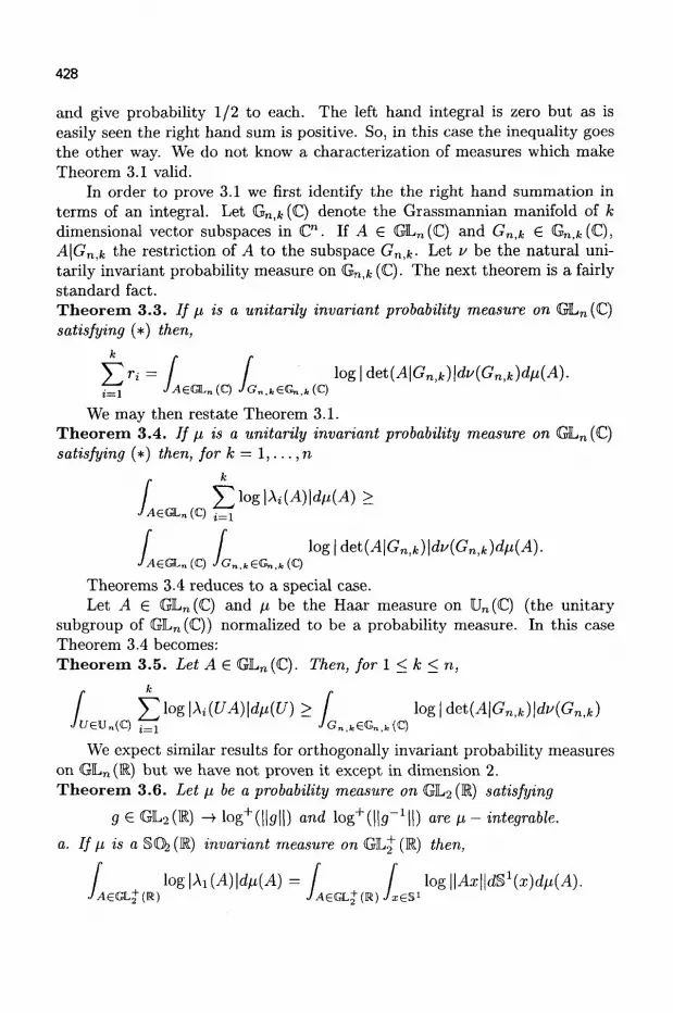
428

and give probability 1/2 to each. The left hand integral is zero but as is easily seen the right hand sum is positive. So, in this case the inequality goes the other way. We do not know a characterization of measures which make Theorem 3.1 valid.

In order to prove 3.1 we first identify the the right hand summation in terms of an integral. Let Gn,k (C) denote the Grassmannian manifold of k dimensional vector subspaces in C". If A £ GL„(C) and Gn^ € Gn>fc(C), A\Gn,k the restriction of A to the subspace Gn,fc. Let v be the natural uni-tarily invariant probability measure on <Gn,k (Q- The next theorem is a fairly standard fact. Theo rem 3.3. If fi is a unitarily invariant probability measure on GL„(C) satisfying (*) then,

J2ri= I I \og\det(A\Gn,k)\dv(Gn,k)dfi(A). i = 1 JAeOLn(C) JG„,keGnik(C)

We may then restate Theorem 3.1. Theo rem 3.4. If fi is a unitarily invariant probability measure on GL„ (C) satisfying (*) then, for k = 1 , . . . , n

k

^og\\i{A)W{A) > A£VLn(C) i=1

[ f \og\det(A\Gn,k)\du(Gn,k)dn(A). JAeGLn{C) ^ G „ , t e G „ , f c ( Q

Theorems 3.4 reduces to a special case. Let A 6 GL„(C) and \i be the Haar measure on Un(C) (the unitary

subgroup of GLn(C)) normalized to be a probability measure. In this case Theorem 3.4 becomes: Theorem 3.5. Let A e GL„ (C). Then, forl<k<n,

k

f Tlog\\i(UA)\dLi(U)> f \og\det(A\Gn,k)\dv(Gn,k) JUeV„(Q i=1 •/G„, f c€G„, f c(C)

We expect similar results for orthogonally invariant probability measures on GLn (E) but we have not proven it except in dimension 2. Theo rem 3.6. Let n be a probability measure on GL2(K) satisfying

g e GL2(K) -> log+(||p||) and log+( | |s_ 1 | | ) are fj, - integrable.

a. If fi is a 80^ (K) invariant measure on GLj (E) then,

[ log\\1(A)\dii(A)= [ f log\\Ax\\dS1(x)d^(A). JAeGL^ (R) J 4 6 G L + (R) JxgS1

/ ,

429

b. If n is a §Cfe(E) invariant measure on QL^~(E), whose support is not contained in MQ)2(K) i.e. in the set of scalar multiples of orthogonal matrices, then

[ \og\\1(A)\dii{A)> f [ log\\Ax\\dS\x)dn(A). JAe€L-(R) J AeGLz (R) JxeS1

Here &L% (E) (resp. GLJ (E)) is the set of invertible matrices with posi­tive (resp. negative) determinant.

4 Proofs and the Complexity of Bezout's Theorem

In our series of papers on complexity and Bezout's theorem, Steve and I con­centrated on the manifold of solutions V = {(P, z) £ V{H(D)) x P(Cn) |P(z) = 0} and the two projections

V rij n2

F(H{D)) ' ^ P(C")

in order to transfer integrals over T(H(D)) to integrals over P(C"). See 4

Here (D) = (di, • • •, dn_i) and H(D) is the vector space of homogeneous polynomials systems P = ( P i , . . . ,Pn-\) where each P; is a homogeneous polynomial of degree di in n complex variables. For a vector space V, P(V) denotes the projective space of V.

Our proof of 3.5 relies heavily on this technique, but with respect to a manifold of fixed points.

A flag F in C™ is a sequence of vector subspaces of C : F = (Fi,F2,... ,Fn), with Fi C Pi+i a n d dimP, = i. The space of flags is called the flag manifold and we denote it by Fn(C). An invertible linear map A : C" -» Cn naturally induces a map A$ on flags by

Ai(F1,F2,...,Fn) = (AF1,AF2,...,AFn).

The flag manifold and the action of a linear map A on F n (C) is closely related to the QR algorithm, see 13 for a discussion of this. In particular if F is a fixed flag for A i.e. A$F = P , then A is upper triangular in a basis corresponding to the flag P , with the eigenvalues of A appearing on the diagonal in some order: \i(A,F), ...,\n{A,F).

Let

VA = {(U,F)eVn(QxFn(Q : {UA)iF = F}.

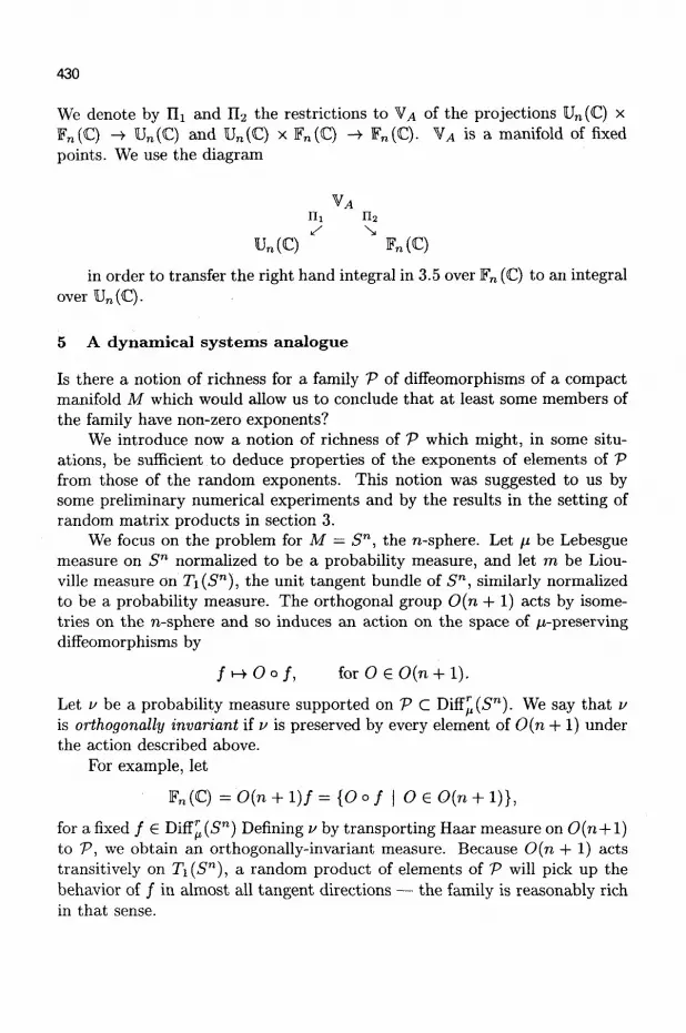
430

We denote by III and n 2 the restrictions to VA of the projections U„ (C) x F„(C) ->• U„(C) and U„(C) x F„ (Q -> F„(C). V^ is a manifold of fixed points. We use the diagram

rii n 2

Un(C) ' ^ F„(C)

in order to transfer the right hand integral in 3.5 over F„ (C) to an integral overU„(C).

5 A dynamical systems analogue

Is there a notion of richness for a family V of diffeomorphisms of a compact manifold M which would allow us to conclude that at least some members of the family have non-zero exponents?

We introduce now a notion of richness of V which might, in some situ­ations, be sufficient to deduce properties of the exponents of elements of V from those of the random exponents. This notion was suggested to us by some preliminary numerical experiments and by the results in the setting of random matrix products in section 3.

We focus on the problem for M = 5" , the n-sphere. Let /J. be Lebesgue measure on Sn normalized to be a probability measure, and let m be Liou-ville measure on Tj(5n) , the unit tangent bundle of Sn, similarly normalized to be a probability measure. The orthogonal group 0(n + 1) acts by isome-tries on the n-sphere and so induces an action on the space of ^-preserving diffeomorphisms by

/ H O O / , for 0 € 0(n + 1).

Let v be a probability measure supported on V C Diff^(5"). We say that v is orthogonally invariant if v is preserved by every element of 0{n + 1) under the action described above.

For example, let

F„(C) =0{n + l)f={Oof | OeO(n + l)},

for a fixed / e Diff^(5") Defining v by transporting Haar measure on 0 (n + l) to V, we obtain an orthogonally-invariant measure. Because 0(n + 1) acts transitively on Ti(Sn), a random product of elements of V will pick up the behavior of / in almost all tangent directions — the family is reasonably rich in that sense.

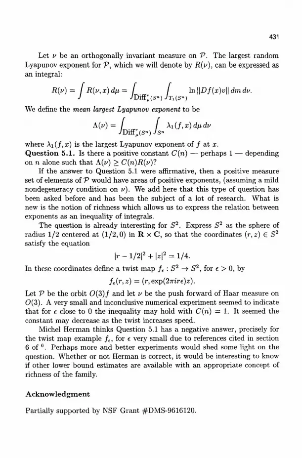
431

Let v be an orthogonally invariant measure on V. The largest random Lyapunov exponent for V, which we will denote by R{v), can be expressed as an integral:

R(i/)= R(u,x)dfj,= [ \n\\Df{x)v\\dmdv. J yDiff;(s»)M(S")

We define the mean largest Lyapunov exponent to be

A(i/) = / / \i(f,x)dndu •/Diff^S") JS"

where Ai (/, x) is the largest Lyapunov exponent of / at x. Question 5.1. Is there a positive constant C(n) — perhaps 1 — depending on n alone such that A(z/) > C{n)R{u)1

If the answer to Question 5.1 were affirmative, then a positive measure set of elements of V would have areas of positive exponents, (assuming a mild nondegeneracy condition on v). We add here that this type of question has been asked before and has been the subject of a lot of research. What is new is the notion of richness which allows us to express the relation between exponents as an inequality of integrals.

The question is already interesting for S2. Express S2 as the sphere of radius 1/2 centered at (1/2,0) in R x C, so that the coordinates (r, z) € S2

satisfy the equation

|r - 1/2|2 + \z\2 = 1/4.

In these coordinates define a twist map / e : S2 -»• S2 , for e > 0, by

fe(r,z) = (r,exp(27rire)z).

Let V be the orbit 0 ( 3 ) / and let v be the push forward of Haar measure on 0(3). A very small and inconclusive numerical experiment seemed to indicate that for e close to 0 the inequality may hold with C{ri) = 1. It seemed the constant may decrease as the twist increases speed.

Michel Herman thinks Question 5.1 has a negative answer, precisely for the twist map example / e , for e very small due to references cited in section 6 of 6. Perhaps more and better experiments would shed some light on the question. Whether or not Herman is correct, it would be interesting to know if other lower bound estimates are available with an appropriate concept of richness of the family.

Acknowledgment

Partially supported by NSF Grant #DMS-9616120.

432

References

1. Abraham, R. and J. Robbin, Transversal Mappings and Flows, W. A. Benjamin, Inc., New York-Amsterdam 1967.

2. Abraham, R. and S. Smale, Nongenericity of fl-stability, 1970 Global Analysis (Proc. Sympos. Pure Math., Vol. XIV, Berkeley, Calif., 1968) pp. 5-8 Amer. Math. Soc, Providence,R.I.

3. Anosov, D. V., Geodesic flows on closed Riemannian manifolds of nega­tive curvature, Proc. Steklov. Inst. Math. 90 (1967).

4. Blum L., F. Cucker, M. Shub, S. Smale Complexity and Real Computa­tion, Springer, 1998.

5. Brezin, J. and C Moore, Flows on homogeneous spaces: a new look. Amer. J. Math. 103 (1981), 571-613.

6. Burns K., C. Pugh, M. Shub and A. Wilkinson, Recent Results about Stable Ergodicity, to appear in: Proceedings on Symposia in Pure Math­ematics, the Seattle Conference of Smooth Ergodic Theory, AMS.

7. Dedieu, J.P. and M. Shub, On random and mean exponents for unitarily invariant probability measures on GL(n, C), preprint.

8. Gol'shied I. Ya. and G- A. Margulis, Lyapunov Indices of a Product of Random Matrices, Russian Math. Surveys 44:5 (1989), pp. 11-71.

9. Moore, C.C. Ergodicity of flows on homogeneous spaces, Amer. J. Math. 88 (1966), 154-178.

10. Oseledec, V. I., A Multiplicative Ergodic Theorem. Lyapunov Character­istic Numbers for Dynamical Systems, Trans. Moscow Math. Soc, 19, (1968), pp. 197-231.

11. Pugh, C. and M. Shub, Ergodic elements of ergodic actions, Compositio Math. Vol. 23 (1971), 115-121.

12. Ruelle, D., Ergodic Theory of Differentiable Dynamical Systems, Publi­cations Mathematiques de 1'IHES, Volume 50, (1979), pp. 27-58.

13. Shub M. and A. Vasquez, Some Linearly Induced Morse-Smale Systems, the QR Algorithm and the Toda Lattice, in: The Legacy of Sonia Ko-valevskaya, Linda Keen Ed., Contemporary Mathematics, Vol. 64, AMS, (1987), pp. 181-193.

14. Smale, S., Structurally stable systems are not dense, Amer. J. Math. 88 (1966), 491-496.

15. Smale, S., Differentiable dynamical systems, Bull.A.M.S. 73 (1967), 747-817.

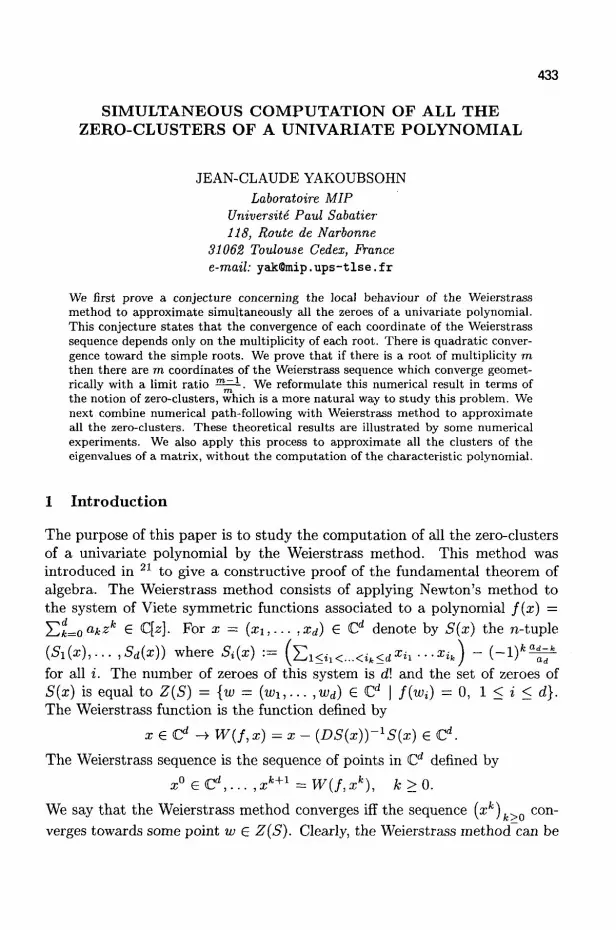
433

SIMULTANEOUS COMPUTATION OF ALL THE ZERO-CLUSTERS OF A UNIVARIATE POLYNOMIAL

JEAN-CLAUDE YAKOUBSOHN Laboratoire MIP

Universite Paul Sabatier 118, Route de Narbonne

31062 Toulouse Cedex, France e-mail: yak@mip.ups-tlse.fr

We first prove a conjecture concerning the local behaviour of the Weierstrass method to approximate simultaneously all the zeroes of a univariate polynomial. This conjecture states that the convergence of each coordinate of the Weierstrass sequence depends only on the multiplicity of each root. There is quadratic conver­gence toward the simple roots. We prove that if there is a root of multiplicity m then there are m coordinates of the Weierstrass sequence which converge geomet­rically with a limit ratio m~1. We reformulate this numerical result in terms of the notion of zero-clusters, which is a more natural way to study this problem. We next combine numerical path-following with Weierstrass method to approximate all the zero-clusters. These theoretical results are illustrated by some numerical experiments. We also apply this process to approximate all the clusters of the eigenvalues of a matrix, without the computation of the characteristic polynomial.

1 Introduction

The purpose of this paper is to study the computation of all the zero-clusters of a univariate polynomial by the Weierstrass method. This method was introduced in 21 to give a constructive proof of the fundamental theorem of algebra. The Weierstrass method consists of applying Newton's method to the system of Viete symmetric functions associated to a polynomial f(x) = ^2k=0a,kZk S C[z}. For x = (x\,... ,xd) S Cd denote by S(x) the n-tuple

(S i (z ) , . . . ,Sd(x)) where Si(x) := (Zi<i1<...<ik<dXh • • • ** ) ~ ( - l ) f c 5 t r for all i. The number of zeroes of this system is d\ and the set of zeroes of S(x) is equal to Z{S) = {w = (wi , . . . ,wd) G Cd \ f(wi) = 0, 1 < i < d}. The Weierstrass function is the function denned by

x € Cd -* W(f,x) =x- (Z?5(a;))-1S(a;) € Cd.

The Weierstrass sequence is the sequence of points in Cd defined by

x° e C d , . . . ,xk+1 =W(f,xk), k>0.

We say that the Weierstrass method converges iff the sequence {%k)k>0 con­verges towards some point w £ Z{S). Clearly, the Weierstrass method can be

434

\xk-w\\<ll) \\x°-w\

used to approximate all the roots of / simultaneously. In this context, it is fundamental to know a condition for the quadratic

convergence of the Weierstrass sequence. In terms of the modern analysis of the Newton method by the alpha-theory of S. Smale 4 , we can state the following theorem. Theorem 1 Let f € C[x] be a polynomial whose roots are all simple. Let us consider w € Z(S) and the quantity

f\\DS-'S(w)DkS(w)\\\^ 7(5, w) = ma* ^ _ U J .

Then for all x € Cd satisfying the inequality

II n^ 3->/7 \\x — w\\ < ——-—-

the Weierstrass sequence initialized at x° = x converges towards w. Moreover

2 f c - l

As it is mentioned, this result holds in the case of simple roots. The purpose of this paper is to investigate the general case of zero-clusters. In fact, the case of multiple zeroes is meaningless, from a numerical analysis point of view, see 24. For that we will use the explicit formulas for the Weierstrass function. It is well-known how to calculate formally the inverse of DS(x) (see 3 ) . We have: i e C -+W(f,x) = (xi u

f{x(l] > , . . . , x d rr^A ) ec

d.

A very good survey of the Weierstrass method and possible extensions is done by Sendov, Andreev, and Kjurkchiev in 18. We recall the result obtained by Kjurkchiev and Markov in 1983. Theorem 18.1 (See page 700 of 1 8 . ) Let f G C[x] be a polynomial of degree d with roots w\,... ,Wd- Let 0 < q < 1, s = min \wi — Wj\ and 0 < c < . 5.

*#j a

where a = 1.7632283... is determined from the equality a = e» . If the initial approximations x ° , . . . ,x° °f ^e roots w\,... ,Wd of f(x) = 0 satisfy the inequalities

\x0i~Wi\<cq, i = l,...,d,

then the sequence {xk}k>o — {(xk,... ,x^)}fc>o satisfies the inequalities

\xk -wi\ < cq2", 2 = 1 , . . . ,d.

435

We will state an alternative version of the above result where knowledge of the spacings of the roots is unneeded: we instead use the quantity 7( / ) defined below and introduced by Smale 4 (see theorem 2 of the next section). Indeed, the hypotheses of our result will ensure that the quantity s = min,^- \u>i — Wj\ is positive. This is done through the point estimate s > ^rjj (see Lemma 1).

To understand the convergence of Weierstrass method in the general case, consider the polynomial f(z) = zm. Then W(f,x) = mj=^-x. Each coordi­nates, say xk, of the sequence xk+1 = W(zm,xk) converges towards 0 with a geometric rate of convergence ^ ^ following the straight line [x°,0].

The main result of this paper is that the previous example describes the general case, in the following sense: the behaviour of the Weierstrass sequence xk towards a zero-cluster depends of the multiplicity of this cluster. There is a quadratic convergence if the cluster is a simple root and a geometric convergence if the cluster contains m zeroes: see Theorem 3.

In the second part of this paper, we combine a path-following method with the Weierstrass method in order to follow a curve which finishes to a point of Z(S). The complexity of this homotopy method is given in theorem 4. We next give some numerical experiments and we show an application of this process to the computation of all the eigenvalues of a matrix without computation of coefficients of characteristic polynomial.

We conclude this introduction by some short remarks and historical com­ments to explain the context and the new results of this paper. Globally the ideas of this study are those developed by Weierstrass in 21. In fact, Weier­strass has used the Newton iteration applied to the Viete symmetric functions system to give a constructive proof of the Fundamental Theorem of Algebra: in the case of simple roots, he first proves the local quadratic convergence of the method. He then introduced a classical linear homotopy with rational subdivision of the time interval to conclude. Many authors have re-discovered this method which is also known as the Durand-Kerner's method 7, 12, 13. Most of the earlier literature only studied the local behaviour of this method in the context of circular arithmetic: see 17 and 16. The use of classical linear homotopy or other can be found in 20 and 6. The cited authors were primar­ily interested in polynomials with simple roots. The dependence of the rate of convergence of the Durand-Kerner method on the multiplicity of the root has been numerically observed in 9,14,10,2. However, the proof of a precise numerical result along these lines has not appeared before in the literature.

436

2 Main Results

Denote by

d d

f{z) = ^Z akzk = ad X\SZ ~ W^ k=0 i= l

a complex polynomial of degree d > 2. We will let w = (w\,... , w<j)- The analysis of the convergence will be done with respect to the quantities

Pm(f,z)= „ max 0<k<m — 1

lm(f,z) = max fc>m+l

m !/<*>(*) fc!/(m)(z)

m!/<fc)(z) A:!/(m)(z)

2 6 C,m > 1,

z G C,m > 1.

These quantities were first introduced in 24. We first treat the case where all the roots of polynomial / are simple and state a 7-theorem, see 4 Theorem 1 page 156. For that we introduce the quantity:

7 ( / ) = max:/yi(f,Wi). l<i<d

Theorem 2 Let us consider x — (x±,... ,Xd) € Cd be such that

Then the Weierstrass sequence defined by

x° = x, xk+1 =W(f,xk), k>0

converge towards w with error bound:

/ 1 \ 2 * - 1

\Xi~m\<[j) k ° - ^ l , l<i<d.

This result is based on the following lemma which appears in 24. Lemma 1 Following the notation above, if Wi ^ Wj then \wi — Wj\ > YTT) '

We now consider the case of zeroes clusters. Recall that an m-cluster of / is a disk which contains m roots of / . We will denote by D(x,r) any disk around x of radius r and cD(x,r) the disk D(cx,cr). We assume without loss of generality that the roots of / can be partitioned to lie in p disjoint clusters where, for all i G {1, • • • ,p}, the i— cluster is an m^-cluster D(zi,r). Denote the roots in the rrij-cluster D(zi,r) by wn,... ,Wimi and let Mi —

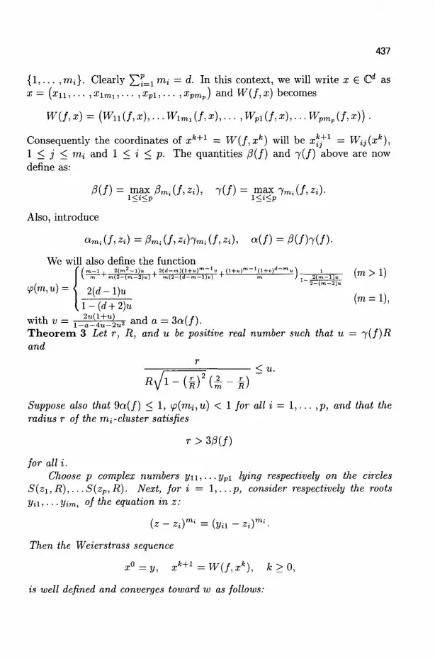
437

{ 1 , . . . ,m,i}. Clearly 5Zf=1 m; = d. In this context, we will write x € Cd as x = ( x n , . . . ,xlmi,... ,xpl,... ,xpmp) and W(f,x) becomes

W(f,x) = (Wn(f,x),... Wlmi (f,x),... , Wpl(f,x),... WpmF(f,x)) .

Consequently the coordinates of xk+l = W(f,xk) will be xk^~x — Wtj(xk), 1 < j < mi and 1 < i < p. The quantities /3(f) and j(f) above are now define as:

/3(f) = max /3mi(f,Zi), y(f) = max -ym.(f,Zi). l<i<p IS'SP

Also, introduce

ami (f, Zi) = Pmi (/, Zi)-ymi (/, Zi), a(f) = /3(f)~/(f).

We will also define the function 7 m - l , 2(m2-l)u . 2(<j-m)(H-u)"'-1v . (1+.)"—J (l+v)d-mu \ j Cm > 1 "l

, . I 2-(m-2)u

¥>("»,«)=< 2(d- l )u

Irrp^ (m=1)' w i t h « = i4- ( 4u-L" a n d ° = 3 a ( / ) -Theorem 3 Let r, R, and u be positive real number such that u = j(f)R and

r

<u. V1-(*)'(£-*)

Suppose also that 9a(f) < 1, ip(mi,u) < 1 for all i = 1 , . . . ,p, and that the radius r of the rrii-cluster satisfies

r > ms) for all i.

Choose p complex numbers yn,---ypi lying respectively on the circles S(z1,R),.. .S(zp,R). Next, fori = l,...p, consider respectively the roots 2/iij • • -yirm of the equation in z:

(z - zt)m' = (ya - Zi)m<.

Then the Weierstrass sequence

x°=y, xk+1 =W(f,xk), k>0,

is well defined and converges toward w as follows:

438

1. For all i such that m, > 1 and for all x\p j G Mi, which satisfies r < u\x\j — Zi\, we have:

\%ij ~ z%\ < <p(mi,u)k(R + r),l < j < mu k> 0.

Moreover each x\p j G Mi, lies in the disk ip(mi,u)kD(x°j,r).

2. On other hand, if Wi is a simple root (mi — 1), we have

We now say how to simultaneously find all the clusters. For that, we intro­duce the homotopy studied in 4,23, and 24. Denote by S — {x = (xi,... , Xd) € Cd | 3i / j , Xi = Xj}. Let z° G Cd - E. For t G [0,1], let us consider the family of map St defined by:

x G Cd - • St(x) = S(x) - tS(z°).

A straightforward computation shows that the polynomial ft associated to St

is equal to

ft(z) = (l-t)f(z) + tg(z), d-l

with g(z) = adzd + ^2(-l)d~kadSd-k{z°)zk. Hence the homotopy defined

fc=0 with the function St induces a linear homotopy with the polynomials f(z) and g(z). Let w1 = (w\,... ,wd) the curve of Cd such that 5 t(w') = 0. The linear map DSt(wt) is invertible for all t €]0,1]. To follow numerically the curve wl, consider a positive real number M < 1, the sequences (tk)k>o and (zk)k>o defined respectively by

t0 = l,tk = Mk,

zk+1=W(fk+llzk)

where fk — ftk • The purpose is to quantify the computational complexity of the preceding numerical path-following method. More precisely, we estimate the number of steps k such that each coordinates zf of zk is a point which is closed to a zero of / . Toward this end, let us introduce the following quantities where u > 0 and i are given a priori:

• D(xi,r) is an mj-cluster which contains the root Wi = iu° of / . If mi = 1 then Xi = Wi and r = 0.

439

Let R be such that u = j(f)R.

tf = suP{* e]o, l] Wf - W{ = R}.

g = maxj max (+<K1 j(ft)

b — max; (maxt+

h = max0<i<i

"<t<i /,'K) I J' a-b9-mi'.g(wt

i)

Theorem 4 Suppose u < 5J_2> 4u^ < 1 and /?(/) < uR. Let i be given

and denote by fcj the index satisfying tk{ < tf < £fc;_i. Then, the following

assertions hold:

1. For all k such that tk > tf, the points z\'s are well defined and are approximate zeroes of wf.

2. The value tf is bounded by

h{u)Rmi rrii — 1

at + h(u)Rmi-x <t1

3. \zk wA <R+%.

3 Practical Algorithms and Numerical Experiments

Our first numerical experiment will be per­formed on the polynomial f(z) g i v e n b y z15 + (-6.30211 - 6.51486i)z14 + (-4.602131368 + 34.33661782 i)zl3 + (63.59234833 -17.54183753 i) z12

+ (7.872508933 - 100.8166243») z11 + (-222.2761285 - 64.53993948»") z10 + (-167.1645824 + 289.8629099 »') z9

+ (388.8936599 + 490.8785827 i) zs + (642.5739956 - 425.4499699 i) z7 + (78.15261237 - 888.3687140 i) z6

+ (-1127.773435 - 316.6287328»') z5 + (-750.6198536 + 605.88985631) z4 + (441.7642441 + 974.1649811 i) z3

+ (422.0315160 + 163.1681751 i) z2 + (416.5648287 - 448.9257391 i) z + 8.41840810 - 48.40497033 i T h i s p o l y n o m i a l h a s t h e five « -c lus t e r s D(zi, 0 .05) w i t h :

Zl = -0.071 + 0.043i , z2 = -1.227 + 0.179* , z3 = -0.686 - 0.855* 24 = 0.388 + 1.825* , z5 = 1.866 + 0.275*.

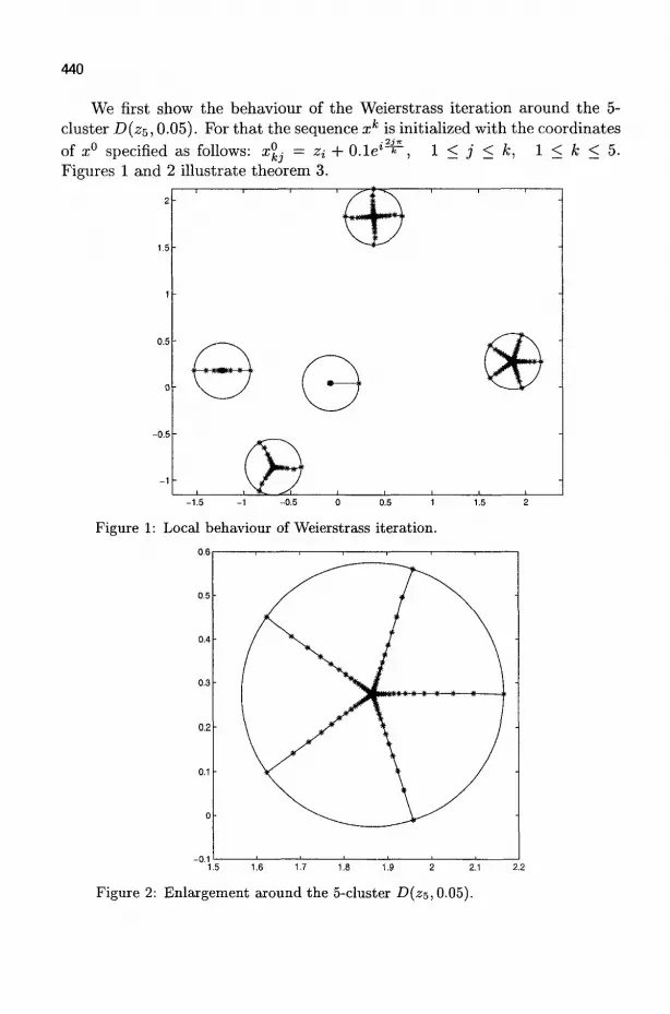
440

We first show the behaviour of the Weierstrass iteration around the 5-cluster D(z$, 0.05). For tha t the sequence xk is initialized with the coordinates of x° specified as follows: x°k, = Zi + O.le* -* -, 1 < j < k, 1 < k < 5-Figures 1 and 2 illustrate theorem 3.

-1.5 -1 -0.5 0 0.5 1 1.5 2

Figure 1: Local behaviour of Weierstrass iteration.

1.5 1.6 1.7 1.8 1.9 2 2.1

Figure 2: Enlargement around the 5-cluster D(zs, 0.05).

441

We next illustrate the numerical path-following using Weierstrass method via the algorithm described below. Recall that ft(z) = (1 - t)f(z) + tg(z) is defined previouly and Wft is the Weierstrass operator associated to ft- For a given integer nu > 2 we will denote W?" the repeated composition of the operator Wft nu times.

Weierstrass Path-Following Algorithm Inputs: / a polynomial of degree d, z° € Cd , e a positive real number,

nu > 2 an integer and 0 < M < 1. /? = 2e, t0 = 1, ti = 1 - M. while p > e or t0 > 0 Compute the point z1 = W£'(z°).

/? = n ' ' i i if /3 < e and t\ = 0 Determine the clusters and stop, i ij^i zi zj

if 0 > e and tx > 0 replace tx by ^ ± ^ -If P < e and ti > 0 replace t0 by t i , t\ by max(3ti - 2t0,0) and z° by z1. end Outputs: the set of all the clusters. The proof of the convergence of this algorithm is given in 23. It also has

been used in 24 to compute only one cluster. The figure below was derived by taking z£ = e - ^ , 1 < k < d.

Figure 3: Simultaneous computation of all the zeroes-clusters.

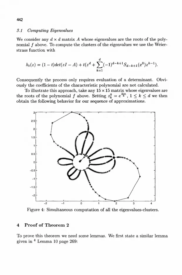
442

3.1 Computing Eigenvalues

We consider any d x d matrix A whose eigenvalues are the roots of the poly­nomial / above. To compute the clusters of the eigenvalues we use the Weier-strass function with

d

ht(z) = (1 - t)det(zl -A)+ t(zd + £ ( - l ) d _ f c + % - * + i ( z V _ 1 ) -fc=i

Consequently the process only requires evaluation of a determinant. Obvi­ously the coefficients of the characteristic polynomial are not calculated.

To illustrate this approach, take any 15 x 15 matrix whose eigenvalues are the roots of the polynomial / above. Setting z ° = e " ^ L , l < f c < d w e then obtain the following behavior for our sequence of approximations.

Figure 4: Simultaneous computation of all the eigenvalues-clusters.

4 Proof of Theorem 2

To prove this theorem we need some lemmas. We first state a similar lemma given in 4 Lemma 10 page 269:

443

L e m m a 2

/ i M y - 1 _ P - I k>2 \P U>

Proof: It is sufficient to prove that ( - (£) ) is a decreasing function of

k. For that verify

p\k + lj ~ \p \kj

This inequality is equivalent to

( p - l ) . . . ( p - f c ) < ^ ( p _ i ) . . . ( p _ f c + i ) y + i i T

(fc + 1)! - V A! /

We first have f(P~1)-"^-k + 1)\ fc_1 > p ~ * + 1 . On the other hand,

we have g=* < ^ ± i . Hence

( p - l ) - - - ( p - A ; + l ) y + ^ T ( p - l ) - - - ( p - f c + l ) p - A ; + l

Jfe! / - k\ k ( p - l ) - - - ( p - f c + l ) p - f c

A;! fc + 1'

We are done.B We now give a point estimate for | n ? = i ( l + zj) ~ M improving one given

by Higham on page 75 of n . L e m m a 3 Let p > 1 an integer and e a real number be such that 0 < e < - ^ . Considerp complex numbers z\,... ,zp satisfying \ZJ\ < e. Then,

Moreover | = 1 ( 1 + zj)\ > 1 - ^f^.

Proof: We have ] l j= i ( l + zi) ~ 1 = YJk=\ ak(zi, • • • ,zp) where the ak's are the Viete symmetric functions of z\,... ,zp. We know \ak(z\,... , zp)\ <

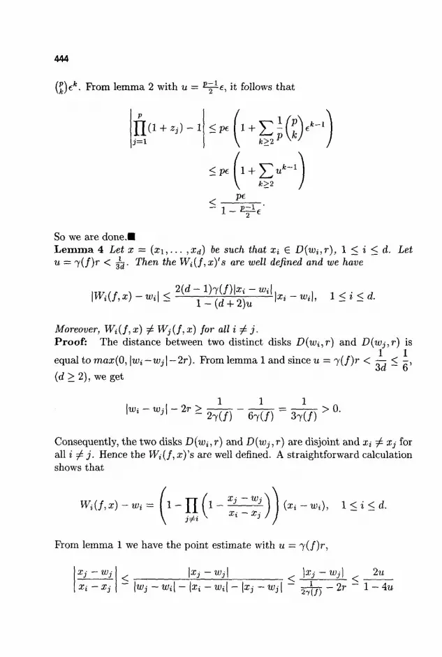
444

(£)efc. Prom lemma 2 with u = ^ ^ e , it follows that

Y[(l + Zj)-l

<pe f 1 + ^V" 1

k>2

< pe l-Z=±e

So we are done.B L e m m a 4 Z€£ ar = (xi,... ,Xd) be such that X* 6 D{wi,r), 1 < i < d. Let u — l(f)r < J3- Then the Wi(f,x)'s are well defined and we have

m i f ^ ) - ^ ^ - 1 ^ ; - ^ ^ - ^ i<i<d. 1 — (a + z)u

Moreover, Wi(f,x) ^ Wj(f,x) for all i ^ j . Proof: The distance between two distinct disks D(wi,r) and D(wj,r) is

equal to max(0, \wi— Wj\ — 2r). From lemma 1 and since u = "/(f)r < — < - , 3a 6

(d > 2), we get

\wi — Wj\ — 2r > 27(/) 67( / ) 37 ( / )

> 0 .

Consequently, the two disks D(wi,r) and D(vjj,r) are disjoint and X, ^ x - for all i ^ j . Hence the Wi(f, x)'s are well defined. A straightforward calculation shows that

Wi(f,x)-Wi= ( l -nf 1 -^—))^-^) , 1 < * < d-

From lemma 1 we have the point estimate with u — j(f)r,

Xj — Wj

K -Wi\ -

\Xj -Wj\

- \X{ -Wi\ --\Xj~Wj\

/ \xj-Wj\ ^ 2w

27(/) ^ i iU

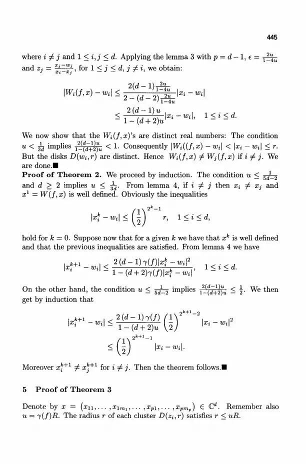
445

_ 2M where i ^ j and 1 < i, j < d. Applying the lemma 3 with p = d—l,e=j^ and zi = l^ff' for 1 ^ 3 < d > J : t ' we obtain:

2(d— 1) 2"

\wi(f,x)-Wi\ < \ y-% \Xi-Wi\ 2 ( d - l ) w , , , .

We now show that the Wj(/, x)'s are distinct real numbers: The condition u < jg implies 1_tJ+l)u < 1- Consequently \Wi((f,x) — wi\ < \xi — Wj| < r. But the disks D{wi,r) are distinct. Hence Wi(f,x) ^ Wj(f,x) if i ^ j . We are done.B Proof of T h e o r e m 2. We proceed by induction. The condition u < ^jz2 and d > 2 implies u < ^ . From lemma 4, if i ^ j then a 7 Xj and x1 = W(f, x) is well defined. Obviously the inequalities

\xi-Wi\<(-) r, l<i<d,

hold for k = 0. Suppose now that for a given k we have that xk is well defined and that the previous inequalities are satisfied. From lemma 4 we have

\x^-w\< ^ - l ) 7 ( / ) i ^ - ^ l 2 1 < i < d

I*. W ' l ^ l - ( d + 2 ) 7 ( / ) | : B » - « , i | ' - ~

On the other hand, the condition u < ^ ^ implies x_i^Z^)u < | - We then get by induction that

l*' w * l ^ l _ ( d + 2 ) u ^2 J |Xt W i |

< f 2 ) \xi ~wi\-

Moreover x\+1 ^ xk+1 for i ^ j . Then the theorem follows.•

5 Proof of T h e o r e m 3

Denote by x = (x\\,... ,ximi,... ,xP\,... ,xpmp) 6 Cd. Remember also u — 7( /) iJ . The radius r of each cluster D(zi,r) satisfies r < uR.

446

Lemma 5 Let i and j € Mi be given. Let Xik, 1 < k < rrii the roots of the equation in z

yZ Zi) — \%ij Zi) 5

such that Xn = Xij. Let us suppose

(a) \xik - Xik\ < u\xij - Xik\, 1 < k < rrii, k ^ j

(b) \zi — Wik\ < u\xij — Zi\, 1 < k < rrii, and k ^ j .

Then 2 ( m ? - l ) «

2. n

Lk€Mi,k^j Xij-Xik

<

< rm-l + 2 - ( m , - 2 ) n

fceMi.fc^j nj—ijfc

V1 2-(m i-2)u //

(! + ")" / 2 ( m ; - l ) u \ -

m ' ^ 2 - ( m , - - 2 ) « ;

Proof: Since the x ^ are the roots of the equation given in this lemma, we n a v e HkeMi,kyij(xij - %ik) = mi(xij - Zi)mi~l. We can then write

T T Xjj -Wjk _ (Xjj - Zj)mi~l U.k€Mj,k^j [l + xij-'zi )

„M. w , XH ~ xik UkeMiM(xiJ - xik) UteMuW (X + f ^ f ^ ) k€Mi,kj:j

n mi Uk£Mi ,*#,- ( l + ftt^ftt) *€«< .**> ^ Xii

1 + Zi - Wik

- Zi

= m < - i + m < ( n t 6 M . > f > i ( i + ^ i ^ ) - i ) - ( n t 6 M < , w ( i + ^ ^ ) - 0

Using lemma 3 with p = mi — 1, e = u, and the assumptions 1 and 2, a straightforward computation gives successively

n •^ij ^ik

kEMt^j Xii Xik

<

<

1 . 2mi(mj — \)u . 2(roj —l)n mi J- + 2-(m,--2)« + 2 - ( m j - 2 ) «

/ 1 _ 2 ( m < - l ) u \ m t ^ 2-(mi-2)u)

_ -i , 2 (m?- l )u m ' i + 2 - ( m ; - 2 ) u

m. f 1 _ ^p=^-) 1 y 2 — {rrii— 2)u /

Just as n keMi,k^j Xij-xik before, we have

—^ V . . ^ - . ^ IlfceM*,*^ f1 + f # = t ) > a n d u P ° n u s i n S l e m m a 3>

part 2 is directly obtained. •

447

Lemma 6 Let i be given. Let Xki £ D(zk,r), I = 1 , . . . ,mjt and k = l,...p. Suppose 9a(f) < 1, r > 30(/) and r < uR. Then

1. Fork^i we have \Zi -wki\> ^ j y - §/?(/)•

2. For (k,l) ^ (i,j) we have

3. Moreover

Xkl-Wkl Xij—Xkl < i - a - t o - L " = V> Witfl ° = 3 a ( / ) -

B = n kjLi,l£Mk

1 + Xkl ~ Wkl

< 2(d — mi)v

2 — (d — rrii — l)v

B + l<(l + v)d-mi.

Proof: (1): Let us consider w a zero of / which don't lies in D(zi,r). We have successively:

I/(«OI = O= ^ = 0 = & i ) ( u , _ Z i )

> l £^£ i ] iu ,_ z . r — m;!

_ v m ; - l | /W( Z < ) | W — Zi\ sk>m.i + l i^imun-W-Zi

^ m i! I1" Z'l \ l L,k=0 W\!^i\zi)\\W Z%\ Lkymi+l jfe!|/("H>(zi) \W Z'\ )

> u^w - *r (i - E:=O x ( ^ ) m ' ~ * - E,>mi+1 (7m;(/)i^ - *ip- f c

Via the inequality 7 m i (/) < 7 ( / ) we finally get:

0 > 1 -\W-Zi\

1 JUL

-y(f)\w- Zj\ 1--Y(f)\w-Zi

>

\W-Zi\

-2j(f)\w - Zi\2 + (1 + 3 7 ( / ) / ? ( / ) )k - *i\ - W )

{l-lU)\v-Zi\){\v-Zi\-PU))

Under the condition 9a ( / ) < 1, the polynomial

- 2 7 ( / ) i 2 + (l + 3 7 ( / ) /3 ( / ) ) i -2 /? ( / )

has two real roots: r± _ l + 3 a ( / ) - > / l - 1 0 a ( / ) + 9 a ( / ) 2 a n d

47 ( / ) ^2 =

l + 3 a ( / ) + v / l - 1 0 a ( / ) + 9 a ( / ) 2

-2j(f)\w - Zi\2 + (1 + 3 7 ( / ) / ? ( / ) )k - *i| " 20(f) < 0

4 ,.> . It is then easy to see that the assumption r > 30(f) implies r > r j . Since \w — Zi\ > r, the inequality

448

holds when \w - zt\ > r2 . A lower bound for r2 is ^rjj ~ \P(f)- ^n

fact, the study of the function t e [0, | ] -> i+st+Vi-iot+m s h o w s t h a t

i-\-3t+y/i-iot+9t2 > | _ |£ Replace t by a and divide the previous inequality by 7 ( / ) , we find the lower bound announced for r2 . By definition of /?(/) and 7( / ) we finally have

\w - zA > WT)-\m-

yij

(2): From part (1) we have

\Xii -Xkl\ = \Xij -Zi + Zi- Wki + Wkt - Zk+ Zk - Xkl

> \Zi - Wkl\ - \Xij - Zi\ - \wkl - Zk\

1 3 >

Zk - Xkl

5^-i«fl-M-r. Since r < uR, it follows

Xkl ~ Wkl

Xij Xkl <

<

R + r

27(7)

2u(l + u)

\P{f)-2R-r

= v, 1 — a — Au — 2u2

with a = 3a( / ) . (3): There are d — rrii factors in the product of the quantity B. From lemma 3 and part (2) we get

2(d — rrii)v B < (1 + v)d-mi - 1 <

2 — (d — m,i — l)v'

The quantity B + 1 is obviously bounded by: B + 1 < (1 + v)d m' We are done.B

r 2 Lemma 7 Let R, r and be two positive real numbers which such that — < —.

R m Introduce the point y — (y\,... ym) such that yj1 — Rm, 1 < j <m. For c < 1, consider the sequence of disks

£ ° = D(yj,r), D) = ckD (yj,r) ,l<j<m,k>l.

Then for k be fixed, we have DjflDi = 0 and the distance between two distinct disks is greater than

449

Proof: Each disk Dj is contained in a wedge of angle 26 such that sin 6 = -^, see figure. It is obvious that D) n D\ = 0 for j ^ / if ^ - 2(9 > 0. But ^ = sin# > ^0. Hence, using the assumption -^ < ~, the inequality

2TT „ „ 2n irr 2(9 > > 0

m m R

holds. Elementary geometric considerations in the triangle OAB (see figure )

show that the distance between two distinct disks Dj and D® is greater than

Since sin ( ^ - 9) > ^ — ^ , the result follows.•

Dl(Vi,rL D(yj,r)

^ - 26> 0

Figure 5: Illustration of the proof of lemma 7.

450

Lemma 8 Let us consider positive real numbers r, R, and u such that

r

V1-^)2^-*) < u.

Suppose also that 9a(f) < 1 and r > 30(f). Introduce p complex numbers 2/ni • • • >Vpi be such that \z% — yn\ < R •

For all i, 1 < i < p, consider respectively the roots yii,...yimi of the equations

(z - Zi)m< = (yn - Zi)

m<.

Let x be such that Xij £ D(yij,r), j £ Mit 1 < i < p.

Suppose for alii, (p(m,i,u) < 1, and \z%— Wij < u\xij — Zi\. We then have:

1. For all i, 1 <i <p such that rm > 1 we have:

\Wij(f,x) - Zi\ < ip(mi:u)\xij - Zi\, 1 < j < mi. The Wij(f,x) respectively belong to the disks <fi(mi,u)D(yij,r), j £ Mi, 1 < i < p. Moreover, these disks are pair-wise disjoint.

2. For all i, 1 < i < p such that rrii = 1 we have:

WaU^x) -Wi\ < - , , , „ , Fti -ml 1 — (a + 2)u

Proof: Let us first consider an index i such that m; > 1. A straightforward computation shows that:

wij{f,X)-zi=(i- n 2^?rW-*)- n 2^f^-^)-

We first bound 1 - n ^ ) ^ ) ^ f f f For that we write

1 _ TT J' — i _ TT J" ~ ' TT fii

(k,i)?(i,j) Xij ~ Xkl w Xij ~ Xil k^i Xii

ift xv Xi1 k^i

l-A-AB

Xij -Wil TT l, , xkl ~ wkl

ij kl

451

with A = n w %^% and B = U^ ( l + f ™ ) - 1- Hence, using the

assumtion |ZJ — Wij\ < u\x{j — Zi\, we get

\Wij(f,x) - Zi\ < (|1 - 4 | + |AB| + \A(B + l)|u) |xy - z4|.

Verify the assumption 2 of lemma 5 to bound |1 - A\. With the point Xij, construct the roots Xik of the equation (z — Zi)mi — (ijj - Zi)mi as in lemma 5. By definition of rjij and since x^ G D(yij,r), we have £** € D(yij,r). Hence \xik — xtk\ < 2r. Using lemma 7, the distance between two distinct disks D(yij,r) and D(yik,r) is greater than

Hence, for all A; 7 j , 1 < k < mi, we have

\xik -Xik\ , r < , = < u.

The assumptions of lemma 5 hold. Consequently |1 — A\ is bounded by

_ 1 , 2 (m?- l )u \1-A\< ^ 2-(mi-2)«

mil- 2(m;~1)" V "'« ^ 2-(rrn-2)u)

We bound the quantities 5 and J3 + 1 using the lemma 6:

B < 2{d-mj)v

~ 2 — (d — rrii — l)v

B + 1 < (1 + v)d-mi,

where v is defined in the introduction. From part 2 of lemma 5 we bound A

With all these point estimates, we obtain the following upper bound on \Wij(f,x) — Z{\: (n.j-1 2(m?-l)„ 2(J-mi)(l + »)" i - '„ (H.,)"»i-l(l+ ,^- '".-,\ t , , w m r h I mf +m;(2- (m j -2 )«)+ r»j (2- (d-m; -1)„) + mf I 2 ( ^ - 1 ) - ' X ' J Z>>' W I 1 1 U 1 V ' 2-(mi-2)u

in turn is bounded above by ip(rm,u)\xij — Zi\. Hence the point Wij(f,x) lies in the disk (p(rrii,u)D (yij, \xij — Zi\). Lemma 7 shows that the Wij's are distinct points. We have thus proved the first part.

Let us now suppose there exists an index i be such that m; = 1. In this case, the point estimate is a direct consequence of lemma 4. So we are done.

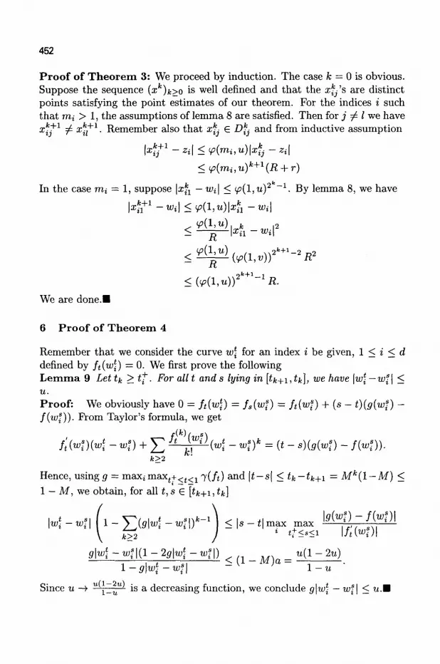
452

Proof of Theorem 3: We proceed by induction. The case k = 0 is obvious. Suppose the sequence (xh)k>o is well defined and that the x^'s are distinct points satisfying the point estimates of our theorem. For the indices i such that m,i > 1, the assumptions of lemma 8 are satisfied. Then for j ^ I we have x^1 ^ a^+1. Remember also that a;*- e D^ and from inductive assumption

k * / 1 ~Zi\< <p{muu)\xij - zt\

<<p{mi,u)k+1{R + r)

In the case m, = 1, suppose |x*x — iUi| < y>(l,u)2 - 1 . By lemma 8, we have

|a&+ 1-u/i |<¥>(l,u) |a:$i-Tt;i |

D \xil W*l

V?(l,u) 9 k + l

^Mi.u))2**1-1^.

We are done.I

6 Proof of Theorem 4

Remember that we consider the curve w\ for an index i be given, 1 < i < d defined by ft{w\) = 0. We first prove the following Lemma 9 Lett/. > tf. For allt ands lying in [tk+i,tk], we have \w\ — w\\ < u. Proof: We obviously have 0 = /t(u>f) = fs{wl) = ft(wf) + {s — t)(g(wf) — /(wf)). From Taylor's formula, we get

f't(wt)(wl - «,?) + £ ^ J ^ - <)" = (*- s)(9«) ~ /Ks))-fc>2

Hence, usingg = maxjmax t + < t < 1 7( / t ) and \t-s\ < tk~tk+i = M f c ( l - M ) <

1 — M, we obtain, for all t,s € [tfc+i>*k]

1 - y^(g|w* - w1\)h 1\ < | s - t | m a x max \W*.-W'\ I i - ^t~\...t .....Mfe-i I ^ i„ + i _ _ l f f « ) - / K s ) l I/;K)I

ffK-ti;f|(l-2gK-W||) _ = u(l - 2u) 1 -g\w\ -w?\ ~ 1 - M

Since u —• tZ is a decreasing function, we conclude g\w\ — wf\ < u.t

453

Lemma 10 Let h(u) = ( 1 ^ " . Then tf := sup{i e]0,l] | \w\ - w{\ = R} satisfies

h{u)Rmi-1 +

at + h^R™'-1 -**

Proof: Let D(zi,r) be a rrii cluster and Wi £ D(xt,r) be a zero of / . Denote t = tf. We have 0 = ft{w\) = (1 - t)f(w\) + tg{w\). Consequently

(1 _ t) ^ - , f^M{wl. ^ + / ^ w _ ^ + ^ + i / ( ^ _ ^ = tj(u{)_

As in the proof of lemma 6, we obtain from \w\— Wi\ = R and /?(/) < Ru that...

(1 - 0 (l - EET1 ( ^ ) m ' " * - Efc>m.+1(7(/^i)i?)fc-"") *"- < ma^K, | ^ g | t So (1 - t) (l - Y f f e - I ^ $ ? R ) 7 ( / ) i? m i < Oi* and thus

(1 - t ) * 1 " ^ ) " ^ - * < ait. The inequality of our lemma follows. •

Proof of Theorem 4: Let an index i and tf be such that \w\ — Wi\ = R. For all t € [*i")l], the polynomial ft only has simple roots. The quantity g = maxjmax t+< i < : i 7(/t) is bounded and we have, from lemma 1

(1): We first prove by induction that the zf's are approximate zeroes of fk

associated to wf for all index k such that tk G [tf, 1]. It is obvious for k = 0.

Suppose the z\ are distinct points and we have g\z\ — w\\ < u.Then prove

9\zi+1 ~ wi+11 < u- Applying lemma 9, we have

g\z\ - w\+11 < g\z\ - wki \ + g\w* - w\+1 \<u + u = 2u.

Since u < j-jrf, we have from theorem 2 for all k be such that tk 6 [tf, 1]:

g\z!+1-w*+1\<±g\z!-w*+1\<u.

Prove now that the z\ are distinct points. For i ^ j we have from the assumption Aug < 1:

k*+1 - 4+11 > kfc+1 - ^fc+11 - \4+1 - ™t+11 - Kfc+1 - 4+ 11 > ^ - 2« > 0.

Hence the z^+1's are distinct points and W(ft,zk+1) is well defined.

(2): Part 2 follows from lemma 10.

454

(3): Prom lemma 9 and the part 1 of this theorem,the point zi * is an approx-t+

imate zero of wt' . Hence

\4' - Wi\ < \wf - Wi\ + |z,*- -wf\<R+ -^

We are done.B

References

1. ABERTH, 0 . , Iteration methods for finding all zeroes of a polynomial simultaneously, Mathematics of Computation, Vol.27, 1973, pp. 39-344.

2. ALEFED, G., HERZBERGER, J., On the convergence speed of some algo­rithms for simultaneous approximation of polynomial roots, SIAM Jour­nal Numerical Analysis, 11, pp. 237-243, 1974.

3. BELLIDO,A.^Construction de fonctions d'iterations pour le calcul simul-tane des solutions d'equations et de systemes d'equations algebriques, These Universite Paul Sabatier,1992.

4. BLUM, L., CUCKER, F. , SHUB, M., SMALE, S., Complexity and Real Computation, Springer-Verlag, 1998.

5. CARSTENSEN, C , PETROVIC, M . C . , T R A J K O V I C , M., Weierstrass for­mula and zero finding methods, Numerische Mathematik, 69, 1995, pp. 353-372.

6. DEREN, W., FENGGUANG, Z., The Globalization of Durand-Kerner Al­gorithm, preprint 1995.

7. DURAND, E. Solution numerique des equations algebriques, Tome 1, Mas-son, Paris, 1968.

8. GREEN, M.W., KORSACK, A.J., PEASE, M.C., Simultaneous iteration towards all roots of a complex polynomial, SIAM Review, Vol.18, pp. 501-502, 1976.

9. FARMER, M.R., Loizou, G., A clazs of iterations functions for improv­ing, simultaneously, approximations to the zeroes of a polynomial, BIT 15, pp. 250-258, 1975.

10. FRAIGNIAUD, P , The Durand-Kerner's Polynomial Roots-Finding in Case of Multiple Roots, BIT 31, pp. 112-123, 1991.

11. HIGHAM N.J. , Accuracy and Stability of Numerical Algorithm, SIAM, 1996.

12. KERNER, I.O. Ein Gesamtschrittverfarhen zur Berechnung der Null-stellen von Polynomem, Numerische Mathematik, Vol. 8, pp. 290-294, 1966.

455

13. KERNER, 1.0. Algorithm 283, Communications ACM, Vol.9, P.273, 1966.

14. KJELLBERG, G.,Two Observations on Durand-Kerner's Root-Finding Methods, BIT 24, pp. 556-559, 1984.

15. PASQUINI, L., TRIGIANTE, D.,^4 Globally Convergent Method for Si­multaneously Finding Polynomials Roots, Mathematics of Computation, Vol.44,169, pp. 135-149, 1985.

16. PETKOVIC, M.S., STEFANOVIC, L.V., On some iterations functions for the simultaneous computation of multiple complex polynomial zeroes, BIT, 27, pp. 111-122, 1987.

17. PETKOVIC, M.S., Iterative Methods for Simultaneous Inclusion of Poly­nomial Zeros, Springer, Berlin, 1989.

18. SENDOV, B L . , ANDREEV, A., KJURKCHIEV, N.,Numerical solution of polynomial equations, in Handbook of Numerical Analysis, Vol 3, Ciarlet-Lions Editors, 1994.

19. TlLLl, P . Convergence conditions of some methods for the simultaneous computations of polynomial zeroes, University of Pisa, preprint 1995.

20. TlLLl, P . , Polynomial root finding by means of continuation, University of Pisa, preprint 1995.

21. WEIERSTRASS, K., Neuer beweis des satzes, dass jede ganze rationale function einer verdnderlichen dargestellt werden kann als ein product aus linearen functionen derselben verdnderlichen, Mathematische Werke, tome 3, Mayer u. Miiller, Berlin, pp. 251-269, 1903.

22. WERNER, W., On the simultaneous determination of polynomials roots, in Iterative Solutions of Nonlinear Systems of Equations, Lecture Notes in Math., Vol. 43, 167, pp. 205-217, 1984.

23. YAKOUBSOHN, J .C. , Contraction, Robustness and Numerical Path-Following Using Secant Maps, Journal of Complexity, 16, 1, 286-310, (2000).

24. YAKOUBSOHN, J .C. , Finding a Cluster of Zeros of Univariate Polyno­mials, Journal of Complexity, 16, 3, 603-638, (2000).

457

CROSS-CONSTRAINED VARIATIONAL PROBLEM A N D NONLINEAR SCHRODINGER EQUATION

JIAN ZHANG Department of Mathematics, Sichuan Normal University, Chengdu, 610066, China*

E-mail: jianzhan@mail.sc.cninfo.net

By constructing a type of cross constrained variational problem and establishing so-called cross-invariant manifolds of the evolution flow, we derive a sharp criterion for global existence and blowup of the solutions to the nonlinear Schrodinger equation. The instability of the standing waves in the equation is also shown.

1 Introduction

We are concerned with the following nonlinear Schrodinger equation

iipt + Aip + \<p\p- V = 0, t>0,xeRN, (1.1)

where 1 < p < ( J^t^+ (we use the convention: 1^-2)+ = ° ° w n e n N = 1,2 and (n - 2)+ = N - 2 when N>3).

Ginibre and Vero 5 established the local existence of (1.1) and the global existence of (1.1) for 1 < p < 1 + -fa, as well as 1 + -^ < p < (^Jh

22)+ w i t ^

small initial data. Glassey 6 , Ogawa and Tsutsumi 9 '10 studied the blowup properties of (1.1) for some initial data. Berestycki and Cazenave 1 as well as Weinstein 16 showed some interesting sharp criteria for blowup and global existence of (1.1), as well as the strong instability of the standing waves in (1.1) by variational arguments. The related work also sees 15 and 19 etc.

In the present paper, we construct a type of cross-constrained variational problem and establish it's property, then apply it to the nonlinear Schrodinger equation (1.1). By studying the corresponding cross-invariant manifolds un­der the flow of equation (1.1), we establish the sharp criterion for global existence and blowup of the solutions. By this criterion and the property of the cross-constrained variational problem, we also show the strong instabil­ity of the standing waves in equation (1.1). Berestycki and Cazenave x as well as Weinstein 16 have studied the similar problems. But in x and 16, the related variational problems have to be solved, the Schwarz symmetrization and complicated variational computation have to be conducted. By our new variational argument, we can refrain from solving the attaching variational

•Former address: Department of Mathematical Sciences, The University of Tokyo, 3 - 8 - 1 Komaba, Meguro-Ku, Tokyo 153, Japan

458

problems, and directly establish the sharp criterion for global existence and blowup of equation (1.1), which is different from 1 and 16. Furthermore By us­ing our sharp criterion for blowup, the strong instability of the standing waves in equation (1.1) is also shown. Moreover we see that the argument proposed here may be developed to treat nonlinear Schrodinger equation with potentials as well as systems. For these equations, in solving the attaching variational problems, we often meet some essential difficulties (for example see 12 and n ) .

In the following, we first state some preliminaries for nonlinear Schrodinger equation in section 2. Next we establish the cross-constrained variational problem and the invariant manifolds in section 3. Then we derive the sharp criterion for global existence and blowup in section 4. Lastly we show the strong instability of the standing waves in section 5.

2 Preliminaries

We impose the initial data of (1.1) as follows.

ip{0,x) = ipo(x), i e f . (2.1)

From Ginibre and Velo 5, we have the following local well-posedness for the Cauchy problem (1.1)—(2.1). Theo rem 2.1 Let </?o £ Hl{KN). Then there exists a unique solution <p(t,x) of the Cauchy problem (1.1) - (2.1) in C([0, T); H1^)) for some T e (0, oo) (maximal existence time), either T = oo, or else T < oo and

lim ||¥>(i,-)||jyi(R") = ° o -

Furthermore for Vt 6 [0, T), if(t, x) satisfies

[ \<p(t,x)\2dx= [ \<p0(x)\2dx, (2.2) JRN J R «

E(<P) •= [ Wt,aoi2--4Ti¥>(i,aori

2 p+ 1

dx = E{<p0). (2.3)

From Glassey 6 and Cazenave 3, we have the following result. Theorem 2.2 Let <p0 6 F 1 ^ ) , | • \(p0(-) 6 L2(RN) and<p(t,x) be a solution of the Cauchy problem (l.l)-(Z.l). Put J{t) := fRN ±\x\2\<p(t,x)\2dx. Then

J"(t) = [ 4 (W|2 - ^tzl\v^) dx. (2.4) JRN \ 2 p+l )

459

3 The cross-constrained variational problem and invariant manifolds

For u e if1(KJV) and 1 < p < (J^_j"2^+ , we define the following functionals.

/ W : = L ( 5 l " | 2 + l | v" | 2-^ l"r') f c (31)

S(u):= [ {\u\2 + \Vu\2-\u\p+1)dx. (3.2)

(«) == f (|Vt Q(u) := I ( \Vu\2 - ^ £ _ | | „ | i ' + ^ dx. (3.3)

From the Sobolev's embedding theorem, the above functionals are well defined. In addition, we define a manifold as follows.

M :={u£H1(RN), Q(u) = 0, S{u) < 0}. (3.4)

In section 5, we will give a remark to explain that M is not empty. Now we consider the following two constrained variational problems.

d : = inf I(u). (3.5) {«eff1(RJV)\{o},s(«)=o}

d,M '•= inf I(u). (3.6) M

First from (3.5) we have the result. Lemma 3.1 d > 0. Proof: From S(u) = 0 and the Sobolev's embedding inequality, we have

E+i

/ Jut.

( \u\p+1dx<c( f \u\p+1dx) 2 . (3.7) M" \JRN /

Here and hereafter c denotes various positive constants. From p > 1 and u ^ O , (3.7) implies that

/ |u|p+1da; > c > 0. (3.8) JRN

By (3.5), we have

J^ = G-FTi) / R . | t t r l < f a - (3-9) Thus we get d > c > 0.

Next from both (3.5) and (3.6) we have the result.

460

Lemma 3.2 <1M > d provided 1 + -^ < p < n ^ M r -Proof. Let u 6 M and

ux = X^u(Xx) far A > 0. (3.10)

Puta=N+2-/_[N-2\/3=^E^. FVoml + A < p < I ] | ^ T ) w e h a v e

a > 0 ; £<0 ; a = /? + 2. (3.11)

Moreover

5(uA) = A" /" (|Vu|2 - |u|p+1)dx + X0 [ \u\2dx. (3.12) ill" J-RN

Q(ux) = X<* [ (\Vu\2 - ^LP^±\u\*>+l)dx. (3.13) yRN 2 p + 1

Thus S(u) < 0 implies that there exists a unique 0 < A* < 1 such that S(u\*) = 0 . It is clear that u ^ O and u\* ^ 0. By (3.5) it follows that

I{ux-)>d. (3.14)

At the same time, Q(u) = 0 implies that for any A > 0, Q(u\) = 0. It follows that

T^=f NPA^U4^P+ldX+ l \\U^dX- (3-15) JRN 4 (p+ 1J JRN I

S(ux)=[ NP~?P~N~2\uxr>dX+ f \ux\2dx. (3.16)

JRN 2[p+l) JRN

By (3.15), we have

X±I(ux)=aX<* [ ^ ~ f ~ V + 1 ^ + / ^ / i|«|a<fe. (3.17) « A yRw 4(p + 1 ) yRiv 2

Note tha t JVp - AT - 4 = (3(1 - p) and TVp - 2p - JV - 2 = a ( l - p). Then (3.16) and (3.17) imply tha t

xlxI{ux) = \^M- <3-18) So / ( « A ) takes the minimal value at A = A*. Thus for A = 1 > A*, we have

I(u) = I{ux) > I(ux*). Recall (3.14), we get /(«) > d . Therefore dM > d. Remark 3.1 We call the variational problem (3.6) cross-constrained varia­tional problem since there are two constrained conditions in (3.6). The follow­ing corresponding invariant manifold will be called cross-invariant manifold.

461

Theorem 3.1 Define

K:={(t>£H1{MN), I{4>) <d,Q{cf>) <0,S(cf>)<0}.

If 1 + jf < p < (jv^2)+' ^en K is an invariant manifold of (1.1). More precisely, from ipo £ K it follows that the solution p(t,x) of the Cauchy problem (1.1)-(2.1) satisfies ip(t, •) £ K for any t £ [0,T) .

Proof. Let <po £ K. By Theorem 2.1, there exists a unique ip(t, •) £ C([0,T);H1(MN)) with T < oo such that ip(t,x) is a solution of the Cauchy problem (1.1)-(2.1) . From (2.2), (2.3), we have

I(<p(t,-))=I(<po), te[0,T). (3.19)

Thus I((f0) < d implies that I{(p{t, •)) < d for any t £ [0,T). Now we show S(<p{t, •)) < 0 for t € [0, T). If otherwise, from the continuity,

there were a t0 G (0,T) such that S(ip(t0,-)) = 0. By (3.19), ip(t0, •) ^ 0. From (3.5) it follows that I(ip(t0,-)) > d. This is contradictory with I(<p(t, •)) < d for t e [0,T). Therefore S{<p(t,•)) < 0 for all t £ [0,T).

At last we show Q(<p(t, •)) < 0 for t £ [0,T). If otherwise , from the continuity, there were a t\ £ (0,T) such that Q{^p{h, •)) = 0. Because we have showed S{ip(ti,-)) < 0, it follows that f(h,-) £ M. Thus (3.6) and Lemma 3.2 imply that I((p(h, •)) > djvf > d. This is contradictory with I(ip(t, •)) < d for t £ [0,T). Therefore Q(<p(t, •)) < 0 for all t £ [0,T).

From the above we proved <p(t, •) £ K for any t £ [0, T). This completes the proof of this theorem. By the same argument as Theorem 3.1, we get the following results.

Theorem 3.2 Define

K+ := {cf> £ Hl(RN),I{4>) < d,Q(4>) > 0,S(<j>) < 0},

fL. : = { 0 € H 1 ( « / v ) , / ( 0 ) <d,5((/>) < 0},

R+ := {4> £ Hl{RN),I{4>) < d,S{(f>) > 0}.

/ / 1 + jj < p < Tfi^WF,then K+,R- and R+ are all invariant manifolds of (1.1).

4 Sharp criterion for global existence and blow up

Theorem 4.1 / / <fo £ K+ U R+, then the solution tp(t,x) of the Cauchy problem (1.1)-(2.1) exists globally in t £ (0, oo).

462

Proof: Firstly we let </?o € K+. Thus Theorem 3.2 implies that the solution <p(t,x) of the Cauchy problem (1.1)—(2.1) satisfies that <p(t,-) € K+ for t e [0,T). For fixed t G [0, T), denote tp(t, •) = <p. Thus we have I(ip) < d, Q(ip) > 0. It follows that from (3.1) and (3.3)

/ Np-N -4,„ ,, , 1, ,2 - y — \V<p\2dx +-]?)* 2N(p-l) ' i r i 2'

dx < d. (4.1)

First we treat with the critical case p — 1 + ^ . In this case, by (4.1), we have

f h,p\3dx<d. (4.2) JRN I

We put ip1* = fxt+i<p([ix). Noting that p = 1 + ~f, we get

Q(^)=H^ f \V<p\2dx- f EE^±\<p\r+idx. (4.3)

Thus <5(<y?) > 0 implies that there exists a 0 < fi* < 1 such that Q(ip^) = 0 By (3.1), (3.3) , we have

%>"*)=/ V*|2d* = /i*^/" JM2^. (4.4) 7R iV / 7K1V ^

From (4.2), it follows that

I(ip^')<fj,*^d. (4.5)

Now we see S(ip^ ) , which has two possibilities. One is S(</>M*) < 0. In this case, note that Q(ip***) = 0, then Lemma 3.2 implies that

I(<P**)>dM>d>I(<p). (4.6)

It follows that

7 ( ^ ) - 7 ( ^ * ) < 0 . (4.7)

That is

( 1 - / * * * * * ) / hv<p\2dx + (l-f*%) ( h<pfdx<0. (4.8) JRN z

JR" * It follows that

f \Vip\2dx <c f \<p\2dx. (4.9) JRN J R N

463

By (4.2), we get

\V<p\2dx < c. (4.10) / in1'

For S(yM*), the other possible case is S(</?M*) > 0. In this case, from (4.5), we have

%>"*) ^ - S V * ) < / i * * ^ d . (4.11)

It follows that

i\ - ~in) I (lv^*l2 + \^'\2)dx < »*md- (4-12) V2 P+1J 7RN

That is H*i&* [ \Vv\2dx + ti*^& [ \y\2dx< 2{p+l\*^d. (4.13)

It follows that

/ \Vip\2dx < c. (4.14)

(4.10) and (4.14) show that in the critical case p = 1 + JJ, we always get JRJV \Vp\2dx is bounded for any t £ [0,T) . Thus by Theorem 2.1, we get tp(t, x) exists globally in t £ [0, oo).

For the subcritical case 1 < p < 1 + ^ , from 5 , for any ipo £ F1^),</>(*,a;) exists globally in t € [0,oo).

For the supercritical case 1 + jj < p < (jy jU•> from (4.1), we always get

f |V<p|2da; < c. (4.15)

Therefore Theorem 2.1 implies that <p(t,x) exists globally in t £ [0,T). Thus for <p0 £ # + we proved the solution tp(t, x) of the Cauchy problem

(1.1)-(2.1) exists globally in t £ [0,oo). Now we see <po £ -R+. This case is simple. By ipo £ R+, Theorem 3.2

implies that the solution <p(t,x) of the Cauchy problem (1.1)-(2.1) satisfies that <p(t,-) G R+ for t G [0,T). Thus we have I(<p(t,-)) £ R+ for t £ [0,T). Then we have I(tp) < d, S(ip) > 0. It follows that

[\ - - i n ) f (IV(^2 + M2)dx < d- (416)

\2 p+lj JRN

Thus Theorem 2.1 implies that tp{t,x) exists globally in t £ [0, oo).

464

Theo rem 4.2 Let 1 + j ^ <p< jjfz£+- If fo € K and satisfies | • \<fo(-) € L2(M.N), then the solution ip(t,x) of the Cauchy problem (1.1)-(2.1) blows up in a finite time.

Proof: From <p0 6 K, Theorem 3.1 implies that <p(t, •) € K with t 6 [0,T). For J(t) = fRN \\x\2\ip(t,x)\2dx, (2.4) and (3.3) imply that

J"(t) = 4Q(p(t,-)), te[0,T). (4.17)

Fix t £ [0, T) , and denote <p(t, •) = tp. Thus ip satisfies that Q(ip) < 0, S(tp) < 0. For A > 0, we let ipx = \%<p(\x). Thus

S(<px) = \2 f \V<p\2dx + f \iP\2dx-\miTil f \<p\p+1dx. (4.18)

Q ( ^ A ) = A 2 / IVyfdz - A ^ 1 / ^ ^ l M P + i d a ; . (4.19)

Since 1 + ^ < p < , ^ + L , S(ip) < 0 , it yields that there exists 0 < A* < 1 such that S(tpx*) = 0, and when A G (A*, l],S(<px) < 0. For A € [A*, l],Q(<p\) has the following three possibilities.

i)- Q(<Px)<0 for Ae[A*,l] . ii). Q(<p*x) = 0. iii). There exists A* < fj, < 1 such that <3(< M) = 0. For the case i) and ii), we all have S(ipx*) — 0 and Q(fX-) < 0. It follows

that I(if\') > d. Moreover by

I(<p) - I(<px.) = hl- A*2) [ \VV\2dx - - L - [ l - A * " ^ ] / MP+1dz,

(4.20)

0M-0(n-) = (i-A'2)/ | v ^ | 2 & - ^ ^ [ i - A * z ^ ] / M^dx, . /R* A p+ I JRN

(4.21) 0 < A* < 1 and 1 + ^ < p < (J^_+2

+, we have

I(<p) - I (pA . ) > \Q{V) ~ \Q{<PX*) > \Q{<e). (4-22)

For the case iii), we have Q(<Pp) — 0 and 5(yM) < 0. Thus Lemma 3.2 implies that 7(</?M) > d^ > d. And

H<P) - H^) > \Q(<P) - \Q{V») > \Q(<P). (4.23)

465

Since I(V?A«) > d,I{<p„) > d, from (4.22), (4.23), we all get

Q{<p) < 2[J(</>) - d]. (4.24)

From (2.2), (2.3), and (3.1), I(ip) = I(ip0)- Thus by tp0 <= K and (4.17), we have

J"(t) = 4Q{ip)<8[I{p0)-d]<0. (4.25)

Obviously J(t) can not verify (4.25) for all time t. Therefore from Theorem 2.1, it must be the case that T < oo, which implies

hm | M*, 01 Iff MR") = °°-

Remark 4.1 It is clear that

{</>ei?1(KN)\{0}, I(<f>)<d} = R+l>K+UK.

Thus Theorem 4% shows that Theorem 4-1 is sharp.

Corollary 4.1 Let <p0 € i?1(MiV) and satisfy ||</>o||#i(Riv\ < 2d. Then the solution ip(t,x) of the Cauchy problem (1.1)~(2.1) exists globally int G [0,oo). Proof. From ||<A)||jyi(Rjv\ < 2d, we have I{ifo) < d. Moreover we claim that 5(</>0) > 0. If otherwise, there were a 0 < A < 1 such that S(Xipo) = 0. Thus I(Xipo) > d. On the other hand

II^Volli/ifRiV) = A ||vo||ffi(RN) < 2A d < 2d.

It follows that I(Xifo) < d. This is a contradiction. Therefore we have ipo € R+. Thus Theorem 4.1 implies this corollary.

5 Instability of the standing waves

Let u be a solution of (3.5), that is we have

d = min Hu)- (51) {u£H1(KN)\{0},S(u)=0}

Then by a standard variational computation, we have that u is a solution of the following nonlinear Euclidean scalar equation

-Au + u-uluf-1 = 0 , uGi f 1 (E i V ) \ {0} . (5.2)

Thus <p(t,x) — eltu{x) is a standing wave solution of (1.1). Since u is a minimizer of (5.1) , we call u{x) to be a ground state solution of (5.2). 13 and 2 all provided the existence of the minimizer of (5.1) for N > 2. Berestycki

466

and Cazenave * have proved the strong instability of the standing wave. But their proof has to rely on the solvability of the following variational problem

dQ := inf I(u). (5.3) {«eifi(RJ V)\{o},Q(«)=o}

In general this is difficult even though we have got the solvability of (5.1). Now by Lemma 3.2 and Theorem 4.2, we can refrain from solving the problem (5.3), and show the instability directly. Firstly we state two lemmas. Lemma 5.1 Let 4> £ ff1(M;v)\{0}. Then there exists a unique fi > 0 such that S(/J.(j)) = 0 and I{fi<t>) > I(^(f>) for any A > 0 and A ^ /z. Proof. For A > 0, we have

S(\<p) = \2 [ {\(t>\2 + \V<p\2)dx-\r+1 [ \<p\P+1dx. (5.4)

J ^ W ) = A"15(A<A). (5.5)

From (5.4) and (5.5), Lemma 5.1 is obtained immediately.

Lemma 5.2 Let u be a minimizer of (5.1). Then Q{u) = 0.

Proof: Since wis a minimizer of (5.1), u is also a solution of (5.2). Thus we have Pohzaev identity

/ (' u\2 + ^ | V U | 2 - - ^ ) «& = 0, (5.6)

which is obtained from multiplying (5.2) by x - Vu. Note that S(u) = 0. Thus Q(u) = 0.

Remark 5.1 From (5.1), (5.2) and Lemma 5.2, we know that there exists u G i?1(KAr)\{0} such that both S(u) = 0 and Q(u) = 0. As (3.10), we denote ux = \^u{\x) for A > 0. Then from (3.11), (3.12) and (3.13), for A > 1 we always have S(u\) < 0 and Q(u\) = 0. This shows that M in (3.4) is not empty.

Now we give the following theorem which originates in Berestycki and Cazenave 1 as well as Weinstein 16. As stated in the above, our argument in terms of Theorem 4.2 is more direct and simple than ones in 1 and 16. Theorem 5.1 For 1 + -^ < p < r ^ ^ r , let u be a minimizer of (5.1). Then

for any e > 0, there exists <p0 £ i?1(IRN) with \\ipo — U||JJI(RJV) < £ such that the solution <p(t,x) of the Cauchy problem (1.1)-(2.1) blows up in a finite time.

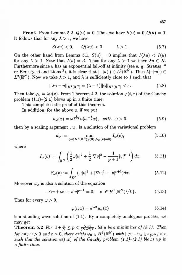
467

Proof. From Lemma 5.2, Q{u) = 0. Thus we have S(u) = 0;Q(u) = 0. It follows that for any A > 1, we have

S(Xu) < 0, Q(\u) < 0, A > 1. (5.7)

On the other hand from Lemma 5.1, S(u) = 0 implies that I(Xu) < I(u) for any A > 1. Note that I(u) = d. Thus for any A > 1 we have Xu € K. Furthermore since u has an exponential fall-off at infinity (see e. g. Strauss 13

or Berestycki and Lions 2 ) , it is clear that | • \u{-) e L2(RN). Thus A| • \u(-) e L2(M.N). Now we take A > 1, and A is sufficiently close to 1 such that

||Au - u||jfi(Rjv) = (A - l)||u||#i(Riv) < e. (5.8)

Then take ip0 = Xu(x). From Theorem 4.2, the solution ip(t,x) of the Cauchy problem (1.1)—(2.1) blows up in a finite time.

This completed the proof of this theorem. In addition, for the above u, if we put

uU)(x) = CJP=TU(U~'5X), with CJ > 0, (5.9)

then by a scaling argument , uu is a solution of the variational problem

where

du ~ min Iu(v), (5.10) { « € H 1 ( H J V ) \ { 0 } , 5 „ ( « ) = 0 }

Uv) := L fa™2 + 5 | V t , | a - F T T H P + 1 ) dx- (5"n)

Su(v) := / {u>\v\2 + |Vv|2 - \v\p+1)dx. (5.12)

Moreover uu is also a solution of the equation

-Av + ujv-v\v\p-x = 0 , v 6 f l 1 ( R " ) \ { 0 } - (5.13)

Thus for every u > 0,

<p(t,x)=ei"tuu{x) (5.14)

is a standing wave solution of (1.1). By a completely analogous process, we may get Theorem 5.2 For 1 + jj <P< /JV^2)+ > 'e* u ^e a minimizes of (5.1). Then for any LJ > 0 and e > 0, there exists ipo € i?1(MN) with \\ipo — «u;||ffi(RN) < £ such that the solution <p(t,x) of the Cauchy problem (1.1)-(2.1) blows up in a finite time.

468

Acknowledgment

I am grateful to Professor H. Matano and Professor Y. Tsutsumi for their helpful comments, and Professor M. Ohta for valuable discussions. This work was partly Supported by the JSPS Research Fellowship and the Monbusho's Grant No. P-98029.

References

1. H. Berestycki and T. Cazenave, Instability des etats stationnaires dans les equations de Schrodinger et de Klein-Gordon non linearires, C. R. Acad. Sci. Paris, Seire I 293, 489-492 (1981).

2. H. Berestycki and P.-L. Lions, Nonlinear scalar field equations, Arch. Rat. Mech. Anal. 82, 313-375 (1983).

3. T. Cazenave, An Introduction to Nonlinear Schrodinger Equations, (Tex-tos de Metodos Matematicos, Vol. 22, Rio de Janeiro, 1989).

4. T. Cazenave and P.-L. Lions, Orbital stability of standing waves for some nonlinear Schodinger equations, Commun. Math. Phys. 85, 549-561 (1982).

5. J. Ginibre and G. Velo, On a class of nonlinear Schrodinger equations, J. Funct. Anal. 32, 1-71 (1979).

6. R. T. Glassey, On the blowing up of solutions to the Cauchy problem for nonlinear Schrodinger equations, J. Math. Phys. 18(9), 1794-1797 (1977).

7. T. Kato, On nonlinear Schrodinger equations, Ann. Inst. H. Poincare , Phys. Theor. 46, 113-129 (1987).

8. M. K. Kwong, Uniqueness of positive solutions of Au — u + up = 0 in RN, Arch. Rat. Mech. Anal. 105, 243-266 (1989).

9. T. Ogawa and Y. Tsutsumi, Blow-up of H1 solution for the nonlinear Schrodinger equation , J. Differential Equations 92(2), 317-330 (1991).

10. T. Ogawa and Y. Tsutsumi, Blow-up of H1 solution for the nonlinear Schrodinger equation with critical power nonlinearity, Proceedings of the American Mathematical Society 111(2), 487-496 (1991).

11. G. Ribeiro, Instability of symmetric stationary states for some nonlinear Schrodinger equations with an external magnetic field, Ann. Inst. Henri Poincare, Phys. Theor. 54, 403-433 (1991).

12. G. Ribeiro, Finite-time blow-up for some nonlinear Schrodinger equations with an external magnetic field, Nonlinear Anal., T. M. A. 16, 941-948 (1991).

13. W. A. Straus, Existence of Solitary waves in high dimensions, Commun.

469

Math. Phys. 55, 149-162 (1977). 14. W. Strauss, Nonlinear Wave Equations, (C.B.M.S. No. 73, Amer. Math.

Soc, Providence, 1989). 15. C. Sulem, and P. L. Sulem, The nonlinear Schrodinger Equation, Self-

focusing and Wave Collapse, (Springer, 1999). 16. M. I. Weinstein, Nonlinear Schrodinger equations and sharp interpola­

tions estimates, Commun. Math. Phys. 87, 567-576 (1993). 17. W. E. Zakharov, Collapse of Langmuir waves, Sov. Phys. JETP 23, 1025-

1033 (1966). 18. J. Zhang, On the finite-time behaviour for nonlinear Schrodinger equa­

tions, Commun. Math. Phys. 162, 249-260 (1994). 19. J. Zhang, Sharp conditions of global existence for nonlinear Schrodinger

and Klein-Gordon equations, to appear in Nonlinear Anal: Theory, Methods and Applications.