Embed Size (px)
Citation preview

Computational Intelligence Techniques for Decision Making
with Applications to the Dairy Industry
Hussein Aly Abbass Amein B.Sc. (Ace), BA (Buss), PG-Dip. (OR), M.Phil. (OR), M.Sc. (AI)
Machine Learning Research Centre School of Computing Science
Faculty of Information Technology Queensland University of Technology
A thesis submitted for the degree of Doctor of Philosophy.
2000

QUT
QUEENSLAND UNIVERSITY OF TECHNOLOGY
DOCTOR OF PHILOSOPHY THESIS EXAMINATION
CANDIDATE NAME:
RESEARCH CONCENTRATION:
PRINCIPAL SUPERVISOR:
ASSOCIATE SUPERVISOR(S):
THESIS TITLE:
Hussein Aly Abbass Amein
Machine Learning
Dr Michael Towsey
Professor Joachim Diederich Dr Julius van der Werf Dr Erhan Kozan
Computational Intelligence Techniques for Decision Making with Applications to the Dairy Industry
Under the requirements of PhD regulation 16.8, the above candidate presented a Final Seminar that was open to the public. A Faculty Panel of three academics attended and reported on the readiness of the thesis for external examination. The members of the panel recommended that the thesis be forwarded to the appointed Committee for examination.
Name: Dr Michael Towsey Panel Chairperson (Principal Supervisor)
Name: Dr Julius van der Werf Panel Member
Name: Dr Erhan Kozan Panel Member
Name: Professor Joachim Diederich Panel Member
Under the requirements of PhD regulations, Section 16, it is hereby certified that the thesis of the .above-named candidate has been examined I recommend on behalf of the Examination Committee that the thesis be accepted in fulfillment of the conditions for the award of the degree of Doctor of Philosophy.
Name: ... ~ .. ~ .. ?.~~ .. .... M .. C?.{.~ ·J· · · ····· Stgnature. Date:.J?/1.0
/
Chair of Examiners (Head of School or nominee) (Examination Commt'ttee)
FORM 8

Keywords
allocation, ant colony optimisation, classification, constraint logic programming, dairy, decision
trees, differential evolution, genetic algorithms, heuristics, immune systems, intelligent decision
support systems, knowledge discovery in databases, mate-selection, neural networks, optimisa
tion, prediction, simulated annealing, tabu search
i

ii
Abstract
The dairy industry is a major resource in the Australian economy. In 1995-96 there were 13,888
dairy farms1 in Australia with 1.924 million dairy cows 2 and a total milk production of 8,716
million litres with a combined value of $AUD3 billion on the wholesale level. The industry's
success is dependent on increased animal productivity through breeding programs and efficient
management. One of the main challenges in the industry therefore, is to improve the productivity
of breeds through the design of efficient breeding programs. These programs aim to improve the
genetic merit as well as the productivity of animals through identifying (selecting) and mating
(allocating) animals with high genetic values, under the prevailing environmental and manage
rial conditions. To solve the selection and allocation problems, we need to predict the progeny's
expected productivity ( ie. milk, fat, and protein yields) arising from any mating.
From the previous discussion, the task of building a breeding program can be decomposed into
three interrelated stages: prediction, selection, and allocation. In prediction, the expected merit
of potential progeny is estimated from information collected and recorded about their parents
and the environment. In selection, a set of sires and a set of dams are chosen for mating ac
cording to the overall goal of the program. In allocation, individual matings among the selected
animals are decided according to the expected progeny merit as well as some preferences and
goals. Reaching an optimal decision is only possible when both selection and allocation are solved
simultaneously and in this case the problem is called mate-selection. The problem is hard when
the planning is for a single generation to optimise a short-term goal. In long-term planning, ad
ditional objectives need to be considered such as the minimisation of inbreeding ( ie. matings of
related individuals). As a result, nonlinearity and conflicting objectives arise within the problem.
Mate-selection decisions require progeny prediction and other information that can be retrieved
from the databases currently kept by the farmers and their organisations for production and
pedigree records.
The objective of this thesis is to integrate Knowledge Discovery from Databases (KDD) with the
Intelligent Decision Support System (IDSS) paradigm, to comprise what we call in this thesis
1Source: Australian Dairy Corporation ADC. 2 Source: Australia Bureau of Statistics.
iii

KDD-IDSS, for designing efficient breeding programs. To achieve this objective, we define three
sub-objectives: (1) to design a generic kernel for the KDD-IDSS. (2) to discover patterns in
the dairy database using KDD, and (3) to formulate and solve one version of the mate-selection
problem. The first objective is achieved by designing a novel constraint logic programming based
language to abstract general operational research and artificial intelligence modules within the
KDD-IDSS. The second objective of the thesis is accomplished in two steps; first, by discover
ing effective predictive patterns to update the predictive model in the model base of the IDSS.
Second, by generating a knowledge base to describe the reasoning behind a certain mating using
a comparison between a rule extraction technique, RULEX, and a decision tree classifier, C5,
to update the knowledge base of the KDD-IDSS. This required the use of a bayesian clustering
method, Autoclass, for grouping the cows according to their milk production. This second ob
jective of the thesis evolved a new method, C-Net, for generating dynamic and non-deterministic
decision trees. The method achieved a balance between the predictive accuracy of neural net
works and the language expressiveness of decision trees.
The third objective is attained through a formulation of a general optimisation model for mate
selection. A number of existing heuristic techniques (ant colony optimisation, genetic algorithms,
immune systems, and simulated annealing), and three newly developed ones (Markov chain Tabu
search, evolving colonies of ants, and dynamic adjustment method), are compared for solving this
model. The two most successful models were Markov chain Tabu search and evolving colonies
of ants. Both models were significantly better than the other heuristics. The overall objective of
the model is to issue the farmer with a mating plan for one-generation resulting from the optimal
strategy for a number of generations.
Overall, the three objectives will make a solid ground for building successful breeding programs
that the industry can use. In so doing, the expected profitability of the dairy industry will
increase on the long term and the current softwares for solving our proposed mate-selection
problem will be able to handle larger problem sizes.
iv

Publications
• Books and Book Chapters
- H.A. Abbass and M. Towsey. "The Application of Artificial Intelligence, Optimisation,
and Bayesian Methods in Agriculture", QUT-Publishing, ISBN 1-86435-463-1, 1999.
- H.A. Abbass. "Introducing Artificial Intelligence to Agriculture", in The Application
of Artificial Intelligence, Optimisation and Bayesian Methods in Agriculture, editors
H.A. Abbass and M. Towsey, QUT-Publishing, pp 1-8, 1999.
- H.A. Abbass, M. Towsey, J. VanderWerf, and G. Finn. "Modelling evolution: the
evolutionary allocation problem", in The Application of Artificial Intelligence, Opti
misation and Bayesian Methods in Agriculture, editors H.A. Abbass and M. Towsey,
QUT-Publishing, pp 117-134, 1999.
- P.E. Macrossan, K. Mengersen, H.A. Abbass, M. Towsey, and G.D. Finn. "Statistics
and artificial neural networks: a comparison of various predictive methods", in The
Application of Artificial Intelligence, Optimisation and Bayesian Methods in Agricul
ture, editors H.A. Abbass and M. Towsey, QUT-Publishing, pp 73-95, 1999.
- P.E. Macrossan, H.A. Abbass, K. Mengersen, M. Towsey, and G.D. Finn. "Bayesian
neural network learning for prediction in the Australian dairy industry", in J. Hand,
J.N. Kok, and M.R. Berthold (Eds.), Lecture Notes in Computer Science LNCS1642,
Intelligent Data Analysis, Springer Verlag, pp 395-406, 1999.
• Journals
- H.A. Abbass, M. Towsey, and G.D. Finn. "C-Net: A method for generating non
deterministic and dynamic multivariate decision trees". International Journal of
Knowledge And Information Systems (KAIS), Springer Verlag, accepted for a forth
coming issue.
- H.A. Abbass, M. Towsey, G.D. Finn, and E. Kozan. "A Meta-Representation for
Integrating OR and AI in an Intelligent Decision Support Paradigm", International
v
Transactions of Operational Research (!TOR), Balckwell Publisher, Vol. 8, No. 1, pp
107-119, 2001.
• Conferences
- H.A. Abbass, M. Towsey, E. Kazan, and J. Van der Werf. "Why do we need to kill all
the ants? An evolutionary approach to ant colony optimisation for large scale dynamic
allocation", accepted for publication at the Proceedings of the 4th Australian-Japan
Workshop for Evolutionary Computation, Japan, 2000.
H.A. Abbass, M. Towsey, E. Kazan, and J. Van der Werf. "The performance of
genetic algorithms on the one-generation mate-selection problem", Proceedings of the
2nd joint International Workshop, Japan, pp 10-17, 2000.
H.A. Abbass, W. Bligh, M. Towsey, M. Tierney, and G.D. Finn. "Knowledge discov
ery in a dairy cattle database: (Automated knowledge acquisition)", Proceedings of
the Fifth International Conference of The International Society for Decision Support
Systems (ISDSS'99), Melbourne, Australia, July, 1999.
H.A. Abbass, M. Towsey and G.D. Finn. "An intelligent decision support system for
dairy cattle mate-allocation". Proceeding of the Australian workshop on Intelligent
Decision Support and Knowledge Management, Sydney, Australia, pp 45-58, 1998.
H.A. Abbass, G.D. Finn and M. Towsey. "OR and data mining for intelligent decision
support system in the Australian dairy industry's breeding program". New Research
in Operations Research Conference, ASOR, Brisbane, pp 1-23, 1998.
vi

Contents
Keywords
Abstract
List of Publications
Table of Contents
List of Figures
List of Tables
List of Acronyms
List of Mathematical Abbreviations
Originality
Acknowledgment
I Introduction
1 Thesis Outlines and Contributions
1.1 Thesis outlines . . . .
1.2 Original contributions
2 Mate-Selection in Animal Breeding
2.1 Genetics .............. .
vii
i
iii
v
vii
xii
xiv
xvii
xix
xxi
xxiii
1
3
4
8
9
9
2.2 Breeding programs
2.3 Methods for selection .
2.4 Selection strategies
2.5 Selected recent keywork in mate-selection .
2.6 Computerised systems for selection in dairy industry
2.7 Conclusion . . . .. . .
II Knowledge Discovery in Databases
3 KDD-IDSS: A Framework for Integrating KDD with IDSS
3.1 Decision making process ..... .
3.2 Intelligent decision support system
3.3 Knowledge discovery in databases .
3.4 A proposed frame for integrating IDSS and KDD
3.4.1 Database
3.4.2 Model base
3.4.3 Knowledge base .
3.4.4 Dialog base
3.4.5 Mining base
3.4.6 Kernel ...
3.5 A meta-language for OR and AI in the KDD-IDSS kernel .
3.5.1 Interfacing AI with OR ..
3.5.2 Interfacing CLP with OR
3.5.3 Interfacing CLP with non-symbolic AI
3.6 The proposed meta language ......... .
3.6.1 Formalising the concept of a decision in KDD-IDSS
3.6.2 The relationship between the proposed concept of a decision and previous
ones ................ .
3.6.3 Using CLP to integrate AI and OR
3.7 An example of the language
3.8 Conclusion ......... .
viii
13
18
22
24
26
28
31
33
34
35
39
41
41
42
42
43
44
45
45
46
46
47
48
48
51
52
57
58

4 Mining the Dairy Database
4.1 The function estimation problem in KDD-IDSS
4.2 Artificial neural networks . . . . .......
4.2.1 The structure and training of MLPs .
4.2.2 Rule extraction from artificial neural networks: RULEX
4.3 Bayesian clustering .....
4.4 Classification decision trees .
4.5 The dairy database . . . . .
4.6 Experiment ( 1): Mining for predictive models
4.6.1 Methods
4.6.2 Results .
4.6.3 Discussion
4.7 Experiment (2): Automated knowledge acquisition.
4.7.1 Methods
4.7.2 Results .
4.7.3 Discussion
4.8 Conclusion . . . .
5 C-Net: A new Method for Generating Non-deterministic and Dynamic Multi-
variate Decision Trees
5.1 Motivation and importance of C-Net
5.2 Previous work in combining ANNs and DTs
5.3 The C-net algorithm
5.3.1 ANN training
5.3.2 Classification of the hidden to output mapping .
5.3.3 Back projection of decision trees .
5.4 Experiments and comparisons ..... .
5.4.1 Methods and performance measures .
5.4.2 Data sets and experimental setup
5.4.3 Results and discussion
5.5 Recurrent C-Net
5.6 Conclusion . . . .
IX
61
62
64
66
68
69
71
73
75
75
76
77
78
78
79
81
82
83
84
85
87
88
88
89
90
90
91
92
95
96

III Optimisation Models
6 Heuristics for Complex Optimisation Problems
7
6.1 Introduction .
6.2 Simulated annealing
6.3 Tabu search
6.4 Genetic algorithm .
6.5 Differential evolution
6.6 Immune systems
6.7 Ant colony optimisation
6.8 Memetic algorithms .
6.9 Constraints
6.9.1 Penalty function
6.9.2 Repair mechanisms
6.10 Multi-objective optimisation
6.11 Conclusion ......... .
Evolutionary Allocation Problem
7.1 Introduction . . . . . . . . .
7.2 Importance of the problem .
7.3 Model assumptions and advantages
7.3.1 Nomenclature . . . . .
7.3.2 The objective function
7.3.3 Constraints
7.4 Model complexity
7.5 Conclusion ....
8 Genetic Algorithm Applied to the Single-stage Model
8.1 A single stage model ............ .
8.2 Genetic algorithm for the single-stage model
8.2.1 Representation
8. 2. 2 Crossover . . .
8.2.3 Repair operator: constraint satisfaction algorithm
X
99
101
101
105
109
111
114
116
118
123
124
125
126
127
128
129
. 129
132
133
133
137
140
. 146
. 147
149
. 149
. 151
. 151
153
154
8.3 Experiments ............ .
8.3.1 The data simulation model.
8.3.2 Experimental design and objective
8.3.3 Results and discussion
8.4 Conclusion . . . . . . . . . . .
9 Solving the Multi-stage Mate-selection Problem
9.1 Customisation of the multi-stage model .
9.1.1 Model complexity ..... .
9.2 Experimental design and objectives
9.2.1 The simulation model for the initial herd
9.2.2 Experimental design for the optimisation model
9.3 Problem preparation ............... .
9.3.1 Representation of the multi-stage solution
9.3.2 Generation of neighbour solutions
9.3.3 Constraint satisfaction method .
9.3.4 Handling the multi-objective problem .
9.4 Experiment 1: Random search . . . . . . . .
9.5 Experiment 2: Sequential genetic algorithm
9.6 Experiment 3: Greedy hill climber .
9. 7 Experiment 4: Simulated annealing
9.8 Experiment 5: Ant colony optimisation
9.9 Experiment 6: Markov chain tabu-search (a new algorithm)
9.10 Experiment 7: Genetic algorithms .
9.11 Experiment 8: Immune systems ..
9.12 Experiment 9: Evolving colonies of ants (a new algorithm)
9.13 Overall discussion .
9.14 Conclusion . . . . .
10 Generation of Mate-selection Index
10.1 Mate-selection Index (MSI)
10.2 Dynamic adjustment of the objective function (a new algorithm)
xi
. 156
. 156
. 158
. 159
. 161
163
. 163
. 166
. 166
. 167
. 168
. 169
. 169
. 171
. 171
. 172
. 172
. 173
. 174
. 175
. 177
. 184
. 192
. 194
. 198
. 199
. 206
207
. 207
. 209
10.3 Hybrid SA + GA .
10.4 Hybrid DE + GA
10.5 Conclusion . . . . .
11 Conclusion and Future Work
11.1 Summary ...... .
11.2 Original contributions
11.3 Future work . . . . . .
References
A The rules generated by C5
B The Code for the Markov Chain Tabu Search Algorithm
xii
. 211
. 214
. 215
217
. 217
. 219
. 221
224
243
247

List of Figures
1.1 A conceptual tree of issues and techniques discussed in this thesis.
3.1 The managerial levels . . .
3.2 The KDD-IDSS paradigm
4.1 Three different ANN's architectures
4.2 The Back-propagation algorithm. .
4.3 The impact of age correction on dam LMV.
5.1 The ANN and the corresponding extracted MDT
5.2 The C-Net algorithm ........ .
5.3 The C-Net conceptual representation.
6.1 Metropolis algorithm ................. .
6.2 General homogeneous simulated annealing algorithm.
6.3 General non-homogeneous simulated annealing algorithm ..
6.4 The Tabu search algorithm.
6.5 A generic genetic algorithm
6.6 The differential evolution algorithm
6. 7 Differential evolution in the two dimensional space .
6.8 The immune system algorithm .......... .
6.9 Autocatalysis and differential path length effects.
6.10 Generic ant colony optimisation heuristic .
6.11 The ant algorithm. . .....
6.12 A generic memetic algorithm.
7.1 The state variables' scope in the EAP model.
xiii
7
35
41
67
68
74
85
90
90
. 106
. 108
. 108
. 109
. 111
. 115
. 117
. 119
. 120
. 121
. 121
. 124
. 135
7.2 The logical relationships between the model's variables ..... .
8.1 The data structure for the chromosome in the single-stage model.
8.2 The gene-based crossover operator.
8.3 The repair operator. ....... .
8.4 The trajectories of the best solution.
8.5 The trajectories of the average population fitness.
9.1 The data structure for a solution in the multi-stages model.
. 141
. 152
. 153
. 155
. 161
. 161
. 170
9.2 Generation of neighbour solutions. . . 171
9.3 The random search algorithm . 173
9.4 The hill climber algorithm . . . 174
9.5 A homogeneous simulated annealing algorithm for the multi-stage model. . 176
9.6 The constructive algorithm for ACO . . . . 179
9.7 The Markov chain tabu search algorithm. . . 186
9.8 The generation of neighbourhood solutions in the MCTS algorithm. . 187
9. 9 The performance of 1-point crossover using the three selection strategies over ten
runs. . . . . . . . . . . . . . . . . . . . . . . . 196
9.10 The antigen-antibody comparison algorithm . 197
9.11 A heuristic for evolving colonies of ants . . . . 199
9.12 The performance of the best results obtained by different algorithms. . 201
10.1 A Hybrid GA+SA algorithm for generating of mate-selection index. . . 213
10.2 A Hybrid GA +DE algorithm for generating of mate-selection index. . 215
xiv
List of Tables
1 List of Acronyms used throughout the thesis . . . . . . . . . . . xvii
2 List of mathematical abbreviations used throughout the thesis xix
4.1 Performance of MLP for different number of hidden units on the dairy database 76
4.2 Summary of data categorisation using Autoclass. 80
4.3 Results of classification with continuous inputs. 80
4.4 Results of classification with discrete inputs. . . 81
5.1 Summaries of statistics for the real life databases . . . . . . . . . . . . . . . . . . 92
5.2 The average percentage bit error of C-Net, C5, and ANN on the test set for the
5.3
5.4
8.1
eight data sets. . . . . . . . . . . . . . . . . . . . . . . . . . . . . . . . . . 93
The average tree-size of C-Net on each architecture for the eight data sets.
Performance of recurrent C-Net on a natural language data set.
The average results of ten G A runs for one of the ten herds . . .
94
96
. 160
9.1 The greedy hill cilmber results with different five neighbourhood lengths. . 175
9.2 Simulated annealing results at temperature levels 10 and 1 respectively. . 177
9.3 Relationship between the number of ants and neighbourhood length. . . 181
9.4 Comparing ACO with constructive algorithms against the repair operator . 182
9.5 Comparing ACO with/without pheromone evaporation . . . . . . . . . . . . 182
9.6 Comparing the ant algorithms with four different pheromone update rules. . 183
9.7 The results for the Markov chain tabu search method. . . . . . . . . . . . . 190
9.8 Genetic algorithms performance on the multi-stage model with population size 30 193
9.9 Genetic algorithms performance on the multi-stage model with population size 40 194
9.10 Genetic algorithms performance on the multi-stage model with population size 50 194
XV
9.11 Genetic algorithms performance on the multi-stage model with population size 60 195
9.12 Genetic algorithms performance on the multi-stage model with population size 70 195
9.13 The Immune algorithm's performance on the multi-stage model .......... 197
9.14 A summary of the best combination found in each experiment and its correspond-
ing t-value relative to the MCTS algorithm . . . . . . . . . . . . . 200
9.15 The effect of the number of stages on the optimisation process. . . 206
10.1 Results of GA + SA Hybrid for MSI. . 213
10.2 Results of GA+DE Hybrid for MSI. . . 216
11.1 The complexity of different mate-selection models. . . 219
xvi

List of Acronyms
ABV ACO
AI AI-sire ANN BP BV CLP DE DT
EBV FLMV
GA IDSS KDD LMV LRU
MCTS MDT MLP MLR MSI MV NT OR
PTL PTS RDT
RMSE SA SI
SLMV TS
UDT VOP
Australian Breeding Value Ant Colony Optimisation Artificial Intelligence Artificial Insemination sire Artificial Neural Networks Back-Propagation Breeding Value Constraint Logic Programming Differential Evolution Decision Tree Estimated Breeding Value First Lactation Milk Volume Genetic Algorithms Intelligent Decision Support systems Knowledge Discovery in Databases Lactation Milk Volume Local Response Unit Markov Chain Tabu Search Multivariate Decision Tree Multi-Layer Perceptron Multiple Linear Regression Mate-Selection Index Milk Volume Number of traits Operations Research Probabilistic Tabu List Probabilistic Tabu Search Recurrent Decision Tree Root Mean Square Error Simulated Annealing Selection Index Second Lactation Milk Volume Tabu Search Univariate Decision Tree Vector Optimisation Problems
Table 1: List of Acronyms used throughout the thesis
xvii

xviii

List of Mathematical Abbreviations
( ) t is the transpose of a vector. Unless indicated
otherwise, the default is a column vector.
S.T. Subject to
<l? Empty set
E Belong to
3 Such that
Given
Maps to
There exists
There exists no
For all
Intersection
If and only if
n
iff ;t Not equal to for vectors
-< rv Less than or equal to for vectors
Table 2: List of mathematical abbreviations used throughout the thesis
xix

XX

Statement of Original Authorship
The work contained in this thesis has not been previously submitted for a degree or
diploma at any other higher education institution. To the best of my knowledge and
belief, the thesis contains no materials previously published or written by another
person except where due reference is made.
Date: __ j}_jJ/_fu-~_L_
XXl

x:x:ii

Acknowledgment
My first gratitude goes to God Almighty for showering me with His boundless grace and mercy,
which sustained me through arduous times during this Ph.D. course.
In acknowledging my debt to all those who helped to make the thesis a memorable intellectual
experience, I wish firstly to record my deep gratitude to my supervision team, Dr Michael Towsey,
Dr. Gerard Finn, Dr. Erhan Kozan, Dr. Julius VanderWerf, and Prof. Joachim Diederich, for
their guidance during the course of the research reported here. Michael has a unique personality
which combines patience and good judgment and an excellent knack for handling independently
minded people! My thanks to him is not enough to substitute the challenges I issued him with,
during the course of my study. Gerard helped me enormously as my first principal supervisor
who supported me through eighteen months of the thesis research. Erhan, with his tremendous
combination of optimisation skills and student management abilities, provided me with the psy
chological and technical support I needed to complete this thesis. Julius was the backbone of this
work; he saved me by making me understand the genetic and animal domain and was my guid
ing light at a time I had decided that the PhD project was unworkable. Joachim is a matchless
person: during discussions of my thesis with him, he surprised me with his phenomenal insight
of my goals. My gratitude to Joachim also extends beyond the supervision. His provision of fi
nancial support during the first two years of my Ph.D. and his constant approval for sending me
to appropriate conferences had a major impact on the quality of the thesis. I am also indebted
to Brian Kinghorn for introducing me to the mate-selection problem and Susan Meszaros for her
useful discussion and sincere advises. My deep gratitude goes also to the dairy group members:
William Bligh, Don Kerr, Paula Macrossan, Kerry Mengersen, and Mick Tierney.
My thanks to all the staff at the Machine Learning Research Centre: a special mention applies
to Robert Andrew, Lawrence Buckingham, Stephen Chalup, Shlomo Geva, Ross Hayward, Jim
Hogan, Fredrick Maire, Richie N a yak, and Alan Tickle. I also wish to thank the staff members
of the Faculty of Information Technology, QUT.
xxiii

The workplace has a strong influence on one's life, and I wish to gratefully acknowledge my
institute in Egypt (Institute of Statistical Studies and Research, Cairo University), where I have
learnt and worked, and was raised scientifically and mentally. I also wish to thank the School
of Computer Science, at the Australian Defence Force Academy, University of New South Wales
for their support during my course of study by minimising the teaching load and holding useful
discussions with all members of the department including Frantz Clermont, Charles Newton, and
Ruhul Sarker. A special mention goes to David Hoffman and Bob McKay for devoting the time
and efforts to read a draft version of this thesis and for their invaluable comments.
Although this thesis represents a work of just a few years, one cannot forget the people who
supported this writer in gaining the necessary knowledge for the completion of this work. My
abiding gratitude to my scientific father Prof. Rasmy who encouraged me and taught me not
only a science, but a way of living as well. Thanks also to Dr. Reem Bahgat who first introduced
me to the field of Constraint Logic Programming and taught me how to like it; and to Geraint
Wiggin, Rama Lakshmanan, and Bill Morton from the University of Edinburgh for their sup
port in my life at the Department of Artificial Intelligence, University of Edinburgh. A special
mention to everyone who taught me in this life including: J. Hallam, G. Hayes, M. Ismael, M.
Khorshed, M. Osman, A. Rafae, P. Ross, and E. Shokry.
I am indebted to my wife Eleni Petraki, the unique creature who fed my soul during those hard
times while studying, with constant encouragement, patience, understanding, love, and invalu
able advice. Thanks are also due to my father, mother, my sisters Soaad and Fatma, and my
brothers Ismael and Mohammed for their lifelong personal support.
My final acknowledgment of sincere gratitude goes to the Australian government, QUT, and the
Machine Learning Research Centre for providing me with financial support during the first two
years of my course of studies.
xxiv

Part I
Introduction
1


Chapter 1
Thesis Outlines and Contributions
The process of creating a breeding system for the Australian dairy industry's artificial insem
ination program naturally divides into a prediction problem and an optimisation problem. In
the former, the objective is to predict the performance of offspring based on some of the genetic
traits of their parents. In the latter, two component sub-problems can be identified, selection
and allocation. In selection, a set of sires and a set of dams are selected for possible mating
based on some suitable criteria for improving animal traits; in allocation, specific matings are
allocated among the selected animals. Solving both problems independently does not guarantee
an optimal solution overall. To achieve an optimal solution, a mathematical model that selects
and allocates simultaneously, called mate-selection, is required.
The objective of this thesis is to develop appropriate problem solving techniques for the efficient
design of dairy cattle breeding systems through the integration of Knowledge Discovery from
Databases (KDD) with the Intelligent Decision Support System (IDSS) paradigm, to comprise
what is called KDD-IDSS. This objective is decomposed into three sub-objectives:
1. designing a generic kernel ( ie. an interface language between the system's components) for
the KDD-IDSS,
2. discovering patterns in the dairy database using KDD, and
3. formulating and solving a mate-selection problem.
The thesis begins with a description of the general mate-selection problem. An information sys
tem framework is then developed for this problem. The framework is based on the integration of
3
KDD and IDSS. A proposed generic meta-language for an interface component of the framework
is then introduced using the constraint logic programming paradigm.
The prediction problem is then investigated in two stages. The first stage is concerned with
point-estimation where a linear regression model is compared against a feed-forward neural net
work. The second stage is concerned with extracting symbolic knowledge from the database and
is handled by a comparison between a rule-extraction technique, RULEX, and a decision tree
classifier, C5. The powers of neural network and decision trees are then combined into a novel
algorithm for generating dynamic and non-deterministic decision trees. Following this, a version
of the mate-selection problem is formulated and problem-solving approaches are developed. Be
low, the detailed thesis outlines are presented.
1.1 Thesis outlines
The thesis is divided into eleven chapters as described below:
In Chapter 1, an introduction to the thesis is presented, followed by the thesis outlines and a list
of scientific contributions.
The main objective of Chapter 2 is to provide the basic concepts of the domain of application,
necessary to build upon the case study of mate-selection pursued in this thesis. The chapter
starts with an introduction to Genetics in Section 2.1, followed by a review of the basic animal
breeding concepts in Section 2.2. Two problems are then identified: selection and allocation. In
Section 2.3, different methods for selection of animals for breeding are discussed, then different
recent strategies for selection are elucidated in Section 2.4. Methods for allocation of animals for
mating are followed in Section 2.5. A review of some computer programs for selection, is then
presented in Section 2.6. Conclusions are drawn in Section 2.7.
The information system framework for the thesis is then introduced in Chapter 3, beginning with
a decision making process summary in Section 3.1, followed by a literature review of intelligent
4

decision support systems (IDSSs) in Section 3.2 and knowledge discovery in databases (KDD)
in Section 3.3. The proposed framework for integrating KDD with IDSS, called KDD-IDSS,
is then presented in Section 3.4. A proposed meta-language is then designed using constraint
logic programming (CLP) for integrating operations research (OR) and artificial intelligence (AI)
components in the KDD-IDSS frame. The three dimensions for the integration are covered in
Section 3.5; these are integrating CLP with optimisation, CLP with AI, and optimisation with
AI. The language is then formulated in Section 3.6 followed by an example of the usefulness of
this formulation in Section 3.7. Conclusions are drawn in Section 3.8.
In Chapter 4, the experiments carried out for the data mining component are presented. Ex
perimental design and objectives are presented in Section 4.1 followed by a review of the mining
techniques that will be used in the chapter starting with an introduction to multi-layer feed
forward artificial neural networks (ANNs) in Section 4.2 followed by Bayesian clustering in Sec
tion 4.3 and classification decision trees (DTs) in Section 4.4. A description of the database is
then presented in Section 4.5. Following this, two experiments are discussed: point estimation
in Section 4.6 and interval estimation in Section 4.7. The first experiment's objectives are to
investigate their predictive power on the progeny performance and to identify a prediction model
that can be used in the KDD-IDSS's model base. The second experiment is concerned with the
automatic extraction of symbolic knowledge to reason about the choice of a mating. This is simi
lar to the point-estimation's experiment, except for the necessity of discretising the output where
Autoclass, a Bayesian clustering algorithm, is used for this purpose. Conclusions are drawn in
Section 4.8.
The experiments, presented in Chapter 4, motivated a novel algorithm, C-Net, used for integrat
ing ANNs and DTs. This algorithm is the focus of Chapter 5. The importance and motivation
of this algorithm are introduced in Section 5.1 followed by previous work in combining ANNs
and DTs in Section 5.2 and the C-Net algorithm in Section 5.3. In Section 5.4, experimental
results and comparisons are discussed and the dynamic version of C-Net is then scrutinised in
Section 5.5. Conclusions are drawn in Section 5.6.
In Chapter 6, the foundation of the heuristic techniques that will be used for solving the mate-
5
selection problem's version that is being addressed in this thesis, are presented. The chapter
begins with an introduction to optimisation theory in Section 6.1. Seven heuristic search tech
niques are then presented, more specifically; simulated annealing (SA) is presented in Section 6.2
followed by tabu search (TS) in Section 6.3, genetic algorithm (GA) in Section 6.4, differential
evolution (DE) in Section 6.5, immune systems (Immune) in Section 6.6, ant colonies optimi
sation (ACO) in Section 6.7, and memetic algorithms (MA) in Section 6.8. Issues arising from
constraints and multi-objectives are discussed in Sections 6.9 and 6.10, respectively. Conclusions
are drawn in Section 6.11.
In Chapter 7, our proposed version of the mate-selection problem is formulated as a multi-stage
optimisation model. An introduction about allocation is presented in Section 7.1, followed by the
importance of mate-selection in Section 7.2. In Section 7.3, the problem is formulated, and the
complexity of its search-space is discussed in Section 7.4. Conclusions are drawn in Section 7.5.
In Chapter 8, the single-stage mate-selection problem is derived from the generic formulation
and a set of GA operators that results in a good solution of the single-stage model, is identified.
In Section 8.1, a case study is presented with ten herds where cows were mated solely to artificial
insemination bulls. In Section 8.2, a genetic algorithm design for the single-stage model is pre
sented followed by a number of experiments with the aim of identifying a set of genetic algorithm
operators that reach the optimal solution quickly and reliably in Section 8.3. Conclusions are
drawn in Section 8.4.
In Chapter 9, the multi-stages mate-selection problem is derived from the generic formulation
and different heuristics are applied to solve the model. In Section 9.1, the derivation of the model
is shown, followed by the experimental design in Section 9.2. Different strategies for solving the
model are then presented in Sections 9.4, 9.5, 9.6, 9.7, 9.8, 9.9, 9.10, 9.11, and 9.12. Lastly, Sec
tion 9.13 presents an overall comparison between the proposed solution strategies. Conclusions
are drawn in Section 9.14.
In Chapter 10, the proof for the existence and non-uniqueness of the mate-selection index is
established in Section 10.2. Two methods for generating this index are then introduced in Sec-
6

Breeding Programs Design
I Information Prediction
t Mate-Selection
System ~ramework ~
KD;-IDSS /lint 1
Interval Fonnulalion
CLP-Based Artificial Mulople Univ0Mult' · t
Single Stage
t L. 1-vana e
Meta-Language Neural mear Genetic Algorithms
Networks Regression
Discretisation
t Autoclass
f Random
Search Simkated Annealing
r l
Rulex C5 C-Net
Non-population Basyd
t Markov Mulfl-Stage Aht
I
Multi Stage
Mate Selection Index
1\ SAt DE+ GA GA
Population Based
Chain Tabu
Search
Genetic Colony Algorithm Optirmsation
Evoloving Colonies of Ants
Genetic Algorithm
Figure 1.1: A conceptual tree of issues and techniques discussed in this thesis.
tions 10.3 and 10.4. Conclusions are drawn in Section 10.5.
In Chapter 11, conclusions about the thesis findings are drawn and points for further research
are discussed. This chapter concludes the thesis.
A conceptual diagram representing different techniques in the thesis and the overall structure is
given in Figure 1.1.
7
1.2 Original contributions
The following original contributions have been achieved in this thesis and are listed below:
1. In Chapter 3, a new generic frame, KDD-IDSS, for integrating knowledge discovery in
databases with intelligent decision support systems is proposed.
2. Chapter 3 also proposes a constrained logic programming based meta-language for inter
facing OR and AI models in the KDD-IDSS frame.
3. In Chapter 4, the knowledge governing the outcome of a mating is extracted from the dairy
database.
4. Chapter 5 presents a novel algorithm, C-Net, for generating non-deterministic and dynamic
decision trees.
5. Chapter 7 introduces a generic formulation for our proposed mate-selection problem, and
to my knowledge, is a first time attempt to study the overall problem's complexity.
6. In Chapter 8, the single-stage mate-selection model is derived from the generic formulation
as a quadratic transportation model, and genetic algorithm is used to solve the model. A
new crossover operator, gene-based crossover, and a repair operator are developed.
7. In Chapter 9, a proposed mate-selection problem for farms depending on artificial insemi
nation is derived from the generic model. Two novel algorithms, Markov chain Tabu search,
and evolving colonies of ants, are developed.
8. In Chapter 10, a new method for creating a mate-selection index, called dynamic adjust
ment of the objective function, is introduced. The existence and non-uniqueness of the
mate-selection index is proved mathematically.
8
Chapter 2
Mate-Selection in Animal Breeding
Designing a breeding program is one of the issues that animal breeding research has focused
on, in recent decades. Generally the outcome of a breeding program is a long-term product
and requires careful design. Two crucial components in a breeding program are the definition
of a suitable breeding objective(s) and the mate-selection problem. The latter is in two parts:
first, selection or which animals will be selected for mating and which for culling; and second,
allocation or the choice of the suitable mating pairs among those animals selected for mating.
In this chapter, the mate-selection problem is scrutinised. The genetic background necessary
to introduce it, is presented in Section 2.1 followed by basic concepts in animal breeding in
Section 2.2. Section 2.3 introduces different methods for selection of animals for breeding, and
different recent strategies for selection are then elucidated in Section 2.4. Methods for mate
selection follow in Section 2.5, concluded with a review of some computer programs for selection
in Section 2.6. This chapter's main objective is to provide the basic concepts of mate-selection
necessary to build upon the case study pursued in this thesis.
2.1 Genetics
The word genetics derives from the Greek root !EVVW, which means "to become" or "to grow"
(Winchester 1966). The classical definition of genetics introduced by William Bateson, who
named the field of study in 1906 (Schmidt and Van-Vleck 1974), is:
genetics is the science dealing with heredity and variation seeking to discover laws
9

governing similarities and differences in individuals related by descent (Van-Vleck
et al. 1987).
In short, genetics is the science of inheritance (Daniel 1994). The gene is a chemical entity that
influences an inherited trait from parents to their children. Each gene, at a given locus, can take
various forms called alleles. For example, if the colour of an animal is either white, black, or
gray, it is determined according to a pair of genes with the alleles "w" for white and "b" for
black. If the pair of genes is the same (eg. "ww" for a white animal or "bb" for a black one),
the organism is called homozygous otherwise heterozygous (eg. "wb" for a gray animal). If the
animal is heterozygous and an allele conceals the effect of its pair member ( eg. the pair of genes
is "wb" and the colour is black), it is called dominant, "b", otherwise recessive. A group of
chromosomes constitutes the organism's genotype which is the genetic constitution or sometimes
called the genetic makeup (Falconer 1989). The observable traits of an organism constitute its
phenotype (Daniel 1994).
The science of genetics was discovered by the Austrian monk Gregor Mendel in 1865 (Franisco
and John 1984). Mendel introduced two laws that were rediscovered in 1900 by the European
botanists Correns, De-Vries, and Tschermark. The first is the law of "segregation" which defines
the amount of genetic materials transmitted during a mating. It states that during combination,
a gene pair separates into the reproductive or sex cells formed by an individual, so that half carry
one member of the gene pair and half carry the other (Van-Vleck et al. 1987). The second is the
law of ((independent assortment" which states that "during gamete formation, segregating pairs of
unit factors assort independently of each othe'f' (Klug and Cummings 1999). Unit factors (Klug
and Cummings 1999) are particulate for each trait which serve as the main units of heredity and
are passed unchanged from generation to generation, determining various traits expressed by
each individual. From these two laws we can define what is called a Mendelian sampling. Since
the segregation of genes occurs independently, and half of the gene pair is transmitted to the
offspring during the mating, there is no guarantee which gene will be transmitted. Accordingly,
although we know that the progeny have one half of their father's and their mother's genes,
siblings will differ since they will take different combination of genes. The variation due to this
sampling causes variation within full sib families, and is indicated as the Mendelian sampling. A
formal equation for it will be defined later in this chapter.
10

In 1908, British mathematician G.H. Hardy and German physician W. Weinberg introduced the
Hardy- Weinberg equilibrium law (Franisco and John 1984), forming the basis of population ge
netics. The law assumes an absence of selection and states that the process of heredity changes
neither allelic frequencies nor genotypic frequencies at a given locus within a very large, closed,
randomly breeding population. Additionally, the equilibrium genotypic frequencies at any given
locus are attained in one single generation of random mating whenever the allelic frequencies are
the same in the two sexes.
Mendelian genetics studies the principles of transmitting the genetic material from the parents to
the offspring generation. Population genetics is the study of Mendelian genetics in populations.
It is concerned with the frequencies of genotypes and phenotypes (Falconer 1989), and is limited
to the inheritance of qualitative traits. Quantitative genetics was introduced by Fisher in 1918
and is concerned with the study of the effects of individual genes (Van-Vleck et al. 1987), as
well as the study of correlation and regression between the genetic and phenotypic values. As
opposed to population genetics, it concentrates on quantitative traits.
The qualitative traits (Daniel 1994) are those traits controlled by one or a few loci, in a way
that allele has a marked effect on the phenotype and individuals can be phenotypically classified
into one of a group. For example, the human blood groups designated A, B, 0, or AB are
determined by three types of alleles denoted IA, IB, and IO. The blood group of any person is
determined by the particular pair of alleles present in his or her genotype. In quantitative traits,
there are many loci, a gradation of phenotypes, and small effects of single alleles. Quantitative
traits usually follow a normal distribution (Falconer 1989) and can be found in three categories,
continuous, meristic and threshold traits (Franisco and John 1984). Continuous traits vary, with
no clear-cut breaks, from one phenotypic extreme to the other, such as milk production in cattle.
In Meristic traits, the phenotype is determined by such counting as the number of eggs laid
by a hen. Threshold traits have only two or few phenotypic classes, but their inheritance is de
termined by the effects of multiple genes together with the environment, such as twining in cattle.
11

The phenotypic value of an animal trait (Schmidt and Van-Vleck 1974) is measured by the
difference between the animal's trait value and an appropriate base group. This base group can
be the average of all animals within the herd born in the same year, the herd average at the
breeding program's commencement, or any other appropriate base. The phenotypic value ( P)
(Schmidt and Van-Vleck 1974) of an animal for a specific trait is the sum of the animal genotypic
value (G) and the environmental deviation (E); that is
(2.1)
The environmental deviation is a term used in the field to represent the effects of all non-genetic
factors such as seasons, feeding systems, management, etc. An animal's genotypic value can be
further decomposed into three measurements: the breeding or the additive genetic value (A), the
dominance deviation (D), and the epistasis or interaction deviation (I).
(2.2)
Gene action is said to be additive if the differences between the heterozygote and the two ho
mozygotes are equal (Schmidt and Van-Vleck 1974). Inheritance depends on the additive effects
of genes and represents the value of an individual's genes to its progeny. Generally, the offspring
inherit only the average additive component of their parents. The dominance deviation causes
a heterozygous animal to be more like one of the homozygous genotypes. For example, assume
a homozygous black cow is worth $4 and a homozygous red cow is worth $2. If the gene for
black colour is dominant, a heterozygous cow will look black and will be worth $4 although it
should be worth only $3 ( 4j 2). The $3 represents the additive genetic value and the additional $1
represents the dominance deviation. The epistasis is a measure of the effect of other genes on the
gene in question; that is, sometimes the expression of an allele at a locus requires the presence of
a particular allele at another locus. Now, we can rewrite the equation for the phenotypic value
as:
P=A+D+l+E (2.3)
A basic concept in genetics is heritability. To illustrate this concept, the concepts of phenotypic
and genotypic variances are presented. The phenotypic variance, Vp, is the sum of the population
genotypic variance, Va, and the environmental variance, VE; that is
(2.4)
12

where
(2.5)
and VA is the additive genetic variance whereas the sum of Vn and V1 is the non-additive genetic
variance (dominance and epistasis). Heritability, h2, is the ratio between the additive genetic
and phenotypic variances; that is
h2 =VA Vp
(2.6)
Since VA is always less than Vp, the heritability is always in the range [0,1]. The higher the
heritability, the more important it is for the breeder to use breeding systems which utilise the
additive genetic variation. One way; although not necessary the best, to estimate the heritability
of a trait is to regress the offspring on the parents; that is, the correlation coefficient between the
offspring and the parents phenotypic values for the trait. However, it is better to use multi-trait
animal models because they use all the available information from relatives.
Animal genetics is the study of the principles of inheritance in animals whereas animal breeding
applies these principles with the goal of animal improvement (Van-Vleck et al. 1987). This study
will be concerned with quantitative genetics, especially the continuous traits, for dairy cattle.
2.2 Breeding programs
Cattle are a monotocous species; the female produces a single egg at a time and consequently
normally produces a single offspring each parity. They form one of the main agricultural re
sources in Australia. In 1995-96, there were 13,888 dairy farms1 in Australia with 1.924 million
dairy cows 2 and a total milk production of 8, 716 million litres with a value of $3 billion on the
wholesale level. The industry success depends on increased animal productivity through breeding
programs and efficient management.
A breeding program's main objective is to maximise the progeny's productivity measured with
their production traits. The merit of breeding animals is estimated using the (estimated) breeding
1Source: Australian Dairy Corporation ADC. 2Source: Australia Bureau of Statistics.
13
values (EBVs) which define the (estimated) value of an animal in a breeding program, measured
in terms of the expected progeny performance relative to the population mean. The breeding
value is twice the difference between the expected offspring mean and the mean population (geno
typic) value. The breeding value is referred to as the animal's additive genetic merit. (Van-Vleck
et al. 1987)
The breeder requires a system to screen the genotypes to select the animals with the highest
breeding value (the measures computed by screening programs are used for selecting bulls and
cows for mating). An animal's merit in a selection decision depends on both the value of future
progeny (genetic value) and their own expected performance (production value). The process
of selecting animals as future parents in the herd uses either a selection index (for long term
planning) or production index (for short term planning) (Garner et al. 1995). The former ex
presses the likely merit of an animal's progeny, thereby indicating its worth as a breeding animal.
A set of economic weights is employed to express economic preferences among different traits.
For the latter, the economic weights in the selection index are replaced by the actual profit
represented by a profit function. Furthermore, if the breeding program is designed for the short
term, selection should be based on the real producing ability ( ie. a percentage of the difference
between the animal production record and the herd average (Schmidt and Van-Vleck 1974)). If
the program is designed for the long term, selection should be based on the genetic gain. In
practice, a combination of both short and long term objectives is required.
Two potential sources of information exist that may determine the breeding value of animals -
the pedigree and performance data. The progeny deviation represents the parents' transmitting
ability. Accordingly, a progeny test is undertaken by mating an animal to obtain progeny for
observation. The probability that the estimated breeding value is a good estimate of the true
breeding values increases with the number of progeny records available for each animal. This
introduces the reliability of a breeding value, which equals the square of the correlation between
true and estimated breeding values. In the Australian breeding values (ABVs), a sire ABV is
qualified for publication if it has at least 15 effective (productive) daughters across 5 herds (AD
HIS 1997). Generally, if a cow has one performance record, the reliability of her milk figure is
25%, which is the heritability of milk (Schmidt and Van-Vleck 1974). Six records about the
14

cow with 50 paternal half sisters is enough to reach 70% reliability (Van-Vleck et al. 1987).
The breeder's computer system is used to provide information that assists in measuring the two
crucial parameters in any breeding program - genetic gain and inbreeding.
Genetic Gain
One of the key objectives of breeding program design is to maximise herd's genetic improvement
or gain. There are four main factors that control genetic improvement (Schmidt and Van-Vleck
1974): variation, intensity of selection, accuracy of selection, and generation interval. The genetic
gain per year, assuming a large population as the normal case in practice, is generally measured
by the following equation:
. <7A i r Geneticgmnjyear = L (2.7)
where r, the accuracy of predicting genetic value, equals the correlation coefficient between pre
dicted and true genetic values of an animal. The selection intensity (i) is technically known as
the standardised selection differential. Selection differential is the difference in measurement be
tween the average of the animals selected for breeding and the average of the population to start
with. This measure is in the trait's units; if the trait is litres of milk, the selection differential is
in litres. Selection intensity represents the difference between the selected parents (xselected) and
all potential parents (xau) in phenotype standard deviation units; that is, i = x.ezecterxazz. The Up
genetic variation ( o-A) can be estimated from the between and within family variance components
and has an indirect relation with the amount of inbreeding in the population. The generation in
terval (L) is the mean age of parents of all progeny born. With new technologies such as embryo
transfer and cloning (Boer 1994), one can decrease the generation interval. Nevertheless, these
technologies are new and still expensive. For a bull, the generation interval ranges from 5 to 9
years, whereas for a dam, it ranges from 5 to 6 years. Optimal breeding programs need to balance
these components as in Equation 2. 7 because they tend to be interdependent. For example, a
higher replacement rate decreases generation interval but decreases also selection intensity. Also,
a progeny test increases the accuracy (is a gain) but it lengthens the generation interval (is a loss).
15

Inbreeding
The relationship between animals is measured using the inbreeding coefficient, F, which mea
sures the probability that both genes at a locus are identical by descent (Van-Vleck et al. 1987).
It represents the probability that two alleles will have arisen from the replication of the same
piece of DNA in the common ancestor. These alleles could be at a single locus in one individual
(in which case the individuals are said to be inbred) or they may be either one of two alleles
present at the same locus in each of two individuals (in which case the individuals are said to be
relatives). All those identical by descent alleles are alike in state, that is they occur at the same
locus and are of the same type, although the reverse is not true. Therefore, two alleles may be
alike in state by chance and not necessarily because they are identical by descent. Therefore, we
usually need to define a reference or base population when calculating inbreeding.
If we assume that an animal has an inbreeding coefficient of 50%, this indicates that 50% of all
loci in this animal are expected to be identical by descent. Other measures of inbreeding are the
coefficient of relationship, fxy, and the coefficient of coancestry, Fcoancestry, or the coefficient of
kinship (Falconer 1989). The former measures the likelihood that two individuals carry alleles
that are identical by descent. The latter is the probability that the same two individuals will both
produce gametes that carry identical by descent alleles. That is, the coefficient of coancestry
is half the coefficient of relationship and equals exactly the expected coefficient of inbreeding
for the progeny if these two animals were to be mates. Assuming that there is no selection,
the inbreeding rate per generation, !:::..F, is approximated classically by the following equation
(Wright 1931), assuming equal progeny per parent:
(2.8)
where Nm and Nf are the number of males and females, respectively, entering the population
every year. The average coancestry among a group of offspring can be calculated using the
following equation (Wray and Goddard 1994):
F Coancestory = xt AX (2.9)
where X is a vector of the proportions of the contributions made by each parent (with male and
female part adding to 0.5 each) in the breeding system; that is, the proportion of matings for this
16
animal, and A is the numerator relationship matrix which indicates the additive genetic rela
tionship among these parents. Henderson (1975b) introduces a recursive function for calculating
the matrix A. The algorithm depends on ordering the animals in the pedigree such that parents
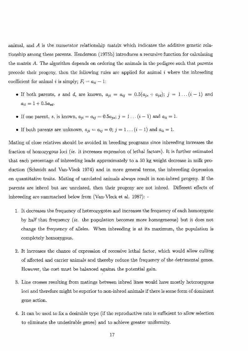
precede their progeny, then the following rules are applied for animal i where the inbreeding
coefficient for animal i is simply; Fi = aii - 1:
• If both parents, s and d, are known, aji
aii = 1 + 0.5asd·
• If one parent, s, is known, aji = aij = 0.5ajs; j = 1 ... (i- 1) and aii = 1.
• If both parents are unknown, aji = aij = 0; j = 1 ... ( i - 1) and aii = 1.
1. .. (i- 1) and
Mating of close relatives should be avoided in breeding programs since inbreeding increases the
fraction of homozygous loci ( ie. it increases expression of lethal factors). It is further estimated
that each percentage of inbreeding leads approximately to a 50 kg weight decrease in milk pro
duction (Schmidt and Van-Vleck 1974) and in more general terms, the inbreeding depression
on quantitative traits. Mating of unrelated animals always result in non-inbred proge;ny. If the
parents are inbred but are unrelated, then their progeny are not inbred. Different effects of
inbreeding are summarised below from (Van-Vleck et al. 1987): -
1. It decreases the frequency of heterozygotes and increases the frequency of each homozygote
by half that frequency ( ie. the population becomes more homogeneous) but it does not
change the frequency of alleles. When inbreeding is at its maximum, the population is
completely homozygous.
2. It increases the chance of expression of recessive lethal factor, which would allow culling
of affected and carrier animals and thereby reduce the frequency of the detrimental genes.
However, the cost must be balanced against the potential gain.
3. Line crosses resulting from matings between inbred lines would have mostly heterozygous
loci and therefore might be superior to non-inbred animals if there is some form of dominant
gene action.
4. It can be used to fix a desirable type (if the reproductive rate is sufficient to allow selection
to eliminate the undesirable genes) and to achieve greater uniformity.
17

5. Inbreeding within a population leads to a loss of genetic variation, and therefore a loss of
future reliability to make genetic change.
The expected additive genetic merit, ai of the progeny i resulting from mating sire si and dam
di can be calculated as (der Werf 1990):
(2.10)
1 1 1 var(ai) = 4var(asJ + 4var(adJ + 2cov(a8i, adJ + var(¢i) (2.11)
1 1 2 var(</Ji) = 2[1- 2(Fsi + FdJ]aai (2.12)
where </Ji is the Mendelian sampling, a8i and adi are the additive genetic values of the sire and
the dam respectively, var(a8 ) and var(ad) are the additive genetic variance for both the sire
and the dam respectively, cov( a8 , ad) is the covariance between the additive genetic values of the
sire and the dam, var( ¢) is the variance of Mendelian sampling, F8 and Fd are the inbreeding
coefficients for the sire and dam respectively, a~ is the additive genetic variance for the population.
2.3 Methods for selection
Dekkers (1998) summarised the current trends in designing breeding programs and suggested
that the four main components of a breeding program are the formulation of a breeding goal,
methods for evaluation of potential breeding stock, methods for selection, and mating strate
gies. He states that the crucial criteria for designing breeding programs are the rates of genetic
progress and inbreeding, although the overall goal is an economic one. Banks (1988) emphasised
two types of decisions: strategic and tactical. Strategic decisions are the choice of a breed
ing goal, breeds, and selection or crossing system(s). The tactical decisions are the method for
selecting animals for mating, and the mating system or the method to allocate animals for mating.
There are a number of methods for selecting animals including: independent culling levels, the
classical selection index- which is also known as best linear predictor (BLP), restricted indices,
multi-stage index selection, and the best linear unbiased predictor (BLUP). Actually, these meth
ods are used to estimate the genetic merit (breeding values) of animals and then these estimates
18

are used for the purpose of selection. Before proceeding with a description for each of these
methods, some concepts are required.
We must first differentiate between the selection objectives and the selection criteria (Banks
et al. 1996; Kinghorn 1995). Sometimes the breeder may wish to optimise a trait that cannot
be measured directly, indirect selection. In this case, they utilise another trait that is correlated
with the one they wish to optimise and can also be measured: for example, using ultrasonic mea
surement of live animals (selection criterion) to predict carcass quality of slaughtered animals
(selection objective).
There are three main types of correlations between traits: genetic, phenotypic, and environmental
correlation. Genetic correlation, rG, is the correlation coefficient between the breeding values of
two traits. Phenotypic correlation, rp, is the correlation coefficient between the observed values
of two traits. Finally, the environmental correlation, rE, is the correlation coefficient between
environmental effects on two traits. Let us assume that we have two traits T1 and T2 , where the
first represents the selection objective and the second is the selection criterion. The correlated
response measures the response's strength on the trait representing the selection objective, when
the selection is carried out on the trait representing the selection criteria. The correlated response,
CRr1 (r2 ), in T1 from selection on T2 , can be calculated as:
(2.13)
where ir1 is the selection intensity, rG(r2-r1 ) is the genotypic correlation between T1 and T2, h2T1
and h2T2 are the heritability of T1 and T2 respectively, and O"p,r1 is the phenotypic standard
deviation of T1 .
Independent culling levels
One method of simple selection strategy is by setting a threshold on the trait, and the animal
is selected if its value for this trait is higher than the threshold. Another way of applying this
strategy is by determining a number of replacements and a certain proportion of animals is cho
sen on the basis of each trait.
19

Classical selection index
The classical selection index theory (Hazel1943) is based on calculating a set of economic weights
and then building an index as the sum of the phenotypic values of all traits weighted with the
corresponding economic weights. The economic weight is defined as (Banks et al. 1996):
"the profit margin as a result of a unit increase in the estimated breeding value of a
trait while the other traits' genetic merit are held constant".
Given the vector of economic weights, b, the phenotypic variance-covariance matrix of the se
lection objective's traits, P, the genotypic variance-covariance matrix of the selection criteria's
traits, G, and the vector of economic values a, then the selection index I is:
(2.14)
where the vector of economic weights is calculated as:
b = p-1Ga (2.15)
The genetic gain from using the index can be calculated as
Genetic gain = i x a1 (2.16)
where i is the selection intensity and a1 is the index standard deviation. In this thesis, we are not
going to use the classical selection index, and therefore, this index will not be discussed further.
Restricted indices
This is a special case of the selection index where the index is used to maximise a trait while
minimising or maintaining the level of another trait (Kempthorne and Nordskog 1959), for ex
ample, maximising the milk volume while maintaining the fat percentage. This can be done by
simply including the restricted trait, fat percentage, in the objective function and giving it a zero
economic value.
20
Multi-stage index selection
This form of selection takes place in two or more stages. In each stage, the proportion to be
selected is set, then a selection index is constructed and the proportion of animals is selected
according to their index value.
Best linear unbiased predictor (BL UP)
The selection index theory provides a best linear prediction (Mrode 1996). Generally, BLUP is
a selection index (Henderson 1975a), but additionally it corrects for fixed effects (Parnell and
Hammond 1985). A multitrait BLUP simply calculates EBVs for each trait. Similar to the
classical selection index theory, BL UP ranks the animals according to their EBV s weighted with
their relative economic value. BLUP (Mrode 1996) is best because it maximises the correlation
between the animal's true and predicted breeding value, linear since it uses linear models, unbi
ased since the expected EBV which results from BLUP equals the expected true breeding value,
and prediction since it predicts the true breeding values. BLUP has proven a great success in
the dairy industry and other industries such as the pig industry (Gardner 1985).
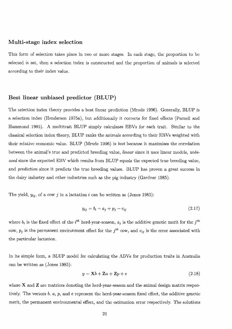
The yield, Yij, of a cow j in a lactation i can be written as (Jones 1985):
(2.17)
where bi is the fixed effect of the ith herd-year-season, aj is the additive genetic merit for the lh
cow, Pi is the permanent environment effect for the jth cow, and eij is the error associated with
the particular lactation.
In its simple form, a BLUP model for calculating the ABVs for production traits in Australia
can be written as (Jones 1985):
y = Xb + Za + Zp + e (2.18)
where X and Z are matrices denoting the herd-year-season and the animal design matrix respec
tively. The vectors b, a, p, and e represent the herd-year-season fixed effect, the additive genetic
merit, the permanent environmental effect, and the estimation error respectively. The solutions
21
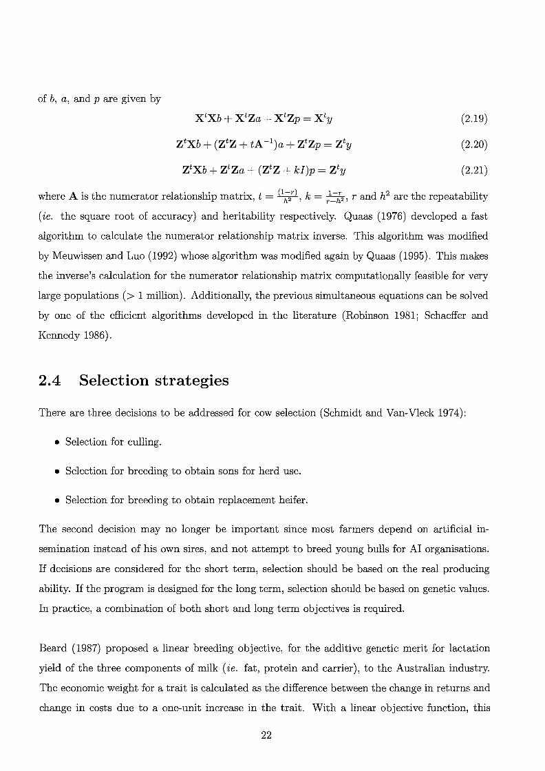
of b, a, and pare given by
xtxb + xtza + xtzp = xty
ztxb + (ztz + tA-l )a + ztzp = zty
ztxb + ztza + (ztz + ki)p = zty
(2.19)
(2.20)
(2.21)
where A is the numerator relationship matrix, t = (l~r), k = /~{2 , rand h2 are the repeatability
(ie. the square root of accuracy) and heritability respectively. Quaas (1976) developed a fast
algorithm to calculate the numerator relationship matrix inverse. This algorithm was modified
by Meuwissen and Luo (1992) whose algorithm was modified again by Quaas (1995). This makes
the inverse's calculation for the numerator relationship matrix computationally feasible for very
large populations (> 1 million). Additionally, the previous simultaneous equations can be solved
by one of the efficient algorithms developed in the literature (Robinson 1981; Schaeffer and
Kennedy 1986).
2.4 Selection strategies
There are three decisions to be addressed for cow selection (Schmidt and Van-Vleck 1974):
• Selection for culling.
• Selection for breeding to obtain sons for herd use.
• Selection for breeding to obtain replacement heifer.
The second decision may no longer be important since most farmers depend on artificial in
semination instead of his own sires, and not attempt to breed young bulls for AI organisations.
If decisions are considered for the short term, selection should be based on the real producing
ability. If the program is designed for the long term, selection should be based on genetic values.
In practice, a combination of both short and long term objectives is required.
Beard (1987) proposed a linear breeding objective, for the additive genetic merit for lactation
yield of the three components of milk (ie. fat, protein and carrier), to the Australian industry.
The economic weight for a trait is calculated as the difference between the change in returns and
change in costs due to a one-unit increase in the trait. With a linear objective function, this
22

rate of change is valid over the whole domain of each variable. The environmental effects are
not considered in the work. In Beard's study, the resultant economic weights for fat, protein and
carrier are $0.8695, $1.1162 and -$0.0294 per kg, respectively.
Quinton et al. (1992) present a very useful comparison between different selection methods
taking into consideration inbreeding side-effects. They cite that neither Best Linear Unbiased
Predictor (BLUP) nor unrestricted selection based on estimated breeding values (which is also
based on BLUP) may always be optimal. That is, these selection methods are only suitable for
short-term issues.
Meuwissen (1997) introduced a method for maximising the genetic level of selected animals while
maintaining an upper bound on the average coancestry to a user-defined value. The index is
the breeding values penalised with the coancestry level. The penalty term is represented by the
Lagrange multiplier. This index, although it takes the coancestry into account, does not consider
the mating pair and consequently it would probably under-estimate short term inbreeding. Such
selection methods may therefore lead to more inbreeding. Meuwissen was interested in max
imising long term response while maintaining a certain level of new inbreeding each generation.
However, as shown in Kinghorn, Shepherd, and Woolliams (1999), even greater responses in
mean breeding values can be achieved using both long and short term inbreeding in an MSI in
conjunction with the EBV of selected parents. This requires use of mate selection as progeny
(short term) inbreeding requires the selection of mating pairs ( ie. mate selection).
Howarth and Goddard (1998) discuss selection in terms of multiple objectives. They studied two
strategies with the farmer optimising two different objectives. In the first strategy (called the
specialised strategy), the herd is divided into two sub-herds and each is selected for one of the
objectives. In the second strategy, called average, the two objectives average is calculated and
the selection is carried out as a single composite objective. The study suggests that the "average"
strategy should be used when the objectives are positively correlated and the time horizon to be
considered is short-term, or when the herd size limits the specialised strategy usefulness.
23

Furthermore, specialised strategy generates the greatest response in the short-term, but does this
only if the correlations between the objectives are negative (assuming that the economic values
of the traits have the same sign). Actually, this result is not new in multi-objective optimisation.
The unfavourable correlation merely indicates that there is a conflict between the two objectives.
A positive correlation means that there is no conflict between the objectives ( ie. the maximisa
tion of one objective will maximise the other one). In this case, maximising the average of the
two is a reasonable approximation that should result in a non-dominated solution.
Hirooka (1998) illustrates the use of five linear programming based strategies for sire selection.
These are unrestricted selection, zero-gain restricted selection, non-zero gain restricted selection,
proportional restricted selection and desired gain selection. Unrestricted selection is based on the
selection index. In the zero and non-zero gain restricted selections, selection is carried out to
maximise the selection index and also to maintain the level of a desired trait. For zero-gain, the
goal would be to equalise the level of a specific trait within the population. For non-zero gain,
the goal would be to maintain a certain level of the difference between the value of sire trait
and the mean value for this trait within the set of sires. In proportional restricted selection, the
constraint is to maintain the ratio of sires' traits to a certain level. For desired gain selection,
selection can be undertaken using zero or non-zero gain restricted selection or proportional se
lection with the relaxation of the constraint by altering from equality to inequality.
Kinghorn et al. (1999) show that, for certain breeding objectives, optimal selection decisions will
depend on how the mates are allocated and the optimal allocation depends on which animals
are selected. Consequently, the separation between selection and allocation will result in a
suboptimal solution. To summarise, the theory of selection does not consider the interactions
among bulls, dams, and the environment, but instead it suggests carrying out the selection on
additive genetic values of each animal independently which does not guarantee global optimality.
2. 5 Selected recent keywor k in mate-selection
A number of algorithms exist for mate-selection (Shepherd and Kinghorn 1999). Generally, there
are two steps for implementing the mate-selection problem: developing an objective function,
24

and developing and implementing a mate-selection algorithm (Kinghorn 1998). In 1985, the first
use of optimisation methods in the mate-selection problems appears to have been suggested by
Jansen and Wilton (1985) with a conventional linear transportation model for selecting mating
pairs. This model easily incorporates different aspects of a real life problem such as inbreeding.
However, it does not consider nonlinear genetic objectives.
Kinghorn (1987) compares four mate-selection strategies, three of which are heuristic while the
fourth employs linear programming technique. He states that the time for the linear program
ming calculation increases dramatically with the increase in the population size. The heuristic
of sequential allocation of the best pair from the remaining candidates is found to be close to
optimal in most cases, although the study is limited to a single generation. However, linear pro
gramming computerised solvers have improved dramatically during the last decade. For example,
until1987, Linear programming solvers were using the Simplex method, which is an exponential
algorithm (Ami 1993). In 1986, Karmarkar (Hooker 1986) introduced the interior point method
which is a polynomial-time algorithm.
Klieve et al. (1994) propose an approximate quadratic programming model for mate-selection
using portfolio analysis to construct a quadratic objective for the problem. Additive genetic
merit is used as the gain measure (profit) and inbreeding is used as a measure of the risk asso
ciated with different levels of merit. Stochastic simulation is used to evaluate different selection
strategies with respect to both additive genetic response and inbreeding. The proposed quadratic
model results in close to a 50% reduction in inbreeding over the random mating strategy.
In recent work, Kinghorn (1998) proposes clustering to facilitate group mate-selection together
with an individual-animal mate selection step for fine-tuning. Cluster analysis is used to form
groups of animals within each sex based on nominated factors such as breed, herd, age, and EBV.
Mate selection is then performed on groups. The objective is to select 20 sires and 500 dams
for breeding, from 816 sires and 1784 dams across 3 breeds. The study reports a considerable
reduction in computation time from 394.2 seconds for full mate selection to 0.28 seconds for
group mate selection although the cluster analysis took an additional 162 seconds. The max
imum number of clusters is chosen arbitrarily as four times the square root of the number of
25
candidates available. However, the work is certainly important for reducing the search space
complexity.
Shepherd and Kinghorn (1994) propose a binary nonlinear programming model for mate-selection
over two generations only with cross-breeding. The model accounts for two groups of predicted
progeny, those intended for commercial purposes and those for selection and mating. The breed
ing objective is to maximise the combined return from commercial animals for both one and two
generations into the future. The model is limited since it is very difficult to generalise over more
than two generations. They also introduced a method to parameterise mate selection.
In summary, the mate-selection problem has not been efficiently solved and a general model to
optimise multiple generation seems to be an inevitable requirement within the field.
2.6 Computerised systems for selection in dairy industry
In the literature of animal breeding, decision support systems appear to be mainly management
information systems or expert systems and are hardly decision support systems, in the sense
used in this dissertation. MacNeil et al. (1998) reviews four decision support systems for the
breeding of beef cattle two of which (SIMUMATE and HOTCROSS) are computer programs for
prediction and the other two (CROSS-CHOICE and X-BREED) are expert systems. Archer et
al. (1998) has suggested the development of a distributed decision support system over the World
Wide Web. The proposal discusses the system's functionality but does not show the technical
design.
In Canada, interesting research has been undertaken (Lacroix et al. 1997; Wade and Lacroix
1994) which investigated the prediction of milk production for the first lactation of Canadian
Holstein dairy cows, using artificial neural networks (ANNs). It was found that it is essential
to determine which additional inputs add significantly to the prediction process, and which are
reasonable in terms of the process's biology. The effect of data pre-processing on the performance
of ANNs in predicting milk production is investigated by Lacroix et al. (1997). It is reported
that the neural network's ability to predict patterns is highly affected by the class frequencies in
26

the training set.
The Victorian Department of Agriculture (Bowman et al. 1996) developed a computer pro
gram (Selectabull) for selecting the most suitable set of bulls for a farmer's herd and ranking
them according to the predictive profitability of each. The profitability is determined accord
ing to information submitted by the farmer. Four scenarios are implemented in Selectabull,
namely: Manufacturing, Liquid/Quota, Workability, and Altered prices. In each scenario, a
selection index is formulated and bulls ranked accordingly. The program also allows for dif
ferent payment systems. As an example, the breeding objective for Victoria is calculated as
$ :.___ 0.02 * Milk+ $1.2 * Fat+ $3.9 * Protein+ $4.9 * Survival+ $1.1 * Milkingspeed +
$1.8 *Temperament- $0.7 * Mature_body_weight. The weights in the objective function are
calculated according to the farmer's herd data, milk payment system and the farmers own value
judgment if desired.
The difference between Selectabull and the method introduced by Beard (1987) as discussed
earlier, is that Beard presented a selection index regardless of the farm information. Selectabull
creates a population index to create a team of artificial insemination bulls then it creates a
consumer index for each farmer to select from the team. The program achieved its intended
goals although it has a number of limitations which motivated this thesis:
• It does not capture important genetic principles such as inbreeding.
• It chooses the bulls for the whole herd without considering the cows' individual character
istics (in short, Selectabull is not designed to solve the mate-selection problem).
• It ranks bulls according to the selected scenario for a breeding objective, without consid
ering the statistical significance of this ranking. It is noted by Bowman et al. (1996) that
although the economic weights used for each scenario differed substantially, the correlations
between the selection indices are very high.
A system developed by the Machine Learning Research Centre at the Queensland University of
Technology called Connectibull (Finn et al. 1996) is designed around a neural network specific
for each bull, but has a number of limitations.
27

• Its employment of a single ANN for each sire does not allow for network generalisation of
the effects of sire traits or the general relationship between the progeny and their sires,
dams, and the environment.
• It ranks sires for mating with a dam only in terms of predicted production traits of potential
daughters ( ie. similar to Selectabull, it ignores other factors such as inbreeding).
• It is inappropriate for new sires within the artificial insemination program because the
number of records available for these sires will be insufficient for training the ANN.
Kinghorn and Shepherd (1999) introduce the total genetic resource management (TGRM) ap
proach and propose the mate-selection index (MSI) which replaces the classical selection index.
MSI is calculated for a mating strategy and not for individual animals. TGRM is a breeding aid
program driven by specifying desired outcomes ( eg. outcomes in genetic gains) (Kinghorn 1999).
The user determines the level for each outcome (s)he is satisfied with and the program uses
evolutionary algorithms for solving the mate selection problem for one generation while trying
to meet the user expectations. Therefore, the program depends somehow on the user to set the
goals while these goals may be far from optimal in themselves. This might be a disadvantage
but a necessity for the package to optimise the processing time. Also the prediction problem
discussed in this thesis is not an issue in TGRM since TGRM does not consider the production
values and concentrates instead on the breeding values. TGRM is considered as the state of the
art in the field for mate-selection and demonstrates the practical importance of this problem.
2. 7 Conclusion
To summarise, the mate-selection problem has not been solved efficiently so far. Current infor
mation systems contain the necessary information for the mate-selection problem but none of
the existing information systems is qualified to decide on the allocation part except the TG RM
system which handle the problem for two generations. This raises two issues: (1) how to design
an efficient computer information system for a breeding program, and (2) how to model the multi
stage mate-selection problem. The first issue is covered in the next chapter, where it is suggested
to integrate knowledge discovery from databases with intelligent decision support systems to
solve the problem. The second issue is covered by the remaining chapters where the prediction
28

problem is investigated and a generic mathematical model for solving the mate-selection problem
is proposed and solved.
29

30
Part II
Knowledge Discovery in Databases
31


Chapter 3
KDD-IDSS: A Framework for
Integrating KDD with IDSS
The following refereed publication arose out of this chapter:
H.A. Abbass, M. Towsey, G. Finn, and E. Kazan. "A Meta-Representation for integrating OR
and AI". International Transactions of Operations Research (!TOR), accepted for a forthcoming
issue.
This chapter's main objective is to introduce the proposed information system framework, and
to present a new meta-level modular representation for integrating operations research (OR) and
artificial intelligence (AI) models using constraint logic programming (CLP). The importance of
this language relies on representing a problem generically, and therefore hiding the implementa
tion details from the user.
The chapter begins with a summary of the decision making process (Section 3.1), followed by
a literature review of intelligent decision support systems (IDSSs) (Section 3.2). In Section 3.3,
the process of knowledge discovery in databases (KDD) is reviewed and a framework for inte
grating KDD and IDSS is proposed in Section 3.4. A proposed meta-language for the kernel in
the KDD-IDSS is then described in Sections 3.5 and 3.6. Previous work in integrating AI with
OR, CLP with OR, and non-symbolic AI with CLP, is presented in Section 3.5 followed by the
proposed meta language in Section 3.6. The chapter concludes with an example from the dairy
industry (Section 3. 7).
33

3.1 Decision making process
Problems are recognisable through symptoms of abnormal behaviour of system's components.
If the symptoms are not recognised early enough, the problem may become a crisis. With an
excellent computerised system that has the ability of problem recognition, crises can be evaded.
One way to perceive the existence of a problem is suggested by Ata (1988), who defines problem
recognition as the process of comparing actual values of some selected variables to their stan
dards. Whenever these standards are violated, the corresponding variable( s) is( are) placed on
a list of symptoms. Once symptoms are shown and the problem is identified, one may start by
decomposing the problem into sub-problems. By determining the causes and the set of possible
actions to solve the sub-problems, the overall problem can be solved. The problem's solution is
called the decision.
Problem solving (decision making) is defined when there is a gap between what is desired (the
goal state) and what is given (the initial state), and in which the transitions that need to be
followed to reach this goal are unknown. The process of solving a problem (identifying the tran
sitions) is called decision making whereas the process of implementing the solution is decision
taking. According to the scientific approach in management (Klein 1995), decision making pro
cess consists of the following five steps: viz, problem recognition, problem definition, problem
formulation, setting goals and designing actions, and evaluation of actions to select the best. The
decision maker proposes the selected action to the decision taker who decides whether to take it
or not.
As depicted in Figure 3.1 (Trave-Massuyes 1991), there are three types of problems: unstruc
tured, semi-structured, and structured. According to the problem type, the managerial levels are
classified into strategic, tactical and operational respectively. From my point of view, resource
allocation should not be considered as a managerial level but a common function between the
strategic and tactical level. Simon (1960) defines a structured decision as the decision where
all the steps required for it can be pre-specified. Simon's definition is influenced by information
34

A UNSTRUCTURED
[ __________ s_T_RA_~ __ or_c_LE-~----------~J
[ RESOURCE ALLOCATION J I SEMI-STRUCTURED
I STRUCTURED
I
Figure 3.1: The managerial levels
systems whereas most researchers (Fox and Krause 1991; Thrban 1990) refer to a problem to be
structured if it can be quantified. Tactical problems are semi-structured in that they have both
quantitative and qualitative dimensions. DSSs (Thrban 1990) provide solutions for the tactical
level whereas IDSSs provide solutions for all managerial levels within the system.
3.2 Intelligent decision support system
Decision support systems originated from two research areas during the 1960s. The first is "the
oretical studies of human problem solving and decision making" during the 1950s and the 1960s
at the Carnegie Institute of Technology. The second is "interactive computer systems" during
the 1960s at the Massachusetts Institute of Technology. The two areas became, what was later
called in the 1970s, decision support systems. DSS is an integrated information system for deci
sion making.
Despite the emergence of the DSS in the 1970s, presently there is no consensus on the answer
to the question: What is a DSS? Some researchers (Sharda et al. 1988) think of a DSS as a
collection of theoretical studies driven by a technology push, rather than by a managerial pull.
Eierman et al. (1995) propose a theoretical framework for DSS to overcome this claim although
the study concentrates on the managerial side without considering the informatics one. To better
understand what is a DSS, each of the words Decision, Support, and System is defined.
35

System A system is mostly defined as a group of components/items that interact together to
achieve an overall objective(s) (Gdaellenbach 1995). Each of these components is a system
in itself, ie. it has sub-components and it has an objective(s). For example, the farm as
a system has many sub-components such as the animals, lands, machineries, etc. Each of
these sub-components is a system in itself. For example, the animal is a system where its
components are organs, genetics, etc.
Each component in the system may have local objective(s) which should contribute to the
overall system's objective(s). Nevertheless, the component may have an objective that
conflicts with the overall system's objective. Unless the component's objective is imposed
on the system by a higher power ( ie. a larger system), it will be rejected. For example,
maintaining a certain amount of milk production contradicts the farm objective in max
imising the return. Yet the farmer may be obliged to maintain this level of milk production
because the Department of Primary Industries assigns to each farmer a milk quota that
should not be exceeded. This represents an external rigid constraint. If the level of milk
production is determined by an internal policy within the farm and it can not be changed,
the requirement represents an internal rigid constraint. If the internal policy is flexible, (ie.
can be changed), the requirement becomes a soft constraint. If the policy is to maximise
the milk production, without knowing to what extent, it becomes an objective. If the milk
production level is planned (known), it becomes a goal.
Support A computer support system is "a computer system which is placed at the decision
maker's disposal who may use data or models to recognise, understand, and formulate a
problem, and make use of analytical aids to evaluate alternatives" (Klein 1995). The pro
cess of supporting the decision-maker in making a decision, is a continuous process that
starts before a decision is made and continues even in the future. Strictly speaking, the
system should show some dynamics.
Decision The word decision has been defined and classified in the previous section. Although
decision-making and decision-taking may appear to be independent processes, they are not.
36
Usually in real life applications, some difficulties face the decision-taker when applying the
decision. This requires adjusting the decision to cope with the new constraints. The
dynamic nature of DSS plays the main role here.
In data mining, DSS has a limited definition where Bigus (1996) defines a DSS as "a query
application integrated with a graphical display system" . In the literature, the concept of a DSS
has evolved. In the early 1970s, Scott-Morton (1971) defined DSS as "decision support systems
couple the intellectual resources of individuals with the capabilities of the computer to improve
the quality of decisions". As a refinement of Scott-Morton's definition, Little (1970) considers
a DSS as "A model-based set of procedures for processing data and judgments to assist a man
ager in his decision making". In the early 1980s, Bonczek et al. (1980) defined a DSS as: "A
computer-based system consisting of three interacting components: 1) A language system - a
mechanism to provide communication between the user and other components of the DSS, 2)
A knowledge system- the repository of problem domain knowledge embodied in a DSS, either
as data or procedures, and 3) A problem processing system- the link between the other two
components, containing one or more of the general problem manipulatory capabilities required
for decision making" .
In the late 1980s, Hicks (1987) defined a DSS as "an integrated set of computer tools that allow
a decision maker to interact directly with computers to retrieve information useful in making
semi-structured and unstructured decisions". In 1990, Turban (1990) introduced a famous defini
tion of a DSS: "an interactive computer-based information system that utilises decision rules and
models coupled with a comprehensive database and the decision maker's own insights, leading to
specific, implementable decision in solving problems that would not be amenable to management
science optimisation models per se". Lastly, in 1996, Dutta (1996) defined a DSS as "an area
concerned with computer based structures and procedures that augment human decision making
capabilities". From the previous definitions, the concept of DSS started as a general information
system and ended as a structured one in Turban's definition.
To my knowledge, Holsapple is the first to use the term IDSS in his doctoral thesis (Holsapple
1977). The study concentrates mainly on data representation. He suggests having an information
base, which is a combination of models and knowledge, where a model, from his point of view,
37
can be seen as any piece of data. He used network databases which facilitated his concept of
a model. The work lacked modularity and interaction and the research in AI at this time was
premature.
The term IDSS was not used much since then until 1988. The term expert decision support
systems was introduced by Sen and Biswas (1985). The term knowledge-based decision support
system was suggested by Turban (1990) in 1990. In 1995, Klein (1995) suggested the framework
knowledge-based decision support system in a work undertaken in France.
IDSS, as used throughout this dissertation, holds a broader scope and deeper dimension. The
following definition for IDSS is proposed:
IDSS is an interactive, structured, and dynamic management information system,
that fully or partially automates the decision making process by combining a set of
models with a set of symbolic knowledge, while utilising the available databases, in
an integrated environment that is capable of reasoning about the decisions it makes.
From the previous definition, 11 keywords are accentuated. Interactive reflects the dialogue
base component and it places an emphasis on the IDSS's ability to interact with the user and
the user role in the system. Structured stresses the IDSS modularity. Dynamical is achieved
in terms of the user feedback and includes the possibility that the system evolves by correcting
its mistakes while updating its internal states. Management information system highlights
the IDSS's original roots and identification as a management information system. Fully or
partially automate is one of the main features that will be emphasised throughout this work.
It represents the IDSS's potential to be an independent environment.
Decision making process places an emphasis on the fact that the purpose of an IDSS is to
support or even replace the decision maker although it won't be able to replace the decision taker's
perception or job. Models, knowledge, and databases represent the other three components
of an IDSS where the first is the dialogue base discussed in the beginning of the definition in terms
of the interaction. Integrated environment emphasises the fact that the IDSS should not be
isolated from, but rather be integrated with, and become a piece of, the surrounded environment.
Environment represents the information system, the surrounding pieces of softwares, as well
38

as the decision making environment. Lastly, reasoning reflects the system power to rationalise
and persuade the decision taker with the decisions it makes.
3.3 Knowledge discovery in databases
Knowledge discovery in databases is simply the task of identifying patterns within a database
system. A revised version of the definition in (Frawley et al. 1991) is given by (Fayyad et al.
1996):
Knowledge discovery in databases is the non-trivial process of identifying valid, novel,
potentially useful, and ultimately understandable patterns in data.
Data mining (DM) is a step in the KDD process representing the process of applying the discov
ery algorithm. There is a common misconception between the use of the term DM and KDD.
In academia, DM is a step in KDD (Fayyad et al. 1996) although among the public, DM and
KDD seem to be used interchangeably (John 1997). It is becoming apparent that even in modern
academia people tend to use the term DM when they mean KDD.
A definition of KDD that suits its intended task within the IDSS paradigm is introduced. KDD
is:
The process of abstraction from large databases and the process of searching for
patterns and symptoms within the abstracted model.
There are four keywords in the definition: abstraction, search, patterns, and symptoms. The
database is a conventional element in KD D.
Abstraction: Abstraction is the process of mapping the system language .C1 to an approxi
mately equivalent language .C21 . The mapping is strong when it maps the system while
neither losing existing patterns (completeness) nor introducing new patterns (soundness).
Search: It is more convenient to see the discovery process in terms of search. Therefore, one can
measure the complexity, and in turn the feasibility, of the process by studying the search
1Formally, Giunchiglia and Walsh (1992) define an abstraction, written f : E1 =? Ez, as a pair of formal
systems (E1,E2 ) with languages A1 and Az respectively, and an effective total function fA: A1--+ Az.
39

space. Most KDD steps can be seen as search-space reduction techniques. For example, the
main goal for creating a target data set, data cleaning, and data reduction and projection
is reducing the noise in the data and selecting a representative sample which then reduces
the search space. The mining algorithm is the search technique used to achieve the overall
process objective.
Patterns: A pattern is "an expression, £, in a language, £, describing a subset of facts, Fc;,
from the total facts, F, which exist in the database" (Fayyad et al. 1996).
Symptoms: Although the symptoms can be seen as patterns, the process of discovering the
symptoms has more dimensions than finding simple descriptive patterns. Identification of
symptoms is a major task for KDD, if it is the intention to use it for IDSS. The KDD pro
cess's role is to clear the noise within the system and discover abnormal signals (symptoms)
that may contribute to potential problems.
There are many applications reported in the literature for KDD (Fayyad et al. 1996; Matheus
et al. 1996; Smyth et al. 1996; Apte and Hong 1996). Although it seems that there is no general
agreement on what the steps for KDD should be, some researchers have tried to structure the
KDD process. Fayyad et al. (1996) identify nine steps: application domain understanding,
creating a target data set, data cleaning and processing, data reduction and projection, choosing
the mining task, choosing the mining algorithm, mining the data, interpreting the mined patterns,
and consolidating the discovered knowledge. John (1997) sums up these steps into six, data
extraction, data cleaning, data engineering, algorithm engineering, running the mining algorithm,
and analysing the results. Regarding the issue of the basis for selecting KDD applications,
Fayyad et al. (1996) define four practical criteria and five technical criteria for selecting KDD
applications. The former are: the potential for the application's significant impact, no good
alternatives exist, organisation support and potential for privacy and legal issues. The latter are,
the availability of sufficient data, relevance of attributes, low noise levels in the data, confidence
intervals, and prior knowledge.
40

3.4 A proposed frame for integrating IDSS and KDD
The proposed KDD-IDSS paradigm is shown in Figure 3.2. The conventional IDSS paradigm is
extended with a mining base component. This extension influences both the model and knowledge
base components. While the set of models and knowledge in the conventional IDSS are static
(ie. built once and manually updated when necessary), they are dynamic in KDD-IDSS. For
example, the mining base continuously builds predictive models and updates the model base
with the models it finds. Therefore, if we have a linear regression model in the model base,
the parameters in the model are updated every time a change, which may influence this model,
occurs in the data. Also the set of rules generated from a mining task may be used to update
existing rules in the knowledge base. In short, the system is somehow self-adaptive where the
mining base is updating the systems' components based on new changes in the environment. A
short description of each component follows.
Model
Base
3.4.1 Database
Model
Manager
Data
Manager Base
Directory
Dialog Dialog
Manager Manager Base
Figure 3.2: The KDD-IDSS paradigm
A set of data that may be directly or indirectly related to the problem. As an example, the ABV s
is a datum that is directly related to the problem. The inflation rate, which could be used to
predict the prices, is the sort of data which are indirectly related to the problem. A database is
usually accompanied by a data manager that organises the way the data is stored, updated, and
retrieved. KDD-IDSS interfaces with the database through the data manager and it should not
access the data directly for security and efficiency reasons. Also, it can access the data directory
41
(the logical design and/or meta-data) although it cannot change or add to it.
Rob and Coronel (1997) distinguish between the operational data and DSS data using three
criteria: time span, granularity, and dimensionality. DSS data are historical, summarised, and
normally multidimensional although operational data are up-to-date, atomic-detailed and one
dimension databases. One of the new advances in databases which is motivated by DSS is data
warehouses. A data warehouse, introduced by Inman (1994), is defined as: "an integrated,
subject-oriented, time variant, non-volatile database that provides support for decision making".
Another recent advance in databases is the on-line analytical processing introduced by Codd
(1993) who defines it as: "on-line analytical processing is the dynamic synthesis, analysis and
consolidation of large volumes of multidimensional data". Later, Han (1997) introduced the on
line analytical mining which combines on-line analytical processing with data mining techniques.
3.4.2 Model base
A set of models which are required to solve the problem under consideration. Like the database,
the set of models in the model base interfaces with the system through a model manager and a
description of these models is stored in the model directory.
3.4.3 Knowledge base
A set of facts and symbolic rules about the problem under consideration. The knowledge in an
IDSS may be used for the following purposes :-
1. Providing explanation for the system behaviour.
2. Reducing the search space complexity for some models. For example, utilising previous
knowledge for decomposing a linear programming problem or eliminating dependent vari
ables and/ or constraints from an optimisation model.
3. Generating/ expanding the input space for some models. For example, generating or ex
panding a sample space to be used by neural networks or genetic algorithms.
4. Solving a sub-problem. For example, calculating the inbreeding coefficients.
42
5. Post-processing of outputs. For example, interpreting the outputs from the linear program
ming solver.
6. Determining the models' calling sequence. For example, if the decision-maker would like
to optimise two years ahead, the calling path may be predictor ---t optimiser ---t predictor
---t optimiser. If the performance in the current year is known, the calling path will be
optimiser ---t predictor ---t optimiser.
7. Model selection. For example, according to some criteria either a genetic algorithm module
or a conventional optimiser may be called.
8. Helping tool. For example, providing help to the farmer about artificial insemination.
Lastly, rules-weights, probabilities or fuzzy membership functions may be associated with the
set of facts and rules in the knowledge base.
As with the previous two KDD-IDSS components, a knowledge base has also a manager which
handles the way it is represented and infers new knowledge. Also, items of knowledge are grouped
and classified with the description of each group and class stored within the knowledge directory.
3.4.4 Dialog base
The dialog base is the direct outcome of the DSS foundation. Dialog base is based on studies in
Human-Computer Interaction. Schneiderman (1987) defines five main styles for human-computer
interaction: viz menus, forms, command languages, natural languages, and direct manipulations
or graphical interfaces.
1. In menus, the user is restricted with a list of choices and one of them should be selected
otherwise the default choice is assumed.
2. In forms, the user is required to fill the parameters within the provided spaces in the form.
3. In command language, the user interacts with the system through a command language in
which the language syntax and semantic are predefined.
43

4. In natural language, the user interacts with the system in a natural language ( eg. English)
and the system asks the user questions in turn. This type of interface is very complicated
to design and/ or implement although it is more convenient for novice users.
5. In direct manipulations or graphic based, the user defines the problem in a graphic form
( eg. dragging the sign "X" and placing it on a cow shape may be a way of representing a
constraint such as the cow is not available for mating).
The actual dialog base may combine some or all of the previous types. The word "dialog base"
is used here rather than the conventional word "user interface" to emphasise the idea of interac
tion in decision support systems. Different studies in human-computer interaction (Molich and
Nielsen 1990; Norman 1986; Ravden and Johnson 1989; Scheiderman 1987) concentrates on the
user interface as an important part in the program. Norman (1986) associates two properties
with an interface language to measure its validity as an interface for a dialog base. The first prop
erty is the articularity directness, in which the distance between the physical form, or syntax, of
expressions in the interface language and the meaning of the expression is measured. The second
property is the semantic directness, in which the distance between the meaning of the input or
output expressions in the interface language and the user's intentions or goals, are evaluated.
3.4.5 Mining base
The mining base contains a set of scenarios for the KDD process. These scenarios are a high
level description of different pre-designed discovery tasks in the system. The mining base does
not store any mining algorithm as these algorithms belong to the model base. Also, database
manipulation is no longer the mining base responsibility but rather of the database component.
Additionally, data visualisation within the IDSS is the user interface's responsibility and no
longer of the mining base concern. In summary, the mining base contains an abstraction of the
KDD process for each discovery task. The mining manager organises the storage, retrieval, and
updating of different scenarios within the mining base. Furthermore, information about each
discovery task is stored within the mining base directory.
44

3.4.6 Kernel
The kernel is the main interface, sometimes called the operating system, through which all pre
vious IDSS parts interact. This is the most difficult and technical component in the IDSS. To
today, there is no generic language for representing the kernel. The contribution of this chapter is
to provide such a language for interfacing operations research and artificial intelligence modules
within the kernel of KDD-IDSS.
3.5 A meta-language for OR and AI in the KDD-IDSS
kernel
The rest of this chapter explores the suitability of CLP as the kernel language for integrating
OR and AI. CLP was introduced in 1986 by Jaffar and Lassez (1986), who also developed the
first CLP language, CLP(R) (Jaffer et al. 1990). The CLP paradigm overcame the mathe
matical deficiency in Logic Programming (LP) by introducing new domains ( eg. real, rational,
boolean, finite trees, etc.) and by defining a suitable set of operands and operations over these
domains. The goal of using constraints partially solved the problem of recovery from failure (in
conventional logic programming) since constraints can be used in the system as a mechanism to
generate a solution space that avoids failure. If the solution space is empty, the system reports
failure instead of continuing the search. This reduces the search space as well as providing early
detection of failure. CLP continues to be successfully applied to a variety of OR problems such
as scheduling (Gosselin 1993), planning (Perrett 1991), quadratic programming (Abbass 1998),
multi-criteria decision making (Abbass et al. 1997), and network optimisation (Abbass et al.
1999a; Abbass et al. 1999b). For a typical set of CLP applications, see (Hentenryck 1990). A
technical review about the foundations of CLP can be found in (Jaffer and Maher 1994).
In this section, previous attempts to integrate AI with OR, CLP with OR, and non-symbolic
AI with CLP, are presented. This section provides the reader with the three dimensions of the
integration as a basis for, and to give the motivation for, the meta-language to be illustrated in
the following section.
45

3.5.1 Interfacing AI with OR
Holsapple et.al. (1994) examined this integration and found that both OR and AI involve the
use of descriptive knowledge (data and information), embodying measurements, observations,
or beliefs about the state of some real or hypothetical world. They conclude that OR focuses
on the management of procedural knowledge, whereas AI tends to emphasis the management of
reasoning knowledge. The integration of OR and AI has been discussed in many papers and
books such as Barahona and Ribeiro (1990), Donald and Chelsea (1990), Dutta (1996), Hol
sapple et.al. (1994), Lee (1990), and Moon et.al. (1993). In this chapter, we are taking this
research a further step up by formalising the underlying concepts in these works. More specifi
cally, most of these studies were problem specific but a more general frame will be presented here.
Research has been carried out to design frameworks for exchanging data between symbolic AI
and quantitative OR techniques. Barahona and Ribeiro (1990) suggest using CLP for integrating
expert DSS and OR. This work is not formalised but is illustrated by a conventional example
in CLP. Moreover, it considers neither a formal frame for the integration nor the expert DSS
components. Turban and Trippi (1990) provide an excellent conceptualisation of the integration
between expert systems and OR with different concepts for different types of integration although
they do not provide an implemental formal frame. Belz and Mertens (1996) combine knowledge
base systems with simulation to solve rescheduling problems. They have three main intelligent
components: one to initialise the simulation run, the second to supervise it and the third to anal
yse the simulation output. Their model appears to be well designed for the integration although
it was specific to knowledge basis and simulation. A formal generic frame for integrating AI and
OR should be developed, on the basis of these studies.
3.5.2 Interfacing CLP with OR
CLP has a pertinent relation to OR as it is centred on constraint solving mechanisms. However,
the paradigm is hampered by the conventional limitations of first order predicate logic. CLP
implementations can optimise a function with numeric variables but cannot optimise a concept
46
representation. For illustrative purposes, suppose the concept of customer satisfaction can be
represented using the following predicate:-
satisfied(X) : -
customer( X),
budget(X, Y),
like(X, Z),
price(Z, M),
M<Y,
bought(X, Z).
This is read as "an object X is satisfied if (X is a customer), (the budget of X is Y), (X likes an
object Z), (the price of Z isM), (the price M is within the budget limit of X which is Y) and (X
bought the object Z)". Now, suppose that the objective is to maximise (VX, satisfied(X)), that
is to maximise the satisfaction of all customers. The problem can be formulated quantitatively
except for the predicate like (this problem could possibly be handled by borrowing techniques
from decision making, such as utility functions). It is inherent to CLP that it is limited by first
order predicate logic (Abbass et al. 1995).
3.5.3 Interfacing CLP with non-symbolic AI
So far, artificial neural networks (ANNs) have not been sufficiently considered in a CLP envi
ronment. Montesi (1996) proposes a model for representing ANNs within CLP in which current
CLP semantics for equations are used to represent the network as a system of equations. The
network is trained outside the CLP paradigm and then embedded within CLP. This would have
been more efficient if CLP were capable of training the network so that retraining would not
require updating the CLP program.
To my knowledge, the use of a genetic algorithm (GA) solver in CLP has not been considered.
We consider that it has potential to enrich the power of CLP paradigms by making all successful
applications of GA available to CLP as well.
47
3.6 The proposed meta language
This section essentially describes the details of the proposed language used for the integration.
First, the concept of decision making is structured using CLP-like syntax, allowing the decision
to be decomposed by CLP into a set of component predicates. Each component predicate can
be an optimisation, a neural network, natural language, or knowledge based system. The com
ponent predicates are then constructed as a set of predicates in CLP-like language. In this way,
all component predicates are abstracted and, consequently, the meta-language is independent of
any specific implementation. Therefore, the intelligent problem solving process can be illustrated
using a three layered system.
• The first layer is the meta-language, used to abstract a particular problem.
• The second layer is a classifier system, where a decision tree is employed to identify the type
of models required to solve the problem. For example, if the user requires the optimisation
of a problem, the classifier system will analyse the objectives and constraints to determine
the more appropriate optimisation model.
• The third layer is the detailed implementation level where the actual coding for each algo
rithm is implemented.
This chapter is concerned only with the first layer. The second layer is assumed to be a single
path decision in this thesis, whereas the third layer is the subject of the remaining chapters.
3.6.1 Formalising the concept of a decision in KDD-IDSS
From the previous section, we have seen that the KDD-IDSS is very flexible since it isolates the
mechanism for solving a problem from the problem formulation stage. Therefore, if the problem
complexity increases and the KDD-IDSS requires more sophisticated techniques to handle the
new version of the problem, all it requires to do is to call a different appropriate solver. For
example, calling a Simplex solver for a medium size linear programming and calling an interior
point solver for a large size linear programming.
48
Given a set of decision variables Variables, a set of constraints Constraints, and a set of
criteria Objectives, a decision requires the values of Variables to meet the set Constraints
and optimise the set Objectives. Formally speaking, the decision can be defined as a function
D = select(Variables, Solution, Objectives) where Solution = solve(Variables, Constraints),
that is the predicate solve returns a set of solutions where the predicate select evaluates them
and selects the optimal. This definition illustrates two important stages in problem solving.
The first stage is the process of finding a set of feasible solutions (ie. alternatives) represented,
using the predicate solve/2 (namejn means that the predicate name has n arguments). This is
equivalent to the feasibility stage in OR. The second stage is equivalent to the optimality stage
in OR where the elements in the set resulting from the feasibility stage are evaluated, and the
one which best satisfies the criteria is selected using the predicate select/3.
We then have to define the criteria's nature. For global optimality, one can implement the pred
icate select/3 either by using exhaustive search or formulating the problem as an optimisation
model. Both ways are computationally expensive but optimisation is much less though, since it
does not exhaust the search space but instead searches a sub-space in a systematic way until the
optimal solution is reached.
The second type of criteria that can be used is the concept of satisfaction (introduced by Simon
(Simon 1960) and also called the Simonian philosophy), which attempts to satisfy a set of goals
rather than to optimise a set of objectives. The goal is always partially satisfied to some aspi
ration level (possibly 0%) so that one or more solutions always exist. If the constraint system
is not satisfied, the solution space will be empty. Bearing this difference between a constraint
and a goal in mind, a satisfaction problem can be handled using an updated version of the tech
niques used for solving a normal optimisation problem by adding a free variable to each goal
equation. Then, for any set of decision variables' values, a goal equation is satisfiable for some
values of its free variable. The free variables can be minimised later subject to a set of user
preferences (eg. goal programming). Therefore, we may have a multi-dimensional objective, as
well as goals that may be prioritised - see (Abbass 1994) for an update to the CLP language,
SICStus, to handle goal programming problems. Next, we can rewrite the literal Solution as
follows: Solution= solve_new(Variables, Constraints_rigidn Constraints_soft). Therefore, in
49
recasting the optimisation model as a satisfaction model Constraints became Constraints_rigid
and Objectives became Constraints_soft. Further, solve/2 for optimisation is a special case of
a new predicate solve_new /2 for satisfaction, where
solve(Variables, Constraints) = solve_new(Variables, Constraints_rigid U ¢),Constraints =
C onstraints_rigid.
where <I> is the empty set. Accordingly, for the satisfaction models the decision can be redefined as:
D = select(Variables,Solution,Objectives), where
Solution= solve_new(Variables, Constraints_rigid U Constraints_soft).
We consider all possible cases.
D = select(Variables, ¢,Objectives)=¢-+ No Solution
D = select(Variables, Solution,¢) = Solution -+ Satisfaction problem
D = select(Variables,Solution,Objectives) =X, Solution -j. ¢and X=/=¢.
If the cardinality of X is 1, we have a unique solution; otherwise, we have multiple solutions.
However, the set Dis not necessarily finite- it may indeed be uncountable infinite, in which case
we may represent D by a set of constraints called the "most general form" .
The set of constraints over D can be further classified as predicates and functions. Predi
cates are functions that take the values 0 or 1 (ie. true or false) and are used extensively
to represent symbolic knowledge. Unfortunately, propositional logic is insufficient to represent
some important relations. For example, in order to generalise the concept of grand-fatherhood
we need to enumerate propositions for this relationship in the world. In first-order predicate
logic, grand-fatherhood can be expressed more naturally in terms of the concept of fatherhood:
grandfather(X, Y) : - father(X, Z), father(Z, Y). This means that if X is the father of Z and
Z is the father of Y, then X is the grandfather of Y where there is an implicit use of universal
quantification. For all people X, Y, and Z require only that the concept father is defined in
50

context. We can still represent the relation grandfather using an integer model. For illustration
purpose, let grandfather(X, Y), father(X, Z), and father(Z, Y) be denoted as Cl, C2, and C3
respectively. Now, the predicate can be represented as Cl = HC2 + C3), where Cl, C2, and C3
are binary variables. Yet we are unable to represent here the universal quantifier, although the
binary variables can be related to domains where the universal quantification is applied on the
domain. Finally, we can rewrite our definition for a decision in the following way:
D = select(Variables, Solution, Pred_Objectives U Func_Objectives) where
Solution= solve_new(Variables, Pred U Constraints_rigid U Constraints_soft).
This definition represents an abstract problem representation. The Pred_Objectives compo
nent, representing the qualitative objectives, can be handled by the knowledge base, whereas the
Func_Objectives component, representing the quantitative objectives, can be handled by the
optimisation module.
3.6.2 The relationship between the proposed concept of a decision
and previous ones
The goal of using the Prolog environment as a kernel for DSS is not new. Fox (1991), presents a
DSS based on first order predicate logic (FOPL) in medicine. He does not employ optimisation
techniques to build the DSS. Lee et.al. (1996) propose the following representation for quantita
tive/ qualitative constraint satisfaction ( QQCSP) problem, W = [ E, R_E, F _E] U [ N, R_N, F _N] U
[E UN, R_EN, F _EN]; where Eisa set of symbolic objects, R_E and F _E are sets of relations
and numeric functions on the set E respectively, N is a set of symbolic objects, R_N and F _N
are sets of relations and numeric functions on the set N respectively, and R_EN and F _EN are
sets of relations and functions on both E and N. They also compare the use of mixed integer
programming and constraint logic programming and conclude that models are easy to represent
and modify and the solution could be partial if we used CLP instead of mixed integer program
ming. Actually, their representation of QQCSP is not sufficient to handle our definition of a
decision since we need to incorporate the evaluation criteria (the objective function). Therefore,
we have updated Lee at.al. representation to
51
D = select([E UN], Solution, Pred_Objectives U Func_Objectives)
where
Solution= [E,R_E,F_EJ u [N,RN,F .NJ U [EU N,R_EN,F ..EN].
This illustrates the need for a method of evaluating the alternatives for solving the QQCSP.
This can be handled quantitatively, provided there are no symbolic objectives; that is, the term
Pred_Obj ectives.
In the rest of the chapter, the (-) sign denotes that the variable is not instantiated and is used
as a predicate output. The ( +) sign denotes that the variable should be instantiated before it is
used as an input to the predicate.
3.6.3 Using CLP to integrate AI and OR
The purpose of this section is to abstract different functionalities in AI and OR systems using
CLP. Thus, each component predicate hides the implementation details for some complicated
functionalities. A problem is then defined by a synthesis of these predicates in a CLP-like pro
gram.
Optimisation
Optimisation models can be considered as a predicate optimise(-Variables, +Objectives, +Constrc
that takes as its inputs the set of uninstantiated variables -Variables, constraints +Constraints,
and objective +Objective and -Variables will be instantiated with a solution if exists. In the
optimisation model, the input space is known and the solution algorithm uses the projective
transformation to generate the null space. This can be written in CLP-like syntax as: -
52

optimise(-Variables, +Objectives, +Constraints) : -
solve(-Variables, +Constraints, -Solution_space),
select(-Variables, +Objectives, +Solution_space),
bind_multioptimals(-Variables).
Predicate optimise fails if the predicate solve fails and succeeds otherwise. Elements in the
list -Variables will be instantiated if the select predicate returns a single solution, otherwise
it is a representation of the objective function's projection on the null space. In any case, the
predicate bind_multioptimals binds the values in -Variables to a single value (using a pre
specified heuristic) and with backtracking, more optimal solutions can be generated.
Neural networks
In multi-layer feed-forward artificial neural networks - also known as multi-layer perceptron
(MLPs) - we sample both the input and output spaces and seek a representation of the mapping
function from the input space to the output space. MLPs can be represented as M LP( +I np_samp,
+OuLsamp, +Architecture, -Function) where an input space's sample +lnp_samp and the
corresponding output space +Out_samp is input to the network, as well as the the network
topology represented by +Architecture. The predicate M LP returns the set of parameters for
the function -Function. The optimisation module can be used for optimising the weights during
the network training. MLPs can be represented as :-
M LP( +I np_samp, +OuLsamp, +Architecture, -Function) : -
generate_parameter s (+Architecture, -Parameters),
train(+ I np_samp, +OuLsamp, +Architecture, -Parameters),
construct_function( +Architecture,+ Parameters, -Function).
The predicate generate_parameters generates the set of parameters (weights and biases) -Parameters
associated with a pre-defined architecture +Architecture. The predicate train undertakes the
training process of the MLP then passes the set of instantiated parameters to the predicate
construcLfunction which synthesises the function and returns it as a mathematical representa-
tion of the neural network.
53

Expert systems
A production system is a concept inspired by human psychology where human cognition is viewed
as a set of condition-action pairs called productions, and the programs that control human be
haviour are organised as production systems. A production system consists of a production
memory, a working memory, and a control strategy. Pairs of condition-action rules are stored in
the production memory. In the working memory, the world's current state is matched against
the rules. The control strategy is the mechanism of firing (activating/ executing) a rule. Pro
duction systems are general, simple, and flexible frameworks for search with the advantage
that knowledge is separated from control. This framework is language independent and the
explanation can be carried out very easily. Knowledge based systems can be represented as
expert_system( +I nitiaLstate, + Kb, +GoaLstate, -Path).
The inputs are a set of rules +Kb, the initial state +InitiaLstate and a goal state +GoaLstate.
The function returns the reasoning or the path of rules, -Path, taken to reach the goal state
from the initial state. Expert systems can be represented using the following predicate :-
expert_system(+InitiaLstate, +Kb, -GoaLstate, -Path) :
experLsystem_con( +[I nitiaLstate IKb], +I nitiaLstate, -GoaLstate, 0, -Path).
expert_system_con( + Kb, +GoaLstate, +GoaLstate, +Path,-Path).
expert_system_con( +Kb, _, -GoaLstate, +Path_in, -Path_out) : -
select_a_rule_to_fire( +Kb, -Fired_rule),
fire_rule( + Fired_rule, - N ew_state),
remove_rule_from_kb(+kb, +Fired_rule, -N ew_kb),
expert_system_con( +[N ew_stateiN ew__Kb], +N ew_state, +GoaLstate,
+[Fired_ruleiPath_in], -Path_out).
The predicate expert_system_con expands the predicate experLsystem for programming rea
sons. The predicate select_a_rule_to-fire selects a rule from the knowledge base according to
the conflict strategy. The predicate fire_rule fires the selected rule which is also added to the
reasoning path. Note that the predicate expert_system can be implemented in various ways; this
is an example for illustration. The predicate optimise can be called from within two predicates,
54
select_a_rule_to_fire and fire_rule predicate. Sometimes, the rules in the knowledge base are
weighted, with the weights possibly derived from an optimisation problem, and influence which
rule should be fired. Firing a rule may also cause the optimisation module to be called.
Nat ural language processing
There are eight different types of linguistic analyses used in natural language processing: prosody,
phonology, morphology, lexis, syntax, semantics, pragmatics, and world knowledge. Prosody
deals with rhythm and intonation; phonology with sound patterns; morphology with the small
est grammatical units in the language (morphemes) contributing to the formation of words (un-,
anti, etc.). Lexis is the set of tokens that constructs the language and constitutes the dictionary.
Syntax deals with the structure of words and the rules of grammar. Semantics is concerned with
the sentences' and lexis' interpretation. Pragmatics is the discipline that discusses contextual
aspects of the sentences or the lexis such as speech roles. World knowledge consists of cultural
aspects which are conducive to understanding the language.
In its simple form, natural language processing can be viewed in terms of a function !(sentence,
rules, dictionary) that takes as its inputs the sentence to be analysed, the set of rules and the
dictionary and outputs a suitable analysis for the sentence. The output may be "valid" or "in
valid" if this sentence is valid/invalid in the language. If valid, further output of the sentence's
"grammatical structure", a sentence's "semantic representation", and a "reply" might be gener
ated. Each of these outputs requires a corresponding suitable analysis. For example, the second
output will need lexical and syntax analysis whereas the fourth output will need in addition
semantics and pragmatics. Problems, up to the stage of pragmatic analysis, can be written as: -
nlp(+8entence_in, -8entence_out) : -
parse ( + 8 entence_in, -8 entence_structure_in),
semantic( +8 entence_structure_in, -8 emantic_representation_in),
pragmatic( +8 emantic_representation_in, -8 emantic_representation_out),
semantic(-8 entence_structure_out, + 8 emantic_representation_out),
parse( -8entence_out, +8entence_structure_out).
55

The predicate parse either takes a sentence and returns its structure or vice-versa. The predicate
nlp always succeeds as long as parse succeeds and fails only when parse fails. At this stage, we
assume that it is the predicate parse responsibility to determine not only the sentence structure
but also whether or not the sentence is defined as a valid sentence within the semantic structure.
The predicate semantic either takes a sentence structure and returns its semantic structure or
vice-versa, while the predicate pragmatic takes a semantic representation and returns an equiv
alent semantic representation, sometimes in a different representational language. Notice that
we may have all or part of the process (ie. predicate nlp). Additionally, we can embed within
the natural language process an optimisation problem, by adding to the semantic predicate the
capability to extract the correct inputs for the predicate optimise, where the semantic repre
sentation here is the mathematical model. Furthermore, the predicate optimise's output can be
passed back to the user as a reply. In this case, the nlp predicate is used as a front-end to the
optimisation problem. To demonstrate how to implement a "what-if" analysis scenario using
optimisation techniques (sensitivity analysis) in our proposed framework, we employ:
what_if( +Sentence, -Output) : -
parse( +Sentence, -S1),
semantic( +S1, -[Variables, Objectives, Constraints]),
optimise(-Variables, +Objectives, +Constraints),
semantic( -S2, +[Variables, Objectives, Constraints]),
parse(S2, -Output).
Additionally, the optimisation predicate can use the expert system predicate to select from a
multi-optimal set, or to prioritise goals in goal programming, etc. Furthermore, when solving a
decomposed problem, neural networks can be used to relate the outputs of various sub-problems
to predict the master problem's objective value. However, it is difficult to envision a role for
natural language processing within the optimisation problem. The previous definitions of sub
systems components in terms of CLP predicates, set a structure for calling any component from
the others. CLP is the centre around which these predicates are built.
56

3. 7 An example of the language
In mate-selection, the farmer collects all possible data about the herd, and the system is re
quired to construct a mating plan which optimises a set of genetic and economic objectives. The
database contains data about the farm and any other related data. The model base contains
solvers for the optimisation models, and prediction's models. The knowledge base has produc
tion rules, which are generated from the mining base. The mining base contains a scenario for
mining the database to find out why a specific mating should take place. The kernel contains the
meta-language for controlling the overall process. A scenario for this work will now be presented
as an example.
Assume that the farmer would like to optimise the mating-plan for a single year. The system
will first submit a query for solving the problem as follows:
?mating_plan( +My-farm, -Plan).
where the system is asking for a mating plan for the database called My_farm. The mating_plan/2
predicate is expanded into its components.
mating_plan(+Farm, -Plan):
geLmating_objective( -CurrenLobjective),
get_farm_cows(+Farm, -Cows),
get_farm_bulls(+Farm, -Bulls),
generate_M LP _data( +Cows,+ Bulls, -I np_samp, -OuLsamp, -Architecture),
M LP( +I np_samp, +OuLsamp, +Architecture, -Function),
predicLalLcombinations( +Cows, +Bulls, +Function, -Progeny),
generate_mating_constrainLsystem( +Cows, +Bulls, +Progeny,
+CurrenLobjective, -Objectives, -Constraints),
optimise(-Variables, +Objectives, +Constraints),
semantic( -S, +[Variables, Objectives, Constraints]),
parse(+S, -Plan).
that is, get_mating_objective/1 retrieves the objective, which the farmer wishes to optimise, from
57

the database. Then, get_farm_cowsl2 and get_farm_bullsl2 retrieve the cows' and the bulls'
data from the farm database. After that, generate_M LP _datal5 retrieves from the database a
pre-defined architecture and a data set required to construct a regression model, which will be
constructed by the neural network predicate M LP I 4. Once the regression model is constructed,
predict_alLcombinations I 4 enumerates all possible mating pairs and uses the regression model to
predict the progeny's outcome. We may not need to predict all possible combination of matings
because it is an expensive task; therefore, we just predict a combination when it is required. The
predicate generate_mating_constraint_systeml6 generates the mathematical model using the
set of cows, bulls, and progeny, in addition to the farmer objective. The model is solved using
optimisel3, an English-like sentence's structure is constructed using semanticl2, and parsel2
puts the sentence together to construct the mating plan.
This scenario illustrates one of the practical applications of the meta-language defined in the pre
vious section. It shows the power of using such language in problem solving since the problem
is described in a natural and abstract way, leaving out the details to the system. The system
analysts need not worry about which model is solving the mathematical model or which learning
algorithm is used to train the neural network. Instead their only concern would be to worry
about the problem's logical description.
3.8 Conclusion
In this chapter, a generic information system framework for integrating IDSS and KDD is pro
posed to automate the breeding program's design process. The kernel of the proposed framework
requires a generic meta-language for problem representation. Therefore, a meta-level modular
language is presented using constraint logic programming as a framework for integrating oper
ations research and artificial intelligence modules. The language provides a high-level abstract
description of the steps needed to solve problems that require operations research and artificial
intelligence modules. The proposed language extends previous attempts in the literature with a
general problem independent syntax. The potential usefulness of this language is demonstrated
using an example from the dairy industry. In this example, it is shown that the language is
58

generic and isolates the user from the implementation's details.
This chapter emphasises the first thesis sub-objective; designing a generic kernel for the KDD
IDSS. The rest of the thesis will discuss the second and third thesis sub-objectives; that is,
discovering patterns in the dairy database using KDD, and formulating and solving the mate
selection problem.
59

60
Chapter 4
Mining the Dairy Database
The following refereed publications arose out of this chapter and the contributions of the other
authors are excluded except where it is mentioned otherwise
*) P.E. Macrossan, H.A. Abbass, K. Mengersen, M. Towsey, and G.D. Finn. ((Bayesian neural
network learning for prediction in the Australian dairy industry", Lecture Notes in Computer
Science LNCS1642, Intelligent Data Analysis, pages 395-406, 1999.
*) H.A. Abbass, W. Bligh, M. Towsey, M. Tierney, and G.D. Finn. ((Knowledge discovery in a
dairy cattle database: (Automated knowledge acquisition)", Proceedings of the Fifth International
Conference of The International Society for Decision Support Systems (ISDSS '99), Melbourne,
Australia, July, 1999.
In the design of KDD-IDSS, a distinction must be made between the single-value of a prediction
technique and the reasoning surrounding the prediction. Point-estimation methods are commonly
used to construct a single-value prediction model, whereas interval estimation methods are useful
to generate the reasoning behind the prediction. The problem under scrutiny is the prediction of
a progeny's productivity given information about its sire, dam, and environment. This chapter
investigates the suitable technique(s) for point and interval estimation for this problem. Multiple
linear regression is compared against artificial neural networks, for point-estimation. For interval
estimation, RULEX and C5 are compared. The Bayesian unsupervised learner Autoclass is used
to cluster the continuous variables as a pre-processing step for interval estimation. The relative
success of each method in satisfying the objectives of a breeding program is presented.
61

This chapter is structured as follows: The function estimation problem in KDD-IDSS is pre
sented in Section 4.1 followed by multi-layer feed-forward artificial neural networks (MLPs) in
Section 4.2, Autoclass as a Bayesian classifier in Section 4.3, and decision trees (DTs) in Sec
tion 4.4. Although ANNs are biologically motivated, this thesis will emphasise their applica
tion as non-parametric statistical methods, rather than their biological foundation. The dairy
database is then presented in Section 4.5, and the point-estimation experiment in Section 4.6, fol
lowed by the interval-estimation experiment in Section 4. 7. Conclusions are drawn in Section 4.8.
4.1 The function estimation problem in KDD-IDSS
In practice, two types of estimation methods are used during building real-life KDD-IDSSs: point
and interval function estimation. The former, normally known as prediction, maps an input vec
tor to a single point in the output space. The latter, usually referred to as classification, maps
a vector of intervals in the input space to an interval in the output space. Both methods have
advantages and disadvantages within an KDD-IDSS.
Point function estimation methods are normally useful in an application where a single predicted
value is required, usually for subsequent inclusion in some numerical function. Examples may
include using the predicted value as a coefficient in the objective function of a linear program
ming model, or in the domain of animal breeding, using the predicted value in the calculation
of a selection index. The main disadvantage of point estimation methods is their inadequacy for
use in reasoning through the application of IF-THEN rules. IF-THEN rules need intervals in
both the rule's body and head. Without intervals, the number of rules would be unwieldy, due
to the necessity of attaching some meaning to each point in the problem space.
Interval function estimation methods, overcome this disadvantage of point estimation methods by
dividing the continuous input and output spaces into intervals that can then be related to mean
ingful symbolic descriptions, such as "low" and "high". Such descriptions facilitate the reasoning
associated with a particular result. Using the dairy industry domain for example, a predictive
IF-THEN rule might be "if the dam production figure is low then the daughter production figure
62

is low". The word "low" here may have different meanings or bindings for each attribute about
which we are reasoning, such as milk volume. Nevertheless, it is necessary to hide the bindings
from the user to overcome the problems associated with the interpretation of rigid boundaries.
For example, the interval for "low" production might be determined by an expert opinion to range
from zero to 5000 litres of milk. If the boundaries were visible to the user, he or she may ask
what difference there exists between a dam that produces 5000 litres to one that produces 5001
litres? Is one litre of milk production sufficient to consider the dam producing 5001 litres as no
longer a "low" producer? These types of questions can be avoided by assigning labels to intervals.
Although in practice the questions are avoided, in reality the problem of arbitrary interval ranges
and class boundaries remains, and a number of potential problems exist with the interval ap
proach. First, if the predictor and response variables are continuous, a break-point or boundary
must be imposed between intervals to implement the IF-THEN criterion. This break-point might
be subjective- perhaps based on prior or expert opinion- or objective, based on some statistical
or information theory methods. However, experts potentially suffer from criticisms of bias, while
objective methods may be influenced by a high correlation with other predictor variables. In
either case, the correlation between two variables may be reduced to a weak or non-existent one,
for example, with a change in the break-point. The second disadvantage is that the information
lost in the collapse of a continuous variable through a binary split, may be greater than the
benefit gained from the resultant inference.
This chapter aims to compare two methods that predict progeny performance. Specifically, the
contribution of MLPs and DTs in solving the estimation problem in general is investigated. The
output of the adopted point estimation model may be used as input to the optimisation model
in KDD-IDSS. The output of the adopted interval estimation model may be used to generate
the knowledge base in a KDD-IDSS.
63
4.2 Artificial neural networks
The human brain has been a mystery that motivated the research into biologically plausible
models for modeling the brain functionalities. The biological models are called neural networks
and their counterparts in computer science are called artificial neural networks (ANNs). The
fundamental nature of either artificial or biological, neural network's concept is a large number
of neurons can display an emergent intelligence based on the approach in which the neurons
are interconnected (Towsey 1998). The fundamental cognitive activity of a neural network is
pattern recognition and completion (Bechtel and Abrahamsen 1991). The cognitive model of
neural network is also known as connectionism and from the computer science perspective as
parallel distributed processing. The difference of ANNs from other computational systems is that
their data structure mimics some known features of the human brain anatomy and physiology.
Nevertheless, ANNs, although they are inspired by biological neural networks, do depart from
them for practical reasons.
The first idea for computational or neural modeling originated with the work of McCulloch and
Pitts (1943). They introduced the concept of a simple type of linear learning machines, the
perceptron, which is a simple thresholding element with some inputs, each of which is either 0 or
1. Each input is modified by a multiplicative weight and the output of the perceptron is 1 if the
weighted sum of its inputs exceeds a certain threshold; otherwise 0. By relaxing the constraint
that each input is binary, the perceptron is in essence a linear function capable of discriminating
linearly separable objects in Rn. Each input vector is called an instance, or input pattern, and the
output is called an output pattern. The input-space is usually referred to as the feature space and
the output-space as the hypothesis space. The process of updating the weights until the network
correctly maps the inputs to the outputs is called learning. The data are usually partitioned into
three sets, a set for learning the function called the training set, a set for validating the model
called the validation set, and a set for testing the generalisation of the model called the test set.
By generalisation we mean the ability of the learning machine ( ie. the learning algorithm) to
give the correct output on unseen data (data which are not included in the training or validation
sets). The learning machine is said to over-fit if it is biased towards the training set instead of
learning the underlying function; that is, it memorises the training set and does not generalise
over the feature space.
64
There are two categories of learning algorithms: supervised and unsupervised (Hertz et al. 1991).
In supervised learning, the output is used as a teacher which guides the network while it is updat
ing its weights, by comparing the network output against the original output. In unsupervised
learning, the output is not available and the network is required to generate such an output.
For example, if we would like to group (cluster) cows together but we do not know on what
basis we should discriminate between cows, the task is an unsupervised learning one. However,
if we choose to discriminate between cows based on their level of milk production, and we wish
to identify from a set of features the causes that a cow is a low milk producer, then the task
is a supervised learning task. The process of assigning a cow to a class is called classification
or interval estimation while the process of determining the expected milk of the cow is called
prediction or point estimation. An ANN which contains a number of intermediate layers (maybe
1) of perceptrons is called multi-layer perceptron (MLP).
Fifteen years following the discovery of the perceptron, a substantial number of studies has been
undertaken. Some noteworthy works are listed below:
• Von Neumann (1956) introduced the idea ofredundancy to remove (prune) unreliable parts
of the network,
• Rosenblatt (1962) proved the convergence of a learning algorithm for an ANN without
intermediate layers, and
• Minsky (1967) showed that ANNs are capable of universal computations,
• The abundonment of the computer science community to the field of ANNs for almost
20 years following the book Perceptrons, by Minsky and Papert in 1969, that showed the
perceptron is incapable of learning some types of functions such as XOR.
Research in ANNs flourished again with the introduction of Back-propagation (BP), a learning
algorithm for adjusting the weights of an MLP until the network approximates the underlying
function, by Rumelhart et al. (1986). Essentially, BP was developed by Werbos (1974) and then
developed independently by Rumelhart group. This algorithm will be explained in more detail
later in the section.
65
For the sake of brevity, the limitations of ANN technology are explained. The obvious criticism
for non-symbolic techniques, including ANNs, is that the technique is a black box; that is, the
knowledge incorporated into the model (network) and the reasoning underlying the technique's
behaviour are opaque to the user. In some domains, this is a severe disadvantage since the
decision cannot be explained in a rational way to the decision taker. The attempts to overcome
this limitation culminated in several techniques for rule extraction from ANNs (see (Andrews
et al. 1995)).
4.2.1 The structure and training of MLPs
We may define an ANN by a graph: G ( N, A, 'ljJ), where N is a set of neurons (also called nodes),
A denotes the connections (also called arcs or synapses) between the neurons, and 'ljJ represents
the learning rules whereby neurons are able to adjust the strengths of their interconnections. The
neuron receives its inputs (also called activation) from an external source or from other neurons
in the network. It then undertakes some processing on this input and sends the result as an
output. The underlying function of a neuron is called the activation function. When the inputs
to the neuron are the outputs of other neurons, the activation, a, is calculated as a weighted
sum of these outputs in addition to a constant value called the bias. From herein, the following
notations will be used for a single hidden layer MLP:
• I, J, and K are the number of input, hidden, and output units respectively.
• XP E X = (xi, ~, ... , xj), p = 1, ... P, is the pth pattern in the input feature space X of
dimension I, and P is the total number of patterns.
• YP E Y is the corresponding class of pattern XP in the hypothesis space Y.
• Wij is the weight connecting input unit i, i = 1 ... I, to hidden unit j, j = 1 ... J.
• Wjk is the weight connecting hidden unit j to output unit k, k = 1 ... K.
• Hj(XP) = o-(aj); aj = 2:{=0 Wijxf, j = 1 ... J, is the hidden unit's output j corresponding
to the input pattern XP, where aj is the input to hidden unit j, and a-(.) is the activation
function that is taken in this thesis to be the logistic function where a-( z) = 1+e1 nz , with D
the function's sharpness or steepness and is taken to be 1 unless it is mentioned otherwise.
66

• Y{ = o-(ak); ak = L,f=o WjkHj(XP) is the output of unit kin the output layer, k = 1 ... K,
for the input pattern XP.
The network topology may vary considerably from an application domain to another (since
the topology defines the underlying function the network tries to approximate). Typical ANNs
architectures are shown in Figure 4.1.
Figure 4.1: Three different ANN's architectures.
left, a three-layer feedforward neural network; centre, a recurrent neural network with a feedback
from the hidden units to the inputs; and right, a fully connected Hopfield neural network.
MLPs from statistical perspective
MLPs are in essence non-parametric regression methods which approximate underlying function
ality in data by minimising a loss function. This task can be defined formally as follows:
Given a set of input-output ordered pairs, < XP, YP >, the task of an MLP is to find a set of
parameters, a ( ie. weights and biases), which approximates the underlying data distribution.
The network task is achieved by the minimisation of a risk function (Vapnik 1995) of the form,
R(a) = J L(Y, f(X, a))dF(X, Y) (4.1)
where£(.,.) is a loss function, F(., .) is a joint probability distribution function of occurrence of
observation instances, and f (., a) is the mapping function of the MLP for parameter set a. The
data are presented to the network and the risk function is approximated empirically by summing
over all data instances. The common loss functions used for training an MLP are the quadratic
67
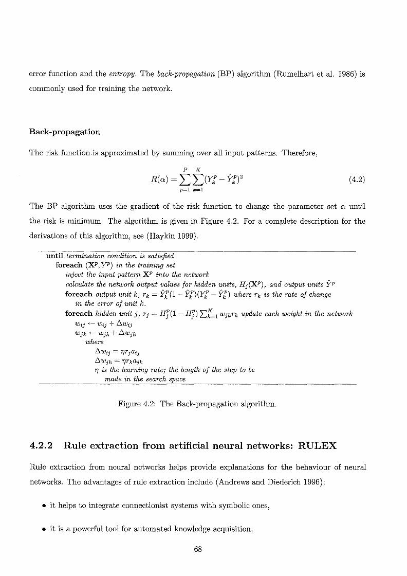
error function and the entropy. The back-propagation (BP) algorithm (Rumelhart et al. 1986) is
commonly used for training the network.
Back-propagation
The risk function is approximated by summing over all input patterns. Therefore,
P K
R(a) = LL)Yf- Yf? (4.2) p=l k=l
The BP algorithm uses the gradient of the risk function to change the parameter set a until
the risk is minimum. The algorithm is given in Figure 4.2. For a complete description for the
derivations of this algorithm, see (Haykin 1999).
until termination condition is satisfied foreach (XP, YP) in the training set
inject the input pattern XP into the network calculate the network output values for hidden units, Hj(XP), and output units YP foreach output unit k, rk = Yf(l- Yf)(Yf- Yf) where rk is the rate of change
in the error of unit k.
foreach hidden unit j, rj = Hj(l- Hj) I:f"=l Wjkrk update each weight in the network Wij +-- Wij + b..Wij Wjk +-- Wjk + b..Wjk
where b..wij = 'T]rjaij b..wjk = rJrkajk 'TJ is the learning rate; the length of the step to be
made in the search space
Figure 4.2: The Back-propagation algorithm.
4.2.2 Rule extraction from artificial neural networks: RULEX
Rule extraction from neural networks helps provide explanations for the behaviour of neural
networks. The advantages of rule extraction include (Andrews and Diederich 1996):
• it helps to integrate connectionist systems with symbolic ones,
• it is a powerful tool for automated knowledge acquisition,
68

• the rules sometimes generalise better than the networks from which they are extracted,
and
• the rules may expose previously un-recognised dependencies.
There are many techniques for rule extraction; in this thesis only one technique is described,
RULEX, which is used during the experiment. For a set of techniques, the reader may use
Andrews and Diederich (1996) as a guide. RULEX (Andrews et al. 1995) is a technique de
veloped at QUT's Machine Learning Research Centre, for extracting rules from neural networks
that have been trained by the "rapid-backprop" algorithm. Each node in the network is a local
response unit (LRU). The network is trained by adjusting the centres, widths and steepness of
the bumps ( ie. intersections of sigmoid functions inn dimension) to minimise the output error.
When training is complete, rules are extracted by a direct encoding of the response field of each
hidden unit.
There is an additional rule-refinement phase which reduces and simplifies the rules to increase
comprehensibility. The three refinement operations are negation, elimination, and absorption.
If all possible values of an attribute but one occur within a rule, negation of the absent value
is used instead. If all possible values of an attribute make the corresponding ridge active, that
attribute is eliminated because it does not contribute to discrimination. Absorption refers to the
elimination of an attribute's negation when it is redundant.
In general, RULEX depends on the LRUs' configuration. This has the disadvantage of rules be
ing local by definition and global structure may be undetectable. Nevertheless, these techniques
are easy and fast to train and the resulting refined rule set can be accurate and concise. Andrews
et al. (1995) compared a number of rule extraction techniques and found that RULEX alone did
not need parameter initialisation.
4.3 Bayesian clustering
Bayesian clustering is based on Bayes rules in statistics. Bayes theorem provides a unique
approach to assign a degree of plausibility to any proposition, hypothesis, or model. Note that
69

the Bayesian approach is not directly concerned with model creation, but with assessing a model
with respect to the available data and knowledge. Surprisingly, it can be proved, in a strict
mathematical sense using Cox-Jaynes axioms, that Bayesian inference is the only consistent way
of reasoning in the presence of uncertainty (Baldi and Brunak 1999). To describe the Bayesian
inference, let us assume a set of data D, and a model M = M ( w) parameterised over the set of
parameters W. The Bayesian theorem states that
P(MID) = P(DIM)P(M) P(D)
(4.3)
where, P(M) is called the prior probability and represents our belief or knowledge about the
model, P(DIM) is called the likelihood and represents the probability that this data set is driven
from the model, M, P(D) represents the probability of the data, and finally P(MID) represents
the posterior probability or our updated belief in the model. It is usually difficult to calculate
P(D) and since it is independent of any model, M, we can rewrite Bayesian theorem as
P(MID)aP(DIM)P(M) (4.4)
Now, let us assume two models that we would like to compare, M1 and M 2 , and that we lack any
prior knowledge about the problem; therefore it is reasonable to assume each is equally likely,
giving P(M1 ) = P(M2 ) = 0.5. In this case, maximising our posterior probability P(MID) will
be equivalent to maximising the likelihood P(DIM). This approach is called maximum likelihood
approach. It is worth mentioning that if the error in the data follows a standard normal distri
bution, a neural network with quadratic error function is equivalent to the maximum likelihood
approach (Mitchell 1997).
Auto class
Autoclass (Cheeseman and Stutz 1996) is an unsupervised clustering algorithm based on Bayes
theorem. In unsupervised learning, the task is to discover clusters or classes in the data rather
than generate class descriptions from labeled examples as in supervised learning. Autoclass is
based on the classical finite mixture distribution, which is a two-part model. In the first part,
given a data set and a probability density function, one seeks the posterior parameter values that
give the maximum interclass mixture probability that an instance belongs to the class. Instead of
70
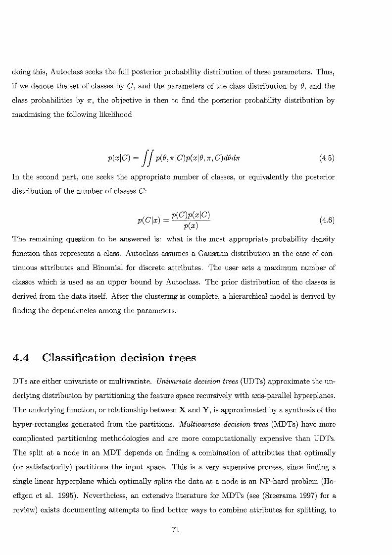
doing this, Autoclass seeks the full posterior probability distribution of these parameters. Thus,
if we denote the set of classes by C, and the parameters of the class distribution by (), and the
class probabilities by 1r, the objective is then to find the posterior probability distribution by
maximising the following likelihood
p(xiC) = j j p(e, 1riC)p(xle, 1r, C)ded1r (4.5)
In the second part, one seeks the appropriate number of classes, or equivalently the posterior
distribution of the number of classes C:
(4.6)
The remaining question to be answered is: what is the most appropriate probability density
function that represents a class. Autoclass assumes a Gaussian distribution in the case of con
tinuous attributes and Binomial for discrete attributes. The user sets a maximum number of
classes which is used as an upper bound by Autoclass. The prior distribution of the classes is
derived from the data itself. After the clustering is complete, a hierarchical model is derived by
finding the dependencies among the parameters.
4.4 Classification decision trees
DTs are either univariate or multivariate. Univariate decision trees (UDTs) approximate the un
derlying distribution by partitioning the feature space recursively with axis-parallel hyperplanes.
The underlying function, or relationship between X andY, is approximated by a synthesis of the
hyper-rectangles generated from the partitions. Multivariate decision trees (MDTs) have more
complicated partitioning methodologies and are more computationally expensive than UDTs.
The split at a node in an MDT depends on finding a combination of attributes that optimally
(or satisfactorily) partitions the input space. This is a very expensive process, since finding a
single linear hyperplane which optimally splits the data at a node is an NP-hard problem (Ho
effgen et al. 1995). Nevertheless, an extensive literature for MDTs (see (Sreerama 1997) for a
review) exists documenting attempts to find better ways to combine attributes for splitting, to
71

prune resultant trees, to deal with missing values, and to handle noisy inputs.
Optimisation and statistical methods play a significant role in the determination of MDTs.
Breiman et al. (1984) was one of the first to develop methods for generating MDTs by intro
ducing Classification and Regression Trees. Brown and Pittard (1993) use a linear programming
formulation for each class at each node to determine the variable mix required to optimally
split the data. However, this is computationally very expensive. Another attempt was made
to formulate MDTs as an optimisation model, by Bennett (1994), which has the advantage of
determining all splits simultaneously but with the disadvantage of a resultant non-linear opti
misation model. The model solutions in cases of high dimensionality are very difficult and time
consuming especially since the objective function is usually non-differentiable. In an attempt to
overcome this drawback, a Tabu-based algorithm was suggested by Bennett and Blue (1997) in
which a re-formulation of the optimisation model is employed to optimise an existing decision
tree rather than generating the tree from scratch. Although the model results in a tree with
higher accuracy, it does not guarantee a globally optimal tree structure.
C5
C5 (Quinlan 1997), is a supervised-learning decision tree classifier and an enhancement of the
earlier version C4.5 (Quinlan 1993). C5 maximises information gain by branching on that at
tribute which minimises an entropy function. Most importantly, the default parameter settings
for C5 are extremely robust in that, they yield good results for a wide range of problem domains
and data sets. Having constructed a complete decision tree, C5 proceeds to extract rules. It
suffers the disadvantage that if the data is separable by a function such as x < y for two at
tributes x and y, 100% accuracy is achievable only with a tree of infinite size because C5 synthesis
the decision boundary with hyper-rectangles. Furthermore, redundancies in the training set can
cause difficulties for C5.
72

4.5 The dairy database
The objective of the experiments to be presented is to predict the expected progeny milk pro
duction from any given mating. The original data set is obtained from the Australian Dairy
Herd Improvement Scheme. The data set consists of 48 text files containing both raw and sum
mary data of milk production in dairy herds around Australia. The subset of data used in this
thesis applies to Holstein dairy cattle from the State of Victoria. Records are filtered to remove
those containing incomplete milk volume, fat and protein data, those records that lacked sire
and dam information, and also to include only those records where the number of test days per
lactation is greater than seven (a reliability measure). An exploratory data technique, principal
component analysis 1, is carried out on the resultant data set to determine which variables are
to be included in the final feature set. This analysis indicated that some of the variations in
the predictor can be explained by the dam season of calving. As a result, the final feature set
includes dam second lactation milk volume SLMV, sire ABV for milk, dam herd mean milk yield
excluding first lactation and dam season of calving (autumn, summer, winter, spring).
Data pre-processing
It is common practice in the dairy industry to correct milk production values for age (Schmidt
and Van-Vleck 1974), since mean production yields vary with age at lactation. The production
traits are corrected for the effect of age and the season of calving is included as an input since
it was difficult to identify its trend from the available data. Consequently, the features dam
SLMV and the daughter first lactation milk volume (FLMV) required to be corrected for age.
The correction factor, CF, is calculated as
CF = MV(mature) MV(group)
(4.7)
where MV(mature) is the average milk volume (MV) of all mature cows aged 5 to 7 years
(when production is at a peak) and MV(group) is the average MV of all cows in the age group
being corrected. Cows are grouped by age where each age group is of one year length. In Fig
ure 4.3, the average dam lactation milk volume (LMV) as a function of age (in months) before
1The principal component analysis was done by Paula Macrossan (2000).
73
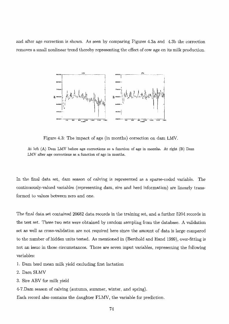
and after age correction is shown. As seen by comparing Figures 4.3a and 4.3b the correction
removes a small nonlinear trend thereby representing the effect of cow age on its milk production.
(A)
eo ;oo 120 140 ;eo AGE
(B)
eo 100 120 ;4o 100 AQE
Figure 4.3: The impact of age (in months) correction on dam LMV.
At left (A) Dam LMV before age corrections as a function of age in months. At right (B) Dam
LMV after age corrections as a function of age in months.
In the final data set, dam season of calving is represented as a sparse-coded variable. The
continuously-valued variables (representing dam, sire and herd information) are linearly trans
formed to values between zero and one.
The final data set contained 20682 data records in the training set, and a further 5204 records in
the test set. These two sets were obtained by random sampling from the database. A validation
set as well as cross-validation are not required here since the amount of data is large compared
to the number of hidden units tested. As mentioned in (Berthold and Hand 1999), over-fitting is
not an issue in these circumstances. There are seven input variables, representing the following
variables:
1. Dam herd mean milk yield excluding first lactation
2. Dam SLMV
3. Sire ABV for milk yield
4-7.Dam season of calving (autumn, summer, winter, and spring).
Each record also contains the daughter FLMV, the variable for prediction.
74

4.6 Experiment (1): Mining for predictive models
Mining for predictive models is not an easy task for two reasons. (1) There is no general algo
rithm that can ascertain in advance whether linear model is more suitable than a nonlinear one
for the data. (2) Even if the data fits a nonlinear model better than a linear one, "what is the
best nonlinear model that should be used to fit the date" is still a hard question. Consequently,
experimenting with techniques such as neural networks appears to be a logical solution even
though they are computationally expensive.
The problem of predicting the daughter milk production from sire and dam production records
appears to have many characteristics which might make an ANN solution more attractive than
that obtained using other machine learning paradigms. ANNs have a tolerance to both noise
and ambiguity in data (Widrow et al. 1994). The dairy data, like other agricultural data, is
noisy due to many random and unpredictable effects. The database contains indicators repre
senting genetic and environmental influences (Finn et al. 1996). ANNs are able to approximate
non-linear relationships between sets of inputs and their corresponding sets of outputs (Lacroix
et al. 1994). The dairy data could be expected to better fit a non-linear model. The ability of
ANNs to generalise well (Rumelhart et al. 1994) and to learn concepts involving real-valued fea
tures (Dietterich 1990) are potential advantages with this exercise, since the predicted daughter
responses are continuous variables.
4.6.1 Methods
Two approaches are compared here: MLPs and multiple linear regression (MLR) (Abbass et al.
1999). There are many statistical techniques more sophisticated than MLR such as generalised
linear models (Berthold and Hand 1999). However, MLR was used as a simple benchmark tech
nique. The full training set of 20682 records is used for model's construction in both approaches,
with the full test set of 5204 records used to verify the predictions obtained.
The data are modeled using an MLP with seven input units, one for each data input, one hidden
layer of 1, 2, 3, or 4 logistic units, and a single output unit representing daughter first milk
75
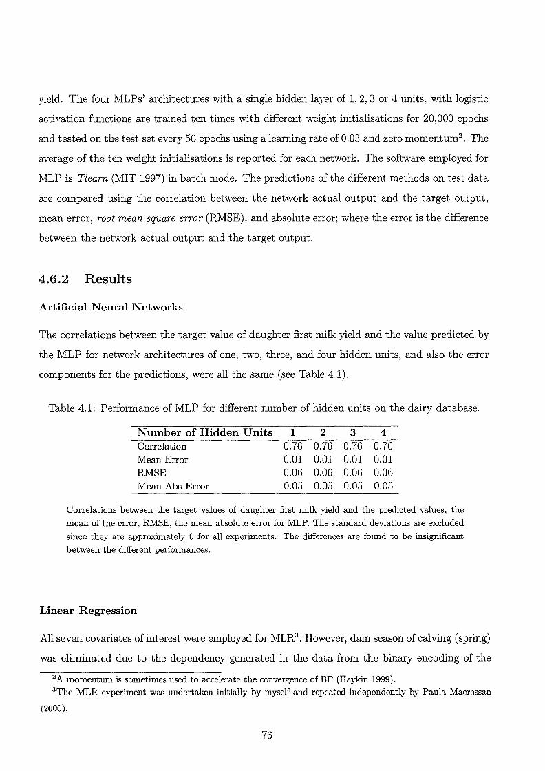
yield. The four MLPs' architectures with a single hidden layer of 1, 2, 3 or 4 units, with logistic
activation functions are trained ten times with different weight initialisations for 20,000 epochs
and tested on the test set every 50 epochs using a learning rate of 0.03 and zero momenturn2 . The
average of the ten weight initialisations is reported for each network. The software employed for
MLP is Tlearn (MIT 1997) in batch mode. The predictions of the different methods on test data
are compared using the correlation between the network actual output and the target output,
mean error, root mean square error (RMSE), and absolute error; where the error is the difference
between the network actual output and the target output.
4.6.2 Results
Artificial Neural Networks
The correlations between the target value of daughter first milk yield and the value predicted by
the MLP for network architectures of one, two, three, and four hidden units, and also the error
components for the predictions, were all the same (see Table 4.1).
Table 4.1: Performance of MLP for different number of hidden units on the dairy database.
Number of Hidden Units 1 2 3 4 Correlation 0.76 0.76 0.76 0.76 Mean Error 0.01 0.01 0.01 0.01 RMSE 0.06 0.06 0.06 0.06 Mean Abs Error 0.05 0.05 0.05 0.05
Correlations between the target values of daughter first milk yield and the predicted values, the
mean of the error, RMSE, the mean absolute error for MLP. The standard deviations are excluded
since they are approximately 0 for all experiments. The differences are found to be insignificant
between the different performances.
Linear Regression
All seven covariates of interest were employed for MLR3 . However, dam season of calving (spring)
was eliminated due to the dependency generated in the data from the binary encoding of the
2 A momentum is sometimes used to accelerate the convergence of BP (Haykin 1999). 3The MLR experiment was undertaken initially by myself and repeated independently by Paula Macrossan
(2000).
76
seasonal effects.
MLR gave similar results as MLP. The correlation coefficient between the target values of daugh
ter first milk yield and the predicted values was 0.76, the error mean was almost 0, the RMSE
0.06, and the mean absolute error 0.05.
4.6.3 Discussion
Two main conclusions arise from the studies carried out in this experiment. First, the data fits a
linear model (MLR) as accurate as a nonlinear model (MLP), which did not improve the predic
tive accuracy of the model. Therefore, both approaches (MLP and MLR) are equivalent in terms
of their predictive accuracy on the dairy data, as indicated by a test of correlation coefficients
between target and predicted value of daughter first milk yield.
Second, it is apparent from this study that each different method has its own distinctive advan
tages. On the one hand, linear regression provides straightforward descriptions of the relationship
being portrayed, and some quantification of the importance of each input attribute, by way of
the coefficients in the linear equation. On the other hand, the MLP approach supported our
belief that the data fits a linear model as good as a nonlinear one.
Experimenting with neural networks is a very costly task in terms of both time and computational
complexity. Usually, people see this as a disadvantage of neural network although (Elder and
Pregibon 1996) shows that this is an advantage. In their comments about neural networks Elder
and Pregibon wrote,
"... they appear so over-parameterised, and the weight adjustment procedure is
a local gradient method, sequential, and interminable (leading to a crude type of
regularisation wherein moderating the runtime becomes the principle way to avoid
overfit). However, these weaknesses cancel somewhat, as the slow, local search does
not allow the excess of parameters to be overfit easily. . . . The danger of overfit can
depend on the training duration, since many random node weights lead to essentially
linear functions (nodes operating in either the middle or an extreme of the sigmoid)
and such linear functions are absorbed by subsequent layers. Only as nodes get
pushed into the curved part of the sigmoids during training do many parameters
77
become active. (This may explain the common observation that the performance
of an MLP on a problem is often surprisingly robust with respect to changes in its
network structure)."
4.7 Experiment (2): Automated knowledge acquisition
In KDD-IDSS, the system requires continuous source of knowledge to update the knowledge base.
The expert is a subjective and expensive source of knowledge. This experiment's objective is
to use machine learning tools to automate the knowledge acquisition process. The experiments
are carried out in two stages. In the first stage, the attributes are discretised using Autoclass
(presented in Section 4.3). In the second stage, a comparison between RULEX (presented in
Section 4.2.2) and C5 (presented in Section 4.4) is carried out to select the suitable technique.
4. 7.1 Methods
In this experiment, the four attributes used in the previous experiment, herd not FLMV ( ie.
all lactations excluding the first), sire ABV milk, dam SLMV, and the season of calving, are
preserved here. Autoclass is used to categorise daughter FLMV. However, Autoclass defines its
clusters using the mean and standard deviation of a Gaussian distribution. In order to obtain the
boundary, b, between any two classes having means fJ-1 and fJ-2 (fJ-2 > fJ-1) and standard deviations
0"1 and 0"2 respectively, the following formula was used (Abbass et al. 1999):
(4.8)
Then, the sets of rules obtained are compared using two types of inputs representation, contin
uous and discrete, using Autoclass and two types of rule induction algorithm, RULEX and C5.
Comparisons are based on three criteria: the rule set accuracy, the number of rules and the aver
age number of antecedents per rule. Rule set accuracy is determined by calculating the average
of precision and recall for each output class. Precision is defined as the percent of positive cases
correctly classified in the class to the total number of cases classified as positive. Recall is the
percentage of positive cases correctly classified in the class to the total number of positive cases
originally belonging to this class (Witten and Frank 2000).
78

The number of rules and average number of antecedents per rule affords an objective measure
of rule set comprehensibility. Comparisons between C5 and RULEX are difficult in this regard
because, unlike C5, RULEX combines rules using disjunctions and negations. To make compar
isons more fair, the rule refinement step of RULEX is reversed by decomposing disjunctive rules
into simpler elemental rules.
For example, a rule of the form "if (V or W) and (X or Y) then Z" consists of four elemental
rules after Boolean operator distribution. A trade-off between the three criteria reflects gen
eralisation. For example, in the average class for the discrete case in Table 4.4, the accuracy
of RULEX at 48% is 12% more than C5 but at the cost of having additional 121 rules (134
versus 13). In knowledge basis, it is important to balance between the accuracy of prediction
and comprehensibility or the number of rules used for prediction. Accordingly, we claim that C5
is better in this case than RULEX even though it has slightly lower accuracy.
4.7.2 Results
Table 4.2 presents a summary description of the categorisation of continuous variables resulting
from Autoclass. The attributes average herd MV, dam SLMV, sire ABV and daughter FLMV
are divided into 6, 5, 7, and 3 categories respectively. Accuracy and comprehensibility results
for the rule sets extracted by C5 and RULEX are shown in Tables 4.3 and 4.4 for continuous
and discrete inputs respectively.
In most cases, the accuracy of the rule sets produced with continuous and discrete inputs are
similar. Only in one discrete case is there a major difference (the "average" class in Table 4.4).
There are however, quite distinct differences in the numbers of rules. RULEX produces more
rules when the inputs are discrete (Column 4 in Table 4.4) and C5 produces more rules when
the inputs are continuous (Column 4 in Table 4.3). Accordingly, in terms of comprehensibility,
RULEX has the advantage with continuous data, whereas C5 holds advantage with discrete data.
79

Table 4.2: Summary of data categorisation using Autoclass.
Class Upper bound Frequencies (%) Herd milk Average Volume Low 4794 24 Below Average 5306 20 Average 5613 12 Above Average 5986 14 High 6300 10 Very High N/A 20 Dam SLMV Low 4346 13 Below Average 5039 14 Average 5830 20 Above Average 6350 13 High N/A 40 Sire ABV Milk Very Low 278 02 Low 623 12 Below Average 735 11 Average 842 12 Above Average 1108 24 High 1475 26 Very High N/A 13 Daughter FLMV Low 4632 44 Average 5624 30 High N/A 26
Table 4.3: Results of classification with continuous inputs.
Output Classifier accuracy number of average number of Class rules antecedents per rule Low (44%) RULEX 75 2 3
C5 75 28 4 Average ( 30%) RULEX 39 4 3
C5 41 43 5 High (26%) RULEX 53 3 3
C5 65 21 3
80

Table 4.4: Results of classification with discrete inputs.
Output Classifier accuracy number of average number of Class rules antecedents per rule Low (44%) RULEX 76 36 3
C5 76 12 2 Average ( 30%) RULE X 48 134 4
C5 36 13 3 High (26%) RULEX 66 30 3
C5 65 6 2
4. 7.3 Discussion
The human domain expert preferred the rule sets derived from discrete variables even in cases
where there are more rules for discrete. The domain expert's opinion is that, where rules are
to be used to support a decision, it is semantically easier to employ category labels rather than
numeric intervals. For example, a rule such as "if the herd milk average is low then the daughter
milk production is low" is easier for the user to appreciate than "if the herd milk average <
4 794 then the daughter milk production < 4632". Additionally, the expert noted that rules with
discretised variables remain valid even if improvements in breeding and management practices
increase absolute animal yields and therefore change the boundaries determining the categories.
Consequently, we judge that discrete inputs are more convenient in our case.
As noted above, C5 performs better than RULEX on the discretised data, the preferred method
of data representation by the domain expert. This leads to selection of C5 as the classifier for
the knowledge base in the KDD-IDSS. RULEX has the disadvantage that it is restricted to
learning two class problems. For problems with more than two classes as in this case, a sep
arate neural network must be trained for each class, adding considerably to the computation
effort, therefore each record is classified a number of times. Where contradictions exist among
a record's intermediate classification, some sort of conflict resolution is required. C5 by contrast
can handle classification problems involving large numbers of classes. The data discretisation
did not vary the prediction accuracy much. Therefore, the results are insensitive to discretisation.
To summarise, C5 appears to be more suitable than RULEX for this application, because it
81

produces smaller and more comprehensible rules sets and performs well with a default set of
parameters, therefore obviating the need for user interaction. The set of rules generated by C5
are included in Appendix A. We may notice that the order of rules is important in C5.
4.8 Conclusion
In this chapter, two experiments are carried out to estimate the expected daughter's milk volume
giving information about the dam, sire, and environment. The estimation problem scrutinised
in the two experiments is investigated as both a point and an interval estimation problem.
This chapter emphasises the second thesis sub-objective; discovering patterns in the dairy database
using KDD. The experiments presented in this chapter inspire a new method for generating mul
tivariate decision trees. This new method is the context of the next chapter. The rest of the
thesis will then discuss the third thesis sub-objectives; that is, formulating and solving the mate
selection problem.
82

Chapter 5
C-Net: A new Method for Generating
Non-deterministic and Dynamic
Multi-variate Decision Trees
The following refereed publication arose out of this chapter and the contribution of the other
authors are mentioned in the relevant places
H.A. Abbass, M. Towsey, and G. Finn. ((C-Net: A Method for Generating Non-deterministic and
Dynamic Multi-variate Decision Trees". Knowledge and Information Systems (KAIS), Springer
Verlag, accepted for a forthcoming issue.
Although ANNs are universal function approximators, their "black box nature" (that is, their
lack of direct interpretability or expressive power) limits their utility. In contrast, UDTs have
expressive power, although usually they are not as accurate as ANNs. An improvement, C-Net,
is proposed for both the expressiveness of ANNs and the accuracy of UDTs by consolidating
both technologies for generating MDTs. Additionally, a new concept, recurrent decision trees, is
introduced, where C-Net uses recurrent neural networks to generate an MDT with a recurrent
feature. That is, a memory is associated with each node in the tree with a recursive condition
which replaces the conventional linear one.
Furthermore, it will be shown empirically that, in test cases, the proposed method achieves a
balance of comprehensibility and accuracy intermediate between ANNs and UDTs. MDTs are
83
found to be intermediate since they are more expressive than ANNs and, more accurate than
UDTs. Furthermore, in all cases MDTs are more compact ( ie. smaller tree size) than UDTs.
The importance and motivation of this algorithm are introduced in Section 5.1 followed by pre
vious work in combining ANNs and DTs in Section 5.2 and the C-Net algorithm in Section 5.3.
In Section 5.4, experimental results and comparisons are presented and the recurrent version of
C-Net is then scrutinised in Section 5.5. Conclusions are drawn in Section 5.6.
5.1 Motivation and importance of C-Net
Since the introduction of constraint logic programming in 1986 (Jaffer and Lassez 1986), con
straints have become an acceptable form for both knowledge representation and reasoning. In
some domains, the representation of attributes in symbolic format is neither efficient nor natural.
For example, in the galaxy classification problem of Sreerama (1997) it is more natural to relate
coordinates of the image with a mathematical relation. Additionally, one can sometimes inter
pret the constraints as logical formulae when the variables are binary. For example, if X 1 and
X 2 are two binary variables, X 1 + X 2 2: 1 is equivalent to the logic function OR. This motivates
the research into multivariate classification trees where a condition on a node is represented by
a linear combination of some, or all of the attributes.
In this chapter, a simple novel algorithm, C-Net, is proposed for generating MDTs from ANNs.
In the implementation, Quinlan's C5 (an enhancement of his earlier C4.5 (Quinlan 1993)) is
employed for constructing UDTs. The algorithm employs the gain ratio calculated by C5 to
compute a composite variable, to engineer a decision split at a node. The algorithm has three
stages. Firstly, a single hidden layered ANN is trained on a suitable training set until perfor
mance is deemed to be satisfactory. Secondly, the training set is presented once more to the
now-trained ANN but the outputs of the hidden units become the input feature vector to C5,
with the target output still playing its usual role in defining the hypothesis space. Thirdly, the
UDT in the new feature space of hidden unit outputs is readily converted to an MDT in the
original feature space X.
84
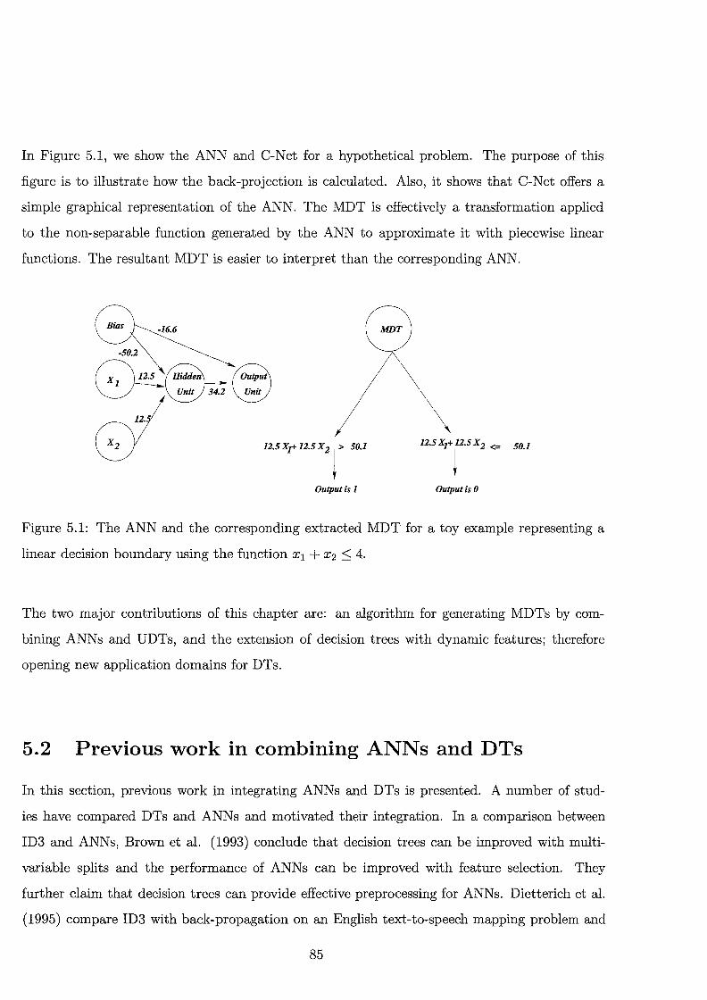
In Figure 5.1, we show the ANN and C-Net for a hypothetical problem. The purpose of this
figure is to illustrate how the back-projection is calculated. Also, it shows that C-Net offers a
simple graphical representation of the ANN. The MDT is effectively a transformation applied
to the non-separable function generated by the ANN to approximate it with piecewise linear
functions. The resultant MDT is easier to interpret than the corresponding ANN.
G
12.5 X.z+ 12.5 X 2 ~ > 50.1
Output is 1
\
125 x,T.s x, ¢ so.1
Output is 0
Figure 5.1: The ANN and the corresponding extracted MDT for a toy example representing a
linear decision boundary using the function x1 + x 2 ::; 4.
The two major contributions of this chapter are: an algorithm for generating MDTs by com
bining ANNs and UDTs, and the extension of decision trees with dynamic features; therefore
opening new application domains for DTs.
5.2 Previous work in combining ANNs and DTs
In this section, previous work in integrating ANNs and DTs is presented. A number of stud
ies have compared DTs and ANNs and motivated their integration. In a comparison between
ID3 and ANNs, Brown et al. (1993) conclude that decision trees can be improved with multi
variable splits and the performance of ANNs can be improved with feature selection. They
further claim that decision trees can provide effective preprocessing for ANNs. Dietterich et al.
(1995) compare ID3 with back-propagation on an English text-to-speech mapping problem and
85

find that ANNs capture statistical information whereas ID3 does not. They argue that the two
methods' accuracy is comparable if ID3 is augmented with a simple statistical learning procedure.
One form of the integration is to grow an ANN as a DT using Neural-trees. Neural-trees are
ANNs of restricted structure that can be easily interpreted as DTs. The Neural-tree algorithm
(Sirat and Nadal 1990) is inspired by the tiling algorithm but with connections among neurons
in the hidden layers disallowed. The resultant network can be visualised as a DT whose nodes
correspond directly to hidden units. An improvement on Neural-trees, called Trio-Learning, was
introduced by D'Alche-Buc et al. (1994) who utilised the fact that each intermediate node in
the tree has two child nodes. Accordingly, training is carried out on a small tree consisting of a
root node and its two child nodes. The results are slightly better than those of the Neural-Tree
algorithm although at the expense of more extensive computations at each node.
Another way to integrate DTs and ANN s is to initialise the latter with the former in order to
expedite and improve the convergence of ANN training. A version of ID3, called continuous
ID3 (Cios and Liu 1992), converts UDTs into ANNs. Each level in the tree generated by ID3 is
mapped to a hidden layer in the ANN being constructed but for large UDTs, the corresponding
ANN architecture becomes impractical. In another attempt to speed up ANN training, Park
(1994) introduced an algorithm for initialising an ANN with a linear tree classifier. The algo
rithm maps any linear tree classifier into an ANN with either one or two hidden layers. He has
shown that every convex decision region enclosed by a subset of explicit hyperplanes of a tree,
can be mapped to a neuron in the hidden layer. From my point of view, this is a very expensive
process since the number of convex decision regions is exponential in the number of hyperplanes.
Finally, oblique rules have been generated from ANNs by Setiono and Huan (1995) who intro
duced a three-phase algorithm for extracting oblique rules from single hidden-layer ANNs. In the
first phase, a network is trained with a weight decay term, and pruned in the second phase, with
the activation values of hidden units discretised with a clustering algorithm in a third phase.
The extraction process becomes easy after discretisation with rules effectively generated. The
algorithm is computationally expensive at both the pruning and discretisation phases. As an
enhancement, in a later paper (Setiono and Huan 1997) they re-present the training set to the
86

ANN after the training is completed, when outputs from the hidden units are discretised by a
clustering algorithm using the statistical x2 test.
Maire (1999) introduced a general algorithm with a solid theoretical foundation, in terms of opti
misation theory, for back projection of a set of polyhedra that define decision regions. He utilises
a threshold selected by the user for the ANN, which determines whether the instance belongs to
a positive or a negative class. This threshold is used as a constraint on the output unit and by
back projection of this constraint through the network, polyhedra are determined. He proposes
discretising the polyhedra after projecting back to the input layer. The main advantage is that
this delayed discretisation guarantees high fidelity between the network and the resultant rules.
The salient drawback of this algorithm, regardless of its generality and theoretical foundation,
is the computational effort involved. For example, during the affine transformation phase in the
algorithm, one of the steps requires the removal of redundant inequalities. Computationally,
this is very expensive since for each inequality, a system of constraints should be solved to check
whether or not the inequality is redundant. Even with fast algorithms for solving linear program
ming (Ami 1993) or employing sensitivity analysis, the computations involved are still expensive.
In summary, most of the integration between DTs and ANN s takes the form of growing ANN s
as DTs and only a few studies concentrate on extracting oblique rules from ANNs. To my
knowledge, none of the previous studies investigated the use of UDTs to generate MDTs from
ANNs. Furthermore, integration efficiency is an outstanding issue and there remains the need
for a simple, efficient algorithm for extracting oblique relations from an ANN which retains high
fidelity with the network.
5.3 The C-net algorithm
The proposed algorithm, C-Net, has three stages and employs an ANN with a single hidden layer
which is not a severe constraint since a neural network with a single hidden layer can approximate
any arbitrary function to any degree of accuracy (Irie and Miyake 1988). There is no constraint
on the type of the activation functions employed.
87
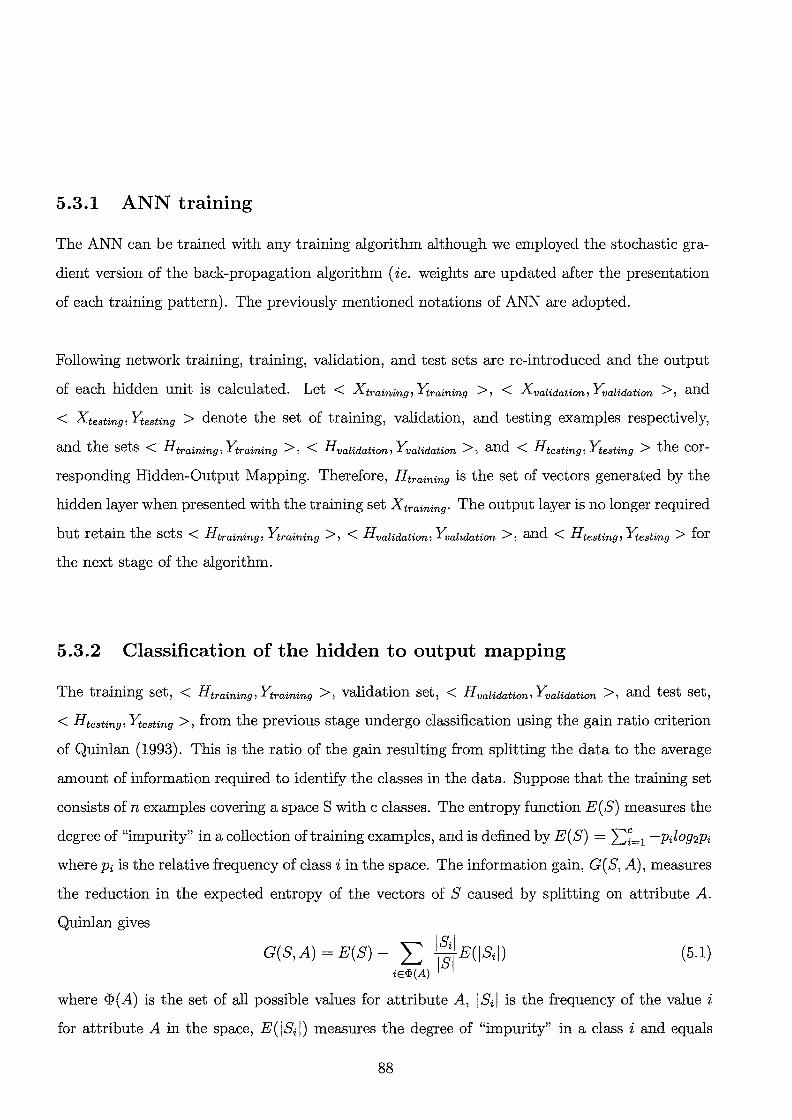
5.3.1 ANN training
The ANN can be trained with any training algorithm although we employed the stochastic gra
dient version of the back-propagation algorithm ( ie. weights are updated after the presentation
of each training pattern). The previously mentioned notations of ANN are adopted.
Following network training, training, validation, and test sets are re-introduced and the output
of each hidden unit is calculated. Let < Xtraining, Y'training >, < Xvalidation, Yvalidation >, and
< Xtesting, Ytesting > denote the set of training, validation, and testing examples respectively,
and the sets < Htrainin9 , Y'training >, < Hvalidation, Yvalidation >, and < Htestin9 , Y'testing > the cor-
responding Hidden-Output Mapping. Therefore, Htraining is the set of vectors generated by the
hidden layer when presented with the training set Xtraining· The output layer is no longer required
but retain the sets < Htrainin9 , Y'training >, < Hvalidatian, Yvalidation >, and < Htesting, Y'testing > for
the next stage of the algorithm.
5.3.2 Classification of the hidden to output mapping
The training set, < Htraining, Y'training >, validation set, < Hvalidation' Yvalidation >, and test set,
< Htesting, Ytesting >, from the previous stage undergo classification using the gain ratio criterion
of Quinlan (1993). This is the ratio of the gain resulting from splitting the data to the average
amount of information required to identify the classes in the data. Suppose that the training set
consists of n examples covering a space 8 with c classes. The entropy function E(S) measures the
degree of "impurity" in a collection of training examples, and is defined by E(S) = 2.:::~= 1 -pilog2pi
where Pi is the relative frequency of class i in the space. The information gain, G(S, A), measures
the reduction in the expected entropy of the vectors of S caused by splitting on attribute A.
Quinlan gives
'"""' ISil G(S, A) = E(S)- L.. ISTE(ISil) iE1>(A)
(5.1)
where <I>(A) is the set of all possible values for attribute A, jSil is the frequency of the value i
for attribute A in the space, E(jSij) measures the degree of "impurity" in a class i and equals
88

-pilog2pi, and we use lSI to denote 2.: ISil· However, this measure is biased toward attributes
with many values (Mitchell1997) since splitting on these attributes results in a higher value of the
information gain because of the decrease in the number of instances in each subset. Subsequently,
Quinlan adopted the gain ratio, R = fj, where T is the information split criterion which measures
how broadly and uniformly the attribute splits the data and is given by
(5.2)
5.3.3 Back projection of decision trees
A DT is a disjunction of polyhedra where each polyhedron is a conjunction of linear constraints.
In the resultant decision tree from the previous section, each constraint takes the form Hi ::;
RHSj, where RHSj is a scalar specifying the split on that attribute and Hi is the output of
hidden unit j as defined previously. To project back this axis-parallel hyperplane, the inverse of
RH Si is calculated viz o--1 ( RH Si) and Hi is replaced by the weighted sum of the corresponding
input units, that is
I
L wijxi::; o--1(RHSj) (5.3) i=1
It is obvious that projecting back an axis-parallel hyperplane is computationally less expensive
than projecting back an oblique hyperplane as in (Maire 1999) since the former one generates two
halfspaces while the latter results in a set of polyhedra. In our implementation, the activation
function is taken to be the logistic function where the inverse is,
1 1- z o--1 (z) =-Dln(-z-), z =J 0 (5.4)
As an example, assume that one of the conditions on a node is H1 ::; 0.5, where H 1 = o-(3 x X 1 -
4 x X 2 + 3). Since o--1 (0.5) = 0, the condition on the node will be (3 x X 1)- (4 x X 2) ::; -3 or
equivalently ( -3 x X 1) + ( 4 x X 2) > 3.
89

5.4 Experiments and comparisons
5.4.1 Methods and performance measures
The three stages in the algorithm are summarised in Figure 5.2 where we use C5, with standard
parameters settings and without pruning, for discretising the hidden-output mapping. The acti
vation function for the neural network is the sigmoid with a sharpness of 1.
• Train a neural network with < X training, rtraining >, until it reaches a satisfactory
performance on < Xvalidatiom Yvalidation > ·
• {1} Re-present< Xtraining, rtraining >, < Xvalidation, Yvalidation >, and
< Xtesting, Ytesting > to the trained network and store < Htraining, rtraining >,
< Hvalidation, Yvalidation >, and< Htesting, Ytesting >.
(2} Train C5 with< Htraining, rtraining > and< Hvalidation, Yvalidation >.
{3} Test C5 with< Htesting, Ytesting >.
• Replace each condition in the resultant UDT, (Hj op RHSj),
opE{::;,<, 2:, >, = }, with (l:{=1 WijXi op ()- 1 (RHSj)),
Figure 5.2: The C-Net algorithm
0 0 0 : ~ cs
Output ' '
'0/ UDTLayer (Output Layer)
Hidden Input Layer Layer
Figure 5.3: The C-Net conceptual representation.
To clarify this chapter's essential concepts, two types of comprehensibility are distinguished. The
90
first type, expressiveness, refers to the human brain's ability to understand the representational
language of the classifier. The second, compactness, refers to the ability of representing a system
with the minimum number of relations and symbols. Compactness is similar to the minimum
description length principle (Quinlan and Rivest 1989) if we consider the message as the system
and the string as a single relation to be transformed. It is clear that UDTs are more expressive
than ANNs, since their representational language can easily be transferred into a set of "If ...
Then" rules which are easily interpretable by the human brain. However, ANNs usually produce
more accurate results than UDTs (Quinlan 1993) and they are also more compact.
Two performance measures have been used for the comparison between C5 and C-Net:
1. The percent bit error; that is, the percentage of misclassified cases on the test set. This
measures the generalisation accuracy of the algorithm.
2. The tree size or the number of paths in the tree which is a measure of compactness and is
equivalent to the number of paths (or leaves) in the DT (without pruning).
5 .4. 2 Data sets and experimental setup
Firstly, four real-life data sets were used to test C-Net. Three of these - Liver, Haberman,
and Wisconsin Breast Cancer data sets- were down-loaded from the UCI repository of machine
learning (Murphy and Aha 1992). The fourth data set is the dairy data. Each of the three
UCI data sets were divided into a training, validation, and test sets consisting of 80%, 10%,
and 10% of the data respectively (Quinlan 1993). The dairy data was divided into 25%, 25%,
and 50% for training, validation, and testing respectively. Ten-fold cross-validation 1 was used
while maintaining the class-distribution in the training, validation, and test sets. For the dairy
data, the ten-fold were generated by sampling from the data at random without replacement. In
Table 5.1, some statistics about the four data sets are summarised.
Secondly, the effectiveness of the C-Net algorithm on the following polynomials, which define the
1In cross-validation, the data is divided into ten subsets and the experiments are repeated ten times with each
of these subsets as the test set and the other nine divided into one for validation and eight for training.
91

Table 5.1: Summaries of statistics for the real life databases
Database Number of Number of The domain of instances input attributes each attribute
Breast Cancer 699 9 discrete values 1-10 Haberman 306 3 discrete values
Liver 345 6 continuous values Dairy 25985 3 continuous values
decision boundary of the classification problem, are examined:
{
1, if x1 + x~ 2: 4, y=
0, if x1 + x~ < 4. (5.5)
for n = 2, 3, 4, or 5, forming the problems P2, ... , P5. Each variable, X 1 and X 2 , is sampled from
independent uniform distributions in the interval [0,5] subject to the constraint, 3 ::;: x1 + x~ ::;: 5
so that the data are intensively sampled around the class boundary. A data set with 4000 points
was generated for each model. Ten-fold cross-validation was adopted where the training, valida
tion, and test sets contained 80%, 10%, and 10% of the data, respectively, while maintaining the
class-distribution in the three sets.
For all problems, a learning rate of 0.03 and zero momentum were used for training four ANNs ar
chitectures with 2, 3, 4, and 5 hidden units. The networks for each of the 10-fold cross-validations
were initialised with different weights, randomly drawn from independent uniform distributions
in the range [-0.1, 0.1]. Each network ran for 10,000 epochs with validation performed after each
epoch and the network with the smallest error on the validation set over all epochs was chosen.
After ANN training is completed the training, validation, and test sets were re-presented to the
trained network, and the hidden output mapping was generated for subsequent presentation to
C5 to generate the MDT.
5.4.3 Results and discussion
In Table 5.2, the performance of C-Net, C5, and ANN, on the eight data sets, is shown. The
ANN, and its corresponding C-Net, shown in the table is the one whose number of hidden units
92
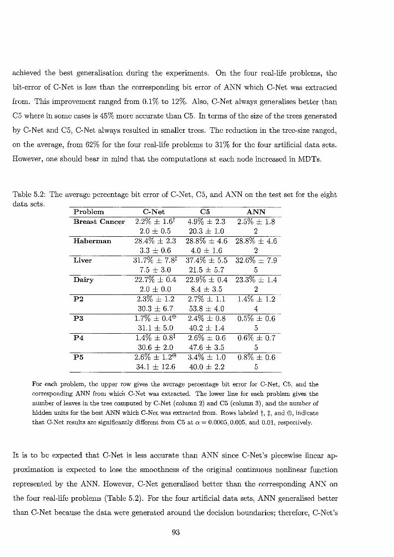
achieved the best generalisation during the experiments. On the four real-life problems, the
bit-error of C-Net is less than the corresponding bit error of ANN which C-Net was extracted
from. This improvement ranged from 0.1% to 12%. Also, C-Net always generalises better than
C5 where in some cases is 45% more accurate than C5. In terms of the size of the trees generated
by C-Net and C5, C-Net always resulted in smaller trees. The reduction in the tree-size ranged,
on the average, from 62% for the four real-life problems to 31% for the four artificial data sets.
However, one should bear in mind that the computations at each node increased in MDTs.
Table 5.2: The average percentage bit error of C-Net, C5, and ANN on the test set for the eight data sets.
Problem C-Net C5 ANN Breast Cancer 2.2% L6t 4.9% ± 2.3 2.5% ± 1.8
2.0 ± 0.5 20.3 ± 1.0 2 Haberman 28.4% ± 2.3 28.8% ± 4.6 28.8% ± 4.6
3.3 ± 0.6 4.0 ± 1.6 2 Liver 31.7% ± 7.8+ 37.4% ± 5.5 32.6% ± 7.9
7.5 ± 3.0 21.5 ± 5.7 5 Dairy 22.7% ± 0.4 22.9% ± 0.4 23.3% ± 1.4
2.0 ± 0.0 8.4 ± 3.5 2 P2 2.3% ± 1.2 2.7% ± 1.1 1.4% ± 1.2
30.3 ± 6.7 53.8 ± 4.0 4 P3 1.7% ± 0.4E9 2.4% ± 0.8 0.5% ± 0.6
31.1 ± 5.0 40.2 ± 1.4 5 P4 1.4% ± 0.8* 2.6% ± 0.6 0.6% ± 0.7
30.6 ± 2.0 47.6 ± 3.5 5 P5 2.6% ± 1.2E9 3.4% ± 1.0 0.8% ± 0.6
34.1 ± 12.6 40.0 ± 2.2 5
For each problem, the upper row gives the average percentage bit error for C-Net, C5, and the
corresponding ANN from which C-Net was extracted. The lower line for each problem gives the
number ofleaves in the tree computed by C-Net (column 2) and C5 (column 3), and the number of
hidden units for the best ANN which C-Net was extracted from. Rows labeled t, t, and EB, indicate
that C-Net results are significantly different from C5 at o: = 0.0005, 0.005, and 0.01, respectively.
It is to be expected that C-Net is less accurate than ANN since C-Net's piecewise linear ap
proximation is expected to lose the smoothness of the original continuous nonlinear function
represented by the ANN. However, C-Net generalised better than the corresponding ANN on
the four real-life problems (Table 5.2). For the four artificial data sets, ANN generalised better
than C-Net because the data were generated around the decision boundaries; therefore, C-Net's
93
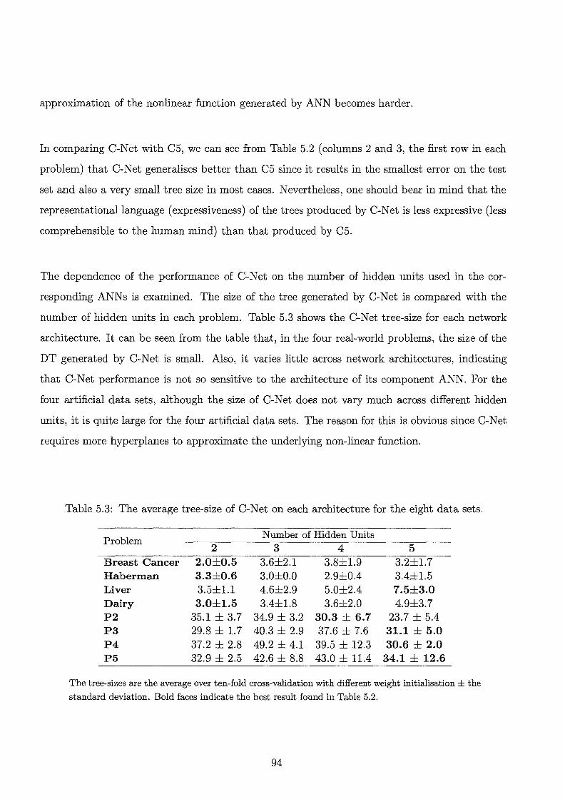
approximation of the nonlinear function generated by ANN becomes harder.
In comparing C-Net with C5, we can see from Table 5.2 (columns 2 and 3, the first row in each
problem) that C-Net generalises better than C5 since it results in the smallest error on the test
set and also a very small tree size in most cases. Nevertheless, one should bear in mind that the
representational language (expressiveness) of the trees produced by C-Net is less expressive (less
comprehensible to the human mind) than that produced by C5.
The dependence of the performance of C-Net on the number of hidden units used in the cor
responding ANNs is examined. The size of the tree generated by C-Net is compared with the
number of hidden units in each problem. Table 5.3 shows the C-Net tree-size for each network
architecture. It can be seen from the table that, in the four real-world problems, the size of the
DT generated by C-Net is small. Also, it varies little across network architectures, indicating
that C-Net performance is not so sensitive to the architecture of its component ANN. For the
four artificial data sets, although the size of C-Net does not vary much across different hidden
units, it is quite large for the four artificial data sets. The reason for this is obvious since C-Net
requires more hyperplanes to approximate the underlying non-linear function.
Table 5.3: The average tree-size of C-Net on each architecture for the eight data sets.
Problem Number of Hidden Units 2 3 4 5
Breast Cancer 2.0±0.5 3.6±2.1 3.8±1.9 3.2±1.7 Haberman 3.3±0.6 3.0±0.0 2.9±0.4 3.4±1.5 Liver 3.5±1.1 4.6±2.9 5.0±2.4 7.5±3.0 Dairy 3.0±1.5 3.4±1.8 3.6±2.0 4.9±3.7 P2 35.1 ± 3.7 34.9 ± 3.2 30.3 ± 6.7 23.7 ± 5.4 P3 29.8 ± 1.7 40.3 ± 2.9 37.6 ± 7.6 31.1 ± 5.0 P4 37.2 ± 2.8 49.2 ± 4.1 39.5 ± 12.3 30.6 ± 2.0 P5 32.9 ± 2.5 42.6 ± 8.8 43.0 ± 11.4 34.1 ± 12.6
The tree-sizes are the average over ten-fold cross-validation with different weight initialisation± the standard deviation. Bold faces indicate the best result found in Table 5.2.
94
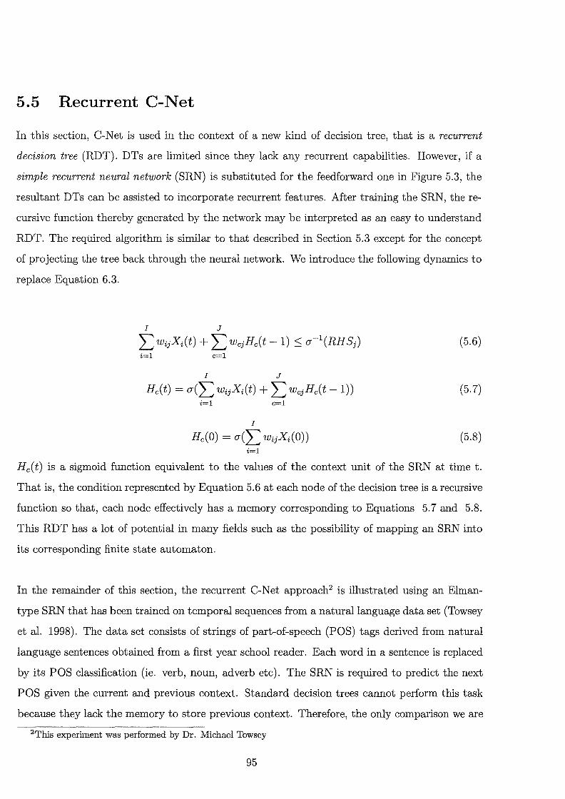
5.5 Recurrent C-Net
In this section, C-Net is used in the context of a new kind of decision tree, that is a recurrent
decision tree (RDT). DTs are limited since they lack any recurrent capabilities. However, if a
simple recurrent neural network (SRN) is substituted for the feedforward one in Figure 5.3, the
resultant DTs can be assisted to incorporate recurrent features. After training the SRN, there
cursive function thereby generated by the network may be interpreted as an easy to understand
RDT. The required algorithm is similar to that described in Section 5.3 except for the concept
of projecting the tree back through the neural network. We introduce the following dynamics to
replace Equation 6.3.
I J
L WijXi(t) + L WcjHc(t- 1) :S cr-1(RHSj) (5.6) i=l c=l
I J
Hc(t) = cr(L WijXi(t) + L WcjHc(t- 1)) (5.7) i=l c=l
I
Hc(O) = cr(L WijXi(O)) (5.8) i=l
Hc(t) is a sigmoid function equivalent to the values of the context unit of the SRN at time t.
That is, the condition represented by Equation 5.6 at each node of the decision tree is a recursive
function so that, each node effectively has a memory corresponding to Equations 5. 7 and 5.8.
This RDT has a lot of potential in many fields such as the possibility of mapping an SRN into
its corresponding finite state automaton.
In the remainder of this section, the recurrent C-Net approach2 is illustrated using an Elman
type SRN that has been trained on temporal sequences from a natural language data set (Towsey
et al. 1998). The data set consists of strings of part-of-speech (POS) tags derived from natural
language sentences obtained from a first year school reader. Each word in a sentence is replaced
by its POS classification (ie. verb, noun, adverb etc). The SRN is required to predict the next
POS given the current and previous context. Standard decision trees cannot perform this task
because they lack the memory to store previous context. Therefore, the only comparison we are
2This experiment was performed by Dr. Michael Towsey
95

making is between the performance of C-Net and the standard Elman SRN.
When applying the Elman SRN to the natural language data, error on the test set decreased
from 44.8% to 31.4% as the number of hidden units was increased from 2 to 8 (Table 5.4). The
test error of C-Net also tended to decrease as the number of hidden units increased but less
steeply. Consequently, C-Net performed better than the SRN for 2, 3 and 4 hidden units but
worse when 8 or more hidden units was used. The optimum number of hidden units for C-net
was 4 and for SRN was 8. These results suggest that with a small number of hidden units, the
output layer of the SRN is unable to capture all the information encoded in the outputs from the
hidden units, whereas C5 is better in this respect. However once the number of hidden units is 8
or more for this problem, the SRN output layer is better suited than C5 to learning the hidden
unit representation.
Table 5.4: Performance of recurrent C-Net on a natural language data set.
Problem Number of Hidden Units
2 3 4 6 8 SRN % Bit error 44.8% ± 2.9 40.9% ± 2.5 37.6% ± 1.9 33.4% ± 1.8 31.4% ± 1.5 C-Net % Bit error 36.5% ± 3.6 33.9% ± 1.4 33.1% ± 2.1 33.4% ± 1.7 34.4% ± 1.7 C-Net Tree size 29.1 6.3 37.7 ± 7.3 44.2 ± 12.0 49.9 ± 12.1 56.8 ± 7.5
Percent bit error obtained by SRN and C-Net on a test set of natural language data for SRNs
having different numbers of hidden units and the size of the tree generated in each case. Averages
and standard deviations are for 10 repeats of SRN initialised with different initial weights. For
all hidden unit numbers (except 6 hidden units), the difference between SRN error and C-Net is
significant at confidence level 0.001.
5.6 Conclusion
In this chapter, a novel algorithm, C-Net, is introduced for generating multivariate decision trees
from artificial neural networks using a univariate decision tree, C5. The resultant tree, when
compared with the tree generated by C5 alone, is more compact and accurate. Furthermore, it is
more expressive than the corresponding artificial neural network. We believe that using a hybrid
system which combines C5, as one of the strongest decision tree classifiers, and the multi-layer
96

feedforward ANN, as a strong non-parametric nonlinear regression model, results in a hybrid
method that is an enhancement for both technologies. Although for our problems, C-Net was
always more accurate than C5, it is not conclusive that this is the universal case. Rather, meth
ods are more or less more suitable for specific domains. Our conclusion is that the integration of
decision trees and artificial neural networks is a necessity if the application domain requires ac
curate, compact, and expressive predictive ability, in which case, C-Net can play a significant role.
Additionally, C5 employs the statistical x2 test for deciding when to cease training. This is found
to be robust against the number of hidden units used for the ANN. This point is illustrated when
the size of the trees generated by C-Net was almost identical regardless of the number of hidden
units in some cases (for example Haberman). This indicates that the addition of more hidden
units in some cases was not required and can be used as an indication of redundancies in the
ANN's architecture.
Furthermore, C-Net can be used to generate recurrent decision trees where a memory is asso
ciated with each node in the tree and the conventional linear condition attached to each node
is replaced by a recursive function. The potential of recurrent decision trees is enormous and it
opens a new area of application to conventional DTs.
C-Net looks promising since it has the advantage of conventional ANNs, that, with their piece
wise linear approximation, they are expected to be more accurate than UDTs. Also, it has
the advantage of UDTs, that their representational language is more expressive than ANNs.
Furthermore, it combines the two technologies, UDTs and ANNs, in a frame that is easy to
implement and balances between compactness, expressiveness, and accuracy better than any of
these technologies in isolation.
In the previous chapter, we experimented with both ANNs and DTs. This motivated the idea
of C-Net. The current chapter presented still some results regarding the prediction problem;
therefore emphasizing the second thesis sub-objective; discovering patterns in the dairy database
using KDD. The rest of the thesis will discuss the third thesis sub-objectives; that is, formulating
and solving the mate-selection problem.
97

98
Part III
Optimisation Models
99

Chapter 6
Heuristics for Complex Optimisation
Problems
This chapter's main objective is to introduce the foundations of the techniques to be used for
solving the mate-selection problem in the following chapters. A general introduction is given in
Section 6.1 and seven heuristic search techniques are then presented. More specifically, simulated
annealing (SA) is presented in Section 6.2 followed by tabu search (TS) in Section 6.3, genetic
algorithm (GA) in Section 6.4, differential evolution (DE) in Section 6.5, immune systems in
Section 6.6, ant colony optimisation (ACO) in Section 6.7, and memetic algorithms (MA) in
Section 6.8. Issues arising with constraints and multi-objectives are discussed in Sections 6.9
and 6.10, respectively.
6.1 Introduction
Optimisation theory provides a compact set of techniques to handle different types of optimisation
problems. Unfortunately, real life problems are known to be messy, complex, multi-objective,
dynamic, uncertain, and large scale; that is, the problem has large numbers of variables and
constraints. Conventional optimisation techniques cannot handle these complex problems in a
reasonable time. Heuristic search techniques provide a means for handling these complex prob
lems at the cost of returning a near, in contrast to an exact, optimal solution. There used to be
a distinction between conventional optimisation techniques and heuristics but this is becoming
increasingly less clear because there is much in common between the two.
101

The general optimisation problem (hereafter referred to as P1) can be stated as:-
(P1): Minimise f(x)
subject to: M = {x E RniG(x) ~ 0}
where xis the set of decision variables, f(x) is the objective function, G(x) is a set of constraints,
and M is the set of feasible solutions. If the optimisation problem is maximisation, it is equiva
lent to a minimisation problem after multiplying the objective by (-1). Also, if a constraint is an
equation, it can be represented by two inequalities one is "less than or equal" while the other is
"greater than or equal" . A "greater than or equal" inequality can be transformed to a "less than
or equal" inequality by multiplying both sides by (-1). In summary, any optimisation problem
can be represented in the previous general form.
Let us define three sets, M1 = {x E Rnlxj is integer, j = 1 ... n}, M2 = {x E Rnlxj is integer,
j E J C {1. .. n}}, and M3 = {x E Rnlxj E {0, 1},j = 1. .. n}. Three special cases from the
general optimisation problem- the pure integer, mixed integer, and binary optimisation problems
- can be defined respectively as follows:
(P2): Minimise f(x)
subject to: M n M1
(P3): Minimise f(x)
subject to: M n M2
(P4): Minimise f(x)
subject to: M n M3
Hereafter, O(x) will be used generically to represent the feasible region of any optimisation prob
lem. For example, O(x) isM in P1, M n M1 in P2, M n M2 in P3, and M n M3 in P4.
Two important types of optimal solutions will be referred to in the rest of this thesis, local and
global optimal solutions. Let us define the open ball ( ie. a neighbourhood centred on x and
defined by the Euclidean distance) B5(x) = {x E Rnl llx- xll < o}.
102
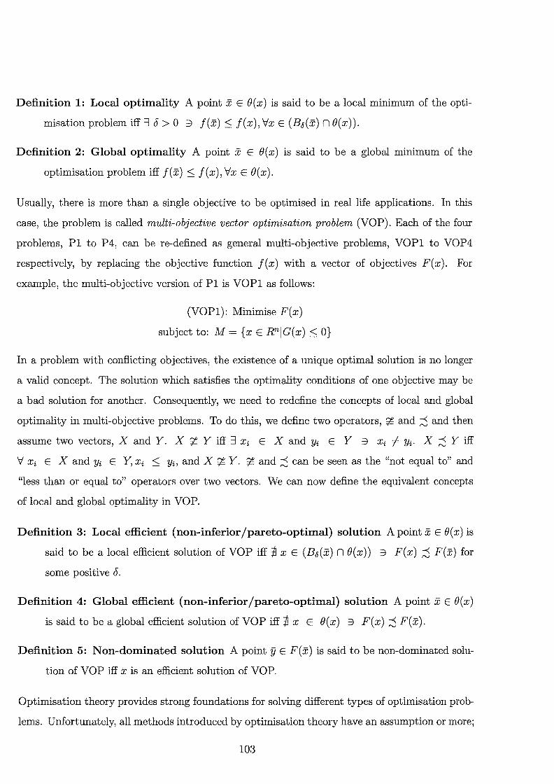
Definition 1: Local optimality A point x E ()(x) is said to be a local minimum of the opti
misation problem iff 3 o > 0 3 f(x) ::::; f(x), Vx E (B,s(x) n ()(x)).
Definition 2: Global optimality A point x E ()(x) is said to be a global minimum of the
optimisation problem iff f(x) ::::; f(x), Vx E ()(x).
Usually, there is more than a single objective to be optimised in real life applications. In this
case, the problem is called multi-objective vector optimisation problem (VOP). Each of the four
problems, Pl to P4, can be re-defined as general multi-objective problems, VOPl to VOP4
respectively, by replacing the objective function f(x) with a vector of objectives F(x). For
example, the multi-objective version of Pl is VOPl as follows:
(VOPl): Minimise F(x)
subject to: M = {x E RniG(x) ::::; 0}
In a problem with conflicting objectives, the existence of a unique optimal solution is no longer
a valid concept. The solution which satisfies the optimality conditions of one objective may be
a bad solution for another. Consequently, we need to redefine the concepts of local and global
optimality in multi-objective problems. To do this, we define two operators, ~ and ;::) and then
assume two vectors, X and Y. X ~ Y iff 3 Xi E X and Yi E Y 3 Xi -=/:- Yi· X ;::) Y iff
V Xi E X and Yi E Y, Xi ::::; Yi, and X ~ Y. ~ and ;::) can be seen as the "not equal to" and
"less than or equal to" operators over two vectors. We can now define the equivalent concepts
of local and global optimality in VOP.
Definition 3: Local efficient (non-inferior /pareto-optimal} solution A point x E O(x) is
said to be a local efficient solution of VOP iff~ x E (B,s(x) n ()(x)) 3 F(x) ;::) F(x) for
some positive o.
Definition 4: Global efficient (non-inferior/pareto-optimal) solution A point x E O(x)
is said to be a global efficient solution of VOP iff~ X E e(x) 3 F(x) ;::) F(x).
Definition 5: Non-dominated solution A pointy E F(x) is said to be non-dominated solu
tion of VOP iff x is an efficient solution of VOP.
Optimisation theory provides strong foundations for solving different types of optimisation prob
lems. Unfortunately, all methods introduced by optimisation theory have an assumption or more;
103

least of which is that they are specific to a particular model. This lack of a general algorithm
which does not have pre-assumptions about the model, causes optimisation theory to fail in
front of some complex real life problems. However, if an optimisation method is suitable for a
specific model, it guarantees optimality if it exists (although not necessarily global optimality).
By contrast, heuristic algorithms provide a means for solving general optimisation problems at
the cost of returning a near optimal solution. If the problem for optimisation is in formulating
the model so that it closely resembles reality without violating the assumptions of the technique
(for example, convexity assumption), the problem for heuristic algorithms is in determining an
appropriate value for the search parameter(s) in each problem.
Before proceeding with the rest of this chapter, it is important to first introduce some basic
terminologies in complexity theory that we will use in later chapters, and also introduce multi
stage decision models, which is the formulation approach used in later chapters. The following
definition is extracted from (Ansari and Hou 1997).
Suppose f and g are positive functions defined for positive integers, f, g
and Q and Prob are two problems, then
1. f = O(g), if 3 positive constants c and N such that f(n) ::::; cg(n), V n 2: N.
2. If Prob can be solved in a polynomial time and 3 a polynomial time algorithm
L where L can transform Q to Prob (ie. polynomial time reduction), then 3 a
polynomial time algorithm to solve Q.
3. A particular class of decision problems that can be solved in polynomial time
by a nondeterministic computer is known as N P.
Multi-stage decision modeling is a modeling approach rather than a solution mechanism ( eg.
linear programming). Thus, it is an art for decomposing large scale problems in terms of stages
linked with a set of transitions. The model can be solved afterward with dynamic programming
(Bellman and Dreyfus 1962) or other mathematical programming techniques. Sniedovich (1992)
defines a multi-stage decision model as:
"A collection (N, S, D, T, 8 1 , g) where
104

1. N is a positive integer specifying the number of decision stages comprising the
decision-making process. Define N = 1, 2, 3, ... , N. Thus, for N = oo the set
N denotes the set of positive integers.
2. S is a non-empty set entitled the state space. Its elements are called states.
3. Dis a function that to each pair (n, s) EN x S, it assigns a subset of some set
'D. The set D(n, s) is referred to as the set of feasible decisions pertaining to
state s at stage n. If the set D( n, s) is empty, the state s is considered to be
non-feasible at stage n. The set Dis named the decision space.
4. T is a function on N x S x 'D with values in S called the transition function.
For any triplet (n, s, x) such that n EN, s E S, and x E D(n, s), the element
s = T( n, s, x) designates the states at stage n + 1 resulting from the decision x
application to the state s at stage n.
5. 8 1 is a non-empty subset of S whose elements are named initial states.
6. g is a real-valued function on sl X 'DN termed the objective function. The value
yielded by g(s, x1 , x2 , ... , XN) is understood to specify the overall cost or benefit
arising from the decisions (xb ... , XN) made at stages 1, 2, 3, ... , N respectively,
given that the initial process state is s E 81."
In this chapter, seven heuristic search techniques are introduced: SA, TS, GA, DE, Immune,
ACO, and MA. Whether we are using conventional optimisation or heuristic methods to solve a
general optimisation problem, two issues usually arise: how to handle the constraints, and how
to solve the VOP. These two issues are discussed at the end of the chapter.
6.2 Simulated annealing
In the process of physical annealing (Rodrigues and Anjo 1993), a solid is heated until all parti
cles randomly arrange themselves in the liquid state. A slow cooling is then used to crystallise
the liquid. That is, the particles are free to move at high temperature and gradually lose their
mobility by decreasing the temperature (Ansari and Hou 1997). This process is described by the
early work in statistical mechanics of Metropolis (Metropolis et al. 1953) and is well-known as
105

the Metropolis algorithm, Figure 6.1.
Define the transition of the substance from state i with energy E(i) to state j with energy E(j) at temperature level T
If E(i)::::; E(j) then accept i---> j If E(i) > E(j) then accept i---> j with probability exp(E(i~,ff(j))
where K is the Boltzmann constant
Figure 6.1: Metropolis algorithm
Kirkpatrick et. al. (1983) defined an analogy between the Metropolis algorithm and the search
for solutions in complex combinatorial optimisation problems where he developed the idea of SA.
Simply speaking, SA is a stochastic computational technique that searches for global optimal
solutions in optimisation problems. In complex combinatorial optimisation problems, it is usually
easy to be trapped in a local optimum. The main goal here is to give the algorithm more time in
the search space exploration by accepting moves, which may degrade the solution quality, with
some probability depending on a parameter called the "temperature". When the temperature
is high, the algorithm behaves like random search. A cooling mechanism is used to gradually
reduce the temperature and the algorithm performs similar to a greedy hill-climbing algorithm
when the temperature is frozen to zero. If this process is given sufficient time, there is a high
probability that it will result in a global optimal solution (Ansari and Hou 1997). The algorithm
escapes a local optimal solution by moving with some probability to those solutions which degrade
the current one and accordingly gives a high opportunity to explore more of the search space.
The probability of accepting a bad solution, 1r(T), follows a Boltzmann (also known as Gibbs)
distribution of:
(T) = (E(i)- E(j)) 7r exp KT (6.1)
where E(i) is the energy or objective value of the current solution, E(j) is the previous solu
tion's energy, T is the temperature and K is a Boltzmann constant. In actual implementation,
K can be taken as a scaling factor to keep the temperature between 0-1, if it is desirable that
the temperature falls within this interval. Unlike GA, there is a proof for the convergence of SA
(Ansari and Hou 1997) assuming that the time spent at each temperature level is sufficient.
106

The algorithm
There are two main approaches in SA: homogeneous and non-homogeneous (Vidal1993). In the
former, the temperature is not updated after each step in the search space, although for the latter
it does. It is found that in homogeneous SA, the transitions or generations of solutions for each
temperature level represent a Markov chain of length equal to the number of transitions at that
temperature level. The homogeneous and non-homogeneous algorithms are shown in Figures 6.2
and 6.3 respectively.
The homogeneous algorithm starts with three inputs from the user, the initial temperature T,
the initial Markov chain length L, and the neighbourhood length (. Then, it generates anini
tial solution, evaluates it, and stores it as the best solution found so far. After that, for each
temperature level, a new solution is generated from the current solution neighbourhood N(x', ()
(refer to Section 9.3.2 for our definition of a neighbourhood), tested, and replaces the current
optimal if it is better than it. The new solution is then tested against the previous solution,
if it is better, the algorithm accepts it; otherwise it is accepted with a certain probability as
specified previously. After completing each Markov chain of length L, the temperature and the
Markov chain length are decreased. The question now is: how to update the temperature Tor
the cooling schedule.
Cooling schedule
In the beginning of the simulated annealing run, we need to find a reasonable value ofT such
that most transitions are accepted. This value can be easily found through a small amount of
experimentation. We then increase T with some factor until all transitions are accepted. Another
way to do it is to generate a set of random solutions and find the minimum temperature T that
guarantees the acceptance of these solutions. Following the determination of T, we need to define
a cooling schedule for it. Two methods are usually used in the literature. The first is static,
where we need to define a discount parameter a. After the completion of each Markov chain, k,
adjust T as follows (Vidal 1993):
(6.2)
107

initialise the temperature to T initialise the chain length to L initialise the neighbourhood length ( xo E O(x), fo = f(xo) initialise optimal solution Xopt to be xo and its objective value fopt = fo initialise current solution x' to be xo and its objective value f' = fo repeat
for j = 0 to L i=i+1 Xi E N(x', (), fi = f(xi) b.(f) = fi - f' if fi < fopt then Xopt = Xi, fopt = fi if fi < f' then x' = Xi, f' = fi else if exp( -b..(f)/T) > random (0,1} then x' =Xi, f' = fi
next j update L and T
until loop condition is satisfied return Xopt and !opt
Figure 6.2: General homogeneous simulated annealing algorithm.
initialise the temperature to T initialise the number of iterations to L initialise the neighbourhood length ( xo E O(x), fo = f(xo) initialise optimal solution Xopt to be xo and its objective value fopt = fo initialise current solution x' to be xo and its objective value f' = fo fori= 0 to L
Xi E N(x', (), fi = f(xi) b.(f) = fi- !' if fi < fopt then Xopt =Xi, !opt= fi if fi < f' then x' = Xi and f' = fi else if exp( -b..(f)/T) > random (0,1} then x' =Xi, f' = fi updqte T
next i return Xopt and !opt
Figure 6.3: General non-homogeneous simulated annealing algorithm.
The second is dynamic, where one of its versions was introduced by Huang, Romeo, and Sangiovanni
Vincetilli, 1986. Here,
(6.3)
(6.4)
where at is the variance of the accepted solutions at temperature level Tk·
108

6.3 Tabu search
Glover (1989, 1990) introduced tabu search (TS) as a method for escaping from a local opti
mum. The goal is to obtain a list of forbidden (tabu) solutions/directions in the neighbourhood
of a solution to avoid cycling between solutions while allowing a direction which may degrade
the solution although it may help in escaping from the local optimum. Similar to SA, we need
to specify how to generate solutions in the current solution's neighbourhood. Furthermore, the
temperature parameter in SA is replaced with a list of forbidden solutions/directions updated
after each step. When generating a solution in the neighbourhood, this solution should not be in
any of the directions listed in the tabu-list, although a direction in the tabu-list may be chosen
with some probability if it results in a solution which is better than the current one. In essence,
the tabu-list aims to constrain or limit the search scope in the neighbourhood while still having
a chance to select one of these directions.
The algorithm
initialise the neighbourhood length to ( xo E (), fo = f(xo).
Xopt = Xo, !opt = fo x' = xo, f' = fo, k = 1 while the stopping condition is not met do
k=k+l choose Xk E N(x', () if f(xk) < f(xopt) then Xopt = Xk, !opt= fk if f(xk) < f(x') then x' = Xk, !' = fk else if Xk tj. M then x' = Xk, f' = fk update M with Xk
end while
Figure 6.4: The Tabu search algorithm
The TS algorithm is presented in Figure 6.4. A new solution Xk is generated within the current
solution's neighbourhood N(x', () 1. If the new solution is better than the optimal solution, it is
accepted and saved as the optimal. If the new solution is better than the current solution, it is
accepted and saved as the current solution. If the new solution is not better than the current
1The neighbourhood, as used in our implementation, will be defined in Section 9.3.2.
109

solution and it is not in a direction within the tabu list M, it is accepted as the current solution
and the search continues from there. If the solution is tabu, the current solution remains the
same. After accepting a solution, M is updated to forbid returning to this solution again. The
function choose can be implemented in many different ways (refer to Section 9.9 for our imple
mentation of this function).
The list M can be a list of the tabu solutions visited in the last n iterations. However, this
is a memory consuming process and it is a limited type of memory. Another possibility is to
define the neighbourhood in terms of a set of moves. Therefore, instead of storing the solution,
the reverse of the move which produced this solution is stored instead. Clearly, this approach
prohibits, not only returning to where we came from, but also many other possible solutions.
Notwithstanding, since the tabu list is a short term memory, at some point in the search, the
reverse of the move will be eliminated from the tabu list, therefore, allowing to explore this part
of the search space which was tabu.
A very important parameter here, in addition to the neighbourhood length which is a critical
parameter for many other heuristics such as SA, is the choice of the tabu-list size which is referred
in the literature as the method's adaptive memory. This is a problem-dependent parameter, since
the choice of large size would be inefficient in terms of memory capacity and the time required
to scan the list. On the other hand, choosing the list size to be small would result in a cycling
problem; that is, revisiting the same state again (Glover 1989). In general, the tabu-list's size is
a very critical issue for the following reasons:-
1. The performance of tabu search is sensitive to the size of the tabu-list in many cases.
2. There is no general algorithm to determine the optimal tabu-list size apart from experi
mental results.
3. Choosing a large tabu-list is inefficient in terms of speed and memory.
110

6.4 Genetic algorithm
In trying to understand evolutionary mechanisms, Holland (1998) devised a new search mecha
nism, which he called genetic algorithm, based on Darwin's (1859) principle of natural selection.
In its simple form, genetic algorithm recursively applies the concepts of selection, crossover, and
mutation to a randomly generated population of promising solutions with the best solution found
being reported. A generic GA algorithm is presented in Figure 6.5. GA is contingent upon cod
ing the parameters. Therefore, the choice of the right representation is a crucial issue (Goldberg
1989). In its early stage, Holland (1998) coded the strings in GA using the binary set of alpha
bets {0,1 }, that is binary representation. He introduced the Schema Theorem, which provides a
lower bound on the change in the sampling rate for a single hyperplane from one generation to
another. A schema is a subset of the solution space whose elements are identical in particular
loci. It is a building block that samples one or more hyperplanes. Other representations use
integer or real numbers.
let G denote a generation, P a population, and x1 the l th chromosome in P initialise the initial population of M solutions Pa=o = { x~=O' ... , x{1=0 }
evaluate every x1 E Pa=o, l = 1, ... , M k=l while the stopping criteria is not satisfied do
select P' (an intermediate population) from Pa=k-1 Pa=k +- crossover elements in P' mutate elements in Pa=k evaluate every x1 E Pa=k, l = 1, ... , M k=k+1
return x = argmaxl f(x1),x1 E Pa=k, the best encountered solution
Figure 6.5: A generic genetic algorithm
The algorithm
Selection
As with animal breeding, there are many alternatives for selection in GA. One method is based
on the principle of "living for the fittest" or fitness-proportionate selection, (Jong 1975), where
the objective functions' values for all the population's individuals are scaled and an individual
111
is selected in proportion to its fitness. The fitness of an individual is the scaled objective value
of that individual. The objective values can be scaled in differing ways. Let us define Obj1 and
Fitness1 to be the objective and fitness values of chromosome l respectively. Let the population
size be M. Roulette wheel selection is a fitness-proportionate selection where the scaled fitness is
. Objz Fztness1 = M .
Lj=l Ob)j (6.5)
Each individual is then assigned a slot on a roulette wheel equivalent to its fitness. Every time the
wheel spins, the imaginary ball (random number) falls in one of the slots and the corresponding
individual is selected. Other types of scaling are window-scaling:
. Obj1 - minj(Obj) Fztness1 = maxj(Obj) ( ) - minj Obj
(6.6)
and sigma-scaling:
Objz ~~1 Objj Fitnessz = ---:-.,---,-..!!M"---
a-(Obj) (6.7)
Another way to adopt the fitness-proportionate selection is to use rank-based selection where
all individuals in the population are ranked according to their objective values, and selection is
carried out in proportion to the rank.
Another alternative is stochastic-Baker selection (Goldberg 1989), where the objective values of
all the individuals in the population are divided by the average to calculate the fitness, and the
individual is copied into the intermediate population a number of times equal to the integer
part, if any, of the fitness value. The population is then sorted according to the fraction part
of the fitness, and the intermediate population is completed with a fitness-proportionate selection.
Tournament selection is another famous strategy (Wetzel 1983), where N chromosomes are cho
sen uniformly irrespective of their fitness and the fittest of these is placed into the intermediate
population. As this is usually expensive, a modified version called modified tournament selec
tion (Ross 1996) works by selecting an individual at random and up to N trials are made to pick
a fitter one. The first fitter individual encountered is selected; otherwise, the first individual wins.
112

Reproduction strategies
A reproduction strategy is the process of building a population of individuals in a generation
from a previous generation. There are a number of reproduction strategies presented in the
literature, among them, canonical, simple, and breedN. Canonical GA (Whitley 1994) is simi
lar to Schwefel's (1981) evolutionary strategy where the offspring replace all the parents; that
is, the crossover probability is 1. In simple GA (Ross 1996), two individuals are selected and
the crossover occurs with a certain probability. If the crossover takes place, the offspring are
placed in the new population; otherwise the parents are cloned. Breeder Genetic Algorithm
(Muhlenbein and Schlierkamp-Voosen 1993; Muhlenbein and Schlierkamp-Voosen 1994) or the
breedN strategy is based on quantitative genetics. It assumes that there is an imaginary breeder
who performs selection of the best N strings in a population and breed among them. Muhlenbein
(1994) comments that if "GA is based on natural selection", "breeder GA is based on artificial
selection" .
Another popular reproduction strategy, parallel genetic algorithm (Muhlenbein et al. 1988;
Muhlenbein 1991), employs parallelism. In parallel GA, a number of populations evolve in
parallel but independently, and migration occurs among the population intermittently. A com
bination of breeder GA and parallel GA is known as the distributed breeder genetic algorithm
(Muhlenbein and Schlierkamp-Voosen 1993). In a comparison between parallel GA and breeder
GA, Muhlenbein (1993) states that "parallel GA models evolution which self-organises" but
"breeder GA models rational controlled evolution".
Crossover
Many crossover operators have been developed in the GA literature. Here, four crossover op
erators (one-point, two-points, uniform, and even-odd) are reported from the literature. To
disentangle the explication, assume that we have two individuals that we would like to crossover,
x = (x1, x2, x3, ... , Xn) andy = (YI, Y2, y3, ... , Yn) to produce two children, cl and c2.
In one-point crossover (sometimes written 1-point) (Holland 1998), a cut point, p1 , is gener
ated at random in the range [1, n) and the corresponding parts to the right or left of the
113

cut-point are swapped. Assuming that p1 = 2, the two children are formulated as c1 =
(x1, x2, y3, ... , Yn) and c2 = (y1, Y2, X3, ... , Xn)· In two-points crossover (sometimes written
2-points) (Holland 1998; Jong 1975), two cut points, p1 < p2 , are generated at random in the
range [1, n) and the two middle parts in the two chromosomes are interchanged. Assuming that
p1 = 1 and P2 = 5, the two children are formulated as eel = (x1, Y2, y3, y4, y5, x 6, ... , Xn) and
c2 = (y1 , x2, x 3, X4, X5, Y6, ... , Yn)· In uniform crossover (Ackley 1987), for each two correspond
ing genes in the parents' chromosomes, a coin is flipped to choose one of them (50-50 chance) to
be placed in the same position in the child. In even-odd crossover, those genes in the even posi
tions of the first chromosome and those in the odd positions of the second are placed in the first
child and vice-versa for the second; that is, cl = (y1, x2, y3, ... , Xn) and c2 = (x1, Y2, X3, ... , Yn)
assuming n is even.
Mutation
Mutation is a basic operator in GAs that introduces variation within the genetic materials, to
maintain enough variations within the population, by changing the loci's value with a certain
probability. If an allele is lost due to selection pressure, mutation increases the probability of
retrieving this allele again. In our implementation, a repair operator is used to replace the con
ventional mutation operator to maintain the feasibility of the chromosomes.
6.5 Differential evolution
DE (Storn and Price 1995) is a branch of evolutionary algorithms developed by Rainer Storn
and Kenneth Price in 1995 for optimisation problems with continuous decision variables. DE
represents each variable's value in the chromosome with a real number. The approach works by
creating a random initial population of potential solutions, where it is guaranteed that the value
of each variable is within its boundary constraints. An individual is then selected systematically
for replacement. Three different individuals are selected randomly as parents. One of these three
individuals is selected as the main parent. Each variable in the main parent is changed with some
probability while at least one variable should be changed. The change is undertaken by adding
114

let G denotes a generation, P a population of size M, and x~=k the lth individual of dimension N in population P in generation k, and C R denotes the crossover probability
input N, M 2:: 4, FE (0, 1), CR E [0, 1], and initial bounds: lower( xi), upper( xi), i = 1, ... N
initialise Pa=o = { x~=O' ... , xlf=o} as foreach individual l E Pa=o
xLG=O =lower( xi)+ random[O, 1] x (upper( xi) -lower(xi)), i = 1, ... , N evaluate every x1 E Pa=o, l = 1, ... , M k=1 while the stopping criterion is not satisfied do
foreach l :S M randomly select r1, r2, r3 E (1, ... , M), l =/=- r1 =/= r2 =/= r3 randomly select irand E (1, ... , N)
Vi< N x~ = xi,G=k-1 xi,G=k-1 xi,G=k-1 {
r3 +Fx(r1 _ r2 ) if (random[O, 1) < CR 1\ i = irand) - ' ~ l xi,G=k-1
xl _ = { x' if f(x') :S f\xb=k- 1) } G-k x1 otherw2se G=k-1
otherwise
k=k+1 evaluate every x1 E Pa=k, l = 1, ... , M
return x = arg ma;xz f(x1), x1 E PG=k, the best encountered solution
Figure 6.6: The differential evolution algorithm
to the variable's value in the main parent, a ratio of the difference between the two values of
this variable in the other two parents. In essence, the main parent's vector is perturbed with the
other two parents' vector. If the resultant vector is better than the one chosen for replacement, it
replaces it; otherwise the chosen vector for replacement is retained in the population. Therefore,
DE differs from GAin a number of points:
1. DE uses real number representation while GA uses binary, integer, or real number repre
sentation.
2. In GA, two parents are selected for crossover and the child is a recombination of its parents.
In DE, three parents are selected for crossover and the child is a perturbation of one of
these parents.
3. The new child in DE replaces a randomly selected vector from the population only if it is
better than it. In canonical GA, children necessarily replace the parents.
115

The algorithm
To formally introduce DE, consider a multi-dimensional vector x1 = (x1 , ... , XN f representing
a solution l. A population at generation G = k is a vector of M solutions (M > 4) 2, PG=k· The
initial population, PG=O = { x~=O' . .. , x~0}, is initialised as
xi,G=O = lower(xi) + randi[O, 1] x (upper(xi)- lower(xi)), l = 1, ... , M, i = 1, 2, ... , N (6.8)
where M is the population size, N is the solution's dimension, and each variable i in a so
lution vector l in the initial generation G = 0, xi,G=o' is initialised within its boundaries
(lower( xi), upper( xi)). Selection is carried out to select four different solutions indexes r 1 , r2 , r3 , l E
[0, ( M- 1) ]. The values of each variable in the child are changed with some crossover probability,
CR, to
Vi< N X~= { - ' t l
xi,G=k-1 otherwise
(6.9)
where FE (0, 1) is a problem parameter determining the amount the main parent is perturbed.
The new solution replaces the old one if it is better than it and at least one of the variables should
be changed (represented in the algorithm by randomly selecting a variable, irand E (1, N)). After
crossover, if one or more of the variables in the new solution are outside their boundaries, the
following repair rule is applied
xt0 +lower(xi) 2
l ( ) x; 0 -upper(xi)
ower xi + ' 2
l xi,G
if x~ G < lower( xi) '
if xi,G > upper(xi)
otherwise
(6.10)
The DE algorithm is presented in Figure 6.6. Figure 6. 7 depicts a graphical interpretation of the
update rule for the differential evolution algorithm. It is clear from the figure that vector Xj is
a perturbation of the parent X1 vector with some degree depending on the two parents X2 and
X3.
6.6 Immune systems
In biological immune systems (Hajela and Yoo 1999), type-specific antibodies recognise and
eliminate the antigens ( ie. pathogens representing foreign cells and molecules). It has been
2M has to be greater than 4 since we select one vector for replacement and three different vectors as parents
116

F(x2- xl)
Figure 6.7: Differential evolution in the two dimensional space.
Two dimensional example of an objective function showing its contour and the process for generating Xj.
estimated that the immune system is able to recognise at least 1016 antigens; an overwhelming
recognition task given that the genome contains about 105 genes. For all possible antigens that
are likely to be encountered, the immune system must use segments of genes to construct the
necessary antibodies. For example, there are between 107 and 108 different antibodies in a typi
cal mammal. In biological systems, this recognition problem translates into a complex geometry
matching process. The antibody molecule region contains a specialised portion, the paratope,
which is constructed from amino acids and is used for identifying other molecules. The amino
acids determine the para tope as well as the antigen molecules' shapes that can be attached to
the paratope. Therefore, the antibody can have a geometry that is specific to a particular antigen.
To recognise the antigen segment, a subset of the gene segments' library is synthesised to encode
the genetic information of an antibody. The gene segments act cooperatively to partition the
antigen recognition task. In Immune, an individual's fitness is determined by its ability to recog
nise - through chemical binding and electrostatic charges - either a specific or a broader group
of antigens.
117
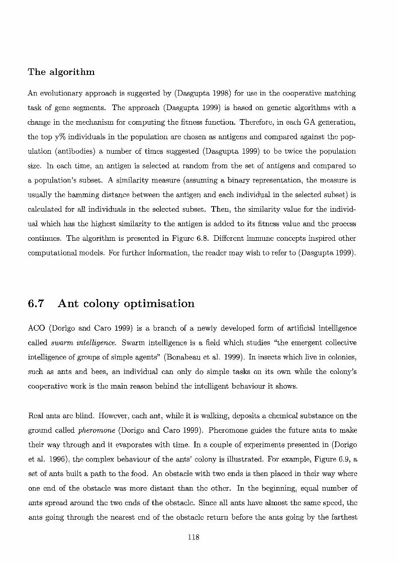
The algorithm
An evolutionary approach is suggested by (Dasgupta 1998) for use in the cooperative matching
task of gene segments. The approach (Dasgupta 1999) is based on genetic algorithms with a
change in the mechanism for computing the fitness function. Therefore, in each GA generation,
the top y% individuals in the population are chosen as antigens and compared against the pop
ulation (antibodies) a number of times suggested (Dasgupta 1999) to be twice the population
size. In each time, an antigen is selected at random from the set of antigens and compared to
a population's subset. A similarity measure (assuming a binary representation, the measure is
usually the hamming distance between the antigen and each individual in the selected subset) is
calculated for all individuals in the selected subset. Then, the similarity value for the individ
ual which has the highest similarity to the antigen is added to its fitness value and the process
continues. The algorithm is presented in Figure 6.8. Different immune concepts inspired other
computational models. For further information, the reader may wish to refer to (Dasgupta 1999).
6. 7 Ant colony optimisation
ACO (Dorigo and Caro 1999) is a branch of a newly developed form of artificial intelligence
called swarm intelligence. Swarm intelligence is a field which studies "the emergent collective
intelligence of groups of simple agents" (Bonabeau et al. 1999). In insects which live in colonies,
such as ants and bees, an individual can only do simple tasks on its own while the colony's
cooperative work is the main reason behind the intelligent behaviour it shows.
Real ants are blind. However, each ant, while it is walking, deposits a chemical substance on the
ground called pheromone (Dorigo and Caro 1999). Pheromone guides the future ants to make
their way through and it evaporates with time. In a couple of experiments presented in (Dorigo
et al. 1996), the complex behaviour of the ants' colony is illustrated. For example, Figure 6.9, a
set of ants built a path to the food. An obstacle with two ends is then placed in their way where
one end of the obstacle was more distant than the other. In the beginning, equal number of
ants spread around the two ends of the obstacle. Since all ants have almost the same speed, the
ants going through the nearest end of the obstacle return before the ants going by the farthest
118

let G denote a generation and P a population initialise the initial population of solutions Pc=o = { x~=O' ... , x"2f=o} evaluate every x1 E Pc=o, l = 1, ... , M compare_with_antigen_and_update_fitness(Pc=o) k=1 while the stopping criteria is not satisfied do
select P' (an intermediate population) from Pa=k-1 Pa=k +-- crossover individuals in P' mutate elements in Pc=k evaluate every x1 E Pc=k, l = 1, ... , M compare_ with_antigen_and_ update_fitness (P G=k)
k=k+1 return x = arg mruq f(x1), x1 E Pa=b the best encountered solution
procedure compare_ with_antigen_and_ update_fitness (P G=k) antigen= top y% in (Pc=k) l=O while l < 2 x M
antibodies C Pa=k randomly select y E antigen find x where similarity(y, x) = arg maxx' similarity(y, x' ), x' E antibodies add similarity(y, x) to the fitness of x E Pc=k l=l+1
end procedure
Figure 6.8: The immune system algorithm
end (differential path effect). With time, the amount of pheromone the ants deposit increases
on the shortest path and more ants prefer this path. This positive effect is called autocatalysis.
The difference between the two paths is called the preferential path effect and it is the cause of
pheromone increase on each side of the obstacle since the ants following the shortest path will
make more visits to the source than those following the longest path. Because of pheromone
evaporation, pheromone on the longest path vanishes with time.
The algorithm
The Ant System (AS) (Dorigo et al. 1991) is the first algorithm based on the behaviour of real
ants for solving combinatorial optimisation problems. The algorithm worked well on small prob
lems but did not scale well for large scale problems (Bonabeau et al. 1999). Many algorithms
119
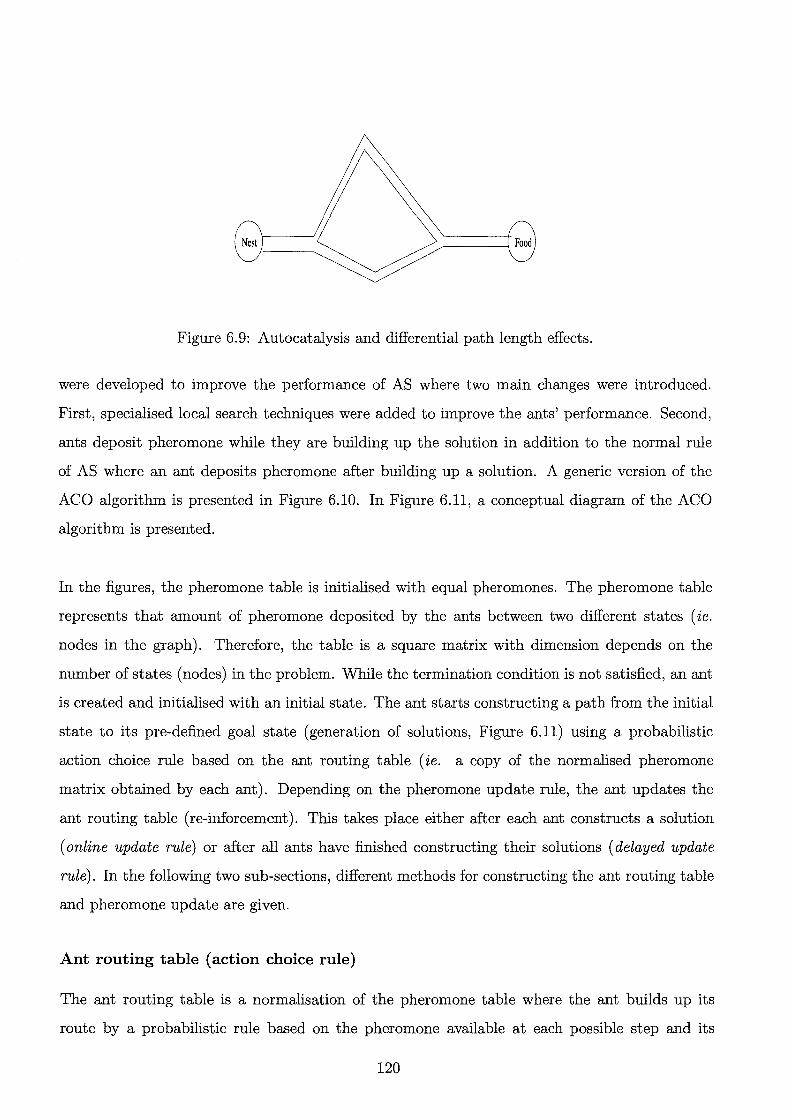
Figure 6.9: Autocatalysis and differential path length effects.
were developed to improve the performance of AS where two main changes were introduced.
First, specialised local search techniques were added to improve the ants' performance. Second,
ants deposit pheromone while they are building up the solution in addition to the normal rule
of AS where an ant deposits pheromone after building up a solution. A generic version of the
ACO algorithm is presented in Figure 6.10. In Figure 6.11, a conceptual diagram of the ACO
algorithm is presented.
In the figures, the pheromone table is initialised with equal pheromones. The pheromone table
represents that amount of pheromone deposited by the ants between two different states ( ie.
nodes in the graph). Therefore, the table is a square matrix with dimension depends on the
number of states (nodes) in the problem. While the termination condition is not satisfied, an ant
is created and initialised with an initial state. The ant starts constructing a path from the initial
state to its pre-defined goal state (generation of solutions, Figure 6.11) using a probabilistic
action choice rule based on the ant routing table ( ie. a copy of the normalised pheromone
matrix obtained by each ant). Depending on the pheromone update rule, the ant updates the
ant routing table (re-inforcement). This takes place either after each ant constructs a solution
(online update rule) or after all ants have finished constructing their solutions (delayed update
rule). In the following two sub-sections, different methods for constructing the ant routing table
and pheromone update are given.
Ant routing table (action choice rule)
The ant routing table is a normalisation of the pheromone table where the ant builds up its
route by a probabilistic rule based on the pheromone available at each possible step and its
120

procedure A CQ_heuristic() initialise pheromone_table while (termination_criterion_noLsatisfied)
foreach ant k do initialise_ ant(); M +---- update_anLmemory(); n +---- a set of problem's constraints while (current-state =/= targeLstate)
A = read_locaLant-routing_table(); P = compute_transition_probabilities(A,M,D); next-state = apply_anLdecision_policy (P, n); move_to_nexLstate(nexLstate); if ( online_step_by_step_pheromone_update) then
deposiLpheromone_on_the_ visited_ arc(); update_anLrouting_table();
M +---- update_internaLstate(); if ( online_delayed_pheromone_ update) then foreach visited_arc do
deposiLpheromone_on_the_ visited_ arc(); update_anLrouting_table();
die(); Update_the_pheromone_table ();
end procedure
Figure 6.10: Generic ant colony optimisation heuristic
Initial data Action choice rule Local objective information
Re-inforcement Generation of
solutions
Figure 6.11: The ant algorithm.
memory. There are a number of suggestions in the literature for the probabilistic decision (aij
is the element in row i column j in the matrix A (Figure 6.10) representing the probability that
the ant will move from the current state ito the next potential state j). The first is the following
rule:
(6.11)
121

Here, the ant utilises the pheromone information ( Tij is the pheromone between the current
state i and the next potential state j) only to decide on its next step ( Ni is the set of possible
transitions from state i). This rule does not require any parameter settings, however it is a biased
exploratory strategy which can quickly lead to stagnation (Bonabeau et al. 1999). Another rule
suggested by (Dorigo et al. 1991) is
(6.12)
where we need two parameters a and {3. The heuristic value 'r/ij is used for the intensification of
search by means of a greedy behavior. For example, the heuristic value can be the immediate
change in the objective resulting from increasing the value of a variable with 1 unit regardless
of the effect of this increase on the overall solution. When {3 = 1, a = 0, the algorithm behaves
like local search and when {3 = 0, a = 1 stagnation may occur as previously mentioned. A
balance is usually required between a (the pheromone information's weight) and {3 (the local
search's weight). However, this rule is computationally expensive because of the exponents. As
an attempt to overcome this, (Dorigo and Gambardella 1997) suggested the following rule:
(6.13)
where only one parameter {3 is used. However, the exponent is still an issue. More recently, the
following rule is suggest for the quadratic assignment problem by (Maniezzo 1998):
(6.14)
Here, only one parameter is required and the multiplication is computationally less expensive
than the power.
Pheromone update (re-inforcement) rule
Each time a pheromone update is required, the ants use the following rule:
(6.15)
where pis a discount factor for pheromone evaporation, ij represents a transition between state
i and state j, and k is the number of ants. A number of suggestions were used in the literature
122

for calculating the rate of pheromone's change LlTi;(t -1). For example, in MMAS-QAP system,
k _ { 1/ ]best if ant k moves from LlTij(t- 1) -
0 otherwise
state i to state j (6.16)
where Jbest is the objective value of the best solution found by the colony. We may note here that
when the objective value increases, the rate of pheromone's change decreases, enabling search's
intensification. Another suggestion to calculate .6. Tk ( t - 1) (Bonabeau et al. 1999) is
if ant k moves from state i to state j
otherwise (6.17)
where, K is the set of ants visited ij, Jk is the objective value of the solution generated by ant k, C
is a constant representing a lower bound on the solutions that will be generated by the algorithm.
To summarise, at the beginning of the algorithm, the pheromone matrix is initialised. In each
step, the pheromone matrix is normalised to construct the ant routing table. The ants generate a
set of solutions (one solution per ant) by moving from a state to another using the action choice
rule. Each element in the pheromone matrix is then updated using the pheromone update step
and the algorithm continues.
6.8 Memetic algorithms
In his book, "The Selfish Gene", Richard Dawkins (1976) first coined the word meme to describe a
unit of culture transmission as opposed to gene for genetic transmission. In the same timeframe,
Lumsden and Wilson introduced a similar concept, culturgen, published later in their books
"Genes, Mind, and Culture" (Lumsden and Wilson 1981) and "Promethean Fire" (Lumsden
and Wilson 1983). The culturgen theory incorporates cultural transfer subject to epigenetic
rules ("genetically determined procedures that direct the assembly of the mind, including the
screening of stimuli by peripheral sensory filters, the internuncial cellular organising processes,
and the deeper processes of directed cognition" (Lumsden and Wilson 1983)). Furthermore, they
claimed that culture acts to slow the rate of genetic evolution, while both genetic and cultural
evolution leads to major change in epigenetic rules over a minimum time of 1000 years. Examples
123
of memes are ideas, fashions, and any culture and behavioral unit that is learnt with a certain
degree of fidelity. An example of an extremely powerful electronic meme is the computer-virus.
Culture as defined by (Boyd and Richerson 1985) is:
information capable of affecting individuals' phenotypes which they acquire from
other conspecifics by teaching or imitation.
MAs are inspired by the previous idea and were first introduced in 1989 by Moscato (1989). In
this work, it was suggested that cultural evolution can be a better working metaphor to escape
from the biologically constrained thinking. The concept of cultural evolution in optimisation is
a metaheuristic, where a heuristic is used to improve the solutions in an evolutionary algorithm
following reproduction. MA has been applied extensively to many combinatorial optimisation
problems (see (Moscato 1999) for a list). A generic version of MA is presented in Figure 6.12.
In the figure, a local search procedure, locaLsearch(x'), is called after crossover and mutation.
This procedure can be a hill-climbing or any other algorithm.
let G denotes a generation, P a population, and xl the lth chromosome in P. initialise the initial population of solutions Pa=o = { x~=O' ... , xtf=o} foreach xl E Pa=o do xl +- locaLsearch(xl) evaluate every xl E Pa=o, l = 1, ... , M k=l; while the stopping criteria is not satisfied do
select P' (an intermediate population) from Pa=k-1 Pa=k +- crossover elements in P' foreach xl E Pa=k do xl +- local_search(xl) evaluate every xl E Pa=k, l = 1, ... , M mutate elements in Pa=k foreach xl E Pa=k do xl +- local_search(xl) evaluate every xl E Pa=k, l = 1, ... , M k=k+1
return x = arg maxz f(xl), xl E Pa=k, the best encountered solution
Figure 6.12: A generic memetic algorithm
6.9 Constraints
Normally, optimisation problems contain constraints. In conventional optimisation theory, the
problem may be solved in two stages. First, the algorithm searches for feasibility (satisfying the
124

constraint system). Second, while maintaining feasibility, the algorithm searches for optimal
ity. Sometimes this is an easy task, if we have a single feasible region as in the case of linear
programming. If the feasible region is discontinuous, this approach may not work. Constraints
have received considerable attention in the literature of optimisation. Here, two main techniques
for handling constraints are discussed: penalty function and repair methods. The choice of an
appropriate technique is, sometimes, a problem-dependent task. For example, if the cardinality
of the set of feasible solutions is small compared with the set of infeasible solutions, the penalty
approach such as the death penalty may not be appropriate as demonstrated in the next section.
6.9.1 Penalty function
In this method, the basic goal is to define an objective function of two parts: the first is the
original objective function (optimality criterion) and the second represents a measure of infeasi
bility (feasibility criterion). This means that the two components of the new objective function
will compete together during the optimisation process. As such, this may be a problem since
one component may subsume the other. Therefore, a weight factor for the measure of infeasi
bility is required to overcome this problem during the search. This weight factor, known as the
penalty term/value, is the bottleneck of this technique. If the penalty value is under-estimated,
feasibility may be broken and the algorithm converges to an infeasible solution. Over-estimating
this term may cause problems to the heuristic technique (for example, in the case of GA, over
estimating the penalty term results in a GA-hard problem (Davis 1987; Riche et al. 1995)). The
optimisation problem can be re-written as:
Min. f(x) + !'I(x).
S.T.
{
0, ifx E B(x) I(x) =
L, otherwise (6.18)
where I' > 0 is a penalty term, and I(x) is an evaluation function which returns 0 if xis a fea
sible solution and L, which is a measure of constraints violation, if x is infeasible. The amount
of constraints violation may be measured in terms of the number of constraints violated, the
amount of violation, or the amount of effort required to retrieve the feasibility (Dasgupta and
125
Michalewicz 1997).
Usually, the appropriate penalty value is learnt while the algorithm is searching for solutions
(Richardson et al. 1989). A static penalty approach is suggested in Homaifar et al. (1994)
where the user defines several levels of constraint violations, and associates with each level a
suitable fixed penalty value, which increases when the level of violations increases. Annealing
penalties (Michalewicz and Attia 1994) is an approach based on SA. In this method, the penalty
value increases while the temperature decreases over time. Another penalty approach is adaptive
penalties, introduced by Hadj-Alouane and Bean (1992), where it is determined while the search
progresses. The penalty value decreases if all best individuals in the previous k generations were
feasible and increases if they were infeasible; otherwise, the penalty value does not change. The
importance of adaptive penalties is emphasised in Michalewicz (1996). Another interesting ap
proach (Morales and Quezada 1998) is called the "death penalty" where an infeasible solution
is evaluated in terms of the number of constraints it violates. The solution is not accepted if
it exceeds a certain threshold on the number of violated constraints. Notice that this approach
may prove inefficient when the cardinality of the set of feasible solutions is too small compared
with that one of infeasible solutions (Michalewicz and Nazhiyath 1995).
In summary, when infeasibility is encountered, a penalty term can be added to the objective
function to comprise a pressure on the search mechanism to retrieve feasibility again. Yet, the
appropriate penalty value is a critical issue and none of the previous approaches is guaranteed to
work all the time. Penalty functions are usually difficult to handle (Schoenauer and Xanthakis
1993) and they may not be the most suitable method for handling equality constraints (Coello
1999b).
6.9.2 Repair mechanisms
If repairing an infeasible solution is a cheap process, this approach can be a good one. In the
literature of constraint satisfaction and local search algorithms (Lemaztre and Verfaillie 1997;
Minton et al. 1992), the use of a repair mechanism to retrieve broken feasibility is the con
ventional way to proceed. In the literature of GAs, it is shown that a repair operator results
126

in a better performance and is faster than other methods (Liepins and Vose 1990; Liepins and
Potter 1991). GENOCOP III (Michalewicz and Nazhiyath 1995) is one of the most famous
co-evolutionary systems which handle linear constraints using a repair operator. Repair opera
tors can be found in many other studies such as Muhlenbein (1992), Michalewicz and Janikow
(1991), Orvosh and Davis (1994), Riche and Haftka (1994), Riche et al. (1995), Xiao et al.
(1997), and Xiao et al. (1996). Two main approaches are followed in this literature. The first
is to use a repair algorithm in the solution's evaluation without replacing the infeasible solution
with the repaired solution. Instead, the fitness of the repaired solution is used as the fitness of
the infeasible solution. The idea here is that sometimes infeasible solutions may help to escape
local optimum and may contains good bits. The second is to map the infeasible solution into a
feasible solution and continuing the search from the new feasible solution. The problem with the
second method is in the bias within the repair mechanism which may prejudice the search to a
local optimum. This is not a problem in constraint satisfaction, since the objective is to reach a
feasible solution without considering optimality. However, in optimisation this methodology may
cause a premature convergence or being easily trapped in a local optimum, unless it is handled
with randomisation as proposed in the following chapters.
6.10 Multi-objective optimisation
Normally, optimisation problems contain conflicting objectives. The literature of optimisation
theory is rich in providing different methods for solving VOP. Unfortunately, these methods
add a burden on the optimisation process, especially when problems are originally difficult to
solve. There are three families of methods for solving VOP - E-method, goal programming, and
weighted-sum (aggregated) method.
TheE method (Ritzel et al. 1994) optimises the problem under each objective in order. After the
optimisation of the first objective, the objective is added to the model as a constraint bounded
with its optimal value ± a small value called E. The second objective is then optimised under
the original constraints and the new constraint obtained by adding the optimal solution of the
first objective as a constraint. The process continues in a similar fashion. We need to alter the
127
values of E to generate the set of pareto optimal solutions. The problem with this method is that
it results in weak pareto-optimal solutions (Coello 1999a).
In its early stages, Archimedian goal programming approach ( Charnes and Cooper 1961) was
formulated within the framework of non-preemptive weights. In 1965, Ijiri (1965) introduced a
preemptive approach. The Archimedian approach has been coined as weighted goal programming
and the preemptive approach as lexicographic goal programming. A good introduction to goal
programming can be found in (Ignizio 1976).
In the weighted-sum method (Kuhn and Tucker 1951), assume the vector of objective functions
F(x) = {!I(x), ... ,jk(x)}. If W = {wb ... ,wk} is a normalised weight vector, the single
objective optimisation problem is formulated as
k
min L wi x fi(x) (6.19) i=l
If one objective dominates another, the weights used in this optimisation process will not reflect
the real importance of each objective. Therefore, scaling the objectives may be necessary (Coello
1999a). k
min Lwi x ci x fi(x) (6.20) i=l
where Ci is a scaling factor, usually taken to be the reciprocal of the standard deviation of each
objective over randomly generated sample.
6.11 Conclusion
In this chapter, the heuristic techniques, that will be used to solve the optimisation problem
in the rest of the thesis, are presented. A wide range of techniques is covered, ranging from
conventional techniques- such as simulated annealing, tabu search, and genetic algorithms- to
more recent techniques such as ant colony optimisation and immune. In the next chapters, these
techniques will be compared relative to their performance on the mate-selection problem. In
addition, new techniques will be developed.
128

Chapter 7
Evolutionary Allocation Problem
Allocation is a common problem in Operations Research where the general idea is to allocate a
limited number of finite resources to a limited number of objects. This problem can be solved
using either general optimisation techniques such as linear programming or specialised techniques
such as network optimisation. Usually the allocation is done for one time-slot but sometimes
dynamic allocation is required. This chapter has two objectives:
1. Introducing and formulating a new type of dynamic allocation, Evolutionary Allocation
Problem (EAP).
2. Estimating the problem complexity.
The chapter does not present a solution to the general problem although in the next chapters we
will see how simplified versions of this problem can be solved. An introduction to allocation is
presented in Section 7.1, followed by the problem importance in Section 7.2. In Section 7.3, the
EAP's assumptions and advantages are stated, and the complexity of its search-space is discussed
in Section 7.4 and conclusions are drawn in Section 7.5.
7.1 Introduction
The allocation problem is commonly found in daily activities. For example, in the beginning of
each month we may need to allocate our salary to different expenses so that the monthly savings
are maximum. The allocated values can be real or integer numbers. In the former, the prob
lem is usually easier since techniques such as linear programming can handle it efficiently. The
129

problem becomes computationally expensive when the number of units allowed for allocation
are constrained to be integer. In this case, techniques such as integer programming (Salkin and
Mathur 1989) and constraint satisfaction (Gent and Walsh 1994; Hentenryck 1989) can solve
problems of small to medium size.
When the dimension grows, specialised techniques can be more effective but limited in their scope.
For example, if the problem is to assign a set of jobs to a set of machines so that every machine
can process a single job, every job can be assigned to one machine only, and the total cost is to
be minimised, then we deal with an assignment problem and a technique such as the Hungarian
algorithm (Kuhn 1955) can efficiently solve it. Another type is the transportation problem where
an integer number of units are required to be transported from a location to another so that the
total cost is minimum. The transportation problem can be solved using an updated version of
the Simplex method (Dantzig 1951). The underlying assumption of these techniques is that the
problem is linear (linear objective with linear constraints). When the linearity assumption is re
laxed, the problem becomes more difficult and more specialised techniques are required to solve it.
Papadimitriou et.al. (1982) show that the satisfiability problem and integer linear programming
are NP-Complete problems. This is an interesting finding since it entails that until someone
proves the unsolved dilemma NP=P, there cannot exist a polynomial algorithm which can effi
ciently solve these problems. This causes the research in these fields to be endless since none of
the general algorithms can perform well on all problems, and specialised algorithms are required
whenever a new problem arises.
In this chapter, a new type of allocation problem - the Evolutionary Allocation Problem- will
be presented, which to my knowledge, has not yet been formulated in the operations research
literature. The use of the term "evolutionary" in this context represents the evolving nature of
the problem as opposed to an evolutionary algorithm for solving the problem. An evolutionary
allocation problem can be defined formally as:
Given a set of males, M, females, F, a number of years, Y, and criteria C, assuming
the individuals are considered mature after G years from their date of birth, find the
optimal set of mating-pairs between M and F for each year in Yin order to maximise
130
C. The progeny can be of either sex and they are available for allocation in subsequent
years only when their age is greater than or equal to G.
The general representation will be illustrated with the assumption that the male individuals are
bulls and the females are cows. Although this does not restrict the formulation, a fixed number
of years is required for individuals from their date of birth to maturity. This is usually finite
and to create a more understandable model, the domain of dairy industry is used as the model
context. The mating of an animal can take place when it is one year old and the animal gives
its first offspring at two years.
We do not know in advance whether a mating will result in a male or a female and this requires
to be represented stochastically. Also, some of the animals may be culled and therefore cease to
exist in later years. Additionally, the model must allow progeny to be unavailable for allocation
until they become mature and therefore reproductive. Each animal is represented by a time
dependent binary vector component, which takes the value 1 only when the animal it represents
is alive.
The problem is represented using a stochastic multi-objective multi-stage decision model. If the
stochastic and the multi-objective components are ignored and selection of each individual in
each generation is carried out independently and in advance, the problem is reduced to a dynamic
transportation model. Here, it is assumed that the bull can be allocated to multiple dams. If the
bull is allowed only to mate with at most one dam in a single generation, the problem is reduced
to a dynamic assignment problem.
The difference between the conventional transportation model and the one presented here, is
that source and destination nodes in the conventional model are known and are available for al
location in advance. In the current model, these nodes are non-deterministic. Non-determinism
is handled in the model by attaching binary state variables to those nodes which determine the
animal status (unborn, alive, reproductive, or dead) and reproductive behaviour in the genera
tion.
131
7.2 Importance of the problem
The evolutionary allocation problem appears in many domains. The first is the economic do
main which may be observed when a decision maker would like to model a dynamic economic
system. In this case, investors and projects can be taken as the male and female individuals.
Investors enter and leave the market, can invest in finite number of projects, and would like to
compromise among conflicting objectives. Furthermore, the projects have a lifetime depending
on whether they are long or short term investments and there is always a risk associated with
the investment's outcome which represents the stochastic element here. A second domain is the
financial domain. For example, in portfolio decisions, there may be a single source of money
(maybe more) and many types of investments (shares, bonds, etc.). Additionally, every source
of investment has two major characteristics, an interest and a risk which represent conflicting
objectives. These problems can be seen as EAPs for one generation or can be extended to multi
generations.
The above examples are special cases of EAP. For instance, we may not need the parent-progeny
relationship, therefore excluding the variables relating the progeny with the parents. Also, we
may not need the concept of reproductive individuals since money does not need time to be
usable. Nevertheless, if the outcome of an investment is insufficient to start a new project, this
delayed investment may be considered equivalent to the concept of reproductive individuals.
Another domain is the dairy industry, the application domain of this thesis, where the farmer
would like to allocate bulls to cows in order to optimise a number of objectives. Also, it can be
applied to other animals such as lambs and pigs.
In summary, the EAP is an umbrella that can be customised to match many allocation problems
in real life. The rest of this chapter is devoted to present a general formulation of this problem.
This formulation can be customised to certain situations later on as demonstrated in chapter 9;
there, it is customised to farmers using the artificial insemination program.
132
7.3 Model assumptions and advantages
The proposed model's assumptions are :-
1. Every animal has a unique index (position in state vectors) that it carries through all years
whether or not it is yet to be born, alive, or dead.
2. Each mating results in a subsequent birth (the model does not allow for a probability of
conception-failure). The offspring gender is determined stochastically.
The proposed model's advantages are:
1. It allows for overlapping generations; that is, the mother and the daughter can both be
alive and giving birth in the same year.
2. It takes into account that animals are only reproductive after certain age.
3. There is no limit on the number of years to be optimised apart from the requirements of
computer storage.
7.3.1 Nomenclature
Each year is equivalent to a stage in the model. The existence of reproductive animals, cows
and bulls, is represented using the state variables D P and S P respectively. They also repre
sent the availability of an animal, cow or bull, for mating. The existence of non-reproductive
animals, one-year old cows and bulls, is represented using the state variables Dl, and Sl re
spectively. The introduction of progeny into the herd is represented in relation to their parents
and genders. These are four state variables, DD, SD, DS, and SS for the female child in rela
tion to her mother and father and the male child in relation to his mother and father respectively.
The goal state is the optimal (best) herd composition over all years in the optimisation. Finally,
the decision in each stage is the determination of whether an animal should be culled or mated.
Furthermore, in the case of mating, which animal from the other sex should be involved in the
mating. The variable Mij represents these types of decisions between sire i and dam j. If the
index of i is that of a special pseudo-sire c(t), it means that the lh dam is allocated for culling.
133
The same applies to the sire when j = c( t) and the bull is paired with a special pseudo-dam.
In this model, a stage is taken to be 1 year. The years are denoted by t = 1, 2, ... , T, where T
is the total number of years being modelled. We adopt the term "bull" generally for any male
animals in the herd not yet mated. We reserve the term "sire" specifically for male animals that
have been mated. Thus 81 defines young bulls and SP defines reproductive bulls some of which
may actually be sires already. The vector X ( t) identifies those bulls that have been mated in
year t and so they may more appropriately be called sires. Similar remarks apply to the vector
Y(t) which identifies for cows (corresponding to bulls) and dams (corresponding to sires).
If the model is to be solved using simulation techniques, at the start of simulation time unit
t, all bulls and cows that are reproductive are reflected by the vectors SP and DP. Thus, if
bull i is mature (that is, was conceived in the beginning of time t- 2, was born at the end of
the same year, and so is older than one unit of simulation time, may or may not have offspring
but has not been culled) then SPi(t) = 1. If at time t, it is selected for mating then the ith
component of X, Xi(t) is set to 1, otherwise Xi(t) is set to 0. At simulation timet+ 1, SPi(t+ 1)
is set to 1 if S1i(t) = 1 (that is, the bull has just become reproductive at t + 1 and will be now
available for mating) and in addition Xi(t) = 1 (that is, the bull was reproductive at timet and
was not selected for culling). Accordingly, the variable Xi ( t) is a transition variable used to hold
components for the purpose of helping update the new set of reproductive bulls SP(t + 1). In a
strict mathematical sense the vector X is superfluous, however it is very convenient for purposes
of structuring the set of transitions in the model. Similar reasons apply to the corresponding
transition vector Y, used for cows. Figure 7.1 depicts the scope of each state variable when a
conception takes place.
134
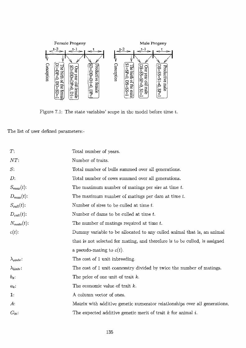
Female Progeny Male Progeny
t-2 t-1 t
~< ~~~)~)I J-2 t-1 t
~< ~~~/~)I n t:;l~
~0 v n ~~ t::lo t:;l 41 0 I!::T 0 :::s II :::s II ::T 1f:::s en ("";) t:;lg_ II :::s ("";) en(!) II 0
~ t:;l(l) v (1) ~sr. en(!) en §" '"'0 ...... v '"0 en'< en II :::::1. t:;l~ :;:t. II :::::1. II (1) a. c;· o::r II !:; II 0 ~0 ::T enl:i II
:::s ~ 0 v :::s oo en < o- t::lo ....... '"'CO ....... (1)
~-- II ~ en::!".' II ....... II s t::'S'- II 0.. ~0 s II ::T oO.. ~0 II (1) p~ en(!) ~ s e:.. ~~ v e:.. lfS en~» en (1) os (1) ............. '"'0 II E3 -e:.. '"'0 ....... a II (1) II -~» II (1)
II (1) - .......
Figure 7.1: The state variables' scope in the model before timet.
The list of user defined parameters:-
T:
NT:
S:
D:
Smax(t):
Dmax(t):
Scuu(t):
Dcuu(t):
Nmate(t):
c(t):
Asinbr:
1:
A:
Gki:
Total number of years.
Number of traits.
Total number of bulls summed over all generations.
Total number of cows summed over all generations.
The maximum number of matings per sire at time t.
The maximum number of matings per dam at time t.
Number of sires to be culled at timet.
Number of dams to be culled at timet.
The number of matings required at time t.
Dummy variable to be allocated to any culled animal that is, an animal
that is not selected for mating, and therefore is to be culled, is assigned
a pseudo-mating to c( t).
The cost of 1 unit inbreeding.
The cost of 1 unit coancestry divided by twice the number of matings.
The price of one unit of trait k.
The economic value of trait k.
A column vector of ones.
Matrix with additive genetic numerator relationships over all generations.
The expected additive genetic merit of trait k for animal i.
135

pki:
The list of state variables:-
S1i(t):
SPi(t):
D1j(t):
DPj(t):
DDij(t + 1):
The phenotypic value of trait k for animal i.
Bull i at timet is one year old (and non-reproductive).
Bull i at time t is reproductive (age > 1).
Cow j at timet is one year old (and non-reproductive).
Cow j at time t is reproductive (age > 1).
The density function of a Bernoulli distribution where
_ _ { 1, if the stochastic variable x ;::: 0. 5 DDij(t + 1)- f(x)-
0, otherwise
If DDij(t + 1) is 1 then at t + 1 dam i become the mother of cow j,
resulting from a mating at t. xis a uniformly distributed
independent random variable.
The density function of a Bernoulli distribution where
_ _ { 1, ifthestochasticvariablex;::: 0.5 DSij(t + 1)- f(x)-
0, otherwise
If D Sij ( t + 1) is 1 then at t + 1 dam i become the mother of bull j,
resulting from a mating at t. xis a uniformly distributed
independent random variable.
The density function of a Bernoulli distribution where
{
1, if the stochasticvariablex ;::: 0.5 SDij(t + 1) = f(x) =
0, otherwise
If SDij(t + 1) is 1 then at t + 1 sire i become the father of cow,
resulting from a mating at t. x is a uniformly distributed
independent random variable.
The density function of a Bernoulli distribution where
{
1, if the stochasticvariablex ;::: 0.5 ssij(t + 1) = f(x) =
0, otherwise
If s sij ( t + 1) is 1 then at t + 1 sire i become the father of bull j'
resulting from a mating at t. x is a uniformly distributed
independent random variable.
136

The list of decision variables are:
Xi(t): A binary variable set to 1 if bull (reproductive male) i is alive in timet and is
not culled; otherwise 0.
1j(t): A binary variable set to 1 if cow (reproductive female) j is alive in timet and is
not culled; otherwise 0.
Mij(t): A binary variable set to 1 if the ith sire is mated with the jth dam in timet;
otherwise 0. Mij is an element in the mating matrix M.
An extra row and column is added to represent culling.
7.3.2 The objective function
In this section, some interesting objectives are introduced from the dairy industry view point.
These objectives can be changed independently of the constraint systems. It is guaranteed that
the constraint systems are valid regardless of the objective's nature by isolating the domain spe
cific components in the objective function, omitting the general constraints in an evolutionary
allocation problem. Therefore, there is not domain specific knowledge in the system of con
straints. It may be added here that each sub-objective can be transformed into a constraint by
setting the appropriate bound(s) on it.
A typical sub-objective to be maximised in a breeding program is the genetic gain. Kinghorn
(1987) finds that mate-selection has no value when the genetic traits are additive. In this case,
mating the selected individuals randomly will result in the optimal solution (at least for the
next stage); that is, mate randomly the best bulls with the highest genetic values with the best
cows. If there is an interaction between parents, the objective function becomes nonlinear, eg.
due to dominance, heterosis, inbreeding depression, or other nonlinear breeding phenomena. In
addition, for the longer term, the objective function is nonlinear due to the effect of co-ancestry.
In designing the breeding sub-objectives, a compromise between short and long term objectives
137

is required. Short term objectives will apply to those criteria which will contribute to the short.
term (the following year or two). For example, culling cows with low phenotypic production
value will increase the average production per cow within the farm. Two short term objectives
are considered: the profit of not culling an animal in the current period taken to be its expected
production profit in the following stage, and the short term inbreeding depression represented
with the average inbreeding (in producing animals) multiplied by the cost of 1 unit inbreeding
depression.
Two long term objectives are defined: genetic gain and long term inbreeding ( coancestry). Long
term gain also is affected by genetic variation. Matings can create more or less variation and
therefore affect future merit. The impact of improving the genetic makeup in a herd appears after
a number of years ( eg. in dairy cattle, after one generation, which is about 5 years). Long term
inbreeding, known as coancestry (Wray and Goddard 1994), is the second long term objective.
The idea here is simply to minimise the level of relationship between the animals within each
year so that inbreeding is minimised on the long run.
The four sub-objectives for short and long term planning can be formulated as follows:
1. 01: the first short term objective representing the production index:
T D NT
Maximise 01 = LL>Lbk x Pkj(t)) x Yj(t). (7.1) t=l j=l k=l
In this sub-objective a production index, 2::;:~ bk x Pkj(t), is calculated by multiplying the
price of trait k, bk, by the phenotypic value of this trait for animal j, Pkj(t), at timet, where
NT is the number of traits. The index's value is significant only if the animal is alive and
reproductive; that is, Yj ( t) = 1. We may note that the value of production is meaningful
only for the female and consequently, the males are not included in this objective.
2. 02: the second short term objective representing short term inbreeding:
138

T
Minimise 02 = L Asinb X ([Xt(t), yt(tW X (Diag(A)- 1)). (7.2) t=l
In this sub-objective, Diag(A) returns the diagonal elements of the numerator relationship
matrix as a column vector and by subtracting from it a vector of ones, 1, the result is simply
the inbreeding coefficient for each animal which, if multiplied by the vector [Xt(t), yt(t)]t,
the result will be the total inbreeding in generation t. Multiplying this value by the cost
of one-unit inbreeding, Asinb, results in the total short-term inbreeding cost/penalty. The
matrix A can be constructed easily using the algorithm of Henderson (1975b) where the
matrices D S, S D, D D, and S S provide the pedigree information required for constructing
A.
3. 03: the first long term objective representing the breeding values:
T S NT T D NT
Maximise 03 = L LXi(t) x L(ak x Gki(t)) + L LYJ(t) x L(ak x Gk(S+j)(t)). t=l i=l k=l t=l j=l k=l
(7.3)
In this sub-objective, a selection index, L:~~(ak x Gki(t)), is calculated by multiplying the
economic value of trait k, ak, by the expected genotypic value of this trait for animal i,
Gki(t), at timet. The index value is significant only for alive animals (males and females),
Xi(t) = 1 and Yj(t) = 1.
4. 04: the second long term objective representing long term inbreeding:
T D s Minimise 04 = LAlinb X [ 2:: Mij(t), ( 2:: Mij(t))t] x Ax
t=l j=l,#c(t) i=l,i#c(t) D s
[( 2:: Mij(t))t, 2:: Mij(t)]. (7.4) j=l,#c(t) i=l,i#c(t)
In this sub-objective, the coancestry relationship is calculated by multiplying a row vector
of the proportional contribution of each animal, ['L:f=l,#c(t) Mij(t), ('2:7=l,i#c(t) Mij(t))t],
times the numerator relationship matrix, times the transpose of the vector representing the
139

contribution of each animal. If this value is multiplied by the cost/penalty of coancestry
divided by twice the number of matings, Alinb, the resultant value is the cost of long
term inbreeding ( der Werf 1990). The two components in the square brackets represent
a concatenation of two vectors. Each component is derived from matrix M by summing
either the rows ( ie. i = 1 ... S) or the columns ( ie. j = 1 ... D), which yields a column or
row vector respectively.
The problem can also be formulated as a single objective stochastic multi-stage decision model
by introducing a set of preferential weights, a, /3, "(, and 6,. The negative weights are assigned
to transform a minimisation sub-objective to a maximisation one. In this case, the objective
function will be,
Maximise a x 01 + f3 x 02 + "( x 03 + 6 x 04, a,"! ~ 0, /3, 6 :::; 0 (7.5)
7.3.3 Constraints
There are two types of constraints in the model: explicit and implicit or logical constraints.
Explicit constraints are marked (Explicit). The model involves a considerable number of logical
constraints to be satisfied by the state variables. These constraints fall into categories, we call
A, B, ... , F, with the constraints within a category being somewhat similar. A special category
(logical) is designated for logical constraints not associated with the state variables. If we con
sider state variables in their vector or matrix form (for example, X = (X 1 , X 2 , ... ) ) , then each
constraint affects a number of state variables that tend to occur in pairs. As an aid to visualise
the constraints, we have presented in Figure 7.2 a graph with nodes labelled with the state vari
ables and arcs labelled with constraint categories. The arcs connecting pairs of variables (nodes)
are labelled with the relevant constraint category. For example, the arc labelled "A1" joining
nodes M (the mating matrix) and DD (the mother-daughter relationship matrix) refers to a
constraint category between M and DD that is similar to constraints between M and DS, SS
and SD which are also labelled "A1", "A2", and "A2" in the figure. The arrows in the figure
are used to suggest causation. For example, the matrix D D follows as a result of a mating via
the matrix M producing female offspring. Therefore, the arc is directed from M toDD.
140

Figure 7.2: The logical relationships between the model's variables
1. The number of matings for each sire (dam) is not allowed to exceed the maximum number
of matings allowed for a sire (dam) in year t (the matings take place between vectors S P ( t)
(productive sires) and DP(t) (productive dams) as illustrated before. (Category Explicit)
s I: Mij(t) ::; Dmax(t), j = 1. .. D, t = 1. .. T.
i=l,i;;ofc(t)
D
I: Mij(t) ::; Smax(t), i = 1. .. S, t = 1. .. T. j=l,j;;ofc(t)
(7.6)
(7.7)
2. The total number of allocations should equal the total number of matings required. (Cat
egory Explicit)
s D
I: I: Mij(t) = Nmat(t), t = 1 ... T. (7.8) i=l#c(t) j=l,#c(t)
3. The total number of bulls/cows allocated for culling should equal the total number of
culling required. All cows, which are non-mated in a generation, are culled at the end of
that generation. (Category Explicit)
D
L Mc(t),j(t) = Dcuu(t), t = 1 ... T. j=l,#c(t)
141
(7.9)

s L Mi,c(t)(t) = Scuzz(t), t = 1 ... T.
i=l,i'fc(t)
(7.10)
4. A sire or dam that is allocated for mating cannot be allocated for culling in the same years.
(Category logical)
D
Mi,c(t)(t) X L Mij(t) = 0, i = 1 ... S, t = 1 ... T. j=l,j'fc(t)
s Mc(t),j(t) X L Mij(t) = 0, j = 1 ... D, t = 1 ... T.
i=l#c(t)
(7.11)
(7.12)
5. A logical constraint preventing the mating between the two special culling nodes in each
year. This constraint is essential to prevent cycling. (Category logical)
Mc(t),c(t)(t) = 0, t = 1 ... T. (7.13)
6. Each sire (dam) mated at the beginning of year t has a number of progeny in the end of
the year equal to the number of its matings. (Category A1 and A2)
S D S
L Mij(t)- L:nnjk(t)- L:nsjz(t) = o, j = 1 ... D,t = 1 ... T. (7.14) i=l,i'fc(t) k=! l=l
D D S
L Mij(t) - L SDik(t) - L SSil(t) = 0, i = 1 ... s, t = 1 ... T. (7.15) j=l,#c(t) k=l l=!
7. If a mating Mij occurred, the offspring gender in the year for both the sire and the dam is
the same.
D S
Mij(t)- L DDjk(t) x SDik(t)- L DSjz(t) x SSil(t) = 0 k=l l=l
, i = 1 ... S, j = 1 ... D, t = 1 ... T. (7.16)
142

8. For all sires in each year, the number of male progeny equals the number of female progeny.
Here it is required that the actual number of males and females offspring equal the expected
number. However, to count for the case where the total number of progeny is an odd
number, it is required that the difference between the number of males and females progeny
to be less than or equal to one. (Category B)
S D S S
L L SDik(t) - L L SSil(t) ::; 1, t = 1 ... T. (7.17) i=l k=l i=l l=l
9. Progeny conceived in the current year (t) will be one-year-old non-reproductive individuals
in the next year ( t+ 1) and each child has precisely one mother and one father. (Category C)
• Each male child has one mother.
D
L DSli(t) = S1i(t + 1), i = 1. .. s, t = 1. .. (T- 1). (7.18) l=l
• A one-year-old male child in year t cannot be a new child of any dam in year t.
D
S1i(t) + L DSu(t) ::; 1, i = 1. .. S, t = 1. .. T. (7.19) l=l
• A reproductive male child in year t cannot be a new child of any dam in year t.
D
S~(t) + L DSli(t) ::; 1, i = 1. .. s, t = 1. .. T. (7.20) l=l
• Each male child has one father.
s L SSu(t) = S1i(t + 1), i = 1 ... S, t = 1 ... (T- 1). (7.21) l=l
• A one-year-old male child in year t cannot be a new child of any sire in year t.
s S1i(t) + L SSu(t) :=:; 1, i = 1. .. S, t = 1. .. T. (7.22)
l=l
143

• Each female child has one mother.
D
L DDzj(t) = D1j(t + 1), j = 1 ... D, t = 1 ... (T- 1). (7.23) l=l
• A one-year-old female child in year t cannot be a new child of any dam in year t.
D
D 1 j ( t) + L D Dzj ( t) ::; 1, j = 1 ... D, t = 1 ... T. (7.24) l=l
• A reproductive female child in year t cannot be a new child of any dam in year t.
D
D pj ( t) + L D Dlj ( t) ::; 1' j = 1 ... D' t = 1 ... T. (7.25) l=l
• Each female child has one father.
s L SDzj(t) = D1j(t + 1), j = 1 ... D, t = 1 ... (T- 1). (7.26) l=l
• A one-year-old female child in year t cannot be a new child of any sire in year t.
s D1j(t) + L SDzj(t) ::; 1, j = 1 ... D, t = 1 ... T. (7.27)
l=l
10. Any reproductive bull/cow in the next year is either a one year old bull/cow in the current
year, or it is a sire/dam in the current year and has not been culled. This also forces a
bull/cow to be either reproductive or not. (Category D)
SPi(t + 1) = S1i(t) + Xi(t), i = 1 ... S, t = 1 ... (T- 1). (7.28)
SPi(t) + S1i(t) ::; 1, i = 1 ... S, t = 1 ... T. (7.29)
DPj(t + 1) = D1j(t) + Yj(t), j = 1 ... D, t = 1 ... (T- 1). (7.30)
DPj(t) + D1j(t) ::; 1, j = 1 ... D, t = 1 ... T. (7.31)
144

11. A flag constrains Xi(t) to refer to sires that are not culled in year t. If sire i had a real
mating in year t then we must force Xi(t) to be 1. Similar results apply to lj(t) for dams.
(Category F)
D
(1- Xi(t)) X L Mij(t) = 0, i = 1. .. s, t = 1. .. T. j=l,#c(t)
D
-Xi(t) + L Mij(t) 2:: 0, i = 1. .. s, t = 1. .. T. j=l,jfc(t)
s ( 1 - lj ( t)) X L Mij ( t) = 0, j = 1. .. D' t = 1. .. T.
i=l#c(t)
s -lj(t) + L Mij(t) 2:: 0, j = 1. .. D, t = 1. .. T.
i=l,ifc(t)
(7.32)
(7.33)
(7.34)
(7.35)
12. The bulls/cows are available for allocation in year t if and only if they are reproductive
in year t. In the first constraint, if bull i is mated or culled, it must be reproductive and
SPi(t) forced to 1. In the second constraint, if bull i is not mated or culled then it is non
reproductive and SPi(t) is forced to 0. The same interpretation applies for the subsequent
two constraints for a cow. (Category H)
• If bull i is allocated then it must be reproductive.
D
(1- SPi(t)) X L Mij(t) = 0, i = 1 ... s, t = 1 ... T. (7.36) j=l
• If it is reproductive, then it must be allocated (even for culling).
D
-SPi(t) + L Mij(t) 2:: 0, i = 1. .. s, t = 1. .. T. j=l
• If cow i is allocated then it must be reproductive.
s
(7.37)
(1- DPj(t)) X L Mij(t) = 0, j = 1. .. D, t = 1. .. T. (7.38) i=l
145

• If it is reproductive, then it must be allocated (even for culling).
s -DPj(t) + LMij(t) 2: 0, j = 1 ... D, t = 1 ... T. (7.39)
i=1
• The progeny born in year t must be guaranteed not to exist as individuals in previous
years ( ie. 0 .. . ( t - 1)).
D (t-1)
L D8ki(t) X L Xi(l) = 0, i = 1 ... 8, t = 1 ... T. (7.40) k=1 l=1
s (t-1)
L 88ki(t) x L xi(Z) = o, i = 1 ... 8, t = 1 ... T. (7.41) k=1 l=1
D (t-1)
L DDkj(t) X L Yj(l) = 0, j = 1 ... D, t = 1 ... T. (7.42) k=1 l=1
s (t-1)
L 8Dkj(t) X L Yj(l) = 0, j = 1 ... D, t = 1 ... T. (7.43) k=1 l=1
7.4 Model complexity
This model can be solved either as a Stochastic Multi-objective Multi-stage decision Model or
expanded and solved as a stochastic multi-objective binary nonlinear model.
In the former, the number of variables in each year is D 2 + 8 2 + 2D x S +3D+ 38 + D x S,
which simplifies to (D + 8) 2 + 3 x (D + S) + D x S. These values are derived from Equations 7.6
to 7.43. There are up to 16D + 168 + D x 8 + 5 constraints. The search space in each year
will be approximately 2(D+S)2+3x(D+S)+Dxs. For example, if we have 200 dams and 10 sires and
we wish to optimise for 5 years, there will be 46,730 variables in each year with at most 5,365
constraints, and approximately search space size of 1014067 .
In the latter, the number of variables is Tx ((D+8) 2 +3x (D+8)+Dx 8) with 16xTx (D+S)+
T X D x S + 5 X T- 3 x (8 +D) constraints. The search space will be 2Tx((D+S?+3x(D+S)+DxS).
In the previous example, there will be 233,650 variables in all years with 26,195 constraints, and
146

approximately search space size of 1070335 .
7. 5 Conclusion
This chapter emphasises the formulation aspect of the third thesis sub-objective; formulating and
solving the version of the mate-selection problem to be solved in this thesis, where a stochastic
multi-objective multi-stage decision model was formulated for our generic mate-selection problem.
The model with its very high complexity, is definitely not solvable by conventional optimisation
techniques. The complexity presented here assumes our formulation, and raises a number of
questions.
Q: Is the proposed formulation, the best one?
A: One may argue that there are better formulations. For example, why do we not have a single
vector for all dams, where each cell in the vector is an index ( eg. -1 for culling, 0 for birth, 1 for
one year old, and 2 for reproductive)? The same may apply for the bulls. This is an interesting
way to combine the binary vectors D1, DP, and Y into a single vector and accordingly may
reduce the search space. Let us call the proposed vector of multiple values V. The question now
is how to formulate the constraint that if V ( t) is 1 then V ( t + 1) should be 2? The answer is
simple; introduce a flag (binary variable) to indicate that the value of V(t) is 1 and use this flag
to force the value of V(t + 1) to be 2 (notice that the constraint 2 x V(t) - V(t + 1) = 0 is
not a valid choice here because when V(t) = 0, V(t + 1) should be 0 as well but the animal can
live many years after being mature). But we have introduced a binary variable for this logical
equation and we require different ones for each logical equation. Essentially, this means that we
paid much more than what we saved!
It is not claimed here that this is the best formulation that can ever be found. Formulation is
an art. Nevertheless, many different ways to formulate the problem have been investigated and
this was the best method found.
147
Q: Do we need a complex formulation? We build simulation models and all logical
constraints are controlled by simple "if ... then ... " rules. Why do we require this
complicated model if the problem can be programmed in few lines? Do we need to
waste over 20 pages to present the problem?
A: The quote in the beginning of this chapter by Albert Einstein answered these questions
already. Life is simple but controlling it is not. The fact that this problem can be coded into
a computer program or can be simulated does not contradict our finding that the search space
is enormous. The first useful contribution of the proposed formulation is that no one can claim
a tractable algorithm for solving the problem and reaching an optimal solution. The second
is to understand the dimension of the problem we are dealing with instead of dreaming with
optimality. This may save a lot of time and wasted efforts. The third is that it provides a formal
representation as a rational starting point to solve a complex problem. The fourth contribution
is that it embraces the complete picture, where one can start with a simplified version and then
increase the complexity gradually once a suitable algorithm is found.
In the following chapters, customised versions of this model are presented for farmers depending
completely on artificial insemination bulls. It will also be shown that the reduction of this
model to single stage is a quadratic transportation problem (quadratic objective with linear
constraint). The single stage model will be solved using genetic algorithms in Chapter 8 as well
as the customised version of the multi-stage model in Chapter 9.
148
Chapter 8
Genetic Algorithm Applied to the
Single-stage Model
This chapter aims at formulating a single stage mate-selection model and then finding the best
set of GA operators that result in a prompt effective solution for the problem. This set of GA
operators is essential for the next chapter in the process of solving the multi-stage model. In
Section 8.1, the formulation of the evolutionary allocation problem, presented in Chapter 7, will
be customised for farms dependent on the artificial insemination program; where natural mating
is not allowed. In Section 8.2, a genetic algorithm design for the single-stage model is presented
followed by a number of experiments with the aim of identifying a set of genetic algorithm
operators that reach the best solution found quickly and reliably in Section 8.3.
8.1 A single stage model
In Chapter 7, the evolutionary allocation problem formulation was shown. It was found that the
problem is very complex, both in reality (for an animal breeder) and in its mathematical rep
resentation. In this chapter, the problem is simplified to a degree by assuming female offspring
and sires are coming from an artificial insemination service with all sires genetically unrelated
to the initial set of cows. Also, a stage is taken to be two years to reduce the complexity of the
model by eliminating those transitions and state variables which keep track of the animal age.
In this section, the multi-stage model will be reduced to a single-stage model that will be solved
149
and used as a basis for solving the former. In the single-stage model, a considerable number of
variables and constraints will be removed. All transition variables and all state variables except
the matrix Mare obliterated from the model. The single-stage model is then1 :
Maximise ax 01 + f3 x 02 + 'Y x 03 + c5 x 04, a, 'Y;::::: 0, /3, c5::; 0 (8.1)
where
subject to:
D NT S
01 = LLbk X pkj X L Mij j=l k=l i=l,i#c
02 = Asinb X Et X (Diag(A) - 1) D S NT
03 = L L Mij x L(ak x Gk(S+j)) j=l i=l,i#c k=l
D S D
04 = Atinb X [ L Mij, ( L Mij)t] X A X [( L Mij)t, j=l,#c i=l,i#c j=l,j#c
s L Mij ::; 1, j = 1. .. D i=l
D
L Mij ::; Smax, i = 1 ... S j=l
S D
L LMij=Nmat i=l,i#c j=l
D
LMcj = Dcull j=l
Mij E {0, 1}, i = 1. .. S, j = 1. .. D
(8.2)
(8.3)
(8.4)
s L Mij] (8.5)
i=l,i#c
(8.6)
(8.7)
(8.8)
(8.9)
(8.10)
Several changes have been introduced to the model. Since no culling is allowed for sires, the
vector E is introduced in the second objective with dimensionS+ D +number of progeny.
The first S + D elements in E are 08 and the others are 18 • Therefore, the short term inbreeding
is, as usual, a function of the progeny. The term concerning the genotypic values for sires is
excluded from the third objective since again, the farmer's own sires are not considered here.
1 Because the model is reduced to a single-stage one, only explicit constraints remain.
150
The single-stage model is now reduced to a quadratic transportation model ( ie. quadratic ob
jective function with linear constraints). The source of the quadratic term is 04, the coancestry
term. Actually, this model is highly non-linear if we consider how the matrix A is generated.
Recalling from Chapter 2, A is generated by a set of recursive functions over the family tree of
the animals. In the rest of this chapter, this model will be solved using GA. Assuming 200 dams
and 10 sires, the search space is 10660.
8. 2 Genetic algorithm for the single-stage model
To present the application of GA for solving the single-stage model, a number of issues still
need to be addressed. These are representation, crossover operators, and the repair operator
( ie. method of maintaining the constraint-system's feasibility). The repair operator is effectively
replacing the mutation operator, since it introduces variations to the model when the chromo
some's feasibility is broken.
8.2.1 Representation
The selected representation for the problem will be introduced followed by a discussion of some
alternatives and the extent of their pertinence. In the chosen representation, the dams and sires
are randomly assigned a unique index between 0- ( D- 1) and 0- ( S- 1) respectively. The chro
mosome is represented with an array of dimension equal to the number of dams. Each position j
in the array is analogous to dam j in the model and each cell in the array can take one of S + 2
integer values, where S is the number of sires and the additional two values are -1 for culling
and -2 for not selected. For example, having the value 3 in cell 1 signifies that the dam number
1 is allocated to sire number 3. This representation guarantees the feasibility of Constraint 8.6
since there is only one cell per dam. Consequently, every dam will be bound to a single decision
(mating, culling, or no-action). In contrast, Constraints 8.7, 8.8, and 8.9, may be broken.
Therefore, a strategy to retrieve the feasibility will be explained in Section 8.2.3. Assuming 200
dams and 10 sires, the search space, using the proposed representation, is reduced from 10660 to
10208 . A typical chromosome in the GA for the single stage model is as shown in Figure 8.1.
151
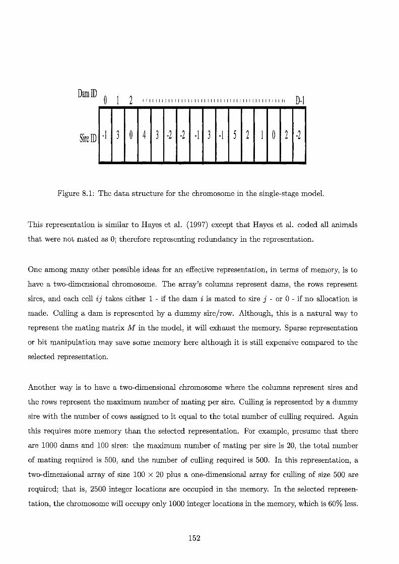
DamiD 0 2 I I I I I I I I I I I I I I I I I I I I I I I I I I I I I I I I I I I I I I I I I I I II D-1
Sire ID -1 j 0 4 j -2 -2 -1 j -1 5 2 1 0 2 -2
Figure 8.1: The data structure for the chromosome in the single-stage model.
This representation is similar to Hayes et al. (1997) except that Hayes et al. coded all animals
that were not mated as 0; therefore representing redundancy in the representation.
One among many other possible ideas for an effective representation, in terms of memory, is to
have a two-dimensional chromosome. The array's columns represent dams, the rows represent
sires, and each cell ij takes either 1 - if the dam i is mated to sire j - or 0 - if no allocation is
made. Culling a dam is represented by a dummy sire/row. Although, this is a natural way to
represent the mating matrix Min the model, it will exhaust the memory. Sparse representation
or bit manipulation may save some memory here although it is still expensive compared to the
selected representation.
Another way is to have a two-dimensional chromosome where the columns represent sires and
the rows represent the maximum number of mating per sire. Culling is represented by a dummy
sire with the number of cows assigned to it equal to the total number of culling required. Again
this requires more memory than the selected representation. For example, presume that there
are 1000 dams and 100 sires: the maximum number of mating per sire is 20, the total number
of mating required is 500, and the number of culling required is 500. In this representation, a
two-dimensional array of size 100 x 20 plus a one-dimensional array for culling of size 500 are
required; that is, 2500 integer locations are occupied in the memory. In the selected represen
tation, the chromosome will occupy only 1000 integer locations in the memory, which is 60% less.
152

8.2.2 Crossover
Additional to the crossover operators mentioned in Chapter 6, a biased version of the uniform
crossover is proposed, gene-based crossover. In gene-based crossover, the goal here is to calculate
the contribution of each gene to the total fitness, and to then use the relative gene fitness as a
crossover probability. The reason is that we assume in gene-based crossover an additive model;
where the overall fitness of a chromosome is the summation of the individual fitness of each gene.
It is essential to distinguish between fitness distribution as introduced here, and the fitness distri
bution analysis (Fogel and Ghozeil1996) recently presented in the literature. Fitness distribution
analysis is used to predict the variation operators' effect in the population, mainly for continuous
optimisation. Here, fitness distribution means distributing the total chromosome fitness among
its genes. This does not necessarily require that the components of the fitness function be separa
ble as will be exemplified soon. The algorithm for the gene-based crossover is given in Figure 8.2.
re-distribute the two chromosomes' fitness on all genes if the first chromosome's fitness > the second
begin foreach gene, g1, in the first chromosome and its corresponding gene in the second chromosome, g2
if fitness(g1) > fitness(g2) then choose g1 or g2 with a probability proportion to their fitness else assign 50% chance for g1 and g2 to be chosen
end else begin
foreach gene, g1, in the first chromosome and its corresponding gene in the second chromosome, g2 if fitness(g1) < fitness(g2) then choose g1 or g2 with a probability proportion to their fitness else assign 50% chance for 91 and g2 to be chosen
end
function fitness(gi) sum= 0 add to sum the genotypic, phenotypic, and inbreeding values of the animal add to sum the animal's contribution in the coancestry term return sum
end function
Figure 8.2: The gene-based crossover operator.
The distribution of the chromosome's fitness among its genes is easy if the objective function
153
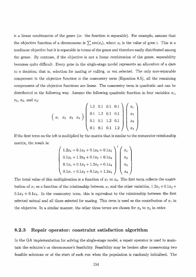
is a linear combination of the genes ( ie. the function is separable). For example, assume that
the objective function of a chromosome is I: sin( xi), where xi is the value of gene i. This is a
nonlinear objective but it is separable in terms of the genes and therefore easily distributed among
the genes. By contrast, if the objective is not a linear combination of the genes, separability
becomes quite difficult. Every gene in the single-stage model represents an allocation of a dam
to a decision; that is, selection for mating or culling, or not selected. The only non-separable
component in the objective function is the coancestry term (Equation 8.5), all the remaining
components of the objective functions are linear. The coancestry term is quadratic and can be
distributed in the following way. Assume the following quadratic function in four variables xi,
x2 , x 3 , and x 4 :
1.2 0.1 0.1 0.1 XI
( XI X4 )
0.1 1.2 0.1 0.1 x2 X2 x3
0.1 0.1 1.2 0.1 x3
0.1 0.1 0.1 1.2 X4
If the first term on the left is multiplied by the matrix that is similar to the numerator relationship
matrix, the result is:
1.2xi + 0.1x2 + 0.1x3 + 0.1x4 xi
O.lxi + 1.2x2 + 0.1x3 + 0.1x4 x2
0.1xi + 0.1x2 + 1.2x3 + 0.1x4 X3
0.1xi + 0.1x2 + 0.1x3 + 1.2x4 X4
The total value of this multiplication is a function of XI to x4 . The first term reflects the contri
bution of XI as a function of the relationship between XI and the other variables, 1.2xi + 0.1x2 + 0.1x3 + 0.1x4. In the coancestry term, this is equivalent to the relationship between the first
selected animal and all those selected for mating. This term is used as the contribution of XI in
the objective. In a similar manner, the other three terms are chosen for x2 to x4 in order.
8.2.3 Repair operator: constraint satisfaction algorithm
In the GA implementation for solving the single-stage model, a repair operator is used to main
tain the solution's or chromosome's feasibility. Feasibility may be broken after crossovering two
feasible solutions or at the start of each run when the population is randomly initialised. The
154

repair operator is unbiased in the sense that all changes are made by random selection, which
has a similar effect to mutation. The algorithm is presented in Figure 8.3.
count the number of allocations, alloc;, per each sire, i, and the total number of culling, Cull foreach sire i
if alloc; > maximum_number _of _sire_allocations then while alloci :f. maximum_number _of _sire_allocations do
randomly select one of the dams allocated to i assign the value -2 to it alloc; = alloci - 1
next i if Cull > number _of _allowed_culling then
while Cull :f. number_of_allowed_culling do randomly select a dam j if j has a value -1 then assign -2 to j, Cull= Cull- 1
else if Cull< number _of _allowed_culling then while Cull :f. number _of _allowed_culling do
randomly select a dam j if j has a value -2 then assign -1 to j else if j has a value > -1 then
alloc; = alloc; - 1, i is the sire allocated to j assign -1 to j Cull = Cull + 1
count the total number of mating, Mat if Mat> number_of_allowed_mating then
while Mat :f. number _of _allowed_mating do randomly select a dam j if j has a value > -1 then
alloc; = alloci - 1, i is the sire allocated to j assign -2 to j Mat=Mat-1
if Mat < number _of _allowed_mating then while Mat :f. number _of _allowed_mating do
randomly select a dam j if j has a value -2 then
randomly select a sire i, alloci < maximum_number _of _sire_allocations assign i to j Mat=Mat+1 alloc; = alloci + 1
Figure 8.3: The repair operator.
The algorithm starts with counting the number of allocations for each sire. A loop is then con
structed, over all sires. If a sire exceeds the maximum number of allowed mating per sire, the
excess is eliminated by randomly selecting a dam from those mated to this sire and assigning to
155
it the symbol -2, denoting a no action decision. This process is repeated until all sires meet the
maximum allowed mating per sire constraint. The next step is to calculate the total number of
dams selected for culling. If this number exceeds the number of culling requested by the user, a
dam which is assigned to culling is selected at random and the symbol -2 is then assigned to it.
The step is repeated until the total number of dams assigned for culling equals the number of
culling required. If the total number of culling is less than that determined by the user, a dam
is selected at random. If the value assigned to this dam is -2, it is set to -1 and the total number
of culling is increased by one. If the value assigned to this dam is greater than -1 - the dam is
selected for mating and is being assigned to a bull - the number of mating for the bull allocated
to this dam is reduced by one, the total number of mating is reduced by one, and the dam is
assigned -1. The process is repeated until the total number of culling equals the number of culling
required by the user. Then, the total number of mating in the chromosome is calculated. If the
total number of mating is greater than the number of mating required by the user, a dam which
is being assigned to a bull is selected at random and assigned -2. The total number of mating is
then reduced by 1 and the algorithm loops until the total number of mating equals the number
of mating required by the user.
If the total number of mating is less than the number of mating required by the user, a dam
which is assigned -2 is selected at random and a bull that has not reached maximum number of
mating per bull, is chosen at random and is assigned to this dam. The total number of mating
is increased by one and the algorithm loops until the total number of mating is equal to the
number of mating required by the user.
8.3 Experiments
8.3.1 The data simulation model
Ten artificial herds were generated at random with different seeds and evolved for 20 years. The
following steps were repeated for each of the ten herds. In year 0, 40 sires and 60 dams were
randomly generated then mated for 20 years. In each year, 20 dams were selected at random for
culling and 27 were selected at random for mating to simulate a random mating strategy, with
156
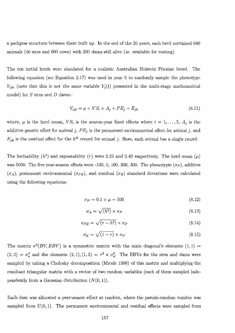
a pedigree structure between them built up. In the end of the 20 years, each herd contained 640
animals ( 40 sires and 600 cows) with 200 dams still alive ( ie. available for mating).
The ten initial herds were simulated for a realistic Australian Holstein Friesian breed. The
following equation (see Equation 2.17) was used in year 0 to randomly sample the phenotype
Yijk (note that this is not the same variable 1j(t) presented in the multi-stage mathematical
model) for S sires and D dams:-
(8.11)
where, J-L is the herd mean, Y Si is the season-year fixed effects where i = 1, ... , 5, Aj is the
additive genetic effect for animal j, P Ej is the permanent environmental effect for animal j, and
Ejk is the residual effect for the kth record for animal j. Here, each animal has a single record.
The heritability (h2) and repeatability (r) were 0.25 and 0.40 respectively. The herd mean (J-L)
was 5000. The five year-season effects were -100, 0, 100, 200, 300. The phenotypic (ap), additive
(aA), permanent environmental (apE), and residual (aE) standard deviations were calculated
using the following equations:
ap = 0.1 x J-L = 500
a A = ..j(hf) x ap
apE= V(r-h2 ) Xap
aE = v(l- r) X ap
(8.12)
(8.13)
(8.14)
(8.15)
The matrix a2 (BV, EBV) is a symmetric matrix with the main diagonal's elements (1, 1) =
(2, 2) = a~ and the elements (2, 1), (1, 2) = r 2 x a~. The EBVs for the sires and dams were
sampled by taking a Cholesky decomposition (Mrode 1996) of this matrix and multiplying the
resultant triangular matrix with a vector of two random variables (each of them sampled inde
pendently from a Gaussian distribution (N(O, 1)).
Each dam was allocated a year-season effect at random, where the pseudo-random number was
sampled from U(O, 1). The permanent environmental and residual effects were sampled from
157
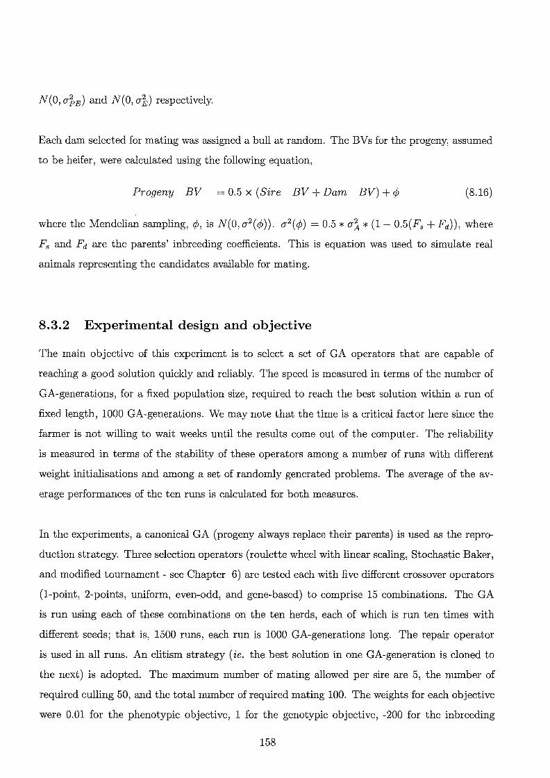
N(O, CJ~E) and N(O, CJ1) respectively.
Each dam selected for mating was assigned a bull at random. The BV s for the progeny, assumed
to be heifer, were calculated using the following equation,
Progeny BV = 0.5 x (Sire BV +Dam BV) + ¢ (8.16)
where the Mendelian sampling,¢, is N(O,CJ2 (¢)). CJ2 (¢) = 0.5 * CJ~ * (1- 0.5(F8 + Fd)), where
Fs and Fd are the parents' inbreeding coefficients. This is equation was used to simulate real
animals representing the candidates available for mating.
8.3.2 Experimental design and objective
The main objective of this experiment is to select a set of GA operators that are capable of
reaching a good solution quickly and reliably. The speed is measured in terms of the number of
GA-generations, for a fixed population size, required to reach the best solution within a run of
fixed length, 1000 GA-generations. We may note that the time is a critical factor here since the
farmer is not willing to wait weeks until the results come out of the computer. The reliability
is measured in terms of the stability of these operators among a number of runs with different
weight initialisations and among a set of randomly generated problems. The average of the av
erage performances of the ten runs is calculated for both measures.
In the experiments, a canonical GA (progeny always replace their parents) is used as the repro
duction strategy. Three selection operators (roulette wheel with linear scaling, Stochastic Baker,
and modified tournament- see Chapter 6) are tested each with five different crossover operators
(1-point, 2-points, uniform, even-odd, and gene-based) to comprise 15 combinations. The GA
is run using each of these combinations on the ten herds, each of which is run ten times with
different seeds; that is, 1500 runs, each run is 1000 GA-generations long. The repair operator
is used in all runs. An elitism strategy ( ie. the best solution in one GA-generation is cloned to
the next) is adopted. The maximum number of mating allowed per sire are 5, the number of
required culling 50, and the total number of required mating 100. The weights for each objective
were 0.01 for the phenotypic objective, 1 for the genotypic objective, -200 for the inbreeding
158
objective, and -1 for the coancestry objective. These weights were selected after 20 initial runs
to overcome the problem of magnitude for each objective. Therefore, the the four objectives have
actually the same value while the differences between the weights reflect the magnitude of each
objective. A different strategy to overcome this problem will be discussed in the following chapter.
8.3.3 Results and discussion
Two criteria are used to evaluate the results: the number of GA-generations elapsed to find the
best solution within 1000 GA-generations, and the average best solution value. The first criterion
measures the speed, and the second quantifies the operators' ability to reach a good solution in
a fixed number of GA-generations. The average of the number of GA-generations to find the
best solution, and the average values of the best solution found at GA-generation 1000 for the
population over the averages of ten runs with different seeds ± the standard deviation are shown
in Table 8.1.
As can be seen from Table 8.1 in the third column and row 1 through 10, gene-based crossover
outperforms all crossover operators when using fitness proportionate and Stochastic Baker se
lection operators. Notwithstanding, 1-point and 2-points crossover are better with the modified
tournament selection. Also, it was noticed that the gene-based crossover operator is always
outperforming the uniform crossover operator, which indicates that the bias introduced by the
gene-based crossover improved the conventional uniform crossover operator in this problem. Nev
ertheless, it is outperformed by the 1-point and 2-points crossover when the modified tournament
selection operator is used. However, it can be seen from Figures 8.4 8.5, that the gene-based
crossover performs better in the first 100 GA-generations but the 1-point operator also then
improves. In the same figures, the convergence to the best solution over 1000 GA-generations in
the ten runs is shown for gene-based crossover, using fitness proportionate and Stochastic Baker
selection operators, and 1-point crossover using modified tournament selection. The variations
among the ten runs (in terms of the standard deviations of the best solution found in each run)
were small; therefore suggesting that there is a consistency in the behaviour among different
runs. This is very important since it indicates that the behaviour of the three combinations of
operators is not sensitive to the initial seed. Also, the previous trends were consistent for the
159

other nine herds. Therefore, one can conclude that the operators' performance for this problem
is stable.
In summary, the choice is between the 1-point and 2-points crossover with modified tournament
selection. This choice is because, on the average, there is little difference between the best
solution found by both operators as can be seen from Table 8.1 - rows 12 and 13 respectively.
Since there is not much difference in the computations required for both of them, it was decided
to adopt the 1-point crossover with modified tournament selection operator, for subsequent GA
experiments in subsequent chapters, since it has the highest average (over the ten herds, 20810 ±
2440 compared to 20760 ± 2500 for two-points crossover operator). Furthermore, the standard
deviation is lower than that for the 2-point crossover. It is clear that we did not need to try
more than 2 points crossover since the solution did not improve with the increase in the number
of crossover points.
Table 8.1: The average results of ten GA runs for one of the ten herds
Selection Crossover Iterations Fitness of to Best the Best
Fitness proportion 1-point 940 ± 34 17915 ± 689 2-points 945 ± 45 18714 ± 588 uniform 770 ± 201 15112 ± 439 even-odd 215 ± 176 14625 ± 2165 gene-based 852 ± 133 19423 ± 266
Stochastic Baker 1-point 965 ± 38 20889 ± 431 2-points 908 175 20971 ± 437 uniform 928 ± 53 20721 ± 458 even-odd 225 ± 111 15593 ± 2122 gene-based 963 ± 25 22306 ± 247
Modified Tournament 1-point 913 ± 76 23152 ± 205 2-points 921 44 23235 ± 200 uniform 892 ± 102 21554 ± 225 even-odd 68 ± 23 15701 1941 gene-based 864 ± 166 20852 ± 324
160

26000
24000
22000
l 20000
1 .s
I 18000
.s _:g Jii '0 16000
~ '-£:
14000
12000
10000 0
1-point crossover with modified t:ouma.m.ent gene-based crossover with un-sealed selection
gene-based crossover with Stochastic Baker selection
100 200 300 400 500 600 700 800 GA-generation number
900 1000
Figure 8.4: The trajectories of the best solution over 1000 GA-generations for a single run.
26000
24000
22000 15 -~ :,;., 1 20000
.s
·! ..,. 8: 18000
Jii '0
! = t
16000
;;:;
~ 14000
12000
10000 0
1-point crossover with modified tournament gene-based crossover with un-sealed selection
gene-based crossover with Stochastic Baker selection
100 200 300 400 500 600 700 800 GA-generation number
900 1000
Figure 8.5: The trajectories of the average population fitness over 1000 GA-generations for a single run.
8.4 Conclusion
This chapter emphasises the solution of the single-stage mate-selection problem- that is being
discussed in the previous chapter - as a step to solve the multi-stage mate-selection problem 161

which is the third thesis sub-objective; formulating and solving the mate-selection problem. The
single-stage mate-selection problem is solved using genetic algorithms. The problem's solution
is represented using a one-dimensional array and a repair operator is developed to maintain the
feasibility of each solution-array. Three selection operators and five crossover operators are com
pared. The proposed gene-based crossover operator performes the best with fitness proportion
and Stochastic Baker selection operators while the one-point crossover operator performes the
best overall. It is also found that the performance of all operators is stable over all problems and
initialisations.
162

Chapter 9
Solving the Multi-stage Mate-selection
Problem
In this chapter, the formulation of the evolutionary allocation problem, presented in Chapter 7,
will be customised for farms only using the artificial insemination program, where natural mating
is not allowed. The problem is solved for five stages and it will be shown that the complexity
is reduced although still high. In Section 9.1, the customisation of the EAP model to farms
using the artificial insemination program is shown. The experimental design is introduced in
Section 9.2. Different strategies for solving the model are then presented in Sections 9.4 to 9.5,
9.6, 9.7, 9.8, 9.9, 9.10, 9.11, and 9.12. Section 9.13 presents a summary of the best result found
in each experiment and an overall comparison between the proposed solution strategies.
9.1 Customisation of the multi-stage model
In the previous chapter, the assumptions of the multi-stage model were set. In summary, the
farmer uses only artificial insemination bulls, a stage is two years, and all the progeny are as
sumed to be females. It is worth mentioning here that a stage is taken to be two years to reduce
the complexity of the model by eliminating those transitions and state variables which keep
track on the animal age. The multi-stage model is solved for five stages but the farmer is given
the results of the first stage only. This can be seen as a mate-selection index which discounts
the future impact of current allocations (see next chapter). The reason for that is, giving the
farmer a mate-selection schedule for the next five stages ( ie. ten years) is associated with high
163

risk such as the gender of progeny, death of animals, and failure of conception. The advantages
of the general model are still valid for the customised multi-stage model presented in this chapter.
Equations 7.10 to 7.13 are not required any more since males are artificial insemination bulls.
Equations 7.17 to 7.22, 7.28 to 7.29, 7.32 to 7.33, 7.36 to 7.37, and 7.40 to 7.41 are excluded
since male progeny are not allowed. The customised multi-stage model for farms using the ar
tificial insemination program is similar to the one presented in Chapter 7 with the previous
modifications. For clarity, the complete model follows. However, the relations in this model have
been previously presented in Chapter 7.
Maximise ax 01 + f3 x 02 + /' x 03 + c5 x 04, a,/' 2 0, /3, c5::; 0 (9.1)
where
T D NT
Maximise 01 = L :~:::>I: bk x Pkj(t)) x }j(t). t=l j=l k=l
T
Minimise 02 = LAsinb X ([Xt(t), yt(t)]i X (Diag(A) -1)). t=l
T D NT
Maximise 03 = LLYJ(t) x L(ak x Gk(S+j)(t)). t=l j=l k=l
T D S D
Minimise 04 = L Alinb X [L Mij(t), ( L Mij(t))t] X A X [(L Mij(t))t, t=l
subject to:
j=l i=l,i;"'c(t) j=l
s L Mij ( t) ::; 1' j = 1. .. D' t = 1. .. T.
i=l,i;"'c(t)
D
L Mij(t) ::; Smax(t), i = 1. .. S, t = 1. .. T. j=l
S D
L L Mij(t) = Nmat(t), t = 1 ... T. i=l,i#c(t) j=l
164
(9.2)
(9.3)
(9.4)
s
I: i=l,i;"'c(t)
(9.5)
(9.6)
(9.7)
(9.8)
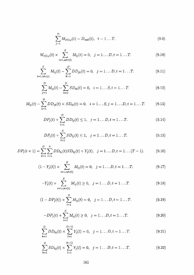
D
L Mc(t),j(t) = Dcuu(t), t = 1 ... T. j=1
s Mc(t),j(t) X L Mij(t) = 0, j = 1 ... D, t = 1 ... T.
i=1,i;6c(t)
S D
L Mij(t) - L DDjk(t) = 0, j = 1 ... D, t = 1 ... T. i=1,i;6c(t) k=1
D D
L Mij(t) - L SDik(t) = 0, i = 1 ... s, t = 1 ... T. j=1 k=1
D
(9.9)
(9.10)
(9.11)
(9.12)
Mij(t)- L DDjk(t) X SDik(t) = 0, i = 1 ... s, j = 1 ... D, t = 1 ... T. (9.13) k=1
D
DPj(t) + L DDzj(t) ::; 1, j = 1 ... D, t = 1 ... T. (9.14) 1=1
s D Pj ( t) + L S Dzj ( t) ::; 1, j = 1 ... D, t = 1 ... T. (9.15)
1=1
D S
DPj(t + 1) = L L DDkj(t)SDkj(t) + Yj(t), j = 1 ... D, t = 1 ... (T- 1). (9.16) k=1 1=1
s (1- Yj(t)) X L Mij(t) = 0, j = 1 ... D, t = 1 ... T. (9.17)
i=1,i#c(t)
s -Yj(t) + L Mij(t) 2:: 0, j = 1 ... D, t = 1 ... T. (9.18)
i=1,i;6c(t)
s (1- DPj(t)) XL Mij(t) = 0, j = 1 ... D, t = 1 ... T. (9.19)
i=1
s -DPj(t) + L Mij(t) 2:: 0, j = 1 ... D, t = 1 ... T. (9.20)
i=l
D (t-1)
LDDkj(t) XL Yj(l) = 0, j = 1 ... D,t = 1 ... T. (9.21) k=1 1=1
s (t-1)
L SDkj(t) X L Yj(l) = 0, j = 1 ... D, t = 1 ... T. (9.22) k=1 1=1
165

9.1.1 Model complexity
If the model is solved as a multi-stage model, the number of variables in each stage will be
D 2 + 2 x D + 2 x D x S with up to 12 x D + 2 x S + S x D + 2 constraints. The search space
in each stage will be approximately 2D2+2 xD+2xSxD. For example, if we have 200 dams and 10
sires and we would like to optimise for 5 stages, there will be 44,400 variables in each stage with
at most 2,422 constraints, and approximately search space size of 1013•365 .
If the model is expanded as a single-stage non-linear binary model, the number of variables will
be T x D 2 + 2 x D x T + 2 x D x S x T with 12 x D x T + 2 x S x T + D x S x T + 2 x T - D
constraints. The search space will be 2TxD2+2 xDxT+2 xDxDxT. In the previous example, there
will be 222,000 variables in all stages with 11,910 constraints, and approximately search space
size of 1066828 .
9.2 Experimental design and objectives
The experiments' objective (to be presented in the rest of the chapter) is to evaluate different
heuristics for mate-selection over 5 stages. It is common practice in animal genetics to simulate
a herd with characteristics derived from real life situations. Consequently, we need to simulate
a herd that endorses a relatively real life scenario. Therefore, the simulated model incorporates
some of the potential aspects of the problem. A more realistic version of the simulation model
presented in Section 8.3 is used in this chapter. The differences between the simulation model
used for the previous single-stage experiment and the one used for the multi-stage experiment,
presented in this chapter, include:
1. The season-year-effect, Y Si, in Equation 8.11 is separated into a year effect, Ye, and a
season effect, Si, in Equation 9.23.
2. The herd mean, Min Equation 9.23, is 5500 to match the latest figures of Australia.
3. To simulate a more realistic situation, two herds were simulated: a nucleus herd for gener
ating AI -sires to be used by a commercial herd.
166

For the reader's convenience, a summary of the simulation model will follow with the previous
modifications. The experimental setup is divided into two parts. First, we need to simulate
AI-sires and an initial starting herd. Second, we need to optimise the process of selection and
allocation between the cows in this herd and the AI-sires. The experimental design for these two
parts are discussed in the following two sub-sections.
9.2.1 The simulation model for the initial herd
Two herds were simulated. The first was used to generate AI-sires for each year for the second
herd to use. The following model was used to simulate an Australian Holstein Friesian breed in
both herds to generate the initial set of animals. The records were generated by sampling from
the following equation.
(9.23)
where J-t is the herd mean, Ye is the year effect, Si is the season fixed effects where i = 1, ... , 4,
Aj is the additive genetic effect for animal j, P Ej is the permanent environmental effect for
animal j, and Ejk is the residual effect for the kth record of animal j. Here, we have a single
record for each animal.
The heritability (h2 ) and repeatability (r) were 0.25 and 0.40 respectively. The herd mean (J-t)
was 5500. The four season effects were -100, 0, 100, 200. The year effect was sampled using
a uniform distribution between 0-200. The phenotypic (O"p), additive (O"A), permanent environ
mental (O"PE), and residual (O"E) standard deviations were calculated using Equations 8.12-8.15.
The breeding values for the sires and the dams were sampled as mentioned in Section 8.3.1.
Each dam was allocated a season effect at random, where the pseudo-random number was sam
pled from a uniform distribution U(O, 1). The year effect was sampled from U(O, 200) for each
year. The permanent environmental and residual effects were sampled from N(O, O"~E) and
N(O, 0"1) respectively. The Mendelian sampling, ¢, in Equation 8.16, is N(O, 0"2 (¢)). 0"2(¢) =
0.5 * O"~ * (1- 0.5(Fs + Fd)), where F8 and Fd are the parents' inbreeding coefficients.
167
The nucleus herd
A nucleus herd was simulated to generate AI-sires required for breeding commercial herds. To
mimic a practical genetic relationship structure, simulation of both a nucleus herd and a com
mercial herd is required. In year 0, 500 dams and 250 sires were generated independently using
the previous model. For each year, the best 10 sires were saved in the AI-sires' list and mated
with 100 dams at random. Additionally, 100 sires, not including any AI-sire, and 100 dams
were selected at random for culling. The mating ratio between sires and dams was 1:10 and the
simulation was carried out for 21 years. Each mating resulted in two progeny, one male and one
female, for replacement. The AI-sires' list in each year was saved in a list to be available for
mating for the cows in the commercial herd.
The commercial herd
In year 0, 200 dams were simulated using the previous model. The population was mated at
random for 20 years. In each year, half of the dams was selected at random for culling and the
other half was mated at random with the AI-sires generated previously. One may notice that the
number of years for the nucleus herd is 1 year more than the initial herd. The AI-sires generated
in the additional year are used for the optimisation model. Each dam selected for mating was
assigned an AI-sire at random and the progeny is assumed to be a heifer.
9.2.2 Experimental design for the optimisation model
The experiments to be presented here are very computationally expensive because of the relation
ship matrix's generation. A complete run of length 30,000 objective-evaluations took around 30
hours on a 400Mhz PC. Two super-computers and 1 Sun-Spare server were utilised to distribute
the experiments. In solving the multi-stage model, it is not practical to wait until the algorithm
converges to a solution since the farmer requires to reach a solution within a reasonable time.
Consequently, the number of objective function evaluations is used as a criteria to terminate the
search. The main objective of this experiment therefore is to select the heuristic that results in
the best solution within a maximum of 30,000 objective evaluations. Additionally, the search is
168
terminated if the algorithm does not improve the best solution found so far within 3,000 objective
evaluations. This number is obtained by randomly searching for solutions. It is found, as will
be described later in Section 9.4, that the average number of steps needed by random search to
stabilise (to reach the best solution found) is less than 3,000 objective evaluations. Therefore, it
is decided that an algorithm which does not improve the solution within 3,000 objective evalua
tions is to be terminated. Both criteria are valid in the literature (Michalewicz and Fogel 2000).
The variance of the best solutions found over 10 different runs with different seeds, is used as a
measure for the stability of these heuristics.
One nucleus and one commercial herd were simulated using the model discussed in the previous
sub-section. The total number of sires and dams was 45 and 1250, respectively, representing
the total number of animals required for calculating pedigree information for the herd. The
commercial herd contained 200 dams still alive ( ie. available for mating) and the nucleus herd
contained 10 AI-sires. The maximum number of matings allowed per sire was 20, the number of
required culling 100, and the total number of required matings 100. Each experiment is repeated
ten times with ten different seeds. The same ten seeds are used for all experiments to guarantee
a fair comparison among the algorithms since all algorithms will start from the same point in
the search space.
In the optimisation model, as virtual matings are being evaluated for the future, we assume for
simplicity that the progeny breeding value is half of the parents as in Equation 8.16 but without
the Mendelian term. However, in Shepherd and Kinghorn (Shepherd and Kinghorn 1994), a
Look Ahead Mate Selection (LAMS) algorithm was proposed to predict the outcomes of virtual
matings.
9.3 Problem preparation
9.3.1 Representation of the multi-stage solution
In the proposed strategies, a solution is represented using a two-dimensional array where each
row represents a single stage. Each cell in each row is associated with a dam, which is available
for allocation, as shown in Figure 9.1. It is obvious in this representation that the pedigree
169

DamiD O 2 • • • • • • • • • • • • • • • • • • • • • • • • • • • • • • • • • • • • • • • • • • • •• D-1
-1 3 0 4 3 -2 -2 -1 3 -1 5 2 1 0 2 -2
' 4 0 4 -1 I~ -1 4 -2 -1 i -2 -2 -1 4 -2 0
~
5 3 0 4 5 3 ~ 0 1 -1 -1 -1 1 0 0 -2 - ----- - \ - -------~/ ----Stre IDs
Figure 9.1: The data structure for a solution in the multi-stages model.
information is missing. To illustrate how the pedigree information exists in the proposed rep
resentation, consider the value "-1" in the first column and first row. This value entails that
the first dam is to be culled in the first stage. The first mating in the first stage is taking
place between the second dam and sire number "3". Therefore, the first cell in the second row,
which corresponds to the first culled cow from the first stage, corresponds now to the first progeny.
In summary, in stage t + 1, the progeny of stage t - 1 take the culled animals' places in stage t
in the same order of which the matings in stage t - 1 and culling in stage t occurred. It is worth
mentioning that, which progeny occupy which cell does not affect the solution, since each index
in the chromosome has a significant meaning only when it is associated with an animal. Having
this representation, the logical constraints connecting the stage with each others are satisfied.
Additionally, we do not need to store the pedigree information for all possible solutions, which
is not a feasible thing to do, since it can be generated using the heuristic defined above when
required. This representation reduces the search space to
( T X D ) X s(TxD-C)
TxD-C (9.24)
where T is the number of stages, D the number of dams, S the number of sires, and C the number
of culling. When T = 5, D = 200, S = 10, and C = 100, the search space is approximately 101000!
It is important to emphasise here that this representation removes redundancy from the opti
misation model without excluding any possible optimal solutions. Therefore, the whole search
space of the original model is still preserved in this representation, but in a compact way while
it is guaranteed that the optimal solution is reachable by this representation ( ie. it is one of the
170

101000 solutions).
function neighbour(x', () x +-- x' neighbour_length = ( x random() foreach row i in x
for k = 1 to neighbour_length j = random() xx x[i][j] = random() x number_of_sires
next k next i repair(x) return x
end function
Figure 9.2: Generation of neighbour solutions.
9.3.2 Generation of neighbour solutions
A solution x is generated in the neighbourhood of another solution x' by randomly changing up
to (cells in each stage of x', where (is the maximum neighbourhood length. The neighbourhood
length is measured in terms of the number of cells with different values in both solutions, and is
equivalent to the hamming distance between both solutions if they were mapped to the mating
matrix M. Figure 9.2 presents the algorithm used for generating neighbour solutions. We
will reserve the term neighbourhood size to represent the number of solutions examined in a
neighbourhood. Therefore, a neighbourhood size of 20 requires calling the algorithm in Figure 9.2
20 times.
9.3.3 Constraint satisfaction method
The repair operator is used in all experiments to satisfy the constraint system. The algorithm
is similar to the one presented for the single-stage model, Figure 8.3, with the addition of a
loop over all stages. It is important to note here that the additional constraints connecting the
animals in different stages are satisfied by the solution's representation.
171

9.3.4 Handling the multi-objective problem
Since this is a multi-objective problem, one of the methods for handling multi-objective prob
lems, discussed in Chapter 6, should be used. Similar to the single-stage model, the weighted-sum
method will be used for combining the objectives. However, this is a difficult process when the
objectives are from different dimensions. We may assume here that the preferential weights
unify the dimensions of different objectives, but the problem of the magnitude of each objective
remains. In Chapter 8, we overcame this problem by choosing preferential weights reflecting
each objective's magnitude. Therefore, each weight represented the importance of each objective
in addition to its magnitude. This might not be a desirable thing to have. To overcome this
problem, each objective is divided by a constant representing an estimation of the standard devi
ation of the values of this objective. Ten runs were undertaken for 200 objective-evaluations each
and the standard deviation of each objective was calculated. In all experiments, each objective
was scaled by this constant before being evaluated. These constants are 160331 for phenotypic
values, 14936.3 for genotype, 29.6864 for inbreeding, and 815.292 for coancestry. The following
differential weights were then used: a = 1, f3 = 1, "/ = -1, and 6 = -1 for phenotypic, genotypic,
inbreeding, and coancestry respectively. In real life, different weights may be used according to
an economic model. In this thesis, we assume that all the weights are equal since changing them
will change the values obtained by each heuristic, although it should not change the conclusion
in terms of which heuristic is better. All the results are presented after unsealing the objectives.
Therefore, while each technique is optimising the problem, each of these objectives have equal
influence on the optimisation process. It is important, however, to emphasise that the decision
of what is the best set of weights is problem specific and outside the scope of this thesis. This
decision needs the employment of economic models for the farm. However, for any set of weights
to be significant, the problem of the objectives' magnitude should be solved. Therefore, we em
phasise in this thesis the problem of magnitude.
9.4 Experiment 1: Random search
A random search algorithm is used to provide a lower bound on the acceptance of the solutions
generated by all other algorithms. This is similar to a mate selection strategy where the farmer
172

select and mate the animals at random. The algorithm is presented in Figure 9.3. It generates
solutions randomly then each solution is introduced to the repair operator for constraint sat
isfaction. Following the repair, the solution is evaluated by the objective function and if it is
found to be better than the present best solution found, it is saved as the new best solution found.
function random_search
Generate x 0 at random
repair(xo), fo = f(xo)
Xopt = Xo, fopt = fo
k=l while k < 30, 000 do
Generate Xk at random
repair(xk), fk = f(xk)
if f(xk) > j(Xopt) then Xopt = Xk, fopt = fk
k=k+l
return Xopt, !opt
end function
Figure 9.3: The random search algorithm
The algorithm is run for 30,000 objective-evaluations ten different times with different seed ini
tialisation. The average of the best solutions found for the ten runs was 2,013,620 ± 23,100.
These solutions were found after 2,940 ± 1,710 objective-evaluations on the average. The best
solution among the ten runs was 2,058,400. These values will be used as a lower bound for the
acceptance of the heuristics' solutions that will be used in the rest of the chapter to solve the
problem.
9.5 Experiment 2: Sequential genetic algorithm
The objective of this experiment is to test the level of interactions among the five stages by opti
mising each stage independently, then evaluating the resultant solutions. The genetic algorithm
approach presented in Chapter 8 is used together with the best set of parameters found in the
chapter; that is, one-point crossover with modified tournament selection. The algorithm is run
ten different times with different seed initialisations. The average best solutions found for the
173

function hilLclimber_search
Input: (
Generate x 0 at random
repair(xo), fo = f(xo)
Xopt = Xo, fopt = fo
k=l
while k < 30,000 do
Generate Xk E neighbour(xopt' ()
repair(xk)
if f(xk) > f(xopt) then Xopt = Xk, fopt = fk
k=k+l
return Xopt, !opt
end function
Figure 9.4: The hill climber algorithm
ten runs was 3,429,260 ± 30,500. The best solution among the ten runs was 3,483, 700.
9.6 Experiment 3: Greedy hill climber
Methods
A greedy hill climber algorithm is used to solve the problem. The algorithm is presented in Fig
ure 9.4. It generates solutions from the neighbourhood (using the function neighbour presented
in Figure 9.2 and the function repair described in Section 9.3.3) of the best solution found so
far. If the resultant solution is better than the best solution found, the new solution becomes the
best solution found and the search continues from there; otherwise the new solution is rejected
and another one is generated.
The algorithm is run for 30,000 objective-evaluations ten different times with different seed ini
tialisation. The run is terminated if 3,000 objective-evaluations elapse without an improvement
in the best solution found. Five neighbourhood lengths are tried; 100%, 50%, 10%, 5%, and 1%
of the chromosome length.
174
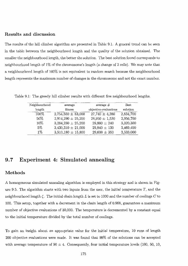
Results and discussion
The results of the hill climber algorithm are presented in Table 9.1. A general trend can be seen
in the table between the neighbourhood length and the quality of the solution obtained. The
smaller the neighbourhood length, the better the solution. The best solution found corresponds to
neighbourhood length of 1% of the chromosome's length (a change of 2 cells). We may note that
a neighbourhood length of 100% is not equivalent to random search because the neighbourhood
length represents the maximum number of changes in the chromosome and not the exact number.
Table 9.1: The greedy hill cilmber results with different five neighbourhood lengths.
Neighbourhood average average# Best
length fitness objective-evaluations solution
100% 2, 754,550 ± 83,000 27,740 ± 4,380 2,834,700 50% 2,914,290 ± 25,200 28,950 ± 1,530 2,956,700 10% 3,284,230 ± 25,200 29,800 240 3,320,300 5% 3,430,310 ± 21,000 29,840 ± 130 3,469,400 1% 3,510,180 15,800 29,600 ± 350 3,533,000
9. 7 Experiment 4: Simulated annealing
Methods
A homogeneous simulated annealing algorithm is employed in this strategy and is shown in Fig
ure 9.5. The algorithm starts with two inputs from the user, the initial temperature T, and the
neighbourhood length(. The initial chain length Lis set to 1000 and the number of coolings C to
100. This setup, together with a decrement in the chain length of 0.968, guarantees a maximum
number of objective evaluations of 30,000. The temperature is decremented by a constant equal
to the initial temperature divided by the total number of coolings.
To gain an insight about an appropriate value for the initial temperature, 10 runs of length
200 objective evaluations were made. It was found that 99% of the solutions can be accepted
with average temperature of 90 ± 4. Consequently, four initial temperature levels (100, 50, 10,
175
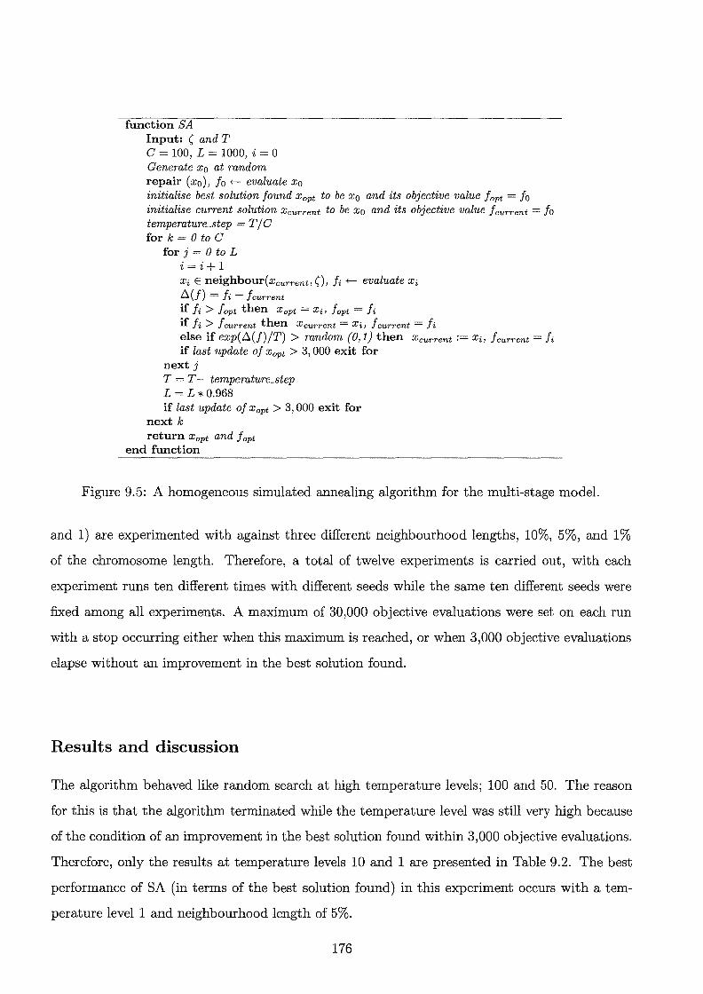
function SA Input: ( and T C = 100, L = 1000, i = 0 Generate x 0 at random repair (xo), fo t- evaluate xo initialise best solution found Xopt to be xo and its objective value !opt = fo initialise current solution Xcurrent to be xo and its objective value !current = fo temperature_step = T / C fork= 0 to C
for j = 0 to L i=i+l Xi E neighbour(Xcurrent, (), fit- evaluate Xi !':!..(!) = fi -!current if fi > !opt then X0 pt =Xi, !opt = fi if fi > !current then Xcurrent =Xi, !current = fi else if exp(f:l.(f)jT) > random {0,1} then Xcurrent :=Xi, !current= fi if last update of Xopt > 3, 000 exit for
next j T = T- temperature_step L = L*0.968 if last update of X opt > 3, 000 exit for
next k return Xopt and !opt
end function
Figure 9.5: A homogeneous simulated annealing algorithm for the multi-stage model.
and 1) are experimented with against three different neighbourhood lengths, 10%, 5%, and 1%
of the chromosome length. Therefore, a total of twelve experiments is carried out, with each
experiment runs ten different times with different seeds while the same ten different seeds were
fixed among all experiments. A maximum of 30,000 objective evaluations were set on each run
with a stop occurring either when this maximum is reached, or when 3,000 objective evaluations
elapse without an improvement in the best solution found.
Results and discussion
The algorithm behaved like random search at high temperature levels; 100 and 50. The reason
for this is that the algorithm terminated while the temperature level was still very high because
of the condition of an improvement in the best solution found within 3,000 objective evaluations.
Therefore, only the results at temperature levels 10 and 1 are presented in Table 9.2. The best
performance of SA (in terms of the best solution found) in this experiment occurs with a tem
perature level 1 and neighbourhood length of 5%.
176

Table 9.2: Simulated annealing results at temperature levels 10 and 1 respectively.
Neighbourhood average average# Best
length fitness objective-evaluations solution
Temperature = 10
10% 2, 032, 540 ± 24, 200 2, 220 ± 1, 740 2,063,600 5% 2, 042,000 ± 20,000 3, 420 ± 2, 060 2,068,400 1% 1, 976, 840 ± 16, 800 2, 710 ± 1, 410 2,000,200
Temperature = 1
10% 2,404,580 41,000 2, 730 ± 1, 870 2,474,600 5% 2,407,730 34,700 2, 370 ± 950 2,493,000 1% 2, 419, 290 ± 36, 800 2, 550 ± 1760 2,469,700
9.8 Experiment 5: Ant colony optimisation
Methods
To describe any ant system for combinatorial optimisation problems, Bonabeau et al. (1999)
require the definition of five components:-
1. Problem representation
A graph representation inherently exists in the problem. Due to the dynamic nature of
the problem, it might be difficult to imagine this graph. We have three dimensions in each
solution- dams, sires, and time. If we fix the time dimension ( ie. a single-stage problem),
the problem is a transportation model and can be expanded as an assignment model. A set
of nodes representing the dams are fully connected to a different set of nodes representing
the sires. A path is defined by starting from one dam, moving to a sire, moving to a dif
ferent dam, and so on. The goal is to step over all the nodes for the dams while satisfying
the other constraints.
177

Now, let us add the third dimension; the time. Actually, in every stage, the previous defi
nition of a graph is preserved. But how do we connect the stages together? The additional
nodes at stage t + 1 depend on the visited arcs in stage t (A female node in stage t + 1 is
the daughter resulted from an allocation of a sire to a dam - visiting the arc connecting
this sire and that dam - in stage t). This is very interesting since the graph structure is
dynamic, and varies according to the visited arcs in each stage.
2. Heuristic desirability
The ACO strategy adopted here is similar to the MMAS-QAP (Stutzle 1998), where no
heuristic information is used. Therefore, the pheromone is deposited as presented in Equa
tion 6.11.
3. Constraint satisfaction method
Two constraint satisfaction methods are implemented. The first uses the repair operator
previously mentioned in Section 9.3.3 (see Figure 8.3). The second is a constructive heuris
tic for building up the solution. The constructive algorithm is given in Figure 9.6.
The constructive algorithm builds up a solution using the probabilistic choice rule while
maintaining the feasibility of the chromosome. It starts with assigning the dams in each
stage to culling with a probability proportional to the amount of the pheromone allocated
to the culling decision of this dam. After satisfying the culling constraint, the same pro
cess is repeated to satisfy the number of mating required. We may recall that culling is
represented with a dummy sire in the pheromone matrix. Therefore, mating decisions are
undertaken in the same way as culling decisions.
4. Pheromone updating rule
Two pheromone update rules are used. One does not use pheromone evaporation while
178
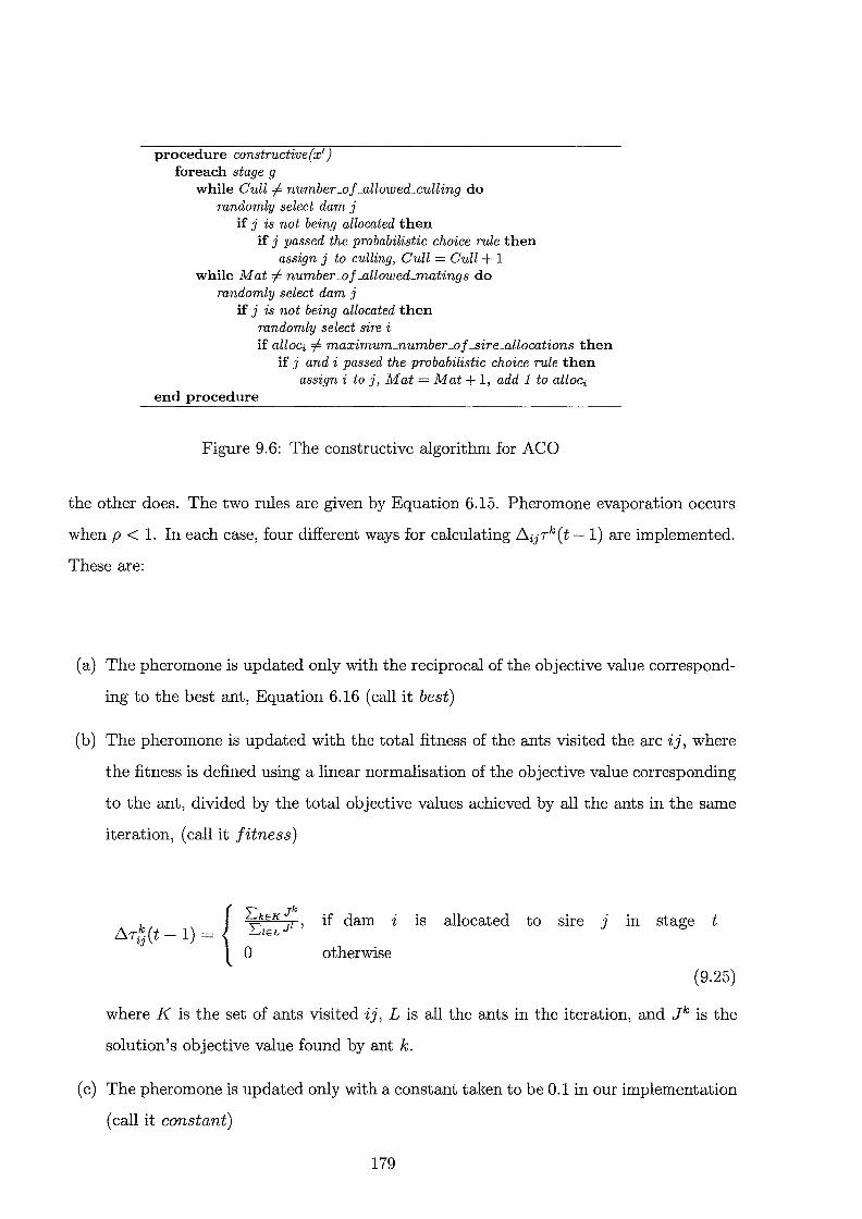
procedure constructive(x') foreach stage g
while Cull ::f. number _of _allowed_culling do randomly select dam j
if j is not being allocated then if j passed the probabilistic choice rule then
assign j to culling, Cull = Cull + 1 while Mat ::f. number _of _allowed_matings do
randomly select dam j if j is not being allocated then
randomly select sire i if alloe;, I- maximum_number _of _sire_allocations then
if j and i passed the probabilistic choice rule then assign i to j, Mat = Mat + 1, add 1 to alloci
end procedure
Figure 9.6: The constructive algorithm for ACO
the other does. The two rules are given by Equation 6.15. Pheromone evaporation occurs
when p < 1. In each case, four different ways for calculating tlijTk ( t - 1) are implemented.
These are:
(a) The pheromone is updated only with the reciprocal of the objective value correspond
ing to the best ant, Equation 6.16 (call it best)
(b) The pheromone is updated with the total fitness of the ants visited the arc ij, where
the fitness is defined using a linear normalisation of the objective value corresponding
to the ant, divided by the total objective values achieved by all the ants in the same
iteration, (call it fitness)
if dam 'l is allocated to sire J in stage t
otherwise
(9.25)
where K is the set of ants visited ij, L is all the ants in the iteration, and Jk is the
solution's objective value found by ant k.
(c) The pheromone is updated only with a constant taken to be 0.1 in our implementation
(call it constant)
179

k _ { K x a if dam "' 1s b.Tij(t- 1) -
0 otherwise
allocated to sire J in stage t
(9.26)
where, K is the number of ants visited ij at iteration t.
(d) The pheromone is updated only with the reciprocal of the objective value correspond
ing to all ants, Equation 6.16, where C in the equation is taken to be 1000 in our
implementation. (call it objective)
5. A probabilistic transition rule
The ACO probabilistic transition rule adopted here is similar to the MMAS-QAP (Stutzle
1998) and is given by Equation 6.11.
After constructing a solution, each ant applies the local search algorithm to improve its current
solution. The new improved solution, if it exists, replaces the ant's original solution. The number
of trials the ant attempts to improve is the neighbourhood size to be searched for this ant. A
population of 1 and 5 ants were experimented with. The use of a single ant is similar to the
FANT algorithm (Taillard 1998). To limit the maximum total number of objective evaluations
to 30,000, the following equation should hold
number of ants x the neighbourhood size x the number of iterations= 30,000
Three neighbourhood sizes are tried: 50, 100, 150 for 1 ant and 10, 20, 30 for 5 ants. To see
the impact of neighbourhood size, the number of ants x the neighbourhood size is fixed (50 x 1
corresponds to 10 x 5, 100 x 1 corresponds to 20 x 5, and 150 x 1 corresponds to 30 x 5). Therefore,
96 experiments are carried out (each experiment is run 10 times with different seeds) to find the
best combination of parameters which will result in the best solution.
Results and discussion
The central focus of the experimental design aims to compare the appropriateness of four con
figurations:
180

Table 9.3: Relationship between the number of ants and neighbourhood length.
a single ant Neighbour hood Size
50 100 150 A vg best solutions 2,097,990 ± 68,300 2,168,620 ± 94,900 2,314,360 ± 32,100
# of objective-evaluations 2,420 ± 2,010.0 2,330 ± 1,920.0 2,650 ± 2,090.0 Best solution found 2,229,500 2,346,700 2,414,900
five ants Neighbourhood Size
10 20 30 A vg best solutions 2,033,640 ± 28,000 2,076,690 ± 24,100 2,111,680 ± 25,900
# of objective-evaluations 2,590 ± 1,970.0 2,430 ± 2,010.0 2,700 ± 1,860.0 Best solution found 2,128,900 2,153,700 2,194,000
• fewer ants and longer neighbourhood length vs more ants with shorter neighbourhood
length,
• constructive algorithms vs repair operator,
• with pheromone evaporation vs without pheromone evaporation, and
• the four pheromone update rule.
Fewer ants/longer neighbourhood vs more ants/shorter neighbourhood
In this section, the results for the 96 experiments are grouped according to the number of ants
and the neighbourhood size. The key question here is: are fewer ants with longer neighbourhood
search better than more ants with shorter neighbourhood search? This question can be restated
in a different, still equivalent, way: where does the real improvement in the ants algorithm come
from, the ants or the local search technique?
In Table 9.3, the best performance occurred with a single ant and neighbourhood size of 150 but
the differences are not statistically significant. This result may suggest that longer neighbourhood
size has more influence than the number of ants used. ACO algorithms suffer from a severe
scalability problem (Dorigo and Caro 1999). This may seem to be the reason behind the influence
of the neighbourhood size in our problem.
181

Table 9.4: Comparing ACO with constructive algorithms against the repair operator
A vg best solutions #of objective-evaluations
Best solution found
Constructive algorithm 2,138,440 ± 111,600
2,630 ± 1,990.0 2,414,900
Repair operator 2,129,550 ± 97,100
2,410 ± 1,960.0 2,387,600
Table 9.5: Comparing ACO with/without pheromone evaporation
A vg best solutions # of objective-evaluations
Best solution found
With pheromone evaporation
2,157,770 ± 105,400 2,430 ± 2,020.0
2,414,900
Constructive algorithm vs repair operator
Without pheromone evaporation
2,110,510 ± 98,600 2,610 ± 1,930.0
2,387,600
In this section, the results for the 96 experiments are grouped according to the means of creating
a step in the local search. The first means is the constructive algorithm presented in the previous
section. The second is randomly then repairing the resultant solution. The crucial point here
is to answer the question: does the constructive algorithm, which uses the ants routing table,
improve the solutions generated within the neighbourhood?
In Table 9.4, the constructive algorithm performed better than the repair operator but the dif
ferences are not statistically significant. This result entails that the constructive algorithm has
a positive bias ( ie. a bias which helps in improving the solution), an important characteristic in
large search spaces.
With/without pheromone evaporation
In this section, the results for the 96 experiments are grouped according to whether or not
pheromone evaporation is used. The fundamental issue here is to answer the question: does
pheromone evaporation help in this problem?
In Table 9.5, the best performance occurred with pheromone evaporation but the differences are
182

Table 9.6: Comparing the ant algorithms with four different pheromone update rules.
A vg best solutions # of objective-evaluations
Best solution found
A vg best solutions # of objective-evaluations
Best solution found
best 2,139,090 ± 103,800
2,590 ± 2,010.0 2,414,900 objective
2,137,520 105,400 2,620 ± 1,940.0
2,414,900
fitness 2,131,710 ± 100,900
2,480 ± 2,040.0 2,387,600 constant
2,127,710 108,600 2,380 ± 1,920.0
2,371,100
not statistically significant. Therefore, pheromone evaporation helped to improve the solutions'
quality.
Pheromone update rule
In this section, the results for the 96 experiments are grouped according to the pheromone update
rule. The four pheromone update rules are: best, fitness, objective, and constant. The first
(best) and third (objective) rules are extracted from the literature as pointed in the previous
section. The second (fitness) and fourth (constant) are proposed here. fitness pheromone
update rule measures the value of adding the concept of competition between the ants through
adjusting the pheromone update matrix by the fitness of each. constant reverse this impact and
simply looks at all ants as if they are similar.
In Table 9.6, it is found that both best and objective succeeded to find the best solution but the
differences are not statistically significant. However, best was better (although statistically not
significant) in terms of the average of the ten runs, their standard deviations, and the number
of objective-evaluations.
Summary of ACO results
Although individually they were statistically indifferent, overall, the best performance of the ACO
algorithm occurred with one ant, a neighbourhood size of 150 using the constructive algorithm
with pheromone evaporation and either the best or objective pheromone update rule. However,
it is worth noting that SA produced better results than the ACO. SA found a better best solution
183

and better average best solution with less standard deviations. This does not mean that ACO
is not suitable, but it does have a scalability problem. This issue will be further investigated in
the conclusion of the chapter.
9.9 Experiment 6: Markov chain tabu-search (a new al
gorithm)
Methods
Paulli (1993) found that the choice of the tabu-list's size has a large influence on the solution's
quality and it varies considerably among problems. Furthermore, he claimed that SA is much
better than TS for the quadratic assignment problem. Recalling from the previous chapter that
the single-stage problem is a quadratic transportation model, and the multi-stage model dis
cussed in the current chapter is a dynamic transportation model, this gives an expected bad
performance for tabu search. The side-effects of the tabu-list's size has been discussed in Chap
ter 6.
The previous points motivated the development of a new version of TS which we called markov
chain tabu search (MCTS). Here, the tabu-list will be referred to as the probabilistic tabu-list
(PTL). There is almost no relation between M CTS as presented here and a version of tabu search
called probabilistic tabu search (PTS) (Laguna 1997). Glover and Manuel (1997) list PTS under
neglected tabu search strategies. In the end of this section, we will present the differences be
tween MCTS and PTS. In MCTS, the PTL's size is always fixed and the structure depends on the
representation. For example, in our problem a solution is represented using a two-dimensional
array where one dimension, t, represents the number of stages and the second dimension, j,
represents the dams. The PTL is represented using a three-dimensional array where in addition
to the two-dimensional solution array, a third dimension, i, is added of size equal to the number
of sires. Each cell in the three-dimensional array represents the probability that sire i is to be
allocated to dam j in stage t. If we refer to this probability as 1rtij, then the following conven
tional probability conditions should be satisfied all the time:
184
0 :s; 7Ttij :s; 1
S+l
2:: 7Ttij = 1 i=l
(9.27)
(9.28)
where S is the number of sires. The matrix is initialised with all values equal to 8~1 . The
reward/penalty is initialised with 1% of the initial value used in the PTL; that is, loox(s+I)"
The algorithm is depicted in Figure 9.7. It is worth noting that this algorithm is different from
the Penalty search version of tabu search (Shivastava and Chen 1993), as we always center the
neighbourhood search over the best-solution found so far, whereas the penalty search version of
tabu search does not.
One may ask if this is still a tabu search algorithm, although we do not have an explicit tabu
list. The answer is simply yes. Since the elements in the PTL matrix can reach the threshold,
and therefore are tabu, the definition of "tabu" is still preserved in the PTL matrix.
Every time the MCTS algorithm selects a new solution from the neighbourhood, a reward and/or
a penalty is assigned to each cell in the PTL which is present in the solution. If the new solution is
better than the previous best solution found, the assignments corresponding to the previous best
solution found are penalised and those corresponding to the new solution are rewarded. That
is, if sire 5 is allocated to dam 3 in stage 1 in the previous best solution found, the cell which
corresponds to sire 5, stage 1, and dam 3 in the PTL is decreased by a constant. If the previous
best solution found is still better than the new solution, the best solution found is rewarded and
the new solution is penalised. Therefore, the algorithm uses a double re-inforcement approach.
In this way, instead of storing the set of directions which are tabu, they are indirectly penalised in
the probabilistic tabu-list. The algorithm is based on Markov chain since each new PTL depends
only on the previous one and represents a transition matrix between states. The update rule can
be represented as a transition matrix as well, with all cells equal to 0 except those needing to
be rewarded or penalised, which they are set to the penalty /reward constant. Note that keeping
rewarding the best solution found as long as it does not change, helps to speed up the algorithm,
although it may cause stagnation which will be overcome as will be explained in the discussion
of the function choose. Speeding up the algorithm is a necessity for two reasons:
185
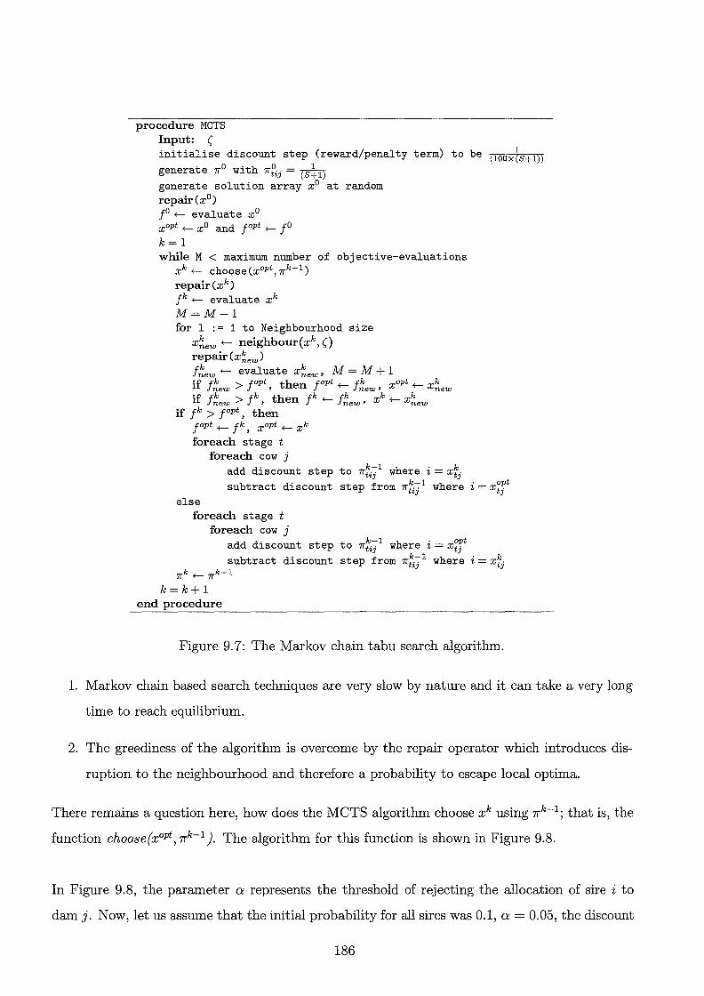
procedure MCTS Input: ( initialise discount step (reward/penalty term) to be c1ooxcs+1))
t O·h0_1 genera e 1r Wlt 1ftij- (S+ 1)
generate solution array x0 at random repair(x0 )
f 0 +- evaluate x 0
xopt +- xo and fopt +- fo
k=l while M < maximum number of objective-evaluations
xk +- choose (xopt, 1fk-1 )
repair(xk) fk +- evaluate xk
M=M+l for 1 := 1 to Neighbourhood size
x~ew +- neighbour(xk, () repair ( x~ew) f~ew +- evaluate x~ew, M = M + 1 if fk > fopt then fopt +- fk xopt +- xk
new ' new ' new if f~ew > fk , then Jk +- f~ew , xk +- X~ew
if fk > rpt' then fopt +- Jk, xopt +- xk
foreach stage t foreach cow j
dd d . k-1 h . k a 1scount step to 1ftij w ere 2 = xtj
subtract discount step from 1r~j 1 where i = x~r else
foreach stage t foreach cow j
dd d . k-1 h . opt a 1scount step to 1ftij w ere 2 = xtj
f k-1 h . k subtract discount step rom 1rtij w ere 2 = xtj 1fk +- 1fk-1
k=k+l end procedure
Figure 9.7: The Markov chain tabu search algorithm.
1. Markov chain based search techniques are very slow by nature and it can take a very long
time to reach equilibrium.
2. The greediness of the algorithm is overcome by the repair operator which introduces dis
ruption to the neighbourhood and therefore a probability to escape local optima.
There remains a question here, how does the MCTS algorithm choose xk using ?rk-l; that is, the
function choose(xopt, ?rk-I ). The algorithm for this function is shown in Figure 9.8.
In Figure 9.8, the parameter a represents the threshold of rejecting the allocation of sire i to
dam j. Now, let us assume that the initial probability for all sires was 0.1, a= 0.05, the discount
186

function choose(xopt, 1rk 1)
x' f- xopt
foreach stage t randomly select J < number of dams for j = 1 to J
randomly select sire i if 1rtij > a then
return x' end function
I . Xtj = ~
Figure 9.8: The generation of neighbourhood solutions in the MCTS algorithm.
step= 0.01, the solution did not improve after 5 objective-evaluations from the start, and sire i
was allocated to dam j in all last 5 stages. Therefore, 7rfij = 0.05 since we kept penalising the
probability. The algorithm illustrated in Figure 9.8 will force dam j to be allocated to a different
sire. The question is, can sire i be allocated later on to dam j? The answer is yes, since the
repair operator does not see the probability matrix 1r; therefore, even though that it is decided
by the probability matrix that this sire is tabu, the repair operator introduces some distortion
to the influence of the probability matrix.
To guarantee that the algorithm will not stagnate at some point ( ie. a sire is always allocated
to the same dam), we need to choose the value of o: carefully. Assume that we need to run
the algorithm for up to 1,000 objective-evaluations; the initial probability is 0.1, the discount
factor is 0.01, o: = 0.05, and we have 10 sires (including a dummy sire for culling). In this case,
after around 45 objective-evaluations without an improvement in the best solution found, there
is a possibility that the algorithm will keep on this sire for this dam forever. We need to avoid
stagnation if this occurs to all dams in the solution. Note that the solution does not change and
the repair operator has no effect since the solution is still feasible. The obvious way to overcome
this, is to add the discount factor every some number of objective-evaluations to those cells in the
probability matrix which reached the minimum rejection level o:. This would force the algorithm
to change the current solution and escape the current local optimum.
It is important to mention here that the algorithm differs from any tabu search since it starts
all the time from the best solution found (the input to the function choose(x0Pt, 1rk-1)). This
may imply that this algorithm is a greedy algorithm. However, this is not the case because the
187
neighbourhood of the step generated by the function choose is searched regardless of whether
this step generated a better solution than the best found so far or not. Also, every point in the
search space is reachable from the best solution found (see the fourth line in the function choose).
We can imagine the algorithm as a search technique which starts with the best solution found
and try to take steps in the space to find a better neighbourhood, while these steps themselves
may downgrade the best solution found. The differences between the MCTS and PTS are:
• In essence, PTS is a hybrid of simulated annealing and tabu search. It is considered as a
generalisation of tabu search through the use of a simulated annealing approach to decide
on the acceptance of a move. MCTS is a reinforcement approach to tabu search. It does
not use the probability matrix to accept or reject a solution, but to generate a solution.
• In PTS, the next step is always accepted, while in MCTS the next step within the neigh
bourhood is always accepted within the neighbourhood but it is not accepted to change
the current neighbourhood's centre unless it improves it.
• In PTS, the probability matrix represents the transition probability from a solution to
another, while in MCTS the probability matrix represents the transition probability of
each variable in the problem.
• In PTS, a new solution is generated within the neighbourhood based on the probability
matrix. In MCTS, a new solution is generated from the best solution found so far using
the probability matrix and a step within the neighbourhood is generated regardless of the
probability matrix.
• In PTS, the probability matrix is updated based on the evaluation of the solution, whereas
in MCTS the probability matrix is updated using a constant.
• In PTS, a solution is accepted based on the probability matrix using the relative prob
abilities, whereas in MCTS a solution is generated from the probability matrix using a
threshold function.
Results and discussion
The three parameters that we may need to determine in the MCTS algorithm are: the rejection
level, the neighbourhood size, and neighbourhood length. We keep the discount factor constant
188
- since it is correlated to the rejection level - and change the rejection level instead. The initial
probability is 1/11 ~ 0.091 for each cell in the probability matrix, the discount factor is taken to
be 0.001, and a E {0.02, 0.05, 0.08, 0.09}. Every 100 objective-evaluations, the discount factor is
added to random number of elements in the matrix reached the rejection level and subtracted
from random number of elements in the matrix exceeding the rejection level. Six neighbourhood
sizes of 150, 100, 50, 10, 5, and 1 and neighbourhood lengths of 10%, 5%, and 1% were tested as
shown in Table 9. 7. A neighbourhood size of 1 means that the algorithm is one-step look ahead
algorithm.
In Table 9.7, the best combination is found with the shortest neighbourhood size (1), the shortest
neighbourhood length (1% of the chromosome size or equivalently 2 cells for each stage), and the
highest rejection level (0.09). On the contrary to ACO, a shorter neighbourhood size is better
in MCTS. Generally, MCTS outperformed the four previous techniques.
The previous results need further explanation. We may notice that there is a relation between
the neighbourhood size and the number of points visited in the space. With a large neighbour
hood size, the algorithm spends most of the time in exploring the neighbourhood (intensification
of local search) while reducing the exploration of the overall search space (sacrificing with diver
sification of global search) because the number of objective evaluations is fixed. With a small
neighbourhood size, the reverse is occurring. The probability matrix is different. Continuous
update of the probability matrix emphasises the exploration of the overall search space (intensi
fication of global search). Therefore, the results found here suggest that the intensification of the
search while globally exploring the search space through the probability matrix is more beneficial
than the local intensification of the search through the neighbourhood. This result is consistant
with the fact that the search space is huge; therefore, spending time in the neighbourhood may
not be a good idea.
189

Table 9. 7: The results for the Markov chain tabu search method.
Neighbourhood Size
a ( 150 100 50 0.02 10% A vg best solutions 2,357,290 ± 28,400 2,323,650 ± 21,000 2,277,410 ± 22
# of obj-evaluations 3,220 1,630 3,100 ± 2,190 3,770 ± 2,H Best solution found 2,397,500 2,352,200 2,310,100
0.05 10% A vg best solutions 2,358,340 ± 33,600 2,316,300 ± 24,200 2,299,480 ± 8t # of obj-evaluations 3,450 ± 1,800 2,390 ± 1,140 5,520 ± 5,9' Best solution found 2,425,600 2,352,200 2,485,700
0.08 10% A vg best solutions 2,370,950 ± 36,800 2,345, 720 ± 68,300 2,523,340 ± 13 #of obj-evaluations 3,200 ± 1,900 4,130 ± 6,640 15,870 ± 9,2 Best solution found 2,445,900 2,535,400 2,690,800
0.09 10% A vg best solutions 2,408,780 ± 46,200 2,462,380 ± 82,000 2,535,950 ± 7~ #of obj-evaluations 4,040 ± 2,490 9,910 ± 5,630 13,690 ± 6,9 Best solution found 2,482,000 2,561,500 2,724,600
0.02 5% A vg best solutions 2,453,970 ± 30,500 2,399,320 ± 33,600 2,329,960 ± 31 # of obj-evaluations 2,830 ± 1,510 2,820 ± 1,490 4,150 ± 3,0' Best solution found 2,489,600 2,444,000 2,382,200
0.05 5% A vg best solutions 2,456,070 ± 32,600 2,388,810 ± 37,800 2,358,340 ± 10. #of obj-evaluations 2,980 ± 1,900 2,170 1,830 5,800 ± 7,01 Best solution found 2,501,600 2,444,000 2,646,400
0.08 5% A vg best solutions 2,461,330 ± 44,100 2,418,240 ± 80,900 2,633,690 ± 12, #of obj-evaluations 4,040 ± 2,210 5,200 ± 5,970 15,560 ± 8,0 Best solution found 2,520,800 2,562,200 2,806,100
0.09 5% A vg best solutions 2,531,740 ± 82,000 2,605,310 ± 132,400 2,754,550 ± 89 #of obj-evaluations 10,090 ± 9,260 12,600 ± 7960 20,260 ± 7,1 Best solution found 2,653,100 2,735,000 2,891,800
0.02 1% A vg best solutions 2,439,260 ± 44,100 2,326,810 ± 46,200 2,256,390 ± 43 #of obj-evaluations 4,740 ± 2,310 4,030 ± 2,900 4,930 ± 2,n Best solution found 2,517,900 2,395,000 2,312,900
0.05 1% A vg best solutions 2,436,110 ± 43,100 2,337,320 ± 43,100 2,287,920 ± 17( #of obj-evaluations 4,350 ± 2,020 3,200 ± 1,820 6,040 ± 7,m Best solution found 2,503,100 2,395,000 2,747,200
0.08 1% A vg best solutions 2,459,230 ± 76,700 2,616,870 ± 252,200 2,948,970 ± 47 #of obj-evaluations 5,150 ± 4,340 13,220 ± 10,580 28,680 ± 1,5 Best solution found 2,607,700 2,953,400 3,021,400
0.09 1% A vg best solutions 2,800, 790 ± 288,000 3,033,050 ± 33,600 3,068,780 ± 98 #of obj-evaluations 16,7 40 ± 12,600 27,050 ± 3,620 25,410 ± 6,6 Best solution found 3,085,000 3,087,400 3,158,100
190

Neighbourhood Size
a ( 10 5 1
0.02 10% A vg best solutions 2,837,570 ± 45,200 3,139,190 ± 56,800 3,293,680 ± 82,000 # of obj-evaluations 29,760 ± 120 29,760 140 20,850 ± 2,310 Best solution found 2,887,200 3,212,900 3,386,800
0.05 10% A vg best solutions 2,948,970 ± 65,200 3,260,050 ± 58,900 3,190,690 ± 70,400 # of obj-evaluations 28,540 ± 3,940 29,930 ±50 15,890 ± 2,390 Best solution found 3,011,100 3,346,700 3,338,500
0.08 10% A vg best solutions 3,156,010 ± 46,200 3,151,810 ± 88,300 3,050,910 ± 46,200 # of obj-evaluations 29,920 ± 100 24,620 3,190 7,590 ± 2,030 Best solution found 3,263,300 3,265,000 3,123,300
0.09 10% A vg best solutions 3,152,860 ± 45,200 3,091,900 ± 36,800 2,962,630 ± 74,600 # of obj-evaluations 28,780 ± 1,510 16,290 ± 2,610 5,010 ± 1,610 Best solution found 3,219,700 3,155,100 3,063,700
0.02 5% A vg best solutions 2,869,100 ± 63,100 3,195,950 ± 30,500 3,369,350 ± 86,200 # of obj-evaluations 28,250 ± 3,460 29,710 ± 250 26,030 ± 3,860 Best solution found 2,947,600 3,269,500 3,498,700
0.05 5% Avg best solutions 3,012,030 ± 41,000 3,118,170 ± 88,300 3,345,180 ± 72,500 # of obj-evaluations 29,640 460 29,880 ± 100 23,300 ± 6,310 Best solution found 3,067,100 3,346,100 3,442,000
0.08 5% A vg best solutions 3,267,410 ± 33,600 3,332,570 ± 50,400 3,340,980 ± 53600 # of obj-evaluations 29,940 ±50 29500 ± 720 22,590 ± 4,210 Best solution found 3,324,000 3,436,300 3,436,300
0.09 5% A vg best solutions 3,356,740 ± 39,900 3,360,940 ± 38,900 3,274,770 ± 87200 # of obj-evaluations 29,880 170 26,440 ± 4,290 17,140 ± 8,740 Best solution found 3,415,300 3,409,500 3,397,700
0.02 1% A vg best solutions 2,998,370 42,000 3,263,210 ± 39,900 3,642,600 ± 147,100 # of obj-evaluations 29,410 730 29,780 ± 190 27,630 ± 7,450 Best solution found 3,064,500 3,320,800 3,715,300
0.05 1% A vg best solutions 3,148,650 ± 33,600 3,463,940 ± 31,500 3,737,190 ± 14,700 # of obj-evaluations 29,530 ± 540 29,860 ± 120 29,990 ± 10 Best solution found 3,209,500 3,505,100 3,756,700
0.08 1% A vg best solutions 3,489,160 ± 27,300 3,703,550 ± 23,100 3,800,240 ± 10,500 # of obj-evaluations 29,930 ± 60 29,920 110 29,970 ± 40 Best solution found 3,537,500 3,744,100 3,815,800
0.09 1% A vg best solutions 3,659,410 ± 22,100 3,767,660 ± 12,600 3,805,500 ± 13,700 # of obj-evaluations 29,950 ± 30 29,970 ± 30 29,910 ± 110 Best solution found 3,680,100 3,782,700 3,824,600
191

9.10 Experiment 7: Genetic algorithms
Methods
This strategy employs a GA approach for the multi-stage problem. A chromosome in the multi
stage problem has two dimensions. Therefore, for one and two point crossover operators, the
crossover point is calculated for each stage independently from the others. If we have two stages,
the crossover point for the first stage may be different from the second stage. Apart from this,
all other operators are working in the same way presented in Chapter 6.
Results and discussion
Results for five population sizes are presented in Table 9.8 for population size 30, Table 9.9 for
population size 40, Table 9.10 for population size 50, Table 9.11 for population size 60, and
Table 9.12 for population size 70. When the population size was 70, the performance declined.
To be more confident that the solution did not improve after that, a population size of 100 was
tried, but the performance was downgraded again, therefore suggesting that the best population
size is 60 under the current experimental configurations.
For population sizes 40, 50, and 60; that is, Tables 9.9, 9.10, and 9.11, a consistent phenomenon
is that 1-point crossover with modified tournament reproduction strategy resulted in the best
performance overall although it is not statistically significant with respect to 2-points crossover.
With population size 30, the uniform crossover operator performed the best with modified tour
nament, suggesting that with small population size, it had better effect as shown in Table 9.8.
With population size of 70, Table 9.12, the two-point crossover operator outperformed the one
point crossover operator although it was worse than that with population size of 60. The best
population size which gives the best results based on the setup of these experiments is found
to be 60. Surprisingly, gene-based crossover was the worst in the three reproduction strate
gies. This is not consistent with the results for the single-stage model and may suggest that the
interaction between the stages downgraded the performance of the gene-based crossover opera
tor. A consistent trend in all G A experiments is that modified tournament was better than the
other two selection strategies for all crossover operators except gene-based crossover. Therefore,
192
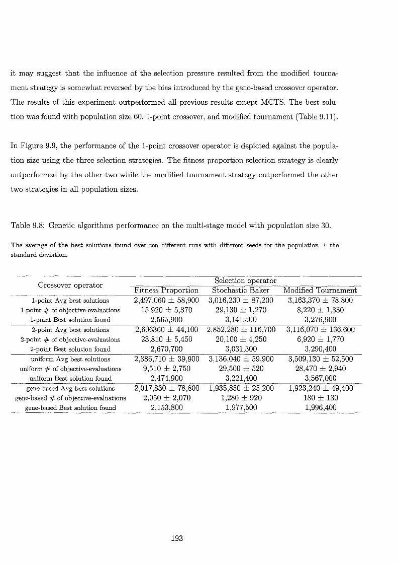
it may suggest that the influence of the selection pressure resulted from the modified tourna
ment strategy is somewhat reversed by the bias introduced by the gene-based crossover operator.
The results of this experiment outperformed all previous results except MCTS. The best solu
tion was found with population size 60, 1-point crossover, and modified tournament (Table 9.11).
In Figure 9. 9, the performance of the 1-point crossover operator is depicted against the popula
tion size using the three selection strategies. The fitness proportion selection strategy is clearly
outperformed by the other two while the modified tournament strategy outperformed the other
two strategies in all population sizes.
Table 9.8: Genetic algorithms performance on the multi-stage model with population size 30.
The average of the best solutions found over ten different runs with different seeds for the population ± the
standard deviation.
Crossover operator Selection operator
Fitness Proportion Stochastic Baker Modified Tournament 1-point Avg best solutions 2,497,060 ± 58,900 3,016,230 ± 87,200 3,163,370 ± 78,800
1-point # of objective-evaluations 15,920 ± 5,370 29,130 ± 1,270 8,220 ± 1,330 1-point Best solution found 2,565,900 3,141,500 3,276,900 2-point Avg best solutions 2,606360 ± 44,100 2,852,280 ± 116,700 3,116,070 ± 136,600
2-point # of objective-evaluations 23,810 ± 5,450 20,100 ± 4,250 6,920 ± 1,770 2-point Best solution found 2,670,700 3,031,300 3,290,400 uniform A vg best solutions 2,386,710 ± 39,900 3,136,040 ± 59,900 3,509,130 ± 52,500
uniform # of objective-evaluations 9,510 ± 2,750 29,500 ± 520 28,470 ± 2,940 uniform Best solution found 2,474,900 3,221,400 3,567,000
gene-based Avg best solutions 2,017,830 ± 78,800 1,935,850 ± 25,200 1,923,240 ± 49,400 gene-based # of objective-evaluations 2,950 ± 2,070 1,280 ± 920 180 ± 130
gene-based Best solution found 2,153,800 1,977,500 1,996,400
193

Table 9.9: Genetic algorithms performance on the multi-stage model with population size 40.
Crossover operator Selection operator
Fitness Proportion Stochastic Baker Modified Tourname 1-point Avg best solutions 2,383,560 68,300 2,973,140 ± 78,800 3,349,380 ± 80,901
1-point # of objective-evaluations 15,080 ± 5,100 29,820 ± 100 12,900 ± 2,380 1-point Best solution found 2,463,300 3,082,000 3,498,400 2-point Avg best solutions 2,440,310 ± 90,400 2,884,860 72,500 3,344,130 ± 56,801
2-point # of objective-evaluations 17,820 ± 7,650 29,050 ± 1,370 12,200 ± 1,290 2-point Best solution found 2,602,300 2,976,300 3,447,000 uniform A vg best solutions 2,279,510 ± 55,700 2,840,720 ± 76,700 3,252,700 ± 59,90(
uniform # of objective-evaluations 8,120 ± 2,760 26,620 ± 4,320 20,350 ± 5,590 uniform Best solution found 2,355,900 2,951,000 3,365,400
gene-based Avg best solutions 2,134,480 ± 62,000 1,974,740 ± 32,600 1,940,060 ± 34,70( gene-based # of objective-evaluations 4,420 ± 1,180 2,940 2,170 300 ± 250
gene-based Best solution found 2,200,000 2,025,000 1,994,400
Table 9.10: Genetic algorithms performance on the multi-stage model with population size 50.
Crossover operator Selection operator
Fitness Proportion Stochastic Baker Modified Tourname 1-point Avg best solutions 2,316,300 ± 45,200 2,910,090 ± 26,300 3,497,570 ± 42,00(
1-point # of objective-evaluations 11,750 ± 3,610 29,730 ± 260 21,840 ± 2,050 1-point Best solution found 2,366,200 2,946,900 3,544,200 2-point Avg best solutions 2,383,560 ± 50,400 2,799,740 ± 67,300 3,473,400 ± 42,00(
2-point # of objective-evaluations 16,490 5,460 29,480 ± 650 19,750 ± 1,960 2-point Best solution found 2,465,400 2,928,700 3,531,200 uniform A vg best solutions 2,197,540 ± 27,300 2,708,300 ± 80,900 3,168,620 ± 37,80(
uniform# of objective-evaluations 4,920 ± 1,880 26,270 ± 4,300 18,040 ± 6,280 uniform Best solution found 2,239,400 2,858,500 3,229,400
gene-based Avg best solutions 2,125,020 ± 71,500 1,999,960 ± 39,900 1,953, 720 ± 37,80( gene-based # of objective-evaluations 5,740 ± 1,750 4,650 ± 2,650 560 ± 270
gene-based Best solution found 2,232,200 2,054,800 2,028,400
9.11 Experiment 8: Immune systems
Methods
The objective of this experiment is to test whether or not immune systems will improve the
performance of GA or not? In this experiment, the optimal set of operators found for GA in
194
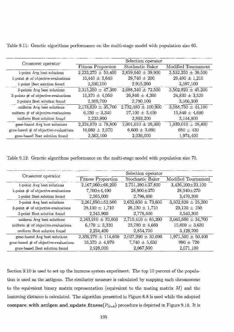
Table 9.11: Genetic algorithms performance on the multi-stage model with population size 60.
Crossover operator Selection operator
Fitness Proportion Stochastic Baker Modified Tournament 1-point Avg best solutions 2,233,270 ± 50,400 2,859,640 ± 39,900 3,532,250 ± 30,500
1-point # of objective-evaluations 10,440 ± 3,640 29,740 ± 200 29,490 ± 1,210 1-point Best solution found 2,330,100 2,915,200 3,597,100 2-points Avg best solutions 2,315,250 ± 47,300 2,688,340 ± 72,500 3,502,820 ± 45,200
2-points # of objective-evaluations 15,370 ± 4,050 26,840 4,300 24,830 ± 3,520 2-points Best solution found 2,368,700 2,790,100 3,566,300 uniform A vg best solutions 2,178,620 ± 35,700 2, 732,480 ± 100,900 3,088,750 ± 44,100
uniform # of objective-evaluations 6,230 ± 3,340 27,100 ± 3,400 15,840 ± 4,690 uniform Best solution found 2,235,900 2,893,200 3,144,900
gene-based A vg best solutions 2,224,870 ± 78,800 2,001,010 ± 26,300 1,939,010 ± 28,400 gene-based # of objective-evaluations 10,080 ± 2,670 6,600 ± 3,090 680 430
gene-based Best solution found 2,363,100 2,036,000 1,974,400
Table 9.12: Genetic algorithms performance on the multi-stage model with population size 70.
Crossover operator Selection operator
Fitness Proportion Stochastic Baker Modified Tournament 1-point Avg best solutions 2,167,060±66,200 2,751,390±37,800 3,426,100±23,100
1-point # of objective-evaluations 7, 700±4,490 28,900±370 28,940±270 1-point Best solution found 2,265,000 2,796,400 3,470,300 2-point Avg best solutions 2,261,650±52,500 2,632,630 ± 73,600 3,502,820 ± 25,200
2-point # of objective-evaluations 28,130 ± 1,710 28,130 1,710 29,120 ± 150 2-point Best solution found 2,345,900 2,778,400 3,540,300 uniform A vg best solutions 2,163,910 ± 32,600 2, 710,410 ± 65,200 3,045,660 ± 34,700
uniform # of objective-evaluations 6,170 3,330 23,780 ± 4,660 15,600 ± 3,630 uniform Best solution found 2,224,400 2,854,700 3,128,200
gene-based Avg best solutions 2,336,270 ± 114,600 2,027,290 ± 32,600 1,971,590 ± 50,400 gene-based # of objective-evaluations 16,370 ± 4,970 7,740 ± 5,630 990 ± 720
gene-based Best solution found 2,528,000 2,067,500 2,071,100
Section 9.10 is used to set up the immune system experiment. The top 10 percent of the popula
tion is used as the antigens. The similarity measure is calculated by mapping each chromosome
to the equivalent binary matrix representation (equivalent to the mating matrix M) and the
hamming distance is calculated. The algorithm presented in Figure 6.8 is used while the adopted
compare_with_antigen_and_update_fitness(Pa=k) procedure is depicted in Figure 9.10. It is
195
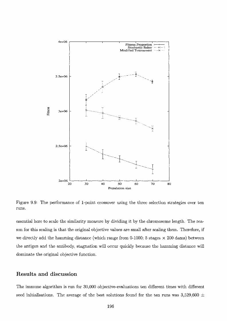
4e+06 ,--------.---,--------,---,------.--------,
3.5e+06
3e+06
2.5e+06
I ::j;
Fitness Proportion 1----+----l Stochastic Baker e---x---:
Modified Tournament >-·-*-·-·'
2e+06 '-----'----'-----'----'-----'------' 20 30 40 50
Population size
60 70 80
Figure 9.9: The performance of 1-point crossover using the three selection strategies over ten runs.
essential here to scale the similarity measure by dividing it by the chromosome length. The rea
son for this scaling is that the original objective values are small after scaling them. Therefore, if
we directly add the hamming distance (which range from 0-1000; 5 stages x 200 dams) between
the antigen and the antibody, stagnation will occur quickly because the hamming distance will
dominate the original objective function.
Results and discussion
The immune algorithm is run for 30,000 objective-evaluations ten different times with different
seed initialisations. The average of the best solutions found for the ten runs was 3,529,600 ±
196
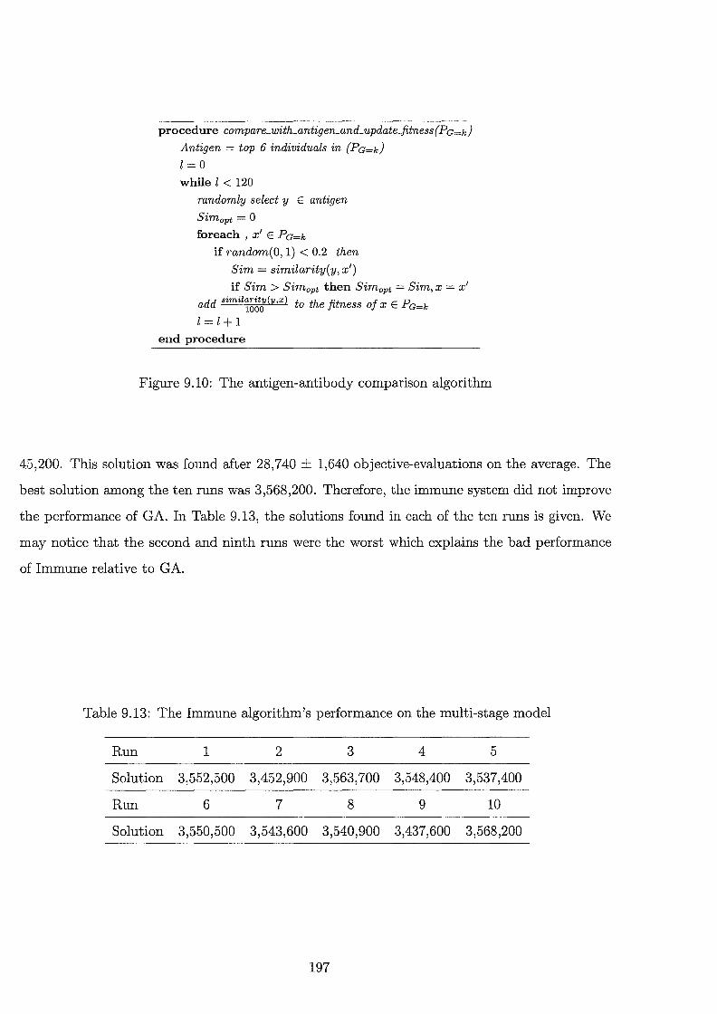
procedure compare_with_antigen_and_update_fitness{Pc=k)
Antigen = top 6 individuals in (Pc=k)
l=O
while l < 120
randomly select y E antigen
Simopt = 0
foreach, x' E Pc=k
if random(O, 1) < 0.2 then
Sim = similarity(y, x')
if Sim > Simopt then Simopt = Sim, x = x' add simil~~~tg(y,x) to the fitness of x E Pc=k
l=l+1
end procedure
Figure 9.10: The antigen-antibody comparison algorithm
45,200. This solution was found after 28,740 1,640 objective-evaluations on the average. The
best solution among the ten runs was 3,568,200. Therefore, the immune system did not improve
the performance of GA. In Table 9.13, the solutions found in each of the ten runs is given. We
may notice that the second and ninth runs were the worst which explains the bad performance
of Immune relative to GA.
Table 9.13: The Immune algorithm's performance on the multi-stage model
Run 1 2 3 4 5
Solution 3,552,500 3,452,900 3,563,700 3,548,400 3,537,400
Run 6 7 8 9 10
Solution 3,550,500 3,543,600 3,540,900 3,437,600 3,568,200
197
9.12 Experiment 9: Evolving colonies of ants (a new al
gorithm)
Methods
In this experiment the optimal set of operators found for GAin Section 9.10 is used in conjunction
with the ACO to set up the hybrid algorithm. The goal here is, instead of improving each ant
independently, GA is used to evolve the ants instead. The algorithm is depicted in Figure 9.11.
In the first generation, five ants are generated using the pheromone table. The colony of ants
evolves (by means of crossover) for 96 objective-evaluations, then all ants die but the fittest ant,
which is preserved in the colony. The reason for choosing 96 objective-evaluations is that only
4 ants are generated, and consequently evaluated, in subsequent iterations since the fittest ant
is always kept. Therefore, in each cycle, 100 objective evaluations are undertaken. Although
the best performance for the ant algorithm occurred with 1 ant, we use five ants here to have a
population.
Results and discussion
The algorithm is run for up to 300 cycles with a condition that the last improvement in the best
solution found does not take place for more than the last 30 cycles, where in each cycle, 100
objective evaluations are undertaken as previously mentioned in order to preserve the maximum
of 30,000 objective evaluations. It is found that the algorithm resulted in a better solution than
GA and ACO in isolation. The results are statistically different at 99.9% confidence level using
the correlated paired t-test. The t values were 93.44 and 4.99 for ACO and GA respectively. The
average best solutions found for the ten runs was 3,579,540 ± 25,200. This solution was found
after 29,700 ± 160 objective-evaluations on the average. The best solution among the ten runs
was 3,615,100. Therefore, this method overcomes the scalability problem in ACO and improves
the performance of GA.
198
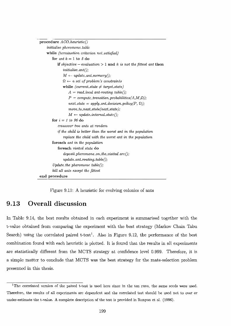
9.13
procedure ACO_heuristic()
initialise pheromone_table
while (termination_criterion_not_satisfied}
for ant k = 1 to 5 do
if objective - evaluation > 1 and k is not the fittest ant then
initialise_ant();
M +- update_ant_memory();
n +- a set of problem's constraints
while {current_state =1- target_state)
A = read_local_ant-routing_table();
P = compute_transition_probabilities( A,M,O}; next_state = apply_ant_decision_policy(P, OJ;
move_ to_next_state ( next_state);
M +- update_internaLstate();
for i = 1 to 96 do
crossover two ants at random
if the child is better than the worst ant in the population
replace the child with the worst ant in the population
foreach ant in the population
foreach visited state do
deposit_pheromone_on_the_ visited_ arc();
update_ant_routing_table();
Update_the_pheromone_table();
kill all ants except the fittest
end procedure
Figure 9.11: A heuristic for evolving colonies of ants
Overall discussion
In Table 9.14, the best results obtained in each experiment is summarised together with the
t-value obtained from comparing the experiment with the best strategy (Markov Chain Tabu
Search) using the correlated paired t-test1 . Also in Figure 9.12, the performance of the best
combination found with each heuristic is plotted. It is found that the results in all experiments
are statistically different from the MCTS strategy at confidence level 0.999. Therefore, it is
a simple matter to conclude that MCTS was the best strategy for the mate-selection problem
presented in this thesis.
1The correlated version of the paired t-test is used here since in the ten runs, the same seeds were used.
Therefore, the results of all experiments are dependent and the correlated test should be used not to over or
under-estimate the t-value. A complete description of the test is provided in Runyon et al. (1996).
199

One should be careful in interpreting the results of these experiments. As we used a fixed number
of objective evaluation, the results may change if we increase the number of objective evaluations.
However, we cannot wait until each algorithm converges as this may take forever. Therefore,
using a fixed number of objective evaluations is a fair thing to do. Also, since the number of
objective evaluations is fixed, the CPU time is almost the same among the different algorithms.
The reason is that the overhead of each algorithm is negligible compared to the time of evaluating
a solution.
Table 9.14: A summary of the best combination found in each experiment and its corresponding t-value relative to the MCTS algorithm
Experiment A vg best solutions # of objective-evaluations Best solution found t-value
Markov Chain TS 3,805,500 ± 13,700 29,910 ± 110 3,824,600 Evolving colonies of ants 3,579,540 ± 25,200 29,700 160 3,615,100 23.48 GA 3,532,250 ± 30,500 29,490 1,210 3,597,100 23.43 Immune 3,529,600 ± 45,200 28,7 40 ± 1,640 3,568,200 18.18 Hill climber 3,510,180 ± 15,800 29,600 ± 350 3,533,000 46.87 Sequential GA 3,429,260 ± 30,500 N/A 3,483,700 47.97 SA 2,407,730 34,700 2,370 ± 950 2,493,000 94.29 Ant Colony 2,345,670 ± 32,300 3,200 ± 2,900 2,414,900 189.44 Random 2,013,620 ± 23,100 2,940 ± 1,710 2,058,400 199.10
The results of this chapter are very interesting. Conventional ACO suffered from a scalability
problem and performed very badly relative to SA. However, when merged with GA, the hybrid
algorithm performed the best after MCTS. This finding required some interpretations. We know
from Chapter 6 that SA uses Markov chains and if it is given enough time, it will converge.
ACO also depends on a Markov chain. To observe this, let us momentarily ignore the local
search procedure used to improve the ants performance. Moreover, let us forget the ants and
just concentrate our attention on the normalised pheromone matrix that we may envisage as
the ants' vision of the probability distribution of the transitions an ant needs to take to find
the best solution found in the world. The ants are generated based on this probability matrix
(prior distribution) that is then updated based on what the ants have found (posterior distri
bution). Let us sum all the updates in a single objective-evaluation in one matrix and let us
normalise this matrix. The ants algorithm can be now seen in terms of these two matrices: the
200

4 .--------.---------.--------~------~r-------~
3.5
3
\0 < s >< "' "' <!)
.s ~
2.5 r-
I
2
1.5 L.._--------'----------'----------L-------__JL---------' 0 2 4 6 8 10
Algorithm
Figure 9.12: The performance of the best results obtained by different algorithms.
The x-axis represents the heuristic; 1-MCTS, 2-Evolving colonies of ants, 3-GA, 4-Immune, 5-Hill
climbing, 6-Sequential GA, 7-SA, 8-ACO, 9-Random. They-axis is the average fitness of ten runs.
201

normalised pheromone matrix and the normalised update matrix. In each objective-evaluation,
the normalised pheromone matrix is updated based on the normalised update matrix. The new
pheromone matrix depends only on the previous one; therefore a Markov characteristic is inher
ent to ACO.
MCTS can also be seen as a series of Markov chains, where the probabilistic tabu list is updated in
each objective-evaluation and the new one depends only on the previous one. The real difference
between ACO, TS, and MCTS is that ACO uses positive knowledge only with a positive search
strategy (ie. keep rewarding good solutions and bias the search towards these good areas), TS
uses negative knowledge only with a positive search strategy ( ie. prohibiting previously visited
states and bias the search to previously un-visited and potentially good states), but MCTS uses
both types of knowledge (positive and negative) with a positive search strategy ( ie. rewarding
good solutions, penalising bad solutions, and biasing the search towards potentially good areas).
SA is somewhat different since it does not use any of these knowledge but instead uses a mixture
of positive and negative search strategies with a certain probability. To illustrate this point,
in the beginning of the search, SA emphasises a negative search strategy since it accepts bad
steps most of the time while the temperature is high. In the end of the search, the situation
is reversed. However, there is no guarantee that this is always good. Perhaps a negative or
positive knowledge is more important during the search in some problems. This may provide an
interpretation of the better performance achieved when using MCTS.
I have illustrated in the previous discussion that SA, ACO, and MCTS have a Markovian char
acteristic. Therefore, when the search space is huge, as in our case, any of these algorithms is
expected to need so much time to reach equilibrium; a problem that does not exist with GAs.
However, MCTS performed the best due to the search intensification through a continuous re
ward for the best solution found and a continuous penality for bad solutions.
GAs easily outperformed SA and ACO since it survived the condition of an improvement every
3,000 objective evaluations. SA and ACO did not survive this condition because they were be
having like random search to explore the search space. The temperature of SA did not have time
to cool and the pheromone matrix of ACO did not have time to reach a steady state. In GA,
202

the selection pressure resulted from the modified tournament strategy proved to have a positive
effect in our problem. Also, the 1-point crossover operator managed successfully to sustain good
schemas while the repair operator adds some mutations from time to time when feasibility is
broken by recombination.
Immune systems did not improve the performance of GAs. With the pressure introduced by the
similarity measure, the schemas inherited in the best solutions in each stage are rewarded in the
rest of the population. This type of pressure may have been beneficial if it is given enough time.
However, in our case, it did not improve the performance of GAs. Surprisingly enough, the re
sults obtained from the immune algorithm were statistically different from the MCTS algorithm
with at-value lower than that obtained for GAs. After investigating this case, it was found that
in one of the ten runs, the behaviour of the immune algorithm dropped dramatically while the
behaviour of GAs using the same seed was very good 2 . However, in seven out of the ten runs,
the immune algorithm was better than its corresponding GAs.
The ACO+GA algorithm presented another successful step to improve the performance of GA
and to overcome the scalability and slow convergence problems of ACO. MCTS gave the best
results overall and achieved significantly better solutions than all other algorithms. It is therefore
chosen as our preferred strategy for solving the version of the multi-stage mate-selection problem
presented in this thesis.
One last important issue needs still to be discussed here; that is, the practicality of the model
solved in this chapter. This issue will be argued using questions and answers.
Q: Does it make sense that certain algorithms are better suited for solving the mate-selection
problem than others?
A: This is a very important question concerned with the problem's features which make an
algorithm more suitable for the problem than another. The mate-selection problem is similar
2 This was the seed where the best solution of GAs over the ten runs was obtained. Also, it was the seed
corresponding to the worst immune algorithm's performance.
203

to many combinatorial optimisation problems. Therefore, it is difficult to say when a heuristic
will work and when it will not objectively. However, I might give here a guideline to assist the
practitioners. The problem in hand is a large scale problem, therefore the search space is huge.
Even with a greedy local search algorithm, it will take very long time to reach a local optimal
solution. In practice we don't have such time given that we will get a weak local optimal solution.
Obviously, the ideal situation is to get the global optimal solution but the practical one is to get
a better local optimal solution. On the one hand, population based heuristics, such as genetic al
gorithms, depend on the diversity in the population to better sample the search space. But when
a huge search space exists, a fair sample of the search space is very costly and the convergence is
slow. For a non-population based heuristics, such as simulated annealing, ant colony, and tabu
search, the huge search space causes a scalability problem. SA and ACO will need a tremendous
time to reach equilibrium. The conventional TS approach will not work because of the large size
of the neighbourhood. To see this last point, assume our solution's representation is of length
1000 and we define the neighbourhood by a two cells' change; therefore the neighbourhood size is
bounded with 0(10002). Actually in this case it is around 105
. In this huge neighbourhood, what
is the probability of cycling? It is almost zero. Therefore, we need huge memory to handle this
problem. The obvious question now is why did the MCTS algorithm work? Because in MCTS,
the neighbourhood is centred on the best solution found so far and is defined by the overall search
space; that is, any point in the search space is reachable from the best solution found so far.
However, not every point is reachable with the same probability. After the algorithm performs
a number of iterations, the probability transition matrix restricts the search space. To forbid
quick stagnation, some random values are added to the probability matrix so that the matrix
itself does not trap in a local optimum. The update of the matrix is undertaken by a double
re-inforcement approach (penalising bad solutions and rewarding good ones.). This approach of
global intensification of the search seems to be very benefecial in the mate-selection problem.
Therefore, I would suggest a carefully designed re-inforcement approach, such as MCTS, for the
mate-selection problem.
Q: How can the model take into account the probability of conception failure?
A: Let us assume that the farmer requires ten matings and the probability of conception failure
204

is 10%, the farmer may ask the system for eleven matings instead; therefore, overcoming the risk
of conception failure. It is important here to recognise that this method, although very simple,
does provide a practical approach to handle the problem of conception failure. The reason is
that it is not clear which cow will suffer from this problem (unless we have a trait for cow's
conception). Therefore, we may seek the best eleven matings, assuming that one will fail.
Q: How can the model take into account the gender of the progeny?
A: How can we tell in advance if the result of a mating will be a male or a female? This is
a difficult question and the same trick, of the previous question, will be used. Assume that we
require fifty daughter. We may ask for the best one hundred matings instead, therefore with a
probability 0.5, the expected number of daughters will be 50 as required. Note that in reality,
the farmer does not know in advance if a mating will take place or not, if the outcome of a
mating is a male or a female, or if the progeny will live or die. Therefore, over-estimating the
number of required matings is a wise strategy, as long as it is reasonable; otherwise the farmer
will do unnecessarily matings which represent cost on the farm. This point is outside the scope
of the thesis; however, an economic model for this type of decisions can be an interesting piece
of research for future work.
Q: Is there a difference between optimising two stages or five stages?
A: This question arises from discussions regarding the reason for more than two-stage optimisa
tion. The answer is that by minimising the problem for five stages, we require enough variance in
the first generation's assignment so that inbreeding is minimum over the 5 generations. However,
we can get a similar effect if we increase the weight of inbreeding in the two-stage optimisation.
Actually, we do not need to optimise initially for two stages and one stage would be sufficient if we
know the right combination of weights. Notwithstanding, we cannot know the right combination
of weights without building sophisticated economic models for each herd independently. There
fore, adding more generations will add implicitly more weights on short and long term inbreeding.
To further illustrate our point, we need an experiment. The best set of parameters obtained by
MCTS (using the seed corresponding to the best solution found for MCTS) was used to optimise
205

the same problem we presented in this chapter for 2, and 5 stages. The matings of the first stage
in each of the two experiments are reported here in order to observe the impact of multi-stage
optimisation on the first stage. We should expect that the more stages we optimise, the more
the population is penalised for inbreeding. Therefore, we should expect lower inbreeding (higher
variance) and lower expected breeding values (as a result of penalising the matings for long term
inbreeding). The results of this experiment are presented in Table 9.15. The numbers in this
figure are approximated for three significant numbers.
Table 9.15: The effect of the number of stages on the optimisation process.
Objective Two Stages Five Stages
01: Production 632000 631000 02: Inbreeding -17 -16 03: Breeding Values 69300 69200 04: Coancestry -5870 -5860
As can be seen from the table, the production and breeding values for the two-stage model are
higher than that for the five-stage model, and inbreeding is also higher. However, we have to say
that to test if this result is statistically significant or not, one needs to carry out a number of
runs. In any case, whether we optimise for two or more generations, the purpose of this chapter is
to discuss the problem from optimisation point of view. As will be suggested in the last chapter
of the thesis, an interesting piece of research for future work would be to analyse the results of
this thesis within an economic model to generate appropriate weights, for the objective function,
that will influence the results of the optimisation model. Such a model is outside the scope of
the thesis and is proposed for future work.
9.14 Conclusion
This chapter is concerned with the third sub-objective of the thesis; solving the proposed ver
sion of the multi-stage mate-selection problem presented in this thesis. Nine different heuristic
techniques, two of which (evolving colonies of ants and Markov chain tabu search) were newly
developed in this thesis, are used to solve the problem. The MCTS is significantly better than
the rest and resulted in the best overall performance.
206

Chapter 10
Generation of Mate-selection Index
The main objective of this chapter is to generate a mate-selection index. The mate-selection
index is introduced in Section 10.1 followed by a mathematical proof for the existence of this
index in Section 10.2. In Sections 10.3 and 10.4, two methods are envisaged for generating this
index using an SA+GA hybrid and DE+GA hybrid respectively. The chapter is concluded with
Section 10.5.
10.1 Mate-selection Index (MSI)
An index for mate-selection is suggested by Kinghorn et.al. (1999). In their paper, the index
ranks the animals according to their potential as mating animals. They showed that such an
index is very beneficial and it is different from the conventional selection index, because the
latter does not account for issues like inbreeding, coancestry, and mate-selection, whereas the
MSI does. This chapter is about the generation of MSI. However, MSI is defined here as a vector
of weights rather than ranks as in Kinghorn et.al. (1999). Therefore, the problem discussed in
the current chapter is to find a vector of weights (a single weight for each animal) such that
if the mate-selection problem is optimised for each stage independently using the MSI vector
(referred to by R(t) for stage t or simply R for all stages) to form a linear objective function
CL.'-{'=0 R(t) x [X(t)Y(t)]) for the breeding program, the result will be the optimal solution of
the multi-stage problem using the aggregated objective defined in Section 9.3.4. Therefore, the
weights in the MSI hides the contribution of each animal in terms of the four objectives defined
in the previous chapter. This problem is more complex than the multi-stage problem presented
207

in the previous chapter. To find the MSI, we have two search spaces; the first is to search for the
MSI vector, and the second is the multi-stage problem presented in the previous chapter using
the MSI vector as the objective function coefficients. To explain the concept of this problem,
let us recall that the sequential GA method in the previous chapter failed to give the best solu
tion for the multi-stage problem because of the interaction between the objectives over stages.
Therefore, what we are looking for is a linear objective function which if used to optimise each
stage independently, the result would be the optimal solution of the multi-stage problem using
the four objective functions defined in Section 9.3.4. The coefficients of the animals in this lin
ear function is the MSI vector. Based on this discussion, a heuristic search may proceed as follows:
1. find an MSI R(t) for each stage t,
2. optimise the objective function for each stage independently using 2:-;=0 R(t) x [X(t)Y(t)],
3. evaluate the resultant solution using the aggregated nonlinear function from the previous
chapter, Equation 9.1, then
4. keep adjusting R(t) for all stages t such that the resultant solution using the aggregated
nonlinear function is as maximum as possible.
This approach will be called dynamic adjustment of the objective function. It is easy to see
that the complexity of the problem increased because the continuous search space of the linear
objective functions (MSis) added complexity to the original search space of animal allocations.
However, four questions remain to be answered before attempting to solve this problem:
1. Does the MSI as defined here exist?
2. If it exists, does it guarantee the optimality of the mate-selection problem?
3. If it does, how can we generate such an index?
4. Is it unique?
The answers to these four questions are the foci of this chapter. In the next section, It will be
proven mathematically that this index exists and does guarantee the optimality of the problem.
Also, it will be shown that this index is not unique. Two attempts for finding this index are
carried out later in the chapter.
208
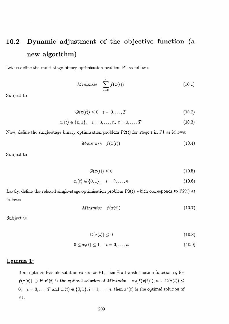
10.2 Dynamic adjustment of the objective function (a
new algorithm)
Let us define the multi-stage binary optimisation problem P1 as follows:
T
Minimise L f(x(t)) t=O
Subject to
G(x(t)):s;O t=O, ... ,T
xi(t) E {0, 1 }, i = 0, ... , n, t = 0, ... , T
(10.1)
(10.2)
(10.3)
Now, define the single-stage binary optimisation problem P2(t) for stage tin P1 as follows:
Minimise f(x(t))
Subject to
G(x(t)) :::; 0
Xi(t) E {0, 1}, i = 0, ... ,n
(10.4)
(10.5)
(10.6)
Lastly, define the relaxed single-stage optimisation problem P3(t) which corresponds to P2(t) as
follows:
Minimise f(x(t))
Subject to
G(x(t)) :::; 0
0:::; xi(t) :::; 1, i = 0, ... , n
Lemma 1:
(10.7)
(10.8)
(10.9)
If an optimal feasible solution exists for P1, then :3 a transformation function at for
f(x(t)) 3 if x*(t) is the optimal solution of Minimise at(f(x(t))), s.t. G(x(t)) :::;
0; t = 0, ... , T and xi(t) E {0, 1}, i = 1, ... , n, then x*(t) is the optimal solution of
Pl.
209

Proof
The proof of this lemma is very straight forward. The real problem with P1 is there's no guaran
tee that by optimising every stage independently, the optimal solution for each stage will be an
optimal solution for Pl. That is, if x+(t), t = 1 ... Tis the optimal solution of P2(t), t = 1 ... T,
then there is no guarantee that x+(t), t = 1 ... T is the optimal solution of P1, because of the
interaction among the stages. But if the optimal solution for P1, x*(t), exists, then x*(t) must
be a feasible solution of P2(t). Since any feasible solution is also optimal for some objective
functions, this implies that there must be an objective function f*(x(t)) such that x*(t) is the
optimal solution of Minimise f*(x(t)), s.t. G(x(t)) :S; 0; t = 0, ... , T and x(t) E {0, 1} 1 .
But this implies that 3 a transformation function <:xt for f(x(t)) 3 <:xt(f(x(t))) = f*(x(t)). ¢
Lemma 2:
3j*, a linear function, 3 if x*(t) is the optimal solution of P3(t) under J*, then x*(t)
is the optimal solution of Pl.
Proof
In Lemma 1, it was shown that 3 an objective for each P2(t) which if used to optimise each
P2(t) independently, the result is the optimal solution of Pl. In the current lemma, it will be
shown that 3 a linear version of this objective but for P3(t). But this is true since P3(t) is the
relaxed version of P2(t). To make this clear, we have the constraint 0 :S; x(t) :S; 1 in P3(t) which
will result in a hypercube. But we know from the theory of linear programming that the optimal
solution is always on an extreme point of the polyhedra of the feasible solutions' set. Since P2(t)
is binary, then all feasible solutions for the problem are located on the extreme point of the
polyhedra, the feasible solutions set for P3(t). This entails that for any feasible solution, x*(t),
for P2(t), 3 a linear objective f* 3 by optimising P3(t) using J*, the optimal solution is x*(t).
<>
1An obvious objective is a circle centred on x*(t) with a zero radius
210
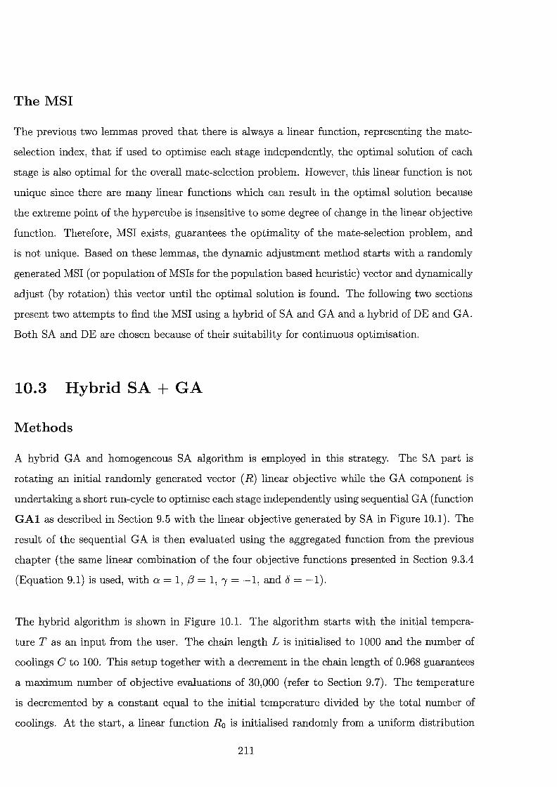
The MSI
The previous two lemmas proved that there is always a linear function, representing the mate
selection index, that if used to optimise each stage independently, the optimal solution of each
stage is also optimal for the overall mate-selection problem. However, this linear function is not
unique since there are many linear functions which can result in the optimal solution because
the extreme point of the hypercube is insensitive to some degree of change in the linear objective
function. Therefore, MSI exists, guarantees the optimality of the mate-selection problem, and
is not unique. Based on these lemmas, the dynamic adjustment method starts with a randomly
generated MSI (or population of MSis for the population based heuristic) vector and dynamically
adjust (by rotation) this vector until the optimal solution is found. The following two sections
present two attempts to find the MSI using a hybrid of SA and GA and a hybrid of DE and GA.
Both SA and DE are chosen because of their suitability for continuous optimisation.
10.3 Hybrid SA+ GA
Methods
A hybrid GA and homogeneous SA algorithm is employed in this strategy. The SA part is
rotating an initial randomly generated vector (R) linear objective while the GA component is
undertaking a short run-cycle to optimise each stage independently using sequential GA (function
GAl as described in Section 9.5 with the linear objective generated by SA in Figure 10.1). The
result of the sequential GA is then evaluated using the aggregated function from the previous
chapter (the same linear combination of the four objective functions presented in Section 9.3.4
(Equation 9.1) is used, with a= 1, f3 = 1, "! = -1, and 8 = -1).
The hybrid algorithm is shown in Figure 10.1. The algorithm starts with the initial tempera
ture T as an input from the user. The chain length L is initialised to 1000 and the number of
coolings C to 100. This setup together with a decrement in the chain length of 0.968 guarantees
a maximum number of objective evaluations of 30,000 (refer to Section 9.7). The temperature
is decremented by a constant equal to the initial temperature divided by the total number of
coolings. At the start, a linear function R0 is initialised randomly from a uniform distribution
211

between 0-1. Simulated annealing is then used to rotate Ri using the function rotate which ran
domly changes 10% of the values in Ri by adding to each of these values a uniformly distributed
random number between 0-0.1. Each time the linear function Ri is generated, sequential GA,
function GAl, is used to optimise the problem using the linear function Ri· The sequential GA
consists of a population of 20 individuals and run for 50 GA-generations using 1-point crossover
and the modified tournament strategy. The number of GA-generations is chosen based on the
results shown in Figure 8.4 where in the first 50 GA-generations, GA improved the solution
very fast. Also, we reduced the population size to increase the pressure so that we get a fast
estimate. The number of objective evaluations carried out by the function GAl are not being
accounted for in the 30,000 objective-evaluations condition. The reason for that is GAl uses
a linear function which can be evaluated in a negligible time compared to the evaluation time
needed by the aggregated function where inbreeding and coancestry are calculated. We may
note that the functions fnew(x), fcurrent(x), and fopt(x) evaluate a solution using the original
aggregated function (Equation 9.1).
To gain an insight about an appropriate value for the initial temperature, 10 runs of length 200
objective evaluations were made. It was found that 99% of the solutions can be accepted with
average temperature of 70. Consequently, three initial temperature levels (70, 40, and 1) are
experimented with. Therefore, a total of 3 experiments is carried out, with each experiment runs
ten different times with different seeds. A maximum of 30,000 objective evaluations were set on
each run with a stop occurring either when this maximum is reached or when 3000 objective
evaluations elapse without an improvement in the best solution found.
Results and discussion
The results of this experiment are shown in Table 10.1. It can be seen from the table that the
algorithm is similar to random search, since it was incapable of improving the results obtained
from random search in the previous chapter. The reason behind this is that the complexity
of the search problem is increased. The additional search for the MSI added a burden to the
original search for the best solution found. The results are not statistically significant. The best
value obtained in this experiment is associated with temperature level 40 where the average of
212

function SA+GA Input: T C = 100, L = 1000, i = 0 Generate Ro at random initialise best solution found Ropt to be Ro initialise current solution Rcurrent to be Ro
Xcurrent +---- GAl(Ro) Xopt +---- Xcurrent f(xopt) +---- f(xcurrent) temperature_step = T / C fork= 0 to C
for j = 0 to L
i=i+l ~ +---- rotate(Rcurrent) Xnew +----GAl(~) fl(f) = f(Xnew)- f(Xcurrent) if f(xnew) > f(xopt) then , Ropt = ~' Xopt = Xnew, j(Xopt) = f(Xnew)
if J(xnew) > f(Xcurrent) then , Rcurrent = ~' Xcurrent = Xnew, f(xcurrent) = f(Xnew) else if exp(b..(f)jT) > random {0,1) then Rcurrent = Ri, Xcurrent = Xnew, f(xcurrent) = f(xnew) if last update of !opt > 3000 exit for
T = T- temperature_step
L = L * 0.968 if last update of fopt > 3000 exit for
return the best MSI found Ropt end function
Figure 10.1: A Hybrid GA+SA algorithm for generating of mate-selection index.
the best solutions in the ten runs is 1948470 ± 37800 and is found on the average at iteration
2230 ± 1480. The best solution found during the experiment is 2029600. The SA algorithm
could not survive the condition of improving the best solution found within each 3,000 objective
evaluations and therefore terminated early.
Table 10.1: Results of GA/SA Hybrid for MSI. Columns represent the three different temperature levels.
Criteria
average fitness
average # iterations
Best solution
70 1,939,010 ± 28,400
1,840 ± 1,910.0 2,002,000
Temperature 40
1,948,470 ± 37,800 2,230 ± 1,480.0
2,029,600
213
1 1,937,960 ± 22,100
1, 710 ± 1,200.0 1,966,400

10.4 Hybrid DE + GA
Methods
A hybrid GA and DE algorithm is employed in this strategy and shown in Figure 10.2. The
algorithm starts with two inputs from the user, the crossover probability CR and the step size
F. The GA consists of a population of 20 individuals and run for 50 GA-generations using
1-point crossover and modified tournament strategy. The initial population of MSis (R) in DE
is initialised randomly from a uniform distribution between 0-1. The DE part is rotating the
initial population of MSis (R) using crossover, while the GA component is undertaking a short
run-cycle to optimise each stage independently. Differential evolution is described in Section 6.5.
Four crossover probabilities of 1.0, 0.8, 0.4, and 0.1 and three step sizes of 0.8, 0.4, and 0.1 were
used to conduct 12 experiments, with each experiment runs ten different times with different
seeds. A maximum of 30,000 objective evaluations were set on each run with a stop occurring
either when this maximum is reached or when 3000 objective evaluations elapse without an im
provement in the best solution found.
Results and discussion
The results of this experiment are shown in Table 10.2. Once more, it can be seen from the table
that the algorithm is similar to random search although it was capable to improve the results
obtained from SA+GA in the previous section. The results are not statistically significant. The
best value obtained in this experiment is associated with crossover probability 0.8 and step size
0.8. The average of the best solutions in the ten runs is 1962130 ± 37800 and is found on the
average at iteration 3910 ± 3310. The best solution found during the experiment is 2030900.
The DE algorithm could not survive the condition of improving the best solution found within
each 3,000 objective evaluations and therefore terminated early.
214
function DE+GA Input: CR and FE (0, 1) let G denote a DE-Generation, P a population of size M, and Rb=k the jth individual of
dimension N in population P in stage k, and CR denotes the crossover probability initialise Pa=o = {R~=O' ... , RM"=o} as foreach individual Rb=o E Pa=o
foreach i EN
R{a=o = random(O, 1), i = 1, ... , N
Xnew +-- GAl (Rb=o) let the fitness value, F(Rb=0 ), of Rb=o be f(xnew)
k=l; while the stopping criterion is not satisfied do
forall j :::; M randomly select r1, r2, r3 E (1, ... , M), j -1- r1 -1- r2 -1- r3 randomly select irand E (1, ... , N)
v· < N RZ = { R~,~=k-1 + F x (R~}i=k-1- R~P=k-1) 'l- ' t RJ
i,G=k-1
Xnew +-- GAl (R') let the objective value, F(R'), of R' be f(xnew)
Ri = { R'. if F(R') :::; F(Rb=k-1) } G=k R~=k- 1 otherwise
k=k+1 return the best encountered MSI R E Pa=k·
end function
if (random[O, 1) < CR 1\ i = irand)
otherwise
Figure 10.2: A Hybrid GA +DE algorithm for generating of mate-selection index.
10.5 Conclusion
This chapter shows that the MSI exists and that it guarantees the optimality of the original
mate-selection problem. However, the experiments show that searching for this index increased
the complexity of the mate-selection problem and as a result, the best solutions found here were
inferior to those obtained directly in the previous chapter. More precisely, it is inferior to the
random search procedure presented in the first experiment of the previous chapter. A number of
alternatives maybe investigated to improve the results of this chapter. For example, using linear
programming instead of the sequential-GA module. Also, trying gradient-based optimisation
techniques might be a worthwhile attempt. These suggestions are left for future work.
This chapter concludes the third sub-objective of the thesis; that is, formulating and solving
the mate-selection problem. This sub-objective is achieved by formulating a general multi-stage
mate-selection model in Chapter 7 which is then customised and solved to a single-stage model in
215
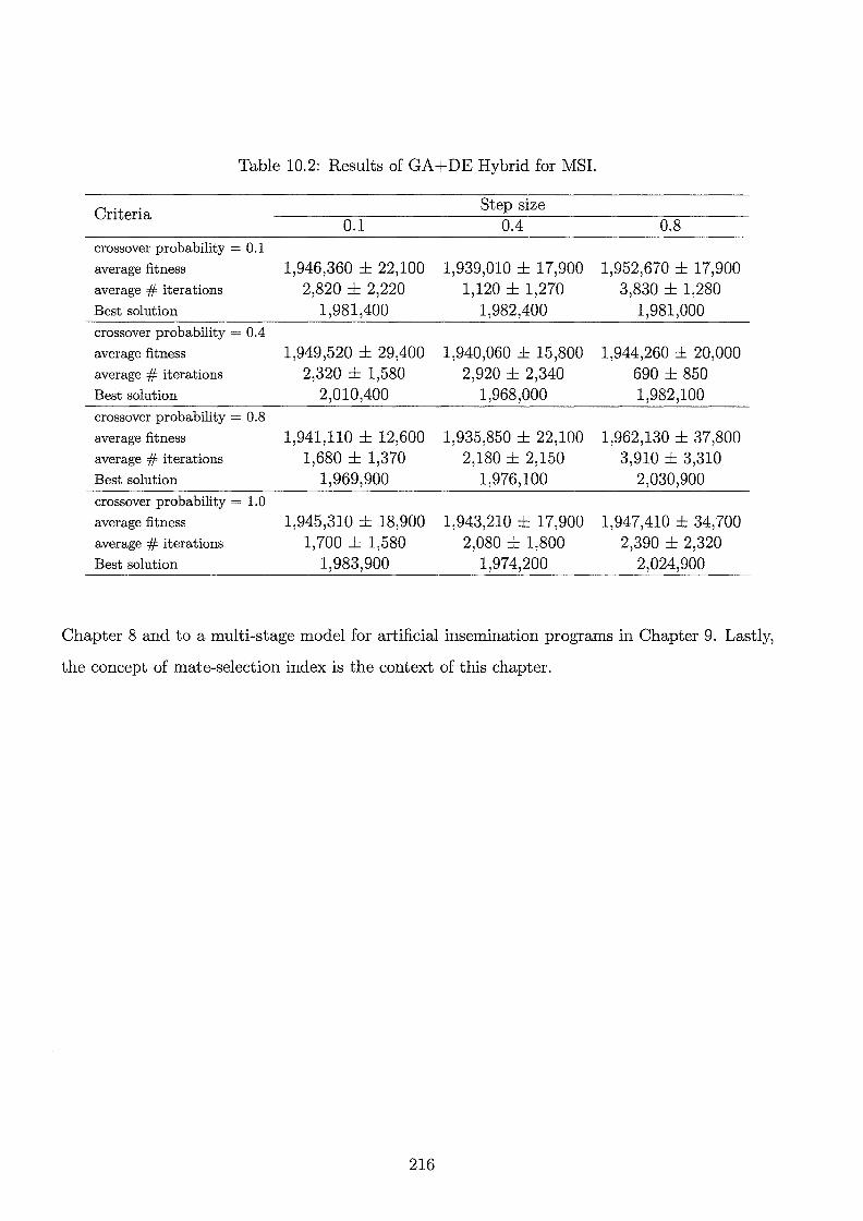
Table 10.2: Results of GA+DE Hybrid for MSI.
Criteria Step size
0.1 0.4 0.8 crossover probability = 0.1
average fitness 1,946,360 ± 22,100 1,939,010 ± 17,900 1,952,670 ± 17,900 average # iterations 2,820 ± 2,220 1,120 ± 1,270 3,830 ± 1,280 Best solution 1,981,400 1,982,400 1,981,000 crossover probability = 0.4
average fitness 1,949,520 ± 29,400 1,940,060 ± 15,800 1,944,260 ± 20,000 average # iterations 2,320 ± 1,580 2,920 ± 2,340 690 ± 850 Best solution 2,010,400 1,968,000 1,982,100 crossover probability = 0.8
average fitness 1,941,110 ± 12,600 1,935,850 ± 22,100 1,962,130 ± 37,800 average # iterations 1,680 ± 1,370 2,180 ± 2,150 3,910 ± 3,310 Best solution 1,969,900 1,976,100 2,030,900 crossover probability= 1.0
average fitness 1,945,310 18,900 1,943,210 ± 17,900 1,947,410 ± 34,700 average # iterations 1,700 ± 1,580 2,080 ± 1,800 2,390 ± 2,320 Best solution 1,983,900 1,974,200 2,024,900
Chapter 8 and to a multi-stage model for artificial insemination programs in Chapter 9. Lastly,
the concept of mate-selection index is the context of this chapter.
216

Chapter 11
Conclusion and Future Work
11.1 Summary
This thesis has investigated the problem-solving techniques for the efficient design of dairy cat
tle breeding programs. To achieve this, a generic information system framework (KDD-IDSS)
was established, through the integration of knowledge discovery from databases with intelligent
decision support systems, to identify the crucial component of a breeding program's information
system. To this end, three sub-objectives were identified:
1. designing a generic kernel (ie. an interface language between the system's components) for
the KDD-IDSS,
2. discovering patterns in the dairy database using KDD, and
3. formulating and solving the version of the mate-selection problem presented in this thesis.
The first sub-objective was achieved by designing a meta-language, using the constraint logic pro
gramming paradigm, to integrate operations research and artificial intelligence modules within a
KDD-IDSS. KDD enables the IDSS paradigm to update its knowledge and models dynamically,
and therefore, provide up-to-date knowledge and models to improve the decision making process.
An example obtained from the dairy industry of the language's implementation was discussed.
The second sub-objective was achieved by experiments involving point and interval function esti
mation. Point function estimation methods provide a value prediction for the expected progeny
217
milk production. Interval function estimation methods provide an explanation capability for the
system regarding the prediction it makes. Artificial neural networks and linear regression were
used for point estimation and rule extraction from artificial neural networks (RULEX) and the
decision tree classifier (C5) were used for interval estimation. The prediction accuracy of the ar
tificial neural network method was similar to that of the linear regression model. Since the linear
regression model is simple and as accurate as the artificial neural network model on the used
dairy database, it was chosen as the best model. For the interval estimation experiments, C5 had
less rules than RULEX on the discrete inputs; therefore suggesting that C5 is more suitable for
this estimation task. These experiments motivated the development of a new algorithm, C-Net,
for generating multivariate decision trees. This algorithm achieved a performance intermediate
between artificial neural networks and univariate decision trees. It was intermediate because it
was better than C5 in terms of generalisation and sometimes generalised better than the neural
network itself. Also, it was more expressive than the neural network but less expressive than the
corresponding univariate decision tree. In this algorithm, we also introduced for the first time
the concept of recurrent decision trees, where conventional decision trees were extended with
some recurrent features.
The third sub-objective of the thesis was achieved by developing a generic formulation of a mate
selection problem called the evolutionary allocation problem (EAP). The EAP was found to be
very complex. Table 11.1 summarises the complexity of the mathematical models presented in
this thesis, as well as the complexity of a benchmark problem (traveling salesman problem). The
representation for the heuristic techniques removed redundancy from the optimisation model
without excluding any optimal solution; therefore, the optimisation model's search space was
preserved within the heuristic techniques' representation. One can also see in the table that
the search space of the multi-stage problem is similar to a traveling salesman problem with 500
cities. However, there are a lot of redundancy in the traveling salesman's search space using
the representation that obtained the complexities presented in the table. In the multi-stage cus
tomised version of the EAP problem, the representation is very compact and therefore represent
larger space. In summary, the multi-stage mate-selection problem is non-trivial and hides many
complexity issues.
218

Mathematical Programming Heuristic
General EAP 1070335 NA
Single-Stage 10660 10208
Multi-Stage 1066828 101000
Sym. TSP (200 cities) 10374 10374
Sym. TSP ( 500 cities) 101134 101134
Table 11.1: The complexity of different mate-selection models.
To solve the multi-stage mate-selection problem, we compared nine techniques, where two of
them were newly developed in this thesis. My two proposed techniques, called evolving colonies
of ants and Markov chain tabu search, outperformed the other techniques. MCTS achieved re
sults which were statistically significantly better than all the others. The mate-selection index
was also investigated (Chapter 10) and the theoretical proofs for its existence and non-uniqueness
were provided.
From a research perspective, the thesis represents a multi-disciplinary research project. To make
the thesis readable by people from different backgrounds came at the cost of having a long, but
still compact, document. In what follows, the contributions of the thesis are visited once more
followed by points for future work.
11.2 Original contributions
The original contributions achieved in this thesis are listed below:
• In Chapter 3, a generic and domain independent novel frame, KDD-IDSS, was established
for integrating knowledge discovery in databases with intelligent decision support systems.
It automated the overall decision-making process, beginning with the ability of problem
recognition and ending with a continuous feedback about the decision's outcome.
• Chapter 3 also presented a constrained logic programming based meta-language for inter
facing optimisation and AI modules in the KDD-IDSS frame. The language represented
219

a level of abstraction used to isolate the user from the problem solving details. A mate
selection example was used to illustrate the potential usefulness of this language.
• In Chapter 4, the rules governing the outcome of a mating were extracted from the dairy
database using RULEX and C5. Autoclass was used to discretise the inputs and the output.
The domain expert suggested that discrete inputs are more comprehensible than continuous
inputs. Therefore, C5 was chosen since it produced less rules than RULEX with similar
accuracy.
• Chapter 5 introduced a novel algorithm, C-Net, for integrating ANNs and DTs. The algo
rithm achieved a performance which was intermediate to this achieved by neural networks
and decision trees in isolation. It outperformed the C5 algorithm in terms of classification
error and used a representational language simpler than the neural network from which it
was extracted. On some of the datasets, C-Net even generalised better than the neural
network from which it was extracted.
• In Chapter 7, a multi-stage mate-selection problem was formulated generically. The com
plexity of the problem was examined and it was found that solving this problem to optimal
ity is impossible with the current state-of-the-art in optimisation theory. To my knowledge,
this is the first time EAP was generically formulated.
• Chapter 8 presented a single-stage mate-selection model, simplified from the generic for
mulation presented in Chapter 7. The model was formulated as a quadratic transportation
model, and genetic algorithm was used to solve it. A repair operator was developed to re
trieve the feasibility of the chromosomes. Also, a new crossover operator, called gene-based
crossover, was developed. The best GA result was achieved with the one-point crossover
operator with modified tournament selection.
• Chapter 9 introduced a multi-stage mate-selection problem for farms dependent on artificial
insemination. The model was derived from the generic model and a methodical set of
experiments was undertaken to examine a suitable heuristic technique for solving this
problem. Random search, sequential genetic algorithms, hill climbing, genetic algorithms,
simulated annealing, ant colony optimisation, and immune systems were all examined for
solving this model. Additionally, a new heuristic search strategy was developed, called
220
Markov-chain Tabu search, for solving the problem. Furthermore, a new hybrid-algorithm
(ACO+GA) for evolving colonies of ants by combining ant colony optimisation and genetic
algorithms was developed. The ACO+GA hybrid resulted in the best performance among
the population based algorithms (which included Sequential GA, ACO, GA, and Immune)
whereas Markov-chain Tabu search (MCTS) resulted in the best overall performance.
• In Chapter 10, a method for creating a mate-selection index, called dynamic adjustment of
the objective function, was introduced. The theoretical foundations for this method were
established and two hybrid algorithms, simulated annealing-genetic algorithms (SA+GA)
hybrid, and differential evolution-genetic algorithms (DE+GA) hybrid, were developed and
tested. The latter resulted in the better performance of the two methods.
11.3 Future work
This thesis presented an overall information system framework (KDD-IDSS) for the efficient
design of breeding programs. No work is ever truly complete; otherwise we should stop research.
Some interesting research questions therefore arise from this work. A list is given below in two
categories; information technology points of further research and agriculture ones.
1. Future work from information technology point of view
• The first research point is how to extend the design of the meta-language to cover all
aspects of the KDD-IDSS. The KDD-IDSS has a hierarchal architecture consisting of
agents which control other agents and controlled by other agents. This leads us to
think of each predicate as an agent which is responsible for a specific task. Each mod
ule in the KDD-IDSS is also responsible from an agent which co-ordinates the other
agents. Therefore, we have a hierarchal architecture for the KDD-IDSS using multi
agent systems. In this case, the meta-language defines the communication language
among the agents and a description for the overall task the agent can do.
• Building up a prototype of the KDD-IDSS system is a very important open question.
It is a multi-disciplinary project that requires a team of scientists. From a practical
perspective, the proposed system is achievable, based on my own experience. The
expected profit from developing such a system would be very high since the system
221

will not be developed just for farmers or the mate-selection problem. Because of its
modularity, the system can be used for many problems like transportation and budget
programming.
• The dynamic decision trees concept, (C-Net, Chapter 5), is a new concept introduced
in this thesis and it has lots of potential. For example, using the approach presented
in the thesis for integrating artificial neural networks and decision trees, can be a
means for extracting and representing finite state automaton from recurrent neural
networks. Furthermore, the applications of dynamic decision trees are enormous and
this opens a new area of research in this direction.
2. Future work from animal breeding point of view
• Developing more techniques for decomposing and handling the multi-stage model is
also an open question. More studies can be undertaken in this area to compare the
results obtained in the thesis against new technologies emerging in the future.
• Analysing the underlying dairy principles in the optimisation process from the breeder
perspective. It was sufficient for us to show that the total objective value for the multi
stage model is better than that obtained from the sequential GA experiment. But,
what is the economic value of this improvement? Moreover, instead of scaling the ob
jectives to overcome the magnitude problem, can we develop an economic model which
calculates precisely the economic value of each objective? These are still open ques
tions that need the employment of economic models which can be a very interesting
piece of research if undertaken properly.
• Selectabull as discussed in Chapter 2 does not consider the mate-selection problem.
It would be interested to extend this package with mate-selection. Also, it does
not capture important genetic principles such as inbreeding and it would be more
appropriate to incorporate inbreeding (both short and long term) within Selectabull.
• Industrial Significance: Total genetic resource management (TGRM) (Kinghorn and
Shepherd 1999) is a breeding aid program driven by specifying desired outcomes ( eg.
outcomes in genetic gains) (Kinghorn and Shepherd 1999). The program was devel
oped by a group of animal breeders from the University of New England led by Prof.
222

Brian Kinghorn, Dr. Robert Bank, and Dr. Ross Shepherd. It is currently the state
of the art in the field of mate-selection. The approach relies on the use of an evo
lutionary algorithm (differential evolution) for optimising the mating pairs. TGRM
demonstrates the importance of mate-selection. I believe that utilising the results of
this thesis would improve the performance of TGRM. I may recall that the differential
evolution approach did not work as well as the others. Therefore, it would be inter
esting to apply Markov Chain Tabu Search within the TGRM package and compare
the results with the differential evolution approach.
223

224

Bibliography
Abbass, H. (1994). Goal programming within the frame of constraint logic programming.
Master's thesis, Dept. of Computer Science, Cairo University.
Abbass, H. (1998). A quadratic optimizer in a constraint logic programming paradigm. The
workshop of constraint, 11th Australia Joint Conference in Artificial Intelligence, Australia.
Abbass, H., R. Bahgat, and M. Rasmy (1995). Evaluation of constraint logic programming from
an operations research point of view. Proceedings of the Third International Conference in
Artificial Intelligence, American University in Cairo, Egypt.
Abbass, H., R. Bahgat, and M. Rasmy (1997). From constraint logic programming (clp) to
decision making logic programming ( dmlp). Proceedings of the First European Conference
on Intelligent Management Systems in Operations (IMSO), Manchester, UK.
Abbass, H., W. Bligh, M. Towsey, M. Tierney, and G. Finn (1999). Knowledge discovery in a
dairy cattle database: automated knowledge acquisition. Fifth International Conference of
the International Society for Decision Support Systems (ISDSS'99), Melbourne, Australia.
Abbass, H., G. Wiggin, R. Lakshmanan, and B. Morton (1999a). Constraint logic programming
as a paradigm for heat exchanger network retrofit. The International Journal of Computers
and Chemical Engineering S-ESCAPE-9, 8127-8130.
Abbass, H., G. Wiggin, R. Lakshmanan, and B. Morton (1999b). Constraint programming
for process synthesis. Proceedings of the First International Conference on the Practical
Application of Constraint Technologies and Logic Programming(PACLP99), London, UK.
Ackley, D. (1987). A connectionist machine for genetic hill climbing. Kluwer Academic Pub
lisher.
ADHIS (1997). The ABV book: Australian breeding values for dairy sires. Dairy Research and
225

Development Corportation, Australia.
Ami, A. (1993). Exploring the interior-point linear programming: algorithms and softwares.
MIT.
Andrews, R. and J. Diederich (1996). Rules and networks. Proceedings of the Rule Extraction
from Trained Artificial Neural Network Workshop, University of Sussex, Brighton, U.K.
Andrews, R., J. Diederich, and A. Tickle (1995). A survey and critique of techniques for
extracting rules from trained artificial neural networks. Knowledge Based Systems 8(6),
373-389.
Ansari, N. and E. Hou (1997). Computational intelligence for optimization. Kluwer Academic
Publisher.
Apte, C. and S. Hong (1996). Predicting equity returns from securities data with minimal rule
generation. In U. Fayyad, G. Piatetsky-Shapiro, P. Smyth, and R. Uthurusamy (Eds.),
Advances in knolwedge discovery and data mining, pp. 541-560. AAI/MIT press.
Archer, A., R. Lacroix, and K. Wade (1998). Implementing decision support systems for dairy
herd improvement on the world wide web. The Sixth World Congress on Genetics Applied
to Livestock Production, 23-28.
Ata-Mohammed, N., J. Courtney, and D. Paradice (1988). A prototype dss for structuring
and diagnosing managerial problems. IEEE Transactions on Systems Man and Cybernet
ics 18(6), 899-907.
Baldi, P. and S. Brunak (1999). Bioinformatics: the machine learning approach. MIT press.
Banks, R. (1988). Industry structures and breeding strategies: Meat- and wool-sheep. Pro
ceeding of the 4th Australian Association Animal Breeding Genetics, 248-259.
Banks, R., M. Goddard, H. Graser, D. Johnston, M. Katz, B. Kinghorn, S. Sivarajasingam, and
W. Upton (1996). Quantitative genetics: Lecturer Notes GENE 422. School of Rural Science
and Natural Resources, Faculty of the Sciences, University of New England, Australia.
Barahona, P. and R. Ribeiro (1990). Building expert decision support system: the integration
of artificial intelligence and operations research methods. Knowledge, Data, and Computer
Assisted Decisions 61, 155-167.
226

Beard, K. (1987). Efficiency of index selection for dairy cattle using economic weights for major
milk constituents. Australian Jounral for Agriculture Research 38, 273-284.
Bechtel, W. and A. Abrahamsen (1991). Connectionism and the mind - an introduction to
parallel processing in networks. Basil Blackwell Inc, Cambridge MA, USA.
Bellman, R. and S. Dreyfus (1962). Applied dynamic programming. Princeton University press.
Belz, R. and P. Mertens (1996). Combining knowledge-based systems and simulation to solve
rescheduling problems. Decision Support Systems 17, 141-157.
Bennett, K. (1994). Global tree optimization: a non-greedy decision tree algorithm. Proceedings
of Interface 94: The 26th Symposium on the Interface.
Bennett, K. and J. Blue (1997). An extreme point tabu search method for data mining. Tech
nical Report 228, Department of Mathematical Sciences, Rensselaer Polytechnic Institute.
Berthold, M. and D. Hand (1999). Intelligent data analysis: an introduction. Springer Verlag.
Bigus, J. (1996). Data mining with neural networks: solving business problems from application
development to decision support. McGraw-Hill.
Boer, I. D. (1994). The use of clones in dairy cattle breeding. Ph. D. thesis, Wageningen
Agriculture University, The Netherlands.
Bonabeau, E., M. Dorigo, and G. Theraulaz (1999). Swarm intelligence: from natural to
artificial systems. Oxford Press.
Bonczek, R., C. Holsapple, and A. Whinston (1980). Foundations of decision support systems.
Academic press, London.
Bowman, P., P. Visscher, and M. Goddard (1996). Customized selection indices for dairy bulls
in australia. Animal Science 62, 393-403.
Boyd, R. and P. Richerson (1985). Culture and the evolutionary process. Chicago University
Press.
Breiman, L., J. Friedman, R. Olshen, and C. Stone (1984). Classification and decision trees.
Belmont Calif: Wadsworth International Group.
Brown, D., V. Corruble, and C. Pittard (1993). A comparison of decision tree classifiers with
backpropagation neural networks for multimodal classification problems. Pattern Recogni
tion 26(6), 953-961.
227

Brown, D. and C. Pittard (1993). Classification trees with optimal multi-variate splits. Inter
national Conference on Systems, Man and Cybernetics 3, 475-477.
Charnes, A. and W. Cooper (1961). Management models and industrial applications of linear
programming, volume 1. John Wiley, New York.
Cheeseman, P. and J. Stutz (1996). Bayesian classification (autoclass): theory and results.
In U. Fayyad, G. Piatetsky-Shapiro, P. Smyth, and R. Uthurusamy (Eds.), Advances in
knolwedge discovery and data mining, pp. 153-180. AAI/MIT press.
Cios, K. and N. Liu (1992). A machine learning method for generation of a neural network
architecture: a continuous id3 algorithm. IEEE Transactions on Neural Networks 3(2),
280-291.
Codd, E. and Associates (1993). Providing olap to user-analysis: an it mandate. Technical
report, Codd and Associates.
Coello, C. (1999a). A comprehensive survey of evolutionary-based multiobjective optimization
techniques. Knowledge and Information Systems 1 (3), 269-308.
Coello, C. (1999b). Self-adaptive penalties for ga-based optimization. 1999 Congress on Evo
lutionary Computation 1, 573-580.
D'alche-Buc, F., D. Zwierski, and J. Nadal (1994). Trio learning: a new strategy for building
hybrid neural trees. Neural Systems 5(4), 255-274.
Daniel, L. (1994). Genetics (3 ed.). Jones and Bartlett Publisher, London.
Dantzig, G. (1951). Application of the simplex method to a transportation problem. In
T. Koopmans (Ed.), Activity of production and allocation, pp. 359-373. John Wiley and
Sons, New York.
Darwin, C. (1859). The origins of species by means of natural selection. London, Penguin
Classics.
Dasgupta, D. (1998). Artificial immune systems and their applications. Springer-Verlag.
Dasgupta, D. (1999). Information processing in immune system. In D. Corne, M. Dorigo, and
F. Glover (Eds.), New ideas in optimization, pp. 161-166. McGraw-Hill.
Dasgupta, D. and Z. Michalewicz (1997). Evolutionary algorithms in engineering applications.
Springer-Verlag, Berlin.
228
Davis, L. (1987). Genetic algorithms and simulated annealing. Pitman, London.
Dawkins, R. (1976). The selfish gene. Oxford Press.
Dekkers, J. (1998). Design of breeding programs: chairman's summary. The Sixth World
Congress on Genetics Applied to Livestock Production 23-28, 405-406.
der Werf, J. V. (1990). Models to estimate genetic parameters in crossbred dairy cattle popu
lations under selection. Ph. D. thesis, Wageningen Agriculture University.
Dietterich, T. (1990). Machine learning. Annual Review of Computer Science 4, 225-306.
Dietterich, T., H. Hild, and G. Bakiri (1995). A comparison of id3 and backpropagation for
english text-to-speech mapping. Machine Learning 18, 51-80.
Donald, E. and C. Chelsea (1990). Operations research and artificial intelligence: the integra
tion of problem solving strategies. Kluwer academic publishers, Boston.
Dorigo, M. and G. Caro (1999). The ant colony optimization meta-heuristic. In D. Corne,
M. Dorigo, and F. Glover (Eds.), New ideas in optimization, pp. 11-32. McGraw-Hill.
Dorigo, M. and L. Gambardella (1997). Ant colony system: a cooperative learning approach
to the travelling salesman problem. IEEE Transactions on evolutionary computation 1,
53-66.
Dorigo, M., V. Maniezzo, and A. Colorni (1991). Positive feedback as a search strategy. Tech
nical Report 91-016, Deipartimento di Elettronica, Politecnico do Milano, Italy.
Dorigo, M., V. Maniezzo, and A. Colorni (1996). The ant system: optimization by a colony of
cooperating agents. IEEE Transactions on Systems, Man, and Cybernetics 26(1), 1-13.
Dutta, A. (1996). Integrating ai and optimization for decision support: a survey. Decision
Support Systems 18, 217-226.
Eierman, M., F. Niederman, and C. Adams (1995). Dss theory: a model of constructs and
relationships. Decision Support Systems 14, 1-26.
Elder, J. and D. Pregibon (1996). A statistical perspective on knowledge discovery in databases.
In U. Fayyad, G. Piatetsky-Shapiro, P. Smyth, and R. Uthurusamy (Eds.), Advances in
knolwedge discovery and data mining, pp. 83-116. AAI/MIT press.
Falconer, D. (1989). Introduction to quantitative genetics (3 ed.). Longman Group Limited,
London.
229
Fayyad, U., S. Djorgovski, and N. Weir (1996). Automating the analysis and cataloging of
sky surveys. In U. Fayyad, G. Piatetsky-Shapiro, P. Smyth, and R. Uthurusamy (Eds.),
Advances in knolwedge discovery and data mining, pp. 471-494. AAI/MIT press.
Fayyad, U., G. Piatetsky-Shapiro, and P. Smyth (1996). Knowledge discovery and data mining:
Towards a unifying framework. In U. Fayyad, G. Piatetsky-Shapiro, P. Smyth, and R. Uthu
rusamy (Eds.), Advances in knolwedge discovery and data mining, pp. 1-36. AAI/MIT
press.
Finn, G., R. Lister, R. Szabo, D. Simonetta, H. Mulder, and R. Young (1996). Neural networks
applied to a large biological database to analyse dairy breeding patterns. Neural Computing
and Applications 4, 237-253.
Fogel, D. and A. Ghozeil (1996). Using fitness distributions to design more efficient evolution
ary computations. In Proc. of 1996 IEEE Conf. on Evolutionary Computation, New York,
pp. 11-19. IEEE Press.
Fox, J. and P. Krause (1991, July). Decision theory and autonomous systems. In D'Ambrosio,
Bruce D., Smets, Philippe, and P. P. Bonissone (Eds.), Proceedings of the 7th Confer
ence on Uncertainty in Artificial Intelligence, San Mateo, CA, USA, pp. 103-110. Morgan
Kaufmann Publishers.
Franisco, J. and A. John (1984). Modern genetics (2 ed.). The Benjamin/Cummings.
Frawley, W., G. Piatetsky-Shapiro, and C. Matheus (1991). Knowledge discovery in databases:
an overview. In G. Piatetsky-Shapiro and B. Frawley (Eds.), Knolwedge Discovery in
Databases. Cambridge, Mass: AAAI/MIT press.
Gardner, J. (1985). Blup: A major advance in estimating genetic merit. Australian Pork
Journal 7(7), 15.
Garner, S., G. Holmes, R. McQueen, and I. Witten (1995). Machine learning from agricultural
databases: practice and experience. New-Zealand Journal of Computing 6, 69-73.
Gdaellenbach, H. (1995). Systems and decision making: a management science approach. John
Wiley and Sons.
Gent, I. and T. Walsh (1994). The satisfiability constraint gap. Technical Report 702, Univer
sity of Edinburgh.
230

Giunchiglia, F. and T. Walsh (1992). A theory of abstraction. Artificial Intelligence 56(2),
323-390.
Glover, F. (1989). Tabu search: part 1. ORSA Journal on Computing 1 (3), 190-206.
Glover, F. (1990). Tabu search: part 2. ORSA Journal on Computing 2(1), 4-32.
Goldberg, D. (1989). Genetic algorithms: in search, optimisation and machine learning. Ad
dison Wesely.
Gosselin, V. (1993). Train scheduling using constraint programming techniques. Thirteenth
International Conference, Avigon, France.
Hadj-Alouane, A. and J. Bean (1992). A genetic algorithm for the multiple-choice integer pro
gram. Technical Report TR-92-50, Department of Industrial and Operations Engineering,
The University of Michigan.
Hajela, P. and J. Yoo (1999). Immune network modelling in design optimization. In D. Corne,
M. Dorigo, and F. Glover (Eds.), New ideas in optimization, pp. 203-216. McGraw-Hill.
Han, J. (1997). Olap mining: an integration of olap with datamining. IFIP.
Hayes,. B., R. Shepherd, and S. Newman ( 1997). Selecting mating pairs with genetic algorithms.
Proceedings of the 12th Conference of the Association of Advances in Animal Breeding
Genetics, 108-112.
Haykin, S. (1999). Neural networks- a comprehensive foundation (2 ed.). Prentice Hall, USA.
Hazel, L. (1943). The genetic basis for constructing selection indices. Genetics 28, 476-490.
Henderson, C. (1975a). Best linear unbiased estimation and prediction under a selection model.
Biometrics 31, 423-447.
Henderson, C. (1975b). Use of all relatives in intraherd prediction of breeding values and
producing abilities. Dairy Science 58, 1910-1916.
Hentenryck, P. (1989). Constraint satisfaction in logic programming: from theory to applica
tions. MIT Press.
Hentenryck, P. V. (1990, October). Constraint logic programming: From theory to applica
tions. In M. Debray, Saumya; Hermenegildo (Ed.), Proceedings of the 1990 North American
Conference on Logic Programming, Austin, TX, pp. 831-831. MIT Press.
231

Hertz, J., A. Krogh, and R. Palmer (1991). Introduction to the theory of neural computation.
Santa Fe Institute.
Hicks, J. (1987). Management information systems: a user prespective. West publishing com
pany, New York.
Hirooka, H. (1998). A unified procedure for restricted selection of sires using linear program
ming. The Sixth World Congress on Genetics Applied to Livestock Production, 23-28.
Hoeffgen, K., H. Simon, and K. Van-Horn (1995). Robust trainability of single neurons. Com
puter System Sciences 50(1), 114-125.
Holland, J. (1998). Adaptation in natural and artificial systems. MIT press.
Holsapple, C. (1977). Framework for a generalised intelligent decision support system. Ph. D.
thesis, Purdue University.
Holsapple, C., V. Jacob, and A. Whinston (1994). Operations research and artificial intelli
gence. Aplex publishing corporation.
Homaifar, A., S. Lai, and X. Qi (1994). Constrained optimisation via genetic algorithms.
Simulation 62(4), 242-254.
Hooker, J. (1986). Karmarkar's linear programming algorithm. Interfaces 16, 75-90.
Howarth, J. and M. Goddard (1998). Maximising response and profit under multiple objective
selection. The Sixth World Congress on Genetics Applied to Livestock Production, 23-28.
Ignizio, J. (1976). Goal programming and extension. Lexington Books, Lexington Press.
Ijiri, Y. (1965). Management goals and accounting for control. North-holland, Amsterdam.
Inmon, W. and C. Kelley (1994). The 12 rules of data warehouse for a client server world.
Data Management Review.
Irie, B. and S. Miyake (1988). Capabilities of three-layered perceptrons. In Proceedings of
the IEEE International Conference on Neural Networks, Volume 1, San Diego, CA, pp.
641-648. IEEE.
Jaffer, J. and J. Lassez (1986). Constraint logic programming. Proceeding of the 14th ACM
POPL conference, Munich.
232

Jaffer, J. and M. Maher (1994). Constraint logic programming: A survey. Journal of Logic
Programming 19-20.
Jaffer, J., S. Michaylov, P. Stuckey, and R. Yap (1990). The clp(r) language and system.
Technical Report 16292, IBM Research Division.
Jansen, G. and J. Wilton (1985). Selecting mating pairs with linear programming. Dairy
Science 68, 1302-1305.
John, G. (1997). Enhancements to the data mining process. Ph. D. thesis, Dept. of Computer
Science, Stanford University.
Jones, L. (1985). Australian breeding values for production characters. Proceedings of the Fifth
Conference of the Association for the Advancement of Animal Breeding and Genetics, 242-
247.
Jong, K. D. (1975). An analysis of the behavior of a class of genetic adaptive systems. Ph. D.
thesis, University of Michigan.
Kempthorne, 0. and A. Nordskog (1959). Restricted selection indices. Biometrics 15, 10-19.
Kinghorn, B. (1987). On computing strategies for mate allocation. Animal Breeding and Ge
netics 104, 12-22.
Kinghorn, B. (1995). Quantitative genetics manual. Lecturer Notes GENE 315/325. School of
Rural Science and Natural Resources, Faculty of the Sciences, University of New England,
Australia.
Kinghorn, B. (1998). Mate selection by groups. Dairy Science 81, 55-63.
Kinghorn, B. (1999). Total resource management: tactical optimisation of vertically inte
grated animal production systems. In H. Abbass and M. Towsey (Eds.), The Application
of Artificial Intelligence, Optimisation, and Bayesian Methods in Agriculture, pp. 95-100.
QUT-Publication.
Kinghorn, B. and R. Shepherd (1999). Mate selection for the tactical implementation of breed
ing programs. Proceedings of the Thirteenth Conference of the Association for the Advance
ment of Animal Breeding and Genetics, 130-133.
Kinghorn, B., R. Shepherd, and J. Woolliams (1999). An index of estimated breeding value,
parental coancestry, and progeny inbreeding to help maximise genetic gains. Proceedings
233
of the Thirteenth Conference of the Association for the Advancement of Animal Breeding
and Genetics, 412-415.
Kirkpatrick, S., C. Gelatt, and M. Vecchi (1983). Optimization by simulated annealing. Sci
ence 220, 671-680.
Klein, M. (1995). Knowledge-based decision support systems: with applications in business.
John-Wiley and Sons.
Klieve, H., B. Kinghorn, and S. Barwick (1994). The joint regulation of genetic gain and
inbreeding under mate selection. Journal of Animal Breeding Genetics 111, 81-88.
Klug, W. and M. Cummings (1999). Genetics. Prentice-Hall.
Kuhn, H. (1955). The hungarian method for the assignment problem. Naval Research Logistics
Quarterly 2, 1-2.
Kuhn, H. W. and A. W. Tucker (1951). Nonlinear programming. In J. Neyman (Ed.), Pro
ceedings of the Second Berkeley Symposium on Mathematical Statistics and Probability,
Berkeley, 1950, Berkeley, California, pp. 481-492. University of California Press.
Lacroix, R., F. Salehi, X. Yang, and K. Wade (1997). Effects of data preprocessing on the
performance of artificial neural networks for dairy yield prediction and cow culling classi
fication. Transactions of the ASAE 40, 839-846.
Lacroix, R., K. Wade, R. Kok, and J. Hayes (1994). Predicting 305-day milk, fat and protein
production with an artificial neural network. Proceeding of the third International Dairy
Housing Conference: Dairy Systems for the 21st Century, 201-208.
Laguna, F. G. M. (1997). Tabu search. Kluwer Academic Publisher, Boston.
Lee, H., R. Lee, and G. Yu (1996). Constraint logic programming for qualitative and quanti
tative constraint satisfaction problems. Decision support systems 16, 67-83.
Lee, J. (1990). Integration and competition of ai with quantitative methods for decision sup
port. Expert system with applications 1, 329-333.
Lemaitre, M. and G. Verfaillie (1997). An incomplete method for solving distributed valued
constraint satisfaction problems. AAAI-97 Workshop on Constraints and Agents.
Liepins, G. and W. Potter (1991). A genetic algorithm approach to multiple-fault diagnosis.
In L. Davis (Ed.), Handbook of Genetic Algorithms, pp. 237-250. Van Nostrand Reinhold.
234
Liepins, G. and M. Vose (1990). Representational issues in genetic optimization. Journal of
Experimental and Theoretical Computer Science 2(2), 4-30.
Little, J. D. C. (1970, April). Models and managers: The concept of a decision calculus.
Management Science 16(8), 466-485.
Lumsden, C. and E. Wilson (1981). Genes, Mind, and Culture. Harvard University Press,
Cambridge.
Lumsden, C. and E. Wilson (1983). Promethean Fire. Harvard University Press, Cambridge.
MacNeil, M., S. Newman, W. Lamberson, and Z. Hochman (1998). Decision support systems
to aid beef producers in choosing a crossbreeding strategy. The Sixth World Congress on
Genetics Applied to Livestock Production 23-28.
Macrossan, P. (2000). Statistical methods applicable to on-farm animal breeding decisions.
Master's thesis, Queensland University of Technology.
Maire, F. (1999). Rule extraction by backpropagation of polyhedra. Neural Networks 12(4-5),
717-725.
Maniezzo, V. (1998). Exact and approximate nondeterministic tree-search procedures for the
quadratic assignment problem. Technical Report CSR 98-1, Corso di Laurea in Scienze
dell'Informazione, Universita di Bologna, Sede di Cesena, Italy.
Matheus, C., G. Piatetsky-Shapiro, and D. McNeill (1996). Selecting and reporting what is
interesting: the kefir application healthcare data. In U. Fayyad, G. Piatetsky-Shapiro,
P. Smyth, and R. Uthurusamy (Eds.), Advances in knolwedge discovery and data mining,
pp. 495-516. AAI/MIT press.
McCulloch, W. and W. Pitts (1943). A logical calculus of ideas immanent in nervous activity.
Bulletin of Mathematical Biophysics 5, 115-133.
Miihlenbein, H. (1991). Evolution in time and space: the parallel genetic algorithm. In G. Rawl
ins (Ed.), Foundations of Genetic Algorithms, pp. 316-337. San Mateo, CA: Morgan
Kaufman.
Miihlenbein, H. (1992). Parallel genetic algorithms in combinatorial optimization. In 0. Balci,
R. Sharda, and S. Zenios (Eds.), Computer Science and Operations Research, pp. 441-456.
Pergamon Press.
235

Muhlenbein, H., M. Gorges-Schleuter, and 0. Kramer (1988). Evolutionary algorithms in
combinatorial optimization. Parallel Computing 7, 65-88.
Muhlenbein, H. and D. Schlierkarnp-Voosen (1993). Predictive models for the breeder genetic
algorithms: continuous parameter optimization. Evolutionary Computation 1 (1), 25-49.
Mii,hlenbein, H. and D. Schlierkamp-Voosen (1994). The science of breeding and its application
to the breeder genetic algorithm bga. Evolutionary Computation 1 (4), 335-360.
Metropolis, N., A. Rosenbluth, M. Rosenbluth, A. Teller, and E. Teller (1953). Equations of
state calculations by fast computing machines. Chemical Physics 21, 1087-1092.
Meuwissen, T. (1997). Maximising the response of selection with a predefined rate of inbreed
ing. Animal Science 75, 934-940.
Meuwissen, T. and z. Luo (1992). Computing inbreeding coefficients in large populations.
Genetique, Selection, Evolution 24, 305-313.
Michalewicz, Z. and N. Attia (1994). Evolutionary optimization of constrained problems. Pro
ceedings of the 3rd Annual Conference on Evolutionary Programming, 98-108.
Michalewicz, Z., D. Dasgupta, R. L. Riche, and M. Schoenauer (1996). Evolutionary algorithms
for constrained engineering problems. Computer and Industrial Engineering Journal 30(4),
851-870.
Michalewicz, Z. and D. Fogel (2000). How to solve it: modern heuristic. Springer verlag.
Michalewicz, Z. and C. Janikow (1991). Handling constraints in genetic algorithms. In
L. Booker (Ed.), Proceedings of the Fourth International Conference on Genetic Algo
rithms, pp. 151-157. Morgan Kaufmann.
Michalewicz, Z. and G. Nazhiyath (1995). Genocop iii: A co-evolutionary algorithm for numer
ical optimization with nonlinear constraints. In D. Fogel (Ed.), Proceedings of the Second
IEEE International Conference on Evolutionary Computation, pp. 647-651. IEEE Press.
Minsky, M. (1967). Computation: finite and infinite machines. Prentice-Hall.
Minton, S., M. Johnston, A. Philips, and P. Laird (1992). Minimizing conflicts: a heuristic
method for constraint-satisfaction and scheduling problems. Artificial Intelligence 58, 161-
205.
236

MIT (1997). Tlearn software. version 1.0.1. exercises in rethinking innateness: a handbook for
connectionist simulations. MIT Press.
Mitchell, T. (1997). Machine learning. McGraw-Hill.
Molich, R. and J. Nielsen (1990). Improving a human-computer dialog. Communications of
the ACM 33(3).
Montesi, D. (1996). Heterogeneous knowledge representation: integrating connectionist and
symbolic computation. Knowledge-Based Systems 9, 501-507.
Moon, C., T. Moore, and S. Nassar (1993). Managing product quality by integrating operations
research and artificial intelligence technologies. IBM ind. Sec. IAAI.
Morales, A. and C. Quezada (1998). A universal eclectic genetic algorithm for constrained
optimization. Proceedings of the 6th European Congress on Intelligent Techniques and Soft
Computing, EUFIT'98, 518-522.
Morton, S. (1971). Management decision systems: computer-based support for decision making.
Cambridge, MA: Division of Research, Harvard University.
Moscato, P. (1989). On evolution, search, optimization, genetic algorithms and martial arts:
towards memetic algorithms. Technical Report 826, California Institute of Technology,
Pasadena, California, USA.
Moscato, P. (1999). Memetic algorithms: a short introduction. In D. Corne, M. Dorigo, and
F. Glover (Eds.), New ideas in optimization, pp. 219-234. McGraw-Hill.
Mrode, R. (1996). Linear models for the prediction of animal breeding values. CAB Interna
tional.
Murphy, P. and D. Aha (1992). Uci repository of machine learning database [machine-readable
data repository]. Department of Information and Computer Science, University of Califor
nia, Irvine.
Norman, D. (1986). Cognitive engineering. In Norman and Draper (Eds.), User centered system
design. Lawrence Erlbaum Association, Hillsdale N J.
Orvosh, D. and L. Davis (1994). Using genetic algorithm to optimize problems with feasibility
constraints. Proceedings of the First IEEE Conference on Evolutionary Computation, 548-
553.
237

Papadimitriou, C. and K. Steiglitz (1982). Combinatorial optimization: algorithms and com
plexity. Prentice-Hall.
Park, Y. (1994). A comparison of neural net classifiers and linear tree classifiers: their simi
larities and differences. Pattern Recognition 27(11), 1493-1503.
Parnell, P. and K. Hammond (1985). The use of blup for estimation of genetic merit in livestock
improvement programs. Chiasma 85, 33-35.
Paulli, J. (1993). A computational comparison of simulated annealing and tabu search ap
plied to the quadratic assignment problem. In R. Vidal (Ed.), Applied simulated annealing.
Springer-Verlag.
Perrett, M. (1991). Using constraint logic programming techniques in container port planning.
ICL Technical Journal, 537-545.
Quaas, R. (1976). Computing the diagonal elements of a large numerator relationship matrix.
Biometrics 32.
Quaas, R. (1995). Fx algorithms. An unpublished note.
Quinlan, J. (1993). C4.5: programs for machine learning. Morgan Kaufman.
Quinlan, J. (1997). C5 software. http:/ /www.rulequest.comjsee5-info.html.
Quinlan, M. and R. Rivest (1989). Inferring decision trees using the minimum description
length principle. Information and Computation 80, 227-248.
Quinton, M., C. Smith, and M. Goddard (1992). Comparison of selection methods at the same
level of inbreeding. Animal Science 70, 1060-1067.
Ravden, S. and G. Johnson (1989). Evaluating usability of human-computer interfaces: a
practical method. John Wiley and Sons.
Richardson, J., M. Palmer, G. Liepins, and M. Hilliard (1989). Some guidelines for genetical
gorithms with penalty functions. In J. Schaffer (Ed.), Proceedings of the Third International
Conference on Genetic Algorithms, pp. 191-197. Morgan Kaufmann Publisher.
Riche, R. L. and R. Haftka (1994). Improved genetic algorithm for minimum thickness com
posite laminate design. Composites Engineering 3(1), 121-139.
238

Riche, R. L., C. Knopf-Lenoir, and R. Haftka (1995). A segregated genetic algorithms for
constraint structural optimisation. In L. Eshelman (Ed.), Proceedings of the sixth inter
national conference on genetic algorithms, pp. 558-565. San Mateo, California, July 1995.
University of Pittsburgh, Morgan Kaufmann.
Ritzel, B., J. Eheart, and S. Ranjithan (1994). Using genetic algorithms to solve a multiple
objective groundwater pollution containment problem. Water Resources Research 30(5),
1589-1603.
Rob, P. and C. Coronel (1997). Database systems: design, implementation, and management.
Course Technology.
Robinson, G. (1981). The national dairy herd improvement scheme. Technical Report 5, De
partment of Agriculture, Victoria.
Rodrigues, M. and A. Anjo (1993). On simulating thermodynamics. In R. Vidal (Ed.), Applied
simulated annealing. Springer-Verlag.
Rosenblatt, F. (1962). The principles of neurodynamics. New York: Spartan.
Ross, P. (1996). Genetic algorithms and genetic programming: Lecturer Notes. University of
Edinburgh, Department of Artificial Intelligence.
Rumelhart, D., G. Hinton, and R. Williams (1986). Learning internal representations by error
propagation. In J. M. D.E. Rumelhart and the PDP Research Group Eds (Eds.), Parallel
Distributed Processing: Explorations in the Microstructure of Cognition., Foundations, 1,
318,. MIT Press Cambridge.
Rumelhart, D., B. Widrow, and M. Lehr (1994). The basic ideas in neural networks. Commu
nications of the ACM 37, 87-92.
Runyon, R., A. Haber, D. Pittenger, and K. Coleman (1996). Fundamentals of behavioral
statistics. McGraw Hill.
Salkin, H. and K. Mathur (1989). Foundations of integer programming. North-Holland.
Schaeffer, L. and B. Kennedy (1986). Computing solutions to mixed model equations. Proc. of
the 3rd World Congress on genetics applied to livestock production. Lincoln, Nebraska 12,
382-393.
239

Scheiderman, B. (1987). Designing the user interface: strategies for effective human computer
interaction. Addison Wesley, Reading MA.
Schmidt, G. and L. Van-Vleck (1974). Principles of dairy science. W.H. Freeman and Com
pany.
Schoenauer, M. and S. Xanthakis (1993). Constrained ga optimization. The Fourth Interna
tional Conference on Genetic Algorithms, ICGA93.
Schwefel, H. (1981). Numerical optimization of computer models. Wiler, Chichester.
Sen, A. and G. Biswas (1985). Decision support systems: an expert systems approach. Decision
Support Systems 1.
Setiono, R. and L. Huan (1995). Understanding neural networks via rule extraction. Interna
tional Joint Conference in Artificial Intelligence: IJCAI.
Setiono, R. and L. Huan (1997). Neurolinear: from neural networks to oblique decision rules.
Neurocomputing 17, 1-24.
Sharda, R., S. Barr, and J. McDonnell (1988). Decision support system effectiveness: a review
and an empirical test. Management Science.
Shepherd, R. and B. Kinghorn (1994). A tactical approach to the design of crossbreeding
programs. The Fifth World Congress on Genetics Applied to Livestock Production 18,
255-261.
Shepherd, R. and B. Kinghorn (1999). Algorithms for mate selection. Proceedings of the Thir
teenth Conference of the Association for the Advancement of Animal Breeding and Genet
ics, 126-129.
Shivastava, B. and W. Chen (1993). Part type selection problem in flexible manufacturing
systems: Tabu search algorithms. Annals of Operations Research 41, 279-297.
Simon, H. (1960). The new science of management decisions. Harper and Row, New York.
Sirat, J. and J.-P. Nadal (1990). Neural trees: a new tool for classification. Computation in
Neural Network 1 (4), 423-438.
Smyth, P., M. Burl, U. Fayyad, and P. Perona (1996). Modeling subjective uncertainty in
image annotation. In U. Fayyad, G. Piatetsky-Shapiro, P. Smyth, and R. Uthurusamy
(Eds.), Advances in knolwedge discovery and data mining, pp. 517-540. AAI/MIT press.
240

Sniedovich, M. (1992). Dynamic programming. Marcel Dekker, Inc.
Sreerama, K. (1997). On growing better decision trees from data. Ph. D. thesis, Johns Hopkins
University.
Storn, R. and K. Price (1995). Differential evolution: a simple and efficient adaptive scheme
for global optimization over continuous spaces. Technical Report TR-95-012, International
Computer Science Institute, Berkeley.
Stutzle, T. (1998). Local search algorithms for combinatorial problems: analysis, improvements,
and new applications. Ph. D. thesis, Fachbereich Informatik, TU Darmstadt, Germany.
Taillard, E. (1998). Fant: fast ant system. Technical Report IDSIA-46-98, IDSIA.
Towsey, M. (1998). The use of neural networks in the automated analysis of the electroen
cephalogram. Ph. D. thesis, University of Queensland.
Towsey, M., J. Diederich, I. Schellhammer, S. Chalup, and C. Brugman (1998). Natural lan
guage learning by recurrent neural networks: a comparison with probabilistic approaches.
Proc. Joint Conf. on New Methods in Language Processing and Computational Natural
Language Learning, 3-10.
Trave-Massuyes, L. (1991). Qualitative reasoning from different aspects and potential appli
cations to decision support systems. Proceedings of the !MAGS international workshop on
decision support systems and qualitative reasoning, France.
Turban, E. (1990). Decision support and expert systems: management support systems.
Macmillan series in information systems.
Van-Vleck, L., E. Pollak, and E. Oltenacu (1987). Genetics for the animal sciences. W.H.
Freeman and Company, New York.
Vapnik, V. (1995). The nature of satisticalleaming theory. Springer-Verlag.
Vidal, R. (1993). Applied simulated annealing. Springer-Verlag.
von Neumann, J. (1956). Probabilistic logics and the synthesis of reliable organisms from
unreliable components. In C. Sharron and J. McCarthy (Eds.), Automata studies, pp. 43-
98. Princeton University Press.
Wade, K. and R. Lacroix (1994). The role of artificial neural networks in animal breeding. The
Fifth World Congress on Genetics Applied to Livestock Production, 31-34.
241

Werbos, P. (1974). Beyond regression: new tools for prediction and analysis in the behavioral
sciences. Ph. D. thesis, Harvard University.
Wetzel, A. (1983). Evaluation of the effectiveness of genetic algorithms in combinatorial opti
mization. Technical report, University of Pittsburgh.
Whitley, D. (1994). A genetic algorithm tutorial. Statistics and Computing 4, 65-85.
Widrow, B., D. Rumelhart, and M. Lehr (1994). Neural networks: applications in industry,
business and science. Communications of the ACM 37, 93-105.
Winchester, A. (1966). Genetics: a survey of the principles of heredity. Houghton Mifflin
Company.
Witten, I. and E. Frank (2000). Data mining: practical machine learning tools and techniques
with Java implementations. Morgan Kaufmann.
Wray, N. and M. Goddard (1994). Increasing long-term response to selection. Genetique Se
lection and Evolution 26, 431-451.
Wright, S. (1931). Evolution in mendelian populations. Genetics 16, 97-159.
Xiao, J., Z. Michalewicz, and K. Trojanowski (1997). Adaptive evolutionary planner/navigator
for mobile robots. IEEE Transactions on Evolutionary Computation 1 (1), 18-28.
Xiao, J., Z. Michalewicz, and L. Zhang (1996). Evolutionary planner/navigator: operator
performance and self-tuning. Proceedings of the 3rd IEEE International Conference on
Evolutionary Computation.
242
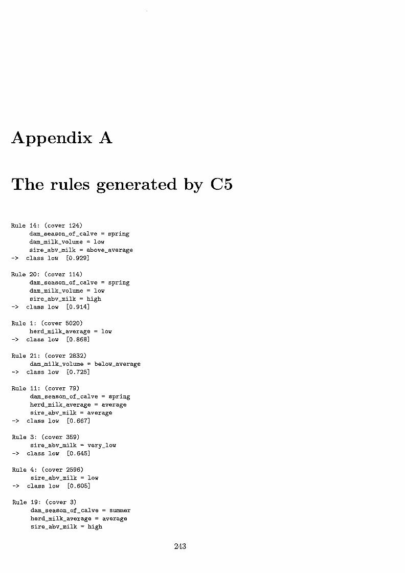
Appendix A
The rules generated by C5
Rule 14: (cover 124) dam_season_of calve spring dam_milk_volume = low sire_abv_milk = above_average
-> class low [0.929]
Rule 20: (cover 114) dam_season_of_calve spring dam_milk_volume = low sire_abv_milk = high
-> class low [0.914]
Rule 1: (cover 5020) herd_milk_average low
-> class low [0.868]
Rule 21: (cover 2832) dam_milk_volume = below_average
-> class low [0.725]
Rule 11: (cover 79) dam_season_of calve spring herd_milk_average = average sire_abv_milk = average
-> class low [0.667]
Rule 3: (cover 359) sire_abv_milk = very_low
-> class low [0.645]
Rule 4: (cover 2596) sire_abv_milk = low
-> class low [0.605]
Rule 19: (cover 3) dam_season_of calve = summer herd_milk_average = average sire_abv_milk = high
243

-> class low [0.600]
Rule 22: (cover 836) dam_season_of_calve spring dam_milk_volume = average
-> class low [0.584]
Rule 2: (cover 4201) herd_milk_average
-> class low [0.571]
Rule 9: (cover 2378)
below_average
sire_abv_milk = below_average -> class low [0.509]
Rule 12: (cover 337) dam_season_of_calve = winter herd_milk_average = average sire_abv_milk = above_average
-> class low [0.507]
Rule 34: (cover 2) herd_milk_average = high dam_milk_volume = low sire_abv_milk = high
-> class average [0.750]
Rule 35: (cover 2) dam_season_of_calve = autumn herd_milk_average = high dam_milk_volume = below_average sire_abv_milk = high
-> class average [0.750]
Rule 26: (cover 9) dam_season_of_calve = autumn herd_milk_average = above_average dam_milk_volume = above_average sire_abv_milk = below_average
-> class average [0.727]
Rule 10: (cover 6) dam_season_of_calve = summer herd_milk_average = average sire_abv_milk = average
-> class average [0.625]
Rule 25: (cover 71) herd_milk_average = above_average dam_milk_volume = average sire_abv_milk = below_average
-> class average [0.603]
Rule 13: (cover 93) dam_season_of_calve = autumn herd_milk_average = average
244
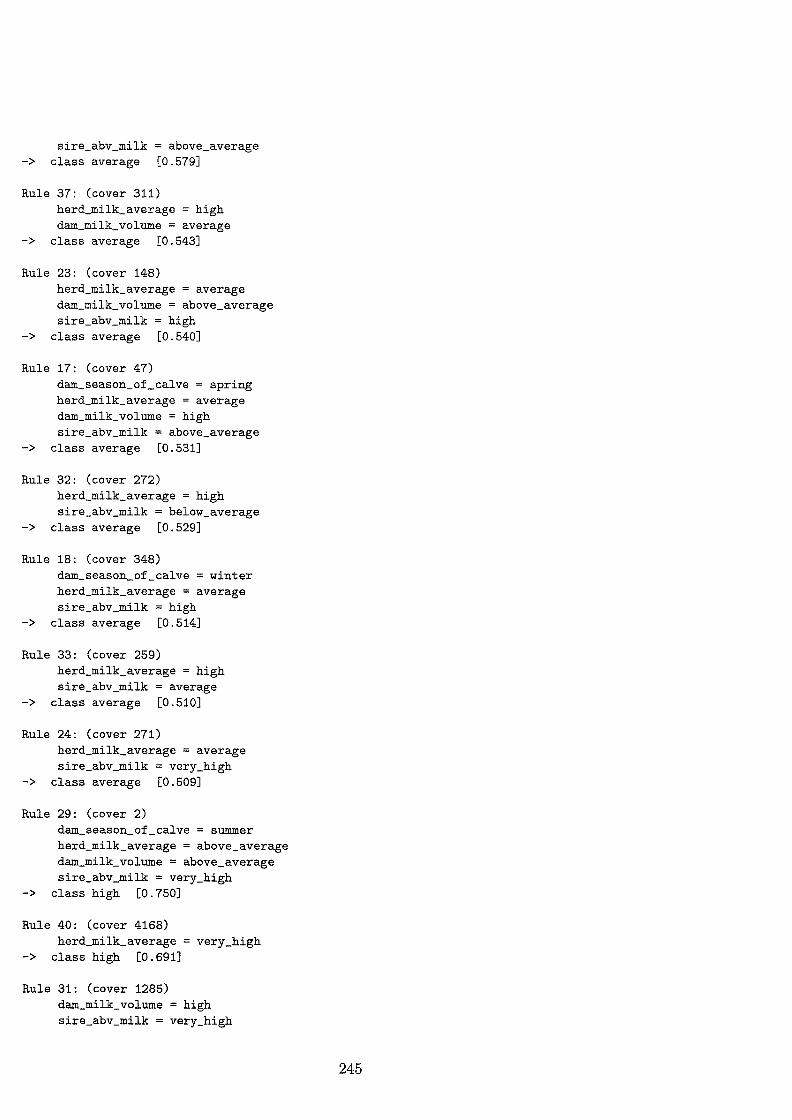
sire_abv_milk = above_average -> class average [0.579]
Rule 37: (cover 311) herd_milk_average = high dam_milk_volume = average
-> class average [0.543]
Rule 23: (cover 148) herd_milk_average = average dam_milk_volume = above_average sire_abv_milk = high
-> class average [0.540]
Rule 17: (cover 47) dam_season_of_calve spring herd_milk_average = average dam_milk_volume = high sire_abv_milk = above_average
-> class average [0.531]
Rule 32: (cover 272) herd_milk_average = high sire_abv_milk = below_average
-> class average [0.529]
Rule 18: (cover 348) dam_season_of_calve = winter herd_milk_average = average sire_abv_milk = high
-> class average [0.514]
Rule 33: (cover 259) herd_milk_average = high sire_abv_milk = average
-> class average [0.510]
Rule 24: (cover 271) herd_milk_average = average sire_abv_milk = very_high
-> class average [0.509]
Rule 29: (cover 2) dam_season_of calve = summer herd_milk_average = above_average dam_milk_volume = above_average sire_abv_milk = very_high
-> class high [0.750]
Rule 40: (cover 4168) herd_milk_average very_high
-> class high [0.691]
Rule 31: (cover 1285) dam_milk_volume high sire_abv_milk = very_high
245

-> class high [0.632]
Rule 39: (cover 278) herd_milk_average = high sire_abv_milk = very_high
-> class high [0.575]
Rule 38: (cover 2363) dam_milk_volume = high sire_abv_milk = high
-> class high [0.556]
Rule 28: (cover 84) dam_season_of_calve = autumn herd_milk_average = above_average sire_abv_milk = very_high
-> class high [0.512]
246

Appendix B
The Code for the Markov Chain Tabu
Search Algorithm
Markov Chain Tabu Search
Copyright (c) 1999 Hussein Aly Abbass
//Title: //Version: //Copyright: //Author: //Company: //Description:
Machine Learning Research Center The main contoller for MCTS
#include <stdlib.h> #include <math.h> #include <iostream.h> #include <fstream.h> #include <iomanip.h> #include <string.h> #include <assert.h>
#include "MCTS_Operator.h"
Operator ee2; void GA_read_parameter_file();
main(int argc,char *argv[]) {
GA_read_parameter_file(); if (argc != 10)
{
cout << endl << endl; cout << "There should be 7 parameters cout << ''----------------------------cout << "00- Seed cout << "01- Number_of_runs cout << "02- Number_of children cout << "03- Maximum_number_of_mating_per_sire cout << "04- Number_of_generations cout << "05- Neighbourhood_ size
247
II << endl; II << endl; II << endl; II << endl; II << endl; II << endl; II << endl; II << endl;
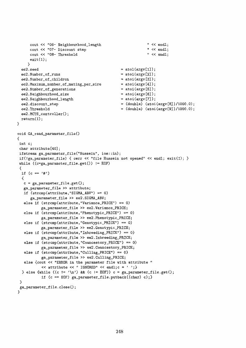
}
}
cout << "06- Neighbourhood_length cout << "07- Discount step cout << "08- Threshold exit(!);
ee2.seed ee2.Number_of_runs ee2.Number_of children ee2.Maximum_number_of_mating_per_sire ee2.Number_of_generations ee2.Neighbourhood_size ee2.Neighbourhood_length ee2.discount_step ee2.Threshold ee2.MCTS_controller(); return(!);
" << endl; " << endl; " << endl;
atol(argv[1]); atoi (argv [2]) ; atoi (argv [3]) ; atoi(argv[4]); atoi ( argv [5] ) ; atoi (argv [6]) ; atoi (argv [7]) ; (double) (atoi(argv[S])/1000.0); (double) (atoi(argv[9])/1000.0);
void GA_read_parameter_file() {
int c; char attribute[40]; ifstream ga_parameter_file("Hussein", ios: :in); if (! ga_parameter_file) { cerr « "file Hussein not opened" << endl; exit (1); } while ((c=ga_parameter_file.get()) != EOF) {
if (c == '#') {
c = ga_parameter_file.get(); ga_parameter_file >> attribute; if (strcmp(attribute, "SIGMA_ABV") == 0)
ga_parameter_file >> ee2.SIGMA_ABV; else if (strcmp(attribute, "Variance_PRICE") == 0)
ga_parameter_file >> ee2.Variance_PRICE; else if (strcmp(attribute,"Phenotypic_PRICE") == 0)
ga_parameter_file >> ee2.Phenotypic_PRICE; else if (strcmp(attribute,"Genotypic_PRICE") == 0)
ga_parameter_file >> ee2.Genotypic_PRICE; else if (strcmp(attribute,"Inbreeding_PRICE") == 0)
ga_parameter_file >> ee2.Inbreeding_PRICE; else if (strcmp(attribute,"Coancestory_PRICE") == 0)
ga_parameter_file >> ee2.Coancestory_PRICE; else if (strcmp(attribute,"Culling_PRICE") == 0)
ga_parameter_file >> ee2.Culling_PRICE; else {cout << "ERROR in the parameter file with attribute "
<<attribute<<" IGNORED"<< endl;c =' ';} } else {while ((c != '\n') && (c != EOF)) c = ga_parameter_file.get();
if (c == EOF) ga_parameter_file.putback((char) c);} }
ga_parameter_file.close(); }
248
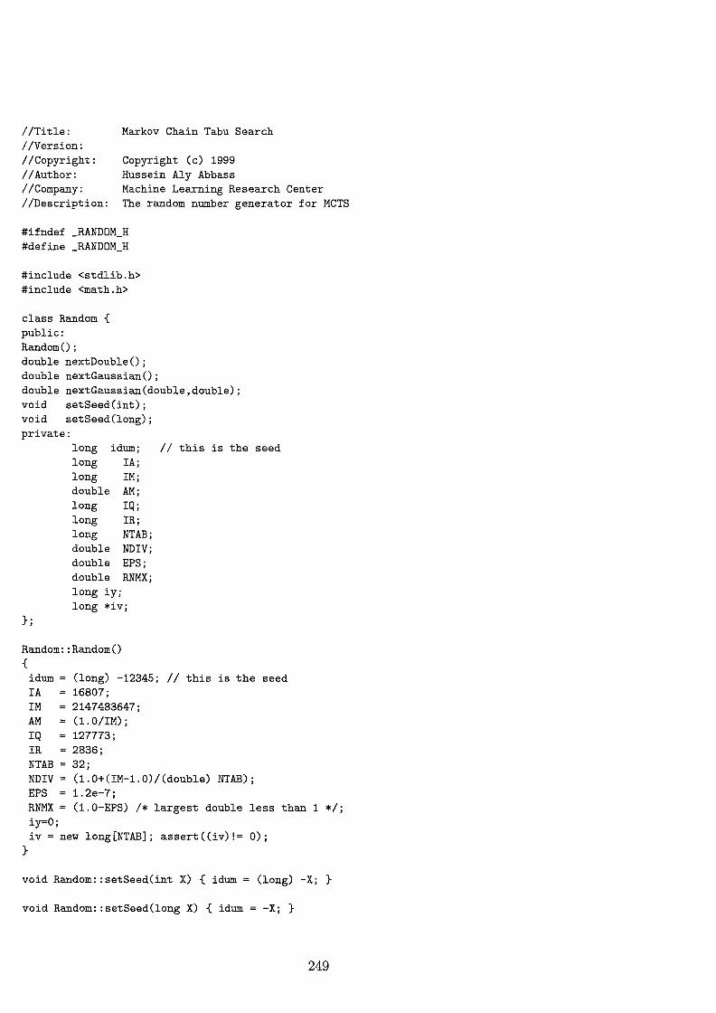
Markov Chain Tabu Search
Copyright (c) 1999 Hussein Aly Abbass
//Title: //Version: //Copyright: //Author: //Company: //Description:
Machine Learning Research Center The random number generator for MCTS
#ifndef _RANDOM_H #define _RANDOM_H
#include <stdlib.h> #include <math.h>
class Random { public: Random(); double nextDouble(); double nextGaussian(); double nextGaussian(double,double); void setSeed(int); void setSeed(long); private:
long idum; II this is the seed long IA; long IM; double AM·
' long IQ; long IR; long NTAB; double NDIV; double EPS; double RNMX; long iy; long *iv;
};
Random::Random() {
idum = (long) -12345; II this is the seed IA 16807; IM 2147483647; AM (1. 0/IM); IQ 127773; IR 2836; NTAB 32; NDIV = (1.0+(IM-1.0)/(double) NTAB); EPS 1.2e-7; RNMX = (1.0-EPS) I* largest double less than 1 *I; iy=O; iv =new long[NTAB]; assert((iv)!= 0);
}
void Random: :setSeed(int X) { idum = (long) -X; }
void Random::setSeed(long X) { idum =-X; }
249

double Random: :nextGaussian(double mean,double stdev) {
double x = (double) nextGaussian(); return (double) (x * stdev +mean); }
double Random: :nextDouble() {
int j; long k; double temp; if (idum <=0 II ! iy)
{
if (-idum < 1) idum=1; else idum -idum; for (j=NTAB+7;j>=O;j--)
{
k = (long) (idum I (double) IQ ); idum=IA*(idum-k*IQ)-IR*k; if (idum < 0)
idum +=IM; if (j < NTAB) iv[j] = idum;
}
}
iy=iv[O];
k= (long) (idum/ (double) IQ ); idum=IA*(idum-k*IQ)-IR*k; if (idum < 0) idum += IM; j= (int) (iy/NDIV); iy=iv[j]; iv[j]= idum; if ((temp=AM*iy) > RNMX) return RNMX; else return temp;
}
double Random: :nextGaussian() {
static int iset=O; static double gset; double fac,rsq,v1,v2; if (iset ==0)
{
do {
v1=2.0*nextDouble()-1.0; v2=2.0*nextDouble()-1.0; rsq=v1*v1+v2*v2; }
while(rsq>=1.0 I lrsq ==0.0);
}
fac =sqrt(-2.0*log(rsq)/(double) rsq); gset=v1*fac;· iset=1; return v2*fac;
else {
}
iset=O; return gset;
}
#endif
250

//Title: //Version: //Copyright: //Author: //Company: //Description:
Markov Chain Tabu Search
Copyright (c) 1999 Hussein Aly Abbass Machine Learning Research Center The objective evaluator for MCTS
#ifndef OBJECTIVE_H #define OBJECTIVE_H
#include <math.h> #include <assert.h>
#include "MCTS_Random.h"
class Objective {
public:
void
double
void
int
int int int int int int int
double double double double double double
double double double
double double double double double double
private:
Objective(); Initialise();
Evaluate_individual(int,int **);
Repair_Chromosome(Random &,int **);
number_of_genes;
Number_of_animals_in_previous_generations; Number_of_available_dams; Number_of_available_sires; Number_of_generations; Maximum_number_of_mating_per_sire; Number_of_culling; Number_of_children;
Phenotypic_PRICE; Genotypic_PRICE; Inbreeding_PRICE; Coancestory_PRICE; Culling_PRICE; Variance_PRICE;
STDEV_PE; STDEV_E; SIGMA_ABV;
!_genotype; !_phenotype; !_inbreeding; T_coancestry; T_culling; !_variance;
int Number_of_animals_in_current_generation; int Number_of_animals_in_all_generations;
251
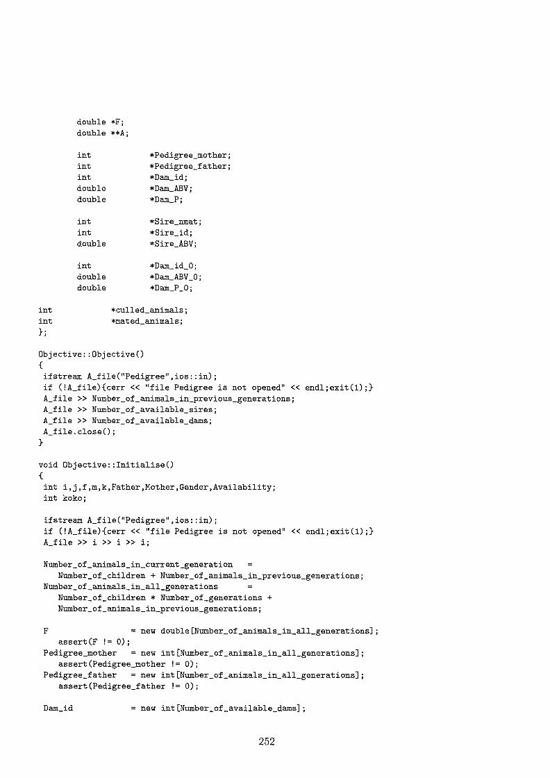
double double
int int int double double
int int double
int double double
*F; **A;
*Pedigree_mother; *Pedigree_father; *Dam_id; *Dam_ABV; *Dam_P;
*Sire_nmat; *Sire_id; *Sire_ABV;
*Dam_id_O; *Dam_ABV _0; *Dam_P_O;
int int };
*culled_animals; *mated_animals;
Objective: :Objective() {
}
if stream A_file("Pedigree", ios:: in); if (!A_file){cerr << "file Pedigree is not opened" « endl;exit(1) ;} A_file >> Number_of_animals_in_previous_generations; A_file >> Number_of_available_sires; A_file >> Number_of_available_dams; A_file. close();
void Objective: :Initialise() {
int i,j,f,m,k,Father,Mother,Gender,Availability; int koko;
ifstream A_file("Pedigree" ,ios: :in); if (!A_file){cerr «"file Pedigree is not opened"« endl;exit(1);} A_file >> i >> i >> i;
Number_of_animals_in_current_generation Number_of_children + Number_of_animals_in_previous_generations;
Number_of_animals_in_all_generations
F
Number_of_children * Number_of_generations + Number_of_animals_in_previous_generations;
new double[Number_of_animals_in_all_generations]; assert(F != 0);
Pedigree_mother new int[Number_of_animals_in_all_generations]; assert(Pedigree_mother != 0);
Pedigree_father =new int[Number_of_animals_in_all_generations]; assert(Pedigree_father != 0);
Dam_id =new int[Number_of_available_dams];
252

assert(Dam_id != 0); Dam_ABV =new double[Number_of_available_dams];
assert(Dam_ABV != 0); Dam_P =new double[Number_of_available_dams];
assert(Dam_P != 0);
Dam_id_O =new int[Number_of_available_dams]; assert(Dam_id != 0);
Dam_ABV_O =new double[Number_of_available_dams]; assert(Dam_ABV != 0);
Dam_P_O =new double[Number_of_available_dams]; assert(Dam_P != 0);
Sire_nmat =new int[Number_of_available_sires]; assert(Sire_nmat != 0);
Sire_id =new int[Number_of_available_sires]; assert(Sire_id != 0);
Sire_ABV =new double[Number_of_available_sires]; assert(Sire_ABV != 0);
culled_animals =new int[Number_of_children]; assert(culled_animals != 0);
mated_animals =new int[Number_of_children]; assert(mated_animals != 0);
A= (double**) new double[Number_of_animals_in_all_generations]; assert(A != 0);
for (i=O;i<Number_of_animals_in_all_generations;i++) {
}
A[i] =(double*) new double[Number_of_animals_in_all_generations]; assert(A[i] != 0);
for (i=O;i<Number_of_animals_in_all_generations;i++) {
}
for (j=O;j<Number_of_animals_in_all_generations;j++) A[i] [j] 0.0; F[i] = 0;
for (i=O,m=O, f=O;i<Number_of_animals_in_previous_generations;i++) {
A_file >> k >> Gender >> Availability >> Father >> Mother; Pedigree_mother[i] = Mother; Pedigree_father[i] = Father; if ((Gender == 0) && (Availability == 1)) {
}
A_file >> Sire_ABV[m]; Sire_id[m]=i; if (m<Number_of_available_sires) m++;
else if((Gender == 1) && (Availability 1)) {
A_file >> Dam_ABV[f] >> Dam_P[f]; Dam_id[f]=i; Dam_id_O[f]=Dam_id[f]; Dam_ABV_O[f]=Dam_ABV[f]; Dam_P_O[f]=Dam_P[f];
253

}
f++; }
else if((Gender == 1) && (Availability== 0)) A_file >> koko >> koko;
else A_file » koko;
A [i] [i] = 1; if ((Father != -1) && (Mother != -1)) {
}
for (j=O;j<i;j++) {
}
A [i] [j] = 0. 5 * (A [j] [Father] + A [j] [Mother]); A[j][i] = A[i][j];
A[i] [i] += 0.5 * A[Father] [Mother];
else if ((Father == -1) && (Mother != -1)) for (j=O;j<i;j++) {
}
A[i] [j] = 0.5 * A[j] [Mother]; A[j] [i] = A[i] [j];
else if ((Father != -1) && (Mother == -1)) for (j=O;j<i;j++) {
}
A[i] [j] = 0.5 * A[j] [Father]; A~] [i] = A[i] [j];
F [i] = A [i] [i] - 1;
A_f ile. close() ; }
void Objective::Repair_Chromosome(Random &Rand,int **individual) {
int i,i2,i3,Value,Flage,N_Culling,N_Mating;
for (i2=0;i2<Number_of_generations;i2++) {
N_Culling = 0; for (i=O;i<Number_of_available_sires;i++) Sire_nmat[i] for (i3=0;i3<number_of_genes;i3++) {
}
Value = (int) individual[i2] [i3]; if (Value>= 0) Sire_nmat[Value]+=1;
else if (Value == -1) N_Culling+=1;
II Satisfying the maximum number of mating per sire constraint
for (i=O;i<Number_of_available_sires;i++) if (Sire_nmat[i] > Maximum_number_of_mating_per_sire) {
254
O· '

}
for (i3=0;i3<number_of_genes;i3++)
i--;
if ((individual[i2] [i3] == i) && (Rand.nextDouble() < 0.5)) {
}
individual[i2] [i3] = -2; Sire_nmat[i]-=1; if (Sire_nmat[i] == Maximum_number_of_mating_per_sire)
i3 = number_of_genes;
II Satisfying the number of culling constraint
while (N_Culling > Number_of_culling) {
}
i3 = (int) (number_of_genes * Rand.nextDouble()); if (individual[i2] [i3] == -1) {
}
individual[i2] [i3] = -2; N_Culling--;
while (N_Culling < Number_of_culling) {
}
i3 = (int) (number_of_genes * Rand.nextDouble()); if (individual[i2] [i3] != -1) {
}
individual[i2] [i3] = -1; N_Culling++;
II Calculating the number of mating constraint
N_Mating = 0; for (i3=0;i3<number_of_genes;i3++) {
}
Value = (int) individual[i2] [i3]; if (Value >= 0) N_Mating ++;
II Satisfying the number of mating constraint
while (N_Mating < Number_of_children) {
i3 = (int) (number_of_genes * Rand.nextDouble()); if (individual[i2] [i3] == -2) {
Flage=O; while (!Flage) {
i = (int) (Number_of_available_sires * Rand.nextDouble()); if (Sire_nmat[i] < Maximum_number_of_mating_per_sire) {
individual[i2] [i3] = i;
255
}
} }
} }
}
N_Mating++; Sire_nmat[i]++; Flage=1;
while (N_Mating > Number_of_children) {
}
i3 = (int) (number_of_genes * Rand.nextDouble()); if (individual[i2] [i3] > -1) {
}
individual[i2] [i3] -2; N_Mating--;
double Objective::Evaluate_individual(int coutflage,int **Individual) { int i,j,i3,l,i4,SIRE,DAM,DAM_id,SIRE_id,CHECK,Father,Mother,Value,mated,culled; int N_anims_all_prev_gens,N_anims_curr_gen,Generation_ID;
double Pheno_VALUE,Geno_VALUE,Inbr_VALUE,TMP1,TMP2,Coanc_VALUE,Culling_VALUE,Total; double VarianceO, V_2, V, Variance_VALUE;
T_inbreeding 0; T_coancestry 0; T_genotype 0·
' T_phenotype 0· ' T_culling 0· ' T_variance O· '
for (i=O;i<Number_of_available_dams;i++) {
}
Dam_id[i] = Dam_id_O[i]; Dam_ABV[i] = Dam_ABV_O[i]; Dam_P[i] = Dam_P_O[i];
1 = Number_of_animals_in_previous_generations; for (Generation_ID=O;Generation_ID<Number_of_generations;Generation_ID++) {
N_anims_all_prev_gens = Number_of_children * Generation_ID + Number_of_animals_in_previous_generations;
N_anims_curr_gen = Number_of_children * (Generation_ID + 1) + Number_of_animals_in_previous_generations;
II Updating the A matrix for (i=O,mated=O,culled=O;i<number_of_genes;i++) {
Value= (int) Individual[Generation_ID] [i]; if (Value -1) { culled_animals[culled]=i; culled++; } if (Value >= 0) {
256
}
}
mated_animals[mated]=i; Pedigree_father[N_anims_all_prev_gens+mated] = Sire_id[Value]; Pedigree_mother[N_anims_all_prev_gens+mated] = Dam_id[i]; mated++;
for (i=N_anims_all_prev_gens;i<N_anims_curr_gen;i++) {
}
Father = Pedigree_father[i]; Mother= Pedigree_mother[i]; A[i] [i] = 1; for (j=O;j<i;j++) { A[i] [j] = 0.5 * (A[j] [Father] + A[j] [Mother]);
A[j] [i] = A[i] [j]; } A[i] [i] += 0.5 * A[Father] [Mother]; F [i] = A [i] [i] - 1;
II End of Updating the A matrix V_2 = 0.0; v = 0.0; for (i3=0;i3<number_of_genes;i3++) {
Pheno_VALUE 0.0; Geno_VALUE 0.0; Inbr_VALUE 0.0; Coanc_VALUE = 0.0; Culling_VALUE = 0.0; CHECK= (int) Individual[Generation_ID] [i3]; if (CHECK > -1) {
SIRE CHECK; i3; DAM
Geno_VALUE
v
(double) (Genotypic_PRICE * 0.5 * (Dam_ABV[DAM]+Sire_ABV[SIRE]));
+= Geno_VALUE;
}
V_2 Pheno_VALUE Inbr_VALUE l++;
+= Geno_VALUE * Geno_VALUE; (double) (Phenotypic_PRICE (double) (Inbreeding_PRICE
TMP1 TMP2 for
0.0; 0.0;
(i4=0;i4<number_of_genes;i4++) if (Individual[Generation_ID] [i4] {
> -1)
* Dam_P [DAM] ) ; * F [l]);
SIRE= (int) Individual[Generation_ID] [i4]; DAM = (int) i4;
}
SIRE_id = (int) Sire_id[SIRE]; DAM_id = (int) Dam_id[DAM]; TMP1 += A[i3] [SIRE_id]; TMP2 += A[i3] [DAM_id];
Coanc_VALUE =(double) (Coancestory_PRICE * (TMP1 + TMP2));
else if (CHECK == -1) Culling_VALUE = Culling_PRICE; else if (CHECK == -2) {DAM = Dam_id[i3]; Inbr_VALUE = (double)
257
}
}
}
(Inbreeding_PRICE * F[DAM]);} T_inbreeding += Inbr_VALUE; T_coancestry T_culling T_genotype T_phenotype
+= Coanc_VALUE; += Culling_VALUE; += Geno_VALUE; += Pheno_VALUE;
if (Generation_ID 0) VarianceO = (double) (V_2 - ( (double) (V *VI Number_of_children) ) );
else Variance_VALUE = (double) (V_2 - ( (double) (V *VI Number_of_children) );
if (Generation_ID != 0) if (Variance_VALUE < (0.8 * VarianceO)) T_variance += (double)
(Variance_PRICE * ((VarianceO * 0.8) - Variance_VALUE));
for (i=O;i<Number_of_children;i++) {
}
culled= culled_animals[i]; mated= mated_animals[i]; Value = (int) Individual[Generation_ID] [mated]; Dam_id[culled] = N_anims_all_prev_gens + i; Dam_ABV[culled] = (double) (0.5 * (Dam_ABV[mated]+Sire_ABV[Value])); Dam_P[culled] =(double) (5000.0 + 0.5 * (Sire_ABV[Value]+Dam_ABV[mated]));
T_variance Total
(double) ( ((int) (T_variance * 1000)) I 1000.0); = T_phenotype + T_genotype + T_inbreeding + T_coancestry +
T_culling + T_variance; if (coutflage
« setw(8) « setw(8) « setw(8)
return Total;
1) cout << 11 GT 11 << setw(8) << T_phenotype << 11 11
<< T_genotype << " 11 << setw(8) << T_inbreeding << 11 11
<< T_coancestry << 11 11 << setw(8) << T_culling << 11 11
<< T_variance << " 11 << setw(8) << Total;
#endif
258
Markov Chain Tabu Search
Copyright (c) 1999 Hussein Aly Abbass
//Title: //Version: //Copyright: //Author: //Company: //Description:
Machine Learning Research Center The operators for MCTS
#ifndef _OPERATOR_H #define OPERATOR_H
#include <stdlib.h> #include <iostream.h> #include <iomanip.h> #include <fstream.h>
#include "MCTS_Objective.h" #include "MCTS_Random.h"
class Operator { public:
Operator();
void MCTS_controller(); void Generate();
Random Rand; int number_of_genes; long seed;
int Number_of_runs; int Number_of_ants; int Neighbourhood_size; int Neighbourhood_length;
int Number_of_available_dams; int Number_of_available_sires; int Number_of_animals_in_previous_generations; int Number_of_children; int Number_of_culling; int Maximum_number_of_mating_per_sire;
double discount_step; double Threshold;
double Phenotypic_PRICE; double Genotypic_PRICE; double Inbreeding_PRICE; double Coancestory_PRICE; double Culling_PRICE; double Variance_PRICE;
double Phenotypic_weight; double Genotypic_weight; double Inbreeding_weight; double Coancestory_weight;
259
double double
int
Culling_weight; SIGMA_ABV;
Number_of_generations;
private:
Objective Obj;
int BEST; int BEST_IT;
int **optimal_solution_vector; int **current_solution_vector; int **new_solution_vector; int *Sire_nmat;
double ***Probability;
double BEST_FITNESS; double BEST_INBREEDING; double BEST_COANCESTRY; double BEST_GENOTYPE; double BEST_PHENOTYPE; double BEST_CULLING; double BEST_ VARIANCE; double F_optimal; double F_O; int Iteration;
};
Operator: :Operator() { }
void Operator::MCTS_controller() {
int t,i,j,i1,j1,i2,Sire; F_optimal = -1.0e99; double discount_step = 1.0/Number_of_children;
Number_of_animals_in_previous_generations Number_of_available_dams Number_of_available_sires number_of_genes
Obj.Number_of_animals_in_previous_generations; Obj.Number_of_available_dams; Obj.Number_of_available_sires; Number_of_available_dams;
Sire_nmat assert(Sire_nmat != 0);
(int *) new int[Number_of_available_sires];
optimal_solution_vector (int **) new int[Number_of_generations]; assert(optimal_solution_vector != 0);
current_solution_vector = (int **) new int[Number_of_generations]; assert(current_solution_vector != 0);
new_solution_vector = (int **) new int[Number_of_generations]; assert(new_solution_vector != 0);
Probability assert(Probability
(double***) new double[Number_of_generations]; != 0);
260

for (i=O;i<Number_of_generations;i++) {
optimal_solution_vector[i] = (int *)new int[number_of_genes]; assert(optimal_solution_vector[i] != 0);
current_solution_vector[i] = (int *)new int[number_of_genes]; assert(current_solution_vector[i] != 0);
new_solution_vector[i] = (int *)new int[number_of_genes]; assert(new_solution_vector[i] != 0);
Probability[i] =(double**) new double[number_of_genes]; assert(Probability[i] != 0);
for (j=O;j<number_of_genes;j++) {
Probability[i] [j] = (double *) new double[Number_of_available_sires+1]; assert(Probability[i] [j] !=0);
for (i1=0;i1<Number_of_available_sires+1;i1++) Probability[i] [j] [i1] = 1.01(1.0+Number_of_available_sires);
}
}
Rand.setSeed(seed); Obj.Phenotypic_PRICE Obj.Genotypic_PRICE Obj.Inbreeding_PRICE Obj.Coancestory_PRICE Obj.Variance_PRICE Obj.Culling_PRICE
(double) (Phenotypic_PRICE I 160331); (double) (Genotypic_PRICE I 14936.3); (double) (Inbreeding_PRICE I 29.6864); (double) (Coancestory_PRICE I 8152.92); (double) (Variance_PRICE I 641934); Culling_PRICE;
Obj.SIGMA_ABV Obj.number_of_genes Obj.Number_of_generations
Obj.Maximum_number_of_mating_per_sire Obj.Number_of_children Obj.Number_of_culling Number_of_culling
Obj.Initialise();
Iteration=O; cout << "Iteration: " << setw(3) << Iteration;
SIGMA_ABV; number_of_genes; Number_of_generations;
Maximum_number_of_mating_per_sire; Number_of_children; Number_of_children; Number_of_children;
for (i=O;i<Number_of_generations;i++) for (j=O;j<number_of_genes;j++) {
current_solution_vector[i] [j] -2; optimal_solution_vector[i] [j] -2;
}
int Dam; for (i=O;i<Number_of_generations;i++)
{
j=O; while (j<Number_of_culling)
{
Dam= (int) (number_of_genes * Rand.nextDouble()); if ((current_solution_vector[i] [Dam] != -1) &&
(Probability[i] [Dam] [Number_of_available_sires] > Threshold))
261

} }
{
}
current_solution_vector[i] [Dam] -1; optimal_solution_vector[i] [Dam] -1; j++;
for (i=O;i<Number_of_generations;i++) {
}
for (j=O;j<Number_of_available_sires;j++) Sire_nmat[j] for (j=O;j<Number_of_children;j++)
if (current_solution_vector[i] [j] != -1) while (current_solution_vector[i] [j] < 0
{
O· '
Sire= (int) (Rand.nextDouble() * Number_of_available_sires); if ((Probability[i] [j] [Sire] > Threshold) && (Sire_nmat[Sire] <
Maximum_number_of_mating_per_sire)) {
}
}
current_solution_vector[i] [j] = Sire; optimal_solution_vector[i] [j] = Sire; Sire_nmat[Sire] = Sire_nmat[Sire] + 1;
F_O Obj.Evaluate_individual(1,current_solution_vector); F_optimal = F_O; BEST_IT = Iteration; cout << " " << F_optimal << " " << BEST_IT << endl;
t=O; for (Iteration=1; Iteration<Number_of_runs; Iteration++)
{
cout << "Iteration: " << setw(3) << Iteration; for (i=O;i<Number_of_generations;i++) for (j=O;j<number_of_genes;j++)
current_solution_vector[i] [j] = optimal_solution_vector[i] [j]; for (i=O;i<Number_of_generations;i++)
{
j = (int) (number_of_genes * Rand.nextDouble()); for (j1=0;j1<j;j1++)
{
}
Sire= (int) (Rand.nextDouble() * Number_of_available_sires); Dam= (int) (number_of_genes * Rand.nextDouble()); if (Probability[i] [Dam] [Sire] > Threshold)
current_solution_vector[i] [Dam] = Sire;
}
Obj.Repair_Chromosome(Rand,current_solution_vector); F_O = Obj.Evaluate_individual(1,current_solution_vector); cout << " " << F_optimal << " " << BEST_IT << endl; if (F_O > F_optimal)
{
for (i=O;i<Number_of_generations;i++) for (j=O;j<number_of_genes;j++)
optimal_solution_vector[i] [j] = current_solution_vector[i] [j];
262

}
BEST_IT = Iteration; F_optimal = F_O;
Generate();
if (F_O > F_optimal) {
}
for (i=O;i<Number_of_generations;i++) for (j=O;j<number_of_genes;j++)
{
}
Sire = optimal_solution_vector[i] [j]; if (Sire != -1) Probability[i] [j] [Sire] -= discount_step; else Probability[i] [j] [Number_of_available_sires] -= discount_step; Sire = current_solution_vector[i] [j]; if (Sire != -1) Probability[i] [j] [Sire] += discount_step; else Probability[i] [j] [Number_of_available_sires] += discount_step; optimal_solution_vector[i] [j] = Sire;
BEST_IT Iteration; F_optimal = F_O;
else
t++; if (t
{
for (i1=0;i1<Number_of_generations;i1++) for (j1=0;j1<number_of_genes;j1++) {
}
Sire = current_solution_vector[i1] [j1]; if (Sire != -1) Probability[i1] [j1] [Sire] -= discount_step;
else Probability[i1] [j1] [Number_of_available_sires] -= discount_step; Sire = optimal_solution_vector[i1] [j1]; if (Sire != -1) Probability[i1] [j1] [Sire] += discount_step;
else Probability[i1] [j1] [Number_of_available_sires] += discount_step;
((0.091 - Threshold) * 1000))
t=O; for (i1=0;i1<Number_of_generations;i1++)
{ for (i=O;i<number_of_genes;i++)
{
}
j1 = (int) (number_of_genes * Rand.nextDouble()); Sire= (int) (Number_of_available_sires * Rand.nextDouble()); while (Probability[i1] [j1] [Sire] == Threshold)
{
}
Probability[i1] [j1] [Sire] += discount_step; t++;
while (t > 0) {
j1 (int) (number_of_genes * Rand.nextDouble()); Sire (int) (Number_of_available_sires * Rand.nextDouble()); if (Probability[i1] [j1] [Sire] > (Threshold + discount_step))
{
}
Probability[i1] [j1] [Sire] += discount_step; t--;
263

} }
t=O; }
if ((Iteration - BEST_IT) > 3000) Iteration }
cout << "Iteration: " << setw(3) << BEST_IT;
Number_of_runs+1;
BEST_FITNESS = Obj.Evaluate_individual(1,optimal_solution_vector); cout << " " << F_optimal << " " << BEST_IT << endl;
BEST_INBREEDING BEST_COANCESTRY BEST_GENDTYPE BEST_PHENOTYPE BEST_CULLING BEST_VARIANCE
Obj.T_inbreeding; Obj.T_coancestry; Obj.T_genotype; Obj.T_phenotype; Obj.T_culling; Obj.T_variance;
II End of Simulated Annealing Algorithm II ------------------------------------
cout << "Run Summary " << endl; cout << "------------------------------------------- " << endl;
cout << "Best _solution_found_at II << BEST_IT << endl;
cout << "fitness II << BEST_FITNESS « cout << "inbreeding II << BEST_INBREEDING cout << "coancestry II << BEST_COANCESTRY cout << "genotype II << BEST_GENOTYPE <<
endl; << endl; << endl;
endl; cout << "phenotype II << BEST_PHENDTYPE << endl; cout << "culling II << BEST_CULLING « endl; cout << "variance II << BEST_VARIANCE << endl;
cout << "seed II << seed « endl; cout << "Number_of_available_dams II << Number_of_available_dams << endl; cout << "Number_of_available_sires II << Number_of_available_sires << endl; cout << "Number_of_animals_in_previous_generations II <<
Number_of_animals_in_previous_generations << endl; cout << "Number_of_children II << Number_of_children << endl; cout << "Number_of_culling II << Number_of_culling << endl; cout << "Maximum_number_of_mating_per_sire II << Maximum_number_of_mating_per_sire
}
void Operator: :Generate() {
int i,j,jj,k,Sire,Dam; int l1,l2,Alloc1,Alloc2,Neighb; double F_1;
for (k=O;k < Neighbourhood_size; k++) {
cout << "Iteration: " << setw(3) << ++Iteration; for (i=O;i<Number_of_generations;i++)
for (j=O;j<number_of_genes;j++) new_solution_vector[i] [j] = current_solution_vector[i] [j];
264
<<

}
for (i=O;i<Number_of_generations;i++) {
Neighb = (int) (Neighbourhood_length * Rand.nextDouble()); for (j=O;j < Neighb; j++)
{
jj = (int) (Rand.nextDouble() * number_of_genes); new_solution_vector[i] [jj] = (int)
(Rand.nextDouble() * Number_of_available_sires); }
}
Obj.Repair_Chromosome(Rand,new_solution_vector); F_1 = Obj.Evaluate_individual(1,new_solution_vector); cout << 11 11 << F_optimal << 11 11 << BEST_IT << endl;
if (F_1 > F_O) {
}
for (i=O;i<Number_of_generations;i++) for (j=O;j<number_of_genes;j++)
current_solution_vector[i] [j] F_O F_1;
if (F_1 > F_optimal) {
} }
for (i=O;i<Number_of_generations;i++) for (j=O;j<number_of_genes;j++)
optimal_solution_vector[i] [j] F_optimal = F_1; BEST_IT = Iteration;
new_solution_vector[i] [j];
new_solution_vector[i] [j];
#endif
265