arX

iv:h

ep-t

h/01

0216

2v1

23

Feb

2001

KL-TH 01/02

Composite fields, generalized hypergeometric functions and theU(1)Y symmetry in the AdS/CFT correspondence∗

L. Hoffmann 1, T. Leonhardt 2, L. Mesref 3, W. Ruhl 4

Department of Physics, Theoretical Physics

University of Kaiserslautern, Postfach 3049

67653 Kaiserslautern, Germany

Abstract

We discuss the concept of composite fields in flat CFT as well as in the context of AdS/CFT. Further-

more we show how to represent Green functions using generalized hypergeometric functions and apply

these techniques to four-point functions. Finally we prove an identity of U(1)Y symmetry for four-point

functions.

∗Talk given by W. Ruhl at the XXXVIIth Winter School on Theoretical Physics, Karpacz, Poland, February 20011email:hoffmann@physik.uni-kl.de2email:tleon@physik.uni-kl.de3email:lmesref@physik.uni-kl.de4email:ruehl@physik.uni-kl.de

1

1 The concept of composite fields

Consider a renormalizable CFT in D spacetime dimensions defined by k fundamental fields φ1, φ2, . . . , φk

of respective conformal dimensions δ1, δ2, . . . , δk and polynomial interactions. We assume that this CFT

is “perturbative”: any n-point function can be expanded into “skeleton graphs” with renormalized prop-

agators

〈φi(x)φj(0)〉 = δi,jAi(x2)−δi . (1.1)

These propagator normalizations Ai can be cast on the vertex where

φi1φi2 . . . φif(1.2)

meet. Then this vertex obtains a coupling constant

z(i1, i2, . . . , if)1

2 =

( if∏

j=i1

Aj

)1

2

. (1.3)

Assume that all vertices are also “dressed”. Then the whole theory is characterized by the dimensions

δi and the couplings zi. For each propagator and each type of vertex there is a bootstrap equation

which replace the dynamical equations of the theory. They can be evaluated perturbatively. In the limit

of vanishing coupling, the CFT degenerates into a generalized free field theory which admits normal

products. The perturbative corrections of these normal product fields are the composite fields. The

composite fields must be conformal (or quasi-primary); this eliminates ambiguities in this perturbative

definition.

CFTs possess operator product expansions (OPEs): Each pair of conformal fields can be expanded

into (“blocks” of) conformal fields and this expansion converges if inserted into any n-point function in

the maximal sphere excluding the locations of the other n−2 fields. All conformal fields appearing in

such an OPE which are not fundamental are composite. A CFT with k fundamental fields may possess

a sub - CFT (closed under OPE) consisting solely of composite fields. E.g. a CFT with bosonic and

fermionic fields possesses a sub -CFT consisting of only the bosonic fields of the CFT. If all fundamental

fields are fermionic the sub - CFT consists of bosonic composite fields. In a 1-particle reducible graph

with exchange of a fundamental field φi integration over the vertices attached to the φi-propagator gives

two terms

∼ F (δi)(x2)−δi + F (d − δi)(x

2)−(d−δi), (1.4)

which is the original propagator plus a “shadow propagator” . This symmetrization is the consequence

of conformal invariant integration. This shadow propagator can be attributed to a shadow field φ(s)i of

dimension δ(s)i = D − δi, if Wightman positivity allows this, i.e. for a scalar field besides the positivity

2

condition for φi

δi ≥D

2− 1 (1.5)

also the positivity condition for φ(s)i has to be fulfilled:

D − δi ≥D

2− 1. (1.6)

This means that δi must obey

D

2+ 1 ≥ δi ≥

D

2− 1. (1.7)

Let us assume that this is fulfilled. Then we can formulate

Theorem 1. The CFT admits two different but equivalent representations. In the first we have φi

external legs, but no φ(s)i legs; in the second we have φ

(s)i external legs but no φi legs.

Proof. The internal propagators are symmetric in φi and φ(s)i . An external φi-leg goes into a φ

(s)i -leg by

amputation (their propagators are inverses as integral kernels), and vice versa.

Remark. An artificial “symmetrization” by adding a φi-leg and a φ(s)i -leg is of no meaning.

Turning our attention to OPEs we discover

Theorem 2. Fundamental fields appear with a direct and a shadow term, composite fields only with a

direct term, if OPEs are applied to n-point functions.

This is just everybody’s experience with applications of OPEs. There is a complementary theorem:

Theorem 3. The shadow field of a fundamental field cannot appear as a composite field. The bootstrap

equation for the propagator of a fundamental field is equivalent to the absence of its shadow field as

composite field.

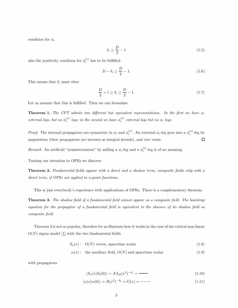
Theorem 3 is not so popular, therefore let us illustrate how it works in the case of the critical non-linear

O(N) sigma model [1] with the two fundamental fields

Sa(x) : O(N) vector, spacetime scalar (1.8)

α(x) : the auxiliary field, O(N) and spacetime scalar (1.9)

with propagators

〈Sa(x)Sb(0)〉 = Aδab(x2)−δ1 = (1.10)

〈α(x)α(0)〉 = B(x2)−δ2 = G(x) = (1.11)

3

with dimensions

δ1 =1

2D − 1 + O(

1

N), δ2 = 2 + O(

1

N) (1.12)

and interaction term

z1

2

∫

dxSa(x)Sa(x)α(x), with z1

2 = AB1

2 . (1.13)

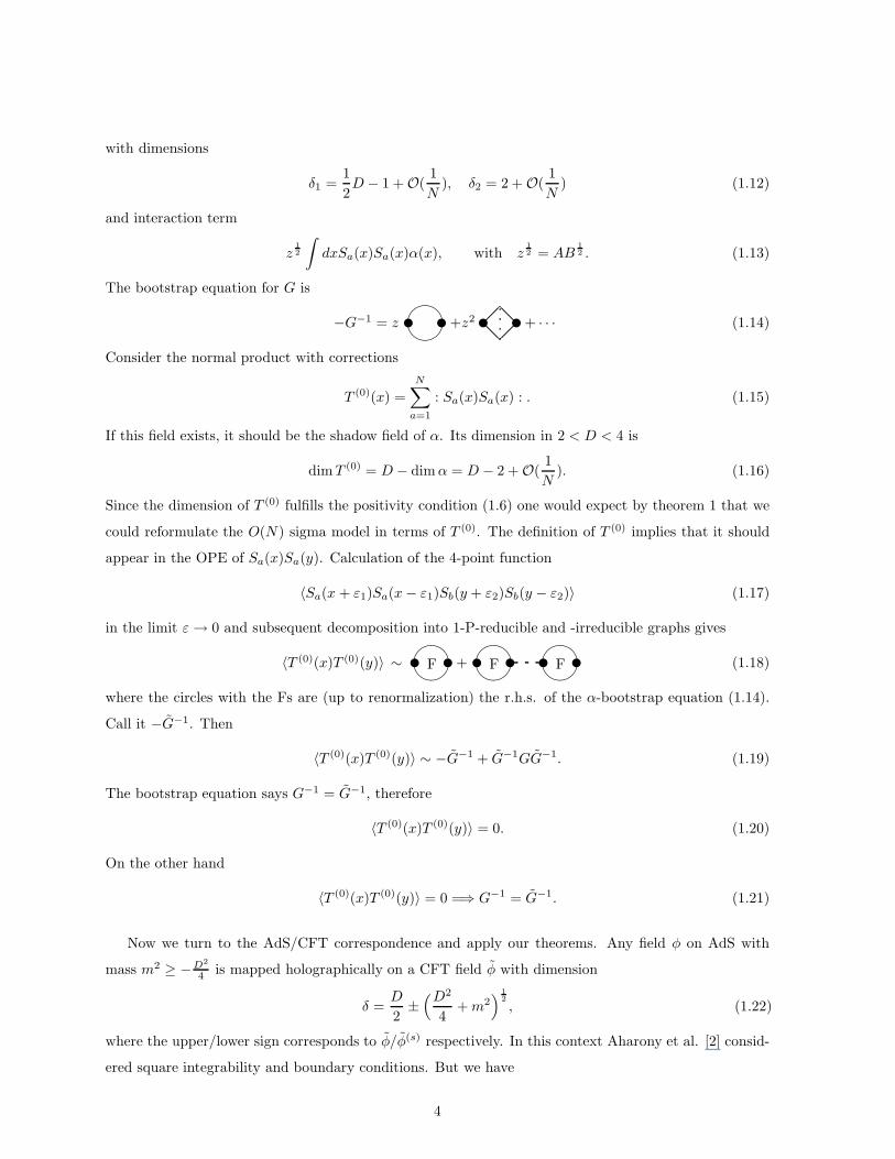
The bootstrap equation for G is

−G−1 = z ����u u+z2 u��

@@@@��

u+ · · · (1.14)

Consider the normal product with corrections

T (0)(x) =

N∑

a=1

: Sa(x)Sa(x) : . (1.15)

If this field exists, it should be the shadow field of α. Its dimension in 2 < D < 4 is

dimT (0) = D − dim α = D − 2 + O(1

N). (1.16)

Since the dimension of T (0) fulfills the positivity condition (1.6) one would expect by theorem 1 that we

could reformulate the O(N) sigma model in terms of T (0). The definition of T (0) implies that it should

appear in the OPE of Sa(x)Sa(y). Calculation of the 4-point function

〈Sa(x + ε1)Sa(x − ε1)Sb(y + ε2)Sb(y − ε2)〉 (1.17)

in the limit ε → 0 and subsequent decomposition into 1-P-reducible and -irreducible graphs gives

〈T (0)(x)T (0)(y)〉 ∼ u����

F u+ u����

F u u F����u (1.18)

where the circles with the Fs are (up to renormalization) the r.h.s. of the α-bootstrap equation (1.14).

Call it −G−1. Then

〈T (0)(x)T (0)(y)〉 ∼ −G−1 + G−1GG−1. (1.19)

The bootstrap equation says G−1 = G−1, therefore

〈T (0)(x)T (0)(y)〉 = 0. (1.20)

On the other hand

〈T (0)(x)T (0)(y)〉 = 0 =⇒ G−1 = G−1. (1.21)

Now we turn to the AdS/CFT correspondence and apply our theorems. Any field φ on AdS with

mass m2 ≥ −D2

4 is mapped holographically on a CFT field φ with dimension

δ =D

2±

(D2

4+ m2

)1

2

, (1.22)

where the upper/lower sign corresponds to φ/φ(s) respectively. In this context Aharony et al. [2] consid-

ered square integrability and boundary conditions. But we have

4

Theorem 4. Square integrability of an AdS wave function and Wightman positivity of the corresponding

CFT field are the same thing.

Thus we arrive at the conclusion: Taking for a field always the upper sign or always the lower sign (if

Wightman positivity allows this) leads to two different but equivalent CFTs.

By evaluating AdS exchange graphs and analyzing the result one finds that there are no shadow terms

[3]. This leads us to

Theorem 5. The holographic image of an AdS field theory is a CFT without fundamental fields.

In fact in the standard example of N = 4 SYM4, which is dual to type IIB superstring theory on

AdS5 × S5, the relevant coupling constant is ‘t Hooft’s

λ = g2Y MN. (1.23)

It is a perturbative CFT if λ → 0 with (say) the gauge supermultiplett as fundamental fields. They

belong to the adjoint representation of the gauge group SU(N). The holographic image possesses only

gauge invariant fields which are therefore composed of at least two fundamental fields with the adjoint

representation matrices “traced” away.

But the content of Theorem 5 derives from the geometry of AdS5 and not from gauge invariance. In

other examples compositeness and gauge invariance may not have the same effect.

2 Generalized hypergeometric functions

A “star graph” (vertex) of m scalar fields in AdSD+1 conformal field theory

123.4

m

. ...

Figure 1: AdSD+1 “star graph” (vertex)

defines a Green function (xi ∈ RD = ∂AdSD+1)

Γ(x1, ..., xm) = π−D2

∫

y0>0

dD+1y

yD+10

m∏

i=1

(y0

y20 + (~y − ~xi)2

)αi (2.1)

5

where{αi} are field dimensions constrained only by

αi ≥1

2D − 1. (2.2)

In conformal field theory on RD such a vertex is given by

Gm(x1, ..., xm) = π−D2

∫

RD

dDy

m∏

i=i

((y − xi)2)−αi (2.3)

with the conformal “uniqueness” condition

m∑

i=1

αi = D. (2.4)

The usual parametric representation of Gm

Gm(x1, ..., xm) = [

m∏

i=1

Γ(αi)]−1(

m∏

i=1

∫ ∞

0

dti tαi−1i )T−D

2 e−1

T

∑

i<jtitjx2

ij (2.5)

with

T =

m∑

i=1

ti. (2.6)

allows to continue analytically in {αi} and D independently, such that one has the Green function

Gm(D; α1, ..., αm). (2.7)

The AdSD+1 function Γm is [6]

Γm(D; α1, ..., αm) =1

2Γ(

1

2(

m∑

i=1

αi − D))Gm(m

∑

i=1

αi; α1, ..., αm). (2.8)

All the Green functions Gm have been represented in the form of a Mellin-Barnes integral and by expansion

in generalized hypergeometric form by K. Symanzik [7]. For m = 4 and with the biharmonic ratios

u =x2

13x224

x212x

234

, v =x2

14x223

x212x

234

(2.9)

we get

G4(x1, x2, x3, x4) = [4

∏

i=1

Γ(αi)]−1(x2

12)α4−

1

2D(x2

14)1

2D−α1−α4(x2

24)1

2D−α2−α4(x2

34)−α3F (u, v) (2.10)

with

F (u, v) =u− 1

2(α1+α3)

∞∑

n,m=0

un(1 − v)m

n!m!{u 1

2(α1+α3)Γ(

1

2(α2 + α4 − α1 − α3))

× Γ(α1 + n)Γ(12D − α2 + n)Γ(α3 + n + m)Γ(1

2D − α4 + n + m)

Γ(α1 + α3 + 2n + m)(12 (α1 + α3 − α2 − α4) + 1)n

+ u1

2(α2+α4)

× Γ(1

2(α1 + α3 − α2 − α4))

Γ(α4 + n)Γ(12D − α3 + n)Γ(α2 + n + m)Γ(1

2D − α1 + n + m)

Γ(α2 + α4 + 2n + m)(12 (α2 + α4 − α1 − α3) + 1)n

.

(2.11)

6

This form converges in a complex neighborhood of

u = 0, v = 1 (2.12)

and is therefore suited for an operator product expansion (OPE) in the limit, “t-channel”

x13 −→ 0, x24 −→ 0. (2.13)

The analytic continuation to the “s-channel”

x12 −→ 0, x34 −→ 0,

u −→gt→s

u′ =1

u,

v −→gt→s

v′ =v

u(2.14)

and to the “u-channel”

x14 −→ 0, x23 −→ 0,

u −→gt→u

u′′ = v,

v −→gt→u

v′′ = u (2.15)

can be obtained by two methods

1. using the symmetry group of the graphs [6];

2. using the Kummer formulae for 2F1-functions [8].

The AdS graphs at order O( 1N2 ) for dilaton-axion four-point functions with

m2 = 0 −→ ∆ = 4 (D = 4) (2.16)

can all be represented by

Γ4(x1, x2, x3, x4)|α1=α3=∆,α2=α4=∆′;∆,∆′∈N;∆′≥∆ = π− 1

2D(x2

12)−∆(x2

24)∆−∆′

(x234)

−∆G∆∆′(u, v) (2.17)

with

G∆∆′(u, v) =π2

2

Γ(∆ + ∆′ − 2)

Γ(∆)2Γ(∆′)2

∞∑

m=0

(1 − v)m

m!{∆′−∆−1

∑

n=0

(−1)nun

n!(∆′ − ∆ − n − 1)!

× Γ(∆ + n)2Γ(∆ + n + m)2

Γ(2∆ + 2n + m)+

∞∑

n=∆′−∆

(−1)∆′−∆un

n!(n − ∆′ + ∆)!

Γ(∆ + n)2Γ(∆ + n + m)2

Γ(2∆ + 2n + m)

× [−log u + Ψ(n − ∆′ + ∆ + 1)

+ Ψ(n + 1) − 2Ψ(∆ + n) + 2Ψ(2∆ + 2n + m) − 2Ψ(∆ + n + m)]}. (2.18)

7

In the other channels one has

G∆∆′(u′, v′) =π2

2

Γ(∆ + ∆′ − 2)

Γ(∆)2Γ(∆′)2u∆

∞∑

n,m=0

un(1 − v)m

(n!)2m!

× Γ(∆ + n)Γ(∆′ + n)Γ(∆ + n + m)Γ(∆′ + n + m)

Γ(∆ + ∆′ + 2n + m){−log u + 2Ψ(n + 1) − Ψ(∆ + n)

− Ψ(∆′ + n) − Ψ(∆ + n + m) − Ψ(∆′ + n + m) + 2Ψ(∆ + ∆′ + 2n + m)} (2.19)

and

G∆∆′(u′′, v′′) =π2

2

Γ(∆ + ∆′ − 2)

Γ(∆)2Γ(∆′)2v∆′−∆

∞∑

n,m=0

un(1 − v)m

(n!)2m!

× Γ(∆′ + n)2Γ(∆ + n + m)2

Γ(∆ + ∆′ + 2n + m){−log u + 2Ψ(n + 1) − 2Ψ(∆ + n) − 2Ψ(∆′ + n + m)

+ 2Ψ(∆ + ∆′ + 2n + m)}. (2.20)

.

3 U(1)Y symmetry

In the standard model of AdS/CFT correspondence

AdS5 × S5 −→ SYM4 (3.1)

the U(1)Y symmetry carries over to the strong coupling domain of SYM4 and makes predictions on three

and four-point functions [4]. We will discuss here an identity of two four-point functions [6]. Let

Dilaton : Φ(y) −→ Φ(x) ∼ Tr(Fµν(x)Fµν(x))

Axion : C(y) −→ C(x) ∼ Tr(Fµν(x)Fµν(x)) (3.2)

and consider

Oτ (x) = Φ(x) + iC(x). (3.3)

This field has U(1)Y charge q = −4. Therefore

<

4∏

i=1

Oτ (x) >= 0, (3.4)

due to charge non-conservation (∑

i qi 6= 0). Introducing the bilocal operators

Ψ∓(x1, x3) =1√2[∓Φ(x1)Φ(x3) + C(x1)C(x3)] (3.5)

Ψ0(x1, x3) =1√2[Φ(x1)C(x3) + C(x1)Φ(x3)] (3.6)

8

which by OPE produce tensor fields of even rank with opposite parities, we obtain from (3.4)

< Ψ−(x1, x3)Ψ−(x2, x4) > − < Ψ0(x1, x3)Ψ0(x2, x4) >= 0. (3.7)

This relation can be worked out up to order O( 1N2 ) at present. At leading order O(1), both four-point

functions are

(x212x

234)

−4(1 + v−4) with v =x2

14x223

x212x

234

. (3.8)

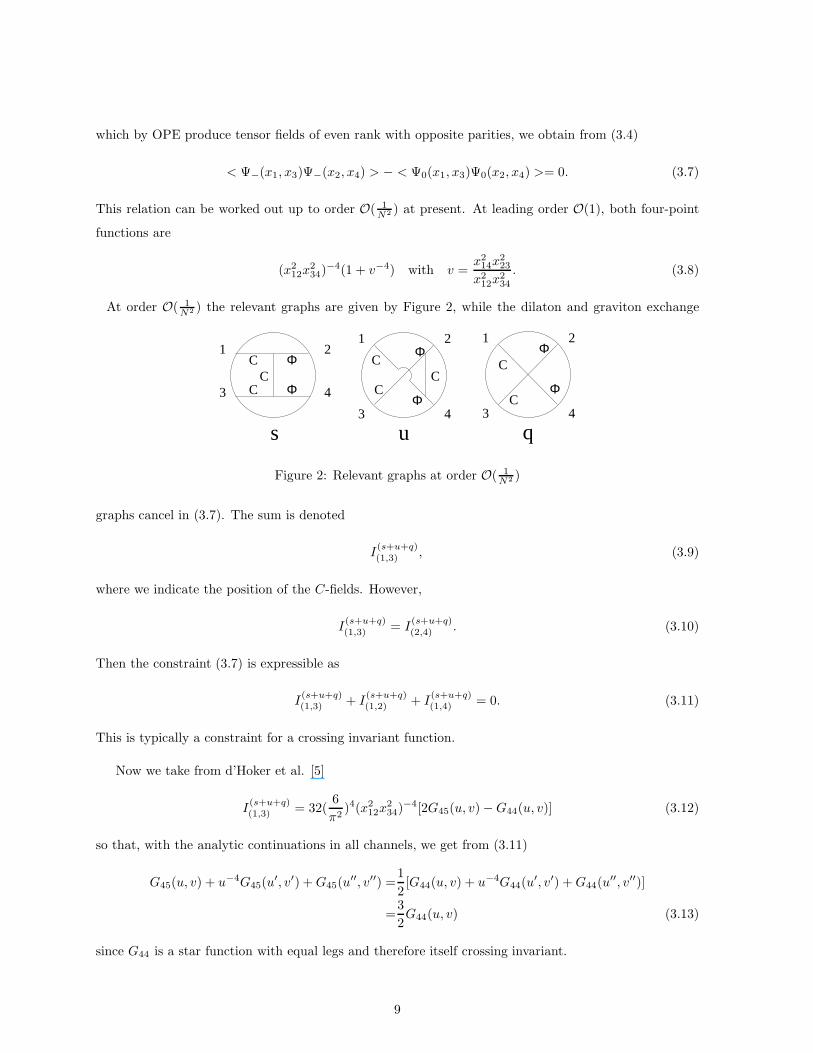
At order O( 1N2 ) the relevant graphs are given by Figure 2, while the dilaton and graviton exchange

1

3 4

2

Φ

s

CC

C

Φ1

3 4

C

2

u

Φ

Φ

CC

1

3 4

2

Φ

q

C

C

Φ

Figure 2: Relevant graphs at order O( 1N2 )

graphs cancel in (3.7). The sum is denoted

I(s+u+q)(1,3) , (3.9)

where we indicate the position of the C-fields. However,

I(s+u+q)(1,3) = I

(s+u+q)(2,4) . (3.10)

Then the constraint (3.7) is expressible as

I(s+u+q)(1,3) + I

(s+u+q)(1,2) + I

(s+u+q)(1,4) = 0. (3.11)

This is typically a constraint for a crossing invariant function.

Now we take from d’Hoker et al. [5]

I(s+u+q)(1,3) = 32(

6

π2)4(x2

12x234)

−4[2G45(u, v) − G44(u, v)] (3.12)

so that, with the analytic continuations in all channels, we get from (3.11)

G45(u, v) + u−4G45(u′, v′) + G45(u

′′, v′′) =1

2[G44(u, v) + u−4G44(u

′, v′) + G44(u′′, v′′)]

=3

2G44(u, v) (3.13)

since G44 is a star function with equal legs and therefore itself crossing invariant.

9

In fact the following identity can be proved

G∆,∆+1(u, v) + u−∆G∆,∆+1(u′, v′) + G∆,∆+1(u

′′, v′′) =2∆ − 2

∆G∆,∆(u, v). (3.14)

It is a recursion for the generalized hypergeometric function G.

For the proof of (3.14) we do not use the explicit form of G∆,∆′ given earlier, but make use of an

“ǫ-trick”

G∆,∆′(u, v) = limǫ→0

∂

∂ǫ[π2

2

Γ(∆ + ∆′ − 2)

Γ(∆)2Γ(∆′)2(−1)∆

′−∆∆′−∆∏

k=1

(n − ∆′ + ∆ + k − ǫ)

×∞∑

m,n=0

un−ǫ(1 − v)m

Γ(n + 1 − ǫ)2m!

Γ(∆ + n − ǫ)2Γ(∆ + n + m − ǫ)2

Γ(2∆ + 2n + m − 2ǫ)], (3.15)

u−∆G∆,∆′(u′, v′) =limǫ→0

∂

∂ǫ[π2

2

Γ(∆ + ∆′ − 2)

Γ(∆)2Γ(∆′)2

∞∑

m,n=0

un−ǫ(1 − v)m

Γ(n + 1 − ǫ)2m!

× Γ(∆ + n − ǫ)Γ(∆′ + n − ǫ)Γ(∆ + n + m − ǫ)Γ(∆′ + n + m − ǫ)

Γ(∆ + ∆′ + 2n + m − 2ǫ)], (3.16)

G∆,∆′(u′′, v′′) = limǫ→0

∂

∂ǫ[π2

2

Γ(∆ + ∆′ − 2)

Γ(∆)2Γ(∆′)2

∞∑

m,n=0

un−ǫ(1 − v)m

Γ(n + 1 − ǫ)2m!

Γ(∆′ + n − ǫ)2Γ(∆ + n + m − ǫ)2

Γ(∆ + ∆′ + 2n + m − 2ǫ)].

(3.17)

Since ∆′ − ∆ ∈ N0, we can sum the coefficients as

Γ(∆ + n − ǫ)2Γ(∆ + n + m − ǫ)2

Γ(∆ + ∆′ + 2n + m − 2ǫ){(2∆ + 2n + m − 2ǫ)∆′−∆

∆′−∆∏

k=1

(∆′ − ∆ − n − k + ǫ)

+ (∆ + n − ǫ)2∆′−∆ + (∆ + n − ǫ)∆′−∆(∆ + n + m − ǫ)∆′−∆} (3.18)

For ∆′ = ∆ + 1 we have

{...} = ∆(2∆ + 2n + m − 2ǫ) (3.19)

which leads to G∆∆ by the formula given above. This completes the proof.

Let us quote some detailed results on the OPE of the bilocal fields Ψ+,−,0 [6].

1. Ψ+(x1, x3) expands into the stress-energy tensor plus the towers of conformal fields: tensor rank

l ∈ 2N0, parity (+1) and dimension

δ+(l, t) = 8 + l + 2t + η+(l, t); t ∈ N0(tower label, twist); η+ = O(1

N2) (3.20)

2. Ψ−(x1, x3) expands into conformal fields: tensor rank l ∈ 2N0, parity (+1) and dimension

δ−(l, t) = 8 + l + 2t + η−(l, t); t ∈ N0, η− = O(1

N2) (3.21)

10

3. Ψ0(x1, x3) expands into conformal fields: tensor rank l ∈ 2N0, parity (−1) and dimension

δ0(l, t) = 8 + l + 2t + η0(l, t); t ∈ N0, η0 = O(1

N2) (3.22)

For t = 0 we obtain

η−(l, 0) = η0(l, 0) = − 96

N2(l + 1)(l + 6)(3.23)

and the corresponding fusion constants squared

ǫ−(l, 0) = ǫ0(l, 0) =1

18(2l + 7)(l + 1)6 (3.24)

The remaining quantities η+, ǫ+ and η− = η0(t 6= 0), ǫ− = ǫ0(t 6= 0) are easily accessible by using

computer manipulations. One has to solve infinite linear equations with triangular matrices, where t

counts the off-diagonality of the matrix elements. The main labor resides in calculating the matrix

elements in a generic form (no numbers).

References

[1] K. Lang, W. Ruhl,“The scalar ancestor of the energy momentum field in critical sigma models at

2 < d < 4”, Phys. Lett. B275, (1992), 93.

[2] O. Aharony, S.S. Gubser, J. Maldacena, H. Ooguri and Y. Oz, “Large N field theories, string theory

and gravity”, Phys.Rept.323, (2000), 183, hep-th/9905111.

[3] H. Liu, “Scattering in Anti-de-Sitter space and Operator Product Expansion”, Phys.Rev. D60 (1999)

106005, hep-th/9811152

[4] K. Intriligator, “Bonus symmetry of N = 4 Super-Yang-Mills correlation functions via AdS duality”,

Nucl. Phys. B551 (1999) 575, hep-th/9811047; K. Intriligator and W. Skiba, “Bonus symmetry

and operator product expansion of N = 4 Super-Yang-Mills”, Nucl. Phys. B559 (1999) 165, hep-

th/9905020

[5] E. D’Hoker, D.Z. Freedman, S.D. Mathur, A. Matusis and L. Rastelli, “Graviton exchange and

complete 4-point functions in the AdS/CFT correspondence”, Nucl. Phys. B562 (1999) 353, hep-

th/9903196.

[6] L. Hoffmann, L. Mesref, W. Ruhl, “Conformal partial wave analysis of AdS amplitudes for dilaton-

axion four-point functions”, hep-th/0012153.

[7] K. Symanzik,“On Calculations in Conformal Invariant Field Theories”, Lett. Nuovo Cim. 3 (1972)

734.

11

[8] I. S. Gradshteyn and I. M. Ryzhik, Table of Integrals, Series and Products, 4th Ed. Academic Press

(1965).

12