Complex aerodynamic admittance function role in buffeting response of a bridge deck

Journal of Wind Engineering

and Industrial Aerodynamics 90 (2002) 2057–2072

Complex aerodynamic admittance function rolein buffeting response of a bridge deck

Giorgio Diana, Stefano Bruni, Alfredo Cigada,Emanuele Zappa*

Dipartimento di Meccanica, Politecnico di Milano, Via La Masa, 34 20158 Milano, Italy

Abstract

The estimated response of a long-span suspended bridge deck to turbulent wind, depends on

the deck section, on the average horizontal wind speed and on the turbulence characteristics.

The aerodynamic admittance function describes the relationship between the smooth and

turbulent wind response of the deck. A new experimental technique, based on the use of an

active turbulence generator, is here applied in order to measure a complex aerodynamic

admittance function. This admittance function is then used in a new expression of the

buffeting forces. Comparison between spring-supported sectional model response in wind

tunnel and numerical simulation is shown. The introduced force expression is then applied to

an FEM model of the Humber Bridge, and the predicted response is compared with full-scale

measurements.

r 2002 Elsevier Science Ltd. All rights reserved.

Keywords: Active generation; Complex admittance; Buffeting response

1. Introduction

Mathematical models of the bridge response to the wind action are generally basedon two different approaches: the Scanlan’s flutter derivatives [1] and the quasi-steadycorrected theory (QStCT [2]). While in Scanlan’s approach the basic hypothesis is thesuperposition of effects (linear approach), in the QStCT equivalence between thewind attack angle and the bridge deck rotation is assumed, trying in some way toaccount for the nonlinearities, related to the wind-to-deck relative angle variationaround the static bridge configuration. Both these approaches have some limits in

*Corresponding author. Tel.: +39-02-23998445; fax: +39-02-23998492.

E-mail address: [email protected] (E. Zappa).

0167-6105/02/$ - see front matter r 2002 Elsevier Science Ltd. All rights reserved.

PII: S 0 1 6 7 - 6 1 0 5 ( 0 2 ) 0 0 3 2 1 - 5

taking into account the effect of the wind turbulence. An attempt to join theaeroelastic stability to the buffeting response is the actual border of many researchgroups [4].

Both the Scanlan flutter derivatives and the QStCT coefficients are usuallyobtained by means of wind tunnel testing on section models in smooth flow (free orforced oscillation methods). The further step, the object of this paper, consists inmodifying the existing experimental set-up, in order to get the aerodynamiccoefficients, also accounting for the turbulent wind effects. This additional set-upconsists in an active turbulence generator creating a harmonic (or even morecomplex) time varying wind, though coherent along the deck axis direction. The nextpoint is an attempt to write down the buffeting components relying on the dataderived from the experimental tests in harmonic flow.

Unlike the usually adopted passive turbulence generation methods, the proposedmethod can give every spectral turbulence component at a time; this allows toseparate and investigate in details the effect of parameters like the reduced velocityand the gust wavelength. Even if it is possible to drive the turbulence generatingdevice with any given motion law (also reproducing the real wind spectrum), theharmonic wind is considered more suitable. While the former solution has alreadybeen investigated [6,11], the latter is new, and it is considered worthy of attentionbecause it gives a check on the hypothesis of linearity and produces a complexadmittance function, accounting for both amplitude and phase of the turbulent windresponse.

2. Wind tunnel tests in turbulent flow

2.1. Active turbulence generator

The active turbulence generator (Fig. 1) is made up of a series of wings linkedtogether to produce a wind tunnel flow with an almost constant horizontal velocitycomponent and a harmonic oscillating vertical velocity component (see [7]).

The rotation of the wings is driven by a hydraulic exciter: the amplitude andfrequency of the motion are user selectable. Measurements are carried out with botha fixed, dynamometric model and with a spring-supported one. The deck sectionadopted for the tests is a 1:80 scale section model of the Humber Bridge (see Fig. 2)because a lot of experimental data concerning wind tunnel tests in smooth flow havebeen collected in the past years. Moreover, data from two full-scale measurementcampaigns carried out on the real Humber Bridge are available (see [8]), allowing fora final check of the new procedure for generating the turbulent flow and thesubsequent modifications of the numerical model of the bridge–wind interaction.

2.2. Fixed model tests

The first series of tests was carried out keeping the model fixed with zero-meanangle of attack with respect to the mean flow, and measuring the turbulence-induced

G. Diana et al. / J. Wind Eng. Ind. Aerodyn. 90 (2002) 2057–20722058

forces and moment due to moving wings: the wings have been driven with aharmonic motion. The aim of these tests, widely described in [7], is to get theaerodynamic admittance of the deck section, by superimposing the single harmonicresponse. Fig. 3 shows the measured time histories of the vertical force and momentplotted together with the wind angle of attack and the wings motion. Theinstantaneous attack angle is measured by means of a two component hot filmprobe, placed in a reference position (0.16m upwind the leading edge), where thewind can be considered as free flow (not affected by the bridge presence).

It is noted that, assuming the harmonic wings motion as the system input, theoutput, in terms of force, is at the same frequency and exhibits a phase lag dependingon the reduced velocity and the distance between the bridge deck and the wind anglemeasurement point.

Since just one vertical wind speed component is present at a time (with frequencyf ), it is possible (and easy) to define both amplitude and phase of the complexadmittance function for the vertical force and moment (L and M) wL;M defined by

Fig. 1. Active turbulence generator.

Dynamometric

Dummy

LT

B

Dummy

L

L2

D2

L1

D1

Fig. 2. Dynamometric Humber Bridge model.

G. Diana et al. / J. Wind Eng. Ind. Aerodyn. 90 (2002) 2057–2072 2059

(see also Fig. 6):

wLðf Þ ¼IðLðtÞÞ

1=2rU2BDðKL0 þ CD0ÞIðaðtÞÞ; ð1aÞ

wM ðf Þ ¼IðMðtÞÞ

1=2rU2B2DKM0IðaðtÞÞð1bÞ

being I the Fourier transform component at frequency f ; LðtÞ; (MðtÞ) the verticalforce (moment) time history, aðtÞ ¼ amax sinð2pftÞ the wind attack angle time history.D and r are the model length and the air density, while CD0 is the drag coefficient inthe reference horizontal position, with smooth horizontal flow, and KL0; (KM0) is thederivative of the lift (moment) curve around zero angle (i.e. horizontal deck).

The possibility to obtain a complex admittance function is one of the mostimportant features of the proposed experimental technique.

During the wind tunnel tests it was proved that the maximum amplitude of thewind attack angle amax does not affect the admittance value, at least in theinvestigated angular range of 751.

Using the fixed model tests and with a one harmonic component flow, the lift andmoment aerodynamic admittance have been measured. Magnitude and phase of theobtained functions are shown in Fig. 4 versus the reduced velocity V � ¼ U=ðfBÞ: Itcan be seen that, accordingly to the theory, the reduced velocity is the governingparameter not only for the magnitude, but also for the phase. As expected, at veryhigh reduced velocity values (close to stationary conditions), the magnitude of theadmittance function tends to one and the phase tends to zero.

The check on the feasibility of superposition of effects has been carried out, bytesting the bridge deck model with a two harmonic flow and comparing results withthose obtained with single harmonic incoming flow. In Fig. 4 the vertical forceaerodynamic admittance function is shown as a function of the reduced velocity,both in case of one and two harmonic components. To obtain the data shown inFig. 4 each attack angle harmonic component has an amplitude ranging between 2.51and 51.

-0.1

0

0.1

Time [sec]

8-0.5

0

0.5 Vertical force

Moment

Ver

tica

l fo

rce

[N]

Mom

ent

[N m

]

42 60 0 2 4 6 8 -3

-2

-1

0

1

2

3

4

Time [sec]

Angle

[°]

Wings angle Wind angle

Fig. 3. Fixed model, harmonic turbulence: resulting forces and moment.


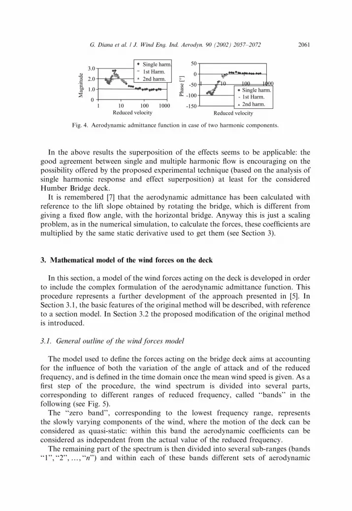
In the above results the superposition of the effects seems to be applicable: thegood agreement between single and multiple harmonic flow is encouraging on thepossibility offered by the proposed experimental technique (based on the analysis ofsingle harmonic response and effect superposition) at least for the consideredHumber Bridge deck.

It is remembered [7] that the aerodynamic admittance has been calculated withreference to the lift slope obtained by rotating the bridge, which is different fromgiving a fixed flow angle, with the horizontal bridge. Anyway this is just a scalingproblem, as in the numerical simulation, to calculate the forces, these coefficients aremultiplied by the same static derivative used to get them (see Section 3).

3. Mathematical model of the wind forces on the deck

In this section, a model of the wind forces acting on the deck is developed in orderto include the complex formulation of the aerodynamic admittance function. Thisprocedure represents a further development of the approach presented in [5]. InSection 3.1, the basic features of the original method will be described, with referenceto a section model. In Section 3.2 the proposed modification of the original methodis introduced.

3.1. General outline of the wind forces model

The model used to define the forces acting on the bridge deck aims at accountingfor the influence of both the variation of the angle of attack and of the reducedfrequency, and is defined in the time domain once the mean wind speed is given. As afirst step of the procedure, the wind spectrum is divided into several parts,corresponding to different ranges of reduced frequency, called ‘‘bands’’ in thefollowing (see Fig. 5).

The ‘‘zero band’’, corresponding to the lowest frequency range, representsthe slowly varying components of the wind, where the motion of the deck can beconsidered as quasi-static: within this band the aerodynamic coefficients can beconsidered as independent from the actual value of the reduced frequency.

The remaining part of the spectrum is then divided into several sub-ranges (bands‘‘1’’; ‘‘2’’;y; ‘‘n’’) and within each of these bands different sets of aerodynamic

0

1.0

2.0

3.0

1 10 100 1000

Reduced velocity

Mag

nit

ude

Single harm.

1st Harm.

2nd harm.

-150

-100

-50

0

50

1 10 100 1000

Reduced velocity

Phas

e [°

]

Single harm.

1st Harm.

2nd harm.

Fig. 4. Aerodynamic admittance function in case of two harmonic components.


coefficients are assumed and considered as constant with frequency, due to thelimited range of reduced frequency covered by the single band.

It is important to point out that the choice of the frequency band boundaries isperformed in order to follow the aerodynamic coefficients variability with thereduced frequency, and not depending on the values of the structure naturalfrequencies.

For each band, a separate time history for the horizontal and vertical windcomponents is generated, using the Wave Superposition method [8]; in this way, n

vectors collecting the horizontal uðtÞ and vertical wðtÞ components of the turbulentwind pertaining to each band are obtained:

V0 ¼u0ðtÞ

w0ðtÞ

( ); V1 ¼

u1ðtÞ

w1ðtÞ

( );y;Vn ¼

unðtÞ

wnðtÞ

( ):

The total response of the structure to the turbulent wind, in terms of verticaldisplacement yðtÞ and rotation yðtÞ of the sectional model is then represented as thesum of the responses to the different wind bands:

X ¼yðtÞ

yðtÞ

( )¼ X0ðtÞ þ X1ðtÞ þ?þ XnðtÞ:

The response X0ðtÞ of the structure to the slowly varying wind components V0ðtÞ iscomputed using the quasi-static corrected theory as described in [2], thereby allowingto account for the nonlinear effects associated to relatively large variations of theangle of attack (typically 75–101) which are mainly induced by the low frequencyturbulence. For this calculation, the aerodynamic admittance is assumed to be realvalued and equal to unity, as demonstrated by the experimental results shown inFig. 4.

The response of the structure to the wind components pertaining to the otherfrequency bands is then obtained by performing a linearisation of the bridgeequations of motion around the slowly varying time dependent structure state,represented by the result of the previous calculation X0ðtÞ:

0.1-

0.01-

"0" "1" "2" "n"

f*

f* S

u(f

)

u2

1-

0.01 0.1 1

Fig. 5. Wind bands.


The linearised expression of the wind forces (lift force L and aerodynamic momentM) can be symbolically represented as follows:

F ¼L

M

( )

¼FnlðV0;X0; ’X0Þ þqF

qV

��0

%V1 þqF

qX

��0

%X1 þqF

q ’X

��0

’%X1 þ?

þqF

qV

��0

%Vn þqF

qX

��0

%Xn þqF

q ’X

��0

’%Xn: ð2Þ

By introducing this linearised expansion of the wind forces into the equations ofmotion of the structure

m .y þ ry ’y þ kyy ¼ L;

J .Wþ rW ’Wþ kWW ¼ M ð3Þ

and separating the terms pertaining to each single frequency band, n linear systemsof equations with time varying parameters are obtained, one for each band

½M� .X1 þ ½R� ’X1 þ ½K �X1 ¼ Fae1 þ Fb1 ;

^

½M� .Xn þ ½R� ’Xn þ ½K �Xn ¼ Faenþ Fbn

ð4Þ

having defined

Faei¼

Laei

Maei

( )¼

qF

q ’X

��0

’Xi þqF

qX

��0

Xi;

Fbi¼

Lbi

Mbi

( )¼

qF

qV

��0

ViðtÞ: ð5Þ

The advantage of this method with respect to the traditional frequency responsebased method is that linearisation is performed around a slowly varying state,representing the nonlinear response of the bridge to low frequency wind turbulentcomponents. This allows to include nonlinear effects (at least for the low frequencycomponents, which show the largest angles), as well as reduced velocity dependenteffects.

As shown by formulae (4) and (5), thanks to the linearisation of the forces aroundthe large slowly varying condition represented by vectors V0ðtÞ;X0ðtÞ; ’X0ðtÞ; the windforces pertaining to a single wind band are automatically divided into aeroelasticforces and buffeting forces. The new formulation of the aerodynamic admittance canbe, therefore, used to modify the expression of the buffeting forces, as described inSection 3.2.


3.2. Modified expression of buffeting forces

For the ith band (i ¼ 1; 2;y; n), the aeroelastic forces are written according to theexpression [9]

Laei¼

1

2rBLU2 �ðKLO þ CD0Þh1i

’y

U� ðKLO þ CD0Þh2i

B ’WU

�

þh3iKL0Wþ

h4ip

2V �2

y

B

�;

Maei¼

1

2rB2LU2 �KM0a1i

’y

U� KM0a2i

B ’WU

þ a3iKM0Wþ

a4ip

2V�2

y

B

� �ð6Þ

where V � is the reduced velocity (V � ¼ U=ðfBÞ), h and a coefficients are related tothe Scanlan’s flutter derivatives as described in [9], while CD0 is the drag coefficient atzero attack angle, KL0 and KM0 are the derivatives of lift and moment coefficients,respectively, also measured with zero-mean angle of attack.

The coefficients h and a are measured by means of wind tunnel tests in smoothflow, where a vertical or torsional or combined motion of the deck is imposed [10].These coefficients are then tabulated as function of the reduced velocity/frequencyand of the angle of attack. When performing the numerical integration of Eqs. (4), ateach time step, the angle of attack is assumed known from the time histories of windspeed and deck motion corresponding to the zero band, and the actual values of theh and a coefficients are obtained by interpolation of the measured data. This resultsin a linear expression of the aeroelastic forces with time varying coefficients.

As to the buffeting forces, the new formulation proposed in this paper is firstintroduced in the frequency domain, using a complex notation, according to theprocessing of the experimental measurements represented by formulae (1a) and (1b):

Lbi¼

1

2rBDU2ðKL0 þ CD0Þ½aiReðwLÞ þ jaiImðwLÞ�;

Mbi¼

1

2rB2DU2KM0½aiReðwMÞ þ jaiImðwM Þ�; ð7Þ

where j is the imaginary unit and ai is the high frequency component of the angle ofattack corresponding to the ith band, expressed as

ai ¼ artgwi

ui

� �:

Note that the vertical force admittance function wL is, in general, different from themoment one wM : The above formulation is related to the adopted experimentalprocedure, in which the admittance is obtained as a deterministic transfer functionbetween an input, the wind, described by a harmonic function, and an output, theglobal force, also harmonic.

In order to introduce the above formulation into the systems of Eqs. (4), it isnecessary to rewrite the expression of the buffeting forces (7) in the time domain. Tothis end, it is observed that if the ith band angle of attack ai is a harmonic function of


time, using a complex notation, it can be represented as: aiðtÞ ¼ ai0ejot then its time

derivative is expressed as: ’aiðtÞ ¼ joai0ejot and therefore the imaginary term into

Eq. (7) can be rewritten as: jai ¼ ’a=o:Introducing this expression into Eq. (7) the final expression of the buffeting forces

is obtained:

Lbi¼

1

2rBDU2ðKLO þ CD0Þ aiReðwLÞ þ

’ai

oImðwLÞ

� �;

Mbi¼

1

2rB2DU2KM0 aiReðwMÞ þ

’ai

oImðwMÞ

� �: ð8Þ

The ‘‘quadrature terms’’ ’a=o ImðwL;MÞ accounts for the phase effect in thecomplex aerodynamic admittance wL;M ; and establish a dependence of the buffetingforce not only from the wind turbulence angle, but also from its derivative withrespect to time. For each ith band (i ¼ 1; 2;y; n) the parameter oi is assumed equalto the circular frequency corresponding to the mean value of reduced frequency ofthat specific band.

4. Verification on the section model

As a final step of the work, a verification of the new formulation for the buffetingforces has been performed. This comparison was carried out for two different cases:the first one is represented by the two d.o.f. motion of the elastically suspendedmodel subjected to the actively generated turbulence, which was measured in thewind tunnel experiments. The second stage of comparison concerns the response ofthe full 3D structure of the Humber Bridge. These two topics are detailed in thefollowing.

The 2D motion of the spring-supported model (Fig. 6) is measured using animage-based technique: the deck model moves in a plane and, being rigid, its motionis described by two reflecting markers fixed to it. Position and motion are thereforeobtained by a pre-calibrated digital camera and then a dedicated software extractsthe instantaneous deck vertical and torsional motion of the images: this methodprevents from load effect (it is a no contact one). As the adopted algorithms work inthe sub-pixel field, resolution is very high (1/10mm) for the adopted frame field(within 400mm), allowing for uncertainties in measurements below 1%. The more

y

� B

U

α

Fig. 6. Spring-supported model.


recent digital cameras offer a compromise between resolution, data file dimensions,frame field and frequency rate, bringing the optimal frequency rate to 25Hz for theconsidered case.

The natural frequencies of the spring-supported model are 2.6 and 4.2Hz (along y

and y; respectively).The section model has been left free of moving under the turbulent flow (only the

longitudinal motion has been prevented by means of guy cables).In Fig. 7 an example of the measured motion (vertical displacement and rotation

angle) is shown, in the case of incoming flow containing two harmonic componentsat 2 and 3Hz, respectively, with 5m/s horizontal wind speed.

Fig. 8 shows the spectrum of the time records shown history in Fig. 7. Harmoniccomponents contained in both vertical and torsional motion are almost exclusivelythose contained in the incoming flow (2 and 3Hz) and no significant secondharmonic appears: the small contribution around 4.2Hz is due to the torsion naturalfrequency of the model. Of course further and more extensive analysis must beperformed to define the effect of changing the average angle of the deck (in thesetests equal to zero), anyway it seems to be possible, at least for the Humber Bridgedeck section, to model the physical behaviour with a simple linear mathematicalmodel.

-8

-6

-4

-2

0

2

4

6

8

0 2 4 6Time [s]

Ver

tica

l m

oti

on [

mm

].

-0.6

-0.4

-0.2

0

0.2

0.4

0.6

0 2 4 6Time [s]

Rota

tion a

ngle

[°]

.

Fig. 7. Deck motion in case of two harmonic components in incoming flow.

0

1

2

3

4

0 4

0.2

0.4

0 Rota

tion a

ngle

[°]

Vet

ical

moti

on [

mm

]

Frequency [Hz]

2 6

Fig. 8. Spectrum module of signal showed in Fig. 7.


While the structural parameters (stiffness k and damping r) were obtained bymeans of smooth flow decay tests, the flutter derivatives were measured in [3] usingthe controlled displacements technique, then verified by the free oscillation method,at least for those flutter derivatives of major interest to stability problems.

By means of the mathematical model described in Section 3, it is possible tosimulate the deck behaviour under the measured wind and to compare the numericalpredicted motion with the measured one. In Fig. 9 a sample comparison is shown.While numerical end experimental time histories are very close each other, in the caseof vertical motion a slightly larger difference is present in torsional time histories.This is probably due to the fact that the rotation angles are very small, and the noiselevel becomes more significant.

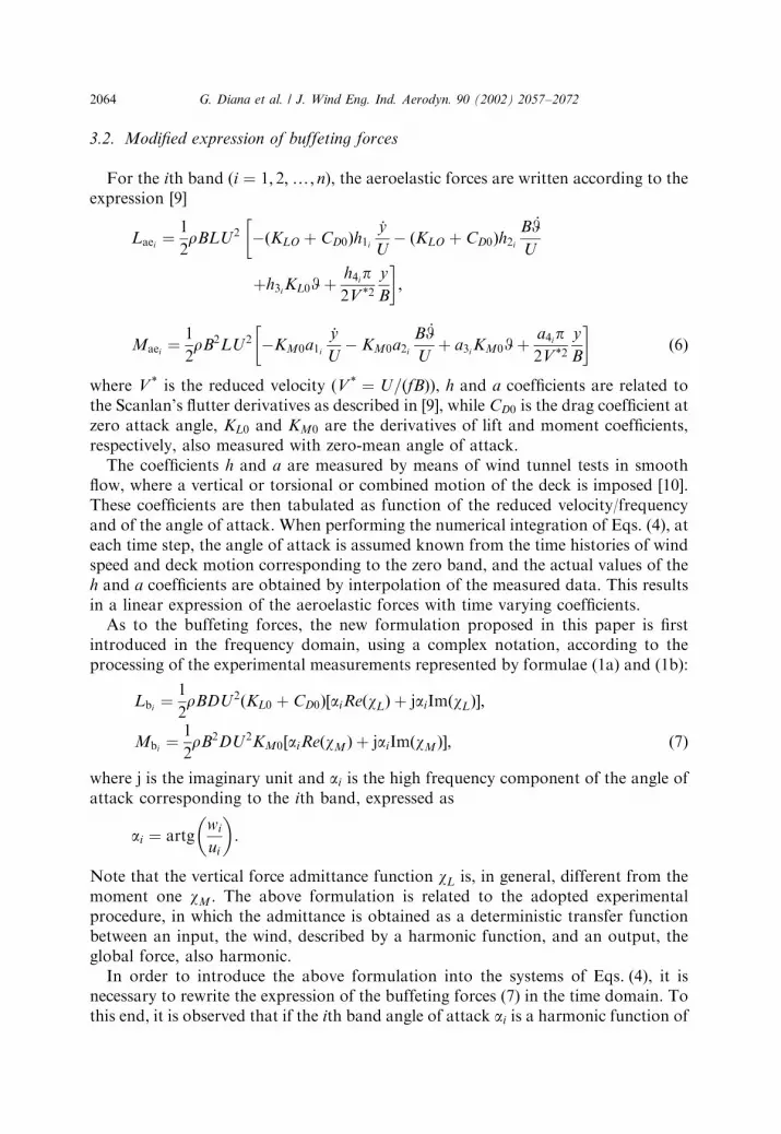
In Figs. 10 and 11 results from a number of numerical–experimental comparisonare shown, in terms of the ratio between the numerically predicted and the windtunnel measured oscillation amplitudes. The data dispersion in Figs. 10 and 11 isprobably due to the small wind tunnel used for the tests and to the block ratio(around 6%). Anyway the shown average value of the ratios are reasonably close toone, which means that a good agreement between numerical and experimental datahas been obtained.

0 2 4 6 8 -5

0

5 Vertical motion [mm]

Time [sec]

Am

plitu

de [

mm

]

Numeric Experimental

0 2 4 6 8 -0.3

-0.2

-0.1

0

0.1

0.2

0.3

0.4 Torsional motion [˚]

Time [sec]

Am

plitu

de [

˚]

Numeric Experimental

Fig. 9. Measured and simulated vertical and torsional motion under measured wind.

0.0

0.2

0.4

0.6

0.8

1.0

1.2

1.4

0 1 2 3 4 5 6

Frequency [Hz]

Ver

tica

l

Fig. 10. Two d.o.f. model: numeric/experimental vertical oscillation amplitude.


The easiest way to check the influence of turbulence on the bridge stability wouldprobably be to identify the flutter derivatives with turbulent wind, with the freeoscillation method. At this stage, however, as the buffeting forces are an importantpercentage in the overall force, the needed parameter identification is still difficult,due to the low signal-to-noise ratio.

The fact that the flutter derivatives identified in smooth flow are capable ofdescribing the deck response even with turbulent flow, if confirmed on other decks,would lead to assess a separation of the aeroelastic and buffeting terms, the formeraffecting stability, the latter mainly the RMS response.

The agreement between numerical and experimental results is satisfactory in thissimple situation. Since the described experimental set-up can be driven with a morecomplex time history, the next step of the research is to consider more realisticturbulent flow conditions and therefore to check the capability of the model toreproduce the effect of several harmonics components of turbulence acting at thesame time.

At the present research stage, simulations are carried out assuming admittancevalues coming from a fixed horizontal model. Another opportunity given by theactive turbulence generator is to analyse the model behaviour with a nonzero-meanattack angle to test the effect of this parameter on the deck response (the oscillatingwings can actually be driven even with an angular offset, or, alternatively, the bridgeitself can be rotated).

5. Application on a real case: complete 3D model of the Humber Bridge

The final step of this preliminary study consists in testing the new buffeting forceformulation on the full model of the Humber Bridge, by means of an FEMnumerical simulation (Fig. 12).

The structural model of the bridge has been set up and the lowest naturalfrequencies of the structure have been computed and compared to the measuredones. As reported in Table 1, the correspondence between the numerical andexperimental results are satisfactory.

0.0

0.2

0.4

0.6

0.8

1.0

1.2

0 1 2 3 4 5 6

Frequency [Hz]

Tors

ional

Fig. 11. Two d.o.f. model: numeric/experimental torsion oscillation amplitude.


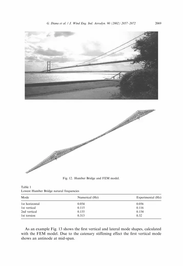
As an example Fig. 13 shows the first vertical and lateral mode shapes, calculatedwith the FEM model. Due to the catenary stiffening effect the first vertical modeshows an antinode at mid-span.

Fig. 12. Humber Bridge and FEM model.

Table 1

Lowest Humber Bridge natural frequencies

Mode Numerical (Hz) Experimental (Hz)

1st horizontal 0.054 0.056

1st vertical 0.115 0.116

2nd vertical 0.155 0.154

1st torsion 0.313 0.32


In order to validate the FEM model of the full bridge, a comparison was carriedout between the measured and numerical values of the static lateral displacement atthe mid-span, under different mean wind speeds. Fig. 14 shows the results of thiscomparison: a good agreement can be observed up to 24m/s, that is the maximumwind speed recorded during the measurement champagne on the Humber Bridge [8].

Sure of the structural FEM model capability of reproducing the real bridgebehaviour, at least the static and free dynamic ones, a comparison about theturbulent wind response has been performed.

Fig. 15 shows, as an example, a comparison between a real bridge averaged dataacquisition and the corresponding values from the numerical simulation, adoptingthe new admittance function. The considered wind speed is 18m/s and the torsionalacceleration at mid-span has been observed.

The peaks corresponding to two different torsional modes exhibit similaramplitude, even if the 1st torsional mode is a little bit underestimated in thenumerical simulation.

Perhaps the most interesting comparison is the one giving the differences betweentwo numerical simulations, one performed using the complex admittance function(right Fig. 16) and the other with the commonly used real admittance, taken as theabsolute value of the measured complex admittance (left Fig. 16). The effect of usingthe complex admittance function is more evident for the first mode, and leads to an

Fig. 13. First lateral and vertical mode shapes.

0

0.2

0.4

0.6

0.8

1

1.2

14 16 18 20 22 24

Wind speed [m/s]

Lat

eral

dis

pal

cem

ent

½ s

pan

[m

]

Numeric

Experimental

Fig. 14. Lateral displacement: FEM results and full-scale measurement.


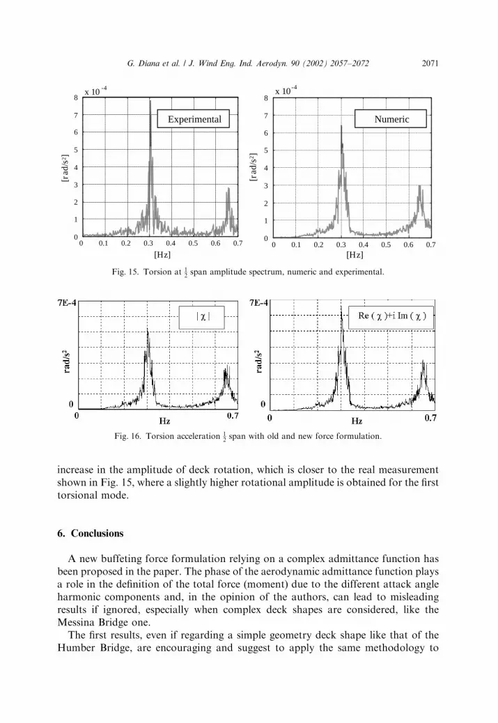
increase in the amplitude of deck rotation, which is closer to the real measurementshown in Fig. 15, where a slightly higher rotational amplitude is obtained for the firsttorsional mode.

6. Conclusions

A new buffeting force formulation relying on a complex admittance function hasbeen proposed in the paper. The phase of the aerodynamic admittance function playsa role in the definition of the total force (moment) due to the different attack angleharmonic components and, in the opinion of the authors, can lead to misleadingresults if ignored, especially when complex deck shapes are considered, like theMessina Bridge one.

The first results, even if regarding a simple geometry deck shape like that of theHumber Bridge, are encouraging and suggest to apply the same methodology to

Fig. 16. Torsion acceleration 12span with old and new force formulation.

0 0.1 0.2 0.3 0.4 0.5 0.6 0.70

1

2

3

4

5

6

7

8x 10 -4

[Hz]

[rad

/s2 ]

0 0.1 0.2 0.3 0.4 0.5 0.6 0.70

1

2

3

4

5

6

7

8x 10-4

[Hz][r

ad/s

2 ]

Experimental Numeric

Fig. 15. Torsion at 12span amplitude spectrum, numeric and experimental.


more complicated deck shapes, where a higher difference between the traditional andthe new formulations may be expected.

A further improvement may consist in trying to get the aerodynamic admittancevalues for lower reduced velocities than those studied in this work. To this end, theopening of the new wind tunnel of Politecnico di Milano, having a much larger testsection than the present one, will be for sure of great help.

References

[1] R.H. Scanlan, On flutter and buffeting mechanism in long-span bridges, Prob. Eng. Mech. 3 (1)

(1988) 22–27.

[2] G. Diana, S. Bruni, A. Cigada, A. Collina, Turbulence effect on flutter velocity in long span

suspended bridges, J. Wind Eng. Ind. Aerodyn. 48 (1993) 329–342.

[3] M. Falco, A. Curami, A. Zasso, Nonlinear effects in sectional model aeroelastic parameters

identification, J. Wind Eng. Ind. Aerodyn. 41–44 (1992) 1321–1332.

[4] M. Kawatani, N. Toda, M. Sato, H. Kobayashi, Vortex-induced torsional oscillations of bridge

girders with basic sections in turbulent flows, J. Wind Eng. Ind. Aerodyn. 83 (1999) 327–336.

[5] G. Diana, F. Cheli, A. Zasso, M. Bocciolone, Suspension bridge response to turbulent wind, 10th

ICWE Copenhagen, Denmark, June 1999.

[6] H.W. Teunissen, Simulation of the planetary boundary layer in a multiple jet wind tunnel, Atmos.

Environ. 9 (1975) 145–174.

[7] G. Diana, A. Cigada, E. Zappa, On the response of a bridge deck to turbulent wind: a new

experimental approach, Third EACWE 2–6 July 2001, Eindhoven, The Netherlands.

[8] M. Bocciolone, F. Cheli, A. Curami, A. Zasso, Wind measurements on the Humber Bridge and

numerical simulations, J. Wind Eng. Ind. Aerodyn. 41–44 (1992) 1393–1404.

[9] A. Zasso, Flutter derivatives: advantages of a new representation convention, J. Wind Eng. Ind.

Aerodyn. 60 (1996) 35–47.

[10] A. Zasso, A. Curami, Extensive identification of bridge deck aeroelastic coefficients: average angle of

attack, Reynolds number and other parameters effects, Proceedings of the Third Asian Pacific

Symposium on Wind Engineering, Hong Kong, 1993, pp. 143–148.

[11] A. Hatanaka, H. Tanaka, New estimation method of Aerodynamic Admittance Function Journal of

Wind Engineering 89, The Fifth Asia-Pacific Conference on Wind Engineering, Kyoto, 2001.


Documents

Complex aerodynamic admittance function role in buffeting response of a bridge deck